the perturbation of a turbulent boundary layer …franklin/images/franklin_ayek(2013).pdf · 2...

J. Braz. Soc. Mech. Sci. Eng. manuscript No.

(will be inserted by the editor)

THE PERTURBATION OF A TURBULENT

BOUNDARY LAYER BY A TWO-DIMENSIONAL

HILL

Erick de Moraes Franklin · Guilherme

Augusto Ayek

Received: date / Accepted: date

Abstract Turbulent boundary layers over flat walls in the presence of a hill arefrequently found in nature and industry. Some examples are the air flows over hillsand desert dunes, but also water flows over aquatic dunes inside closed conduits.The perturbation of a two-dimensional boundary layer by a hill introduces newscales in the problem, changing the way in which velocities and stresses are dis-tributed along the flow. When in the presence of sediment transport, the stress dis-tribution along the hill is strongly related to bed instabilities. This paper presentsan experimental study on the perturbation of a fully-developed turbulent bound-ary layer by a two-dimensional hill. Water flows were imposed over a hill fixedon the bottom wall of a closed conduit and the flow field was measured by Parti-cle Image Velocimetry. From the flow measurements, mean and fluctuation fieldswere computed. The general behaviors of velocities and stresses are compared topublished asymptotic analyses and the surface shear stress is analyzed in terms ofinstabilities of a granular bed.

Keywords Turbulent boundary layer · hill · perturbation · instabilities

Accepted Manuscript for the Journal of the Brazilian Society of Mechanical Sciences andEngineering, v. 35, p. 337-346, 2013. The final publication is available at Springer viahttp://dx.doi.org/10.1007/s40430-013-0024-z

Erick M. FranklinFaculty of Mechanical Engineering, University of Campinas - UNICAMPTel.: +55-19-35213375E-mail: [email protected]

Guilherme A. AyekFaculty of Mechanical Engineering, University of Campinas - UNICAMPE-mail: [email protected] Present address: Benteler Automotive

2 Erick de Moraes Franklin, Guilherme Augusto Ayek

1 Introduction

Turbulent boundary layers over flat walls are frequently found in environmentaland industrial applications and, for this reason, they have been extensively studiedfor over a century. However, in some cases a small hill is present on the ground,perturbing the boundary layer. In nature, some examples are the air flows overhills and desert dunes, and water flows over river dunes. In industry, examples arerelated to flows over sand ripples and dunes in closed conduits such as petroleumpipelines, dredging lines and sewer systems.

The perturbation of the boundary layer introduces new scales in the problem,changing the way in which velocities and stresses are distributed along the flow.The new velocity and stress distributions are of importance for many engineer-ing applications. For instance, when in the presence of sediment transport thestress distribution along the hill is an essential parameter to understand the bedinstabilities [1–3].

Over the last decades, many studies were devoted to the perturbation of aturbulent boundary layer by a low hill. Some of them, based on asymptotic meth-ods, have improved our knowledge on the subject. In these methods, the turbulentboundary layer over a hill of small aspect ratio (height to length ratio of O(0.1)) isdivided in a two-region structure that can be employed to determine the perturbedflow [4]. Furthermore, each of these regions is sometimes subdivided in two layersin order to correctly match each other and the boundary conditions.

Jackson and Hunt [5] presented an asymptotic analysis of a turbulent boundarylayer perturbed by a low hill. In their analysis, the unperturbed boundary layerwas given by the law of the wall

u+ =1

κln

(

y

y0

)

=1

κln(y+) +B (1)

where κ = 0.41 is the von Karman constant, y is the vertical distance from thewall, y0 is the roughness length, u+ = u/u∗ is the longitudinal component of themean velocity normalized by the shear velocity, u(y) is the longitudinal component

of the mean velocity V, u∗ = ρ−1/2τ−1/20 is the shear velocity, τ0 is the shear stress

of the unperturbed flow, ρ is the specific mass of the fluid, y+ = yu∗/ν is thevertical distance normalized by the viscous length, ν is the kinematic viscosityand B is a constant. The second and the third terms are equivalent, the secondone being generally employed in hydraulic rough regimes while the third one isemployed in hydraulic smooth regimes.

Jackson and Hunt [5] divided the perturbed boundary layer in two regions. Theinner region, close to the bed, is a region where the turbulent vortices can adaptto equilibrium conditions with the mean flow. In this region, the time scale for thedissipation of the energy-containing eddies is much smaller than the time scale fortheir advection, so that this region is in local equilibrium. The local-equilibriumcondition allows the use of turbulent stress models, such as the mixing-lengthmodel. In addition, as this region has a small thickness that does not changesignificantly along the hill, the perturbations are driven by the pressure field ofthe outer region.

The outer region is considered far enough from the bed so that the energy-containing vortices cannot adapt to equilibrium conditions with the mean flow:

Title Suppressed Due to Excessive Length 3

the time scale for the dissipation of the energy-containing eddies is much largerthan the time scale for their advection, and the flow is not in local equilibrium. Forthis reason, the mean flow in this region is almost unaffected by the shear stressperturbations and a potential solution is expected at the leading order.

Jackson and Hunt [5] matched these two regions and obtained a solution forthe perturbation. Their composite solution shows that most of the perturbationoccurs in the inner region (at each longitudinal position, the maximum of thespeed-up is at approximately 1/10 of the inner region thickness). In addition, theyfound that the longitudinal evolution of the perturbation has a peak upstream ofthe bedform crest.

Hunt et al. [6] improved the analysis of Jackson and Hunt [5] by subdividingeach region. They divided the inner region in two layers. In the inner surface

layer, closer to the bed, the flow is determined by pressure and shear effects (theinertial effects are negligible) and its lower part matches the boundary conditionson the bed surface. In the shear stress layer, closer to the outer region, the flowis determined by pressure, shear, and inertial effects and its upper part matchesthe outer region. Hunt et al. [6] also divided the outer region in two layers. Inthe upper layer, the external part of this region, the ratio between the Reynoldsstress gradient and the inertial effects is very small and the flow is approximatelypotential. In this layer, the flow is dominated by pressure effects. In the middle

layer, lower part of this region, the shear dominates, so that the flow is inviscid,but rotational. This layer must match the shear stress layer. In addition, Hunt etal. [6] extended the analysis to three-dimensional hills.

The results obtained by Hunt et al. [6] are in agreement with that of Jacksonand Hunt [5]. Hunt et al. [6] also showed that the maximum of the perturbationvelocity occurs in the shear stress layer and that near the surface the relativeincrease of the surface stress is greater than that of velocity.

Weng et al. [7] further developed the works of Jackson and Hunt [5] and Hunt etal. [6]. They computed the velocity perturbations until the second order, obtaininga smoother matching, and applied the results to forms with higher aspect ratios.Their proposed expressions for the surface stresses, at the first order, are largelyemployed.

Sauermann [8] and Kroy et al. [9,10] simplified the results of Weng et al. [7]for the surface stress and obtained an expression containing only the dominantphysical effects of the perturbation, making clear the reasons for its upstreamshift. For a hill with local height h and a length 2L between the half-heights (totallength ≈ 4L), they showed that the perturbation of the longitudinal shear stress(dimensionless) is

τx = A

(

1

π

∫

∂xh

x− ξdξ + Be∂xh

)

(2)

where ξ is an integration variable and A and Be are considered as constants, asthey vary with the logarithm of L/y0. Variations in three orders of magnitudeof L/y0, L/y0 = 103, L/y0 = 104 and L/y0 = 105, give A = 4.0, A = 3.6 andA = 3.3 and Be = 0.63, Be = 0.46 and Be = 0.36, respectively. The first termin the parentheses, the convolution product, is symmetric, similar to the potentialsolution of the flow perturbation by a hill. It comes from the pressure perturbationscaused by the hill on the outer region. The second term in the parentheses, whichtakes into account the local slope, is anti-symmetric. It comes from the nonlinear


inertial terms of the turbulent flow and can be seen as a second order correctionof the potential solution, with minor changes in the magnitude of the first ordersolution, but causing an upstream shift. In the Fourier space, Eq. 2 may be writtenas (dimensionless)

τk = Ah(|k|+ iBek) (3)

where k = 2πλ−1 is the longitudinal wavenumber (λ is the wavelength) and i isthe imaginary number. If the perturbation is supposed small compared to a basicflow, the fluid flow over the bed can be written as a basic flow, unperturbed, plusa flow perturbation. For the shear stress on the bed surface

τ = τ0(1 + τ) (4)

In the case of loose granular beds, the longitudinal evolution of the shear stressdetermines if the fluid flow is an unstable mechanism, so that Eqs. 2 to 4 are ofimportance for stability analyses of sand ripples and dunes [1–3,11].

Formally, asymptotic methods are applied to hills with aspect ratios ofhmax (4L)

−1 < 0.05 [5,6,12], where the total length of the bedform is approxi-mately 4L and hmax corresponds to its maximum height. Carruthers and Hunt[13] showed that reasonable results are obtained when applied to slopes up tohmax (4L)

−1 = 0.3 (note that the aspect ratio of dunes is hmax (4L)−1 = O(0.1)).

In particular, when hmax (4L)−1 = O(0.1), the obtained equations shall be applied

to an envelope formed by the bedform and the recirculation bubble [7].Recently, Franklin and Charru [14] and Charru and Franklin [15] studied the

isolated three-dimensional dunes, known as barchans, in the specific case of closed-conduit water flows. In particular, the evolution of the shear stress along thesymmetry plane of the dune was investigated. Different from the aeolian case,the authors found that the surface shear stress is not shifted upstream of thedune crest. If this is true, the liquid flow is not the unstable mechanism and theformation of aquatic barchans cannot be understood. The absence of an upstreamshift was not explained by the authors, the reason being probably linked to theflow three-dimensionality.

This paper presents an experimental study of the perturbation of a turbulentboundary layer by a two-dimensional hill. A closed-conduit water flow was im-posed over a triangular ripple and the flow was measured by PIV (Particle ImageVelocimetry). From the flow measurements, the mean velocities and the fluctua-tions were computed, so that the shear stress over the ripple could be determined.The general behaviors of velocities and stresses are compared to published asymp-totic analyses and the surface stress over the ripple is discussed in terms of bedinstabilities.

Section 3 presents the experimental set-up and Section 4 presents and discussesthe experimental results. The conclusion section follows.

2 Nomenclature

A = constantB = constantBe = constant


f = Darcy friction factorg = acceleration of gravity, ms−2

H = channel height, mh = hill’s local height, mHeff = distance from the PVC bed to the top wall, mi = imaginary numberk = wavenumber, m−1

L = longitudinal distance between the crest and the position where the local heightis half of its maximum value, mQ = water flow rate, m3/hRe = channel Reynolds number, Re = U2Heff/νU = cross-section mean velocity of the fluid, m/su = longitudinal component of the mean fluid velocity, ms−1

u′ = longitudinal component of the velocity fluctuation, ms−1

u∗ = shear velocity, ms−1

u+ = dimensionless velocity, u+ = u/u∗

−u′v′ = xy component of the Reynolds shear stress, (m/s)2

V = mean fluid velocity, ms−1

v = vertical component of the mean fluid velocity, ms−1

v′ = vertical component of the velocity fluctuation, ms−1

x = longitudinal coordinate, my = vertical coordinate, myd = displaced vertical coordinate, my0 = roughness length, my+ = dimensionless vertical coordinate, y+ = yu∗/ν

Greek symbols

κ = von Karman constantλ = wavelength, mν = kinematic viscosity, m2/sρ = specific mass of the fluid, kg/m3

τ = shear stress on the bed, N/m2

ξ = integration variable, m

Subscripts

k = relative to the Fourier spacex = relative to the real space0 = relative to the flat wall (except in y0)

Superscripts

ˆ= relative to the perturbation′ = fluctuation

3 Experimental set-up

The experimental device consisted of a water reservoir, a progressive pump, a flowstraightener, a 5m long transparent channel of rectangular cross section (160mm


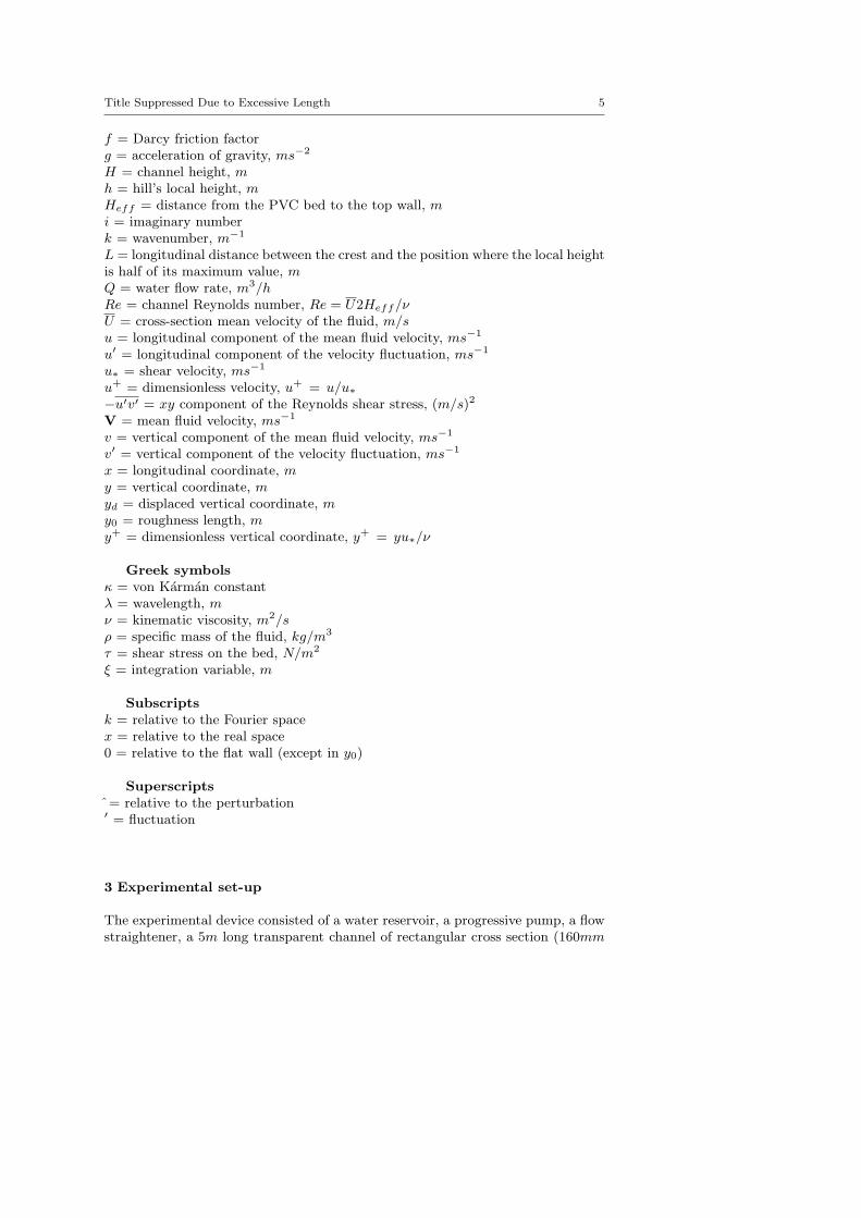
Fig. 1 Layout of the experimental device: (a) side-view; (b) cross section.

wide by 50mm high), a settling tank and a return line, so that the water flowedin a closed loop.

The flow straightener was placed at the channel inlet and consisted of a divergent-convergent nozzle filled with d = 3mm glass spheres, whose function was to ho-mogenize the water flow profile. The channel test section was 1m long and startedat 40 hydraulic diameters (3m) downstream of the channel inlet. There was an-other 1m long section connecting the test section exit to a settling tank and thereturn line. A layout of the experimental device is presented in Fig. 1

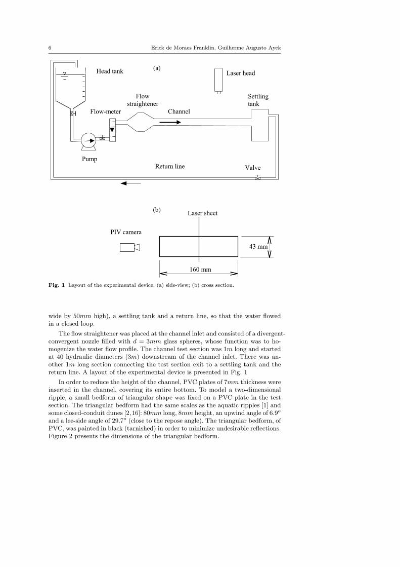
In order to reduce the height of the channel, PVC plates of 7mm thickness wereinserted in the channel, covering its entire bottom. To model a two-dimensionalripple, a small bedform of triangular shape was fixed on a PVC plate in the testsection. The triangular bedform had the same scales as the aquatic ripples [1] andsome closed-conduit dunes [2,16]: 80mm long, 8mm height, an upwind angle of 6.9o

and a lee-side angle of 29.7o (close to the repose angle). The triangular bedform, ofPVC, was painted in black (tarnished) in order to minimize undesirable reflections.Figure 2 presents the dimensions of the triangular bedform.


Fig. 2 Bedform of triangular profile employed as a model ripple (in the figure, the flow isdownwards).

The employed flow rates varied between 5 and 10m3/h. They were controlledby changing the excitation frequency of the pump and measured by an electromag-netic flow-meter. These flow rates corresponded to cross-section mean velocitiesU within 0.20 and 0.40m/s and to Reynolds numbers Re = U2Heff/ν within1.7 · 104 and 3.5 · 104, where Heff is the distance from the surface of the PVCplates to the top wall of the channel. For different flow rates, measurements wereperformed without and with the ripple in the closed conduit.

Particle Image Velocimetry was employed to obtain the instantaneous velocityfields of the water stream. The employed light source was a dual cavity Nd:YAGQ-Switched laser, capable to emit at 2 × 130mJ at a 15Hz pulse rate. The powerof the laser beam was fixed at 80% of the maximum power in order to assurea good balance between the image contrasts and undesirable reflection from thechannel walls. Suspension of particles already present in the city (tap) water and10µm hollow glass beads (S.G. = 1.05) were employed as seeding particles.

The PIV images were captured by a 7.4µm×7.4µm (px2) CCD (charge coupleddevice) camera with a spatial resolution of 2048px × 2048px and acquiring pairs ofimages at 4Hz. The total field employed was of 140mm × 140mm, correspondingto a magnification of 0.1, and the employed interrogation area was of 8px × 8px,corresponding to 60µm×60µm in the CCD. Considering diffraction, the diameterof the seeding particles was around 4µm in the CCD. The computations weremade with 50% of overlap, corresponding to 512 interrogation areas and to aspatial resolution of 0.27mm. The minimum distance from the wall from whichmeasurements were considered valid was of the order of 1mm.

Each experimental run acquired 1000 pairs of images for the tests with theripple and 500 pair of images for the tests without the ripple, from which the fieldsof instantaneous velocity, of time-averaged velocity and of the velocity fluctuationswere computed in fixed Cartesian grids by the PIV controller software. MatLab


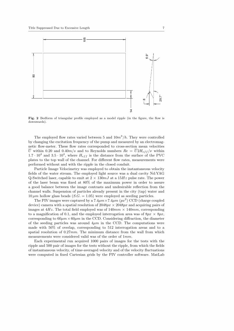
Fig. 3 Image of a PIV experiment in the presence of a ripple. In this image, the flow is fromright to left.

scripts were written to post-process these fields (spatio-temporal averaged profiles,shear velocities, stresses on the ripple coordinate system, longitudinal evolutions,etc.). Figure 3 presents an example of PIV image for the experiments with a ripple.

4 Results

4.1 Channel flow

The water flow was first measured in the absence of the ripple, corresponding thento a turbulent, fully-developed channel flow. This case is indicated in the followingby the subscript 0. For each test, the instantaneous fields were time-averaged andthe fluctuation fields (second-order moments) were computed and time-averaged.As the flow was fully developed, the time-averaged fields were space-averagedin the longitudinal direction. With this procedure, vertical profiles of the meanvelocities and of second-order moments were obtained taking advantage of thespatial resolution of the PIV equipment.

For a fully-developed turbulent flow in a two-dimensional channel, only thelongitudinal component of the mean velocity is present and Eq.1 is valid. Theshear velocity u∗,0 for each Reynolds number was then determined by fitting theexperimental data in the logarithmic region (70 < y+ < 200) with Eq. 1 for ahydraulic smooth regime (B0 = B ≈ 5.5) [17]. The obtained values of u∗,0 and B0

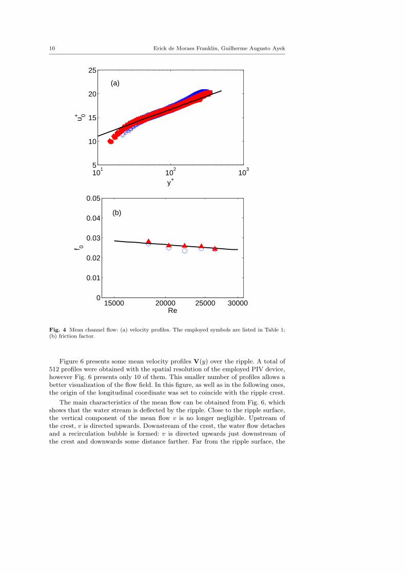
as well as the symbols employed in Fig. 4a are presented in table 1.Figure 4a presents the log-normal profiles of the mean velocities for different

Reynolds numbers. The abscissa is in logarithmic scale and represents the verticaldistance from the channel walls (bottom or top) normalized by the viscous length,y+. The ordinate is in linear scale and corresponds to the mean velocities nor-


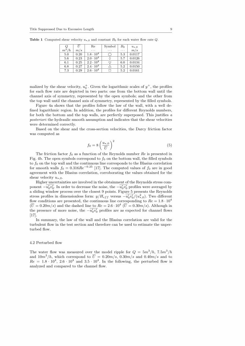
Table 1 Computed shear velocity u∗,0 and constant B0 for each water flow rate Q.

Q U Re Symbol B0 u∗,0

m3/h m/s · · · · · · · · · m/s5.0 0.20 1.8 · 104 © 5.3 0.01175.6 0.23 2.0 · 104 ♦ 5.7 0.01266.1 0.25 2.2 · 104 ▽ 6.0 0.01346.8 0.27 2.4 · 104 △ 5.2 0.01507.3 0.29 2.6 · 104 � 5.2 0.0161

malized by the shear velocity, u+0 . Given the logarithmic scales of y+, the profiles

for each flow rate are depicted in two parts: one from the bottom wall until thechannel axis of symmetry, represented by the open symbols; and the other fromthe top wall until the channel axis of symmetry, represented by the filled symbols.

Figure 4a shows that the profiles follow the law of the wall, with a well de-fined logarithmic region. In addition, the profiles for different Reynolds numbers,for both the bottom and the top walls, are perfectly superposed. This justifies a

posteriori the hydraulic smooth assumption and indicates that the shear velocitieswere determined correctly.

Based on the shear and the cross-section velocities, the Darcy friction factorwas computed as

f0 = 8

(

u∗,0

U

)2

(5)

The friction factor f0 as a function of the Reynolds number Re is presented inFig. 4b. The open symbols correspond to f0 on the bottom wall, the filled symbolsto f0 on the top wall and the continuous line corresponds to the Blasius correlationfor smooth walls f0 = 0.316Re−0.25 [17]. The computed values of f0 are in goodagreement with the Blasius correlation, corroborating the values obtained for theshear velocity u∗,0.

Higher uncertainties are involved in the obtainment of the Reynolds stress com-ponent −u′

0v′

0. In order to decrease the noise, the −u′

0v′

0 profiles were averaged bya sliding window process over the closest 9 points. Figure 5 presents the Reynoldsstress profiles in dimensionless form: y/Heff versus −u′

0v′

0/(u2∗,0). Two different

flow conditions are presented, the continuous line corresponding to Re = 1.8 · 104

(U = 0.20m/s) and the dashed line to Re = 2.6 · 104 (U = 0.30m/s). Although inthe presence of more noise, the −u′

0v′

0 profiles are as expected for channel flows[17].

In summary, the law of the wall and the Blasius correlation are valid for theturbulent flow in the test section and therefore can be used to estimate the unper-turbed flow.

4.2 Perturbed flow

The water flow was measured over the model ripple for Q = 5m3/h, 7.5m3/hand 10m3/h, which correspond to U = 0.20m/s, 0.30m/s and 0.40m/s and toRe = 1.8 · 104, 2.6 · 104 and 3.5 · 104. In the following, the perturbed flow isanalyzed and compared to the channel flow.


101

102

103

5

10

15

20

25

y+

u+ 0(a)

15000 20000 25000 300000

0.01

0.02

0.03

0.04

0.05

Re

f 0

(b)

Fig. 4 Mean channel flow: (a) velocity profiles. The employed symbols are listed in Table 1;(b) friction factor.

Figure 6 presents some mean velocity profiles V(y) over the ripple. A total of512 profiles were obtained with the spatial resolution of the employed PIV device,however Fig. 6 presents only 10 of them. This smaller number of profiles allows abetter visualization of the flow field. In this figure, as well as in the following ones,the origin of the longitudinal coordinate was set to coincide with the ripple crest.

The main characteristics of the mean flow can be obtained from Fig. 6, whichshows that the water stream is deflected by the ripple. Close to the ripple surface,the vertical component of the mean flow v is no longer negligible. Upstream ofthe crest, v is directed upwards. Downstream of the crest, the water flow detachesand a recirculation bubble is formed: v is directed upwards just downstream ofthe crest and downwards some distance farther. Far from the ripple surface, the


−1.5 −1 −0.5 0 0.5 10

0.2

0.4

0.6

0.8

1

(−u´0v´

0)/u

*,02

y/H

eff

Fig. 5 Profiles of the xy component of the Reynolds stress in dimensionless form: y/Heff

versus −u′

0v′0/(u2

∗,0). The continuous line corresponds to Re = 1.8 · 104 (U = 0.20m/s) and

the dashed line corresponds to Re = 2.6 · 104 (U = 0.30m/s)

−0.06 −0.04 −0.02 0 0.02 0.04 0.06

0.005

0.01

0.015

0.02

0.025

0.03

0.035

0.04

x (m)

y (m

)

Fig. 6 Some profiles of the perturbed mean velocities V over the ripple. The flow is from leftto right and Re = 3.5 · 104.


values of v are negligible. However, although v ≈ 0, the longitudinal component uis accelerated in this region, as expected from the mass conservation.

To proceed with a boundary-layer analysis, different velocity profiles must haveas reference the solid surface, i.e., the vertical position where V = 0. In the upperregion, far from the ripple surface, the channel walls are suitable references andthe vertical coordinate y can be employed. In the lower region, close to the ripple,the ripple surface is the reference and therefore the displaced vertical coordinateyd, given by Eq. 6, is the proper coordinate

yd = y − h (6)

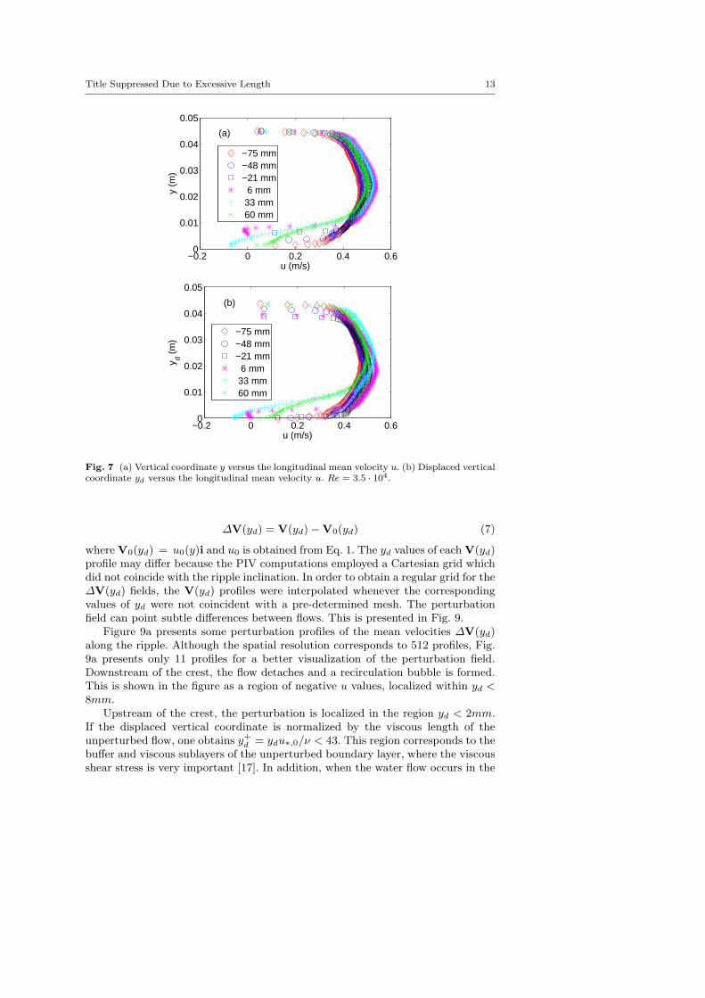
Figure 7 presents the longitudinal component of some mean velocity profilesfor different longitudinal positions. Each employed symbol corresponds to the lon-gitudinal position indicated in the legends. Figure 7(a) presents y versus u, beingsuitable for the analysis of the core flow and upper wall regions, called here upper

region. In the upper region, u increases as the flow approaches the position ofthe ripple crest (x = 0m), reaching a maximum near x = 0m. The longitudinalacceleration is due to the restriction caused by the combined effects of the ripplesurface and the recirculation bubble so that the maximum of u does not occurexactly at x = 0m. Downstream of x ≈ 0m, u decelerates.

Figure 7(b) presents yd versus u, being suitable for the analysis of the regionclose to the ripple surface, called here lower region. We observe in this region anincrease of u as the flow approaches the ripple crest, however the acceleration isstronger then in the upper region. A great part of the perturbation is confined inthe lower region (this will become clearer later), therefore the maximum of thelongitudinal velocity does not coincide with that of the upper region. Downstreamof the crest, the flow detaches and u has negative values.

The longitudinal evolution of the perturbed flow is of importance to understandthe formation of sand ripples. For the growth of ripples, the fluid flow must bean unstable mechanism, which means that the surface shear stress caused by thefluid must reach its maximum upstream of the bedform crests [1–3,11]. Therefore,in the following we focus our attention on the region upstream of the ripple crest.

Figure 8 presents the mean velocity profiles upstream of the ripple crest. Figure8(a) presents the displaced vertical coordinate yd versus the longitudinal meanvelocity u and shows a convective acceleration of u towards the ripple crest. Thedegree of acceleration varies with yd and therefore the longitudinal position wherethe maximum of u is reached for each value of yd is not clear in Fig. 8a. This ispresented in more detail in Fig. 9b.

Figure 8(b) presents the displaced vertical coordinate yd versus the verticalmean velocity v. The values of v are one order of magnitude smaller than that of uas expected from the dimensional analysis of the perturbation. The profiles showthat v increases from zero at the ripple surface, reaches a maximum and decreasesto zero as yd approaches the upper wall. At x = −75mm, the maximum occursaround the center of the channel. Towards the crest, the maximum becomes closerto the ripple surface (yd ≈ 2mm). Longitudinally, the maximum of v increasesmonotonically as the flow approaches the crest.

The perturbation field can be defined as the difference between the flow overthe ripple and that over a flat wall, having as reference the solid walls [5]. For themean velocity


−0.2 0 0.2 0.4 0.60

0.01

0.02

0.03

0.04

0.05

u (m/s)

y (m

)

(a)

−75 mm−48 mm−21 mm 6 mm 33 mm 60 mm

−0.2 0 0.2 0.4 0.60

0.01

0.02

0.03

0.04

0.05

u (m/s)

y d (m

)

(b)

−75 mm−48 mm−21 mm 6 mm 33 mm 60 mm

Fig. 7 (a) Vertical coordinate y versus the longitudinal mean velocity u. (b) Displaced verticalcoordinate yd versus the longitudinal mean velocity u. Re = 3.5 · 104.

∆V(yd) = V(yd)−V0(yd) (7)

where V0(yd) = u0(y)i and u0 is obtained from Eq. 1. The yd values of each V(yd)profile may differ because the PIV computations employed a Cartesian grid whichdid not coincide with the ripple inclination. In order to obtain a regular grid for the∆V(yd) fields, the V(yd) profiles were interpolated whenever the correspondingvalues of yd were not coincident with a pre-determined mesh. The perturbationfield can point subtle differences between flows. This is presented in Fig. 9.

Figure 9a presents some perturbation profiles of the mean velocities ∆V(yd)along the ripple. Although the spatial resolution corresponds to 512 profiles, Fig.9a presents only 11 profiles for a better visualization of the perturbation field.Downstream of the crest, the flow detaches and a recirculation bubble is formed.This is shown in the figure as a region of negative u values, localized within yd <8mm.

Upstream of the crest, the perturbation is localized in the region yd < 2mm.If the displaced vertical coordinate is normalized by the viscous length of theunperturbed flow, one obtains y+d = ydu∗,0/ν < 43. This region corresponds to thebuffer and viscous sublayers of the unperturbed boundary layer, where the viscousshear stress is very important [17]. In addition, when the water flow occurs in the


0 0.2 0.4 0.60

0.01

0.02

0.03

0.04

0.05

u (m/s)

y d (m

)

(a)

−75 mm−62 mm−48 mm−35 mm−21 mm −8 mm

0 0.01 0.02 0.03 0.04 0.050

0.01

0.02

0.03

0.04

0.05

v (m/s)

y d (m

)

(b)

−75 mm−62 mm−48 mm−35 mm−21 mm −8 mm

Fig. 8 Mean velocity profiles upstream of the ripple crest: (a) displaced vertical coordinate ydversus the longitudinal mean velocity u; (b) displaced vertical coordinate yd versus the verticalmean velocity v. Re = 3.5 · 104.

presence of a granular bed, the transport of grains as bed load takes place veryoften in the region y+d < 20. Bed load can be defined as a mobile layer of grainsrolling and sliding over a fixed bed [18].

One of the objectives of this paper is to shed light on the role of the waterstream in the formation of sand ripples. As the perturbation and the granulartransport (if present) are localized in the region close to the ripple surface, weinvestigate next the flow in this region.

Figure 9b presents the longitudinal evolution of |∆V| in the y+d < 20 region.Due to the PIV spatial resolution, the presented |∆V| values correspond to threedifferent vertical positions, y+d = 6, 11 and 17. Although the noise is significant,the experimental data show that the perturbation velocity tends to decrease as theflow approaches the crest. Figure 9b shows that the maximum of the perturbationvelocity occurs upstream of the ripple crest, and that the longitudinal distancebetween the maximum perturbation and the crest decreases as yd increases.

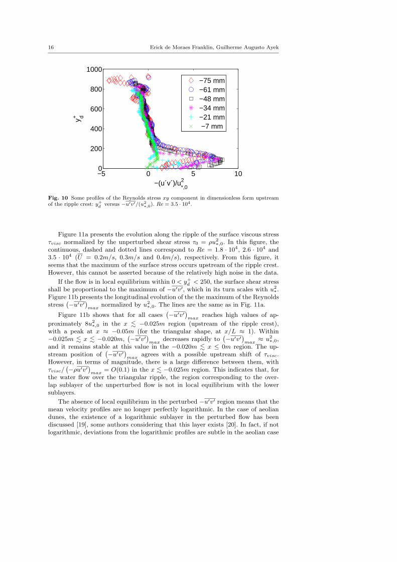
Figure 10 presents some profiles of the xy component of the Reynolds stressesin dimensionless form, y+d versus −u′v′/(u2

∗,0), upstream of the ripple crest. Inorder to decrease the noise, the obtained −u′v′ profiles were averaged by a slidingwindow process over the closest 9 points. Figure 10 shows that the Reynolds stress


−0.05 0 0.050

0.002

0.004

0.006

0.008

0.01

x (m)

y d (m

)

(a)

−0.08 −0.06 −0.04 −0.02 00

0.1

0.2

0.3

0.4

x (m)

|∆ V

| (m

/s)

(b)

yd+ = 6

yd+ =11

yd+ =17

Fig. 9 (a) Some perturbation profiles of the mean velocities ∆V. (b) Longitudinal evolution

of |∆V| for three different vertical positions: y+d = 6, 11 and 17. Re = 3.5 · 104.

−u′v′ is perturbed in the 50 < y+d < 250 region, that corresponds to the overlapsublayer of the unperturbed boundary layer [17]. If the flow is in local equilibriumin the y+d < 250 region, the shear stress on the surface shall scale with −u′v′ andtherefore the longitudinal evolution of the latter is of importance. Figure 10 alsoshows that, longitudinally, the perturbation of −u′v′ decreases near the crest.

To understand if the water flow is an unstable mechanism and if the flow isin local equilibrium within 0 < y+d < 250, the viscous shear stress on the ripplesurface τvisc was evaluated as

τvisc = µ

(

∂uθ

∂yd,θ+

∂vθ∂xθ

)

≈ µ∂uθ

∂yd,θ(8)

where uθ and vθ are, respectively, the aligned and perpendicular components ofthe mean velocity with respect to the ripple surface, yd,θ is a displaced coordinateperpendicular to the ripple surface and xθ is the coordinate aligned with theripple surface. The derivative was evaluated from a first order Taylor expansion.This component of the viscous stress is the responsible for the transport of grainsbecause any grain transported as bed load shall roll or slide over the ripple surfacein a direction aligned with the mean flow.


−5 0 5 100

200

400

600

800

1000

−(u´v´)/u*,02

y d+

−75 mm−61 mm−48 mm−34 mm−21 mm −7 mm

Fig. 10 Some profiles of the Reynolds stress xy component in dimensionless form upstreamof the ripple crest: y+d versus −u′v′/(u2

∗,0). Re = 3.5 · 104.

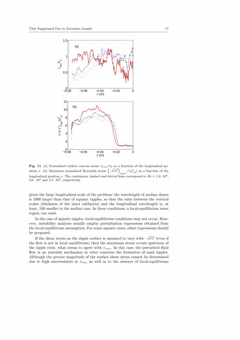
Figure 11a presents the evolution along the ripple of the surface viscous stressτvisc normalized by the unperturbed shear stress τ0 = ρu2

∗,0. In this figure, thecontinuous, dashed and dotted lines correspond to Re = 1.8 · 104, 2.6 · 104 and3.5 · 104 (U = 0.2m/s, 0.3m/s and 0.4m/s), respectively. From this figure, itseems that the maximum of the surface stress occurs upstream of the ripple crest.However, this cannot be asserted because of the relatively high noise in the data.

If the flow is in local equilibrium within 0 < y+d < 250, the surface shear stressshall be proportional to the maximum of −u′v′, which in its turn scales with u2

∗.Figure 11b presents the longitudinal evolution of the the maximum of the Reynoldsstress

(

−u′v′)

maxnormalized by u2

∗,0. The lines are the same as in Fig. 11a.

Figure 11b shows that for all cases(

−u′v′)

maxreaches high values of ap-

proximately 8u2∗,0 in the x . −0.025m region (upstream of the ripple crest),

with a peak at x ≈ −0.05m (for the triangular shape, at x/L ≈ 1). Within−0.025m . x . −0.020m,

(

−u′v′)

maxdecreases rapidly to

(

−u′v′)

max≈ u2

∗,0,and it remains stable at this value in the −0.020m . x ≤ 0m region. The up-stream position of

(

−u′v′)

maxagrees with a possible upstream shift of τvisc.

However, in terms of magnitude, there is a large difference between them, withτvisc/

(

−ρu′v′)

max= O(0.1) in the x . −0.025m region. This indicates that, for

the water flow over the triangular ripple, the region corresponding to the over-lap sublayer of the unperturbed flow is not in local equilibrium with the lowersublayers.

The absence of local equilibrium in the perturbed −u′v′ region means that themean velocity profiles are no longer perfectly logarithmic. In the case of aeoliandunes, the existence of a logarithmic sublayer in the perturbed flow has beendiscussed [19], some authors considering that this layer exists [20]. In fact, if notlogarithmic, deviations from the logarithmic profiles are subtle in the aeolian case


−0.08 −0.06 −0.04 −0.02 00

0.5

1

1.5

x (m)

τ visc

/τ0

(a)

−0.08 −0.06 −0.04 −0.02 00

2

4

6

8

10

12

(−u´

v´) m

ax/u

*,0

2

x (m)

(b)

Fig. 11 (a) Normalized surface viscous stress τvisc/τ0 as a function of the longitudinal po-

sition x. (b) Maximum normalized Reynolds stress(

−u′v′)

max/(u2

∗,0) as a function of the

longitudinal position x. The continuous, dashed and dotted lines correspond to Re = 1.8 · 104,2.6 · 104 and 3.5 · 104, respectively.

given the large longitudinal scale of the problem: the wavelength of aeolian dunesis 1000 larger than that of aquatic ripples, so that the ratio between the verticalscales (thickness of the inner sublayers) and the longitudinal wavelength is, atleast, 100 smaller in the aeolian case. In these conditions, a local-equilibrium innerregion can exist.

In the case of aquatic ripples, local-equilibrium conditions may not occur. How-ever, instability analyses usually employ perturbation expressions obtained fromthe local-equilibrium assumption. For some aquatic cases, other expressions shouldbe proposed.

If the shear stress on the ripple surface is assumed to vary with −u′v′ (even ifthe flow is not in local equilibrium) then the maximum stress occurs upstream ofthe ripple crest, what seems to agree with τvisc. In this case, the perturbed fluidflow is an unstable mechanism in what concerns the formation of sand ripples.Although the precise magnitude of the surface shear stress cannot be determineddue to high uncertainties in τvisc as well as to the absence of local-equilibrium


conditions, the present findings contribute to the understanding of the unstablerole of the water flow.

5 CONCLUSIONS

This paper investigated the perturbation of a liquid turbulent boundary layer by atwo-dimensional ripple in the hydraulic smooth regime. Measurements of a closed-conduit water flow perturbed by a model ripple of triangular shape were made byPIV and the obtained mean and turbulent fields were compared with the unper-turbed flow fields. Some known characteristics of the boundary-layer perturbationby a low hill were confirmed by the experimental results: a recirculation bubble isformed downstream of the ripple crest and the perturbation is localized in a regionclose to the ripple surface (y+d . 40). However, some characteristics not considereduntil now, or for which a consensus has not been achieved, had their importanceshown by the presented results.

Due to the relatively large ratio between the vertical and longitudinal flowscales (when compared to the aeolian case), the inner regions of the perturbedflow are not in local-equilibrium for some aquatic ripples. This means that asymp-totic expressions for the boundary-layer perturbation based on local-equilibriumconditions must be used with care in the case of aquatic sand ripples of triangularshape, specially if Reynolds numbers are Re < 105. To the authors’ knowledge, thisis the first time that absence of local-equilibrium conditions is proposed for the flowover a triangular ripple in moderate Reynolds numbers (10000 < Re < 50000).

The maximum of the shear stress on the ripple surface occurs upstream of theripple crest. For the triangular ripple, the maximum surface shear stress was foundto occur at 50% of the ripple length (in this case, ≈ L). However, more experimentsemploying other shapes as well as increased PIV spatial resolutions are necessaryto quantify the characteristic length of the shift. This shift is necessary to explainthe instabilities giving rise to aquatic ripples in the hydraulic smooth regime. Thepresent experimental findings are of importance to understand the formation, theevolution and the stability of bedforms under turbulent liquid flows.


Acknowledgements The authors are grateful to Petrobras S.A. (contract number 0050.0045763.08.4).Erick M. Franklin is grateful to FAEPEX/UNICAMP (conv. 519.292, project 1435/12) and toFAPESP (contract number 2012/19562-6).

References

1. E.M. Franklin, J. Braz. Soc. Mech. Sci. Eng. 32(4), 460 (2010)2. E.M. Franklin, J. Braz. Soc. Mech. Sci. Eng. 33(3), 265 (2011)3. E.M. Franklin, Appl. Math. Model. 36, 1057 (2012)4. S.E. Belcher, J.C.R. Hunt, Ann. Rev. Fluid Mech. 30, 507 (1998)5. P.S. Jackson, J.C.R. Hunt, Quart. J. R. Met. Soc. 101, 929 (1975)6. J.C.R. Hunt, S. Leibovich, K.J. Richards, Quart. J. R. Met. Soc. 114, 1435 (1988)7. W.S. Weng, J.C.R. Hunt, D.J. Carruthers, A. Warren, G.F.S. Wiggs, I. Livingstone, I. Cas-

tro, Acta Mechanica pp. 1–21 (1991)8. G. Sauermann, Modeling of wind blown sand and desert dunes. Ph.D. thesis, Universitat

Stuttgart (2001)9. K. Kroy, G. Sauermann, H.J. Herrmann, Phys. Rev. E 66(031302) (2002)

10. K. Kroy, G. Sauermann, H.J. Herrmann, Phys. Rev. Lett. 88(054301) (2002)11. E.M. Franklin, Appl. Math. Model. (accepted)12. R.I. Sykes, J. Fluid Mech. 101, 647 (1980)13. D.J. Carruthers, J.C.R. Hunt, Atmospheric Processes over Complex Terrain 23, 83 (1990)14. E.M. Franklin, F. Charru, J. Fluid Mech. 675, 199 (2011)15. F. Charru, E.M. Franklin, J. Fluid Mech. 694, 131 (2012)16. E.M. Franklin, F. Charru, Powder Technology 190, 247 (2009)17. H. Schlichting, Boundary-layer theory (Springer, 2000)18. A.J. Raudkivi, Loose boundary hydraulics, 1st edn. (Pergamon Press, 1976)19. R.A. Bagnold, The physics of blown sand and desert dunes (Chapman and Hall, 1941)20. E.J.R. Parteli, V.O. Schwammle, H.J. Herrmann, L.H.U. Monteiro, L.P. Maia, Geomor-

phology 81, 29 (2006)

the perturbation of a turbulent boundary layer …franklin/images/franklin_ayek(2013).pdf · 2...

Documents