the piano tuner's tale -

2The Piano Tuner's Tale

SCALES AND KEYSAny journey, however long or short, must begin from somewhere and the point of departure for this

journey came from my work as a piano tuner; so it is amongst the somewhat arcane details of notes and

scale and keys, but above all ratios, that we set out.

One of the luxuries of this line of work is that it requires, even allows me to demand, a quiet and

tranquil environment free from interruption. Quite a luxury but one not without dangers: time to think,

time for the mind to wander. A thought that strayed into my mind recently was that, as a piano tuner, my

work involved endless hours of performing a process not unlike calculus: And indeed, ultimately, what is

a piano tuner but a humble mathematician of ratios, the journeyman-geometer of musical sound? The

process of tuning involves listening to the interference or interaction between the tuning note and another

reference note and adjusting the tuning note in accordance with changes heard in the combined sound. A

visual analogue of these combined sounds could be imagined as somewhat like throwing two pebbles into

a placid unruffled pond and watching the ripples from the dual impacts intermingle. The two radiating

patterns on the pond’s surface being something like the mixing of sound waves that a tuner relies on to

gauge fine differences between notes, and judge when notes are in tune.

Figure 2.1 The intermingling of waves on the surface of a pond.

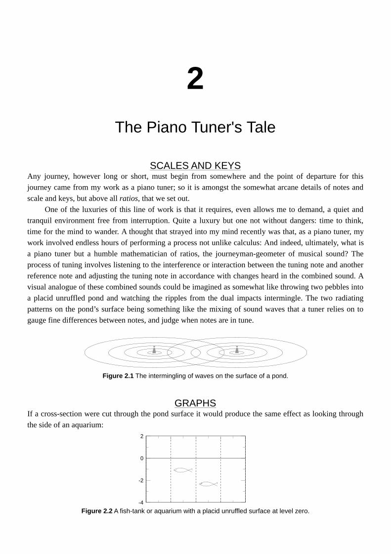
GRAPHSIf a cross-section were cut through the pond surface it would produce the same effect as looking through

the side of an aquarium:

-4

-2

0

2

Figure 2.2 A fish-tank or aquarium with a placid unruffled surface at level zero.

and if a pebble were dropped into the left-hand end of the aquarium, the ripples would spread out across

the formerly smooth surface.

90 180 270 360

(rip

ple

disp

lace

men

t)

ripples

Am

plitu

de

0 45-4

-2

0

2

-1

1

Figure 2.3 The ripples from a single pebble dropped into the aquarium travel across the unruffled surface. Four andone-half ripples shown, with one complete ripple enclosed in a dash-line box on the left-hand side, lying between

plus 1 and minus 1 displacement.

The units on the left-hand side allow us to measure the distance or displacement between the top/

peak and bottom/trough of each ripple. The overall amplitude of this ripple is two units, as it rises to plus

one at the peak and falls to minus one at the trough; and, over the time period from the pebble actuating

the ripples to the front ripple reaching the far side, there will have been eight ripples created in all.

Therefore forty-five of the units shown below the aquarium, measure the time or frequency of each

individual ripple. If the front ripple took one second to span the length of the aquarium (eight ripple

lengths) the time or frequency of each ripple would be one-eighth of a second or eight ripples-per-second.

The time measurement of ripples, or fluctuation, or cycles per second, are by convention named hertz

(abbreviation Hz) after the nineteenth century scientist Heinrich Hertz.

Now if the ripple or wave pattern of the first pebble were marked on the side of the aquarium as a

dotted line so that the ripples of a second pebble could be viewed against it, this might reveal a picture

somewhat like Figure 2.4: with two ripples of slightly different frequency which begin and finish together

but diverge gradually toward the center of the tank.

0 90 180 270 360

(rip

ple

disp

lace

men

t)A

mpl

itude

45

ripple frequency 7ripple frequency 8

-4

-2

0

2

-1

1

Figure 2.4 Two ripples or waves viewed one against the other.

Next the question is what would happen if the two pebbles where dropped in the tank

simultaneously? What effect would the ripples have on each other? One way to approaching this question

is to imagine one ripple as the surface over which the other ripple travels. (For convenience I shall call

JOURNEY TO THE HEART OF MUSIC2.2

them wave frequency seven and eight and abbreviate to wave[f=7] and wave[f=8].) So instead of the

formerly flat surface of the aquarium, now the surface is imagined to be the dotted line trace made by

wave[f=8] and on to this undulating surface the additional ripples of wave[f=7] are appended.

0 90 180 270 360-4

-3

-2

-1

0

1

2

(rip

ple

disp

lace

men

t)A

mpl

itude

wave[f=8]wave[f=8] + wave[f=7]

Figure 2.5 The superimposition (sometimes termed superposition) of wave[f=7] onto the 'surface’ of wave[f=8].

Comparing Figures 2.4 and 2.5, it can be seen that at the left and right edges the two superimposed

ripples or waves augment each other, with peaks and troughs roughly coinciding, so in combination

doubling the amplitude or displacement. However, in the middle section the opposite is true, wave[f=8]’s

trough coincides with wave[f=7]’s peak and vice versa, resulting in the two waves cancelling each other

out. In the middle the amplitude of the combined waves dies away to a fraction of the amplitude found at

the left and right hand sides. Thus by causing two slightly different waves to intermingle or interfere the

result is to produce large (double) waves at the edges which die away to small waves around the middle.

The effect doesn’t necessarily happen in such a straightforward way with all waves, the right conditions

for obtaining this result are that the waves begin and end together over a commensurate period and their

frequencies and amplitudes are not too different. Waves that begin and end together, that keep in step with

one another over some portion of time are said to be in phase, and the complete interval over which a

system repeats is often referred to as the period. For the most part, out in the real world, sound waves are

are all jumbled up and out of phase, as they stream away from their source(s), bouncing off solid objects

at odd angles, perhaps repeatably, before being absorbed by softer surfaces or lost to the open air.

However, as the human ear doesn’t register phase differences to a significant degree, much of this chaotic

intermingling is filtered out, leaving the mechanisms of aural cognition with a relatively clear signal to

process.

By convention, matters relating to the interference of waves (and many other phenomena connected

with waves and periodic behaviour) are linked to a circle and the period divided up into 360 units or

degrees – the angle through which the radius of a circle travels (anti-clockwise) before returning to the

starting position. The units running along the base or x-axis of Figures 2.1 to 2.5 are degrees, 360 per

period; while the units of amplitude of the wave or ripple (the volume or loudness of a sound wave) are

written on the y-axis: on the left hand side. There are many more fish-tanks in this book, graphs that is;

there is no reason to be daunted by them. Essentially they are snapshots of a (usually repeating) pattern of

relationship between quantities. Here we have been looking at the repeating pattern of amplitude

(displacement from the equilibrium of a smooth surface – zero on the y-axis) of two intermingling waves

of slightly different frequencies – wave[f=7] and wave[f=8].

SCALES AND KEYS 2.3

Graphs are a compact, easy to read, way of describing a relationship. Just imagine how difficult it

would be to express in words, or write in figures, the precise ever changing contour of the interference

pattern of Figure 2.5 – that the eye grasps in an instant. Graphs are worth making your friends, they have

a lot to offer. Yet, on the other hand, care must be taken not to confuse the often simplified or sanitised

picture they present, for the often complex objective reality. At their best graphs draw out relationships,

highlighting salient features from what may be a dense data set. In particular, in this book, they are used

in the form of a ‘halfway-house’ between reality and formality that hopefully captures the essential

characteristics under discussion. For example, sound waves are generally presented with unit amplitude

(strictly double unit amplitude) and uniform phase. In the real environment sound is hardly ever this

simple; yet, as alluded to above, the ear and processes of aural cognition filter out much of this objective

complexity by decomposing the dense raw interference pattern, and so, a ‘sanitised’ graph can capture

both something of the objective complexity of the sound and something of the simplicity of the perceived

underlying relationships.

❍

❍

❍

❍

❍

❍

❍

❍

❍

❍

❍

❍

❍

❍

❍

❍

❍

❍

❍

❍

❍

❍

❍

❍

●

●

●

●

●

●

●

●

3

6

9

12

15

18

21

24

energy/complexity -->

harm

onic

s

1

❍ C-h1 through h24● G-h3, h6, h9, h12, h15, h21, h24

G-h3

nest

ed s

erie

s bu

ilt o

n G

-h3

fundamental serie

s C-h1 th

rough h24

C-h1

G

G-h3

C-h1

G

D

B

G

D

F

notes/tones

G-h6

D-h9

G-h12

B-h15

D-h18

F-h21

G-h24

C-h2

G-h6

D-h9

G-h12

B-h15

D-h18

F-h21

G-h24

G-h3

C-h1C-h2G-h3

nested series(stepping in groups of three

ratios of the fundamental series)

Figure 2.6 On the left, in graph format; two harmonic series, one based on G-h3 (continuous line) contained ornested within the ratios of a broader, more fundamental series built on C-h1 (dotted line); and to the right the same

arrangement illustrated in music notation and as a rectilinear number pattern.

Another way graphs are used in this book, in addition to mapping out the effects waves have on each

other, is for the charting of harmonic series. This is rather more straightforward. The vertical axis (y-axis)

counts off the subdivisions from the fundamental tone ‘h1’ in whole numbers; while the horizontal axis

(x-axis) registers the increasing energy and complexity of the ‘system’, in unspecified amounts. Again the

great advantage of the format is that the eye immediately picks up the relationships: in this case those of

one harmonic series contained (nested) within another. This is illustrated in Figure 2.6. where the

fundamental series based on C-h1 contains a second harmonic series built on G-h3. Both series illustrated

in Figure 2.6 reach up to the twenty-fourth harmonic, the fundamental series by brute addition of every

harmonic – H1 through H24. In contrast, the nested series built on G-h3 steps more lightly in groups of

three: h6, h9, h12, h15, h18, h21 and h24. Viewed from the standpoint of mutable numbers, the

fundamental series represents the prime state digit sequence of mutable number twenty-four; whilst the


nested series, plus H1 and H2 (from the fundamental series), represents an intermediate digit sequence of

the same number. Written in the factor and subscript formats, they are:

Mutable Base Numbers: Prime state: 1×24 (MBN 241) and Intermediate state: 3×8 (MBN 83 01)

Returning now to the topic of tuning a piano (we never really left it), and the thought that piano

tuning could be viewed as a process not unlike that branch of abstract mathematics called calculus. It can

be seen in Figure 2.7 how two waves start out together, but because the wavelength of one note is slightly

longer, by the time they approach the right-hand side they are totally out of step. The waves begin

together, in phase, but end completely out of phase, with peak against trough. If the diagram were

extended further to the right they would come back together again just as in Figure 2.5. If these two waves

are summed up into a single interference pattern, as two sounds in the air would be by forming a single

complex wave, clearly they will compound each other on the left-hand side and cancel each other out

around 180 degrees, the middle of their period, on the right.

Degrees

-1

0

1

Am

plitu

de (

arbi

trar

y un

its)

in phase out of phase

0 180

tuning notereference note

Figure 2.7 Two waves of close but not identical wavelength, a tuning note and reference note.

In the graph Figure 2.8 there are again two waves of nearly the same frequency, a tuning note and

reference note. In this graph the waveforms of both notes are shown as dotted lines, and because many

cycles of the tuning and reference notes are packed into the overall period of the graph, they appear as a

rather fuzzy band between plus one and minus one on the vertical y-axis. When these two notes are

summed together, that is the two waveforms intermingle, the resulting interference pattern – the sum of

the two waves – is shown by the continuous line. The effect produced by the near equal interference

between tuning and reference notes is termed beats and the shape of the continuous line vividly illustrates

the swelling and dying away of beats when heard. Three times in Figure 2.8 this process of addition and

subtraction creates the swelling sound of beats. The rate of beating, the regular swelling and dying away,

depends on how quickly one wave catches up with the other – how quickly they come into, and out of,

phase. Subtracting the frequency in hertz (vibrations per second) of one note from the other, will yield the

absolute rate of beats per second heard. For example, reference note A440Hz minus tuning note 437Hz

equals three beats per second.

SCALES AND KEYS 2.5

0 90 180 270 360 450 540 630 720 810 900 990 1080-2

-1

0

1

2

Degrees (3 beat cycles)

Am

plitu

de (

arbi

trar

y un

its)

Figure 2.8 Two notes of nearly the same frequency/wavelength (dotted lines) begin in phase compounding theiramplitudes, but then gradually work their way out of phase, cancelling out each other’s amplitudes. Three cycles or

periods of this process or ‘interference pattern’ are illustrated.

If the beats are relatively slow, say below four or five per second, they are not unpleasant, adding an

undulating character to the sound. This feature is used in some compound organ stops and can be heard in

the tone of the string section of an orchestra. Once the rate of beating climbs much above six per second it

soon becomes most unpleasant to the ear as the resonant vibration of the two frequencies diverge

sufficiently to destructively interfere with each other on the ear’s detector membrane. However, going in

the opposite direction – slowing the beats down further – so the wavelength (and therefore also the

frequency of each complete vibration) of the tuning note approaches that of the reference note, causes the

interference pattern, the time between beats, to lengthen. This slowing to the point of vanishing guides the

tuner to a perfect match between the two notes. Once the beats disappear, the tuning note has reached the

same wavelength and frequency as the reference note. (The trick also works for tuning notes which

achieve a close multiple of the reference note, most usefully the octave multiple of two and intervals of a

fifth and fourth). Thus in a calculus-like manner, as the tuning note tends to unity with the reference

frequency, so the period between beats lengthens, tending towards infinity.

The process of tuning, of listening to beats and adjusting the string tension accordingly, is like

pulling a lever which is attached to a ‘black box’ process. The tuner doesn’t have to know how or what

goes on inside the blackbox, he or she only have to move the lever according to the signal that emerges

from the process – until the beats, the fluctuations in volume, disappear. The necessary and quite complex

calculations, concerning string tension, mass, elasticity, which could be done in abstract mathematics,

thankfully, have been devolved into the physical process. Essentially piano tuners have an oscillatory

computer to help them in their work... and it comes free with a pair of ears!

And, in a similar manner to the piano tuner’s calculus-like methods of working, the physical process

of music-making and listening – the performance of tonal music – can be understood as the execution of

mathematics in musical sound. For, as I seek to demonstrate in this document, via the perspective of MOS

model and mutable base numbers, it is apparent that the human ear and aural cognitive processes

effectively form a ‘blackbox’ system through which the mathematics inherent in tonal music are made both

sensibly satisfying and intuitively intelligible to the human mind.


SCALESAn interval of a fifth, such as the notes A below E played together, produce a sonorous and harmonious

combination. Figure 2.9 shows the wave pattern which results when these two notes are sounded together

with an equal volume (amplitude) and uniform phase. It can be seen from the graph that this pattern

repeats at a frequency equivalent to the note which is exactly one octave below the lower note A –

‘frequency 1’ in the figure. It is the introduction of this lower period which unites the objective sounding

notes A and E, creating a harmonious union. The lower period is the one, the unit, within which the two

elements of the ratio 2:3 can coexist. In essence, the interval has created, or at least implied, the

beginnings of a harmonic series A-h1, A-h2, E-h3. Any two (or more) notes viewed as whole numbered

ratios, whatever their frequency, have a shared h1, a common fundamental frequency which acts as a

reference point to the relationship they have with each other. For example, the more dissonant and

awkward relationship of A#h17 and B-h18 (17:18) equally find a common bond in A-h1. Though the ear

struggles to recognise such distant relationships, it is remarkably flexible and accommodating it its ability

to comprehend irregular ratios that are capable of being construed as an approximation to a simpler, low

number ratio relationship.

0 30 60 90 120 150 180 210 240 270 300 330 360

-2

-1

0

1

2

Degrees

Am

plitu

de (

arbi

trar

y un

its)

<----- frequency 3 ----><------------- frequency 2 -----------><------------------------------------- frequency 1 -------------------------------->

notes A plus E (frequency 1)note A (frequency 2)note E (frequency 3)

A-h1A-h2E-h3

Figure 2.9 The interference pattern formed by notes A and E (frequency ratio 2:3) has a period twice that of A andthree times that of E. On the right is a number pattern which encapsulates the harmonic relationships.

The pitch or frequency ratio between the notes of a truly perfect fifth is 2:3, or 1:1.5. However,

though the interval A to E on the piano is often referred to as a perfect fifth, it is normally a ‘perfect’

tempered fifth, with a ratio of approximately 2:2.9966 or 1:1.4983. Pianos are not tuned to perfectharmony! Beats, which are the hallmark of out-of-tuneness, are surprisingly present in all intervals of a

correctly tuned piano; though difficult to detect except in the most simple intervals (octaves, fifths and

fourths) where the interfering harmonics are close to the fundamental tones. Even the octaves, which are

in theory tuned true, are deliberately stretched by tuners to brighten the perceived tone and keep pace with

the sharp harmonics generated by the thicker, stiffer strings of notes lower down. The reason why a piano,

or many other fixed pitch instruments, are tuned with ever so slightly out of tune intervals (i.e. the

tempered fifth A to E, 1:1.4983) is to accommodate playing in all keys, harmoniously. Each key of the

SCALES AND KEYS 2.7

piano keyboard must produce a range of notes, not just one, and contribute to many varied relationships

within different chords. The F-sharp key must also do service as G-flat, not to mention E-double-sharp.

The compromise that has come to be generally accepted to allow each keyboard key to stand in for a

range of different notes, is equal temperament: the equal spacing of all semitones within the octave. The

adjustment of note pitches to something other than the true whole number relationships of the harmonic

series. This deliberate introduction of out-of-tuneness, is called tempering. Historically many different

systems of temperament have been used, though today equal temperament prevails.

The perfect octave, should one ever be found, has the ratio 1:2, and to make twelve equal divisions

between one and two, we need to find the twelfth root of two – the number which multiplied by itself

twelve times will yield two. The number is 1.05946 approximately and this number delivers the sequence

of frequency relationships shown in Figure 2.10. Thus, while a perfect octave is 1:2, the ratio of the

tempered major-second A to B is 1:1.1225 and that of a tempered major-third A to C#, 1:1.2599 –

considerably wider (sharper) than the natural or perfect interval of the harmonic series 1:1.25 (4:5). For

the most part, we accept these small imperfections, the accommodating tolerance of the ear smoothing

over the irregularities. But this is not how piano tuners set a scale, not by using abstract mathematics to

multiply 1 × 1.05946 twelve times.

1:2

A = 2.0000 G# = 1.8887 G = 1.7818 F# = 1.6818 F = 1.5874 E = 1.4983 D# = 1.4142 D = 1.3348 C# = 1.2599 C = 1.1892 B = 1.1225 A# = 1.0595 A = 1.0000

Figure 2.10 The relationships of the equal tempered scale. The true fifth A to E, 1:1.5, is adjusted downward to1:1.4983 and the true fourth, 1:1.3333..., up to 1:1.3348 (A to D).

To set an equally tempered scale, twelve imperfect fifths, must be squeezed into seven perfect

octaves. The slightly squashed fifths are only about one tenth of one percent flatter or smaller than the

true fifth (1:1.5). The tuner listens to the beats generated by the second harmonic of the upper note and

third harmonic of the lower note in the interval, as a guide. The process is essentially the reverse of tuning

two notes to be identical frequencies described above, as the aim here is to start with a truly perfect fifth

and introduce a tiny (and controlled) amount of imperfection! Tuners ‘un-tune’ the true fifth as it were,

into a tempered fifth.

Starting from the lowest note on a standard piano keyboard the ascending sequence of fifths, A, E,

B, F#, C#, G#, D#, A#, F, C, G, D and A – thirteen notes forming twelve fifths set within seven octaves,

illustrated by gray keys in Figure 2.11 – yields in open array, the twelve semitone notes of the scale. For

reasons of practicality, tuners abbreviate this to a pattern of up a fifth, down a fourth, in the middle range

of the keyboard, where the beating partials two to three octaves higher, lie near the ear’s most sensitive

range.


A E B F# C# G# D# A# F C G D A

A A A A A A A A<--------- Seven Perfect Octaves --------->

<--------- Twelve Imperfect (slightly squashed) Fifths --------->

Figure 2.11 It requires twelve successive ‘squashed’ fifths to fit exactly into the span of seven true octaves.

Once the pattern is laid out over the keyboard, it is plain to see that if the seven A to A octaves were

superimposed one octave on top of another, and the relationships of the twelve squashed fifths (1.1.4983)

taken with them, the resulting single octave A to A would have the configuration of a twelve note scale as

shown in Figure 2.10.

However, in contrast to the above Figures 2.10/11, beginning again with bottom A (set to the

nominal frequency ‘1’), if twelve true fifths (1:1.5 relationship) were actually laid out across the seven

octaves, at the top end the two schemes don’t quite match. That is, by multiplying 1.5 by itself twelve

times (rather than the tempered 1.4983...) the final result is 129.74 approximately – larger than the

product of 2 multiplied by itself seven times (i.e seven octaves), 128.

A1 : 1.5 : 2.25 : 3.37 : 5.06 : 7.59 : 11.39 : 17.08 : 25.62 : 38.44 : 57.66 : 86.49 : 129.74E B F# C# G# D# A# F C G D AA

A2 A4 A8 A16 A32 A64 A128A1

Figure 2.12 The relationships of twelve true fifths, the cumulative total gained by multiplying by 1.5 twelve times,doesn’t exactly match seven octaves – the cumulative total of multiplying by 2 seven times –

1.512 is slightly larger than 27.

The difference between 128 and 129.74, which works out to be just under one quarter of a semitone,

is named the Pythagorean Comma. A comma here means simply the difference between two schemes of

measurement. This is the quantity of out-of-tuneness, twenty-four percent of a semitone, that equal

temperament shares out between the twelve equally spaced notes of the scale.

Strictly, the true fifth relationships of Figure 2.12 though close, are perhaps not the final source of

the scale. For the ultimate source lies at the root of the harmonic series, where the simplest and most

fundamental whole number relationships are found. Above unity, or the unison interval (1:1), the two

most basic relationships the harmonic series allows are those of 1:2 and 1:3 – in music the intervals of an

octave and a twelfth. The extrapolation of these two whole number relationships, in the sequence 2, 22,

23,... 219 and 3, 32, 33,... 312, produces in essence the same outcome as that of Figure 2.12 (conducted in

octaves and fifths). Ultimately, two and three (1:2 and 1:3), whether three is thought of in musical terms

as a fifth or a twelfth, represent the most fundamental measuring rods that the harmonic series makes

available to us. In setting the scale of twelve notes, these two measuring rods are laid out from a common

starting point, with each unit octave or twelfth counted off respectively, until they again (almost) coincide,

nineteen octaves and twelve twelfths from the beginning. Interestingly, from this expanded scheme of

octaves and twelfths it is apparent that no matter how far the measuring rods are taken (that is the positive

non-zero powers 2n and 3m) they will never perfectly coincide, as no power of one prime number can

SCALES AND KEYS 2.9

equal the power of another. There will always be a comma.

To use Rameau’s language, from nature’s gift, out of the most basic relationships furnished by the

harmonic series – the whole numbers one, two and three – comes the structure of the twelve note scale. In

terms of mutable numbers, the two measuring rods are formed from the ground states of the two large and

similar magnitudes:

MBN factor format: 1x2x2x2x2x2x2x2x2x2x2x2x2x2x2x2x2x2x2x2 and 1x3x3x3x3x3x3x3x3x3x3x3x3

Or in decimal 524288 and 531441 respectively. Both numbers being capable of producing highly efficient

mutable digit sequences –i.e. many nested layers of low order prime oscillatory patterns. We will return to

the spiral of fifths/twelfths with the more dynamical approach of the modulating oscillatory system model

in Chapter 9, but for the present, see Figure 2.18 and perhaps peek a look at Figure 9.20.

| | | | | | | | | | | | |

h1-C *C (f=1)0%comma *C (f=1.0136x128)+1.36% 2-C 3-G *G (f=1.5x2)0%comma 4-C 5-E *E (f=5.0625)+1.25% 6-G 7-A# *A#(f=7.2081)+2.97% 8-C 9-D *D (f=2.25x4)0%comma 10-E 11-F# *F#(f=11.3906)+3.55% 12-G 13-A *A (f=3.375x4)+3.84% 14-A# 15-B *B (f=7.5937x2)+1.25% 16-C 17-C# *C#(f=17.0859)+0.5% 18-D 19-D# *D#(f=19.2216)+1.16% 20-E 21-F *F (f=21.6243x4)+2.97% .. 25-G# *G#(f=25.6289)+2.51%

--- 2:3 Steps of the Twelve Note Scale --> (Spiral/Cycle of Fifths)

<--

- R

atio

s of

the

Har

mon

ic S

erie

s --

-

CG D A E B F# C#G#D# A# FC

Figure 2.13 Graph of the twelve note natural scale, –i.e. derived from exact 2:3 rather than tempered relationships(frequencies reduced or augmented where required), plotted against the fundamental harmonic series of origin.

(Example derivation of F: 1.5 multiplied by itself eleven times, divided by four – F = 1.511/4 = 21.6289...)

As well as being derived from the most fundamental relationships capable of extension within the

harmonic series, the twelve note scale possesses two other attributes. Firstly, it has a balance between

economy and variety: neither too few, nor too many notes to sustain a variety of interesting relationships

whilst also maintaining an underlying unity. And secondly, the twelve note scale presents a particularly

rich set of low whole number ratio combinations relative to the total number of intervals (as noted by

James Jeans1) which the smoothing effect of equal temperament generalizes across all notes. In its natural

state, and allowing small commas/margins-of-error, the twelve notes of the scale stray no farther from

their fundamental tone (h1) than the twenty-fifth ratio of the harmonic series – illustrated in Figure 2.13.

What the configuration of twelve tonal centers of traditional music offers is a particularly full set of

(exact or close) inter-relationships between the fundamental harmonic series of origin and the frequency


positions of the cycle/spiral of 2:3 steps. The economical scale of twelve notes contains a wealth of

intervals with low integer ratios: fifth 2:3, fourth 3:4, major-third 4:5, minor-third 5:6, etc. And perhaps

significantly, the first three steps of C major, G major and D major, the tonal centers of the II–V–I

harmonic relationship, are perfectly in tune with the fundamental harmonic series of origin, setting the

scale on sure foundations, combined with a firm sense of direction. As shown in Figure 2.13.

Ove

rton

e S

erie

s of

Tru

e H

arm

onic

Par

tials

---

----

----

----

----

----

----

----

->

Tw

elve

Equ

al-t

empe

red

Not

es -

----

----

----

----

----

----

----

----

----

----

->

G-h24 -h23 F#h22 F-h21 -- 21.357Hz -F E-h20 D#h19 -- 19.027Hz -D# D-h18 C#h17 -- 16.951Hz -C# C-h16 B-h15 -- 15.102Hz -B A#h14 A-h13 -- 13.454Hz -A G-h12 F#h11 -- 11.314Hz -F# E-h10 D- h9 -- 8.980Hz -D C- h8 A# h7 -- 7.127Hz -A# G- h6 E- h5 -- 5.040Hz -E C- h4 G- h3 -- 2.997Hz -G C- h2 C- h1 -- 1.000Hz -C

G#h25 -- 25.398Hz -G#

A-h27 -- 26.908Hz -A A-h26

Figure 2.14 The ‘true’ whole number relationships of the harmonic series compared with the adjusted frequenciesof the equally tempered scale. Both columns can be read as ‘h’ numbers or hertz (cycles per second). The

frequencies of the twelve notes of the equal tempered scale have been raised to the octave where their equivalentpartial first appears in the harmonic series.

As Figures 2.13 and 2.14 make clear, there is some disagreement between the notes of the tempered

scale and the true whole number relationships of the harmonic series from which they are ultimately

derived. Notwithstanding this fact, it is convenient and useful to label the partials of the harmonic series

with the note letters of the scale, and generally, to treat the adjusted relationships of keyboard music

making, in principle, as if they were the whole relationships of the harmonic series. It is the graceful

tolerance of the ear and processes of aural cognition which allow this extraction of a precise relational

‘meaning’ from the approximations which are inevitably the objective experience. Noticeably, toward the

top of Figure 2.14, the divergence between the relationships of the uniform tempered scale and the curve

of the harmonic series begin to break down. There is no note that corresponds to h23. The semitones

shrink, from a wide B-h15 to C-h16, down through C#h17 to D-h18 which comes closest to the equal

tempered semitone (1.0588 against 1.0594 for the twelfth root of two), to the narrow G-h24 to G#h25

(1.0416), while the double entry for A-h26/h27 represents the beginning of a separation between the keys

(tonal centers) of C major and G major. However, overall, such variations in intervallic distance are

generally of no greater significance than the irregularities of tempered relationships, given the

accommodating flexibility of aural cognition.

SCALES AND KEYS 2.11

Other ScalesApart from the various forms of pentatonic scales2 common to many cultures and of great antiquity –

scales that probably first arose through experimentation but were latterly also generated by sequences of

fifths or fourths (as in the Chinese tradition) – there are other ‘measuring rod’ type sequences possible.

For example, two and five (1:2 and 1:5) producing a three-note scale in major-thirds: A, C#, F, (A) – with

a negative comma of minus 2.4%; or two and seven yielding a four-note scale A, C, D, E, (A) – with a

comma of +2.5%. However, such odd scales were never more than theorising and lack sufficient variety.

Rameau, the greatest of the eighteenth century theorists, knew of these relationships and extracted the

proportions of 2, 3 and 5 from the corps sonore to underpin his harmonic schemes in the form of double,

triple and quintuple geometric progressions.

Through the nineteenth century the equally tempered form of the twelve-note scale came into almost

universal application for keyboard and other fixed-pitch instruments. However, many other systems have

been suggested or experimented with at different times. A system extending the measuring rods of octave

and fifth to fifty-three fifths spread over thirty-one octaves (231 and 1.553 ! with a comma of just 3.57% of

a semitone) was proposed by Nicolas Mercator, the mathematician and map-maker, but as we have only

ten fingers at our disposal, with fifty-three notes in an octave, it never gained support – though

experimental instruments using this scale have been constructed. It is also believed that such scales were

know in China at a far earlier date and in recent years the sequence of fifths and octaves has been

calculated to ever more extraordinary lengths.

Just intonations – or more generally all non-equally tempered tuning schemes where some keys are

more in tune than others – were in wide use up to the end of the eighteenth century but, in the long run,

the demands of composers for ever broader tonal reference condemned them to history. However, in the

context of early music performance, they are probably aesthetically superior, encouraging the ear to

rediscover a subtle purity, which later generations traded for the courser utility of equal temperament. And

perhaps one day, music technology will provide keyboard instruments with a smoothly varying intonation

in all keys. (For comparison the file SCALES.PDF in the EXTRAS directory/folder charts all the equally

tempered octave scales from twelve to twenty-four steps. Of these the division of the octave into nineteen

equal-tempered steps might support an interesting tonal music with some subtle micro-intervallic effects.

The rest make for rather difficult listening.)

Distinctly different from the fine-grained equal-tempered fifty-three note scale or the rather exotic

scale of nineteen notes, both of which would support traditional tonal harmony, are the non-twelve-note

scales proposed and investigated by John Pierce3 and William Setheares4 amongst others. With these

scales the overtones are adjusted to non-whole numbered positions and/or deleted so as to match or

‘harmonise’ with the particular scale steps chosen (e.g. ten-tone equal temperament). To gain a

perspective on these various scales – without going into the detail – one could draw an analogy between

the four-square ‘Euclidian’ space of traditional tonal music and the many possible ‘curved’ non-Euclidian

geometries representing these other possibilities (see also Chapter 13, page 2). The parallel rule of Euclid

might similarly be conceptualized as the ‘tramlines’ of whole numbered harmonic relationships basic to

tonal music. When this rule of allowing only whole relationships of harmony and tone is relaxed,

completely new and strangely different musical possibilities emerge. It is perhaps too soon to know what

can or will be made of these unusual scales, but certainly the linking of scale structure to the overtone

spectra of the constituent scale notes is a most powerful idea and a concept that may be equally well


applied to traditional tonal music with ‘straight’ whole numbered harmonic spectra. I suspect here lies

music’s real frontier.

Significantly, the twelve-note scale is generated from intervals which have their origin in the

harmonic series and so the scale is not the fundamental object of music. Scales are devised by mankind,

the tempered fifth merely a utilitarian measure accepted by our ears as near enough true. Since Rameau’s

time the ultimate origin of music has been placed in the physical world, lying within the natural modes of

vibration of a material object. Prior to this realisation the divisions of a string were taken to be the point of

origin, this gave a more abstract numerical slant to music’s foundations than the structuralism inherent in

the physical reality of the harmonic series. Latterly, in the twentieth century, the rise of atonal music has

revived this more mathematical approach to some extent, with the equal-tempered twelve-note scale being

viewed in terms of the integers (modulo 12) in atonal set theory. However, the essentially mathematical

procedures of atonal theory and practice are not intuitively understood by the ear – in the way that tonal

procedures are – and therefore must appeal to other than traditional musical sensibilities.

Though equal-tempered scales can look rather like the set of integers modulo ‘n’; and in particular

the twelve-tone equal-tempered scale like the numbers – C-0 C#1 D-2 D#3 E-4 F-5 F#6 G-7 G#8 A-9

A#10 B-11 – under recursive division by twelve. There is, I believe a difficulty, an issue at least for me:

The ear appears determined to mishear such abstract arithmetic in favor of the simple relationships and

ratios of the harmonic series. To be wholly relevant musically, the identification of the equally spaced

integers with the equally spaced tempered scale would require the human ear and processes of aural

cognition to be able to fully appreciate such equality – to be able to hear the beautiful mathematics of

atonal set theory. I do not believe that this is the case; indeed contrariwise, the ear does its utmost to hear

inequality, turning the equal irrational relationships of the tempered scale into understandable unequal

whole ratios whenever possible, thereby fostering an intuitive apprehension of tonal music’s own

embedded mathematics – mutable numbers. I fear, perhaps obtusely, the wonderful and extensive

mathematics of atonal theory is just that, wonderful and extensive (abstract) mathematics, conducted in

musical sound.

TONAL CENTERS (KEYS)Although the twelve-note scale provides the raw material for music-making, generally, most pieces of

music emphasise a limited number of tones, by singling out just seven notes for particular prominence,

from the twelve available notes (though the other five notes can and do appear). These seven note

groupings are the diatonic scales, which are mainly constructed in steps of whole tones (i.e. two

semitones), rather than the entirely regular semitone steps of the twelve-note scale. The core difference

between the two types of scale lies in their contrasting structure. The totally uniform regularity of the

equally tempered twelve-note scale doesn’t favour or give prominence to any one note above the others.

The twelve-note scale is amorphous, undivided; it is atonal in itself. In contrast, the diatonic scales

distinctly isolate and emphasise one particular note, the tonic or home tone of the key or tonal center, by

means of the seven note scale’s unequal structure. The diatonic scales create a form of relational gravity, a

sense of being drawn toward a tonal center, the tonic note of a key. [In general, the term key is used in

these documents as meaning the twelve tonal centers of the cycle of fifths rather than twenty-four major

and minor modes; however, where specific reference to the major or minor mode is required, then, for

example, a phrase such as ‘the key of D major’ is used.]

The pattern of spacing between the notes for a major diatonic scale is: (whole)tone, tone, semitone,


tone, tone, tone, semitone – C, D, E, F, G, A, B and C. There are also a variety of separate minor diatonic

scales recognised in theory; however, in practice music often slips back and forth between the major and

minor modes as if the minor is no more than an inflection of a single tonal framework, based on the one

tonal ‘center of gravity’ and the exact details of their construction need not trouble us. For the major

diatonic scale – the pre-eminent scale of a tonal center or key – it is principally the attraction between the

notes separated by the narrow interval of a semitone, that single out the tonic or ‘home’ note above all

others, as the central tonal reference point.

I II III IV V VI VII (I)

- Tonic- Supertonic- Mediant- Subdominant- Dominant- Submediant- Leading Note

Semitones

IIIIIIIVVVIVII

C D E F G A B C

Figure 2.15 The seven degrees of the C-major scale.

The leading note B, tends generally to rise to the tonic C and the subdominant F to fall to the

mediant E. This force, often referred to as voice leading, is most strongly felt in a full cadence (V7– I).

Notice that in Figure 2.16 the motion of the leading note and subdominant, notes B and F, squeeze out or

at least leave no space for D, the fifth in the G7-major chord.

h8-G G-h6 h7-F | | E-h5 h6-D | | C-h4 h5-B | h4-G G-h3 h3-D | | C-h2 h2-G | | C-h1 h1-G

G7th resolves to C major

Figure 2.16 The voice leading of notes B and F in a full cadence are marked by black arrows (G-maj7th to C-maj).

On the keyboard of a piano, playing any seven consecutive white notes (plus upper octave) will

produce a diatonic scale or mode, for example, FGABCDEF. This is the Lydian mode, the names deriving

from ancient Greece, although it is essentially a product of the medieval epoch. It is one of a wealth of

different church modes or scales used in that period. However, only two of these medieval scales, the

Ionian CDEFGABC and the Aeolian ABCDEFGA survived into the modern era to become our major and


generic minor scales. On the keyboard these are the seven successive white notes beginning on C and A. It

is an interesting question as to why only these two scales escaped the great ‘extinction of modes’ that

occurred at the dawn of the tonal era – circa 1500 to 1600 AD.

Both scales, the Ionian/major and the Aeolian/minor, traverse an octave but the spacing of the notes

is sequentially dissimilar, the positioning of the semitone intervals are different in the major and minor

scales (and also somewhat variable in the minor); and this gives each a distinctive relational ‘flavor’ – the

bright major scale and a sad or intense minor. By using a combination of black and white keys, both these

scales can be reproduced on any note; for example, DEF#GABC#D is the major scale (the same spacing

of notes as CDEFGABC) but built on D instead of C. A melody using these notes and often starting on D

would be said to be ‘in the key of D major’. Equally, a piece using a minor scale beginning on D would be

‘in the key of D-minor’. However, as noted above, most non-trivial compositions mix elements of both

scales and it is usually preferable to think in terms of the tonal center of D, or the tonal center of

whichever other tone of the twelve note scale lies at the center of a web of (in principle) whole number

frequency relationships. Indeed, in sophisticated and extensive compositions there is likely to be a

hierarchy of temporary tonal centers (tonicisations) circling around an overarching key-center. For

example, temporary movements from an overarching key of D major, to A major (D major’s dominant’s

key-center), to B minor (D major’s relative minor, i.e. same key signature), to D minor (D major’s parallel

minor) and so forth.

D tonal center

Figure 2.17 The harmonic relationships of an example melody exhibit the ratios:D:D 1:2, D:G 3:4, D:A 2:3, D:F# 4:5, D:D 1:1 to the key note D;

and sequentially D->G 3:2, G->A 8:9, A->F# 6:5, F#->D 5:4.

The building of a diatonic scale on a particular note, such as C or D or F# or any other, is crucial for

our ears and aural cognition to be able to understand and interpret music. The sound (pitch/frequency) of

the tonal center, in this discussion D, is held in our memory and used as a reference point, whereby the

ratio to the frequencies of the other notes in the melody can be assessed. In the key of D major, a simple

melody such as that given in Figure 2.17 consists of a few simple whole number relationships –

disregarding the approximations introduced by equal temperament. Most of the time not even a musicians

would think in terms of these ratios; rather, unconsciously, that fabulous processor attached to our ears

crunches the numbers and delivers the intervallic information – that the music makes sense, that the ratios

are commensurable (or not). This happens without conscious effort, just as with spoken language, vast

amounts of low-level processing go unnoticed.

The remarkable achievement of European music was to develop this natural scheme of melodic and

harmonic reference (the ratios of the scale) into an extended system of twelve interlocking tonal centers.

As we have seen in Figure 2.12, in actual fact the natural set of 2:3 relationships (fifth) doesn’t quite close

the circle, but overshoots the seven octaves – by 1.36%. Thus while the adjusted or equal tempered fifth

(1:1.4983) forms a cycle of tonal centers or keys, in its natural state the true fifth produces, a spiral of 2:3

relationships. While composers kept to just a few closely related keys, or even better one key, themismatch between the notes of keys generated by a spiral of exact 2:3 relationships remained tolerable.

However, as composers explored more key relationships within individual compositions, the difficulties


for fixed pitch instruments became increasingly acute. After attempts to adapt the keyboard with divided

keys failed, e.g. different keyboard keys for G# and A-flat, equal temperament or something approaching

it, was the only answer.

KeyCycleRatio1:1.49

Figure 2.18 The closed cycle of fifths: formed from the tempered ratio 1:1.4983 between twelve adjacent tonalcenters or keys.

Within this system of twelve tonal centers, usually referred to as the cycle of fifths, a piece of music could

move from one reference home key to another, and another, and so on... and, usually, back to the initial

home key to finish the piece – a journey through the relationships of the scale(s) set within the broader

relationships of tonal centers.

KEY: D major ------------------------------> 3:4 G major ------------>

Figure 2.19 The example melody of Figure 2.17 steps from the reference tonal center (key) of D to the nextadjacent, downward, tonal center of G. (The relationship between the D and G tonal centers is 3:2 – descending

the cycle of fifths – but here 3:4, as the melodic line rises upward to G.)

Nesting Scales in KeysThe music in Figures 2.21a/b illustrates a real example of the nesting of scales (i.e. melodies made from

notes of a particular scale) within keys (tonal centers). The example is a short prelude from a trio sonata

by Corelli (Op.2/07). The music has the melodic intervals of the upper part interpreted as ratios of

exchange, with the keys traversed shown below the staves. All proportions are idealised pure intervals,

rather than tempered relationships, which is what aural cognition divines from musical sound.

The prelude’s ‘home’ key is F major, a scale built on F – measures 1–4. The music then moves to

C major – measures 5–8, a scale built on C with a 2:3 relationship to the home key F. At measure 8 the

music just ‘touches’ the key of G major. In measure 9, the piece falls back into C major, where it

continues until measure 14. At measure 14 the music moves dramatically forward into the key of D minor,

a scale built on D. This is the denouement, marked by the rapid tonal motion from C to D, a relationship

of 4:9 with the added intensity of also moving to an alternative D (minor) scale. Measures 15–17, in D

minor, are succeeded by an equally rapid fall back toward the home key of F, dropping through C at the

beginning of measure 18. The home tonal centre is re-established in measures 19–22 (see Figure 2.20).


Below the topmost staff of Figures 2.21a/b are the proportions of the upper melody line relative to

the current key or tonal center. Thus ‘F: 2:3, 3:5, 2:3, 3:4, etc.’ indicates that the scale is built on F and the

relationship between this reference note F, and the note in the melody is 2:3, etc. In these ratios the first

digit represents the reference tonal center and the second digit the melody note. The tonic key or home

tonal center is a scale built on F; this is the fundamental reference point, and the sequence of tonal centers

or keys is:F major, C major, G major, C major, D minor, C major and back to F major.

Thus the sequence of key relationships to the tonic key (home scale) could be written:

F: 1:1, 2:3, 4:9, 2:3, 8:27, 2:3, 1:1.

This might be called the ‘key melody’ – the route mapped out by the succession of the prelude’s large-

scale units of structure. In this example by Corelli, a rather restricted definition of the extent of a key is

being used to help illustrate the crucial role that ratios play in tonal music. Under different circumstances

a more liberal view of key might well be appropriate.

Within each of these large units of structure are nested small units of structure – each melodic phrase

– which exhibit similar proportional relationships, for example, in measures 10 and 11, where we find a

pattern not fundamentally different from the ‘key melody’ above.

C: 1:1, 16:15, 3:2, 2:3, 3:4, 4:5, 8:9, 1:1

Such patterns of nesting will usually extend out to the relationship between the home keys in each of the

movements of a larger piece of music, a typical pattern being: C major, G major, A minor and back to

C major.C: 1:1, 2:3, 3:5, 1:1

Thus, in a large musical work, it is possible to perceive levels of nesting from the whole composition,

down through movements, sections, sub-sections, composite phrases, single phrases to an individual

fragmentary motive.

Key/Scale built on C (F:C = 2:3)

Key/Scale built on F (F:F = 1:1)

Key/Scale built on G (C:G = 2:3, F:G = 4:9)

Key/(minor)Scale built on D (G:D = 2:3, F:D = 8:27)

measures

key

(ton

al c

entr

e) G

D

1

1.5

2.25

5.0625

3.375

C

F

1 2 3 4 5 6 7 8 9 10 11 12 13 14 15 16 17 18 19 20 21 22

Figure 2.20 Tonal center (key) trace of the prelude by Corelli (Op2/7, Figures 21a/b) with key relationships markedas ratios (e.g. F:C = 2:3) and on the y-axis as a cycle of fifths – 1 : 1.5 : 2.25 : 3.37 : 5.06.


Arcangelo Corelli

F: 2:3 3:5 3:4 4:5 8:9 (C: 2:3)

C: 2:3 3:5 3:4 4:5 3:5 8:9 (G: 2:3)2:3

2:3 3:5

C: 4:5 8:9,1:1,16:15,3:2,2:3 3:4 4:5 8:9 1:1

Key: F

2:3 Key: G2:3 Key: C

3:2 Key: C

Preludio

Trio Sonata Opus 2 No. 7

Figure 2.21a Prelude Opus 2 No.7 by Arcangelo Corelli


3:5,15:8,1:2... 3:4 4:5 3:5 2:3 (D: 3:4)

Dmin: 5:6 8:9 1:1 9:8 17:15 2:3,3:4,5:64:3(C: 2:3,3:4,4:5,3:2,1:2)

F: 2:3,3:4,3:10

F: 8:9 1:1,6:5,16:15, 1:1... 16:15,1:1 3:2 6:5 16:15,1:1 1:1,16:15,1:1

1:1

Key: C

4:9 Key: D 3:2 Key: C, 3:2 Key: F

Key: F

Figure 2.21b Prelude Opus 2 No.7 by Arcangelo Corelli


The graph, Figure 2.20, charts the course taken by the prelude from one tonal center to another, and

eventually back to the original key, described above. It is typical of the patterns of tonal (center) structure

found in traditional music. Significantly once the home key has been established most of the action and

development happens in tonal centres at some distance away. This maintains a tonal tension throughout

the arching span of the piece, holding the whole structure taut and together, while providing for a

satisfying sense of return, of arriving unmistakably at a meaningful destination.

Thus the twelve-note division of the octave provides twelve possible reference frequencies for our

ears and aural cognition to keep track of through the composition, in regard to both the current scale being

used by the melody at any point in the music and how this current scale (key) relates to a fundamental

home scale – usually the key where the melody began. Though in most compositions not all twelve tonal

centers are used but rather a smaller subset of closely related keys; and, you will no doubt have noticed

that this is an example of a nested structure – twelve notes nested within twelve keys.

Notes of Scale of C

Key:

Figure 2.22 Twelve notes nested within each of the twelve tonal centres (keys)

THE LANGUAGE OF MUSICMusic has an almost universal appeal; there are few people indeed to whom music communicates little or

nothing. And if there is communication there must be a code, a language commonly understood. It is

reported by Josef Haydn’s friend and biographer A.C. Dies5, that at their last meeting in Vienna, on the

eve of Haydn departure for London, Mozart remonstrated with his esteemed friend, that England was a

faraway and dangerous place, and besides:

"Papa you can’t speak English."

To which Haydn made his famous riposte:

"My language is understood throughout the world."

Indeed, though they speak to us with different accents, we all understand Haydn’s language, Bach’s

language and Beethoven’s language, Josquin’s and Janacek’s: it is also the language of Louis Armstrong,

Cole Porter and the Beatles. We all understand the language of tonality – the common tongue of

traditional classical and popular music – sometimes called the music of common practice. The language

of music, at its most fundamental structural (harmonic) level, in performance, is, more or less, a scheme

of relative magnitudes – a physical number system. It is not a representation of relative magnitudes by

material tokens, that is abstract mathematics, a symbolic formal system; but rather tonally organised

music appears to mimic the real thing – physical mathematics in the raw state. In principle, a tonal

composition could be viewed as a dynamic system in the physical world. Thus the language of music is


everyone’s native tongue because it is the language of everyone’s native land: we are all inhabitants of the

great, wide, material world.

Almost certainly, there are both elements of nature and nurture involved in the acquisition of this

common musical tongue, just as the young human mind has attributes which favor the learning of spoken

languages – that only require a suitable external environment for language skills to quickly develop.

Similarly, and at an earlier stage, musical cognition is apparent. Indeed, many babies will have learnt to

recognise the theme tunes of popular television before birth; and later, they will be taught their first words

by sing-song repetition. In all musical traditions, these learning faculties no doubt unfold under the

influence of the particular culture, but probably along broadly similar lines. The basic elements of rhythm

and pitch are pretty universal. However, the various musical cultures of the world have followed different

paths, more or less, in regard to the development of particular characteristics. One might almost call them

‘specialisms’ in the skills of their members: the rhythmic complexities of many African traditions, micro-

tonal inflections in Indian and Arabic music or the refining minimalism of Buddhist influence in Japanese

music, for example.

Under the influence of western tonal music, it is the computational aspect of harmonic progression

that has been intensively developed and taken to atypical lengths by European musical culture. In so

doing, the western tradition came upon an awesome discovery: a number system. This might well have

occurred in any musical culture; it was just that the western culture happened to explore this particular

aspect through the development of polyphony. (One wonders, has it occurred before in another culture

and then fizzled out, in a similar way, for example, to the disappearance of the central American Mayan

positional number system?) Although the musicians of the European tradition didn’t understand exactly

what they were uncovering, they could feel its visceral power, and once the flame of harmonic

computation had ignited in their minds, there was to be no turning back. Indeed, I suspect, once the

system of harmonic computation becomes embedded in a culture, it becomes almost impossible to turn

back the clock – that is without breaking the flow of the tradition through the generations. Sadly I suspect,

the members of a music culture which have learnt the art of tonal computation will have difficulty again

hearing the music of their past without placing it within the framework of this powerful system. There is a

parallel here with the growth and spread of the decimal number system, though many other cultures

developed their own counting schemes, e.g. Roman numerals; and some their own positional systems, e.g.

Chinese stick notation, all have fallen before the power of the now near universal Indo-arabic (decimal)

number system. Interestingly, a similar ‘takeover’ in reverse appears to be occurring in India, where, care

of Bollywood and general exposure to western influence, indigenous melodies, tonescapes and forms are

being fitted onto an underlying structure of western harmony. And in a way reminiscent of the spread of

the subcontinent’s great invention – Hindu positional number notation – the West’s tonal positional

number system is infiltrating India’s native musical culture. A similar intrusion upon indigenous musiccultures is also evident in East Asia. In Japan, South Korea and now China the influence of western music

both classical and popular is finding a growing acceptance: indeed the piano and its tonal literature has

acquired a respected position in the education of the young in these countries.

The fully fledged tonal system of twelve scales nested in twelve keys (tonal centers) was not

invented overnight, but grew up rather slowly in Europe as each generation of composers explored the

boundaries... until, moving forward through ever more keys, eventually brought the system back to where

it had started from, approximately. It was to take about six hundred years of the ‘random walk’ of artistic

creativity, from the beginnings of music in parts – polyphony – in the cathedrals and monasteries of the


late medieval period, to the writing of The Well-tempered Clavier in 1722 – Bach’s definitive essay on the

key cycle. This remarkable artistic device, the cycle of tonal center relationships, built on the foundations

of nature’s gift – the harmonic series – was a collective, evolutionary achievement, the work of many,

over an extended period of time. It was, and still is, the keystone topping out the edifice of tonal

computation – the system of mutable numbers expressed in musical sound.

min.

max.

-- styles/eras, centuries AD -->

-- d

egre

e of

har

mon

ic c

ompu

tatio

n --

>

baro

que

clas

sica

l

rom

antic

post

-ton

al

burg

undi

an rena

issa

nce

late

r m

iddl

e ag

es

1200 1300 1400 1500 1600 1700 1800 1900 2000

Figure 2.23 A schematic representation of the growth of harmonic computation: the discovery and development ofan underlying number system in western tonal music.

Tonality appears to be more than a transitory style, though many composers of the twentieth century

attempted to ‘move on’, they struggled to find a convincing alternative language or system. The lighter

gray area, in Figure 2.23, stretching out from the zenith of harmonic computation during the later baroque

and classical periods, indicates the continuing hold the underlying number system has maintained over the

aural perceptions and predilections of the vast majority in the western musical tradition. Though most

twentieth century composers generally diluted or blurred the sharply focused tonal computation of earlier

times, through the addition of extraneous elements and the avoidance of previous formulas, few dared to

dispense with the language of mutable numbers entirely, and of those that bravely did, none appear to

have found a wholly convincing substitute.


Notes1. Jeans, J., Science and Music, (Cambridge University Press 1937/Dover: New York, 1968) p189.

2. Pentatonic scales are spaced like the five black piano keys, beginning on each of these five black keys results infive different arrangements of intervals. See James Beament, How We Hear Music, (The Boydell Press,Woodbridge, Suffolk, UK, 2005) from page 18, for an interesting discussion of their nature and origin.

3. Pierce, J.R., The Science of Musical Sound, (Freeman W.H., New York, 1992).

4. Sethares, W.A., Tuning, Timbre, Spectrum, Scale, (Springer, London, 2005).

5. Dies, A.C., Biographical Accounts of Joseph Haydn, (Vienna, 1810). Eng. trans: Gotwals, V, Haydn: TwoContemporary Portraits, (Uni. of Wisconsin Press, Milwaukee, 1963).

Copyright P.J. Perry © 2003, 2006, 2009, 2014. This document may be reproduced and used for non-commercialpurposes only. Reproduction must include this copyright notice and the document may not be changed in any way.The right of Philip J. Perry to be identified as the author of this work has been asserted by him in accordance with

the UK Copyright, Designs and Patents Act, 1988.


the piano tuner's tale -

Documents