The Poincare ConjectureCOLIN ROURKE

The Poincare Conjecture states that a homotopy 3–sphere is a genuine 3–sphere. Itarose from work of Poincare in 1904 and has attracted a huge amount of attentionin the meantime. It can be generalised to all dimensions and was proved for n = 2in the 1920s, for n ≥ 5 in the 1960s and for n = 4 in the 1980s. The Perelmanprogram for proving the original case of n = 3, following earlier work of Hamilton,has been the subject of intense scrutiny over the last four years with several authorsworking hard on details. The prognosis is good, but it is probably still too soon tostate categorically that the conjecture has been proved.

In this essay I shall discuss all cases of the generalised conjecture and outline theproofs for dimensions 4 and higher. Then I shall turn to Thurston’s GeometrisationConjecture (which implies the Poincare Conjecture) and the Perelman program forproving it.

57M40; 57N10, 57R60, 57Q30, 57R65

1 Introduction

Near the end of his Cinquieme Complement a L’Analysis Situs published in 1904, HenriPoincare asks the following question:

“Est-il possible que le groupe fondamental de V se reduise a la substitutionidentique, et que pourtant V ne soit pas simplement connexe?”

[9, page 498, lines 14–15]. From the context V refers here to any closed 3–manifoldand note that by simplement connexe Poincare means

“simplement connexe au sens propre du mot, c’est-a-dire homeomorphe al’hypersphere”

[9, page 436, lines 2–3]. Thus Poincare is asking: Can a closed 3–manifold have trivialfundamental group and yet not be homeomorphic to the 3–sphere?

Since Poincare’s time, “simply-connected” has become synonymous with “trivialfundamental group” and the negative answer to Poincare’s question—every closedsimply-connected 3–manifold is homeomorphic to the 3–sphere—has come to be known

2 Colin Rourke

as the Poincare Conjecture, though it is important to note that Poincare himself madeno guess about the answer to his question.

Poincare’s work on the subject is interesting. He originally announced that any homologysphere (ie a 3–manifold whose first homology group is zero) is necessarily the 3–sphere,but then discovered that this is false. He found the famous Poincare sphere, now usuallyknown as dodecahedral space, which is a homology sphere with a fundamental groupof order 120.

In the intervening 103 years, the Poincare Conjecture has elicited a huge amount ofwork. It is now seen as a central problem in the understanding of 3–manifolds. Manyproofs have been announced by famous (and otherwise highly reliable) mathematicians,only to be withdrawn when difficulties in the proofs became apparent. In 2003, GrishaPerelman placed a detailed sketch of a proof on a public preprint website [8]. Thisproof follows naturally from earlier work of Richard Hamilton, indeed can be regardedas the completion of Hamilton’s program for proving it. So far this proof appears tobe an exception: although many difficulties have been found, it has proved possible toovercome them all. There is not yet a broad consensus that the proof is complete andcorrect, but the prognosis is very good and it seems likely that the conjecture has finallybeen proved.

In this essay, I shall first set the conjecture in its context by discussing the problem ofclassifying manifolds in general and then discuss the generalisations of the conjecture tohigher dimensions, which have all been proved. Finally I shall come back to dimensionthree and discuss Thurston’s Geometrisation Conjecture, which sets the PoincareConjecture in a wider context, and the Perelman program for proving Thurston’sconjecture.

2 The classification of manifolds

Topology is the study of spaces under continuous deformation (the technical term ishomeomorphism). It arose from Poincare’s work at the end of the nineteenth century. Ithas been one of the major strands of mathematics throughout the twentieth century andthe start of the twenty-first.

The most important examples of topological spaces are manifolds. A manifold isa space which is locally like ordinary space of some particular dimension. Thus a1–manifold is locally like a line, a 2–manifold is locally like a plane, a 3–manifoldlike ordinary 3–dimensional space and so on. In order to avoid pathological examples,

The Poincare Conjecture 3

it is usual to insist that a manifold has some additional structure, which tames it; theprincipal extra structures which are assumed are (a) differential (Diff) structure—theability to do analysis on the manifold—and (b) piecewise-linear (PL) structure, whichis roughly equivalent to assuming that the manifold can be made of straight pieces. Inlow dimensions (less than seven) these two seemingly opposed structures are in factequivalent, and we shall freely assume either of them as necessary.

Let us explore manifolds by starting in low dimensions and working upwards. Indimension 1, there is very little to discuss. If we assume that our manifold has a PLstructure, then it must consist of a number of intervals laid end to end. If we also assumethat it is connected (all in one piece) then it either comprises an infinite collectionof intervals forming a line or it comprises a finite collection forming a circuit. Thusa connected 1–manifold is homeomorphic either to a line or to a circle. Of theseonly the circle is compact (a technical notion equivalent to being made of a finitenumber of straight pieces). So there is just one compact, connected 1–manifold up tohomeomorphism.

∼=. . . . . .

Moving on to dimension 2, one of the early successes of topology was the completeclassification of compact connected 2–manifolds up to homeomorphism. It was provedin the 1920s that there is a simple list of such manifolds, which we shall describe below.It fact the classification of PL surfaces was given by Dehn and Heegaard in 1907. Itwas not until 1925 that a proof was given (by Rado) that any 2–manifold can be given aPL structure, thus completing the classification.

The simplest 2–manifold is the 2–sphere (the surface of a ball).

The next simplest and easily visualised is the torus (the surface of an american doughnut).

4 Colin Rourke

An infinite family of surfaces can now be described. Join two tori together by a tube toform a double torus. (This joining operation is called connected sum.)

(2–1)

Now repeat to form a sequence of multiple tori (or pretzels):

. . .

. . .

There is another infinite family of 2–manifolds, which is not quite so easy to visualise.Start with the projective plane (or cross-cap). The simplest description of this, is as adisc with opposite points on the boundary glued together:

glue thesepoints

glue thesepoints

The resulting surface cannot be embedded in 3–space, but it can be immersed, that islocally embedded. The nicest immersion is the famous Boy’s surface (here in the formof a sculpture installed in the Mathematishes ForshungsInstitut Oberwolfach):

The Poincare Conjecture 5

Another nice description is to take a Mobius band. This is a surface with a boundarywhich is very easy to visualise:

(2–2)

Now take the boundary of the band and cap it with a disc to form a surface withoutboundary which is in fact the projective plane again.

glue boundary to boundary

6 Colin Rourke

The second infinite family of surfaces is obtained by forming a repeated connected sumof projective planes.

(2–3)

The classification theorem for 2–manifolds can now be stated. Any compact connectedsurface is homeomorphic to one of these two infinite lists. No two surfaces in the listsare homeomorphic.

This is the perfect classification theorem. We have a complete list and a simpledescription of any surface in the list. It is a theorem of this type that we would like tohave for all dimensions.

Moving up to dimension 3, there may be a similar (but rather more complicated)complete list of manifolds. There is a consensus of what should go on the list. But it hasnot been proved. Indeed one of the major ingredients of the proof would be a proof ofthe Geometrisation Conjecture, which implies the Poincare Conjecture. There has beena lot of recent progress with classification assuming the Geometrisation Conjecturewhich now remains the major step in the program. We shall discuss this conjecture andthe Perelman program in detail in the last two sections of this essay.

Moving up further to dimension 4, it has been proved that there is no complete list ofmanifolds similar to the list in dimension 2 or the conjectured list in dimension 3. Thisis for a simple, but highly technical reason. It is possible to construct a well-defined4–manifold with any given finite presentation for its fundamental group. Now it isknown that there is no algorithm which will decide, given two group presentations,whether the groups are isomorphic. A homeomorphism between two manifolds inducesan isomorphism of fundamental groups. It follows that it is not possible to decidewhether two 4–manifolds are homeomorphic.

Similarly, there is no hope of classifying manifolds of dimension bigger than 4. Howeverthe Poincare Conjecture does not deal with a general manifold and so, as we shall shortlysee, the failure of classification does not imply the failure of proof of the PoincareConjecture.

The Poincare Conjecture 7

For basic topological background, including the fundamental group (outlined in thenext section) and for further reading on the classification of 2–manifolds, I recommendArmstrong [1].

3 The conjecture and its generalisations

It is time to examine in detail what the conjecture actually says in all dimensions. Wegave the statement for n = 3 in Section 1. Let us start by examining this statementin greater detail. It turns on the fundamental group. This is an invariant constructedby Poincare. What we do is to consider loops in the manifold. A loop is just a paththat starts and ends at a chosen basepoint. We add loops by concatenating them, ie bymaking a new path which is the first path followed by the second. This addition makesthe set of loops into a group. This is a bit of a simplification. We need to allow loops tovary continuously (called homotopy). Then the homotopy classes of loops under loopaddition defines the fundamental group. Having trivial fundamental group is the sameas having the property that every loop is shrinkable (homotopic to the constant loop).

Next we need to define spheres in each dimension. A 1–sphere is just a circle. A2–sphere was described above. It is the surface of a ball. In each case we couldhave defined the sphere to be the points in ordinary space (Euclidean space) at unitdistance from the origin. Thus the circle comprises all points in the plane (2–space) atunit distance from the origin. The 2–sphere is all points in ordinary 3–space at unitdistance from the origin. We can now generalise. The n–sphere comprises all points in(n + 1)–space at unit distance from the origin. We use the notation Sn for the n–sphere.We have defined the 3–sphere (S3 ) using 4–space. However it is a mistake to thinkof S3 as 4–dimensional. It is in fact just ordinary 3–space with an extra point thrownin. The way to think of this is to think about maps of the earth. There is a map called“stereographic projection” which maps the surface of the earth onto a plane, with thenorth pole omitted (it goes to infinity). Reversing this map, we can think of the surfaceof the earth (ie a 2–sphere) as the plane with just one point added at infinity. In a similarway we can think of Sn , for general n, as n–space with just one point added. So S3

really is a 3–dimensional object.

The Poincare Conjecture is that a (compact connected) 3–manifold whose fundamentalgroup is trivial is homeomorphic to S3 .

For 2–manifolds (surfaces) the conjecture makes sense in exactly the same terms: every(compact connected) 2–manifold whose fundamental group is trivial is homeomorphic

8 Colin Rourke

to S2 . Indeed looking at the list of 2–manifolds given earlier, it is easy to see that allhave non-trivial fundamental groups apart from S2 . So this is in fact a theorem not aconjecture. However if we move up to dimension 4 then it is easy to construct compactconnected 4–manifolds with trivial fundamental group which are not the 4–sphere. Onesimple example is “complex projective space”, which is the complex analogue of theprojective plane described earlier. Since this manifold plays no further role in this essay,I shall say no more about it.

Moving up to higher dimensions, it is again easy to find compact connected manifoldswith trivial fundamental group which are not the sphere of the appropriate dimension.Therefore to generalise the conjecture to higher dimensions sensibly we need to changeit to an equivalent conjecture. The idea of “homotopy equivalence” is the key one.

The concept of homeomorphism was touched on briefly before. A homeomorphismbetween two spaces is a continuous bijection between them with continuous inverse.The idea is that it may change sizes—it may deform the space—but it may not tear itapart. This is what continuity means.

The idea of homotopy equivalence is to allow general maps rather than bijections andask that the compositions be merely homotopic to bijections rather than actually beingbijections. The homotopy allows great flexibility and makes the relationship much moregeneral.

For a simple example, consider an annulus. This can be squeezed down to a circle:

This squeezing is not a homeomorphism but it is a homotopy equivalence. In a similarway a Mobius band (figure 2–2) can be deformed to a circle by squeezing onto thecentre line. Thus all three (Mobius band, annulus and circle) are homotopy equivalent.Homotopy equivalence captures the global algebraic invariants of a space, whilst losingthe local geometry.

Let us call an n–manifold a “homotopy sphere” if it is homotopy equivalent to Sn .Now it can be proved that a 3–manifold is a homotopy sphere if and only if it is

The Poincare Conjecture 9

simply-connected (has trivial fundamental group). Thus the Poincare Conjecture can bereformulated:

Every homotopy 3–sphere is homeomorphic to S3 .

This statement can easily be generalised to any dimension. Further there are now noeasy counterexamples:

Generalised Poincare Conjecture Every homotopy n–sphere is homeomorphic to Sn .

As remarked above this is a true theorem for n = 2. In the next two sections we discussthe cases n ≥ 5, which were proved in the 1960s, and the case n = 4, which wasproved in the 1980s. After that we return to dimension 3 and the Perelman program forthe proof of the original conjecture.

4 High dimensions: n ≥ 5

It may seem paradoxical, but the generalised conjecture is far easier to prove in highdimensions. It is not hard to explain the proof in general terms and I shall attempt to dothis. There were two independent lines of proof,

(1) using the idea of engulfing (independently due to Zeeman and Stallings, usingsomewhat different formulation), and

(2) using handle theory (Smale).

The engulfing theorem in its most powerful form—suitable for proving all the casesn ≥ 5—was first worked out by Zeeman. The Stallings and Smale approaches wereinitially limited to n ≥ 7. However all three methods can be used to prove all casesn ≥ 5 and it is usual to credit all three of these mathematicians (Smale, Stallings andZeeman) with these results.

The Smale approach is far more powerful. Using handle theory it is possible to recoverengulfing. Handle theory proves stronger versions of the generalised conjecture: forall three approaches it is necessary to assume that the homotopy sphere has a PL orDiff structure. Using handle theory it can be proved that the homotopy sphere ishomeomorphic to the genuine sphere preserving this extra structure (to be precise, thisis true for PL structures in all dimensions ≥ 5 and for Diff for n = 5 or 6: for n ≥ 7there are smooth homotopy spheres constructed by Kervaire and Milnor which arehomeomorphic but not diffeomorphic to genuine spheres). Using engulfing, all that canbe deduced is a homeomorphism without the extra structure.

10 Colin Rourke

However, for historical interest, and because it is easy to do so, I shall outline theengulfing approach first, following a suggestion of Zeeman in the late 1960s whichgives a great simplification.

The idea of the proof by engulfing is to cut the homotopy sphere M into complementarypieces which contain the parts of the PL structure up to about half the dimension (thetechnical name for these is “skeleta” and one of these uses the “dual” skeleton) and thenprove (using the fact that M is a homotopy sphere) that each of these pieces is containedin a ball, ie engulfed by the ball, where a ball means a homeomorphic copy of half asphere. Then by a simple pushme–pullyou argument we can assume that these ballscover M . Push a neighbourhood of X which is inside the ball engulfing X out untilit is close to X′ . Then pulling it back pulls the ball engulfing X′ to cover everythingnot covered by the one engulfing X . It then follows by using a result known as theSchoenflies Theorem that the manifold is in fact a sphere. So the guts of the proof is toprove that a skeleton X of M of about half the dimension is contained in a ball.

Since M is a homotopy sphere we can find a deformation of X to a point in M . Thisdefines a map of the cone C(X) on X into M :

C(X)

X

The cone is a concrete realisation of the deformation of X to a point. We can deformdown the cone lines in a systematic way known as collapsing. If the map of C(X) doesnot meet itself (we say it is non-singular) then the collapsing process can be reversed topull a little ball at the cone point back over the whole of C(X) and we have engulfed X .However, we cannot expect the map to be non-singular. At this point we use generalposition which is a simple technique to reduce the dimension of the singular set as faras possible. For example suppose that we have a map of the circle into the plane, thenwe expect the self-intersections to be isolated points.

Similarly two planes in 3–space meet each other in a line in general position. In generalposition a map of a p–dimensional object into an m–manifold has singular set (where it

The Poincare Conjecture 11

meets itself) of dimension 2p− q. Now assume that M has dimension m and that Xhas dimension ≤ m− 4 (we say X has codimension ≥ 4) then C(X) has codimension≥ 3 and S the singular set has dimension ≤ 2m− 6−m = m− 6. Now the collapseof C(X) to the conepoint induces a collapse of the image of C(X) in M to the shadowX′ of S in C(X):

collapseX′ = shadow of S

S

Now X′ has dimension ≤ m− 5 and if we can engulf X′ then by reversing the collapsewe can engulf X . So we have replaced the problem of engulfing X by engulfing X′

which has smaller dimension. We repeat this argument reducing dimension at eachstage until we get to dimension 0 when engulfing is obvious.

If M has dimension ≥ 7 then this argument proves the conjecture. We choose for Xthe 3–skeleton of M and let X′ be the dual (m − 4)–skeleton. These suffice for thepushme–pullyou argument, and since each can be engulfed in a ball, we are done. Tomake the argument cover n ≥ 5 we need to work with subsets of codimension 3 ratherthan 4. In this case the argument stalls at the first stage beacuse X′ could be the samedimension as X instead of smaller. This is where the Zeeman trick comes in. Thetop dimensional singularities come in pairs σ1, σ2 which get identified in the image,as indicated at the left in the diagram below. What we do is to find subcones C1, C2

containing σ1, σ2 , then remove the inside of C2 . At this point C1 collapses. After thecollapse we put back C2 and collapse it in turn. The result is Y . If we can engulf Ythen running the process backwards, we can engulf X . But the singularities in Y areone dimension lower and the argument used in codimension ≥ 4 applies to engulf it.The whole argument is encapsulated in the following diagram:

C1 C2 C1 C2X X

σ1 σ2 Y

Now let us look briefly at Smale’s handle theory argument.

The idea of a handle decomposition is to describe a manifold as a union of standardobjects. This is best understood by example:

12 Colin Rourke

01

1

2 core of1–handle

The figure shows a torus made by starting from a small disc (0-handle) and attachingtwo bands (1–handles) and finally filling in the resulting hole with a big disc (2–handle).Each handle is a disc, but the way of thinking of them varies according to the index. Forexample we think of the 1–handles as neighbourhoods of their 1–dimensional “cores”which are the central intervals. It is a standard result in differential (or PL) topologythat any manifold can be given such a decomposition.

The Smale proof is based on the idea of an “h–cobordism” which is a manifold W withtwo boundaries (ends) each homotopy equivalent to the whole manifold.

top end

bottom end

W

The h–cobordism theorem states that if dimension is at least six then any h–cobordismis trivial (ie a product with an interval) and in particular the two ends are homeomorphic.To prove the Poincare Conjecture from the h–cobordism theorem, remove two ballsfrom the homotopy sphere. The result is an h–cobordism.

If it is trivial then it can be seen that the homotopy sphere is a genuine sphere. Thisargument works for dimension ≥ 6. For dimension 5, a preliminary argument is usedto construct an h–cobordism from the homotopy sphere to a standard sphere.

The Poincare Conjecture 13

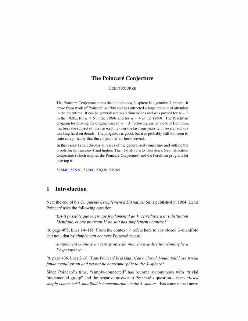
The method of proof of the h–cobordism theorem is to read the homology groups ofthe manifold from the decomposition. Since the inclusions of the ends are homotopyequivalences the relative homology groups all vanish. Reading this back to the handledecomposition, we can prescribe a number of simple moves which will trivialisethe decomposition (and prove the h–cobordism theorem). The key move is “handlecancellation”. If two handles of adjacent index are arranged like this, with the attachingsphere of the second handle meeting the belt sphere of the first in a single point thenthey cancel.

first handleSb = belt sphereof first handle

core of second handle

Sa = attaching sphereof second handle

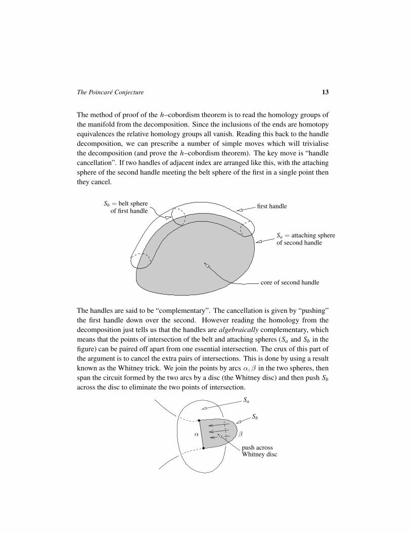
The handles are said to be “complementary”. The cancellation is given by “pushing”the first handle down over the second. However reading the homology from thedecomposition just tells us that the handles are algebraically complementary, whichmeans that the points of intersection of the belt and attaching spheres (Sa and Sb in thefigure) can be paired off apart from one essential intersection. The crux of this part ofthe argument is to cancel the extra pairs of intersections. This is done by using a resultknown as the Whitney trick. We join the points by arcs α, β in the two spheres, thenspan the circuit formed by the two arcs by a disc (the Whitney disc) and then push Sb

across the disc to eliminate the two points of intersection.

Sa

Sb

push acrossWhitney disc

α β

14 Colin Rourke

Once all the unnecessary points of intersection have been removed, the handles becomecomplementary and cancel.

The Whitney trick works nicely if the dimension of the ambient manifold is at least 5,when the required disc exists by general position. In the next section I shall sketch howthe proof was modified for the case of 4–manifolds.

For further reading on the proofs of the higher dimensional Poincare Conjecture, Irecommend Buoncristiano and Rourke [2] for the engulfing argument and Milnor [6](Diff case) or Rourke and Sanderson [10] (PL case) for the Smale proof using handletheory.

5 Dimension 4

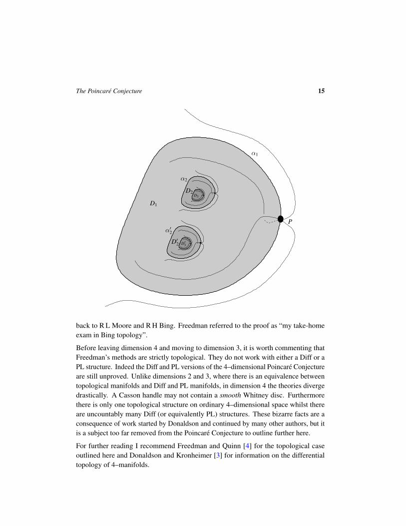
The case n = 4 of the Generalised Poincare Conjecture took a further 20 years to beproved. The eventual method of proof was similar to the Smale proof in dimension ≥ 5,using handle theory methods, but the extension was highly non-trivial. The problem isthe Whitney trick. If we try to push the argument outlined above down to dimension4, then the Whitney disc D is not obviously embedded. It may have double points ofits own. So the argument simply trades the pair of points of intersection of Sa andSb , which we need to eliminate, for one or more double points in the Whitney disc.Casson’s brilliant idea was to repeat the argument infinitely many times. Consider adouble point P in D and draw a curve in D from one of the sheets at P round to theother forming a loop α1 which in turn bounds a disc D1 (figure below). Now D1 mayhave further double points. Find such a disc D2 , D′

2 etc, for each double point in D1

and then do it again for each double point in each disc D2 , D′2 and so on, and keep

repeating this for each new disc that we use. The resulting infinite construction is atower of discs with double points indicated in the figure.

The neighbourhood of the Casson tower in the 4–manifold we are considering is calleda Casson handle. Casson’s hope was that the problem of finding an embedded versionof the original disc D might somehow be pushed to infinity by this construction. It iseasy to see that the fundamental group obstruction is killed by the construction but thisis a far cry from proving that there is an embedded disc. Casson’s hope was brilliantlyvindicated by Freedman (about 10 years later) who proved, in an argument too intricateto give any real flavour of here, that a Casson handle is a genuine topological handle.Then the Whitney disc can be found and the h–cobordism theorem, and hence thePoincare Conjecture, proved. Freedman’s argument uses a style of topology which goes

The Poincare Conjecture 15

P

D1

α1

D2

α2

D′2

α′2

D3

D′3

back to R L Moore and R H Bing. Freedman referred to the proof as “my take-homeexam in Bing topology”.

Before leaving dimension 4 and moving to dimension 3, it is worth commenting thatFreedman’s methods are strictly topological. They do not work with either a Diff or aPL structure. Indeed the Diff and PL versions of the 4–dimensional Poincare Conjectureare still unproved. Unlike dimensions 2 and 3, where there is an equivalence betweentopological manifolds and Diff and PL manifolds, in dimension 4 the theories divergedrastically. A Casson handle may not contain a smooth Whitney disc. Furthermorethere is only one topological structure on ordinary 4–dimensional space whilst thereare uncountably many Diff (or equivalently PL) structures. These bizarre facts are aconsequence of work started by Donaldson and continued by many other authors, but itis a subject too far removed from the Poincare Conjecture to outline further here.

For further reading I recommend Freedman and Quinn [4] for the topological caseoutlined here and Donaldson and Kronheimer [3] for information on the differentialtopology of 4–manifolds.

16 Colin Rourke

6 Thurston’s program

We now return to dimension 3. The excursion we have made into higher dimensionswas worth the time if only because it gives a good flavour of the kind of argumentthat mathematicians found impossible to push through in dimension 3. The methodsthat appear likely to have solved the 3–dimensional problem are, as we shall see, quitedifferent.

However, one idea that works well in other dimensions also works well in dimension 3,namely the idea of connected sum. An early result (1929) of Kneser proves that any3–manifold is the connected sum of prime 3–manifolds, ie 3–manifolds which are notthemselves connected sums (a corresponding uniqueness result was later proved byMilnor). The picture is similar to the one for surfaces given earlier (figures 2–1 and2–3) but now the connecting tubes have cross-section a 2–sphere instead of a circle(1–sphere).

(6–1)M1

M2

M3

For 3–manifolds there is another finer (and again unique) decomposition given by cuttingalong tori and Kein bottles. This is the JSJ (Jaco–Shalen–Johannson) decomposition.

P1

P2

P3

Let us call the pieces into which the 3–manifold is cut by both decompositions the“elementary pieces”. Thurston’s Geometrisation Conjecture can now be stated:

The Poincare Conjecture 17

Geometrisation Conjecture (Thurston) Each elementary piece admits a uniquegeometric structure.

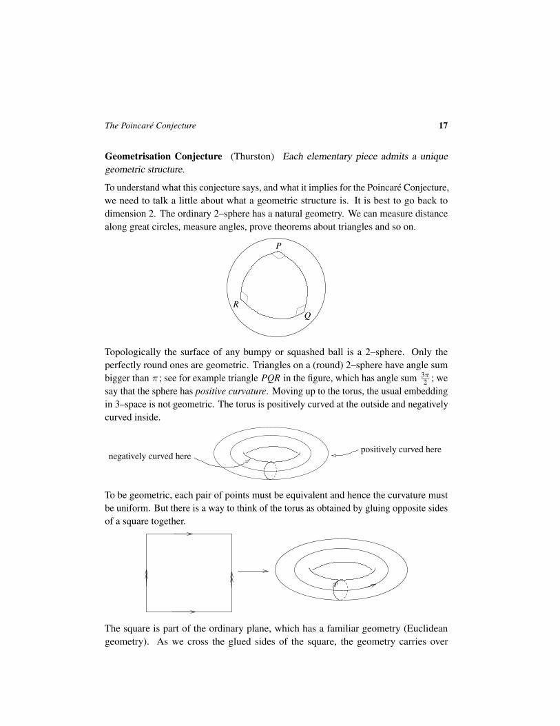
To understand what this conjecture says, and what it implies for the Poincare Conjecture,we need to talk a little about what a geometric structure is. It is best to go back todimension 2. The ordinary 2–sphere has a natural geometry. We can measure distancealong great circles, measure angles, prove theorems about triangles and so on.

P

QR

Topologically the surface of any bumpy or squashed ball is a 2–sphere. Only theperfectly round ones are geometric. Triangles on a (round) 2–sphere have angle sumbigger than π ; see for example triangle PQR in the figure, which has angle sum 3π

2 ; wesay that the sphere has positive curvature. Moving up to the torus, the usual embeddingin 3–space is not geometric. The torus is positively curved at the outside and negativelycurved inside.

negatively curved herepositively curved here

To be geometric, each pair of points must be equivalent and hence the curvature mustbe uniform. But there is a way to think of the torus as obtained by gluing opposite sidesof a square together.

The square is part of the ordinary plane, which has a familiar geometry (Euclideangeometry). As we cross the glued sides of the square, the geometry carries over

18 Colin Rourke

unchanged and thus we have a natural geometric structure on the torus. Triangles inthis geometry have angle sum exactly π and we say that this is a flat geometry or thatthe torus has zero curvature. Moving on to the double torus, we can again regard it as apolygon (in fact an octagon) with sides glued, but to get the angle right at the vertex,we need to use a non-Euclidean octagon with all angles π

4 . Then the non-Euclideangeometry of the octagon carries over to give a geometric structure to the double torus.

a

aa

b

b

bc

c

c

ddd

In the figure we have shown the octagon as part of the Poincare disc model for non-Euclidean geometry. Triangles in this geometry have angle sum less than π and we sayit has negative curvature. A similar (rather more complicated) construction works formultiple tori, which all admit geometric structures of negative curvature.

There is an analogous way to put geometric structures on connected sums of projectiveplanes. The projective plane itself can be thought of as the 2–sphere with oppositepoints identified and so has a natural geometry of positive curvature. The connectedsum of two projective planes is a Klein bottle, which has a flat geometry by a similarconstruction to the torus, and connected sums of three or more projective planes havenatural geometric structures of negative curvature.

The best way to think of the Geometrisation Conjecture is as the 3–dimensionalanalogue of this geometric description of surfaces. There are three geometries whichare analogous to the three used in dimension 2, namely:

• Spherical: the geometry of S3 (positive curvature)

• Flat: the geometry of ordinary 3–space (zero curvature)

• Hyperbolic: the geometry of non-Euclidean or hyperbolic 3–space (negativecurvature)

There are five other geometries that are needed to geometrise 3–manifolds but forunderstanding the Perelman program as it applies to the Poincare Conjecture, we can

The Poincare Conjecture 19

safely push them to the background. All we need to know is that any elementary piecewhich has a geometry other than spherical must have an infinite fundamental group.This follows from some elementary covering space theory. The universal cover (awell-defined simply-connected space which can always be constructed for manifoldsand other locally well-behaved spaces) is a copy of the archetype of the geometry (egS3 for spherical, R3 for flat etc) and all except S3 are infinite, which implies that thefundamental group of the manifold is infinite.

So now suppose that we have a prime homotopy 3–sphere. By the GeometrisationConjecture it has a geometric structure and by the remark just made it must be spherical.Then the universal cover is a copy of S3 as remarked above, but being simply-connectedit is already its universal cover, in other words it is itself a copy of S3 . So theGeometrisation Conjecture implies the Poincare Conjecture.

Before moving on to the Perelman program, it is worth remarking that progresson the classification of geometric 3–manifolds (and therefore of all 3–manifolds ifthe Geometrisation Conjecture is proved) is very advanced. There is a completeclassification of geometric 3–manifolds for all geometries except hyperbolic. Theclassification of hyperbolic 3–manifolds is currently an intense research area.

For further reading I recommend Thurston’s notes [11].

7 Perelman’s program

The Perelman program is based on work of Hamilton, who introduced the idea of theRicci flow on a differentiable manifold. We assume that our manifold has a metric, ie aprecise way of measuring distances. The Ricci flows acts on the metric. The idea isthat it should smooth out the irregularities in the metric and result in a perfectly regularmetric, in other words a geometric structure. Before wading into the technicalitiesof this program it is worth remarking that this technique is quite different from thetechniques that proved the higher dimensional Poincare Conjecture and which weoutlined in sections 4 and 5. In the engulfing proofs we considered nice subsets of themanifold and operated on them, and in the handle theory arguments we cut the manifoldup into nice pieces and then moved them around. The proofs work by passing intothe detailed makeup of the manifold. By contrast the Hamilton–Perelman program isholistic. It takes the entire manifold and operates on it all at once.

The Ricci flow is defined by a partial differential equation on the space of metrics on a

20 Colin Rourke

given manifold M . Here is the equation which defines the flow:

(7–1)∂g∂t

= −2Ricg

In the equation g denotes the metric and Ricg denotes the Ricci curvature of the metric.The equation has to be understood as an evolution equation. We consider all possiblemetrics on our manifold and we let the metric evolve so that the rate of change at anypoint is −2Ricg .

To understand this term, we need to talk about curvature. We mentioned it in the lastsection in connection with geometric surfaces. To decide how curved a surface is, lookat triangles drawn on it and compute the angle sum. One way to detect a triangle withangle sum different from π is to transport a vector around it. Below we have illustratedthe result of transporting a vector around a triangle on a sphere. The resulting vector isnot parallel to the starting vector. This corresponds to the fact that the angle sum of thetriangle is bigger than π .

It is not neceesary to use a triangle to detect curvature. Transporting a vector around anyclosed curve on the sphere results in a non-parallel vector. The same idea can be used inany manifold with a metric. By transporting vectors around small curves we can definecurvature. If we choose our curve to lie in a plane, we get the notion of the curvatureof that plane. But notice that this is a vector—the discrepancy after transport—not anumber. To define the Ricci curvature, choose a fixed vector and average curvature overall planes containing that vector. Unlike the 2–dimensional case, where there is just onelocal curvature, the Ricci curvature in dimension three is a “tensor” with 9 components(each curvature has three components and there are three independent directions to use).But there is some symmetry and there are in fact just 6 independent components. Thediagonal components of the Ricci curvature are the sectional curvatures which we canthink of as directly analogous to the curvature of a surface; these are the curvatures ofthree mutually perpendicular hyperplanes measured in a perpendicular direction. If weadd these three we get the scalar curvature which gives a rough idea of how curved the

The Poincare Conjecture 21

manifold is. It was Hamilton’s insight, vindicated by Perelman, that the Ricci curvatureis the correct notion of curvature to use to evolve a general metric.

Perhaps the best way to try to understand the Ricci flow (equation 7–1) is by analogywith other, more intuitive, flows. The heat equation describes the diffusion of heat in asolid body. we have a very clear idea of how heat flows. It evens itself out. Highs getlower, lows get higher and the (asymptotic) end result is a uniform distribution witheach point having the same temperature. The Ricci flow equation describes a similarflow on the metric of a manifold: it smoothes out local variations. But there are obviousdifferences. The metric does not necessarily become uniform. If we start in a regionwhere the Ricci curvature is negative then the equation says that the metric grows, inother words points get pushed apart and the curvature moves upwards towards flatness.Conversely if we start where the curvature is positive then points get pulled togetherand the curvature becomes more intense.

A remarkable early result of Hamilton on the Ricci flow is that, if all points have positiveRicci curvature, then the flow does even the curvature out perfectly. The manifoldshrinks towards a round 3–sphere (or a manifold which is covered by a round 3–sphere).This proves the Poincare Conjecture for manifolds which admit metrics of positiveRicci curvature. However we cannot expect anything so nice to happen for a general3–manifold. A general 3–manifold does not admit a perfectly uniform metric (ie ageometric structure). We need to cut the manifold into pieces first. So if the Ricciflow is going to prove the Geometrisation Conjecture then it must naturally lead tosingularities whose resolution causes us to cut the manifold into pieces. Hamilton knewthis but he could not analyse all the cases of what can happen when the flow goessingular, and his program ground to a halt.

It is easy to see that the flow must go singular in finite time for many starting conditions.This is because there is an evolution equation for minimum of the scalar curvature. Itmust change to become greater. If it ever becomes positive, then it must go to infinity infinite time, in other words the flow must become singular.

It is here that Perelman takes over the story. His first breakthrough was a “no localcollapsing” result which completely overcame the problems that Hamilton ran into.Using this result and some very sharp and careful analysis he controls closely whathappens when the Ricci flow becomes singular. What he proves is that the singularitieswhich appear all have a tubular region which is a 2–sphere cross a line. What he thendoes is to cut across and glue in caps to fill in the 2–sphere. This is called “surgery”.

22 Colin Rourke

After surgery the Ricci flow can be restarted. The change is sufficiently simple thatit can be described topologically. Indeed the topological picture is very similar to theconnected sum decomposition pictured in figure 6–1. At this point, let us assume thatwe have started with a prime homotopy sphere. Then the surgeries can only removetrivial parts of the manifold and exactly one bit must be the manifold we started with.We now consider the sequence: flow −→ surgery −→ flow −→ surgery etc, which iscalled a Ricci flow with surgery. There are a number of careful estimates which can bemade for the Ricci flow after surgery in terms of the flow before and we can analyse thewhole sequence, just as if we were not changing the manifold. The crux of the proofnow is to prove two key results:

(1) Surgery times do not accumulate: we are not forced to perform infinitely manysurgeries in a finite time interval.

(2) The whole flow becomes extinct after a finite time.

It then follows that, after a finite number of surgeries which discard trivial parts of theoriginal manifold, we arrive at a situation where the whole manifold shrinks to a point,which can be recognised as the end of the Hamilton proof for positive Ricci curvature.In other words we have arrived at a 3–sphere (or a manifold covered by a 3–sphere: butsince we are assuming simple-connectivity, this latter case does not arise) and provedthe Poincare Conjecture.

The proof of (1) is one of the most delicate parts of the whole program. There areseveral parameters which are chosen each time we do a surgery. What Perelman provesis that these parameters can be chosen so that the amount of volume lost by the surgery(notice that some part of the original manifold gets cut out at surgery) is greater thata certain small amount. If we had infinitely many surgeries in a finite time, then aninfinite volume would be lost. But it is easy to estimate the amount of volume gainedby the flow and not enough is gained. So this proves (1).

The Poincare Conjecture 23

To prove (2) Perelman uses an estimate for the change of area of minimal surfaces underRicci flow with surgery, which is proved by an integral calculation. The area changes ina way which shows that area must decrease to zero in a finite time. If we could fill thewhole manifold with such surfaces, then the whole manifold would shrink to zero, inother words the flow would become extinct.

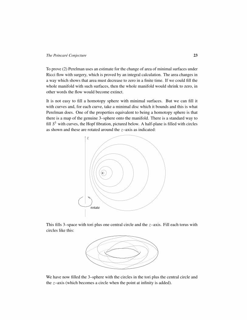
It is not easy to fill a homotopy sphere with minimal surfaces. But we can fill itwith curves and, for each curve, take a minimal disc which it bounds and this is whatPerelman does. One of the properties equivalent to being a homotopy sphere is thatthere is a map of the genuine 3–sphere onto the manifold. There is a standard way tofill S3 with curves, the Hopf fibration, pictured below. A half-plane is filled with circlesas shown and these are rotated around the z–axis as indicated:

rotate

z

This fills 3–space with tori plus one central circle and the z–axis. Fill each torus withcircles like this:

We have now filled the 3–sphere with the circles in the tori plus the central circle andthe z–axis (which becomes a circle when the point at infinity is added).

24 Colin Rourke

If we now use the map of S3 onto our homotopy sphere then the homotopy sphere is alsofilled by curves. For each such curve we find a minimal disc which it bounds. We letthe Ricci flow act and we also let the curves flow using the curve-shrinking flow. Thisis a natural way to make curves in a manifold more uniform. Again we can think of itas analogous to heat flow: curves move uniformly towards curves of minimal curvaturewhich are called geodesics. A similar integral calculation shows that the area of theminimal discs must then go to zero in finite time and again this calculation applies toRicci flows with surgery.

However there is a serious technical problem to be solved. Like the Ricci flow, thecurve-shrinking flow can run into singularities where the curvature of a curve goesinfinite. Indeed the family of curves that we start with will very probably have suchsingularities in-built before the flow starts. Below we have sketched the genericsingularity in a family of this type. It is called a cusp singularity.

The diagram shows part of a 2–parameter family of curves in a 3–manifold. The centralcurve has a cusp; around it in a circle are curves which resolve the cusp in all possibleways.

To overcome this problem, Perelman uses a technique originally applied to plane curves(called “ramps”) which, under the right conditions, allows the flow to pass throughsingularities. If we could use smooth general position at this point, then the singularitieswould be isolated (each curve would be singular for a finite number of times) and thistechnique would complete the proof. But general position does not apply to analytic

The Poincare Conjecture 25

flows of this type and instead Perelman uses the ramp technique, but not to the finallimit. He stops near the limit and makes some very delicate estimates. These show thatthe time occupied by the singularities is small enough that the estimate, which showsthat a minimal disc must shrink to zero in finite time, applies to all the discs in thefamily and they must all shrink to zero in finite time proving that the flow with surgerybecomes extinct.

This completes the outline of the Perelman program for proof of the Poincare Conjecture.For completeness I would like to finish by giving some idea of how the program provesthe Geometrisation Conjecture. For this it is not possible to work only for a finitetime. With a general 3–manifold, the Ricci flow continues indefinitely and indeed it ispossible that there are an infinite number of surgeries (or rather it has not been provedthat there are only a finite number). What Perelman does is to use similar estimatesto those used to control the singularities to give a picture of the long-term behaviourof the flow. Eventually the flow settles down to give a decomposition of the manifoldinto a “thick” part and a “thin” part. To decide whether we are in a thick or thin part,we consider how far we can walk in all possible directions without coming back to ourstarting position. I have sketched this decomposition below.

thick

thick

thin

thin

In the thin part, a short walk around one of the tubes gets us back to our starting position.The thick part has uniformly negative curvature, in other words a hyperbolic geometricstructure. The thin part is what is know as a “graph” manifold. These manifolds can bedescribed explicitly (they are connected sums of Seifert fibre spaces and surface bundles)and all have appropriate geometric structures; it is here that the geometries other thanspherical and hyperbolic must be used. The final picture proves the GeometrisationConjecture.

26 Colin Rourke

For further reading of an introductory nature on the Perelman program for the PoincareConjecture, I recommend the introduction to Morgan and Tian [7] and for the Geometri-sation Conjecture, the introduction and outlines of Perelman’s papers to be found in thenotes of Kleiner and Lott [5]. For more detail on both topics, read the main texts of [7]and [5].

References

[1] M A Armstrong, Basic topology, Springer Undergrad. Text Ser. (1983)

[2] Sandro Buoncristiano and Colin Rourke, Fragments of topology from the sixties, Geom.Topol. Monogr. 6 (2003–7)

[3] Simon Donaldson and Peter Kronheimer, The geometry of four-manifolds, Oxford Math.Monogr. OUP (1990)

[4] Michael Freedman and Frank Quinn, Topology of 4–manifolds, Princeton Math. Ser. 39,Princeton UP (1990)

[5] Bruce Kleiner and John Lott, Notes on Perelman’s papers, arXiv:math.DG/0605667

[6] John Milnor, Lectures on the h–cobordism theorem, Princeton University Press (1965)

[7] John W Morgan and Gang Tian, Ricci flow and the Poincare Conjecture,arXiv:math.DG/0607607

[8] Grisha Perelman, The entropy formula for the Ricci flow and its geometric appli-cations, Ricci flow with surgery on three-manifolds, and Finite extinction time forthe solutions to the Ricci flow on certain three-manifolds, arXiv:math.DG/0211159,arXiv:math.DG/0303109, arXiv:math.DG/0307245

[9] Henri Poincare, Cinquieme complement a l’analysus situs, Ouvres de Poincare, Ed.Gauthier-Villars, Tome VI, Paris (1953) 435–498: Originally published: Rendiconti deCircolo Matematica di Palermo, 18 (1904) 45–110

[10] Colin Rourke and Brian Sanderson, Introduction to piecewise-linear topology, SpringerStudy Edition (1982)

[11] William P Thurston, The geometry and topology of three-manifolds, available on-line at:http://www.msri.org/publications/books/gt3m/

Mathematics Institute, University of WarwickCoventry CV4 7AL, UK

cpr@msp.warwick.ac.uk