The Power of Choice in Data-Aware Cluster Scheduling

Shivaram Venkataraman1, Aurojit Panda1, Ganesh Ananthanarayanan2, Michael J. Franklin1, Ion Stoica1

1UC Berkeley 2 Microsoft Research

AbstractProviding timely results in the face of rapid growth indata volumes has become important for analytical frame-works. For this reason, frameworks increasingly operateon only a subset of the input data. A key property ofsuch sampling is that combinatorially many subsets ofthe input are present. We present KMN, a system thatleverages these choices to perform data-aware schedul-ing, i.e., minimize time taken by tasks to read their in-puts, for a DAG of tasks. KMN not only uses choices toco-locate tasks with their data but also percolates suchcombinatorial choices to downstream tasks in the DAGby launching a few additional tasks at every upstreamstage. Evaluations using workloads from Facebook andConviva on a 100-machine EC2 cluster show that KMNreduces average job duration by 81% using just 5% ad-ditional resources.

1 Introduction

Data-intensive computation frameworks drive manymodern services like web search indexing and recom-mendation systems. Computation frameworks (e.g.,Hadoop [14], Spark [60], Dryad [38]) translate a job intoa DAG of many small tasks, and execute them efficientlyon compute slots across large clusters. Tasks of inputstages (e.g., map in MapReduce or extract in Dryad) readtheir data from distributed storage and pass their out-puts to the downstream intermediate tasks (e.g., reducein MapReduce or full-aggregate in Dryad).

The efficient execution of these predominantly I/O-intensive tasks is predicated on data-aware scheduling,i.e., minimizing the time taken by tasks to read their data.Widely deployed techniques for data-aware schedulingexecute tasks on the same machine as their data (ifthe data is on one machine, as for input tasks) [8, 59]and avoid congested network links (when data is spreadacross machines, as for intermediate tasks) [13, 24].However, despite these techniques, we see that produc-tion jobs in Facebook’s Hadoop cluster are slower by87% compared to perfect data-aware scheduling (§2.3).This is because, in multi-tenant clusters, compute slotsthat are ideal for data-aware task execution are often un-available.

A1

A2

A3

A4

Existing Scheduler

app input:two blocksA1, A3

A1

A2

A3

A4

app input: anytwo blocks from{A1, A2, A3, A4}(6 choices)

KMN Scheduler

App providesall subsets

(a) (b)

App selects two blocks(e.g. A1, A3)

Figure 1: “Late binding” allows applications to specifymore inputs than tasks and schedulers dynamically choosetask inputs at execution time.

The importance of data-aware scheduling is increasingwith rapid growth in data volumes [31]. To cope withthis data growth and yet provide timely results, there is atrend of jobs using only a subset of their data. Examplesinclude sampling-based approximate query processingsystems [5,12] and machine learning algorithms [16,42].A key property of such jobs is that they can computeon any of the combinatorially many subsets of the in-put dataset without compromising application correct-ness. For example, say a machine learning algorithmlike stochastic gradient descent [16] needs to computeon a 5% uniform random sample of data. If the data isspread over 100 blocks then the scheduler can choose any5 blocks and has

(1005

)input choices for this job.

Our goal is to leverage the combinatorial choice of in-puts for data-aware scheduling. Current schedulers re-quire the application to select a subset of the data onwhich the scheduler runs the job. This prevents thescheduler from taking advantage of available choices. Incontrast, we argue for “late binding” i.e., choosing thesubset of data dynamically depending on the current stateof the cluster (see Figure 1). This dramatically increasesthe number of data local slots for input tasks (e.g., maptasks), which increases the probability of achieving datalocality even during high cluster utilizations.

Extending the benefits of choice to intermediate stages(e.g., reduce) is challenging because they consume allthe outputs produced by upstream tasks. Thus, they haveno choice in picking their inputs. When upstream out-puts are not evenly spread across machines, the over-subscribed network links, typically cross-rack switch

1

links [24], become the bottleneck. We introduce choicesfor intermediate stages by launching a small number ofadditional tasks in the previous stage. As an example,consider a job with 400 map tasks and 50 reduce tasks.By launching 5% extra map tasks (420 tasks), we canpick the 400 map outputs that best avoid congested links.

Choosing the best upstream outputs used by interme-diate stages is non-trivial due to complex communica-tion patterns like many-to-many (for reduce tasks) andmany-to-one (for joins). In fact, selecting the best up-stream outputs can be shown to be NP-hard. We developan efficient round-robin heuristic that attempts to bal-ance data transfers evenly across cross-rack switch links.Further, upstream tasks do not all finish simultaneouslydue to stragglers [13, 61]. We handle stragglers in up-stream tasks using a delay-based approach that balancesthe gains in balanced network transfers against the timespent waiting for stragglers. In the above example, forinstance, it may schedule reduce tasks based on the ear-liest 415 map tasks and ignore the last 5 stragglers.

In summary, we make the following contributions:

• Identify the trend of combinatorial choices in inputsof jobs and leverage this for data-aware scheduling.

• Extend the benefits of choices to a DAG of stagesby running a few extra tasks in each upstream stage.

• Build KMN, a system for analytics frameworks toseamlessly benefit from the combinatorial choices.

We have implemented KMN inside Spark [60]. Weevaluate KMN using jobs from a production workload atConviva, a video analytics company, and by replaying atrace from a production Hadoop cluster at Facebook. Ourexperiments on an EC2 cluster with 100 machines showthat we can reduce average job duration by 81% (93% ofideal improvements) compared to Spark’s scheduler. Ourgains are due to KMN achieving 98% memory locality forinput tasks and improving intermediate data transfers by48%, while using ≤ 5% extra resources.

2 Choices and Data-Awareness

In this section we first discuss application trends that re-sult in increased choices for scheduling (§2.1). We thenexplain data-aware scheduling (§2.2) and quantify its po-tential benefit in production clusters (§2.3).

2.1 Application Trends

With the rapid increase in the volume of data collected,it has become prohibitively expensive for data analyticsframeworks to operate on all of the data. To provide

timely results, there is a trend towards trading off accu-racy for performance. Quick results obtained from justpart of the dataset are often good enough.(1) Approximate Query Processing: Many analyt-ics frameworks support approximate query processing(AQP) using standard SQL syntax (e.g., BlinkDB [5],Presto [29]). They power many popular applicationslike exploratory data analysis [19,54] and interactive de-bugging [3]. For example, products analysts could useAQP systems to quickly decide if an advertising cam-paign needs to be changed based on a sample of clickthrough rates. AQP systems can bound both the timetaken and the quality of the result by selecting appropri-ately sized inputs (samples) to met the deadline and errorbound. Sample sizes are typically small relative to theoriginal data (often, one-twentieth to one-fifth [43]) andmany equivalent samples exist. Thus, sample selectionpresents a significant opportunity for smart scheduling.(2) Machine Learning: The last few years has seen thedeployment of large-scale distributed machine learningalgorithms for commercial applications like spam clas-sification [40] and machine translation [18]. Recent ad-vances [17] have introduced stochastic versions of thesealgorithms, for example stochastic gradient descent [16]or stochastic L-BFGS [53], that can use small randomdata samples and provide statistically valid results evenfor large datasets. These algorithms are iterative andeach iteration processes only a small sample of the data.Stochastic algorithms are agnostic to the sample selectedin each iteration and support flexible scheduling.(3) Erasure Coded Storage: Rise in data volumes havealso led to clusters employing efficient storage tech-niques like erasure codes [50]. Erasure codes providefault tolerance by storing k extra parity blocks for everyn data blocks. Using any n data blocks of the (n+ k)blocks, applications can compute their input. Such stor-age systems also provide choices for data-aware schedul-ing.

Note that while the above applications provide an op-portunity to pick any subset of the input data, our systemcan also handle custom sampling functions, which gen-erate samples based on application requirements.

2.2 Data-Aware Scheduling

Data aware scheduling is important for both the inputas well as intermediate stages of jobs due to their IO-intensive nature. In the input stage, tasks reads their in-put from a single machine and the natural goal is localityi.e. to schedule the task on a machine that stores its input(§2.2.1). For intermediate stages, tasks have their inputspread across multiple machines. In this case, it is notpossible to co-locate the task with all its inputs. Instead,the goal in this case is to schedule the task at a machine

2

that minimizes the time it takes to transfer all remote in-puts. As over-subscribed cross-rack links are the mainbottleneck in reads [22], we seek to balance the utiliza-tion of these links (§2.2.2).

2.2.1 Memory Locality for Input Tasks

Riding on the trend of falling memory prices, clustersare increasingly caching data in memory [11, 58]. Asmemory bandwidths are about 10×−100× greater thanthe fastest network bandwidths, data reads from memoryprovide dramatic acceleration for the IO-intensive ana-lytics jobs. However, to reap the benefits of in-memorycaches, tasks have to be scheduled with memory locality,i.e., on the same machine that contains their input data.Obtaining memory locality is important for timely com-pletion of interactive approximate queries [9]. Iterativemachine learning algorithms typically run 100’s of iter-ations and lack of memory locality results in huge slow-down per iteration and the overall job.

Achieving memory locality is a challenging problemin clusters. Since in-memory storage is used only asa cache, data stored in memory is typically not repli-cated. Further, the amount of memory in a cluster isrelatively small (often by three orders of magnitude [9])when compared to stable storage: this difference meansthat replicating data in memory is not practical. There-fore, techniques for improving locality [8] developed fordisk-based replicated storage are insufficient; they relyon the probability of locality increasing with the numberof replicas. Further, as job completion times are dictatedby the slowest task in the job, improving performancerequires memory locality for all its tasks [11].

These challenges are reflected in production Hadoopclusters. A Facebook trace from 2010 [8, 21] shows thatless than 60% of tasks achieve locality even with threereplicas. As in-memory data is not replicated, it is harderfor jobs to achieve memory locality for all their tasks.

2.2.2 Balanced Network for Intermediate Tasks

Intermediate stages of a job have communication pat-terns that result in their tasks reading inputs from manymachines (e.g., all-to-all “shuffle” or many-to-one “join”stages). For I/O intensive intermediate tasks, the timeto access data across the network dominates the run-ning time, more so when intermediate outputs are storedin memory. Despite fast network links [56] and newertopologies [6, 35], bandwidths between machines con-nected to the same rack switch are still 2× to 5× higherthan to machines outside the rack switch via the net-work core. Thus the runtime for an intermediate stageis dictated by the amount of data transferred acrossracks. Prior work has also shown that reducing cross-

Rack Switch Rack Switch Rack Switch Rack Switch

R1

Rack Switch Rack Switch

M1 M2 M3 M4

R2 R3 R4

M1 M2 M3 M4

R1 R2 R3 R4

d12

d13

d14

d22

d23

d24

d31

d41

d31

d34

d12

d22

d42

d13

d23

d43

d41

d42

d43

d14

d24

d34

d14

d23

d24

d13

d13

d23

d43

d32

d34

d31

d14

d24

d34

d41

d42

d43

Reduce task

Map task Mi Rj Transfer from Mi to Rj di

j

d41

d32

d42

d31

(a) (b)

Figure 2: Value of balanced network usage for a job with 4map tasks and 4 reduce tasks. The left-hand side has unbal-anced cross-rack links (maximum of 6 transfers, minimumof 2) while the right-hand side has better balance (maxi-mum of 4 transfers, minimum of 3).

1 2 5 10 20 50

0.00.20.40.60.81.0

Ratio of transfers on most loaded rack to transfers on least loaded rack

CD

F

< 50 tasks50−150 tasks>150 tasks

Figure 3: CDF of cross-rack skew for the Facebook tracesplit by number of map tasks. Reducing cross-rack skewimproves intermediate stage performance.

rack hotspots, i.e., optimizing the bottleneck cross-racklink [13, 24] can significantly improve performance.

Given the over-subscribed cross-rack links and theslowest tasks dictating job completion, it is important tobalance traffic on the cross-rack links [15]. Figure 2 il-lustrates the result of having unbalanced cross-rack links.The schedule in Figure 2(b) results in a cross-rack skew,i.e., ratio of the highest to lowest used network links, ofonly 4

3 (or 1.33) as opposed to 62 (or 3) in Figure 2(a).

To highlight the importance of cross-rack skew, weused a trace of Hadoop jobs run in a Facebook clusterfrom 2010 [21] and computed the cross-rack skew ratio.Figure 3 shows a CDF of this ratio and is broken downby the number of map tasks in the job. From the figurewe can see that for jobs with 50− 150 map tasks morethan half of the jobs have a cross-rack skew of over 4×.For larger jobs we see that the median is 15× and the90th percentile value is in excess of 30×.

2.3 Potential Benefits

How much do the above-mentioned lack of locality andimbalanced network usage hurt jobs? We estimate thepotential for data-aware scheduling to speed up jobs us-ing the same Facebook trace (described in detail in §6).

3

0.0 0.2 0.4 0.6 0.8 1.0

0.0

0.2

0.4

0.6

0.8

1.0

Utilization

Pro

b. A

ll Ta

sks

Loca

l K=100

N=2000N=1000N=300N=200Pre−selected

0.0 0.2 0.4 0.6 0.8 1.0

0.0

0.2

0.4

0.6

0.8

1.0

Utilization

K=10

N=200N=100N=30N=20Pre−selected

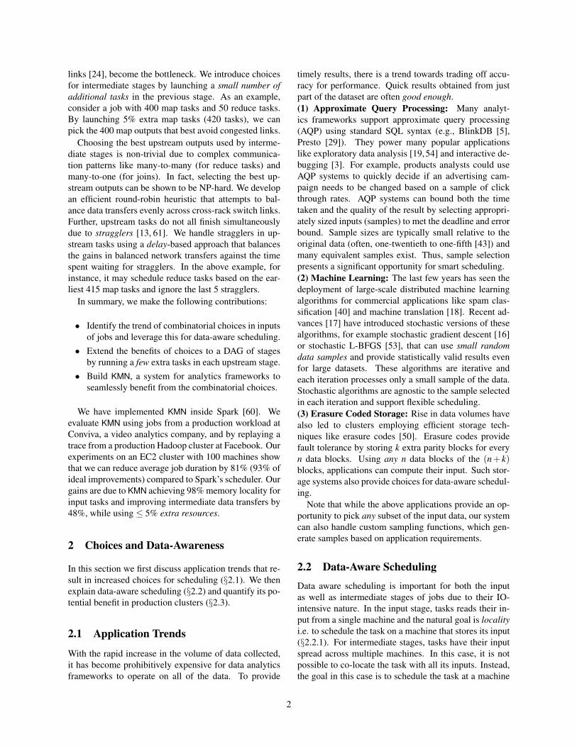
Figure 4: Probability of input-stage locality when choosingany K out of N blocks. The scheduler can choose to executea job on any of

(KN)

samples.

We mimic job performance with an ideal data-awarescheduler using a “what-if” simulator. Our simulator isunconstrained and (i) assigns memory locality for all thetasks in the input phase (we assume 20× speed up formemory locality [45] compared to reading data over thenetwork based on our micro-benchmark) and (ii) placestasks to perfectly balance cross-rack links. We see thatjobs speed up by 87.6% on average with such ideal data-aware scheduling.

Given these potential benefits, we have designedKMN, a scheduling framework that exploits the availablechoices to improve performance. At the heart of KMN liescheduling techniques to increase locality for input (§3)stages and balance network usage for intermediate (§4)stages. In §5, we describe an interface that allows appli-cations to specify all available choices to the scheduler.

3 Input Stage

For the input stage (i.e., the map stage in MapReduceor the extract stage in Dryad) accounting for combinato-rial choice leads to improved locality and hence reducedcompletion time. Here we analyze the improvements inlocality in two scenarios: in §3.1 we look at jobs whichcan use any K of the N input blocks; in §3.2 we look atjobs which use a custom sampling function.

We assume a cluster with s compute slots per ma-chine. Tasks operate on one input block each and inputblocks are uniformly distributed across the cluster, this isin line with the block placement policy used by Hadoop.For ease of analysis we assume machines in the clusterare uniformly utilized (i.e., there are no hot-spots). Inour evaluation §6) we consider hot-spots due to skewedinput-block and machine popularity.

3.1 Choosing any K out of N blocksMany modern systems e.g., BlinkDB [5], Presto [29],AQUA [2] operate by choosing a random subset ofblocks from shuffled input data. These systems rely

0.0 0.2 0.4 0.6 0.8 1.0

0.0

0.2

0.4

0.6

0.8

1.0

Utilization

Pro

b. A

ll Ta

sks

Loca

l K=100

f=20f=10f=5f=2f=1

0.0 0.2 0.4 0.6 0.8 1.0

0.0

0.2

0.4

0.6

0.8

1.0

Utilization

K=10

f=20f=10f=5f=2f=1

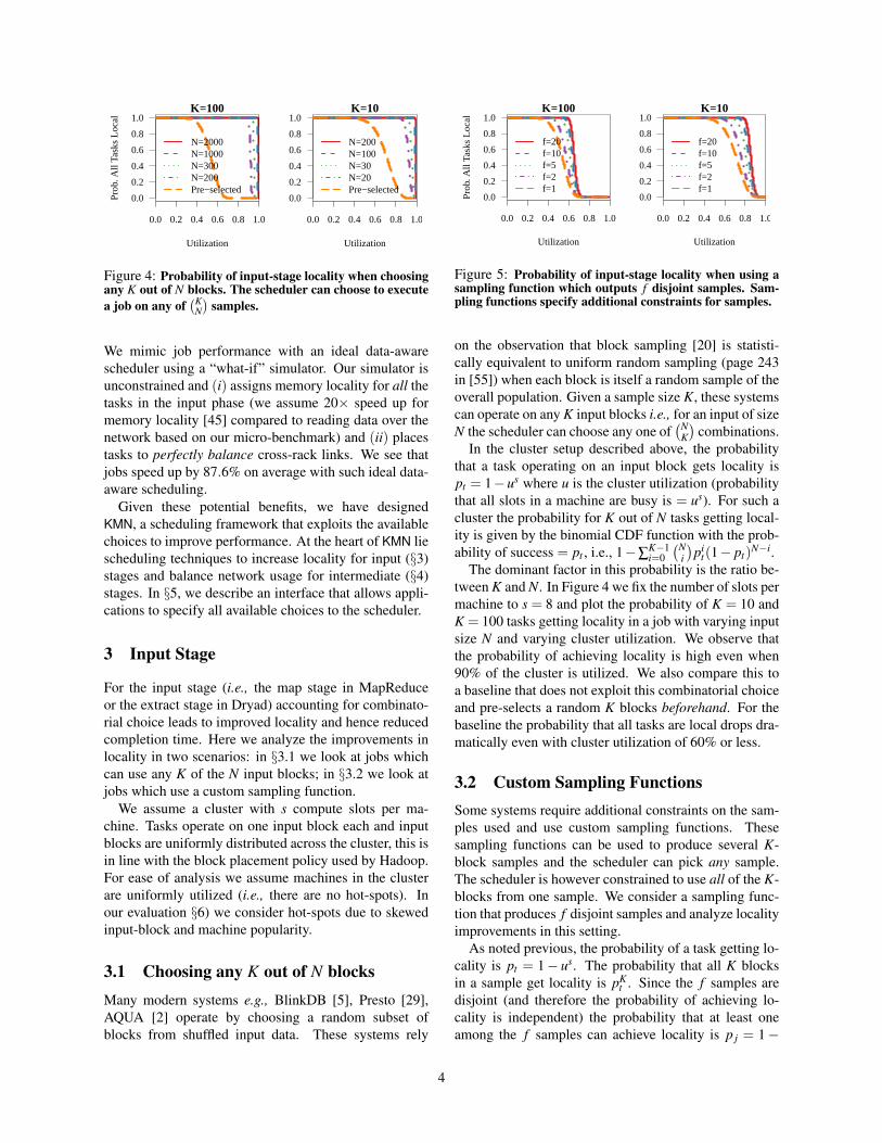
Figure 5: Probability of input-stage locality when using asampling function which outputs f disjoint samples. Sam-pling functions specify additional constraints for samples.

on the observation that block sampling [20] is statisti-cally equivalent to uniform random sampling (page 243in [55]) when each block is itself a random sample of theoverall population. Given a sample size K, these systemscan operate on any K input blocks i.e., for an input of sizeN the scheduler can choose any one of

(NK

)combinations.

In the cluster setup described above, the probabilitythat a task operating on an input block gets locality ispt = 1−us where u is the cluster utilization (probabilitythat all slots in a machine are busy is = us). For such acluster the probability for K out of N tasks getting local-ity is given by the binomial CDF function with the prob-ability of success = pt , i.e., 1−∑

K−1i=0

(Ni

)pi

t(1− pt)N−i.

The dominant factor in this probability is the ratio be-tween K and N. In Figure 4 we fix the number of slots permachine to s = 8 and plot the probability of K = 10 andK = 100 tasks getting locality in a job with varying inputsize N and varying cluster utilization. We observe thatthe probability of achieving locality is high even when90% of the cluster is utilized. We also compare this toa baseline that does not exploit this combinatorial choiceand pre-selects a random K blocks beforehand. For thebaseline the probability that all tasks are local drops dra-matically even with cluster utilization of 60% or less.

3.2 Custom Sampling FunctionsSome systems require additional constraints on the sam-ples used and use custom sampling functions. Thesesampling functions can be used to produce several K-block samples and the scheduler can pick any sample.The scheduler is however constrained to use all of the K-blocks from one sample. We consider a sampling func-tion that produces f disjoint samples and analyze localityimprovements in this setting.

As noted previous, the probability of a task getting lo-cality is pt = 1− us. The probability that all K blocksin a sample get locality is pK

t . Since the f samples aredisjoint (and therefore the probability of achieving lo-cality is independent) the probability that at least oneamong the f samples can achieve locality is p j = 1−

4

(1− pKt )

f . Figure 5 shows the probability of K = 10and K = 100 tasks achieving locality with varying uti-lization and number of samples. We see that the proba-bility of achieving locality significantly increases with f .At f = 5 we see that small jobs (10 tasks) can achievecomplete locality even when the cluster is 80% utilized.

We thus find that accounting for combinatorial choicescan greatly improve locality for the input stage. Next weanalyze improvements for intermediate stages.

4 Intermediate Stages

Intermediate stages of jobs commonly involve one-to-all (broadcast), many-to-one (coalesce) or many-to-many(shuffle) network transfers [23]. These transfers arenetwork-bound and hence, often slowed down by con-gested cross-rack network links. As described in §2.2.2,data-aware scheduling can improve performance by bet-ter placement of both upstream and downstream tasks tobalance the usage of cross-rack network links.

While effective heuristics can be used in schedulingdownstream tasks to balance network usage (we dealwith this in §5), they are nonetheless limited by thelocations of the outputs of upstream tasks. Schedul-ing upstream tasks to balance the locations of their out-puts across racks is often complicated due to many dy-namic factors in clusters. First, they are constrained bydata locality (§3) and compromising locality is detrimen-tal. Second, the utilization of the cross-rack links whendownstream tasks start executing are hard to predict inmulti-tenant clusters. Finally, even the size of upstreamoutputs varies across jobs and are not known beforehand.

We overcome these challenges by scheduling a few ad-ditional upstream tasks. For an upstream stage with Ktasks, we schedule M tasks (M > K). Additional tasksincrease the likelihood that task outputs are distributedacross racks. This allows us to choose the “best” K outof M upstream tasks, out of

(MK

)choices, to minimize

cross-rack network utilization. In the rest of this sec-tion, we show analytically that a few additional upstreamtasks can significantly reduce the imbalance (§4.1). §4.2describes a heuristic to pick the best K out of M up-stream tasks. However, not all M upstream tasks mayfinish simultaneously because of stragglers; we modifyour heuristic to account for stragglers in §4.3.

4.1 Additional Upstream TasksWhile running additional tasks can balance network us-age, it is important to consider how many additional tasksare required. Too many additional tasks can often lead toworsening of overall cluster performance.

We analyze this using a simple model of the schedul-ing of upstream tasks. For simplicity, we assume that

1.0 1.2 1.4 1.6

1234567

200 tasks100 tasks50 tasks10 tasks

Uniform

M/K values

Cro

ss−

rack

ske

w

(a)

1.0 1.2 1.4 1.6

1

2

5

10

20200 tasks100 tasks50 tasks10 tasks

Log−Normal

M/K values

Cro

ss−

rack

ske

w

(b)

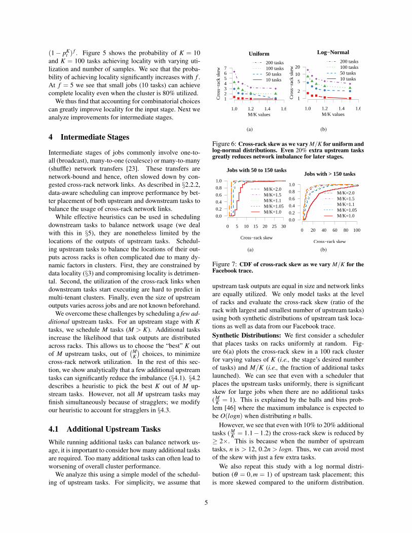
Figure 6: Cross-rack skew as we vary M/K for uniform andlog-normal distributions. Even 20% extra upstream tasksgreatly reduces network imbalance for later stages.

0 5 10 15 20 25 30

0.0

0.2

0.4

0.6

0.8

1.0

M/K=2.0M/K=1.5M/K=1.1M/K=1.05M/K=1.0

Jobs with 50 to 150 tasks

Cross−rack skew

(a)

0 20 40 60 80 100

0.0

0.2

0.4

0.6

0.8

1.0

Cross−rack skew

M/K=2.0M/K=1.5M/K=1.1M/K=1.05M/K=1.0

Jobs with > 150 tasks

(b)

Figure 7: CDF of cross-rack skew as we vary M/K for theFacebook trace.

upstream task outputs are equal in size and network linksare equally utilized. We only model tasks at the levelof racks and evaluate the cross-rack skew (ratio of therack with largest and smallest number of upstream tasks)using both synthetic distributions of upstream task loca-tions as well as data from our Facebook trace.Synthetic Distributions: We first consider a schedulerthat places tasks on racks uniformly at random. Fig-ure 6(a) plots the cross-rack skew in a 100 rack clusterfor varying values of K (i.e., the stage’s desired numberof tasks) and M/K (i.e., the fraction of additional taskslaunched). We can see that even with a scheduler thatplaces the upstream tasks uniformly, there is significantskew for large jobs when there are no additional tasks( M

K = 1). This is explained by the balls and bins prob-lem [46] where the maximum imbalance is expected tobe O(logn) when distributing n balls.

However, we see that even with 10% to 20% additionaltasks ( M

K = 1.1−1.2) the cross-rack skew is reduced by≥ 2×. This is because when the number of upstreamtasks, n is > 12, 0.2n > logn. Thus, we can avoid mostof the skew with just a few extra tasks.

We also repeat this study with a log normal distri-bution (θ = 0,m = 1) of upstream task placement; thisis more skewed compared to the uniform distribution.

5

However, even with a log-normal distribution, we againsee that a few extra tasks can be very effective at reduc-ing skew. This is because the expected value of the mostloaded bin is still linear and using 0.2n additional tasksis sufficient to avoid most of the skew.Facebook Distributions: We repeat the above analy-sis using the number and location of upstream tasks ofa phase in the Facebook trace (used in §2.2.2). Recallthe high cross-rack skew in the Facebook trace. Despitethat, again, a few additional tasks suffices to eliminate alarge fraction of the skews. Figure 7 plots the results forvarying values of M

K for different jobs. A large fractionof the skew is reduced by running just 10% more tasks.This is nearly 66% of the reductions we get using M

K = 2.In summary we see that running a few extra tasks is an

effective strategy to reduce skew, both with synthetic aswell as real-world distributions. We next look at mecha-nisms that can help us achieve such reduction.

4.2 Selecting Best Upstream OutputsThe problem of selecting the best K outputs from the Mupstream tasks can be stated as follows: We are givenM upstream tasks U = u1...uM , R downstream tasks D =d1...dR and their corresponding rack locations. Let usassume that tasks are distributed over racks 1...L and letU ′⊂U be some set of K upstream outputs. Then for eachrack we can define the uplink cost C2i−1 and downlinkcost C2i using a cost function Ci(U ′,D). Our objectivethen is to select U ′ to minimize the most loaded link i.e.

argminU ′

maxi∈2L

Ci(U ′,D)

While this problem is NP-Hard [57], many approxi-mation heuristics have been developed. We use a heuris-tic that corresponds to spreading our choice of K outputsacross as many racks as possible.1

Our implementation for this approximation heuristic isshown in Algorithm 1. We start with the list of upstreamtasks and build a hash map that stores how many taskswere run on each rack. Next we sort the tasks first bytheir index within a rack and then by the number of tasksin the rack. This sorting criteria ensures that we first seeone task from each rack, thus ensuring we spread ourchoices across racks. We use an additional heuristic offavoring racks with more outputs to help our downstreamtask placement techniques (§5.2.2). The main computa-tion cost in this method is the sorting step and hence thisruns in O(MlogM) time for M tasks.

1This problem is an instance of the facility location problem [26]where we have a set of clients (downstream tasks), set of potential fa-cility locations (upstream tasks), a cost function that maps facility lo-cations to clients (link usage). Our heuristic follows from picking afacility that is farthest from the existing set of facilities [30].

Algorithm 1 Choosing K upstream outputs out of Musing a round-robin strategy

1: Given: upstreamTasks - list with rack, index within rackfor each task

2: Given: K - number of tasks to pick

3: // Number of upstream tasks in each rack

4: upstreamRacksCount = map()5:6: // Initialize

7: for task in upstreamTasks do8: upstreamRacksCount[task.rack] += 19: end for

10:11: // Sort the tasks in round-robin fashion

12: roundRobin = upstreamTasks.sort(CompareTasks)13: chosenK = roundRobin[0 : K]14: return chosenK15:16: procedure COMPARETASKS(task1, task2)17: if task1.idx != task2.idx then18: // Sort first by index

19: return task1.idx < task2.idx20: else21: // Then by number of outputs

22: numRack1 = upstreamRacksCount[task1.rack]23: numRack2 = upstreamRacksCount[task2.rack]24: return numRack1 > numRack225: end if26: end procedure

4.3 Handling Upstream Stragglers

While the previous section described a heuristic to pickthe best K out of M upstream outputs, waiting for allM can be inefficient due to stragglers. Stragglers inthe upstream stage can delay completion of some taskswhich cuts into the gains obtained by balancing thenetwork links. Stragglers are a common occurrencein clusters with many clusters reporting significantlyslow tasks despite many prevention and speculation solu-tions [10, 13, 61]. This presents a trade-off in waiting forall M tasks and obtaining the benefits of choice in pickingupstream outputs against the wasted time for completionof all M upstream tasks including stragglers. Our solu-tion for this problem is to schedule downstream tasks atsome point after K upstream tasks have completed butnot wait for the stragglers in the M tasks. We quantifythis trade-off with analysis and micro-benchmarks.

4.3.1 Stragglers vs. Choice

We study the impact of stragglers in the Facebook tracewhen we run 2%, 5% and 10% extra tasks (i.e., M

K =1.02,1.05,1.1). We compute the difference between thetime taken for the fastest K tasks and the time to com-

6

1 to 10 11 to 50 51 to 150 >150

Number of upstream tasks

% In

crea

se w

aitin

g fo

rad

ditio

nal u

pstr

eam

task

s

0

20

40

60

80

1002% Extra5% Extra10% Extra

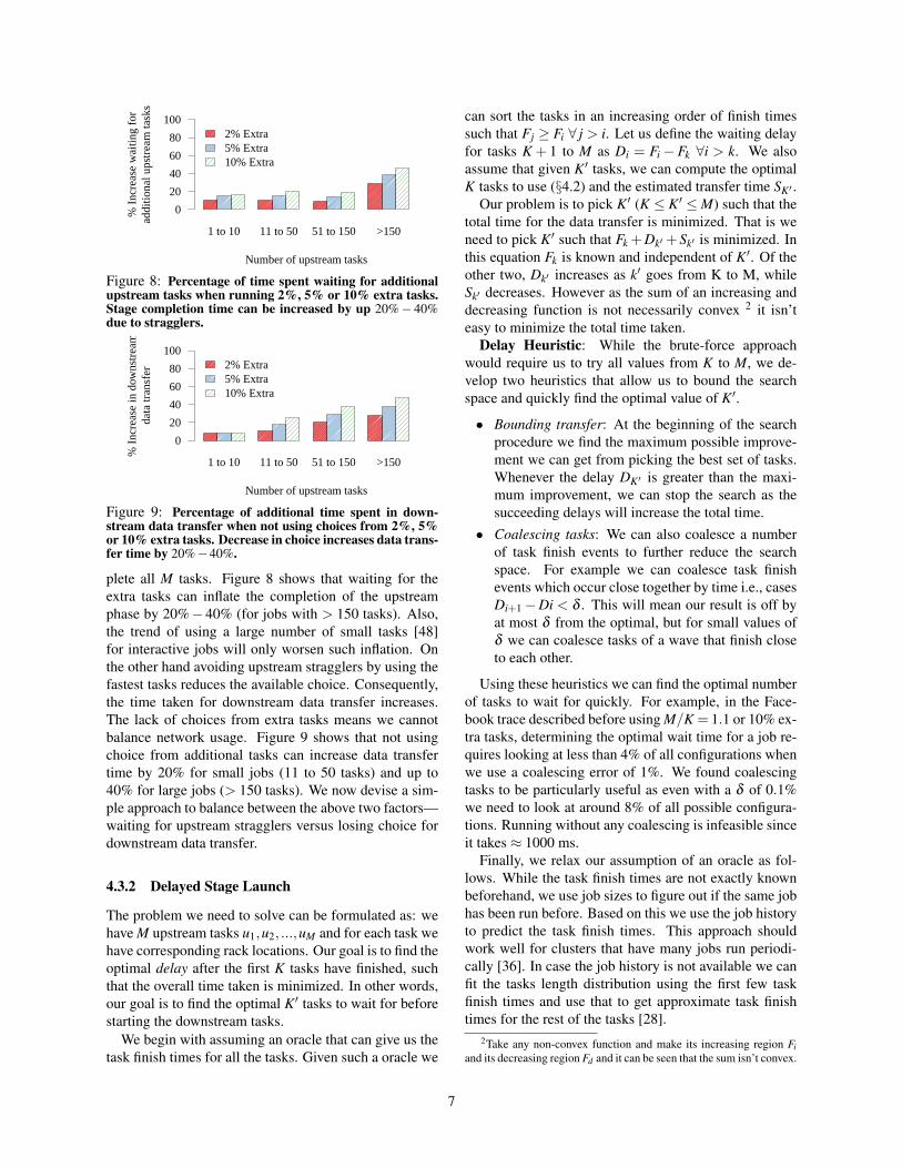
Figure 8: Percentage of time spent waiting for additionalupstream tasks when running 2%, 5% or 10% extra tasks.Stage completion time can be increased by up 20%− 40%due to stragglers.

1 to 10 11 to 50 51 to 150 >150

Number of upstream tasks

% In

crea

se in

dow

nstr

eam

data

tran

sfer

0

20

40

60

80

1002% Extra5% Extra10% Extra

Figure 9: Percentage of additional time spent in down-stream data transfer when not using choices from 2%, 5%or 10% extra tasks. Decrease in choice increases data trans-fer time by 20%−40%.

plete all M tasks. Figure 8 shows that waiting for theextra tasks can inflate the completion of the upstreamphase by 20%−40% (for jobs with > 150 tasks). Also,the trend of using a large number of small tasks [48]for interactive jobs will only worsen such inflation. Onthe other hand avoiding upstream stragglers by using thefastest tasks reduces the available choice. Consequently,the time taken for downstream data transfer increases.The lack of choices from extra tasks means we cannotbalance network usage. Figure 9 shows that not usingchoice from additional tasks can increase data transfertime by 20% for small jobs (11 to 50 tasks) and up to40% for large jobs (> 150 tasks). We now devise a sim-ple approach to balance between the above two factors—waiting for upstream stragglers versus losing choice fordownstream data transfer.

4.3.2 Delayed Stage Launch

The problem we need to solve can be formulated as: wehave M upstream tasks u1,u2, ...,uM and for each task wehave corresponding rack locations. Our goal is to find theoptimal delay after the first K tasks have finished, suchthat the overall time taken is minimized. In other words,our goal is to find the optimal K′ tasks to wait for beforestarting the downstream tasks.

We begin with assuming an oracle that can give us thetask finish times for all the tasks. Given such a oracle we

can sort the tasks in an increasing order of finish timessuch that Fj ≥ Fi ∀ j > i. Let us define the waiting delayfor tasks K + 1 to M as Di = Fi−Fk ∀i > k. We alsoassume that given K′ tasks, we can compute the optimalK tasks to use (§4.2) and the estimated transfer time SK′ .

Our problem is to pick K′ (K ≤ K′ ≤M) such that thetotal time for the data transfer is minimized. That is weneed to pick K′ such that Fk +Dk′ +Sk′ is minimized. Inthis equation Fk is known and independent of K′. Of theother two, Dk′ increases as k′ goes from K to M, whileSk′ decreases. However as the sum of an increasing anddecreasing function is not necessarily convex 2 it isn’teasy to minimize the total time taken.

Delay Heuristic: While the brute-force approachwould require us to try all values from K to M, we de-velop two heuristics that allow us to bound the searchspace and quickly find the optimal value of K′.

• Bounding transfer: At the beginning of the searchprocedure we find the maximum possible improve-ment we can get from picking the best set of tasks.Whenever the delay DK′ is greater than the maxi-mum improvement, we can stop the search as thesucceeding delays will increase the total time.

• Coalescing tasks: We can also coalesce a numberof task finish events to further reduce the searchspace. For example we can coalesce task finishevents which occur close together by time i.e., casesDi+1−Di < δ . This will mean our result is off byat most δ from the optimal, but for small values ofδ we can coalesce tasks of a wave that finish closeto each other.

Using these heuristics we can find the optimal numberof tasks to wait for quickly. For example, in the Face-book trace described before using M/K = 1.1 or 10% ex-tra tasks, determining the optimal wait time for a job re-quires looking at less than 4% of all configurations whenwe use a coalescing error of 1%. We found coalescingtasks to be particularly useful as even with a δ of 0.1%we need to look at around 8% of all possible configura-tions. Running without any coalescing is infeasible sinceit takes ≈ 1000 ms.

Finally, we relax our assumption of an oracle as fol-lows. While the task finish times are not exactly knownbeforehand, we use job sizes to figure out if the same jobhas been run before. Based on this we use the job historyto predict the task finish times. This approach shouldwork well for clusters that have many jobs run periodi-cally [36]. In case the job history is not available we canfit the tasks length distribution using the first few taskfinish times and use that to get approximate task finishtimes for the rest of the tasks [28].

2Take any non-convex function and make its increasing region Fiand its decreasing region Fd and it can be seen that the sum isn’t convex.

7

// SQL Query

SELECT status, SUM(quantity)

FROM items

GROUP BY status

// Spark Query

kv = file.map{ li =>

(li.l linestatus,li.quantity)}result = kv.reduceByKey{(a,b) =>

a + b}.collect()

// KMN Query

sample = file.blockSample(0.1, sampler=None)

kv = sample.map{ li =>

(li.l linestatus,li.quantity)}result = kv.reduceByKey{(a,b) =>

a + b}.collect()

Figure 10: An example of a query in SQL, Spark and KMN

5 System Implementation

We have built KMN on top of Spark [60], an open-sourcecluster computing framework. Our implementation isbased on Spark version 0.7.3 and KMN consists of 1400lines of Scala code. In this section we discuss the featuresof our implementation and implementation challenges.

5.1 Application Interface

We define a blockSample operator which jobs can useto specify input constraints (for instance, use K blocksfrom file F) to the framework.The blockSample opera-tor takes two arguments: the ratio K

N and a sampling func-tion that can be used to impose constraints. The samplingfunction can be used to choose user-defined sampling al-gorithms (e.g., stratified sampling). By default the sam-pling function picks any K of N blocks.

Consider an example SQL query and its correspond-ing Spark [60] version shown in Figure 10. To run thesame query in KMN we just need to prefix the query withthe blockSample operator. The sampler argument is aScala closure and passing None causes the scheduler touse the default function which picks any K out of the Ninput blocks. This design can be readily adapted to othersystems like Hadoop MapReduce and Dryad.

KMN also provides an interface for jobs to introspectwhich samples where used in a computation. This canbe used for error estimation using algorithms like Boot-strap [4] and also provides support for queries to be re-peated. We implement this in KMN by storing the K parti-tions used during computation as a part of a job’s lineage.Using the lineage also ensures that the same samples areused if the job is re-executed during fault recovery [60].

5.2 Task SchedulingWe modify Spark’s scheduler in KMN to implement thetechniques described in earlier sections.

5.2.1 Input Stage

Schedulers for frameworks like MapReduce or Sparktypically use a slot-based model where the scheduler isinvoked whenever a slot becomes available in the cluster.In KMN, to choose any K out of N blocks we modify thescheduler to run tasks on blocks local to the first K avail-able slots. To ensure that tasks don’t suffer from resourcestarvation while waiting for locality, we use a timeout af-ter which tasks are scheduled on any available slot. Notethat, choosing the first K slots provides a sample similaror slightly better in quality compared to existing systemslike Aqua [2] or BlinkDB [5] that reuse samples for shorttime periods. To schedule jobs with custom samplingfunctions, we similarly modify the scheduler to chooseamong the available samples and run the computation onthe sample that has the highest locality.

5.2.2 Intermediate Stage

Existing cluster computing frameworks like Spark andHadoop place intermediate stages without accounting fortheir dependencies. However smarter placement whichaccounts for a tasks’ dependencies can improve perfor-mance. We implemented two strategies in KMN:

Greedy assignment: The number of cross-rack trans-fers in the intermediate stage can be reduced by co-locating map and reduce tasks (more generally any de-pendent tasks). In the greedy placement strategy wemaximize the number of reduce tasks placed in the rackwith the most map tasks. This strategy works well forsmall jobs where network usage can be minimized byplacing all the reduce tasks in the same rack.

Round-robin assignment: While greedy placementminimizes the number of transfers from map tasks to re-duce tasks it results in most of the data being sent toone or a few racks. Thus the links into these racks arelikely to be congested. This problem can be solved bydistributing tasks across racks while simultaneously min-imizing the amount of data sent across racks. This can beachieved by evenly distributing the reducers across rackswith map tasks. This strategy can be shown to be opti-mal if we know the map task locations and is similar innature to the algorithm described in §4.2. We perform amore detailed comparison of the two approaches in §6

5.3 Support for extra tasksOne consequence of launching extra tasks to improveperformance is that the cluster utilization could be af-

8

Q1 Q2 Q3 Q4

Tim

e (s

econ

ds)

0

2

4

6

8

10

92 % 77.1 % 71.1 % 74.7 %

KMN−M/K=1.05Baseline

(a) Conviva queries with 1% Sampling

Q1 Q2 Q3 Q4

Tim

e (s

econ

ds)

0

5

10

15

83.1 % 78.9 %

39.3 %38.6 %

KMN−M/K=1.05Baseline

(b) Conviva queries with 5% Sampling

Q1 Q2 Q3 Q4

Tim

e (s

econ

ds)

0

5

10

15

20

79.8 % 77.8 %

26.9 %

24.7 %KMN−M/K=1.05Baseline

(c) Conviva queries with 10% Sampling

Figure 11: Comparing baseline and KMN-1.05 with sampling-queries from Conviva. Numbers on the bars represent per-centage improvement when using KMN-M/K = 1.05.

fected by these extra tasks. To avoid utilization spikes,in KMN the value for M/K (the percentage of extra tasksto launch) can only be set by the cluster administratorand not directly by the application. Further, we imple-mented support for killing tasks once the scheduler de-cides that the tasks’ output is not required. Killing tasksin Spark is challenging as tasks are run in threads andmany tasks share the same process. To avoid expensiveclean up associated with killing threads [1], we modifiedtasks in Spark to periodically poll and check a status bit.This means that tasks sometimes could take a few sec-onds more before they are terminated, but we found thatthis overhead was negligible in practice.

In KMN, using extra tasks is crucial in extending theflexibility of many choices throughout the DAG. In §3and §4 we discussed how to use the available choices inthe input and intermediate stages in a DAG. However,jobs created using frameworks like Spark or DryadLINQcan extend across many more stages. For example, com-plex SQL queries may use a map followed a shuffle to doa group-by operation and follow that up with a join. Onesolution to this would be run more tasks than required inevery stage to retain the ability to choose among inputsin succeeding stages. However we found that in prac-tice this does not help very much. In frameworks likeSpark which use lazy evaluation, every stage followingthan the first stage is treated as an intermediate stage.As we use a round-robin strategy to schedule intermedi-ate tasks (§5.2.2), the outputs from the first intermediatestage are already well spread out across the racks. Thusthere isn’t much skew across racks that affects the per-formance of following stages. In evaluation runs we sawno benefits for later stages of long DAGs.

6 Evaluation

We evaluate the benefits of KMN using two approaches:first we run approximate queries used in production atConviva, a video analytics company, and study how KMNcompares to using existing schedulers with pre-selectedsamples. Next we analyze how KMN behaves in a sharedcluster, by replaying a workload trace obtained from

Facebook’s production Hadoop cluster.Metric: In our evaluation we measure percentage im-

provement of job completion time when using KMN. Wedefine percentage improvement as:

% Improvement =Baseline Time−KMN Time

Baseline Time×100

Our evaluation shows that,

• KMN improves real-world sampling-based queriesfrom Conviva by more than 50% on average acrossvarious sample sizes and machine learning work-loads by up to 43%.

• When replaying the Facebook trace, on an EC2cluster, KMN can improve job completion time by81% on average (92% for small jobs)

• By using 5% – 10% extra tasks we can balancebottleneck link usage and decrease shuffle times by61% – 65% even for jobs with high cross-rack skew.

6.1 SetupCluster Setup:We run all our experiments using 100m2.4xlarge machines on Amazon’s EC2 cluster, witheach machine having 8 cores, 68GB of memory and 2local drives. We configure Spark to use 4 slots and 60GB per machine. To study memory locality we cache theinput dataset before starting each experiment. We com-pare KMN with a baseline that operates on a pre-selectedsample of size K and does not employ any of the shuf-fle improvement techniques described in §4, §5. We alsolabel the fraction of extra tasks run (i.e., M/K), so KMN-M/K = 1.0 has K = M and KMN-M/K = 1.05 has 5%extra tasks. Finally, all experiments were run at leastthree times and we plot median values across runs anduse error bars to show minimum and maximum values.Workload: Our evaluation uses a workload trace fromFacebook’s Hadoop cluster [21]. The traces are from amix of interactive and batch jobs and capture over halfa million jobs on a 3500 node cluster. We use a scaleddown version of the trace to fit within our cluster and usethe same inter-arrival times and the task-to-rack mapping

9

.

.

.

Aggregate 2

Aggregate 3

Aggregate 1Gradient

Figure 12: Execution DAG for Stochastic Gradient Descent(SGD).

22.01 15.28

13.73 12.52

0 5 10 15 20 25

1

Average time for Stochastic Gradient Descent (s)

KMN-M/K=1.1 KMN-M/K=1.05 KMN-M/K=1.0 Baseline

Figure 13: Overall improvement when running StochasticGradient Descent using KMN

as in the trace. Unless specified, we use 10% samplingwhen running KMN for all jobs in the trace.

We begin by showing overall gains with KMN (§6.2),then present benefits for input stages from KMN (§6.3)and finally show how KMN affects intermediate stages( §6.4).

6.2 Benefits of KMN

We evaluate the benefits of using KMN on three work-loads: real-world approximate queries from Conviva, amachine learning workload running Stochastic GradientDescent and a Hadoop workload trace from Facebook.

6.2.1 Conviva Sampling jobs

We first present results from running 4 real-world sam-pling queries obtained from Conviva, a video analyticscompany. The queries were run on access logs obtainedacross a 5-day interval. We treat the entire data set as Nblocks and vary the sampling fraction (K/N) to be 1%,5% and 10%. We run the queries at 50% cluster utiliza-tion and run each query multiple times.

Figure 11 shows the median time taken for each queryand we compare KMN-M/K = 1.05 to the baseline thatuses pre-selected samples. For query 1 and query 2 wecan see that KMN gives 77%–91% win across 1%, 5%and 10% samples. Both these queries calculate summarystatistics across a time window and most of the compu-tation is performed in the map stage. For these queriesKMN ensures that we get memory locality and this re-sults in significant improvements. For queries 3 and 4,we see around 70% improvement for 1% samples, andthis reduces to around 25% for 10% sampling. Both

0.00 5.00 10.00 15.00 20.00

Job

Aggregate1

Aggregate2

Aggregate3

Time (s)

KMN (First Three Stages) KMN (First Two Stages) KMN (First Stage) KMN-M/K=1.0

Figure 14: Breakdown of aggregation times when usingKMN for different number of stages in SGD

Job Size % Overall % Map Stage % Shuffle1 to 10 92.8 95.5 84.61

11 to 100 78 94.1 28.63> 100 60.8 95.4 31.02

Table 1: Improvements over baseline, by job size and stage

these queries compute the number of distinct users thatmatch a specified criteria. While input locality also im-proves these queries, for larger samples the reduce tasksare CPU bound (while they aggregate values).

6.2.2 Machine learning workload

Next, we look at performance benefits for a machinelearning workload that uses sampling. For our analysis,we use Stochastic Gradient Descent (SGD). SGD is an it-erative method that scales to large datasets and is widelyused in applications such as machine translation and im-age classification. We run SGD on a dataset contain-ing 2 million data items, where each each item contains4000 features. The complete dataset is around 64GB insize and each of our iterations operates on a 1% sample1% of the data. Thus the random sampling step reducesthe cost of gradient computation by 100× but maintainsrapid learning rates [52]. We run 10 iterations in eachsetting to measure the total time taken for SGD.

Each iteration consists of a DAG comprised of a mapstage where the gradient is computed on sampled dataitems and the gradient is then aggregated from all points.The aggregation step can be efficiently performed by us-ing an aggregation tree as shown in Figure 12. We imple-ment the aggregation tree using a set of shuffle stages anduse KMN to run extra tasks at each of these aggregationstages.

The overall benefits from using KMN are shown inFigure 13. We see that KMN-M/K = 1.1 improves per-formance by 43% as compared to the baseline. Theseimprovements come from a combination of improvingmemory locality for the first stage and by improvingshuffle performance for the aggregation stages. We fur-ther break down the improvements by studying the ef-fects of KMN at every stage in Figure 14.

10

0−10

11−100

>100

Job Completion Time (seconds)

0 10 20 30 40 50

92.8 %

78 %

60.8 %

BaselineKMN−M/K=1.05

Job

Siz

e

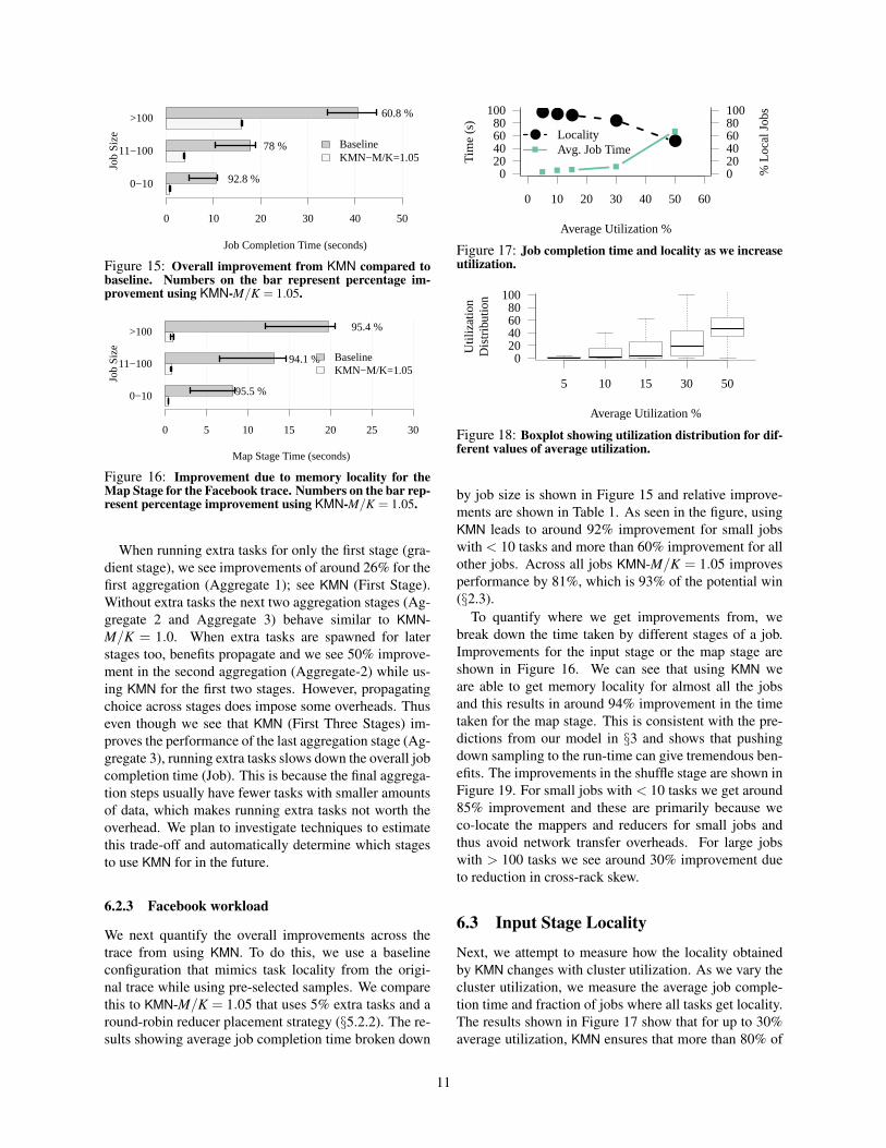
Figure 15: Overall improvement from KMN compared tobaseline. Numbers on the bar represent percentage im-provement using KMN-M/K = 1.05.

0−10

11−100

>100

Map Stage Time (seconds)

0 5 10 15 20 25 30

95.5 %

94.1 %

95.4 %

BaselineKMN−M/K=1.05

Job

Siz

e

Figure 16: Improvement due to memory locality for theMap Stage for the Facebook trace. Numbers on the bar rep-resent percentage improvement using KMN-M/K = 1.05.

When running extra tasks for only the first stage (gra-dient stage), we see improvements of around 26% for thefirst aggregation (Aggregate 1); see KMN (First Stage).Without extra tasks the next two aggregation stages (Ag-gregate 2 and Aggregate 3) behave similar to KMN-M/K = 1.0. When extra tasks are spawned for laterstages too, benefits propagate and we see 50% improve-ment in the second aggregation (Aggregate-2) while us-ing KMN for the first two stages. However, propagatingchoice across stages does impose some overheads. Thuseven though we see that KMN (First Three Stages) im-proves the performance of the last aggregation stage (Ag-gregate 3), running extra tasks slows down the overall jobcompletion time (Job). This is because the final aggrega-tion steps usually have fewer tasks with smaller amountsof data, which makes running extra tasks not worth theoverhead. We plan to investigate techniques to estimatethis trade-off and automatically determine which stagesto use KMN for in the future.

6.2.3 Facebook workload

We next quantify the overall improvements across thetrace from using KMN. To do this, we use a baselineconfiguration that mimics task locality from the origi-nal trace while using pre-selected samples. We comparethis to KMN-M/K = 1.05 that uses 5% extra tasks and around-robin reducer placement strategy (§5.2.2). The re-sults showing average job completion time broken down

0 10 20 30 40 50 60

020406080

100

Average Utilization %

Tim

e (s

)

● ● ●●

●

020406080100

% L

ocal

Job

s

● LocalityAvg. Job Time

Figure 17: Job completion time and locality as we increaseutilization.

5 10 15 30 50

020406080

100

Average Utilization %

Util

izat

ion

Dis

trib

utio

n

Figure 18: Boxplot showing utilization distribution for dif-ferent values of average utilization.

by job size is shown in Figure 15 and relative improve-ments are shown in Table 1. As seen in the figure, usingKMN leads to around 92% improvement for small jobswith < 10 tasks and more than 60% improvement for allother jobs. Across all jobs KMN-M/K = 1.05 improvesperformance by 81%, which is 93% of the potential win(§2.3).

To quantify where we get improvements from, webreak down the time taken by different stages of a job.Improvements for the input stage or the map stage areshown in Figure 16. We can see that using KMN weare able to get memory locality for almost all the jobsand this results in around 94% improvement in the timetaken for the map stage. This is consistent with the pre-dictions from our model in §3 and shows that pushingdown sampling to the run-time can give tremendous ben-efits. The improvements in the shuffle stage are shown inFigure 19. For small jobs with < 10 tasks we get around85% improvement and these are primarily because weco-locate the mappers and reducers for small jobs andthus avoid network transfer overheads. For large jobswith > 100 tasks we see around 30% improvement dueto reduction in cross-rack skew.

6.3 Input Stage Locality

Next, we attempt to measure how the locality obtainedby KMN changes with cluster utilization. As we vary thecluster utilization, we measure the average job comple-tion time and fraction of jobs where all tasks get locality.The results shown in Figure 17 show that for up to 30%average utilization, KMN ensures that more than 80% of

11

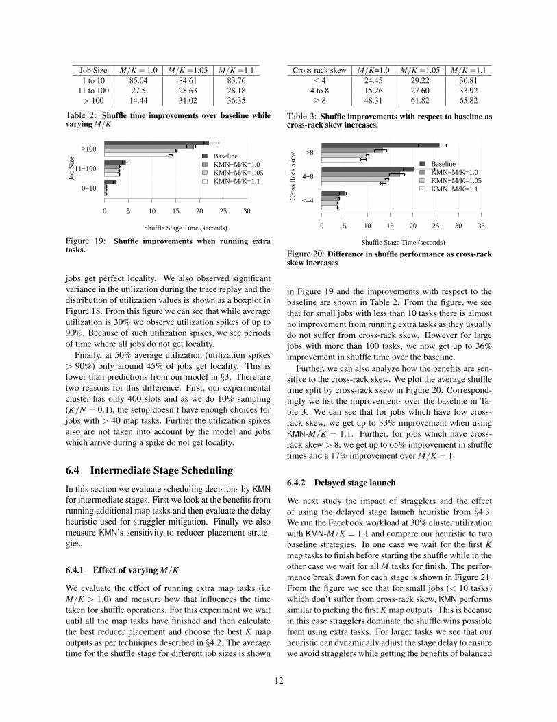
Job Size M/K = 1.0 M/K =1.05 M/K =1.11 to 10 85.04 84.61 83.76

11 to 100 27.5 28.63 28.18> 100 14.44 31.02 36.35

Table 2: Shuffle time improvements over baseline whilevarying M/K

0−10

11−100

>100

Shuffle Stage Time (seconds)

0 5 10 15 20 25 30

BaselineKMN−M/K=1.0KMN−M/K=1.05KMN−M/K=1.1Jo

b S

ize

Figure 19: Shuffle improvements when running extratasks.

jobs get perfect locality. We also observed significantvariance in the utilization during the trace replay and thedistribution of utilization values is shown as a boxplot inFigure 18. From this figure we can see that while averageutilization is 30% we observe utilization spikes of up to90%. Because of such utilization spikes, we see periodsof time where all jobs do not get locality.

Finally, at 50% average utilization (utilization spikes> 90%) only around 45% of jobs get locality. This islower than predictions from our model in §3. There aretwo reasons for this difference: First, our experimentalcluster has only 400 slots and as we do 10% sampling(K/N = 0.1), the setup doesn’t have enough choices forjobs with > 40 map tasks. Further the utilization spikesalso are not taken into account by the model and jobswhich arrive during a spike do not get locality.

6.4 Intermediate Stage Scheduling

In this section we evaluate scheduling decisions by KMNfor intermediate stages. First we look at the benefits fromrunning additional map tasks and then evaluate the delayheuristic used for straggler mitigation. Finally we alsomeasure KMN’s sensitivity to reducer placement strate-gies.

6.4.1 Effect of varying M/K

We evaluate the effect of running extra map tasks (i.eM/K > 1.0) and measure how that influences the timetaken for shuffle operations. For this experiment we waituntil all the map tasks have finished and then calculatethe best reducer placement and choose the best K mapoutputs as per techniques described in §4.2. The averagetime for the shuffle stage for different job sizes is shown

Cross-rack skew M/K=1.0 M/K =1.05 M/K =1.1≤ 4 24.45 29.22 30.81

4 to 8 15.26 27.60 33.92≥ 8 48.31 61.82 65.82

Table 3: Shuffle improvements with respect to baseline ascross-rack skew increases.

<=4

4−8

>8

Shuffle Stage Time (seconds)

Cro

ss R

ack

skew

0 5 10 15 20 25 30 35

BaselineKMN−M/K=1.0KMN−M/K=1.05KMN−M/K=1.1

Figure 20: Difference in shuffle performance as cross-rackskew increases

in Figure 19 and the improvements with respect to thebaseline are shown in Table 2. From the figure, we seethat for small jobs with less than 10 tasks there is almostno improvement from running extra tasks as they usuallydo not suffer from cross-rack skew. However for largejobs with more than 100 tasks, we now get up to 36%improvement in shuffle time over the baseline.

Further, we can also analyze how the benefits are sen-sitive to the cross-rack skew. We plot the average shuffletime split by cross-rack skew in Figure 20. Correspond-ingly we list the improvements over the baseline in Ta-ble 3. We can see that for jobs which have low cross-rack skew, we get up to 33% improvement when usingKMN-M/K = 1.1. Further, for jobs which have cross-rack skew > 8, we get up to 65% improvement in shuffletimes and a 17% improvement over M/K = 1.

6.4.2 Delayed stage launch

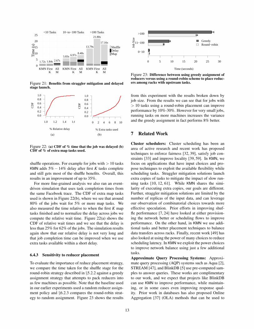
We next study the impact of stragglers and the effectof using the delayed stage launch heuristic from §4.3.We run the Facebook workload at 30% cluster utilizationwith KMN-M/K = 1.1 and compare our heuristic to twobaseline strategies. In one case we wait for the first Kmap tasks to finish before starting the shuffle while in theother case we wait for all M tasks for finish. The perfor-mance break down for each stage is shown in Figure 21.From the figure we see that for small jobs (< 10 tasks)which don’t suffer from cross-rack skew, KMN performssimilar to picking the first K map outputs. This is becausein this case stragglers dominate the shuffle wins possiblefrom using extra tasks. For larger tasks we see that ourheuristic can dynamically adjust the stage delay to ensurewe avoid stragglers while getting the benefits of balanced

12

<10 Tasks 10−to−100 Tasks >100 Tasks

1.72s1.84s2.67s

5.83s6.97s8.48s

13.79s

21.80s

17.16s

0

5

10

15

20

25

KMN FirstK

AllM

KMN FirstK

AllM

KMN FirstK

AllM

Tim

e (s

)

ShuffleDelayMap

Figure 21: Benefits from straggler mitigation and delayedstage launch.

1.0 1.2 1.4 1.6

0.00.20.40.60.81.0

% Relative delay

CD

F

(a)

0 2 4 6 8 10

0.00.20.40.60.81.0

% Extra tasks used

CD

F

(b)

Figure 22: (a) CDF of % time that the job was delayed (b)CDF of % of extra map tasks used.

shuffle operations. For example for jobs with > 10 tasksKMN adds 5%− 14% delay after first K tasks completeand still gets most of the shuffle benefits. Overall, thisresults in an improvement of up to 35%.

For more fine-grained analysis we also ran an event-driven simulation that uses task completion times fromthe same Facebook trace. The CDF of extra map tasksused is shown in Figure 22(b), where we see that around80% of the jobs wait for 5% or more map tasks. Wealso measured the time relative to when the first K maptasks finished and to normalize the delay across jobs wecompute the relative wait time. Figure 22(a) shows theCDF of relative wait times and we see that the delay isless than 25% for 62% of the jobs. The simulation resultsagain show that our relative delay is not very long andthat job completion time can be improved when we useextra tasks available within a short delay.

6.4.3 Sensitivity to reducer placement

To evaluate the importance of reduce placement strategy,we compare the time taken for the shuffle stage for theround-robin strategy described in §5.2.2 against a greedyassignment strategy that attempts to pack reducers intoas few machines as possible. Note that the baseline usedin our earlier experiments used a random reducer assign-ment policy and §6.2.3 compares the round-robin strat-egy to random assignment. Figure 23 shows the results

0−10

11−100

>100

Time (seconds)

0 5 10 15 20 25 30

GreedyRound−robin

Job

Siz

e

Figure 23: Difference between using greedy assignment ofreducers versus using a round-robin scheme to place reduc-ers among racks with upstream tasks.

from this experiment with the results broken down byjob size. From the results we can see that for jobs with> 10 tasks using a round-robin placement can improveperformance by 10%-30%. However for very small jobs,running tasks on more machines increases the varianceand the greedy assignment in fact performs 8% better.

7 Related Work

Cluster schedulers: Cluster scheduling has been anarea of active research and recent work has proposedtechniques to enforce fairness [32, 39], satisfy job con-straints [33] and improve locality [39, 59]. In KMN, wefocus on applications that have input choices and pro-pose techniques to exploit the available flexibility whilescheduling tasks. Straggler mitigation solutions launchextra copies of tasks to mitigate the impact of slow run-ning tasks [10, 12, 61]. While KMN shares the simi-larity of executing extra copies, our goals are different.Further, straggler mitigation solutions are limited by thenumber of replicas of the input data, and can leverageour observation of combinatorial choices towards moreeffective speculation. Prior efforts in improving shuf-fle performance [7, 24] have looked at either provision-ing the network better or scheduling flows to improveperformance. On the other hand, in KMN we use addi-tional tasks and better placement techniques to balancedata transfers across racks. Finally, recent work [49] hasalso looked at using the power of many choices to reducescheduling latency. In KMN we exploit the power choicesto improve network balance using just a few additionaltasks.Approximate Query Processing Systems: Approxi-mate query processing (AQP) systems such as Aqua [2],STREAM [47], and BlinkDB [5] use pre-computed sam-ples to answer queries. These works are complimentaryto our work, and we expect that projects like BlinkDBcan use KMN to improve performance, while maintain-ing, or in some cases even improving response qual-ity. Prior work in databases has also proposed OnlineAggregation [37] (OLA) methods that can be used to

13

present approximate aggregation results while the inputdata is processed in a streaming fashion. Recent exten-sions [25, 51] have also looked at supporting OLA-stylecomputations in MapReduce. In contrast, KMN can beused for scheduling sampling applications which do notprocess the entire dataset and process a fixed and smallsample of data.Machine learning frameworks: Recently, a large bodyof work has focused on building cluster computingframeworks that support machine learning tasks. Ex-amples include GraphLab [34, 44], Spark [60], DistBe-lief [27], and MLBase [41]. Of these, GraphLab andSpark add support for abstractions commonly used inmachine learning. Neither of these frameworks provideany explicit system support for sampling. For instance,while Spark provides a sampling operator, this operationis carried out entirely in application logic, and the Sparkscheduler is oblivious to the use of sampling.

8 Conclusion

The rapid growth of data stored in clusters, increasingdemand for interactive analysis, and machine learningworkloads have made it inevitable that applications willoperate on subsets of data. It is therefore imperative thatschedulers for cluster computing frameworks exploit theavailable choices to improve performance. As a first steptowards this goal we have presented KMN, a system thatimproves data-aware scheduling for jobs with combina-torial choices. Using our prototype implementation, wehave shown that KMN can improve performance by in-creasing locality and balancing intermediate data trans-fers.

Acknowledgments

We are indebted to Ali Ghodsi, Kay Ousterhout, ColinScott, Peter Bailis, the various reviewers and our shep-herd Yuanyuan Zhou for their insightful comments andsuggestions. This research is supported in part byNSF CISE Expeditions Award CCF-1139158, LBNLAward 7076018, and DARPA XData Award FA8750-12-2-0331, and gifts from Amazon Web Services,Google, SAP, The Thomas and Stacey Siebel Foun-dation, Adobe, Apple, Inc., Bosch, C3Energy, Cisco,Cloudera, EMC, Ericsson, Facebook, GameOnTalis,Guavus, HP, Huawei, Intel, Microsoft, NetApp, Pivotal,Splunk, Virdata, VMware, and Yahoo!.

References

[1] Why is Thread.stop deprecated. http://docs.

oracle.com/javase/1.5.0/docs/guide/misc/

threadPrimitiveDeprecation.html.

[2] S. Acharya, P. Gibbons, and V. Poosala. Aqua: A fast de-cision support systems using approximate query answers.In Proceedings of the International Conference on VeryLarge Data Bases, pages 754–757, 1999.

[3] S. Agarwal, A. P. Iyer, A. Panda, S. Madden, B. Mozafari,and I. Stoica. Blink and it’s done: interactive queries onvery large data. Proceedings of the VLDB Endowment,5(12):1902–1905, 2012.

[4] S. Agarwal, H. Milner, A. Kleiner, A. Talwarkar, M. Jor-dan, S. Madden, B. Mozafari, and I. Stoica. KnowingWhen Youre Wrong: Building Fast and Reliable Approx-imate Query Processing Systems. In Proceedings of the2014 ACM SIGMOD International Conference on Man-agement of data. ACM, 2014.

[5] S. Agarwal, B. Mozafari, A. Panda, M. H., S. Madden,and I. Stoica. Blinkdb: Queries with bounded errors andbounded response times on very large data. In Proceed-ings of the 8th European conference on Computer Sys-tems. ACM, 2013.

[6] M. Al-Fares, A. Loukissas, and A. Vahdat. A scalable,commodity data center network architecture. In ACMSIGCOMM 2008, Seattle, WA.

[7] M. Al-Fares, S. Radhakrishnan, B. Raghavan, N. Huang,and A. Vahdat. Hedera: Dynamic flow scheduling fordata center networks. In NSDI, 2010.

[8] G. Ananthanarayanan, S. Agarwal, S. Kandula, A. Green-berg, I. Stoica, D. Harlan, and E. Harris. Scarlett: copingwith skewed content popularity in mapreduce clusters.In Proceedings of the European conference on Computersystems (Eurosys’11), pages 287–300. ACM, 2011.

[9] G. Ananthanarayanan, A. Ghodsi, S. Shenker, and I. Sto-ica. Disk-locality in datacenter computing consideredirrelevant. In Proceedings of the 13th USENIX confer-ence on Hot topics in operating systems, pages 12–12.USENIX Association, 2011.

[10] G. Ananthanarayanan, A. Ghodsi, S. Shenker, and I. Sto-ica. Effective straggler mitigation: Attack of the clones.In 10th USENIX Symposium on Networked Systems De-sign and Implementation (NSDI), April 2013.

[11] G. Ananthanarayanan, A. Ghodsi, A. Wang,D. Borthakur, S. Kandula, S. Shenker, and I. Sto-ica. Pacman: Coordinated memory caching for paralleljobs. In USENIX NSDI, 2012.

[12] G. Ananthanarayanan, M. C.-C. Hung, X. Ren, I. Stoica,A. Wierman, and M. Yu. Grass: Trimming stragglers inapproximation analytics. NSDI, 2014.

[13] G. Ananthanarayanan, S. Kandula, A. Greenberg, I. Sto-ica, Y. Lu, B. Saha, and E. Harris. Reining in the outliersin Map-Reduce clusters using Mantri. In Proceedings ofthe 9th USENIX conference on Operating systems designand implementation. USENIX Association, 2010.

[14] Apache Hadoop NextGen MapReduce (YARN). Re-trieved 9/24/2013, URL: http://hadoop.apache.

org/docs/current/hadoop-yarn/hadoop-yarn-

site/YARN.html.

14

[15] P. Bodık, I. Menache, M. Chowdhury, P. Mani, D. A.Maltz, and I. Stoica. Surviving failures in bandwidth-constrained datacenters. In Proceedings of ACM SIG-COMM 2012, pages 431–442. ACM, 2012.

[16] L. Bottou. Large-scale machine learning with stochas-tic gradient descent. In Proceedings of the 19th Interna-tional Conference on Computational Statistics (COMP-STAT’2010), pages 177–187, Paris, France, August 2010.Springer.

[17] L. Bottou and O. Bousquet. The tradeoffs of large scalelearning. In Advances in Neural Information ProcessingSystems, volume 20, pages 161–168. NIPS Foundation,2008.

[18] T. Brants, A. C. Popat, P. Xu, F. J. Och, and J. Dean. Largelanguage models in machine translation. In Proceedingsof the 2007 Joint Conference on Empirical Methods inNatural Language Processing and Computational Nat-ural Language Learning (EMNLP-CoNLL), pages 858–867, Prague, Czech Republic, June 2007.

[19] M. Cafarella, E. Chang, A. Fikes, A. Halevy, W. Hsieh,A. Lerner, J. Madhavan, and S. Muthukrishnan. Datamanagement projects at Google. SIGMOD Record,37(1):34–38, Mar. 2008.

[20] S. Chaudhuri, G. Das, and U. Srivastava. Effective use ofblock-level sampling in statistics estimation. In Proceed-ings of the 2004 ACM SIGMOD international conferenceon Management of data, pages 287–298. ACM, 2004.

[21] Y. Chen, S. Alspaugh, and R. Katz. Interactive analyticalprocessing in big data systems: a cross-industry study ofmapreduce workloads. Proceedings of the VLDB Endow-ment, 5(12):1802–1813, 2012.

[22] M. Chowdhury, S. Kandula, and I. Stoica. Leveragingendpoint flexibility in data-intensive clusters. In Pro-ceedings of ACM SIGCOMM 2013, pages 231–242, HongKong, China, 2013.

[23] M. Chowdhury and I. Stoica. Coflow: a networking ab-straction for cluster applications. In Proceedings of the11th ACM Workshop on Hot Topics in Networks, pages31–36. ACM, 2012.

[24] M. Chowdhury, M. Zaharia, J. Ma, M. I. Jordan, andI. Stoica. Managing data transfers in computer clus-ters with orchestra. In Proceedings of the ACM SIG-COMM 2011 Conference, pages 98–109, Toronto, On-tario, Canada, 2011. ACM.

[25] T. Condie, N. Conway, P. Alvaro, J. M. Hellerstein,K. Elmeleegy, and R. Sears. MapReduce Online. InProceedings of the 7th USENIX conference on Networkedsystems design and implementation, 2010.

[26] G. Cornuejols, G. L. Nemhauser, and L. A. Wolsey. Theuncapacitated facility location problem. Technical report,DTIC Document, 1983.

[27] J. Dean, G. Corrado, R. Monga, K. Chen, M. Devin,Q. Le, M. Mao, A. Senior, P. Tucker, K. Yang, et al.Large scale distributed deep networks. In Advances inNeural Information Processing Systems 25, pages 1232–1240, 2012.

[28] C. Delimitrou and C. Kozyrakis. Quasar: Resource-efficient and qos-aware cluster management. ASPLOS,2014.

[29] Facebook Presto. Retrieved 9/21/2013, URL:http://gigaom.com/2013/06/06/facebook-

unveils-presto-engine-for-querying-250-pb-

data-warehouse/.

[30] T. Feder and D. Greene. Optimal algorithms for approxi-mate clustering. In Proceedings of the Twentieth AnnualACM Symposium on Theory of Computing, STOC ’88,pages 434–444, Chicago, Illinois, USA, 1988. ACM.

[31] J. Gantz and D. Reinsel. Digital universe study: Extract-ing value from chaos, 2011.

[32] A. Ghodsi, M. Zaharia, B. Hindman, A. Konwinski,S. Shenker, and I. Stoica. Dominant resource fairness:Fair allocation of multiple resource types. In USENIXNSDI, 2011.

[33] A. Ghodsi, M. Zaharia, S. Shenker, and I. Stoica. Choosy:Max-min fair sharing for datacenter jobs with constraints.In Proceedings of the 8th European conference on Com-puter Systems. ACM, 2013.

[34] J. Gonzalez, Y. Low, H. Gu, D. Bickson, and C. Guestrin.Powergraph: Distributed graph-parallel computation onnatural graphs. In Proc. of the 10th USENIX conferenceon Operating systems design and implementation, 2012.

[35] A. Greenberg, J. R. Hamilton, N. Jain, S. Kandula,C. Kim, P. Lahiri, D. A. Maltz, P. Patel, and S. Sengupta.VL2: A Scalable and Flexible Data Center Network. InACM SIGCOMM 2009, Barcelona, Spain.

[36] B. He, M. Yang, Z. Guo, R. Chen, W. Lin, B. Su,H. Wang, and L. Zhou. Wave computing in the cloud.In HotOS, 2009.

[37] J. M. Hellerstein, P. J. Haas, and H. J. Wang. Online ag-gregation. In ACM SIGMOD Record, volume 26, pages171–182. ACM, 1997.

[38] M. Isard, M. Budiu, Y. Yu, A. Birrell, and D. Fetterly.Dryad: distributed data-parallel programs from sequentialbuilding blocks. Proc. of the 2nd European Conference onComputer Systems, 41(3), 2007.

[39] M. Isard, V. Prabhakaran, J. Currey, U. Wieder, K. Talwar,and A. Goldberg. Quincy: Fair scheduling for distributedcomputing clusters. In Proceedings of the ACM SIGOPS22nd Symposium on Operating Systems Principles, 2009.

[40] P. Kolari, A. Java, T. Finin, T. Oates, and A. Joshi. De-tecting spam blogs: A machine learning approach. In Pro-ceedings of the National Conference on Artificial Intelli-gence, volume 21, page 1351, 2006.

[41] T. Kraska, A. Talwalkar, J. Duchi, R. Griffith, M. J.Franklin, and M. Jordan. MLbase: A distributed machine-learning system. In Conference on Innovative Data Sys-tems Research (CIDR), 2013.

[42] J. Langford. The Ideal Large-Scale Machine LearningClass. http://hunch.net/?p=1729.

15

[43] N. Laptev, K. Zeng, and C. Zaniolo. Early accurate resultsfor advanced analytics on mapreduce. Proceedings of theVLDB Endowment, 5(10):1028–1039, 2012.

[44] Y. Low, D. Bickson, J. Gonzalez, C. Guestrin, A. Kyrola,and J. M. Hellerstein. Distributed GraphLab: A frame-work for machine learning and data mining in the cloud.Proceedings of the VLDB Endowment, 2012.

[45] J. McCalpin. STREAM update for Intel Xeon PhiSE10P. http://www.cs.virginia.edu/stream/

stream_mail/2013/0015.html.

[46] M. Mitzenmacher. The power of two choices in random-ized load balancing. IEEE Transactions on Parallel andDistributed Systems, 12(10):1094–1104, 2001.

[47] R. Motwani, J. Widom, A. Arasu, B. Babcock, S. Babu,M. Datar, G. Manku, C. Olston, J. Rosenstein, andR. Varma. Query processing, resource management,and approximation in a data stream management system.CIDR, 2003.

[48] K. Ousterhout, A. Panda, J. Rosen, S. Venkataraman,R. Xin, S. Ratnasamy, S. Shenker, and I. Stoica. The casefor tiny tasks in compute clusters. HotOS, 2013.

[49] K. Ousterhout, P. Wendell, M. Zaharia, and I. Stoica.Sparrow: distributed, low latency scheduling. In Proceed-ings of the Twenty-Fourth ACM Symposium on OperatingSystems Principles, pages 69–84. ACM, 2013.

[50] M. Ovsiannikov, S. Rus, D. Reeves, P. Sutter, S. Rao, andJ. Kelly. The quantcast file system. Proceedings of theVLDB Endowment, 2013.

[51] N. Pansare, V. R. Borkar, C. Jermaine, and T. Condie.Online aggregation for Large Mapreduce Jobs. PVLDB,4(11):1135–1145, 2011.

[52] B. Recht, C. Re, S. Wright, and F. Niu. Hogwild: A lock-free approach to parallelizing stochastic gradient descent.In Advances in Neural Information Processing Systems,pages 693–701, 2011.

[53] N. Schraudolph, J. Yu, and S. Gunter. A stochastic quasi-newton method for online convex optimization. Journalof Machine Learning Research, 2:428–435, 2007.

[54] L. Sidirourgos, M. Kersten, and P. Boncz. Sciborq: Sci-entific Data Management with Bounds on Runtime andQuality. In Proceedings of the International Confer-ence on Innovative Data Systems Research (CIDR), pages296–301, 2011.

[55] P. Sukhatme and B. Sukhatme. Sampling theory of sur-veys: with applications. Asia Publishing House, 1970.

[56] A. Vahdat, M. Al-Fares, N. Farrington, R. N. Mysore,G. Porter, and S. Radhakrishnan. Scale-Out Networkingin the Data Center. IEEE Micro, 30(4):29–41, July 2010.

[57] J. Vygen. Approximation algorithms facility locationproblems. Technical Report 05950, Research Institute forDiscrete Mathematics, University of Bonn, 2005.

[58] R. Xin, J. Rosen, M. Zaharia, M. J. Franklin, S. Shenker,and I. Stoica. Shark: SQL and Rich Analytics at Scale.In Proceedings of the 2013 ACM SIGMOD InternationalConference on Management of data, 2013.

[59] M. Zaharia, D. Borthakur, J. Sen Sarma, K. Elmeleegy,S. Shenker, and I. Stoica. Delay scheduling: A SimpleTechnique for Achieving Locality and Fairness in ClusterScheduling. In Proceedings of the 5th European confer-ence on Computer systems, pages 265–278, 2010.

[60] M. Zaharia, M. Chowdhury, T. Das, A. Dave, J. Ma,M. McCauley, M. Franklin, S. Shenker, and I. Stoica. Re-silient distributed datasets: A fault-tolerant abstraction forin-memory cluster computing. In Proceedings of the 9thUSENIX conference on Networked Systems Design andImplementation, 2012.

[61] M. Zaharia, A. Konwinski, A. Joseph, R. Katz, and I. Sto-ica. Improving mapreduce performance in heterogeneousenvironments. In Proceedings of the 8th USENIX confer-ence on Operating Systems Design and Implementation,pages 29–42, 2008.

16