the professor proposes

The Professor Proposes

ECO404 | April 2nd, 2014

Alejandro Bilbao, Alex Trivanovic, Lisa Guo

2

Agenda

1. Overview and Issue Statement

2. Analysis

3. Recommendation

3

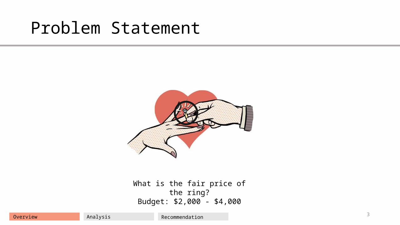
Problem Statement

What is the fair price of the ring?Budget: $2,000 - $4,000

Overview Analysis Recommendation

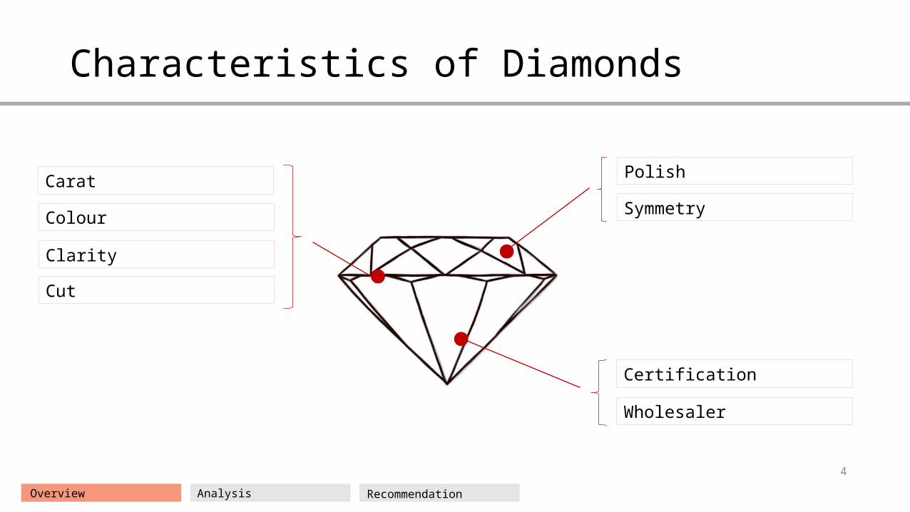
Characteristics of Diamonds

4

Carat

Colour

Cut

Clarity

Polish

Symmetry

Certification

Wholesaler


5

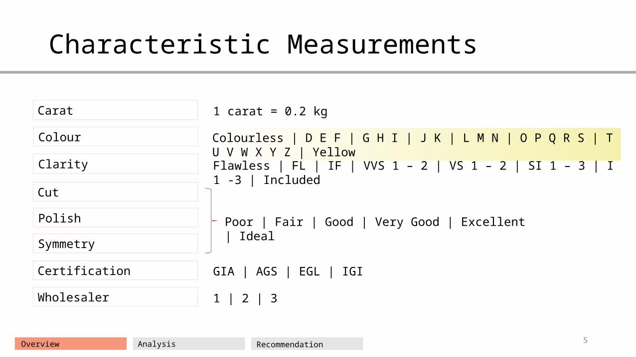
Characteristic Measurements


Carat

Colour

Cut

Clarity

Polish

Symmetry

Certification

Wholesaler

1 carat = 0.2 kg

Colourless | D E F | G H I | J K | L M N | O P Q R S | T U V W X Y Z | Yellow

Poor | Fair | Good | Very Good | Excellent | Ideal

GIA | AGS | EGL | IGI

1 | 2 | 3

Flawless | FL | IF | VVS 1 – 2 | VS 1 – 2 | SI 1 – 3 | I 1 -3 | Included

6

The Engagement Ring

Characteristic Diamond Rating

Carat Weight 0.9

Cut Very Good

Color J (Faint Yellow)

Clarity S12 (Few inclusions at 10x)

Polish Good

Symmetry Very Good

Certification GIA


$3,100

7

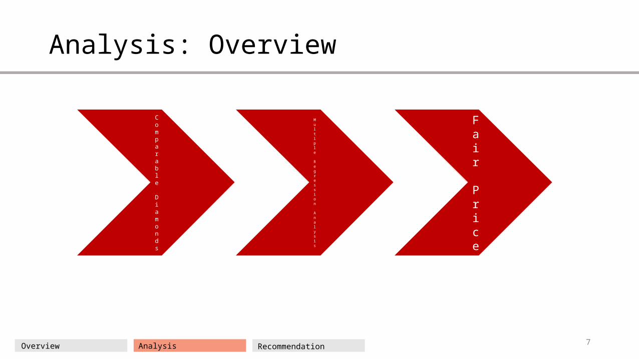
Analysis: Overview


Comparable Diamonds

Multiple Regression Analysis

Fair Price

8

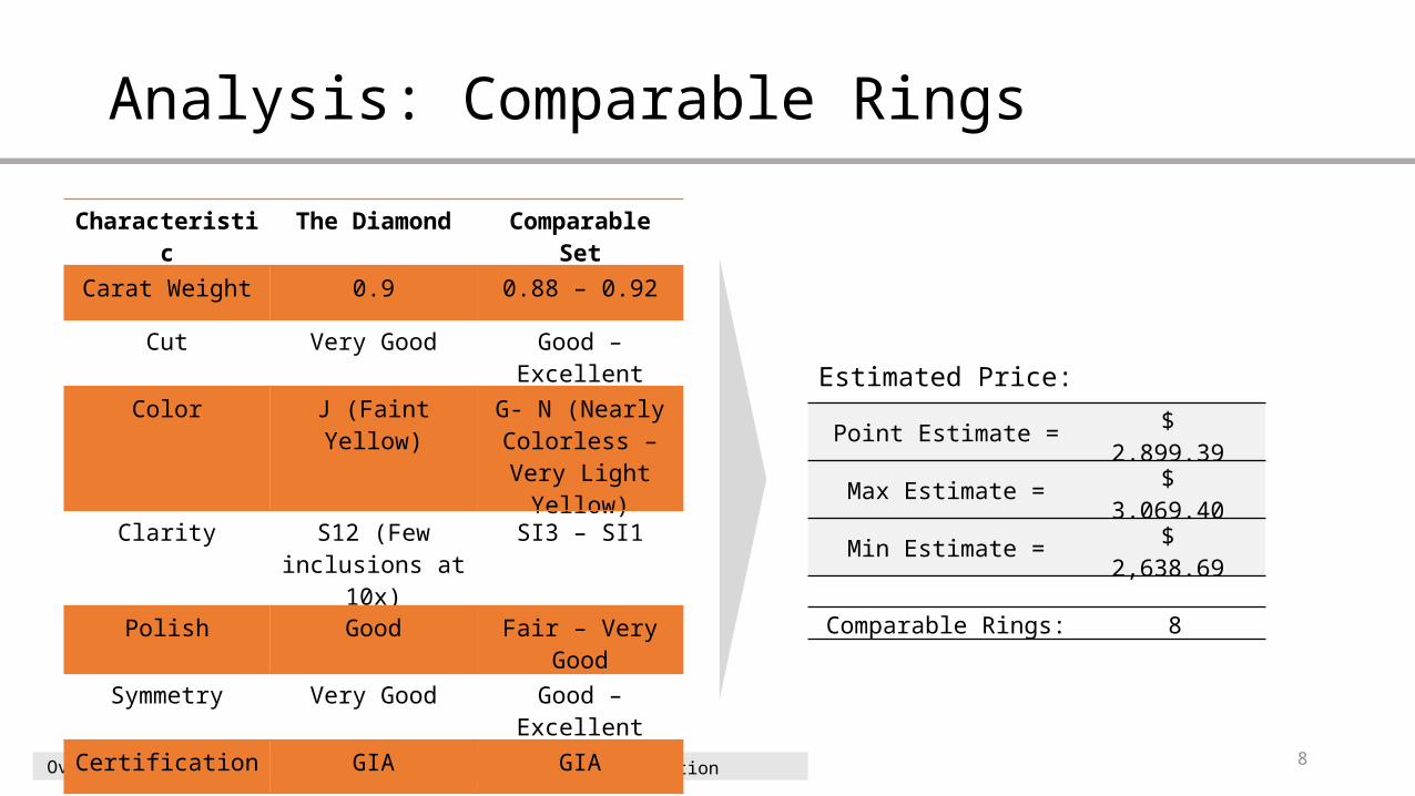
Analysis: Comparable Rings


Point Estimate = $ 2,899.39 Max Estimate = $ 3,069.40 Min Estimate = $ 2,638.69

Comparable Rings: 8

Estimated Price:

Characteristic The Diamond Comparable Set

Carat Weight 0.9 0.88 – 0.92

Cut Very Good Good – Excellent

Color J (Faint Yellow) G- N (Nearly Colorless – Very

Light Yellow)


SI3 – SI1

Polish Good Fair – Very Good

Symmetry Very Good Good – Excellent

Certification GIA GIA

9

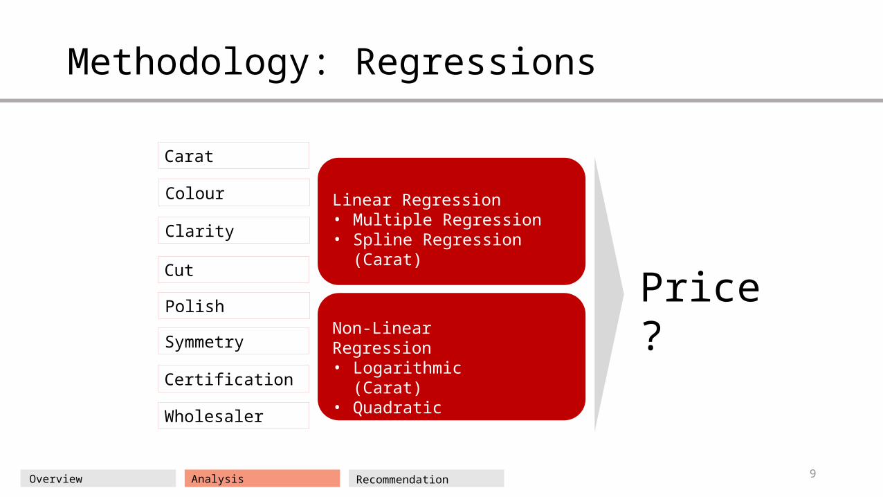
Methodology: Regressions


Carat

Colour

Cut

Clarity

Polish

Symmetry

Certification

Wholesaler

Price?

Linear Regression• Multiple Regression• Spline Regression (Carat)

Non-Linear Regression• Logarithmic (Carat)• Quadratic (Carat)

10

Analysis: Continuous Variables


Number of Observations: 440

Average Range Std. Dev

Price $1716.74 $160 - $3145 $1175.689

Carat 0.66925 0.09 – 1.58 0.3798

050

100

150

Fre

quen

cy

0 1000 2000 3000Price

050

100

150

Fre

quen

cy

0 .5 1 1.5Carat

Price Distribution Carat Distribution

11

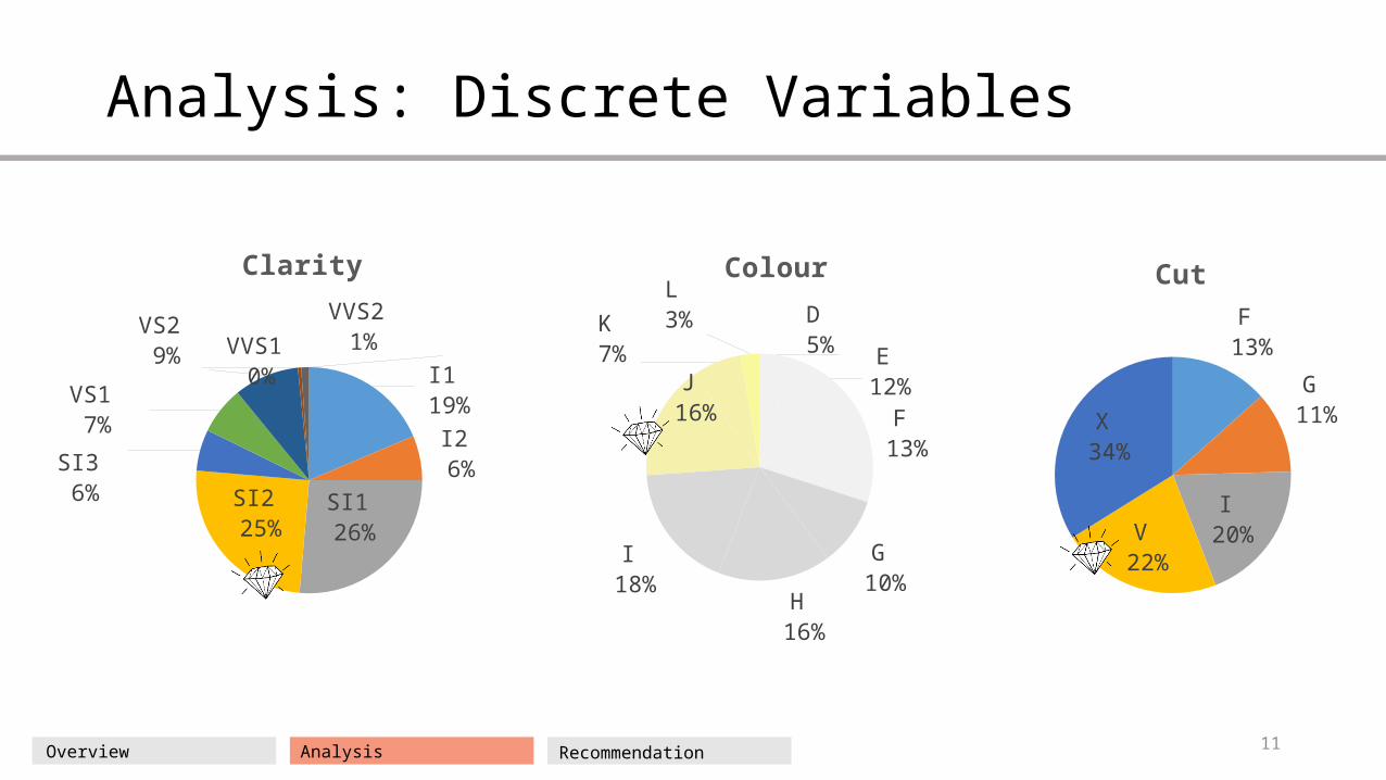
Analysis: Discrete Variables


I1 19% I2

6%

SI1 26%

SI2 25%

SI3 6%

VS1 7%

VS2 9% VVS1

0%

VVS2 1%

Clarity

D 5%

E 12%

F 13%

G 10%

H 16%

I 18%

J 16%

K 7%

L 3%

Colour

F 13%

G 11%

I 20% V

22%

X 34%

Cut

12

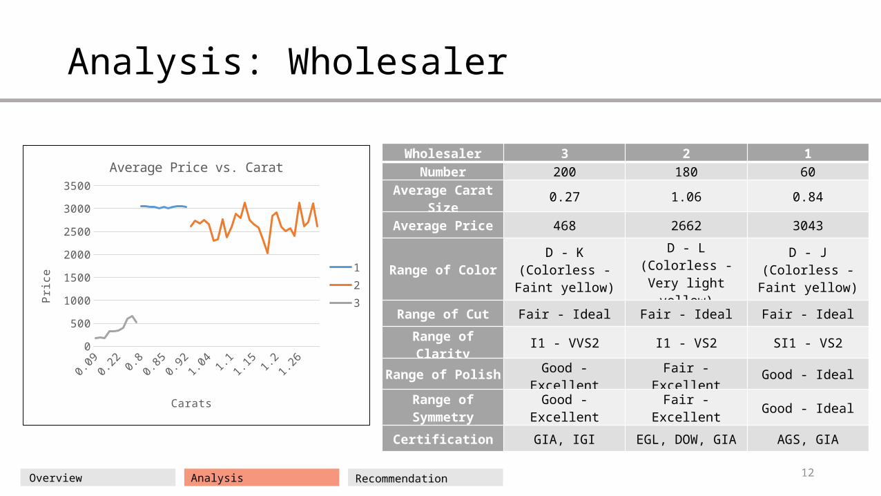
Analysis: Wholesaler


Wholesaler 3 2 1

Number 200 180 60

Average Carat Size 0.27 1.06 0.84

Average Price 468 2662 3043

Range of ColorD - K (Colorless -

Faint yellow)D - L (Colorless - Very light yellow)

D - J (Colorless - Faint yellow)

Range of Cut Fair - Ideal Fair - Ideal Fair - Ideal

Range of Clarity I1 - VVS2 I1 - VS2 SI1 - VS2

Range of Polish Good - Excellent Fair - Excellent Good - Ideal

Range of Symmetry

Good - Excellent Fair - Excellent Good - Ideal

Certification GIA, IGI EGL, DOW, GIA AGS, GIA

0.09

0.21

0.28

0.82

0.87

0.92

1.03

1.07

1.12

1.16 1.

21.

251.

430

500

1000

1500

2000

2500

3000

3500

Average Price vs. Carat

123

Carats

Pri

ce

13

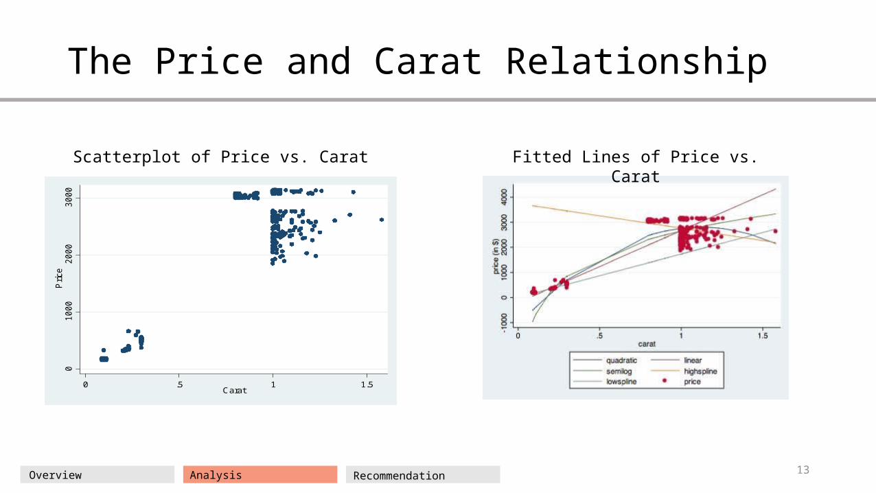
The Price and Carat Relationship


010

00

20

00

30

00

Price

0 .5 1 1.5Carat

Scatterplot of Price vs. Carat Fitted Lines of Price vs. Carat

14

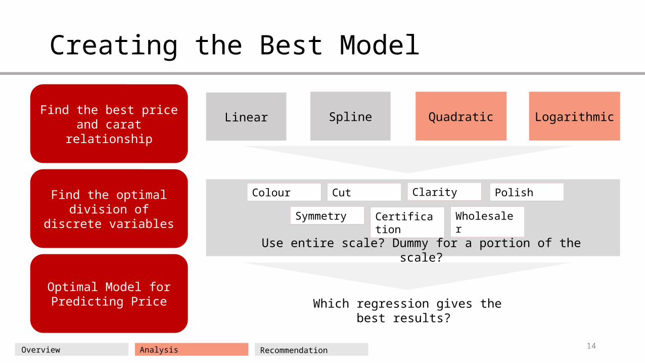
Creating the Best Model


Find the best price and carat relationship

Find the optimal division of discrete variables

Optimal Model for Predicting Price

Linear Spline Quadratic Logarithmic

Colour Cut Clarity Polish

Symmetry Certification Wholesaler

Use entire scale? Dummy for a portion of the scale?

Which regression gives the best results?

15

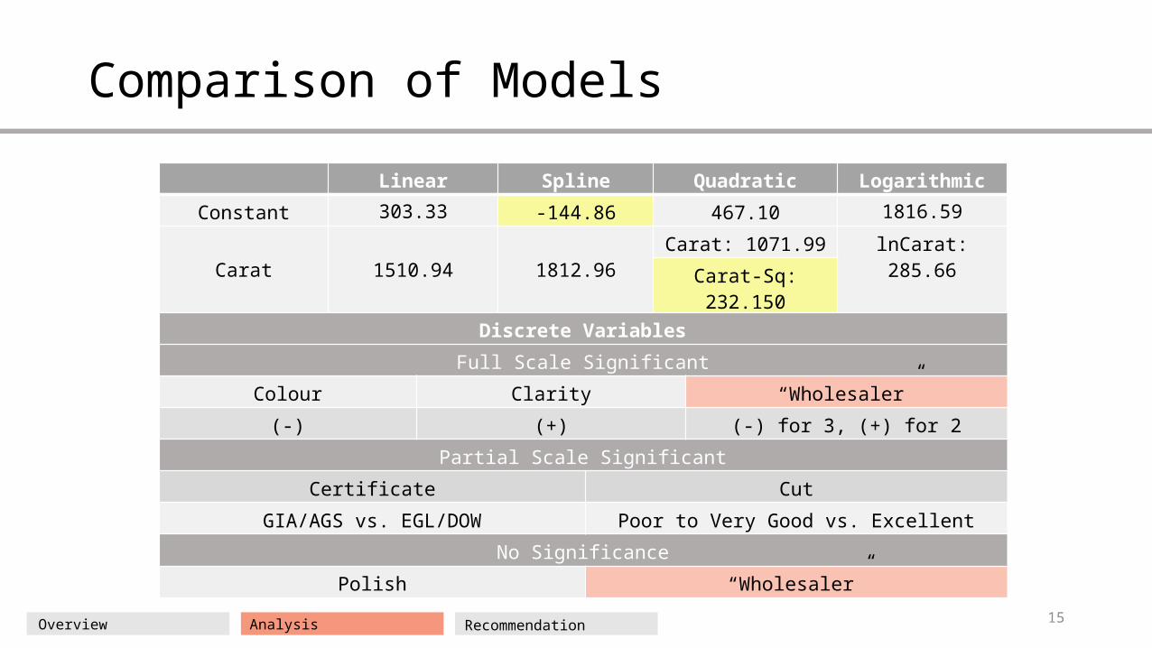
Comparison of Models



Constant 303.33 -144.86 467.10 1816.59

Carat 1510.94 1812.96Carat: 1071.99 lnCarat: 285.66

Carat-Sq: 232.150

Discrete Variables

Full Scale Significant

Colour Clarity “Wholesaler”

(-) (+) (-) for 3, (+) for 2

Partial Scale Significant

Certificate Cut

GIA/AGS vs. EGL/DOW Poor to Very Good vs. Excellent

No Significance

Polish “Wholesaler”

16

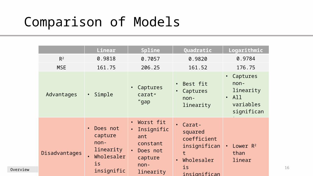
Comparison of Models



R2 0.9818 0.7057 0.9820 0.9784

MSE 161.75 206.25 161.52 176.75

Advantages • Simple• Captures

carat “gap”

• Best fit• Captures non-

linearity

• Captures non-linearity

• All variables significant

Disadvantages

• Does not capture non-linearity

• Wholesaler is insignificant

• Worst fit• Insignificant

constant• Does not

capture non-linearity

• Reduces sample size

• Carat-squared coefficient insignificant

• Wholesaler is insignificant

• Lower R2 than linear

17

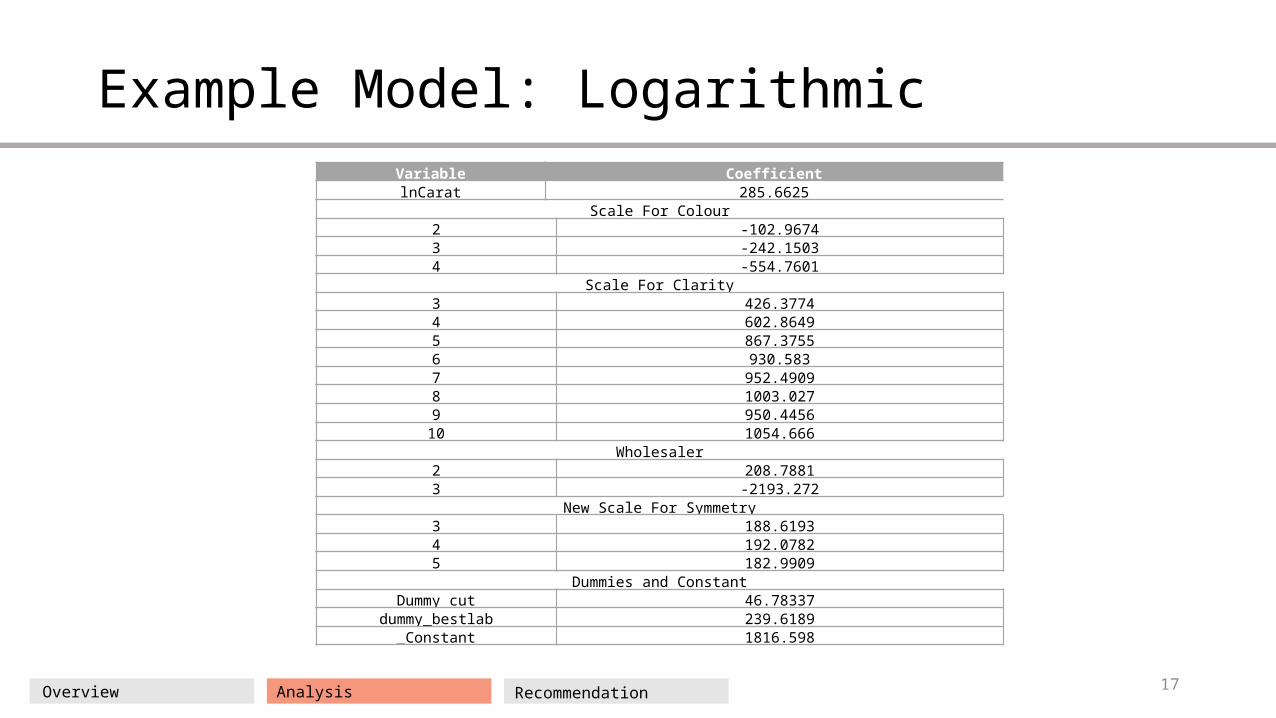
Example Model: Logarithmic


Variable CoefficientlnCarat 285.6625

Scale For Colour2 -102.96743 -242.15034 -554.7601

Scale For Clarity3 426.37744 602.86495 867.37556 930.5837 952.49098 1003.0279 950.4456

10 1054.666Wholesaler

2 208.78813 -2193.272

New Scale For Symmetry3 188.61934 192.07825 182.9909

Dummies and ConstantDummy cut 46.78337

dummy_bestlab 239.6189_Constant 1816.598

18

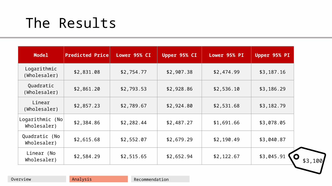
The Results

Model Predicted Price Lower 95% CI Upper 95% CI Lower 95% PI Upper 95% PI

Logarithmic (Wholesaler)

$2,831.08 $2,754.77 $2,907.38 $2,474.99 $3,187.16

Quadratic (Wholesaler)

$2,861.20 $2,793.53 $2,928.86 $2,536.10 $3,186.29

Linear (Wholesaler) $2,857.23 $2,789.67 $2,924.80 $2,531.68 $3,182.79

Logarithmic (No Wholesaler)

$2,384.86 $2,282.44 $2,487.27 $1,691.66 $3,078.05

Quadratic (No Wholesaler)

$2,615.68 $2,552.07 $2,679.29 $2,190.49 $3,040.87

Linear (No Wholesaler)

$2,584.29 $2,515.65 $2,652.94 $2,122.67 $3,045.91


$3,100

19

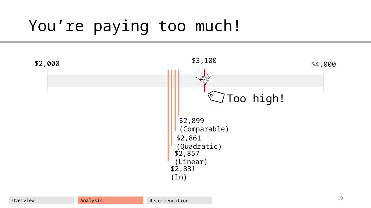
You’re paying too much!


$2,000 $4,000$3,100

$2,899 (Comparable)

$2,861 (Quadratic)

$2,857 (Linear)

$2,831 (ln)

Too high!

20

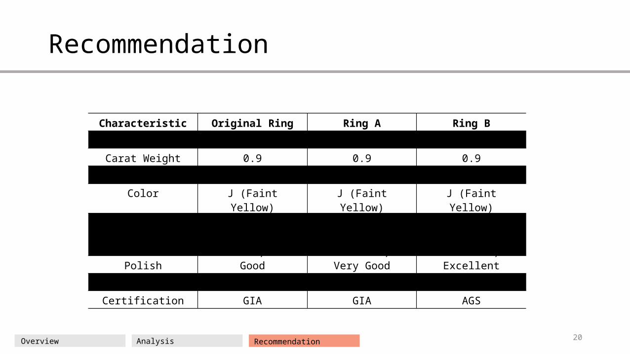
Recommendation


Characteristic Original Ring Ring A Ring B

Price $3,100 $3,006 $3,064

Carat Weight 0.9 0.9 0.9

Cut Very Good Very Good Good

Color J (Faint Yellow) J (Faint Yellow) J (Faint Yellow)


VS2 (Very Slightly Included)

VS2 (Very Slightly Included)

Polish Good Very Good Excellent

Symmetry Very Good Very Good Excellent

Certification GIA GIA AGS

Thank-you,Questions?

22

Appendix

• Link to spreadsheet – for comparability

23

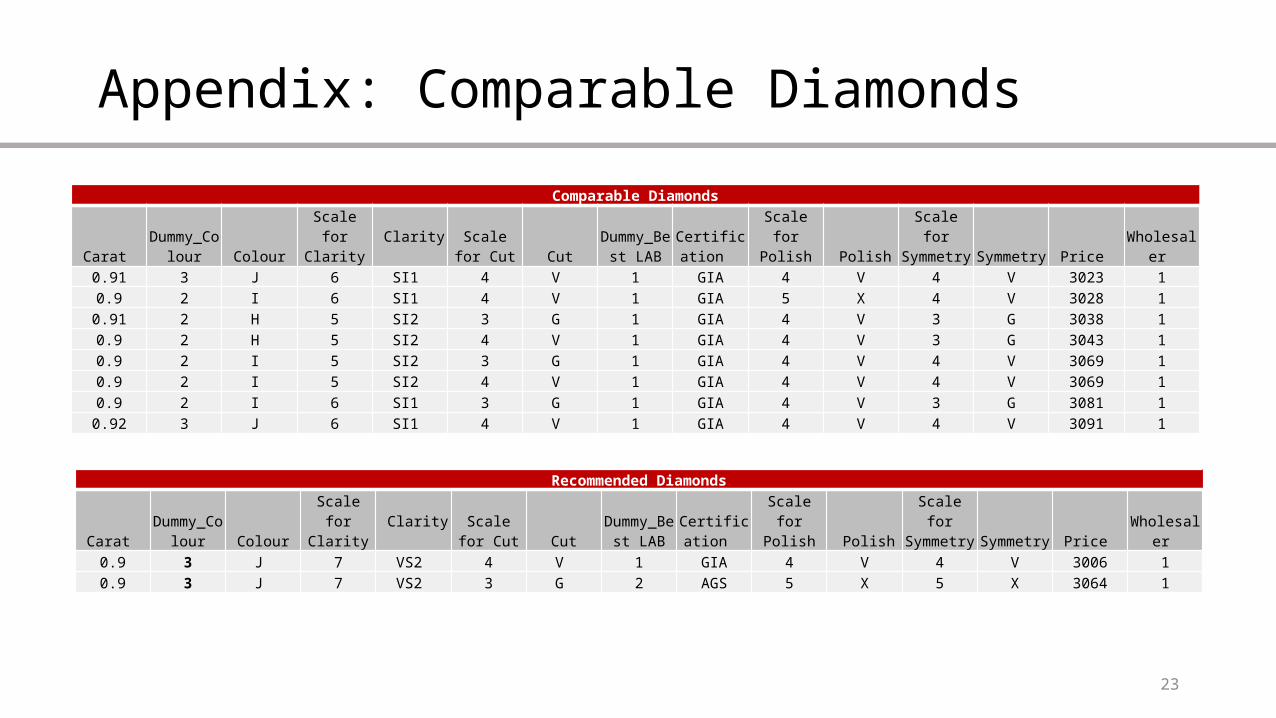
Appendix: Comparable Diamonds

Comparable Diamonds

Carat Dummy_C

olour Colour Scale for

Clarity Clarity Scale for

Cut Cut Dummy_B

est LAB

Certificatio

n Scale for

Polish PolishScale for

Symmetry Symmetry Price

Wholesaler

0.91 3 J 6 SI1 4 V 1 GIA 4 V 4 V 3023 1

0.9 2 I 6 SI1 4 V 1 GIA 5 X 4 V 3028 1

0.91 2 H 5 SI2 3 G 1 GIA 4 V 3 G 3038 1

0.9 2 H 5 SI2 4 V 1 GIA 4 V 3 G 3043 1

0.9 2 I 5 SI2 3 G 1 GIA 4 V 4 V 3069 1

0.9 2 I 5 SI2 4 V 1 GIA 4 V 4 V 3069 1

0.9 2 I 6 SI1 3 G 1 GIA 4 V 3 G 3081 1

0.92 3 J 6 SI1 4 V 1 GIA 4 V 4 V 3091 1

Recommended Diamonds

Carat Dummy_C

olour Colour Scale for

Clarity Clarity Scale for

Cut Cut Dummy_B

est LAB

Certificatio

n Scale for

Polish PolishScale for

Symmetry Symmetry Price

Wholesaler 0.9 3 J 7 VS2 4 V 1 GIA 4 V 4 V 3006 10.9 3 J 7 VS2 3 G 2 AGS 5 X 5 X 3064 1

24

Appendix: Results

• Carat Graphs

25

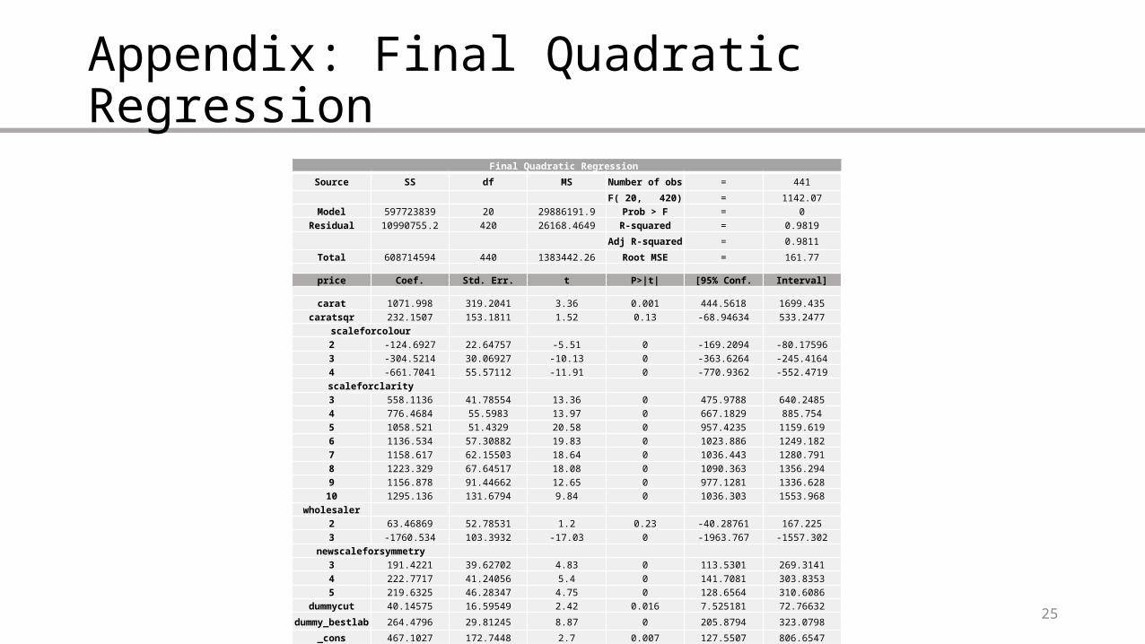
Appendix: Final Quadratic Regression

Final Quadratic Regression

Source SS df MS Number of obs = 441

F( 20, 420) = 1142.07Model 597723839 20 29886191.9 Prob > F = 0

Residual 10990755.2 420 26168.4649 R-squared = 0.9819

Adj R-squared = 0.9811

Total 608714594 440 1383442.26 Root MSE = 161.77

price Coef. Std. Err. t P>|t| [95% Conf. Interval]

carat 1071.998 319.2041 3.36 0.001 444.5618 1699.435caratsqr 232.1507 153.1811 1.52 0.13 -68.94634 533.2477

scaleforcolour2 -124.6927 22.64757 -5.51 0 -169.2094 -80.175963 -304.5214 30.06927 -10.13 0 -363.6264 -245.41644 -661.7041 55.57112 -11.91 0 -770.9362 -552.4719

scaleforclarity3 558.1136 41.78554 13.36 0 475.9788 640.24854 776.4684 55.5983 13.97 0 667.1829 885.7545 1058.521 51.4329 20.58 0 957.4235 1159.6196 1136.534 57.30882 19.83 0 1023.886 1249.1827 1158.617 62.15503 18.64 0 1036.443 1280.7918 1223.329 67.64517 18.08 0 1090.363 1356.2949 1156.878 91.44662 12.65 0 977.1281 1336.62810 1295.136 131.6794 9.84 0 1036.303 1553.968

wholesaler2 63.46869 52.78531 1.2 0.23 -40.28761 167.2253 -1760.534 103.3932 -17.03 0 -1963.767 -1557.302

newscaleforsymmetry3 191.4221 39.62702 4.83 0 113.5301 269.31414 222.7717 41.24056 5.4 0 141.7081 303.83535 219.6325 46.28347 4.75 0 128.6564 310.6086

dummycut 40.14575 16.59549 2.42 0.016 7.525181 72.76632

dummy_bestlab 264.4796 29.81245 8.87 0 205.8794 323.0798

_cons 467.1027 172.7448 2.7 0.007 127.5507 806.6547

26

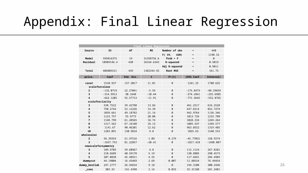
Appendix: Final Linear Regression

Final Linear Regression


F( 19, 420) = 1198.52Model 595816375 19 31358756.6 Prob > F = 0

Residual 10989146.4 420 26164.6343 R-squared = 0.9819


Total 606805521 439 1382244.92 Root MSE = 161.75

price. Coef Std. Err. t P>|t| [95% Conf. Interval]

carat 1510.937 137.2017 11.01 0 1241.25 1780.625scaleforcolour

2 -132.0719 22.27041 -5.93 0 -175.8473 -88.296593 -314.9913 30.1648 -10.44 0 -374.2841 -255.69854 -662.1205 55.57713 -11.91 0 -771.3645 -552.8765


wholesaler2 56.39354 51.97516 1.09 0.279 -45.77031 158.55743 -1657.753 81.22857 -20.41 0 -1817.418 -1498.087


dummycut 44.19004 16.43469 2.69 0.007 11.88554 76.49454

dummy_bestlab 247.2777 26.94654 9.18 0 194.3108 300.2446

_cons 303.33 141.4398 2.14 0.033 25.31188 581.3481

27

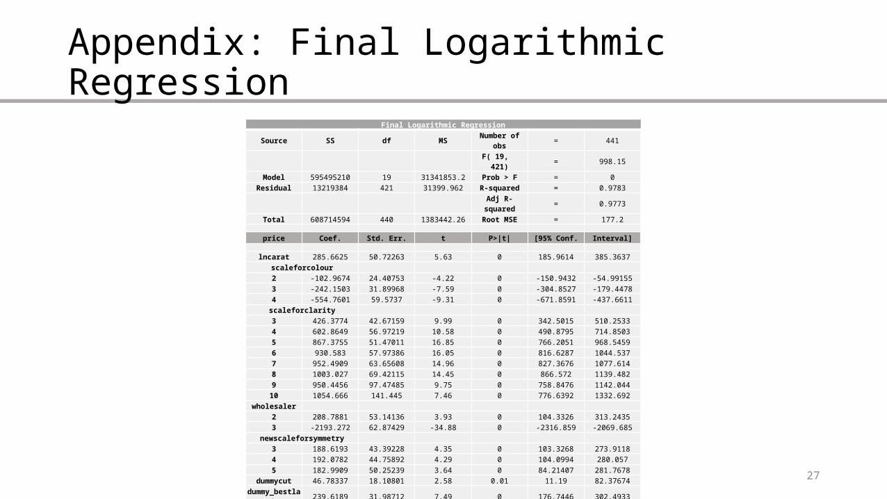
Appendix: Final Logarithmic RegressionFinal Logarithmic Regression


F( 19, 421) = 998.15Model 595495210 19 31341853.2 Prob > F = 0

Residual 13219384 421 31399.962 R-squared = 0.9783


Total 608714594 440 1383442.26 Root MSE = 177.2

price Coef. Std. Err. t P>|t| [95% Conf. Interval]

lncarat 285.6625 50.72263 5.63 0 185.9614 385.3637scaleforcolour

2 -102.9674 24.40753 -4.22 0 -150.9432 -54.991553 -242.1503 31.89968 -7.59 0 -304.8527 -179.44784 -554.7601 59.5737 -9.31 0 -671.8591 -437.6611


wholesaler2 208.7881 53.14136 3.93 0 104.3326 313.24353 -2193.272 62.87429 -34.88 0 -2316.859 -2069.685


dummycut 46.78337 18.10801 2.58 0.01 11.19 82.37674dummy_bestla

b239.6189 31.98712 7.49 0 176.7446 302.4933

_cons 1816.598 85.39026 21.27 0 1648.753 1984.442

the professor proposes

Technology

fair price

estimated price

giaaleks12the price

colorless faint yellowd

comparable set8methodology

light yellowclaritys12

discrete variablesexplain

excellentfair excellentgood