The Relative Earnings of Young Mexican, Black, and White Women

Heather Antecol and Kelly Bedard*

* Heather Antecol is an assistant professor at Claremont McKenna College and Kelly

Bedard is an assistant professor at the University of California, Santa Barbara. We thank Eric

Helland, Peter Kuhn, Lonnie Magee, Shelley Phipps, Harriet Duleep, and Joanne Roberts for

helpful comments. We gratefully acknowledge financial support from the Canadian

International Labour Network (CILN) at McMaster University. The paper was revised while the

first author was visiting the University of Illinois at Urbana-Champaign, and she thanks that

institution for its hospitality.

Copies of the computer programs used to generate the results presented in the paper are

available from Heather Antecol at Claremont McKenna College, Department of Economics, 500

East Ninth Street, Claremont, California, 91711.

Abstract

Using the NLSY, we find that young Mexican women earn 8.7% less than young white women

while young black women earn 15.4% less than young white women. Although young Mexican

women earn less than young white women, they do surprisingly well compared to young black

women. We show that it is crucially important to account for actual labor market experience.

We further show that low labor force attachment is the most important determinant of the black-

white wage differential for young women while education is the most important explanation for

the Mexican-white wage gap for young women.

2

Recent research (Trejo 1997 and 1998; Reimers 1994; Chavez 1991; Smith 1991; Chapa

1990) has renewed interest in the relatively poor labor market performance of Mexican men.

Trejo (1997) finds that lower levels of education, English deficiencies, and the relative youth of

Mexican men explains 75% of the gap between Mexican and white wages. In contrast, these

factors explain less than 30% of the black-white wage gap. Despite the flurry of recent research

exploring the poor performance of Mexican men, we are aware of only one study that includes

women (Mora and Davila 1998), and they focus on the differential return to English fluency

across gender. We therefore seek to add to the current debate regarding Mexican labor market

performance by comparing the ‘plight’ of young Mexican women with their black and white

counterparts.

Previous work focused on men because higher participation rates mean that Mincer

experience measures more accurately reflect actual experience and selection issues are less

important. While Mincer experience may be a relatively good approximation of true experience

for men with high labor force attachment, it is a poor proxy for women and possibly some

minority groups. We are able to overcome this measurement problem using the National

Longitudinal Survey of Youth (NLSY). In particular, the longitudinal nature of the NLSY

allows us to construct true experience measures, as well as complete education, childbirth, and

marital histories. Since these factors may play important roles in determining the labor market

participation decisions and success of women, the NLSY is well suited to this study.

It is well established that women tend to move in and out of the labor market more

frequently than men, and that job interruptions surrounding childbirth have long-term

implications for women’s wages (Jacobsen and Levin 1995; Waldfogel 1997 and 1998).

Waldfogel (1997, 1998) shows that children have a negative impact on earnings despite controls

3

for actual labor market experience. In her 1997 paper, Waldfogel finds that women who are

covered by formal maternity leave programs, and return to their former employer after childbirth,

earn higher wages than women who do not return to their former employer after childbirth and

are not covered by formal maternity leave. Further, Waldfogel (1998) shows that the positive

impact of maternity leave outweighs the negative effect of children by increasing the probability

that women return to their former employer after childbirth. Echoing Waldfogel, Phipps, Burton,

and Lethbridge (1998) find that returning to the pre-birth employer has a positive impact on

wages for Canadian women. Unfortunately, we are unable to determine whether or not a woman

returns to her pre-birth employer or has access to maternity leave in the NLSY for the entire

cohort. We do, however, allow for the possibility that a woman’s experience profile may change

slope after successive childbirth experiences.

Accounting for the wage gap between race groups for women clearly requires a careful

accounting of differences in labor market participation and family structure in addition to

educational differences. In 1994, the average young Mexican woman earned 9.5% less than the

average young white woman while the average young black women earned 13.2% less than the

average young white woman.1 Education, fertility, and labor force attachment differences at

various points in the lifecycle play a crucial role in determining differences across racial/ethnic

groups. We show that low labor force attachment is a particularly important explanation for the

black-white wage differential, while education plays a more prominent role in explaining the

Mexican-white wage gap.

2. Data

We use the National Longitudinal Survey of Youth (NLSY) which contains longitudinal

data from 1979-1998 for a sample of men and women aged 14-22 in 1979. There are several

4

features of these data that are crucial for our purposes. First, the NLSY contains information that

allows us to construct actual (rather than potential) work experience. This is particularly

important when studying women. Secondly, these data include detailed information regarding

marital and childbirth patterns. Finally, the NLSY allows us to identify non-immigrants and

separate individuals into racial/ethnic origin groups.

The NLSY contains 2350 non-immigrant Mexican, black, and white women who were

employed and report an hourly wage between $1 and $100 per hour in 1993 or 1994 and are not

self-employed.2 1993 data are only used if the respondent failed to report the information

required to construct an hourly wage measure in 1994, but did report this information in 1993.

Similar to Waldfogel (1998), we use wage data for multiple years to maintain an adequate

sample of young Mexican women and mitigate sample selection. Hourly wages for 1994 are

defined as annual wages and salaries reported in 1994 for the past calendar year divided by the

number of annual hours worked in the past calendar year.3 Hourly wages for 1993 are calculated

analogously but are inflated into 1994 dollars. All variables are matched to the hourly wage

data. For instance, marital status in 1994 is replaced with marital status in 1993 if the hourly

wage data is missing in 1994, but available in 1993.

Given our interest in the number of children present in 1993/94, we construct all child

variables using the number of children ever born. The lone exception is children born during

1993. Since the number of children ever born was not reported in 1993, we use retrospective

day, month, and year of birth reports from 1994-1998 and the day and month of the interview

date in 1993 to calculate the number of children born in 1993. We then add the number of

children born in 1993 to the number of children reported in 1992.

5

We use two measures of experience: Mincer experience and actual experience. Mincer

experience is calculated as age minus years of education minus six. Actual experience is years

of employment for individuals greater than 18 years of age reported between 1976 and 1994 and

is based on weeks worked since the last NLSY interview. We convert the weekly experience

into annual experience by dividing total weekly experience by 52.

Individuals are assigned to a racial/ethnic origin group by reports of first, or only,

racial/ethnic origin. We focus on three racial/ethnic groups: Mexicans, blacks and whites. An

individual is considered Mexican if she claims to be Mexican or Mexican American. Similarly,

an individual is considered black if she claims to be black. A respondent is considered white if

she claims to be English, French, German, Greek, Irish, Italian, Polish, Portuguese, Russian,

Scottish, Welsh, or American, and is not black or Mexican.

Place of birth is used to define immigrant status. An individual is considered a non-

immigrant if she was born in the United States. The results are not sensitive to this definition.

All results are similar if we require that the respondent and both parents be U.S. born, or require

that the respondent and at least one parent be U.S. born. Restricting our analysis to non-

immigrants allows for easier comparison with previous work by Trejo (1997, 1998) and reduces

the potential influence of English proficiency, for which we have no measure.

3. Socioeconomic Characteristics

Table 1 presents descriptive statistics for the main variables used in the cross-sectional

analysis. Inspection of Table 1 reveals that the average young Mexican woman earns 9.5% less

than the average young white woman, while the average young black woman earns 13.2% less

than the average young white woman. The obvious question is: Why do young Mexican women

fare relatively better than their black counterparts?

6

Part of the relative success enjoyed by young Mexican women may be due to differences

in socioeconomic characteristics. For example, race-specific fertility differences may be an

important determinant of wages. Waldfogel (1997, 1998) and Korenman and Neumark (1992)

find that children have a negative effect on wages for women, all else being equal. Larger

relative black families might therefore help explain the relative success of young Mexican

women. While young white women have significantly fewer children than their Mexican and

black counterparts, Table 1 reveals that the average Mexican woman has more rather than fewer

children than her average black counterpart. It is therefore unlikely that childbearing differences

play a significant role in explaining differences in Mexican and black labor market performance,

unless it is through the timing of children. The average black woman has her first child when

she is 20 and her second when she is 24, while the average Mexican woman does not have her

first child until she is 21 and has her second child when she is 24.

The second obvious question is: Are young Mexican women more educated than young

black women? Table 1 clearly shows that the answer is again no. The average young Mexican

woman has 12.8 years of education, while the black women average 13.3 years of education and

the average white women has 13.7 years of education.

The third obvious question is: Are young Mexican women more attached to the labor

force than their black counterparts? Both Mexicans and blacks spend less time in the labor

market than white women. For instance, the average 30-year-old Mexican woman has 9.2 years

of post-schooling experience while her black counterpart has only 7.9 years and her white

counterpart has 9.8 years. However, factoring in educational differences, Mexicans and blacks

have similar amounts of experience.

7

Marriage patterns are the most pronounced difference across young female ethnic groups.

In our sample, 61.8% of Mexican women and 65.9% of white women are married. In contrast,

only 36.6% of black women are married in 1994, or 1993 if missing information has forced the

use of the previous year. While it is not entirely clear how marital status differences impact

labor market participation, Moffitt (1992) finds that female heads with children under age

eighteen work about the same amount as single women and more than married women most of

whom also have children. Although the average wages of married and single black women are

almost identical, 87.2% of black married women are employed while only 72.7% of unmarried

black women are employed.4 We will return to the possibility of non-random labor market

participation in Section 6.

The similarities in average socioeconomic characteristics across young Mexican and

black women do not of course imply that the time patterns, variation within race groups, or the

return to certain attributes are the same across all race groups. In fact, they clearly indicate that

some, or all, of these factors must differ. We draw two main conclusions, or more accurately

hypotheses, from this preliminary perusal of descriptive statistics. First, if fertility rate

differences play a role in explaining the wage gap between Mexicans and blacks it must be

through the timing of childbirth and a differential impact on experience. Secondly, education

and experience differences between Mexicans and blacks must therefore play an important role

in explaining their respective wages gaps compared to white women. The remainder of the

paper more formally explores these possibilities.

4. Wages

Following standard practice, we compare the wages of ethnic-specific groups by running

log hourly wage regressions of the following form:5

8

ri

rri

rri Xw εβα ++= (1)

where w is the log hourly wage, r denotes race (r = M, B, or W), i denotes individual, and X

includes: experience, education, marital status, child variables, region of residence, SMSA, and

a year dummy (set to 1 if the reporting year is 1994), and a constant. 6

There are several noteworthy results presented in the middle column of Panel A of Table

2. First, education has a positive impact on the wages of young women in all racial/ethnic origin

groups. Secondly, consistent with Waldfogel (1997, 1998) and Neumark (1992), we find that

children have a negative impact on wages for young white women. Thirdly, while potential

experience and experience squared are jointly statistically significant for young black women

they are not significantly related to white or Mexican wages.

There are, of course, many good reasons to be skeptical about estimates based on Mincer

experience for women. The movement of women in and out of the labor market, especially

surrounding childbirth, may render Mincer experience an extremely inaccurate proxy for actual

experience for many women. The right-hand column of panel A of Table 2 replicates the base

regressions replacing Mincer experience with actual experience and age. Comparing these

results to the base estimates highlights the importance of measuring actual experience. While

the experience and experience squared terms are not individually statistically significant, the one

exception is the level experience term for black women which is significant at the 1% level,

experience and experience squared are jointly significant at the 1% level for all racial/ethnic

groups.7 Age is included along with actual experience and education to capture out of the labor

force spells. In other words, conditional on actual experience and education older people have

been out of the labor force longer. Time out of the labor force has a negative effect on wages for

all groups, but it is only significant at the 10% level or better for white and black women. White

9

women face a larger penalty for out of the labor force spells than do black women or Mexican

women. In particular, each year of absence from the labor market reduces wages by 2.8%, 1.9%

and 4.8% for Mexican, black, and white women, respectively (although the Mexican estimates

are quite imprecise). The large out of the labor force penalty faced by white women may exist

because they are more likely to work in high skilled fields where both career advancement and

skill depreciation are relatively fast. As a result, white women returning to work after an

absence from the labor market suffer greater skill losses and missed promotion opportunities

compared to their black and Mexican counterparts.

The pattern of socioeconomic influences change very little when Mincer experience is

replaced by actual experience, although the magnitudes do change somewhat. Education

continues to have a positive and statistically significant impact on wages, although smaller in

magnitude for all racial/ethnic groups. Each additional year of education increases wages by

2.9%, 7.7%, and 7.7% for Mexican, black, and white women, respectively. In contrast, 2 or

more children is no longer statistically significant for black or white women.

Education enters all Panel A regressions as a continuous (linear) variable. Since it seems

likely that the relationship between educational attainment and wages is non-linear, for at least

some racial/ethnic groups, Panel B replicates Panel A with education entering as three dummy

variables: high school graduate, some college, and college graduate, with high school drop-out

being the excluded category. The middle column of Panel B of Table 2 illustrates the instability

in the estimates of the returns to experience based on potential experience rather than actual

experience. In particular, adding controls for non-linear education leads to insignificant returns

(both individually and jointly) of potential experience and potential experience squared for all

racial/ethnic groups, confirming that potential experience is a poor proxy for actual labor market

10

experience for young women. Therefore, focusing on the regression that includes actual labor

market experience and age, it is clear that the impact of educational attainment differs

substantially across racial/ethnic groups. Relative to whites, Mexicans earn a lower return from

college graduation, and blacks earn a higher return from all levels of education.

What Explains the Wage Gap?

Quantification of racial earnings gaps requires computing what minority workers would

earn if they had the same characteristics as majority workers. Following Oaxaca (1973), there

are two ways to decompose the white/Minority (w/m) earnings gap.

)ˆˆ()ˆˆ(ˆ)( mwmwmwmwmw XXXww ααβββ −+−+−=− or, (2a)

).ˆˆ()ˆˆ(ˆ)( mwmwwmmwmw XXXww ααβββ −+−+−=− (2b)

Bars denote means and hats denote predicted values from equation (1).

The decomposition results using both the white weights (2a) and the minority weights

(2b) are reported in Table 3. The first row reports the total log wage differential. The second

and third blocks report the proportion of the total wage differential attributable to differences in

average socioeconomic characteristics and differences in the returns to these characteristics,

respectively.

Unlike Trejo (1997), we do not find that observable characteristics play a larger role in

explaining the relative labor market performance of Mexicans than blacks. We do, however,

find that different factors are more important in explaining the Mexican/white gap and the

black/white gap. All else being equal, observable differences in education account for 31%-34%

of the black/white gap and 58%-65% of the Mexican/white gap. Ranges bound the white and

minority weighted decompositions. In contrast, observable differences in experience account for

54%-61% of the black/white gap but only 40%-41% of the Mexican/white gap. Finally,

11

observable differences in childbearing account for 0%-2% of both the black/white gap and the

Mexican/white gap. Interestingly, when the Mexican weights are used, the other category,

which includes region, SMSA, and a year dummy, can over-explain the entire Mexican/white

gap. This is largely driven by the fact that the small number of Mexicans who live in the

Northeast earn a relatively higher wage than Mexicans who live in the West. Overall,

observable factors explain the entire black/white and Mexican/white wage gaps.

The differences in coefficients also yield some interesting results. In particular, the age

effect in the bottom panel of Table 3 for Mexican (black) women and white women are very

large. From an empirical point of view, this is mostly due to the to the fact that the returns to

time out of the labor force for white women are substantially more negative than the returns to

time out of the labor force for Mexican (black) women. Despite this large age effect, the results

in the last line of Table 3 suggest that Mexican, black and white women all face a similar wage

structure.

To check that our results are not driven by the omission of occupational differences

across racial/ethnic groups, we replicate the right-hand side of Panel B of Table 2 and the

decomposition in Table 3, respectively, with the addition of three occupational dummy variables:

professional, blue collar (including the military and farm laborers), and services, with sales being

the excluded category. The regression and decomposition results are largely similar.8

Interestingly, occupation has no significant relationship to wages for Mexican women while

black and white professionals earn a premium compared to saleswomen and white service

workers earn less than saleswomen. Turning to the decomposition results, occupation explains

14%-19% of the Mexican/white gap and 22%-30% of the black/white gap, however, it does not

cause the magnitude of the other explanatory factors, in particular education and experience, to

12

change very much. Given the possibility that labor market discrimination may be working

through occupation and the similarity of results in Table 3 and those described above, the

remainder of the analysis excludes occupation.

Selection

Selection effects that differ across racial lines may bias cross-sectional estimates of

discrimination. Preferences for work, or motivation may differ across races in ways that are

difficult to measure directly. Stated somewhat differently, the decision to participate in the labor

market is not random and may differ systematically across ethnic groups. Wage gap measures

that fail to account for such differences may be biased by unmeasured preference and

motivational differences.

The Heckman selection model is one way to account for non-random labor market

participation. However, in our sample very few women are not working: the 1994 employment

rates are 81.8%, 77.4%, and 84.1% for Mexicans, blacks, and whites, respectively. Furthermore,

we lack suitable controls for the participation equation. Although we have information on the

education level of each individual’s mother and father, the presence of a library card, newspaper

subscription, and magazine subscription in the household at age 14, and non-labor income, many

of these variables are not well reported. For example, 5% of the sample does not report

mother’s education, 15% of the sample does not report father’s education, and 16% of the

sample does not report non-labor income (defined as total family income minus the respondent’s

wages and salaries during the past calendar year). This non-reporting reduces the Mexican

sample size to an unacceptable level.

We instead address selection using two-stage panel estimation. This approach has the

advantage of separating individual-specific characteristics that are constant over time from other

13

factors affecting earnings by including individual-specific intercepts. Following a given

individual purges the estimates of idiosyncratic person-specific and time-invariant factors,

rendering unbiased estimates of labor market factors. More concretely, Equation (1) is re-

written in a form appropriate for panel data,

rit

ri

rri

rrit

rit ZXw εαγβ +++= (3)

where denotes time-varying characteristics, denotes time-invariant characteristics, are

unobservable individual fixed effects, and represents the usual residual, that is, it is mean

zero, uncorrelated with itself, X, Z, and α, and homoskedastic.

ritX r

iZ riα

ritε

Following Polachek and Kim (1994), we estimate equation (3) using a fixed effect model

(within estimator). The fixed effect model transforms equation (3) into its mean deviation form,

that is, we subtract each individual’s mean variable values from each observation. Although this

transformation eliminates the unobserved individual fixed effects, it also eliminates all time-

invariant factors making a second-stage analysis of residuals necessary to obtain estimates of the

time invariant coefficients.

In particular, we obtain consistent estimates of β using OLS from the following first stage

regression,

)~()~()~( ri

rit

rri

rit

ri

rit XXww εεβ −+−=−

where tildas denote averages over t and X contains all Table 2 variables with the exception of

education.9 To identify γ we substitute from the first stage into the individual-specific

averaged version of equation (3). In other words, equation (3) averaged for each individual over

time to obtain

rβ̂

ri

rri

ri

ri

rrri

rri

rri

ri ZXZXw νγεαββγβ +=++−+=− )ˆ(~ˆ~~ (4)

14

where ri

ri

rrri

ri X εαββν ++−= )ˆ(~ . Making the usual assumption that is uncorrelated with

, equation (4) can be estimated using OLS. Z includes education and a constant.

riν

riZ

The panel estimates for each racial/ethnic group are reported in Table 4(a). These

regressions include all previously included variables and cover the period 1982-1994.10

Individuals do not enter the panel until they are 19 years of age or older and have completely

finished their education. For example, if an individual was 19 in 1982 and had 12 years of

education in 1982 and 1983, but in 1984 reported 13 years of education, and from 1985 onward

had 14 years of education, the individual would not enter the panel until 1986. As in the cross

section, we only include women who are employed and earning between $1 per hour and $100

per hour and are not self-employed. All remaining variables are as defined in the cross section

(see Section 2).

While the magnitude of some results differ across the panel and cross-sectional estimates,

the pattern of results are remarkably similar. The most notable difference is the re-appearance of

a negative and statistically significant relationship between two or more children and wages for

white women. These coefficients continue to be insignificantly different from zero for both

Mexican and black women. The estimated returns to experience are also interesting. First, both

experience and experience squared are significant at the 10% level or better for all racial/ethnic

groups. Secondly, the returns to experience are now larger for Mexican women relative to black

women. Finally, marriage now has a negative and significant effect on the wages of Mexican

women.

Two-stage estimation makes decomposing the wage-gap between races somewhat more

complicated. The race specific mean wage is ,ˆˆ)/1(1

rrn

i

ri

rr Xnwr

βα += ∑=

where bars denote

15

averages over i and t for time-varying variables and over i for time-invariant variables.

Removing education from the fixed-effects, ,ˆˆ)/1(ˆ̂1

rrn

i

ri

rr Znr

γαα −= ∑=

allows us to write average

wages as .ˆˆˆ̂ rrrrrr ZXw γβα ++= The Oaxaca (1973) decomposition is then given by:

)ˆ̂ˆ̂()ˆˆ(ˆ)()ˆˆ(ˆ)( mwmwmwmwmwmwmwmw ZZZXXXww ααγγγβββ −+−+−+−+−=− (5a)

or,

)ˆ̂ˆ̂()ˆˆ(ˆ)()ˆˆ(ˆ)( mwmwwmmwmwwmmwmw ZZZXXXww ααγγγβββ −+−+−+−+−=− (5b)

Table 4(b) reports the decomposition results for the panel estimates. The biggest

difference between the panel and cross-section results lies in the raw wage gap; the

Mexican/white gap is 0.8 percentage points smaller while the black/white gap is 2.2 percentage

points larger. Thus, raising the estimated advantage that Mexican women enjoy relative to black

women. However, education and experience continue to be the driving explanatory factors.

Experience explains approximately 20%-49% of the Mexican/white gap and 19%-37% of the

black/white gap. Education accounts for 73%-76% of the Mexican/white gap but only 23%-26%

of the black/white gap.

Using the white weights we are able to explain more than 100% of the Mexican/white

gap and 71% of the black/white gap. In contrast, using minority weights we explain only 3%

and 43% of the Mexican/white and black/white gaps, respectively. For the black/white gap this

is largely due to the decline in the relative importance of experience. The importance of

experience falls in the black-weighted panel decomposition because the coefficient on

experience in the black regression is similar in magnitude in both the cross-section and panel

models while the mean difference in experience between black and white women is smaller in

the panel model. This is the result of averaging experience over both individuals and time in the

16

panel model which places less weight on individuals who are less attached to the labor market

compared to the point in time cross-section experience mean. In the Mexican/white case, the

difference is almost entirely due to the large negative effect of the “other” category. In contrast

to the cross-sectional analysis, the coefficient on Northeast is large and negative in the Mexican

regression. Once fixed effects are accounted for, the small number of Mexican women who

move in and/or out of the Northeast do relatively poorly while in the Northeast. Thus, in

contrast to the Mexican-weighted cross-section decomposition, the Northeast enters the

observable component as a large negative in the Mexican-weighted panel decomposition. The

effect is further magnified because the average percentage of the white sample living in the

Northeast, which is large, minus the average percentage of the Mexican sample living in the

Northeast, which is small, is weighted by the negative coefficient.

5. Conclusion

There has been increasing interest in the relatively poor labor market outcomes of

economically disadvantaged groups in the United States. However, with the exception of one

study, all existing research focuses on the labor market outcomes of economically disadvantaged

men. This paper attempts to fill this void by examining the relative labor market outcomes of

two economically disadvantaged groups of young women, Mexicans and blacks. We find that

young Mexican and black women earn 8.7 percent and 15.4 percent less than young white

women, respectively, but that the factors driving the relative wage gaps differ. The most

important determinant of the Mexican/white wage gap is low levels of education, while low

levels of labor force attachment is the most important determinant of the black/white wage gap.

The results presented in this paper are encouraging for Mexican women because it seems

more likely that we can develop programs to encourage young Mexican women to stay in school

17

than that we will be successful in encouraging black women to participate in the labor market.

Numerous studies, see Moffitt (1992) for a survey, have shown that female labor supply is highly

inelastic and that welfare reforms, negative income tax schemes, and the like therefore have little

impact on labor supply behavior. On the other hand, head-start programs have proven somewhat

successful with Hispanic children (Currie and Thomas 1997). The combination of childhood

intervention and financial aid for post-secondary education might therefore significantly change

educational attainment levels for Mexican women, and hence their wages and poverty status.

18

References Chapa, Jorge. 1990. “The Myth of Hispanic Progress: Trends in the Educational and

Economic Attainment of Mexican Americans.” Journal of Hispanic Policy, Vol. 4, pp. 3-18.

Chavez, Linda. 1991. Out of the Barrio: Towards a New Politics of Hispanic

Assimilation. New York: Basic Books. Currie, Janet and Duncan Thomas.1997. “Do the Benefits of Early Childhood Education Last?”

Policy Options, (July/August), pp. 47-50. Jacobsen, Joyce P. and Laurence M. Levin. 1995. “Effects of Intermittent Labor Force

Attachment on Women’s Earnings.” Monthly Labor Review, Vol. 118, No. 9 (September), pp. 14-19.

Korenman, Sanders, and David Neumark. 1992. “Marriage, Motherhood, and Wages.”

Journal of Human Resources, Vol. 27, No. 2 (Spring), pp. 233-55. Moffitt, Robert. 1992. “Incentive Effects of the U.S. Welfare System: A Review.” Journal of

Economic Literature, Vol. 30, No. 1 (March), pp. 1-61. Mora, Marie T., and Alberto Davila. 1998. “Gender, Earnings, and the English Skill

Acquisition of Hispanic Workers in the United States.” Economic Inquiry, Vol. 36, No. 4 (October), pp. 631-44.

Oaxaca, Ronald. 1973. “Male-Female Wage Differentials in Urban Labor Markets.”

International Economic Review, Vol. 14, No. 3 (October), pp. 693-709. Phipps, Shelley, Peter Burton, and Lynn Lethbridge. 1998. “In and Out of the Labour

Market: Long-Term Income Consequences of Interruptions in Paid Work.” Unpublished paper, Dalhousie University.

Polachek, Solomon, and Moon-Kak Kim. 1994. “Panel Estimates of Male-Female Earnings

Functions.” Journal-of-Human-Resources, Vol. 29, No. 2 (Spring), pp. 406-28. Reimers, Cordelia. 1994. “Caught in the Widening Skill Differential: Native-Born

Mexican American Wages in California in the 1980s.” Unpublished manuscript, New York: Hunter College.

Smith, James P. 1991. “Hispanics and the American Dream: An Analysis of Hispanic

Male Labor Market Wages 1940-1980.” Forthcoming book. Trejo, Stephen J. 1997. “Why Do Mexican Americans Earn Low Wages?” Journal of

Political Economy, Vol. 105, No. 6 (December), pp. 1235-68.

19

Trejo, Stephen J. 1998. “Intergenerational Progress of Mexican-Origin Workers in the U.S. Labor Market.” Unpublished paper, University of Texas at Austin.

Waldfogel, Jane. 1997. “Working Mothers Then and Now: A Cross-Cohort Analysis of the

Effects of Maternity Leave on Women’s Pay.” in Blau, Francine and Ronald G. Ehrenberg, eds., Gender and Family Issues in the Workplace, New York: Russell Sage, pp 92-126.

Waldfogel, Jane. 1998. “The Family Gap for Young Women in the United States

and Britain: Can Maternity Leave Make a Difference?” Journal of Labor Economics, Vol. 16, No. 3 (July), pp. 505-545.

20

Endnotes 1 These percentages are based on NLSY data from 1994 (and 1993 when 1994 data are

unavailable).

2 An individual is considered self-employed if they report being self-employed or working

without pay in their current/most recent job.

3 Alternatively, we could have utilized the “key” variable hourly rate of pay in the current/most

recent job created by the NLSY. However, this variable is problematic at extreme values (see

Section 1.35 of the NLSY User’s Guide). Furthermore, for the panel estimation discussed

below, it seems more reasonable to have all information corresponding with the past calendar

year rather than since last interview. For instance, some individuals have an hourly rate of pay

but did not work during the past calendar year. Having said this, the cross section results are

similar when hourly rate of pay is used.

4 Similarly, 86.0% of married black women with children work while only 67.8% of single black

women with children are employed.

5 All regressions and decompositions are estimated using STATA.

6 We also ran regressions including parental education, number of siblings, and husband’s

employment status to check that we were not missing important variables. The results for these

regressions are not reported since the additional variables were generally statistically

insignificant and their inclusion does not change the results presented. We also ran all

regressions using Hispanic in place of Mexican as the race definition, again the results did not

differ in any substantive way.

7 In order to allow for the possibility that experience profiles differ across birth patterns, we

experimented with allowing the slope to change after childbirth experiences. To do this we

21

constructed three experience measures. The first measure is years of actual experience until the

year in which the first child is born, or until the cut-off (1993/94) if there is no first child. The

second measure is years of actual experience between the years of the first and second births, or

until the cut-off if there is no second child, and zero otherwise. The third measure is years of

actual experience after the year of the second birth, and zero if there is no second child.

However, we find little evidence that experience profiles change slope after childbirth

experiences for any of the racial/ethnic groups and therefore do not report the results.

8 As such, they are not reported in the paper. They are, however, available from the authors

upon request.

9 The race-specific average fixed effects are given by where bars

denote averages over i and t for time-varying variables and over i for time-invariant variables.

,ˆˆ)/1(1

rrrn

i

ri

r Xwnr

βα −=∑=

10 Data from 1979-1981 are not utilized in the analysis because the number of children born was

reported in a different manner than the time period 1982-1994.

22

Table 1. Sample Means

Mexican Black White

Mean St. Dev. Mean St. Dev. Mean St. Dev.

Log Hourly Wages 2.148 0.553 2.111 0.617 2.243 0.629Age 32.557 2.424 32.647 2.342 32.660 2.336

ExperienceMincer 13.786 3.518 13.349 3.173 12.924 3.388Actual 10.974 3.782 10.323 3.869 11.580 3.574

EducationYears of Education 12.770 2.646 13.298 2.125 13.736 2.507Less than High School 0.220 0.415 0.119 0.324 0.103 0.304High School Graduate 0.327 0.470 0.354 0.478 0.352 0.478Some College 0.298 0.458 0.345 0.476 0.236 0.425College Graduate 0.155 0.362 0.182 0.386 0.309 0.462

Marital StatusMarried 0.618 0.487 0.366 0.482 0.659 0.474

Fertility1 Child 0.157 0.364 0.212 0.409 0.219 0.4142+ Children 0.639 0.481 0.561 0.497 0.468 0.499

Sample Size 250 854 1246

All estimates based on 1994 weights.

Table 2. OLS Regressions (Dependent Variable: Log Hourly Wages)

Mincer Experience Actual Experience

Mexican Black White Mexican Black White

Panel A

Experience -0.056 0.075 0.057 0.031 0.071 0.034(0.087) (0.044) (0.029) (0.037) (0.023) (0.025)

Experience2 0.003 -0.002 -0.002 0.001 -0.001 0.001(0.003) (0.002) (0.001) (0.002) (0.001) (0.001)

Age -0.028 -0.019 -0.048(0.024) (0.010) (0.010)

Education 0.062 0.123 0.087 0.029 0.077 0.077(0.027) (0.014) (0.010) (0.017) (0.010) (0.007)

Married -0.027 0.050 0.091 -0.088 0.017 0.035(0.094) (0.040) (0.036) (0.090) (0.038) (0.035)

1 Child 0.036 0.001 -0.116 0.083 -0.008 -0.078(0.134) (0.061) (0.045) (0.135) (0.057) (0.043)

2+ Children -0.119 -0.088 -0.175 -0.002 0.004 -0.034(0.096) (0.055) (0.041) (0.085) (0.052) (0.040)

Sample Size 250 854 1246 250 854 1246R2 0.140 0.225 0.210 0.233 0.310 0.287P-Value: Joint Significance 0.501 0.041 0.141 0.000 0.000 0.000of Experience

Panel B

Experience 0.036 0.030 0.037 0.037 0.074 0.043(0.076) (0.044) (0.030) (0.037) (0.023) (0.025)

Experience2 -0.001 -0.001 -0.002 0.001 -0.001 0.001(0.003) (0.002) (0.001) (0.002) (0.001) (0.001)

Age -0.042 -0.016 -0.049(0.022) (0.011) (0.010)

High School Graduate -0.021 0.363 0.126 -0.195 0.200 0.001(0.097) (0.082) (0.062) (0.102) (0.073) (0.058)

Some College 0.148 0.503 0.244 -0.051 0.274 0.106(0.111) (0.089) (0.069) (0.087) (0.076) (0.060)

College Graduate 0.642 0.871 0.548 0.368 0.558 0.446(0.158) (0.105) (0.076) (0.116) (0.083) (0.060)

Married -0.047 0.032 0.087 -0.105 0.007 0.030(0.089) (0.041) (0.036) (0.086) (0.039) (0.034)

1 Child 0.054 0.011 -0.123 0.115 0.001 -0.079(0.123) (0.062) (0.045) (0.116) (0.058) (0.043)

2+ Children -0.101 -0.087 -0.175 0.053 0.002 -0.039(0.092) (0.056) (0.041) (0.084) (0.053) (0.040)

Sample Size 250 854 1246 250 854 1246R2 0.206 0.223 0.207 0.318 0.308 0.290P-Value: Joint Significance 0.452 0.248 0.440 0.000 0.000 0.000of Experience

Absolute value of heteroscedastic consistent standard errors are in parentheses. All regressions also include region of residence, SMSA, a dummy variable if 1993 data is used, and a constant. 1994 weights are used in all cases. Bold coefficients are statistically significant at the 10% level or better.

Table 3. Decomposition of Log Hourly Wage Differences

Whites & Mexicans Whites & Blacks

Based on Actual Experience White Mexican White BlackWeight Weight Weight Weight

Total Log Wage Differential 0.095 0.095 0.132 0.132

Attributable to Differences in CharacteristicsExperience 0.039 0.038 0.081 0.071

(41.228) (40.364) (61.916) (53.698)Age -0.005 -0.004 -0.001 0.000

(-5.263) (-4.513) (-0.477) (-0.160)Education 0.062 0.055 0.045 0.041

(65.545) (57.968) (34.351) (31.006)Marriage 0.001 -0.004 0.009 0.002

(1.255) (-4.484) (6.566) (1.462)Children 0.002 -0.002 0.003 0.000

(1.916) (-2.043) (2.337) (-0.104)Other -0.005 0.152 0.006 0.042

(-5.075) (159.428) (4.847) (31.988)

Total 0.095 0.235 0.144 0.155(99.605) (246.719) (109.541) (117.888)

Attributable to Differences in CoefficientsIntercept -0.082 -0.082 1.049 1.049

(-86.662) (-86.662) (797.483) (797.483)Experience 0.038 0.039 -0.081 -0.070

(39.965) (40.829) (-61.723) (-53.504)Age -0.225 -0.226 -1.053 -1.053

(-236.611) (-237.360) (-800.555) (-800.872)Education 0.123 0.131 -0.149 -0.144

(129.643) (137.221) (-113.020) (-109.675)Marriage 0.083 0.089 0.008 0.015

(87.744) (93.483) (6.389) (11.493)Children -0.089 -0.085 -0.040 -0.036

(-93.747) (-89.788) (-30.130) (-27.689)Other 0.152 -0.004 0.253 0.217

(160.063) (-4.440) (192.015) (164.875)

Total 0.000 -0.140 -0.013 -0.024(0.395) (-146.719) (-9.541) (-17.888)

Based on regression results presented in Table 2, Panel B for actual experience. 1994 weights areused in all cases. Percentage of the total differential explained in parentheses.

Table 4(a). Two-Stage Panel Estimates

Mexican Black White

Experience 0.084 0.081 0.127(0.022) (0.011) (0.009)

Experience2 -0.004 -0.003 -0.003(0.001) (0.000) (0.000)

Age 0.020 0.006 -0.030(0.014) (0.008) (0.007)

High School Graduate -0.008 0.166 0.005(0.070) (0.037) (0.028)

Some College 0.133 0.298 0.146(0.078) (0.039) (0.032)

College Graduate 0.458 0.579 0.441(0.102) (0.042) (0.031)

Married -0.071 0.020 -0.011(0.035) (0.017) (0.012)

1 Child -0.032 0.030 -0.057(0.046) (0.026) (0.015)

2+ Children -0.048 0.016 -0.044(0.056) (0.035) (0.021)

Average Fixed Effect 1.242 1.496 2.151(0.289) (0.181) (0.134)

Number of Observations 2288 8056 15324Number of Groups 312 1113 2275P-Value: Joint Significance of Experience 0.000 0.000 0.000

Bold coefficients are statistically significant at the 10% level or better. All regressions also include region of residence, and SMSA. 1979 weights are used in all cases. All results are similar if yearspecific weights are used in place of base year weights. The dependent variable is the mean differenced log hourly wage.

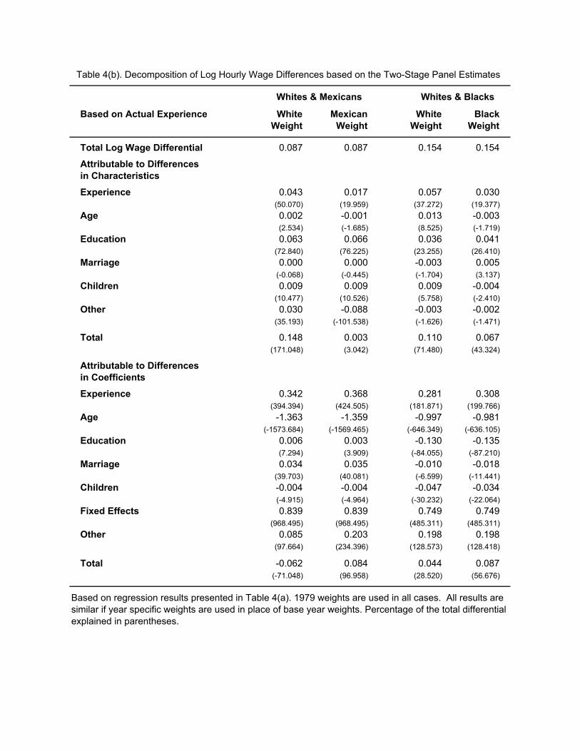
Table 4(b). Decomposition of Log Hourly Wage Differences based on the Two-Stage Panel Estimates

Whites & Mexicans Whites & Blacks

Based on Actual Experience White Mexican White BlackWeight Weight Weight Weight

Total Log Wage Differential 0.087 0.087 0.154 0.154

Attributable to Differences in CharacteristicsExperience 0.043 0.017 0.057 0.030

(50.070) (19.959) (37.272) (19.377)Age 0.002 -0.001 0.013 -0.003

(2.534) (-1.685) (8.525) (-1.719)Education 0.063 0.066 0.036 0.041

(72.840) (76.225) (23.255) (26.410)Marriage 0.000 0.000 -0.003 0.005

(-0.068) (-0.445) (-1.704) (3.137)Children 0.009 0.009 0.009 -0.004

(10.477) (10.526) (5.758) (-2.410)Other 0.030 -0.088 -0.003 -0.002

(35.193) (-101.538) (-1.626) (-1.471)

Total 0.148 0.003 0.110 0.067(171.048) (3.042) (71.480) (43.324)

Attributable to Differences in CoefficientsExperience 0.342 0.368 0.281 0.308

(394.394) (424.505) (181.871) (199.766)Age -1.363 -1.359 -0.997 -0.981

(-1573.684) (-1569.465) (-646.349) (-636.105)Education 0.006 0.003 -0.130 -0.135

(7.294) (3.909) (-84.055) (-87.210)Marriage 0.034 0.035 -0.010 -0.018

(39.703) (40.081) (-6.599) (-11.441)Children -0.004 -0.004 -0.047 -0.034

(-4.915) (-4.964) (-30.232) (-22.064)Fixed Effects 0.839 0.839 0.749 0.749

(968.495) (968.495) (485.311) (485.311)Other 0.085 0.203 0.198 0.198

(97.664) (234.396) (128.573) (128.418)

Total -0.062 0.084 0.044 0.087(-71.048) (96.958) (28.520) (56.676)

Based on regression results presented in Table 4(a). 1979 weights are used in all cases. All results aresimilar if year specific weights are used in place of base year weights. Percentage of the total differential explained in parentheses.