The shape and dynamics of a heliotropic dusty ringlet

in the Cassini Division

M.M. Hedmana, J.A. Burta,b, J.A. Burnsa,c, M.S. Tiscarenoa

a Department of Astronomy, Cornell Unviersity, Ithaca NY 14853

b Department of Astronomy and Astrophysics, University of California, Santa Cruz, CA95064

c College of Engineering, Cornell University, Ithaca NY 14853

Keywords: Celestial Mechanics; Planetary Dynamics; Planetary Rings; Saturn, rings

Corresponding Author: Matthew HedmanSpace Sciences BuildingCornell UniversityIthaca NY 14853607-255-5913mmhedman@astro.cornell.edu

– 2 –

The so-called “Charming Ringlet” (R/2006 S3) is a low-optical-depth, dusty ringletlocated in the Laplace gap in the Cassini Division, roughly 119,940 km from Saturn center.This ringlet is particularly interesting because its radial position varies systematically withlongitude relative to the Sun in such a way that the ringlet’s geometric center appears to bedisplaced away from Saturn’s center in a direction roughly toward the Sun. In other words,the ringlet is always found at greater distances from the planet’s center at longitudes nearthe sub-solar longitude than it is at longitudes near Saturn’s shadow. This “heliotropic”behavior indicates that the dynamics of the particles in this ring are being influenced bysolar radiation pressure. In order to investigate this phenomenon, which has been predictedtheoretically but not observed this clearly, we analyze multiple image sequences of thisringlet obtained by the Cassini spacecraft in order to constrain its shape and orientation.These data can be fit reasonably well with a model in which both the eccentricity andthe inclination of the ringlet have “forced” components (that maintain a fixed orientationrelative to the Sun) as well as “free” components (that drift around the planet at steadyrates determined by Saturn’s oblateness). The best-fit value for the eccentricity forcedby the Sun is 0.000142 ± 0.000004, assuming this component of the eccentricity has itspericenter perfectly anti-aligned with the Sun. These data also place an upper limit ona forced inclination of 0.0007. Assuming the forced inclination is zero and the forcedeccentricity vector is aligned with the anti-solar direction, the best-fit values for the freecomponents of the eccentricity and inclination are 0.000066±0.000003 and 0.0014±0.0001,respectively. While the magnitude of the forced eccentricity is roughly consistent withtheoretical expectations for radiation pressure acting on 10-to-100-micron-wide icy grains,the existence of significant free eccentricities and inclinations poses a significant challengefor models of low-optical-depth dusty rings.

1. Introduction

Images taken by the cameras onboard the Cassini spacecraft have revealed that severalof the wider gaps in Saturn’s main rings contain low-optical-depth, dusty ringlets (Porcoet al. 2005). One of these ringlets is located in the 200-km wide space in the outer CassiniDivision between the inner edges of the Laplace Gap and the Laplace Ringlet, 119,940 kmfrom Saturn’s center. This ringlet has a peak normal optical depth of around 10−3 andits photometric properties (such as a dramatic increase in brightness at high phase angles)indicate that it is composed primarily of small dust grains less than 100 microns across(Horanyi et al. 2009). While this feature is officially designated R/2006 S3 (Porcoet al.2006), it is unofficially called the “Charming Ringlet” by various Cassini scientists, and wewill use that name here. Regardless of its name, this ringlet is of special interest because itsradial position varies systematically with longitude relative to the Sun in such a way thatthe ringlet’s geometric center appears to be displaced away from Saturn’s center towardsthe Sun. In other words, this ringlet always appears some tens of kilometers further fromthe planet’s center at longitudes near the sub-solar longitude than it is at longitudes nearSaturn’s shadow (see Figure 1). This “heliotropic” behavior suggests that non-gravitational

– 3 –

forces such as solar radiation pressure are affecting the particles’ orbital dynamics, as pre-dicted by various theoretical models (e.g. Horanyi and Burns 1991, Hamilton 1993).

While other dusty ringlets, like those in the Encke Gap, may also show heliotropicbehavior (Hedman et al. 2007), the Charming Ringlet provides the best opportunity tobegin investigations of this phenomenon. Unlike the Encke Gap ringlets, the CharmingRinglet does not appear to contain bright clumps or noticeable short-wavelength “kinks”in its radial position. The absence of such features makes the global shape of the ringleteasier to observe and quantify. Furthermore, the radial positions of the edges of the Laplacegap and ringlet only vary by a few kilometers (Hedman et al. 2010), so this gap is a muchsimpler environment than other gaps (like the Huygens gap) where the radial locations ofthe edges can vary by tens of kilometers. Finally, the observations of the Charming Ringletare more extensive than those of some other dusty ringlets.

In this paper, we build upon the preliminary work reported in Hedman et al. (2007)and Burt et al. (2008) in order to develop a model for the three-dimensional shape andorientation of the Charming Ringlet and to explore what such a model implies about theparticle dynamics in this ring. First, we provide a brief summary of the data that will be usedin this analysis and then fit the different data sets to models of an eccentric, inclined ringlet.These fits indicate that the shape and orientation of the ringlet change significantly overtime. Next, we review the theoretical predictions for how particle orbits should behave underthe influence of solar radiation pressure. Based on this theory, we develop a global modelthat includes both forced and free components in the ringlet’s eccentricity and inclination;these can reproduce the observations reasonably well. Finally, we discuss the implicationsof such a model for the dynamics of this ringlet.

2. Observations and data reduction

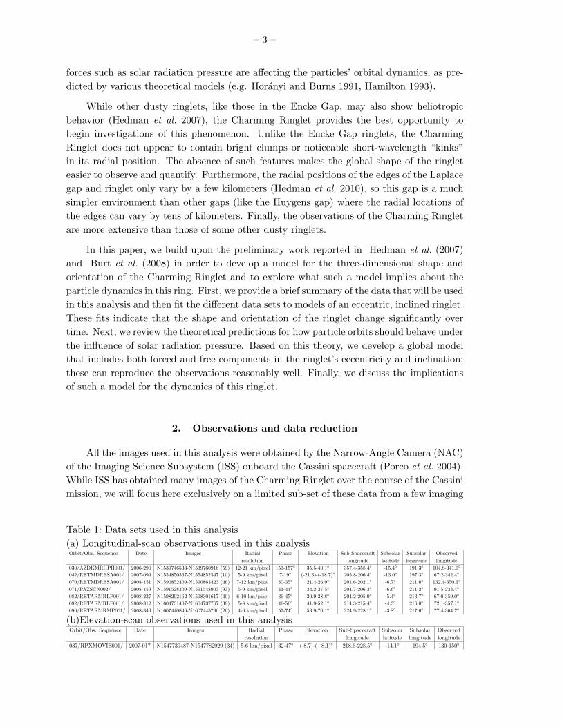
All the images used in this analysis were obtained by the Narrow-Angle Camera (NAC)of the Imaging Science Subsystem (ISS) onboard the Cassini spacecraft (Porco et al. 2004).While ISS has obtained many images of the Charming Ringlet over the course of the Cassinimission, we will focus here exclusively on a limited sub-set of these data from a few imaging

Table 1: Data sets used in this analysis(a) Longitudinal-scan observations used in this analysisOrbit/Obs. Sequence Date Images Radial Phase Elevation Sub-Spacecraft Subsolar Subsolar Observed

resolution longitude latitude longitude longitude030/AZDKMRHPH001/ 2006-290 N1539746533-N1539760916 (59) 12-21 km/pixel 153-157 35.5-40.1 357.4-358.4 -15.4 191.3 104.8-341.9

042/RETMDRESA001/ 2007-099 N1554850367-N1554852347 (10) 5-9 km/pixel 7-19 (-21.3)-(-18.7) 205.8-206.4 -13.0 197.3 67.2-342.4

070/RETMDRESA001/ 2008-151 N1590852409-N1590863423 (46) 7-12 km/pixel 30-35 21.4-26.9 201.6-202.1 -6.7 211.0 132.4-350.1

071/PAZSCN002/ 2008-159 N1591528309-N1591548903 (93) 5-9 km/pixel 41-44 34.2-37.5 204.7-206.3 -6.6 211.2 91.5-233.4

082/RETARMRLP001/ 2008-237 N1598292162-N1598301617 (40) 6-10 km/pixel 36-45 30.9-38.8 204.2-205.0 -5.4 213.7 67.0-359.0

092/RETARMRLF001/ 2008-312 N1604731407-N1604737767 (39) 5-8 km/pixel 46-56 41.9-52.1 214.3-215.4 -4.3 216.0 72.1-357.1

096/RETARMRMP001/ 2008-343 N1607440846-N1607445736 (26) 4-6 km/pixel 57-74 53.9-70.1 224.9-228.1 -3.8 217.0 77.4-364.7

(b)Elevation-scan observations used in this analysisOrbit/Obs. Sequence Date Images Radial Phase Elevation Sub-Spacecraft Subsolar Subsolar Observed

resolution longitude latitude longitude longitude037/RPXMOVIE001/ 2007-017 N1547739487-N1547782929 (34) 5-6 km/pixel 32-47 (-8.7)-(+8.1) 218.6-228.5 -14.1 194.5 130-150

– 4 –

Fig. 1.— Sample images of the Charming Ringlet in the Cassini Division obtained by thenarrow-angle camera onboard the Cassini spacecraft. The top two images were obtained onday 343 of 2008 as part of the RETARMRMP observation in Orbit 96, when the sub-solarlongitude was 217 (see Table 1). The two images have been separately cropped, rotated andstretched to facilitate comparisons. In both images, radius in the rings increases towardsto upper right. The arrows at the top of the image point to the Charming Ringlet in theLaplace gap. Note that in the left-hand image (N1607440846, observed longitude=5) ofa region near Saturn’s shadow, the ringlet is closer to the inner edge of the gap, whilein the right-hand image (N1609443806, observed longitude=192) of a region near to thesub-solar longitude, the ringlet is closer to the outer edge of the gap. The bottom image(N1547759879) was obtained on day 17 of 2007 as part of the RPXMOVIE observation inOrbit 37, when the ring opening angle was only -0.36. The image has been rotated so thatSaturn’s north pole points upwards. Ring radius increases from right to left, and the arrowpoints to the Charming Ringlet in the Laplace Gap. Note that the ringlet appears slightlydisplaced upwards in this image relative to the edges of the gap (the upper arm of the ringdisappears into the glare of the edge of the gap faster than the lower arm). This suggeststhat this ringlet is inclined.

– 5 –

sequences. Each of these sequences was obtained over a relatively short period of time andcovers a sufficient range of longitudes or viewing geometries that it can provide useful con-straints on the shape and orientation of the ring. These data sets are therefore particularlyuseful for developing a shape model for this ring. In principle, once a rough model hasbeen established, additional data can be used to refine the model parameters and test themodel. However, such an analysis is beyond the scope of this paper and therefore will bethe subject of future work.

Two different types of observation sequences will be utilized in the present study, “lon-gitudinal scans” and “elevation scans”. Each longitudinal scan consists of a series of imagesof the Cassini Division, with different images centered at different inertial longitudes in therings. These scans provide maps of the apparent radial position of the Charming Ringlet asa function of longitude relative to the Sun. The seven such scans used in this analysis (listedin Table 1a) are all the scans obtained prior to 2009 that contain the Charming Ringlet,have sufficient radial resolution to clearly resolve the ringlet and also cover a sufficientlybroad range of longitudes (> 140) to provide a reliable measurement of both the ringlet’seccentricity and inclination (see below).

By contrast, elevation scans consist of a series of images of the ring ansa taken overa period of time when the spacecraft passed through the ring-plane, yielding observationscovering a range of ring-opening angles B around zero. Such images provide limited infor-mation about the ringlet’s eccentricity, however, observable shifts in the ringlet’s apparentposition relative to other ring features provide evidence that the ringlet is inclined (seeFig 1). These observations therefore can furnish additional constraints on the ringlet’svertical structure. Thus far, only one image sequence (given in Table 1b) has sufficient res-olution and elevation-angle coverage to yield useful constraints on the ringlet’s orientation.

All of these images were processed using the standard CISSCAL calibration routines(version 3.6) (Porco et al. 2004) that remove backgrounds, flat-field the images, and convertthe raw data numbers into I/F (a standardized measure of reflectance where I is theintensity of the scattered radiation while πF is the solar flux at Saturn). We then extractedmeasurements of the ringlet’s radial position with the following procedures.

First, all the relevant images were geometrically navigated employing the appropriateSPICE kernels to establish the position and approximate pointing of the spacecraft. Thepointing was refined using the outer edge of the Jeffreys Gap (called OEG 15 in Frenchet al. 1993, assumed to be circular and lie at 118,968 km) as a fiducial feature. RecentCassini occultation measurements demonstrate that this feature is circular to better than1 km (Hedman et al. 2010; French et al. 2010), making it a reliable reference point in therings.

Once each image was navigated, the brightness data were converted into radial bright-ness profiles by averaging the brightness at each radius over a range of longitudes. For thelongitudinal scans, each image covered a sufficiently small range of longitudes that varia-tions in the radial position of the ringlet within an image could be ignored. Consequently,a single radial scan was derived from each image by averaging the data over all observed

– 6 –

longitudes. By contrast, for the elevation scans, variations in the radial position of theringlet were apparent within individual images. A series of 8-20 radial brightness profileswas therefore extracted from each image, with each profile being the average brightnessof the ring in a range of longitudes between 0.5 and 1.0 wide. Note that for all theseprofiles, the radius scale corresponds to the projected position of any given feature onto thering-plane.

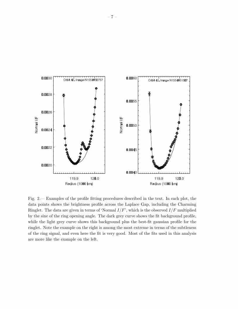
The Charming Ringlet could be detected as a brightness peak within the Laplace gapin all of these radial scans. The radial position of the ringlet was estimated from each scanby fitting the ringlet’s brightness profile to a Gaussian. For the high-phase observations inOrbit 30, the ringlet was sufficiently bright that the Gaussian could be fit directly to theradial profile. For the other (lower-phase) profiles, however, the ringlet was considerablyfainter and the brightness variations within the gap due to various instrumental effects couldnot be ignored. In these situations, a background light profile for the gap was computedusing the data outside the ringlet (the edges of the ringlet were determined based on wherethe slope of the brightness profile around the ringlet was closest to zero). This backgroundwas interpolated into the region under the ringlet (using a spline interpolation of the profilesmoothed over three radial bins) and a Gaussian was fit to the background-subtractedringlet profile. Figure 2 shows examples of the raw profile, the interpolated background andthe background plus the fitted Gaussian, demonstrating that this procedure yields sensibleresults even when the ringlet is rather subtle.

The above process yielded a series of measurements of the apparent radial position ofthe ringlet as a function of longitude. Figure 3 shows these data for the seven differentlongitudinal scans. Note that in all cases the ringlet is found furthest from the planet ata point near to the sub-solar longitude. This is not just a coincidence of when the ringletwas observed, but is instead the evidence for the “heliotropic” character of this ringlet.However, we can also observe that the apparent shape of the ringlet varies significantlyamong the different observations. This implies that the ringlet does not simply maintaina fixed orientation relative to the Sun, but instead has a more complex and time-variableshape.

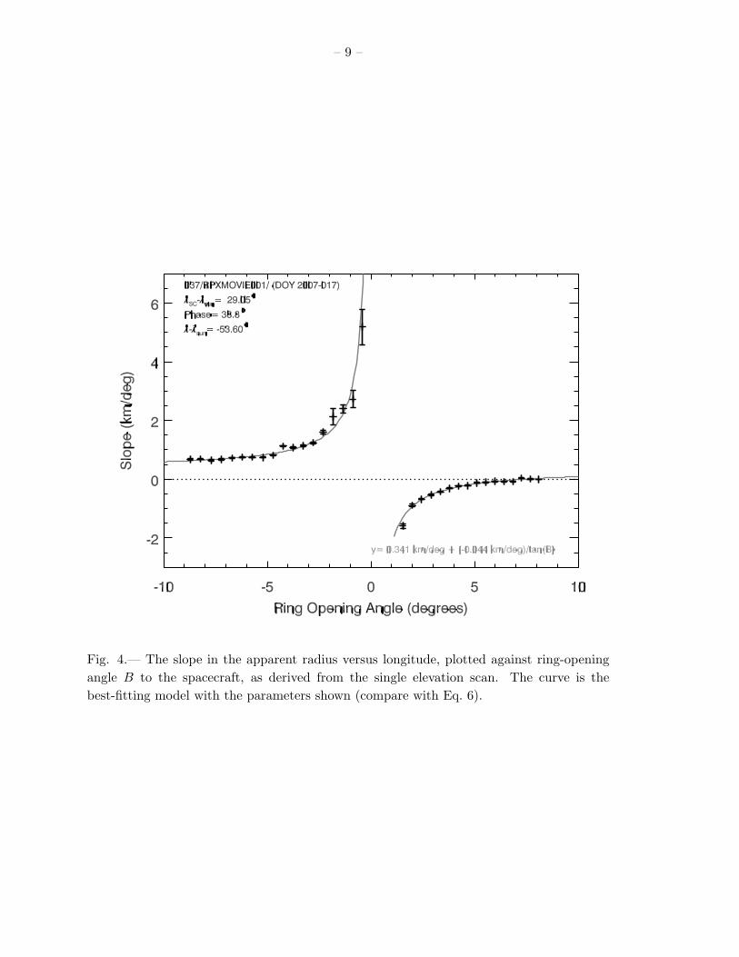
For the elevation scan, the radial position of the ringlet versus longitude from eachimage can be fit to a line. Figure 4 shows the slopes of the line derived from these images asa function of ring-opening angle B. The slope changes dramatically as the spacecraft crossesthe ringplane. This strongly suggests that this portion of the ring is vertically displacedfrom the ringplane (Burt et al. 2008), and means that we will need a three-dimensionalmodel to fully describe the shape of this ringlet.

3. Ringlet shape estimates from individual observations

The above evidence for time-variable and three-dimensional structure obviously com-plicates our efforts to quantify the Charming Ringlet’s shape. Fortunately, it turns out thatthe data from individual scans can be reasonably well fit by simple models of eccentric,

– 7 –

Fig. 2.— Examples of the profile fitting procedures described in the text. In each plot, thedata points shows the brightness profile across the Laplace Gap, including the CharmingRinglet. The data are given in terms of ‘Normal I/F ’, which is the observed I/F multipliedby the sine of the ring opening angle. The dark grey curve shows the fit background profile,while the light grey curve shows this background plus the best-fit gaussian profile for theringlet. Note the example on the right is among the most extreme in terms of the subtlenessof the ring signal, and even here the fit is very good. Most of the fits used in this analysisare more like the example on the left.

– 8 –

Fig. 3.— The apparent radius of the Charming Ringlet (projected onto the ring-plane) asa function of longitude relative to the Sun, derived from the seven longitudinal scans. Theobservations are shown as crosses. The dark grey curve shows the best-fit model to eachdata set with the parameters listed on each plot (compare with Eq. 5). The light grey curveis the same model with the term ∝ sin(2λ) removed to illustrate the importance of thisterm to the overall fit.

– 9 –

Fig. 4.— The slope in the apparent radius versus longitude, plotted against ring-openingangle B to the spacecraft, as derived from the single elevation scan. The curve is thebest-fitting model with the parameters shown (compare with Eq. 6).

– 10 –

inclined ringlets. By fitting each scan to such a model, we can further reduce the data to asmall number of shape/orbital parameters, which may change with time.

Each scan consists of measurements of the apparent radial position of the ringlet pro-jected on the ringplane r versus longitude relative to the Sun λ − λ = λ′. Assuming theringlet can have both an inclination and an eccentricity, the radial and vertical positions ofthe ringlet versus longitude are for small eccentricities and inclinations well approximatedby:

r = a− ae cos(λ′ −$′) (1)

z = ai sin(λ′ − Ω′), (2)

where a, e and i are the semi-major axis, eccentricity and inclination of the ringlet, and $′

and Ω′ are the longitudes of pericenter and ascending node relative to the Sun.

If z is nonzero, the apparent position of the ringlet will be displaced when it is projectedonto the ringplane. Assuming the observer is sufficiently far from the ring, this displacementis simply

δr = − z

tanBcos(λ′ − λ′c), (3)

where B is the ring opening angle to the observing spacecraft and λ′c is the longitude of thespacecraft relative to the Sun. Substituting in the above value for z, we find:

δr =−ai

2 tanB[sin(2λ′ − Ω′ − λ′c)− sin(Ω′ − λ′c)]. (4)

The apparent radial position of such a ringlet is therefore:

r = r + δr = a +ai

2 tanBsin(Ω′ − λ′c)− ae cos(λ′ −$′)− ai

2 tanBsin(2λ′ − Ω′ − λ′c). (5)

Note that this expression contains two terms that depend on the longitude λ′: one pro-portional to e and one proportional to i. Since these two terms depend on longitude indifferent ways, it should be possible to determine both the eccentricity and inclination fromany observation sequence that covers a sufficiently broad range of longitudes. Also, sincethe terms involving i depend on the ring opening angle B while those involving e do not,the effects of inclination and eccentricity on the apparent position of the ringlet should alsobe separable when the observation sequences cover a sufficient range in B.

3.1. Elevation Scan

Over the limited range of longitudes observed in each image of the elevation scan, theapparent-radius-versus-longitude curve is well fit by a straight line. Figure 4 shows theslope of this line as a function of ring opening angle, with error bars derived from the linearfit.

Given the above expression (Eq. 5) for the apparent radial position of the ring versuslongitude, these measured slopes can be identified with the quantity:

m =dr

dλ′= ae sin(λ′ −$′)− ai

tanBcos(2λ′ − Ω′ − λ′c) (6)

– 11 –

In other words, m = C − z/ tanB, where C is the constant background slope due to theeccentricity of the ringlet and z is its vertical displacement at the observed longitude. Fittingthe data from the elevation scan to an equation of this form, we find that at the observedlongitude and time:

z = ai cos(2λ′ − Ω′ − λ′c) = 2.54± 0.02 km, (7)

C = ae sin(λ′ −$′) = 19.5± 0.2 km. (8)

The curve plotted on Fig. 4 shows this best-fit function, which reproduces the trends in thedata rather well. However, the χ2 of this fit is 206 for 32 degrees of freedom, indicatingthat the errors on the individual slope measurements have been underestimated. Thus theabove uncertainties on z and C should probably be increased by a factor of 2.5. Note thatwhile these data alone cannot provide exact estimates on eccentricity and inclination, wecan establish that ai is at least 2.5 km and ae is at least 19 km.

3.2. Longitudinal Scans

Figure 3 shows the estimated position of the Charming Ringlet versus longitude relativeto the Sun for each of the seven longitudinal scans. Each of these data sets has been fit toa function of the form (cf Eq. 5)

r = ro + r1 cos(λ′ − φ1) + r2 cos(2λ′ − φ2). (9)

The best fit solutions, shown as the dark grey curves in Fig. 3, satisfactorily reproduce thetrends seen in the real data. We can therefore use the parameters of this fit and Equation 5to derive the ring-shape parameters a, e, i,$′ and Ω′ (see Table 2). The error bars on theorbital parameters are computed using the rms residuals from the fit to estimate the errorbars on each data point. These residuals are always less than one kilometer, or about afactor of 10 better than the image resolution (see Tables 1 and 2), and probably reflectsmall errors and uncertainties in the fitted locations of the fiducial edge and ringlet center.The small scatter in these data therefore confirms the stability of the pointing and fittingalgorithms within each of these sequences.

Let us consider each of these different parameters in turn, starting with the semi-majoraxis a. No formal error bars on this parameter are given here because this parameter is theone most likely to be affected by systematic pointing uncertainties between the differentscans caused by differences in the appearance and contrast of the fiducial edge. Neverthe-less, the scatter in these values is still only a few kilometers and well below the resolutionsof the images (compare to Table 1), providing further confirmation that the fitting proce-dures employed here are robust. Note that all the observations give a values within a fewkilometers of 119,940 km, which is very close to exactly halfway between the inner edge ofthe Laplace Gap at 119,845 km and the inner edge of the Laplace ringlet at 120,036 km(Hedman et al. 2010).

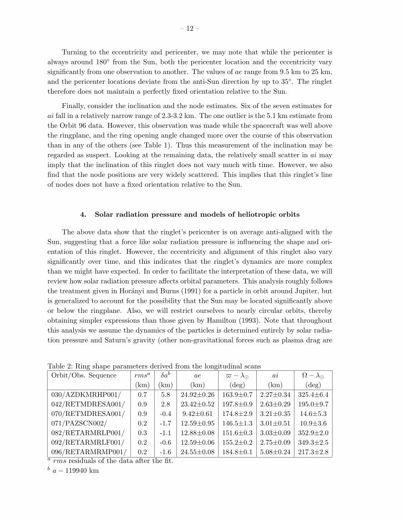
– 12 –

Turning to the eccentricity and pericenter, we may note that while the pericenter isalways around 180 from the Sun, both the pericenter location and the eccentricity varysignificantly from one observation to another. The values of ae range from 9.5 km to 25 km,and the pericenter locations deviate from the anti-Sun direction by up to 35. The ringlettherefore does not maintain a perfectly fixed orientation relative to the Sun.

Finally, consider the inclination and the node estimates. Six of the seven estimates forai fall in a relatively narrow range of 2.3-3.2 km. The one outlier is the 5.1 km estimate fromthe Orbit 96 data. However, this observation was made while the spacecraft was well abovethe ringplane, and the ring opening angle changed more over the course of this observationthan in any of the others (see Table 1). Thus this measurement of the inclination may beregarded as suspect. Looking at the remaining data, the relatively small scatter in ai mayimply that the inclination of this ringlet does not vary much with time. However, we alsofind that the node positions are very widely scattered. This implies that this ringlet’s lineof nodes does not have a fixed orientation relative to the Sun.

4. Solar radiation pressure and models of heliotropic orbits

The above data show that the ringlet’s pericenter is on average anti-aligned with theSun, suggesting that a force like solar radiation pressure is influencing the shape and ori-entation of this ringlet. However, the eccentricity and alignment of this ringlet also varysignificantly over time, and this indicates that the ringlet’s dynamics are more complexthan we might have expected. In order to facilitate the interpretation of these data, we willreview how solar radiation pressure affects orbital parameters. This analysis roughly followsthe treatment given in Horanyi and Burns (1991) for a particle in orbit around Jupiter, butis generalized to account for the possibility that the Sun may be located significantly aboveor below the ringplane. Also, we will restrict ourselves to nearly circular orbits, therebyobtaining simpler expressions than those given by Hamilton (1993). Note that throughoutthis analysis we assume the dynamics of the particles is determined entirely by solar radia-tion pressure and Saturn’s gravity (other non-gravitational forces such as plasma drag are

Table 2: Ring shape parameters derived from the longitudinal scansOrbit/Obs. Sequence rmsa δab ae $ − λ ai Ω− λ

(km) (km) (km) (deg) (km) (deg)030/AZDKMRHP001/ 0.7 5.8 24.92±0.26 163.9±0.7 2.27±0.34 325.4±6.4042/RETMDRESA001/ 0.9 2.8 23.42±0.52 197.8±0.9 2.63±0.29 195.0±9.7070/RETMDRESA001/ 0.9 -0.4 9.42±0.61 174.8±2.9 3.21±0.35 14.6±5.3071/PAZSCN002/ 0.2 -1.7 12.59±0.95 146.5±1.3 3.01±0.51 10.9±3.6082/RETARMRLP001/ 0.3 -1.1 12.88±0.08 151.6±0.3 3.03±0.09 352.9±2.0092/RETARMRLF001/ 0.2 -0.6 12.59±0.06 155.2±0.2 2.75±0.09 349.3±2.5096/RETARMRMP001/ 0.2 -1.6 24.55±0.08 184.8±0.1 5.08±0.24 217.3±2.8

a rms residuals of the data after the fit.b a− 119940 km

– 13 –

neglected).

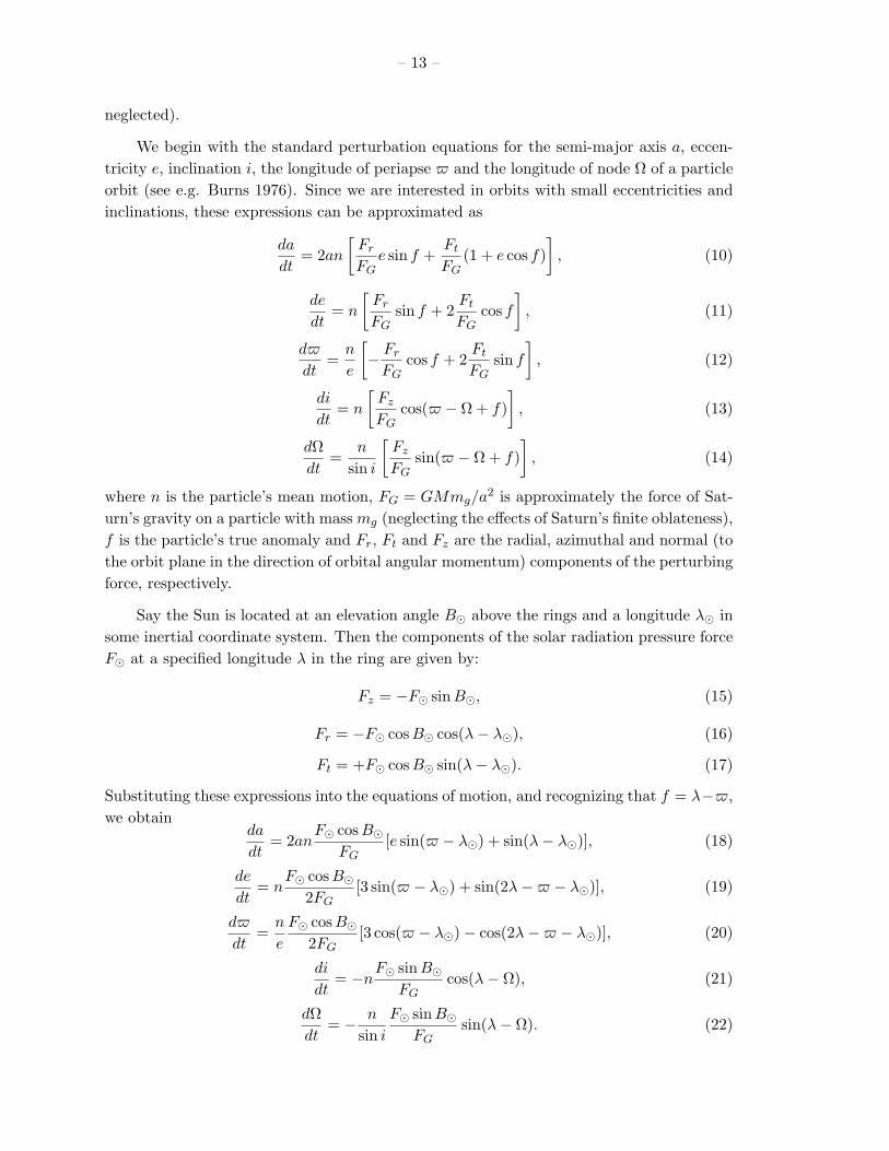
We begin with the standard perturbation equations for the semi-major axis a, eccen-tricity e, inclination i, the longitude of periapse $ and the longitude of node Ω of a particleorbit (see e.g. Burns 1976). Since we are interested in orbits with small eccentricities andinclinations, these expressions can be approximated as

da

dt= 2an

[Fr

FGe sin f +

Ft

FG(1 + e cos f)

], (10)

de

dt= n

[Fr

FGsin f + 2

Ft

FGcos f

], (11)

d$

dt=

n

e

[− Fr

FGcos f + 2

Ft

FGsin f

], (12)

di

dt= n

[Fz

FGcos($ − Ω + f)

], (13)

dΩdt

=n

sin i

[Fz

FGsin($ − Ω + f)

], (14)

where n is the particle’s mean motion, FG = GMmg/a2 is approximately the force of Sat-urn’s gravity on a particle with mass mg (neglecting the effects of Saturn’s finite oblateness),f is the particle’s true anomaly and Fr, Ft and Fz are the radial, azimuthal and normal (tothe orbit plane in the direction of orbital angular momentum) components of the perturbingforce, respectively.

Say the Sun is located at an elevation angle B above the rings and a longitude λ insome inertial coordinate system. Then the components of the solar radiation pressure forceF at a specified longitude λ in the ring are given by:

Fz = −F sinB, (15)

Fr = −F cos B cos(λ− λ), (16)

Ft = +F cos B sin(λ− λ). (17)

Substituting these expressions into the equations of motion, and recognizing that f = λ−$,we obtain

da

dt= 2an

F cos BFG

[e sin($ − λ) + sin(λ− λ)], (18)

de

dt= n

F cos B2FG

[3 sin($ − λ) + sin(2λ−$ − λ)], (19)

d$

dt=

n

e

F cos B2FG

[3 cos($ − λ)− cos(2λ−$ − λ)], (20)

di

dt= −n

F sinBFG

cos(λ− Ω), (21)

dΩdt

= − n

sin i

F sinBFG

sin(λ− Ω). (22)

– 14 –

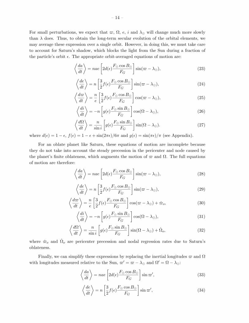
For small perturbations, we expect that $, Ω, e, i and λ will change much more slowlythan λ does. Thus, to obtain the long-term secular evolution of the orbital elements, wemay average these expression over a single orbit. However, in doing this, we must take careto account for Saturn’s shadow, which blocks the light from the Sun during a fraction ofthe particle’s orbit ε. The appropriate orbit-averaged equations of motion are:⟨

da

dt

⟩= nae

[2d(ε)

F cos BFG

]sin($ − λ), (23)

⟨de

dt

⟩= n

[32f(ε)

F cos BFG

]sin($ − λ), (24)⟨

d$

dt

⟩=

n

e

[32f(ε)

F cos BFG

]cos($ − λ), (25)⟨

di

dt

⟩= −n

[g(ε)

F sin BFG

]cos(Ω− λ), (26)⟨

dΩdt

⟩=

n

sin i

[g(ε)

F sinBFG

]sin(Ω− λ). (27)

where d(ε) = 1− ε, f(ε) = 1− ε + sin(2πε)/6π and g(ε) = sin(πε)/π (see Appendix).

For an oblate planet like Saturn, these equations of motion are incomplete becausethey do not take into account the steady precession in the pericenter and node caused bythe planet’s finite oblateness, which augments the motion of $ and Ω. The full equationsof motion are therefore:⟨

da

dt

⟩= nae

[2d(ε)

F cos BFG

]sin($ − λ), (28)

⟨de

dt

⟩= n

[32f(ε)

F cos BFG

]sin($ − λ), (29)⟨

d$

dt

⟩=

n

e

[32f(ε)

F cos BFG

]cos($ − λ) + $o, (30)⟨

di

dt

⟩= −n

[g(ε)

F sin BFG

]cos(Ω− λ), (31)⟨

dΩdt

⟩=

n

sin i

[g(ε)

F sinBFG

]sin(Ω− λ) + Ωo, (32)

where $o and Ωo are pericenter precession and nodal regression rates due to Saturn’soblateness.

Finally, we can simplify these expressions by replacing the inertial longitudes $ and Ωwith longitudes measured relative to the Sun, $′ = $ − λ and Ω′ = Ω− λ:⟨

da

dt

⟩= nae

[2d(ε)

F cos BFG

]sin$′, (33)

⟨de

dt

⟩= n

[32f(ε)

F cos BFG

]sin$′, (34)

– 15 –

⟨d$′

dt

⟩=

n

e

[32f(ε)

F cos BFG

]cos $′ + $′

o, (35)⟨di

dt

⟩= −n

[g(ε)

F sinBFG

]cos Ω′, (36)⟨

dΩ′

dt

⟩=

n

sin i

[g(ε)

F sinBFG

]sinΩ′ + Ω′

o, (37)

where $′o = $o− λ and Ω′

o = Ωo− λ will be referred to here as the “modified” pericenterprecession and nodal regression rates, respectively.

Assuming that B changes sufficiently slowly, then for any semi-major axis a there isa unique steady-state solution to these equations where

⟨dadt

⟩=

⟨dedt

⟩=

⟨d$′

dt

⟩=

⟨didt

⟩=⟨

dΩ′

dt

⟩= 0. This steady-state orbital solution has the following orbital parameters (assuming

sin i ' i):

ef =n

$′o

[32f(ε)

FFG

cos B

], (38)

$f = λ + π, (39)

if =n

|Ω′o|

[g(ε)

FFG

sin |B|]

, (40)

Ωf = λ +π

2B|B|

. (41)

This orbit has a finite eccentricity ef with the pericenter anti-aligned with the Sun, so thatthe apoapse of the orbit points towards the Sun. This is grossly consistent with the observedheliotropic behavior of the Charming Ringlet shown in Figs. 3 and 4. Furthermore, if Bis non-zero, then this orbit also has a finite inclination, and the ascending node is located±90 from the sub-solar longitude, depending on whether the Sun is north or south of theringplane. The orbit will therefore be inclined so that it is on the opposite side of theequator plane as the Sun at longitudes near local noon.

However, this steady-state solution is a special case. More general solutions to theequation of motion can be most clearly described using the variables (Horanyi and Burns1991, see also Murray and Dermott 1999, equations 7.18-7.19):

h = e cos($ − λ) = e cos $′, (42)

k = e sin($ − λ) = e sin$′, (43)

p = i cos(Ω− λ) = i cos Ω′, (44)

q = i sin(Ω− λ) = i sinΩ′. (45)

In terms of these variables, the above equations of motion reduce to:⟨da

dt

⟩=

4d(ε)3f(ε)

aef $′ok, (46)

⟨dh

dt

⟩= −$′

ok, (47)

– 16 –

⟨dk

dt

⟩= $′

o(h + ef ), (48)⟨dp

dt

⟩= −Ω′

o

(q − if

B|B|

), (49)⟨

dq

dt

⟩= Ω′

op, (50)

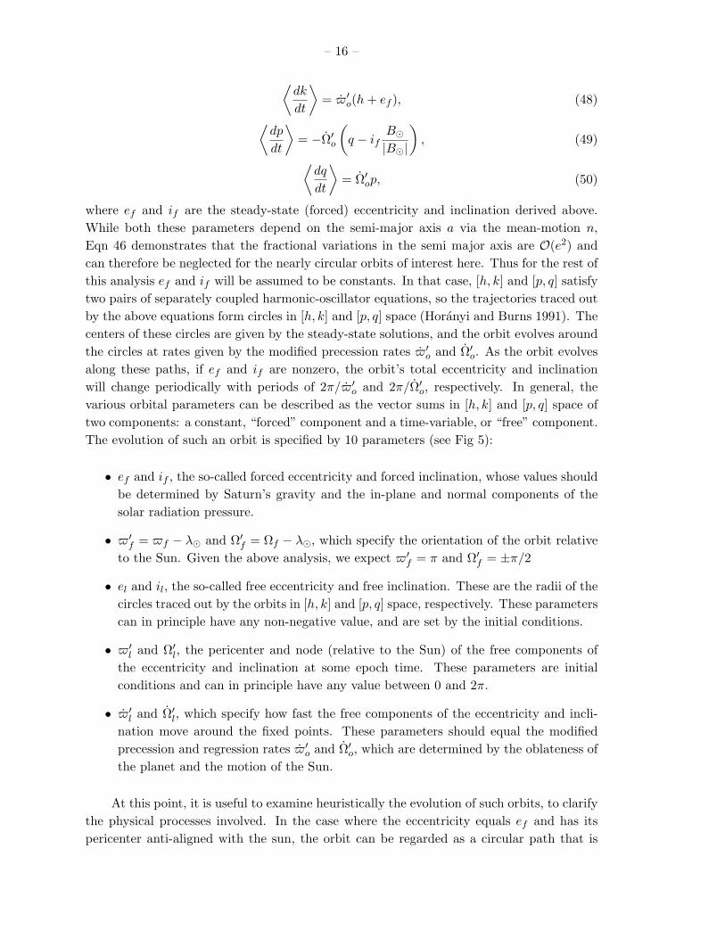
where ef and if are the steady-state (forced) eccentricity and inclination derived above.While both these parameters depend on the semi-major axis a via the mean-motion n,Eqn 46 demonstrates that the fractional variations in the semi major axis are O(e2) andcan therefore be neglected for the nearly circular orbits of interest here. Thus for the rest ofthis analysis ef and if will be assumed to be constants. In that case, [h, k] and [p, q] satisfytwo pairs of separately coupled harmonic-oscillator equations, so the trajectories traced outby the above equations form circles in [h, k] and [p, q] space (Horanyi and Burns 1991). Thecenters of these circles are given by the steady-state solutions, and the orbit evolves aroundthe circles at rates given by the modified precession rates $′

o and Ω′o. As the orbit evolves

along these paths, if ef and if are nonzero, the orbit’s total eccentricity and inclinationwill change periodically with periods of 2π/$′

o and 2π/Ω′o, respectively. In general, the

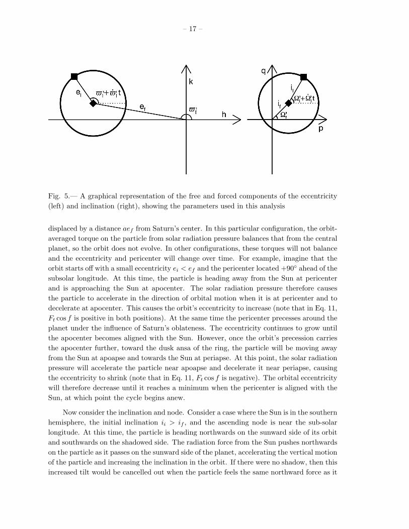
various orbital parameters can be described as the vector sums in [h, k] and [p, q] space oftwo components: a constant, “forced” component and a time-variable, or “free” component.The evolution of such an orbit is specified by 10 parameters (see Fig 5):

• ef and if , the so-called forced eccentricity and forced inclination, whose values shouldbe determined by Saturn’s gravity and the in-plane and normal components of thesolar radiation pressure.

• $′f = $f − λ and Ω′

f = Ωf − λ, which specify the orientation of the orbit relativeto the Sun. Given the above analysis, we expect $′

f = π and Ω′f = ±π/2

• el and il, the so-called free eccentricity and free inclination. These are the radii of thecircles traced out by the orbits in [h, k] and [p, q] space, respectively. These parameterscan in principle have any non-negative value, and are set by the initial conditions.

• $′l and Ω′

l, the pericenter and node (relative to the Sun) of the free components ofthe eccentricity and inclination at some epoch time. These parameters are initialconditions and can in principle have any value between 0 and 2π.

• $′l and Ω′

l, which specify how fast the free components of the eccentricity and incli-nation move around the fixed points. These parameters should equal the modifiedprecession and regression rates $′

o and Ω′o, which are determined by the oblateness of

the planet and the motion of the Sun.

At this point, it is useful to examine heuristically the evolution of such orbits, to clarifythe physical processes involved. In the case where the eccentricity equals ef and has itspericenter anti-aligned with the sun, the orbit can be regarded as a circular path that is

– 17 –

Fig. 5.— A graphical representation of the free and forced components of the eccentricity(left) and inclination (right), showing the parameters used in this analysis

displaced by a distance aef from Saturn’s center. In this particular configuration, the orbit-averaged torque on the particle from solar radiation pressure balances that from the centralplanet, so the orbit does not evolve. In other configurations, these torques will not balanceand the eccentricity and pericenter will change over time. For example, imagine that theorbit starts off with a small eccentricity ei < ef and the pericenter located +90 ahead of thesubsolar longitude. At this time, the particle is heading away from the Sun at pericenterand is approaching the Sun at apocenter. The solar radiation pressure therefore causesthe particle to accelerate in the direction of orbital motion when it is at pericenter and todecelerate at apocenter. This causes the orbit’s eccentricity to increase (note that in Eq. 11,Ft cos f is positive in both positions). At the same time the pericenter precesses around theplanet under the influence of Saturn’s oblateness. The eccentricity continues to grow untilthe apocenter becomes aligned with the Sun. However, once the orbit’s precession carriesthe apocenter further, toward the dusk ansa of the ring, the particle will be moving awayfrom the Sun at apoapse and towards the Sun at periapse. At this point, the solar radiationpressure will accelerate the particle near apoapse and decelerate it near periapse, causingthe eccentricity to shrink (note that in Eq. 11, Ft cos f is negative). The orbital eccentricitywill therefore decrease until it reaches a minimum when the pericenter is aligned with theSun, at which point the cycle begins anew.

Now consider the inclination and node. Consider a case where the Sun is in the southernhemisphere, the initial inclination ii > if , and the ascending node is near the sub-solarlongitude. At this time, the particle is heading northwards on the sunward side of its orbitand southwards on the shadowed side. The radiation force from the Sun pushes northwardson the particle as it passes on the sunward side of the planet, accelerating the vertical motionof the particle and increasing the inclination in the orbit. If there were no shadow, then thisincreased tilt would be cancelled out when the particle feels the same northward force as it

– 18 –

is heading southward on the planet’s far side. However, because sunlight is blocked fromthis side of the rings by the planet’s shadow, the torque is not cancelled and the inclinationincreases. Meanwhile, the node regresses due to Saturn’s oblateness (if i > if , then thesecond term on the left hand side of Eq. 37 dominates). Thus the inclination continues togrow until the ascending node reaches a point 90 behind the Sun. After this point, theascending node will head into the shadow and the descending node will move towards thesub-solar longitude. In this case, the particle is moving southwards while it is exposed tosolar radiation pressure that drives it northwards, so the radiation pressure will deceleratethe vertical motion and cause the inclination to lessen until it reaches a minimum when theascending node is 90 ahead of the solar point, at which point the cycle starts again.

The orbital evolution described above is not specific to solar radiation pressure, butwill occur whenever the ring particles feel forces with a fixed direction in inertial space.To demonstrate that solar radiation pressure in particular is a reasonable explanation forthe shape and orientation of the Charming Ringlet, let us now evaluate numerically thestrength of the solar radiation pressure force F and the resulting ef and if .

The solar radiation pressure force F is given by (Burns et al. 1979):

F = SAQpr/c, (51)

where c is the speed of light, S is the solar energy flux, A is the cross-sectional area ofthe particles, and Qpr is an efficiency factor that is of order unity in the limit of geometricoptics. The force ratio for quasi-spherical grains can therefore be written as:

FFG

=34

S

c

a2

GM

Qpr

ρrg, (52)

where ρ is the particle’s density and rg is the particle’s radius. If we now assume S = 14W/m2 at Saturn, c = 3 ∗ 108 m/s, GM = 3.8 ∗ 1016 m3/s2, a =119,940 km (appropriate forthe Charming Ringlet) and ρ = 103 kg/m3 (appropriate for ice-rich grains) we find:

FFG

= 1.3 ∗ 10−5 Qpr

rg/1 µm. (53)

The other parameters in Eqs 38 and 40 can also be estimated. For the observations consid-ered here, the shadow covers roughly 80 in longitude, so ε ' 0.2, in which case f(ε) ' 0.85and g(ε) ' 0.2. Also, given Saturn’s gravitational harmonics (Jacobson et al. 2006), theorbital and precession rates in the vicinity of the Charming Ringlet are n = 736/day and$′

o ' |Ω′o| ' 4.7/day. With these values, the forced eccentricities and inclinations are:

ef ' 0.0026 cos BQpr

rg/1 µm, (54)

if ' 0.00041 sin |B|Qpr

rg/1 µm. (55)

Note that over the course of Saturn’s year, cos B ranges from 0.9 to 1.0, while sin |B|ranges from 0 to 0.5. Thus if can change significantly on seasonal time scales, while ef

should remain approximately constant.

– 19 –

The ae observed in the Charming Ringlet range between 10 and 30 km. This wouldbe consistent with the ef predicted by this model if rg/Qpr is between 10 and 30 microns,which are perfectly reasonable values. These findings therefore support the notion thatsolar radiation pressure influences this ringlet’s dynamics.

The variations in the ringlet’s eccentricity, pericenter and node relative to the Sun couldpotentially also be explained by this sort of model in terms of non-zero free eccentricitiesand inclinations. Indeed, we will show below that just such a model can provide a usefuldescription of the ring’s shape. However, at the same time, we must recall that the aboveanalysis was for the orbital properties of a single particle, whereas the observed ringlet iscomposed of many particles. One would expect that these particles would have a rangeof sizes, and some dispersion in their orbital parameters. While the shape of the ringletshould reflect the average orbital parameters of all its constituent particles, one might haveexpected that this averaging would wash out any free component in the eccentricity orinclination. Such a model therefore raises a number of questions about the dynamics of thisringlet, which will be discussed in more detail below.

5. Combining the observations

Keeping in mind the above caveats about applying a model appropriate to an individualparticle’s orbit to the entire ringlet, we will now attempt to fit the observational datato a ten-parameter global model that includes both forced and free components in theeccentricity and inclination.

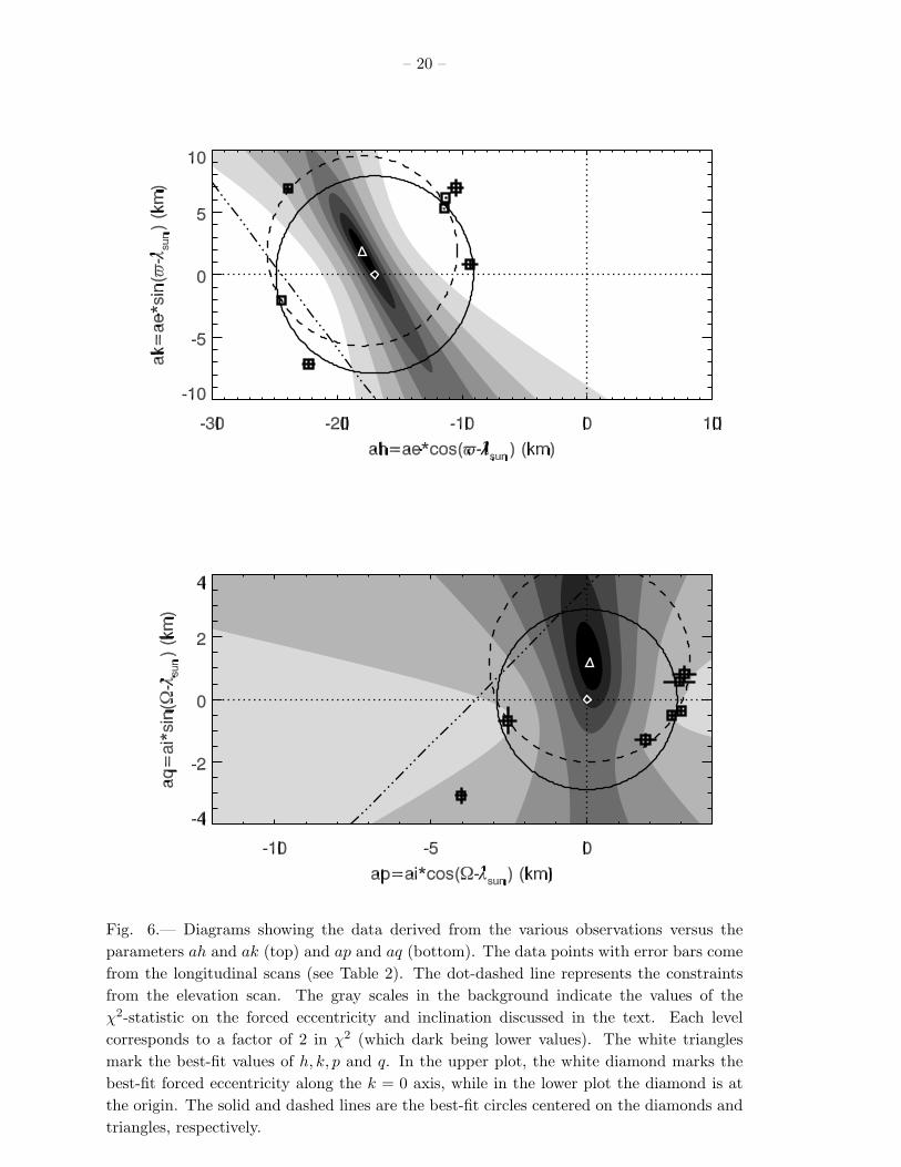
As discussed above, an orbit with forced and free orbital elements will trace out circlesin [h, k] and [p, q] space as the orbit evolves. Therefore, we plot the orbital elements derivedfrom the above fits in this space (see Fig. 6). Intriguingly, the admittedly sparse data doseem to describe a circle in [h, k] space, centered roughly at [ah, ak] = [−17, 0] km. In [p, q]space, the situation is less clear. Neglecting the outlying data from Orbit 96 (discussedabove), the data could be consistent with a circle centered near the origin, but most of thedata points are clustered to one side of the circle, making it difficult to be certain.

To make these visual impressions more quantitative, we found the circles in [h, k] and[p, q] that best describe the data. We used the following procedures for the [h, k] data: Foreach possible value of [h, k], we computed the distance between this point and the locationof every one of the longitudinal scan data points [hj , kj ]:

Rj(h, k) =√

(h− hj)2 + (k − kj)2. (56)

(Note the data from the elevation scan are not included in this analysis because they donot constrain h and k or p and q separately). We also calculate a typical error for each datapoint σj , which is the average of the errors on h and k (the difference in the errors on theseparameters was not considered large enough to justify complicating the analysis). We thencompute the average value of the appropriate Rj , weighting the observations by their error

– 20 –

Fig. 6.— Diagrams showing the data derived from the various observations versus theparameters ah and ak (top) and ap and aq (bottom). The data points with error bars comefrom the longitudinal scans (see Table 2). The dot-dashed line represents the constraintsfrom the elevation scan. The gray scales in the background indicate the values of theχ2-statistic on the forced eccentricity and inclination discussed in the text. Each levelcorresponds to a factor of 2 in χ2 (which dark being lower values). The white trianglesmark the best-fit values of h, k, p and q. In the upper plot, the white diamond marks thebest-fit forced eccentricity along the k = 0 axis, while in the lower plot the diamond is atthe origin. The solid and dashed lines are the best-fit circles centered on the diamonds andtriangles, respectively.

– 21 –

bars, to obtain the mean distance R. We then compute the following χ2 statistic:

χ(h, k)2 =∑ (Rj(h, k)− R)2

σ2j

. (57)

This statistic measures the goodness of fit of the data to the best-fit circle centered at agiven value of h and k. The [p, q] space analysis is essentially the same, except that thedata from Orbit 96 are excluded from the fit for the reasons described above. The contoursin Fig. 6 illustrate how χ2 varies with [h, k] and [p, q].

For the [h, k] plot, the best-fit solution is at [ah, ak] = [−18, 1.9] km. This wouldimply that the periapse leads the anti-solar direction by 6. However, the best-fit solutionassuming the pericenter is exactly anti-aligned with the Sun is not obviously worse thanthe overall best fit. Note that even for these best-fitting models, the χ2 fit is still quitepoor (74 for 4 degrees of freedom). This is consistent with a visual inspection of the data,which scatter around the circle by more than their error bars. This excess scatter couldoccur for a number of reasons. The data used here come from a range of phase anglesand are sensitive to different parts of the size distribution, which may lead to differences inthe apparent shape of the ringlet. Also, our background subtraction algorithm and otherprocedures used to derive the radial positions of the ringlet may have introduced systematicerrors between different scans.

For the [p, q] plot, the best-fitting model has [ap, aq] = [0, 1.2] km. Here the χ2 value isgood (3.1 for 3 degrees of freedom). However, the difference in the quality of the fit betweenthis and [p, q] = [0, 0] is only marginally significant (assuming no forced inclination, the χ2

is 9.9 for 5 degrees of freedom). Furthermore, since the Sun is in the southern hemisphere,and B is negative, we expect that the best-fit q should be negative, not positive. Thusthe best-fitting model is a bit of a surprise. Since B changes significantly over the timeperiod covered by these observations, a more complete model would include a time-variableforced inclination. However, given the weak evidence for any forced inclination at all, wechose not to consider such complications at this time.

Despite these uncertainties, we can now explore whether the temporal evolution of theshape parameters are consistent with the above model, which suggests that the parame-ters should drift around the circles at nearly constant rates determined by the modifiedpericenter-precession and nodal-regression rates. Given the sparseness of the data, we can-not establish easily whether any given solution is unique. However, preliminary examinationof the data showed that they were approximately consistent with the expected drift rates($′

o ' −Ω′o ' 4.7/day). Therefore, for each posssible solution for ef , el, if and il, we

determined the phase of the shape for each longitudinal-scan observation, unwrapped thephase assuming drift rates close to those expected, and fitted the resulting phases versusobservation time to a line to obtain estimates of the rates $′

l and Ω′l, as well as the lon-

gitudes at epoch $′l and Ω′

l (the epoch time being taken as the time of the first image inthe Orbit 42 sequence 2007-099T22:19:10, see Table 1). Regardless of whether we acceptedthe best-fit solution (triangles/dashed circles in Fig 6) or a simplified solution assuming$′

f = 180 and if = 0 (diamonds/solid circles in Fig 6), we obtain roughly the same rates.

– 22 –

$′l = 4.66/day and Ω′

l = −4.75/day. Recall that these are the modified precession ratesin a reference frame tied to the Sun. The precession rates in an inertial coordinate systemmust account for the movement of Sun λ = 0.03/day. Thus the precession rates are actu-ally: $l = 4.69/day and Ωl = −4.72/day. The expected rates at 119940 km are 4.71/dayand -4.68/day, respectively, so these numbers are close to theoretical expectations. Thismodel therefore can provide a useful parametrization of the available data.

Table 3 summarizes the model parameters for the shape of the Charming Ringlet.Model 1 is the simplified model in which $f is taken to be exactly anti-aligned with theSun and the forced inclination is assumed to be zero. Model 2 is the more complex modelthat allows both $′

f and if to have their “best-fit” values.

Table 3: Model parameters for the Charming RingletModel aef $′

f aela $′

lb $′

lb,c aif Ω′

f aila Ω′

lb Ω′

lb,c

(km) (deg) (km) (deg/day) (deg) (km) (deg) (km) (deg/day) (deg)1 17.0±0.5d 180 7.9±0.4 4.66±0.01 230±3 – – 2.9±0.2 -4.73±0.02 -152±92 18.1 174 7.6±0.4 4.67±0.01 225±4 1.3 +90 3.3±0.1 -4.77±0.02 -158±9

a Errors are the standard deviations of the values Rj , see Eqn 56.b Errors from linear fit, assuming central values for aef , ael, aif and ailc Longitudes relative to Sun at epoch=2007-099T22:19:10 (time of first observation in Orbit042).d Error based on factor of 2 increase in χ2 relative to best-fit valueNote Rev 96 data excluded from inclination/node fits.

– 23 –

Table 4: Comparison of model predictions for eccentricity and pericenter with observedlongitudinal scan dataOrbit/Obs. Sequence ae (km) ae (km) ae (km) Observed- Observed- $′ (deg) $′ (deg) $′ (deg) Observed- Observed-

Observed Model 1 Model 2 Model 1 Model 2 Observed Model 1 Model 2 Model 1 Model 2030/AZDKMRHP001/ 24.9 23.3 23.5 +1.6 +0.8 163.9 166.1 161.1 -2.1 +2.9042/RETMDRESA001/ 23.4 22.9 23.9 +0.5 -0.2 197.8 195.3 188.6 +2.5 +9.2070/RETMDRESA001/ 9.4 9.4 10.7 +0.0 -1.7 174.8 170.0 161.9 +4.9 +12.9071/PAZSCN002/ 12.5 13.2 14.1 -0.6 -2.4 146.5 153.3 149.7 -6.8 -3.2082/RETARMRLP001/ 12.9 13.8 14.9 -0.9 -2.8 151.6 152.7 149.3 -1.1 +2.3092/RETARMRLF001/ 12.6 12.2 13.4 +0.4 -1.6 155.2 154.9 150.5 +0.2 +2.6096/RETARMRMP001/ 24.6 24.9 25.5 -0.3 -1.0 184.8 182.2 178.3 +2.6 +6.5Mean +0.11 -1.27 +0.02 +5.04St. Dev. 0.86 1.29 3.85 5.19

Table 5: Comparison of model predictions for inclination and node with observed longitu-dinal scan dataOrbit/Obs. Sequence ai (km) ai (km) ai (km) Observed- Observed- Ω′ (deg) Ω′ (deg) Ω′ (deg) Observed- Observed-

Observed Model 1 Model 2 Model 1 Model 2 Observed Model 1 Model 2 Model 1 Model 2030/AZDKMRHP001/ 2.3 2.9 2.6 -0.6 -0.3 325.3 316.1 337.5 +9.3 -12.7042/RETMDRESA001/ 2.6 2.9 3.1 -0.3 -0.4 195.0 207.7 179.2 -12.7 +15.8070/RETMDRESA001/ 3.2 2.9 3.9 +0.3 -0.6 14.6 33.1 33.1 -18.5 -18.5071/PAZSCN002/ 3.0 2.9 3.1 +0.1 -0.1 10.9 -4.0 -0.4 +14.8 +11.2082/RETARMRLP001/ 3.0 2.9 2.8 +0.1 +0.3 352.9 345.0 345.3 +7.9 +7.6092/RETARMRLF001/ 2.8 2.9 2.8 +0.1 -0.1 349.3 351.9 350.2 -2.5 -0.8096/RETARMRMP001/ 5.1 2.9 3.6 +2.2 +1.5 217.3 203.3 156.8 +14.1 +60.5Mean (excluding 096 data) -0.06 -0.21 -0.28 +0.53St. Dev. (excluding 096 data) 0.34 0.33 13.24 13.54

Table 6: Comparison of model predictions with elevation scan observationae (km) $′ (deg) ai (km) Ω′ (deg) C (km/rad) z

Observation 19.5 2.54Model 1 24.3 188.2 2.9 237.7 22.0 2.78Model 2 25.2 186.2 2.4 216.6 22.4 2.37

– 24 –

6. Comparing model predictions with the observations

Tables 4, 5 and 6 compare the observed shape parameters measured by the variousobservations with the predictions from the two models derived above. While the modelparameters were derived using weighted averages of data from different observations, thesecomparisons do not consider variations in the uncertainties in the observations. This isbecause, as noted above, these simplified models were unable to fit the [h, k] data to withinthe error bars. Thus an unweighted analysis will provide a conservative estimate of howwell these models describe the data.

Table 4 presents the model predictions for the eccentricity and pericenter locationsfrom the longitudinal scans. Note that the only observation where the more complex Model2 does a better job predicting the eccentricity and pericenter than the simpler Model 1 isin the Orbit 30 data. This is consistent with Fig 6, where the dashed circle (Model 2) getscloser to the point in the upper left (from Orbit 30) than the solid circle (Model 1), but forall the other data points the dashed circle is not obviously a better fit than the solid one.Note the Orbit 30 data were taken at a substantially higher phase angle than the otherobservations, so this observation may probe a different part of the size distribution and theshape parameters may not be perfectly comparable to the others. Therefore, we concludethat the simpler model that assumes the forced component of the pericenter is perfectlyanti-aligned with the Sun is a preferable model for the shape of the ring. This model recoversthe eccentricity of the ringlet with an rms residual of 1 km and the pericenter location withan rms residual of 4.

Table 5 presents the model predictions for the inclinations and nodes for the longitu-dinal scans. In this case, there is not a clear difference between the two models. Given thatincluding a forced inclination does not substantially reduce the scatter in the observations,for the sake of simplicity we favor the use of the simpler Model 1 in this case as well. Herethe model predicts the inclination with an rms residual of 0.3 km and the node locationwith an rms residual of 14.

Finally, Table 6 compares the model predictions for the z and C parameters for theelevation scan (see Eqs 7 and 8). This is a critical check on the model, which was developedusing only the longitudinal scan data. Here, we can see that both models give values for z

and C that are reasonably consistent with the observed values.

In conclusion, while Model 1 is clearly over-simplified and does not provide a perfectlyaccurate description of the observed data, it nevertheless appears to be a useful approximatedescription of the ringlet’s shape and time variability.

7. Interpretation

We can now compare the observed shape parameters of this ringlet with theoreticalexpectations. The forced eccentricity and inclination can be relatively easily understood interms of the solar radiation forces discussed above. By contrast, the free components of the

– 25 –

eccentricity and inclination are surprising and more difficult to explain.

7.1. Forced eccentricity and inclination

Equations 54 and 55 indicate that solar radiation pressure should produce a ring withif/ef ' 0.16 tan |B|. For the observations described here |B| ranges between 16 and 3,so if/ef would be between 0.04 and 0.01. This is consistent with the observed values ofaef ' 17 km and aif < 1 km. Furthermore, the observed aef suggests a typical particle sizerg ' 20µm∗Qpr, which is not unreasonable. However, we must caution that the particles inthe Charming Ringlet probably have a distribution of sizes, and this estimated value of rg

may only be an effective average value for this distribution. The particle size distribution willbe investigated in more detail in a future study of the ring’s spectrophotometric propertiesand detailed morphology.

7.2. Free eccentricity and inclination

While nonzero free eccentricities and inclinations are acceptable solutions to the equa-tion of motion for a single particle’s orbit, it is surprising for the ringlet as a whole toexhibit such terms, because they imply that all the component particles’ orbits not onlyhave comparable finite values of el and il, but also have similar values of $l and Ωl. Suchan asymmetry in these components of the ring’s shape could be due to one of three things:(1) an asymmetry in the initial conditions of the ring particles, (2) an explicit longitudi-nal asymmetry in the equations of motion, or (3) a spontaneous symmetry-breaking in theringlet. We will consider each of the possibilities below.

7.2.1. Asymmetric initial conditions

There are various ways to produce a collection of particles with the same values for $l

and Ωl. For example, an impact near the present location of the ringlet could release a cloudof dust from one point in space, suddenly injecting a collection of particles into the gap thathave similar orbital elements. Alternatively, particles could be supplied into the ring over anextended period of time, but for some reason dust grains with certain orbital parameters aregenerated at higher rates than others. In this case, the relevant source bodies for the dustwould almost certainly be too large to have any detectable forced eccentricity due to solarradiation pressure. Thus the observed heliotropic ring could not be simply be low-velocityimpact debris tracing the orbit of its source material, but instead must reflect some morecomplex production process involving various interactions with the local plasma and dustenvironment.

Regardless of how the particles were injected into the ring, the observable ring particlesmust be relatively young in order for any asymmetry in the initial conditions to be visible

– 26 –

in the present ringlet. The Charming Ringlet has a full-width at half-maximum of about30 km. If we assume a comparable spread in semi-major axes, then the precession ratesof the particles in the ring will vary by about 0.003/day. The values of $l and Ωl wouldtherefore spread over all possible longitudes in a few hundred years. While this time-scalecould be extended if we assume the radial width of the ring is due to variable eccentricitiesrather than semi-major axes, even then the visible particles in the ring probably cannot bemore than a few thousand years old if they are to preserve any asymmetry in their initialconditions. Such ages are not entirely unreasonable, for small dust grains like those seen inthe Charming Ringlet can be rapidly destroyed by energetic particle bombardment (Burnset al. 2001), or lost by adhering to larger objects in the Cassini Division. However, we mustcaution that the production and loss of dust grains within narrow gaps has not been studiedin great detail yet.

Another important constraint on these sorts of models is the lack of gross variationsin the brightness or morphology of the ring with longitude. This argues against any largesource bodies existing within the ringlet itself, as such objects would tend to scatter andperturb the material in their vicinity, producing either gaps or possibly clumps similar tothose visible in the Encke gap ringlets; such gaps and clumps are not seen in the CharmingRinglet. It also requires that the ringlet grains exist long enough to spread evenly over alllongitudes, which takes a few years or decades.

7.2.2. Asymmetric terms in the equations of motion

Instead of an asymmetric source, it is also conceivable that the equations of motioncontain terms that depend on $l and Ωl. Recently, Hedman et al. (2010) demonstratedthat a combination of perturbations from Mimas and the massive B-ring outer edge couldgive rise to terms in the equation of motion like:⟨

d2$

dt2

⟩= −f2

o sin($ − $rt), (58)

where fo and $r are constants. Such a term acts as a restoring force on the pericenterlocation of any particle’s orbit. Thus, in a region where the precession rate $ ' $r,this term aligns the pericenters of all freely-precessing eccentric orbits. If such a termwas effective on the Charming Ringlet, it could explain how all the particles in the ringlethappen to have the same value of $l.

One difficulty with this sort of model is that the particles in the Charming Ringlet seemto have both $l and Ωl aligned. While one could imagine expressions similar to Eqn 58involving the node instead of the pericenter, it is difficult to have both terms operate at thesame location. Like any other resonant term in the equations of motion, such terms canonly be effective over a narrow range of semi-major axes (or equivalently, narrow rangesof $ and/or Ω), and resonances involving nodes typically occur at different locations fromthose involving pericenters (Murray and Dermott 1999). It therefore would be quite acoincidence if the Charming Ringlet just happened to fall at a location where both angles

– 27 –

could be effectively constrained.

7.2.3. Spontaneous symmetry breaking

A ringlet with finite free eccentricity and free inclination can in principle form spon-taneously without any terms in the equations of motion that depend explicitly on $l andΩl, and without any strong asymmetry in the particle’s initial conditions. Such phenomenahave been discussed almost exclusively in the context of massive, dense ringlets (Borderieset al. 1985). However, one can argue that this sort of “spontaneous symmetry-breaking”could also occur in low-optical-depth dusty rings via dissipative processes like collisions,provided that there are terms in the individual particle’s equations of motion that favor thedevelopment of a nonzero el and il comparable to those observed for the entire ringlet.

Dissipative collisions are often invoked as a mechanism that causes narrow rings tospread in semi-major axis (Goldreich and Tremaine 1982), so it might seem surprising thatsuch collisions could also align pericenter or node locations. However, unlike the semi-majoraxis, the longitudes of pericenter and node have no direct effect on a particles’ orbital energy.Thus, while the dissipation of orbital energy requires that particles’ orbital semi-major axesevolve in a particular direction, this is not the case for pericenters or nodes. Instead, theevolution of pericenters and nodes should be driven primarily by the collisons’ dissipationof relative motions.

To illustrate how such collisions can align pericenters and nodes, consider the follow-ing simple situation: There is a ringlet composed of many particles with similar orbitalproperties, and there is a single particle whose orbit is misaligned with the others. For sim-plicity, assume that both the ringlet and the particle have zero eccentricity and zero forcedinclination. Furthermore, assume that both the ringlet and the particle have the same freeinclination i but different longitudes of ascending node Ωr and Ωp, respectively. If Ωr 6= Ωp,then the particle’s orbit will cross the ringlet at two longitudes λc = (Ωp + Ωr)/2±π/2. Atthese two longitudes the particle will feel a force due to its collisions with the particles inthe ringlet, and the vertical component of that force Fz will be proportional to the verticalvelocity of the particles in the ringlet, so Fz ∝ cos(λc−Ωr). Inserting this into Equation 14,we can express the perturbation to the particle’s node position due to its interactions withthe ringlet as:

dΩp

dt= 2D sin(λc − Ωp) cos(λc − Ωr) (59)

where D is a constant. Substituting in the above expression for the crossing longitudes λc

and simplifying, this expression reduces to the simple form:

dΩp

dt= −D sin(Ωp − Ωr). (60)

The forces applied to the particle’s orbit during the ringlet crossings therefore do tend toalign the particle’s orbital node position with that of the ringlet. A similar calculationdemonstrates that the same basic phenomenon acts to align pericenters as well. Thus colli-

– 28 –

sions can indeed align pericenters and nodes, provided the collisions are frequent (and lossy)enough, and provided the particles maintain some finite (free) eccentricity and inclination.

The requirement that collisions are frequent enough to align pericenters is probably metfor the Charming Ringlet. While this ringlet has a low normal optical depth (roughly 10−3),the orbital period is sufficiently short (around 0.5 days) that the collisional timescale is stillonly a few years or decades, much less than the typical erosion timescales of thousands ofyears (Burns et al. 2001).

On the other hand, the persistance of the nonzero free eccentricities and inclinationsprobably requires some modifications to the individual particles’ dynamics. If the particles’equations of motion were just given by Eqs 47- 50 above, dissipative collisions would (as-suming the initial conditions were not highly asymmetric) tend to produce a ringlet withel = il = 0. Thus, we probably need to add some additional terms to these equations toproduce something similar to the Charming Ringlet’s observed shape. One relatively simpleway to accomplish this is to add non-linear damping terms into the equations:⟨

dh

dt

⟩= −$′

ok + γh(h + ef )

[1−

(h + ef

el

)2]

, (61)

⟨dk

dt

⟩= $′

o(h + ef ) + γkk

[1−

(k

el

)2]

, (62)

⟨dp

dt

⟩= −Ω′

o

(q − if

B|B|

)+ γpp

[1−

(p

il

)2]

, (63)

⟨dq

dt

⟩= Ω′

op + γq

(q − if

B|B|

) [1−

(q − ifB/|B|

il

)2]

, (64)

where γh, γk << $′o and |γp|, |γq| << |Ω′

o| quantify the magnitude of the damping terms.These terms transform the [h, k] and [p, q] systems from simple harmonic oscillators intovan der Pol oscillators (Baierlein 1983). Such oscillators are characterized by a limit cyclewhich the system will asymtotically approach no matter where it is started in [h, k] and[p, q] space. These limit cycles are circles centered at [h, k] = [−ef , 0] and [p, q] = [0,±if ]with radii of el and il, and the orbit traces out the circles at rates given by $′

o and Ω′o.

These equations of motion therefore cause any particle’s orbit to evolve to the same pathas the observed ringlet. On their own, particles started at different points in phase spacewill wind up at different points along this cycle. However, if the relative motions among theparticles are efficiently dissipated, then all the particles should eventually clump togetherin phase space such that they all move around the limit cycle together, as observed.

Models of this sort have the advantage that the additional terms in the equations ofmotion do not have explicit frequency-dependent terms that can only be effective at specificlocations in the rings. Such terms are therefore more likely to show up in a broader rangeof contexts, and could even be generic features of small dust grains’ dynamics in narrowgaps. For example, the nonlinear damping terms in the above equations contain either el

or il. While these are small numbers in absolute terms, they are not much smaller than the

– 29 –

fractional gap width δa/a, so such factors could arise due to interactions between the ringletparticles and the gap edges. This would not be unreasonable, as small particles could beattracted to the edges by the force of gravity, or even repelled if the small grains in thering have a sufficient electrical charge. Furthermore, variations in the plasma environmentwithin the gap could also possibly produce perturbations on the grains’ motions with theappropriate positional dependence.

One clue to the exact nature of these forces is that the observed ring traces out a circlethat is centered on the point [h, k] = [−ef , 0] and excludes the origin [h, k] = [0, 0]. Basedon some preliminary analyses, it appears that a limit cycle of this type cannot be createdby non-linear damping terms involving only e or $ , but instead requires terms that containk and/or h + ef , like the ones given above (note that only one of the two terms γh andγk has to be non-zero to produce the desired limit cycle). Since h and k are tied to thelocation of the Sun, this implies that these damping terms might also have some connectionwith the Sun. One possibility is that these terms reflect the influence of Saturn’s shadow.When small particles enter the shadow, electrons are no longer being ejected from theirsurfaces via the photoelectric effect. This can significantly change their electric charge andthereby lead to significant forces that would preferentially damp or drive h or k. Furtherinvestigation is needed to explore whether the perturbations from these or other processescould account for the observed shape of the Charming Ringlet.

Acknowledgments

We acknowledge the support of NASA, the Cassini Project and the Imaging ScienceTeam for obtaining the images used in this analysis. This work was also supported by CassiniData Analysis Program grants NNX07AJ76G and NNX09AE74G. We wish to thank P.D.Nicholson and M.R. Showalter for useful conversations, and S. Charnoz and J. Schmidt fortheir helpful reviews of this manuscript.

Appendix: Orbit averages including shadow effects

Equations 23-27 are derived from Equations 18-22 by averaging over all longitudes λ.This averaging procedure is complicated by the presence of Saturn’s shadow, which blockssunlight from reaching part of the rings. If a fraction ε of the ring is in Saturn’s shadow,then the ring particles only feel the solar radiation pressure when |λ−λ| < π(1− ε). Thusif X is any of the radiation-pressure-induced terms on the right-hand sides of Eqs 18-22,then the orbit-averaged value of X is:

< X >=12π

∫ +π(1−ε)

−π(1−ε)Xd(λ− λ). (65)

Equations 18-22 contain terms proportional to λ0, sin(λ − λ), sin(2λ − $ − λ),cos(2λ − $ − λ), sin(λ − Ω), and cos(λ − Ω). Inserting these factors into Eqn 65 yields

– 30 –

the following expressions:< λ0 >= (1− ε), (66)

< sin(λ− λ) >= 0, (67)

< sin(λ− Ω) >= −sin(πε)π

sin(Ω− λ), (68)

< cos(λ− Ω) >= +sin(πε)

πcos(Ω− λ), (69)

< sin(2λ−$ − λ) >= +sin(2πε)

2πsin($ − λ), (70)

< cos(2λ−$ − λ) >= −sin(2πε)2π

cos($ − λ). (71)

The appropriate combination of these terms then yields the factors d(ε), f(ε) and g(ε) inEqs 23-27.

REFERENCES

Baierlein, R. 1983. Newtonian Dynamics. McGraw-Hill.

Borderies, N., P. Goldreich, and S. Tremaine 1985. A granular flow model for dense planetaryrings. Icarus 63, 406–420.

Burns, J. A. 1976. Elementary derivation of the perturbation equations of celestial mechan-ics. American Journal of Physics 44, 944–949.

Burns, J. A., D. P. Hamilton, and M. R. Showalter 2001. Dusty rings and circumplanetarydust: Observations and simple physics. In E. Grun, B. Gustafson, S. Dermott, andH. Fechtig (Eds.), Interplanetary Dust, pp. 641–725. Springer.

Burns, J. A., P. L. Lamy, and S. Soter 1979. Radiation forces on small particles in the solarsystem. Icarus 40, 1–48.

Burt, J., M. M. Hedman, M. S. Tiscareno, and J. A. Burns 2008. The where And why OfSaturn’s inclined ”Charming Ringlet”. BAAS 40, 445.

French, R. G., E. A. Marouf, N. J. Rappaport, and C. A. McGhee 2010. Occultationobservations of Saturn’s B ring and Cassini Division. AJ 139, 1649–1667.

French, R. G., P. D. Nicholson, M. L. Cooke, J. L. Elliot, K. Matthews, O. Perkovic,E. Tollestrup, P. Harvey, N. J. Chanover, M. A. Clark, E. W. Dunham, W. Forrest,J. Harrington, J. Pipher, A. Brahic, I. Grenier, F. Roques, and M. Arndt 1993.Geometry of the Saturn system from the 3 July 1989 occultation of 28 SGR andVoyager observations. Icarus 103, 163–214.

Goldreich, P., and S. Tremaine 1982. The dynamics of planetary rings. ARA&A 20, 249–283.

– 31 –

Hamilton, D. P. 1993. Motion of dust in a planetary magnetosphere - Orbit-averagedequations for oblateness, electromagnetic, and radiation forces with application toSaturn’s E ring. Icarus 101, 244–264.

Hedman, M. M., J. A. Burns, M. S. Tiscareno, and C. C. Porco 2007. The Heliotropic Ringsof Saturn. BAAS 38, 427.

Hedman, M. M., P. D. Nicholson, K. H. Baines, B. J. Buratti, C. Sotin, R. N. Clark,R. H. Brown, R. G. French, and E. A. Marouf 2010. The architecture of the CassiniDivision. AJ 139, 228–251.

Horanyi, M., and J. A. Burns 1991. Charged dust dynamics - Orbital resonance due toplanetary shadows. J. Geophys. Res. 96, 19283–19289.

Horanyi, M., J. A. Burns, M. M. Hedman, G. H. Jones, and S. Kempf 2009. Diffuse Rings.In Dougherty, M. K., Esposito, L. W., & Krimigis, S. M. (Ed.), Saturn from Cassini-Huygens, pp. 511–536. Springer.

Jacobson, R. A., P. G. Antreasian, J. J. Bordi, K. E. Criddle, R. Ionasescu, J. B. Jones, R. A.Mackenzie, M. C. Meek, D. Parcher, F. J. Pelletier, W. M. Owen, Jr., D. C. Roth,I. M. Roundhill, and J. R. Stauch 2006. The Gravity Field of the Saturnian Systemfrom Satellite Observations and Spacecraft Tracking Data. AJ 132, 2520–2526.

Murray, C. D., and S. F. Dermott 1999. Solar System Dynamics. Cambridge UniversityPress.

Porco, C. C., E. Baker, J. Barbara, K. Beurle, A. Brahic, J. A. Burns, S. Charnoz,N. Cooper, D. D. Dawson, A. D. Del Genio, T. Denk, L. Dones, U. Dyudina, M. W.Evans, B. Giese, K. Grazier, P. Helfenstein, A. P. Ingersoll, R. A. Jacobson, T. V.Johnson, A. McEwen, C. D. Murray, G. Neukum, W. M. Owen, J. Perry, T. Roatsch,J. Spitale, S. Squyres, P. Thomas, M. Tiscareno, E. Turtle, A. R. Vasavada, J. Vev-erka, R. Wagner, and R. West 2005. Cassini imaging science: Initial results onSaturn’s rings and small satellites. Science 307, 1226–1236.

Porco, C. C., R. A. West, S. Squyres, A. McEwen, P. Thomas, C. D. Murray, A. Delgenio,A. P. Ingersoll, T. V. Johnson, G. Neukum, J. Veverka, L. Dones, A. Brahic, J. A.Burns, V. Haemmerle, B. Knowles, D. Dawson, T. Roatsch, K. Beurle, and W. Owen2004. Cassini imaging science: Instrument characteristics and anticipated scientificinvestigations at saturn. Space Science Reviews 115, 363–497.

Porco, C.C. and the Cassini Imaging Team. 2006. Rings of Saturn (R/2006 S 1, R/2006 S2, R/2006 S 3, R/2006 S 4). IAU Circ. 8759, 1.

This preprint was prepared with the AAS LATEX macros v5.0.