the spatial effect of ab 109 (public safety realignment ... · the spatial effect of ab 109 (public...
TRANSCRIPT

The Spatial Effect of AB 109 (Public Safety Realignment) on Crime Rates in San
Diego County
By
Charles Dixon Jones
A Thesis Presented to the
Faculty of the USC Graduate School
University of Southern California
In Partial Fulfillment of the
Requirements for the Degree
Master of Science
(Geographic Information Science and Technology)
May 2016

Copyright ® 2016 by Charles Jones

To my beautiful, wonderful, amazing wife Darci, and Mother and Father without whose support
this project would not have been possible.

iv
Table of Contents
List of Figures ............................................................................................................................... vii
List of Tables ............................................................................................................................... viii
Acknowledgements ........................................................................................................................ ix
List of Abbreviations ...................................................................................................................... x
Abstract .......................................................................................................................................... xi
Chapter 1 Introduction .................................................................................................................... 1
1.1 Background ..........................................................................................................................1
1.2 History of the CDCR ...........................................................................................................2
1.3 Justification ..........................................................................................................................3
1.4 Research Questions and Objectives .....................................................................................5
1.5 San Diego County ................................................................................................................5
1.6 Thesis Organization .............................................................................................................8
Chapter 2 Literature Review ........................................................................................................... 9
2.1 Offender Characteristics ......................................................................................................9
2.2 Recidivism .........................................................................................................................10
2.3 Crime Analysis ...................................................................................................................11
2.4 The Modifiable Areal Unit Problem or MAUP .................................................................14

v
Chapter 3 Methods and Data......................................................................................................... 17
3.1 Study Area and Software ...................................................................................................17
3.2 Data Sources ......................................................................................................................17
3.3 Data Processing ..................................................................................................................21
3.4 Data Issues .........................................................................................................................24
3.5 Methods ..............................................................................................................................25
Chapter 4 Results .......................................................................................................................... 35
4.1 Descriptive Statistics ..........................................................................................................35
4.1.1. Non AB 109 Categorized Offenses ..........................................................................39
4.1.2. AB 109 Categorized Offenses .................................................................................42
4.1.3. Crimes Against Property ..........................................................................................44
4.1.4. Crimes Against Persons ...........................................................................................46
4.1.5. Crimes Against Society............................................................................................49
4.2 Spatial Statistics .................................................................................................................51
4.2.1. Crimes Against Property ..........................................................................................51
4.2.2. AB 109 Categorized Offenses .................................................................................54
4.2.3. Non AB 109 Categorized Offenses ..........................................................................56
4.2.4. Crimes Against Society............................................................................................58
4.2.5. Crimes Against Persons ...........................................................................................60
vi
Chapter 5 Discussion and Conclusions ......................................................................................... 65
5.1 Conclusions ........................................................................................................................66
5.2 Sources of Error .................................................................................................................68
5.3 Future Work .......................................................................................................................69
REFERENCES ............................................................................................................................. 71
Appendix A: Social and Physical OLS Variables......................................................................... 75

vii
List of Figures
Figure 1: San Diego County and Surrounding Regions.................................................................. 6
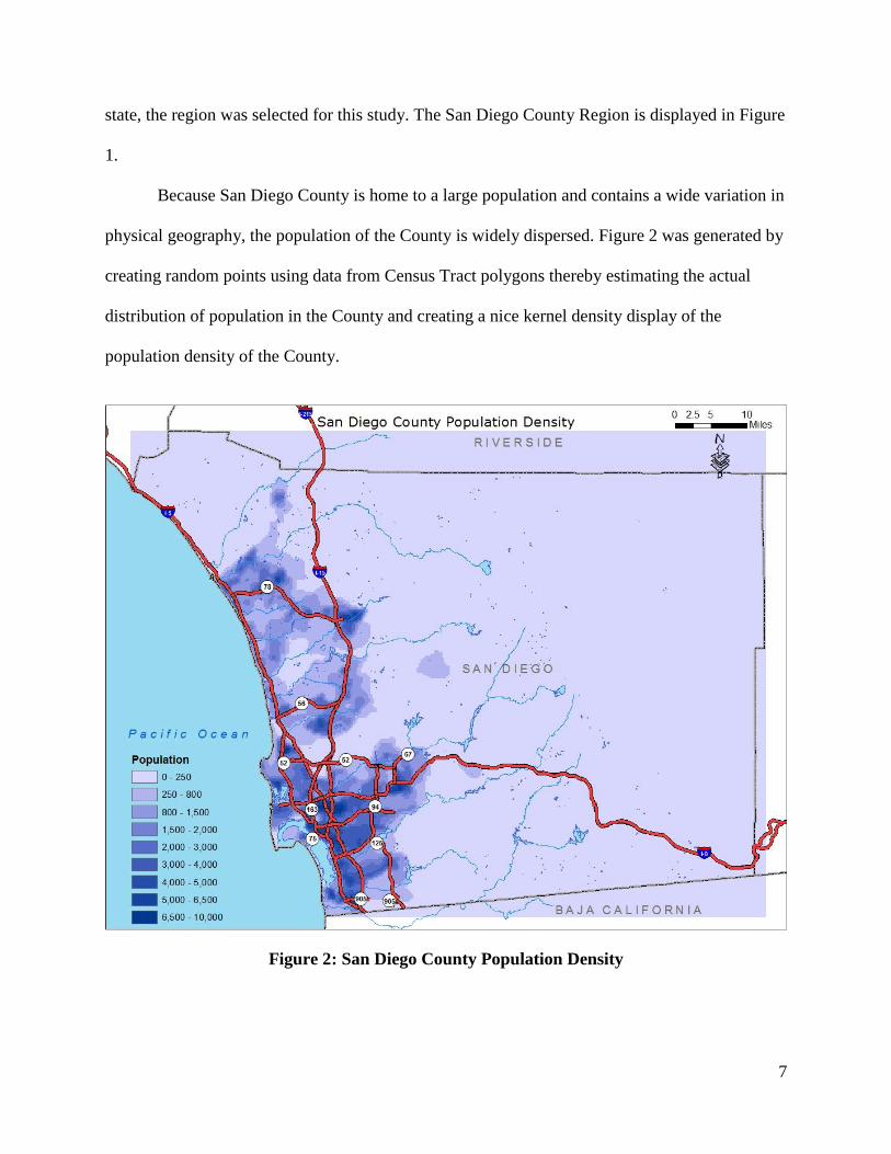
Figure 2: San Diego County Population Density ............................................................................ 7
Figure 3: An Illustration of the MAUP and how Re-aggregation can affect Results ................... 15
Figure 4: 2013 Crime Data in Native CSV Format ...................................................................... 23
Figure 5: Property Crime Rates (Crimes per 1000 people) between 1 October 2011 and 30
September 2013 - Data Aggregated by Census Tract .................................................... 27
Figure 6: Re-Aggregation of Offender Counts from Zip Codes to Census Tracts ....................... 30
Figure 7: Example of Moran’s I Tool Output Testing Autocorrelation of Residuals ................... 34
Figure 8: Theft/Larceny Trend (1 October - 30 September)......................................................... 37
Figure 9: Burglary Trend (1 October - 30 September) ................................................................. 38
Figure 10: Variance of Non AB 109 Crime Rate Difference Values ........................................... 41
Figure 11: Variance of AB 109 Category Crime Rate Difference Values ................................... 43
Figure 12: Variance of Property Crime Rate Difference Values .................................................. 46
Figure 13: Variance of Persons Crime Rate Difference Values ................................................... 48
Figure 14: Variance of Societal Crime Rate Difference Values ................................................... 50
Figure 15: Property Crime Hot Spots ........................................................................................... 52
Figure 16: AB 109 Categorized Offenses Crime Rate Change Hot Spot ..................................... 55
Figure 17: Non AB 109 Categorized Offenses Crime Rate Change Hot Spot ............................. 57
Figure 18: Societal Crime Rate Change Hot Spot ........................................................................ 59
Figure 19: Persons Crime Rate Change Hot Spot ......................................................................... 61
Figure 20: Standard Residuals of the OLS Crimes Against Persons Model ................................. 64
viii
List of Tables
Table 1: Total Incidents and Rates per Year (1 October-30 September) ...................................... 18
Table 2: 2013 Probation Totals ..................................................................................................... 19
Table 3: 2013 Probation Counts ................................................................................................... 24
Table 4: AB 109 Offenses vs Non AB 109 Offenses queried from 1 October to 30 September . 35
Table 5: NIBRS Crime Category Counts for San Diego County - 1 Oct 2007- 30 Sep 2013 ...... 36
Table 6: Degree of Change in Crime Rates from the Crime Categories Studied ......................... 40
Table 7: Wilcoxon Signed Rank Test of Non AB 109 Offenses Results ..................................... 40
Table 8: Wilcoxon Signed Rank Test of AB 109 Offenses Results ............................................. 42
Table 9: Crime Rate Change between Studied Temporal Periods ................................................ 44
Table 10: Wilcoxon Signed Rank Test of Property Crime Offenses Results ............................... 45
Table 11: Wilcoxon Signed Rank Test of Crimes Against Persons Offenses Results ................. 47
Table 12: Wilcoxon Signed Rank Test of Crimes Against Society Offenses Results .................. 49
Table 13: Range of Property Hot Spot Rate Increase ................................................................... 52
Table 14: Results of Misspecified Property Crime Rate Model ................................................... 54
Table 15: Range of AB 109 Rate Increase Hot Spot .................................................................... 55
Table 16: Range of Non AB 109 Rate Increase Hot Spot ............................................................ 57
Table 17: Range of Societal Crime Rate Increase Hot Spot ......................................................... 59
Table 18: Range of Persons Crime Rate Increase Hot Spot ......................................................... 60
Table 19: Persons Crime Rate Change Hot Spot OLS Model Results ......................................... 62
Table 20: Moran’s I Result of Crimes Against Persons OLS Residuals ...................................... 63

ix
Acknowledgements
I am grateful to my mentor, Dr. Darren Ruddell, for the direction I needed and the unrelenting
help he offered during the course of the project. I am also grateful to my other thesis committee
members, Dr. Su Jin Lee and Dr. Yao-Yi Chiang who gave me assistance when I needed it and
to Dr. John Wilson for allowing me to finish my research. I would like to thank Kurt Smith and
Milan Muller of The Omega Group, who assisted me with data collection and forming my
research idea. I am also grateful for the probation data provided to me by the San Diego County
Probation Department and the assistance in thesis practice and support given by my friends,
Ryan and Rob.

x
List of Abbreviations
GIS Geographic information system
GISci Geographic information science
SSI Spatial Sciences Institute
USC University of Southern California
CDCR California Department of Corrections and Rehabilitation
MAUP Modifiable Areal Unit Problem
NIBRS National Incident Based Reporting System
OLS Ordinary Least Squares
FBI Federal Bureau of Investigation
CSV Comma Separated Value
MS Mandatory Supervision
PCRS Post Release Community Supervision\
SANDAG San Diego Association of Governments

xi
Abstract
AB 109 (Public Safety Realignment) widely changed the way criminal offenders are processed
in California, starting 1 October 2011. It is widely purported that AB 109 is affecting crime rates
in the State of California. This paper studies the spatial effects of AB 109 on crime rates in San
Diego County. Studies have shown Criminal Offenders will likely commit offenses near their
place of residence. Recidivism is a complex and serious problem in California, the United States
and the World. Regression and hot spot analysis as well as traditional statistics methods were
used to analyze crime rates, or crime events per 1000 persons at the census tract level. Five
categories of crime were studied: AB 109 categorized offenses or offenses falling under the AB
109 statute, Non AB 109 offenses, Crimes Against Persons, Crimes Against Property and Crimes
Against Society. Analyses indicated that crime rates for most categories studied decreased.
Property crime rates exhibited a median increase of 0.7 events per 1000 persons at the census
tract level. Spatial OLS analysis indicated a correlation between residence locations of AB 109
offenders and a hot spot of property crime rate increase however the model was misspecified.
Other category hot spots exhibited no correlation with AB 109 offenders. Variance of the crimes
against persons hot spot was explained by different variables. Some other combination of
complex variables not listed or tested as part of this study is responsible for the variance of the
hot spots of other categories. The implementation of AB 109 appears to have been successful in
that offenders are being diverted to County facilities and reducing the State prison populations
and is associated with several categories of crime rate decrease in San Diego County. However
property crime has exhibited a statistically significant increase in crime rates across San Diego
County coinciding with AB 109. However no significant correlation was found between
populations of AB 109 offenders and crime rate increase of any categories.
1
Chapter 1 Introduction
1.1 Background
A constitutional guarantee of the United States is to protect the “Life, Liberty and Property” of
its citizenry (Heyman, 1991, pp.512). As a primary function of this guarantee, it can be inferred
that it is the government’s duty to make every effort to prevent crime and apprehend criminals.
At the center of this assumption is the new California law, “AB 109” or “Public Safety
Realignment.” As a result of the excessive overcrowding of California’s State Prisons, and a
Supreme Court order to reduce the number of inmates housed in the State Prison system, the
“Public Safety Realignment Act” was passed in 2011 in an effort to mitigate the overcrowding of
California’s State Prisons (Couzens, 2013 pp.217; Weisberg and Quan, 2014).
This new law represents a “significant change” in the way convicted offenders are
sentenced. Specifically “non-serious, nonviolent or non-sex” offenders will now serve time in
“county jail” or receive a “sentence” of “probation” as a replacement for the “State” correctional
facility “sentence” they would have received before the new law (Californians for Safety and
Justice, 2013). Additionally, “AB 109,” represents a change in the way offenders will serve time
while remanded and a change in post remand correctional supervision. Previously, offenders of
the AB 109 type offenses would typically serve time in a State correctional facility and would be
supervised by the State Parole board post release. Under AB 109, offenders will now serve their
sentence in county jail, serve probation only with no remand, or have their sentence split
between county jail and county probation with no post remand supervision (Couzens, 2013 pp.
218).
AB 109 was signed into law in April of 2011 and took effect in October 2011; Its primary
purpose was to decrease the number of inmates remanded to the State prisons from 150,000 to

2
110, 000 and continue this trend (Californians for Safety and Justice, 2013). As a consequence,
the obligation to supervise those convicted of “non-serious, nonviolent or non-sex felony
offenses” was shifted from the State of California to the Counties of California (Californians for
Safety and Justice, 2013). Current offenders serving a sentence in state prison are not released
early as a result of this legislation, however all future convictions will be punished in this manner
(Californians for Safety and Justice, 2013). As a result of this shift in sentencing and supervision,
it is vital to understand the relationships between the new law, offenders, and crime rates.
This work attempts to study the relationship, if any, between offenders sentenced under
the AB 109 provision and crime rates. The methods used to evaluate and identify this and other
relationships is described further in Chapter 3.
1.2 History of the CDCR
The History of the CDCR or the California Department of Corrections and Rehabilitation is
fascinating, and as this work attempts to study the effect of a law designed to affect the prison
population, it is important to understand the history of the CDCR. California is known as the
Golden State, and if gold was measured in terms of population, it seems to live up to its name.
During the 2010 Census, California’s total population was recorded as 37,253,956; up 10% from
33,871,648 in 2000. (U.S. Census Bureau, 2015; U.S. Census Bureau, 2002).
With any growth in population it should be expected that the rate of persons incarcerated
would grow at the same rate. In California, this was the case for many years, however toward the
end of the 20th century the numbers or persons imprisoned and ratio of persons per total
population grew sharply (Zimring and Hawkins, 1994). Zimring and Hawkins note that the
numbers of persons imprisoned grew at a stable ratio from 1950 to 1970 however in the “1980s”

3
the number of persons imprisoned increased from “24,569” to “97,309” by 1990, an increase of
296% (Zimring and Hawkins, 1994 pp. 84).
Before the population explosion, the State prison system had sites focused on offender
rehabilitation. At one site, “Chino,” there was a different philosophy, vocational training and
education for inmates, however, at one point the vocational training disappeared (Wilkinson,
2005 pp. 10). After the disappearance of certain rehabilitation programs, the prisons appear to
have continued to deteriorate to the point that the Supreme Court determined the “health care”
provided by the CDCR was in violation of the Constitution due to extreme poor quality
(Californians for Safety and Justice, 2013).
As a result of the poor “health care,” a “2009 a three judge… order” mandated reduction
of “prison population” (Weisberg and Quan, 2014 pp. 7). The “U.S. Supreme Court” upheld the
decision and found “prison overcrowding to be ‘the primary cause of the state’s unconstitutional
failure to provide adequate medical and mental health care to California prisoners” (Weisberg
and Quan, 2014 pp. 15).
1.3 Justification
Many people and organizations are striving to understand the effects of AB 109 and its
relationship to crime rates. Many authors and organizations have researched this issue and
concluded that crime rates have risen since the implementation of AB 109 (Beard et al, 2013;
Lofstrom and Raphael, 2013,). A Public Policy Institute report authored by Magnus Lofstrom
and Steven Raphael indicates “violent” and “property crime [rates]” are “up” in California
(Lofstrom and Raphael, 2013, pp 2). The report contends the “increase in violent crime” seems
to be a societal inclination toward increased “violent crime” exhibited in “other states,” however
the report also found “robust evidence that realignment is related to increased property crime”

4
(Lofstrom and Raphael, 2013, pp 2). Additionally a report published by the CDCR indicates the
probability of “offenders released… during the first year” of AB 109 to be detained for a
“felony” was higher “post-realignment” and “offenders” were detained for a “serious or violent”
crime at a higher rate than pre- AB 109 (Beard et al, 2013 pp i-ii).
The studied effects of AB 109 are not all negative. The CDCR report mentioned above,
published in December 2013, indicates “that there [was] very little difference between the one-
year arrest and conviction rates of offenders released pre- and post-Realignment” (Beard et al,
2013 pp i).
Due to the nature of AB 109 unintended consequences of the statute have presented
themselves. Due to the shifting of responsibility for offenders, subject to the AB 109 provision,
from the state to the counties, it has been found that county incarceration facilities are reaching
capacity due to the increase in inmates and as a result, more counties are reporting the early
release of inmates (Beard et al, 2013; Lofstrom and Raphael, 2013). According to the
Californians for Safety and Justice website that outlines the changes that have taken place under
AB 109, no inmates have been released from “State Prison” before their sentence was completed
because of AB 109, and AB 109 has not changed “sentence lengths” as prescribed in the “penal
code” (Californians for Safety and Justice, 2013). As AB 109 was not intended to release
inmates from prison early, and was designed to abide by the existing prescribed sentences by
law; if an offender who would have been serving their sentence in the State Prison previously,
and would now serve their sentence in a county facility, being potentially released early, would
certainly represent an unintended consequence of the law.
The unintended consequence of early release of inmates together with the uncertain
nature of crime trends in California related to the implementation of AB 109 are the prime

5
motivations for this study. As new laws are passed and implemented, an understanding of the
effects and consequences of laws are necessary to move forward as an educated and informed
society.
1.4 Research Questions and Objectives
This study analyzes crime rates, comparing two main temporal periods, to determine the
effect of a new law on society. To conduct this analysis, four research questions were asked:
1) What is the trend in reported crime rates in San Diego County before and after
the implementation of AB 109? And what is the spatial distribution of reported
crimes?
2) Which types of crime are increasing?
3) Are populations of offenders sentenced under the AB 109 provision correlated
with crime rate increase?
4) Are other factors or variables responsible for crime rate increase?
Three research objectives were identified to help answer these questions. First: Determine
the median crime rate change and statistical significance for crime categories. Second:
Determine correlation between hot spot of crime rate increase for each crime category studied
and populations of AB 109 offenders. Third and finally: Determine the correlation between hot
spot of crime rate increase for each crime category studied and other explanatory variables.
The methods and data behind each of the aforementioned objectives are explained in
greater detail in Chapter 3 Methods and Data.
1.5 San Diego County
San Diego County is home to 3,095,313 persons or 8.3% of the total population of California, as
counted in the 2010 Census, and was chosen as the region for this study.

6
San Diego has a very mild climate with low variability in weather and temperature (Cities
of the United States, 2006). Sandi Cain, of the San Diego Business Journal noted “San Diego
County is a microcosm of the entire state, embracing coastal resorts and plains, foothills,
mountains and desert. Its rejuvenated downtown has a mix of commerce, residents and visitors
that makes it a vibrant community” (Cain, 2005). As the physical geography of San Diego
provides wide variability and the population provides a large sample size of the population of the
Figure 1: San Diego County and Surrounding Regions
7
state, the region was selected for this study. The San Diego County Region is displayed in Figure
1.
Because San Diego County is home to a large population and contains a wide variation in
physical geography, the population of the County is widely dispersed. Figure 2 was generated by
creating random points using data from Census Tract polygons thereby estimating the actual
distribution of population in the County and creating a nice kernel density display of the
population density of the County.
Figure 2: San Diego County Population Density

8
1.6 Thesis Organization
The organization of this paper is as follows: the paper begins with a review of relevant crime and
offender literature that lays the foundation for the research contained in the document.
Following the literature review, Chapter 3 contains a section detailing the methods and
data used in the study. This section describes how multiple sources were used to obtain crime
and offender data, as well as a detailed explanation of the data processing methods, such as how
zonal statistics and geocoding were performed. The methods and data section also contains a
brief section detailing the geographic study area of San Diego County.
Chapter 4 of this work contains a detailed explanation of the analysis results. An
inferential statistical and spatial statistical analysis were performed on the Crime Data for San
Diego County. The results of the analysis, including an ordinary least squares (OLS) and spatial
regression analysis of the relationship between offender residence locations and crime rate
increase hot spots, are explored in this section.
The final chapter, Discussion and Conclusion, explores the results of the study in depth
and provides a sources of error discussion as well as future work recommendations.

9
Chapter 2 Literature Review
2.1 Offender Characteristics
This study attempts to identify spatial relationships between residence locations of convicted
offenders and crime locations. Relevant literature was consulted to better understand spatial
characteristics of offenders.
The body of knowledge regarding the subject of spatial characteristics between offenders
and their target crime location, or Criminal Profiling, focuses primarily on the characteristics and
understanding of violent predatory offenders. The focus is logical because this type of offender is
a greater threat to society than other types of offenders. While it is the assumption of this study
that this type of offender would not be sentenced under the AB 109 provision, the body was
consulted with this assumption in mind to identify the spatial range of offenders.
In a survey of serial killers by Maurice Godwin, and David Canter, the average distance
an offender traveled to “abduct the victims” was 1.45 miles with a standard deviation of 1.25
(Godwin & Canter 1997). This identifies that violent predatory offenders will offend close to
their sphere of activity.
D. Kim Rossmo outlines a geographic profiling distance decay function that can be used
to predict the “Offender’s Residence” (Serial Killers) based on the number of Crime locations
within an area (Rossmo, 1997). The inverse of this function indicates that an Offender will
likely commit Crime near their place of residence.
In addition to Rossmo, many authors have noted that offenders are more likely to operate
near areas that are familiar to them, such as their residence or place of employment
(Brantingham and Brantingham, 1981; Godwin & Canter, 1997; Rhodes and Conly, 1981;
Rossmo, 1997). As an example, violent predatory offenders or rapists are likely to operate very

10
close to their residence, within an average distance of 1.25 miles (Godwin & Canter, 1997). In
contrast, robbers operate within an average of 2.10 miles and burglars operate within an average
of 1.62 miles (Brantingham and Brantingham, 1981).
It is interesting to note that while the majority of the work regarding criminal profiling
has been focused primarily on violent predatory offenders. Brantingham and Brantingham
studied all types of offenders and their sphere of influence, noting the mean center of burglaries
and robberies.
The body of knowledge on criminal profiling suggests that an offender will likely commit
an offense near their residence. With this assumption this study attempts to find a correlation
between crime rate increase, or Census Tracts that exhibited an increase in crime rates, and the
residence locations of AB 109 offenders. The assumption being: if Census Tracts where crime
increased are correlated with AB 109 offenders, a relationship between AB 109 and increased
crime rates likely exists.
2.2 Recidivism
The literature suggests that offenders will likely commit offenses near their place of
residence. To further determine the risk of changing the supervision type of convicted offenders,
the literature was consulted on the subject of recidivism.
Recidivism can also be thought of as “reoffending” or a person’s tendency toward
criminal behavior after being released from a supervised sentence (Beard et al, 2013 pp. 5). This
measure is significant as it can potentially gauge the effectiveness of certain institutions or
programs on rehabilitating criminal behavior.
Recidivism rates in the United States are problematic and suggest offenders are likely to
commit a new offense when released from prison. A report studying two thirds of offenders in
11
the United States noted a recidivism rate of 67.5% for those released in 1994 and 62.5% for
those released in 1983; averaging the values the overall recidivism rate in the United States in
65% within three years of “release” (Langan and Levin, 2002 pp. 1). The report further found
those who serve the longest sentences, “61 months or more,” experienced a “significantly lower”
recidivism rate of 54.2% (Langan and Levin, 2002 pp. 11). “Recidivism” rates calculated in the
report include new convictions as well as arrests (Langan and Levin, 2002 pp. 1).
Research comparing recidivism rates of California offenders pre and post AB 109 suggest
similar results. The year preceding AB 109 experienced 58.9% recidivism and the year following
experienced 56.2% recidivism (Beard et al, 2013).
Recidivism is not only a problem in the United States, but in other countries as well,
suggesting a global phenomenon. An article by Ignacio Munyo and Martín A. Rossi, studying
recidivism on the day of release in Uruguay, found for every “four” offenders “released,” one
additional “reported crime” is expected (Munvo and Rossi, 2015 pp. 89). Additionally, the article
found recidivism rates are similar, between 58 – 60%, in the “Netherlands,” and “England and
Wales” (Munvo and Rossi, 2015 pp. 81).
The literature suggests a high likelihood, 65% in the United States, offenders released
from prison will commit a new offense, or be arrested, within three years of release. This is
significant as it represents almost two thirds of offenders released from prison.
2.3 Crime Analysis
The subject of crime analysis was studied in depth in an effort to better understand the best
methods used in the field. The opinions and methods of multiple articles were studied and are
included below.
Temporal considerations are vital in determining the dataset that will be used in a crime

12
study. Rebecca Paynich, editor, from the International Association of Crime Analysts, notes
when detecting “high crime areas” the analyst must determine the temporal range of the data
(International Association of Crime Analysts, 2013, pp. 11). This suggests the temporal range of
any Crime Analysis should be determined by the analyst. Careful consideration was taken when
selecting the temporal time frame for this research. Trends needed to be established in order for
new patterns to be identified.
In addition to the work noted above, an example was taken from an analysis conducted
on a police operation in Philadelphia. The goal of the analysis was to determine the results of
“Operation Safe Streets,” a tactical operation performed by the Philadelphia Police Department
in an effort to reduce “violent and “drug crimes” (Lawton et al. 2005 pp. 433). The analysis was
conducted using approximately two years of data, 20 months, which was obtained from the
Philadelphia police department (Lawton et al. 2005).
Using the methods presented in the “Operation Safe Streets” analysis, two year periods
were determined to be the optimal temporal unit to capture data regarding a crime trend. As AB
109 took effect on 1 October 2011, the two year periods used to study crime trends related to the
implementation of the law were separated into 1 October – 30 September 365 day (one year)
units.
As a baseline for crime analysis, it is expected that areas with a higher population density
will experience a higher rate of crime (Harries, 2006; Brandmüller and Önnerfors, 2011). As the
body of work on the subject of crime analysis expects areas with higher population density to
experience higher rates of crime, a strategy was developed for this research to overcome this
obstacle. The crime points data were normalized to best determine crime trends over the entire
county; offense counts were divided by population counts to determine crimes rates, or the

13
number of crime events, per number of people; methods on how crime rates were calculated are
found in Chapter 3.
It is common knowledge that crimes committed in any jurisdiction vary from low level
misdemeanors to serious felony violent crimes. In order to differentiate crimes for the study
literature was consulted to determine the best method for categorizing crime types. The National
Incident Based Reporting System or NIBRS categorizes multiple offenses into 3 categories:
“Crimes Against Persons… Property… and Society” (LESS and CSMU, 2013, pp. 13). As part
of this analysis, some of the cohorts studied consisted of crime counts divided into the NIBRS
categories and counted. As other authors have studied typical crime groups such as NIBRS
categories, this study will also investigate those crime types. Section 4.1 Descriptive Statistics
contains counts of Incidents Categorized under NIBRS categories.
In addition to the division of crime types, an investigation on factors that influence crime
was also completed. The Federal Bureau of Investigation, or FBI, has published a list of factors
that “Historically” have influenced crime rates such as “Modes of transportation and highway
system” and “Economic conditions, including median income, poverty level, and job
availability” (Federal Bureau of Investigation, 2006). These factors including others were
considered when determining variables to include in this analysis. While it is noted that many
different factors, including those published by the FBI, affect crime rates, only some of these
factors are considered in this study. The availability and complexity of data, as well as the
complexity of the analysis related to equifinality of the model were considered when determining
the variables included in the analysis.
14
2.4 The Modifiable Areal Unit Problem or MAUP
As this study involves the comparison of aggregated units with regression analysis to
determine if a correlation exists, there will no doubt be affects from the Modifiable Areal Unit
Problem or MAUP. As such, a discussion of the MAUP and its effects on this study follow.
To begin the discussion, this study first attempts to describe the MAUP. The
Encyclopedia of Geographic Information Science contains a very good definition of the MAUP
written by Martin Charlton. Charlton defines the MAUP “as [a]… scaling and aggregation (or
zoning) problem… [where] the number of areal units in a given study region affects the outcome
of an analysis [or where there can be]… many different ways in which a study region can be
partitioned into the same number of areal units” (Charlton, 2008, pp. 289). Meaning if 10 events
were observed, a relationship established from this original set of data would differ from that of a
relationship of the same 10 observed events, aggregated into two polygons. Additionally the first
and second observation of the 10 events would further differ if the two polygons were
aggregated further, creating four polygons.
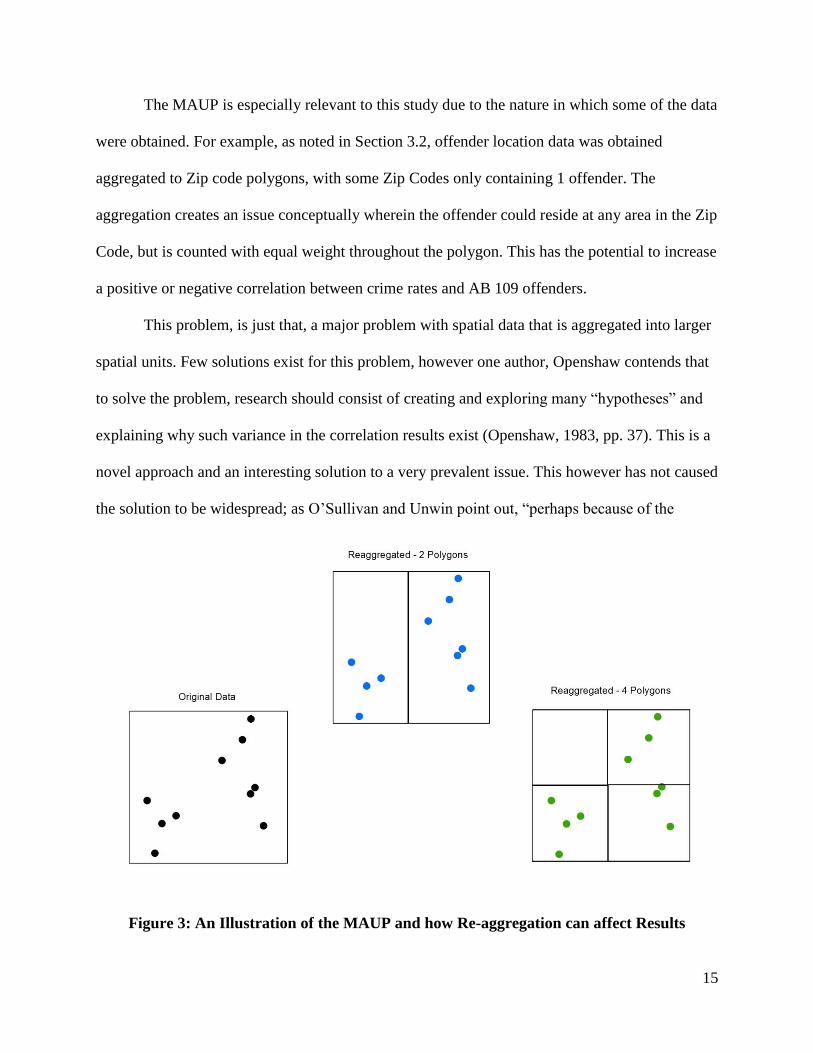
Notice in Figure 3 when the un-aggregated data is aggregated into polygons the number
of events in each polygon begins to change with each transformation; starting at 10 originally
and receding all the way down to zero in one of the polygons as the original data was divided
into four polygons. The MAUP creates a significant problem, because though the manipulation
of aggregate units, the researcher can essentially create the correlation outcome desired or a
stronger correlation simply by re-aggregating the study data. O’Sullivan and Unwin highlight
this problem by noting that “if the spatial units in a particular study were specified differently,
we might observe very different patterns and relationships” (O’Sullivan and Unwin, 2010, pp.
37).
15
The MAUP is especially relevant to this study due to the nature in which some of the data
were obtained. For example, as noted in Section 3.2, offender location data was obtained
aggregated to Zip code polygons, with some Zip Codes only containing 1 offender. The
aggregation creates an issue conceptually wherein the offender could reside at any area in the Zip
Code, but is counted with equal weight throughout the polygon. This has the potential to increase
a positive or negative correlation between crime rates and AB 109 offenders.
This problem, is just that, a major problem with spatial data that is aggregated into larger
spatial units. Few solutions exist for this problem, however one author, Openshaw contends that
to solve the problem, research should consist of creating and exploring many “hypotheses” and
explaining why such variance in the correlation results exist (Openshaw, 1983, pp. 37). This is a
novel approach and an interesting solution to a very prevalent issue. This however has not caused
the solution to be widespread; as O’Sullivan and Unwin point out, “perhaps because of the
Figure 3: An Illustration of the MAUP and how Re-aggregation can affect Results
16
computational complexities and the implicit requirement for the very detailed individual-level
data, this idea has not been widely taken up” (O’Sullivan and Unwin, 2010, pp. 38).
Although O’Sullivan and Unwin note that Openshaw’s theory “has not been widely taken
up,” they do however offer guidance to dealing with the MAUP when examining “point
pattern[s]” (O’Sullivan and Unwin, 2010, pp. 122). Specifically, among other factors for
analysis, they suggest that a “study area should be objectively determined… [and] be
independent of the pattern of events… it might be given by the borders of a country, shoreline of
an island, or edge of a forest” (O’Sullivan and Unwin, 2010, pp. 122). This is an interesting note,
as the MAUP is attempted to be solved, at least partially, by using natural or man-made barriers
to end a continuous surface. This study, attempts to abide by this suggestion, at least partially, to
mitigate the effects of the MAUP on the study results.

17
Chapter 3 Methods and Data
3.1 Study Area and Software
While other studies and reports mentioned previously have studied crime and recidivism rates by
establishing relationships by numbers alone, this study attempts to establish relationships using
numbers and spatial relationships.
As AB 109 represents a large shift in the way that criminal offenders are sentenced and
supervised, this paper studies the effect of the new law on crime rates in San Diego County.
Other counties were considered and debated for this study, however among other factors briefly
stated in the Introduction, the availability of data was a key factor in selecting the study area. As
it is the case in most spatial studies conducted by students in academic programs the availability
of quality data is severely restricted or carries a high price.
To accomplish this task, this study utilized ESRI’s ArcGIS Desktop platform as well as
The Omega Group’s CrimeView Desktop Software. The AcrGIS desktop platform provides a
robust platform complete with a full suite of tools that enable geographic analysis. In addition to
ArcGIS, CrimeView Desktop, a proprietary extension, which runs inside of ArcGIS, provides
extra analysis tools that are specifically designed for crime analysis. IBM SPSS and SAS institute
JMP software were also used.
3.2 Data Sources
Taking into account the literature review of crime analysis techniques discussed in Section 2.2,
the relevant data for this study was determined to be crime point data, a polygon layer containing
counts of offenders being supervised under the AB 109 provision and population counts to
normalize the data. Other population data, such as poverty status, income status and marital
18
status, was desired to provide variables for the spatial regression analysis model used in this
study (discussed in greater detail below).
The initial data acquired for the study consisted of a point data layer that contained the
locations of crimes in San Diego County from January 1, 2007 to December 31, 2012 and April
1-31, 2013. This large crime point dataset was obtained from a data portal website, the San
Diego Regional Data Library, located at “http://data.sandiegodata.org/dataset/clarinova_com-
crime-incidents-casnd-7ba4-extract.” This dataset provided a majority of the crime data needed
for the study, however supplemental data was needed to complete the 2013 year.
To supplement the initial crime dataset, multiple 180 day comma separated value, or
CSV, files, containing locations of crimes, were acquired from the SANDAG website for the
missing months of 2013. This data was used to fill in the gaps of the missing months of the initial
crime points dataset that had been gathered.
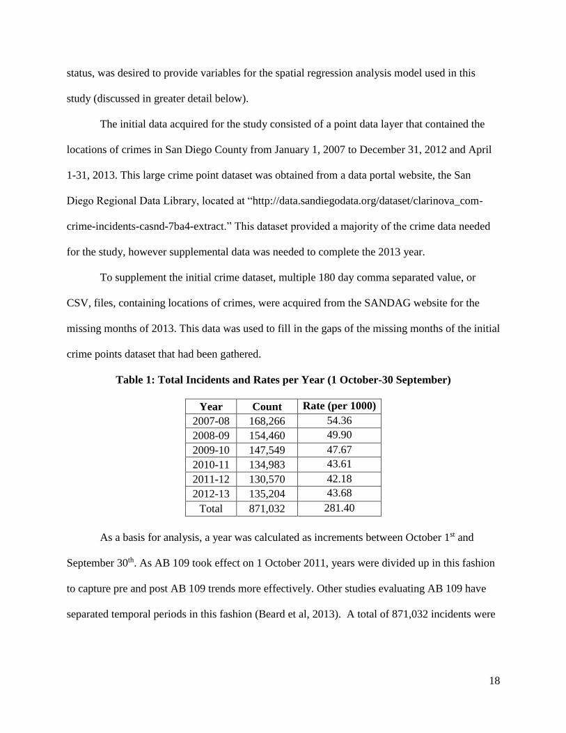
Table 1: Total Incidents and Rates per Year (1 October-30 September)
Year Count Rate (per 1000)
2007-08 168,266 54.36
2008-09 154,460 49.90
2009-10 147,549 47.67
2010-11 134,983 43.61
2011-12 130,570 42.18
2012-13 135,204 43.68
Total 871,032 281.40
As a basis for analysis, a year was calculated as increments between October 1st and
September 30th. As AB 109 took effect on 1 October 2011, years were divided up in this fashion
to capture pre and post AB 109 trends more effectively. Other studies evaluating AB 109 have
separated temporal periods in this fashion (Beard et al, 2013). A total of 871,032 incidents were
19
observed from the temporal range of the data; the results of initial data counts are visible in
Table 1.
The temporal resolution of the Crime data set is 6 years, or from 1 October 2007 to 30
September 2013. As stated above in Chapter 2.2 Crime Analysis, the goal of this research was to
gather two year crime point datasets, one on each side of the AB 109 implementation date, pre
and post, to successfully establish crime trends. In addition to the primary datasets gathered for
the study, an extra two years of data were obtained to further describe crime patterns and trends
in the study region.
With the crime data gathered, it was necessary to supplement the data with additional
datasets to explain patterns and trends in the data. As noted above in Section 2.2, criminal
offenders usually operate within close proximity to their residence. To simulate this effect on AB
109 crime rates, it was determined the location of offenders serving probation time under the AB
109 statute should be included in the analysis. Including this data enabled the evaluation of the
relationship between, at least some, persons convicted and sentenced under the AB 109 provision
and the change in crime rates.
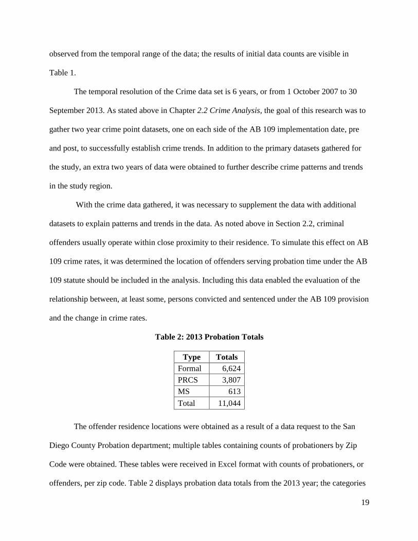
Table 2: 2013 Probation Totals
Type Totals
Formal 6,624
PRCS 3,807
MS 613
Total 11,044
The offender residence locations were obtained as a result of a data request to the San
Diego County Probation department; multiple tables containing counts of probationers by Zip
Code were obtained. These tables were received in Excel format with counts of probationers, or
offenders, per zip code. Table 2 displays probation data totals from the 2013 year; the categories

20
of probation are as follows: the “Formal” count could contain AB 109 offenders sentenced to a
full felony probation sentence as well as offenders already serving a probation sentence before
the passage of AB 109, “PCRS” or “Post-Release Community Supervision” contains counts of
offenders released from prison after serving an AB 109 type offense, and “MS” or “Mandatory
Supervision” contains counts of offenders serving probation after a “split sentence” as part of AB
109 sentencing (Californians for Safety and Justice, 2013). Because the formal count of
offenders contains AB 109 and other offenders, only PCRS and MS counts of offenders were
included as residence locations for AB 109 offenders.
Population data was gathered for San Diego County from the U.S. Census Bureau.
Census geography was downloaded in Census Tracts and Zip Codes for San Diego County from
the U.S. Census website. The corresponding data tables, containing population counts, were also
downloaded from the Census’ American Fact Finder website; the data tables were then linked to
polygons and the result was two population layers, Census Tracts and Zip Codes, containing total
population counts for the respective polygon features with data from the 2010 Census.
In addition to population data, additional variable data for the analysis was obtained from
the Census Bureau. Data tables gathered were: Educational Attainment, Employment Status,
Marital Status, Poverty Status, Median Household Income, Work Status, and Household and
Families. These sources were obtained in table format from the 2010 Census and 2013 ACS
Census counts. Both 2010 and 2013 Census data tables were tied to the 2010 polygon layer noted
above. The requirement for these data variables was determined using the FBI’s “Variables
Affecting Crime” webpage (Federal Bureau of Investigation, 2006). A further explanation of the
social variables obtained from the Census Bureau is contained in Appendix A.
21
In addition to the explanatory variables identified by the FBI above, when performing
initial regression analysis, it was noted that a variable might be missing. After mapping residuals
it was noted that over and under estimated tracts were clustered around the interstates in the area.
In an attempt to compensate for the over and under estimation, a distance, in miles, from the
freeway was calculated and added as an explanatory variable.
In connection with the relevant study data, multiple geography point, line and
polygon layers were gathered from SANDAG for cartography and analysis purposes. These
layers include streets and natural features such as lakes and streams.
3.3 Data Processing
While the majority of the datasets acquired for this study were obtained in usable GIS
formats, a portion of data needed to be processed in order to be used within the ESRI ArcGIS
platform. The data processing completed and data processing methods are listed below.
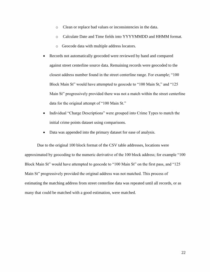
To fill gaps in the initial crime points dataset’s 2013 year, and complete the overall Crime
Dataset, two CSV files were gathered from the SANDAG website at:
http://www.sandag.org/index.asp?subclassid=21&fuseaction=home.subclasshome. These tables
contained multiple fields including the offense date, charge description and address generalized
to the 100 block; a sample block of records from one of the tables is contained in Figure 4. A
table in this form contains a wealth of valuable information, however heavy processing is
necessary to transform the table into a usable GIS format. To transform the tables into a usable
GIS point layer the following steps were performed:
CSV tables were appended using date range.
“Block” or “Blk” was removed from address field with the Field Calculate tool
The Omega Group’s Import Wizard Data processing tool was used to:
22
o Clean or replace bad values or inconsistencies in the data.
o Calculate Date and Time fields into YYYYMMDD and HHMM format.
o Geocode data with multiple address locators.
Records not automatically geocoded were reviewed by hand and compared
against street centerline source data. Remaining records were geocoded to the
closest address number found in the street centerline range. For example; “100
Block Main St” would have attempted to geocode to “100 Main St,” and “125
Main St” progressively provided there was not a match within the street centerline
data for the original attempt of “100 Main St.”
Individual “Charge Descriptions” were grouped into Crime Types to match the
initial crime points dataset using comparisons.
Data was appended into the primary dataset for ease of analysis.
Due to the original 100 block format of the CSV table addresses, locations were
approximated by geocoding to the numeric derivative of the 100 block address; for example “100
Block Main St” would have attempted to geocode to “100 Main St” on the first pass, and “125
Main St” progressively provided the original address was not matched. This process of
estimating the matching address from street centerline data was repeated until all records, or as
many that could be matched with a good estimation, were matched.

23
Probation counts by Zip Code were obtained in Microsoft Excel table format. Tables
contained two counts of only AB 109 offenders per Zip Code; the “Mandatory Supervision”
count and the “Post Release Community Supervision” count (Californians for Safety and Justice,
2013). Both probation types, “Mandatory Supervision” and “Post Release Community
Supervision” are both new designations of probation types that were created for AB 109; “Post
Release Community Supervision” is designated as the probation supervision of those released
from State Prison after serving time for an AB 109 type offense. “Mandatory Supervision” is the
designation of supervision after an offender is released from county “jail” on a “Split-Sentence”
(Californians for Safety and Justice, 2013). Data was processed by joining the Probation tables to
a Zip Code polygon table by the Zip Code field. Multiple polygon layers were created for each
agency Charge_Description_Orig activityDate BLOCK_ADDRESS ZipCode community
ESCONDIDO CARRY CONCEALED DIRK OR DAGGER7/1/2013 23:16 E WASHINGTON AVENUE / N FIG STREET ESCONDIDO
ESCONDIDO DISORDERLY CONDUCT: ALCOHOL 7/2/2013 12:30 1600 E BLOCK WASHINGTON AVENUE 92027 ESCONDIDO
ESCONDIDO MINOR POSSESS ALCOHOL 7/4/2013 20:20 300 N BLOCK BROADWAY ESCONDIDO
ESCONDIDO POSSESS CONTROLLED SUBSTANCE7/4/2013 20:20 300 N BLOCK BROADWAY ESCONDIDO
ESCONDIDO ALCOHOL RELATED 7/5/2013 18:50 WAVERLY PLACE / CLARK STREET ESCONDIDO
ESCONDIDO ALCOHOL RELATED 7/5/2013 18:50 WAVERLY PLACE / CLARK STREET ESCONDIDO
LA MESA USE ANOTHER PERSONAL IDENTIFICATION TO OBTAIN CREDIT/ETC7/29/2013 22:00 7600 BLOCK NORMAL AVENUE 91941 LA MESA
LA MESA BATTERY ON PERSON 7/16/2013 14:00 8800 BLOCK FLETCHER PARKWAY 91942 LA MESA
ESCONDIDO BURGLARY/UNSPECIFIED 8/6/2013 10:00 300 W BLOCK EL NORTE PARKWAY 92026 ESCONDIDO
SHERIFF USE/UNDER INFL OF CONTROLLED SUBS (M)7/21/2013 12:05 N MAIN AVENUE / E IVY STREET 92028 FALLBROOK
OCEANSIDE DRUNK IN PUBLIC: ALCOHOL, DRUGS, COMBO OR TOLUENE (M)11/26/2013 17:45 600 BLOCK DOUGLAS DRIVE 92058 OCEANSIDE
ESCONDIDO USE ANOTHER PERSONAL IDENTIFICATION TO OBTAIN CREDIT/ETC8/17/2013 0:01 500 W BLOCK EL NORTE PARKWAY 92026 ESCONDIDO
ESCONDIDO GRAND THEFT:MONEY/LABOR/PROPERTY OVER $9508/19/2013 21:30 2100 BLOCK STANLEY WAY 92027 ESCONDIDO
ESCONDIDO GET CREDIT/ETC OTHERS ID 8/20/2013 14:10 800 E BLOCK MISSION AVENUE 92025 ESCONDIDO
ESCONDIDO TAKE VEHICLE W/O OWNER'S CONSENT/VEHICLE THEFT8/19/2013 18:00 1900 BLOCK SUNSET DRIVE 92025 ESCONDIDO
ESCONDIDO TAKE VEHICLE W/O OWNER'S CONSENT/VEHICLE THEFT8/18/2013 13:50 1400 BLOCK VIEW POINTE AVENUE 92027 ESCONDIDO
ESCONDIDO EXHIBIT DEADLY WEAPON (OTHER THAN FIREARM)8/19/2013 13:58 800 N BLOCK FIG STREET 92026 ESCONDIDO
ESCONDIDO TAKE VEHICLE W/O OWNER'S CONSENT/VEHICLE THEFT8/19/2013 21:42 1200 BLOCK REMBRANDT GLEN 92026 ESCONDIDO
EL CAJON DUI ALC/0.08 PERCENT (M) 8/4/2013 1:30 200 BLOCK JAMACHA ROAD 92019 EL CAJON
ESCONDIDO TAKE VEHICLE W/O OWNER'S CONSENT/VEHICLE THEFT8/20/2013 23:00 900 BLOCK HOWARD AVENUE 92029 ESCONDIDO
ESCONDIDO PETTY THEFT 7/12/2013 12:00 1400 BLOCK OAK HILL DRIVE 92027 ESCONDIDO
ESCONDIDO BURGLARY/UNSPECIFIED 7/19/2013 20:30 200 E BLOCK VIA RANCHO PARKWAY 92025 ESCONDIDO
ESCONDIDO GRAND THEFT:MONEY/LABOR/PROPERTY OVER $9508/23/2013 13:48 300 W BLOCK EL NORTE PARKWAY 92026 ESCONDIDO
SHERIFF PETTY THEFT(All Other Larceny) (M)7/7/2013 21:45 30800 BLOCK OLD HIGHWAY 395 92026 ESCONDIDO UNINC
ESCONDIDO GET CREDIT/ETC OTHERS ID 8/20/2013 15:45 400 BLOCK DALE AVENUE 92026 ESCONDIDO
ESCONDIDO PETTY THEFT 8/20/2013 16:00 1300 E BLOCK VALLEY PARKWAY 92027 ESCONDIDO
ESCONDIDO VANDALISM (LESS THAN $400) 8/21/2013 1:43 3100 BLOCK SYCAMORE CREST PLACE 92027 ESCONDIDO
Figure 4: 2013 Crime Data in Native CSV Format

24
year of probation data received. MS counts and PRCS counts were added together to attain a full
count of AB 109 offenders per Zip Code. A sample block of records from the 2013 probation
table can be found in Table 3.
Table 3: 2013 Probation Counts
ZIP CODE FORMAL PROBATION PRCS MS
Blank 1234 957 131
92021 156 103 16
92024 34 11 5
92025 141 57 14
92026 84 51 16
3.4 Data Issues
The data collected for this study are very complete and robust, however a few data issues
existed; a discussion of the various data issues follows.
First, the probation tables obtained are in very good condition, however, as displayed in
Table 3, a record containing a “Blank” Zip Code corresponds with a count of offenders. Because
no location information was tied to these counts they were not included in the study in an effort
to preserve the spatial distribution of the data.
Second, the SANDAG website that allows for the download of Crime CSV files is based
on a previous 180 day range. The data was gathered beyond the date range, omitting 8 days of
data at the start of the 2013 year. The date range of the missing data is 2013-01-01 to 2013-01-
09. As this date range represents 2.2% of a year the effect of the missing data on the study should
be negligible.
25
3.5 Methods
With the aggregate of the information gathered, an extensive analysis was performed to
determine if a relationship exists between residence locations of AB 109 offenders and crime rate
increase across San Diego County. Other variables were also tested to in an attempt to provide
alternative explanations for changes in crime rates. The assumptions and statistical methods
used for the study follow.
ESRI’s ArcGIS software suite was used to perform the majority of the analyses as it
provides very useful statistical tools. Tools provided by the ArcGIS platform are extensive and
allow for many operations, including regression analysis and zonal statistics. In Addition to the
tools provided with the ArcGIS platform, the analysis tools provided by the Omega Group’s
CrimeView Desktop software were used to perform analysis. CrimeView Desktop provides a full
suite of tools that can be used to analyze crime including hot spot analysis and a Crime Rate
Generator. IBM SPSS and SAS Institute JMP statistical programs were also used to analyze the
data.
To begin the analysis, a major requirement of the data was to be divided into temporal
periods and crime categories for comparison. An in depth procedure of how the data was divided
follows.
The crime points dataset, or reported crimes in San Diego County, was first separated
into two datasets for comparison; pre and post AB 109 temporal periods. Reported crimes, or
crime points, from 1 October 2009 – 30 September 2011 was established as the pre AB 109
temporal period. Conversely reported crimes occurring between 1 October 2011 – 30 September
2013 was established as the post AB 109 temporal period for comparison. An additional two year
period, 1 October 2007 – 30 September 2009, is included in descriptive statistics to offer

26
additional insight into crime trends in San Diego County during this period. It should be noted
however that the main temporal periods studied immediately preceded and followed
implementation of AB 109 (1 October 2009 – 30 September 2011 and 1 October 2011 – 30
September 2013).
In addition to dividing the reported crime events into two temporal periods, crimes were
further divided into several categories for comparison to ascertain the effect of AB 109 on each
crime category. Reported crime events were separated into the following cohorts:
AB 109 categorized events
Non AB 109 categorized events
Crimes Against Property
Crimes Against Society
Crimes Against Persons
The cohorts categorized under NIBRS categories, “Crimes Against Persons… Society” and
“Property,” investigated previous claims of affected crime trends in California (LESS and
CSMU, 2013, pp. 13; Beard et al, 2013; Lofstrom & Raphael, 2013). The cohorts comparing AB
109 offenses to non- AB 109 offenses, help to further study the crime trends occurring in
California due to the new law.
As noted previously in this paper: it is expected that areas with a higher population
density will experience a higher rate of crime (Brandmüller and Önnerfors, 2011; Harries, 2006).
To normalize for this expectation a crime rate was determined by obtaining the number of crimes
per 1000 persons for each Census Tract in San Diego County; the CrimeView Desktop software
extension Crime Rate Generator and the Spatial Join and Field Calculator functions of ArcGIS
were used to calculate crime rate numbers. Crime rates were generated by querying NIBRS
27
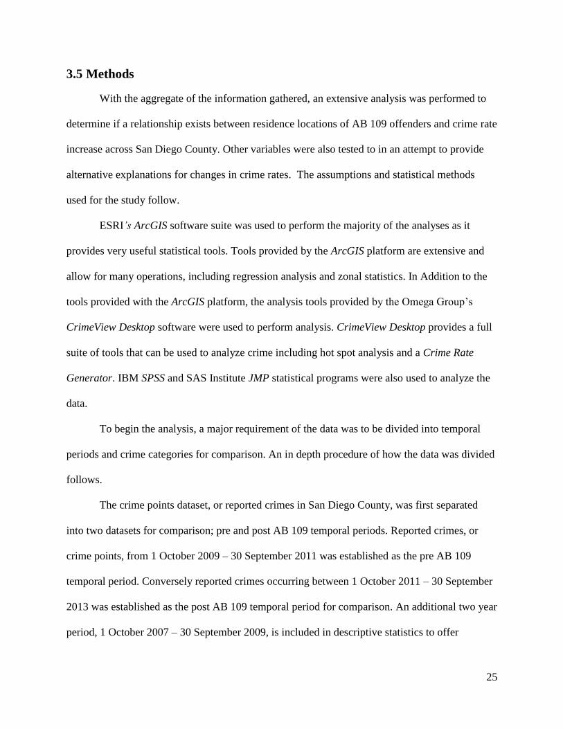
categories and groups classified as AB 109/Non AB 109 crime types, for 2 year periods to
establish a control or a baseline for comparison. Crime rates for one of the temporal periods
studied are displayed in Figure 5.
Upon initial review of the Non AB 109 cohort, a box plot test was performed to
determine if the distribution of the data was normal. Upon completion of the test outliers were
determined to be present in the data more than 1.5 box plots away (Laerd Statistics, 2015). Some
outliers, where the population was lower than 1000 persons, were removed to normalize the data.
The outliers, where a larger number crimes than the total population are reported or if the
Figure 5: Property Crime Rates (Crimes per 1000 people) between 1 October 2011 and 30
September 2013 - Data Aggregated by Census Tract

28
population for the census tract was lower than 1000, contained abnormally skewed crime rates. A
total of 4 outliers were removed from the crime rate analysis to mitigate the effect of the outliers
on the data. This however did not mitigate the effect of all the outliers; several outliers, many of
them extreme outliers remained in the analysis. Because of the nature of the extreme outliers in
the data, a “Wilcoxon signed-rank test” was performed on the cohorts to determine the statistical
significance of the findings (Laerd Statistics, 2015).
In order to calculate, measure and normalize the data for population in San Diego
County, crime rates were calculated for each census tract in the county. Crime rates for this study
are defined as crimes per 1000 persons as displayed in the equation below (New Jersey State
Police, 2015). Crime rates were calculated by dividing the total number of reported crimes in
each census tract, by the population of the census tract and multiplying the result by 1000.
𝐶𝑟𝑖𝑚𝑒 𝑅𝑎𝑡𝑒 = (𝑅𝑒𝑝𝑜𝑟𝑡𝑒𝑑 𝐶𝑟𝑖𝑚𝑒/𝑃𝑜𝑝𝑢𝑙𝑎𝑡𝑖𝑜𝑛) ∗ 1000
Once crime rates were established, the difference was calculated between the control and
the variable time periods, 1 October 2009 to 30 September 2011 being the control, and 1 October
2011 to 30 September 2013 being the variable. Having established the change in crime rates
during the two year period, multiple analyses were performed to determine the significance, if
any, of the relationship between the difference in crime rates and the populations of AB 109
designated offenders as well as other variables such as median household income and single
parent households. An inferential statistical analysis and spatial analysis was performed on the
data.
As noted above in Section 3.2 offender data was gathered and obtained in table form
with counts of offenders aggregated by Zip Code. This presented a problem as polygons used

29
for population and other demographic data were aggregated by Census Tract and regression
analysis cannot be performed between different areal units.
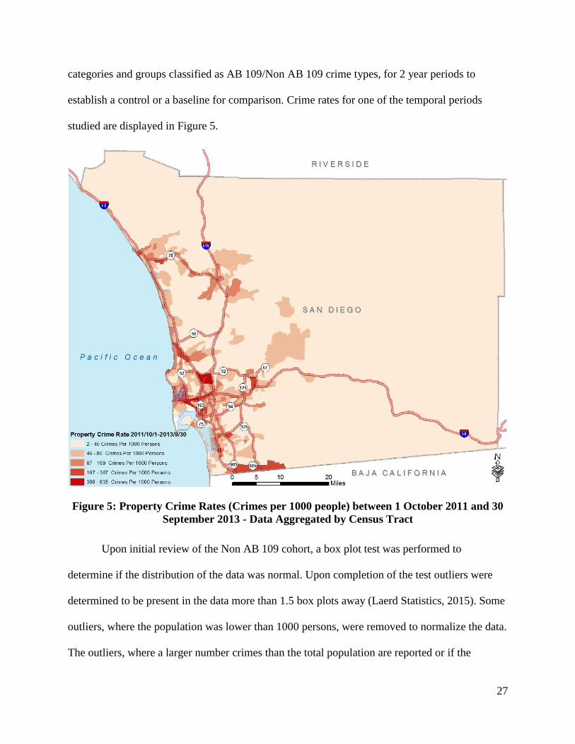
Operating under the assumption that the counts of probationers in each Zip code were
evenly distributed throughout the polygon Zonal Statistics were used to re-aggregate the offender
or probationer data to Census Tract polygons. The Identify and Dissolve ArcGIS tools and Field
Calculator were used to perform this task. The Identify tool combined the Zip code and Census
tract polygons to create a multitude of polygons by cutting polygons at each intersecting point.
The new polygons contained the attributes of each original Census tract and Zip code polygon.
After creating the polygons, the geometry, in square kilometers, of each new polygon was then
calculated and the percentage of each new polygon comprising each individual Zip Code was
calculated. The aerial percentage of each polygon was then multiplied by the offender count
from the Zip Code it was created from. The new polygons were then dissolved into Census tract
using the ID of each Census Tract. When dissolving, a sum of the offender counts was produced.
The final result was a layer that contained an equal percentage of offenders per tract to the areal
percentage of each Zip Code. Figure 6 illustrates the re-aggregation of offender data from Zip
code polygons to Census tract polygons.
30
Figure 6: Re-Aggregation of Offender Counts from Zip Codes to Census Tracts

31
This study used traditional and spatial statistics methods to analyze crime rate data at the
census tract level. Traditional statistics methods were used to calculate the general trend of the
data by calculating a median increase or decrease value and calculating probability. Spatial
statistics used hot spot and regression analysis to determine the correlations between crime rates
and variables studied.
To calculate the trend of crime rates in San Diego County during the studied temporal
periods, IBM SPSS statistical tools were used. A Wilcoxon signed-rank test was performed on
each crime category to determine the Z-score and probability of the cohort. In addition to the
Wilcoxon signed-rank test, the median crime rate difference value was calculated to determine
the direction of the trend; for example, an increase or decrease in crime rates.
As this study attempts to determine the spatial effects of offender residence locations and
other variables to crime events, regression analysis was used to determine the extent of the
relationship between the difference in crime rates during the period studied and the variables
selected for the study. Regression analysis is a common statistical method and is seen in many
scientific studies. This form of analysis was determined to be the most useful and descriptive
statistic to calculate the correlation between the variables.
When considering performing any spatial analysis, including regression, it is important to
note that spatial statistic assumptions are generally different than those of a traditional statistical
analysis. Specifically, in traditional statistics methods, an underlying assumption of the data is
that the “samples” or data collected for the study, “must be random,” whereas spatial data carries
the assumption of “spatial autocorrelation” (O’Sullivan and Unwin, 2010, pp. 34). Spatial
autocorrelation carries the assumption that in geography, closer phenomena are likely to be

32
similar in characteristic, than distant phenomena in a spatial environment (O’Sullivan and
Unwin, 2010, pp. 34).
When considering using regression analysis, it is also important to note; while many GIS
questions ask “Where” events are occurring Regression analysis examines “Why” events are
occurring (Murak, 2015, pp. 3).
To ask why, as noted above, it is important to understand where events are occurring. To
this end, multiple analyses were performed on the crime rate data to answer the questions: Are
Crime Rates in San Diego increasing? If so, where? Which types of crime are increasing?
To answer these questions, hot spot maps were produced to determine areas where
statistically significant increases in crime had occurred. Once these areas were identified,
regression analysis was used to test the relationship between the independent and explanatory
variables in the hot spot. This method is covered in more detail later in this section.
The ArcGIS suite provides various tools to perform regression analysis. This study
utilized the Ordinary Least Squares tool to perform regression analysis. In addition to the
ArcGIS OLS tool, a statistical software program JMP, published by the SAS institute, was used
to help determine variables to include in the OLS analysis. These tools were used to analyze the
difference in crime rates from the NIBRS and AB 109/Non AB 109 categories.
Regression analysis is used to display a correlation, positive or negative. A correlation
can be thought of as a relationship between two variables. The independent variable for the
regression analysis in the study was the difference in crime rates between the temporal periods
studied. The explanatory variables examined were: the residence location of AB 109 offenders
serving probation in San Diego County during the 2013 year, Educational Attainment,
Employment Status, Marital Status, Poverty Status, Median Household Income, and Work

33
Status. The explanatory variables are explained in more detail in Appendix A. The data source of
the explanatory variables as well as the independent variable can be found in Chapter 3.2.
The Ordinary Least Squares tool functions by providing useful data about the strength of
and descriptive potential of each variable, as well as overall model strength. A few of the useful
indicators supplied by the model follow: the “Variance Inflation Factor (VIF)” indicates
“redundancy among explanatory variables,” the “Joint F-Statistic and Joint Wald Statistic”
indicate “overall model statistical significance,” and the “Probability” aides in determining
“Statistical Significance” of an “explanatory variable. (ESRI, 2013). All of these indicators and
more were used in determining the strength of the relationship between explanatory variables
and the difference in crime rates.
The JMP software platform provides a Fit Model tool to run step wise regression, among
other functions. The Fit Model tool functions as follows: the type of analysis to be run is
selected, a Y variable is selected, and multiple X variables can be selected. Once variables are
selected, an automated step wise regression analysis can be performed, forward and backward. A
minimum model fitness value can be selected to stop the step wise regression at that point; for
example minimum AIC or BIC.
Step wise regression was performed using the crime rate difference as the Y variable and
the explanatory variables, described above, as the X variables. The tool was run forward and
backward to determine the best variables to use in the regression model. Minimum AIC and BIC
values were considered when running the analysis. The results of step wise regression were used
to perfect the spatial OLS models constructed as part of the study.
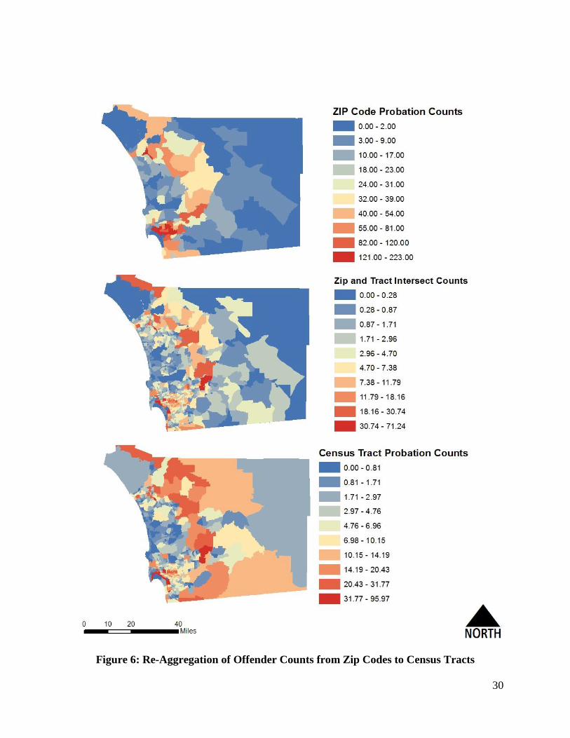
As it was more than likely that spatial autocorrelation was present in the data collected
for this study, a widely used calculation, Moran’s I, was used to determine the amount of
34
autocorrelation in the data after running regression analysis (O’Sullivan and Unwin, 2010). The
ArcGIS “Spatial Autocorrelation (Moran’s I)” tool was used to test the residuals of the regression
analyses to determine the validity of the result (ESRI, 2013). An illustration of the Moran’s I
output and statistics can be found in Figure 7.
Figure 7: Example of Moran’s I Tool Output Testing Autocorrelation of
Residuals

35
Chapter 4 Results
4.1 Descriptive Statistics
After thorough data processing was performed on a majority of the data, an initial exploration, or
descriptive statistical analysis of the data was conducted. The summary of the statistical analysis
is described in detail below.
When comparing trends between the AB 109 categorized offenses and Non AB 109
categorized offenses, it was found that both cohorts saw a decrease in both overall incident
counts and crime rates following the implementation of the law. The AB 109 Offense cohort
experienced a 4.7% decrease between the two temporal periods studied. The Non AB 109 cohort
experienced a larger decrease of 14.8% during the same period. Counts for both categories
separated by year are displayed in Table 4. This observed decrease in crime rates between these
two cohorts is interesting, particularly as the AB 109 group of crimes exhibited a decrease in
crime rates during the period studied. As noted below, when crime types were further divided
into NIBRS crime categories, two out of the three categories exhibited an overall increase.
Table 4: AB 109 Offenses vs Non AB 109 Offenses queried from 1 October to 30 September
Pre/Post AB 109 Time Period AB 109 Offenses Non AB 109 Offenses Total
Crimes
Pre AB 109 2009 - 2010 120,659 (81.8%) 26,897 (18.2%) 147,549
Pre AB 109 2010 - 2011 110,482 (82.9%) 24,504 (16.5%) 134,983
Post AB 109 2011-2012 108,622 (83.2%) 21,960 (16.8%) 130,570
Post AB 109 2012 -2013 111,760 (82.7%) 23,051 (17.0%) 135,204
Of the three NIBRS cohorts studied, Property Crime, is of particular interest to this study;
as many authors have contended that property crime is rising due to AB 109 (Beard et al, 2013;

36
Lofstrom and Raphael, 2013). In contrast to the overall event count, and the AB 109 vs Non 109
cohorts, the NIBRS crime event datasets display different trends. When the dataset was further
divided, trends in the data were much more pronounced. For example, the Crimes against
Property category saw a decrease of 36,277 (-17.97%) events during the 2009-11 period.
However an increase of 3,741 (+2.26%) occurred during the 2011-13 period, as compared to the
2009-11 period. Overall the property crime cohort exhibited a decrease of 32,536 (-16.12%) for
the range of the data. However it is important to note that although property crime rates have
decreased overall, they exhibited a rising trend during the last data period. This has the potential
to be significant due to the large drop in crime rates from the previous period. Meaning, property
crime was trending down sharply and has now experienced an increase immediately following
the implementation of AB 109, reflecting the claims of previous studies.
Table 5: NIBRS Crime Category Counts for San Diego County - 1 Oct 2007- 30 Sep 2013
Period Societal Crime Personal Crime Property Crime
2007-09 89,365 27,962 201,893
2009-11 89,444 (+0.09%) 24,129 (-13.71%) 165,616 (-17.97%)
2011-13 68,116 (-23.85%) 24,549 (+1.74%) 169,357 (+2.26%)
In stark contrast to the property crime cohort, the crimes against society, or societal
crime, cohort exhibited almost no change, an increase of just 79 events (+0.09%) during the
2009-11 period, displayed in Table 5, indicating that the societal crime trend was steady leading
up to the implementation of AB 109. In addition to the steady rate leading up to the
implementation of AB 109, a sharp decrease of -21,328 events (-23.85%) during the 2011-13
period as compared to the previous period also sharply contrasts the property crime cohort.

37
In addition, Crimes against persons also remained relatively unchanged after a sharp drop
from the 2007-09 period. During the 2009-11 period San Diego County saw a drop of 3833
Crimes against Persons events or a 13.71% decrease. In contrast, the 2011-13 period exhibited a
much less pronounced change; an increase of 425 events (+1.7%) increase. Table 5 displays the
event counts for Crimes against Persons.
As property crime was the only cohort that exhibited any type of significant increase
during the temporal period following AB 109 implementation; and as an increase in crime rates
is of the greatest concern to society, selected property crime types were studied in addition to the
overall cohort.
For example, thefts or larcenies were investigated more closely and revealed an
interesting trend. The property crime cohort exhibited an overall decline during the temporal
range studied, however thefts or larceny events exhibited a significant increase during the
temporal range. The dataset displayed an initial decrease of 2,363 (-5.72%) events during the
2009-11 period as displayed in Figure 8. However thefts increased by 5,722 (14.69%) events
41311
38948
44670
2007-09 2009-11 2011-13
inci
den
t C
ou
nt
Period
THEFT/LARCENY
Figure 8: Theft/Larceny Trend (1 October - 30 September)

38
during the 2011-13 period as compared to the 2009-11 period and displayed a total increase of
3,359 (8.13%) during the temporal range of the study. The data from this cohort exhibits an
interesting pattern, because although it follows the general pattern of property crimes, it
exhibited a far greater increase immediately following the implementation of AB 109.
In addition to the theft/larceny crime type, the burglary crime type of the property crime
cohort was studied to further investigate trends. While not as dramatic, the burglary dataset
exhibited a similar pattern to the theft/larceny dataset. As with larcenies burglaries decreased by
4,293 (-14.06%) events during the 2009-11 period. Again however, burglaries exhibited an
increase of 5052 (+19.25%) during the 2011-13 period as compared to the previous period and
exhibited an overall increase of 759 (+2.49%) events during the temporal range of the data as
displayed in Figure 9. As with theft/larceny, burglary followed the overall trend displayed by the
property crime cohort, however exhibited the highest measurement at the end of the temporal
range of the data, immediately following implementation of AB 109. These trends are troubling,
because although the larger, more inclusive, property crime cohort exhibited a small increase at
30537
26244
31296
2007-09 2009-11 2011-13
Inci
den
t C
ou
nt
Period
BURGLARY
Figure 9: Burglary Trend (1 October - 30 September)
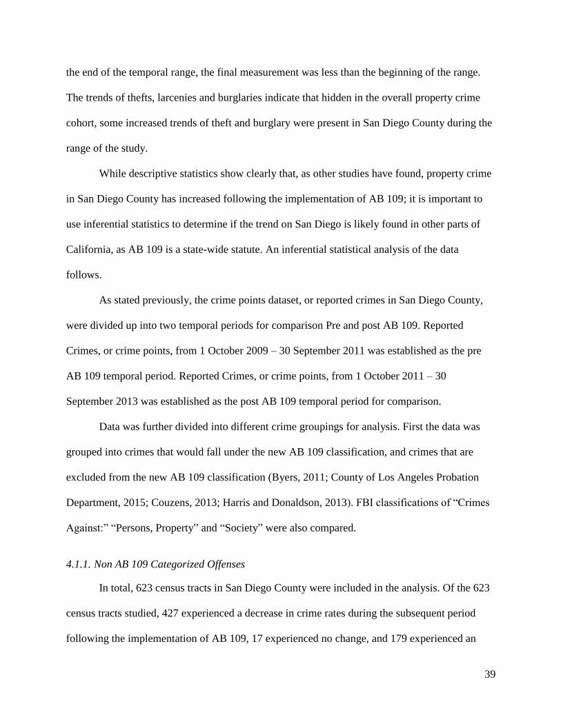
39
the end of the temporal range, the final measurement was less than the beginning of the range.
The trends of thefts, larcenies and burglaries indicate that hidden in the overall property crime
cohort, some increased trends of theft and burglary were present in San Diego County during the
range of the study.
While descriptive statistics show clearly that, as other studies have found, property crime
in San Diego County has increased following the implementation of AB 109; it is important to
use inferential statistics to determine if the trend on San Diego is likely found in other parts of
California, as AB 109 is a state-wide statute. An inferential statistical analysis of the data
follows.
As stated previously, the crime points dataset, or reported crimes in San Diego County,
were divided up into two temporal periods for comparison Pre and post AB 109. Reported
Crimes, or crime points, from 1 October 2009 – 30 September 2011 was established as the pre
AB 109 temporal period. Reported Crimes, or crime points, from 1 October 2011 – 30
September 2013 was established as the post AB 109 temporal period for comparison.
Data was further divided into different crime groupings for analysis. First the data was
grouped into crimes that would fall under the new AB 109 classification, and crimes that are
excluded from the new AB 109 classification (Byers, 2011; County of Los Angeles Probation
Department, 2015; Couzens, 2013; Harris and Donaldson, 2013). FBI classifications of “Crimes
Against:” “Persons, Property” and “Society” were also compared.
4.1.1. Non AB 109 Categorized Offenses
In total, 623 census tracts in San Diego County were included in the analysis. Of the 623
census tracts studied, 427 experienced a decrease in crime rates during the subsequent period
following the implementation of AB 109, 17 experienced no change, and 179 experienced an

40
increase in crime rates. The results of the Wilcoxon signed-rank test, displayed in Table 7, found
a statistically significant median decrease in crime rates, -1.6, during the temporal period studied,
z=-12.213, p < 0.0005. The small P value indicates that the probability of the null hypothesis,
AB 109 had no effect on crime rates, occurring, is less than 1%, indicating statistical
significance.
Table 6: Degree of Change in Crime Rates from the Crime Categories Studied
Category Median Maximum Increase Maximum
Decrease
Non AB 109 -1.6 45.02 -43.40
AB 109 -2.0 175.55 -241.92
Property 0.7 130.79 -124.72
Societal -3.5 71.14 -240.34
Personal -0.1 14.79 -18.47
The median value of -1.6 exhibited by the Non AB 109 category, indicates that crimes in
this grouping decreased by an average of 1.6 events per 1000 persons in each census tract. As
displayed by the data, and Table 6, this category of crimes displayed an overall decrease between
the control and variable temporal periods. It appears from the initial statistical analysis, that the
temporal period coinciding with the implementation of AB 109 experienced a decrease in crimes
that are not punishable under the new AB 109 statue.
Table 7: Wilcoxon Signed Rank Test of Non AB 109 Offenses Results
Observations (N) 623
Increase Exhibited 179
Decrease Exhibited 427
No Change 17
Z Score 12.213
Probability < 0.0005

41
During the period, as stated above, 427 (68.54%) tracts experienced a decrease in crime
rates during the subsequent period following the implementation of AB 109, as exhibited in in
Table 9 below, 17 (2.73%) experienced no change, and 179 (28.73%) experienced an increase in
crime rates. The maximum rate increase of this cohort was 45.02 in Census Tract 89.02, and the
maximum decrease was -43.40 in Census Tract 183. The variance of the data, represented by
standard deviations, is displayed in Figure 10.
These Crimes are basically the opposite of the AB 109 categorized crimes and hence
include the “Violent, Serious and Sexual” crime not specified by the law (Californians for Safety
and Justice, 2013). These crimes include murder, rape, robbery, etc.; the median decrease in
Figure 10: Variance of Non AB 109 Crime Rate Difference Values

42
crime rates related to this group, is a positive as the crimes listed above are especially heinous
and are detrimental to society.
4.1.2. AB 109 Categorized Offenses
As stated above with Non AB 109 offenses, in total, 623 census tracts in San Diego
County were included in the analysis of AB 109 Categorized Offenses. Of the 623 census tracts
studied, 351 experienced a decrease in crime rates during the subsequent period following the
implementation of AB 109, 7 experienced no change, and 265 experienced an increase in crime
rates. The results of the Wilcoxon signed-rank test, displayed in Table 8, indicated a statistically
significant median decrease in crime rates of 2.0 events per 1000 people during the temporal
period studied, z= -4.694, p < .0005. Again, the small P value indicates the probability of the null
hypothesis, AB 109 had no effect on crime rates, occurring, is less than 1%, indicating statistical
significance.
Table 8: Wilcoxon Signed Rank Test of AB 109 Offenses Results
Observations (N) 623
Increase Exhibited 265
Decrease Exhibited 351
No Change 7
Z Score -4.694
Probability < 0.0005
The median value of -2.0 exhibited by the AB 109 category, indicates that crimes in this
grouping decreased by an average of 2.0 in each census tract. The maximum rate increase of this
cohort was 175.55, and the maximum decrease was -241.92, as displayed in Table 6. As
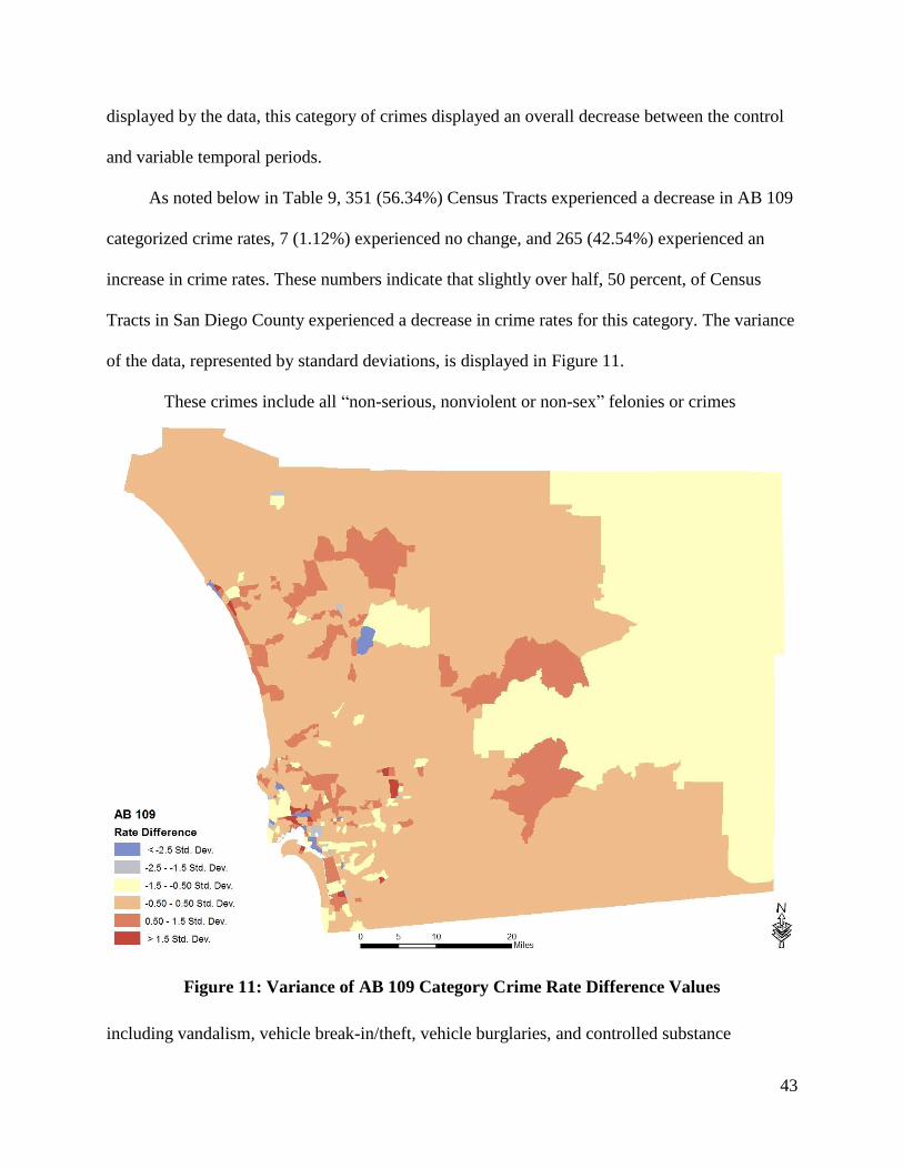
43
displayed by the data, this category of crimes displayed an overall decrease between the control
and variable temporal periods.
As noted below in Table 9, 351 (56.34%) Census Tracts experienced a decrease in AB 109
categorized crime rates, 7 (1.12%) experienced no change, and 265 (42.54%) experienced an
increase in crime rates. These numbers indicate that slightly over half, 50 percent, of Census
Tracts in San Diego County experienced a decrease in crime rates for this category. The variance
of the data, represented by standard deviations, is displayed in Figure 11.
These crimes include all “non-serious, nonviolent or non-sex” felonies or crimes
including vandalism, vehicle break-in/theft, vehicle burglaries, and controlled substance
Figure 11: Variance of AB 109 Category Crime Rate Difference Values
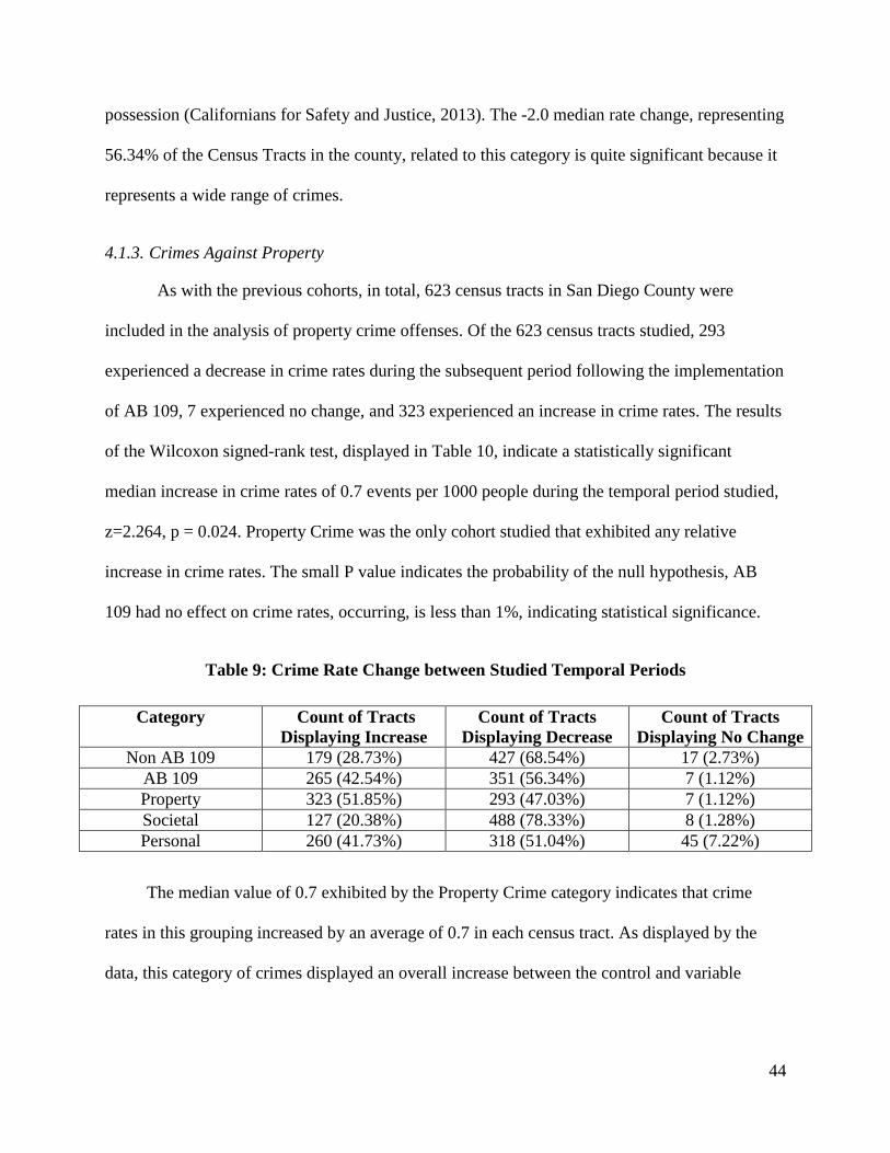
44
possession (Californians for Safety and Justice, 2013). The -2.0 median rate change, representing
56.34% of the Census Tracts in the county, related to this category is quite significant because it
represents a wide range of crimes.
4.1.3. Crimes Against Property
As with the previous cohorts, in total, 623 census tracts in San Diego County were
included in the analysis of property crime offenses. Of the 623 census tracts studied, 293
experienced a decrease in crime rates during the subsequent period following the implementation
of AB 109, 7 experienced no change, and 323 experienced an increase in crime rates. The results
of the Wilcoxon signed-rank test, displayed in Table 10, indicate a statistically significant
median increase in crime rates of 0.7 events per 1000 people during the temporal period studied,
z=2.264, p = 0.024. Property Crime was the only cohort studied that exhibited any relative
increase in crime rates. The small P value indicates the probability of the null hypothesis, AB
109 had no effect on crime rates, occurring, is less than 1%, indicating statistical significance.
Table 9: Crime Rate Change between Studied Temporal Periods
Category Count of Tracts
Displaying Increase
Count of Tracts
Displaying Decrease
Count of Tracts
Displaying No Change
Non AB 109 179 (28.73%) 427 (68.54%) 17 (2.73%)
AB 109 265 (42.54%) 351 (56.34%) 7 (1.12%)
Property 323 (51.85%) 293 (47.03%) 7 (1.12%)
Societal 127 (20.38%) 488 (78.33%) 8 (1.28%)
Personal 260 (41.73%) 318 (51.04%) 45 (7.22%)
The median value of 0.7 exhibited by the Property Crime category indicates that crime
rates in this grouping increased by an average of 0.7 in each census tract. As displayed by the
data, this category of crimes displayed an overall increase between the control and variable

45
temporal periods. The Property Crime category was the only category studied to exhibit any type
of increase.
Table 10: Wilcoxon Signed Rank Test of Property Crime Offenses Results
Observations (N) 623
Increase Exhibited 323
Decrease Exhibited 293
No Change 7
Z Score 2.264
Probability 0.024
As displayed in Table 9, 293 (47.03%) Census Tracts experienced a decrease in Property
Crime categorized crime rates, 7 (1.12%) experienced no change, and 323 (51.85%) experienced
an increase in crime rates. These numbers indicate that slightly over half, 52 percent, of Census
Tracts in San Diego County experienced an increase in crime rates for this category. And as with
other cohorts the crime rate changes were distributed throughout the county, as opposed to
focused in a single area. The variance of the data, represented by standard deviations, is
displayed in Figure 12.

46
4.1.4. Crimes Against Persons
623 census tracts in San Diego County were included in the analysis of Crimes Against
Persons Offenses. Of the 623 census tracts studied, 318 experienced a decrease in crime rates
during the subsequent period following the implementation of AB 109, 45 experienced no
change, and 260 experienced an increase in crime rates. The results of the Wilcoxon signed-rank
test, displayed in Table 11, indicate a statistically significant median decrease in crime rates of
0.1 events per 1000 people during the temporal period studied, z=-2.658, p = 0.008. Again, the
small P value indicates the probability of the null hypothesis, AB 109 had no effect on crime
Figure 12: Variance of Property Crime Rate Difference Values

47
rates, occurring, is less than 1%, indicating statistical significance. Although this test indicated
that a statistically significant drop in crimes against persons occurred during the time studied; the
median decrease in crime rates for the areas studied was -0.1 indicating the change was very
small, 0.1 crimes per 1000 residents.
Table 11: Wilcoxon Signed Rank Test of Crimes Against Persons Offenses Results
Observations (N) 623
Increase Exhibited 260
Decrease Exhibited 318
No Change 45
Z Score -2.658
Probability 0.008
Although the median decrease of 0.1 crimes per 1000 people is relatively small
compared to the other cohorts studied, it is important to note, as displayed in Table 6, that the
maximum personal crime rate decrease for any Census Tract in the county was 18.47, which is
also relatively small compared to other decreases noted.
As displayed in Table 9, 318 (51.04%) Census Tracts experienced a decrease in personal
crime rates, 45 (7.22%) experienced no change, and 260 (41.73%) experienced an increase in
crime rates. These numbers indicate that slightly over half, 50 percent, of Census Tracts in San
Diego County experienced a decrease in crime rates for this category. Also, as indicated by the
small median decrease in crime rates, these statistics indicate that close to 10% of census tracts
remained stable during the temporal period studied. The variance of the data, represented by
standard deviations, is displayed in Figure 13.

48
The findings of the analysis are interesting as the statistically significant median value for
the census tracts in the county was negative, whereas compared to the aggregate statistics in
Section 4.1, counts displayed an increase of 24,549 (1.74%). The negative median finding also
contrasts Lofstrom and Raphael’s report that indicated “violent crime [rates]” have increased in
California, as the crimes against persons cohort is represented mostly by violent crime types.
(Lofstrom and Raphael, 2013, pp 2).
Figure 13: Variance of Persons Crime Rate Difference Values

49
4.1.5. Crimes Against Society
As stated above with the other cohorts, in total, 623 census tracts in San Diego County
were included in the analysis of Crimes Against Society categorized Offenses. Of the 623 census
tracts studied, 488 experienced a decrease in crime rates during the subsequent period following
the implementation of AB 109, 8 experienced no change, and 127 experienced an increase in
crime rates. The results of the Wilcoxon signed-rank test, displayed in Table 12, indicated a
statistically significant decrease in crime rates of 3.5 events per 1000 people during the temporal
period studied, z=-14.905, p < 0.0005.
Table 12: Wilcoxon Signed Rank Test of Crimes Against Society Offenses Results
Observations (N) 623
Increase Exhibited 127
Decrease Exhibited 488
No Change 8
Z Score -14.905
Probability < 0.0005
The median value of -3.5 exhibited by the Societal Crime category indicates that crime
rates in this grouping decreased by an average of 3.5 events per 1000 people in each census tract.
As displayed by the data, this category of crimes displayed an overall decrease between the
control and variable temporal periods. The Societal Crime category exhibited the largest median
decrease of all crime types studied.
The Societal Crime maximum decrease displayed in Table 6 of -240.34 was the also the
largest decrease of crime rates of any of the cohorts studied. This finding reflects the data
displayed in Section 4.1.

50
As displayed in Table 9, 488 (78.33%) Census Tracts experienced a decrease in Societal
Crime categorized crime rates, 8 (1.28%) experienced no change, and 127 (20.38%) experienced
an increase in crime rates. These numbers indicate that a large majority, almost 80 percent, of
Census Tracts in San Diego County experienced a decrease in crime rates for this category, as
reflected by the median decrease in crime rates. The variance of the data, represented by standard
deviations, is displayed in Figure 14.
All tests contained a small P value indicating the probability of the null hypothesis, that
AB 109 had no effect on crime rates, occurring, is less than 1%, indicating statistical
significance.
Figure 14: Variance of Societal Crime Rate Difference Values

51
4.2 Spatial Statistics
Having analyzed the numbers and statistical trend of the data it is clear that property crimes in
San Diego County have the increased slightly since the implementation of AB 109. Studies on
this subject have also contended that property crime has increased as a result of AB 109; for
example Magnus Lofstrum contends there is “robust evidence that realignment is related to
increased property crime” (Lofstrom and Raphael, 2013, pp 2). Although Lofstrom’s study
focused on the State of California as a whole, the data from San Diego County suggest similar
results (Lofstrom and Raphael, 2013).
Additionally, although other cohorts did not exhibit an increase in crime rates over the
period studied, as with any county, San Diego experienced hot spots of crime where each cohort
exhibited a statistically significant increase and cold spots where the cohorts exhibited a
statistically significant decrease. Hot spots from each cohort were identified and studied using
hot spot and regression analysis, to determine explanatory variables.
4.2.1. Crimes Against Property
Traditional statistics, from this study and others, suggest property crime rates throughout the
county have increased slightly immediately following the implementation of Realignment. In an
attempt to further study this trend, several spatial factors were analyzed to assess their
relationship, if any, to the slight increase in property crime exhibited by the data.
Areas where crime increased, or hot spots, were first identified. As displayed in Figure
15, a hot spot of crime rate increase, identified with a 90% and above confidence level, was
located in the Torrey Pines/Del Mar area and extended eastward into the Rancho Bernardo area
of San Diego County. Interestingly, no cold spots were identified when analyzing the property
crime data aggregated at the census tract level. Within the hot spot, the maximum crime rate

52
increase was 29.1 as displayed in Table 13. Conversely the minimum crime rate change
exhibited in the hot spot was reported as -47.2. The mean difference was 1.9 over the area of the
hot spot.
Table 13: Range of Property Hot Spot Rate Increase
Maximum 29.1
Minimum -47.2
Mean 1.9
Figure 15: Property Crime Hot Spots

53
The Hot Spot Analysis (Getis Ord Gi*) tool, identifies relationships between neighboring
features, therefore, a range of scores for each polygon is possible, as neighboring polygons may
exhibit influence where lower scores are exhibited, hence the -47.2 score.
Once the property crime hot spot was identified, an ordinary least squares model was
constructed and tested on a selection of the census tracts contained within the hot spot. The
ordinary least squares model or OLS was used to determine the relationship between the
variables identified in this study. The dependent variable identified, was the difference in crime
rates for the category specified. The explanatory variables identified were Educational
Attainment, Employment Status, Marital Status, Poverty Status, Median Household Income,
Work Status, Household and Families, and AB 109 Offender locations. Many tests and
exploration of the data were completed.
After completion of the model, using JMP and ArcGIS tools, it was determined that the
only variable exhibiting any type of statistical significance was the residence locations of AB
109 offenders with an R² of 0.315 and adjusted R² of 0.302 as displayed in Table 14. However,
upon investigation of the residuals of the model, it was determined that the residuals were
autocorrelated, and therefore the model could not be trusted. Many attempts were made to obtain
a complete model, however it was determined with any combination or transformation of
variables tested in this study, every model constructed was misspecified. As all models were
misspecified and only one variable was identified as being statistically significant as part of a
misspecified model, it was determined that no significant relationship existed between the hot
spot of increase in property crime rates and any of the explanatory variables tested when
aggregated at the census tract level. Some other combination of complex variables not listed or

54
tested as part of this study is responsible for the variance of the hot spot of property crime rate
increase when aggregated at the census tract level.
Table 14: Results of Misspecified Property Crime Rate Model
Observations (N) 52
R² 0.315
Adjusted R² 0.302
AIC 377.74
Joint F-Statistic 23.04*
Joint-Wald Statistic 15.40*
* Indicates Statistical Significance
4.2.2. AB 109 Categorized Offenses
AB 109 categorized offenses displayed a significant decrease in median crime rates between the
periods studied. However, even though the entire county exhibited an overall decrease, some
areas exhibited an increase as identified by hot spot analysis. The hot spot for this crime category
was located, and OLS analysis was performed to determine the relationship, if any with the
variables studied in this work.
Areas where crime increased, or hot spots, were identified. As displayed in Figure 16, a
hot spot of crime rate increase, identified with a 90% and above confidence level, was located in
the north western region of San Diego County. A cold spot was also identified in the south
western region of the County when aggregated at the census tract level. Within the hot spot, the
maximum crime rate increase was 113.0 as displayed in Table 15. Conversely the minimum
crime rate change exhibited in the hot spot was -241.9. The mean difference was 1.1 over the

55
area of the hot spot. The wide range in crime rate change values indicate a large variance in the
clustered hot spot of crime rate increase.
Table 15: Range of AB 109 Rate Increase Hot Spot
Maximum 113.0
Minimum -241.9
Mean 1.1
As with property crime rates, an OLS analysis of the AB 109 hot spot was completed.
After completion of the model, using the JMP and ESRI tools, it was determined that none of the
Figure 16: AB 109 Categorized Offenses Crime Rate Change Hot Spot

56
variables tested exhibited any type of statistically significant influence on the change in crime
rates. Many attempts were made to obtain a complete model, however it was determined any
combination or transformation of variables tested in this study, produced a misspecified model
with no statistically significant variables. As all models were misspecified, it was determined
that no significant relationship existed between the hot spot of increase in AB 109 crime rates
and any of the explanatory variables tested when aggregated at the census tract level. Some other
combination of complex variables not listed or tested as part of this study is responsible for the
variance of the hot spot of AB 109 crime rate increase when aggregated at the census tract level.
4.2.3. Non AB 109 Categorized Offenses
Non AB 109 categorized offenses also displayed a significant decrease in median crime rates
between the periods studied. As with AB 109 offenses, the data was studied to determine if there
was a significant hot spot where crime rates increased or decreased. A hot spot was identified for
this crime category, and OLS analysis was performed to determine the relationship, if any with
the variables studied.
Areas where crime increased, or hot spots, were identified. As displayed in Figure 17, a
hot spot of crime rate increase, identified with a 90% and above confidence level, was located in
the north western region of San Diego County. A cold spot was also identified in the south
western region of the County when aggregated at the census tract level. Within the hot spot, the
maximum crime rate increase was 14.9 as displayed in Table 16. Conversely the minimum crime
rate change exhibited in the hot spot was -43.4. The mean difference was -1.4 over the area of
the hot spot.

57
Table 16: Range of Non AB 109 Rate Increase Hot Spot
Maximum 14.9
Minimum -43.4
Mean -1.4
As with property crime rates and AB 109 crime rates, an OLS analysis of the Non AB
109 hot spot was completed. After completion of the model, using the JMP and ESRI tools, it
was determined that the only variable exhibiting any type of statistical significance was Poverty
Status with an R² of 0.041 and adjusted R² of 0.035. However, upon investigation of the model
parameters, it was determined that the “Jarque-Bera Statistic” was statistically significant, and
Figure 17: Non AB 109 Categorized Offenses Crime Rate Change Hot Spot

58
therefore the model could not be trusted as a statistically significant “Jarque-Bera” values
indicates non-normal residual distribution and possible model misspecification (ESRI, 2013).
Many attempts were made to obtain a complete model, however it was determined with any
combination or transformation of variables tested in this study, every model constructed was
misspecified. As all models were misspecified and only one variable was identified as being
statistically significant as part of a misspecified model, it was determined that no significant
relationship existed between the hot spot of increase in Non AB 109 crime rates and any of the
explanatory variables tested when aggregated at the census tract level. Even though the poverty
status of the population was identified as possibly being statistically significant, the R² value was
less than 0.05, meaning that only 5% of the variance was potentially explained with this variable.
Therefore it was determined that some other combination of complex variables not listed or
tested as part of this study is responsible for the variance of the hot spot of Non AB 109 crime
rate increase when aggregated at the census tract level.
4.2.4. Crimes Against Society
Societal Crime rates displayed the most significant decrease in median crime rates between the
periods studied. As with AB 109 offenses, the data was studied to determine if a significant hot
spot of crime rate increase or decrease between the periods studied was exhibited. After
investigation, a hot spot was identified for this crime category, and OLS analysis was performed
to determine the relationship, if any with the variables studied.
Areas where crime increased, or hot spots, were identified. As displayed in Figure 18, a
hot spot of crime rate increase, identified with a 90% and above confidence level, was located in
the north western region of San Diego County. A cold spot was also identified in the south
western region of the County when aggregated at the census tract level. Within the hot spot, the

59
maximum crime rate increase was 54.7 as displayed in Table 17. Conversely the minimum crime
rate change exhibited in the hot spot was -206.4. The mean difference was -1.5 over the area of
the hot spot. The wide range in crime rate change values indicate a large variance in the clustered
hot spot of crime rate increase.
Table 17: Range of Societal Crime Rate Increase Hot Spot
Maximum 54.7
Minimum -206.4
Mean -1.5
Figure 18: Societal Crime Rate Change Hot Spot

60
As with property crime rates, an OLS analysis of the societal crime rate hot spot was
completed. After completion of the model, using the JMP and ESRI tools, it was determined that
none of the variables tested exhibited any type of statistically significant influence on the change
in crime rates. Many attempts were made to obtain a complete model, however it was determined
any combination or transformation of variables tested in this study, produced a misspecified
model with no statistically significant variables. As all models were misspecified, it was
determined that no significant relationship existed between the hot spot of increase in societal
crime rates and any of the explanatory variables tested when aggregated at the census tract level.
Some other combination of complex variables not listed or tested as part of this study is
responsible for the variance of the hot spot of societal crime rate increase when aggregated at the
census tract level.
4.2.5. Crimes Against Persons
Unlike the other categorized offense types, crimes against persons in San Diego County, did not
exhibit a significant increase or decrease in crime rates. The median change in crime rates
between the periods studied was very small; almost zero. Hot spot analysis was used to
determine if any areas of significant increase in persons crime rates occurred. An OLS analysis
was performed on the hot spot and statistically significant variables were identified.
Table 18: Range of Persons Crime Rate Increase Hot Spot
Maximum 2.4
Minimum -2.5
Mean 0.0
Areas where crime increased, or hot spots, were identified. As displayed in Figure 19, a
hot spot of crime rate increase, identified with a 90% and above confidence level, was located in

61
the Rancho Bernardo area of San Diego County. A cold spot was also identified in the south
eastern region of the County when aggregated at the census tract level. Within the hot spot, the
maximum crime rate increase was 2.4 as displayed in Table 18. Conversely the minimum crime
rate change exhibited in the hot spot was -2.5. The mean difference was 0.0 over the area of the
hot spot.
Figure 19: Persons Crime Rate Change Hot Spot
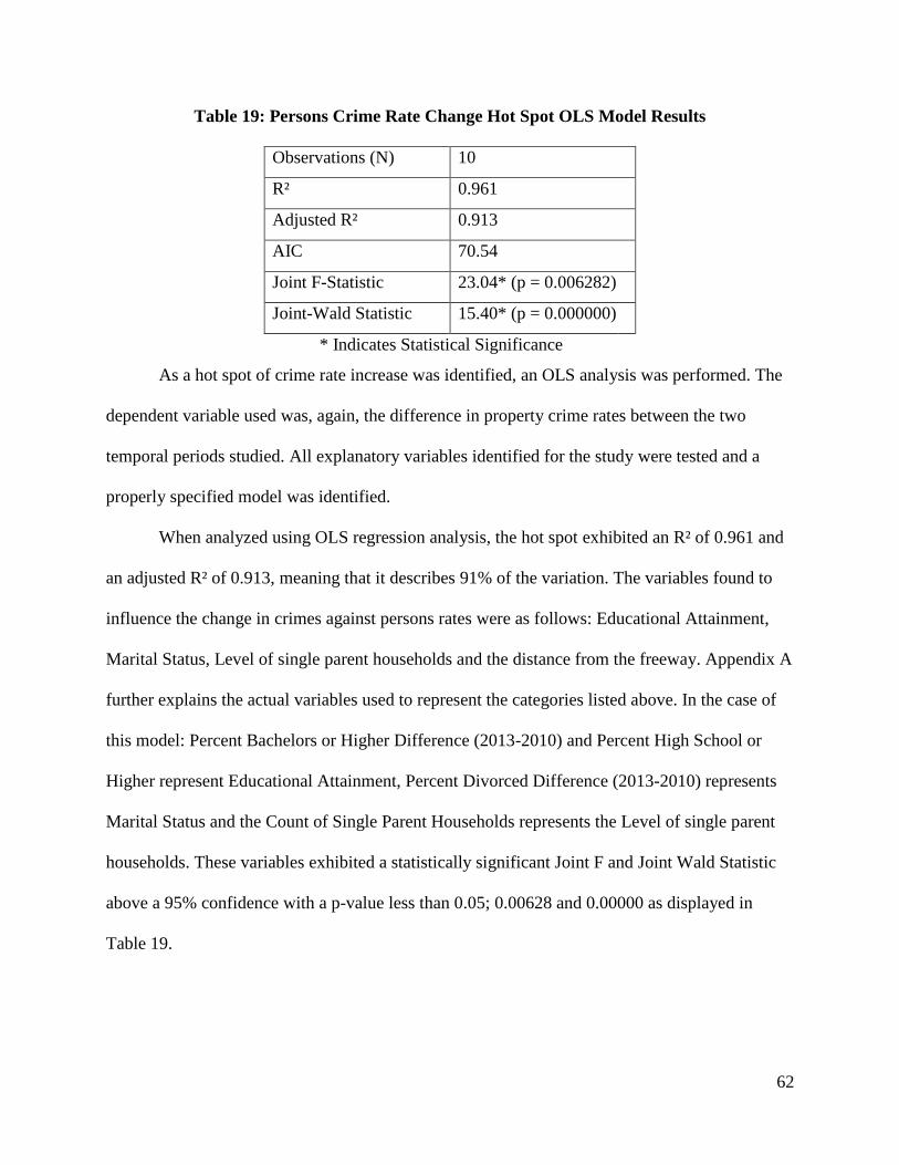
62
Table 19: Persons Crime Rate Change Hot Spot OLS Model Results
Observations (N) 10
R² 0.961
Adjusted R² 0.913
AIC 70.54
Joint F-Statistic 23.04* (p = 0.006282)
Joint-Wald Statistic 15.40* (p = 0.000000)
* Indicates Statistical Significance
As a hot spot of crime rate increase was identified, an OLS analysis was performed. The
dependent variable used was, again, the difference in property crime rates between the two
temporal periods studied. All explanatory variables identified for the study were tested and a
properly specified model was identified.
When analyzed using OLS regression analysis, the hot spot exhibited an R² of 0.961 and
an adjusted R² of 0.913, meaning that it describes 91% of the variation. The variables found to
influence the change in crimes against persons rates were as follows: Educational Attainment,
Marital Status, Level of single parent households and the distance from the freeway. Appendix A
further explains the actual variables used to represent the categories listed above. In the case of
this model: Percent Bachelors or Higher Difference (2013-2010) and Percent High School or
Higher represent Educational Attainment, Percent Divorced Difference (2013-2010) represents
Marital Status and the Count of Single Parent Households represents the Level of single parent
households. These variables exhibited a statistically significant Joint F and Joint Wald Statistic
above a 95% confidence with a p-value less than 0.05; 0.00628 and 0.00000 as displayed in
Table 19.

63
Table 20: Moran’s I Result of Crimes Against Persons OLS Residuals
Moran's Index: -0.228088
Expected Index: -0.111111
Variance: 0.017442
z-score: -0.885728
p-value: 0.375764
Moran's Index: -0.228088
To ensure that the Ordinary Least Squares model was not autocorrelated, the ArcGIS
Spatial Autocorrelation (Moran’s I) tool was used to analyze the residuals. Moran’s I will
determine if there is clustering within the residuals and indicate if the model is misspecified. The
residuals of the model were identified as random with no clustering. The residuals of the crimes
against persons model are displayed in Figure 20 and the results from the Moran’s I tool used to
test the clustering of residuals are contained in Table 20.

64
Figure 20: Standard Residuals of the OLS Crimes Against Persons Model

65
Chapter 5 Discussion and Conclusions
With all of the statistics calculated and completed, it is important to discuss the reasons and
assumptions of the research and draw any conclusions from the results. The primary purpose of
this study was to determine the spatial effect of AB 109 on crime rates in San Diego County. A
literature review was completed studying the spatial characteristics of criminal offenders and
assumptions were made. It is a hope of this work that identifying spatial relationships behind
changes in crime rates will help determine the reasons why crime rates are changing and
hopefully make solutions more apparent.
The general purpose of this work, as stated above, is to determine the spatial effect of AB
109, if any, on crime rates in San Diego County. A primary assumption in this work is that
offenders will likely commit offenses near their place of residence. With this assumption, a
primary hypothesis and null hypothesis were formed. The hypothesis can be stated as “Do areas
where larger numbers of AB 109 offenders reside exhibit an increase in crime rates?” Therefore
the null hypothesis can be stated as “Areas in which larger numbers of AB 109 offenders reside
do not exhibit an increase in crime rates.”
To study this hypothesis, a traditional statistical analysis and a spatial OLS regression
analysis were completed on five categories of crimes. To reject the null hypothesis and indicate
that AB 109 is having an effect on crime rates in San Diego County, this study would expect to
see clustered areas exhibiting an increase in crime rates, correlated to populations of AB 109
offenders. Each category was studied individually using a multitude of variables identified as
historically having an influence on crime rates by the FBI as well as residence locations of AB
109 offenders to determine if locations of AB 109 offender or any other social/physical
characteristic had an influence on crime rates (Federal Bureau of Investigation, 2006).

66
5.1 Conclusions
The results of the traditional statistical analysis indicated that of the five crime categories
studied, four exhibited an overall median decrease in crime rates across the county and one,
property crime, exhibited a slight increase. This indicates that overall, crime rates have decreased
in San Diego County following the implementation of AB 109. Societal crime exhibited the
largest decrease in crime rates when aggregated at the census tract level, a median decrease of -
3.5 crimes per 1000 persons.
A closer look into the statistics reveals some interesting trends have occurred since the
implementation of AB 109. For example, while societal crime exhibited a large decrease in crime
rates and overall counts, property crime exhibited a slight increase. A closer investigation into
the property crime cohort indicates that burglary counts, a type of crime falling under the
property crime cohort, have increased following the implementation of AB 109, to their highest
levels over the temporal period studied. Thefts and larcenies also exhibited a similar increase, the
cohort exhibited the highest count during the period following the implementation of
Realignment.
The temporal statistics indicate that realignment may have had an effect of property
crime in San Diego County. The conclusion that property crime rates have increased as a result
of realignment has been drawn by other studies using temporal statistics (Beard et al, 2013;
Lofstrom and Raphael, 2013). This study investigated this claim with temporal statistics and
found that the data for San Diego County supported this conclusion.
This study further investigated this increase through the use of spatial statistics. An OLS
regression model was constructed to establish the variables behind the increase in a hot spot if
census tracts identified in the county. After multiple attempts were made to identify a model that
67
explained the variance behind the hot spot of crime rate increase, it was determined that all
models constructed were misspcified, and therefore could not be trusted. The results of the OLS
models suggested that some other combination of complex variables not listed or tested as part of
this study is responsible for the variance of the hot spot of property crime rate increase when
aggregated at the census tract level.
Therefore the null hypothesis, “Areas in which larger numbers of AB 109 offenders
reside do not exhibit an increase in crime rates” could not be rejected for the property crime
cohort. Therefore the results of this study suggest increased populations of AB 109 offenders do
not correlate with an increase of property crimes rates when data are aggregated at the census
tract level.
Apart from property crime, no other crime category cohorts exhibited any type of
significant relationship between their respective crime rate increase hot spots and AB 109
offenders. Therefore the null hypothesis, “Areas in which larger numbers of AB 109 offenders
reside do not exhibit an increase in crime rates” could not be rejected.
Additionally a secondary hypothesis of the study, “do other social and physical variables
explain the hot spot of increase in crime rates?” was tested by using other social and physical
variables as part of the OLS models. The secondary null hypothesis could not be rejected for all
cohorts except crimes against persons.
AB 109 and Non-AB 109 categorized offenses as well as crimes against society exhibited
no significant correlation or relationship to any variable tested and no variables contained a
strong p-value, when compared against the identified hot spots of crime rate increase. Therefore
the null hypothesis associated with the secondary hypothesis, “other social and physical variables
do not explain the hot spot of increase in crime rates” could not be rejected.
68
However one cohort’s hot spot, crimes against persons, displayed a very high R² value of
0.961 and adjusted R² value of 0.913, displayed in Table 19, explaining 91% of the variance for
the hot spot with the other social and physical variables. The variables found to explain this
cohort’s hot spot were: Educational Attainment, Marital Status, Level of single parent
households and the distance from the freeway. Therefore it can be stated that the implementation
of AB 109 or realignment did not have any ascertainable effect on crimes against persons rates.
Traditional statistics methods indicated that the median decrease of crime rates in census tracts
across the county was almost zero and the spatial statistics studying the hot spot of crime rate
increase clearly illustrate a different combination of variables apart from AB 109 offenders is
correlated with the hot spot of crime rate increase.
5.2 Sources of Error
After the analysis of the data was complete, possible sources of error were identified; a
brief discussion of the sources of error follow.
AB 109 and Non AB 109 categories were identified and analyzed as part of the study.
The list of statutes punishable under the AB 109 provision are not always straight forward; for
example, certain types of burglaries are now sentenced under AB 109 guidelines, while other
types of burglaries are not (Couzens, 2013; Harris and Donaldson, 2013). DUIs represent another
crime type where certain types of DUIs fall under AB 109 sentencing guidelines and some others
do not (Byers, 2011). To account for this the data was evaluated and crimes were divided into
each category based on estimation, as the only data to determine whether or not a crime could be
sentenced under the AB 109 provision was a brief description field in the data. For the purposes
of this analysis, burglaries fell under the AB 109 category and DUIs fell under the Non AB 109
category however it was noted that some misclassification could have occurred.
69
In conjunction with the complication of querying the data for complex categories of
crimes, it also noted that the queries used to separate the AB 109 and Non AB 109 categories
were also complex. The queries were constructed as to separate certain types of crime and to
select other types in order to make the best effort to properly select the crimes for each category.
Due to the complexity of the queries and the crime category divisions, it is noted that a small
number of reported crimes were selected for both categories. Additionally it is noted that some
reported crimes may not been selected due to the complexity of the query. It is estimated that this
error source affected 415 (0.076%) out of 548,306 records.
Additionally when aggregating incident counts at the census tract level, a spatial join
technique was used, creating double counts in some cases. When a spatial join is used, the tool
counts the number of features that intersect the feature being joined. A point may be counted
twice, once in each polygon, if the point or other feature falls on the boundary of two intersecting
polygons. There is no good way to determine where this might occur and no easy workaround,
therefore it is included as a source of error in the analysis.
5.3 Future Work
This work has indicated that many crime categories have exhibited a decrease in crime
rates following the implementation of AB 109, however property crime has increased slightly.
Other works, studying the state as a whole and using temporal statistics, have also concluded that
realignment is correlated with the increase in property crime rates across the state (Beard et al,
2013; Lofstrom and Raphael, 2013). This work would suggest that as a slight increase was
exhibited in San Diego County, other counties should also be studied to determine similarities or
differences between the results.

70
Additionally, this work analyzed crime rates and trends coinciding with the
implementation of AB 109 through 2013. Future work could study the property crime trend for
future years.
Lastly, this work studied a statue that represents a major restructuring in the way that
offenders are sentenced. This work investigated the effect of the statute on crime rates in San
Diego County. In the time that this work was completed, another statue, California Proposition
47, was passed, which would change how offenders of similar crime types are sentenced. Future
work should be done to assess the impact of proposition 47 as it also represents a major shift in
the way offenders are processed.

71
REFERENCES
"San Diego: Geography and Climate." 2006. In Cities of the United States. 5th ed. ed. Vol. 2,
193. Detroit: Gale.
Beard, Jeffrey A., Diana Toche, Bryan Beyer, Wayne Babby, Denise Allen, Kevin Grassel, and
Dionne Maxwell. 2013. Realignment Report: An Examination of Offenders Released from
State Prison in the First Year of Public Safety Realignment. Sacramento: California
Department of Corrections And Rehabilitation.
http://www.cdcr.ca.gov/Adult_Research_Branch/Research_Documents/Realignment_1_Yea
r_Report_12-23-13.pdf.
Brandmüller, Teodóra and Åsa Önnerfors, eds. 2011. Eurostat Regional Yearbook 2011. 1st ed.
Luxembourg: Publications Office of the European Union.
Brantingham, Paul J. and Patricia L. Brantingham. 1981. "Introduction: The Dimensions of
Crime." In Environmental Criminology, edited by Paul J. Brantingham and Patricia L.
Brantingham. 1st ed., 7. Beverly Hills: Sage.
Byers, Garrick. 2011. Realignment. 1st ed. Continuing Education of the Bar: California.
ceb.com/lawalerts/realignment.doc.
Cain, Sandi. 2005. "San Diego Coast, Downtown are Visitor Magnets: Diverse Geography and
Activities Keep Tourists Coming Back." San Diego Business Journal 26 (27): A-19.
http://bi.galegroup.com.libproxy2.usc.edu/essentials/article/GALE;A135021433?u=usocal_
main;.
Californians for Safety and Justice. "About Public Safety Realignment." Californians for Safety
and Justice, last modified 2013, accessed 02/07, 2015,
http://www.safeandjust.org/CalRealignment/About-Realignment.
Charlton, Martin. 2008. "Modifiable Areal Unit Problem (MAUP)." In Encyclopedia of
Geographic Information Science, edited by Karen K. Kemp. 0th ed., 289-291: SAGE
Publications, Inc. doi:http://dx.doi.org/10.4135/9781412953962".
County of Los Angeles Probation Department. "Ab 109." County of Los Angeles, accessed
September/28, 2015,
http://probation.lacounty.gov/wps/portal/probation/!ut/p/b0/04_Sj9CPykssy0xPLMnMz0vM
AfGjzOLdDAwM3P2dgo3cvX2NDBwNHD0d_T3DDE3cTfULsh0VAXzjOO8!/.
Couzens, J. Richard. 2013. "Realignment and Evidence-Based Practice: A New Era in
Sentencing California Felonies." Federal Sentencing Reporter 25 (4, Realigning California

72
Corrections): 217-219.
http://www.jstor.org.libproxy.usc.edu/stable/10.1525/fsr.2013.25.4.217.
ESRI. "Interpreting OLS Results." ESRI, last modified 4/18/2013, accessed 12/7, 2015,
http://resources.arcgis.com/en/help/main/10.1%20/index.html#/Interpreting_OLS_results/00
5p00000030000000/.
Federal Bureau of Investigation. "Variables Affecting Crime." U.S. Department of Justice, last
modified September 2006, accessed 10/25, 2015,
https://www2.fbi.gov/ucr/05cius/about/variables_affecting_crime.html.
Godwin, Maurice and David Canter. 1997. "Encounter and Death the Spatial Behavior of US
Serial Killers." Policing 20 (1): 24.
http://search.proquest.com.libproxy.usc.edu/docview/211290067?accountid=14749.
Harries, Keith. 2006. "Property Crimes and Violence in the United States: Analysis of the
Influence of Population Density." International Journal of Criminal Justice Sciences 1 (2).
http://www.sascv.org/ijcjs/harries.html.
Harris, Heather and Donaldson, Michael. "AB 109: Eligible 1170(h) Felonies List." County
Santa Clara Public Defender Office, last modified 3/13/2013, accessed September/28, 2015,
https://www.sccgov.org/sites/pdo/Pages/AB-109--Eligible-1170(h)-Felonies-List.aspx.
Heyman, Steven J. 1991. "The First Duty of Government: Protection, Liberty and the Fourteenth
Amendment." Duke Law Journal 41 (3): 507-571.
International Association of Crime Analysts. 2013. Identifying High Crime Areas (White Paper
2013-02). Overland Park, KS: International Association of Crime Analysts.
Laerd Statistics. "Paired-Samples T-Test in SPSS Statistics." Laerd Statistics. Lund Research
Ltd, accessed 11/23, 2015, https://statistics.laerd.com/premium/pstt/paired-samples-t-test-in-
spss-8.php.
Langan, Patrick and David Levin. 2002. Recidivism of Prisoners Released in 1994: United
States. Washington, DC: U.S. Department of Justice: Bureau of Justice Statistics.
http://www.bjs.gov/content/pub/pdf/rpr94.pdf.
Law Enforcement Support Section (LESS) and Crime Statistics Management Unit (CSMU).
2013. Criminal Justice Information Services (CJIS) Division Uniform Crime Reporting
(UCR) Program National Incident-Based Reporting System (NIBRS) User Manual: U. S.
Department of Justice.
Lawton, Brian A., Ralph B. Taylor, and Anthony J. Luongo. 2005. "Police Officers on Drug
Corners in Philadelphia, Drug Crime, and Violent Crime: Intended, Diffusion, and
Displacement Impacts." Justice Quarterly : JQ 22 (4): 427-451.
http://search.proquest.com.libproxy.usc.edu/docview/228177699?accountid=14749.

73
Lofstrom, Magnus and Steven Raphael. 2013. Public Safety Realignment and Crime Rates in
California. San Francisco: Public Policy Institute of California.
www.ppic.org/main/publication.asp?i=1075.
Munyo, Ignacio and Martin A. Rossi. 2015. "First-Day Criminal Recidivism." Journal of Public
Economics 124: 81-90. doi:10.1016/j.jpubeco.2014.12.002.
Murack, Jennie. "Regression Analysis using ArcMap” MIT Libraries, accessed 9/20, 2015,
https://libraries.mit.edu/files/gis/regression.pdf.
New Jersey State Police."Calculations of Rates and Trends." New Jersey State Police, accessed
11/23, 2015, http://www.njsp.org/info/ucr2000/pdf/calc_ucr2000.pdf.
Openshaw, Stan. 1983. The Modifiable Areal Unit Problem. Concepts and Techniques in
Modern Geography 38. Norwich, England: Geo Books.
O'Sullivan, David, 1966 and D. (David John) Unwin. 2010. Geographic Information Analysis.
2nd ed. Hoboken, N.J: John Wiley & Sons.
Rhodes, William M. and Catherine Conly. 1981. "Crime and Mobility: An Empirical Study." In
Environmental Criminology, edited by Paul J. Brantingham and Patricia L. Brantingham. 1st
ed., 167. Beverly Hills: Sage.
Rossmo, D. Kim. 1997. "Geographic Profiling." In Offender Profiling: Theory, Research and
Practice, edited by Janet L. Jackson and Debra A. Bekerian, 159.
U.S. Census Bureau. 2002. California: 2000: Census 2000 Profile: U.S. Department of
Commerce. http://www.census.gov.libproxy2.usc.edu/prod/2002pubs/c2kprof00-ca.pdf.
———. "State & County QuickFacts: San Diego County, California." U.S. Department of
Commerce, last modified 04 Dec 2014, accessed 02/07, 2015,
http://quickfacts.census.gov/qfd/states/06/06073.html.
———. "State & County QuickFacts: California." U.S. Department of Commerce, last modified
05 Feb 2015, accessed 02/07, 2015, http://quickfacts.census.gov/qfd/states/06000.html.
Weisberg, Robert and Lisa T. Quan. 2014. Assessing Judicial Sentencing Preferences After
Public Safety Realignment: A Survey of California Judges. Stanford: Stanford Criminal
Justice Center. https://www.law.stanford.edu/publications/assessing-judicial-sentencing-
preferences-after-public-safety-realignment-a-survey-of-california-judges.
Wilkinson, William Richard, John C. 1929- (John Chynoweth) Burnham, and Joseph F. Spillane.
2005. Prison Work: A Tale of Thirty Years in the California Department of Corrections.
Columbus: Ohio State University.

74
Zimring, Franklin E. and Gordon Hawkins. 1994. "The Growth of Imprisonment in California."
The British Journal of Criminology 34 (SPEISS): 83-96.
http://www.jstor.org.libproxy2.usc.edu/stable/23638189.
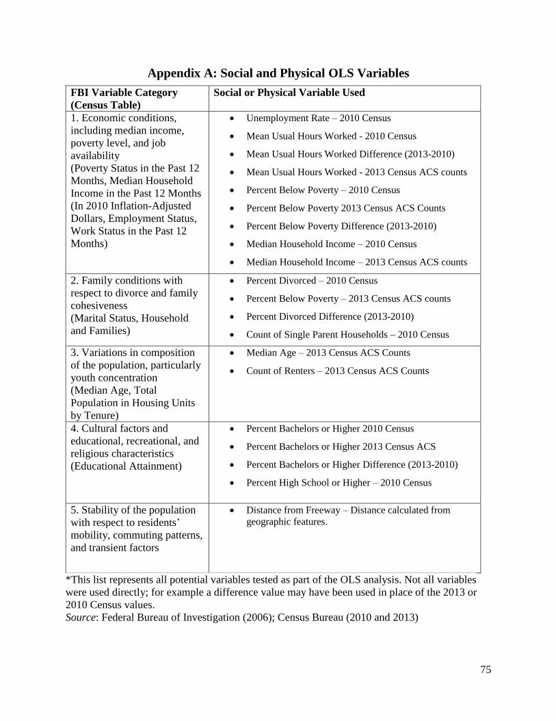
75
Appendix A: Social and Physical OLS Variables
FBI Variable Category
(Census Table)
Social or Physical Variable Used
1. Economic conditions,
including median income,
poverty level, and job
availability
(Poverty Status in the Past 12
Months, Median Household
Income in the Past 12 Months
(In 2010 Inflation-Adjusted
Dollars, Employment Status,
Work Status in the Past 12
Months)
Unemployment Rate – 2010 Census
Mean Usual Hours Worked - 2010 Census
Mean Usual Hours Worked Difference (2013-2010)
Mean Usual Hours Worked - 2013 Census ACS counts
Percent Below Poverty – 2010 Census
Percent Below Poverty 2013 Census ACS Counts
Percent Below Poverty Difference (2013-2010)
Median Household Income – 2010 Census
Median Household Income – 2013 Census ACS counts
2. Family conditions with
respect to divorce and family
cohesiveness
(Marital Status, Household
and Families)
Percent Divorced – 2010 Census
Percent Below Poverty – 2013 Census ACS counts
Percent Divorced Difference (2013-2010)
Count of Single Parent Households – 2010 Census
3. Variations in composition
of the population, particularly
youth concentration
(Median Age, Total
Population in Housing Units
by Tenure)
Median Age – 2013 Census ACS Counts
Count of Renters – 2013 Census ACS Counts
4. Cultural factors and
educational, recreational, and
religious characteristics
(Educational Attainment)
Percent Bachelors or Higher 2010 Census
Percent Bachelors or Higher 2013 Census ACS
Percent Bachelors or Higher Difference (2013-2010)
Percent High School or Higher – 2010 Census
5. Stability of the population
with respect to residents’
mobility, commuting patterns,
and transient factors
Distance from Freeway – Distance calculated from
geographic features.
*This list represents all potential variables tested as part of the OLS analysis. Not all variables
were used directly; for example a difference value may have been used in place of the 2013 or
2010 Census values.
Source: Federal Bureau of Investigation (2006); Census Bureau (2010 and 2013)