the super decisions software thomas l. saaty - cash flow

1

The Essentials of the Analytic Network Process with Seven Examples (2)

Decision Making with Dependence and Feedback

The Super Decisions Software

Thomas L. Saaty

1) At Low Level, which attribute is satisfied best?

2) At Intermediate Level, which attribute is satisfied best?

3) At High Level, which attribute is satisfied best?

Low Level DamF R E Eigenvector

Flood Control 1 3 5 .637Recreation 1/3 1 3 .258Hydro-Electric 1/5 1/3 1 .105

PowerConsistency Ratio = .033

Intermediate Level DamF R E Eigenvector

Flood Control 1 1/3 1 .200Recreation 3 1 3 .600Hydro-Electric 1 1/3 1 .200


High Level DamF R E Eigenvector

Flood Control 1 1/5 1/9 .060Recreation 5 1 1/4 .231Hydro-Electric 9 4 1 .709


2

The six eigenvectors were then introduced as columns of the following stochastic supermatrix.

F R E L M H

0 0 0 .637 .200 .0600 0 0 .258 .600 .2310 0 0 .105 .200 .709

.722 .072 .058 0 0 0

.205 .649 .207 0 0 0

.073 .279 .735 0 0 0

One must ensure that all columns sum to unity exactly.

FRELMH

The final priorities for both, the height of the dam and for thecriteria were obtained from the limiting power of the supermatrix. The components were not weighted here because the matrix is already column stochastic and would give the same limiting result for the ratios even if multiplied by the weighting constants.

Its powers stabilize after a few iterations. We have

F R E L M H

0 0 0 .241 .241 .2410 0 0 .374 .374 .3740 0 0 .385 .385 .385

.223 .223 .223 0 0 0

.372 .372 .372 0 0 0

.405 .405 .405 0 0 0

FRELMH

3

Adjustment PeriodRequired forTurnaround

Primary Factors

Subfactors

Date and Strength of Recovery of U.S. Economy

The U.S. Holarchy of Factors for Forecasting Turnaround in Economic Stagnation

Conventional Economicadjustment Restructuring

Consumption (C) Financial Sector (FS)Exports (X) Defense Posture (DP)Investment (I) Global Competition (GC)Fiscal Policy (F)Monetary Policy (M)Confidence (K)

3 months 6 months 12 months 24 months

Consumption (C)Exports (E)Investment (I)Confidence (K)Fiscal Policy (F)Monetary Policy (M)

1 7 5 1/5 1/2 1/5 0.1181/7 1 1/5 1/5 1/5 1/7 0.0291/5 5 1 1/5 1/3 1/5 0.0585 5 5 1 5 1 0.3342 5 3 1/5 1 1/5 0.1185 7 5 1 5 1 0.343

C E I K F M WeightsVector

FS DP GC WeightsVector

Financial Sector (FS)Defense Posture (DS)Global Competition (GC)

1 3 3 0.584

1/3 1 3 0.281

1/3 1/3 1 0.135

Panel B: Which subfactor has the greater potential to influence Economic Restructuring and how strongly?

Panel A: Which subfactor has the greater potential to influence Conventional Adjustment and how strongly?

Table 1: Matrices for subfactor importance relative to primary factors influencing the Timing of Recovery

4

Table 2: Matrices for relative influence of subfactors on periods of adjustment (months) (Conventional Adjustment)

For each panel below, which time period is more likely to indicate a turnaround if the relevant factor is the sole driving force?

Panel D: Relative importance of targeted time periods for fiscal policy to drive a turnaround

Panel B: Relative importance of targeted time periods for exports to drive a turnaround

Panel C: Relative importance of targeted time periods for investment to drive a turnaround

Panel A: Relative importance of targeted time periods for consumption to drive a turnaround

Panel E: Relative importance of targeted time periods for monetary policy to drive a turnaround

Panel F: Expected time for a change of confidence indicators of consumer and investor activity to support a turnaround in the economy

3 6 12 24 Vec. Wts. 3 6 12 24 Vec. Wts.

3 6 12 24 Vec. Wts. 3 6 12 24 Vec. Wts.

3 6 12 24 Vec. Wts. 3 6 12 24 Vec. Wts.

3 months 1 1/5 1/7 1/7 .0436 months 5 1 1/5 1/5 .113

12 months 7 5 1 1/3 .31024 months 7 5 3 1 .534

3 months 1 1 1/5 1/5 .0836 months 1 1 1/5 1/5 .083

12 months 5 5 1 1 .41724 months 5 5 1 1 .417

3 months 1 1 1/5 1/5 .0786 months 1 1 1/5 1/5 .078

12 months 5 5 1 1/3 .30524 months 5 5 3 1 .538

3 months 1 1 1/3 1/5 .0996 months 1 1 1/5 1/5 .087

12 months 3 5 1 1 .38224 months 5 5 1 1 .432

3 months 1 5 7 7 .6056 months 1/5 1 5 7 .262

12 months 1/7 1/5 1 1/5 .04224 months 1/7 1/7 5 1 .091

3 months 1 3 5 5 .5176 months 1/3 1 5 5 .305

12 months 1/5 1/5 1 5 .12424 months 1/5 1/5 1/5 1 .054

Table 3: Matrices for relative influence of subfactors on periods of adjustment (months) (Economic Restructuring)

For each panel below, which time period is more likely to indicate a turnaround if the relevant factor is the sole driving force?

Panel B: Defense readjustment time

Panel C: Global competition adjustment time

Panel A: Financial system restructuring time3 6 12 24 Vec. Wts. 3 6 12 24 Vec. Wts.

3 6 12 24 Vec. Wts.

3 months 1 1/3 1/5 1/7 .0496 months 3 1 1/5 1/7 .085

12 months 5 5 1 1/5 .23624 months 7 7 5 1 .630

3 months 1 1/3 1/5 1/7 .0496 months 3 1 1/5 1/7 .085

12 months 5 5 1 1/5 .23624 months 7 7 5 1 .630

3 months 1 1 1/5 1/5 .0786 months 1 1 1/5 1/5 .078

12 months 5 5 1 1/3 .30524 months 5 5 3 1 .538

Table 4: Most likely factor to dominate during a specified time period

Which factor is more likely to produce a turnaround during the specified time period? Conventional Adjustment CARestructuring R

Panel A: 3 Months Panel B: 6 Months Panel C: 1 Year Panel D: 2 Years

CA R Vec. Wts. CA R Vec. Wts. CA R Vec. Wts. CA R Vec. Wts.CA 1 5 .833 CA 1 5 .833 CA 1 1 CA 1 1/5 .167R 1/5 1 .167 R 1/5 1 .167 R 1 1 R 5 1 .833.500

.500

5

Table 5: The Completed Supermatrix Conven. Economic. Consum. Exports Invest. Confid. Fiscal Monet. Financ. Defense Global 3 mo. 6 mo. 1 yr. ≥ 2 years Adjust Restruc. Policy Policy Sector Posture Compet.

Conven. 0.0 0.0 0.0 0.0 0.0 0.0 0.0 0.0 0.0 0.0 0.0 ¦ 0.833 0.833 0.500 0.167 Adjust ¦Economic. 0.0 0.0 0.0 0.0 0.0 0.0 0.0 0.0 0.0 0.0 0.0 ¦ 0.167 0.167 0.500 0.833 Restru. +--------------------------

------+Consum. 0.118 ¦ 0.0 0.0 0.0 0.0 0.0 0.0 0.0 0.0 0.0 0.0 0.0 0.0 0.0 0.0

¦Exports 0.029 ¦ 0.0 0.0 0.0 0.0 0.0 0.0 0.0 0.0 0.0 0.0 0.0 0.0 0.0 0.0

¦Invest. 0.058 ¦0.0 0.0 0.0 0.0 0.0 0.0 0.0 0.0 0.0 0.0 0.0 0.0 0.0 0.0 ¦Confid. 0.334 ¦0.0 0.0 0.0 0.0 0.0 0.0 0.0 0.0 0.0 0.0 0.0 0.0 0.0 0.0 ¦Fiscal 0.118 ¦0.0 0.0 0.0 0.0 0.0 0.0 0.0 0.0 0.0 0.0 0.0 0.0 0.0 0.0 Policy ¦Monetary 0.343 ¦0.0 0.0 0.0 0.0 0.0 0.0 0.0 0.0 0.0 0.0 0.0 0.0 0.0 0.0 Policy ------+

+----+Financ. 0.0 ¦0.584¦ 0.0 0.0 0.0 0.0 0.0 0.0 0.0 0.0 0.0 0.0 0.0 0.0 0.0 Sector ¦ ¦

¦ ¦Defense 0.0 ¦0.281¦ 0.0 0.0 0.0 0.0 0.0 0.0 0.0 0.0 0.0 0.0 0.0 0.0 0.0 Posture ¦ ¦

¦ ¦Global 0.0 ¦0.135¦ 0.0 0.0 0.0 0.0 0.0 0.0 0.0 0.0 0.0 0.0 0.0 0.0 0.0 Compet. +----+

+------------------------------------------------------------------+3 months 0.0 0.0 ¦ 0.043 0.083 0.078 0.517 0.099 0.605 0.049 0.049 0.089 ¦ 0.0 0.0 0.0 0.0

¦ ¦6 months 0.0 0.0 ¦ 0.113 0.083 0.078 0.305 0.086 0.262 0.085 0.085 0.089 ¦ 0.0 0.0 0.0 0.0

¦ ¦1 year 0.0 0.0 ¦ 0.310 0.417 0.305 0.124 0.383 0.042 0.236 0.236 0.209 ¦ 0.0 0.0 0.0 0.0

¦ ¦≥ 2 years 0.0 0.0 ¦ 0.534 0.417 0.539 0.054 0.432 0.091 0.630 0.630 0.613 ¦ 0.0 0.0 0.0 0.0

Conven. Economic. Consum. Exports Invest. Confid. Fiscal Monet. Financ. Defense Global 3 mo. 6 mo. 1 yr. ≥ 2 years Adjust Restruc. Policy Policy Sector Posture Compet.

Conven. 0.0 0.0 0.484 0.484 0.484 0.484 0.484 0.484 0.484 0.484 0.484 0.0 0.0 0.0 0.0 Adjust Economic 0.0 0.0 0.516 0.516 0.516 0.516 0.516 0.516 0.516 0.516 0.516 0.0 0.0 0.0 0.0 Restru.

Consum. 0.0 0.0 0.0 0.0 0.0 0.0 0.0 0.0 0.0 0.0 0.0 0.057 0.057 0.057 0.057 Exports 0.0 0.0 0.0 0.0 0.0 0.0 0.0 0.0 0.0 0.0 0.0 0.014 0.014 0.014 0.014 Invest. 0.0 0.0 0.0 0.0 0.0 0.0 0.0 0.0 0.0 0.0 0.0 0.028 0.028 0.028 0.028 Confid. 0.0 0.0 0.0 0.0 0.0 0.0 0.0 0.0 0.0 0.0 0.0 0.162 0.162 0.162 0.162 Fiscal 0.0 0.0 0.0 0.0 0.0 0.0 0.0 0.0 0.0 0.0 0.0 0.057 0.057 0.057 0.057 Policy Monetary 0.0 0.0 0.0 0.0 0.0 0.0 0.0 0.0 0.0 0.0 0.0 0.166 0.166 0.166 0.166 Policy Financ. 0.0 0.0 0.0 0.0 0.0 0.0 0.0 0.0 0.0 0.0 0.0 0.301 0.301 0.301 0.301 Sector Defense 0.0 0.0 0.0 0.0 0.0 0.0 0.0 0.0 0.0 0.0 0.0 0.145 0.145 0.145 0.145 Posture Global 0.0 0.0 0.0 0.0 0.0 0.0 0.0 0.0 0.0 0.0 0.0 0.070 0.070 0.070 0.070 Compet. 3 months 0.224 0.224 0.0 0.0 0.0 0.0 0.0 0.0 0.0 0.0 0.0 0.0 0.0 0.0 0.0 6 months 0.151 0.151 0.0 0.0 0.0 0.0 0.0 0.0 0.0 0.0 0.0 0.0 0.0 0.0 0.0 1 year 0.201 0.201 0.0 0.0 0.0 0.0 0.0 0.0 0.0 0.0 0.0 0.0 0.0 0.0 0.0 ≥ 2 years 0.424 0.424 0.0 0.0 0.0 0.0 0.0 0.0 0.0 0.0 0.0 0.0 0.0 0.0 0.0

Table 6: The Limiting Supermatrix

6

Synthesis/Results

When the judgments were made, the AHP framework was used to perform a synthesis that produced the following results. First a meaningful turnaround in the economy would likely require an additional ten to eleven months, occurring during the fourth quarter of 1992. This forecast is derived from weights generated in the first column of the limiting matrix in Table 6, coupled with the mid-points of the alternate time periods (so as to provide unbiased estimates:

.224 x 1.5 + .151 x 4.5 + .201 x 9 + .424 x 18 =10.45 months from late December 1991/early January 1992

US Economy Turnaround 2001-2002

7

1Cons~

2Expo~

3Inves~

4Conf~

5Fisca~

6Monet~

7Expect~

Wts.

1Consumption

1 7 5 1/5 1/2 1/5 1 .0979

2Exports 1 1/5 1/5 1/5 1/7 1/7 .0209

3Investment 1 1/5 1/3 1/5 1 .0564

4Confidence 1 5 1 1/3 .2220

5Fiscal Policy 1 1/5 1/3 .0835

6Monetary P. 1 1/5 .3540

7Expectations 1 .1653

The Judgments for Aggregate Demand Factors with respect to the Aggregate Demand Node

Labor Costs Natural Resources

Expectations

Wts.

Labor Costs 1 1/7 1 .11940

Natural Resources 1 5 .74705

Expectations 1 .13356

The Judgments for the Aggregate Supply Factors with respect to the Aggregate Supply Node

The Judgments for the Geopolitical Context Factors with respect to the Geopolitical Context Node

Int’l Political Rel. Int’l Economic Rel. Wts.

Int’l Political Rel. 1 1/2 .66667

Int’l Economic Rel. 1 .33333

The Judgments for the Alternatives with respect to Consumption3 Months 6 Months 12 Months 24 Months Wts.

3 Months 1 1/5 1/7 1/7 .04259

6 Months 1 1/5 1/5 .11347

12 Months 1 1/3 .31014

24 Months 1 .53380

8

The Judgments for the Alternatives with respect to Exports

3 Months 6 Months 12 Months 24 Months Wts.

3 Months 1 1 1/5 1/5 .08333

6 Months 1 1/5 1/5 .08333

12 Months 1 1 .41667

24 Months 1 .41667

The Judgments for the Alternatives with respect to Investment


3 Months 1 1 1/5 1/5 .07829

6 Months 1 1/5 1/5 .07829

12 Months 1 1/3 .30508

24 Months 1 .53834

The Judgments for the Alternatives with respect to Confidence3 Months 6 Months 12 Months 24 Months Wts.

3 Months 1 3 5 5 .51682

6 Months 1 5 5 .30465

12 Months 1 5 .12441

24 Months 1 .05412

The Judgments for the Alternatives with respect to Fiscal Policy


3 Months 1 1 1/3 1/5 .09902

6 Months 1 1/5 1/5 .08637

12 Months 1 1 .38275

24 Months 1 .43186

The Judgments for the Alternatives with respect to Monetary Policy


3 Months 1 5 7 7 .60523

6 Months 1 5 7 .26161

12 Months 1 1/5 .04241

24 Months 1 .09075

The Judgments for the Alternatives with respect to Expectations


3 Months 1 1 5 7 .45624

6 Months 1 3 5 .37074

12 Months 1 1 .09583

24 Months 1 .07718

9

The Judgments for the Alternatives with respect to Labor Costs


3 Months 1 1 1/5 1/7 .08420

6 Months 1 1 1/3 .1514812 Months 1 1/3 .2306724 Months 1 .53365

The Judgments for the Alternatives with respect to Natural Resources


3 Months 1 1/3 1/5 1/7 .05529

6 Months 1 1/3 1/5 .11750

12 Months 1 1/3 .26220

24 Months 1 .56501

The Judgments for the Alternatives with respect to Expectations


3 Months 1 3 5 7 .56015

6 Months 1 4 6 .29205

12 Months 1 1 .08073

24 Months 1 .06707

The Judgments for the Alternatives with respect to Major International Political Relations


3 Months 1 1/3 1/5 1/7 .05529

6 Months 1 1/3 1/5 .11750

12 Months 1 1/3 .26220

24 Months 1 .56501

The Judgments for the Alternatives with respect to Major International Economic Relations


3 Months 1 1/3 1/5 1/7 .05529

6 Months 1 1/3 1/5 .11750

12 Months 1 1/3 .26220

24 Months 1 .56501

The Judgments for the Primary Factors with respect to the 3 Month Time Period

Aggr. Demand

Aggr. Supply Geopolitical Wts.

Aggr. Demand

1 7 9 .78539

Aggr. Supply 1 3 .14882

Geopolitical 1 .06579

10


Aggr. Demand Aggr. Supply Geopolitical Wts.

Aggr. Demand 1 7 9 .78539













The Unweighted Matrix

1 Aggregate 2 Aggregate 3 Geopolitical 1 Consumption 2 Exports 3 Investment 4 Confidence 5 Fiscal 6 Monetary 7 ExpectationsDemand Supply Context Policy Policy

1 Primary 1 Aggregate Demand 0.0000 0.0000 0.0000 0.0000 0.0000 0.0000 0.0000 0.0000 0.0000 0.0000Factors 2 Aggregate Supply 0.0000 0.0000 0.0000 0.0000 0.0000 0.0000 0.0000 0.0000 0.0000 0.0000

3 Geopolitical Context 0.0000 0.0000 0.0000 0.0000 0.0000 0.0000 0.0000 0.0000 0.0000 0.00002 Aggregate 1 Consumption 0.0979 0.0000 0.0000 0.0000 0.0000 0.0000 0.0000 0.0000 0.0000 0.0000Demand Factors 2 Exports 0.0209 0.0000 0.0000 0.0000 0.0000 0.0000 0.0000 0.0000 0.0000 0.0000

3 Investment 0.0564 0.0000 0.0000 0.0000 0.0000 0.0000 0.0000 0.0000 0.0000 0.00004 Confidence 0.2220 0.0000 0.0000 0.0000 0.0000 0.0000 0.0000 0.0000 0.0000 0.00005 Fiscal Policy 0.0835 0.0000 0.0000 0.0000 0.0000 0.0000 0.0000 0.0000 0.0000 0.00006 Monetary Policy 0.3540 0.0000 0.0000 0.0000 0.0000 0.0000 0.0000 0.0000 0.0000 0.00007 Expectations 0.1653 0.0000 0.0000 0.0000 0.0000 0.0000 0.0000 0.0000 0.0000 0.0000

3 Aggregate 1 Labor Costs 0.0000 0.1194 0.0000 0.0000 0.0000 0.0000 0.0000 0.0000 0.0000 0.0000Supply Factors 2 Natural 0.0000 0.7470 0.0000 0.0000 0.0000 0.0000 0.0000 0.0000 0.0000 0.0000

Resource Costs3 Expectations 0.0000 0.1336 0.0000 0.0000 0.0000 0.0000 0.0000 0.0000 0.0000 0.0000

4 Geopolitical 1 Major Int'l Pol. Rel 0.0000 0.0000 0.6667 0.0000 0.0000 0.0000 0.0000 0.0000 0.0000 0.0000Contexts 2 Major Int'l Eco. Rel 0.0000 0.0000 0.3333 0.0000 0.0000 0.0000 0.0000 0.0000 0.0000 0.00004Alternatives 1 Three months 0.0000 0.0000 0.0000 0.0426 0.0833 0.0783 0.5168 0.0990 0.6052 0.4562

2 Six months 0.0000 0.0000 0.0000 0.1135 0.0833 0.0783 0.3046 0.0864 0.2616 0.37073 Tw elve months 0.0000 0.0000 0.0000 0.3101 0.4167 0.3051 0.1244 0.3827 0.0424 0.09584 Tw enty four months 0.0000 0.0000 0.0000 0.5338 0.4167 0.5383 0.0541 0.4319 0.0907 0.0772

2 Aggregate Demand Factors1 Primary Factors

11

The Unweighted Matrix Cont’d

1 Labor 2 Natural 3 Expectations 1 Major Int'l 2 Major Int'l 1 Three months 2 Six months 3 Tw elve months 4 Tw enty four Costs Resource Costs Political Economic months

Relationships Relationships0.0000 0.0000 0.0000 0.0000 0.0000 0.7854 0.7854 0.4545 0.45450.0000 0.0000 0.0000 0.0000 0.0000 0.1488 0.1488 0.4545 0.45450.0000 0.0000 0.0000 0.0000 0.0000 0.0658 0.0658 0.0909 0.09090.0000 0.0000 0.0000 0.0000 0.0000 0.0000 0.0000 0.0000 0.00000.0000 0.0000 0.0000 0.0000 0.0000 0.0000 0.0000 0.0000 0.00000.0000 0.0000 0.0000 0.0000 0.0000 0.0000 0.0000 0.0000 0.00000.0000 0.0000 0.0000 0.0000 0.0000 0.0000 0.0000 0.0000 0.00000.0000 0.0000 0.0000 0.0000 0.0000 0.0000 0.0000 0.0000 0.00000.0000 0.0000 0.0000 0.0000 0.0000 0.0000 0.0000 0.0000 0.00000.0000 0.0000 0.0000 0.0000 0.0000 0.0000 0.0000 0.0000 0.00000.0000 0.0000 0.0000 0.0000 0.0000 0.0000 0.0000 0.0000 0.00000.0000 0.0000 0.0000 0.0000 0.0000 0.0000 0.0000 0.0000 0.00000.0000 0.0000 0.0000 0.0000 0.0000 0.0000 0.0000 0.0000 0.00000.0000 0.0000 0.0000 0.0000 0.0000 0.0000 0.0000 0.0000 0.00000.0000 0.0000 0.0000 0.0000 0.0000 0.0000 0.0000 0.0000 0.00000.0842 0.0553 0.5602 0.0553 0.0553 0.0000 0.0000 0.0000 0.00000.1515 0.1175 0.2921 0.1175 0.1175 0.0000 0.0000 0.0000 0.00000.2307 0.2622 0.0807 0.2622 0.2622 0.0000 0.0000 0.0000 0.00000.5336 0.5650 0.0671 0.5650 0.5650 0.0000 0.0000 0.0000 0.0000

4Alternatives3 Aggregate Supply Factors 4 Geopolitical Contexts

The Limit Matrix – note that each column is the same

1 Aggregate 2 Aggregate 3 Geopolitical 1 Consumption 2 Exports 3 Investment 4 Conf idence 5 Fiscal 6 Monetary 7 ExpectationsDemand Supply Context Policy Policy

1 Primary 1 Aggregate Demand 0.207939 0.207939 0.207939 0.207939 0.207939 0.207939 0.207939 0.207939 0.207939 0.207939Factors 2 Aggregate Supply 0.099374 0.099374 0.099374 0.099374 0.099374 0.099374 0.099374 0.099374 0.099374 0.099374

3 Geopolitical Context 0.026020 0.026020 0.026020 0.026020 0.026020 0.026020 0.026020 0.026020 0.026020 0.0260202 Aggregate 1 Consumption 0.020358 0.020358 0.020358 0.020358 0.020358 0.020358 0.020358 0.020358 0.020358 0.020358Demand Factors 2 Exports 0.004353 0.004353 0.004353 0.004353 0.004353 0.004353 0.004353 0.004353 0.004353 0.004353

3 Investment 0.011729 0.011729 0.011729 0.011729 0.011729 0.011729 0.011729 0.011729 0.011729 0.0117294 Conf idence 0.046165 0.046165 0.046165 0.046165 0.046165 0.046165 0.046165 0.046165 0.046165 0.0461655 Fiscal Policy 0.017353 0.017353 0.017353 0.017353 0.017353 0.017353 0.017353 0.017353 0.017353 0.0173536 Monetary Policy 0.073605 0.073605 0.073605 0.073605 0.073605 0.073605 0.073605 0.073605 0.073605 0.0736057 Expectations 0.034377 0.034377 0.034377 0.034377 0.034377 0.034377 0.034377 0.034377 0.034377 0.034377

3 Aggregate 1 Labor Costs 0.011863 0.011863 0.011863 0.011863 0.011863 0.011863 0.011863 0.011863 0.011863 0.011863Supply Factors 2 Natural 0.074237 0.074237 0.074237 0.074237 0.074237 0.074237 0.074237 0.074237 0.074237 0.074237

Resource Costs3 Expectations 0.013275 0.013275 0.013275 0.013275 0.013275 0.013275 0.013275 0.013275 0.013275 0.013275

4 Geopolitical 1 Major Int'l Pol. Rel 0.017346 0.017346 0.017346 0.017346 0.017346 0.017346 0.017346 0.017346 0.017346 0.017346Contexts 2 Major Int'l Eco. Rel 0.008673 0.008673 0.008673 0.008673 0.008673 0.008673 0.008673 0.008673 0.008673 0.0086734Alternatives 1 Three months 0.101936 0.101936 0.101936 0.101936 0.101936 0.101936 0.101936 0.101936 0.101936 0.101936

2 Six months 0.068609 0.068609 0.068609 0.068609 0.068609 0.068609 0.068609 0.068609 0.068609 0.0686093 Tw elve months 0.060602 0.060602 0.060602 0.060602 0.060602 0.060602 0.060602 0.060602 0.060602 0.0606024 Tw enty four months 0.102187 0.102187 0.102187 0.102187 0.102187 0.102187 0.102187 0.102187 0.102187 0.102187

1 Primary Factors 2 Aggregate Demand Factors

12

1 Labor 2 Natural 3 Expectations 1 Major Int'l 2 Major Int'l 1 Three months 2 Six months 3 Tw elve months 4 Tw enty four Costs Resource Costs Political Economic months

Relationships Relationships0.207939 0.207939 0.207939 0.207939 0.207939 0.207939 0.207939 0.207939 0.2079390.099374 0.099374 0.099374 0.099374 0.099374 0.099374 0.099374 0.099374 0.0993740.026020 0.026020 0.026020 0.026020 0.026020 0.026020 0.026020 0.026020 0.0260200.020358 0.020358 0.020358 0.020358 0.020358 0.020358 0.020358 0.020358 0.0203580.004353 0.004353 0.004353 0.004353 0.004353 0.004353 0.004353 0.004353 0.0043530.011729 0.011729 0.011729 0.011729 0.011729 0.011729 0.011729 0.011729 0.0117290.046165 0.046165 0.046165 0.046165 0.046165 0.046165 0.046165 0.046165 0.0461650.017353 0.017353 0.017353 0.017353 0.017353 0.017353 0.017353 0.017353 0.0173530.073605 0.073605 0.073605 0.073605 0.073605 0.073605 0.073605 0.073605 0.0736050.034377 0.034377 0.034377 0.034377 0.034377 0.034377 0.034377 0.034377 0.0343770.011863 0.011863 0.011863 0.011863 0.011863 0.011863 0.011863 0.011863 0.0118630.074237 0.074237 0.074237 0.074237 0.074237 0.074237 0.074237 0.074237 0.074237

0.013275 0.013275 0.013275 0.013275 0.013275 0.013275 0.013275 0.013275 0.0132750.017346 0.017346 0.017346 0.017346 0.017346 0.017346 0.017346 0.017346 0.0173460.008673 0.008673 0.008673 0.008673 0.008673 0.008673 0.008673 0.008673 0.0086730.101936 0.101936 0.101936 0.101936 0.101936 0.101936 0.101936 0.101936 0.1019360.068609 0.068609 0.068609 0.068609 0.068609 0.068609 0.068609 0.068609 0.0686090.060602 0.060602 0.060602 0.060602 0.060602 0.060602 0.060602 0.060602 0.0606020.102187 0.102187 0.102187 0.102187 0.102187 0.102187 0.102187 0.102187 0.102187

4Alternatives3 Aggregate Supply Factors 4 Geopolitical Contexts

The Limit Matrix – cont’d

Time period Midpoint of time period Priority of Time period Midpt x Priority(in months from 0)

Three months 0 + (3 – 0 )/2 = 1.5 .30581 .45871Six months 3 + (6 – 3)/2 = 4.5 .20583 .92623Twelve months 6 + (12 – 6)/2 = 9.0 .18181 1.63629Twenty Four 12 + (24 – 12)/2 = 18.0 .30656 5.51808

TOTAL 8.53932

This exercise was done in early April, 2001 and therefore the forecast is that the recovery from the slow down will occur around the end of the year.

13

Turnaround of present slump in U.S. economy is predicted in about 8 1/2 months from April 2001 which would be around Dec. 2001

Using midpts of Alternative Times2001 Prediction made April 7, 2001

Months Midpoint Priorities Midpt x PrioritiesZero 0 0Three Months 3 1.5 0.30581 0.458715Six Months 6 4.5 0.20583 0.926235Twelve Months 12 9 0.18181 1.63629Twenty Four Months 24 18 0.30656 5.51808

SUM 8.53932

This exercise was done in early April, 2001 and therefore the forecast is that the economy will recover from the slow down about 8 ½ months from now, or around the end of the year.

14

The Wall Street JournalFriday, July 18, 2003

Despite Job Losses, the RecessionIs Finally Declared Officially OverJON E. HILSENRATH

The National Bureau of Economic Research said the U.S. economic recessionthat began in March 2001 ended eightmonths later, not long after the Sept. 11terrorist attacks.

Most economists concluded more thana year ago that the recession ended in late2001. But yesterday's declaration by theNBER-a private, nonprofit economic research group that is considered the officialarbiter of recession timing-came after alengthy internal debate over whetherthere can be an economic recovery if the labor market continues to contract. The bureau's answer: a decisive yes.

When calling the end to a recession,the NBER focuses heavily on two economicindicators: the level of employmentand gross domestic product, or thetotal value of the nation's goods and services. Since the fourth quarter of 2001, GDP has expanded slowly but consistently-rising 4 % through March of 2003.

Employers, however, have eliminated938,000 payroll jobs since November 2001.In addition, 150,000 people have droppedout of the labor force because they arediscouraged about their job prospects, according to the government.

"It has been an inadequate recovery,"said N. Gregory Mankiw, chairman ofPresident Bush's Council of Economic Advisers, who served on the NBER commit-tee that determines recession dates untilhe joined the Bush administration earlierthis year. He said the White House isexpecting growth to accelerate to a rateof slightly less than 4 in the monthsahead, which should begin to bring downunemployment.

The group's long-running debate onthe timing of the recession sheds light onbroader structural shifts that have madethis business cycle much different fromprevious cycles and on how the economyresponded to the shocks of Sept. 11.

In typical recoveries since the end ofWorld War II, economic output hasbounced back sharply as businessesrushed to rebuild inventories and invest innew equipment. With demand for theirproducts and services growing morequickly than their ability to produce, managers soon started hiring additional workers.

This time, economic growth has beenunusually slow-a product of intense com-petition from abroad, the hangover fromthe technology and stock-market collapse, terrorism concerns and other factors.At the same time, the productivityof workers has been unusually strong,meaning that business can meet sluggishdemand for products while still eliminatingjobs. The result has been a recoveryin the eyes of economists that doesn'tfeel like one to many workers.

"This is meaningless from the point ofview of people worried about their jobs,but meaningful for economic researchers,”said Lawrence Mishel, president ofthe Economic Policy Institute, a left-leaningWashington think tank.

The NBER acknowledged as much inits statement announcing that the recessionended 20 months ago. "The main reason that the committee's decision in this episode was particularly difficult was the divergent behavior of employment," the NBER said in a statement.

"In terms of the decline in output, it ranks as a relatively mild recession,“ said Robert Hall, a Stanford University economics professor who is chairman of the NBER committee. "The labor market side is quite different.”

15

Hamburger ModelEstimating Market Share of Wendy’s, Burger King and McDonald’s

with respect to the single economic control criterion

How to Pose the Question toMake Paired Comparisons

• One must answer questions of the following kind: givenMcDonald’s (in the Alternatives cluster) is its economicstrength derived more from Creativity or from Frequency(both in the Advertising cluster)? Conversely, givenCreativity in the Advertising cluster who is moredominant, McDonald’s or Burger King?

• Then, again, by comparing the dominance impact of theclusters of Advertising and Quality of Food on theeconomic success of McDonald by weighting andnormalizing we can relate the relative effect of elements inthese different clusters.

How to Pose the Question toMake Paired Comparisons

• One must answer questions of the following kind: givenMcDonald’s (in the Alternatives cluster) is its economicstrength derived more from Creativity or from Frequency(both in the Advertising cluster)? Conversely, givenCreativity in the Advertising cluster who is moredominant, McDonald’s or Burger King?

• Then, again, by comparing the dominance impact of theclusters of Advertising and Quality of Food on theeconomic success of McDonald by weighting andnormalizing we can relate the relative effect of elements inthese different clusters.

16

Local: Menu Cleanliness

Speed Service Location Price Reputation

TakeOut

Portion Taste Nutrition

Frequency

Promotion

Creativity

Wendy’s BurgerKing

McDon-ald’s

Menu Item 0.0000 0.0000 0.0000 0.0000 0.0000 0.0000 0.1930 0.0000 0.0000 0.0000 0.0000 0.3110 0.1670 0.1350 0.1570 0.0510 0.1590Cleanliness 0.6370 0.0000 0.0000 0.5190 0.0000 0.0000 0.2390 0.0000 0.0000 0.0000 0.0000 0.0000 0.0000 0.0000 0.2760 0.1100 0.3330Speed 0.1940 0.7500 0.0000 0.2850 0.0000 0.0000 0.0830 0.2900 0.0000 0.0000 0.0000 0.0000 0.0000 0.0000 0.0640 0.1400 0.0480Service 0.0000 0.0780 0.1880 0.0000 0.0000 0.0000 0.0450 0.0550 0.0000 0.0000 0.0000 0.0000 0.0000 0.0000 0.0650 0.1430 0.0240Location 0.0530 0.1710 0.0000 0.0980 0.0000 0.5000 0.2640 0.6550 0.0000 0.0000 0.0000 0.1960 0.0000 0.7100 0.1420 0.2240 0.1070Price 0.1170 0.0000 0.0000 0.0000 0.0000 0.0000 0.0620 0.0000 0.8570 0.0000 0.0000 0.0000 0.8330 0.0000 0.0300 0.2390 0.0330Reputation 0.0000 0.0000 0.0810 0.0980 0.0000 0.0000 0.0570 0.0000 0.0000 0.0000 0.0000 0.4930 0.0000 0.1550 0.2070 0.0420 0.2230Take-Out 0.0000 0.0000 0.7310 0.0000 0.0000 0.5000 0.0570 0.0000 0.1430 0.0000 0.0000 0.0000 0.0000 0.0000 0.0590 0.0510 0.0740Portion 0.2290 0.0000 0.0000 0.0000 0.0000 0.8330 0.2800 0.0000 0.0000 0.0000 0.0000 0.0000 0.0000 0.0000 0.0940 0.6490 0.5280Taste 0.6960 0.0000 0.0000 0.0000 0.0000 0.0000 0.6270 0.0000 0.0000 0.0000 0.0000 0.0000 0.0000 0.0000 0.2800 0.0720 0.1400Nutrition 0.0750 0.0000 0.0000 0.0000 0.0000 0.1670 0.0940 0.0000 0.0000 0.0000 0.0000 0.0000 0.0000 0.0000 0.6270 0.2790 0.3320Frequency 0.7500 0.0000 0.0000 0.0000 0.0000 0.1670 0.5500 0.0000 0.0000 0.0000 0.0000 0.0000 0.6670 0.8750 0.6490 0.7090 0.6610Promotion 0.1710 0.0000 0.0000 0.0000 0.0000 0.8330 0.3680 0.0000 0.0000 0.0000 0.0000 0.5000 0.0000 0.1250 0.0720 0.1130 0.1310Creativity 0.0780 0.0000 0.0000 0.0000 0.0000 0.0000 0.0820 0.0000 0.0000 0.0000 0.0000 0.5000 0.3330 0.0000 0.2790 0.1790 0.2080Wendy's 0.3110 0.5000 0.0990 0.5280 0.0950 0.0950 0.1010 0.1960 0.2760 0.6050 0.5940 0.0880 0.0880 0.1170 0.0000 0.1670 0.2000Burger King 0.1960 0.2500 0.3640 0.1400 0.2500 0.2500 0.2260 0.3110 0.1280 0.1050 0.1570 0.1950 0.1950 0.2680 0.2500 0.0000 0.8000McDonald’s 0.4930 0.2500 0.5370 0.3330 0.6550 0.6550 0.6740 0.4940 0.5950 0.2910 0.2490 0.7170 0.7170 0.6140 0.7500 0.8330 0.0000

Hamburger Model Supermatrix

Cluster: Other Quality Advertising CompetitionOther 0.198 0.500 0.131 0.187Quality 0.066 0.000 0.000 0.066Advertising 0.607 0.000 0.622 0.533Competition 0.129 0.500 0.247 0.215

Cluster Priorities Matrix

Other

Q

AdComp

Other Quality CompetitionAdvertising

Weighted Supermatrix

Weighted: Menu Cleanliness


TakeOut


Frequency

Promotion

Creativity


McDon-ald’s

Menu Item 0.0000 0.0000 0.0000 0.0000 0.0000 0.0000 0.0382 0.0000 0.0000 0.0000 0.0000 0.0407 0.0219 0.0177 0.0293 0.0095 0.0297Cleanliness 0.1262 0.0000 0.0000 0.3141 0.0000 0.0000 0.0473 0.0000 0.0000 0.0000 0.0000 0.0000 0.0000 0.0000 0.0516 0.0205 0.0622Speed 0.0384 0.4544 0.0000 0.1725 0.0000 0.0000 0.0164 0.1755 0.0000 0.0000 0.0000 0.0000 0.0000 0.0000 0.0120 0.0261 0.0090Service 0.0000 0.0473 0.1138 0.0000 0.0000 0.0000 0.0089 0.0333 0.0000 0.0000 0.0000 0.0000 0.0000 0.0000 0.0121 0.0267 0.0045Location 0.0105 0.1036 0.0000 0.0593 0.0000 0.0990 0.0523 0.3964 0.0000 0.0000 0.0000 0.0257 0.0000 0.0930 0.0265 0.0418 0.0200Price 0.0232 0.0000 0.0000 0.0000 0.0000 0.0000 0.0123 0.0000 0.4287 0.0000 0.0000 0.0000 0.1091 0.0000 0.0056 0.0446 0.0062Reputation 0.0000 0.0000 0.0490 0.0593 0.0000 0.0000 0.0113 0.0000 0.0000 0.0000 0.0000 0.0646 0.0000 0.0203 0.0387 0.0078 0.0417Take-Out 0.0000 0.0000 0.4426 0.0000 0.0000 0.0990 0.0113 0.0000 0.0715 0.0000 0.0000 0.0000 0.0000 0.0000 0.0110 0.0095 0.0138Portion 0.0151 0.0000 0.0000 0.0000 0.0000 0.0550 0.0185 0.0000 0.0000 0.0000 0.0000 0.0000 0.0000 0.0000 0.0062 0.0428 0.0348Taste 0.0460 0.0000 0.0000 0.0000 0.0000 0.0000 0.0414 0.0000 0.0000 0.0000 0.0000 0.0000 0.0000 0.0000 0.0185 0.0047 0.0092Nutrition 0.0050 0.0000 0.0000 0.0000 0.0000 0.0110 0.0062 0.0000 0.0000 0.0000 0.0000 0.0000 0.0000 0.0000 0.0413 0.0184 0.0219Frequency 0.4554 0.0000 0.0000 0.0000 0.0000 0.1014 0.3338 0.0000 0.0000 0.0000 0.0000 0.0000 0.4149 0.5444 0.3455 0.3773 0.3519Promotion 0.1038 0.0000 0.0000 0.0000 0.0000 0.5056 0.2233 0.0000 0.0000 0.0000 0.0000 0.3110 0.0000 0.0778 0.0383 0.0601 0.0697Creativity 0.0474 0.0000 0.0000 0.0000 0.0000 0.0000 0.0498 0.0000 0.0000 0.0000 0.0000 0.3110 0.2071 0.0000 0.1485 0.0953 0.1107Wendy's 0.0401 0.1974 0.0391 0.2082 0.0950 0.0123 0.0130 0.0773 0.1381 0.6044 0.5940 0.0217 0.0217 0.0289 0.0000 0.0359 0.0429Burger King 0.0253 0.0987 0.1436 0.0552 0.2500 0.0323 0.0291 0.1226 0.0640 0.1049 0.1570 0.0482 0.0482 0.0662 0.0537 0.0000 0.1718McDonald‘s 0.0636 0.0987 0.2118 0.1313 0.6550 0.0845 0.0869 0.1948 0.2976 0.2907 0.2490 0.1771 0.1771 0.1517 0.1611 0.1788 0.0000

17

Synthesized:Global

Menu Cleanliness


TakeOut


Frequency

Promotion

Creativity


McDon-ald’s

Menu Item 0.0234 0.0234 0.0234 0.0234 0.0234 0.0234 0.0234 0.0234 0.0234 0.0234 0.0234 0.0234 0.0234 0.0234 0.0234 0.0234 0.0234Cleanliness 0.0203 0.0203 0.0203 0.0203 0.0203 0.0203 0.0203 0.0203 0.0203 0.0203 0.0203 0.0203 0.0203 0.0203 0.0203 0.0203 0.0203Speed 0.0185 0.0185 0.0185 0.0185 0.0185 0.0185 0.0185 0.0185 0.0185 0.0185 0.0185 0.0185 0.0185 0.0185 0.0185 0.0185 0.0185Service 0.0072 0.0072 0.0072 0.0072 0.0072 0.0072 0.0072 0.0072 0.0072 0.0072 0.0072 0.0072 0.0072 0.0072 0.0072 0.0072 0.0072Location 0.0397 0.0397 0.0397 0.0397 0.0397 0.0397 0.0397 0.0397 0.0397 0.0397 0.0397 0.0397 0.0397 0.0397 0.0397 0.0397 0.0397Price 0.0244 0.0244 0.0244 0.0244 0.0244 0.0244 0.0244 0.0244 0.0244 0.0244 0.0244 0.0244 0.0244 0.0244 0.0244 0.0244 0.0244Reputation 0.0296 0.0296 0.0296 0.0296 0.0296 0.0296 0.0296 0.0296 0.0296 0.0296 0.0296 0.0296 0.0296 0.0296 0.0296 0.0296 0.0296Take-Out 0.0152 0.0152 0.0152 0.0152 0.0152 0.0152 0.0152 0.0152 0.0152 0.0152 0.0152 0.0152 0.0152 0.0152 0.0152 0.0152 0.0152Portion 0.0114 0.0114 0.0114 0.0114 0.0114 0.0114 0.0114 0.0114 0.0114 0.0114 0.0114 0.0114 0.0114 0.0114 0.0114 0.0114 0.0114Taste 0.0049 0.0049 0.0049 0.0049 0.0049 0.0049 0.0049 0.0049 0.0049 0.0049 0.0049 0.0049 0.0049 0.0049 0.0049 0.0049 0.0049Nutrition 0.0073 0.0073 0.0073 0.0073 0.0073 0.0073 0.0073 0.0073 0.0073 0.0073 0.0073 0.0073 0.0073 0.0073 0.0073 0.0073 0.0073Frequency 0.2518 0.2518 0.2518 0.2518 0.2518 0.2518 0.2518 0.2518 0.2518 0.2518 0.2518 0.2518 0.2518 0.2518 0.2518 0.2518 0.2518Promotion 0.1279 0.1279 0.1279 0.1279 0.1279 0.1279 0.1279 0.1279 0.1279 0.1279 0.1279 0.1279 0.1279 0.1279 0.1279 0.1279 0.1279Creativity 0.1388 0.1388 0.1388 0.1388 0.1388 0.1388 0.1388 0.1388 0.1388 0.1388 0.1388 0.1388 0.1388 0.1388 0.1388 0.1388 0.1388Wendy's 0.0435 0.0435 0.0435 0.0435 0.0435 0.0435 0.0435 0.0435 0.0435 0.0435 0.0435 0.0435 0.0435 0.0435 0.0435 0.0435 0.0435Burger King 0.0784 0.0784 0.0784 0.0784 0.0784 0.0784 0.0784 0.0784 0.0784 0.0784 0.0784 0.0784 0.0784 0.0784 0.0784 0.0784 0.0784McDonald’s 0.1579 0.1579 0.1579 0.1579 0.1579 0.1579 0.1579 0.1579 0.1579 0.1579 0.1579 0.1579 0.1579 0.1579 0.1579 0.1579 0.1579

{

Limiting Supermatrix

Relative local weights: Wendy’s= 0.156, Burger King =0.281, and McDonald’s=0.566

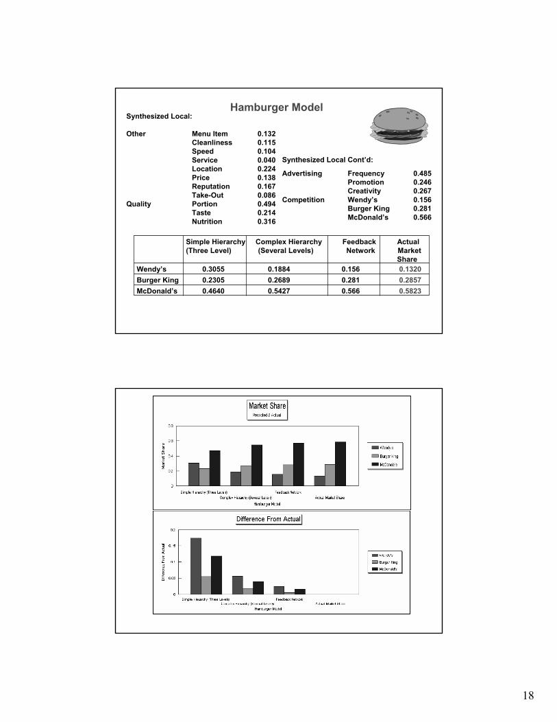
Validation

The same problem worked as a simple and

a complex hierarchy and as a feedback network.

18

Hamburger ModelSynthesized Local:

Other Menu Item 0.132Cleanliness 0.115Speed 0.104Service 0.040Location 0.224Price 0.138Reputation 0.167Take-Out 0.086

Quality Portion 0.494Taste 0.214Nutrition 0.316

Advertising Frequency 0.485Promotion 0.246Creativity 0.267

Competition Wendy’s 0.156Burger King 0.281McDonald’s 0.566

Synthesized Local Cont’d:

Simple Hierarchy Complex Hierarchy Feedback Actual(Three Level) (Several Levels) Network Market

ShareWendy’s 0.3055 0.1884 0.156 0.1320Burger King 0.2305 0.2689 0.281 0.2857McDonald’s 0.4640 0.5427 0.566 0.5823

19

14.613.01,032,000TESS

20.922.51,778,951BCP

64.564.55,104,000TELESP

7,914,051Total

RelativeShare(Model)

RelativeShare(Income)

Income

20

Airlines’ Market SharesModel Results Actual

(yr 2000)

American 23.9 24.0

United 18.7 19.7

Delta 18.0 18.0

Northwest 11.4 12.4

Continental 9.3 10.0

US Airways 7.5 7.1

Southwest 5.9 6.4

American West 4.4 2.9

21

Alternatives Nike Reebok Others

Actual Market Share

Estimated Mkt Shr 40.670 15.040 11.330 32.970

39.200 15.100 10.900 34.800

Adidas

22

Saaty Compatibility IndexGiven two sets of positive numbers, form the matrix

of ratios of all the numbers in one set;Then form the matrix of ratios of all the numbers

in the second set.Take the transpose of the second matrix.Multiply the two matrices elementwise

(i.e., perform Hadamard multiplication).Add all the resulting numbers and divide by n2.

If the two sets of numbers are identical the result would be equal to one.

If, after dividing by n2, the ratio is 1.1 or less the two sets of numbers are said to be compatible, otherwise not.

Estimate American, Asian, European Car Maker’s Market Share

Model by Y. Voravetvudhikun, March 2002

23

Using a single feedback network that incorporated what are thought to be the driving factors in automaker market share, the relative market share was estimated at:

American 53.8%Asian 30.3%European 15.9%

Model Share Estimate from Model

The results were compared to the real market share ofpassenger cars in US in 2000 from US Business Reporterwebsite: www. activemedia-guid.com/automrkt mrkt.htm

From their data the Big Three: GM, Ford and Daimler Chrysler, were grouped together to get the actual American Share at 55%; Toyota, Honda, Nissan and Hyundai were grouped for Asian at 28.4%; and VW, BMW, Mercedes Benz, Volvo, Audi, Fiat, etc. were grouped for European at 16.6%.

15.9%16.6%European30.3%28.4%Asian53.8%55%American

ModelMkt Share

ActualMkt Share

Car maker

24

Predictive decisions are objective as their outcome depends on what is likely to happen. Non-predictive decisions are subjective and depend on how much people value their benefits, opportunities, costs, and risks (BOCR).

PREDICTING AND DECIDING

Step 1. Problem Description

• Describe the decision problem in detail including its objectives, criteria and subcriteria, actors and their objectives and the possible outcomes of that decision.

• Give details of influences that determine how that decision may come out.

25

Twelve ANP Steps

• Kindly follow the algorithm in the following twelve steps for successful completion of your ANP project

Step 2: Determine Control and SubCriteria

• Determine the control criteria and subcriteria in the four control hierarchies one each for the benefits, opportunities, costs and risks of that decision

• obtain their priorities from paired comparisons matrices.

• If a control criterion or subcriterion has a global priority of 3% or less, you may consider carefully eliminating it from further consideration.

26

Step 3. Determine the most general network of clusters

• Determine the most general network of clusters or components) and their elements that applies to all the control criteria.

• Number and arrange the clusters and their elements in a convenient way (perhaps in a column).

• Use the identical label to represent the same cluster and the same elements for all the control criteria.

• Determine the most general network of clusters

Step 4. Determine Clusters and Elements

• For each control criterion or subcriterion, determine the clusters of the general feedback system with their elements

• Connect them according to their outer and inner dependence influences.

• An arrow is drawn from a cluster to any cluster whose elements influence it.

• Describe the decision problem in detail including its objectives, criteria and subcriteria, actors and their objectives and the possible outcomes of that decision.

the super decisions software thomas l. saaty - cash flow

Documents