the supply chain matrix - wordpress.com

THE SUPPLY CHAIN MATRIXA Prospective Study of the Spatial and Economic Connections

within the Region’s Meat Industry

2The Supply Chain Matrix

Foreword from the President and CEO of The Reinvestment Fund, Don Hinkle-Brown

Introduction

1. Methodology: How to Use This Model Theoretical, Not Actual The Industry: Meat as a Pilot Study The Region: The Reach of the Matrix Factors in the Model A Walk through the Supply Chain 2. Regional First: Maximizing Local Sources Showing Economic Connectivity

3. Identifying Supply Chain Gaps Assessment of an Actual Market Flow

4. Applying Results to Define the Policy: The Macro Perspective Keeping It Regional Room for Growth A Clear Opportunity

Conclusion Future Applications Broader Impacts

Appendices A: Industrial Supply Chains: A Literature Review B. Data Sources and Software C: Industry Location Quotients D: Economic Multipliers E: Employment Impacts F: The Meat Supply Chain Matrix Table: Selected Industries

Glossary

3

4

666778

1111

1313

15151516

171718

19192425252627

29

Contents


Since 2004, TRF has been implementing a reinvestment strategy to enhance fresh food access in underserved communities. What we began in Pennsylvania, we have now started to replicate in neighboring states like New Jersey and Maryland. We have connected our effort with individual, corporate, philanthropic and public sector investors. These funds in turn have been deployed to create more than equitable food access; they have helped local businesses and communities flourish.

For TRF, this work has been more than intermediating credit. It has been an opportunity to create systemic changes to how we address the challenges of food access. To this end, we analyze and study what contributes to inequitable access and how we as a nation can begin to tackle this problem. Our Limited Supermarket Access analysis is one such example. We continue to share our learning and our experience with others across the country, seeking to improve food access in their own communities and states. And on a national scale, we have helped to advocate for public policies that make building healthy communities a priority.

Investing in fresh food access is an investment towards revitalizing communities. The success of the Pennsylvania Fresh Food Financing Initiative (FFFI) showed us that. In economic development terms, many people obtained employment and the public sector benefitted through increased revenues. In community development terms, communities adjacent to new or improved stores increased in value. In sustainability terms, our tool kit included energy-efficiency support focused on greener and cost-efficient features and equipment. This study represents a natural next step in our efforts to maximize the impact of our food retail investments. It is an effort to understand how investments in food access might reinforce and build the local and regional economies.

Our efforts to explore food production systems, and this study, would not have been possible without the patient encouragement of our funders, especially the William Penn Foundation and the Surdna Foundation. Both Gerry Wang and Michelle Knapik from these foundations helped steer us towards a more sustainable set of objectives, and we thank them for that encouragement. As we began to explore the local food supply chain, we were shepherded by a few local leaders as well. Glenn Bergman of Weavers Way Co-op and Marilyn Anthony of the Pennsylvania Association for Sustainable Agriculture were instrumental in introducing and vouching for TRF within the community of local producers and processors.

TRF will continue to bridge our work, founded in social and economic justice, to the worlds of environmentalism and sustainability. We at TRF see a vital connection between the two—one that could make a positive difference to the disparity that is inherent to our current economy and food systems.

Don Hinkle-BrownPresident and Chief Executive OfficerThe Reinvestment Fund

FOREWORD

About The Reinvestment FundTRF is a national leader in rebuild-ing America’s distressed towns and cities and does this work through the innovative use of capital and information. TR F has invested $1.2 billion in mid-Atlantic commu-nities since 1985. As a Community Development Financial Institution (CDFI), TRF finances projects related to housing, community facilities, food access, commercial real estate and energy efficiency. It also provides public policy expertise by helping clients identify practical solutions and by sharing data and analyses via PolicyMap. Beginning with the Pennsylvania Fresh Food Financing Initiative (FFFI) in 2004, TRF has brought a comprehensive approach to improving the food landscape in low-income, underserved com-munities. The approach includes flexible capital as well as rigorous quantitative and qualitative analysis to inform our activities and measure the impact of our work. To date, our financing has supported 121 food access projects, provided approximately $150 mil-lion to healthy food access projects in the mid-Atlantic region and has served as a national model. It has helped operators and developers to overcome barriers to opening or maintaining stores in low-income communities. Beyond its financing efforts, TR F has developed a nationwide geo-spatial analysis of low-access food areas, available freely on www.PolicyMap.com. To learn more, visit www.trfund.com.


TRF’s food system initiative seeks to offer financing to businesses engaged in food production and processing, expand overall local food production and support intra-regional business activity—buying and selling between businesses. Building on TRF’s financing programs for retail food outlets, TRF’s Policy Solutions team explored the potential of this new initiative. This report reflects our initial research in helping to identify and evaluate potential business opportunities, borrowers and industry partners. If successful, this prospective research, in conjunction with a financing program, could help to retain and expand food producers and processors in the region.

The supply chain research presented here is part of a larger body of work that supported TRF’s venture into a lending program that expands beyond the retail sector and goes further back in the supply chain, to food producers and processors. This includes the original meat suppliers—farms and feedlots—as well as the 1st-stage processors (such as meatpackers) and 2nd-stage processors (who develop specific food products). This report seeks to identify new areas for lending and technical assistance that would have a direct impact on how a local industry sources its products.

The analysis of supply chain design has often focused on international patterns of production, processing and shipping, and the food system exists within this global, industrialized supply chain. As the distance between points in the supply chain increases, the importance of that distance gains relevance as a topic of study. Spatial analysis and modeling of food supply chains have been limited and under-theorized, although researchers have identified the need to address such research questions. (For a detailed review of the literature on industrial supply chains, see Appendix A.) This report moves into a valuable area for future research, which is examining the most effective means for producers and processors to shift their products to alternative supply chains.

As is so often the case for TRF, lending and research happen concurrently, or one can proceed a bit in advance of the other. This is an instance in which initial investigations into lending opportunities transformed into an opportunity to do research that would inform that process of identifying candidates for lending.

INTRODUCTION


Given the known challenges of trying to find lending opportunities within the region’s agricultural sector, this report goes beyond present-day scenarios to present an instructive model for a potential, more sustainable future. This research identifies potential borrowers based on their potential to play a significant role in the regional food system. Targeted financing to these businesses could support existing businesses to remain in the region, and even possibly expand their capabilities.

TRF maintains that CDFIs should lend in markets that are not maximizing the social and economic potential of their nearby communities. This is similar to financing a new supermarket in a low-access community where conventional operators do not see profitability, even if at a regional level. Accordingly, a financing or incentive program informed by this model could increase the output of the regional supply chain, which in turn leads to a number of other positive outcomes, including:

• increases in regional employment (see Appendix E)

• decreases in the food industry’s carbon footprint, by mitigating the environmental impacts associated with global food distribution. Reducing the distance food travels from farm to supermarket (and ultimately to plate)—by sourcing regionally—requires less energy expenditure, resulting in fewer greenhouse gas emissions and less infrastructure degradation.

Expanding this research to other food supply chains would support TRF’s broader objective to mitigate impediments to the production, processing and distribution of regionally produced foods via CDFI lending. Other organizations have recognized the importance of using supply chain relationships to facilitate regional economic growth and may find its utility as well. We hope to continue to explore the practical application of this research by partnering with other organizations that are seeking to maximize local and regional food production.

CDFI: Community Development Financial Institution


To examine how the Supply Chain Matrix (SCM) applies to regional food businesses, we must first establish a baseline understanding of the factors at play and the parameters of the model. This section provides this rationale and reviews basic steps in the supply chain and the role of industry pricing. These discussions set up subsequent sections of the report, describing the implications of applying the model in this particular region.

Theoretical, Not ActualIt is important to establish that we have used the SCM to generate tables and graphic illustrations of the potential geographic and economic flow of meat products, as they move through the supply chain. The model does not represent the actual flow of products through the supply chain, but rather identifies economic relationships that would minimize the distance that meat travels from farms to processors (at multiple stages) before it is distributed to wholesale and retail outlets.

The Industry: Meat as a Pilot StudyThe meat supply chain serves as the pilot industry for this research.1 We determined that examining a single identifiable food chain could demonstrate the model more clearly than using smaller segments of several industries. We selected meat in lieu of another agricultural industry in part because it is so readily produced in this region.2

Furthermore, anecdotal evidence suggests that regional meat processors (slaughter and meatpacking facilities) lack enough capacity to process the region’s meat production (farms and feedlots). This may act as a bottleneck to impede growth, but it also presents a potential opportunity to expand existing businesses and attract new ones to the region.

Future work could explore additional food industries, and yet the supply chain matrix is not limited to food: We could incorporate into the model other industry supply chains that involve multiple stages of production and processing, including light and heavy manufacturing subsectors.

METHODOLOGY: HOW TO USE THIS MODEL

1. By “meat” we refer to beef, lamb, pork, and any other non-poultry land animals.

2. Beef cattle farms and feedlots are the primary producers in the region’s meat supply chain. Beef cattle farms constitute 58% of all businesses op-erating in the entire food shed’s meat industry, and beef cattle feedlots represent another 18%. Meatpacking plants, which purchase beef cattle from farms and feedlots, comprise 4% of all industry businesses (source: NETS. See Appendix B).

1


3. This study’s target area is an extension of the William Penn Foundation’s primary target area, which is the Philadelphia metropol-itan area. Our extended study area includes agriculturally significant rural counties that supply the region.

4. The Huff retail gravity model is used to calculate the probability that households will shop at a supermarket based on the store’s size and its proximity. For the adaptation of this model, we made significant modifications to accommodate the distinct economic relationships be-tween meat producers and processor. By incorporating a producer/pro-cessor matrix into the Huff model, we have created a distinct gravity model for each producer/processor relationship, based on their SIC codes and proximity.

5. Although buyers don’t likely decide where to make purchases based on a supplier’s sales, within the model buyers are limited to purchasing a finite amount of inputs based on the seller’s available sales.

The Region: The Reach of the MatrixAs a pilot for the model, we focused on the meat industry’s supply chain in a specific local area.3 Our research resulted in a geographic model designed to identify local lending opportunities in the meat supply chain. The model is geographically flexible, and we could replicate it in other regional markets within the United States. The model requires a defined area, however, so future research could analyze a region, a Metropolitan Statistical Area (MSA) or any other geographic unit that meets the model’s minimum requirements.

Factors in the ModelTRF’s SCM minimizes distance by matching food buyers and sellers within the supply chain, based on three factors:

• physical proximity• segment of the supply chain (industry code assignment or Standard Industrial

Classification—SIC)• sales volume

The SCM is a modified version of the Huff retail gravity model.4 While the Huff model uses sales volume as a proxy for attractiveness, we cannot assume this same causal relationship between producers and processors in our model. Ours is a geographic model of how the meat industry’s supply chain would look if—when deciding where to source their inputs—buyers considered only a seller’s proximity, product availability and capacity to supply enough product.5

Clearly, the factors of pricing and legacy relationships do exert a strong influence on where buyers source their inputs (which explains why some regional buyers purchase cattle from Mexico and pork from China). However, this model supports our interests in exploring opportunities for connecting regional buyers with regional sellers, with the goal of increasing the output by those regional sellers.

Map 1:TARGET AREA FOR RESEARCH


A Walk through the Supply ChainThe SCM builds spatial and economic relationships between businesses (producers; in this case, farms and feedlots) that produce goods and those that purchase those goods (meatpackers and other 1st-stage processors), characterized here as inputs to the model. In turn, these processors produce new items to be sold to the next purchaser in the supply chain (2nd- and 3rd-stage processors).

For example:

Livestock Farmersells cattle to a...

Meat Processorwho converts the cuts into ground beef (or other meat products) and sells it to either ...

Another Meat Processorwho processes the ground beef into meat pies or other products and sells the products to a...

Distributor or Grocer

Meatpackerwho slaughters the cattle and sells the cuts of meat to a...

PRODUCER

1ST-STAGE PROCESSOR

2ND-STAGE PROCESSOR

3RD-STAGE PROCESSOR

WHOLESALE OR RETAIL

DISTRIBUTION

Focus of this report:The SCM currently focuses on supply chain stages that occur prior to wholesale and retail segments, though we could display wholesale and retail locations to help users better understand their spatial distribution and potential connectivity to the supply chain.

or a...


The Role of Price in the Supply Chain The SCM table (Appendix F) captures the relationship between producers and processors at various stages in the supply chain. We used 2010 USDA data on price spreads for beef (see Figure 1) to calculate the dollar value of:

• purchases that meatpackers (1st-stage processors) make from cattle farms and feedlots (producers)

• purchases that 2nd-stage processors make from 1st-stage processors

We then converted these purchase values to a percentage of sales to create the matrix.

Figure 1:2010 USDA BEEF PRICE SPREADS

Farm Value (Producer) $204

1st-Stage Wholesale Value (1st-Stage Processor) $241

Percentage of 1st-Stage Processor’s Sales Spent on Inputs from Farm 85%

2nd-Stage Wholesale Value (2nd-Stage Processor) $340

Percentage of 2nd-Stage Processor’s Sales Spent on Inputs from 1st-Stage Processor

71%

Retail Value $440

Percentage of Sales Spent on Inputs from 2nd-Stage Processor 77%

Source: USDA ERS Beef and Pork Price Spreads, 2012.

The easiest way to understand the model is to walk through an example, using the price spread table (Figure 1).

1st StageAccording to USDA price spreads (Figure 1), if a meatpacker (1st-stage processor) buys a cow from a farmer (producer) for $204 and processes the cow, it can then sell the meat to a processor of beef stew (2nd-stage processor) for $241. Figure 1 reflects that the meatpacker spent 85% of its revenue from that sale (to the 2nd-stage processor) on the cow ($204/$241); the remaining 15% of revenue represents the meatpacker’s value-added costs and profit margins. (For more on how this relates to the matrix, see Appendix F.)

2nd Stage If a processor of beef stew buys one cow’s worth of processed meat from a meatpacker for $241, and further processes it, it can then sell the finished product to retailers for $340. Figure 1 reflects that the beef stew processor spent 71% of its revenue from that sale (to the retailer) on the cow ($241/$340); the remaining 29% of revenue represents the beef stew processor’s value-added costs and profit margins.

Following the Flow: The Supply Chain Matrix Through One Example


Working Outward from Processor to Producers

• The SCM reaches out geographically (using straight-line distance) from each meatpacker to identify those nearby farms and feedlots (producers) with adequate sales volume to satisfy that buyer’s demand.

• If the nearest farms and feedlots can fulfill the meatpacker’s total demand, then the SCM stops searching; if not, the model allocates to the meatpacker the sales volume of the next-closest farm, until it has identified enough producers to fulfill the meatpacker’s demand.6

The matrix applies the same formula to 2nd-stage processing, reaching out from each 2nd-stage processor geographically, to find the closest meatpackers (1st-stage processors) with adequate sales volume to fulfill 71% of the beef stew processor’s total sales.

Why do the ratios change?The fact that the input price ratio for 2nd-stage processing (71%) is significantly lower than for 1st-stage processing (85%) reflects the greater level of value-added processing that occurs in the 2nd stage. (Whereas a meatpacker cuts and packs meat, a processor of beef stew cooks the meat, mixes it with other ingredients and packages the product in a format for wholesale distribution or retail sale.)

These examples illustrate the SCM’s application and interpretation. The next sections explore micro and macro applications of the model that shed new light on the meat industry and the potential for its supply chain.

6. A relevant factor here is the effect of competing meatpackers, which explains why so many meatpackers are unable (potentially) to fulfill their demand within the region.


REGIONAL FIRST: MAXIMIZING LOCAL SOURCES2

Map 2:

FARMS AND FEEDLOTS ( ) AND MEATPACKERS ( ) IN THE TARGET AREA ( )

While the region’s meat industry supply chain likely has a global reach, this research estimates the portion of a region’s supply chain that could, ideally, be produced and processed within the region. One of the model’s most important uses is assessing the ideal market based upon proximity and identifying potential buyer/seller (processor/producer) relationships.

Showing Economic ConnectivityMap 2 focuses in closer than the SCM’s entire range of data to show the farms and meatpackers in the target area. This map reveals the density of potential local farm sources for meatpackers.

The area around Lancaster, PA, is a notable example of the potential economic linkages between cattle farms and feedlots (producers) and meatpackers (1st-stage processors). Map 3 (following page) illustrates the geo-economic connections between a large meatpacker in Lancaster (buyer) and the farms and feedlots (sellers) in every direction from which it could purchase livestock.

Lancaster, PA


Map 3:

ANALYSIS OF A POTENTIAL SUPPLY CHAIN for an actual Lancaster, PA meatpacker

Dots represent farms and feedlots;

their size/color indicates their potential for sales to

the meatpacker.

Gray dots represent farms and feedlots that (the model suggests) could supply a nearby meatpacker in Fredericksburg rather than the Lancaster meatpacker that is the focus here.

Sales Levels from Farm/Feedlot (Producer) to Meatpacker (1st-stage Processor):

of the meatpacker’s demand can be met by these 5 local farms/feedlots.




91%of this meatpacker’s supply can be met within 35 miles of its facility. This scenario presumes that all producers and processors in the community are maximizing their ability to buy and sell locally.


IDENTIFYING SUPPLY CHAIN GAPS3Beyond maximizing benefits from proximity, the SCM also helps to identify which aspects of the region’s supply chain appear to have gaps in terms of input and output (or production and processing).

Assessment of an Actual Market Flow TRF used the SCM to create a list of meatpacking businesses that—theoretically, within the parameters of the model—would be unable to satisfy their purchasing needs from regional farmers and feedlots (see Figure 3, on next page).

A Sample Meatpacker For example, one of the largest meatpackers in Figure 3 (by sales volume: Firm B) can theoretically only fulfill 0.3% of its inputs regionally. In terms of sustainability, this is certainly a low figure, but it also represents an opportunity to interview this firm to determine whether it is purchasing from any regional producers, and if so, which ones.

From a regional economic development perspective, any producers that might already be selling to Firm B would be prime candidates for expansion. If Firm B were to purchase more regionally, we would expect that, subsequently, it would purchase less volume from producers outside the region. In this way, the SCM leads us directly to import substitution—an essential component of sustainable food production and economic development. If those processors that rely on a lower percentage of regional sources were to start purchasing more regional output, they could potentially represent an opportunity for economic expansion.


Firm ALancaster, PA Firm BPhiladelphia, PAFirm CSouderton, PAFirm DPhiladelphia, PAFirm EHarleysville, PAFirm FShrewsbury, NJ Firm GWestville, NJ Firm HVineland, NJ Firm IBensalem, PAFirm JAston, PA Firm KUpper Darby, PAFirm LEmmaus, PA Firm MTrenton, NJFirm NQuakertown, PA Firm OSalem, NJ Firm PPhiladelphia, PA

Meatpacking Company

Percentage of Inputs Available Regionally

Input Met Regionally (black)

Input Not Met Regionally (yellow)

91.1%

4.4%

0.3%

2.7%

2.7%

16.4%

3.6%

20.2%

50.7%

2.6%

13.9%

97.8%

4.8%

10.9%

74.1%

100%

Figure 3:

MEATPACKERS WITH DEMAND THAT EXCEEDS REGIONAL SUPPLY reveal $176 million of potential supply revenue

$176Mis what the top 16 regional meatpackers could be spending on local inputs. These 16 meatpackers within the target area have requirements for processed meat that are (theoretically, based on SCM methodology) too large to be sourced by regional suppliers. These 16 have a total input—buying power—of $262 million (in black plus yellow), and yet regional suppliers can meet only $86 million (33%) of this demand (in black). The $176 million difference (in yellow) represents potential supply revenue, which is currently a lost opportunity within the regional economy.

Source: NETS, 2010.


Some of the SCM’s real value emerges when we examine its output at the macro level (industry-wide in the region) alongside that at the micro level (of individual businesses). The micro-level analysis can identify businesses that are lacking, adequate or abundant in terms of their output within a certain segment of the supply chain. The macro-level analysis can not only identify specific supply chain segments that are lacking, adequate or abundant within the region, but also provide aggregated data on the collective relationships between the region’s producers and processors.

Figure 4 reflects how, for several meat products in the target region, the collective demand differs from the collective supply. The discrepancies reveal not only lost income for existing regional producers, but also opportunities for new businesses in the region that could help to narrow these gaps by buying up some of the supply.

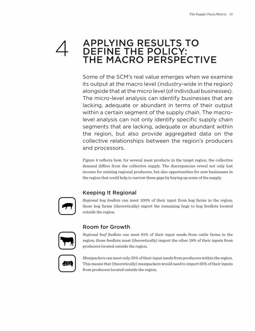
Keeping It RegionalRegional hog feedlots can meet 100% of their input from hog farms in the region; those hog farms (theoretically) export the remaining hogs to hog feedlots located outside the region.

Room for GrowthRegional beef feedlots can meet 81% of their input needs from cattle farms in the region; those feedlots must (theoretically) import the other 19% of their inputs from producers located outside the region.

Meatpackers can meet only 35% of their input needs from producers within the region. This means that (theoretically) meatpackers would need to import 65% of their inputs from producers located outside the region.

APPLYING RESULTS TO DEFINE THE POLICY: THE MACRO PERSPECTIVE

4


Region’s Output Purchased by Buyers Within the Region Farms and Feedlots ( ) Meatpackers ( )

vs. Region’s Output Sold Outside the Region

81%

19%

35%

65%

0%

100%

Figure 4:

AGGREGATED MEAT INDUSTRY FIGURES

A Clear OpportunityIn a situation where the region’s producers create more output than its processors could be expected to purchase as inputs (as with hog farms and feedlots in this example), there is potential for expanding existing processors and attracting new ones. The converse is also true, whereby producers that are creating insufficient output to satisfy processors’ input requirements would indicate the potential to expand existing producers and attract new producers (in this case, beef and cattle producers falling short of meatpacker demand).

Sources: NETS, 2010; USDA, 2012


CONCLUSION

The results of this analysis can help determine which industries show the best potential for import substitution, and we can use these results to identify industries for possible development and expansion. If the model proves to be useful to businesses, organizations engaged in the meat industry or related economic development agencies, we could move on to analyzing another subsection of the larger food system, such as vegetables or poultry.

Future ApplicationsThe model’s level of detail allows users to identify individual businesses that would likely be unable to fulfill their input requirements from regional suppliers—suggesting that nearby regional suppliers represent opportunities for expansion, as a way to fill the input requirement gap. Additionally, users can explore options for facilitating commerce between buyers and sellers as a means to facilitate regional economic expansion. A logical next step for this research would be to interview major buyers, to determine whether they are in fact sourcing inputs from nearby sellers, as the model proposes.

The meatpackers listed in Figure 3 represent good candidates for interviews, to better understand the needs of 1st-stage meat processors. This should include a discussion of their suppliers’ locations and sales volume, to gauge the extent to which meatpackers are already sourcing from regional suppliers. In essence, the interviews will help us to evaluate the extent to which the model has real-world applicability.

The SCM generates tables and maps that illustrate industry clusters and the geographic flow of products, which allows us to understand which industries impact the food system, their geographic features and their directional flow from farm to wholesaler/retailer. These spatial features, along with survey responses from relevant businesses, will help us to identify key impediments to growth among firms operating in the meat industry, especially those impediments that could be mitigated by financing mechanisms.

Employment and Other Economic ImpactsBecause the SCM estimates the economic impacts (earnings, jobs, total output) of shifting a processor’s purchases from non-regional producers to those within the region (see Appendix E), this would allow lenders to prioritize their outreach efforts to favor those processors with the greatest opportunity to create jobs and related economic impact. These calculations translate the output from the SCM output into more accessible figures.


Target Businesses: From Large to SmallThe grant allowed that our work was relatively agnostic in terms of the scale of individual producers and processors; we are concerned with creating economic growth in the region’s food industries overall, which would in turn create growth in numerous indirect and induced industries.

Future outreach is less likely to target larger farms and processors, which tend to gain financing from conventional banks and not to rely on the kinds of resources funders would offer. Given the tendency for small- to medium-size businesses to rely on self-financing and cash purchases, businesses of this scale would be a more likely target for possible funding. While our model does not favor connections between larger buyers and larger sellers, we hope to draw upon existing research, as well as qualitative responses from food producers and processors, to account for scaled relationships in future versions of our model.

Broader ImpactsWhile we developed this model through the lens of a CDFI, it is our hope that this analysis could prove useful to others as well, including: departments of agriculture; economic development agencies; agricultural economists; private banks, foundations and investors; urban and regional planning agencies (including specialized food systems planners); small businesses; and food advocacy organizations.

In particular we envision that nonprofit organizations actively seeking to build relationships within particular industries would find the model useful, as they go about building sustainable community networks. We recognize that, given the difficulty of taking on some kinds of change in isolation, this model could serve as a valuable tool to convene like-minded individuals and support them in processing information at this micro and macro level.


APPENDICES

Appendix AIndustrial Supply Chains: A Literature Review

The analysis of supply chain design and management in an ever-globalizing economy has often focused on long-haul, international patterns of production, processing and shipping. Within this global, industrialized supply chain is the food system, as raw and processed foods and commodity crops have increasingly been traded across markets and borders, largely due to disparities in production costs (i.e., labor and land). As the distance between points in the supply chain increases (with the expansion of international trade), the importance of that distance gains relevance as a topic of study, despite the economic advantages associated with lower production costs and relatively low or stable international shipping costs for certain goods.

Spatial analysis and the use of GIS to model food supply chains have been limited, although researchers have identified the need to address such research questions. Marsden, Murdoch and Morgan (1999) stated that “the spatial development of food…has been largely under-theorized.” They challenge future research to examine the most effective means by which local producers and processors can shift their products to alternative supply chains.

While research on supply chains in general has focused on inter-regional or international trade across long distances, there is a movement towards food supply chains within a much smaller regional footprint. Research by Marsden, Banks and Bristow (2000) identifies these regional, food-based alternatives as SFSCs, in which added value is derived through local sales, as opposed to “low-quality/high-output production systems (in which they are often ‘locked’)” (p. 300). SFSCs for highly perishable food products become all the more relevant, as reducing the time between harvest and point of sale can reduce the potential loss in retail value (Blackburn & Scudder, 2009).

Many of the food supply chain analyses that feature a spatial component have focused on markets outside the U.S., often tied to research on food contamination (Bosona & Gebresenbet, 2011; Beni et al., 2011; and Van der Fels-Klerx et al., 2009). GIS analysis combined with RFID tags can track and contain potential food contaminations, whether they are plant- or animal-based (Jones et al., 2004; Ruiz-Garcia, Steinberger & Rothmund, 2010).

The research has identified three types of SFSCs (Marsden, Banks & Bristow, 2000, p. 425). First, SFSCs include face-to-face sales to consumers, where direct sales of food products are made from producer to consumer, such as in the case of farmer’s

GIS: Geographic Information Systems

SFSC: Short Food Supply Chains

RFID: Radio Frequency Identification


markets and farm share programs (or CSAs). Marsden, Banks and Bristow (2000) also include internet food sales as a type of face-to-face sales medium. Secondly, SFSCs provide “spatial proximity,” where food products are sold within a geographic footprint that overlaps with their site of production. The key aspect to this spatial proximity is the marketing towards consumers, wherein the sellers describe, label and recognize products as “local” in some way. Lastly, SFSCs are “spatially extended,” whereby the sellers market the place of production and/or the producers to consumers who do not live within the same area as the production, and yet still derive “value and meaning” from the product because of where it is produced (e.g., Florida oranges, Wisconsin cheese, Napa wine). This conveys meaning despite the consumers having little or no direct connection to the region of production. Relatedly, the role of supplier certification is also a relevant consideration for deriving value in the supply chain, as Pagell and Wu noted (2009). The importance of supplier certification is certainly relevant for the food supply chain, as certification for niche markets such as “organic” or “grass-fed” meats experience rapid growth in demand for products.

Marsden, Banks and Bristow (2000) identify SFSCs as an alternative response to traditional market supply chains from the perspective of both producers and consumers, one in which both parties can derive increased value: “Notable here are the additional identifiers which link price with quality criteria and the construction of quality” (p. 425). The relationship between producer and supplier is emphasized as a primary source from which value is derived. As food supply chains continue to grow within an SFSC model, the study of regional production and processing of food becomes all the more relevant, especially for smaller, non-institutional producers.

The research of Bosona and Gebresenbet (2011) provides an additional template for the use of GIS research in the food supply chain, focusing on local food producers throughout Sweden. Their research objectives were to: map producers and large-scale food distribution centers (LSFDCs), develop clusters of producers, identify prime locations for each cluster with LSFDCs and delineate optimized delivery routes. They draw their conclusions around increasing route efficiency for producers, with the goals of reducing costs, expanding market share, decreasing environmental impact and improving traceability as a means for increasing food quality and safety.

While the concept of an SFSC provides a valid conceptual model to understand the shifting nature of regional food networks, there appears to be a lack of publicly available spatial research and analysis that tracks the potential or actual flow of products from specific producers to processors using point-level location data. However, GIS software has been used to identify optimal transportation modes and routes for moving products from segment to segment along numerous supply chains.

CSA: Community Supported Agriculture


For example, Delen et al. (2011) used GIS to examine supply chain improvements for the delivery of blood. Their use of point-level data within a GIS model provides a compelling visualization of product distribution between segments; as long as researchers use current point-level data, this model has the flexibility to shift with changes in supply and demand over time. Another important feature the authors note is the ability of spatial features to highlight and differentiate critical supply chain restraints, denoting issues that challenge the entire supply chain versus isolated issues located at a specific blood facility. They describe a GIS model’s ability to pinpoint abnormal patterns of product flow, which can then address supply chain restraints in a more timely and appropriate fashion.

This blood supply chain study provides context to the analysis of food supply chains, as both blood and food products are subject to similarly “strict storage and handling requirements” (Delen et al., 2011, p. 181) because of their perishable nature; thus, an improved understanding and increased efficiency of product delivery mechanisms can significantly affect the quality of food and blood alike.

A second example of using GIS to analyze supply chains comes from Higgins and Laredo’s (2006) research of sugar production in Australia. The purpose of using GIS in their research was twofold. First, they describe their use of GIS as adding value to technical processing, so they could manage large datasets in their logistics modeling, including 15,000 farm paddocks and 470 railway siding locations. Much of the GIS functionality was used to improve transportation logistics and plan harvesting schedules. Second, GIS allows end-users to view research models as a product or service, such as a user interface that provides spatial data intended to help less-technical users (farmers, growers and producers) to better understand the relationship between transportation logistics and efficient harvests.

Randall and Ulrich (2001) provide additional insight into the relationship between distance and economies of scale within supply chains. While their research focuses on bicycle production, their concepts apply to food production as well. Their description of the supply chain focuses upon two key factors: first, the distance from the place of production to the targeted market, and second, the extent to which a place of production is able to produce efficiently at a scale that matches buyer demand. As in just about any industry, we expect that economies of scale play a major role in establishing economic relationships between buyers and sellers within the food supply chain. While our model does not favor connections between larger buyers and larger sellers, we hope to draw upon existing research, as well as qualitative responses from food producers and processors, to account for scaled relationships in future versions of our model.


The distance from place of production to point of sale has a positive relationship to a product’s cost, though one can offset increased costs due to distance by increasing the scale of production (economies of scale). That is, firms can gain economies of scale, thereby lowering the marginal cost of production per product as the total volume of production increases; however, increased production volume can also bring additional costs, as firms may need to source inputs from farther distances to meet their increased capacity (MacCormack, Newman & Rosenfield, 1994). At the end of the supply chain, increases in production can also translate into increased distances to ship a product to market, depending upon saturation levels of local demand for the product (Hadley & Whitin, 1963; Stevenson 1996).

GIS software measures these distance calculations, which are integral to the conceptual relationships among value, cost, scalability and distance. As noted above, GIS can add value by providing a geographic visualization of the supply chain network that would otherwise not be possible, especially in complex scenarios with multiple buyers and sellers.

Much of the above research focuses on minimizing the distance between supply chain segments at a rather micro level, in the sense that the goal is to potentially reduce travel times by 10%. However, there appears to be little research on the economic connectivity of supply chains based on the detailed buyer/seller relationships that form individual segments of a supply chain. The objective of this research is to illustrate opportunities to reduce the distance traveled from farm to meatpacker and from meatpacker to processor by a much larger magnitude—more on the order of 1,500 to 250 miles, as opposed to from 300 to 250 miles, for example. As long as the distance is within a regional footprint, the model meets the research objectives.

ReferencesBeni, L. H., Villeneuve, S., LeBlanc, D. I. & Delaquis, P. (2011). A GIS-based approach in support of an assessment of food safety risks. Transactions in GIS, 15(s1), 95–108.

Blackburn, J. & Scudder, G. (2009). Supply chain strategies for perishable products: the case of fresh produce. Production and Operations Management, 18(2), 129–137.

Bosona, T. G. & Gebresenbet, G. (2011). Cluster building and logistics network integration of local food supply chain. Biosystems Engineering, 108(4), 293–302.

Delen, D., Erraguntla, M., Mayer, R. & Chang-Nien, W. (2011). Better management of blood supply-chain with GIS-based analytics. Annals of Operations Research [serial online]. May 2011; 185(1), 181–193. Available from Academic Search Complete, Ipswich, MA. Retrieved May 28, 2013.


Hadley, G. & Whitin, T. M. (1963). Analysis of inventory systems. Englewood Cliffs, NJ: Prentice-Hall.

Higgins, A. J. & Laredo, L. A. (2006). Improving harvesting and transport planning within a sugar value chain. Journal of the Operational Research Society, 57(4), 367–376.

Jones, P., Clarke-Hill, C., Shears, P., Comfort, D. & Hillier, D. (2004). Radio frequency identification in the UK: Opportunities and challenges. International Journal of Retail & Distribution Management, 32(3), 164–171.

MacCormack, A. D., Newman, L. J. & Rosenfield, D. B. (1994). The new dynamics of global manufacturing site location. Sloan Management Review, 35, 69.

Marsden, T., Banks, J. & Bristow, G. (2000). Food supply chain approaches: exploring their role in rural development. Sociologia ruralis, 40(4), 424–438.

Marsden, T., Murdoch, J. & Morgan, K. (1999). Sustainable agriculture, food supply chains and regional development: editorial introduction. International Planning Studies, 4(3), 295–301.

Pagell, M. & Wu, Z. (2009). Building a more complete theory of sustainable supply chain management using case studies of 10 exemplars. Journal of Supply Chain Management, 45(2), 37–56.

Randall, T. & Ulrich, K. (2001). Product variety, supply chain structure, and firm performance: Analysis of the U.S. bicycle industry. Management Science, 47(12), 1588–1604.

Ruiz-Garcia, L., Steinberger, G. & Rothmund, M. (2010). A model and prototype implementation for tracking and tracing agricultural batch products along the food chain. Food Control, 21(2), 112–121. Stevenson, W. (1996). Production/Operations Management. Chicago, IL: Irwin.

Van der Fels-Klerx, H. J., Kandhai, M. C., Brynestad, S., Dreyer, M., Börjesson, T., Martins, H. M., Uiterwijk, M., Morrison, E. & Booij, C. J. (2009). Development of a European system for identification of emerging mycotoxins in wheat supply chains. World Mycotoxin Journal, 2(2), 119–127.


Appendix BData Sources and Software

National Establishment Time Series (NETS) database, 2010 In order to build spatial and economic relationships between food producers and processors, we purchased a comprehensive listing of businesses operating in industries relevant to the food supply chain from Walls & Associates, which maintains the NETS database and is sourced by Dun and Bradstreet. NETS provides address-level locations, annual sales and employment estimates, and the highest level of detail for industrial categorization, being eight-digit codes from the Standard Industrial Classification (SIC) System. We purchased listings far beyond the target region as a way to account for edge effects and to better understand the region’s extended food shed. The full range of purchased listings extends beyond the target area, reaching as far south as Virginia, into western Pennsylvania, and to the northern and northeastern portions of New York.

U.S. Census Bureau Standard Industrial Classification CodesWe used SIC codes to build the SCM that connects meat producers (sellers) with processors (buyers), based on each business’s assigned SIC code in the NETS database. USDA price spreads (below) were used to calculate the magnitude of each producer/processor relationship.

ESRI ArcGISWe used ArcGIS to calculate Euclidian distances between producers and processors that the SCM identified as having relationships. Euclidian distances represent straight-line or “as the crow flies,” versus more intensive street and road network distance calculations. We would have the option of incorporating network distances if additional funding were to become available.

USDA Beef Price Spreads, 2010USDA’s Economic Research Services (ERS) publishes quarterly and annual price spreads for most major food categories, including distinct price spreads for beef and pork. Price spreads show average prices paid per beef cow and hog at each general stage of the supply chain, being farmer, wholesaler (processor, butcher, packer, etc.) and retailer. Price spreads were used to calculate the percentage of a buyer’s total revenue that is spent on raw inputs (i.e., cows or hogs) for each producer/processor relationship identified in the SCM.

Microsoft SQL Management Studio We executed nearly all of the tabular calculations and some of the spatial processing tasks using SQL scripts. SQL was also used to execute the more complex spatial calculations between buyers and sellers, in lieu of ArcGIS.

SIC: Standard Industrial Classification or industry code assignment


Appendix CIndustry Location Quotients

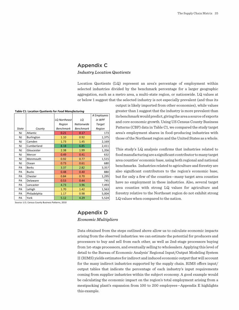
Location Quotients (LQ) represent an area’s percentage of employment within selected industries divided by the benchmark percentage for a larger geographic aggregation, such as a metro area, a multi-state region, or nationwide. LQ values at or below 1 suggest that the selected industry is not especially prevalent (and thus its

output is likely imported from other economies), while values greater than 1 suggest that the industry is more prevalent than its benchmark would predict, giving the area a source of exports and core economic growth. Using US Census County Business Patterns (CBP) data in Table C1, we compared the study target area’s employment shares in food-producing industries with those of the Northeast region and the United States as a whole.

This study’s LQ analysis confirms that industries related to food manufacturing are a significant contributor to many target area counties’ economic base, using both regional and national benchmarks. Industries related to agriculture and forestry are also significant contributors to the region’s economic base, but for only a few of the counties—many target area counties have no employment in these industries. Also, several target area counties with strong LQ values for agriculture and forestry relative to the Northeast region do not exhibit strong LQ values when compared to the nation.

Appendix DEconomic Multipliers

Data obtained from the steps outlined above allow us to calculate economic impacts arising from the observed industries: we can estimate the potential for producers and processors to buy and sell from each other, as well as 2nd-stage processors buying from 1st-stage processors, and eventually selling to wholesalers. Applying this level of detail to the Bureau of Economic Analysis’ Regional Input/Output Modeling System II (RIMS) yields estimates for indirect and induced economic output that will account for the many indirect industries supported by the supply chain. RIMS offers input/output tables that indicate the percentage of each industry’s input requirements coming from supplier industries within the subject economy. A good example would be calculating the economic impact on the region’s total employment arising from a meatpacking plant’s expansion from 100 to 200 employees—Appendix E highlights this example.

Table C1: Location Quotients for Food Manufacturing

State County

LQ Northeast Region

Benchmark

LQ Nationwide Benchmark

# Employees in WPF Target Region

NJ Atlantic 0.21 0.17 173NJ Burlington 1.10 0.92 1,375NJ Camden 1.73 1.45 2,169NJ Cumberland 8.18 6.85 2,411NJ Gloucester 2.38 1.99 1,356NJ Mercer 0.49 0.41 632NJ Monmouth 0.92 0.77 1,515NJ Ocean 0.73 0.61 680PA Berks 3.37 2.82 3,357PA Bucks 0.48 0.40 880PA Chester 0.84 0.70 1,295PA Delaware 0.53 0.44 745PA Lancaster 4.73 3.96 7,493PA Lehigh 1.70 1.42 1,563PA Philadelphia 1.17 0.98 5,004PA York 5.12 4.29 5,524

Source: U.S. Census County Business Patterns, 2010


Appendix EEmployment Impacts

RIMS data include economic multipliers for output, earnings and employment. Table E1 shows employment multipliers for meat producing and processing industries at the six-digit NAICS level, for both Pennsylvania and New Jersey. We also include each state’s industry average employment multiplier, to establish relativity.

Pennsylvania industries engaged in the processing of livestock (NAICS 311611 and 311612) show extraordinarily high employment multipliers of 7.9 and 6.4, respectively—these are well over twice the statewide industry average (3.0). Using the above example of a meatpacking plant expanding its employment from 100 to 200, the state

would see an additional 688 jobs created throughout the industries that supply inputs to and purchase outputs from meatpackers (livestock slaughter).

High employment multipliers indicate strong economic connectivity within the state’s food processing industries. We cannot conclude that high multipliers confirm the notion that regional buyers are purchasing their inputs from regional sellers, nor that regional buyers are then selling their output to regional customers; however, their magnitude only strengthens the case for expanding production and employment among the region’s food producers and processors to maximize impacts on output, employment and earnings.

New Jersey’s employment multipliers for industries that process livestock are not as high as Pennsylvania’s. New Jersey’s multipliers exceed the state average for all industries, but by a much lower margin than in Pennsylvania. Nonetheless, an expansion from 100 to 200 employees would create an additional 270 jobs throughout the state. And New Jersey’s high LQ values for food processing and manufacturing make those industries an important contributor to the state’s economic base.

Table E1: Employment Multipliers for Food Production and Processing IndustriesNAICS NAICS Description PA NJ

311611 Animal, except poultry, slaughtering 7.9 3.7311612 Meat processed from carcasses 6.4 3.4311613 Rendering and meat byproduct processing 4.1 3.4311990 All other food manufacturing 3.0 4.3Average Average All Industries 3.0 2.9Source: Bureau of Economic Analysis RIMS II, 2010

Table E1: Employment Multipliers for Food Production and Processing Industries


Appendix FThe Meat Supply Chain Matrix Table: Selected IndustriesSelected Industries in the Meat Supply Chain MatrixColumn Industries Purchase from Row Industries 20110000 20119907 20130101 20130300 20139903

8-‐Digit SIC Code Industry Description # Firms

% All Firms

Meat packing plants

Sausages, from meat slaughtered on site

Beef stew, from purchased meat

Sausages and related products, from purchased meat

Cooked meats, from purchased meat

02110000 Beef cattle feedlots 892 17.9% 0.8457 0.7771 0 0 002120000 Beef cattle, except feedlots 2,351 47.2% 0.8457 0.7771 0 0 002130000 Hogs 325 6.5% 0.8457 0.6509 0 0 002139901 Hog feedlot 36 0.7% 0.8457 0.6509 0 0 002140000 Sheep and goats 53 1.1% 0.8457 0.7771 0 0 002140100 Goats 8 0.2% 0.8457 0.7771 0 0 002140101 Goat farm 34 0.7% 0.8457 0.7771 0 0 002140102 Goats' milk production 11 0.2% 0.8457 0 0 0 002140103 Mohair production 2 0.0% 0 0 0 0 002140200 Sheep 73 1.5% 0.8457 0.7771 0 0 002140201 Lamb feedlot 7 0.1% 0.8457 0.7771 0 0 002140202 Sheep feeding farm 3 0.1% 0.8457 0.7771 0 0 002140203 Sheep raising farm 72 1.4% 0.8457 0.7771 0 0 002140204 Wool production 8 0.2% 0 0 0 0 002190000 General livestock, nec 547 11.0% 0.8457 0.7771 0 0 020110000 Meat packing plants 194 3.9% 0 0 0.7085 0.624 0.708520110100 Beef products, from beef slaughtered on site 20 0.4% 0 0 0.7085 0.624 0.708520110101 Boxed beef, from meat slaughtered on site 3 0.1% 0 0 0.7085 0.624 0.708520110102 Corned beef, from meat slaughtered on site 0.0% 0 0 0.7085 0 0.708520110103 Veal, from meat slaughtered on site 11 0.2% 0 0 0 0.624 0.708520110200 Pork products, from pork slaughtered on site 6 0.1% 0 0 0 0.624 0.62420110201 Bacon, slab and sliced, from meat slaughtered on site 2 0.0% 0 0 0 0 0.62420110202 Hams and picnics, from meat slaughtered on site 3 0.1% 0 0 0 0 0.62420110300 Lamb products, from lamb slaughtered on site 2 0.0% 0 0 0 0.624 0.708520110301 Mutton, from meat slaughtered on site 1 0.0% 0 0 0 0.624 0.708520110400 Meat by-‐products, from meat slaughtered on site 6 0.1% 0 0 0.7085 0.624 0.708520110403 Lard, from carcasses slaughtered on site 1 0.0% 0 0 0.7085 0.624 0.708520119901 Canned meats (except baby food), meat slaughtered on site 3 0.1% 0 0 0 0 020119902 Cured meats, from meat slaughtered on site 1 0.0% 0 0 0 0 020119903 Dried meats, from meat slaughtered on site 0.0% 0 0 0 0 020119905 Horse meat, for human consumption: slaughtered on site 1 0.0% 0 0 0 0 020119906 Luncheon meat, from meat slaughtered on site 1 0.0% 0 0 0 0 020119907 Sausages, from meat slaughtered on site 1 0.0% 0 0 0 0 0.62420130000 Sausages and other prepared meats 114 2.3% 0 0 0 0 0.62420130100 Prepared beef products, from purchased beef 13 0.3% 0 0 0 0 0.708520130101 Beef stew, from purchased meat 2 0.0% 0 0 0 0 020130102 Beef, dried: from purchased meat 2 0.0% 0 0 0 0 020130104 Corned beef, from purchased meat 2 0.0% 0 0 0 0 020130105 Pastrami, from purchased meat 0.0% 0 0 0 0 020130106 Roast beef, from purchased meat 2 0.0% 0 0 0 0 020130200 Prepared pork products, from purchased pork 18 0.4% 0 0 0 0 020130201 Bacon, side and sliced: from purchased meat 3 0.1% 0 0 0 0 020130202 Ham, boiled: from purchased meat 1 0.0% 0 0 0 0 0.62420130205 Ham, roasted: from purchased meat 1 0.0% 0 0 0 0 0.62420130206 Ham, smoked: from purchased meat 2 0.0% 0 0 0 0 0.62420130207 Pigs' feet, cooked and pickled: from purchased meat 0.0% 0 0 0 0 020130208 Pork, cured: from purchased meat 8 0.2% 0 0 0 0 0.62420130209 Pork, pickled: from purchased meat 0.0% 0 0 0 0 020130211 Pork, smoked: from purchased meat 0.0% 0 0 0 0 0.62420130300 Sausages and related products, from purchased meat 10 0.2% 0 0 0 0 0.62420130301 Bologna, from purchased meat 3 0.1% 0 0 0 0 0.62420130302 Frankfurters, from purchased meat 1 0.0% 0 0 0 0 0.62420130303 Sausage casings, natural 12 0.2% 0 0.6509 0 0.624 020130304 Sausages, from purchased meat 61 1.2% 0 0 0 0 0.62420130305 Vienna sausage, from purchased meat 0.0% 0 0 0 0 0.624


The SCM table reflects the 85% shown in Figure 1 (page 9), where the meatpacker column (5th across) intersects with the “general livestock” row (15th down, under “industry description”) with a value of 0.8457. The matrix then multiplies this factor by the meatpacker’s total sales (obtained from NETS) to determine how much of its demand the meatpacker could satisfy from nearby farms/feedlots (producers), in order to maximize this regional advantage.

The 71% shown in Figure 1 (page 9) is reflected on the SCM table (Appendix F), where the beef stew column (7th across) intersects with the “meatpacking plants” row (16th down, under “industry description”) with a value of 0.7085. The matrix then multiplies this factor by the beef stew processor’s total sales (obtained from NETS) to determine how much of its demand the beef stew processor would need to satisfy from nearby meatpackers (1st-stage processors), in order to maximize this regional advantage.


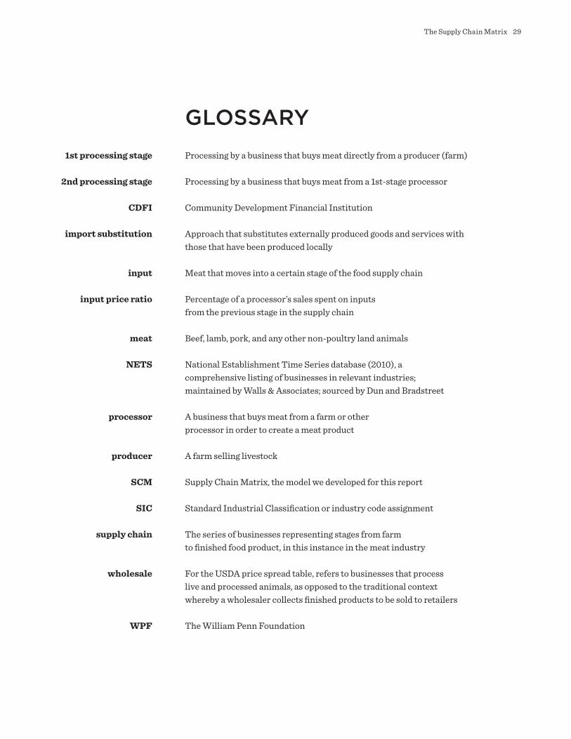
GLOSSARY

Processing by a business that buys meat directly from a producer (farm)

Processing by a business that buys meat from a 1st-stage processor

Community Development Financial Institution

Approach that substitutes externally produced goods and services with those that have been produced locally

Meat that moves into a certain stage of the food supply chain

Percentage of a processor’s sales spent on inputs from the previous stage in the supply chain

Beef, lamb, pork, and any other non-poultry land animals

National Establishment Time Series database (2010), a comprehensive listing of businesses in relevant industries; maintained by Walls & Associates; sourced by Dun and Bradstreet

A business that buys meat from a farm or other processor in order to create a meat product

A farm selling livestock

Supply Chain Matrix, the model we developed for this report

Standard Industrial Classification or industry code assignment

The series of businesses representing stages from farm to finished food product, in this instance in the meat industry

For the USDA price spread table, refers to businesses that process live and processed animals, as opposed to the traditional context whereby a wholesaler collects finished products to be sold to retailers

The William Penn Foundation

1st processing stage

2nd processing stage

CDFI

import substitution

input

input price ratio

meat

NETS

processor

producer

SCM

SIC

supply chain

wholesale

WPF


TRF has published a range of reports about food access. For details, please visit the Food Access section of TRF’s Policy Publications site at www.trfund.com/resource/policypubs.html:

“Access to Supermarkets in Inner-City Communities” (2008) Reinvestment Brief

“Estimating Supermarket Access and Market Viability: Summary of TRF’s Research and Analysis” (2010) Reinvestment Brief

“The PA Fresh Food Financing Initiative: Case Study of Rural Grocery Store Investments” (2012)

“Searching for Markets” (2011) LSA Analysis

Research conducted by Policy Solutions at The Reinvestment FundLance Loethen, Research AssociateScott Haag, Research AssociateBill Schrecker, Research AnalystIra Goldstein, President

Editing: Alison Rooney Communications, LLCLayout and Illustrations:Andee Mazzocco, Whole-Brained Design, LLC

July 2013

the supply chain matrix - wordpress.com

Documents