the swedish car movement data project final report....
TRANSCRIPT

The Swedish car movement data project Final report
Sten Karlsson
PRT Report 2013:1, Rev 2
Nov 2013
Division of Physical resource Theory Department of Energy and Environment
Chalmers University of Technology SE-41296 Gothenburg, Sweden

2
Summary The aim of this project has been to gather and analyze a larger amount of data on the characteristics and distribution of the movement patterns of individual, privately driven cars in Sweden by measurement with GPS equipment. Potential cars to be logged were recruited from a stratified random selection of cars from the Swedish motor-vehicle register. The GPS equipment was sent by mail to be installed by the owner/driver. Over 700 cars have installed the equipment for around two months each in 9 campaigns with up to around 100 logging units. The first measurement period started in June 2010 and the last ended in Sept 2012. The data (timestamp, position (horizontal and vertical) and velocity (speed and direction, and identity of used satellites) gathered with 2.5 Hz was transmitted via the mobile net to a intermediary server, for later transfer to a final storage together with road information in a source database, from which various basic data and statistics for the trips and cars have been extracted and stored, Fig S.1. The intended goal of the project has been to finally have high quality car movement data for at least one month for each of at least 500 representative cars.
Fig S.1 Overview of the Swedish car movement data project.
The project has resulted in a unique dataset on the detailed movements of representative vehicles from the current fleet of privately driven cars in Sweden. The database contains 714 cars with data, of which 528 cars have loggings exceeding 30 days and over 450 cars more than 50 days. The measurement project was initiated for the purpose of achieving appropriate data for various types of analyses connected to the electrification of cars. It is currently used extensively for such purposes. However, the databases freely available for all kinds of research devoted to vehicle movements, energy efficiency, and environmental performance as well as traffic safety and societal planning. Due to the privacy character of some of the data, the availability is further classified according to type. This revised final report presents the layout of the project, the performed measurements, experiences, and contrary to an earlier version results based on all the gathered data. This report is available at the project homepage (www.chalmers.se/brd).
Privately driven ICE cars
Position Velocity Satellite-id
Tele- matics server
Analysis database
Source database
GPS
Road data
Trip identif., statistics

3
Keywords — GPS measurement, car movement pattern, representative private driving, PHEV, Sweden Sammanfattning Syftet med detta projekt har varit att samla och analysera en större mängd data om egenskaper och fördelning av rörelsemönster för privatkörda personbilar i Sverige genom mätning med GPS-utrustning. Potentiella bilar att logga rekryterades brevledes från ett stratifierat slumpmässigt urval av bilar från bilregistret. GPS-utrustningen skickades med post att installeras av ägare/förare, Fig. S.1. Mer än 700 bilar har haft utrustning installerad i omkring två månader vardera i 9 kampanjer med upp till runt 100 utrustningar. Den första mätperioden startade i juni 2010 och den sista slutade i september 2012. Den med 2,5 Hz insamlade datan (tid, position (horisontellt och vertikalt), hastighet (fart och riktning), och identitet på använda satelliter) sändes via mobilnätet till en mellanhand server för överföring senare till en slutlig lagring tillsammans med väginformation i en källdatabas från vilken resor, och statistik för resor och bilar har extraherats och lagrats i en analysdatabas. Målet med projektet har varit att få högkvalitativa data för minst en månads bilrörelser för 500 representativa bilar. Projektet har resulterat i ett unikt dataset med detaljerade rörelsedata för representativa fordon från den nuvarande flottan av privatdrivna bilar i Sverige. Databasen innehåller 714 bilar med data varav 528 bilar med loggningar överskridande 30 dagar och över 450 bilar med mer än 50 dagars mätningar. Mätningen initierades för att få underlag för olika typer av analyser kopplade till elektrifiering av bilar. Datan används redan i stor utsträckning för sådana ändamål. Men databaser är fritt tillgänglig för alla typer av forskning ägnade åt fordons rörelser, energieffektivitet eller miljöprestanda samt trafiksäkerhet och samhällsplanering. På grund av den personliga karaktären av vissa data, klassificeras tillgängligheten ytterligare efter typ. I denna reviderade slutrapport presenteras utformningen av projektet, utförda mätningar, erfarenheter samt till skillnad från tidigare version resultat baserade på alla insamlade data. Denna rapport finns tillgänglig på projektets hemsida (www.chalmers.se/brd).

4
Table of contents
THE SWEDISH CAR MOVEMENT DATA PROJECT............................................................................6 1. WHY GATHER CAR MOVEMENT DATA? ........................................................................................7 2. SELECTION OF VEHICLES ...................................................................................................................9 2.1 EXCERPT OF CARS FROM THE MOTOR-‐VEHICLE REGISTER ............................................................................ 9 2.1.1 Vehicles ..............................................................................................................................................................9 2.1.2 Region ................................................................................................................................................................9
2.2 FURTHER REFINEMENT OF THE EXTRACTED OF CARS ................................................................................. 10 2.2.1 Type of cars................................................................................................................................................... 11 2.2.2 Owner’s addresses...................................................................................................................................... 11 2.2.3 Private driving............................................................................................................................................. 11 2.2.4 Car age............................................................................................................................................................ 12 2.1.5 Stratification ................................................................................................................................................ 13
2.3 RECRUITMENT .................................................................................................................................................... 19 2.3.1 The request ................................................................................................................................................... 19 2.3.2 Questionnaire response ........................................................................................................................... 19 2.3.3 Agreement..................................................................................................................................................... 20
2.4 TWENTY ELECTRIC VEHICLES........................................................................................................................... 20 3. THE LOGGING EQUIPMENT AND DATA HANDLING SYSTEM............................................... 22 3.1 LOGGING EQUIPMENT ........................................................................................................................................ 22 3.1.1 The GPS equipment ................................................................................................................................... 22 3.1.2 Modifications and repair ........................................................................................................................ 23 3.1.3 Logged signals ............................................................................................................................................. 23 3.1.4 Installation.................................................................................................................................................... 24 3.1.5 Logging procedure .................................................................................................................................... 24
3.2 DATA HANDLING................................................................................................................................................. 25 4. PROCESSED AND STORED DATA .................................................................................................. 27 4.1 DATA TRANSFERRED INTO THE SOURCE DATABASE AND THE ANALYSIS DATABASE............................. 27 4.1.1 Source database structure ..................................................................................................................... 27 4.1.2 Stored signals............................................................................................................................................... 27 4.2.3 Complementary data................................................................................................................................ 31
4.2 DERIVED DATA IN THE ANALYSIS DATABASE ................................................................................................ 31 4.4 WEB INTERFACE................................................................................................................................................. 33 4.5 AVAILABILITY...................................................................................................................................................... 33 4.6 POSSIBLE FURTHER POST-‐PROCESSING.......................................................................................................... 33
5. THE QUESTIONNAIRE ...................................................................................................................... 34 6. RESULTS ............................................................................................................................................... 35 6.1 PARTICIPATING CARS AND THEIR HOUSEHOLDS........................................................................................... 35 6.2 LOGGED DRIVING ................................................................................................................................................ 40 6.3 DATA LOSSES....................................................................................................................................................... 45 6.4 THE CAR MOVEMENTS ....................................................................................................................................... 47
7. EXPERIENCES...................................................................................................................................... 53 7.1 EXPERIENCES FROM THE ADMINISTRATION OF THE CAMPAIGNS.............................................................. 53 7.2. TECHNICAL ACCOMPLISHMENT OF THE MEASUREMENT............................................................................ 53 7.3. ACCOMPLISHMENT OF DATA HANDLING ....................................................................................................... 54 7.4. DRIVERS’ EXPERIENCES.................................................................................................................................... 54

5
8. CONCLUSIONS ..................................................................................................................................... 56 9. REFERENCES ....................................................................................................................................... 57 APPENDIX A. PAPERS, REPORTS AND PRESENTATIONS OF THE PROJECT ........................ 59 APPENDIX B. THE RECRUITMENT LETTER.................................................................................... 61 APPENDIX C. THE AGREEMENT SIGNED BY THE PARTICIPANTS........................................... 64 APPENDIX D. THE MOUNTING INSTRUCTIONS FOR THE MEASUREMENT EQUIPMENT 65 APPENDIX E. THE ROAD CLASSIFICATION..................................................................................... 67 APPENDIX F. THE DATA IN THE ANALYSIS DATABASE ............................................................. 68 APPENDIX G. THE QUESTIONNAIRE ................................................................................................ 79

6
THE SWEDISH CAR MOVEMENT DATA PROJECT
The aim of this project has been to gather and analyze a larger amount of data on the characteristics and distribution of the movement patterns of individual, privately driven cars in Sweden by measurement with GPS equipment. The project has been a research project titled “Measurement and analysis of vehicle movements in the Swedish car fleet of relevance to future electrification” (Sw.: Mätning och analys av bilrörelser i den svenska bilparken av relevans för framtida elektrifiering) in the Program Energy and Environment within the co-operation Strategic Vehicle Research and Innovation (Sw.: Fordonsstrategisk Forskning och Innovation (FFI)) at the Swedish Energy Agency (Sw.: Energimyndigheten) and Sweden’s Innovation Agency (Sw.: Vinnova). It has also from the beginning had financial support from Consat Sustainable Energy Systems AB, Göteborg Energy Research Foundation, Lindholmen Science Park AB, and Vattenfall AB. Telenor has contributed with provision of free of charge data traffic on its GPRS net. Also Chalmers University of Technology, through the Chalmers Energy Initiative, the Department of Energy and Environment and the Department of Signal and Systems, has financially supported the project. The build-up of the source database, the analysis database and the web page used for the project have been supported by the program Test Site Sweden at Lindholmen Science Park AB. The project was lead by Lindholmen Science Park (LSP) and the program Test Site Sweden (TSS). The scientific responsibility has been at the Department of Energy and Environment (Division of Physical Resource Theory) at Chalmers University of Technology, which also has developed the analyses database. The daily administration of the measurements and data storage has been performed by Consat Sustainable Energy Systems AB, Gothenburg. Chalmers Teknologkonsulter AB has been involved in the development of the webpage. A project steering group consisting of represents from the initial financial partners (which not included Telenor) have met a number of times during the project to discuss various issues of importance in the project. The project also had a reference group consisting of persons from other involved or interested parties: Telenor, The Swedish Road Administration/The Swedish Transport Administration, SUST, and SAFER and SHC at Chalmers University of Technology, that met a few times and was informed about and discussed the progress of the project.

7
1. WHY GATHER CAR MOVEMENT DATA?
For plug-in hybrid electric vehicles (PHEV), the optimal design, consumer viability, and its potential for transforming transportation to electric propulsion are dependent on the possibilities of the individual vehicles to substitute electricity for fuel. Major factors determining the possible driving on electricity are the battery capacity, the movement pattern of the individual car and the recharging possibilities in the form of available suitable infrastructure [1,2]. To facilitate a well-informed and efficient transition to electrified vehicles such as PHEVs we thus need knowledge of the distribution of individual vehicle’s movements over longer periods. Today there is a lack of good data on the movement patterns for the cars. What is at needed is enhanced data on car trip lengths and trip characteristics such as speed, load and orography to be able to determine the possible energy use for individual trips, time and duration both for the trips and the stops in between the trips. The position of the car, especially for the stops, can also be of importance for evaluation of possible recharging options. It is necessary to have car movement data for a longer period of time. The individual vehicle’s movement may not be fully captured without a time period of several months, or a year, considering the possible seasonality of driving, varying weather conditions and the low frequency of some purposes of the driving such as vacations. This is a type of data that has not been requested and gathered earlier, but which now with a possible approaching electrification of transport is urgently needed. National or regional travel survey data is regularly gathered in many countries. However, in most cases, as in Sweden [3], there is not a tracking of cars’ movements but of persons’ only, and in many countries also for one day each only. In Western Europe only a few countries in their National Travel Surveys gather information specifically on the movements for several days of the cars, for instance, UK for one week (and four weeks for long distance travel), and France for five days [3]. Also the data quality can be hampered by the survey method when based on questionnaires or interviews. It is commonly recognized that this type of self-reporting will give an underestimate of the travelling, due to a certain share of non-reported trips [4,5]. This type of data does not give the exact position of the vehicles trips and their stops. The purposes of the trips, divided into different categories such at to work, leisure activities, shopping, visits etc, are commonly gathered in travel surveys, though. Continuous measurement of time, speed and position with GPS (Global Positioning System) equipment is then a possibility to gather lacking information on car movement statistics. One drawback with this type of data is the lack of information of the purposes of the trips. On the other hand the position can give some clue to the some of the trips; regular workday parking in a non-residential area suggests trips for work. To actually excerpt this

8
information with a high degree of quality will require some effort, though, and availability of information on positions of working sites, etc [6]. It can also be argued that measurement of today’s car movement will not be representative for tomorrow’s battery electric vehicles. These are in the near future probably very limited by range and therefore used in other ways than the current cars, maybe only in cities and as second car. However, for plug-in hybrid electric vehicles the range will not be as great a concern and it can be a reasonable assumption that these vehicles will be used in similar way as today’s car. In countries like Sweden, with a fleet of for European condition relatively large cars, and which are also less subject to traffic jams, PHEVs will be the dominant electric vehicle type, according to many expert judgments. Therefore the movement patterns of current conventional vehicle fleet are of considerable interest. Other direct measurements of car movements with for instance GPS equipment have been sparse, for specific purposes, or focusing vehicles in specific areas. For instance, an old tracking of cars for one day each were performed in St Louis [7]. Puget Sound Regional Council in the Seattle area, performed a logging with GPS of three months driving of 450 vehicles from 275+ volunteer households recruited among potential participants before and after hypothetical tolls were charged for use of major freeways and arterials in the Seattle metropolitan area [8, 9]. In USA travel surveys with GPS, not directly focusing cars, have been performed or are planned in, Baltimore, Washington, Chicago, and California [10-13]. In Australia cars have been tracked for the purpose of investigating driver behavior such as speeding [14,15]. In Italy a unique commercial dataset for car movements is from the GPS tracking of currently around 650 000 cars for insurance profiling performed by the company Octotelematics [16]. In Canada, Department of Geography at University of Winnipeg within the AUTO21 program, has been logging 76 cars in Winnipeg with GPS at one-second intervals for up to 12 months, to be able to, for instance, assess the prerequisites for electrification with PHEVs. A further logging of 50 rural vehicles often commuting into Winnipeg has also been performed. [17, 18, 19] In Sweden specific datasets with GPS tracking are available for a small set of 29 cars logged for about two weeks for the purpose of driving behavior – emissions modeling verification [1]. In this case equipment was installed in 5 specifically prepared vehicles, which then were successively placed in 29 families, where they substituted a car of similar size. In another measurement for the evaluation of the impact and acceptability of Intelligent Speed Adaptation (ISA) equipment, about 200 cars were tracked for roughly 100 days [2]. Although valuable, both these datasets are covering limited geographic regions and are at this moment more than ten years old.

9
2. SELECTION OF VEHICLES
2.1 Excerpt of cars from the motor-vehicle register First, for each campaign an excerpt of cars from the Swedish motor-vehicle register (Sw.: bilregistret) is performed, see Table 2.1.
Table 2.1 Excerpt of cars from the Swedish motor-vehicle register.
Parameter Selection Type of vehicle Passengers cars, type I
Use of vehicle Non-commercial vehicle (Sw.: ej yrkestrafik)
Model year Car model 2002 and younger
Region in Sweden Registered in Västra Götaland county or Kungsbacka municipality
2.1.1 Vehicles The excerpt is restricted to passenger cars of type I in the motor-vehicle register, Table 2.1. A passenger car is a car mainly aimed for person transport and restricted to a maximum of 8 passengers apart from the driver, i.e., a maximum total of 9 persons, and with a weight of maximum 3.5 tons. Passenger car of type I excludes type II cars which comprise cars with a bodywork permanently equipped with an accommodation unit, e.g., campers (SIKA Fordon 2009, SFS 2001:559 2§).
Vehicles, which, according to the vehicle register, are used in commercial traffic, such as taxicabs, are not included in the excerpt due to the focus on privately driven cars. The excerpt is also restricted to cars of model year 2002 and younger.
2.1.2 Region The extracted cars are registered in the county of Västra Götaland or in Kungsbacka municipality. The region is in South-West of Sweden and has around 1.6 million inhabitants and 0.75 million cars (roughly 1/6 of Swedish totals, respectively), Table 2.2 and Figure 2.1. It is reasonably representative of Sweden concerning average driving distance and car ownership and with its mixture of larger and smaller towns and rural areas. It contains Gothenburg, the second-largest town of Sweden. It is lacking very sparsely populated areas as in north of Sweden, though, which is reflected in the population density of around 65 inhabitants/km2; three times the average for Sweden, but reasonable representative for the southern parts of Sweden where most of the inhabitants live.

10
Table 2.2 Data for the selected region at the end of 2010a.
Parameter Västra Götaland (VG) county and Kungsbacka municipality
Sweden Quota for Region/Sweden
Inhabitantsa 1 655 322 9 415 570 0.176 Land areab (km2) 25 424 449 964 0.0565 Inhabitant/area (km-2) 65 21 3.1 Registered cars in usec 749 814 4 335 182 0.173 Cars/1000 inhabitants 453 460 0.984 Average driving distance in 2008d (km)
13 610 (VG only) 13390 1.016
a [SCB, Folkmängd i riket, län och kommuner 31 december 2010 och befolkningsförändringar 2010] b Wikipedia.se Accessed 2011-05-13 c [Trafikanalys, Fordon i län och kommuner 2010] d [Trafikanalys, Körsträckor 2008]
a) b)
Figure 2.1 The selected region for the Swedish car movement data project, a) the Västra Götaland county is marked in darker blue on this map of Sweden; b) A larger map of Västra Götaland county with its 49 municipalities. The Kungsbacka municipality in the county of Halland, also included in the selected region, is the uppermost coastal municipality on the west coast south of Västra Götaland.
2.2 Further refinement of the extracted of cars A further refinement of the extracted cars is performed to achieve the final selection.

11
2.2.1 Type of cars Electric vehicles, of which only a few exist though, are excluded, due to their range limitation and therefore possible specific movement pattern. (In the project specifically also 20 electric cars are logged, but from another selection, see Chapter 2.4.)
2.2.2 Owner’s addresses Several cars have their owners not living within the region or companies situated in another area according to the registered postal address. This can concern cars with owner in a completely different part of the country such as Stockholm. It can also be owners with addresses belonging to a postal office close to, but outside the border. The selection is further restricted to owners of the cars with their addresses belonging to postal offices within the region. This restriction is accomplished by only including cars with owners having addresses with postal code number between 40000 – 54999 and 66000 – 66999. This realization of the selection may introduce ambiguity in some areas where the postal and county/municipality borders do not overlap. However, this should not be any concern for the purpose of this project.
The effects of the further refinements mentioned above is that about 0.5‰ of the cars belonging to natural persons (≈ 340 000) was excluded, and 1.5% of the cars registered for juridical persons (≈ 43 000) was not included in the final selection.
2.2.3 Private driving Cars owned by companies or public institutions may be used in specific ways dependent on the situation specific for each vehicle, for instance, to transport personnel between patients in the eldercare. Use patterns of these cars are less representative and can sometimes be reasonably gathered by other means and have therefore not been included in this study focusing privately driven cars. In the Swedish motor-vehicle register the owner/leaser is either a juridical person or a natural person. For the fleet from which the recruitment of cars occurs, the share of juridical persons is almost 12%. Many of these cars are company cars, i.e., cars leased or owned by companies or institutions, but to a large extent used by a person for his private driving. Roughly every second new car in Sweden is a company car. They are normally kept for 3 years, before entering the private car market as used cars. The Swedish motor-vehicle register does not keep track of company cars; it is not an administrative but a fiscal issue. A company car is supposed to be a fringe benefit in the Swedish income tax return if used for private driving more than 10 times a year or more than 1000 km/yr. If so, the taxed fringe benefit is relatively high and independent of the amount of private driving. It is therefore not favorable to have a company car if you do not drive much. The amount of private driving can therefore be supposed to be a strong selection for privately driven cars with juridical person ownership. In this study we extract the company cars by, for cars with a juridical person ownership, addressing the inquiry letter to the driver of the specified car and ask if it is a company car. If so, it is of interest to the project. Also cars registered as owned by a natural person can be a car owned by a private firm and not used for private

12
driving. Also for these cars we thus need to in the inquiry initially ask if it is a privately driven car. By a communication mistake this question were not included in the request, though. A few of the cars in the final dataset have therefore not been privately driven. Company cars (Sw.: förmånsbilar) consist of two categories of vehicles, private cars and light trucks. The private cars are largely a fringe benefit for employees in usually a bit larger companies or organizations. The owner in the motor-vehicle register is then a juridical person, who may be the employer, which either owns or leases the vehicle from a leasing company. The vehicle can also be registered for a company that leases the car to the company where the beneficiary is employed. Whoever owns depends on how the lease/loan agreement is designed, but the case in which the employer is the owner is the most common. But in both cases the vehicle may be registered in a place other than that where the beneficiary lives. First, of course, work place and residence address may differ. But the company that is the registered owner can have the car registered anywhere else than on the beneficiary’s workplace address. In larger companies with workplaces and offices at various places in the country, this is rather likely. In the case that a leasing company owns the car, this is very likely. Large such firms may operate nationally with a head office and the cars registered in for instance the Stockholm area. Light trucks are driven as company cars by employees in any company or by individual entrepreneurs. For employees most often holds, determined by the employer, that the truck may not be used for private purposes other than perhaps for commuting between work place and home if the truck is stationed there. This private driving to and from work is then not due to benefit taxation. For individual businesses the situation is different, especially if they do not have access to another car for personal driving. If they have no access to another car privately it can be difficult to demonstrate to the tax authorities that the truck is not used privately, and these light trucks must most probably be handled as a fringe benefit. The number of company cars, as well as how many of these are light trucks, are not available in official statistics. By using the tax register it is possible to obtain the number of company cars to private individuals resident (tax purposes) in different regions. A difficulty arises when one wants to discern how many of these are passenger cars, though. Also a linking to the vehicle register is not possible. Thus one has to estimate or guess how many company cars. In this project it has been assumed that 97% and 70% of natural and juridical persons’ cars, respectively, are privately driven. These figures have been used in a weighting to achieve a representative selection.
2.2.4 Car age In the register excerpt the car model year is limited to 2002 and younger in order to focus on that part of the car lifetime, which mostly influences the economic viability considerations and the purchase decision for new cars. As the study and selection is stretched out over one and a half year, the registration date is successively shifted toward later dates thus keeping constant the age of the oldest cars in the selected fleet. Initially for

13
the first period the registration date is set to March 1, 2002 and younger. It is then for the later campaigns shifted according to Table 2.3. The small difference in age is mainly due to differences between the expected campaign periods at the time for selections of cars and the actual campaign periods. This selection of younger cars constitutes roughly 45% of the car fleet and 60% of the total driving distance [15]. For the oldest cars the market value has sunk even more. Thus the selection represents a major share of the total economic value of the car fleet.
Table 2.3 Selections of cars according to age. Measurement campaign
Cars model year Cars registered at or later than
Campaign started Time since first registration (months)
1 2002+ March 1, 2002 Beg. of July 2010 ≈ 100 2 2002+ May 1, 2002 Mid of Sept 2010 ≈ 100.5 3a 2002+ July 1, 2002 End of Jan 2011 ≈ 103 4 2002+ Dec 1, 2002 Mid of May 2011 ≈ 101.5 4:1b 2002+ Feb 15, 2003 Beg. of July 2011 ≈ 100.5 4:2 2002+ May 1, 2003 Mid of Sept 2011 ≈ 100.5 5 2002+ July 1, 2003 Mid of Nov 2011 ≈ 100.5 6 2003+c Oct 1, 2003 Mid of March 2012 ≈ 101.5 7 2003+ Feb 1, 2004 Mid of June 2012 ≈ 100.5 a In campaign 3 the excerpt from the motor-vehicle register was the same as in campaign 2, which means that possible new cars registered between campaign 2 excerpt and the campaign 3 intended excerpt are missing in campaign 3. b No separate selection from the car register, but taken from unused positive responses from campaign 4. Same remark as in note 1 can be done. c The increase in model year from 2002 to 2003 excludes about 2200 cars with register date later than Oct 1, 2003.
2.1.5 Stratification The random selection is stratified into 14 groups along five parameters, which are known or thought to statistically influence the car movement patterns, Table 2.4. The cars are divided into privately owned cars and cars owned by juridical persons, the two categories available in the motor-vehicle register. The juridical cars focused here, the company cars, are supposed to possibly have another movement pattern then private cars, although this can not be directly confirmed in official statistics. In the statistics the driving by the juridical cars is larger than for private cars, see Table 2.5, which shows the average driving distance for cars of different owners. But the category juridical cars also contains other cars than company cars, for instance fleet cars and taxis. However, the privately seen capital costs for juridical cars are the direct and indirect effects of any salary adjustment and the tax on fringe benefit for the car (Sw. förmånsvärdet), which is independent of the yearly driving. Also the running costs can be lower. It is therefore reasonable to assume that these cars are chosen and driven by persons who expect to drive and will drive more than the average driver. Table 2.5 also shows the “leased cars” category, which probably to a large extent consists of company cars. Apparently this data does not contradict the assumption.

14
Table 2.4 The applied stratification of the vehicle selection into 14 groups.
Stratification parameter Fleet Ownership Geographic
areaa Fuel Car ageb Kerb
weightc
Strata designation
Heavy GB7T Young Light GB7L
Heavy GB6T
All other fuelse
(AOF) Old
Light GB6L Young GD7
Gothenburg, Mölndal, Partille
Diesel Old GD6
Heavy ÖB6T Young Light ÖB6L Heavy ÖB7T
AOF
Old Light ÖB7L
Young ÖD7
Natural persond
Remaining region
Diesel Old ÖD6
AOF JB
Selected fleet
Juridical persond
Diesel JD
a Place of registration: Gothenburg, Mölndal and Partille are the three more densely populated municipalities in and around Gothenburg These are determined by the LKF-code (Sw.: LKF-kod) 1480xx, 1481xx, and 1402xx, respectively. b Car model year: Young = model year 2007 and younger. The registration date is successively adjusted for the selections to later campaigns, see Table 4. c Kerb weight (Sw.: tjänstevikt) (vehicle mass + 75 kg for driver): Heavy ≥ 1500 kg. d 30% of the vehicles owned by a juridical person are initially assumed not to be privately driven to a large extent. Corresponding figure for vehicles owned by a natural person are assumed to be 3%. e Except electricity. In the end of April 2012, there were in the geographic area in question 81 electric vehicles registered of model year 2003 and newer, of which 79 were registered for juridical persons.
Table 2.5 Average yearly driving for cars of different owners in year 2008 [Source: Trafikanalys, Körsträckor 2008] Owner Average annual driving
distance (km) Natural persons 12 420 - Men 11 890 - Women 12 680 Juridical persons 16 800 - of which personal enterprises 15 140 Total 13 390 - of which leased cars 20 140 - of which taxi 72 240 The diesel car is more expensive than the corresponding gasoline model, while the operating costs are lower due to the more energy efficient engine and also cheaper fuel (in recent years not always per liter (SKR/liter) but so far per energy unit due to the higher energy density (MJ/liter) of diesel). This leads to an expected considerably larger yearly driving for diesel cars, which is also reflected in the statistics, see Table 2.6. The diesel cars have almost twice the driving distance compared to gasoline cars. Due to the relatively recent interest in the diesel cars, these are also newer which should explain part o the difference.

15
Table 2.6 Average yearly driving for cars with different fuels in Sweden 2008. [Source: Trafikanalys, Körsträckor 2008] Fuel Number of cars
Average annual driving distance (km)
Gasoline 4 202 558 12 180 Diesel 469 922 22 740 Natural gas/Biogas 12 570 23 620 E85 143 168 16 950 Electricity 157 5 310 Others 14 068 17 610 Total 4 842 443 13 390
Table 2.7 Average yearly driving for cars of different model year/manufacturing year in 2008. [Source: Trafikanalys, Körsträckor 2008]
Model year/ manufacturing yeara
Average annual driving distance (km)
2000 13 960 2001 14 620 2002 15 250 2003 15 880 2004 17 370 2005 18 220 2006 19 310 2007 19 730
a Denotation according to the data source, which do not differ between model and manufacturing year. We have stratified the cars geographically in two groups: those situated in or around Gothenburg and the rest of the selected area. The Gothenburg area includes the municipalities of Partille and Mölndal, which are indivisible parts of the town area. It is assumed that the movement pattern in this larger town area can possibly differ considerably from the rest in various aspects. Younger cars are often used more intensively than older ones, see Table 2.7. The cars are stratified along age in two groups according to Table 2.8. Table 2.9 and Figure 2.2 give the resulting number of vehicle in the different strata for the 9 different measurement campaigns. We can observe that during the measurement campaigns covered by the project, the number of diesel cars have increased considerable on the expense of cars propelled by other fuels, although the total number of cars has increased with around 2% in this period. The distribution of cars in different strata over four groups of differently sized municipalities is exemplified in Fig 2.3. We can conclude that diesel cars, especially older ones, are more common in the smaller municipalities, while new and smaller gasoline cars are more common in larger cities, (a-c). Cars owned by juridical persons are more common in larger cities, and especially in the Gothenburg area, (d). Also, there is a tendency that the cars in larger municipalities are smaller and less old, (e-f).

16
Table 2.8 Determination of the strata “young cars” in the age stratification in the different logging campaigns.
Young car if Campaign
Model year Registered at or later than
Measurement campaign started roughly
Time since first registration of oldest car in the young car strata [months]
1 2007+ March 1, 2007 Beg. of July 2010 ≈ 40
2 2007+ May 1, 2007 Mid of Sept 2010 ≈ 40.5 3 2007+ Sept 16, 2007 End of Jan 2011 ≈ 40.5 4 2007+ Dec 1, 2007 Mid of May 2011 ≈ 41.5 4:1 2007+ Feb 15, 2008 Beg. of July 2011 ≈ 40.5 4:2 2007+ May 1, 2008 Mid of Sept 2011 ≈ 40.5 5 2007+ July 1, 2008 Mid of Nov 2011 ≈ 40.5 6 2008+ Oct 1, 2008 Mid of March 2012 ≈ 41.5 7 2008+ Feb 1, 2008 Mid of June 2012 ≈ 40.5
Table 2.9 Number of vehicles in the different strata at the time for excerpt of the data from the motor-vehicle register.
Strata desig-nation
Measurement campaigna / date for excerpt of natural person (P) and juridical person (J) cars
1 2010-04-28 (P) 2010-04-27 (J)
2 2010-07-28(P) 2010-07-28(J)
4 2011-02-14(P) 2011-02-14(J)
5 2011-10-09(P) 2011-10-09(J)
6 2012-01-12(P) 2012-01-12(J)
7 2012-04-26(P) 2012-04-24(J)
Mid date valueb
Share (%)
Mid date value, privately drivenc,
Share (%)
GB7T 5 202 5 089 4 464 4 759 4108 4095 4584 1.26 4446 1.31 GB7L 17 123 17 324 15 678 15 354 14681 14700 15831 4.36 15357 4.51 GB6T 21 844 22 037 21 082 19 853 19244 18763 20579 5.66 19962 5.86 GB6L 37 413 37 573 37 725 37 599 37060 36470 37344 10.28 36223 10.63 GD7 8 321 8 804 10 168 12 545 12745 14046 10966 3.02 10637 3.12 GD6 4 099 4 504 6 028 8 012 8932 9950 6866 1.89 6660 1.95 ÖB7T 12644 12 584 11 007 4 759 10361 10520 11401 3.14 11059 3.25 ÖB7L 28 934 29 945 27 596 15 354 26699 26896 27976 7.70 27136 7.97 ÖB6T 55 832 56 114 53 334 19 853 49377 48542 52592 14.47 51014 14.97 ÖB6L 78 438 78 043 77 004 37 599 74063 72503 76033 20.93 73752 21.65 ÖD7 24 114 24 473 27 063 12 545 33196 36938 29526 8.13 28641 8.41 ÖD6 17 225 18 325 23 811 8 012 32237 35480 26049 7.17 25267 7.42 JD 18 645 19 419 21 579 25 194 26398 27613 22987 6.33 16091 4.72 JB 24 112 21 987 20 663 19 478 18757 18183 20618 5.67 14433 4.24 TOTAL 353 946 356 221 357 202 372 277 367858 374699 363352 100 340678 100 a In campaign 3 the excerpt from the motor-vehicle register was the same as in campaign 2, adjusted for age of cars and in the division between age strata. This means that new cars registered between the excerpt for campaign 2 and any possible date for excerpt for campaign 3 is missing. b Linear regression to day 365 after first excerpt 2010-04-28 (or ≈ 2011-04-28. i.e., ≈ 12 months ) c For natural and juridical person 97% and 70%, respectively, are assumed to be privately driven.

17
Figure 2.2 Number of vehicles in the different strata at the time for excerpt of the data from the motor-vehicle register.
0
10000
20000
30000
40000
50000
60000
70000
80000
90000
0 200 400 600 800
Num
ber of cars
Days from Qirst extract
GB7T
GB7L
GB6T
GB6L
GD7
GD6
ÖB7T
ÖB7L
ÖB6T
ÖB6L
ÖD7
ÖD6
JD
JB

18
a) b)
c) d)
e) f)
Figure 2.3 Distribution of weighted privately driven cars in various strata in four groups of municipalities from large to small ones according to the size of the car fleet in the municipality. GBG, PRT, MDL = Göteborg, Partille, Mölndal. Data from the Swedish motor-vehicle register excerpt 2011-02-14 to campaign 4.
0,6 0,7 0,8 0,9 1
1,1 1,2 1,3 1,4 1,5 1,6
B7T
B7L
B6T
B6L 0,6 0,7 0,8 0,9 1
1,1 1,2 1,3 1,4 1,5 1,6
D7
D6
0,6 0,7 0,8 0,9 1
1,1 1,2 1,3 1,4 1,5 1,6
viktad B
viktad D 0,6 0,7 0,8 0,9 1
1,1 1,2 1,3 1,4 1,5 1,6
JD
JB
0,6 0,7 0,8 0,9 1
1,1 1,2 1,3 1,4 1,5 1,6
Viktad T
Viktad L 0,6 0,7 0,8 0,9 1
1,1 1,2 1,3 1,4 1,5 1,6
Viktad 7
Viktad 6

19
2.3 Recruitment
2.3.1 The request The recruitment of vehicles was accomplished with a request to a random selection of car owners contained in the refined excerpt from the motor-vehicle register. A request letter was sent to the owner with an inquiry to participate in the measurement campaign. The second campaign was checked for overlap with the first one. Due to the time consuming process this was not performed in the later campaigns. It can be estimated that about 150 cars have been contacted more than ones. Also owners may have been contacted for different vehicles. In the final measurement one car has been logged twice: in campaign 1 as well as in campaign 5, though. Table 2.10 gives the number of persons contacted in each campaign.
Table 2.10 Number of person inquired for participation in the project. Campaign Number of cars/persons inquired Positive answerb
1 1603 (in two batches) ≈ 98 2 2000 ≈ 228 3a 340 n.a. 4 1939 ≈ 135
4:1a - - 4:2 475 ≈ 30 5 2000 ≈ 130 6 2000 ≈ 150 7 2000 ≈ 161
All 12357 ≈ 932 a In campaigns 3 and 4:1, leftover inquiries from the proceeding campaigns was used. b Somewhat ambigious, when extra positive answers can have been registered after the specific moment at which the numbers were counted (around three 3-4 weeks after inquiry). For private cars the request was addressed to the owner of the vehicle. For car owned/leased by juridical persons the addressing was to the driver of the selected vehicle specified by its registration number but with postal address of the juridical person. Small changes to the originally formulated recruitment letter have occurred with time due to achieved experience and successive changes in the implementation of the project. For instance, it was only from campaign 3 and forward explicitly stated that we were only interested in privately driven cars. The recruitment letter as sent out in the latest campaigns is reproduced in Appendix B.
2.3.2 Questionnaire response Table 2.10 gives an estimate of number of positive responses from the inquired persons. Altogether more than 900 persons have agreed to participate in the different campaigns. The figures are given as rough numbers. Because we need the response within a certain time to be useful, the exact number depends on at which time you count them. In campaign

20
2 a larger number of persons gave a positive answer. It was used to decrease the amount of requests in campaign 3. The in-time positive response frequency of the inquiry for participation in the campaigns has been around 7.5%. The number of requests is a balance between fulfilling the requirements set up and the costs for the mailings and handling of the answers. It can’t be guaranteed that enough positive answers can be obtained with a specific number of requests, especially if it is also required that each of the strata should be filled with enough vehicles. The actual number (around 2000 requests per campaign) is therefore a compromise between costs and fulfillment of the requirements. In practice each of the strata has not always been filled up. The number of necessary requests was a learning process. From campaign 2 and on it has been about 20 times the number of actually needed cars in the campaigns, with some adjustment in the different strata due to size and response frequency, although it has been difficult to see a stable response frequency between different strata. In the first campaign two batches of requests were sent out before we had enough participants. Also, in the first campaign a reminder was sent out a week after the second batch. The effect of the reminder on the response frequency was low though, why this reminder for cost reasons has been skipped in the requests for later campaigns. Instead a large enough number of requests was decided to be sent out.
2.3.3 Agreement A positive response to the request is announced by sending back a signed agreement, which was sent together with the request. The agreement is reproduced in Appendix C. With the signing, the participant confirms that he/she will participate in the logging, install and take care of the equipment and send it back when the measurement is finished, and allows the gathered data to be stored and be used for research concerning movement patterns, energy efficiency and environmental properties of vehicles, and concerning traffic and social planning. The participant is free to leave the project at any time without motivation.
2.4 Twenty electric vehicles Within the project also 20 electric vehicles should be logged in the same manner as the 500 ordinary cars. In the current situation not enough electric vehicles have been available, i.e., vehicles that are of newer model year in the region in question, see Table 2.11. The electric cars owned by juridical person are (almost) exclusively not driven for private reasons.
Table 2.11 Number of electric vehicles of model year in question (see Table 2.3) in this study in Västra Götaland + Kungsbacka.
Owner Date Juridical person Private person
April 2010 8 2 May 2012 79 2

21
It was decided in the steering committee, though, that for fulfillment of the project goal it was enough to refer to the data that has been gathered from loggings of electric cars driven in Malmö in the EU project Green eMotion. The logged data is stored in the same way in the same databases as for this project. The results of the Green eMotion project are not further discussed here.

22
3. THE LOGGING EQUIPMENT AND DATA HANDLING SYSTEM
3.1 Logging equipment
3.1.1 The GPS equipment During the start-up phase of the project needed to select suitable logger equipment. A requirement for the choice of equipment has been to avoid any possible inference with the car’s electronic system, for instance, by a connection to the CAN bus. Also, after consideration of the possible handling costs for different ways of distributing/installing the equipment, it was decided that the equipment should be able to be sent to the car owner/driver by ordinary mail services for installation by her/himself. Several alternatives were examined, including a smart phone with GPS, but problems with the accuracy made it unsuitable. At the end a commercially available logger from Host Mobility was selected, the MX3, Fig 3.1. It is a dedicated GPS logger with GSM modem and the possibility to store data locally on a memory card. The equipment includes a roof-mounted (magnetic holder) antenna, supplied from the 12V outlet in the car. The logged data is successively transmitted in batches (after intermediate storage on a micro SD-card situated in the equipment box) on the mobile net (gprs) for intermediary storage on a server. The micro-card storage allows for storing data for a longer period without contact with the mobile net. This means, for instance, that also movement patterns for driving abroad can be gathered.
Table 3.1 Specifications of the Fastrax IT500 GPS module [Source: Fastrax datasheet] General SPS 22 + 66 channels
Update rate 1 fix/s (user configurable)
Position 1.8 m (CEP) Circular Error of Probability (horizontal position)
Velocity 0.1 m/s
Accuracy
Time +/- 50ns RMS
Cold Start 34 s typical
Warm Start 3 s typical
TTFF
Hot start 1 s typical
Acquisition (cold) -148 dBm
Navigation -165 dBm
Sensitivity
Re-acquisition -160 dBm
Operating temperature -40°C to +85°C
Chip set MediaTek MT3329
Other
Firmware AXN 1.3
Memory 4 Mbit Flash

23
The gprs communication is bidirectional making updating of the software and control of the equipment possible.
Figure 3.1 The GPS equipment. The logger is contained in a box with antenna for gprs communication (short stick mounted to the right). It is powered via a connector plug for 12 V outlet ((black/red in the middle) and supported with a GPS antenna with a magnetic holder for car roof mounting (blue “puck” to the left).
3.1.2 Modifications and repair The unit was adapted for the project. The sampling frequency was increased from 1 to 2.5 Hz, to get a better basis for using the data for simulation. A larger memory card was installed to be able to store data for a longer period without mobile net coverage, for instance, when abroad. The equipment was also adjusted for handling the different applied power outlet strategies when the car is turned off. During the project the software has also been updated due to detected malfunctioning, further discussed later in Section 7.2.
3.1.3 Logged signals The signals logged by the equipment are
• Timestamp (current and last valid) • Position (latitude, longitude and altitude) • Velocity (speed and direction) • Used satellites (identity) • Dilution of precision (pdop, hdop, vdop)

24
• Over-the-air-provision OTAP Further specification of the logged and stored signals is given in Ch 4.
3.1.4 Installation The equipment was sent to the driver/owner by ordinary mail in a protected envelope. The users are supposed to install the equipment in the chosen car as soon as possible when they receive it. The installation of the equipment and the measurement campaigns are supported by information appended to the equipment, see Appendix D. This information has also been available at the project’s homepage [21]. The installation is very easy, the unit should be placed somewhere where it is not in the way and then place the magnetic antenna on the roof and the power cord in the cigarette lighter outlet. A branch connector to be put in the 12 V power outlet make it possible to also connect other equipments to the same outlet as the logging equipment. A branch connector has been available on request from the beginning of the project, but not many persons have requested one. We have seen in the data and in the comments done in the questionnaire that persons have disconnected the GPS to, for instance, charge their mobile phone or occasionally connect entertainment facilities. In campaign 6 a branch connector has been included in the measurement equipment and sent out together with all the GPS units. Because a considerable share of these were not returned with the equipment after the campaign, it was decided in campaign 7 to once again only send out these connectors on request.
3.1.5 Logging procedure When installed the unit will work autonomously. Each time the car is started the MX3 will power up and start recording GPS positions etc to its working memory. When a certain number of measurements have been made, the MX3 will normally connect via GSM to the TSS Telematics server and transmit the data. If it is not possible to connect the data will be saved on the memory card and it will be transmitted later when the MX3 has GSM coverage again. This can occur for example, when the car is in a tunnel or abroad. The GSM subscription was only for Sweden. When the logging period comes to its end, a signal is sent to the unit by the administrator. The unit will then beep the first time it is active. The user is then supposed to disconnect the unit, put it in the supplied, padded and addressed envelope and put it in a mailbox. From campaign 4-2 and on, the car odometer readings at the mounting and uninstall of the equipment were asked for. The readings are then possible to use for, for instance, comparison to the actually logged total distances. (The readings are not stored in the database, though.)

25
3.2 Data handling A system for communication and handling of the data has been built for this as well as other projects at Lindholmen Science Park The complete data handling system is still (2012) at a constant developing state due to the requirements of new project and new types of measurements. The basic parts of the system are shown in Fig 3.2.
Figure 3.2 Data collection, storage and analysis system for car movement data.
The MX3’s collect data in packages corresponding to 1 – 3 minutes of data and transmit them as byte streams via tcp/ip to the TSS Telematics server. The Telematics server translates the data and packs and stores measurements into files. The Telematics server then, normally once a day, automatically puts together files from each MX3 unit in a new file, marks and pushes it to an FTP server. The TSS server pulls (so far by a manual initiation of the administrator) the files from the FTP server and places each measurement in the SQL database (Schema “tss-ev”). The script also assigns a road point to each data point with the help a shape file derived from the The Swedish National Road Database (NVDB), and adds an identifier for road type and speed limit into the TSS SQL database. The SQL database is organized in an expandable way, so that additional data sources can be introduced continuously without affecting already collected data. Now super users can pull data from the source database and do advanced analyses on the data. But this requires good SQL knowledge, which may not be the case for most users. Therefore also basic analyses of the data are made (also so far manually initiated) and the

26
results are placed in a separate analysis database (Schema “tss_calc”). From the analysis database, a web server will present the analyzed data on a web page. On this web page normal users can analyze and download their own data in an easy but yet powerful way. (The scheme for the data handling presented here is not restricted to the car movement data project, but is used for other measurements as well.)

27
4. PROCESSED AND STORED DATA
4.1 Data transferred into the source database and the analysis database
4.1.1 Source database structure The current (autumn 2012) basic data structure of the source database (Schema “tss_ev”) is shown in Fig 5.2.
4.1.2 Stored signals As mentioned the signals logged are • Timestamps (current and last valid) • Position (latitude, longitude and altitude) • Velocity (speed and direction) • Used satellites (identity) • Dilution of precision (pdop, hdop, vdop) • OTAP
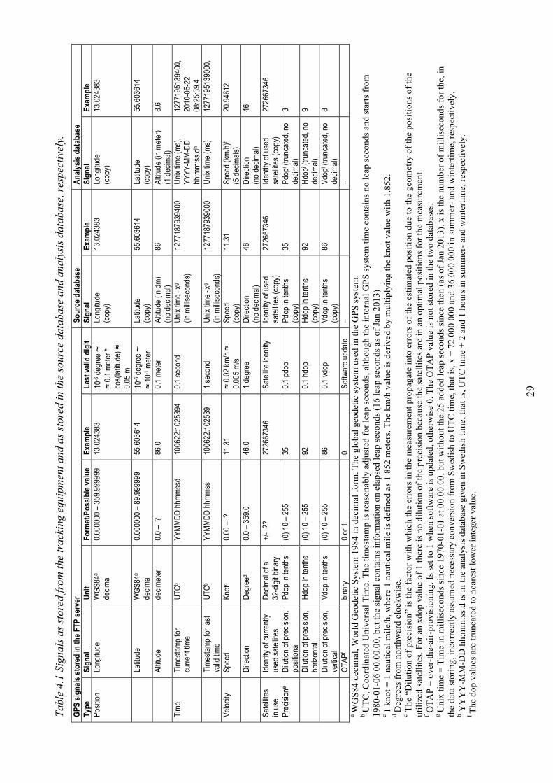
The logging frequency for all data is 2.5 Hz, i.e., the position and speed etc are logged every 0.4 second. Table 4.1 gives the signals stored in the source database (Schema “tss_ev”, Tables “SAMPLE_BRD_SET1-9”) and in the analysis database (Schema “tss_calc”, Tables “device_data”) and their format. The horizontal position is given in longitude and latitude according to the standard used in the GPS system, WGS84. The values are given with six decimals and copied into the databases. One degree in latitude corresponds to roughly 105 meters why the last digit corresponds to roughly decimeters. The last digit in the longitude must be multiplied by the cosine for the latitude, which at our latitude (around 58 degrees in Västra Götaland) gives that the last digit corresponds to only around half a decimeter. The vertical position, the altitude, is given in decimeters above the modeled mean sea level (msl) in WGS84. The used msl local value is probably interpolated from a lock-up table if state of the art for cheap GPS receiver technology is used, which it is no reason to question. This WGS84 mean sea level can differ considerably from the real sea level locally, why the absolute value in the altitude can be less accurate.

Fi
gure
4.1
Dat
abas
e st
ruct
ure
of th
e TS
S SQ
L so
urce
dat
abas
e (S
chem
a “t
ss_e
v”) a
s of O
ct 2
012.
29
Tabl
e 4.
1 Si
gnal
s as s
tore
d fr
om th
e tr
acki
ng e
quip
men
t and
as s
tore
d in
the
sour
ce d
atab
ase
and
anal
ysis
dat
abas
e, re
spec
tivel
y.
GPS
sig
nals
sto
red
in th
e FT
P se
rver
So
urce
dat
abas
e An
alys
is d
atab
ase
Type
Si
gnal
Un
it
Form
at/P
ossi
ble
valu
e
Exam
ple
Last
val
id d
igit
Sign
al
Exam
ple
Sign
al
Exam
ple
Posi
tion
Long
itude
W
GS8
4a de
cim
al
0.00
0000
– 3
59.9
9999
9 13
.024
383
10-6
deg
ree !
! 0.
1 m
eter
* co
s(la
titud
e) !
0.
05 m
Long
itude
(c
opy)
13
.024
383
Long
itude
(c
opy)
13
.024
383
La
titud
e W
GS8
4a
deci
mal
0.
0000
00 –
89.
9999
99
55.6
0361
4 10
-6 d
egre
e !
! 10
-1 m
eter
La
titud
e (c
opy)
55
.603
614
Latit
ude
(cop
y)
55.6
0361
4
Al
titud
e de
cim
eter
0.
0 –
?
86.0
0.
1 m
eter
Al
titud
e (in
dm
) (n
o de
cim
al)
86
Altit
ude
(in m
eter
) (1
dec
imal
) 8.
6
Tim
e
Tim
esta
mp
for
curre
nt ti
me
U
TCb
YYM
MD
D:h
hmm
ssd
1006
22:1
0253
94
0.1
seco
nd
Uni
x tim
e - xg
(in m
illise
cond
s)
1277
1879
3940
0 U
nix
time
(ms)
, YY
YY-M
M-D
D
hh:m
m:s
s.dh
1277
1951
3940
0,
2010
-06-
22
08:2
5:39
.4
Ti
mes
tam
p fo
r las
t va
lid ti
me
U
TCb
YYM
MD
D:h
hmm
ss
1006
22:1
0253
9 1
seco
nd
Uni
x tim
e - xg
(in m
illise
cond
s)
1277
1879
3900
0 U
nix
time
(ms)
1277
1951
3900
0,
Ve
loci
ty
Spee
d Kn
otc
0.00
– ?
11
.31
! 0.
02 k
m/h
!
0.00
5 m
/s
Spee
d
(cop
y)
11.3
1 Sp
eed
(km
/h)b
(5 d
ecim
als)
20
.946
12
D
irect
ion
Deg
reed
0.0
– 35
9.0
46.0
1
degr
ee
Dire
ctio
n
(no
deci
mal
) 46
D
irect
ion
(n
o de
cim
al)
46
Sate
llites
in
use
Id
entit
y of
cur
rent
ly
used
sat
ellit
es
Dec
imal
of a
32
-dig
it bi
nary
+/
- ??
27
2667
346
Sate
llite
iden
tity
Iden
tity
of u
sed
sate
llites
(cop
y)
2726
6734
6 Id
entit
y of
use
d sa
tellit
es (c
opy)
27
2667
346
Prec
isio
ne D
ilutio
n of
pre
cisi
on,
posi
tiona
l Pd
op in
tent
hs
(0) 1
0 –
255
35
0.1
pdop
Pd
op in
tent
hs
(cop
y)
35
Pdop
i (tru
ncat
ed, n
o de
cim
al)
3
D
ilutio
n of
pre
cisi
on,
horiz
onta
l H
dop
in te
nths
(0
) 10
– 25
5 92
0.
1 hd
op
Hdo
p in
tent
hs
(cop
y)
92
Hdo
pi (tru
ncat
ed, n
o de
cim
al)
9
D
ilutio
n of
pre
cisi
on,
verti
cal
Vdop
in te
nths
(0
) 10
– 25
5 86
0.
1 vd
op
Vdop
in te
nths
(c
opy)
86
Vd
opi (
trunc
ated
, no
deci
mal
) 8
O
TAPf
bina
ry
0 or
1
0 So
ftwar
e up
date
–
–
a W
GS8
4 de
cim
al, W
orld
Geo
detic
Sys
tem
198
4 in
dec
imal
form
. The
glo
bal g
eode
tic sy
stem
use
d in
the
GPS
syst
em.
b U
TC, C
oord
inat
ed U
nive
rsal
Tim
e. T
he ti
mes
tam
p is
reas
onab
ly a
djus
ted
for l
eap
seco
nds,
alth
ough
the
inte
rnal
GPS
syst
em ti
me
cont
ains
no
leap
sec
onds
and
star
ts fr
om
1980
-01-
06 0
0.00
.00,
but
the
sign
al c
onta
ins i
nfor
mat
ion
on e
laps
ed le
ap se
cond
s (16
leap
seco
nds a
s of J
an 2
013)
c 1
knot
= 1
nau
tical
mile
/h, w
here
1 n
autic
al m
ile is
def
ined
as 1
852
met
ers.
The
km/h
val
ue is
der
ived
by
mul
tiply
ing
the
knot
val
ue w
ith 1
.852
. d D
egre
es fr
om n
orth
war
d cl
ockw
ise.
e T
he “
Dilu
tion
of p
reci
sion
” is
the
fact
or w
ith w
hich
the
erro
rs in
the
mea
sure
men
t pro
paga
te in
to e
rror
s of t
he e
stim
ated
pos
ition
due
to th
e ge
omet
ry o
f the
pos
ition
s of t
he
utili
zed
sate
llite
s. Fo
r an
xdop
val
ue o
f 1 th
ere
is n
o di
lutio
n of
the
prec
isio
n be
caus
e th
e sa
telli
tes a
re in
an
optim
al p
ositi
ons f
or th
e m
easu
rem
ent.
f OTA
P =
over
-the-
air-
prov
isio
ning
. Is s
et to
1 w
hen
softw
are
is u
pdat
ed, o
ther
wis
e 0.
The
OTA
P va
lue
is n
ot st
ored
in th
e tw
o da
taba
ses.
g U
nix
time
= Ti
me
in m
illis
econ
ds si
nce
1970
-01-
01 a
t 00.
00.0
0, b
ut w
ithou
t the
25
adde
d le
ap se
cond
s sin
ce th
en (a
s of J
an 2
013)
. x is
the
num
ber o
f mill
isec
onds
for t
he, i
n th
e da
ta st
orin
g, in
corr
ectly
ass
umed
nec
essa
ry c
onve
rsio
n fr
om S
wed
ish
to U
TC ti
me,
that
is, x
= 7
2 00
0 00
0 an
d 36
000
000
in su
mm
er- a
nd w
inte
rtim
e, re
spec
tivel
y.
h Y
YY
Y-M
M-D
D h
h:m
m:s
s.d is
in th
e an
alys
is d
atab
ase
give
n in
Sw
edis
h tim
e, th
at is
, UTC
tim
e +
2 an
d 1
hour
s in
sum
mer
- and
win
terti
me,
resp
ectiv
ely.
I Th
e do
p va
lues
are
trun
cate
d to
nea
rest
low
er in
tege
r val
ue.

The two timestamps (“actual” and last valid) out from the GPS equipment are given in UTC = Coordinated Universal Time, in the format YYMMDD:hhmmssd and YYMMDD:hhmmss,, respectively, that is, the actual timestamp is given in tenth of a second. (The accuracy of this timestamp is higher though, see Table 3.1.) When stored in the source database the timestamps are converted to Unix time, that is, the number of seconds elapsed since the Unix Epoch at 1970-01-01 at 00:00:00. (The Unix time is always given without the leap seconds (25 leap seconds as of Jan 2013) though, which have been inserted since then in UTC to adjust for the length of the year. The actual number of seconds elapsed is thus 25 more than what the Unix time says.) However, by a mistake, in the storage script it has been assumed that the timestamp is given in Swedish time, not UTC. The time difference between Sweden and UTC was therefore first withdrawn before conversion. The stored Unix timestamps are therefore Unix times corresponding to UTC time – 3 600 000 milliseconds (= 1 hour) during wintertime, and UTC – 7 200 000 milliseconds (= 2 hours) when summertime prevailed. Thus currently it is not accurate values of the Unix time in the source database. In the analysis database the mistake has been adjusted. In the analysis database the timestamps and last valid timestamp are given as Unix time. The timestamp is also given in Swedish time, that is UTC + 1 hour in wintertime and UTC + 2 hours in summertime. The format is a text string: YYYY-MM-DD hh:mm:ss.d. The mistake and its correction may introduce an occasional ambiguity. In spring when going from winter- to summertime, data from the two hours surrounding the time point of change will have got the same Unix time value in the source database. Very few if any data points from these nightly hours in 2011 and 2012 are there in the source database, though. The GPS unit gives the velocity in the form of speed and direction. The speed is given in knots with is stored with two decimals in the source database. For the analysis database this value is multiplied with a factor 1.852 to get the speed in km/h. The direction is given in degrees and stored as an integer value in the databases. The GPS unit transfers the satellites used for the calculation of each position in the form of a binary number with 32 digits, one for each satellite. This number is in the Telematics server converted into the corresponding decimal number, which is stored in the source database and the analysis database. The dilution of precision gives the factor by which the error variance in the position should be multiplied due to the relative geometry only of the satellites-GPS receiver involved in the calculation the position. The hdop is the factor for the horizontal position, vdop for the vertical position (altitude), and pdop is for the combination of both. The hdop values are typically in the range of one to two, but are larger when the used satellites happen to be more aligned. The uncertainty in the vertical is normally larger than in the horizontal because the satellites are all always on one side of the
31
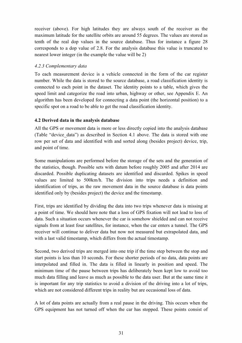
receiver (above). For high latitudes they are always south of the receiver as the maximum latitude for the satellite orbits are around 55 degrees. The values are stored as tenth of the real dop values in the source database. Thus for instance a figure 28 corresponds to a dop value of 2.8. For the analysis database this value is truncated to nearest lower integer (in the example the value will be 2)
4.2.3 Complementary data To each measurement device is a vehicle connected in the form of the car register number. While the data is stored to the source database, a road classification identity is connected to each point in the dataset. The identity points to a table, which gives the speed limit and categorize the road into urban, highway or other, see Appendix E. An algorithm has been developed for connecting a data point (the horizontal position) to a specific spot on a road to be able to get the road classification identity.
4.2 Derived data in the analysis database All the GPS or movement data is more or less directly copied into the analysis database (Table “device_data”) as described in Section 4.1 above. The data is stored with one row per set of data and identified with and sorted along (besides project) device, trip, and point of time. Some manipulations are performed before the storage of the sets and the generation of the statistics, though. Possible sets with datum before roughly 2005 and after 2014 are discarded. Possible duplicating datasets are identified and discarded. Spikes in speed values are limited to 500km/h. The division into trips needs a definition and identification of trips, as the raw movement data in the source database is data points identified only by (besides project) the device and the timestamp. First, trips are identified by dividing the data into two trips whenever data is missing at a point of time. We should here note that a loss of GPS fixation will not lead to loss of data. Such a situation occurs whenever the car is somehow shielded and can not receive signals from at least four satellites, for instance, when the car enters a tunnel. The GPS receiver will continue to deliver data but now not measured but extrapolated data, and with a last valid timestamp, which differs from the actual timestamp. Second, two derived trips are merged into one trip if the time step between the stop and start points is less than 10 seconds. For these shorter periods of no data, data points are interpolated and filled in. The data is filled in linearly in position and speed. The minimum time of the pause between trips has deliberately been kept low to avoid too much data filling and leave as much as possible to the data user. But at the same time it is important for any trip statistics to avoid a division of the driving into a lot of trips, which are not considered different trips in reality but are occasional loss of data. A lot of data points are actually from a real pause in the driving. This occurs when the GPS equipment has not turned off when the car has stopped. These points consist of

32
data with (almost) zero speed and no/little change in position. Data is therefore discarded if the speed is less then 0.1 km/h for more than 10 minutes. Only the data after the 10 minutes is discarded. And the data is possibly divided into two trips as a consequence.
Table 4.2 Movement statistics per vehicle and per trip available in the analysis database and available at the web interface (see Section 4.4). Statisticsa for each device/vehicle Statisticsa for each trip Parameter Web Parameter Web Number of trips x Start time x Start time for first trip x Stop time x Stop time for last trip x Trip duration x Total duration of the trips x Pause time before trip x Total travel distance x Pause time after trip x Average trip distance x Start horizontal position Maximum trip distance x Stop horizontal position Trip distance histogram x Travel distance x Maximum speed x Maximum speed Average speed x Average speed x Average of speed squared Average of speed squared Average of speed cubed Average of speed cubed Speed histogram x Final speed x Average of positive acceleration • speed Average of negative acceleration • speed Average number of trips per daya Maximum number of trips per daya Pause time histogram x Travel timepoints-of-the-day histogram Travel distance per day histograma Number of trips per day histograma Acceleration vs Speed diagram a Applied definitions: Day: The break point of time between days is 03.00 in the morning. Trips starting before this point of time is accounted to the day before; Time: The start and stop times for a trip is the time for start and stop of the logging, whether the car moves or not. This definition is used also in the estimates of the averages.
Table 4.3 Data quality and analysis statistics per vehicle and per trip available in the analysis database. Device/vehicle Trip Number of defect entries discarded Final speed Number of early entries discarded Number of corrected speed values Number of late entries discarded Number of interpolated regions Number of overlapping entries discarded Number of interpolated points Number of zero-speed entries discarded Number of corrected speed values Number of interpolated regions Number of interpolated points
Statistics are then generated for vehicles movements (Table “device_stats”) as well as for trips (Table “trip_stats”). In a specific array (Array “arrays”) is stored the statistical

33
distribution of acceleration vs. speed for the different vehicles. Table 4.2 lists the movement statistics currently available in the analysis database. Furthermore, the analysis database contains some statistics for the quality of the dataset and the manipulation of the data, which have been done before the copying into the Table “device_data”. This generated statistics are listed in Table 4.3. The parameters given in this section on the identification of trips as well as many others used in the analysis are input parameters to the analysis program and possible to change. A new compilation and running of the program is then necessary, though. Appendix F gives a further description of the derived data in the analysis database and the parameters used.
4.4 Web interface A web interface is connected to the analysis database. There excerpts of the data in the analysis database are presented, see Fig 4.2. This data can also be downloaded as Excel files. The web interface is under continuous development.
4.5 Availability The use of the data is restricted to research concerning vehicle movements, energy efficiency and environment issues, as well as traffic safety and societal planning, in accordance with the agreement with the car owners. Due to the privacy character of some of the data, the availability will further be classified according to type. Access to the data is administered by Lindholmen Science Park.
4.6 Possible further post-processing Post-processing of the positional data is planned to achieve enhanced positional data quality and make possible more correct and easier assignment of data to the national road database. The accuracy for the used type of GPS equipment should be a few meters for non-disturbed conditions. Still this can be a problem for accurate assignment to correct road, especially in urban or other environments with parallel or crossing overhead roads [23]. Also, in urban canyons the accuracy can be much less due to signal scattering. The intended post-processing will possibly utilize SWEPOS, the Swedish national network of permanent reference stations for GPS. The expected horizontal accuracy will then be increased to around one meter [24]. Furthermore, discussions are ongoing on connecting also weather data to the data points.

34
5. THE QUESTIONNAIRE
As a complement to the GPS data, we have, by a questionnaire intended to be sent back with the equipment, surveyed the specific environment for each car, such as, commuting habits, working site addresses, number of persons and driving licenses in the household, yearly mileages, etc. We have also made an identification of the possibility to charge an electric vehicle at home and at the possible working place. We have also tried to reveal specific characters of the driving during the measurement period in relation to their driving in general. Finally there has been a check if there have been specific problems with the installation, etc. This data is not available in the source database, though. The questionnaire is reproduced in Appendix G. The questionnaire has been answered to a very high degree, Table 5.1. The questionnaire was sent with the equipment and therefore it has been answered more or less independently of the amount and quality of gathered data, although participants, who for different reasons returned the equipment early were more reluctant to answer. Besides to achieve the above-mentioned data, the answers have been used for control of which vehicle actually has been measured by a device as the car register number was collected also in the questionnaire. For instance, the equipment has occasionally been installed in another vehicle belonging to the household instead of into the one originally intended, the car has been sold and a new one bought instead, etc. For a number of vehicles the identity has in this way been possible to correct in the database.
Table 5.1 Answers to the questionnaire. Vehicle with data Vehicle w/o data Total answers Answers 667 30 697 No answers 47 Total with data 714

35
6. RESULTS
We will here present the logging in terms of the involved cars, their household and spatial distribution, report the outcome of the measurement and its quality, and give some exemplary results concerning the car movements. Altogether around 770 cars have had GPS equipment sent to them for measurement of their movements. Some of these have not installed the equipment or the equipment has not registered any data. 714 cars have delivered data. (These cars are directly available in for instance the analysis database.) Of these cars 528 cars have had their movements logged for 30 days or more, that is, the difference between first and last gathered data is at least 30 days. (Still there can be missing data within this logging period.) (These 528 cars can relatively easily be extracted from the analysis database.) We will in the continuation term the 714 cars Data All Cars and the 528 vehicles Data Cars 30d+. We have also derived a dataset, for which we have interpolated apparent missing data (non-continuity in position) and excluded time periods for which possibly missing data have not been possible to identify. See further discussion on this procedure in Section 6.3. This data set contains 445 vehicles with data for 30 days or more. Here we call this dataset Data Cars Corr 30d+. (This last vehicle excerpt is not directly available in the analysis database, but require some data manipulation.) The 697 answers to the questionnaire (see Chapter 5) we will term Questionnaire.
6.1 Participating cars and their households The recruitment procedure has not lead to any significant misrepresentation concerning the properties of the cars. Table 6.1 shows that the 714 cars with data are fairly representative for the vehicles they are supposed to represent as determined in the excerpt from the vehicle register described in Section 2.2.3.
Table 6.1. Average values for selected parameters of vehicles in Data All Cars in comparison to the vehicles in the vehicle register. Parameter Average for cars with data
(Data All Cars) Averagea from vehicle
register Model year 2006.37 2006.12 Maximum engine power (kW) 98.2 99.5 Cylinder volume (cm3) 1819 1812 Kerb weight (kg) 1456 1457 Fuel use (liter/100km) 7.22 7.26 CO2 emission (g CO2/km) 176 177 a Weighted average between juridical and private cars in the same proportion as in the excerpt from the vehicle register further discussed in Section 2.2.3. Over 70% of the cars are in households with 2 adults, see Fig 6.1. The figure also shows that most of the adults in the households have driving licenses. A majority of the cars belongs to households with more than one car, see Fig 6.2. We can also see that compared to the Swedish households in general there is a slight overrepresentation of

36
households with more than one car. This is probably (partly) due to the fact that this study is directed towards newer cars, which predominantly may belong to wealthier household with several cars. The comparably low age of “our car” also explains why it also has somewhat longer yearly driven distance than the other car(s) in the households, see Fig 6.3. In average it is not perceived bigger than the other cars though, see Fig 6.4. 63% of the selected cars are used for commuting, although not necessarily during the measurement period, with an estimated average commuting (one-way) distance of 29 km, see Fig 6.5. The outcome concerning the distribution of the cars over the different strata is shown in Table 6.2. It agrees reasonably with the desired distribution. There is a major over-representation for newer diesel cars in the Gothenburg area as well as a major underrepresentation of juridical cars, especially diesel cars. Most of the juridical cars are situated in the Gothenburg area, are relatively new cars and diesels. These misrepresentations may therefore concern close categories of customers, why they to some extent may compensate for each other.
Table 6.2 Distribution of the logged vehicle over the different strata (se Table 2.4). Source: Data All Cars. Strata Outcome
(Data All Cars) (Number)
Outcome (Data All Cars)
(%)
Desired distributiona
(Number)
Desired distributiona
(%) GB7T 10 1.40 9.3 1.31 GB7L 33 4.62 32.2 4.51 GB6T 41 5.74 41.8 5.86 GB6L 71 9.94 75.9 10.63 GD7 29 4.06 22.3 3.12 GD6 15 2.10 14.0 1.95 ÖB7T 26 3.64 23.2 3.25 ÖB7L 59 8.26 56.9 7.97 ÖB6T 110 15.41 106.9 14.97 ÖB6L 147 20.59 154.6 21.65 ÖD7 62 8.68 60.0 8.41 ÖD6 52 7.28 53.0 7.42 JD 29 4.06 33.7 4.72 JB 27 3.78 30.2 4.24 Unknown 3 0.42 0 0 Sum 714 100 714 100 a Values at mid-project point of time for privately driven cars. (From last column in Table 2.9.) The geographical distribution of the cars is shown in Table 6.3. The representation of the single municipality varies especially for small municipalities, in which the desired numbers of cars are very small. However when aggregated into 4 groups with municipalities of different sizes (the three municipalities in the Gothenburg area are aggregated in a separate group), the various sizes are well represented. We can see a small overrepresentation of smaller cities, while the other groups have fewer cars than desired.

37
Table 6.3 Distribution of cars over the different municipalities in the region. Source: Data All Cars and The Swedish motor-vehicle register. Municipality Distribution over
municipalities (Data All Cars)
Desireda distr. over the municipalities
Distribution over four subregionsb (Data All Cars)
Desireda distr. over the four subregions
GÖTEBORG 167 183.7 MÖLNDAL 31 27.8 PARTILLE 22 15.5
220 227
BORÅS 34 47.0 KUNGSBACKA 46 40.9
80 88
SKÖVDE 31 25.1 UDDEVALLA 24 23.3 TROLLHÄTTAN 21 22.4 KUNGÄLV 23 20.4 LERUM 14 19.0 HÄRRYDA 24 16.8 ALINGSÅS 25 17.1 LIDKÖPING 25 17.1 MARK 22 16.1 VÄNERSBORG 12 15.3 FALKÖPING 21 13.2 ALE 8 12.8 STENUNGSUND 16 12.6 ULRICEHAMN 7 11.4 MARIESTAD 11 10.5 SKARA 6 8.1
290 261
TJÖRN 10 8.0 ORUST 9 7.6 VARA 3 7.3 LYSEKIL 4 6.6 TANUM 8 6.4 GÖTENE 7 6.2 STRÖMSTAD 3 6.0 ÖCKERÖ 3 5.7 TRANEMO 7 6.0 LILLA EDET 3 5.6 SVENLJUNGA 5 5.1 TIDAHOLM 0 4.7 ÅMÅL 7 4.8 VÅRGÅRDA 3 4.8 SOTENÄS 2 4.9 BOLLEBYGD 5 4.6 TIBRO 1 4.6 MUNKEDAL 7 4.6 BENGTSFORS 6 4.4 MELLERUD 4 3.8 HJO 1 3.8 HERRLJUNGA 2 3.9 TÖREBODA 8 3.8 KARLSBORG 2 3.1 FÄRGELANDA 2 2.7 GRÄSTORP 2 2.5 ESSUNGA 1 2.3 GULLSPÅNG 4 2.3 DALS-ED 2 2.0
124 138
Unknown 3 0 3 0 ALL 714 714.0 714 714 a The desired distribution is in proportion to the distribution of cars over the different municipalities in the selection of cars used in campaign 4, roughly corresponding to the mid-project point of time. Data from the Swedish motor-vehicle register 2011-02-14. b Same four subregions of differently sized municipalities as used in Figure 2.3.

38
Figure 6.1 Number of adults and driving licenses in the households. Source: Questionnaire.
Figure 6.2 Share of the cars belonging to household with different number of cars in this study (BRD). For comparison the corresponding figures for whole of Sweden given in The Swedish Travel Survey (RES 2005-2006). Source: Questionnaire and SIKA 2007.
0
10
20
30
40
50
60
70
80
1 2 3 ≥4
Share (%
)
persons 18+ yrs
Adults and driving licenses per household
4 licences
3
2
1
0%
10%
20%
30%
40%
50%
60%
1 car 2 cars 3 cars 4+ cars
Share of the cars in household with a certain number of cars
BRD
RES 2005-‐2006

39
Figure 6.3 Owner’s ranking of the car’s yearly driving distance in comparison to the other cars in the household, where rank 1 = longest yearly driving distance. Source: Questionnaire.
Figure 6.4 Owner’s ranking of the size of the car in comparison to the other cars in the household, where rank 1 = largest. Source: Questionnaire.
0
5
10
15
20
25
30
35
40
45
50
2 3 ≥4
Share of hsoueholds (%
)
Number of cars in the household
Ranking of the car's yearly driving distance
rank 4+
rank 3
rank 2
rank 1
0 5 10 15 20 25 30 35 40 45
2 3 ≥4
Share (%
)
Number of cars in the household
Ranking of the car's size
rank 4+
rank 3
rank 2
rank 1

40
Figure 6.5 Stated commuting for the vehicles (not necessarily during the logging period) Source: Questionnaire.
6.2 Logged driving Table 6.4 gives some basic statistics for the logging Table 6.4 Basic statistics for the logged car movements. Data All Cars Data Cars 30d+ Data Cars Corr 30d+ Number of cars with data 714 528 445 Total distance (km) 1 314 002 1 207 141 1 174 298 Total travel time (hour) 24 801 22 776 n. a. Average distance (km) 1 840 2 286 2 639 Average speed (km/h) 53 53 n. a. Number of tripsa 134 425 124 458 113 293 Average number of tripsa 188 236 255 Average trip lengtha (km) 9.8 9.6 10.4 Average number of trips per daya 3.8 3.7 4.4 a Trip statistics are sensitive to the division of the car movements into trips. Here we use the procedure discussed in Section 4.2 to divide the data into trips. The intention has been to distribute the logging over the year, although simultaneously a continuity of the campaigns and the availability of equipment must be taken into account. Figure 6.6 gives the distribution of the performed logging over the year. We can see that there is a somewhat larger concentration of loggings in the summertime during the Swedish vacation period in July. Several campaigns started just before the vacation period, because otherwise it had to be delayed to after be summer. The length of the actual measurement period, shown in Fig 6.7, is for many vehicle much shorter than intended due to malfunction of the equipment as further discussed in Section 7.2. 528 vehicles have loggings for more than 30 days (= Data Cars 30d+) and over 450 for more than 50 days.
0%
10%
20%
30%
40%
50%
60%
70%
no comm commutes 0-‐5 km 6-‐15 km 16-‐30 km 31-‐50km >51 km no data
Share of cars and distance commuting (one-‐way)

41
Many vehicle have logged distances between one and two thousands kilometer, see Fig 6.8, although the variation between the cars is large. Figure 6.9 shows the extrapolated logged distance in comparison to the yearly driving of the vehicles as stated by the owner/driver in the questionnaire. The variation in the fit between individual vehicles is large. However, the average of the extrapolated logged distances are somewhat shorter than what could be expected from the stated driving. It can be due to overstated yearly driving, non-representative logging periods, or missing data in the loggings. The age of the main driver/owner of the logged cars are somewhat older than expected from car owner data as shown in Fig 6.10. Older people may thus be more willing than younger ones to participate in this type of investigations. No compensation for this effect was done in the recruitment, as it was not part of any predetermined strata. The in the questionnaire stated number of persons in the car when driving are shown in Fig 6.11. 60% of the driving have been done without passengers, in which here children younger than 10 years were not included. The Swedish Travel survey gives higher shares for driving with two or more passengers, but this figure form the travel survey includes also younger children, which contributes to the difference. Half of the cars have been equipped with a towbar, see Fig 6.12. Over 20% of these have been towing a larger load for an estimated mean distance of 480 km during the logging period, see Fig 6.13.
Figure 6.6 Distribution in time of the logging periods for the vehicles. Source: Data All Cars.
0
50
100
150
200
250
1 6 11 16 21 26 31 36 41 46 51
Logged vehicles
Week of the year
Seasonal distribution of logged vehicles

42
Figure 6.7 Distribution of the length of the measurement period for the different vehicles. Source: Data All Cars.
Figure 6.8 Distribution of the logged driving distance. Source: Data Cars 30d+.
0
50
100
150
200
250
300
0-‐1 1-‐10 11-‐20 20-‐30 30-‐40 40-‐50 50-‐60 60-‐70 70+
Vehicles
Days
Length of measurement period
0 20 40 60 80 100 120
Vehicles
Distance (km)
Length of distance driven

43
Figure 6.9 Yearly driving distances for the vehicles. Stated yearly driving (from Questionnaire) compared to logged data extrapolated to one year (Data Cars Corr 30d+).
Figure 6.10 Age of the main driver compared to the owners/beneficiaries of comparable vehicles in the investigated region, weighted between juridical (estimated) and private cars in the same proportion as in the excerpt from the vehicle register (see Section 2.2.3). Source: Questionnaire and Swedish vehicle register.
20 40 60
20
40
60
Measured distance extrapolated to one year of driving (1000 km)
Stat
ed y
early
dis
tanc
e (1
000
km)
0
5
10
15
20
25
30
35
40
<30y 31-‐45 46-‐60 >60
Share (%
)
Age (yrs)
Age distribution of main driver
region
main driver

44
Figure 6.11 Stated distribution of the driving with different number of person in the car for this project compared to results from the Swedish national travel survey for the years 2005-06. Source: Questionnaire and SIKA 2007.
Figure 6.12 Availability and stated use of the towbar during the logging period. Source: Questionnaire.
0
10
20
30
40
50
60
70
1 2 ≥3
Share (%
)
Persons in the car
Share of distance driven with a certain number of persons in the car
BRD
RES 2005-‐2006
0%
10%
20%
30%
40%
50%
60%
towbar no towbar
Share of cars
Availability and use of towbar
Used
Not used

45
Figure 6.13 Stated towing distance during the logging period. Source: Questionnaire.
6.3 Data losses The start up of the GPS involves an initialization delay of at least half a minute before logging data appears. Therefore most of the trips do not begin exactly from where the last one stopped. Loss of data can also give a division of the travel into several trips and introduce distances between trip stop and the next start. Also for instance ferry tours will contribute to these differences in stop and start position of successive trips. Including all cars, 71% of the trips have a difference in position between its start and the stop for the preceding trip shorter than 100 m, around 88% have less than 500 meters, and 93.4% less than 2 km, see Fig 6.14. Some of the losses are connected to cars that due to malfunctioning equipment got many of their trips divided into more broken trips. Some of these units are responsible for many broken trips. Figure 6.15 gives the number of cars left for different tolerance of missing data. Here a trip is treated as a “potentially damaged trip” if the distance between its start and the stop of the preceding trip is larger than 2 km. Depending of the use of the data, different types of data losses are more or less important. When focus is not on second for second details but on for instance how long the trips are and when they occur, some data losses can be replaced with interpolated data. This can de done for instance, when missing data can be replaced with a good fit with interpolated data corresponding to a reasonable car speed on the actual type of road. Figure 6.15 also shows the effect of one such a simple repair technique. For instance, for a tolerance of 5% of the trips to have potentially lost data, this technique enables about 40% of the earlier filtered out cars to be accepted, giving a total of 460 cars left. This selection is here called Data Cars Corr 30d+.
0
5
10
15
20
25
<30 30–100 100–300 300–1000 1000–3000 >3000
Num
ber of cars
km towing
Towing distance

46
Figure 6.14 Distribution of the distances between first logging position and the last position before the stop. Source: Data Cars 30d+.
Figure 6.15 Number of vehicles left in data after filtering for different levels of tolerance of potentially damaged trips. With and without a simple repair technique. Source: Data Cars 30d+.
0 500 1000 1500 2000 2500 3000 3500 4000 4500 50000
0.1
0.2
0.3
0.4
0.5
0.6
0.7
0.8
0.9
1percentage of trips that have a distance longer than x between start and former stop
distance between start and former stop (m)
shar
e of
trip
s
0 1 2 3 5 7 10 15 25 400
100
200
300
400
500
600
Toleration of potentially damaged trips for one device (%)
Num
ber o
f of v
ehic
les
pass
ing
filte
ring
original datadata after repairtotal number of cars

47
6.4 The car movements We will here present some basic data of the logged driving and indicate some implication especially for electrification of vehicles. Figure 6.16 depicts the distribution of the number and length of the trips. (Trips defined according the procedure described in Section 4.2) While the number of trips is dominated by short trips, the most common driving belongs to a trip between 30 and 50 kilometer. Not much more than 10% of the driving belongs to trips longer than 100 kilometer. A similar relation holds for the pauses between trips, Fig 6.17. The number of pauses are dominated by short breaks, but at any time a random car not driving have probably stood there for a long time. The time between trips are totally dominated by longer pauses, almost 90% of the time a car is parked belongs to a pause longer than 8 hours. Figure 6.18 gives the fleet average number of daily pauses longer than T hours, indicating for instance the opportunities for charging when a certain length of the pauses is required for a charging to possibly occur. In average only 0.7 pauses per day are 10 hours or longer. Many cars are not used every day and some drivers do not have a 10 h break over night, thus keeping the average down. If the time needed for charging is reduced to 4 hours this will roughly mean a possibility to 50 % more recharging opportunities on a fleet level. The potential occasions are again doubled if one allow for charging every half an hour. Figure 6.19 depicts the distribution in time for pauses of different lengths. A clear pattern appears. Longer pauses (>10 hours) occur mainly during the night, while pauses of between 6 and 10 h length preferentially occur during around the middle of the day, and reasonably this is parking in connection to workplaces. Shorter stops also take place later into the evenings. Figure 6.19 also gives the implied charging during these parking times, for an assumed specific charging pattern. The cars are assumed to be plug-in hybrids (PHEV), charging with a rate of 2 kW and have a battery of 10 kWh. The need for charging is dependent on the distance travelled since last charging occasion. With this kind of charging behavior most of the charging will for the 10 h case be conducted between 6 and 10 pm. This is still during hours of high load in the Swedish power grid. Increased possibilities to charge at the workplace could also lead to increased power need in hours with already high load, assuming many of the breaks of 6 to 10 h length occur at the workplace. The peak is in this case occurring between 7 and 9 am. Finally, Figures 6.20-23 gives some statistics for speed, acceleration, power, and energy needs in Swedish car driving. Different movement patterns have large differences in speed characteristics, Fig 6.20. There is also a large variation in the amount of power needed for acceleration for patterns with the same average speed, Fig 6.21. Also the

48
average normalized power need at the wheels vary with movement pattern but is for most cars between 6 and 10 kW, Fig 6.22. The power need is calculated from the speed-acceleration pattern for the vehicles applied to a ”normalized” mid-size car with an assumed mass of 1500 kg, air resistance coefficient times frontal area of cdA = 0.66 m2, and rolling resistance coefficient cr = 0.01. Some or sometimes much of the power going to acceleration is recovered to overcome air and rolling resistance when the car decelerates, the rest is lost when braking or in powertrain friction. The power need depicted in Figure 6.22 is thus an overestimate of the sum of these power needs in reality. On the other hand the given power need do not include the power needed for going uphill along the road. Also this later need is to a large extent recovered in real driving in deceleration or when going downhill, though. The average normalized energy need at the wheels per distance driven for the different vehicles corresponding to the power need of Fig 6.22 is given in Fig 6.23. We can note that the comments made to Fig 6.22 are applicable also to this figure. The normalized specific energy need (as defined here) is around 1.5 kWh per 10 km for Swedish driving, while the ultimate losses in average are less than 1 kWh/10km. The variation in energy need gives an indication in the actual range for an electric vehicle due to this factor alone. (Other factors of importance can be the auxiliary energy need and energy conversion efficiency within the vehicle. Also energy recovery is of larger importance for electrified vehicles than for conventional ones.)
Figure 6.16 Distribution of trip distances. Source: Data Cars 30d+.
0%
5%
10%
15%
20%
25%
30%
35%
Share
Trip distance
Trip distance distribution
Share of trips
Share of distance

49
Figure 6.17 Distribution of the length of stops. Source: Data Cars 30d+.
0%
5%
10%
15%
20%
25%
30%
Share
Break time T
Distribution of stops
Share of stop occasions
Share of stop time
0.5 2 4 6 8 10 120
0.5
1
1.5
2
2.5
Break time T [h]
Aver
age
num
ber o
f pau
ses
per d
ay

50
Figure 6.18 Fleet average number of stops per day longer than break time T. Source: Data Cars Corr 30d+.
Figure 6.19 Distribution in time for parking of different lengths and potential charging during these pauses. Presented as shares of total measurement time for the vehicle fleet. Assumed: PHEVs with 2 kW charging immediately after parking which continue until battery is full (10 kWh) or pause ends. Energy use 0.2 kWh/km in CD mode. Source: Data Cars Corr 30d+.
0 6 12 18 240
0.1
0.2
0.3
0.4
0.5
0.6
0.7
0.8
0.9
Hour of the day
Shar
e of
tota
l tim
eDistribution of parking and potential charging
>10h pauses6 10h pauses2 6h pausesCharging, >10h pausesCharging, 6 10h pausesCharging, 2 6h pauses
0 20 40 60 80 100 1200
5
10
15
20Speed Distribution
Shar
e of
driv
ing
time
(%)
Speed (km/h)
all cars10% fastest10% slowest

51
Figure 6.20 Speed distribution in 10 km/h intervals (first interval 2-10 km/h, though) when driving ≥ 2 km/h, given as average values for all cars and for the deciles with the highest and lowest average speed, respectively. From Kullingsjö and Karlsson [2012].
Figure 6.21 Vehicle average acceleration power need and average speed when driving ≥ 2 km/h. From Kullingsjö and Karlsson [2012].
Figure 6.22 Vehicle average power need when driving ≥ 2 km/h. The power includes power need for overcoming rolling and air drag resistance and achieving the necessary
20 30 40 50 60 70 80 900.5
1
1.5
2
2.5
3
3.5
4Average specific acceleration power need
Aver
age
acce
lera
tion
pow
er (W
/kg)
Average speed (km/h)
0 25 50 75 1000
2
4
6
8
10
12
14
16
18Distribution of average normalized power need
Aver
age
pow
er (k
W)
Accumulated share of vehicles (%)

52
acceleration. For comparison of movement patterns, the power need is for all the vehicles normalized to the properties of an assumed midsize car (mass M = 1500 kg, air resistance Cd *A = 0.70 m2, and rolling resistance cr = 0.01). (Source: Data Cars Corr 30d+).
Figure 6.23 Vehicle average specific energy need at the wheel when driving ≥ 2 km/h. The need is estimated as the sum of energy needs for overcoming rolling and air resistance and energy for achieving the positive acceleration. For comparison of
movement patterns, the energy need is for all the vehicles normalized to the properties of an assumed midsize car (mass M = 1500 kg, air resistance Cd *A = 0.70 m2, and
rolling resistance cr = 0.01). Source: Data Cars Corr 30d+.
0 25 50 75 1000
0.2
0.4
0.6
0.8
1
1.2
1.4
1.6
1.8
2
Accumulated share of vehicles (%)
Aver
age
spec
ific
ener
gy u
se (k
Wh/
10 k
m)
acceleration, airdrag and rolling resistanceairdrag and rolling resistance

53
7. EXPERIENCES
7.1 Experiences from the administration of the campaigns As the measurement was organized, the original time schedule for the campaigns was overly optimistic about the time necessary for changing between the campaigns. For a complete exchange a lot of people are expected to
• get an end-of-campaign signal • recognize this signal (only recognizable when using the car) • uninstall the equipment • fill in the questionnaire • pack the equipment in the earlier received envelope • mail the equipment at a post office
The administration need then to
• get the equipment • demount the equipment to extract and empty the memory card for any possible
non-communicated data • check the equipment for functioning and possible repair • repack the equipment • mail the equipment
All the next drivers are then supposed to
• get the equipment by mail • install the equipment in the car • use the car after the installation
The chain are not stronger than its weakest link and the total time elapsed is the sum of the times for each step. All these steps in each campaign with many persons and situations involved mean that the whole process realistically needs one month and also some spare equipment to compensate for some inevitable delays and losses along the chain. Between the selection of cars and the actual measurement and during measurement some cars have been sold/exchanged. Also some equipment has deliberately been installed in other cars than the selected one. It has been an extra administrative burden to investigate and confirm which car has actually been measured.
7.2. Technical accomplishment of the measurement To finally achieve data for about 500 vehicles for at least a month each, the project has needed the intention to measure over 700 vehicles. There have been losses for two main reasons. The equipment has not always been connected to the power outlet and the equipment has not always functioned as intended.

54
The loss of power is partly unintentional. During the use of the car the plug has occasionally been loose, unintentionally withdrawn from the power outlet, or even damaged. The fit of the connection plug may also have varied between different car brands. Sometimes the connection has been unplugged deliberately, most often to free the outlet for other uses. (As mentioned and further discussed in Section 3.1.4, to alleviate this a branching connector have been available on request or sent with the equipment.) There have been three major malfunctions of the equipment. Different cars have different ways of dealing with the power to the power outlet when the car is turned off. Some disrupt the power, others not. The initial equipment software developed for handling the power when the car stopped did not work as intended in all situations. Some equipment did not turn off the logging, finally leading to a halt of all logging. This has led to a large tap of data in the first four campaigns. Later in campaign 5 a software error led to repeated losses of data packages for shorter periods for some of the cars. Both these malfunctions have been corrected. Still in the two last campaigns, extensive repeated losses of data occurred for many vehicles and the equipment have once again been updated. We can conclude that the functional robustness of the equipment has not been enough tested and evaluated initially, and after hardware and software changes. Complementary odometer readings and notes of installation and demounting points of time will facilitate in the control of equipment and obtained logging data.
7.3. Accomplishment of data handling The transfer of data to the source database has been slow for several reasons. The database has been developed in parallel to the project and all routines were not there from the start. The data flux from the measurements has been large, and the pure computer time needed to transfer the data have been significant in comparison. The completion of the database has relied on manual handling and there has also been a large cost and competition with other projects both when it comes to man- and computer power. The analysis database and the statistics generated there facilitate to get an overview of the data. This instrument was not developed until late in the project, though, and also not as a part of the project. Altogether these peculiarities have hampered early scrutiny of the data and the feedback to any possible malfunction of the measurement equipment has been too slow. Work is now ongoing to automate the data handling and speed up the process.
7.4. Drivers’ experiences In the questionnaire the drivers/passengers were asked about their experience of the measurement campaigns. Very few have had problem with understanding the installation instructions and with the installation itself.

55
87% state that the equipment has worked flawlessly. Among the critical, the overwhelming part concerns a loose connection plug or the supplied branch connector. Others mention that the equipment often or occasionally beeps. A few have also argued that the battery has been discharged too quickly due to the equipment. (The drivers have not been able to recognize if the equipment works and are logging the car as intended. The only external sign is that the lights are on, when power is supplied.) During use of the car some have experienced the equipment disturbing. It has mostly been connected to the antenna cord being in the way, the beeping and the loose plug mentioned above, and that the power outlet has been occupied. Some have also experienced problem with leaking water along the antenna cord.

56
8. CONCLUSIONS
The described car movement data project has resulted in a unique large dataset on the detailed movements of representative vehicles from the current fleet of privately driven cars in Sweden. The measurement project was initiated for the purpose of achieving appropriate data for various types of analyses connected to the electrification of cars. It is currently, as well as will be, used extensively for such purposes. However, it is a database freely available for all kinds of research devoted to vehicle movements, energy efficiency, and environmental performance as well as traffic safety and societal planning. Due to the privacy character of some of the data, the availability is further classified according to type.

57
9. REFERENCES
[1] Karlsson S, 2009. Optimal size of PHEV batteries from a consumer perspective – estimation using car movement data and implications for data harvesting. WEVA Journal. (World Electric Vehicle Journal) vol 3 (ISSN 2032-6653) http://www.wevaonline.net/
[2] Karlsson S, E Jonson, 2011. Electrification potential of the car – estimate using individual car movement data from a mid-size Swedish town. WEVA Journal. (World Electric Vehicle Journal) vol 4 (ISSN 2032-6653) http://www.wevaonline.net/
[3] Karlsson S, T Wiedemann, 2010. G4V: Impact and possibilities of a mass introduction of electrified vehicles on the electricity networks in Europe. In Proceedings of EVS25. Nov 5-9, 2010, Shenzhen, China.
[4] Wolf J, M Loechl, M Thompson, C Arce, 2003. Trip rate analysis in GPS-enhanced personal travel surveys. In Stopher P, P Johns (Eds.). Transport Survey Quality and Innovation. Pergamon Press, pp. 483-498.
[5] Stopher P, C FitzGerald, M Xu, 2005. Assessing the accuracy of the Sydney Household Travel Survey with GPS. Transportation Vol 34, 723-741.
[6] Stopher P, Y Zhang, Q Jiang, 2010. Tour-Based Analysis of Multi-Day GPS Data. Proceedings of the 12:th WCTRS. July 5-9, 2010, Lisboa.
[7] Household travel survey Final Report of Survey Methodology. East-West Gateway Coordinating Council. Austin, Texas. 2003.
[8] http://psrc.org/transportation/traffic Acc 2012-08-15 [9] Khan M, K M Kockelman, 2012. Predicting the market potential of plug-in electric
vehicles using multiday GPS data. Energy Policy 46, 225–233. [10] http://www.baltometro.org/transportation-planning/household-travel-survey. Acc
2010-08-19. [11] http://www.mwcog.org/transportation/activities/hts/ Acc 2010-08-19.
[12] http://www.cmap.illinois.gov/TravelTrackerData.aspx Acc 2010-08-19. [13] http://www.scag.ca.gov/travelsurvey/index.htm Acc 2010-08-19
[14] Greaves S, S Fifer, R Ellison, R Familiar, 2010. Development and implementation of a GPS/internet-based design for longitudinal before-and-after travel behaviour studies. In Proceedings of the 12:th WCTRS. July 5-9, 2010, Lisboa.
[15] Greaves S, R Ellison, 2010. Personality. Risk Aversion and Speeding: An Empirical Investigation. In Proceedings of the 12:th WCTRS. July 5-9, 2010, Lisboa.
[16] Mitrovich S, G Montesano, F Pugliese, M Mancini, G Valenti, 2010. Using GPS data from a sample of private cars for modelling the urban traffic. In Proceedings of the 12:th WCTRS. July 5-9, 2010, Lisboa.
[17] Smith R, S Shahidinejad, D Blair, E L Bibeau, 2011. Characterization of urban commuter driving profiles to optimize battery size in light-duty plug-in electric vehicles. Transportation Research Part D 16, 218–224.

58
[18] Smith R, M Morison, D Capelle, C Christie, D Blair, 2011. GPS-based optimization of plug-in hybrid electric vehicles’ power demands in a cold weather city. Transportation Research Part D 16, 614–618.
[19] http://auto21.uwinnipeg.ca/index.html.
[20] SIKA 2008. Fordon 2008. Swedish Institute for Transport and Communications Analysis. Östersund, Sweden.
[21] http://www.chalmers.se/ee/SV/forskning/ forskargrupper/fysiskresursteori/forskning/forskningsprojekt/bilrorelsedata (mainly in Swedish only)
[22] http://www.lindholmen.se/en/activities/test-site-sweden
[23] Quddus M A, W Y Ochieng, R B Noland, 2007. Current Map Matching Algorithm for Transport Applications: State-of-the Art and Future Research Direction. Transportation Research Part C 15, 312-328.
[24] http://swepos.lmv.lm.se/english/index.htm
[25] SIKA 2007. RES 2005-2006. The national travel survey. Statistics Communication patterns 2007:19. Swedish Institute for Transport and Communications Analysis. Östersund, Sweden. Available at http://www.trafa.se/Statistik/Resvanor/
[26] Kullingsjö L-H, S Karlsson, 2012. The Swedish car movement data project. In: Proceedings of EEVC 2012, Nov 20-22, 2012, Brussels, Belgium.

59
APPENDIX A. PAPERS, REPORTS AND PRESENTATIONS OF THE PROJECT
Papers Karlsson S, 2010. The Swedish car movement data project – rationale, methodology and
first results. In Proceedings to EVS25. Shenzhen. China. Nov 5-9 2010. Karlsson S, E Jonson, 2011. The importance of car movement data for determining
design, viability and potential of PHEVs. In: Proceedings of International Mobility Advanced Forum (IAMF), March 8-9, 2011, Geneva.
Karlsson S, and T Wiedemann. 2010. G4V: Impact and possibilities of a mass introduction of electrified vehicles on the electricity networks in Europe. In: Proceedings of EVS25. Nov 5-9, 2010, Shenzhen, China.
Kullingsjö L-H, S Karlsson, 2012. Estimating the PHEV potential in Sweden using GPS derived movement patterns for representative privately driven cars. In: Proceedings of EVS26. May 6-9, 2012, Los Angeles, USA.
Kullingsjö L-H, S Karlsson, 2012. The Swedish car movement data project. In: Proceedings of EEVC 2012, Nov 20-22, 2012, Brussels, Belgium.
Karlsson S, L-H Kullingsjö, 2013. GPS measurement of Swedish car movements for assessment of possible electrification. In Proceedings of EVS27 Symposium, Barcelona, Spain, Nov 17-20, 2013.
Reports Jonson E, S Karlsson, 2010. Möjligheter att utnyttja data från databasen LUNDAvISA
för analys av laddhybrider. Fysisk resursteori. PRT Report 2010:5. Chalmers Tekniska Högskola. Göteborg. (in Swedish)
Karlsson S, 2013. The Swedish car movement data project. Final report. PRT report
2013:1 Rev 2. Nov 2013. Division of Physical resource, Theory Dep of Energy and Environment, Chalmers University of Technology, Gothenburg, Sweden.
Presentations Karlsson S, 2009. Climate relevance, risks and pitfalls in systems design. Invited
presentation at IEA End-Use working party: Workshop on electricity in the future transport system. Sept 17, 2009, Stockholm.
Karlsson S, 2009. Electrification of Transport in Energy Scenarios – With a focus on plug-in hybrids. Invited presentation at Uppsala Energy 2009. Oct 21, 2009, Uppsala.
Karlsson S, 2010. Laddhybriders laddmöjligheter – Analys av bilars verkliga rörelsemönster. Presentation at Sveriges Energiting March 16-17, 2010. Stockholm. (in Swedish)
Karlsson S, G Zettergren, 2010. Mätning och analys av bilrörelser i den svenska bilparken av relevans för framtida elektrifiering. Presentation at Energirelaterad fordonsforskning 2010. May 18-19, 2010, Skövde. (in Swedish)
Karlsson S, 2010. Är din bil med? Bilrörelseprojektet – ett underlag för elektrifiering. Presentation at Chalmers Energidag. Nov 4, 2010, Göteborg. (in Swedish)

60
Karlsson S, 2010. Bilrörelseprojektet – ett underlag för elektrifiering. Presentation at Göteborg Energis Forsknings- och utvecklingsforum. Dec 8, 2010, Göteborg. (in Swedish)
Karlsson S, 2012. Driving patterns matter. Presentation at Chalmers Energy Conference, March 28-29, 2012, Gothenburg.
Kullingsjö L-H, S Karlsson, 2012. The Swedish car movement data project. Presentation at The first national Swedish transport conference, Oct 18-19, 2012, Stockholm.
Kullingsjö L-H, S Karlsson, 2013. Mätning och analys av fordonsrörelser som underlag för elektrifiering. Presentation at Energirelaterad fordonsforskning 2013. April 10-11, 2013, Örebro. (in Swedish)
Personnel from Test Site Sweden have also made several oral and poster presentations of the project in various contexts.
E-media Karlsson S, L-H Kullingsjö, 2013. Electric vehicles and driving patterns. Ch10 in
Sandén B, (ed) System Perspectives on Electromobility, Chalmers Univ of technology. http://www.chalmers.se/energy
www.chalmers.se/brd The project has from early on had a webpage at Department of Energy and Environment at Chalmers University of Technology, Sweden.
http://www.goteborgenergi.se/Privat/Projekt_och_etableringar/Forskning_och_utveckling/Forskningsstiftelsen The project has from early on been presented at Göteborg Energi Forskningsstiftelse. (in Swedish)

Vill du medverka i en studie för att mäta bilars körmönster?
TSS • Lindholmen Science Park • Box 8077 • SE-402 78 • Göteborg • Sweden Tel. +46 (0)31-340 00 76 • Fax +46 (0)31 764 70 49 • www.testsitesweden.eu
Sida 1(3)
Detta brev är en förfrågan om du vill vara med i ett forskningsprojekt där vi ska mäta hur bilar används. Att just du tillfrågas beror på att vi har gjort ett slumpmässigt urval av bilar i Västra Götaland och Kungsbacka med hjälp av bilregistret. Forskningsprojektet leds av Test Site Sweden (TSS) inom Lindholmen Science Park i samarbete med Chalmers Tekniska Högskola och Consat AB. Data från mätningarna ställs samman och analyseras vid Institutionen för Energi och miljö, Chalmers Tekniska Högskola. Projektet finansieras också av Energimyndigheten inom programmet Fordonsstrategisk forskning och innovation (FFI), Göteborg Energis stiftelse för Forskning och Utveckling, Vattenfall, Lindholmen Science Park samt Telenor. Studiens Syfte För att göra bilar mer energisnåla pågår det utveckling för att driva dem med el. Mätningen från studien kommer att ge viktigt underlag till forskning och industri för att bättre förstå och kunna dimensionera och planera t.ex. batteristorlek och laddinfrastruktur mm. Hur långt och hur ofta, var och när bilar kör kommer att vara viktiga faktorer för hur mycket elbilar eller så kallade laddhybrider kan ladda och utnyttja batteriet. Detta påverkar exempelvis den enskilde bilägarens ekonomi, hur bilen ska dimensioneras och hur infrastrukturen i form av laddmöjligheter kan behöva byggas ut. Data över bilars rörelsemönster finns idag inte att tillgå, vi vill därför samla in data för hur olika bilar rör sig under en längre tidsperiod. Läs gärna mer om projektet på följande sidor och på www.chalmers.se/brd Tycker du att det här låter spännande och gärna deltar? Skicka in ditt godkännande av deltagande så snart som möjligt i det bifogade svarskuvertet. Vi skulle uppskatta att ha ditt svar inom 10 dagar efter att du mottagit denna förfrågan. Med vänliga hälsningar Sten Karlsson Peter Lindgren Energi och Miljö Test Site Sweden Chalmers Tekniska Högskola Lindholmen Science Park
APPENDIX B THE REQRUITMENT LETTER
61

TSS • Lindholmen Science Park • Box 8077 • SE-402 78 • Göteborg • Sweden Tel. +46 (0)31-340 00 76 • Fax +46 (0)31 764 70 49 • www.testsitesweden.eu
Sida 2(3)
Beskrivning av studien Rörelsemönstret av ett antal bilar kommer att loggas under en mätperiod av två månader. Vi kommer att logga position (latitud, longitud, altitud), hastighet och tidpunkt. Totalt planerar vi att genomföra studien på 500 bilar, fördelat på 7 olika mätperioder med upp till 100 bilar i varje period. Projektet kommer att pågå under två år med start i mitten av juni, 2010. Det är viktigt att vi får tillräcklig bredd i undersökningen, så oavsett om du är ung eller gammal eller om du kör mycket eller lite är din medverkan betydelsefull. För de bi lägare som vi l l de l ta i s tudien går det t i l l på fö l jande sät t :
• Du skriver under och skickar in det bifogade dokumentet ”godkännande av deltagande” i
det bifogade svarskuvertet. Du kan endast delta med det efterfrågade fordonet. • Vi skickar en liten loggningsutrustning till dig som du själv mycket enkelt installerar i
fordonet. Instruktioner följer med loggern. Med hjälp av GPS-positionering sänds mätdata om hur fordonets framförs. Du ska köra bilen precis som vanligt.
• Utrustningen skickar kontinuerligt data till vår server under hela mätperioden.
• Det statistiska underlag som blir resultat av studien kommer att visa hur körmönstret ser
ut idag för svenska bilar på olika typer av vägar. • De insamlade uppgifterna användas endast i forskningssyfte och hanteras enligt
personuppgiftslagen. All mätdata hanteras konfidentiellt.
Vi hoppas att du vill vara med i den spännande utveckling som pågår!
APPENDIX B THE REQRUITMENT LETTER
62

TSS • Lindholmen Science Park • Box 8077 • SE-402 78 • Göteborg • Sweden Tel. +46 (0)31-340 00 76 • Fax +46 (0)31 764 70 49 • www.testsitesweden.eu
Sida 3(3)
Frivilligt deltagande Ditt deltagande i studien är helt och hållet frivilligt. Rätt att avbryta Du har rätt att när som helst begära att insamlingen av data avbryts utan att ange något skäl. Eventuella risker Vi vill att du kör precis som vanligt och därför innebär denna studie inga andra risker utöver vad som är förknippat med vanlig körning. Det är alltså du som förare (alternativa förare) som fortfarande har det fulla ansvaret för ett säkert framförande av fordonet. Informationsplikt Du är skyldig att informera alternativa förare om datainsamlingen. Behandling av personuppgifter och data När du deltar i denna studie kommer vissa personuppgifter att samlas in om dig. Utöver det som insamlas automatiskt i fordonet, kommer vi att be dig om vissa uppgifter om dig och eventuellt andra förare, t.ex. ålder och kön på förare och deras ungefärliga andel av totala körningen. För behandlingen av alla uppgifter som går att härröra till dig som person gäller reglerna i personuppgiftslagen (1998:204), PuL. Kontakt och support Om du har några frågor eller kommentarer gällande studien har du möjlighet att besöka vår hemsida www.chalmers.se/brd. På hemsidan kan du fylla i din fråga i ett frågeformulär så hör vi av oss. Alternativt kan du ringa vår supporttelefon 031-340 00 76 (telefonsupporten går via Consat AB).
APPENDIX B THE REQRUITMENT LETTER
63

Godkännande av deltagande
Om studien
Lindholmen Science Park AB (”Lindholmen”) bedriver tillsammans med Chalmers Tekniska Högskola och Consat AB ett forskningsprojekt innefattande en studie som syftar till att mäta bilrörelser (”Studien”). Studien är tänkt att utgöra ett underlag till forskning och industri för att bättre förstå och kunna dimensionera t ex batteristorlek och laddinfrastruktur. Studien genomförs i enlighet med de regler som anges i personuppgiftslagen (1998:204), med Lindholmen som personuppgiftsansvarig. Insamlade personuppgifter kommer enbart att användas i forskningssyfte samt behandlas konfidentiellt, såvida inte informationen måste lämnas ut enligt lag, förordning eller myndighetsföreskrift.
Deltagarna har rätt att en gång om året, kostnadsfritt, få information om vilka personuppgifter Lindholmen har om dem samt om hur dessa används. Sådan begäran från deltagare ska göras skriftligen. Deltagarna har också alltid rätt att skriftligen begära rättelse av felaktiga personuppgifter och att återkalla lämnade samtycken. Kontakta Lindholmen för begäran om information, rättelse etc., på följande adress: TSS, Lindholmen Science Park AB, Box 8077, 402 78 Göteborg.
Om mitt deltagande
Jag godkänner att följande villkor gäller för mitt deltagande i Studien.
1. Jag har läst och förstått den information som jag har fått om Studien och jag samtycker till att information om min bils rörelsemönster (och därmed, indirekt, information om mig eller andra förare av bilen) samlas in, lagras och analyseras. Jag samtycker också till att uppgifterna sparas och återanvänds i framtida forskningsprojekt som rör bilars rörelsemönster, energieffektivitet, miljöegenskaper, trafiksäkerhet och/eller samhällsplanering.
2. Jag förbinder mig att, i enlighet med bifogade instruktioner, installera den loggningsutrustning som skickas till mig, inklusive GPS-enhet, kablar, dator och sändare. Jag åtar mig att vårda loggningsutrustningen varsamt samt inom en vecka efter Lindholmens begäran avinstallera utrustningen och returnera den i bifogat kuvert. Om problem uppstår med loggningsutrustningen under Studien kommer jag så snart som möjligt kontakta Lindholmen och följa de ytterligare instruktioner som jag då får.
3. Jag är införstådd med att bilen förväntas framföras på samma sätt som vanligt och att det är den som kör bilen som är ansvarig för körningen.
4. Jag förbinder mig att informera eventuella andra förare av bilen om Studien och att loggningsutrustningen kommer att registrera även deras körning. Jag kommer även att informera eventuella passagerare om Studien och inte tvinga någon att köra eller åka med i bilen som på grund av Studien inte vill det.
5. Jag förstår att mitt deltagande i Studien är frivilligt och att jag när som helst kan välja att avbryta det.
6. Jag accepterar att jag inte är berättigad till någon ersättning för mitt deltagande i Studien.
* * *
Nej, jag vill inte delta i Studien och vill inte ha mer information eller påminnelser
Motivera gärna kort varför du inte vill delta i studien: __________________________________
Dina kontaktuppgifter: telefon: e-post: Bilens registreringsnummer: Datum och plats:
Signatur:_____________________ Namnförtydligande:
APPENDIX C. THE AGREEMENT SIGNED BY THE PARTICIPANTS
64

Instruktioner för deltagare i projektet Bilrörelsedata
TSS • Lindholmen Science Park • Box 8077 • SE-402 78 • Göteborg • Sweden Tel. +46 (0)31-340 00 76 • Fax +46 (0)31 764 70 49 • www.testsitesweden.eu
Sida 1(2)
Bästa deltagare!
Du får här mätutrustningen som ska användas i projektet Bilrörelsedata. Var vänlig att installera utrustningen enligt anvisningarna nedan så snart som möjligt, och senast 7 dagar efter leverans. När mätningen är slut kommer enheten att börja pipa; det är då dags att skicka tillbaka utrustningen. Vi tackar vänligast för din medverkan.
Du kan följa projektets utveckling på hemsidan: www.chalmers.se/brd, där finns även ytterliggare information och kontaktuppgifter. Maila i första hand dina frågor till [email protected], i andra hand kan vi även bistå med hjälp på supporttelefonen: 031-340 00 76.
1) Torka bort grus och smuts och placera den magnetiska GPS-antennen mitt på taket.
• Har du tyg, glas eller plasttak får antennen placeras inne i bilen så nära taket som möjligt. • Tänk på att plocka in antennen vid biltvätt!
2) Låt sladden från GPS-antennen klämmas fast i bildörren, förslagsvis på passagerarsidan.
• Sladdarna kan vara känsliga, har du barn i bilen placeras enhet med sladdar lämpligen utom räckhåll för barnet.
APPENDIX D
THE MOUNTING INSTRUCTIONS FOR THE MEASUREMENT EQUIPMENT
65

TSS • Lindholmen Science Park • Box 8077 • SE-402 78 • Göteborg • Sweden Tel. +46 (0)31-340 00 76 • Fax +46 (0)31 764 70 49 • www.testsitesweden.eu
Sida 2(2)
3) Placera enheten i sätesfickan.
• Har du andra lämpliga ställen att lägga enheten på går det lika bra, tänk dock på att sladden inte får vara i vägen och att enheten inte får utsättas för sparkar eller smuts.
4) Kontakten ska alltid vara inkopplad i 12volts-uttaget (cigarettändaruttaget). Välj det uttag i
bilen som passar dig bäst.
• När enheten får ström skall lamporna lysa/blinka.
• Behöver du använda cigarettuttaget till annat, efterfråga en förgreningskontakt av oss.
• Om lamporna på enheten lyser även när tändningen är av och bilen förväntas stå stilla mer än 10 dagar bör kontakten kopplas ur för att undvika att bilbatteriet laddas ur.
5) Fyll i bilens mätarställning vid mätperiodens början på etiketten som sitter på enhetens
ovansida. När mätperioden är slut fylls mätarställningen vid den tidpunkten i. Anledningen till att detta är viktigt är för att vi ska kunna analysera om enheterna har fungerat bra under mätperioden och tagit upp all data vi behöver.
6) Kör som vanligt. Om vi inte skulle få någon signal kontaktar vi dig och ser om det är något som gått fel.
7) Efter ungefär två månader börjar utrustningen att pipa. Det betyder att mätningarna är klara. Koppla ur utrustningen och packa den varsamt i det medföljande bubbelkuvertet. Fyll även i enkäten och lägg i kuvertet. Lägg kuvertet direkt i brevlådan, det är förberett med frankering och adress.
APPENDIX D
THE MOUNTING INSTRUCTIONS FOR THE MEASUREMENT EQUIPMENT
66

67
APPENDIX E. THE ROAD CLASSIFICATION
Table E.1. The ID for road classification categories connected to each data point. ID NAME SPEED_LIMIT IS_URBAN IS_HIGHWAY 1 Testsite_Sweden50 50 1 0 2 Sverige10051270 70 0 0 3 Sverige10051250 50 1 0 4 Sverige1005120 0 1 0 5 Sverige10051230 30 1 0 6 Sverige10051230 30 0 0 7 Sverige10051280 80 0 0 8 Sverige10051260 60 0 0 9 Sverige10051250 50 0 0 10 Sverige1005120 0 0 0 11 Sverige100512110 110 0 1 12 Sverige10051250 50 0 1 13 Sverige10051270 70 0 1 14 Sverige10051270 70 1 0 15 Sverige10051290 90 0 1 16 Sverige10051250 50 1 1 17 Sverige1005120 -120 1 1 18 Sverige10051230 30 1 1 19 Sverige10051270 70 1 1 20 Sverige10051280 80 0 1 21 Sverige10051290 90 1 1 22 Sverige1005120 0 0 1 23 Sverige10051290 90 0 0 24 Sverige10051240 40 1 1 25 Sverige10051230 30 0 1 26 Sverige1005125 5 1 0 27 Sverige10051240 40 1 0 28 Sverige10051260 60 0 1 29 Sverige10051260 60 1 1 30 Sverige100512110 110 1 1 31 Sverige10051260 60 1 0 32 Sverige1005125 5 1 1 33 Sverige100512120 120 0 1 34 Sverige100512120 120 1 1 35 Sverige100512100 100 0 1 36 Sverige100512100 100 0 -20 37 Sverige10051280 80 1 1 38 Sverige10051280 80 1 0 39 Sverige10051290 90 1 0 40 Sverige100512120 120 0 0 41 Sverige1005120 0 1 1 42 Sverige100512100 100 1 1 43 Sverige100512110 110 0 0 44 Sverige100512100 100 0 0 45 Sverige10051240 40 0 0 46 Sverige100512100 100 1 0 47 Sverige10051220 20 1 0 48 Sverige100512110 110 1 0

This
is a
docu
men
tatio
n of
the
BRD
.jar a
pplic
atio
n, so
urce
cod
e an
d th
e ca
lcul
atio
ns th
at a
re d
one,
as w
ell a
s an
over
view
of t
he su
rroun
ding
dat
abas
e str
uctu
re.
1 Th
e so
urce
and
des
tinat
ion
data
base
s, an
d th
e BR
D.ja
r ap
plic
atio
n.
The
sour
ce d
atab
ase
(tss_
ev) i
s whe
re d
ata
is sto
red
in ra
w fo
rmat
, and
the
desti
onat
ion
data
base
(tss
_cal
c) is
whe
re d
ata
is sto
red
afte
r cal
cula
tions
are
com
plet
ed. T
he p
urpo
se o
f BRD
.jar i
s to
read
dat
a fro
m th
eso
urce
dat
abas
e, d
ivid
e it
into
trip
s, m
ake
calc
ulat
ions
and
writ
e th
e re
sults
bac
k to
the
desti
natio
n da
taba
se.
1.1
Sour
ce d
atab
ase
(tss_
ev)
The
struc
ture
of t
he so
urce
dat
abas
e is
not d
iscus
sed
here
.
1.2
Des
tinat
ion
data
base
(tss
_cal
c)
The
desti
natio
n da
taba
se c
onat
ains
the
follo
win
g ta
bles
.Ta
ble
nam
eD
escr
iptio
nde
vice
_dat
aCo
ntai
ns a
ll th
e lo
gged
dat
a. O
ne ro
w p
er lo
gged
set o
f dat
a.tri
p_sta
tsCo
ntai
ns in
form
atio
n on
the
trip
leve
l. O
ne ro
w p
er tr
ip.
devi
ce_s
tats
Cont
ains
dat
a on
the
devi
ce le
vel.
One
row
per
dev
ice.
arra
ysCo
mpl
emen
t to
the
devi
ce_s
tats
tabl
e. C
onta
ins 2
D d
ata
for d
evic
es th
at n
ot a
re su
itabl
e to
stor
e in
the
devi
ce_s
tats
tabl
e (c
urre
ntly
onl
y ac
cele
ratio
n vs
. spe
ed h
istog
ram
).
1.2.
1 Th
e de
vice
_dat
a ta
ble
A si
ngle
row
in th
e de
vice
_dat
a ta
ble
cont
ains
the
follo
win
g co
lum
ns. (
Not
e th
at e
ach
ROW
in th
is ta
ble
corre
spon
ds to
a C
OLU
MN
in th
e de
vice
_dat
a ta
ble)
Col
umn
nam
e in
data
base
tabl
eU
nit/f
orm
atD
escr
iptio
nH
ow th
is is
calc
ulat
ed b
y BR
D.ja
r
idde
vice
_dat
a-
Uni
que
id.
-pr
ojec
t-
Proj
ect i
d as
spec
ified
in ts
s_ev
.PRO
JECT
SM
anua
ly e
nter
ed in
to th
e BR
D a
pplic
atio
n at
cal
cula
tion.
-de
vice
-Th
e de
vice
this
devi
ce d
ata
belo
ngs t
o.Tr
ansf
ered
from
the
DEV
ICES
_ID
that
is a
ssoc
iate
d to
eac
h sa
mpl
e in
the
sour
ce d
atab
ase.
trip
-Th
e tri
p th
is be
long
s to.
Cou
nts f
rom
one
and
up
for e
ach
devi
ce.
The
Trip
Bund
le d
ivid
es a
ll da
ta fr
om a
sing
le d
evic
e in
to a
set o
f ord
ered
trip
s. Th
is nu
mbe
rre
flect
s to
whi
ch tr
ip in
that
ord
er th
is de
vice
dat
a be
long
s to.
times
tam
pm
illise
cond
sU
NIX
tim
esta
mp.
(Unc
erta
in if
leap
seco
nds a
re in
clud
ed o
r not
)Co
pied
from
the
mill
iseco
nds v
alue
in th
e so
urce
dat
abas
e. (I
n ca
se th
e sa
telli
tes,
Xdo
p va
lues
are
zero
, thi
s is a
n in
terp
olat
ed v
alue
bet
wee
n th
e th
e la
st an
d ne
xt d
evic
e da
ta w
ith n
on z
ero
sate
llite
and
Xdo
p va
lues
.)
times
tam
p_str
ing
"YY
YY-
MM
-DD
HH
:MM
:SS.
d"Ti
mes
tam
p on
the
form
at "Y
YY
Y-M
M-D
D H
H:M
M:S
S.d"
.Co
nver
ted
from
the
mill
iseco
nds v
alue
.
altit
ude
mA
ltitu
de in
m. (
Unk
now
n ho
w re
liabl
e th
is va
lue
is).
Copi
ed fr
om th
e al
titud
e va
lue
in th
e so
urce
dat
abas
e. (I
n ca
se th
e sa
telli
tes,
Xdo
p va
lues
are
zer
o,th
is is
an in
terp
olat
ed v
alue
bet
wee
n th
e th
e la
st an
d ne
xt d
evic
e da
ta w
ith n
on z
ero
sate
llite
and
Xdo
p va
lues
.)
latit
ude
degr
ees
Latit
ude
Copi
ed fr
om th
e la
titud
e va
lue
in th
e so
urce
dat
abas
e. (I
n ca
se th
e sa
telli
tes,
Xdo
p va
lues
are
zer
o,th
is is
an in
terp
olat
ed v
alue
bet
wee
n th
e th
e la
st an
d ne
xt d
evic
e da
ta w
ith n
on z
ero
sate
llite
and
Xdo
p va
lues
.)
1 av
11
APPENDIX F THE DATA IN THE ANALYSIS DATABASE
68

long
itude
degr
ees
Long
itude
Copi
ed fr
om th
e lo
ngitu
de v
alue
in th
e so
urce
dat
abas
e. (I
n ca
se th
e sa
telli
tes,
Xdo
p va
lues
are
zero
, thi
s is a
n in
terp
olat
ed v
alue
bet
wee
n th
e th
e la
st an
d ne
xt d
evic
e da
ta w
ith n
on z
ero
sate
llite
and
Xdo
p va
lues
.)
spee
dkm
/hSp
eed
in k
m/h
.Co
pied
from
the
spee
d va
lue
in th
e so
urce
dat
abas
e. (I
n ca
se th
e sa
telli
tes,
Xdo
p va
lues
are
zer
o,th
is is
an in
terp
olat
ed v
alue
bet
wee
n th
e th
e la
st an
d ne
xt d
evic
e da
ta w
ith n
on z
ero
sate
llite
and
Xdo
p va
lues
.)
dire
ctio
nde
gree
sD
irect
ion
in d
egre
es.
Copi
ed fr
om th
e di
rect
ion
valu
e in
the
sour
ce d
atab
ase.
(In
case
the
sate
llite
s, X
dop
valu
es a
reze
ro, t
his i
s an
inte
rpol
ated
val
ue b
etw
een
the
the
last
and
next
dev
ice
data
with
non
zer
o sa
telli
tean
d X
dop
valu
es.)
last_
valid
_tim
esta
mp
mill
iseco
nds
Last
valid
tim
esta
mp
in m
illise
cond
s (pr
eciss
ion
is do
wn
to se
cond
s,so
two
and
thre
e en
tries
alte
rnat
ing
are
equa
l to
each
oth
er e
ven
whe
n ev
eryt
hing
is a
lrigh
t.)
Copi
ed fr
om th
e m
illise
cond
s val
ue in
the
sour
ce d
atab
ase.
(In
case
the
sate
llite
s, X
dop
valu
es a
reze
ro, t
his i
s an
inte
rpol
ated
val
ue b
etw
een
the
the
last
and
next
dev
ice
data
with
non
zer
o sa
telli
tean
d X
dop
valu
es.)
sate
llite
s-
Num
ber i
ndic
atin
g w
hich
sate
llite
s whe
re u
sed
to m
easu
re th
ese
valu
es.
Copi
ed fr
om th
e sa
telli
tes v
alue
in th
e so
urce
dat
abas
e. (I
n ca
se th
e sa
telli
tes,
Xdo
p va
lues
are
zero
, thi
s val
ue b
elon
gs to
a d
evic
e da
ta fo
r whi
ch v
alue
s hav
e be
en in
terp
olat
ed b
etw
een
the
last
and
next
dev
ice
data
with
non
zer
o sa
telli
te a
nd X
dop
valu
es.)
pdop
-Po
sitio
nal (
3D) d
ilutio
n of
pre
cisio
n. (M
ultip
lied
by a
fact
or te
n).
Copi
ed fr
om th
e pd
op v
alue
in th
e so
urce
dat
abas
e. (I
n ca
se th
e sa
telli
tes,
Xdo
p va
lues
are
zer
o,th
is va
lue
belo
ngs t
o a
devi
ce d
ata
for w
hich
val
ues h
ave
been
inte
rpol
ated
bet
wee
n th
e la
st an
dne
xt d
evic
e da
ta w
ith n
on z
ero
sate
llite
and
Xdo
p va
lues
.)
hdop
-H
oriz
onta
l dilu
tion
of p
reci
sion.
(Mul
tiplie
d by
a fa
ctor
ten)
.Co
pied
from
the
hdop
val
ue in
the
sour
ce d
atab
ase.
(In
case
the
sate
llite
s, X
dop
valu
es a
re z
ero,
this
valu
e be
long
s to
a de
vice
dat
a fo
r whi
ch v
alue
s hav
e be
en in
terp
olat
ed b
etw
een
the
last
and
next
dev
ice
data
with
non
zer
o sa
telli
te a
nd X
dop
valu
es.)
vdop
-Ve
rtica
l dilu
tion
of p
reci
sion.
(Mul
tiplie
d by
a fa
ctor
ten)
.Co
pied
from
the
vdop
val
ue in
the
sour
ce d
atab
ase.
(In
case
the
sate
llite
s, X
dop
valu
es a
re z
ero,
this
valu
e be
long
s to
a de
vice
dat
a fo
r whi
ch v
alue
s hav
e be
en in
terp
olat
ed b
etw
een
the
last
and
next
dev
ice
data
with
non
zer
o sa
telli
te a
nd X
dop
valu
es.)
1.2.
2 Th
e tr
ip_s
tats
tabl
e
A si
ngle
row
in th
e tri
p_sta
ts ta
ble
has t
he fo
llow
ing
struc
ture
. (N
ote
that
eac
h RO
W in
this
tabl
e co
rresp
onds
to a
CO
LUM
N in
the
trip_
stats
tabl
e)C
olum
n na
me
in d
atab
ase
tabl
eU
nit/f
orm
atD
escr
iptio
nH
ow th
is is
calc
ulat
ed b
y BR
D.ja
rTh
e fu
nctio
n in
BR
D.ja
r th
at r
etur
ns th
isva
lue.
idtri
p_sta
ts-
Uni
que
id-
-pr
ojec
t-
Proj
ect i
d as
spec
ified
in ts
s_ev
.PRO
JECT
SM
anua
ly e
nter
ed in
to th
e BR
D a
pplic
atio
n at
cal
cula
tion.
-
devi
ce-
the
devi
ce th
is tri
p be
long
s to.
Tran
sfer
ed fr
om th
e D
EVIC
ES_I
D th
at is
ass
ocia
ted
with
each
dev
ice
data
that
bel
ongs
to th
is de
vice
in th
e so
urce
data
base
.-
trip
-A
from
1 m
onot
onel
y in
crea
sing
id th
at u
niql
y id
entifi
es th
etri
p fo
r thi
s dev
ice.
The
Trip
Bund
le d
ivid
es a
ll da
ta fr
om a
sing
le d
evic
e in
to a
set o
f ord
ered
trip
s. Th
is nu
mbe
r refl
ect w
hich
num
ber i
nth
is or
der t
his t
rip h
as.
-
final
_vel
ocity
km/h
The
velo
city
at t
he e
nd o
f the
trip
(km
/h).
(To
be a
ble
toid
entif
y tri
ps th
at h
as e
nded
bec
ause
the
data
stre
am st
oped
for s
ome
reas
on o
ther
than
that
the
car s
tope
d. T
hat i
s, if
the
end
velo
city
not
is c
lose
to z
ero.
)
Spee
d va
lue
for t
he la
st da
ta p
oint
s.Tr
ip::g
etAv
erag
edFi
nalV
eloc
ity()
start_
latit
ude
degr
ees
The
latit
ude
at th
e sta
rt po
int.
Take
n fro
m th
e la
titud
e co
ordi
nate
for t
he fi
rst d
evic
e da
ta in
this
trip.
Trip
::get
Star
tLat
itude
()
start_
long
itude
degr
ees
The
long
itude
at t
he st
art p
oint
.Ta
ken
from
the
long
itude
coo
rdin
ate
for t
he fi
rst d
evic
e da
taTr
ip::g
etSt
artL
ongi
tude
()
2 av
11
APPENDIX F THE DATA IN THE ANALYSIS DATABASE
69

in th
is tri
p.
stop_
latit
ude
degr
ees
The
latit
ude
at th
e sto
p po
int.
Take
n fro
m th
e la
titud
e co
ordi
nate
for t
he la
st de
vice
dat
a in
this
trip.
Trip
::get
Stop
Latit
ude(
)
stop_
long
itude
degr
ees
The
long
itude
at t
he st
op p
oint
.Ta
ken
from
the
long
itude
coo
rdin
ate
for t
he la
st de
vice
dat
ain
this
trip.
Trip
::get
Stop
Long
itude
()
aver
age_
velo
city
km/h
Aver
age
velo
city
. (km
/h)
Calc
ulat
ed a
s the
sum
of t
he sp
eed
valu
es fo
r eac
h de
vice
data
in th
is tri
p, d
ivid
ed b
y th
e nu
mbe
r of d
evic
e da
ta in
this
trip.
Trip
::get
Aver
ageV
eloc
ity()
aver
age_
velo
city
_squ
ared
km/h
(not
km^2
/h^2
)Th
e sq
uare
root
of t
he a
vera
ge o
f the
squa
red
velo
city
. (km
/h)
Calc
ulat
ed b
y su
mm
ing
the
squa
res o
f the
spee
d va
lues
for
each
dev
ice
data
in th
is tri
p, th
en d
ivid
ing
by th
e to
tal
num
ber o
f dev
ice
data
in th
e tri
p, a
nd fi
nally
taki
ng th
esq
uare
root
of t
he w
hole
exp
ress
ion.
Trip
::get
Aver
ageV
eloc
itySq
uare
d()
aver
age_
velo
city
_cub
edkm
/h (n
otkm
^3/h
^3)
The
cube
root
of t
he a
vera
ge o
f the
cub
ed v
eloc
ity. (
km/h
)
calc
ulat
ed b
y su
mm
ing
the
cube
of t
he sp
eed
valu
es fo
r eac
hde
vice
dat
a in
this
trip,
then
div
idin
g by
the
tota
l num
ber o
fde
vice
dat
a in
this
trip,
and
fina
lly ta
king
the
cube
root
of t
hew
hole
exp
ress
ion.
Trip
::get
Aver
ageV
eloc
ityCu
bed(
)
dista
nce
kmTh
e di
stanc
e tra
vele
d du
ring
this
trip.
(km
)Ca
lcul
ated
by
inte
grat
ing
the
spee
d va
lues
ove
r all
devi
ceda
ta.
Trip
::get
Dist
ance
()
paus
e_be
fore
seco
nds
The
num
ber o
f mill
iseco
nds b
etw
een
the
end
of th
e la
st tri
pan
d th
e sta
rt of
this,
and
then
div
ided
by
1000
. Zer
o if
this
isth
e fir
st tri
p. (s
econ
ds)
Calc
ulat
ed a
s the
diff
eren
ce in
the
mill
iseco
nds v
alue
for t
hefir
st de
vice
dat
a in
this
trip
and
the
last
devi
ce d
ata
in th
epr
evio
us tr
ip. O
r zer
o if
ther
e is
no p
revi
ous t
rip.
Trip
::get
Paus
eBef
ore(
)
paus
e_af
ter
seco
nds
The
num
ber o
f sec
onds
bet
wee
n th
e en
d of
this
trip
and
the
start
of th
e ne
xt. Z
ero
if th
is is
the
last
trip.
(sec
onds
)
Calc
ulat
ed a
s the
diff
eren
ce in
the
mill
iseco
nds v
alue
for t
hefir
st de
vice
dat
a in
the
next
trip
and
the
last
devi
ce d
ata
inth
is tri
p, a
nd th
en d
ivid
ed b
y 10
00. O
r zer
o if
ther
e is
nopr
evio
us tr
ip.
Trip
::get
Paus
eAfte
r()
dura
tion
seco
nds
The
dura
tion
of th
is tri
p in
seco
nds.
(sec
onds
)Ca
lcul
ated
as t
he d
iffer
ence
in m
illise
cond
s bet
wee
n th
e fir
stan
d la
st de
vice
dat
a fo
r thi
s trip
, and
then
div
ided
by
1000
.Tr
ip::g
etD
urat
ion(
)
start_
time
mill
iseco
nds
UN
IX ti
mes
tam
p fo
r the
star
t of t
his t
rip.
Take
n fro
m th
e m
illise
cond
s val
ue in
the
first
devi
ce d
ata
for
this
trip.
Trip
::get
Star
tTim
e()
stop_
time
mill
iseco
nds
UN
IX ti
mes
tam
p fo
r the
stop
of t
his t
rip.
Take
n fro
m th
e m
illise
cond
s val
ue in
the
last
devi
ce d
ata
for
this
trip.
Trip
::get
Stop
Tim
e()
start_
time_
strin
g"Y
YY
Y-M
M-D
DH
H:M
M:S
S"St
art t
ime
for t
his t
rip in
the
form
at "Y
YY
Y-M
M-D
DH
H:M
M:S
S".
Conv
erte
d fro
m th
e m
illise
cond
s val
ue fo
r the
firs
t dev
ice
data
in th
is tri
p.Tr
ip::g
etSt
artT
imeS
tring
()
stop_
time_
strin
g"Y
YY
Y-M
M-D
DH
H:M
M:S
S"St
op ti
me
for t
his t
rip in
the
form
at "Y
YY
Y-M
M-D
DH
H:M
M:S
S"Co
nver
ted
from
the
mill
iseco
nds v
alue
for t
he la
st de
vice
data
in th
is tri
p.Tr
ip::g
etSt
opTi
meS
tring
()
num
_cor
rect
ed_s
peed
_val
ues
-N
umbe
r of s
peed
val
ues t
hat w
as c
orre
cted
with
Trip
::cor
rect
BadS
peed
Valu
es()
for t
his t
rip.
Incr
emen
ted
each
tim
e a
spee
d va
lue
is co
rrect
ed b
y th
efu
nctio
n Tr
ip::c
orre
ctBa
dSpe
edVa
lues
().Tr
ip::g
etN
umbe
rOfc
orre
cted
Spee
dVal
ues(
)
num
_int
erpo
latio
n_re
gion
s-
Num
ber o
f reg
ions
whe
re tr
ips h
ave
been
mer
ged
toge
ther
and
data
has
bee
n in
terp
olat
ed b
y th
e fu
nctio
nTr
ipBu
ndle
::mer
geSh
ortP
ause
Trip
s.
Incr
emen
ted
each
tim
e tw
o tri
ps a
re m
erge
d in
Trip
Bund
le::m
erge
Shor
tPau
setri
ps().
Trip
::get
Num
berO
fInte
rpol
atio
nReg
ions
()
num
_int
erpo
latio
n_po
ints
-N
umbe
r of p
oint
s tha
t was
inte
rpol
ated
whe
n tri
ps w
here
mer
ged
with
Trip
Bund
le::m
erge
Shor
tPau
seTr
ips(
).In
crem
ente
d ea
ch ti
me
an in
terp
olat
ed v
alue
is a
dded
in th
efu
nctio
n Tr
ipBu
ndle
:mer
geSh
ortP
ause
Trip
s().
Trip
::get
Num
berO
fInte
rpol
atio
nPoi
nts(
)
1.2.
3 Th
e de
vice
_sta
ts ta
ble
3 av
11
APPENDIX F THE DATA IN THE ANALYSIS DATABASE
70

A si
ngle
row
in th
e de
vice
_sta
ts ta
ble
has t
he fo
llow
ing
struc
ture
(Not
e th
at e
ach
ROW
in th
is ta
ble
corre
spon
ds to
a C
OLU
MN
, or a
set o
f col
umns
in th
e ca
se o
f a h
istog
ram
, in
the
devi
ce_s
tats
tabl
e)C
olum
n na
me
in d
atab
ase
tabl
eU
nit/f
orm
atD
escr
iptio
nH
ow th
is is
calc
ulat
ed b
y BR
D.ja
rTh
e fu
nctio
n in
BR
D.ja
r th
at r
etur
ns th
is va
lue.
idde
vice
_sta
ts-
Uni
que
id.
--
proj
ect
-Pr
ojec
t id
as sp
ecifi
ed in
tss_
ev.P
ROJE
CTS
Man
ualy
ent
ered
into
the
BRD
app
licat
ion
atca
lcul
atio
n.-
devi
ce-
The
devi
ce th
is tri
p be
long
s to.
Tran
sfer
ed fr
om th
e D
EVIC
ES_I
D th
at is
acco
siate
d w
ith e
ach
devi
ce d
ata
that
bel
ongs
toth
is de
vice
in th
e so
urce
dat
abas
e.-
num
_trip
s-
Num
ber o
f trip
s for
this
devi
ce.
The
num
ber o
f trip
s tha
t the
Trip
Bund
le d
ivid
esth
e D
evic
eLog
into
.Tr
ip::g
etN
umbe
rOfT
rips(
)
first_
time
mill
iseco
nds
UN
IX ti
mes
tam
p fo
r the
firs
t log
ged
valu
e fo
rth
is de
vice
.Ta
ken
from
the
mill
iseco
nds v
alue
for t
he fi
rst
devi
ce d
ata
in th
e fir
st tri
p.Tr
ipBu
ndle
::get
Firs
tTim
e()
last_
time
mill
iseco
nds
UN
IX ti
mes
tam
p fo
r the
last
logg
ed v
alue
for
this
devi
ce.
Take
n fro
m th
e m
illise
cond
s val
ue fo
r the
last
devi
ce d
ata
in th
e la
st tri
p.Tr
ipBu
ndle
::get
LastT
ime(
)
first_
time_
strin
g"Y
YY
Y-M
M-D
DH
H:M
M:S
S"Ti
me
for t
he fi
rst l
ogge
d va
lue
for t
his d
evic
ein
the
form
at "Y
YY
Y-M
M-D
D H
H:M
M:S
S".
Conv
erte
d fro
m th
e m
illise
cond
s val
ue fo
r the
first
devi
ce d
ata
in th
e fir
st tri
p.Tr
ipBu
ndle
::get
Firs
tTim
eStri
ng()
last_
time_
strin
g"Y
YY
Y-M
M-D
DH
H:M
M:S
S"Ti
me
for t
he la
st lo
gged
val
ue fo
r thi
s dev
ice
inth
e fo
rmat
"YY
YY-
MM
-DD
HH
:MM
:SS"
.Co
nver
ted
from
the
mill
iseco
nds v
alue
for t
hela
st de
vice
dat
a in
the
last
trip.
Trip
Bund
le::g
etLa
stTim
eStri
ng()
tota
l_le
ngth
kmTo
tal d
istan
ce tr
avel
ed b
y th
is de
vice
. (km
)Ca
lcul
ated
as t
he su
m o
f the
indi
vidu
al tr
ips
dista
nces
.Tr
ipBu
ndle
::get
Tota
lTrip
Leng
th()
mea
n_tri
p_le
ngth
kmAv
erag
e tri
p le
ngth
. (km
)Ca
lcul
ated
as t
he to
tal t
rip le
ngth
, div
ided
by
the
num
ber o
f trip
s.Tr
ipBu
ndle
::get
Mea
nTrip
Leng
th()
max
_trip
_len
gth
kmM
axim
um tr
ip le
ngth
. (km
)Ca
lcul
ated
by
findi
ng th
e m
ax o
f the
indi
vidu
altri
p le
ngth
s.Tr
ipBu
ndle
::get
Max
Trip
Leng
th()
num
_def
ect_
entri
es_d
iscar
ded
-N
umbe
r of e
ntrie
s tha
t was
disc
arde
d be
caus
eno
t all
valu
es fo
r tha
t dev
ice
data
exi
sted.
Each
tim
e a
devi
ce d
ata
that
miss
es o
ne o
rse
vera
l val
ues i
s filte
red
away
inD
evic
eLog
::filte
r(), t
his v
alue
is in
crem
ente
d.Tr
ipBu
ndle
::num
berO
fDef
ectE
ntrie
sDisc
arde
d()
num
_ear
ly_e
ntrie
s_di
scar
ded
-
Num
ber o
f ent
ries t
hat w
as d
iscar
ded
beca
use
they
had
a ti
mes
tam
p th
at w
as b
efor
e th
eU
NIX
tim
esta
mp
defin
ed b
yPa
ram
eter
s::D
ISCA
RD_E
NTR
IES_
BEFO
RE.
Each
tim
e an
ear
ly e
ntry
(as d
efine
d by
hav
ing
a U
NIX
tim
esta
mp
that
is e
arlie
r tha
nPa
ram
eter
s::D
ISCA
RD_E
NTR
IES_
BEFO
RE)
is en
coun
tere
d by
the
func
tion
Dev
iceL
og::fi
lter()
, tha
t val
ue is
disc
arde
d an
dth
e co
unte
r is i
ncre
men
ted.
Trip
Bund
le::n
umbe
rOfE
arly
Disc
arde
dEnt
ries
num
_lat
e_en
tries
_disc
arde
d-
Num
ber o
f ent
ries t
hat w
as d
iscar
ded
beca
use
they
had
a ti
mes
tam
p th
at w
as la
rger
than
the
UN
IT ti
mes
tam
p de
fined
by
Para
met
ers::
DIS
CARD
_EN
TRIE
S_A
FTER
.
Each
tim
e a
late
ent
ry (a
s defi
ned
by h
avin
g a
UN
IX ti
mes
tam
p th
at is
late
r tha
nPa
ram
eter
s::D
ISCA
RD_E
NTR
IES_
AFT
ER) i
sen
coun
tere
d by
the
func
tion
Dev
iceL
og::fi
lter()
,th
at v
alue
is d
iscar
ded
and
the
coun
ter i
sin
crem
ente
d.
Trip
Bund
le::n
umbe
rOfE
arly
Disc
arde
dEnt
ries
num
_ove
rlapp
ing_
entri
es_d
iscar
ded
-N
umbe
r of e
ntrie
s tha
t was
disc
arde
d by
Dev
iceL
og::fi
lter()
bec
ause
they
wer
em
ultip
les o
f an
alre
ady
exist
ing
devi
ce d
ata.
Each
tim
e a
mul
tiple
of a
dev
ice
data
isen
coun
tere
d by
Dev
iceL
og::fi
lter,
the
valu
e is
disc
arde
d an
d a
coun
ter i
ncre
men
ted.
Trip
Bund
le::n
umbe
rOfO
verla
ppin
gEnt
riesD
iscar
ded(
)
num
_zer
o_sp
eed_
entri
es_d
iscar
ded
-N
umbe
r of e
ntrie
s tha
t was
disc
arde
d by
Dev
iceL
og::fi
lter()
bec
ause
they
whe
re p
art o
fa
cont
inuo
us st
ream
of z
ero-
spee
d-va
lues
that
Whe
n a
cont
inuo
us st
ream
of m
ore
than
10
min
utes
of d
evic
e da
ta w
ith sp
eed
valu
essm
alle
r tha
n 0.
1 is
enco
unte
red
by th
e fu
nctio
nTr
ipBu
ndle
::num
berO
fOve
rlapp
ingE
ntrie
sDisc
arde
d()
4 av
11
APPENDIX F THE DATA IN THE ANALYSIS DATABASE
71

was
long
er th
an 1
0 m
inut
es. (
The
first
10m
inut
es a
re n
ot d
iscar
ded)
Dev
iceL
og::fi
lter()
, the
ent
ries a
fter t
he in
itial
10 m
inut
e pe
riod
are
disc
arde
d un
til a
val
uew
ith la
rger
vel
ocity
is e
ncou
nter
ed. E
ach
time
such
a v
alue
is d
iscar
ded
a co
unte
r is
incr
emen
ted.
trip_
leng
th_h
istog
ram
_(x)
-
16 c
olum
ns th
at to
geth
er fo
rm a
hist
ogra
mov
er tr
ip le
ngth
s. Ea
ch c
olum
n in
ord
erco
ntai
ns th
e nu
mbe
r of t
rips t
hat f
alls
with
inth
e fo
llow
ing
inte
rval
s (Th
e va
lue
(x) a
t the
end
of e
ach
colu
mn
nam
e be
ing
the
right
han
dlim
it fo
r the
inte
rval
): 0-
1, 1
-2, 2
-3, 3
-5, 5
-7,
7-10
, 10-
15, 1
5-20
, 20-
30, 3
0-50
, 50-
70,
70-1
00, 1
00-2
00, 2
00-3
00, 3
00-5
00, 5
00+.
(km
)
Calc
ulat
ed b
y ste
ppin
g th
roug
h al
l the
trip
s for
this
devi
ce a
nd in
crem
entin
g th
e pi
le w
hich
corre
spon
ds to
the
trips
leng
th.
Trip
Bund
le::g
etTr
ipLe
ngth
Hist
ogra
m()
tota
l_tra
vel_
time
seco
nds
Tota
l tim
e th
is de
vice
hav
e m
easu
red
data
.(s
econ
ds)
Calc
ulat
ed b
y ad
ding
the
dura
tion
for e
ach
each
trip.
Trip
Bund
le::g
etTo
talT
rave
lTim
e()
max
_spe
edkm
/hTh
e m
axim
um sp
eed.
(km
/h)
Calc
ulat
ed b
y fin
ding
the
devi
ce d
ata
with
larg
est s
peed
val
ue.
Trip
Bund
le::g
etM
axSp
eed(
)
aver
age_
velo
city
km/h
Aver
age
velo
city
. (km
/h)
Calc
ulat
ed b
y ad
ding
the
aver
age
velo
city
for
each
trip
mul
tiplie
d by
the
dura
tion
of th
at sa
me
trip,
and
fina
lly d
ivid
ing
the
ansv
er b
y th
e to
tal
trave
l tim
e.
Trip
Bund
le::g
etAv
erag
eVel
ocity
()
aver
age_
velo
city
_squ
ared
km/h
(not
km^2
/h^2
)Sq
uare
root
of t
he a
vera
ge v
eloc
ity sq
uare
d.(k
m/h
)
Calc
ulat
ed b
y ad
ding
the
aver
age
velo
city
squa
red
for e
ach
trip
mul
tiplie
d by
the
dura
tion
of th
at sa
me
trip,
and
fina
lly d
ivid
ing
the
answ
er b
y th
e to
tal t
rave
l tim
e an
d ta
king
the
squa
re ro
ot.
Trip
Bund
le::g
etAv
erag
eVel
ocity
Squa
red(
)
aver
age_
velo
city
_cub
edkm
/h (n
otkm
^3/h
^3)
Cube
root
of t
he a
vera
ge v
eloc
ity c
ubed
.(k
m/h
)
Calc
ulat
ed b
y ad
ding
the
the
aver
age
velo
city
cube
d fo
r eac
h tri
p m
ultip
lied
by th
e du
ratio
n of
that
sam
e tri
p, a
nd fi
nally
div
idin
g th
e an
swer
by th
e to
tal t
rave
l tim
e an
d ta
king
the
cube
root
.Trip
Bund
le::g
etAv
erag
eVel
ocity
Squa
red(
)
spee
d_hi
stogr
am_(
x)se
cond
s
14 c
olum
ns th
at to
geth
er fo
rm a
hist
ogra
mov
er sp
eeds
. Eac
h co
lum
n co
ntai
ns th
e nu
mbe
rof
seco
nds t
hat h
as b
een
been
spen
t in
the
corre
spon
ding
spee
d in
terv
al (T
he v
alue
(x) a
tth
e en
d of
eac
h co
lum
n na
me
bein
g th
e rig
htha
nd li
mit
for t
he in
terv
al).
Inte
rval
s: 0-
0.1,
0.1-
10, 1
0-20
, 20-
30, 3
0-40
, 40-
50, 5
0-60
,60
-70,
70-
80, 8
0-90
, 90-
100,
100
-110
,11
0-12
0, 1
20+.
(km
/h)
Calc
ulat
ed b
y ste
ppin
g th
roug
h al
l the
dev
ice
data
for t
his d
evic
e an
d in
crem
entin
g th
e pi
lew
hich
cor
resp
onds
to th
e sp
eed
valu
e, a
ndfin
ally
div
idin
g by
the
sam
plin
g fre
quen
cy(2
.5H
z).
Trip
Bund
le::g
etSp
eedH
istog
ram
()
aver
age_
posit
ive_
acce
lera
tion_
times
_spe
edm
^2/s^
3Th
e av
erag
e va
lue
for t
he p
ositi
veac
cele
ratio
n*sp
eed
(sum
of p
ositi
ve v
alue
s,di
vide
d by
the
tota
l tra
vel t
ime)
. (m
^2/s^
3)
Calc
ulat
ed b
y su
mm
ing
all p
ositi
veac
cele
ratio
n*sp
eed
valu
es, a
nd th
en d
ivid
ing
byth
e to
tal t
rave
l tim
e. (N
ote
that
sum
mat
ion
only
occu
rs fo
r a su
bset
, whi
le d
ivisi
on o
ccur
s by
the
who
le se
t.)
Trip
Bund
le::g
etAv
erag
ePos
itive
Acc
eler
atio
nTim
esSp
eed(
)
aver
age_
nega
tive_
acce
lera
tion_
times
_spe
edm
^2/s^
3Th
e av
erag
e va
lue
for t
he n
egat
ive
acce
lera
tion*
spee
d (s
um o
f neg
ativ
e va
lues
,Ca
lcul
ated
by
sum
min
g al
l neg
ativ
eac
cele
ratio
n*sp
eed
valu
es, a
nd th
en d
ivid
ing
byTr
ipBu
ndle
::get
Aver
ageN
egat
iveA
ccel
erat
ionT
imes
Spee
d()
5 av
11
APPENDIX F THE DATA IN THE ANALYSIS DATABASE
72

divi
ded
by th
e to
tal t
rave
l tim
e). (
m^2
/s^3)
the
tota
l tra
vel t
ime.
(Not
e th
at su
mm
atio
n on
lyoc
curs
for a
subs
et, w
hile
div
ision
occ
urs b
y th
ew
hole
set.)
num
_cor
rect
ed_s
peed
_val
ues
-
Num
ber o
f spe
ed v
alue
s tha
t fel
l out
side
of th
ein
terv
al+/
-Par
amet
ers::
VALI
D_S
PEED
_CU
TOFF
and
was
cor
rect
ed b
yTr
ipBu
ndle
::cor
rect
BadS
peed
Valu
es().
Whe
n co
rrect
ion
of b
ad sp
eed
valu
es is
don
e by
Trip
Bund
le::c
orre
ctBa
dSpe
edVa
lues
(), a
coun
ter i
s inc
rem
ente
d ea
ch ti
me
a va
lue
outsi
de o
f the
allo
wed
inte
rval
is c
orre
cted
.
Trip
Bund
le::g
etN
umbe
rOfC
orre
cted
Spee
dVal
ues(
)
num
_int
erpo
latio
n_re
gion
s-
Num
ber o
f reg
ions
whe
re in
terp
olat
ed v
alue
sha
ve b
een
inse
rted.
Whe
n tri
ps a
re m
erge
d an
d in
term
edia
te v
alue
sin
terp
olat
ed in
Trip
Bund
le::m
erge
Shor
tPau
seTr
ips(
), a
coun
ter
is in
crem
ente
d ea
ch ti
me
two
trips
are
mer
ged
and
poin
ts ar
e in
serte
d in
bet
wee
n.
Trip
Bund
le::g
etN
umbe
rOfIn
terp
olat
ionR
egio
ns()
num
_int
erpo
latio
n_po
ints
-N
umbe
r of p
oint
s tha
t whe
re in
terp
olat
ed w
ithTr
ipBu
ndle
::mer
geSh
ortP
ause
Trip
s().
Whe
n tri
ps a
re m
erge
d an
d in
term
edia
te v
alue
sin
terp
olat
ed in
Trip
Bund
le::m
erge
Shor
tPau
seTr
ips(
), a
coun
ter
is in
crem
ente
d ea
ch ti
me
an in
terp
olat
ion
poin
tis
inse
rted.
Trip
Bund
le::g
etN
umbe
rOfIn
terp
olat
ionP
oint
s()
aver
age_
num
_trip
s_pe
r_da
y-
Aver
age
num
ber o
f trip
s per
day
.
Calc
ulat
ed a
s the
tota
l num
ber o
f trip
s div
ided
by th
e le
ngth
of t
he m
easu
rein
g pe
riod.
Whe
reth
e le
ngth
of t
he m
easu
ring
perio
d is
defin
ed a
sth
e tim
e be
twee
n th
e fir
st an
d la
st lo
gged
val
ue+
one
aver
age
paus
e tim
e. ()
Trip
Bund
le::g
etAv
erag
eNum
berO
fTrip
sPer
Day
()
max
_num
_trip
s_pe
r_da
y-
Max
imum
num
ber o
f trip
s per
day
.
Calc
ulat
ed a
s the
max
imum
num
ber o
f trip
sth
at h
as o
ccur
red
betw
een
03:0
0-03
:00
two
days
in a
row.
Not
e th
at th
e da
y in
this
calc
ulat
ion
not i
s defi
ned
to b
e 00
:00-
24:0
0be
caus
e it
can
be e
xpec
ted
that
som
e tri
ps h
ome
afte
r a la
te e
veni
ng w
ill st
art a
fter 2
4:00
but
still
mos
t int
uitiv
ely
is co
unte
d as
bel
ongi
ng to
the
prev
ious
day
.
Trip
Bund
le::g
etM
axN
umbe
rOfT
ripsP
erD
ay()
paus
e_tim
e_hi
stogr
am_(
x)-
13 c
olum
ns th
at to
geth
er fo
rm a
hist
ogra
mov
er p
ause
tim
es. E
ach
colu
mn
cont
ains
the
num
ber o
f pau
ses t
hat h
as th
e co
rresp
ondi
ngpa
use
leng
th (T
he v
alue
(x) a
t the
end
of e
ach
colu
mn
nam
e be
ing
the
right
han
d lim
it fo
r the
inte
rval
). In
terv
als:
0-0.
1, 0
.1-0
.5, 0
.5-1
, 1-2
,2-
4, 4
-6, 6
-8, 8
-10,
10-
15, 1
5-24
, 24-
48, 4
8-96
,96
+. (h
ours
)
Calc
ulat
ed b
y ste
ppin
g th
roug
h th
e tri
ps (e
xcep
tth
e la
st) a
nd in
crem
entin
g th
e pi
le th
atco
rresp
onds
to th
e pa
use
leng
th o
f the
pau
seaf
ter t
hat t
rip.
Trip
Bund
le::g
etPa
uset
imeH
istog
ram
()
trave
l_tim
e_po
int_
histo
gram
_(x)
seco
nds
24 c
olum
ns th
at to
geth
er fo
rm a
hist
ogra
mov
er th
e tim
es a
t whi
ch th
e de
vice
has
bee
ntu
rned
on.
Eac
h co
lum
n co
ntai
ns th
e nu
mbe
r of
seco
nds t
hat t
he d
evic
e ha
s bee
n on
in th
eco
rresp
ondi
ng ti
me
inte
rval
(The
val
ue (x
) at
the
end
of e
ach
colu
mn
nam
e be
ing
the
right
hand
lim
it fo
r the
inte
rval
). In
terv
als:
00:0
0-01
:00,
01:
00-0
2:00
, 02:
00-0
3:00
,
Calc
ulat
ed b
y ste
ppin
g th
roug
h ea
ch d
evic
eda
ta a
nd in
crem
entin
g th
e pi
le th
at c
orre
spon
dsto
the
hour
(con
verte
d fro
m th
e m
illise
cond
sva
lue)
of t
hat d
ata
and
final
ly d
ivid
ing
the
resu
ltby
the
sam
plin
g fre
quen
cy (2
.5H
z)
Trip
Bund
le::g
ettra
velT
imeP
oint
Hist
ogra
m()
6 av
11
APPENDIX F THE DATA IN THE ANALYSIS DATABASE
73

03:0
0-04
:00,
04:
00-0
5:00
, 05:
00-0
6:00
,06
:00-
07:0
0, 0
7:00
-08:
00, 0
8:00
-09:
00,
09:0
0-10
:00,
10:
00-1
1:00
, 11:
00-1
2:00
,12
:00-
13:0
0, 1
3:00
-14:
00, 1
4:00
-15:
00,
15:0
0-16
:00,
16:
00-1
7:00
, 17:
00-1
8:00
,18
:00-
19:0
0, 1
9:00
-20:
00, 2
0:00
:21:
00,
21:0
0-22
:00,
22:
00-2
3:00
, 23:
00-2
4:00
.
trip_
leng
th_p
er_d
ay_h
istog
ram
_(x)
-
17 c
olum
ns th
at to
geth
er fo
rm a
hist
ogra
mov
er d
aily
trip
leng
ths.
Each
col
umn
cont
ains
the
num
ber o
f day
s tha
t the
trip
leng
th fe
ll in
the
corre
spon
ding
inte
rval
(The
val
ue (x
) at t
heen
d of
eac
h co
lum
n na
me
bein
g th
e rig
ht h
and
limit
for t
he in
terv
al).
Inte
rval
s: 0,
0-1
, 1-2
,2-
3, 3
-5, 5
-7, 7
-10,
10-
15, 1
5-20
, 20-
30, 3
0-50
,50
-70,
70-
100,
100
-200
, 200
-300
, 300
-500
,50
0+. (
km)
Calc
ulat
ed b
y ste
ppin
g th
roug
h th
e tri
ps a
ndad
ding
the
trip
leng
ths f
or tr
ips t
hat s
tart
betw
een
03:0
0 on
e da
y an
d 03
:00
the
next
day
,an
d th
en in
crem
entin
g th
e pi
le w
hich
corre
spon
ds to
the
trip
leng
th a
chiv
ed. N
ote
that
the
day
starts
at 0
3:00
inste
ad o
f 00:
00 b
ecau
seit'
s mor
e na
tura
l to
coun
t trip
s tha
t sta
rts in
the
early
par
ts of
the
day
as b
elon
ging
to th
epr
evio
us d
ay.
Trip
Bund
le::g
etTr
ipLe
ngth
PerD
ayH
istog
ram
()
num
_trip
s_pe
r_da
y_hi
stogr
am_(
x)-
11 c
olum
ns th
at to
geth
er fo
rm a
hist
ogra
m o
ver
num
ber o
f trip
s per
day
. Eac
h co
lum
n co
ntai
nsth
e nu
mbe
r of d
ays t
hat h
ad th
e co
rresp
ondi
ngnu
mbe
r of t
rips (
The
valu
e (x
) at t
he e
nd o
fea
ch c
olum
n na
me
bein
g th
e rig
ht h
and
limit
for t
he in
terv
al).
Inte
rval
s: 0,
0-1
, 1-2
, 2-3
, 3-4
,4-
5, 5
-6, 6
-7, 7
-8, 8
-9, 9
+.
Calc
ulat
ed b
y ste
ppin
g th
roug
h th
e tri
ps a
ndin
crem
entin
g a
coun
ter e
ach
time
a ne
w tr
ipth
at st
arts
the
sam
e da
y as
the
prev
ious
trip
and
rese
tting
the
coun
ter t
o 1
each
tim
e a
trip
starts
at th
e ne
xt d
ay. T
hus c
alcu
latin
g th
e nu
mbe
r of
trips
in a
day
. Bef
ore
rese
tting
the
coun
ter w
hen
a tri
p fro
m a
new
day
is e
ncou
nter
ed th
e pi
leth
at c
orre
spon
ds to
the
num
ber o
f trip
s jus
tco
unte
d is
incr
emen
ted
by o
ne. I
f the
trip
that
resta
rts th
e co
untin
g is
seve
ral d
ays a
fter t
hela
st tri
p, th
e nu
mbe
r of d
ays b
etw
een
thes
e to
trips
(not
cou
ntin
g th
e da
ys o
f the
cur
rent
or
prev
ious
trip
) is a
dded
to th
e ze
ro p
ile th
atco
unts
the
num
ber o
f day
s the
re w
ere
no tr
ips.
Not
e th
at th
e da
y sta
rts a
t 03:
00 in
stead
of
24:0
0 be
caus
e it'
s mor
e na
tura
l to
asso
ciat
etri
ps th
at st
arts
in th
e ve
ry e
arly
hou
rs w
ith th
epr
evio
us d
ay.
Trip
Bund
le::g
etN
umbe
rOfT
ripsP
erD
ayH
istog
ram
()
1.2.
4 Th
e ar
rays
tabl
e
The
arra
ys ta
ble
has a
diff
eren
t stru
ctur
e th
an th
e ot
her t
able
s, an
d it
is a
com
plem
ent t
o th
e de
vice
_sta
ts ta
ble
for s
torin
g tw
o di
men
siona
l stru
ctur
es. C
urre
ntly
onl
y th
e ac
cele
ratio
n vs
. spe
ed h
istog
ram
. Eac
h ro
w in
this
tabl
e co
rresp
onds
to a
n en
try fo
r a sp
ecifi
c co
ordi
nate
in a
spec
ific
2D a
rray.
The
dev
ice
row
iden
tifies
whi
ch d
evic
e th
e da
ta b
elon
gs to
, whi
le th
e ty
pe c
olum
n de
fines
wha
t arra
y it
belo
ngs t
o (c
urre
ntly
onl
y ty
pe=1
whi
chis
acce
lera
tion
vs sp
eed
histo
gram
). Th
e th
ree
othe
r col
umns
are
the
x an
d y
coor
dina
te a
nd th
e va
lue
at th
at c
oord
inat
e. T
he v
alue
s tha
t fal
l out
side
of th
e di
agra
m fa
lls in
to th
e bo
unda
ry. T
hat i
s, th
e ro
ws w
ith e
xtre
me
(max
or m
in) c
oord
inat
es c
onta
ins v
alue
s tha
t are
the
sum
of t
he e
ntrie
s tha
t fal
ls ou
tside
the
boun
dary
at t
hat x
or y
val
ue. (
Not
e th
at e
ach
ROW
her
e co
rresp
onds
to a
CO
LUM
N in
the
arra
ys ta
ble.
)C
olum
n na
me
in d
atab
ase
tabl
eD
escr
iptio
nid
arra
ysU
niqu
e id
.pr
ojec
tPr
ojec
t id
as sp
ecifi
ed in
tss_
ev.P
ROJE
CTS
devi
ceTh
e de
vice
this
arra
y be
long
s to.
valu
eTh
e va
lue
at th
e co
ordi
nate
giv
en in
the
x an
d y
colu
mns
.ty
peTy
pe o
f arra
y (=
1 fo
r acc
eler
atio
n vs
. spe
ed h
istog
ram
)
7 av
11
APPENDIX F THE DATA IN THE ANALYSIS DATABASE
74

xx
coor
dina
te.
yy
coor
dina
te.
The
Para
mte
rs c
lass
All
calc
ulat
ion
are
depe
nden
t upo
n th
e va
lues
defi
ne in
the
Para
mte
rs c
lass
. The
val
ues i
n th
is fil
e ar
e su
mm
ariz
ed in
the
follo
win
g ta
ble.
Para
met
erD
escr
iptio
nC
urre
nt v
alue
Use
d in
DEB
UG
_MO
DE
If tru
e, o
nly
a sm
all s
ubse
t of
valu
es fo
r a si
ngle
dev
ice
will
be
load
ed fr
om th
e so
urce
dat
abas
e.To
allo
w q
uick
testi
ng o
f cod
e.
false
Dat
abas
e::lo
adD
evic
e()
WRI
TELE
SS_D
EBU
G_M
OD
EIf
true,
no
data
will
be
writ
ten
toth
e de
stina
tion
data
base
.fa
lseBR
DCa
lcul
ator
::run
()
FORC
E_ES
TABL
ISH
ED_C
ON
NEC
TIO
N
Will
mak
e th
e pr
ogra
m q
uit i
f aco
nnec
tion
to th
e so
urce
or
desti
natio
n da
taba
se n
ot c
an b
ees
tabl
ished
.
true
Dat
abas
e::c
onne
ctTo
Dat
abas
es(in
t por
t)
DIS
CARD
_EN
TRIE
S_BE
FORE
Defi
nes a
UN
IX ti
mes
tam
p fo
rw
hich
dev
ice
data
will
be
disc
arde
d if
thei
r tim
esta
mp
isle
ss th
an. (
To g
et ri
d of
bad
valu
es)
1100
0000
0000
0l (a
bout
yea
r 200
5)D
evic
eLog
::filte
r()
DIS
CARD
_EN
TRIE
S_A
FTER
Defi
nes a
UN
IX ti
mes
tam
p fo
rw
hich
dev
ice
data
will
be
disc
arde
d if
thei
r tim
esta
mp
isla
rger
than
. (To
get
rid
of b
adva
lues
)
1400
0000
0000
0l (a
bout
yea
r 201
4)D
evic
eLog
::filte
r()
DEV
ICE_
DAT
A_P
AG
E_SI
ZE
Num
ber o
f dev
ice
data
stor
ed o
n a
singl
e pa
ge. (
Use
d to
be
able
topa
ge in
and
out
subs
ets o
f the
dat
ato
avo
id m
emor
y us
age
runn
ing
high
)
350
Dev
iceD
ataS
tora
ge
PAG
ES_P
ER_D
EVIC
E_D
ATA
_PA
GE_
OU
T
Num
ber o
f pag
es th
at a
re p
aged
out e
ach
time
the
max
imum
pag
esin
mem
ory
is re
ache
d. (U
sed
to b
eab
le to
pag
e in
and
out
subs
ets o
fth
e da
ta to
avo
id m
emor
y us
age
runn
ing
high
)
25D
evic
eDat
aSto
rage
::pag
eOut
()
MA
X_N
UM
_PA
GES
_IN
_MEM
ORY
Max
imum
num
ber o
f pag
es in
mem
ory
befo
re d
ata
is pa
ged
out.
(Use
d to
be
able
to p
age
in a
ndou
t sub
sets
of th
e da
ta to
avo
idm
emor
y us
age
runn
ing
high
)
4000
Dev
iceD
ataS
tora
ge
MY
SQL_
PAG
E_SI
ZEM
axim
um n
umbe
r of r
ows t
hat
are
read
from
the
sour
ce d
atab
ase
at a
tim
e. (A
diff
eren
t pag
ing
than
5000
00D
atab
ase:
:load
Dev
ice(
)
8 av
11
APPENDIX F THE DATA IN THE ANALYSIS DATABASE
75

the
othe
r thr
ee v
alue
s are
rela
ted
to)
SAM
PLIN
G_F
REQ
UEN
CYN
umbe
r of s
ampl
ings
per
seco
nd.
2.5
Trip
, Trip
::get
Spee
dHist
ogra
m(),
Trip
::get
Trav
elTi
meP
oint
Hist
ogra
m(),
Trip
::get
Acc
eler
atio
nVsS
peed
Hist
ogra
m(),
trip:
:cal
cula
teM
inM
axA
ccel
erat
ionT
imes
Spee
d().
SAM
PLIN
G_I
NTE
RVA
LN
umbe
r of m
illise
cond
s bet
wee
ntw
o co
nsec
utiv
e lo
gged
val
ues.
(=10
0/SA
MPL
ING
_FRE
QU
ENCY
)40
0Tr
ipBu
ndle
::mer
geSh
ortP
ause
Trip
s()
TRIP
_DIV
ISIO
N_I
NTE
RVA
L
Max
imum
num
ber o
fm
illise
cond
s bet
wee
n tw
oco
nsec
utiv
e de
vice
dat
a th
at is
allo
wed
with
out m
akin
g a
brea
kpoi
nt b
etw
een
two
trips
inth
e fir
st di
visio
n in
to tr
ips.
400
Trip
Bund
le::T
ripBu
ndle
(Dev
iceL
og d
evic
eLog
)
VALI
D_S
PEED
_CU
TOFF
+/-V
ALI
D_S
PEED
_CU
TOFF
(km
/h) i
s use
d as
a w
indo
w fo
rac
cept
able
spee
d va
lues
. Use
d to
iden
tify
bad
spee
d va
lues
.
500
Trip
::cor
rect
BadS
peed
Valu
es()
SHO
RT_P
AU
SE_C
UTO
FF
Two
cons
ecut
ive
trips
with
apa
use
betw
een
that
is sm
alle
r tha
nth
is (in
mill
iseco
nds)
are
mer
ged
into
a si
ngle
trip
with
line
arly
inte
rpol
ated
val
ues w
here
the
paus
e w
as.
10*1
000
(10
seco
nds)
, or 6
0*10
00(6
0 se
cond
s) d
epen
ding
on
vers
ion.
So
far B
RD b
een
run
with
10 se
cond
s to
prio
ritiz
e m
inim
alam
ount
of i
nter
pola
ted
data
, whi
lepr
ojec
t 6,7
,8 h
as b
een
run
with
60
seco
nds t
o pr
iorit
ize
that
trip
s not
get d
ivid
ed in
to m
ultip
le tr
ips
beca
use
of sh
ort p
erio
ds o
f los
tda
ta.
Trip
Bund
le::m
erge
Shor
tPau
seTr
ips(
)
FIN
AL_
VEL
OCI
TY_A
VER
AG
ING
_IN
TERV
AL
Num
ber o
f dev
ice
data
ent
ries
that
are
use
d to
ave
rage
ove
rw
hen
calc
ulat
ing
the
velo
city
at
the
end
of th
e tri
p.
5Tr
ip::g
etAv
erag
edFi
nalV
eloc
ity()
INFI
NIT
YLa
rge
num
ber u
sed
to re
pres
ent
infin
ity in
the
histo
gram
lim
its.
0xFF
FFFF
FF (=
429
4967
295)
Para
mte
rs
TRIP
_LEN
GTH
_HIS
TOG
RAM
_IN
TERV
ALS
Arra
y of
righ
t han
d va
lues
for t
riple
ngth
hist
ogra
m in
terv
als i
n km
.(L
eft h
and
limit
in th
e co
lum
nbe
fore
, and
firs
t lef
t han
d lim
it is
0)
1, 2
, 3, 5
, 7, 1
0, 1
5, 2
0, 3
0, 5
0, 7
0,10
0, 2
00, 3
00, 5
00, I
NFI
NIT
YTr
ipBu
ndle
::get
Trip
Leng
thH
istog
ram
()
SPEE
D_H
ISTO
GRA
M_I
NTE
RVA
LS
Arra
y of
righ
t han
d va
lues
for
spee
d hi
stogr
am in
terv
als i
nkm
/h. (
Left
hand
lim
it in
the
colu
mn
befo
re, a
nd fi
rst l
eft h
and
limit
is 0)
10, 2
0, 3
0, 4
0, 5
0, 6
0, 7
0, 8
0, 9
0,10
0, 1
10, 1
20, I
NFI
NIT
YTr
ip::g
etSp
eedH
istog
ram
(),Tr
ipBu
ndle
::get
Spee
dHist
ogra
m()
PAU
SE_T
IME_
HIS
TOG
RAM
_IN
TERV
ALS
Arra
y of
righ
t han
d va
lues
for
paus
e tim
e hi
stogr
am in
terv
als i
n36
0000
, 180
0000
, 360
0000
,72
0000
0, 1
4400
000,
216
0000
0,Tr
ipBu
ndle
::get
Paus
eTim
eHist
ogra
m()
9 av
11
APPENDIX F THE DATA IN THE ANALYSIS DATABASE
76

mill
iseco
nds.
(Lef
t han
d lim
it in
the
colu
mn
befo
re, a
nd fi
rst l
eft
hand
lim
it is
0)
2880
0000
, 360
0000
0, 5
4000
000,
8640
0000
, 172
8000
00,
3456
0000
0, IN
FIN
ITY
TRAV
EL_T
IME_
POIN
T_H
ISTO
GRA
M_I
NTE
RVA
LS
Arra
y of
righ
t han
d va
lues
for
trave
l tim
e po
int h
istog
ram
inte
rval
s in
hour
s of t
he d
ay. (
Left
hand
lim
it in
the
colu
mn
befo
re,
and
first
left
hand
lim
it is
0)
1, 2
, 3, 4
, 5, 6
, 7, 8
, 9, 1
0, 1
1, 1
2,13
, 14,
15,
16,
17,
18,
19,
20,
21,
22, 2
3, 2
4
Trip
::get
Trav
elTi
meP
oint
Hist
ogra
m(),
tripB
undl
e::g
etTr
avel
Tim
ePoi
ntH
istog
ram
()
NU
MBE
R_O
F_TR
IPS_
PER_
DAY
_HIS
TOG
RAM
_IN
TERV
ALS
Arra
y of
righ
t han
d va
lues
for
num
ber o
f tip
s per
day
hist
ogra
min
terv
als.
(Lef
t han
d lim
it in
the
colu
mn
befo
re. F
irst c
olum
n is
exac
tly 0
)
0, 1
, 2, 3
, 4, 5
, 6, 7
, 8, 9
,IN
FIN
ITY
tripB
undl
e::g
etN
umbe
rOfT
ripsP
erD
ayH
istog
ram
()
TRIP
_LEN
GTH
_PER
_DAY
_HIS
TOG
RAM
_IN
TERV
ALS
Arra
y of
righ
t han
d va
lues
for t
riple
ngth
per
day
hist
ogra
m in
terv
als
in k
m. (
Left
hand
lim
it in
the
colu
mn
befo
re. F
irst c
olum
n is
exac
tly 0
)
0, 1
, 2, 3
, 5, 7
, 10,
15,
20,
30,
50,
70, 1
00, 2
00, 3
00, 5
00, I
NFI
NIT
YTr
ipBu
ndle
::get
Trip
Leng
thPe
rDay
Hist
ogra
m()
AVER
AG
ED_F
INA
L_V
ELO
CITI
ES_H
ISTO
GRA
M_I
NTE
RVA
LS
Arra
y of
righ
t han
d va
lues
for
aver
aged
fina
l vel
ociti
eshi
stogr
am in
terv
als i
n km
/h. (
Left
hand
lim
it in
the
colu
mn
befo
re,
and
first
left
hand
lim
it is
0)
10, 2
0, 3
0, 4
0, 5
0, 6
0, 7
0, 8
0, 9
0,10
0, 1
10, 1
20, 1
30, 1
40, 1
50, 1
60,
170,
180
, 190
, IN
FIN
ITY
Trip
Bund
le::g
etAv
erag
edFi
nalV
eloc
ities
Hist
ogra
m()
ACC
ELER
ATIO
N_V
S_SP
EED
_HIS
TOG
RAM
_SPE
ED_M
INM
inim
um v
alue
on
spee
d ax
is fo
rac
cele
ratio
n vs
spee
d hi
stogr
am in
km/h
.0
Trip
::get
Acc
eler
atio
nVsS
peed
Hist
ogra
m(),
Trip
Bund
le::g
etA
ccel
erat
ionV
sSpe
edH
istog
ram
()
ACC
ELER
ATIO
N_V
S_SP
EED
_HIS
TOG
RAM
_SPE
ED_M
AX
Max
imum
val
ue o
n sp
eed
axis
for
acce
lera
tion
vs sp
eed
histo
gram
inkm
/h.
150
Trip
::get
Acc
eler
atio
nVsS
peed
Hist
ogra
m(),
Trip
Bund
le::g
etA
ccel
erat
ionV
sSpe
edH
istog
ram
()
ACC
ELER
ATIO
N_V
S_SP
EED
_HIS
TOG
RAM
_SPE
ED_I
NTE
RVA
LS_P
ER_U
NIT
Spee
d in
terv
al si
ze fo
rac
cele
ratio
n vs
spee
d hi
stogr
am in
1/(k
m/h
).1/
2Tr
ip::g
etA
ccel
erat
ionV
sSpe
edH
istog
ram
(),Tr
ipBu
ndle
::get
Acc
eler
atio
nVsS
peed
Hist
ogra
m()
ACC
ELER
ATIO
N_V
S_SP
EED
_HIS
TOG
RAM
_ACC
ELER
ATIO
N_M
INM
inim
um v
alue
on
acce
lera
tion
axis
for a
ccel
erat
ion
vs sp
eed
histo
gram
in m
/s^2.
-10
Trip
::get
Acc
eler
atio
nVsS
peed
Hist
ogra
m(),
Trip
Bund
le::g
etA
ccel
erat
ionV
sSpe
edH
istog
ram
()
ACC
ELER
ATIO
N_V
S_SP
EED
_HIS
TOG
RAM
_ACC
ELER
ATIO
N_M
AX
Max
imum
val
ue o
n ac
cele
ratio
nax
is fo
r acc
eler
atio
n vs
spee
dhi
stogr
am in
m/s^
2.10
Trip
::get
Acc
eler
atio
nVsS
peed
Hist
ogra
m(),
Trip
Bund
le::g
etA
ccel
erat
ionV
sSpe
edH
istog
ram
()
ACC
ELER
ATIO
N_V
S_SP
EED
_HIS
TOG
RAM
_ACC
ELER
ATIO
N_I
NTE
RVA
LS_P
ER_U
NIT
Acc
eler
atio
n in
terv
al si
ze fo
rac
cele
ratio
n vs
spee
d hi
stogr
am in
1/(m
/s^2)
.40
Trip
::get
Acc
eler
atio
nVsS
peed
Hist
ogra
m(),
Trip
Bund
le::g
etA
ccel
erat
ionV
sSpe
edH
istog
ram
()
DAY
_BRE
AK
_PO
INT
Defi
nes w
hat h
our o
f the
day
atri
p is
coun
ted
to b
elon
g to
one
or
anot
her h
our.
(To
mak
e su
re th
attri
ps th
at st
arts
afte
r 24:
00, b
ut is
hom
e tri
ps fo
r lat
e ev
enin
g ev
ents
are
coun
ted
as b
elon
ging
to th
e
3Tr
ip::g
etSt
artD
ay()
10 a
v 11
APPENDIX F THE DATA IN THE ANALYSIS DATABASE
77

prev
ious
day
.)
ZERO
_SPE
ED_C
UTO
FFVa
lue
used
in D
evic
eLog
::filte
r()to
iden
tify
whe
n th
e ca
r is
stand
ing
still.
(km
/h)
0.1
Dev
iceL
og::fi
lter()
MA
X_Z
ERO
_SPE
EDS_
IN_A
_RO
W
How
man
y ze
ro-s
peed
ent
ries t
oac
cept
in d
evic
eLog
::filte
r()be
fore
star
ting
to th
row
aw
ay th
eva
lues
. To
get r
id o
f dat
aco
llect
ed w
hen
the
car w
as tu
rned
of, b
ut th
e de
vice
still
con
tinue
dto
wor
k. (S
houl
d no
t be
too
smal
lbe
caus
e da
ta c
olle
cted
whi
le in
queu
es, a
t red
ligh
ts, a
nd o
ther
norm
al st
ops s
houl
d no
t be
thro
wn
away
).
5*60
*SA
MPL
ING
_FRE
QU
ENCY
(= 5
min
)D
evic
eLog
::filte
r()
MA
X_S
PEED
_AV
ERA
GIN
G_I
NTE
RVA
LN
umbe
r of d
evic
e da
ta th
at a
reav
erag
ed o
ver w
hen
max
spee
d is
calc
ulat
ed.
10Tr
ip::g
etM
axSp
eed(
)
KN
OT_
TO_K
M_H
Conv
ersio
n fa
ctor
from
kno
t to
km/h
.1.
852
Dev
iceL
og::l
oadD
evic
e()
11 a
v 11
APPENDIX F THE DATA IN THE ANALYSIS DATABASE
78

Enkät för deltagare i projekt Bilrörelsedata
TSS • Lindholmen Science Park • Box 8077 • SE-402 78 • Göteborg • Sweden Tel. +46 (0)31-340 00 76 • Fax +46 (0)31 764 70 49 • www.testsitesweden.eu
Det här är en mindre enkät som vi vill att alla bilägare som deltagit i projekt Bilrörelsedata ska fylla i och sända tillbaka tillsammans med utrustningen när mätningen är slut. Den behandlar fyra områden: Bilen och hushållet, körningen och förarna, laddmöjligheter samt erfarenheter av undersökningen. Vid frågor om enkäten, hör gärna av dig. Tackar på förhand Sten Karlsson Institutionen för Energi och miljö Chalmers Tekniska Högskola 412 96 Göteborg
Telefon: 031 – 772 3149 Mobil: 0737 – 55 33 98 E-post: [email protected]
A. Bilen och hushållet
a) Bilens registreringsnummer? ________
b) Antal personer i hushållet över 18 år? ________
c) Antal personer i hushållet under 18 år? ________
d) Antal körkort i hushållet? ________
e) Antal bilar i hushållet? ________
Om fler än en bil i hushållet: På vilken plats i rangordningen av dessa (1:a, 2:a, 3:e, …) kommer bilen vad gäller:
e.1) Körsträcka (längst körsträcka = 1:a) ________
e.2) Ålder (yngst = 1:a) ________
e.3) Storlek (störst = 1:a) ________
B. Körningen, förarna och lasten under mätperioden
a) Ungefärligt antal mil som bilen körs per år? ________ mil/år
b) Användes bilen under mätperioden regelbundet för pendling till arbete/studier?
Ja, bilen stod då oftast parkerad på följande adress/området:
Ja, men bilen stod inte parkerad på någon särskilt plats under arbetstid (den användes oftast i arbetet, på olika arbetsplatser, etc.)
Nej
APPENDIX G THE QUESTIONNAIRE
79

TSS • Lindholmen Science Park • Box 8077 • SE-402 78 • Göteborg • Sweden Tel. +46 (0)31-340 00 76 • Fax +46 (0)31 764 70 49 • www.testsitesweden.eu
Sida 2(3)
c) Uppskatta hur stor andel av körsträckan under mätperioden som olika personer har varit förare.
Markera även respektive förares ålder med ett kryss i tabellen.
Andel av körsträcka:
Ålder: 16-30 år 31-45 år 46-60 år > 60 år
Förare 1 %
Förare 2 %
Förare 3 %
Övriga %
Totalt 100 %
d) Uppskatta hur stor andel av körsträckan under mätperioden som bilen framfördes utan passagerare, med en passagerare samt med fler än en passagerare (passagerare äldre än 10 år):
Ingen passagerare: % av körsträckan under mätperioden.
En passagerare: % av körsträckan under mätperioden.
Fler än en passagerare: % av körsträckan under mätperioden.
Totalt: 100 %
e) Har bilen dragkrok?
Ja, men den användes inte för att dra någon större last under mätperioden.
Ja, och bilen drog en större last (t ex husvagn eller tyngre släpkärra) under
delar av mätperioden, motsvarande en sträcka på ________ mil.
Nej, bilen har ingen dragkrok.
f) Var körningen under mätperioden ”mycket onormal” i relation till hur det brukar vara? Ja Nej Med ja avser vi verkligt udda händelser som under en längre period påverkade hur bilen användes, exempelvis: Bilen stod på verkstad tre veckor (några dagar anses normalt) eller föraren var sjuk en månad och körde inte till arbetet som han/hon brukar (en enstaka vecka, eller semester är normalt).
f.1) Du får gärna, men behöver inte, ange vad som var ”onormalt” och vilken tidsperiod: _____________________________________________________________________ _____________________________________________________________________ _____________________________________________________________________
APPENDIX G THE QUESTIONNAIRE
80

TSS • Lindholmen Science Park • Box 8077 • SE-402 78 • Göteborg • Sweden Tel. +46 (0)31-340 00 76 • Fax +46 (0)31 764 70 49 • www.testsitesweden.eu
Sida 3(3)
C. Möjligheter att ladda en eventuell elbil/laddhybrid
a) Finns det idag ett eluttag tillgängligt där bilen parkeras/skulle kunna parkeras större delen av dygnet?
Ja, eluttag finns nära
Nej inte nu, men jag skulle kunna installera
Nej inte nu, men jag kan enkelt ha en förlängningskabel
Nej, inget av ovanstående
b) Används bilen regelbundet för pendling till arbete/studier (inte bara under mätperioden)? Ja Nej
b.1) Om ja, ungefär hur lång sträcka enkel väg? _________ km/dag
b.2) Om ja, parkeras bilen regelbundet på ett ställe? Ja Nej
b.2.1) Om ja, finns det på detta ställe tillgång till eluttag, t ex uttag för motorvärmare? Vet ej Ja Nej
D. Dina och andras erfarenheter av mätningen
a) Tycker du/ni att utrustningen var lätt att installera? Ja Nej Om nej, vad skulle kunna förbättras?
_______________________________________________________________
b) Har utrustningen fungerat klanderfritt? Ja Nej Om nej, vad har krånglat?
_______________________________________________________________
c) Har utrustningen fungerat utan att störa förare eller passagerare? Ja Nej Om nej, vad har varit irriterande?
_______________________________________________________________
d) Tycker du/ni att informationen har varit tillräcklig? Ja Nej Om nej, vad skulle kunna förbättras?
_______________________________________________________________
Var vänlig att skicka tillbaka enkäten tillsammans med utrustningen när mätningen är slut.
APPENDIX G THE QUESTIONNAIRE
81