the symplectic properties of the -gluing...

THE SYMPLECTIC PROPERTIES OF THE PGL(n,C)-GLUINGEQUATIONS

STAVROS GAROUFALIDIS AND CHRISTIAN K. ZICKERT

Abstract. In [12] we studied PGL(n,C)-representations of a 3-manifold via a general-ization of Thurston’s gluing equations. Neumann has proved some symplectic properties ofThurston’s gluing equations that play an important role in recent developments of exact andperturbative Chern-Simons theory. In this paper, we prove similar symplectic properties ofthe PGL(n,C)-gluing equations for all ideal triangulations of compact oriented 3-manifolds.

Contents

1. Introduction 22. Preliminaries and statement of results 32.1. Triangulations 32.2. Thurston’s gluing equations 32.3. Neumann’s chain complex 42.4. Symplectic properties of the gluing equations 52.5. Statement of results 62.6. A side comment on quivers 83. Shape assignments and gluing equations 83.1. X-coordinates 104. Definition of the chain complex 104.1. Definition of the terms 104.2. Formulas for β and β∗ 114.3. Formulas for α and α∗ 115. Characterization of Im(β∗) 125.1. Quad relations 135.2. Hexagon relations 146. The outer homology groups 146.1. Computation of H1(J g) 156.2. Computation of H2(J g) 156.3. Computation of H4(J g) and H5(J g). 217. The middle homology group 21

Date: October 8, 2013.The authors were supported in part by the National Science Foundation.

1991 Mathematics Classification. Primary 57N10. Secondary 57M27.Key words and phrases: ideal triangulations, generalized gluing equations, PGL(n,C)-gluing equations,shape coordinates, symplectic properties, Neumann-Zagier equations, quivers.

1

2 STAVROS GAROUFALIDIS AND CHRISTIAN K. ZICKERT

7.1. Cellular decompositions of the boundary 227.2. The intersection form ω 237.3. Definition of δ 237.4. Definition of γ 257.5. Proof of Theorem 2.9 308. Cusp equations and rank 308.1. Cusp equations 318.2. Linearizing the cusp equations 318.3. Proof of Corollaries 2.11 and 2.12 34Acknowledgment 34References 34

1. Introduction

Thurston’s gluing equations are a system of polynomial equations that were introducedto concretely construct hyperbolic structures. They are defined for every compact, oriented3-manifold M with arbitrary, possibly empty, boundary together with a topological idealtriangulation T . The system has the form

(1.1)∏j

zAijj

∏j

(1− zj)Bij = εi,

where A and B are integer matrices whose columns are parametrized by the simplices of Tand εi ∈ −1, 1. Each non-degenerate (zj /∈ 0, 1,∞) solution explicitly determines (upto conjugation) a representation of π1(M) in PGL(2,C) = PSL(2,C).

The matrices A and B in (1.1) have some remarkable symplectic properties that play afundamental role in exact and perturbative Chern-Simons theory for PSL(2,C) [9, 4, 6, 8,11, 13, 5].

In [12] Garoufalidis, Goerner and Zickert generalized Thurston’s gluing equations to rep-resentations in PGL(n,C), i.e. they constructed a system of the form (1.1) such that eachsolution determines a representation of π1(M) in PGL(n,C). The PGL(n,C)-gluing equa-tions are expected to play a similar role in PGL(n,C)-Chern-Simons theory as Thurston’sgluing equations play in PSL(2,C)-Chern-Simons theory.

In this paper we focus on the symplectic properties of the PGL(n,C)-gluing equations.This was initiated in [12], where we proved that the rows of (A|B) are symplectically orthog-onal. The symplectic properties for n = 2 play a key role in the definition of the formal powerseries invariants of [8] (conjectured to be asymptotic to all orders to the Kashaev invariant)and in the definition of the 3D-index of Dimofte–Gaiotto–Gukov [6] whose convergence andtopological invariance was established in [11] and [13]. Our results fulfill a wish of the physicsliterature [5], and may be used for an extension of the work [8, 13, 3] to the setting of thePGL(n,C)-representations.

THE SYMPLECTIC PROPERTIES OF THE PGL(n, C)-GLUING EQUATIONS 3

2. Preliminaries and statement of results

2.1. Triangulations. Let M denote a compact, connected, oriented 3-manifold with (possi-

bly empty) boundary, and let M be the space obtained from M by collapsing each boundarycomponent to a point. In the following, a simplex always refers to a 3-simplex, i.e. a tetra-hedron.

Definition 2.1. A triangulation of M is an identification of M with a closed 3-cycle, i.e. aspace obtained from a collection of simplices by gluing together pairs of faces via affinehomeomorphisms.

We refer to Neumann [17, Section 4] for the precise definition of a closed 3-cycle. Inparticular, we will make use of the fact that the link of each vertex is connected.

Definition 2.2. A concrete triangulation is a triangulation together with an identificationof each simplex of M with a standard ordered 3-simplex. A concrete triangulation is orientedif for each simplex, the orientation induced by the identification with a standard simplexagrees with the orientation of M .

Fix an oriented triangulation T of M .

Remark 2.3. All of our results can be generalized to arbitrary concrete triangulations(e.g. ordered triangulations) by introducing additional signs. For the sake of notationalsimplicity, we shall not do this here. The census triangulations are all oriented (when M isorientable).

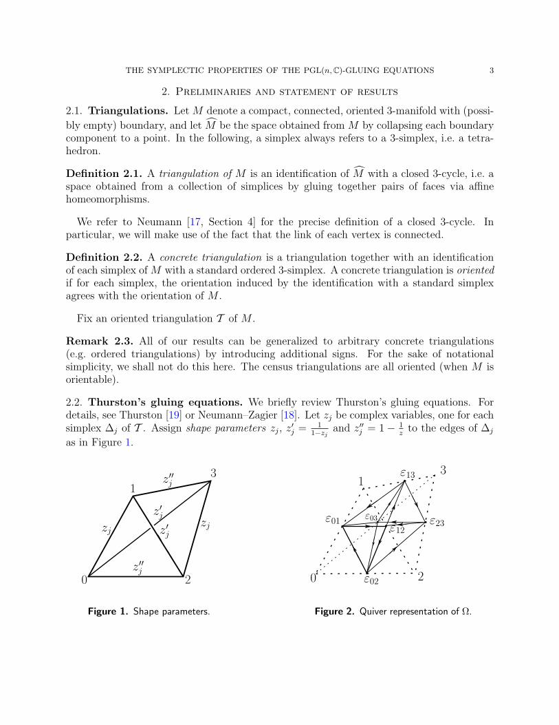
2.2. Thurston’s gluing equations. We briefly review Thurston’s gluing equations. Fordetails, see Thurston [19] or Neumann–Zagier [18]. Let zj be complex variables, one for eachsimplex ∆j of T . Assign shape parameters zj, z

′j = 1

1−zj and z′′j = 1− 1z

to the edges of ∆j

as in Figure 1.

zj

0

1

2

3

zjz′j

z′j

z′′j

z′′j

ε01

ε02

ε23

ε13

ε12

ε03

20

13

Figure 1. Shape parameters. Figure 2. Quiver representation of Ω.


2.2.1. Edge equations. We have a gluing equation for each 1-cell e of T defined by settingequal to 1 the product of all shape parameters assigned to the edges identified with e. Thegluing equation for e can thus be written in the form

(2.1)∏j

(zj)A′e,j∏j

(z′j)B′e,j∏j

(z′′j )C′e,j = 1, or

∏j

(zj)Ae,j∏j

(1− zj)Be,j = εe

where A = A′ − C ′ and B = C ′ − B′ are the so-called gluing equation matrices. Each non-degenerate (zj ∈ C \ 0, 1,∞) solution determines a representation π1(M) → PGL(2,C).Note that the rows of the gluing equation matrices are parametrized by 1-cells, and thecolumns by the simplices of T .

2.2.2. Cusp equations. Each (non-degenerate) solution z = zj to the edge equations givesrise to a cohomology class C(z) ∈ H1(∂M ; C∗). This is defined by taking a class α ∈ H1(M)to the product of the shape parameters of the edges passed by traversing a normal curvein M representing α. One can show that C(z) is trivial if and only if the representationcorresponding to z is boundary-unipotent. Fixing a system of generators of H1(∂M), thevanishing of C(z) is equivalent to a system of equations

(2.2)∏j

(zj)A′ cuspλ,j

∏j

(z′j)B′ cuspλ,j

∏j

(z′′j )C′ cuspλ,j = 1, or

∏j

(zj)Acuspλ,j

∏j

(1− zj)Bcuspλ,j = ελ

of the form (2.1) with an equation for each generator λ. Note that the rows of the cuspequation matrices are parametrized by generators λ of H1(∂M), and the columns by thesimplices of T .

2.3. Neumann’s chain complex. For an ordered 3-simplex ∆, let J∆ denote the freeabelian group generated by the unoriented edges of ∆ subject to the relations

ε01 = ε23, ε12 = ε03, ε02 = ε13(2.3)

ε01 + ε12 + ε02 = 0.(2.4)

Here εij denotes the edge between vertices i and j of ∆. Note that (2.3) states that twoopposite edges are equal, and that (2.3) and (2.4) together imply that the sum of the edgesincident to a vertex is 0.

The space J∆ is endowed with a non-degenerate skew symmetric bilinear form Ω defineduniquely by

Ω(ε01, ε12) = Ω(ε12, ε02) = Ω(ε02, ε01) = 1.(2.5)

The form Ω may be represented by the quiver in Figure 2. Namely, each edge of ∆ corre-sponds to a vertex of the quiver, and Ω(ε, ε′) = 1 if and only if there is a directed edge inthe quiver going from ε to ε′.

Neumann [17, Thm 4.1] encoded the symplectic properties of the gluing equations in termsof a chain complex J = J (T )

(2.6) 0 // C0(T )α // C1(T )

β // J(T )β∗ // C1(T )

α∗ // C0(T ) // 0

defined combinatorially from the triangulation T . Here

• Ci(T ) is the free Z-module of the unoriented i-simplices of T .


• J(T ) =⊕

∆∈T J∆, with Ω extended orthogonally.• α takes a 0-cell to the sum of incident 1-cells (with multiplicity).• β takes a 1-cell to the sum of its edges.• α∗ maps an edge to the sum of its endpoints.• β∗ is the unique rotation equivariant map taking ε01 to [ε03] + [ε12]− [ε02]− [ε13].• α∗ and β∗ are the duals of α and β (using that J(T ) ∼= J(T )∗ via Ω).

Since β∗ β = 0, Ker(β∗) is Ω-orthogonal to Im(β), so Ω descends to a form on H3(J ). Thisform remains non-degenerate on H3(J ) modulo torsion.

The complex J is indexed such that J5 is the leftmost C0(T ), and J0 the rightmost.

Theorem 2.4 (Neumann [17, Thm 4.2]). The homology groups of J are given by

(2.7)H5(J ) = 0, H4(J ) = Z/2Z, H3(J ) = K ⊕H1(M ; Z/2Z)

H2(J ) = H1(M ; Z/2Z), H1(J ) = Z/2Z,

where K = Ker(H1(∂M,Z) −→ H1(M,Z/2Z)

). Moreover, the isomorphism

(2.8) H3(J )/torsion ∼= K

identifies Ω with the intersection form (restricted to K) on H1(∂M).

Remark 2.5. Under the isomorphism

(2.9) H3(J )⊗ Z[1/2] ∼= H1(∂M ; Z[1/2]),

the form Ω corresponds to twice the intersection form [17, Theorem 4.1].

2.4. Symplectic properties of the gluing equations. Neumann’s result implies someimportant symplectic properties of the gluing equation matrices. We formulate them herein a way that generalizes to the PGL(n,C) setting.

By the definition of β we have for each 1-cell e

(2.10) β(e) =∑j

A′e,jε01,j+∑j

B′e,jε12,j+∑j

C ′e,jε02,j =∑j

Ae,jε01,j+∑j

Be,jε12,j ∈ J(T ).

Similarly, for a generator λ of H1(∂M), we have the element

(2.11) δ(λ) =∑j

Acuspλ,j ε01,j +

∑j

Bcuspλ,j ε12,j ∈ J(T ).

Neumann shows that this element is in Ker(β∗), so that we have a map δ : H1(∂M)→ H3(J ).

Corollary 2.6. Let wJ be the standard symplectic form on Z2t given by J =(

0 I−I 0

), where

t is the number of simplices of T and let ι denote the intersection form on H1(∂M).

(i) For any rows x and y of (A|B), wJ(x, y) = 0.(ii) For any rows x of (A|B) and y of (Acusp|Bcusp), wJ(x, y) = 0.

(iii) For any rows x and y of (Acusp|Bcusp) corresponding to λ and µ in H1(∂M), respectively,wJ(x, y) = Ω(δ(λ), δ(µ)) = 2ι(λ, µ).

Proof. The first and second statement follow from the fact that β∗β = 0, which implies thatKer(β∗) is symplectically orthogonal to Im(β). The third result is proved in Neumann [17],c.f. Remark 2.5. Namely δ : H1(∂M)→ H3(J ) induces the isomorphism in (2.9).


Corollary 2.7. The rank of (A|B) is the number of edges minus the number of cusps.

Proof. It follows from (2.10), that the matrix representation for β in the basis ε01,j, ε12,jfor J(T ) is the transpose of (A|B). The result now follows from the fact that H4(J ) is zeromodulo torsion.

Remark 2.8. A simple argument that uses the Euler characteristic shows that the numberof edges of T equals t+ c−h, where t is the number of simplices, h = 1

2rank(H1(∂M)) and c

is the number of boundary components. Hence, the matrix (A|B) has size (t+c−h)×2t. Inparticular, if all boundary components are tori (the case of most interest), the size is t× 2t.If we extend a basis for the row span of (A|B) by rows of (Acusp|Bcusp), the resulting t× 2tmatrix has full rank, and is thus the upper half of a symplectic matrix. Such matrices playa crucial role in [4, 8, 7, 6, 13].

2.5. Statement of results. The PGL(n,C)-gluing equations [12] are defined in terms ofcomplex variables zs,∆, one for each subsimplex s (Definition 3.1) of each simplex ∆ of T .There is a gluing equation for each non-vertex integral point p of T (Definition 3.3), whichcan be written in the form

(2.12)∏(s,∆)

(zs,∆)Ap,(s,∆)

∏(s,∆)

(1− zs,∆)Bp,(s,∆) = εp,

where A and B are integer matrices whose rows are parametrized by the (non-vertex) integralpoints of T and columns by the set of subsimplices of the simplices of T .

Furthermore there is a cusp equation for each generator λ ⊗ er of H1(∂M ; Zn−1) of theform

(2.13)∏(s,∆)

(zs,∆)Acuspλ⊗er,(s,∆)

∏(s,∆)

(1− zs,∆)Bcuspλ⊗er,(s,∆) = ελ⊗er

for matricesAcusp andBcusp whose rows are parametrized by generators λ⊗er ofH1(∂M ; Zn−1)and columns by the set of subsimplices of the simplices of T .

In Section 4 below we define a chain complex J g = J g(T ) (indexed so that J g5 is the

leftmost Cg0(T ))

(2.14) 0 // Cg0(T )

α // Cg1(T )

β // Jg(T )β∗ // Cg

1(T )α∗ // Cg

0(T ) // 0

generalizing (2.6). Here g denotes the Lie algebra of SL(n,C), the notation being in antici-pation of a generalization to arbitrary simple, complex Lie algebras. The three middle termsof J g appeared already in Garoufalidis–Goerner–Zickert [12]. There is a non-degenerate an-tisymmetric form on Jg(T ) descending to a non-degenerate form on H3(J g) modulo torsion.

Theorem 2.9. Let h = 12

rank(H1(∂M)). The homology groups of J g are given by

(2.15)H5(J g) = 0, H4(J g) = Z/nZ, H3(J g) = K ⊕H1(M ; Z/nZ)

H2(J g) = H1(M ; Z/nZ), H1(J g) = Z/nZ,

where K ⊂ H1(∂M,Zn−1) is a subgroup of index nh. Moreover, the isomorphism

(2.16) H3(J g)⊗ Z[1/n] ∼= H1(∂M ; Z[1/n]n−1)


identifies Ω with the non-degenerate form ωAg on H1(∂M ; Z[1/n]n−1) given by

(2.17) ωAg(λ⊗ v, µ⊗ w) = ι(λ, µ)〈v,Agw〉,

where ι is the intersection form on H1(∂M), 〈, 〉 the canonical inner product on Rn, and Ag

the Cartan matrix of g.

Remark 2.10. Presumably, K = Ker(H1(∂M ; Zn−1) → H1(M ; Z/nZ)

), where Z/nZ is

regarded as the quotient of Zn−1 by the column space of the Cartan matrix. This would bea natural generalization of the K in Theorem 2.4.

As explained in Section 4.1, the group Jg(T ) is generated by terms (s, e)∆, where e is anedge of a subsimplex s of a simplex ∆ of T . As in (2.10) we have

(2.18) β(p) =∑(s,∆)

Ap,(s,∆)(s, ε01)∆ +∑(s,∆)

Bp,(s,∆)(s, ε12)∆ ∈ Jg(T ).

Also, as in (2.11), we have for each generator λ⊗ er of H1(∂M ; Zn−1) an element

(2.19)∑(s,∆)

Acuspλ⊗er,(s,∆)(s, ε01)∆ +

∑(s,∆)

Bcuspλ⊗er,(s,∆)(s, ε12)∆ ∈ Jg(T ),

in the kernel of β∗. In fact it equals δ′(λ ⊗ er) for a map δ′ : H1(∂M ; Zn−1) → H3(J g)which induces the isomorphism (2.16) (see Section 8.2). The following is the analogue ofCorollary 2.6.

Corollary 2.11. The rows of (A|B) are orthogonal to the rows of (Acusp|Bcusp) with re-spect to the standard symplectic form ωJ . Moreover, if x and y are rows of (Acusp|Bcusp)corresponding to λ⊗ er and µ⊗ es, respectively, we have

(2.20) ωJ(x, y) = Ω(δ′(λ⊗ er), δ′(µ⊗ es)

)= ι(λ, µ)〈er, Ages〉.

The proof of the following result is identical to that of Corollary 2.7. In the case where allboundary components are tori, the number of non-vertex integral points is

(n+1

3

)times the

number of simplices (see Lemma 3.5).

Corollary 2.12. The rank of (A|B) is the number of non-vertex integral points minusc(n− 1), where c is the number of boundary components.

Remark 2.13. If all boundary components are tori, (A|B) has twice as many columns asrows, and c(n − 1) = 1

2rankH1(∂M ; Zn−1). It follows that one can extend a basis for the

row space of (A|B) by adding rows of (Acusp|Bcusp) to obtain a matrix with full rank. Thismatrix is then the upper part of a symplectic matrix and as stated in the introduction playsa crucial role in extending the work of [4, 8, 7, 6, 13] to the PGL(n,C) setting.

Remark 2.14. The computation of the rational homology of H3(J g) was obtained forn = 3 by Bergeron–Falbel–Guilloux [2] (using a different, but isomorphic chain complex). Ageneralization to n > 3 by Guilloux [15] yields results similar to ours.


2.6. A side comment on quivers. If you take a quiver as in Figure 2 for each subsimplexand superimpose them canceling edges with opposite orientations, you get the quiver shownin Figure 3. Everything cancels in the interior. The quiver on the face equals the quiver inFock–Goncharov [10, Fig. 1.5], and also appears for n = 3 in Bergeron–Falbel–Guilloux [2,Fig. 4]. One can go from the quiver on two of the faces to the quiver on the two otherfaces by performing quiver mutations (see e.g. Keller [16]). The quiver mutations changethe X-coordinates and Ptolemy coordinates by cluster mutations [?], and there is a one-onecorrespondence between quiver mutations and subsimplices. Although we do not need anyof this here, this observation was a major motivation for [14] and [12].

1

0 2

1

3

2

Figure 3. Superposition of copies of the quiver in Figure 2, one for each subsimplex.

3. Shape assignments and gluing equations

We identify each simplex of M with the simplex

(3.1) ∆3n =

(x0, x1, x2, x3) ∈ R4

∣∣ 0 ≤ xi ≤ n, x0 + x1 + x2 + x3 = n.

Let ∆3n(Z) denote the integral points of ∆3

n, and ∆3n(Z) denote the integral points with the

4 vertex points removed. The natural left A4-action on ∆3n given by

(3.2) σ(x0, . . . , x3) = (xσ−1(0), . . . , xσ−1(3))

induces A4-actions on ∆3n(Z) and ∆3

n(Z) as well.

Definition 3.1. A subsimplex of ∆3n is a subset S of ∆3

n obtained by translating ∆32 ⊂ R4

by an element s in ∆3n−2(Z) ⊂ Z4, i.e. S = s+ ∆3

2. Note that |∆3n(Z)| =

(n+1

3

).

We shall identify the edges of an ordered simplex with ∆32(Z), e.g. the edges ε01 and ε12

correspond to (1100) and (0110).

Definition 3.2. A shape assignment on ∆3n is an assignment

(3.3) z : ∆3n−2(Z)× ∆3

2(Z)→ C \ 0, 1, (s, e) 7→ zes

satisfying the shape parameter relations


(3.4) zε01s = zε23

s =1

1− zε02s, zε12

s = zε03s =

1

1− zε01s, zε02

s = zε13s =

1

1− zε12s

One may think of a shape assignment as an assignment of shape parameters to the edgesof each subsimplex. The ad hoc indexing of the shape parameters by z, z′ and z′′ is replacedby an indexing scheme, in which a shape parameter zes,∆ is indexed according to the edge eof the subsimplex s of the simplex ∆ to which it is assigned.

Definition 3.3. An integral point of T is an equivalence class of points in ∆3n(Z) identified

by the face pairings of T . We view an integral point as a set of pairs (t,∆) with t ∈ ∆3n(Z)

and ∆ ∈ T . An integral point is either a vertex point, an edge point, a face point, or aninterior point.

Definition 3.4. A shape assignment on T is a shape assignment zes,∆ on each simplex ∆ ∈ Tsuch that for each non-vertex integral point p, the generalized gluing equation

(3.5)∏

(t,∆)∈p

∏s+e=t

zes,∆ = 1.

is satisfied. Here, the first product is over pairs (t,∆) representing p, and the second is overpairs (s, e) ∈ ∆3

n−2(Z)× ∆32(Z) such that s+ e = t.

The gluing equation for p sets equal to 1 the product of the shape parameters of all edgesof subsimplices having p as midpoint, see Figures 4 and 5 (taken from [12]). The producthas 6 terms if p is an interior point or a face point, and ν terms if p is an edge point on anedge of valence ν.

13

2

0

32

0

0

1

3

2

z11001200,0

z01100120,2

z01010102,1

0

21

3

0

21

3

∆0 ∆1

Figure 4. Edge equation for n = 5:

z11001200,0z

01010102,1z

01100120,2 = 1.

Figure 5. Face equation for n = 6:

z00112011,0z

10011021,0z

10101012,0z

00110211,1z

01010121,1z

01100112,1 = 1.

Lemma 3.5. If all boundary components are tori, the number of non-vertex integral pointsis(n+1

3

)τ , where τ is the number of simplices of T . Hence, the number of variables is the

same as the number of equations.


Proof. Letting ε, and ψ denote the number edges, and faces, respectively, the number q ofnon-vertex integral points is given by

(3.6) q = (n− 1)ε+(n− 1)(n− 2)

2ψ +

(n− 1)(n− 2)(n− 3)

6τ.

Clearly, ψ = 2τ , and if all boundary components are tori, a simple Euler characteristicargument shows that τ = ε. It thus follows that q =

(n+1

3

)τ , as desired.

Note that the gluing equation for p can be written in the form

(3.7)∏(s,∆)

(z(s,∆))Ap,(s,∆)

∏(s,∆)

(1− z(s,∆))Bp,(s,∆) = εp.

Theorem 3.6 (Garoufalidis–Goerner–Zickert [12]). A shape assignment on T determines(up to conjugation) a representation π1(M)→ PGL(n,C).

3.1. X-coordinates. The X-coordinates are defined on the face points of T , and are usedin Section 8 to define the cusp equations. They agree with the X-coordinates of Fock andGoncharov [10].

Definition 3.7. Let z be a shape assignment on ∆3n and let t ∈ ∆3

n(Z) be a face point. TheX-coordinate at t is given by

(3.8) Xt = −∏s+e=t

zes ,

i.e. it equals (minus) the product of the shape parameters of the 3 edges of subsimpliceshaving t as a midpoint.

Remark 3.8. Note that the gluing equation for a face point p = (t1,∆1), (t2,∆2) statesthat Xt1Xt2 = 1.

4. Definition of the chain complex

We now define the chain complex (2.14).

4.1. Definition of the terms. Let Cg0(T ) = C0(T )⊗Zn−1 and let Cg

1(T ) be the free abeliangroup on the non-vertex integral points of T . Letting e1, . . . , en−1, denote the standard basisvectors of Zn−1, it follows that Cg

0(T ) is generated by symbols x⊗ ei, where x is a 0-cell ofT . It will occasionally be convenient to define e0 = en = 0. Let

(4.1) Jg(T ) =⊕∆∈T

⊕s∈∆3

n−2(Z)

J∆32

be a direct sum of copies of J∆32, one for each subsimplex of each simplex of T . The group

Jg(T ) is thus generated by the set of all edges e of all subsimplices s of the simplices ∆ ofT , and we denote a generator by (s, e)∆. The generators are subject to relations

(s, ε01)∆ = (s, ε23)∆, (s, ε12)∆ = (s, ε03)∆, (s, ε02)∆ = (s, ε13)∆(4.2)

(s, ε01)∆ + (s, ε12)∆ + (s, ε02)∆ = 0.(4.3)

It thus follows that (s, ε01)∆, (s, ε12)∆ is a basis for Jg(T ).


The form Ω on J∆32

induces by orthogonal extension a form on Jg(T ) also denoted by Ω.

Since Ω is non-degenerate it induces a natural identification of Jg(T ) with its dual. Similarly,the natural bases of Cg

0(T ) and Cg1(T ) induce natural identifications with their respective

duals.

4.2. Formulas for β and β∗. Define

(4.4) β : Cg1(T )→ Jg(T ), p = (t,∆) 7→

∑(∆,t)∈p

∑e+s=t

(s, e)∆.

Hence, β takes p to the formal sum of all the edges of subsimplices whose midpoint is p. By[12, Lemma 7.3], the dual map β∗ : Jg(T )→ Cg

1(T ) is the unique map satisfying

(4.5)

β∗((s, ε01)∆) = [(s+ ε03,∆)] + [(s+ ε12,∆)]− [(s+ ε02,∆)]− [(s+ ε13,∆)]

β∗((s, ε12)∆) = [(s+ ε02,∆)] + [(s+ ε13,∆)]− [(s+ ε01,∆)]− [(s+ ε23,∆)]

β∗((s, ε02)∆) = [(s+ ε01,∆)] + [(s+ ε23,∆)]− [(s+ ε23,∆)]− [(s+ ε12,∆)].

We refer to an element of the form β∗((s, εij)∆) as an elementary quad relation, see Fig-ures 6, 7 and 8.

0

1

2

3

−

++

−

0

1

2

3

+

+

− −

0

1

2

3

−+

−+

Figure 6. β∗(s, ε01). Figure 7. β∗(s, ε12). Figure 8. β∗(s, ε02).

Lemma 4.1. [Garoufalidis–Goerner–Zickert [12, Prop. 7.4]] β∗ β = 0.

4.3. Formulas for α and α∗. For a 0-cell x of T and a simplex ∆, let I∆(x) ⊂ 0, 1, 2, 3 bethe set of vertices of ∆ that are identified with x. Also, for t ∈ ∆3

n(Z) and k ∈ 1, . . . , n−1,let

(4.6) ct,∆,k(x) = |i ∈ I∆(x) | ti = k| .

Note that if (t,∆) and (t′,∆′) define the same integral point, then ct,∆,k(x) = ct′,∆′,k(x).Define

(4.7) α : Cg0(T )→ Cg

1(T ), x⊗ ek 7→∑p

ct,∆,k(x)p,

where the sum is over all integral points p, and (t,∆) is any representative of p. Also, define

(4.8) α∗ : Cg1(T )→ Cg

0(T ), [(t,∆)] 7→3∑i=0

xi ⊗ eti ,


where xi is the 0-cell of T defined by the ith vertex of ∆ (recall that e0 = 0). Informally,α takes x ⊗ ek to the integral points at distance k from x (counted with multiplicity), andα∗ sends an integral point to its coordinates with respect to any simplex containing it (seeFigures 9 and 10). It is elementary to check that α∗ is well defined, and that it is the dualof α.

x

x y

1

1

2

x

y z

t

Figure 9. α(x⊗e2) for n = 4. Figure 10. α∗([t,∆]) = x⊗ e2 + y⊗ e1 + z⊗ e1.

Lemma 4.2. We have α∗ β∗ = 0.

Proof. Let s ∈ ∆3n−2(Z) be a subsimplex. We have

α∗ β∗(s, ε01)∆ = α∗([(s+ ε03,∆)]) + α∗([(s+ ε12,∆)])

− α∗([(s+ ε02,∆)])− α∗([(s+ ε13,∆)])

= x0 ⊗ es0+1 + x1 ⊗ es1 + x2 ⊗ es2 + x3 ⊗ es3+1

+ x0 ⊗ es1 + x1 ⊗ es1+1 + x2 ⊗ es2+1 + x3 ⊗ es3− x0 ⊗ es0+1 − x1 ⊗ es1 − x2 ⊗ es2+1 − x3 ⊗ es3− x0 ⊗ es0 − x1 ⊗ es1+1 − x2 ⊗ es2 − x3 ⊗ es3+1 = 0

Similarly, α∗ β∗(s, ε12)∆ = α∗ β∗(s, ε02)∆ = 0.

By duality, β α is also 0, so by Lemmas 4.1 and 4.2 we have a chain complex J g(T ):

(4.9) 0 // Cg0(T )

α // Cg1(T )

β // Jg(T )β∗ // Cg

1(T )α∗ // Cg

0(T ) // 0

Note that when n = 2, J g equals J .

Convention 4.3. When there can be no confusion, we shall sometimes suppress the simplex∆ from the notation. For example, we sometimes write (s, e) instead of (s, e)∆, and if t isan integral point of a simplex ∆ of T , we denote the corresponding integral point of T by[t] or sometimes just t instead of [(t,∆)].

5. Characterization of Im(β∗)

We develop some relations in Cg1(T )/Im(β∗) that are needed for computing H2(J g). These

relations may be of independent interest.


5.1. Quad relations.

Definition 5.1. A quadrilateral (quad for short) in ∆3n is the convex hull of 4 points

(5.1) p0 = a+ (k, 0, 0, l), p1 = a+ (k, 0, l, 0), p2 = a+ (0, k, l, 0), p3 = a+ (0, k, 0, l),

or the image of such under a permutation in S4. Here k, l are positive integers with k+ l ≤ nand a ∈ ∆n−k−l(Z). A quad determines a quad relation in Cg

1(T ) given by the alternatingsum p0 − p1 + p2 − p3 of its corners.

Figure 11 shows 3 quad relations for n = 4.

Lemma 5.2. A quad relation is in the image of β∗, and is thus zero in H2(J g).

Proof. This follows from the fact that any quad relation is a sum of the elementary quadrelations in Figures 6, 7 and 8. For an algebraic proof, note that

(5.2) p0 − p1 + p2 − p3 =∑

1<i≤k,1<j≤l

β∗(a+ (k − i, i− 1, j − 1, l − j), ε01

).

-

--

-

++

+

0

1

2

3

-+

++ -

-

0 2

1

t

+ --

--

+

++

20

1

Figure 11. Quad rela-

tions.

Figure 12. Hexagon

relation.

Figure 13. Long

hexagon relation.

Recall that we have divided integral points into edge points, face points and interior points.We shall need a finer division.

Definition 5.3. The type of a point t ∈ ∆n(Z) is the orbit of t under the S4 action.

Note that the type is preserved under face pairings, so it makes sense to define the typeof an integral point p = [(t,∆)] to be the type of any representative.

Proposition 5.4. Let p and q be integral points of the same type. Then

(5.3) p− q ∈ Im(β∗) + E,

where E is the subgroup of Cg1(T ) generated by edge points.

Proof. We first assume that the points lie in the same simplex. The quad relation (togetherwith similar relations obtained by permutations)

(5.4) (a, b, c, d)− (a, b, c+ d, 0) + (b, a, c+ d, 0) + (b, a, c, d)


shows that the difference between two interior points of the same type is equal modulo Im(β∗)to the difference between two face points of the same type. Similarly, the relation

(5.5) (a, b, 0, c)− (a, b, c, 0) + (0, a+ b, c, 0)− (0, a+ b, 0, c)

shows that the difference between two face points (of the same type) in distinct faces is inIm(β∗) + E. Finally, the two quad relations

(5.6)(0, a, b, c) = (a, 0, b, c) + (0, a, 0, b+ c)− (a, 0, 0, b+ c),

(0, a, c, b) = (a, 0, c, b) + (0, a, b+ c, 0)− (a, 0, b+ c, 0)

in Cg1(T )/Im(β∗) imply that the difference between two face points (of the same type) in the

same face is also in Im(β∗) + E. This concludes the proof when the points are in the samesimplex. The quad relation

(5.7) (a, b, c, d) = (a, b, c+ d, 0)− (0, b+ a, c+ d, 0) + (0, a+ b, c, d)

shows that (a, b, c, d) modulo E + Im(β∗) is a sum of face points, which we (by the above)may move to the same face. This proves the result for p and q in adjacent simplices, and thegeneral case follows from the fact that M is connected.

5.2. Hexagon relations. Besides the quad relations, we shall need further relations thatlie entirely in a face.

Lemma 5.5. For any face point t, the element β∗(∑

s+e=t(s, e))

is an alternating sum ofthe corners of a hexagon with center at t (see Figure 12).

Proof. By rotational symmetry, we may assume that t = (t0, t1, t2, 0). We thus have

(5.8) β∗( ∑s+e=t

(s, e))

= β∗(t− ε01, ε01) + β∗(t− ε12, ε12) + β∗(t− ε02, ε02).

Using the formula (4.5) for β∗, (5.8) easily simplifies to

(5.9) β∗( ∑s+e=t

(s, e))

= −[t+ (−1, 1, 0, 0)] + [t+ (−1, 0, 1, 0)]− [t+ (0,−1, 1, 0)]

+ [t+ (1,−1, 0, 0)]− [t+ (1, 0,−1)] + [t+ (0, 1,−1, 0)].

This corresponds to the configuration in Figure 12.

Definition 5.6. An element as in Lemma 5.5 is called a hexagon relation. By taking sumsof hexagon relation, we obtain relations as shown in Figure 13. We refer to these as longhexagon relations (a hexagon relation is also regarded as a long hexagon relation).

6. The outer homology groups

We focus here on the computation of H1(J g) and H2(J g); the computation of H5(J g)and H4(J g) will follow by a duality argument (see Section 6.3).


6.1. Computation of H1(J g).

Proposition 6.1. H1(J g) = Z/nZ.

Proof. Consider the map

ε : Cg0(T )→ Z/nZ, x⊗ ek 7→ k.

We must prove that ε is surjective and that Ker(ε) = Im(α∗). Surjectivity is obvious, andthe inclusion Im(α∗) ⊂ Ker(ε) follows from the fact that the sum of the coordinates ofany point in ∆3

n(Z) is n. To prove the other inclusion, let [σ] ∈ Ker(ε)/

Im(α∗), and let

σ =∑N

i=1 εixi⊗ eki be a representative with N minimal and εi = ±1. We wish to prove thatN = 0, so suppose N > 0. We start by showing that modulo Im(α∗), the relations

(6.1) x⊗ ek + y ⊗ en−k = 0, x⊗ ek − y ⊗ ek = 0

hold for all 0-cells x, y. Pick an edge path of odd length between x and y with vertices x0 =x, x1, . . . , x2k−1 = y. For z, w vertices joined by an edge e, let (z, w; k) be the edge point of Tcorresponding to the point on e at distance k from w. Then α∗(z, w; k) = z⊗ ek +w⊗ en−k.We thus have

(6.2) x⊗ ek + y ⊗ en−k = α∗((x, x1; k)− (x1, x2;n− k) + · · ·+ (x2k−2, y; k)

).

This proves the first equation in (6.1). The second follows similarly by considering an edgepath of even length.

Clearly N 6= 1, and it follows from (6.1) that [σ] = 0 if N = 2. Hence, we may assumethat N ≥ 3, and also (using (6.1)) that ki ≤ n/2 for all i. Up to switching the sign of σ andreordering the summands, we may thus assume that

(6.3) σ = x1 ⊗ ek1 + x2 ⊗ ek2 +∑i>2

εixi ⊗ eki .

Fix three 0-cells x, y, z lying on a face, and let p be the unique integral point satisfying

(6.4) α∗(p) = x⊗ ek1 + y ⊗ ek2 + z ⊗ en−k1−k2 .

Subtracting α∗(p) from σ and using (6.1), we can thus construct a representative of [σ] withfewer than N terms, contradicting minimality of N . Hence, σ = 0.

6.2. Computation of H2(J g). In this section we prove that H2(J g) = H1(M ; Z/nZ). Thefact that H2(J g) is torsion is crucial, and is used in the proof of Proposition 7.9. We see noway of proving that H2(J g) is torsion without computing it explicitly.

Let εoriij denote the oriented edge (from i to j) between i and j.

6.2.1. Definition of a map ν : H2(J g)→ H1(M ; Z/nZ). Consider the map

(6.5) ν : Z[∆3n(Z)]→ C1(∆3; Z/nZ), (t0, t1, t2, t3) 7→ t1ε

ori01 + t2ε

ori02 + t3ε

ori03 .

Note that modulo boundaries in C1(∆3; Z/nZ), we have

(6.6) t1εori01 +t2ε

ori02 +t3ε

ori03 = t0ε

ori10 +t2ε

ori12 +t3ε

ori13 = t0ε

ori20 +t1ε

ori21 +t3ε

ori23 = t0ε

ori30 +t1ε

ori31 +t2ε

ori32 .


Lemma 6.2. The map (6.5) induces a well defined map

(6.7) ν : Cg1(T )→ C1(M ; Z/nZ)

/boundaries

which takes cycles to cycles and boundaries to 0.

Proof. If the triangulation T is ordered (all face pairings are order preserving), so that alledges of T are canonically oriented, the fact that ν is well defined is a simple consequence

of (6.6). The general case follows from the fact that if εoriij,∆ and εori

kl,∆′ are identified in M ,

their images in C1(M) differ by a sign, which is positive if and only if i − j and k − l havethe same sign. To see that cycles map to cycles consider the diagram

(6.8)

Cg1(T )

ν //

α∗

C1(M ; Z/nZ)/boundaries

∂

Cg0(T )

ν0 // C0(M ; Z/nZ),

where ν0 is the map given by

(6.9) ν0 : Cg0(T )→ C0(M ; Z/nZ), x⊗ ei 7→ ix.

We must prove that (6.8) is commutative. This follows from

(6.10) ∂(ν(t)) = ∂(t1εori01 + t2ε

ori02 + t3ε

ori03 ) =

t1(x1 − x0) + t2(x2 − x0) + t3(x3 − x0) = t0x0 + t1x1 + t2x2 + t3x3 = ν α∗(t).

We must check that ν takes β∗(Jg(T )) to 0. By rotational symmetry, it is enough to provethat ν takes β∗(s, ε01) to 0. Using (4.5) we have

(6.11) ν(β∗(s, ε01)

)=(s1ε

ori01 + s2ε

ori02 + (s3 + 1)εori

03

)+((s1 + 1)εori

01 + (s2 + 1)εori02 + s3ε

ori03

)−(s1ε

ori01 + (s2 + 1)εori

02 + s3εori03

)−((s1 + 1)εori

01 + s2εori02 + (s3 + 1)εori

03

)= 0.

This concludes the proof.

Hence, ν induces a map

(6.12) ν : H2(J g)→ H1(M ; Z/nZ).

6.2.2. Construction of a map µ : H1(M ; Z/nZ) → H2(J g). We prove that ν is an isomor-phism by constructing an explicit inverse. Let k ∈ 1, 2, . . . , n− 1.

Definition 6.3. Let e be an oriented edge of T . If f is a face containing e, the pathconsisting of the two other edges in f is called a tooth of e.

Given a tooth Te of an edge e, let µk(e)Te ∈ Cg1 be the element shown in Figure 14.

Lemma 6.4. For any two teeth Te and T ′e of e, we have

(6.13) µk(e)Te = µk(e)T ′e ∈ Cg1(T )

/Im(β∗).


Proof. Since any two teeth of e are connected through a sequence of flips past simplices inthe link of e, it is enough to prove the result when Te and T ′e are teeth in a single simplex.Hence, we must prove that a configuration as in Figure 15 represents zero in Cg

1(T )/

Im(β∗).This is a consequence of the quad relation (Definition 5.1).

e

k

1 −1

Te

e

k1 −1

−1 1Te

T ′e

Figure 14. A tooth Te of e and

µk(e)Te .Figure 15. µk(e)Te − µk(e)T ′e is a

quad relation.

It follows that we have a map

(6.14) µk : C1(M)→ Cg1(T )

/Im(β∗), e 7→ µk(e)Te .

We shall also consider the map µk : C1(M) → Cg1(T ) taking an oriented edge e of T to the

integral point on e at distance k from the initial point of e. Note that if f1 and f2 are thefirst and second edge of some tooth of e, µk(e) = µk(f1)− µn−k(f2). This is immediate fromthe definition of µk and µk.

Lemma 6.5. If e1 and e2 are two consecutive oriented edges,

(6.15) µk(e1 + e2) = µk(e1)− µn−k(e2) ∈ Cg1(T )

/Im(β∗).

Proof. We must show that a configuration as in Figure 16 represents 0 in Cg1(T )

/Im(β∗).

By flipping the teeth of e1 and e2 (which by Lemma 6.4 does not change the element inCg

1(T )/

Im(β∗)), we can tranform the configuration into a configuration as in Figure 17 wherethe two teeth meet at a common edge e (the fact that this is always possible follows fromthe fact that each vertex link is connected). This configuration also represents µn−k(e)Te −µn−k(e)T ′e for two teeth Te and T ′e of e, so is zero by Lemma 6.4.

Corollary 6.6. µk induces a map µk : H1(M)→ H2(J g).

Proof. The fact that µk takes cycles to cycles is immediate from the definition of α∗. Lete1 + e2 + e3 be an oriented path representing the boundary of a face in T . We have

(6.16) µk(e1 + e2 + e3) = µk(e1 + e2) + µk(e3) =

µk(e1)− µn−k(e2) + µk(e3) = −µk(e3) + µk(e3) = 0,

where the third equality follows from the fact that e1 + e2 is a tooth of e3. This proves theresult.


kk

1−1

−1 1

1

−1

k k

e1 e2

Te1 Te2

−1

1

1

−1

eTe T ′e

e1 e2

Figure 16. Configuration represent-

ing µk(e1 + e2)− µk(e1) + µn−k(e2).

Figure 17. Configuration represent-

ing µk(e)Te − µk(e)T ′e = 0.

Lemma 6.7. We have µk = −µn−k : H1(M)→ H2(J g).

Proof. Let α ∈ H1(M). Since H1(M) is generated by edge cycles, we may assume that α isrepresented by an edge cycle e1 + e2 + · · ·+ e2l, which we may assume to have even length.We thus have (indices modulo 2l)

(6.17) µk(α) =l∑

i=1

(µk(e2i−1)− µn−k(e2i)

)=

l∑i=1

(− µn−k(e2i) + µk(e2i+1)

)= −µn−k(α),

where the first and third equality follow from Lemma 6.5 and the second equality followsfrom shifting indices by 1.

Lemma 6.8. For each k, we have µk = kµ1 : H1(M)→ H2(J g).

Proof. Let α = e1 + e2 + · · ·+ e2l as in the proof of Lemma 6.7. We can represent kµ1(ei)−µk(ei) as in Figure 18. By applying long hexagon relations (k−d relations at distance d fromei) in the direction parallel to ei, the configuration is equivalent to that of Figure 19. Nowconsider two consecutive edges ei and ei+1 as in Figure 20. By flipping teeth (which doesn’tchange the homology class), we may transform the configuration into that of Figure 21,and by further flipping, we may assume that the configuration lies in a single simplex. Itis now evident, that the points near the common edge e represents a sum of k − 1 quadrelations. Hence, all the points near e vanish. By flipping the teeth back, we end up witha configuration as in Figure 20, but with only points near the leftmost and rightmost edgeremaining. Since α is a cycle, it follows that everything sums to zero.

By the above lemmas we have a map

(6.18) µ : H1(M ; Z/nZ)→ H2(J g), e⊗ k 7→ µk(e).

6.2.3. The map µ is the inverse of ν.

Lemma 6.9. The composition ν µ is the identity on H1(M ; Z/nZ).


ei

k

1 k

−1 1

−kei

k

1k − 1

1

1− k

11

1

1

−1−1−1

−1

−1−1−1

−1

11

1

Figure 18. kµ1(ei)− µk(ei). Figure 19. kµ1(ei) − µk(ei) after

adding long hexagon relations.

k

1 e1 e2

111

1 1

11

11

11

11

111

−1

−1−1−1

−1

−1−1−1

−1

−1−1−1

−1

−1−1−1

k − 11− k k − 1

1− k

k

e1 e2

1

111 −1

−1−1

−1

1−k k−1

Figure 20. kµ1(ei)− µk(ei). Figure 21. Figure 20 after flipping.

Proof. First observe that for each 1-cell e of T , we have ν µk(e) = ke. Consider a repre-

sentative α = e1 + · · · + e2l ∈ C1(M ; Z) of a homology class in H1(M). As in (6.17), wehave

(6.19) ν µk(α) = ν( l∑i=1

(µk(e2i−1)− µn−k(e2i)

))=

l∑i=1

e2i−1 ⊗ k − e2i ⊗ (n− k) = α⊗ k ∈ C1(M ; Z/nZ)/boundaries.

This proves the result.

We now show that µ ν is the identity on H2(J g). The idea is that every homology classin H2(J g) can be represented by edge points. Consider the set

(6.20) T =

(t0, t1, t2, 0) ∈ ∆3n(Z)

∣∣ t0 ≥ t1 ≥ t2 ≥ 0

of points on a face of a fixed simplex of T . By Proposition 5.4 (and (5.7)), we can representeach homology class in H2(J g) by an element τ + e, where e consists entirely of edge points,and τ consists of terms in T . Note that by adding and subtracting edge points in T to τ ,


one may further assume that α∗(τ) = 0. Hence, we shall study elements in Ker(α∗) of theform

(6.21) τ =∑t∈T

ktt, kt ∈ Z.

We say that a term t ∈ T is in τ if kt 6= 0. For j = 1, . . . , n− 1, consider the map

(6.22) πj : Cg0(T )→ Z, x⊗ ei 7→ δij,

where δij is the Kronecker δ. For k ∈ N, let τti=k =∑

ti=kktt be the sum of the terms in τ

with ti = k.

Lemma 6.10. For any k > n/2, τt0=k is a linear combination of terms of the form

(6.23) Ct1,t′1,k = (k, t1, t2, 0)− (k, t′1, t′2, 0), t1 > t′1.

Proof. It is enough to prove that∑

t0=k kt = 0. Since α∗(τ) = 0, this follows from

(6.24) 0 = πk α∗(τ) = πk α∗(τt0=k) =∑t0=k

kt,

which is an immediate consequence of the definition of α∗.

Proposition 6.11. The kernel of α∗ : Cg1(T )→ Cg

0(T ) is generated modulo Im(β∗) by edgepoints. In other word, each homology class can be represented by edge points.

Proof. Let x ∈ H2(J g). As explained above, we can represent x by an element τ + e, wheree consists entirely of edge points, and τ =

∑t∈T ktt ∈ Ker(α∗). We wish to show that τ

is a linear combination of long hexagon relations. We start by inductively decreasing themaximal value tmax

0 of t0 among the terms in τ by adding long hexagon relations in thedirection parallel to the edge opposite vertex 0. More specifically, one adds the long hexagonrelations with corners at the two terms involved in Ct1,t′1,tmax

0(see Figure 22). If a long

hexagon has a vertex outside of t, this vertex is replaced by the unique vertex in T of thesame type. By Lemma 6.10 we can remove all terms with t0 > n/2 in this way. We thencontinue adding long hexagon relations until we end up with a configuration τ ′, where allterms satisfy that t0− t1 ≤ 2, i.e. where all terms are either on the line t0 = t1 or on the sawshaped curve in Figure 23. Note that for any k, the number xk of terms in τ ′ with t2 = k iseither 0, 1 or 2. Using that πk α∗(τ ′) = 0, we see that xk can’t be 1, and that if xk = 2, thecoefficient of the term with t0 > t1 is −2 times the coefficient of the term with t0 = t1. Hence,all terms of τ ′ lie on the square indicated in Figure 23. But this contradicts that α∗(τ ′) = 0,since the corner terms of the square can’t cancel. It thus follows that τ ′ = 0, hence, that τis a sum of long hexagon relations, hence 0 in H2(J g). This proves the result.

Corollary 6.12. The composition µ ν is the identity on H2(J g).

Proof. By Proposition 6.11, one may represent a class in H2(J g) by a linear combination xof edge points. Since α∗(x) = 0, x must be a linear combination of elements of the form

(6.25) σ =l∑

i=1

(µk(e2i)− µn−k(e2i−1)

)


t2 = 01

−1

1 t1 = t2

t0 = t1−1−1

1

1

−1 −1

1−1

1

2

−1

−1

t0 = t1

t1 = t2

t2 = 0

−2

1

2

−1

−2

1

Figure 22. Driving terms up by adding long

hexagon relations.

Figure 23. Final config-

uration.

This follows from the well known fact that the cycles in C1(M) are generated by edge loops.We now have

(6.26) µ ν(σ) = µ((e1 + · · ·+ e2l)⊗ k

)= µk(e1 + · · ·+ e2l) = σ,

where the first equality follows from (6.19), and the third from Lemma 6.5.

The following now follows from Lemma 6.9 and Corollary 6.12.

Proposition 6.13. We have an isomorphism H2(J g) ∼= H1(M ; Z/nZ).

6.3. Computation of H4(J g) and H5(J g). Since J g is self dual, the universal coefficienttheorem implies that

(6.27) Hk(J g) = H6−k((J g)∗) ∼= Hom(H6−k(J g),Z)⊕ Ext(H6−k−1(J g),Z).

It thus follows from Propositions 6.1 and 6.13 that H5(J g) = 0 and that H4(J g) = Z/nZ.

Remark 6.14. One can show that the sum τ of all integral points of T generates H4(J g) =Z/nZ. If M has a single boundary component, corresponding to the 0-cell x of T , we have

(6.28) nτ = α( n−1∑i=1

ix⊗ ei).

We shall not need this, so we leave the proof to the reader.

7. The middle homology group

By (6.27) and Proposition 6.13, the torsion in H3(J g) equals Ext(H1(M ; Z/nZ)), which

is isomorphic to H1(M ; Z/nZ). We now analyze the free part. Following Neumann [17,Section 4], the idea is to construct maps

(7.1) δ : H1(∂M ; Zn−1)→ H3(J g), γ : H3(J g)→ H1(∂M ; Zn−1),

which are adjoint with respect to the intersection form w on H1(∂M ; Zn−1) and the form Ωon H3(J g). When n = 2, our δ and γ agree with those of [17].


7.1. Cellular decompositions of the boundary. The ideal triangulation T of M inducesa decomposition of M into truncated simplices such that the cut-off triangles triangulate theboundary of M . We call this decomposition of ∂M the standard decomposition and denote itby T ∆

∂M . The superscript ∆ is to stress that the 2-cells are triangles. We shall also consider

another decomposition of ∂M , the polygonal decomposition T D∂M , which is obtained from

T ∆∂M by replacing the link of each vertex v of T ∆

∂M with the polygon whose vertices are themidpoints of the edges incident to v. The polygonal decomposition thus has a vertex foreach edge of T ∆

∂M , 3 edges for each face of T ∆∂M , and 2 types of faces; a triangular face for

each face of T ∆∂M , and a polygonal face (which may or may not be a triangle) for each vertex

of T ∆∂M .

Figure 24. The standard decomposi-

tion.

Figure 25. The polyhedral decompo-

sition.

We denote the cellular chain complexes corresponding to the two decompositions by

C∗(T ∆∂M) and C∗(T D

∂M), respectively. Hence, we have canonical isomorphisms

(7.2) H∗(C∗(T D

∂M))

= H∗(C∗(T ∆

∂M))

= H∗(∂M).

7.1.1. Labeling and orientation conventions. We orient ∂M with the counter-clockwise ori-

entation as viewed from an ideal point. The edges of T D∂M each lie in a unique simplex of T

and we orient them in the unique way that agrees with the counter-clockwise orientation fora polygonal face, and the clockwise orientation for a triangular face. The triangular faces

of T D∂M are thus oriented opposite to the orientation inherited from ∂M . An edge of T ∆

∂M isonly naturally oriented after specifying which simplex it belongs to.

The vertex of T D∂M near the ith vertex of ∆ on the face opposite the jth vertex is denoted

by vij∆, and the vertex of T ∆∂M near the ith vertex on the edge ij is denoted by V ij

∆ . The

(oriented) edge of T D∂M near vertex i and perpendicular to edge ij of ∆ is denoted by eij∆,

and the (oriented) edge of T ∆∂M near vertex i and parallel to the edge jk of ∆ is denoted

by Eijk∆ . The triangular 2-faces of T D

∂M and T ∆∂M are denoted by by τ i∆ and T i∆, respectively,

where i is the nearest vertex of ∆. The polygonal 2-face of T D∂M whose boundary edges are

eiljl∆lis denoted by pil,jl. The subscript ∆ will occasionally be omitted (e.g. when only one

simplex is involved).


1

20

3

v13e10

τ1

V 21

T 2

E231

Figure 26. Labeling of vertices, edges and faces of T ∆∂M and T D

∂M .

7.2. The intersection form ω. Let ι denote the intersection form on H1(∂M) and let 〈, 〉denote the canonical inner product on Zn−1. Consider the pairing

(7.3) ω : H1(∂M ; Zn−1)×H1(∂M ; Zn−1)→ Z, (λ⊗ v, µ⊗ w) 7→ ι(λ, µ)〈v, w〉

where λ and µ are in H1(∂M). and v and w in Zn−1. We shall refer to ω as the intersectionform on H1(∂M ; Zn−1).

7.3. Definition of δ. Define

(7.4) δ : C1(T D∂M ; Zn−1)→ Jg(T ), eij∆ ⊗ er 7→

∑ti=r

∑s+e=t

tj(s, e)∆.

Remark 7.1. In (7.4) and in many other places, the symbol∑

ti=kmeans a sum over terms

t = (t0, t1, t2, t3) ∈ ∆3n(Z) with ti = k. Similarly, the symbol

∑si=k

means a sum over

subsimplices s ∈ ∆3n−2 with si = k.

2

eij

5

4

3

2

1

42 31

Figure 27. δ(eij⊗e2) for n = 7. Each dot represents an integral point t contributing a term∑s+e=t(s, e). Interior terms are not shown, c.f. Remark 7.3.

Note that δ preserves rotational symmetry, i.e. it is a map of Z[A4]-modules, where A4

acts trivially on Zn−1.


2

τ i

5

5

5

5

5

55 555

55

55

5

25

4

3

2

1

42 31

∆lT il

piljl

jl

il

Figure 28. δ2(τ i ⊗ e2) for n = 7.

Interior terms not shown.Figure 29. δ2(piljl ⊗ e2) for n = 7.

Interior terms not shown.

Proposition 7.2. The map δ induces a map

(7.5) δ : H1(∂M ; Zn−1)→ H3(J g).

Proof. The result will follow by proving that there is a commutative diagram

(7.6)

C2(T D∂M ; Zn−1)

∂ //

δ2

C1(T D∂M ; Zn−1)

∂ //

δ

C0(T D∂M ; Zn−1)

δ0

Cg1(T )

β // Jg(T )β∗ // Cg

1(T ).

Define δ2 by

(7.7) piljl ⊗ er 7→m∑l=1

∑til=r

tjl [(t,∆l)], τ i∆ ⊗ er 7→∑ti=r

(n− r)[t,∆].

Commutativity of the lefthand square can be proved geometrically by inspecting Figures 27,28 and 29. An algebraic proof for triangular faces follows from

(7.8)

δ ∂(τ i∆ ⊗ er) =∑j 6=i

δ(eij∆ ⊗ er)

=∑ti=r

∑s+e=t

∑j 6=i

tj(s, e)

=∑ti=r

∑s+e=t

(n− ti)(s, e)

=β δ2(τ i∆ ⊗ er).Note that β∗ δ(eij ⊗ er) =

∑ti=r

tjβ∗(∑

s+e(s, e)), which is a sum of hexagon relations(interior terms cancel). These involve only points on the faces determined by the start andend point of e, proving the existence of δ0.

Remark 7.3. In the formula for δ interior points may be ignored. This is because if t is aninterior point, then

∑s+e=t tj(s, e) = tjβ(t) ∈ Im(β).


7.4. Definition of γ. The group A4 acts transitively on the set of pairs of opposite edgesof a simplex with stabilizer

(7.9) D4 = 〈id, (01)(23), (02)(13), (03)(12)〉 ⊂ A4.

Hence, there is a one-one correspondence between D4-cosets in A4 and pairs of oppositeedges. Explicitly,

(7.10)Φ: A4

/D4 →

ε01, ε23, ε12, ε03, ε02, ε13

D4 7→ ε01, ε23, (012)D4 7→ ε12, ε03, (021)D4 7→ ε02, ε13.

Consider the map

(7.11)

γ : Jg(T )→ C1(T ∆∂M ; Zn−1)

(s, e) 7→∑

σ∈Φ−1(e,e)

Eσ(1)σ(2)σ(3) ⊗ vs,σ(1), vs,i = esi+1 − esi

The map γ is illustrated in Figures 30, 31, and 32. For example, we have

(7.12) γ(s, ε01) = γ(s, ε23) = E032 ⊗ vs,0 + E123 ⊗ vs,1 + E210 ⊗ vs,2 + E301 ⊗ vs,3.

0

13

2

⊗vs,1

⊗vs,0⊗vs,2

⊗vs,3

0

13

2

⊗vs,1

⊗vs,0⊗vs,2

⊗vs,3

0

13

2

⊗vs,1

⊗vs,0⊗vs,2

⊗vs,3

Figure 30. γ(s, ε01). Figure 31. γ(s, ε12). Figure 32. γ(s, ε02).

To see that γ is well defined, note that (s, ε01) + (s, ε12) + (s, ε02) maps to the boundaryof∑3

i=0 Ti ⊗ vs,i.

Lemma 7.4. γ takes cycles to cycles and boundaries to boundaries.

Proof. We wish to show that γ fits in a commutative diagram

(7.13)

Cg1(T )

β //

γ2

Jg(T )β∗ //

γ

Cg1(T )

γ0

C2(T ∆

∂M ; Zn−1)∂ // C1(T ∆

∂M ; Zn−1)∂ // C0(T ∆

∂M ; Zn−1),


where γ2 and γ0 are defined by(7.14)

γ2(p) =

∑(t,∆)∈p

∑i|ti>0

T i∆ ⊗ (eti − eti−1) p = edge point∑(t,∆)∈p

∑i

T i∆ ⊗ (eti − eti−1) p = face point∑(t,∆)∈p

∑i

T i∆ ⊗ (eti+1− eti−1) p = interior point

, γ0(p) = −∑i,j

tjVij

∆ ⊗ eti .

In the formula for γ0, (t,∆) is any representative of p. Commutativity of the lefthand sideis shown for edge points in Figure 33. On the left, the 6 Eijk edges parallel to the edgecontaing p cancel, and on the right, identified edges cancel. The remaining terms are thusthe same on the left and on the right. We leave the similar geometric proofs for face pointsand interior points to the reader. To prove commutativity of the righthand side it is byrotational symmetry enough to consider (s, ε01). We have

(7.15) ∂ γ(s, ε01) = (V 02 − V 03)⊗ (es0+1 − es0) + (V 13 − V 12)⊗ (es1+1 − es1)+

(V 13 − V 12)⊗ (es2+1 − es2) + (V 31 − V 30)⊗ (es3+1 − es3).

When expanding γ0 β∗(s, ε01), one gets a sum of 12 (possibly vanishing) terms of theform CijV

ij ⊗ wij, where Cij ∈ Z, wij ∈ Zn−1, and one must check that the terms agreewith (7.15) (for example, we must have C03 = 1, w03 = es0+1 − es0). We check this for theterms involving V 01 and V 02, and leave the verification of the other terms to the reader.Since, β∗(s, ε01) = [s+ ε03] + [s+ ε12]− [s+ ε02]− [s+ ε13], the term of γ0 β∗(s, e) involvingV 01 equals

(7.16) s1V01 ⊗ es0+1 + (s1 + 1)V 01 ⊗ es0 − s1V

01 ⊗ es0+1 − (s1 + 1)V 01 ⊗ es0 = 0.

Similarly, the term involving V 02 equals

(7.17) −s2V02⊗es0+1−(s2+1)V 02es0 +(s2+1)V 02⊗es0+1+s2V

02⊗es0 = V 02⊗(es0+1−es0).


Hence, we have

(7.18) γ : H3(Jg)→ H1(∂M ; Zn−1).

Proposition 7.5. The maps δ and γ are adjoint, i.e. we have

(7.19) Ω(δ(λ⊗ er), κ

)= ω

(λ⊗ er, γ(κ)

),

where λ ∈ H1(∂M) and κ ∈ H3(J g).

Proof. Clearly, Ω(δ(λ ⊗ er), κ

)is a sum of local contributions Ω

(δ(eij ⊗ er), (s, ε01)

). By

rotational symmetry it is enough to consider e = ε01. We have

(7.20) Ω(δ(eij ⊗ er), (s, ε01)

)= Ω

(∑ti=r

∑s+ε=t

tj(s, ε), (s, ε01)).


p

p

p

0

13

2

E123

λ

Figure 33. γ β(p) and ∂ γ2(p)for an edge point p.

Figure 34. ι(λ,E123) = −1 = Ω(ε12, ε01).

Since Ω((s′, e′), (s, e)

)= 0 when s 6= s′, it follows that

(7.21) Ω(δ(eij ⊗ er), (s, ε01)

)=

Ω(∑εi=0

(sj + εj)(s, ε), (s, ε01))

si = r

Ω(∑εi=1

(sj + εj)(s, ε), (s, ε01))

si = r − 1

0 otherwise.

An inspection of Figure 2 shows that this further simplifies to

(7.22) Ω(δ(eij ⊗ er), (s, ε01)

)= Ω(εij, ε01)〈er, vs,i〉.

As illustrated in Figure 34, it is now easy to see that the local contributions add up toω(λ⊗ er, γ(κ)). This proves the result.

It will be convenient to rewrite the formula for δ.

Lemma 7.6. We have

(7.23) δ(eij ⊗ er) =∑

si=r−1

(s, εij)−∑si=r

(s, εkl),

where k and l are such that i, j, k, l = 0, 1, 2, 3.


Proof. By rotational symmetry, we may assume that i = 0 and j = 1. Using the rela-tions (4.2) and (4.3), we have

(7.24)

δ(e01 ⊗ er) =∑t0=r

∑s+e=t

t1(s, e)

=∑

s0=r−1

(s1 + 1)(s, ε01) +∑s0=r

s1(s, ε23)+∑s0=r−1

s1(s, ε02) +∑s0=r

(s1 + 1)(s, ε13)+∑s0=r−1

s1(s, ε03) +∑s0=r

(s1 + 1)(s, ε12)

=∑

s0=r−1

(s, ε01)−∑s0=r

(s, ε23).


Lemma 7.7. Let D = diag(n− 1, n− 2, . . . , 1) and let Ag denote the Cartan matrix of g.

(7.25) γ δ(eij ⊗ er) = Eikl ⊗ (1

2DAgDer) +

(Ejlk + Ekij + Elji

)⊗ en−r.

where k and l are such that the permutation taking ijkl to 0123 is negative.

Proof. We may assume that i = 0 and j = 1. Then k = 3 and l = 2. One thus has

(7.26)

γ δ(e01 ⊗ er) =∑

s0=r−1

γ(s, ε01)−∑s0=r

γ(s, ε23)

=∑

s0=r−1

E123 ⊗ (er − er−1)−∑s0=r

E123 ⊗ (er+1 − er)+∑s0=r−1

E032 ⊗ (es1+1 − es1)−∑s0=r

E032 ⊗ (es1+1 − es1)+∑s0=r−1

E210 ⊗ (es2+1 − es2)−∑s0=r

E210 ⊗ (es2+1 − es2)+∑s0=r−1

E301 ⊗ (es3+1 − es3)−∑s0=r

E301 ⊗ (es3+1 − es3).

The number of subsimplices with s1 = c equals 12(n− c)(n− c− 1). We thus have

(7.27)∑

s0=r−1

(er − er−1)−∑s0=r

(er+1 − er) =

− 1

2(n− r + 1)(n− r)er−1 + (n− r)2er −

1

2(n− r)(n− r − 1)er+1 =

1

2DAgDer.


By telescoping, we have

(7.28)∑

s0=r−1

Exyz ⊗ (esi+1 − esi)−∑s0=r

Exyz ⊗ (esi+1 − esi) =

Exyz ⊗n−1−r∑m=0

(em+1 − em) = Exyz ⊗ en−r.

Plugging (7.27) and (7.28) into (7.26) we end up with

(7.29) γ δ(e01 ⊗ er) = E032 ⊗ 1

2DAgDer + E123 ⊗ en−r + E210 ⊗ en−r + E301 ⊗ en−r,

which proves the result.

Proposition 7.8. The composition γ δ : H1(∂M ; Zn−1)→ H1(∂M ; Zn−1) is given by

(7.30) γ δ = id⊗DAgD.

Proof. Let α =∑ame

imjm∆m

be a cycle in C1(T D∂M). In the proof of [17, Lemma 4.3] (see also

Bergeron–Falbel–Guilloux [2, Figures 12,13]), Neumann proves that the “near contribution”

(7.31)∑

amEimkmlm

is homologous to 2α, whereas the “far contribution”

(7.32)∑

am(Ejmlmkm + Ekmimjm + Elmjmim

)is null-homologous. The result now follows from Lemma 7.7.

Proposition 7.9. The groups H3(J g) and H1(∂M ; Zn−1) have equal rank.

Proof. Since all the outer homology groups have rank 0, the rank of H3(J ) is the Eulercharacteristic χ(J ) of J . Let ν, ε, ψ, and τ denote the number of vertices, edges, faces andtetrahedra, respectively, of T . By a simple counting argument we have

(7.33)rank(Cg

0(T )) = (n− 1)ν, rank(J g(T )) = 2

(n+ 1

3

)τ,

rank(Cg1(T )) = (n− 1)ε+

(n− 1)(n− 2)

2ψ +

(n− 1)(n− 2)(n− 3)

6τ.

Using the fact that ψ = 2τ we obtain

(7.34) χ(J ) = 2 rank(Cg0(T ))− 2 rank(Cg

1(T )) + rank(Jg(T )) =

2(n− 1)(ν − ε+ τ) = 2(n− 1)(ν − ε+ ψ − τ) = 2(n− 1)χ(M).

The result now follows from the elementary fact (proved by an Euler characteristic count)

that χ(M) = 1/2 rank(H1(∂M)).

Corollary 7.10. The groups H3(J g) and H1(∂M ; Zn−1) are isomorphic modulo torsion.


7.5. Proof of Theorem 2.9. We now conclude the proof of Theorem 2.9. All that re-mains are the statements about the free part of H3(J g). We first show that γ and δ admitfactorizations

(7.35)δ : H1(∂M ; Zn−1)

id⊗D // H1(∂M ; Zn−1)δ′ // H3(J g)

γ : H3(J g)γ′ // H1(∂M ; Zn−1)

id⊗D // H1(∂M ; Zn−1).

The factorization of δ is constructed in the next section (see Proposition 8.5), and thefactorization of γ thus follows from Proposition 7.5. By Proposition 7.8, we thus have

(7.36) γ′ δ′ = id⊗Ag.

Since det(Ag) = n, it follows that γ′ maps onto a subgroup of H1(∂M ; Zn−1) of index hn,where h = 1

2rank(H1(∂M)). This shows that δ′ induces an isomorphism

(7.37) H1(∂M ; Z[1/n]n−1)→ H3(J g)⊗ Z[1/n]

with inverse (id⊗A−1g ) γ′. The fact that Ω corresponds to the form ωAg in (2.17) follows

from

(7.38) ωAg(α⊗v, β⊗w) = ω(λ⊗v, µ⊗Aw) = ω(λ⊗v, γ′δ′(µ⊗w)) = Ω(δ′(λ⊗v), δ′(µ⊗w)

),

where λ and µ are in H1(∂M), and v and w in Zn−1.

8. Cusp equations and rank

We express the cusp equations in terms of yet another decomposition of ∂M . This decom-position was introduced in Garoufalidis–Goerner–Zickert [12], and is the induced decompo-sition on ∂M induced by the decomposition of M obtained by truncating both vertices andedges. We call it the doubly truncated decomposition and denote it by T 7

∂M . As in [12], welabel the edges by γijk and βijk. The superscript ijk of an edge indicates the initial vertex(denoted by vijk) of the edge, i being the nearest vertex of ∆, ij, the nearest edge and ijkthe nearest face. As in Section 7.1.1, we label the hexagonal faces by τ i and the polygonalfaces by pil,jl.

0

1

3

2

β132

γ123

τ2

Figure 35. Doubly truncated decom-

position of ∂M .

Figure 36. Labeling conventions.


8.1. Cusp equations. For a shape assignment z consider the map

(8.1)

C(z) : C1(T 7∂M ; Zn−1)→ C∗,

γijk ⊗ er 7→ (zεij(r−1)vi+(n−r−1)vj

)−εijk , βijk ⊗ er 7→

∏t∈face(ijk)

ti=r

(Xt)εijk ,

where εijk is the sign of the permutation taking ijkl to 0123, and the Xt’s are X-coordinates(Definition 3.7). It follows from [12, Section 13] that C(z) is a cocycle (it is the ratio ofconsecutive diagonal entries in the natural cocycle [12] associated to z). Hence, C(z) maybe regarded as a cohomology class C(z) ∈ H1(∂M ; (C∗)n−1). This class vanishes if an onlyif for each generator λ of H1(∂M), we have

(8.2) C(z)(λ⊗ er) = 1.

We refer to (8.2) as the cusp equation for λ⊗ er. The above discussion is summarized in theresult below.

Theorem 8.1 (Garoufalidis–Goerner–Zickert [12]). The PGL(n,C)-representation deter-mined by a shape assignment z is boundary-unipotent if and only if all cusp equations aresatisfied. Equivalently, if and only if C(z) is trivial in H1(∂M ; (C∗)n−1).

By (8.1), the cusp equation for λ⊗ er can be written in the form

(8.3)∏s,∆

zAcuspλ⊗er,(s,∆)

s,∆

∏s,∆

(1− zs,∆)Bcuspλ⊗er,(s,∆) = ±1.

8.2. Linearizing the cusp equations. Let

(8.4) v0 = (1, 0, 0, 0), v1 = (0, 1, 0, 0), v2 = (0, 0, 1, 0), v3 = (0, 0, 0, 1)

be the vertices of ∆31, and consider the map

(8.5)

δ′ : C1(T 7∂M ; Zn−1)→ Jg(T )

γijk ⊗ er 7→ −εijk

((r − 1)rvi + (n− r − 1)vj, εij

), βijk ⊗ er 7→ εijk

∑t∈face(ijk)

ti=r

∑s+e=t

(s, e)

We may think of δ′ as a linear version of (8.1). We wish to prove that δ′ induces a map inhomology.

Lemma 8.2. Let ∆3n(Z) ⊂ ∆3

n(Z) denote the interior points. For each r = 1, . . . , n− 1, wehave

(8.6)∑

t∈∆3n(Z),ti=r

β(t) = −∑

t∈∂∆3n(Z),ti=r

∑s+e=t

(s, e).

Proof. Consider a slice of ∆3n(Z) consisting of integral points with ti = r as shown in Figure 37

for n − r = 4. Each dot represents an integral point t and each vertex of each triangleintersecting t represents an edge e of a subsimplex s with s + e = t. By (4.2) and (4.3) thesum of the vertices (regarded as pairs (s, e)) of each triangle is zero. Using this it easily


follows that the sum of all interior edges equals minus the sum of the boundary edges.Figure 37 shows the proof for n− r = 4.

+

+ +

=++++++

++++ ++++ ++++

---

--

--

--- -- --

-----

--

-

- - -

-

-

- --

β

Figure 37. Proof of Lemma 8.2 for n− r = 4.

Proposition 8.3. The map δ′ induces a map on homology.

Proof. We wish to extend δ′ to a commutative diagram

(8.7)

C2(T 7∂M ; Zn−1)

∂ //

δ′2

C1(T 7∂M ; Zn−1)

∂ //

δ′

C0(T 7∂M ; Zn−1)

δ′0

Cg1(T )

β // Jg(T )β∗ // Cg

1(T ).

Define

(8.8)

δ′2 : C2(T 7∂M ; Zn−1)→ Cg

1(T )

τ i ⊗ er 7→ −∑

t∈∆3n(Z),ti=r

[t], piljl 7→∑l

[(rvil + (n− r)vjl ,∆l)]

and

(8.9)

δ′0 : C0(T 7∂M ; Zn−1)→ Cg

1(T ),

vijk ⊗ er 7→ [(r + 1)vi + (n− r − 1)vj]− [rvi + (n− r)vj]+[(r − 1)vi + vk + (n− r)vj]− [rvi + vk + (n− r − 1)vj]

The fact that β δ′2(piljl⊗r) = δ′ ∂(piljl⊗ er) is immediate, and the fact that β δ′2(τ i⊗er) = δ′∂(τ i⊗er) follows from Lemma 8.2. The terms involved in δ′0∂(βijk⊗er) are the onesinvolved in a long hexagon relation, and exactly correspond to the terms in β∗ δ′(βijk⊗ er),which are a sum of hexagon relations. Finally, the equality β∗δ′(γijk⊗er) = δ′0∂(γijk⊗er)follows from the fact that the four edge terms of δ′0∂(γijk⊗er) cancel out, and the remaining4 terms are exactly those of β∗ δ′(γijk ⊗ er).

Let z be a shape assignment on T . Since z1100s,∆ z0110

s,∆ z1010s,∆ = −1 for each subsimplex s of

each simplex ∆ of T , it follows that z defines an element z ∈ Hom(Jg(T ); C∗/±1), and

since the gluing equations are satisfied, we obtain an element z ∈ H3(J g; C∗/±1).

Dual to δ′ we have δ′∗ : H3(J g; C∗) → H1(∂M ; (C∗)n−1). The following follows immedi-ately from the definitions.


Proposition 8.4. We have δ′∗(z) = C(z) ∈ H1(∂M ; (C∗/±1)n−1).

In particular, δ′∗ is given by

(8.10) δ′∗(z) : H1(M ; Zn−1)→ C∗

/±1, λ⊗ er 7→

∏(s,∆)

zAλ,(s,∆)

s,∆

∏(s,∆)

(1− zs,∆)Bλ,(s,∆) .

For any abelian group A, we shall use the canonical identifications

(8.11) Hom(H1(∂M ; Zn−1), A) ∼=(Hom(H1(∂M), A)

)n−1 ∼= H1(∂M ;An−1).

If φ is an element of Hom(H1(∂M ; Zn−1), A) or H1(∂M ;An−1), we let φr : H1(∂M) → Adenote the rth coordinate function.

Proposition 8.5. We have

(8.12) δ = δ′ (id⊗D) ∈ Hom(H1(∂M ; Zn−1), H3(J g)

), D = diag(n− 1, n− 2, . . . , 1).

Equivalently, the coordinate functions of δ and δ′ satisfy δr = (n− r)δ′r.

Proof. We prove the second statement. Every class in H1(∂M) can be represented by a curveλ which is a sequence of left and right turns as shown in Figure 38. We can represent λ in

C1(T D∂M) and C1(T 7

∂M) as follows: The representation in C1(T D∂M) is the natural one, and the

representation in C1(T 7∂M) is obtained by replacing a left turn by a γ edge, and a right turn by

a concatenation of 3 edges of type β, γ and β (see Figure 39). The contribution to δ′r(λ) andδr(λ) from a left and right turn are shown schematically in Figures 40 and 41 (the interiorpoints are ignored, c.f. Remark 7.3). Each dot represents an integral point t, contributing theterms

∑s+e=t(s, e). We wish to prove that δr(λ) = (n− r)δ′r(λ), whenever λ is a cycle. This

can be seen by inspecting Figures 42 and 43. Namely, the figures show that if we considertwo consecutive turns, the terms involved in the difference δ(λ ⊗ er) − (n − r)δ′(λ ⊗ er) lieentirely on the faces containing the starting point and the ending point, respectively. Thefact that the middle terms cancel out follows from the fact that when two faces are paired,the terms on each side differ by an element in the image of β.

left

right

right

Figure 38. Left and right turns. Figure 39. Representing a curve in

C1(T D∂M ) and C1(T 7

∂M ).


4

3

2 13

2

1

1 −4

−3

−2 −1−3

−2

−1

−1

−1

−1 −1−1

−1

−1

Figure 40. δ and δ′ for a left turn. Figure 41. δ and δ′ for a right turn.

C(z)

4 12

3

2

1

−1

−2

−3−1 −2 −3−4

3 1

−1

−1

−1−1−1 −1−1

−1

−2

−3

−1

−2

−3−1 −2 −3−4

−1

−1

−1

−1

−1

−1−1 −1 −1−1

−4

−2

−1 −1

−1

−1−3 −1

Figure 42. δ and δ′ for a left turn

followed by a right turn.

Figure 43. δ and δ′ for two right

turns.

8.3. Proof of Corollaries 2.11 and 2.12. By comparing the generalized gluing equa-tion (3.5) with the definition (4.4) of β we obtain that

(8.13) β(p) =∑(s,∆)

Ap,(s,∆)(s, ε01)∆ +∑(s,∆)

Bp,(s,∆)(s, ε12)∆.

Also, by definition of δ′, we have

(8.14) δ′(p) =∑(s,∆)

Acuspλ⊗er,(s,∆)(s, ε01)∆ +

∑(s,∆)

Bcuspλ⊗er,(s,∆)(s, ε12)∆,

and is in Ker(β∗). Since β∗β = 0, Ker(β∗) is orthogonal to Im(β) proving the first statementof Corollary 2.11. The second statement follows from (7.38). Finally, Corollary 2.12 followsimmediately from the fact that H4(J g) is zero modulo torsion.

Acknowledgment. The authors wish to thank Matthias Goerner and Walter Neumann foruseful conversations. We also thank the referees for providing many helpful comments.

References

[1] Arkady Berenstein, Sergey Fomin, and Andrei Zelevinsky. Cluster algebras. III. Upper bounds anddouble Bruhat cells. Duke Math. J., 126(1):1–52, 2005.

[2] Nicolas Bergeron, Elisha Falbel, and Antonin Guilloux. Tetrahedra of flags, volume and homology ofSL(3). Geom. Topol., 18(4):1911–1971, 2014.


[3] Francis Bonahon and Helen Wong. The Witten-Reshetikhin-Turaev representation of the Kauffmanskein algebra. arXiv:1309.0921. Preprint 2013.

[4] Tudor Dimofte. Quantum Riemann surfaces in Chern-Simons theory. Adv. Theor. Math. Phys.,17(3):479–599, 2013.

[5] Tudor Dimofte, Maxime Gabella, and Alexander B. Goncharov. K-Decompositions and 3d Gauge The-ories. arXiv:1301.0192. Preprint 2013.

[6] Tudor Dimofte, Davide Gaiotto, and Sergei Gukov. 3-manifolds and 3d indices. Adv. Theor. Math.Phys., 17(5):975–1076, 2013.

[7] Tudor Dimofte, Davide Gaiotto, and Sergei Gukov. Gauge theories labelled by three-manifolds. Comm.Math. Phys., 325(2):367–419, 2014.

[8] Tudor Dimofte and Stavros Garoufalidis. The quantum content of the gluing equations. Geom. Topol.,17(3):1253–1315, 2013.

[9] Tudor Dimofte, Sergei Gukov, Jonatan Lenells, and Don Zagier. Exact results for perturbative Chern-Simons theory with complex gauge group. Commun. Number Theory Phys., 3(2):363–443, 2009.

[10] Vladimir Fock and Alexander Goncharov. Moduli spaces of local systems and higher Teichmuller theory.Publ. Math. Inst. Hautes Etudes Sci., (103):1–211, 2006.

[11] Stavros Garoufalidis. The 3D index of an ideal triangulation and angle structures. arXiv:1208.1663.Preprint 2012.

[12] Stavros Garoufalidis, Matthias Goerner, and Christian K. Zickert. Gluing equations for PGL(n,C)-representations of 3-manifolds. Algebr. Geom. Topol., to appear, arXiv:1207.6711, 2012.

[13] Stavros Garoufalidis, Craig D. Hodgson, Hyam Rubinstein, and Henry Segerman. 1-efficient triangula-tions and the index of a cusped hyperbolic 3-manifold. Geometry and Topology, in press, 2015.

[14] Stavros Garoufalidis, Dylan P. Thurston, and Christian K. Zickert. The complex volume of SL(n,C)-representations of 3-manifolds. Duke Math. J., to appear, ArXiv:/1111.2828, 2011.

[15] Antonin Guilloux. Representations of 3-manifold groups in PGL(n, 3) and their restriction to the bound-ary. arXiv:1310.2907. Preprint 2013.

[16] Bernhard Keller. Cluster algebras and derived categories. In Derived categories in algebraic geometry,EMS Ser. Congr. Rep., pages 123–183. Eur. Math. Soc., Zurich, 2012.

[17] Walter D. Neumann. Combinatorics of triangulations and the Chern-Simons invariant for hyperbolic3-manifolds. In Topology ’90 (Columbus, OH, 1990), volume 1 of Ohio State Univ. Math. Res. Inst.Publ., pages 243–271. de Gruyter, Berlin, 1992.

[18] Walter D. Neumann and Don Zagier. Volumes of hyperbolic three-manifolds. Topology, 24(3):307–332,1985.

[19] William P. Thurston. The geometry and topology of three-manifolds. 1980 Princeton lecture notes,available at http://library.msri.org/books/gt3m/.

School of Mathematics, Georgia Institute of Technology, Atlanta, GA 30332-0160, USAhttp://www.math.gatech.edu/~stavros

E-mail address: [email protected]

University of Maryland, Department of Mathematics, College Park, MD 20742-4015, USAhttp://www2.math.umd.edu/~zickert

E-mail address: [email protected]

http://library.msri.org/books/gt3m/

http://www.math.gatech.edu/~stavros

http://www2.math.umd.edu/~zickert

the symplectic properties of the -gluing...

Documents