The Tail that Wags the Economy: Beliefs and Persistent

Stagnation

Julian Kozlowski

NYU

Laura Veldkamp

NYU Stern, CEPR, NBER

Venky Venkateswaran∗

NYU Stern, NBER

March 22, 2018

Abstract

The Great Recession was a deep downturn with long-lasting effects on credit, employ-

ment and output. While narratives about its causes abound, the persistence of GDP below

pre-crisis trends remains puzzling. We propose a simple persistence mechanism that can

be quantified and combined with existing models. Our key premise is that agents don’t

know the true distribution of shocks, but use data to estimate it non-parametrically.

Then, transitory events, especially extreme ones, generate persistent changes in beliefs

and macro outcomes. Embedding this mechanism in a neoclassical model, we find that it

endogenously generates persistent drops in economic activity after tail events.

JEL Classifications: D84, E32

Keywords: Stagnation, tail risk, propagation, belief-driven business cycles

∗kozjuli@nyu.edu; lveldkam@stern.nyu.edu; vvenkate@stern.nyu.edu. We thank our four anonymous refereesand our Editor, Harald Uhlig, as well as Mark Gertler, Mike Golosov, Mike Chernov, Francois Gourio, ChristianHellwig and participants at the Paris Conference on Economic Uncertainty, IMF Secular Stagnation confer-ence, Einaudi, SED and NBER summer institute for helpful comments and Philippe Andrade, Jennifer La’O,Franck Portier and Robert Ulbricht for their insightful discussions. Veldkamp and Venkateswaran gratefullyacknowledge financial support from the NYU Stern Center for Global Economy and Business.

The Great Recession was a deep downturn with long-lasting effects on credit markets, labor

markets and output. Why did output remain below trend long after financial markets had

calmed and uncertainty diminished? This recession missed the usual business cycle recovery.

Such a persistent, downward shift in output (Figure 1) is not unique to the 2008 crisis. Financial

crises, even in advanced economies, typically fail to produce the robust GDP rebound needed

to restore output to its pre-crisis trend.1

1960 1970 1980 1990 2000 2010 2020

ln(G

DP

per

cap

ita),

195

2 =

1

0.5

1

1.5

2

2.5

12%

Figure 1: Real GDP in the U.S. and its trend.Dashed line is a linear trend that fits data from 1950-2007. In 2014, real GDP was 0.12 log points below trend.

Our explanation is that crises produce persistent effects because they scar our beliefs. For

example, in 2006, few people entertained the possibility of financial collapse. Today, the possi-

bility of another run on the financial sector is raised frequently, even though the system today

is probably much safer. Such persistent changes in the assessments of risk came from observing

new data. We thought the U.S. financial system was stable. Economic outcomes taught us that

the risks were greater than we thought. It is this new-found knowledge that is having long-lived

effects on economic choices.

The contribution of the paper is a simple tool to capture and quantify this scarring effect,

which produces more persistent responses from extreme shocks than from ordinary business

cycle shocks. We start from a simple assumption: agents do not know the true distribution

of shocks in the economy, but estimate the distribution using realtime data, exactly like an

econometrician would. Data on extreme events tends to be scarce, makes new tail observations

1See Reinhart and Rogoff (2009), fig 10.4.

2

particularly informative. Therefore, tail events trigger larger belief revisions. Furthermore,

because it will take many more observations of non-tail events to convince someone that the

tail event really is unlikely, changes in tail risk beliefs are particularly persistent. To explore

these changes in a meaningful way, we need to use an estimation procedure that does not unduly

constrain the shape of the distribution’s tail. Therefore, we assume that our agents adopt a

non-parametric approach to learning about the distribution of aggregate shocks. Each period,

they observe one more piece of data and update their estimates using a standard kernel density

estimator. Section 1 shows that this process leads to long-lived responses of beliefs to transitory

events, especially extreme, unlikely ones. The mathematical foundation for persistence is the

martingale property of beliefs. The logic is that once observed, the event remains in agents’

data set. Long after the direct effect of the shock has passed, the knowledge of that tail event

continues to affect estimated beliefs and restrains the economic recovery.

To illustrate the economic importance of these belief dynamics, Section 2 applies our belief

updating tool to an existing model of the great recession. The model in Gourio (2012, 2013)

is well-suited to our exploration of the persistent real effects of financial crises because the

underlying assumptions are carefully chosen to link tail events to macro outcomes, in a quanti-

tatively plausible way. It features firms that are subject to bankruptcy risk from idiosyncratic

profit shocks and aggregate capital quality shocks. This set of economic assumptions is not

our contribution. It is simply a laboratory we employ to illustrate the persistent economic

effects from observing extreme events. Section 3 describes the data we feed into the model

to discipline our belief estimates. Section 4 combines model and data and uses the resulting

predictions to show how belief updating quantitatively explains the persistently low level of

output colloquially known as “secular stagnation.” We compare our results to those from the

same economic model, but with agents who have full knowledge of the distribution, to pinpoint

belief updating as the source of the persistence.

Our main insight about why tail events have persistent effects does not depend on the specific

structure of the Gourio (2012) model. To engage our persistence mechanism, three ingredients

are needed. One is a shock process that captures the extreme, unusual aspects of the Great

Recession. These were evident mainly in real estate and capital markets. Was this the first

time we have ever seen such shocks? In our data set, which spans the post-WWII period in

the US, yes. Total factor productivity, on the other hand, does not meet this criterion.2 The

capital quality shock specification is arguably the most direct one that does. Of course, similar

extreme events have been observed before in global history – e.g. in other countries or during

the Great Depression. Section 4.3 explores the effect of expanding the data set to include

2It begins to fall prior to the crisis and by an amount that was not particularly extreme. See Appendix D.5for an analysis of TFP shocks.

3

additional infrequent crises and shows that it does temper persistence, but only modestly.

The second ingredient is a belief updating process that uses new data to estimate the

distribution of shocks, or more precisely, the probability of extreme events. It is not crucial

that the estimation is frequentist.3 What is important is that the learning protocol does not

rule out fat tails by assumption (e.g. by imposing a normal distribution).

The third necessary ingredient is an economic model that links the risk of extreme events

to real output. The model in Gourio (2012, 2013) has the necessary curvature (non-linearity

in policy functions) to deliver sizable output responses from modest changes in disaster risk.

The assumptions about preferences and debt/bankruptcy, that make Gourio’s model somewhat

complex, are there to deliver that curvature. This also makes the economy more sensitive to

disaster risk than extreme boom risk. Section 4.5 explores the role of these ingredients, by

turning each on and off. That exercise shows that even though these assumptions deliver a

large drop in output (though not in investment), they do not in any way guarantee the success

of our objective, which is to generate persistent economic responses. In other words, when

agents do not learn from new data, the same model succeeds in matching the size of the initial

output drop, but fails to produce persistent stagnation.

Finally, we find that recent data on asset prices and debt are also consistent with an increase

in tail risk. At first pass, one might think that financial market data are at odds with our story.

For instance, Hall (2015a) objects to tail risk as a driver of the recent stagnation on the grounds

that an increase in tail risk should show up as high credit spreads. In the data, credit spreads

– the difference between the return on a risky loan and a riskless one – were only a few basis

points higher in 2015 relative to their pre-crisis levels. Similarly, one would think a rise in tail

risk should push down equity prices, when in fact, they too have recovered. Our model argues

against both these conjectures – it shows that when tail risk rises, firms borrow less to avoid the

risk of bankruptcy, lowering credit risk and increasing the value of their equity claims. Thus,

low credit spreads and a rise in equity prices are not inconsistent with tail risk. Others point to

low interest rates as a potential cause of stagnation. Our story complements this narrative by

demonstrating how heightened tail risk makes safe assets more attractive, depressing riskless

rates in a persistent fashion. In sum, none of these patterns disproves our theory about elevated

tail risk, though, in fairness, they also do not distinguish it from others.

There are other asset market variables that speak more directly to tail risk, in particular

options on the S&P 500. The SKEW index, published by the Chicago Board Options Exchange,

uses these to back out the implied measure of skewness. Figure 2 shows that this index has

stayed persistently high. In Section 4.4, where we review the asset pricing evidence, we use

3For an example of Bayesian estimation of tail risks in a setting without an economic model, see Orlik andVeldkamp (2014).

4

1990 1995 2000 2005 2010 2015110

112

114

116

118

120

122

124

126

128

130

Figure 2: The SKEW Index.An index of skewness in returns on the S&P 500, constructed using option prices. Source: Chicago Board

Options Exchange (CBOE). 1990:2014.

this series construct measures of tail risk – e.g. third moment of equity returns and the implied

probability of large negative returns – and show that the model’s predictions for changes in these

objects lines up quite well with the data. Finally, other rough proxies for beliefs also show signs

of persistently higher tail risk today. Google searches for the terms “economic crisis,” “financial

crisis,” or “systematic risk” all rose during the crisis and never returned to their pre-crisis levels

(see Appendix D.1).

Comparison to the literature There are many theories now of the financial crisis and its

consequences, many of which provide a more detailed account of its mechanics (e.g., Gertler

et al. (2010), Gertler and Karadi (2011), Brunnermeier and Sannikov (2014) and Gourio (2012,

2013)). Our goal is not a new explanation for why the crisis arose, or a new theory of business

cycles. Rather, we offer a velief-based mechanism that complements these theories by adding

endogenous persistence. It helps explain why extreme events, like the recent crisis, lead to

more persistent responses than milder downturns. In the process, we also develop a new tool

for tying beliefs firmly to data that is compatible with modern, quantitative macro models.

A few uncertainty-based theories of business cycles also deliver persistent effects from tran-

sitory shocks. In Straub and Ulbricht (2013) and Van Nieuwerburgh and Veldkamp (2006),

a negative shock to output raises uncertainty, which feeds back to lower output, which in

turn creates more uncertainty. Fajgelbaum et al. (2014) combine this mechanism with an ir-

5

reversible investment cost, a combination which can generate multiple steady-states. These

uncertainty-based explanations leave two questions unanswered. First, why did the depressed

level of economic activity continue long after measures of uncertainty (like the VIX index) had

recovered? Our theory emphasizes tail risk. Unlike measures of uncertainty, tail risk has lin-

gered (as Figure 2 reveals), making it a better candidate for explaining continued depressed

output. Second, why were credit markets most persistently impaired after the crisis? Rises in

tail risk hit credit markets because default risk is particularly sensitive to tail events.

Our belief formation process is similar to the parameter learning models by Johannes et al.

(2015), Cogley and Sargent (2005) and Orlik and Veldkamp (2014) and is advocated by Hansen

(2007). However, these papers focus on endowment economies and do not analyze the potential

for persistent effects in production settings. Pintus and Suda (2015) embed parameter learning

in a production economy, but feed in persistent leverage shocks and explore the potential for

amplification when agents hold erroneous initial beliefs about persistence. In Moriera and

Savov (2015), learning changes demand for shadow banking (debt) assets. But, again, agents

are learning about a hidden two-state Markov process, which has a degree of persistence built

in.4 While this literature has taught us a lot about the mechanisms that triggered declines in

lending and output, it often has to resort to exogenous persistence. We, on the other hand,

have transitory shocks and focus on endogenous persistence. In addition, our non-parametric

approach allows us to talk about tail risk.

Finally, our paper contributes to the recent literature on secular stagnation. Eggertsson and

Mehrotra (2014) argue that a combination of low effective demand and the zero lower bound

on nominal rates can generate a long-lived slump. In contrast, Gordon (2014), Anzoategui

et al. (2015) and others attribute stagnation to a decline in productivity, education or shift in

demographics. But, these longer-run trends may well be suppressing growth, they don’t explain

the level shift in output after with the financial crisis. Hall (2015a) surveys these and other

theories. While all these alternatives may well be part of the explanation, our simple mechanism

reconciles the recent stagnation with economic, financial and internet search evidence suggesting

heightened tail risk.

The rest of the paper is organized as follows. Section 1 describes the belief-formation

mechanism. Section 2 presents the economic model. Section 3 shows the measurement of

shocks and calibration of the model. Section 4 analyzes the main results of the paper while

Section 4.5 decomposes the key underlying economic forces. Finally, Section 5 concludes.

4Other learning papers in this vein include papers on news shocks, such as, Beaudry and Portier (2004),Lorenzoni (2009), Veldkamp and Wolfers (2007), uncertainty shocks, such as Jaimovich and Rebelo (2006),Bloom et al. (2014), Nimark (2014) and higher-order belief shocks, such as Angeletos and La’O (2013) or Huoand Takayama (2015).

6

1 Belief Formation

A key contribution of this paper is to explain why tail risk fluctuates and why such fluctuations

are persistent. Before laying out the underlying economic environment, we begin by explaining

the novel part – belief formation and the persistence of belief revisions.

In order to explore the idea that beliefs about tail risk changed, it is essential to depart from

the assumption that agents know the true distribution of shocks to the economy. Specifically, we

will assume that they estimate such distributions, updating beliefs as new data arrives. The first

step is to choose a particular estimation procedure. A common approach is to assume a normal

distribution and estimate its parameters (namely, mean and variance). While tractable, this

has the disadvantage that the normal distribution, with its thin tails, is unsuited to thinking

about changes in tail risk. We could choose a distribution with more flexibility in higher

moments. However, this will raise obvious concerns about the sensitivity of results to the

specific distributional assumption used. To minimize such concerns, we take a non-parametric

approach and let the data inform the shape of the distribution.

Specifically, we employ a kernel density estimation procedure, one of most common ap-

proaches in non-parametric estimation. Essentially, it approximates the true distribution func-

tion with a smoothed version of a histogram constructed from the observed data. By using the

widely-used normal kernel, we impose a lot of discipline on our learning problem but also allow

for considerable flexibility. We also experimented with a handful of other kernel and Bayesian

specifications, which yielded similar results (see Appendix C.12).

Setup Consider a shock φt whose true density g is unknown to agents in the economy. The

agents do know that the shock φt is i.i.d. Their information set at time t, denoted It, includes

the history of all shocks φt observed up to and including t. They use this available data to

construct an estimate gt of the true density g. Formally, at every date, agents construct the

following normal kernel density estimator of the pdf g

gt (φ) =1

ntκt

nt−1∑s=0

Ω

(φ− φt−s

κt

)

where Ω (·) is the standard normal density function, nt is the number of available observations

at date t and κt is the smoothing or bandwidth parameter. We use the optimal bandwidth

κt = σ (4/3nt)1/5, where σ is an estimate of the standard deviation.5 For example, using the

1950-2007 data, we obtain κ2007 = 0.0056. As new data arrives, agents add each new observation

to their data set and update their estimates, generating a sequence of beliefs gt.5The optimal bandwidth minimizes the expected squared error when the underlying density is normal. It

is widely used and is the default option in MATLAB’s ksdensity function.

7

The key mechanism in the paper is the persistence of belief changes induced by transitory φt

shocks. This stems from the martingale property of beliefs: conditional on time-t information

(It), the estimated distribution is a martingale. Thus, on average, the agent expects her future

belief to be the same as her current beliefs. This property holds exactly if the bandwidth

parameter κt is set to zero.6

Kernels smooth the density but this smoothing creates a deviation from the martingale

property. Numerically, deviations of beliefs from a martingale are minuscule, both for the

illustrative example in this section and in our full model. In other words, the kernel density

estimator with the optimal bandwidth is, approximately, a martingale Et [ gt+j (φ)| It] ≈ gt (φ).

As a result, any changes in beliefs induced by new information are, in expectation, permanent.

This property, which also arises with parametric learning (Hansen and Sargent, 1999; Johannes

et al., 2015), plays a central role in generating long-lived effects from transitory shocks.

We now illustrate how this belief formation mechanism works by applying the estimation

procedure described above to a time series of U.S. capital quality shocks. Since our goal here

is purely to illustrate the effects of outlier realizations on beliefs, we could have used any time

series with an outlier. So we postpone this discussion of what these shocks are and how they

are measured until Section 3. We proceed using this series as an almost-arbitrary time series

to illustrate how belief formation works.

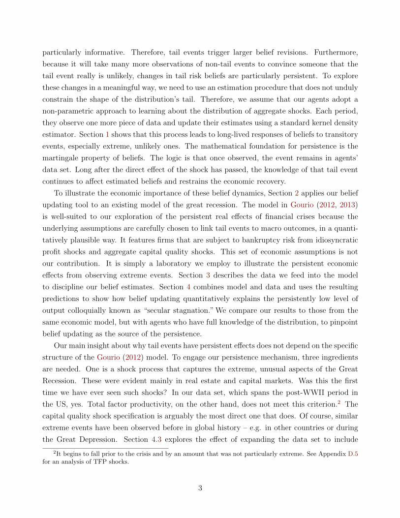
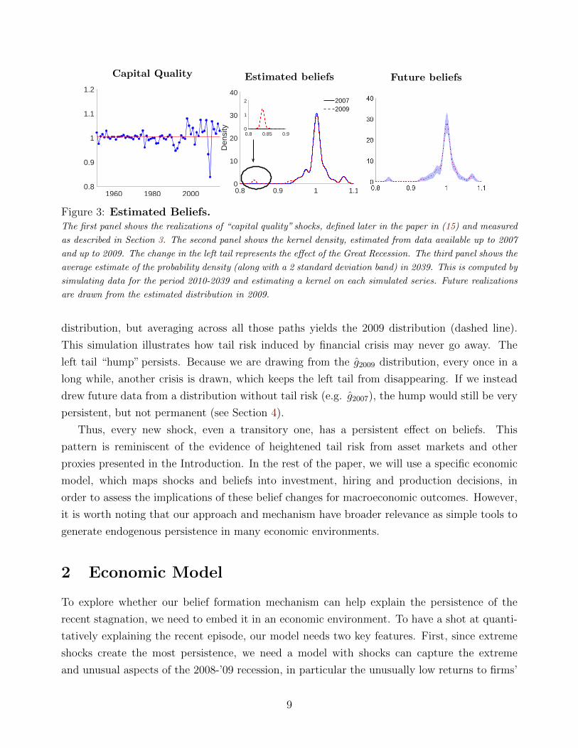
Estimated belief changes The second panel of Figure 3 takes all the data up to and includ-

ing 2007 and shows the estimated probability distribution, based on that (pre-crisis) data. Then

it takes all data up to and including 2009 (post-crisis) to plot the new probability distribution

estimate. The two adverse realizations in ’08 and ’09 lead to an increase in the assessment

of tail risk: The 2009 distribution, g2009 shows a pronounced hump in the density around the

2008 and 2009 realizations, relative to the pre-crisis one. Crucially, even though these negative

realizations were short-lived, this increase in left tail risk persists. To see how persistent beliefs

are, we ask the following question: What would be the estimated probability distribution in

2039? To answer this question, we need to simulate future data. Since our best estimate of

the distribution of future data in 2009 is g2009, we draw many 30-year sequences of future data

from this g2009 distribution. After each 30-year sequence, we re-estimate the distribution g,

using all available data. The shaded area in the third panel of Figure 3 shows the results from

this Monte Carlo exercise. Obviously, each simulated path gives rise to a different estimated

6When κt = 0, the kernel puts positive probability mass only on realizations seen before. In other words,an event that isn’t exactly identical to one in the observed sample is assigned zero probability, even if thereare other observations arbitrarily close to it in the sample. This is probably too extreme a specification for ourpurposes – since events are never identical in actual macro data, every observation will have zero probabilitybefore it occurs.

8

Capital Quality

1960 1980 20000.8

0.9

1

1.1

1.2

Estimated beliefs

0.8 0.9 1 1.10

10

20

30

40

Den

sity

20072009

0.8 0.85 0.90

1

2

Future beliefs

Figure 3: Estimated Beliefs.The first panel shows the realizations of “capital quality” shocks, defined later in the paper in (15) and measured

as described in Section 3. The second panel shows the kernel density, estimated from data available up to 2007

and up to 2009. The change in the left tail represents the effect of the Great Recession. The third panel shows the

average estimate of the probability density (along with a 2 standard deviation band) in 2039. This is computed by

simulating data for the period 2010-2039 and estimating a kernel on each simulated series. Future realizations

are drawn from the estimated distribution in 2009.

distribution, but averaging across all those paths yields the 2009 distribution (dashed line).

This simulation illustrates how tail risk induced by financial crisis may never go away. The

left tail “hump” persists. Because we are drawing from the g2009 distribution, every once in a

long while, another crisis is drawn, which keeps the left tail from disappearing. If we instead

drew future data from a distribution without tail risk (e.g. g2007), the hump would still be very

persistent, but not permanent (see Section 4).

Thus, every new shock, even a transitory one, has a persistent effect on beliefs. This

pattern is reminiscent of the evidence of heightened tail risk from asset markets and other

proxies presented in the Introduction. In the rest of the paper, we will use a specific economic

model, which maps shocks and beliefs into investment, hiring and production decisions, in

order to assess the implications of these belief changes for macroeconomic outcomes. However,

it is worth noting that our approach and mechanism have broader relevance as simple tools to

generate endogenous persistence in many economic environments.

2 Economic Model

To explore whether our belief formation mechanism can help explain the persistence of the

recent stagnation, we need to embed it in an economic environment. To have a shot at quanti-

tatively explaining the recent episode, our model needs two key features. First, since extreme

shocks create the most persistence, we need a model with shocks can capture the extreme

and unusual aspects of the 2008-’09 recession, in particular the unusually low returns to firms’

9

(non-residential) capital. To generate large fluctuations in returns, we use a shock to capital

quality. These shocks, which scale up or down the effective capital stock, are not to be inter-

preted literally. A decline in capital quality captures the idea that a Las Vegas hotel built in

2007 may deliver less economic value after the financial crisis, e.g. because it is consistently

half-empty. This would be reflected in a lower market value, a feature we will exploit later in

our measurement strategy. This specification is not intended as a deep explanation of what

triggered the financial crisis. Instead, it is a summary statistic that stands in for many possible

explanations and allows the model to speak to both financial and macro data.7 This agnostic

approach to the cause of the crisis also puts the spotlight on our contribution, which is the

ability of learning to generate persistent responses to extreme events.

Second, we need a setting where economic activity is sensitive to the probability of extreme

capital shocks. Gourio (2012, 2013) presents a model optimized for this purpose. Two key

ingredients – namely, Epstein-Zin preferences and costly bankruptcy – combine to generate

significant sensitivity to tail risk. Adding the assumption that labor is hired in advance with

an uncontingent wage increases the effective leverage of firms and therefore, accentuates the

sensitivity of investment and hiring decisions to tail risk. Similarly, preferences that shut down

wealth effects on labor avoid a surge in hours in response to crises.

Thus, this combination of assumptions offers a laboratory to assess the quantitative poten-

tial of our belief revision mechanism. It is worth emphasizing that none of these ingredients

guarantees persistence, our main focus. The capital quality shock has a direct effect on output

upon impact but, absent belief revisions, does not change the long-run trajectory of the econ-

omy. Similarly, the non-linear responses induced by preferences and debt influence the size of

the economic response, but by themselves do not generate any internal propagation. They in-

fluence the magnitude of the response, but persistence comes solely from the belief mechanism,

which is capable of generating persistence even without these ingredients.

To this setting, we add a novel ingredient, namely our belief-formation mechanism. We

model beliefs using the non-parametric estimation described in the previous section and show

how to discipline this procedure with observable macro data.

7Capital quality shocks have been employed for a similar purpose in Gourio (2012), as well as in a numberof recent papers on financial frictions, crises and the Great Recession (e.g., Gertler et al. (2010), Gertler andKaradi (2011), Brunnermeier and Sannikov (2014)). Their use in macroeconomics and finance, however, goesback at least to Merton (1973), who uses them to generate highly volatile asset returns.

10

2.1 Setup

Preferences and technology: An infinite horizon, discrete time economy has a representa-

tive household, with preferences over consumption (Ct) and labor supply (Lt):

Ut =

[(1− β)

(Ct −

L1+γt

1 + γ

)1−ψ

+ βEt(U1−ηt+1

) 1−ψ1−η

] 11−ψ

(1)

where ψ is the inverse of the intertemporal elasticity of substitution, η indexes risk-aversion, γ

is inversely related to the elasticity of labor supply, and β represents time preference.8

The economy is also populated by a unit measure of firms, indexed by i and owned by the

representative household. Firms produce output with capital and labor, according to a standard

Cobb-Douglas production function kαitl1−αit . Firms are subject to an aggregate shock to capital

quality φt. A firm that enters the period t with capital kit has effective capital kit = φtkit.

These capital quality shocks, i.i.d. over time and drawn from a distribution g(·), are the only

aggregate disturbances in our economy. The i.i.d. assumption is made in order to avoid an

additional, exogenous, source of persistence.9

Firms are also subject to an idiosyncratic shock vit. These shocks scale up and down the

total resources available to each firm (before paying debt, equity or labor)

Πit = vit[kαitl

1−αit + (1− δ)kit

](2)

where δ is the rate of capital depreciation. The shocks vit are i.i.d. across time and firms and

are drawn from a known distribution, F .10 The mean of the idiosyncratic shock is normalized

to be one:∫vit di = 1. The primary role of these shocks is to induce an interior default rate

in equilibrium, allowing a more realistic calibration, particularly of credit spreads.

Labor, credit markets and default: We make two additional assumptions about labor

markets. First, firms hire labor in advance, i.e. before observing the realizations of aggre-

gate and idiosyncratic shocks. Second, wages are non-contingent – in other words, workers

are promised a non-contingent payment and face default risk. These assumptions create an

additional source of leverage.

8This utility function rules out wealth effects on labor, as in Greenwood et al. (1988). Appendix C.9 relaxesthis assumption.

9The i.i.d. assumption also has empirical support. In the next section we use macro data to construct atime series for φt. We estimate an autocorrelation of 0.15, statistically insignificant. In Appendix C.10, we showthat this generates almost no persistence in the economic response.

10This is a natural assumption - with a continuum of firms and a stationary shock process, firms can learnthe complete distribution of any idiosyncratic shocks after one period.

11

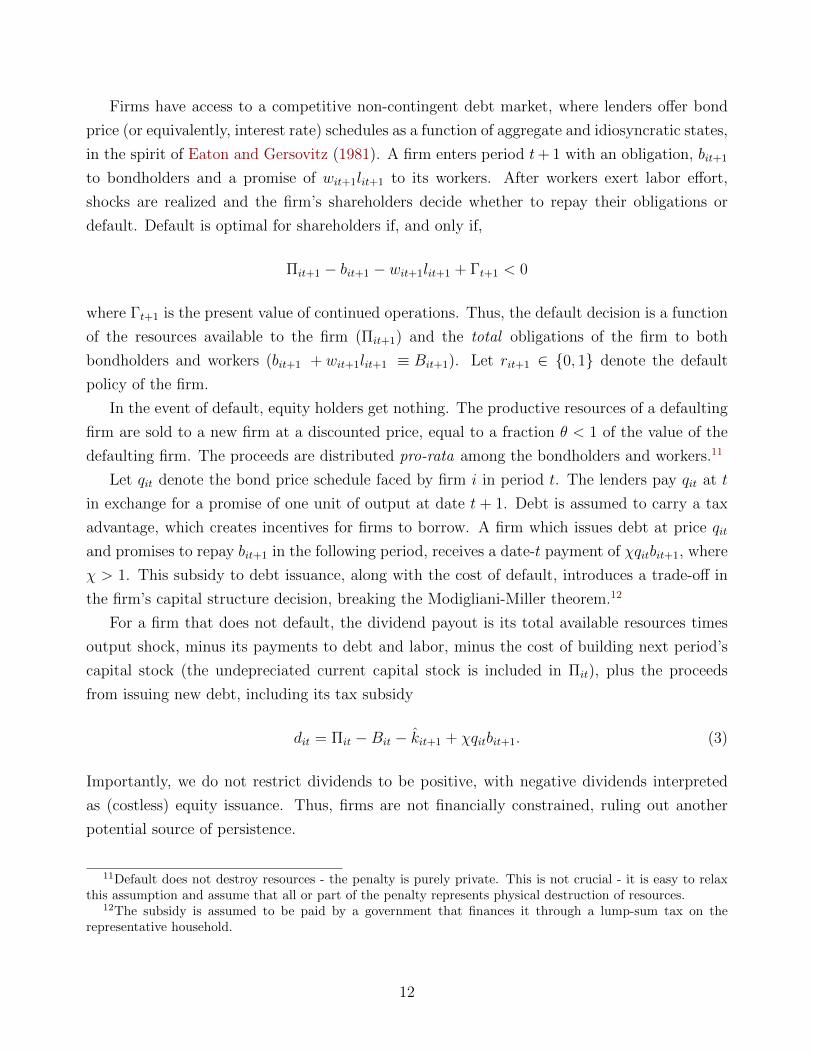
Firms have access to a competitive non-contingent debt market, where lenders offer bond

price (or equivalently, interest rate) schedules as a function of aggregate and idiosyncratic states,

in the spirit of Eaton and Gersovitz (1981). A firm enters period t+ 1 with an obligation, bit+1

to bondholders and a promise of wit+1lit+1 to its workers. After workers exert labor effort,

shocks are realized and the firm’s shareholders decide whether to repay their obligations or

default. Default is optimal for shareholders if, and only if,

Πit+1 − bit+1 − wit+1lit+1 + Γt+1 < 0

where Γt+1 is the present value of continued operations. Thus, the default decision is a function

of the resources available to the firm (Πit+1) and the total obligations of the firm to both

bondholders and workers (bit+1 + wit+1lit+1 ≡ Bit+1). Let rit+1 ∈ 0, 1 denote the default

policy of the firm.

In the event of default, equity holders get nothing. The productive resources of a defaulting

firm are sold to a new firm at a discounted price, equal to a fraction θ < 1 of the value of the

defaulting firm. The proceeds are distributed pro-rata among the bondholders and workers.11

Let qit denote the bond price schedule faced by firm i in period t. The lenders pay qit at t

in exchange for a promise of one unit of output at date t + 1. Debt is assumed to carry a tax

advantage, which creates incentives for firms to borrow. A firm which issues debt at price qit

and promises to repay bit+1 in the following period, receives a date-t payment of χqitbit+1, where

χ > 1. This subsidy to debt issuance, along with the cost of default, introduces a trade-off in

the firm’s capital structure decision, breaking the Modigliani-Miller theorem.12

For a firm that does not default, the dividend payout is its total available resources times

output shock, minus its payments to debt and labor, minus the cost of building next period’s

capital stock (the undepreciated current capital stock is included in Πit), plus the proceeds

from issuing new debt, including its tax subsidy

dit = Πit −Bit − kit+1 + χqitbit+1. (3)

Importantly, we do not restrict dividends to be positive, with negative dividends interpreted

as (costless) equity issuance. Thus, firms are not financially constrained, ruling out another

potential source of persistence.

11Default does not destroy resources - the penalty is purely private. This is not crucial - it is easy to relaxthis assumption and assume that all or part of the penalty represents physical destruction of resources.

12The subsidy is assumed to be paid by a government that finances it through a lump-sum tax on therepresentative household.

12

Timing and value functions:

1. Firms enter the period with capital kit, labor lit, outstanding debt bit, and a wage obliga-

tion witlit.

2. The aggregate capital quality shock φt and the firm-specific profit shock vit are realized.

Production takes place.

3. The firm decides whether to default or repay (rit ∈ 0, 1) its bond and labor claims.

4. The firm makes capital kit+1 and debt bit+1 choices for the following period, along with

wage/employment contracts wit+1 and lit+1. Workers commit to next-period labor supply

lit+1. Note that all these choices are made concurrently.

In recursive form, the problem of the firm is

V (Πit, Bit, St) = max

[0, max

dit,kit+1,bit+1,wit+1,lit+1

dit + EtMt+1V (Πit+1, Bit+1, St+1)

](4)

subject to

Dividends: dit ≤ Πit −Bit − kit+1 + χqitbit+1 (5)

Discounted wages: Wt ≤ wit+1qit (6)

Future obligations: Bit+1 = bit+1 + wit+1lit+1 (7)

Resources: Πit+1 = vit+1

[(φt+1kit+1)αl1−αit+1 + (1− δ)φt+1kit+1

](8)

Bond price: qit = EtMt+1

[rit+1 + (1− rit+1)

θVit+1

Bit+1

](9)

The first max operator in (4) captures the firm’s option to default. The expectation Etis taken over the idiosyncratic and aggregate shocks, given beliefs about the aggregate shock

distribution. The value of a defaulting firm is simply the value of a firm with no external

obligations, i.e. V (Πit, St) = V (Πit, 0, St).

In (6), the firm’s wage promise wit+1 is multiplied by bond price because wages are only paid

if the firm does not default. It is as if workers are paid in bonds (but without the tax advantage

of debt). The condition (6) requires the value of this promise be at least as large as Wt, the

representative household’s marginal rate of substitution. This Wt, along with the stochastic

discount factor Mt+1, are defined using the representative household’s utility function:

Wt =

(dUtdCt

)−1dUtdLt+1

Mt+1 =

(dUtdCt

)−1dUtdCt+1

(10)

13

The aggregate state St consists of (Πt, Lt, It) where Πt ≡ AKαt L

1−αt + (1 − δ)Kt is the

aggregate resources available, Lt is aggregate labor input (chosen in t−1) and It is the economy-

wide information set. Equation (9) reveals that bond prices are a function of the firm’s capital

kit+1, labor lit+1 and debt Bit+1, as well as the aggregate state St. The firm takes the aggregate

state and the function qit = q(kit+1, lit+1, Bit+1, St

)as given, while recognizing that its firm-

specific choices affect its bond price.

Information and beliefs The set It includes the history of all shocks φt observed up to

and including time-t. For now, we specify a general function, denoted Ψ, which maps It into

an appropriate probability space. The expectation operator Et is defined with respect to this

space. Agents use the kernel density estimation procedure outlined in section 1 to map the

information set into beliefs.

Equilibrium Definition. For a given belief function Ψ, a recursive equilibrium is a set

of functions for (i) aggregate consumption and labor that maximize (1) subject to a budget

constraint, (ii) firm value and policies that solve (4− 8) , taking as given the bond price function

(9) and the stochastic discount factor and aggregate MRS functions in (10) and are such that

(iii) aggregate consumption and labor are consistent with individual choices.

2.2 Solving the Model

Here, we show the key equations characterizing the equilibrium, relegating detailed derivations

to Appendix B. First, use the binding dividend and wage constraints (5) and (6) to substitute

out for dit and wit in the firm’s problem (4). This leaves 3 choice variables (kit+1, lit+1, bit+1) and

a default decision. The latter is characterized by a threshold rule in the idiosyncratic output

shock vit:

rit =

0 if vit < vit

1 if vit ≥ vit

It turns out to be more convenient to cast the problem as a choice of kit+1, leverage, levit+1 ≡Bit+1

kit+1, and the labor-capital ratio, lit+1

kit+1. Since all firms make symmetric choices, we can suppress

the i subscript: kit+1 = Kt+1, lit+1 = Lt+1, levit+1 = levt+1, vit+1 = vt+1. The optimality

condition for Kt+1 can be written as:

1 + χWtLt+1

Kt+1

= E[Mt+1Rkt+1] + (χ− 1)levt+1qt − (1− θ)E[Mt+1R

kt+1h(vt+1)] (11)

where Rkt+1 =

φαt+1Kαt+1L

1−αt+1 + (1− δ)φt+1Kt+1

Kt+1

(12)

14

The term Rkt+1 is the average ex-post per-unit, pre-wage return on capital, while h (v) ≡∫ v

−∞ vf(v)dv is the expected value of the idiosyncratic shock in the default states.

The first term on the right hand side of (11) is the usual expected direct return from

investing, weighted by the stochastic discount factor. The other two terms are related to debt.

The second term reflects the indirect benefit from the tax advantage of debt – for each unit

of capital, the firm raises levt+1qt from the bond market and earns a subsidy of χ − 1 on the

proceeds. The last term is the cost of this strategy – default-related losses, equal to a fraction

1− θ of available resources.

The optimal labor choice equates the expected marginal cost of labor,Wt, with its expected

marginal product, adjusted for the effect of additional wage promises on the cost of default:

χWt = Et

[Mt+1 (1− α)φαt+1

(Kt+1

Lt+1

)α

J l(vt+1)

](13)

where J l(v) = 1+h (v) (θχ− 1)−v2f (v)χ (θ − 1) is the effect of labor being chosen in advance

in exchange for a debt-like promise. Finally, the choice of leverage is governed by:

(1− θ)Et[Mt+1vt+1f

(vt+1

)]=

(χ− 1

χ

)Et[Mt+1

(1− F

(vt+1

))]. (14)

The left hand side is the marginal cost of increasing leverage. Higher leverage shifts the default

threshold v, raising the expected losses from the default penalty (a fraction 1− θ of the firm’s

value). The right hand side is the marginal benefit – higher leverage brings in more subsidy

(the tax benefit times the value of debt issued).

The three firm optimality conditions, (11), (13), and (14) , along with those from the house-

hold side (10) and the economy-wide resource constraint, characterize the equilibrium.

3 Measurement, Calibration and Solution Method

This section describes how we use macro data to estimate beliefs and parameterize the model,

as well as our computational approach. One of the key strengths of our theory is that we can

use observable data to estimate beliefs at each date.

Measuring capital quality shocks Recall from Section 1 that the Great Recession saw

unusually low returns to non-residential capital, stemming from unusually large declines in the

market value of capital. To capture this, we need to map the model’s aggregate shock, namely

the capital quality shock, into market value changes. A helpful feature of capital quality shocks

is that their mapping to available data is straightforward. A unit of capital installed in period

15

t − 1 (i.e. as part of Kt) is, in effective terms, worth φt units of consumption goods in period

t. Thus, the change in its market value from t− 1 to t is simply φt.

We apply this measurement strategy to annual data on non-residential capital held by US

corporates. Specifically, we use two time series Non-residential assets from the Flow of Funds,

one evaluated at market value and the second, at historical cost.13 We denote the two series

by NFAMVt and NFAHCt respectively. To see how these two series yield a time series for φt,

note that, in line with the reasoning above, NFAMVt maps directly to effective capital in the

model. Formally, letting P kt the nominal price of capital goods in t, we have P k

t Kt = NFAMVt .

Investment Xt can be recovered from the historical series, P kt−1Xt = NFAHCt −(1− δ)NFAHCt−1.

Combining, we can construct a series for P kt−1Kt:

P kt−1Kt = (1− δ)P k

t−1Kt−1 + P kt−1Xt

= (1− δ)NFAMVt−1 +NFAHCt − (1− δ)NFAHCt−1

Finally, in order to obtain φt = KtKt

, we need to control for nominal price changes. To do this,

we proxy changes in P kt using the price index for non-residential investment from the National

Income and Product Accounts (denoted PINDXt).14 This yields:

φt =Kt

Kt

=

(P kt Kt

P kt−1Kt

)(PINDXk

t−1

PINDXkt

)=

[NFAMV

t

(1− δ)NFAMVt−1 +NFAHCt − (1− δ)NFAHCt−1

](PINDXk

t−1

PINDXkt

)(15)

Using the measurement equation (15), we construct an annual time series for capital quality

shocks for the US economy since 1950. The left panel of Figure 3 plots the resulting series. The

mean and standard deviation of the series over the entire sample are 1 and 0.03 respectively.

The autocorrelation is statistically insignificant at 0.15.

As Figure 3 shows, for most of the sample period, the shock realizations are in a relatively

tight range around 1. However, we saw two large adverse realizations during the Great Re-

cession: 0.93 in 2008 and 0.84 in 2009. These reflect the large drops in the market value of

non-residential capital stock – in 2009, for example, the aggregate value of that stock fell by

about 16%. What underlies these large fluctuations? The main contributor was a fall in the

value of commercial real estate (which is the largest component of non-residential assets).15

13These are series FL102010005 and FL102010115 from Flow of Funds. See Appendix D.3.14Our results are robust to alternative measures of nominal price changes, e.g. computed from the price

index for GDP or Personal Consumption Expenditure, see Appendix C.1.15One potential concern is that the fluctuations in the value of real estate stem mostly from land price

movements. While the data in the Flow of Funds do not allow us to directly control for changes in the market

16

Through the lens of the model, these movements are mapped to a change in the economic value

of capital – in the spirit of the hypothetical example of the Las Vegas hotel at the beginning of

Section 2 whose market value falls.

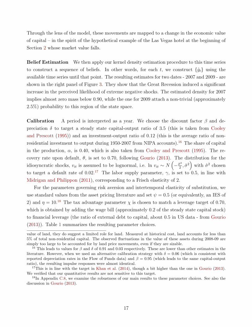
Belief Estimation We then apply our kernel density estimation procedure to this time series

to construct a sequence of beliefs. In other words, for each t, we construct gt using the

available time series until that point. The resulting estimates for two dates - 2007 and 2009 - are

shown in the right panel of Figure 3. They show that the Great Recession induced a significant

increase in the perceived likelihood of extreme negative shocks. The estimated density for 2007

implies almost zero mass below 0.90, while the one for 2009 attach a non-trivial (approximately

2.5%) probability to this region of the state space.

Calibration A period is interpreted as a year. We choose the discount factor β and de-

preciation δ to target a steady state capital-output ratio of 3.5 (this is taken from Cooley

and Prescott (1995)) and an investment-output ratio of 0.12 (this is the average ratio of non-

residential investment to output during 1950-2007 from NIPA accounts).16 The share of capital

in the production, α, is 0.40, which is also taken from Cooley and Prescott (1995). The re-

covery rate upon default, θ, is set to 0.70, following Gourio (2013). The distribution for the

idiosyncratic shocks, vit is assumed to be lognormal, i.e. ln vit ∼ N(− σ2

2, σ2)

with σ2 chosen

to target a default rate of 0.02.17 The labor supply parameter, γ, is set to 0.5, in line with

Midrigan and Philippon (2011), corresponding to a Frisch elasticity of 2.

For the parameters governing risk aversion and intertemporal elasticity of substitution, we

use standard values from the asset pricing literature and set ψ = 0.5 (or equivalently, an IES of

2) and η = 10.18 The tax advantage parameter χ is chosen to match a leverage target of 0.70,

which is obtained by adding the wage bill (approximately 0.2 of the steady state capital stock)

to financial leverage (the ratio of external debt to capital, about 0.5 in US data - from Gourio

(2013)). Table 1 summarizes the resulting parameter choices.

value of land, they do suggest a limited role for land. Measured at historical cost, land accounts for less than5% of total non-residential capital. The observed fluctuations in the value of these assets during 2008-09 aresimply too large to be accounted for by land price movements, even if they are sizable.

16 This leads to values for β and δ of 0.91 and 0.03 respectively. These are lower than other estimates in theliterature. However, when we used an alternative calibration strategy with δ = 0.06 (which is consistent withreported depreciation rates in the Flow of Funds data) and β = 0.95 (which leads to the same capital-outputratio), the resulting impulse responses were almost identical.

17This is in line with the target in Khan et al. (2014), though a bit higher than the one in Gourio (2013).We verified that our quantitative results are not sensitive to this target.

18In Appendix C.8, we examine the robustness of our main results to these parameter choices. See also thediscussion in Gourio (2013).

17

Parameter Value DescriptionPreferences:β 0.91 Discount factorη 10 Risk aversionψ 0.50 1/Intertemporal elasticity of substitutionγ 0.50 1/Frisch elasticityTechnology:α 0.40 Capital shareδ 0.03 Depreciation rateσ 0.25 Idiosyncratic volatilityDebt:χ 1.06 Tax advantage of debtθ 0.70 Recovery rate

Table 1: Parameters

Numerical solution method Given the importance of curvature in policy functions for

our results, we solve the non-linear system of equations (11)− (14) using collocation methods.

Appendix A describes the iterative procedure. In order to maintain tractability, we need to

make one approximation. Policy functions at date-t depend both on the current estimated

distribution, gt(φ), and the distributionH over next-period estimates, gt+1(φ). Keeping track of

H(gt+1(φ)), (a distribution over a distribution, i.e. a compound lottery) as a state variable would

render the analysis intractable. However, the approximate martingale property of gt discussed

in Section 1 offers an accurate and computationally efficient approximation to this problem. The

martingale property implies that the average of the compound lottery is Et[gt+1(φ)] ≈ gt(φ),

∀φ. Therefore, when computing policy functions, we approximate H(gt+1(φ)) with its mean

gt(φ), the current estimate of the distribution. Appendix C.2 uses a numerical experiment to

show that this approximation is quite accurate. Intuitively, future estimates gt+1 are tightly

centered around gt(φ), i.e. H(gt+1) has a relatively small variance. The shaded area in the

third panel of Figure 3 reveals that even 30 periods out, gt+30(φ) is still quite close to its mean

gt(φ). For 1-10 quarters ahead, where most of the utility weight is, this error is even smaller.

4 Main Results

In this section, we evaluate, quantitatively, the ability of the model of generate persistent

responses from tail events and confront its predictions with data. The key model feature behind

persistence is the assumption that people estimate the distribution of aggregate economic shocks

from available data. To isolate its role, we compare results from our model to those from the

same model where the distribution of shocks is assumed to be known with certainty. In this

18

“no learning” economy, agents know the true probability of the tail event and so, observing

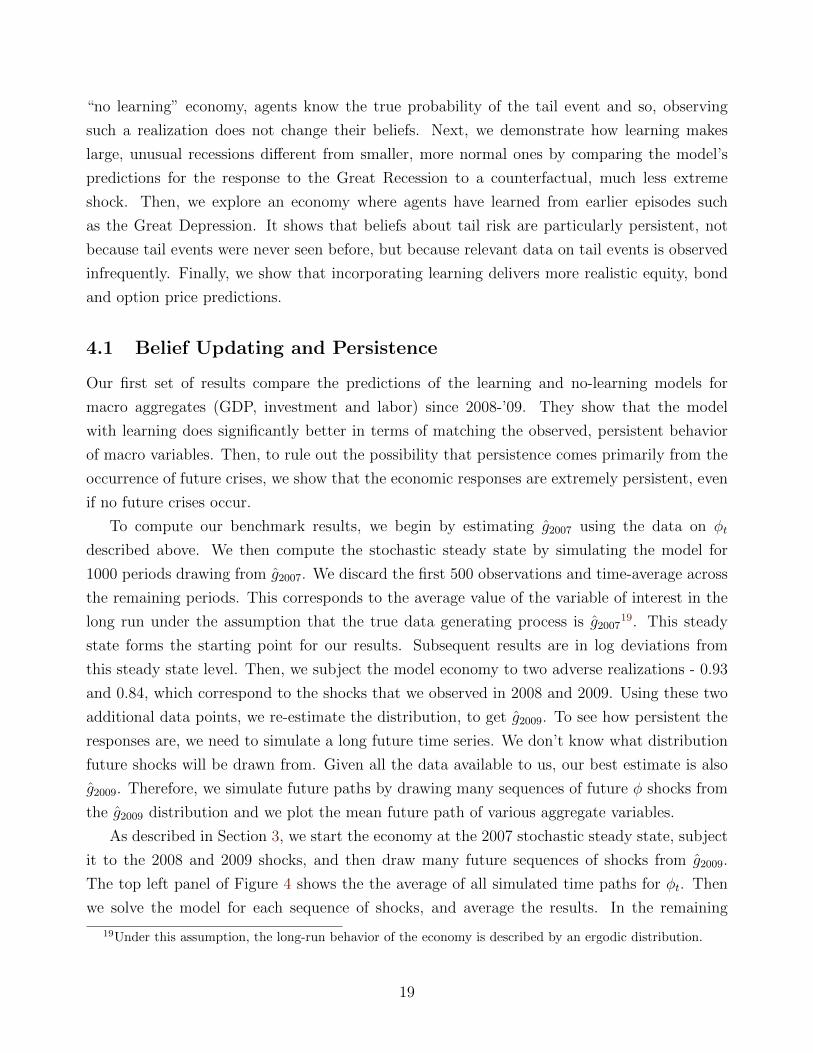
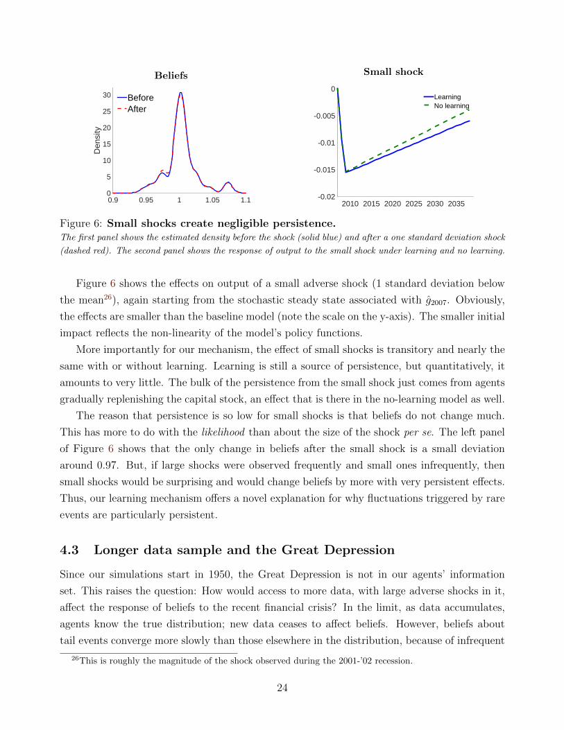
such a realization does not change their beliefs. Next, we demonstrate how learning makes

large, unusual recessions different from smaller, more normal ones by comparing the model’s

predictions for the response to the Great Recession to a counterfactual, much less extreme

shock. Then, we explore an economy where agents have learned from earlier episodes such

as the Great Depression. It shows that beliefs about tail risk are particularly persistent, not

because tail events were never seen before, but because relevant data on tail events is observed

infrequently. Finally, we show that incorporating learning delivers more realistic equity, bond

and option price predictions.

4.1 Belief Updating and Persistence

Our first set of results compare the predictions of the learning and no-learning models for

macro aggregates (GDP, investment and labor) since 2008-’09. They show that the model

with learning does significantly better in terms of matching the observed, persistent behavior

of macro variables. Then, to rule out the possibility that persistence comes primarily from the

occurrence of future crises, we show that the economic responses are extremely persistent, even

if no future crises occur.

To compute our benchmark results, we begin by estimating g2007 using the data on φt

described above. We then compute the stochastic steady state by simulating the model for

1000 periods drawing from g2007. We discard the first 500 observations and time-average across

the remaining periods. This corresponds to the average value of the variable of interest in the

long run under the assumption that the true data generating process is g200719. This steady

state forms the starting point for our results. Subsequent results are in log deviations from

this steady state level. Then, we subject the model economy to two adverse realizations - 0.93

and 0.84, which correspond to the shocks that we observed in 2008 and 2009. Using these two

additional data points, we re-estimate the distribution, to get g2009. To see how persistent the

responses are, we need to simulate a long future time series. We don’t know what distribution

future shocks will be drawn from. Given all the data available to us, our best estimate is also

g2009. Therefore, we simulate future paths by drawing many sequences of future φ shocks from

the g2009 distribution and we plot the mean future path of various aggregate variables.

As described in Section 3, we start the economy at the 2007 stochastic steady state, subject

it to the 2008 and 2009 shocks, and then draw many future sequences of shocks from g2009.

The top left panel of Figure 4 shows the the average of all simulated time paths for φt. Then

we solve the model for each sequence of shocks, and average the results. In the remaining

19Under this assumption, the long-run behavior of the economy is described by an ergodic distribution.

19

Capital quality shock

2010 2020 2030-0.3

-0.2

-0.1

0

0.1

0.2

GDP

2010 2020 2030-0.3

-0.2

-0.1

0

0.1

0.2LearningNo learningData

Investment

2010 2020 2030-0.3

-0.2

-0.1

0

0.1

0.2

Labor

2010 2020 2030-0.3

-0.2

-0.1

0

0.1

0.2

Figure 4: Persistent responses in output, investment and labor.Solid line shows the change in aggregates (relative to the stochastic steady state associated with g2007). The

circles show de-trended US data for the period 2008-2014. For the dashed line (no learning), agents believe that

shocks are drawn from g2009 and never revise those beliefs.

panels, output, investment and employment show a pattern of prolonged stagnation, where the

economy (on average) never recovers from the negative shocks in 2008-’09. Instead, all aggregate

variables move towards the new, lower (stochastic) steady state. These results do not imply

that stagnation will continue forever. The flat response tells us that, from the perspective of

an agent with the 2009 information set, recovery is not expected.20

The solid line with circles in Figure 4 plots the actual data (in deviations from their re-

spective 1950-2007 trends) for the US economy.21 As the graph shows, the model’s predictions

for GDP and labor line up well with the recent data, though none of these series were used in

20Appendix C.13 shows that a large fraction of the persistence response is due to changes in beliefs ratherthan the fact that the shock hits the actual capital.

21Data on output and labor input are obtained from Fernald (2014). Data on investment comes from theseries for non-residential investment from the NIPA published by the Bureau of Economic Analysis, adjustedfor population and price changes. Each series is detrended using a log-linear trend estimated using data from1950-2007, see Appendix D.4.

20

the calibration or measurement of the aggregate shock φt. The predicted path for employment

lags and slightly underpredicts the actual changes, largely due to the assumption that labor

is chosen in advance. Including shock realizations post-2009 does not materially change these

findings (see Appendix C.3).22

For investment, the model performs poorly. It predicts less than half of the observed drop.

However, without learning, the results are much worse. When agents do not learn, investment

surges, instead of plummets. The reason is that the effective size of the capital stock was

already diminished by the capital quality shock. The shock itself is like an enormous, exogenous

disinvestment. We could solve this problem by adding more features and frictions.23 But our

main point is about learning and persistence. Despite only partially fixing the investment

problem of the capital quality model, Figure 4 clearly demonstrates the quantitative potential

of learning as a source of persistence.

Table 2 summarizes the long-run effects of the belief changes, by comparing averages in

the stochastic steady states under g2007 and g2009. As mentioned earlier, these are the average

levels that the economy ultimately converges to, under the assumption that the data-generating

process (and therefore, long-run beliefs) is g2007 or g2009. Capital and labor are, on average,

17% and 8% lower under the post-crisis beliefs g2009, which translates into a 12% lower output

and consumption level, in the long run. Investment falls by 7% 24 Thus, even though the φt

shocks experienced during the Great Recession were transitory, the resulting changes in beliefs

persistently reduce economic activity.

Stochastic steady state levels Changeg2007 g2009

Output 6.37 5.67 -12 %Capital 27.52 22.80 -17%Investment 0.71 0.66 - 7%Labor 2.40 2.20 -8%Consumption 5.66 5.01 -12%

Table 2: Belief changes from 2008-’09 shocks lead to significant reductions in eco-nomic activity.Columns marked g2007 and g2009 represent average levels in the stochastic steady state of a model where shocks

are drawn from g2007 or g2009 distributions respectively.

22Additional outcomes are reported in Appendix C.5.23Financial frictions which impeded investment include those in Gertler and Karadi (2011) and Brunnermeier

and Sannikov (2014). Alternative amplification mechanisms are studied in Adrian and Boyarchenko (2012);Jermann and Quadrini (2012); Khan et al. (2014); Zetlin-Jones and Shourideh (2014); Bigio (2015); Morieraand Savov (2015), among others.

24The fall in investment is smaller than that of capital because the shock distribution has also changed. Forexample, under g2009, the mean shock is slightly lower (relative to g2007). Intuitively, this acts like a slightlyhigher depreciation rate – so, even though capital is lower by 17%, the drop in investment is only 7%.

21

Turning off belief updating To demonstrate the role of learning, we plot average simulated

outcomes from an otherwise identical economy where agents know the final distribution g2009

with certainty, from the very beginning (dashed line in Figure 4). Now, by assumption, agents

do not revise their beliefs after the Great Recession. This corresponds to a standard rational

expectations econometrics approach, where agents are assumed to know the true distribution

of shocks hitting the economy and the econometrician estimates this distribution using all the

available data. The post-2009 paths are simulated as follows: each economy is assumed to be

at its stochastic steady state in 2007 and is subjected to the same sequence of shocks – two

large negative ones in 2008 and 2009 and subsequently, sequences of shocks drawn from the

estimated 2009 distribution.

Without belief revisions, the negative shocks lead to an investment boom, as the economy

replenishes the lost effective capital. While the curvature in utility moderates the speed of this

transition, the overall pattern of a steady recovery back to the original steady state is clear.25

This shows that learning is key to generating persistent reductions in economic activity.

What if shocks are persistent? An alternative explanation for persistence is that there was

no learning. Instead, the shocks simply had persistently bad realizations. In Appendix C.10,

we show that allowing for a realistic amount of persistence in the φt shocks does not materially

change the dynamics of aggregate variables. This is because the the observed autocorrelation

of the φt process is too low to generate any meaningful persistence.

What if there are no more crises? In the results presented above, we put ourselves on the

same footing as the agents in our model and draw future time paths of shocks using the updated

beliefs g2009. One potential concern is that persistent stagnation comes not from belief changes

per se but from the fact that future paths are drawn from a distribution where crises occur

with non-trivial probability. This concern is not without merit. If we draw future shocks from

the distribution, g2007, where the probability of a crisis is near zero, beliefs are not Martingales.

In that world, beliefs change by the same amount on impact, but then converge back to their

pre-crisis levels. Without the permanent effect on beliefs, persistence should fall.

However, Figure 5 shows that the persistence over a 30 year horizon is almost the same with

and without future crises (solid and dashed lines). The reason belief effects are still so long-

lived is that it takes many, many no-crisis draws to convince someone that the true probability

of a crisis is less than an already-small probability. For example, if one observed 100 periods

without a crisis, this would still not be compelling evidence that the odds are less than 1%. This

25 Since the no-learning economy is endowed with the same end-of-sample beliefs as the learning model, theyboth ultimately converge to the same levels, even though they start at different points (normalized to 0 for eachseries).

22

GDP

2010 2020 2030-0.3

-0.2

-0.1

0

0.1

0.2With crisisNo more crisisData

Investment

2010 2020 2030-0.3

-0.2

-0.1

0

0.1

0.2

Labor

2010 2020 2030-0.3

-0.2

-0.1

0

0.1

0.2

Figure 5: What if there are no more crises?Solid (With crisis) line shows the change in aggregates when the data generating process is g2009 and agent

updates beliefs. Dashed line (No more crisis) is an identical model in which future shocks are drawn from g2007.

The circles show de-trended US data for the period 2008-2014.

highlights that beliefs about tail probabilities are persistent because tail-relevant data arrives

infrequently.

The fact that most data is not relevant for inferring tail probabilities is a consequence of our

non-parametric approach. If instead, we imposed a parametric form like a normal distribution,

then probabilities (including those for tail events) would depend only on the mean and variance

of the distribution. Since mean and variance are informed by all data, tail probability revisions

are frequent and small. As a result, the effects of observing the ‘08 and ‘09 shocks are more

transitory. See Appendix C.11 for more details.

4.2 Shock Size and Persistence

The secular stagnation puzzle is not about why all economic shocks are so persistent. The

question is why this recession had more persistent effects than others. Assuming that shocks

are persistent does not answer this question. Our model explains why persistent responses arise

mainly after a tail event. Every decline in capital quality has a transitory direct effect (it lowers

effective capital) and a persistent belief effect. Thus, the extent to which a shock generates

persistent outcomes depends on the relative size of these two effects. Observing a tail event,

one we did not expect, change beliefs a lot and generates a large persistent effect. A small

shock has a negligible effect on beliefs and therefore, generates little persistence. This finding

– that learning does not matter when ‘normal’ shocks hit – is also the reason why we focus

on the Great Recession. We could use the model to explore regular business cycles, but the

versions with and without learning would be almost observationally equivalent, yielding little

insight into the role of learning.

23

Beliefs

0.9 0.95 1 1.05 1.1

Den

sity

0

5

10

15

20

25

30 BeforeAfter

Small shock

2010 2015 2020 2025 2030 2035-0.02

-0.015

-0.01

-0.005

0LearningNo learning

Figure 6: Small shocks create negligible persistence.The first panel shows the estimated density before the shock (solid blue) and after a one standard deviation shock

(dashed red). The second panel shows the response of output to the small shock under learning and no learning.

Figure 6 shows the effects on output of a small adverse shock (1 standard deviation below

the mean26), again starting from the stochastic steady state associated with g2007. Obviously,

the effects are smaller than the baseline model (note the scale on the y-axis). The smaller initial

impact reflects the non-linearity of the model’s policy functions.

More importantly for our mechanism, the effect of small shocks is transitory and nearly the

same with or without learning. Learning is still a source of persistence, but quantitatively, it

amounts to very little. The bulk of the persistence from the small shock just comes from agents

gradually replenishing the capital stock, an effect that is there in the no-learning model as well.

The reason that persistence is so low for small shocks is that beliefs do not change much.

This has more to do with the likelihood than about the size of the shock per se. The left panel

of Figure 6 shows that the only change in beliefs after the small shock is a small deviation

around 0.97. But, if large shocks were observed frequently and small ones infrequently, then

small shocks would be surprising and would change beliefs by more with very persistent effects.

Thus, our learning mechanism offers a novel explanation for why fluctuations triggered by rare

events are particularly persistent.

4.3 Longer data sample and the Great Depression

Since our simulations start in 1950, the Great Depression is not in our agents’ information

set. This raises the question: How would access to more data, with large adverse shocks in it,

affect the response of beliefs to the recent financial crisis? In the limit, as data accumulates,

agents know the true distribution; new data ceases to affect beliefs. However, beliefs about

tail events converge more slowly than those elsewhere in the distribution, because of infrequent

26This is roughly the magnitude of the shock observed during the 2001-’02 recession.

24

observations. In this section, we approximate data extending back to the 19th century and show

that the belief changes induced by the 2008-09 experience continue to have a large, persistent

effect on economic activity.

2010 2020 2030-0.15

-0.1

-0.05

0[ , ] = [1,1][ , ] = [1,0.99][ , ] = [2,0.99]

Figure 7: Extending the data sample tempers persistence slightly.Each line shows the response of GDP to the 2008-09 shocks under a hypothetical information set, starting

from 1890. To fill in the data for the period 1890-1949, we use the observed time series from 1950-2009, with

φ1929, φ1930 = φε2008, φε2009. The parameter λ indexes the extent to which older observations are discounted

where λ = 1 represents no discounting. The parameter ε represents the severity of the shocks in the Great

Depression where ε = 1 represents that it was similar to the Great Recession.

The difficulty with extending the data is that the non-financial asset data used in φt is avail-

able only for the post-WW II period. Other macro and financial series turn out to be unreliable

proxies.27 But our goal here is not to explain the Great Depression. It is to understand how

having more data, especially previous crises, affects learning today. So we use the post-WW II

sample to construct pre-WW II scenarios. Specifically, we assume that φt realizations for the

period from 1890-1949 were identical to those in 1950-2009, with one adjustment: The Great

Depression shocks were as bad or worse those in the Great Recession. To make this adjustment,

we set φ1929, φ1930 = φε2008, φε2009, with ε ≥ 1. Recall that φ in 2008 and 2009 are less than

one. So, raising them to a power greater than one makes them smaller.

We then repeat our analysis under the assumption that agents are endowed with this ex-

panded 1890-2007 data series. Now, when the financial crisis hits, the effect on beliefs is

moderated by the larger data sample, which contains a similar or worse previous crisis.

Once we include data from a different eras, the assumption that old and new data are treated

as equally relevant becomes less realistic. We consider the possibility that agents discount older

27We projected the measured φt series post-1950 on a number of variables and used the estimated coefficientsto impute values for φt pre-1950. However, this did not produce accurate estimates in-sample. Specifically, itmissed crises. We explored a wide range of macro and asset pricing variables - including GDP, unemployment,S&P returns and the Case-Shiller index of home prices. We also experimented with lead-lag structures. Acrossspecifications, the resulting projections for 1929-1930 showed only modestly adverse realizations.

25

observations. This could reflect the possibility of unobserved regime shifts or experiential learn-

ing with overlapping generations (Malmendier and Nagel, 2011).28 To capture such discounting,

we modify our kernel estimation procedure. Observation from s periods earlier are assigned a

weight λs, where λ ≤ 1 is a parameter. When λ = 1, there is no discounting.

Figure 7 reveals that, even without discounting (λ = 1), the difference between the model

with and without Great Depression data is modest, as of 2016: There is a similar output drop on

impact, with attenuated persistence from the additional data. When older data is discounted

by 1% (λ = 0.99, the center panel), this attenuation almost completely disappears and the

impulse responses replicate our baseline estimates.29

Perhaps the true magnitude of the Great Depression shocks is far larger than those seen

in 2008-09. Suppose ε = 2, so that (φ1929, φ1930) = (0.86, 0.70). These are very large shocks

– 5 and 10 standard deviations below the mean. Taken together, they imply an erosion of

almost 50% in the stock of effective capital. Figure 7 shows that, with 1% annual discounting

(λ = 0.99), persistence is attenuated, but only modestly.

In sum, expanding the information set by adding more data does not drastically alter our

main conclusions, especially once we assume that agents discount older data.

4.4 Evidence from Asset Markets

Our framework stays close to a standard neoclassical macro paradigm and therefore, inherits

many of its limitations when it comes to asset prices. Our goal in this section is not to resolve

these shortcomings but to show that the predictions of the model are broadly in line with the

patterns in asset markets. As with macro aggregates, effects of learning are detectable only

after tail events, so we focus on the period since the Great Recession. In Table 3, we compare

the predictions of the model for various asset market variables, both pre- and post-crisis, with

their empirical counterparts. We construct the latter by averaging over 1990-07 and 2010-15

respectively.30 The model does not quite match levels, but our focus is on the changes induced

by the 2008-09 experience. We find that while the model’s predictions for the change in credit

spreads and equity prices are broadly consistent with the data, these variables are not very

sensitive to, and therefore, not very informative about tail risk. On the other hand, the model’s

predictions for option-implied tail risk, i.e. the probabilities of extreme events priced into

28This type of discounting is similar to Sargent (2001), Cho et al. (2002) and Evans and Honkapohja (2001).29With stronger discounting, the decline in GDP becomes bigger. Intuitively, higher discounting increases

the weight of recent observations relative to undiscounted case. For example, with λ = 0.98, the persistent dropin GDP is about 16%.

30The overall pattern of the model’s performance is not sensitive to the time periods chosen. In an earlier,we used shorter samples for both pre- and post-crisis and the conclusions were very similar. We did not include2008 and 2009 in order to avoid picking up outsized fluctuations in asset markets at the height of the crisis.

26

options, which is a much better indicator, line up quite well with the observed changes.

Credit spreads – the difference between the interest on a risky and a riskless loan – are

commonly interpreted as a measure of risk. The first row of the table shows that by 2015

spreads are only slightly higher than their pre-crisis levels (they spiked at the height of the

crisis but then came back down). Hall (2015a), for example, uses this observation to argue that

a persistent increase tail risk is not a likely explanation for stagnation.

Model Datag2007 g2009 Change 1990-2007 2010-2015 Change

Asset prices and debtCredit Spreads 0.75% 0.77% 0.02% 1.89% 2.23% 0.34%Equity Premium 1.09% 2.51% 1.41% 3.29% 7.50% 4.21%Equity/Assets 46.63% 47.27% 0.65% 55.28% 56.87% 1.59%Risk free rate 9.57% 9.03% -0.54% 1.42% -1.32% -2.74%Debt -17% 3% -23% -26%Tail risk for equityThird moment (×102) 0.00 -0.26 -0.26 -1.34 -1.59 -0.25Tail risk 0.0% 1.5% 1.5 % 9.3% 11.2% 1.9%

Table 3: Changes in financial market variables, Model vs data.Model: shows average values in the stochastic steady state under g2007 and g2009. The equity/assets is the ratio

of the market value of equity claims to capital Kt. Third moment is E[(Re − Re

)3], where Re is the return on

equity and Tail risk is Prob(Re − Re ≤ −0.3

), where both are computed under the risk-neutral measure. Without

learning, all changes are zero.

Data: For credit spreads, we use the average spread on senior unsecured bonds issued by non-financial firms

computed as in Gilchrist and Zakrajek (2012). For the equity premium, we follow Cochrane (2011) and Hall

(2015b) and estimate the one-year ahead forecast for real returns on the S&P 500 from a regression using Price-

Dividend and aggregate Consumption-GDP ratios. See footnote 34 for details. Equity/assets is the ratio of the

market value of equities to value of non-financial assets from Table B.103 in the Flow of Funds. The risk free

real interest rate is computed as the difference between nominal yield of 1-year US treasuries and inflation. Debt

is measured as total liabilities of nonfinancial corporate business from the Flow of Funds (FL104190005, Table

B.103), adjusted for population growth and inflation. The numbers reported are deviations from a log-linear

1952-2007 trend. The third moment and tail risk are computed from the VIX and SKEW indices published by

CBOE. See footnote 36 and Appendix C.7 for details.

The results in Table 3 argue against this conclusion. The connection between spreads and

tail risk is weak – our calibrated model predicts a negligible rise in spreads, about 2 basis points.

Since the model without learning predicts no long-run changes in asset prices, this small change

means that credit spreads are not a useful device for divining beliefs about tail risk. This is

due, in part, to equilibrium effects: an increase in bankruptcy risk induces firms to issue less

debt. Debt in the new steady state is about 17% lower.31 In the data, total liabilities of non-

31The leverage ratio (debt and wage obligation divided by total assets) is also slightly lower, by about 0.5%.

27

financial corporations (relative to trend)32 show a similar change – a drop of about 26%. This

de-leveraging lowers default risk and therefore, offsets the rise in credit spreads. In the model,

the net effect of higher tail risk and lower firm debt on spreads is nearly zero. Thus, the fact

that spreads are almost back to their pre-crisis levels does not rule out tail risk – one of the

surprising predictions of the model.

Similarly, one might think that equity should be worth less when risk is high. The fact

that equity prices have surged recently and are higher than their pre-crisis levels thus appears

inconsistent with a rise in tail risk. But again, this logic is incomplete – while higher tail

risk does increase the risk premium, it also induces firms to cut debt, which mitigates the

increase in risk (Modigliani and Miller, 1958). The net effect in the model is to slightly raise

the market value of a dividend claim associated with a unit of capital under the post-crisis

beliefs relative to the pre-crisis ones. In other words, the combined effect of the changes in tail

risk and debt is mildly positive.33 In the data, the ratio of the market capitalization of the

non-financial corporate sector to their (non-financial) asset positions also shows an increase.

While the magnitudes differ – we don’t claim to solve all equity-related puzzles here – our point

is simply that rising equity valuations are not evidence against tail risk.

Furthermore, the changes in equity premia (the difference between expected return on equity

and the riskless rate) are in the right ballpark, even though the model underpredicts the level

relative to the data (reflecting its limitations as an asset pricing model). The higher tail risk

under the 2009 beliefs implies an rise of 1.5% in the equity premium, relative to that under

the 2007 beliefs. To compute the analogous object in the data, we follow the methodology in

Cochrane (2011) and Hall (2015b)34, which estimates that equity premia in 2010-15 were about

4.21% higher than the pre-crisis average. In other words, tail risk can account for about a third

of the recent rise in equity premia. Of course, our measure of equity premia, like all others, is

noisy and volatile. We are not claiming that the model can explain all the fluctuations – no

model can – but it doesn’t seem to be at odds with recent trends in equity market variables.

The table also shows the model’s predictions for riskless rates. Again, as with the equity

premium, the model does not quite match the level35, but does a better job predicting the change

32Total liabilities of nonfinancial corporate business is taken from series FL104190005 from Table B.103 in theFlow of Funds. As with the other macro series, we adjust for inflation and population growth and then detrendusing a simple log-linear trendline. The numbers reported in the table are the (averages of the) deviations froma log-linear trend, computed from 1952-2007.

33The aggregate market capitalization in the model is obtained by simply multiplying the value of the dividendclaim by the aggregate capital stock.

34We estimate one-year ahead forecast from a regression where the left-hand variable is the one-year realreturn on the S&P and the right hand variables are a constant, the log of the ratio of the S&P at the beginningof the period to its dividends averaged over the prior year, and the log of the ratio of real consumption todisposable income in the month prior to the beginning of the period.

35This is partly due to our choice of a relatively low value for the discount factor, β. As we discussed in

28

since the Great Recession. Higher tail risk increases the premium for safe assets, reducing the

riskless rate. Under our calibration, the change in beliefs induced by the 2008-09 realizations

leads to a 54 bp drop in the riskless rate. In the data, the real rate on Treasuries (computed

as the difference between nominal yield of the 1-year Treasury and inflation) averaged -0.81

% between 2013-15, as against 0.61% during 2005-07, a drop of about 1.4%. Thus, the model

underpredicts the drop. In ongoing work – Kozlowski et al. (2018) – we show how higher tail

risk can interact with liquidity needs of firms, amplifying the drop in government bond yields.

In sum, none of these trends in asset markets is at odds with the tail risk story we are

advancing. If credit spreads and equity premia are not clear indicators of tail risk, what is?

For that, we need to turn to option prices, in particular options on the S&P 500, which can

be used to isolate changes in perceived tail risk. A natural metric is the third moment of

the distribution of equity returns. It is straightforward to compute this from the SKEW and

VIX indices reported by the CBOE.36 As Table 3 shows, the market-implied distribution has

became more negatively skewed after the Great Recession. We compute the same risk-neutral

third moment in the model (using the distribution for stock returns under the 2009 and 2007

beliefs). The model underpredicts the skewness in levels37, but predicts a change (-0.0026) that

lines up almost exactly with the data. To show how this change maps into probabilities of tail

events, we also report the numbers for the implied (risk-neutral) odds of a return realization

30% less than the mean.38 Again, the model-implied level is too low, but the predicted change

(1.5%) is quite close to the corresponding object in the data (2.2%).39

4.5 Understanding the Economic Response to Belief Changes

What model ingredients are needed for belief to have substantial aggregate effects and why?

To answer this, we perform a series of experiments, varying and turning off specific features of

the model – learning about the mean vs higher order moments, curvature in utility and debt

– one-by-one in order to isolate how much each one contributes. The bottom panel of Table 4

shows that removing any of these elements would eliminate between one-fourth and one-half of

footnote 16, an alternative calibration strategy with a higher value for β yields very similar results.36 Formally, the third central moment under the risk-neutral measure is given by

E(Re − Re

)3=

100− SKEWt

10· V IX3

t .

For more information, see http://www.cboe.com/micro/skew/introduction.aspx.37Fixing this would require additional shocks and/or amplification mechanisms.38For details of the computation, see Appendix C.7.39Including shock realizations post-2009 does not materially change these findings, see Appendix C.15.

29

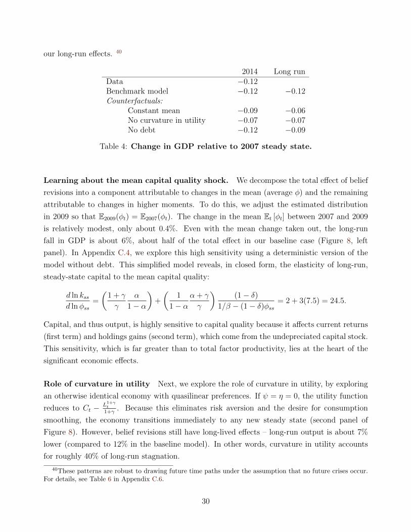
our long-run effects. 40

2014 Long runData −0.12Benchmark model −0.12 −0.12Counterfactuals:

Constant mean −0.09 −0.06No curvature in utility −0.07 −0.07No debt −0.12 −0.09

Table 4: Change in GDP relative to 2007 steady state.

Learning about the mean capital quality shock. We decompose the total effect of belief

revisions into a component attributable to changes in the mean (average φ) and the remaining

attributable to changes in higher moments. To do this, we adjust the estimated distribution

in 2009 so that E2009(φt) = E2007(φt). The change in the mean Et [φt] between 2007 and 2009

is relatively modest, only about 0.4%. Even with the mean change taken out, the long-run

fall in GDP is about 6%, about half of the total effect in our baseline case (Figure 8, left

panel). In Appendix C.4, we explore this high sensitivity using a deterministic version of the

model without debt. This simplified model reveals, in closed form, the elasticity of long-run,

steady-state capital to the mean capital quality:

d ln kssd lnφss

=

(1 + γ

γ

α

1− α

)+

(1

1− αα + γ

γ

)(1− δ)

1/β − (1− δ)φss= 2 + 3(7.5) = 24.5.

Capital, and thus output, is highly sensitive to capital quality because it affects current returns

(first term) and holdings gains (second term), which come from the undepreciated capital stock.

This sensitivity, which is far greater than to total factor productivity, lies at the heart of the

significant economic effects.

Role of curvature in utility Next, we explore the role of curvature in utility, by exploring

an otherwise identical economy with quasilinear preferences. If ψ = η = 0, the utility function

reduces to Ct − L1+γt

1+γ. Because this eliminates risk aversion and the desire for consumption

smoothing, the economy transitions immediately to any new steady state (second panel of

Figure 8). However, belief revisions still have long-lived effects – long-run output is about 7%

lower (compared to 12% in the baseline model). In other words, curvature in utility accounts

for roughly 40% of long-run stagnation.

40These patterns are robust to drawing future time paths under the assumption that no future crises occur.For details, see Table 6 in Appendix C.6.

30

Constant mean

2010 2015 2020 2025 2030 2035-0.2

-0.15

-0.1

-0.05

0

0.05BaselineConstant mean

No risk aversion

2010 2015 2020 2025 2030 2035-0.2

-0.15

-0.1

-0.05

0

0.05BaselineNo risk aversion

No debt

2010 2015 2020 2025 2030 2035-0.2

-0.15

-0.1

-0.05

0

0.05BaselineNo debt

Figure 8: Understanding the role of expected return, risk aversion and debt.Change in ln GDP under 3 different scenarios: (1) the mean capital quality shock E[φt] is held fixed; (2) no

risk aversion, and (3) no debt.

Risk aversion matters because it introduces a risk premium for capital and labor. Tail risk

raises this premium, further dampening incentives to invest and hire. Appendix C.8 shows that

the effect of tail risk on macro aggregates is increasing, albeit modestly, in both risk aversion

and the intertemporal elasticity of substitution. These results highlight the role of Epstein-Zin

preferences. With CRRA preferences, high risk aversion implies low intertemporal elasticity,

dampening the drop in long-run economic activity.

Role of debt When we set the tax advantage parameter χ to 1, all investment is financed

through equity. Debt and leverage are 0. The third panel of Figure 8 shows that belief revisions

trigger a 9% long-run reduction in output without debt, compared to 12% with debt. Thus,

defaultable debt contributes about a fourth of the long run stagnation.

Debt also plays an important role in one of the main questions of the paper, namely why

some shocks generate more persistent responses than others. The attractiveness of debt (and

therefore, the incentives to borrow) is affected disproportionately by perceived tail risk - and

since larger shocks changes belief further out in the tail, they are amplified by debt. Since tail

risk is the source of persistence, by amplifying its effects increases persistence as well.

In Figure 9, we subjected our model economy to shocks ranging in size from 1 to 5 standard

deviations and plotted the corresponding long-run GDP effect. The responsiveness to small

shocks is almost the same with and without debt. Because debt adds aggregate non-linearity,

larger shocks see significant amplification. Since the risk of a larger shock is what persists, debt

makes the severity and persistence of unusual events differ from common downturns.

31

Shock size (standard deviations)-5 -4 -3 -2 -1 0

Long

run

effe

ct o

n ou

tput

-0.07

-0.06

-0.05

-0.04

-0.03

-0.02

-0.01

0With debtWithout debt

Figure 9: Debt amplifies belief revisions from large shocks.Change in long-run GDP both with (solid line) and without debt (dashed line) in response to negative shocks of

various sizes. The initial condition is the g2007 steady state.

4.6 Open Questions

While the analysis in the preceding sections demonstrates the quantitative potential for belief

revisions, both for macro aggregates and financial market variables, it also points to shortcom-

ings in our approach and raises new questions – both conceptual and empirical. These are areas

where future research might be fruitful.

One obvious shortcoming of the model is its inability to reproduce the plunge in investment

seen in the data. This is due to the nature of the shock – an negative shock reduces capital

available for production, creating huge incentives to replenish that capital stock. This is a stark

simplification – in reality, the events in 2008-09 probably reduced the economic value of capital

without mechanically pushing up returns on new investments. Fixing this would requires some

innovation on the modeling front: either a novel way of shocking capital returns – i.e. one

which is capable of generating large adverse realizations, but does not reduce effective capital

– or new mechanisms which limit incentives to invest following a tail event.

Another direction is an Bayesian approach to learning about tail risk. This would allow us to

incorporate the risk of future belief changes into agents’ current decisions, a channel we abstract

from in our classical non-parametric approach. Bayesian parameter learning has been shown

to improve asset pricing predictions in an endowment setting (Collin-Dufresne et al., 2016).

Embedding this into a model with production could bring to light new implications for macro

phenomena as well. We conjecture that tail events will have large, persistent effects even in a

Bayesian setting, provided two conditions are satisfied. First, the specification is sufficiently

flexible, e.g. one or more parameters governing tail risk. Second, the priors about these

parameters reflects substantial uncertainty. Otherwise, there is not much scope for learning.

An open question is whether recent events reflect changes in beliefs or preferences. It is

nearly impossible to disentangle the two with aggregate macroeconomic data. We took what

we believe to be the most fruitful approach – hold preferences fixed and discipline beliefs with

32

data. But, new approaches to preference formation could shed more light on this question and

provide a deeper understanding on the role of tail events.

Finally, there are surely other surprising and extreme economic events. Agents who learn

from those events might also exhibit persistent responses. Also, there were many outcomes

in the great recession that were not extreme. Why did capital returns, in particular, reshape

people’s beliefs? Why didn’t they focus on the less extreme GDP numbers instead? Pairing

learning about tail events with limited attention might reveal that agents focused on investment

returns because they are payoff relevant and because they were extreme, and thus highly-

informative events.

5 Conclusion

Economists typically assume that agents in their models know the distribution of shocks. In this

paper, we showed that relaxing this assumption has important implications for the response of

the economy to tail events. The agents in our model behave like classical econometricians, re-

estimating distributions as new data arrives. Under these conditions, observing a tail event like

the 2008-09 Great Recession in the US, causes agents to assign larger weights to similar events

in the future, depressing investment and output. Crucially, these effects last for a long time,

even when the underlying shocks are transitory. The rarer the event that is observed, the larger

and more persistent the revision in beliefs. The effects on economic activity are amplified when

investments are financed with debt. This is because debt payoffs (and therefore, borrowing

costs) are particularly sensitive to the probability of extreme negative outcomes.

When this mechanism is quantified using data for the US economy, the predictions of the

model resemble observed macro and asset market outcomes in the wake of the Great Recession,

suggesting that the persistent nature of the recent stagnation is due, at least partly, to the fact

that the events of 2008-09 changed the way market participants think about tail risk.

References

Adrian, T. and N. Boyarchenko (2012). Intermediary leverage cycles and financial stability.

Angeletos, G.-M. and J. La’O (2013). Sentiments. Econometrica 81 (2), 739–779.

Anzoategui, D., D. Comin, M. Gertler, and J. Martinez (2015). Endogenous technology adop-

tion and r & d as sources of business cycle persistence. New York University working paper.

33

Backus, D. K., S. Foresi, and L. Wu (2008). Accounting for biases in black-scholes. SSRN

Working Paper Series .

Bakshi, G., N. Kapadia, and D. Madan (2003). Stock return characteristics, skew laws, and the

differential pricing of individual equity options. Review of Financial Studies 16 (1), 101–143.

Beaudry, P. and F. Portier (2004). An exploration into pigou’s theory of cycles. Journal of

Monetary Economics 51, 1183–1216.

Bigio, S. (2015). Endogenous liquidity and the business cycle. American Economic Review .

Bloom, N., M. Floetotto, N. Jaimovich, I. Sapora-Eksten, and S. Terry (2014). Really uncertain

business cycles. NBER working paper 13385.

Brunnermeier, M. and Y. Sannikov (2014). A macroeconomic model with a financial sector.

American Economic Review 104 (2).

Cho, I.-K., N. Williams, and T. J. Sargent (2002). Escaping nash inflation. The Review of

Economic Studies 69 (1), 1–40.

Cochrane, J. H. (2011). Presidential address: Discount rates. The Journal of Finance 66 (4),

1047–1108.

Cogley, T. and T. Sargent (2005). The conquest of us inflation: Learning and robustness to

model uncertainty. Review of Economic Dynamics 8, 528–563.

Collin-Dufresne, P., M. Johannes, and L. Lochstoer (2016). Parameter learning in general

equilibrium: The asset pricing implications. American Economic Review 106 (3), 664–98.

Cooley, T. and E. Prescott (1995). Frontiers of Business Cycle Research, Chapter Economic

Growth and Business Cycles. Princeton University Press.

Eaton, J. and M. Gersovitz (1981). Debt with potential repudiation: Theoretical and empirical

analysis. The Review of Economic Studies , 289–309.

Eggertsson, G. and N. Mehrotra (2014). A model of secular stagnation. NBER Working Paper

No. 20574.

Evans, G. W. and S. Honkapohja (2001). Learning and expectations in macroeconomics. Prince-

ton University Press.

Fajgelbaum, P., E. Schaal, and M. Taschereau-Dumouchel (2014). Uncertainty traps. NBER

Working Paper No. 19973.

34

Fernald, J. (2014). A quarterly, utilization-adjusted series on total factor productivity. Federal

reserve bank of San Francisco working paper 19.

Gertler, M. and P. Karadi (2011). A model of unconventional montary policy. Journal of

Monetary Economics 58, 17–34.

Gertler, M., N. Kiyotaki, et al. (2010). Financial intermediation and credit policy in business

cycle analysis. Handbook of monetary economics 3 (3), 547–599.

Gilchrist, S. and E. Zakrajek (2012, June). Credit spreads and business cycle fluctuations.

American Economic Review 102 (4), 1692–1720.

Gomme, P., B. Ravikumar, and P. Rupert (2011). The return to capital and the business cycle.

Review of Economic Dynamics 14 (2), 262–278.

Gordon, R. (2014). The demise of u. s. economic growth: Restatement, rebuttal, and reflections.

NBER working paper 19895.

Gourio, F. (2012). Disaster risk and business cycles. American Economic Review 102(6),

2734–66.

Gourio, F. (2013). Credit risk and disaster risk. American Economic Journal: Macroeco-

nomics 5(3), 1–34.

Greenwood, J., Z. Hercowitz, and G. W. Huffman (1988). Investment, capacity utilization, and

the real business cycle. The American Economic Review , 402–417.

Hall, R. (2015a). Macroeconomics of persistent slumps. Handbook of Macroeconomics .

Hall, R. E. (2015b, October). High discounts and high unemployment. Hoover Institution,

Stanford University.

Hansen, B. E. (2015). Econometrics.

Hansen, L. (2007). Beliefs, doubts and learning: Valuing macroeconomic risk. American

Economic Review 97(2), 1–30.

Hansen, L. and T. Sargent (1999). The Conquest of American Inflation. Princeton University

Press.

Huo, Z. and N. Takayama (2015). Higher order beliefs, confidence, and business cycles. Uni-

versity of Minnesota working paper.

35

Jaimovich, N. and S. Rebelo (2006). Can news about the future drive the business cycle?

American Economic Review 99(4), 1097–1118.

Jermann, U. and V. Quadrini (2012). Macroeconomic effects of financial shocks. American

Economic Review 102 (1), 238–71.

Johannes, M., L. Lochstoer, and P. Collin-Dufresne (2015). The asset pricing implications of

priced structural parameter uncertainty.

Johannes, M., L. Lochstoer, and Y. Mou (2015). Learning about consumption dynamics.

Journal of Finance forthcoming.

Khan, A., T. Senga, and J. K. Thomas (2014). Default risk and aggregate fluctuations in an

economy with production heterogeneity. Technical report, Ohio State University working

paper.

Kozlowski, J., L. Veldkamp, and V. Venkateswaran (2018). The tail that keeps the riskless rate

low. National Bureau of Economic Research, Macroeconomics Annual forthcoming.

Lorenzoni, G. (2009). A theory of demand shocks. American Economic Review 99 (5), 2050–84.

Malmendier, U. and S. Nagel (2011). Depression babies: Do macroeconomic experiences affect

risk taking?*. The Quarterly Journal of Economics 126 (1), 373–416.

Merton, R. (1973). An intertemporal capital asset pricing model. Econometrica 41 (5), 867–887.

Midrigan, V. and T. Philippon (2011). Household leverage and the recession.

Modigliani, F. and M. Miller (1958). The cost of capital, corporation finance and the theory of

investment. The American Economic Review 48 (3), 261–297.

Moriera, A. and A. Savov (2015). The macroeconomics of shadow banking. New York University

working paper.

Navarro, G. (2014). Financial crises and endogenous volatility. manuscript, New York Univer-

sity .

Nimark, K. (2014). Man-bites-dog business cycles. American Economic Review 104(8), 2320–

67.

Orlik, A. and L. Veldkamp (2014). Understanding uncertainty shocks and the role of the black

swan. Working paper.

36

Pintus, P. and J. Suda (2015). Learning financial shocks and the great recession. Aix Marseille

working paper.

Sargent, T. J. (2001). The conquest of American inflation. Princeton University Press.

Straub, L. and R. Ulbricht (2013). Credit crunches, information failures, and the persistence

of pessimism. Toulouse School of Economics working paper.

Van Nieuwerburgh, S. and L. Veldkamp (2006). Learning asymmetries in real business cycles.

Journal of Monetary Economics 53(4), 753–772.

Veldkamp, L. and J. Wolfers (2007). Aggregate shocks or aggregate information? costly infor-

mation and business cycle comovement. Journal of Monetary Economics 54, 37–55.

Zetlin-Jones, A. and A. Shourideh (2014). External financing and the role of financial frictions

over the business cycle: Measurement and theory. Working paper.

37

A Appendix: Solution Method

The equilibrium is characterized by the following non-linear system:

1 + χWtLt+1

Kt+1

= E[Mt+1Rkt+1] + (χ− 1)levt+1qt − (1− θ)E[Mt+1R

kt+1h(vt+1)]

(16)

χWt = EMt+1

[(1− α)φα

(Kt+1

Lt+1

)α]J l(vt+1) (17)

(1− θ)Et[Mt+1vt+1f

(vt+1

)]=

(χ− 1

χ

)Et[Mt+1

(1− F

(vt+1

))](18)

Mt+1 = β[E(U1−ηt+1

)] η−ψ1−η Uψ−η

t+1

(u (Ct+1, Lt+1)

u (Ct, Lt)

)−ψ(19)

Wt = Lγt+1EMt+1 (20)

where

Ct = φαt Kαt L

1−αt + (1− δ)φtKt − Kt+1 (21)

Ut =

[(1− β) (u (Ct, Lt))

1−ψ + βE(U1−ηt+1

) 1−ψ1−η

] 11−ψ

(22)

Rkt+1 =

φαt+1Kαt+1L

1−αt+1 + (1− δ)φt+1Kt+1

Kt+1

(23)

vt+1 =levt+1

φαt+1

(Kt+1

Lt+1

)α−1

+ (1− δ)φt+1

(24)

J l(v) = 1 + v2f (v)χ (1− θ)− (1− χθ)h (v) (25)

Solution Algorithm To solve the system described above at any given date t (i.e. after any

observed history of φt), we recast it in recursive form with grids for the aggregate state (Π, L)

and the shocks φ. We then use the following iterative procedure:

• Estimate g on the available history using the kernel density estimator.

• Start with a guess (in polynomial form) for U(Π, L), C(Π, L).

• Solve (16)-(18) for K ′(Π, L), L′(Π, L), lev′(Π, L) using a non-linear solver.

• Update the guess for U,C using (21)-(22) and iterate until convergence.

38

Online Appendix

This material is for a separate, on-line appendix and not intended to be printed with the paper.

B Model solution and derivations 2

C Additional Results 4

C.1 Measurement of φt: Alternative price indices . . . . . . . . . . . . . . . . . . . 4

C.2 Numerical accuracy of solution method . . . . . . . . . . . . . . . . . . . . . . . 4

C.3 Effect of 2010-2014 shocks . . . . . . . . . . . . . . . . . . . . . . . . . . . . . . 5

C.4 Steady State Analysis . . . . . . . . . . . . . . . . . . . . . . . . . . . . . . . . . 7

C.5 Behavior of Consumption . . . . . . . . . . . . . . . . . . . . . . . . . . . . . . 8

C.6 What if there are no more crises? . . . . . . . . . . . . . . . . . . . . . . . . . . 9

C.7 Computing option-implied tail probabilities . . . . . . . . . . . . . . . . . . . . 9

C.8 Role of Risk Aversion, Intertemporal Elasticity of Substitution . . . . . . . . . . 10

C.9 Role of GHH preferences . . . . . . . . . . . . . . . . . . . . . . . . . . . . . . . 11

C.10 Exogenous persistence in φt . . . . . . . . . . . . . . . . . . . . . . . . . . . . . 12

C.11 Learning with a Normal distribution . . . . . . . . . . . . . . . . . . . . . . . . 14

C.12 Alternative kernels . . . . . . . . . . . . . . . . . . . . . . . . . . . . . . . . . . 15

C.13 Tail Shocks vs Beliefs . . . . . . . . . . . . . . . . . . . . . . . . . . . . . . . . 16

C.14 Asymmetry: Right vs left tail events . . . . . . . . . . . . . . . . . . . . . . . . 17

C.15 Response of asset prices to 2010-2014 shocks . . . . . . . . . . . . . . . . . . . 18

D Other evidence 18

D.1 Internet search behavior . . . . . . . . . . . . . . . . . . . . . . . . . . . . . . . 18

D.2 Stock market . . . . . . . . . . . . . . . . . . . . . . . . . . . . . . . . . . . . . 18

D.3 Returns during the Great Recession . . . . . . . . . . . . . . . . . . . . . . . . 19

D.4 De-trending . . . . . . . . . . . . . . . . . . . . . . . . . . . . . . . . . . . . . . 20

D.5 Productivity . . . . . . . . . . . . . . . . . . . . . . . . . . . . . . . . . . . . . 21

1

B Model solution and derivations

Define

Rkit+1 ≡ φt+1

α

(lit+1

kit+1

)1−α

+ (1− δ)φt+1.

Substituting for dividends and wages from (5) and (6), the firm’s contiuation value can be

expressed as the solution to the following maximization problem:

Γit = maxkit+1, levit+1,

lit+1

kit+1

kit+1

(−1− χWt

lit+1

kit+1

+ χqitlevit+1 + EMt+1rit+1

(vitR

kit+1 − levit+1 +

Γit+1

kit+1

))

where

qit = EMt+1

rit+1 + (1− rit+1) θvit+iR

kit+1 + Γit+1

kit+1

levit+1

.Leverage levit+1 includes debt and the wage promises made to workers. However, wage promises

(or operating leverage) is different from debt, in that it does not earn a tax advantage. Since

the above formulation credits the firm with tax advantage χ on all leverage, the wage obligation

Wt ends up being multiplied by χ, i.e. as if the firm pays back the tax advantage from labor

payments. The net effect is that only external debt ends up accruing the advantage.

We guess (and later verify) that Γit+1 = 0.41 Using the threshold characterization of the

default decision,

Γit = max kit+1

(−1− χWt

lit+1

kit+1

+ χqitlevit+1 + EMt+1

∫ ∞vit+1

(vRk

it+1 − levit+1

)dF (v)

)

= max kit+1

(−1− χWt

lit+1

kit+1

+ χqitlevit+1 + EMt+1

[(1− h

(vit+1

))Rkit+1 − levit+1

(1− F

(vit+1

))])where

qit = EMt+1

[1− F

(vit+1

)+ h

(vit+1

)θRkit+1

levit+1

]vit+1 =

levit+1

Rkit+1

Capital choice: Note that qit is only a function of levit+1 and Rkit+1 (which only depends

on the labor-capital ratio lit+1

kit+1). As a result, the objective function is linear in kit+1. At an

41Intuitively, given constant returns to scale, the firm’s problem turns out to be linear in capital. In equilib-rium, therefore, in order for the firm’s value to be bounded, we must have Γit = 0. See Navarro (2014).

2

interior optimum, we must have:

1 + χWtlit+1

kit+1

= χqitlevit+1 + EMt+1

[(1− h

(vit+1

))Rkit+1 − levit+1

(1− F

(vit+1

))]= EMt+1R

kit+1 + χqitlevit+1 − EMt+1

[h(vit+1

)Rkit+1 + levit+1

(1− F

(vit+1

))]= EMt+1R

kit+1 + χqitlevit+1 − levit+1EMt+1

[h(vit+1

) Rkit+1

levit+1

+(1− F

(vit+1

))]= EMt+1R

kit+1 + χqitlevit+1 − levit+1

[qit + (1− θ)EMt+1h

(vit+1

) Rkit+1

levit+1

]= EMt+1R

kit+1 + (χ− 1) qitlevit+1 − (1− θ)EMt+1h

(vit+1

)Rkit+1 . (26)

Note that this verifies our guess that Γit+1 = 0. Labor and leverage choice are the solutions to

maxlevit+1,

lit+1

kit+1

−1−χWtlit+1

kit+1

+χqitlevit+1 +EMt+1

[(1− h

(vit+1

))Rkt+1 − levit+1

(1− F

(vit+1

))]which, after substituting for qit, becomes

maxlevit+1,

lit+1

kit+1

−1− χWtlit+1

kit+1

+ EMt+1Rkit+1J

k(vit+1)

where Jk(v) = 1 + (χ− 1) v (1− F (v)) + (χθ − 1)h (v)

Labor choice: The first order condition with respect to lit+1

kit+1is

χWt = EMt+1Rkit+1

∂Jk(vit+1)

∂ lit+1

kit+1

+ EMt+1∂Rk

∂ lit+1

kit+1

Jk(vit+1),

Now,

Rkit+1

∂Jk(vit+1)

∂ lt+1

kit+1

= Rkit+1

∂vit+1

∂ lt+1

kit+1

((χ− 1)

(1− F

(vit+1

))− vit+1 (χ− 1) f

(vit+1

)+ (χθ − 1)

∂h(vit+1

)∂vit+1

)∂vit+1

∂ lit+1

kit+1

= − levit+1(Rkit+1

)2

∂Rkit+1

∂ lit+1

kit+1

= −v2it+1

levit+1

∂Rkit+1

∂ lit+1

kit+1

dh(vit+1

)dvit+1

= vit+1f(vit+1

)∂Rk

it+1

∂ lit+1

kit+1

= (1− α)φt+1α

(kit+1

lit+1

)α

.

3

Substituting and rearranging terms yields

χWt = E

[Mt+1 (1− α)φt+1

α

(kit+1

lit+1

)α

J l(vit+1)

](27)

J l(v) = 1 + h (v) (χθ − 1)− v2f (v)χ (θ − 1) ,

Leverage choice: The first order condition with respect to leverage is

EMt+1Rkit+1

∂Jk(vit+1)

∂levit+1

= 0,

where

∂Jk(vit+1)

∂levit+1

=∂vit+1

∂levit+1

((χ− 1)

(1− F

(vit+1

))− (χ− 1) vit+1f

(vit+1

)+ (χθ − 1) vit+1f

(vit+1

))=

1

Rkit+1

((χ− 1)

(1− F

(vit+1

))− χ (1− θ) vit+1f

(vit+1

)).

Substituting and re-arranging,

(1− θ)Et[Mt+1vit+1f

(vit+1

)]=

(χ− 1

χ

)Et[Mt+1

(1− F

(vit+1

))]. (28)

Finally, since all firms make symmetric choices, we can suppress the i subscript, so

kit+1 = Kt+1 lit+1 = Lt+1 levit+1 = levt+1 vit+1 = vt+1 .

Using this, equations (26)− (28) become (11)− (14) in the main text.

C Additional Results

C.1 Measurement of φt: Alternative price indices

Figure 10 shows that the measurement of capital quality shocks is unaffected when we use

the price index for GDP or Personal Consumption Expenditure to control for nominal price

changes.

C.2 Numerical accuracy of solution method

To test the numerical accuracy of our solution method, we perform the following exercise.

Starting from the steady state of g2007, we simulate time paths for two different economies. In

4

1950 1960 1970 1980 1990 2000 20100.8

0.85

0.9

0.95

1

1.05

1.1

1.15

1.2Capital quality shock

InvestmentGDPPersonal Consumption Expenditures

Figure 10: Time series of shocks φt using different indices to control for nominalprice changes.

Model I, as new data arrives, we update beliefs and policy functions at each date and history. In

Model II, beliefs and policy functions are fixed at g2007. In our solution, we essentially assume

that agents use Model II as an approximation for Model I, while evaluating continuation values.

Table 5 shows the sample mean and coefficient of variation for output at different horizons for

these two versions.42 It is easy to see that aggregates (or at least, the first two moments

thereof) are very well-approximated by replacing the sequence of future distributions with their

conditional mean. Recall that this numerical procedure works reasonable well thanks to the

martingale property of beliefs.

C.3 Effect of 2010-2014 shocks

Here, we subject our baseline calibrated model to the full sequence of shocks, from 2008 through

2014. Agents’ decisions in each year are a function of the estimated distribution at that date.

The resulting time paths are plotted in Figure 11, along with the de-trended data. We note

that the patterns implied by the model are quite close to the observed ones.

42These are averages over 4000 paths. Other aggregate variables, e.g. capital and labor, show similar patterns.

5

Horizons = 1 s = 5 s = 10 s = 15

Et [yt+s]Model I: 6.378 6.385 6.393 6.397Model II: 6.378 6.385 6.394 6.398CVt [yt+s]Model I: 0.010 0.032 0.042 0.046Model II: 0.010 0.031 0.040 0.044

Table 5: Numerical accuarcy.The rows labeled Model I show the actual moments under the assumption that beliefs g2007+s are re-estimated

at each date. Model II corresponds to the assumption underlying our solution method, where future beliefs are

replaced by g2007.

Capital quality shock

2010 2020 2030

-0.2

0

0.2GDP

2010 2020 2030

-0.2

0

0.2DGP 2014Data

Investment

2010 2020 2030

-0.2

0

0.2Labor

2010 2020 2030

-0.2

0

0.2

Figure 11: Macro Aggregates: Model vs data, 2008-2014.Solid line is the baseline model subjected to the observed sequence of shocks from 2008-2014. The red circles are

US data, in deviations from their pre-crisis trends.

6

C.4 Steady State Analysis

To dig a little deeper into why long-run outcomes are so sensitive to φ, we turn to a special

case - a deterministic version of our economy without debt. The level of steady state capital is

given by the following equation43

ln kss = Const. +

(1 + γ

γ

α

1− α

)lnφss −

(1

1− αα + γ

γ

)ln

(1

β− (1− δ)φss

). (29)

Hence, the effect of the mean shock on steady sate capital is given by

d ln kssd lnφss

=

(1 + γ

γ

α

1− α

)+

(1

1− αα + γ

γ

)(1− δ)

1/β − (1− δ)φss.

Under our parameterization,

1 + γ

γ

α

1− α= 2,

1

1− αα + γ

γ= 3,

((1− δ)

1/β − (1− δ)φss

)φss=1

= 7.5

which implies d ln kssd lnφss

= 2 + 3(7.5) = 24.5. This simple calculation shows the source of the high

sensitivity - the fact that capital quality shock affects not just the current return component

but also the portion that comes from the undepreciated stock.

43In steady state, Mt = 1 and the intertemporal Euler equation and labor optimality conditions reduce to

1 = β(αφαssk

α−1ss l1−αss + φss (1− δ)

)lγss = Wss = (1− α)φαssk

αssl

−αss .

Substituting for lss from the second into the first and re-arranging yields the expression (29).

7

C.5 Behavior of Consumption

Figure 12 shows that the behavior of consumption, as predicted by the model and the corre-

sponding pattern in the data. The model overpredicts the drop in consumption in the years

immediately following impact – the flip side of its inability to match the full extent of the drop

in investment during that time – but over a longer horizon, the predicted drop lines up quite

well with the data.

2010 2020 2030-0.3

-0.2

-0.1

0

0.1

0.2ModelData

Figure 12: Response of consumption.

8

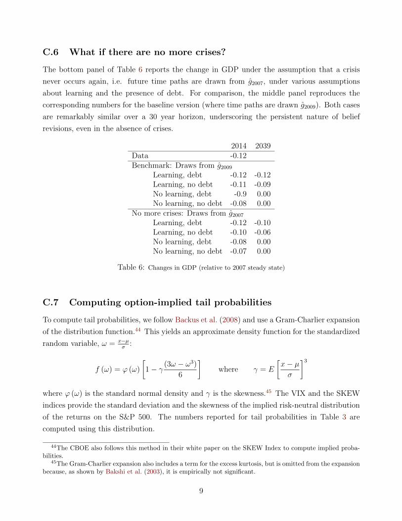
C.6 What if there are no more crises?

The bottom panel of Table 6 reports the change in GDP under the assumption that a crisis

never occurs again, i.e. future time paths are drawn from g2007, under various assumptions

about learning and the presence of debt. For comparison, the middle panel reproduces the

corresponding numbers for the baseline version (where time paths are drawn g2009). Both cases

are remarkably similar over a 30 year horizon, underscoring the persistent nature of belief

revisions, even in the absence of crises.

2014 2039Data -0.12Benchmark: Draws from g2009

Learning, debt -0.12 -0.12Learning, no debt -0.11 -0.09No learning, debt -0.9 0.00No learning, no debt -0.08 0.00

No more crises: Draws from g2007

Learning, debt -0.12 -0.10Learning, no debt -0.10 -0.06No learning, debt -0.08 0.00No learning, no debt -0.07 0.00

Table 6: Changes in GDP (relative to 2007 steady state)

C.7 Computing option-implied tail probabilities

To compute tail probabilities, we follow Backus et al. (2008) and use a Gram-Charlier expansion

of the distribution function.44 This yields an approximate density function for the standardized

random variable, ω = x−µσ

:

f (ω) = ϕ (ω)

[1− γ (3ω − ω3)

6

]where γ = E

[x− µσ

]3

where ϕ (ω) is the standard normal density and γ is the skewness.45 The VIX and the SKEW

indices provide the standard deviation and the skewness of the implied risk-neutral distribution

of the returns on the S&P 500. The numbers reported for tail probabilities in Table 3 are

computed using this distribution.

44The CBOE also follows this method in their white paper on the SKEW Index to compute implied proba-bilities.

45The Gram-Charlier expansion also includes a term for the excess kurtosis, but is omitted from the expansionbecause, as shown by Bakshi et al. (2003), it is empirically not significant.

9

C.8 Role of Risk Aversion, Intertemporal Elasticity of Substitution

Parameters Epstein-Zin CRRARisk Aversion (η) 10 10 5 0.5 2IES (1/ψ) 2 1 2 2 0.5Change inGDP -0.12 -0.09 -0.09 -0.08 -0.07Labor -0.18 -0.15 -0.15 -0.12 -0.11Investment -0.06 -0.03 -0.03 -0.01 0.01

Table 7: Role of risk aversion and intertemporal elasticity of substitution. The second panel reports thedifference in the value of the variable in the new (post-crisis) and old (pre-crisis) stochastic steady states.

Risk aversion, IES and debt all play a role in determining the magnitude of the effects

of increased tail risk. In order to show how much, here we compare our baseline results to

a number of alternative parameterizations/assumptions. The results for the role of recursive

preferences and assumptions are collected here in Table 7. The first column reproduces our

benchmark results, which sets risk aversion = 10 and IES = 2. The next two columns vary,

respectively, risk aversion holding IES constant and IES holding risk aversion constant. The

last 2 columns show results under CRRA utility, with a risk aversion coefficient of 2 and 0.5

respectively.

Our estimate for the IES is drawn from the macro and asset-pricing literature – see, e.g.,

Bansal and Yaron (2004), Barro (2009), Baron et. al. (2014). In order to assess the robustness

of our results to this parameter, we ran the model with an IES of 1 – the results are presented

in Column 2. Under this parameterization, the model predicts a slightly lower, but importantly

just as persistent, drop in GDP (9% vs 12% in the benchmark). This is due to a precautionary

channel – agents dislike intertemporal fluctuations in consumption, so faced with the increased

likelihood of a tail event, they have an incentive to hold more capital to mitigate the potential

consumption drop. This channel is stronger, the lower is IES. In fact, as the IES approaches 0,

this channel becomes so powerful that it can overwhelm the disincentives to invest and can lead

agents to increase investment in response to higher tail risk. However, in the region that the

macro and asset-pricing literature typically focuses on, the effects of varying IES are relatively

modest.

Analogously, column 3 reveals that the size of the drop in economic activity from increased

tail risk is lower when agents are less risk averse. This is intuitive – the extent to which agents

dislike the increased riskiness of investment depends on their aversion to risk. However, as with

IES, the magnitude of our effects is not particularly sensitive to this parameter.

The previous two exercises show that the magnitude of effects of increased tail risk on the

macro economy are increasing, albeit modestly, in both risk aversion and IES. Under CRRA

10

utility, of course, the two are tightly (and negatively) linked – a high risk aversion necessarily

implies a low IES and vice-versa. For example, in Column 4 of Table 7, we show results for a

CRRA specification with the same IES as the benchmark parameterization. However, this now

comes with a much lower risk aversion (0.5 vs 10), which attenuates the long-run drop in GDP

(from 11% to 8%). Finally, Column 5 shows results for a CRRA specification with an IES of

0.5 (or equivalently, risk aversion of 2). Now, GDP in the new steady state is lower by about

7%.

C.9 Role of GHH preferences

The GHH specification of utility has criticized as being inconsistent with the facts on long run

growth, specifically the observation that labor input is more or less constant (or maybe, slightly

declining) in most advanced economies. One resolution is the following specification proposed

by Jaimovich and Rebelo (2006):

u(Ct, Lt) = Ct −XtL1+γt

1 + γXt = X1−%

t−1 C%t

Now, on the balanced growth path, the state variable Xt grows at the same rate as wages,

ensuring labor stays constant. The parameter % governs the strength of wealth effects on labor

supply away from the long run. The lower value of %, the closer the behavior of the economy is

to the GHH specification in the short-to-medium run. In their baseline calibration, Jaimovich

and Rebelo use % = 0.001 at a quarterly frequency.

Solving this version of our model with learning involves an additional state variable and

considerable computational complexity. However, a simple back-of-the-envelope calculation

suggests that the drop in GDP and consumption over a 30 year horizon would only be slightly

lower than our baseline (GHH) specification (about 10% instead of 12%). To see why, a 10%

drop in consumption, along with % = 0.001, implies a change in Xt over 30 years of approxi-

mately 0.1(1 − 0.999120) = 0.011. Assuming that wages change by about the same as in the

baseline, the optimality conditions for labor and capital imply that the drops in Lt and Kt are

about 2% lower than under GHH (6% instead of 8% and 15% instead of 17%, respectively),

which are consistent with the conjectured 10% drop in GDP and consumption. Over shorter

horizons, e.g. the 7 years or so for which we actually have data, the two specifications would

be virtually indistinguishable. 46

46As an additional robustness exercise, we repeated the steady-state exercise in Appendix C.4 with Cobb-Douglas preferences: u(Ct, Lt) = Cκ

t (1− Lt)1−κ . The responsiveness of capital and output to a change in thesteady-state level of φ is about 70% of the elasticity in the baseline case. In other words, even with wealtheffects on labor supply, the effects of increased tail risk in the long run are quite significant.

11

C.10 Exogenous persistence in φt

In this section, we show that the observed degree of persistence in the data is just not enough

to explain the prolonged stagnation since 2008-’09 in the absence of learning. To do this, we

solved a rational expectations (i.e. no learning) version of our model where the φt shocks are

no longer iid, but follow an AR(1) process (computationally, this requires an additional state

variable). Recall from Section 3 that the autocorrelation of the observed φt series was 0.15. In

Figure 13, we plot the impulse responses from the large negative realizations observed during

2008-09 in this version of the model, with persistence set to 0.15 . As the graph shows, the

implications are quite similar to the iid, no-learning case – investment surges and the economy

slowly but steadily recovers back to the pre-crisis level. Even if we used a shock process that

was twice as persistent (ρ = 0.30) as the data, the results do not change significantly, as we see

in Figure 14. From these results, it seems reasonable to conclude that persistence of the shock

itself is an unlikely explanation for the last 8 years.

2010 2020 2030-0.2

-0.1

0

0.1

0.2Capital quality shock

2010 2020 2030-0.2

-0.1

0

0.1

0.2GDP

2010 2020 2030-0.2

-0.1

0

0.1

0.2Investment

2010 2020 2030-0.2

-0.1

0

0.1

0.2Labor

Figure 13: No learning model, with persistent shocks (dashed line, ρ = 0.15) vs. learning modelwith iid shocks.

12

2010 2020 2030-0.2

-0.1

0

0.1

0.2Capital quality shock

2010 2020 2030-0.2

-0.1

0

0.1

0.2GDP

2010 2020 2030-0.2

-0.1

0

0.1

0.2Investment

2010 2020 2030-0.2

-0.1

0

0.1

0.2Labor

Figure 14: No learning model, with 2× estimated persistence (dashed line, ρ = 0.30) vs.learning model with iid shocks (solid line).

13

C.11 Learning with a Normal distribution

Here, we repeat our analysis under the assumption that agents fit a normal distribution to the

available data. The resulting beliefs revisions are shown in the second panel of figure 15 (the first

panel reproduces the baseline kernel density estimates). The large, negative tail realizations

in 2008-09 lowers the mean and increases the variance of the estimated normal distribution.

Qualitatively, these belief revisions are also long-lived, for the same reason as those under

the kernel density estimation. The economic implications are also sizable and similar to our

baseline, especially in the short run. This is partly the result of the direct impact of the shock

itself and partly from the fact that changes in the first two moments have an substantial effect

in this highly non-linear setting.

However, the two procedures imply different time paths for beliefs and economic activity.

This is seen most clearly in the exercise where we simulate the economy by drawing time paths

from the pre-crisis distribution. The third panel compares the average path for GDP when

agents estimate a lognormal distribution to the baseline (kernel density) case. The graph shows

faster recovery for macro variables under the former. This is because realizations anywhere in

the support contain information about the mean and variance of the normal distribution. The

kernel estimate of the distribution at a particular point in the support, on the other hand, places

relatively more weight on the observed history close to it, making learning more ‘local’. The

non-parametric procedure captures the idea that tail events are harder to learn about, because

they are, by definition, rare. Imposing a parametric form on the distribution essentially allows

the agent to learn about the probability of disasters from more normal times, and therefore,

ties learning about tail risk much more closely to learning about the rest of the distribution.

Obviously, if the parametric form of the distribution was known, this is the efficient thing to

do, but this exercise illustrates how the assumption can have a significant effect.

0.8 0.9 1 1.10

10

20

30

Den

sity

20072009

0.8 0.9 1 1.10

10

20

30

Den

sity

20072009

2010 2020 2030-0.2

-0.15

-0.1

-0.05

0

0.05

GD

P

Kernel, DGP 2007Normal, DGP 2007

Figure 15: Learning with a Normal distribution.Beliefs under our baseline non-parametric proecudure (first panel) and assuming a normal dis-tribution (second panel). The third panel shows the exercise where we simulate the economy bydrawing time paths from the pre-crisis distribution.

14

C.12 Alternative kernels

We estimated our belief process using alternative kernel densities. In the benchmark solution

Ω (·) is the normal density. This appendix consider another two common kernel densities: (i)

the Epanechnikov, Ω (x) = 34

(1− x2), and (ii) the box or uniform density, Ω (x) = 12.47 Figure

16 shows that these approaches yielded similar changes in tail probabilities and therefore,

similar predictions for economic outcomes. A Bayesian approach is conceptually similar –

posterior beliefs exhibit the martingale property, the key source of persistence. However, the

departure from normality needed to capture tail risk, requires particle filtering techniques,

making it difficult to integrate it into any but the simplest economic environments. For a

detailed discussion of nonparametric estimation, see Hansen (2015).

Beliefs 2007

0.8 1 1.20

20

40NormalBoxEpanechnikov

Beliefs 2009

0.8 1 1.20

10

20

30

GDP

2010 2020 2030

-0.2

0

0.2

Figure 16: Alternative Kernel densitiesThe solution of the model is very similar under normal, box or epanechnikov kernel densities.

47We find similar results under further additional distributions: (i) the Champernowne transformation (whichis designed to better capture tail risk), (ii) semi-parametric estimators, e.g. with Pareto tails and (iii) the g-and-h family of distributions which allows for a flexible specification of tail risk using various transformationsof the normal distribution.

15

C.13 Tail Shocks vs Beliefs

The time path of aggregate variables in our baseline model – e.g. in Figure 4 – reflect the

combined effects of the tail realizations in 2008-09 as well as the belief changes they induce.

Here, we perform an exercise intended to highlight the role of belief changes. A large fraction of

the persistence response is due to changes in beliefs rather than the fact that the shock hits the

actual capital In Figure 17, we plot the time path of GDP under the assumption that beliefs

(and therefore, policy functions) jump in 2009 to g2009 from g2007 but the realizations in 2008

and 2009 are not tail events (instead, we simulate shocks for those two years by drawing from

g2009 and average over time paths). As a result, output does not drop immediately but the

economy steadily reduces its capital (by investing less) and converges to the new steady state.

Importantly, even without the large negative shocks, we obtain a significant and persistent drop

in economic activity, underscoring the key role played by belief changes in driving our results.

2010 2020 2030-0.2

0

0.2BenchmarkNo tail realization

Figure 17: Decomposition: Beliefs vs ShocksResponse of GDP under the counterfactual in which beliefs change in 2009 but there is no actualrealization of tail events φt that hit the capital stock.

16

C.14 Asymmetry: Right vs left tail events

Figure 18 compares the response of the economy after left and right tail events (i.e., φ2008 = 1.07

and φ2009 = 1.16, instead of φ2008 = 0.93 and φ2009 = 0.84). The long-run changes are smaller

when the economy is hit by a positive tail event than under negative ones. This asymmetry is

the result of non-linearities in the model – from risk aversion and the presence of debt.

Capital quality shock

2010 2020 20300

0.05

0.1

0.15ab

s( G

DP

)

Left tailRight tail

Figure 18: Response of GDP to left and right tail shocks.Solid (dashed) line shows the absolute change in GDP after a left (right) tail event.

17

C.15 Response of asset prices to 2010-2014 shocks

Figure 19 compares the response of the economy when we use the full sequence of realized φt

shocks from 2008 through 2014 to the benchmark exercise which uses the realized shocks upto

2009. The behavior of tail risk (the third moment of equity returns as detailed in Table 3) and

credit spreads is almost identical in both cases. Debt (the third panel) shows some recovery –

essentially, the positive shocks between 2010 and 2014 generates a transitory rebound in capital

(and therefore, in debt) – but remains persistently below the pre-crisis level.

Third moment

2010 2020 2030

-0.4

-0.2

0

0.2Shocks 08-09Shocks 08-14

Credit spreads

2010 2020 2030-5

0

5

10

15

2010-3

Debt

2010 2020 2030-30

-20

-10

0

10

20

30

Figure 19: Persistent responses in tail risk, credit spreads, and debt.The solid line shows the change in the third moment, credit spreads and debt in the benchmark impulse response

(using the realized shocks in 2008 and 2009). For the dashed line (model shocks 2008-2014), we use the full

sequence of shocks, from 2008 through 2014.

D Other evidence

D.1 Internet search behavior

Data on internet search behavior lends support to the idea that assessments of tail risk are

persistently higher after the financial crisis. Figure 20 shows that the frequency of searches

for the terms “financial crisis,” “economic crisis,” and “systemic risk” spiked during the crisis

and then came back down. But this search frequency did not return to its pre-crisis level.

In each case, there was some sustained interest in crises at a higher level than pre-2007. We

find similar results for searches on the terms “economic collapse,” “financial collapse,” and “tail

risk” yielded similar results.

D.2 Stock market

One question that often arises is whether other unusual events, such as the large stock market

drop in 2008, might trigger a persistent economic response. Here, we illustrate what belief

18

2004 2006 2008 2010 2012 2014 2016

20

40

60

80

100

Economic Crisis

Financial Crisis

Systemic Risk

Figure 20: Tail risk-related Google searches rose permanently after 2008.Search frequency for the terms ’financial crisis,’ ’economic crisis,’ and ’systemic risk’ world-wide, from December

2003 - September 2016. Each series is normalized so that the highest intensity month is set to 100. Source:

Google trends.

revisions would look like for agents learning about the distribution of stock returns. Of course,

we acknowledge that this is not the driving force in our model. It is only intended to further

illustrate possible future applications of our persistence mechanism.

Figure 21 shows the belief revision after observing 2008-09 equity returns, and the distri-

bution of future beliefs under two different assumptions about the true distribution of shocks.

Annual returns 1950-2009 come from Robert Shiller’s website.

What we see is that large negative equity returns during 2008-09 are not all that unusual.

The stock market has plunged many times. Seeing one more drop, while not very common, was

not so unusual as to change beliefs by much. We conclude that while stock returns can also

generate some persistence through belief updating, this force is not a likely candidate for the

recent stagnation, relative to the capital quality shock, because the downturn in stock prices

was less unusual.

D.3 Returns during the Great Recession

Not all authors agree that the Great Recession was an unusual event. For example, Gomme

et al. (2011) present a series for returns on capital that show adverse realizations for 2008-

09 that are not as extreme as our measures. The difference stems from their measurement

strategy. To compute capital gains, they use data from the NIPA, which values non-residential

capital (structures, equipment and software) at replacement cost. During 2008-09, we saw

massive declines in the market value (particularly, for commercial real estate), even though the

replacement cost of structures fell only modestly. While appropriate for their purposes, these

NIPA measures miss one of the unusual aspects of the Great Recession – large declines in the

market value of business capital, notably commercial real estate.

19

1960 1980 2000

-0.4

-0.2

0

0.2

0.4

0.6

(a) Stock Market Returns

-0.5 0 0.50

1

2

320072009

-0.5 -0.4 -0.3 -0.20

0.2

0.4

(b) Estimated beliefs

-0.5 0 0.50

1

2

3

(c) Future beliefs under g2009

-0.5 0 0.50

1

2

3

(d) Future beliefs under g2007

-0.5 0 0.50

1

2

3Under 2007 beliefsUnder 2009 beliefs

(e) Future beliefs under g2007 and g2009

Figure 21: Estimated beliefs about stock market returns.The first panel shows the realized returns on the stock market. The second panel shows the estimated kernel

density for 2007 and 2009. The third panel shows the mean belief (along with a 2 standard deviation band) in

2039 (computed by simulating data for the period 2010-2039 using the estimated distribution in 2009).

D.4 De-trending

Our learning mechanism generates persistent movements in aggregate variables after extreme

events. Therefore, in order to make a meaningful comparison with the data, the choice of

the right de-trending procedure for the data is very important. We use a log-linear trend,

which removes only the lowest-frequency (permanent) part of the series. A common approach

in business cycle analysis is to non-linear filters (like the Hodrick-Prescott filter), which take

out more of the persistent movements in the series. By design, what is left will not have

much persistence left. In figure 22, we illustrate this using aggregate non-residential investment

(other aggregate series show very similar patterns). As the graph reveals, the trend component

of the HP filter (smoothing parameter 100) picks up some of the deviation from the linear

trend. Given that our focus is on low-frequency or persistent components, a linear detrending

procedure seems most appropriate.

20

1950 1960 1970 1980 1990 2000 2010 2020−11.5

−11

−10.5

−10

−9.5

−9

Investment (log)Linear trendHP trend

Figure 22: Non-residential Investment, with log-linear and HP trends.

D.5 Productivity

While a productivity slowdown may have contributed to low output, it does not explain the

timing or the rise in tail risk indicators. Figure 23 shows the time series of raw total factor

productivity, constructed as dtfpt = dYt − αtdkt − (1 − αt)(dhourst + dLQt) from Fernald

(2014). When we examine instead utilization-adjusted TFP, we find a slight decline during the

recession, but a decline that is will within two-standard deviation bands of the distribution of

TFP changes. Productivity did not have a precipitous decline that could be considered a tail

event.

21

1957 1971 1984 1998 2012

log(TFP)

0

0.2

0.4

0.6

0.8

1

-0.15 -0.1 -0.05 0 0.05 0.1

2

4

6

8

10

12

14

16

18

202007

2009

Figure 23: Productivity.

22