the temple of quantum computing - · pdf filechapter 1 introduction 1.1 what is quantum...
TRANSCRIPT

The Temple of Quantum Computing
by Riley T. Perry
Version 1.0 - December 19, 2004

Contents
Acknowledgements vii
1 Introduction 11.1 What is Quantum Computing? . . . . . . . . . . . . . . . . . . . . 11.2 Why Another Quantum Computing Tutorial? . . . . . . . . . . . . 2
1.2.1 The Bible of Quantum Computing . . . . . . . . . . . . . . 2
2 Computer Science 32.1 Introduction . . . . . . . . . . . . . . . . . . . . . . . . . . . . . . . 32.2 History . . . . . . . . . . . . . . . . . . . . . . . . . . . . . . . . . . 32.3 Turing Machines . . . . . . . . . . . . . . . . . . . . . . . . . . . . . 6
2.3.1 Binary Numbers and Formal Languages . . . . . . . . . . 62.3.2 Turing Machines in Action . . . . . . . . . . . . . . . . . . 102.3.3 The Universal Turing Machine . . . . . . . . . . . . . . . . 112.3.4 The Halting Problem . . . . . . . . . . . . . . . . . . . . . . 12
2.4 Circuits . . . . . . . . . . . . . . . . . . . . . . . . . . . . . . . . . . 142.4.1 Common Gates . . . . . . . . . . . . . . . . . . . . . . . . . 152.4.2 Combinations of Gates . . . . . . . . . . . . . . . . . . . . . 172.4.3 Relevant Properties . . . . . . . . . . . . . . . . . . . . . . . 182.4.4 Universality . . . . . . . . . . . . . . . . . . . . . . . . . . . 18
2.5 Computational Resources and Efficiency . . . . . . . . . . . . . . . 182.5.1 Quantifying Computational Resources . . . . . . . . . . . 202.5.2 Standard Complexity Classes . . . . . . . . . . . . . . . . . 222.5.3 The Strong Church-Turing Thesis . . . . . . . . . . . . . . . 232.5.4 Quantum Turing Machines . . . . . . . . . . . . . . . . . . 25
2.6 Energy and Computation . . . . . . . . . . . . . . . . . . . . . . . 262.6.1 Reversibility . . . . . . . . . . . . . . . . . . . . . . . . . . . 262.6.2 Irreversibility . . . . . . . . . . . . . . . . . . . . . . . . . . 26
i
ii CONTENTS
2.6.3 Landauer’s Principle . . . . . . . . . . . . . . . . . . . . . . 26
2.6.4 Maxwell’s Demon . . . . . . . . . . . . . . . . . . . . . . . 27
2.6.5 Reversible Computation . . . . . . . . . . . . . . . . . . . . 28
2.6.6 Reversible Gates . . . . . . . . . . . . . . . . . . . . . . . . 29
2.6.7 Reversible Circuits . . . . . . . . . . . . . . . . . . . . . . . 31
2.7 Artificial Intelligence . . . . . . . . . . . . . . . . . . . . . . . . . . 32
2.7.1 The Chinese Room . . . . . . . . . . . . . . . . . . . . . . . 32
2.7.2 Quantum Computers and Intelligence . . . . . . . . . . . . 33
3 Mathematics for Quantum Computing 353.1 Introduction . . . . . . . . . . . . . . . . . . . . . . . . . . . . . . . 35
3.2 Polynomials . . . . . . . . . . . . . . . . . . . . . . . . . . . . . . . 36
3.3 Logical Symbols . . . . . . . . . . . . . . . . . . . . . . . . . . . . . 36
3.4 Trigonometry Review . . . . . . . . . . . . . . . . . . . . . . . . . . 37
3.4.1 Right Angled Triangles . . . . . . . . . . . . . . . . . . . . 37
3.4.2 Converting Between Degrees and Radians . . . . . . . . . 38
3.4.3 Inverses . . . . . . . . . . . . . . . . . . . . . . . . . . . . . 38
3.4.4 Angles in Other Quadrants . . . . . . . . . . . . . . . . . . 38
3.4.5 Visualisations and Identities . . . . . . . . . . . . . . . . . . 39
3.5 Logs . . . . . . . . . . . . . . . . . . . . . . . . . . . . . . . . . . . . 40
3.6 Complex Numbers . . . . . . . . . . . . . . . . . . . . . . . . . . . 41
3.6.1 Polar Coordinates and Complex Conjugates . . . . . . . . 42
3.6.2 Rationalising and Dividing . . . . . . . . . . . . . . . . . . 44
3.6.3 Exponential Form . . . . . . . . . . . . . . . . . . . . . . . . 45
3.7 Matrices . . . . . . . . . . . . . . . . . . . . . . . . . . . . . . . . . 47
3.7.1 Matrix Operations . . . . . . . . . . . . . . . . . . . . . . . 47
3.8 Vectors and Vector Spaces . . . . . . . . . . . . . . . . . . . . . . . 51
3.8.1 Introduction . . . . . . . . . . . . . . . . . . . . . . . . . . . 51
3.8.2 Column Notation . . . . . . . . . . . . . . . . . . . . . . . . 54
3.8.3 The Zero Vector . . . . . . . . . . . . . . . . . . . . . . . . . 55
3.8.4 Properties of Vectors in Cn . . . . . . . . . . . . . . . . . . . 55
3.8.5 The Dual Vector . . . . . . . . . . . . . . . . . . . . . . . . . 56
3.8.6 Linear Combinations . . . . . . . . . . . . . . . . . . . . . . 56
3.8.7 Linear Independence . . . . . . . . . . . . . . . . . . . . . . 57
3.8.8 Spanning Set . . . . . . . . . . . . . . . . . . . . . . . . . . 57
3.8.9 Basis . . . . . . . . . . . . . . . . . . . . . . . . . . . . . . . 57
The Temple of Quantum Computing - c©Riley T. Perry 2004
CONTENTS iii
3.8.10 Probability Amplitudes . . . . . . . . . . . . . . . . . . . . 58
3.8.11 The Inner Product . . . . . . . . . . . . . . . . . . . . . . . 59
3.8.12 Orthogonality . . . . . . . . . . . . . . . . . . . . . . . . . . 61
3.8.13 The Unit Vector . . . . . . . . . . . . . . . . . . . . . . . . . 61
3.8.14 Bases for Cn . . . . . . . . . . . . . . . . . . . . . . . . . . . 62
3.8.15 The Gram Schmidt Method . . . . . . . . . . . . . . . . . . 64
3.8.16 Linear Operators . . . . . . . . . . . . . . . . . . . . . . . . 64
3.8.17 Outer Products and Projectors . . . . . . . . . . . . . . . . 65
3.8.18 The Adjoint . . . . . . . . . . . . . . . . . . . . . . . . . . . 68
3.8.19 Eigenvalues and Eigenvectors . . . . . . . . . . . . . . . . 70
3.8.20 Trace . . . . . . . . . . . . . . . . . . . . . . . . . . . . . . . 71
3.8.21 Normal Operators . . . . . . . . . . . . . . . . . . . . . . . 73
3.8.22 Unitary Operators . . . . . . . . . . . . . . . . . . . . . . . 73
3.8.23 Hermitian and Positive Operators . . . . . . . . . . . . . . 76
3.8.24 Diagonalisable Matrix . . . . . . . . . . . . . . . . . . . . . 76
3.8.25 The Commutator and Anti-Commutator . . . . . . . . . . 77
3.8.26 Polar Decomposition . . . . . . . . . . . . . . . . . . . . . . 78
3.8.27 Spectral Decomposition . . . . . . . . . . . . . . . . . . . . 79
3.8.28 Tensor Products . . . . . . . . . . . . . . . . . . . . . . . . . 79
3.9 Fourier Transforms . . . . . . . . . . . . . . . . . . . . . . . . . . . 81
3.9.1 The Fourier Series . . . . . . . . . . . . . . . . . . . . . . . 82
3.9.2 The Discrete Fourier Transform . . . . . . . . . . . . . . . . 85
4 Quantum Mechanics 894.1 History . . . . . . . . . . . . . . . . . . . . . . . . . . . . . . . . . . 90
4.1.1 Classical Physics . . . . . . . . . . . . . . . . . . . . . . . . 90
4.1.2 Important Concepts . . . . . . . . . . . . . . . . . . . . . . 91
4.1.3 Statistical Mechanics . . . . . . . . . . . . . . . . . . . . . . 93
4.1.4 Important Experiments . . . . . . . . . . . . . . . . . . . . 94
4.1.5 The Photoelectric Effect . . . . . . . . . . . . . . . . . . . . 96
4.1.6 Bright Line Spectra . . . . . . . . . . . . . . . . . . . . . . . 97
4.1.7 Proto Quantum Mechanics . . . . . . . . . . . . . . . . . . 98
4.1.8 The New Theory of Quantum Mechanics . . . . . . . . . . 103
4.2 Important Principles for Quantum Computing . . . . . . . . . . . 106
4.2.1 Linear Algebra . . . . . . . . . . . . . . . . . . . . . . . . . 107
4.2.2 Superposition . . . . . . . . . . . . . . . . . . . . . . . . . . 107
The Temple of Quantum Computing - c©Riley T. Perry 2004
iv CONTENTS
4.2.3 Dirac Notation . . . . . . . . . . . . . . . . . . . . . . . . . 1084.2.4 Representing Information . . . . . . . . . . . . . . . . . . . 1104.2.5 Uncertainty . . . . . . . . . . . . . . . . . . . . . . . . . . . 1104.2.6 Entanglement . . . . . . . . . . . . . . . . . . . . . . . . . . 1114.2.7 The Four Postulates of Quantum Mechanics . . . . . . . . 112
5 Quantum Computing 1135.1 Elements of Quantum Computing . . . . . . . . . . . . . . . . . . 113
5.1.1 Introduction . . . . . . . . . . . . . . . . . . . . . . . . . . . 1135.1.2 History . . . . . . . . . . . . . . . . . . . . . . . . . . . . . . 1135.1.3 Bits and Qubits . . . . . . . . . . . . . . . . . . . . . . . . . 1145.1.4 Entangled States . . . . . . . . . . . . . . . . . . . . . . . . 1275.1.5 Quantum Circuits . . . . . . . . . . . . . . . . . . . . . . . . 129
5.2 Important Properties of Quantum Circuits . . . . . . . . . . . . . . 1425.2.1 Common Circuits . . . . . . . . . . . . . . . . . . . . . . . . 142
5.3 The Reality of Building Circuits . . . . . . . . . . . . . . . . . . . . 1485.3.1 Building a Programmable Quantum Computer . . . . . . . 148
5.4 The Four Postulates of Quantum Mechanics . . . . . . . . . . . . . 1495.4.1 Postulate One . . . . . . . . . . . . . . . . . . . . . . . . . . 1495.4.2 Postulate Two . . . . . . . . . . . . . . . . . . . . . . . . . . 1495.4.3 Postulate Three . . . . . . . . . . . . . . . . . . . . . . . . . 1505.4.4 Postulate Four . . . . . . . . . . . . . . . . . . . . . . . . . . 153
6 Information Theory 1556.1 Introduction . . . . . . . . . . . . . . . . . . . . . . . . . . . . . . . 1556.2 History . . . . . . . . . . . . . . . . . . . . . . . . . . . . . . . . . . 1566.3 Shannon’s Communication Model . . . . . . . . . . . . . . . . . . 156
6.3.1 Channel Capacity . . . . . . . . . . . . . . . . . . . . . . . . 1576.4 Classical Information Sources . . . . . . . . . . . . . . . . . . . . . 158
6.4.1 Independent Information Sources . . . . . . . . . . . . . . 1586.5 Classical Redundancy and Compression . . . . . . . . . . . . . . . 160
6.5.1 Shannon’s Noiseless Coding Theorem . . . . . . . . . . . . 1616.5.2 Quantum Information Sources . . . . . . . . . . . . . . . . 1636.5.3 Pure and Mixed States . . . . . . . . . . . . . . . . . . . . . 1636.5.4 Schumacher’s Quantum Noiseless Coding Theorem . . . . 164
6.6 Noise and Error Correction . . . . . . . . . . . . . . . . . . . . . . 1716.6.1 Quantum Noise . . . . . . . . . . . . . . . . . . . . . . . . . 172
The Temple of Quantum Computing - c©Riley T. Perry 2004

CONTENTS v
6.6.2 Quantum Error Correction . . . . . . . . . . . . . . . . . . 173
6.7 Bell States . . . . . . . . . . . . . . . . . . . . . . . . . . . . . . . . 178
6.7.1 Same Measurement Direction . . . . . . . . . . . . . . . . . 179
6.7.2 Different Measurement Directions . . . . . . . . . . . . . . 180
6.7.3 Bell’s Inequality . . . . . . . . . . . . . . . . . . . . . . . . . 181
6.8 Cryptology . . . . . . . . . . . . . . . . . . . . . . . . . . . . . . . . 185
6.8.1 Classical Cryptography . . . . . . . . . . . . . . . . . . . . 186
6.8.2 Quantum Cryptography . . . . . . . . . . . . . . . . . . . . 187
6.8.3 Are we Essentially Information? . . . . . . . . . . . . . . . 191
6.9 Alternative Models of Computation . . . . . . . . . . . . . . . . . 191
7 Quantum Algorithms 193
7.0.1 Introduction . . . . . . . . . . . . . . . . . . . . . . . . . . . 193
7.1 Deutsch’s Algorithm . . . . . . . . . . . . . . . . . . . . . . . . . . 194
7.1.1 The Problem Defined . . . . . . . . . . . . . . . . . . . . . . 194
7.1.2 The Classical Solution . . . . . . . . . . . . . . . . . . . . . 194
7.1.3 The Quantum Solution . . . . . . . . . . . . . . . . . . . . . 195
7.1.4 Physical Implementations . . . . . . . . . . . . . . . . . . . 197
7.2 The Deutsch-Josza Algorithm . . . . . . . . . . . . . . . . . . . . . 198
7.2.1 The Problem Defined . . . . . . . . . . . . . . . . . . . . . . 198
7.2.2 The Quantum Solution . . . . . . . . . . . . . . . . . . . . . 199
7.3 Shor’s Algorithm . . . . . . . . . . . . . . . . . . . . . . . . . . . . 200
7.3.1 The Quantum Fourier Transform . . . . . . . . . . . . . . . 200
7.3.2 Fast Factorisation . . . . . . . . . . . . . . . . . . . . . . . . 205
7.3.3 Order Finding . . . . . . . . . . . . . . . . . . . . . . . . . . 206
7.4 Grover’s Algorithm . . . . . . . . . . . . . . . . . . . . . . . . . . . 212
7.4.1 The Travelling Salesman Problem . . . . . . . . . . . . . . 212
7.4.2 Quantum Searching . . . . . . . . . . . . . . . . . . . . . . 212
8 Using Quantum Mechanical Devices 217
8.1 Introduction . . . . . . . . . . . . . . . . . . . . . . . . . . . . . . . 217
8.2 Physical Realisation . . . . . . . . . . . . . . . . . . . . . . . . . . . 217
8.2.1 Implementation Technologies . . . . . . . . . . . . . . . . . 219
8.3 Quantum Computer Languages . . . . . . . . . . . . . . . . . . . . 220
8.4 Encryption Devices . . . . . . . . . . . . . . . . . . . . . . . . . . . 221
The Temple of Quantum Computing - c©Riley T. Perry 2004

vi CONTENTS
A Complexity Classes 223A.1 Classical . . . . . . . . . . . . . . . . . . . . . . . . . . . . . . . . . 223A.2 Quantum . . . . . . . . . . . . . . . . . . . . . . . . . . . . . . . . . 225
Bibliography 227
Index 235
The Temple of Quantum Computing - c©Riley T. Perry 2004
AcknowledgementsThanks to Brian Lederer, my supervisor, who always provided detailed an-swers to my questions. Brian is directly responsible for some parts of this text.He wrote the section on Bell states, some parts of the chapter on quantum me-chanics, and a substantial amount of the other chapters. Without his help thiswork would never have been completed. Also, thanks to those of you who areproof reading this version. Your names will appear here in subsequent ver-sions.


Chapter 1
Introduction
1.1 What is Quantum Computing?
In quantum computers we exploit quantum effects to compute in ways that arefaster or more efficient than, or even impossible, on conventional computers.Quantum computers use a specific physical implementation to gain a computa-tional advantage over conventional computers. Properties called superpositionand entanglement may, in some cases, allow an exponential amount of paral-lelism. Also, special purpose machines like quantum cryptographic devicesuse entanglement and other peculiarities like quantum uncertainty.
Quantum computing combines quantum mechanics, information theory, andaspects of computer science [Nielsen, M. A. & Chuang, I. L. 2000]. The fieldis a relatively new one that promises secure data transfer, dramatic computingspeed increases, and may take component miniaturisation to its fundamentallimit.
This text describes some of the introductory aspects of quantum computing.We’ll examine some basic quantum mechanics, elementary quantum comput-ing topics like qubits, quantum algorithms, physical realisations of those algo-rithms, basic concepts from computer science (like complexity theory, Turingmachines, and linear algebra), information theory, and more.
1

2 Why Another Quantum Computing Tutorial?
1.2 Why Another Quantum Computing Tutorial?
Most of the books or papers on quantum computing require (or assume) priorknowledge of certain areas like linear algebra or physics. The majority of theliterature that is currently available is hard to understand for the average com-puter enthusiast, or interested layman. This text attempts to teach basic quan-tum computing from the ground up in an easily readable way. It contains a lotof the background in math, physics, and computer science that you will need,although it is assumed that you know a little about computer programming.
At certain places in this document, topics that could make interesting researchtopics have been identified. These topics are presented in the following format:
Question The topic is presented in bold-italics.
1.2.1 The Bible of Quantum Computing
Every Temple needs a Bible right? Well there is one book out there that is by farthe most complete book available for quantum computing, Quantum Computa-tion and Quantum Information by Michael A. Nielsen and Isaac L. Chuang, whichwe’ll abbreviate to QCQI. The main references for this work are QCQI and agreat set of lecture notes, also written by Nielsen. Nielsen’s lecture notes arecurrently available at http://www.qinfo.org/people/nielsen/qicss.
html . An honourable mention goes out to Vadim V. Bulitko who has man-aged to condense a large part of QCQI into 14 pages! His paper, entitled OnQuantum Computing and AI (Notes for a Graduate Class) is available at www.cs.
ualberta.ca/ ∼bulitko/qc/schedule/qcss-notes.pdf .
QCQI may be a little hard to get into at first, particularly for those withouta strong background in math. So the Temple of Quantum Computing is, inpart, a collection of worked examples from various web sites, sets of lecturenotes, journal entries, papers, and books which may aid in understanding ofsome of the concepts in QCQI.
The Temple of Quantum Computing - c©Riley T. Perry 2004
Chapter 2
Computer Science
2.1 Introduction
The special properties of quantum computers force us to rethink some of themost fundamental aspects of computer science. In this chapter we’ll see howquantum effects can give us a new kind of Turing machine, new kinds of cir-cuits, and new kinds of complexity classes. This is important as it was thoughtthat these things were not affected by what the computer was built from, but itturns out that they are.
A distinction has been made between computer science and information the-ory. Although information theory can be seen as a part of computer science itis treated separately in this text with its own dedicated chapter. This is becauseThe quantum aspects of information theory require some of the concepts intro-duced in the chapters that follow this one.
There’s also a little math and notation used in this chapter which is presentedin the first few sections of chapter 3 and some basic C and javascript code forwhich you may need an external reference.
2.2 History
The origins of computer science can at least be traced back to the invention ofalgorithms like Euclid’s Algorithm (c. 300 BC) for finding the greatest com-mon divisor of two numbers. There are also much older sources like early
3
4 History
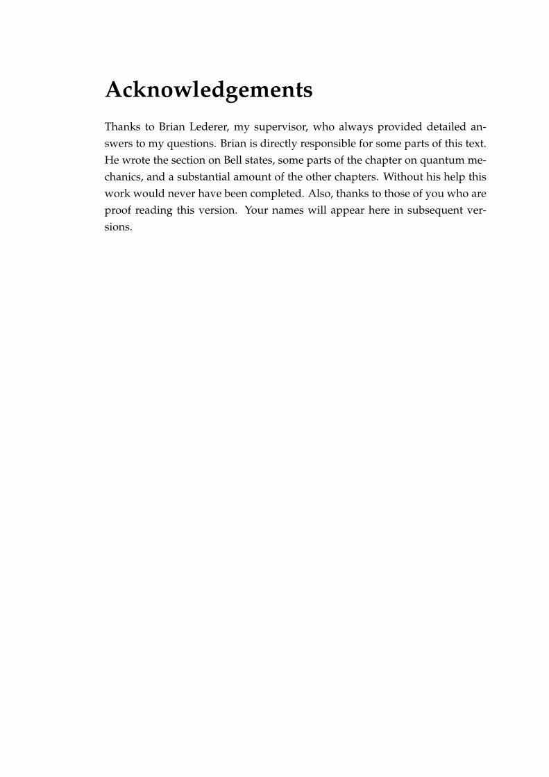
Figure 2.1: Charles Babbage and Ada Byron.
Babylonian cuneiform tablets (c. 2000 - 1700 BC) that contain clear evidence ofalgorithmic processes [Gilleland M. ? 2000]. But up until the 19th century it’sdifficult to separate computer science from other sciences like mathematics andengineering. So we might say that computer science began in the 19th century.
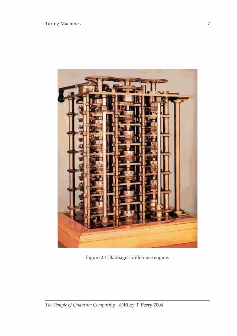
In the early to mid 19th century Charles Babbage, 1791 - 1871 (figure 2.1) de-signed and partially built several programmable computing machines (see fig-ure 2.4 for the difference engine built in 1822) that had many of the features ofmodern computers. One of these machines called the analytical engine had re-movable programs on punch cards based on those used in the Jacquard loom,which was invented by Joseph Marie Jacquard (1752 - 1834) in 1804 [Smithso-nian NMAH 1999]. Babbage’s friend, Ada Augusta King, Countess of Lovelace,1815 - 1852 (figure 2.1) and the daughter of Lord Byron is considered by someas the first programmer for her writings on the Analytical engine. Sadly, Bab-bage’s work was largely forgotten until the 1930s and the advent of moderncomputer science. Modern computer science can be said to have started in1936 when logician Alan Turing, 1912 - 1954 (figure 2.2) wrote a paper whichcontained the notion of a universal computer.
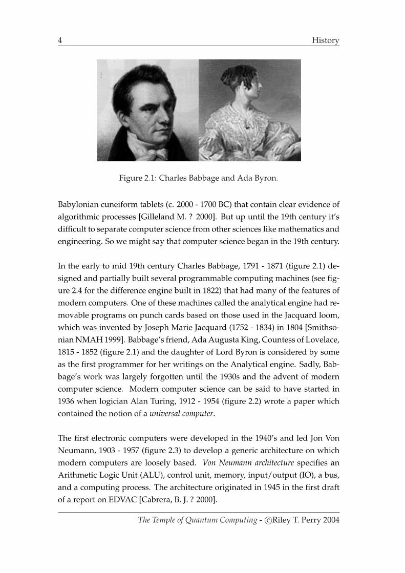
The first electronic computers were developed in the 1940’s and led Jon VonNeumann, 1903 - 1957 (figure 2.3) to develop a generic architecture on whichmodern computers are loosely based. Von Neumann architecture specifies anArithmetic Logic Unit (ALU), control unit, memory, input/output (IO), a bus,and a computing process. The architecture originated in 1945 in the first draftof a report on EDVAC [Cabrera, B. J. ? 2000].
The Temple of Quantum Computing - c©Riley T. Perry 2004
History 5
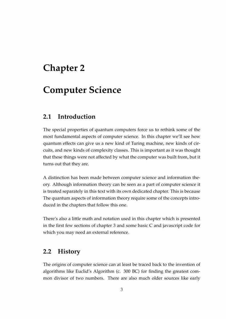
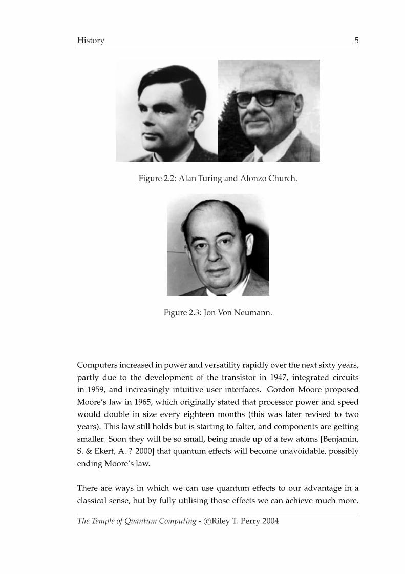
Figure 2.2: Alan Turing and Alonzo Church.
Figure 2.3: Jon Von Neumann.
Computers increased in power and versatility rapidly over the next sixty years,partly due to the development of the transistor in 1947, integrated circuitsin 1959, and increasingly intuitive user interfaces. Gordon Moore proposedMoore’s law in 1965, which originally stated that processor power and speedwould double in size every eighteen months (this was later revised to twoyears). This law still holds but is starting to falter, and components are gettingsmaller. Soon they will be so small, being made up of a few atoms [Benjamin,S. & Ekert, A. ? 2000] that quantum effects will become unavoidable, possiblyending Moore’s law.
There are ways in which we can use quantum effects to our advantage in aclassical sense, but by fully utilising those effects we can achieve much more.
The Temple of Quantum Computing - c©Riley T. Perry 2004

6 Turing Machines
This approach is the basis for quantum computing.
2.3 Turing Machines
In 1928 David Hilbert, 1862 - 1943 (figure 2.5) asked if there was a universalalgorithmic process to decide whether any mathematical proposition was true.His intuition suggested ”yes”, then, in 1930 he went as far as claiming thatthere were no unsolvable problems in mathematics [Natural Theology 2004].This was promptly refuted by Kurt Godel, 1908 - 1976 (figure 2.5) in 1931 byway of his incompleteness theorem which can be roughly summed up as follows:
You might be able to prove every conceivable statement about num-bers within a system by going outside the system in order to comeup with new rules and axioms, but by doing so you’ll only create alarger system with its own unprovable statements. [Jones, J. Wilson,W. 1995, p. ?]
Then, in 1936 Alan Turing and Alonzo Church, 1903 - 1995 (figure 2.2) indepen-dently came up with models of computation, aimed at resolving whether ornot mathematics contained problems that were ”uncomputable”. These wereproblems for which there were no algorithmic solutions (an algorithm is a pro-cedure for solving a mathematical problem that is guaranteed to end after anumber of steps). Turing’s model, now called a called a Turing Machine (TM) isdepicted in figure 2.6. It turned out that the models of Turing and Church wereequivalent in power. The thesis that any algorithm capable of being devisedcan be run on a Turing machine, as Turing’s model was subsequently called,was given the names of both these pioneers, the Church-Turing thesis [Nielsen,M. A. 2002].
2.3.1 Binary Numbers and Formal Languages
Before defining a Turing machine we need to say something about binary num-bers, since this is the format in which data is presented to a Turing machine (seethe tape is figure 2.6).
The Temple of Quantum Computing - c©Riley T. Perry 2004
Turing Machines 7
Figure 2.4: Babbage’s difference engine.
The Temple of Quantum Computing - c©Riley T. Perry 2004

8 Turing Machines
Figure 2.5: David Hilbert and Kurt Godel.
Binary Representation
Computers represent numbers in binary form, as a series of zeros and ones,because this is easy to implement in hardware (compared with other forms,e.g. decimal). Any information can be converted to and from zeros and onesand we call this representation a binary representation.
Example Here are some binary numbers and their decimal equivalents:
The binary number, 1110 in decimal is 14.The decimal 212 when converted to binary becomes 11010100.
The binary numbers (on the left hand side) that represent the decimals0-4 are as follows:
0 = 0
1 = 1
10 = 2
11 = 3
100 = 4
A binary number has the form bn−1 . . . b2b1b0 where n is the number of binarydigits (or bits, with each digit being a 0 or a 1) and b0 is the least significant digit.We can convert the binary string to a decimal number D using the following
The Temple of Quantum Computing - c©Riley T. Perry 2004
Turing Machines 9
formula:
D = 2n−1(bn−1) + . . . + 22(b1) + 21(b1) + 20(b0). (2.1)
Here is another example:
Example Converting the binary number 11010100 to decimal:
D = 27(1) + 26(1) + 25(0) + 24(1) + 23(0) + 22(1) + 21(0) + 20(0)
= 128 + 64 + 16 + 4
= 212
We call the binary numbers a base 2 number system because it is based onjust two symbols 0 and 1. By contrast, in decimal which is base 10, we have0, 1, 2, 3, . . . , 9.
All data in modern computers is stored in binary format; even machine instruc-tions are in binary format. This allows both data and instructions to be storedin computer memory and it allows all of the fundamental logical operations ofthe machine to be represented as binary operations.
Formal Languages
Turing machines and other computer science models of computation use formallanguages to represent their inputs and outputs. We say a language L has an al-phabet
∑. The language is a subset of the set
∑∗ of all finite strings of symbolsfrom
∑.
Example If∑
= 0, 1 then the set of all even binary numbers0, 10, 100, 110, ... is a langauge over
∑.
It turns out that the ”power” of a computational model (or automaton) i.e. theclass of algorithm that the model can implement, can be determined by consid-ering a related question:
What type of ”language” can the automaton recognise?
A formal language in this setting is just a set of binary strings. In simple lan-guages the strings all follow an obvious pattern, e.g. with the language:
01, 001, 0001, . . .
The Temple of Quantum Computing - c©Riley T. Perry 2004

10 Turing Machines
Figure 2.6: A Turing machine.
the pattern is that we have one or more zeroes followed by a 1. If an automa-ton, when presented with any string from the language can read each symboland then halt after the last symbol we say it recognises the language (provid-ing it doesn’t do this for strings not in the language). Then the power of theautomaton is gauged by the complexity of the patterns for the languages it canrecognise.
2.3.2 Turing Machines in Action
A Turing machine (which we’ll sometimes abbreviate to TM) has the followingcomponents [Copeland, J. 2000]:
1. A tape - made up of cells containing 0, 1, or blank. Note that this gives us alanguage of
∑= 0, 1, blank.
2. A read/write head - reads, or overwrites the current symbol on each step andmoves one square to the left or right.
3. A controller - controls the elements of the machine to do the following:1. read the current symbol2. write a symbol by overwriting what’s already there4. move the tape left or right one square5. change state6. halt.
The Temple of Quantum Computing - c©Riley T. Perry 2004

Turing Machines 11
4. The controller’s behaviour - the way the TM switches states depending on thesymbol it’s reading, represented by a finite state automata (FSA).
The operation of a TM is best described by a simple example:
Example Inversion inverts each input bit, for example:
001 → 100
The behaviour of the machine can be represented by a two state FSA. TheFSA is represented below in table form (where the states are labelled 1 and2: 1 for the start state, and 2 for the halt state).
State Value New State New Value Direction1 0 1 1 Move Right
1 1 1 0 Move Right
1 blank 2 - HALT blank Move Right
2 - HALT N/A N/A N/A N/A
2.3.3 The Universal Turing Machine
A Universal Turning Machine (UTM) is a TM (with an in built mechanism de-scribed by a FSA) that is capable of reading, from a tape, a program describingthe behaviour of another TM. The UTM simulates the ordinary TM performingthe behaviour generated when the ordinary TM acts upon its data. When theUTM halts its tape contains the result that would have been produced by theordinary TM (the one that describes the workings of the UTM).
The great thing about the UTM is that it shows that all algorithms (Turing ma-chines) can be reduced to a single algorithm. As stated above, Church, Godel,and a number of other great thinkers did find alternative ways to represent al-gorithms, but it was only Turing who found a way of reducing all algorithmsto a single one. This reduction in algorithms is a bit like what we have in infor-mation theory where all messages can be reduced to zeroes and ones.
The Temple of Quantum Computing - c©Riley T. Perry 2004
12 Turing Machines
2.3.4 The Halting Problem
This is a famous problem in computer science. Having discovered the simple,but powerful model of computation (essentially the stored program computer)Turing then looked at its limitations by devising a problem that it could notsolve.
The UTM can run any algorithm. What, asked Turing, if we have another UTMthat, rather than running a given algorithm, looks to see whether that algorithmacting on it’s data, will actually halt (in a finite number of steps rather thanlooping forever or crashing). Turing called this hypothetical new TM called H(for halting machine). Like a UTM, H can receive a description of the algorithmin question (its program) and the algorithm’s data. Then H works on this in-formation and produces a result. When given a number, say 1 or 0 it decideswhether or not the given algorithm would then halt. Is such a machine possi-ble (so asked Turing)? The answer he found was ”no” (look below). The veryconcept of H involves a contradiction! He demonstrated this by taking, as thealgorithm description (program) and data that H should work on, a variant ofH itself!! The clue to this ingenious way of thinking came from the liar’s para-dox - the question of whether or not the sentence:
This sentence is false.
can be assigned a truth value. Just as a ”universal truth machine” fails in as-signing this funny sentence a truth value (try it), so to does H fail to assign ahalting number 1 or 0 to the variant (the design of the latter involving the sameingredients, self-reference and negation - that made the sentence problematic).
This proof by contradiction only applies to Turing machines, and machinesthat are computationally equivalent. It still remains unproven that the haltingproblem cannot be solved in all computational models.
The next section contains a detailed explanation of the halting problem bymeans of an example. This can be skipped it you’ve had enough of Turingmachines for now.
The Temple of Quantum Computing - c©Riley T. Perry 2004

Turing Machines 13
The Halting Problem - Proof by Contradiction
The halting problem in Javascript [Marshall, J. 2001].
The proof is by contradiction, say we could have a program that could de-termine whether or not another program will halt.
function Halt(program, data)
if ( ...Code to check if program can halt... )
return true;
else
return false;
Given two programs, one that halts and one that does not:
function Halter(input)
alert(’finished’);
function Looper(input)
while (1==1) ;
In our example Halt() would return the following:
Halt("function Halter(1)alert(’finished’);", 1)
\\ returns true
Halt("function Looper(1)while (1==1) ;", 1)
\\ returns false
So it would be possible given these special cases, but is it possible for all al-gorithms to be covered in the ...Code to check if program can halt...
section? No - here is the proof, given a new program:
function Contradiction(program)
if (Halt(program, program) == true)
while (1 == 1) ;
else
The Temple of Quantum Computing - c©Riley T. Perry 2004
14 Circuits
alert(’finished’);
If Contradiction() is given an arbitrary program as an input then:
• If Halt() returns true then Contradiction() goes into an infinite loop.
• If Halt() returns false then Contradiction() halts.
If Contradiction() is given itself as input then:
• Contradiction() loops infinitely if Contradiction() halts (given itselfas input).
• Contradiction() halts if Contradiction() goes into an infinite loop(given itself as input).
Contradiction() here does not loop or halt, we can’t decide algorithmicallywhat the behaviour of Contradiction() will be.
2.4 Circuits
Although modern computers are no more powerful than TM’s (in terms of thelanguages they can recognise) they are a lot more efficient (for more on effi-ciency see section 2.5). However, what a modern or conventional computergives in efficiency it loses in transparency (compared with a TM). It is for thisreason that a TM is still of value in theoretical discussions, e.g. in comparingthe ”hardness” of various classes of problems.
We won’t go fully into the architecture of a conventional computer. Howeversome of the concepts needed for quantum computing are related, e.g. circuits,registers, and gates. For this reason we’ll examine conventional (classical) cir-cuits.
Classical circuits are made up of the following:
1. Gates - which perform logical operations on inputs. Given input(s) withvalues of 0 or 1 they produce an output of 0 or 1 (see below). These oper-ations can be represented by truth tables which specify all of the differentcombinations of the outputs with respect to the inputs.
The Temple of Quantum Computing - c©Riley T. Perry 2004
Circuits 15
2. Wires - carry signals between gates and registers.
3. Registers - made up of cells containing 0 or 1, i.e. bits.
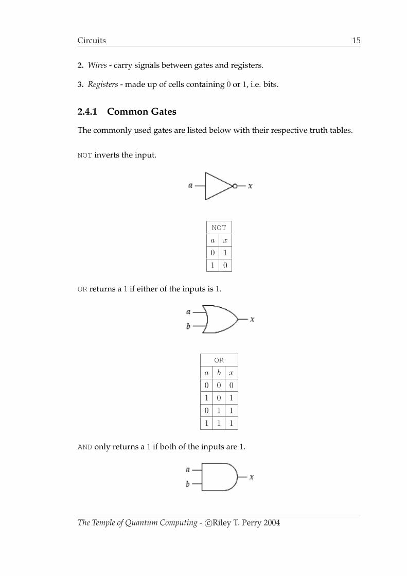
2.4.1 Common Gates
The commonly used gates are listed below with their respective truth tables.
NOTinverts the input.
NOT
a x
0 1
1 0
ORreturns a 1 if either of the inputs is 1.
OR
a b x
0 0 0
1 0 1
0 1 1
1 1 1
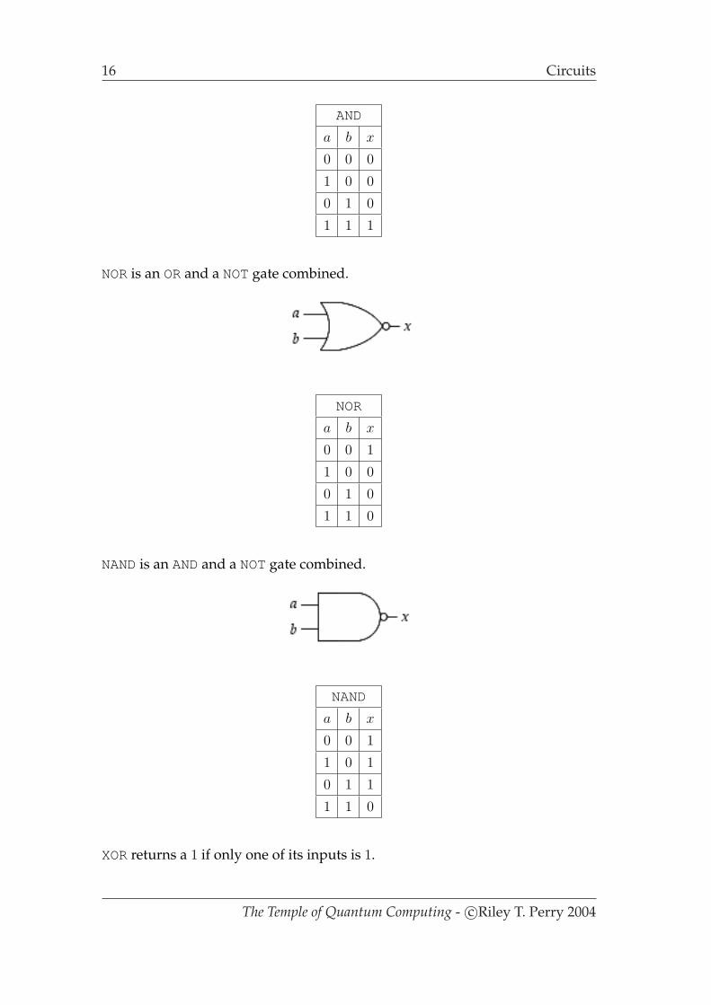
ANDonly returns a 1 if both of the inputs are 1.
The Temple of Quantum Computing - c©Riley T. Perry 2004
16 Circuits
AND
a b x
0 0 0
1 0 0
0 1 0
1 1 1
NORis an ORand a NOTgate combined.
NOR
a b x
0 0 1
1 0 0
0 1 0
1 1 0
NANDis an ANDand a NOTgate combined.
NAND
a b x
0 0 1
1 0 1
0 1 1
1 1 0
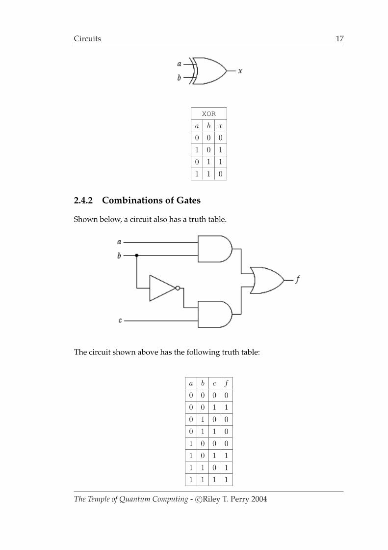
XORreturns a 1 if only one of its inputs is 1.
The Temple of Quantum Computing - c©Riley T. Perry 2004
Circuits 17
XOR
a b x
0 0 0
1 0 1
0 1 1
1 1 0
2.4.2 Combinations of Gates
Shown below, a circuit also has a truth table.
The circuit shown above has the following truth table:
a b c f
0 0 0 0
0 0 1 1
0 1 0 0
0 1 1 0
1 0 0 0
1 0 1 1
1 1 0 1
1 1 1 1
The Temple of Quantum Computing - c©Riley T. Perry 2004
18 Computational Resources and Efficiency
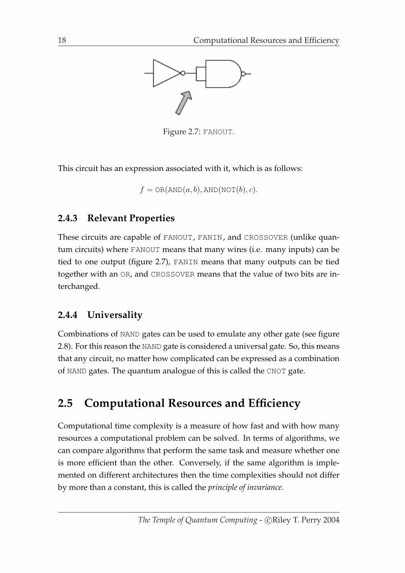
Figure 2.7: FANOUT.
This circuit has an expression associated with it, which is as follows:
f = OR(AND(a, b), AND(NOT(b), c).
2.4.3 Relevant Properties
These circuits are capable of FANOUT, FANIN , and CROSSOVER(unlike quan-tum circuits) where FANOUTmeans that many wires (i.e. many inputs) can betied to one output (figure 2.7), FANIN means that many outputs can be tiedtogether with an OR, and CROSSOVERmeans that the value of two bits are in-terchanged.
2.4.4 Universality
Combinations of NANDgates can be used to emulate any other gate (see figure2.8). For this reason the NANDgate is considered a universal gate. So, this meansthat any circuit, no matter how complicated can be expressed as a combinationof NANDgates. The quantum analogue of this is called the CNOTgate.
2.5 Computational Resources and Efficiency
Computational time complexity is a measure of how fast and with how manyresources a computational problem can be solved. In terms of algorithms, wecan compare algorithms that perform the same task and measure whether oneis more efficient than the other. Conversely, if the same algorithm is imple-mented on different architectures then the time complexities should not differby more than a constant, this is called the principle of invariance.
The Temple of Quantum Computing - c©Riley T. Perry 2004

Computational Resources and Efficiency 19
Figure 2.8: The universal NANDgate.
A simple example of differing time complexities is with sorting algorithms,i.e. algorithms used to sort a list of numbers. The following example uses thebubble sort and quick sort algorithms. Some code for bubble sort is given be-low, but the code for quick sort is not given explicitly. We’ll also use the codefor the bubble sort algorithm in an example on page 22.
Bubble sort:
for(i = 1;i < = n - 1;i ++)
for(j = n;j > = i + 1;j --)
if (list[j]<list[j - 1])
Swap(list[j],list[j - 1]);
The Temple of Quantum Computing - c©Riley T. Perry 2004
20 Computational Resources and Efficiency
Example Quick sort vs. bubble sort.
Bubble Sort:Each item in a list is compared with the item next to it, they are swappedif required. This process is repeated until all of the numbers are checkedwithout any swaps.
Quick Sort:The quick sort has the following four steps:
1. Finish if there are no more elements to be sorted (i.e. 1 or less elements).
2. Select a pivot point.
3. The list is split into two lists - with numbers smaller than the pivot valuein one list and numbers larger than the pivot value in the other list.
4. Repeat steps 1 to 3 for each list generated in step 3.
On average the bubble sort is much slower than the quick sort, regardless ofthe architecture it is running on.
2.5.1 Quantifying Computational Resources
Let’s say we’ve gone through an algorithm systematically and worked out, lineby line (see the end of this section for an example) how fast it is going to rungiven a particular variable n which describes the ”size” of the input. E.g. thenumber of elements in a list to be sorted. Suppose we can quantify the compu-tational work involved as function of n, consider the following expression:
3n + 2 log n + 12.
The important part of this function is 3n as it grows more quickly than the otherterms, i.e. n grows faster than log n and the constant. We say that the algorithmthat generated this result has,
O(n)
time complexity (i.e. we ignore the 3). The important parts of the function areshown here:
The Temple of Quantum Computing - c©Riley T. Perry 2004

Computational Resources and Efficiency 21
0
10
20
30
40
50
0 10 20 30 40 50
3n + 2 log n + 123n
2 log n12
¢¢
So we’ve split the function 3n + 2 log n + 12 into its parts : 3n, 2 log n, and 12.
More formally Big O notation allows us to set an upper bound on the behaviourof the algorithm. So, at worst this algorithm will take approximately n cyclesto complete (plus a vanishingly small unimportant figure). Note that this is theworst case, i.e. it gives us no notion of the average complexity of an algorithm.The class of O(n) contains all functions that are quicker than O(n). for example,3n ≤ 3n2 so 3n is bounded by the class O(3n2) (∀ positive n).
For a lower bound we use big Ω notation (Big Omega).
Example 2n is in Ω(n2) as n2 ≤ 2n (∀ sufficiently large n).
Finally, big Θ is used to show that a function is asymptotically equivalent in bothlower and upper bounds. formally:
f(n) = Θ(g(n)) ⇐⇒ O(g(n)) = Ω(g(n)). (2.2)
Example 4n2 − 40n + 2 = Θ(n2) 6= Θ(n3) 6= Θ(n).
As promised, here is a more in-depth example of the average complexity ofan algorithm.
The Temple of Quantum Computing - c©Riley T. Perry 2004
22 Computational Resources and Efficiency
Example Time Complexity: Quick sort vs. bubble sort [Nielsen, M. A. &Chuang, I. L. 2000].
Here our n is the number of elements in a list, the number of swapoperations is:
(n− 1) + (n− 2) + ... + 1 =n(n− 1)
2
The most important factor here is n2. The average and worst case timecomplexities are O(n2), so we say it is generally O(n2).
If we do the same to the quick sort algorithm, the average time com-plexity is just O(n log n). So now we have a precise mathematical notion forthe speed of an algorithm.
2.5.2 Standard Complexity Classes
Computational complexity is the study of how hard a problem is to compute.Or put another way, what is the least amount of resources required by the bestknown algorithm for solving the problem. There are many types of resources(e.g. time and space); but we are interested in time complexity for now. Themain distinction between hard and easy problems is the rate at which theygrow. If the problem can be solved in polynomial time, that is it is boundedby a polynomial in n, then it is easy. Hard problems grow faster than anypolynomial in n, for example:
n2
is polynomial, and easy, whereas,
2n
is exponential and hard. What we mean by hard is that as we make n large thetime taken to solve the problem goes up as 2n, i.e. exponentially. So we say thatO(2n) is hard or intractable.
The complexity classes of most interest to us are P (Polynomial) and NP (Non-Deterministic Polynomial).
P means that the problem can be solved in polynomial time, NP means that
The Temple of Quantum Computing - c©Riley T. Perry 2004

Computational Resources and Efficiency 23
it probably can’t, and NP complete means it almost definitely can’t. More for-mally:
The class P consists of all those decision problems that can be solvedon a deterministic sequential machine in an amount of time thatis polynomial in the size of the input; the class NP consists of allthose decision problems whose positive solutions can be verified inpolynomial time given the right information, or equivalently, whosesolution can be found in polynomial time on a non-deterministicmachine [wikipedia.org 2004].
Where:
• A decision problem is a function that takes an arbitrary value or values as inputand returns a yes or a no. Most problems can be represented as decisionproblems.
• Witnesses are solutions to decision problems that can be checked in polyno-mial time. For example, checking if 7747 has a factor less than 70 is adecision problem. 61 is a factor (61× 127 = 7747) which is easily checked.So we have a witness to a yes instance of the problem. Now, if we ask if7747 has a factor less than 60 there is no easily checkable witnesses for theno instance [Nielsen, M. A. 2002].
• Non deterministic Turing machines (NTMs) differ from normal deterministicTuring machines in that at each step of the computation the Turing ma-chine can ”spawn” copies, or new Turing machines that work in parallelwith the original. It’s a common mistake to call a quantum computer anNTM, as we shall see later we can only use quantum parallelism indi-rectly.
• It is not proven that P 6= NP it is just very unlikely as this would mean thatall problems in NP can be solved in polynomial time.
See appendix A.1 for a list of common complexity classes.
2.5.3 The Strong Church-Turing Thesis
Originally, the strong Church-Turing thesis went something like this:
The Temple of Quantum Computing - c©Riley T. Perry 2004
24 Computational Resources and Efficiency
Any algorithmic process can be simulated with no loss of efficiencyusing a Turing machine [Banerjee, S. ? 2004].
We are saying a TM is as powerful as any other model of computation in termsof the class of problems it can solve; any efficiency gain due to using a particu-lar model, is at most polynomial.
This was challenged in 1977 by Robert Solovay and Volker Strassen, who intro-duced truly randomised algorithms, which do give a computational advantagebased on the machine’s architecture [Nielsen, M. A. & Chuang, I. L. 2000]. So,this led to a revision of the strong Church-Turing thesis, which now relates to aprobabilistic Turing machine (PTM).
A probabilistic Turing machine can be described as:
A deterministic Turing machine having an additional write instruc-tion where the value of the write is uniformly distributed in the Tur-ing machine’s alphabet (generally, an equal likelihood of writing a1 or a 0 on to the tape) [TheFreeDictionary.com 2004].
This means that algorithms given the same inputs can have different run times,and results if necessary. An example, of an algorithm that can benefit from aPTM is quicksort. Although on average quicksort runs in O(n log n) it still has aworst case running time of O(n2) if say the list is already sorted. Randomisingthe list before hand ensures the algorithm runs more often in O(n log n). ThePTM has its own set of complexity classes, some of which are listed in appendixA.1.
Can we efficiently simulate any non-probabilistic algorithm on a probabilisticTuring machine without exponential slowdown? The answer is ”yes” accord-ing to the new strong Church-Turing thesis:
Any model of computation can be simulated on a probabilistic Tur-ing machine with at most a polynomial increase in the number ofelementary operations [Bettelli, S. 2000, p.2].
A new challenge came from another quarter when in the early eighties RichardFeynman, 1918 - 1988 (figure 2.9) suggested that it would be possible to sim-ulate quantum systems using quantum mechanics - this alluded to a kind of
The Temple of Quantum Computing - c©Riley T. Perry 2004

Computational Resources and Efficiency 25
Figure 2.9: Richard Feynman.
proto-quantum computer. He then went on to ask if it was possible to simulatequantum systems on conventional (i.e. classical) Turing machines. It is hard(time-wise) to simulate quantum systems effectively, in fact it gets exponen-tially harder the more components you have [Nielsen, M. A. 2002]. Intuitively,the TM simulation can’t keep up with the evolution of the physical system it-self: it falls further and further behind, exponentially so. Then, reasoned Feyn-man, if the simulator was ”built of quantum components” perhaps it wouldn’tfall behind. So such a ”quantum computer” would seem to be more efficientthan a TM. The strong Church-Turing thesis would seem to have been violated(as the two models are not polynomially equivalent).
The idea really took shape in 1985 when, based on Feynman’s ideas, DavidDeutsch proposed another revision to the strong Church Turing thesis. He pro-posed a new architecture based on quantum mechanics, on the assumption thatall physics is derived from quantum mechanics (this is the Deutsch - Church -Turing principle [Nielsen, M. A. 2002]). He then demonstrated a simple quan-tum algorithm which seemed to prove the new revision. More algorithms weredeveloped that seemed to work better on a quantum Turing machine (see below)rather than a classical one (notably Shor’s factorisation and Grover’s searchalgorithms - see chapter 7).
2.5.4 Quantum Turing Machines
A quantum Turing machine (QTM) is a normal Turing machine with quantumparallelism. The head and tape of a QTM exist in quantum states, and each
The Temple of Quantum Computing - c©Riley T. Perry 2004

26 Energy and Computation
cell of the tape holds a quantum bit (qubit) which can contain what’s called asuperposition of the values 0 and 1. Don’t worry too much about that now asit’ll be explained in detail later; what’s important is that a QTM can performcalculations on a number of values simultaneously by using quantum effects.Unlike classical parallelism which requires a separate processor for each valueoperated on in parallel, in quantum parallelism a single processor operates onall the values simultaneously.
There are a number of complexity classes for QTMs, see appendix A.2 for alist of some of them and the relationships between them.
Question The architecture itself can change the time complexity of algorithms.Could there be other revisions? If physics itself is not purely based on quantummechanics and combinations of discrete particles have emergent properties forexample, there could be further revisions.
2.6 Energy and Computation
2.6.1 Reversibility
When an isolated quantum system evolves it always does so reversibly. Thisimplies that if a quantum computer has components, similar to gates, that per-form logical operations then these components, if behaving according to quan-tum mechanics, will have to implement all the logical operations reversibly.
2.6.2 Irreversibility
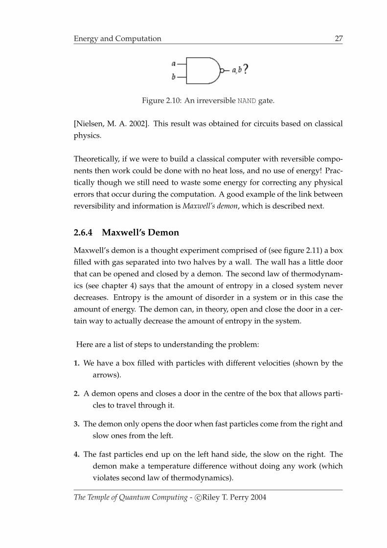
Most classical circuits are not reversible. This means that they lose informationin the process of generating outputs from inputs, i.e. they are not invertible. Anexample of this is the NANDgate (figure 2.10). It is not possible in general, toinvert the output. E.g. knowing the output is 1 does not allow one to determinethe input: it could be 00, 10, or 01.
2.6.3 Landauer’s Principle
In 1961, IBM physicist Rolf Landauer, 1927 - 1999 showed that, when infor-mation is lost in an irreversible circuit that information is dissipated as heat
The Temple of Quantum Computing - c©Riley T. Perry 2004
Energy and Computation 27
Figure 2.10: An irreversible NANDgate.
[Nielsen, M. A. 2002]. This result was obtained for circuits based on classicalphysics.
Theoretically, if we were to build a classical computer with reversible compo-nents then work could be done with no heat loss, and no use of energy! Prac-tically though we still need to waste some energy for correcting any physicalerrors that occur during the computation. A good example of the link betweenreversibility and information is Maxwell’s demon, which is described next.
2.6.4 Maxwell’s Demon
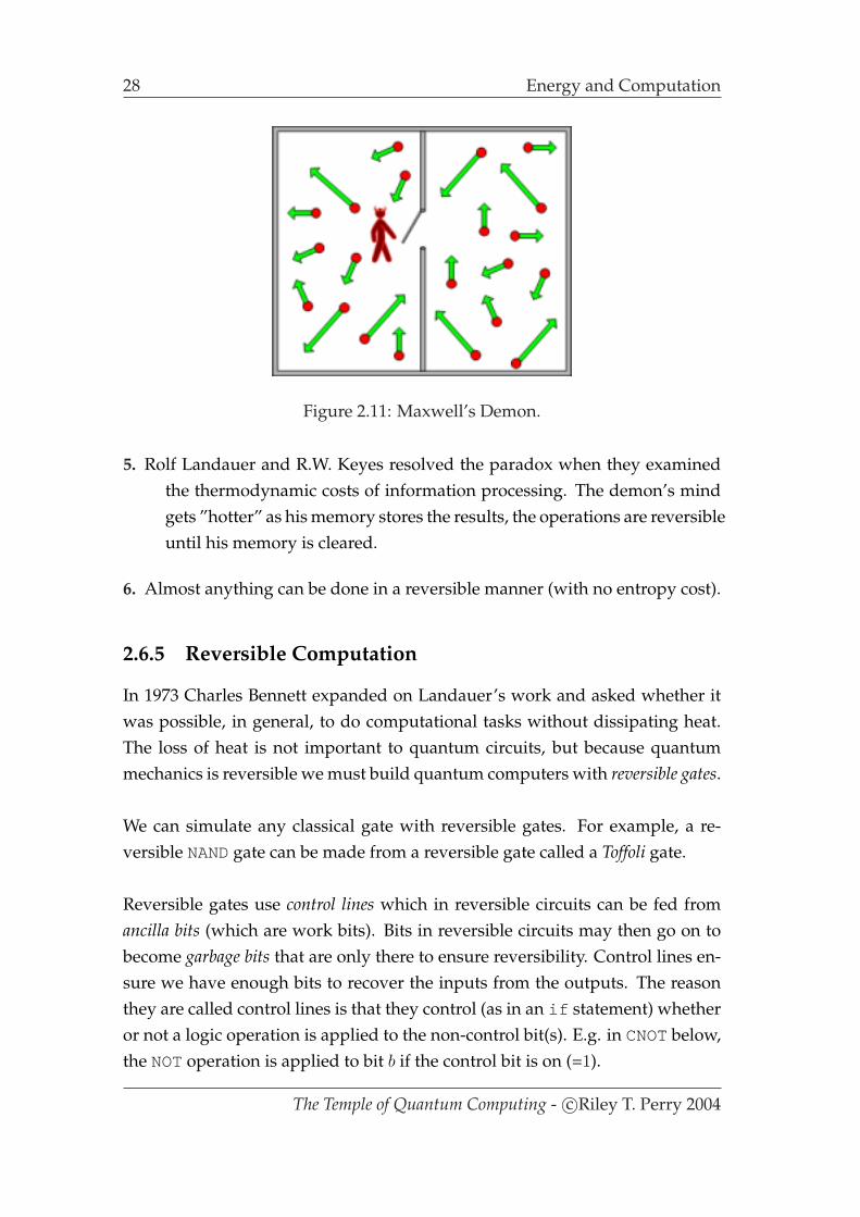
Maxwell’s demon is a thought experiment comprised of (see figure 2.11) a boxfilled with gas separated into two halves by a wall. The wall has a little doorthat can be opened and closed by a demon. The second law of thermodynam-ics (see chapter 4) says that the amount of entropy in a closed system neverdecreases. Entropy is the amount of disorder in a system or in this case theamount of energy. The demon can, in theory, open and close the door in a cer-tain way to actually decrease the amount of entropy in the system.
Here are a list of steps to understanding the problem:
1. We have a box filled with particles with different velocities (shown by thearrows).
2. A demon opens and closes a door in the centre of the box that allows parti-cles to travel through it.
3. The demon only opens the door when fast particles come from the right andslow ones from the left.
4. The fast particles end up on the left hand side, the slow on the right. Thedemon make a temperature difference without doing any work (whichviolates second law of thermodynamics).
The Temple of Quantum Computing - c©Riley T. Perry 2004
28 Energy and Computation
Figure 2.11: Maxwell’s Demon.
5. Rolf Landauer and R.W. Keyes resolved the paradox when they examinedthe thermodynamic costs of information processing. The demon’s mindgets ”hotter” as his memory stores the results, the operations are reversibleuntil his memory is cleared.
6. Almost anything can be done in a reversible manner (with no entropy cost).
2.6.5 Reversible Computation
In 1973 Charles Bennett expanded on Landauer’s work and asked whether itwas possible, in general, to do computational tasks without dissipating heat.The loss of heat is not important to quantum circuits, but because quantummechanics is reversible we must build quantum computers with reversible gates.
We can simulate any classical gate with reversible gates. For example, a re-versible NANDgate can be made from a reversible gate called a Toffoli gate.
Reversible gates use control lines which in reversible circuits can be fed fromancilla bits (which are work bits). Bits in reversible circuits may then go on tobecome garbage bits that are only there to ensure reversibility. Control lines en-sure we have enough bits to recover the inputs from the outputs. The reasonthey are called control lines is that they control (as in an if statement) whetheror not a logic operation is applied to the non-control bit(s). E.g. in CNOTbelow,the NOToperation is applied to bit b if the control bit is on (=1).
The Temple of Quantum Computing - c©Riley T. Perry 2004

Energy and Computation 29
2.6.6 Reversible Gates
Listed below are some of the common reversible gates and their truth tables.Note: the reversible gate diagrams, and quantum circuit diagrams were builtwith a LATEX macro package called Q-Circuit which is available at http://
info.phys.unm.edu/Qcircuit/ .
Controlled NOT
Like a NOTgate (on b) but with a control line, a. b′ can also be expressed as a
XORb.
a • a′
b ÂÁÀ¿»¼½¾ b′
CNOT
a b a′ b′
0 0 0 0
0 1 0 1
1 0 1 1
1 1 1 0
Properties of the CNOTgate, CNOT(a, b):
CNOT(x, 0) : b′ = a′ = a = FANOUT. (2.3)
Toffoli Gate
If the two control lines are set it flips the third bit (i.e. applies NOT). The Toffoligate is also called a controlled-controlled NOT.
a • a′
b • b′
c ÂÁÀ¿»¼½¾ c′
The Temple of Quantum Computing - c©Riley T. Perry 2004
30 Energy and Computation
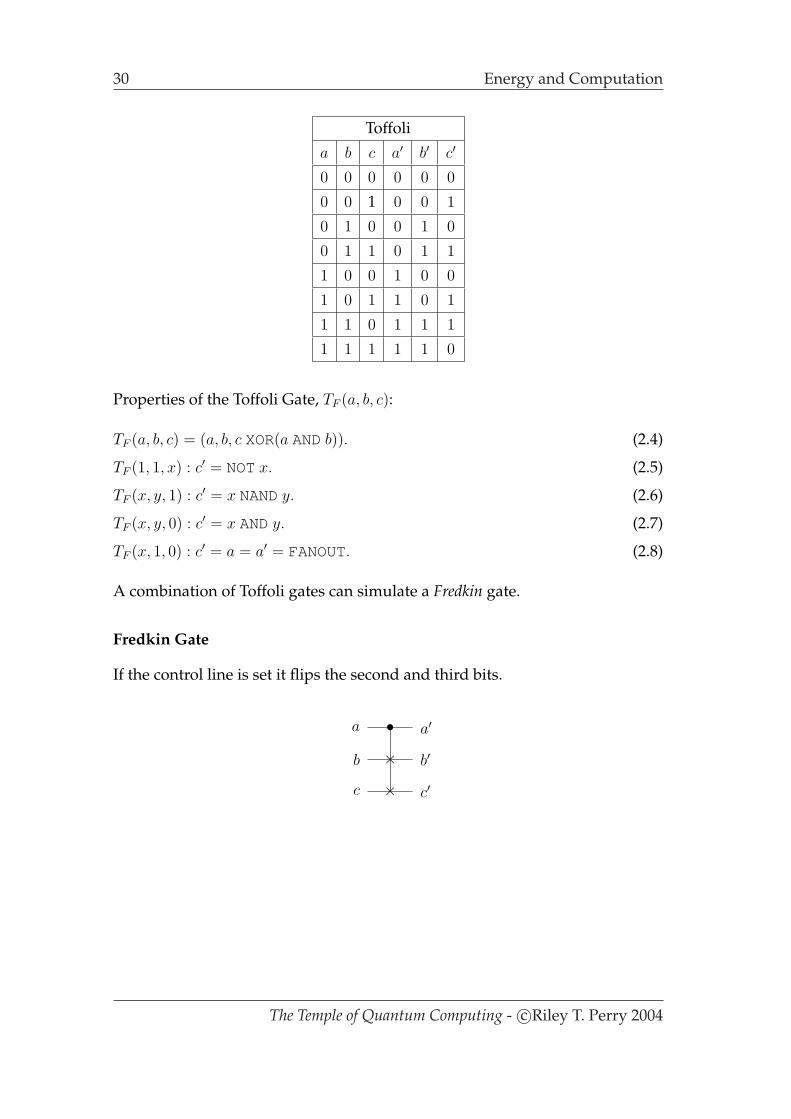
Toffoli
a b c a′ b′ c′
0 0 0 0 0 0
0 0 1 0 0 1
0 1 0 0 1 0
0 1 1 0 1 1
1 0 0 1 0 0
1 0 1 1 0 1
1 1 0 1 1 1
1 1 1 1 1 0
Properties of the Toffoli Gate, TF (a, b, c):
TF (a, b, c) = (a, b, c XOR(a ANDb)). (2.4)
TF (1, 1, x) : c′ = NOTx. (2.5)
TF (x, y, 1) : c′ = x NANDy. (2.6)
TF (x, y, 0) : c′ = x ANDy. (2.7)
TF (x, 1, 0) : c′ = a = a′ = FANOUT. (2.8)
A combination of Toffoli gates can simulate a Fredkin gate.
Fredkin Gate
If the control line is set it flips the second and third bits.
a • a′
b × b′
c × c′
The Temple of Quantum Computing - c©Riley T. Perry 2004
Energy and Computation 31
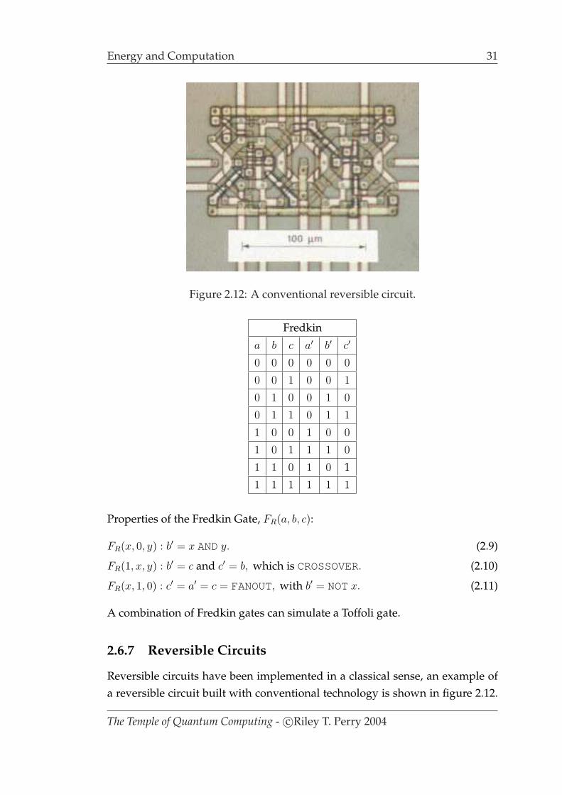
Figure 2.12: A conventional reversible circuit.
Fredkin
a b c a′ b′ c′
0 0 0 0 0 0
0 0 1 0 0 1
0 1 0 0 1 0
0 1 1 0 1 1
1 0 0 1 0 0
1 0 1 1 1 0
1 1 0 1 0 1
1 1 1 1 1 1
Properties of the Fredkin Gate, FR(a, b, c):
FR(x, 0, y) : b′ = x ANDy. (2.9)
FR(1, x, y) : b′ = c and c′ = b, which is CROSSOVER. (2.10)
FR(x, 1, 0) : c′ = a′ = c = FANOUT, with b′ = NOTx. (2.11)
A combination of Fredkin gates can simulate a Toffoli gate.
2.6.7 Reversible Circuits
Reversible circuits have been implemented in a classical sense, an example ofa reversible circuit built with conventional technology is shown in figure 2.12.
The Temple of Quantum Computing - c©Riley T. Perry 2004

32 Artificial Intelligence
Quantum computers use reversible circuits to implement quantum algorithms.Chapters 6 and 7 contain many examples of these algorithms and their associ-ated circuits.
2.7 Artificial Intelligence
Can an algorithm think? that’s really what we are asking when we ask if a com-puter can think, because a modern computer’s architecture is arbitrary. This isthe kind of intelligence that is tested with the Turing test which simply asks ifresponses from a hidden source can be determined to be human, or artificial.Turing said that if one can’t distinguish between the two then the source canbe considered to be intelligent. This is called strong AI, but a more realistic ap-proach in which the modelling of mental processes is used in the study of realmental processes is called weak AI.
2.7.1 The Chinese Room
John Searle has a good example of how the Turing test does not achieve its goal.
Consider a language you don’t understand. In my case, I do not un-derstand Chinese. To me Chinese writing looks like so many mean-ingless squiggles. Now suppose I am placed in a room containingbaskets full of Chinese symbols. Suppose also that I am given a rulebook in English for matching Chinese symbols with other ChineseSymbols. The rules identify the symbols entirely by their shapes anddo not require that I understand any of them. Imagine that peopleoutside the room who understand Chinese hand in small bunches ofsymbols and that in response to the rule book and hand back moresmall bunches of symbols [Searle, J. R. 1990, p. 20].
This system could pass the Turing test - in programming terms one could al-most consider a case statement to be intelligent. Clearly, the Turing test hasproblems. Intelligence is intimately tied up with the ”stuff” that goes to makeup a brain.
The Temple of Quantum Computing - c©Riley T. Perry 2004
Artificial Intelligence 33
2.7.2 Quantum Computers and Intelligence
The idea that consciousness and quantum mechanics are related is a core partof the original theory of quantum mechanics [Hameroff, S. ? 2003]. There aretwo main explanations of what consciousness is. The Socratic, in which con-scious thoughts are products of the cerebrum and the Democritan in which con-sciousness is a fundamental feature of reality accessed by brain. Currently themodern Socratic view prevails, that is that consciousness is an emergent prop-erty and proponents of the emergent theory point to many emergent phenom-ena (Jupiter’s red spot, whirlpools, etc.). Contrasting this, modern Democri-tans believe consciousness to be irreducible, and fundamental. For example,Whiteheads (1920) theory of panexperientielism suggests that quantum state re-ductions (measurements) in a universal proto-conscious field [Arizona.edu 1999]cause individual conscious events. There are many other theories of conscious-ness that relate to quantum effects like electron tunnelling, quantum indeter-minacy, quantum superposition/interference, and more.
Question Given the new quantum architecture can quantum computers think?because of their fundamental nature do they give new hope to strong AI? Or arethey just another example of an algorithmic architecture which isn’t made ofthe ”right stuff”?
The Temple of Quantum Computing - c©Riley T. Perry 2004

Chapter 3
Mathematics for QuantumComputing
3.1 Introduction
In conventional computers we have logical operators (gates) such as NOTthatacts on bits. The quantum analogue of this is a matrix operator operating on aqubit state vector. The maths we need to handle this includes:
• Vectors to represent the quantum state.
• Matrices to represent gates acting on the values.
• Complex numbers, because the components of the quantum state vector are,in general complex.
• Trig functions for the polar representation of complex numbers and thefourier series.
• Projectors to handle quantum measurements.
• Probability theory for computing the probability of measurement outcomes.
As well as there being material here that you may not be familiar with (com-plex vector spaces for example), chances are that you’ll know at least some ofthe math. The sections you know might be useful for revision, or as a reference.This is especially true for the sections on polynomials, trigonometry, and logswhich are very succinct.
35

36 Polynomials
So what’s not in here? There’s obviously some elementary math that is notcovered. This includes topics like fractions, percentages, basic algebra, powers,radicals, summations, limits, factorisation, and simple geometry. If you’re notcomfortable with these topics then you may need to study them before contin-uing on with this chapter.
3.2 Polynomials
A polynomial is an expression in the form:
c0 + c1x + c2x2 + ... + cnx
n (3.1)
where c0, c1, c2, ..., cn are constant coefficients with cn 6= 0.
We say that the above is a polynomial in x of degree n.
Example Different types of polynomials.
3v2 + 4v + 7 is a polynomial in v of degree 2, i.e. a quadratic.4t3 − 5 is a polynomial in t of degree 3, i.e. a cubic.6x2 + 2x−1 is not a polynomial as it contains a negative power for x.
3.3 Logical Symbols
A number of logical symbols are used in this text to compress formulae; theyare explained below:
∀ means for all.
Example ∀ n > 5, f(n) = 4 means that for all values of n greater than 5 f(n)
will return 4.
∃ means there exists.
Example ∃ n such that f(n) = 4 means there is a value of n that will makef(n) return 4. Say if f(n) = (n− 1)2 +4, then the n value in question is n = 1.
The Temple of Quantum Computing - c©Riley T. Perry 2004
Trigonometry Review 37
iff means if and only if.
Example f(n) = 4 iff n = 8 means f(n) will return 4 if n = 8 but for noother values of n.
3.4 Trigonometry Review
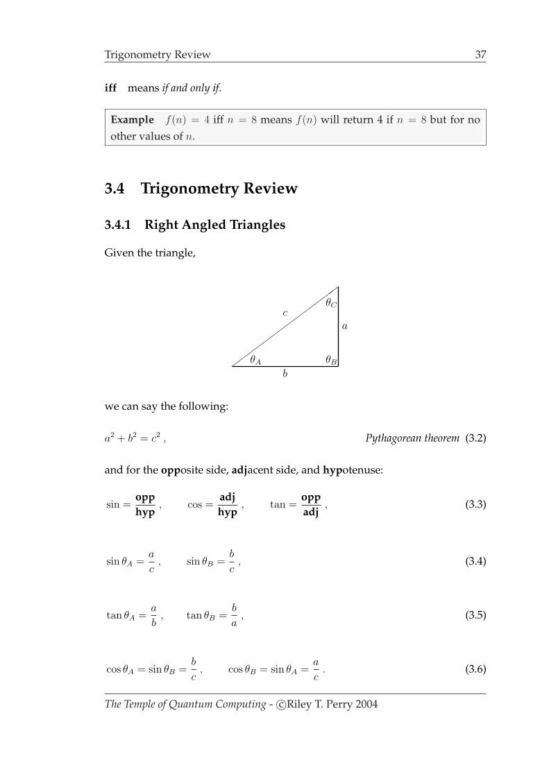
3.4.1 Right Angled Triangles
Given the triangle,
½½
½½
½½
½½
½½
½½
b
ac
θA θB
θC
we can say the following:
a2 + b2 = c2 , Pythagorean theorem (3.2)
and for the opposite side, adjacent side, and hypotenuse:
sin =opphyp
, cos =adjhyp
, tan =oppadj
, (3.3)
sin θA =a
c, sin θB =
b
c, (3.4)
tan θA =a
b, tan θB =
b
a, (3.5)
cos θA = sin θB =b
c, cos θB = sin θA =
a
c. (3.6)
The Temple of Quantum Computing - c©Riley T. Perry 2004

38 Trigonometry Review
3.4.2 Converting Between Degrees and Radians
Angles in trigonometry can be represented in radians and degrees. For con-verting degrees to radians:
rads =n × π
180. (3.7)
For converting radians to degrees we have:
n =180× rads
π. (3.8)
Some common angle conversions are:
360 = 0 = 2π rads.1 = π
180rads.
45 = π4
rads.90 = π
2rads.
180 = π rads.270 = 3π
2rads.
1 rad = 57.
3.4.3 Inverses
Here are some inverses for obtaining θ from sin θ, cos θ, and tan θ:
sin−1 = arcsin = θ from sin θ. (3.9)
cos−1 = arccos = θ from cos θ. (3.10)
tan−1 = arctan = θ from tan θ. (3.11)
3.4.4 Angles in Other Quadrants
The angles for right angled triangles are in quadrant 1 (i.e. from 0 to 90). Ifwe want to measure larger angles like 247 we must determine which quadrantthe angle is in (here we don’t consider angles larger than 360). The followingdiagram has the rules for doing so:
The Temple of Quantum Computing - c©Riley T. Perry 2004
Trigonometry Review 39
0 ≤ θ ≤ 9090 ≤ θ ≤ 180
180 ≤ θ ≤ 270 270 ≤ θ ≤ 360(0)
No changeMake cos and tan negativeChange θ to 180 − θ
Make sin and cos negativeChange θ to θ − 180
Make sin and tan negativeChange θ to 360 − θ
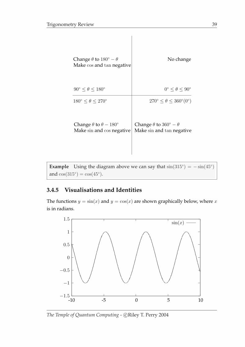
Example Using the diagram above we can say that sin(315) = − sin(45)
and cos(315) = cos(45).
3.4.5 Visualisations and Identities
The functions y = sin(x) and y = cos(x) are shown graphically below, where x
is in radians.
−1.5
−1
−0.5
0
0.5
1
1.5
-10 -5 0 5 10
sin(x)
The Temple of Quantum Computing - c©Riley T. Perry 2004

40 Logs
−1.5
−1
−0.5
0
0.5
1
1.5
-10 -5 0 5 10
cos(x)
Finally, here are some important identities:
sin2 θ + cos2 θ = 1. (3.12)
sin(−θ) = − sin θ. (3.13)
cos(−θ) = cos θ. (3.14)
tan(−θ) = − tan θ. (3.15)
3.5 Logs
The logarithm of a number (say x) to base b is the power of b that gives back thenumber, i.e. blogb x = x. E.g. The log of x = 100 to base b = 10 is the power (2) of10 that gives back 100, i.e. 102 = 100. So log10 100 = 2.
Put another way, the answer to a logarithm is the power y put to a base b givenan answer x, with:
y = logb x (3.16)
and,
x = by (3.17)
where x >= 0, b >= 0, and b 6= 1.
Example log2 16 = 4 is equivalent to 24 = 16.
The Temple of Quantum Computing - c©Riley T. Perry 2004

Complex Numbers 41
-
6
?
¾ ¡¡
¡¡
¡µa
b
z
r
θ
3
3
Figure 3.1: Representing z = a+ ib in the complex plane with coordinates a = 3
and b = 3.
3.6 Complex Numbers
A complex number, z is a number in the form:
z = a + ib (3.18)
where a, b ∈ R (the real numbers) where i stands for√−1. The complex num-
ber z is said to be in C (the complex numbers). z is called complex because it ismade of two parts, a and b. Sometimes we write z = (a, b) to express this.
Except for the rules regarding i, the operations of addition, subtraction, andmultiplication of complex numbers follow the normal rules of arithmetic. Di-vision requires using a complex conjugate, which is introduced in the next sec-tion. With these operations defined via the examples in the box below.
The system of complex numbers is closed in that, except for division by 0, sums,products, and ratios of complex numbers give back a complex number: i.e. westay within the system. Here are examples of i itself:
i−3 = i, i−2 = −1, i−1 = −i, i =√−1, i2 = −1, i3 = −i, i4 = 1, i5 = i, i6 = −1.
So the pattern (−i, 1, i,−1) repeats indefinitely.
The Temple of Quantum Computing - c©Riley T. Perry 2004
42 Complex Numbers
Example Basic complex numbers.
Addition:(5 + 2i) + (−4 + 7i) = 1 + 9i
Multiplication:
(5 + 2i)(−4 + 3i) = 5(−4) + 5(3) + 2(−4)i + (2)(3)i2
= −20 + 15i− 8i− 6
= −26 + 7i.
Finding Roots:
(−5i)2 = 5i2
= 52i2
= 25(−1)
= −25.
−25 has roots 5i and −5i.
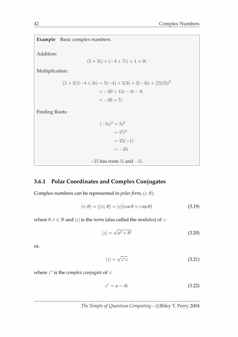
3.6.1 Polar Coordinates and Complex Conjugates
Complex numbers can be represented in polar form, (r, θ):
(r, θ) = (|z|, θ) = |z|(cos θ + i sin θ) (3.19)
where θ, r ∈ R and |z| is the norm (also called the modulus) of z:
|z| =√
a2 + b2 (3.20)
or,
|z| =√
z∗z (3.21)
where z∗ is the complex conjugate of z:
z∗ = a− ib. (3.22)
The Temple of Quantum Computing - c©Riley T. Perry 2004

Complex Numbers 43
-
6
?
¾ ¡¡
¡¡
¡µ
@@
@@
@R
@@
@@
@I
¡¡
¡¡
¡ª
−z∗ z
z∗−z
Figure 3.2: z, z∗, −z∗, and −z.
Polar Coordinates
For polar coordinates (figure 3.1) we can say that θ is the angle between a linedrawn between a point (a, b) of length r on the complex plane and the x axiswith the coordinates being taken for the complex number as x = a and y = b.The horizontal axis is called the real axis and the vertical axis is called the imag-inary axis. It’s also helpful to look at the relationships between z, z∗, −z∗ and -zgraphically. These are shown in figure 3.2.
So for converting from polar to cartesian coordinates:
(r, θ) = a + bi (3.23)
where a = r cos θ and b = r sin θ. Conversely, converting cartesian to polar formis a little more complicated:
a + bi = (r, θ) (3.24)
where r = |z| =√
a2 + b2 and θ is the solution to tan θ = ba
which lies in thefollowing quadrant:
1. If a > 0 and b > 0
2. If a < 0 and b > 0
The Temple of Quantum Computing - c©Riley T. Perry 2004
44 Complex Numbers
3. If a < 0 and b < 0
4. If a > 0 and b < 0.
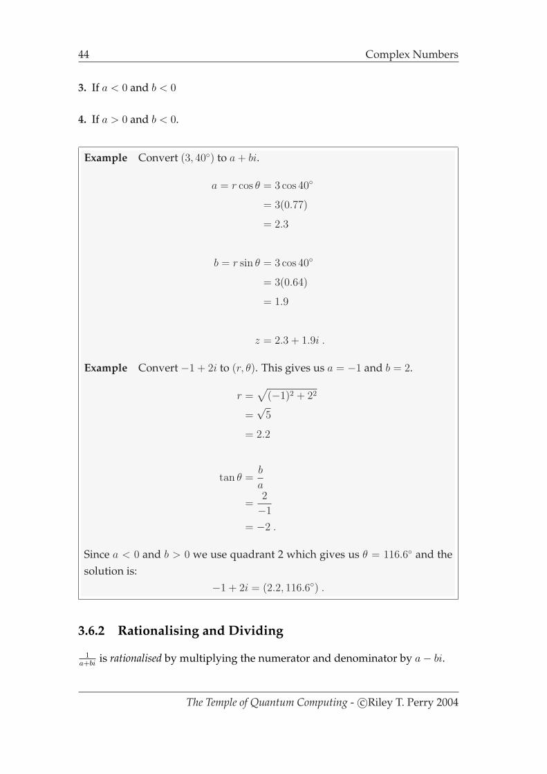
Example Convert (3, 40) to a + bi.
a = r cos θ = 3 cos 40
= 3(0.77)
= 2.3
b = r sin θ = 3 cos 40
= 3(0.64)
= 1.9
z = 2.3 + 1.9i .
Example Convert −1 + 2i to (r, θ). This gives us a = −1 and b = 2.
r =√
(−1)2 + 22
=√
5
= 2.2
tan θ =b
a
=2
−1
= −2 .
Since a < 0 and b > 0 we use quadrant 2 which gives us θ = 116.6 and thesolution is:
−1 + 2i = (2.2, 116.6) .
3.6.2 Rationalising and Dividing
1a+bi
is rationalised by multiplying the numerator and denominator by a− bi.
The Temple of Quantum Computing - c©Riley T. Perry 2004

Complex Numbers 45
Example Rationalisation.
1
5 + 2i=
1
5 + 2i
(5− 2i)
(5− 2i)
=5
29− 2
29i .
Division of complex numbers is done by rationalising in terms of the denomi-nator.
Example Division of complex numbers.
3 + 2i
2i=
3 + 2i
2i
(−2i)
(−2i)
=−6i− 4i2
−4i2
=−6i + 4
4
= 1− 3
2i .
3.6.3 Exponential Form
Complex numbers can also be represented in exponential form:
z = reiθ. (3.25)
The derivation of which is:
z = |z|(cos θ + i sin θ)
= r(cos θ + i sin θ)
= reiθ.
This is because:
eiθ = cos θ + i sin θ, (3.26)
e−iθ = cos θ − i sin θ. (3.27)
which can be rewritten as:
cos θ =eiθ + e−iθ
2, (3.28)
sin θ =eiθ − e−iθ
2i. (3.29)
The Temple of Quantum Computing - c©Riley T. Perry 2004

46 Complex Numbers
To prove (3.26) we use a power series exponent (which is an infinite polyno-mial):
ex = 1 + x +x2
2!+
x3
3!+ . . . , (3.30)
eiθ = 1 + iθ − iθ2
2!− iθ3
3!+
θ4
4!− . . . (3.31)
= 1− θ2
2!+
θ4
4!+ i(θ − iθ3
3!+ . . .) (3.32)
= cos θ + i sin θ. (3.33)
Example Convert 3+3i to exponential form. This requires two main steps,which are:
1. Find the modulus.
r = |z| =√
32 + 32
=√
18.
2. To find θ, we can use the a and b components of z as opposite and adjacentsides of a right angled triangle in quadrant one which means need toapply arctan. So given tan−1 3
3= π
4then z in exponential form looks
like: √18eπi/4 .
Example Convert eπi3/4 to the form: a + bi (also called rectangular form).
eπi3/4 = ei(3π/4)
= cos3π
4+ i sin
3π
4
= cos 135 + i sin 135
=−1√
2+
i√2
=−1 + i√
2.
Properties:
z∗ = re−iθ. (3.34)
e−i2π = 1. (3.35)
The Temple of Quantum Computing - c©Riley T. Perry 2004
Matrices 47
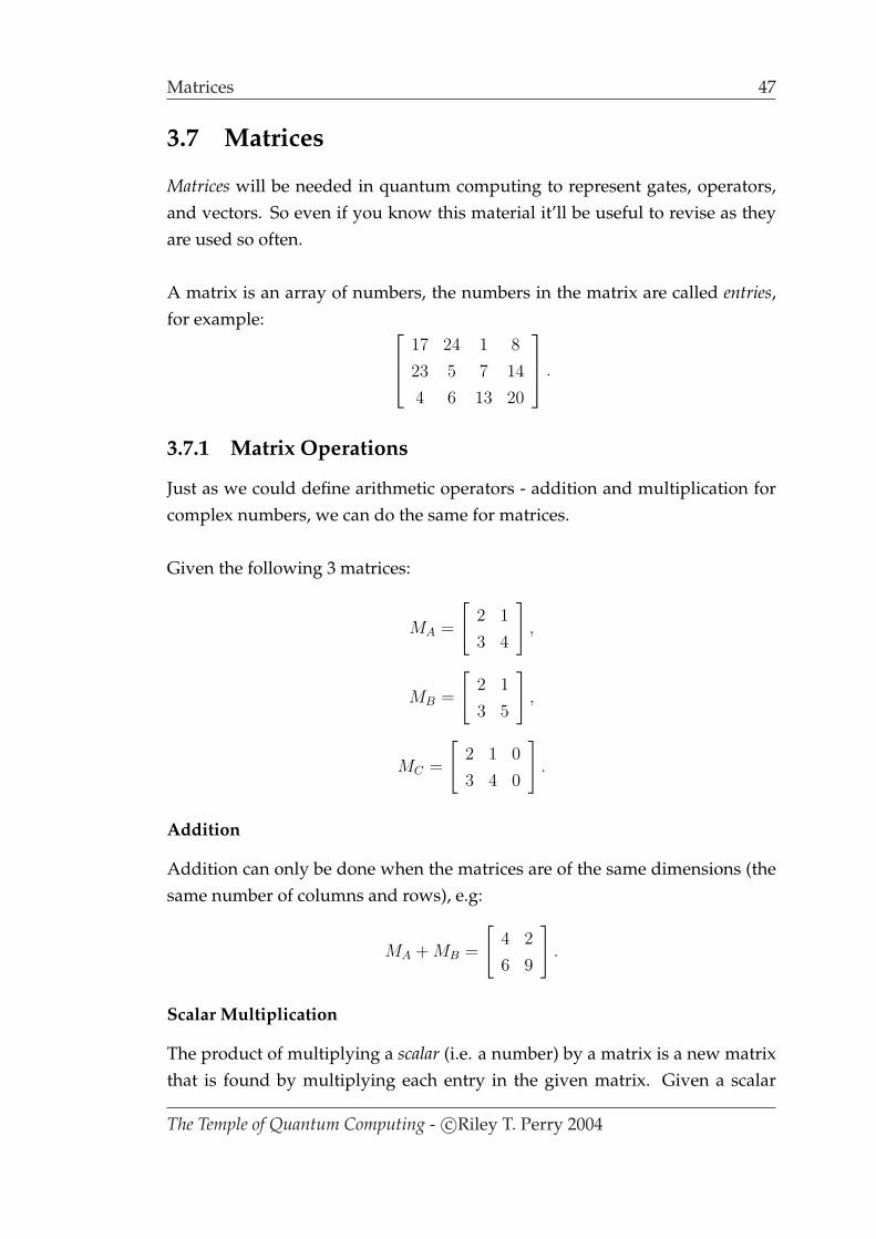
3.7 Matrices
Matrices will be needed in quantum computing to represent gates, operators,and vectors. So even if you know this material it’ll be useful to revise as theyare used so often.
A matrix is an array of numbers, the numbers in the matrix are called entries,for example:
17 24 1 8
23 5 7 14
4 6 13 20
.
3.7.1 Matrix Operations
Just as we could define arithmetic operators - addition and multiplication forcomplex numbers, we can do the same for matrices.
Given the following 3 matrices:
MA =
[2 1
3 4
],
MB =
[2 1
3 5
],
MC =
[2 1 0
3 4 0
].
Addition
Addition can only be done when the matrices are of the same dimensions (thesame number of columns and rows), e.g:
MA + MB =
[4 2
6 9
].
Scalar Multiplication
The product of multiplying a scalar (i.e. a number) by a matrix is a new matrixthat is found by multiplying each entry in the given matrix. Given a scalar
The Temple of Quantum Computing - c©Riley T. Perry 2004

48 Matrices
α = 2 :
αMA =
[4 2
6 8
].
Matrix Multiplication
The product of multiplying matrices M and N with dimensions M = m×r andN = r×n is a matrix O with dimension O = m×n. The resulting matrix is foundby Oij =
∑rk=1 MirNrj where i and j denote row and column respectively. The
matrices M and N must also satisfy the condition that the number of columnsin M is the same as the number of rows in N .
MBMC =
[(2× 2) + (1× 3) (2× 1) + (1× 4) (2× 0) + (1× 0)
(3× 2) + (5× 3) (3× 1) + (5× 4) (3× 0) + (5× 0)
]
=
[7 6 0
21 23 0
].
Basic Matrix Arithmetic
Suppose M , N , and O are matrices and α and β are scalars:
M + N = N + M. Commutative law for addition (3.36)
M + (N + O) = (M + N) + O. Associative law for addition (3.37)
M(NO) = (MN)O. Associative law for multiplication (3.38)
M(N + O) = MN + MO. Distributive law (3.39)
(N + O)M = NM + OM. Distributive law (3.40)
M(N −O) = MN −MO. (3.41)
(N −O)M = NM −OM. (3.42)
α(N + O) = αN + αO. (3.43)
α(N −O) = αN − αO. (3.44)
(α + β)O = αO + αO. (3.45)
(α− β)O = αO − αO. (3.46)
(αβ)O = α(βO). (3.47)
α(NO) = (αN)O = N(αO). (3.48)
The Temple of Quantum Computing - c©Riley T. Perry 2004

Matrices 49
You may have noticed that there is no commutative law for multiplication. It isnot always the case that MN = NM . This is important in quantum mechanics,which follows the same non-commutative multiplication law.
Zero Matrix
The special case of a matrix filled with zeroes.
0 =
[0 0
0 0
]. (3.49)
Identity Matrix
A matrix multiplied by the identity matrix (corresponding to unity in the ordi-nary numbers) will not change.
I =
[1 0
0 1
], (3.50)
MAI =
[2 1
3 4
].
Inverse Matrix
A number a has an inverse a−1 where aa−1 = a−1a = 1. Equivalently a matrixA has an inverse:
A−1 where AA−1 = A−1A = I. (3.51)
Even with a simple 2×2 matrix it is not a trivial matter to determine its inverses(if it has any at all). An example of an inverse is below, for a full explanation ofhow to calculate an inverse you’ll need to consult an external reference.
M−1A =
[45
−15
−35
25
].
Note A−1 only exists iff A has full rank (see Determinants and Rank below).
The Temple of Quantum Computing - c©Riley T. Perry 2004
50 Matrices
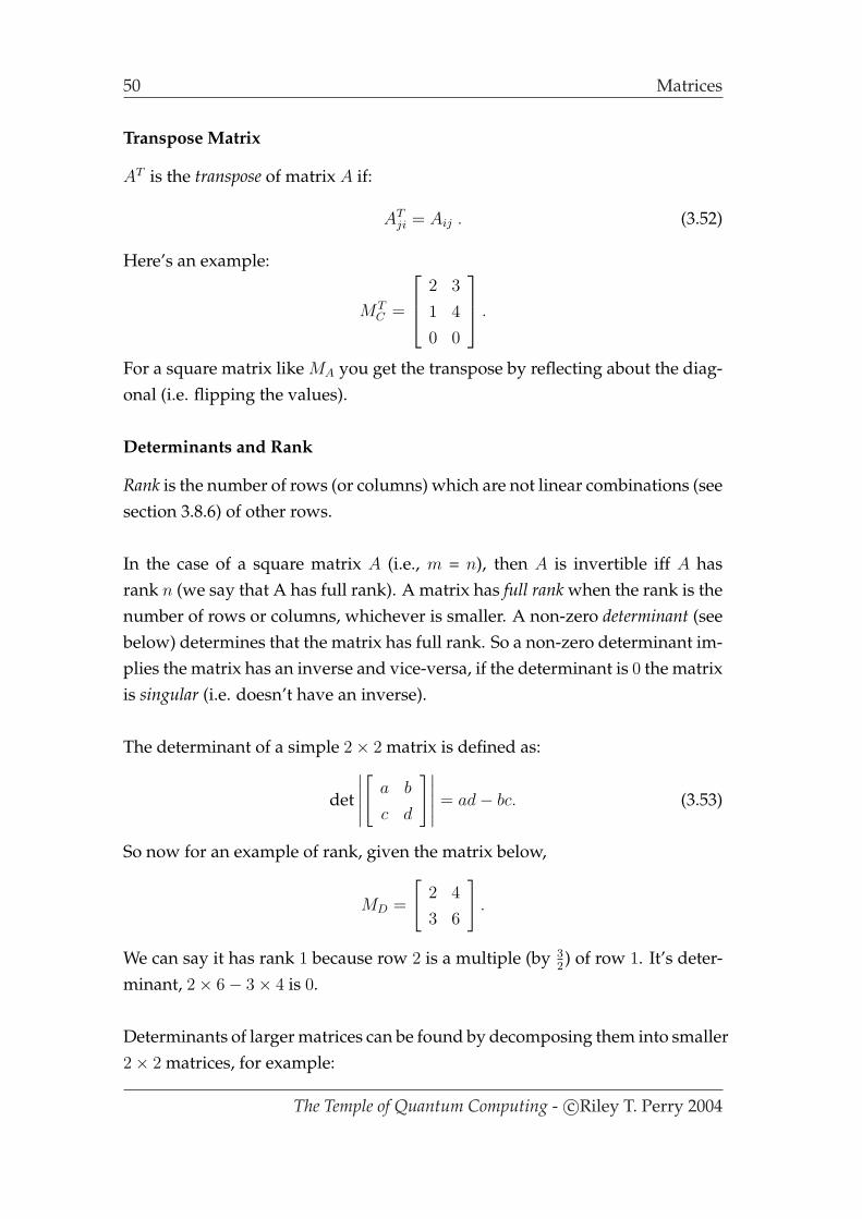
Transpose Matrix
AT is the transpose of matrix A if:
ATji = Aij . (3.52)
Here’s an example:
MTC =
2 3
1 4
0 0
.
For a square matrix like MA you get the transpose by reflecting about the diag-onal (i.e. flipping the values).
Determinants and Rank
Rank is the number of rows (or columns) which are not linear combinations (seesection 3.8.6) of other rows.
In the case of a square matrix A (i.e., m = n), then A is invertible iff A hasrank n (we say that A has full rank). A matrix has full rank when the rank is thenumber of rows or columns, whichever is smaller. A non-zero determinant (seebelow) determines that the matrix has full rank. So a non-zero determinant im-plies the matrix has an inverse and vice-versa, if the determinant is 0 the matrixis singular (i.e. doesn’t have an inverse).
The determinant of a simple 2× 2 matrix is defined as:
det
∣∣∣∣∣
[a b
c d
]∣∣∣∣∣ = ad− bc. (3.53)
So now for an example of rank, given the matrix below,
MD =
[2 4
3 6
].
We can say it has rank 1 because row 2 is a multiple (by 32) of row 1. It’s deter-
minant, 2× 6− 3× 4 is 0.
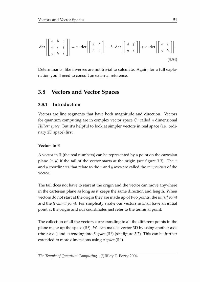
Determinants of larger matrices can be found by decomposing them into smaller2× 2 matrices, for example:
The Temple of Quantum Computing - c©Riley T. Perry 2004
Vectors and Vector Spaces 51
det
∣∣∣∣∣∣∣
a b c
d e f
g h i
∣∣∣∣∣∣∣= a · det
∣∣∣∣∣
[e f
h i
]∣∣∣∣∣− b · det
∣∣∣∣∣
[d f
g i
]∣∣∣∣∣ + c · det
∣∣∣∣∣
[d e
g h
]∣∣∣∣∣ .
(3.54)
Determinants, like inverses are not trivial to calculate. Again, for a full expla-nation you’ll need to consult an external reference.
3.8 Vectors and Vector Spaces
3.8.1 Introduction
Vectors are line segments that have both magnitude and direction. Vectorsfor quantum computing are in complex vector space Cn called n dimensionalHilbert space. But it’s helpful to look at simpler vectors in real space (i.e. ordi-nary 2D space) first.
Vectors in R
A vector in R (the real numbers) can be represented by a point on the cartesianplane (x, y) if the tail of the vector starts at the origin (see figure 3.3). The x
and y coordinates that relate to the x and y axes are called the components of thevector.
The tail does not have to start at the origin and the vector can move anywherein the cartesian plane as long as it keeps the same direction and length. Whenvectors do not start at the origin they are made up of two points, the initial pointand the terminal point. For simplicity’s sake our vectors in R all have an initialpoint at the origin and our coordinates just refer to the terminal point.
The collection of all the vectors corresponding to all the different points in theplane make up the space (R2). We can make a vector 3D by using another axis(the z axis) and extending into 3 space (R3) (see figure 3.7). This can be furtherextended to more dimensions using n space (Rn).
The Temple of Quantum Computing - c©Riley T. Perry 2004

52 Vectors and Vector Spaces
-
6
?
¾ ¡¡
¡¡
¡µ
@@R
XXXXXXy
(3, 3)
(−1,−1)
(−3, 1)
Figure 3.3: Vectors in R2 (i.e. ordinary 2D space like a table top).
-
6
¢¢
¢¢
¢¢¢®
¡¡
¡¡µ
¢¢
¢¢
@@
@@
@@
@@
x
y
z
ux
uy
uz
u = (ux, uy, uz)
Figure 3.4: A 3D vector with components ux, uy, uz.
The Temple of Quantum Computing - c©Riley T. Perry 2004
Vectors and Vector Spaces 53
-
6
?
¾
@@
@@
@R
@@
@@
@R
@@
@@
@R
¡µ
@@
@I
a b
c
d
e
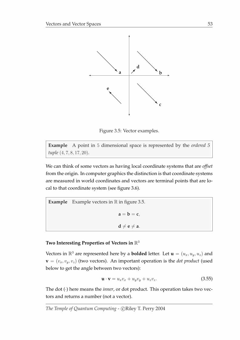
Figure 3.5: Vector examples.
Example A point in 5 dimensional space is represented by the ordered 5tuple (4, 7, 8, 17, 20).
We can think of some vectors as having local coordinate systems that are offsetfrom the origin. In computer graphics the distinction is that coordinate systemsare measured in world coordinates and vectors are terminal points that are lo-cal to that coordinate system (see figure 3.6).
Example Example vectors in R in figure 3.5.
a = b = c,
d 6= e 6= a.
Two Interesting Properties of Vectors in R3
Vectors in R3 are represented here by a bolded letter. Let u = (ux, uy, uz) andv = (vx, vy, vz) (two vectors). An important operation is the dot product (usedbelow to get the angle between two vectors):
u · v = uxvx + uyvy + uzvz. (3.55)
The dot (·) here means the inner, or dot product. This operation takes two vec-tors and returns a number (not a vector).
The Temple of Quantum Computing - c©Riley T. Perry 2004

54 Vectors and Vector Spaces
Knowing the components we can calculate the magnitude (the length of the vec-tor) using Pythagoras’ theorem as follows:
‖u‖ =√
uxux + uyuy + uzuz. (3.56)
Example if u = (1, 1, 1) then ‖u‖ =√
3.Example if u = (1, 1, 1) and v = (2, 1, 3) then:
cos θ =2 + 1 + 3√
3√
14
=
√6
7.
Vectors in C
V = Cn is a complex vector space with dimension n, this is the set containing allcolumn vectors with n complex numbers laid out vertically (the above exam-ples were row vectors with components laid out horizontally). We also define avector subspace as a non empty set of vectors which satisfy the same conditionsas the parent’s vector space.
3.8.2 Column Notation
In C2 for example, the quantum mechanical notation for a ket can be used torepresent a vector.
|u〉 =
[u1
u2
](3.57)
where u1 = a1 + b1i and u2 = a2 + b2i.
The Temple of Quantum Computing - c©Riley T. Perry 2004

Vectors and Vector Spaces 55
Example Column Notation.
|0〉 =
[1
0
]and, |1〉 =
[0
1
].
Example Here’s a more complex example:
|u〉 = (1 + i)|0〉+ (2− 3i)|1〉
=
[1 + i
2− 3i
].
3.8.3 The Zero Vector
The 0 vector is the vector where all entries are 0.
3.8.4 Properties of Vectors in Cn
Given scalars (α, β) ∈ C and vectors (|u〉, |v〉, |w〉) ∈ Cn.
Scalar Multiplication and Addition
Listed here are some basic properties of complex scalar multiplication and ad-dition.
α|u〉 =
αu1
...αun
. (3.58)
α(β|u〉) = αβ|u〉. (3.59)
α(|u〉+ |v〉) = α|u〉+ α|v〉. Associative law for scalar multiplication (3.60)
(α + β)|u〉 = α|u〉+ β|u〉. Distributive law for scalar addition (3.61)
α(|u〉+ |v〉) = α|u〉+ α|v〉. (3.62)
Vector Addition
A sum of vectors can be represented by:
|u〉+ |v〉 =
u1 + v1
...un + vn
. (3.63)
The Temple of Quantum Computing - c©Riley T. Perry 2004
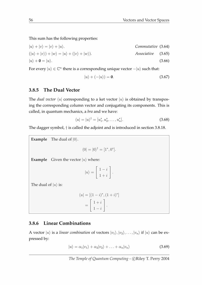
56 Vectors and Vector Spaces
This sum has the following properties:
|u〉+ |v〉 = |v〉+ |u〉. Commutative (3.64)
(|u〉+ |v〉) + |w〉 = |u〉+ (|v〉+ |w〉). Associative (3.65)
|u〉+ 0 = |u〉. (3.66)
For every |u〉 ∈ Cn there is a corresponding unique vector −|u〉 such that:
|u〉+ (−|u〉) = 0. (3.67)
3.8.5 The Dual Vector
The dual vector 〈u| corresponding to a ket vector |u〉 is obtained by transpos-ing the corresponding column vector and conjugating its components. This iscalled, in quantum mechanics, a bra and we have:
〈u| = |u〉† = [u∗1, u∗2, . . . , u
∗n]. (3.68)
The dagger symbol, † is called the adjoint and is introduced in section 3.8.18.
Example The dual of |0〉.
〈0| = |0〉† = [1∗, 0∗].
Example Given the vector |u〉 where:
|u〉 =
[1− i
1 + i
].
The dual of |u〉 is:
〈u| = [(1− i)∗, (1 + i)∗]
=
[1 + i
1− i
].
3.8.6 Linear Combinations
A vector |u〉 is a linear combination of vectors |v1〉, |v2〉, . . . , |vn〉 if |u〉 can be ex-pressed by:
|u〉 = α1|v1〉+ α2|v2〉+ . . . + αn|vn〉 (3.69)
The Temple of Quantum Computing - c©Riley T. Perry 2004

Vectors and Vector Spaces 57
where scalars α1, α2, . . . , αn are complex numbers.
We can represent a linear combination as:
|u〉 =n∑
i=1
αi|vi〉. (3.70)
3.8.7 Linear Independence
A set of non-zero vectors |υ1〉, ..., |υn〉 is linearly independent if:
n∑i=1
ai|υi〉 = 0 iff a1 = ... = an = 0. (3.71)
Example Linear dependence. The row vectors (bras) [1,−1], [1, 2], and [2, 2]
are linearly dependent because:
[1,−1] + [1, 2]− [2, 1] = [0, 0]
i.e there is a linear combination with a1 = 1, a2 = 1, a3 = −1 (other than thezero condition above) that evaluates to 0; So they are not linearly indepen-dent.
3.8.8 Spanning Set
A spanning set is a set of vectors |υ1〉, ..., |υn〉 for V in terms of which every vec-tor in V can be written as a linear combination.
Example Vectors u = [1, 0, 0], v = [0, 1, 0], and w = [0, 0, 1] span R3 becauseall vectors [x, y, z] in R3 can be written as a linear combination of u, v, and wlike the following:
[x, y, z] = xu + yv + zw.
3.8.9 Basis
A basis is any set of vectors that are a spanning set and are linearly independent.
Most of the time with quantum computing we’ll use a standard basis, calledthe computational basis. This is also called an orthonormal basis (see section
The Temple of Quantum Computing - c©Riley T. Perry 2004
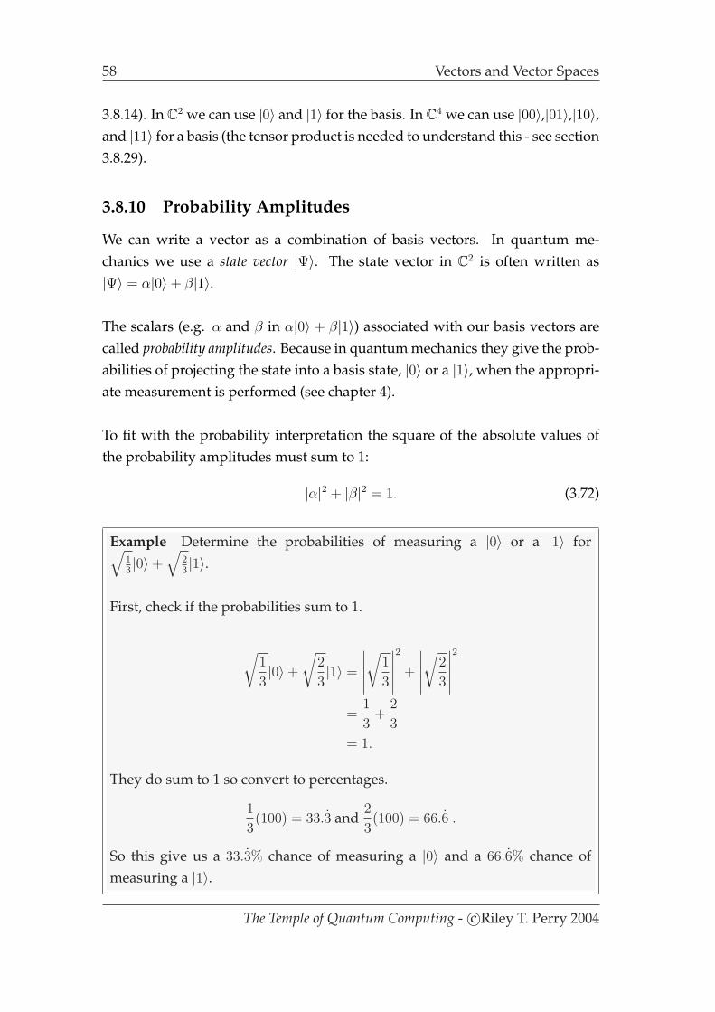
58 Vectors and Vector Spaces
3.8.14). In C2 we can use |0〉 and |1〉 for the basis. In C4 we can use |00〉,|01〉,|10〉,and |11〉 for a basis (the tensor product is needed to understand this - see section3.8.29).
3.8.10 Probability Amplitudes
We can write a vector as a combination of basis vectors. In quantum me-chanics we use a state vector |Ψ〉. The state vector in C2 is often written as|Ψ〉 = α|0〉+ β|1〉.
The scalars (e.g. α and β in α|0〉 + β|1〉) associated with our basis vectors arecalled probability amplitudes. Because in quantum mechanics they give the prob-abilities of projecting the state into a basis state, |0〉 or a |1〉, when the appropri-ate measurement is performed (see chapter 4).
To fit with the probability interpretation the square of the absolute values ofthe probability amplitudes must sum to 1:
|α|2 + |β|2 = 1. (3.72)
Example Determine the probabilities of measuring a |0〉 or a |1〉 for√13|0〉+
√23|1〉.
First, check if the probabilities sum to 1.
√1
3|0〉+
√2
3|1〉 =
∣∣∣∣∣
√1
3
∣∣∣∣∣
2
+
∣∣∣∣∣
√2
3
∣∣∣∣∣
2
=1
3+
2
3
= 1.
They do sum to 1 so convert to percentages.
1
3(100) = 33.3 and
2
3(100) = 66.6 .
So this give us a 33.3% chance of measuring a |0〉 and a 66.6% chance ofmeasuring a |1〉.
The Temple of Quantum Computing - c©Riley T. Perry 2004
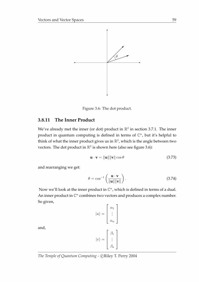
Vectors and Vector Spaces 59
-
6
?
¾ ³³³³³³³1
¡¡
¡¡
¡µ
θ
Figure 3.6: The dot product.
3.8.11 The Inner Product
We’ve already met the inner (or dot) product in R2 in section 3.7.1. The innerproduct in quantum computing is defined in terms of Cn, but it’s helpful tothink of what the inner product gives us in R2, which is the angle between twovectors. The dot product in R2 is shown here (also see figure 3.6):
u · v = ‖u‖‖v‖ cos θ (3.73)
and rearranging we get:
θ = cos−1
(u · v‖u‖‖v‖
). (3.74)
Now we’ll look at the inner product in Cn, which is defined in terms of a dual.An inner product inCn combines two vectors and produces a complex number.So given,
|u〉 =
α1
...αn
and,
|v〉 =
β1
...βn
The Temple of Quantum Computing - c©Riley T. Perry 2004

60 Vectors and Vector Spaces
we can calculate the inner product:
[α∗1, ..., α∗n]
β1
...βn
= 〈u| × |v〉 (3.75)
= 〈u|v〉. (3.76)
An inner product can also be represented in the following format:
(|u〉, |v〉) = 〈u|v〉. (3.77)
So for C2 the following are equivalent:([
u1
u2
],
[v1
v2
])= (|u〉, |v〉) = 〈u|× |v〉 = 〈u|v〉 = [u∗1, u
∗2]
[v1
v2
]= u∗1v1 +u∗2v2.
Example Using the inner product notation from above we can extract aprobability amplitude if we use one of the basis vectors as the original vec-tor’s dual:
〈0|(α|0〉+ β|1〉) = [1∗, 0∗]
[α
β
]= α
or using dot product notation,
〈0|(α|0〉+ β|1〉) =
[1
0
]•
[α
β
]= α.
This is called bra-ket notation. Hilbert space is the vector space for complexinner products.
Properties:
〈u|v〉 = 〈v|u〉∗. (3.78)
〈u|αv〉 = 〈α∗u|v〉 = α〈u|v〉. (3.79)
〈u|v + w〉 = 〈u|v〉 = 〈u|w〉. (3.80)
∀ |u〉 ∈ R and 〈u|u〉 ≥ 0. (3.81)
If 〈u|u〉 = 0 then |u〉 = 0. (3.82)
|〈u|v〉|2 ≤ 〈u|u〉〈v|v〉. The Cauchy-Schwartz inequality (3.83)
The Temple of Quantum Computing - c©Riley T. Perry 2004
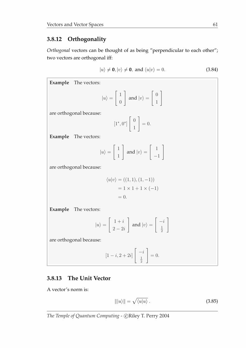
Vectors and Vector Spaces 61
3.8.12 Orthogonality
Orthogonal vectors can be thought of as being ”perpendicular to each other”;two vectors are orthogonal iff:
|u〉 6= 0, |v〉 6= 0, and 〈u|v〉 = 0. (3.84)
Example The vectors:
|u〉 =
[1
0
]and |v〉 =
[0
1
]
are orthogonal because:
[1∗, 0∗]
[0
1
]= 0.
Example The vectors:
|u〉 =
[1
1
]and |v〉 =
[1
−1
]
are orthogonal because:
〈u|v〉 = ((1, 1), (1,−1))
= 1× 1 + 1× (−1)
= 0.
Example The vectors:
|u〉 =
[1 + i
2− 2i
]and |v〉 =
[−i12
]
are orthogonal because:
[1− i, 2 + 2i]
[−i12
]= 0.
3.8.13 The Unit Vector
A vector’s norm is:
‖|u〉‖ =√〈u|u〉 . (3.85)
The Temple of Quantum Computing - c©Riley T. Perry 2004

62 Vectors and Vector Spaces
A unit vector is a vector where its norm is equal to 1.
‖|u〉‖ = 1. (3.86)
If we want to make an arbitrary vector a unit vector, which here is representedby theˆ(hat) symbol. We must normalise it by dividing by the norm:
|u〉 =|u〉‖|u〉‖ . (3.87)
Example Normalise |u〉 =
[1
1
](= |0〉+ |1〉).
First we find the norm:
‖|u〉‖ =
√√√√[1∗, 1∗]
[1
1
]
=√
2 .
Now we normalise ‖|u〉‖ to get:
|u〉 =
[1
1
]
√2
=1√2
[1
1
]
=
[1√2
1√2
]
=1√2|0〉+
1√2|1〉.
3.8.14 Bases for Cn
Cn has a standard basis (see 3.7.9) which is:
1
0
. . .
0
,
0
1
. . .
0
, . . . ,
0
0
. . .
1
. (3.88)
The Temple of Quantum Computing - c©Riley T. Perry 2004

Vectors and Vector Spaces 63
-
6
¢¢
¢¢
¢¢¢®
-
6
¢¢®
x
y
z
Figure 3.7: A local coordinate system.
This is written as |0〉, |1〉, . . . , |n − 1〉. Any other vector in the same space canbe expanded in terms of |0〉, |1〉, ..., |n − 1〉. The basis is called orthonormal be-cause the vectors are of unit length and mutually orthogonal. There are otherorthonormal bases in Cn and, in quantum computing, it is sometimes conve-nient to switch between bases.
Example Orthonormal bases |0〉, |1〉 and 1√2(|0〉+ |1〉), 1√
2(|0〉−|1〉) are often
used for quantum computing.
It’s useful at this point to consider what an orthonormal basis is in R3. The”ortho” part of orthonormal stands for orthogonal, which means the vectorsare perpendicular to each other, for example the 3D axes (x, y, z) are orthog-onal. The ”normal” part refers to normalised (unit) vectors. We can use anorthonormal basis in R3 to separate world coordinates from a local coordinatesystem in 3D computer graphics. In this system we define the position of thelocal coordinate system in world coordinates and then we can define the po-sitions of individual objects in terms of the local coordinate system. In thisway we can transform the local coordinates system, together with everythingin it while leaving the world coordinates system intact. In figure 3.7 the localcoordinate system forms an orthonormal basis.
The Temple of Quantum Computing - c©Riley T. Perry 2004
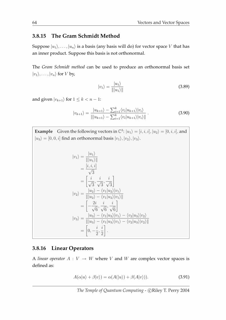
64 Vectors and Vector Spaces
3.8.15 The Gram Schmidt Method
Suppose |u1〉, . . . , |un〉 is a basis (any basis will do) for vector space V that hasan inner product. Suppose this basis is not orthonormal.
The Gram Schmidt method can be used to produce an orthonormal basis set|v1〉, . . . , |vn〉 for V by,
|v1〉 =|u1〉‖|u1〉‖ (3.89)
and given |vk+1〉 for 1 ≤ k < n− 1:
|vk+1〉 =|uk+1〉 −
∑ki=1〈vi|uk+1〉|vi〉
‖|uk+1〉 −∑k
i=1〈vi|uk+1〉|vi〉‖. (3.90)
Example Given the following vectors inC3: |u1〉 = [i, i, i], |u2〉 = [0, i, i], and|u3〉 = [0, 0, i] find an orthonormal basis |v1〉, |v2〉, |v3〉.
|v1〉 =|u1〉‖|u1〉‖
=[i, i, i]√
3
=
[i√3,
i√3,
i√3
]
|v2〉 =|u2〉 − 〈v1|u2〉|v1〉‖|u2〉 − 〈v1|u2〉|v1〉‖
=
[− 2i√
6,
i√6,
i√6
]
|v3〉 =|u3〉 − 〈v1|u3〉|v1〉 − 〈v2|u3〉|v2〉‖|u3〉 − 〈v1|u3〉|v1〉 − 〈v2|u3〉|v2〉‖
=
[0,− i
2,i
2
].
3.8.16 Linear Operators
A linear operator A : V → W where V and W are complex vector spaces isdefined as:
A(α|u〉+ β|v〉) = α(A(|u〉) + β(A|v〉)). (3.91)
The Temple of Quantum Computing - c©Riley T. Perry 2004
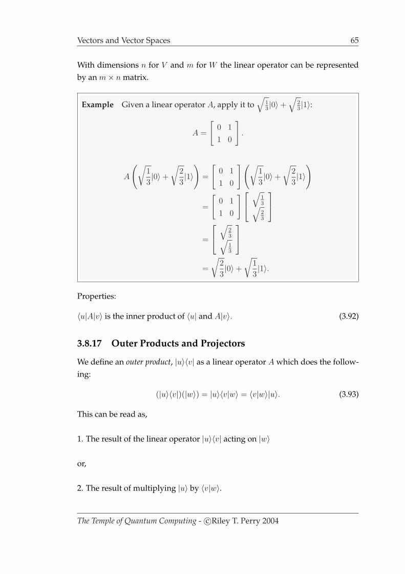
Vectors and Vector Spaces 65
With dimensions n for V and m for W the linear operator can be representedby an m× n matrix.
Example Given a linear operator A, apply it to√
13|0〉+
√23|1〉:
A =
[0 1
1 0
].
A
(√1
3|0〉+
√2
3|1〉
)=
[0 1
1 0
](√1
3|0〉+
√2
3|1〉
)
=
[0 1
1 0
]
√13√23
=
√23√13
=
√2
3|0〉+
√1
3|1〉.
Properties:
〈u|A|v〉 is the inner product of 〈u| and A|v〉. (3.92)
3.8.17 Outer Products and Projectors
We define an outer product, |u〉〈v| as a linear operator A which does the follow-ing:
(|u〉〈v|)(|w〉) = |u〉〈v|w〉 = 〈v|w〉|u〉. (3.93)
This can be read as,
1. The result of the linear operator |u〉〈v| acting on |w〉
or,
2. The result of multiplying |u〉 by 〈v|w〉.
The Temple of Quantum Computing - c©Riley T. Perry 2004
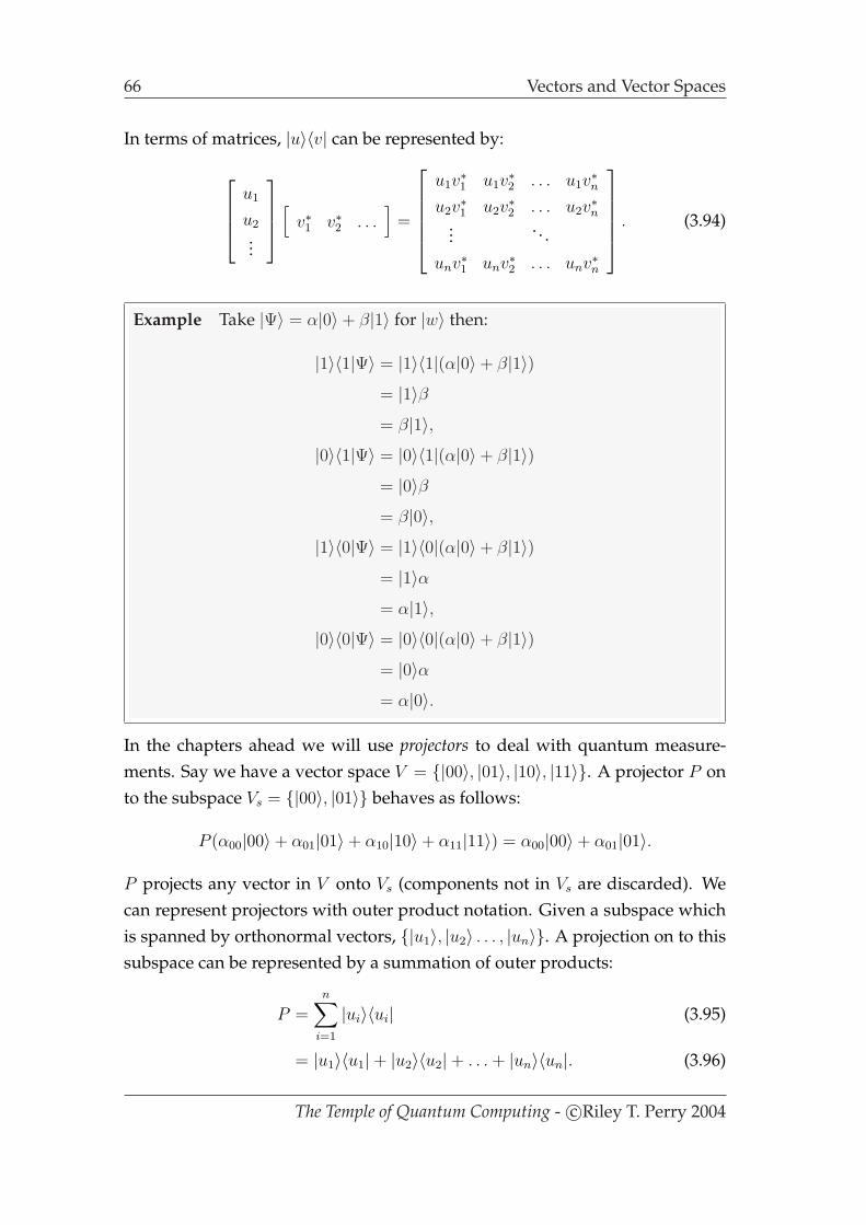
66 Vectors and Vector Spaces
In terms of matrices, |u〉〈v| can be represented by:
u1
u2
...
[v∗1 v∗2 . . .
]=
u1v∗1 u1v
∗2 . . . u1v
∗n
u2v∗1 u2v
∗2 . . . u2v
∗n
... . . .
unv∗1 unv∗2 . . . unv∗n
. (3.94)
Example Take |Ψ〉 = α|0〉+ β|1〉 for |w〉 then:
|1〉〈1|Ψ〉 = |1〉〈1|(α|0〉+ β|1〉)= |1〉β= β|1〉,
|0〉〈1|Ψ〉 = |0〉〈1|(α|0〉+ β|1〉)= |0〉β= β|0〉,
|1〉〈0|Ψ〉 = |1〉〈0|(α|0〉+ β|1〉)= |1〉α= α|1〉,
|0〉〈0|Ψ〉 = |0〉〈0|(α|0〉+ β|1〉)= |0〉α= α|0〉.
In the chapters ahead we will use projectors to deal with quantum measure-ments. Say we have a vector space V = |00〉, |01〉, |10〉, |11〉. A projector P onto the subspace Vs = |00〉, |01〉 behaves as follows:
P (α00|00〉+ α01|01〉+ α10|10〉+ α11|11〉) = α00|00〉+ α01|01〉.
P projects any vector in V onto Vs (components not in Vs are discarded). Wecan represent projectors with outer product notation. Given a subspace whichis spanned by orthonormal vectors, |u1〉, |u2〉 . . . , |un〉. A projection on to thissubspace can be represented by a summation of outer products:
P =n∑
i=1
|ui〉〈ui| (3.95)
= |u1〉〈u1|+ |u2〉〈u2|+ . . . + |un〉〈un|. (3.96)
The Temple of Quantum Computing - c©Riley T. Perry 2004

Vectors and Vector Spaces 67
So, we can replace the projector notation P with the explicit outer product no-tation:
(|00〉〈00|+ |01〉〈01|)(α00|00〉+ α01|01〉+ α10|10〉+ α11|11〉) = α00|00〉+ α01|01〉.We can also represent a matrix (an operator for example) using outer productnotation, as shown in the next example.
Example Representing operators X and Z. These two matrices are definedbelow, but it turns out they are quite handy for quantum computing. We’llbe using them frequently in the chapters ahead:
|0〉〈1| =[
1
0
] [0∗ 1∗
]
=
[0 1
0 0
],
|1〉〈1| =[
0
1
] [0∗ 1∗
]
=
[0 0
0 1
],
|0〉〈0| =[
0
1
] [0∗ 1∗
]
=
[1 0
0 0
],
|1〉〈0| =[
0
1
] [1∗ 0∗
]
=
[0 0
1 0
].
X =
[0 1
1 0
]
= |0〉〈1|+ |1〉〈0|,
Z =
[1 0
0 −1
]
= |0〉〈0| − |1〉〈1|.
The Temple of Quantum Computing - c©Riley T. Perry 2004
68 Vectors and Vector Spaces
Properties:∑
i
|i〉〈i| = I for any orthonormal basis |i〉. The completeness relation
(3.97)
Given a subspace Vs = |1〉 , . . . , |k〉then V = |1〉 , . . . , |k〉 |k + 1〉 , . . . , |d〉 . (3.98)
Each component |u〉 〈u| of P is hermitian
and P itself is hermitian (see 3.8.23). (3.99)
P † = P. (3.100)
P 2 = P. (3.101)
Q = I − P is called the orthogonal complement
and is a projector onto |k + 1〉 , . . . , |d〉 in 3.98. (3.102)
Notice how we have slightly changed the notation here for∑
. By saying∑i |i〉〈i| we actually mean ”for each element n in the set |i〉 then add |n〉〈n|
to the total”.
Later we’ll look at quantum measurements, and we’ll use Mm to representa measurement. If we use a projector (i.e. Mm = P ) for measurement then theprobability of measuring m is:
pr(m) = 〈Ψ|M †mMm |Ψ〉 .
By 3.100 and 3.101 we can say that this is equivalent to:
pr(m) = 〈Ψ|Mm |Ψ〉 .
3.8.18 The Adjoint
The adjoint A† is the matrix obtained from A by conjugating all the elements ofA (to get A∗) and then forming the transpose:
A† = (A∗)T . (3.103)
Example An adjoint.
[1 + i 1− i
−1 1
]†=
[1− i −1
1 + i 1
].
The Temple of Quantum Computing - c©Riley T. Perry 2004
Vectors and Vector Spaces 69
Properties:
A|u〉 = 〈u|A†. (3.104)
〈u|Av〉 = 〈A†u|v〉. (3.105)
(AB)† = B†A†. (3.106)
(A†)† = A. (3.107)
(|u〉)† = 〈u|. (3.108)
(A|u〉)† = 〈u|A† but not A|u〉 = 〈u|A†. (3.109)
(αA + βB)† = α∗A† + β∗B†. (3.110)
Example Example of 〈u|Av〉 = 〈A†u|v〉. Given,
|u〉 =
[1
i
], |v〉 =
[1
1
]and A =
[1 + i 1− i
−1 1
].
A|v〉 =
[1 + i 1− i
−1 1
][1
1
]
=
[2
0
],
〈u|Av〉 = 2,
A†|u〉 =
[1 + i 1− i
−1 1
][1
i
]
=
[1− 2i
1 + 2i
],
〈A†u|v〉 =[
1 + 2i 1− 2i] [
1
1
]
= 2.
The Temple of Quantum Computing - c©Riley T. Perry 2004

70 Vectors and Vector Spaces
3.8.19 Eigenvalues and Eigenvectors
The complex number λ is an eigenvalue of a linear operator A if there existsvector |u〉 such that:
A|u〉 = λ|u〉 (3.111)
where |u〉 is called an eigenvector of A.
Eigenvalues of A can be found by using the following equation, called the char-acteristic equation of A:
c(λ) = det(A− λI) = 0. (3.112)
This comes from noting that:
A|u〉 = λ|u〉 ⇔ (A− λI)|u〉 = 0 ⇔ A− λI is singular ⇔ det(A− λI) = 0.
Solving the characteristic equation gives us the characteristic polynomial of A.We can then solve the characteristic polynomial to find all the eigenvalues forA. If A is an n × n matrix, there will be n eigenvalues (but some may be thesame as others).
Properties:
A’s ith eigenvalue λi has eigenvector |ui〉 iff A|ui〉 = λi|ui〉. (3.113)
An eigenspace for λi is the set of eigenvectors that satisfies
A|uj〉 = λi|uj〉, here j is the index for eigenvectors of λi. (3.114)
An eigenspace is degenerate when it has dimension > 1
i.e. more than one eigenvector. (3.115)
Note: The eigenvectors that match different eigenvalues are linearly indepen-dent, which means we can have an orthonormal set of eigenvectors for an op-erator A.
An example is on the next page.
The Temple of Quantum Computing - c©Riley T. Perry 2004

Vectors and Vector Spaces 71
Example Eigenvalues and eigenvectors of X .
X =
[0 1
1 0
].
det(X − λI) =
[−λ 1
1 −λ
]
= λ2 − 1.
This is the characteristic polynomial. The two solutions to λ2 − 1 = 0 areλ = −1 and λ = +1. If we use the eigenvalue of λ = −1 to determine thecorresponding eigenvector |λ−1〉 of X we get:
X|λ−1〉 = −1|λ−1〉[0 1
1 0
][α
β
]=
[−α
−β
]
[α
β
]=
[−α
−β
].
We get α = −β, so after normalisation our eigenvector is:
|λ−1〉 =1√2|0〉 − 1√
2|1〉.
Notice that we’ve used the eigenvalue λ = −1 to label the eigenvector |λ−1〉.
3.8.20 Trace
The trace of A is the sum of its eigenvalues, or:
tr(A) =n∑
i=1
aii (3.116)
i.e. the sum of its diagonal entries.
The Temple of Quantum Computing - c©Riley T. Perry 2004
72 Vectors and Vector Spaces
Example Trace of X and I
X =
[0 1
1 0
].
I =
[1 0
0 1
].
tr(X) = 0 + 0 = 0 or the sum of the eigenvalues 1 + (−1) = 0. For I we havetr(I) = 2.
Properties:
tr(A + B) = tr(A) + tr(B). (3.117)
tr(αA + B) = αtr(A) + αtr(B). (3.118)
tr(AB) = tr(BA). (3.119)
tr(|u〉〈v|) = 〈u|v〉. (3.120)
tr(αA) = αtr(A). (3.121)
tr(UAU †) = tr(A). Similarity transform for U (3.122)
tr(U †AU) = tr(A). (3.123)
tr(A|u〉〈u|) = 〈u|A|u〉 if |u〉 is unitary. (3.124)
For unit norm |u〉:
tr(|u〉〈u|) = tr(|u〉〈u||u〉〈u|) (3.125)
= 〈u||u〉〈u||u〉 (3.126)
= 〈u|u〉〈u|u〉 (3.127)
= ||u〉|4 (3.128)
= 1. (3.129)
As stated, the trace of A is the sum of its eigenvalues. We can also say that:
U †AU =
λ1
. . .
λn
.
which also has a trace which is the sum the eigenvalues of A as tr(U †AU) =
tr(A) (see section 3.8.24 below).
The Temple of Quantum Computing - c©Riley T. Perry 2004
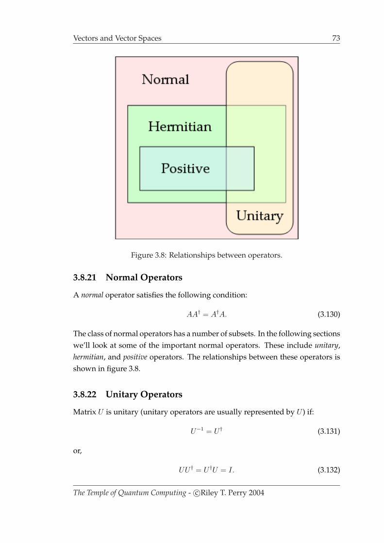
Vectors and Vector Spaces 73
Figure 3.8: Relationships between operators.
3.8.21 Normal Operators
A normal operator satisfies the following condition:
AA† = A†A. (3.130)
The class of normal operators has a number of subsets. In the following sectionswe’ll look at some of the important normal operators. These include unitary,hermitian, and positive operators. The relationships between these operators isshown in figure 3.8.
3.8.22 Unitary Operators
Matrix U is unitary (unitary operators are usually represented by U ) if:
U−1 = U † (3.131)
or,
UU † = U †U = I. (3.132)
The Temple of Quantum Computing - c©Riley T. Perry 2004

74 Vectors and Vector Spaces
Eigenvectors of unitary matrices have a modulus of 1:
‖U |u〉‖ = ‖|u〉‖ ∀ |u〉. (3.133)
Unitary operators have the property that they preserve norm, and are invert-ible. There are some particularly important operators called the Pauli operators.We’ve seen some of them already, they are referred to by the letters I, X, Y,
and Z. In some texts X,Y, and Z are referred to by another notation, whereσ1 = σX = X, σ2 = σY = Y, and σ3 = σZ = Z. The Pauli operators are definedas:
I =
[1 0
0 1
], (3.134)
X =
[0 1
1 0
], (3.135)
Y =
[0 −i
i 0
], (3.136)
Z =
[1 0
0 −1
]. (3.137)
Example I, X, Y, and Z are unitary because:
II† = I2 =
[1 0
0 1
][1 0
0 1
]=
[1 0
0 1
].
XX† = X2 =
[0 1
1 0
][0 1
1 0
]=
[1 0
0 1
].
Y Y † = Y 2 =
[0 −i
i 0
][0 −i
i 0
]=
[1 0
0 1
].
ZZ† = Z2 =
[1 0
0 −1
] [1 0
0 −1
]=
[1 0
0 1
].
Note: I = I†, X = X†, Y = Y †, and Z = Z†.
The Temple of Quantum Computing - c©Riley T. Perry 2004

Vectors and Vector Spaces 75
Properties (of unitary operators):
U =∑
j
|j〉〈j|. (3.138)
(U |u〉, U |v〉) = 〈u|U †U |v〉 = 〈u|v〉. (3.139)
Unitary matrices are also normal. (3.140)
Unitary matrices allow for spectral decomposition,
(see section 3.8.28). (3.141)
Unitary matrices allow for reversal, i.e. U †(U |u〉) = I|u〉 = |u〉. (3.142)
Unitary matrices preserve inner product
(U |u〉, U |v〉) = (|u〉, |v〉) = 〈u|v〉. (3.143)
Unitary matrices preserve norm ‖U |u〉‖ = ‖u〉‖. (3.144)
Given an orthonormal basis set |ui〉, U |ui〉 = viis also an orthonormal basis with U =
∑i
|vi〉〈ui|. (3.145)
Unitary matrices have eigenvalues of modulus 1. (3.146)
If(|u〉, A|u〉) > 0 ∀|u〉 in V (all positive eigenvalues). (3.147)
The Temple of Quantum Computing - c©Riley T. Perry 2004

76 Vectors and Vector Spaces
3.8.23 Hermitian and Positive Operators
A hermitian matrix A has the property:
A = A†. (3.148)
The eigenvalues of a hermitian matrix are real numbers and hermitian matricesare also normal (although not all normal matrices need real eigenvalues).
Example The matrix X is Hermitian because:
X =
[0 1
1 0
]=, X† =
[0 1
1 0
].
Properties:
A = B + iC can represent any operator if B and C are hermitian
with C = 0 if A itself is hermitian. (3.149)
If A is hermitian then for |u〉, 〈u|A|u〉 ∈ R. (3.150)
If A is hermitian then A is a positive operator iff for |u〉, 〈u|Au〉 ∈ Rand 〈u|Au〉 ≥ 0. (3.151)
If A is positive it has no negative eigenvalues. (3.152)
3.8.24 Diagonalisable Matrix
An operator A is diagonalisable if:
A =∑
i
λi|ui〉〈ui|. (3.153)
The vectors |ui〉 form an orthonormal set of eigenvectors for A, with eigenval-ues of λi. This is the same as saying that A can be transformed to:
λ1
. . .
λn
. (3.154)
The Temple of Quantum Computing - c©Riley T. Perry 2004
Vectors and Vector Spaces 77
Example Representing operator X :
X =
[0 1
1 0
].
The two normalised eigenvectors for X are:
1√2|0〉 − 1√
2|1〉 and
1√2|0〉+
1√2|1〉.
The two vectors are orthogonal (with eigenvalues −1 and +1),[
1√2〈0| − 1√
2〈1|
] [1√2|0〉+
1√2|1〉
]=
1
2[〈0|0〉 − 〈0|1〉+ 〈1|0〉 − 〈1|1〉]
=1
2[1− 0 + 0− 1]
= 0.
So X is diagonalisable and is given by:
X =1
2[|0〉+ |1〉][〈0|+ 〈1|]− 1
2[|0〉 − |1〉][〈0| − 〈1|].
Which expanded is:
1
2([〈0|0〉+ 〈0|1〉+ 〈1|0〉+ 〈1|1〉])− 1
2([〈0|0〉 − 〈0|1〉 − 〈1|0〉+ 〈1|1〉]).
3.8.25 The Commutator and Anti-Commutator
Here is a set of properties for the Commutator and Anti-Commutator which relateto commutative relationships between two operators A and B.
Commutator:
[A,B] = AB −BA, A and B commute (AB = BA) if [A,B] = 0. (3.155)
Anti-commutator:
A,B = AB + BA, we say A and B anti-commute if A,B = 0. (3.156)
The Temple of Quantum Computing - c©Riley T. Perry 2004

78 Vectors and Vector Spaces
Example We test X and Z against the commutator.
[X, Z] =
[0 1
1 0
][1 0
0 −1
]−
[1 0
0 −1
][0 1
1 0
]
=
[0 −2
2 0
]
6= 0.
So X and Z do not commute.
The simultaneous diagonalisation theorem says that if HA and HB are hermitian,[HA, HB] = 0 if ∃ a set of orthonormal eigenvectors for both HA, HB so:
HA =∑
i
λ′i|i〉〈i| and HB =
∑i
λ′′i |i〉〈i|. (3.157)
i.e. they are both diagonal in a common basis.
Properties:
AB =[A,B] + A,B
2. (3.158)
[A,B]† = [A†, B†]. (3.159)
[A,B] = −[B,A]. (3.160)
[HA, HB] is hermitian if HA, HB are hermitian. (3.161)
3.8.26 Polar Decomposition
Polar decomposition says that any linear operator A can be represented as A =
U√
A†A (called the left polar decomposition) =√
AA†U (called the right polardecomposition) where U is a unitary operator.
Single value decomposition says that if a linear operator A that is a square ma-trix (i.e. the same input and output dimension) then there exist unitaries UA
and UB, and D a diagonal matrix with non-negative elements in R such thatA = UADUB.
The Temple of Quantum Computing - c©Riley T. Perry 2004
Vectors and Vector Spaces 79
3.8.27 Spectral Decomposition
A linear operator is normal (A†A = AA†) iff it has orthogonal eigenvectors andthe normalised (orthonormal) versions ui of the eigenvectors can diagonalisethe operator:
A =∑
i
λi|ui〉〈ui|. (3.162)
Example Spectral decomposition of X and Z.
Z =
[1 0
0 −1
]
= |0〉〈0| − |1〉〈1|.
X =
[0 1
1 0
]
= |+〉〈+| − |−〉〈−|.
X has eigenvectors |+〉 = 1√2|0〉+ |1〉, and |−〉 = 1√
2|0〉 − |1〉 and eigenvalues
of +1, and −1 Then, if we expand, we get back X :
|+〉〈+| − |−〉〈−| = 1
2
[1
1
][11]− 1
2
[1
−1
][1− 1]
=1
2
[1 1
1 1
]− 1
2
[1 −1
−1 1
]
=
[0 1
1 0
].
Properties:
A = UDU † where U is a unitary and D is a diagonal operator. (3.163)
If A is normal then it has a spectral decomposition of∑
a
|a〉〈a|. (3.164)
3.8.28 Tensor Products
In a tensor product we have a combination of two smaller vector spaces to forma larger one. The elements of the smaller vector spaces are combined whilstpreserving scalar multiplication and linearity, formally:
The Temple of Quantum Computing - c©Riley T. Perry 2004

80 Vectors and Vector Spaces
If |u〉 and |v〉 are bases for V and W respectively then |u〉 ⊗ |v〉 form abasis for V ⊗W . We can write this in the following way:
|u〉 ⊗ |v〉 = |u〉|v〉 = |u, v〉 = |uv〉. (3.165)
Example A simple tensor product.
|1〉 ⊗ |0〉 = |1〉|0〉 = |1, 0〉 = |10〉.
The Kronecker product is defined as:
A⊗B =
[a b
c d
]⊗
[x y
v w
](3.166)
=
[a ·B b ·Bc ·B d ·B
](3.167)
=
ax ay bx by
av aw bv bw
cx cy dx dy
cv cw dv dw
. (3.168)
where A and B are linear operators.
Example A Kronecker product on Pauli matrices X . and Y
X =
[0 1
1 0
]and Y =
[0 −i
i 0
].
X ⊗ Y =
[0 · Y 1 · Y1 · Y 0 · Y
]
=
[0 1
1 0
][0 −i
i 0
]
=
0 0 0 −i
0 0 1 0
0 −i 0 0
i 0 0 0
.
The Temple of Quantum Computing - c©Riley T. Perry 2004
Fourier Transforms 81
Properties:
Tensor products are related to the inner product:
(|uv〉, |u′v′〉) = (|u〉, |u′〉)(|v〉, |v′〉) (3.169)
= 〈u|u′〉〈v|v′〉. (3.170)
|u〉⊗k = (|u〉 ⊗ . . .⊗ |u〉)k k times. (3.171)
(A⊗B)∗ = A∗ ⊗B∗. (3.172)
(A⊗B)T = AT ⊗BT . (3.173)
(A⊗B)† = A† ⊗B†. (3.174)
|ab〉† = 〈ab|. (3.175)
α(|u, v〉) = |αu, v〉 = |u, αv〉. (3.176)
|u1 + u2, v〉 = |u1, v〉+ |u2, v〉. (3.177)
|u, v1 + v2〉 = |u, v1〉+ |u, v2〉. (3.178)
|uv〉 6= |vu〉. (3.179)
For linear operators A and B, A⊗B(|uv〉) = A|u〉 ⊗ A|v〉. (3.180)
For normal operators NA and NB, NA ⊗NB will be normal. (3.181)
For hermitian operators HA and HB, HA ⊗HB will be hermitian. (3.182)
For unitary operators UA and UB, UA ⊗ UB will be unitary. (3.183)
For positive operators PA and PB, PA ⊗ PB will be positive. (3.184)
3.9 Fourier Transforms
The Fourier transform, which is named after Jean Baptiste Joseph Fourier, 1768- 1830 (figure 3.9), maps data from the time domain to the frequency domain. Thediscrete Fourier transform (DFT) is a version of the Fourier transform which, un-like the basic Fourier transform, does not involve calculus and can be directlyimplemented on computers but is limited to periodic functions. The Fouriertransform itself is not limited to periodic functions.
The Temple of Quantum Computing - c©Riley T. Perry 2004

82 Fourier Transforms
Figure 3.9: Jean Baptiste Joseph Fourier.
3.9.1 The Fourier Series
Representing a periodic function as a linear combination of sines and cosines iscalled a Fourier series expansion of the function. We can represent any periodic,continuous function as a linear combination of sines and cosines. In fact, like |0〉and |1〉 forms an orthonormal basis for quantum computing, sin and cos forman orthonormal basis for the time domain based representation of a waveform.One way to describe an orthonormal basis is:
That which you measure against.
The fourier series has the form:
f(t) =a0
2+
∞∑n=1
an sin(nt) +∞∑
n=1
bn cos(nt). (3.185)
So if we have a waveform we want to model we only need to find the coeffi-cients a0, a1, . . . , an and b0, b1, . . . , bn and the number of sines and cosines. Wewon’t go into the derivation of these coefficients (or how to find the number ofsines and cosines) here. The definition will be enough, as this is only meant tobe a brief introduction to the Fourier series. For example, suppose we’ve founda1 = 0.5, a4 = 2 and b2 = 4 and all the rest are 0; then the Fourier series is:
f(t) = 0.5 sin(πt) + 2 sin(4πt) + 4 cos(2πt)
which is represented by the following graph:
The Temple of Quantum Computing - c©Riley T. Perry 2004
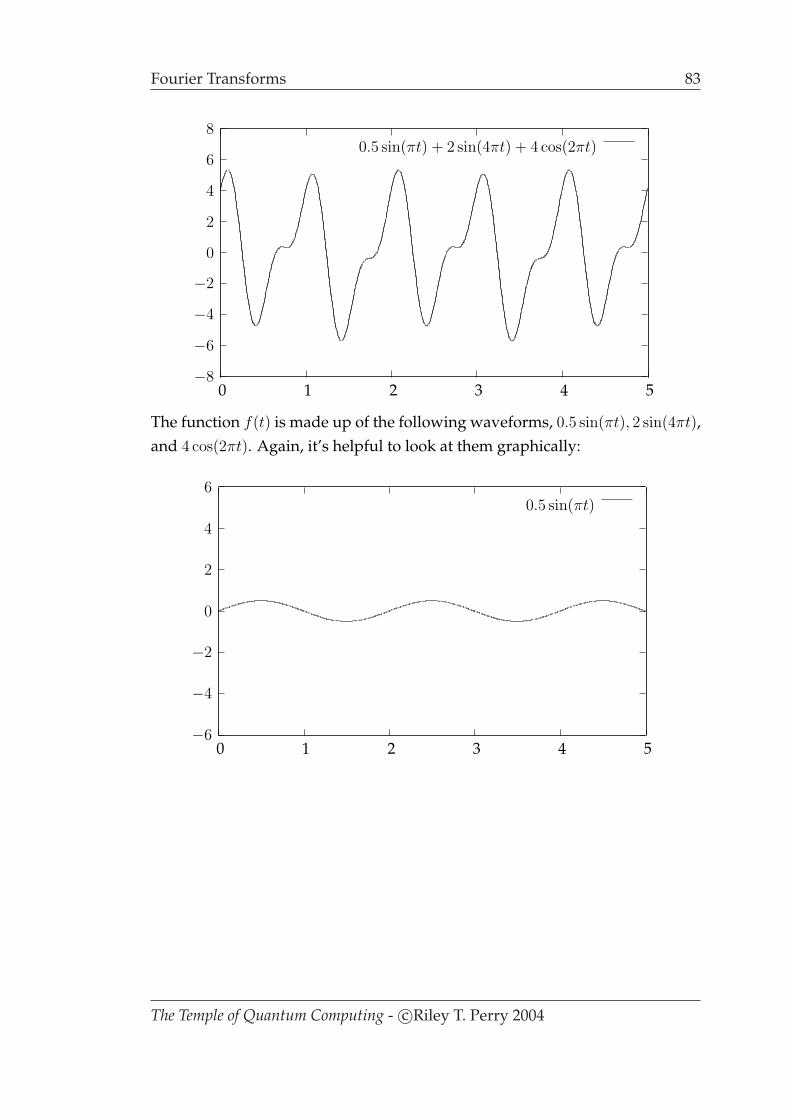
Fourier Transforms 83
−8
−6
−4
−2
0
2
4
6
8
0 1 2 3 4 5
0.5 sin(πt) + 2 sin(4πt) + 4 cos(2πt)
The function f(t) is made up of the following waveforms, 0.5 sin(πt), 2 sin(4πt),and 4 cos(2πt). Again, it’s helpful to look at them graphically:
−6
−4
−2
0
2
4
6
0 1 2 3 4 5
0.5 sin(πt)
The Temple of Quantum Computing - c©Riley T. Perry 2004
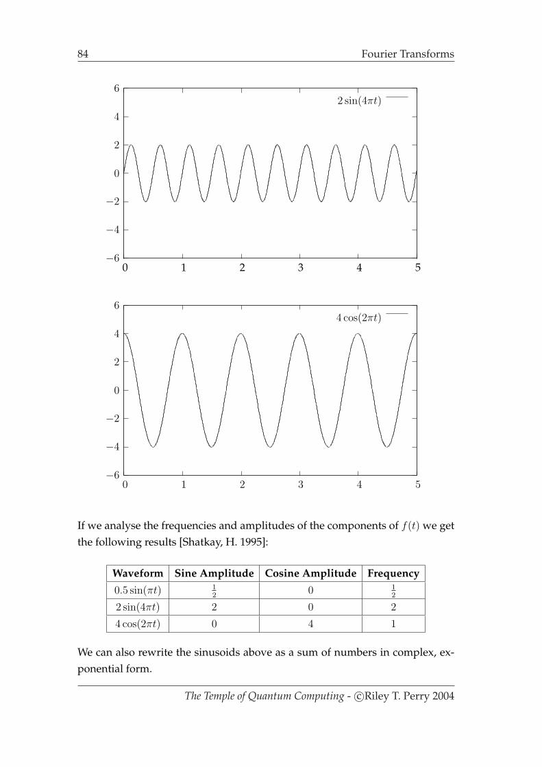
84 Fourier Transforms
−6
−4
−2
0
2
4
6
0 1 2 3 4 5
2 sin(4πt)
−6
−4
−2
0
2
4
6
0 1 2 3 4 5
4 cos(2πt)
If we analyse the frequencies and amplitudes of the components of f(t) we getthe following results [Shatkay, H. 1995]:
Waveform Sine Amplitude Cosine Amplitude Frequency0.5 sin(πt) 1
20 1
2
2 sin(4πt) 2 0 2
4 cos(2πt) 0 4 1
We can also rewrite the sinusoids above as a sum of numbers in complex, ex-ponential form.
The Temple of Quantum Computing - c©Riley T. Perry 2004

Fourier Transforms 85
3.9.2 The Discrete Fourier Transform
The DFT maps from a discrete, periodic sequence tk to a set of coefficients rep-resenting the frequencies of the discrete sequence. The DFT takes as input andoutputs an array of complex numbers. The number of elements in the array isgoverned by the sampling rate and the length of the waveform. Formally, TheN complex numbers t0, ..., tN−1 are transformed into the N complex numbersf0, ..., fN − 1 according to the formula:
fj =N−1∑
k=0
tke− 2πi
Njk j = 0, . . . , N − 1. (3.186)
The DFT is a linear operator with an invertible matrix representation, so we cantake the conversion back to its original form using:
tk =1
N
N−1∑j=0
fje2πiN
kj k = 0, . . . , N − 1. (3.187)
We have chosen to represent our periodic functions as a sequence of sines andcosines. To use the above formulas they need to be converted to complex, expo-nential form. Because the sequence we are after is discrete we need to samplevarious points along the sequence. The sample rate N determines the accuracyof our transformation. With the lower bound on the sampling rate being foundby applying Nyquist’s theorem (which is beyond the scope of this paper).
Let’s look at doing a DFT on f(t) = 0.5 sin(πt) + 2 sin(4πt) + 4 cos(2πt) andadjust the sampling rate until we get an acceptable waveform in the frequencydomain:
The graph below is just f(t) = 0.5 sin(πt)+2 sin(4πt)+4 cos(2πt) with samplingpoints at the whole numbers (1, 2, . . . , N) as you can see if we only sample atthis point we get no notion of a wave at all.
The Temple of Quantum Computing - c©Riley T. Perry 2004
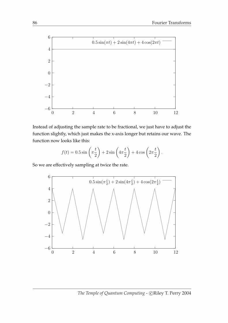
86 Fourier Transforms
−6
−4
−2
0
2
4
6
0 2 4 6 8 10 12
0.5 sin(πt) + 2 sin(4πt) + 4 cos(2πt)
Instead of adjusting the sample rate to be fractional, we just have to adjust thefunction slightly, which just makes the x-axis longer but retains our wave. Thefunction now looks like this:
f(t) = 0.5 sin
(π
t
2
)+ 2 sin
(4π
t
2
)+ 4 cos
(2π
t
2
).
So we are effectively sampling at twice the rate.
−6
−4
−2
0
2
4
6
0 2 4 6 8 10 12
0.5 sin(π t2) + 2 sin(4π t
2) + 4 cos(2π t
2)
The Temple of Quantum Computing - c©Riley T. Perry 2004
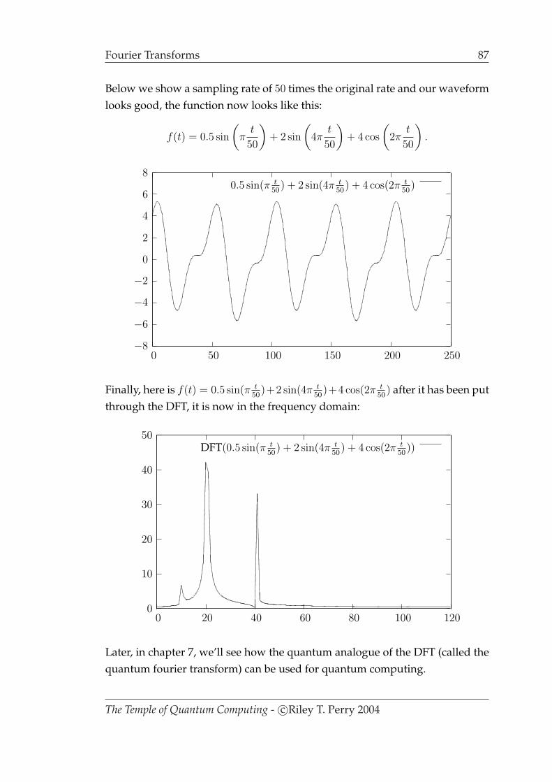
Fourier Transforms 87
Below we show a sampling rate of 50 times the original rate and our waveformlooks good, the function now looks like this:
f(t) = 0.5 sin
(π
t
50
)+ 2 sin
(4π
t
50
)+ 4 cos
(2π
t
50
).
−8
−6
−4
−2
0
2
4
6
8
0 50 100 150 200 250
0.5 sin(π t50
) + 2 sin(4π t50
) + 4 cos(2π t50
)
Finally, here is f(t) = 0.5 sin(π t50
)+2 sin(4π t50
)+4 cos(2π t50
) after it has been putthrough the DFT, it is now in the frequency domain:
0
10
20
30
40
50
0 20 40 60 80 100 120
DFT(0.5 sin(π t50
) + 2 sin(4π t50
) + 4 cos(2π t50
))
Later, in chapter 7, we’ll see how the quantum analogue of the DFT (called thequantum fourier transform) can be used for quantum computing.
The Temple of Quantum Computing - c©Riley T. Perry 2004


Chapter 4
Quantum Mechanics
Quantum mechanics is generally about the novel behaviour of very small things.At this scale matter becomes quantised, this means that it can be subdivided nomore. Quantum mechanics has never been wrong, it explains why the starsshine, how matter is structured, the periodic table, and countless other phe-nomena. One day scientists hope to use quantum mechanics to explain every-thing, but at present the theory remains incomplete as it has not been success-fully combined with classical theories of gravity.
Some strange effects happen at the quantum scale. The following effects areimportant for quantum computing:
• Superposition and interference
• Uncertainty
• Entanglement
This chapter is broken into two parts. In the first part we’ll look briefly at thehistory of quantum mechanics. Then, in the second part we will examine someimportant concepts (like the ones above) of quantum mechanics and how theyrelate to quantum computing.
The main references used for this chapter are, Introducing Quantum Theory byJ.P. McEvoy and Oscar Zarate, and Quantum Physics, Illusion or Reality by Alas-tair Rae. Both of these are very accessible introductory books.
89

90 History
Figure 4.1: James Clerk Maxwell and Isaac Newton.
Figure 4.2: Nicolaus Copernicus and Galileo Galilei.
4.1 History
4.1.1 Classical Physics
Classical physics roughly means pre-20th century physics, or pre-quantum physics.Two of the most important classical theories are electromagnetism, by JamesClerk Maxwell, 1831 - 1879 (figure 4.1) and Isaac Newton’s mechanics. IsaacNewton, 1642 - 1727 (figure 4.1) is arguably the most important scientist of alltime due to the large body of work he produced that is still relevant today. Priorto this, Nicolaus Copernicus, 1473 - 1543 and Galileo Galilei, 1564 - 1642 (fig-ure 4.2) created the modern scientific method (we might also include LeonardoDavinci, 1452 - 1519) by testing theories with observation and experimentation.
Classical physics has a number of fundamental assumptions, they are:
The Temple of Quantum Computing - c©Riley T. Perry 2004

History 91
• The universe is a giant machine.
• Cause and effect, i.e. all non-uniform motion and action is caused by some-thing (uniform motion doesn’t need a cause, this is Galileo’s principle ofinertia).
• Determinism, if a state of motion is known now then because the universe ispredictable, we can say exactly what it has been and what it will be at anytime.
• Light is a wave that is completely described by Maxwell’s wave equations.These are four equations that describe all electric and magnetic phenom-ena.
• Particles and waves exist, but they are distinct.
• We can measure any system to an arbitrary accuracy and correct for any er-rors caused by the measuring tool.
It’s all proven, or is it? No, the above assumptions do not hold for quantummechanics.
4.1.2 Important Concepts
In the lead up to quantum mechanics there are some important concepts fromclassical physics that we should look at. These are the concepts of atoms, ther-modynamics, and statistical analysis.
Atoms
Atoms are defined as indivisible parts of matter first postulated by Democritus,460 - 370 BC (figure 4.3). The idea was dismissed as a waste of time by Aristotle,(384 - 322 BC) but two thousand years later the idea started gaining acceptance.The first major breakthrough was in 1806 when John Dalton, 1766 - 1844 (figure4.3) predicted properties of elements and compounds using the atomic concept.
Thermodynamics
Thermodynamics is the theory of heat energy. Heat is understood to be disor-dered energy; e.g. the heat energy in a gas is the kinetic energies of all the
The Temple of Quantum Computing - c©Riley T. Perry 2004

92 History
Figure 4.3: Democritus and John Dalton.
Figure 4.4: Hermann von Helmholtz and Rudolf Clausius.
molecules. The temperature is a measure of how fast the molecules are trav-elling (if a gas or liquid; if solid, how fast they are vibrating about their fixedpositions in the solid).
Thermodynamics is made up of two laws:
• The first law of thermodynamics
In a closed system, whenever a certain amount of energy dis-appears in one place an equivalent amount must appear else-where in the system is some form.
This law of conservation of energy was originally stated by Herman VonHelmholtz, 1824 - 1894 (figure 4.4).
• The second law of thermodynamics
The Temple of Quantum Computing - c©Riley T. Perry 2004

History 93
Figure 4.5: Maxwell distribution.
Rudolf Clausius, 1822 - 1888 (figure 4.4) called the previous law the firstof two laws. He introduced a new concept, entropy which in terms of heattransfer is:
The total entropy of a system increases when heat flows froma hot body to a cold one. Heat always flows from hot to cold[Rae, A. 1996, p.18].
So this implies that an isolated system’s entropy is always increasing untilthe system reaches thermal equilibrium (i.e. all parts of the system are atthe same temperature).
4.1.3 Statistical Mechanics
In 1859, J.C. Maxwell, using the atomic model, came up with a way of statisti-cally averaging the velocities of randomly chosen molecules of a gas in a closedsystem like a box (because it was impossible to track each one). The graph isshown in figure 4.5, remember hotter molecules tend to go faster, the graph’s n
axis denotes the number of molecules (this particular graph shows CO2). The v
axis denotes velocity. The letters a, b, and c represent molecules at 100K, 400K,and 1600K respectively.
The Temple of Quantum Computing - c©Riley T. Perry 2004

94 History
Figure 4.6: Ludwig Boltzmann and Niels Bohr.
In the 1870s Ludwig Boltzmann, 1844 - 1906 (figure 4.6) generalised the the-ory to any collection of entities that interact randomly, are independent, andare free to move. He rewrote the second law of thermodynamics to say:
As the energy in a system degrades the system’s atoms becomemore disordered and there is an increase in entropy. to measure thisdisorder we consider the number of configurations or states that thecollection of atoms can be in.
If this number is W then the entropy S is defined as:
S = k log W (4.1)
where k is Boltzmann’s constant k = 1.38× 10⁻²³ J/K.
So the behaviour of ”large things” could now be predicted by the average sta-tistical behaviour of the their smaller parts, which is important for quantummechanics. There also remains the probability that a fluctuation can occur, astatistical improbability that may seem nonsensical but nonetheless the theorymust cater for it. For example, if we have a box containing a gas a fluctuationcould be all particles of the gas randomly clumping together in one corner ofthe box.
4.1.4 Important Experiments
There are two major periods in the development of quantum theory, the firstculminating in 1913 with the Niels Bohr, 1885 - 1962 (figure 4.6) model of the
The Temple of Quantum Computing - c©Riley T. Perry 2004
History 95
atom and ending in about 1924. This is called old quantum theory. The newquantum theory began in 1925. The old quantum theory was developed in somepart to explain the results of three experiments which could not be explainedby classical physics, they are:
• Black body radiation, and the ultraviolet catastrophe.
• The Photoelectric effect.
• Bright Line Spectra.
These experiments, and their subsequent explanations are described in the nextthree sections.
Black Body Radiation
A black body absorbs all electromagnetic radiation (light) that falls on it andwould appear black to an observer because it reflects no light. To determinethe temperature of a black body we have to observe the radiation emitted fromit.
Associates of Max Planck, 1858 - 1947, (figure 4.8) measured the distributionof radiation and energy over frequency in a cavity, a kind of oven with a littlehole for a small amount of heat (light, radiation) to escape for observation. Be-cause the radiation is confined in the cavity it settles down to an equilibriumdistribution of the molecules in a gas. They found the frequency distributionsto be similar to Maxwell’s velocity distributions. The colour of the light emit-ted is dependent on the temperature. E.g. the element of your electric stovegoes from red hot to white hot as the temperature increases. It didn’t takelong for physicists to apply a Maxwell style statistical analysis to the waves ofelectromagnetic energy present in the cavity. The difference being is that classi-cal physics saw waves as continuous which means that more and more wavescould be packed into a ”box” as the wavelengths get smaller, i.e. the frequencygets longer. This means that as the temperature was raised the radiation shouldkeep getting stronger and stronger indefinitely. This was called the ultravioletcatastrophe. If nature did indeed behave in this way you would get singed sit-ting in front of a fire by all the ultraviolet light coming out of it. fortunately thisdoesn’t occur so the catastrophe is not in nature but in classical physics which
The Temple of Quantum Computing - c©Riley T. Perry 2004
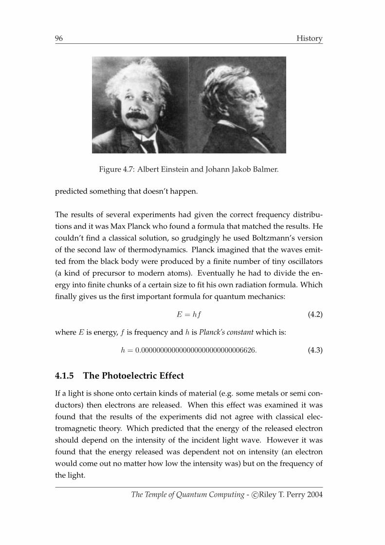
96 History
Figure 4.7: Albert Einstein and Johann Jakob Balmer.
predicted something that doesn’t happen.
The results of several experiments had given the correct frequency distribu-tions and it was Max Planck who found a formula that matched the results. Hecouldn’t find a classical solution, so grudgingly he used Boltzmann’s versionof the second law of thermodynamics. Planck imagined that the waves emit-ted from the black body were produced by a finite number of tiny oscillators(a kind of precursor to modern atoms). Eventually he had to divide the en-ergy into finite chunks of a certain size to fit his own radiation formula. Whichfinally gives us the first important formula for quantum mechanics:
E = hf (4.2)
where E is energy, f is frequency and h is Planck’s constant which is:
h = 0.000000000000000000000000006626. (4.3)
4.1.5 The Photoelectric Effect
If a light is shone onto certain kinds of material (e.g. some metals or semi con-ductors) then electrons are released. When this effect was examined it wasfound that the results of the experiments did not agree with classical elec-tromagnetic theory. Which predicted that the energy of the released electronshould depend on the intensity of the incident light wave. However it wasfound that the energy released was dependent not on intensity (an electronwould come out no matter how low the intensity was) but on the frequency ofthe light.
The Temple of Quantum Computing - c©Riley T. Perry 2004
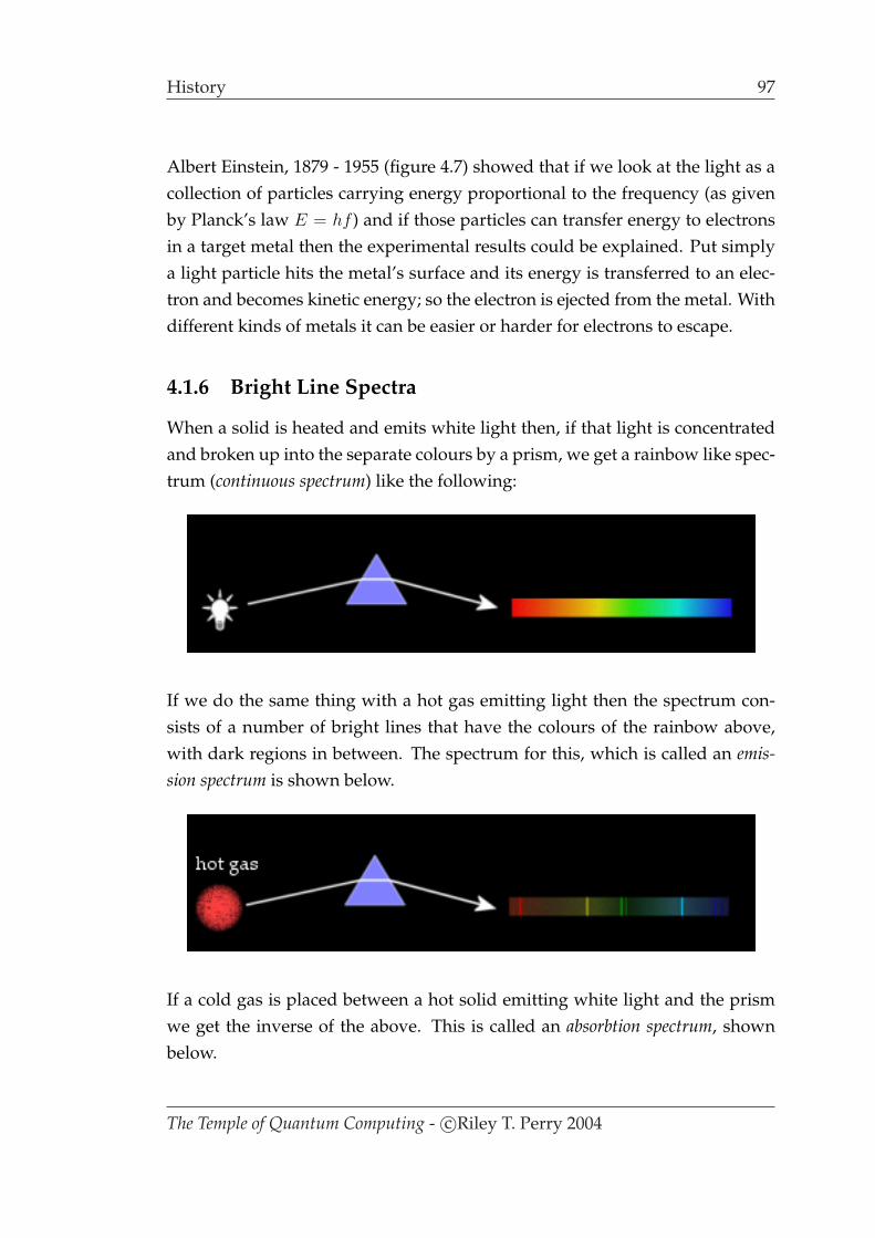
History 97
Albert Einstein, 1879 - 1955 (figure 4.7) showed that if we look at the light as acollection of particles carrying energy proportional to the frequency (as givenby Planck’s law E = hf ) and if those particles can transfer energy to electronsin a target metal then the experimental results could be explained. Put simplya light particle hits the metal’s surface and its energy is transferred to an elec-tron and becomes kinetic energy; so the electron is ejected from the metal. Withdifferent kinds of metals it can be easier or harder for electrons to escape.
4.1.6 Bright Line Spectra
When a solid is heated and emits white light then, if that light is concentratedand broken up into the separate colours by a prism, we get a rainbow like spec-trum (continuous spectrum) like the following:
If we do the same thing with a hot gas emitting light then the spectrum con-sists of a number of bright lines that have the colours of the rainbow above,with dark regions in between. The spectrum for this, which is called an emis-sion spectrum is shown below.
If a cold gas is placed between a hot solid emitting white light and the prismwe get the inverse of the above. This is called an absorbtion spectrum, shownbelow.
The Temple of Quantum Computing - c©Riley T. Perry 2004
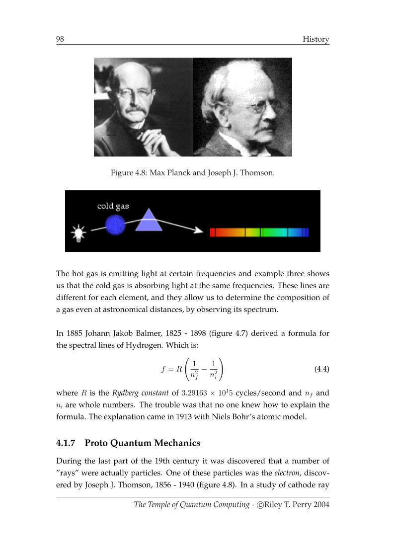
98 History
Figure 4.8: Max Planck and Joseph J. Thomson.
The hot gas is emitting light at certain frequencies and example three showsus that the cold gas is absorbing light at the same frequencies. These lines aredifferent for each element, and they allow us to determine the composition ofa gas even at astronomical distances, by observing its spectrum.
In 1885 Johann Jakob Balmer, 1825 - 1898 (figure 4.7) derived a formula forthe spectral lines of Hydrogen. Which is:
f = R
(1
n2f
− 1
n2i
)(4.4)
where R is the Rydberg constant of 3.29163 × 10¹⁵ cycles/second and nf andni are whole numbers. The trouble was that no one knew how to explain theformula. The explanation came in 1913 with Niels Bohr’s atomic model.
4.1.7 Proto Quantum Mechanics
During the last part of the 19th century it was discovered that a number of”rays” were actually particles. One of these particles was the electron, discov-ered by Joseph J. Thomson, 1856 - 1940 (figure 4.8). In a study of cathode ray
The Temple of Quantum Computing - c©Riley T. Perry 2004

History 99
Figure 4.9: Ernest Rutherford and Arnold Sommerfeld.
Figure 4.10: Thomson’s atomic model.
Figure 4.11: Rutherford’s atomic model.
The Temple of Quantum Computing - c©Riley T. Perry 2004

100 History
tubes Thompson showed that electrically charged particles (electrons) are emit-ted when a wire is heated. Thomson went on to help develop the first modelof the atom which had his (negatively charged) electrons contained within apositively charged sphere (figure 4.10).
This first atomic model was called the Christmas pudding model. Then, in 1907,Ernest Rutherford, 1871 - 1937 (figure 4.9), developed a new model, which wasfound by firing alpha particles (Helium ions) at gold foil and observing that,very occasionally, one would bounce back. This model had a tiny but massivenucleus surrounded by electrons (figure 4.11).
The new model was like a mini solar system with electrons orbiting the nu-cleus, but the atomic model was thought to still follow the rules of classicalphysics. However, according to classical electromagnetic theory an orbitingelectron, subject to centripetal acceleration (the electron is attracted by the pos-itively charged nucleus) would radiate energy and so rapidly spiral in towardsthe nucleus. But this did not happen: atoms were stable, and all the atomsof an element emitted the same line spectrum. To explain this Bohr assumedthat the atom could exist in only certain stationary states - stationary because,even if the electron was orbiting in such a state (and, later, this was questionedby Heisenberg) it would not radiate, despite what electromagnetic theory said.However, if the electron jumped from a stationary state to one of lower energythen the transmission was accompanied by the emission of a photon; vice versathere was absorption of light in going from a lower to a higher energy.
In this scheme there was a lowest stationary state, called the ground state be-low which the electron could not jump; so this restored stability to the atom.
The frequency of the light emitted as a jump was given by Einstein’s formula:
f =E
h(4.5)
where E is the difference in the energies of the stationary states involved. Theseenergies of the stationary states could be calculated from classical physics if oneadditional assumption was introduced: that the orbital angular momentumwas an integer multiple of Planck’s constant. Then the calculated frequencieswere found to agree with those observed.
The Temple of Quantum Computing - c©Riley T. Perry 2004

History 101
Figure 4.12: Bohr’s first atomic model.
So Bohr developed a model based on stable orbital shells which only gave acertain number of shells to each atom. Bohr quantised electron orbits in unitsof Planck’s constant. He gave us the first of several quantum numbers which areuseful in quantum computing, the shell number, n (see figure 4.12).
Of particular interest are the ground state at n = 1 and the excited state at n > 1
of an atom. Bohr developed a formula for the radius of the electron orbits in ahydrogen atom:
r =
(h2
4π2mq2
)n2 (4.6)
where r is the radius of the orbital, h is Planck’s constant, and m and q are themass and charge of the electron. In real terms the value of r is 5.3 nanometresfor n = 1.
Bohr went on with this model to derive the Balmer’s formula for hydrogenby two postulates:
1. Quantum angular momentum:
L = n
(h
2π
). (4.7)
The Temple of Quantum Computing - c©Riley T. Perry 2004

102 History
Figure 4.13: Wolfgang Pauli and Louis de Broglie.
2. A jump between orbitals will emit or absorb radiation by:
hf = Ei − Ef (4.8)
where Ei is the initial energy of the electron and Ef is the final energy ofthe electron.
Although very close, it didn’t quite match up to the spectral line data. ArnoldSommerfeld, 1868 - 1951 (figure 4.9) then proposed a new model with ellipticalorbits and a new quantum number was added, k to deal with the shape of theorbit, Bohr then introduced quantum number m to explain the Zeeman effectwhich produced extra spectral lines when a magnetic field was applied to theatom (i.e. the direction the field was pointing).
It was soon discovered that m could not account for all the spectral lines pro-duced by magnetic fields. Wolfgang Pauli, 1900 - 1958 (figure 4.13) hypoth-esised another quantum number to account for this. It was thought, but notaccepted by Pauli that the electron was ”spinning around” and it turns out thatPauli was right but the name stuck, so we still use spin up and spin down to de-scribe this property of an electron. Pauli then described why electrons fill thehigher energy levels and don’t just occupy the ground state which we now callthe Pauli exclusion principle. Niels Bohr went on to explain the periodic tablein terms of orbital shells with the outer most shell being the valence shell thatallows binding and the formation of molecules.
The Temple of Quantum Computing - c©Riley T. Perry 2004

History 103
Figure 4.14: Werner Heisenberg and Erwin Schrodinger.
4.1.8 The New Theory of Quantum Mechanics
In 1909, a few years after demonstrating the photoelectric effect, Einstein usedhis photon hypothesis to obtain a simple derivation of Planck’s black body dis-tribution. Planck himself had not gone as far as Einstein: he had indeed, as-sumed that the transfer of energy between matter (the oscillators in the wallsof the cavity) and radiation was quantised (i.e. the energy transferred to/froman oscillator occurred in ”grains” less than h times the frequency of the oscil-lator). But Planck had assumed the energy in the electromagnetic field, in thecavity, was continuously distributed, as in classical theory. By contrast, it wasEinstein’s hypothesis that the energy in the field itself was quantised: that forcertain purposes, the field behaved like an ideal gas, not of molecules, but ofphotons, each with energy h times frequency, with the number of photons be-ing proportional to the intensity. The clue to this was Einstein’s observationthat the high frequency part of Planck’s distribution for black body radiation(described by Wien’s law) could be derived by assuming a gas of photons andapplying statistical mechanics to it. This was in contrast to the low frequencypart (described by the Rayleigh-Jeans law) which could be successfully obtainedusing classical electromagnetic theory, i.e. assuming waves. So you had bothparticles and waves playing a part. Furthermore, Einstein looked at fluctua-tions of the energy about its average value, and observed that the formula ob-tained had two forms, one which you would get if light was made up of wavesand the other if it was made up of particles. Hence we have wave-particle du-ality. In 1924, Louis de Broglie, 1892 - 1987 (figure 4.13) extended the particleduality for light to all matter. He stated:
The Temple of Quantum Computing - c©Riley T. Perry 2004

104 History
The motion of a particle of any sort is associated with the propaga-tion of a wave.
This is the idea of a pilot wave which guides a free particle’s motion. de Brogliethen suggested the idea of electron waves be extended to bound particles inatoms, meaning electrons move around the nucleus guided by pilot waves. So,again a duality, de Broglie waves and Bohr’s particles. de Broglie was able toshow that Bohr’s orbital radii could be obtained by fitting a whole number ofwaves around the nucleus. This gave an explanation of Bohr’s angular mo-mentum quantum condition (see above).
The new quantum theory was developed between June 1925 and June 1926.Werner Heisenberg, 1901 - 1976 (figure 4.14), using a totally different and moresimple atomic model (one that did not use orbits) worked out a code to con-nect quantum numbers and spectra. He also discovered that quantum me-chanics does not follow the commutative law of multiplication i.e pq 6= qp. WhenMax Born, 1882 - 1970 (figure 4.15) saw this he suggested that Heisenberg usematrices. This became matrix mechanics, eventually all the spectral lines andquantum numbers were deduced for hydrogen. The first complete version ofquantum mechanics was born. It’s interesting to note that it was not observa-tion, or visualisation that was used to deduce to theory - but pure mathematics.Later, We will see matrices cropping up in quantum computing.
At around the same time Erwin Schrodinger, 1887 - 1961 (figure 4.14) built onde Broglie’s work on matter waves. He developed a wave equation (for whichΨ is the solution) for the core of bound electrons, as in the Hydrogen atom. Itturns out that the results derived from this equation agree with the Bohr model.He then showed that Heisenberg’s matrix mechanics and his wave mechanicswere equivalent.
Max Born proposed that Ψ, the solution to Schrodinger’s equation can be in-terpreted as a probability amplitude, not a real, physical value. The prob-ability amplitude is a function of the electron’s position (x, y, x) and, whensquared, gives the probability of finding the electron in a unit volume at thepoint (x, y, x). This gives us a new, probabilistic atomic model, in which thereis a high probability that the electron will be found in a particular orbital shell.A representation of the ground state of hydrogen is shown in figure 4.16 and
The Temple of Quantum Computing - c©Riley T. Perry 2004

History 105
at the places where the density of points is high there is a high probability offinding the particle. The linear nature of the wave equation means that if Ψ1
and Ψ2 are two solutions then so is Ψ1 + Ψ2, a superposition state (we’ll lookat superposition soon). This probabilistic interpretation of quantum mechanicsimplies the system is in both states until measured.
Schrodinger was unhappy with the probabilistic interpretation (superposition)and created a scenario that would show it was false. This is called Schrodinger’scat, a paradox, which simply put refers to the situation of a cat being in bothstates of dead Ψ1 and alive Ψ2 until it is observed.
Paul Dirac, 1902 - 1984 (figure 4.15) developed a new approach and the bra-ketnotation we use for quantum computing. His approach expanded to a quan-tum field theory, he expanded Schrodinger’s equation, incorporated spin, andEinstein’s relativity, and predicted antimatter.
In 1927 Heisenberg made his second major discovery, the Heisenberg uncertaintyprinciple which relates to the position and momentum of a particle. It states thatthe more accurate our knowledge of a particle’s position, the more inaccurateour knowledge of its momentum will be and vice versa. The uncertainty is dueto the uncontrollable effect on the particle of any attempt to observe it (becauseof the quantum interaction; see 4.25). This signalled the breakdown of deter-minism.
Now back to Niels Bohr. In 1927 Niels Bohr described the concept of comple-mentarity: it depends on what type of measurement operations you are usingto look at the system as to whether it behaves like a particle or a wave. Hethen put together various aspects of the work by Heisenberg, Schrodinger, andBorn and concluded that the properties of a system (such as position and mo-mentum) are undefined having only potential values with certain probabilitiesof being measured. This became know as the Copenhagen interpretation of quan-tum mechanics.
Einstein did not like the Copenhagen interpretation and, for a good deal oftime, Einstein kept trying to refute it by thought experiment, but Bohr alwayshad an answer. But in 1935 Einstein raised an issue that was to later have pro-
The Temple of Quantum Computing - c©Riley T. Perry 2004

106 Important Principles for Quantum Computing
Figure 4.15: Max Born and Paul Dirac.
Figure 4.16: Born’s atomic model.
found implications for quantum computation and lead to the phenomenon wenow call entanglement, a concept we’ll look at in a few pages.
4.2 Important Principles for Quantum Computing
The main parts of quantum mechanics that are important for quantum com-puting are:
• Linear algebra.
• Superposition.
• Dirac notation.
• Representing information.
The Temple of Quantum Computing - c©Riley T. Perry 2004

Important Principles for Quantum Computing 107
• Uncertainty.
• Entanglement.
• The 4 postulates of quantum mechanics.
4.2.1 Linear Algebra
Quantum mechanics leans heavily on linear algebra. Some of the concepts ofquantum mechanics come from the mathematical formalism, not thought ex-periments - that’s what can give rise to counter intuitive conclusions.
4.2.2 Superposition
Superposition means a system can be in two or more of its states simultaneously.For example a single particle can be travelling along two different paths at once.This implies that the particle has wave-like properties, which can mean that thewaves from the different paths can interfere with each other. Interference cancause the particle to act in ways that are impossible to explain without thesewave-like properties.
The ability for the particle to be in a superposition is where we get the parallelnature of quantum computing: If each of the states corresponds to a differentvalue then, if we have a superposition of such states and act on the system, weeffectively act on all the states simultaneously.
An Example With Silvered Mirrors
Superposition can be explained by way of a simple example using silvered andhalf silvered mirrors [Barenco, A. Ekert, A. Sanpera, A. & Machiavello, C. 1996].
A half silvered mirror reflects half of the light that hits it and transmits the otherhalf of the light through it (figure 4.17). If we send a single photon through thissystem then this gives us a 50% chance of the light hitting detector 1 and a50% chance of hitting detector 2. It is tempting to think that the light takesone or the other path, but in fact it takes both! It’s just that the photo detectorthat measures the photon first breaks the superposition, so it’s the detectors thatcause the randomness, not the half silvered mirror. This can be demonstrated
The Temple of Quantum Computing - c©Riley T. Perry 2004
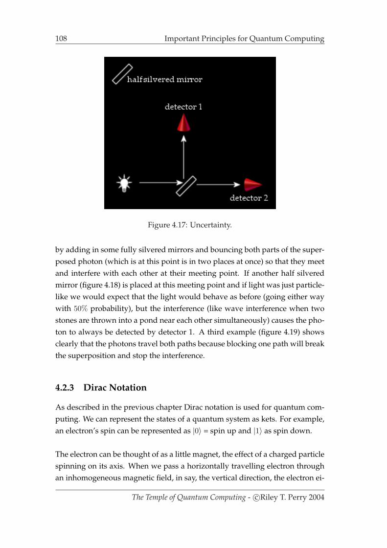
108 Important Principles for Quantum Computing
Figure 4.17: Uncertainty.
by adding in some fully silvered mirrors and bouncing both parts of the super-posed photon (which is at this point is in two places at once) so that they meetand interfere with each other at their meeting point. If another half silveredmirror (figure 4.18) is placed at this meeting point and if light was just particle-like we would expect that the light would behave as before (going either waywith 50% probability), but the interference (like wave interference when twostones are thrown into a pond near each other simultaneously) causes the pho-ton to always be detected by detector 1. A third example (figure 4.19) showsclearly that the photons travel both paths because blocking one path will breakthe superposition and stop the interference.
4.2.3 Dirac Notation
As described in the previous chapter Dirac notation is used for quantum com-puting. We can represent the states of a quantum system as kets. For example,an electron’s spin can be represented as |0〉 = spin up and |1〉 as spin down.
The electron can be thought of as a little magnet, the effect of a charged particlespinning on its axis. When we pass a horizontally travelling electron throughan inhomogeneous magnetic field, in say, the vertical direction, the electron ei-
The Temple of Quantum Computing - c©Riley T. Perry 2004
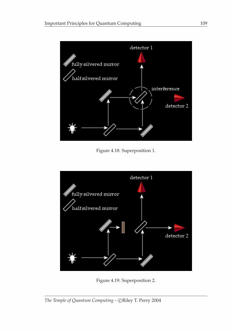
Important Principles for Quantum Computing 109
Figure 4.18: Superposition 1.
Figure 4.19: Superposition 2.
The Temple of Quantum Computing - c©Riley T. Perry 2004
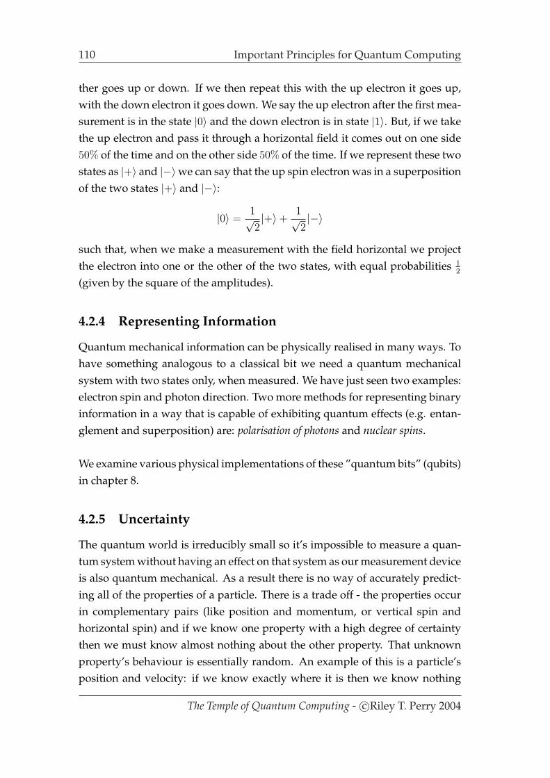
110 Important Principles for Quantum Computing
ther goes up or down. If we then repeat this with the up electron it goes up,with the down electron it goes down. We say the up electron after the first mea-surement is in the state |0〉 and the down electron is in state |1〉. But, if we takethe up electron and pass it through a horizontal field it comes out on one side50% of the time and on the other side 50% of the time. If we represent these twostates as |+〉 and |−〉we can say that the up spin electron was in a superpositionof the two states |+〉 and |−〉:
|0〉 =1√2|+〉+
1√2|−〉
such that, when we make a measurement with the field horizontal we projectthe electron into one or the other of the two states, with equal probabilities 1
2
(given by the square of the amplitudes).
4.2.4 Representing Information
Quantum mechanical information can be physically realised in many ways. Tohave something analogous to a classical bit we need a quantum mechanicalsystem with two states only, when measured. We have just seen two examples:electron spin and photon direction. Two more methods for representing binaryinformation in a way that is capable of exhibiting quantum effects (e.g. entan-glement and superposition) are: polarisation of photons and nuclear spins.
We examine various physical implementations of these ”quantum bits” (qubits)in chapter 8.
4.2.5 Uncertainty
The quantum world is irreducibly small so it’s impossible to measure a quan-tum system without having an effect on that system as our measurement deviceis also quantum mechanical. As a result there is no way of accurately predict-ing all of the properties of a particle. There is a trade off - the properties occurin complementary pairs (like position and momentum, or vertical spin andhorizontal spin) and if we know one property with a high degree of certaintythen we must know almost nothing about the other property. That unknownproperty’s behaviour is essentially random. An example of this is a particle’sposition and velocity: if we know exactly where it is then we know nothing
The Temple of Quantum Computing - c©Riley T. Perry 2004

Important Principles for Quantum Computing 111
about how fast it is going. This indeterminacy is exploited in quantum cryp-tography (see chapter 7).
It has been postulated (and currently accepted) that particles in fact DO NOThave defined values for unknown properties until they are measured. This islike saying that something does not exist until it is looked at.
4.2.6 Entanglement
In 1935 Einstein (along with colleagues Podolski and Rosen) demonstrated aparadox (named EPR after them) in an attempt to refute the undefined na-ture of quantum systems. The results of their experiment seemed to show thatquantum systems were defined, having local state BEFORE measurement. Al-though the original hypothesis was later proven wrong (i.e. it was proven thatquantum systems do not have local state before measurement). The effect theydemonstrated was still important, and later became known as entanglement.
Entanglement is the ability for pairs of particles to interact over any distanceinstantaneously. Particles don’t exactly communicate, but there is a statisti-cal correlation between results of measurements on each particle that is hard tounderstand using classical physics. To become entangled, two particles are al-lowed to interact; they then separate and, on measuring say, the velocity of oneof them (regardless of the distance between them), we can be sure of the valueof velocity of the other one (before it is measured). The reason we say thatthey communicate instantaneously is because they store no local state [Rae, A.1996] and only have well defined state once they are measured. Because of thislimitation particles can’t be used to transmit classical messages faster than thespeed of light as we only know the states upon measurement. Entanglementhas applications in a wide variety of quantum algorithms and machinery, someof which we’ll look at later.
As stated before, it has been proven that entangled particles have no local state;this is explained in section 6.7.
The Temple of Quantum Computing - c©Riley T. Perry 2004
112 Important Principles for Quantum Computing
4.2.7 The Four Postulates of Quantum Mechanics
The theory of quantum mechanics has four main postulates. These are intro-duced here as simple sentences. Later, in section 5.4, they will be explained inmore detail in terms of quantum computing.
1. In a closed quantum system we need a way of describing the state of all theparticles within it. The first postulate gives us a way to do this by usinga single state vector to represent the entire system. Say the state is to be avector in Cn, this would be C2 for a spin system.
2. The evolution of a closed system is a unitary transform. Say that, while thesystem is evolving under its own steam - no measurement - the state atsome stage |Ψ′〉 is related to the state at some previous stage (or time)|Ψ〉 by a unitary transform |Ψ′〉 = U |Ψ〉. This means that we can totallydescribe the behaviour of a system by using unitary matrices.
3. The third postulate relates to making measurements on a closed quantumsystem, and the affect those measurements have on that system.
4. Postulate four relates to combining or separating different closed quantumsystems using tensor products.
The Temple of Quantum Computing - c©Riley T. Perry 2004

Chapter 5
Quantum Computing
5.1 Elements of Quantum Computing
5.1.1 Introduction
Generally we’ll think of a quantum computer as a classical computer with aquantum circuit attached to it with some kind of interface between conven-tional and quantum logic. Since there are only a few things a quantum com-puter does better than a classical computer it makes sense to do the bulk of theprocessing on the classical machine.
This section borrows heavily from [Nielsen, M. A. & Chuang, I. L. 2000] and[Dawar, A. 2004] so the use of individual citations for these references has beendropped.
5.1.2 History
In 1982 Richard Feynman theorised that classic computation could be dramat-ically improved by quantum effects, building on this, David Deutsch devel-oped the basis for quantum computing between 1984 and 1985. The next majorbreakthrough came in 1994 when Peter Shor described a method to factor largenumbers in quantum poly-time (which breaks RSA encryption). This becameknown as Shor’s algorithm. At around the same time the quantum complex-ity classes were developed and the quantum Turing machine was described.Then in 1996 Lov Grover developed a fast database search algorithm (knownas Grover’s algorithm). The first prototypes of quantum computers were also
113
114 Elements of Quantum Computing
built in 1996. In 1997 quantum error correction techniques were developed atBell labs and IBM. Physical implementations of quantum computers improvedwith a three qubit machine in 1999 and a seven qubit machine in 2000.
5.1.3 Bits and Qubits
This section is about the ”nuts and bolts” of quantum computing. It describesqubits, gates, and circuits.
Quantum computers perform operations on qubits which are analogous to con-ventional bits (see below) but they have an additional property in that they canbe in a superposition. A quantum register with 3 qubits can store 8 numbersin superposition simultaneously [Barenco, A. Ekert, A. Sanpera, A. & Machi-avello, C. 1996] and a 250 qubit register holds more numbers (superposed) thanthere are atoms in the universe! [Deutsch, D. & Ekert, A. 1998].
The amount of information stored during the ”computational phase” is essen-tially infinite - its just that we can’t get at it. The inaccessibility of the infor-mation is related to quantum measurement: When we attempt to readout asuperposition state holding many values the state collapses and we get onlyone value (the rest get lost). This is tantalising but, in some cases, can be madeto work to our computational advantage.
Single Qubits
Classical computers use two discrete states (e.g. states of charging of a capac-itor) to represent a unit of information, this state is called a binary digit (or bitfor short). A bit has the following two values:
0 and 1.
There is no intermediate state between them, i.e. the value of the bit cannotbe in a superposition.
Quantum bits, or qubits, can on the other hand be in a state ”between” 0 and1, but only during the computational phase of a quantum operation. Whenmeasured, a qubit can become either:
The Temple of Quantum Computing - c©Riley T. Perry 2004
Elements of Quantum Computing 115
|0〉 or |1〉
i.e. we readout 0 or 1. This is the same as saying a spin particle can be in asuperposition state but, when measured, it shows only one value (see chapter4).
The |〉 symbolic notation is part of the Dirac notation (see chapters 3 and 4).In terms of the above it essentially means the same thing as 0 and 1 (this isexplained a little further on), just like a classical bit. Generally, a qubit’s stateduring the computational phase is represented by a linear combination of statesotherwise called a superposition state.
α|0〉+ β|1〉.Here α and β are the probability amplitudes. They can be used to calculate theprobabilities of the system jumping into |0〉 or |1〉 following a measurement orreadout operation. There may be, say a 25% chance a 0 is measured and a 75%
chance a 1 is measured. The percentages must add to 100%. In terms of theirrepresentation qubits must satisfy:
|α|2 + |β|2 = 1. (5.1)
This the same thing as saying the probabilities add to 100%.
Once the qubit is measured it will remain in that state if the same measure-ment is repeated provided the system remains closed between measurements(see chapter 4). The probability that the qubit’s state, when in a superposition,will collapse to states |0〉 or |1〉 is
|α|2 for |0〉
and
|β|2 for |1〉.
|0〉 and |1〉 are actually vectors, they are called the computational basis statesthat form an orthonormal basis for the vector space C2.
The Temple of Quantum Computing - c©Riley T. Perry 2004

116 Elements of Quantum Computing
The state vector |Ψ〉 of a quantum system describes the state at any point intime of the entire system. Our state vector in the case of one qubit is:
|Ψ〉 = α|0〉+ β|1〉. (5.2)
The α and β might vary with time as the state evolves during the computationbut the sum of the squares of α and β must always must be equal to 1.
Quantum computing also commonly uses 1√2(|0〉 + |1〉) and 1√
2(|0〉 − |1〉) as a
basis forC2, which is often shortened to just |+〉, and |−〉. These bases are some-times represented with arrows which are described below, and are referred toas rectilinear and diagonal which can say refer to the polarisation of a photon.You may find these notational conventions being used:
|0〉 = | →〉. (5.3)
|1〉 = | ↑〉. (5.4)1√2(|0〉+ |0〉) = |+〉 = | 〉. (5.5)
1√2(|0〉 − |0〉) = |−〉 = | 〉. (5.6)
Some examples of measurement probabilities are on the next page.
The Temple of Quantum Computing - c©Riley T. Perry 2004
Elements of Quantum Computing 117
Example Measurement probabilities.
|Ψ〉 =1√2|0〉+
1√2|1〉.
The probability of measuring a |0〉 is:
(∣∣∣ 1√2
∣∣∣)2
=1
2.
The probability of measuring a |1〉 is:
(∣∣∣ 1√2
∣∣∣)2
=1
2.
So 50% of the time we’ll measure a |0〉 and 50% of the time we’ll measure a|1〉.Example More measurement probabilities.
|Ψ〉 =
√3
2|0〉 − 1
2|1〉.
The probability of measuring a |0〉 is:
(∣∣∣√
3
2
∣∣∣)2
=3
4.
The probability of measuring a |1〉 is:
(∣∣∣12
∣∣∣)2
=1
4.
So 75% of the time we’ll measure a |0〉 and 25% of the time we’ll measure a|1〉.
The sign in the middle of the two values can change, which affects the internalevolution of the qubit, not the outcome of a measurement. When measuring inthe basis |0〉, |1〉 the sign is actually the relative phase of the qubit. So,
α|0〉+ β|1〉
andα|0〉 − β|1〉
have the same output values and probabilities but behave differently duringthe computational phase. Formally we say they differ by a relative phase fac-
The Temple of Quantum Computing - c©Riley T. Perry 2004

118 Elements of Quantum Computing
tor. So in the case of the qubits above they differ by a phase factor of -1. It iscalled a phase factor because it always has magnitude 1 and so its value, as acomplex number, is determined entirely by the phase.
The other type of phase is called global phase. Two states can differ by a globalphase factor and still be considered the same, as the global phase factor is notobservable. One reason for this is that the probabilities for the outcomes |α| and|β| are unaffected if α and β are each multiplied by the same complex numberof magnitude 1. Likewise the relative phase (which figures in interference ef-fects) is unaffected if α and β are multiplied by a common phase factor. Whatthis means is that if we have a state on n qubits we can put a complex factor infront of the entire state to make it more readable. This is best described by anexample (below).
Example Global phase.
|Ψ〉 =−i√
2|0〉+
1√2|1〉.
can be rewritten as:
|Ψ〉 = −i
(1√2|0〉 − i√
2|1〉
).
Remembering that −i × −i = +1 we say the factor at the front of ourstate vector (−i) is a global phase factor. We can also say here that because−i = e−i π
2 we have a phase of −π2.
Example More global phase.
|Ψ〉 =1
2(−|00〉+ |01〉 − |10〉+ |11〉).
can be rewritten as:
|Ψ〉 = (−1)1
2(|00〉 − |01〉+ |10〉+ |11〉).
The Temple of Quantum Computing - c©Riley T. Perry 2004

Elements of Quantum Computing 119
-
6
?
¾ ¡¡
¡¡
¡µ
@@
@@
@R
a
b
|1〉
|0〉
− |1〉
Figure 5.1: 2D qubit representations.
The Ket |〉
Part of Dirac’s notation is the ket (|〉). The ket is just a notation for a vector. Thestate of a single qubit is a unit vector in C2. So,
[α
β
]
is a vector, and is written as:α|0〉+ β|1〉
with
|0〉 =
[1
0
](5.7)
and
|1〉 =
[0
1
]. (5.8)
Two Dimensional Qubit Visualisation
Single qubits can be represented in value and relative phase in two dimensionsby the diagram in figure 5.1 which is similar to the way we represent polar co-ordinates for complex numbers. The graph shows the general form of 2D qubit
The Temple of Quantum Computing - c©Riley T. Perry 2004

120 Elements of Quantum Computing
representation where a = 1√2|0〉+ 1√
2|1〉 and b = 1√
2|0〉 − 1√
2|1〉.
This diagram is ok for real numbered values of α and β but cannot accuratelydepict all the possible states of a qubit. For this we need three dimensions.
Three Dimensional Qubit Visualisation - The Bloch Sphere
The Bloch sphere is a tool with which the state of single qubit can be viewed inthree dimensions and is useful for visualising all single qubit operations. Wecan say that the state of a single qubit can be written as:
|Ψ〉 = eiγ(cosθ
2|0〉+ eiϕ sin
θ
2|1〉). (5.9)
We can ignore the global phase factor in front so |Ψ〉 becomes:
|Ψ〉 = cosθ
2|0〉+ eiϕ sin
θ
2|1〉. (5.10)
So, in terms of the angle θ and ϕ the Bloch sphere looks like this:
Note: An applet written by Jose Castro was used to generate the images ofthe Bloch sphere which is available at http://pegasus.cc.ucf.edu/∼jcastro/java/BlochSphere.html .
What’s probably more helpful at this stage is to see where all of the potentialstates of a qubit lie on the Bloch sphere. This is shown below with the pointsx, y, and z labelling each positive axis:
The Temple of Quantum Computing - c©Riley T. Perry 2004

Elements of Quantum Computing 121
As stated in chapter 4, individual qubits can be physically realised using vari-ous quantum two state systems, here are a few ways this can be done:
• Polarisations of a photon.
• Nuclear spins.
• Ground and excited states of an atom (i.e. the energy level, or orbital).
We now look at the equivalent of a register: i.e. a composite system of qubits,e.g. Ions in a trap (see chapter 8).
Multiple Qubits
The potential amount of information available during the computational phasegrows exponentially with the size of the system, i.e. the number of qubits.This is because if we have n qubits the number of basis states is 2n. E.g. ifwe have two qubits, forming a quantum register then there are four (= 22)
The Temple of Quantum Computing - c©Riley T. Perry 2004

122 Elements of Quantum Computing
computational basis states: forming,
|00〉, |01〉, |10〉, and |11〉. (5.11)
Here |01〉 means that qubit 1 is in state |0〉 and qubit 2 is in state |1〉, etc. Weactually have |01〉 = |0〉 ⊗ |1〉, where ⊗ is the tensor product (see below).
Like a single qubit, the two qubit register can exist in a superposition of the fourstates (below we change the notation for the complex coefficients, i.e. probabil-ity amplitudes):
|Ψ〉 = α0|00〉+ α1|01〉+ α2|10〉+ α3|11〉. (5.12)
Again all of the probabilities must sum to 1, formally for the general case of n
qubits this is can be written as:
2n−1∑i=0
|αi|2 = 1. (5.13)
Example n = 5 (5 qubits). We can have up to 32 (= 25) basis states in asuperposition.
Ψ = α0|00000〉+ α1|00001〉+ ... + α2n−1|11111〉.
We don’t have to represent values with 0s and 1s. A qudit has the followingformat in CN :
Ψ = α0|0〉+ α1|1〉+ α2|2〉+ . . . + αn−1|N − 1〉 =
α0
α1
α2
...αN − 1
. (5.14)
If N = 2n we require an n qubit register.
The Temple of Quantum Computing - c©Riley T. Perry 2004
Elements of Quantum Computing 123
Tensor Products
A decomposition into single qubits of a multi-qubit system can be representedby a tensor product, ⊗.
Example Decomposition using a tensor product.
1
2(|00〉+ |01〉+ |10〉+ |11〉) =
1√2(|0〉+ |1〉)⊗ 1√
2(|0〉+ |1〉).
A tensor product can also be used to combine different qubits.
(α0|0〉+ α1|1〉)⊗ (β0|0〉+ β1|1〉) = α0β0|00〉+ α0β1|01〉+ α1β0|10〉+ α1β1|11〉.(5.15)
Partial Measurement
We can measure a subset of an n-qubit system. i.e. we don’t have to get readouts on all the qubits (some can be left unmeasured). We’ll first consider non-entangled states. The simplest way to measure a subset of states is shown inthe following example with two qubits.
An example is presented on the next page.
The Temple of Quantum Computing - c©Riley T. Perry 2004

124 Elements of Quantum Computing
Example measuring the first bit in a two qubit system.
1. We prepare a quantum system in the following state, the qubit we aregoing to measure is bolded, a non-entangled state would mean that allthe probability amplitudes are non-zero:
Ψ = α0|00〉+ α1|01〉+ α2|10〉+ α3|11〉.
2. We now measure, so the probability of it being 0 is:
pr(0) = |α0|2 + |α1|2
and, the probability of it being 1 is:
pr(1) = |α2|2 + |α3|2.
3. If we measured a |0〉 the post measurement state is:
|0〉 ⊗ α0|0〉+ α1|1〉√|α0|2 + |α1|2
(i.e. we project on to the |00〉, |01〉 subspace and the α2 and α3 termsdrop out). Similarly, if we measured a |1〉 measured the post measure-ment state is:
|1〉 ⊗ α2|0〉+ α3|1〉√|α2|2 + |α3|2
.
We can do the same for qubit two, the probability of qubit two being a |0〉 is:
pr(0) = |α0|2 + |α2|2
and its post measurement state would be:
α0|0〉+ α2|1〉√|α0|2 + |α2|2
⊗ |0〉.
This logic can be extended to n qubits.
The Temple of Quantum Computing - c©Riley T. Perry 2004
Elements of Quantum Computing 125
Quantum measurement can be described as a set Mm of linear operators with1 ≤ m ≤ n where n is the number of possible outcomes. For a single qubitwith an orhtonormal basis of |0〉 and |1〉 we can define measurement operatorsM0 = |0〉 〈0| and M1 = |1〉 〈1| (which are also both projectors).
If we have a system in state |Ψ〉 then outcome m has a probability of:
pr(m) = 〈Ψ|M †mMm|Ψ〉. (5.16)
If the outcome is m then the state collapses to:
Mm|Ψ〉√〈Ψ|M †
mMm|Ψ〉. (5.17)
Example Another way of looking at measuring the first bit in a two qubitsystem.
|Ψ〉 =1√30|00〉+
2√30|01〉+
3√30|10〉+
4√30|11〉
When we measure qubit one the resulting states would look like this (unnor-malised):
|Ψ〉 = |0〉 ⊗(
1√30|0〉+
2√30|1〉
)
for measuring a |0〉 and for measuring a |1〉:
|Ψ〉 = |1〉 ⊗(
3√30|0〉+
4√30|1〉
).
Now we must make sure that the second qubit is normalised, so we multiplyit by a factor:
|Ψ〉 =
√5√30|0〉 ⊗
(1√5|0〉+
2√5|1〉
)+
5√30|1〉 ⊗
(3
5|0〉+
4
5|1〉.
)
This gives us∣∣∣√
5√30
∣∣∣2
= 16
probability of measuring a |0〉 and a∣∣∣ 5√
30
∣∣∣2
= 56
prob-ability of measuring a |1〉. So if we measure a |0〉 then our post measurementstate is:
|Ψ〉 = |0〉 ⊗(
1√5|0〉+
2√5|1〉
)
and if we measure a |1〉 then our post measurement state is:
|Ψ〉 = |1〉 ⊗(
3
5|0〉+
4
5|1〉
).
The Temple of Quantum Computing - c©Riley T. Perry 2004

126 Elements of Quantum Computing
Example Measurement of qubit one in a two qubit system using a simpleprojector.
|Ψ〉 =1√30|00〉+
2√30|01〉+
3√30|10〉+
4√30|11〉.
We find the probability of measuring a |0〉 by using a projector |00〉〈00| +
|01〉〈01|:
(|00〉〈00|+ |01〉〈01|)(
1√30|00〉+
2√30|01〉+
3√30|10〉+
4√30|11〉
)
= (|00〉〈00|+ |01〉〈01|) |Ψ〉=
1√30|00〉+
2√30|01〉.
Say we change our measurement basis to |0〉 , |1〉 then we can represent pro-jectors P0 and P1 as |0〉 〈0| and |1〉 〈1| respectively. We measure the probabil-ity of the first qubit being 0 by using P0 on qubit one and I on qubit two, i.e.P0⊗I . If we wanted to measure the probability of the first qubit being 1 thenwe would use P1 ⊗ I .
pr(0) = 〈Ψ|P0 ⊗ I|Ψ〉= 〈Ψ| |0〉 〈0| ⊗ I|Ψ〉= 〈Ψ| 1√
30|00〉+
2√30|01〉
=1
6
and this gives us a post-measurement state of:
|Ψ′〉 =P0 ⊗ I|Ψ〉√〈Ψ|P0 ⊗ I|Ψ〉
=
1√30|00〉+ 2√
30|01〉
√16
= |0〉 ⊗
1√30|0〉+ 2√
30|1〉
√16
= |0〉 ⊗(
1√5|0〉+
2√5|1〉
).
The Temple of Quantum Computing - c©Riley T. Perry 2004

Elements of Quantum Computing 127
Properties:
All probabilities some to 1,m∑
i=1
pr(i) =m∑
i=1
〈Ψ|M †i Mi|Ψ〉 = 1 this is
the result of the completeness equation, i.e.m∑
i=1
M †i Mi = I. (5.18)
Note: our basis needs to be orthogonal, otherwise we can’t reliably distinguishbetween two basis states |u〉 and |v〉, i.e. 〈u|v〉 6= 0 means |u〉 and |v〉 are notorthogonal.
Projective Measurements
Projective measurements are a means by which we can accomplish two tasks,they are:
1. Apply a unitary transform to |Ψ〉.
2. Measure |Ψ〉.
So we need a unitary transform U and |Ψ〉 to perform a measurement. The uni-tary transform is called the observable, which is denoted here by OM .
First we need to find the spectral decomposition of OM (Z for example), forOM we have:
OM =∑m
mPm (5.19)
where m is each eigenvalue and Pm is a projector made up of Pm = |m〉〈m|.
5.1.4 Entangled States
Subatomic particles can be entangled, this means that they are connected, re-gardless of distance. Their effect on each other upon measurement is instanta-neous. This can be useful for computational purposes.
Consider the following state (which is not entangled):
1√2(|00〉+ |01〉)
The Temple of Quantum Computing - c©Riley T. Perry 2004
128 Elements of Quantum Computing
it can be expanded to:
1√2|00〉+
1√2|01〉+ 0|10〉+ 0|11〉.
Upon measuring the first qubit (a partial measurement) we get 0 100% of thetime and the state of the second qubit becomes:
1√2|0〉+
1√2|1〉
giving us equal probability for a 0 or a 1.
If we try this on an entangled state (in this case an EPR pair or Bell state, seesection 6.7) we find that the results for the qubits are correlated.
Example Consider:1√2(|00〉+ |11〉) .
When expanded this is:
1√2|00〉+ 0|01〉+ 0|10〉+
1√2|11〉.
Measuring the first qubit gives us |00〉 50% of the time and |11〉 50% of thetime. So the second qubit is always the same as the first, i.e. we get two qubitvalues for the price of one measurement.
This type of correlation can be used in a variety of ways in application to thefirst or second qubit to give us correlations that are strongly statistically con-nected. This is a distinct advantage over classical computation. Measuringentangled states accounts for the correlations between them. The next exampleshow the measurement of a partially entangled state.
The Temple of Quantum Computing - c©Riley T. Perry 2004

Elements of Quantum Computing 129
Example The following state vector represents an entangled system.
|Ψ〉 =2
3|01〉+
i2
3|10〉+
1
3|00〉.
If we separate out the qubits (tensor decomposition) The state looks like this(unnormalised):
|Ψ〉 = |0〉 ⊗(
2
3|1〉+
1
3|0〉
)+ |1〉 ⊗ i2
3|0〉.
Now we must make sure that the second qubit is normalised, so we multiplyit by a factor:
|Ψ〉 =
√5
3|0〉 ⊗
(2√5|0〉+
1√5|1〉
)+
i2
3|1〉 ⊗ |0〉.
Now say we measure qubit 1. Upon measurement of |0〉 the state collapsesto:
|Ψ′〉 = |0〉 ⊗(
2√5|0〉+
1√5|1〉
).
Upon measuring a |1〉 the state collapses to:
|Ψ′〉 = |1〉 ⊗ |0〉.
5.1.5 Quantum Circuits
If we take a quantum state, representing one or more qubits, and apply a se-quence of unitary operators (quantum gates). The result is a quantum circuit.We now take a register and let gates act on qubits, in analogy to a conventionalcircuit.
U1 U2Input states
U3
NM°°°
This gives us a simple form of quantum circuit (above) which is a series ofoperations and measurements on the state of n-qubits. Each operation is uni-tary and can be described by an 2n × 2n matrix.
The Temple of Quantum Computing - c©Riley T. Perry 2004
130 Elements of Quantum Computing
Each of the lines is an abstract wire, the boxes containing Un are quantum logicgates (or a series of gates) and the meter symbol is a measurement. Together, thegates, wires, input, and output mechanisms implement quantum algorithms.Unlike classical circuits which can contain loops, quantum circuits are ”oneshot circuits” that just run once from left to right (and are special purpose: i.e.we have a different circuit for each algorithm).
It should be noted that it is always possible to rearrange quantum circuits sothat all the measurements are done at the end of the circuit.
Single Qubit Gates
Just as a single qubit can be represented by a column vector, a gate acting onthe qubit can be represented by a 2 × 2 matrix. The quantum equivalent of aNOTgate, for example, has the following form:
[0 1
1 0
].
The only constraint these gates have to satisfy (as required by quantum me-chanics) is that they have to be unitary, where a unitary matrix is one that sat-isfies the condition underneath. This allows for a lot of potential gates.
U †U = I.
The matrix acts as a quantum operator on a qubit. The operator’s matrix mustbe unitary because the resultant values must satisfy the normalisation condi-tion. Unitarity implies that the probability amplitudes must still sum to 1. If(before the gate is applied)
|α|2 + |β|2 = 1
then, after the gate is applied:
|α′|2 + |β′|2 = 1 (5.20)
where α′ and β′ are the values for the probability amplitudes for the qubit afterthe operation has been applied.
The Temple of Quantum Computing - c©Riley T. Perry 2004
Elements of Quantum Computing 131
Here are some examples:
Pauli I Gate
This is the identity gate.
σ0 = I =
[1 0
0 1
](5.21)
which gives us the following:
|0〉 → I → |0〉, (5.22)
|1〉 → I → |1〉, (5.23)
α|0〉+ β|1〉 → I → α|0〉+ β|1〉. (5.24)
Pauli X Gate
The Pauli X gate is a quantum NOTgate.
X
σ1 = σX = X =
[0 1
1 0
](5.25)
which gives us the following:
|0〉 → X → |1〉, (5.26)
|1〉 → X → |0〉, (5.27)
α|0〉+ β|1〉 → X → β|0〉+ α|1〉. (5.28)
The operation of the Pauli X gate can be visualised on the Bloch sphere asfollows:
The Temple of Quantum Computing - c©Riley T. Perry 2004
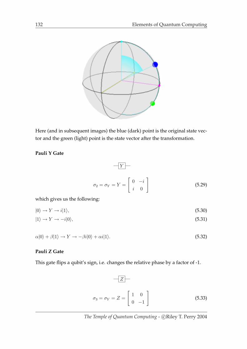
132 Elements of Quantum Computing
Here (and in subsequent images) the blue (dark) point is the original state vec-tor and the green (light) point is the state vector after the transformation.
Pauli Y Gate
Y
σ2 = σY = Y =
[0 −i
i 0
](5.29)
which gives us the following:
|0〉 → Y → i|1〉, (5.30)
|1〉 → Y → −i|0〉, (5.31)
α|0〉+ β|1〉 → Y → −βi|0〉+ αi|1〉. (5.32)
Pauli Z Gate
This gate flips a qubit’s sign, i.e. changes the relative phase by a factor of -1.
Z
σ3 = σY = Z =
[1 0
0 −1
](5.33)
The Temple of Quantum Computing - c©Riley T. Perry 2004
Elements of Quantum Computing 133
which gives us the following:
|0〉 → Z → |0〉, (5.34)
|1〉 → Z → −|1〉, (5.35)
α|0〉+ β|1〉 → Z → α|0〉 − β|1〉. (5.36)
Phase Gate
S
S =
[1 0
0 i
](5.37)
which gives us the following:
|0〉 → S → |0〉, (5.38)
|1〉 → S → i|1〉, (5.39)
α|0〉+ β|1〉 → S → α|0〉+ βi|1〉. (5.40)
Note, the Phase gate can be expressed in terms of the T gate (see below):
S = T 2 (5.41)
π8
Gate (T Gate)
T
T =
[1 0
0 ei π4
](5.42)
which gives us the following:
|0〉 → T → |0〉, (5.43)
|1〉 → T → ei π4 |1〉, (5.44)
α|0〉+ β|1〉 → T → α|0〉+ ei π4 β|1〉. (5.45)
If we apply T again we get the same as applying S once.
The Temple of Quantum Computing - c©Riley T. Perry 2004
134 Elements of Quantum Computing
Hadamard Gate
Sometimes called the square root of NOT gate, it turns a |0〉 or a |1〉 into a su-perposition (note the different sign). This gate is one of the most important inquantum computing. We’ll use this gate later for a demonstration of a simplealgorithm.
H
H =
[1 1
1 −1
](5.46)
which gives us the following:
|0〉 → H → 1√2(|0〉+ |1〉), (5.47)
|1〉 → H → 1√2(|0〉 − |1〉), (5.48)
α|0〉+ β|1〉 → H → α
( |0〉+ |1〉√2
)+ β
( |0〉 − |1〉√2
). (5.49)
Example Using H and Z gates and measuring in the |+〉, |−〉 basis.
(1) We can put |0〉 into state |+〉 by using an H gate:
|0〉 → H → 1√2(|0〉+ |1〉).
(2) We can put |0〉 into state |−〉 by using an H gate followed by a Z gate :
|0〉 → H → 1√2(|0〉+ |1〉) → Z → 1√
2(|0〉 − |1〉).
The operation of the H gate can be visualised on the Bloch sphere as follows:
The Temple of Quantum Computing - c©Riley T. Perry 2004
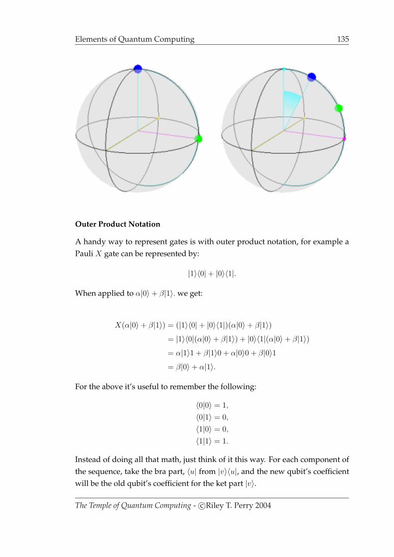
Elements of Quantum Computing 135
Outer Product Notation
A handy way to represent gates is with outer product notation, for example aPauli X gate can be represented by:
|1〉〈0|+ |0〉〈1|.
When applied to α|0〉+ β|1〉. we get:
X(α|0〉+ β|1〉) = (|1〉〈0|+ |0〉〈1|)(α|0〉+ β|1〉)= |1〉〈0|(α|0〉+ β|1〉) + |0〉〈1|(α|0〉+ β|1〉)= α|1〉1 + β|1〉0 + α|0〉0 + β|0〉1= β|0〉+ α|1〉.
For the above it’s useful to remember the following:
〈0|0〉 = 1,
〈0|1〉 = 0,
〈1|0〉 = 0,
〈1|1〉 = 1.
Instead of doing all that math, just think of it this way. For each component ofthe sequence, take the bra part, 〈u| from |v〉〈u|, and the new qubit’s coefficientwill be the old qubit’s coefficient for the ket part |v〉.
The Temple of Quantum Computing - c©Riley T. Perry 2004
136 Elements of Quantum Computing
Example Say we use this method on the Pauli Y outer product representa-tion,
i|1〉〈0| − i|0〉〈1|.When applied to |Ψ〉 = α|0〉+ β|1〉) we’ll see what we get:
The first part of the outer product notation is i|1〉〈0| so this means wetake the α|0〉 part of |Ψ〉 and convert it to iα|1〉 so our partially built statenow looks like:
|Ψ〉 = . . . + iα|1〉.Now we take the second part, −i|0〉〈1| and β|1〉 becomes −iβ|0〉 and finallywe get:
|Ψ〉 = −iβ|0〉+ iα|1〉.Finally, the coefficients of outer product representations are the same as thematrix entries, so for the matrix:
[α00 α01
α10 α11
].
The outer product representation looks like:
α00|0〉〈0|+ α01|0〉〈1|+ α10|1〉〈0|+ α11|1〉〈1|.
Further Properties of the Pauli Gates
Next we’ll look at the eigenvectors, eigenvalues, spectral decomposition, andouter product representation of the Pauli gates.
I has eigenvectors |0〉, and |1〉 with eigenvalues of 1 and 1 respectively. Us-ing the spectral decomposition theorem:
I = 1 · |0〉〈0|+ 1 · |1〉〈1|= |0〉〈0|+ |1〉〈1|. (5.50)
X has eigenvectors 1√2(|0〉+ |1〉), and 1√
2(|0〉 − |1〉) with eigenvalues of 1 and -1
The Temple of Quantum Computing - c©Riley T. Perry 2004

Elements of Quantum Computing 137
respectively.
X = 1 · 1√2(|0〉+ |1〉) 1√
2(〈0|+ 〈1|) + (−1) · 1√
2(|0〉 − |1〉) 1√
2(〈0| − 〈1|)
= |1〉〈0|+ |0〉〈1|. (5.51)
Y has eigenvectors 1√2(−i|0〉+ |1〉), and 1√
2(|0〉− i|1〉) with eigenvalues of 1 and
-1 respectively.
Y = 1 · 1√2(−i|0〉+ |1〉) 1√
2(i〈0|+ 〈1|) + (−1) · 1√
2(|0〉 − i|1〉) 1√
2(〈0|+ i〈1|)
= i|1〉〈0| − i|0〉〈1|. (5.52)
Z has eigenvectors |0〉, and |1〉 with eigenvalues of 1 and -1 respectively.
Z = 1 · |0〉〈0|+ (−1) · |1〉〈1|= |0〉〈0| − |1〉〈1|. (5.53)
The Pauli matrices are:
Unitary (σk)† = I ∀ k. (5.54)
Hermitian (σk)† = σk ∀ k. (5.55)
Rotation Operators
There are three useful operators that work well with the Bloch sphere. Theseare the rotation operators RX , RY , and RZ .
RX =
[cos θ
2−i sin θ
2
−i sin θ2
cos θ2
](5.56)
= e−iθX/2, (5.57)
RY =
[cos θ
2− sin θ
2
sin θ2
cos θ2
](5.58)
= e−iθY/2, (5.59)
RZ =
[e−iθ/2 0
0 e−iθ/2
](5.60)
= e−iθZ/2. (5.61)
The Temple of Quantum Computing - c©Riley T. Perry 2004
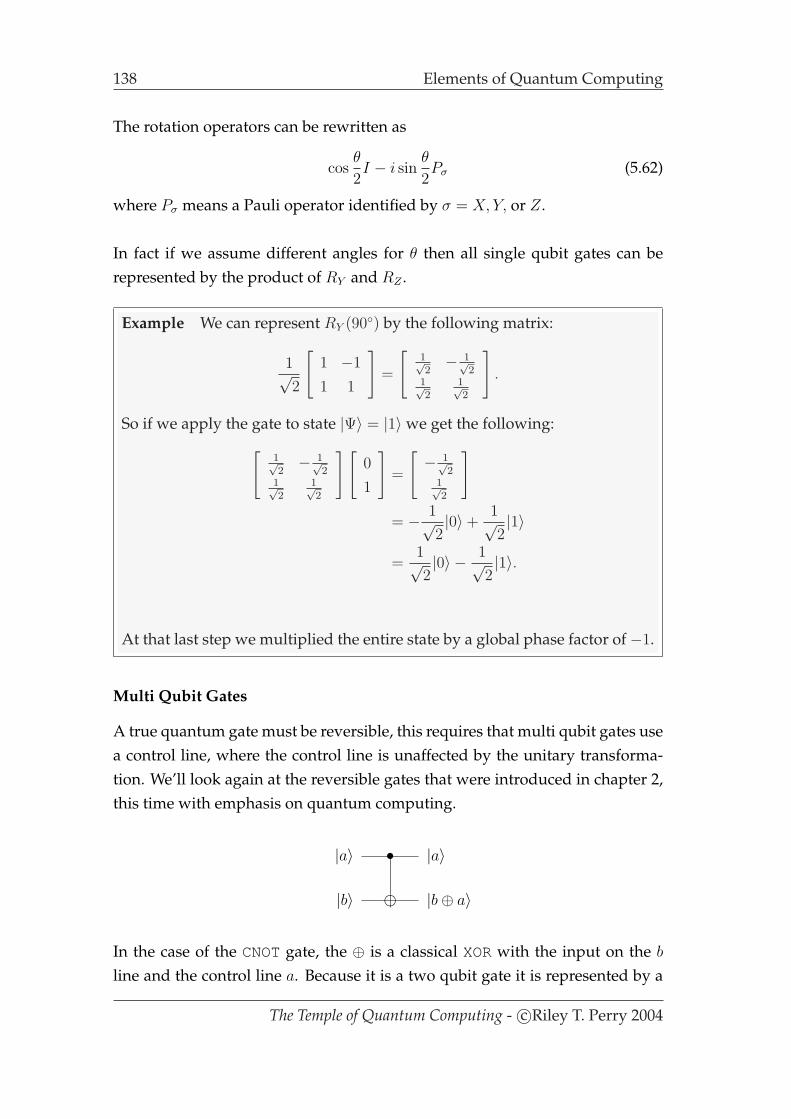
138 Elements of Quantum Computing
The rotation operators can be rewritten as
cosθ
2I − i sin
θ
2Pσ (5.62)
where Pσ means a Pauli operator identified by σ = X,Y, or Z.
In fact if we assume different angles for θ then all single qubit gates can berepresented by the product of RY and RZ .
Example We can represent RY (90) by the following matrix:
1√2
[1 −1
1 1
]=
[1√2− 1√
21√2
1√2
].
So if we apply the gate to state |Ψ〉 = |1〉 we get the following:[
1√2− 1√
21√2
1√2
][0
1
]=
[− 1√
21√2
]
= − 1√2|0〉+
1√2|1〉
=1√2|0〉 − 1√
2|1〉.
At that last step we multiplied the entire state by a global phase factor of −1.
Multi Qubit Gates
A true quantum gate must be reversible, this requires that multi qubit gates usea control line, where the control line is unaffected by the unitary transforma-tion. We’ll look again at the reversible gates that were introduced in chapter 2,this time with emphasis on quantum computing.
|a〉 • |a〉
|b〉 ÂÁÀ¿»¼½¾ |b⊕ a〉
In the case of the CNOTgate, the ⊕ is a classical XORwith the input on the b
line and the control line a. Because it is a two qubit gate it is represented by a
The Temple of Quantum Computing - c©Riley T. Perry 2004
Elements of Quantum Computing 139
4× 4 matrix:
1 0 0 0
0 1 0 0
0 0 0 1
0 0 1 0
(5.63)
which gives the following:
|00〉 → CNOT→ |00〉, (5.64)
|01〉 → CNOT→ |01〉, (5.65)
|10〉 → CNOT→ |11〉, (5.66)
|11〉 → CNOT→ |10〉, (5.67)
(α|0〉+ β|1〉)|1〉 → CNOT→ α|00〉+ β|10〉), (5.68)
|0〉(α|0〉+ β|1〉) → CNOT→ α|00〉+ β|01〉), (5.69)
|1〉(α|0〉+ β|1〉) → CNOT→ α|11〉+ β|10〉). (5.70)
Example Evaluating (α|0〉+ β|1〉)|0〉 → CNOT→ α|00〉+ β|11〉).
α|0〉+ β|1〉)|0〉 expanded is α|00〉+ β|10〉, so in matrix form we have:
1 0 0 0
0 1 0 0
0 0 0 1
0 0 1 0
α
0
β
0
=
α
0
0
β
= α|00〉+ β|11〉.
The Temple of Quantum Computing - c©Riley T. Perry 2004
140 Elements of Quantum Computing
Qubit Two NOTGate
As distinct from the CNOTgate we have a NOT2 gate, which just does NOTonqubit two and has the following matrix representation:
0 1 0 0
1 0 0 0
0 0 0 1
0 0 1 0
(5.71)
which gives the following:
|00〉 → NOT2 → |01〉, (5.72)
|01〉 → NOT2 → |00〉, (5.73)
|10〉 → NOT2 → |11〉, (5.74)
|11〉 → NOT2 → |10〉. (5.75)
Although it’s not a commonly used gate it’s interesting to note that the gatecan be represented as a Kronecker product of I and X as follows [Knill, E.Laflamme, R. Barnum, H. Dalvit, D. Dziarmaga, J. Gubernatis, J. Gurvits, L.Ortiz, G. Viola, L. & Zurek, W.H. 2002]:
NOT2 = I ⊗X =
[1 0
0 1
]⊗
[0 1
1 0
](5.76)
=
1
[0 1
1 0
]0
[0 1
1 0
]
0
[0 1
1 0
]1
[0 1
1 0
]
. (5.77)
So, as well as using the NOT2 notation we can use the tensor product of Pauligates on qubits one and two, shown below:
|00〉 → I ⊗X → |01〉, (5.78)
|01〉 → I ⊗X → |00〉, (5.79)
|10〉 → I ⊗X → |11〉, (5.80)
|11〉 → I ⊗X → |10〉. (5.81)
The Temple of Quantum Computing - c©Riley T. Perry 2004

Elements of Quantum Computing 141
Toffoli Gate
The Toffoli gate was first introduced in chapter 2. Here we’ll look at some prop-erties that relate to quantum computing. The most important property beingthat any classical circuit can be emulated by using Toffoli gates.
|a〉 • |a′〉|b〉 • |b′〉|c〉 ÂÁÀ¿»¼½¾ |c′〉
The Toffoli gate can simulate NANDgates and it can perform FANOUT, whichis classical bit copying (but we can’t copy superposed probability amplitudes).FANOUTis easy in classical computing, but impossible in quantum computingbecause of the no cloning theorem (see chapter 6).
A Toffoli gate can be simulated using a number of H, T, and S gates.
Fredkin Gate Also introduced in chapter 2, the Fredkin gate is another threequbit gate. This gate can simulate AND, NOT, CROSSOVER, and FANOUT, it alsohas the interesting property that it conserves 1’s.
|a〉 • |a′〉|b〉 × |b′〉|c〉 × |c′〉
The Temple of Quantum Computing - c©Riley T. Perry 2004

142 Important Properties of Quantum Circuits
Classical circuit
Quantum circuit
x f(x)
x f(x)
ancilla bits garbage bits
Figure 5.2: Garbage and ancilla bits.
5.2 Important Properties of Quantum Circuits
Quantum circuit diagrams have the following constraints which make themdifferent from classical diagrams.
1. They are acyclic (no loops).
2. No FANIN, as FANIN implies that the circuit is NOT reversible, and thereforenot unitary.
3. No FANOUT, as we can’t copy a qubit’s state during the computational phasebecause of the no-cloning theorem (explained in chapter 6).
All of the above can be simulated with the use of ancilla and garbage bits ifwe assume that no qubits will be in a superposition (figure 5.2). As statedin chapter 2, Garbage bits are useless qubits left over after computation andancilla bits are extra qubits needed for temporary calculations.
5.2.1 Common Circuits
Controlled U Gate
Let U be a unitary matrix, which uses an arbitrary number of qubits. A con-trolled U gate is a U gate with a control line, i.e. if the control qubit is |1〉 then
The Temple of Quantum Computing - c©Riley T. Perry 2004

Important Properties of Quantum Circuits 143
U acts on its data qubits, otherwise they are left alone.
•
U
Bit Swap Circuit
This circuit swaps the values of qubits between lines.
|a〉 • ÂÁÀ¿»¼½¾ • |b〉
|b〉 ÂÁÀ¿»¼½¾ • ÂÁÀ¿»¼½¾ |a〉
The circuit can be simplified to:
|a〉 × |b〉|b〉 × |a〉
Here are some examples:
|0〉 × |1〉|1〉 × |0〉
|1〉 × |0〉|0〉 × |1〉
Copying Circuit
If we have no superposition then we can copy bits in a classical sense with aCNOT.
The Temple of Quantum Computing - c©Riley T. Perry 2004
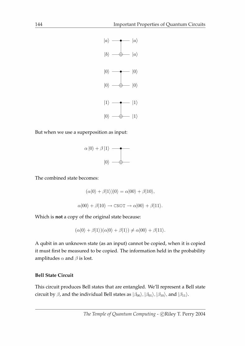
144 Important Properties of Quantum Circuits
|a〉 • |a〉
|b〉 ÂÁÀ¿»¼½¾ |a〉
|0〉 • |0〉
|0〉 ÂÁÀ¿»¼½¾ |0〉
|1〉 • |1〉
|0〉 ÂÁÀ¿»¼½¾ |1〉
But when we use a superposition as input:
α |0〉+ β |1〉 •
|0〉 ÂÁÀ¿»¼½¾
The combined state becomes:
(α|0〉+ β|1〉)|0〉 = α|00〉+ β|10〉,
α|00〉+ β|10〉 → CNOT→ α|00〉+ β|11〉.
Which is not a copy of the original state because:
(α|0〉+ β|1〉)(α|0〉+ β|1〉) 6= α|00〉+ β|11〉.
A qubit in an unknown state (as an input) cannot be copied, when it is copiedit must first be measured to be copied. The information held in the probabilityamplitudes α and β is lost.
Bell State Circuit
This circuit produces Bell states that are entangled. We’ll represent a Bell statecircuit by β, and the individual Bell states as |β00〉, |β01〉, |β10〉, and |β11〉.
The Temple of Quantum Computing - c©Riley T. Perry 2004

Important Properties of Quantum Circuits 145
|a〉 H • |a〉
|b〉 ÂÁÀ¿»¼½¾ |b⊕ a〉
|00〉 → β → 1√2(|00〉+ |11〉) = |β00〉,
|01〉 → β → 1√2(|01〉+ |10〉) = |β01〉,
|10〉 → β → 1√2(|00〉 − |11〉) = |β10〉,
|11〉 → β → 1√2(|01〉 − |10〉) = |β11〉.
Superdense Coding
It’s possible, by using entangled pairs, to communicate two bits of informationby transmitting one qubit. Here’s how:
1. Initially Alice and Bob each take one half of an EPR pair, say we start withβ00. This means that Alice has the bolded qubit in 1√
2(|00〉 − |11〉) and
Bob has the bolded qubit in 1√2(|00〉 − |11〉). They then move apart to an
arbitrary distance.
2. Depending on which value Alice wants to send to Bob, she applies a gate(or gates) to her qubit. This is described below and the combined state isshown after the gate’s operation with Alice’s qubit shown bolded:
|00〉 → I → 1√2(α|00〉+ β|11〉),
|01〉 → Z(Z|0〉 = |0〉, Z|1〉 = −|1〉) → 1√2(α|00〉 − β|11〉),
|10〉 → X(X|0〉 = |1〉, X|1〉 = |0〉) → 1√2(α|10〉+ β|01〉),
|11〉 → XZ → 1√2(α|10〉 − β|01〉).
3. Alice now sends her qubit to Bob via a classical channel.
The Temple of Quantum Computing - c©Riley T. Perry 2004

146 Important Properties of Quantum Circuits
4. Bob now uses a CNOTwhich allows him to ”factor out the second qubit”while the first one stays in a superposition.
1√2(α|00〉+ β|11〉) → CNOT→ 1√
2(α|00〉+ β|11〉) =
1√2(α|0〉+ β|1〉)|0〉,
1√2(α|10〉+ β|01〉) → CNOT→ 1√
2(α|11〉+ β|01〉) =
1√2(α|0〉+ β|1〉)|1〉,
1√2(α|00〉 − β|11〉) → CNOT→ 1√
2(α|00〉 − β|10〉) =
1√2(α|0〉 − β|1〉)|0〉,
1√2(α|01〉 − β|10〉) → CNOT→ 1√
2(α|01〉 − β|11〉) =
1√2(α|0〉 − β|1〉)|1〉.
5. Now Bob applies an H gate to the first bit to collapse the superposition.
1√2(α|0〉 − β|1〉) → H → |1〉,
1√2(α|0〉+ β|1〉) → H → |0〉.
So Bob gets the following:
1√2(α|0〉+ β|1〉)|0〉 → (H ⊗ I) → |00〉,
1√2(α|0〉+ β|1〉)|1〉 → (H ⊗ I) → |01〉,
1√2(α|0〉 − β|1〉)|0〉 → (H ⊗ I) → |10〉,
1√2(α|0〉 − β|1〉)|1〉 → (H ⊗ I) → |11〉.
Bob can now measure the two qubits in the computational basis and the resultwill be the value that Alice wanted to send.
Teleportation Circuit
Teleportation is basically the opposite of superdense coding, i.e. superdensecoding takes a quantum state to two classical bits. Teleportation takes two clas-sical bits to one quantum state.
Alice’s circuit
|Ψ〉 • HNM
°°°
β00ÂÁÀ¿»¼½¾
NM°°°
The Temple of Quantum Computing - c©Riley T. Perry 2004
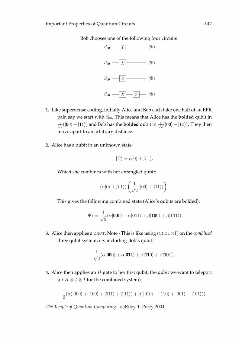
Important Properties of Quantum Circuits 147
Bob chooses one of the following four circuits
β00 I |Ψ〉
β00 X |Ψ〉
β00 Z |Ψ〉
β00 X Z |Ψ〉
1. Like superdense coding, initially Alice and Bob each take one half of an EPRpair, say we start with β00. This means that Alice has the bolded qubit in1√2(|00〉− |11〉) and Bob has the bolded qubit in 1√
2(|00〉− |11〉). They then
move apart to an arbitrary distance.
2. Alice has a qubit in an unknown state:
|Ψ〉 = α|0〉+ β|1〉.
Which she combines with her entangled qubit:
(α|0〉+ β|1〉)(
1√2(|00〉+ |11〉)
).
This gives the following combined state (Alice’s qubits are bolded):
|Ψ〉 =1√2(α|000〉+ α|011〉+ β|100〉+ β|111〉).
3. Alice then applies a CNOT. Note - This is like using (CNOT⊗I) on the combinedthree qubit system, i.e. including Bob’s qubit.
1√2(α|000〉+ α|011〉+ β|110〉+ β|101〉).
4. Alice then applies an H gate to her first qubit, the qubit we want to teleport(or H ⊗ I ⊗ I for the combined system):
1
2(α(|000〉+ |100〉+ |011〉+ |111〉) + β(|010〉 − |110〉+ |001〉 − |101〉)).
The Temple of Quantum Computing - c©Riley T. Perry 2004
148 The Reality of Building Circuits
Now we rearrange the state to move amplitudes α and β so that we canread the first two bits leaving the third in a superposition.
=1
2(|00〉α|0〉+ |10〉α|0〉+ |01〉α|1〉+ |11〉α|1〉+ |01〉β|0〉 − |11〉β|0〉
+ |00〉β|1〉 − |10〉β|1〉),=
1
2(|00〉(α|0〉+ β|1〉) + |01〉(α|1〉+ β|0〉) + |10〉(α|0〉 − β|1〉)
+ |11〉(α|1〉 − β|0〉)).
5. Alice now performs measurements on her state to determine which of theabove bolded states her qubits are in. She then communicates via a clas-sical channel what she measured (i.e. a |00〉, |01〉, |10〉, or a |11〉) to Bob.
6. Bob now may use X and/or Z gate(s) to fix up the phase and order of theprobability amplitudes, (he selects gates based on what Alice tells him)so that the result restores the original qubit. Summarised below are thegates he must use:
Case 00 = α|0〉+ β|1〉 → I → α|0〉+ β|1〉,Case 01 = α|1〉+ β|0〉 → X → α|0〉+ β|1〉,Case 10 = α|0〉 − β|1〉 → Z → α|0〉+ β|1〉,Case 11 = α|1〉 − β|0〉 → XZ → α|0〉+ β|1〉.
5.3 The Reality of Building Circuits
There is a general theorem: Any unitary operation on n qubits can be imple-mented using a set of two qubit operations. This can include CNOTs and othersingle bit operations. This result resembles the classical result that any booleanfunction can be implemented with NANDgates. This is helpful because some-times we are limited in what we can use to build a quantum circuit.
5.3.1 Building a Programmable Quantum Computer
Is it Possible to Build a Programmable Quantum Computer
Can we build a programmable quantum computer? This means a quantumcomputer that has an architecture similar to Von Neumann (or Harvard) archi-tecture? No! This is because:
The Temple of Quantum Computing - c©Riley T. Perry 2004
The Four Postulates of Quantum Mechanics 149
Distinct unitary operators U0...Un require orthogonal programs |U0〉, ...|Un〉[Nielsen, M. A. 2002]
This is called the no programming theorem.
If we were to have a programmable quantum computer our ”program” wouldconsist of one or more unitary operators. Since there are an infinite number ofthese unitary operators the program register would have to be infinite in size(that is our input to the quantum computer that contains the program) [Nielsen,M. A. 2002].
5.4 The Four Postulates of Quantum Mechanics
Now we can look at the four postulates in a bit more detail than in chapter 4,in terms of quantum computing.
5.4.1 Postulate One
An isolated system has an associated complex vector space called a state space.We will use a state space called a Hilbert space.
The state of the quantum system can be described by a unit vector in this spacecalled a state vector.
Example The simplest system we are interested in is a qubit which is in C2.A qubit is a unit vector |Ψ〉 inC. Most of the time we’ll attach an orthonormalbasis (like |0〉, |1〉). Our qubit can be described by:
|Ψ〉 = α|0〉+ β|1〉 =
[α
β
]
here α and β are known as probability amplitudes and we say the qubit is ina quantum superposition of states |0〉 and |1〉.
5.4.2 Postulate Two
Simple form
The Temple of Quantum Computing - c©Riley T. Perry 2004
150 The Four Postulates of Quantum Mechanics
An isolated (closed) system’s evolution can be described by a unitary trans-form.
|Ψ′〉 = U |Ψ〉. (5.82)
Form including time
If we include time (as quantum interactions happen in continuous time):
|Ψ(t2)〉 = U(t1, t2)|Ψ(t1)〉 (5.83)
here t1 and t2 are points in time and U(t1, t2) is a unitary operator than can varywith time.
We can also say that the process is reversible, because:
U †U |Ψ〉 = |Ψ〉. (5.84)
The history of the quantum system does not matter as it is completely describedby the current state (this is know as a Markov process).
Note: We can rewrite the above in terms of Schrodinger’s equation, but thatis beyond the scope of this paper.
5.4.3 Postulate Three
Simple form
This deals with what happens if |Ψ〉 is measured in an orthonormal basis:
|O1〉, |O1〉, . . . , |On〉.We’ll measure a particular outcome j with probability:
pr(j) = |〈Oj|Ψ〉|2. (5.85)
Example If we measure in the computational basis we have:
pr(0) = |〈0|Ψ〉|2
= |〈0|(α |0〉+ β |1〉)|2
= |α|2
and pr(1) = |β|2.
The Temple of Quantum Computing - c©Riley T. Perry 2004

The Four Postulates of Quantum Mechanics 151
After the measurement the system is in state |Oj〉. This is because measure-ment disturbs the system.
If |u1〉 and |u2〉 are not orthogonal (i.e. 〈u1|u2〉 6= 0) then we can’t reliably dis-tinguish between them on measurement.
Projectors
Suppose we have a larger quantum system which is a combination of smallersystems, i.e. we have an orthonormal basis A = |e1〉, . . . , |en〉 where n is thedimension of A. Then we have a larger quantum system B such that A ⊂ B.
If we measure A what is the effect on B?
We can say that |O1〉, . . . , |On〉 is part of or comprised of one or many of theorthogonal subspaces V1, V2, . . . , Vm which are connected in the following way:
V = V1 ⊕ V2 ⊕ . . .⊕ Vm. (5.86)
Example The state vectoe:
|Ψ〉 = (α|O1〉+ β|O2〉) + γ|O3〉
can be rewritten as:
V (|O1〉, |O2〉, |O3〉) = V1(|e1〉, |e2〉)⊕ V2(|e3〉).
We can use projectors (P1, . . . , Pm) to filter out everything other than the sub-space we are looking for (i.e. everything orthogonal to our subspace V ).
Example From the last example, projector P1 on V1(|e1〉, |e2〉) gives us:
P1(α|e1〉+ β|e2〉+ γ|e3〉) = α|e1〉+ β|e2〉.
The Temple of Quantum Computing - c©Riley T. Perry 2004
152 The Four Postulates of Quantum Mechanics
Formally, if P1, . . . , Pm is a set of projectors which covers all the orthogonalsubspaces of the state space, upon measuring |Ψ〉 we have,
pr(j) = 〈Ψ|Pj|Ψ〉 (5.87)
leaving the system in the post measurement state:
Pj|Ψ〉√〈Ψ|Pj|Ψ〉. (5.88)
Example Given a qutrit |Ψ〉 = α|0〉+ β|1〉+ γ|2〉).
P1 on V1(|0〉, |1〉) and P2 on V2(|2〉) gives us:
pr(1) = 〈Ψ|P1|Ψ〉
= [α∗β∗γ∗]
α
β
0
= |α|2 + |β|2,pr(2) = 〈Ψ|P2|Ψ〉
= [α∗β∗γ∗]
0
0
γ
= |γ|2.
So our separated look like this:
|Ψ1〉 =P1|Ψ〉√〈Ψ|P1|Ψ〉
=α|0〉+ β|1〉√|α|2 + |β|2 ,
|Ψ2〉 =P2|Ψ〉√〈Ψ|P2|Ψ〉
=γ|2〉√|γ|2 .
The Temple of Quantum Computing - c©Riley T. Perry 2004

The Four Postulates of Quantum Mechanics 153
More importantly we can look at partial measurement of a group of qubits, thefollowing example uses the tensor product which is also part of postulate 4. Ifthe system to be measured in the basis |O1〉, |O2〉 then we use the projectorwith a tensor product with I on the qubit we don’t want to measure. e.g. for|O2〉 of qubit two we use (I ⊗ P2).
Example If |Ψ〉 = α00|00〉+ α01|01〉+ α10|10〉+ α11|11〉:
For measuring qubit one in the computational basis we get |0〉 withprobability:
pr(0) = 〈Ψ|P0 ⊗ I|Ψ〉= (α00|00〉+ α01|01〉+ α10|10〉+ α11|11〉) • (α00|00〉+ α01|01〉)= |α00|2 + |α01|2.
There is another type of measurement called a POVM (Positive Operator Val-ued Measure) of which projectors are a certain type. POVMs are beyond thescope of this text.
5.4.4 Postulate Four
A tensor product of the components of a composite physical system, describesthe system. So the state spaces of the individual systems are combined so:
Cn ⊗ Cn = Cn2
. (5.89)
An example is on the next page.
The Temple of Quantum Computing - c©Riley T. Perry 2004

154 The Four Postulates of Quantum Mechanics
Example C4 ⊗ C4 = C16 can look like:
(|ΨA〉 = |1〉+ |2〉+ |3〉+ |4〉)⊗ (|ΨB〉 = |a〉+ |b〉+ |c〉+ |d〉)
and can be written as:
|ΨAB〉 = |1a〉+ |1b〉+ |1c〉+ . . . + |4d〉.
Example If Alice has |ΨA〉 = |u〉 and Bob has |ΨB〉 = |v〉, if their systemsare combined the joint state is:
|ΨAB〉 = |u〉 ⊗ |v〉.
If Bob applies gate U to this system it means I ⊗ U is applied to the jointsystem.
Example Given the following:
|Ψ〉 =√
0.1|00〉+√
0.2|01〉+√
0.3|10〉+√
0.4|11〉
then,
|Ψ〉 → (I ⊗X) → |Ψ〉 =√
0.1|01〉+√
0.2|00〉+√
0.3|11〉+√
0.4|10〉,
|Ψ〉 → (X ⊗ I) → |Ψ〉 =√
0.1|10〉+√
0.2|11〉+√
0.3|00〉+√
0.4|01〉.
The Temple of Quantum Computing - c©Riley T. Perry 2004
Chapter 6
Information Theory
6.1 Introduction
Information theory examines the ways information can be represented andtransformed efficiently [Steane, A. M. 1998]. This information can be repre-sented in many different ways to express the same meaning. E.g. ”How areyou?” and ”Comment allez vous?” express the same meaning. All knownways of representing this information must have a physical medium like mag-netic storage or ink on paper. The Information stored on a particular physicalmedium is not ”tied” to that medium and can be converted from one form toanother. If we consider information in these terms then it becomes a propertylike energy that can be transferred from one physical system to another.
We are interested in quantum information, which has many parallels in con-ventional information theory. Conventional information theory relies heavilyon the classical theorems of Claude E. Shannon, 1916 - 2001 (figure 6.1). Thereare a number of quantum equivalents for the various parts of his classical the-orems. In this chapter we’ll look at these and other related topics like quantumerror correction, and quantum cryptology. Also, as promised, there is a fairlyin-depth section on Bell states and the chapter ends with some open questionson the nature of information and alternate methods of computation.
As with chapter 5 individual references to QCQI have been dropped as theywould appear too frequently.
155
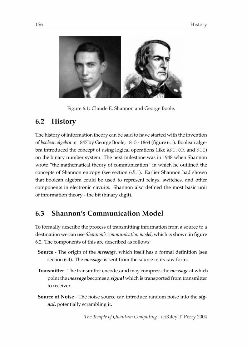
156 History
Figure 6.1: Claude E. Shannon and George Boole.
6.2 History
The history of information theory can be said to have started with the inventionof boolean algebra in 1847 by George Boole, 1815 - 1864 (figure 6.1). Boolean alge-bra introduced the concept of using logical operations (like AND, OR, and NOT)on the binary number system. The next milestone was in 1948 when Shannonwrote ”the mathematical theory of communication” in which he outlined theconcepts of Shannon entropy (see section 6.5.1). Earlier Shannon had shownthat boolean algebra could be used to represent relays, switches, and othercomponents in electronic circuits. Shannon also defined the most basic unitof information theory - the bit (binary digit).
6.3 Shannon’s Communication Model
To formally describe the process of transmitting information from a source to adestination we can use Shannon’s communication model, which is shown in figure6.2. The components of this are described as follows:
Source - The origin of the message, which itself has a formal definition (seesection 6.4). The message is sent from the source in its raw form.
Transmitter - The transmitter encodes and may compress the message at whichpoint the message becomes a signal which is transported from transmitterto receiver.
Source of Noise - The noise source can introduce random noise into the sig-nal, potentially scrambling it.
The Temple of Quantum Computing - c©Riley T. Perry 2004

Shannon’s Communication Model 157
Figure 6.2: Shannon’s communication model.
Receiver - The receiver may decode and decompress the signal back into theoriginal message.
Destination - The destination of the raw message.
6.3.1 Channel Capacity
A message is chosen from a set of all possible messages and then transmitted.Each symbol transferred takes a certain amount of time (which is called thechannel capacity).
Shannon’s name for channel capacity on a binary channel is ”one bit per timeperiod” e.g. 56, 000 bits per second. His expression for capacity is:
C = limT→∞
log2 N
T(6.1)
where N is the number of possible messages of length T .
The Temple of Quantum Computing - c©Riley T. Perry 2004
158 Classical Information Sources
Example For binary we have:
2 bits = 4 different messages in 2 time periods.3 bits = 8 different messages in 3 time periods.
so,N(T ) = 2T
and,
C =log2 N
T
= 1 bit per time period.
Example Another example is morse code, where dashes take longer totransmit than dots. If dashes are represented by 1110 and a dot is 10 forthis we have:
C = 0.34 bit per time period.
6.4 Classical Information Sources
A source of information produces a discrete set of symbols from a specific al-phabet. The alphabet that is most commonly used is binary (1 and 0), but itcould in principle be any series of symbols.
The way an information source can be modelled is via a probability that cer-tain letters or combinations of letters (words) will be produced by the source.An example for this probability distribution would be, given an unknown book -one could, in advance, predict to a certain degree of accuracy the frequency ofwords and letters within the book [Nielsen, M. A. 2002].
6.4.1 Independent Information Sources
An independent and identically Distributed (IID) information source is an infor-mation source in which each output has no dependency on other outputs fromthe source, and furthermore each output has the same probability of occurring
The Temple of Quantum Computing - c©Riley T. Perry 2004

Classical Information Sources 159
each time it is produced [Nielsen, M. A. 2002].
An IID is an information source with an alphabet (i.e a set of symbols or out-puts ai):
A = a1, . . . , an (6.2)
with probabilities pr(a1),pr(a2), . . . ,pr(an) such that:n∑
i=1
pr(ai) = 1 where 0 ≤ pr(ai) ≤ 1 ∀ i. (6.3)
This source will produce a letter with probability pr(ai) with no dependencyon the previous symbols. Independent information sources are also called zeromemory information sources (i.e. they correspond to a Markov process).
Example [Nielsen, M. A. 2002] A biased coin is a good example of an IID.The biased coin has a probability p of heads and a probability of 1−p of tails.Given a language
∑= heads, tails:
pr(heads) = 0.3,
pr(tails) = 0.7 .
Our coin will come up tails 70% of the time.
Strictly speaking, Shannon’s results only hold for a subset of information sourcesthat conform to the following:
1. Symbols must be chosen with fixed probabilities, one by one with no depen-dency on current symbols and preceding choices.
2. An information source must be an ergodic source. This means that thereshould be no statistical variation (with a probability of 1) between possi-ble sources. I.e. all systems should have the same probabilities for lettersto appear in their alphabets.
Not many sources are perfect like the above. The reason is that, for examplea book has correlations between syllables, words, etc. (not just letters) like”he” and ”wh” [Nielsen, M. A. 2002]. We can measure certain qualities andthe source becomes more like an IID (like JUST letter frequency). Shannonsuggested that most information sources can be approximated.
The Temple of Quantum Computing - c©Riley T. Perry 2004

160 Classical Redundancy and Compression
6.5 Classical Redundancy and Compression
Compression of data means using less information to represent a message andreconstructing it after it has been transmitted. When we talk about compressionin this section we mean simple algorithmic compression that can be applied toall information sources. This is distinct from say, changing the text in a sen-tence to convey the same meaning or using special techniques to only workon a subset of messages or information sources (like using a simple formula toexactly represent a picture of a sphere).
We often talk about using a coding K to represent our message. Formally, acoding is a function that takes a source alphabet A to a coding alphabet B, i.e.K : A → B. For every symbol a in the language A, K(a) is a word with lettersfrom B.
A word, w = a1a2 . . . an in A is found by:
K(w) = K(a1)K(a2) . . . K(an). (6.4)
Example A simple coding.
A = A,B, C, D,B = 0, 1.
Possible encodings are:A → 0001,
B → 0101,
C → 1001,
D → 1111.
So we encode the word ABBA as:
K(ABBA) = 0001 0101 0101 0001.
Length of Codes
We define the size of an alphabet A as |A| and the length of a word w can beshown with |w|.
The Temple of Quantum Computing - c©Riley T. Perry 2004

Classical Redundancy and Compression 161
Example |A| and |w|.
A = a, b, c, d, e, f,B = 0, 1, 2.
Possible encodings are:
a → 0,
b → 1,
c → 20,
d → 220,
e → 221,
f → 222.
We get:|K(a)| = 1, |K(c)| = 2, |K(f)| = 3, |A| = 6, |B| = 3.
6.5.1 Shannon’s Noiseless Coding Theorem
Shannon demonstrated that there is a definite limit to how much an informa-tion source can be compressed. Shannon Entropy H(S) is the minimum numberof bits needed to convey a message. For a source S the entropy is related to theshortest average length coding Lmin(S) by:
H(S) ≤ Lmin(S) ≤ H(S) + 1. (6.5)
We can find the Shannon Entropy, of a particular source distribution measuredin bits by:
H(X) = −∑
i
pri log2 pri. (6.6)
Here, log2 (a log of base 2) means that the Shannon entropy is measured in bits.pri is a measure of probability (i.e. the frequency with which it is emitted) for asymbol being generated by the source and the summation is a sum over all thesymbols i = 1, 2, . . . , n generated by the source.
The Temple of Quantum Computing - c©Riley T. Perry 2004

162 Classical Redundancy and Compression
Example Random and dependent sources.
Random Each symbol is chosen from the source totally randomly (with Aand B having equal probability), with no dependencies, this source isuncompressible with Shannon Entropy of 1 bit per symbol.
Dependent Every second symbol is exactly the same as the last, which ischosen randomly (e.g. AABBBBAABB). This has Shannon Entropy of12
bit(s) per symbol.
Example We have a language A,B, C, D, E of symbols occurring withthe following frequency:
A = 0.5, B = 0.2, C = 0.1, D = 0.1, E = 0.1 .
The entropy is:
H(X) = −[(0.5 log2 0.5 + 0.2 log2 0.2 + (0.1 log2 0.1)× 3)]
= −[−0.5 + (−0.46438) + (−0.9965)]
= −[−1.9]
= 1.9.
So we need 2 bits per symbol to convey the message.
The minimum entropy is realised when the information source produces a sin-gle letter constantly, this gives us a probability of 1 for that letter.
The maximum entropy is realised when we have no information about theprobability distribution of the source alphabet (when all symbols are equallylikely to occur).
A special case of the entropy is binary entropy where the source has just twosymbols with probabilities of p and 1 − p like the biased coin toss for exam-ple. Note a fair coin toss has maximum entropy of 1 bit and a totally unfair,weighted coin that always comes up heads or tails has minimum entropy of 0
bits.
The Temple of Quantum Computing - c©Riley T. Perry 2004

Classical Redundancy and Compression 163
6.5.2 Quantum Information Sources
Shannon entropy gives us a lower bound on how many bits we need to storea particular piece of information. The question is, is there any difference whenwe use quantum states? The answer is yes if we use a superposition.
If the qubits involved are in well defined states (like |0〉 and |1〉) a semiclas-sical coin toss [Nielsen, M. A. 2002] gives us:
|0〉 with probability of 12,
|1〉 with probability of 12,
H
(1
2
)= 1.
If we replace one of these states with a superposition then a ”quantum cointoss” gives us:
|0〉 with probability of 12,
|0〉+|1〉√2
with probability of 12,
H
(1 + 1√
2
2
)= 0.6 .
Better than Shannon’s rate!
Generally a quantum information source produces state: |Ψj〉 with probabil-ities pr(j), and our quantum compression performs better than the Shannonrate H(pr(j)).
6.5.3 Pure and Mixed States
A quantum system is said to be in a pure state if its state is well defined. Thisdoes not mean the state vector will always collapse to a known value; but atleast the state vector is known as distinct from what it collapses to. For examplegiven a photon and a polariser the photon can be in three states, horizontal (H),vertical (V), and diagonal (D). If we make our photon diagonal at 45 then we
The Temple of Quantum Computing - c©Riley T. Perry 2004

164 Classical Redundancy and Compression
have an equal superposition of H and V.
|D〉 =1√2|H〉+
1√2|V〉.
Now if we measure polarisation we have a 50% chance of detecting an |H〉 or a50% of detecting a |V〉. The state was well defined before measurement, so wecall it pure (i.e. we have a well defined angle of polarisation viz 45, and if wemeasure with a polariser in this direction the result is certain). We don’t havethis situation if there is no direction in which the result is certain. So the state isnot well defined and we call this state mixed. For example, if we have a numberof photons, 50% of which are polarised horizontally and 50% vertically, now wehave a mixed state. Each photon has a well defined state |H〉 or |V〉, but not thegroup. This situation is indistinguishable from a photon that is in an entangledstate.
When closed quantum systems get affected by external systems our pure statescan get entangled with the external world, leading to mixed states. This iscalled decoherence, or in information theory terms, noise.
It is possible to have a well defined (pure) state that is composed of subsys-tems in mixed states. Entangled states like Bell states are well defined for thecomposite system (whole), but the state of each component qubit is not welldefined, i.e. mixed.
6.5.4 Schumacher’s Quantum Noiseless Coding Theorem
The quantum analogue of Shannon’s noiseless coding theorem is Schumacher’squantum noiseless coding theorem. Which is as follows [Nielsen, M. A. 2002]:
The best data rate R achievable is S(ρ). (6.7)
where S is Von Neumann entropy and ρ is the density matrix. ρ holds equivalentinformation to the quantum state Ψ and quantum mechanics can be formulatedin terms of ρ as an alternative to Ψ. We now look at ρ.
The Density Matrix
In studying quantum noise it turns out to be easier to work with the densitymatrix than the state vector (think of it as just a tool; not a necessary compo-
The Temple of Quantum Computing - c©Riley T. Perry 2004

Classical Redundancy and Compression 165
nent of quantum computing).
According to Nielsen [Nielsen, M. A. 2002] there are three main approachesto the density matrix, the ensemble point of view, subsystem, and fundamentalapproaches. They are described briefly here:
Ensemble - This is the basic view of the density matrix which gives us mea-surement statistics in a compact form.
Subsystem - If quantum system A is coupled to another quantum system Bwe can’t always give A a state vector on its own (it is not well defined).But we can assign an individual density matrix to either subsystem.
Fundamental - It is possible to restate the four postulates of quantum mechan-ics in terms of the density matrix.
For example, as mentioned above, we can view the statistics generated by anentangled photon as equivalent to that of the corresponding ensemble.
Ensemble Point of View
Consider a collection of identical quantum systems in states in |Ψj〉 with prob-abilities prj . The probability of outcome k when a measurement, which is de-scribed by Pk, is:
k = tr(ρPk) (6.8)
where,
ρ =∑
j
prj|ψj〉〈ψj| (6.9)
is the density matrix. ρ completely determines the measurement statistics. Theset of all probabilities and their associated state vectors prj, |ψj〉 is called anensemble of pure states.
If a measurement is done, with projectors Pk on a system with density matrix ρ
the post measurement density matrix ρk is:
ρk =PkρPk
tr(PkρPk). (6.10)
The Temple of Quantum Computing - c©Riley T. Perry 2004
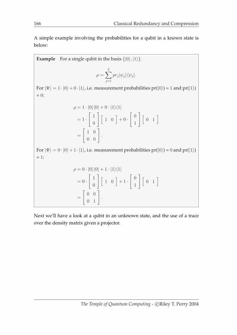
166 Classical Redundancy and Compression
A simple example involving the probabilities for a qubit in a known state isbelow:
Example For a single qubit in the basis |0〉, |1〉.
ρ =2∑
j=1
prj|ψj〉〈ψj|.
For |Ψ〉 = 1 · |0〉+ 0 · |1〉, i.e. measurement probabilities pr(|0〉) = 1 and pr(|1〉)= 0:
ρ = 1 · |0〉〈0|+ 0 · |1〉〈1|
= 1 ·[
1
0
] [1 0
]+ 0 ·
[0
1
] [0 1
]
=
[1 0
0 0
].
For |Ψ〉 = 0 · |0〉+ 1 · |1〉, i.e. measurement probabilities pr(|0〉) = 0 and pr(|1〉)= 1:
ρ = 0 · |0〉〈0|+ 1 · |1〉〈1|
= 0 ·[
1
0
] [1 0
]+ 1 ·
[0
1
] [0 1
]
=
[0 0
0 1
].
Next we’ll have a look at a qubit in an unknown state, and the use of a traceover the density matrix given a projector.
The Temple of Quantum Computing - c©Riley T. Perry 2004

Classical Redundancy and Compression 167
Example Given measurement probabilities pr(|0〉) = p and pr(|1〉) = 1− p.
ρ = p|0〉〈0|+ (1− p)|1〉〈1|
= p
[1
0
] [1 0
]+ (1− p)
[0
1
] [0 1
]
= p
[1 0
0 0
]+ 1− p
[0 0
0 1
]
=
[p 0
0 1− p
].
So, given a density matrix ρ and a projector P = |0〉〈0| we can extract thefinal probability from ρ, say we measure in an orthonormal basis, |0〉, |1〉then:
pr(|0〉) = tr(ρ|0〉〈0|)
= tr
([p 0
0 1− p
] [1 0
0 0
])
= tr
([p 0
0 0
])
= p + 0
= p,
pr(|1〉) = tr(ρ|1〉〈1|)
= tr
([p 0
0 1− p
] [0 0
0 1
])
= tr
([0 0
0 1− p
])
= 0 + (1− p)
= 1− p.
How does a the density matrix evolve?
Suppose a unitary transform U is applied to a quantum system: i.e. U |Ψ〉;
The Temple of Quantum Computing - c©Riley T. Perry 2004

168 Classical Redundancy and Compression
what is the new density matrix? To answer this, using the ensemble view, wecan say that if the system can be in states |Ψj〉 with probabilities trj then, afterthe evolution occurs, it will be in state U |Ψ〉 with probabilities prj .
Initially we have ρ =∑
j prj|ψj〉〈ψj|. So, after U is applied, we have:
ρ′ =∑
j
prjU |ψj〉〈ψj|U † (6.11)
= U
(∑j
prjU |ψj〉〈ψj|)
U † (6.12)
= UρU †. (6.13)
Note that when |ψj〉 goes to U |ψj〉, 〈ψj| = |ψj〉† goes to (U |ψj〉)† = 〈ψj|U †.
Example Given measurement probabilities pr(|0〉) = p and pr(|1〉) = 1 − p
then ρ =
[p 0
0 1− p
].
If X is applied to ρ then:
ρ′ = XρX
=
[1− p 0
0 p
].
Example For |Ψ〉 = 1√2|00〉+ 1√
2|11〉 we have pr(|00〉) = 1
2and pr(|11〉) = 1
2.
This gives us a what is called completely mixed state and ρ = I2. So,
ρ′ = UI
2U †
=I
2because UU † = 1.
Properties:
tr(ρ) = 1. (6.14)
ρ is a positive matrix. (6.15)
Subsystem Point of View
The density matrix can describe any subsystem of a larger quantum system,including mixed subsystems. Subsystems are described by a reduced density
The Temple of Quantum Computing - c©Riley T. Perry 2004
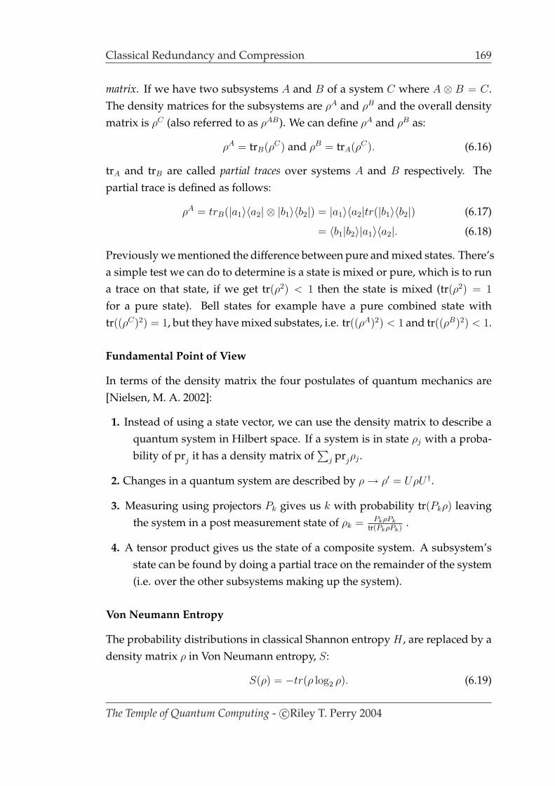
Classical Redundancy and Compression 169
matrix. If we have two subsystems A and B of a system C where A ⊗ B = C.The density matrices for the subsystems are ρA and ρB and the overall densitymatrix is ρC (also referred to as ρAB). We can define ρA and ρB as:
ρA = trB(ρC) and ρB = trA(ρC). (6.16)
trA and trB are called partial traces over systems A and B respectively. Thepartial trace is defined as follows:
ρA = trB(|a1〉〈a2| ⊗ |b1〉〈b2|) = |a1〉〈a2|tr(|b1〉〈b2|) (6.17)
= 〈b1|b2〉|a1〉〈a2|. (6.18)
Previously we mentioned the difference between pure and mixed states. There’sa simple test we can do to determine is a state is mixed or pure, which is to runa trace on that state, if we get tr(ρ2) < 1 then the state is mixed (tr(ρ2) = 1
for a pure state). Bell states for example have a pure combined state withtr((ρC)2) = 1, but they have mixed substates, i.e. tr((ρA)2) < 1 and tr((ρB)2) < 1.
Fundamental Point of View
In terms of the density matrix the four postulates of quantum mechanics are[Nielsen, M. A. 2002]:
1. Instead of using a state vector, we can use the density matrix to describe aquantum system in Hilbert space. If a system is in state ρj with a proba-bility of prj it has a density matrix of
∑j prjρj .
2. Changes in a quantum system are described by ρ → ρ′ = UρU †.
3. Measuring using projectors Pk gives us k with probability tr(Pkρ) leavingthe system in a post measurement state of ρk = PkρPk
tr(PkρPk).
4. A tensor product gives us the state of a composite system. A subsystem’sstate can be found by doing a partial trace on the remainder of the system(i.e. over the other subsystems making up the system).
Von Neumann Entropy
The probability distributions in classical Shannon entropy H , are replaced by adensity matrix ρ in Von Neumann entropy, S:
S(ρ) = −tr(ρ log2 ρ). (6.19)
The Temple of Quantum Computing - c©Riley T. Perry 2004
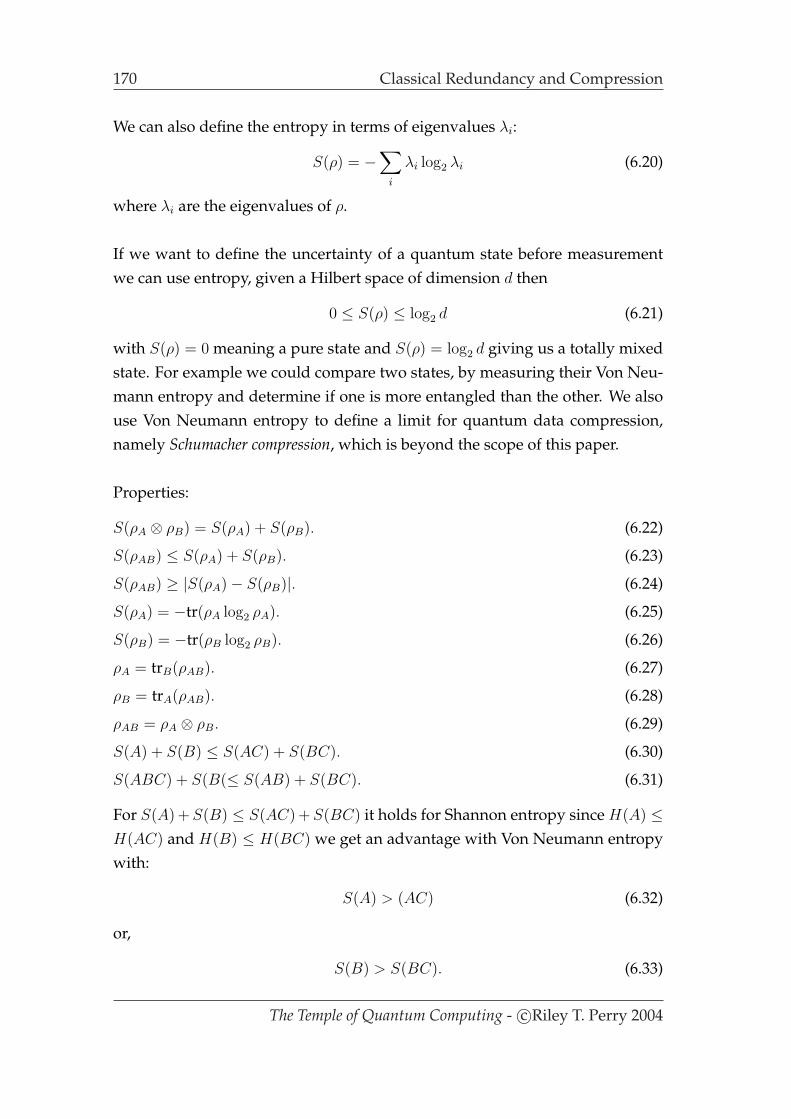
170 Classical Redundancy and Compression
We can also define the entropy in terms of eigenvalues λi:
S(ρ) = −∑
i
λi log2 λi (6.20)
where λi are the eigenvalues of ρ.
If we want to define the uncertainty of a quantum state before measurementwe can use entropy, given a Hilbert space of dimension d then
0 ≤ S(ρ) ≤ log2 d (6.21)
with S(ρ) = 0 meaning a pure state and S(ρ) = log2 d giving us a totally mixedstate. For example we could compare two states, by measuring their Von Neu-mann entropy and determine if one is more entangled than the other. We alsouse Von Neumann entropy to define a limit for quantum data compression,namely Schumacher compression, which is beyond the scope of this paper.
Properties:
S(ρA ⊗ ρB) = S(ρA) + S(ρB). (6.22)
S(ρAB) ≤ S(ρA) + S(ρB). (6.23)
S(ρAB) ≥ |S(ρA)− S(ρB)|. (6.24)
S(ρA) = −tr(ρA log2 ρA). (6.25)
S(ρB) = −tr(ρB log2 ρB). (6.26)
ρA = trB(ρAB). (6.27)
ρB = trA(ρAB). (6.28)
ρAB = ρA ⊗ ρB. (6.29)
S(A) + S(B) ≤ S(AC) + S(BC). (6.30)
S(ABC) + S(B(≤ S(AB) + S(BC). (6.31)
For S(A) + S(B) ≤ S(AC) + S(BC) it holds for Shannon entropy since H(A) ≤H(AC) and H(B) ≤ H(BC) we get an advantage with Von Neumann entropywith:
S(A) > (AC) (6.32)
or,
S(B) > S(BC). (6.33)
The Temple of Quantum Computing - c©Riley T. Perry 2004
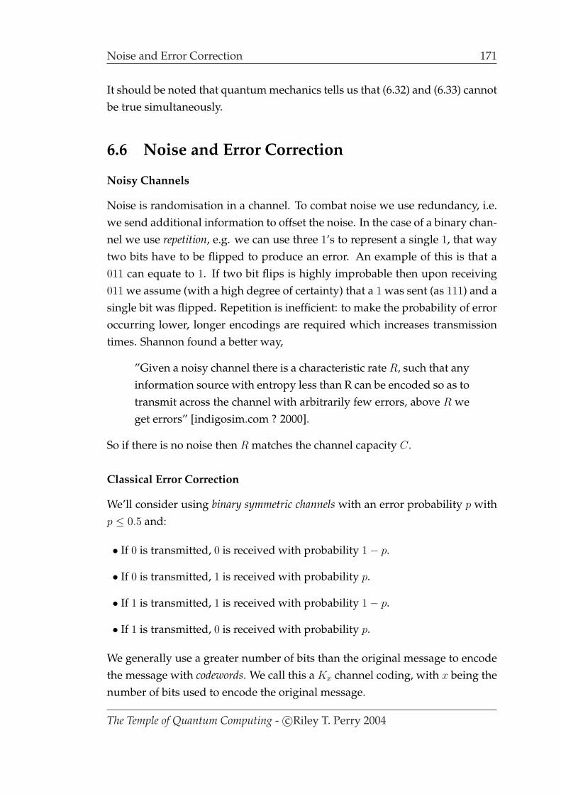
Noise and Error Correction 171
It should be noted that quantum mechanics tells us that (6.32) and (6.33) cannotbe true simultaneously.
6.6 Noise and Error Correction
Noisy Channels
Noise is randomisation in a channel. To combat noise we use redundancy, i.e.we send additional information to offset the noise. In the case of a binary chan-nel we use repetition, e.g. we can use three 1’s to represent a single 1, that waytwo bits have to be flipped to produce an error. An example of this is that a011 can equate to 1. If two bit flips is highly improbable then upon receiving011 we assume (with a high degree of certainty) that a 1 was sent (as 111) and asingle bit was flipped. Repetition is inefficient: to make the probability of erroroccurring lower, longer encodings are required which increases transmissiontimes. Shannon found a better way,
”Given a noisy channel there is a characteristic rate R, such that anyinformation source with entropy less than R can be encoded so as totransmit across the channel with arbitrarily few errors, above R weget errors” [indigosim.com ? 2000].
So if there is no noise then R matches the channel capacity C.
Classical Error Correction
We’ll consider using binary symmetric channels with an error probability p withp ≤ 0.5 and:
• If 0 is transmitted, 0 is received with probability 1− p.
• If 0 is transmitted, 1 is received with probability p.
• If 1 is transmitted, 1 is received with probability 1− p.
• If 1 is transmitted, 0 is received with probability p.
We generally use a greater number of bits than the original message to encodethe message with codewords. We call this a Kx channel coding, with x being thenumber of bits used to encode the original message.
The Temple of Quantum Computing - c©Riley T. Perry 2004

172 Noise and Error Correction
If we have a code (called a binary block code) K of length n it has an infor-mation rate of:
R(K) =k
n(6.34)
if it has 2k codewords (k = 1 in the example below).
This means, we have an original message of k bits and we use codewords on n
bits.
Repetition Codes
Using repetition codes we have a greater chance of success by increasing thenumber of coding bits for a bit to be transmitted and averaging the result bits.Repetition codes have an information rate of R(K) = 1
n.
Example A K3 channel coding could be:
0 → 000,
1 → 111.
With a channel decoding of:
000 → 0, 001 → 0, 010 → 0, 100 → 0,
111 → 0, 110 → 0, 101 → 0, 011 → 0.
So our information rate is:R(K3) =
1
3.
So, bit flips in 1 out of 3 bits in codeword are fixable, but the informationrate is down to 1
3.
6.6.1 Quantum Noise
In practice we cannot make perfect measurements and it’s hard to prepare andapply quantum gates to perfect quantum states because real quantum systemsare quite noisy.
The Temple of Quantum Computing - c©Riley T. Perry 2004

Noise and Error Correction 173
6.6.2 Quantum Error Correction
Quantum error correction codes have been successfully designed, but the areastill remains a hot topic. Some scientists still believe that quantum computingmay be impossible due to decoherence which is external influences destroyingor damaging quantum states. We use quantum error correction codes in placeof classical ones. The fact that they are quantum gives us a number of extraproblems:
1. No Cloning.
2. Continuous errors, many types of error can occur on a single qubit (not justa bit flip as with a classical circuit). E.g. we might have a change of phase:α|0〉+ β|1〉 → α|0〉+ eiθβ|1〉.
3. Measurement destroys quantum information (so if we used a repetition code,how do we apply majority logic to recover the qubits?).
Below are some simple examples of quantum errors.
Example A qubit’s relative phase gets flipped:
a|0〉+ b|1〉 → a|0〉 − b|1〉.Example A qubit’s amplitudes get flipped:
a|0〉+ b|1〉 → b|0〉+ a|1〉.Example A qubit’s amplitudes and relative phase get flipped:
a|0〉+ b|1〉 → b|0〉 − a|1〉.
Quantum Repetition Code
A quantum repetition code is the analogue of a classical repetition code, forclassical states (states not in a superposition) this is easy:
|0〉 → |000〉,
|1〉 → |111〉.
The Temple of Quantum Computing - c©Riley T. Perry 2004
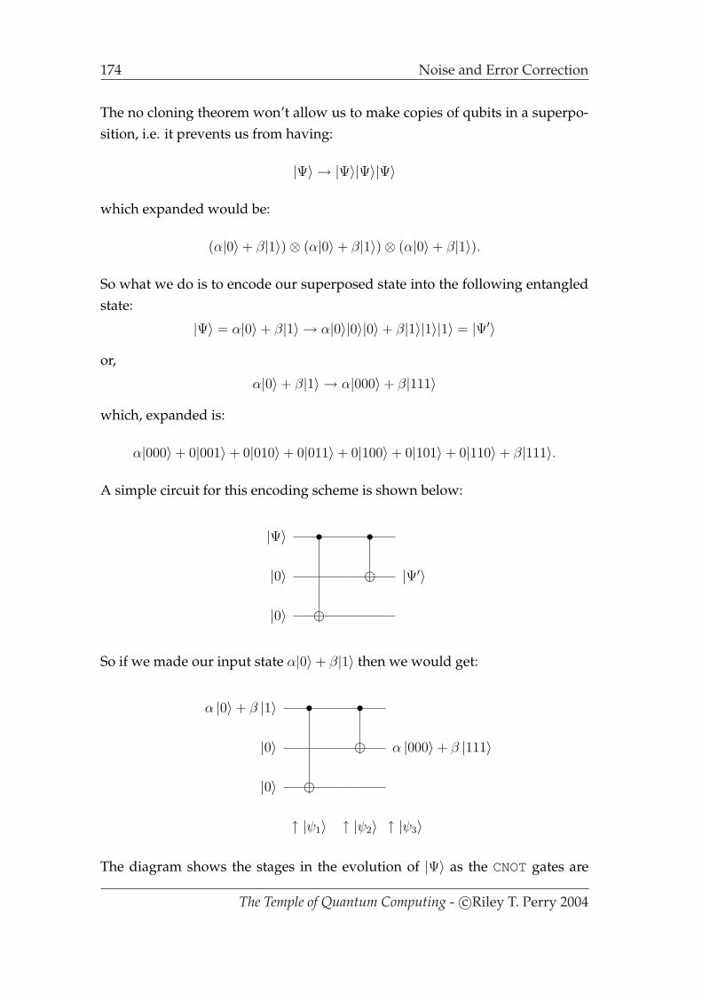
174 Noise and Error Correction
The no cloning theorem won’t allow us to make copies of qubits in a superpo-sition, i.e. it prevents us from having:
|Ψ〉 → |Ψ〉|Ψ〉|Ψ〉
which expanded would be:
(α|0〉+ β|1〉)⊗ (α|0〉+ β|1〉)⊗ (α|0〉+ β|1〉).
So what we do is to encode our superposed state into the following entangledstate:
|Ψ〉 = α|0〉+ β|1〉 → α|0〉|0〉|0〉+ β|1〉|1〉|1〉 = |Ψ′〉
or,
α|0〉+ β|1〉 → α|000〉+ β|111〉
which, expanded is:
α|000〉+ 0|001〉+ 0|010〉+ 0|011〉+ 0|100〉+ 0|101〉+ 0|110〉+ β|111〉.
A simple circuit for this encoding scheme is shown below:
|Ψ〉 • •
|0〉 ÂÁÀ¿»¼½¾ |Ψ′〉
|0〉 ÂÁÀ¿»¼½¾
So if we made our input state α|0〉+ β|1〉 then we would get:
α |0〉+ β |1〉 • •
|0〉 ÂÁÀ¿»¼½¾ α |000〉+ β |111〉
|0〉 ÂÁÀ¿»¼½¾
↑ |ψ1〉 ↑ |ψ2〉 ↑ |ψ3〉
The diagram shows the stages in the evolution of |Ψ〉 as the CNOTgates are
The Temple of Quantum Computing - c©Riley T. Perry 2004
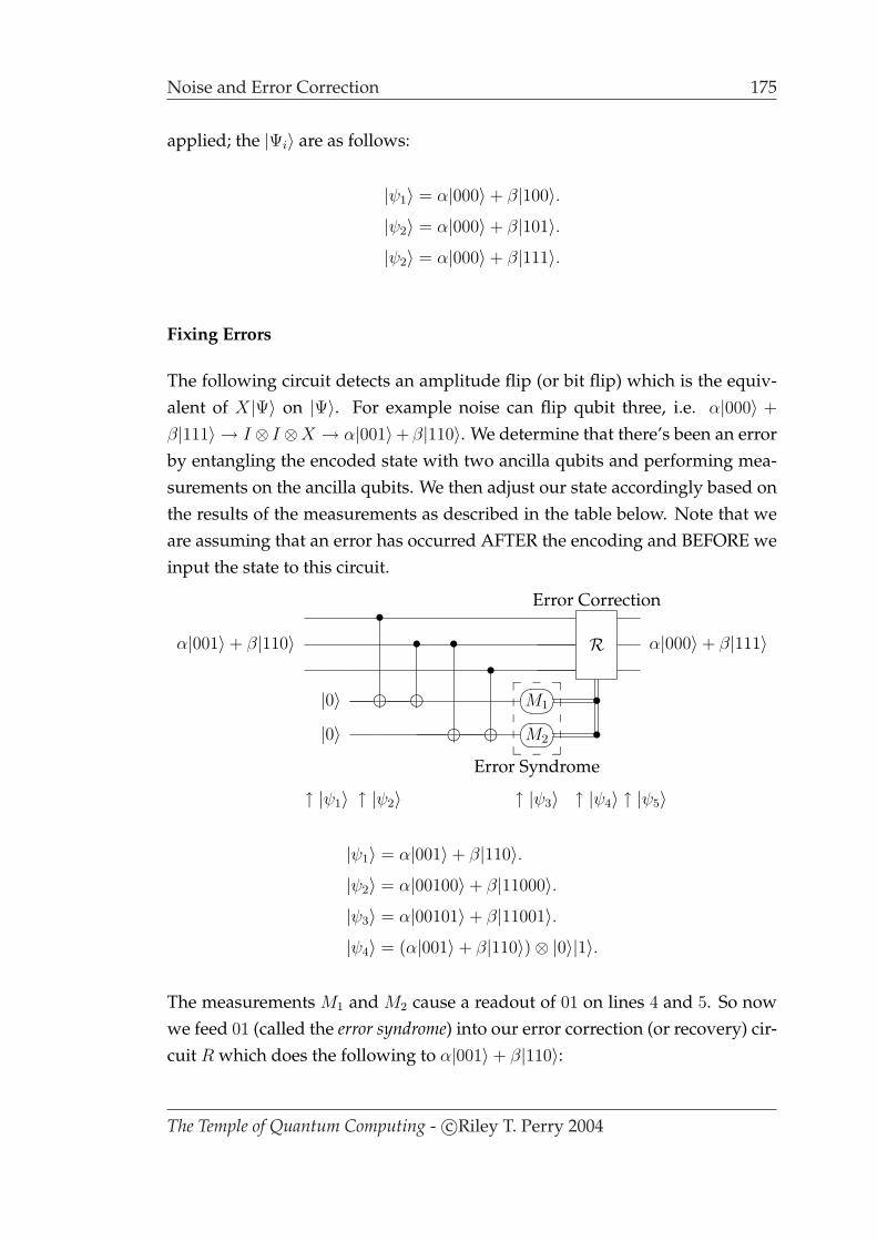
Noise and Error Correction 175
applied; the |Ψi〉 are as follows:
|ψ1〉 = α|000〉+ β|100〉.|ψ2〉 = α|000〉+ β|101〉.|ψ2〉 = α|000〉+ β|111〉.
Fixing Errors
The following circuit detects an amplitude flip (or bit flip) which is the equiv-alent of X|Ψ〉 on |Ψ〉. For example noise can flip qubit three, i.e. α|000〉 +
β|111〉 → I ⊗ I ⊗X → α|001〉+ β|110〉. We determine that there’s been an errorby entangling the encoded state with two ancilla qubits and performing mea-surements on the ancilla qubits. We then adjust our state accordingly based onthe results of the measurements as described in the table below. Note that weare assuming that an error has occurred AFTER the encoding and BEFORE weinput the state to this circuit.
Error Correction•
Rα|001〉+ β|110〉 • • α|000〉+ β|111〉•
|0〉 ÂÁÀ¿»¼½¾ ÂÁÀ¿»¼½¾ 76 5401 23M1 •|0〉 ÂÁÀ¿»¼½¾ ÂÁÀ¿»¼½¾ 76 5401 23M2
_ _ _ÂÂÂÂÂ
ÂÂÂÂÂ
_ _ _•
Error Syndrome
↑ |ψ1〉 ↑ |ψ2〉 ↑ |ψ3〉 ↑ |ψ4〉 ↑ |ψ5〉
|ψ1〉 = α|001〉+ β|110〉.|ψ2〉 = α|00100〉+ β|11000〉.|ψ3〉 = α|00101〉+ β|11001〉.|ψ4〉 = (α|001〉+ β|110〉)⊗ |0〉|1〉.
The measurements M1 and M2 cause a readout of 01 on lines 4 and 5. So nowwe feed 01 (called the error syndrome) into our error correction (or recovery) cir-cuit R which does the following to α|001〉+ β|110〉:
The Temple of Quantum Computing - c©Riley T. Perry 2004

176 Noise and Error Correction
M1 M2 Action0 0 no action needed, e.g. |111〉 → |111〉0 1 flip qubit 3, e.g. |110〉 → |111〉1 0 flip qubit 2, e.g. |101〉 → |111〉1 1 flip qubit 1, e.g. |011〉 → |111〉
So we apply a qubit flip to line 3 giving:
|ψ5〉 = α|000〉+ β|111〉.
This circuit will fix a single bit flip in our three qubit repetition code. All that re-mains is to decode |Ψ〉 to return to our original state. We get a problem thoughif we have a relative phase error, i.e.:
α|000〉+ β|111〉 → α|000〉 − β|111〉
which, decoded is:
α|0〉+ β|1〉 → α|0〉 − β|1〉.
It turns out we have to change our encoding method to deal with a relativephase flip, which we can do with the following circuit:
α |0〉+ β |1〉 • • H
|0〉 ÂÁÀ¿»¼½¾ H
|0〉 ÂÁÀ¿»¼½¾ H
The error correction circuit for a relative phase flip is almost exactly the same asthe error correction circuit for an amplitude flip, we just add in some Hadamardgates at the start to deal with the superpositions we generated with the initialencoding (shown immediately above). Again remember that any errors thatdo happen, happen between the encoding and the circuit we are about to intro-duce:
The Temple of Quantum Computing - c©Riley T. Perry 2004
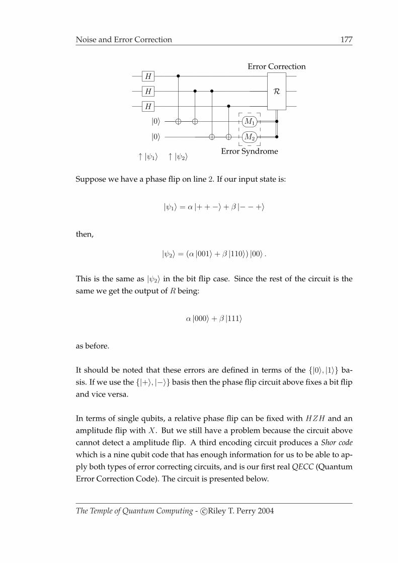
Noise and Error Correction 177
Error CorrectionH •
RH • •H •|0〉 ÂÁÀ¿»¼½¾ ÂÁÀ¿»¼½¾ 76 5401 23M1 •|0〉 ÂÁÀ¿»¼½¾ ÂÁÀ¿»¼½¾ 76 5401 23M2
_ _ _ÂÂÂÂÂ
ÂÂÂÂÂ
_ _ _•
Error Syndrome↑ |ψ1〉 ↑ |ψ2〉
Suppose we have a phase flip on line 2. If our input state is:
|ψ1〉 = α |+ +−〉+ β |− −+〉
then,
|ψ2〉 = (α |001〉+ β |110〉) |00〉 .
This is the same as |ψ2〉 in the bit flip case. Since the rest of the circuit is thesame we get the output of R being:
α |000〉+ β |111〉
as before.
It should be noted that these errors are defined in terms of the |0〉, |1〉 ba-sis. If we use the |+〉, |−〉 basis then the phase flip circuit above fixes a bit flipand vice versa.
In terms of single qubits, a relative phase flip can be fixed with HZH and anamplitude flip with X . But we still have a problem because the circuit abovecannot detect a amplitude flip. A third encoding circuit produces a Shor codewhich is a nine qubit code that has enough information for us to be able to ap-ply both types of error correcting circuits, and is our first real QECC (QuantumError Correction Code). The circuit is presented below.
The Temple of Quantum Computing - c©Riley T. Perry 2004

178 Bell States
|Ψ〉 • • H • •
|0〉 ÂÁÀ¿»¼½¾
|0〉 ÂÁÀ¿»¼½¾
|0〉 ÂÁÀ¿»¼½¾ H • •
|0〉 ÂÁÀ¿»¼½¾
|0〉 ÂÁÀ¿»¼½¾
|0〉 ÂÁÀ¿»¼½¾ H • •
|0〉 ÂÁÀ¿»¼½¾
|0〉 ÂÁÀ¿»¼½¾
The Shor code is one of many QECCs, another example is the Steane code. Theseboth in turn are CSS codes (Calderbank, Shor, Steane). CSS codes are part of amore general group of QECCs called Stabiliser codes.
6.7 Bell States
As mentioned in chapter 4 the EPR experiment showed that entangled particlesseem to communicate certain quantum information instantly over an arbitrarydistance upon measurement. Einstein used this as an argument against thenotion that particles had no defined state until they were measured (i.e. he ar-gued that they had ”hidden variables”). John Bell, 1928 - 1990 proved in 1964that there could be no local hidden variables. In the following description ofhis proof consider the fact that we can measure the spin of a particle in severaldifferent directions which can be thought of as measuring in different bases.During this section we’ll refer to Einstein’s position as EPR and the quantummechanical position as QM.
The Temple of Quantum Computing - c©Riley T. Perry 2004

Bell States 179
Bell takes a system of two entangled spin particles being measured by tworemote observers (observers 1 and 2, say, who observe particles 1 and 2, respec-tively). He shows that, if the observers measure spin in the same direction (e.g.z) there is no empirical difference between the results predicted by the two po-sitions (QM or EPR). For the purposes of our example we’ll begin by definingthe following entangled state:
|ΨA〉 =1√2|0112〉 − 1√
2|1102〉. (6.35)
We’ve introduced the notation |0112〉 to distinguish between qubits 1 and 2,which will become important later.
If we allow the directions to be different it is possible to get a empiricallytestable difference. The intuition for this is that if, as QM says, what happens atobserver 2 is dependent on what happens at observer 1, and the latter is depen-dent on the direction at 1, then what happens at 2 will involve both directions(we imagine that a measurement at 1, in some direction, causes state collapseso that particle 2 ”points” in the antiparallel direction to 1 and is then measuredin observer 2’s direction; the probability for an outcome, spin up or spin down,is dependent on the angle between the two directions - see below). Whereas,in the EPR view, what happens at observer 2 cannot in any way involve the di-rection at observer 1: what happens at observer 2 will, at most, be determinedby the value particle 2 carries away at emission and the direction at observer 2.
6.7.1 Same Measurement Direction
To see that same direction measurements cannot lead to a testable differencefirst imagine that there are two separated observers, Alice and Bob, who runmany trials of the EPR experiment with spin particles. Let each measure thespin of the particle that flies towards them. If they both measure in the samedirection, say z, then the results might be represented as follows:
Alice Bob Frequencyz z
1 0 50%
0 1 50%
The Temple of Quantum Computing - c©Riley T. Perry 2004
180 Bell States
We soon realise that we can’t use this case to discriminate between the two po-sitions.
QM position. This explains the result by saying that, upon Alice’s measure-ment of 1, the state vector superposition |ΨA〉 collapses into one or other of thetwo terms.
either |0112〉 or |1102〉
with 50% probability for Alice measuring 0 or 1. But then we no longer havea superposition (Alice’s measurement has ”produced” a 0 on particle 1 and a1 on particle 2, or vice versa) and Bob’s measurement outcome on 2 is com-pletely determined (relative to the outcome on 1) and will be the opposite ofAlice’s outcome.
EPR position. This says the particles actually have well defined values at themoment they are emitted, and these are (anti-)correlated and randomly dis-tributed between 01 and 10 over repeated trials. When Alice measures 0 Bobmeasures 1 not because Alice’s measurement has ”produced” anything; butsimply because the 1 is the value the particle had all along (which the measure-ment reveals). The randomness here is due to initial conditions (emission); notto collapse.
Either way we have the same prediction.
6.7.2 Different Measurement Directions
Bell’s innovation was to realise that a difference will occur if we bring in differ-ent measurement directions. The intuition for this might go as follows.
Suppose there are two directions a(= z) and b. Start with |ΨA〉 and allow Aliceto measure particle 1 in the a direction. This causes a collapse, as before, andwe have:
either |0112〉 or |1102〉.
Alice’s measurement has ”produced” a 1 (spin down) in the a direction on par-ticle 2 (to take the first case). Bob now measures particle 2 in the b direction. Towork out what happens according to QM we have to express |12〉 in terms of a
The Temple of Quantum Computing - c©Riley T. Perry 2004

Bell States 181
b basis. If b is at angle θ to a this turns out to be:
|12〉 = sin
(θ
2
)|+2〉+ cos
(θ
2
)|−2〉 (6.36)
where |+2〉 means spin up along the b axis. This looks right. If θ = 90 (the casewhen b = x) we get 1√
2, as before; when θ = 0 (the case when b = z) we get |−2〉
(= |1〉 in that case). Likewise, for |02〉:
|02〉 = cos
(θ
2
)|+2〉 − sin
(θ
2
)|−2〉. (6.37)
The significant point is that, since θ is the angle between a and b, the directionof Alice’s measurement is entering into (influencing) what happens for Bob.
But this can’t happen in a realist local view as, espoused by EPR, because:
1. The spin values of the particles are determined at the moment of emission,and are not ”produced” at some later moment as a result of an act ofmeasurement (realism);
2. by construction, the events at Bob’s end are beyond the reach of the eventsat Alice’s end (locality).
The rat is cornered: by bringing different directions of measurement into it, weshould get a detectable difference. So reasons Bell.
6.7.3 Bell’s Inequality
It turns out we need three directions. So allow Alice and Bob to measure inthree possible directions labelled a, b, and c; we will actually take the case wherethese directions are all in the plane, perpendicular to line of flight, and at 120
to one another. When Alice and Bob measure in the same direction, say a anda, they will observe correlation: 1 with 0, or 0 with 1, as above. However, ifthey measure in different directions, say a and b, there is no requirement forcorrelation, and Alice and Bob might both observe 1, for example (as in row 3
below).
QM View
If we put θ = 120 into 6.38 we have:
|12〉 =
√3
2|+2〉+ 1/2|−2〉.
The Temple of Quantum Computing - c©Riley T. Perry 2004
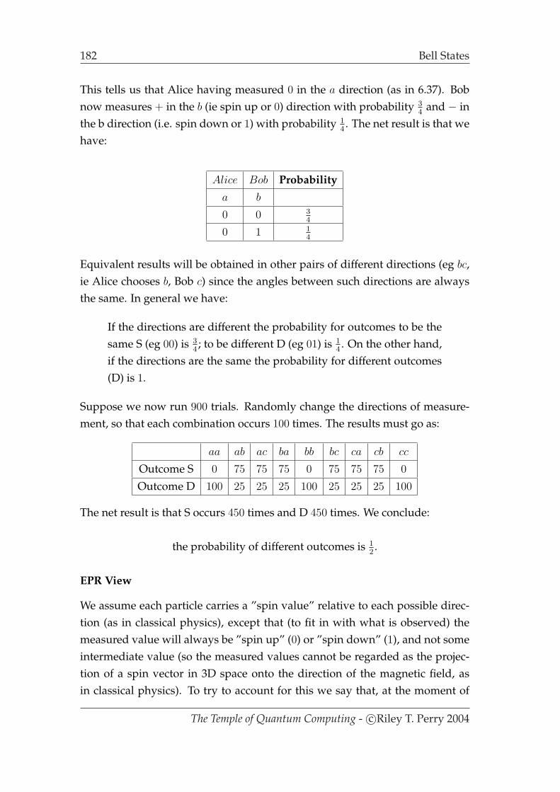
182 Bell States
This tells us that Alice having measured 0 in the a direction (as in 6.37). Bobnow measures + in the b (ie spin up or 0) direction with probability 3
4and − in
the b direction (i.e. spin down or 1) with probability 14. The net result is that we
have:
Alice Bob Probabilitya b
0 0 34
0 1 14
Equivalent results will be obtained in other pairs of different directions (eg bc,ie Alice chooses b, Bob c) since the angles between such directions are alwaysthe same. In general we have:
If the directions are different the probability for outcomes to be thesame S (eg 00) is 3
4; to be different D (eg 01) is 1
4. On the other hand,
if the directions are the same the probability for different outcomes(D) is 1.
Suppose we now run 900 trials. Randomly change the directions of measure-ment, so that each combination occurs 100 times. The results must go as:
aa ab ac ba bb bc ca cb cc
Outcome S 0 75 75 75 0 75 75 75 0
Outcome D 100 25 25 25 100 25 25 25 100
The net result is that S occurs 450 times and D 450 times. We conclude:
the probability of different outcomes is 12.
EPR View
We assume each particle carries a ”spin value” relative to each possible direc-tion (as in classical physics), except that (to fit in with what is observed) themeasured value will always be ”spin up” (0) or ”spin down” (1), and not someintermediate value (so the measured values cannot be regarded as the projec-tion of a spin vector in 3D space onto the direction of the magnetic field, asin classical physics). To try to account for this we say that, at the moment of
The Temple of Quantum Computing - c©Riley T. Perry 2004

Bell States 183
emission, each particle leaves with an ”instruction” (the particle’s property, orhidden variable, or key, or component) - one for each possible direction (a, b, c)
in which it can be measured - which determines the measured outcome in thatdirection (in the conventional, pre-quantum, sense that the measurement justdiscovers or reveals what is already there). Since the measurement in the a di-rection can discover two possible values, 0 or 1, the corresponding property,which we call the A component, must have two values: either A=0, or A=1,which determines the measurement outcome (as noted above, we cannot allowrandomness in the act of measurement - this would destroy the aa correlation,etc ; the only possible randomness that can occur is in the assignment of initialcomponent values at the moment of emission, see below). Likewise, we haveB=0 or B=1; and C=0 or C=1. (It might seem we need an infinity of these prop-erties to cater for the infinity of possible measurement directions. This doesn’tconstitute a problem in classical physics where we have spin behaving like amagnetic needle: the infinity of possible observed components of the magneticmoment, dependent on measurement direction, is no more mysterious than theinfinity of shadow lengths projected by a stick dependent on the sun’s direc-tion. But note that it would seem strange to account for the infinity of shadowlength’s by saying the stick had an infinity of components - or ”instructions” -specifying what shadow should appear, depending on the angle of the sun!).
The A,B,C values are set for each particle at the time of emission and carried offby them. They can be randomly assigned except that, to obey conservation, ifA=0 for particle 1 then A=1 for particle 2 etc. But we can have A=0 for particle1 and B=0 for particle 2 since, empirically, the spins are not correlated if wemeasure in different directions (in this case if the measurements were in the a
and b directions the result would be 00).
Suppose particle 1 has the assignment A=0, B=1, C=1; ie 011. Interestingly, weimmediately know what the components for particle 2 must be: A=1, B=0, C=0;ie 100. This is necessary if the two particles are going to give anti-correlated re-sults for the case where we do same direction measurements in each direction(a, b, c).
We can then lay out the possible assignments of component values, as follows:
The Temple of Quantum Computing - c©Riley T. Perry 2004
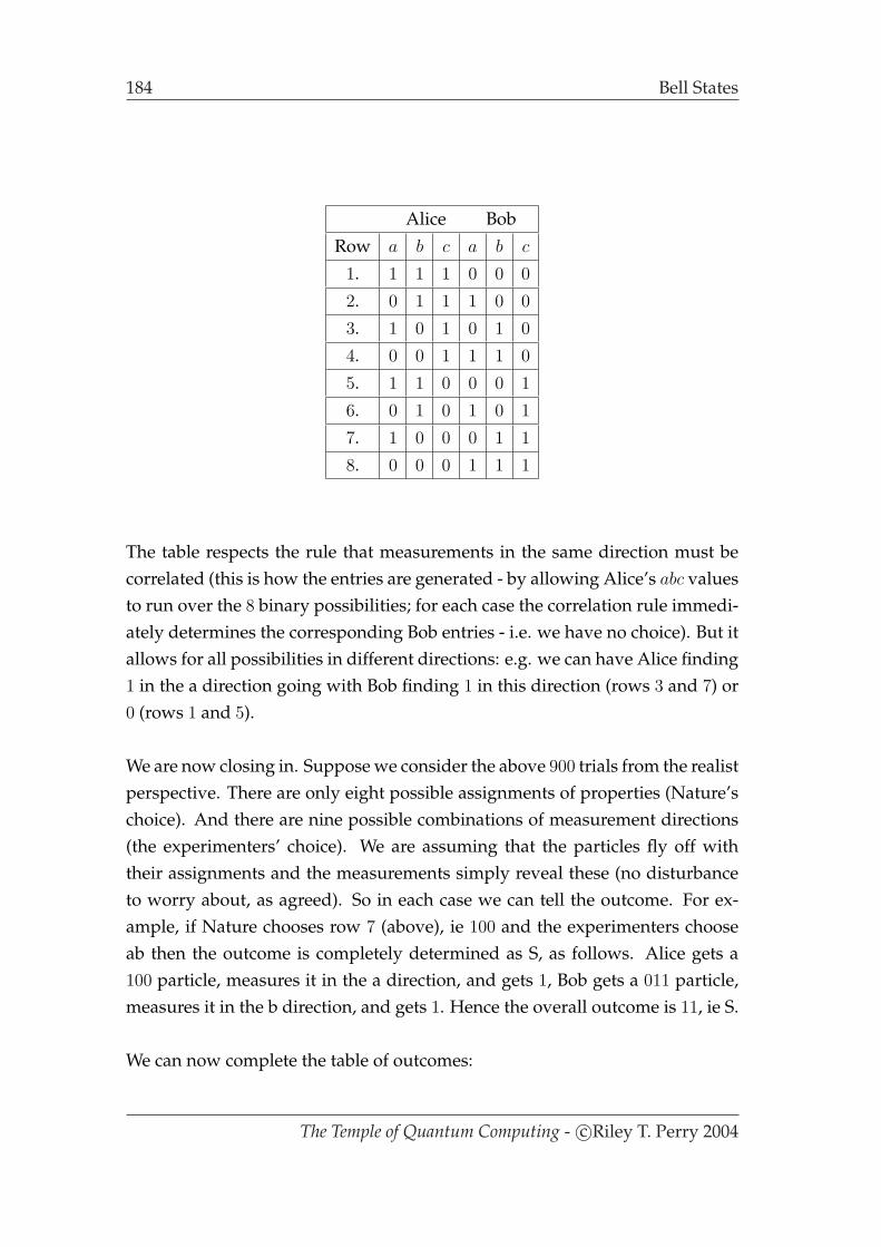
184 Bell States
Alice Bob
Row a b c a b c
1. 1 1 1 0 0 0
2. 0 1 1 1 0 0
3. 1 0 1 0 1 0
4. 0 0 1 1 1 0
5. 1 1 0 0 0 1
6. 0 1 0 1 0 1
7. 1 0 0 0 1 1
8. 0 0 0 1 1 1
The table respects the rule that measurements in the same direction must becorrelated (this is how the entries are generated - by allowing Alice’s abc valuesto run over the 8 binary possibilities; for each case the correlation rule immedi-ately determines the corresponding Bob entries - i.e. we have no choice). But itallows for all possibilities in different directions: e.g. we can have Alice finding1 in the a direction going with Bob finding 1 in this direction (rows 3 and 7) or0 (rows 1 and 5).
We are now closing in. Suppose we consider the above 900 trials from the realistperspective. There are only eight possible assignments of properties (Nature’schoice). And there are nine possible combinations of measurement directions(the experimenters’ choice). We are assuming that the particles fly off withtheir assignments and the measurements simply reveal these (no disturbanceto worry about, as agreed). So in each case we can tell the outcome. For ex-ample, if Nature chooses row 7 (above), ie 100 and the experimenters chooseab then the outcome is completely determined as S, as follows. Alice gets a100 particle, measures it in the a direction, and gets 1, Bob gets a 011 particle,measures it in the b direction, and gets 1. Hence the overall outcome is 11, ie S.
We can now complete the table of outcomes:
The Temple of Quantum Computing - c©Riley T. Perry 2004
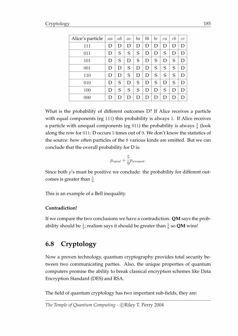
Cryptology 185
Alice’s particle aa ab ac ba bb bc ca cb cc
111 D D D D D D D D D
011 D S S S D D S D D
101 D S D S D S D S D
001 D D S D D S S S D
110 D D S D D S S S D
010 D S D S D S D S D
100 D S S S D D S D D
000 D D D D D D D D D
What is the probability of different outcomes D? If Alice receives a particlewith equal components (eg 111) this probability is always 1. If Alice receivesa particle with unequal components (eg 011) the probability is always 5
9(look
along the row for 011: D occurs 5 times out of 9. We don’t know the statistics ofthe source: how often particles of the 8 various kinds are emitted. But we canconclude that the overall probability for D is:
pequal +5
9punequal.
Since both p’s must be positive we conclude: the probability for different out-comes is greater than 5
9
This is an example of a Bell inequality.
Contradiction!
If we compare the two conclusions we have a contradiction. QM says the prob-ability should be 1
2; realism says it should be greater than 5
9so QM wins!
6.8 Cryptology
Now a proven technology, quantum cryptography provides total security be-tween two communicating parties. Also, the unique properties of quantumcomputers promise the ability to break classical encryption schemes like DataEncryption Standard (DES) and RSA.
The field of quantum cryptology has two important sub-fields, they are:
The Temple of Quantum Computing - c©Riley T. Perry 2004

186 Cryptology
1. Cryptography - The use of secure codes.
2. Cryptanalysis - Code breaking.
We’ll concentrate on cryptography in this chapter. Later, in chapter 7 we lookat Shor’s algorithm, which can be used to break RSA encryption.
6.8.1 Classical Cryptography
Secret codes have a long history - dating back to ancient times, one famousancient code is the Caesar cipher which simply shifts each letter by three.
A → D, B → E,X → A. (6.38)
This is not very secure as it’s easy to guess and decrypt. Modern codes usea key. A simple form of key is incorporated into a code wheel, an example ofwhich follows.
Example An example of a code wheel with the key: ABCDEF is describedbelow:
Key A B C D E F A B C D E F
Shift By 1 2 3 4 5 6 1 2 3 4 5 6
Message Q U A N T U M C O D E S
Encoding R W D R Y A N E R H J Y
With time secret keys and their respective codes got more complicated, cul-minating in modern codes, e.g. codes called DES and IDEA were implementedwith typically 64 and 128 bit secret keys.
There is another kind of key, a public key. Public key encryption (e.g. RSA 1976Diffie Hellman) uses a combination of a public and a secret key. In a publickey encryption scheme a public key encrypts a message but cannot decrypt it.This is done by a secret decryption key known only to the owner. Surmisingthe decryption key from public (encryption) key requires solving hard (timecomplexity wise) problems.
Some codes are stronger than others, for example the DES and IDEA secret
The Temple of Quantum Computing - c©Riley T. Perry 2004

Cryptology 187
key codes are stronger than Caesar cipher codes. Possibly the strongest codeis the one-time PAD. A one-time PAD is a key that is large as the message to besent (for example a random binary file) and the sender and receiver both havea copy of this key. The PAD is used only once to encrypt and decrypt the mes-sage. The problem with one-time PADs is that the key needs to be transmittedevery time and eavesdroppers could be listening in on the key. Quantum keydistribution resolves this issue by providing perfectly secure key distribution.
6.8.2 Quantum Cryptography
Modern classical public key cryptographic systems use a trap door function withsecurity based on mathematical assumptions, notably that it is difficult to fac-tor large integers. This assumption is now at risk from Shor’s algorithm.
The main advantage of quantum cryptography is that it gives us perfectlysecure data transfer. The first successful quantum cryptographic device wastested in 1989 by C.H. Bennet, and G. Brassard [Castro, M. 1997]. The devicecould translate a secret key over 30 centimetres using polarised light, calcitecrystal(s), and other electro-optical devices. This form of cryptography doesnot rely on a trap door function for encryption, but on quantum effects like theno-cloning theorem.
A simple example of the no-cloning theorem’s ability to secure data is describedbelow. After that we’ll look at why it’s impossible to listen in on a quantumchannel, and finally we’ll examine a method for quantum key distribution.
Quantum Money
Stephen Wiesner wrote a paper in 1970 (unpublished until 1983) in which hedescribed uncounterfeitable quantum bank notes [Braunstein, S. L. & Lo, H. K.2000].
Each bank note contains a unique serial number and a sequence of randomlypolarised photons (90, 180, 45, and 135). The basis of polarisation is kept se-cret (either diagonal or rectilinear). The bank can verify the validity of a note bymatching a serial number with known (only known by the bank) polarisations.This enables the bank to verify the polarisations without disturbing the quan-
The Temple of Quantum Computing - c©Riley T. Perry 2004

188 Cryptology
tum system (see the example below). Finally, the counterfeiter can’t counterfeitthe note due to the no cloning theorem. Remember, the no cloning theoremsays that given an unknown quantum state it is impossible to clone that stateexactly without disturbing the state.
Example Let’s say the bank receives a bank not with serial number 1573462.The bank checks its ”quantum bank note archive” to find the polarisationsfor bank note 1573462. The banks’ records give the following:
1573462 = H, H, 135, V, 45.H, H, 135, V, 45 is a record of the note polarisations, but our copy protec-tion system does not distinguish between H and V or 135 and 45. Becausethe photons are not in superpositions relative to the basis we measure in (asspecified by the serial numbers) the bank doesn’t disturb the states uponmeasurement. The bank only determines the basis of each photon, which is|0〉, |1〉, (rectilinear) or |+〉, |1〉, (diagonal). It should be noted that statesare always superpositions if we don’t say what the basis is.
Because the counterfeiter does not know the basis of each polarisedphoton on the quantum bank note, he must measure using a random basis.He could, theoretically measure each one and recreate it if he knows thebasis by which to measure each one. The chances of the counterfeiterrandomly measuring in the correct basis decrease by a 1
2for each successive
polarised photon on the note. So the more polarised photons the bank notehas the harder it is to counterfeit.
Quantum Packet Sniffing
Quantum packet sniffing is impossible - so the sender and receiver can be surethat no-one is listening in on their messages (eavesdropping). This phenomenais due to the following properties of quantum mechanics:
1. Quantum uncertainty, for example given a photon polarised in an unknownstate (it might be horizontally (180), vertically (90), at 45, or at 135)we can’t tell with certainty which polarisation the photon has withoutmeasuring it.
The Temple of Quantum Computing - c©Riley T. Perry 2004
Cryptology 189
2. The no cloning theorem.
3. Disturbance (information gain), if a measurement is done (distinguishingbetween two non-orthogonal states) the signal is forever disturbed.
4. Measurements are irreversible, any non orthogonal state will collapse ran-domly into a resultant state - losing the pre-measurement amplitudes.
Quantum Key Distribution
We can ensure secure communications by using one-time pads in conjunctionwith quantum key distribution. The main drawback for classical one-time pads isthe distribution of encryption/decrytion keys, this is not a problem for quan-tum cryptography as we can transfer key data in a totally secure fashion.
Quantum key distribution (QKD) is a means of distributing keys from oneparty to another, and detecting eavesdropping (it is inspired by the quantummoney example). An unusually high error rate is a good indicator of eaves-dropping. Even with a high error rate the eavesdropper cannot learn any use-ful information. It should be noted that this method does not prevent Denial ofservice (DOS) attacks.
An example follows on the next page.
The Temple of Quantum Computing - c©Riley T. Perry 2004

190 Cryptology
Example Alice and Bob want to use a key based encryption method,they communicate on two channels. One channel is used to transmit theencrypted message and another is used to transmit the encryption key. Butthey need a way to avoid Eve eavesdropping on their conversation on thekey channel [Ekert, A. 1993].
The following steps allow a totally secure (in terms of eavesdropping)transfer of the key (later we need to encrypt the message and send it via aclassical channel).
1. Alice randomly polarises photons at 45, 90 ,135, and 180 - these aresent to Bob over a quantum channel (which is secure due to quantumeffects, i.e. no eavesdropping).
2. Bob does measurements on the photons. he randomly uses either a rec-tilinear (180/90) or diagonal polarising filter (45/135), and recordswhich one was used for each bit. Also for each bit he records the mea-surement result as a 1 for 135 or 180 or 0 for 45 or 90 polarisations.
3. On a normal (insecure channel) Alice tells Bob which bits Bob used theright polarisation on (which he also communicates over the classicalchannel).
4. Alice and Bob check for quantum errors to gauge whether or not an eaves-dropper (Eve) was listening.
Comments
The following can be said about the key exchange:
• Eve can’t clone the bit and send it on, her measurements put Bob’s bits in anew random state. Alice and Bob decide on an acceptable error rate, ifthe key exchange’s error rate is higher than that (which means Eve mayhave been listening) then they resend the message.
• Eve could do an DOS attack by constantly measuring on the key channel.
• Eve could shave off some of the light if each bit is represented by more thanone photon, so each bit transferred must only be represented by one qubit.
The Temple of Quantum Computing - c©Riley T. Perry 2004

Alternative Models of Computation 191
• Eve could listen to a small number of bits and hope to be unnoticed - Aliceand Bob can prevent this by shrinking down their key.
• In 1984 Bennet and Brassard developed BB84, a method of mutual key gen-eration, the first QKD system which is based in concepts similar to theabove.
6.8.3 Are we Essentially Information?
John Archibald Wheeler, in the early 90s stated that the main focus of physicsshould be on information. When examined in terms of information, quantumsystems break down to elementary systems that each carry one bit of informa-tion.
This makes sense as we can only ask yes or no questions - and the answersare yes or no.
Physicist Anton Zellinger says the world appears quantised because the infor-mation that describes the world is quantised [Baeyer, H. C. 2001]. He says that 1bit of information can be represented by an elementary proposition, e.g. that anelectron’s spin along a certain axis is up or down. Once measured the bit is usedup and the other properties are random. His theory goes on to explain entan-glement, in terms of information. Finally, Zellinger (and his student Brubeker)have created an alternative measure of information, which is the number ofbits in a system. It is called total information and it takes quantum effects intoaccount.
6.9 Alternative Models of Computation
There are other candidates for physical phenomena to enhance computationalpower. Some disciplines cannot currently be described by quantum mechanics,like relativity and complexity theory (or chaos theory).
Question Is there a universal computation model? or will there always besome phenomena which is not well understood that has the potential to beexploited for the purposes of computation?
The Temple of Quantum Computing - c©Riley T. Perry 2004


Chapter 7
Quantum Algorithms
7.0.1 Introduction
Quantum algorithms are ways of combining unitary operations in a quantumsystem to achieve some computational goal. Over the past twenty years a num-ber of algorithms have been developed to harness the unique properties offeredby quantum computers. These algorithms have been designed to give specialadvantages over their classical counterparts.
Shor’s algorithm (1995) gives the factorisation of arbitrarily large numbers atime complexity class of O((log N)3), where that classical equivalent is roughlyexponential. This is extremely important for cryptography. For example, RSArelies on factorisation being intractable, which means that no polynomial solu-tion exists that covers all instances of the problem. Another example is Grover’sdatabase search algorithm which provides a quadratic speedup when search-ing a list of N items. This takes the classical value of a linear search from O(N)
time to O(N12 ) time [TheFreeDictionary.com 2004]. Most known quantum al-
gorithms have similarities to, or partially borrow from, these two algorithms.
Some properties of Shor and Grover type algorithms are:
• Shor type algorithms use the quantum Fourier transform. These include: fac-toring, the hidden subgroup problem, discrete logarithms, and order find-ing (all variations on a theme).
• Grover type search algorithms can be used for applications like fast databasesearching and statistical analysis.
193
194 Deutsch’s Algorithm
There are also hybrid algorithms like quantum counting that combine elementsfrom both, and more esoteric algorithms like quantum simulators. In this chap-ter we’ll look at Deutsch’s algorithm, the Deutsch-Josza algorithm, Shor’s al-gorithm, and Grover’s algorithm.
As with chapters 5 and 6 individual references to QCQI have been dropped.
7.1 Deutsch’s Algorithm
Deutsch’s algorithm is a simple example of quantum parallelism. The prob-lem it solves is not an important one, but its simple nature makes it good fordemonstrating the properties of quantum superposition.
7.1.1 The Problem Defined
We have a function f(x) where f(x) : 0, 1 → 0, 1 with a one bit domain.This means that f(x) takes a bit (either a 0 or a 1) as an argument and returnsa bit (again, either a 0 or a 1). Therefore both the input and output of this func-tion can be represented by a bit, or a qubit.
We want to test if this function is one to one (balanced), where one to onemeans:
f(1) = 1 and f(0) = 0 or f(0) = 1 and f(1) = 0.
The other alternative is that f(x) is not one to one (i.e. it is constant), in whichcase we would get:
f(1) = 0 and f(0) = 0 or f(0) = 1 and f(1) = 1.
The circuit for determining some property of a function is called an oracle. It’simportant to note that the thing that quantum computers do well is to testglobal properties of functions, not the results of those functions given particularinputs. To do this efficiently we need to look at many values simultaneously.
7.1.2 The Classical Solution
The solution is as follows:
The Temple of Quantum Computing - c©Riley T. Perry 2004

Deutsch’s Algorithm 195
iff f(0)⊕ f(1) = 1 the function is one to one (where ⊕ is equivalent to XOR).
This is made up of three operations, involving two function evaluations:
1. x = f(0),
2. y = f(1),
3. z = x⊕ y.
Can we do better with a quantum computer?
7.1.3 The Quantum Solution
The quantum circuit below performs the first two steps in the classical solutionin one operation, via superposition.
x |0〉 H
Uf
xH
y |1〉 Hy ⊕ f(x)
H
↑ |ψ1〉 ↑ |ψ2〉 ↑ |ψ3〉 ↑ |ψ4〉
Below are the steps |ψ1〉 to |ψ4〉 we need to solve the problem quantum me-chanically.
|ψ1〉 The qubits x and y have been set to the following (we call x the queryregister and y the answer register):
x = |0〉,y = |1〉.
|ψ2〉 Apply H gates to the input registers so our state vector is now:
|Ψ〉 =
[|0〉+ |1〉√
2
][|0〉 − |1〉√
2
].
|ψ3〉 Uf acts on qubits x and y, specifically we use |Ψ〉 → Uf → |x〉 |y ⊕ f(x)〉.After some algebraic manipulation the result ends up in x, and y seems
The Temple of Quantum Computing - c©Riley T. Perry 2004
196 Deutsch’s Algorithm
unchanged (see the example below).
For f(0) 6= f(1) (balanced) we get:
|Ψ〉 = ±[|0〉 − |1〉√
2
][|0〉 − |1〉√
2
]
and for f(0) = f(1) (constant):
|Ψ〉 = ±[|0〉+ |1〉√
2
][|0〉 − |1〉√
2
].
Note: The ± at the start of the state is just a result of internal calculations,it does not matter whether it is positive or negative for the result of thiscircuit (global phase factors have no significance).
|ψ4〉 x is sent through the H gate again. The H gate, as well as turning a 1or a 0 into a superposition will take a superposition back to a 1 or a 0(depending on the sign):
[|0〉+ |1〉√
2
]→ H → |0〉,
[|0〉 − |1〉√
2
]→ H → |1〉.
So at step 4, for f(0) 6= f(1) we get:
|Ψ〉 = ±|1〉[|0〉 − |1〉√
2
]
and for f(0) = f(1):
|Ψ〉 = ±|0〉[|0〉 − |1〉√
2
].
At this point our state is, combining both cases:
|Ψ〉 = ±|f(0)⊕ f(1)〉[|0〉 − |1〉√
2
].
Up until now y has been useful to us, now we don’t care about it as x
holds the result. We can just do a partial measurement on x and discard y
as garbage. If x = 0 then the function is constant, and if x = 1 the functionis balanced.
The Temple of Quantum Computing - c©Riley T. Perry 2004
Deutsch’s Algorithm 197
Example There’s only four possible combinations for f(x) , we’ll look attwo here. Given our state at |ψ2〉 is 1√
2[|0〉 + |1〉] 1√
2[|0〉 − |1〉] our state at |ψ3〉
will look like the following:
|Ψ〉 =
[|0〉+ |1〉√
2
][|0⊕ f(x)〉 − |1⊕ f(x)〉√
2
]
=1
2(|0〉 |0⊕ f(0)〉 − |0〉 |1⊕ f(0)〉+ |1〉 |0⊕ f(1)〉 − |1〉 |1⊕ f(1)〉).
Keeping in mind that 0⊕ 0 = 0, 1⊕ 0 = 1, 1⊕ 1 = 0, and 0⊕ 1 = 1 we’ll startwith the constant function f(0) = 0 and f(1) = 0:
|Ψ〉 =1
2(|0〉 |0⊕ 0〉 − |0〉 |1⊕ 0〉+ |1〉 |0⊕ 0〉 − |1〉 |1⊕ 0〉)
=1
2(|00〉 − |01〉+ |10〉 − |11〉)
=
[|0〉+ |1〉√
2
][|0〉 − |1〉√
2
].
Now for a balanced function f(0) = 1 and f(1) = 0:
|Ψ〉 =1
2(|0〉 |0⊕ 1〉 − |0〉 |1⊕ 1〉+ |1〉 |0⊕ 0〉 − |1〉 |1⊕ 0〉)
=1
2(|01〉 − |00〉+ |10〉 − |11〉)
=1
2(− |00〉+ |01〉+ |10〉 − |11〉)
= (−1)1
2(|00〉 − |01〉 − |10〉+ |11〉)
= −1
[|0〉 − |1〉√
2
][|0〉 − |1〉√
2
].
Notice that (-1) has been moved outside of the combined state, it is a globalphase factor and we can ignore it. At |ψ4〉 we put our entire state throughH ⊗H and get |01〉 for the constant function and |11〉 for the balanced one.
7.1.4 Physical Implementations
In theory A simple quantum computer implementing Deutsch’s algorithm canbe made out of a cardboard box, three mirrors, and two pairs of sunglasses[Stay, M. 2004]. The sunglasses (in a certain configuration) polarise light ini-tially into a non-orthogonal state (a superposition) then back again. The mir-
The Temple of Quantum Computing - c©Riley T. Perry 2004
198 The Deutsch-Josza Algorithm
rors within the box reflect the light in a certain way depending on their con-figuration (at different angles depending on the type of function you want tosimulate). A torch is then shone into the box, if light comes out the functionis balanced, if not then it is constant. Now, if we use a special optical deviceto send just one photon into the box and we have a sensitive photo detector atthe other end then we have an architecture that is a theoretically more efficientoracle than any classical computer.
Deutsch’s algorithm can of course be executed on any quantum computer ar-chitecture, and has been successfully implemented. For example, in 2001 thealgorithm was run on an NMR computer (see chapter 8) [Dorai, K. Arvind, ?.Kumar, A. 2001]. Due to the relatively small number of qubits that can be cur-rently made to work together many of the other quantum algorithms have notbeen satisfactorily tested.
7.2 The Deutsch-Josza Algorithm
The Deutsch-Josza algorithm is an extension of Deutsch’s algorithm which canevaluate more than one qubit in one operation. We can extend it to evaluateany number of qubits simultaneously by using an n-qubit query register for x
instead of a single qubit.
7.2.1 The Problem Defined
The problem we are trying solve is slightly different to the one presented inDeutsch’s algorithm, that is: is f(x) the same (constant) for all inputs? Or isf(x) equal to 1 for half the input values and equal to 0 for the other half (whichmeans it is balanced)?
The Temple of Quantum Computing - c©Riley T. Perry 2004

The Deutsch-Josza Algorithm 199
7.2.2 The Quantum Solution
The circuit looks like this:
x |0〉 /n H⊗n
Uf
xH⊗n
y |1〉 Hy ⊕ f(x)
H
↑ |ψ1〉 ↑ |ψ2〉 ↑ |ψ3〉 ↑ |ψ4〉
The input (x) and output (y) registers have an H gate for each qubit in theregister. This is denoted by H⊗n and the /n notation just means n wires for n
qubits.
Here are the steps |ψ1〉 to |ψ4〉 we need to solve the problem quantum mechan-ically.
|ψ1〉 The registers x and y have been set to the following:
x = |0〉⊗n,
y = |1〉.
|ψ2〉 Apply H gates to both the x and y registers so our state vector is now:
|Ψ〉 =1√2n
2n−1∑x=0
|x〉[|0〉 − |1〉√
2
].
|ψ3〉 Uf acts on registers x and y (remember y is just a single qubit because theresult of evaluating f is, by definition, just a 0 or 1). This time we use|Ψ〉 = Uf |Ψ2〉 |0〉 = |x1, x2, . . . , xn〉 |y ⊕ f(x)〉 to evaluate f(x).
|ψ4〉 x is sent through H⊕n and y through an H gate also. This leaves us with aset of output qubits and a 1 in the answer register, i.e.
|Ψ〉 = |x1, x2, . . . , xn〉 |1〉 .
Now the rule is simple: if any of the qubits in the query (x) register are|1〉 then the function is balanced, otherwise it is constant.
The Temple of Quantum Computing - c©Riley T. Perry 2004

200 Shor’s Algorithm
Example Here’s an example with a two qubit query register for the bal-anced function f with f(00) = 0, f(01) = 0, f(10) = 1, and f(11) = 1. So atstate |ψ1〉 we have:
|Ψ〉 = |001〉 .Then at state |ψ2〉, after the H gates we get:
|Ψ〉 =
[|0〉+ |1〉√
2
][|0〉+ |1〉√
2
][|0〉 − |1〉√
2
].
We are now ready to examine our state at |ψ3〉:
|Ψ〉 =
[|0〉+ |1〉√
2
][|0〉+ |1〉√
2
][|0⊕ f(x)〉 − |1⊕ f(x)〉√
2
]
=
[|00〉+ |01〉+ |10〉+ |11〉√
4
][|0⊕ f(x)〉 − |1⊕ f(x)〉√
2
]
=1√8(|00〉 |0⊕ f(00)〉 − |00〉 |1⊕ f(00)〉+ |01〉 |0⊕ f(01)〉
− |01〉 |1⊕ f(01)〉+ |10〉 |0⊕ f(10)〉 − |10〉 |1⊕ f(10)〉+ |11〉 |0⊕ f(11)〉 − |11〉 |1⊕ f(11)〉)
=1√8(|000〉 − |001〉+ |010〉 − |011〉+ |101〉 − |100〉+ |111〉 − |110〉)
=1√8(|000〉 − |001〉+ |010〉 − |011〉 − |100〉+ |101〉 − |110〉+ |111〉)
=
[|00〉+ |01〉 − |10〉 − |11〉√
4
][|0〉 − |1〉√
2
]
=
[|0〉 − |1〉√
2
][|0〉+ |1〉√
2
][|0〉 − |1〉√
2
].
At |ψ4〉 we put our entire state through H ⊗ H ⊗ H and get |101〉 meaningthat our function is balanced.
7.3 Shor’s Algorithm
7.3.1 The Quantum Fourier Transform
The quantum analogue of the discrete Fourier transform (see chapter 4) is thequantum Fourier transform (QFT ). The DFT takes a series of N complex num-
The Temple of Quantum Computing - c©Riley T. Perry 2004

Shor’s Algorithm 201
bers, X0, X1, ..., XN−1 and produces a series complex numbers Y0, Y1, ..., YN−1.Similarily, the QFT takes a state vector:
|Ψ〉 = α0|0〉+ α1|1〉+ ... + αN−1|N − 1〉 (7.1)
and performs a DFT on the amplitudes of |Ψ〉 giving us:
|Ψ〉 = β0|0〉+ β1|1〉+ ... + βN−1|N − 1〉. (7.2)
The main advantage of the QFT is the fact that it can do a DFT on a superposi-tion of states. This can be done on a superposition like the following:
1√4(|00〉+ |01〉 − |10〉 − |11〉)
or a state where the probability amplitudes are of different values. E.g. the fol-lowing state has probability amplitudes of 0 for the majority of its basis states:
1√3(|001〉+ |011〉 − |111〉).
It’ll helpful over the next few sections to use integers when we are describingstates with a large number of qubits, so the previous state could have beenwritten as:
1√3(|1〉+ |3〉 − |7〉).
The QFT is a unitary operator, and is reversible. In fact we use the inversequantum fourier transform (QFT †) for Shor’s algorithm. The QFT is defined asfollows:
Given a state vector |Ψ〉:
|Ψ〉 =2n−1∑x=0
αx |x〉 (7.3)
where n is the number of qubits, QFT |Ψ〉 is defined as:
|Ψ′〉 = QFT |Ψ〉 =2n−1∑x=0
2n−1∑y=0
αxe2πixy/2n
√2n
|y〉 . (7.4)
We can also represent the QFT as a matrix:
The Temple of Quantum Computing - c©Riley T. Perry 2004
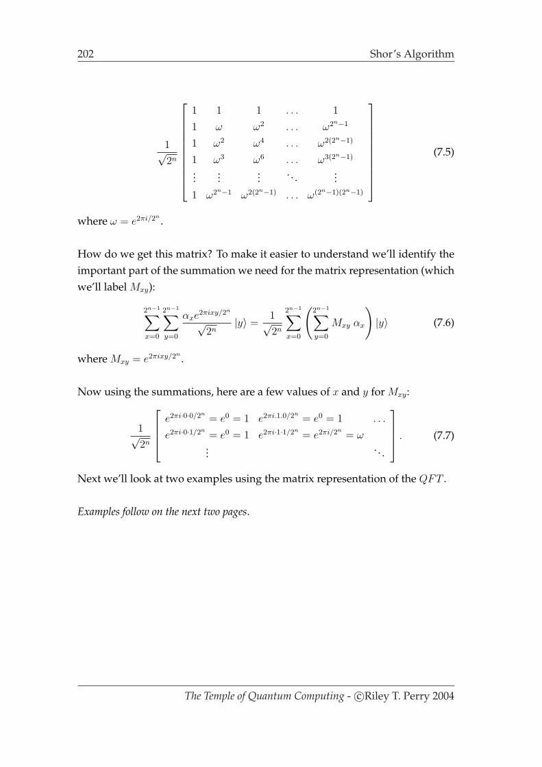
202 Shor’s Algorithm
1√2n
1 1 1 . . . 1
1 ω ω2 . . . ω2n−1
1 ω2 ω4 . . . ω2(2n−1)
1 ω3 ω6 . . . ω3(2n−1)
......
... . . . ...1 ω2n−1 ω2(2n−1) . . . ω(2n−1)(2n−1)
(7.5)
where ω = e2πi/2n .
How do we get this matrix? To make it easier to understand we’ll identify theimportant part of the summation we need for the matrix representation (whichwe’ll label Mxy):
2n−1∑x=0
2n−1∑y=0
αxe2πixy/2n
√2n
|y〉 =1√2n
2n−1∑x=0
(2n−1∑y=0
Mxy αx
)|y〉 (7.6)
where Mxy = e2πixy/2n .
Now using the summations, here are a few values of x and y for Mxy:
1√2n
e2πi·0·0/2n= e0 = 1 e2πi.1.0/2n
= e0 = 1 . . .
e2πi·0·1/2n= e0 = 1 e2πi·1·1/2n
= e2πi/2n= ω
... . . .
. (7.7)
Next we’ll look at two examples using the matrix representation of the QFT .
Examples follow on the next two pages.
The Temple of Quantum Computing - c©Riley T. Perry 2004

Shor’s Algorithm 203
Example A simple one qubit QFT . Given:
|Ψ〉 =2√5|0〉+
1√5|0〉 .
Find,|Ψ′〉 = QFT |Ψ〉 .
We’ll use the matrix representation, which is:
1√2
[1 1
1 eiπ
].
This matrix is actually just an H gate (since eiπ = −1), so we get:
|Ψ′〉 =1√2
[1 1
1 eiπ
][2√5
1√5
]
=
[2√10
+ 1√10
2√10
+ eπi√10
]
=
[3√10
2√10
+ −1√10
= 1√10
]
=3√10|0〉+
1√10|1〉 .
The Temple of Quantum Computing - c©Riley T. Perry 2004
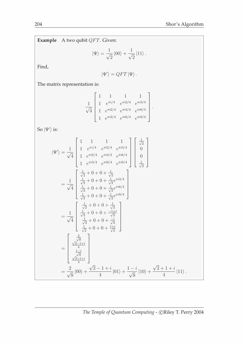
204 Shor’s Algorithm
Example A two qubit QFT . Given:
|Ψ〉 =1√2|00〉+
1√2|11〉 .
Find,|Ψ′〉 = QFT |Ψ〉 .
The matrix representation is:
1√4
1 1 1 1
1 eπi/4 eπi2/4 eπi3/4
1 eπi2/4 eπi4/4 eπi6/4
1 eπi3/4 eπi6/4 eπi9/4
.
So |Ψ′〉 is:
|Ψ′〉 =1√4
1 1 1 1
1 eπi/4 eπi2/4 eπi3/4
1 eπi2/4 eπi4/4 eπi6/4
1 eπi3/4 eπi6/4 eπi9/4
1√2
0
01√2
=1√4
1√2
+ 0 + 0 + 1√2
1√2
+ 0 + 0 + 1√2eπi3/4
1√2
+ 0 + 0 + 1√2eπi6/4
1√2
+ 0 + 0 + 1√2eπi9/4
=1√4
1√2
+ 0 + 0 + 1√2
1√2
+ 0 + 0 + −1+i√2
1√2
+ 0 + 0 + −i√2
1√2
+ 0 + 0 + 1+i√2
=
2√8√
2−1+i4
1−i√8√
2+1+i4
=2√8|00〉+
√2− 1 + i
4|01〉+
1− i√8|10〉+
√2 + 1 + i
4|11〉 .
The Temple of Quantum Computing - c©Riley T. Perry 2004

Shor’s Algorithm 205
How Do we Implement a QFT?
As stated before, a one qubit QFT has the following rather simple circuit:
H
A three qubit QFT has a more complicated circuit:
H S T ×
• H S
• • H ×We can extend this logic to n qubits by using H and n − 2 different rotationgates (Rk - see below) where:
Rk =
[1 0
1 e2πi/2k
]. (7.8)
For n qubits we use gates R2 . . . Rn. For more information on generic QFT
circuits you’ll need to consult an external reference like QCQI.
7.3.2 Fast Factorisation
Finding unknown factors p and q such that p × q = 347347 is very slow com-pared to the reverse problem: calculating 129 × 156. We don’t yet know fastalgorithms for factorising on classical machines but we do now know (thanksto Shor) a fast factorisation algorithm we can run on a quantum computer.
Public key encryption systems like RSA algorithm rely on the fact that it’s hardto factorise large numbers; if we could find the factors we could use the infor-mation provided in the public key to decrypt messages encrypted with it. Interms of RSA our task is simple. Given an integer N we know n = pq where p
and q are large prime numbers we want to calculate p and q.
The Temple of Quantum Computing - c©Riley T. Perry 2004
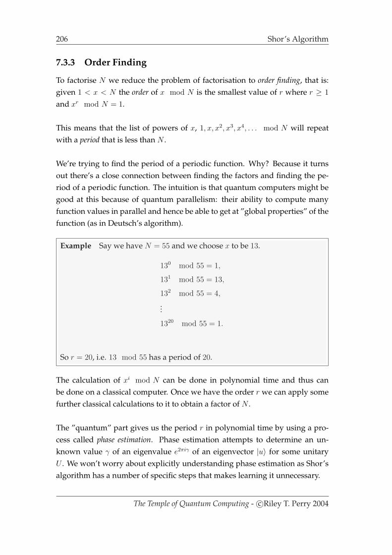
206 Shor’s Algorithm
7.3.3 Order Finding
To factorise N we reduce the problem of factorisation to order finding, that is:given 1 < x < N the order of x mod N is the smallest value of r where r ≥ 1
and xr mod N = 1.
This means that the list of powers of x, 1, x, x2, x3, x4, . . . mod N will repeatwith a period that is less than N .
We’re trying to find the period of a periodic function. Why? Because it turnsout there’s a close connection between finding the factors and finding the pe-riod of a periodic function. The intuition is that quantum computers might begood at this because of quantum parallelism: their ability to compute manyfunction values in parallel and hence be able to get at ”global properties” of thefunction (as in Deutsch’s algorithm).
Example Say we have N = 55 and we choose x to be 13.
130 mod 55 = 1,
131 mod 55 = 13,
132 mod 55 = 4,
...
1320 mod 55 = 1.
So r = 20, i.e. 13 mod 55 has a period of 20.
The calculation of xi mod N can be done in polynomial time and thus canbe done on a classical computer. Once we have the order r we can apply somefurther classical calculations to it to obtain a factor of N .
The ”quantum” part gives us the period r in polynomial time by using a pro-cess called phase estimation. Phase estimation attempts to determine an un-known value γ of an eigenvalue e2πiγ of an eigenvector |u〉 for some unitaryU . We won’t worry about explicitly understanding phase estimation as Shor’salgorithm has a number of specific steps that makes learning it unnecessary.
The Temple of Quantum Computing - c©Riley T. Perry 2004

Shor’s Algorithm 207
Before we look at the circuit for Shor’s algorithm. A necessary component ofShor’s algorithm, the continued fractions algorithm, is introduced.
The Continued Fractions Algorithm
The continued fractions algorithm allows us to calculate an array of integers torepresent a fraction. We simply split the fraction into its whole and fractionalparts, store the whole part, and repeat the process until we have no fractionalparts left. Here’s an example:
Example Convert 119
to integer array representation.
11
9= 1 +
2
9
= 1 +1
2
9
= 1 +1
1 +1
9
2
= 1 +1
1 +1
4 +1
2.
So, we end up with the following list:
[1, 1, 4, 2]
which is a four element array (that took four steps) that represents 119.
Now we’ll look at the fast factorisation algorithm...
The Temple of Quantum Computing - c©Riley T. Perry 2004
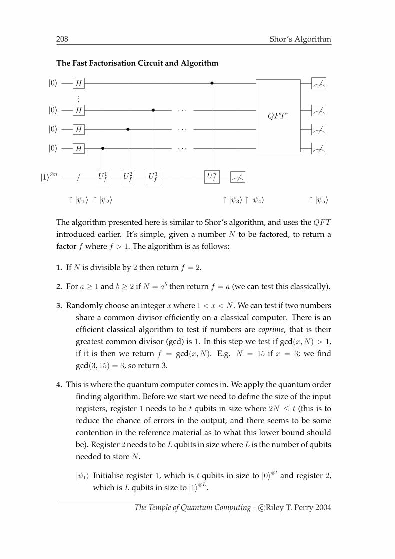
208 Shor’s Algorithm
The Fast Factorisation Circuit and Algorithm
|0〉 H •
QFT †
NM°°°
...|0〉 H • . . .
NM°°°
|0〉 H • . . .NM
°°°
|0〉 H • . . .NM
°°°
|1〉⊗n / U1f U2
f U3f Un
f NM°°°
↑ |ψ1〉 ↑ |ψ2〉 ↑ |ψ3〉 ↑ |ψ4〉 ↑ |ψ5〉
The algorithm presented here is similar to Shor’s algorithm, and uses the QFT
introduced earlier. It’s simple, given a number N to be factored, to return afactor f where f > 1. The algorithm is as follows:
1. If N is divisible by 2 then return f = 2.
2. For a ≥ 1 and b ≥ 2 if N = ab then return f = a (we can test this classically).
3. Randomly choose an integer x where 1 < x < N . We can test if two numbersshare a common divisor efficiently on a classical computer. There is anefficient classical algorithm to test if numbers are coprime, that is theirgreatest common divisor (gcd) is 1. In this step we test if gcd(x,N) > 1,if it is then we return f = gcd(x,N). E.g. N = 15 if x = 3; we findgcd(3, 15) = 3, so return 3.
4. This is where the quantum computer comes in. We apply the quantum orderfinding algorithm. Before we start we need to define the size of the inputregisters, register 1 needs to be t qubits in size where 2N ≤ t (this is toreduce the chance of errors in the output, and there seems to be somecontention in the reference material as to what this lower bound shouldbe). Register 2 needs to be L qubits in size where L is the number of qubitsneeded to store N .
|ψ1〉 Initialise register 1, which is t qubits in size to |0〉⊗t and register 2,which is L qubits in size to |1〉⊗L.
The Temple of Quantum Computing - c©Riley T. Perry 2004

Shor’s Algorithm 209
|ψ2〉 Create a superposition on register 1:|Ψ〉 = 1√
2t
∑2t−1
r1=0 |R1〉 |1〉.|ψ3〉 Apply UfR2 = xR1 mod N to register 2:
|Ψ〉 = 1√2t
∑2t−1
r2=0 |R1〉∣∣xR1 mod N
⟩.
|ψ4〉 We measure register 2, because it is entangled with register 1 andour state becomes subset of the values in register 1 that correspondwith the value we observed in register 2.
|ψ5〉 We apply QFT † to register 1 and then measure it.
|ψ6〉 (not shown) Now we apply the continued fractions algorithm to |Ψ〉2t
and the number of steps it takes will be the period r.
5. With the result r first test if r is even the see if xr/2 6= −1 mod N then cal-culate f =gcd(xr/2±, N). If the result is not 1 or N then return f as it is afactor, otherwise the algorithm has failed and we have to start again.
Over the next two pages we’ll look at a couple of worked examples of Shor’s algorithm.
The Temple of Quantum Computing - c©Riley T. Perry 2004

210 Shor’s Algorithm
Example Find the factors for N = 15
1. N is not even, continue.
2. N 6= ab so continue.
3. We choose x = 7 gcd(7, 15) = 1 so continue.
4. t = 11 qubits for register 1 and L = 4 qubits for register 2.
|ψ1〉 Initialise both the registers so the combined state becomes |Ψ〉 =
|000000000001111〉.
|ψ2〉 Create a superposition on register 1, so we get |Ψ〉 = 1√2048
(|0〉 + |1〉 +
|2〉+ . . . + |2047〉) |15〉.
|ψ3〉 applying xR1 mod 15 gives us the following:
R1 |0〉 |1〉 |2〉 |3〉 |4〉 |5〉 |6〉 |7〉 |8〉 |9〉 |10〉 . . .
R2 |1〉 |7〉 |4〉 |13〉 |1〉 |7〉 |4〉 |13〉 |1〉 |7〉 |4〉 . . .
|ψ4〉 We Measure R2 and randomly get a 4 leaving |Ψ〉 in the following postmeasurement state:
R1 |2〉 |6〉 |10〉 . . .
R2 |4〉 |4〉 |4〉 . . .
Remember that both registers are actually part of the same state vec-tor, it’s just convenient to think of them separately. The state above isactually an entangled state that looks like (R2 is bolded):
|Ψ〉 =1√512
(|000000000101000〉+ |000000001101000〉+ . . .) .
|ψ5〉 After applying QFT † we get either 0, 512, 1024, or 1536 with a probabil-ity of 1
4. Say we observe 1536.
|ψ6〉 The result from the continued fractions algorithm for 15362048
is 4.
5. r is even and satisfies r26= −1 mod N . So we try gcd(72 − 1, 15) = 3 and
gcd(72 + 1, 15) = 5. Now, by testing that 3 × 5 = 15 = N we see wehave now found our factors.
The Temple of Quantum Computing - c©Riley T. Perry 2004
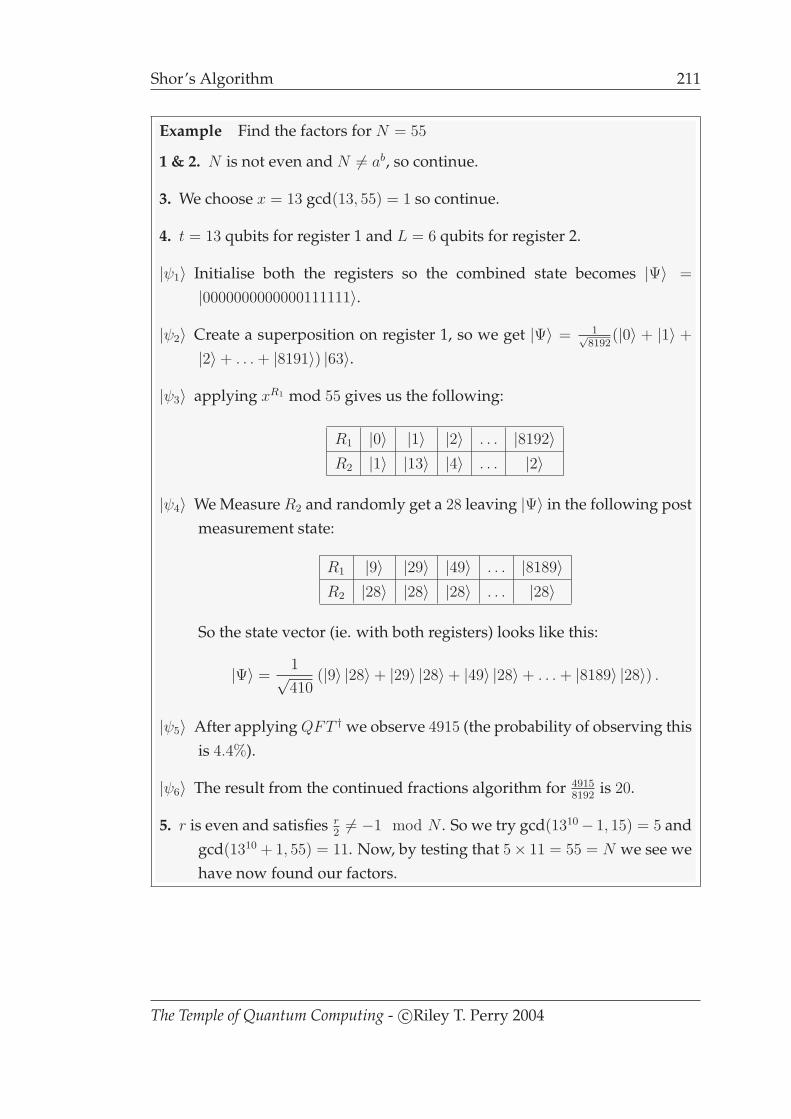
Shor’s Algorithm 211
Example Find the factors for N = 55
1 & 2. N is not even and N 6= ab, so continue.
3. We choose x = 13 gcd(13, 55) = 1 so continue.
4. t = 13 qubits for register 1 and L = 6 qubits for register 2.
|ψ1〉 Initialise both the registers so the combined state becomes |Ψ〉 =
|0000000000000111111〉.
|ψ2〉 Create a superposition on register 1, so we get |Ψ〉 = 1√8192
(|0〉 + |1〉 +
|2〉+ . . . + |8191〉) |63〉.
|ψ3〉 applying xR1 mod 55 gives us the following:
R1 |0〉 |1〉 |2〉 . . . |8192〉R2 |1〉 |13〉 |4〉 . . . |2〉
|ψ4〉 We Measure R2 and randomly get a 28 leaving |Ψ〉 in the following postmeasurement state:
R1 |9〉 |29〉 |49〉 . . . |8189〉R2 |28〉 |28〉 |28〉 . . . |28〉
So the state vector (ie. with both registers) looks like this:
|Ψ〉 =1√410
(|9〉 |28〉+ |29〉 |28〉+ |49〉 |28〉+ . . . + |8189〉 |28〉) .
|ψ5〉 After applying QFT † we observe 4915 (the probability of observing thisis 4.4%).
|ψ6〉 The result from the continued fractions algorithm for 49158192
is 20.
5. r is even and satisfies r26= −1 mod N . So we try gcd(1310− 1, 15) = 5 and
gcd(1310 + 1, 55) = 11. Now, by testing that 5× 11 = 55 = N we see wehave now found our factors.
The Temple of Quantum Computing - c©Riley T. Perry 2004
212 Grover’s Algorithm
7.4 Grover’s Algorithm
Grover’s algorithm gives us a quadratic speed up to a wide variety of clas-sical search algorithms. The most commonly given examples of search algo-rithms that can benefit from a quantum architecture are shortest route findingalgorithms and algorithms to find specific elements in an unsorted database.
7.4.1 The Travelling Salesman Problem
An example of shortest route finding is the travelling salesman problem. Put sim-ply, given a number of interconnected cities, with certain distances betweenthem. Is there a route of less than k kilometres (or miles) for which the sales-man can visit every city?
With Grover’s algorithm it is possible to complete to search for a route of lessthan k kilometres in O(
√N) steps rather than an average of N
2(which is O(N))
steps for the classical case. Suppose we have M different solutions for k then
the time complexity for Grover’s algorithm is O(√
MN
).
7.4.2 Quantum Searching
For the purpose of explaining Grover type algorithms we’ll use an unsorteddatabase table as an example.
Given a database table with N elements (it is best if we choose an N that isapproximately 2n where n is the number of qubits) with an index i. Our tableis shown below:
0 element 1
1 element 2
2 element 3...
N − 1 element N
Suppose there are M solutions where 1 < M ≤ N .
The Temple of Quantum Computing - c©Riley T. Perry 2004
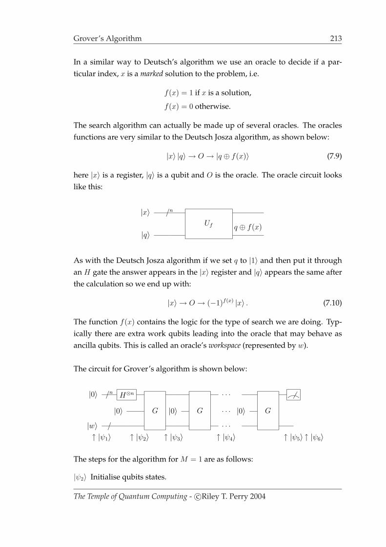
Grover’s Algorithm 213
In a similar way to Deutsch’s algorithm we use an oracle to decide if a par-ticular index, x is a marked solution to the problem, i.e.
f(x) = 1 if x is a solution,
f(x) = 0 otherwise.
The search algorithm can actually be made up of several oracles. The oraclesfunctions are very similar to the Deutsch Josza algorithm, as shown below:
|x〉 |q〉 → O → |q ⊕ f(x)〉 (7.9)
here |x〉 is a register, |q〉 is a qubit and O is the oracle. The oracle circuit lookslike this:
|x〉 /n
Uf
|q〉q ⊕ f(x)
As with the Deutsch Josza algorithm if we set q to |1〉 and then put it throughan H gate the answer appears in the |x〉 register and |q〉 appears the same afterthe calculation so we end up with:
|x〉 → O → (−1)f(x) |x〉 . (7.10)
The function f(x) contains the logic for the type of search we are doing. Typ-ically there are extra work qubits leading into the oracle that may behave asancilla qubits. This is called an oracle’s workspace (represented by w).
The circuit for Grover’s algorithm is shown below:
|0〉 /n H⊗n
G G
. . .
G
NM°°°
|0〉 |0〉 . . . |0〉|w〉 / . . .
↑ |ψ1〉 ↑ |ψ2〉 ↑ |ψ3〉 ↑ |ψ4〉 ↑ |ψ5〉 ↑ |ψ6〉
The steps for the algorithm for M = 1 are as follows:
|ψ2〉 Initialise qubits states.
The Temple of Quantum Computing - c©Riley T. Perry 2004
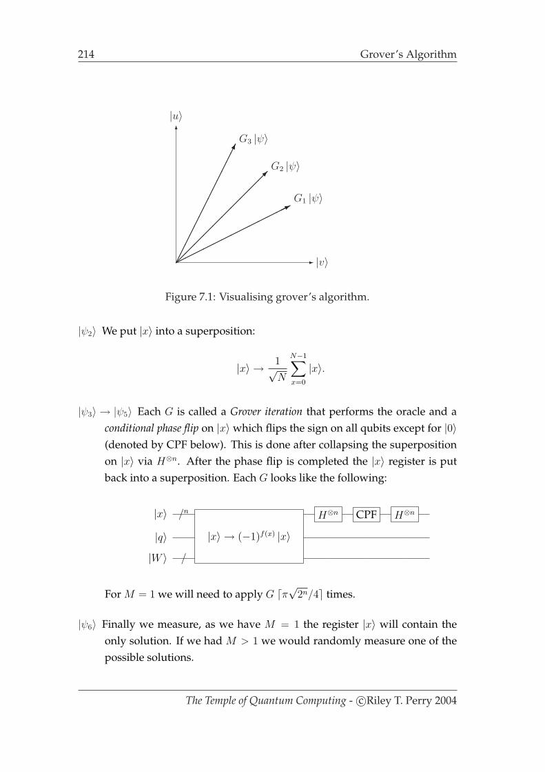
214 Grover’s Algorithm
-
6
¢¢¢¢¢¢¢¢¢¢¢¢¢
¡¡
¡¡
¡¡
¡¡
¡¡µ
©©©©©©©©©©©©©*
|v〉
|u〉
G1 |ψ〉
G2 |ψ〉
G3 |ψ〉
Figure 7.1: Visualising grover’s algorithm.
|ψ2〉 We put |x〉 into a superposition:
|x〉 → 1√N
N−1∑x=0
|x〉.
|ψ3〉 → |ψ5〉 Each G is called a Grover iteration that performs the oracle and aconditional phase flip on |x〉 which flips the sign on all qubits except for |0〉(denoted by CPF below). This is done after collapsing the superpositionon |x〉 via H⊗n. After the phase flip is completed the |x〉 register is putback into a superposition. Each G looks like the following:
|x〉 /n
|x〉 → (−1)f(x) |x〉H⊗n CPF H⊗n
|q〉|W 〉 /
For M = 1 we will need to apply G dπ√2n/4e times.
|ψ6〉 Finally we measure, as we have M = 1 the register |x〉 will contain theonly solution. If we had M > 1 we would randomly measure one of thepossible solutions.
The Temple of Quantum Computing - c©Riley T. Perry 2004

Grover’s Algorithm 215
Visualising Grover’s Algorithm
We can define the superposition of solutions to Grover’s algorithm as:
|u〉 =1√M
∑=
|x〉 (7.11)
and the superposition of values that are not solutions as:
|v〉 =1√
N −M
∑
6=|x〉 . (7.12)
The operation of Grover’s algorithm can be seen if figure 7.1 as a series of ro-tations of |Ψ〉 from |v〉 to |u〉. With each individual rotation being done by G, agrover iteration.
A simple exmample follows:
Example Suppose we have an index size of 4, which gives us N = 4. Wehave only one solution so M = 1 and our function, f(x) has a marked solu-tion at x = 0. This is like saying the element we are looking for is at indexi = 0. These are the results returned by an oracle call:
f(0) = 1, f(1) = 0, f(2) = 0, and f(3) = 0.
The size of register |x〉 is 2 qubits. We also have a workspace of 1 qubit (whichwe set to |1〉), which we put through an H gate at the same time as the qubitsin |x〉 initially go through their respective H gates (we’ll ignore oracle qubitq for this example). The steps for the algorithm are as follows:
|ψ1〉 We initialise |x〉 and |w〉, so |Ψ〉 = |001〉.
|ψ2〉 |x〉 and |w〉 go through their H gates giving us |x〉 = 1√4[|00〉 + |01〉 +
|10〉+ |11〉] and |w〉 = 1√2[|0〉 − |1〉].
|ψ3〉 A single grover iteration is all we need to rotate |x〉 to match |u〉 (themarked solution) so we jump straight to |ψ5〉.
|ψ5〉 Now |x〉 = |00〉.
|ψ6〉 Measuring register |x〉 gives us a 0.
The Temple of Quantum Computing - c©Riley T. Perry 2004


Chapter 8
Using Quantum Mechanical Devices
8.1 Introduction
Today’s manufacturing methods can make chips (figure 8.1) with transistorsa fraction of a micron wide. As they get smaller, chips also tend to get faster.Computer power doubles every few years (according to Moore’s law) and we’llsoon reach the threshold below which transistors will not work because ofquantum effects. At tens of nanometres (which we are close to now) electronscan tunnel between parts of a circuit, so transistor technology may not be ableto shrink much further [Benjamin, S. & Ekert, A. ? 2000].
In 1998 Neil Gershenfeld (MIT) built a three qubit device, then in 2000 RayLaFlemme built a seven qubit quantum computer. Currently we are still lim-ited to tens of qubits and hundreds of gates with implementations being slowand temperamental. The architectures of these machines vary, with scientistseven talking about using cups of coffee and small amounts of chloroform tobuild a working quantum computer [Blume, H. 2000].
8.2 Physical Realisation
We’ll take a quick look at physical realisations here, but a warning for thoseexpecting detail - this section is mainly here for completeness and is strictly anintroduction.
According to Nielsen and Chuang [Nielsen, M. A. & Chuang, I. L. 2000] there
217

218 Physical Realisation
Figure 8.1: A silicon chip [Benjamin, S. & Ekert, A. ? 2000].
are four basic requirements for the physical implementation of a quantum com-puter. They are:
1. Qubit implementation - The biggest problem facing quantum computing isthe fickle nature of the minute components they work with. Qubits canbe implemented in various ways, like the spin states of a particle, groundand excited states of atoms, and photon polarisation.
There are several considerations for implementing qubits, one consider-ation is high decoherence times (low stability). E.g. 10−3 seconds for anelectron’s spin, and 10−6 seconds for a quantum dot (a kind of artificialatom). Another consideration is speed, the stronger the qubit implemen-tation can interact with the environment, the faster the computer. E.g.nuclear spins give us much slower ”clock speed” than electron spins, be-cause of the nuclear spin’s weak interactions with the ”outside world”.
There are two types of qubits, material qubits like the stationary onesdescribed above and flying qubits (usually photons). Stationary qubits aremost likely to be used to build quantum hardware, whereas flying qubitsare most likely to be used for communication.
2. Control of unitary evolution - How we control of the evolution of the cir-
The Temple of Quantum Computing - c©Riley T. Perry 2004

Physical Realisation 219
cuits.
3. Initial state preparation (qubits) - Setting the values of initial qubits. Weneed to be able to initialise qubits to values like |000 . . .〉. This is not justfor initial values of a circuit. E.g. quantum error correction needs a con-stant supply of pre-initialised, stable qubits.
4. Measurement of the final state(s) - Measuring qubits. We need a way ofmeasuring the state of our qubits. We need to do this in a way that doesnot disturb other parts of our quantum computer. we also need to con-sider if the measurement is a non destructive measurement, which for ex-ample leaves the qubit in the state which can be used later for initialisa-tion. Another issue is that measurement techniques are less than perfect,so we have to consider ”copying” values of the output qubits and aver-aging the results.
Also, David P. Divenco [Divincenzo, D.P. 2003] has suggested two more ”fun-damental requirements”:
5. Decoherence times need to be much longer than quantum gate times.
6. A universal set of quantum gates.
8.2.1 Implementation Technologies
There are many theoretical ways to implement a quantum computer, all ofwhich, at present suffer from poor scalability. Two of the important methodsare listed below [Black, P.E. Kuhn, D.R. & Williams, C.J. ? 2000].
• Optical photon computer - This is the easiest type of quantum computerto understand. One of the ways qubits can be represented is by the fa-miliar polarisation method. Gates can be represented by beamsplitters.Measurement is done by detecting individual photons and initial statepreparation can be done by polarising photons. In practice, photons donot interact well with the environment, although there are new methodsthat use entanglement to combat this problem. There remain other prob-lems with single photon detection (which is very hard to do), and the factthat photons are hard to control as they move at the speed of light.
The Temple of Quantum Computing - c©Riley T. Perry 2004

220 Quantum Computer Languages
• Nuclear magnetic resonance - NMR uses the spin of an atomic nucleus torepresent a qubit. Chemical bonds between spins are manipulated by amagnetic field to simulate gates. Spins are prepared by magnetising, andinduced voltages are used for measurement. Currently it is thought thatNMR will not scale to more than about twenty qubits.
Several atomic spins can be combined chemically in a molecule. Eachelement resonates at a different frequency so we can manipulate differentspins by producing a radio wave pulse at the correct frequency. This spinis ”rotated” by the radio pulse (the amount of which depends on the am-plitude and direction). A computation is made up of a series of timed,and sized radio pulses. We are not limited to using atoms as they canbe combined to form a macroscopic liquid with same state spins for allthe component atoms. A seven qubit computer has been made from fivefluorine atoms whose spins implement qubits.
To explain these in detail is beyond the scope of this text and there are manymore implementation technologies like ion traps (a number of ions, trappedin a row in a magnetic field), SQUIDS (superconducting quantum interferencedevices), electrons on liquid helium, optical lattices, and harmonic oscillators.
8.3 Quantum Computer Languages
Even though no quantum computer has been built that hasn’t stopped the pro-liferation of papers on various aspects of the subject. Many such papers havebeen written defining language specifications. Some quantum languages arelisted below [Glendinning, I. 2004].
• QCL - (Bernhard Omer) C like syntax and very complete. Accessible at http:
//tph.tuwien.ac.at/ ∼oemer/qcl.html .
• qGCL - (Paolo Zuliani and others) Resembles a functional programming lan-guage and claims to be better than Bernhard Omer’s QCL because QCLdoes not include probabilism and nondeterminism, has no notion of pro-gram refinement, and only allows standard observation. Accessible viahttp://web.comlab.ox.ac.uk/oucl/work/paolo.zuliani/ .
The Temple of Quantum Computing - c©Riley T. Perry 2004
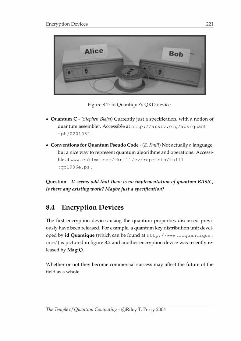
Encryption Devices 221
Figure 8.2: id Quantique’s QKD device.
• Quantum C - (Stephen Blaha) Currently just a specification, with a notion ofquantum assembler. Accessible at http://arxiv.org/abs/quant
-ph/0201082 .
• Conventions for Quantum Pseudo Code - (E. Knill) Not actually a language,but a nice way to represent quantum algorithms and operations. Accessi-ble at www.eskimo.com/ ∼knill/cv/reprints/knill
:qc1996e.ps .
Question It seems odd that there is no implementation of quantum BASIC,is there any existing work? Maybe just a specification?
8.4 Encryption Devices
The first encryption devices using the quantum properties discussed previ-ously have been released. For example, a quantum key distribution unit devel-oped by id Quantique (which can be found at http://www.idquantique.
com/ ) is pictured in figure 8.2 and another encryption device was recently re-leased by MagiQ.
Whether or not they become commercial success may affect the future of thefield as a whole.
The Temple of Quantum Computing - c©Riley T. Perry 2004

Appendix A
Complexity Classes
A.1 Classical
Here is a summary of some of the main complexity classes. Most of these defi-nitions are copied verbatim from [cs.umbc.edu.edu 2003]:
P - the set of languages accepted by deterministic Turing machines in polyno-mial time.
NP - the set of languages accepted by nondeterministic Turing machines inpolynomial time.
NPI (NP intermediate) - the set of languages in NP but not in NP-complete.
co-NP - the set of languages rejected by nondeterministic Turing machines inpolynomial time.
NP-complete - a decision problem in NP is NP-complete if all other problemsin NP are reducible to it.
EXP - the set of languages accepted by deterministic Turing machines in t(n) =
2cn time.
NEXP - the set of languages accepted by nondeterministic Turing machines int(n) = 2cn time.
PEXP - the set of languages accepted by deterministic Turing machines in t(n) =
2p(n) time.
223

224 Classical
NPEXP - the set of languages accepted by nondeterministic Turing machinesin t(n) = 2p(n) time.
UP - the set of languages accepted by unambiguous nondeterministic Turingmachines, that have at least one accepting computation on any input, inpolynomial time.
The next set of classes relate to space complexity - which is the amount of space(storage) required by the algorithm.
LOGSPACE - the set of languages accepted by deterministic Turing machinesin logarithmic space.
PSPACE - the set of languages accepted by deterministic Turing machines inpolynomial space.
NPSPACE - the set of languages accepted by nondeterministic Turing ma-chines in polynomial space.
NLOGSPACE - the set of languages accepted by nondeterministic Turing ma-chines.
The final set of classes refer to probabilistic Turning machines:
PP - the set of languages accepted by probabilistic polynomial-time Turing ma-chines (not proved random = pseudo random).
BPP - the set of languages accepted by bounded probabilistic polynomial-timeTuring machines (balanced probability).
RP - the set of languages accepted by random probabilistic polynomial-timeTuring machines (one sided probability).
co-RP - the set of languages accepted by RP machines with accept and rejectprobabilities reversed.
ZPP - RP intersection co-RP, the set of languages accepted by zero probabilityof error polynomial-time Turing machines.
Some of the main classes are related in the following way [Nielsen, M. A. &Chuang, I. L. 2000]:
• L ⊆ P ⊆ NP ⊆ PSPACE ⊆ EXP.
The Temple of Quantum Computing - c©Riley T. Perry 2004

Quantum 225
• Factoring is thought to be in NPI and not proven to be in NP-complete.
• Graph isomorphism is thought to be in NPI and not proven to be in NP-complete.
• Time hierarchy theorem: TIME(f(n)) ⊂ TIME(f(n) log2(f(n))).
• Space hierarchy theorem: SPACE(f(n)) ⊂ SPACE(f(n) log(f(n))).
A.2 Quantum
Some of the quantum complexity classes are listed below. These definitions arecopied verbatim from [Meglicki, Z. 2002]:
QP - the problem can certainly be solved by a QTM in polynomial time atworst, with P ⊂ QP.
ZQP - the problem can be solved by a QTM without errors in polynomial time,with ZP ⊂ ZQP.
BQP - the problem can be solved by a QTM in polynomial time at worst withprobability greater than 2
3. I.e. in 1
3of cases the computer may return an
erroneous result, also BPP ⊆ BQP.
Some of the quantum complexity classes are related in the following way [Nielsen,M. A. & Chuang, I. L. 2000]:
• It is known that polynomial quantum algorithms are in PSPACE.
• It is thought that NP-complete problems cannot be solved by QTMs in poly-nomial time but NPI problems can.
The Temple of Quantum Computing - c©Riley T. Perry 2004

Bibliography
Arizona.edu 1999, Lecture 1 [Online]. Available: http://www.consciousness.
arizona.edu/quantum/Library/qmlecture1.htm [Accessed 5 December 2004]
Baeyer, H. C. 2001, In the Beginning was the Bit, New Scientist, February 17
Banerjee, S. ? 2004, Quantum Computation and Information Theory - Lecture 1 [On-line]. Available: http://www.cse.iitd.ernet.in/ \∼suban/quantum/lectures/
lecture1.pdf [Accessed 4 July 2004]
Barenco, A. Ekert, A. Sanpera, A. & Machiavello, C. 1996, A Short Introductionto Quantum Computation [Online]. Available: http://www.Qubit.org/library/
intros/comp/comp.html [Accessed 30 June 2004]
Benjamin, S. & Ekert, A. ? 2000, A Short Introduction to Quantum-Scale Comput-ing. [Online]. Available: http://www.qubit.org/library/intros/nano/nano.
html [Accessed 4 July 2004]
Bettelli, S. 2000, Introduction to Quantum Algorithms [Online]. Available: sra.
itc.it/people/serafini/quantum-computing/seminars/20001006-slides.ps
[Accessed 5 December 2004]
Black, P.E. Kuhn, D.R. & Williams, C.J. ? 2000, Quantum Computing and Commu-nication [Online]. Available: http://hissa.nist.gov/ ∼black/Papers/
quantumCom.pdf [Accessed 7 December 2004]
Blume, H. 2000, Reimagining the Cosmos. [Online]. Available: http://www.
theatlantic.com/unbound/digicult/dc2000-05-03.htm [Accessed 4 July 2004]
227
228 BIBLIOGRAPHY
Braunstein, S. L. & Lo, H. K. 2000, Scalable Quantum Computers - Paving the Wayto Realisation, 1st edn, Wiley Press, Canada.
Bulitko, V.V. 2002, On Quantum Computing and AI (Notes for a Graduate Class).[Online]. Available: www.cs.ualberta.ca/ ∼bulitko/qc/schedule/qcss-notes.
pdf [Accessed 10 December 2004]
Cabrera, B.J. ? 2000, John von Neumann and von Neumann Architecture for Comput-ers [Online]. Available: http://www.salem.mass.edu/ ∼tevans/VonNeuma.htm
[Accessed 9 September 2004]
Castro, M. 1997, Do I Invest in Quantum Communications Links For My Company?[Online]. Available: http://www.doc.ic.ac.uk/ ∼nd/surprise 97/journal/
vol1/mjc5/ [Accessed 4 July 2004]
Copeland, J. 2000, What is a Turing Machine? [Online]. Available: http://www.
alanturing.net/turing archive/pages/ReferenceArticles
/WhatisaTuringMachine.html [Accessed 9 August 2004]
cs.umbc.edu.edu 2003, Complexity Class Brief Definitions [Online]. Available:http://www.csee.umbc.edu/help/theory/classes.shtml [Accessed 7 Decem-ber 2004]
Dawar, A. 2004, Quantum Computing - Lectures. [Online]. Available: http:
//www.cl.cam.ac.uk/Teaching/current/QuantComp/ [Accessed 4 July 2004]
Dorai, K. Arvind, ?. Kumar, A. 2001, Implementation of a Deutsch-like quan-tum algorithm utilising entanglement at the two-qubit level on an NMR quantum-information processor [Online]. Available: http://eprints.iisc.ernet.in/archive
/00000300/01/Deutsch.pdf [Accessed 4 July 2004]
Designing Encodings ? 2000, Designing Encodings [Online]. Available: http:
//www.indigosim.com/tutorials/communication/t3s2.htm
Deutsch, D. & Ekert, A. 1998, Quantum Computation, Physics World, March
The Temple of Quantum Computing - c©Riley T. Perry 2004
BIBLIOGRAPHY 229
Divincenzo, D.P. 2003, The Physical Implementation of Quantum Computa-tion, quant-ph/0002077, vol. 13 April.
Ekert, A. 1993, Quantum Keys for Keeping Secrets, New Scientist, Jan 16
Forbes, S. Morton, M. Rae H. 1991, Skills in Mathematics Volumes 1 and 2, 2ndedn, Forbes, Morton, and Rae, Auckland.
Gilleland, M. ? 2000, Big Square Roots [Online]. Available: http://www.
merriampark.com/bigsqrt.htm [Accessed 9 September 2004]
Glendinning, I. 2004, Quantum Programming Languages and Tools. [Online]. Avail-able: http://www.vcpc.univie.ac.at/ ∼ian/hotlist/qc/programming.shtml
[Accessed 4 July 2004]
Hameroff, S. ? 2003, Consciousness at the Millennium: Quantum Approaches toUnderstanding the Mind, Introductory Lectures [Online]. Available: http://www.
consciousness.arizona.edu/Quantum/ [Accessed 30 June 2004]
Hameroff, S. & Conrad, M. ? 2003, Consciousness at the Millennium: QuantumApproaches to Understanding the Mind, Lecture 6 [Online]. Available: http://
www.consciousness.arizona.edu/Quantum/week6.htm [Accessed 30 June 2004]
Jones, J. Wilson, W. 1995, An Incomplete Education , ? edn, ?, ?
Knill, E. Laflamme, R. Barnum, H. Dalvit, D. Dziarmaga, J. Gubernatis, J. Gurvits,L. Ortiz, G. Viola, L. & Zurek, W.H. 2002, Introduction to Quantum InformationProcessing
Marshall, J. 2001, Theory of Computation [Online]. Available: http://pages.
pomona.edu/ ∼jbm04747/courses/fall2001/cs10/lectures/Computation
/Computation.html [Accessed 9 August 2004]
McEvoy, J.P. & Zarate, 0. 2002, Introducing Quantum Theory, 2nd edn, IconBooks, UK.
The Temple of Quantum Computing - c©Riley T. Perry 2004
230 BIBLIOGRAPHY
Meglicki, Z. 2002, Quantum Complexity and Quantum Algorithms [Online]. Avail-able: http://beige.ucs.indiana.edu/B679/node27.html [Accessed 7 Decem-ber 2004]
Natural Theology 2004, Goedel [Online]. Available: http://www
.naturaltheology.net/Synopsis/s26Goedel.html
Nielsen, M. A. 2002, Eight Introductory Lectures on Quantum Information Science[Online]. Available: http://www.qinfo.org/people/nielsen/qicss.
html [Accessed 30 June 2004]
Nielsen, M. A. & Chuang, I. L. 2000, Quantum Computation and Quantum In-formation, 3rd edn, Cambridge Press, UK.
Odenwald, S. 1997, Ask the Astronomer (Question) [Online]. Available: http:
//www.astronomycafe.net/qadir/q971.html [Accessed 30 June 2004]
Rae, A. 1996, Quantum Physics: Illusion or Reality?, 2nd edn, Cambridge Press,UK.
Searle, J. R. 1990, Is the Brain’s Mind a Computer Program, Scientific Ameri-can, January, pp. 20-25.
Shatkay, H. 1995, The Fourier Transform - A Primer [Online]. Available: http://
citeseer.ist.psu.edu/shatkay95fourier.html [Accessed 10 December 2004]
Smithsonian NMAH 1999, Jacquard’s Punched Card [Online]. Available: http:
//history.acusd.edu/gen/recording/jacquard1.html [Accessed 9 September2004]
Stay. M. 2004, Deutsch’s algorithm with a pair of sunglasses and some mirrors [On-line]. Available: http://www.cs.auckland.ac.nz/ ∼msta039/deutsch.txt [Ac-cessed 4 July 2004]
Steane, A. M. 1998, Quantum Computing, Rept.Prog.Phys., vol. 61 pp. 117-173
The Temple of Quantum Computing - c©Riley T. Perry 2004

BIBLIOGRAPHY 231
TheFreeDictionary.com 2004, Grover’s Algorithm [Online]. Available: http://
encyclopedia.thefreedictionary.com/groversalgorithm
[Accessed 4 July 2004]
TheFreeDictionary.com 2004, Probabilistic Turing machine [Online]. Available:http://encyclopedia.thefreedictionary.com/Probabilistic+Turing+machine
[Accessed 3 December 2004]
wikipedia.org 2004, Complexity classes P and NP [Online]. Available: http://
en.wikipedia.org/wiki/Complexity classes P and NP [Accessed 3 November2004]
Wolfram, S. 2002, A New Kind of Science, 1st edn, Wolfram Media, USA
Image References
Figure 2.1http://www.mathe.tu-freiberg.de/ ∼dempe/schuelerpr neu/babbage.htm
http://www.inzine.sk/article.asp?art=8491
Figure 2.2http://www.cs.us.es/cursos/tco/
http://www-groups.dcs.st-and.ac.uk/ ∼history/Mathematicians
/Turing.html
Figure 2.3http://www-groups.dcs.st-and.ac.uk/ ∼history/Mathematicians
/Von Neumann.html
Figure 2.4aima.cs.berkeley.edu/cover.html
Figure 2.5http://www.phy.bg.ac.yu/web projects/giants/hilbert.html
http://www-groups.dcs.st-and.ac.uk/ ∼history/Mathematicians/Godel.html
The Temple of Quantum Computing - c©Riley T. Perry 2004

232 BIBLIOGRAPHY
Figure 2.9http://pr.caltech.edu/events/caltech nobel/
Figure 2.12http://www.elis.UGent.be/ELISgroups/solar/projects/computer.html
Figure 3.9http://www-gap.dcs.st-and.ac.uk/ ∼history/PictDisplay/Fourier.html
Figure 4.1http://www-gap.dcs.st-and.ac.uk/ ∼history/Mathematicians/Maxwell.html
http://www-gap.dcs.st-and.ac.uk/ ∼history/Mathematicians/Newton.html
Figure 4.2http://www-gap.dcs.st-and.ac.uk/ ∼history/Mathematicians
/Copernicus.html
http://www-gap.dcs.st-and.ac.uk/ ∼history/PictDisplay/Galileo.html
Figure 4.3http://www.svarog.org/filozofija/graph/democritus.jpg
http://www.slcc.edu/schools/hum sci/physics/whatis/biography
/dalton.html
Figure 4.4http://www-gap.dcs.st-and.ac.uk/ ∼history/PictDisplay/Helmholtz.html
http://www.eat-online.net/english/education/biographies/clausius \.htm
Figure 4.6http://www-gap.dcs.st-and.ac.uk/ ∼history/Mathematicians
/Boltzmann.html
http://www-gap.dcs.st-and.ac.uk/ ∼history/Mathematicians/bohr.html
Figure 4.7http://www-gap.dcs.st-and.ac.uk/ ∼history/PictDisplay/Einstein.html
http://www-gap.dcs.st-and.ac.uk/ ∼history/PictDisplay/Balmer.html
The Temple of Quantum Computing - c©Riley T. Perry 2004

BIBLIOGRAPHY 233
Figure 4.8http://www-gap.dcs.st-and.ac.uk/ ∼history/Mathematicians/Planck.html
http://www.trinityprep.org/MAZZAR/thinkquest/History/Thomson.htm
Figure 4.9http://www.chemheritage.org/EducationalServices/chemach/ans/er.html
http://www-gap.dcs.st-and.ac.uk/ ∼history/Mathematicians
/Sommerfeld.html
Figure 4.13http://www-gap.dcs.st-and.ac.uk/ ∼history/PictDisplay/Pauli.html
http://www-gap.dcs.st-and.ac.uk/ ∼history/Mathematicians/Broglie.html
Figure 4.14http://www-groups.dcs.st-and.ac.uk/ ∼history/Mathematicians
/Schrodinger.html
http://www-gap.dcs.st-and.ac.uk/ ∼history/PictDisplay/Born.html
Figure 4.15http://www-gap.dcs.st-and.ac.uk/ ∼history/Mathematicians/Born.html
http://www-gap.dcs.st-and.ac.uk/ ∼history/PictDisplay/Dirac.html
Figure 6.1http://www-history.mcs.st-andrews.ac.uk/history/PictDisplay
/Shannon.html
http://www-gap.dcs.st-and.ac.uk/ ∼history/PictDisplay/Boole.html
Figure 8.1http://www.qubit.org/oldsite/intros/nano/nano.html
Figure 8.2http://www.idquantique.com/
The Temple of Quantum Computing - c©Riley T. Perry 2004

Index
Absorbtion spectrum, 97Adjoint, 68Analytical engine, 4Ancilla bits, 28, 142ANDgate, 15Angles in other quadrants, 38Anti-Commutator, 77Aristotle, 91Artificial intelligence, 32Asymptotically equivalent, 21Atoms, 91Automaton, 9
Babbage, Charles, 4Balmer, Johann Jakob, 98Basis, 57BB84, 191Bell state circuit, 144Bell states, 128, 178Bennet, C.H., 187Bennett, Charles, 28Big Ω notation, 21Big Θ notation, 21Big O notation, 21Binary entropy, 162Binary numbers, 6Binary representation, 8Binary symmetric channels, 171Bit swap Circuit, 143Bits, 8Black body, 95Black body radiation, 95Bloch sphere, 120Bohr, Niels, 94Boltzmann’s constant, 94Boltzmann, Ludwig, 94
Boole, George, 156Boolean algebra, 156Born, Max, 104Bra, 56Bra-ket notation, 60Brassard, G., 187Bright line spectra, 97Bubble sort, 19
Caesar cipher, 186Cauchy-Schwartz inequality, 60Cause and effect, 91Cavity, 95Channel capacity, 157Characteristic equation, 70Characteristic polynomial, 70Chinese room, 32Christmas pudding model, 100Church, Alonzo, 6Church-Turing thesis, 6Classical circuits, 14Classical complexity classes, 223Classical Cryptography, 186Classical error correction, 171Classical gates, 14Classical information sources, 158Classical physics, 90Classical redundancy and compression, 160Classical registers, 15Classical wires, 15Clausius, Rudolf , 92CNOTgate, 29, 138Code wheel, 186Codewords, 171Column notation, 54Commutative law of multiplication, 104
235

236 INDEX
Commutator, 77Completely mixed state, 168Completeness relation, 68Complex conjugate, 42Complex number, 41Complex plane, 43Complexity classes, 223Computational basis, 57Computational Resources and Efficiency, 18Constant coefficients, 36Continued fractions algorithm, 207Continuous spectrum, 97Control lines, 28Control of unitary evolution, 219Controlled U gate, 142Conventions for quantum pseudo code, 221Converting between degrees and radians, 38Copenhagen interpretation, 105Copernicus, Nicolaus, 90Copying circuit, 143CROSSOVER, 18Cryptology, 185CSS codes, 178
de Broglie, Louis, 103Decision problem, 23Decoherence, 164, 173Degenerate, 70Degrees, 38Democritan, 33Democritus, 91Density matrix, 164Determinant, 50Determinism, 91Deterministic Turing machines, 23Deutsch - Church - Turing principle, 25Deutsch’s algorithm, 194Deutsch, David, 25Deutsch-Josza algorithm, 198Diagonal polarisation, 116Diagonalisable matrix, 76Dirac, Paul, 105Discrete fourier transform, 81Dot product, 53, 59
Dual vector, 56
Eigenspace, 70Eigenvalue, 70Eigenvector, 70Einstein, Albert, 97Electromagnetism, 90Electron, 98Emission spectrum, 97Ensemble point of view, 165Entangled states, 127Entanglement, 111Entropy, 93EPR, 111EPR pair, 128, 178Error syndrome, 175Excited state, 101Exponential form, 45
FANIN, 18FANOUT, 18Fast factorisation, 205Fast Factorisation algorithm, 208Fast Factorisation circuit, 208Feynman, Richard, 24Finite state automata, 11First law of thermodynamics, 92Fluctuation, 94Flying qubits, 218For all, 36Formal languages, 9Four postulates of quantum mechanics, 112,
149, 169Fourier series, 82Fourier transform, 81Fourier, Jean Baptiste Joseph, 81Fredkin gate, 30, 141Frequency domain, 81Full rank, 50Fundamental point of view, 169
Godel’s incompleteness theorem, 6Godel, Kurt, 6Galilei, Galileo, 90
The Temple of Quantum Computing - c©Riley T. Perry 2004

INDEX 237
Garbage bits, 28, 142Global phase, 118Global properties of functions, 194Gram Schmidt method, 64Ground state, 100Grover workspace, 213Grover’s algorithm, 212Grover, Lov, 113
Hadamard gate, 134Haltig problem, 12Heisenberg uncertainty principle, 105Heisenberg, Werner, 104Helmholtz, Von, 92Hermitian operator, 73, 76Hilbert space, 51, 60Hilbert, David, 6
id Quantique, 221Identity matrix, 49If and only if, 37Imaginary axis, 43Independent and identically distributed, 158Initial point, 51Inner product, 53, 59Interference, 107Intractable, 22, 193Inverse matrix, 49Inverse quantum fourier transform, 201Invertible, 26
Jacquard, Joseph Marie, 4
Ket, 54, 119Keyes, R.W., 28King, Ada Augusta, 4Kronecker product, 80
Landauer’s principle, 26Landauer, Rolf, 26Least significant digit, 8Length of codes, 160Linear combination, 56Linear operator, 64Linearly independent, 57
Local state, 111Logarithms, 40Logical symbols, 36
MagiQ, 221Marked solution, 213Markov process, 150Matrices, 47Matrix addition, 47Matrix arithmetic, 47Matrix entries, 47Matrix multiplication, 48Maxwell’s demon, 27Maxwell, James Clerk, 90Measurement of final states, 219Message Destination, 157Message Receiver, 157Message Source, 156Message Transmitter, 156Mixed states, 163Modulus, 42Moore’s law, 5Moore, Gordon, 5Multi qubit gates, 138Mutual key generation, 191
NANDgate, 16Neumann, Jon Von, 4New quantum theory, 95Newton, Issac, 90Newtonian mechanics, 90No programming theorem, 149Noisy channels, 171Non destructive measurement, 219Non deterministic Turing machines, 23Non-deterministic polynomial time, 22NORgate, 16Norm, 42Normal operator, 73Normalise, 62NOTgate, 15NOT2 gate, 140NP, 22Nuclear Magnetic Resonance, 220
The Temple of Quantum Computing - c©Riley T. Perry 2004
238 INDEX
Nuclear spins, 110
Observable, 127Old quantum theory, 95One-time PAD, 187Optical photon computer, 219ORgate, 15Oracle, 194Order, 206Order finding, 206Orthogonal, 61Orthonormal basis, 63Outer product, 65Outer product notation, 135
P, 22Panexperientielism, 33Partial Measurement, 123Partial measurement, 123Pauli exclusion principle, 102Pauli gates, 130, 136Pauli operators, 74Pauli, Wolfgang, 102Period, 206Phase estimation, 206Phase gate, 133Photoelectric effect, 96π8 gate, 133Planck’s constant, 96Polar coordinates, 43Polar decomposition, 78Polar form, 42Polarisation of photons, 110Polynomial time, 22Polynomially equivalent, 25Polynomials, 36Positive operator, 73, 76POVMs, 153Principle of invariance, 18Probabilistic complexity classes, 224Probabilistic Turing machine, 24Probability amplitudes, 58Probability distribution, 158Programmable quantum computer, 148
Projective measurements, 127Projectors, 66, 127, 151Proto-conscious field, 33Public key encryption, 186Pure states, 163Pythagorean theorem, 37
QCL, 220qGCL, 220Quantised, 89Quantum bits, 114Quantum C, 221Quantum circuits, 129Quantum complexity classes, 225Quantum computer languages, 220Quantum cryptography, 187Quantum dot, 218Quantum fourier transform, 200Quantum fourier transform circuits, 205Quantum information sources, 163Quantum key distribution, 189Quantum logic gates, 130Quantum mechanics, 89Quantum money, 187Quantum noise, 172Quantum numbers, 101Quantum packet sniffing, 188Quantum repetition code, 173Quantum searching, 212Quantum Turing machine, 25Qubit implementation, 218Qubit initial state preparation, 219Qubits, 114Quick sort, 20
Radians, 38Rank, 50Rationalising and dividing complex numbers,
44Rayleigh-Jeans law, 103Rectilinear polarisation, 116Reduced density matrix, 168Relative phase, 117Repetition, 171
The Temple of Quantum Computing - c©Riley T. Perry 2004

INDEX 239
Repetition codes, 172Reversible circuits, 31Reversible computation, 28Reversible gates, 28Reversibly, 26Right angled triangles, 37Rotation operators, 137RSA, 186, 193, 205Rutherford, Ernest, 100Rydberg constant, 98
Scalar, 47Scalar multiplication by a matrix, 47Schrodinger’s cat, 105Schrodinger, Erwin, 104Schumacher compression, 170Schumacher’s quantum noiseless coding the-
orem, 164Searle, John, 32Second law of thermodynamics, 92Shannon Entropy, 161Shannon’s communication model, 156Shannon’s noiseless coding theorem, 161Shannon, Claude E., 155Shor code, 177Shor’s algorithm, 200Shor, Peter, 113Shortest route finding, 212Simultaneous diagonalisation theorem, 78Single qubit gates, 130Single value decomposition, 78Singular, 50Socratic, 33Sommerfeld, Arnold, 102Source of Noise, 156Spanning set, 57Spectral decomposition, 79Spin, 102Square root of NOT gate, 134Stabiliser codes, 178State vector, 58, 116Statistical correlation, 111Statistical mechanics, 93Steane code, 178
Strong AI, 32Strong Church-Turing thesis, 23subsystem point of view, 168Superdense coding, 145Superposition, 107
Teleportation circuit, 146Tensor product, 79, 123Terminal point, 51There exists, 36Thermodynamics, 91Thomson, Joseph J., 98Time domain, 81Toffoli gate, 29, 141Total information, 191Trace, 71Transpose matrix, 50Trap door function, 187Travelling salesman problem, 212Trigonometric inverses, 38Trigonometry, 37Trigonometry identities, 40Truth tables, 14Turing Machine, 6Turing test, 32Turing, Alan, 4
Uncertainty, 110Unit vector, 62Unitary operator, 73Universal computer, 4Universal Turning Machine, 11
Vector addition, 55Vector scalar multiplication and addition, 55Vectors, 51Visualising grover’s algorithm, 215Von Neumann architecture, 4Von Neumann entropy, 164, 169
Weak AI, 32Wheeler, John Archibald , 191Wien’s law, 103Wiesner, Stephen, 187Wire, 130
The Temple of Quantum Computing - c©Riley T. Perry 2004
240 INDEX
Witnesses, 23
XORgate, 16
Zellinger, Anton, 191Zero matrix, 49Zero memory information sources, 159Zero vector, 55
The Temple of Quantum Computing - c©Riley T. Perry 2004