The tourist area lifecycle and the unit roots test. A new

economic perspective for a classic paradigm in tourism.

Authors: Antonio Alcover Casasnovas (Corresponding author)

Andreu Sansó Rosselló

Abstract

As many traditional tourist destinations have experienced a slow down in tourist arrivals

and expenditure, Butler’s (1980) Tourist Area Life Cycle (TALC) model seems to

attract new attention from tourist researchers. The TALC describes the evolution of a

tourist area from its discovery to its final stage picturing an evolutionary path

represented with an S shaped curve associated to the logistic function. The limits of

growth and the shape of the curve represent the existence of congestion problems and

upper carrying capacity limits. But the TALC has been repeatedly criticized by its lack

of operability and its departures from the anticipated curve. An alternative way to test

its existence is to estimate its theoretical logistic curve and test the presence of unit

roots. The application of this new technique to Majorca concludes that the evolutionary

path predicted by the TALC does not apply in this particular case. Even more, the

empirical results could imply that shocks that affect to this destination will have not

temporary but permanent effects, encouraging the adoption of pro-active policy

measures.

Keywords: Destination lifecycle, carrying capacity, logistic function, unit root test.

1. Introduction

In recent years many traditional coastal tourist areas in Southern Europe have

experienced difficulties to maintain or increase their level of arrivals, tourist expenditure

and/or total number of stays average. In this context the concept “mature destination”

has become increasingly used to qualify traditional destinations that experience

difficulties to expand or even maintain their level of tourist activity. As many coastal

areas of Southern Europe have developed local and regional economies strongly

dependent on tourist activity, the possible stagnation and/or decline of their tourist

activity has become a major issue from an economic, social and political point of view.

The concept of mature destination seems apparently linked to the evolutionary tourist

authors and especially to the tourist area lifecycle model of Butler (1980). Early

evolutionary authors focused their attention on change trying to determinate the factors

and processes that rule the evolution of tourism or the development of their structures

(Pearce, 1995), putting special attention in the investigation of tourist destinations. As

Pearce (1995) points out, Cristaller (1963) was probably the first to describe the

evolution of a tourist destination. Latter on, Miossec, (1977), Plog, (1973), Stansfield

(1978) or Thurot, (1973) followed him presenting alternative theories to describe the

evolution of tourist areas. For all of them the final step of the evolution consisted in the

popularization of the destination and the decline of its tourist activity.

Probably, the most relevant of these authors was Butler (1980). His Tourist Area

Lifecycle model (TALC hereafter) synthesizes the contributions of the main preceding

evolutionary authors gathering together the main factors under destination dynamics

and decline like: the changes in the type of visitor (Cristaller, 1963; Thurot, 1973;

Plog,1972; Cohen, 1972), the possible degradation or change of the physical plant

(Stansfield, 1978) and the replacement or even disappearance of the original natural and

cultural attractions which were responsible for the initial popularity of the area

(Cristaller, 1963; Cohen, 1972; Miossec, 1977).

In Butler’s TALC (1980), traditional tourist areas traverse during its life span six stages:

exploration, involvement, development, consolidation and stagnation, arriving to a final

post-stagnation stage. However, it must be remarked that this last stage (post-

stagnation) was in fact open (Butler admitted a final stage where sharp decline,

rejuvenation or other intermediate solutions were possible). Each stage was

characterized by a different rhythm of growth, the change of attitude and composition of

the main actors (tourists, administration, local entrepreneurs, international corporations,

local residents and immigrants) and the variation of the main attractions (original or

human made). The result of this evolution was an S shape or logistic curve representing

the arrivals of tourist or visitors until the stagnation stage (see figure 1). The upper limit

of this curve was determined by the social, physical or economical carrying capacity of

the tourist area destination.

Figure 1. Evolution of tourist area by the TALC

Number of A

Tourists Rejuvenation B

Critical range of Stagnation

elements of capacity Consolidation C

D

Development

Decline E

Involvement

Exploration

Time

Mature destinations are normally described using TALC terminology and are normally

associated to the post stagnation stage. Getz (1992) referring to Hovinen (1982)

described maturity as the stage where “elements of consolidation, stagnation, decline

and rejuvenation co-exist. It is a constant battle to remain competitive and profitable,

both at the micro and macro levels” (Getz, 1992;762). The problem of this definition is

the doubts and problems that rise the TALC model, specially its real nature and the need

for a method to validate it and to determinate its level of irreversibility

Since 1980 many authors have applied the model to describe the evolution of a number

of destinations including: Lancaster county (Hovinen,1982, 2002), Malta (Oglethorpe,

1984), Grand Island in Louisiana (Meyer Arendt, 1985), some Caribbean islands

(Wilkinson, 1987, Debbage, 1990), small pacific nations islands (Weaver, 1990, 1998,

2000; Choy, 1992), the isle of Man (Cooper & Jackson, 1989; Lundtorp and Wanhill,

2001), Niagara Falls (Getz, 1992), Cyprus (Ioannides, 1992), Pattaya (Smith, 1992),

Minorca (Williams, 1993), Italy (Formica and Uysal, 1996), Alpine areas of Australia

(Digance, 1997), mountain regions of Tennessee (Tooman, 1997), Southern England

resorts (Agarwal, 1997, 2002), North Wales (Galle and Botterill, 2005), Costa Brava

(Priestley y Mundet, 1998) Kenia (Akama, 1999), Algarve (Gonçalves and Aguas,

1997), the Dead Sea (Karplus and Kranover, 2004), Tenerife (Oreja et al., 2007),

Balearic Island (Picornell and Picornell, 2002) and other destinations (Leglewski, 2005)

The results obtained by most of the studies tend to support Butler’s model, although,

many deviations from the idealized model have been noted (Prideaux, 2000).

Departures from it (Hovinen, 1981; Haywood, 1986, Cooper & Jackson, 1989; Choy;

1992, Getz, 1992) and some of them criticized some of their aspects or see the TALC

just a hypothetic model (Aguiló, Alegre and Sard, 2005). Eventhough, some authors

express the idea that the TALC is provably the cornerstone in the research of tourism

development (Prideaux, 2000; Karplus and Kracover, 2005) and that As Gonçalves and

Aguas (1997) explain the concept of life cycle can be used for both descriptive and

prescriptive purposes. Most of the studies mentioned above focus on the descriptive

component of the model (e.g., number of tourist, type of tourist, resident’s attitude,

etc.). Gonçalves and Aguas see two reasons to explain it. First, the descriptive

component of the product life cycle concept focused on these studies can be seen as a

support to the prescriptive one, because this latter needs the results given by the first

one. And second, prescription as theoretical instrument is not sufficiently developed.

The idea that the TALC is more descriptive than normative was already present in

Haywood (1981), Oppermann (1998) and still today some authors argue that the model

doesn’t need a quantitative approach to be accepted. Te critical realism of Gale and

Boterill (2005) as opposed to the positivism or the Teleogical perspective (Oreja et al.

2007) are gaining support as an alternative to accept the usefulness of the TALC.

Some studies have tried to full this gap in a much different way using stochastic tools to

explain some of the departures of the model. Gonçalves and Aguas (1997) use time

series forecasting models using linear, exponential and third degree polynomial (cubic)

and logistic (Pearl) models. Referring to the traditional critics to the TALC model

Karplus and Kracover (2005) explain that “most of the critical studies have based their

findings on interpretive analysis of the data and have not used statistical procedures to

substantiate their findings. Without first translating Butler’s model into a mathematical

expression and then testing the correlation between the observed data and the

conceptual model, it is hard to assess the significance of the deviations from the life

cycle model. Nevertheless, only a handful of papers ventured into statistical testing

(Foster and Murphy, 1991; Getz, 1992; Benedeto and Bojanic, 1993; Berry, 2001,

Lundtrop and Wanhill, 2001; Moss et al., 2003).

As we can see, one of the main problems that can difficult the application of the TALC

is the presence of elements initially no contemplated by the model that can affect its

evolutionary path (Agarwal, 1994; Haywood, 1986; Hovinen, 1981; Knowles y Curtis,

1999). Butler wrote his article at the end of the seventies when the international

economic environment was evolving from decades of recovery and stable growth to a

more unstable and confusing situation. In parallel, most of the applications of the TALC

normally obtained good results until the oil crisis at the beginning of the seventies

presenting difficulties and discrepancies with the expected curve between the first and

second oil crisis (1979) and at the beginning of the nineties. In many cases, these

changes of behavior were attributed to an early transition to new stages (consolidation,

stagnation, early decline) or as the crisis were resolved to rejuvenation process.

The importance of this problem is remarked by Gale and Botterill (2005). For these

authors the TALC does not take into account the tourism system in its entirety, “with

the result that it overlooked exogenous forces such as variations in the economic cycle

of source regions and countries” (2005: 159). As both authors say: this limitation was

highlighted by Leiper’s 2004 critique “arguably the most scathing appraisal of the

model to date”, which he asserts “should now be assigned to the archives of history – as

a former theory, now discredited, shown to be false” (2004:135).

On the other hand, we can try to resolve this problem from an economic perspective. It

could be assumed that Butler’s curve pictures the economic growth path and the

structural changes that usually experiences one specific geographic area when it gets

specialized in tourist activities and becomes a consolidated tourist destination. In such a

case, the resulting growth path of the destination during a period of economic stability

(when markets grow steadily without any major economic turbulence) can be easily

observed, giving as a result the well know S shaped logistic curve that Butler pictured in

his article. But, as it can be observed in the case of Majorca, under non-stable economic

conditions the interpretation of the evolutionary path of the destination can become

more complex. In this scenario, it could be assumed that under economic shocks the

evolutionary path of the destination can temporary differ from its structural path due to

the temporary effects caused by the existence of economic instability, but in the long

term the S shaped curve would be the usual path followed by classical destinations.

This work pretends to go forward in the interpretation of the TALC from a more

estructurated perspective. In order to reach this objective the work has been divided in

three parts. In first place, we study the functional form of the model. The traditionally

logistic curve of the model can be attributed to two origins. On one hand, it can come

from supply side limitations (maximum carrying capacity) due to the limited

reproducibility of the original natural attraction and congestion effects, and on the other

hand, it can be caused by demand side limitations (lifecycle product theory-word of

mouth mechanism). This second point of view is represented by Lundtorp and Wanhill

(2001) model. 1

The second part of this work deepens in the analysis of the nature of the logistic curve

(as a model to represent the evolution of tourist area) using the discrepancies between

the observed data and the estimated logistic growth path. That is to say, the study of the

random shocks that affect to the variable that measures the evolution of the tourism in

the selected destination. In this way, it can shown that the persistence proprieties of the

random shocks determine if, on one hand, the path described by the logistic curve can

be interpreted as a long term evolutionary trajectory or, on the other hand, it doesn’t

determine the long run and thus the validity of the TALC (and its associated logistic

curve) to describe long term behavior of a tourist destination. The statistical test of this

idea can be done through a slow transition unit root test suggested by Leybourne et alt.

(1998). As it is well know, the presence of unit roots can drive to a non cautious

researcher to obtain spurious results if he doesn’t take in a count its presence. In the 1 This curve could be also the result of a growth model with constant factors (Lozano, 2002)

present case, the Leybourne et alt. (1998) test, more than a slow transition unitary root

test with structural change, can be interpreted as test over the suitability of the logistic

curve, and thus the TALC, to describe the evolution of a tourist destination. In this

sense, if the deviations from the logistic curve present a unit root, it will mean that they

are permanent and not transitory and as a result of it the TALC is not consistent with the

observed data.

Finally, we apply this new technique to Majorca using the data of arrivals, tourists and

days expended by tourist in the island commenting the results and their implications.

2. The functional form in Butler’s model.

In this section we present a formal model for the S-shaped curve of the transit activity

from two different points of view. First, we reinterpret the demand oriented model of

Lundtorp and Wanhill, (2001) and in second place, we complement it with a supply

oriented model based on the carrying capacity concept that also results in a similar S

shaped path of expansion.

2.1. Demand side limitations: the product lifecycle and the potential market.

The Butler’s (1980) TALC model has been traditionally associated with the product life

cycle and to the logistic curve. The product lifecycle assumes that products go through

several stages in the market (introduction, growth, stagnation and decline) like any

living organism. The initially growing sales stage is usually identified with the

increasing knowledge of the product and with buyer’s curiosity for new goods. In

contrast, maturity and stagnation stages are associated with market saturation (the

potential market already knows or has tried the product) and increasing dependence on

loyalty and repeated consumption. Finally, it’s assumed that the product will decline if a

better or cheaper substitute appears.2

From this point of view, the TALC could be taken as a variety of the product lifecycle

model where the product is a destination. The number of clients or visitors of a tourist

area will grow as its knowledge spreads into the market reaching its peak (stagnation

stage) when all the potential clients know about its existence. The functional

specification of this phenomenon must be coherent with the visitor’s curve usually

observed in these areas, using as principal explanatory arguments a representative

variable of the number of the destination clients (visitors, tourists or tourist per day) and

the knowledge speed expansion of the destination in the market.

This interpretation of the lifecycle was used by Lundtorp and Wanhill (2001) to create a

model that intended to represent the evolution of tourist destinations. In their case the

logistic form of the curve derives from a word of mouth mechanism. They suppose a

potential market of M potential clients, where Mt represents the people that already

know the destination at time t. If the awareness of the destination expands in the market

at the speed of >0, during the lag of time dt, Mt will grow dMt/dt = γ(M-Mt)/M, where

(M-Mt)/M represents the proportion of people that haven’t heard yet from the

destination. Integrating dMt/dt we may write:

2 Even if TALC has been usually associated with Vernon (1966), authors like Sinclair and Stabler (1997) remark the differences between the product lifecycle studied in economics (Vernon, 1966) and the product lifecycle theory studied from the industrial economics perspective. For them, Vernon’s vision could be used to explain the expansion of the international tourism meanwhile TALC could be closer to the product lifecycle concept developed by the Industrial Organization Theory (even if both of them have in common Postner -1961- and Vernon -1966- works). This same differentiation can be found in the first evolutionary authors who distinguished between the evolution of a particular destination and the international tourist evolution. From their point of view, it was clear that any particular destination in the more advanced stages of its evolution (stagnation or decline) could still maintain a relevant (but significant lower) level of tourist activity focusing in the upper social levels or in specialized segments of the market, living the most standardized activities to new destinations that still enjoy all their original attractions and cost advantages.

(2.1)

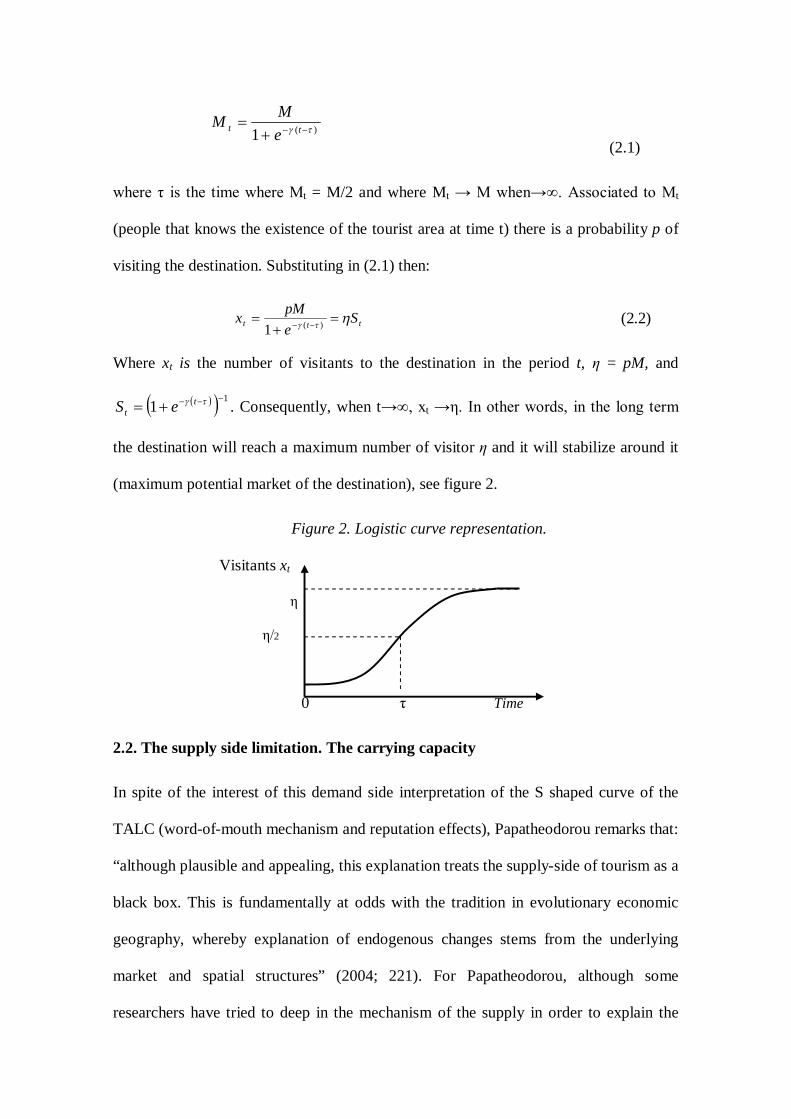
where τ is the time where Mt = M/2 and where Mt → M when→∞. Associated to Mt

(people that knows the existence of the tourist area at time t) there is a probability p of

visiting the destination. Substituting in (2.1) then:

(2.2)

Where xt is the number of visitants to the destination in the period t, η = pM, and

11

tt eS . Consequently, when t→∞, xt →η. In other words, in the long term

the destination will reach a maximum number of visitor η and it will stabilize around it

(maximum potential market of the destination), see figure 2.

Figure 2. Logistic curve representation.

Visitants xt

η

η/2

0 τ Time

2.2. The supply side limitation. The carrying capacity

In spite of the interest of this demand side interpretation of the S shaped curve of the

TALC (word-of-mouth mechanism and reputation effects), Papatheodorou remarks that:

“although plausible and appealing, this explanation treats the supply-side of tourism as a

black box. This is fundamentally at odds with the tradition in evolutionary economic

geography, whereby explanation of endogenous changes stems from the underlying

market and spatial structures” (2004; 221). For Papatheodorou, although some

researchers have tried to deep in the mechanism of the supply in order to explain the

)(1 tt e

MM

ttt SepMx

)(1

TALC (Tremblay, 1998; Britton, 1991; Debbage, 1990) “these research efforts remain

without substantial continuation” (2004: 220). 3

But, as Butler (1980) remarks, the carrying capacity concept plays a central role in the

TALC acting as a supply limitation. Originally, each destination, depending on their

initial stock of resources and the tourist modality developed, will have a maximum

amount η of visitors that could be attended in the best suitable conditions (Oreja et al.

2007). In fact, probably the S shaped curve of the TALC, so many times observed in

different tourist destinations, could owe more to the carrying capacity than to the

behavior of the consumers into the tourist markets.

Although TALC related literature has given great importance to the carrying capacity

concept (Butler, 20005b; Oreja et al. 2007), the complexity of the tourist product has

generated some controversy over the elements that must be present in its definition and

the interpretation that must be given to them. Nowadays, one of the definitions that

seems to be more accepted in tourist literature (Oreja et al. 2007) stands that: carrying

capacity of a tourist area is: the maximum number of tourist that can be tolerated

without an unacceptable or irreversible deterioration of the physic environment and

without a sensible decrease on user’s satisfaction (Mathieson y Wall, 1982: 21, Tisdell

1988: 244, Davis y Tisdell, 1996: 232).

In this last definition there are two main elements: deterioration of the environment and

the satisfaction obtained by the user (tourist). Destinations will keep attracting visitors

as far as they satisfy their expectations and they will loose clients if they deceive them.

The tourist area demand (or the demand of its tourist services) depends, as the vast

majority of economic goods, on its utility or capability to satisfy needs. The problem of 3 Papatheodourou (2004:220-21) referring to TALC: “evolutionary theory can have truly useful policy implications only if it can explain the casual mechanisms of development … To do so, such a framework should primarily focus on inherent system dynamics or the endogenous changes in tourism destinations”.

tourist areas is that many of their attractions (beaches, forests, traditions, etc.) are public

goods with limited reproducibility and subject to congestion problems. If we accept the

former carrying capacity definition, its existence implies a maximum ceiling of visitor

η. But, even if a majority of tourist experts accept today that most of the tourist areas

have a certain upper limit in their development, many of them reject the idea that the

usual trajectory to reach it must be the logistic curve pictured by the TALC (Aguiló et

al. 2005). And as will see this is at odds with the origin of the concept.

The origin of the carrying capacity concept is attributed to Robert Malthus. In his book

An Essay on the Principle of Population (1986, first Ed. 1798) he introduced his

population theory where food resources acted as a growth limiting factor. In a world

where population grew at a geometric rhythm meanwhile food resources increased

arithmetically, the population was condemned to misery and starvation. Thanks to its

simplicity, Malthus population theory was broadly accepted without been empirically

tested and exerted an important influence on science during the XIX century, especially

on Darwin writings and in his natural selection theory that afterwards became the

foundations of the actual biology, evolutionary ecology and human demography (Seidl

y Tisdell, 1999). As these two last authors remark, the mathematical expression of the

Malthusian idea of an explosive growth of population only limited by natural resources,

was first established and empirically tested by Pierre Verhulst in 1938 using population

data ranging from the beginning of the XIX century of some countries (Belgium,

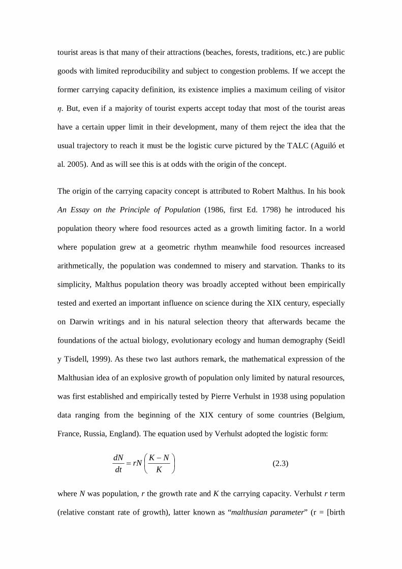
France, Russia, England). The equation used by Verhulst adopted the logistic form:

K

NKrNdtdN

(2.3)

where N was population, r the growth rate and K the carrying capacity. Verhulst r term

(relative constant rate of growth), latter known as “malthusian parameter” (r = [birth

rate b–death rate d]) introduces the Malthusian assumption of the exponential growth

(mathematically rNdtdN / ), whereas the parameter K (carrying capacity) introduces the

population limitation associated to the limited provision of food.

Figure 3 Graphic expression of Verhulst formula.

Nt (Population) dN/dt = rN (exponential growth)

K dN/dt = rN (K –N)/K (logistic growth)

O t (time)

When population level reaches K (figure 3), birth rate equals to death rate and the

growth is cero (stationary estate).4

As Seidl and Tisdell (1999) remark, carrying capacity concept (and its dynamic

application in the logistic growth of populations) has become a basic supposition for

particular ecosystems in biology (is more difficult to accept in complex populations). In

ecology this term is especially important in the study of particular habitats or

ecosystems (like cattle prairies, wild ecosystems or tourism) or to illustrate the ecologic

impacts and limits of human growth and the consumption of resources (Club of Rome).

But the application carrying capacity to human beings requires the acceptance that, in

contrast to biology, social carrying capacity is essentially determined by social aspects

(consumption patterns, institutional framework, technology, environmental impacts,

cultural level, etc.) that may play a more important role than the biological.

4 Latter on in 1920, Pearl and Reed, unknowing the works of Verhulst, formulated a logistic curve adapted to the evolution of the United States census (Pearl and Read, 1920). Their success is reflected in the fact that today we refer to the Verhulst-Pearl logistic equation (Seidl y Tisdell, 1999).

Figure 4 Social and biophysics’ carrying capacity limits.

Nt (Population in t)

KB

KS

O t (time)

In consequence, for human beings there will be a biophysical (KB) and social carrying

capacity (KS) with the former always higher than the second (KB>KS) (Harding, 1986).

Biophysical carrying capacity (KB) determines the maximum level of human population

that can be maintained with a given technology and natural resources, meanwhile, social

carrying capacity (KS), determines the maximum population that can be maintained

under different social systems (Daily y Ehrlich, 1992).

This last aspect could raise some doubts over the stability the carrying capacity in a

tourist destination. As we know today, Malthus’ pessimistic perspectives never became

reality thanks to the technologic advances in food production, but at the same time the

increase of the minimal subsistence salary (or minimal level of social subsistence)

avoided the explosive increase of the population in high developed countries.

As it happened with Malthus’ prophecies, the introduction of technical advances and

new management techniques in the tourist industry and destinations seems to potentially

increase destination’s carrying capacity level. But these improvements can even be

outset by the increasing quality standard required by tourist (Morgan, 1990), or by the

supply limitation strategies adopted in mature destinations (Oreja et al. 2007). In our

case we can assume the hypothesis that tourist quality standards evolve at least at the

same rhythm than the resources saved with the use of new technical advances and

destination management improvements. In this case, destination’s carrying capacity will

stable and the natural way to reach it will be the logistic curve pictured in figure 4.

3. The estimation of the logistic curve and its validation as a long term path.

3.1 Estimation of the logistic

Either if Butler´s curve is interpreted from the supply side (carrying capacity limitation)

or from the demand side (market exhaustion), the logistic function is the most logical

functional form to represent the evolution of a tourist area. It is coherent with both

interpretations and apparently fits with the evolution observed in many destinations.

Assuming the possibility of fluctuations in its evolution due to exogenous factors, we

can return to 2.1 expression and introduce an error term u = xt-St, in order to collect the

discrepancies between the observed values xt and the path forecasted by St model so:

tt

ttt ueuSx 1)( )1( (3.1)

The logistic curve is non-linear in its parameters, so it requires to be estimated by non

lineal least squares (NLLS). The proprieties of these estimators will depend on the

stochastic characteristics of the error term ut and, specially, of its persistency degree as

will be see ahead.

On the other hand, the model (3.1) could be generalized to allow more general forms in

the systemic part of the model. In this way, we can consider the specifications:

ttt uSx (3.2)

ttt uStx (3.3)

tttt utSStx (3.4)

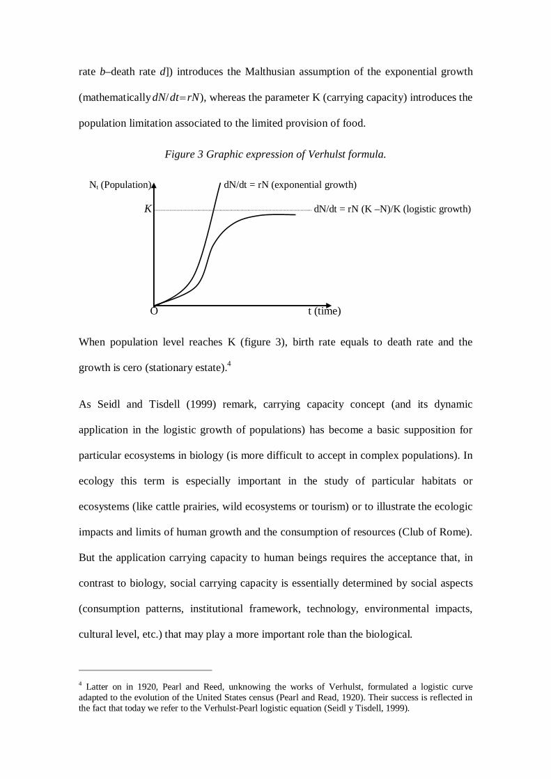
3.2. The logistic curve as a long term relation.

Unit roots. The test of Leybourne et alt. (1996) and its application to TALC.

Let consider again the model given by the expression (3.1). Both, the validity of the

NLLS estimators and the interpretation of the model depend on the same (stochastic)

properties of error term ut. As it has been previously indicated, this term is the

discrepancy between the observed values and the forecasted evolution of the logistic

curve. On one hand, this term collects the effects that have on tourist destinations

exogenous random shocks such as increases in oil prices, changes in the economic

conjuncture of tourist sending markets, natural or terrorist disasters, etc. In

consequence, it collects all the short-run factors that can not be considered in long term

stylized evolutionary model given by a logistic curve. And on the other hand, ut could

also collect all the effects on tourist demand of commercial policies applied by public

administrations and/or tourist companies provided that they do not represent a structural

change in the parameters of the logistic curve.

In any case, if the term ut tends to be very high and to move permanently away from the

growth path tS , we can not assume that this trajectory constitutes an equilibrium path.

If we want to achieve this last goal, we need that the fluctuations collected by ut will be

transitory.

Therefore, it is required that random shocks ut have finite memory and in consequence

they have transitory effects. That does not mean that they do not show signs of

autocorrelation but these shouldn’t be very intensive. To illustrate the idea more

formally, we may assume that ut behaves as an AR(1) process,

ttt uu 1 (3.6)

where εt is white noise, that is, it has null mean, constant variance and it is not

autocorrelated. Although this set of assumptions is very restrictive (so it will be relaxed

ahead), it helps us to center our attention in a simplified model and in the role played by

ρ parameter. When -1< ρ <1, the expression (3.6) is a first order autoregressive process

AR(1), that includes, as a particular case, the situation in which ut is uncorrelated (ρ =

0). The AR(1) process is stationary and εt have a transitory effect on the values taken by

ut. That is to say, the shock effects of εt over ut+h tend to cero as h horizon gets higher.

In consequence, the sequence of values that adopts εt does not have influence on the

values that will have ut in the future. In fact, as it is well known, the best forecast that it

can be make for ut at long term is its unconditional expectation, which in our case is

cero. Thus, if the error term ut is a stationary AR(1), then the best long-run forecast of xt

will be given by the logistic curve:

httththtttht SxxuESxxxE ,...,,..., 11 (3.7)

when h, given that, in this case 0,..., 1 htttht uExxuE . In this situation, we

can interpret the logistic curve as the long-run trajectory and the fact that xt does not

continually adopt the values forecasted by this curve is due to transitory disturbances

that temporally move it away from this evolutionary path. In the case that nothing

disturbs the system, its followed evolution will match with the logistic curve.

Lets consider now the case where ρ=1, in such a way the model given by (3.6), is

known as random walk. In this case, if we replace recursively in (3.6), we can write:

h

jjttht uu

1

(3.8)

that replaced in (2.2), actualized to t+h and taking conditioned expectances results in:

tht

tththtttht

uSxxuESxxxE

,...,,..., 11 (3.9)

for any h>0, so all the forecasts on the future evolution of xt depend on the present

value of ut, unlike AR(1) case shown in (3.7). On the other hand, as ut is a random walk

and (even if it has a cero mean) its variance increases lineally with the time, the

probability that ut takes very high values (in absolute terms) in relation to tS gets each

time bigger. That is to say, the provability that xt moves away from the deterministic

path tS will keep growing. Moreover, a random walk is characterized by: its high

persistence (where each value is its preceding value plus a little change); the lack of any

tendency to repeat past values; the presence of long series of positive values (ut<0) that

can be followed by other negative (ut>0), or vice versa; and finally, there is not limit to

the variation. All these facts imply that at long term, the evolution of xt will basically

depend on ut so Butler’s model doesn’t apply for that destination.

From this point of view, a easy and simply way to empirically test if one specific

destination fulfil with Butler’s model will consist in contrasting if ut is a random walk or

AR(1) process, or even in a more general way, if ut has a unit root (and thus it looks like

an random walk) or it is stationary in variance in such way that its better long term

forecast is cero. To do so, we can use the unit roots test developed by Leybourne et al.

(1996). Although this test was developed for a context of unit roots with gradual

structural change, it looks appropriated to resolve the proposed problem because it’s

equally based on (3.2) to (3.4) expressions.

We must also remark that expression (3.8) shows that the value ut (and the value of xt in

the long-run) is in fact the accumulation all part random shocks. In consequence, if all

the policies applied by the enterprises and administrations had obtained positive (or

negative) effects, they will accumulate so there is place for the political action in order

to find positive results.

3.3. Unit roots test of Leybourne, Newbold y Vougas (1998).

Leybourne et al. (1998) consider three (auxiliary) regressions to contrast the null

hypothesis of one unit root against the alternative of stationarity around a determinist

path that experiments a soft (logistic) transition between two states.

They consider three auxiliary regressions given by the expressions (3.2) to (3.4) where

ut is a stationary process of zero mean. If we assume that vt is a zero order integrated

process I(0), then model (3.2) implies that xt is stationary around a value (a mean) that

gradually changes from an initial value of to a final value of . Model (3.3) is

quite similar but allows the presence of a term that represents the existence of a constant

slope (β). And finally, model (3.4) allows not only the variation of the intercept from

to , but also the variation of the slope parameter (with the same transition speed)

from to . If 0 , the initial and final states switch, but the parameter’s

interpretation remains the same. Consequently, if we wish to test the TALC, the

appropriate auxiliary regression to be used is model (3.2.). The other two models allow

an indefinitely growth of xt being, for this reason, incompatible with Butler’s model.

The null hypothesis of Leybourne et al. (1998) test is that xt is a random walk

ttt XX 1 (3.10)

while the alternative to the null hypothesis is one of the three models given by (3.2) to

(3.4) expressions, where t and tu are assumed to be stationary process of null mean.

The test of the hypothesis are made in a two step process:

- First: Using a non-linear lest square algorithm (NLLS), we estimate the deterministic

component of the model and we compute the residuals (ût) for A, B or C models.

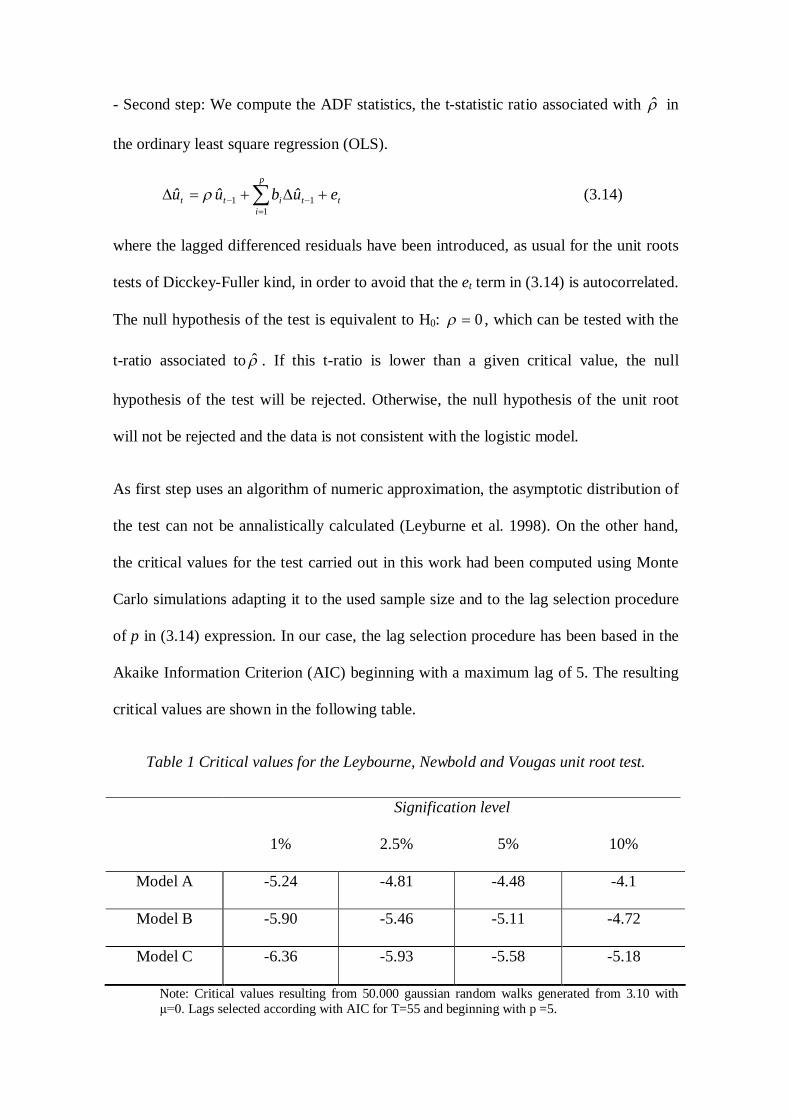
- Second step: We compute the ADF statistics, the t-statistic ratio associated with ̂ in

the ordinary least square regression (OLS).

t

p

ititt eûbûû

111 (3.14)

where the lagged differenced residuals have been introduced, as usual for the unit roots

tests of Dicckey-Fuller kind, in order to avoid that the et term in (3.14) is autocorrelated.

The null hypothesis of the test is equivalent to H0: 0 , which can be tested with the

t-ratio associated to ̂ . If this t-ratio is lower than a given critical value, the null

hypothesis of the test will be rejected. Otherwise, the null hypothesis of the unit root

will not be rejected and the data is not consistent with the logistic model.

As first step uses an algorithm of numeric approximation, the asymptotic distribution of

the test can not be annalistically calculated (Leyburne et al. 1998). On the other hand,

the critical values for the test carried out in this work had been computed using Monte

Carlo simulations adapting it to the used sample size and to the lag selection procedure

of p in (3.14) expression. In our case, the lag selection procedure has been based in the

Akaike Information Criterion (AIC) beginning with a maximum lag of 5. The resulting

critical values are shown in the following table.

Table 1 Critical values for the Leybourne, Newbold and Vougas unit root test.

Signification level

1% 2.5% 5% 10%

Model A -5.24 -4.81 -4.48 -4.1

Model B -5.90 -5.46 -5.11 -4.72

Model C -6.36 -5.93 -5.58 -5.18

Note: Critical values resulting from 50.000 gaussian random walks generated from 3.10 with µ=0. Lags selected according with AIC for T=55 and beginning with p =5.

4. Results obtained in the empirical application to Majorca

In this section we apply the Leybourne, Newbold and Vougas (LNV) test to the

evolution of Majorca. As we have already explained, the results obtained with this test

will be very important to know if a tourist area like the island of Majorca has followed a

coherent path with the TALC.

Majorca is one of the most popular tourist destinations of Spain. In the year 2005 the

island received more than 9 millions tourists representing around 17% of Spanish

international tourist arrivals (INE, 2006). Majorca by itself receives more international

tourist arrivals than countries like Belgium, Switzerland, Australia, Ireland or Japan

(UNWTO, 2007). The important role play by Majorca in the in the international tourist

industry added to the fact that Majorca is an island and has old records of tourist arrivals

makes this destination a very interesting case to study its evolution.

We have considered three variables representing the tourist activities of Majorca:

number of arrivals, tourist and tourist per day. The election of these variables is founded

in the belief that even if tourist or tourist per day data seem to be more representative of

the degree of use of tourist assets in a particular destination and the congestion

problems related to them, the data problems that seem to affect the homogeneity of

these series recommend the use of more reliable variable like the destination arrivals.

Even with some reserves over accuracy of the tourist data available, we present the

results obtained with the LNV test to all three series (arrivals, tourist and tourist per

day) and to the auxiliary regressions given by expressions (3.2) to (3.4) in order to test

the robustness of the obtained results. The span of the series is from 1950 to 2004.

The data comes from different sources. Initial figures of passenger arrivals come from

the annual reports of local Trade, Industry and Navigation Chamber, latter completed in

the fifties with data published by the Diputacion de Mallorca5 and from the eighties

with data coming from the Conselleria de Turisme de les Illes Balears in its annual

publication “El Turisme a les Illes Balears. Dades Informatives”. These publications

have been also used to obtain the data referred to tourist and average tourist length in

the destination.

The following Charts (1 and 2) show the adjustment of the model (3.2) in tourist and

tourist per day data series of Majorca, estimated by NLLS. Apparently, there seems to

be a good adjustment although its proprieties will depend on the existence of unit roots

in the error term ut.

Chart 1. Adjust of the logistic model (1.2) to the tourist per day series.

Chart 2. Adjust of the logistic model (1.2) to the tourist series.

5 “Diputación de Mallorca” also published data referred to the number of tourist arrivals and the average length spent in the island that have been also used to elaborate this study.

As we can observe in the evolution of ut in Charts 1 and 2 there are some signals that

point to a random walk of these variables. Contents of table 2 confirm this first opinion.

Table 2 LNV tests of passenger arrivals, tourist and tourist per day units (1950–2004) ADF (LNV)

Variable Yt Ln Yt

Model 3.2 0.3924 -1.5093

Passengers

arrivals Model 3.3 -2.0267 -1.9341

Model 3.4 -3.0459 -3.6351

Model 3.2 2.8070 -2.1349

Tourists Model 3.3 -1.9296 -3.9067

Model 3.4 -2.9356 -5.7509**

Model 3.2 -3.3775 -2.5586

Tourist per day Model 3.3 -3.3175 -3.4259

Model 3.4 -2.5954 -4.6909

Note: ***, ** y * respectively indicate signification levels of 0.01, 0.05 y 0.10

Table 2 shows the results obtained by the application of the unit roots test to all three

series. These results do not allows us (in all three cases) to reject the null hypothesis that

the series xt have an unit root (the results of the LNV tests are beyond the critical values

tabulated in table 1). Even more, the generalization of the test to the tourist and tourist

per day series between the years 1950 and 2004 obtain similar results. In all three cases

the alternative hypothesis represented by (3.2) to (3.4) models are rejected. In order to

test the robustness of these results we have made the same operations in logarithmic

terms (as it can bee observed in the second column of table 2). The results obtained in

this case are similar to those obtained in the former case with exception of the model

(3.4) using tourists (as it had been explained before, model (3.4) is the less

representative of the TALC). But in any case, even if this last model would be adequate,

the results obtained by the unit roots tests applied to the evolution of Majorca conclude

that there is strong evidence that this particular destination does not follow the patterns

predicted by the TALC.

5. Conclusions

These results allow us to assert at least three relevant conclusions. In first place, we can

not assert that Majorca’s tourism evolutionary behavior is coherent with the TALC. The

logistic evolutionary path sustained by this model do not fulfill in the case of Majorca.

In contrast, the island presents an apparently random evolutionary path. In second place,

the non stationary nature of the data implies that the apparently maturity state of

Majorca do not imply the stationary state of its activity. The number of visitors, tourist

or tourist per day in the destination probably could register up and down random

variations in the future. And in third place, the random nature of this series implies that

all the shocks that affect this tourist area will have not only temporary but permanent

effects. These shocks include policy measures adopted by local or state authorities

(public investments in tourist infrastructure, subsidies to develop new tourist products,

etc). In consequence, in this case if the destination begins to show the signal of

stagnation, the local or state authorities must act fast and strongly if they want to

maintain the growth of their destination. There is not such thing as a deterministic law

that hampers the growth of the destiny and makes useless the attempts to overpass it.

In conclusion, even if nowadays Majorca presents all the typical characteristics of the

stagnation stage of the TALC model, the statistical validation of the Butler Model for

this island rejects its validity. Even more, the results obtained seem to reveal some clues

about its future. The black prophecies for old mass tourist destinations like Majorca

pointed out by many of the early evolutionist authors (Cristaller, 1963; Thurot, 1973;

Plog, 1976), or the more directly and recently exposed by authors like Knowles y Curtis

(1999) are confronted with the results obtained. The deterministic assumptions of these

authors do not have to disappoint or prevent the application of tourist policies by local

or central authorities. Policy makers, specifically in this case, must be aware that the

application of pull-out policies backed by some authors or the wait and see policies

could be costly if they do not strongly back pro-active action. The hesitation face to this

situation can drive in these situations to adopt auto self-fulfilled measures.

On the other hand, in the same way that positive shock cumulates and can give result to

a high level of tourist activity, the accumulation of negative shocks could give place to a

prolonged decadence of the destination. Both possibilities are compatible with the

existence of unit roots.

Of course, this work is focus in the case of Majorca. Future research must apply the

same method to other tourist destinations to see if they follow the logistic path

described by the TALC. If the results are similar to Majorca, the TALC could be

definitely challenged as one of the most important paradigms in tourism.

References

Agarwal, S. (1994). The resort cycle revisited: implications for resorts. In Cooper, C.P.

& Lockwood, A. (Eds.), Progress in Tourism, Recreation and Hospitality Management.

Vol. 5 (194-208). Chichester: Wiley.

Agarwal, S. (1997). The resort cycle and seaside tourism: an assessment of its

applicability and validity. Tourism Management, 18(2), 65-73.

Agarwal, S. (2002). Restructuring seaside tourism. The resort lifecycle. Annals of

Tourism Research, 29(1), 25-55.

Aguiló, E. Alegre, J. and Sard, M. (2005). The persistence of the sun and sand tourism

model. Tourism Management, 26 (2), 219-231

Akama, J.S. (1999). The evolution of tourism in Kenya. Journal of Sustainable

Tourism, Vol. 7 (1), 6-25

Britton, S.G. (1991). Towards a critical Geography of Tourism. Environment and

planning D. Society and Space, 9, 451-478.

Buhalis, D. (2000). Marketing the competitive destination of the future. Tourism

Management, 21(1), 97-116

Butler R.W. (1980). The concept of a tourist area cycle of evolution: implications for

management of resources. Canadian Geographer, 24, 5-12.

Butler R.W. (2005a). The TALC Volume I: Applications and Limitations, Clevedon

Chanel View Publications, Clevendon, England.

Butler R.W. (2005b). The TALC Volume II: Conceptual and Theoretical issues,

Clevedon Chanel View Publications, Clevendon, England.

Choy D.J.L. (1992). Life cycle models for pacific islands. Journal of Travel Research,

30 (3), 26-31.

Christaller, W. (1963). Some considerations of tourism location in Europe: The

Peripheral Regions -Underdeveloped Countries- Recreation Areas. Regional Science

Association Papers, 12, 95-105.

Cohen, E. (1973). Towards a sociology of international tourism. Social Research, 39,

164-182.

Cooper C. and Jackson, S. (1989). Destination life cycle: the Isle of Man case. Annals of

Tourism Research, 16, 377-398.

Daily, G.C. & Ehrlich P.R. (1997). Population, sustainability, and earth’s carrying

capacity. In Elgar Reference Collection, The development of ecological economics (465-

75), International library of critical writings in economics, vol. 75. United Kingdom.

Cheltenham.

Davis, D and C. Tisdell (1996) “Economic management of recreational scuba diving

and the environment. Journal of Environmental Management, 48, 229-248.

Debbage K.G. (1990). Oligopoly and the Resort Cycle in the Bahamas, Annals of

Tourism Research, 17, 513-527.

Formica, S. & Uysal, M. (1996). The revitalization of Italy as a tourist destination.

Tourism Management, 17 (5), 323-331.

Getz, D. (1992). Tourism planning and destination life cycle. Annals of Tourism

Research, 19, 752-770.

Goncalves, V. F. da C. and Aguas, P. M. R. (1997). “The concept of life cycle: an

application to the tourist product”, Journal of Travel Research, 36(2), pp.12-22.

Harding, G. (1986). Cultural carrying capacity: a biological approach to human

problems”, BioScience, Vol. 36 (9), pp: 559-604.

Haywood, K.M., (1986). Can the tourist-area life cycle be made operational? Tourism

Management, 7, 154-167.

Hovinen, G.R. (1981): "A Tourist Cycle in Lancaster County Pennsylvania", Canadian

Geographer, Vol. 25, pp 283-286.

Hovinen, G.R. (2002). Revisiting the destination lifecycle model. Annals of Tourism

Research, 29(1), 209-230.

INE (Instituto Nacional de Estadística) (yearly). Hostelería y Turismo (in Cifras INE y

Últimas cifras; INE Base Servicios). www.ine.es (date of access: 05/03/2006)

Ioannides, D. (1992). Tourism development agents: the Cypriot resort cycle. Annals of

Tourism Research, 19, 711-731.

Karplus, Y. and S. Kracover (2005). Stochastic multivariable approach to modeling

tourism area life cycles. Tourism and Hospitability Research, 5 (3), 235-253.

Knowles, T. & Curtis, S. (1999). The market viability of european mass tourist

destinations. A post-stagnation life-cycle analysis. Journal of Tourism Research. 1(2),

87-96.

Leybourne, S. Newbold, P. & Vougas, D. (1998). Unit roots and smooth transitions.

Journal of Time Series Analysis, 19 (1), 83-97

Leiper, N. (2004). Tourism Management, French Forests: Pearson Education, Australia

Lozano, J. (2002). Crecimiento Económico con Restricciones Medioambientales en

Economías Turísticas. PHD Thesis. Palma de Majorca, Universitat de les Illes Balears.

Lundtorp, S and Wanhill, S (2001). The resort lifecycle theory: generating processes

and estimation. Annals of Tourism Research, 28 (4), 947-964.

Mathieson, A. and Wall, G. (1982). Tourism: Economic, Physical and Social Impacts,

New York: Longman House.

Meyer-Arendt, K. (1985). The Grand Isle, Louisiana resort cycle. Annals of Tourism

Research,12, 449-465.

Miossec, J.M. (1977). Un modèle de l'espace touristique. L'Espace Géographique, 6,

41-48.

Morgan, M. (1991). Dressing up to survive. Marketing Majorca anew. Tourism

Management, 12 (1), 15-20.

Oreja Rodríguez, J. R. Parra-López, E. Yanes-Estévez, V. (2008). The sustainability of

island destinations: Tourism area life cycle and teleological perspectives. The case of

Tenerife. Tourism Management 29(1), 53-65

Oglethorpe, M. (1984). Tourism in Malta. A crisis of dependence. Leisure Studies, 3,

147-162.

Papatheodorou, A. (2004). Exploring the evolution of tourism resorts. Annals of

Tourism Research, 31 (1), 219-237.

Pearce, D.G. (1995). Tourism Today. A Geographical Analysis, Longman Group

Limited, Essex (England).

Piconell, C. and Picornell, M. (2002). L’espai turístic de les Illes Balears. Un cicle de

vida d’una àrea turistica? Evolució i planificació a la darrera década. In L’Espai Turístic

(Ed. Picornell y Picornell), Palma de Mallorca, INESE (Institut d’Estudis Ecològics).

Prideaux, B. (2000). The resort development spectrum (a new approach to modeling

Resort development). Tourism Management, 21, 225-240.

Priestley, G. and Mundet L. (1998). The post-stagnation phase of the resort cycle.

Annals of Tourism Research, 25 (1), 85-111.

Plog, S. C. (1973). Why destination areas rise and fall in popularity? The Cornell Hotel

and Restaurant Administration Quarterly, 14, 55-58.

Smith, R.A. (1992). Beach resort evolution: implications for planning. Annals of

tourism Research, 19, 304-322.

Seidl, I. & C. Tisdell (1999). Carrying capacity reconsidered: from Malthus’ population

theory to cultural carrying capacity. Ecological Economics, 31, 395-408.

Sinclair, M. T. & Stabler, M. (1998). The Economics of Tourism. London. Routledge,

Stansfield, C.A. (1978). Atlantic City and the resort cycle: background to the legislation

of gambling. Annals of Tourism Research, 5, 238-251

Tisdell, C. (1988). Sustaining and maximizing economic gains from tourism based on

natural sites: Analysis with reference to the Galapagos. in Tisdell, C.A, Aislabie, C. J,

Stanton J. C. (Eds.), Economics of Tourism: Case Studies and Analysis. (229-251).

Newcastle: Institute of Industrial Economics, University of Newcastle.

Thurot, J.M. (1973). Le Tourisme tropical Balnéaire: le modele caraibe et ses

extensions, CHET. Aix en provence.

Tremblay, P. (1998). The economic organization of tourism. Annals of Tourism

Researc1h 25, 837–859.

UNWTO (2007). Tourism Highlights, Edition 2006. web document obtained in

http://unwto.org/facts/eng/pdf/highlights/highlights06_sp_hr.pdf (date of access:

05/04/2007).

Vernon, R., (1966). International investments and international trade in the product

Cycle, Quarterly Journal of Economics, 80(2), 190-207.

Weaver, D.B. (1990). Grand Cayman Islands and the resort cycle concept. Journal of

Travel Research, 29(2), 9-15.

Weaver, D.B. (1998). Peripheries of the peripheries: Tourism in Tobago and Bermuda",

Annals of Tourism Research, 25(2)

Weaver, D.B. (2000). A broad Context Model of Development Scenarios, Tourist

Management, 21(3), 217-224

Willians, M.T. (1993). An expansion of the tourist site cycle model: The case of

Minorca (Spain). The Journal of Tourism Studies, 4(2), 24-32.

Wilkinson, P.F. (1987). Tourism in small islands nations: A fragile dependence. Leisure

Studies, 6, 127-146.