the university of hong kong librariesebook.lib.hku.hk/hkg/b35836660.pdf · unit 12 first order...
TRANSCRIPT
THE UNIVERSITY OF HONG KONG
LIBRARIES
This book was receivedin accordance with the Books
Registration OrdinanceSection
SYLLABUSES
FOR
SECONDARY SCHOOLS
APPLIED MATHEMATICS
(ADVANCED LEVEL)
BOOJKREGlSTRATiON ORDINANCEChapter 142
Number:
PREPARED BYTHE CURRICULUM DEVELOPMENT COUNCILRECOMMENDED FOR USE IN SCHOOLS BY
THE EDUCATION DEPARTMENTHONG KONG
1992

Printed and Published by the Government Printer Hong Kong
CONTENTS
PagePREAMBLE 9
1. FOREWORD 10
2. GUIDE TO THE SYLLABUS 11-13
3. SYLLABUS 14-155Topic Area I Vectors and MechanicsUnitl Vectors 14-311.1 Basic Knowledge1.2 Vector Addition
(a) Triangle Law and parallelogram law(b) Properties of vector addition
(i) Commutative law(ii) Associative law
1.3 Zero Vector, Negative Vector and Vector Substraction1.4 Scalar Multiple and its Properties
(a) Associative law(b) Distributive laws
1.5 Components of Vectors(a) Resolution of vectors(b) The unit vectors i , j and k and the resolution of
vectors in the rectangular coordinate system(c) Direction ratios and direction cosines
1.6 Position Vectors and Vector Equation of a Straight Line1.7 Scalar Product
(a) Definition(b) Properties of scalar product(c) Scalar product in cartesian components(d) Orthogonality
1.8 Vector Product(a) Definition(b) Properties of vector product(c) Vector product in cartesian components(d) Perpendicular vectors and parallel vectors
1.9 Triple Product(a) Scalar triple product(b) Vector triple product
1.10 Vector Function, Differentiation and Integration(a) "Vector as a function of a scalar variable(b) Differentiation of a vector function with respect to
a scalar variable(c) Integration of a vector function with respect to a
scalar variable
Page
1.11 Vectors in Polar Coordinates1.12 Application of Vectors
(a) Force as a Vector(b) Kinematics in R2
Unit 2 Statics and Friction 32-40
2.1 Forces, Resultant and Resolution of Forces2.2 Resultant of Parallel Forces, Moments and Couples2.3 Equilibrium of a System of Coplanar Forces2.4 Nature of Friction
(a) Laws of friction(b) Angle of friction
2.5 Equilibrium of Rigid Bodies
Unit3 Kinematics 41-47
3.1 Displacement Velocity and Acceleration3.2 Angular Displacement, Angular Velocity and Angular
Acceleration3.3 Resultant Velocity3.4 Relative Motion3.5 Resolution of Velocity and Acceleration Along and
Perpendicular to Radius Vector
Unit 4 Newton's Laws of Motion 48-52
4.1 Newton's Laws of Motion4.2 Rectilinear Motion of a Particle under Variable Forces
Unit 5 Momentum, Work, Energy, Power and 53-56Conservation Laws
5.1 Momentum and Conservation of Momentum5.2 Work, Energy, Power and Conservation of Energy
Unit 6 Impact 57-62
6.1 Impulse6.2 Impact of Elastic Bodies6.3 Direct Impact6.4 Impact of a Smooth Sphere on Smooth Surface6.5 Oblique Impact
Unit 7 Motion of a projectile under Gravity 63-67
7.1 Motion of Projectile7.2 Trajectory of Projectile7.3 Range on an Inclined Plane7.4 Further Application of Projectile
Page
Unit 8 Circular Motion 68-70
8.1 Circular Motion8.2 Motion in a Vertical Circle
Unit9 Simple Harmonic Motion 71-76
9.1 Simple Harmonic Motion9.2 Damped Oscillation9.3 Forced Oscillation
Unit 10 Motion of a Particle in a Plane 77-79
10.1 Motion of a Particle in a Plane
Unit 11 Motion of a Rigid Body 80-91
11.1 Centre of Mass(a) Introduction(b) Centre of mass by integration(c) Centre of mass of a composite body
11.2 Moment of Inertia(a) Introduction(b) Moment of inertia by integration(c) Parallel and perpendicular axes theorem(d) Moment of inertia of a composite body
11.3 Motion of a Rigid Body about a Fixed Axis(a) Conservation of energy(b) Law of angular momentum(c) Applications
11.4 General Motion of a Rigid Body(a) Introduction(b) Equation of Motion(c) Rolling and sliding(d) General expression of the kinetic energy of a rigid
body
Topic Area II Differential Equations
Unit 12 First Order Differential Equations and its 92-97Applications
12,1 Basic Concepts and Ideas12.2 Formation of Differential Equations12.3 Solution of Equations with Variables Separable12.4 Solution of Linear Differential Equations12.5 Solution of Equations Reducible to Variables Separable
Type or Li near Type
Page
Unit 13 Second Order Differential Equations and its 98-104Applications
13.1 Classification of Types13.2 Principle of Superposition13.3 Solution of Homogeneous Equations with Constant
Coefficients13.4 Solution of Non-homogeneous Equations with
Constant Coefficients(a) Complementary function and particular integral(b) Method of undetermined coefficients
13.5 Reduction of Equations to Second Order DifferentialEquations with Constant Coefficients
13.6 Systems of two First Order Differential Equations13.7 Applications in Practical Problems
Topic Area HI Numerical Methods
Unit 14 Interpolation and Lagrange Interpolating 105-108Polynomial
14.1 Interpolation and Interpolating Polynomials14.2 Construction of Lagrange Interpolating Polynomials14.3 Use of Lagrange Interpolating Polynomial14.4 Error Estimation of Interpolating Polynomial
Unit 15 Approximation 109-113
15.1 Treatment of Errors; their Estimation and AlgebraicManipulation(a) Three basic types of errors
(i) Inherent error(ii) Truncation error(iii) Round-off error
(b) Absolute and relative error(c) Estimation of errors(d) Combining errors
15.2 Approximation of Functional Values using Taylor'sExpansion(a) Taylor's series expansion of a function(b) Error estimation
Unit 16 Numerical Integration 114-118
16.1 Numerical Integration16.2 Trapezoidal Rule
(a) Derivation of the trapezoidal rule(b) Estimation of the error(c) Application of trapezoidal rule
Page
16.3 Simpson's Rule(a) Derivation of Simpson's rule(b) Estimation of the error(c) Application of Simpson's rule
Unit 17 Numerical Solution of Equations 119-125
17.1 Method of Fixed-point Iteration(a) Algorithm of the method(b) The condition of convergence(c) Estimation of error
17.2 Newton's Method(a) Algorithm of the method(b) The condition of convergence and error estimation(c) Application of Newton's method
17.3 Secant Method(a) Derivation of the secant method(b) Application of the secant method
17.4 Method of False Position(a) Derivation of the method of false position(b) Application of the method of false position
Topic Area IV Probability and Statistics
Unit 18 Introductory Probability Theory 126-131
18.1 Basic Definitions18.2 Ways of Counting18.3 Probability Laws18.4 Bayes' Theorem18.5 Recurrence Relation
Unit 19 Basic Statistical Measures 132-133
19.1 Basic Knowledge19.2 Calculation of Mean19.3 Calculation of Standard Deviation and Variance
Unit 20 Random Variables, Discrete and Continuous 134-147Probability Distributions
20.1 Random Variable(a) Discrete probability function(b) Probability density function
20.2 Expectations and Variances20.3 Binomial Distribution
(a) Binomial trials, Binomial probability(b) Binomial distribution(c) Applications
Page
20.4 Normal Distribution(a) Basic definitions(b) Standard normal curve and the use of normal table(c) Applications(d) Binomial approximated to normal distribution
20.5 Linear Combination of Independent Normal Variables
Unit 21 Statistical inference 148-155
21.1 Basic Concept21.2 Estimation of a Population Mean from a Random
Sample21.3 Confidence Interval for the Mean of a Normal
Population with Known Variance21.4 Hypothesis Testing21.5 Type I and Type II Errors
APPENDIX: MATHEMATICS REFERENCE BOOKS 156-173
PREAMBLE
This syllabus is one of a series prepared for use in secondary schools by theCurriculum Development Council Hong Kong. The Curriculum Develop-ment Council, together with its co-ordinating committees and subjectcommittees, is widely representative of the local educational community,membership including heads of schools and practising teachers fromgovernment and non-government schools, lecturers from tertiary institutionsand colleges of education, officers of the Hong Kong ExaminationsAuthority, as well as those of the Curriculum Development Institute, the Ad-visory Inspectorate and other divisions of the Education Department. Themembership of the Council also includes parents and employers.
All syllabuses prepared by the Curriculum Development Council for thesixth form will lead to appropriate Advanced and/or Advanced Supple-mentary level examinations provided by the Hong Kong ExaminationsAuthority.
This syllabus is recommended for use in Secondary 6 and 7 by theEducation Department Once the syllabus has been implemented,progress will be monitored by the Advisory Inspectorate and the CurriculumDevelopment Institute of the Education Department. This will enable theApplied Mathematics Subject Committee (Sixth Form) of the CurriculumDevelopment Council to review the syllabus from time to time in the lightof classroom experiences.
All comments and suggestions on the syllabus may be sent to:
Principal Curriculum Planning Officer (Sixth Form),Curriculum Development Institute,Education Department,Wu Chung House, 13/F,197-221 Queen's Road EastWanchai,Hong Kong.
1. FOREWORD
This syllabus has been prepared by the Applied Mathematics SubjectCommittee (Sixth Form) of the Curriculum Development Council inresponse to the recommendation of the Sixth Form Coordinating Com-mittee, The syllabus has been scheduled for implementation in schools witheffect from September 1992 at Secondary 6 and will be adopted in the HongKong Advanced Level Examination in 1994. It does not pretend to providea great new insight into what mathematics teachers should be trying toachieve, rather it seeks to provide suggestions to the way of teaching andthe depth of treatment of a certain topic. Its overall objectives are:
1. to develop students' mathematical skills in solving mechanical andreal-life problems;
2. to develop students' confidence and interest in applying mathe-matics;
3. to provide students with a foundation of mathematical knowledgerequired in scientific and technological studies at sixth form andbeyond.
This syllabus contains very few items which are entirely new to theexisting sixth form mathematics curriculum. Teachers who are familiar withthe existing curriculum should find no difficulty in adopting this syllabus.
10
2. GUIDE TO THE SYLLABUS
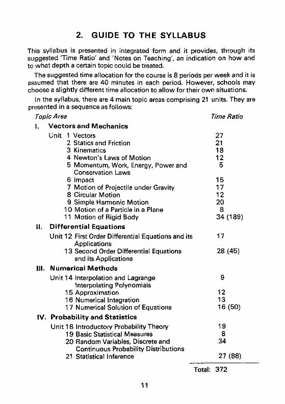
This syllabus is presented in integrated form and it provides, through itssuggested Time Ratio' and 'Notes on Teaching', an indication on how andto what depth a certain topic could be treated.
The suggested time allocation for the course is 8 periods per week and it isassumed that there are 40 minutes in each period. However, schools maychoose a slightly different time allocation to allow for their own situations.
In the syllabus, there are 4 main topic areas comprising 21 units. They arepresented in a sequence as follows:
Topic Area Time RatioI. Vectors and Mechanics
Unit 1 Vectors 272 Statics and Friction 213 Kinematics 184 Newton's Laws of Motion 125 Momentum, Work, Energy, Power and 5
Conservation Laws6 Impact 157 Motion of Projectile under Gravity 178 Circular Motion 129 Simple Harmonic Motion 20
10 Motion of a Particle in a Plane 811 Motion of Rigid Body 34 (189)
II. Differential EquationsUnit 12 First Order Differential Equations and its 17
Applications13 Second Order Differential Equations 28 (45)
and its ApplicationsIII. Numerical Methods
Unit 14 Interpolation and Lagrange 9Interpolating Polynomials
15 Approximation 1216 Numerical Integration 1317 Numerical Solution of Equations 16 (50)
IV. Probability and StatisticsUnit 18 Introductory Probability Theory 19
19 Basic Statistical Measures 820 Random Variables, Discrete and 34
Continuous Probability Distributions21 Statistical Inference 27 (88)
Total: 372
11
Teachers should note that the sequence presented in this syllabus is justan example. In fact they are free to choose their own teaching sequences.For example, the topic areas may be taught in the sequence:
'Differential Equations', 'Vectors and Mechanics', 'Numerical Methods','Probability and Statistics'.
Similarly, the 11 units in the topic area 1 may be presented in the sequence:
'Vectors', 'Statics and Frictions', 'Kinematics', 'Motion of Projectile underGravity', 'Newton's Laws of Motion', 'Momentum, Work, Energy, Powerand Conservation Laws', 'Circular Motion', 'Motion of a Particle in aPlane', 'Impact', 'Simple Harmonic Motion', 'Motion of a Rigid Body'.
It is hoped that the presentation in the syllabus will provide teachers withmaximum flexibility so that courses can be adjusted to meet the individualteaching situation.
The time ratio given in each unit (and hence in each topic area) is thenumerator of a fraction whose denominator, 380, is related to the total timespent on the subject during the two years. This has taken into account thetime spent on classroom tests and examinations. It is intended that this timeratio will indicate what fraction of the total time may be spent on the unit inquestion. It can be seen that the total time ratio is still 8 running short. Thisamount of time is expected to be spent in revising the various units at theend of the course.
Specific objectives are given for each unit, and in the 'Detailed Content',the subject matter of the unit is broken down into sub-units.
The teaching methods suggested in the notes on teaching are by nomeans exhaustive. While providing an example of a way in which each giventopic may be taught, the notes also try to indicate the type of treatment re-quired. However, in order to gear to the overall objectives of the syllabus,teachers are advised to provide students with more well-structured mechan-ical and real-life problems (such as decay, growth, cooling, quality inspec-tion etc). In this way, students will be helped to develop analytic, critical andindependent thinking (as they have to analyze the relevant information givenand select the appropriate methods to tackle the problems). Moreover, anunderstanding of the concepts and principles of mathematical processes andtheir relations to different situations (including the situation of mechanics)will arouse and stimulate students' interest and nurture their appreciation ofthe power and usefulness of mathematics. Adequate practice and frequentexposure to the success of solving problems will also elevate students'confidence in applying mathematics.
Finally, teachers should regard the notes on teaching as a guide to thespirit of the syllabus rather than a rigid teaching plan that must be followedclosely. They are encouraged to explore and discover their own teachingmethods and approaches as they think suitable.
12

In the Appendix, titles of mathematics books, including glossaries andencyclopedias which are useful in the teaching of the Advanced LevelApplied Mathematics course are listed for teachers' reference. To get theupdated references, teachers must however, keep themselves informed ofnew and recent developments in the teaching of the course.
13
3. SYLLABUS
UNIT 1: VECTORS
Specific Objectives:
1, To learn the nature of vectors and their basic properties in R2 and R3,2, To be familiar with the basic operations of vectors in R2 and R3.3, To learn the differentiation and integration of vectors with respect to a scalar variable.4, To apply the vector method to solve problems on the resolution and reduction of a system of forces in R2 and R3.5, To apply the vector method to solve some kinematic problems in R2.
Detailed Content Time Ratio Notes on Teaching
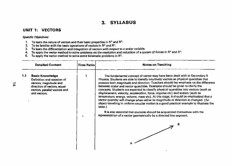
1.1 Basic KnowledgeDefinition and notation ofvectors, magnitude anddirection of vectors, equalvectors, parallel vectors andunit vectors.
The fundamental concept of vector may have been dealt with in Secondary 5Physics. Students are able to identify intuitively vectors as physical quantities thatpossess both magnitude and direction. Teachers should lay emphasis on the differencebetween scalar and vector quantities. Examples should be given to clarify theconcepts. Students are expected to classify physical quantities into vectors (such asdisplacement, velocity, acceleration, force, impulse etc) and scalars (such astemperature, energy, volume, mass etc). At this stage, it should be emphasized that avector quantity will change when either its magnitude or direction is changed. (Anobject travelling in uniform circular motion is a good practical example to illustrate thelatter.)
It is also essential that students should be acquainted themselves with therepresentation of a vector geometrically by a directed line segment.
Detailed Content Time Ratio Notes on Teaching
CJi1.2 Vector Addition
(a) Triangle law andparallelogram law
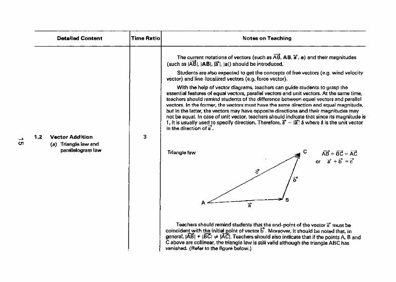
The current notations of vectors (such as AB, AB, a*, a) and their magnitudes(such as |A§|, |AB|, III, |a|) should be introduced.
Students are also expected to get the concepts of free vectors (e.g. wind velocityvector) and line-localized vectors (e.g. force vector).
With the help of vector diagrams, teachers can guide students to grasp theessential features of equal vectors, parallel vectors and unit vectors. At the same time,teachers should remind students of the difference between equal vectors and parallelvectors. In the former, the vectors must have the same direction and equal magnitude,but in the latter, the vectors may have opposite directions and their magnitudes maynot be equal. In case of unit vector, teachers should indicate that since its magnitude is1, it is usually used to specify direction. Therefore, a* = |i*l a where £ is the unit vectorin the direction of a .
Triangle law AE? + §2 = A(5
r a* + b* = c*
Teachers should remind students that the end-point of the vector a* must becoincidentwith the initiajpoint of vector b*. Moreover, it should be noted that, ingeneral, |ABj + |BC| ^ |AC|. Teachers should also indicate that if the points A, B andC above are collinear, the triangle law is stilt valid although the triangle ABC hasvanished. (Refer to the figure below.)

Detailed Content Time Ratio Notes on Teaching
In this case, |AE?| + |§2{ = |A5|
Parallelogram law
A§ +A6 = A3or a* + b* = (?
With the help of the above figure, teachers should again remind students that theinitial points of the two vectors a" and b* must be coincident. The equivalence of thetriangle law and the parallelogram law is worth discussing.
_^ In jMther of the above cases, students should know that <? is called the resultant ofa and b .
It is worthwhile for students to note that the triangle law is convenient for addingfree vectors. However, we may apply the parallelogram law to add up line-localizedvectors, when the lines of action are taken into account. Actually, m the above figure,the line AD is the line of action of the resultant of AJ& and A3.
Detailed Content Time Ratio Notes on Teaching
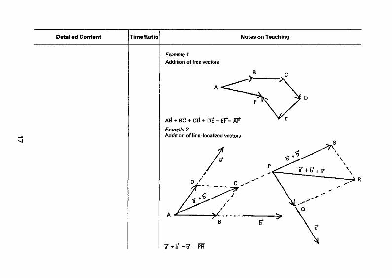
Example 1Addition of free vectors
+ B(5 -f cB + D? + EF*= A?
Example 2Addition of line-localized vectors
Detailed Content Time Ratio Notes on Teaching
(b) Properties of vectoraddition(i) Commutative law:
00
(ii) Associative law:
1.3 Zero Vector, NegativeVector and VectorSubtraction
This example shows the addition of 3 coplanar vectors a*, i? and c*. In the figure,A3 = a*, A§ = b*, A3 = a* + J?, and AC is the line of action of the resultant ofa* and b*. Also, R?=a* + ?, 3 = ?,^ = ? + ? + <?,and P^is the line of action ofthe resultant of a*, ? and ?.
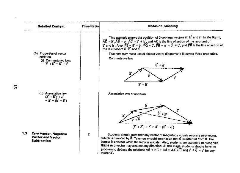
Teachers may make use of simple vector diagrams to illustrate these properties.Commutative law
Associative law of addition
Students should note that any vector of magnitude equals zero is a zero vector,which is denoted by "5. Teachers should emphasize thattf is different from 0. Theformer is a vector while the latter is a scalar. Also, students are expected to recognizethat a zero vector may assume any direction. At this stage, students should have noproblem to deduce the relations A3 + B(5 + cX = AX ="3 and? +"3 = i* for any
*vector a*.
Detailed Content Time Ratio Notes on Teaching
<D
1,4 Scalar Multiple and itsProperties(a) Associative law
(b) Distributive laws _^a(a* + I?) = aa* + oci?(a + p) I* = txa* + pa*
Intuitively, students can see that negative vectors are vectors having equalmagnitude but opposite directions. With this concept, the vector subtraction a* - bcan be introduced by considering it as the vector sum of the vector a* and the negativeof the vector b*, i.e. a* + ("b*). The relative velocity is a practical application of thevector subtraction.
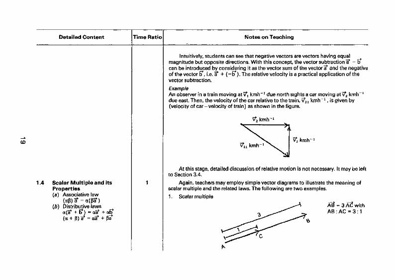
ExampleAn observer in a train moving at v^ kmh"1 due north sights a car moving at v^ kmh"1
due east. Then, the velocity of the car relative to the train, v*21 kmh~1, is given by(velocity of car - velocity of train) as shown in the figure.
v^kmrr1
*i kmh"1
At this stage, detailed discussion of relative motion is not necessary. It may be leftto Section 3.4.
Again, teachers may employ simple vector diagrams to illustrate the meaning ofscalar multiple and the related laws. The following are two examples.
1 , Scalar multiple
AS = 3 AS withAB:AC = 3:1
Detailed Content Time Ratio Notes on Teaching
1.5 Components of Vectors(a) Resolution of vectors
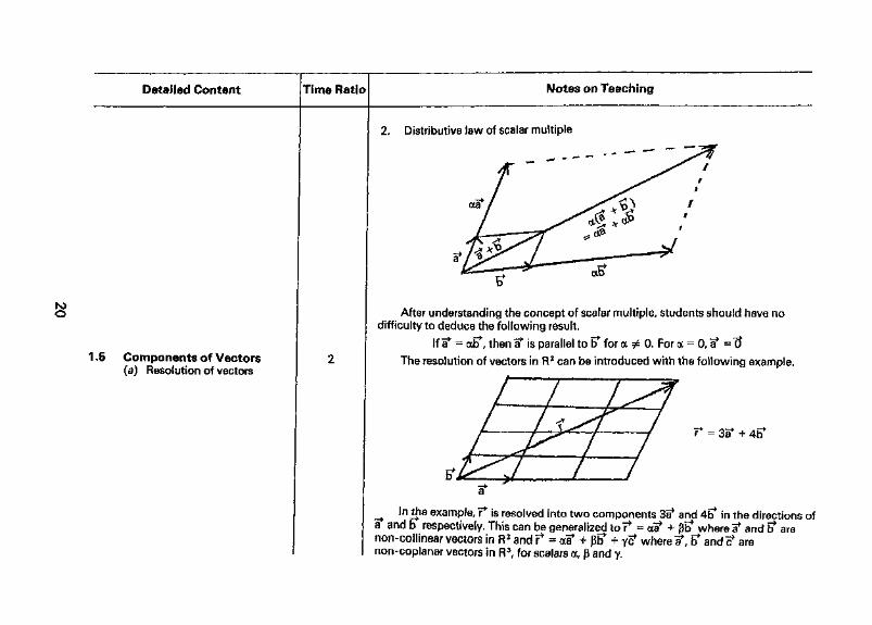
2. Distributive law of scalar multiple
oca7
After understanding the concept of scalar multiple, students should have nodifficulty to deduce the following result.
If If - afcT, then I* is parallel to 6* for a 0. For a = 0, a* = "3"
The resolution of vectors in R2 can be introduced with the following example.
•• 31* + 45*
/ 7^ ln_the example, 7* is resolved into two components 31* and 4b* in the directions ofa and b respectively. This can be generalized tor* = a? + pE* where a* and 5* arenon-collinear vectors in R2 and r* = aa* + p5* + 7? where a*, b* and ? arenon-coplanar vectors in R3, for scalars a, p and y.
Detailed Content Time Ratio Notes on Teaching
(b) The unit vectors i , jand 1? (also denoted asTJandR) and theresolution of vectors in therectangular coordinatesystem.
(c) Direction ratios anddirection cosines
The unit vectors in the dy-ections of the positive x-, y- and z-axis are denotedbyT*,]T and 1? respectively. Any vector in R2 or R3 can be expressed in the form7* = af + bf + ck*.
Students are required to be familiar with the following properties of vectors interms of T,~? andk^:
bf
r=1X (af
yr=1
+ cl?) - (Xa)T + (Xb)r=1+ (Xc)
yr)Tr=1
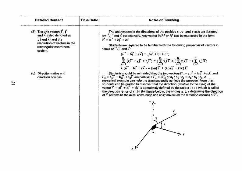
Students should be reminded that the two vectors 7*! = aj + bj +ctk and7*2 = aj* + b2l* +c2l? are parallel if 7^ = ar^2 or 3j : bt : ct = a2 : b2 : c2. Anumerical example can help the teachers easily achieve the purpose. From this,students can be guided to discover that the direction (relative to the axes) of thevector 7* = aT* + bjT + ck* is completely defined by the ratio a : b : c which is calledthe direction ratios of 7*. In the figure below, the angles a, p, y determine the directionof 7* relative to the axes, cosa, cosp and cosy are called the direction cosines of 7".
Detailed Content Time Ratio Notes on Teaching
1.6 Position Vectors andVector Equation of aStraight Line
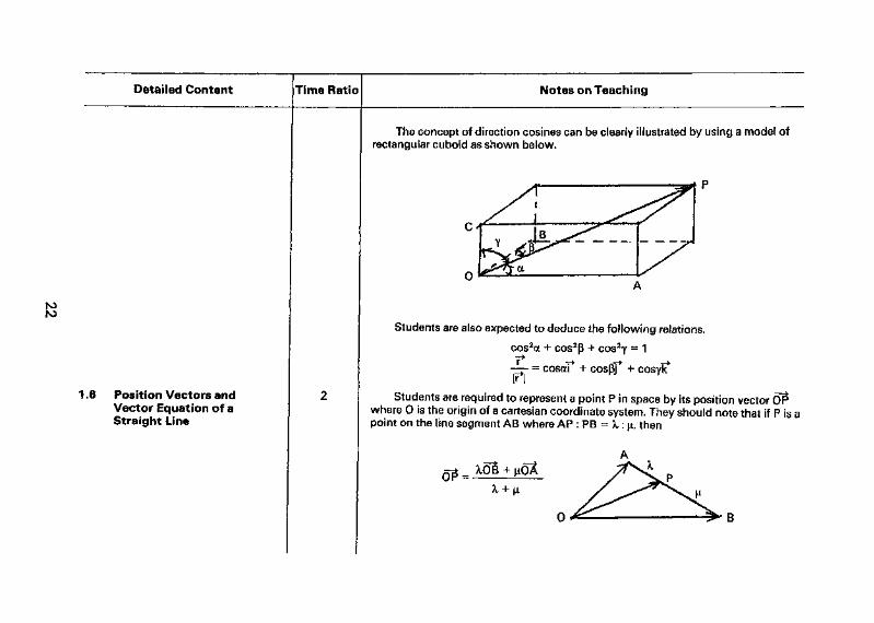
The concept of direction cosines can be clearly illustrated by using a model ofrectangular cuboid as shown below.
Students are also expected to deduce the following relations.
cos2a + cos2p + cos2y = 1
-^- = cosaT + cospj* + cosyk*
Students are required to represent a point P in space by its position vector 0?where O is the origin of a cartesian coordinate system. They should note that if P is apoint on the line segment AB where AP : PB = X : \JL, then

Detailed Content Time Ratio Notes on Teaching
roGO
1.7 Scalar Product(a) Definition
Teachers should iead students to recognize that a straight line can be fullyspecified when the position of a point on the line and the direction of the line areknown. Basing on this idea, students should be able to deduce the vector equation of aline (7* = a* + AJ? for a scalar X) from the following figure.
At this stage, teachers are advised to emphasize to students the meanings of thevectors a* and B*. (The former represents the position of the given point P on the linewhile the latter the direction of the line.) Once the concepts are clarified, studentsshould have no problem to see that the two lines 7*! = a*^ + Xb^ and 7*2 = a^ + i&?2are
1. parallel if 5*! is parallel to b^2;2. perpendicular if &*! is perpendicular to b*2,
and the lines intersect each other if there exist X' and jo,' such that a^ + X't^ -a*2 + P>'b^2- Also, the fact that the angle between the lines is equal to the angle betweenb*! and b 2 is obvious.
In introducing the definition, teachers should point out to students that the name'scalar' is used because the product defined in this way gives a scalar quantity.Students are also expected to know the other name for scalar product, i.e. dot product.Hence, a" • & is read as 'a* dot 6*'.
Detailed Content Time Ratio Notes on Teaching
(6) Properties of scalarproduct
(c) Scalar product in cartesiancomponents
(cf) Orthogonality
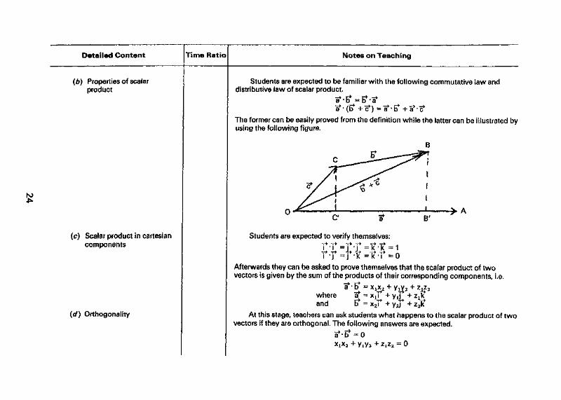
Students are expected to be familiar with the following commutative law anddistributive law of scalar product
The former can be easily proved from the definition while the latter can be illustrated byusing the following figure.
C' t B'
Students are expected to verify themselves:-r* T* T» T» T* T*i • ! = j - j = k -k = 1*r» T* 4* 4* -r» -r* rti - j = j -k = k - i = 0
Afterwards they can be asked to prove themselves that the scalar product of twovectors is given by the sum of the products of their corresponding components, i.e.
whereand
If =i? =
+ yj +Z ik+ y2f + z2l?
At this stage, teachers can ask students what happens to the scalar product of twovectors if they are orthogonal. The following answers are expected.
sf-tf = 0XiX2 + y^z + ZjZ2 = 0

Detailed Content Time Ratio Notes on Teaching
1 .8 Vector Product(a) Definition
a* x 5* = |a*| | | sin 9 n
ro01
Teachers should provide students with examples involving application of scalarproduct. For example, in plane geometry, the theorems The perpendiculars from thevertices of a triangle to the opposite sides are concurrent.' and The perpendicularbisectors of the sides of a triangle are concurrent/ can be proved by using scalarproduct.
In introducing the definition, teachers shouldemphasize the 'vector' feature of the product which isdifferent from the scalar product introduced in Section1.7, The other name for vector product, cross product, isalso introduced and a* x E* is read as 'a cross b'. Theright-handed system used for the determination of theproduct direction (i.e. in the direction of the unit vectorft in the definition) should be clearly explained. Thefigure shown will be helpful.
Simple applications of vector product can be introduced to arouse students'interest. The following are two examples.1. Area of triangle
Area of AABC= JAB -AC sinG= i 1A§ x AS|
Detailed Content Time Ratio Notes on Teaching
O)
(b) Properties of vectorproduct
(c) Vector product in cartesiancomponents
(d) Perpendicular vectors andparallel vectors
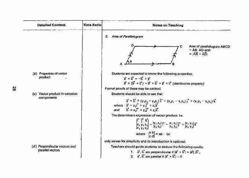
2, Area of Parallelogram
D, Area of parallelogram ABCD= AB • AD sine
Students are expected to know the following properties.
a* x (b* + (?) = a* x E* + a* x c? (distributive property)
Formal proofs of these may be omitted.
Students should be able to see that
af x B* " " ~* ~*where a* = Xj
j tT*1 ~rr ~*~* T*and b == x2i + y2j + z2k .
The determijiant expression of vector product, i.e.T* T* -T+
i J kYi zi
where
Xi ZiX2Z2
j +
= ad - be
only serves for simplicity and its introduction is optional.
Teachers should guide students to deduce the following results.
*\. a*, b* are perpendicular if |a* x fc^ = |a*| jb^i,2. a*, ff are parallel if |i* x E^J = 0
Detailed Content Time Ratio Notes on Teaching
1.9 Triple Product(a) Scalar triple product
(b) Vector triple product
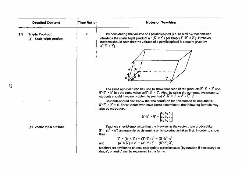
By considering the volume of a parallelepiped (i.e. be sinO h), teachers canintroduce the scalar triple product a** (6* x cf) (or simply a*'b* * ?). However,students should note that the volume of a parallelepiped is actually given by
The_same approach can be usecko show that each of the products b* • e? x a* and(? • a* x B* has the same value as a* • 5* x (f. Also, by using the commutative property,students should have no problem to see that a* • b x <? = a* x b • (?.
Students should also know that the condition for 3 vectors to be coplanar isa*1 r? x <? =0. For students who have learnt determinant, the following formula mayalso be introduced.
a*-b* x^ =
Teachers should emphasize that the brackets in the vector triple product like
a2 b2 c2
b3 c.
I xthat
x <?) are essential to determine which product is taken first. In order to show
and (a" x ft) x ? = (a*-?) I? -{!?•<?)?,teachers are advised to choose appropriate cartesian axes (by rotation if necessary) sothat i*, b* and c? can be expressed in the forms.
Detailed Content Time Ratio Notes on Teaching
oo
1.10 Vector Function,Differentiation andIntegration(a) Vector as a function of a
scalar varfabie
(b) Differentiation of a vectorfunction with respect to ascalar variable
(c) Integration of a vectorfunction with respect to ascalar variable
a ^i^ i|-> . T* . T*
b = bji -f b2j
c* = c^ + CjT + c3k*
From the above results, students should be able to find thata* x (B* x (f) ^ (aT x B^) x c*\
Students are expected to be familiar with notations like 7*(t), v*(9) etc, where?*and v*" are vector functions of the scalar variables t and 6 respectively.
Students should be able to differentiate vector functions in component form, i.e.
when r*(t) = f (t)T + g(t)f + h(t)l?,
-~-~ tnt)] = f (t) + g'(t)f
They are also expected to be familiar with the differentiation of scalar multiples, scalarproducts and vector products:
dt
Adt
dt dt
dt dt
dt dt dt
Teachers should emphasize to students that integration of a vector function is thereverse process of differentiation. In this way, students should have no problem tocarry out integration like
Jr*(t) dt = Jf (t) dtf + |g(t) dt j* + Jh(t) dt i? + c*where r^t) = f (t) T + g (t) f + h (t) I?and <? is a constant vector.
Detailed Content Time Ratio Notes on Teaching
1.11 Vectors in PolarCoordinates
roCD
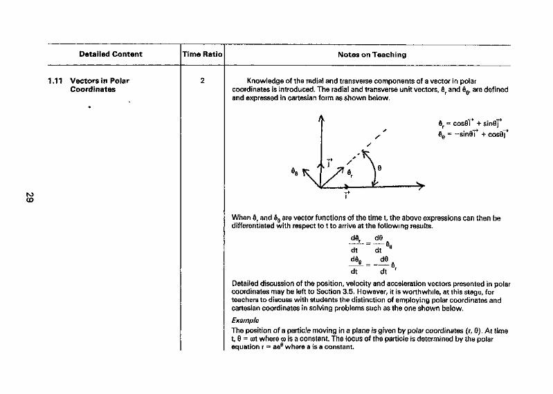
Knowledge of the radial and transverse components of a vector in polarcoordinates is introduced. The radial and transverse unit vectors, er and ee, are definedand expressed in cartesian form as shown below.
e, = cos9fee = -sin0T + cos9j*
When er and ee are vector functions of the time t, the above expressions can then bedifferentiated with respect to t to arrive at the following results.
!Ldt
~dT
d9
dtde
dt
Detailed discussion of the position, velocity and acceleration vectors presented in polarcoordinates may be left to Section 3.5. However, it is worthwhile, at this stage, forteachers to discuss with students the distinction of employing polar coordinates andcartesian coordinates in solving problems such as the one shown below.
ExampleThe position of a particle moving in a plane is given by polar coordinates (r, 9). At timet, 9 = eot where co is a constant, The locus of the particle is determined by the polarequation r = aee where a is a constant.
Detailed Content Time Ratio Notes on Teaching
1.12 Application of Vectors
(a) Force as a vector
Students are expected to develop their skills in tackling problems related tovectors and their applications.
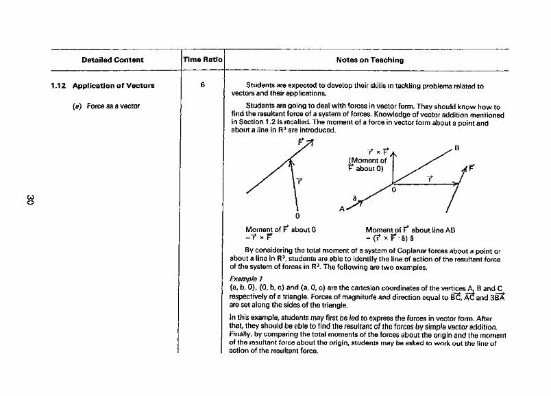
Students are going to deal with forces in vector form. They should know how tofind the resultant force of a system of forces. Knowledge of vector addition mentionedin Section 1.2 is recalled. The moment of a force in vector form about a point andabout a line in R3 are introduced.
Moment of f about 0 Moment of P about line AB= (? x f - a )a
By considering the total moment of a system of Coplanar forces about a point orabout a line in R3, students are able to identify the line of action of the resultant forceof the system of forces in R3. The following are two examples.
Example 1(a, b, 0), (0, b, c) and (a, 0, c) are the cartesian coordinates of the vertices A, B and Crespectively of a triangle. Forces of magnitude and direction equal to §2, AC? and 3B^are set along the sides of the triangle.
In this example, students may first be led to express the forces in vector form. Afterthat, they should be able to find the resultant of the forces by simple vector addition.Finally, by comparing the total moments of the forces about the origin and the momentof the resultant force about the origin, students may be asked to work out the line ofaction of the resultant force.
Detailed Content Time Ratio Notes on Teaching
(b) Kinematics in R2
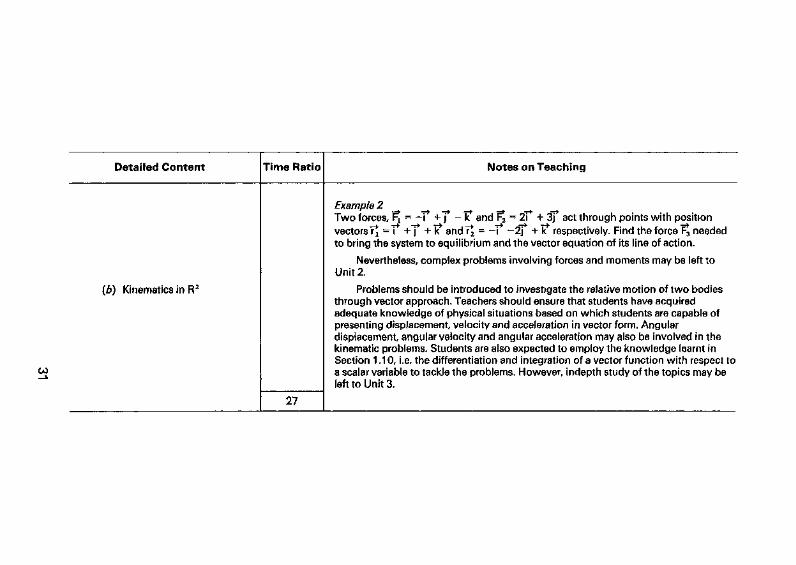
Example 2 _^ _^ _^ _ > _ _ > . _ _ »Two forces, F^ = -T* +1* -1? and F^ = 27* + 3j* act through points with positionvectors7[ =T +~j* + k* and 7^ = -I* -2~f +1? respectively. Find the force F^ neededto bring the system to equilibrium and the vector equation of its line of action.
Nevertheless, complex problems involving forces and moments may be left toUnit 2.
Problems should be introduced to investigate the relative motion of two bodiesthrough vector approach. Teachers should ensure that students have acquiredadequate knowledge of physical situations based on which students are capable ofpresenting displacement, velocity and acceleration in vector form. Angulardisplacement angular velocity and angular acceleration may also be involved in thekinematic problems. Students are also expected to employ the knowledge learnt inSection 1.10, i.e. the differentiation and integration of a vector function with respect toa scalar variable to tackle the problems. However, indepth study of the topics may beleft to Unit 3.
27
UNIT 2: STATICS AND FRICTIONSpecific Objectives:
1, To understand the nature of forces, moments and couples,2, To learn the resultant and resolution of a system of coplanar forces.3, To understand the nature of frictional forces and the laws of friction.4, To learn the conditions of equilibrium of particles and rigid bodies under a system of coplanar forces and to solve practical problems
involved.
Detailed Content Time Ratio Notes on Teaching
OJro
2.1 Forces, Resultant andResolution of Forces
Fundamental knowledge of the vector nature of forces should have been comeacross in studying Secondary Physics. At this stage, teachers should emphasize tostudents the following basic factors which determine the effect on a body to which aforce is applied:
(1) The magnitude of the applied force.(2) The line of action of the applied force, i.e. the direction and the point of
application in which the force is applied.
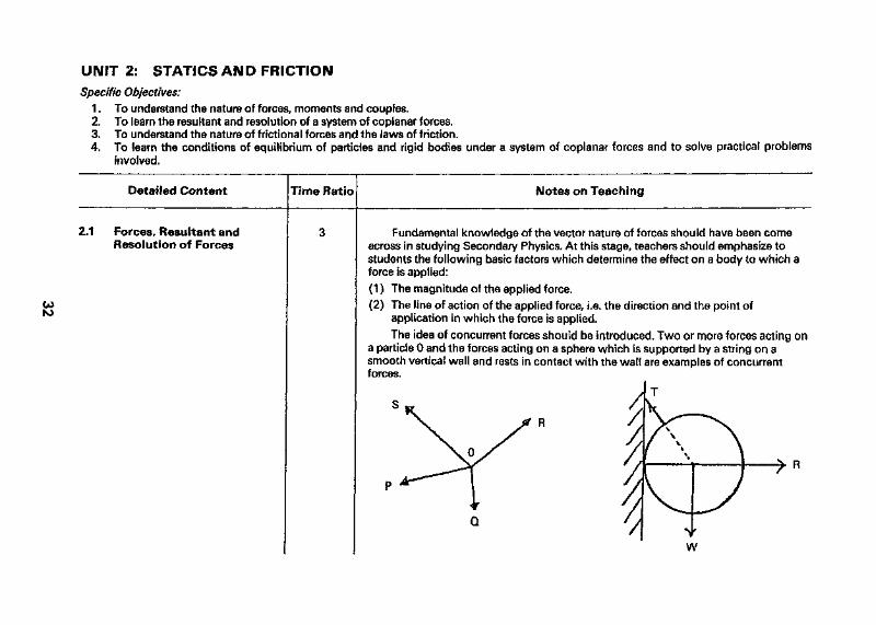
The idea of concurrent forces should be introduced. Two or more forces acting ona particle 0 and the forces acting on a sphere which is supported by a string on asmooth vertical wall and rests in contact with the wall are examples of concurrentforces.
Detailed Content Time Ratio Notes on Teaching
00
2.2 Resultant of ParallelForces, Moments andCouples
A system of forces can be reduced to a single resultant force. Students should beable to find the resultant of any two forces by the triangle law or parallelogram law. Bysuccessive application of either of the two laws, the resultant of a system of coplanarforces can be obtained. Knowledge of vector addition mentioned in Section 1.2 maybe referred.
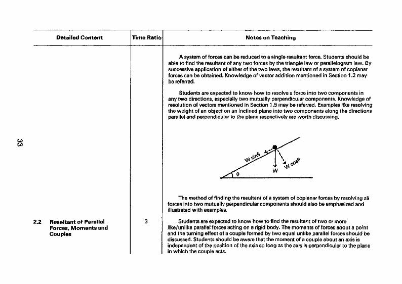
Students are expected to know how to resolve a force into two components inany two directions, especially two mutually perpendicular components. Knowledge ofresolution of vectors mentioned in Section 1.5 may be referred. Examples like resolvingthe weight of an object on an inclined plane into two components along the directionsparallel and perpendicular to the plane respectively are worth discussing.
W
The method of finding the resultant of a system of copianar forces by resolving allforces into two mutually perpendicular components should also be emphasized andillustrated with examples.
Students are expected to know how to find the resultant of two or morelike/unlike parallel forces acting on a rigid body. The moments of forces about a pointand the turning effect of a couple formed by two equal unlike parallel forces should bediscussed. Students should be aware that the moment of a couple about an axis isindependent of the position of the axis so long as the axis is perpendicular to the planein which the couple acts.

Detailed Content Time Ratio Notes on Teaching
to
moment of couple = Fa
The fact that the algebraic sum of the moments of two forces about any point intheir plane is equal to the moment of their resultant force about the same point shouldbe introduced. The underlying concept is then extended to the Principle of Moments(the algebraic sum of moments of any number of coplanar forces acting on a rigidbody about any point in their plane is equal to the moment of their resultant about thesame point), Students are also expected to make use of the above principle to reduce asystem of coplanar forces to a single force or a couple. Determination of the centres ofgravity of figures of regular shapes and uniform bodies is one of the applications of thePrinciple of Moments. Details may be referred to Unit 1 1 .
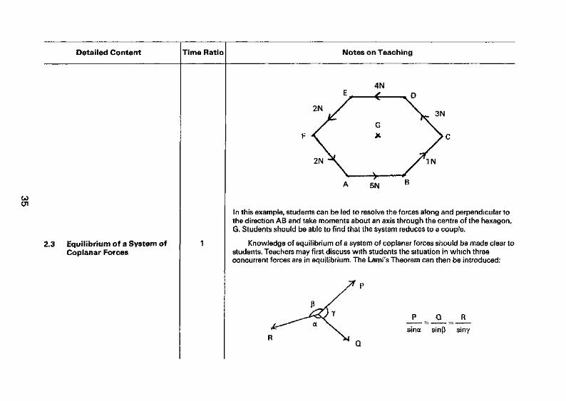
ExampleABCDEF is a regular hexagon of side 2 £ . Forces of mand 2N act respectively along the sides AB, §3, CD,
nitude 5N, 1 N, 3N, 4N, 2NEF*and R?.
Detailed Content Time Ratio Notes on Teaching
01
2.3 Equilibrium of a System ofCoplanar Forces
2N
4NE . . . _ _ . . . x . D
2N
A 5N
In this example, students can be led to resolve the forces along and perpendicular tothe direction AB and take moments about an axis through the centre of the hexagon,G. Students should be able to find that the system reduces to a couple.
Knowledge of equilibrium of a system of coplanar forces should be made clear tostudents. Teachers may first discuss with students the situation in which threeconcurrent forces are in equilibrium. The Lami's Theorem can then be introduced:
P = Q _ R
sina sinp siny
Detailed Content Time Ratio Notes on Teaching
2.4 Nature of Friction(a) Laws of friction
Sufficient exercises on applying the Lami's Theorem to solve three-force problemsshould be given.
beAt this stage, students should be aware that a system of coplanar forces may either
(a) reduced to a single resultant force,
(b) reduced to a couple, or
(c) in equilibrium.
Teachers should remind students that for a system of forces in R2 to be inequilibrium, the following simultaneous conditions are satisfied and are helpful insolving the problem:
(1) ZFX = 0, £Fy = 0 and
(2) ZMp = 0where Fx, Fy are component forces in R2 and M are their respective momentsabout any point P,
Students are expected to know that when a body moves or tends to move on asurface, friction always exists and it tends to prevent the body from moving.
Two different types of friction should be distinguished, namely, the static frictionand the kinetic friction. The former refers to the frictional force acting on a body whichremains static (but it tends to move), while the latter refers to the frictionai force actingon a moving body. The law of static friction and the law of kinetic friction should bestated and students are expected to know that the coefficient of static friction, jo. isgreater than the coefficient of kinetic friction, jik.
s
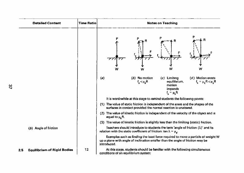
Teachers should emphasize that the relationship between friction f and normalreaction R is f SR, and f = isR only when a limiting equilibrium is reached. Thefollowing figures may be helpful to illustrate this concept. (In the figures, P is theresultant of frictional force and normal reaction.)
Detailed Content
(b) Angle of friction
2.5 Equilibrium of Rigid Bodies
Time Ratio
12
Notes on Teaching
F/
<
V
(a}
3 P _
^PI \
vU77 />>'
' V
\l V
P
i v%\i %
F » ^• — ». f, j, N
'\l V
p\ R /IT"7
|\I * fk L \
I/ V\f
(b) No motion (c) Limiting (d) Motion exists^s<^ls^ equilibrium, fk = jikR<jjR
motionimpends
It is worthwhile at this stage to remind students the following points:
(1 ) The value of static friction is independent of the areas and the shapes of thesurfaces in contact provided the normal reaction is unaltered.
(2) The value of kinetic friction is independent of the velocity of the object and isequal to nkR.
(3) The value of kinetic friction is slightly less than the limiting (static) friction.
Teachers should introduce to students the term 'angle of friction (X)' and itsrelation with the static coefficient of friction; tan X = ps.
Examples such as finding the least force required to move a particle of weight Wup a plane with angle of inclination smaller than the angle of friction may beintroduced.
At this stage, students should be familiar with the following simultaneousconditions of an equilibrium system:
Detailed Content Time Ratio Notes on Teaching
GO00
(1) The resultant force of the system is zero.
(2) The resultant moment of the system about any point is zero.
Students are expected to be able to make use of the above two conditions and thelaws of friction to set up independent equations and inequalities from a given physicalsituation. Students are also expected to know that condition (1) alone is sufficient forshowing a system of concurrent forces to be in equilibrium.
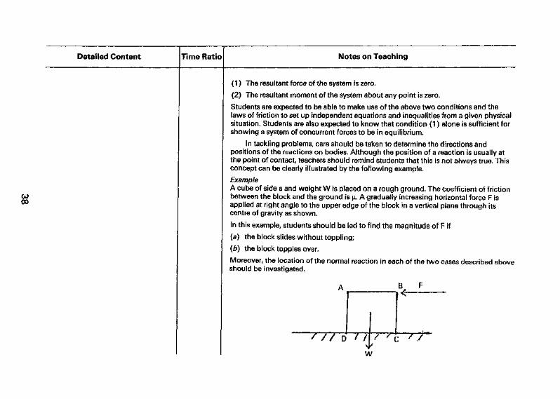
In tackling problems, care should be taken to determine the directions andpositions of the reactions on bodies. Although the position of a reaction is usually atthe point of contact, teachers should remind students that this is not always true. Thisconcept can be clearly illustrated by the following example.
ExampleA cube of side a and weight W is placed on a rough ground. The coefficient of frictionbetween the block and the ground is p.. A gradually increasing horizontal force F isapplied at right angle to the upper edge of the block in a vertical plane through itscentre of gravity as shown.
In this example, students should be led to find the magnitude of F if
(a) the block slides without toppling;
(b) the block topples over.
Moreover, the location of the normal reaction in each of the two cases described aboveshould be investigated.

Detailed Content Time Ratio Notes on Teaching
On the other hand, teachers should ensure that students can determine the correcldirection of a reaction on a body. For instance, as shown in the diagram, studentsshould know that S (instead of R) is the normal reaction on the rod at A.
Students are expected to be familar with the limiting positions of equilibrium ofrigid bodies. Teachers should encourage students to draw free-body diagrams insolving problems.
Example 1Two uniform rods AB,AC of equal length are freely hinged at A as shown in thediagram. AB is twice as heavy as AC. The system rests on a rough horizontal ground ina vertical plane and is in limiting equilibrium.
Detailed Content Time Ratio Notes on Teaching
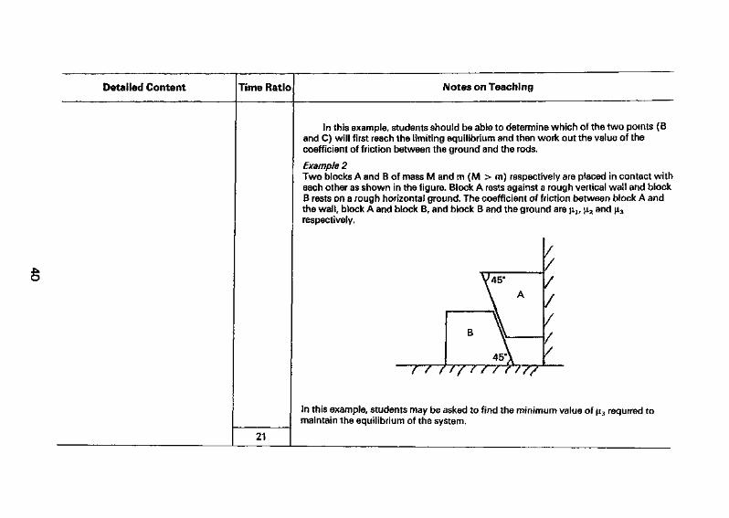
In this example, students should be able to determine which of the two points (Band C) will first reach the limiting equilibrium and then work out the value of thecoefficient of friction between the ground and the rods.
Example 2Two blocks A and B of mass M and m (M > m) respectively are placed in contact witheach other as shown in the figure. Block A rests against a rough vertical wall and blockB rests on a rough horizontal ground. The coefficient of friction between block A andthe wall, block A and block B, and block B and the ground are \ilt ji2 and fi3respectively.
In this example, students may be asked to find the minimum value of ^3 required tomaintain the equilibrium of the system.
21
UNIT 3: KINEMATICSSpecific Objectives:
To understand the meaning of displacement, velocity and acceleration, and their corresponding angular quantities.To understand resultant velocity and relative motion.
1,2,3. To recognize the radial and transverse component of velocity and acceleration.4. To solve relevant practical problems.
Detailed Content Time Ratio Notes on Teaching
3,1 Displacement, Velocity andAcceleration
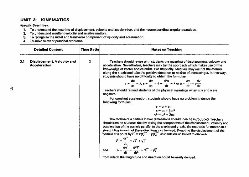
Teachers should revise with students the meaning of displacement, velocity andacceleration, Nevertheless, teachers may try the approach which makes use of theknowledge of vector and calculus. For simplicity, teachers may restrict the motionalong the x-axis and take the positive direction to be that of increasing x. In this way,students should have no difficulty to obtain the formulae
dx dv d2x dv dvv = — = x, a = — = v = —-— = x or a = — = v—.
dt dt dt dt dxTeachers should remind students of the physical meanings when x, v and a arenegative.
For constant acceleration, students should have no problem to derive thefollowing formulae:
v = u + atx = ut + iat2
v2 = u2 + 2axThe motion of a particle in two dimensions should then be introduced. Teachers
should remind students that by taking the components of the displacement, velocity andacceleration of the particle parallel to the x-axis and y-axis, the methods for motion m astraight line in each of these djrectionsjcan be used. Denoting the displacement of the"particle at a point by 7* = x(t)~T + y(tjf, students could be led to discover.
v^^iL=*[» + ••*»dt X l VJ
and..yj
dt dt2
from which the magnitude and direction could be easily derived.
Detailed Content Time Ratio Notes on Teaching
At this stage, the use of parametric equations for the motion of a particle whosepath is described by an equation in the rectangular coordinates should be emphasized.Students are expected to use the techniques and knowledge of Section 1 .1 0 in thesolution of problems. Some of which are as follows.
Example 1The velocity vector 7 (ir^ms"1) of a particle P starting from a point 0 is given byv* = 8oT + (50 + 1 Ot2)~f. The position vector relative to 0 and the acceleration vectorof P at time t can be easily obtained by integrating and differentiating v* respectively,
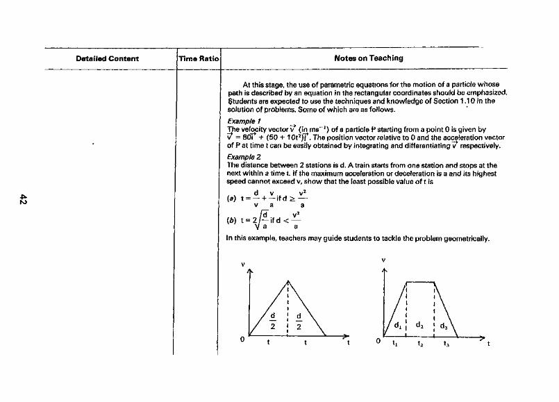
Example 2The distance between 2 stations is d. A train starts from one station and stops at thenext within a time t. If the maximum acceleration or deceleration is a and its highestspeed cannot exceed v, show that the least possible value of t is
d v v2
(a) t = — + — if d > —v a a
(b) t = 2/— ifdV a
v2
—a
In this example, teachers may guide students to tackle the problem geometrically.
Detailed Content Time Ratio Notes on Teaching
3.2 Angular Displacement,Angular Velocity andAngular Acceleration
3.3 Resultant Velocity
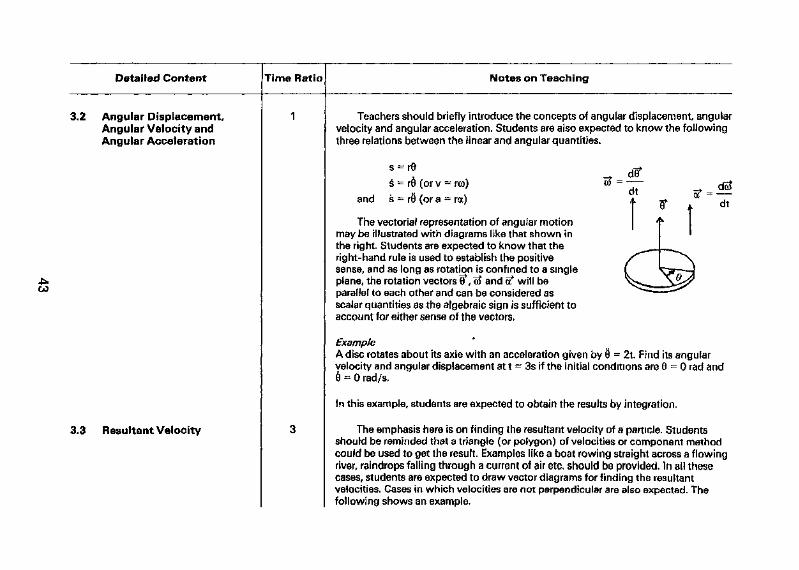
Teachers should briefly introduce the concepts of angular displacement angularvelocity and angular acceleration. Students are also expected to know the followingthree relations between the linear and angular quantities.
s = r6 (or v = rco) G> =
and s = r0 (or a = rot)
The vectorial representation of angular motionmay be illustrated with diagrams like that shown inthe right. Students are expected to know that theright-hand rule is used to establish the positivesense, and as long as rotation is confined to a singleplane, the rotation vectors 9*, o> and a* will beparallel to each other and can be considered asscalar quantities as the algebraic sign is sufficient toaccount for either sense of the vectors.
ExampleA disc rotates about its axle with an acceleration given by 9 = 2t. Find its angularvelocity and angular displacement at t - 3s if the initial conditions are 6 = 0 rad and8 = 0 rad/s.
In this example, students are expected to obtain the results by integration.
The emphasis here is on finding the resultant velocity of a particle. Studentsshould be reminded that a triangle (or polygon) of velocities or component methodcould be used to get the result. Examples like a boat rowing straight across a flowingriver, raindrops falling through a current of air etc. should be provided, In all thesecases, students are expected to draw vector diagrams for finding the resultantvelocities, Cases in which velocities are not perpendicular are also expected. Thefollowing shows an example.
Detailed Content Time Ratio Notes on Teaching
3.4 Relative Motion
ExampleA cargo ship leaves a port and heads N50°E at a speed of 25 kmh"1 with respect to stillwater, while a westward sea current drifts at 4.5 kmrT1. What is the resultant velocityof the cargo ship?
In this example, apart from resolving the velocities in the north and west direction,students could also find the resultant velocity by using the sine rule and cosine rule.
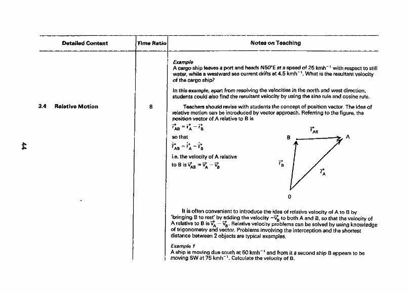
Teachers should revise with students the concept of position vector. The idea ofrelative motion can be introduced by vector approach. Referring to the figure, theposition vector of A relative to B is
so that
i.e. the velocity of A relative
It is often convenient to introduce the idea of relative velocity of A to B by'bringing B to resj/ by adding the velocity -v£ to both A and B, so that the velocity ofA relative to B is v^ - Vg. Relative velocity problems can be solved by using knowledgeof trigonometry and vector. Problems involving the interception and the shortestdistance between 2 objects are typical examples.
Example 1A ship is moving due south at 50 kmh"1 and from it a second ship B appears to bemoving SW at 75 kmrT1. Calculate the velocity of B.
Detailed Content Time Ratio Notes on Teaching
Oi
3.5 Resolution of Velocity andAcceleration Along andPerpendicular to RadiusVector
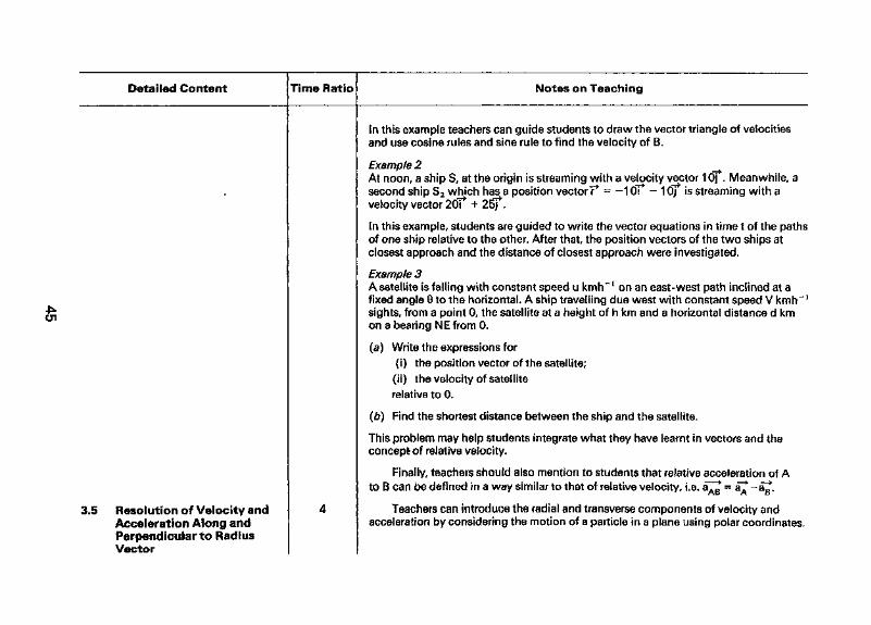
In this example teachers can guide students to draw the vector triangle of velocitiesand use cosine rules and sine rule to find the velocity of B.
Example 2At noon, a ship S, at the origin is streaming with a velocity vector 1 of. Meanwhile, asecond ship S2 which has a position vector?* = -1 Oi - 10j is streaming with avelocity vector 2dT + 25f.
In this example, students are guided to write the vector equations in time t of the pathsof one ship relative to the other. After that, the position vectors of the two ships atclosest approach and the distance of closest approach were investigated.
Example 3A satellite is falling with constant speed u kmh"1 on an east-west path inclined at afixed angle 8 to the horizontal, A ship travelling due west with constant speed V kmh"1
sights, from a point 0, the satellite at a height of h km and a horizontal distance d kmon a bearing NE from 0.
(a) Write the expressions for(i) the position vector of the satellite;(ii) the velocity of satelliterelative to 0.
(6) Find the shortest distance between the ship and the satellite.
This problem may help students integrate what they have learnt in vectors and theconcept of relative velocity.
Finally, teachers should also mention to students that relative acceleration of Ato B can be defined in a way similar to that of relative velocity, i.e. a^ = a^ ~a^.
Teachers can introduce the radial and transverse components of velocity andacceleration by considering the motion of a particle in a plane using polar coordinates.

o>
Detailed Content Time Ratio Notes on Teaching
y se
/— / ^^ p
A / Jx^
^T-0
/"S B
'*Suppose P is the position of a particle at time t, APB is the path of the particle and thepolar coordinates of P are (r, 0),
Then 0? = 7* = re where ef and ee are the unit vectors in the directions paralleland perpendicular to 7* respectively.
In Section 1 .1 1, students have learnt that 4r = 0ee and £0 = -9ef. By directdifferentiation, students should have no problem to get the following results
7* = fe"r + r9ee and r* = (r - r02) er + (r20) kse-
Tabulating the results will facilitate students in recognizing the expression
RadialComponent 1
Velocity f
Acceleration if - r02
"ransverse component
rerO + 2r9
orTdF
Detailed Content Time Ratio Notes on Teaching
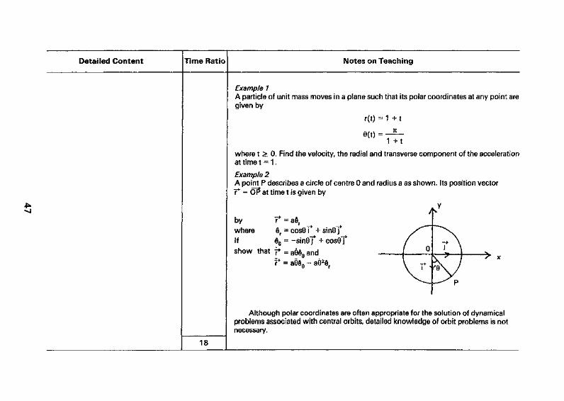
Example 1A particle of unit mass moves in a plane such that its polar coordinates at any point aregiven by
r(t) = 1 + t
r\j \ ft
1 +t
where t > 0. Find the velocity, the radial and transverse component of the accelerationat time t = 1.
Example 2A point P describes a circle of centre 0 and radius a as shown. Its position vector7* = O? at time t is given by
by 7* = aer
where er = cosGT* + sin0TIf ee = -sineT + cos97show that - d
s" x
Although polar coordinates are often appropriate for the solution of dynamicalproblems associated with central orbits, detailed knowledge of orbit problems is notnecessary.
18
UNIT 4: NEWTON'S LAWS OF MOTION
Specific Objectives:
1, To understand Newton's Laws of Motion.2, To apply Newton's Laws of motion to solve problems in dynamics.
Detailed Content Time Ratio Notes on Teaching
4.1 Newton's Laws of Motion The Newton's Laws of Motion should be clearly stated and explained to students.Problems involving variable mass need not be taught.
Students should be able to distinguish external forces and internal forces actingon a particle or a system of particles.
Students are expected to apply Newton's Laws to solve problems in statics anddynamics.
In dynamics, students may first study the motion of a particle. The treatmentshould also apply to a body whose rotational effects are negligible and its motion canbe approximated by the centre of mass of the body. Students may then be guided tostudy the motion of a system of particles or bodies moving in a plane.
The basis of analysis is Newton's Second Law which may take the form:
F* = ma*
where m is the mass of the particle,
F* is the resultant force acting on the particle,
a* is the resultant acceleration of the particle.
The procedure of analysis may be arranged as follows:
Detailed Content Time Ratio Notes on Teaching
(1) Analyse the forces on the particle:The first step in analysing a problem in dynamics is to construct a force diagram.The force diagram for a particle should include all physically identifiable forcesacting on the particle. Students should know that a force is physically identifiableif they can identify its origin, e.g. the force of gravity, the reaction of a body, africtional force, a spring force etc. Teachers should remind students that a forceshould not be postulated on the basis of its supposed effect
(2) Analyse the kinematics of the particle:Students should be advised to write down the acceleration a~* in some coordinatesystem (rectangular or polar) but it should be emphasized that Newton's Laws ofMotion should apply to motions relative to an inertial frame of reference, i.e. thecoordinate system chosen should not be accelerating or rotating. For a simpleproblem the acceleration may be indicated on the force diagram, but usually it isdesirable to draw another diagram for the acceleration(s).
(3) The equation of motion is then given by relating (1) and (2) in F* = ma*:Students should try to minimize the variables in the force equation by choosingproper direction(s) for resolving the forces and accelerations and should try to setup minimum number of equations in solving the problems.
Problems involving system of pulleys and motion on the surface of a wedge areworth discussing and knowledge of relative acceleration for two accelerating bodiesshould be revised.
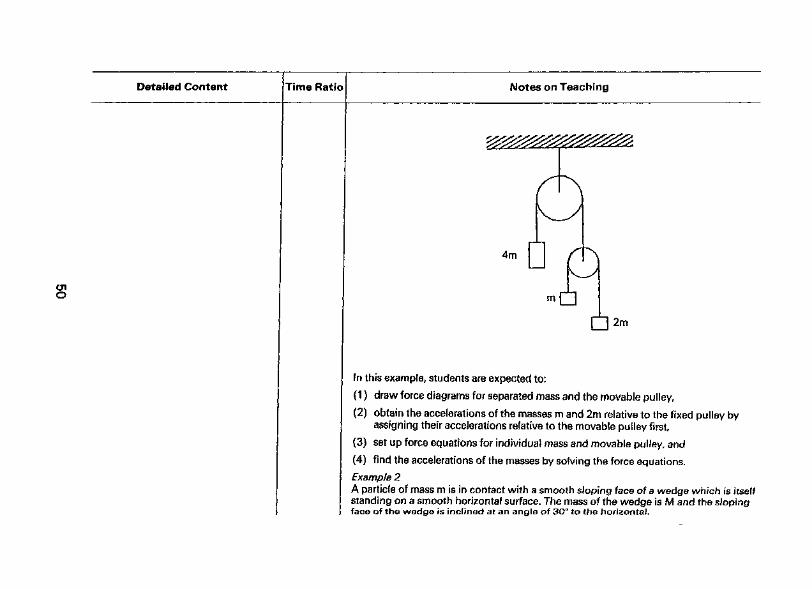
Example 1Two masses m, 2m, are connected by a light inextensible string which passes over asmooth pulley, mass m. The axle of the pulley is fastened to one end of a second stringwhich passes over a smooth fixed pulley and has a mass 4m attached at the other endThe system is free to move in a vertical plane.
Detailed Content Time Ratio Notes on Teaching
4m
01o m
U2m
In this example, students are expected to:
(1) draw force diagrams for separated mass and the movable pulley,
(2) obtain the accelerations of the masses m and 2m relative to the fixed pulley byassigning their accelerations relative to the movable pulley first
(3) set up force equations for individual mass and movable pulley, and
(4) find the accelerations of the masses by solving the force equations.
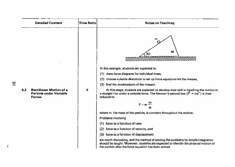
Example 2A particle of mass m is in contact with a smooth sloping face of a wedge which is itselfstanding on a smooth horizontal surface. The mass of the wedge is M and the slopingface of the wedge is inclined at an angle of 3O° to the horizontal.
Detailed Content Time Ratio Notes on Teaching
4.2 Rectilinear Motion of aParticle under VariableForces
m
In this example, students are expected to:
(1) draw force diagrams for individual mass,
(2) choose suitable directions to set up force equations for the masses,
(3) find the accelerations of the masses.
At this stage, students are expected to develop their skill in handling the motion ina straight line under a variable force. The Newton's second law (F = ma*) is thenreduced to
dvF = m —
dt
where m, the mass of the particle, is constant throughout the motion.
Problems involving
(1) force as a function of time,
(2) force as a function of velocity, and
(3) force as a function of displacement
are worth discussing, and the method of solving the problems by simple integrationshould be taught. Moreover, students are expected to identify the physical motion ofthe particle after the force equation has been solved.
Detailed Content Time Ratio Notes on Teaching
en
12
The following are some examples:
Example 1A stone of mass m, fails vertically from rest the air resistance being kv where k is aconstant and v is the velocity of the stone at time t.
in this problem, teachers may guide students to find the velocity of the stone in time tby integration. Also, students should be able to know that the velocity will beterminated as time tends to infinity. Moreover, the terminal velocity can be determined.
Example 2A body of mass 5 kg is moving in a straight line under the action of a force (4/s)newtons towards a fixed point 0 in that straight line, where s metres is the distance ofthe body from 0. The body is initially at rest and is 1 m from 0.
In this problem, students are expected to find the velocity of the body for a particulardistance s from 0 by simple integration. Moreover, teachers may guide students to findthe time elapsed for a particular s by integrating the first result.
UNIT 5: MOMENTUM, WORK, ENERGY, POWER AND CONSERVATION LAWS
Specific Objectives:
1, To recognize momentum, work, energy and power,2. To understand and use the Conservation Laws of Momentum and Energy.
Detailed Content
5.1 Momentum andConservation ofMomentum
5.2 Work, Energy, Power andConservation of Energy
Time Ratio
2
3
Notes on Teaching
Newton's second law may take the form
_> d(mv*) dP*
dt dt
where P* = mv* is the momentum of the particle. In the absence of external force, themomentum P = mv* of the particle should remain constant. The conservation ofmomentum may be extended to a system of particles. Examples such as recoil of gun,collision of trucks (assuming that they couple together after impact) etc. should beprovided to illustrate how the law of conservation of momentum can be used.However, detailed discussion of impact problems is not necessary here and can be leftto Unit 6.
Teachers should remind students of the fundamental concepts of work, energyand power. Students are expected to know that:
1 . the work done by F on moving a particle from a to b along the positive direction ofthe x-axis is f F-dx,
2. the kinetic energy of a particle of mass m moving with velocity v is imv2.
3. the gravitational potential energy of a particle of mass m at a height h above anarbitrary origin is mgh, and
4. the power of F is the rate of work done by F.
After that, teachers may introduce the relation between work and energy for somemechanical systems. The following show two of them.
1 . A particle moves along a horizontal straight line under the action of a force F, Theincrease in K.E, of the particle is equal to the work done to the particle by F.
enoo

Detailed Content Time Ratio Notes on Teaching
01
2, When an elastic string is being extended, the work done to the string is equal tothe potential energy stored in the string. Students are expected to know that the
Xx2
P.E. stored in an extended string is —— where X is modulus, 1 is the natural length
and x is the extension.
Finally, teachers should emphasize how to use the conservation of energy to solvemechanical problems, i.e.
/WorkdoneX /changeX /changeX /WorkdoneX( to the I = I in I + ( in I + I against 1.\ system / \ K.E. / \ P.E. / \ friction /
At this stage, students should have no problem to see that if there is no friction and nowork done to the system, then the above expression can be reduced to
(increaseX _ /decrease inXinK,E.j ^ P.E. J
or /decreaseX _ /increase inX^ in P.E. J~{ K.E. J
Example 1A car of mass 1000 kg climbs a hill at a constant speed of 10ms"1. The inclination ofthe hill is1 in 10.(a) Find the work done by the car against gravitation in one minute.(b) If the total work done by the car in this time is 9 x 10 J, find the resistance to
motion.
In this example, students should be able to see that the work done by the car againstgravitation in one minute is equal to the P.E. gained by the car in the same timeinterval. Then, by seeing that there is no K.E. change of the car, students should beable to use the conservation law of energy to find the work done against friction andhence the resistance to motion.
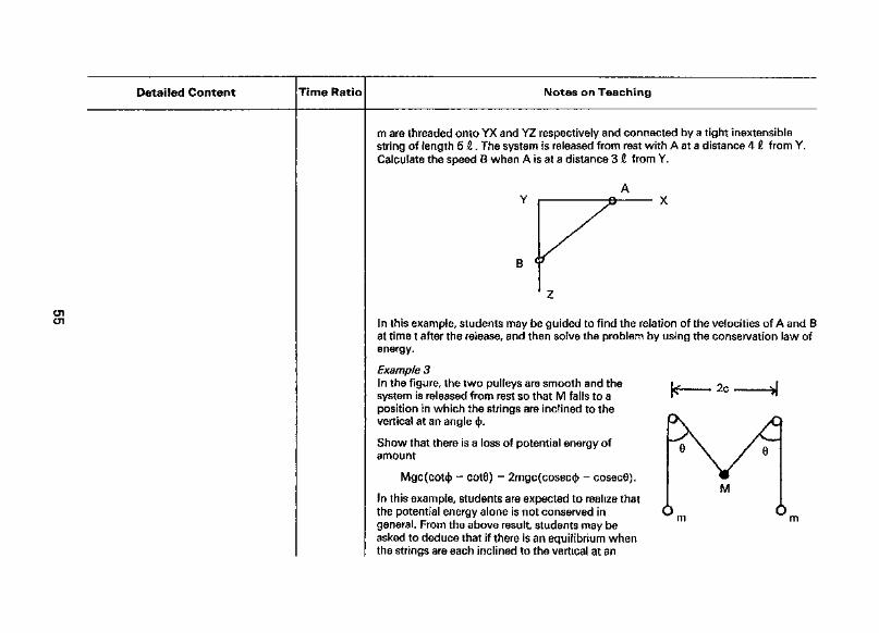
Example 2The figure shows a smooth wire XYZ in a vertical plane. The straight portion YX and YZof the wire are at right angles and YX is horizontal. Smooth rings A and B each of mass
Detailed Content Time Ratio Notes on Teaching
m are threaded onto YX and YZ respectively and connected by a tight inextensiblestring of length 5 £ . The system is released from rest with A at a distance 4 £ from Y.Calculate the speed B when A is at a distance 3 # from Y.
01CJl In this example, students may be guided to find the relation of the velocities of A and B
at time t after the release, and then solve the problem by using the conservation law ofenergy.
Example 3In the figure, the two pulleys are smooth and thesystem is released from rest so that M falls to aposition in which the strings are inclined to thevertical at an angle cj>.
Show that there is a loss of potential energy ofamount
Mgc(cot<|> - cot0) - 2mgc(cosec(|> - cosecO).
In this example, students are expected to realize thatthe potential energy alone is not conserved ingeneral. From the above result students may beasked to deduce that if there is an equilibrium whenthe strings are each inclined to the vertical at an
Detailed Content Time Ratio Notes on Teaching
OiO)
angle a, and the system is released from a position in which the strings are eachinclined to the vertical at an angle 0, it will next come to instantaneous rest when theinclination is <j> where
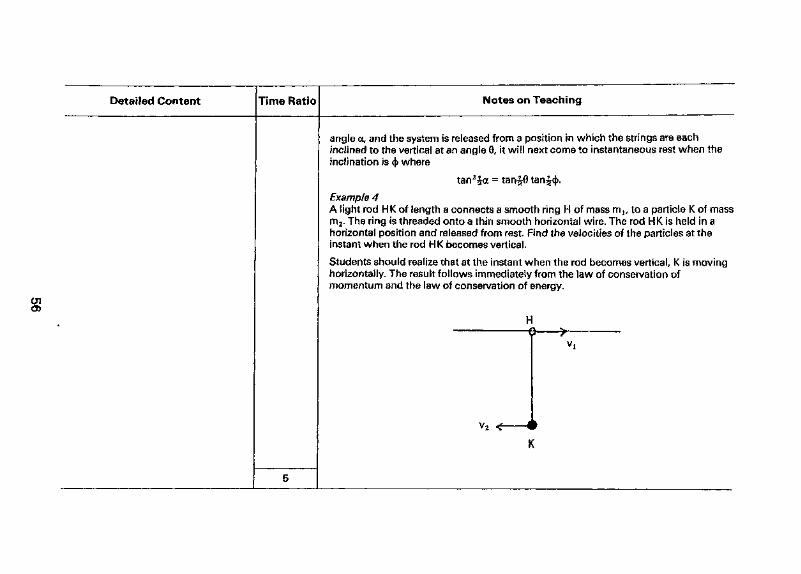
Example 4A light rod HK of length a connects a smooth ring H of mass m^ to a particle K of massm2. The ring is threaded onto a thin smooth horizontal wire. The rod HK is held in ahorizontal position and released from rest. Find the velocities of the particles at theinstant when the rod HK becomes vertical.
Students should realize that at the instant when the rod becomes vertical, K is movinghorizontally. The result follows immediately from the law of conservation ofmomentum and the law of conservation of energy.
UNIT 6: IMPACT
Specific Objectives:
1. To distinguish between elastic and inelastic impacts.2. To understand Newton's Law of Restitution.3. To apply Newton's Law of Restitution to solve problems of direct and oblique impacts.
Detailed Content Time Ratio Notes on Teaching
6,1 impulse
CTJ
6,2 impact of Elastic Bodies
The impulse of a force may be defined as the product of the force and the time tfor which it acts. With this definition and starting from Newton's Second Law ofMotion, it is not hard to arrive at the relationship Ft = mv - mu. Thus, students shouldhave no problem to see that the impulse of a force is equal to the change in momentumwhich it produces.
Students are also expected to realize the meaning of impulsive force. Examplesinclude the blow of a hammer, the impact of water on a surface, the impact of a bulleton a target, the collision of balls etc.
Teachers should revise with students the Principle of Conservation of LinearMomentum and remind them this principle is usually used in dealing with problems inwhich impacts or impulsive forces occur. The above-mentioned examples can be usedfor illustration, but problems involving impulsive tensions are not necessary.
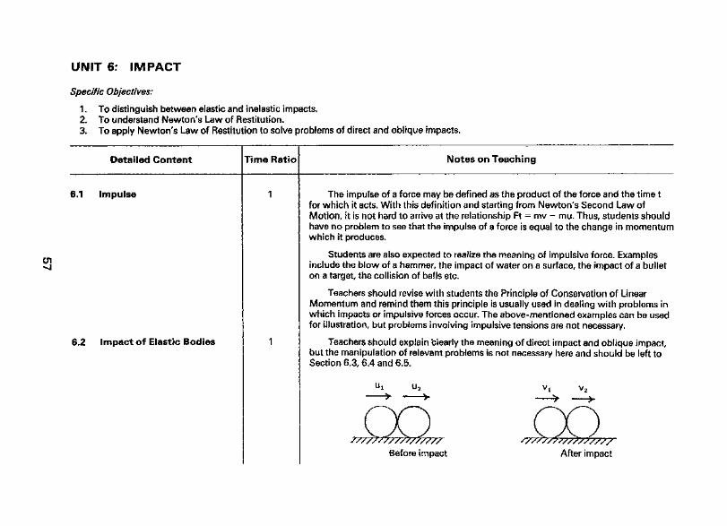
Teachers should explain clearly the meaning of direct impact and oblique impact,but the manipulation of relevant problems is not necessary here and should be left toSection 6,3, 6 A and 6.5,
P/////7///7/77777'Before impact After impact

Detailed Content Time Ratio Notes on Teaching
0100
6.3 Direct Impact
Newton's experimental taw (i.e. -~ U 2
= -e) should be introduced at this
stage. The positive constant e is known as coefficient of restitution or coefficient ofelasticity. Teachers should remind students of the negative sign adhering to e in the
law. (If the law is introduced as — - - L = e, then teachers should remind students of"i - "2
the sequences of subtraction in the numerator and the denominator.)
The different values of e for different bodies should be discussed. In particular,bodies with e = 0 are said to be perfectly inelastic while those with e = 1 are said to beperfectly elastic. For other elastic bodies, 0 < e < 1 .
Students are expected to know in perfectly elastic impact kinetic energies areconserved while in perfectly inelastic impact, the two bodies after impact will adhereand move with a common velocity. The imperfectly elastic impact is in between thetwo extreme cases.
Teachers should emphasize that unless the impact is perfectly elastic, kineticenergy is not conserved. This fact can further be verified by guiding students todevelop the expression:
/'lossin kineticenergy"\ _ J_ n^nr^\ due to direct impact ) 2 m1+m2
( U i - u 2 ) 2 ( 1 - e 2 )
Clearly, the loss is zero if e = 1. Teachers should not encourage students to memorizethe expression. Instead, they should encourage students to derive it when necessaryAs a matter of fact, in most numerical cases, it is not hard to find directly the velocitiesof the bodies after impact. The loss can then be obtained easily by subtracting thekinetic energy after impact from that before.
Various types of examples should be provided to acquaint students with thetechnique. Typical examples including finding the velocities after impact, the kineticenergy loss due to impact, the momentum transferred from one sphere to the otherafter impact etc.
Detailed Content Time Ratio Notes on Teaching
6.4 Impact of a Smooth Sphereon a Smooth Surface
01CD
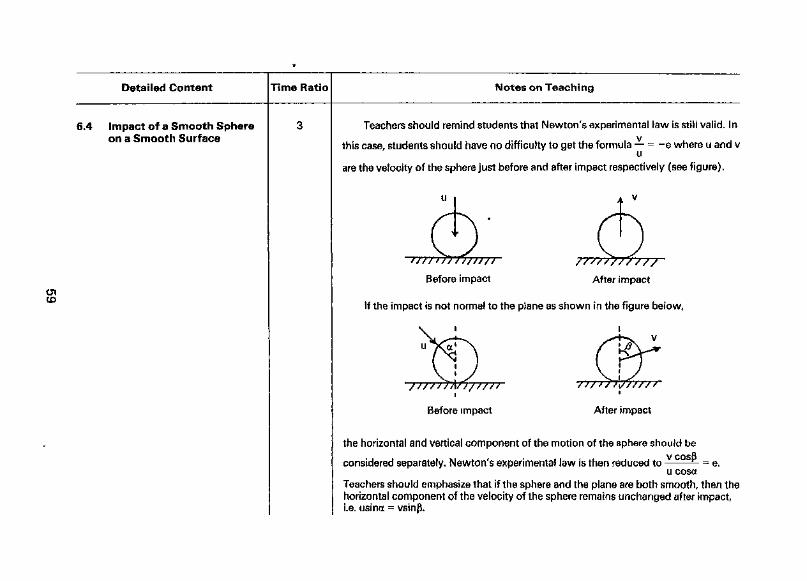
Teachers should remind students that Newton's experimental law is still valid. In
this case, students should have no difficulty to get the formula — = -e where u and v
are the velocity of the sphere just before and after impact respectively (see figure).
Before impact After impact
If the impact is not normal to the plane as shown in the figure below.
' ///////I///////i
Before impact After impact
the horizontal and vertical component of the motion of the sphere should be
considered separately, Newton's experimental law is then reduced to — = e.u cosa
Teachers should emphasize that if the sphere and the plane are both smooth, then thehorizontal component of the velocity of the sphere remains unchanged after impact,i.e. usina = vsinp.
Detailed Content Time Ratio Notes on Teaching
0>o
6,5 Oblique Impact
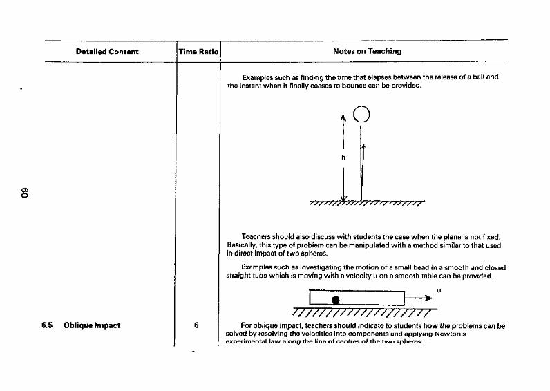
Examples such as finding the time that elapses between the release of a ball andthe instant when it finally ceases to bounce can be provided.
tO
V
Teachers should also discuss with students the case when the plane is not fixed.Basically, this type of problem can be manipulated with a method similar to that usedin direct impact of two spheres,
Examples such as investigating the motion of a small bead in a smooth and closedstraight tube which is moving with a velocity u on a smooth table can be provided,
For oblique impact, teachers should indicate to students how the problems can besolved by resolving the velocities into components and applying Newton'sexperimental law along the line of centres of the two spheres.
Detailed Content Time Ratio Notes on Teaching
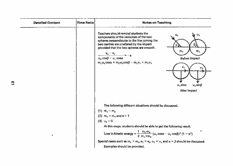
Teachers should remind students thecomponents of the velocities of the twospheres perpendicular to the line joining thetwo centres are unaltered by the impactprovided that the two spheres are smooth.
eu2cosp - ut cosa
m2u2cosp = + m2v2
o>u2sinp
After Impact
The following different situations should be discussed.
(1) m1 = m2
(2) mL = m2 and e = 1
(3) u2 = 0
At this stage, students should be able to get the following result.
. 1 rrij m2 **Loss in kinetic energy = (Uj cosa - u2 cosp)2 (1 - e2)
Special cases such as m£ = m2, et = e2, ut = u2 and a = p should be discussed.
Examples should be provided.
Detailed Content Time Ratio Notes on Teaching
o>
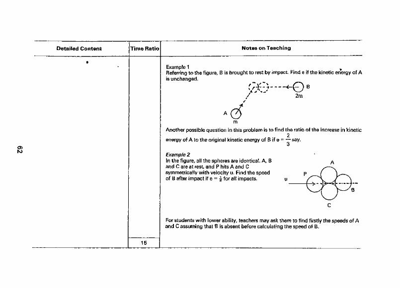
Example 1 vReferring to the figure, B is brought to rest by impact. Find e if the kinetic energy of Ais unchanged,
2m
Another possible question in this problem is to find the ratio of the increase in kinetic2
energy of A to the original kinetic energy of B if e = — say.
Example 2in the figure, all the spheres are identical. A, Band C are at rest, and P hits A and Csymmetrically with velocity u, Find the speedof B after impact if e = i f°r a" impacts.
For students with lower ability, teachers may ask them to find firstly the speeds of Aand C assuming that B is absent before calculating the speed of B.
15
UNIT 7: MOTION OF PROJECTILE UNDER GRAVITY
Specific Objectives:
1 „ To understand the motion of projectile as a simple case of two-dimensional problems.2. To recognize the path of a projectile as a parabola.3. To solve related problems.
Detailed Content Time Ratio Notes on Teaching
CDCO
7,1 Motion of Projectile
7.2 Trajectory of Projectile
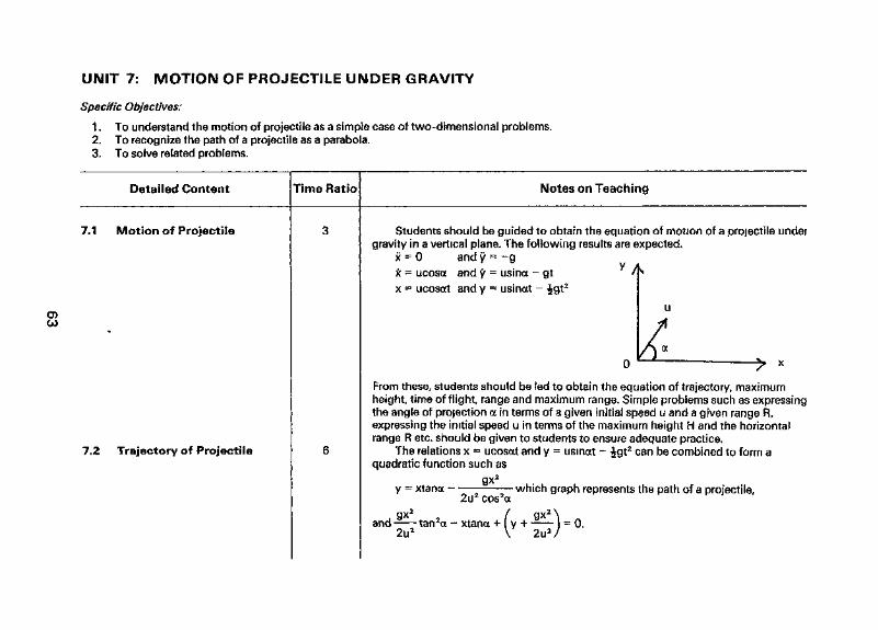
Students should be guided to obtain the equation of motion of a projectile undergravity in a vertical plane. The following results are expected,
x = 0 and y = -gx = ucosa and y = usince - gtx = ucosat and y = usinoct - igt2
0
From these, students should be led to obtain the equation of trajectory, maximumheight, time of flight, range and maximum range. Simple problems such as expressingthe angle of projection a in terms of a given initial speed u and a given range R,expressing the initial speed u in terms of the maximum height H and the horizontalrange R etc, should be given to students to ensure adequate practice.
The relations x = ucosat and y = usmat - |gt2 can be combined to form aquadratic function such as
gx2
y = xtanot — which graph represents the path of a projectile,2u2 cos2ct
gx2
and tan2ot - xtana +2u2
Detailed Content Time Ratio Notes on Teaching
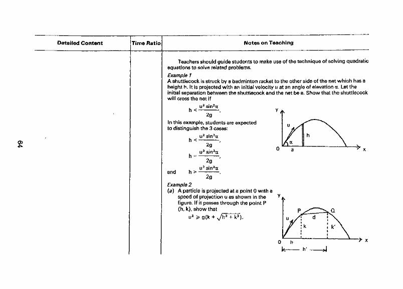
Teachers should guide students to make use of the technique of solving quadraticequations to solve related problems.
Example 1A shuttlecock is struck by a badminton racket to the other side of the net which has aheight h. It is projected with an initial velocity u at an angle of elevation a. Let theinitial separation between the shuttlecock and the net be a. Show that the shuttlecockwill cross the net if
h <u2 sin2a
2gIn this example, students are expectedto distinguish the 3 cases:
h <
and
2gu2 sin2oc
2g '
2gExample 2(a) A particle is projected at a point 0 with a
speed of projection u as shown in thefigure. If it passes through the point P(h, k), show that Q
Detailed Content Time Ratio Notes on Teaching
7.3 Range on an Inclined Plane
01
7.4 Further Application ofProjectile
If otj and cc2 are the two possible angles of projection, show that
tan(aA + a2) = —-.K
(b) If Q(h', k') is another point in the path such that the distance between P and Q isd, show that the minimum velocity with which the particle is projected so as topass through both points P and Q is /g(d + k + k').
In (b), students should be able to make use of the results in (a) and the principle ofconservation of energy to arrive at the result.
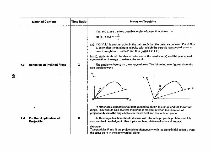
The emphasis here is on the choice of axes. The following two figures show thetwo possible ways.
In either case, students should be guided to obtain the range and the maximumrange. They should also see that the range is maximum when the direction ofprojection bisects the angle between the vertical and the inclined plane.
At this stage, teachers should discuss with students projectile problems whichalso involve knowledge of other topics such as relative velocity and impact.
ExampleTwo particles P and Q are projected simultaneously with the same initial speed u fromthe same point in the same vertical plane.
Detailed Content Time Ratio Notes on Teaching
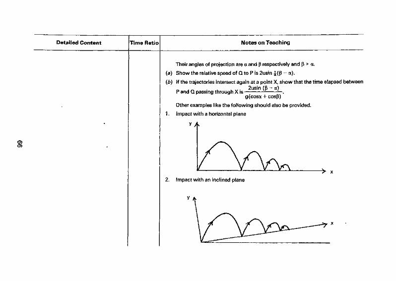
Their angles of projection are a and p respectively and p > a.
(a) Show the relative speed of Q to P is 2usin ^(p - a).
(b) If the trajectories intersect again at a point X, show that the time elapsed between
P and Q passing through X is .g(cosa + cosp)
Other examples like the following should also be provided.
1. Impact with a horizontal plane
y A
o>
2. Impact with an inclined plane
Detailed Content Time Ratio Notes on Teaching
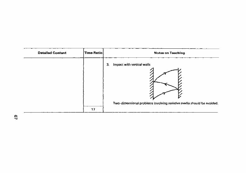
3. Impact with vertical waifs
I 2£
Two-dimensional problems involving resistive media should be avoided.
17
o>
UNIT 8: CIRCULAR MOTIONSpecific Objectives:
To study the dynamics of a particle in circular motion.1.2. To solve problems involving circular motion,
Detailed Content Time Ratio Notes on Teaching
00
8.1 Circular Motion
8.2 Motion in a Vertical Circle
Teachers may advise students to analyze the kinematics of a particle moving ina circle of radius r. Teachers may start with 7* = rer and guide students to obtain the
v2 dvacceleration7* = -r92er + r6ee or?* = er + —e0. Here, students are expected to
know that if the particle is moving with constant speed around the circle, thenv2
0 = 0 and?* = -r02er = ——er which is called the centripetal acceleration and is
always pointing towards the centre of the circle (as indicated by its negative sign). The
corresponding centripetal force (of magnitude mr92 or ) should be provided by
some identifiable forces acting on it. For example, the tension of a string, a reactionforce or a frictional force.
Examples such as a car moving without skidding at a constant speed in ahorizontal circle (with or without banking) and conical pendulum should be provided.
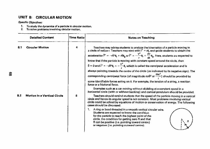
Teachers should remind students that the speed of the particle moving in a verticalcircle and hence its angular speed is not constant. Most problems involving verticalcircle could be solved by equations of motion or conservation of energy. The followingcases should be discussed.
1. A ring or bead threaded in a smooth vertical circular wire.Students are expected to know the conditionfor the particle to reach the highest point of thecircle, the condition for getting zero R and thatR can be positive (i.e. pointing toward centre)or negative (i.e. pointing outward centre).
Detailed Content Time Ratio Notes on Teaching
2.
0>CD
3,
4.
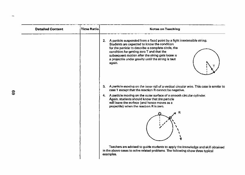
A particle suspended from a fixed point by a light inextensibie stringStudents are expected to know the conditionfor the particle to describe a complete circle, thecondition for getting zero T and that thesubsequent motion after the string gets loose isa projectile under gravity until the string is tautagain.
A particle moving on the inner rail of a vertical circular wire. This case is similar tocase 1 except that the reaction R cannot be negative.
A particle moving on the outer surface of a smooth circular cylinder.Again, students should know that the particlewill leave the surface (and hence moves as aprojectile) when the reaction R is zero.
Teachers are advised to guide students to apply the knowledge and skill obtainedin the above cases to solve related problems. The following show three typicalexamples.
Detailed Content Time Ratio Notes on Teaching
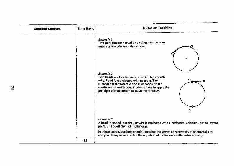
Example 1Two particles connected by a string move on theouter surface of a smooth cylinder.
Example 2Two beads are free to move on a circular smoothwire. Bead A is projected with speed u. Thesubsequent motion of A and B depends on thecoefficient of restitution. Students have to apply theprinciple of momentum to solve the problem.
Example 3A bead threaded to a circular wire is projected with a horizontal velocity u at the lowestpoint. The coefficient of friction is \L
In this example, students should note that the law of conservation of energy fails toapply and they have to solve the equation of motion as a differential equation.
12

UNIT 9: SIMPLE HARMONIC MOTION
Specific Objectives:
1. To recognize simple harmonic motion.2. To recognize damped and forced oscillation.3. To solve related problems.
Detailed Content Time Ratio Notes on Teaching
9.1 Simple Harmonic Motion 12 Teachers may illustrate the concept of simple harmonic motion (S.H.M.) by usingexamples like simple pendulum and simple mass-spring system.
x = -—-x x = xm£ m£
Students should know that any motion satisfying the equation of motion x =-o)2x is simple harmonic and they should be aware of the negative sign in theequation. Teachers may relate this unit with Topic Area II (Differential Equations).
After acquiring the relevant concept, teachers should guide students to obtain thefundamental formulae of S.H.M. which are listed collectively below;
Acceleration x = -to2xVelocity x = Aoocos (cot + ot) = co^/A2 - x2
Displacement x = Asin (cot + a)
Period T = —CO
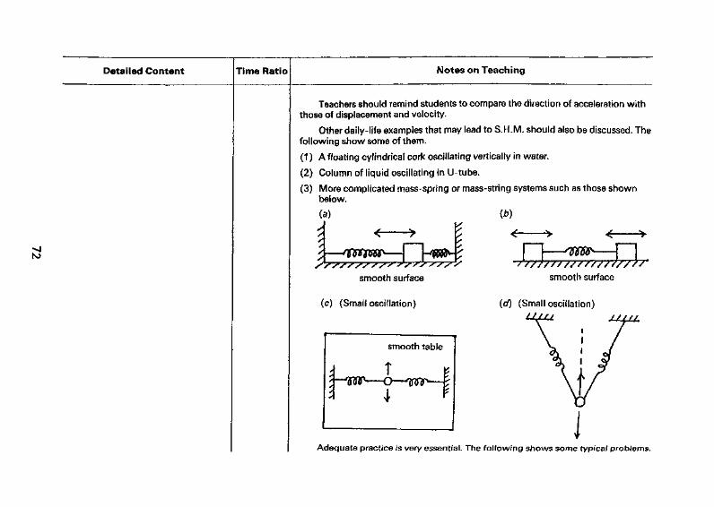
Detailed Content Time Ratio Notes on Teaching
Teachers should remind students to compare the direction of acceleration withthose of displacement and velocity.
Other daily-life examples that may lead to S.H.M. should also be discussed. Thefollowing show some of them,
(1) A floating cylindrical cork oscillating vertically in water.
(2) Column of liquid oscillating in U-tube.
(3) More complicated mass-spring or mass-string systems such as those shownbelow,
(a) (b)
—wow—| fWfa- —^QfWs—
smooth surface
(c) (Small oscillation)
smooth surface
(of) (Small oscillation)
smooth table
T
r
Adequate practice is very essential. The following shows some typical problems.
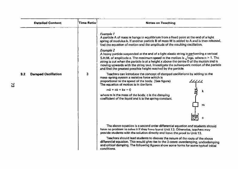
Detailed Content Time Ratio Notes on Teaching
9,2 Damped Oscillation
Example 1A particle A of mass m hangs in equilibrium from a fixed point at the end of a lightspring of modulus k. If another particle B of mass M is added to A and is then released,find the equation of motion and the amplitude of the resulting oscillation.
Example 2A heavy particle suspended at the end of a light elastic string is performing a verticalS.H.M. of amplitude a. The maximum speed in the motion is /nga, where n > 1, Thestring is cut when the particle is at a height x above the centre 0 of the motion and ismoving upwards with the string taut. Investigate the subsequent motion of the particleand find the greatest possible height reached by the particle.
Teachers can introduce the concept of damped oscillations by adding to themass-spring system a resistive force which isproportional to the speed of the body. (See figure)The equation of motion is in the form
JTJX + ex + kx == 0
where m is the mass of the body, c is the dampingcoefficient of the liquid and k is the spring constant.
The above equation is a second order differential equation and students shouldhave no problem to solve it if they have learnt Unit 13. Otherwise, teachers mayprovide students with the solution directly and leave the proof to Unit 13.
Teachers should lead students to discuss the nature of the roots of the abovedifferential equation. This would give rise to the 3 cases: overdamping, underdampingand critical damping. The following figures show some forms for some typical initialconditions.
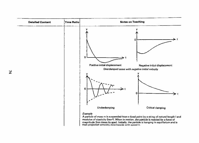
Detailed Content Time Ratio Notes on Teaching
Positive initial displacement Negative initial displacement
Overdamped cases with negative initial velocity
Underdamping Critical damping
ExampleA particle of mass m is suspended from a fixed point by a string of natural length I andmodulus of elasticity 5mn2l, When in motion, the particle is resisted by a force ofmagnitude 2mn times its sped. Initially, the particle is hanging in equilibrium and isthen projected vertically downwards with speed V.
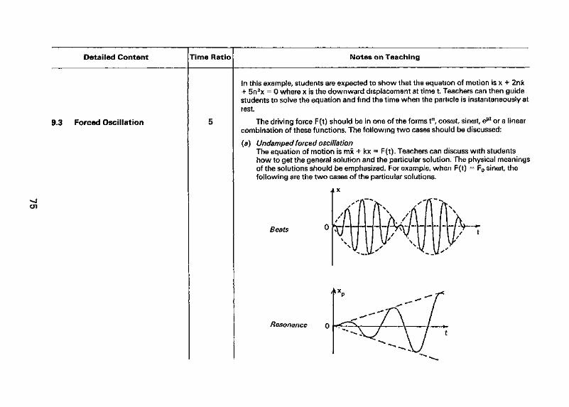
Detailed Content Time Ratio Notes on Teaching
9,3 Forced Oscillation
01
In this example, students are expected to show that the equation of motion is x + 2nx+ 5n2x = 0 where x is the downward displacement at time t. Teachers can then guidestudents to solve the equation and find the time when the particle is instantaneously atrest.
The driving force F(t) should be in one of the forms tn, coso>t, sinoot, eMt or a linearcombination of these functions. The following two cases should be discussed:
(a) Undamped forced oscillationThe equation of motion is mx + kx = F(t). Teachers can discuss with studentshow to get the general solution and the particular solution. The physical meaningsof the solutions should be emphasized. For example, when F(t) = F0 sincot, thefollowing are the two cases of the particular solutions.
Beats
Resonance
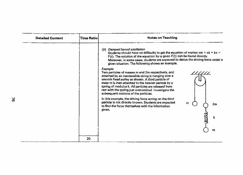
Detailed Content Time Ratio Notes on Teaching
05
20
(£) Damped forced oscillationStudents should have no difficulty to get the equation of motion mx + ex + kx =F(t). The solution of the equation for a given F(t) can be found directly.Moreover, in some cases, students are expected to derive the driving force under agiven situation. The following shows an example.
ExampleTwo particles of masses m and 2m respectively, andattached by an inextensible string is hanging over asmooth fixed pulley as shown. A third particle ofmass m is then attached to the heavier particle by aspring of modulus k. All particles are released fromrest with the spring just unstretched. Investigate thesubsequent motions of the particles.
In this example, the driving force acting on the thirdparticle is not directly known. Students are expected m ( ) /"S 2mto find the force themselves with the information m
given.
m
O
UNIT 10: MOTION OF A PARTICLE IN A PLANE
Specific Objective:
To solve problems involving motion of a particle in a plane by various techniques.
Detailed Content Time Ratio Notes on Teaching
10.1 Motion of a Particle in aPlane
In order to solve the general motion of particle in a plane, two coordinate systems,i.e. the cartesian coordinate and polar coordinate systems, should be introduced to thestudents. It is also worthwhile for teachers to discuss with students the distinction ofemploying polar coordinates and cartesian coordinates in solving such problems.
Simple integration is worthwhile as the major solving technique for this kind ofproblems. However, students should be told that the skill learnt from the differentialequations may also be employed where necessary.
Some examples using cartesian coordinates may be introduced to students. Belowis one:
ExampleA particle moving in a plane is subject to a force acting towards the x-axis andproportional to its distance from that axis. Initially, it is projected from the origin with avelocity v in a direction making an angle 9 with the x-axis.
In this problem, students are asked to set up force equations along the x- andy-direction, and to find the velocity and position of the particle at time t by directintegration or by using the technique of differential equation.
Moreover, students should be reminded that projectile motion is a kind of motionthat employs cartesian coordinates.
Before teaching students to handle the problems using polar coordinates, theknowledge of resolution of velocity and acceleration along and perpendicular to theradius vector learnt should be recalled. Sufficient practical examples in which theposition, velocity and acceleration vectors (as well as their radial and transversecomponents) of an object which could be represented in polar coordinates should begiven. However, teachers should note that velocity and acceleration components intangential-normal form are not required.
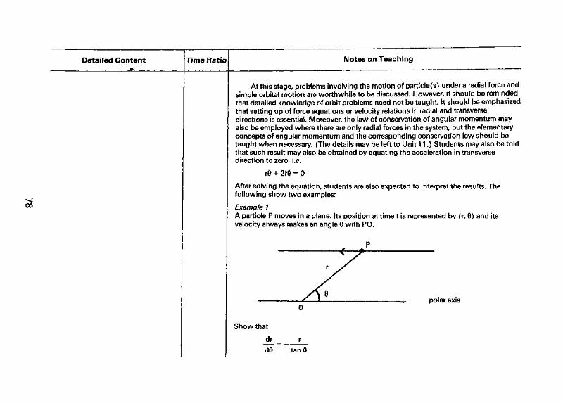
00
Detailed Content Time Ratio Notes on Teaching
At this stage, problems involving the motion of particle(s) under a radial force andsimple orbital motion are worthwhile to be discussed. However, it should be remindedthat detailed knowledge of orbit problems need not be taught. It should be emphasizedthat setting up of force equations or velocity relations in radial and transversedirections is essential. Moreover, the law of conservation of angular momentum mayalso be employed where there are only radial forces in the system, but the elementaryconcepts of angular momentum and the corresponding conservation law should betaught when necessary. (The details may be left to Unit 11.) Students may also be toldthat such result may also be obtained by equating the acceleration in transversedirection to zero, i.e.
r§ + 2f0 = 0
After solving the equation, students are also expected to interpret the results. Thefollowing show two examples:
Example 1A particle P moves in a plane. Its position at time t is represented by (r, 9) and itsvelocity always makes an angle 0 with PO.
P— «.,•,.„„,. ... • jf - £-
S\§
0
Show that
dr r
d9 tan 0
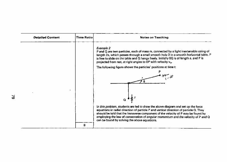
Detailed Content Time Ratio Notes on Teaching
Example 2P and Q are two particles, each of mass m, connected by a light inextensible string oflength 2a, which passes through a small smooth hole 0 in a smooth horizontal table. Pis free to slide on the table and Q hangs freely. Initially OQ is of length a, and P isprojected from rest, at right angles to OP with velocity v0.
The following figure shows the particles' positions at time t:
P
CO • > «M
In this problem, students are led to draw the above diagram and set up the forceequations in radial direction of particle P and vertical direction of particle Q. Theyshould be told that the transverse component of the velocity of P may be found byemploying the law of conservation of angular momentum and the velocity of P and Qcan be found by solving the above equations.
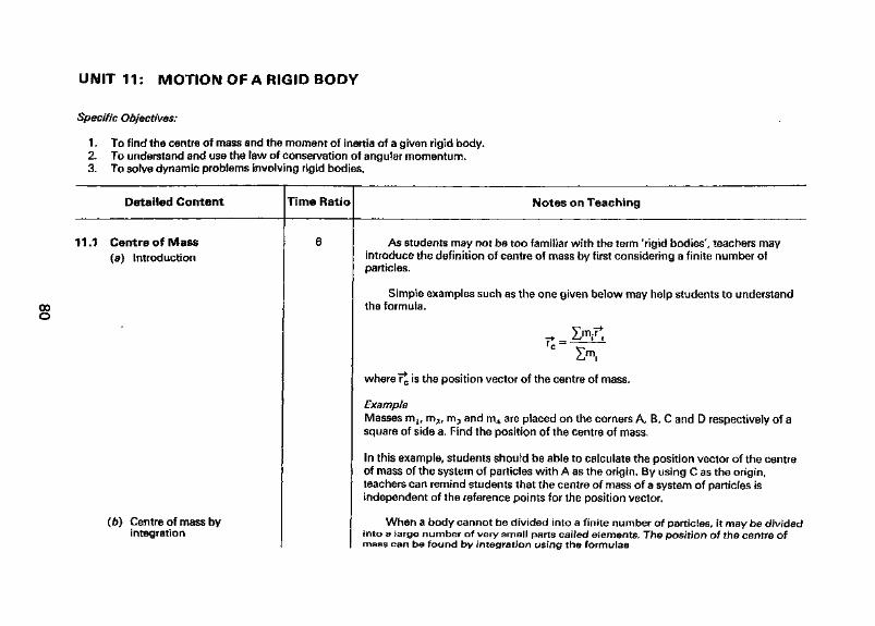
UNIT 11: MOTION OF A RIGID BODY
Specific Objectives:
1. To find the centre of mass and the moment of inertia of a given rigid body.2. To understand and use the law of conservation of angular momentum.3. To solve dynamic problems involving rigid bodies.
Detailed Content Time Ratio Notes on Teaching
11,1 Centre of M ass(a) Introduction
(b) Centre of mass byintegration
As students may not be too familiar with the term 'rigid bodies', teachers mayintroduce the definition of centre of mass by first considering a finite number ofparticles.
Simple examples such as the one given below may help students to understandthe formula.
where 7^ is the position vector of the centre of mass.
ExampleMasses mlr m2/ m3 and m4 are placed on the corners A, B, C and D respectively of asquare of side a. Find the position of the centre of mass.
In this example, students should be able to calculate the position vector of the centreof mass of the system of particles with A as the origin. By using C as the origin,teachers can remind students that the centre of mass of a system of particles isindependent of the reference points for the position vector.
When a body cannot be divided into a finite number of particles, it may be dividedinto a large number of very small parts called elements. The position of the centre ofmass can be found by integration using the formulae
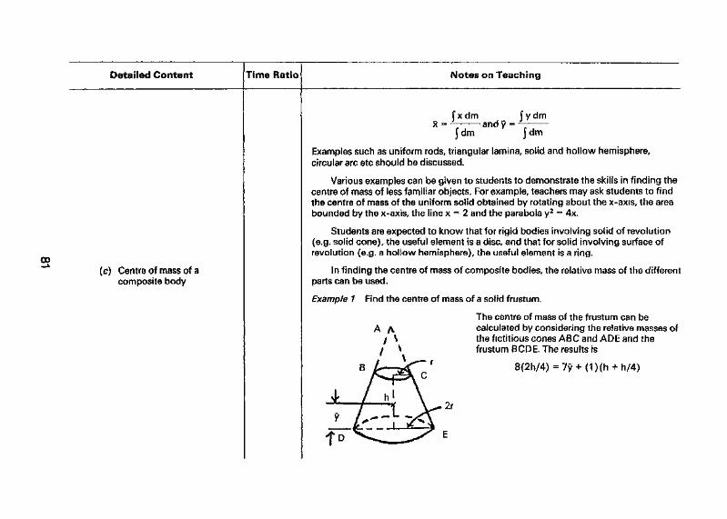
Detailed Content Time Ratio Notes on Teaching
00(c) Centre of mass of a
composite body
f x d m±- -Jdm
fydm-^ -jdm
Examples such as uniform rods, triangular lamina, solid and hollow hemisphere,circular arc etc should be discussed.
Various examples can be given to students to demonstrate the skills in finding thecentre of mass of less familiar objects. For example, teachers may ask students to findthe centre of mass of the uniform solid obtained by rotating about the x-axis, the areabounded by the x-axis, the line x = 2 and the parabola y2 = 4x.
Students are expected to know that for rigid bodies involving solid of revolution(e.g. solid cone), the useful element is a disc, and that for solid involving surface ofrevolution (e.g. a hollow hemisphere), the useful element is a ring.
In finding the centre of mass of composite bodies, the relative mass of the differentparts can be used.
Example 1 Find the centre of mass of a solid frustum.
The centre of mass of the frustum can becalculated by considering the relative masses ofthe fictitious cones ABC and ADE and thefrustum BCDE. The results is
8{2h/4) =7y
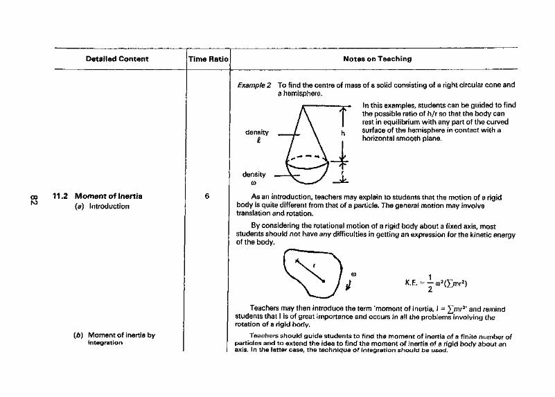
Detailed Content Time Ratio Notes on Teaching
oo 11.2 Moment of Inertia^ (a) Introduction
(b) Moment of inertia byintegration
Example 2 To find the centre of mass of a solid consisting of a right circular cone anda hemisphere.
in this examples, students can be guided to findthe possible ratio of h/r so that the body canrest in equiiibrium with any part of the curvedsurface of the hemisphere in contact with ahorizontal smooth plane.
As an introduction, teachers may explain to students that the motion of a rigidbody is quite different from that of a particle. The general motion may involvetranslation and rotation.
By considering the rotational motion of a rigid body about a fixed axis, moststudents should not have any difficulties in getting an expression for the kinetic energyof the body,
Teachers may then introduce the term 'moment of inertia, I = £mr2' and remindstudents that I is of great importance and occurs in all the problems involving therotation of a rigid body.
Teachers should guide students to find the moment of inertia of a finite number ofparticles and to extend the idea to find the moment of inertia of a rigid body about anaxis. In the latter case, the technique of integration should be used.
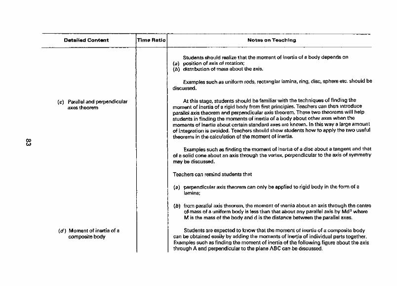
Detailed Content Time Ratio Notes on Teaching
(c) Parallel and perpendicularaxes theorem
ooCO
(cf) Moment of inertia of acomposite body
Students should realize that the moment of inertia of a body depends on(a) position of axis of rotation;(b) distribution of mass about the axis.
Examples such as uniform rods, rectanglar lamina, ring, disc, sphere etc. should bediscussed.
At this stage, students should be familiar with the techniques of finding themoment of inertia of a rigid body from first principles. Teachers can then introduceparallel axis theorem and perpendicular axis theorem. These two theorems will helpstudents in finding the moments of inertia of a body about other axes when themoments of inertia about certain standard axes are known. In this way a large amountof integration is avoided. Teachers should show students how to apply the two usefultheorems in the calculation of the moment of inertia.
Examples such as finding the moment of inertia of a disc about a tangent and thatof a solid cone about an axis through the vertex, perpendicular to the axis of symmetrymay be discussed.
Teachers can remind students that
(a) perpendicular axis theorem can only be applied to rigid body in the form of alamina;
(b) from parallel axis theorem, the moment of inertia about an axis through the centreof*mass of a uniform body is less than that about any parallel axis by Md2 whereM is the mass of the body and d is the distance between the parallel axes.
Students are expected to know that the moment of inertia of a composite bodycan be obtained easily by adding the moments of inertia of individual parts together.Examples such as finding the moment of inertia of the following figure about the axisthrough A and perpendicular to the plane ABC can be discussed.
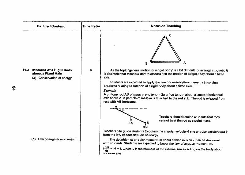
Detailed Content Time Ratio Notes on Teaching
11.3 Moment of a Rigid Bodyabout a Fixed Axis(a) Conservation of energy
oo
(d) Law of angular momentum
As the topic 'general motion of a rigid body' is a bit difficult for average students, itis desirable that teachers start to discuss first the motion of a rigid body about a fixedaxis.
Students are expected to apply the law of conservation of energy in solvingproblems relating to rotation of a rigid body about a fixed axis.ExampleA uniform rod AB of mass m and length 2a is free to turn about a smooth horizontalaxis about A. A particle of mass m is attached to the rod at B. The rod is released fromrest with AB horizontal.
Teachers should remind students that theycannot treat the rod as a point mass.
mgmg
Teachers can guide students to obtain the angular velocity 6 and angular acceleration 6from the law of conservation of energy.
The definition of angular momentum about a fixed axis can then be discussedwith students. Students are expected to know the law of angular momentum.
I—j— = I0 = L where L is the moment of the external forces acting on the body aboutthe fjxed ax»s
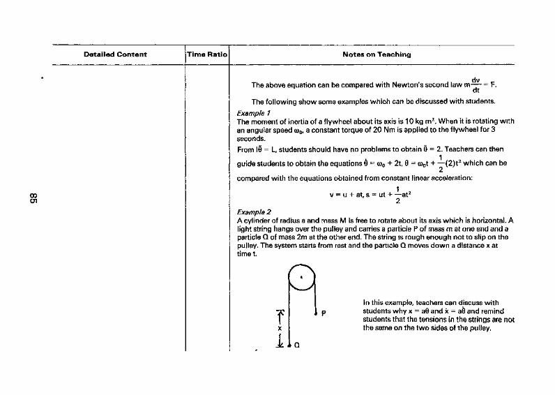
Detailed Content Time Ratio Notes on Teaching
0001
dvThe above equation can be compared with Newton's second law m—- = F.
dt
The following show some examples which can be discussed with students.
Example 1The moment of inertia of a flywheel about its axis is 10 kg m2. When it is rotating withan angular speed co0/ a constant torque of 20 Nm is applied to the flywheel for 3seconds.
From !9 = L, students should have no problems to obtain 0 = 2. Teachers can then
guide students to obtain the equations 9 = co0 + 2t, 0 = o)0t + —(2)t2 which can be
compared with the equations obtained from constant linear acceleration:
v = u + at, s = ut + —at2
2
Example 2A cylinder of radius a and mass M is free to rotate about its axis which is horizontal. Alight string hangs over the pulley and carries a particle P of mass m at one end and aparticle Q of mass 2m at the other end. The string is rough enough not to slip on thepulley, The system starts from rest and the particle Q moves down a distance x attime t.
TX
i
In this example, teachers can discuss withstudents why x = a0 and x = a0 and remindstudents that the tensions in the strings are notthe same on the two sides of the pulley.
Q
Detailed Content Time Ratio Notes on Teaching
ooO5
(c) Applications
11.4 General Motion of a RigidBody(a) Introduction
16
Students may be guided to set up the equations of motion for P, Q and the cylinder.Also, teachers can discuss with students the possibility of using energy conservation inthis case.
The Law of conservation of angular momentum should be introduced and can beillustrated by considering simple examples such as the one given below:
ExampleA uniform disc of mass m and radius a is rotating with constant angular velocity G> in ahorizontal plane about a vertical axis through its centre A. A particle P of mass 2m isplaced gently without slipping on the disc at a point distant a/2 from A.
Teachers can explain to students that sincethere is no external torque acting on the system,angular momentum must be conserved.
Students can be guided to find the new angularvelocity of the disc (which is the same as theparticle).
Other examples such as the work done by a couple J Ld8, the impulse of thetorque J Ldt, compound pendulum etc should also be discussed through workedexamples.
The general motion of a rigid body can be illustrated by diagrams.
Detailed Content Time Ratio Notes on Teaching
00
(b) Equation of motion
Students should know that the general motionconsists of two parts;
(1) translation of the centre of mass
(2) rotation about the centre of mass
Teachers may derive the necessary equations required but emphasis should be placedon the application rather than derivation.
It is important for students to realize that the general motion of a rigid body can beanalysed by considering independently
(a) the linear motion of the centre of mass
(b) the rotation about an axis through the centre of mass.
Teachers can discuss with students the law of angular momentum which can begeneralized as follows?
The rate of change of angular momentum of the body about the axis through thecentre of mass is equal to the sum of moments of the external forces about the axis.
Examples should be introduced to demonstrate the techniques in solvingproblems relating to genera! motion.
Detailed Content Time Ratio (Motes on Teaching
Example 1A uniform rod AB of length 2a and mass m isheld vertically with one, end resting on ahorizontal plane which is rough enough toprevent slipping and is then released.
It is important for students to realize the factthat the motion of the centre of mass of arigid body acted on by any forces, is the sameas if the whole mass were collected at thecentre of mass and all the forces were appliedat that point.
mg
Since the centre of mass is performing circular motion, students can be guided toobtain the equation of motion of centre of mass. By taking moment about A andconsidering the energy, 82 and 0 can be obtained, thus F and R can be calculated.
Students may also be asked to write down the equation of motion by consideringthe forces along AB and perpendicular to AB.

Detailed Content Time Ratio Notes on Teaching
00CD
(c) Rolling and sliding
Example 2A uniform rod of length 2a slides down avertical plane, its ends being in contact withtwo smooth planes, one horizontal and onevertical. The co-ordinates of the centre ofmass is (x, y).
ma \.t^////?w>,^By considering the translational motion of the centre of mass and the rotational motionabout the centre of mass, S and R can be obtained.
Among the topics of the general motion of rigid bodies, 'pure rolling' and 'rollingwith slipping' are two important ones, Below are some examples which can bediscussed with students.
Example 1A cylinder of radius a rolls down a rough inclined plane. Students should have nodifficulties in getting the equations
16 = Fa &mx = mg sinot - F
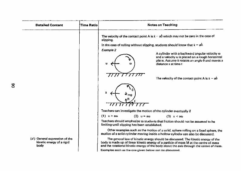
Detailed Content Time Ratio Notes on Teaching
toO
(of) General expression of thekinetic energy of a rigidbody
The velocity of the contact point A is x - a0 which may not be zero in the case ofslipping,
In the case of rolling without slipping, students should know that x = a9.
Example 2A cylinder with a backward angular velocity toand a velocity u is placed on a rough horizontalplane. Assume it rotates an angle 9 and moves adistance x at time t
///TV / / / /'/The velocity of the contact point A is x - a9
/ / / / / / v ? / / /Teachers can investigate the motion of the cylinder eventually if
(1) u > aco (2) u = aw (3) u < ao>
Teachers should emphasize to students that friction should not be assumed to belimiting until slipping has been established.
Other examples such as the motion of a solid, sphere rolling on a fixed sphere, themotion of a solid cylinder moving inside a hollow cylinder can also be discussed.
The general law of kinetic energy should be discussed. The kinetic energy of thebody is made up of linear kinetic energy of a particle of mass M at the centre of massand the rotational kinetic energy of the body about the axis through the centre of mass.Examples such as the one given below can be discussed.
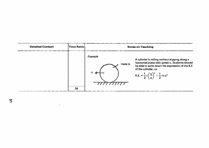
Detailed Content Time Ratio
34
Notes on Teaching
ExampleA cylinder is rolling without slipping along a
-r mass m horizontal plane with speed u. Students shouldX*^ "" X1 be able to write down the expression of the K.E.
f \ of the cylinder, i.e.
"^ ) «-H7H»*/ / / / / / /V/ f
CD
UNIT 12: FIRST ORDER DIFFERENTIAL EQUATIONS AND ITS APPLICATIONS
Specific Objectives:
1. To acquire skills in solving some specific first order differential equations,,2. To apply relevant skills of forming and solving first order differential equations in some given physical situations.3. To be able to interpret the solutions of first order differential equations.
Detailed Content Time Ratio Notes on Teaching
CD
12.1 Basic Concepts and Ideasdy d2y
Teachers may make use of simple examples like —- = x2 and —— = x3 to
introduce the general concept of differential equations (equations containingdifferential coefficients) and ask students to find the solutions of examples so given,Students should have no problem as those examples can be solved by simpleintegration, (The solution of the first is given by integrating x2 once while that of the
d2y dysecond by integrating x3 twice.) But how about the equation —- + — + y = 0?
dx2 dx
For students' interest, teachers may introduce the term 'ordinary differentialequation'. But since only one independent variable is considered in this topic area, thiscan be simply called differential equation if no ambiguity arises.
Students are also expected to recognise the terms 'order', 'degree', 'linear' and'non-linear' in differential equations. Examples should be given to clarify the variousconcepts.
The meaning of a solution of a differential equation should be clearly explained.This can be done through examples. For example, f (x) = e2x is a solution of the
dydifferential equation 2y = 0 because f'(x) - 2f(x) = 0.
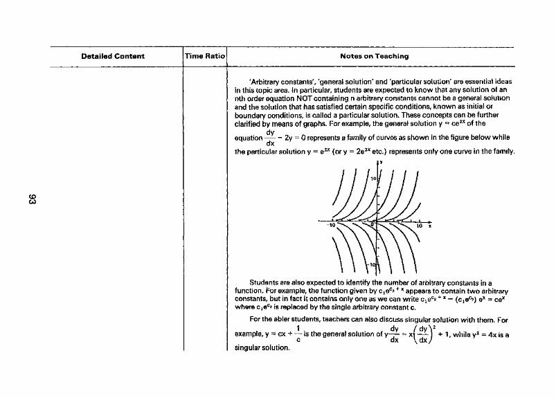
Detailed Content Time Ratio Notes on Teaching
'Arbitrary constants', 'general solution' and 'particular solution' are essential ideasin this topic area. In particular, students are expected to know that any solution of annth order equation NOT containing n arbitrary constants cannot be a general solutionand the solution that has satisfied certain specific conditions, known as initial orboundary conditions, is called a particular solution. These concepts can be furtherclarified by means of graphs. For example, the general solution y = ce2X of the
dyequation 2y = 0 represents a family of curves as shown in the figure below while
dxthe particular solution y = e2X (or y = 2e2X etc.) represents only one curve in the family.
co
Students are also expected to identify the number of arbitrary constants in afunction. For example, the function given by Cje^ + x appears to contain two arbitraryconstants, but in fact it contains only one as we can write c^*+ x = (Cje^) ex = cex
where c^e^ is replaced by the single arbitrary constant c.
For the abler students, teachers can also discuss singular solution with them. For1 dy /dy\2
example, y = ex + — is the genera! solution of y—- = x —— + 1, while y2 = 4x is ac dx \dx/
singular solution.
Detailed Content Time Ratio Notes on Teaching
12.2 Formation of DifferentialEquations
1 2.3 Solution of Equations withVariables Separable
CD
The emphasis here is on the formation of differential equations from physicalsituations. The solving of the resulting equations is left to the later sections. Teachersmay provide some illustrative examples to indicate to students how this can be done. Atypical example is the problem of growth in which the rate of change of population of
dPa certain species, — - at any time t is proportional to the value of P at that instant.
dtdP dP
Students should be able to write down the relation - a P or - = kP where k,dt dt
known as the growth constant, is a positive constant.
Students should be able to identify differential equations with variables separableand reduce them to the form g(y) dy = f (x) dx. Accordingly, students should have noproblem to solve the equations by simple integration, Since in many real lifeapplications, people are not so interested in the general solution of a given differentialequation but only in the particular solution satisfying a given initial condition, teachersare advised to provide more initial value problems to their students.
There are many physical problems which can lead to first order differentialequations of variables separable type. The following are some of them.
1 . Population growthThe population of a given species is decreased at a constant rate of n people perannum by emigration. And the population due to birth and death is increased at aconstant rate of X% of the existing population per annum. If the initial populationis N people, then the population x people after t years is given bydx
"dT TooExponential decayThe rate of decay of a radioactive substance at time t is proportional to the mass
x(t) of the substance left at that time. Thus, - = -^x where jn is a positivedt
constant.
Detailed Content Time Ratio Notes on Teaching
CDCJ1
3. Law of coolingThe rate of change of temperature of a body is proportional to the differencebetween the temperature of the body and the temperature 6 of the surrounding
dTmedium .Suppose T is the temperature of the body at time t, then — = k(T - 6)
dtwhere k < 0.
4. DiffusionA porous pot containing a solution of a substance of concentration of x mgcrrr3
is placed in a large vessel containing the same solution but of higherconcentration c mgcrrT3. The concentration of the solution in the pot will increasedue to diffusion. Assuming that c is constant, the rate of increase of concentrationof the solution in the pot is proportional to the difference in concentration.
Thus x satisfies the differential equation — = k(c - x) where k is a positivedt
constant,
5. EvaporationA wet and porous substance loses its moisture at a rate proportional to the
moisture content, x(t). Thus, the equation is — = -kx where k is a positivedt
constant.
6. Chemical reactionIf the temperature is kept constant, the velocity of a chemical reaction isproportional to the product of the concentration of the substances which arereacting. If x represents the amount of the substance formed in the reaction, then
x must satisfy the equation — = k (a - x) (b - x) where k is a positive constant
while a and b are the original amounts of the two reacting substancesrespectively.

Detailed Content Time Ratio Notes on Teaching
CDO> 12,4 Solution of Linear
Differential Equationsdy— + p(x)y =
7, Logistic law of population growthAn improved population model makes use of the differentia! equationdN—- = aN - bN2 in which aN is the birth rate, -bN2 is the death rate anddtN is the population at that instant. Here a and b are positive constants.
8, Spread of disease ^Here the equation considered is ——
dt: kN(P - N) where N is the population that
is infected at time t, P is the total population which is susceptible to infection,and the rate of change of N is assumed to be proportional to the product of N andP-N.In the above examples, teachers, apart from guiding students to set up and solve
the differential equations, should emphasize on the interpretation of the solutions,
dyFor equations which can be reduced to the linear form + p(x)y = q(x), the
solutions can be obtained by the use of integrating factor. Teachers should emphasizethat as the equation is of the first order the solution contains only one arbitraryconstant Therefore, the integrating factor eJp(x)dx should contain no constant ofintegration as any primitive of p(x) will serve the purpose. By experience, students mayeasily forget the form of the integrating factor and some even take efp(xjdx+c as thesolution of the given equation. Therefore, more practice should be given to ensure thatstudents master the technique.
Physical examples which give rise to first order linear differential equations arerecommended. The following are two examples.1, Mixture
A tank contains 100 L of solution in which 10 kg of chemical is dissolved.Solution containing 2 kg of the chemical per litre flows into the tank at 5 Lmin"1.The mixture is well-stirred and drawn off at 4 Lmin"1. If x kg is the mass of the
dx 4xchemical in the tank, then x satisfies the differential equation —7— + — =10
dt 1OO + twith initial condition x = 10 at t = O.

Detailed Content Time Ratio Notes on Teaching
12.5 Solution of EquationsReducible to VariablesSeparable Type or LinearType
2. Chain reactionRadioactive element X decays into radioactive element Y which in turns decaysinto element Z. The sum of the masses of X, Y and Z at time t (denoted by x, y andz respectively) is constant. Suppose the respective rate of decay is proportional tothe corresponding mass at time t and x = M, y = z = 0 at t = 0. Then the relevant
dx dydifferential equations are—— = -kjX and — = kjX - k2y. The first equation gives
dt dt
x = Me^M while the second one becomes— + k2y = kjMe"*'1 by substitution.dt
Students are expected to be able to reduce a differential equation to one of theabove types by using a given substitution. For example, the non-linear differential
dyequation — + P(x)y = Q(x)yn, n 0, n 1, known as Bernoulli's equation, can be
reduced to a linear equation by substituting u = y1~n. Also, the differential equation ofdy
the form —— + P(x)y + Q(x)y2 = R(x), known as Riccati equation, can be reduced to
a first order linear differential equation by using the substitution y = Y + — if Y is au
known solution (i.e. a particular solution Y is known).
17
UNIT 13: SECOND ORDER DIFFERENTIAL EQUATIONS AND ITS APPLICATIONS
Specific Objectives:1. To acquire skills in solving some specific second order differential equations.2. To apply relevant skills of forming and solving second order differential equations in some given physical situations.3. To be able to interpret the solutions of first order differential equations.
Detailed Content Time Ratio Notes on Teaching
13.1 Classification of Types
CO00
13.2 Principle of Superposition
This is an extension of the first order differential equations. Here the emphasis ison the linear equations of the second order, i.e. equations of the type
The main feature of this equation (i.e. it is linear in y and its derivatives while p, q and fare any given functions of x) should be clearly stated. Teachers should provideadequate examples to help students identify the various types of second orderdifferential equations, namely, homogeneous linear equations (f (x) = 0),non-homogeneous linear equations (f(x) ^ 0) and non-linear equations (equationswhich cannot be written in the above form).
At this stage, teachers may introduce examples like oscillation of a body hung onthe bottom of a suspended spring, free falling of a body under the influence of aconstant gravitational force and a resistance proportional to the speed, and pricingpolicy for optimum inventory level etc to indicate to students how second orderdifferential equations arise in the real-life world.
The principle can be introduced by using a concrete example. For example,students may be asked to verify that y = x and y = x2 are solutions of the equation
d2y dyx2— 2~ 2x— + 2y = 0. Then, they are encouraged to go a step further to verify that
y = 3x + 4x2 is also a solution. After trying a few examples in this way, teachers mayguide students to prove the principle. However, for less able students, the formal proofcan be omitted.
Teachers are reminded that a formal knowledge of linear independence ofsolutions is not expected.
Detailed Content Time Ratio Notes on Teaching
13.3 Solution of HomogeneousEquations with ConstantCoefficients
d2y dya—— + b—- + cy = 0
dx2 dx
COCO
13.4 Solution ofNon-homogeneousEquations with ConstantCoefficients
d2y dya-^bir+cy=fw
(a) Complementary functionand particular integral
The invalidity of the principle of superposition for non-homogeneous linearequations or non-linear equations can be introduced by the use of examples such
d2yas 4- y = 1 in which y = 1 + sin x and y = 1 + cos x are solutions but
dx2
y = 3(1 + sin x) and y = (1 + sin x) + 2 (1 + cos x) are not. Students should then beclear that the principle only holds for homogeneous linear differential equations.
Here students are only expected to use the method of auxiliary equation (orcharacteristic equation). Other methods are unneccessary.
Teachers should discuss with students separately the 3 cases arisen, i.e. when theauxiliary equation has 2 real and distinct roots, 2 real and equal roots, and 2 complexconjugate roots. For the last case, if the roots are u ± vi, the standard solutionsy = (c^os vx + c2sin vx)eux can be obtained by the use of substitution y = zeux. Then
d2zthe equation becomes —— + v2z = 0. Clearly, z = cos vx and z = sin vx are two
dx2
distinct solutions. Hence, by the principle of superposition, the general solution isz = Cjcos vx + c2sin vx. After putting back z (= ye~ux), the result follows. For ablerstudents, teachers may apply the identity e'9 = cos 9 + isin 0 in the proof.
This section is of great use for later work. Thus, more practice should be given toensure that students master the technique. Real-life applications may be left to section13.7.
The following theorem should be introduced and clearly explained.
The general solution of a non-homogeneous linear differential equation is the sumof a general solution of the reduced homogeneous equation (i.e. with f (x) settingzero) and an arbitrary particular solution of the non-homogeneous equation.
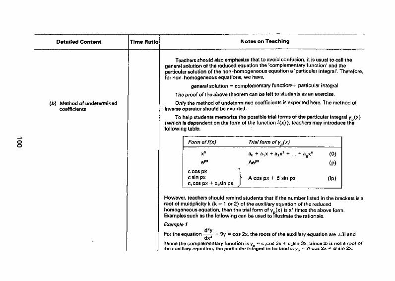
Detailed Content
(b) Method of undeterminedcoefficients
Time Ratio Notes on Teaching
Teageneralparticul.for non-
The
Oninverse <
To(whichfoflowin
Howeveroot of nhomogeExample
Example
For the e
hence ththe auxil
chers should also emphasize that to avoid confusion, it is usual to call thesolution of the reduced equation the 'complementary function' and thear solution of the non-homogeneous equation a 'particular integral'. Therefore,homogeneous equations, we have,
general solution = complementary function** particular integral
proof of the above theorem can be left to students as an exercise.
y the method of undetermined coefficients is expected here. The method ofoperator should be avoided,
nelp students memorize the possible trial forms of the particular integral y (x)s dependent on the form of the function f(x) ), teachers may introduce theg table.
Form of f(x) Trial form of y (x)
xn a0 + a tx + a2x2 + ... +anxn (0)
eP* AePx (p)
c cos px 1c sin px > A cos px + B sin px (ip)Cjcos px + c2sin px J
r, teachers should remind students that if the number listed in the brackets is aluftiplicity k (k = 1 or 2) of the auxiliary equation of the reducedneous equation, then the trial form of yp(x) is xk times the above form,s such as the following can be used to illustrate the rationale.
;d2y
quation — — + 9y = cos 2x, the roots of the auxiliary equation are ±3i and
e complementary function is yc = Cjcos 3x + c2sin 3x. Since 2i is not a root ofiary equation, the particular integral to be tried is yp = A cos 2x + B sin 2x.

Detailed Content Time Ratio Notes on I eacning
d2yHowever, if the equation is —— + 9y = cos 3x, the complementary function remains
the same but since 3i is a root of the auxiliary equation, the particular integral to betried should be yp = x (A cos 3x + B sin 3x).
In either case, students should be clear that they have to substitute yp into the equationto calculate the values of A and B.
Example 2d2y dy
For the equation —- + 2— = x2, since 0 is one of the roots of the auxiliary equationdx2 dx
(whose roots are 0 and -2), the particular integral to be tried is yp = x (A + Bx + Cx2).Again, the values of A, B and C can be calculated by putting back yp into the equation.
Students may have difficulty when dealing with equations where f (x) is a linearcombination of functions in the first column of the above table. Therefore, teachersshould provide examples such as that shown below to illustrate that the trial form ofyp(x) is the linear combination of the functions of the corresponding lines.
Exampled2y dy
For the equation -— - 3— + 2y = 4x + e3X, roots of the auxiliary equation are
1 and 2. Since 0 and 3 are not roots of the auxiliary equation, the trial form of yp(x) is
v = A -4- A y + Rp3xYp Mo ^ Mix ^ De •
Teachers should indicate that A0 + AjX is the particular solution for 4x while Be3X isthat for e3X.
d2y dyHowever, if the equation is —- - 3— + 2y = 4x + ex, then since 1 (coefficient of
dx2 dxx in the index of ex) is a root of the auxiliary equation, the trial form of yp(x) is
c + Bxex.yp = A0
for 4x for ex
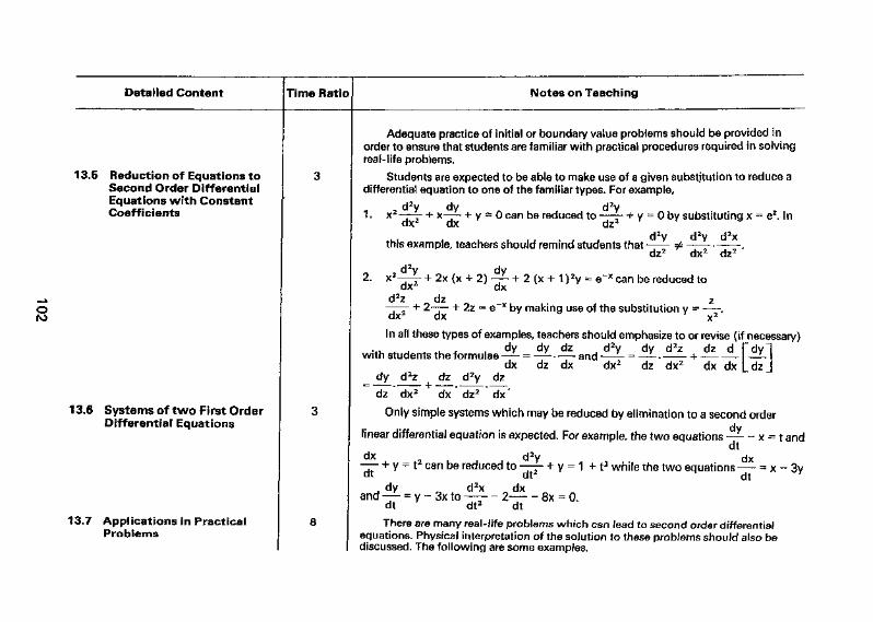
Detailed Content Time Ratio Notes on Teaching
13.5 Reduction of Equations toSecond Order DifferentialEquations with ConstantCoefficients
Oro
13,6 Systems of two First OrderDifferential Equations
13,7 Applications in PracticalProblems
Adequate practice of initial or boundary value problems should be provided inorder to ensure that students are familiar with practical procedures required in solvingreal-life problems.
Students are expected to be able to make use of a given substitution to reduce adifferential equation to one of the familiar types. For example,
, d2y dy rt d2yx2—— + x—— + y * 0 can be reduced to —-
dx2 dx dz2
this example, teachers should remind students that
+ y = 0 by substituting x = ez. In
d2y d2y d2x.
dz2dz2 dx2
2. d2y dv~^T + 2x (x + 2) ~- + 2 (x + 1 )2y = e~x can be reduced to
d2z dz z2 + 2—— + 2z = e x by making use of the substitution y = — — .
In all these types of examples, teachers should emphasize to or revise (if necessary)•*u . . x , dy dy dz d2y dy d2z dz d fdyl
with students the formulae — - = — - --- and — - = — • - + -- —dx dz dx dx2 dz dx2 dx dx L dz J
_ dy d2z dz d2y dz~ dz ' dx2 UK' dz2 'Ux~*
Only simple systems which may be reduced by elimination to a second order
linear differential equation is expected. For example, the two equations — - x = t anddt
dx d2y dx— + y = t2 can be reduced to -— + y = 1 + t2 while the two equations — = x - 3ydt dt2 dt
. dy d2x dxand — - = y - 3x to — - - 2 -- 8x = 0.
dt dt2 dt
There are many real-life problems which can lead to second order differentialequations. Physical interpretation of the solution to these problems should also bediscussed. The following are some examples.
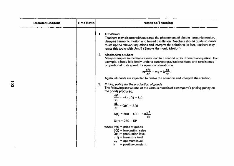
Detailed Content Time Ratio Notes on Teaching
2.
Oto
OscillationTeachers may discuss with students the phenomena of simple harmonic motion,damped harmonic motion and forced oscillation. Teachers should guide studentsto set up the relevant equations and interpret the solutions. In fact, teachers mayrelate this topic with Unit 9 (Simple Harmonic Motion).
Mechanical problemMany examples in mechanics may lead to a second order differential equation. Forexample, a body falls freely under a constant gravitational force and a resistanceproportional to its speed. Its equation of motion is
d2x dx
Again, students are expected to derive the equation and interpret the solution.
3. Pricing policy for the production of goodsThe following shows one of the various models of a company's pricing policy onthe goods produced.
dPdt
- -k (L(t) - L0)
- Q(t) - s(t)
S(t) = 500 - 40P - 1
dldt
dt
Q(t) = 250 - 5P
where P(t) - price of goodsS(t) = forecasting salesQ{t) = production levelL(t) = inventory levelL0 = optimum levelk = positive constant
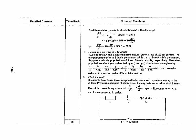
Detailed Content Time Ratio
28
Notes on Teaching
By differentiation, students should have no difficulty to get
- -• — — JK " '" ' — K^vJl^t^ o\tj fdt dt
dP2 = -M-250 + 35P + 10— )
or ^~ + 1 0k-™- + 35kP - 250kdt2 dt
4. Pop u/at/on gro wths of 2 countriesTwo countries A and B have the same natural growth rate of X% per annum. Theemigration rate of A to B is a % per annum while that of B to A is b % per annum.Suppose the initial populations of A and B are NA and N2 respectively. Then theirpopulations after t years (denoted by x(t) and y(t) respectively) are given bydx Xx ax by dy Xy by ax
reduced to a second order differential equation.5. Electric c
If studenA- level F
One of tr
and L are
Circuitts have learnt the concepts of inductance and capacitance (say in the'hysics), examples of electric circuits may be introduced for their interest.
ie possible equations is L— —- + R— - + -—I = E0cocoscot when R, Cdt dt C
\ connected in series,
R C L
E(t) = E0cosfot

UNIT 14: INTERPOLATION AND LAGRANGE INTERPOLATING POLYNOMIALS
Specific Objectives:
1. To learn the concept of interpolation.2. To learn Lagrange Interpolating Polynomial,3. To apply Lagrange Interpolating Polynomial to approximate functions, and estimate the errors.
Detailed Content Time Ratio Notes on Teaching
14.1 Interpolation andInterpolating Poiynomials
14.2 Construction of LagrangeInterpolating Polynomials
Students are expected to know the meaning of interpolation:
Interpolation involves estimating the values of a function f (x) for argumentsbetween x0/ xlf ...,xnat which the values f(x0), fCxJ, ...,f(xn) are known.
They are also expected to know that approximation by polynomial is one of themost heavily used in numerical methods, A polynomial p(x) is used as a substitute forthe function f (x) because polynomials are easy to compute, only simple integralpowers being involved; their derivatives and integrals are found without muchdifficulty and are themselves polynomials; roots of polynomial equations are also easyto locate.
As an introduction, teachers may demonstrate Lagrange Interpolating Polynomial(LI.P.), pn(x) for n = 1. A graph as shown below may be used to give students aphysical meaning.
> x
Students should have no problem to see that they are just asked to approximatethe curve y = f(x) inbetween x0 and x± by the polynomial pt(x) = a tx + a0.
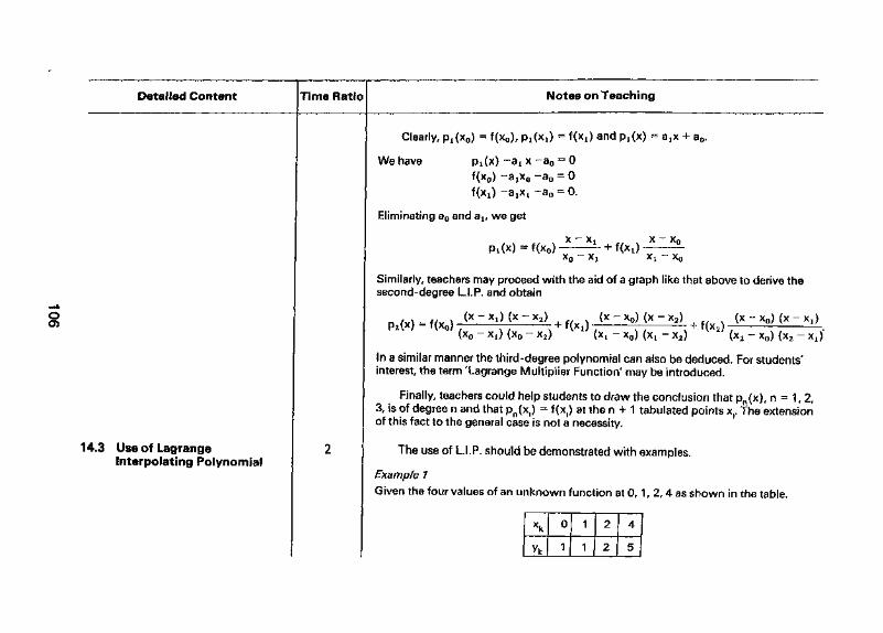
Detailed Content Time Ratio Notes on Teaching
14.3 Use of LagrangeInterpolating Polynomial
Clearly,
We have
Q) = f(x0),
pA(x) -Sf(x0) -ajf(x t) -a
= f(x4) and Pi( a,x + a0.
x -a0 = 0
Xo -a0 = 0
j -a0 = 0.
Eliminating a0 and alr we get
X0Xl
Similarly, teachers may proceed with the aid of a graph like that above to derive thesecond-degree LI. P. and obtain
MX) = f(X0) (x0 - Xl) (x0 - x2)f(Xl)
(X -X .XX-X . )
(x2 - x0) (x2 - Xl)
In a similar manner the third-degree polynomial can also be deduced. For students'interest the term 'Lagrange Multiplier Function' may be introduced.
Finally, teachers could help students to draw the conclusion that pn(x), n = 1 , 2,3, is of degree n and that pn(x,) = f (x,) at the n + 1 tabulated points xr The extensionof this fact to the general case is not a necessity.
The use of L.I. P. should be demonstrated with examples.
Example 1
Given the four values of an unknown function at 0, 1 , 2, 4 as shown in the table.
xkYk
0
1
1
1
2
2
4
5
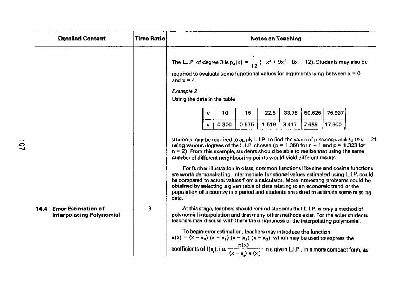
Detailed Content Time Ratio Notes on Teaching
14.4 Error Estimation ofinterpolating Polynomial
The LI.P. of degree 3 is p3(x) = (-x3 + 9x2 -8x + 12). Students may also be
required to evaluate some functional values for arguments lying between x = 0and x = 4.
Example 2Using the data in the table
V
y
10
0.300
15
0,675
22.5
1,519
33.75
3,417
50.625
7,689
75.937
17.300
students may be required to apply LI.P. to find the value of p corresponding to v = 21using various degrees of the L.I.P. chosen (p = 1.350 for n = 1 and p = 1.323 forn = 2), From this example, students should be able to realize that using the samenumber of different neighbouring points would yield different results.
For further illustration in class, common functions like sine and cosine functionsare worth demonstrating. Intermediate functional values estimated using L.I.P. couldbe compared to actual values from a calculator. More interesting problems could beobtained by selecting a given table of data relating to an economic trend or thepopulation of a country in a period and students are asked to estimate some missingdata.
At this stage, teachers should remind students that L.I.P. is only a method ofpolynomial interpolation and that many other methods exist For the abler studentsteachers may discuss with them the uniqueness of the interpolating polynomial.
To begin error estimation, teachers may introduce the functionrc(x) = (x - x0) (x - x t) (x - x2) (x - x3), which may be used to express the
coefficients of f (xt), i.e. - _ „ in a given LI.P., in a more compact form, as(x X() n (Kt)
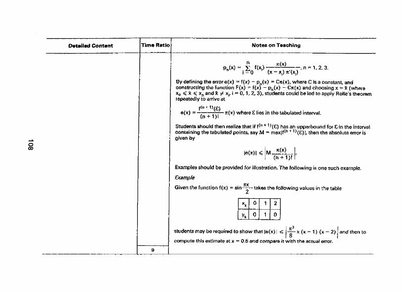
Detailed Content Time Ratio Notes on Teaching
Ooo
X - Xj) Tc'(Xj)
By defining the error e(x) = f (x) - pn(x) = Cir(x), where C is a constant, andconstructing the function F(x) = f(x) - pn(x) - CTC(X) and choosing x = x (wherex0 < x < xn and x xs, i = 0,1, 2, 3), students could be led to apply Rolle's theoremrepeatedly to arrive at
e(x)=- TC(X) where £ lies in the tabulated interval.
Students should then realize that if f*n +1)(£) has an upperbound for £ in the intervalContaining the tabulated points, say M = max(f(n +1)(£)1, then the absolute error isgiven by
M_
Examples should be provided for illustration. The following is one such example.
Example
Given the function f(x) = sin—-—takes the following values in the table
students may be required to show that le(x) | :
compute this estimate at x = 0.5 and compare it with the actual error.
and then to

UNIT 15: APPROXIMATION
Specific Objectives:
1. To learn the idea of approximation and the treatment of error,2. To learn Taylor's series expansion.3. To apply Taylor's series expansion to approximate functions and estimate the resulting errors.
Detailed Content
1 5,1 Treatment of Errors: theirEstimation and AlgebraicManipulation
(a) Three basic types of errors
(i) Inherent error
(ii) Truncation error
(iii) Round -off error
Time Ratio
6
Notes on Teaching
Analysis of the error in a numerical result is basic to any computation, whetherdone manually, with a calculator or a computer. Input values are seldom exact sincethey are often based on experiments or estimates, and the numerical processesthemselves introduce errors of various types. In order to know how well the numericalresults are, students are expected to be able to carry out simple error analysis in acalculation.
Students are expected to know that there are three basic types of errors in anumerical computation: inherent error, truncation error and round-off error.
Inherent errors are errors in the values of data caused by uncertainty inmeasurement or by the necessarily approximating nature of representing in some finitenumber of digits a number that canot be represented exactly in the number of digitsavailable.
Truncation errors and round-off errors both refer to errors that are introduced bynumerical procedures when the data are operated upon. The error introduced bytruncating an infinite mathematical process is called truncation error. In numericalmethods in this course, many of the procedures studied are infinite (in the sense that toobtain an exact solution would require an infinite number of iterations), so the subjectof truncation error assumes major importance.
When a calculator or computer is used to perform real number calculations,round-off error occurs. This arises because the arithmetic performed in a machineinvolves numbers with only a finite number of digits, with the result that manycalculations are performed with approximate representation of the actual numbers.
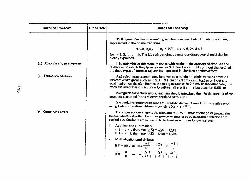
Detailed Content Time Rati Notes on Teaching
(b) Absolute and relative error
(c) Estimation of errors
(d) Combining errors
To illustrate the idea of rounding, teachers can use decimal machine numbers,represented in the normalized form
±0.d1d2d3.....,dk
for i = 2, 3, 4, ..,,.,, k. The idea of rounding up and rounding down should also beclearly explained.
It is preferable at this stage to revise with students the concept of absolute andrelative error, which they have learned in S.3, Teachers should point out that each ofthe three types of errors in (a) can be expressed in absolute or relative form.
A physical measurement may be given to a number of digits with the limits oninherent errors given such as in 2.3 ± 0.1 cm or 2.3 cm (2 sig. fig.) or without anyqualification on the significance of the digits such as in 2.3 cm. In the latter case, it isoften assumed that it is accurate to within half a unit in the last place i.e. 0.05 cm.
As regards truncation errors, teachers should introduce them in the context of theprocedures studied in the relevant sections of this unit.
It is useful for teachers to guide students to derive a bound for the relative errorusing k-digit rounding arithmetic which is 0,5 * 1 0~k+1.
The major concern here is the question of how an error at one point propagates,that is, whether its effect becomes greater or smaller as subsequent operations arecarried out. Students are expected to be familiar with the following facts.
1 . Addition and subtractionIf S - a + b then max! AS) = j Aa| + | Ab|.If K = a - b then max|AK| = |Aa| + iAbJ.
2, Multiplication and division
If P = ab then max
If Q = —— then maxIAQfor
Aa
aIAa
"I a
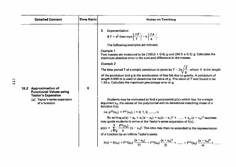
Detailed Content Time Ratio Notes on Teaching
15.2 Approximation ofFunctional Values usingTaylor's Expansion(a) Taylor's series expansion
of a function
3, Exponentiation
If F = ak then maxAF
= k
The following examples are relevant.
Example 1Two masses are measured to be (100.0 ± 0.4) g and (94.0 ± 0,3) g. Calculate themaximum absolute error in the sum and difference in the masses.
Example 2nr
The time period T of a simple pendulum is given by T = 2n I— , where G, is the lengthV 9
of the pendulum and g is the acceleration of free fall due to gravity. A pendulum oflength 0.600 m is used to determine the value of g. The value of T was found to be1.55 s. Calculate the maximum percentage error in g.
Students may be motivated to find a polynomial p(x) which has, for a singleargument x0, the values of the polynomial and its derivatives matching those of afunction f(x)
Le,P<')(x0)=ff !>(x0),i = 0,1,2 ,n.
By writing p(x) = a0 + a^x - x0) + a2(x - x t)2 + + an (x - x0)
n teachersmay guide students to arrive at the Taylor's series expansion of f (x),
n f^(x0)P(x) = 2 —: ^x ~ xo^'-Tnis idea mav tnen be extended to the representation
of a function by an infinite Taylor's series
(x - x0) «,,, % (x ~ x0)f(x) = f (x0) + f(1>(x0) - 1! 21
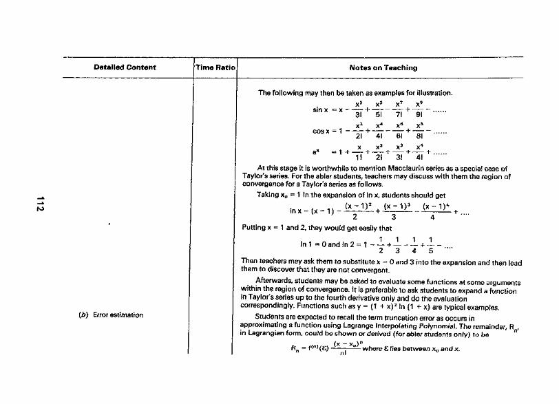
Detailed Content Time Rati Notes on Teaching
(b) Error estimation
The following may then be taken as examples for illustration.
Xs_ X7
_X
—
cos x — 1 --- *• — — • -- 121 4! 6! 81
X X2
ex = 1 + - + -11 2!
X3 X4
+ - + . .....3S 4!
At this stage it is worthwhile to mention Macclaurin series as a special case ofTaylor's series. For the abler students, teachers may discuss with them the region ofconvergence for a Taylor's series as follows,
Taking x0 = 1 in the expansion of In x, students should get
In x = (x - 1) - -
Putting x = 1 and 2, they would get easily that
In 1 = 0 and In 2 = 1 - ~ -f — - -1 + — -2 3 4 5 ""
Then teachers may ask them to substitute x = 0 and 3 into the expansion and then leadthem to discover that they are not convergent.
Afterwards, students may be asked to evaluate some functions at some argumentswithin the region of convergence. It is preferable to ask students to expand a functionin Taylor's series up to the fourth derivative only and do the evaluationcorrespondingly. Functions such as y = (1 + x)2 In (1 + x) are typical examples.
Students are expected to recall the term truncation error as occurs inapproximating a function using Lagrange Interpolating Polynomial. The remainder, R ,in Lagrangian form, could be shown or derived (for abler students only) to be "
/x _ x \nRn
= f(nj(€) —— where € lies between x0 and x.

Detailed Content Time Ratio Notes on Teaching
Students should have no difficulty in seeing that the maximum error by truncating aseries is given by
M(x ~ x0)
n
n!
where M = max|f^(£)l for every £ between x0 and x.
Given this error term, students may be asked to do examples iike estimating themaximum error committed if 3 terms in the series expansion of
cosx-1- — + — -
are used to evaluate cos — , and finding the number of terms of the Taylor's serieso
expansion of
...,to evaluate e so that the maximum error is less than 0.0001
12
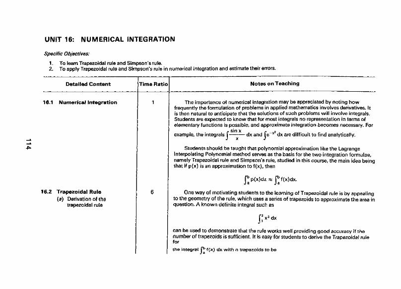
UNIT 16: NUMERICAL INTEGRATION
Specific Objectives;
1. To learn Trapezoidal rule and Simpson's rule.2, To apply Trapezoidal rule and Simpson's rule in numerical integration and estimate their errors.
Detailed Content
16.1 Numerical Integration
1 6.2 Trapezoidal Rule(a) Derivation of the
trapezoidal rule
Time Ratio
1
6
Notes on Teaching
The importance of numerical integration may be appreciated by noting howfrequently the formulation of problems in applied mathematics involves derivatives. Itis then natural to anticipate that the solutions of such problems will involve integrals.Students are expected to know that for most integrals no representation in terms ofelementary functions is possible, and approximate integration becomes necessary. For
Students should be taught that polynomial approximation like the LagrangeInterpolating Polynomial method serves as the basis for the two integration formulae,namely Trapezoidal rule and Simpson's rule, studied in this course, the main idea beingthat if p(x) is an approximation to f (x), then
fbp(x)dz* fbf(x)dx.Ja Ja
One way of motivating students to the learning of Trapezoidal rule is by appealingto the geometry of the rule, which uses a series of trapezoids to approximate the area inquestion. A known definite integral such as
J'x'dx
can be used to demonstrate that the rule works well providing good accuracy if thenumber of trapezoids is sufficient. It is easy for students to derive the Trapezoidal rulefor
the integral fb f (x) dx with n trapezoids to be
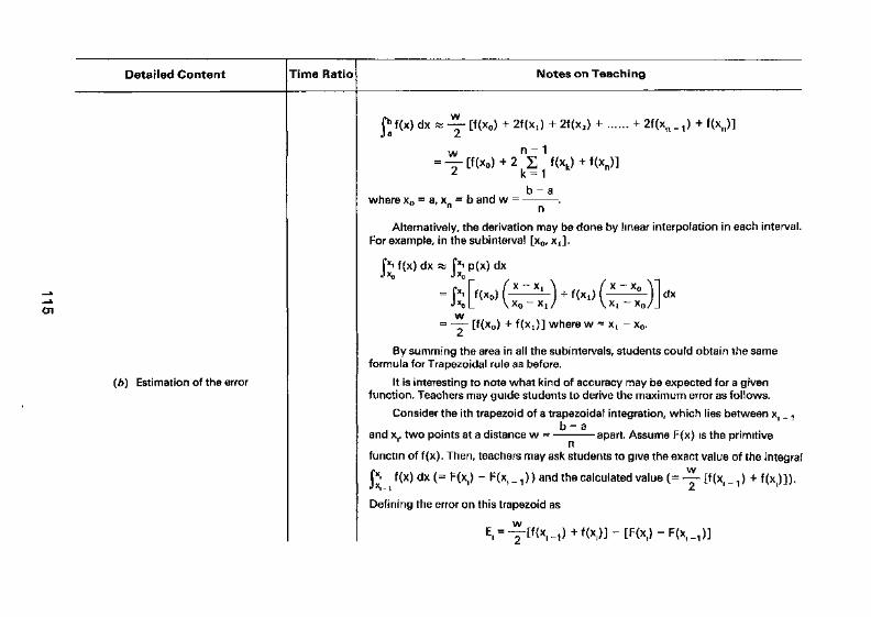
Detailed Content Time Ratio Notes on Teaching
en
(b) Estimation of the error
2f(xn _ , f(xn)]f(x) dx « - [f(x0) + 2f(Xl) + 2f(x2)
w n ~ 1
= — [ f (x0)+2 S f(xk)+f(xn)]2 k = 1
b-awhere x0 = a, x = b and w = .n n
Alternatively, the derivation may be done by linear interpolation in each interval.For example, in the subinterval [x0, xj.
f*i f(x) dx w f*i p(x) dx*
= -r- [f(*o) + *(xi)l where w = x^ - x0.
By summing the area in all the subintervals, students could obtain the sameformula for Trapezoidal rule as before.
It is interesting to note what kind of accuracy may be expected for a givenfunction. Teachers may guide students to derive the maximum error as follows.
Consider the ith trapezoid of a trapezoidal integration, which lies between x, _ 1
b -aand x(, two points at a distance w = apart. Assume F(x) is the primitive
functm of f(x). Then, teachers may ask students to give the exact value of the integral
J*. f(x) dx (= F(x,) - F(x, _,)) and the calculated value (- -—• [f(x, _,) + f(x,)]).
Defining the error on this trapezoid as
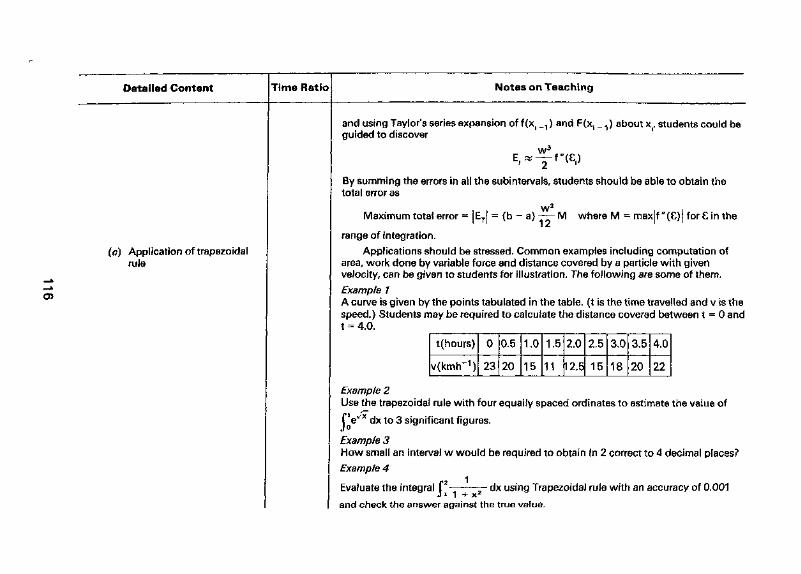
Detailed Content Time Ratio Notes on Teaching
(c) Application of trapezoidalrule
o>
and using Taylor's series expansion of f(xl _.,) and F(xs _ 1) about x|f students could beguided to discover
By summing the errors in all the subintervals, students should be able to obtain thetotal error as
Maximum total error = JET| = (b - a) M where M = maxjf "(£)j for £ in the
range of integration.Applications should be stressed. Common examples including computation of
area, work done by variable force and distance covered by a particle with givenvelocity, can be given to students for illustration. The following are some of them./Example 1A curve is given by the points tabulated in the table, (t is the time travelled and v is thespeed.) Students may be required to calculate the distance covered between t = 0 andt = 4.0.
t(hours)
v(kmrT1)
0
23
0.5
20
1.0
15
1.5
11
2.0
12.5
2.5
15
3.0
18
3.5
20
4.0
22
Example 2Use the trapezoidal rule with four equally spaced ordinates to estimate the value of
f !eN/x dx to 3 significant figures.
Example 3How small an interval w would be required to obtain In 2 correct to 4 decimal places?Example 4
Evaluate the integral P—+ 2 dx using Trapezoidal rule with an accuracy of 0.001
and check the answer against the true value.
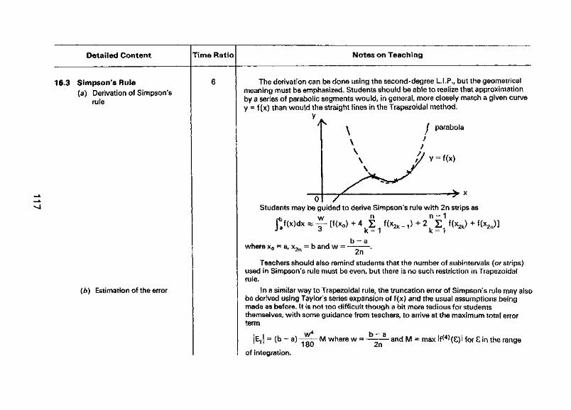
Detailed Content
16.3 Simpson's Rule(a) Derivation of Simpson's
rule
(b) Estimation of the error
Time Ratio
6
Notes on Teaching
The derivation canmeaning must be emphby a series of parabolicy = f (x) than would the
y J/
be done using the second-degree LI. P., but the geometricalasized. Students should be able to realize that approximationsegments would, in general, more closely match a given curvestraight lines in the Trapezoidal method.
\ f parabola
\ ^y = f(x)
0 /Students may be guided to derive Simpson's rule with 2n strips as
. w n n — 1Pf(x)dx« — [f(Xo)+4 £ f(X2k.1)+2 2 *(*2k) + f(X2n)]J ^ k = 1 k - 1
b - awhere x0 — a, X2n — b and w —
Teachers should also remind students that the number of subintervals (or strips)used in Simpson's rule must be even, but there is no such restriction in Trapezoidalrule.
In a similar way to Trapezoidal rule, the truncation error of Simpson's rule may alsobe derived using Taylor's series expansion of f (x) and the usual assumptions beingmade as before. It is not too difficult though a bit more tedious for studentsthemselves, with some guidance from teachers, to arrive at the maximum total errorterm
|ET (b o) n M where w - • and M max IP ' (C) I for € in the rangeI oU ^n
of integration.
Detailed Content Time Ratio Notes on Teaching
(c) Application of Simpson'srule
13
Basically, the kinds of problems resemble those of Trapezoidal rule. Here the emphasis,apart from the application of the technique itself, should be placed on the comparisonof the degree of accuracy between the two formulae. Two examples follow.
Example 1
Evaluate the integral fe In (cosx) dx by Simpson's rule. Find the least number of strips
required so that the error is less than 10~6 in magnitude.
Example 2
Find the value of the integral f2
J i 1 + xwith 6 strips, Compare their accuracy with the standard result.
dx using both Trapezoidal and Simpson's rule

UNIT 17: NUMERICAL SOLUTION OF EQUATIONS
Specific Objectives:
1, To learn fixed point iteration method, Newton's method, Secant method and method of false position.2. To acquire the skill in using the relevant methods to find approximate roots of equations, and compute the errors of the roots.
Detailed Content Time Ratio Notes on Teaching
CO
17,1 Method of Fixed-pointIteration(a) Algorithm of the method
In scientific and engineering work, a frequently occurring problem is to find theroots of equations of the form f (x) = 0. For quadratic, cubic or quartic equations, exactsolutions are readily obtained using algebraic methods. However, when f (x) is apolynomial of higher degree than four or a transcendental function such asex - 4 cos x, algebraic methods are not easily available. It is natural to find the solutionby approximate methods.
Students should be taught that the method consists of several steps.
1 . Rearranging the equation f (x) = 0 in the form x = g(x), where g(x) is called theiteration function.
2, Making an initial guess x0 by basing on a sketch of the appropriate graph (s)where necessary.
3. Obtaining a sequence of X0,x1/x2, ...... , xn, ..., a by substituting in the equation asfollows.
*i = g(x0)x2 = g(Xi)x3 = g(x2)
It is hoped that a fixed point a is obtained such that a = g(a).
4. An approximate root of f (x) = 0 is the fixed point a.
Teachers may demonstrate the method using some examples of equations withsuitable initial guesses and iteration functions that converge.
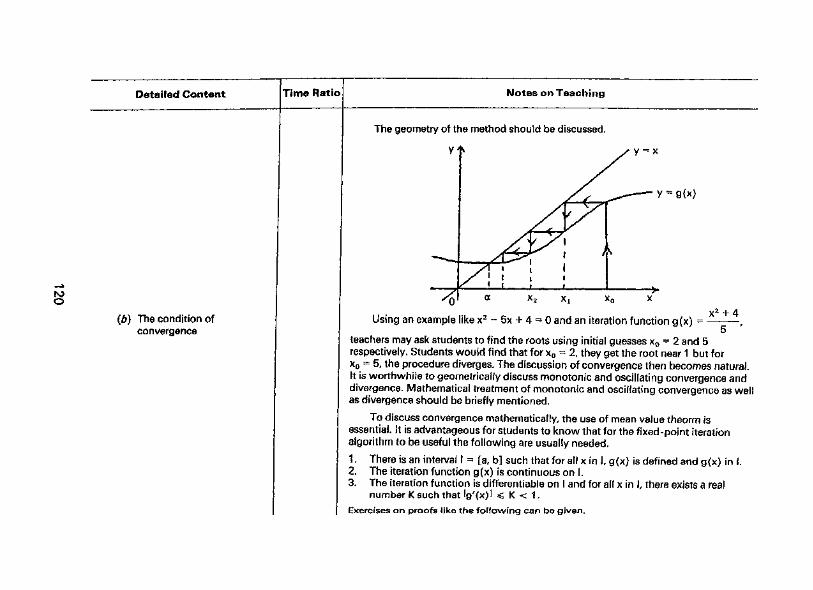
Detailed Content
(b) The condition ofconvergence
Time Ratio Notes on Teaching
The geometry of ti
y
4Using an example
teachers may ask studerespectively. Students \x0 = 5, the procedure dIt is worthwhile to geordivergence. Mathematias divergence should b<
To discuss convergessential, it is advantagalgorithm to be useful tl
1 . There is an interval2. The iteration functi3. The iteration functi
number K such thatExercises on proofs like
ie method should be discussed.
*
/ <
^£/ ,A^^ * y
^ '/ i , i/^ i i * i
s y = x
r^— — y = o(x)
^
a X2 xt X0 X"
x2 + 4ike x 5x + 4 0 and an iteration function g(x) ,
5nts to find the roots using initial guesses x0 = 2 and 5vould find that for x0 = 2, they get the root near 1 but foriverges. The discussion of convergence then becomes natural,netrically discuss monotonic and oscillating convergence andnal treatment of monotonic and oscillating convergence as well3 briefly mentioned,
ence mathematically, the use of mean value theorm issous for students to know that for the fixed-point iterationie following are usually needed.
= [a, b] such that for all x in I, g(x) is defined and g(x) in I.on g(x) is continuous on I.on is differentiable on and for all x in I, there exists a reallg'(x)i ^ K < 1.
the following can be given.
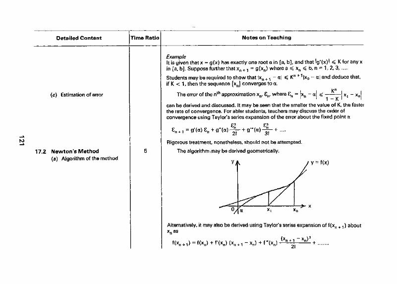
Detailed Content Time Ratio Notes on Teaching
(c) Estimation of error
17.2 Newton's Method(a) Algorithm of the method
ExampleIt is given that x = g(x) has exactly one root a in [a, b], and that lg'(x)l < K for any xin [a, b]. Suppose further that xn +1 = g(xn) where a s$ xn *$ b, n = 1, 2, 3, ....
Students may be required to show that |xn +1 - aj < Kn +1 |x0 - a| and deduce that,if K < 1, then the sequence {xn} converges to a.
The error of the nth approximation xn, €n, where 8n = xn - a! < J xt - x0 j1 K '
can be derived and discussed. It may be seen that the smaller the value of K, the fasterthe rate of convergence. For abler students, teachers may discuss the order ofconvergence using Taylor's series expansion of the error about the fixed point a
n n 2{ 3!
Rigorous treatment, nonetheless, should not be attempted.
The algorithm may be derived geometrically.
•>- x
Alternatively, it may also be derived using Taylor's series expansion of f(xn + 1) aboutxnas
f (Xn + ,) « f (X,,) + f <Xn) (Xn + i - Xn) + f "(Xn) (Xn+1~Xn)2 +
Detailed Content Time Ratio Notes on Teaching
(b) The condition ofconvergence and errorestimation
roro
(c) Application of Newton'smethod
When xn > a and xn ^ 0, students should be able to arrive at
It is necessary that students know that Newton's method is a special case of thefixed-point iteration.
As such, the condition of convergence is the same as the general fixed-pointiteration method. It is interesting to discuss the rate of convergence of Newton'smethod as compared with that of the general method. Students could easily find that
f(x)f"(x) £Jg'(x) = and g'(a) = 0 if a is a simple root, and that £n +1 % g"(a) ——.
L* \xj j 2!Examples in which Newton's method excels others should be given. An examplefollows.
ExampleThe root in [0, 0.8] of the equation x3 + 2x - 1 = 0 is to be determined by an iterationformula
12 n
Students may be asked to find a with x0 = 0 and then required to do the same usingNewton's method. Finally they may be required to account for the faster rate ofconvergence of the latter over the former.
It is profitable for students to know that when a is a double root Newton's methodis not that fast and it is preferable to discuss the pitfalls for the method as well in orderto make the study of Newton's method more complete.
Problems on polynomial equations of degree higher than two and transcendentalequations are relevant. For example, finding the root between x = 0 and x = 1 of theequation 2x3 + x2 - 20x + 20 = 0 with an accuracy of 10~6, and deriving Newton's
formula xn + 1 = xn [~T~ f°r finding the kth root of a are common questions
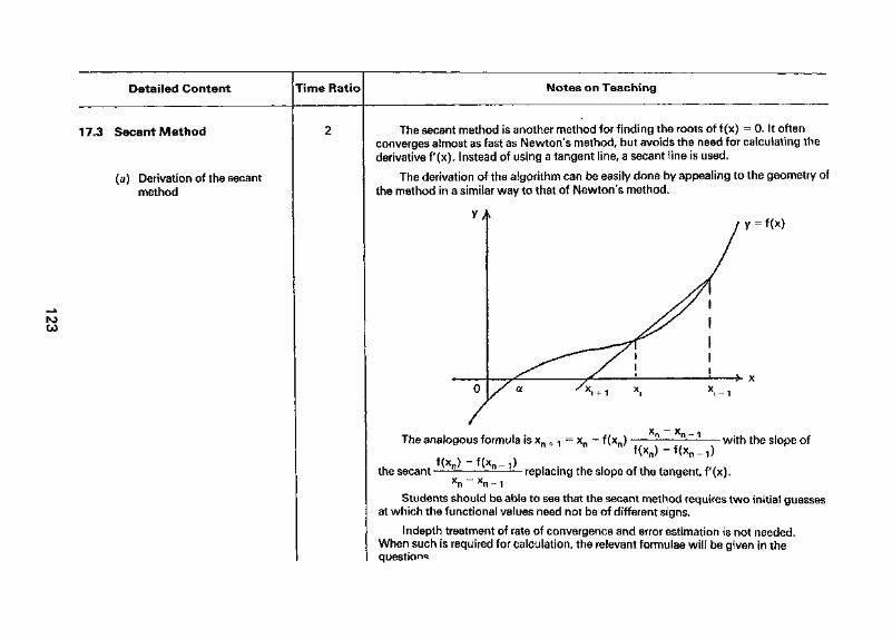
Detailed Content Time Ratio Notes on Teaching
17,3 Secant Method
(a) Derivation of the secantmethod
GO
The secant method is another method for finding the roots of f (x) = 0, It oftenconverges almost as fast as Newton's method, but avoids the need for calculating thederivative f(x). Instead of using a tangent line, a secant line is used.
The derivation of the algorithm can be easily done by appealing to the geometry oithe method in a similar way to that of Newton's method.
The analogous formula is xn +1 = xn - f (xn)
the secant
x X -
f<*n>-f<*n-l )
replacing the slope of the tangent, f (x).
with the slope of
xn ~~ xn - 1
Students should be able to see that the secant method requires two initial guessesat which the functional values need not be of different signs.
Indepth treatment of rate of convergence and error estimation is not needed.When such is required for calculation, the relevant formulae will be given in thequestion^
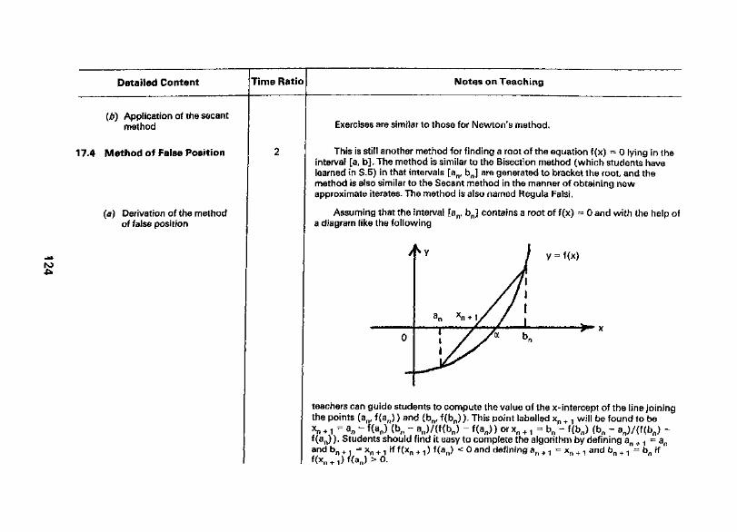
Detailed Content Time Ratio Notes on Teaching
(b) Application of the secantmethod
17.4 Method of False Position
(a] Derivation of the methodof false position
Exercises are similar to those for Newton's method.
This is still another method for finding a root of the equation f (x) = 0 lying in theinterval [a, b]. The method is similar to the Bisection method (which students havelearned in S.5) in that intervals [an, bn] are generated to bracket the root, and themethod is also similar to the Secant method in the manner of obtaining newapproximate iterates. The method is also named Regula Falsi,
Assuming that the interval [an, bn] contains a root of f (x) = 0 and with the help ofa diagram like the following
= f(x)
teachers can guide students to compute the value of the x- intercept of the line joiningthe points (an/ f (an) ) and (bn, f (bn) ). This point labelled xn + 1 will be found to bexn + 1 = an - f («„) (bn - an)/(f (bn) - f (an) ) or xn + , = bn - f (bn) (bn - an)/(f (bn) -f(an) ). Students should find it easy to complete the algorithm by defining an + 1 = anand b if f(xn + f(an) < 0 and defining an + 1 = xn + 1 and bn + ., = bn if
Detailed Content Time Ratio Notes on Teaching
(b) Application of the methodof false position
fo
Students should be reminded that two initial guesses are required by the methodand that the functional values at these initial guesses must be of different signs for themethod to be applicable. Exercises similar to those for Newton's method and Secantmethod are appropriate. Following are some examples.
Example 1Show that the equation x3 + 3x - 12 = 0 has exactly one root in the interval [1, 2] andfind this root by the method of false position correct to 3 decimal places.
Example 2The method of false position is used to find the root of x3 = 2x + 5 in the interval[2,3]. Show that the sequence of iterates {xj is given by
x, +1 — 316x, - 48
3 - 2x - 211 = 1,2,3, .......
Hence find the root correct to 4 significant figures.
As in the case of Secant method, detailed treatment of convergence and errorestimation is not recommended.
16
UNIT 18; INTRODUCTORY PROBABILITY THEORY
Specific Objectives:
1. To know the use and the importance of probability in daily life.2. To learn the basic laws of probability and their applications in real-life problems.
Detailed Content Time Ratio Notes on Teaching
18.1 Basic DefinitionsSample points, sample space,equiprobable space, probabilityof events
Students may have learnt some of the concepts in this sub-topic. However, sincethese concepts are essential for the study of this topic area, a brief discussion isworthwhile to recaii and consolidate what they have learnt.
Students should be familiar with the meaning of sample space and event. Samplepoints may be new to some students. Examples such as throwing of coins should bediscussed and teachers are advised to emphasize to students that sample space in anexperiment is not unique, For example, the two possible sample spaces in a throw of 3coins are {(H, H, H), (H, H, T), (H, T, H), (H, T, T), (T, H, H), (T, H, T), (T, T, H),(T, T, T)} and {no head, 1 head, 2 heads, 3 heads}
Teachers should remind students of the meaning of equiprobable space. In theprevious example, the former sample space is equiprobable while the latter is not. Thefollowing example may also be used for illustration.
ExampleA man who goes to work every day may or may not be killed in a traffic accident.However, the probability that he will be killed in a traffic accident when he is going towork one day is not equal to J because the two outcomes ('killed' and 'not killed') arenot equally likely to happen,
Once the concept is clarified, students can be led to recall the definition ofprobability:
n(E)P(E) =
n(S)where E is the event, S is the equiprobable sample space
Teachers should emphasize that 0 < P(E) < 1. The cases of certainty (P(£) =and impossibility (P(E) = 0) should also be discussed.

Detailed Content Time Ratio Notes on Teaching
18,2 Ways of Counting To facilitate the finding of the number of outcomes, different ways of countingshould be introduced. One of the ways of counting is the Multiplication Principle asshown below.
nl elementsn2 elements
'2 '" %
n elements x,r "r
It is possible to form n1-n2" .^ordered r tuples (a j, t x } ) containing oneelement of each kind. f
ExampleSuppose that the students of a certain school are classified according to sex, age andthe house to which they belong. If there are 4 houses, 5 age groups, then there are2 x 4 x 5 = 40 groups in all.
Other ways of counting include Permutation and Combination and their relatedformulae such as
n! n!
(n-r)!:C" ai
r (n-i
Cn + Cn t
should be clearly taught. Emphasis should be laid on the difference betweenPermutation and Combination. Examples such as finding the probability that each of ncells will be occupied when n balls are randomly placed in them, and the probabilitiesof winning different prizes in Mark Six will help students to consolidate the idea of theways of counting.
Students are only required to master the basic techniques of using permutationsand combinations to solve simple problems. It is not worthwhile for the teachers to puttoo much effort on this topic.

Detailed Content Time Ratio Notes on Teaching
00
18,3 Probability LawsSum and product rulesMutually exclusive eventsIndependent eventsConditional probability
For the abler students, teachers may discuss with them the following generalformula,
Among n elements, of which pi elements (type 1) are similar, p2 elements (type 2)are similar,...... pk elements are similar (type k), they can be arranged (orderly)
in ways.Pi!p2l ,.,pk!
Other applications, such as 'simple hypergeometric probabilities' may also bediscussed, but knowledge of the term is not necessary. Daily life examples such asQuality Inspection problem and Estimation of number of fish in a pond could bediscussed. The following are two examples.
Example 1In a shipment of n video tape recorders containing r defective items, a sample of pitems are chosen at random without replacement for inspection (r < n and p < n).Students are required to calculate the probability that there are exactly q defectiverecorders if q < r and q < p.
Students may be asked to calculate the probability that at least 2 defective video taperecorders are found if n =80, r = 10, p = 15.
Example 2From an estimated population of N fish in a pond, a sample of r is caught, marked andput back to the pond. After the population is thoroughly mixed, a second sample of r istaken again.
It is not difficult to find the probability that there will be n marked fish in the secondsample. Also teachers can discuss with students how to find the most probablenumber of fish in the pond.
Students should have no difficultly to learn the definitions of mutually exclusiveevents and independent events. The corresponding sum and product rules i.e.P(E U F) = P(E) + P(F) and P(E fl F) = P(E) • P(F) should be discussed. Typicalexamples such as tossing coins, drawing balls and throwing dice can help students torecall the above concepts.
Detailed Content Time Ratio Notes on Teaching
CD
Teachers should teach the meaning and notation of conditional probabilitythrough examples.
Now, teachers should introduce to students the cases of dependent events andevents that are not mutually exclusive. The sum and product rules then respectivelybecome P(A U B) = P(A) + P(B) - P(A fl B) and P(A fl B) = P(A) P(BJA).
The general formula for P(E1 fl E2 f) 0 Eq) may be discussed. Also itis worthwhile to mention that two events A, B are independent if and only ifP(A|B) = P(A) or P(A 0 B) = P(A) - P(B)
In handling problems of which the outcomes can occur in a finite number ofways, tree diagram is an efficient way to enumerate all the possible outcomes.Appropriate examples should be chosen to demonstrate the use of the rules. Thefollowing are some possible examples:Example 1A bag A contains 4 red and 6 black balls, and a bag B contains 6 red and 4 black balls.A ball (first ball) is drawn at random from A and placed in B. After mixing, a ball(second ball) is drawn at random from B and placed in A. Finally, a ball (third ball) isdrawn from A,
In this example, teachers may ask students to find the probability that ith ball is red(i = 1, 2, 3). Students may be reminded that all the possible outcomes can berepresented graphically using a tree diagram.Example 2John is available to meet his friend at home during the weekend (Friday to Sunday).Given that the probability Mary goes to visit John on Friday is 1 /q. On each of theother two days, the probability that she goes, given that she has gone the previousday, is 1 /m and the probability that she goes, given that she has not gone the previousday, is 1 /n.
The possible questions in this example include finding the probability that Mary goeson Sunday, and finding P(BlA) and P(BfA~) where A denotes the event that Mary goeson Friday while B the event that she goes on Sunday. Teachers can lead students todraw the tree diagram which will definitely help students to exhaust all the possiblecases and to solve the problem.

Detailed Content Time Ratio Notes on Teaching
18.4 Bayes' Theorem
18.5 Recurrence Relation
After the students are acquainted with the conditional probability, teachers can gofurther to Bayes' Theorem which is stated as follows:Let the sample space Q be partitioned by mutually exclusive events Aj ...... An> Let Bbe another event so that P(B) ^0.
P(B)P(BA()P(A.)
As students are not expected to derive the theorem, teachers may use numericalexamples to explain the meaning of each term in this theorem. In most of the problemsinvolving Bayes' theorem, tree diagram is a commonly used technique to help studentsto solve the problems. The following is one of the possible examples.
ExampleThree urns contain respectively 6 black and 9 white balls, 1 2 black and 3 white balls, 8black and 7 white balls. One urn is chosen at random and a ball is drawn from it.
Teachers may ask students to draw the tree diagram and discuss with them howP(black) can be obtained. Then, students should have no difficulty to get the value ofP(ball came from second urnjblack).
Teachers should help students to identify the sort of situation where theprobability of the nth event depends on the result of the previous event(s). Studentsare expected to form an equation relating them. The following examples may be usefulin explaining the concept of recurrent situations.Example 1There are two new brands of soft drink to be introduced on the market. Inconsideration of the different ways of packing, there is a probability of 0.55 that a girlwill choose Brand X and a probability of 0.45 that she will choose Brand Y. ft isassumed that she drinks one and only one of the two brands of soft drink each day. Ifthe last brand she chose was X, there is a probability of 0.6 of choosing Brand X on thesubsequent day and a probability of 0.4 of choosing Brand Y, On the other hand, if shelast drank Y, she will choose X with a probability of O 3 and Y with a probability ofO7
Detailed Content Time Ratio Notes on Teaching
In this example, a tree diagram can be used to show the relationship betweenPn _ 1,1 - Pn _ 1* Pn and 1 - Pn where Pn denotes the probability that she buys X on
the nth occasion. From the tree diagram, it is easy to express Pn in terms of Pn _ <\,
Most of the students should be able to express Pn in terms of Pl and n. Students maybe interested to know that the ultimate share of market of brand X is actually lim Pn.n -* oc "
Example 2From a bag containing 4 white balls and 9 black balls, one ball is drawn and replaced,this operation being performed n times, Qn is the probability that no two consecutivedraws produce two black balls. Teachers can show to the students the way to obtain arelation between Qn, Qn _ 1 and Qn _ 2 (n > 3). They may also ask students to writedown Qi, Q2 and Q3 and hence calculate Q4, Q5
Markov Chain and difference equations are not expected.
19

UNIT 19: BASIC STATISTICAL MEASURESSpecific Objectives:
1, To revise the basic concepts of mean, median, mode, standard deviation and variance,2» To solve related problems.
Detailed Content Time Ratio Notes on Teaching
19.1 Basic Knowledge
19.2 Calculation of Mean
19.3 Calculation of StandardDeviation and Variance
Teachers should revise with students the concepts of grouped and ungroupeddata, organisation of data, presentation of data, measures of central tendency (mean,median and mode) and measures of dispersion (range, interquartile range, standarddeviation, variance etc). In particular, calculation of mean and standard deviation (orvariance) requires a more detailed elaboration.
At this stage, students are expected to use the formulae
and
x = — (for ungrouped data)n
x = (for grouped data)n
to deal with some harder problems.Example 1A set of m numbers has a mean of \it. Another set of n numbers has a mean of \i2 •Students are expected to find the mean for the combined set of m + n numbers.Example 2Let x be the mean of a set of n numbers, ff each number x, (i = 1, 2,3,.... n) istransformed to yr = ax, + b. Students are expected to find the mean y of thetransformed values.
From the basic relation that variance - (standard deviation)2, students couldfocus their attention to the techniques in manipulating the variance. The formulae
s2 = -
and s2 £f(x-x)2
n
x2 (for ungrouped data)
x2 (for grouped data)
Detailed Content Time Ratio Notes on Teaching
COGO
should be explained clearly and students are also expected to make use of them insolving problems.
Example 1The heights of 22 boys in a class have a mean of 170 cm and a standard deviation of10 cm. The heights of 18 girls in the same class have a mean of 160 cm and a standarddeviation of 8 cm. Students are expected to calculate the mean height and thestandard deviation of the whole class.
Example 2The scores x of 100 students in an examination have a mean of 4.6 and a standarddeviation of 0.5. The scores are to be scaled by the formula y = 10x + 4. Evaluate themean and the standard deviation of y.
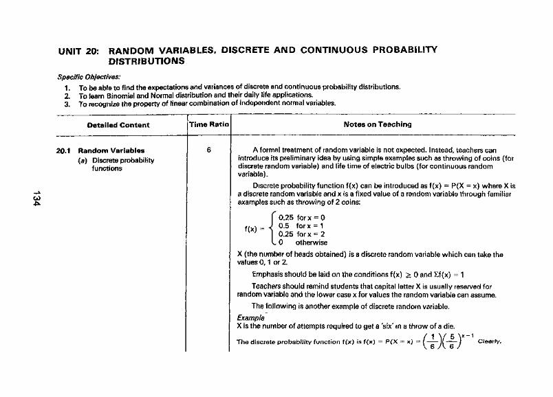
UNIT 20: RANDOM VARIABLES, DISCRETE AND CONTINUOUS PROBABILITYDISTRIBUTIONS
Specific Objectives:To be able to find the expectations and variances of discrete and continuous probability distributions.1.
2.3,
To learn Binomial and Normal distribution and their daily life applications.To recognize the property of linear combination of independent normal variables.
Detailed Content
20,1 Random Variables(a) Discrete probability
functions
Time Ratio
6
Notes on Teaching
A formal treatment of random variable is not expected. Instead, teachers canintroduce its preliminary idea by using simple examples such as throwing of coins (fordiscrete random variable) and life time of electric bulbs (for continuous randomvariable) .
Discrete probability function f(x) can be introduced as f(x) = P(X = x) where X isa discrete random variable and x is a fixed value of a random variable through familiarexamples such as throwing of 2 coins:
fo.25 fo rx -0f (x)= J 0.5 forx = 1( ) I 0.25 forx = 2
L 0 otherwise
X (the number of heads obtained) is a discrete random variable which can take thevalues 0, 1 or 2.
Emphasis should be laid on the conditions f (x) > 0 and Ef (x) = 1
Teachers should remind students that capital letter X is usually reserved forrandom variable and the lower case x for values the random variable can assume.
The following is another example of discrete random variable.
ExampleX is the number of attempts required to get a 'six' in a throw of a die.
/ 1 V 5 V-iThe discrete probability function f (x) is f (x) = P(X = x) = f li 1 dearly,
GO
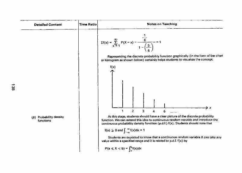
Detailed Content Time Ratio Notes on Teaching
01
Probability densityfunctions
00
x = 1 1
Representing the discrete probability function graphically (in the form of bar chartor histogram as shown below) certainly helps students to visualize the concept.
f(x)
1 2 3 4 5 .....
At this stage, students should have a clear picture of the discrete probabilityfunction. We can extend this idea to continuous random variable and introduce thecontinuous probability density function (p.d.f.) f (x). Students should note that
f(x) >0andf °°f(x)dx =J-eo
Students are expected to know that a continuous random variable X can take anyvalue within a specified range and it is related to p.d.f. f (x) by
P(a X < b) = fbf(x)dx

Detailed Content Time Ratio Notes on Teaching
in fact, graphs of p.d.f. can be interpreted as frequency curves of continuous datain statistics.
Also students should note that
P(X = a) = 0 and P(a X < b) = P(a < X < b) = P(a < X
The following are some examples,
Example 1 (rectangular distribution)The p.d.f. of X is defined as
b) = P(a X < b)
f(x) = for 0 < xotherwise
4, k is a constant
k can be determined from f °°f(x)dx = 1J -co
Also P (-2 < X < 1) = Tf(x)dxandP(X> 3) -1 - Pf(x)dx - Tf(x)dx
Students may be asked.to find IVl in terms of b if P(X < M) = b. They should note thatwhen b = 0.5, M is the median.
Example 2The scheduled time of arrival of a fhght to a certain city is 8:00 a.m. However, theactual time of arrival is (8 + X) am, where X is a random variable having the followingp.d.f.:
f(x) =
3(4 - x2)for -2 < x < 2
elsewhere
Possible questions include finding the probability that a flight will be between7:00 a.m. and 8:00 a.m. and between 9:00 a.m. and 10:00 a.m.
It is worthwhile to spare some time to discuss with students the meaning of the termcumulative distribution function <f>(t).
Detailed Content Time Ratio Notes on Teaching
20.2 Expectations and Variances
4>(t) = E f(x>X < t
f(x)dx
in discrete case
in continuous case
Examples such as the two shown below may be used to illustrate these two cases.
1. Discrete' in a throw of 2 dice, the probability of getting a sum greater than 10 is 1 - 4>(10).(c|>(10) is the probability that the sum is equal to or smaller than 10.)
2, ContinuousIf (|>(a) denotes the probability that the life time of an electric bulb is smaller thana, then P(X < a) = 4>(a), P(a < X < b) = 4>(b) - <|>(a) and P(X > a) = 1 - <|>(a).
A brief revision on the meaning and physical significance of mean and standarddeviation will facilitiate students' learning the concepts of expectation. The meaning ofexpectation can be introduced through simple example such as that shown below.
ExampleA man has a probability p = 0.01 of winning a prize x = $200. We say that his chanceis worth px = ($200) • (0.01) = $2. Then the teacher can extend this idea to n discretevalues of X.
Teachers should define the expectation of a discrete random variable
(E(X) = Spx) and that of a continuous random variable (E(X) = f c°xf(x)dx).J-oo
Teachers may also discuss with students the definition of expectation of a function ofX. The following shows the two definitions.
E[s(X)] - £pg(x) discrete random variable
E[g(X)]=f c°f(x)g(x)dx continuous random variableJ ~oo
In the case of discrete random variables, students are expected to know themeanings of E(X) (=ji) and E[(X - n)2] (= Var(X) = or2). In particular, teachersshould indicate that ji is a measure of central tendency while a2 is a measure ofdispersion of X about \i.
Interesting examples can be discussed.

Detailed Content Time Ratio Notes on Teaching
GO03
ExampleThe probability of a candidate passing an examination at any one attempt is 0.4. if hefails, he carries on entering until he passes and each entry costs him $120. Teachersmay discuss with students the expected cost of his passing the examination.
Calculations involving fair games, expected gain/loss are best illustrated byreal-life examples. The following are two of them.
Example 1In an investment a man can make a profit of $5 000 with a probability of 0.62 or a lossof $8 000 with a probability of 0.38.
E(X) = p, and Var(X) = cr2 can be calculated fromp. = $(5 000) (0.62) + $(-8 000) (0.38) = $60a2 = (5 000 - 60)2 (0.62) + (-8 000 - 60)2 (0.38)
p. is called the expected gain.
Example 2A gambling machine has four windows and each of them displays one of the fourdifferent colours: red, orange, yellow and blue. Each of the colours is equally likely tobe displayed and the colour displayed by the machine on one window is independentof the colour displayed on the other windows. A man pays $a for a game. He receives$5 if all the colours displayed in the four windows are different. He receives $30 if allthe colours displayed are the same. In all other cases, he loses. $X is the net amount hereceived in playing a game.
In this example, teachers can discuss the following with students.
1. When E(X) = 0, the game is a fair game. What is the fair price (i.e. $a)?2. Suppose a = 1, what are E(X) and Var(X)?
Most of the students should realize that E(X) < 0 in most of the gambling games.Teachers may also ask students to work out the new \i and or2 when all the money isdoubled and to find the relations between the new and old parameters. For ablerstudents, teachers may ask them to guess the value of E(Y) where $Y is the net amountthe man receives if he plays the games twice.

Detailed Content Time Ratio Notes on Teaching
In the case of continuous random variables, examples showing the steps incalculating E(X) and Var(X) should be provided.
ExampleOrange juice is delivered to a fast food shop every morning. The daily demand fororange juice is a continuous random variable X distributed with a probability densityfunction f(x) of the form
f(x) - { «ax(b - x) 0 ^ x 1
otherwise
CA>CD
The mean daily demand is 0.625 units.a and b can be calculated from the equation
fc°f(x)dx = 1 and f °°xf(x)dx = 0.625J-oo J-oo
The orange juice container at this fast food shop is filled to their total capacity of 0.8units every morning.
The probability P that in a given day, the fast food shop cannot meet the demand fororange juice is given by P = 1 - <|>(0,8) = f 1 f(x)dx
j 0 8
For abler students, teachers may guide them to prove the two formulaeE [ag(X) + b] = a E [g(X>] + b and Var (aX + b) = a2Var(X) where a, b are constants.
Also, it is not difficult for an average student to show that
E [g(X) + h(X>] = E [g(X)] + E [h(X)]and Var(X) = E(X2) - [E(X)]2 = E(X2) - n2
The following example shows the use of the above formulae,
ExampleGiven Z = 2X2 - 3X + 5 where X is a random variable with mean jj, and variance cr2.E(Z) can be obtained from E(Z) = E(2X2 - 3X + 5) = E(2X2) - E(3X) + E(5)
= 2(^i2 + a2) - 3^ + 5
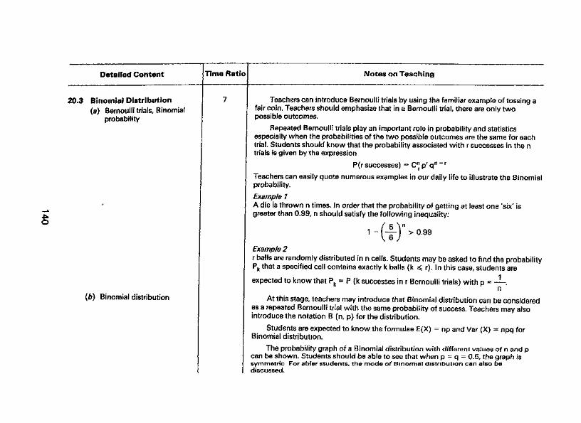
Detailed Content Time Rati Notes on Teaching
20.3 Binomial Distribution(a) Bernoulli trials. Binomial
probability
(b) Binomial distribution
Teachers can introduce Bernoulli trials by using the familiar example of tossing afair coin. Teachers should emphasize that in a Bernoulli trial, there are only twopossible outcomes.
Repeated Bernoulli trials play an important role in probability and statisticsespecially when the probabilities of the two possible outcomes are the same for eachtrial. Students should know that the probability associated with r successes in the ntrials is given by the expression
P(r successes) = Cnr p
r qn ~ r
Teachers can easily quote numerous examples in our daily life to illustrate the Binomialprobability.
Example 1A die is thrown n times. In order that the probability of getting at least one 'six' isgreater than 0.99, n should satisfy the following inequality:
1 -(JLVUJ
>0.99
Example 2r balls are randomly distributed in n cells. Students may be asked to find the probability
r). In this case, students arePk that a specified cell contains exactly k balls (k
expected to know that Pk = P (k successes in r Bernoulli trials) with p =n
At this stage, teachers may introduce that Binomial distribution can be consideredas a repeated Bernoulli trial with the same probability of success. Teachers may alsointroduce the notation B (n, p) for the distribution.
Students are expected to know the formulae E(X) = np and Var (X) = npq forBinomial distribution.
The probability graph of a Binomial distribution with different values of n and pcan be shown. Students should be able to see that when p = q = 0.5, the graph issymmetric For abler students, the mode of Binomial distribution can also bediscussed.
Detailed Content Time Ratio Notes on Teaching
(c) Applications Binomial probability distribution is useful in describing many real-life events. Thefollowing are three possible applications.
Example 1A student sits for a test which contains only 4 multiple choice questions. With hisknowledge of the subject he has a probability of 0.7 of knowing the correct answer ofeach question. There are 5 options in each question, thus the student has theprobability 0.2 of getting the correct answer in each question through guessing. Hehas attempted all the questions.
The probability that the student knows the correct answers of 3 questions isCt(0.7)3(0.3).
Since the student can get the correct answer of a question simply by guessing,P (correct answer for a question) = p can be calculated from the two cases (a) heknows the question and (b) he guesses it correctly.
Suppose X is the number of correct answer(s) obtained, students may be asked tocalculate E(X) (= 4p), Var (X) {= 4p (1 - p)) and P (X - 1). (= Cf (p)1 (1 - p)3)The following questions can also be raised.
1. 2 marks will be awarded for a correct answer and 1 mark will be deducted for awrong answer. Suppose Y is the total score obtained by the student, calculateE(Y)andVar(Y).
2. Given that the student only knows the correct answers of 3 questions, what is theprobability that the student obtains full marks?
3. Given that the student only gets one correct answer, what is the probability thathe gets it through guessing?
Example 25% of light bulbs are defective. A large batch of light bulbs is tested according to thefollowing rules,
(a) A sample of 10 light bulbs is tested.
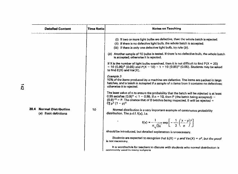
Detailed Content Time Rati Notes on Teaching
20.4 Normal Distribution(a) Basic definitions
10
(i) If two or more light bulbs are defective, then the whole batch is rejected,(ii) If there is no defective fight bulb, the whole batch is accepted,(iii) If there is only one defective light buib, try rufe (b).
(b) Another sample of 10 bulbs is tested. If there is no defective bulb, the whole batchis accepted; otherwise it is rejected.
If X is the number of light bulbs examined, then it is not difficult to find P(X = 20)= 10 (0.95)9 (0.05) and P(X = 10) = 1 - 10 (0.95)9 (0.05). Students may be askedtofindE(X)andVar(X),
Example 310% of the items produced by a machine are defective. The items are packed in largebatches, and a batch is accepted if a sample of n items from it contains no defectives;otherwise it is rejected.
The least value of n to ensure the probability that the batch will be rejected is at least0.95 satisfies (0.9)n < 1 - 0.95. If n = 10, then P (the batch being accepted) «(0.9)10 = P. The chance that of 8 batches being inspected, 5 will be rejected =Cfp3(1-p)5
Normal distribution is a very important example of continuous probabilitydistribution. The p.d.f. f(x), i.e.
f (x)=- exp ~
should be introduced, but detailed explanation is unnecessary.
Students are expected to recognize that E(X) = ji and Var(X) = a2, but the proofis not necessary.
It is worthwhile for teachers to discuss with students why normal distribution iscommonly used in many subjects
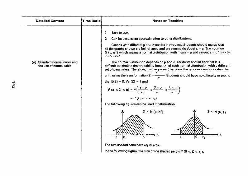
Detailed Content Time Ratio Notes on Teaching
(b) Standard normal curve andthe use of normal table
1. Easy to use.
2. Can be used as an approximation to other distributions.
Graphs with different \i and cr can be introduced, Students should realize thatall the graphs shown are bell-shaped and are symmetric about x = ji. The notationN (ji, a2) which means a normal distribution with mean = jj. and variance = a2 may beintroduced.
The normal distribution depends on \i and cr. Students should find that it isdifficult to tabulate the probability function of each normal distribution with a differentset of parameters. Therefore, it is necessary to express the random variable in standard
unit, using the transformation Z = . Students should have no difficulty in seeingo*
that E(Z) = 0, Var(Z) = 1 and
P(a <X<b) =j a a
= P (Z, < Z < 22)
The following figures can be used for illustration.
X - N (ji, a2) N(0 f1)
The two shaded parts have equal area.
In the following figure, the area of the shaded part is P (0 < Z <
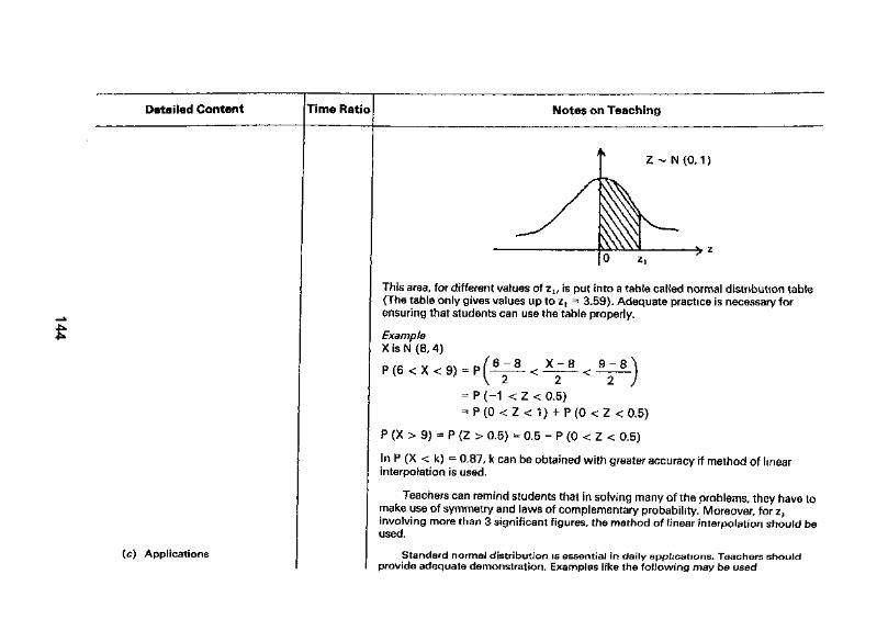
Detailed Content
(c) Applications
Time Ratio Notes on Teaching
y* Z - N (0, 1 )
0 z,
This area, for different values of zjt is put into a table called normal distribution table(The table only gives values up to zt = 3,59). Adequate practice is necessary forensuring that students can use the table properly.
ExampleX is N (8, 4)
p(6 <x .m ?(6~8 * X ~ 8 - Q~B}r \ v < . A < j ) - r \ 2 v. ^ v. — - i
= P (-1 <Z< 0.5)
= P ( 0 < Z < 1 ) - h P ( 0 < 2 <0,5)
P (X > 9) = P (Z > 0.5) = 0,5 - P (0 < Z < 0.5)
In P (X < k) = 0.87, k can be obtained with greater accuracy if method of linearinterpolation is used.
Teachers can remind students that in solving many of the problems, they have tomake use of symmetry and laws of complementary probability. Moreover, for ZL
involving more than 3 significant figures, the method of linear interpolation should beused,
Standard normal distribution is essential in daily applications. Teachers shouldprovide adequate demonstration. Examples like the following may be used
01
Detailed Content Time Ratio Notes on Teaching
Example 1A manufacturer uses a machine to produce resistors. He found that 1 0% of the resistorsare less than 95Q and 20% of the resistors are above 1 1 0Q. The distribution of theresistances X is normal.
ji and CT can be calculated from the two equations
P fY - QK^ P 1 7 - 1 fi 1i \A -^ yoj i i £. < i u. i\ o- // 110 - u\P/v - 11 A\ p I 7 i A i(A > J 1 U) — r 1 Z > I — U.2.
\ <* /
Example 2Suppose X, the length of a rod, is a normally distributed random variable with mean and variance 1 . If X does not meet certain specifications, then the manufacturer willsuffer a loss. Specifically, the profit M (per rod) is the following function of X.
f 3 i f 8 < X < 1 0M = X -1 i f X < 8
[ -5 i fX>10 ,The expected profit, E(M), is given by E(M) = 8<|> (10 - ji) - 4<|> (8 - fi) - 5
f 1where <j>(z) — 1 - e * dt is the cumulative probability function.
J"00^Suppose that the manufacturing process can be adjusted so that different values of ju,may be achieved. The value of n corresponding to maximum profit can be determinedby differentiating E(M) with respect to jx.
Example 3A factory produces soft drinks contained in bottles. The normal volume contained in abottle is 1 .25 litres. However, due to random fluctations in the automatic bottlingmachine, the actual volume per bottle varies according to a normal distribution. It isobserved that 1 5% of the bottles contain less than 1 .25 litres whereas 1 0% containmore than 1 .30 litres.
Detailed Content Time Rati Notes on Teaching
Binomial approximated tonormal distribution
a>
20.5 Linear Combination ofIndependent NormalVariables
Students should have no difficulty in finding the mean JA and standard deviation a ofthe volume distribution,
The cost in cents of producing a bottle containing x litres of soft drinks is C - 36 + 62x+ 5x2 where x is the random variable having the above distribution.
The expected cost of a bottle = E(C) where E(C) = 36 + 62jA + 5 (\i2 + a2).The expected cost of 20 000 bottles is 20 OOOE(C).
Students should be made clear that the binomial probability can be calculated byusing normal approximation only when n is large. In this case, the mean and variancecan be taken as np and npq respectively. Students should also be reminded that 'endcontinuity corrections' is required in this approximation.
ExampleA coin is tossed 400 times.
If X represents the number of heads obtained, then X is B (400, 0.5).When it approximates to N (200,100),
200 _ 210.5-2001010
Students may be interested to know thatP (195 < X < 210) ^ P (195 < X < 210). *
Students should recognize that the sum of scalar multiples of independent normalvariables is also normal. From this, it is not hard to see that:
If X and Y are two independent normal variables such that X ~ N (\L± , o^ 2) andY - N (ji2, cr2
2), then aX + bY ~ N (a^ + bj^, a2a12 + b2a2
2) for any realvalues a and b.
The above result can be extended easily to n independent normal variables. Teachersshould also quote examples to illustrate the usefulness of the above fact in daily-lifeapplication.
Detailed Content Time Ratio Notes on Teaching
Example 1Cakes are sold in packets of 6. The mass of each cake is a normal variable with mean25 g and standard deviation 2 g. The mass of the packing material is a normal variablewith mean 30 g and standard deviation 4 g. Find the distribution of the total mass ofeach packet of cakes and hence find the probability that the total mass of a packet isless than 142 g.
Example 2The thickness, A cm, of a paperback is normally distributed with mean 2 cm andvariance 0.63 cm2, The thickness, B cm, of a hardback is normally distributed withmean 5 cm and variance 1.42 cm2. The distribution of X = 2A - B can be determinedand hence the probability that a randomly chosen paperback is less than half thethickness of a randomly chosen hardback can be evaluated by using the standardnormal distribution table.
34
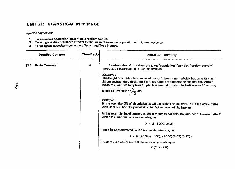
UNIT 21: STATISTICAL INFERENCE
Specific Objectives;
1. To estimate a population mean from a random sample.2. To recognize the confidence interval for the mean of a normal population with known variance.3. To recognize hypothesis testing and Type I and Type H errors.
Detailed Content Time Ratio Notes on Teaching
21.1 Basic Concept Teaehers should introduce the terms 'population', 'sample', 'random sample','population parameter' and 'sample statistic'.
Example 1The height of a particular species of plants follows a normal distribution with mean20 cm and standard deviation 8 cm, Students are expected to see that the samplemean of a random sample of 10 plants is normally distributed with mean 20 cm and
Q
standard deviation .— cm
Example 2It is known that 3% of electric bulbs will be broken on delivery. If 1 000 electric bulbswere sent out, find the probability that 5% or more will be broken.
In this example, teachers may guide students to consider the number of broken bulbs Xwhich is a binomial random variable, i.e.
X - B (1 000, 0.03)
It can be approximated by the normal distribution, i.e.
X ~ N ((0.03)(1 000), (1 000) (0.03) (0.97))
Students can easily see that the required probability is
P (X > 49.5)

Detailed Content Time Ratio Notes on Teaching
21.2 Estimate of a PopulationMean from a RandomSample
Alternatively, teachers may make use of the concept of sample proportion Ps = —
which can be approximated by
P ~ where q = 1 - p
In this case, the required probability is P(PS ^ 0.0495)
It is worthwhile, at this stage, for teachers to introduce the concept of estimationof an unknown population parameter from a sample statistic. Examples like estimatinga population mean p, by using a sample mean x can be used for illustration.
Teachers should indicate to students that there may be several sample statisticswhich can be used as estimators. For examples, sample mean, median and mode couldalso be used to estimate the population mean ji. In view of this, students are expectedto know that the best estimator b among the various sample statistics used to estimatethe population parameter p should
(1) be unbiased, i.e. E(b) = p and(2) has the smallest variance.
Example 1Let Xj, X2/ X3 be random samples taken from a population with mean \i and variance
y -i- OYT - * 2
I 2 ~" Z
i + 2X2 + 3X3
are estimators of .
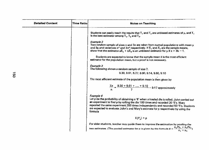
Detailed Content Time Ratio Notes on Teaching
Students can easily reach the results that Tj and T2 are unbiased estimates of \i, and Txis the best estimator among Tlr T2 and T3.
Example 2Two random sample of sizes n and 3n are taken from normal populations with mean fjiand 3j4, and variances a2 and 3a2 respectively. If Xj and X2 are the sample means,show that the estimator aXi + bX2 is an unbiased estimator for jj, if a + 3b = 1,
Students are expected to know that the sample mean x is the most efficientestimator for the population mean, but a proof is not necessary.
Example 3The following shows a random sample of size 7.
9.30, 9.61, 8.27, 8.90, 9.14, 9,90, 9.10
The most efficient estimate of the population mean is then given by
9.30 + 9,61 + .,... + 9.10Exn
: 9.17 approximately
Example 4Let p be the probability of obtaining a '6' when a loaded die is rolled. John carried outan experiment to find p by rolling the die 100 times and recorded 20 '6's. Maryrepeated the same experiment 200 times independently and recorded 50 '6's. Studentsare expected to evaluate John's and Mary's estimate for p respectively by using theformula
E(P.)=P
For abler students, teacher may guide them to improve the estimation by pooling the
two estimates. (The pooled estimator for p is given by the formula p = — —)
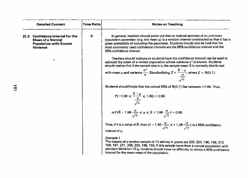
Detailed Content Time Ratio Notes on Teaching
21.3 Confidence Interval for theMean of a NormalPopulation with KnownVariance
In general, teachers should point out that an interval estimate of an unknownpopulation parameter (e.g. the mean fi) is a random interval constructed so that it has agiven probability of including the parameter. Students should also be told that themost commonly used confidence intervals are the 95% confidence interval and the99% confidence interval.
Teachers should indicate to students how the confidence interval can be used toestimate the mean of a normal population whose variance cr2 is known. Studentsshould realize that if the sample size is n, the sample mean X is normally distributed
a2 X- fiwith mean u and variance —. Standardizing, Z = , where Z ~ N(0.1).
n <j
Students should know that the central 95% of N(0.1) lies between ±1.96. Thus,
P(-1.96 ^ —- < 1.96) = 0.95
orP(X- 1.96-^r-< \i^X+ 1.96-™-) =0.95.
Thus, if x is a value of *X, then (x - 1.96 -—=-, x •*•1.96 -—) is a 95% confidence
interval of ji.
Example 1The masses of a random sample of 12 articles in grams are 200, 204,196,198, 210,189,197,221, 205, 203,196,199. If this sample came from a normal population withstandard deviation 10 g, students should have no difficulty to obtain a 95% confidenceinterval for the mean mass of the population.
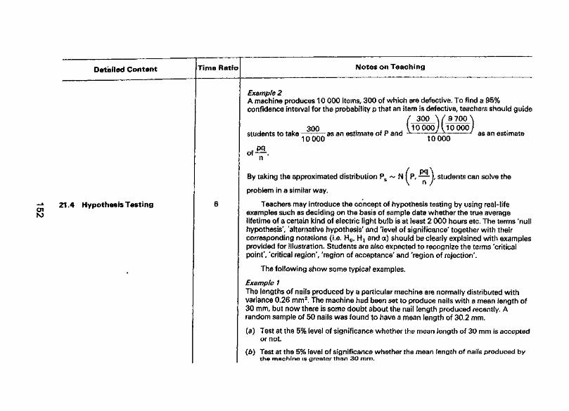
Detailed Content Time Ratio Notes on Teaching
—* 21,4 Hypothesis Testing01
Example 2A machine produces 10 000 items, 300 of which are defective. To find a 95%confidence interval for the probability p that an item is defective, teachers should guide
/ 300 \ / 9 700 \300 . fn _, \10000A10000/
students to take —rr^r as an estimate of P and10000 10000
as an estimate
, PQof—.
n
By taking the approximated distribution Ps ~ N I P, —), students can solve the
problem in a similar way.
Teachers may introduce the concept of hypothesis testing by using real-lifeexamples such as deciding on the basis of sample data whether the true averagelifetime of a certain kind of electric light bulb is at least 2 000 hours etc, The terms 'nullhypothesis', 'alternative hypothesis' and 'level of significance' together with theircorresponding notations (i.e. H0, Ht and a) should be clearly explained with examplesprovided for Illustration. Students are also expected to recognize the terms 'criticalpoint', 'critical region', 'region of acceptance' and 'region of rejection'.
The following show some typical examples.
Example 1The lengths of nails produced by a particular machine are normally distributed withvariance 0.26 mm2. The machine had been set to produce nails with a mean length of30 mm, but now there is some doubt about the nail length produced recently. Arandom sample of 50 nails was found to have a mean length of 30.2 mm.
(a) Test at the 5% level of significance whether the mean length of 30 mm is acceptedor not.
(b) Test at the 5% level of significance whether the mean length of nails produced bythe machine is greater than 3O mm.
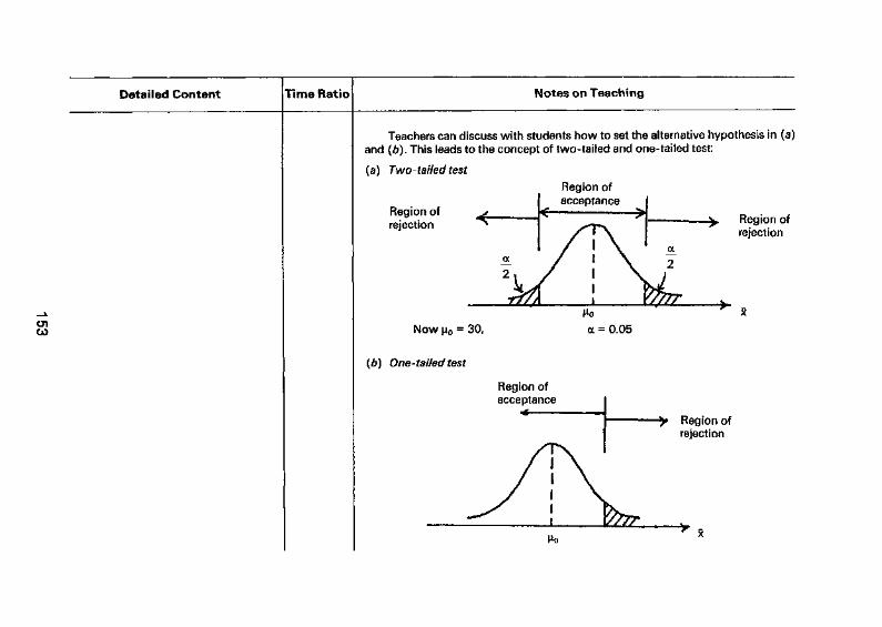
Detailed Content Time Ratio Notes on Teaching
at
Teachers can discuss with students how to set the alternative hypothesis in (a)and (b). This leads to the concept of two-tailed and one-tailed test:
(a) Two-tailed testRegion ofacceptance
Region ofrejection
Region ofrejection
Now MO = 30,
(b) One-tailed test
Region ofacceptance
^ Region ofrejection
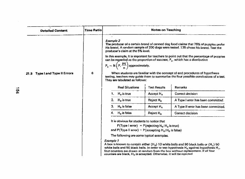
Detailed Content Time Ratio Notes on Teaching
.5 Type 1 and Type II Errors
Example 2The producer of a certain brand of canned dog food claims that 75% of puppies preferhis brand. A random sample of 200 dogs were tested. 135 chose his brand. Test theproducer's claim at the 5% level.
In this example, it is important for teachers to point out that the percentage of puppiescan be regarded as the proportion of success, Ps, which has a distribution
N ( P, — |approximately.
When students are familiar with the concept of and procedures of hypothesistesting, teachers may guide them to summarize the four possible conclusions of a test.They are tabulated as follows:
Real Situations
1 . H0 is true
2. HO is true
3. H0 is false
4. H0 is false
Test Results
Accept H0
Reject H0
Accept H0
Reject H0
Remarks
Correct decision
A Type I error has been committed.
A Type II error has been committed.
Correct decision
It is obvious for students to notice thatP(Type I error) = P(rejecting H0| H0 is true)
and PfType II error) = P(accepting H0|H0 is false)
The following are some typical examples.
Example 1A box is known to contain either (H0) 1 0 white balls and 90 black balls or (Hi) 50white balls and 50 black balls. In order to test hypothesis H0 against hypothesis Hltfour counters are drawn at random from the box without replacement. If all fourcounters are black, H0 is accepted. Otherwise, it will be rejected
Detailed Content Time Ratio Notes on Teaching
In this example, students should be able to find the probability of the Type I and TypeII errors for this test by using the above relations.
Example 2The ingredients for concrete are mixed together to obtain a mean breaking strength of2 000 newtons. If the mean breaking strength drops below 1 800 newtons, then thecomposition must be changed. The distribution of the breaking strength is normal withstandard deviation 200 newtons. Samples are taken in order to investigate thehypothesis:
H0 , = 2 000 newtons, = 1 800 newtons
Ol01
How many samples must be tested so that
P(Type I error) =0.05and P(Type II error) = 0.1 ?
Example 3The calibration of a scale is to be checked by weighing a 1 0 kg test specimen 25 times.Suppose the results of different weightings are independent of one another and thatthe weight on each trial is normally distributed with cr = 0.200 kg. Let ji denote thetrue weight reading on the scale,(a) What hypothesis should be tested?(b) Suppose the scale is to be recalibrated if either x ^ 1 0.1 032 or x ^ 9.8968. What
is the probability that recaiibration is carried out when it is actually unnecessary?Which type of error would that be?
(c) What is the probability that recaiibration is judged unnecessary when in fact |i =1 0,1 ? When = 9,8? Which type of error are these?
27
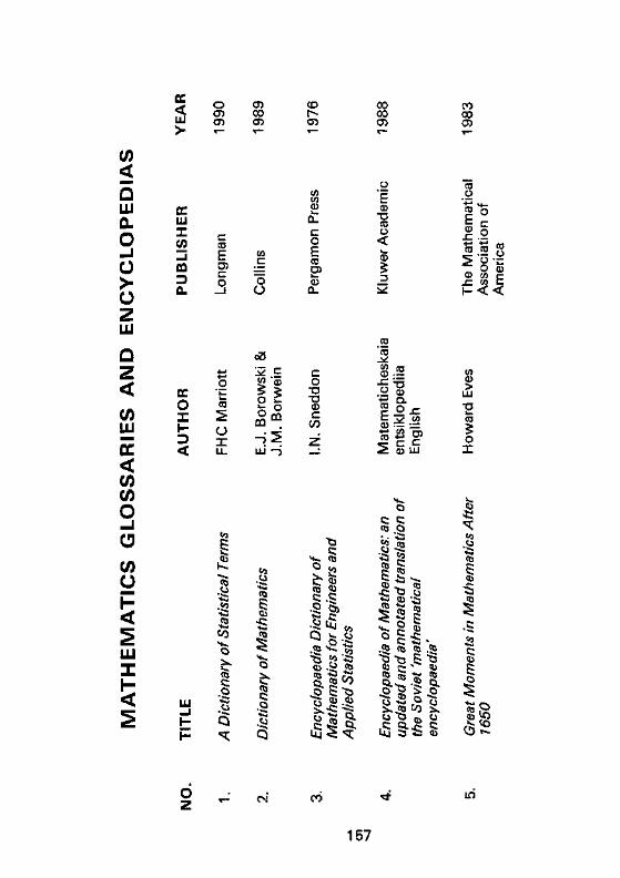
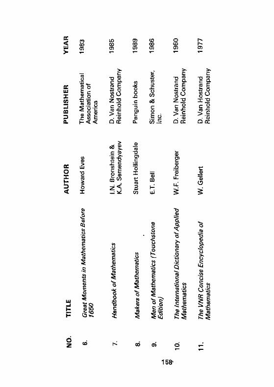
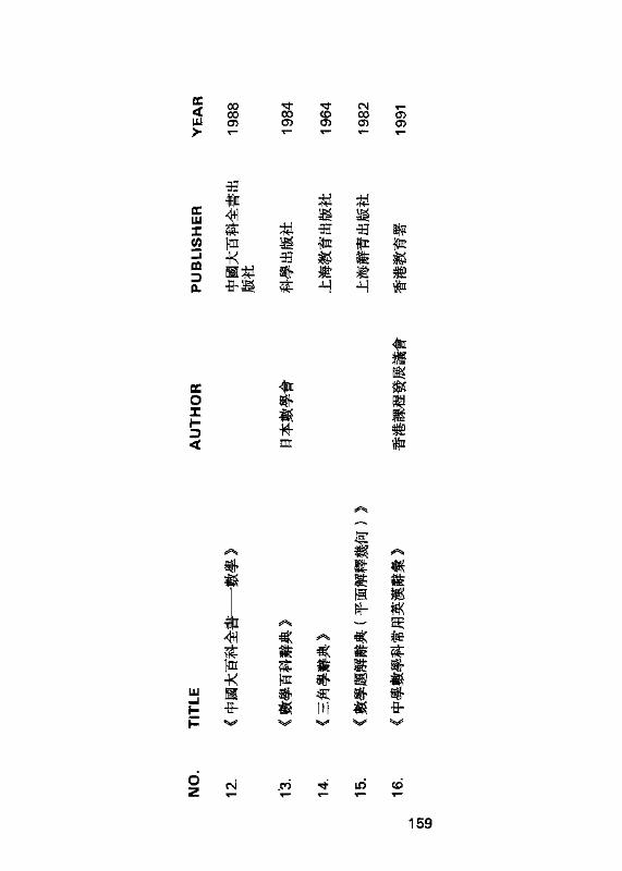
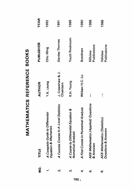
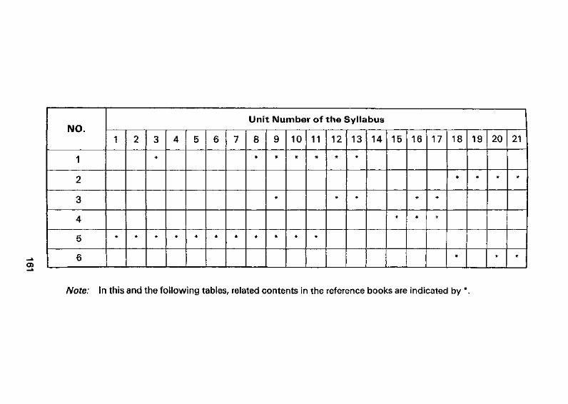
NO.
1
2
3
4
5
6
Unit Number of the Syllabus
1 2 3
*
4 5 6 7 8 9
#
10 11 12
*
13
*
14 15
*
16
#
*
17
*
#
18
#
#
19
*
20
*
*
21
*
*
o>
Note: In this and the following tables, related contents in the reference books are indicated by *.
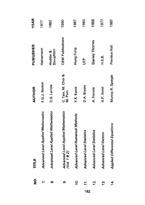
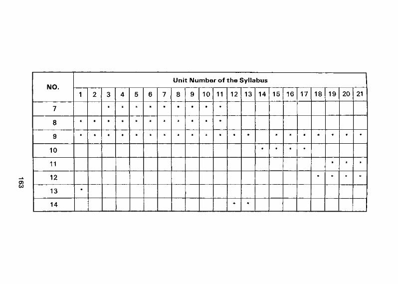
0>
NO.
7
8
9
10
11
12
13
14
Unit Number of the Syllabus
1
*
2 3 4 5 6 7 8 9 10 11 12
*
13
*
14
*
15
*
16
#
17
*
18
*
19
*
*
20
*
*
21
*
#
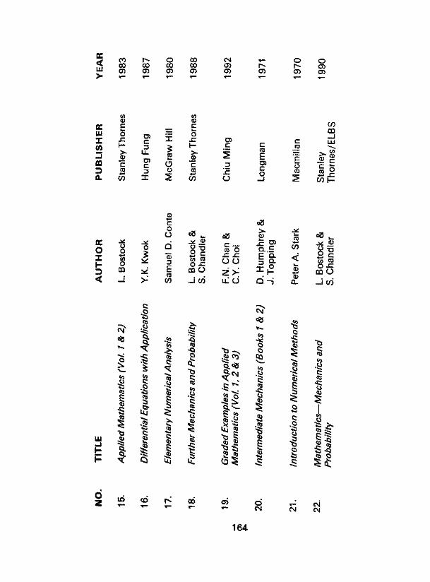
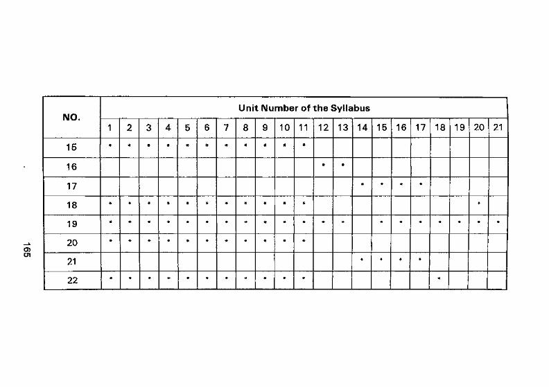
05Ol
NO.
15
16
17
18
19
20
21
22
Unit Number of the Syllabus
1 2 3 4 5 6 7 8 9 10 11 12
*
13
*
14
*
*
15
*
*
16
*
*
17
*
*
18
*
19 20
#
21
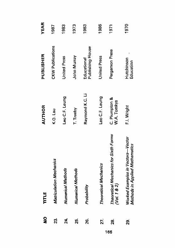

o>
NO.
23
24
25
26
27
28
29
Unit Number of the Syllabus
1
#
2 3 4 5 6 7 8 9 10 11 12 13 14
#
15
*
*
16
#
*
17
*
*
18
•*
19 20 21
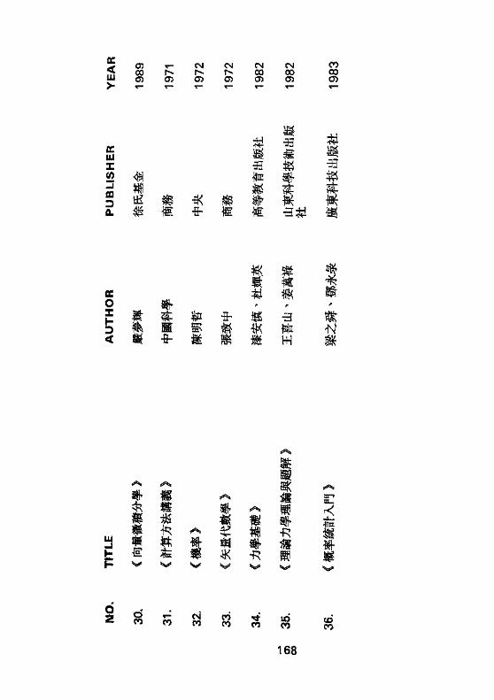
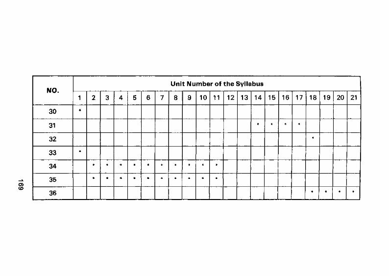
0)CO
NO.
30
31
32
33
34
35
36
Unit Number of the Syllabus
1
*
»
2 3 4 5 6 7 8 9 10 11 12 13 14
*
15
*
16
*
17
#
18
*
*
19
*
20
*
21
#


NO.
37
38
39
40
41
42
43
44
Unit Number of the Syllabus
1 2 3 4 5 6 7 8 9 10 11
#
12
*
13 14 15 16 17 18
*
*
•*
*
19
*
#
#
20
*
*
#
21
#
*
*
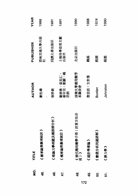

NO.
45
46
47
48
49
50
51
Unit Number of the Syllabus
1 2
*
3 4 5 6 7 8 9 10 11 12 13 14
*
15
#
*
16 17
#
18
*
*
#
19
*
*
20
*
#
#
21
*
#
*