The Untyped Lambda CalculusExamination of theory and practice

Jonas Biedermann

HS2015

Abstract

The untyped lambda-calculus is a concept to describe computability. It has a math-ematical notation that allows to formalize the evaluation of functions. Functionsin the untyped lambda-calculus can also be translated to a program that can runon a machine.

The untyped lambda-calculus is a topic that can be difficult to understand. Thereis a lot of literature available on this topic. However there is a large gap betweenvery high-level information sources that are hard to understand and the simplearticles on wikipedia that often lack sophisticated sources.

This document fills this gap by giving a broad overview over the topic of theuntyped lambda-calculus and discussing the points that are relevant for softwareengineers in detail.

At the end of the article, a basic implementation of the untyped lambda-calculusin C# will be shown.

1

Contents

1 Introduction 31.1 The λ-calculus . . . . . . . . . . . . . . . . . . . . . . . . . . . . . . 31.2 λ-calculus usages . . . . . . . . . . . . . . . . . . . . . . . . . . . . . 31.3 Models of computation . . . . . . . . . . . . . . . . . . . . . . . . . . 31.4 The Church-Turing thesis . . . . . . . . . . . . . . . . . . . . . . . . 4

2 Basics of the λ-calculus 52.1 Syntax . . . . . . . . . . . . . . . . . . . . . . . . . . . . . . . . . . . 62.2 Operational semantics . . . . . . . . . . . . . . . . . . . . . . . . . . 82.3 Nameless representation of terms . . . . . . . . . . . . . . . . . . . . 9

3 Programming in the lambda calculus 103.1 Untyped expressions . . . . . . . . . . . . . . . . . . . . . . . . . . . 103.2 Evaluation . . . . . . . . . . . . . . . . . . . . . . . . . . . . . . . . . 113.3 Arithmetic expressions . . . . . . . . . . . . . . . . . . . . . . . . . . 153.4 Stuck terms . . . . . . . . . . . . . . . . . . . . . . . . . . . . . . . . 15

4 Enrichment of the lambda calculus 154.1 Multiple arguments . . . . . . . . . . . . . . . . . . . . . . . . . . . . 164.2 Church Booleans . . . . . . . . . . . . . . . . . . . . . . . . . . . . . 164.3 Church Numerals . . . . . . . . . . . . . . . . . . . . . . . . . . . . . 174.4 Recursion . . . . . . . . . . . . . . . . . . . . . . . . . . . . . . . . . 17

5 λ-calculus via C# 175.1 C# concepts . . . . . . . . . . . . . . . . . . . . . . . . . . . . . . . 175.2 Church Booleans . . . . . . . . . . . . . . . . . . . . . . . . . . . . . 19

6 Conclusion 21

2

1 Introduction

1.1 The λ-calculus

The lambda-calculus is a formal language that allows to study functions. It isdescribed by the definition of functions and bound parameters. It was introducedin 1930 by Alonzo Church and Stephen Cole Kleene. [Jun04]

In the lambda-calculus, everything is a function. The following example explainswhat that means:

Consider the number 3. It can also be written as 0 + 1 + 1 + 1. If we nowdefine a function succ(x) → x + 1 we can also write 3 as succ(succ(succ(0))).This approach allows us to define an arbitrary number of functions which can takeother functions as parameters and also yield functions as result.

This alternative approach can be seen as a new interpretation of mathematics.In contrary to the axiomatic approach which has sets as basic objects, the lambda-calculus has universal functions as basic objects.[Chu32]

How this approach can be useful will be explained in this document.

1.2 λ-calculus usages

The lambda-calculus has two key roles:

• It is a simple mathematical foundation of sequential, functional, higher-ordercomputational behaviour.

• It is a representation of proofs in constructive logic.

Each role for itself is not very exciting. Its the combination of the two thatmakes the concept interesting. It allows to formulate a computation in a mathe-matical way by formulating lambda-terms. These terms can be translated into aprogram. Now if this program compiles correctly, it can be regarded as a proofthat the mathematical formulation was correct as well. It also works the otherway and makes it possible to verify programs in a mathematical way. This is alsoknown as the Curry-Howard correspondence[Gri15]. It represents a dual view of thelambda-calculus, as mathematical proof or as programming language (sequential,functional, higher-order languages).

As for the theory domain, the lambda-calculus is used in the areas of mathemat-ics, philosophy[Cud07] and linguistics[Moo88].

For a more practical domain, the lambda-calculus played a major role in thedevelopment of the theory of programming languages[mod]. Furthermore, func-tional programming languages implement the lambda-calculus[Mic11]. For exam-ple Haskell has a syntax that is almost equivalent to the lambda-calculus syntax.

These concepts can be formalized to the general model of computability whichis described in the next section.

1.3 Models of computation

Computation is often specified as how the evaluation of a function or programcan progress. This is expressed as the description of some kind of conceptualautomation[mod].

3

Although it is mathematically unprovable, the thesis exists that there is a rea-sonable intuitive definition of ”computable”[Squ]. This thesis is equivalent to thislist of provably equivalent formal models of computation:

• Turing machines

• Lambda Calculus

• Post Formal Systems

• Partial Recursive Functions

• Unrestricted Grammars

• Recursively Enumerable Languages

Naturally speaking, these models describe what is computable by a computerprogram written in any reasonable programming language. This thesis is alsoknown as the Church-Turing thesis described in the next section 1.4.

1.4 The Church-Turing thesis

The Church-Turing thesis is a hypothesis about the nature of computable functions.It states that a function on natural numbers is computable if it is computable bya turing machine.

The notion of the Church-Turing thesis is, to provide an effective or mechanicalmethod in logic and mathematics. Effective and its synonym mechanical are termsto describe a function M.[Cop02]

A function M is called effective or mechanical just in case all of the followingstatements are true:

• M is set out in terms of a finite number of exact instructions (each instructionbeing expressed by means of a finite number of symbols);

• M will, if carried out without error, produce the desired result in a finitenumber of steps;

• M can (in practice or in principle) be carried out by a human being unaidedby any machinery, only with paper and pencil;

• M demands no insight or ingenuity on the part of the human being carryingit out.

This set of statements can also be interpreted in relation to the lambda-calculus:

• A lambda term is reduced to its normal form in a finite number of reductions

• In the untyped lambda-calculus a well formed lambda-term has exactly onederivation tree without branches and therefore is guaranteed that the termsfinal derivation is an axiom

4

• Every lambda term has a finite length so it can be reduced with pen andpaper within a finite amount of space in a finite amount of time.

• A lambda term on paper can be compiled into a program that can be executedon a computer

This leads to the assumption that both Turing Machines and the lambda-calculuscan make the statement: Is a function calculable by a machine? The rest ofthis document will now examine the lambda-calculus in detail and show that thestatements mentioned above hold.

2 Basics of the λ-calculus

The key feature of the lambda-calculus is functional abstraction. Abstracted func-tions are exactly what is needed to drive efficient and deterministic computationboth in theory, proofs, simulations and programming languages. This was explainedin section 1.2 and section 1.4.

Abstraction allows us to write a function that executes the code genericallyinstead of writing the same code over and over again. Each time the function iscomputed, it is instantiated with an individual set of one or more named parametersthat alters the outcome of the computation. Upon instantiation, a value for eachparameter is needed.

For example consider the difference of two factorials:

(5*4*3*2*1) - (3*2*1)

This term would be much easier to write as:

factorial(5) - factorial(3)

It is quite natural to implement the factorial as a recursive function. In pseudocode one could write:

factorial(n) = if n=0 then 1 else n * factorial(n-1)

In the untyped lambda-calculus we can write “λn. . . ” instead which means “thefunction that for n, yields. . . ”:

factorial = λn. if n=0 then 1 else n * factorial(n-1)

In the lambda-calculus everything is a function. A function can only have otherfunctions as arguments and it can only yield another function as result, so to speak.How this is achieved is explained in this section. The information in this sectionis derived from the book Types and Programming Languages from Benjamin C.Pierce.[Pie02]

5

2.1 Syntax

The syntax of the lambda-calculus is surprisingly simple. It consists of only threekinds of terms. This can be summarized by the following grammar:

(1) t ::= x (variable)(2) t ::= λx. t (abstraction)(3) t ::= t t (application)

The next section will briefly discuss the three different types of terms.

2.1.1 The grammar in detail

To describe the grammar, we will look at each rule individually and examine howit can help to abstract problems from the real world .

Variable A variable x (and y,z) by itself is a term. It represents a function whichcannot be further evaluated. A variable is a term in normal form as explainedin section 3.2.1. These variables are also called object language variables. Thiscan be thought of as if this variables have a certain meaning in the context of thelanguage. For example true can be such a variable because it might give an exactmeaning to the outcome of a calculation which a person can understand.t (and s,u) are meta-variables. They can stand for an arbitrary term. These

terms have to be lambda-terms. This basically means that terms can be furtherreduced (evaluated). This is explained in section 3.2.

Application In the lambda-calculus, function application is the act of applying afunction to an argument, which in the lambda calculus is another function. Con-stant arguments like booleans or number literals are considered as terms in normalform, since they can not be computed any further. Nevertheless, they are alsofunctions as we will see in section 3.1.

In mathematics, functions are usually written f(x). In the lambda calculus theparentheses are usually omitted. We can simply write f x.

Since the result and parameters in the lambda-calculus are also functions thisleads to the question in what order they are executed. According to Pierce [Pie02]application associates to the LEFT. For example s t u stands for (s t) u. Thatmeans that u is applied to the result function of the s t applications.

Abstraction Abstraction is a technique to separate complexity into a hierarchy.In the syntax of the lambda-calculus abstraction is introduced in rule (2) where tappears on the right side of the definition. Since t can be of form (2) as well, it ispossible to formally describe a computation over multiple layers.

(λx. x(λy. y((λz. z) t) u) s

Like with the application, the parentheses for abstraction are usually omitted.According to Pierce [Pie02], abstraction associates to the RIGHT. For exampleλx.λy. x y x stands for λx.(λy.((xy)x).

6

2.1.2 Scope of variables

Variables can be bound or free in the context of an abstraction. If we consider theabstraction λx.t then λx is a binder whose scope is t.

• x is bound when it occurs in the body of t

• x is free when it is not bound by an enclosing abstraction (binder) on x

The following examples show the difference between bound and free variables:

x y (occurrences of x are free)λy. x y (occurrences of x are free)λx. x (occurrences of x are bound)λz.λx.λy. x (y z) (occurrences of x are bound)(λx. x) x (first occurrence of x is bound second is free)

2.1.3 Abstract and concrete syntax

Because of the Curry-Howard correspondence [Gri15] it is at least necessary to havetwo representations of the same program. One that is machine readable and onethat is easy to write for a programmer.

What a programmer writes is usually source code. While a programmer canread source code and understand it, a machine has to do additional steps to beable to execute a program. This leads to concrete and abstract syntax which aretwo different representations of the same calculation.

concrete syntax: String of characters the programmer writes directlyabstract syntax: Simpler internal representation as labeled trees (ASTs)

Transformation Abstract syntax is a natural fit for compilers. But because con-crete syntax is what the programmer writes, there must be a way to convert betweenthe two.

From concrete to abstract syntax The conversion from source code to an ASTusually includes a number of steps that are specific for a concrete implementationof the language. But almost every time they contain a lexer and a parser.

The lexer converts the source file into a stream of tokens and also gathers asmuch information about them as possible (keyword, constant, punctuation, etc.).Additionally it also takes care of dumping white spaces and comments from thecode since they have no relevancy for the execution of the computation.

The parser then converts the sequence of tokens into an AST which can be pro-cessed by a machine. During this process operator precedence and associativity istaken into account. This leads to less parentheses to be written by the programmer.

7

From abstract to concrete syntax It is also possible to convert an AST backto concrete syntax. This can be accomplished with a print visitor that visits thewhole AST and prints every node in order. Although white-spaces and commentscan not be recovered this way.

2.2 Operational semantics

The most basic concept of computation can be seen in the application of functionto arguments (which themselves are functions). All other primitives that are com-mon in programming languages like numbers, arithmetic operations, conditionals,records, loops, sequencing, I/O, etc. are built on top of this concept. This will beexamined in detail in section 3.

2.2.1 Computation

The computation of terms which are reducible can be subdivided into steps. Eachstep of computation consists of rewriting an application whose left hand side isan abstraction.

Rewriting means substituting the right hand component of the applicationfor the bound variable in the abstraction body. This is shown in the followingexample:

(λx. t12) t2 → [x→ t2]t12

[x→ t2]t12 means that all free occurrences of x in t12 have to be replaced by t2.

Additional examples:

(λx. x) y evaluates to y (identity function)(λx. x(λx. x))(u r) evaluates to u r (λx. x)

A term in the form (λx. t12) t2 is called a redex (“reducible expression”). A redexis a term on which a step of evaluation can be performed. The rewrite operationdescribed here is also called beta-reduction[Pie02].

It would be interesting to know why the phrase beta-reduction was chosen todescribe this kind of process. Sadly I could not find any information, who inventedthis phrase.

2.2.2 Evaluation strategies

There are several evaluation strategies how a redex can be reduced. To show thesedifferent approaches the sample lambda-term (λx. x)((λx. x)(λz. (λx. x) z)) issimplified to: id(id(λz. id z)). The id function in this example is simply a shorterform of writing λx. x which is the identity function that just returns its argument.

8

Full beta-reduction At each step of computation we can choose a redex anywhereinside the term and reduce it. There is no particular rule, which redex is chosen forreduction at each step of evaluation. In the following example we choose to alwaysreduce the innermost redex first:

id(id(λz. id z))→ id(id(λz. z))→ id(λz. z)→ λz. z 6→

Normal order strategy The leftmost, outermost redex is reduced first:

id(id(λz. id z))→ id(λz. id z)→ λz. id z → λz. z 6→

Call by name This strategy is more restrictive because it does not allow reductionsinside abstractions. When this criteria is not fulfilled anymore, the resulting termis regarded as normal form. Example:

id(id(λz. id z))→ id(λz. id z)→ λz. id z 6→

Call by value This strategy appears in most languages. The outermost redex isreduced first and it will only be reduced if its right hand side has already beenreduced to a value before.

id(id(λz. id z))→ id(λz. id z)→ λz. id z 6→

In the pure untyped lambda-calculus there are only values that are lambda-terms in normal form. Richer calculi will allow additional values like: numeric andboolean constants, strings, etc.

The call by value strategy is very strict because the arguments of functions areevaluated regardless if they are used in the body or not. In contrast, non-strict(or lazy) strategies, like the strategies above, evaluate only the arguments that areactually used.

In many implementations however, this eager evaluation strategy is often realizedwith the lazy evaluation where arguments are only evaluated if they actually appearin the function body. This is mainly done to avoid repeating evaluations of thesame argument.

One reason why call by value is so popular is that it is easy to enrich it withfeatures like exceptions and references. This can be read in Pierce chapter 14 and13 [Pie02].

2.3 Nameless representation of terms

Another problem that is worth mentioning is that of variable name clashes. If a freevariable in a term happens to be the same as a variable under substitution it wouldgive the term a different meaning. For example in the body of the abstractionof the term (λx.x + y)(y), the free variable y would have nothing to do with theargument (y).

To solve these problems there are many approaches, and to mention them all isout of the scope of this document. However a simple approach is just to rename

9

every variable consequently to a unique name (more exactly: to a number). Thisguarantees that there are no name clashes.

Church used the term alpha-conversion for the operation of consistently renaminga bound variable in a term[Pie02].

3 Programming in the lambda calculus

After analyzing the untyped lambda-calculus in a formal way, it is now time to getour hands dirty and examine the specifics of the untyped lambda-calculus in detail.

First we define a basic grammar that can be expressed in the untyped lambda-calculus. As this section goes on, we will improve the language with extensionsthat are common for programming languages. The theoretical part of this sectionwill be written according to Pierce [Pie02].

3.1 Untyped expressions

Since the untyped lambda-calculus does not include types, we call the language,that we discuss here, untyped expressions. This is a very vague definition, andthere are several ways to formalize untyped expressions. The most intuitive way isto define a grammar.

3.1.1 Grammar

t ::= true | false (constant true/false)t ::= if t then t else t (conditional)t ::= 0 (constant zero)t ::= succ t (successor)t ::= pred t (predecessor)t ::= iszero t (zero test)

This simple grammar will be the first thing we use to describe untyped systems.The style of the grammar is close to the BNF which is suited for simpler parsingby machines very well. On the right hand side of the rules, t may substitute to anyother term t. For readability, parentheses are omitted.

3.1.2 Syntax

There are several different ways of defining the syntax of untyped expressions.One is the grammar that we saw in the last paragraph 3.1.1. The next threeparagraphs will describe different approaches.

Inductively Untyped expressions are defined with the theory of sets. Since thisis very theoretical and not machine-readable, we will not discuss this approach inmore detail.

10

Inference rules Inference rules are a very visual way to describe untyped expres-sions. With inference rules, the set of terms from the above grammar is defined asfollows:

true ε T false ε T 0 ε T

t1 ∈ T

succ t1 ∈ T

t1 ∈ T

pred t1 ∈ T

t1 ∈ T

iszero t1 ∈ T

t1 ∈ T t2 ∈ T t3 ∈ T

if t1 then t2 else t3 ∈ T

Inference rules are read: “If we have established the statement in the premise(s)listed above the line, then we may derive the conclusion below the line.” Ruleswithout premises are called axioms.

This leads to rule the scheme: Premises including a meta-variable lead to aninfinite set of rules, obtained by replacing each t by every possible term.

Concretely Lastly, it is possible to construct untyped expressions explicitly. Theidea behind this is to start with an empty set of terms and successively add everypossible term in a recursive (inductive) fashion.

3.1.3 Induction on terms

It is also worth mentioning that with induction on terms some information can begained about terms.

Size It is possible to derive the size of a term in a recursive fashion:

(1) size(true) = size(false) = size(0) = 0(2) size(succ t1) = size(pred t1) = size(iszero t1) = size(t1) + 1(3) size(if t1 then t2 else t3) = size(t1) + size(t2) + size(t3) + 1

The size of a term is equal to the number of nodes that the term would have inan AST representation. It also represents the number of constants + the numberof redexes.

Depth It is also possible to derive the depth of the AST of a term with induction.The formulas (1) and (2) are identical to the calculation of size. Rule (3) is:depth(if t1 then t2 else t3) = max(depth(t1) + depth(t2) + depth(t3)) + 1

3.2 Evaluation

Now that we are able to form terms according to a syntax, the next step is toevaluate such a term.

For evaluation, we define a set of values that are possible final results of eval-uation. If a term cannot be evaluated any further it is in normal form. If thenormal form is a value, then it is the result of a calculation. If it is not a value,the computation got stuck (see section 3.4).

11

To be able to evaluate a term, we augment our simple sample grammar from3.1.1 with rules for evaluation. In a first step this is shown for boolean types.Evaluation rules (t→ t′) mean, that t evaluate to t′ in one step of evaluation, e.g.a machine in state t can at any given moment perform one step of evaluation tochange its state to t′.

if true then t2 else t3 → t2 (E-If-True)

if false then t2 else t3 → t3 (E-If-True)

t1 → t′1if t1 then t2 else t3

(E-If)

→ if t′1 then t2 else t3

Because these rules are inference rules it is easy to see the dynamic of computa-tion that they are representative for. The first two rules are axioms and thereforeif we have a term in the form on the left hand side of the rules, we are guaranteedto receive the term on the right.

In the third rule, the inference notation tells us that if another machine cantake one step to get from t to t′, our machine can take one step to get fromif t1 then t2 else t3 to if t′1 then t2 else t3. This means that for one instance ofan inference rule (explained in the next section), the premises of it can be regardedas axioms for the instance.

3.2.1 Formal definition

Pierce [Pie02] formulated evaluation of terms with a number of definitions thatdefine if and how a term must be evaluated according to the untyped lambda-calculus. This section briefly discusses these definitions.

To evaluate a conditional term in the form described in the grammar above, itsguard has to be evaluated first. So if we encounter a term that is a conditional wecan make two distinctions according to what rule shall be applied:

• Computation rule: If the E-IfTrue or E-IfFalse rule applies, it tells us whatto do when we reach the end of this terms evaluation.

• Congruence rule: E-If tells us that we can evaluate the guard and thereforemore work has to be done to evaluate the term.

The rest of this section explains the formal steps of how the reduction of a termis done. Essentially it is a process that maps a lambda-calculus term that containsreducible expressions to one particular reducible expression that is going to bereduced next.

Instance of a rule For one particular inference rule, an instance of it can be ob-tained by consistently replacing each meta-variable with a different term. This hasto be done for all meta-variables in the rules conclusion and all its premises. Itis important to notice that the variables that appear in the conclusion, or one ormore of the premises, have to be replaced with the SAME term per variable. Toclarify this, consider the following two examples:

12

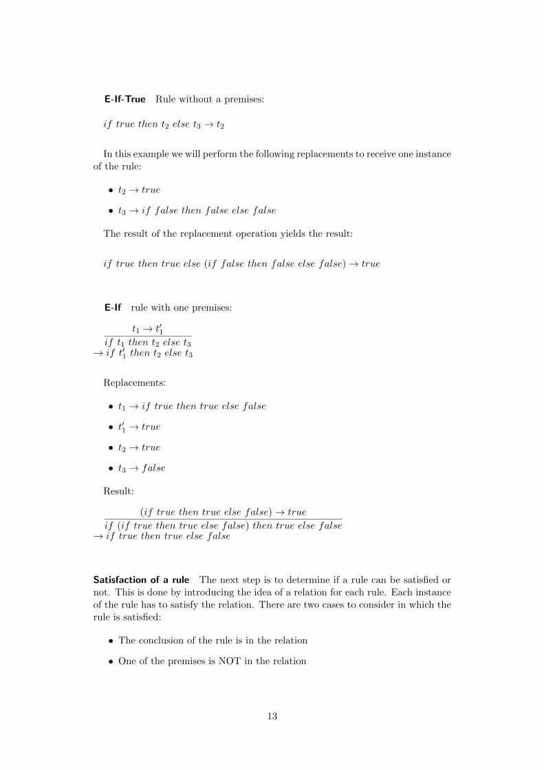
E-If-True Rule without a premises:

if true then t2 else t3 → t2

In this example we will perform the following replacements to receive one instanceof the rule:

• t2 → true

• t3 → if false then false else false

The result of the replacement operation yields the result:

if true then true else (if false then false else false)→ true

E-If rule with one premises:

t1 → t′1if t1 then t2 else t3

→ if t′1 then t2 else t3

Replacements:

• t1 → if true then true else false

• t′1 → true

• t2 → true

• t3 → false

Result:

(if true then true else false)→ true

if (if true then true else false) then true else false→ if true then true else false

Satisfaction of a rule The next step is to determine if a rule can be satisfied ornot. This is done by introducing the idea of a relation for each rule. Each instanceof the rule has to satisfy the relation. There are two cases to consider in which therule is satisfied:

• The conclusion of the rule is in the relation

• One of the premises is NOT in the relation

13

This means if one of the premises is not derivable, the whole relation is not.The above example of the E-If rule instance would satisfy the relation of the

premises and therefore CAN take one step of evaluation.Lets make another example and consider the premises of the E-If rule:

t1 → t′1if t1 then t2 else t3

→ if t′1 then t2 else t3

It is NOT derivable with the following replacements:

• t1 → if true then true else false

• t′1 → false

The premises does not hold which means that this instance of the rule is notsatisfied:

(if true then true else false) 6→ false

One-step evaluation If a given term satisfies the evaluation relation that is de-scribed above, it can take one more step of evaluation. The derivation of an instanceof a rule can be seen as a tree. The internal nodes represent the congruence rulesand its leafs represent the computation rules.

Example:

s ::= if true then false else falset ::= if s then true else trueu ::= if false then true else false

—————————————————— E-IfTrueif true then false else false→ false

————————————————————————— E-Ifif s then true else true→ if false then true else true

—————————————————————————– E-Ifif t then false else false→ if u then false else false

It is important to notice that in our sample grammar all rule instances lead toa distinct derivation tree. This is because there are no rules with more then onepremises which could lead to branches in the tree.

Normal form A term is in normal form when no evaluation rule applies to it. Thisalso means that values are always in normal form, since they can not be evaluatedfurther. The contradiction is also true in most cases: if t is in normal form, its avalue. It only fails if a term is not computable (stuck).

14

Multi-step evaluation It is deterministic, that a series of single-step evaluationsresult in the same computation rule.

3.3 Arithmetic expressions

It is natural for computer programs to perform calculation on numbers so it makessense to extend the simple language that only supports booleans until now tosupport numbers (arithmetic expression).

Since there is an infinite number of natural numbers, we can not define them allas values. Instead, we use lambda-terms to construct natural numbers.

For this purpose a new type of variables is introduced, the numeric values. Thissyntactical construct has the intention of providing a method to allow numericvalues as final result of evaluation. This concept also allows to define rules toprevent malformed terms like for example succ(true) which should be an error andnot a value.

This introduces additional evaluation rules to support natural numbers. Thefollowing rules need to be added:

t1 → t′1succ t1 → succ t′1

(E-Succ)

pred 0→ 0 (E-PredZero)

pred(succ nv1)→ nv1 (E-PredSucc)

t1 → t′1pred t1 → pred t′1

(E-Pred)

iszero 0→ true (E-IsZeroZero)

iszero(succ nv1)→ false (E-IsZeroSucc)

t1 → t′1iszero t1 → iszero t′1

(E-IsZero)

3.4 Stuck terms

It has already been mentioned several times in this document, that there are sit-uations when a calculation gets stuck. Formally spoken: A closed term (term inwhich all variables are bound) if it is in normal form and not a value. “Stuckness”is the equivalent for run-time errors.

4 Enrichment of the lambda calculus

In order to improve the pure untyped lambda-calculus there are several conceptsthat can be easily implemented with the existing infrastructure to provide commontools for programmers.

15

4.1 Multiple arguments

By default, the untyped lambda-calculus does not support multiple arguments.Instead of adding new rules to support multiple arguments it is easier to achievethe same effect using currying of higher-order functions (functions that can takemultiple steps of evaluation).

So to apply multiple arguments to a function, the first argument is applied to thefunction. The second argument then can be applied to the function that was yieldedas a result from the first function. This process is repeated until all arguments areapplied.

4.2 Church Booleans

In the lambda-calculus it is also possible to evaluate boolean conditionals. Thisis possible by defining lambda-terms that behave exactly like the evaluation rulesmentioned in 3.2.

If we for example want to evaluate the E-If rule:

t1 → t′1if t1 then t2 else t3→ if t′1 then t2 else t3

We can defined a function test b v w that reduces to v or w depending on whetherthe boolean b is true or false. It is now possible to define combinators that yieldthe expected reduction:

true = λt. λf. t; (true combinator)false = λt. λf. f ; (false combinator)test = λl. λm. λn. l m n; (test combinator)

This example shows the reduction of an example term test true v w that yieldsvas result:

test true v w (replace test with definition)= (λl. λm. λn. l m n) true v w (reducing the leftmost redex)

→ (λm. λn. true m n) v w (reducing the leftmost redex)

→ (λn. true v n) w (reducing the leftmost redex)

→ true v w (replace true with definition)= (λt. λf. t) v w (reducing the leftmost redex)

→ (λf. v) w (reducing the leftmost redex)

→ v (result term)

In the same fashion it is also possible to define boolean operators like AND, OR,etc.

16

4.3 Church Numerals

Similar to Church Booleans it is also possible to define lambda functions to operateon natural numbers.

4.4 Recursion

Recursion causes kind of a break of the lambda-calculus. A recursive term cannever evaluate to normal form and therefore a term would not be guaranteed toevaluate. This is why in the pure lambda-calculus there is no recursion.

Although I will not fully explain how recursion can be implemented regardless,I want to mention the omega combinator, which is the key idea to implement re-cursion. This divergent combinator will always return itself:

omega = (λx. x x)(λx. x x)

Now in order to fully implement recursion also the fix combinator is needed todefine the break condition of a recursive function. With these two combinators itis possible do design recursion.

5 λ-calculus via C#

The Blog of Yan Dixin [Dix15] contains a sophisticated section about the lambda-calculus via C#. This section will discuss some of his examples that represent theconcepts that have already been discussed above in this document.

5.1 C# concepts

In his article, Dixin deeply examines lambda expressions and the lambda calculus- how it comes, what it does, and why it matters. And - all of that is accom-plished by using only functions and anonymous functions. He uses C# functionsto demonstrate how lambda expressions model a computation.

5.1.1 C# closures

The base builds a simple concept in C# called closure. It is actually a generalconcept that is also used in other programming languages. “In computer science,a closure is a first-class function with free variables that are bound in the lexicalenvironment.”[Eth10] In Listing 1 the variable foo is a free variable, only boundby the environment. The fact that myFunc accesses this variable, is called a closuresince it is not local in myFunc.

1 var foo = "this is over 9000";

2 Func <string ,string > myFunc = delegate(string arg) {

3 return arg + foo;

4 };

Listing 1: Closures in C]

17

5.1.2 Currying and partial application

To write code in C# in a lambda style fashion, several language features can beused. The most important concepts are shown in Listing 2.

1 private static void LambdaBasics ()

2 {

3 // Simple function

4 Func <int , int , int > add = (x, y) => x + y;

5 int result = add(1, 2);

67 // Lambda style - anonymous function without name

8 result = new Func <int , int , int >((x, y) => x + y)(1, 2);

910 // Apply multiple arguments with currying

11 Func <int , Func <int , int >> curriedAdd = x => new Func <int ,

int >(y => x + y);

1213 // The return type function declaration can be infered by

the compiler

14 curriedAdd = x => y => x + y;

1516 // Applying add to the first argument yields a function

as result

17 Func <int , int > add1 = curriedAdd (1);

18 // Now the second argument can be applied to add1

19 result = add1 (2);

20 }

Listing 2: Currying and partial application

Line 4 in Listing 2 shows the declaration of a simple function which is evaluatedon line 5.

The declaration of a function can also be omitted when an anonymous functionis used (line 8). To support longer lambda terms, functions can also be curried.The declaration of this can be seen on line 11 and 14. The partial application ofthe function can be seen on line 17 and 19.

It is important to notice, that the yielded result of a function in this case isanother function, which is passed to the next function as a closure.

5.1.3 => associativity

The C# lambda operator is right-associative. Because of this fact, we can omit thebrackets in the examples to improve readability. x => y => x + y for example isidentical to x => (y => x + y).

This is important to understand the evaluation order of lambda-expressions inC#. With curried application, always the leftmost redex is reduced first. Moreinformation on evaluation strategies can be found in section 2.2.2.

Now to clarify this we will look at the lambda term λx.λy.x + y. In C# itcan be written x => y => x + y. We will evaluate this lambda term by applyingtwo arguments, to both show the lambda derivation and the equivalent curriedapplication in C#.

18

In this example for simplification, we assume that the constants 1 and 2 and thesymbol + are values (object language variables).

(λx.λy.x+ y) (1) (2) (reducing the leftmost redex)

→ (λy.1 + y) (2) (reducing the leftmost redex)

→ 1 + 2 (final result)

And now the equivalent in C#:

1 Func <int , Func <int , int >> add = x => y => x + y;

23 // add1: y => 1 + y;

4 Func <int , int > add1 = add (1);

56 // result: 1 + 2

7 int result = add1 (2);

Listing 3: Example reduction

5.2 Church Booleans

Encoding Church booleans in C# is surprisingly easy and serves as a good exampleof how to implement something useful with the lambda-calculus in C#.

5.2.1 Encoding Church Booleans

Listing 4 shows how the Church Booleans from section 4.2 can be implemented inC#.

1 private static void ChurchBooleans ()

2 {

3 // True := λt.λf.t4 Func <object , Func <object , object >> True =

5 (object @true) => @false => @true;

67 // False := λt.λf.f8 Func <object , Func <object , object >> False =

9 (object @true) => @false => @false;

1011 // True Test

12 object result = True (1)("2"); // result = 1

13 result = True("a")(null); // result = "a"

14 object @object = new object ();

15 result = True(@object)(null); // result = @object

1617 // False Test

18 result = False (1)("2"); // result = "2"

19 result = False("a")(null); // result = null

20 @object = new object ();

21 result = False(@object)(null);// result = null

22 }

Listing 4: Church boolean encoding

19

The effect that the evaluation of the these combinators have is that the True

combinator will return the first argument and the False combinator the second.

5.2.2 Church Boolean arithmetic

The last example of the untyped lambda-calculus in C# shows how the Churchbooleans can be used to perform boolean logic. In listing 5 the same True andFalse combinators (simplified with a function type alias) as in Listing 4 are usedto define lambda terms that can be used to calculate boolean logic. As an example,the And and Or combinator are shown.

1 // Alias for Func <object , Func <object , object >>

2 public delegate Func <object , object > Boolean(object @true);

34 public static class ChurchBoolean

5 {

6 // True := λt.λf.t7 public static Boolean True = @true => @false => @true;

89 // False := λt.λf.f

10 public static Boolean False = @true => @false => @false;

1112 // And = a => b => a(b)(False)

13 public static Boolean And

14 (this Boolean a, Boolean b) =>

15 (Boolean)a(b)(new Boolean(False));

1617 // Or = a => b => a(True)(b)

18 public static Boolean Or

19 (this Boolean a, Boolean b) =>

20 (Boolean)a(new Boolean(True))(b);

2122 // ...

23 }

Listing 5: Church boolean encoding

Listing 6 shows how to use the combinators to perform boolean logic operations.However, since such an operation yields a function as a result (how it should be inthe lambda-calculus), the effect in C# is that there is no way to display this resultfunction. The correct way to deal with this would be to implement a translationbetween Church Booleans and System.Bool. However this is out of scope of thisdocument.

1 private static void BooleanLogic ()

2 {

3 Boolean True = ChurchBoolean.True;

4 Boolean False = ChurchBoolean.False;

56 True.And(True); // true && true

7 True.And(False); // true && false

8 False.And(True); // false && true

9 False.And(False); // false && false

10

20

11 True.Or(True); // true || true

12 True.Or(False); // true || false

13 False.Or(True); // false || true

14 False.Or(False); // false || false

15 }

Listing 6: Church boolean test

6 Conclusion

The untyped lambda-calculus is a very interesting construct. At first when I startedresearching it, it appeared very strange and unfamiliar. This was mainly becausethe nature of the lambda calculus differs from everything that I have learned andused so far. It took me quite a while to understand the intention of this conceptand how it can be used.

Now that I have a basic understanding of the untyped lambda-calculus it getsmuch easier to think of areas where it can be quite useful. In my opinion, it is usefulto keep this concept in mind, when designing domain specific languages. Becauseof the mathematical feel of the lambda-calculus it is imaginable to formalize theevaluation of terms of a language in the lambda-calculus.

After all for me the lambda-calculus in modern programming languages is afeature that I really like and that changed the way I write my programs. To beable to yield a function as a function result and to use a function as an argument is afeature of programming languages that I use over and over when I am programming.

It was a very interesting time researching the untyped lambda-calculus. To learnthe mathematical foundation behind λ-expressions in programming languages waswhat I liked best about the seminar.

21

References

[Chu32] Alonzo Church. A set of postulates for the foundation of logic. Annals ofmathematics, 1932.

[Cop02] B. Jack Copeland. The church-turing thesis. Stanford Encyclopedia ofPhilosophy, 2002.

[Cud07] Ann E Cudd. Stanford encyclopedia of philosophy ”contractarianism”.Stanford Encyclopedia of Philosophy, 2007.

[Dix15] Yan Dixin. Lambda calculus via c-sharp. https://weblogs.asp.net/

dixin/Tags/Lambda%20Calculus, 2015.

[Eth10] Justin Etheredge. C closures explained. http://www.codethinked.com/c-closures-explained, 2010.

[Gri15] Jannis Grimm. Curry-Howard Isomorphism Down to Earth, 2015.

[Jun04] Achim Jung. A short introduction to the lambda calculus. School ofComputer Science, The University of Birmingham, 2004.

[lcs14] What is the contribution of lambda calculus to the field of theory ofcomputation?, 2014.

[Mic11] Greg Michaelson. An introduction to functional programming throughlambda calculus. Courier Corporation, 2011.

[mod] Models of computation. http://www.c2.com/cgi/wiki?

ModelsOfComputation.

[Moo88] Michael Moortgat. Categorial investigations: Logical and linguistic aspectsof the Lambek calculus. Number 9. Walter de Gruyter, 1988.

[Pie02] Benjamin C. Pierce. Types and Programming Languages. MIT Press,Cambridge, MA, USA, 2002.

[Squ] Dr. Jon Squire. Definitions of computable. http://www.csee.umbc.edu/

~squire/reference/computable.shtml#Church.

The title image is taken from Dixin’s Blog.[Dix15]

22