The Valuation and InformationContent of Options on Crude-Oil

Futures Contracts

J. Glenn Andrews

and

Ehud I. Ronn

Department of Finance

University of Texas at Austin

Feb. 2009

Revised: May 26, 2009

Communications

Author: Ehud I. Ronn

Address: Department of FinanceMcCombs School of Business

1 University Station, B6600

University of Texas at AustinAustin, TX. 78712-1179

Tel.: (512) 471-5853

FAX: (512) 471-5073E-mail: eronn@mail.utexas.edu

Abstract

Using market prices for crude-oil futures options and the prices of their un-

derlying futures contracts, we estimate the volatility skew in two ways. As a

benchmark for our theoretical model, on each date we first estimate a cross-

sectional polynomial structure for each maturity to demonstrate the strength

and weaknesses of a purely-mechanical model. We then apply to the empir-

ical data a Merton-style jump-diffusion model, with a rich structure of cross-

sectional constraints on the parameters. Both models are tested with respect

to their mark-to-market accuracy over time, as well as their efficacy in hedg-

ing intertemporal option price changes. The postulated Merton-style model is

shown to yield useful parameters from which market prices can be computed,

option prices can be market-to-market and (imperfectly) hedged, as well as an

informationally-rich structure covering the time period of the turbulent past six

months.

Key Words: Crude-oil futures and options

i

The Valuation and Information Content

of Options on Crude-Oil Futures Contracts

1 Introduction

The market for crude-oil futures and option contracts, traded on the New York Mercantile

Exchange, is one of the deepest and certainly one of the most important futures and options

markets in the world. In this paper, we seek to extend our knowledge and understanding of the

pricing of futures options the presence of the volatility “skew” but as importantly we seek to

infer what market prices are “telling us about the future,” what might be termed the “Message

from Markets.”

The literature on the pricing of futures and futures options, even when restricted to the

crude-oil contracts is extremely rich. The literature includes one- through four-factor models

which address the movements of prices and volatilities over time. The range of relevant literature

which pertains to the crude-oil futures literature includes equilibrium models that simultane-

ously address all futures prices (and implicitly, options), production/extraction and investment

decisions, and Heath-Jarrow-Morton (HJM) models.

Our purpose in this paper is to address the valuation, calibration and understanding of

the volatility “skew” through the use of both a model, and a model-free, approach, the latter

constituting a benchmark for the specific model we will examine. The modeling approach we

postulate takes each futures price as given, and does not attempt to embed that futures contract

in a more-general limited-number-of-factors model. Rather, our approach is in the spirit of the

HJM models, in which the term structure of prices is allowed to be totally general.

The literature is rich with equilibrium-based models which strive to explain the cross-

sectional term structure of Gibson and Schwartz (1990), Brennan (1991), Schwartz (1997),

Hilliard and Reis (1998), Schwartz and Smith (2000), Richter and Sørensen (2002), Nielsen and

Schwartz (2004) and Casassus and Collin-Dufresne (2005) and more recently Trolle and Schwartz

(2008). These models attempt to represent the set of futures contracts and their accompanying

options with a small set of factors, in some cases including an additional factor representing

volatility. In the current model, we take the futures prices as exogenously specified, in the spirit

of the HJM model, and we impose a cross-sectional constraint on the parameters of the futures

contract via the imposition and calibration of a Merton (1976) jump-diffusion model.

Another important strand of the literature is that of estimation of stochastic processes.

With respect to the modeling of the implied-vol “skew,” the two primary approaches have been

1

stochastic volatility, jump-diffusion and their variants and combinations. The relevant literature

begins with Merton (1976), continues with the Ball-Torous (1983) estimation of such processes

in stocks, Bates (1996)

We begin our approach by utilizing a “model-free” approach, in which the maturity-specific

cross-sectional of volatilities is estimated by estimating a polynomial structure to each maturity.

This model-free approach is complemented by demonstrating its strengths and weaknesses with

respect to a measure of intertemporal mark-to-market accuracy, as well as its effectiveness in

yielding a prescription for the hedging of intertemporal option price changes. We then turn to

applying the empirical data to a Merton-style jump-diffusion model, endowed with a structure of

cross-sectional constraints on the parameters. This model, too, is tested with respect to mark-

to-market accuracy and hedging efficacy. The postulated Merton-style model is shown to yield

useful parameters from which market prices can be computed, option prices can be marked-to-

market and (imperfectly) hedged, as well as an informationally-rich structure covering the time

period of the turbulent past six months.

This paper is now organized as follows. Section 2 applies what we term a curve-fitting

approach to the cross-sectional of futures options, and investigates the model’s properties as well

as its intertemporal properties in marking-to-market and hedging. Whereas Section 3 briefly

describes the data, Section 4 considers the Merton (1976) model, implements the cross-sectional

parameter constraint approach, considers the model’s mark-to-market and hedging properties

— and then proceeds to explore the model’s informational content over the turbulent period of

2008. Section 5 considers several tests across the curve-fitting and Merton-(1976) methodologies.

Section 6 concludes.

2 An Atheoretic Curve-Fitting Approach

As a benchmark to the Merton (1976) jump-diffusion model, alternatively using quadratic or

cubic polynomials, we initially estimate a purely-technical curve-fitting exercise cross-sectionally

at each point in time. This will establish some empirical regularities of the volatility skew, to

be subsequently contrasted with the Merton model.

2.1 Curve-Fitting Model

In this approach, we estimate two smooth polynomial curves, one of the quadratic and cubic

forms, to the observed Term Structure of Volatility (TSOV) and the volatility skews.

Thus, we observe the following data:

2

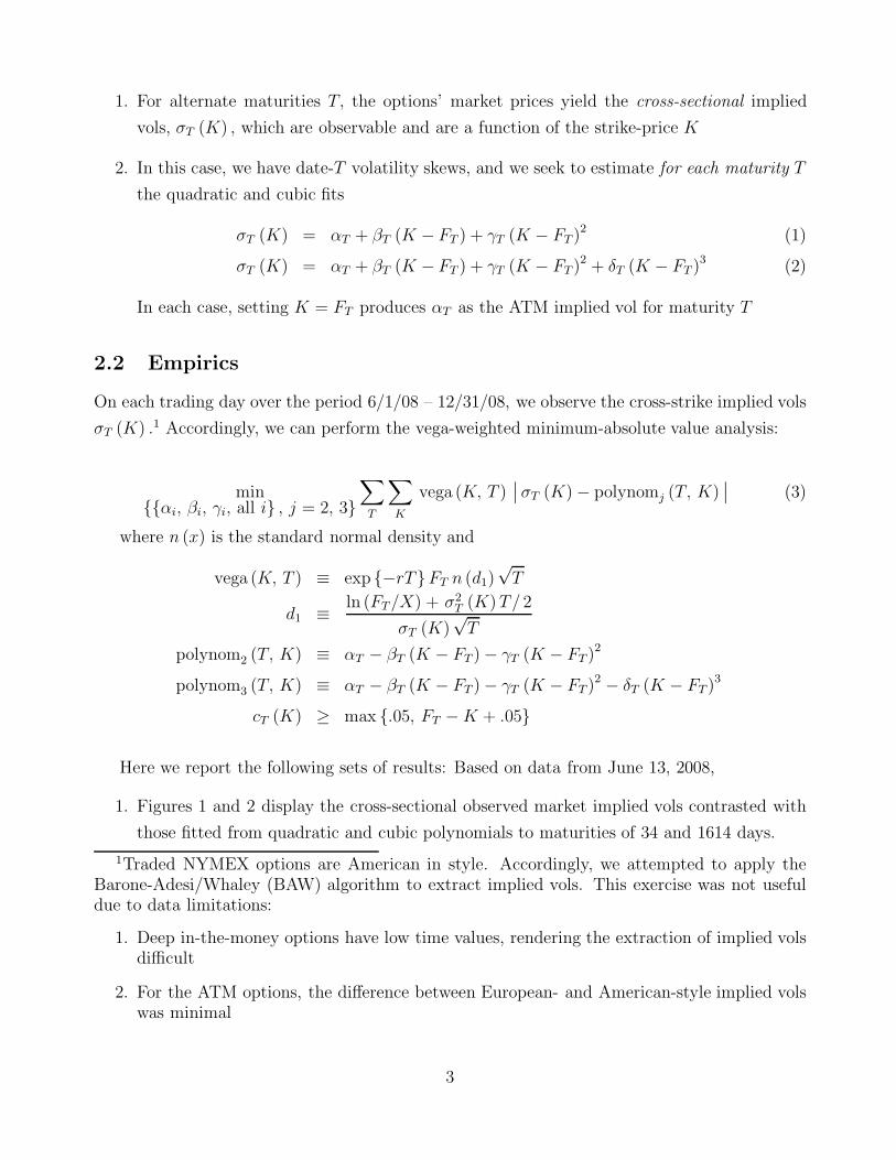
1. For alternate maturities T, the options’ market prices yield the cross-sectional implied

vols, σT (K) , which are observable and are a function of the strike-price K

2. In this case, we have date-T volatility skews, and we seek to estimate for each maturity T

the quadratic and cubic fits

σT (K) = αT + βT (K − FT ) + γT (K − FT )2 (1)

σT (K) = αT + βT (K − FT ) + γT (K − FT )2 + δT (K − FT )3 (2)

In each case, setting K = FT produces αT as the ATM implied vol for maturity T

2.2 Empirics

On each trading day over the period 6/1/08 – 12/31/08, we observe the cross-strike implied vols

σT (K) .1 Accordingly, we can perform the vega-weighted minimum-absolute value analysis:

min{{αi, βi, γi, all i} , j = 2, 3}

∑

T

∑

K

vega (K, T )∣∣ σT (K) − polynomj (T, K)

∣∣ (3)

where n (x) is the standard normal density and

vega (K, T ) ≡ exp {−rT}FT n (d1)√

T

d1 ≡ ln (FT/X) + σ2T (K)T / 2

σT (K)√

T

polynom2 (T, K) ≡ αT − βT (K − FT ) − γT (K − FT )2

polynom3 (T, K) ≡ αT − βT (K − FT ) − γT (K − FT )2 − δT (K − FT )3

cT (K) ≥ max {.05, FT − K + .05}

Here we report the following sets of results: Based on data from June 13, 2008,

1. Figures 1 and 2 display the cross-sectional observed market implied vols contrasted with

those fitted from quadratic and cubic polynomials to maturities of 34 and 1614 days.

1Traded NYMEX options are American in style. Accordingly, we attempted to apply theBarone-Adesi/Whaley (BAW) algorithm to extract implied vols. This exercise was not usefuldue to data limitations:

1. Deep in-the-money options have low time values, rendering the extraction of implied volsdifficult

2. For the ATM options, the difference between European- and American-style implied volswas minimal

3

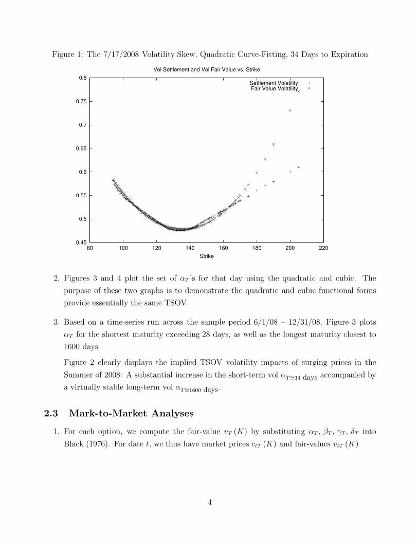
Figure 1: The 7/17/2008 Volatility Skew, Quadratic Curve-Fitting, 34 Days to Expiration

0.45

0.5

0.55

0.6

0.65

0.7

0.75

0.8

80 100 120 140 160 180 200 220

Strike

Vol Settlement and Vol Fair Value vs. Strike

Settlement VolatilityFair Value Volatility

2. Figures 3 and 4 plot the set of αT ’s for that day using the quadratic and cubic. The

purpose of these two graphs is to demonstrate the quadratic and cubic functional forms

provide essentially the same TSOV.

3. Based on a time-series run across the sample period 6/1/08 – 12/31/08, Figure 3 plots

αT for the shortest maturity exceeding 28 days, as well as the longest maturity closest to

1600 days

Figure 2 clearly displays the implied TSOV volatility impacts of surging prices in the

Summer of 2008: A substantial increase in the short-term vol αT∼=34 days accompanied by

a virtually stable long-term vol αT∼=1600 days.

2.3 Mark-to-Market Analyses

1. For each option, we compute the fair-value vT (K) by substituting αT , βT , γT , δT into

Black (1976). For date t, we thus have market prices ctT (K) and fair-values vtT (K)

4

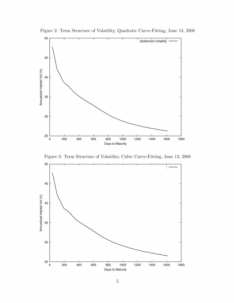
Figure 2: Term Structure of Volatility, Quadratic Curve-Fitting, June 13, 2008

25

30

35

40

45

50

0 200 400 600 800 1000 1200 1400 1600 1800

An

nu

aliz

ed

Im

plie

d V

ol (%

)

Days to Maturity

Settlement Volatility

Figure 3: Term Structure of Volatility, Cubic Curve-Fitting, June 13, 2008

25

30

35

40

45

50

0 200 400 600 800 1000 1200 1400 1600 1800

An

nu

aliz

ed

Im

plie

d V

ol (%

)

Days to Maturity

;

5

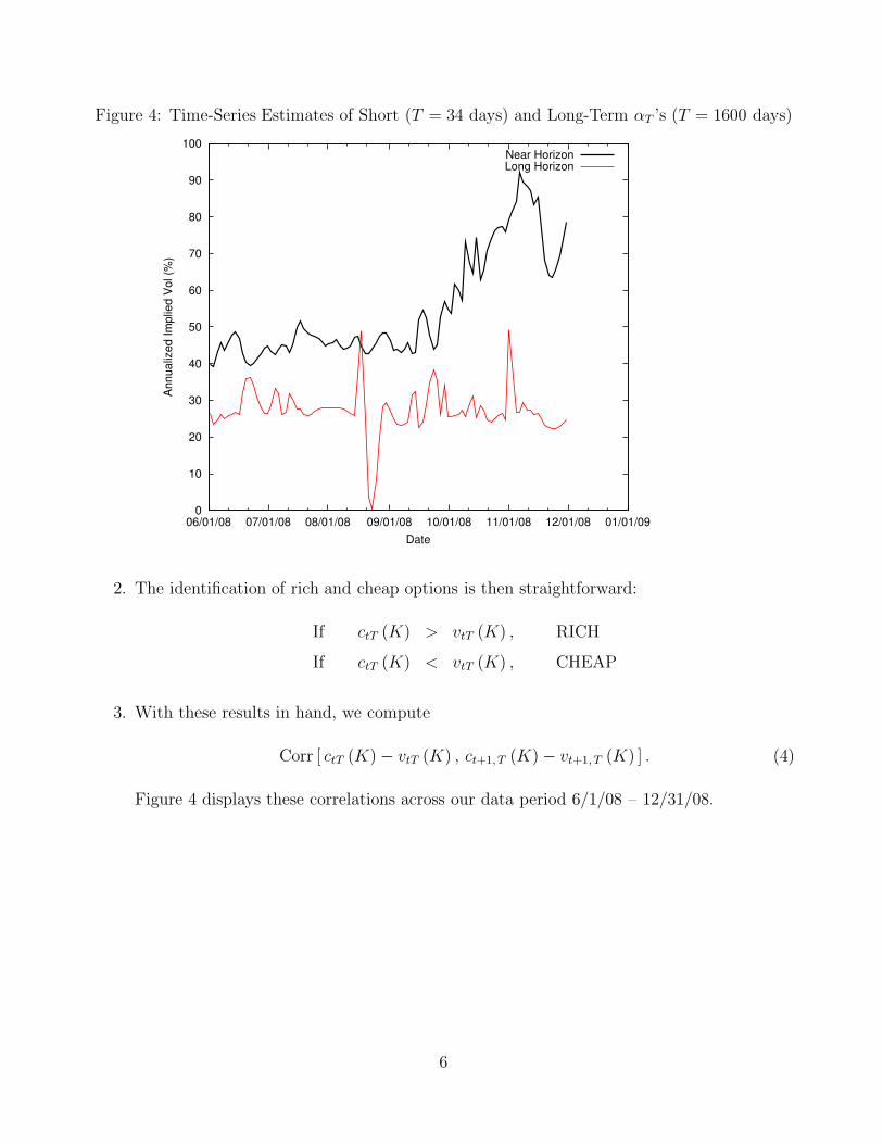
Figure 4: Time-Series Estimates of Short (T = 34 days) and Long-Term αT ’s (T = 1600 days)

0

10

20

30

40

50

60

70

80

90

100

06/01/08 07/01/08 08/01/08 09/01/08 10/01/08 11/01/08 12/01/08 01/01/09

An

nu

aliz

ed

Im

plie

d V

ol (%

)

Date

Near HorizonLong Horizon

2. The identification of rich and cheap options is then straightforward:

If ctT (K) > vtT (K) , RICH

If ctT (K) < vtT (K) , CHEAP

3. With these results in hand, we compute

Corr [ ctT (K) − vtT (K) , ct+1, T (K) − vt+1, T (K) ] . (4)

Figure 4 displays these correlations across our data period 6/1/08 – 12/31/08.

6

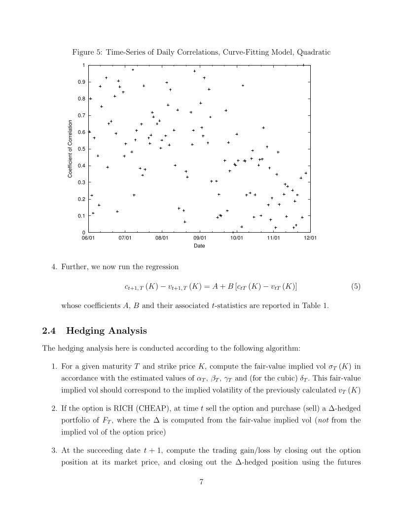
Figure 5: Time-Series of Daily Correlations, Curve-Fitting Model, Quadratic

0

0.1

0.2

0.3

0.4

0.5

0.6

0.7

0.8

0.9

1

06/01 07/01 08/01 09/01 10/01 11/01 12/01

Co

eff

icie

nt

of

Co

rre

latio

n

Date

4. Further, we now run the regression

ct+1, T (K) − vt+1, T (K) = A + B [ctT (K) − vtT (K)] (5)

whose coefficients A, B and their associated t-statistics are reported in Table 1.

2.4 Hedging Analysis

The hedging analysis here is conducted according to the following algorithm:

1. For a given maturity T and strike price K, compute the fair-value implied vol σT (K) in

accordance with the estimated values of αT , βT , γT and (for the cubic) δT . This fair-value

implied vol should correspond to the implied volatility of the previously calculated vT (K)

2. If the option is RICH (CHEAP), at time t sell the option and purchase (sell) a ∆-hedged

portfolio of FT , where the ∆ is computed from the fair-value implied vol (not from the

implied vol of the option price)

3. At the succeeding date t + 1, compute the trading gain/loss by closing out the option

position at its market price, and closing out the ∆-hedged position using the futures

7

contract Ft+1, T at date t + 1. Using the computed hedge ratios, the tracking gain/loss Π

for an option designated RICH is given by:

Π ≡ ctT (K) − ct+1, T (K) − ∆ (FtT − Ft+1, T ) .

If the option is CHEAP, report −Π.

3 Data

For the period 6/1/2008 – 12/31/2008, on each trading day we observe NYMEX data for crude-

oil futures contracts and option prices:

1. Futures prices for maturities T : FT

2. Call option prices for maturity T, cT (K) , or implied vols σT (K) which can be converted

into option prices thru Black (1976)’s

cT (K) = e−rT[FTN (d) − KN

(d − σT (K)

√T

)], (6)

where

d ≡ log (FT/ K)

σT (K)√

T+ 1

2σT (K)

√T

σT (K) = annualized futures volatility

4 The Merton (1976) Jump-Diffusion Model

4.1 Analytical Model

Recall that Merton (1976) option pricing model is given by:

vT (KT ) =

∞∑

n=0

e−λ′T (λ′T )n

n!cn (FT , X, T, rn, q, σn) (7)

where

vT (KT ) = European call option

λ′ = λ(1 + k

)

T = option expiration

8

cn (FT , X, T, rn, q, σn) = Black-Scholes [not Black (1976)] call option value with

parameters {FT , X, T, rn, q, σn} , where q is the dividend yield

cn (FT , X, T, rn, q, σn) = FT e−qT N(d) −Ke−rnTN(d − σn

√T )

d ≡ ln (FT/ K) + (rn − q)T

σn

√T

+ 1

2σn

√T

σ2n = σ2 + nδ2/ T

rn = r − λk + n ln(1 + k

)/T

q = r

Notes:

1. Although in principle (7) requires a summation over an infinite number of terms, in practice

the option value converges after a summation over the first ten terms.

2. The parameters of the jump process are:

λ = Intensity of the jump process

k = Average amplitude of the jump process

δ2 = Variance of the jump process amplitude

σ2 = Variance of the diffusion process

3. q = r in this case, since the FT ’s are futures contracts

4.2 Modeling λ, k, δ2

Tand σ2

T

The modeling of these four sets of parameters is guided by the following intuition:

1. When a crude-oil price shock occurs, it occurs at all maturities

2. Such a shock is more profoundly felt at the lower maturities, and “dies off” for succeedingly

longer maturities. This is modeled as an exponentially-declining function, where the three

parameters are the initial value, the asymptotic value and the rate of decline

Accordingly, we impose the following time-declining functional forms on λ, kT , δ2T and σ2

T :

λ = const. for all T (8)

kT = (bk − ak) exp {−ckT}+ ak (9)

δ2

T = (bδ − aδ) exp{−cδT}+ aδ (10)

σ2T = (bσ − aσ) exp{−cσT} + aσ (11)

9

As previously noted, the unitary λ across all T reflects the attribute that when a price shock

occurs, it occurs at all maturities.

Across the three sets of parameters kT , δ2T and σ2

T , this modeling has the characteristics that:

1. For T → 0,

k0

δ20

σ20

=

bk

bδ

bσ

,

where bk can be of either sign.

2. For T → ∞,

k∞

δ2∞

σ2∞

=

ak

aδ

aσ

.

3. The rates of decline for each parameter are given by the respective magnitudes of ck, cδ

and cσ.2

4. There are several parameter constraints imposed on the set of parameters

{λ, bk, ak, ck, bδ, aδ, cδ, bσ, aσ, cσ} , most of which were empirically non-binding:

Table 2 — Set of Parameter Constraints

# Constraint Motivation

1. bk ≥ −0.95 bk is the expected magnitude of the jump at the T = 0 end ofthe futures curve cannot be lower than −100%

2. abs (bk) ≥ abs (ak) Recall ak is the average magnitude of the jump size at the T →∞ end of the futures curve. Irrespective of the sign of bk, theabsolute magnitude of ak should be no greater than that of bk

3. bδ ≥ aδ ≥ 0,bσ ≥ aσ ≥ 0

The variance rates of the jump (δ) and diffusion (σ) processesshould be greater at T = 0 than at T → ∞, and should alwaysbe non-negative

2In alternate tests, we have permitted σ2T to be unconstrained/unmodeled, with results es-

sentially similar to those obtained when the exponential model was in fact imposed.

10

4.3 Calibration and Statistical Significance

We now consider the values of the estimated parameters and derive the appropriate tests for

their statistical significance:

1. With observed prices given by ctT (KT ) , and their theoretical (7) counterparts given by

vT (KT ) , the objective function is:

min{λ, bk, ak, ck, bδ, aδ, cδ, bσ, aσ, cσ}

∑

T

∑

K

vega (T, K) | cT (K) − vT (K) | (12)

Here, using all options satisfying

cT (K) ≥ max {.05, FT − K + .05}

observable at a given point in time t,3 we seek to find the set of {bk, ak, ck, bδ, aδ, cδ, bσ, aσ, cσ}parameters, as well as the single jump-intensity parameter λ, that best explain the cross-

section of option prices.

Non-linear estimation of necessity requires a set of initial parameter estimates. To provide

such a set, the estimation procedure utilized a three-step process:

(a) Initially, set ak = bk = ck = 0. This eliminates the optimization over these three

parameters and the constraints that pertain to ak and bk : bk ≥ −.95 and abs(bk) ≥abs (ak) .

(b) Using the final values of the previous stage, restrict ak to equal 0, and reintroduce

the constraint bk ≥ −.95

(c) Using the final values of the previous run as initial values, now optimize with respect

to all variables including bk and ck

2. We ran several tests to determine the level of statistical significance of the estimated

parameters. Specifically, using standard non-linear analysis — see e.g., Judge, Griffiths,

Hill and Lee (1980) — for a value of β∗ which minimizes the objective function, the

3The constraint cT (K) ≥ max {.05, FT − K + .05} is imposed as we observed numerousinstances of low-time value and -open interest options whose prices appear substantially “out ofline” with the remaining same-date T options.

11

relevant variance-covariance matrix is Σ2 :

y (β) = f (X, β) + e

e ∼ N(0, σ2 IT

)

f (X, β) ∼= f (X, β∗) +

[∂f

∂β′

∣∣∣∣β∗

](β − β∗)

S (β) ≡ [y − f (X, β)]′ [y − f (X, β)]

σ2 =S (β∗)

T − K

Σ2 = σ2

[∂f

∂β

∣∣∣∣β∗

∂f

∂β′

∣∣∣∣β∗

]−1

, (13)

where∂f

∂β′

∣∣∣∣β∗

is a matrix of first-order derivatives evaluated at the optimal point β∗.

The statistical tests took two alternate forms:

(a) To obtain a smoothly-differentiable objective function, we replaced the objective

function∑

T

∑K vega (T, K) | cT (K) − vT (K) | with its sum-of-squares analogue

∑T

∑K vega (T, K) [ cT (K) − vT (K) ]

2.

(b) In testing for the rank of the ten-parameter matrix f (X, β) , we found it to have

eight significant eigenvalues. Accordingly, we reduced the estimation to eight param-

eters by setting the T → ∞ values of the average jump amplitude and its variance

to zero: ak = aδ = 0.

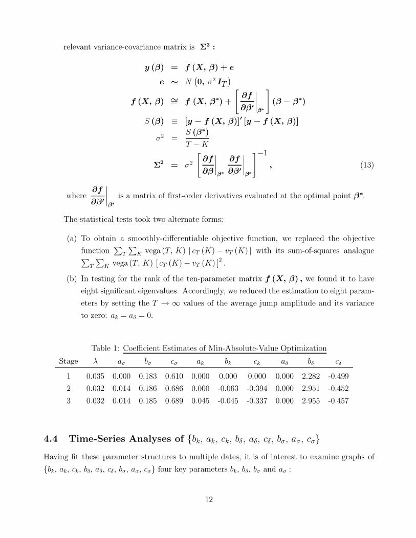
Table 1: Coefficient Estimates of Min-Absolute-Value Optimization

Stage λ aσ bσ cσ ak bk ck aδ bδ cδ

1 0.035 0.000 0.183 0.610 0.000 0.000 0.000 0.000 2.282 -0.499

2 0.032 0.014 0.186 0.686 0.000 -0.063 -0.394 0.000 2.951 -0.452

3 0.032 0.014 0.185 0.689 0.045 -0.045 -0.337 0.000 2.955 -0.457

4.4 Time-Series Analyses of {bk, ak, ck, bδ, aδ, cδ, bσ, aσ, cσ}Having fit these parameter structures to multiple dates, it is of interest to examine graphs of

{bk, ak, ck, bδ, aδ, cδ, bσ, aσ, cσ} four key parameters bk, bδ, bσ and aσ :

12

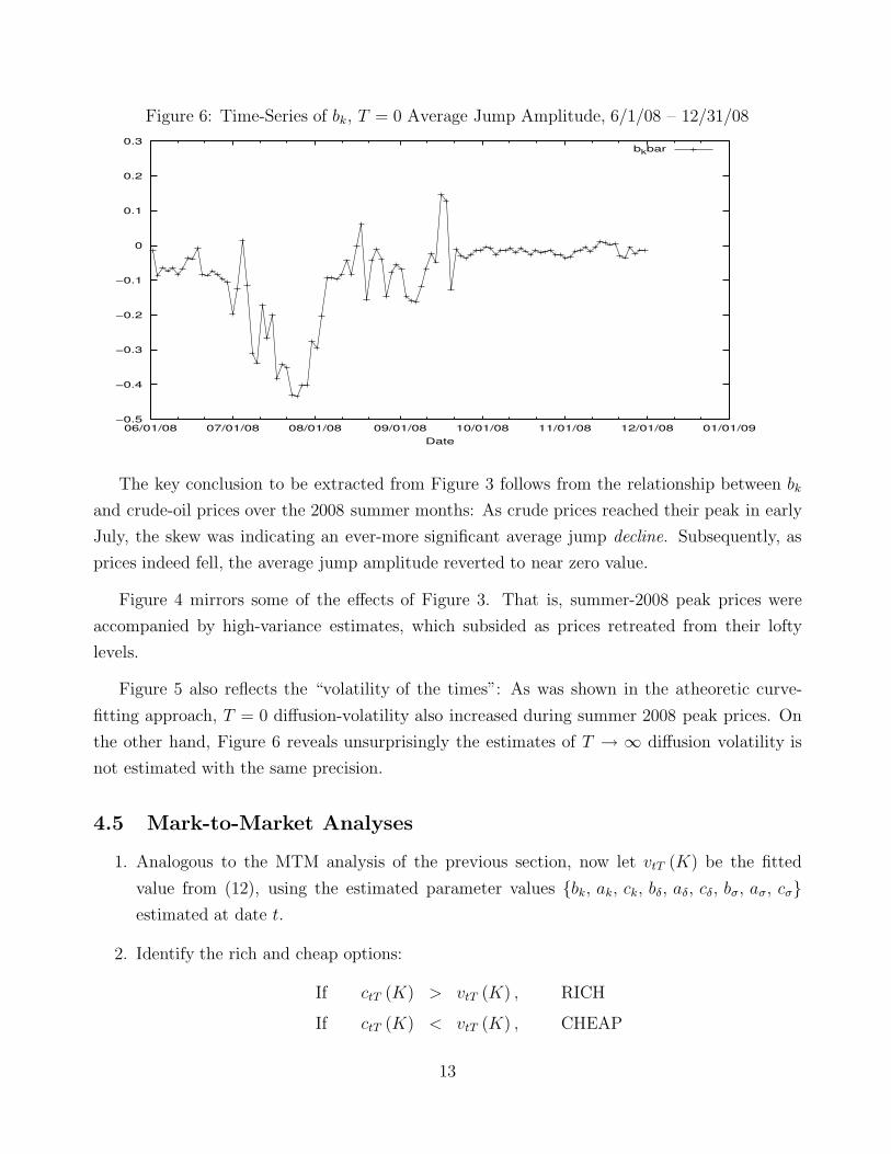
Figure 6: Time-Series of bk, T = 0 Average Jump Amplitude, 6/1/08 – 12/31/08

−0.5

−0.4

−0.3

−0.2

−0.1

0

0.1

0.2

0.3

06/01/08 07/01/08 08/01/08 09/01/08 10/01/08 11/01/08 12/01/08 01/01/09

Date

bkbar

The key conclusion to be extracted from Figure 3 follows from the relationship between bk

and crude-oil prices over the 2008 summer months: As crude prices reached their peak in early

July, the skew was indicating an ever-more significant average jump decline. Subsequently, as

prices indeed fell, the average jump amplitude reverted to near zero value.

Figure 4 mirrors some of the effects of Figure 3. That is, summer-2008 peak prices were

accompanied by high-variance estimates, which subsided as prices retreated from their lofty

levels.

Figure 5 also reflects the “volatility of the times”: As was shown in the atheoretic curve-

fitting approach, T = 0 diffusion-volatility also increased during summer 2008 peak prices. On

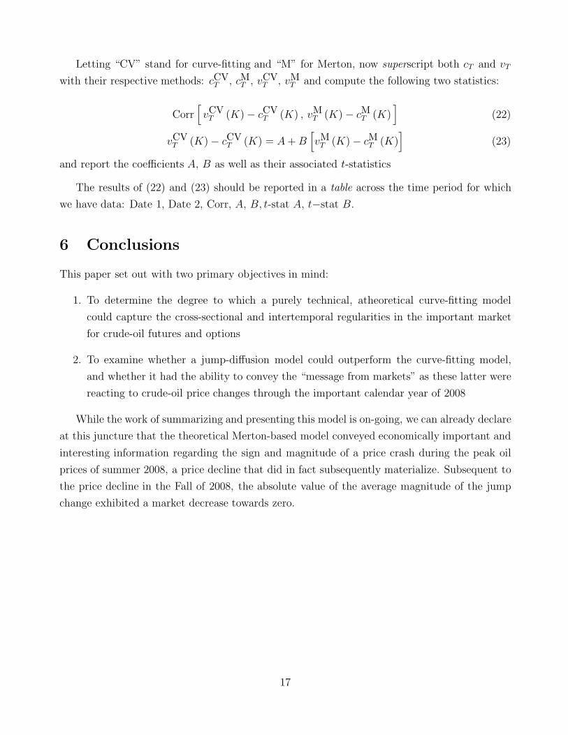
the other hand, Figure 6 reveals unsurprisingly the estimates of T → ∞ diffusion volatility is

not estimated with the same precision.

4.5 Mark-to-Market Analyses

1. Analogous to the MTM analysis of the previous section, now let vtT (K) be the fitted

value from (12), using the estimated parameter values {bk, ak, ck, bδ, aδ, cδ, bσ, aσ, cσ}estimated at date t.

2. Identify the rich and cheap options:

If ctT (K) > vtT (K) , RICH

If ctT (K) < vtT (K) , CHEAP

13

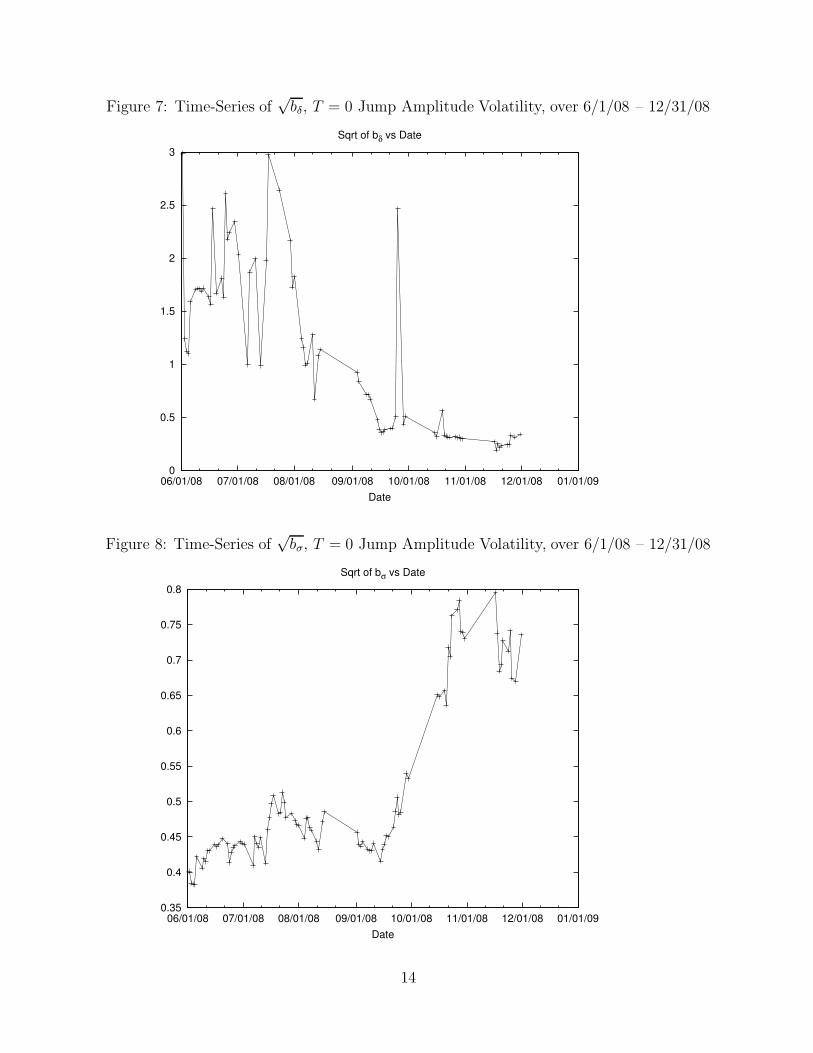
Figure 7: Time-Series of√

bδ, T = 0 Jump Amplitude Volatility, over 6/1/08 – 12/31/08

0

0.5

1

1.5

2

2.5

3

06/01/08 07/01/08 08/01/08 09/01/08 10/01/08 11/01/08 12/01/08 01/01/09

Date

Sqrt of bδ vs Date

Figure 8: Time-Series of√

bσ, T = 0 Jump Amplitude Volatility, over 6/1/08 – 12/31/08

0.35

0.4

0.45

0.5

0.55

0.6

0.65

0.7

0.75

0.8

06/01/08 07/01/08 08/01/08 09/01/08 10/01/08 11/01/08 12/01/08 01/01/09

Date

Sqrt of bσ vs Date

14

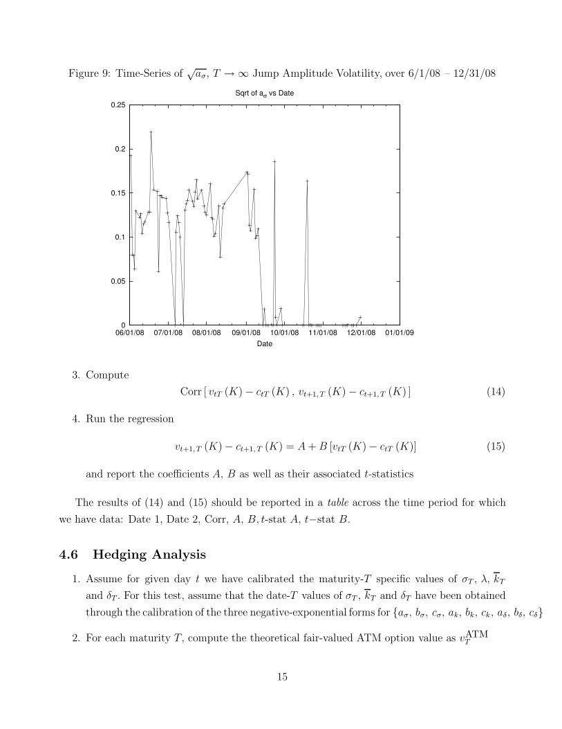
Figure 9: Time-Series of√

aσ, T → ∞ Jump Amplitude Volatility, over 6/1/08 – 12/31/08

0

0.05

0.1

0.15

0.2

0.25

06/01/08 07/01/08 08/01/08 09/01/08 10/01/08 11/01/08 12/01/08 01/01/09

Date

Sqrt of aσ vs Date

3. Compute

Corr [ vtT (K) − ctT (K) , vt+1, T (K) − ct+1, T (K) ] (14)

4. Run the regression

vt+1, T (K) − ct+1, T (K) = A + B [vtT (K) − ctT (K)] (15)

and report the coefficients A, B as well as their associated t-statistics

The results of (14) and (15) should be reported in a table across the time period for which

we have data: Date 1, Date 2, Corr, A, B, t-stat A, t−stat B.

4.6 Hedging Analysis

1. Assume for given day t we have calibrated the maturity-T specific values of σT , λ, kT

and δT . For this test, assume that the date-T values of σT , kT and δT have been obtained

through the calibration of the three negative-exponential forms for {aσ, bσ, cσ, ak, bk, ck, aδ, bδ, cδ}

2. For each maturity T, compute the theoretical fair-valued ATM option value as vATMT

15

3. For all options of maturity T (including the ATM one), compute two partial derivatives:

∂vT

∂FT

(16)

vega (K, T ) ≡ ∂vT

∂ΣKT

, (17)

where ΣKT is the specific option’s fitted implied vol

4. For each option with maturity T, let the hedge portfolio be obtained from the equation

vT = α1vATMT + α2FT . (18)

Thus, solve the two-equation system

∂vT

∂FT

= α1

∂vATMT

∂FT

+ α2 (19)

∂vT

∂ΣKT

= α1

∂vATMT

∂ΣATMKT

(20)

You can solve for α1 from (19) and substitute that result into (20) to solve for α2.

5. Now, using the computed hedge ratios α̂1, α̂2 from (19) and (20), the tracking gain/loss

Π for an option designated RICH is given by4:

Π ≡ ctT (K) − α1vATMtT − ct+1, T (K) + α1v

ATMt+1, T − α2 (FtT − Ft+1, T ) . (21)

If the option is CHEAP, report −Π.

5 Analyses across Curve-Fitting and Merton Analyses

Consider the contemporaneous richness/cheapness analyses conducted under the two primary

estimation methods, the Curve-Fitting and Merton (1976) Analyses. At date t, the relevant

definitions in both cases are:5

If cT (K) > vT (K) , RICH

If cT (K) < vT (K) , CHEAP

4Although the date t + 1 ATM option will likely have a different strike price, for purpose ofthe tracking error computation, it is important to retain the previously-defined date-t ATM.

5The subscript t is omitted, since these are correlations computed at a given point in time,not across time.

16

Letting “CV” stand for curve-fitting and “M” for Merton, now superscript both cT and vT

with their respective methods: cCVT , cMT , vCV

T , vMT and compute the following two statistics:

Corr[vCV

T (K) − cCVT (K) , vM

T (K) − cMT (K)]

(22)

vCVT (K) − cCV

T (K) = A + B[vM

T (K) − cMT (K)]

(23)

and report the coefficients A, B as well as their associated t-statistics

The results of (22) and (23) should be reported in a table across the time period for which

we have data: Date 1, Date 2, Corr, A, B, t-stat A, t−stat B.

6 Conclusions

This paper set out with two primary objectives in mind:

1. To determine the degree to which a purely technical, atheoretical curve-fitting model

could capture the cross-sectional and intertemporal regularities in the important market

for crude-oil futures and options

2. To examine whether a jump-diffusion model could outperform the curve-fitting model,

and whether it had the ability to convey the “message from markets” as these latter were

reacting to crude-oil price changes through the important calendar year of 2008

While the work of summarizing and presenting this model is on-going, we can already declare

at this juncture that the theoretical Merton-based model conveyed economically important and

interesting information regarding the sign and magnitude of a price crash during the peak oil

prices of summer 2008, a price decline that did in fact subsequently materialize. Subsequent to

the price decline in the Fall of 2008, the absolute value of the average magnitude of the jump

change exhibited a market decrease towards zero.

17

References

1. Barone-Adesi, G. and R. Whaley (1987): “Efficient analytic approximation of american

option values,” Journal of Finance, 42:301320.

2. Bates, D. S. (1996): “Jumps and stochastic volatility: Exchange rate processes implicit

in Deutsche Mark options,” Review of Financial Studies, 9:69107. (2000): “Post-87 crash

fears in the S&P 500 futures option market,” Journal of Econometrics, 94:181238.

3. Bessembinder, H., J. F. Coughenour, P. J. Seguin, and M. M. Smoller (1995): “Mean-

reversion in equilibrium asset prices: Evidence from the futures term structure,” Journal

of Finance, 50:361375. 53

4. Black, F. (1976): “The pricing of commodity contracts,” Journal of Financial Economics,

3:167179.

5. Brennan, M. J. (1991): “The price of convenience and the valuation of commodity con-

tingent claims,” in, Diderik Lund, and Bernt ksendal, eds.: Stochastic Models and Option

Values, North-Holland, Amsterdam.

6. Broadie, M., M. Chernov, and M. Johannes (2004): “Model specification and risk premi-

ums: Evidence from futures options,” Working paper, Columbia University, forthcoming

in Journal of Finance.

7. Carlson, M., Z. Khoker, and S. Titman (2006): “Equilibrium exhaustible resource price

dynamics,” Working paper, NBER # 12000.

Clewlow, L. and C. Strickland (1999): “A multi-factor model for energy derivatives,”

Working paper, University of Technology, Sydney.

8. Cortazar, G. and E. S. Schwartz (1994): “The valuation of commodity contingent claims,”

Journal of Derivatives, pages 2739.

Deaton, A. and G. Laroque (1992): “On the behaviour of commodity prices,” Review of

Economic Studies, 59:123. (1996): “Competitive storage and commodity price dynamics,”

Journal of Political Economy, 104:896923.

9. Duan, J.-C. and J.-G. Simonato (1999): “Estimating and testing eksponential-affine term

structure models by Kalman filter,” Review of Quantitative Finance and Accounting,

13:111135.

18

10. Eraker, B. (2004): “Do Stock Prices and Volatility Jump? Reconciling Evidence from

Spot and Option Prices,” Journal of Finance, 59:13671403.

11. Eydeland, A. and H. Geman (1998): “Pricing power derivatives,” Risk, September.

12. Gibson, R. and E. S. Schwartz (1990): “Stochastic convenience yield and the pricing of oil

contingent claims,” Journal of Finance, 45:959976.

13. Heath, D., R. Jarrow, and A. Morton (1992): “Bond pricing and the term structure

of interest rates: A new methodology for contingent claims valuation,” Econometrica,

60:77105.

14. Heston, S. (1993): “A closed form solution for options with stochastic volatility,” Review

of Financial Studies, 6:327343.

15. Hilliard, J. E. and J. Reis (1998): “Valuation of commodity futures and options under

stochastic convenience yields, interest rates and jump diffusions in the spot,” Journal of

Financial and Quantitative Analysis, 33:6186.

16. Judge, George G., William E. Griffiths, R. Carter Hill and Tsoung-Chao Lee, The Theory

and Practice of Econometrics, 1980, John Wiley & Sons, New York.

17. Litzenberger, R. H. and N. Rabinowitz (1995): “Backwardation in oil futures markets:

Theory and empirical evidence,” Journal of Finance, 50:15171545.

18. Longstaff, F. and E. Schwartz (2001): “Valuing American options by simulation: A simple

least-square approach,” Review of Financial Studies, 14:113147.

19. Lund, J. (1997): “Econometric analysis of continuous-time arbitrage-free models of the

term structure of interest rates,” Working paper, Aarhus School of Business.

20. Miltersen, K. (2003): “Commodity price modelling that matches current observables: A

new approach,” Quantitative Finance, 3:5158.

21. Miltersen, K. and E. S. Schwartz (1998): “Pricing of options on commodity futures with

stochastic term structures of convenience yields and interest rates,” Journal of Financial

and Quantitative Analysis, 33:3359.

22. Ng, V. K. and C. Pirrong (1994): “Fundamentals and volatility: Storage, spreads and the

dynamics of metal prices,” Journal of Business, 67:203230.

19

23. Nielsen, M. J. and E. S. Schwartz (2004): “Theory of Storage and the Pricing of Com-

modity Claims,” Review of Derivatives Research, 7:524.

24. Richter, M. and C. Srensen (2002): “Stochastic volatility and seasonality in commodity

futures and options: The case of soybeans,” Working paper, Copenhagen Business School.

25. Routledge, B. R., D. J. Seppi, and C. S. Spatt (2000): “Equilibrium forward curves for

commodities,” Journal of Finance, 55:12971338.

26. Schwartz, E. S. (1997): “The stochastic behavior of commodity prices: Implications for

valuation and hedging,” Journal of Finance, 52:923973.

27. Schwartz, E. S. and J. E. Smith (2000): “Short-term variations and long-term dynamics

of commodity prices,” Management Science, 46:893911. 57

28. Trolle, A. B. and E. S. Schwartz (2006): “A general stochastic volatility model for the

pricing of interest rate derivatives,” Working paper, UCLA, forthcoming in Review of

Financial Studies. 58

20