the value and real effects of implicit guarantees
TRANSCRIPT

The Value and Real Effects of Implicit Guarantees*
Shuang Jin
Hong Kong University of Science and Technology†
Wei Wang
Queen’s University‡
Zilong Zhang
City University of Hong Kong§
First version: June 2017
This version: January 2018
Abstract
Exploiting the first default by a large state-owned enterprise (SOE) in China’s onshore bond
market for identification, we find that implicit government guarantees account for 1.45 - 1.77% of
bond value. This translates into a total value of more than 93 billion CNY (15 billion USD) in
China’s domestic bond markets for the corporate sector. Implicit guarantees account for a greater
value for firms in sectors operating at overcapacity and with high default risk but a smaller value
for firms that receive direct government subsidy and firms that rely primarily on banks for
financing. We further document that implicit guarantees have real effects on corporate investment
and financing policies. The reduction of implicit guarantees leads to a decline in investment and
net debt issuance, an increase in cash holdings, and an improvement in investment efficiency for
SOEs compared to non-SOEs.
Keywords: implicit guarantees, bonds, investment, cash, state-owned enterprise, China
JEL classification: G12, G15, G30, G38
* We would like to thank Bernie Black, Doron Levit, Song Ma, Paul Malatesta, Frank Milne, Luke Taylor, Gang Xiao,
and seminar and conference participants at Queen’s University and the Journal of Law, Finance, and Accounting 2017
Conference for helpful comments. All errors are our own. † HKUST Business School, Clear Water Bay, Kowloon, Hong Kong; email: [email protected]. ‡ Smith School of Business, Queen’s University, Kingston, ON, K7L 3N6; email: [email protected]. § College of Business, City University of Hong Kong, Hong Kong; email: [email protected].

1
“Baoding Tianwei Group, a power-equipment manufacturer, became China’s first state-owned company
to default on domestic debt.”
– Wall Street Journal (April 21, 2015)
“A little-known power equipment manufacturer became the first state-owned company to default in
China’s huge domestic bond market, throwing doubt on the long-held notion that such businesses have
implicit government backing.”
– New York Times (April 21, 2015)
I. Introduction
It is well known that government bails out large financial institutions to keep them afloat
to avoid systemic risks. The value of such implicit guarantees is large for the financial sector in
the US.1 The experience of GM and Chrysler during the 2008–2009 financial crisis also highlights
US government support in bailing out systemically important non-financial corporations during
economic downturns. In fact, real-sector firms in many countries have implicit government
guarantees (Faccio, Masulis, and McConnell, 2006). 2 Moody’s (2014) articulates that such
implicit guarantees have real implications for firms’ credit ratings and financing costs. Despite the
prevalence and importance of implicit guarantees for firms in the real sector, little is known about
their value embedded in corporate bonds and their effects on corporate investment and financial
policies. Our paper intends to fill this void. We examine the effects of implicit guarantees on
corporate policies, in addition to quantifying the economic magnitude of such guarantees, by
exploiting a natural event that occurs in the world’s largest transitional economy.
1 For example, Veronesi and Zingales (2010) show a distribution of $21–$44 billion from taxpayers to banks during
financial crises. Ueda and di Mauro (2012) suggest that large banks worldwide enjoyed an estimated funding cost
advantage of 80 basis points during the 2008–2009 financial crisis, which transforms to a taxpayer subsidy of $83
billion. Tsesmelidakis and Merton (2013) show that the wealth transfer to investors through implicit guarantees ex-
ante amounts to $365 billion. Moody’s (2011) also provides methodologies for quantifying the value of implicit
government guarantees for large financial institutions. 2 Examples of real-sector firms that have been bailed out by their home governments include Groupe Bull SA
(France), Norilsk Nickel (Russia), Bangkok Land (Thailand), Malaysian Airline System (Malaysia), and Railtrack
(UK), among others.
2
The implicit government-guarantee provision is also known as the “soft budget constraint”
phenomenon, prevalent in most socialist and mixed economies (Kornai, 1986; Lin and Tan, 1999).
Firms in those economies enjoy implicit guarantees for two primary reasons: political
considerations – government’s goal of creating jobs, supporting strategic industries, or gaining
political support – and accountability problems and policy burdens. However, the ex-ante effects
of implicit guarantees on firms’ investment policies remain unclear. On the one hand, they help
firms alleviate their financial constraints and thus encourage investment as government promises
lenders that it is willing to intervene to pre-empt defaults by directly injecting capital or
guaranteeing new capital raising. On the other hand, implicit guarantees may directly influence the
efficiency of firms through their effect on the expectations of managers (Maskin and Xu, 2001).
They may weaken the disciplinary effect of debt (Jensen and Meckling, 1976; Jensen, 1986) and
thus discourage managers from exerting efforts on projects.
State-owned enterprises (SOEs) in China shoulder more political responsibilities than non-
SOEs, such as creating jobs and maintaining stability. Central and local governments typically
subsidize SOEs, explicitly or implicitly. Investors have long held the view that the Chinese
government would never let large SOEs default since such an event might create unexpected
catastrophic consequences (Zhu, 2016).3 However, on April 21, 2015, Baoding Tianwei Group, a
large SOE owned by the central government, shocked the markets by announcing that it was
defaulting on one of its onshore bonds; this was the first bond default by an SOE in China.
Investors perceived it as a reduction or even removal of implicit guarantees on SOEs, as Chinese
3 When SOEs become financially distressed and have difficulty meeting debt obligations, local governments may
provide direct cash injection, arrange for stronger SOEs to provide loans and assets, merge with them, or ask banks
to extend debt maturities and provide payment waivers (Moody’s, 2016b).

3
leaders start to adopt a market-based approach to restructuring troubled companies in the middle
of an unprecedented credit boom.4
The reduction in implicit guarantees should increase the perceived risk of borrowers and
thus be reflected in corporate bond price. To quantify the value of implicit guarantees, we adopt
an event study to compute the abnormal bond returns of SOEs and non-SOEs around the Tianwei
event. Our results show that the bonds of SOEs experience significantly greater negative returns
than those of non-SOEs. On average, the abnormal bond returns of SOEs are 1.45% to 1.77%
lower (39-48 basis points higher in yield spread given the average bond duration of 3.64) than
those of non-SOEs. This translates into a total value of up to 93 billion CNY (15 billion USD) in
China’s domestic bond markets for the corporate sector. Our estimated value, however, likely
reflects the lower bound of the true expected value of implicit guarantees in bond prices, given
that the market’s expected probability of a government bailout of SOEs was not necessarily 1
before Tianwei and that such probability does not necessarily go down to zero after the event.
Our heterogeneity tests show that the bond price decline is more pronounced for SOEs in
sectors operating at overcapacity, which are likely to see a greater reduction in government
support, and SOEs that have high default risks and, thus, greater need for government backing.
The price decline is less if SOEs receive a large amount of direct government subsidy or rely
primarily on bank loans (not corporate bonds) for financing. Taken together, our results suggest
that implicit guarantees account for a sizable value of corporate bonds, enabling SOEs to borrow
at costs that do not reflect the risks otherwise inherent in their operations compared to non-SOEs.
4 China’s corporate debt accounted for 160% of its gross domestic product as of 2016; see Lingling Wei, “China
lays out guidelines on debtor-for-equity swaps between banks, companies,” Wall Street Journal, October 11, 2016.
4
After quantifying the economic magnitude of implicit guarantees, we investigate the effects
of such guarantees on corporate investment and financial policies. Presumably, a reduction or loss
of implicit guarantees exacerbates a firm’s financial constraints, as investors perceive the borrower
to be more risky. As a result, we expect the firm to reduce investment and hoard cash for
precautionary purposes as external funding costs increase. In contrast, we expect to observe an
increase in investment if the reduction of implicit guarantees reflects a reduction in government
interference, thereby allowing a firm greater autonomy in its policy-making. To test these
conjectures, we adopt a difference-in-differences (DID) analysis with firm and time fixed effects
to account for unobservable heterogeneity. We find that SOEs reduce their total investments by up
to 3.3% of book assets semiannually, compared to non-SOEs, in the three semiannual fiscal periods
after the Tianwei default. Furthermore, in response to the reduction of government guarantees,
SOEs reduce their net debt issuance (by 0.6% of book assets semiannually) and increase their cash
holding (by 1.0% of book assets semiannually) more than non-SOEs.
One important question that remains to be answered is whether investment efficiency
improves as a result of the reduction of implicit guarantees. On the one hand, a reduction in implicit
guarantees results in increased corporate funding costs but no reduction in the policy burden faced
by SOEs. This may lead to a weakening of a firm’s ability to capture all growth opportunities and,
thus, a reduction in investment efficiency. On the other hand, when the budget constraint is
hardened for SOEs, managers have stronger incentives to choose better investment projects
accommodate higher funding costs and to avoid possible default. This reflects the strengthening
of the disciplinary effect of debt. Investment efficiency improves as a result.
We investigate net changes in investment efficiency, measured by both the occurrence of
under- and over-investment and asset turnover ratio post Tianwei default, between SOEs and non-
5
SOEs. Our results show an increase in the investment efficiency of SOEs relative to non-SOEs.
The evidence suggest that hardened budget constraint helps reinforce the disciplinary role of debt
for corporate managers.
There are two potential concerns about our DID test results. First, our results may be driven
by unobserved heterogeneity that correlates with the SOE status and government ownership of
companies. Second, the first default event of China’s SOEs may not reflect the reduction of
implicit guarantees but rather be correlated with a macro shock that affects SOEs and non-SOEs
differently. The differential effects of the shock thus drive later investment and financing
decisions. To address these concerns, we conduct several tests. First, we conduct a propensity-
score-matching (PSM) analysis, in which we match each non-SOE with an SOE in the same
industry and with the closest propensity of being a non-SOE. The matched groups of firms should
be similar on all observable matched dimensions and thus similarly susceptible to the macro shock.
Our main results are robust to using the matched sample. Second, we perform a falsification test
using the first non-SOE default as a pseudo–SOE-default event. Our results show no difference in
bond price reactions between SOEs and non-SOEs around this event. Third, we conduct a placebo
DID test around the first non-SOE default and find no significant changes in investment between
SOEs and non-SOEs. The evidence is inconsistent with the notion that the first SOE default event
coincides with a macro shock to SOEs.
This paper contributes to the literature on government implicit guarantees. Understanding
the effects of implicit guarantees on bond prices and corporate policies is important and relevant
to not only policymakers who pay close attention to the long-term, sustainable growth of the
economy but also debt investors who devote efforts to the assessment of default risks of borrowers.
Our paper differs from prior studies on three counts. First, to the best of our knowledge, our study
6
constitutes the first effort to document the magnitude of implicit guarantees in the real sector, while
existing studies in this area predominantly focus on guarantees extended to large financial
institutions (Demirgüç-Kunt and Detragiache, 2002; Ueda and di Maro, 2012; Tsesmelidakis and
Merton, 2013; Mariathasan, Merrouche, and Werger, 2014; Ghandi and Lustig, 2015; Acharya et
al., 2016; Kelly et al., 2016). Second, the first-ever, large SOE default provides a desirable
experimental setting, allowing us to measure the causal effects of implicit government guarantees
on industrial firms. Third, despite the appealing theoretical framework of soft budget constraints
(Lin and Tan, 1999; Maskin and Xu, 2001), no prior empirical studies study their effects on firm
investment and financial policies. Taking advantage of the Tianwei event, our empirical findings
advance the literature by providing the first evidence of the real effects of soft budget constraints.
Our paper also relates to the literature on the effects of financial constraints. There is
ongoing research on how financing frictions are factored into the real activities of corporations
and asset prices (see, e.g., Fazzari, Hubbard, and Petersen, 1988; Hoshi, Kashyap, and Scharfstein,
1991; Whited, 1992; Kaplan and Zingales, 1997; Whited and Wu, 2006; Campello, Graham, and
Harvey, 2010; Almeida, et al., 2012; Farre-Mensa and Ljungqvist, 2015; Whited and Zhao, 2016).
We extend this line of research by delineating the effects of financial constraints, arising from the
reduction of implicit guarantees, on corporate investments. Our findings suggest that even though
financial constraints arising from the reduction of implicit guarantees seem to discourage corporate
investments, they may strengthen the disciplinary role of debt and help resolve agency problem.
The remainder of the paper is organized as follows. Section II describes the background of
the Chinese bond market and the first SOE default. Section III introduces the data source, while
Section IV lays out the empirical methodology. Section V presents our empirical results, and
Section VI concludes.

7
II. Background on China’s Bond Markets and First SOE Default
II.1. China’s Bond Markets
China’s bond markets have grown rapidly in recent years and are now the third largest in
the world, behind only the United States and Japan. Government bonds, financial bonds, and repos
all trade in the interbank market – equivalent to the over-the-counter (OTC) market in the US,
while bonds issued by corporations vary in both type and the market where they trade. There are
three types of corporate bonds traded in China: corporate bond, enterprise bond, and mid-term note
(MTN). Corporate bonds trade in securities exchanges under the regulation of the China Securities
Regulatory Commission (CSRC); MTNs trade in the interbank market under the regulation of the
People’s Bank of China (PBC); and enterprise bonds trade both in the interbank market and on
securities exchanges, regulated by the National Development and Reform Commission (NDRC).
China’s corporate bond markets have experienced an unprecedented boom since the mid-2000s
(see Figure 1). The rapid expansion of the bond markets is mainly due to the government’s
intention to boost direct financing in capital markets.5
[Insert Figure 1 about here]
Investors considered bonds issued by corporations in China’s domestic markets to have
implicit guarantees by the government and were optimistic that the government would bail out
systemically important enterprises, if necessary. However, in March 2014, China’s domestic bond
markets experienced the first bond default by a privately owned company – a solar panel
manufacturer called Shanghai Chaori Solar Energy (Chaori hereinafter). The default by Chaori
5 In May 2014, the State Council issued the Guiding Principles for the Healthy Development of Capital Markets, a
policy document that called for the government to increase its share of direct financing in the economy and ease
restrictions on bond issuance.
8
signaled that the government might back off its practice of bailing out troubled private enterprises.
The default event indicates the government’s changing tolerance for corporate failures and its
attempts to give market forces a more decisive role in the economy. However, since Chaori is a
privately owned company, its default had a limited effect on investors’ expectations about the
government’s implicit guarantees for SOEs.
II.2. First SOE Default – Default of Baoding Tianwei Group
Baoding Tianwei Group Co., Ltd. (hereinafter referred to as Tianwei) was a wholly owned
subsidiary of China South Industries Group (CSIG), which was owned by the central government
of China and was ranked 102 on the Fortune Global 500 in 2016. Established in 1958, Tianwei
was a manufacturer in the power transmission and distribution industry and the renewable energy
industry (photovoltaic power and wind power). It sold products in more than 30 countries,
including the United States. Tianwei invested aggressively in the photovoltaic industry, which fell
into a weak cycle in 2011: overcapacity in the industry led to falling product prices and declining
profits for manufacturers of photovoltaic equipment. As a result, Tianwei suffered a net operating
loss of 1.54 billion CNY in 2011, and losses continued in the next three years. During the same
period, Tianwei’s credit rating was downgraded several times, from AA+ in 2011 to BBB in 2014.6
From July 2013 through December 2014, Tianwei and several of its subsidiaries could not repay
overdue interest on loans provided by the Bank of China and the Export-Import Bank of China.
6 Product market competition was not the only cause of Tianwei’s failure. In 2013, Tianwei gradually transferred its
shares of Baobian Electric, one of its subsidiaries, to the parent company, CSIG, which then became the controlling
shareholder of Baobian. Later in 2013, through a series of asset swaps, Tianwei substituted most of its profitable
assets (producing power transformers) for the non-profitable assets (producing photovoltaic equipment) of Baobian.
These operations further aggravated Tianwei’s financial status, jeopardizing its ability to repay debtholders. Several
other lenders even sued Tianwei for its asset swap transactions with Baobian and appealed for their revocation; this
was later rejected by the court.

9
The lenders requested the government to freeze Tianwei’s assets to secure their claims. During the
same period, interest on corporate bonds was duly paid.
On April 13, 2015, Tianwei announced that the Agriculture Bank of China had accessed
its deposits to recoup its loan to the company. As a result, the company lacked enough cash to pay
the interest on its bonds. Tianwei tried to secure a government bailout, something that had
previously been standard government policy toward state-backed companies but failed.
Consequently, Tianwei officially announced its default on its interest payments of 11 Tianwei
MTN2 on April 21. The giant maker of power transformers became the first central government-
backed company to default on an onshore bond. Five months later, Baoding Tianwei Group Co.
and three of its business units filed for bankruptcy.7
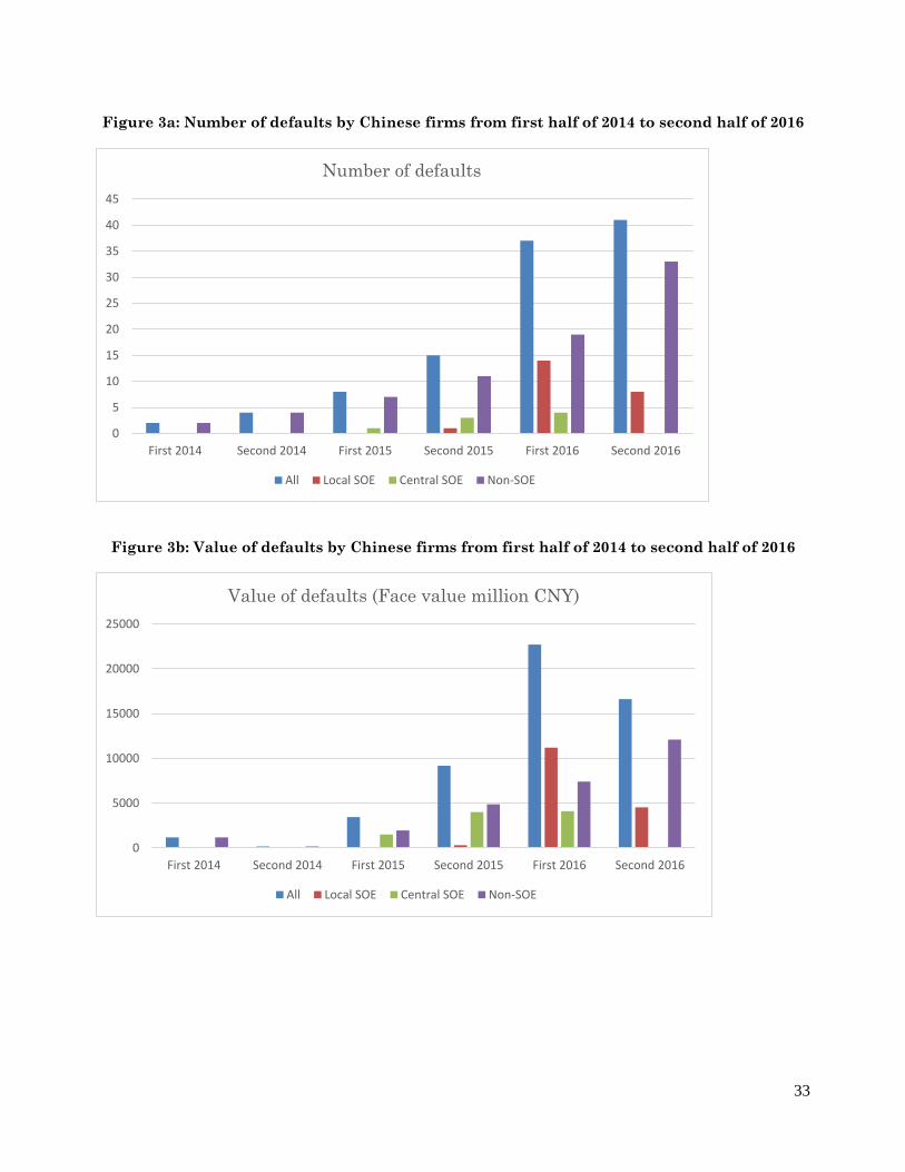
Figure 2 shows a graphical illustration of events leading to the Tianwei default. The default
of an SOE was a shocking event for investors as government support failed to materialize. In fact,
several large SOEs have defaulted or restructured debt since Tianwei’s default in 2015 (see Figures
3a and 3b).8 The serial defaults of SOEs indicate that the absence of government guarantees of
Tianwei is not an isolated event, and the fact that the Chinese government would never let state-
owned borrowers default has officially become history.9 Chinese corporate bond markets cooled
7 See Bloomberg, “Baoding Tianwei Group to File for Bankruptcy after April Default,” September 18, 2015. 8 We list several examples of SOE defaults on bonds. In October 2015, Sinosteel Co., a state-owned steelmaker,
failed to pay interest due on 2 billion CNY notes maturing in 2017. On March 28, 2016, Dongbei Special Steel
Group, owned by the government of Liaoning province, failed to make an 852 million CNY bond payment and filed
for bankruptcy on October 10, 2016. In April 2016, Shanxi Huayu, which is 49% owned by state-owned China
National Coal Group Corp., failed to pay 637.7 million CNY in principal and interest on its domestic short-term
commercial paper. In April 2016, China Railway Materials Co., China’s largest supplier of iron-rail track and other
railroad building materials, suspended trading of 16.8 billion CNY worth of outstanding bonds and was pursuing
potential debt restructuring plans with creditors. 9 In the aftermath of the Tianwei default, Moody’s states, “Chinese regional and local governments (RLGs) have
less scope to support state-owned enterprises (SOEs) facing financing distress than before. Recent episodes of SOE
distress show that RLG’s autonomy to provide direct financial support to struggling SOEs is diminishing as a result
of restrictive central government regulations” (Moody’s, 2016b).

10
down after Tianwei. Anecdotes indicate that from 2014 through 2016, around 70 companies have
canceled or postponed new bond issuance.10
[Insert Figure 2 and Figures 3a and 3b about here]
III. Data and Sample
We obtain bond characteristics from the China Stock Market & Accounting Research
(CSMAR) Database and WIND for three types of bonds – corporate bonds, enterprise bonds, and
MTNs. CSMAR provides daily, security-specific trading information for bonds, including open
price, close price, yield to maturity, trading volume, accrued interest, and daily return. However,
the database only covers corporate bonds (all exchange-traded) and a subsample of dual-listed
enterprise bonds, which are also traded both on the exchange and the interbank market. We rely
on the WIND database for MTN characteristics and trading information. For the event study, most
of our analysis is based on the CSMAR sample. That is, we use all the exchange-traded bonds
because they are more liquid than those traded in the interbank market.11 Our initial sample
consists of 10,748 corporate bonds issued and traded in China’s domestic market during the period
June 2012 to June 2016.
Our sample of bond-issuing firms includes both public (listed) and private firms (non-
listed). PBC imposes regulations on the financial reporting of firms issuing bonds: they are
required to disclose audited semiannual and annual financial statements for the three years before
bond issuance, for each year after issuance, and before the maturity date of the bond (PBC, 2012).12
We collect semiannual financial information for bond-issuing firms from the WIND database. Our
10 See Federal Reserve Bank of San Francisco, “China’s Bond Market: Larger, More Open, and Riskier,” 2016. 11 In robustness tests, we manually collect trading prices of MTNs for the event study. 12 Rules for Information Disclosure on Debt Financing Instruments of Non-financial Enterprises in the Inter-bank
Bond Market, 2012, National Association of Financial Market Institutional Investors (under PBC).
11
sample is restricted to a period between January 2013 and December 2016, and include all firms
that have at least one bond (corporate, enterprise or MTN) outstanding at that period. We also
collect information on the ownership structure of each issuer, including the identity, ownership,
and characteristics (individual, central SOE, local SOE, private firm, foreign firm) of the
controlling shareholder. The issuer is classified into central SOE, local SOE, and non-SOE, based
on the type of controlling shareholder. We rely upon industry definitions from the CSRC to classify
the bond issuers by sector.13
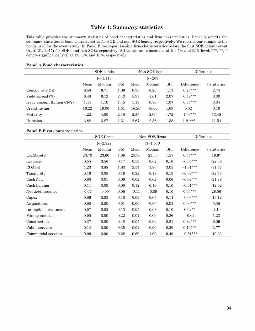
Table 1 provides key summary statistics of the variables used in the paper, while Appendix
Table A.I defines the respective variables. To mitigate the influence of outliers, we winsorize all
continuous variables at the 1st and 99th percentiles. Panel A reports summary statistics for the
characteristics of 1,387 unique bonds that are used in our event study, including 1,118 SOE bonds
and 269 non-SOE bonds that traded at least once in the 30-day window before Tianwei default
date and at least once in the 30-day window after the Tianwei default date.14 Panel A shows that
bonds issued by SOEs tend to carry higher coupon rates and have higher yield spreads than those
issued by non-SOEs. They also have a larger issue size, carry higher credit ratings, and have a
longer maturity than non-SOE bonds.
[Insert Table 1 here]
13 These sectors consist of Agriculture, Mining and Steel, Manufacturing, Utility, Construction, Retail and
Wholesale, Transportation/Storage/Postal, Hotel and Restaurant, IT, Finance, Real Estate, Rental and Commercial
Services, Environmental and Public Facilities, Residential Services, Health and Community Services,
Entertainment, Others. They are further classified into four groups: Mining and Steel, Construction, Public Services
(Utility, Agriculture, Transportation/Storage/Postal, Environmental and Public Facilities), and Commercial Services
(the remainder). 14 There are altogether 4,409 bonds outstanding during our event window. We compare 1,438 bonds used for the
event study and 2,679 bonds that did not trade during the event window and find that they are not statistically
different in their coupon rate, yield spread, bond issuance size, maturity, or credit ratings.

12
Panel B reports issuing-firm characteristics for SOEs and non-SOEs separately. SOEs and
non-SOEs are different in a number of dimensions. SOEs have larger total assets, lower leverage,
lower ROA, lower asset tangibility, less cash flow, lower cash holdings, and lower capital
expenditures than non-SOEs. Furthermore, SOE firms tend to have stronger dominance in the
construction and public services sectors, while non-SOEs tend to compete in commercial services
and manufacturing.
IV. Methodology
Our identification strategy for studying the effects of government implicit guarantees on
corporate policies exploits the first-ever bond default by a Chinese SOE. Although the firm had
been in trouble for more than two years, the default was unexpected. This is evidenced by the
stable YTM curve of Tianwei’s MTNs before the default, despite a series of legal suits and rating
downgrades (see Figure 2 above). The yield to maturity of the notes surged from 14.5% to 345%
immediately after the default was announced.
The worsening financial condition of Tianwei was originally a stand-alone event. However,
the default became a market-wide shock that changed the perception of the markets and corporate
managers. Since implicit guarantees generally apply only to SOEs, the default event can be viewed
as an exogenous reduction of implicit guarantees to these firms. We first adopt an event study to
quantify the value of implicit guarantees and then conduct DID tests to examine the effects of the
loss of implicit guarantees on corporate policies.
IV.1. Event Study
To estimate the value of implicit guarantees, we conduct event studies of bond returns
around the date of the first SOE default (April 21, 2015). Given the low trading frequency of
corporate bonds, we select a relatively large event window – 30 days before to 30 days after the
13
event date – to cover sufficient bond trading; this approach follows prior studies (Billett, King, and
Mauer, 2004; Bessembinder, et al., 2009; Klein and Zur, 2011). We keep bonds that that traded at
least once in the 30-day window before Tianwei default date and at least once in the 30-day
window after the Tianwei default date, resulting in 1,387 unique bonds for our study.
We adopt three different methods to compute the abnormal bond returns in the event
window. First, we compute the cumulative abnormal return (CAR) of the event window by
defining abnormal returns as the bond raw return in excess of the China Securities Index Co.’s
(CSI) Aggregate Bond Index return.15
Second, we calculate CAR using a market model (using CSI Aggregate Bond Index returns
as a proxy for market returns) with an estimation window of 200 days (day –240 to day –41). We
drop those bonds with fewer than five observations in the estimation window to ensure a fair
estimation of beta.
Finally, we follow Klein and Zur (2011) to construct a matched bond sample. Since we
have more SOE bonds than non-SOE bonds, we conduct the matching in a reverse way – i.e., by
finding matched SOE bonds for each non-SOE bond. First, for each non-SOE bond, we find a
group of SOE bonds that are in the same industry classification by WIND as the non-SOE bond.
Second, from this group of bonds, we choose those that have the same bond rating as that of the
non-SOE bond to ensure that the default risks of the matched bonds are similar. Third, we pare
down potential matches by choosing SOE bonds with similar remaining maturities as the non-SOE
bonds – the difference between remaining maturities is less than a year – thereby controlling for
15 The CSI Aggregate Bond Index contains samples from treasury bonds, corporate bonds, and financial bonds. That
explains why both SOE and non-SOE bonds underperformed the index in our later tests.
14
differences in bond returns attributable to the term structure of the bond yield. These procedures
yield a sample of 572 matched SOE bonds for 269 non-SOE bonds.
We run the following OLS regressions of CAR:
𝐶𝐴𝑅𝑖 = 𝛼 × 𝑆𝑂𝐸𝑖 + 𝛾 × 𝐶𝑜𝑛𝑡𝑟𝑜𝑙𝑠𝑖 + 𝑃𝑖 + 𝐼𝑖 + 𝜀𝑖,𝑡, (1)
where 𝑆𝑂𝐸𝑖 is an indicator variable that takes on the value of 1 if the bond issuer is an SOE;
𝐶𝑜𝑛𝑡𝑟𝑜𝑙𝑠𝑖 represents a vector of bond characteristics, including time-to-maturity, issuance
amount, rating, and coupon rate as well as firm characteristics including leverage, ROA, size,
and tangibility; 𝑃𝑖 and 𝐼𝑖 stand for the province and industry fixed effects, respectively. We have
31 provinces and primary municipalities, and 17 industries classified by the CSRC.
To show that our findings are genuinely due to the effect of loss of implicit guarantees on
SOEs, we further use equation (1) to conduct a falsification test around the default date of Chaori
– the first default by a non-SOE.
IV.2. Difference-in-Differences Tests
To capture the real effects of implicit guarantees, we estimate the DID model as follows:16
𝑦𝑖,𝑡 = 𝛼 × 𝑆𝑂𝐸𝑖 + 𝛽 × 𝑃𝑜𝑠𝑡𝑡 × 𝑆𝑂𝐸𝑖 + 𝛾 × 𝐶𝑜𝑛𝑡𝑟𝑜𝑙𝑠𝑖,𝑡 + 𝐼𝑖 + 𝜏𝑡 + 𝜀𝑖,𝑡 (2)
where y is the outcome variable, including investment, net debt issuance, and cash balance; SOE
equals one for SOEs and zero for non-SOEs; Post equals one for the three semiannual periods after
the first SOE default (excluding the period ending June 30, 2015) and zero for the three semiannual
periods before that; 𝐼𝑖 represents industry fixed effects, and 𝜏𝑡 represents semiannual time fixed
16 We are not the first study that tries to build causal inferences using SOE and matched non-SOEs. Liao, Liu, and
Wang (2014), among others, study the effect of privatization using the Split-Share Structure Reform that granted
trading rights to state-owned shares of listed SOEs.

15
effects; i indexes firms, and t indexes semiannual period. The coefficient of interest is 𝛽, which
captures the treatment effect with respect to the counterfactual control group.
To capture firm-level, unobservable, time-invariant heterogeneity, we replace the industry
fixed effects presented in equation (2) with firm fixed effects and estimate the following DID
model:
𝑦𝑖,𝑡 = 𝛽 × 𝑃𝑜𝑠𝑡𝑡 × 𝑆𝑂𝐸𝑖 + 𝛾 × 𝐶𝑜𝑛𝑡𝑟𝑜𝑙𝑠𝑖,𝑡 + 𝛼𝑖 + 𝜏𝑡 + 𝜀𝑖,𝑡, (3)
where 𝛼𝑖 represents firm fixed effects.
Although the series of defaults by SOEs in China (see Figures 3a and 3b above) justifies
our identification of the loss of government implicit guarantees, it may be correlated with the
declining performance of traditional industries. For example, coal mining, power equipment, and
steel production, industries in which SOEs have a dominant presence, have experienced significant
underperformance in recent years. One may be concerned that the effect we capture in the study is
attributable to an economic downturn in these industries/sectors, or to a systematic shock that
negatively affected all SOEs in China, rather than to the loss of implicit guarantees.
This is unlikely to hold for our identification strategy. First, our regressions control for
industry fixed effects that capture industry time-invariant heterogeneity. Our results are robust to
the inclusion of high-dimensional fixed effects that are based on the interactions of industry and
semiannual fixed effects. Second, it is apparent that Tianwei’s overcapacity problem and
declining performance had persisted for at least three years before it defaulted. Investors and
managers of SOEs in related industries had sufficient time to take the impact of such
fundamental shocks into account. Note that our identification strategy takes advantage of the
exact default date of Tianwei, thus capturing any effect after the default. Unless the economic
downturn for the entire SOE system started on the same date, our findings should be attributed to

16
the loss of implicit guarantees from the government. Third, we use the default event of Chaori to
perform a falsification test to examine the differences in bond abnormal returns between SOEs
and non-SOEs.
To further address the concern that our results may be driven by a systematic shock to
SOEs that occurs after Tianwei’s default, we adopt a PSM DID test on investment, debt issuance,
and cash policies. We build our propensity score using a wide range of firm characteristics
including industry, size, leverage, and performance. Finally, we also perform a placebo DID test
around the Chaori default event for corporate investment.
V. Empirical Results
V.1. Value of Implicit Guarantees
Table 2 presents the univariate results of bond returns using various measures for the event
study. Panel A shows that SOE bonds decline more than 0.91% over non-SOE bonds during the
event window. Panel B shows that the difference becomes even larger when the market model is
considered: SOE bonds have a negatively significant CAR of –1.468%, while that of non-SOE
bonds is –0.254% and not significant. The difference in their returns is statistically significant.
Furthermore, Panel C shows that the average return difference is –1.314% using the matched
sample. All three panels suggest that SOE bonds declined significantly more than non-SOE bonds
in the event window. The univariate analysis in Table 2 confirms our conjecture that investors
adjust their valuation of SOE bonds immediately after the first SOE default event, and such a
negative abnormal return approximates the value of reduction in implicit guarantees embedded in
the SOE bonds before the default event.
[Insert Table 2 about here]
17
Table 3 presents the regression analysis of CAR based on the market model on an SOE
dummy and a set of control variables: province fixed effects and industry fixed effects. In columns
(1) to (4), we keep the most actively traded bond of each firm. In columns (1) and (2), the
regression estimates show that the abnormal return differences between SOE bonds and non-SOE
bonds are –0.96% and –1.04%, statistically significant at the 1% level. In columns (3) and (4), we
instead include a central SOE dummy and a local SOE dummy. Both types of SOE bonds react
negatively to the default event. Although central SOEs seem to react more negatively than local
SOEs, the difference in coefficient estimates is not statistically significant.
[Insert Table 3 about here]
Considering that a potential selection bias may result by selecting the most liquid bond for
each firm, we include all bonds that were traded during the event window for our regressions in
columns (5) to (8). For a firm with multiple bonds, we weight each bond return by the number of
bonds in that firm to ensure the balance of comparison across firms. The results remain almost
unchanged. Bonds issued by SOEs react –1.23% to –1.25% more than SOE bonds. To further
account for the fact that SOE and non-SOE bonds could be systematically different in many
dimensions, we run the regression with a matched sample, as specified in Section IV. Columns (9)
and (10) show that the SOE bonds react –1.45% to –1.77% more than non-SOE bonds (or 39-48
basis points higher in yield spread given the average bond duration of 3.64).
Our results suggest that implicit guarantees from the government account for up to 1.8%
of the value of SOE bonds. Given the total market value of SOE bonds at roughly 8.5 trillion CNY
in 2016 (from WIND), our results reveal that implicit guarantees account for a market value of 93
billion CNY ($15 billion USD) in the domestic bond markets. Notably, to the extent that the
expected probability of a government bailout of large SOEs was not necessarily one before the
18
Tianwei event and that such probability does not necessarily go down to zero after the event, our
estimates serve as a lower bound for the actual value of implicit guarantees in the Chinese bond
markets.
In robustness tests, we use two different samples for our event study. First, we drop the
dual-listed enterprise bonds in the CSMAR sample from our sample and find that the coefficients
for SOE, Central_SOE, and Local_SOE are all larger than those presented in Table 3. Our results
in Table 4 (columns (1)-(4)) shows that the implicit guarantees account for as large as 2.3% of the
bond value. Next, we manually collect trading prices or MTNs from WIND and add them to our
original sample. Columns (5)-(8) of Table 4 show that the coefficient for SOE remains statistically
significant at the 1% level with a smaller magnitude of –0.78%.
[Insert Table 4 about here]
To substantiate our findings, we perform subsample analysis. First, we partition our sample
by industry. We identify coal mining and steel production as the sectors with potential overcapacity
and public services as the sector with the greatest government support (Moody’s, 2016b). The
central government is less likely to provide direct support to distressed SOEs in sectors with
overcapacity after the Tianwei event; it is likely to focus on reducing overcapacity, while it
continues to support sectors that produce public goods (Moody’s, 2016a). Therefore, we expect
that the effect of the reduction of implicit guarantees will be more pronounced in sectors with
overcapacity and less pronounced in sectors producing public goods. Second, to develop urban
infrastructure and utility, local governments often issue urban-construction investment bonds
(“Chengtou” bonds) using financing vehicles (Ang, Bai, and Zhou, 2016; Chen, He, and Liu,
2017). Chengtou bonds are essentially municipal bonds and are regarded largely as local

19
government liabilities rather than corporate liabilities; thus, they are not the genuine focus of our
study. We exclude bonds that are potentially issued by these firms from our sample.17
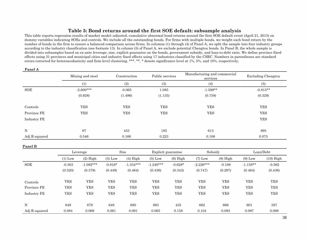
Panel A of Table 5 shows the results from the subsample tests. We find that the decline in
bond returns is more pronounced for firms in the mining and steel sectors and manufacturing and
commercial service sectors but insignificant for firms in construction and public services.
Moreover, the results in column (5) show that our results hold after excluding bonds issued by
Chengtou firms.
[Insert Table 5 about here]
Next, we divide the sample into subsamples based on ex-ante leverage, size, explicit
guarantee on the bonds (i.e., a bond has a guarantor), government subsidy, and loan-to-debt ratio.
The results are reported in Panel B of Table 5. Columns (1) and (2) suggest that the lifting of
implicit guarantees affects bondholders of financially risky firms more severely. Columns (3) and
(4) suggest that larger firms are more affected by the loss of implicit guarantees as SOE firms are
usually larger firms. Columns (5) through (10) show that bonds with a lower explicit guarantee,
government subsidy, and loan-to-debt ratio are more affected by the default, indicating that firms
relying more on other forms of finance/financial support could be flexible enough to substitute
these supports for implicit guarantees. Taken together, the heterogeneous responses of bond
returns suggest that the value of implicit government guarantees is more important for firms with
a higher default risk and firms with fewer alternative sources of financial support.
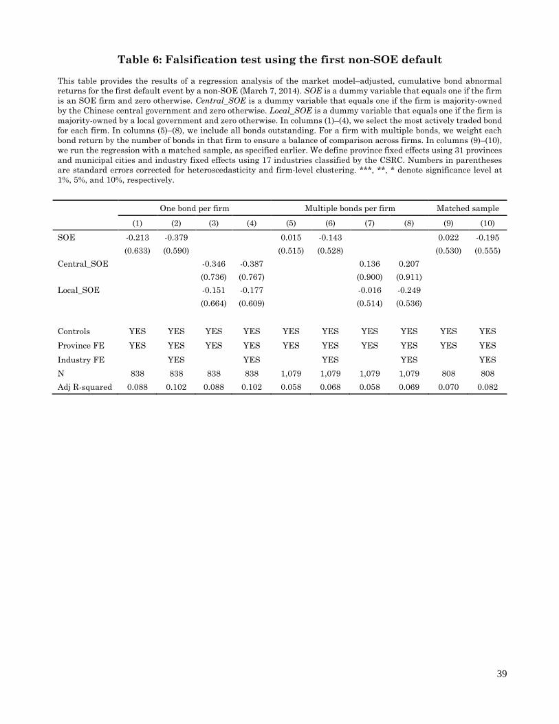
To further confirm that the negative abnormal returns of SOE bonds are due to the unique
effect of the reduction of guarantees on SOEs, we conduct a falsification test. Specifically, we
17 We retrieved a list of potential Chengtou firms from industry experts. We checked the company names manually
and excluded Chengtou firms from our sample.

20
define a pseudo-event: the first corporate bond default by a non-SOE, Shanghai Chaori Solar
Energy, on March 7, 2014. This event is similar to the Tianwei default not only because it
symbolizes the first default of its kind (SOE versus non-SOE) but also because both defaults
operate in the solar power sector. However, since non-SOEs are not believed to have implicit
guarantees in the first place, we should not observe any differential abnormal returns on SOEs and
non-SOEs. We compute CAR for SOE and non-SOE bonds around the pseudo-event using the
market model, then regress them on SOE dummies, bond and issuing-firm characteristics, and
province and/or industry fixed effects. The results reported in Table 6 indeed show that none of
the SOE dummies is significant.
[Insert Table 6 about here]
One remaining concern is that the government would bail out an SOE because the
government itself is a large shareholder in the firm rather than the firm being systemically
important. What we want to capture is the effect of the latter. To differentiate these effects, we
explicitly control for equity ownership by the government. Specifically, we replace the three SOE
dummies (SOE, Central SOE, Local SOE) with the exact ownership by, first, both central and local
governments and, second, central government and local governments separately. The results are
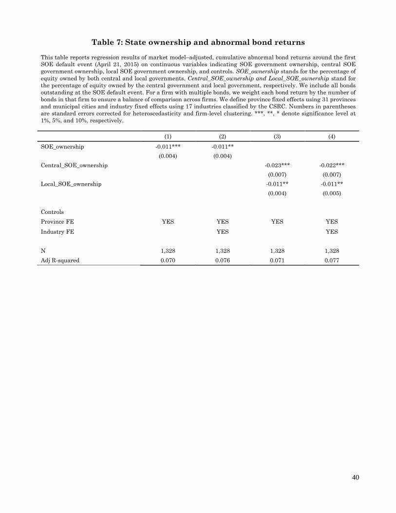
reported in Table 7. Columns (1) and (2) indicate that a 50% increase in state ownership holdings
leads to a 55 basis points reduction in abnormal returns. To interpret this finding, an absolute
majority holding by the government produces only a 0.65% bond value, around one-third of the
total value of the guarantees we estimated earlier (1.45% to 1.77%). Therefore, this evidence does
not alter our interpretation that most of the loss in value of a corporate bond is derived from implicit,
rather than explicit, government guarantees.
[Insert Table 7 about here]
21
V.2. Real Effects of Implicit Guarantees
A. Corporate investment
Our evidence so far has shown that bond prices of SOEs react negatively to the Tianwei
default event, indicating that the reduction of implicit guarantees results in higher borrowing costs
for SOEs. This may exacerbate the financial constraints faced by SOEs and lead to a reduction in
investment. To test this conjecture, we adopt DID tests of firms’ investment policies, as specified
in equations (2) and (3), with firm and time fixed effects to account for unobservable
heterogeneity.18
Table 8 presents the results using three different measures of investment (all scaled by
lagged total assets): capital expenditures are shown in columns (1) through (3), capital
expenditures plus investments in intangible assets in columns (4) through (6), and capital
expenditures plus investments in intangible assets plus cash acquisitions in columns (7) through
(9). For the sake of brevity, we describe the results controlling only for firm and time fixed effects.
On average, after the Tianwei default, the reduction in capital expenditures, in capital expenditures
plus investment in intangibles, and in capital expenditures plus investment in intangibles plus cash
acquisitions amounts to 1.6%, 1.6%, and 1.9%, respectively.19 Note that since we are using
semiannual variables, these estimates double in annualized terms.
[Insert Table 8 about here]
18 All our empirical results in this section are robust to control for industry×year fixed effects. 19 We run the same regressions after deleting potential Chengtou firms. In untabulated results, the reduction for the
three investment measures amounts to 1.5%, 1.3%, and 1.5%, respectively, all significant at the 1% level.

22
We further conduct a PSM algorithm to ensure the robustness of our finding. We match
SOEs and non-SOEs on observable characteristics to ensure that the two groups of firms are not
systematically different before the Tianwei event – specifically, in the first stage we estimate, for
each firm, the propensity score of being a non-SOE. The estimation is based on a Logit model, in
which the dependent variable equals one when the firm is a non-SOE and zero otherwise; the
control variables include firm size, ROA, sales growth, leverage, tangibility, and 17 industry fixed
effects. The first-stage Logit regression results are presented in Appendix Table A.II. The
estimated coefficients are used to compute the fitted probability of being a non-SOE. Then we
perform a nearest-neighbor, one-to-one match – that is, we match each non-SOE with an SOE that
has the closest value of propensity score with replacement. The results are reported in columns (3),
(6), and (9) in Table 8 for the three investment measures, respectively. We find that the coefficients
are even larger than those based on the entire sample (and statistically significant). Specifically,
the respective reduction in the three investment measures is 2.6%, 3.1%, and 3.3%, respectively.
To verify whether the parallel trend assumption – that the outcome variable of non-SOEs
is parallel to that of SOEs before the event – holds for our analysis, we examine the time dynamics
of the effect of the Tianwei event on corporate investment in Table 9. We interact the SOE dummy
with period dummy variables indicating the two semiannual periods before the event and the three
semiannual periods after the event. The insignificant coefficients for the pre-treatment periods
indicate that the investments of SOEs and non-SOEs are not substantially different from each other
compared to the benchmark period (i.e., the six-month period ending December 31, 2013). The
evidence ensures that the identification assumption holds in our DID regressions. We also perform
the same set of regressions using a PSM sample. Compared with the whole sample regressions,
23
the parallel trend before the event is even better satisfied (coefficient magnitudes are smaller), and
the decline in investment after the event is more salient (coefficient magnitudes are larger).
[Insert Table 9 about here]
To further rule out any concern about endogeneity regarding the investment results, we
apply the placebo DIP test using the first non-SOE default. The identifying assumptions are similar
to those we use when we conduct a similar analysis using bond returns. If what we document were
due to an industry-wide shock or a macro-level structural change, we should observe similar
findings using the pseudo-event. We use the PSM sample to conduct the placebo test and present
the results in Appendix Table A.III. The results show that, after the Chaori default, the decline in
corporate investment of SOEs is economically small and statistically insignificant. This buttresses
our previous inference that the decline in corporate investment after the Tianwei default is uniquely
due to the loss of implicit guarantees.
B. Debt issuance and cash holdings
In addition to documenting the real effects on investment activities, we explore how the
loss of implicit guarantees impacts firms’ financing and cash policies. Specifically, we examine
firms’ net debt issuance (debt issuance minus debt retirement) and cash balance, both scaled by
lagged total book assets. After the Tianwei default, SOEs may choose to rely more on internally
generated cash flows to finance investment activities as the cost of financing through bond markets
rises. As a result, firms are expected to issue less debt and keep a larger cash balance. In Table 10,
we use the whole sample in columns (1) and (2) for net debt issuance and in columns (4) and (5)
for cash holdings. Furthermore, column (3) and column (6) use the PSM sample for net debt
issuance and cash holdings, respectively.
[Insert Table 10 about here]

24
Table 10 shows that, on average, SOEs reduce net debt issuance by 0.3% to 0.7% of total
assets in each semiannual period, compared with non-SOEs. In annualized terms, this amounts to
0.6% to 1.4% of the total assets of SOE firms. Given that the average asset size of SOEs is 52
billion CNY, the total reduction in annual bond issuance amounts to 300 to 800 million CNY.
Moreover, after controlling for firm and semiannual year fixed effects, we find that, after the
default of Tianwei, average cash holdings of SOEs increase by 0.8% of total assets relative to non-
SOEs (1.6% annually). Using a PSM sample generates similar results. The evidence reveals SOEs’
inability to maintain sufficient financing from the debt market and their greater reliance on internal
cash as an alternative financing policy. A higher level of cash holdings also suggests that they
decide to operate more conservatively after the loss of government support.
C. Investment efficiency
Our evidence so far suggests that SOEs reduce investment, issue less debt for financing,
and hoard more cash on their balance sheets after a reduction in the provision of implicit guarantees
resulting in hardened budget constraint for SOEs. However, it remains unclear whether the
reduction or the removal of implicit guarantees helps reinforce the disciplinary role of debt for
corporate managers such that managers invest more efficiently. On the one hand, a reduction in
implicit guarantees leads to an increase in corporate financing costs and, thus, exacerbates a firm’s
financing constraints. Shouldering policy burdens, SOEs may forgo growth opportunities, and
investment efficiency decreases as a result. On the other hand, when SOEs’ budget constraints are
hardened, managers facing higher funding costs have a greater incentive to improve investment
efficiency and avoid possible defaults. Investment efficiency improves as a result of the
strengthening disciplinary effects of debt.

25
Because our sample contains mostly private firms whose q values cannot be computed, we
are not able to use the investment-q sensitivity to examine investment efficiency (Hayashi, 1982;
Blundell, et al., 1992). We instead follow Biddle, Hilary, and Verdi (2009) to measure under- and
over-investment relative to a benchmark level to determine investment efficiency. Specifically, we
estimate the following regression model at the industry-semiannual level:
𝐼𝑛𝑣𝑒𝑠𝑡𝑚𝑒𝑛𝑡𝑖,𝑡 = α + 𝛽 × 𝑆𝑎𝑙𝑒𝑠 𝑔𝑟𝑜𝑤𝑡ℎ𝑖,𝑡−1 + 𝜀𝑖,𝑡, (4)
Investment is measured by the total of capital expenditures, investments in intangibles, and
acquisitions, scaled by lagged assets.
After obtaining regression estimates, we classify the firm-semiannual observations into
four quintiles based on the residuals for each industry-semiannual. Firms whose residuals are in
the top quintile are treated as overinvesting firms, while firms whose residuals are in the bottom
quintile are regarded as underinvesting firms. The middle two quintiles are used as benchmarks.
Using the two indicators of over- or underinvesting as dependent variables, we then apply the
difference-in-differences analysis to estimate the likelihood of a firm overinvesting or
underinvesting as opposed to the benchmark quintiles.
Table 11 report the difference-in-difference regression results.20 Compared with non-
SOEs, SOEs are less likely to over-invest or under-invest after the Tianwei default. The evidence
suggests that SOEs make less abnormal investment relative to the benchmark group after the
Tianwei default, potentially reflecting SOE’s optimal response to investment opportunities. To
determine whether such changes in abnormal investment reflect improvement in investment
efficiency, we provide further evidence on the asset turnover between SOEs and non-SOEs in the
20 The over-investing sample drops the observations in the bottom quintiles, while the under-investing sample drops
the observations in the top quintile. That is number of observations in Table 11 is smaller than that in Table 8.
26
post-Tianwei period, We further find, in Table 12, that SOEs enjoy a significant gain in their
asset turnover ratio, indicating SOEs become more efficient in utilizing their assets. Taken
together, the evidence is consistent with the disciplinary effects induced by the removal of soft
budget constraint.
[Insert Tables 11, 12 about here]
VI. Conclusion
We exploit the first bond default by a large SOE in China – Baoding Tianwei Group – to study
the effects of the government’s implicit guarantees on corporate investment and financing policies.
We first adopt an event study around the default date of Tianwei to estimate the value of
implicit guarantees and find that they account for 1.45% to 1.77% of SOEs’ bond value. This
translates into a total value of 93 billion CNY (15 billion USD) in China’s domestic bond markets
for the corporate sector. Our estimate of the value of implicit guarantees provides a lower bound
of the true value. Our results show that the reduction in implicit guarantees is more pronounced
for firms in industries experiencing overcapacity and firms with high default risk, firms that receive
lower government subsidies, and firms that rely more heavily on bond financing.
Our DID tests, which include both firm and time fixed effects to account for unobservable
heterogeneity, show that SOEs subsequently reduce their investment more than non-SOEs. In
response to the reduction in implicit guarantees, SOEs borrow less in external financing markets
and hoard more cash on their balance sheets. We adopt a number of robustness tests to further
support our empirical findings.
27
Finally, we find that the investment efficiency of SOEs improves after the reduction of implicit
guarantees, suggesting that moral-hazard problems arising from soft budget constraints are
lessened as managers become more disciplined. This finding is consistent with the long-run
objective of the Chinese government – to develop a more market-oriented economy and improve
the long-term value of corporations.

28
References
Acharya, V. V., D. Anginer, and A. J. Warburton, 2016. The end of market discipline? Investor
expectations of implicit government guarantees, working paper, NYU.
Almeida, H., M. Campello, B. Laranjeira, and S. Weisbenner, 2012. Corporate debt maturity and the
real effects of the 2007 credit crisis, Critical Finance Review 1: 3–58.
Ang, A., J. Bai, and H. Zhou, 2016. The great wall of debt: real estate, political risk, and Chinese local
government credit spreads, working paper, SSRN 2603022
Bessembinder, H., K. M. Kahle, W. F. Maxwell, and D. Xu, 2009. Measuring abnormal bond
performance, Review of Financial Studies 22: 4219–4258.
Biddle, G.C., Hilary, G. and Verdi, R.S., 2009. How does financial reporting quality relate to
investment efficiency?. Journal of Accounting and Economics, 48(2-3), 112-131.
Billett, M. T., T. H. D. King, and D. C. Mauer, 2004. Bondholder wealth effects in mergers and
acquisitions: New evidence from the 1980s and 1990s, The Journal of Finance 59: 107–135.
Blundell R., S. Bond, M. Devereux and F. Schiantarelli, 1992. Investment and Tobin’s Q: Evidence
from company panel data. Journal of Econometrics, 51(1-2):233-257.
Campello, M., J. R. Graham, and C. R. Harvey, 2010. The real effects of financial constraints:
Evidence from a financial crisis, Journal of Financial Economics 97: 470–487.
Chen, Z., Z. He, and C. Liu, 2017. The financing of local government in China: stimulus loan wanes
and shadow banking waxes, working paper.
Demirgüç-Kunt, A., and E. Detragiache, 2002. Does deposit insurance increase banking system
stability? An empirical investigation, Journal of Monetary Economics 49: 1373–1406.
Faccio, M., R. W. Masulis, and J. McConnell, 2006. Political connections and corporate bailouts, The
Journal of Finance 61: 2597–2635.
Farre-Mensa, J., and A. Ljungqvist, 2015. Do measures of financial constraints measure financial
constraints? Review of Financial Studies 29: 271–308.
Fazari, S., G. Hubbard, and B. Petersen, 1988. Financing constraints and corporate investment,
Brookings Papers on Economic Activity 19: 141–95.
Ghandi, P. and H. Lustig, 2015. Size anomalies in U.S. bank stock returns, Journal of Finance 70:
733–768.
Hayashi, F., 1982. Tobin’s marginal q and average q: A neoclassical interpretation. Econometrica, 50:
213-224.
29
Hoshi T., A. Kashyap, and D. Scharfstein, 1991. Corporate structure, liquidity, and investment:
Evidence from Japanese industrial groups, Quarterly Journal of Economics 106: 33-60.
Jensen, Michael C. (1986), “Agency Costs of Free Cash Flow, Corporate Finance, and Takeovers,”
American Economic Review, 76: 323-29.
Jensen, M.C. and W.H. Meckling, 1976, Theory of the firm: managerial behavior, agency costs and
ownership structure, Journal of Financial Economics 3: 305-360
Kaplan, S., and L. Zingales, 1997. Do investment-cash flow sensitivities provide useful measures of
financing constraints? Quarterly Journal of Economics 112: 169–215.
Kelly, B., H. Lustig, and S. Van Nieuwerburgh, 2016. Too-systematic-to-fail: what option markets
imply about sector-wide government guarantees, American Economic Review 106: 1278-1319.
Klein, A. and Zur, E., 2011. The impact of hedge fund activism on the target firm’s existing
bondholders. Review of Financial Studies 24: 1735–1771.
Kornai, J., 1986. The soft budget constraint, Kyklos 39: 3–30.
Liao, L., B. Liu, and H. Wang, 2014. China׳s secondary privatization: Perspectives from the Split-
Share Structure Reform, Journal of Financial Economics 113: 500–518.
Lin, J. Y., and G. Tan, 1999. Policy burdens, accountability, and the soft budget constraint, The
American Economic Review 89: 426–431
Mariathasan M., M. Ouarda, and C. Werger, 2014. Bailouts and moral hazard: How implicit
government guarantees affect financial stability, working paper.
Maskin, E., and C. Xu, 2001. Soft budget constraint theories: From centralization to the
market, Economics of transition 9: 1-27.
Moody’s, 2011. Quantifying the value of implicit government guarantees for large financial
institutions, Modelling Methodology, Moody’s Analytics.
Moody’s, 2014. Government-related issuers, Moody’s Investors Service.
Moody’s, 2016a. Moody’s support assumptions for entities owned by Chinese RLGs, Moody’s
Investors Service.
Moody’s, 2016b. FAQ: RLG’s approach to supporting distressed state-owned enterprise, Moody’s
Investors Service.
Tsesmelidakis, Z., and R. C. Merton, 2013. The value of implicit guarantees, working paper, MIT.
Ueda, K., and B. W. di Mauro, 2012. Quantifying structural subsidy values for systematically
important financial institutions, IMF working paper.
Veronesi, P., and L. Zingales, 2010. Paulson’s gift, Journal of Financial Economics 97, 339–368.
30
Whited, T. M., 1992. Debt, liquidity constraints, and corporate investment, evidence from panel data,
Journal of Finance, 47: 1425–1460.
Whited, T., and G. Wu, 2006. Financial constraints risk, Review of Financial Studies 19: 531–59.
Whited, T. and J. Zhao, 2016. The misallocation of finance, working paper, SSRN 2699817.
Zhu, N, 2016. China’s Guaranteed Bubble, McGraw-Hill

31
Figure 1: Total amount of new bond issues by Chinese enterprises
This figure presents the total amount of new issuance of corporate bonds, enterprise bonds and MTNs in
billions of CNY between 2000 and 2016.
0
500
1000
1500
2000
2500
3000
2000 2001 2002 2003 2004 2005 2006 2007 2008 2009 2010 2011 2012 2013 2014 2015 2016
Yearly issuance (Billion CNY)
Corporate Bond Enterprise Bond MTN

32
Figure 2: Timeline of the first SOE default event
33
Figure 3a: Number of defaults by Chinese firms from first half of 2014 to second half of 2016
Figure 3b: Value of defaults by Chinese firms from first half of 2014 to second half of 2016
0
5
10
15
20
25
30
35
40
45
First 2014 Second 2014 First 2015 Second 2015 First 2016 Second 2016
Number of defaults
All Local SOE Central SOE Non-SOE
0
5000
10000
15000
20000
25000
First 2014 Second 2014 First 2015 Second 2015 First 2016 Second 2016
Value of defaults (Face value million CNY)
All Local SOE Central SOE Non-SOE
34
Table 1: Summary statistics
This table provides the summary statistics of bond characteristics and firm characteristics. Panel A reports the
summary statistics of bond characteristics for SOE and non-SOE bonds, respectively. We restrict our sample to the
bonds used for the event study. In Panel B, we report issuing-firm characteristics before the first SOE default event
(April 21, 2015) for SOEs and non-SOEs separately. All values are winsorized at the 1% and 99% level. ***, **, *
denote significance level at 1%, 5%, and 10%, respectively.
Panel A Bond characteristics
SOE bonds Non-SOE bonds Difference
N=1,118 N=269
Mean Median Std Mean Median Std Difference t-statistics
Coupon rate (%) 6.58 6.71 1.06 6.33 6.20 1.13 0.25*** 2.74
Yield spread (%) 6.48 6.12 2.43 5.99 5.61 2.07 0.49*** 3.30
Issue amount (billion CNY) 1.44 1.10 1.45 1.19 0.80 1.07 0.64*** 3.34
Credit rating 16.22 16.00 1.51 16.20 16.00 1.69 0.02 0.19
Maturity 4.22 4.00 2.18 2.56 2.00 1.72 1.66*** 13.48
Duration 3.88 3.87 1.61 2.67 2.56 1.38 1.21*** 11.54
Panel B Firm characteristics
SOE firms Non-SOE firms Difference
N=2,927 N=1,570
Mean Median Std Mean Median Std Difference t-statistics
Log(Assets) 23.70 23.60 1.09 23.36 23.35 1.57 0.34*** 16.67
Leverage 0.55 0.56 0.17 0.59 0.62 0.16 –0.04*** -22.36
ROA(%) 1.23 0.88 1.83 2.54 1.96 3.05 –1.31*** -31.57
Tangibility 0.16 0.08 0.19 0.22 0.18 0.19 –0.06*** -22.53
Cash flow 0.00 0.01 0.06 0.02 0.02 0.06 –0.02*** -21.28
Cash holding 0.11 0.09 0.08 0.12 0.10 0.10 –0.01*** -12.02
Net debt issuance -0.07 -0.05 0.08 -0.11 -0.09 0.10 0.04*** 28.56
Capex 0.06 0.03 0.10 0.09 0.05 0.14 –0.03*** -13.12
Acquisitions 0.00 0.00 0.01 0.00 0.00 0.03 0.00*** 5.58
Intangible investment 0.07 0.02 0.13 0.05 0.03 0.10 0.02** -2.10
Mining and steel 0.05 0.00 0.22 0.07 0.00 0.26 –0.02 1.23
Construction 0.37 0.00 0.48 0.05 0.00 0.21 0.32*** 9.09
Public services 0.14 0.00 0.35 0.04 0.00 0.20 0.10*** 3.77
Commercial services 0.09 0.00 0.28 0.60 1.00 0.49 –0.51*** -19.23

35
Table 2: Bond returns around the first SOE default
This table presents bond (abnormal) returns based on five different measures in the trading window [–30,+30], where date 0 is April 21, 2015. In Panel A, we
subtract the CSI Aggregate Bond Index returns from bond raw returns. In Panel B, we report abnormal bond returns using a market model (with CSI
Aggregate Bond Index returns to proxy for market returns), with an estimation window of 200 days (day –240 to day –41). In Panel C, we follow Klein and Zur
(2011) to construct matched bond returns. For each non-SOE bond, we select matched SOE bonds based on industry, rating, and years to maturity and report
the difference in returns between the non-SOE bonds and SOE bonds. The numbers in parentheses are standard errors. ***, **, * denote significance level at
1%, 5%, and 10%, respectively.
Panel A: Raw bond returns in excess of market returns (%)
SOE Non-SOE Difference
Mean Mean Mean
CAR (–30,+30) -2.161*** -1.253*** -0.909***
t-statistics (-17.643) (-9.841) (-3.244)
No. of observations 1,187 237
Panel B: Abnormal bond returns with market model (%)
SOE Non-SOE Difference
Mean Mean Mean
CAR (–30,+30) -1.468*** -0.254 -1.213***
t-statistics (-8.189) (-1.105) (-2.874)
No. of observations 1,130 216
Panel C: Matched raw bond returns in excess of market returns (%)
SOE Non-SOE Difference
Mean Mean Mean
CAR(-30,+30) -2.544*** -1.230*** -1.314***
t-statistics (-13.507) (-8.950) (-3.969)
No. of observations 633 218

36
Table 3: Abnormal bond returns of SOEs vs. non-SOEs This table reports regression results of market model–adjusted, cumulative abnormal bond returns around the 1st SOE default event (April 21, 2015) on
dummy variables indicating SOEs, central SOEs, local SOEs, and controls. In columns (1) through (4), we select the most actively traded bond for each issuing
firm. In columns (5) through (8), we include all the outstanding bonds. For firms with multiple bonds, we weight each bond return by the number of bonds in
the firm to ensure a balanced comparison across firms. In columns (9) through (10), we run the regression with a matched sample. We define province fixed
effects using 31 provinces and municipal cities and industry fixed effects using 17 industries classified by the CSRC. Numbers in parentheses are standard
errors corrected for heteroscedasticity and firm-level clustering. ***, **, * denote significance level at 1%, 5%, and 10%, respectively.
One bond per firm Multiple bonds per firm Matched sample
(1) (2) (3) (4) (5) (6) (7) (8) (9) (10)
SOE -0.960*** -1.043*** -1.229** -1.251** -1.766*** -1.450***
(0.326) (0.334) (0.442) (0.582) (0.443) (0.426)
Central_SOE -1.466*** -1.534*** -1.511** -1.645**
(0.424) (0.438) (0.571) (0.718)
Local_SOE -0.898*** -0.940*** -1.204** -1.182*
(0.339) (0.346) (0.444) (0.594)
Month_to_maturity 0.200 0.213 0.202 0.217 0.123 0.142 0.126 0.149 0.235 0.352 (0.185) (0.185) (0.185) (0.185) (0.198) (0.193) (0.199) (0.193) (0.329) (0.342)
Issued amount/assets -0.010 -0.032 -0.009 -0.030 -0.020 -0.044** -0.019 -0.043* -5.977 -6.324
(0.034) (0.035) (0.034) (0.035) (0.025) (0.020) (0.025) (0.020) (4.974) (5.119)
Coupon -1.037*** -1.041*** -1.047*** -1.045*** -1.007** -0.985** -1.015** -0.991** -1.244*** -1.221***
(0.199) (0.202) (0.199) (0.202) (0.414) (0.441) (0.412) (0.439) (0.244) (0.246)
Rating -0.176 -0.228 -0.153 -0.207 -0.203 -0.266 -0.193 -0.253 -0.080 -0.250
(0.261) (0.264) (0.263) (0.265) (0.240) (0.226) (0.236) (0.222) (0.358) (0.384)
Leverage -1.956* -2.314* -1.901* -2.278* -2.087 -2.391* -2.070 -2.366* -3.074** -3.952**
(1.142) (1.220) (1.150) (1.225) (1.335) (1.209) (1.333) (1.198) (1.548) (1.708)
ROA 0.017 -0.027 0.027 -0.018 -0.038 -0.088 -0.034 -0.084 -0.175 -0.207
(0.071) (0.076) (0.072) (0.077) (0.055) (0.054) (0.056) (0.054) (0.116) (0.120)
Size -0.261 -0.258 -0.256 -0.243 -0.250 -0.254 -0.244* -0.238 -0.433 -0.342
(0.161) (0.164) (0.161) (0.164) (0.143) (0.206) (0.134) (0.198) (0.264) (0.261)
Tangibility 1.348* 0.767 1.523** 0.864 0.880 -0.253 0.980 -0.180 0.403 -0.544
(0.744) (0.941) (0.751) (0.941) (0.556) (0.551) (0.581) (0.599) (1.190) (1.633)
Province FE YES YES YES YES YES YES YES YES YES YES
Industry FE YES YES YES YES YES
N 1,039 1,039 1,039 1,039 1,328 1,328 1,328 1,328 841 841
Adj R-squared 0.107 0.114 0.107 0.115 0.070 0.077 0.071 0.078 0.084 0.092

37
Table 4: Abnormal bond returns of SOEs vs. non-SOEs: robustness This table reports regression results of market model–adjusted, cumulative abnormal bond returns around the 1st
SOE default event (April 21, 2015) on dummy variables indicating SOEs, central SOEs, local SOEs, and controls. In
columns (1) through (4), we delete all enterprise bonds from the original sample while in columns (5) through (8), we
add all MTN bonds into the sample. We select the most actively traded bond for each issuing firm in column (1), (2),
(5) and (6). In columns (3), (4), (7) and (8), we include all the outstanding bonds. For firms with multiple bonds, we
weight each bond return by the number of bonds in the firm to ensure a balanced comparison across firms. We define
province fixed effects using 31 provinces and municipal cities and industry fixed effects using 17 industries classified
by the CSRC. Numbers in parentheses are standard errors corrected for heteroscedasticity and firm-level clustering.
***, **, * denote significance level at 1%, 5%, and 10%, respectively.
Corporate bonds only Corporate+Enterprise+MTN
One bond per firm Multiple bonds per firm One bond per firm Multiple bonds per firm
(1) (2) (3) (4) (5) (6) (7) (8)
SOE -2.300** -2.818*** -0.780*** -0.780***
(0.775) (0.767) (0.226) (0.204)
Central_SO
E -3.423** -3.319*** -0.686*** -0.686***
(1.444) (0.956) (0.172) (0.193)
Local_SOE -2.154** -2.713*** -0.809*** -0.809***
(0.797) (0.862) (0.262) (0.235)
Controls YES YES YES YES YES YES YES YES
Province FE YES YES YES YES YES YES YES YES
Industry FE YES YES YES YES YES YES YES YES
N 715 715 890 890 3,378 3,378 3,376 3,376
R-square 0.102 0.110 0.089 0.089 0.033 0.033 0.033 0.033
38
Table 5: Bond returns around the first SOE default: subsample analysis This table reports regression results of market model–adjusted, cumulative abnormal bond returns around the first SOE default event (April 21, 2015) on
dummy variables indicating SOEs and controls. We include all the outstanding bonds. For firms with multiple bonds, we weight each bond return by the
number of bonds in the firm to ensure a balanced comparison across firms. In columns (1) through (4) of Panel A, we split the sample into four industry groups
according to the industry classification (see footnote 13). In column (5) of Panel A, we exclude potential Chengtou bonds. In Panel B, the whole sample is
divided into subsamples based on ex-ante leverage, size, explicit guarantee on the bonds, government subsidy, and loan-to-debt ratio. We define province fixed
effects using 31 provinces and municipal cities and industry fixed effects using 17 industries classified by the CSRC. Numbers in parentheses are standard
errors corrected for heteroscedasticity and firm-level clustering. ***, **, * denote significance level at 1%, 5%, and 10%, respectively.
Panel A
Mining and steel Construction Public services Manufacturing and commercial
services Excluding Chengtou
(1) (2) (3) (4) (5)
SOE -2.600*** -0.065 1.085 -1.599** -0.815**
(0.928) (1.496) (1.135) (0.758) (0.329)
Controls YES YES YES YES YES
Province FE YES YES YES YES YES
Industry FE YES
N 97 433 185 613 895
Adj R-squared 0.546 0.166 0.223 0.106 0.075
Panel B
Leverage Size Explicit guarantee Subsidy Loan/Debt
(1) Low (2) High (3) Low (4) High (5) Low (6) High (7) Low (8) High (9) Low (10) High
SOE -0.303 -1.082*** -0.816* -1.334*** -1.240*** -0.628* -2.226*** -0.198 -1.158** -0.562
(0.520) (0.379) (0.449) (0.464) (0.436) (0.343) (0.747) (0.297) (0.464) (0.436)
Controls YES YES YES YES YES YES YES YES YES YES
Province FE YES YES YES YES YES YES YES YES YES YES
Industry FE YES YES YES YES YES YES YES YES YES YES
N 649 679 648 680 893 435 662 666 601 587
Adj R-squared 0.084 0.069 0.061 0.091 0.065 0.158 0.104 0.093 0.097 0.098
39
Table 6: Falsification test using the first non-SOE default
This table provides the results of a regression analysis of the market model–adjusted, cumulative bond abnormal
returns for the first default event by a non-SOE (March 7, 2014). SOE is a dummy variable that equals one if the firm
is an SOE firm and zero otherwise. Central_SOE is a dummy variable that equals one if the firm is majority-owned
by the Chinese central government and zero otherwise. Local_SOE is a dummy variable that equals one if the firm is
majority-owned by a local government and zero otherwise. In columns (1)–(4), we select the most actively traded bond
for each firm. In columns (5)–(8), we include all bonds outstanding. For a firm with multiple bonds, we weight each
bond return by the number of bonds in that firm to ensure a balance of comparison across firms. In columns (9)–(10),
we run the regression with a matched sample, as specified earlier. We define province fixed effects using 31 provinces
and municipal cities and industry fixed effects using 17 industries classified by the CSRC. Numbers in parentheses
are standard errors corrected for heteroscedasticity and firm-level clustering. ***, **, * denote significance level at
1%, 5%, and 10%, respectively.
One bond per firm Multiple bonds per firm Matched sample
(1) (2) (3) (4) (5) (6) (7) (8) (9) (10)
SOE -0.213 -0.379 0.015 -0.143 0.022 -0.195
(0.633) (0.590) (0.515) (0.528) (0.530) (0.555)
Central_SOE -0.346 -0.387 0.136 0.207
(0.736) (0.767) (0.900) (0.911)
Local_SOE -0.151 -0.177 -0.016 -0.249
(0.664) (0.609) (0.514) (0.536)
Controls YES YES YES YES YES YES YES YES YES YES
Province FE YES YES YES YES YES YES YES YES YES YES
Industry FE YES YES YES YES YES
N 838 838 838 838 1,079 1,079 1,079 1,079 808 808
Adj R-squared 0.088 0.102 0.088 0.102 0.058 0.068 0.058 0.069 0.070 0.082
40
Table 7: State ownership and abnormal bond returns
This table reports regression results of market model–adjusted, cumulative abnormal bond returns around the first
SOE default event (April 21, 2015) on continuous variables indicating SOE government ownership, central SOE
government ownership, local SOE government ownership, and controls. SOE_ownership stands for the percentage of
equity owned by both central and local governments. Central_SOE_ownership and Local_SOE_ownership stand for
the percentage of equity owned by the central government and local government, respectively. We include all bonds
outstanding at the SOE default event. For a firm with multiple bonds, we weight each bond return by the number of
bonds in that firm to ensure a balance of comparison across firms. We define province fixed effects using 31 provinces
and municipal cities and industry fixed effects using 17 industries classified by the CSRC. Numbers in parentheses
are standard errors corrected for heteroscedasticity and firm-level clustering. ***, **, * denote significance level at
1%, 5%, and 10%, respectively.
(1) (2) (3) (4)
SOE_ownership -0.011*** -0.011**
(0.004) (0.004)
Central_SOE_ownership -0.023*** -0.022***
(0.007) (0.007)
Local_SOE_ownership -0.011** -0.011**
(0.004) (0.005)
Controls
Province FE YES YES YES YES
Industry FE YES YES
N 1,328 1,328 1,328 1,328
Adj R-squared 0.070 0.076 0.071 0.077

41
Table 8: The effect of implicit guarantees on investment
This table presents the results of the DID regressions on corporate investment between SOEs and non-SOEs from before and after the Tianwei default. The
dependent variable is capital expenditures scaled by lagged assets for columns (1) through (3), capital expenditures and investments in intangibles scaled by
lagged assets for columns (4) through (6), and capital expenditures, investments in intangibles, and acquisitions scaled by lagged assets for columns (7) through
(9) in a semiannual frequency. Columns (3), (6), and (9) use PSM matched sample. Control variables include cash flow and lagged size, ROA, sales growth,
leverage, and tangibility. The first stage estimation of PSM is based on a Logit model, in which the dependent variable equals one when the firm is an SOE and
zero otherwise, and the control variables include size, ROA, sales growth, cash flow, leverage, tangibility, and industry fixed effect. The estimated coefficients
are used to compute the fitted probability of being an SOE. Then we perform a nearest-neighbor, one-to-one match – that is, we match each non-SOE with an
SOE that has the closest value of propensity score with replacement. Post is a dummy variable that equals one for the three semiannual periods after April 21,
2015 (excluding June 30, 2015), and zero for the three semiannual periods before that. SOE is a dummy variable that equals one if the firm is an SOE and zero
otherwise. Numbers in parentheses are standard errors corrected for heteroscedasticity and firm-level clustering. ***, **, * denote significance level at 1%, 5%,
and 10%, respectively.
Capex Capex+Intangible Capex+Intangible+Acquisition
(1) (2) (3) (4) (5) (6) (7) (8) (9)
SOE*Post -0.015*** -0.016*** -0.026*** -0.015*** -0.016*** -0.031*** -0.018*** -0.019*** -0.033***
(0.004) (0.004) (0.003) (0.004) (0.005) (0.004) (0.005) (0.005) (0.004)
SOE Dummy -0.013 -0.017* -0.020*
(0.010)
(0.010) (0.010)
Firm-level Controls YES YES YES YES YES YES YES YES YES
Semiannual FE YES YES YES YES YES YES YES YES YES
Industry FE YES
YES
YES
Firm FE YES YES YES YES YES YES
PSM
YES
YES
YES
N 22,139 22,139 12,293 22,139 22,139 12,293 22,139 22,139 12,293
Adj R-square 0.084 0.517 0.519 0.090 0.496 0.509 0.093 0.492 0.506
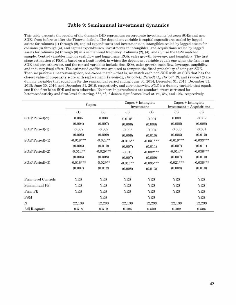
42
Table 9: Semiannual investment dynamics
This table presents the results of the dynamic DID regressions on corporate investments between SOEs and non-
SOEs from before to after the Tianwei default. The dependent variable is capital expenditures scaled by lagged
assets for columns (1) through (2), capital expenditures and investments in intangibles scaled by lagged assets for
columns (3) through (4), and capital expenditures, investments in intangibles, and acquisitions scaled by lagged
assets for columns (5) through (6) in a semiannual frequency. Columns (2), (4), and (6) use the PSM matched
sample. Control variables include cash flow and lagged size, ROA, sales growth, leverage, and tangibility. The first
stage estimation of PSM is based on a Logit model, in which the dependent variable equals one when the firm is an
SOE and zero otherwise, and the control variables include size, ROA, sales growth, cash flow, leverage, tangibility,
and industry fixed effect. The estimated coefficients are used to compute the fitted probability of being an SOE.
Then we perform a nearest-neighbor, one-to-one match – that is, we match each non-SOE with an SOE that has the
closest value of propensity score with replacement. Period(–2), Period(–1), Period(+1), Period(+2), and Period(+3) are
dummy variables that equal one for the semiannual period ending June 30, 2014; December 31, 2014; December 31,
2015; June 30, 2016; and December 31, 2016, respectively, and zero otherwise. SOE is a dummy variable that equals
one if the firm is an SOE and zero otherwise. Numbers in parentheses are standard errors corrected for
heteroscedasticity and firm-level clustering. ***, **, * denote significance level at 1%, 5%, and 10%, respectively.
Capex Capex + Intangible
investment
Capex + Intangible
investment + Acquisitions
(1) (2) (3) (4) (5) (6)
SOE*Period(-2) 0.005 0.000 0.010* -0.001 0.009 -0.002
(0.004) (0.007) (0.006) (0.008) (0.006) (0.008)
SOE*Period(-1) -0.007 -0.002 -0.005 -0.004 -0.006 -0.004
(0.005) (0.009) (0.006) (0.010) (0.006) (0.010)
SOE*Period(+1) -0.018*** -0.024** -0.016** -0.031*** -0.019*** -0.033***
(0.006) (0.010) (0.007) (0.011) (0.007) (0.011)
SOE*Period(+2) -0.014** -0.029*** -0.010 -0.032*** -0.014** -0.036***
(0.006) (0.008) (0.007) (0.009) (0.007) (0.010)
SOE*Period(+3) -0.018*** -0.029** -0.017** -0.035*** -0.021*** -0.038***
(0.007) (0.012) (0.008) (0.013) (0.008) (0.013)
Firm-level Controls YES YES YES YES YES YES
Semiannual FE YES YES YES YES YES YES
Firm FE YES YES YES YES YES YES
PSM YES YES
YES
N 22,139 12,293 22,139 12,293 22,139 12,293
Adj R-square 0.518 0.519 0.496 0.509 0.492 0.506
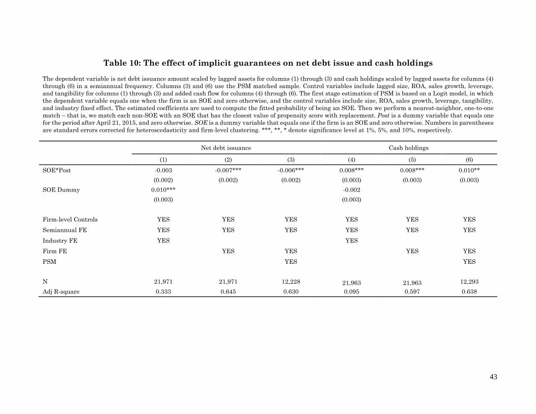
43
Table 10: The effect of implicit guarantees on net debt issue and cash holdings
The dependent variable is net debt issuance amount scaled by lagged assets for columns (1) through (3) and cash holdings scaled by lagged assets for columns (4)
through (6) in a semiannual frequency. Columns (3) and (6) use the PSM matched sample. Control variables include lagged size, ROA, sales growth, leverage,
and tangibility for columns (1) through (3) and added cash flow for columns (4) through (6). The first stage estimation of PSM is based on a Logit model, in which
the dependent variable equals one when the firm is an SOE and zero otherwise, and the control variables include size, ROA, sales growth, leverage, tangibility,
and industry fixed effect. The estimated coefficients are used to compute the fitted probability of being an SOE. Then we perform a nearest-neighbor, one-to-one
match – that is, we match each non-SOE with an SOE that has the closest value of propensity score with replacement. Post is a dummy variable that equals one
for the period after April 21, 2015, and zero otherwise. SOE is a dummy variable that equals one if the firm is an SOE and zero otherwise. Numbers in parentheses
are standard errors corrected for heteroscedasticity and firm-level clustering. ***, **, * denote significance level at 1%, 5%, and 10%, respectively.
Net debt issuance Cash holdings
(1) (2) (3) (4) (5) (6)
SOE*Post -0.003 -0.007*** -0.006*** 0.008*** 0.008*** 0.010**
(0.002) (0.002) (0.002) (0.003) (0.003) (0.003)
SOE Dummy 0.010*** -0.002
(0.003)
(0.003)
Firm-level Controls YES YES YES YES YES YES
Semiannual FE YES YES YES YES YES YES
Industry FE YES
YES
Firm FE YES YES YES YES
PSM
YES
YES
N 21,971 21,971 12,228 21,963 21,963 12,293
Adj R-square 0.333 0.645 0.630 0.095 0.597 0.638

44
Table 11: The effects of implicit guarantee on investment efficiency
This table presents the results of the DID regressions on corporate investment ranks from before and after the
Tianwei default. The dependent variable is based on unexplained investment. Firm-semiannual observations in the
bottom quartile of unpredicted investment are classified as underinvesting, and observations in the top quartile are
classified as overinvesting, and observations in the middle two quartiles are classified as the benchmark group.
Control variables include cash flow and lagged size, ROA, sales growth, leverage, and tangibility. Columns (1)
through (3) report the overinvesting results for the three types of investments as in Table 8. Columns (4) through (6)
report the underinvesting results for the three types of investments as in Table 8. Post is a dummy variable that
equals one for the three semiannual periods after April 21, 2015 (excluding June 30, 2015), and zero for the three
semiannual periods before that. SOE is a dummy variable that equals one if the firm is an SOE and zero otherwise.
Numbers in parentheses are standard errors corrected for heteroscedasticity and firm-level clustering. ***, **, *
denote significance level at 1%, 5%, and 10%, respectively.
Over-investing Under-investing
(1) (2) (3) (4) (5) (6)
SOE*Post -0.033** -0.033** -0.031** -0.026* -0.044*** -0.044***
(0.014) (0.014) (0.014) (0.015) (0.015) (0.015)
Firm-level Controls YES YES YES YES YES YES
Semiannual FE YES YES YES YES YES YES
Firm FE YES YES YES YES YES YES
N 16,992 16,995 16,995 16,702 16,707 16,708
Adj R-square 0.347 0.346 0.346 0.286 0.305 0.304
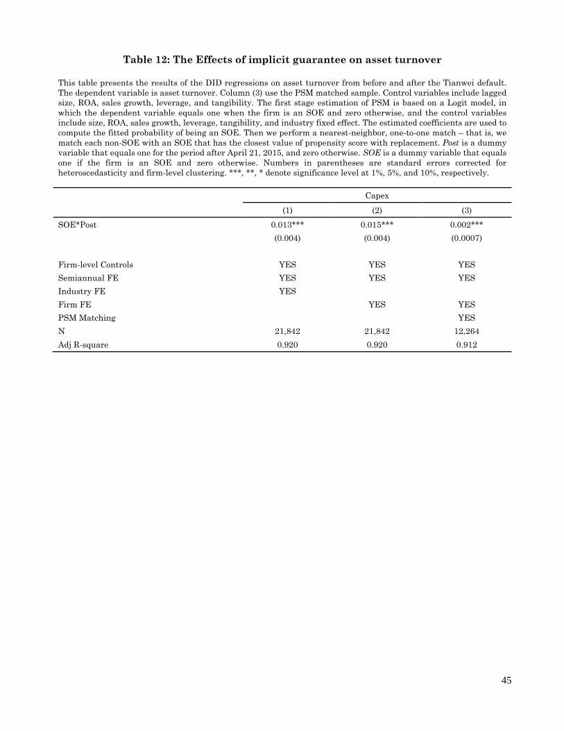
45
Table 12: The Effects of implicit guarantee on asset turnover
This table presents the results of the DID regressions on asset turnover from before and after the Tianwei default.
The dependent variable is asset turnover. Column (3) use the PSM matched sample. Control variables include lagged
size, ROA, sales growth, leverage, and tangibility. The first stage estimation of PSM is based on a Logit model, in
which the dependent variable equals one when the firm is an SOE and zero otherwise, and the control variables
include size, ROA, sales growth, leverage, tangibility, and industry fixed effect. The estimated coefficients are used to
compute the fitted probability of being an SOE. Then we perform a nearest-neighbor, one-to-one match – that is, we
match each non-SOE with an SOE that has the closest value of propensity score with replacement. Post is a dummy
variable that equals one for the period after April 21, 2015, and zero otherwise. SOE is a dummy variable that equals
one if the firm is an SOE and zero otherwise. Numbers in parentheses are standard errors corrected for
heteroscedasticity and firm-level clustering. ***, **, * denote significance level at 1%, 5%, and 10%, respectively.
Capex
(1) (2) (3)
SOE*Post 0.013*** 0.015*** 0.002***
(0.004) (0.004) (0.0007)
Firm-level Controls YES YES YES
Semiannual FE YES YES YES
Industry FE YES
Firm FE YES YES
PSM Matching YES
N 21,842 21,842 12,264
Adj R-square 0.920 0.920 0.912

46
Appendix Table A.I: Variable definitions
Acquisitions: Cash acquisitions scaled by lagged book assets.
Assets: The amount of total book assets.
Assets turnover: Sales divided by lagged book assets.
Bank loan: The amount of total bank loan scaled by lagged book assets.
Capex: Capital expenditures divided by lagged book assets.
Cash flow: Operating cash flow scaled by lagged book assets.
Cash holdings: The sum of cash and marketable securities scaled by lagged book assets.
Central_SOE (Ownership): percentage of shares owned by the central government
Coupon: Annualized coupon rate.
Credit rating: A variable that equals one if the bond-issuing firm has no rating 30 days before the event date; it takes
an integer value of 2–18 if the bond-issuing firm has a rating of C, CC, CCC, B–, B, B+, BB–, BB, BB+, BBB, A–, A, A+,
AA–, AA, AA+, AAA, respectively.
Explicit guarantee: A variable that equals one if the bond has a guarantor and zero otherwise.
Intangible investment: Investments in intangible assets scaled by lagged book assets.
Issue amount: The amount of bond issuance.
Leverage: Total book debt/(total book debt + book value of equity).
Local_SOE (Ownership): percentage of shares owned by the central government
Maturity: Years to maturity.
Net debt issuance: Semiannual issuance of debts minus repayments of debts scaled by lagged book assets.
Operating cash flow: Operating cash flow scaled by lagged book assets.
Period (–2/–1/+1/+2/+3): A dummy variable that equals one for the period ending June 30, 2014; December 31, 2014;
December 31, 2015; June 30, 2016; December 31, 2016; and zero otherwise.
Post: A dummy variable that equals one for the period after April 21, 2015, and zero otherwise.
Overinvesting: A dummy variable that equals one if the firm-semiannual observations in the top quartile of
unpredicted investment and zero if the observations are in the middle two quartiles
ROA: Operating income/total book assets.
R&D: Research and development expenditures scaled by lagged total sales.
Sales: The amount of sales.
Sg: The average sales growth of the last two semiannual periods.
Size: Log(assets).
SOE: A dummy variable that equals one if the firm is a state-owned enterprise.
Subsidy: The amount of subsidy granted by government scaled by lagged book assets.
Tangibility: Property, plant, and equipment divided by total book assets.
Underinvesting: A dummy variable that equals one if the firm-semiannual observations in the bottom quartile of
unpredicted investment and zero if the observations are in the middle two quartiles
Yield spread: The yield difference between the bond and a government with closest remaining maturity.
YTM: Yield to maturity.

47
Appendix Table A.II: Propensity-score matching regression
This table provides Logit estimation for the following equation:
𝑁𝑜𝑛𝑆𝑂𝐸𝑖,𝑡 = 𝑎 × 𝐶𝑜𝑛𝑡𝑟𝑜𝑙𝑠𝑖,𝑡 + 𝐼𝑖 + +𝜀𝑖,𝑡
We use the firm information on December 31, 2014. The dependent variable y is a dummy variable that equals one if
the firm is NOT an SOE firm and zero otherwise. Numbers in parentheses are standard errors corrected for
heteroscedasticity and firm-level clustering. ***, **, * denote significance level at 1%, 5%, and 10%, respectively.
Size -0.081***
(0.006)
Leverage 0.536***
(0.045)
ROA 0.052***
(0.004)
Cash flow 0.305***
(0.059)
Tangibility -0.023
(0.050)
Constant 1.755***
(0.134)
(0.134)
Industry FE YES
N 2,423
Adj. R-squared 0.367

48
Appendix Table A.III: The effect of implicit guarantees on investment:
Placebo test using first non-SOE default
This table presents the results of the PSM matched sample DID regressions on corporate investments between
SOEs and non-SOEs from before and after the Chaori default. The dependent variable is capital expenditures scaled
by lagged assets for columns (1), capital expenditures and investments in intangibles scaled by lagged assets for
columns (2), and capital expenditures, investments in intangibles, and acquisitions scaled by lagged assets for
column (3) in a semiannual frequency. Control variables include cash flow and lagged size, ROA, sales growth,
leverage, and tangibility. The first stage estimation of PSM is based on a Logit model, in which the dependent
variable equals one when the firm is an SOE and zero otherwise, and the control variables include size, ROA, sales
growth, cash flow, leverage, tangibility, and industry fixed effect. The estimated coefficients are used to compute the
fitted probability of being an SOE. Then we perform a nearest-neighbor, one-to-one match – that is, we match each
non-SOE with an SOE that has the closest value of propensity score with replacement. Post is a dummy variable
that equals one for the three semiannual periods after March 8, 2014 (excluding June 30, 2014), and equals zero for
the three semiannual periods before that. SOE is a dummy variable that equals one if the firm is an SOE and zero
otherwise. Numbers in parentheses are standard errors corrected for heteroscedasticity and firm-level clustering.
***, **, * denote significance level at 1%, 5%, and 10%, respectively.
Capex Capex+Intangible Capex+Intangible+Acquisition
(1) (2) (3)
SOE*Post -0.003 -0.002 -0.005
-0.003 -0.004 -0.004
Firm-level Controls YES YES YES
Semiannual FE YES YES YES
Industry FE
Firm FE YES YES YES
PSM YES YES YES
N 12,208 12,208 12,208
Adj R-square 0.431 0.433 0.433