The Value of Reunification in Germany: An Analysis of Changes in Life

Satisfaction

Paul Frijters Tinbergen Institute, Free University Amsterdam

John P. Haisken-DeNew

DIW, Berlin and IZA, Bonn

Michael A. Shields Department of Economics, University of Melbourne and IZA, Bonn

Discussion Paper No. 419 January 2002

IZA

P.O. Box 7240 D-53072 Bonn

Germany

Tel.: +49-228-3894-0 Fax: +49-228-3894-210

Email: iza@iza.org

This Discussion Paper is issued within the framework of IZA’s research area Evaluation of Labor Market Policies and Projects. Any opinions expressed here are those of the author(s) and not those of the institute. Research disseminated by IZA may include views on policy, but the institute itself takes no institutional policy positions. The Institute for the Study of Labor (IZA) in Bonn is a local and virtual international research center and a place of communication between science, politics and business. IZA is an independent, nonprofit limited liability company (Gesellschaft mit beschränkter Haftung) supported by the Deutsche Post AG. The center is associated with the University of Bonn and offers a stimulating research environment through its research networks, research support, and visitors and doctoral programs. IZA engages in (i) original and internationally competitive research in all fields of labor economics, (ii) development of policy concepts, and (iii) dissemination of research results and concepts to the interested public. The current research program deals with (1) mobility and flexibility of labor, (2) internationalization of labor markets, (3) the welfare state and labor markets, (4) labor markets in transition countries, (5) the future of labor, (6) evaluation of labor market policies and projects and (7) general labor economics. IZA Discussion Papers often represent preliminary work and are circulated to encourage discussion. Citation of such a paper should account for its provisional character.

IZA Discussion Paper No. 419 January 2002

ABSTRACT

The Value of Reunification in Germany: An Analysis of Changes in Life Satisfaction

We quantify the value of changes in life circumstances in Germany following reunification. To this end, we develop and implement a fixed-effect estimator for ordinal life satisfaction in the German Socio-Economic Panel. We find strong negative effects on life satisfaction from being recently fired, losing a spouse through either death or separation and time spent in hospital, whilst we find strong positive effects from income and marriage. Using a new causal decomposition technique, we find that East Germans experienced a continued improvement in life satisfaction after 1990 to which increased household incomes contributed around 12%. Most of the increase is explained by improved average circumstances, such as public services. For West Germans, we find virtually no change in satisfaction between 1991 and 1999. JEL Classification: Z1, C23, C25, I31 Keywords: Life satisfaction, German reunification, random and fixed-effects, panel

models, causal decomposition Michael A. Shields Department of Economics University of Melbourne Victoria 3010 Australia Phone: +61 3 8344 4656 Fax: +61 3 8344 6899 Email: mshields@melbecon.unimelb.edu.au

2

1. Introduction

One of the most prominent events of recent decades was the ‘fall’ of the Berlin Wall on

November 9th 1989, effectively marking the collapse of socialism in East Germany. This was a

time of great optimism for both East and West Germans, even though there was considerable

concern about the economic impacts of unification on the West. For East Germans this optimism

was reflected in popular slogans such as ‘Helmut (Kohl), take us by the hand, lead us to the

economic wonderland’ (Bach and Trabold, 2000).

At the time of reunification in July 1990, politicians talked about East-West economic

convergence taking at most only five years to achieve.1 Complete free movement between East

and West was established along with the parity conversion of the East Mark to the West Mark

(DM). Expectations were high as workers from the East, perhaps for the first time in their lives,

had potential access to high paying jobs and goods which were previously unavailable. Such

expectations led 1.8% of East Germans to migrate to the West by 1991, increasing to a

accumulated total of 4.3% by 1992, 6.2% in 1993 and 7.4% in 1994. This mobility was made

easier by a common language, a similar education system, a shared cultural history and a shared

political history prior to the 2nd World War (Hunt, 2000). The number of the East-to-West

migrants, however, had levelled out by 1995 with around 8% of former East Germans today

residing in the West. In sharp contrast to the optimism shared by many politicians about

convergence, economists were far more cautious suggesting a necessary time of up to 20 years.

Despite the introduction of currency union and the massive federal transfers from West to

East, in the order of hundreds of billion of DM, by 1997 GDP per capita in East Germany was

still only 57% of that of the West. Moreover, wages were around 75% and unemployment was

double the Western level (Hunt, 2000). Convergence with the West had essentially come to a halt

and the economic miracle, which had been hoped for, failed to appear (see Bach and Trabold,

2000, for an extended discussion).2

In this paper we provide the first investigation into trends and determinants of life satisfaction

(welfare) for inhabitants of East Germany in the post-reunification period starting 1991 (given

our data) through to 1999. We compare these results with those for West Germans, and

investigate whether there has been a convergence of life satisfaction between the two populations

over the decade. The setting of German reunification is particularly interesting for such a study as

it is as close to a 'natural' experiment as can be experienced in economics. It is well documented

1 For example, Kurt Biedenkopf, a West German member of Chancellor Kohl's Conservative Party wrote in an open letter in February 1990, ‘given the current extremely favourable conditions, the adjustment process of the East Germany economy to that of the West, will only take one or two years to reach the current West German levels.’ 2 See Hunt (2000) for an analysis of the apparent puzzle why net emigration by 1995 from East Germany was close to zero, given free movement and considerably better economic conditions in West Germany.

3

that few people anticipated the 'falling of the wall', nor the resulting rapid endowment of a former

communist country with a set of market institutions. To enable this analysis we use data from the

German Socio-Economic Panel (GSOEP), in which we can follow individuals over time. To

analyse the correlates of life satisfaction we fit random-effects ordered probit models. However,

this approach may fail to capture many individual factors that are known to affect life

satisfaction, such as personality traits (see Kahneman et al., 1999). This would mean that the

coefficients of the observable variables included in the models might be affected by spurious

correlation with unobservables. To investigate causality we therefore implement a conditional

estimator for the fixed-effect ordered logit model that allows for individual heterogeneity. We

then develop a test for the existence of fixed-effects. The estimates from this new model are then

decomposed, using a new technique, in order to identify the factors that drove the average

changes in life satisfaction in both East and West Germany following reunification.

Apart from its focus and these methodological innovations, the paper also contributes to the

existing literature on life satisfaction by using uniquely rich data that incorporate various major

‘life events’. These include changes in health and marital status, family births and deaths, of

internal migration, and changes in income and work status.

The paper is set out as follows. In Section 2 we review the recent economics literature that has

investigated the determinants of life satisfaction and happiness. The findings from these studies

provide us with the baseline individual, economic and demographic characteristics that affect

individual wellbeing, and therefore need to be taken account of in our models. Our data source,

the German Socio-Economic Panel, is described in Section 3, together with the derivation of our

life satisfaction measure and a descriptive analysis of changes in life satisfaction since

reunification. In Section 4 we introduce our econometric and decomposition methodologies. The

empirical results are discussed in Section 5, and Section 6 concludes.

2. The Determinants of Life Satisfaction and Happiness

The investigation of the factors affecting human happiness is central to the discipline of

psychology (see Kahneman et al., 1999, for a detailed review of the relevant psychology

literature). Psychologists recognise that the best method to gain information about how ‘happy’ a

person is with their life or work is to ask them directly. In contrast, it is well known that

economists have traditionally been reluctant to use self-reported subjective measures of welfare

or utility such as life satisfaction, happiness and job satisfaction (Bertrand and Mullainathan,

2001). Economists are cautious about the interpretation of such variables and the validity of inter-

personal comparisons (i.e. a cardinal measure). Moreover, economic theory typically provides

little guidance on how to model such psychological outcomes, thus making the testing of

economic theory difficult (Jahoda, 1982, 1988). Recent years, however, have seen a considerable

4

increase in the willingness by economists to use such variables (See Oswald 1997, for an

informative review). This is partly due to the high level of explanatory power attributable to such

variables in models of labour market behaviour (e.g. absenteeism and turnover) and the ‘sensible’

nature of estimated determinants of life satisfaction and happiness (Frijters, 2000). Moreover, the

great advantage of these wellbeing measures is that they provide directly observable proxies for

‘utility’, which is a concept central to economic research, but is a dependent variable otherwise

rarely available for empirical analysis.3

Unemployment

By far the most heavily researched topic by economists (and psychologists) in this area concerns

the psychological impact of unemployment. Much of this work has utilised longitudinal data that

tracks an individual's self-reported happiness over time. In this respect the British Household

Panel Survey (Clark et al., 1996; Clark and Oswald, 1994; Clark, 1999; Theodossiou, 1998) and

the West German sample of the German Socio-Economic Panel Study (Clark et al., 2001;

Gerlach and Stephan, 1996; Kraft, 2000; Winkelmann and Winkelmann, 1998) have been widely

used. In addition, Ravallion and Lokshin (2001) analysed data from the Russian Longitudinal

Monitoring Survey, Korpi (1997) has used panel data from the Swedish Survey of Youth,

Gerdtham and Johannesson (1997) have examined cross-sectional data from Sweden's Level of

Living Survey and Frey and Stutzer (2000) have used cross-sectional data from Switzerland to

examine this issue. The use of panel data is important in this context since it can enable the

causality running from unemployment to unhappiness to be firmly established. Moreover, the

effect of unobserved individual heterogeneity (e.g. personality traits), that has been found to be

important in explaining variations in reported happiness levels (see Kahneman et al., 1999), can

also be tested and controlled for with longitudinal data.

Whilst the above studies have used a variety of definitions of wellbeing (i.e. life satisfaction

in the German panel, symptoms of psychological distress in the British panel), there can be little

doubt that, for the ‘majority population’, unemployment leads to a significant deterioration in life

satisfaction. This ‘stylised fact’ is validated across countries, time periods and data sources, and

has been widely used to support the belief that unemployment in Europe is predominately

involuntary in nature (Clark and Oswald, 1994; Gerlach and Stephan, 1996; Oswald, 1997). The

psychological cost of unemployment has been found to be higher for men than women (Kraft,

2000) and greatest for younger workers (aged less than 30 years according to Winkelmann and

Winkelmann (1998) or aged 30 – 49 years according to Gerlach and Stephan (1996)).

3 A good example of a study that uses subjective measures of a happiness to examine an important economic issue is Di Tella et al., 2001. In this study the authors estimate the relative importance of inflation and unemployment in determining respondents happiness (or utility) using survey data from the Euro-Barometer Survey Series (1975-1991).

5

Theodossiou (1998) has found that joblessness leads to a marked rise in anxiety and depression

with an associated loss of confidence and self-esteem. Winkelmann and Winkelmann (1998)

found that the non-pecuniary costs of unemployment far exceed the pecuniary costs associated

with loss of income. An important conclusion of these studies is that cost-benefit analyses of

employment generating policies ought to take into account the non-pecuniary costs of

unemployment.

Income and the Non-Pecuniary Value of Work

A central component of economic theory is that utility is positively associated with income.

Consequently, there has been considerable interest in the relationship between income and self-

reported levels of life satisfaction or happiness. However, there exists no clear consensus that this

central axiom of economic theory holds empirically. Campbell et al. (1976) and Easterlin (1974,

1995) found that income is a poor predictor of many measures of individual wellbeing. Oswald

(1997) notes only a small happiness gain from economic growth in Europe and the USA in the

post-war period, with this result being supported in the empirical analysis of Blanchflower and

Oswald (2000). The results from studies that have used survey data from one country to

investigate this relationship are also mixed. Some studies have found a small positive relationship

between income and happiness (Clark et al, 2001; Frey and Stutzer, 2000; Gerdtham and

Johannesson, 1997; Gerlach and Stephan, 1996; Winkelmann and Winkelmann, 1998). Kraft

(2000) found an inverse U-shape relationship with life satisfaction reaching a maximum at

roughly 45,000DM per month. In contrast, Clark and Oswald (1994) were unable to find any

robust effect, whilst Clark (1999) noted evidence of a significant negative relationship between

income and happiness using data from the BHPS. An alternative, commonly held, viewpoint is

that it is 'relative' rather than 'absolute' income that drives psychological wellbeing (Blanchflower

and Oswald, 2000; Van Praag and Frijters, 1999; Clark and Oswald, 1996; Easterlin, 1974, 1995;

McBride, 2001; Oswald, 1997).4

Importantly, it is not just the loss of income, associated with unemployment, which leads to

greater unhappiness, but rather psychologists have found that the benefits of ‘work’ are multi-

facetted. Having a job may be a source of prestige and social recognition, and, as such, provide a

basis for self-respect and self-worth. Going to work also gives structure to the day, maintains a

sense of purpose and provides opportunities for social interaction (see Darity and Young, 1996).

6

Individual Characteristics

A number of interesting and consistent relationships have been established. It has been found that

marriage leads to a welfare gain over being single, and that the experience of divorce or

separation significantly reduces happiness levels (Clark and Oswald, 1994; Clark et al., 2001;

Gerlach and Stephan, 1998; Theodossiou, 1998; Winkelmann and Winkelmann, 1998). In this

respect, Kraft (2000) claims that a rise of 6000DM per month would be needed to produce an

equivalent rise in happiness to exactly offset the loss associated with separation. It has also been

universally found that measures of poor health or disability are significantly associated with

lower levels of self-reported happiness (see Kahneman et al., 1999, for a review). Several studies

have found that individuals may partly adapt to illness and disability over time.

The relationship between other individual characteristics and happiness is less clear. One such

example is that of gender. Clark and Oswald (1994), Clark et al. (1996) and Theodossiou (1998)

have found that men are more likely than women to be observed at the higher end of the

happiness distribution. The latter author argues that his finding is consistent with the belief held

by psychologists that women are typically more critical of themselves and devalue themselves

much more than men (See Black, 1971; Lowenthal et al., 1975). However, Gerdtham and

Johannesson (1997) found the opposite result using Swedish data. In contrast, Frey and Stutzer

(2000) identified no gender difference using Swiss data.

Similarly, whilst some studies have found that happiness is positively related to education

(Clark et al., 2000; Frey and Stutzer, 2000; Gerdtham and Johannesson, 1997), other studies have

found the converse (Clark and Oswald, 1994). The latter authors argue that the more highly

educated have greater life expectations, which if not realised, lead to unhappiness. It has also

been shown that ethnicity plays an important role in determining wellbeing levels (Shields and

Wailoo, 2001). A final interesting result is that having children does not necessary lead to a

happiness gain. Clark and Oswald (1994), Gerdtham and Johannesson (1997) and Theodossiou

(1998) find that being responsible for children significantly reduces reported happiness amongst

British and Swedish individuals. Plug (1997) finds a positive effect of children for the GSOEP

however.

In this paper we investigate the impact of a number of these variables on life satisfaction of

East and West German men and women in the immediate post-reunification period. In addition to

‘level’ effects of these variables, we can also identify the transient effect of changes. We thus

obtain new results for the impact of a number of major ‘life events’ on life satisfaction, such as

being recently separated or divorced, having a new baby, being recently fired from work, health

changes (disabilities and hospital stays) and deaths in the family.

4 See Diener and Oishi (2000) for a review of the relationship between income and happiness found in the psychology literature.

7

3. Data and Sample Characteristics

Data

To examine the impact of reunification and socio-economic characteristics on the life satisfaction

of East and West German residents we use data from the German Socio-Economic Panel

(GSOEP). The GSOEP is a nationally representative panel that has closely followed around

13,500 individuals (living in some 7,000 households) each year since 1984. In 1990, following

reunification, the panel was extended to include residents of the former East Germany.5 The focus

of this paper is the men and women, aged 21-64, who resided in East or West Germany, which

we follow from 1991 up to 1999.6 This is the first paper to investigate the determinants of life

satisfaction separately for East German men and women, and to examine these issues using data

from 1996-1999.

In order to establish the potential welfare benefit of moving from the East to the West

following reunification, we also include ‘movers’ to the West in the Eastern data (276

individuals). Similarly, we observe 80 individuals who moved from the West to the East over the

period, which we have added back into the Western samples in order to estimate the effect of

moving. The total samples we use therefore consist of 25,903 person-year observations (12,592

males; 13,311 females) on East Germans, and 63,868 person-year observations (31,895 males;

31,973 females) on West Germans. This corresponds to repeated observations on just over 4,100

Eastern and 11,365 Western individuals. The average length of time in the panel is 6.4 years

(since 1991). As the data span almost a decade, all income information has been deflated by the

OECD main economic indicators consumer price index (base year 1995).

The Distribution of Life Satisfaction in East and West Germany, 1991-1999

The dependent variable we use in this analysis is based on the question ‘How happy are you at

present with your life as a whole?’ The response runs from 0 (very unhappy) to 10 (very happy).

Table 1 shows the distribution of life satisfaction for our four sub-samples.

It can be seen that the mean level of life satisfaction reported by East German residents is

significantly lower (by around 0.8) than for their Western counterparts. In particular, a

considerably lower percentage of East Germans report life satisfaction above point 8 on the scale

(5.6% of males, 5.9% of females) compared to West Germans (16.2% of males, 17.8% of

females). This difference in average life satisfaction between Easterners and Westerns holds true

5 In this paper we use the German version of the GSOEP data (See Haisken-DeNew and Frick, 2000 for details), although the same analysis can be conducted with the international ‘scientific use’ version, albeit with around 5% fewer observations. 6 We do not analyse here the 1990 data because it is used to create a number of ‘major life’ change variables included in the 1991 data for East Germans.

8

for both males and females, but interestingly we do not observe a large gender gap between East

(6.30 versus 6.26), or Western (7.10 versus 7.13) males and females. However, the former gap is

statistically significant at the 5% level (t=2.02).

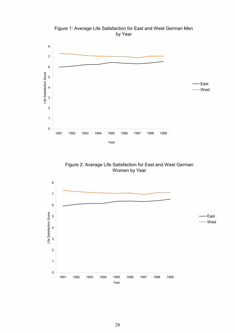
Figures 1 and 2 show the change in the average levels of life satisfaction in the post-

reunification period for each of our four groups. The figures show a number of interesting

patterns. Firstly, life satisfaction in the East is always observed to be significantly below that of

the West in each year since 1991. Secondly, East Germans experienced a continued increase in

their satisfaction levels throughout the decade, while West Germans experienced a continued (but

more gradual) decline in their life satisfaction.

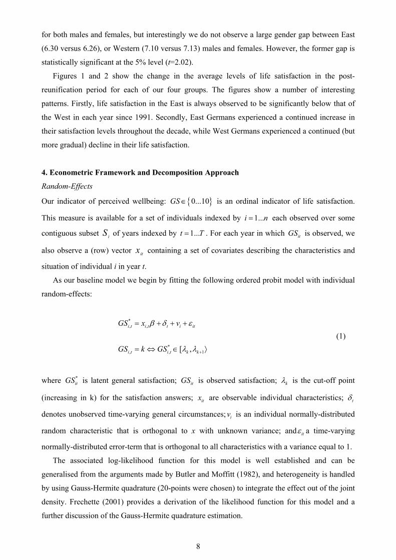
4. Econometric Framework and Decomposition Approach

Random-Effects

Our indicator of perceived wellbeing: { }0...10GS ∈ is an ordinal indicator of life satisfaction.

This measure is available for a set of individuals indexed by 1...i n= each observed over some

contiguous subset iS of years indexed by 1...t T= . For each year in which itGS is observed, we

also observe a (row) vector itx containing a set of covariates describing the characteristics and

situation of individual i in year t.

As our baseline model we begin by fitting the following ordered probit model with individual

random-effects:

*, ,

*, , 1

[ ,

i t i t t i it

i t i t k k

GS x v

GS k GS

β δ ε

λ λ +

= + + +

= ⇔ ∈ ⟩

(1)

where *itGS is latent general satisfaction; itGS is observed satisfaction; kλ is the cut-off point

(increasing in k) for the satisfaction answers; itx are observable individual characteristics; tδ

denotes unobserved time-varying general circumstances; iv is an individual normally-distributed

random characteristic that is orthogonal to x with unknown variance; and itε a time-varying

normally-distributed error-term that is orthogonal to all characteristics with a variance equal to 1.

The associated log-likelihood function for this model is well established and can be

generalised from the arguments made by Butler and Moffitt (1982), and heterogeneity is handled

by using Gauss-Hermite quadrature (20-points were chosen) to integrate the effect out of the joint

density. Frechette (2001) provides a derivation of the likelihood function for this model and a

further discussion of the Gauss-Hermite quadrature estimation.

9

Fixed-Effects

It is very likely that there are important unobservable individual traits and characteristics that are

related to life satisfaction. In fact, the recent psychology literature has found that such fixed

personality traits are important predictors of general satisfaction (see, for example, Argyle, 1999

and Diener et al., 1999). This is particularly problematic for the random-effects estimates if these

traits are related to many of the variables contained in itx . Therefore, the results from the cross-

section analyses based on the above random-effects model cannot generally serve as an indicator

of causality. Therefore, as our main model of causality, we also fit the following fixed-effect

ordered logit model developed in Ferrer and Frijters (2001):

*

,

*1

[ ,

it i t t i it

it it k k

GS x f

GS k GS

β δ ε

λ λ +

= + + +

= ⇔ ∈ ⟩

(2)

where *itGS is latent general satisfaction; itGS is observed satisfaction; kλ is the cut-off point

(increasing in k) for the satisfaction answers; itx is observable time-varying characteristics; tδ

denotes unobserved time-varying general circumstances; if is an individual fixed characteristic;

and itε is a time-varying logit-distributed error-term that is orthogonal to all characteristics. Our

conditional estimator for tδ and β maximizes the following conditional likelihood:

1

1

1

( )

(GS )

( , )

[ ( ),.., ( ) | (GS ) ]

Tit i itt

Tit i itt

i

i i iT i it it

I GS k x

I k x

GS S k c

L I GS k I GS k I k c

e

e

β

β

=

=

>

>

∈

> > > =

∑=

∑

∑

∑

(3)

which is the likelihood of observing which of the T satisfactions of the same individual are above

ki, given that there are c out of the T satisfactions that are above ki. Here, ( , )iS k c denotes the set

of all possible combinations of 1{ ,.., }i iTGS GS such that (GS )it it

I k c> =∑ . Also, GSit is used to

denote the random variable and itGS the realization.

As we see, the fixed-effects have dropped out of this likelihood. It therefore yields estimates

only for tδ and β . This model is an extension of the fixed-effect logit model by Chamberlain

10

(1980). Unlike the Chamberlain methodology that recodes the data such that only crossing over a

barrier that is the same for everyone (say, k) can be used, our model uses crossings over person

specific barriers (say, ik ). When some individuals for instance only report values between 3 and

5, and others only between 6 and 8, then using the same barrier for everyone cannot record

changes for both groups of individuals. Those individuals then have to be dropped from the

estimation procedure. With individual specific barriers all individuals whose satisfactions differ

over time, can be included. The most important advantage is therefore that it allows us to use

more than 90% of the observations. In comparison, the loss of data in applications with the

Chamberlain method is usually over 50% (e.g. Winkelman and Winkelman 1998, Hamermesh

2001, Clark et al. 2001). Furthermore, the log-likelihood is greatly increased by choosing ki

optimally (see Ferrer and Frijters, 2001). The model is estimated by Maximum Likelihood in

GAUSS.

One important methodological point concerns the use of this fixed-effect estimator. One

cannot simultaneously include age, time and fixed-effects in the analyses. To see this note that

0* * *it age i age ageage age tβ β β= + . Now, the effect of 0 *i ageage β is time-invariant and will

therefore be in the individual fixed-effect, and * aget β will be the same for everyone at t and

hence picked up by time dummies. We therefore drop (linear) age as a covariate and note that the

time dummies will include age effects.

Specification Testing: Random or Fixed-Effects

In order to be able to judge the added value of the fixed-effects framework, we here develop a

test of the power of the fixed-effect model compared to the random-effects model.

We denote the estimated coefficients of the random-effects model for the variables that

overlap with the fixed-effects model by RE

β . If there are fixed-effects that are related to

individual characteristics, then the coefficients of the fixed-effects model should be different. We

can hence judge the value of the fixed-effects model by seeing whether the coefficients are

significantly different. Our null-hypothesis is that there are no fixed-effects, i.e.:

H0: (4)REFEβ αβ=

11

whereα is an unknown positive constant that arises because RE

β is estimated under a different

normalisation.7 For a proper comparison, we only include for RE

β those variables that are shared

between the random-effects and fixed-effects models. This includes all the variables in the fixed-

effect model apart from the time dummies: because time dummies represent unobservable

characteristics that will pick up level effects in variables in the random-effects model, they

essentially represent different variables for the two models and should therefore not be in a

specification test.

Under the null hypothesis, we can use the following likelihood ratio test:

FE

ML2L( )-2L( ) ( ) (5)RE

kβ αβ χ∼

Where ˆ FEMLβ denotes the vector of coefficients from the unrestricted maximum likelihood estimate

of the fixed-effects model; k denotes the number of restricted parameters; and L( )RE

αβ denotes

the likelihood of the fixed-effect model when the appropriate parameters are set at RE

αβ . Two

practical problems appear here. The first is that L( )RE

αβ requires re-fitting the free parameters

and hence re-estimation of the model. The second is that α is unknown. To circumvent this, we

can note that:

FE FE

ˆML ML ˆ2L( )-2L( ) 2L( )-max {2L( )} (6)RE RE

αβ α β β αβ>

Hence, by using the α̂ that maximises ˆL( )RE

αβ , we get a lower bound for FE

ML2L( )-2L( )RE

β αβ .

If we thus find that we can reject the null usingFE

ˆML ˆ2L( )-max {2L( )}RE

αβ α β as our test statistic,

we know that the true statistic will reject the null also.

Explanatory Variables

In order to get a baseline specification for the covariates in our life satisfaction models we follow

the previous studies of life satisfaction and happiness described in Section 2. Therefore, in the

random-effects models we control for age (and its quadratic), immigrant status, marital status,

physical disability, years of schooling, number of children, having an invalid in the household

7

REβ is estimated with the full sample of all individuals and has var( itε )=1. In contrast, the fixed-effects model

uses only a selective subset of individuals that are partly selected on itε and hence does not share the same normalisation.

12

(usually a spouse or parent), employment status (particularly unemployment), household income

and broad region of residence.

Variables not used previously in the economic literature include a number of major life

changes that took place over the previous 12 months. These are: becoming separated, becoming

divorced, death of spouse, death of another family member, birth of a child, number of in-patient

days in hospital, being fired from your job and moving house (either within East or West

Germany). We would expect that each of these major life events would have a significant impact

on an individual's level of life satisfaction.

Given our focus on the impact of reunification of East and West Germans we also include

year controls to capture general changes in life satisfaction in the years following reunification.

An important question is whether or not movers from the East to the West (and visa-versa)

experienced a gain (loss) in life satisfaction relative to stayers, and consequently we include

dummy variables in the respective models to capture this change. We have also, uniquely,

derived and included a "Border" variable equalling one (0 otherwise) if the respondent lives on

the border of East and West Germany, as we might expect that the immediate impact of

reunification on life satisfaction would affect those living on the border to the greatest extent.

Given the large transitional nature of German reunification from a socialist to a capitalist system,

we have also include a "Communist" variable in the East German models, to capture the expected

negative impact of reunification on individuals who used to be members of the Communist Party

(i.e. those we might expect to have the greatest attachment to the old system). Finally, to capture

any possible panel effects on individuals' reports of their life satisfaction, we have included a

length of time variable in the panel variable in each of the models (see Landau, 1993, for further

justification). This is an innovation in the literature and turns out to be statistically significant in

each of our random-effects models.8

For the fixed-effects models the effect of the individual time-invariant variables cannot be

estimated, thus no estimates are provided for age, immigrant status, years of education and

numbers of years in the panel. Throughout this paper, given that we might expect that the

determinants of life satisfaction (e.g. with respect to say, children and employment status) to

differ by gender and between East and West Germans, we fit separate models for males and

females as well as for East and West Germans.

8 It has been found that individuals’ responses to subjective variables, such as life satisfaction, may change with repeated questioning independently of changes in economic, social and demographic factors. For example, giving that the same interviewer (in most cases) visits the same individuals each year of the panel, over time respondents may become more familiar with the interviewer which may change their responses (Landau, 1993).

13

Causal Decomposition Analysis

Given our particular interest in evaluating the potential welfare benefits of reunification for East

Germans, we decompose changes in expected latent satisfaction for East German men and

women separately in the post-reunification period using the estimates from the fixed-effects

models. This means we analyse:

* *, 1 ,, 1 , 1 , 1 , { } ( ) ( ) ( )e t e te t e t t t e t e tE GS GS x x E f E fβ δ δ++ + +− = − + − + − (7)

Denote the set of East Germans who are in the sample at time t and at time t+1 as etS . For the

individuals in etS , this decomposition is straightforward, because for them , 1 ,( ) 0e t e tE f E f+ − = . A

complicating factor arises when we consider the importance of those individuals whom are only

observed in either t or t+1, i.e. the inflows and outflows of the GSOEP. For them

, 1 , 1( ) ( )e t e t t tx x β δ δ+ +− + − is still easily computed, but the unknown component , 1 ,( )e t e tE f E f+ −

poses a problem. This term is only 0 when the distribution of the unknown characteristics is

constant over time. This is clearly very improbable because, for instance, education levels and

expectations will differ. From the fixed-effect ordered logit results alone, there is no information

on , 1 ,( )e t e tE f E f+ − . We hence have to use extra information in order to get an estimate of this

term.

In order to get an estimate of , 1 ,( )e t e tE f E f+ − , we make the following assumption:

* * { ( ) ( )} ( )E GS GS GS GS µ σ+ ∆ − = ∆ + ∆ (8)

This assumption implies that the change in observed satisfaction is (by approximation) linear in

the change in latent satisfaction. The responsiveness itself, µ , is taken to be constant over time.

This first-order approximation can now be used, by noting that we can estimate µ by calculating,

for those individuals whom we observe in all time-periods, what the response is of the observed

satisfaction levels to the estimated changes in latent satisfaction. A consistent estimator forµ is

hence:

1

1

( )

( )t

t

t tt S

t tt S

GS GS

x xµ

β

+

+

−=

−

∑∑

∑∑ (9)

where we have dropped the subscript e.

14

Having this estimate of µ , we can now use (5) to get a consistent estimator

of , 1 ,( )e t e tE f E f+ − :

11, 1 , ( ) ( )t t

t te t e tGS GSE f E f x x β

µ+

++−

− = − − (10)

In order to provide additional insight in the factors affecting life satisfaction we further

decompose 1( )t tx x β+ − into separate groups of variables. In particular, we decompose the total

changes in latent satisfaction into changes in:

1. Household Income.

2. Job related variables: fired, employed, non-participation, part-time employed, on parental

leave, spouse fired.

3. Family related variables: the number of children, birth, marital status, divorced, separated.

4. Health related variables: the number of days in hospital, the death of a partner, the

presence of someone disabled in the household.

5. Moving from East to West.

6. Unobserved average variables: age*age (which cannot by itself have an effect) and time

parameters.

7. The unobserved individual effects distribution.

It is possible to attach a causal explanation to the changes due to groups 1 to 5. Given the changes

in characteristics, they explain a part of the changes in latent satisfaction levels. The changes due

to groups 6 and 7 are not explained by anything observed and hence form the ‘true’ unexplained

part of the changes over time. The higher these terms, the less well our variables capture the

important aspects of the changes over time.

We can construct confidence intervals for most elements in the decomposition by noting that,

because ( , )Nβ β Σ∼ , it holds that 1 1 1( ) ( , ( ) ( ) ')t t t t t tx x N x x x xβ β+ + +− − Σ −∼ . When we replace

Σ with its Maximum Likelihood estimate, this yields confidence intervals. Since the term

1t tGS GSµ

+ − in the formula , 1 ,( )e t e tE f E f+ − is not well behaved (i.e. there is no a priori reason

for it to have a bounded mean or variance), we cannot use standard inference or bootstrapping

methods to compute confidence bands for , 1 ,( )e t e tE f E f+ − . What we hence report is whether

15

, 1 ,( )e t e tE f E f+ − contains 0 in the set of values when each of the stochastic elements in

, 1 ,( )e t e tE f E f+ − can range in its 95% confidence interval.

As a final exercise we use the causal model to decompose the differences between East and

West. We use the following decomposition:

* *,1999 ,1999,1999 ,1999 ,1999 ,1999 { ( ) ( )} ( )w ee w e e eE GS x GS x x x β− = − (11)

which tells us how much latent satisfaction changes East Germans would experience if they

moved to the West and attained West characteristics.

The above decomposition does not yet quantify what would have to happen for East Germans

to become equally satisfied or happy as West Germans. Therefore, we also compute how much

the unobserved characteristics would have to change in order for East Germans (who now have

all become West-Germans) to get the same satisfaction levels as current West Germans. This

means calculating:

* *,1999 ,1999 ,1999 ,1999 ,1999 { ( ) }e w w e wE GS x GS E f E f− = − (12)

Having estimated µ already, we can apply the same methodology as described above to estimate

this difference.

If ,1999 ,1999e wE f E f− is small, then the factors that explain the difference between East and

West Germans are included in our model. This would mean that the difference is not then

attributable to different unobserved individual characteristics of East Germans. However, if we

find that this term is large, then there is something fixed about the characteristics of the East

Germans that make them less (or more) satisfied. It would mean that if the observed population

characteristics of East Germany would coincide with that of West Germany and the unobserved

general characteristics of West Germany would apply in East Germany also (general culture,

public good provisions, etc.), East Germans would still not be equally satisfied as West Germans.

5. Empirical Results

Random-Effects Results

We begin by discussing the parameter estimates from the Ordered Probit models with random-

effects for East (Table 2) and West (Table 3) Germans. Following convention, given the non-

linear nature of the model, we also provide marginal effects (ME) estimated at the mean values of

the explanatory variables and setting iν and itε = 0 to ease quantitative interpretation (see

16

equation 1). The ME's are calculated as the change in the probability of reported high life

satisfaction (either 9 or 10) relative to values 8 and below.

For both East and West Germans we find a significant U-shaped relationship between age and

life satisfaction. The minimum is at about 45 years of age for all groups, except for Eastern

Females, who experience their minimum at about 54. With the exceptions of Eastern Females,

being an immigrant is associated with a significant decline in reported satisfaction, with the ME

being particularly large for East German male immigrants (ME= -0.268). Being married is

universally found to correlate with high life satisfaction, with the ME being roughly the same

magnitude for each of the four groups (ME ranges from 0.029 to 0.045). As expected having

separated in the last 12 months is associated with a significant fall in life satisfaction for East and

West Germans. However, the quantitative impact of separation is greater for Eastern men (ME=-

0.052) and women (ME= -0.177) compared to West Germans (ME= -0.040 and -0.031). Perhaps

due to the typical lengthy period between separation and legal divorce in Germany, we find little

evidence that having experienced a divorce in the last 12 months (with the tentative exception of

Eastern Females) is correlated negatively with life satisfaction. As expected, the death of spouse

in the previous year is associated with a very large decline in life satisfaction, this particular

major life event having the largest quantitative effect (combined with unemployment) of all the

variables included in the models. The effect is particularly large for East German men (ME=-

0.290) and women (ME=-0.163). In agreement with previous studies, having a physical disability

is universally associated with a decline in life satisfaction, with the magnitude of this effect being

similar for East and West Germans. In addition, we find new evidence that, conditional on

disability, having been in hospital in the last year leads to a continuing fall in satisfaction as the

number of days in hospital increase.9

Interestingly, we find that having children is associated with higher life satisfaction for East

German males and females, the converse, however, appears to be true for West Germans. In

particular, the ME associated with an additional child is 0.023 for Eastern males and 0.015 for

Eastern females, compared to -0.004 and -0.007 for their respective Western counterparts. In

contrast, having a baby in the last year is associated with increased life satisfaction only for West

German men and women. Having an invalid in the household (usually your spouse or parent)

correlates with lower satisfaction, the ME's being larger for East than West Germans. Years of

schooling is found to be positively related to life satisfaction for West German men and women,

but no significant correlation is found for East or West Germans.

In line with the results from previous studies of life satisfaction in West Germany, we find

that being employed is associated with a large and significant life satisfaction gain relative to

9 This variable is entered in the models as a logarithmic in order to capture the diminishing effects of extra days in a hospital.

17

unemployment. However, we also provide new evidence that this is also the case for both East

German men and women. In fact, the ME's associated with being employed are at least twice as

large for East than West Germans, suggesting that the detrimental effect of being unemployed is

particularly large in the East. Since we have also controlled for household income in our models,

this also implies that the non-pecuniary costs associated with being unemployed might be higher

in the East than the West. This could reflect the poor re-employment chances of laid-off East

German workers and the stress of long-term unemployment there. For females, we additionally

find that both full-time and part-time employment are more favourable labour market states than

being unemployed. This is not that surprising, given the particularly strong traditional attachment

of East German women to the labour market. As Clark and Oswald (1994) argue, these findings

suggest that unemployment in both East and West Germany is predominantly involuntary in

nature (Gerlach and Stephan, 1996; Winkelmann and Winkelmann, 1998). For all our groups, we

find that being a non-participant in the labour market is preferable to being unemployed (but not

as good as being employed). However, the welfare gain is once again largest for East Germans.

We have also found new evidence that being on maternity leave is significantly better than

unemployment for both females groups (but not employment for East German females),

reflecting the more voluntary nature of this life choice. Finally, we find that being fired from your

job in the last 12 months is associated with a significant decline in life satisfaction for all of the

groups. The quantitative impact is greater for East than West Germans. However, whether or not

these effects are indeed causal can only be truly ascertained by the fixed-effect models.

Household income is found to be positively and significantly related to life satisfaction for all

groups, but the gain in satisfaction from increased income is greater in the East than the West.

Finally, it is often said that moving house is one of the most stressful life events, however, we

find no evidence to support this for either East or West Germans. Perhaps this stress is very short

lived, and is not captured in our yearly change variable.

Turning to our reunification-related variables, we find significantly higher life satisfaction for

individuals who, following reunification, moved from the East to the West. This effect is

quantitatively large, increasing the probability of reporting high life satisfaction (i.e. 9 or 10) by

0.161 for males and 0.143 for females. In sharp contrast, moving from the West to the East is

associated with a significant decline in life satisfaction, relative to those who stayed in the West.

Whether this is due to better circumstances in West Germany, or due to the possibility that the

happier move to West Germany, needs to be determined by the fixed-effects model. Contrary to

our expectations, we have found no evidence that living on the border of East and West Germany

had any differential effect on life satisfaction compared to those living away from the border.

Importantly, turning to the year dummies, we see a continued increase in life satisfaction

between 1991 and 1999, with the large ME of 0.259 and 0.285 for 1999, relative to 1991, for East

18

German men and women, respectively. This suggests that Eastern males, for example, had a

0.259 increased probability of reporting high life satisfaction in 1999 relative to 1991, conditional

on controlling for economic and demographic characteristics. Therefore, there existed some

unobservable change, captured in our year variables, which lead to an increased level of life

satisfaction for East Germans in the post-reunification period. A very different time profile is

found for West Germans. The time dummies are negative and significant for both West German

males and females, relative to 1991, suggesting that life satisfaction declined in West Germany

between 1991 and 1997. It then improved slightly up until 1999 (but had not returned to 1991

level by 1999). Some of this might be explained by the massive increase in German public debt

and the "Solidarity Payroll Tax" to finance the reconstruction of the East by the West. This

implies that reunification had some cost in terms of life satisfaction for West Germans. Thus,

reunification cannot be seen as a pure Pareto improvement, although appropriate counterfactuals

are difficult to identify.

Fixed-Effects Results

Tables 4 and 5 provide the causal estimates from the Ordered Logit model with fixed-effects for

East and West German, males and females, respectively. The Tables also show the values of our

test-statistic for the appropriateness of the fixed-effects model relative to the random-effects

specification. For men, the number of restricted parameters is 18, for which the 1% critical value

of the chi-squared distribution is 34.81. For men in West Germany, this means the null of no

difference between the random-effects and fixed-effects model is rejected. In East Germany, the

null is not rejected, though for men in East and West combined it is rejected. For females, the

number of restricted parameters is 20 and the appropriate 1% chi-square critical value is 37.6,

from which we can see that the null hypothesis is strongly rejected for females in West Germany

and even more strongly for females in East Germany. As a test of total changes with the fixed-

effects, it holds that the sum of the test statistics is under the null chi-square distributed with 76

degrees of freedom. The sum of the test-statistics is 185.5 and the 0.1% critical value of the chi-

square distribution with 76 degrees of freedom is 119.9. Bearing in mind that the test statistic was

biased towards accepting the null, our specification tests hence clearly point to the presence of

fixed-effects.

Unfortunately, the fixed-effect model does not provide estimates of the probabilities of having

a particular level of life satisfaction, thus it has no Marginal Effects (ME) proper. By

approximation, however, an increase of 1 in a variable with coefficient β has an effect of µ̂β on

expected life satisfaction. The coefficients from the fixed-effect model can furthermore be

compared with the coefficients from the random-effects model multiplied by the estimate of α.

19

Importantly, many of the key relationships found from the random-effects model hold

qualitatively for the models allowing for fixed-effects. In particular, we find that the effect of a

recent separation, death of spouse or some other family member still have a negative impact on

life satisfaction (although some of these effects are no longer strongly significant). Similarly,

being disabled, spending time in hospital, having an invalid in the household and getting fired are

all estimated to reduce life satisfaction. Importantly, our results with respect to the detrimental

effect of unemployment and the positive effect of employment on life satisfaction remain

statistically robust for both East and West Germans. This clearly points to the involuntary nature

of unemployment in both locations (Clark and Oswald, 1994).

Moving from the East to the West of Germany increases expected satisfaction of East German

males by about ˆ *0.744 0.40µ ≈ . This implies that it is not the (unobserved) happy who moved

from East to West. There is a genuine satisfaction gain from living in West Germany, which is

independent of the possible associated changes in income and other variables included here.

However, we no longer find any evidence that moving from the West to the East had an

unfavourable effect on life satisfaction, which suggests that was the relatively unhappy who

moved to East Germany.

A major difference with the random-effects results is that the effect of marriage is much

smaller, especially in West Germany. This suggests that being married is related to individual

fixed characteristics that increase satisfaction. Apparently, the happier West Germans are more

likely to get married, perhaps because they have characteristics that make them both happier and

more desirable partners. Conversely, having children in East Germany is found to have a much

greater positive effect with the fixed-effect model than with the random-effects model. The fact

that the random effect model did not pick up the positive effect of children implies that it is the

relatively less happy in East Germany who had many children. The results with respect to having

a newborn also suggest that the random-effects model underestimates the positive effect of

children in East Germany especially, indicating a propensity of the less happy to get more

children.

A slight difference occurs with respect to the impact of income: the coefficient for household

income (which is identified from income changes) in East Germany has about double the

satisfaction effect in the fixed-effect case, than it has in the random effect case, and it is much

higher in the East than in the West. An increase of 1 in ln(income) increases expected satisfaction

of East German males by about ˆ *0.430 0.23µ ≈ (and ≈0.33 for females). The large effect

concurs much more with the economists’ intuition that money must surely matter a lot, even

though many other studies find only small effects (e.g. Clark and Oswald 1994). The coefficient

(in comparison to the coefficients of other variables) is amongst the highest found in this

literature, even with the same data (see Ferrer and Frijters, 2001). A potential reason is that our

20

data is very "clean": measuring incomes by surveys is notoriously difficult because respondents

under-report transient elements of income, such as bonuses, side-benefits, holiday payments, etc.

However, the GSOEP contains information on more than 50 sources of income, detailed at the

monthly level. See Burkhauser et al. (1999) for more information on this.

Finally, it is important to note that the year dummies are quite different to those for the

random-effect case, because year effects in the fixed-effects case include age effects and

unobservable variables, making them incomparable. We further investigate the importance of

general changes (captured by our year and age variables) in the post-reunification period,

impacting on the life satisfaction of East Germany, in the following decomposition analysis using

the estimates from the fixed-effects models highlighted in Section 4.

Decomposition Results

The results from our decomposition experiments for East German males and females are

provided in Tables 6 and 7, respectively.

Beginning with females, we see that in the four years after transition (Total Change, 1991-

1995) average latent life satisfaction increased by a 0.715. Changes in the general circumstances

for this group over these years, captured by our year/age variables, accounted for the largest

component of improved wellbeing (i.e. 0.370). In addition, increases in real household income

following reunification additionally accounted for a 0.147 increase in average life satisfaction

(average real household income increased from 40,320 DM to 52,530 DM per year between 1991

and 1995). These gains were somewhat offset by negative changes in job status (the

unemployment rate increased from 10.4% in 1991 to 16.1% in 1995). Family circumstances and

health circumstances seem on average to have become somewhat worse over the entire period,

but their total effects are small compared to income, job and year effects. The unobserved fixed

characteristics of new people in the sample are higher than those for people already in the sample,

explaining about 30% (0.292) of the life satisfaction gain. This might suggest that younger

females (newly entering the panel) were structurally happier than the older female cohorts. A

possible explanation is that younger females might have had less human capital (sunk cost)

written-off in the reunification process and were more flexible, thus able to gain from

reunification.

The decomposition results differ considerably for the later years following reunification (1.e.

1995-1999). Although average life satisfaction increased by 0.339 between 1995 and 1999, this

can mostly be attributed to the higher unobserved fixed-effect of new entrants into the panel. In

sharp contrast to the earlier period, the general change in life satisfaction captured by the year/age

variables was large and negative (-0.428) suggesting that changes to the general living

environment (e.g. political and social, since we capture economic changes through the income

21

and job variables) for East German females worsened after 1995. However, there was a small

improvement due to rising real household income (up to 54,780 DM per year by 1999), as well as

for jobs (unemployment fell to 12.5% by 1999), health and residential mobility within East

Germany. A small negative factor affecting life satisfaction was a slight worsening of family

circumstances.

Looking at the hypothetical assimilation of the entire East German population into West

Germany, we see a large increase in average latent life satisfaction of 1.062. About 6% of this

welfare gain can be attributed to increases in household income, whilst a very small loss in

satisfaction is accounted for by the job variables. Importantly, we find that about 40% of the total

gain in * *,1999 ,1999{ }e wE GS GS− is due to average circumstances in West Germany, picked up by the

moving category (0.419). We find no large change due to differences in job, family or health

characteristics. Finally, around 60% of * *,1999 ,1999{ }e wE GS GS− consists of differences in the fixed-

effects distribution. This suggests that West German females are generally (in unobservables)

'happier' than their East German counterparts. Hence for females, the model does seem to miss

out on individual characteristics (e.g. level of optimism) that differ over East and West that

explain satisfaction levels.

Turning to East German males, we find that average latent life satisfaction in East Germany

rose by 1.014 over the period 1991 to 1999. However, about 80% of this gain occurred in the first

four years of the data (1991-1995). Of this latter increase in satisfaction (0.829), about 50% can

be attributed to improvements in the general living environment in East Germany following

reunification and are captured by our year/age variables. We also see clear evidence of a gain in

satisfaction resulting from increases in real household income (average household income was

42,880 DM per year in 1991, compared to 54,260 DM per year in 1995), but a small fall

attributable to worsening job outcomes (unemployment rose from 7.0% in 1991 to 10.0% by

1995). The satisfaction gain due to improving general living environment and higher incomes,

however, was partly offset by worsening job status, family circumstances and health. A slight

welfare gain is attributable to residential mobility within East Germany. It is also clearly the case

that new entrants into the panel between 1991 and 1995 had a higher unobservable fixed-effect,

accounting for 0.292 of the total satisfaction increase.

As was the case for females, the second half of the period (1995-1999) witnessed a smaller

increase in average male life satisfaction (0.185) than in the immediate years following

reunification (0.829). We also find evidence of a worsening of the general environment (captured

by the year/age variables) after 1995 causing a modest (0.105) decline in average life satisfaction.

In comparison to the immediate year following reunification, only a very small increase in

satisfaction can be attributed to rises in household income (household income only increased

from 54,260 DM per year in 1995 to 56,930 DM per year by 1999). We also find evidence of a

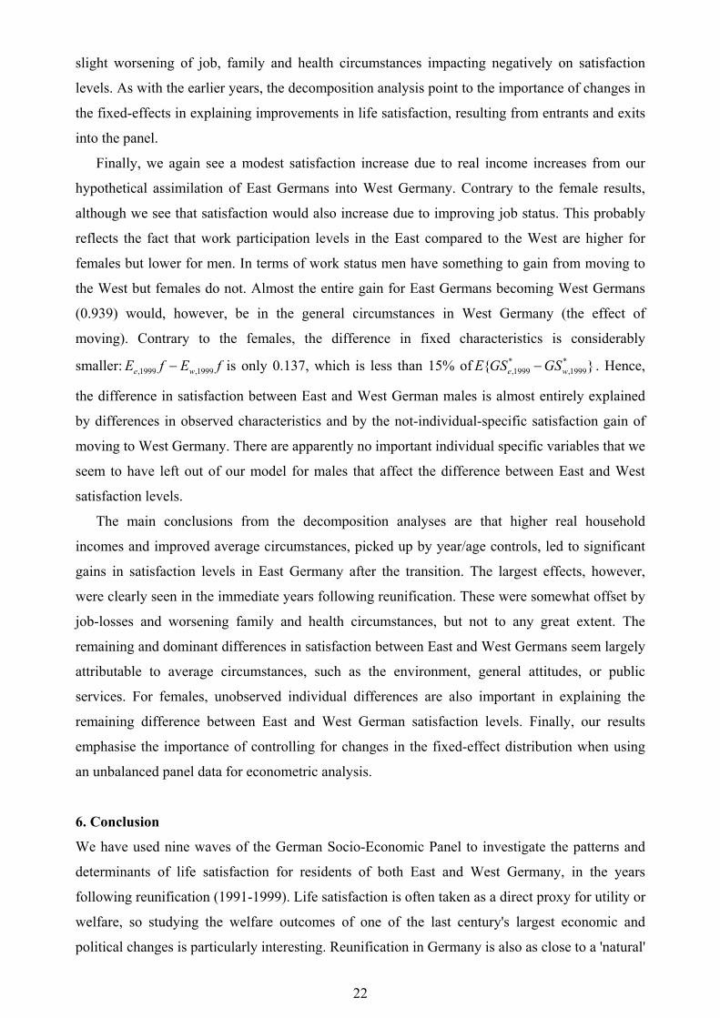
22

slight worsening of job, family and health circumstances impacting negatively on satisfaction

levels. As with the earlier years, the decomposition analysis point to the importance of changes in

the fixed-effects in explaining improvements in life satisfaction, resulting from entrants and exits

into the panel.

Finally, we again see a modest satisfaction increase due to real income increases from our

hypothetical assimilation of East Germans into West Germany. Contrary to the female results,

although we see that satisfaction would also increase due to improving job status. This probably

reflects the fact that work participation levels in the East compared to the West are higher for

females but lower for men. In terms of work status men have something to gain from moving to

the West but females do not. Almost the entire gain for East Germans becoming West Germans

(0.939) would, however, be in the general circumstances in West Germany (the effect of

moving). Contrary to the females, the difference in fixed characteristics is considerably

smaller: ,1999 ,1999e wE f E f− is only 0.137, which is less than 15% of * *,1999 ,1999{ }e wE GS GS− . Hence,

the difference in satisfaction between East and West German males is almost entirely explained

by differences in observed characteristics and by the not-individual-specific satisfaction gain of

moving to West Germany. There are apparently no important individual specific variables that we

seem to have left out of our model for males that affect the difference between East and West

satisfaction levels.

The main conclusions from the decomposition analyses are that higher real household

incomes and improved average circumstances, picked up by year/age controls, led to significant

gains in satisfaction levels in East Germany after the transition. The largest effects, however,

were clearly seen in the immediate years following reunification. These were somewhat offset by

job-losses and worsening family and health circumstances, but not to any great extent. The

remaining and dominant differences in satisfaction between East and West Germans seem largely

attributable to average circumstances, such as the environment, general attitudes, or public

services. For females, unobserved individual differences are also important in explaining the

remaining difference between East and West German satisfaction levels. Finally, our results

emphasise the importance of controlling for changes in the fixed-effect distribution when using

an unbalanced panel data for econometric analysis.

6. Conclusion

We have used nine waves of the German Socio-Economic Panel to investigate the patterns and

determinants of life satisfaction for residents of both East and West Germany, in the years

following reunification (1991-1999). Life satisfaction is often taken as a direct proxy for utility or

welfare, so studying the welfare outcomes of one of the last century's largest economic and

political changes is particularly interesting. Reunification in Germany is also as close to a 'natural'

23

experiment as is typically experienced in economics, as it is well documented that few

commentators anticipated the 'falling of the wall', nor the resulting rapid endowment of a former

communist country with a set of market institutions. The raw data suggests that East Germans

experienced a continued improvement in life satisfaction, whilst West German satisfaction levels

gradually fell, in the years following reunification. However, it remained the case that even by

1999, life satisfaction levels in East German continued to be below those of West Germans.

Given the ordinal nature of the life satisfaction (ranging 0→10) measure included in the data,

we estimate ordered probit models with random-effects (RE), but also develop a conditional

estimator for the fixed-effect ordered logit model (FE) to establish causality and allow for

individual heterogeneity. Separate models are fitted for East and West Germans, males and

females. A test for equality of the estimated parameters of the RE and FE models is then

proposed. We find strong evidence of fixed-effects, which supports the findings in the

psychological literature that (typically unobserved) individual personality traits are important

predictors of life satisfaction (see Diener and Lucas, 1999, for a review). The use of the fixed-

effect ordered logit model is an improvement on previous studies, who have arbitrarily collapsed

the life satisfaction scale into a binary measure in order to estimate conditional fixed-effect binary

logit models. Using the full ordering of the life satisfaction measure allows us to use around 90%

of observations, compared to around 50% for the binary logit model (see, for example, Clark et

al., 20001 and Winkelmann and Winkelmann, 1998).

We have also contributed to the general life satisfaction and happiness literature by exploring

the role of both socio-economic factors and major ‘life-events’ in determining life satisfaction

levels. As with previous studies of Germany we find that unemployment leads to a large decline

in life satisfaction, whilst satisfaction in positively related to household income. These findings

are robust to controls for individual heterogeneity. The former finding supports the belief that

unemployment is predominantly involuntary in West Germany (Gerlach and Stephan, 1996;

Winkelmann and Winkelmann, 1998), but also provides new evidence that this is also the case in

East Germany. Moreover, we find new evidence of the negative impact on life satisfaction of

major 'life-events' such as death of a spouse, death of another family member, marital separation,

illness captured by time spend in hospital and being fired from your job, all in the previous

twelve months. The latter finding, combined with our general finding concerning unemployment,

suggests that people may partly adapt to unemployment with the first twelve months of

unemployment leading to the largest welfare loss. Importantly, we find that movers from the East

to the West of Germany following reunification experienced a large satisfaction gain over those

who stayed in the East. In contrast, we find no significant difference in life satisfaction between

those residing on the borders of the East and West Germany, compared to those living away from

the border.

24

Finally, using the estimates from the FE models, we have developed a new causal

decomposition technique that decomposes changes in latent satisfaction over the years following

reunification. We find evidence for East Germans that average life satisfaction significantly

increased, particularly in the immediate period after reunification, due to increases in real

household incomes and general improvements such as the political and social environment. In

contrast, worsening of employment outcomes, principally due to increasing unemployment, led to

a small decline in satisfaction levels. We also find that the changing distribution of fixed-effects

resulting from entries and exits in the panel were important in explaining the observed increases

in life satisfaction reported by East Germans.

Acknowledgements

We would like to thank Jeff Borland, Lisa Cameron, Lisa Farrell, Paul Gregg, Stephen Wheatley

Price and Mark Wooden for valuable comments. We would also like to thank seminar

participants at the University of Melbourne and the Australian National University.

25

References

Argyle, M. (1999). Causes and correlates of happiness. In Kahneman, D., Diener, E. and Schwarz

N. (eds.), Foundations of Hedonic Psychology: Scientific Perspectives on Enjoyment and

Suffering. Russell Sage Foundation.

Bach, S., Trabold, H. (2000). Ten years after German monetary, economic and social union: An

introduction. Quarterly Journal of Economic Research, 2, 149-151.

Bertrand, M., Mullainthan, S. (2001). Do people mean what they say? Implications for subjective

survey data. American Economic Review, Papers and Proceedings, 91, 67-72.

Black, K. (1971). Transition to aging and self-image. Ageing and Human Development, 2, 296-

304.

Blanchflower, D., Oswald, A. (2000). Wellbeing over time in Britain and the US. Mimeo,

University of Warwick.

Burkhauser, Richard V., Barbara A. Butrica, and Mary C. Daly (1999): The PSID-GSOEP

Equivalent File: A Product of Cross-National Research. In: Wolfgang Voges (ed.), Dynamic

Approaches to Comparative Social Research: Recent Developments and Applications.

Aldershot, Great Britain: Ashgate Publishing Ltd., pp. 53- 66.

Campbell, A., Converse, P., Rodgers, W. (1976). The Quality of American Life. Russell Sage,

New York.

Chamberlain, G. (1980). Analysis of covariance with qualitative data. Review of Economic

Studies, 47, 225-38.

Clark, A. (1999). Unemployment as a social norm: Psychological evidence from panel data.

Mimeo, University d’Orleans.

Clark, A., Georgellis, Y., Sanfrey, P. (2001). Scarring: the psychological impact of past

unemployment. Economica, 68, 221-241.

Clark, A., Oswald, A. (1994). Unhappiness and unemployment. Economic Journal, 104, 648-59.

Clark, A., Oswald, A., Warr, P. (1996). Is job satisfaction U-shaped in age? Journal of

Occupational and Organizational Psychology, 69, 57-81.

Diener, E., Lucas, R. (1999). Personality and subjective wellbeing. In Kahneman, D., Diener, E.,

Schwarz, N. (Eds), Foundations of Hedonic Psychology: Scientific Perspectives on Enjoyment

and Suffering, New York: Russel Sage Foundation.

Diener, E., Oishi, S. (2000). Money and happiness: Income and subjective wellbeing across

nations, in: Diener, E., Eunkook, S. (Eds.), Culture and Subjective Wellbeing. The MIT Press,

Cambridge, MA.

Di Tella, R., MacCulloch, R. and Oswald, A. (2001). Preferences over inflation and

unemployment: Evidence from surveys of happiness. American Economic Review, 91, 335-

341.

26

Easterlin, R. (1974). Does economic growth improve the human lot? Some empirical evidence,

in: David, P., Reder, M. (Eds.), Nations and Households in Economic Growth. Academic

Press, New York and London.

Easterlin, R. (1995). Will raising the incomes of all increase the happiness of all? Journal of

Economic Behaviour and Organisation, 27, 35-48.

Ferrer-i-Carbonel, A., Frijters, P. (2001). The effect of methodology on the determinants of

happiness. Mimeo, Free University, Amsterdam.

Frey, B., Stutzer, A. (2000). Happiness, economy and institutions. Economic Journal, 110, 918-

938.

Frijters, P. (2000). Do individuals try to maximize general satisfaction? Journal of Economic

Psychology, 21, 281-304.

Gerdtham, U., Johannesson, M. (1997). The relationship between happiness, health and socio-

economic factors: results based on Swedish micro data. Working Paper in Economics and

Finance, no. 207, Stockholm School of Economics.

Gerlach, K., Stephan, G. (1996). A paper on unhappiness and unemployment in Germany.

Economics Letters, 52, 325-330.

Johoda, M. (1982). Employment and unemployment: a social psychological approach. Cambridge

University Press, Cambridge.

Jahoda, M. (1988). Economic recession and mental health: some conceptual issues. Journal of

Social Issues, 44, 13-23.

Haisken-DeNew, J. and Frick, J. (2000). Desktop companion to the German Socio-Economic

Panel Study (GSOEP). German Institute for Economic Research: Berlin.

Hamermesh, D. (2001) The changing distribution of job satisfaction. Journal of Human

Resources, 36, 1-30.

Hunt, J. (2000). Why do people still live in East Germany? IZA Discussion Paper no. 123, Bonn.

Kahneman, D., Diener, E., Schwarz, N. (1999, Eds), Foundations of Hedonic Psychology:

Scientific Perspectives on Enjoyment and Suffering. New York: Russel Sage Foundation.

Korpi, Y. (1997). Is utility related to employment status? Employment, unemployment, labour

market policies and subjective wellbeing among Swedish youth. Labour Economics, 4, 125-

47.

Kraft, K. (2000). The short and long-run effects of shocks on life satisfaction: Unemployment,

health problems and separation from the spouse in comparison. Mimeo, University of Essen.

Landua, D. (1993). Changes in reports of satisfaction in panel surveys: An analysis of sime

unintentional effects of the longitudinal design. Kolner Zeitschrift fur Soziologie und

Sozialpsychologie, 45, 453-571.

27

Lowenthal, M., Thurnher, M., Chiriboga, D. (1975). Four Stages of Life. Jossey-Bass, San

Francisco.

McBride, M. (2001). Relative-income effects on subjective wellbeing in the cross-section.

Journal Of Economic Behaviour And Organization, 45, 251-278.

Oswald, A. (1997). Happiness and economic performance. Economic Journal, 107, 1815-1831.

Plug, E. (1997). Leyden Welfare and Beyond. Ph.D. thesis, Thesis Publishers, Amsterdam.

Ravallion, M. and Loskin, M. (2001). Identifying welfare effects from subjective questions.

Economica, 68, 335-357.

Shields, M. and Wailoo, A. (2001). Exploring the determinants of unhappiness for ethnic

minority men in Britain. Scottish Journal of Political Economy, forthcoming.

Theodossiou, I. (1998). The effects of low-pay and unemployment on psychological wellbeing: A

logistic regression approach. Journal of Health Economics, 17, 85-104.

Van Praag, B., Frijters, P. (1999). The measurement of welfare and wellbeing; The Leyden

approach. In Kahneman, D., Diener, E. and Schwarz N. (eds.), Foundations of Hedonic

Psychology :Scientific Perspectives on Enjoyment and Suffering. Russell Sage Foundation.

Winkelmann, L., Winkelmann, R. (1998). Why are the unemployed so unhappy? Evidence from

panel data. Economica, 65, 1-17.

28

Figure 1: Average Life Satisfaction for East and West German Men by Year

0

1

2

3

4

5

6

7

8

1991 1992 1993 1994 1995 1996 1997 1998 1999

Year

Life

Sat

isfa

ctio

n Sc

ore

EastWest

Figure 2: Average Life Satisfaction for East and West German Women by Year

0

1

2

3

4

5

6

7

8

1991 1992 1993 1994 1995 1996 1997 1998 1999

Year

Life

Sat

isfa

ctio

n Sc

ore

EastWest

29

TABLE 1: The Distribution of Life Satisfaction for East and West Germans by Gender:

(1991-99)

Percentage East West Males Females Males Females 10 (very happy) 1.2

(0.09) 1.7

(0.11) 4.9

(0.12) 5.7

(0.13) 9 4.4

(0.18) 4.2

(0.17) 11.3

(0.18) 12.1

(0.18) 8 21.8

(0.37) 21.4

(0.35) 32.1

(0.26) 32.0

(0.26) 7 24.8

(0.38) 23.5

(0.37) 23.0

(0.24) 21.6

(0.23) 6 16.1

(0.33) 15.3

(0.31) 11.3

(0.18) 10.9

(0.17) 5 18.8

(0.35) 20.7

(0.35) 10.3

(0.17) 11.1

(0.18) 4 5.5

(0.20) 5.9

(0.20) 3.1

(0.10) 2.9

(0.09) 3 4.3

(0.18) 4.4

(0.18) 2.2

(0.08) 2.1

(0.08) 2 1.9

(0.12) 1.7

(0.11) 1.0

(0.06) 0.9

(0.09) 1 0.5

(0.06) 0.5

(0.06) 0.4

(0.03) 0.3

(0.03) 0 (very unhappy) 0.7

(0.07) 0.7

(0.07) 0.4

(0.04) 0.5

(0.04) Mean 6.30* 6.26*# 7.10 7.13

Notes: Standard errors are in parentheses. * indicates that the average levels of life satisfaction are significantly lower at the 5% level of significance for East German men and women compared to their West German counterparts. # indicates that the average levels of life satisfaction are significantly difference at the 5% level of significance for East German men compared to East German women (this differential is not significant between West German men and women).

30

TABLE 2: The Determinants of Life Satisfaction for East German Males and Females:

Ordered Probit Models with Random-Effects

Males Females

Covariates β t-stat ME β t-stat ME

Age -0.094 -7.99 -0.034 -0.103 -9.32 -0.037

Age squared/100 0.108 7.92 0.001 0.121 9.26 0.001

Foreigner-born -0.736 -1.99 -0.268 -0.062 -0.12 -0.023

Married 0.124 2.70 0.045 0.087 2.20 0.031

Separated in last 12 months -0.143 -1.65 -0.052 -0.491 -6.15 -0.177

Divorced in last 12 months 0.106 0.58 0.039 -0.214 -1.64 -0.077

Spouse died in last 12 months -0.795 -3.79 -0.290 -0.451 -2.55 -0.163

Death of other family member in last 12 months -0.089 -0.73 -0.033 -0.177 -1.17 -0.064

Disabled -0.152 -2.44 -0.056 -0.139 -2.65 -0.050

Ln(1+number of days in hospital in last year) -0.007 -4.72 -0.003 -0.008 -4.89 -0.003

Number of children 0.064 3.33 0.023 0.042 2.09 0.015

Had a baby in last 12 months -0.005 -0.07 -0.002 0.120 1.33 0.043

Invalid in household -0.270 -3.20 -0.098 -0.484 -6.02 -0.175

Years of schooling 0.017 1.57 0.006 -0.006 -0.53 -0.002

Employed (all employed for males, full-time only for females) 0.636 17.86 0.232 0.567 17.42 0.205

Employed part-time - - - 0.489 11.63 0.177

Maternity leave - - - 0.369 4.66 0.133

Non-participant 0.424 8.46 0.154 0.302 6.60 0.109

Fired in last 12 months -0.115 -2.61 -0.042 -0.098 -1.98 -0.035

Log household income (post tax) 0.209 8.18 0.076 0.195 8.01 0.070

Moved home within East Germany in last 12 months -0.076 -1.12 -0.028 -0.058 -0.94 -0.021

Moved to West Germany following reunification 0.441 5.05 0.161 0.397 4.94 0.143

Live on the border of East and West Germany 0.045 0.79 0.017 0.256 4.65 0.092

Member of the Communist Party before reunification -0.068 -1.13 -0.025 0.023 0.45 0.009

1992 0.105 2.38 0.038 0.174 3.95 0.063

1993 0.225 4.23 0.082 0.263 4.92 0.095

1994 0.290 4.48 0.106 0.313 4.75 0.112

1995 0.491 6.19 0.179 0.478 5.99 0.172

1996 0.465 5.03 0.169 0.560 5.88 0.202

1997 0.470 4.34 0.171 0.564 5.10 0.203

1998 0.544 4.44 0.198 0.660 5.26 0.238

1999 0.711 5.15 0.259 0.790 5.56 0.285

Years in panel -0.036 -2.08 -0.013 -0.050 -2.80 -0.018

Std. Deviation of the random effect 0.919 45.80 - 0.873 45.76 -

Log likelihood -13489 -14459

Sample (observations) 12817 13500

Notes: Constant threshold parameters were also estimated. ME refers to the change in the probability of having high satisfaction (9 or 10) as opposed to 8 or lower.

31

TABLE 3: The Determinants of Life Satisfaction for West German Males and Females:

Ordered Probit Models with Random-Effects

Male Female

Covariates β t-stat ME β t-stat ME

Age -0.053 -6.89 -0.008 -0.051 -7.08 -0.006

Age squared/100 0.061 6.80 0.000 0.056 6.57 0.000

Foreigner-born -0.081 -2.30 -0.012 -0.171 -4.65 -0.021

Married 0.222 8.13 0.032 0.232 9.29 0.029

Separated in last 12 months -0.279 -4.81 -0.040 -0.233 -4.95 -0.031

Divorced in last 12 months -0.012 -0.13 -0.002 -0.061 -0.74 -0.008

Spouse died in last 12 months -0.734 -4.20 -0.106 -0.822 -7.32 -0.103

Death of other family member in last 12 months -0.262 -2.41 -0.038 -0.033 -0.21 -0.004

Disabled -0.267 -7.99 -0.039 -0.374 -9.91 -0.047

Ln(1+number of days in hospital in last year) -0.009 12.36 -0.002 -0.006 -7.97 -0.001

Number of children -0.031 -2.59 -0.004 -0.054 -4.50 -0.007

Had a baby in last 12 months 0.153 4.12 0.022 0.214 5.26 0.027

Invalid in household -0.307 -6.15 -0.044 -0.390 -7.47 -0.049

Years of schooling 0.024 3.86 0.003 0.032 4.79 0.004

Employed (all employed for males, full-time only for females) 0.707 24.82 0.102 0.428 13.18 0.053

Employed part-time - - - 0.405 11.35 0.051

Maternity leave - - - 0.389 8.20 0.049

Non-participant 0.557 15.68 0.081 0.393 11.75 0.049

Fired in last 12 months -0.158 -3.51 -0.023 -0.088 -1.64 -0.012

Log household income (post tax) 0.139 8.73 0.020 0.147 10.15 0.018

Moved home within West Germany in last 12 months -0.052 -1.10 -0.008 0.002 0.04 0.000

Moved to East Germany following reunification -0.392 -3.39 -0.057 -0.430 -4.17 -0.054

Live on the border of East and West Germany -0.027 -0.60 -0.004 -0.042 -0.94 -0.005

1992 -0.044 -1.50 -0.006 -0.060 -2.01 -0.008

1993 -0.139 -4.67 -0.020 -0.091 -3.06 -0.011

1994 -0.141 -4.70 -0.020 -0.140 -4.72 -0.018

1995 -0.164 -5.28 -0.024 -0.127 -4.14 -0.016

1996 -0.158 -5.00 -0.023 -0.109 -3.42 -0.014

1997 -0.254 -7.37 -0.037 -0.189 -5.56 -0.024

1998 -0.136 -4.00 -0.020 -0.096 -2.90 -0.012

1999 -0.113 -3.18 -0.016 -0.059 -1.67 -0.007

Years in panel -0.027 -7.77 -0.004 -0.030 -8.68 -0.004

Std. Deviation of the random effect 0.999 76.38 - 0.981 74.68 -

Log likelihood -31963 -32816

Sample (observations) 31895 31973

Notes: Constant threshold parameters were also estimated. ME refers to the change in the probability of having high satisfaction (9 or 10) as opposed to 8 or lower.

32

TABLE 4: The Determinants of Life Satisfaction for East German Males and Females:

Ordered Logit Models with Fixed-Effects

Males Females

Covariates β t-stat β t-stat

Age squared/100 0.080 1.74 0.170 5.03

Married 0.152 1.01 0.025 0.15

Separated in last 12 months -0.341 -1.65 -0.593 -3.14

Divorced in last 12 months 0.560 1.34 -0.581 -1.89

Spouse died in last 12 months -1.838 -3.57 -1.073 -3.02

Death of other family member in last 12 months -0.050 -0.18 -0.073 -0.25

Disabled -0.093 -0.63 -0.058 -0.38

Ln(1+number of days in hospital in last year) -0.073 -2.00 -0.088 -2.67

Number of children 0.236 3.70 0.105 1.63

Had a baby in last 12 months 0.124 0.76 0.225 1.19

Invalid in household -0.165 -0.74 -0.346 -1.69

Employed (all employed for males, full-time only for females) 0.838 9.60 0.876 10.41

Employed part-time - - 0.711 6.55

Maternity leave - - 0.551 3.15

Non-participant 0.584 4.50 0.317 2.70

Fired in last 12 months -0.037 -0.37 -0.077 -0.72

Log household income (post tax) 0.430 4.62 0.586 6.75

Moved home within East Germany in last 12 months -0.022 -0.19 0.101 0.88

Moved to West Germany following reunification 0.744 2.90 0.538 2.07

Live on the border of East and West Germany -0.047 0.18 0.330 1.47

1992 0.111 1.24 0.148 1.88

1993 0.265 2.27 0.103 1.11

1994 0.198 1.35 0.046 0.43

1995 0.415 2.30 0.201 1.54

1996 0.351 1.64 -0.002 -0.01

1997 0.141 0.57 -0.189 -1.08

1998 0.203 0.71 -0.247 -1.23

1999 0.273 0.85 -0.309 -1.39

Mean Log likelihood -2.308 -2.330 FE

ˆML ˆ2L( )-max {2L( )}RE

αβ α β 22.18 40.13

α̂ 1.39 1.52

µ̂ 0.533 0.561

Sample (individuals) 1777 1834

Notes: By approximation an increase of 1 in a variable with coefficient β has an effect of µ̂ β on latent life satisfaction - proving a 'Pseudo Marginal Effect'. Due to the different normalisations of the random and fixed-effects models the fixed estimates estimate should be multiplied by α̂ to allow direct comparison with the random-effects estimates.

33

TABLE 5: The Determinants of Life Satisfaction for West German Males and Females:

Ordered Logit Models with Fixed-Effects

Males Females

Covariates β t-stat β t-stat

Age squared/100 -0.058 -1.95 -0.018 0.60

Married 0.050 0.62 0.043 0.54

Separated in last 12 months -0.480 -3.94 -0.475 -4.32

Divorced in last 12 months -0.433 -2.19 0.163 0.83

Spouse died in last 12 months -1.052 -2.55 -1.026 -4.33

Death of other family member in last 12 months -0.355 -1.69 0.033 0.12

Disabled -0.012 -0.13 -0.274 -2.46

Ln(1+number of days in hospital in last year) -0.149 -7.03 -0.104 -5.54

Number of children -0.010 -0.28 -0.083 -2.25

Had a baby in last 12 months 0.200 2.58 0.486 5.54

Invalid in household -0.310 -2.33 -0.507 -3.95

Employed (all employed for males, full-time only for females) 0.786 10.50 0.571 7.11

Employed part-time - - 0.547 6.26

Maternity leave - - 0.592 5.32

Non-participant 0.743 8.17 0.517 6.26

Fired in last 12 months -0.156 -1.58 -0.261 -2.24

Log household income (post tax) 0.186 3.30 0.218 4.43

Moved home within West Germany in last 12 months 0.029 0.34 0.063 0.76

Moved to East Germany following reunification 0.159 0.44 0.153 0.38

Live on the border of East and West Germany -0.130 -0.80 -0.017 -0.10

1992 -0.043 -0.65 -0.179 -2.75 1993 -0.206 -2.61 -0.226 -2.85 1994 -0.247 -2.57 -0.360 -3.74 1995 -0.170 -1.47 -0.343 -2.97 1996 -0.185 -1.35 -0.327 -2.40 1997 -0.351 -2.21 -0.483 -3.06 1998 -0.270 -1.49 -0.380 -2.12 1999 -0.235 -1.15 -0.453 -2.25 Mean Log likelihood -2.1919 -2.1780

FE

ˆML ˆ2L( )-max {2L( )}RE

αβ α β 70.23 52.95

α̂ 1.06 1.23

Sample (individuals) 4745 4770

Notes: By approximation an increase of 1 in a variable with coefficient β has an effect of µ̂ β on latent life satisfaction - proving a 'Pseudo Marginal Effect'. Due to the different normalisations of the random and fixed-effects models the fixed estimates estimate should be multiplied by α̂ to allow direct comparison with the random-effects estimates.

34

TABLE 6: Decomposition Results for East German Males

From → To Year/Age Income Job Family Health Moving f Total

1991→ 1992 0.137 0.039 -0.042 -0.018 -0.018 0.012 0.057 0.166

(0.085) (0.008) (0.007) (0.006) (0.013) (0.004)

1992 → 1993 0.202 0.045 -0.012 -0.008 0.001 0.004 -0.012 0.219

(0.087) (0.010) (0.003) (0.002) (0.002) (0.002)

1993 → 1994 -0.080 0.005 0.003 -0.023 0.004 0.015 0.179 0.102

(0.101) (0.001) (0.003) (0.006) (0.002) (0.005)

1994 → 1995 0.231 0.003 0.017 -0.002 -0.006 0.008 0.091 0.342

(0.097) (0.001) (0.002) (0.004) (0.002) (0.005)

Total Change

1991 → 1995 0.490 0.092 -0.034 -0.051 -0.019 0.039 0.315 0.829

1995 → 1996 -0.057 0.018 -0.020 -0.010 -0.001 0.003 -0.087 -0.155

(0.102) (0.004) (0.002) (0.004) (0.001) (0.003)

1996 → 1997 -0.199 -0.012 -0.003 -0.016 -0.003 -0.003 0.134 -0.103

(0.100) (0.002) (0.001) (0.005) (0.002) (0.001)

1997 → 1998 0.076 0.005 -0.017 -0.011 0.000 0.003 0.121 0.177

(0.099) (0.001) (0.002) (0.003) (0.001) (0.003)

1998 → 1999 0.075 0.019 0.021 -0.008 0.000 0.003 0.155 0.265

(0.102) (0.004) (0.003) (0.003) (0.001) (0.001)

Total Change

1995 → 1999 -0.105 0.030 -0.019 -0.045 -0.004 0.006 0.323 0.185

Total Change

1991→ 1999 0.385 0.122 -0.053 -0.096 -0.023 0.045 0.638 1.014

East 1999→ West 1999 -0.036 0.051 0.044 0.035 0.003 0.705 0.137 0.939

(0.021) (0.011) (0.005) (0.008) (0.005) (0.229)

Notes: Standard errors in parentheses. For f an * indicates statistically significant at the 95% confidence level. Some rounding-up error may be present in the calculations of the Total Changes.

35

TABLE 7: Decomposition Results for East German Females

From → To Year/Age Income Job Family Health Moving f Total

1991→ 1992 0.203 0.057 -0.078 -0.008 -0.028 0.006 0.120 0.271 (0.078) (0.009) (0.008) (0.007) (0.013) (0.005)

1992 → 1993 0.020 0.061 -0.001 -0.005 0.007 -0.001 0.029 0.109 (0.085) (0.009) (0.003) (0.002) (0.003) (0.003)

1993 → 1994 -0.058 0.012 -0.011 -0.007 -0.001 0.007 0.074 0.016 (0.090) (0.002) (0.004) (0.004) (0.001) (0.004)

1994 → 1995 0.205 0.017 0.029 -0.005 -0.006 0.009 0.069 0.319 (0.094) (0.003) (0.004) (0.003) (0.002) (0.004)

Total Change

1991 → 1995 0.370 0.147 -0.061 -0.025 -0.028 0.021 0.292 0.715

1995 → 1996 -0.177 0.022 -0.007 -0.004 0.000 0.001 0.244 0.077 (0.093) (0.003) (0.002) (0.004) (0.002) (0.002)

1996 → 1997 -0.176 -0.016 0.006 -0.006 0.003 0.003 0.093 -0.093 (0.100) (0.002) (0.002) (0.003) (0.002) (0.002)

1997 → 1998 -0.037 -0.001 -0.006 -0.001 -0.002 0.005 0.179 0.136 (0.097) (0.000) (0.002) (0.005) (0.001) (0.002)

1998 → 1999 -0.038 0.040 0.023 -0.011 0.002 0.001 0.202 0.219 (0.097) (0.006) (0.003) (0.003) (0.001) (0.001)

Total Change

1995 → 1999 -0.428 0.045 0.016 -0.022 0.003 0.010 0.718 0.339

Total Change

1991→ 1999 -0.058 0.192 -0.045 -0.047 -0.031 0.031 1.010 1.054

East 1999→ West 1999 -0.111 0.060 -0.018 0.022 -0.001 0.419 0.690* 1.062

(0.022) (0.009) (0.015) (0.009) (0.001) (0.233) Notes: Standard errors in parentheses. For f an * indicates statistically significant at the 95% confidence level. Some rounding-up error may be present in the calculations of the Total Changes.