NBER WORKING PAPER SERIES

THE VALUE OF TRADING RELATIONSHIPS IN TURBULENT TIMES

Marco Di MaggioAmir KermaniZhaogang Song

Working Paper 22332http://www.nber.org/papers/w22332

NATIONAL BUREAU OF ECONOMIC RESEARCH1050 Massachusetts Avenue

Cambridge, MA 02138June 2016

We thank Daron Acemoglu, Viral Acharya, John Campbell, Nicolae Gârleanu, Larry Glosten, Jeff Harris, Terry Hendershott, Dwight Jaffee, Charles Jones, Christian Julliard, Pete Kyle, Ben Lester, Christopher Palmer, Chester Spatt, Alireza Tahbaz-Salehi, Hongjun Yan, and Kathy Yuan, as well as seminar participants at the 2015 NYU/NYFRB Financial Intermediation Conference, the Securities and Exchange Commission, the 2015 LSE conference on Economic Networks and Finance, and the Third Annual Conference on Financial Market Regulation for helpful comments. We also thank Calvin Zhang, Jeff Jacobs, Katrina Evtimova and especially Jason Lee for outstanding research assistance. All remaining errors are ours. The views expressed herein are those of the authors and do not necessarily reflect the views of the National Bureau of Economic Research.

NBER working papers are circulated for discussion and comment purposes. They have not been peer-reviewed or been subject to the review by the NBER Board of Directors that accompanies official NBER publications.

© 2016 by Marco Di Maggio, Amir Kermani, and Zhaogang Song. All rights reserved. Short sections of text, not to exceed two paragraphs, may be quoted without explicit permission provided that full credit, including © notice, is given to the source.

The Value of Trading Relationships in Turbulent TimesMarco Di Maggio, Amir Kermani, and Zhaogang SongNBER Working Paper No. 22332June 2016JEL No. G01,G12,G14,G2

ABSTRACT

This paper investigates the ways in which the network of relationships between dealers shapes their trading behavior in the corporate bond market. They charge lower spreads to dealers with whom they have the strongest ties, and this effect is all the more pronounced at times of market turmoil. Moreover, highly connected and systemically important dealers exploit their connections at the expense of peripheral dealers as well as clients, charging higher markups than to other core dealers, especially during periods of uncertainty. We show that following the collapse of a flagship dealer in 2008, trading chains lengthened by almost 20 percent and that the increase was even greater for the institutions that had the closest ties with the defaulted dealer. Finally, we find evidence that dealers drastically reduced their inventory during the financial crisis. These results can help inform the debate on the risks posed by the interconnectedness of the financial system, showing how this could be a source of market fragility and illiquidity.

Marco Di MaggioGraduate School of BusinessColumbia University3022 Broadway, uris Hall 819New York, NY 10027and NBERmdimaggio@columbia.edu

Amir KermaniHaas School of BusinessUniversity of California, Berkeley545 Student Services Building #1900Berkeley, CA 94720and NBERkermani@berkeley.edu

Zhaogang SongThe Johns Hopkins Carey Business School100 International DriveBaltimore, MD 21202zsong8@jhu.edu

A online appendix is available at http://www.nber.org/data-appendix/w22332

1 Introduction

The global financial crisis of 2008 highlighted the key role of the intertwined nature of financial

markets in shaping the transmission of risk and the buildup of fragility throughout the system.

At the same time, the growing importance of off-exchange trading, with many securities traded in

opaque OTC markets (corporate bonds, mortgage-backed securities, credit default swaps, etc.), has

been blamed for the persistent illiquidity of these markets. Even the new regulatory frameworks

adopted in the aftermath of the crisis, from the proposal that clearing houses serve as central

counterparties to the definition of systemically important financial institutions, have incorporated

these views. Yet exactly what role is played by financial system interconnectedness and the ways

in which large financial institutions may affect OTC market liquidity remain at best imperfectly

understood.

This paper investigates dealers’ trading behavior and pricing strategy in the corporate bond

market to shed new light on the role of the network of existing relationships among dealers in

shaping the transmission of risk and influencing market liquidity. The corporate bond market is

one of the world’s largest and most important sources of capital for firms, with outstanding debt

now of about $8 trillion.1 Daily trading volume in the U.S. averages $20 billion, virtually all

between broker-dealers and large institutions in a decentralized OTC market.2 Hence, this market

is ideal for studying how the network of dealer relationships shapes trading behavior and liquidity

provision, and investigating how dealers responded during the crisis.3

We start by showing that the inter-dealer corporate bond market has a definite, persistent core-

periphery network structure. In other words, there are only a few highly interconnected dealers,

the core dealers, which intermediate most of the transactions with other dealers and with clients

1Based on data from SIFMA. See http://sifma.org/research/statistics.aspx.2 In the last few years, investors have been attracted to fixed income securities, and bond issuers have taken

advantage of the low interest rate environment. For instance, FINRA reports that in 2012 issuers borrowed a record$1.54 trillion, up 29% from 2011, owing chiefly to a shift in retail portfolio composition from equities to fixed-incomeinstruments.

3As we make clear in the next section, our empirical findings are informed and guided by the burgeoning theoreticalliterature on networks and off-exchange markets. Following the seminal articles of Allen and Gale (2000) and Freixaset al. (2000), a growing body of work has considered financial networks as a possible mechanism for shock propagationand amplification. For instance, Acemoglu et al. (2015) characterize the extent of contagion when financial institutionsare linked via unsecured debt contracts, and Elliott et al. (2015) study cascading failures in a model of equity cross-holdings. In a similar vein, Stanton et al. (2014) develops a network model in which heterogeneous financial norms andsystemic vulnerabilities are endogenous and tests its implications with data on financial intermediaries’securitizationnetwork.

1

(retail investors, insurance companies, mutual and hedge funds, etc.) and many sparsely connected

ones transacting less frequently, i.e. the peripheral dealers.4 Given this structure, we analyze

how dealers’markups and trading behavior differ according to their counterparties’position in the

network, and how their previous relationships with counterparties affect trading outcomes.5 The

first result is that when dealers trade with clients rather than other dealers, they profit significantly

more. On average, similar bonds in the same industry traded by the same dealer go at a significantly

higher price to non-dealer clients, an extra markup of about 50 basis points. We also show that more

central dealers pay lower spreads while charging significantly higher spreads to their counterparties.6

Importantly, we also find significantly lower spreads between dealers with stronger prior rela-

tionships, as proxied by the fraction of bonds exchanged between two counterparties in the previous

quarter. Here the results do not depend on differences in the type, volume or quality of the trans-

actions of more or less connected dealers, because these characteristics are controlled for. The

magnitude of the effects, moreover, is economically significant: the difference in the terms of trade

between the bottom and the top decile of relationship strength comes to about 20 basis points.

And the results hold even in the most conservative specification, where we control for seller- and

buyer-month fixed effects, to offset time-varying shocks at dealer level that could affect trading

behavior. Overall, our findings constitute evidence that existing trading relationships, which most

of the theoretical literature abstracts from, are crucial in determining trading behavior, at least on

a par with network centrality.

Now we can answer the main questions we want to pose. Does the importance of these prior

relationships vary over time? And do dealers tend to provide liquidity to their counterparties

in times of market turmoil? We capture periods of financial market stress in two ways. One

is a simple volatility index (VIX or MOVE). The second splits the full sample into three sub-

periods, January 2005-December 2006, January 2007-August 2008, and September 2008-July 2009.

4This network structure has been the subject of recent theoretical studies on the risks created by highly intercon-nected institutions (see for instance Babus (2016), Farboodi (2014) and Atkeson et al. (2015)).

5Our main dependent variable is the difference between the price at which a dealer sells a bond and his previousbuying price. We call this the spread, profit margin or markup. We provide results for two different measures. Themore conservative approach considers only trades in which the dealer buys a bond and then sells it within an hour.However, we also provide consistent evidence in which the benchmark buy price is the average at which other dealersbuy the same bond during the same week.

6Given these results, our paper is related to empirical studies on OTC market transaction costs and price discovery,such as Bessembinder et al. (2006), Schultz (2001) Edwards et al. (2007), Green et al. (2007b), and Green et al.(2010). In other related works, Biais (1993) and ?) consider the comparative advantages of bilateral and electronictrading. Our own focus is on how relationships shape dealers’liquidity provision during periods of uncertainty.

2

The first period represents normal times, the second corresponds to the run-up to crisis, and the

third is the peak of the crisis following the default of Lehman Brothers. We find that having

stronger relationships and being a more central dealer are all the more important during periods

of high uncertainty. Specifically, during periods of stress dealers provide less liquidity to clients

and peripheral dealers (than to other core dealers), charging them significantly higher markups.

In other words, at times of market turmoil dealers tend to rely even more heavily on their central

position in the network, as more connected institutions can impose higher spreads and purchase at

significantly lower prices. The results are further confirmed when we split the sample over time:

markups charged are significantly larger for the more central dealers during the run-up and even

more so at the peak of the crisis. In contrast, dealers did provide liquidity to the other institutions

with which they had the strongest relationships, in fact, existing trading relationships drive a

significant portion of the variation in spreads during the peak of the crisis. This implies that in

turmoil dealers rely more heavily on their closest counterparties, as is suggested by Glode and Opp

(2016). Our results carry important implications for the theoretical models of trading in OTC

markets. Essentially, the common random-matching framework, which ignores bilateral trading

relationships, de facto, by assuming that traders interact only in anonymous spot transactions,

misses an important feature of off-exchange markets.

Also, we examine how dealers’trading behavior reacted to the collapse of a flagship dealer that

defaulted in September 2008. We code this dealer as Dealer D.7 First of all, after the failure of Dealer

D the intermediation chains between buyers and sellers lengthened significantly. Since longer chains

are associated with higher spreads, they also have adverse effects on the clients who are seeking

liquidity. Second, we test whether dealers tend to lean against the wind, i.e. accumulating bond

inventories during periods of turmoil. We compute dealers’ inventories in the weeks before and

after Dealer D’s collapse, excluding new issuance and maturing bonds, and find that they shrank

significantly more for the bonds that clients were selling more vigorously. In fact, dealers decreased

their holdings of the bonds that other market participants were selling most intensely by at least

20%. This is strongly suggestive that one of the main factors in the increase in intermediation costs

and market illiquidity was dealers’ inability (or unwillingness) to expand inventories. As further

evidence of this channel, we also show that inventories shrank most for the bonds in whose regard

7Under an agreement with the FINRA, we are not allowed to disclose dealer identities.

3

the intermediation chain lengthened the most. These results can inform the debate on dealers’role

during the crisis and how significantly they aggravated the market disruption.

Finally, if these existing trading relationships are readily replaceable among dealers, then the

failure of Dealer D should not impact on its counterparties. Instead, we find that the dealers most

closely connected with Dealer D reduced their markups significantly after September 2008. One

possible explanatory factor could be a difference in the composition of the bonds traded after the

collapse. Alternatively, the results might also be driven by endogenous matching between more

fragile counterparties. In reality, however, we show that these results persist over time and are

not driven by these factors, by comparing the same bond traded by the same counterparties in

the same week, the only difference being sellers’relative exposure to Dealer D. This suggests that

having lost their main counterparty, dealers had to form new trading relationships, but that these

were significantly less profitable.

Overall, our findings contribute to improving our understanding of the role of financial system

interconnectedness, which has become a theme of policy debate. In the words of Donald Kohn,

the former vice chairman of the Federal Reserve Board: “Supervisors need to enhance their under-

standing of the direct and indirect relationships among markets and market participants, and the

associated impact on the system. Supervisors must also be even more keenly aware of the manner in

which those relationships [...] can change over time and how those relationships behave in times of

stress.”8 These results shed new light on the way in which these prior relationships may sometimes

act as a buffer in periods of distress, but they also show that they accentuate systemic fragility, as

connections with vulnerable dealers might affect trading outcomes even for sound dealers.

For the most part the literature on the role of the network is theoretical, but there are exceptions,

such as Li and Schürhoff (2014), Hollifield et al. (2012), Choi and Shachar (2013), Afonso et al.

(2013) and Hendershott et al. (2016).9 Li and Schürhoff (2014) show that the municipal bond

market has a persistent core-periphery structure, with a trade-off between execution costs (lower

in the periphery) and speed (faster in the core). A similar network structure is uncovered by

Hollifield et al. (2012) in the securitization market. Choi and Shachar (2013) inquire into the

misalignment between corporate bond and CDS spreads during the financial crisis. Afonso et al.

8Senate testimony, June 5, 2008.9See the presidential address by Green (2007) and the references therein as additional studies related to ours.

4

(2013), study the overnight interbank market, finding that borrowers that have more concentrated

lenders may pay higher rates and that banks get lower interest rates from their most important

lenders.10 Finally, Hendershott et al. (2016) use data on insurers’transactions with corporate bond

dealers to document a trade-off between order flow concentration and dealer competition for best

execution. We complement these existing studies by highlighting the time-varying importance of

the relationships between dealers and the role played by the network in the propagation of shocks

such as Dealer D’s collapse.11

Further, cooperation and reputation have been shown to affect liquidity costs in exchange

markets by Battalio et al. (2007), who document an increase in liquidity costs in the trading days

surrounding a stock’s relocation to the floor of the exchange, while Pagano and Röell (1992) and

Benveniste et al. (1992) demonstrate that reputation attenuate the repercussions of information

asymmetries in trading and liquidity provision.12 We complement this strand of the literature with

our evidence that existing relationships are at least as important as bargaining power in explaining

dealers’behavior.

The remainder of the paper is organized as follows. Section 2 gives the data sources and

summary statistics and Section 3 develops, in relation to the theoretical literature, the empirical

hypotheses that we test and outlines our empirical strategy. Section 4 demonstrates the clear

core-periphery structure of the corporate bond market, which shapes trading behavior. Section

5 describes the main results on the importance of the trading relationships at times of market

turmoil and presents evidence on how the failure of Dealer D affected its trading partners and how

the shock was propagated. Section 6 examines the changes in dealers’ inventories to test if they

provided liquidity during bad times. Section 7 concludes and the online appendix presents further

robustness checks.10Another related work is Ang et al. (2013), which compares the characteristics of OTC and listed stocks, showing

that the former exhibit an illiquidity premium several times higher, and even more for stocks held predominantly byretail investors and investors that do not disclose financial information.11A related work is Gabrieli and Georg (2014), which studies liquidity reallocation in the European interbank

market and documents a significant change in the network structure around the bankruptcy of Lehman Brothers.12Also related are Henderson and Tookes (2012) on repeated interactions between placement agents (investment

banks) and investors in the initial pricing of convertible bonds and Cocco et al. (2009), with evidence from theinterbank market that banks provide liquidity to one another at times of financial stress.

5

2 Data and Summary Statistics

We collect information on corporate bonds and transactions in them from an enhanced version of

the Trade Reporting and Compliance Engine (TRACE). For each trade the dealer reports: the

date, the terms and the counterparty identifier. The enhanced TRACE data provided by FINRA

(not publicly available) has several advantages. First, we can observe whether the trade is between

two dealers or with a customer. And we can distinguish buyers and sellers. Thus we can trace the

chains of intermediation; that is, we can see whether a dealer who has gotten a buy order from a

client has then gone to another dealer or another client to acquire the bond demanded. For our

analysis, the most important feature of this proprietary dataset is that we can observe the identity

of the dealers, which allows us not only to construct a panel of dealer-specific variables but also

to measure the existing trading relationships between various dealers and Dealer D and study how

Dealer D’s collapse affected trading in the network.

Table 1 presents the summary statistics. Panel A refers to the bonds and the trades we observe.

Columns (1) and (2) are for the entire dataset, Columns (3) and (4) for our most restrictive sample,

i.e. trades concluded within an hour of their initiation. Finally, Columns (5) and (6) report the

statistics for a less restrictive sample, for which we compute the markup as the difference between

the ask price and the average price at which other dealers have bought the same bond during

the week. We use this broader sample in the appendix to perform robustness checks. Our data

runs from 2005 to 2011, covering more than 56,000 bonds traded and 52 million transactions. Due

to computing limitations, our main analysis and the samples in Columns (3)-(6) relate to a 10%

random sample of the entire TRACE database, reducing the sample from 52 million to about 5

million trades.13 Our principal measure of the spread, which refers to buy and sell transactions

that occur within one hour of each other, further restricts the sample to some 700,000 trades.

Most of these bonds, about 85 percent of all the bonds, are investment-grade, while 15 percent

are high-yield or unrated. The average issue volume is $21 million (85 percent of the issues are

smaller than $100 million), maturity 10 years and rating BBB+. There is no significant difference

in the distribution of bond characteristics between the full sample and our main sample.

Panel B reports the statistics on the main variables. These include dealers’ spread, i.e. the

13The random sample consists of trades whose last CUSIP digit is 0. As Table 1 shows, the sample so reducedlooks very similar to the full sample.

6

difference between the price at which they buy a bond (from another dealer or a client) and

their resale price. The spread averages between 40 and 60 basis points. Our main measure of

network centrality is the eigenvector centrality. This takes account of all direct and indirect trading

partners and is computed by assigning scores to all dealers in the network; connections to more-

connected dealers increase the score more than similar connections to less-connected dealers. In

other words, what counts is not only the number of connections, but with whom they are connected.

However, our qualitative results are robust to alternative measures of centrality, such as the degree

of centrality, between-ness and closeness. We also report statistics on the number of transactions

between core dealers (about 30% of total trades), between peripheral dealers (25%), and between

a core and a peripheral dealer, which account for the remaining 45%.

3 The Empirical Framework

Our paper is informed by recent theoretical work on trading in OTC markets, starting with the

seminal work of Duffi e et al. (2005) and Duffi e et al. (2007) on the asset pricing implications of

OTC trading. Our empirical investigation of the dealers’trading strategy in the OTC corporate

bond market could prove valuable to this literature by showing what types of strategic interaction

are the result of the relationships formed among dealers, and how these relationships affect not

only asset prices but also dealers’response to shocks.

We develop and test four main hypotheses inspired by recent developments in this strand of the

literature.

Hypothesis I: Bilateral inter-dealer existing relationships significantly affect markups.

Formally, we estimate the following specification

Spreadi,j,k,t = β1Fraction Selling to Counterpartyi,j + β2Fraction Buying from Counterpartyi,j

+ΓXi,j,k + λt + φk + θi + εi,j,k,t,

where Spreadi,j,k,t is the difference between the price at which dealer i sold bond k to counterparty j

at time t and the price at which he had bought it.14 The main independent variables considered are14We compute the spread in two different ways. First, we refer only to trades concluded within an hour of their

7

the fraction sold by dealer i to dealer j and the fraction of bonds purchased by dealer i from dealer j

in the previous quarter. To make sure we are comparing similar transactions, the vector X includes

as controls the log of trade size, the bond’s rating and the fraction of bond k held in inventory by

seller i, normalized by the volume outstanding, which proxies for the seller’s market share of this

market segment. We also control for week (λt), CUSIP (φk) and seller (θi) fixed effects. To capture

possible industry-level shocks, in the most conservative specification, we also include industry-

month fixed effects. This ensures that our results are not driven by purchases of bonds in some

particular industry, say energy, that is hit by a common shock, say oil price changes. Throughout,

in computing standard errors we take the most conservative approach, double-clustering them at

both CUSIP and week level. This procedure allows for arbitrary correlation across time and across

bonds.15

If β1 and β2 are negative, this suggests that counterparties benefit from repeated transactions,

as their stronger ties tend to predict lower markups. This possibility is of special interest in that to

date the theoretical literature has generally adopted a random-matching framework, which ignores

bilateral trading relationships, de facto, by assuming that traders interact only in anonymous spot

transactions. Our results might well motivate new theoretical work to accommodate this important

feature of the data.

We can also test if the price discrimination proposed in Hypothesis I becomes even more pro-

nounced at times of market turmoil.

Hypothesis II: Dealers exploit their position in the network more forcefully in times of market

turmoil.

Formally, we test whether during spike periods of the CBOE Volatility Index, dealers take

greater advantage of their position in the network to trade at better terms than in normal times.16

initiation, meaning that we observe both the purchase and the sale by the same dealer i in the same hour. Thisnarrows the field to transactions in which the spread precisely measures the dealer markup. However, the bonds inthese transactions could have special characteristics, such as a particularly high degree of liquidity. To address thisconcern, in robustness checks (in the appendix) we also consider transactions in which the dealer sells directly fromhis inventory, where we do not necessarily observe the previous purchase price. We overcome this limitation by usingthe average price of the bond bought by other dealers in the same week, as a proxy of its actual value. The twomeasures yield similar results.15Single clustering on either of these two dimensions produces smaller standard errors (results available from the

authors).16We also find very similar results using the MOVE index.

8

If confirmed, this hypothesis would relate to Carlin et al. (2007), who describes an equilibrium in

which traders cooperate most of the time through repeated interactions, providing liquidity to one

another. However, cooperation breaks down when the stakes are high, leading to predatory trading

and episodic illiquidity.

We can also test whether dealers actually performed their expected role of liquidity providers

during the crisis. Theoretically, Weill (2007) has examined the conditions under which dealers might

provide liquidity by "leaning against the wind", i.e. accumulating bond inventories in bad times. It

is still being debated whether dealers coped successfully with the increased selling pressure at the

height of the crisis, because as Mitchell and Pulvino (2012) documents, the deleveraging of other

institutions, such as highly leveraged hedge funds, after the Lehman Brothers default significantly

increased the demand for liquidity in the corporate bond market. And adverse shocks may well

induce dealers too to unload their bond positions in periods of distress. This suggests the following

hypothesis:

Hypothesis III: During financial disruptions, market-makers provide liquidity by absorbing ex-

ternal selling pressure.

To test this hypothesis, we use transaction data to construct a measure that captures dealers’

inventory, sorting bonds into three bins depending on the intensity of clients’ selling pressure,

defined as the amount sold by clients to dealers normalized by the amount outstanding; we then

estimate the following specification:

Inventoryi,t = β1Top Tercile× Post+ β2Mid Tercile× Post+ Post+

Top Tercile+Mid Tercile+ θi + λt + εi,t

where we have three observations for dealer i’s inventory in each week, one for each tercile. We

interact our main independent variable with Post, a dummy equal to 1 after the collapse of Dealer

D, and the omitted category is the identifier for the bonds in the lowest tercile of selling pressure

(defined as the amount sold by clients to dealers normalized by the amount outstanding). To be

sure that the inventory variations captured are due to the intensified demand for liquidity and not

to some general trend, we estimate this specification in a narrow window around Dealer D’s default

9

and only for investment-grade bonds. If β1 and β2 are negative, this strongly suggests that dealers

ran down their inventories especially for the bonds that their clients were selling most intensely, by

reselling them immediately. In other words, dealers’unwinding of corporate bond positions might

have exerted heavy selling pressure precisely during the period when many market participants

were selling and demanding liquidity.17

Finally, the data also allows us to trace the trades that involve several layers of intermediation.

Glode and Opp (2016) argue that given asymmetric information, trading an asset through several

heterogeneously informed intermediaries can reduce adverse selection between counterparties and

so preserve the trade effi ciency.18 This result suggests the following testable hypothesis:

Hypothesis IV: The length of the trading chain increases with adverse selection in the market.

We can test this hypothesis by examining the length of the trading chain during periods of

market turmoil, when adverse selection should be more pronounced, for instance, by comparing

lengths before and after the collapse of Dealer D.

4 The Trading Network of in the Corporate Bond Market

Before testing our main hypotheses, let us analyze the type of network that came into being in the

corporate bond market and its persistency. Figure 1 shows the cumulative distribution of all trades

as a function of the seller’s centrality measure. The top 50 dealers account for some 80 percent of

all transactions, suggesting a definite core-periphery structure in the interdealer market. This is

confirmed by Figure 2, which plots the intermediation network using transaction data: each red

circle represents a dealer, the center of the network is occupied by clients, and the links connecting

participants are more intense as the volume of the transactions increases. The network consists of

a few top dealers at the core, carrying out a high volume of trades among themselves and with

clients, and a larger number of peripheral dealers making fewer trades.19

17 If dealers do not lean against the wind but instead sell during periods of market turmoil, bond prices will dropsignificantly. This is one possible reason for the large negative basis of non-AAA bonds during the financial crisis.18The recent literature has also suggested a few other reasons for the emergence of intermediation chains: Afonso

and Lagos (2015) focuses on heterogeneity of banks’reserves, Atkeson et al. (2015) considers the banks’exposure toaggregate default risk, and Hugonnier et al. (2014) and Shen et al. (2015) show how search costs and heterogeneousasset valuations might lead traders with intermediate valuation to act as intermediaries.19 In unreported results, we find that this structure is also highly persistent, with the probability of switching from

the core to the periphery, or viceversa, being negligible.

10

Accordingly, we begin by differentiating three types of market participants: core dealers, pe-

ripheral dealers and clients. The first question is whether core dealers are able to charge other

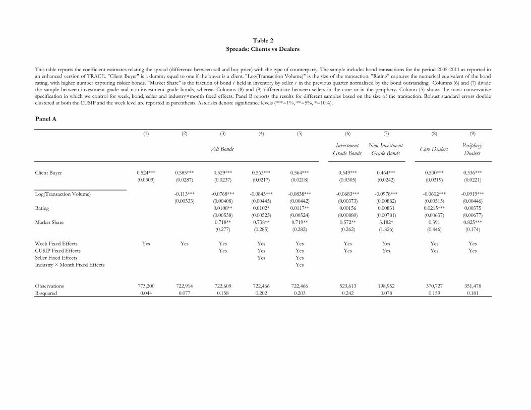
participants higher prices for the assets they sell.20 Columns (1)-(5) of Table 2 (Panel A) consider

the entire sample of transactions, where the relevant coeffi cient is that of the indicator variable

"Client Buyer". Column (1), controlling only for week fixed effects in order to absorb changes in

the average cost of intermediation, shows that on average dealers charge clients 50 basis points

more than they charge other dealers. In Columns (2) and (3) we control for transaction volume,

rating, dealer’s market share and the bond fixed effect (CUSIP); the results are similar. In Column

(4) we also include seller fixed effects, and the results remain unaffected. Finally, in Column (5)

we saturate the model with industry-month fixed effects, so that we exploit variation only for the

bonds in the same industry traded in the same month; again, the results are unaffected. In Column

(6) we restrict the sample to investment-grade bonds and in column (7) to non-investment-grade.

The data show that dealers charge similar prices for the two grades. Columns (8) and (9), instead,

show that both core and peripheral dealers charge their clients about 50 basis points more than

they do other dealers, even controlling for week and bond fixed effects. That is, clients’transaction

costs appear to be about the same regardless of whether their counterparty is a core or a peripheral

dealer. Panel B shows the same regression estimates, but now the markup is related to transaction

size; we find that markups decline with the size of the trade, suggesting that for small trades the

client does not search for the best deal, while for larger transactions there is more competition

among dealers, resulting in reductions in the spread of as much as 60 basis points.

So far we have compared transactions among dealers with those between dealers and clients.

However, Figures 3 and 4 show that even among interdealer transactions there is significant hetero-

geneity. The trades with the lowest spreads are those between core dealers and peripheral-to-core

dealer transactions; core-peripheral dealer and core-client transactions show significantly higher

spreads, and these increase significantly during the crisis that began in the first quarter of 2008. So

we explore these findings further by analyzing interdealer transactions in Table 3. The comparison

group is inter-core-dealer transactions, i.e. trades in which both seller and buyer have a network

20Theoretical support for this hypothesis is provided by Babus and Kondor (2013), and Farboodi (2014). Babusand Kondor (2013) shows that more central dealers can learn faster from the prices of the transactions they execute,increasing their trading gains. Similarly, in the context of an endogenous network formation model, Farboodi (2014)shows that core dealers charge higher average prices to the peripheral dealers than to other core ones.

11

centrality measure in the top 30.21 Column (1) shows a clear ranking among different types of trades

as far as the spread is concerned. Specifically, core-core transactions are the cheapest, periphery-

core trades are slightly more costly, periphery-periphery are about 20 basis points more expensive

than core-core, and core-periphery transactions are the most expensive by almost 30 bp. Columns

(2)-(4) show that these results remain both statistically and economically significant even when we

include controls. Columns (5) and (6) show that core dealers charge the peripheral dealers about

10 basis points more for non-investment-grade than for investment grade bond trades. However,

there is no significant difference by bond rating when peripheral sellers are dealing with core buyers.

It would thus appear that the core dealers can indeed profit more from riskier investments when

they transact with marginal dealers than with other core dealers. Transactions between peripheral

dealers show a similar pattern, with non-investment-grade bond trades exhibiting higher margins.

These results are consistent with the findings of Green et al. (2007a), Green (2007), and Li and

Schürhoff (2014) for other off-exchange markets.

In short, these results establish a very significant relationship between a dealer’s position in the

network and the profits captured in trades with clients or other dealers. Of course, our measure of

network centrality could be proxying for the dealer’s bargaining power, one of the main parameters

common to the theoretical literature on OTC trading. However, we can now show that the prior

bilateral relationships among dealers, which are usually left unmodelled, are at least as important

as bargaining power in predicting spreads.

5 The Main Results

Let us start by analyzing how existing bilateral trading relationships among dealers affect spreads,

especially in times of market turmoil. We then investigate how the network reacts when a core

dealer defaults.

5.1 Trading Relationships

To this point we have considered only position in the network, core versus periphery, as a fac-

tor potentially affecting profit margins. We now turn to a more in-depth analysis of the role of

21The results are qualitatively the same if the sample is narrowed to the top 20 or broadened to the top 40 dealers.

12

prior bilateral relationships in the OTC corporate bond market. We compute the fraction of sales

that seller s had with buyer b in the previous quarter, normalized by the s’s total sales (Fraction

Saless,b/Total Saless), which we label "Fraction Selling to Counterparty". We also compute the

fraction of trades in which buyer b bought bonds from seller s, normalized by b’s total purchases in

the previous quarter (Fraction Purchasess,b/Total Purchasesb), designated "Fraction Buying from

Counterparty".

Table 4 reports the estimation results from our formal test of Hypothesis I. Column (1) shows the

effect of “Fraction Selling to Counterparty”and “Fraction buying from Counterparty”on seller’s

spread controlling for week fixed effects, the volume of the trade, market share and the bond’s

rating. On average a higher fraction of past sales to the buyer predicts significantly lower profit

margins. Similarly, a higher fraction of purchases by the buyer from the same seller, compared

to his total purchases, predicts significantly lower profit margins. The data also confirms that in

general higher transaction volume corresponds to lower profit margins and lower-rated bonds are

associated with higher profit margins.

Column (2) confirms these results by controlling for the bond fixed effects. The coeffi cient is

quite similar and both economically and statistically significant. In other words, comparing the

same bond traded between two different pairs of counterparties in the same week, those with the

stronger past tie have lower spreads. Column (3) adds industry-month fixed effects, to make sure

that the result is not driven by unobserved heterogeneity in the type of bonds traded by some

counterparties and not others. The results are economically significant. There is a difference

in the markup of about 20 basis points between the bottom and the top decile of relationship

strength. The results hold even in our most conservative specification, where we control for seller-

and buyer-month fixed effects, which neutralize any time-varying shocks at dealer level that could

affect trading behavior.

Thus the results show the importance of the existing relationships between counterparties. Now

Column (4) focuses on the positions of the seller and buyer in the network, controlling for week and

bond fixed effects. In this way we test whether or not the importance of bilateral relationships is

subsumed by relative centrality in the network. We find in fact that a more central buyer can get a

lower price from his counterparties than a more peripheral one, while the results for the seller are

weaker, both statistically and economically. Let us emphasize that although this shows that dealer

13

centrality is important in explaining markups (central sellers buy at lower prices), it also shows

that network centrality does not explain the importance of prior bilateral relationships away.

Finally, Columns (5) and (6) demonstrate that the importance of existing bilateral relationships

remains even including seller- and buyer-month fixed effects, thus controlling for time-varying

heterogeneity at dealer level. Overall, there is evidence that existing trading relationships play a

major role in shaping trading behavior, at least as important as the dealer’s degree of network

centrality.

5.2 Dealer Network and Trading Relationships in Times of Market Turmoil

Now we are in a position to address one of our main questions: When are these prior relationships

most valuable? And do dealers demand higher spreads during periods of high uncertainty, especially

from the counterparties that are most dependent on them? In answering we exploit the time series

dimension of our data to test Hypothesis II. Specifically, our dataset covers the financial crisis, so

we can investigate dealers’trading behavior as a function of their existing relationships during the

crisis.

Table 5 shows the results. We take two different approaches. First we interact our measures

of prior trading relationships and of network centrality with the volatility index (VIX). Second,

we split the sample into three periods to capture the different phases of the crisis. We begin, in

Columns (1)-(2), by interacting the intensity of the relationship between seller and buyer with the

volatility index controlling for week and bond fixed effects. Interestingly, if the two parties have a

strong tie the incidence of the trading relationship on the spreads becomes even more pronounced

in periods of intense uncertainty. It is particularly important to hold the bond constant, because

changes in the spreads could be due to a change in the composition of the bonds traded at the peak

of the crisis, as dealers might well be reducing inventories by getting rid of their riskier holdings.

Specifically, comparing the same bond, traded in the same week among different counterparties, we

find that dealers who had previously done a significant fraction of their corporate bond business

with the same counterparties were able to strike a better deal, and that profit margins were lower in

correspondence with spikes in market uncertainty. In terms of magnitude, a one-standard-deviation

increase in the VIX reduces margins by 35 basis points. At the worst of the crisis, the VIX increased

by about three standard deviations, which makes these results economically significant indeed. The

14

results are very similar when we control for industry-month fixed effects. That is, in times of market

distress dealers tended to be liquidity providers for their closest counterparties.

Did dealers also serve as liquidity providers for market participants in general? Columns (4)-

(6) address this issue by testing whether the degree of network centrality becomes more important

during periods of market turmoil. Interacting our centrality measure for buyer and seller with the

volatility index, we find that more central sellers profit even more from their position during periods

of stress, and central buyers too have greater bargaining power, concluding transactions at lower

prices. This means that a core dealer can capture even higher rents by trading with peripheral

dealers in bad times, but peripheral dealers cannot do the same when selling to a core dealer. Thus

the gap between core and peripheral dealers is accentuated in crisis periods, as only the former

can take advantage of their position. This supports the thesis that in bad times dealers provide

liquidity selectively to their closest counterparties only, while exploiting their centrality with other

market participants.

As a complementary strategy, in Panel B of Table 5 we split the sample into three sub-periods,

January 2005-December 2006, January 2007-August 2008, and September 2008-July 2009. The

first period represents normal times, the second the run-up to the financial crisis, and the third the

crisis peak after the failure of Lehman Brothers. Comparing the results in the three columns, we

see that relative to other traders central sellers and buyers capture a significantly larger fraction

of the trading profits during the crisis than in normal times, even controlling for week and bond

fixed effects. The difference is significant statistically as well as economically: sellers charge six

times more during the crisis than during the run-up, and buyers get discounts four times larger.

Specifically, buyers in the top decile of centrality purchase at spreads 50 basis points narrower than

those charged to buyers in the bottom decile, while the markups of the most central sellers are 40

bp higher.

The comparison further confirms that the role of existing relationships was even more important

than in normal times. At the height of the crisis, the presence of a repeated seller or buyer rela-

tionship with a given counterparty led to lower margins than in normal times. Unlike the centrality

measure, whose coeffi cient increases monotonically as the market turmoil intensifies, the bilateral

relationships have the same impact on spread in Columns (1) and (2): their importance only in-

creases significantly at the peak of the crisis (Column 3). The economic effect too is important:

15

the gap between the markups of dealers in the top and in the bottom decile of our measure of

relationship is about 40 bp between the pre-crisis and crisis period. Thus, this analysis confirms

the time-varying role of bilateral relationships in turbulent times and their importance, on a par

with the network centrality.

Figure 3 suggests that all spreads increase significantly around the Lehman Brothers’collapse,

but with considerable heterogeneity across transactions among the different types of market par-

ticipant. This heterogeneity could be due to a variety of factors, such as a change in the pool

of bonds traded by different counterparties, or shocks to specific dealers. We address this issue

formally in Table 6, splitting the transactions between dealer types as in Table 3 and interacting

the main indicator variables with the VIX (Columns (1)-(4)). We also split the sample into our

three periods (Columns (5)-(7)). Interestingly, core dealers are able to extract even higher rents

from peripheral dealers in periods of high volatility, but peripheral dealers are not able to do the

same when selling to core dealers; and transactions at the periphery tend to exhibit higher profit

margins in turbulent times. Comparing Column (3) with Column (4), we can see that core dealers

profit even more at times of greater uncertainty in trading with peripheral dealers when the bond

is non-investment-grade. The results are robust to controls for trade characteristics interacted with

the VIX, as well as week-, bond- and industry-month fixed effects. When transactions are compared

over time (Columns (5)-(7)) the results are very similar, with core dealers profiting about three

times more from peripheral dealers at the peak of the crisis.

These results highlight the main finding of this section: existing relationships are good predictors

of profit margins, and they become even more important under market turmoil. This contrasts with

the theoretical literature on OTC markets, which generally —with the exceptions of Seppi (1990)

and Glode and Opp (2016) —posits that interactions between buyers and sellers are anonymous and

price dispersion is not affected by the parties’transaction history.22 A further original feature of

our study is the discovery that the importance of existing relationships is time-varying. In addition,

relationship-based trading behavior benefits core at the expense of peripheral dealers.

22The models proposed by Seppi (1990) and Glode and Opp (2016) highlight how the identity of the counterpartymight significantly shape the trading process.

16

5.3 Default of a Core Dealer

Having established that prior trading relationships and network centrality shape dealers’rent shares

and liquidity provision, and that their importance is heightened in crisis, we now investigate the

impact on a dealer’s behavior of losing a major trading partner. The question, that is, is whether

these relationships are easily substitutable. If there are no frictions — i.e. if dealers can readily

locate new counterparties and new relationships can be easily formed —losing a tie with a specific

dealer should not affect profitability or transaction costs. We test this hypothesis formally using

the information on dealer identities contained in our regulatory data. In particular, we want to see

how the network reacts to the shock of Dealer D’s default and how this affected the dealers who

had prior relationships with Dealer D.

Table 7 reports the regressions that relate the strength of the relationship with Dealer D with

other dealers’ profit margins after the collapse. For each dealer we compute the fraction of all

bonds sold to Dealer D as the average for the year 2007. This is to make sure we capture a stable

relationship with Dealer D, rather than deleveraging on the eve of the bankruptcy. We consider the

fractions of securities both bought from and sold to Dealer D, but in fact the two are very closely

correlated. Formally, we estimate the following regressions:

Spreadi,j,k,t = β1Fraction of Purchase Transactionsi,D × Post+

β2Fraction of Purchase Transactionsi,D +

ΓXi,j,k + λt + εi,j,k,t

where i and j denote the two counterparties, k indexes the bond and t the week. "Frac-

tion of Purchase Transactionsi,D" proxies the intensity of the relationship between dealer i and

Dealer D in the pre-period. "Post" is a dummy equal to 1 in the period after the default. We

include several controls in the vector Xi,j,k to capture heterogeneity across dealers and bonds, and

all specifications include week fixed effects. The relevant coeffi cient is β1 on the interaction between

the intensity of the pre-default trading relationship with Dealer D and the indicator for the post-

default period. Column (1), controlling for week and CUSIP fixed effects, shows that the dealers

that were buying the most from Dealer D suffered a significant decline in profit margins. The effect

17

is both statistically and economically significant: a one-standard-deviation increase in the fraction

of assets bought from Dealer D narrows the spread by an average of 14 basis points.

This result is robust to the inclusion of trade characteristics (volume and bond rating) and

of our measure of the strength of the relationship (Column 2). Columns (3) and (4) further test

the sensitivity of the result by including in turn the seller and the buyer fixed effects to control

for possible unobserved heterogeneity across dealers more or less closely connected to Dealer D.

Column (5) is our most restrictive specification, controlling also for seller- and buyer-month fixed

effects. This means that comparing transactions in the same period, in the same bond, and by

similar dealers, the dealers who were relying more heavily on Dealer D suffered the most with its

collapse.

Columns (6)-(10) complement these results by studying how the dealers who were selling more

of their assets to Dealer D responded. As before, the main coeffi cient is the interaction between

the dummy Post (equal to 1 after the default), and the average fraction of assets sold to Dealer

D in 2007. As above, we find that dealers more exposed to Dealer D experienced a significant

reduction in profit margins after the default. However, statistical significance is reduced: it is

significant at the 10% level only when seller- and buyer-month fixed effects are included, in Column

(10). Presumably this is because the fractions of sale and purchase transactions are very closely

correlated.

6 Dealers’Inventories in Bad Times

As is discussed in section 3, theoretical work considers whether and how dealers may be able to "lean

against the wind" by expanding inventories at times of distress (see, for instance, Weill (2007)).

We test Hypothesis III by addressing the following question: Were the dealers able to absorb the

selling pressure of other market participants? We can employ transaction data to compute dealers’

inventory around the collapse of Dealer D.23 One problem with calculating inventories from trade

data is that we do not observe the primary market, so our measure necessarily excludes newly issued

bonds. To avoid bias in our computation, we use a very narrow time window around the failure

and exclude both new issues and those maturing within that time. Moreover, the primary market

23To make sure our results are not driven by smaller broker-dealers, we focus on the top 100 by transaction volume.We also ran the same analysis with the top 30 only, with highly similar results.

18

was significantly less active during our period than ordinarily, so our measure can be considered a

good proxy for the dealers’actual inventory in this brief period.

We start by plotting, in Figure 5, the dealers’inventory of bonds characterized by differential

selling pressure, defined as the volume sold by clients to dealers normalized by the amount out-

standing. The idea is that if the dealers are providing liquidity by fulfilling sell orders without

immediately unloading the bonds in order to avoid further price declines, then we should observe

an expansion of inventories of the bonds subject to the most intense selling pressure. Instead, we

find that around the peak of the crisis dealers reduced their inventories most sharply precisely for

these bonds.

Table 8 formally tests and quantifies this hypothesis, dividing bonds into terciles of selling

pressure. The regressions are normalized by dividing the inventory for each dealer for each tercile

by the standard deviation of inventory for that dealer and tercile. Columns (1) and (2) are for a

three-month window around the failure of Dealer D, while Column (3) restricts the sample to a

four-week window. The first two columns show that dealers reduced their inventory of bonds in the

top two terciles of selling pressure significantly, by 25%-30% of 1 standard deviation. The result

holds also for the shorter window in Column (3), which shows a reduction of 20% of 1 standard

deviation for the bonds in the top tercile. These results strongly suggest that in the midst of the

market turmoil dealers did not readily provide liquidity to clients. We can now seek to determine

whether their behavior also increased transaction costs. One possible source of such an increase is

a lengthening of the intermediation chain owing to dealers’inability to increase their inventories.

The prevalence of transactions among intermediaries along intermediation chains has been re-

cently highlighted by Li and Schürhoff (2014) for the municipal bond market, Hollifield et al. (2012)

for securitized products and Weller (2014) for metals futures. However, there is no study of the

way in which these intermediation chains respond to shocks. Specifically, one possible reason why

spreads might have widened following the default of Dealer D could be the lengthening of the

chains, as in Hypothesis IV. To test this hypothesis, Figure 6 plots the estimated week fixed effects

for a regression whose dependent variable is trading chain length. After the failure of Dealer D,

intermediation chains between seller and buyer lengthened significantly. This suggests that with

the disappearance of a major counterparty, dealers had to form new trading relationships, and as

Table 7 has shown these were significantly less profitable than their predecessors. We can also

19

confirm this result in Table 9 by estimating a regression of chain length over the Post indicator

(equal to 1 after the bankruptcy). Even controlling for bond- and industry-month fixed effects and

other trade characteristics, we find that on average the intermediation chain becomes significantly

longer, and the effect appears to be more pronounced when the seller is core rather than peripheral.

This increase in the intermediation length matters because it might increase the overall inter-

mediation cost. Table 10 shows how the spread is allocated among intermediaries along the chain;

we find that being closer to the client yields higher profits. Moreover, since the average spread is

about 60 bps, and the intermediaries other than the one closest to the client charge about 20-30

bps less than the average spread, we have that intermediation costs increases with the length of

the chain.

Is there a relationship between the change in length documented in Table 9 and the change

in dealers’ inventory? On this question, Figure 7 plots our measure of inventory for bonds that

underwent changes in average intermediation chain length above and below the median. By this

measure, inventory shrinks most markedly for the bonds whose chains lengthened, suggesting that

dealers were not providing liquidity, because they were diminishing their inventories, making it

harder to accommodate clients’order requests and thus requiring a longer intermediation chain.

Formally, Table 11 reports the results of the following regression:

Inventoryi,j,t = β1Above Mediani,D × Post+ β2Above Mediani,D + Post+

θi + λt + εi,j,t

where i is the dealer, j is the bond and t is the week. Above Mediani,D equals one for the

bonds whose intermediation chain lengthened by more than the median. Post equals one after the

Dealer D’s default. We control for dealers’(θi) and time fixed effects (λt). Since we cannot observe

the issuance of new bonds, our measure of inventory excludes them. Given the especially turbulent

period covered, however, we are convinced that this does not significantly affect our estimates.

However, to alleviate such concerns, in Columns (1) and (2) we take a three-month window around

the default and in Column (3) a more restrictive four-week window. To simplify interpretation, we

normalize our measure of inventory by dividing the inventory for each dealer above and below the

median by the standard deviation in that dealer’s inventory. In the most restrictive specification,

20

we find a reduction of 20% of inventory for the bonds whose intermediation chain lengthened. This

result does not appear to be driven by differences across dealers or by common shocks to the bond

market, as we control for dealer and time fixed effects. The evidence is that intermediation costs

increased because dealers were deleveraging and holding smaller inventories at the peak of the crisis.

Overall, our results offer new insights into dealers’ behavior during one of the most severe

episodes of financial market turmoil in recent times. Rather than provide price support by absorbing

the excess supply from other market participants, dealers tried to unload these bonds immediately.

And by reducing inventories they also made the market more illiquid, as the average length of the

intermediation chain increased significantly, which means higher transaction costs for clients.

7 Concluding Remarks

The recent crisis has spotlighted the issue of how governments should handle complex financial

institutions that are "too connected to fail". Theoretical contributions have shown how connec-

tions between financial institutions, stemming both from correlation in asset holdings and from an

intricate system of cross-liabilities, could potentially trigger a cascade of bank failures. However,

there is little if any evidence on the role played by existing bilateral relationships among financial

institutions.

This paper focuses on a crucial over-the-counter market, that in corporate bonds, inquiring

into the way in which the network of relationships between dealers shapes trading behavior and

liquidity provision both in normal times and in periods of turmoil. We start by showing the clear

core-periphery structure of the market, in which a few highly interconnected dealers intermediate

most of the trades with other dealers and with clients and many sparsely connected ones trade

less frequently. This structure is highly stable over time. Next we show that the dealers’bilateral

relationships and their degree of network centrality are quite reliable predictors of their transaction

costs, the more central dealers taking advantage of their connections to get better deals. More

important, during periods of distress dealers tend to provide liquidity to the counterparties with

whom they have the strongest ties. But core dealers exploit their connections at the expense of

peripheral dealers and of clients, increasing the spreads they charge to them. In the same vein, the

value of being highly connected and systemically important increases when uncertainty is high.

21

In contrast to most of the empirical studies of the corporate bond market, we are able to learn

the identity of each dealer, and so to see how the network responded to a large shock such as the

failure of Dealer D. We find that Dealer D’s main counterparties had to narrow their spreads after

September 2008, by comparison with other, similar dealers trading the same bonds in the same

period.

To conclude, our results shed new light on the way in which prior bilateral relationships between

financial institutions sometimes serve as a buffer in times of stress, but also reveal that they

heighten the fragility of the system, insofar as connection to more fragile dealers may worsen

trading outcomes even for healthy dealers.

22

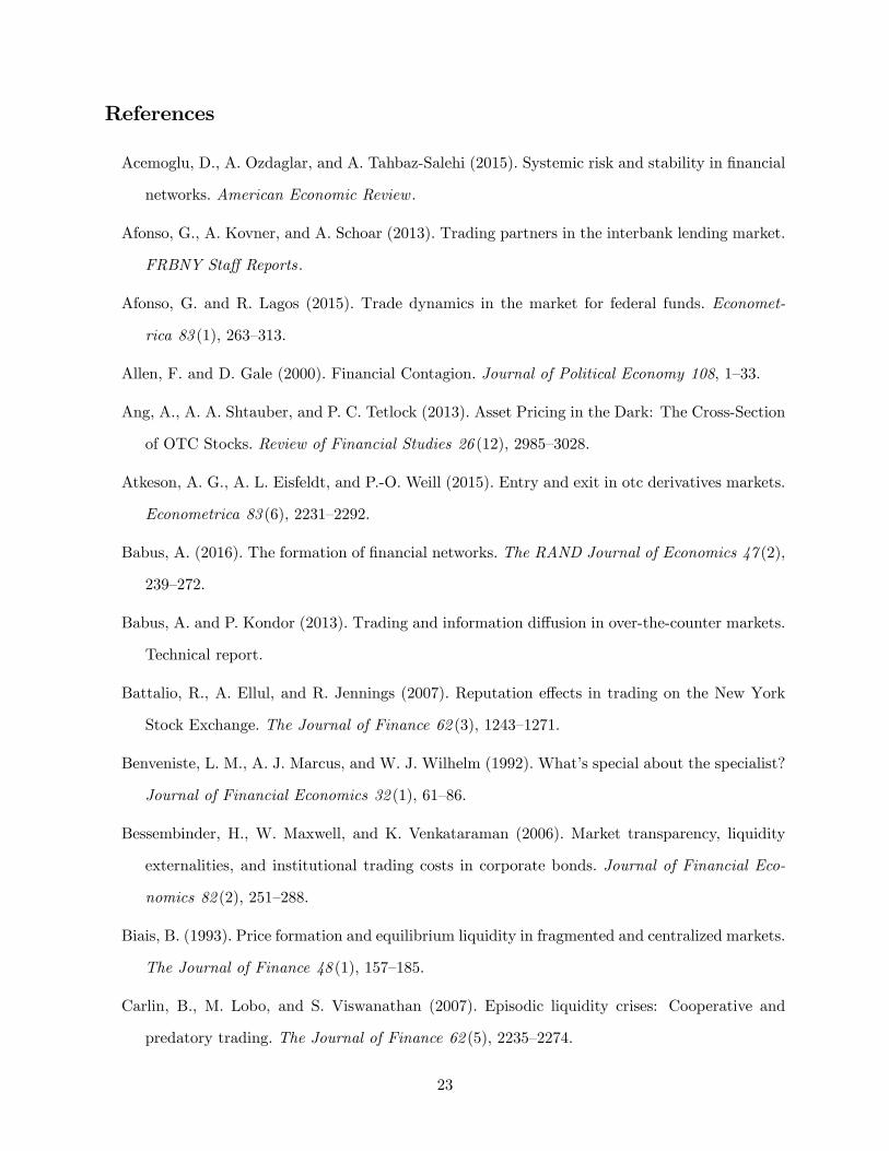
References

Acemoglu, D., A. Ozdaglar, and A. Tahbaz-Salehi (2015). Systemic risk and stability in financial

networks. American Economic Review .

Afonso, G., A. Kovner, and A. Schoar (2013). Trading partners in the interbank lending market.

FRBNY Staff Reports.

Afonso, G. and R. Lagos (2015). Trade dynamics in the market for federal funds. Economet-

rica 83 (1), 263—313.

Allen, F. and D. Gale (2000). Financial Contagion. Journal of Political Economy 108, 1—33.

Ang, A., A. A. Shtauber, and P. C. Tetlock (2013). Asset Pricing in the Dark: The Cross-Section

of OTC Stocks. Review of Financial Studies 26 (12), 2985—3028.

Atkeson, A. G., A. L. Eisfeldt, and P.-O. Weill (2015). Entry and exit in otc derivatives markets.

Econometrica 83 (6), 2231—2292.

Babus, A. (2016). The formation of financial networks. The RAND Journal of Economics 47 (2),

239—272.

Babus, A. and P. Kondor (2013). Trading and information diffusion in over-the-counter markets.

Technical report.

Battalio, R., A. Ellul, and R. Jennings (2007). Reputation effects in trading on the New York

Stock Exchange. The Journal of Finance 62 (3), 1243—1271.

Benveniste, L. M., A. J. Marcus, and W. J. Wilhelm (1992). What’s special about the specialist?

Journal of Financial Economics 32 (1), 61—86.

Bessembinder, H., W. Maxwell, and K. Venkataraman (2006). Market transparency, liquidity

externalities, and institutional trading costs in corporate bonds. Journal of Financial Eco-

nomics 82 (2), 251—288.

Biais, B. (1993). Price formation and equilibrium liquidity in fragmented and centralized markets.

The Journal of Finance 48 (1), 157—185.

Carlin, B., M. Lobo, and S. Viswanathan (2007). Episodic liquidity crises: Cooperative and

predatory trading. The Journal of Finance 62 (5), 2235—2274.

23

Choi, J. and O. Shachar (2013). Did liquidity providers become liquidity seekers? Technical

report, Staff Report, Federal Reserve Bank of New York.

Cocco, J. F., F. J. Gomes, and N. C. Martins (2009). Lending relationships in the interbank

market. Journal of Financial Intermediation 18 (1), 24—48.

Duffi e, D., N. Garleanu, and L. Pedersen (2005). Over-the-Counter Markets. Econometrica 73 (6),

1815—1847.

Duffi e, D., N. Garleanu, and L. Pedersen (2007). Valuation in over-the-counter markets. Review

of Financial Studies 20 (6), 1865—1900.

Edwards, A., L. Harris, and M. Piwowar (2007). Corporate bond market transaction costs and

transparency. The Journal of Finance 62 (3), 1421—1451.

Elliott, M., B. Golub, and M. O. Jackson (2015). Financial Networks and Contagion. American

Economic Review .

Farboodi, M. (2014). Intermediation and voluntary exposure to counterparty risk. Technical

report, Working Paper, University of Chicago.

Freixas, X., B. M. Parigi, and J.-C. Rochet (2000). Systemic Risk, Interbank Relations, and

Liquidity Provision by the Central Bank. Journal of Money, Credit and Banking 32 (3), 611—

638.

Gabrieli, S. and C.-P. Georg (2014). A network view on interbank market freezes.

Glode, V. and C. C. Opp (2016). Adverse Selection and Intermediation Chains. American Eco-

nomic Review.

Green, R. C. (2007). Presidential address: Issuers, underwriter syndicates, and aftermarket trans-

parency. The Journal of Finance 62 (4), 1529—1550.

Green, R. C., B. Hollifield, and N. Schürhoff (2007a). Dealer intermediation and price behavior

in the aftermarket for new bond issues. Journal of Financial Economics 86 (3), 643—682.

Green, R. C., B. Hollifield, and N. Schürhoff (2007b). Financial intermediation and the costs of

trading in an opaque market. Review of Financial Studies 20 (2), 275—314.

24

Green, R. C., D. Li, and N. Schürhoff (2010). Price discovery in illiquid markets: Do financial

asset prices rise faster than they fall? The Journal of Finance 65 (5), 1669—1702.

Hendershott, T., D. Li, D. Livdan, and N. Schürhoff (2016). Relationship Trading in OTC

Markets.

Henderson, B. J. and H. Tookes (2012). Do investment banks’relationships with investors impact

pricing? The case of convertible bond issues. Management Science 58 (12), 2272—2291.

Hollifield, B., A. Neklyudov, and C. S. Spatt (2012). Bid-ask spreads and the pricing of securi-

tizations: 144a vs. registered securitizations.

Hugonnier, J., B. Lester, and P.-O. Weill (2014). Heterogeneity in Decentralized Asset Markets.

Technical report, National Bureau of Economic Research.

Li, D. and N. Schürhoff (2014). Dealer networks. Available at SSRN 2023201 .

Mitchell, M. and T. Pulvino (2012). Arbitrage crashes and the speed of capital. Journal of

Financial Economics 104 (3), 469—490.

Pagano, M. and A. Röell (1992). Auction and dealership markets: what is the difference? Euro-

pean Economic Review 36 (2), 613—623.

Schultz, P. (2001). Corporate bond trading costs: A peek behind the curtain. The Journal of

Finance 56 (2), 677—698.

Seppi, D. J. (1990). Equilibrium block trading and asymmetric information. the Journal of Fi-

nance 45 (1), 73—94.

Shen, J., B. Wei, and H. Yan (2015). Financial Intermediation Chains in an OTC Market.

Stanton, R., J. Walden, and N. Wallace (2014). Securitization Networks and Endogenous Finan-

cial Norms in US Mortgage Markets.

Weill, P. (2007). Leaning against the wind. The Review of Economic Studies 74 (4), 1329—1354.

Weller, B. (2014). Intermediation chains. Working paper.

25

Figure 1

This figure plots the cumulative distribution of seller’s network centrality for all transactions, both

among dealers and with clients.

Figure 2

This figure plots the core-periphery network structure where each link is a transaction, and at the

center there are the transactions with clients. Darker lines indicate a higher number of transactions

between the two nodes.

Client

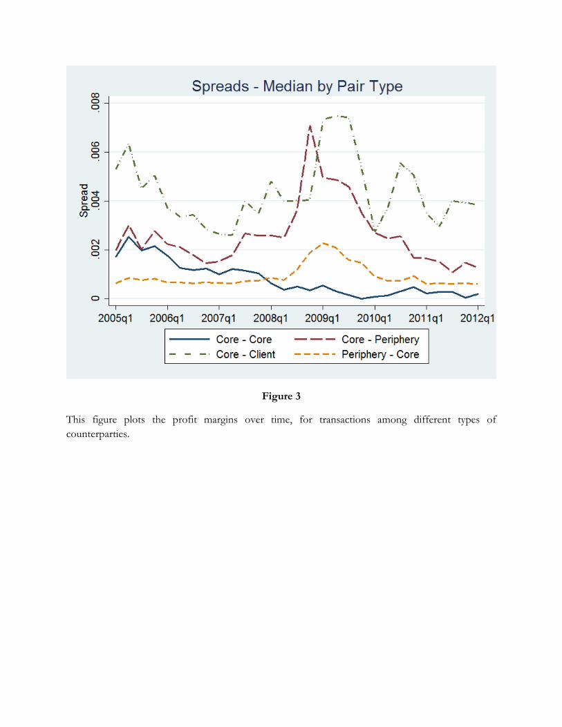
Figure 3

This figure plots the profit margins over time, for transactions among different types of

counterparties.

Figure 4

This figure plots the cumulative distribution of the profit margins for the different types of

counterparties.

Figure 5

This figure plots the dealers’ inventory for bonds that experienced different selling pressure from the

clients, which is defined as the amount sold by clients to dealers normalized by the amount

outstanding.

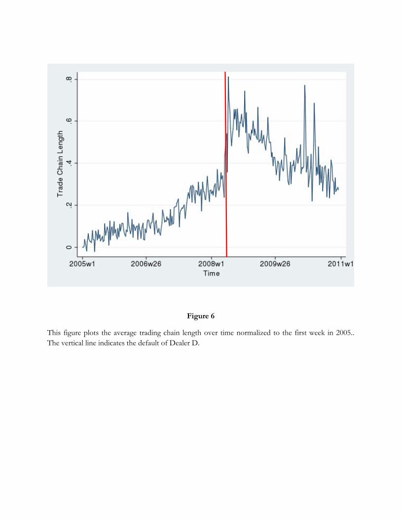
Figure 6

This figure plots the average trading chain length over time normalized to the first week in 2005..

The vertical line indicates the default of Dealer D.

Figure 7

This figure plots the dealers’ inventory, normalized to July 2008, i.e. three months before Dealer D’s

default. The blue solid (red dashed) line shows the inventory for bonds that experienced a change in

the length of the intermediation chain above (below) median, as computed by comparing the length

of the chain before and after the Dealer D’s default.

Panel A

Bonds Trades Bonds Trades Bonds Trades

Number of Bonds and Trades 56,707 52,151,496 4,540 773,200 4,636 5,296,107

Credit Quality Distribution (%)

Superior (AA and UP) 10.0% 9.5% 10.24% 8.90% 10.42% 8.95%

Other Investment Grade (BBB-A) 68.6% 79.7% 74.82% 79.18% 73.47% 81.24%

High-Yield (below BBB) 5.3% 7.3% 5.62% 8.29% 5.65% 6.97%

Not Rated 16.2% 3.5% 9.32% 3.63% 10.46% 2.84%

Issue Size Distribution (%)

Small (< $100 Million) 85.9% 61.4% 86.04% 68.23% 86.48% 64.70%

Medium ($100 - $500 Million) 3.8% 24.4% 3.94% 17.77% 3.77% 21.54%

Large ( > $500 Million) 0.0% 0.14% 0.02% 0.14% 0.02% 0.17%

Missing Offering Data 10.3% 14.1% 10.00% 13.86% 9.73% 13.59%

Maturity Distribution (%)

Under 2 years 7.0% 0.3% 6.34% 0.68% 7.25% 0.41%

2-5 years 20.8% 6.8% 19.60% 6.73% 20.00% 6.54%

5-20 years 59.9% 76.4% 60.00% 76.84% 59.10% 79.91%

20+ years 12.0% 15.8% 13.74% 15.01% 13.33% 12.53%

Missing Maturity Data 0.3% 0.6% 0.31% 0.74% 0.32% 0.61%

Panel B

Statistics for Table 3

(1) (2) (3) (4) (5) (6) (7) (8)

N Mean St. Dev. p1 p10 p50 p90 p99

Average Spread 773,200 0.621 1.427 -1.152 0 0.239 1.976 4.455

Counterparty Buyer 773,200 0.422 0.494 0 0 0 1 1

Network Centrality 730,225 52.16 94.28 1 2 25 107 554

Log(Transaction Volume) 722,914 8.397 2.015 4.630 6.225 7.832 11.58 13.30

Market Share 773,200 0.00553 0.0329 1.33e-06 1.00e-05 0.000233 0.00708 0.102

Rating 773,200 8.555 4.918 0 3 8 16 22

Investment Grade 773,200 0.730 0.444 0 0 1 1 1

Statistics for Tables 4-7

Average Spread 446,854 0.393 1.515 -1.832 0 0.102 1.132 4.999

Fraction Selling to Counterparty 417,640 0.112 0.161 7.79e-05 0.00184 0.0426 0.319 0.727

Fraction Buying from Counterparty 417,639 0.135 0.203 8.64e-05 0.00233 0.0523 0.386 1

Network Centrality Seller 421,221 0.102 0.0397 0.00231 0.0483 0.102 0.151 0.170

Network Centrality Buyer 420,139 0.101 0.0463 0.00104 0.0235 0.113 0.152 0.172

Core-Periphery 446,854 0.185 0.388 0 0 0 1 1

Periphery-Core 446,854 0.244 0.430 0 0 0 1 1

Periphery-Periphery 446,854 0.256 0.437 0 0 0 1 1

Log(Transaction Volume) 424,872 8.466 2.051 4.626 6.223 7.869 11.63 13.21

Market Share 446,854 0.00358 0.0229 1.14e-06 1.00e-05 0.000233 0.00541 0.0554

Rating 446,854 8.984 5.074 0 3 8 17 22

Statistics for Table 8

Average Spread 30,687 0.596 2.549 -7.514 0 0.183 2.064 9.482

Fraction of Sale Transactions with Dealer D 30,687 0.0174 0.0269 0 0.000368 0.00337 0.0678 0.0929

Fraction of Purchase Transactions with Dealer D 30,687 0.0219 0.0279 0 0.000535 0.00995 0.0740 0.104

Fraction Selling to Counterparty 29,582 0.0936 0.129 6.58e-05 0.00194 0.0378 0.256 0.611

Fraction Buying from Counterparty 29,582 0.134 0.218 0.000133 0.00255 0.0522 0.242 1

Log(Transaction Volume) 29,394 8.105 1.891 4.508 6.109 7.749 11.16 12.73

Market Share 446,854 0.00358 0.0229 1.14e-06 1.00e-05 0.000233 0.00541 0.0554

Rating 30,687 8.096 5.366 1 2 6 16 22

Appendix Estimation Sample

The table reports descriptive statistics for the main variables employed in our analysis. In the Panel A, we present the main bond characteristics: the number of bonds and the number of trade,

the bonds' credit quality, issue size and maturity, as provided by a confidential version of TRACE for the period 2005-2011. The first two columns report the statistics for the full data sample.

Due to computing limitations, we focus on a random 10% sample (the draw is based on the last digit of the CUSIP being equal to zero). The remaining columns report the summary statistics for

the main estimation sample which restricts attention to buy and sell transactions observed within an hour from each other, and for the sample used in the robustness checks in the appendix.

Panel B provides summary statistics for these characteristics and for the transactions, such as the bilateral relationships, the profit margins and the seller's centrality measure for the main results.

Summary Statistics

Table 1

Full Sample Estimation Sample

Panel A

(1) (2) (3) (4) (5) (6) (7) (8) (9)

Investment

Grade Bonds

Non-Investment

Grade BondsCore Dealers

Periphery

Dealers

Client Buyer 0.524*** 0.585*** 0.529*** 0.563*** 0.564*** 0.549*** 0.464*** 0.500*** 0.536***

(0.0309) (0.0287) (0.0237) (0.0217) (0.0218) (0.0305) (0.0242) (0.0319) (0.0221)

Log(Transaction Volume) -0.113*** -0.0768*** -0.0843*** -0.0838*** -0.0683*** -0.0978*** -0.0602*** -0.0919***

(0.00533) (0.00408) (0.00445) (0.00442) (0.00373) (0.00882) (0.00515) (0.00446)

Rating 0.0108** 0.0102* 0.0117** 0.00156 0.00831 0.0215*** 0.00375

(0.00538) (0.00523) (0.00524) (0.00880) (0.00781) (0.00637) (0.00677)

Market Share 0.718** 0.738** 0.719** 0.572** 3.182* 0.391 0.825***

(0.277) (0.285) (0.282) (0.262) (1.826) (0.446) (0.174)

Week Fixed Effects Yes Yes Yes Yes Yes Yes Yes Yes Yes

CUSIP Fixed Effects Yes Yes Yes Yes Yes Yes Yes

Seller Fixed Effects Yes Yes

Industry × Month Fixed Effects Yes

Observations 773,200 722,914 722,609 722,466 722,466 523,613 198,952 370,727 351,478

R-squared 0.044 0.077 0.158 0.202 0.203 0.242 0.078 0.159 0.181

Table 2

This table reports the coefficient estimates relating the spread (difference between sell and buy price) with the type of counterparty. The sample includes bond transactions for the period 2005-2011 as reported in

an enhanced version of TRACE. "Client Buyer" is a dummy equal to one if the buyer is a client. "Log(Transaction Volume)" is the size of the transaction. "Rating" captures the numerical equivalent of the bond

rating, with higher number capturing riskier bonds. "Market Share" is the fraction of bond i held in inventory by seller s in the previous quarter normalized by the bond outstanding. Columns (6) and (7) divide

the sample between investment grade and non-investment grade bonds, whereas Columns (8) and (9) differentiate between sellers in the core or in the periphery. Column (5) shows the most conservative

specification in which we control for week, bond, seller and industry×month fixed effects. Panel B reports the results for different samples based on the size of the transaction. Robust standard errors double

clustered at both the CUSIP and the week level are reported in parenthesis. Asterisks denote significance levels (***=1%, **=5%, *=10%).

Spreads: Clients vs Dealers

All Bonds

Panel B

(1) (2) (3) (4)

Client Buyer 0.658*** 0.558*** 0.202*** 0.0850***

(0.0317) (0.0267) (0.0135) (0.0147)

Log(Transaction Volume) -0.0515*** -0.0874*** -0.0801*** -0.0146

(0.00844) (0.00765) (0.00922) (0.0177)

Rating 0.00710 0.0200** 0.0337*** 0.0269***

(0.00668) (0.00842) (0.00818) (0.00554)

Market Share 0.854*** 0.681* 0.0679 1.135

(0.290) (0.398) (0.468) (1.720)

Week Fixed Effects Yes Yes Yes Yes

CUSIP Fixed Effects Yes Yes Yes Yes

Observations 361,106 180,390 107,992 72,039

R-squared 0.216 0.149 0.069 0.056

Transaction Size Below

Median

Transaction Size Above

90th

Transaction Size between

50th and 75th

Transaction Size between

75th and 90th

(1) (2) (3) (4) (5) (6)

Investment Grade

Bonds

Non-Investment

Grade Bonds

Core-Periphery 0.281*** 0.298*** 0.260*** 0.261*** 0.243*** 0.317***

(0.0174) (0.0174) (0.0160) (0.0162) (0.0169) (0.0332)

Periphery-Periphery 0.196*** 0.231*** 0.145*** 0.148*** 0.115*** 0.207***

(0.0169) (0.0159) (0.0137) (0.0137) (0.0148) (0.0293)

Periphery-Core 0.0602*** 0.141*** 0.0905*** 0.0898*** 0.0811*** 0.118***

(0.0138) (0.0159) (0.0143) (0.0143) (0.0180) (0.0230)

Log(Transaction Volume) -0.0746*** -0.0502*** -0.0499*** -0.0426*** -0.0753***

(0.00456) (0.00407) (0.00410) (0.00323) (0.0113)

Rating 0.0160*** 0.0220*** 0.0227*** 0.0129* 0.0165*

(0.00207) (0.00612) (0.00635) (0.00678) (0.00890)

Market Share 1.123*** 0.876** 0.871** 0.445*** 8.942

(0.312) (0.342) (0.342) (0.157) (5.454)

Week Fixed Effects Yes Yes Yes Yes Yes Yes

CUSIP Fixed Effects Yes Yes Yes Yes

Industry × Month Fixed Effects Yes

Observations 446,854 424,872 424,561 424,561 295,843 128,662

R-squared 0.016 0.026 0.062 0.063 0.077 0.065

All Bonds

Table 3

This table reports the coefficient estimates relating the spreads with the type of counterparty. The sample includes bond transactions for the period 2005-

2011 as reported in an enhanced version of TRACE. "Core-Periphery" is a dummy equal to one if the seller is a core dealer and the buyer is a peripheral

dealer, while "Periphery-Periphery" identifies transactions between dealers in the periphery, and "Periphery-Core" is a dummy equal to one for transactions

where the seller is in the periphery and the buyer is in the core. The comparison group are interdealer transactions between core dealers. "Log(Transaction

Volume)" is the size of the transaction. "Rating" captures the numerical equivalent of the bond rating, with higher number capturing riskier bonds. "Market

Share" is the fraction of bond i held in inventory by seller s in the previous quarter normalized by the bond outstanding. Column (4) shows the most

conservative specification in which we control for week, bond, and industry×month fixed effects. Columns (5) and (6) divide the sample between investment

grade and non-investment grade bonds. Robust standard errors double clustered at both the CUSIP and the week level are reported in parenthesis. Asterisks

denote significance levels (***=1%, **=5%, *=10%).

Spreads and Network Structure

(1) (2) (3) (4) (5) (6)

Fraction Selling to Counterparty -0.697*** -0.727*** -0.725*** -0.514*** -0.332*** -0.333***

(0.0424) (0.0389) (0.0390) (0.0310) (0.0746) (0.0748)

Fraction Buying from Counterparty -0.472*** -0.447*** -0.442*** -0.713*** -0.658*** -0.654***

(0.0277) (0.0234) (0.0231) (0.0333) (0.0883) (0.0967)

Log(Transaction Volume) -0.0812*** -0.0581*** -0.0578*** -0.0601*** -0.0534*** -0.0532***

(0.00509) (0.00449) (0.00452) (0.00445) (0.00514) (0.00542)

Rating 0.0153*** 0.0180*** 0.0185*** 0.0204*** 0.0258*** 0.0261***

(0.00210) (0.00571) (0.00598) (0.00597) (0.00433) (0.00477)

Market Share 1.543*** 0.910** 0.903** 0.958** 0.630 0.622

(0.278) (0.354) (0.353) (0.375) (0.391) (0.408)

Seller Network Centrality 0.272

(0.196)

Buyer Network Centrality -2.031***

(0.167)

Week Fixed Effects Yes Yes Yes Yes Yes Yes

CUSIP Fixed Effects Yes Yes Yes Yes Yes

Industry × Month FE Yes Yes

Seller × Month FE Yes Yes

Buyer × Month FE Yes Yes

Observations 397,419 397,102 397,102 375,889 366,748 366,748

R-squared 0.033 0.069 0.070 0.072 0.285 0.286

This table reports the coefficient estimates relating the spreads with the existing of bilateral relationships between seller and buyer and to their network centrality. The

sample includes bond transactions for the period 2005-2011 as reported in an enhanced version of TRACE. "Fraction Selling to Counterparty" is the fraction of sales

of this seller to this buyer computed in the previous quarter. Similarly for the "Fraction Buying from Counterparty". "Log(Transaction Volume)" is the size of the

transaction. "Rating" captures the numerical equivalent of the bond rating, with higher number capturing riskier bonds. "Market Share" is the fraction of bond i held

in inventory by seller s in the previous quarter normalized by the bond outstanding. The centrality measures are computed using the eigenvector centrality measure in

the previous quarter. Column (6) shows the most conservative specification which includes seller×month, buyer×month and industry×month fixed effects in addition

to week and bond fixed effects. Robust standard errors double clustered at both the CUSIP and the week level are reported in parenthesis. Asterisks denote

significance levels (***=1%, **=5%, *=10%).

Spreads and Bilateral RelationshipsTable 4

Panel A

(1) (2) (3) (4) (5) (6)

Fraction Selling to Counterparty × VIX -0.435*** -0.431*** -0.442*** -0.237*** -0.219*** -0.228***

(0.0402) (0.0392) (0.0399) (0.0386) (0.0390) (0.0391)

Fraction Buying from Counterparty × VIX -0.0542** -0.0406* -0.0376* -0.210*** -0.216*** -0.215***

(0.0230) (0.0226) (0.0222) (0.0330) (0.0326) (0.0324)

Seller Network Centrality × VIX 1.078*** 1.262*** 1.253***

(0.212) (0.211) (0.214)

Buyer Network Centrality × VIX -1.085*** -1.222*** -1.250***

(0.183) (0.176) (0.181)

Fraction Selling to Counterparty -0.743*** -0.763*** -0.761*** -0.513*** -0.555*** -0.551***

(0.0380) (0.0344) (0.0347) (0.0359) (0.0313) (0.0312)

Fraction Buying from Counterparty -0.466*** -0.442*** -0.439*** -0.762*** -0.692*** -0.690***

(0.0263) (0.0220) (0.0217) (0.0328) (0.0294) (0.0291)

Seller Network Centrality -0.248 0.267 0.279*

(0.180) (0.169) (0.168)

Buyer Network Centrality -2.435*** -1.981*** -1.993***

(0.164) (0.136) (0.136)

Week Fixed Effects Yes Yes Yes Yes Yes Yes

Controls×VIX Yes Yes Yes Yes Yes Yes

CUSIP Fixed Effects Yes Yes Yes Yes

Industry × Month FE Yes Yes

Observations 397,389 397,072 397,072 376,171 375,859 375,859

R-squared 0.035 0.071 0.072 0.041 0.075 0.077

This table reports the coefficient estimates relating the spread with the existing of bilateral relationships between seller and buyer and to their network centrality.

The sample includes bond transactions for the period 2005-2011 as reported in an enhanced version of TRACE. "Fraction Selling to Counterparty" is the fraction

of sales of this seller to this buyer computed in the previous quarter. Similarly for the "Fraction Buying from Counterparty". VIX is the volatility index as provided

by CBOE. We also control for the bond rating, the market share and the log of the transaction size interacted with the VIX. The centrality measures are computed

using the eigenvector centrality measure in the previous quarter. Panel B reports the coefficient estimates relating the spread with the existing of bilateral

relationships between seller and buyer and to their network centrality for three time periods: January 2005-December 2006 (Column 1), January 2007-August 2008

(Column 2) and September 2008-July 2009 (Column 3). Robust standard errors double clustered at both the CUSIP and the week level are reported in

parenthesis. Asterisks denote significance levels (***=1%, **=5%, *=10%).

Spreads in Turbulent TimesTable 5

Panel B

(1) (2) (3)

Jan 2005-Dec2006 Jan 2007- Aug2008Sep 2008-

July2009

Fraction Selling to Counterparty -0.428*** -0.387*** -1.211***

(0.0572) (0.0434) (0.112)

Fraction Buying from Counterparty -0.397*** -0.517*** -1.176***

(0.0302) (0.0388) (0.0897)

Seller Network Centrality 0.411 0.588** 3.383***

(0.259) (0.255) (0.648)

Buyer Network Centrality -0.953*** -1.407*** -4.138***

(0.179) (0.192) (0.505)

Week Fixed Effects Yes Yes Yes

CUSIP Fixed Effects Yes Yes Yes

Controls Yes Yes Yes

Observations 75,898 59,522 70,347

R-squared 0.083 0.090 0.132

(1) (2) (3) (4) (5) (6) (7)

All Bonds All BondsInvestment Grade

Bonds

Non-Investment

Grade Bonds

Jan 2005-

Dec2006

Jan 2007-

Aug2008

Sep 2008-

July2009

Core-Periphery × VIX 0.145*** 0.146*** 0.143*** 0.203***

(0.0193) (0.0201) (0.0204) (0.0427)

Periphery-Core × VIX -0.0281 -0.0305* -0.0581*** 0.0439

(0.0179) (0.0180) (0.0218) (0.0311)

Periphery-Periphery × VIX 0.0373** 0.0373** 0.0406** 0.0591*

(0.0173) (0.0174) (0.0196) (0.0348)

Core-Periphery 0.247*** 0.248*** 0.211*** 0.373*** 0.0710*** 0.169*** 0.464***

(0.0140) (0.0142) (0.0125) (0.0368) (0.0174) (0.0216) (0.0484)

Periphery-Periphery 0.0802*** 0.0793*** 0.0729*** 0.129*** -0.00613 -0.0118 -0.0175

(0.0152) (0.0152) (0.0179) (0.0272) (0.0226) (0.0189) (0.0572)

Periphery-Core 0.143*** 0.146*** 0.109*** 0.228*** 0.0633*** 0.0520** 0.136**

(0.0143) (0.0143) (0.0144) (0.0346) (0.0206) (0.0207) (0.0555)

Week Fixed Effects Yes Yes Yes Yes Yes Yes Yes

CUSIP Fixed Effects Yes Yes Yes Yes Yes Yes Yes

Controls×VIX Yes Yes Yes Yes Yes Yes Yes

Industry × Month FE Yes

Observations 424,529 424,529 295,815 128,658 81,966 62,125 75,119

R-squared 0.064 0.065 0.080 0.067 0.082 0.088 0.115

This table reports the coefficient estimates relating the spreads with the type of counterparty. The sample in Columns (1)-(4) includes bond transactions for the period 2005-2011 as reported

in an enhanced version of TRACE. "Core-Periphery" is a dummy equal to one if the seller is a core dealer and the buyer is a peripheral dealer, while "Periphery-Periphery" identifies

transactions between dealers in the periphery, and "Periphery-Core" is a dummy equal to one for transactions where the seller is in the periphery and the buyer is in the core. The

comparison group are interdealer transactions between core dealers. VIX is the volatility index as provided by CBOE. We also control for the the log of the transaction size, the bond rating

and the market share interacted with the VIX. Columns (5)-(7) reports the coefficient estimates relating the spread with the type of counterparty for three distinct time periods: January 2005-

December 2006 (Column 5), January 2007-August 2008 (Column 6) and September 2008-July 2009 (Column 7). Robust standard errors double clustered at both the CUSIP and the week

level are reported in parenthesis. Asterisks denote significance levels (***=1%, **=5%, *=10%).

Network Structure and Turbulent TimesTable 6

(1) (2) (3) (4) (5) (6) (7) (8) (9) (10)

Fraction of Purchase Transactions with Dealer D × Post -4.790*** -5.151*** -4.008*** -4.320*** -3.208 -6.528* -5.355* -8.145*** -8.104** -21.93***

(1.089) (1.204) (1.030) (1.058) (3.096) (3.492) (3.009) (2.800) (2.910) (5.161)

Fraction of Purchase Transactions with Dealer D 0.706 -1.214 -4.200** -6.226***

(1.054) (1.113) (1.914) (1.984)

Fraction Selling to Counterparty -2.343*** -1.003*** 0.00630 0.0778 -2.305*** -0.988*** 0.0386 0.116

(0.237) (0.256) (0.425) (0.509) (0.237) (0.256) (0.0347) (0.506)

Fraction Buying from Counterparty -0.464*** -0.546*** -1.067** -1.496*** -0.485*** -0.546*** -1.081*** -1.509***

(0.0873) (0.0664) (0.385) (0.446) (0.0867) (0.0664) (0.387) (0.447)

Fraction of Sale Transactions with Dealer D 6.619*** 6.599***

(1.759) (1.749)

Fraction of Sale Transactions with Dealer D × Post 1.899 0.166 4.847 4.442 21.82**

(3.682) (2.914) (2.995) (3.199) (8.009)

Week Fixed Effects Yes Yes Yes Yes Yes Yes Yes Yes Yes Yes

CUSIP Fixed Effects Yes Yes Yes Yes Yes Yes Yes Yes Yes Yes

Controls Yes Yes Yes Yes Yes Yes Yes Yes Yes Yes

Seller Fixed Effect Yes Yes Yes Yes Yes Yes

Buyer Fixed Effect Yes Yes Yes Yes

Seller × Month Fixed Effects Yes Yes

Buyer × Month Fixed Effects Yes Yes

Observations 29,145 28,074 28,027 27,903 27,396 29,145 28,074 28,027 27,903 27,396

R-squared 0.143 0.157 0.246 0.291 0.371 0.144 0.158 0.247 0.291 0.371

This table reports the coefficient estimates relating the spread with the existing of bilateral relationships between seller and Dealer D. The sample period is the third and fourth quarter of 2008. "Fraction of Purchase Transactions with Dealer

D" is the fraction of bonds purchased by seller i from Dealer D averaged over 2007. "Post" is a dummy equal to one after the Dealer D' default. We control for the log of the size of the transaction, the bond rating, and the fraction of bond i

held in inventory by seller s in the previous quarter normalized by the bond outstanding. All columns include both week and bond fixed effects. Seller and buyer fixed effects are sequentially included in Columns (3) and (4). Columns (5) is the

most conservative specification which includes seller×month and buyer×month fixed effects. "Fraction of Sale Transactions with Dealer D" is the fraction of sales of this seller to this buyer in 2007 and its interaction with Post is included in

columns (6)-(10). Robust standard errors double clustered at both the CUSIP and the week level are reported in parenthesis. Asterisks denote significance levels (***=1%, **=5%, *=10%).

Spreads and Dealer D's CollapseTable 7

Top Tercile Selling Pressure × Post -0.269** -0.302*** -0.205*

(0.104) (0.105) (0.116)

Middle Tercile Selling Pressure × Post -0.248** -0.251** -0.0331

(0.0968) (0.0983) (0.101)

Top Tercile Selling Pressure -0.0952 -0.160** -0.148

(0.0692) (0.0730) (0.114)

Middle Tercile Selling Pressure 0.0326 0.000412 0.0673

(0.0609) (0.0624) (0.106)

Post -0.174* -0.714*** 0.122

(0.0907) (0.182) (0.123)

Time Period around Dealer D's Collapse +/- 3 months +/- 3 months +/- 4 weeks

Dealer and Week Fixed Effects N Y Y

Observations 6,711 6,711 1,937

R-squared 0.033 0.257 0.317

Dealer's Inventory

Table 8

Changes in Dealers' Inventories

This table investigates how the dealers' inventory changes around the collapse of Dealer D for bonds that

experience different degree of selling pressure by the clients, which is defined as the amount sold by

clients to dealers normalized by the amount outstanding. The sample period in Columns (1) and (2) is a

three-month window aroung Dealer D's collapse, while in Column (3) it is a one-month before and after

this event. The dependent variable is the dealer's inventory normalized by the standard deviation of the

inventory for each dealer. "Post" is a dummy equal to one after the Dealer D' default. "Top Tercile

Selling Pressure" is a dummy variable equal to one for the bonds that experience the highest selling

pressure by the clients. "Middle Tercile Selling Pressure" is a dummy variable equal to one for the bonds

that experience an intermediate selling pressure by the clients.The omitted category is the indicator for

the bonds in the bottom tercile. All specifications include dealer and week fixed effects. Robust standard

errors clustered at the dealer level in parenthesis. Asterisks denote significance levels (***=1%, **=5%,

*=10%).

(1) (2) (3) (4)

All Bonds All Bonds Seller is in the CoreSeller is in the

Periphery

Post 0.0280*** 0.0277** 0.0541*** 0.0153

(0.00937) (0.0101) (0.0109) (0.0220)

Log(Transaction Volume) -0.0341*** -0.0342*** -0.0404*** -0.00849

(0.00469) (0.00460) (0.00749) (0.0104)

Rating -0.00515 -0.00524 0.00274 -0.0213

(0.0103) (0.0101) (0.0100) (0.0170)

Market Share 0.561 0.570 -0.526 0.600

(0.522) (0.518) (0.713) (0.800)

Seller Network Centrality -4.118*** -4.124*** 2.076*** -1.397

(0.334) (0.333) (0.617) (0.868)

CUSIP Fixed Effects Yes Yes Yes Yes

Week Fixed Effects Yes Yes Yes Yes

Industry × Month Fixed Effects Yes

Observations 125,527 125,527 69,099 56,102

R-squared 0.193 0.193 0.150 0.275

This table reports the coefficient estimates relating the lenght of the trading chain with Dealer D's default. The

sample period is the third and fourth quarter of 2008. "Post" is a dummy equal to one after the Dealer D'

default. "Log(Transaction Volume)" is the size of the transaction. "Rating" captures the numerical equivalent of

the bond rating, with higher number capturing riskier bonds. "Market Share" is the fraction of bond i held in

inventory by seller s in the previous quarter normalized by the bond outstanding. All columns include both bond

and week fixed effects. Column (2) includes also industry×month fixed effects. Column (3) focus on

transactions where the seller is in the core (top 30 dealers), while Column (4) focus on transactions where the

seller is in the periphery. Robust standard errors double clustered at both the CUSIP and the week level are

reported in parenthesis. Asterisks denote significance levels (***=1%, **=5%, *=10%).

Trading Chains after Dealer D's CollapseTable 9

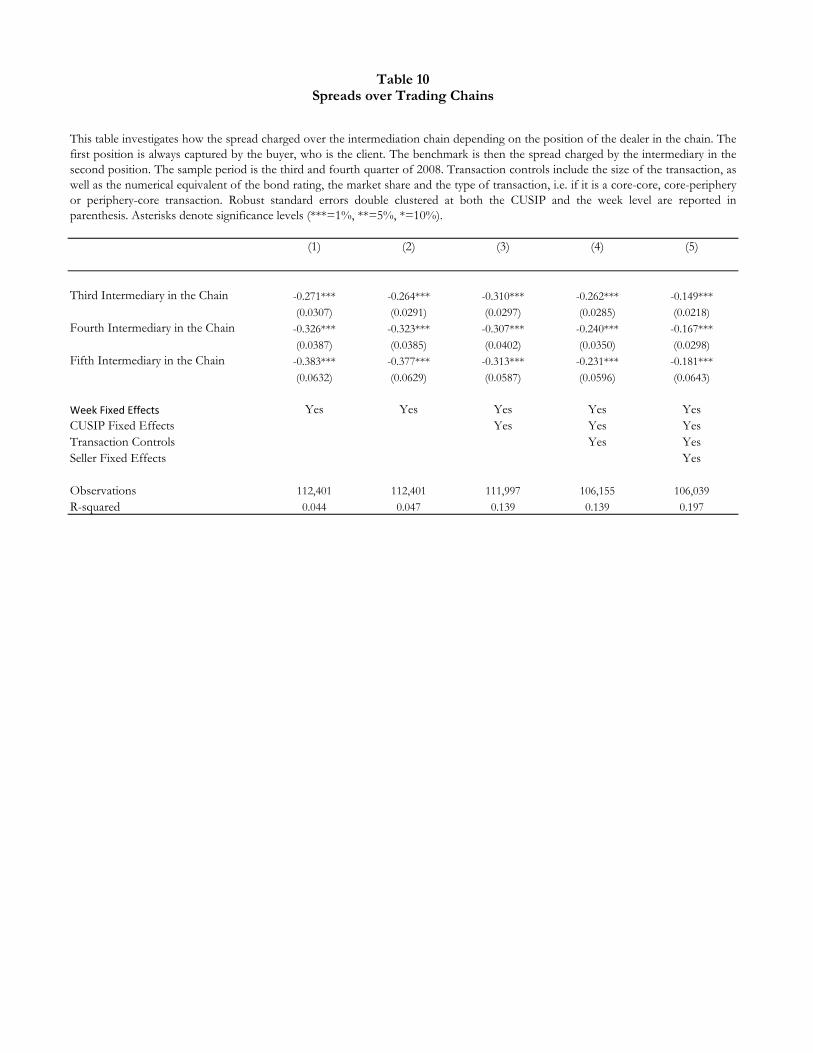
(1) (2) (3) (4) (5)

Third Intermediary in the Chain -0.271*** -0.264*** -0.310*** -0.262*** -0.149***

(0.0307) (0.0291) (0.0297) (0.0285) (0.0218)

Fourth Intermediary in the Chain -0.326*** -0.323*** -0.307*** -0.240*** -0.167***

(0.0387) (0.0385) (0.0402) (0.0350) (0.0298)

Fifth Intermediary in the Chain -0.383*** -0.377*** -0.313*** -0.231*** -0.181***

(0.0632) (0.0629) (0.0587) (0.0596) (0.0643)

Week Fixed Effects Yes Yes Yes Yes Yes

CUSIP Fixed Effects Yes Yes Yes

Transaction Controls Yes Yes

Seller Fixed Effects Yes

Observations 112,401 112,401 111,997 106,155 106,039

R-squared 0.044 0.047 0.139 0.139 0.197

Table 10Spreads over Trading Chains

This table investigates how the spread charged over the intermediation chain depending on the position of the dealer in the chain. The

first position is always captured by the buyer, who is the client. The benchmark is then the spread charged by the intermediary in the

second position. The sample period is the third and fourth quarter of 2008. Transaction controls include the size of the transaction, as

well as the numerical equivalent of the bond rating, the market share and the type of transaction, i.e. if it is a core-core, core-periphery

or periphery-core transaction. Robust standard errors double clustered at both the CUSIP and the week level are reported in

parenthesis. Asterisks denote significance levels (***=1%, **=5%, *=10%).

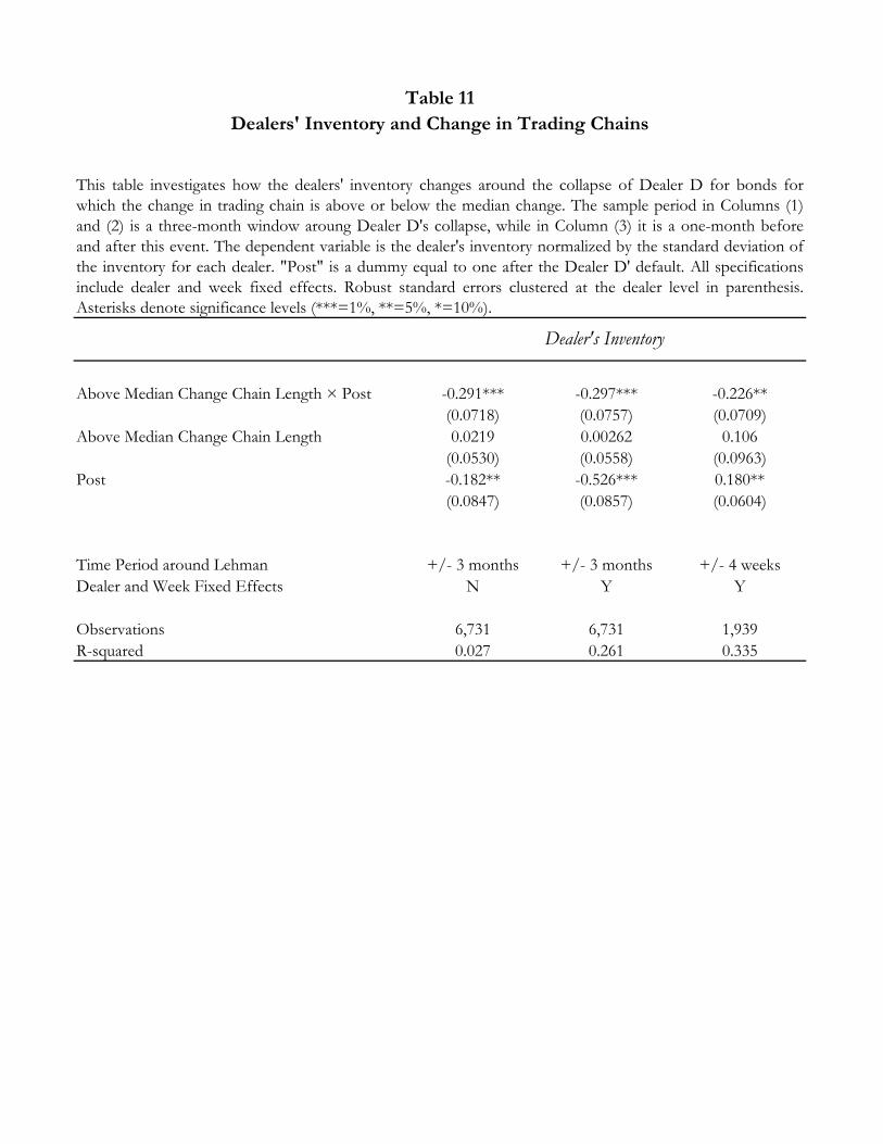
Above Median Change Chain Length × Post -0.291*** -0.297*** -0.226**

(0.0718) (0.0757) (0.0709)

Above Median Change Chain Length 0.0219 0.00262 0.106

(0.0530) (0.0558) (0.0963)

Post -0.182** -0.526*** 0.180**

(0.0847) (0.0857) (0.0604)

Time Period around Lehman +/- 3 months +/- 3 months +/- 4 weeks

Dealer and Week Fixed Effects N Y Y

Observations 6,731 6,731 1,939

R-squared 0.027 0.261 0.335

Dealer's Inventory

This table investigates how the dealers' inventory changes around the collapse of Dealer D for bonds for

which the change in trading chain is above or below the median change. The sample period in Columns (1)

and (2) is a three-month window aroung Dealer D's collapse, while in Column (3) it is a one-month before

and after this event. The dependent variable is the dealer's inventory normalized by the standard deviation of

the inventory for each dealer. "Post" is a dummy equal to one after the Dealer D' default. All specifications

include dealer and week fixed effects. Robust standard errors clustered at the dealer level in parenthesis.

Asterisks denote significance levels (***=1%, **=5%, *=10%).

Dealers' Inventory and Change in Trading Chains

Table 11

Panel A

Full Sample Mean P1 Median P99 Std Dev

By Bonds

Rating BBB+ D A- AAA

Size $21.0 M $400 $2.5 M $798 M $41.2 M

Age 2.9 0 1.9 78.5 3.3

Maturity 9.6 0.5 7.5 100.2 8.6

By Trade

Rating BBB D BBB+ AAA

Size $93.1 M $400 $59.9 M $798 M $97.3 M

Age 3.9 0 3.1 82.0 3.5

Maturity 11.8 0.5 10 100.2 8.8

Estimation Sample

By Bonds

Rating A- D A- AA+

Size $21.8 M $16,700 $2 M $200 M $41.8 M

Age 3.2 0.0 2.1 15.9 3.4

Maturity 10.0 1.0 8.0 31.0 8.7

By Trade

Rating BBB+ D BBB AAA

Size $76 M $125,300 $49 M $398 M $90 M

Age 4.1 0.0 3.2 16.6 3.7

Maturity 11.7 2.0 10.0 31.0 8.2

By Bonds

Rating A- D A AA

Size $21 M $15,600 $1.7 M $ 199 M $41 M

Age 3.1 0.0 2.1 15.7 3.4

Maturity 9.8 1.0 7.8 31.0 8.6

By Trade

Rating BBB+ D BBB AAA

Size $90 M $208,200 $64 M $398 M $92 M

Age 4.1 0.0 3.4 16.4 3.6

Maturity 11.2 3.0 10.0 30.5 7.9

Appendix Estimation Sample

Table A.0

Additional Summary Statistics

The table reports additional descriptive statistics for the main variables employed in our analysis. In the Panel A, we present the main bond characteristics: the

bonds' credit quality, issue size, age and maturity, as provided by a confidential version of TRACE for the period 2005-2011 for the three different samples.

The first set report the statistics for the full data sample. The remaining two sets of rows report the summary statistics for the main estimation sample which

restricts attention to buy and sell transactions observed within an hour from each other, and for the sample used in the robustness checks in the appendix.

Panel B provides summary statistics for these characteristics and for the transactions, such as the profit margins, the volume, the holding period and the seller's

centrality measure.

Panel B

Full Sample Mean P1 Median P99 Std Dev

By Bonds

Volume of Trade 1,785.5 0.2 90 250,000 7,258.3

Holding Period (days) 59.8 0 37.2 1,454.4 69.8

Average Spread 0.0189 -0.7143 0.0068 99 0.6269

Centrality Measure 44.6 1 39.4 844.9 30.8

Number of Trades 920 1 109 138,271 3,527

Market Concentration 54.3% 0% 54.4% 100% 22.8%

By Trade

Volume of Trade 401 0.24 25 619,550 1,777

Holding Period (days) 107 0 16.8 3,447 214

Average Profit Margin 0.1056 0 0.0055 2926.928 0.6

Centrality Measure - Rank 41.7 1 21 1,152 64.4

Estimation Sample

By Bonds

Volume of Trade 1,565.1 4.3 75.0 26,000.0 8,356.1

Average Spread 0.6 -0.1 0.5 3.1 0.8

Centrality Measure 59.1 3.0 51.7 269.7 50.3

Number of Trades 170.3 1.0 37.0 2,037.0 526.8

Market Concentration 0.6 0.0 0.7 1.0 0.2

By Trade

Volume of Trade 443.0 0.0 25.0 5,850.0 2,156.2

Average Profit Margin 0.6 -1.2 0.2 4.5 1.4

Centrality Measure - Rank 52.2 1.0 25.0 554.0 94.3

Appendix Estimation Sample

By Bonds

Volume of Trade 984.8 4.3 66.7 12,695.0 4,375.3

Average Spread 0.3 -0.3 0.2 1.5 0.4

Centrality Measure 56.5 5.0 49.3 208.7 42.1

Number of Trades 1,142.4 1.0 141.0 16,732.0 4,180.1

Market Concentration 0.6 0.0 0.6 1.0 0.2

By Trade

Volume of Trade 314.0 0.0 20.0 5,000.0 1,509.3

Average Profit Margin 0.4 -3.6 0.2 5.8 1.3

Centrality Measure 49.0 1.0 20.0 554.0 95.9

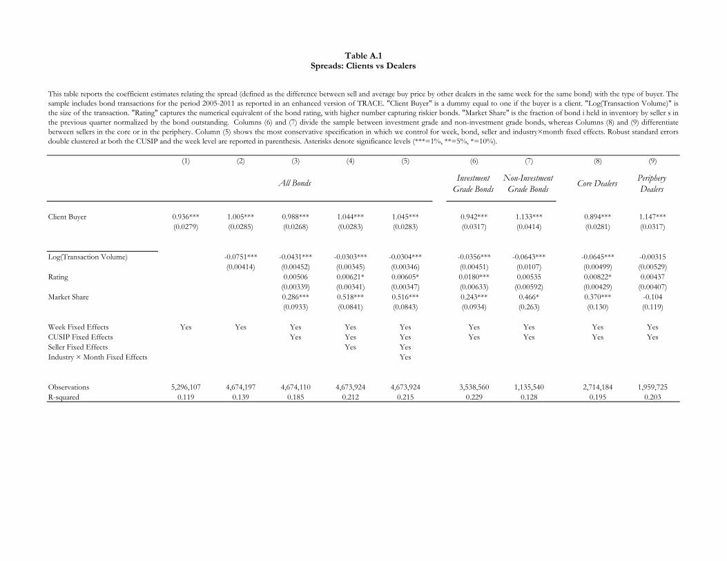
(1) (2) (3) (4) (5) (6) (7) (8) (9)

Investment

Grade Bonds

Non-Investment

Grade BondsCore Dealers

Periphery

Dealers

Client Buyer 0.936*** 1.005*** 0.988*** 1.044*** 1.045*** 0.942*** 1.133*** 0.894*** 1.147***

(0.0279) (0.0285) (0.0268) (0.0283) (0.0283) (0.0317) (0.0414) (0.0281) (0.0317)

Log(Transaction Volume) -0.0751*** -0.0431*** -0.0303*** -0.0304*** -0.0356*** -0.0643*** -0.0645*** -0.00315

(0.00414) (0.00452) (0.00345) (0.00346) (0.00451) (0.0107) (0.00499) (0.00529)

Rating 0.00506 0.00621* 0.00605* 0.0180*** 0.00535 0.00822* 0.00437

(0.00339) (0.00341) (0.00347) (0.00633) (0.00592) (0.00429) (0.00407)

Market Share 0.286*** 0.518*** 0.516*** 0.243*** 0.466* 0.370*** -0.104

(0.0933) (0.0841) (0.0843) (0.0934) (0.263) (0.130) (0.119)

Week Fixed Effects Yes Yes Yes Yes Yes Yes Yes Yes Yes

CUSIP Fixed Effects Yes Yes Yes Yes Yes Yes Yes

Seller Fixed Effects Yes Yes

Industry × Month Fixed Effects Yes

Observations 5,296,107 4,674,197 4,674,110 4,673,924 4,673,924 3,538,560 1,135,540 2,714,184 1,959,725

R-squared 0.119 0.139 0.185 0.212 0.215 0.229 0.128 0.195 0.203

Table A.1Spreads: Clients vs Dealers

This table reports the coefficient estimates relating the spread (defined as the difference between sell and average buy price by other dealers in the same week for the same bond) with the type of buyer. The

sample includes bond transactions for the period 2005-2011 as reported in an enhanced version of TRACE. "Client Buyer" is a dummy equal to one if the buyer is a client. "Log(Transaction Volume)" is

the size of the transaction. "Rating" captures the numerical equivalent of the bond rating, with higher number capturing riskier bonds. "Market Share" is the fraction of bond i held in inventory by seller s in

the previous quarter normalized by the bond outstanding. Columns (6) and (7) divide the sample between investment grade and non-investment grade bonds, whereas Columns (8) and (9) differentiate

between sellers in the core or in the periphery. Column (5) shows the most conservative specification in which we control for week, bond, seller and industry×month fixed effects. Robust standard errors

double clustered at both the CUSIP and the week level are reported in parenthesis. Asterisks denote significance levels (***=1%, **=5%, *=10%).

All Bonds

(1) (2) (3) (4) (5) (6) (1) (3) (4)

Investment

Grade Bonds

Non-Investment

Grade BondsAll Bonds

Investment Grade

Bonds

Non-Investment

Grade Bonds

Core-Periphery 0.110*** 0.0884*** 0.0883*** 0.0893*** 0.0973*** 0.0513*** 0.247*** 0.0834*** 0.0587***

(0.00950) (0.00794) (0.00810) (0.00809) (0.00868) (0.0151) (0.0140) (0.00641) (0.0177)

Periphery-Periphery 0.00233 -0.0173** -0.0440*** -0.0435*** -0.0369*** -0.0792*** 0.0802*** -0.211*** -0.305***

(0.00750) (0.00775) (0.00815) (0.00808) (0.00864) (0.0186) (0.0152) (0.0104) (0.0233)

Periphery-Core -0.172*** -0.193*** -0.212*** -0.213*** -0.206*** -0.248*** 0.143*** -0.0393*** -0.0978***

(0.0120) (0.0119) (0.0126) (0.0126) (0.0125) (0.0230) (0.0143) (0.00834) (0.0188)

Core-Periphery × VIX 0.0441*** 0.0490*** 0.0220

(0.00891) (0.00828) (0.0296)

Periphery-Core × VIX -0.160*** -0.142*** -0.253***

(0.0136) (0.0143) (0.0251)

Periphery-Periphery × VIX -0.0218** 0.00478 -0.126***

(0.0105) (0.0103) (0.0220)

Controls Yes Yes Yes Yes Yes Yes Yes Yes Yes

Controls×VIX Yes Yes Yes

Week Fixed Effects Yes Yes Yes Yes Yes Yes Yes Yes Yes

CUSIP Fixed Effects Yes Yes Yes Yes Yes Yes Yes

Industry × Month Fixed Effects Yes Yes Yes Yes

Observations 3,613,400 3,172,063 3,171,960 3,171,960 2,401,439 770,508 3,171,700 2,401,220 770,467

R-squared 0.009 0.012 0.022 0.026 0.027 0.019 0.027 0.033 0.027

All Bonds

This table reports the coefficient estimates relating the spreads (defined as the difference between sell and average buy price by other dealers in the same week for the same bond) with the type of

counterparty. The sample includes bond transactions for the period 2005-2011 as reported in an enhanced version of TRACE. "Core-Periphery" is a dummy equal to one if the seller is a core dealer and the

buyer is a peripheral dealer, while "Periphery-Periphery" identifies transactions between dealers in the periphery, and "Periphery-Core" is a dummy equal to one for transactions where the seller is in the

periphery and the buyer is in the core. The comparison group are interdealer transactions between core dealers. Controls include: "Log(Transaction Volume)" which is the size of the transaction, "Rating"

which captures the numerical equivalent of the bond rating, and "Market Share" which is the fraction of bond i held in inventory by seller s in the previous quarter normalized by the bond outstanding.

Column (4) shows the most conservative specification in which we control for week, bond, and industry×month fixed effects. Columns (5) and (6) divide the sample between investment grade and non-

investment grade bonds. Columns (7)-(9) perform a similar analysis but controlling for the interaction between the type of transaction (i.e. Core-Periphery, Periphery-Periphery and Periphery-Core) with the

volatility index VIX as provided by CBOE. In these columns we also control for the the log of the transaction size, the bond rating and the market share interacted with the VIX. Robust standard errors

double clustered at both the CUSIP and the week level are reported in parenthesis. Asterisks denote significance levels (***=1%, **=5%, *=10%).

Spreads and Network StructureTable A.2

(1) (2) (3) (4) (5) (6) (7) (8)

Fraction Selling to Counterparty -0.650*** -0.674*** -0.676*** -0.367*** -0.371*** -0.396*** -0.397*** -0.398***

(0.0286) (0.0294) (0.0295) (0.0164) (0.0167) (0.0173) (0.0177) (0.0178)

Fraction Buying from Counterparty 0.595*** 0.626*** 0.629*** 0.332*** 0.359*** 0.337*** 0.364*** 0.366***

(0.0231) (0.0244) (0.0242) (0.0162) (0.0166) (0.0156) (0.0160) (0.0159)

Fraction Selling to Counterparty × VIX -0.126*** -0.130*** -0.130***

(0.0244) (0.0246) (0.0247)

Fraction Buying from Counterparty × VIX -0.0273* -0.0327** -0.0319**

(0.0160) (0.0157) (0.0158)

Seller Network Centrality × VIX 1.149*** 1.210*** 1.237***

(0.139) (0.140) (0.140)

Buyer Network Centrality × VIX -0.959*** -0.987*** -0.986***

(0.121) (0.120) (0.121)

Seller Network Centrality 1.983*** 2.239*** 2.011*** 2.282*** 2.298***

(0.149) (0.156) (0.118) (0.124) (0.124)

Buyer Network Centrality -1.295*** -1.273*** -1.242*** -1.209*** -1.213***

(0.0995) (0.105) (0.0820) (0.0846) (0.0847)

Controls Yes Yes Yes Yes Yes Yes Yes Yes

Controls×VIX Yes Yes Yes Yes

Week Fixed Effects Yes Yes Yes Yes Yes Yes Yes Yes

CUSIP Fixed Effects Yes Yes Yes Yes Yes Yes

Industry × Month FE Yes Yes

Seller × Month FE

Buyer × Month FE

Observations 2,970,946 2,970,842 2,970,842 2,820,028 2,819,921 2,819,779 2,819,672 2,819,672

R-squared 0.015 0.025 0.028 0.020 0.031 0.025 0.037 0.040

This table reports the coefficient estimates relating the spreads (defined as the difference between sell and average buy price by other dealers in the same week for the same bond) with the existing of bilateral relationships

between seller and buyer and to their network centrality. The sample includes bond transactions for the period 2005-2011 as reported in an enhanced version of TRACE. "Fraction Selling to Counterparty" is the fraction

of sales of this seller to this buyer computed in the previous quarter. Similarly for the "Fraction Buying from Counterparty". "Log(Transaction Volume)" is the size of the transaction. "Rating" captures the numerical

equivalent of the bond rating, with higher number capturing riskier bonds. "Market Share" is the fraction of bond i held in inventory by seller s in the previous quarter normalized by the bond outstanding. The centrality

measures are computed using the eigenvector centrality measure in the previous quarter. VIX is the volatility index as provided by CBOE. We also control for the bond rating, the market share and the log of the

transaction size interacted with the VIX. Robust standard errors double clustered at both the CUSIP and the week level are reported in parenthesis. Asterisks denote significance levels (***=1%, **=5%, *=10%).

Spreads and Bilateral Relationships

Table A.3