NBER WORKING PAPER SERIES

THE WAGE IMPACT OF THE MARIELITOS:A REAPPRAISAL

George J. Borjas

Working Paper 21588http://www.nber.org/papers/w21588

NATIONAL BUREAU OF ECONOMIC RESEARCH1050 Massachusetts Avenue

Cambridge, MA 02138September 2015

I am particularly grateful to Alberto Abadie and Larry Katz for very productive discussions of the issues examined in this paper and for many valuable comments and suggestions. I have also benefitted from the reactions and advice of Brian Cadena, Kirk Doran, Richard Freeman, Daniel Hamermesh, Gordon Hanson, Joan Monras, Marta Tienda, and Steve Trejo. I alone am responsible for all errors. The views expressed herein are those of the author and do not necessarily reflect the views of the National Bureau of Economic Research.

NBER working papers are circulated for discussion and comment purposes. They have not been peer-reviewed or been subject to the review by the NBER Board of Directors that accompanies official NBER publications.

© 2015 by George J. Borjas. All rights reserved. Short sections of text, not to exceed two paragraphs, may be quoted without explicit permission provided that full credit, including © notice, is given to the source.

The Wage Impact of the Marielitos: A Reappraisal George J. BorjasNBER Working Paper No. 21588September 2015, revised July 2016JEL No. J2,J31,J61

ABSTRACT

This paper brings a new perspective to the analysis of the Mariel supply shock, revisiting the question armed with the accumulated insights from the literature on the economic impact of immigration. A crucial lesson from that literature is that any credible attempt to measure the wage impact must carefully match the skills of the immigrants with those of the pre-existing workers. At least 60 percent of the Marielitos were high school dropouts. A reappraisal of the Mariel evidence, specifically examining wages in this low-skill group, overturns the finding that Mariel did not affect Miami’s wage structure. The wage of high school dropouts in Miami dropped dramatically, by 10 to 30 percent, suggesting an elasticity of wages with respect to the number of workers between -0.5 and -1.5.

George J. BorjasHarvard Kennedy School79 JFK StreetCambridge, MA 02138and NBERgborjas@harvard.edu

2

The Wage Impact of the Marielitos: A Reappraisal

George J. Borjas*

I. Introduction The study of how immigration affects labor market conditions has been a central

concern in labor economics for nearly three decades. The significance of the question arises

both because of the policy issues involved and because the study of how labor markets

respond to supply shocks can teach us much about how labor markets work. In an

important sense, examining how immigration affects the wage structure confronts directly

one of the fundamental questions in economics: What makes prices go up and down?

David Card’s (1990) classic study of the impact of the Mariel supply shock stands as

a landmark in this literature. On April 20, 1980, Fidel Castro declared that Cuban nationals

wishing to move to the United States could leave freely from the port of Mariel, and around

125,000 Cubans quickly accepted the offer. The Card study was one of the pioneering

attempts to exploit the insight that a careful study of natural experiments, such as the

exogenous supply shock stimulated by Castro’s seemingly random decision to let the

people go, can help identify parameters of great economic interest. In particular, the Mariel

supply shock would let us measure the wage elasticity that shows how the wage of native

workers responds to an exogenous increase in supply.

Card’s analysis of the Miami labor market, and of comparable labor markets that

served as a control group or placebo, indicated that nothing much happened to Miami

despite the very large number of Marielitos. Native wages did not go down in the short run

as would have been predicted by the textbook model of a competitive labor market. Card’s

study has been extremely influential, both in terms of its prominent role in policy

discussions and its methodological approach.1

* Harvard University, National Bureau of Economic Research, and IZA. I am particularly grateful to

Alberto Abadie and Larry Katz for very productive discussions and for many valuable comments and suggestions. I also benefited from the reactions and advice of Josh Angrist, Fran Blau, Brian Cadena, Kirk Doran, Richard Freeman, Daniel Hamermesh, Gordon Hanson, Larry Kahn, Alan Krueger, Joan Llull, Joan Monras, Panu Poutvaara, Jason Richwine, Kevin Shih, Marta Tienda, and Steve Trejo.

1 Many other studies examine exogenous supply shocks and are clearly influenced by the Card framework; see Hunt (1992), Carrington and de Lima (1996), Angrist and Kugler (2003), Friedberg (2001),

3

During the 1980s and 1990s, a parallel (but non-experimental) literature attempted

to estimate the labor market impact of immigration by essentially correlating wages and

immigration across cities (Grossman 1982; Altonji and Card 1991). These spatial

correlations are problematic for two reasons: (1) immigrants are more likely to settle in

high-wage cities, so that the endogeneity of supply shocks induces a spurious positive

correlation between immigration and wages; and (2) native workers and firms respond to

supply shocks by resettling in areas that offer better opportunities, effectively diffusing the

impact of immigration across the national labor market.2

Card’s Mariel study is impervious to both of these criticisms. The fact that the

Marielitos settled in Miami probably had little to do with pre-existing wage opportunities,

and much to do with the fact that Castro suddenly decided to allow the boatlift to occur and

that many of the Cuban-Americans who organized the flotilla lived in South Florida.3

Similarly, the short run nature of Card’s empirical exercise, looking at the impact of

immigration just a few years after the supply shock, means that we should be measuring

the short-run elasticity, an elasticity that is not yet contaminated by labor market

adjustments and that economic theory predicts to be negative.

This paper provides a reappraisal of the evidence of how the Miami labor market

responded to the influx of Marielitos. The paper is not a replication of earlier studies.

Instead, I approach and examine these questions from a fresh perspective, building on what

we have learned from the 30 years of research on the labor market impact of immigration.

One crucial insight from this research is that any credible attempt to measure the impact

must carefully match the skills of the immigrants with the skills of the pre-existing

Saiz (2003), Borjas and Doran (2012), Glitz (2012), Pinotti et al (2013), and Dustmann, Schonberg, and Stuhler (2016).

2 Beginning with Altonji and Card (1991), the endogenous settlement of immigrants across localities has been addressed by using the geographic sorting of earlier waves of immigrants to predict the sorting of the new arrivals. The validity of this instrument, however, depends on whether economic conditions in local labor markets persist over time; see Jaeger, Ruist, and Stuhler (2016).

3 The geographic clustering of the large Cuban community in Miami probably had little to do with the relative economic opportunities offered by the Miami labor market, and much to do with the fact that the flights operated by Pan American Airways that carried almost all of the early refugees out of Cuba had a single destination, the Miami airport. The 1980 census indicates that 50 percent of Cuban immigrants lived in the Miami metropolitan area. Both the 1990 and 2000 censuses report that over 60 percent of the Cuban immigrants who likely were part of the Mariel influx still resided in the Miami metropolitan area.

4

workforce. Borjas (2003), in the study that introduced the approach of correlating wages

and immigration across skill groups in the national labor market, found a significant

negative correlation between the wage growth of specific skill groups, defined by education

and age, and the size of the immigration-induced supply shock into those groups.

The Marielitos were disproportionately low-skill; around 60 percent were high

school dropouts and only 10 percent were college graduates. At the time, about a quarter of

Miami’s pre-existing workers lacked a high school diploma. As a result, even though the

Mariel supply shock increased the number of workers in Miami by 8 percent, it increased

the number of high school dropouts by almost 20 percent.

The unbalanced nature of this supply shock suggests that we should look at what

happened to the wage of high school dropouts in Miami before and after Mariel.

Remarkably, this trivial comparison was not made in Card’s (1990) study and, to the best of

my knowledge, had not been conducted before the first draft of this paper was released.4

By focusing on this very specific skill group, we obtain an entirely new perspective of how

the Miami labor market responded to an exogenous supply shock.

II. Data The migration of large numbers of Cubans to the United States began shortly after

Fidel Castro’s communist takeover on January 1, 1959. By the year 2010, over 1.3 million

Cubans had emigrated.

The first large-scale data set that precisely identifies an immigrant’s year of arrival

is the 2000 decennial census. Prior to 2000, the census microdata reported the year of

arrival in intervals (e.g., 1960-1964). I merged data from various censuses and the

4 Card (1990, Table 7) reports labor market outcomes for the subsample of black high school dropouts, but does not report any other pre-post Mariel differences for the least educated workers. Monras (2014) examined wage trends in the sample of workers who have at most a high school diploma; his evidence is suggestive of the findings reported in this paper. Finally, three months after this study was released as an NBER working paper (Borjas, 2015), Peri and Yasenov (2015) re-examined the data for high school dropouts and concluded that Card’s results stood the test of time. The Peri-Yasenov study, however, looked at wage trends that were contaminated by various sampling decisions. They examined the pooled earnings of men and women, but ignored the changing gender composition of the workforce; included non-Cuban Hispanics in the analysis, even though many of those Hispanics were immigrants who arrived after 1980; and included teenagers aged 16-18, even though most of these teenagers were enrolled in high school and were classified as high school dropouts because they did not yet have a diploma. Borjas (2016) documents the biases created by these methodological choices.

5

American Community Surveys (ACS) to construct a mortality-adjusted number of Cuban

immigrants for each arrival year between 1955 and 2010.5 For example, I used the 1970

census to estimate the number of Cubans who arrived in the United States between 1960

and 1964, and then used the detailed year-of-migration information in the 2000 census to

allocate those early immigrants to specific years within the 5-year band. Figure 1 shows the

trend in the number of Cubans migrating to the United States.

Several patterns emerge from the time series. First, it is easy to see the immediate

impact of the communist takeover of the island. In 1958, only 8,000 Cubans migrated to the

United States. By 1961 and 1962, 52,000 Cubans were migrating annually.6 The Cuban

Missile Crisis abruptly stopped the flow in October 1962, and it took several years for other

escape routes to open up. By the late 1960s, the number of Cubans moving to the United

States was again near the level reached before the Missile Crisis.

The huge spike in 1980, of course, is the Mariel supply shock. Between 1978 and

1980, the number of new Cuban immigrants increased 17-fold, from 6,500 to 110,000. The

figure shows yet another spike in 1994 and 1995, coinciding with the period of Angrist and

Krueger’s (1999) “Mariel Boatlift That Did Not Happen.”7 The census data clearly indicates

that somehow the phantom Cubans from that boatlift ended up in the United States, making

this supply shock a Little Mariel. Although the number of Little Marielitos pales in

comparison to the number of actual Marielitos, it is still quite large; the number of migrants

arriving in 1995 was similar to that of the early Cuban waves in the 1960s. It is also evident

that there has been a steady increase in the number of Cuban migrants since the early

1980s. By 2010, about 40,000 Cubans were arriving annually.

5 In principle, the calculation also adjusts for potential out-migration by Cuban immigrants. I suspect,

however, that the number of Cubans who chose to return is trivially small (although a larger number might have migrated elsewhere).

6 Full disclosure: I am a data point in the 1962 flow.

7 In 1994, Castro again toyed with the idea of permitting a boatlift, but the United States preemptively responded and rerouted many of the potential migrants to the military base in Guantanamo. Angrist and Krueger (1999), writing before the release of the 2000 census, argued that this seemingly phantom flow had an adverse effect on Miami’s black unemployment rate, raising questions about how to interpret the evidence from the Mariel boatlift that did happen.

6

One last detail is worth noting. A disproportionately large number of the Marielitos

ended up residing in the Miami metropolitan area: 62.6 percent resided in Miami in 1990

and 63.4 percent still resided there in 2000.

The empirical analysis initially uses the 1977-1993 March Supplements of the

Current Population Surveys (CPS).8 These surveys report a person’s annual wage and

salary income as well as the number of weeks worked in the previous calendar year. Much

of the analysis will be restricted to men aged 25-59, who report positive values for wage

and salary income, weeks worked, and usual hours worked.9 The age restriction implies

that a worker’s observed earnings are unaffected by transitory fluctuations that occur

during the transitions from school to work and from work to retirement. Similarly, the

restriction to working men ensures that wage trends are not distorted by the entry of large

numbers of women into the workforce in the 1970s and 1980s.10

The 1977-1993 period analyzed throughout much of the paper is selected for two

reasons. First, although the March CPS data files are available since 1962, the Miami

metropolitan area can only be consistently identified in the 1973-2004 surveys. Beginning

with the 1977 survey, the CPS began to identify 44 metropolitan areas (including Miami)

that can be used in the empirical analysis.11 Second, my analysis of wage trends stops with

the 1993 survey to avoid contamination from the Little Mariel supply shock of 1994 and

1995.

The CPS did not report a person’s country of birth before 1994, so that it is not

possible to measure the wage impact of the Mariel supply shock on the native-born

population. I instead examine wage trends among non-Hispanic men (where Hispanic

background is determined by a person’s answer to the Hispanic ethnicity question), a

8 The March surveys are known as the Annual Social and Economic Supplements (ASEC). The data

were downloaded from the Integrated Public Use Microdata Series (IPUMS) website on May 9, 2016.

9 I also exclude persons who reside in group quarters, have a negative sample weight, or have outlying hourly wage rates (less than $1.50 or more than $40 in 1980 dollars). This last restriction roughly excludes workers in the top and bottom 1 percent of the earnings distribution.

10 The sensitivity of the evidence to including working women is discussed below. 11 The Miami-Hialeah metropolitan area is not identified at all before 1973, and is combined with the

Fort Lauderdale metropolitan area after 2004. The 1973-1976 surveys identify only 34 metropolitan areas, and one of them (New York City) is not consistently defined throughout the period; the Nassau-Suffolk metropolitan area is pooled with the New York City metro area in 1976.

7

sample restriction that comes close to isolating Miami’s native-born population at the time.

The 1980 census, conducted days before the Mariel supply shock, reports that 40.7 percent

of Miami’s male workforce was foreign-born, with 65.1 percent of the immigrants born in

Cuba and another 11.2 percent born in other Latin American countries. The restriction to

non-Hispanics also ensures that the post-Mariel wage trends are not skewed by a

composition effect created by the large post-1980 wave of new Hispanic immigrants into

many local labor markets.12

The dependent variable will be the worker’s log weekly earnings, where weekly

earnings are defined as the ratio of annual income in the previous calendar year to the

number of weeks worked.13 I use the Consumer Price Index (CPI) for all urban consumers

to deflate the earnings data (1980 = 100). For expositional consistency and unless

otherwise noted, whenever I refer to a particular year hereafter, it will be the year in which

earnings were actually received by a worker, as opposed to the CPS survey year.14

It is important to document what we know about the skill distribution of the

Marielitos. As noted earlier, the Mariel supply shock began a few days after the 1980 census

enumeration, so that the first large survey that contains a large sample of the Marielitos is

the 1990 census. Nevertheless, a few CPS supplements conducted in the 1980s provide

information on a very small sample of Cuban immigrants who arrived at the time of Mariel.

Table 1 reports the education distribution of the sample of adult Cuban immigrants

who arrived in 1980 (or in 1980-1981, depending on the data set) and who were

enumerated in various surveys sometime between 1983 and 2000. The calculation includes

the entire population of Marielitos (workers and non-workers, as well as men and women)

who were at least 18 years old as of 1980.

12 The restriction to non-Hispanics implies that few of the low-skill workers in the sample are

foreign-born. According to the 1980 census, only 18.7 percent of non-Hispanic high school dropouts in Miami were foreign-born (as compared to 6.4 percent outside Miami). In contrast, 55.1 percent of the non-Hispanic dropouts in Miami were black (as compared to 17.6 percent outside Miami). The key native-born group potentially affected by the Marielitos, therefore, was the low-skill African-American workforce.

13 I replicated the analysis using the log hourly wage as an alternative measure of a worker’s income. Because the measure of usual hours worked weekly in the March CPS is noisy, the results are similar but less precisely estimated.

14 For example, a discussion of the earnings of workers in 1985 refers to the data drawn from the 1986 March CPS.

8

The crucial implication of the table is that the Mariel supply shock consisted of

workers who were very unskilled, with a remarkably large fraction being high school

dropouts.15 Despite the variation in sample size and the almost 20-year span in the surveys

examined in the table, the fraction of Marielitos who lacked a high school diploma hovers

around 60 percent. Table 1 also shows that a very small fraction of these immigrants were

college graduates (around 10 percent).

It is insightful to compare the education distribution of the Marielitos with that of

the pre-existing workforce. The last row of Table 1 shows that only 26.7 percent of labor

force participants in the Miami metropolitan area were high school dropouts. In fact,

Miami’s workforce was remarkably balanced in terms of its skill distribution, with 20 to 30

percent of workers in each of the four education groups.16

Table 2 summarizes what we know about the magnitude of the Mariel supply shock.

There were 176,300 high school dropouts in Miami’s labor force just prior to Mariel (out of

a total of 659,400). According to the 1990 census, 60,100 Cuban workers migrated (as

adults) either in 1980 or 1981. If we make a slight adjustment for the small number who

entered the country in 1981, Mariel increased the size of the labor force by 55,700 persons,

of which almost 60 percent were high school dropouts.17 Although the Mariel supply shock

increased Miami’s workforce by 8.4 percent and increased the number of the most

educated workers by 3 to 5 percent, the number of low-skill workers rose by a remarkable

18.4 percent. Moreover, this supply shock occurred almost overnight. The Coast Guard

reports that the first Marielitos arrived in Florida on April 23, 1980, and that over 100,000

refugees had been admitted by June 3 (Stabile and Scheina 2015).

15 There is also a possibility that the skills of the Marielitos were further downgraded upon arrival, as

in Dustmann, Frattini, and Preston (2013), so that even those immigrants with a high school diploma were competing with the least educated workers in the pre-existing Miami workforce.

16 The pre-existing workforce includes all labor force participants in Miami, regardless of where they were born or their ethnicity.

17 The 2000 census indicates that 92.8 percent of the Cubans who immigrated in either 1980 or 1981 actually entered the country in 1980. Note that the supply shock was probably slightly larger than indicated in Table 2 because the calculation does not account for mortality through 1990.

9

III. Descriptive Evidence The very low skills of the Marielitos indicates that we should perhaps focus our

attention on the labor market outcomes of the least educated workers in Miami to get a

first-order sense of whether the supply shock had any impact on Miami’s wage structure. In

fact, the literature sparked by Borjas (2003) suggests that it is important to match the

immigrants to corresponding native workers by skill groups. Educational attainment is a

skill category that would seem to be extremely relevant in an examination of the Mariel

supply shock.

Any empirical study of the impact of Mariel runs into an immediate data problem:

The number of workers enumerated by the CPS in the Miami labor market is small,

introducing a lot of random noise into the calculations. The top panel of Table 3 reports the

number of men who satisfy the sample restrictions and were enumerated in the Miami

metropolitan area between survey years 1977 and 1993. The average number of

observations in each pre-1990 March CPS was 96.5, and the average number of high school

dropouts was 19.5. The sample size drops dramatically with the 1991 survey, when the

number of non-Hispanic men sampled in Miami falls abruptly (by nearly a third), and the

number of high school dropouts sometimes drops to the single digits. The empirical

analysis reported below will effectively pool at least three years of the CPS (either by

manually aggregating the data or by estimating impacts for three-year intervals) to enable

a more precise calculation of the effect.

I begin by carrying out the most straightforward calculation of the potential wage

impact that uses all the available data. In particular, I simply calculate the average log

weekly wage of high school dropouts in Miami each year between 1972 and 2002, the

period for which the March CPS has a consistent time series for the Miami metropolitan

area.18 Figure 2 illustrates the wage trend and the 95 percent confidence band around the

mean, using a 3-year moving average to smooth out the noise in the time series. The figure

also shows the trend for similarly educated non-Hispanic men working outside Miami. It is

important to emphasize that this simple exercise does not adjust the CPS data in any way

18 The calculation of the average log weekly wage for each year weighs each individual observation

by the product of the person’s sampling weight times the number of weeks worked in the previous calendar year.

10

(other than taking a moving average), so that it provides a very transparent indication of

what happened to low-skill wages in pre- and post-Mariel Miami.

Despite the similarity in wage trends between Miami and the rest of the country

prior to 1980, and despite the small sample size for the Miami metropolitan area, it is

obvious that something happened in 1980 that caused the two wage series to diverge in a

statistically significant way. Before Mariel, the log wage of high school dropouts in Miami

was about 0.1 log points below that of workers in the rest of the country. By 1985, the gap

had widened to 0.4 log points, implying that whatever caused the divergence had lowered

the relative wage of low-skill workers in Miami by about 30 percent. The low-skill wage in

Miami fully recovered by 1990, only to be hammered again in 1995, coincidentally the time

of the Little Mariel supply shock. By 2002, the wage gap between high school dropouts in

Miami and elsewhere had returned to its pre-Mariel normal of about 0.1 log points.

Of course, Miami’s distinctive wage trend may not appear quite as distinctive when

contrasted with what happened in other specific cities. The comparison of Miami to the

aggregate U.S. labor market may be masking a lot of the variation that influences particular

localities and that disappears when averaged out. It may be important, therefore, to create

a control group of comparable cities unaffected by the Mariel supply shock to determine if

the wage trends evident in Miami were due to macroeconomic factors that affected other

similar communities as well.

Beginning with the 1977 survey, the March CPS identifies 43 other metropolitan

areas that can be combined in some fashion to construct a sort of placebo. Card (1980, p.

249; emphasis added) describes the construction of his control group as follows:

For comparative purposes, I have assembled similar data…in four other

cities: Atlanta, Los Angeles, Houston, and Tampa-St. Petersburg. These four

cities were selected both because they had relatively large populations of

blacks and Hispanics and because they exhibited a pattern of economic growth

similar to that in Miami over the late 1970s and early 1980s. A comparison of

employment growth rates…suggests that economic conditions were very

similar in Miami and the average of the four comparison cities between 1976

and 1984.

11

It is important to emphasize that the four cities in the Card placebo were chosen

partly based on employment trends observed after the Mariel supply shock. Put differently,

if Mariel worsened employment conditions in Miami, the Card placebo is comparing the

poorer outcomes of workers in Miami to the outcomes of workers in cities where some

other factor worsened their opportunities as well. It is obviously preferable to exogenize

the choice of a placebo by comparing cities that were roughly similar prior to the treatment,

rather than being similar after one of them was injected with a very large supply shock.

The various panels of Figure 3 illustrate the wage trends in Miami and several

potential placebos between 1976 and 1992.19 The top panel shows that the log wage of

high school dropouts declined dramatically after 1980 when compared to what happened

in the cities that make up the Card placebo. Of course, trends in absolute wages reflect

many factors that are specific to local labor markets, so that it is possible that these ups and

downs capture idiosyncratic shifts that affected all workers in Miami. The Mariel supply

shock, however, specifically targeted the least educated workers and the bottom two

panels of the figure show that the relative wage of high school dropouts in Miami—relative

to either college graduates or high school graduates—also declined dramatically after

Mariel, and also recovered by 1990. In sum, the wage trends observed in Miami

consistently indicate that the economic well-being of the least educated workers in Miami

took a downward turn shortly after 1980, reached its nadir around 1985-1986, and did not

recover fully until 1990.

As noted above, the cities in the Card placebo do not make up a proper control

group because they were chosen, in part, so that post-Mariel employment conditions in the

placebo cities resembled those in Miami. To determine the set of cities that had comparable

employment growth prior to Mariel, I pooled the 1977 and 1978 surveys of the CPS, and

also pooled the 1979 and 1980 surveys. I then used the pooled surveys to calculate the log

of the ratio of the total number of workers in 1979-1980 to the number of workers in

19 The calculation of wage trends in Figures 2 and 3 differs slightly. To calculate the standard error of

the (moving) average in Figure 2, I computed the average by pooling 3 years of micro data. The data in Figure 3, which is used in the regression analysis reported below, calculates the mean log wage for each survey, and then takes a simple moving average of those means.

12

1977-1978.20 Column 1 of Table 4 reports the employment growth rate for each of the 44

metropolitan areas, ranked by the growth rate.

Miami’s pre-Mariel employment conditions were quite robust, ranking 6th in the rate

of employment growth. Note that all the cities that make up the Card placebo had lower

growth rates than Miami between 1977 and 1980. In fact, the average employment growth

rate in those four cities (weighted by the city’s employment) was 6.9 percent, less than half

the 15.3 percent growth rate in Miami.

I use the rankings reported in Table 3 to construct a new placebo, which I call the

“employment placebo”, by simply choosing the four cities that were most similar to Miami

prior to 1980. Specifically, the employment placebo consists of the four cities (Anaheim,

Rochester, Nassau-Suffolk, and San Jose) ranked just above and just below Miami.

Figure 3 clearly shows that the relative decline in the wage of low-educated workers

in Miami is much larger when we compare Miami to cities that had comparable

employment growth than to the cities that make up the Card placebo. Between 1979 and

1985, for instance, the wage of high school dropouts in Miami relative to the Card placebo

fell by 0.25 log points (or 22 percent), but the decline was 0.43 log points (35 percent)

when compared to the cities in the employment placebo. This difference is not surprising.

The comparison of post-Mariel economic conditions in Miami to that of cities where

employment conditions are also poor by construction inevitably masks some of the impact

of the Marielitos.

I also constructed an alternative “low-skill placebo” by choosing the four cities that

had similar pre-Mariel growth for low-skill employment. Column 2 of Table 4 reports the

rate of employment growth for high school dropouts. Miami also ranked 6th by this metric.

Coincidentally, two of the cities with similar low-skill employment growth are in the Card

placebo (Los Angeles and Houston; the other two are Gary and Indianapolis). Figure 3

shows that the post-1980 Miami experience was also unusual when compared to this

placebo, with a wage drop of 30 percent (which lies in between the effects implied by the

Card and employment placebos).

20 A person is employed if he or she works in the CPS reference week. The 1980 survey, collected in

March, is not affected by the supply shock, as the Marielitos did not begin to arrive until late April.

13

The choice of a placebo obviously plays a crucial role in determining the magnitude

of the wage impact of Mariel. There is an element of arbitrariness in how a placebo is

created, so that the researcher’s choice of a particular placebo can exaggerate or attenuate

the wage effect. There are, for example, 123,410 potential 4-city placebos that can be

created from 43 metropolitan areas. It might be reasonable to expect a huge dispersion in

the estimated wage effect of the Marielitos across the 123,410 potential comparisons. I will

report below the distribution of estimated wage impacts across all potential four-city

placebos and show that Mariel had a negative impact regardless of which placebo is chosen.

Alternatively, one can employ the synthetic control method developed by Abadie

and Garbazeadal (2003) and Abadie, Diamond, and Hainmueller (2010). The method

essentially searches across all potential placebo cities and derives a weight that combines

cities to create a new synthetic city. This synthetic city is the one that best resembles the

pre-Mariel Miami labor market along some set of pre-specified conditions. Unlike the

hands-on method that I used to create the employment and low-skill placebos, the

synthetic control allows the construction of the synthetic city to be based on several

characteristics. The synthetic control approach seems to limit the researcher’s ability to

make arbitrary decisions about what the proper placebo should be. Note, however, that

there is still an element of arbitrariness. The researcher must specify the vector of

variables that should be comparable between Miami and the placebo in the pre-treatment

period. As I show below, different choices of control variables lead to different estimates of

the wage impact.

Initially, I construct the synthetic city by using three such control variables: the rate

of employment growth in the 4-year period prior to Mariel (i.e., the variable used to define

the employment placebo); the concurrent rate of employment growth for high school

dropouts (the variable used to define the low-skill placebo); and the concurrent rate of

wage growth for high school dropouts. The last column of Table 3 shows that the low-skill

market in Miami also had robust wage growth prior to Mariel, ranking 13th in the country.

Figure 3 illustrates the wage trends in the “city” that makes up the synthetic control. It is

evident that the post-1980 Miami experience differs markedly from that of the synthetic

control.

14

It is interesting to examine the weights attached to each city by the synthetic control

method. When looking at the log wage of high school dropouts, the method assigns the

largest weights to Anaheim (0.40), Rochester (0.20), San Diego (0.18), and San Jose (0.06).

By looking at the ranking of those cities in Table 3, it is obvious that the synthetic control

method consistently selects metropolitan areas that had robust labor markets prior to

Mariel.

Finally, it is easy to establish that the steep drop in the low-skill wage in post-Mariel

Miami was a very unusual event. The average wage of male high-school dropouts in Miami

fell by about 37 percent between 1976-1979 and 1981-1986. We can calculate the

comparable wage change in every other metropolitan area for all equivalent time periods

between 1976 and 2003 and see if the Mariel experience stands out.21 Obviously, if 37-

percent wage cuts happen frequently in local labor markets, it would be harder to claim

that Miami’s experience had much to do with the Marielitos. Perhaps something else was

going on—a something else that other cities experience often enough at different times—

that just happened to coincide with the timing of Castro’s decision.

To assess how Miami’s post-Mariel experience compares to that of the entire

distribution of wage changes, I calculated the wage change between every single pre-

treatment period τ (1976-1979, 1977-1980,…,1993-1996) and the corresponding post-

treatment period τ′ (1981-1986, 1982-1987,…,1998-2003). Specifically, I pooled the March

CPS data for the four years in each pre-treatment period and the six years in each post-

treatment period, and calculated the average log wage in each city-period permutation. To

replicate the Mariel experiment, I skip a year between each 4-year pre-treatment span and

each 6-year post-treatment span. The exercise generates a total of 774 possible events

outside Miami (43 metropolitan areas and 18 potential treatment years between 1980 and

1997).

The top panel of Figure 4 illustrates the frequency distribution of all observed

changes in the wage of male high school dropouts outside Miami. Between 1976-1979 and

1981-1986, the log wage of high school dropouts in Miami fell by 0.463 log points (or 37.0

21 Garthwaite, Gross, and Notowidigdo (2014) conduct a similar exercise to examine the distribution

of the impact of an experiment in health insurance availability on employment lock.

15

percent). It is visually obvious that such a large wage drop was a rare event. The mean

observed wage change across all city-period permutations was only about -0.16 log points.

The Mariel experience ranks in the first percentile of the distribution of all observed wage

changes between 1976 and 2003 across all metropolitan areas. And the frequency

distribution for the 1980 treatment year shows that the wage drop observed in Miami at

the time of Mariel was the largest wage drop observed among all metropolitan areas.

Equally important, the bottom panel of Table 4 reveals that more educated workers

in Miami did not experience a substantial wage drop. Although it has been claimed that

perhaps high school dropouts and high school graduates are perfect substitutes and should

be pooled to form the low skill workforce, the Mariel data clearly contradicts this

conjecture.22 The mean wage change in the log wage of high school graduates across all

city-period permutations in the years 1976 through 2003 was -0.060, and Miami’s Mariel

experience ranked in the 43rd percentile. The value observed in the Miami metropolitan

area at the time of Mariel was -0.080, ranking 37th out of the 44 metropolitan areas in the

distribution for treatment year 1980.

In short, something unique happened to the economic status of high school

dropouts in Miami in the early 1980s. The event that shocked the wage structure in Miami

at the time of Mariel, whatever it happened to be, happens rarely and its adverse

consequences were targeted very narrowly on workers who lacked a high school diploma.

IV. Robustness of the Descriptive Evidence Given the striking picture that the raw data implies about the labor market impact of

the Marielitos, and given the very contentious debate over immigration policy both in the

United States and abroad, it is important to establish that the evidence is robust. I now

address two distinct issues to evaluate the sensitivity of the results. First, was the decline in

the wage of high school dropouts in the Miami of the early 1980s recorded by other

contemporaneous data sets, such as the CPS Outgoing Rotation Groups (ORG)? And, second,

is the evidence robust to the inclusion of women in the analysis?

22 See the contrasting arguments of Ottaviano and Peri (2012) and Borjas, Grogger, and Hanson

(2012).

16

1. Results from the CPS-ORG

It is well known that wage trends recorded by the March CPS sometimes differ from

the comparable wage trends recorded by the CPS Outgoing Rotation Groups. Unlike the

March CPS, which reports annual earnings in the calendar year prior to the survey, the ORG

gives a measure of the hourly wage for respondents who are paid by the hour and of the

usual weekly wage for all other workers. The ORG time series begins in 1979, so that the

pre-treatment period only contains one year of data. Following Autor, Katz, and Kearney

(2008) and Lemieux (2006), I extend the pre-treatment period back by using the roughly

comparable May CPS supplements for the pre-1979 years.23

One key advantage of the ORG data is that it contains much larger samples; by

construction, roughly three times the size of the March CPS. However, this advantage is

somewhat neutralized by the need to use the May CPS files to create a longer pre-treatment

period. The May files, like the March CPS, are monthly surveys and both have equally small

samples. In fact, as Table 3 shows, the number of high school dropouts enumerated in pre-

Mariel Miami who satisfy the sample restrictions is smaller in the May CPS than in the

March file. The presumed advantage of the ORG file is further neutralized because, in

practice, the ORG does not triple the number of observations in the March CPS. The average

ORG sample between 1981 and 1989 is only 2.2 times as large as the March file (an annual

average of 41.1 versus 18.3 observations). The fact that using the ORG does not triple

sample size indicates that some workers go missing in the ORG analysis.

Those workers disappeared because the March CPS and the ORG measure different

concepts of income, creating very different samples that can be used to analyze wage

trends. The March CPS reports wage and salary income from all jobs held in the previous

calendar year. The ORG measures the wage in the main job held by a person in the week

prior to the survey—if working. The exclusion of persons who happen not to be working in

that particular week (but worked sometime during the year) leads to a noticeable decline

in the potential number of observations in the ORG data. At the same time, however, the

23 I use the pre-1979 May files and the 1979-2003 ORG files archived at the National Bureau of

Economic Research.

17

ORG does allow a more precise calculation of the price of skills. I will use the log hourly

wage rate of a worker, defined as the ratio of usual weekly earnings to usual hours worked

per week, as the dependent variable in the ORG analysis.

The top panel of Figure 5 uses all the available May/ORG surveys where the Miami

metropolitan area is consistently defined (1973 through 2003) and illustrates the 95

percent confidence bands for the trends in the average log hourly wage of low-skill

workers in Miami and in the rest of the country.24 As with the March CPS, the two wage

series are roughly similar before Mariel. Miami’s low-skill wage then tumbled after 1980

and recovered by 1990. The figure also shows a significant wage drop in the mid-1990s,

coinciding with the arrival of the Little Marielitos.

Before proceeding to further document the potential disparities in wage trends

across the different surveys, it is convenient to first adjust the data for differences in the

age distribution of workers in different time periods and in different metropolitan areas. I

used a simple regression model to calculate the age-adjusted mean wage of a skill group in

a particular market. Specifically, I estimated the following individual-level earnings

regression separately in each CPS cross-section:

(1) log wirst = θr + Ai γt + ε,

where wirst is the wage of worker i in city r in education group s at time t; θr is a vector of

fixed effects indicating city of residence; and Ai is a vector of fixed effects giving the

worker’s age.25 The fixed effects θr deflate the log wage for regional wage differences. The

average residual from this regression for cell (r, s, t) gives the age-adjusted mean wage of

24 To increase sample size in the pre-treatment period, the January, February, and March samples of

the 1980 ORG are added to the 1979 data, as those early months are unaffected by Mariel. The calculation of the average log wage in the cell weighs each individual observation by the product of the person’s earnings weight times the usual number of hours worked weekly.

25 I used seven age groups to create the fixed effects (25-29, 30-34, 35-39, 40-44, 45-49, 50-54, and 55-59).

18

that cell. Unless otherwise specified, I use age-adjusted wages for the remainder of the

paper.26

The bottom panel of the figure illustrates the wage trends for Miami and the various

placebos over the period in which the data consistently identifies the 44 metropolitan

areas used in the analysis. It is visually evident that something happened to the low-skill

labor market in Miami in the early 1980s, particularly when Miami’s trend is compared to

the employment, low-skill, or synthetic placebos. The use of the Card placebo in the ORG

data tends to mask much of what went on in post-Mariel Miami.

For example, the wage of high school dropouts in Miami fell by 0.18 log points

between 1979 and 1985. The comparable wage fell by 0.13 log points in the Card placebo,

but by only 0.06 log points in either the employment or synthetic placebos. The use of the

Card placebo would imply that Mariel lowered the wage of high school dropouts in Miami

by only about 5 percent, while both the employment and synthetic placebos would imply

an impact of over 10 percent.

2. Inclusion of Women

It is tempting to increase the number of observations available to examine wage

trends in Miami before and after Mariel by including women in the analysis. However,

female labor force participation was increasing very rapidly in the 1970s and 1980s, so

that wage trends are likely to be affected by the changing gender composition of the

workforce as well as by the selection that marks women’s entry into the labor market.

Moreover, female participation increased differentially across cities. For example, the 1970

decennial census data reports that 35.3 percent of Anaheim’s workforce was female; by

1990, this fraction had risen by almost 10 percentage points to 45.1 percent. The increase

in San Diego was similar, from 34.0 to 42.5 percent. In Miami, however, the increase was

far smaller, from 40.2 percent to 42.1 percent.

The bottom panel of Table 3 shows that including women would indeed increase the

sample size of low-skill workers in Miami, from an average of 19.5 in each pre-1990 March

26 It is worth noting that the wage trends in the age-adjusted data implied by the March CPS look

almost identical to the raw trends illustrated in Figure 3.

19

CPS cross-section to an average of 34.5. Because of the male-female wage gap (which may

itself be changing over time), the differential rates of growth in female labor force

participation across cities distort relative wage trends between Miami and any placebo.

Therefore, an analysis that examines the pooled earnings of men and women must (at the

very least) account for the changing gender composition of the workforce. I adjust for this

composition effect by running the following wage regression in the pooled sample of men

and women in each cross-section of the CPS:

(2) log wirst = θr + Ai γt + Fi δt + ε,

where Fi is a dummy variable set to unity if the worker is female. The residual from this

regression gives the age- and gender-adjusted wage of worker i in year t.

The two panels of Figure 6 illustrate the trends in the average adjusted wage

observed in the pooled sample of men and women in both the March and ORG files. It is

evident that adding women to the sample does not change the insight that something

happened in Miami after 1980. It is important to stress, however, that the gender-adjusted

wage trends are still contaminated by (unknown) differences across cities in the nature of

the selection that motivates only some women to enter the labor market. The statistical

difficulties associated with purging the data from this type of selection bias suggest that the

most credible evidence of the Mariel impact on the price of skills is likely drawn from

samples that examine the wage trends among prime-age men.

V. Regression Results To estimate the impact of the Mariel supply shock relative to the various placebos, I

use the mean age-adjusted log wage of male high school dropouts in city r at time t,

denoted by . This wage becomes the dependent variable in a generic difference-in-

differences regression model:

(3)

20

where θr is a vector of city fixed effects; θt is a vector of year fixed effects; Miami represents

a dummy variable indicating the Miami-Hialeah metropolitan area; and Post-Mariel

indicates if time t occurs after 1980.

The regression uses annual observations between t=1977 and t=1992, but excludes

1980, the year of the supply shock.27 The cities r included in the regression are Miami and

the cities in a specific placebo. For example, if the Miami experience is being compared to

that of cities in the employment placebo, there would be five cities in the data, and each of

these cities would be observed 15 times between 1977 and 1992, for a total of 75

observations. The regression comparing Miami to the synthetic control is similar in spirit,

but there are only two cities in this regression: Miami and the synthetic city, for a total of

30 observations. To allow the wage impact of Mariel to vary over time (and to partially

alleviate the problem of small samples), the post-Mariel variable in equation (3) is initially

a vector of fixed effects indicating whether the observation refers to the three-year

intervals 1981-1983, 1984-1986, 1987-1989, or 1990-1992.

Table 5 presents the estimated coefficients in the vector β (and robust standard

errors) for various specifications of the model.28 Consider initially the coefficients reported

in Panel A, drawn from regressions estimated in the March CPS sample. The various

columns of the table use the alternative placebos introduced in the previous section as well

as an aggregate placebo composed of all other 43 metropolitan areas. The various rows

show how the wage impact varies during the post-Mariel period. The variation in these

coefficients presumably captures the wage effect as the Miami labor market adjusts, and

moves from the short to the long run.

Regardless of the placebo used, the wage effect immediately after Mariel is negative,

indicating an absolute decline in the wage of low-skill workers in Miami. All the regressions

also suggest that the wage impact was stronger between 1983 and 1986 than between

1981 and 1983. On average, it seems that the low-skill wage in the first six years after

27 This time span enables me to estimate the identical regression model in both the March CPS and

ORG samples.

28 The presence of serial correlation in outcomes at the city level requires further adjustments for valid statistical inference, but clustered standard errors are downward biased when the data has few clusters (Cameron and Miller, 2015).

21

Mariel fell by at least 20 or 30 percent. Finally, the evidence indicates that the wage effect

weakened after 1986, and essentially disappeared by 1990.

Panel B reports comparable coefficients from regressions estimated in the ORG data.

Although the wage impact in the first six years after Mariel is again consistently negative, it

is numerically smaller, hovering around 10 percent.29 The ORG regressions also suggest an

eventual attenuation of the impact.

To easily illustrate the sensitivity of the regression evidence, the remainder of the

analysis uses a simpler form of the model in equation (3), focusing on the years between

1977 and 1986 (excluding 1980). The short-run wage effect reported in Table 6 is simply

the interaction between the indicator for the Miami metropolitan area and the indicator for

a post-1980 observation. Among men, the short-run impact ranges from about 10 to 30

percent. The table also reports the analogous coefficient estimated using the age- and

gender-adjusted wage in the pooled sample of men and women. Although these effects are

weaker (between 5 and 20 percent), they are always negative and significant.

It is also instructive to extend the synthetic control approach to estimate the

distribution of short-run wage effects implied by an intriguing counterfactual exercise.

What would the distribution of estimated effects look like if we acted as if each city had

experienced a shock in 1980, and simply calculated the pre-post wage change attributable

to that imaginary supply shock relative to each city’s synthetic control?30 Would the wage

effect estimated for the actual Mariel supply shock look all that unusual when compared to

the entire distribution of hypothetical wage effects?

29 Although the ORG wage effects are one-half to one-third the size of the corresponding effects in the

March CPS, the standard errors imply that the difference is often not statistically significant. A large part of the difference in point estimates between the two data sets can be attributed to labor supply effects and to measurement issues related to labor supply. For example, the short-run wage impact for men using all other metropolitan areas as a placebo is -0.279 (0.062) in the March CPS and -0.086 (0.023) in the ORG. The estimated coefficient in the March CPS falls to -0.263 (0.053) if I used the log hourly wage rate instead of log weekly earnings as the dependent variable. The estimated coefficient falls further, to -0.216 (0.059), if the average wage in a cell was calculated as in the ORG, using a weight equal to the sampling weight times the number of hours worked weekly (rather than the sampling weight times the number of weeks worked annually). Finally, the effect would fall even more, to -0.167 (0.075), if the sample was limited to persons who worked in the reference week (as in the ORG). In short, conceptual and measurement issues related to labor supply account for about half the difference in point estimates.

30 This exercise effectively extends the distributional analysis summarized in Figure 4 by contrasting what actually happened in city r with what happened in city r’s synthetic control.

22

To be more specific, I again define the pre-treatment period as 1977-1979 and the

post-treatment period as 1981-1986. Imagine that the city of Akron was hit by a phantom

supply shock in 1980. We can then calculate the wage trends in Akron and in Akron’s

synthetic control in the pre- and post-treatment periods, and estimate the difference-in-

differences regression model in equation (3). Presumably, the wage effect resulting from

this exercise should be near zero because Fidel Castro did not suddenly decide to relocate

over 100,000 Cubans to Akron in 1980. However, other (random) things may have

happened in post-1980 Akron that we know nothing about and that may have changed the

relative wage of low-skill workers in that city relative to its synthetic control.

I constructed each city’s synthetic control by using the same control variables

introduced earlier: the city’s rate of employment growth, and the concurrent rates of

employment and wage growth for the low-skill workforce. I then estimated the regression

model in equation (3) to calculate the short-run wage impact for each city relative to its

synthetic control. Figure 7 illustrates the distribution of the estimated effects on the log

wage of male high school dropouts. Although there is a lot of dispersion across all the

hypothetical shocks, the mean effect is numerically equal to zero.31 Both the March CPS and

the ORG imply that the wage effect induced by the real Mariel supply shock was the most

negative wage impact observed during the period.

Although the regression results unambiguously indicate that the Mariel supply

shock harmed low-skill workers, the overall evidence may not be consistent with the

textbook model of factor demand. The March CPS data suggest that the adverse wage effect

of the Marielitos initially increased over time before eventually disappearing. This is hard

to square with the theoretical prediction that the wage effect should be largest right after

the supply shock and would weaken as the capital stock adjusted over time.

There has been little research on the dynamics of immigration-induced supply

shocks. But there has been much work on the dynamics of demand shocks. The

presumption that wages are sticky downwards is a common feature in business cycle

models. In fact, many studies, such as those that examine the impact of oil shocks (Hamilton

1983), recognize that the largest effects of demand shocks do not happen immediately. It

31 The mean of the distribution is -0.018 in the March CPS and -0.014 in the ORG.

23

typically takes a few years for the adverse shock to reverberate through the labor market.

In the Mariel context, it may also be that employers exploited sticky nominal wages during

the high inflation of the early 1980s as a way of passing through the wage cuts. Given the

well-documented lags between demand shocks and their consequences, we do not yet

know if the dynamics of the wage data in post-Mariel Miami are consistent with the

expected effects of a supply shock.32

We also do not fully understand why the relative wage of low-skill workers in Miami

recovered after a decade (as illustrated in Figure 3). Economic theory implies that it is the

average wage that will return to its pre-Mariel level if the production function is linear

homogeneous (Borjas 2014). The relative wage effect will not go away unless there has also

been a change in the relative quantities of low- and high-skill labor.

The coefficients reported in Table 6 suggest that the wage of male high school

dropouts in Miami fell by 10 to 30 percent during the first 6 years after Mariel (depending

on the placebo and data set used). The supply shock increased the number of high school

dropouts by around 20 percent, so that the implied wage elasticity (d log w/d log L) is

between -0.5 and -1.5.

Either of these elasticity estimates is far higher than the typical wage effect

estimated in non-experimental cross-city regressions that link wages to immigration

(which sometimes cluster around a negligible number). They are also higher than the wage

elasticities estimated by correlating wages and immigration across skill groups in the

national labor market (Borjas 2003), an elasticity that clusters around -0.3 to -0.4. However,

the estimates are close to those reported in Monras (2015) and Llull (2015), who use new

instruments (including the Peso Crisis in Mexico, natural disasters, armed conflicts, and

32 Another potential explanation for the delayed impact is that perhaps Miami continued to be hit by

large supply shocks, which eventually subsided by the late 1980s. The data from the 1990 census, however, is not consistent with this conjecture. After the entry of the Marielitos, there was a steady flow of low-skill immigrants into Miami, increasing their number by 9.1 percent in 1982-1984, by 8.6 percent in 1985-1986, and by 11.8 percent in 1987-1990. The Miami experience was not unusual. There was a surge in low-skill immigration in the 1980s throughout the country, so that many of the cities that often end up in the placebos experienced similar supply shocks. In Anaheim, new arrivals increased the number of low-skill immigrants by 11.1 percent in 1982-1984, by 11.1 percent in 1985-1986, and by 17.9 percent in 1987-1990. The respective statistics for the cities in the low-skill placebo are 8.6 percent, 7.7 percent, and 10.0 percent, respectively.

24

changes in political conditions) to correct for the endogeneity of migration flows. Monras

reports a wage elasticity of -0.7 while Llull estimates an elasticity of about -1.2.

There are obviously many caveats that need to be resolved regarding the

specification of the regression model and the external validity of the Mariel experience

before we fully buy into an elasticity estimate of between -0.5 and -1.5. Nevertheless, the

key implication of the evidence is unambiguous. The wage of high school dropouts in the

Miami labor market fell significantly after the Mariel supply shock. Any attempt at

rationalizing this fact as due to something other than the Marielitos will need to specify

precisely what those other factors were.

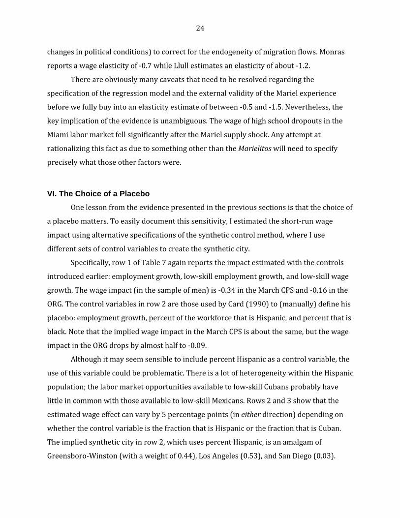
VI. The Choice of a Placebo One lesson from the evidence presented in the previous sections is that the choice of

a placebo matters. To easily document this sensitivity, I estimated the short-run wage

impact using alternative specifications of the synthetic control method, where I use

different sets of control variables to create the synthetic city.

Specifically, row 1 of Table 7 again reports the impact estimated with the controls

introduced earlier: employment growth, low-skill employment growth, and low-skill wage

growth. The wage impact (in the sample of men) is -0.34 in the March CPS and -0.16 in the

ORG. The control variables in row 2 are those used by Card (1990) to (manually) define his

placebo: employment growth, percent of the workforce that is Hispanic, and percent that is

black. Note that the implied wage impact in the March CPS is about the same, but the wage

impact in the ORG drops by almost half to -0.09.

Although it may seem sensible to include percent Hispanic as a control variable, the

use of this variable could be problematic. There is a lot of heterogeneity within the Hispanic

population; the labor market opportunities available to low-skill Cubans probably have

little in common with those available to low-skill Mexicans. Rows 2 and 3 show that the

estimated wage effect can vary by 5 percentage points (in either direction) depending on

whether the control variable is the fraction that is Hispanic or the fraction that is Cuban.

The implied synthetic city in row 2, which uses percent Hispanic, is an amalgam of

Greensboro-Winston (with a weight of 0.44), Los Angeles (0.53), and San Diego (0.03).

25

Simply replacing percent Hispanic with percent Cuban changes the synthetic city to

Greensboro-Winston (0.33), Newark (.46), and Tampa (.21). Not surprisingly, the implied

synthetic city is very sensitive to the choice of control variables, so that careful

consideration needs to be given to which set of variables should be included in the model.

Row 5 of Table 6 presents the most general specification, which adds variables denoting

the fraction of the workforce in each of 11 industries, as well as the fraction of the

workforce that is female or low-skill.33 The estimated wage impact is -0.33 in the March

CPS and -0.10 in the ORG. Put bluntly, the construction of the placebo is not an innocuous

decision—even when the methodology used to construct the placebo is thought to be

relatively free of researcher intervention (as the synthetic control method is sometimes

advertised).

One alternative (and perhaps preferable) way of determining whether the key

finding of a negative wage impact is sensitive to the choice of placebo is to estimate the

wage impact for every potential placebo, and then examine the resulting distribution of

potential wage effects. I illustrate this approach by using the regression model in equation

(3) to estimate the short-run effect in each of the 123,410 possible four-city placebos.

The two panels of Figure 7 illustrate the frequency distribution of estimated effects

when the dependent variable is the log wage of male high school dropouts, while Table 8

reports summary statistics for the distributions. Consider the density of estimated effects

in the March CPS data. The mean effect is -0.283, and almost all of the effects are

statistically significant.

Note that if the set of placebos is restricted to those where the average employment

growth in the four placebo cities was roughly similar to that of pre-Mariel Miami, the mean

wage effect rises to -0.319. If we look at the smaller subset where both average

employment growth and average low-skill employment growth was similar to that of

Miami, the mean wage effect rises further to -0.330. Put differently, the closer we get to a

placebo that seems to replicate the pre-existing conditions in Miami, the more likely we are

33 The industries are agriculture or mining, construction, manufacturing, transportation, wholesale

or retail trade, finance, business and repair services, personal services, entertainment services, professional services, and public administration. The control variables giving the change in local employment or wages were calculated using the March CPS; all other variables were calculated using the 1980 decennial census.

26

to find that the Marielitos had a larger wage effect on low-skill Miamians. Table 8 shows

that the same trend is implied by the frequency distribution of wage effects computed in

the ORG data.

VII. Conclusion Card’s (1990) classic paper on the labor market impact of the Mariel supply shock

stands as a landmark study in labor economics. The finding that the supply shock had little

effect on the labor market opportunities of native workers influenced what we think we

know about the economic consequences of immigration. And the elegance of the

methodological approach—the exploitation of a fascinating natural experiment to estimate

a parameter of economic interest—also influenced the way that many applied economists

frame their questions, organize the data, and search for an answer.

This paper brings a new perspective to the analysis of the Mariel supply shock. I

revisit the question and the data armed with the insights provided by three decades of

research on the economic impact of immigration. One key lesson from the vast literature is

that the effect of immigration on the wage structure depends crucially on the differences

between the skill distributions of immigrants and natives. The direct effect of immigration

is most likely to be felt by those workers who had similar capabilities as the Marielitos.

The Mariel supply shock was composed of disproportionately low-skill workers;

about 60 percent were high school dropouts. Remarkably, none of the previous

examinations of the Mariel experience documented what happened to the pre-existing high

school dropouts in Miami, a group that composed over a quarter of the city’s workforce.

Given the literature sparked by Borjas (2003), it seems obvious that any analysis of the

Mariel supply shock should focus on the labor market outcomes of these low-skill workers.

The examination of wage trends among high school dropouts quickly overturns the

stylized fact that the supply shock did not affect Miami’s wage structure. In fact, the

absolute wage of high school dropouts dropped dramatically, as did their wage relative to

that of either high school graduates or college graduates. The drop in the average wage of

the least skilled Miamians between 1977-1979 and 1981-1986 was substantial, between

10 and 30 percent. In fact, the examination of wage trends in every other city identified by

27

the CPS shows that the steep post-Mariel wage drop experienced by Miami’s low-skill

workforce was a very unusual event.

The reappraisal presented in this paper also illustrates that the researcher’s choice

of a placebo is an important element of any such empirical exercise, and that picking a

different placebo can easily lead to a weaker or stronger measured impact of immigration.

The synthetic control method, for example, can generate very different wage effects

depending on the set of variables that the researcher uses to construct the synthetic city.

Similarly, the magnitude of the wage effect differs substantially across all potential four-

city placebos that can be constructed in the CPS data. It is important to emphasize, however,

that despite the variation in the magnitude of the wage effects across placebos, the

evidence consistently indicates that the Marielitos had a sizable negative effect on the wage

of competing workers.

The evidence has potentially important implications for the literature that purports

to measure the wage impact of immigration. Many studies measure the effect by estimating

spatial correlations between wages and the number of immigrants in a particular locality.

These spatial correlations are plagued both by endogeneity problems (i.e. immigrants

settle in high-wage regions) and by native adjustments (i.e., firms and workers may

respond to the supply shock by relocating to other cities). The fact that the spatial

correlation implied by the Mariel supply shock is strongly negative indicates that the

existing non-experimental literature may not have successfully overcome those statistical

difficulties. There is still some way to go before non-experimental spatial correlations can

be presumed to estimate a parameter of economic interest.

The evidence also has implications for estimates of the economic benefits from

immigration. The benefit that accrues to the native population, or the immigration surplus,

is the flip side of the wage impact of immigration. In fact, the greater the wage impact, the

greater the immigration surplus. Borjas (2014, p. 151) estimates the current surplus to be

around 0.24 percent of GDP, or around $43 billion annually. Because there was a much

larger reduction in the earnings of the workers most likely to be affected by the Marielitos

than was previously believed, we may need to reassess existing estimates of the

immigration surplus. That surplus could easily be two or three times as large if the Mariel

context correctly measures the wage impact.

28

It has been a quarter-century since the publication of Card’s Mariel study. The

reappraisal of the evidence presented in this paper suggests that much can be gained by

revisiting some of those persistent old questions with a new perspective, a perspective that

uses the insights accumulated over the years. If nothing else, the reappraisal of the Mariel

evidence shows that even the most cursory reexamination of some old data with some new

ideas can reveal trends that radically change what we think we know.

29

References Abadie, Alberto, Alexis Diamond, and Jens Hainmueller. 2010. Synthetic Control Methods

for Comparative Case Studies: Estimating the Effect of California’s Tobacco Control Program. Journal of the American Statistical Association 105: 493-505.

Abadie, Alberto and Javier Gardeazabal. 2003. The Economic Costs of Conflict: A Case Study

of the Basque Country. American Economic Review 93: 112–132. Altonji, Joseph G., and David Card. 1991. The Effects of Immigration on the Labor Market

Outcomes of Less-Skilled Natives. In John M. Abowd and Richard B. Freeman (Eds.), Immigration, Trade, and the Labor Market, 201-234. Chicago: University of Chicago Press.

Angrist, Joshua D., and Adriana D. Kugler. 2003. Protective or Counter-Productive?

European Labor Market Institutions and the Effect of Immigrants on EU Natives. Economic Journal 113: F302–F331.

Angrist, Joshua D., and Alan B. Krueger. 1999. Empirical Strategies in Labor Economics. In

Orley Ashenfelter and David Card (Eds.), Handbook of labor economics, Vol. 3, 1277-1366. Amsterdam: Elsevier.

Autor, David H., Lawrence F. Katz, and Melissa S. Kearney. 2008. Trends in U.S. Wage

Inequality: Revising the Revisionists. Review of Economics and Statistics 90: 300-323. Borjas, George J. 2003. The Labor Demand Curve Is Downward Sloping: Reexamining the

Impact of Immigration on the Labor Market. Quarterly Journal of Economics 118: 1335-1374

Borjas, George J. 2014. Immigration Economics. Cambridge, MA: Harvard University Press. Borjas, George J. 2015. The Wage Impact of the Marielitos: A Reappraisal. NBER Working

Paper No. 21588. Cambridge, MA: National Bureau of Economic Research. Borjas, George J. 2016. The Wage Impact of the Marielitos: Additional Evidence. NBER

Working Paper No. 21850. Cambridge, MA: National Bureau of Economic Research. Borjas, George J., and Kirk B. Doran. 2012. The Collapse of the Soviet Union and the

Productivity of American Mathematicians. Quarterly Journal of Economics 127: 1143-1203.

Borjas, George J., Jeffrey Grogger, and Gordon H. Hanson. 2012. On Estimating Elasticities of

Substitution. Journal of the European Economic Association 10: 198-210. Cameron, Colin and Douglas L. Miller. 2015. A Practitioner's Guide to Cluster-Robust

Inference. Journal of Human Resources 50(2): 317-373.

30

Card, David. 1990. The Impact of the Mariel Boatlift on the Miami Labor Market. Industrial

and Labor Relations Review 43: 245-257. Carrington, William J., and Pedro de Lima. 1996. The Impact of 1970s Repatriates from

Africa on the Portuguese Labor Market. Industrial and Labor Relations Review 49: 330-347.

Dustmann, Christian, Tommaso Frattini, and Ian P. Preston. 2013. The Effect of

Immigration along the Distribution of Wages. Review of Economic Studies 80(1): 145-173.

Dustmann, Christian, Uta Schonberg, and Jan Stuhler. 2016. Labor Supply Shocks and the

Dynamics of Local Wages and Employment. Quarterly Journal of Economics, forthcoming.

Friedberg, Rachel. 2001. The Impact of Mass Migration on the Israeli Labor Market.

Quarterly Journal of Economics 116: 1373-1408. Garthwaite, Craig, Tad Gross, and Matthew J. Notowidigdo. 2014. Public Health Insurance,

Labor Supply, and Employment Lock. Quarterly Journal of Economics 129: 653-696. Glitz, Albrecht. 2012. The Labor Market Impact of Immigration: A Quasi-Experiment

Exploiting Immigrant Location Rules in Germany. Journal of Labor Economics 30: 175-213.

Grossman, Jean Baldwin. 1982. The Substitutability of Natives and Immigrants in

Production. Review of Economics and Statistics 54: 596-603. Hamilton, James D. 1983. Oil and the Macroeconomy Since World War II. Journal of Political

Economy 91: 228-248. Hunt, Jennifer. 1992. The Impact of the 1962 Repatriates from Algeria on the French Labor

Market. Industrial and Labor Relations Review 45: 556-572. Jaeger, David, Joakim Ruist, and Jan Stuhler. 2016. “Shift-Share Instruments and the Impact

of Immigration,” mimeo. Katz, Lawrence F., and Kevin M. Murphy. 1992. Changes in the Wage Structure, 1963-87:

Supply and Demand Factors. Quarterly Journal of Economics 107: 35-78. Lemieux, Thomas. 2006. Increased Residual Wage Inequality: Composition Effects, Noisy

Data, or Rising Demand for Skill. American Economic Review, 96(June), 461–498. Llull, Joan. 2015. The Effect of Immigration on Wages: Exploiting Exogenous Variation at

the National Level. Barcelona GSE Working Paper 783.

31

Monras, Joan. 2014. Online Appendix to ‘Immigration and Wage Dynamics: Evidence from

the Mexican Peso Crisis’. Sciences Po, dated January 8, 2014. Monras, Joan. 2015. Immigration and Wage Dynamics: Evidence from the Mexican Peso

Crisis. Sciences Po Economics Discussion Papers 2015-4. Ottaviano, Gianmarco I. P., and Giovanni Peri. 2012. Rethinking the Effect of Immigration on

Wages. Journal of the European Economic Association 10: 152-197. Peri, Giovanni and Vasil Yasenov. 2015. The Labor Market Effects of a Refugee Wave:

Applying the Synthetic Control Method to the Mariel Boatlift. NBER Working Paper No. 21801. Cambridge, MA: National Bureau of Economic Research.

Pinotti, Paolo, Ludovica Gazze, Francesco Fasani, and Marco Tonello. 2013. Immigration

Policy and Crime. Report prepared for the XV European Conference of the Fondazione Rodolfo Debenedetti.

Saiz, Albert. 2003. Room in the Kitchen for the Melting Pot: Immigration and Rental Prices.

Review of Economics and Statistics 85: 502-521. Stabile, Benedict L., and Robert L. Scheina. 2015. U. S. Coast Guard Operations During the

1980 Cuban Exodus. United States Coast Guard, Coast Guard History. Accessed at http://www.uscg.mil/history/articles/uscg_mariel_history_1980.asp (September 30, 2015).

32

Figure 1. Number of Cuban immigrants, by year of migration, 1955-2010

Notes: The specific year of migration (through 1999) is first reported in the 2000 census. The counts are adjusted for mortality and out-migration by using information on the number of arrivals provided by the 1970 through 1990 censuses; see the text for details. The 2000-2008 counts are drawn from the pooled 2009-2011 American Community Surveys (ACS), while the 2009-2010 counts are drawn from the 2012 ACS.

33

Figure 2. Log wage of high school dropouts, 1972-2003 (95 percent confidence band)

Notes: The log weekly wage is a 3-year moving average of the average log wage of high school dropouts in each geographic area. The data are drawn from the March CPS files.

34

Figure 3. Trends in the wage of low-skill workers in the March CPS, 1977-1992

A. Log weekly wage of high school dropouts

B. Log wage of high school dropouts relative to college graduates

C. Log wage of high school dropouts relative to high school graduates

Notes: The figures use a 3-year moving average of the average log wage of high school dropouts, high school graduates, and college graduates in each specific geographic area.

35

Figure 4. Distribution of pre-post wage changes, 1976-2003

A. Log wage of high school dropouts

Across all city-year permutations 1980 treatment year

B. Log wage of high school graduates

Across all city-year permutations 1980 treatment year

Notes: The pre-treatment period lasts 4 years; the post-treatment period lasts 6 years; and the year of the treatment is excluded from the calculation. The data are drawn from the March CPS files.

Mariel Mariel

Mariel Mariel

36

Figure 5. The trend in the wage of high school dropouts in the CPS-ORG, 1973-2003

Notes: The log hourly wage is a 3-year moving average of the average log wage of high school dropouts in each geographic area in Figure 5A, and of the age-adjusted wage in Figure 5B. The data are drawn from the May/CPS-ORG files.

A. 95 percent confidence band

B. Average wage trends in Miami and placebos

37

Figure 6. Trends in the wage of high school dropouts in pooled sample of men and women, 1977-1992

A. March CPS

B. CPS-ORG

Notes: The figures use a 3-year moving average of the age- and gender-adjusted average log wage of the pooled group of men and women in each specific geographic area.

38

Figure 7. Distribution of hypothetical short-run impacts relative to synthetic placebo, assuming a supply shock hits each city in 1980

A. March CPS

B. CPS-ORG

Notes: The pre-treatment period lasts 3 years; the post-treatment period lasts 6 years. The wage effect is estimated from a difference-in-differences regression model that excludes 1980, the year of the treatment.

Mariel

Mariel

39

Figure 8. Distribution of short-run wage impacts across all possible four-city placebos, 1977-1986

A. March CPS

B. CPS-ORG

Notes: The figure shows the distribution of the interaction term from the difference-in-differences regression model in equation (3) resulting from comparing Miami to all possible 123,410 placebos. The regressions use annual observations for each city in the period 1977-1986 (1980 excluded), and the coefficients measure the impact in the short run (i.e., 1981-1986). All regressions were weighted by the number of observations used to calculate the mean wage of high school dropouts in city r at time t.

Low-skill placebo

Card placebo

Employment placebo

Synthetic placebo

Employment placebo Synthetic

placebo Card placebo

Low-skill placebo

40

Table 1. Education distribution of adult Marielitos

Years of education Sample: < 12 12 13 - 15 ≥ 16 Sample size Marielitos:

April 1983 CPS 57.9 25.6 3.5 13.1 31 June 1986 CPS 55.2 28.0 6.4 9.6 31 June 1988 CPS 58.7 26.1 4.4 10.9 46 1990 Census 64.8 15.8 12.9 6.5 4,234 1994 CPS-ORG 61.4 20.5 9.8 8.3 143 2000 Census 59.9 20.0 12.7 7.4 3,301

Miami’s pre-existing labor force:

1980 Census 26.7 28.4 26.0 18.8 32,971 Notes: The statistics are calculated in the sample of persons born in Cuba who migrated to the United States at the time of Mariel and were 18 years old in 1980. In the April 1983 CPS and 2000 census, the Marielitos are identified as persons born in Cuba who migrated to the United States in 1980. In all other samples, the Marielitos are identified as Cubans who entered the country in 1980 or 1981. The pre-existing labor force of Miami includes both natives and immigrants.

41

Table 2. The size of the Mariel supply shock Education group:

Size of Miami’s labor force in 1980 (1000s)

Number of Marielitos in labor

force (1000s)

Percent increase in supply

High school dropouts 176.3 32.5 18.4 High school graduates 187.5 10.1 5.4 Some college 171.5 8.8 5.1 College graduates 124.1 4.2 3.4

All workers 659.4 55.7 8.4 Notes: The pre-existing number of workers in Miami is calculated from the 1980 census; the number of Marielito workers (at least 18 years old at the time of Mariel) is calculated from the 1990 census, and a small adjustment is made because the 1990 census reports the number of Cuban immigrants who entered the country in 1980 or 1981.

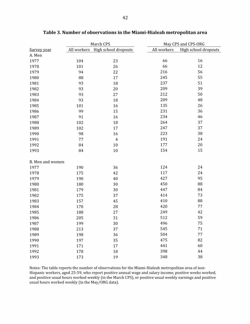
42

Table 3. Number of observations in the Miami-Hialeah metropolitan area March CPS May CPS and CPS-ORG Survey year All workers High school dropouts

All workers High school dropouts

A. Men 1977 104 23

66 16

1978 101 26

66 12 1979 94 22

216 56

1980 88 17

245 55 1981 93 18

237 51

1982 93 20

209 39 1983 93 27

212 50

1984 93 18

209 48 1985 101 16

135 26

1986 99 15

231 36 1987 91 16

234 46

1988 102 18

264 37 1989 102 17

247 37

1990 98 16

223 38 1991 77 4

191 24

1992 84 10

177 20 1993 84 10

154 15

B. Men and women 1977 190 36

124 24

1978 175 42

117 24 1979 190 40

427 95

1980 180 30

450 88 1981 179 30

447 84

1982 175 37

414 73 1983 157 45

410 88

1984 170 28

420 77 1985 188 27

249 42

1986 205 31

512 59 1987 199 30

496 75

1988 213 37

545 71 1989 198 36

504 77

1990 197 35

475 82 1991 171 17

441 60

1992 178 18

398 44 1993 173 19

348 38

Notes: The table reports the number of observations for the Miami-Hialeah metropolitan area of non-Hispanic workers, aged 25-59, who report positive annual wage and salary income, positive weeks worked, and positive usual hours worked weekly (in the March CPS), or positive usual weekly earnings and positive usual hours worked weekly (in the May/ORG data).

43

Table 4. Rates of employment and wage growth before Mariel

Rank Metropolitan area Employment

growth: all workers Employment growth: high school dropouts

Wage growth: high school dropouts

1 San Diego, CA 0.194 0.067 -0.127 2 Greensboro-Winston Salem, NC 0.182 -0.063 -0.336 3 Kansas City, MO/KS 0.179 0.052 -0.178 4 Anaheim-Santa Ana- Garden Grove, CA 0.162 0.257 0.068 5 Rochester, NY 0.153 -0.172 0.019 6 Miami-Hialeah, FL 0.153 0.086 0.012 7 Nassau-Suffolk, NY 0.151 0.056 -0.047 8 San Jose, CA 0.137 0.130 0.138 9 Albany-Schenectady-Troy, NY 0.130 0.065 0.065 10 Boston, MA 0.121 -0.100 -0.024 11 Milwaukee, WI 0.121 -0.006 0.056 12 Indianapolis, IN 0.115 0.071 -0.048 13 Seattle-Everett, WA 0.110 -0.079 -0.051 14 Norfolk-Virginia Beach-Newport News, VA 0.103 0.052 0.110 15 Philadelphia, PA/NJ 0.102 -0.033 0.012 16 Newark, NJ 0.092 -0.116 -0.124 17 Tampa-St. Petersburg-Clearwater, FL 0.083 0.068 0.120 18 Denver-Boulder-Longmont, CO 0.082 -0.139 0.027 19 Houston-Brazoria, TX 0.078 0.090 0.003 20 Sacramento, CA 0.078 0.152 -0.034 21 Dallas-Fort Worth, TX 0.076 0.062 -0.050 22 Portland-Vancouver, OR/WA 0.071 -0.074 -0.020 23 Riverside-San Bernardino, CA 0.071 -0.017 0.254 24 Atlanta, GA 0.069 -0.087 0.014 25 Cincinnati-Hamilton, OH/KY/IN 0.063 0.038 -0.032 26 Washington, DC/MD/VA 0.061 0.028 0.090 27 Detroit, MI 0.060 -0.099 0.010 28 Fort Worth-Arlington, TX 0.058 -0.006 -0.059 29 Los Angeles-Long Beach, CA 0.056 0.075 -0.128 30 Columbus, OH 0.048 -0.324 -0.004 31 Buffalo-Niagara Falls, NY 0.039 0.040 -0.144 32 Chicago-Gary-Lake IL 0.025 -0.082 -0.017 33 St. Louis, MO/IL 0.019 -0.060 -0.060 34 Bergen-Passaic, NJ 0.015 -0.051 0.007 35 Baltimore, MD 0.012 -0.108 -0.001 36 Minneapolis-St. Paul, MN 0.007 -0.050 -0.012 37 Cleveland, OH 0.001 -0.071 -0.014 38 New York, NY 0.000 -0.146 0.074 39 Pittsburg, PA -0.013 -0.111 0.123 40 Birmingham, AL -0.020 -0.172 -0.124 41 San Francisco-Oakland-Vallejo, CA -0.027 -0.200 -0.105 42 Gary-Hammond-East Chicago, IN -0.029 0.119 0.042 43 New Orleans, LA -0.046 -0.313 -0.017 44 Akron, OH -0.110 -0.351 -0.005 Notes: The rate of employment growth is the log ratio of average employment in 1979-1980 to average employment in 1977-1978, calculated from the 1977-1980 survey years of the March CPS. The rate of wage growth is the difference in the (age-adjusted) log weekly wage between 1978-1979 and 1976-1977.

44

Table 5. Difference-in-differences impact of the Marielitos on the wage of high school dropouts

Card placebo

Employment placebo

Low-skill placebo

Synthetic control

All cities

A. March CPS, men 1981-1983 -0.204 -0.290 -0.180 -0.257 -0.191 (0.076) (0.073) (0.081) (0.077) (0.064) 1984-1986 -0.368 -0.454 -0.301 -0.458 -0.393 (0.060) (0.059) (0.054) (0.075) (0.022) 1987-1989 -0.328 -0.303 -0.228 -0.293 -0.286 (0.081) (0.072) (0.060) (0.070) (0.059) 1990-1992 -0.026 -0.056 0.039 -0.188 -0.003

(0.072) (0.123) (0.065) (0.155) (0.032) B. CPS-ORG, men

1981-1983 -0.075 -0.140 -0.079 -0.154 -0.083 (0.026) (0.049) (0.024) (0.026) (0.012) 1984-1986 -0.069 -0.116 -0.076 -0.157 -0.086 (0.057) (0.065) (0.054) (0.056) (0.046) 1987-1989 -0.106 -0.175 -0.101 -0.150 -0.141 (0.036) (0.064) (0.035) (0.023) (0.022) 1990-1992 0.019 -0.070 0.036 -0.079 -0.008 (0.041) (0.062) (0.038) (0.016) (0.023)

Notes: Robust standard errors are reported in parentheses. The data consist of annual observations for each city between 1977 and 1992 (1980 excluded). All regressions include vectors of city and year fixed effects. The table reports the interaction coefficients between a dummy variable indicating if the metropolitan area is Miami and the timing of the post-Mariel period. The regressions that use the Card, employment, or low-skill placebos have 75 observations; the regressions that use the synthetic placebo have 30 observations; and the regressions in the last column have 658 observations. All regressions are weighted by the number of observations used to calculate the dependent variable. The number of observations of the synthetic control is a weighted average of the sample size in the actual cities that make up the synthetic city.

45

Table 6. Sensitivity of estimates of the short-run wage impact, 1977-1986

Men Men and women Placebo March CPS CPS-ORG March CPS CPS-ORG 1. Card placebo -0.280 -0.074 -0.189 -0.040 (0.069) (0.031) (0.061) (0.024) 2. Employment placebo -0.358 -0.131 -0.220 -0.069 (0.064) (0.044) (0.048) (0.033) 3. Low-skill placebo -0.269 -0.078 -0.182 -0.040 (0.072) (0.028) (0.056) (0.022) 4. Synthetic control -0.343 -0.155 -0.175 -0.075 (0.081) (0.028) (0.051) (0.024) 5. All cities placebo -0.279 -0.086 -0.184 -0.036 (0.062) (0.023) (0.051) (0.020)

Notes: Robust standard errors are reported in parentheses. The data consist of annual observations for each city between 1977 and 1986 (1980 excluded). The table reports the interaction coefficients between a dummy variable indicating if the metropolitan area is Miami and if the observation is drawn from the post-Mariel period. See the notes to Table 5 for more details on the regression specification.

46

Table 7. Sensitivity of short-run wage effects to the definition of a synthetic control

Men Men and women Set of control variables:

March CPS

CPS- ORG

March CPS

CPS-ORG

1. ∆ log E, ∆ log EU, ∆ log wU -0.343 -0.155 -0.175 -0.075 (0.081) (0.028) (0.051) (0.024)

2. ∆ log E, percent Hispanic, percent black -0.367 -0.092 -0.264 -0.057 (0.108) (0.032) (0.065) (0.023)

3. ∆ log E, percent Cuban, percent black -0.317 -0.134 -0.251 -0.070 (0.080) (0.039) (0.064) (0.039)

4. ∆ log E, ∆ log EU, ∆ log wU, percent Hispanic, -0.301 -0.072 -0.221 -0.057 percent Cuban, percent black, percent female (0.084) (0.037) (0.051) (0.023)

5. Same as row 4, plus percent low-skill and -0.325 -0.097 -0.254 -0.048 industry mix (0.052) (0.033) (0.044) (0.024)

Notes: Robust standard errors are reported in parentheses. The data consist of annual observations for each city between 1977 and 1986 (1980 excluded). The control variable Δ log E is the city’s employment growth rate between 1977 and 1979; Δ log EU is the concurrent growth rate of low-skill employment; and Δ log wU is the concurrent growth rate of the low-skill wage. The table reports the interaction coefficients between a dummy variable indicating if the metropolitan area is Miami and if the observation is drawn from the post-Mariel period. See the notes to Table 5 for more details on the regression specification.

47

Table 8. The distribution of estimated short-run wage effects across all four-city placebos

Characteristics of distribution: March CPS CPS-ORG Mean -0.283 -0.087 Standard deviation 0.043 0.022 Statistical significance: Fraction of t-statistics above |2.0| 0.998 0.845

Average employment growth of placebo cities within 0.1 standard deviations of Miami (N = 1,148)

Mean -0.319 -0.108 Fraction of t-statistics above |2.0| 1.000 0.863

Average low-skill employment growth of placebo cities within 0.1 standard deviations of Miami (N = 1,096)

Mean -0.297 -0.105 Fraction of t-statistics above |2.0| 1.000 0.973

Average total and low-skill employment growth for placebo cities within 0.1 standard deviations of Miami (N = 74)

Mean -0.330 -0.120 Fraction of t-statistics above |2.0| 1.000 0.986

Notes: The table reports the distribution of the interaction coefficient between a dummy variable indicating if the metropolitan area is Miami and if the observation is drawn from the post-Mariel period. The regressions were estimated separately in all possible 123,410 four-city placebos. . See the notes to Table 5 for more details on the regression specification.