255

Dorian Nedelcu, Petrica Guran, Alexandru Cantaragiu

Theoretical and Experimental Research Performed on the Tesla Turbine - Part I

The paper presents the theoretical and experimental research performed on a Tesla turbine driven by compressed air and designed to equip a teaching laboratory [1], [2]. It introduces the operating principle of the Tesla turbine, which was invented by engineer Nikola Tesla, a turbine which uses discs instead of blades, mounted on a shaft at a small distance between them. The turbine geometry, results from stress and flow calculations performed on the turbine rotor and assembly, using the Simulation modules and SolidWorks Flow Simulation program are presented. After designing the turbine, it becomes the subject of experi-mental research to determine the curve of the speed depending on the pressure. Also, the experimental research focuses on the behaviour of the turbine from a dynamic point of view [3].

Keywords: turbine, Tesla, SolidWorks, Flow Simulation

1. Operating principle

The Tesla turbine was patented by the famous engineer Nikola Tesla on the 6th of May, 1913 [4]. The turbine runner has no hydrodynamic profile blades, but it is composed of a series of discs placed on the shaft at a constant distance [5]. The turbine is driven by a fluid (water or air) through a nozzle directed at the periphery of the disk, which is driven due to the boundary layer effect. The fluid adheres to the surface of a disc due to viscosity, thus leading to the the energy transfer. After the power is transferred from fluid to the runner, the fluid velocity decreases and it is disposed of on a spiral path through the drain holes made in the side wall. To be effective, the Tesla turbine must meet the following conditions: the distance between the discs must be very small, the disc should have a smooth surface to minimize losses. Also, the disc must be very thin to prevent the formation of turbulence on them. This could lead to their deformation, especially in terms of high speed operations and a long life of the turbine.

ANALELE UNIVERSIT ĂŢII

“EFTIMIE MURGU” RE ŞIŢA

ANUL XXII, NR. 2, 2015, ISSN 1453 - 7397

256

2. The Tesla turbine geometry

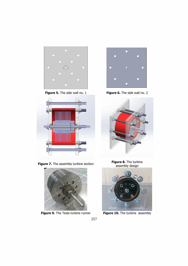
The Tesla turbine geometry is particularly simple. On the shaft, Figure 1, one can find 16 discs, Figure 2, which are equidistant because of the spacers, Figure 3. The ø95 mm diameter discs were recovered from platters of computer hard drives equipped with 8 x Ø10 mm diameter holes. The sequence of disks and spacers are locked on the shaft by an M8 nut and form the turbine runner. The turbine casing has an inner diameter of ø105 mm and a width of 72 mm, Figure 4, and is provided with a fluid inlet hole, and with places for fitting the bearings. The side walls, Figure 5 and Figure 6, close the casing and the runner. One of the side walls, Figure 5, is further provided with outlet holes for the fluid. Figure 7 shows a section through the turbine assembly, and Figure 8 shows the entire assembly. Figures 9 and 10 show the assembled turbine runner and the turbine assembly.

Figure 1. The shaft Figure 2. The disc

Figure 3. The spacer Figure 4. The turbine casing

257

Figure 5. The side wall no. 1 Figure 6. The side wall no. 2

Figure 7. The assembly turbine section Figure 8. The turbine

assembly design

Figure 9. The Tesla turbine runner Figure 10. The turbine assembly

258

3. The resistance calculus of the runner

The resistance calculus of the runner was done through the SolidWorks Simulation software. The analyzed geometry consists of the shaft, disks and spacers, Figure 11. The loads acting on them are due to the action of the working fluid (air), their own weight and the centrifugal force. Since Tesla turbines can operate at very high speeds, the effect of fluid is neglected and centrifugal charging is considered force majeure, which has a maximum speed of 20000 rev/min and corresponds to an angular speed of 2094.4 rad/s, Figure 12. The weight, directed on the Y-axis, and the gravity acceleration with a value of 9.81 m/s2, Figure 13 will also be considered. The runner geometry was modeled as a single solid. The mesh and the mesh parameters are shown in figure 14 and 15. The mesh consists of 302230 finite elements and a number of 532557 knots. The material was selected from the SolidWorks library, a Stainless Steel type with a yield strength of 172.3 MPa.

Figure 11. The resistance calculus geometry

Figure 12. The centrifugal load Figure 13. The weight load

The distribution of displacement and the von Mises stress are presented in

Figures 16 and 17. One can observe that the maximum displacement value is 0.004

259

mm and the maximum stress value is 81.1 MPa, which leads to a safety factor of 2.12.

Figure 14. The mesh parameters Figure 15. The runner mesh

Figure 16. The displacement distribution Figure 17. The von Misses

distribution

4. The flow simulation through the Tesla turbine

The flow simulation through the turbine aims to determine flow trajectories that occur in the turbine. The simulation was done by using the Flow Simulation module, which is integrated in the SolidWorks application interface, for an operating point defined by a maximum inlet pressure of 5 bar. The numerical simulation steps are [6]: • The creation of geometry; • Activation of the Flow Simulation module; • Creation of the Flow Simulation project; • Define the Computational Domain;

• Define boundary conditions; • Define study‘s goal; • Running flow study; • Viewing of the results.

260

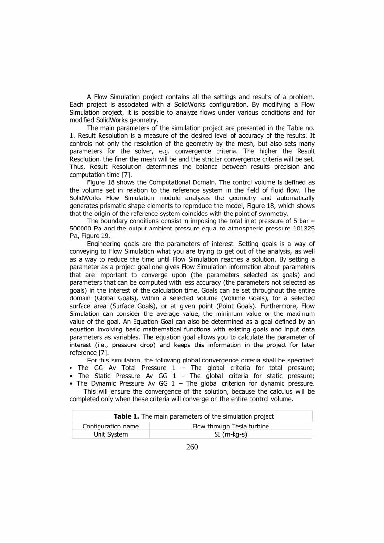
A Flow Simulation project contains all the settings and results of a problem. Each project is associated with a SolidWorks configuration. By modifying a Flow Simulation project, it is possible to analyze flows under various conditions and for modified SolidWorks geometry.

The main parameters of the simulation project are presented in the Table no. 1. Result Resolution is a measure of the desired level of accuracy of the results. It controls not only the resolution of the geometry by the mesh, but also sets many parameters for the solver, e.g. convergence criteria. The higher the Result Resolution, the finer the mesh will be and the stricter convergence criteria will be set. Thus, Result Resolution determines the balance between results precision and computation time [7].

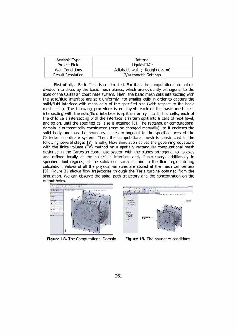
Figure 18 shows the Computational Domain. The control volume is defined as the volume set in relation to the reference system in the field of fluid flow. The SolidWorks Flow Simulation module analyzes the geometry and automatically generates prismatic shape elements to reproduce the model, Figure 18, which shows that the origin of the reference system coincides with the point of symmetry.

The boundary conditions consist in imposing the total inlet pressure of 5 bar = 500000 Pa and the output ambient pressure equal to atmospheric pressure 101325 Pa, Figure 19.

Engineering goals are the parameters of interest. Setting goals is a way of conveying to Flow Simulation what you are trying to get out of the analysis, as well as a way to reduce the time until Flow Simulation reaches a solution. By setting a parameter as a project goal one gives Flow Simulation information about parameters that are important to converge upon (the parameters selected as goals) and parameters that can be computed with less accuracy (the parameters not selected as goals) in the interest of the calculation time. Goals can be set throughout the entire domain (Global Goals), within a selected volume (Volume Goals), for a selected surface area (Surface Goals), or at given point (Point Goals). Furthermore, Flow Simulation can consider the average value, the minimum value or the maximum value of the goal. An Equation Goal can also be determined as a goal defined by an equation involving basic mathematical functions with existing goals and input data parameters as variables. The equation goal allows you to calculate the parameter of interest (i.e., pressure drop) and keeps this information in the project for later reference [7].

For this simulation, the following global convergence criteria shall be specified: • The GG Av Total Pressure 1 – The global criteria for total pressure; • The Static Pressure Av GG 1 - The global criteria for static pressure; • The Dynamic Pressure Av GG 1 – The global criterion for dynamic pressure. This will ensure the convergence of the solution, because the calculus will be completed only when these criteria will converge on the entire control volume.

Table 1. The main parameters of the simulation project

Configuration name Flow through Tesla turbine

Unit System SI (m-kg-s)

261

Analysis Type Internal

Project Fluid Liquids→Air

Wall Conditions Adiabatic wall ; Roughness =0 Result Resolution 3/Automatic Settings

First of all, a Basic Mesh is constructed. For that, the computational domain is

divided into slices by the basic mesh planes, which are evidently orthogonal to the axes of the Cartesian coordinate system. Then, the basic mesh cells intersecting with the solid/fluid interface are split uniformly into smaller cells in order to capture the solid/fluid interface with mesh cells of the specified size (with respect to the basic mesh cells). The following procedure is employed: each of the basic mesh cells intersecting with the solid/fluid interface is split uniformly into 8 child cells; each of the child cells intersecting with the interface is in turn split into 8 cells of next level, and so on, until the specified cell size is attained [8]. The rectangular computational domain is automatically constructed (may be changed manually), so it encloses the solid body and has the boundary planes orthogonal to the specified axes of the Cartesian coordinate system. Then, the computational mesh is constructed in the following several stages [8]. Briefly, Flow Simulation solves the governing equations with the finite volume (FV) method on a spatially rectangular computational mesh designed in the Cartesian coordinate system with the planes orthogonal to its axes and refined locally at the solid/fluid interface and, if necessary, additionally in specified fluid regions, at the solid/solid surfaces, and in the fluid region during calculation. Values of all the physical variables are stored at the mesh cell centers [8]. Figure 21 shows flow trajectories through the Tesla turbine obtained from the simulation. We can observe the spiral path trajectory and the concentration on the output holes.

Figure 18. The Computational Domain Figure 19. The boundary conditions

262

Figure 20. The Basic Mesh

Figure 21. The flow trajectories through Tesla turbine

5. Conclusions

• The Tesla turbine has an advantage over the rest of the turbines used in practice today because of the simplicity of its constructive solution.

• Another advantage is the fact that it only has one rotating piece. • The Tesla turbine can be used in two ways (fluid acting on the discs in the

turbine regime or the runner acting on the fluid in the pumping regime) which makes the Tesla turbine interesting in terms of application.

• Although it can reach very high speeds and power in relation to the reduced overall dimensions of the turbine, disc deformations can occur over time.

• Disc deformations can be prevented by using high-quality materials with su-perior strength.

References

[1] Cantaragiu A., Cercetări asupra unei turbine Tesla. Principiu de funcţionare şi proiectare 3D, Proiect de disertaţie, Universitatea „Eftimie Murgu” din Reşiţa, 2015.

[2] Guran P., Cercetări asupra unei turbine Tesla. Execuție și experimentare, Proiect de disertaţie, Universitatea „Eftimie Murgu” din Reşiţa, 2015.

[3] Nedelcu D., Gillich E.V., Iancu V., Theoretical and experimental research performed on the Tesla turbine-Part II, Multi-Conference on Systems & Structures (Systruc’15), “Eftimie Murgu” University of Reşiţa, 24-26 September, 2015.

[4] Gingerly V., Building the Tesla Turbine, David J. Gingery Publishing LLC, 2004.

[5] ***** https://en.wikipedia.org/wiki/Tesla_turbine. [6] Nedelcu D., Digital prototyping & numerical simulation with SolidWorks,

Eurostampa Publishing, Timisoara, 2011. [7] ***** SolidWorks FlowSimulation 2011. Tutorial. [8] ***** SolidWorks FlowSimulation 2011. Technical_Reference.

263

Addresses:

• Prof. Ph.D. Dorian Nedelcu, “Eftimie Murgu” University of Reşiţa, Traian Vuia Square, no. 1-4, 320085, Reşiţa, d.nedelcu@uem.ro

• Eng. Petrica Guran, “Eftimie Murgu” University of Reşiţa, Traian Vuia Square, no. 1-4, 320085, Reşiţa, petrica.guran@yahoo.com

• Eng. Alexandru Cantaragiu, “Eftimie Murgu” University of Reşiţa, Traian Vuia Square, no. 1-4, 320085, Reşiţa, alex_cantaragiu@yahoo.com