theoretical temperature model with experimental validation ... · theoretical temperature model...

CER

N-T

HES

IS-2

017-

022

21/0

4/20

17

Sara Aasly

Theoretical temperature model with

experimental validation for CLIC

Accelerating Structures

Bachelor thesis

for the degree of Automation Engineering

CERN Geneva, March 2017

HVL

Bachelor of Automation Engineering

Theoretical temperature model with experimental validation for CLIC

Accelerating Structures

Sara Aasly

Supervisor: Steffen Dobert CERN, Geneva, Switzerland

Alex Vamvakas CERN, Geneva, Switzerland

Johan Alme HVL, Norway

Examiner: Svein Haustveit HVL, Norway

Department of Electrical Engineering

Western Norway University of Applied Sciences

5063 Bergen, Norway

Abstract

Micron level stability of the Compact Linear Collider (CLIC) components is one of the

main requirements to meet the luminosity goal for the future 48 km long underground

linear accelerator. The radio frequency (RF) power used for beam acceleration causes

heat generation within the aligned structures, resulting in mechanical movements and

structural deformations. A dedicated control of the air- and water- cooling system in

the tunnel is therefore crucial to improve alignment accuracy.

This thesis investigates the thermo-mechanical behavior of the CLIC Accelerating Struc-

ture (AS). In CLIC, the AS must be aligned to a precision of 10µm. The thesis shows

that a relatively simple theoretical model can be used within reasonable accuracy to

predict the temperature response of an AS as a function of the applied RF power. Dur-

ing failure scenarios or maintenance interventions, the RF power is turned off resulting

in no heat dissipation and decrease in the overall temperature of the components. The

theoretical model is used to explore control approaches that can be used to limit the

temperature changes during such scenarios. The component temperature is highly de-

pendent on the flow rate of the cooling water. The effect of active control of the water

cooling flow rate to decrease temperature changes during failure scenarios (breakdowns)

is investigated theoretically.

Acknowledgements

My special thanks go to Alex Vamvakas for his guidance and ideas - he deserves all the

credit (and none of the blame). I would like to express my gratitude to Steffen Dobert

for his supervision and for giving me the possibility to fulfill my dream of working here

at CERN. I would also like to thank Johan Alme and Svein Haustveit for steering me

in the right direction, and for providing excellent support along the way. Thanks to the

CLIC-module team for sharing all kinds of coffee and knowledge with me the past year.

Thanks to my Dad for always sharing all his knowledge, until today and in the future.

Finally, thanks to you, Francesco Velotti, without your help with Mathematica, I would

still be sitting here solving differential equations by hand.

Geneve, January 22. 2017 Sara Asly

ii

Contents

Abstract i

Acknowledgements ii

List of Figures v

Abbreviations vi

Symbols vii

1 Introduction 1

1.1 Background . . . . . . . . . . . . . . . . . . . . . . . . . . . . . . . . . . . 1

1.2 Basic features of CLIC . . . . . . . . . . . . . . . . . . . . . . . . . . . . . 2

1.3 Aim of the study . . . . . . . . . . . . . . . . . . . . . . . . . . . . . . . . 4

2 System Overview 7

2.1 The CLIC main linac Accelerating Structure . . . . . . . . . . . . . . . . 7

2.2 RF Breakdown . . . . . . . . . . . . . . . . . . . . . . . . . . . . . . . . . 8

2.3 The Cooling system . . . . . . . . . . . . . . . . . . . . . . . . . . . . . . 8

3 Theory 10

3.1 Heat transfer mechanisms . . . . . . . . . . . . . . . . . . . . . . . . . . . 11

3.1.1 Conduction . . . . . . . . . . . . . . . . . . . . . . . . . . . . . . . 11

3.1.2 Convection . . . . . . . . . . . . . . . . . . . . . . . . . . . . . . . 11

3.1.3 Radiation . . . . . . . . . . . . . . . . . . . . . . . . . . . . . . . . 13

3.2 Steady-flow systems . . . . . . . . . . . . . . . . . . . . . . . . . . . . . . 13

3.3 Lumped system analysis . . . . . . . . . . . . . . . . . . . . . . . . . . . . 14

3.3.1 Criteria for lumped system analysis . . . . . . . . . . . . . . . . . 15

3.3.2 Biot number calculation for AS . . . . . . . . . . . . . . . . . . . . 15

3.4 Unit Step Response . . . . . . . . . . . . . . . . . . . . . . . . . . . . . . . 17

4 First-Order System Transient Response 18

4.1 Theoretical analysis . . . . . . . . . . . . . . . . . . . . . . . . . . . . . . 18

4.2 The Step response . . . . . . . . . . . . . . . . . . . . . . . . . . . . . . . 20

4.3 Complex forcing terms . . . . . . . . . . . . . . . . . . . . . . . . . . . . . 22

5 Experimental Setup and Results 23

iii

iv

5.1 Temperature recordings . . . . . . . . . . . . . . . . . . . . . . . . . . . . 23

5.2 Operating conditions . . . . . . . . . . . . . . . . . . . . . . . . . . . . . . 25

5.3 Experimental Results . . . . . . . . . . . . . . . . . . . . . . . . . . . . . . 26

6 Water flow control 28

6.1 Effect of water flow on temperature response . . . . . . . . . . . . . . . . 29

6.2 Simple flow control . . . . . . . . . . . . . . . . . . . . . . . . . . . . . . . 30

6.3 Feedback flow control . . . . . . . . . . . . . . . . . . . . . . . . . . . . . 32

6.4 Effect of system delay . . . . . . . . . . . . . . . . . . . . . . . . . . . . . 34

7 Conclusion and Future Work 36

A Physical constants 38

B Mathematica notebook 39

Bibliography 43

List of Figures

1.1 The CLIC main beam is accelerated by radio-frequency (RF) waves thatare generated by a powerful electron beam (Drive beam) that runs parallelto the main beam [1]. . . . . . . . . . . . . . . . . . . . . . . . . . . . . . 2

1.2 The CLIC two-beam acceleration scheme [1]. . . . . . . . . . . . . . . . . 3

1.3 Left: The Two Beam Module mechanical model in the lab. Right: Sim-plified 3D model. . . . . . . . . . . . . . . . . . . . . . . . . . . . . . . . . 4

1.4 Position measurement of AS point P and best-fit line plotted against AStemperature [2]. . . . . . . . . . . . . . . . . . . . . . . . . . . . . . . . . . 5

2.1 Left: Layout of CTF3. Right: The two-beam test stand in CTF3 [3] . . . 7

2.2 Left: CLIC Accelerating Structure [1]. Right: CLIC Accelerating stucturein test facility . . . . . . . . . . . . . . . . . . . . . . . . . . . . . . . . . . 8

3.1 Free convection . . . . . . . . . . . . . . . . . . . . . . . . . . . . . . . . . 12

3.2 Forced convection . . . . . . . . . . . . . . . . . . . . . . . . . . . . . . . . 12

3.3 Inlet and outlet flow in steady flow system . . . . . . . . . . . . . . . . . 14

3.4 Unit step input and output . . . . . . . . . . . . . . . . . . . . . . . . . . 17

4.1 Step response of AS with 20 ◦C as initial condition . . . . . . . . . . . . . 21

4.2 Examples of heat generated by RF power in red and the expected systemresponses in blue . . . . . . . . . . . . . . . . . . . . . . . . . . . . . . . . 22

5.1 RTD sensors with integrated double-sided tape . . . . . . . . . . . . . . . 23

5.2 Position for inlet, component and outlet temperature sensors AS . . . . . 24

5.3 Effect of removing tracking errors in experimental temperature data . . . 25

5.4 Theoretical model and measurements with error bars . . . . . . . . . . . . 26

5.5 Theoretical model and measurements . . . . . . . . . . . . . . . . . . . . . 26

6.1 Time constants at increasing water flow, with an heat generation of290W , 830W and 910W [2] . . . . . . . . . . . . . . . . . . . . . . . . . . 28

6.2 Temperate response for different water flow rates . . . . . . . . . . . . . . 29

6.3 Power dissipated as heat during an average breakdown . . . . . . . . . . . 30

6.4 Water flow control with corresponding temperature response . . . . . . . 31

6.5 Temperature response for different flow control signals . . . . . . . . . . . 32

6.6 Left: Average power dissipated as heat. Right: Water flow signal as afunction of heat generation. . . . . . . . . . . . . . . . . . . . . . . . . . . 33

6.7 Theoretical temperature response with and without water flow control . . 33

6.8 Instant(blue) and delayed (yellow) water flow control signal during onebreakdown . . . . . . . . . . . . . . . . . . . . . . . . . . . . . . . . . . . . 34

6.9 Model of temperature response with instant and delayed water flow control 35

v

Abbreviations

AS Accelerating Structure

CLIC Compact LInear Collider

CERN Conseil Eurpeen pour la Recherche Nnucleaire

CTF3 CLIC Test Facility 3

DB Drive Beam

DBQ Drive Beam Quadroploe

MBQ Main Beam Quadroploe

LHC Large Hadron Collider

linac Linear Accelerator

MB Main Beam

PETS Power Extraction and Transfer Structure

RF Radio Frequency

WG Waveguide

vi

Symbols

symbol name unit

A surface area m2

C specific heat kJ/kg ◦C

h heat transfer coefficient W/m2 ◦C

k thermal conductivity W/m ◦C

Lc characteristic length m

m mass kg

m rate of mass flow kg/s

Nu Nusselt number

P power W (Js−1)

Q quantity of heat kJ

Q rate of heat transfer W (Js−1)

T temperature ◦C

Tcu AS component temperature ◦C

Ti inlet temperature ◦C

Te outlet temperature ◦C

T∞ ambient temperature ◦C

t time s

v velocity m/s

ρ fluid density kg/m3

vii

Chapter 1

Introduction

European Organization for Nuclear Science (Conseil europeen pour la recherche nucleaire),

CERN, is the world’s largest research facility for high energy physics. At CERN, engi-

neers and physicists work together to explore the fundamental structure of the universe.

To study the basic constituents of matter, CERN use some of the world’s largest particle

accelerators. By accelerating particles to nearly the speed of light and putting them into

collision, physicists are able to test their theories and explore the fundamental laws of

nature [4].

1.1 Background

With a goal of uniting European scientists and share the costs of high energy physics

facilities, CERN was established in 1954 [4].The research facility is based in Geneva close

to the Franco-Swiss border. Today, CERN consists of a total of 22 member states, but

also other non-European countries are involved in the different research programs. There

are 2500 people (as of 2016) employed directly by CERN, and around 12 000 visiting

scientists from other organizations and universities are using the CERN facilities [5]

CERN’s main purpose is to develop accelerator physics technology and run the large

particle accelerator complex. Each accelerator boosts the energy of a particle beam,

before injecting the beam into the next machine in the sequence. The last element in

the chain is the world’s biggest particle accelerator, the Large Hadron Collider (LHC)

[6]. LHC has been in operation by CERN since September 2008 [7]. The accelerator is

1

Introduction 2

placed 100m underground, and has a circumference of 27 km with four main collision

points spread out along the circle. LHC has produced billions of particle collisions, which

have contributed to our understanding of the universe. Especially the discovery of the

Higgs Boson in 2012 [8], which was predicted by Peter Higgs almost 60 years earlier [9].

In a circular accelerator like LHC, the particle beam looses energy through the emission

of electromagnetic radiation when forced along the curved line. Acceleration along a

straight line on the other hand, makes it possible to avoid these loses. To compliment

the LHC, the design of a future 48 km long linear electron-positron collider is being inves-

tigated. The Compact Linear Collider, CLIC, is under development and the technology

is being tested at the CLIC test facilities at CERN [10].

1.2 Basic features of CLIC

CLIC foresees the use of strong accelerating fields to accelerate electrons and positrons

to high enough energies to investigate very accurately production of new particles. The

collisions take place in the middle of two linear accelerators, linacs, where the detector

will be installed [11]. According to the CLIC Conceptual Design Report [1], the CLIC

accelerator will be installed in a 48.3 km long underground tunnel. The CLIC complex

is illustrated in figure 1.1.

The accelerator is divided into two meter long modules, consisting of the different com-

ponents such as magnets, vacuum manifolds, power extracting units (PETS) and accel-

erating structures (AS), required to transport the beam.

Figure 1.1: The CLIC main beam is accelerated by radio-frequency (RF) waves thatare generated by a powerful electron beam (Drive beam) that runs parallel to the main

beam [1].

The CLIC design is based on a two-beam acceleration scheme, as illustrated in figure

1.2. Two-beam acceleration means that the electrons and positrons are accelerated in

Introduction 3

the main beam (MB) accelerating structures, powered by a high-intensity electron drive

beam (DB) that runs parallel with the main linac. The basic concept is to transfer the

energy from the DB to the MB using RF technology [1]. The beam is decelerated in the

DB structure, generating RF power. The Power Extracting Units (PETS) transfer the

energy to the MB accelerating structures, where it is used to accelerate the electrons

and positrons towards the interaction point. The beam is focused by using quadrupole

magnets which are situated along the whole length of the linac. A specialized particle

detector will surround the interaction point to record the fine details of the collisions.

Figure 1.2: The CLIC two-beam acceleration scheme [1].

Introduction 4

1.3 Aim of the study

CLIC technology requires micron precision alignment of the modules for successful pas-

sage of the beam. Deformations and movements in and between the components affect

the beam quality resulting in reducing the luminosity1. The AS components must be

aligned to a precision of 10µ [13], to ensure required beam quality.

Figure 1.3 show the CLIC mechanical test modules with mock up components in a

dedicated Lab for thermo-mechanical, alignment and integration testing [13].

Figure 1.3: Left: The Two Beam Module mechanical model in the lab. Right: Sim-plified 3D model.

Heat dissipation within the structures affect the alignment in and between the differ-

ent components. Temperature has been proved to be directly related to the mechanical

displacement in the Two Beam Module [2]. The results shows that the transient displace-

ment of a point P follows the temperature dynamics. Figure 1.4 shows the experimental

results of position and temperature measurements completed at the Two Beam Module.

Due to this correlation between position and temperature, temperature fluctuations

must be kept to a minimum to prevent structural deformations and movements due to

thermal expansion of the material. Table 1.1 shows the relationship between ∆T and

position of the point P.

1”The quantity that measures the ability of a particle accelerator to produce the required number ofinteractions is called the luminosity and is the proportionality factor between the number of events persecond and the cross section” [12]

Introduction 5

Figure 1.4: Position measurement of AS point P and best-fit line plotted against AStemperature [2].

Table 1.1: Temperature (∆T) and displacement of one point (∆X)

∆T (◦C) ∆X (µm)

Power-up 5 50Power-down 5 55

Further investigations are needed to understand how the different parts of the accelerator

behave in terms of thermo-mechanical movements, individually and with respect to each

other.

The aim of this thesis is to extend the knowledge regarding the temperature behavior

of the CLIC AS. This is done by developing a differential equation to describe the

temperature evolution over time. The model can easily be validated against experimental

results from an AS installed in the CLIC test facility (CTF3). A realistic model facilitates

the understanding of the influence of different factors, such as ambient temperature and

water flow. The model can then be used to predict the effect of temperature control

solutions. From the results in Table 1.1, it can been seen that decreasing the temperature

with as little as 1◦C will reduce the vertical position of the point P with more than 10µm.

This thesis provides a description of the thermo-mechanical behavior of CLIC AS, re-

lated theory and theoretical modeling supported by experimental results. The overview

presented in Chapter 2 provides a brief introduction to the CLIC test facilities and

the basic features of the AS. Thermodynamical concepts required for a general under-

standing of the temperature behavior of an AS are presented in Chapter 3. Chapter 4

describes the temperature Unit Step response of the AS, based on previous studies[2],

followed by a numerical approach required for more complex solutions. In Chapter 5

the numerical model is compared to experimental data from the CTF3 experiment at

Introduction 6

CERN. Chapter 6 explores ideas on how the water cooling system can be used control

the temperature of an AS. Finally, in Chapter 7 the work is concluded and future work

is suggested.

Chapter 2

System Overview

To investigate the principles of CLIC technology, CERN developed the CLIC Test Facil-

ity 3, CTF3. The layout and a picture of the two beam test stand in CTF3 is shown in

Fig. 2.1. The objectives of the test facility were to test the drive beam production, RF

power production and the two beam acceleration scheme in a scaled version [14]. CTF3

has successfully demonstrated these concepts [15].

Figure 2.1: Left: Layout of CTF3. Right: The two-beam test stand in CTF3 [3]

2.1 The CLIC main linac Accelerating Structure

The beam is accelerated in the ASs. The AS comprises a stack of disks, made of oxygen-

free electronic (OFE) copper. The disks are connected together by diffusion bonding at

temperatures close to the melting temperature of the material 1083 ◦C [16]. Fig. 2.2

7

System Overview 8

show a 3D view of one single CLIC AS, followed by a picture of an Super AS 1(SAS)

installed in a CLIC test facility.

Figure 2.2: Left: CLIC Accelerating Structure [1]. Right: CLIC Accelerating stucturein test facility

2.2 RF Breakdown

To build a machine at reasonable cost and size, and still reach a Multi-TeV range, CLIC

requires an accelerating gradient of 100MV/m [1]. Increasing the electric field in the

AS also increase the likelihood for breakdowns within the structure. An RF breakdown

is an electric arc caused in the vacuum by the electromagnetic field. Although vacuum

breakdowns have been studied for over 100 years [17], there is still uncertainties regarding

what really provokes the breakdowns. However, field emission sites are believed to be the

main trigger of breakdown events. They are made from small (17 − 25nm) geometric

deformities on the copper surface, which are able to enhance the local electric field

50−100 times, producing local gradients as high as 10GV/m [18]. CERN hosts dedicated

projects to study the factors affecting the breakdown rate [19]. However, for the purpose

of this thesis, a breakdown can be seen as a short failure scenario, where the RF power

is instantly turned off to prevent damage of the structure.

2.3 The Cooling system

Parts of the RF power used to accelerate the beam is lost due to heat dissipation because

of ohmic losses within the accelerator, hence, CLIC requires a well defined water- and air

1One SAS is two AS placed after each other in the beam direction

System Overview 9

cooling system. To extract heat generated in the components, the system is cooled with

integrated water cooling pipes made of copper. Each AS has an independent cooling

channel, and most of the heat is removed by the water cooling system (copper to water).

The remaining heat is transferred into air from the outer surfaces of the module via

convection (copper to air). The surface of the AS from which heat can be transferred

to air is 0.1m2 [2].

Chapter 3

Theory

Heat can be transferred from one system to another as a result of temperature difference,

and problems dealing with the rate of such transfers is referred to as heat transfer. When

analysing the thermal behaviour of an object, the amount of heat transferred is referred

to as Q. However, it is often more useful to consider the rate of heat transfer, (heat

transferred per unit time), denoted Q, measured in J/s or W . When Q varies with time,

the quantity of heat that is transferred during a process can be found by integrating Q

over the chosen time interval [20]:

Q =

∫Q dt [kJ] (3.1)

The first law of thermodynamics states that energy can neither be created nor destroyed;

it can only change forms. Therefore, every bit of energy must be accounted for during a

process. When there is heat transfer only, and no work interactions the energy becomes

[20]

Q = mCv∆T (J) (3.2)

Specific heat (C)

Specific heat is defined as the energy required to raise the temperature of a unit mass

of a substance by one degree. At constant volume, referred to as Cv, and at constant

10

Theory 11

pressure as Cp. The most common unit for specific heat is kJ/kg ◦C [20], and can be

expressed in differential form as [21]:

Cp =(dQ)pdT

≡(∂Q

∂T

)p

Cv =(dQ)vdT

≡(∂Q

∂T

)v

where (dQ)p and (dQ)v are heat supplied at constant pressure and constant volume

respectively.

3.1 Heat transfer mechanisms

The basic mechanisms of heart transfer are conduction, convection and radiation, these

are explained in short in this section.

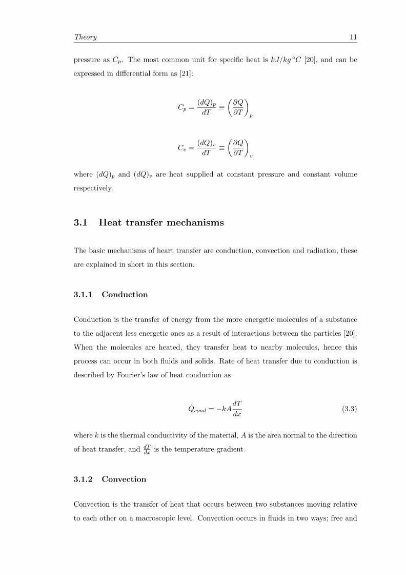
3.1.1 Conduction

Conduction is the transfer of energy from the more energetic molecules of a substance

to the adjacent less energetic ones as a result of interactions between the particles [20].

When the molecules are heated, they transfer heat to nearby molecules, hence this

process can occur in both fluids and solids. Rate of heat transfer due to conduction is

described by Fourier’s law of heat conduction as

Qcond = −kAdTdx

(3.3)

where k is the thermal conductivity of the material, A is the area normal to the direction

of heat transfer, and dTdx is the temperature gradient.

3.1.2 Convection

Convection is the transfer of heat that occurs between two substances moving relative

to each other on a macroscopic level. Convection occurs in fluids in two ways; free and

Theory 12

forced convection. Free convection describes the spreading of particles from areas with

high concentration to areas with lower concentration. Free (or natural) convection in

air occurs when parts of the air comes in contact with a hotter or colder medium, and

gets heated or cooled. Warm air will then raise, and create air flows. The principle of

free convection is illustrated in Fig. 3.1.

Figure 3.1: Free convection

Forced convection is caused by a fluid or air moving due to an external force, such as

a fan or a pump. Convection is strongly dependent on parameters such as velocity and

turbulence. In the case study presented in Chapter 5, only heat transfer due to free

conduction is considered (vair = 0m/s )

Figure 3.2: Forced convection

Newton’s law of cooling states that the rate of heat loss of a body is proportional to the

difference in temperatures between the body and its surroundings. The heat transfer

due to convection is proportional to the surface and the fluid [22]. For an object with

temperature TS and area A with surrounding temperature of T∞ the heat transfer from

the liquid or gas to the solid object described by Newtons law of cooling as:

Q = hcA(TS − T∞) (W) (3.4)

Theory 13

where the heat transfer coefficient hc is an empirical value determined experimentally

for different substances, flow situations and geometries. hc is dependent on all variables

that influence convection such as as the surface geometry, the nature of fluid motion, the

properties of the fluid, and the bulk fluid velocity. For free convection of gases, hc are

usually in the range of 2-25 W/m2 ·K, and for forced convection of gases 25−500W/m2 ·

K.

3.1.3 Radiation

The third main mechanism of heat transfer is radiation. All matter at a tempera-

ture higher than the absolute zero, emits thermal radiation due to the vibrational and

rotational movements at a microscopic level. Radiation propagates in the form of elec-

tromagnetic waves, and is emitted from all points on a surface in all directions into the

hemisphere above the surface. The quantity that describes the magnitude of radiation

is the radiation intensity. Notice that the effect of radiation on the thermal behavior of

the AS is not considered in the case study of this theses [20].

3.2 Steady-flow systems

Many systems involve mass flow in and out. These can be steady or transient. The mass

flow is the amount of mass flowing per unit of time, and is denoted as:

m = ρvAc (kg/s) (3.5)

where ρ is the fluid density, v is the average fluid velocity in the flow direction, and Ac

is the cross-sectional area of the pipe. If the outgoing flow rate is equal to the incoming

flow rate of mass, then then min = mout = m, as illustrated in Fig. 3.3 T1T2

The rate of heat transfer of a steady flow system can then be described as [20]:

Q = mCp∆T (kJ/s) (3.6)

Q = mCp(Te − Ti) (kJ/s) (3.7)

Theory 14

Figure 3.3: Inlet and outlet flow in steady flow system

where Q is the heat transfer rate, m is the mass flow rate, Cp is the specific heat of the

fluid and ∆T is the temperature difference between the inlet and the outlet. Ti and Te

are the fluid temperatures at the inlet and the exit of the water pipes respectively.

3.3 Lumped system analysis

Until now, heat transfer has been described as independent of both time and position.

In most cases the temperature of a body depends on when, as well as where in the solid

it is measured. However, if the temperature of a solid varies with time but remains

uniform throughout the solid at any time, it can be considered as a lumped system.

With a lumped system analysis, the temperature of the body can be described without

a reference to a specific location within the body. Thus, the temperature of the body is

a function of time only, T (x, t) = T (t) [20].

At t = 0 a block of material is placed in a room with surrounding temperature of T∞,

the object itself has an initial temperature of Ti, mass m, volume V , surface area A,

density ρ and specific heat Cp. During the time interval dt, the temperature changes

by dT . Hence, the heat transferred into the object during this time, must equal the

increase in the energy of the object during the same time interval.

hAsurface(T∞ − T )dt = mCPdT (3.8)

Theory 15

The rate of convection heat transfer between the body and its environment can then be

determined from Newton’s law of cooling as

Q(t) = hcA(T (t)− T∞) (W) (3.9)

3.3.1 Criteria for lumped system analysis

The lumped system analysis is a convenient simplification to solve transient heating and

cooling problems. It is therefore important to investigate if this assumption can be used

and still provides a reasonable accuracy.

When dealing with conduction problems involving surface convection effects, it is use-

ful to define a dimensionless parameter called the Biot number[23]. The Biot number

describes the relationship between the convection at the surface of the body and the

conduction within the body. Hence, a Biot number less than one means that the resis-

tance to conduction within the solid is less than the convection at its boundary layer.

Therefore, a Biot number equal to zero, is a perfect lumped system [20]. The error

associated with lumped system analysis is considered small if Bi < 0.1 [23]:

Bi =hLc

k< 0.1, (3.10)

where k is the thermal conductivity of the solid and Lc is defined as the characteristic

length Lc as

Lc =V

As.

3.3.2 Biot number calculation for AS

An AS used in CTF3 has the mass m = 16kg, A = 0.1m2, mass density ρ = 8960kg/m3,

heat transfer coefficient h = 11W/m2 ·◦ C and k = 401W/m ·◦ C. This gives the

characteristic length:

Lc =V

As=

1

56m.

Theory 16

Then the Biot number becomes

Bi =hLc

k=

11W/m2 ·◦ C · 156m

401W/m ·◦ C= 0.00067.

0.00067� 0.1

In a block of copper, the temperature can be considered uniform trough out the body

[20]. The heating of an accelerating structure satisfies the criteria for the lumped system

analysis.

Theory 17

3.4 Unit Step Response

The unit step, us(t), is the simplest function used to analyse the system’s response due

to an instant change in its input, and is defined as

f(t) = us(t) =

0 t < 0

1 t ≥ 0.

The unit step response to a first order differential equation, can be found by converting

to state space, and taking the inverse Laplace transform. For a first order differential

equation

y′(t) + y(y) = f(t) (3.11)

the response can be is found as follows:

y′(t) + y(t) = 1

sY (s) + Y (s) =1

s

Y (s) =1

s(s+ 1)

L−1 {Y (s)} = L−1

{1

s

}+ L−1

{−1

(s+ 1)

}y(t) = 1− e−t

(3.12)

with zero initial conditions, the input and output of the above example is plotted in Fig.

3.4

-2 -1 1 2 3 4 5Time / sec

-0.5

0.5

1.0

1.5u(t)

Output, T(t)

Input, u(t)

Figure 3.4: Unit step input and output

Chapter 4

First-Order System Transient

Response

The response of a first order system can be calculated due to a defined or known input,

f(t). In testing situations, simple functions such as the step or ramp input are commonly

used. However, with numerical tools, it is possible to solve the differential equation with

a more complicated forcing term. In the following chapters, several different inputs are

investigated. The main focus is on the system response to a step function and to a real

RF power signal.

4.1 Theoretical analysis

For simplicity, the RF power can be divided in two; the part used for acceleration, and

the part that is dissipated as heat. The part of the RF power dissipated as heat, is

proportional to the rate of heat transfer Qh from the structure, and is assumed to be

distributed among the AS material (copper) as Qcu, the water cooling pipes Qwater and

the air Qair:

Qh = Qcu + Qwater + Qair. (4.1)

The RF power is time dependent and Q = Q(t). When applying a lumped system

analysis, there is no reference to position. The rate of heat transfer at any time for each

component can then be defined as follow [1]:

18

First-Order System Transient Response 19

To copper : Qcu(t) = mcuCp,cud Tcudt

To water : Qwater(t) = mwCp,w[Tw(t)− Tw(0)]

To air : Qair(t) = hAcu[Tcu(t)− T∞]

(4.2)

where cp,x the heat capacity, mcu the AS mass, Acu the AS surface, m the water mass

flow, h the heat transfer coefficient, and T∞, Tcu and Tw the ambient, AS and outlet

water temperatures respectively [2].

From the Eq(4.2), the total heat flow from the structure can be written as:

Qh(t) = mcucp,cud Tcudt

+ mwcp,w[Tw(t)− Tw(0)] + hAcu[Tcu(t)− T∞]. (4.3)

The component and outlet temperature of an AS differs by ≈ 1◦C [2]. The two are

considered equal through out this analysis, and hence Tcu(t) = Tw(t). Defining A =

mcucp,cu B = mwcp,w C = hAcu, this gives a first order differential equation:

Qh(t) = AdTcudt

+ (B + C)Tcu(t) + (−BTw(0)− CT∞) (4.4)

This equation may be written in the standard form by dividing both sides by (B + C):

Qh(t)

(B + C)=

A

(B + C)

d Tcudt

+ Tcu(t) +(−BTw(0)− CT∞

(B + C)) (4.5)

From Eq(4.5), the time constant of the system can be written as

τ =A

(B + C)=

mcucp,cumwcp,w + hAcu

, (4.6)

where the time constant is defined as the time a first-order system requires to complete

62.3% of the total raise or decay (the steady state) [24].

Notice from Eq.(4.6), that the time constant of the system is independent of the dissi-

pated power. It depends upon the cooling water flow rate, object mass, object surface


area, the heat capacity of copper and water, and the heat transfer coefficient of the

object in air.

4.2 The Step response

If the power is either ON or OFF, the forcing term in the differential equation can be

treated as a step input. The temperature response of an AS can then be found with

the same steps as for the first order unit step response. The solution to the differential

equation (Eq.(4.4)) describing the heat transfer from an AS follows:

With a time independent forcing term, Qh(t) = Qh, Eq.(4.4) simplifies to:

AdTcudt

+ (B + C)Tcu(t) + (−BTw(0)− CT∞ − Qh) = 0 (4.7)

D =(B + C)

A, K = (−BTw(0)−CT∞−Qh)

A (4.8)

d Tcudt

+DTcu(t) +K = 0

dTcudt

+DTcu(t) = −K (4.9)

The unit step response is then found by converting to state space, and multiply the

constant by the state space equivalent to the unit step, 1s :

sTcu(s) +DTcu(s) = −1

sK

Tcu(s)(s+D) = −Ks

Tcu(s) = −Ks· 1

s+D

(4.10)

using the Partial Fraction Expansion to obtain expressions that have a simple inverse

Laplace transforms:

− K

s(s+D)=

A

s+D+B

s

As+B(s+D) = −K(4.11)


(s = 0) BD = −K −→ B = −KD

(s = −D) −AD = −K −→ A =K

D

(4.12)

Tcu(s) =KD

(s+D)+−KD

s

Finally, taking the inverse Laplace transform:

L−1 {Tcu(s)} = L−1

{KD

(s+D)

}+ L−1

{−KD

(s)

}

The analytic solution of Eq(4.9) reads [2]:

Tcu(t) = −KDe−Dt +

K

D(4.13)

With Eq.(4.13), the previous prediction of the time constant is confirmed, as τ = 1D ,

and the time constant is

τ =1

D=

1B+CA

=A

B + C=

mcucp,cumwcp,w + hAcu

. (4.14)

For an AS with mass mcu = 16kg, cooling water flow m = 0.025kg/sec, surface area

Acu = 0.1m2, the time constant is approximately one minute. In Fig.4.1 the step

response for ambient temperature off 20◦C is plotted.

62.3%

of ΔT

ΔT

60 sec

0 100 200 300 400 50018

20

22

24

26

28

30

time / sec

temperature

/ºC

Figure 4.1: Step response of AS with 20 ◦C as initial condition


4.3 Complex forcing terms

Solving Eq.(4.4) with respect to a time dependent forcing term, Qh(t) is complex and

cannot be solved with simple mathematical steps. Mathamatica has been used to pro-

duce a numerical solution to the differential equation using the ND solve function [25]

(the Mathematica notebook can be found in Appendix B).

The RF power pulses used for beam acceleration in the Dog-leg experiment is recorded.

Subtracting the amount used to accelerate the beam, the resulting function is the power

dissipated as heat. This function of power over time is used as the input when cal-

culating the theoretical temperature response of the structure. Fig.4.2 shows the heat

generation (the system input) in red to the left and the theoretical solution as obtained

in Mathematica in blue to the right.

0 2000 4000 6000 8000 10000

0

50

100

150

200

time / sec

Power

/W

0 2000 4000 6000 8000 10000

30.2

30.4

30.6

30.8

31.0

31.2

time / sec

temperature

/ºC

1100 1200 1300 1400 1500

0

50

100

150

200

time / sec

Power

/W

1100 1200 1300 1400 1500

30.2

30.4

30.6

30.8

31.0

31.2

time / sec

temperature

/ºC

Figure 4.2: Examples of heat generated by RF power in red and the expected systemresponses in blue

Chapter 5

Experimental Setup and Results

In this chapter, the experimental setup and results are presented. The experimental

results are also compared to the theoretical prediction from Chapter 4.

5.1 Temperature recordings

RTD temperature sensors (PT 100, 4-wire resistance) are used for measuring tempera-

ture during operation. The sensor accuracy is ± 0.1 ◦C. Fig. 5.1 show the RTD sensor

installed on the AS in the Dog-leg experiment.

Figure 5.1: RTD sensors with integrated double-sided tape

The three temperature sensors are installed on the AS as shown in Fig. 5.2. The inlet

and outlet sensors are taped directly on the water pipe, and is a indirect measure of

the water temperatures trough the copper pipe. The component sensor is taped on the

structure, and is a measure of the copper itself. Both the inlet and ambient temperatures

are ideally kept constant at Tin = 28 ◦C and Tamb = 20 ◦C, respectively. The ambient

temperature is assumed constant throughout this analysis.

23

Experimental Setup and Results 24

The experimental temperatures recorded are:

• inlet water temperature, Tin

• component temperature, Tcomp

• water temperature, Tout

Figure 5.2: Position for inlet, component and outlet temperature sensors AS

Temperature filtering

Water is cooled and supplied by a water chiller. Variations in the temperature of the

water supplied by the chiller cause tracking errors in the temperature recordings of the

component and outlet temperature.

The cooling water temperature varies with up to ≈ ± 0.5 ◦C. Naturally, the temperature

of the component itself and the outlet water temperature varies accordingly. It is impor-

tant to separate the temperature variations caused by a varying Tin temperature, and

the temperature change of interest - the temperature response due to power dissipation

in the structure.

The tracking errors caused by the inlet water can be accounted for by subtracting the

change in inlet temperature from the component and outlet temperate:

Tcomponent filtered = Tcomponent − Tin + Tin constant. (5.1)

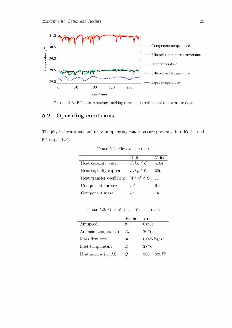
The effect of removing the tracing error is shown in Fig. 5.3. Notice how the component

and outlet temperatures become more steady between the breakdowns.


0 50 100 150 200

29.0

29.5

30.0

30.5

31.0

time / min

temperature

/ºC Component temperature

Filtered component temperature

Out temperature

Filtered out temperature

Input temperature

Figure 5.3: Effect of removing tracking errors in experimental temperature data

5.2 Operating conditions

The physical constants and relevant operating conditions are presented in table 5.1 and

5.2 respectively:

Table 5.1: Physical constants

Unit Value

Heat capacity water J/kg ·◦ C 4184

Heat capacity copper J/kg ·◦ C 386

Heat transfer coefficient W/m2 ·◦ C 11

Component surface m2 0.1

Component mass kg 16

Table 5.2: Operating condition constants

Symbol Value

Air speed vair 0m/s

Ambient temperature T∞ 20 ◦C

Mass flow rate m 0.025 kg/s/

Inlet temperature Ti 28 ◦C

Heat generation AS Q 200− 820W


5.3 Experimental Results

In this section the experimental data is presented and compared to the mathematical

model. In Fig. 5.4 and 5.5 the theoretical model is plotted in blue, together with

the experimental temperature data in red. The sensor accuracy is ±0.1 ◦C, and is

represented with error bars.

0 5000 10000 15000 20000 25000

30.0

30.5

31.0

31.5

time / s

temperature

/ºC

Model

Measurements

Figure 5.4: Theoretical model and measurements with error bars

0 5000 10000 15000 20000 25000

30.0

30.5

31.0

31.5

time / s

temperature

/ºC

Model

Measurements

Figure 5.5: Theoretical model and measurements

The temperature of the component changes 0.5−2 ◦C during an RF breakdown, depen-

dent on the operating conditions (beam or no beam). The model has shown to match

experimental data for all data sets investigated in this analysis. Fig. 5.5 shows a dif-

ferent set of data, again over a time span of around 7 hours. The theoretical analysis


matches the experimental data, and hence the model can be used to predict temperature

response under transient conditions within reasonable accuracy. This is investigated fur-

ther in the following chapter. A reliable model opens the possibility to simulate possible

scenarios and temperature control approaches. These results allows the use of the the-

oretical model developed in Mathematica (Appendix B) to investigate the temperature

response in several possible scenarios.

Chapter 6

Water flow control

From the theoretical analysis, the time constant is found to be directly proportional to

the material and geometry of the AS, and is inversely proportional to the water flow

(Eq. (4.6)). A previous study completed by the CLIC module team on the relationship

between thermal time constant and water flow shows that the two are largely correlated

[2]. The experimental results from this study are illustrated in Fig. 6.1. It is shown

that the time constant clearly decreases with increasing flow rate.

This observation introduces the possibility to control the temperature of an AS through

appropriate regulation of the water flow. In this chapter, some ideas and possible theo-

retical solutions on the design of a dynamic water cooling system are presented.

Figure 6.1: Time constants at increasing water flow, with an heat generation of290W , 830W and 910W [2]

28

Water flow control 29

6.1 Effect of water flow on temperature response

When increasing the flow rate, the average temperature of the AS decreases towards the

temperature of the cooling water. As expected, the fall and raise time decrease with

increasing flow rate. This effect is shown in Fig. 6.2, where the fall time changes with

approximately 2 minutes when the flow changes from 0.02 kg/sec to 0.08 kg/sec, and the

operating temperature decrease from 31.2 ◦C to 29.6◦C. However, such huge increase in

the water flow rate is not realistic due to the capability of the water pipes and pumps.

5000 6000 7000 8000 9000 10000

29.5

30.0

30.5

31.0

time / sec

temperature

/ºC

0.02 kg/sec

0.04 kg/sec

0.08 kg/sec

Figure 6.2: Temperate response for different water flow rates

Providing less cooling during times of decreased heat generation is the logical solution

in terms of water cooling control. By defining a default water flow (determined by the

system, ≈ 0.025 kg/sec for Dog-Leg AS) during normal operation, and decreasing the

flow according to a particular function during times of less heat production, is expected

to limit temperature changes. The optimal solution would be to control the flow as a

direct function of the dissipated power at all times. Another and more simple solution

would be to use the same pre-defined routine when a breakdown is observed. These two

suggestions are investigated further in the following sections.


6.2 Simple flow control

Due to restricted precision of the control valves, more simple control approaches are

investigated in this section. It is possible to apply a pre-defined water flow routine each

time a breakdown is recorded in the system. Fig. 6.3 shows the average heat dissipation

during one breakdown as observed in the test facility.

400 600 800 1000 1200 14000

50

100

150

200

250

300

Time/ sec

Powerdissipation/W

Figure 6.3: Power dissipated as heat during an average breakdown

The flow can be controlled in several possible ways. In the following examples the

breakdown occurs at exactly t = 500. Fig. 6.4 presents some possible ways to control

the flow rate during a breakdown. The purple function is the water flow, and the blue

line represent the corresponding temperature response. The input in all examples is set

as the average power dissipation during a breakdown (see Fig.6.3).

Consider for instance the most simple case; to turn the cooling on/off almost instantly.

The response when the flow is simply turned off for 50 seconds, is presented as ”100%

off”. Notice how the control actually causes the structure to increase the temperature

above the steady state temperature. When the flow rate is only reduced by 50% on

the other hand (referred to as 50% off), the structure is cooled down for the first ≈ 75

seconds, before the structure starts to heat up due to lack of sufficient cooling. However,

in this case the temperature does not increase above its steady temperature, but it causes

a small peak in the temperate at t = 600. These results indicates that decreasing the

cooling drastically within a short time period (∼ 50 sec), will actually cause an increase

in component temperate, or undesired fluctuations.


400 600 800 1000 1200

30.175

30.2

30.225

30.25

30.275

0.0024

0.0077

0.013

0.018

0.024

time / sec

temperature

/ºC

flow rate / kg/secIdeal

400 600 800 1000 1200

29.4

29.6

29.8

30.

30.2

0.0027

0.0078

0.013

0.018

0.023

time / sec

temperature

/ºC

flow rate / kg/secConstant

400 600 800 1000 1200

29.8

30.

30.2

30.4

0.0038

0.011

0.018

0.025

time / sec

temperature

/ºC

flow rate / kg/secRamp 1

400 600 800 1000 120029.6

29.8

30.

30.2

-0.0011

0.0065

0.014

0.022

time / sectemperature

/ºC


400 600 800 1000 1200

29.8

30.

30.2

0.0028

0.011

0.019

time / sec

temperature

/ºC


400 600 800 1000 1200

30.

30.1

30.2

30.3

0.001

0.0092

0.017

0.026

time / sec

temperature

/ºC

flow rate / kg/secSteps

400 600 800 1000 1200

29.75

30.

30.25

30.5

30.75

0.0024

0.0082

0.014

0.02

0.026

time / sec

temperature

/ºC

flow rate / kg/sec100% Off

400 600 800 1000 1200

29.8

30.

30.2

0.0054

0.014

0.022

time / sec

temperature

/ºC

flow rate / kg/sec50% Off

Figure 6.4: Water flow control with corresponding temperature response

The response for the different flow suggestions are plotted on top of each other for easier

comparison in Fig.6.5.


400 600 800 1000 1200

29.0

29.5

30.0

30.5

31.0

time / sec

temperature

/ºC

Ideal

Constant

Ramp 1

Ramp 2

Ramp 3

Steps

Off 100%

Off 50%

Figure 6.5: Temperature response for different flow control signals

• Ideal: the ideal temperature response (when the flow fitted to the heat generation

at any time) is illustrated in red, and is clearly the preferred solution, as it is

causing the minimum temperature variation.

• Ramp: Both ramp2 and ramp3 reduce the temperature change with approximately

50% compared to the constant flow (filled blue), without introducing dominant

peaks. However, Ramp1, which linearly increase the flow rate over 100 seconds,

gives insufficient cooling, and the structure tempearture increase above the steady

temperature.

• Steps: Stepping up the flow in several intervals, results in a small change in tem-

perature. However, the response is not very smooth, and gives several small peeks

in the temperature.

• On/off 100%: Turning the flow to zero during the breakdown actually provides

too little cooling, and the structure is being heated. The same effect is predicted

when the simplest ramp function is applied (dark blue).

• On/off 50%: Reducing the flow by 50% provokes a small peak in the temperature

around t = 600s. However, it differs from the 100% on/off as it does not increase

above the normal operation temperature.

6.3 Feedback flow control

The RF power can be used directly to determine the optimal water flow for minimizing

temperature fluctuations. The left graph in Fig. 6.6 shows a typical RF power signal


over a time period of 4 hours. The same signal is used as the input signal in all the

following examples.

The flow is obtained by scaling the RF power signal with a factor of X and adding a

constant K. The ideal flow rate can then be expresses as: flow(t) = Q(t) ·X +K. The

resulting flow rate is shown to the right in Fig. 6.6. The scaling of the signal is clearly

arbitrary and should be modified according to the requirements of the system and the

capability of the cooling pipes .

0 5000 10000 15000 20000 25000

0

50

100

150

200

time / sec

Power

/W

0 2000 4000 6000 8000 10000

0.000

0.005

0.010

0.015

0.020

0.025

time / sec

Waterflow

/kg

/sec

Figure 6.6: Left: Average power dissipated as heat. Right: Water flow signal as afunction of heat generation.

Fig. 6.7 shows how the water flow algorithm successfully almost eliminates temperature

fluctuations during breakdowns. The blue filled line is the model at a constant water

flow (= 0.025 kg/sec), and the black line presents the predicted response when applying

the flow control. The difference between the two in this example is 0.8 ◦C. As both

models provides the system with same flow during normal operation, = 0.025 kg/sec

in this example, they also predict the same structure temperature (≈ 30.8 ◦C) during

normal operation.

0 5000 10000 15000 20000 25000

30.0

30.2

30.4

30.6

30.8

31.0

time / sec

temperature

/ºC

Constant water flow

Controlled water flow

Figure 6.7: Theoretical temperature response with and without water flow control


6.4 Effect of system delay

In reality, it is not possible for the control valves to adjust instantly as assumed until

now. A breakdown last on a scale of seconds, and the system takes about 2− 3 minutes

to recover back to its steady state temperature. It is therefore interesting to explore if it

is realistic to benefit from a flow control before normal heat generation is reestablished

after the breakdown.

The delay time is referred to as the reaction time from observed breakdown to the flow

changes in the pipes in and around the structure. The electronics can be assumed to

change instantly and the pressure in the pipes is constant. The delay time is therefore

the time it takes for the valve to physically adjust to the chosen flow. To get a better

understanding of tolerances in terms of reaction time, the effect of a delayed flow control

signal is investigated.

Two signals with delay times of 1 and 10 seconds has been chosen for the flowing example.

Fig. 6.8 shows the original water flow control signal in blue together with the delayed

signals in orange and yellow. According to the RF signal, the breakdown starts at

exactly t = 500, and the delayed signals will therefore act at t = 501 and t = 510. Every

point in the function is delayed, shifting the whole function the right. In practical terms

this means that the flow at a specific time is the flow that was perfectly fitted for the

heat generated 1 or 10 seconds earlier.

490 500 510 520 530 540 550 5600.000

0.005

0.010

0.015

0.020

0.025

0.030

time / sec

flowrate

/kg

/sec

Water flow with no delay

Water flow with 1 sec. delay

Water flow with 10 sec. delay

Figure 6.8: Instant(blue) and delayed (yellow) water flow control signal during onebreakdown

In Fig. 6.9 a zoom shows the response based on instant feedback control against the

delayed responses. The model behaves as expected, as the black instant control starts to


stabilize towards normal operation temperature at the exact moment when the break-

down occurs (t = 500). The orange line has a sudden drop at the breakdown point,

before the control sets in and stabilizes the effect after 1 second at t = 501. The re-

sponse to the 10 sec. delayed signal behaves similar to the constant flow response for the

first 10 seconds, before the flow is decreased at t = 510, and the temperature increase

towards the stable temperate. It also cause a small overshoot at t = 600 due to lack of

cooling relative to heat dissipation at this moment. However, note that the overshoot is

less than the accuracy of the temperature sensors (0.1 ◦C) and will most likely not be

noticeable in experimental tests.

500 550 600 650 700 750

29.0

29.5

30.0

30.5

time / sec

temperature

/ºC

Constant water flow

Controlled water flow no delay

Controlled water flow 1 sec. delay

Controlled water flow 10 sec. delay

Figure 6.9: Model of temperature response with instant and delayed water flow control

The difference between the delayed and instant control is according to Fig. 6.9 less

than 0.1 ◦C when there is 1 second delay time, which in perspective is the same as the

accuracy of the temperature sensor. A 10 sec. delay is not as effective, but the control

still decrease temperature changes relative to no control with 0.5 ◦C. There seems to be

no compelling reason to argue that a delay time in the system limits a sufficient water

cooling control of an AS. Difficulties arise, however, due to other technical challenges.

For example, it requires control valves capable of providing an accurate flow at any time.

Chapter 7

Conclusion and Future Work

Conclusions

This thesis outlines the work which was undertaken to investigates the theoretical and ex-

perimental thermal behavior of the CLIC AS. A simple but realistic model was developed

and tested against experimental data. The temperature dynamics follow a first-order

system behavior. A numerical solution obtained with Mathematica provides a model

for the temperature evolution over time. The forcing term in the differential equation

is the heat generation caused by beam acceleration, and is directly proportional to the

applied RF-power. The model was then compared to experimental temperatures from

the Dog-leg experiment. The modelling results are in compliance with the experimental

data.

A realistic model facilitates the understanding of the influence of different factors, such

as ambient temperature and water flow. Moreover, the model was used to qualify several

approaches for water cooling control, in which especially one were found to be theoreti-

cally efficient. The most efficient control approach, referred to as ”ideal flow”, decreased

temperature changes with ∼ 75%. Alignment measurements preformed at the two beam

module, shows that with a ∆T = 1 ◦C, results in a vertical displacement of ∼ 10µm.

With the temperature variation of ∆T = 4 ◦C, this control approach results in reducing

the vertical displacement of a point P (on the AS surface relative to the beam line) from

40µm to 10µm. Considering the tight alignment tolerances of 10µm for the CLIC AS,

the solution suggested in this thesis can play a significant role in improving the overall

36

Conclusion and Future Work 37

alignment of the CLIC components. However, it should be mentioned that controlling

temperature with flow rate can introduce vibrations or other potential complications to

the system.

Furthermore, the effect of a potential delay in the system was investigated. There

seems to be no compelling reason to argue that a short delay time in the system limits a

sufficient water cooling control of an AS. However, challenges arise due to other hardware

limitations. For example, it requires control valves capable of providing an accurate flow

at any time. How these techniques would work in reality is therefore relevant for future

experimental investigation.

Future work

The use of a dedicated flow control to limit temperature changes in an AS should be

evaluated experimentally.

Firstly, the capabilities of the valves should be tested in practice. A experimental char-

acterization of the control valves will disclose the capability of precise water flow control.

Thermal tests should be preformed to investigate the temperature response during dif-

ferent cooling scenarios. The thermal tests of the cooling approaches presented in this

thesis are planned at the CLIC module test facility in 2017.

It is recommended to investigate the possibility of controlling the temperature of the

accelerator over longer shut downs. During longer shut downs, the temperature will fluc-

tuate between ambient (20 ◦C) and operating temperature (30 ◦C). The model developed

in this thesis can be used to examine solutions minimizing temperature fluctuations in

such scenarios, but how these techniques would work in reality is left out for future

investigation.

Appendix A

Physical constants

Constant Name Symbol = Constant Value (with units)

Heat capacity water Cp,w = 4184 J/kg ·K

Heat capacity copper Cp,cu = 386 J/kg ·K

Heat transfer coefficient AS h = 11W/m2 ·K

Mass density copper ρ = 8960 kg/m3

Thermal conductivity copper k = 401W/m ·K

Component surface Acu = 0.1m3

Mass of component m = 16 kg

Ambient temperature T∞ = 20 ◦C

Initial temperature Tw(0) = 28 ◦C

38

Appendix B

Mathematica notebook

39

Author: Sara Aasly

[email protected]

Title: Transient_response_AS

Date: 26/10/2016

Note: remove semicolon ; to show graphs/tables

SetOptions[ListLinePlot, Frame → True, Axes -> False,

LabelStyle → {FontFamily → "Times New Roman", FontSize → 12}, ImageSize → 250];

SetOptions[Plot, Frame → True, Axes -> False,

LabelStyle → {FontFamily → "Times New Roman", FontSize → 12}, ImageSize → 250];

Transient response for AS

Import raw data from file

Read all rows from column 3 =>[[All, 3]], skip 1 header line

path = "\\\\cern.ch\\dfs\\Users\\s\\saasly\\Documents\\TransientResponse\\Sara\\newDoglegData/";

file = "log_20160914-16h.csv";

samplingTime = 2; (* sampling time = 2 sec for Dog-leg .tdms files *)

filename = path <> file;

tempInRaw = Import[filename, "CSV", "HeaderLines" → 1][[All, 4]];

tempMidRaw = Import[filename, "CSV", "HeaderLines" → 1][[All, 5]];

tempOutRaw = Import[filename, "CSV", "HeaderLines" → 1][[All, 3]];

INCmax = Import[filename, "CSV", "HeaderLines" → 1][[All, 7]];

TRAmax = Import[filename, "CSV", "HeaderLines" → 1][[All, 8]];

pulseLength = Import[filename, "CSV", "HeaderLines" → 1][[All, 2]];

Constants

cpw = 4184;(* Heat capacity water - J/Kg/K *)

cpcu = 386;(* Heat capacity cupper - J/Kg/K *)

h = 11;(* Heat transfer coefficient - W/m2°C *)

sas = 0.1;(* Component surface - m2 *)

mas = 16;(* mass of component - Kg *)

tamb = 20; (* Ambient temperature - °C*)

mwas = 0.026;(* Water flow konstant - Kg/s *)

t0as = Mean[tempInRaw](* initial temperature/ In temp - °C*);

aas = mas * cpcu;

bas = mwas * cpw;

cas = h * sas;

das = bas + cas;

kas = -bas * t0as - cas * tamb;

length = Length[INCmax];

signalLength = Length[INCmax] * samplingTime;

Raw data

Convert from RF-power pulses to average power dissipated as heat.

Add time variable to data. Here data is recorded with sampling time of 2 seconds. Sampling time

can be changed under constants.

powerInRaw =(INCmax - TRAmax) * pulseLength

0.02;

powerIn = Table[{samplingTime * x, powerInRaw[[x]]}, {x, 1, length}];

ListLinePlot[powerInRaw, PlotLabel → "Dissipated power signal" ,

PlotRange → All, FrameLabel → {"sample nr", "Power / W"} ];

Create analytical function from the raw data points

Interpolate the data in order to create a function for Mathematica

Then create an analytical function from the interpolated one that is defined from -infinity to

+infinity using the Heaviside π function

fInterPower = Interpolation[powerIn]

InterpolatingFunction Domain: 2., 2.73×104Output: scalar

newFpower[x_] := fInterPower[x] HeavisidePi

xsamplingTime

-length

2

length

Solve y(x)’ + Dy(x) + K = P(x)

Solve numerically the nHDE => here the forcing term is the function created from the input

power data P(x)

The domain is set from 0 to signallength seconds and initial condition as y[x=0] = t0as (the

2 Transient_response_AS.nb

water in temperature at t = 0)

solutionNum = NDSolve[

{aas * y'[x] + das * y[x] + kas ⩵ newFpower[x], y[0] ⩵ t0as}, y[x], {x, 0, signalLength}];

Plot the numerically solution obtained above

model = Plot[Evaluate[(((y[x]) /. solutionNum))],

{x, 0, signalLength}, PlotRange → {{0, signalLength}, {All, All}},

FrameLabel → {"time / s", "temperature / ºC" },

PlotStyle → ColorData[2, "ColorList"], PlotLegends → {"Model"}];

Temperature response

temp = tempMidRaw - tempInRaw + t0as;

tempfiltered = Table[{samplingTime * x, temp[[x]]}, {x, 1, length}];

tempPlot = ListLinePlot[tempfiltered, PlotRange → All,

FrameLabel → {"time / s", "temperature / ºC" }, PlotStyle → ColorData[3, "ColorList"],

FillingStyle → White, PlotLegends → {"Experiment"}];

Plots of temperature data from file

allTemperatures = ListLinePlot[{tempOutRaw, tempMidRaw, tempInRaw},

PlotRange → All, PlotLabel → "Raw temperature measurements",

FrameLabel → {"time / sec", "temperature / ºC" },

PlotLegends → {"Out temperature", "Component temperature", "Input temperature"}];

Plot model vs experiment

Show[{model, tempPlot}, PlotRange → {{0, signalLength}, {30, 31.5}},

PlotLabel → "Theoretical model and measurements" ]

0 5000 10 000 15 000 20 000 25 000

30.0

30.5

31.0

31.5

time / s

tem

pera

ture

/ºC

Theoretical model and measurements

Model

Experiment

Transient_response_AS.nb 3

Bibliography

[1] M. Aicheler, P. Burrows, M. Draper, T. Garvey, P. Lebrun, K. Peach, N. Phinney,

H. Schmickler, D. Schulte, and N. Toge. A multi-tev linear collider based on clic

technology. Clic conceptual design report, CERN, 2012.

[2] E. Daskalaki, S. Dobert, M. Duquenne, H. Mainaud Durand, V. Rude, and A. Vam-

vakas. Study of the Dynamic Response of CLIC Accelerating Structures. (CERN-

ACC-2015-286), 2015. URL https://cds.cern.ch/record/2141828.

[3] P. Lebrun, L. Linssen, A. Lucaci-Timoce, D. Schulte, F. Simon, S. Stapnes, N. Toge,

H. Weerts, and J. Wells. The clic programme: towards a staged e+e- linear collider

exploring the terascale, clic conceptual design report. Technical report, CERN,

2012.

[4] About CERN. Jan 2012. Accessed in September 2016. URL http://cds.cern.

ch/record/1997225.

[5] Member states. 2012. Accessed in November 2016. URL http://cds.cern.ch/

record/1997223.

[6] The accelerator complex. Jan 2012. Accessed in December 2016. URL http:

//cds.cern.ch/record/1997193.

[7] The Large Hadron Collider. Jan 2014. Accessed in September 2016. URL http:


[8] The Higgs boson. Jan 2014. Accessed in December 2016. URL http://cds.cern.

ch/record/1998491.

[9] The Nobel Museum. Peter Higgs - Facts. May 2013. Accessed in December 2016.

URL http://cds.cern.ch/record/1998007.

43

https://cds.cern.ch/record/2141828

http://cds.cern.ch/record/1997225











Bibliography 44

[10] The Compact Linear Collider. Jan 2012. Accessed in November 2016. URL https:


[11] CLICdp. April 2014. Accessed in November 2016. URL http://cds.cern.ch/

record/1998665.

[12] W. Herr and B. Muratori. Concept of luminosity. CERN, 2009.

[13] S. Dobert. Clic module & impact of pacman on its alignment. PACMAN workshop,

2017.

[14] G. Geschonke and A. Ghigo. CTF3 Design Report. Technical Report CERN-

PS-2002-008-RF. CTF-3-NOTE-2002-047. LNF-2002-008-IR, CERN, Geneva, May

2002. URL http://cds.cern.ch/record/559331.

[15] CTF3 general description. Accessed in December 2016. URL http://clic-study.

web.cern.ch/content/ctf3-general-description.

[16] A. Moilanen. Creep effects in diffusion bonding of oxygen- free copper. Master’s

thesis, Aalto University, April 2013.

[17] Z. Insepov, J. Norem, D. Huang, S. Mahalingam, and S. Veitzer. Modeling rf

breakdown arcs. 2010.

[18] A. Descoeudres, Y. Levinsen, S. Calatroni, M. Taborelli, and W. Wuensch. Inves-

tigation of the dc vacuum breakdown mechanism. physical review special topics-

accelerators and beams. vol. 12.9, no. 9, pp. 092001, CERN, 2009.

[19] B. J. Woolley. High Power X-band RF Test Stand Development and High Power

Testing of the CLIC Crab Cavity. PhD thesis, Lancaster University, 2015. Cited on

page 5.

[20] Y. A. Cengel. Heat and Mass Transfer, a practical Approach. McGraw-Hill, 2

edition, 2003. ISBN 0-07-245893-3 / 0.07-115150-8(ISE). Cited on pages 9-17, 26,

and 210-213.

[21] A.K. Saxena and C.M Tiwari. Heat and Thermodynamics, volume 1. Alpha Science,

1 edition, 2014. ISBN 978-1-84265-902-1. Cited on page 1.27.

[22] K. V Wong. Thermodynamics for Engineers, Second Edition. Boca Raton: CRC

Press, 2 edition, 2012. ISBN 9781439845592.






http://clic-study.web.cern.ch/content/ctf3-general-description

http://clic-study.web.cern.ch/content/ctf3-general-description

Bibliography 45

[23] T.L. Bergman, A.S. Lavine, F.P. Incropera, and D.P. Dewitt. Fundamentals of Heat

and Mass Transfer. John Wiley & Sons Incorporated, 2010. ISBN 9780470945377.

Cited on page 283.

[24] Bela G. Liptak. Instrument Engineers’ Handbook: Process control and optimization,

volume 2. CRC Press, 4 edition, 2003. ISBN 0-8493-1081-4.

[25] Walfram Language & System, Documentation Center, NDSolve. Accessed in

December 2016. URL http://reference.wolfram.com/language/ref/NDSolve.

html.

http://reference.wolfram.com/language/ref/NDSolve.html

http://reference.wolfram.com/language/ref/NDSolve.html