theoretical astrophysics - uzhradiative processes in astrophysics, george rybicki and alan lightman...
TRANSCRIPT
Theoretical Astrophysics
Prof. Dr. Romain TeyssierCentre for Theoretical Astrophysics and Cosmology
Institute for Computational ScienceUniversity of Zurich
Authors of this script: Tine Colman and Romain Teyssier
Fall SemesterDecember 3, 2019
Introduction
The purpose of this course is to give third year Bachelor students or first year Master studentsthe foundations of theoretical astrophysics, with a broad overview of astrophysical fluid dy-namics, radiative transfer, self-gravitating systems (in or out of equilibrium) and collisionlesssystems. Throughout the course, we will use a methodology that is based on the kinetic theoryof an ensemble of particles, these particles being either atoms and molecules, photons, or evenstars. This common framework will be very useful for future PhD students in astronomy andastrophysics, aiming at studying stellar structure, star formation and the interstellar medium,galaxy formation and cosmology.
It is strongly required that students attending this course already have a basic knowledgeof quantum mechanics and electrodynamics, as well as some basics in fluid mechanics andthermodynamics. Some familiarity with tensor calculus is also required. During this course,we will try to derive self-consistently all the equations, with a minimal reference to a prioriknowledge in physics. The level of mathematics required is typical of a bachelor in Mathematicsor Physics, not more than that. This course has been designed based on other popular textbooks, of which we give the list below.
• The Physics of Astrophysics. Volume I: Radiation, Frank H. Shu
• The Physics of Astrophysics. Volume II: Gas Dynamics, Frank H. Shu
• Physics of shock waves and high-temperature hydrodynamic phenomena, Ya. Zel’dovichand Yu. Raiser
• Foundations of Radiation Hydrodynamics, Dimitri Mihalas and Barbara Weibel Mihalas
• Radiative Processes in Astrophysics, George Rybicki and Alan Lightman
• Galactic Dynamics, Second Edition, James Binney and Scott Tremaine
Reading these books is not required, but could be useful in case one wants to dive deeper intoone of the topics presented here. This course will be divided into 3 main parts, each associatedwith one particular type of fluid or particles:
1. astrophysics of gases and fluids (chapters 1 and 2)
2. astrophysics of radiation (chapter 3)
3. astrophysics of collisionless fluids (chapter 4)
The first part, sometimes referred to as astrophysical fluid dynamics, will cover the basicsof the microscopic description of a gas. We will describe the kinetic theory of gases, trying topresent the main equation, namely the Boltzmann equation, and many of its properties. Wewill spend some time computing the moments of the Boltzmann equation (the very meaningof moment will become clear in the relevant sections), which will serve as the foundations of

the Euler equations for fluids. A very important aspect of the Euler equations is their validityrange, and the notion of Local Thermodynamical Equilibrium (LTE). We will then derive self-consistently a first-order approximation of the full Boltzmann equation, leading to a consistentderivation of fluid viscosity and heat flux. We will then focus on astrophysical applications,trying to derive analytically equilibrium solutions of the Euler equations in presence of gravityor rotation, leading to important astrophysical results to describe the internal structure of starsor accretion discs. One guiding principle of this course will be to analyse the stability of theseequilibrium solution, checking indeed that these solutions do exists in nature. This will lead usto the description of waves and shocks in fluids, as well as famous hydrodynamical instabilities.
The second part will be the realm of radiative processes. Here again, we will start at themicroscopic level, introducing the radiative transfer equation, and a few analytical solutionsdescribing many radiation flows. One key application will be to describe the interaction betweenradiation and matter through absorption and emission processes. This will lead us to a moremacroscopic description of radiation, here again using the moments of the radiation field. Wewill use some very basic concepts of quantum mechanics and electrodynamics to fully accountfor all main astrophysical radiation fields.
The third and final part of the course will be dedicated to collisionless fluids. As opposedto atoms and photons that interact a lot with one another, the particles of collisionless fluidsnever suffer any binary collision. This is an extreme case, which is relevant for stars in massivegalaxies, or dark matter particles, possibly made of a new and exotic type of particle. Hereagain, we will follow the same methodology, starting at the microscopic level, then deriving theproperties of the distribution of these collisionless particles, and ultimately defining the momentsof their distribution function.
As you will discover, a very similar methodology will be used throughout the course, whereradiation physics echoes with rarefied gas or even stellar dynamics. Many useful tools will beintroduced and used in detailed applications for astrophysics. Our objective would be ideallythat, after this course, you will be able to sustain a conversation with a professional astronomeron a black board, about stars or galaxies, fully equipped with equations and concepts for thefuture theoretical astrophysicists you will surely become.

Contents
1 Kinetic theory in a nutshell 11.1 Introduction . . . . . . . . . . . . . . . . . . . . . . . . . . . . . . . . . . . . . . . 11.2 Particle distribution function . . . . . . . . . . . . . . . . . . . . . . . . . . . . . 1
1.2.1 Definition . . . . . . . . . . . . . . . . . . . . . . . . . . . . . . . . . . . . 11.2.2 Moments of the particle DF . . . . . . . . . . . . . . . . . . . . . . . . . . 2
1.3 Boltzmann equation . . . . . . . . . . . . . . . . . . . . . . . . . . . . . . . . . . 31.3.1 Binary collisions . . . . . . . . . . . . . . . . . . . . . . . . . . . . . . . . 51.3.2 Cross section and collision rate . . . . . . . . . . . . . . . . . . . . . . . . 61.3.3 Collision integral . . . . . . . . . . . . . . . . . . . . . . . . . . . . . . . . 71.3.4 Collision invariants . . . . . . . . . . . . . . . . . . . . . . . . . . . . . . . 8
1.4 Local Thermodynamical Equilibrium . . . . . . . . . . . . . . . . . . . . . . . . . 101.4.1 Maxwell-Boltzmann distribution . . . . . . . . . . . . . . . . . . . . . . . 101.4.2 Boltzmann’s H theorem . . . . . . . . . . . . . . . . . . . . . . . . . . . . 121.4.3 Collision time and mean free path . . . . . . . . . . . . . . . . . . . . . . 121.4.4 Validity of LTE approximations . . . . . . . . . . . . . . . . . . . . . . . . 14
1.5 Moments of the Boltzmann equation and the fluid equations . . . . . . . . . . . . 151.5.1 General case for non-LTE conditions . . . . . . . . . . . . . . . . . . . . . 151.5.2 Euler equations for LTE conditions . . . . . . . . . . . . . . . . . . . . . . 181.5.3 Euler equations in Lagrangian form . . . . . . . . . . . . . . . . . . . . . 19
1.6 Chapman-Enskog theory . . . . . . . . . . . . . . . . . . . . . . . . . . . . . . . . 221.6.1 First-order Chapman-Enskog expansion of the DF . . . . . . . . . . . . . 221.6.2 First-order expansion in the pressure tensor . . . . . . . . . . . . . . . . . 241.6.3 First-order expansion in the heat flux . . . . . . . . . . . . . . . . . . . . 251.6.4 Non-LTE modifications of the Euler equations . . . . . . . . . . . . . . . 261.6.5 Non-LTE effects as diffusion processes . . . . . . . . . . . . . . . . . . . . 271.6.6 Application to astrophysical gases . . . . . . . . . . . . . . . . . . . . . . 28
1.7 Generalized kinetic theory . . . . . . . . . . . . . . . . . . . . . . . . . . . . . . . 291.7.1 Lagrangian and Hamiltonian mechanics . . . . . . . . . . . . . . . . . . . 291.7.2 Relativistic particles . . . . . . . . . . . . . . . . . . . . . . . . . . . . . . 301.7.3 Generalized Boltzmann equation . . . . . . . . . . . . . . . . . . . . . . . 311.7.4 Generalized moments . . . . . . . . . . . . . . . . . . . . . . . . . . . . . 331.7.5 Quantum effects . . . . . . . . . . . . . . . . . . . . . . . . . . . . . . . . 341.7.6 Degenerate gases . . . . . . . . . . . . . . . . . . . . . . . . . . . . . . . . 35
2 Astrophysical fluid dynamics 382.1 Euler equations in integral form . . . . . . . . . . . . . . . . . . . . . . . . . . . . 38
2.1.1 Reynolds Transport Theorem . . . . . . . . . . . . . . . . . . . . . . . . . 392.1.2 Integral conservation laws . . . . . . . . . . . . . . . . . . . . . . . . . . . 402.1.3 Specific variables . . . . . . . . . . . . . . . . . . . . . . . . . . . . . . . . 41
CONTENTS
2.2 Virial Theorem . . . . . . . . . . . . . . . . . . . . . . . . . . . . . . . . . . . . . 422.3 Euler equations in different coordinate systems . . . . . . . . . . . . . . . . . . . 44
2.3.1 Euler equations in cylindrical coordinates . . . . . . . . . . . . . . . . . . 442.3.2 Euler equations in spherical coordinates . . . . . . . . . . . . . . . . . . . 48
2.4 Spherical systems in equilibrium . . . . . . . . . . . . . . . . . . . . . . . . . . . 482.4.1 Uniform spheres . . . . . . . . . . . . . . . . . . . . . . . . . . . . . . . . 492.4.2 Hydrostatic equation for spherical systems . . . . . . . . . . . . . . . . . . 51
2.5 Accretion disks . . . . . . . . . . . . . . . . . . . . . . . . . . . . . . . . . . . . . 562.5.1 Centrifugal equilibrium solution . . . . . . . . . . . . . . . . . . . . . . . . 572.5.2 Viscous disks . . . . . . . . . . . . . . . . . . . . . . . . . . . . . . . . . . 582.5.3 Stationary viscous disk solution . . . . . . . . . . . . . . . . . . . . . . . . 592.5.4 Vertical equilibrium . . . . . . . . . . . . . . . . . . . . . . . . . . . . . . 60
2.6 Spherical Bondi accretion flow . . . . . . . . . . . . . . . . . . . . . . . . . . . . . 612.6.1 First Bernoulli theorem . . . . . . . . . . . . . . . . . . . . . . . . . . . . 612.6.2 Second Bernoulli theorem . . . . . . . . . . . . . . . . . . . . . . . . . . . 622.6.3 Bondi solution . . . . . . . . . . . . . . . . . . . . . . . . . . . . . . . . . 63
2.7 Sound waves . . . . . . . . . . . . . . . . . . . . . . . . . . . . . . . . . . . . . . 662.7.1 Stable propagating waves . . . . . . . . . . . . . . . . . . . . . . . . . . . 662.7.2 Thermal instability . . . . . . . . . . . . . . . . . . . . . . . . . . . . . . . 692.7.3 Jeans instability . . . . . . . . . . . . . . . . . . . . . . . . . . . . . . . . 70
2.8 Shock waves . . . . . . . . . . . . . . . . . . . . . . . . . . . . . . . . . . . . . . . 722.8.1 Wave steepening and shock Formation . . . . . . . . . . . . . . . . . . . . 722.8.2 Rankine-Hugoniot relations . . . . . . . . . . . . . . . . . . . . . . . . . . 752.8.3 Isothermal shocks . . . . . . . . . . . . . . . . . . . . . . . . . . . . . . . 762.8.4 Adiabatic shocks . . . . . . . . . . . . . . . . . . . . . . . . . . . . . . . . 782.8.5 Radiative shocks . . . . . . . . . . . . . . . . . . . . . . . . . . . . . . . . 79
2.9 Astrophysical blast waves . . . . . . . . . . . . . . . . . . . . . . . . . . . . . . . 802.9.1 Spherical uniform model . . . . . . . . . . . . . . . . . . . . . . . . . . . . 812.9.2 Self-similar Sedov solution . . . . . . . . . . . . . . . . . . . . . . . . . . . 822.9.3 Momentum-conserving shell . . . . . . . . . . . . . . . . . . . . . . . . . . 84
2.10 Astrophysical turbulence . . . . . . . . . . . . . . . . . . . . . . . . . . . . . . . . 862.10.1 Some fundamental fluid properties . . . . . . . . . . . . . . . . . . . . . . 862.10.2 Rayleigh-Taylor instability . . . . . . . . . . . . . . . . . . . . . . . . . . . 902.10.3 Kelvin-Helmholtz instability . . . . . . . . . . . . . . . . . . . . . . . . . . 932.10.4 Mean-flow equations for turbulent flows . . . . . . . . . . . . . . . . . . . 952.10.5 Turbulent kinetic energy equation . . . . . . . . . . . . . . . . . . . . . . 992.10.6 Eddy-viscosity and mixing length theory . . . . . . . . . . . . . . . . . . . 1012.10.7 Convective heat flux in stars and planets . . . . . . . . . . . . . . . . . . 1022.10.8 Kolmogorov theory and Burgers turbulence . . . . . . . . . . . . . . . . . 105
3 Radiative processes in astrophysics 1123.1 Radiative transfer equation . . . . . . . . . . . . . . . . . . . . . . . . . . . . . . 112
3.1.1 Boltzmann equation for photons . . . . . . . . . . . . . . . . . . . . . . . 1123.1.2 Radiation specific intensity . . . . . . . . . . . . . . . . . . . . . . . . . . 1133.1.3 Bose-Einstein distribution and the Black Body spectrum . . . . . . . . . . 1143.1.4 Radiative transfer equation in vacuum . . . . . . . . . . . . . . . . . . . . 1153.1.5 Interaction between matter and radiation . . . . . . . . . . . . . . . . . . 115
3.2 Formal solution of the radiative transfer equation . . . . . . . . . . . . . . . . . . 1163.2.1 Optical depth . . . . . . . . . . . . . . . . . . . . . . . . . . . . . . . . . . 117

CONTENTS 0
3.2.2 Source function and Kirchhoff’s law . . . . . . . . . . . . . . . . . . . . . 1173.2.3 Formal solution along the light ray . . . . . . . . . . . . . . . . . . . . . . 117
3.3 Moments of the radiative transfer equation . . . . . . . . . . . . . . . . . . . . . 1193.3.1 Moments of the specific intensity . . . . . . . . . . . . . . . . . . . . . . . 1193.3.2 Radiation energy conservation equation . . . . . . . . . . . . . . . . . . . 1213.3.3 Radiation flux conservation equation . . . . . . . . . . . . . . . . . . . . . 1223.3.4 Eddington tensor and closure relations . . . . . . . . . . . . . . . . . . . . 122
3.4 Radiation hydrodynamics . . . . . . . . . . . . . . . . . . . . . . . . . . . . . . . 1243.5 Diffusion limit . . . . . . . . . . . . . . . . . . . . . . . . . . . . . . . . . . . . . . 1253.6 Relativistic corrections for radiative transfer . . . . . . . . . . . . . . . . . . . . . 127
3.6.1 Lorentz transform to first order in v/c . . . . . . . . . . . . . . . . . . . . 1283.6.2 Moments equations in the laboratory frame . . . . . . . . . . . . . . . . . 1293.6.3 Moments equations in the comoving frame . . . . . . . . . . . . . . . . . . 131
3.7 Matter and radiation interaction . . . . . . . . . . . . . . . . . . . . . . . . . . . 1343.8 Larmor formula . . . . . . . . . . . . . . . . . . . . . . . . . . . . . . . . . . . . . 134
3.8.1 Radiation spectrum of an electromagnetic wave . . . . . . . . . . . . . . . 1353.8.2 Emitted radiation spectrum . . . . . . . . . . . . . . . . . . . . . . . . . . 136
3.9 Bremsstrahlung . . . . . . . . . . . . . . . . . . . . . . . . . . . . . . . . . . . . . 1373.10 Thomson scattering . . . . . . . . . . . . . . . . . . . . . . . . . . . . . . . . . . 139
3.10.1 Planar electromagnetic waves . . . . . . . . . . . . . . . . . . . . . . . . . 1393.10.2 Thomson cross section . . . . . . . . . . . . . . . . . . . . . . . . . . . . . 140
3.11 Atomic and molecular excitation levels . . . . . . . . . . . . . . . . . . . . . . . . 1423.11.1 Electronic, vibrational and rotational states . . . . . . . . . . . . . . . . . 1423.11.2 Collisional excitation . . . . . . . . . . . . . . . . . . . . . . . . . . . . . . 1433.11.3 Level population at LTE . . . . . . . . . . . . . . . . . . . . . . . . . . . . 144
3.12 Line absorption and emission . . . . . . . . . . . . . . . . . . . . . . . . . . . . . 1473.12.1 Emission from a damped harmonic oscillator . . . . . . . . . . . . . . . . 1473.12.2 Line absorption cross-section . . . . . . . . . . . . . . . . . . . . . . . . . 149
3.13 Einstein relations . . . . . . . . . . . . . . . . . . . . . . . . . . . . . . . . . . . . 1513.14 Non-LTE level population . . . . . . . . . . . . . . . . . . . . . . . . . . . . . . . 1533.15 Ionisation and recombinaison . . . . . . . . . . . . . . . . . . . . . . . . . . . . . 155
3.15.1 Saha relation . . . . . . . . . . . . . . . . . . . . . . . . . . . . . . . . . . 1553.15.2 Einstein-Milne relation . . . . . . . . . . . . . . . . . . . . . . . . . . . . . 156
3.16 Bound-free radiation . . . . . . . . . . . . . . . . . . . . . . . . . . . . . . . . . . 1573.17 Recombination and photo-ionisation cross sections . . . . . . . . . . . . . . . . . 1593.18 Non-LTE recombination and ionisation . . . . . . . . . . . . . . . . . . . . . . . . 160
3.18.1 Photo-ionisation rate . . . . . . . . . . . . . . . . . . . . . . . . . . . . . . 1613.18.2 Radiative and stimulated recombination rates . . . . . . . . . . . . . . . . 1613.18.3 Collisional ionisation and three-body recombination rates . . . . . . . . . 1623.18.4 Ionisation rate equation . . . . . . . . . . . . . . . . . . . . . . . . . . . . 163
Chapter 1
Kinetic theory in a nutshell
1.1 Introduction
In this chapter, we will focus on a microscopic description of astrophysical gases, using a verypowerful methodology called kinetic theory. In most, if not all cases, we will consider atomsand molecules to be point-like particles moving in space and interacting through collisions.Describing these collisions as accurately as possible will be our main task. This will lead us toone of the most famous equations in physics, namely the Boltzmann equation, which describesthe dynamics of the particle distribution function. The concept of distribution functions hasbeen introduced in your previous mathematics lectures, and is absolutely central to this course.A particular distribution function is the Maxwell-Boltzmann equilibrium solution, which is thevalid solution when the microscopic state of the gas is at the so-called local thermodynamicalequilibrium (LTE). This particular but also very common limiting case will lead us to the self-consistent derivation of the Euler equations, the mathematical description of fluid dynamics atthe macroscopic level. This transition from microscopic to macroscopic is another key aspect ofthis course, which is performed using the velocity moments. But under certain conditions, themicroscopic state of the gas cannot be considered to be at LTE. We will show that one can stilldescribe the fluid using the Euler equations, but adding as first order corrections viscosity andthermal conduction.
1.2 Particle distribution function
1.2.1 Definition
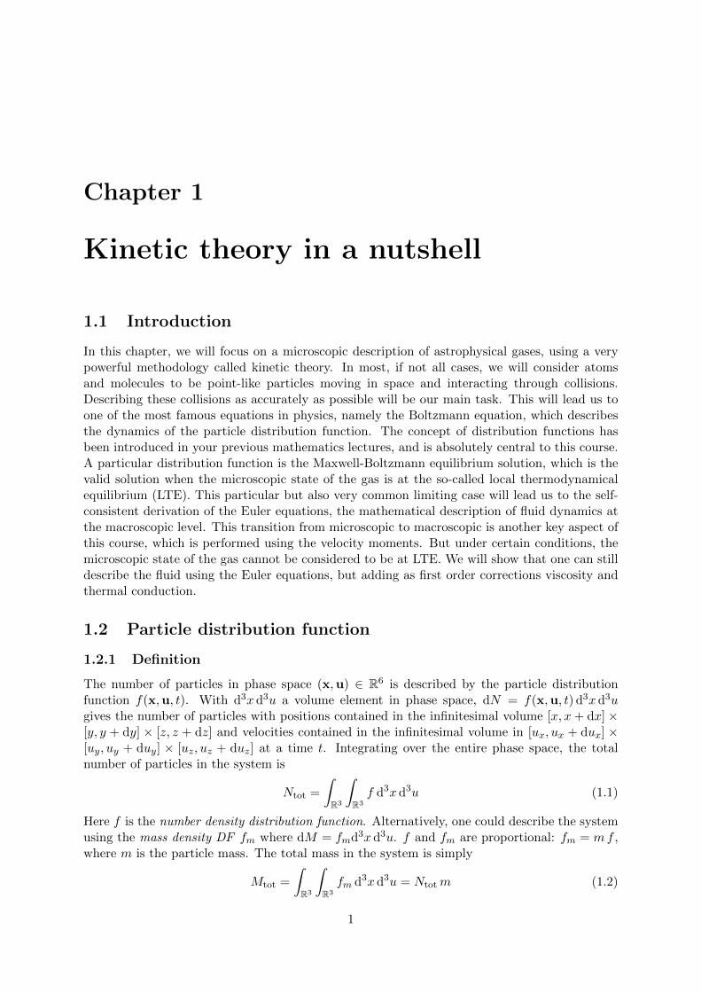
The number of particles in phase space (x,u) ∈ R6 is described by the particle distributionfunction f(x,u, t). With d3x d3u a volume element in phase space, dN = f(x,u, t) d3x d3ugives the number of particles with positions contained in the infinitesimal volume [x, x+ dx]×[y, y + dy] × [z, z + dz] and velocities contained in the infinitesimal volume in [ux, ux + dux] ×[uy, uy + duy] × [uz, uz + duz] at a time t. Integrating over the entire phase space, the totalnumber of particles in the system is
Ntot =
∫R3
∫R3
f d3x d3u (1.1)
Here f is the number density distribution function. Alternatively, one could describe the systemusing the mass density DF fm where dM = fmd3x d3u. f and fm are proportional: fm = mf ,where m is the particle mass. The total mass in the system is simply
Mtot =
∫R3
∫R3
fm d3x d3u = Ntotm (1.2)
1

CHAPTER 1. KINETIC THEORY IN A NUTSHELL 2
Another alternative formulation is to use the probability density DF fp, which expresses theprobability of being inside a phase space element fp(x,v, t). This DF is normalised to 1:
1 =
∫R3
∫R3
fp d3x d3u (1.3)
One can recover the number density DF by multiplying with the total number of particles:
f = Ntot fp(x,u, t) (1.4)
1.2.2 Moments of the particle DF
Other quantities can be derived by taken in the moments of the particle distribution function.By integrating out the velocity dependence, one gets the zeroth order moment, or the numberdensity
n(x, t) =
∫R3
f(x,u, t) d3u (1.5)
One can also define the mass density
ρ(x, t) = mn(x, t) (1.6)
The first order moment, the fluid momentum m(x, t), is defined as
m(x, t) =
∫R3
mf(x,u, t) u d3u (1.7)
and is used to define the fluid bulk or macroscopic velocity v(x, t) as
m(x, t) = ρ(x, t) v(x, t) (1.8)
At each position and time, an important new variable can also be defined as the microscopicrelative velocity
w = u− v(x, t) (1.9)
also known as thermal velocity. In general, arbitrary moments can be defined as
Q(x, t) =
∫R3
q(u, t) f(x,u, t) d3u (1.10)
with q a function of the particle velocity. A fundamentally important quantity can finally bedefined as the second order moment of the distribution function, this is the fluid total energy:
E(x, t) =
∫R3
1
2mu2 f(x,u, t) d3u (1.11)
Using the thermal velocity and the relation u2 = w2 + 2 w ·v + v2, one obtains immediately therelation
E(x, t) =1
2ρ σ2
3D +1
2ρ v2 (1.12)
where we used the following property of the thermal velocity∫R3
f(x,u, t) w d3u = 0 (1.13)

CHAPTER 1. KINETIC THEORY IN A NUTSHELL 3
x0 x
u0
u
Figure 1.1: A volume element moving along a trajectory in phase space
and we introduced the one dimensional, component-wise microscopic velocity dispersion
n(x, t)σ2i (x, t) =
∫R3
f(x,u, t)w2i d3u (1.14)
and the total or three dimensional velocity dispersion as
σ23D(x, t) = σ2
x + σ2y + σ2
z (1.15)
We can now interpret Equation 1.12 as the sum of the fluid thermal energy, which is the kineticenergy associated to microscopic relative motions and the bulk kinetic energy, which is thekinetic energy associated to the bulk, average macroscopic flow.
1.3 Boltzmann equation
Elementary mechanics states that a trajectory in phase space is defined to first order by
x = x0 + u0 dt (1.16)
u = u0 + a(x0, t0) dt (1.17)
where the position x and the velocity u are independent variables. Assume a phase space volumeelement d6V0 = d3x0 d3u0 travels along a trajectory to new a position in phase space (figure1.1). The new volume element d6V = d3x d3u is related to d6V0 through the Jacobian of thecoordinate transformation:
|J| =∣∣∣∣ 1 dt(∂a∂x
)dt 1
∣∣∣∣ = 1−(∂a
∂x
)dt2 (1.18)
Using d6V = |J|d6V0, we deduce
d6V − d6V0
dt' −d6V0
(∂a
∂x
)dt −→ 0 when dt→ 0 (1.19)
In other words, we haveD
Dt
(d6V
)= 0 (1.20)

CHAPTER 1. KINETIC THEORY IN A NUTSHELL 4
u1
u2
u′1
u′2
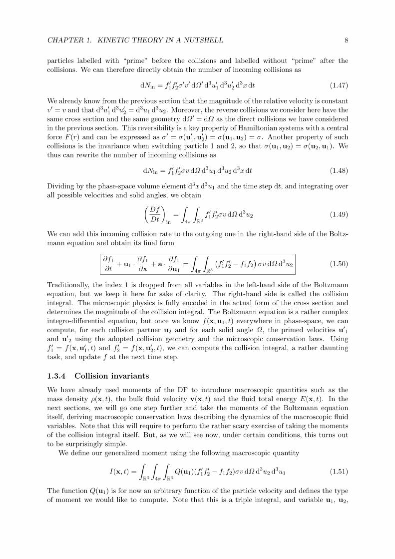
Figure 1.2: Schematic representation of a binary collision
This means the volume element is conserved or d6V = d6V0. This result is known as Liouville’stheorem. If particles cannot be created or destroyed, the particle distribution function is alsoconserved since
dN0 = f0 d3x0 d3u0 (1.21)
dN = f d3x d3u (1.22)
leads tof(x(t+ dt),u(t+ dt), t+ dt) = f(x0,u0, t) (1.23)
This implies that the total time derivative is zero, which can be expressed, using partial deriva-tives and the chain rule, as
Df
Dt=∂f
∂x· x +
∂f
∂u· u +
∂f
∂t= 0 (1.24)
This equation gives the time evolution of the particle distribution function and is also called theVlasov equation. One can rewrite this as
∂f
∂t+ u · ∂f
∂x+ a · ∂f
∂u= 0 (1.25)
Note that this is a partial diffential equation in 6-dimensional phase space.
So far, we have not taken into account any collisions. Binary collisions can add or removeparticles from a phase space element. The change in particle numbers is expressed by thecollision term (
Df
Dt
)coll
=
(Df
Dt
)in
−(Df
Dt
)out
(1.26)
Finally, we get the Boltzmann equation
∂f
∂t+ u · ∂f
∂x+ a · ∂f
∂u=
(Df
Dt
)coll
(1.27)

CHAPTER 1. KINETIC THEORY IN A NUTSHELL 5
1.3.1 Binary collisions
A collision featuring two particles (Fig. 1.2) obeys microscopic conservation laws, which are theconservation of mass, momentum and energy
M = m1 +m2 = m′1 +m′2 (1.28)
MV = m1u1 +m2u2 = m1u′1 +m2u
′2 (1.29)
E =1
2m1u
21 +
1
2m2u
22 =
1
2m1u
′21 +
1
2m2u
′22 (1.30)
when we evaluate the particle properties before and after the collision, but far enough from theimpact point so that the potential energy of the interaction can be ignored. We also consideronly elastic collisions for which the mass of the particles before and after the collision remainunchanged so that m′1 = m1 and m′2 = m2. At the impact point itself, different kinds of potentialenergy come into play. For elastic collisions however, the description of these is unimportantand the collision itself can be viewed as a black box. Note that we introduced the velocity of thecentre of mass V and the total mass of the system M . We can also define the relative velocitiesof the particles (not to be confused with the fluid bulk velocity defined earlier)
v = u1 − u2 (1.31)
and the reduced massm =
m1m2
m1 +m2(1.32)
Quite naturally one defines equivalent sets of variable by noticing that
u1 = V +m2
m1 +m2v (1.33)
u2 = V − m1
m1 +m2v (1.34)
The determinant of the Jacobian matrix of this transformation determines the change in thevolume elements
|J| =∣∣∣∣1 m2
m1+m2
1 − m1m1+m2
∣∣∣∣ = 1 (1.35)
The consequence is that the volume elements between the two sets of variables (v,V) and(u1,u2) are equal.
d3V d3v = d3u1d3u2 (1.36)
This relation is also valid for (u′1,u′2) and (v′,V). Using these new variables, the conservation
of the total energy can also be written as
E =1
2MV 2 +
1
2mv2 =
1
2MV 2 +
1
2mv′2 (1.37)
resulting in ||v|| = ||v′|| or in short v = v′. This is a fundamental result of the theory of binarycollisions: the magnitude of the relative velocity does not change before and after the collision,only the direction of the relative velocity will change. In other words, the transformation betweenv and v′ is a rotation, which also preserves the volume element, so that d3v = d3v′. Combinedwith the previous relations, one finally gets
d3u′1d3u′2 = d3u1d3u2, (1.38)
a result that will prove very usefull later.
CHAPTER 1. KINETIC THEORY IN A NUTSHELL 6
z
v
M
m
b
θ
φ
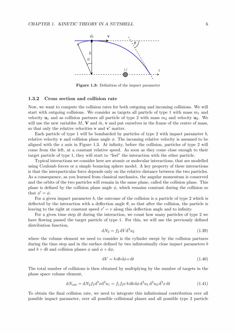
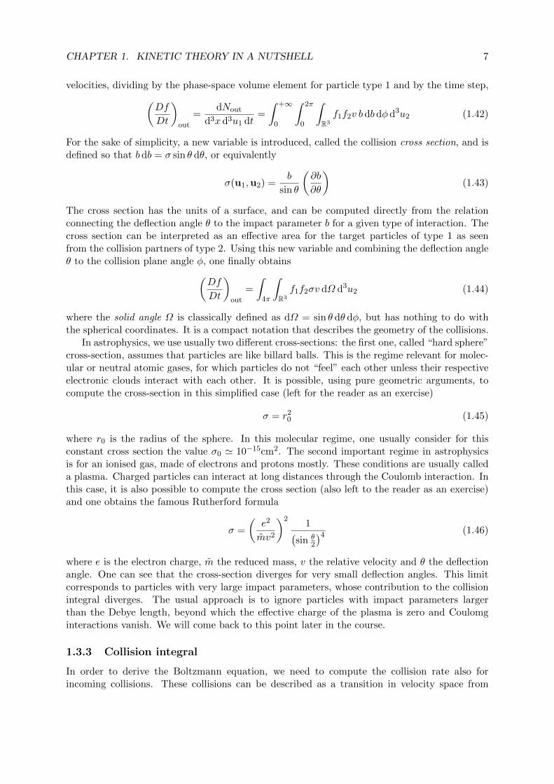
Figure 1.3: Definition of the impact parameter
1.3.2 Cross section and collision rate
Now, we want to compute the collision rates for both outgoing and incoming collisions. We willstart with outgoing collisions. We consider as targets all particle of type 1 with mass m1 andvelocity u1 and as collision partners all particle of type 2 with mass m2 and velocity u2. Wewill use the new variables M , V and m, v and put ourselves in the frame of the centre of mass,so that only the relative velocities v and v′ matter.
Each particle of type 1 will be bombarded by particles of type 2 with impact parameter b,relative velocity v and collision plane angle φ. The incoming relative velocity is assumed to bealigned with the z axis in Figure 1.3. At infinity, before the collision, particles of type 2 willcome from the left, at a constant relative speed. As soon as they come close enough to theirtarget particle of type 1, they will start to “feel” the interaction with the other particle.
Typical interactions we consider here are atomic or molecular interactions, that are modelledusing Coulomb forces or a simple bouncing sphere model. A key property of these interactionsis that the interparticular force depends only on the relative distance between the two particles.As a consequence, as you learned from classical mechanics, the angular momentum is conservedand the orbits of the two particles will remain in the same plane, called the collision plane. Thisplane is defined by the collision plane angle φ, which remains constant during the collision sothat φ′ = φ.
For a given impact parameter b, the outcome of the collision is a particle of type 2 which isdeflected by the interaction with a deflection angle θ, so that after the collision, the particle isleaving to the right at constant speed v′ = v along this deflection angle and to infinity.
For a given time step dt during the interaction, we count how many particles of type 2 wehave flowing passed the target particle of type 1. For this, we will use the previously defineddistribution function,
dN2 = f2 dV d3u2 (1.39)
where the volume element we need to consider is the cylinder swept by the collision partnersduring the time step and in the surface defined by two infintesimally close impact parameters band b+ db and collision planes φ and φ+ dφ,
dV = bdbdφ v dt (1.40)
The total number of collisions is then obtained by multiplying by the number of targets in thephase space volume element,
dNout = dN2f1d3xd3u1 = f1f2v bdbdφ d3u1 d3u2 d3x dt (1.41)
To obtain the final collision rate, we need to integrate this infinitesimal contribution over allpossible impact parameter, over all possible collisional planes and all possible type 2 particle
CHAPTER 1. KINETIC THEORY IN A NUTSHELL 7
velocities, dividing by the phase-space volume element for particle type 1 and by the time step,(Df
Dt
)out
=dNout
d3x d3u1 dt=
∫ +∞
0
∫ 2π
0
∫R3
f1f2v bdbdφ d3u2 (1.42)
For the sake of simplicity, a new variable is introduced, called the collision cross section, and isdefined so that bdb = σ sin θ dθ, or equivalently
σ(u1,u2) =b
sin θ
(∂b
∂θ
)(1.43)
The cross section has the units of a surface, and can be computed directly from the relationconnecting the deflection angle θ to the impact parameter b for a given type of interaction. Thecross section can be interpreted as an effective area for the target particles of type 1 as seenfrom the collision partners of type 2. Using this new variable and combining the deflection angleθ to the collision plane angle φ, one finally obtains(
Df
Dt
)out
=
∫4π
∫R3
f1f2σv dΩ d3u2 (1.44)
where the solid angle Ω is classically defined as dΩ = sin θ dθ dφ, but has nothing to do withthe spherical coordinates. It is a compact notation that describes the geometry of the collisions.
In astrophysics, we use usually two different cross-sections: the first one, called “hard sphere”cross-section, assumes that particles are like billard balls. This is the regime relevant for molec-ular or neutral atomic gases, for which particles do not “feel” each other unless their respectiveelectronic clouds interact with each other. It is possible, using pure geometric arguments, tocompute the cross-section in this simplified case (left for the reader as an exercise)
σ = r20 (1.45)
where r0 is the radius of the sphere. In this molecular regime, one usually consider for thisconstant cross section the value σ0 ' 10−15cm2. The second important regime in astrophysicsis for an ionised gas, made of electrons and protons mostly. These conditions are usually calleda plasma. Charged particles can interact at long distances through the Coulomb interaction. Inthis case, it is also possible to compute the cross section (also left to the reader as an exercise)and one obtains the famous Rutherford formula
σ =
(e2
mv2
)21(
sin θ2
)4 (1.46)
where e is the electron charge, m the reduced mass, v the relative velocity and θ the deflectionangle. One can see that the cross-section diverges for very small deflection angles. This limitcorresponds to particles with very large impact parameters, whose contribution to the collisionintegral diverges. The usual approach is to ignore particles with impact parameters largerthan the Debye length, beyond which the effective charge of the plasma is zero and Coulomginteractions vanish. We will come back to this point later in the course.
1.3.3 Collision integral
In order to derive the Boltzmann equation, we need to compute the collision rate also forincoming collisions. These collisions can be described as a transition in velocity space from
CHAPTER 1. KINETIC THEORY IN A NUTSHELL 8
particles labelled with “prime” before the collisions and labelled without “prime” after thecollisions. We can therefore directly obtain the number of incoming collisions as
dNin = f ′1f′2σ′v′ dΩ′ d3u′1 d3u′2 d3x dt (1.47)
We already know from the previous section that the magnitude of the relative velocity is constantv′ = v and that d3u′1 d3u′2 = d3u1 d3u2. Moreover, the reverse collisions we consider here have thesame cross section and the same geometry dΩ′ = dΩ as the direct collisions we have consideredin the previous section. This reversibility is a key property of Hamiltonian systems with a centralforce F (r) and can be expressed as σ′ = σ(u′1,u
′2) = σ(u1,u2) = σ. Another property of such
collisions is the invariance when switching particle 1 and 2, so that σ(u1,u2) = σ(u2,u1). Wethus can rewrite the number of incoming collisions as
dNin = f ′1f′2σv dΩ d3u1 d3u2 d3x dt (1.48)
Dividing by the phase-space volume element d3x d3u1 and the time step dt, and integrating overall possible velocities and solid angles, we obtain(
Df
Dt
)in
=
∫4π
∫R3
f ′1f′2σv dΩ d3u2 (1.49)
We can add this incoming collision rate to the outgoing one in the right-hand side of the Boltz-mann equation and obtain its final form
∂f1
∂t+ u1 ·
∂f1
∂x+ a · ∂f1
∂u1=
∫4π
∫R3
(f ′1f′2 − f1f2
)σv dΩ d3u2 (1.50)
Traditionally, the index 1 is dropped from all variables in the left-hand side of the Boltzmannequation, but we keep it here for sake of clarity. The right-hand side is called the collisionintegral. The microscopic physics is fully encoded in the actual form of the cross section anddetermines the magnitude of the collision integral. The Boltzmann equation is a rather complexintegro-differential equation, but once we know f(x,u1, t) everywhere in phase-space, we cancompute, for each collision partner u2 and for each solid angle Ω, the primed velocities u′1and u′2 using the adopted collision geometry and the microscopic conservation laws. Usingf ′1 = f(x,u′1, t) and f ′2 = f(x,u′2, t), we can compute the collision integral, a rather dauntingtask, and update f at the next time step.
1.3.4 Collision invariants
We have already used moments of the DF to introduce macroscopic quantities such as themass density ρ(x, t), the bulk fluid velocity v(x, t) and the fluid total energy E(x, t). In thenext sections, we will go one step further and take the moments of the Boltzmann equationitself, deriving macroscopic conservation laws describing the dynamics of the macroscopic fluidvariables. Note that this will require to perform the rather scary exercise of taking the momentsof the collision integral itself. But, as we will see now, under certain conditions, this turns outto be surprisingly simple.
We define our generalized moment using the following macroscopic quantity
I(x, t) =
∫R3
∫4π
∫R3
Q(u1)(f ′1f′2 − f1f2)σv dΩ d3u2 d3u1 (1.51)
The function Q(u1) is for now an arbitrary function of the particle velocity and defines the typeof moment we would like to compute. Note that this is a triple integral, and variable u1, u2,
CHAPTER 1. KINETIC THEORY IN A NUTSHELL 9
Ω are all dummy integration variables. We will now switch the indice 1 and 2 in the previousexpression. As we discussed in the previous section, the collision properties are unchanged underthis rather trivial transformation. So we have
I(x, t) =
∫R3
∫4π
∫R3
Q(u2)(f ′2f′1 − f2f1)σv dΩ d3u1 d3u2 (1.52)
=1
2
∫R3
∫4π
∫R3
[Q(u1) +Q(u2)] (f ′1f′2 − f1f2)σv dΩ d3u1 d3u2 (1.53)
where we use in the second equality the clever trick that if two expressions are equal, they arealso equal to their average. In this new expression, we now switch the prime and the non-primevelocity variables, to obtain
I(x, t) =1
2
∫R3
∫4π
∫R3
[Q(u′1) +Q(u′2)
](f1f2 − f ′1f ′2)σ′v′ dΩ d3u′1 d3u′2 (1.54)
=1
2
∫R3
∫4π
∫R3
[−Q(u′1)−Q(u′2)
](f ′1f
′2 − f1f2)σv dΩ d3u1 d3u2 (1.55)
where we derived the second line using the reversibility of the collisions and the conservationlaws leading to v′ = v and d3u′1d3u′2 = d3u1d3u2. We also put a minus sign in the square bracketto recover the classical collision integral form. Using the same trick as before, namely addingthe two (equal) expressions and dividing by two, we finally obtain the fundamental result
I(x, t) =1
4
∫R3
∫4π
∫R3
[Q(u1) +Q(u2)−Q(u′1)−Q(u′2)
](f ′1f
′2 − f1f2)σv dΩ d3u1 d3u2
(1.56)The still unspecified quantity Q is said to be a collision invariant if it satifies the followingconservation law
Q(u1) +Q(u2) = Q(u′1) +Q(u′2). (1.57)
In this case, according to the previous derivation, its moment vanishes identically so thatI(x, t) = 0 everywhere. Why is this result so powerful? We already know three collisionalinvariants from the microscopic conservation laws for the mass Q(u1) = m1, the momentumQ(u1) = m1u1 and the kinetic energy Q(u1) = 1
2m1u21. This will allow us to take the cor-
responding moments for the Boltzmann equation and the right-hand side, associated to theparticularly scary collision integral, will vanish. We will only have to deal with the left-handside, namely to take the moments of the Vlasov equation, a much simpler task that will occupyus in a future chapter.
CHAPTER 1. KINETIC THEORY IN A NUTSHELL 10
1.4 Local Thermodynamical Equilibrium
In this section, we will discuss a particular case of the Boltzmann equation, for which the collisionintegral vanishes exactly. This case is of particular importance, as it will lead us to the derivationof the Euler equations and the theoretical foundation of astrophysical fluid dynamics. We willuse for the first time in this course the notion of equilibrium solution. The collision integralis the difference between two terms: a source of incoming particles and a sink of outgoingparticles. Under the proper conditions (we will derive the exact requirement later), both thesource and the sink terms can be very large, much larger than all the terms in the left-handside of the Boltzmann equation. In this case, the system will naturally evolve to a state wherethe two collision terms exactly cancel each other, leading to the notion of detailed balance andmore fundamentally to thermodynamical equilibrium. There is a solution to these equilibriumconditions, called the Maxwell-Boltzmann DF and usually noted f0.
1.4.1 Maxwell-Boltzmann distribution
The derivation of the Maxwell-Boltzmann equilibrium DF is the result of requiring detailedbalance of incoming and outgoing collisions in each phase-space element. This is a very strongcondition: one could imagine that the collision term vanishes in a global, weaker sense, after per-forming the integral over velocity space. Detailed balance leads to the equilibrium DF f0(x,v, t)
which satisfies(DfDt
)coll≡ 0 in a strong sense, namely that(
Df
Dt
)coll
=
∫4π
∫R3
(f ′1f′2 − f1f2)︸ ︷︷ ︸≡0
σv dΩ d3u2 (1.58)
so the integrand vanishes everywhere in velocity space, at a given spatial location. This de-tailed balance of incoming and outgoing collisions defines what is called local thermodynamicequilibrium (LTE). We can reformulate this condition as
f1f2 = f ′1f′2 (1.59)
or ln f1 + ln f2 = ln f ′1 + ln f ′2 (1.60)
We see that detailed balance implies that ln f0 is a collision invariant, in addition to the micro-scopic conservation laws we have already introduced.
m1 +m2 = m′1 +m′2 (1.61)
m1u1 +m2u2 = m1u′1 +m2u
′2 (1.62)
1
2m1u
21 +
1
2m2u
22 =
1
2m1u
′21 +
1
2m2u
′22 (1.63)
We have also seen that these three conservation laws are enough, together with the cross sectionσ, to fully specify the properties of the collisions. We cannot have a fourth collision invariantthat brings in new information to the phase-space transform induced by collisions. The onlypossibility is that this fourth invariant is a linear combination of the previous three, so that
ln f0 = αm+ β1
2mu2 + γ ·mu (1.64)
where α(x, t) and β(x, t) are scalar quantities that depend on space and time and γ(x, t) isa vector quantity that depends also on space and time. These quantities are considered asconstant in velocity space for a fixed spatial location, but they are allowed to vary in physical
CHAPTER 1. KINETIC THEORY IN A NUTSHELL 11
space. They are macroscopic properties of the fluid, and can be related to the moments of theMaxwell-Boltzmann DF as follows ∫
R3
f0(u) d3u = n(x, t) (1.65)∫R3
f0(u) u d3u = n(x, t) v(x, t) (1.66)∫R3
f0(u) (u− v)2 d3u = n(x, t)σ23D(x, t) (1.67)
One key property is that this DF is isotropic in velocity space: it depends only on u2 = u2x +
u2y + u2
z so that no direction is preferred. As a consequence, the velocity dispersion satisfies
σ2x = σ2
y = σ2z = σ2
1D =1
3σ2
3D (1.68)
so we can drop the subscripts and use only σ(x, t) for the 1D velocity dispersion. Inverting theprevious three moments (left to the reader as an exercise), one obtains the following closed formfor the Maxwell-Boltzmann DF
f0(x,u, t) =n(x, t)(
2πσ(x, t)2)3/2 exp
(−1
2
(u− v(x, t)
)2σ(x, t)2
)(1.69)
It is quite convenient to introduce the one-dimensional Gaussian distribution, with zero meanand variance σ
G(w) =1√
2πσ2exp
(− w2
2σ2
)(1.70)
and define the three-dimensional Maxwell-Boltzmann distribution as the product of three Gaus-sian
f0(x,u, t) = n(x, t)G(ux − vx)G(uy − vy)G(uz − vz) (1.71)
The arguments of the Gaussian function have been defined earlier: these are the components ofthe thermal velocity w = u − v. The one-dimensional Gaussian distribution has the followingusefull properties ∫ +∞
−∞G(w) dw = 1 and
∫ +∞
−∞wG(w) dw = 0, (1.72)∫ +∞
−∞w2G(w) dw = σ2,
∫ +∞
−∞w3G(w) dw = 0 and
∫ +∞
−∞w4G(w) dw = 3σ4 (1.73)
We will see later that the second-order moment of the Maxwell-Boltzmann DF can be identifiedto the pressure of an ideal gas, for which we have
P = nkBT = ρ σ2 (1.74)
As a consequence, we obtain
σ(x, t) =
√kBT (x, t)
m. (1.75)
The velocity dispersion is thus directly related to the gas temperature. The temperature is thetraditional quantity introduced in statistical mechanics to define thermodynamical equilibrium.

CHAPTER 1. KINETIC THEORY IN A NUTSHELL 12
1.4.2 Boltzmann’s H theorem
In the previous section, we have seen that a sufficient condition for thermodynamical equilibriumis that the DF is equal to the Maxwell-Boltzmann distribution. But it is not clear yet whether anysystem initially out of equilibrium will indeed necessarily relax towards the Maxwell-BoltzmannDF. This important result is the conclusion of the famous Boltzmann’s H theorem. In order tosimplify the discussion, we consider a uniform medium without any external acceleration. Inthis case, we can drop all x dependent variables in the Boltzmann equation, which now containsonly the partial time derivative in the left-hand side and the collision integral in the right-handside.
∂f
∂t=
∫R3
∫4π
(f ′1f′2 − f1f2)σv dΩ d3u2 (1.76)
We now introduce a new moment of the DF, the quantity
H(t) =
∫R3
f(u, t) ln(f(u, t)
)d3u (1.77)
where f is the out-of-equilibrium DF. This quantity is the opposite of the entropy defined instatistical mechanics. Taking the time derivative, one obtains
∂H
∂t=
∫R3
[∂f
∂tln f +
∂f
∂t
]d3u =
∫R3
[ln f + 1]∂f
∂td3u (1.78)
We can now replace the time derivative by the collision integral and obtain a very familiar form
∂H
∂t=
∫R3
∫R3
∫4π
[ln f1 + 1] (f ′1f′2 − f1f2)σv dΩ d3u1 d3u2 (1.79)
=1
4
∫R3
∫R3
∫4π
[ln f1 + ln f2 − ln f ′1 − ln f ′2] (f ′1f′2 − f1f2)σv dΩ d3u1 d3u2 (1.80)
where we apply the results of Section 1.3.4 to derive the second line. We finally rearrange theintegral into
∂H
∂t= −1
4
∫R3
∫R3
∫4π
[ln f ′1f′2 − ln f1f2] (f ′1f
′2 − f1f2)σv dΩ d3u1 d3u2 (1.81)
The logarithm being a growing function of its argument, if X > Y (resp. X < Y ), one haslnX > lnY (resp. lnX < lnY ), so that (lnX − lnY )(X − Y ) is always a positive quantity. Asa consequence, the time derivative of H is always negative and H will necessarily decrease withtime. For a system with finite volume or finite mass, the function will quickly reach a minimumvalue for which the time derivative is zero and the DF is equal to the Maxwell-Boltzmann one.
This theorem has profound consequences for the physics of gases: it introduces the notionof dissipation as a fundamental property of fluid dynamics. It also leads to a paradox: whydo microscopic collisions with purely reversible equation of motions (Hamiltonian systems) leadto a macroscopic dissipative system? One interpretation (among many others) is based onmolecular chaos: even Hamiltonian systems are unpredictive on sufficiently long time scales andare consistent with a dissipative, irreversible evolution.
1.4.3 Collision time and mean free path
A legitimate question follows: how much time does the system need to reach equilibrium? Inkinetic theory, many different time scales can be computed to estimate this relaxation time:the stopping time corresponds to the time required for a particle to loose its initial kinetic
CHAPTER 1. KINETIC THEORY IN A NUTSHELL 13
energy through collisions, the deflection time corresponds to the time required for a particleto be deflected by 90 from its initial trajectory, etc. These different times are all slightlydifferent estimates of what is usually refer to as the collision time. For sake of simplicity, wewill compute it using the rate of outgoing collisions, namely the negative term in the collisionintegral, assuming that the DF is the Maxwell-Boltzmann one and the collision cross section isfor “hard sphere” particles, typical for a molecular or neutral atomic gas.
We define the collision rate as the following zeroth-order moment of the collision integral
Cout =
∫R3
∫R3
∫4πf1f2 σv d3u1 d3u2 dΩ (1.82)
where f1 = f0(u1), f2 = f0(u2) and σ = r20 for hard spheres. We can easily perform the
integration over the solid angle ∫4πσdΩ = 4πr2
0 (1.83)
and we are left with a double integral over velocity space
Cout = 4πr20
∫R3
∫R3
f0(u1)f0(u2) v d3u1 d3u2 (1.84)
Changing variables from (u1,u2) to (V,v), we get (left to the reader as an exercise)
Cout = 8 r20 n
2
(m
kBT
)3 ∫ +∞
0e− 1
2MV 2
kBT V 2dV
∫ +∞
0e− 1
2mv2
kBT v3dv (1.85)
which can be finally integrated as
Cout = n2 4√πr2
0
√kBT
m(1.86)
In this derivation, we see that the collision rate is proportional to the square of the fluid density,to the cross section and to the particle velocity dispersion. In the general case, one usuallyprefers the notation
Cout = n2 〈σv〉 (1.87)
where the angle brackets denote the average over velocity space. For a constant cross sectionσ0, one can quickly derive the approximate formula
Cout ' n2σ0
√kBT
m(1.88)
which is reasonably accurate for hard spheres. For Coulomb interactions, however, computingthe collision rate is much more challenging. We present here only an approximate derivation.The idea is to compute an estimate of the cross section as the square of the typical impactparameter. For a Coulomb interaction, the typical impact parameter can be estimated byconsidering marginally bound orbits, for which
e2
b' 1
2mv2 (1.89)
which gives for the cross section (dropping all dimensionless numbers that are close to unity)
σ ' πb2 '(
e2
mv2
)2
(1.90)

CHAPTER 1. KINETIC THEORY IN A NUTSHELL 14
In the last formula, we replace the relative velocity by the velocity dispersion, which gives usan average cross section that we identified with σ0 in the previous formulae, resulting in thefollowing approximation for the collision rate in the Coulomb case
Cout ' n2 e4
(kBT )2
√kBT
m(1.91)
One last important ingredient is missing, namely the fact that the Coulomb cross section isdiverging for very large impact parameter. This results in a significant increase of the effectivecross section, encoded in what is called the Coulomb logarithm. It is equal to the logarithm ofthe ratio of the maximum impact parameter, taken equal to the Debye length, and the minimumimpact parameter, usually equal to the 90 deflection angle impact parameter. In short, we have
lnΛ = lnbmax
bmin(1.92)
and the final (surprisingly accurate) formula for the Coulomb interaction collision rate is
Cout ' n2 e4
(kBT )2
√kBT
mlnΛ (1.93)
Because of its logarithmic dependence, the Coulomb logarithm takes values lnΛ ' 10 to 30 fora wide range of astrophysical conditions. The best strategy is to assume it is constant withlnΛ = 20.
In order to derive the collision time scale, one just divides the particle density by the collisionrate
τcoll =n
Cout=
1
n 〈σv〉(1.94)
One can also define the mean free path as the typical distance a particle will travel within onecollision time. Since the typical particle velocity is given by the thermal velocity, one obtains
λcoll =
√kBT
mτcoll (1.95)
For hard spheres, one sees that the mean free path depends only on the inverse of the density,and not on temperature. For ionized plasma’s, on the other hand, it depends also on the squareof the temperature.
1.4.4 Validity of LTE approximations
Equipped with these notions of mean free path and relaxation time, we can now go back to theBoltzmann equation
∂f1
∂t+ u · ∂f1
∂x+ a(x) · ∂f1
∂u=
∫R3
∫4π
[f ′1f′2 − f1f2]σv d3u2 dΩ (1.96)
If the right-hand side dominates over the left-hand side, collisions will quickly drive the DFtowards the Maxwell-Boltzmann one, validating the LTE approximation. On the other-hand, ifthe left-hand side dominates, then the LTE approximation won’t be valid anymore and the DFwill deviate strongly from f0. Most of the important terms in the Vlasov equation are spatialgradients of f . If one assume that f ' f0, at least initially, we can estimate the magnitude ofthe gradient terms (left to the reader as an exercise) using the following length scales
1
hn=|∇n|n
or1
hT=|∇T |T
(1.97)
CHAPTER 1. KINETIC THEORY IN A NUTSHELL 15
and compare them the mean free path as an estimate of the magnitude of the collision integral.The Maxwell-Boltzmann DF, or the LTE approximation are therefore valid if the typical lengthscale over which the macroscopic variables vary are much larger than the mean free path or
min(hn, hT , hv) λcoll (1.98)
It is now your responsibility to check a posteriori, after you have found a solution of the fluidequations for your favorite astrophysical objects, that this solution satisfies the validity criterionfor LTE. If not, then you cannot use the fluid equation in the LTE regime, and you have to usemore complex equations that we will derive in the next section.
1.5 Moments of the Boltzmann equation and the fluid equations
In this section, we will derive the fluid equations, which are the mactoscopic version of themicroscopic conservation laws. The key property we will use, is the fact that moments of thecollision integral vanish if we use collision invariants. This property is true for any DF, even farfrom LTE. On the other hand, when the system is close to LTE, the fluid equations simplifyeven more and we obtain the famous Euler equations. Of course, these are valid only if LTEconditions are met, as explained in the previous section.
1.5.1 General case for non-LTE conditions
We now take the moments of the entire Boltzmann equation, by performing the integral overvelocity space∫
R3
Q(u1)
(∂f1
∂t+ u · ∂f1
∂x+ a(x) · ∂f1
∂u
)d3u1 =
∫R3
Q(u1)
(Df
Dt
)coll
d3u1 (1.99)
We have demonstrated earlier that if we use for Q any of m, mux, muy, muz or 12mu
2, inother words any of the microscopic conservation laws, the right-hand side with the collisionintegral vanishes everywhere. So we just have to take the moments of the left-hand side, namelythe Vlasov equation. This is what we will do now, using each microscopic conservation law insequence.
Mass conservation
This is the simplest of the 3 fluid equations. Multiplying by the particle mass m, we obtain 3terms ∫
R3
m∂f
∂td3u+
∫R3
mu · ∂f∂x
d3u+
∫R3
ma(x) · ∂f∂u
d3u = 0 (1.100)
(1) (2) (3)
In order to compute these 3 terms, the key argument is that x, u and t are three independentvariables. Let’s work out each term seperatly. For term (1), we can take the time derivativeoutside of the integral and recover immediately the zeroth-order moment of the DF
∂
∂t
∫R3
mfd3u =∂
∂tρ(x, t) (1.101)
The second term (2) requires to introduce a famous vector calculus relation,
∇ · (fu) = f∇ · u + u · ∇f (1.102)

CHAPTER 1. KINETIC THEORY IN A NUTSHELL 16
but because u and x are independant variables, ∇ · u = 0 in this relation. Term (2) can thenbe simplified as
∂
∂x
∫R3
mufd3u = ∇ · (ρv) (1.103)
where we recognize in the right-hand side the first-order moment of the DF, namely the macro-scopic momentum. The third term is more involving. We first need to decompose the dotproduct into three additional terms
ma(x) ·∫R3
∂f
∂ud3u = max
∫R3
∂f
∂uxd3u+may
∫R3
∂f
∂uyd3u+maz
∫R3
∂f
∂uzd3u (1.104)
Let’s deal with the first one. For this, we introduce the one-dimensional distribution function as
F (ux) =
∫R2
f duyduz for which we have
∫ +∞
−∞
∂F
∂uxdux =
∫R3
∂f
∂uxd3u (1.105)
We see that this function can be directly integrated so that
max
∫R3
∂f
∂uxd3u = max [F (+∞)− F (−∞)] = 0 (1.106)
since F → 0 when ux → ±∞, a required property for distribution function. The same trick canbe used for each direction. The final result is the equation for mass conservation, the first of ourmacroscopic fluid equations.
∂
∂tρ+∇ · (ρv) = 0 (1.107)
Momentum conservation
We now use for our moment’s calculation the quantity Q = mux. We will drop the index x laterwhen it will become clearer. The integration over the Boltzmann equation now becomes∫
R3
mux∂f
∂td3u+
∫R3
mux u · ∇fd3u+
∫R3
mux a(x) · ∂f∂u
d3u = 0 (1.108)
(1) (2) (3)
with again three main terms to integrate. The first term (1) is again quite easy because timeand velocity commute.
(1) =∂
∂t
∫R3
muxfd3u =∂
∂t(ρ vx) (1.109)
The third term can be decomposed in three more terms by developing the dot product
(3) = max
∫R3
ux∂f
∂uxd3u+may
∫R3
ux∂f
∂uyd3u+maz
∫R3
ux∂f
∂uzd3u (1.110)
(3a) (3b) (3c)
The last two terms vanish exactly. One can define, almost like before, but not quite
H(uy) =
∫R2
uxfduxduz (1.111)
so that the second term (3b) can be written as
(3b) = may
∫ +∞
−∞
∂H
∂uyduy = may [H(+∞)−H(−∞)] = 0 (1.112)
CHAPTER 1. KINETIC THEORY IN A NUTSHELL 17
The same result applies to the third term (3c). The term (3a), on the other hand, does notvanish. We define, now exactly like before
F (ux) =
∫R2
fduyduz (1.113)
so that the third term (3) comes only from (3a) that can be integrated by parts
(3) = ax
∫ +∞
−∞mux
∂F
∂uxdux = ax
([muxF (ux)]+∞−∞ −
∫ +∞
−∞mF (ux)dux
)= −ρax (1.114)
The function F inside the brackets is evaluated at infinity, but since it is a distribution function,it converges to zero at infinity faster than ux, so that the bracket vanishes. The remainingintegral with a minus sign is just equal to −ρ.
Let’s now focus on the second term, labeled (2) above. We use the vector calculus relation
∇ · (fuxu) = ux (u · ∇f) + f∇ · (uxu) (1.115)
The rightmost term vanishes because u and x are independent variables. For the same reason,we can take the ∇ operator outside of the integral.
(2) = ∇ ·(∫
R3
muxufd3u
)= ∇ ·
(∫R3
muiujfd3u
)(1.116)
where we switch to Einstein’s notations for the velocity coordinates. We now split the velocityinto ui = vi + wi and develop the product as
(2) = ∇ ·(∫
R3
m (vivj + viwj + vjwi + wiwj)fd3u
)(1.117)
The first of these 4 terms is the easiest to compute, as vivj is a constant in velocity space, sothat
∇ ·(vivj
∫R3
mfd3u
)= ∇ · (ρ vivj) (1.118)
The second and third terms both vanish, because the thermal velocity integrates to zero
∇ ·(vi
∫R3
mwjfd3u
)= ∇ ·
(vj
∫R3
mwifd3u
)= 0 (1.119)
The last term, on the other end, does not lead to any known macroscopic quantity. We thereforedefine the pressure tensor as the 3x3 matrix
Pij =
∫R3
mwiwjf d3u (1.120)
so the final form of the second term of the first-order moment of the Boltzmann equation writesin tensor form
(2) = ∇ · (ρv ⊗ v + P) (1.121)
Putting everything together, we get the macroscopic, fluid equation for momentum conservation
∂
∂t(ρv) +∇(ρv ⊗ v + P) = ρa (1.122)
We cannot say much about this pressure tensor. Only by knowing the exact form of f can wecompute this moment. We can only notice that its trace is familiar, because
Tr P = ρσ2x + ρσ2
y + ρσ2z = ρσ2
3D (1.123)
CHAPTER 1. KINETIC THEORY IN A NUTSHELL 18
Energy conservation
Here we multiply the Boltzmann equation by Q = 12mu
2. We will not derive the third con-servation law, the conservation of total energy. This is left to the reader as exercise. We justsummarize the main results. We have already defined the total energy
E =1
2ρv2 + e (1.124)
where we define e as the internal energy. This is the kinetic energy associated with random,thermal motions.
e =
∫1
2mw2f d3u =
1
2Tr(P) (1.125)
The derivation of the energy conservation equation follows the same methodology as the previousconservation laws. Familiar macroscopic quantities will emerge, like the pressure tensor. Wewill have to introduce a new macroscopic vector, defined as the heat flux
Q =
∫R3
m1
2w2wf d3u (1.126)
The final form of the macroscopic energy conservation equation reads
∂E
∂t+∇ · (E v + P · v + Q) = ρa · u (1.127)
In summary, we have derived these three macroscopic conservation laws
∂
∂tρ+∇ · (ρv) = 0 (1.128)
∂
∂t(ρv) +∇(ρv ⊗ v + P) = ρa (1.129)
∂E
∂t+∇ · (E v + P · v + Q) = ρa · v (1.130)
which are also known as the general fluid equations. These equations are valid for any underlyingDF f . In practice, however, they are not really useful, as the form of P and Q remains unknown,unless we know the exact form of f , which requires to solve the Boltzmann equation. So we areback to square one. We will find explicit forms for these high-order moments in two limitingcases: the LTE regime and the Chapman-Enskog perturbation theory.
1.5.2 Euler equations for LTE conditions
When the fluid is at LTE, the DF takes a very specific form, namely the Maxwell-Boltzmanndistribution
f0(x,u, t) = n
(m
2πkBT
)3/2
e− 1
2mw2
kBT (1.131)
This distribution is an even function of w. As a consequence, if multiply by an odd function ofw, its integral will vanish. This leads to a great simplification because
Pij = 0 for i 6= j and Q = 0 (1.132)
The pressure tensor is the only non-vanishing high-order moment, and it is diagonal. Becausethe Maxwell-Boltzmann distribution is also isotropic, we have
σ2x = σ2
y = σ2z = σ2 =
kBT
m(1.133)
CHAPTER 1. KINETIC THEORY IN A NUTSHELL 19
So the pressure tensor is now proportional to the identity matrix, with
P = P I (1.134)
and P = ρσ2 is the scalar pressure. We obtain in this LTE limit the so-called Euler equations
∂
∂tρ+∇ · (ρv) = 0 (1.135)
∂
∂t(ρv) +∇ · (ρv ⊗ v + P I) = ρa (1.136)
∂E
∂t+∇ · ((E + P ) v) = ρa · v (1.137)
Note that the momentum flux related to the scalar pressure can also be transformed in thepressure gradient using the relation
∇ · (P I) = ∇P (1.138)
In the LTE case, we can also relate the internal energy to the gas pressure using e = 12Tr P, so
that
e =3
2P (1.139)
This last relation is also known as the ideal gas equation of state (noted in short the idealgas EoS). Following up on the analogy with an ideal gas, we recall the relation connecting thevelocity dispersion to the gas temperature, namely
P = ρσ2 = nkBT (1.140)
Interestingly enough, the Euler equations, presented here in their Eulerian form, are a closedsystem. Indeed, if one knows at time t, the mass, momentum and total energy densities, then,one can substract to the total energy the fluid kinetic energy and deduce the fluid internal energy.Using the ideal gas equation of state, one then knows the scalar pressure, so one can computethe time derivatives to update the conservative variables (ρ, ρv, E). There is therefore no needto use any microscopic properties, everything is specified at the macroscopic level. Let’s stressagain that this is valid only if LTE conditions are met, namely that all macroscopic variablesscale lengths are much larger than the collision mean free path.
1.5.3 Euler equations in Lagrangian form
So far we have looked at the problem from an Eulerian perspective, meaning the observer isstatic and watches how the fluid move with respect to his/her reference frame. We will nowlook in the Lagrangian perspective, where the observer moves together with the fluid. TheLagrangian derivative, also known as comoving derivative, is given by
D
Dt=
∂
∂t+ v · ∇ (1.141)
The Euler equations can now be rewritten in Lagrangian form.
Mass conservation
Starting from the mass conservation equation in Eulerian form
∂ρ
∂t+∇(ρv) = 0 (1.142)
CHAPTER 1. KINETIC THEORY IN A NUTSHELL 20
and using the now famous vector relation
∇ · (ρv) = ρ∇ · v + v∇ρ (1.143)
we find the mass conservation equation in Lagrangian form
1
ρ
Dρ
Dt= −∇ · v (1.144)
Momentum conservation
Using the Eulerian mass and momentum conservation laws, together with the definition of theLagrangian derivative, it is possible to derive the Euler equation in Lagrangian form. We startwith the momentum conservation equation for component vx as
∂
∂t(ρvx) +∇ · (ρvxv) +
∂P
∂x= ρax (1.145)
By developing all time and space derivatives, one obtains the following form (left as an exercise)(∂ρ
∂t+ ρ∇ · v + v · ∇ρ
)vx + ρ
(∂vx∂t
+ vxv · ∇vx)
= ρax −∂P
∂x(1.146)
The first parenthesis on the left-hand side is nothing else but the mass conservation equation inEulerian form, so it is equal to zero. The second parenthesis is the Lagrange derivative of vx.The same applies for each component of the momentum, so we get in the end
ρDv
Dt= −∇P + ρa (1.147)
Note that this equation can be obtained directly by applying Newton’s second law, adding thepressure forces to the external acceleration as minus the pressure gradient. This is clearly theeasiest way to remember it.
Energy conservation
A useful trick is to visualize a Lagrangian fluid element as a small volume of fluid containing aconstant mass. If we label this volume V and its mass M , the fluid density is just
ρ =M
V(1.148)
The conservation of mass can be written as
1
M
DM
Dt=
1
V
DV
Dt+
1
V
Dρ
Dt= 0 (1.149)
For a unit mass, V is called the specific volume, or the volume per unit mass. Using the massconservation equation in Lagrangian form, we deduce
1
V
DV
Dt= ∇ · v (1.150)
which states that the rate of change of the volume is given by the divergence of the velocityfield, a very useful interpretation.
CHAPTER 1. KINETIC THEORY IN A NUTSHELL 21
Now we define the total internal energy (in units of [erg]) in our fluid element as
E = eV = Mε (1.151)
where e is the internal energy density defined earlier, or the internal energy per unit volume (inunits of [erg cm−3]), and ε is the specific internal energy, or the internal energy per unit mass (inunits of [erg g−1]). We now use the first law of thermodynamics that states that dE = −PdV ,or in Lagrangian form
DE
Dt= M
Dε
Dt= −P DV
Dt(1.152)
Using the rate of change of the volume derived above, we finally get
ρDε
Dt= −P ∇ · v (1.153)
This is the energy equation in Lagrangian form. Note that we could have obtained the sameresult, starting with the energy equation in Eulerian form, then using both mass and momentumconservation, together with the definition of the Lagrange derivative, at the expense of relativelytedious calculations (left to the reader as exercise). The current approach, based on the firstlaw of thermodynamics, is much easier to remember and strictly equivalent.
CHAPTER 1. KINETIC THEORY IN A NUTSHELL 22
1.6 Chapman-Enskog theory
We have derived in the previous section the Euler equations, which are the fluid equations inthe limiting case of LTE. The Chapman-Enskog theory will allow us to also derive a completeset of fluid equations, which are valid slightly outside LTE conditions. We will introduce fluidviscosity and heat conduction, two physical processes associated to the concept of dissipation.The Chapman-Enskog derivation is also a perturbative technique, used in many other domainsof physics. The derivation we give here is a simplified version of the original Chapman-Enskogtheory, a very rigorous perturbative approach of kinetic theory.
1.6.1 First-order Chapman-Enskog expansion of the DF
When we are not in LTE, the DF is not of Maxwell-Boltzmann form anymore. In the generalcase, we need to solve the full Boltzmann equation, which is, in most cases, untractable. We canhowever follow a perturbative approach, assuming that the fluid is reasonably close to LTE, andthe general DF f is the Maxwell-Boltzmann DF f0 plus a small additive perturbation ∆f f0
f = f0 +∆f (1.154)
Starting with the full Boltzmann equation (without acceleration for sake of simplicity), wewrite
∂f
∂t+ u · ∇f = C(f) (1.155)
where the functional C(f) encodes the collision term as
C(f) =
(Df
Dt
)in
−(Df
Dt
)out
=
∫R3
∫4π
(f ′1f′2 − f1f2)σv dΩ d3u2 (1.156)
We now Taylor expand the collision term to first order, as
C(f) ' C(f0) +∂C∂f∆f (1.157)
By definition, we have C(f0) = 0. The partial derivative is however horribly complex and outsidethe scope of this course. We use here a very simple approximation, for which we assume that
C(f) ' −α(x, t)∆f = α (f0 − f) (1.158)
where α is just a function of position and time. We now determine α by computing the outgoingcollision rate as ∫
R3
α f d3u1 = αn = n2 〈σv〉 =n
τcoll(1.159)
so that
α =1
τcoll(1.160)
The Boltzmann equation can thus be written in the collision time approximation as
∂f
∂t+ u · ∇f = −∆f
τcoll(1.161)
We now use the main trick of the Chapman-Enskog expansion, which is to match terms of thesame order and neglect terms of higher-order. Injecting f = f0 +∆f in the previous equation,we neglect all ∆f terms in the left-hand side. In the right-hand side, however, the ∆f term isdivided by τcoll, which is also a very small quantity. Since the quotient of two small quantities
CHAPTER 1. KINETIC THEORY IN A NUTSHELL 23
can be large, we have to keep the right-hand side as it is, and obtain the first-order expansionof the Boltzmann equation
∂f0
∂t+ u · ∇f0 = −∆f
τcoll(1.162)
The problem is now for us to find a usefull expression for ∆f . Replacing the microscopic velocityby the sum of the bulk velocity and the thermal velocity u = v+w, we can rewrite the previousequation as
∂f0
∂t+ v · ∇f0 + w · ∇f0 = −∆f
τcoll(1.163)
orDf0
Dt+ w · ∇f0 = −∆f
τcoll(1.164)
We now use the explicit form of the Maxwell-Boltzmann distribution
f0 =ρ/m
(2πσ2)3/2exp
(−1
2
(u− v)2
σ2
)(1.165)
but re-written in the following convenient form
ln f0 = ln ρ− 3 lnσ − 1
2
(u− v)2
σ2+ constants (1.166)
Recall that the velocity disperion is related to the temperature by σ =√
kBTm . We can now take
the logarithmic derivative of f0 and obtain
f ′0f0
=ρ′
ρ+ (
w2
σ2− 3)
σ′
σ+
w · v′
σ2(1.167)
where f ′ denotes either the Lagrange derivative DfDt or the gradient ∇f .
Using P = ρσ2 and e = 32ρσ
2 = ρε, we can also rewrite the Euler equations in Lagrangianform in a more appropriate way:
1
ρ
Dρ
Dt= −∇ · v (1.168)
Dv
Dt= −∇P
ρ= −σ2∇ρ
ρ− 2σ∇σ (1.169)
ρDε
Dt= −P ∇ · v or
1
σ
Dσ
Dt= −1
3∇ · v (1.170)
Using these relations we get for the Lagrange time derivative
1
f0
Df0
Dt=
[−∇ · v − 1
3∇ · v (
w2
σ2− 3) + w ·
(−∇ρ
ρ− 2∇σσ
)](1.171)
and for the second term featuring the gradient of f0, we get
1
f0w · ∇f0 =
[w · ∇ρ
ρ+ w · (w
2
σ2− 3)∇σσ
+w · (∇v)w
σ2
](1.172)
where we introduce in the third term the velocity gradient tensor
G = ∇v =∂vi∂xj
(1.173)
CHAPTER 1. KINETIC THEORY IN A NUTSHELL 24
Finally, combining the time derivative and the gradient, we obtain for the perturbation anexplicit form
∆f
f0= −τcoll
[(w2
σ2− 5)
w · ∇σσ
− 1
3(∇ · v)
w2
σ2+
w · (∇v)w
σ2
](1.174)
It is interesting to note that this expression is a polynomial of degree 3 in w, and depends onlyon the gradient of σ (or T ) and v. More importantly for what follows, the temperature gradientsare combined with a polynomial of degree 3, while the velocity gradients are combined with apolynomial of degree 2 in w.
1.6.2 First-order expansion in the pressure tensor
Since P and Q are linear in f , we can write them as
Pij = P δij +∆Pij (1.175)
Qi = 0 +∆Qi (1.176)
where the LTE contribution is an isotropic scalar pressure for the pressure tensor and zero forthe heat flux, so that their first-order correction can be computed as
∆Pij =
∫R3
mwiwj ∆f d3w (1.177)
∆Qi =
∫R3
mw2
2wi∆f d3w (1.178)
At this point, it is more convenient to write ∆f using explicit index summations
∆f
f0= −τcoll
(w2
σ2− 5
)∑i
wiσ
∂σ
∂xi+∑i
w2i
σ2
(∂vi∂xi− 1
3(∇ · v)
)+∑i
∑j 6=i
wiwjσ2
∂vi∂xj
(1.179)
We now compute the pressure tensor components, starting with the off-diagonal terms withi 6= j. Since f0 is an even function of w, all the terms in the integral that are odd in at least onecomponent of w are zero. This leaves us with only two surviving terms in the integral of ∆f
∆Pij =
∫R3
mwiwj ∆f d3w (1.180)
= −τcoll
(∂vi∂xj
+∂vj∂xi
)∫R3
mw2i w
2j
σ2f0 d3w for i 6= j (1.181)
Using∫mw2
iw2jf0 d3w = ρσ4, we get
∆Pij = −ρ τcoll σ2
(∂vi∂xj
+∂vj∂xi
)for i 6= j (1.182)
The diagonal terms are more complicated, so we only focus on Pxx as an example that can beimmediately generalized to Pyy and Pzz
∆Pxx =
∫R3
mw2x∆f d3w (1.183)
CHAPTER 1. KINETIC THEORY IN A NUTSHELL 25
Because now we are dealing with a second-order moment, we have more surviving terms in theintegral
∆Pxx = −τcoll
(∂vx∂x− 1
3(∇ · v)
)∫R3
mw4x
σ2f0 d3w (1.184)
−τcoll
(∂vy∂y− 1
3(∇ · v)
)∫R3
mw2xw
2y
σ2f0 d3w
−τcoll
(∂vz∂z− 1
3(∇ · v)
)∫R3
mw2xw
2z
σ2f0 d3w
We easily compute the remaining moments with∫w4xG(wx) dwx = 3σ4,
∫w2xG(wx) dwx = σ2,
etc. After some simplifications, we get
∆Pii = −ρ τcoll σ2
(2∂vi∂xi− 2
3(∇ · v)
)(1.185)
Combining the results for diagonal and off-diagonal terms, we obtain the following compacttensor form for the pressure tensor
P = P I− µ(G + GT − 2
3(∇ · v)I
)(1.186)
where µ is the viscosity coefficient, that the Chapman-Enskog theory predicts to be
µ = ρ τcollσ2 (1.187)
We will discuss how this coefficient depends on the macroscopic flow variables in the next section.A very important conclusion we would like to make here is the following: based on the first-orderexpansion we just performed, we are able to obtain self-consistently the additional term to theEuler equation traditionally called viscosity. The Chapman-Enskog theory provides a frameworkto derive the shape of the viscous tensor, based on the velocity gradient tensor, as well as theexact value of the viscosity coefficient.
1.6.3 First-order expansion in the heat flux
An analoguous calculation can be done for the heat flux, which is defined as
∆Qi =
∫R3
mw2
2wi∆f d3w (1.188)
All velocity gradient terms vanish because we are dealing now with a third-order moment. Wewill derive only the heat flux for the x-component, with an obvious generalisation for the othertwo components. Using the previous equation on ∆f , we see that the only non-vanishing termis
∆Qx = −τcoll1
σ
∂σ
∂x
∫R3
mw2
2w2x
(w2
σ2− 5
)f0 d3w (1.189)
Developing w2 = w2x + w2
y + w2z and using
∫w6xG(wx) dwx = 15σ6,
∫w4xG(wx) dwx = 3σ4,∫
w2xG(wx) dwx = σ2, etc, we find∫
R3
mw2
2w2x
(w2
σ2− 5
)f0 d3w = 10ρσ4 (1.190)
CHAPTER 1. KINETIC THEORY IN A NUTSHELL 26
Finally, replacing the gradient of the velocity dispersion by the gradient of the temperature,using σ2 = kBT
m ,
2σ∂σ
∂x=
1
T
∂T
∂x(1.191)
we obtain the final form of the heat flux vector
Q = −κ∇T (1.192)
where we introduce the heat conduction coefficient κ, which, according to the Chapman-Enskogtheory, takes the value
κ = 5ρ τcollσ4 1
T(1.193)
As for viscosity, the Chapman-Enskog theory allows us to derive self-consistently an additionalenergy flux to add to the energy equation. This new flux, encoding non-LTE effects, is pro-portional to the gradient of the temperature. This is a classical mechanism using routinely inthermal engineering models, known as Fourier’s law. As a bonus, the Chapman-Enskog theoryalso gave us the exact value of the conduction coefficient κ.
1.6.4 Non-LTE modifications of the Euler equations
Now that we know the explicit form for the pressure tensor and the heat flux, we can close thegeneral fluid equations using the follwing system of conservation laws
∂ρ
∂t+∇ · (ρv) = 0 (1.194)
∂
∂t(ρv) +∇ · (ρv ⊗ v + P I) = ∇ · (µS) + ρg (1.195)
∂E
∂t+∇ · [(E + P ) v] = ∇ · (µSv) +∇ · (κ∇T ) + ρv · g (1.196)
where we introduced a new tensor called the rate of strain tensor, defined as
Sij =∂vi∂xj
+∂vj∂xi− 2
3(∇ · v) δij (1.197)
Note that S is symetric and Tr(S) = 0, so that purely rotating, expanding or compressing flowshave no viscosity. Only shear flows produce enough strain to trigger viscosity. This is of courseonly true for pure Maxwell-Boltzmann gases. In case the particles have internal degrees offreedom, these conclusions do not apply and new terms will appear in these equations. Usingstandard vector and tensor calculus, one can also write the energy equation in Lagrangian form,
ρDε
Dt= −P∇ · v + µ(S : ∇v) +∇ · (κ∇T ) (1.198)
The operator : stands for the contraction of the two tensors. Interestingly, this term is called thedissipation function and noted Φ. After some algebra, it is relatively straightforward to showthat
Φ = µ(S : ∇v) = 2µ∑i,j
[1
2
(∂vi∂xj
+∂vj∂xi
)− 1
3(∇ · v)δij
]2
(1.199)
a quantity that is clearly always positive. This fact is particularly important because it demon-strates that these non-LTE terms are truly dissipative, or in other words, they always lead toan increase of the entropy, in agreement with Boltzmann H theorem.
CHAPTER 1. KINETIC THEORY IN A NUTSHELL 27
1.6.5 Non-LTE effects as diffusion processes
We will now use a simple example to highlight the fact that heat conduction and viscosity canbe seen as diffusion processes, diffusion of energy for the former and diffusion of momentum forthe latter. We consider the case of a uniform density medium ρ = ρ0 at rest v = 0. In this case,the total energy is just the internal energy
E = e =3
2nkBT =
3
2ρσ2 (1.200)
and the energy equation simplified to
∂e
∂t=
3
2nkB
∂T
∂t= ∇ · (κ∇T ) (1.201)
From this, obtain a simple PDE on the gas temperature with
∂T
∂t= ∇ · (ν∇T ) (1.202)
an equation also known as the heat transfer equation, with diffusion coefficient
ν =κ
32nkB
(1.203)
Diffusion processes are quite common in physics and can all be modelled using the heat transferequation. A typical and very useful rule of thumb is that the diffusion coefficient, just based ondimensional argument, must be ν = V L where V is a typical velocity and L a typical lengthscale associated to the diffusion process. In our case, we have no choice than choosing for thevelocity the thermal velocity dispersion σ and for the length scale the mean-free path λcoll.
ν = σλcoll = σ2τcoll (1.204)
Injecting this in the relation connecting ν and κ, we immediately find
κ =3
2nkBσ
2τcoll =3
2ρσ4 1
Tτcoll (1.205)
which is almost exactly the same formula we obtained using Chapman-Enskog theory. This is amuch easier derivation of the heat conduction coefficient.
We can use the same trick for the viscosity coefficient. We consider the simple case ofa stationary flow in a pipe, where the x-velocity depends only on the y coordinate, and they-velocity is zero. In this case, because the velocity divergence is zero, the density remainsconstant. Gravity balances the vertical pressure gradient, and the horizontal pressure gradientvanishes. The momentum conservation equation simplifies to
ρ∂vx∂t
=∂
∂y
(µ∂vx∂y
)−→ ∂vx
∂t=
∂
∂y
(ν∂vx∂y
)(1.206)
which is again the heat transfer equation with this time as diffusion coefficient ν = µ/ρ. Usingthe same trick as before, we can set ν = σλcoll = σ2τcoll, and obtain directly the equation forthe viscosity coefficient
µ = ρσ2τcoll (1.207)
which is exactly the same equation than the one we derived using Chapman-Enskog theory, butrecovered almost immediately.
CHAPTER 1. KINETIC THEORY IN A NUTSHELL 28
1.6.6 Application to astrophysical gases
We can now compute the viscosity and conduction coefficients for typical cases found in as-trophysics, namely neutral and molecular gases described by a constant cross section σ0 '10−15 cm2 and ionized gases described by the Coulomb interaction. For the hard sphere case,one has
1
τcoll= nσ0
√kBT
m(1.208)
so that the conduction coefficient writes
κ = nkB
(kBT
m
)τcoll =
kBσ0
√kBT
m(1.209)
We see that it does not depend on gas density but only on the square root of the gas temperature.We also see that the conduction coefficient is smaller for larger particle masses. The viscositycoefficient, equivalently, can be computed in the hard sphere case as
µ = ρ
(kBT
m
)τcoll =
m
σ0
√kBT
m(1.210)
Similarly, µ does not depend on gas density but on the square root of the temperature. On theother hand, the viscosity is now larger for larger particle masses.
We can also describe the case of a fully ionized plasma where we have positively chargedprotons and negatively charged free electrons. The other distinction between electons and pro-tons is their mass, which is mp = 1.66 × 10⁻²⁴ g for protons and me ' mp/1836 for electrons.When the system is at (or close to) LTE, the velocity dispersion will therefore be much largerfor electrons than for protons
kBT
me kBT
mp(1.211)
We have already seen that we can compute the electrons and protons cross sections as
σ0 'e4
(kBT )2 lnΛ (1.212)
The collision rate is proportional to the product of the cross-section with the thermal velocitydispersion. As a result, the collision rates will always be dominated by collisions with electrons,and one can in most cases neglect collisions with ions or other atoms and molecules.
On the other hand, when one combines these various quantities to compute the electronsand protons viscosity coefficients, we observe that the largest is the one for protons
µp =m3p
e4 lnΛ
(kBT
mp
)5/2
(1.213)
while the largest conduction coefficient is the one for electrons
κe =m2e
e4 lnΛkB
(kBT
me
)5/2
(1.214)
This is why in ionized gases we refer only to the electronic conduction and to the ionic viscosity.
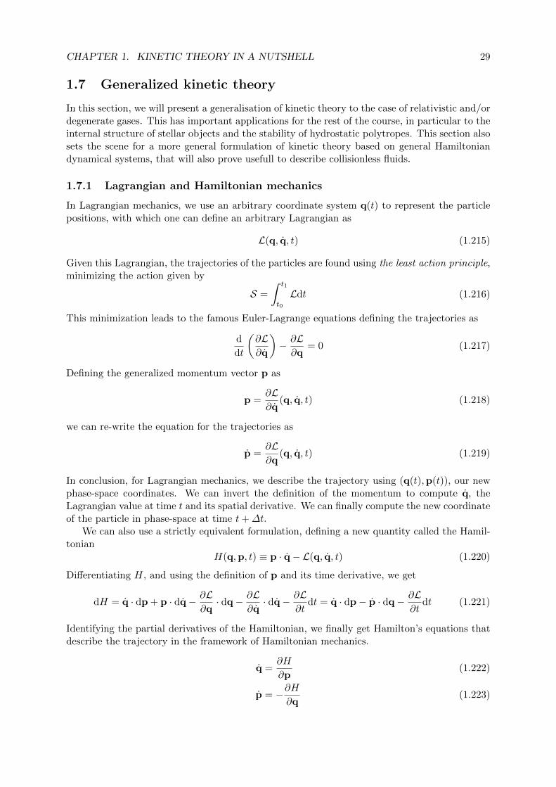
CHAPTER 1. KINETIC THEORY IN A NUTSHELL 29
1.7 Generalized kinetic theory
In this section, we will present a generalisation of kinetic theory to the case of relativistic and/ordegenerate gases. This has important applications for the rest of the course, in particular to theinternal structure of stellar objects and the stability of hydrostatic polytropes. This section alsosets the scene for a more general formulation of kinetic theory based on general Hamiltoniandynamical systems, that will also prove usefull to describe collisionless fluids.
1.7.1 Lagrangian and Hamiltonian mechanics
In Lagrangian mechanics, we use an arbitrary coordinate system q(t) to represent the particlepositions, with which one can define an arbitrary Lagrangian as
L(q, q, t) (1.215)
Given this Lagrangian, the trajectories of the particles are found using the least action principle,minimizing the action given by
S =
∫ t1
t0
Ldt (1.216)
This minimization leads to the famous Euler-Lagrange equations defining the trajectories as
d
dt
(∂L∂q
)− ∂L∂q
= 0 (1.217)
Defining the generalized momentum vector p as
p =∂L∂q
(q, q, t) (1.218)
we can re-write the equation for the trajectories as
p =∂L∂q
(q, q, t) (1.219)
In conclusion, for Lagrangian mechanics, we describe the trajectory using (q(t),p(t)), our newphase-space coordinates. We can invert the definition of the momentum to compute q, theLagrangian value at time t and its spatial derivative. We can finally compute the new coordinateof the particle in phase-space at time t+∆t.
We can also use a strictly equivalent formulation, defining a new quantity called the Hamil-tonian
H(q,p, t) ≡ p · q− L(q, q, t) (1.220)
Differentiating H, and using the definition of p and its time derivative, we get
dH = q · dp + p · dq− ∂L∂q· dq− ∂L
∂q· dq− ∂L
∂tdt = q · dp− p · dq− ∂L
∂tdt (1.221)
Identifying the partial derivatives of the Hamiltonian, we finally get Hamilton’s equations thatdescribe the trajectory in the framework of Hamiltonian mechanics.
q =∂H
∂p(1.222)
p = −∂H∂q
(1.223)

CHAPTER 1. KINETIC THEORY IN A NUTSHELL 30
This gives a more explicit formulation to obtain the trajectory in phase-space, as we do notneed to invert the Lagrangian. Recall however that both formulations are strictly equivalent.To describe a physical system, we can either give the Lagrangian, and deduce the correspond-ing Hamiltonian, or set the Hamiltonian and compute the corresponding Lagrangian. Whichformulation is the more convenient depends on the exact nature of each problem.
For a particular case, however, the Hamiltonian formulation appears more natural. This isfor Lagrangian (or Hamiltonian) functions that do not depend explicitly on time.
∂H
∂t= −∂L
∂t= 0 (1.224)
In this case, we have H(q,p), and using the chain rule, we get
dH
dt=∂H
∂q· q +
∂H
∂p· p = −p · q + q · p = 0 (1.225)
H is therefore a constant of motion along the particle’s trajectory. This lead to a natural choicefor the Hamiltonian, namely the total energy of the particle. In many cases, it can be writtenas
H(q,p) = K(p) + V (q) (1.226)
where K is the kinetic energy and V is the potential energy for the external force. We will comeback to this formulation later to describe relativistic particles.
1.7.2 Relativistic particles
Relativistic dynamics is based on the Lorentz transformation to change coordinates in space-time from the rest frame where the velocity of the particle is zero, to some other arbitrary framewith relative velocity v. The particle 4-momentum, defined as
P =(P 0, P 1, P 2, P 3
)= (E/c, px, py, pz) (1.227)
is a frame-independent quantity, so that its norm in Minkovski space is conserved through aLorentz transformation
− E2
c2+ p2
x + p2y + p2
z = −m2c2 (1.228)
where the right-hand side is the norm of the 4-momentum in the rest frame. This results in thedefinition of the energy of a relativistic particle as
E2 = p2c2 +m2c4 (1.229)
For elastic collisions, the particle rest mass will remain constant and one can define the Hamil-tonian as
H = K(p) + V (q) (1.230)
where K is the relativistic kinetic energy defined as
K =√p2c2 +m2c4 −mc2 (1.231)
Hamilton’s equation become in this case
v = q =∂K
∂p=
pc2
E=
p
γm(1.232)
p = −∂V∂q
(1.233)

CHAPTER 1. KINETIC THEORY IN A NUTSHELL 31
where we introduced the Lorentz boost factor, defined as
γ =E
mc2=
1√1− v2
c2
(1.234)
We can recover two interesting limiting cases: the non-relativistic case for which γ ' 1, v cand p mc, and the ultra-relativistic case for which γ 1, v ' c and p mc. The kineticenergy for each case writes
non-relativistic: K = mc2
√1 +
p2
m2c2−mc2 ' p2
2m(1.235)
ultra-relativistic: K =√p2c2 +m2c4 −mc2 ' pc (1.236)
Hamilton’s equation becomes quite simple in these two limiting cases, with
non-relativistic: v =∂K
∂p=
p
m(1.237)
ultra-relativistic: v =∂K
∂p= cn (1.238)
where in the second case, n = p/p is the unit vector pointing in the direction of the 3-momentum.Before we address the question of generalizing Boltzmann equation, we need to discuss the
issue of frame invariance. In physics, it is important to derive equations independent of theframe of reference. In a Galilean framework, this property is known as the Galilean invarianceof the fluid equations. In the relativistic framework, this is not so easy, as time, space and3-momentum are all affected differently by the Lorentz transformation.
The most important property of the Lorentz transformation we use here is the fact that apure spatial volume element d3x at fixed time will get modified by the Lorentz transform definedby velocity v and its corresponding Lorentz boost γ by
d3x′ = γd3x (1.239)
The 3-momentum is also affected by the Lorentz transform so that
d3p′
E′=
d3p
E(1.240)
This is a frame invariant quantity. These two properties are left to the reader as an exercise.Interestingly, if we use the Lorentz transform to the comoving frame of the particle, we have E =γmc2 and the product of the two d3xd3p = d3x0d3p0, where index 0 refers to the comoving frame.The corresponding phase-space element can therefore be considered also as frame-invariant, aproperty we will use immediately in the next section.
1.7.3 Generalized Boltzmann equation
Since our definition of phase-space has changed, we need to re-define the particle distributionfunction as
dN = f(q,p, t) d3q d3p (1.241)
where dV = d3q d3p is our new frame-invariant phase-space volume element and dN is thenumber of particle in this volume element. Since the particle number is frame-independent, weconclude that the DF is also a frame-invariant scalar. We will prove a generalized version ofLiouville’s theorem (which was introduced in the beginning of this chapter) using the following

CHAPTER 1. KINETIC THEORY IN A NUTSHELL 32
coordinate transformation associated to the trajectory of all particles within an initial phase-space volume element dV0 = d3q0 d3p0, over a small time step ∆t.
q = q0 +∂H
∂p(q0,p0)∆t (1.242)
p = p0 −∂H
∂q(q0,p0)∆t (1.243)
The new volume element can be computed using dV = det(J) dV0, where J is the Jacobianmatrix of the coordinate transformation, shown here for the one-dimensional case for simplicity
J =
[1 + ∂2H
∂p∂q∆t∂2H∂p2 ∆t
−∂2H∂q2 ∆t 1− ∂2H
∂q∂p∆t
](1.244)
We see that
det(J) = 1 +
(∂2H
∂q2
∂2H
∂p2−(∂2H
∂q∂p
)2)∆t2 (1.245)
so that the phase-space volume element remains constant in time. This property holds truefor any Hamiltonian system. We also see that this is reminiscent of the Heisenberg uncertaintyprinciple in quantum mechanics, as we have
d3q d3p = dV0 = constant (1.246)
while the uncertainty principle states that
∆qx∆px ≥~2' h (1.247)
where ∆qx and ∆px are the one-dimensional standard deviations in the position and in themomentum and ~ is the reduced Planck’s constant and h is the Planck constant. They don’thave the same meaning at all. Liouville’s theorem means that if a cloud of particles shrinksin position space, it has to expand in velocity space and vice-versa. Heisenberg uncertaintyprinciple means that if one knows the position of a quantum particle with great accuracy, thenone cannot know the momentum of the same particle very precisely, and vice-versa. On theother hand, the uncertainty principle introduces the interesting notion that there is a minimumphase-space volume element given by
δVmin = h3 (1.248)
within which quantum effects will become important. We will come back to this point later.Using Liouville’s theorem and the conservation of the particle number (in absence of colli-
sions), we conclude that f is also constant in time. Using the chain rule and Hamilton’s equation,we obtain Boltzmann equation in the general case as
∂f
∂t+ q · ∂f
∂q+ p · ∂f
∂p=∂f
∂t+∂H
∂p· ∂f∂q− ∂H
∂q· ∂f∂p
=
(Df
Dt
)coll
(1.249)
We finally get the compact form
∂f
∂t− H, f =
(Df
Dt
)coll
(1.250)
where we define the Poisson’s brackets of two scalars A and B as
A,B =∂A
∂q· ∂B∂p− ∂A
∂p· ∂B∂q
(1.251)
This form of Boltzmann’s equation has many similarities with Schrodinger’s equation in quantummechanics, but this will take us too far away from our topic.

CHAPTER 1. KINETIC THEORY IN A NUTSHELL 33
1.7.4 Generalized moments
We can define a frame-invariant first-order moment of the DF, using the relativistic 4-momentumP = (P 0, P 1, P 2, P 3) and integrating over the frame-invariant momentum-space volume element.We obtain the fluid particle 4-flow N = (N0, N1, N2, N3) for which
N i =
∫R3
P if1
γmd3p (1.252)
Note that the particle mass appears in the denominator to ensure proper units for the particle4-flow vector. Since P 0 = E/c = γmc, we get
N0 =
∫R3
cf d3p = n(x, t)c (1.253)
where we recognize the particle number density. Using for the velocity p = γmv, we also get
N1 = Nx =
∫R3
vxf d3p (1.254)
which is the particle flux in the x-direction.We can also define a second-order moment of the DF using the tensor product of the 4-
momentum and integrating again over momentum space. We obtain the energy-momentumtensor T as
T =
∫R3
P⊗Pf1
γmd3p (1.255)
The first component of the tensor we compute is
T 00 =
∫R3
E2
c2f
1
γmd3p =
∫R3
Ef d3p (1.256)
where we used E = γmc2. We recognize here again the fluid energy density that can bedecomposed into the fluid internal energy density and the fluid rest mass energy density as
T 00 =
∫R3
Kf d3p+ ρ(x, t)c2 = e(x, t) + ρ(x, t)c2 (1.257)
For sake of simplicity, we assume we are in the fluid comoving frame, so that there is no bulkkinetic energy. The space-time component of the tensor write (for x only)
T 0x = T x0 =
∫R3
E
cpxf
1
γmd3p = c
∫R3
pxf d3p (1.258)
where we see the fluid x-momentum density. Finally, the space-space components are just
T ij = Pij =
∫R3
pipjf1
γmd3p =
∫R3
vipjf d3p (1.259)
for which we used pi = γmvi. This is the momentum flux, also known as the pressure tensor (orstress tensor). We can always define a scalar pressure (even if the DF is not Maxwell-Boltzmann)as
P =1
3Tr P =
1
3
∫R3
v · pf d3p =1
3
∫R3
p2c2
Ef d3p (1.260)
We can study our two limiting case, namely non-relativistic (NR) or ultra-relativistic (UR). Forthe non-relativistic case, one has
non-relativistic: p = mv, e =
∫R3
p2
2mf d3p, P =
1
3
∫R3
p2
mf d3p =
2
3e (1.261)
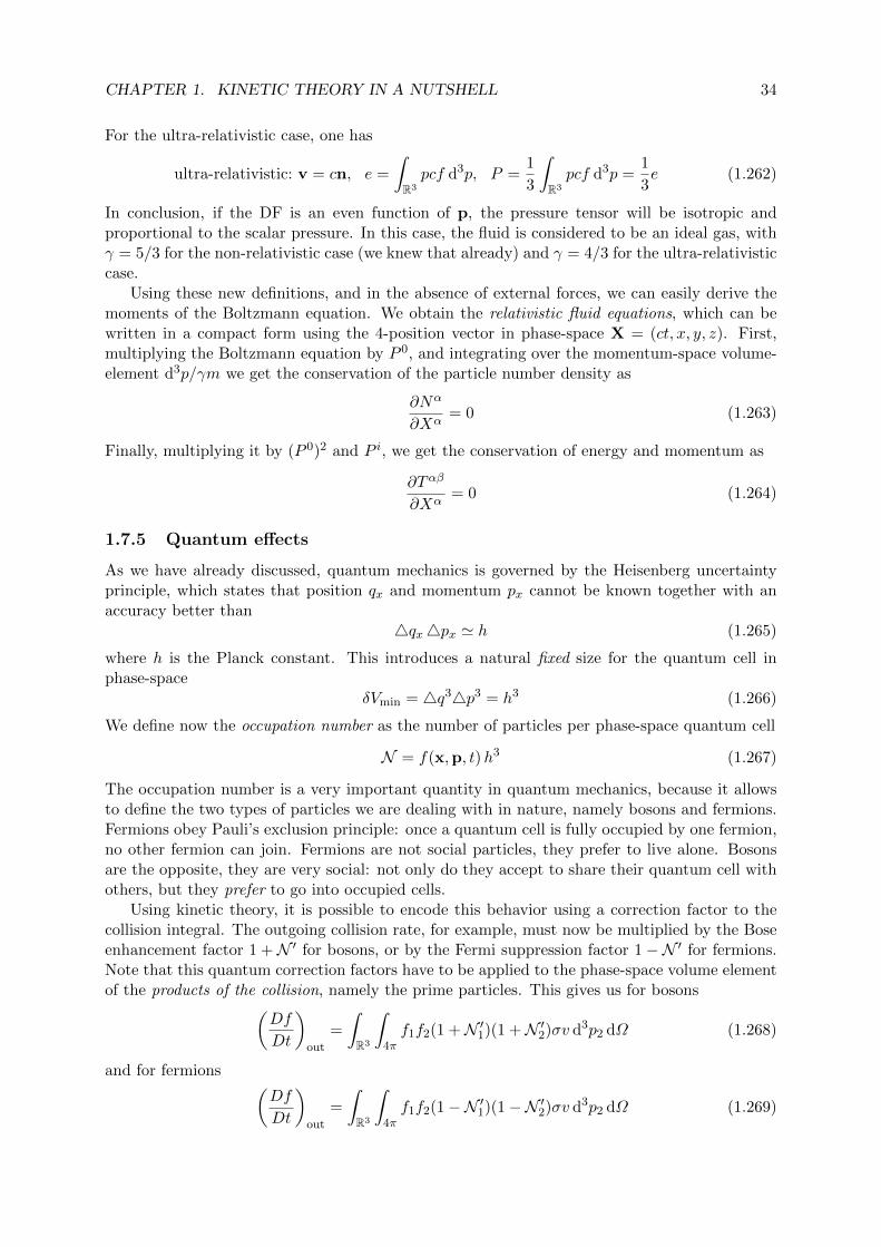
CHAPTER 1. KINETIC THEORY IN A NUTSHELL 34
For the ultra-relativistic case, one has
ultra-relativistic: v = cn, e =
∫R3
pcf d3p, P =1
3
∫R3
pcf d3p =1
3e (1.262)
In conclusion, if the DF is an even function of p, the pressure tensor will be isotropic andproportional to the scalar pressure. In this case, the fluid is considered to be an ideal gas, withγ = 5/3 for the non-relativistic case (we knew that already) and γ = 4/3 for the ultra-relativisticcase.
Using these new definitions, and in the absence of external forces, we can easily derive themoments of the Boltzmann equation. We obtain the relativistic fluid equations, which can bewritten in a compact form using the 4-position vector in phase-space X = (ct, x, y, z). First,multiplying the Boltzmann equation by P 0, and integrating over the momentum-space volume-element d3p/γm we get the conservation of the particle number density as
∂Nα
∂Xα= 0 (1.263)
Finally, multiplying it by (P 0)2 and P i, we get the conservation of energy and momentum as
∂Tαβ
∂Xα= 0 (1.264)
1.7.5 Quantum effects
As we have already discussed, quantum mechanics is governed by the Heisenberg uncertaintyprinciple, which states that position qx and momentum px cannot be known together with anaccuracy better than
4qx4px ' h (1.265)
where h is the Planck constant. This introduces a natural fixed size for the quantum cell inphase-space
δVmin = 4q34p3 = h3 (1.266)
We define now the occupation number as the number of particles per phase-space quantum cell
N = f(x,p, t)h3 (1.267)
The occupation number is a very important quantity in quantum mechanics, because it allowsto define the two types of particles we are dealing with in nature, namely bosons and fermions.Fermions obey Pauli’s exclusion principle: once a quantum cell is fully occupied by one fermion,no other fermion can join. Fermions are not social particles, they prefer to live alone. Bosonsare the opposite, they are very social: not only do they accept to share their quantum cell withothers, but they prefer to go into occupied cells.
Using kinetic theory, it is possible to encode this behavior using a correction factor to thecollision integral. The outgoing collision rate, for example, must now be multiplied by the Boseenhancement factor 1 +N ′ for bosons, or by the Fermi suppression factor 1−N ′ for fermions.Note that this quantum correction factors have to be applied to the phase-space volume elementof the products of the collision, namely the prime particles. This gives us for bosons(
Df
Dt
)out
=
∫R3
∫4πf1f2(1 +N ′1)(1 +N ′2)σv d3p2 dΩ (1.268)
and for fermions (Df
Dt
)out
=
∫R3
∫4πf1f2(1−N ′1)(1−N ′2)σv d3p2 dΩ (1.269)
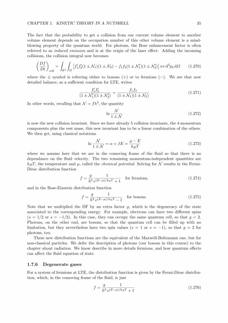
CHAPTER 1. KINETIC THEORY IN A NUTSHELL 35
The fact that the probability to get a collision from our current volume element to anothervolume element depends on the occupation number of this other volume element is a mind-blowing property of the quantum world. For photons, the Bose enhancement factor is oftenreferred to as induced emission and is at the origin of the laser effect. Adding the incomingcollisions, the collision integral now becomes(
Df
Dt
)coll
=
∫R3
∫Ω
[f ′1f′2(1±N1)(1±N2)− f1f2(1±N ′1)(1±N ′2)
]σv d3p2 dΩ (1.270)
where the ± symbol is referring either to bosons (+) or to fermions (−). We see that nowdetailed balance, as a sufficient condition for LTE, writes
f ′1f′2
(1±N ′1)(1±N ′2)=
f1f2
(1±N1)(1±N2)(1.271)
In other words, recalling that N = fh3, the quantity
lnN
1±N(1.272)
is now the new collision invariant. Since we have already 5 collision invariants, the 4-momentumcomponents plus the rest mass, this new invariant has to be a linear combination of the others.We then get, using classical notations
lnN
1±N= α+ βE =
µ− EkBT
(1.273)
where we assume here that we are in the comoving frame of the fluid so that there is nodependance on the fluid velocity. The two remaining momentum-independent quantities arekBT , the temperature and µ, called the chemical potential. Solving for N results in the Fermi-Dirac distribution function
f =g
h3
1
e(E−µ)/kBT + 1for fermions, (1.274)
and in the Bose-Einstein distribution function
f =g
h3
1
e(E−µ)/kBT − 1for bosons. (1.275)
Note that we multiplied the DF by an extra factor g, which is the degeneracy of the stateassociated to the corresponding energy. For example, electrons can have two different spins(s = 1/2 or s = −1/2). In this case, they can occupy the same quantum cell, so that g = 2.Photons, on the other end, are bosons, so that the quantum cell can be filled up with nolimitation, but they nevertheless have two spin values (s = 1 or s = −1), so that g = 2 forphotons, too.
These new distribution functions are the equivalent of the Maxwell-Boltzmann one, but fornon-classical particles. We defer the description of photons (our bosons in this course) to thechapter about radiation. We know describe in more details fermions, and how quantum effectscan affect the fluid equation of state.
1.7.6 Degenerate gases
For a system of fermions at LTE, the distribution function is given by the Fermi-Dirac distribu-tion, which, in the comoving frame of the fluid, is just
f =g
h3
1
e(E−µ)/kBT + 1(1.276)

CHAPTER 1. KINETIC THEORY IN A NUTSHELL 36
where the relativistic energy is E =√p2c2 +m2c4 = K +mc2. Defining the Fermi energy as
KF = µ−mc2 (1.277)
one can rewrite the DF as
f =g
h3
1
e(K−KF )/kBT + 1(1.278)
We see that the Fermi energy marks the transition around N = 0.5. For lower kinetic energiesK < KF , the quantum cells are almost completely occupied and N ' 1, while at larger kineticenergies, N 1, and the quantum cells are almost completely free.
Now we will consider different regimes. We start with the non-degenerate case, which isdefined by E−µ kBT . In this case, we can neglect the +1 term in the Fermi-Dirac distributionand approximate f by
f ' g
h3exp
KFkBT exp
− KkBT (1.279)
For non-relativistic gases, for which K = p2/2m, we recognize the Maxwell-Boltzmann distribu-tion function. Using the definition for the number density n, we have
n(q, t) =
∫R3
fd3p =g
h3exp
KFkBT
∫ +∞
0exp
−KkBT 4πp2dp (1.280)
In order to have a non-degenerate gas, we require the occupation number at p = 0 to be muchsmaller than one, which translates into the condition, for non-relativistic gases
expKFkBT =
nh3
g (2πmkBT )3/2< 1 (1.281)
and into the different condition for ultra-relativistic gases
expKFkBT =
nh3
g8π (kBT/c)3 < 1 (1.282)
We see that in both cases, if the gas is too dense or too cold, it will become degenerate, and Nwill approach 1 dangerously. In this case, we have no other choice but to use the Fermi-Diracdistribution. The Fermi energy can be determined using the number density as
n(q, t) =
∫R3
fd3p =g
h3
∫ +∞
0
1
expKF−KkBT +1
4πp2dp (1.283)
In the last equation, we see that kBT controls how fast the distribition transitions at K = KF
from N ' 1 to N ' 0. This leads us to define another regime for ultra-degenerate gases, forwhich
kBT KF (1.284)
In this case, we can approximate N as the Heaviside function. Defining the Fermi momentum
as KF = K(pf ) =√p2F c
2 +m2c4 −mc2, we finally obtain
n =g
h3
∫ pF
04πp2dp =
4πg
3h3p3F (1.285)
We can also compute easily the scalar pressure and the internal energy density from the previoussection as
P =1
3
g
h3
∫ pF
0
p2c2
E4πp2dp and e =
g
h3
∫ pF
0K4πp2dp (1.286)

CHAPTER 1. KINETIC THEORY IN A NUTSHELL 37
We now consider the limiting case of an ultra-degenerate and ultra-relativistic gas, for whichE ' K ' pc and
P ' 1
3
g
h3
∫ pF
0pc4πp2dp =
πcg
3h3p4F =
πgch
3
(3n
4πg
)4/3
= A( ρm
)4/3(1.287)
This is a so-called polytropic equation of state, for which the pressure depends only on the gasdensity, and not on the temperature anymore. The constant A in this case is just
A =ch
4
(3
4πg
)1/3
(1.288)
The ultra-degenerate and non-relativistic case leads to a different result, because we have nowE ' mc2 and K ' p2/2m, so that
P ' 1
3
g
h3
∫ pF
0
p2
m4πp2dp =
4πg
15mh3p5F =
4πgh2
15m
(3n
4πg
)5/3
= B( ρm
)5/3(1.289)
which is a different polytrope with constant B given by
B =h2
5m
(3
4πg
)2/3
(1.290)
In conclusion, if the gas temperature kBT mc2, we are in the non-relativistic regime. Fordensities lower than the critical density
ncrit =g
h3(2πmkBT )3/2 (1.291)
the gas in non-degenerate, and we are in the Maxwell-Boltzmann regime and the pressure isgiven by P = nkBT = 2
3e. For densities larger than the critical density, however, we enter the
regime of degenerate gases, for which P ∝ ρ5/3 independent on the temperature. If now weconsider temperature kBT mc2, we enter the ultra-relativistic regime. For densities lowerthan the critical density
ncrit =g
h38π
(kBT
c
)3
(1.292)
the gas pressure is P = nkBT = 13e. For larger densities, however, we enter the ultra-degenerate
regime for which P ∝ ρ4/3.
Chapter 2
Astrophysical fluid dynamics
After deriving the Euler equations from first principles using kinetic theory, and the non-LTEsource terms associated to viscosity and heat conduction, we are now in a position to use theseequations to describe astrophysical fluid flows. In this chapter, we will address first the dynamicsand the equilibrium of astrophysical systems, which can be either a galaxy, a star or a molecularcloud. These systems can be studied as a single object, using integral forms of the Eulerequations. We can also describe their internal structure using various geometrical approximation,namely adopting spherical or cylindrical coordinate systems. We will describe in particularaccretion flows within accretion disks and spherical Bondi stationary flows. The key question is:are those equilibrium or stationary solutions stable? This leads to the notion of waves, eitherpropagating with a fixed amplitude (in other words stable) or propagating with an exponentiallygrowing amplitude (in other words unstable). Among different types of waves, we will payparticular attention to shock waves, which play an important role in explosive astrophysicalevents such as supernovae. We will also describe important hydrodynamical instabilities at workin the interstellar medium or inside stars, leading to the theoretical description of astrophysicalturbulence.
2.1 Euler equations in integral form
In order to describe global properties of entire systems, we will derive and use integral forms forthe Euler equation. So far, we have the so-called Eulerian, conservative form
∂ρ
∂t+∇ · (ρv) = 0 (2.1)
∂
∂t(ρv) +∇ · (ρv ⊗ v + P I) = ρg (2.2)
∂E
∂t+∇ · [(E + P ) v] = ρv · g (2.3)
where the gravitational acceleration is described by the vector g = −∇φ and the gravitationalpotential φ is the solution of Poisson’s equation
∆φ = 4πGρ (2.4)
38

CHAPTER 2. ASTROPHYSICAL FLUID DYNAMICS 39
We have also derived the Euler equations in Lagrangian form, using the Lagrange time derivative,or the time derivative following the fluid motions.
Dρ
Dt= −ρ∇ · v (2.5)
ρDv
Dt= −∇P − ρg (2.6)
ρDε
Dt= −P ∇ · v (2.7)
In what follows, we will derive a new, very useful form of the Euler equations, called integralform.
2.1.1 Reynolds Transport Theorem
Before we embark into the derivation of these integral relations, we first need a little help froma well-know theorem for fluid dynamics, namely Reynolds transport theorem. We define atime-dependent scalar quantity I as the integral of an arbitrary fluid quantity α(x, t).
I =
∫V (t)
α d3x (2.8)
where V (t) is the Lagrangian volume of the system. This volume is not fixed, as it moves anddeforms as the system evolves. We are interested in the time derivative of the integral quantityI.
The main trick of Reynolds transport theorem is to introduce a colour function ψ(x), toindicate whether a fluid element x is located inside or outside the volume V (t):
ψ(x) = 1 if x ∈ V (t) (2.9)
ψ(x) = 0 if x 6∈ V (t) (2.10)
This colour function can be seen as painting particles initially inside the volume V (t) in whiteand those initially outside in black. We can express the integral over the volume as an integralover the entire space.
I =
∫V (t)
α d3x =
∫R3
αψ d3x (2.11)
Since the integration bounds are now fixed, we can easily compute the time derivative of I as
I(t) =
∫R3
[∂α
∂tψ + α
∂ψ
∂t
]d3x =
∫R3
[ψ∂α
∂t− αv · ∇ψ
]d3x (2.12)
where we used in the rightmost equation the property that the colour function does not changeif you move with the fluid. In other words, its Lagrange time derivative is zero.
Dψ
Dt=∂ψ
∂t+ v · ∇ψ = 0 (2.13)
We now use the vector calculus relation ∇ · (αψv) = ψ∇ · (αv) + αv · ∇ψ and obtain
I(t) =
∫R3
(ψ
[∂α
∂t+∇ · (αv)
]−∇ · (αψv)
)d3x (2.14)
In order to work out the second term in the integral, we use the divergence theorem∫V0
∇ · v d3x =
∫S0
v · n dS (2.15)
CHAPTER 2. ASTROPHYSICAL FLUID DYNAMICS 40
applied to the vector αψv, using a fixed control volume much larger than V (t). This gives us∫V0
∇ · (αψv) d3x =
∫S0
αψv · n dS = 0 (2.16)
because ψ = 0 on the boundary of this larger control volume since the boundary is entirelyoutside V (t). We now take the limit V0 → +∞ so that the integral over R3 also vanishes. Wethus obtain the final result of Reynolds transport theorem.
dI
dt=
∫V (t)
[∂α
∂t+∇ · (αv)
]d3x (2.17)
2.1.2 Integral conservation laws
Remember that we derived fluid or macroscopic conservation laws by integrating over velocity(or momentum) space the Boltzmann equation using 3 microscopic conservation laws. We nowderive system or integral conservation laws by integrating the Euler equations over the volumeof our system.
The total mass of the system is given by the sum of the mass of all its fluid elements
M =
∫V (t)
ρ d3x (2.18)
Using the Reynolds transport theorem, we can now easily find the rate of change of the totalmass as
dM
dt=
∫V (t)
[∂ρ
∂t+∇ · (ρv)
]d3x = 0 (2.19)
Indeed, the quantity between brackets is nothing else than the continuity equation, which iszero, hence M = 0. The mass of the system defined by V (t) is therefore a constant. The keypoint here is that the volume V (t) is the Lagrangian volume that moves and deforms togetherwith the system. This reasoning is different from taking the integral over a fixed volume V0
independent of the system. In this case
M0 =
∫V0
ρd3x (2.20)
and
M0 =
∫V0
∂ρ
∂td3x = −
∫V0
∇ · (ρv) d3x = −∫S0
ρv · n dS (2.21)
which expressed the total mass flux in/out of the volume.We can also define the total momentum of the system as
MV =
∫V (t)
ρv dV (2.22)
where we exploit the fact that the mass is a constant and we introduced the system velocity V.Taking the time derivative of the total momentum and applying Reynolds transport theorem,we get
MdV
dt=
∫V (t)
[∂
∂t(ρv) +∇ · (ρv ⊗ v)
]dV =
∫V (t)
ρgdV −∫V (t)∇ · (P I) dV (2.23)
CHAPTER 2. ASTROPHYSICAL FLUID DYNAMICS 41
Defining the mean system gravity as
MG =
∫V (t)
ρg dV (2.24)
and using the divergence theorem applied to the isotropic pressure tensor∫V (t)∇ · (P I) dV =
∫S(t)
Pn dS (2.25)
we get the system momentum conservation equation
MdV
dt= MG−
∫S(t)
Pn dS (2.26)
We see that we can describe the trajectory of the system as a whole very much like a singleparticle of mass M , velocity V and gravity G, with an additional drag force due to the pressurefield applied to the surface of the system.
2.1.3 Specific variables
A special and very useful case of the Reynolds transport theorem can be derived, when α canbe expressed as the product of the density and what is called a specific variable: α = ρβ. If αrepresents a physical quantity per unit volume, β represents the same quantity per unit mass.For example, the specific internal energy ε, defined as e = ρε, has units of [erg/g], while e, theinternal energy, has units of [erg/cm3]. As usual, the integral form is written as
I(t) =
∫V (t)
ρβ dV (2.27)
Using Reynolds transport theorem, we write its time derivative as
I(t) =
∫V (t)
[∂
∂t(ρβ) +∇ · (ρβv)
]dV (2.28)
=
∫V (t)
[β∂ρ
∂t+ ρ
∂β
∂t+ β∇ · (ρv) + ρv · ∇β
]dV (2.29)
Using the continuity equation and the definition of the Lagrange time derivative, we obtain thefundamental relation
d
dt
∫V (t)
ρβ dV =
∫V (t)
ρDβ
DtdV (2.30)
We call this equation the second form of Reynolds transport theorem. We can for example definethe system centre of mass coordinates as the vector X
MX =
∫V (t)
ρx dV (2.31)
Using the second form of Reynolds transport theorem, we get
Md
dtX =
∫V (t)
ρDx
DtdV =
∫V (t)
ρv dV = MV (2.32)
CHAPTER 2. ASTROPHYSICAL FLUID DYNAMICS 42
We see that the centre of mass velocity is equal to the system velocity defined earlier. Theposition of the centre of mass is therefore the coordinate of this virtual particle that we use todescribe the system as a whole.
We can also define the specific volume as v = 1/ρ, the volume per unit mass. The totalvolume is trivially computed as
V (t) =
∫V (t)
1 dV =
∫V (t)
ρv dV (2.33)
According to the second form of Reynolds transport theorem, the rate of change of the volumeof the system is now simply
dV
dt=
∫V (t)
ρDv
DtdV =
∫V (t)
1
v
Dv
DtdV (2.34)
We can also use the first form of Reynolds transport theorem with α = 1 and get immediately
dV
dt=
d
dt
∫V (t)
1 dV =
∫V (t)∇ · v dV (2.35)
Identifying the terms under the integral, we deduce that the rate of change of the specific volumeis given be
1
v
Dv
Dt= ∇ · v (2.36)
a relation that proved handy in the first chapter, when we applied the first law of thermodynamicsto the Euler equations in Lagrangian form.
2.2 Virial Theorem
The virial theorem is probably the most famous theorem in theoretical astrophysics. The ideais to derive an expression for the time evolution of the scalar moment of inertia of the systemof interest. The moment of inertia tensor is defined as
Iij(t) =
∫V (t)
ρ xixj dV (2.37)
Taking the trace of the tensor, we can define the scalar moment of inertia as
I(t) =
∫V (t)
ρ |x|2 dV where |x|2 = x2 + y2 + z2 (2.38)
We can also compute the global expansion or contraction rate of the system using the timederivative of the scalar moment of inertia, using the second form of Reynolds theorem
I(t) =dI
dt=
∫V (t)
2ρxDx
DtdV = 2
∫V (t)
ρx · v dV (2.39)
Let’s assume the system is contracting, which corresponds to I < 0. The second-order timederivative will tell us whether the system will keep on contracting at a faster and faster rateI < 0, or if it will eventually stop contracting and even expand later I > 0. In the former case,we say that the system is collapsing. Using again Reynolds theorem, we have
1
2I(t) =
1
2
d2I
d2t=
∫V (t)
[ρ v2 + ρx · Dv
Dt
]dV (2.40)
CHAPTER 2. ASTROPHYSICAL FLUID DYNAMICS 43
We can simplify this by using the Euler equation in Lagrangian form ρDvDt = −∇P + ρg, where
g is the gravitational acceleration
1
2I(t) =
∫V (t)
ρv2 dV +
∫V (t)
ρx · g dV −∫V (t)
x · ∇P dV (2.41)
(1) (2) (3) (2.42)
The first term is exactly twice the kinetic energy of the system
(1) = 2K =
∫V (t)
ρv2 dV (2.43)
The second term is called the virial of the system. It comes from Latin vis that means force.
(2) = V ≡∫V (t)
ρx · g dV (2.44)
Note that this is in general not equal to the gravitational potential of the system, as the gravitycan also come from an external objects. The third term is related to the scalar thermal pressure.Using the vector relation ∇ · (Px) = x · ∇P + P∇ · x, it can be decomposed into
(3) = −∫V (t)
x · ∇P dV = −∫S(t)
P x · n dS +
∫V (t)
3P dV = T − S (2.45)
where we used the trick ∇ · x = 3. We can decompose this term into two contributions: first,the thermal contribution written as
T ≡∫V (t)
3P dV (2.46)
and the surface term
S ≡∫S(t)
P x · n dS (2.47)
This gives us the final form of the virial theorem as 12 I = 2K + V + T − S, or
1
2I(t) =
∫V (t)
ρv2 dV +
∫V (t)
ρx · g dV + 3
∫V (t)
P dV −∫S(t)
P x · n dS (2.48)
For a non-relativistic Maxwell-Boltzmann gas, we have e = 32P , so that the pressure can be
replaced by the internal energy using 2E = T and the kinetic energy is now the sum of thebulk kinetic energy and the thermal kinetic energy we can write the virial theorem in a compactform, quite easy to remember,
1
2I = 2(K + E) + V − S (2.49)
This is a powerful theorem that directly gives us information about the stability of a system.When I < 0, the system is collapsing; when I > 0 it is expanding. When I = 0, the termsbalance each other and the system is in equilibrium.
Analyzing each term, we see that since the kinetic energy (bulk + internal) is always positive,it will always drive the system towards expansion. The virial is often negative, since g pointstowards the main source of gravity, which, for an isolated system, is usually the center of mass.But V can also be positive, if tidal forces from an external object are also present. The surfaceterm comes with a negative sign, driving the system towards contraction. This term correspondsto the pressure of the external environment onto the boundary of the system. If the externalpressure is small compared to the internal pressure, which is usually the case for stars, we canignore the surface term and set S = 0.
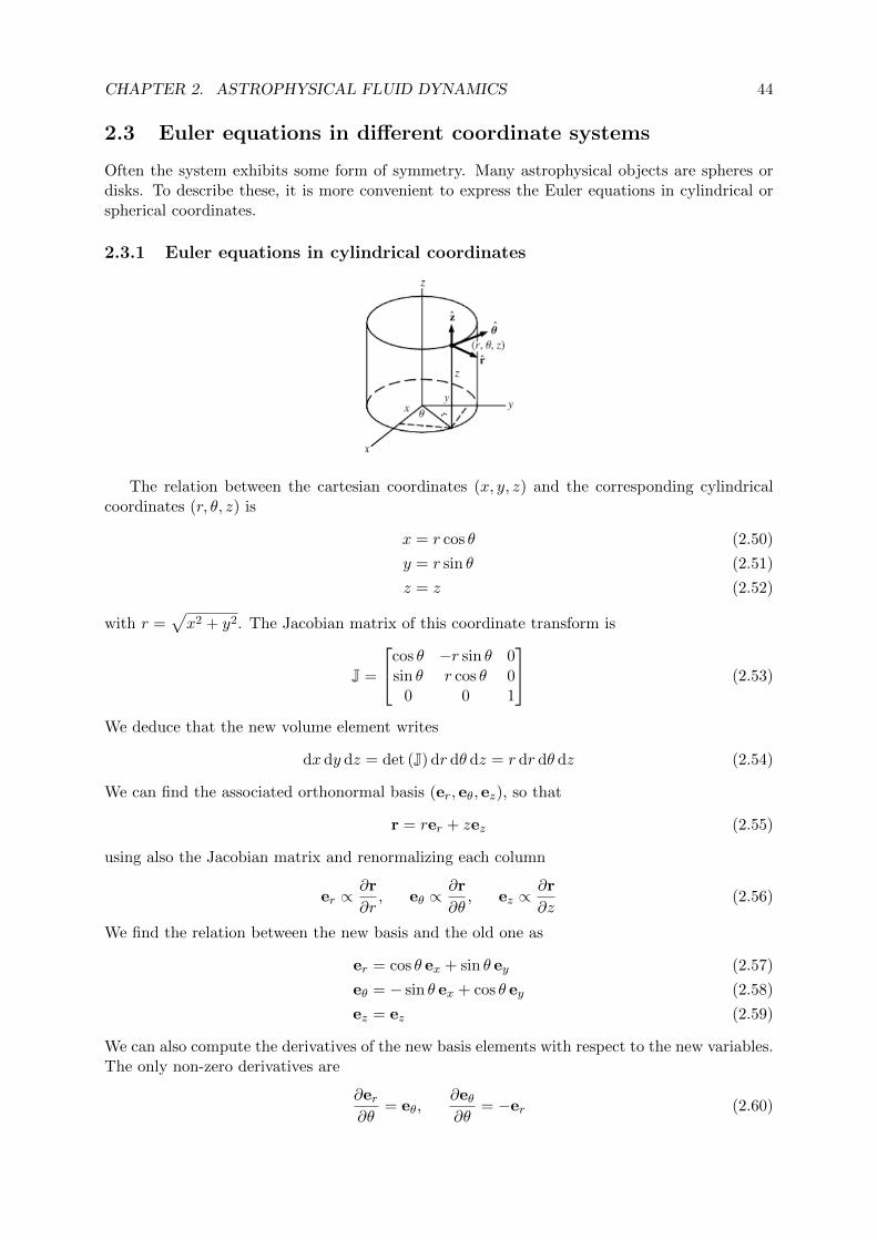
CHAPTER 2. ASTROPHYSICAL FLUID DYNAMICS 44
2.3 Euler equations in different coordinate systems
Often the system exhibits some form of symmetry. Many astrophysical objects are spheres ordisks. To describe these, it is more convenient to express the Euler equations in cylindrical orspherical coordinates.
2.3.1 Euler equations in cylindrical coordinates
The relation between the cartesian coordinates (x, y, z) and the corresponding cylindricalcoordinates (r, θ, z) is
x = r cos θ (2.50)
y = r sin θ (2.51)
z = z (2.52)
with r =√x2 + y2. The Jacobian matrix of this coordinate transform is
J =
cos θ −r sin θ 0sin θ r cos θ 0
0 0 1
(2.53)
We deduce that the new volume element writes
dx dy dz = det (J) dr dθ dz = r dr dθ dz (2.54)
We can find the associated orthonormal basis (er, eθ, ez), so that
r = rer + zez (2.55)
using also the Jacobian matrix and renormalizing each column
er ∝∂r
∂r, eθ ∝
∂r
∂θ, ez ∝
∂r
∂z(2.56)
We find the relation between the new basis and the old one as
er = cos θ ex + sin θ ey (2.57)
eθ = − sin θ ex + cos θ ey (2.58)
ez = ez (2.59)
We can also compute the derivatives of the new basis elements with respect to the new variables.The only non-zero derivatives are
∂er∂θ
= eθ,∂eθ∂θ
= −er (2.60)
CHAPTER 2. ASTROPHYSICAL FLUID DYNAMICS 45
We can now compute the differential form dr which represents a small variation of the positionvector r. Using the chain rule, we have
dr = dr er + r der + dz ez = dr er + r dθ eθ + dz ez (2.61)
The frame invariant definition of the gradient of a scalar function f(r, θ, z) is
df = ∇f · dr (2.62)
We can also compute it using the chain rule as
df =∂f
∂rdr +
∂f
∂θdθ +
∂f
∂zdz (2.63)
Identifying the terms in the two relations, we get for the gradient vector of f in cylindricalcoordinates
∇f =
(∂f
∂r,1
r
∂f
∂θ,∂f
∂z
)T
(2.64)
or in vector form
∇f = er∂f
∂r+ eθ
1
r
∂f
∂θ+ ez
∂f
∂z(2.65)
The divergence of a vector can be computed using the frame invariant notation ∇ · v, takingliterally the scalar product of the gradient operator and the vector v = vrer + vθeθ + vzez.
∇ · v =
(er∂
∂r+ eθ
1
r
∂
∂θ+ ez
∂
∂z
)· (vrer + vθeθ + vzez) (2.66)
The only non-trivial terms are
∂
∂θ(vrer) =
∂vr∂θ
er + vreθ (2.67)
∂
∂θ(vθeθ) =
∂vθ∂θ
eθ − vθer (2.68)
Using the fact that we have an orthonormal basis, we finally get
∇ · v =∂vr∂r
+vrr
+1
r
∂vθ∂θ
+∂vz∂z
(2.69)
Using the same trick, we can also compute the Lagrange derivative of a scalar f in a frameinvariant way as usual
Df
Dt=∂f
∂t+ v · ∇f (2.70)
and take the scalar product between v and the gradient operator in cylindrical coordinate toobtain
Df
Dt=∂f
∂t+ vr
∂f
∂r+vθr
∂f
∂θ+ vz
∂f
∂z(2.71)
The Lagrange derivative of the velocity field (or any vector field for that matter) is written in acoordinate system invariant was as
Dv
Dt=∂v
∂t+ (v · ∇) v (2.72)
CHAPTER 2. ASTROPHYSICAL FLUID DYNAMICS 46
We have already written the operator v · ∇ in cylindrical coordinates,
(v · ∇) = vr∂
∂r+vθr
∂
∂θ+ vz
∂
∂z(2.73)
We apply it now to a vector field
(v · ∇) (vrer + vθeθ + vzez) (2.74)
which gives us the Lagrange derivative of the coordinates that remains parallel to the basisvector, but also of the basis vectors er and eθ, which project to the other dimension
Dv
Dt=DvrDt
er +DvθDt
eθ +DvzDt
ez +vθvrr
eθ −v2θ
rer (2.75)
Using the frame invariant, Lagrangian form of the momentum conservation equation
Dv
Dt= −1
ρ∇P −∇φ (2.76)
where we write the gravitational acceleration as g = −∇φ, we can now write the Euler equationsin cylindrical coordinates
DvrDt
=v2θ
r− 1
ρ
∂P
∂r− ∂φ
∂r(2.77)
DvθDt
= −vrvθr− 1
ρ
1
r
∂P
∂θ− 1
r
∂φ
∂θ(2.78)
DvzDt
= −1
ρ
∂P
∂z− ∂φ
∂z(2.79)
where the geometrical terms have been placed on the right-hand side, together with the pressuregradient and the gravitational acceleration, and are called the centrifugal acceleration. Themass and energy conservation equations are usually expressed in conservative form using theexpression of the divergence operator in cylindrical coordinates
∂ρ
∂t+∇ · (ρv) = 0 (2.80)
∂E
∂t+∇ · [(E + P )v] = ρg · x (2.81)
We can also expressed the stress tensor in cylindrical coordinates using the matrix, componentsform as
S =
Srr Srθ SrzSθr Sθθ SθzSzr Szθ Szz
(2.82)
but also using a tensorial basis as
S =∑i
∑j
Sijei ⊗ ej (2.83)
Index i stands for line number i of the matrix, while index j stands for column number j. Thevelocity gradient tensor writes in Cartesian coordinates
G =∑i
∑j
∂vi∂xj
ei ⊗ ej = v ⊗∇ (2.84)

CHAPTER 2. ASTROPHYSICAL FLUID DYNAMICS 47
where the last form is conveniently independent of the coordinate system. The∇ operator standson the right of the tensor product ⊗, because the column number indicates which variables thederivative is taken from. The transpose of the gradient tensor is just
GT = ∇⊗ v (2.85)
In cylindrical coordinates, we have
G = (vrer + vθeθ + vzeu)⊗(∂(.)
∂rer +
1
r
∂(.)
∂θeθ +
∂(.)
∂zeu
)(2.86)
Here again, we have to take the θ-derivative of the product vrer as
vrer ⊗1
r
∂(.)
∂θeθ =
1
r
∂(vrer)
∂θ⊗ eθ =
1
r
∂vr∂θ
er ⊗ eθ +vθr
eθ ⊗ eθ (2.87)
and the θ-derivative of the product vθeθ as
vθeθ ⊗1
r
∂(.)
∂θeθ =
1
r
∂(vθeθ)
∂θ⊗ eθ =
1
r
∂vθ∂θ
eθ ⊗ eθ −vθr
er ⊗ eθ (2.88)
so that the velocity gradient tensor writes
G =
∂vr∂r 1r∂vr∂θ −
vθr
∂vr∂z
∂vθ∂r
1r∂vθ∂θ + vr
r∂vθ∂z
∂vz∂r
1r∂vz∂θ
∂vz∂z
(2.89)
Finally, the stress tensor, which is given by the coordinate-independent form,
S = G + GT − 2
3(∇ · v) I (2.90)
can be written in cylindrical coordinates as
S =
2∂vr∂r −23 (∇ · v) ∂vθ
∂r + 1r∂vr∂θ −
vθr
∂vz∂r + ∂vr
∂z∂vθ∂r + 1
r∂vr∂θ −
vθr 2
(1r∂vθ∂θ + vr
r
)− 2
3 (∇ · v) ∂vθ∂z + 1
r∂vz∂θ
∂vz∂r + ∂vr
∂z∂vθ∂z + 1
r∂vz∂θ 2∂vz∂z −
23 (∇ · v)
(2.91)
To compute the viscous stress, we need to take the divergence of the stress tensor using theframe invariant form ∇ · S, which writes, using the ∇ operator and the tensorial basis as
∇ · S =[er
∂∂r + eθ
1r∂∂θ + ez
∂∂z
]·
Srrer ⊗ er + Srθer ⊗ eθ + Srzer ⊗ ez+Sθreθ ⊗ er + Sθθeθ ⊗ eθ + Sθzeθ ⊗ ez+Szrez ⊗ er + Szθez ⊗ eθ + Szzez ⊗ ez
(2.92)
For this, we need to take the derivative of the product of three terms such as, for example
1
r
∂
∂θ(Sθθeθ ⊗ eθ) =
1
r
∂Sθθ∂θ
eθ ⊗ eθ −Sθθr
er ⊗ eθ −Sθθr
eθ ⊗ er (2.93)
and then take the scalar product with eθ using
eθ · (eθ ⊗ eθ) = (eθ · eθ) eθ = eθ (2.94)
eθ · (er ⊗ eθ) = (eθ · er) eθ = 0 (2.95)
eθ · (eθ ⊗ er) = (eθ · eθ) er = er (2.96)
We finally obtain the divergence of the tensor in cylindrical coordinates as
∇ · S =
∂Srr∂r + ∂Szr∂z + 1
r∂Sθr∂θ + Srr
r −Sθθr
∂Srθ∂r + ∂Szθ
∂z + 1r∂Sθθ∂θ + Srθ
r + Sθrr
∂Srz∂r + ∂Szz
∂z + 1r∂Sθz∂θ
(2.97)
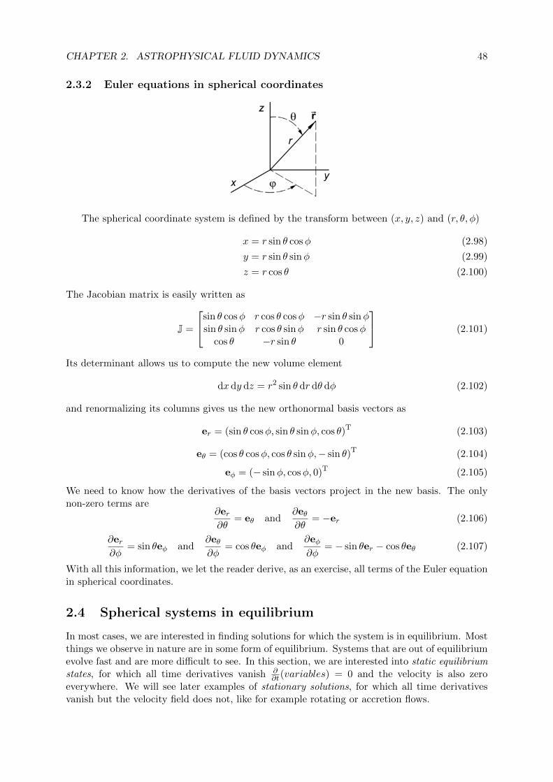
CHAPTER 2. ASTROPHYSICAL FLUID DYNAMICS 48
2.3.2 Euler equations in spherical coordinates
The spherical coordinate system is defined by the transform between (x, y, z) and (r, θ, φ)
x = r sin θ cosφ (2.98)
y = r sin θ sinφ (2.99)
z = r cos θ (2.100)
The Jacobian matrix is easily written as
J =
sin θ cosφ r cos θ cosφ −r sin θ sinφsin θ sinφ r cos θ sinφ r sin θ cosφ
cos θ −r sin θ 0
(2.101)
Its determinant allows us to compute the new volume element
dx dy dz = r2 sin θ dr dθ dφ (2.102)
and renormalizing its columns gives us the new orthonormal basis vectors as
er = (sin θ cosφ, sin θ sinφ, cos θ)T (2.103)
eθ = (cos θ cosφ, cos θ sinφ,− sin θ)T (2.104)
eφ = (− sinφ, cosφ, 0)T (2.105)
We need to know how the derivatives of the basis vectors project in the new basis. The onlynon-zero terms are
∂er∂θ
= eθ and∂eθ∂θ
= −er (2.106)
∂er∂φ
= sin θeφ and∂eθ∂φ
= cos θeφ and∂eφ∂φ
= − sin θer − cos θeθ (2.107)
With all this information, we let the reader derive, as an exercise, all terms of the Euler equationin spherical coordinates.
2.4 Spherical systems in equilibrium
In most cases, we are interested in finding solutions for which the system is in equilibrium. Mostthings we observe in nature are in some form of equilibrium. Systems that are out of equilibriumevolve fast and are more difficult to see. In this section, we are interested into static equilibriumstates, for which all time derivatives vanish ∂
∂t(variables) = 0 and the velocity is also zeroeverywhere. We will see later examples of stationary solutions, for which all time derivativesvanish but the velocity field does not, like for example rotating or accretion flows.
CHAPTER 2. ASTROPHYSICAL FLUID DYNAMICS 49
2.4.1 Uniform spheres
One of the simplest systems imaginable is a spherical gas cloud of radius R with a uniformdensity, collapsing under its own gravity and possibly finding an equilibrium state. To find suchequilibrium conditions, we write the virial theorem as
1
2I = 2K + T + V − S (2.108)
Assuming static equilibrium for our system (v = 0)
K =
∫V
1
2ρv2dV = 0 (2.109)
The thermal term can be also simplified as
T =
∫V
3PdV = 3P
(4π
3R3
)(2.110)
and the surface term is simply
S =
∫SPext(Rer · er)dS = Pext
(4πR3
)(2.111)
where we use the fact that the outward pointing normal vector n = er and we define Pext as theexternal pressure acting on the surface of the sphere.
Gravity of a uniform sphere
To find the virial V , we first have to compute the gravitational acceleration g inside the uniformsphere. The gravitational potential obeys the Poisson equation
4φ = 4πGρ with g = −∇φ (2.112)
We consider a sphere of radius r < R. Integrating over its volume, we get on one hand∫V4φ dV = 4πG
∫VρdV = 4πGM(< r) (2.113)
where M(< r) is the enclosed mass. For a uniform density sphere, the enclose mass is just
M(< r) =
∫ r
0ρ4πr2 dr = ρ
4π
3r3 (2.114)
On the other hand, using the vector calculus relation 4φ = ∇ · (∇φ) = −∇ · g, we apply thedivergence theorem on the same sphere of radius r < R∫
V4φ dV = −
∫V∇ · g dV = −
∫S
g · n dS = −gr4πr2 (2.115)
Combining these equations gives us the gravitational acceleration
gr = −GM(< r)
r2= −4π
3Gρr (2.116)
The virial of the uniform sphere now becomes
V =
∫Vρg · x dV = −ρ
∫ R
0grr4πr
2dr =4π
3Gρ24π
R5
5(2.117)
CHAPTER 2. ASTROPHYSICAL FLUID DYNAMICS 50
Virial equilibrium condition
This results into the equilibrium condition
1
2I = 3P
4
3πR3 − 4π
3Gρ24π
R5
5− Pext4πR
3 = 0 (2.118)
We see that the surface term, if the external pressure is equal to the internal one, balancesout exactly the thermal term, leaving the system with no other choice that collapsing under itsown gravity. The radius will start shrinking, and very quickly, the internal pressure will risesignificantly above the external one, so we can safely assume Pext = 0 in the previous equation.The final equilibrium condition can be written as
P =4π
15Gρ2R2 (2.119)
If we consider now a non-relativistic, non-degenerate Maxwell-Boltzmann gas, the pressure isgiven by
P = ρkBT
m(2.120)
where T is the uniform temperature of the sphere. This lead to the virial condition on the gastemperature as
kBT
m=
1
5
GM
R(2.121)
where we use the definition of the total mass as
M = ρ4π
3R3 (2.122)
The problem here is that we need to know the temperature to determine the size of the star,at fixed mass. Therefore, we need to solve in parallel for the energy equation, with possiblyadditional heating and cooling processes within the star.
Degenerate stars
Degenerate stars are however much simpler, as the pressure depends only on density. We cantherefore use the equation of state we have derived in the previous section as
P = A( ρm
)Γ= A
(M
m4π3 R
3
)Γ(2.123)
where Γ = 53 in the non-relativistic case and Γ = 4
3 in the ultra-relativistic one. We plug thisinto the virial relation to obtain
A
(M
m4π3 R
3
)Γ−2
=4π
15Gm2R2 (2.124)
or, after some manipulations
M =4π
3m
(4πGm2
15A
) 1Γ−2
R3Γ−4Γ−2 (2.125)
In the non-relativistic case, we obtain a possible equilibrium configuration if the system followsthe proper mass-radius relation M ∝ R−3 or strikingly MV =constant. In other words, for

CHAPTER 2. ASTROPHYSICAL FLUID DYNAMICS 51
a given mass, there is always a radius that the star can reach (by contracting or expanding)that corresponds to an equilibrium solution. In the ultra-relativistic case, however, we see thatthe power law vanishes and the only equilibrium solution is for a single mass. Plugging in theconstant A we derived in the last chapter for the ultra-relativistic, ultra-degenerate case, we getthe Chandrasekhar mass
Meq =4π
3m2
(15hc
16πG
) 32(
3
4πg
) 12
' 1.5 M (2.126)
which depends only on fundamental constants. We used for m twice the proton mass mp =1.66× 10⁻²⁴g to account for elements heavier than helium and the degeneracy parameter g = 2.A more accurate computation gives Meq ' 1.4 M, quite close to the present derivation.
Turbulent molecular clouds
We now consider very different objects than white dwarfs or neutrons stars: molecular clouds inthe interstellar medium. We simplify their description assuming they are spherical and uniform.We also use the observational fact that they are turbulent. We will define turbulence rigorouslyin the following chapters, but for the time being, we consider that the kinetic energy term K 6= 0because of macroscopic random motions within the cloud. We write the kinetic term as
K =
∫V
1
2ρv2 dV =
1
2M(σ2
x + σ2y + σ2
z) =3
2Mσ2
1D (2.127)
where σx is the velocity dispersion of the turbulence in the x-direction. The last equationassumes that the turbulence is isotropic so that each direction sees the same dispersion, notedσ1D. Note that the 1D turbulence is precisely what is measured during astronomical observations,as absorption or emission lines give access to line of sight broadening due to turbulence. Theobserved turbulence in the interstellar medium is supersonic. This means that σ1D a, wherea is the isothermal sound speed, related to the isothermal temperature of the ISM by
a =
√kBT0
m(2.128)
Since T0 ' 10 K in the ISM, and the Hydrogen molecule mass is m = 2mp, we have a '0.2 km/sec. The measured velocity dispersion in molecular cloud is much higher with σ1D '1− 5 km/sec. In the virial analysis, we can therefore safely ignore the thermal term, and define
αvir = −2K
V=
5Rσ21D
GM(2.129)
If αvir < 1, the cloud is collapsing, while for αvir > 1, it is expanding. Equilibrium is obtainedfor αvir = 1. Observed molecular clouds have αvir ' 1 − 3, which seems to indicate that theyare slightly super-virial. The fact that we do not see any cloud with αvir < 1 is consistent withthe idea that they are unstable, so they collapse quickly. We do see however many clouds withαvir > 1. They are probably slowly expanding, or we have to take into account the surface termS that may stabilize them.
2.4.2 Hydrostatic equation for spherical systems
When the system is in static equilibrium, the velocity is zero everywhere. As a consequence,gravity and pressure forces must balance each other exactly. The system is said to be in hy-drostatic equilibrium. Such solutions are found using the Euler and the Poisson equations. We
CHAPTER 2. ASTROPHYSICAL FLUID DYNAMICS 52
assume here again that we have a strict spherical symmetry, but this time, the system is notuniform but has an internal structure. We are seeking for a solution in one dimension, thatdepends only on the radial coordinate, so that
ρ = ρ(r) , P = P (r) , φ = φ(r) (2.130)
Because v = 0, the mass and the energy conservation equations are automatically satisfied andall centrifugal terms are zero. The momentum conservation equation, written in Lagrangianform, becomes
DvrDt
= 0 = −1
ρ
∂P
∂r− ∂φ
∂r(2.131)
Using the Poisson equation in spherical coordinates, we have
4φ =1
r2
∂
∂r
(r2∂φ
∂r
)= 4πGρ (2.132)
This leads to a system of two equations that describe our hydrostatic equilibrium
1
ρ
∂P
∂r= −∂φ
∂r(2.133)
1
r2
∂
∂r
(r2∂φ
∂r
)= 4πGρ (2.134)
To be able to solve this system of three unknown variables with only two equations, we need anequation of state for the pressure.
Lane-Emden equation for polytropes
We will study here the internal structure of stellar polytropes. We use the following generalform for our polytropic EoS
P = P0
(ρ
ρ0
)Γ(2.135)
where P0 and ρ0 will be defined later. Replacing the gradient of the potential in the Poissonequation by the gradient of the pressure, we obtain
1
r2
∂
∂r
(r2
ρ
∂P
∂r
)= −4πGρ (2.136)
Now plugging in the EoS, we obtain the following hydrostatic equation
1
r2
∂
∂r
(r2Γ
P
ρ2
∂ρ
∂r
)= −4πGρ (2.137)
This equation is central to the study of stellar interiors. We will now perform a change ofvariable to obtain a dimensionless equation. Introduction x and θ as
x =r
r0, ρ = ρ0θ
n , P = P0θn+1 (2.138)
where the parameter n is defined as
Γ = 1 +1
n(2.139)
and r0, the Lane-Emden radius, is given by
r20 =
n+ 1
4πG
P0
ρ20
(2.140)
CHAPTER 2. ASTROPHYSICAL FLUID DYNAMICS 53
Using these new variables, we get the following second-order, non-linear ordinary differentialequation (ODE) called the Lane-Emden equation
1
x2
∂
∂x
(x2 ∂θ
∂x
)= −θn (2.141)
In the general case, for any value of n, this equation has to be solved numerically, with boundaryconditions
θ(0) = 1 and θ(0)′ = 0 (2.142)
These solutions corresponds to a central density equal to ρ0. The other variable P0 is thecorresponding polytropic pressure, computed as
P0 = A(ρ0
m
)Γ(2.143)
The Lane-Emden radius is then fully specified. An interesting limiting case is n = 5, for whichthe analytical solution is (left to the reader as an exercise)
θ(x) =1√
1 + x2
3
(2.144)
This solution is typical of hydrostatic polytropes, with a central, constant density core of sizercore =
√3r0, surrounded by an envelope with a power law density profile with ρ ∝ r−1.
Bonnor-Ebert sphere for an isothermal gas
We now consider the special case of molecular clouds in the interstellar medium. We have seenthat these objects are dominated by turbulence. In the densest regions of the clouds, whereturbulence dissipates, local collapse is possible and molecular cores are forming. These coresare very difficult to observe because they are completely obscured by dust. Nevertheless, theyappear as quasi-hydrostatic structures and are likely to be the sites of star formation. They arestellar nurseries.
The thermal state of the interstellar medium is governed by cooling and heating processes.We will see in the chapter on radiation processes how to compute these extra terms that appearin the energy equation, written here in Lagrangian form.
ρDε
Dt= −P∇ · v + nΓ0 − n2Λ(T ) (2.145)
Γ0 is called the heating function and depends on the local radiation field, assumed to be constantat a given location in the Galaxy. Λ is the cooling function and depends on the temperature.The heating rate is proportional to the gas density because it features collision between photonsand atoms, while the cooling rate scales as the square of the density because it is due to inelasticcollisions between two atoms or two molecules. In the ISM, especially at higher density, bothterms can dominates over the pdV term and the gas is in thermal equilibrium, defined by
Λ(T ) =Γ0
n→ T = Teq(ρ) (2.146)
We see that the temperature is fixed by a thermostat, and the gas pressure (or its equation ofstate) becomes independent on temperature as
P = ρkBTeq(ρ)
m(2.147)
CHAPTER 2. ASTROPHYSICAL FLUID DYNAMICS 54
At densities larger than 100 H/cc, inside molecular clouds, we have Teq ' 10 K and the gasbecomes isothermal.
In this case, for sake of simplicity, we define the pressure by
P = ρa2 where a =
√kBT0
m(2.148)
where a is called the isothermal sound speed. The name will become clearer in the next sections.In this case, the hydrostatic equation becomes
a2 1
ρ
∂ρ
∂r= −∂φ
∂r(2.149)
and we can inject this simple form for the gradient of the potential in Poisson equation
a2
r2
∂
∂r
(r2 1
ρ
∂ρ
∂r
)= −4πGρ (2.150)
We now perform a change of variables, using
x =r
r0and θ = ln
ρ
ρ0(2.151)
to obtain the Lane-Emden equation for isothermal spheres, which is
1
x2
∂
∂x
(x2 ∂θ
∂x
)= −eθ (2.152)
ρ0 is the central density of the isothermal core, and the Bonnor-Ebert radius r0 is given by
r0 =a√
4πGρ0(2.153)
We will see in the next sections that this is also the Jeans length calculated at the centralcore density. The previous ODE has to be solved numerically, with the non-singular boundaryconditions
θ(0) = 1 and θ′(0) = 0 (2.154)
The solution is called the Bonnor-Ebert sphere and is parametrized by the central density ρ0.
Singular isothermal sphere
Another solution of the same equation can be found if one allows the density profile to be singularat the origin. We use the following ansatz for the solution
ρ = Ar−α so that1
ρ
∂ρ
∂r= −α
r(2.155)
Injecting this into the Poisson equation, we get
a2
r2
∂
∂r
(r2α
r
)= α
a2
r2= 4πGAr−α (2.156)
The only viable solution is for α = 2 and 2πGA = a2 This gives the singular isothermal sphere(SIS) solution as
ρ(r) =a2
2πGr2(2.157)
CHAPTER 2. ASTROPHYSICAL FLUID DYNAMICS 55
The previous Bonnor-Ebert solutions all converge to the SIS solution at large radii. The SIS istherefore a good model to describe dense molecular cores, far from their centers. It depends ononly one parameter, the isothermal sound speed a, while the Bonnor-Ebert sphere also dependson the adopted central density. Note that both models, the Bonnor-Ebert sphere and the SIS,must be truncated at some maximum radius, usually where the density profile reaches the meandensity of the parent molecular cloud. The model is then called a truncated Bonnor-Ebert orsingular isothermal sphere.
CHAPTER 2. ASTROPHYSICAL FLUID DYNAMICS 56
2.5 Accretion disks
In this section, we study accretion disks. Because of angular momentum conservation, manyastrophysical objects settle into a centrifugally supported disk after an initial phase of collapse.Popular disks in astrophysics are galactic disks, circumstellar protoplanetary disks and disksaround black holes. Their physical properties are very different but they share the commonnotion of being in a centrifugal equilibrium. Disks are usually considered to be axisymmetric.They are invariant under a rotation around their rotation axis. The natural coordinate systemis therefore the cylindrical coordinate system. Moreover, in this section, we consider disks thatare not self-gravitating. Self gravitating disks will be one of the main topics of the last chapterof this course. Galactic disks, for example, are self-gravitating. Circumstellar disks or disksaround black holes, on the other hand, are dominated by the gravity of their central object,considered as a point mass at the origin of the coordinate system, so that we have
g = grer + gzez with gz = −GM∗R3
z and gr = −GM∗R3
r (2.158)
We have introduced the spherical radius R, related to our cylindrical space coordinates asR2 = r2 + z2. Because of axisymmetry, we consider that the disk density profile depends onlyon r and z. Moreover, we assume that the vertical velocity is zero, so that we have verticalhydrostatic equilibrium vz = 0. The radial and tangential velocities are however non-zero, aswe allow for rotation and inflow of matter towards the central object. We finally assume thatvr(r) and vθ(r) depends only on the radial coordinate, not on z. This is called a laminar disk.
Using the previously derived Euler equations in cylindrical coordinates, we can write themass conservation equation as
∂ρ
∂t+
1
r
∂
∂r(rρvr) = 0 (2.159)
where we used the fact that all partial derivatives with respect to θ are zero and that vz = 0.We introduce the surface density, a fundamental quantity when describing disks and defined as
Σ(r) =
∫ +∞
−∞ρ(r, z) dz (2.160)
Integrating the mass conservation equation over z,∫∂ρ
∂tdz +
∫1
r
∂
∂r(rρvr) dz = 0 (2.161)
and using the fact that t, r and z are independent, we obtain a new form of the mass conservationequation
∂Σ
∂t+
1
r
∂
∂r(rΣvr) = 0 (2.162)
The total disk mass can be obtained by integrating the surface density over the entire disk as
Mdisk =
∫ +∞
0
∫ 2π
0Σ(r) r dr dθ =
∫ +∞
0Σ(r)2πrdr (2.163)
where we have exploited the axisymmetry of the disk and integrated out the polar angle θ. Wecan also define the mass accretion rate as the net flux though a circle of radius r towards thestar as
M(r) = Σ 2πrvr (2.164)
CHAPTER 2. ASTROPHYSICAL FLUID DYNAMICS 57
We see that in order to have accretion of matter onto the star, the radial velocity cannot bezero, it has to be negative. We also see from the mass conservation equation that a stationarysolution with ∂Σ
∂t = 0 implies M = constant, and the constant has to be also negative.The momentum conservation equation in cylindrical coordinates writes in the radial direction
as
ρ
[∂vr∂t
+ vr∂vr∂r−v2θ
r
]= −∂P
∂r− ρGM?
R3r (2.165)
We again integrate the equation in the z-direction and use the fact that vr and vθ are independantof z. We also assume the disk is thin, so we have R2 = r2 + z2 ' r2.
Σ
[∂vr∂t
+ vr∂vr∂r−v2θ
r
]= −∂Π
∂r−ΣGM∗
r2(2.166)
The equation of state of the gas is considered as locally isothermal, so that
P = ρa2(r) and Π = Σa2(r) (2.167)
The gas temperature is determined by the thermal balance between various heating and coolingprocesses in the disk, and will be determined elsewhere. The only assumption is that the gastemperature depends on the radial coordinate only. The tangential momentum conservationequationn writes similarly as
ρ
[∂vθ∂t
+ vr∂vθ∂r
+vθvrr
]= 0 (2.168)
Indeed, we have no pressure gradients in the θ-direction and the gravity is purely radial.
Σ
[∂vθ∂t
+ vr∂vθ∂r
+vθvrr
]= 0 (2.169)
We conclude that we have coupled three differential equations with three unknown variables Σ,vr and vθ that we can solve, knowing some initial conditions and proper boundary conditions.
2.5.1 Centrifugal equilibrium solution
We are looking for stationary solutions with all ∂∂t = 0. We are also imposing vr = 0 which
correspond to a rotating disk with zero accretion rate. The mass conservation equation andthe tangential momentum equation are both trivially satisfied. We get however in the radialdirection the following constraint
v2θ
r− GM∗
r2=
1
Σ
∂Π
∂r(2.170)
The first term on the left-hand side of the equations is the centrifugal force. The second term isthe gravity of the central object, while the right-hand side is the pressure gradient. We definea cold disk if a(r) vθ so we can neglect the pressure gradient. In this case, centrifugal forcesbalance exactly gravity and we obtain a Keplerian disk. In this case, the tangential speed isgiven by
vθ '√GM∗r≡ vK (2.171)
where the latter is called the Keplerian velocity. It is convenient to define to orbital frequencyas
Ω =vθr
(2.172)
so that the orbital period writes
Torb =2π
Ω(2.173)
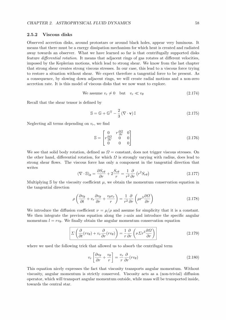
CHAPTER 2. ASTROPHYSICAL FLUID DYNAMICS 58
2.5.2 Viscous disks
Observed accretion disks, around protostars or around black holes, appear very luminous. Itmeans that there must be a energy dissipation mechanism for which heat is created and radiatedaway towards an observer. What we have learned so far is that centrifugally supported disksfeature differential rotation. It means that adjacent rings of gas rotates at different velocities,imposed by the Keplerian motions, which lead to strong shear. We know from the last chapterthat strong shear creates strong viscous stresses. In our case, this lead to a viscous force tryingto restore a situation without shear. We expect therefore a tangential force to be present. Asa consequence, by slowing down adjacent rings, we will create radial motions and a non-zeroaccretion rate. It is this model of viscous disks that we now want to explore.
We assume vr 6= 0 but vr vθ (2.174)
Recall that the shear tensor is defined by
S = G + GT − 2
3(∇ · v) I (2.175)
Neglecting all terms depending on vr, we find
S =
0 r ∂Ω∂r 0
r ∂Ω∂r 0 00 0 0
(2.176)
We see that solid body rotation, defined as Ω = constant, does not trigger viscous stresses. Onthe other hand, differential rotation, for which Ω is strongly varying with radius, does lead tostrong shear flows. The viscous force has only a component in the tangential direction thatwrites
(∇ · S)θ =∂Srθ∂r
+ 2Srθr
=1
r2
∂
∂r
(r2Srθ
)(2.177)
Multiplying S by the viscosity coefficient µ, we obtain the momentum conservation equation inthe tangential direction
ρ
(∂vθ∂t
+ vr∂vθ∂r
+vθvrr
)=
1
r2
∂
∂r
(µr3∂Ω
∂r
)(2.178)
We introduce the diffusion coefficient ν = µ/ρ and assume for simplicity that it is a constant.We then integrate the previous equation along the z-axis and introduce the specific angularmomentum l = rvθ. We finally obtain the angular momentum conservation equation
Σ
(∂
∂t(rvθ) + vr
∂
∂r(rvθ)
)=
1
r
∂
∂r
(νΣr3∂Ω
∂r
)(2.179)
where we used the following trick that allowed us to absorb the centrifugal term
vr
[∂vθ∂r
+vθr
]=vrr
∂
∂r(rvθ) (2.180)
This equation nicely expresses the fact that viscosity transports angular momentum. Withoutviscosity, angular momentum is strictly conserved. Viscosity acts as a (non-trivial) diffusionoperator, which will transport angular momentum outside, while mass will be transported inside,towards the central star.

CHAPTER 2. ASTROPHYSICAL FLUID DYNAMICS 59
2.5.3 Stationary viscous disk solution
As usual, we look for solutions for which all ∂∂t = 0, but this time we allow for vr 6= 0 owing to
the viscous stresses. The angular momentum conservation equation can be written as
Σvr∂
∂r(rvθ) =
1
r
∂
∂r
(νΣr3∂Ω
∂r
)(2.181)
Now, consider our quasi-Keplerian disk model for which
vθ '√GM∗r∝ r−1/2 and Ω '
√GM∗r3∝ r−3/2 (2.182)
Injecting these dependencies in the angular momentum conservation equation, we find the radialvelocity as
vr = − 3
Σr1/2
∂
∂r(νΣr1/2) (2.183)
and the corresponding accretion rate as
M = −6πr1/2 ∂
∂r(νΣr1/2) (2.184)
As already discussed, if we want the solution to be stationary, then the accretion rate has to beconstant. We can easily integrate the previous differential equation and find a solution for thedisk surface density as
Σ = − M
3πν
(1−
√r0
r
)(2.185)
where r0 is the radius where Σ = 0 and the solution is valid only for r > r0. Note that r0 isalso the radius at which vr → −∞. The only physical solution would be to put this singularityat the exact location of the star, namely r0 = 0. This leads to the final solution
Σ(r) = − M
3πν(r)(2.186)
The solution for the gas surface density depends therefore directly on the inverse of the diffusioncoefficient. Assuming that ν is a constant, we can integrate this constant surface density solutionand connect the accretion rate to the total disk mass as
M = −3νMdisk
r2disk
(2.187)
Let’s now consider typical values for observed protoplanetary disks
Mdisk = 10−2M and rdisk = 10 AU (2.188)
Let’s assume that we have a relatively thin disk (see the next section) with a thickness of 1 AU.The mean gas density in the disk will thus be around n ' 1013 H/cc. Using the typical hard-sphere cross section of 10−15 cm2, we get for the mean free path λcoll ' 1 m. With a gastemperature of 300 K corresponding to a sound speed of 1 km/s, we get
ν ' 107cm2 s−1 and M ' 10−15M/yr (2.189)
It is possible to compute the luminosity of the accretion disk, assuming balance between viscousdissipation and radiative cooling (left to the reader as an exercise). We can infer from the
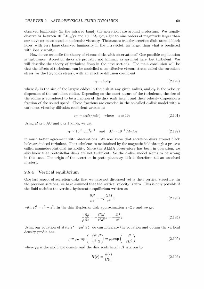
CHAPTER 2. ASTROPHYSICAL FLUID DYNAMICS 60
observed luminosity (in the infrared band) the accretion rate around protostars. We usuallyobserve M between 10−7M/yr and 10−6M/yr, eight to nine orders of magnitude larger thanour naive estimate based on molecular viscosity. The same is true for accretion disks around blackholes, with very large observed luminosity in the ultraviolet, far larger than what is predictedwith ions viscosity.
How do we reconcile the theory of viscous disks with observations? One possible explanationis turbulence. Accretion disks are probably not laminar, as assumed here, but turbulent. Wewill describe the theory of turbulent flows in the next sections. The main conclusion will bethat the effects of turbulence can be modelled as an effective viscous stress, called the turbulentstress (or the Reynolds stress), with an effective diffusion coefficient
νT = `TσT (2.190)
where `T is the size of the largest eddies in the disk at any given radius, and σT is the velocitydispersion of the turbulent eddies. Depending on the exact nature of the turbulence, the size ofthe eddies is considered to be a fraction of the disk scale height and their velocity dispersion afraction of the sound speed. These fractions are encoded in the so-called α-disk model with aturbulent viscosity diffusion coefficient written as
νT = αH(r)a(r) where α ' 1% (2.191)
Using H ' 1 AU and a ' 1 km/s, we get
νT ' 1016 cm2s−1 and M ' 10−6M/yr (2.192)
in much better agreement with observations. We now know that accretion disks around blackholes are indeed turbulent. The turbulence is maintained by the magnetic field through a processcalled magneto-rotational instability. Since the ALMA observatory has been in operation, wealso know that protostellar disks are not turbulent. So the α-disk model seems to be wrongin this case. The origin of the accretion in proto-planetary disk is therefore still an unsolvedmystery.
2.5.4 Vertical equilibrium
One last aspect of accretion disks that we have not discussed yet is their vertical structure. Inthe previous sections, we have assumed that the vertical velocity is zero. This is only possible ifthe fluid satisfies the vertical hydrostatic equilbrium written as
∂P
∂z= −ρGM
r3z (2.193)
with R2 = r2 + z2. In the thin Keplerian disk approximation z r and we get
1
ρ
∂ρ
∂z= −GM
r3a2z = −Ω
2
a2z (2.194)
Using our equation of state P = ρa2(r), we can integrate the equation and obtain the verticaldensity profile has
ρ = ρ0 exp
(−Ω
2
a2
z2
2
)= ρ0 exp
(− z2
2H2
)(2.195)
where ρ0 is the midplane density and the disk scale height H is given by
H(r) =a(r)
Ω(r)(2.196)
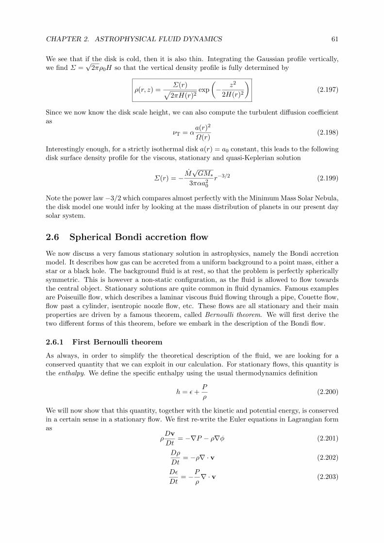
CHAPTER 2. ASTROPHYSICAL FLUID DYNAMICS 61
We see that if the disk is cold, then it is also thin. Integrating the Gaussian profile vertically,we find Σ =
√2πρ0H so that the vertical density profile is fully determined by
ρ(r, z) =Σ(r)√
2πH(r)2exp
(− z2
2H(r)2
)(2.197)
Since we now know the disk scale height, we can also compute the turbulent diffusion coefficientas
νT = αa(r)2
Ω(r)(2.198)
Interestingly enough, for a strictly isothermal disk a(r) = a0 constant, this leads to the followingdisk surface density profile for the viscous, stationary and quasi-Keplerian solution
Σ(r) = −M√GM∗
3παa20
r−3/2 (2.199)
Note the power law−3/2 which compares almost perfectly with the Minimum Mass Solar Nebula,the disk model one would infer by looking at the mass distribution of planets in our present daysolar system.
2.6 Spherical Bondi accretion flow
We now discuss a very famous stationary solution in astrophysics, namely the Bondi accretionmodel. It describes how gas can be accreted from a uniform background to a point mass, either astar or a black hole. The background fluid is at rest, so that the problem is perfectly sphericallysymmetric. This is however a non-static configuration, as the fluid is allowed to flow towardsthe central object. Stationary solutions are quite common in fluid dynamics. Famous examplesare Poiseuille flow, which describes a laminar viscous fluid flowing through a pipe, Couette flow,flow past a cylinder, isentropic noozle flow, etc. These flows are all stationary and their mainproperties are driven by a famous theorem, called Bernoulli theorem. We will first derive thetwo different forms of this theorem, before we embark in the description of the Bondi flow.
2.6.1 First Bernoulli theorem
As always, in order to simplify the theoretical description of the fluid, we are looking for aconserved quantity that we can exploit in our calculation. For stationary flows, this quantity isthe enthalpy. We define the specific enthalpy using the usual thermodynamics definition
h = ε+P
ρ(2.200)
We will now show that this quantity, together with the kinetic and potential energy, is conservedin a certain sense in a stationary flow. We first re-write the Euler equations in Lagrangian formas
ρDv
Dt= −∇P − ρ∇φ (2.201)
Dρ
Dt= −ρ∇ · v (2.202)
Dε
Dt= −P
ρ∇ · v (2.203)

CHAPTER 2. ASTROPHYSICAL FLUID DYNAMICS 62
We want to compute the time evolution of the total specific enthalpy defined as
H = h+v2
2+ φ (2.204)
We first take the Lagrange derivative of the specific kinetic energy
D
Dt
(v2
2
)= v
Dv
Dt= −v
ρ· ∇P − v · ∇φ (2.205)
We then compute the Lagrange derivative of the potential
Dφ
Dt=∂φ
∂t+ v · ∇φ (2.206)
and finally, we compute the Lagrange derivative of the enthalpy, which is slightly more involvedas
Dh
Dt= −P
ρ∇v +
1
ρ
DP
Dt− P
ρ2
Dρ
Dt(2.207)
We now use the mass conservation equation and the Lagrange derivative of the pressure
DP
Dt=∂P
∂t+ v · ∇P (2.208)
Summing up all these equations leads to the first Bernoulli theorem
D
Dt
(v2
2+ φ+ h
)=∂φ
∂t+
1
ρ
∂P
∂t(2.209)
We immediately see that for a stationary flow, the right-hand side vanishes and the Lagrangederivative is zero. For a stationary flow, the trajectories of the fluid elements are called stream-lines. The first Bernoulli theorem tells us that the total specific enthalpy is constant alongstreamlines. A very important precision here: each streamline will have a different constant.This constant is called the Bernoulli constant. This theorem is very general: no assumptionon the flow properties (except stationarity) or on the equation of state have been made. Butit is not so powerful, in the sense that we have now a family of streamlines, each one of themwith a different Bernoulli constant, determined by the boundary conditions. We now discuss thesecond Bernoulli theorem, a much more powerful result, with however an important restriction.
2.6.2 Second Bernoulli theorem
The second Bernoulli theorem is entirely built on a rather complex vector calculus identity. Westart from the Euler equation in Lagrangian form
Dv
Dt=∂v
∂t+ (v · ∇)v = −1
ρ∇P −∇φ (2.210)
and we use the following vector identity
(v · ∇)v = ∇(v2
2
)− v × ω (2.211)
Here we introduced the vorticity of the flow, namely the curl of the velocity field
ω = ∇× v (2.212)
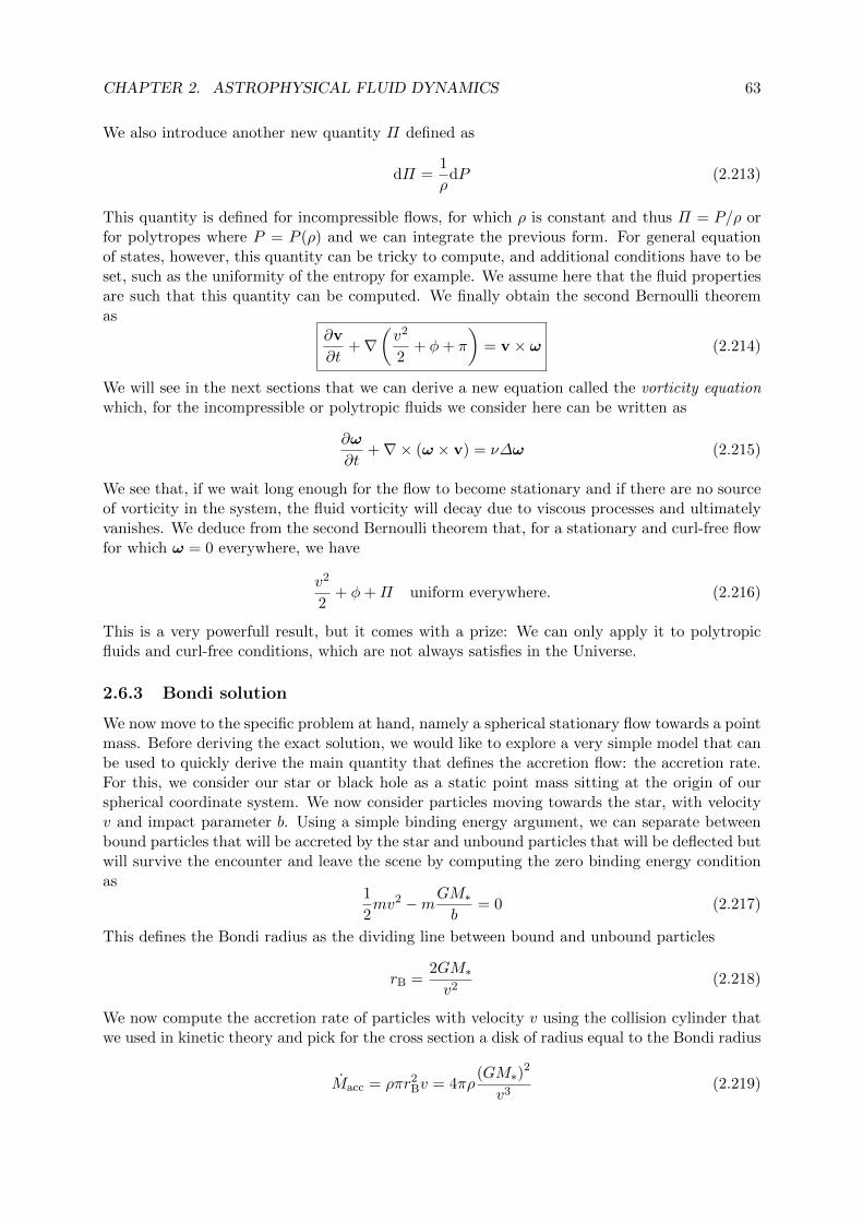
CHAPTER 2. ASTROPHYSICAL FLUID DYNAMICS 63
We also introduce another new quantity Π defined as
dΠ =1
ρdP (2.213)
This quantity is defined for incompressible flows, for which ρ is constant and thus Π = P/ρ orfor polytropes where P = P (ρ) and we can integrate the previous form. For general equationof states, however, this quantity can be tricky to compute, and additional conditions have to beset, such as the uniformity of the entropy for example. We assume here that the fluid propertiesare such that this quantity can be computed. We finally obtain the second Bernoulli theoremas
∂v
∂t+∇
(v2
2+ φ+ π
)= v × ω (2.214)
We will see in the next sections that we can derive a new equation called the vorticity equationwhich, for the incompressible or polytropic fluids we consider here can be written as
∂ω
∂t+∇× (ω × v) = ν∆ω (2.215)
We see that, if we wait long enough for the flow to become stationary and if there are no sourceof vorticity in the system, the fluid vorticity will decay due to viscous processes and ultimatelyvanishes. We deduce from the second Bernoulli theorem that, for a stationary and curl-free flowfor which ω = 0 everywhere, we have
v2
2+ φ+Π uniform everywhere. (2.216)
This is a very powerfull result, but it comes with a prize: We can only apply it to polytropicfluids and curl-free conditions, which are not always satisfies in the Universe.
2.6.3 Bondi solution
We now move to the specific problem at hand, namely a spherical stationary flow towards a pointmass. Before deriving the exact solution, we would like to explore a very simple model that canbe used to quickly derive the main quantity that defines the accretion flow: the accretion rate.For this, we consider our star or black hole as a static point mass sitting at the origin of ourspherical coordinate system. We now consider particles moving towards the star, with velocityv and impact parameter b. Using a simple binding energy argument, we can separate betweenbound particles that will be accreted by the star and unbound particles that will be deflected butwill survive the encounter and leave the scene by computing the zero binding energy conditionas
1
2mv2 −mGM∗
b= 0 (2.217)
This defines the Bondi radius as the dividing line between bound and unbound particles
rB =2GM∗v2
(2.218)
We now compute the accretion rate of particles with velocity v using the collision cylinder thatwe used in kinetic theory and pick for the cross section a disk of radius equal to the Bondi radius
Macc = ρπr2Bv = 4πρ
(GM∗)2
v3(2.219)
CHAPTER 2. ASTROPHYSICAL FLUID DYNAMICS 64
This accretion rate is only for particles of velocity v. We now need to compute the accretionrate for all possible particle velocities following a Maxwell-Boltzmann distribution. For this, we
brute forcely replace v by a, the microscopic velocity dispersion a =√
kBTm , and obtain
Macc = 4πρG2M2
∗a3
(2.220)
This very rough derivation is very approximate, but it contains most of the physics of theproblem. This is the one I encourage you to remember. As we will see now, it is also surprisinglyclose to the exact solution.
Let’s now define more precisely the problem we would like to solve. We assume that thefluid is at rest at infinity, with a uniform density and pressure. We also assume that the gas isisothermal, so that P = ρa2.
At r → +∞, we have ρ→ ρ∞, P → P∞ = ρ∞a2, and v → 0. (2.221)
We are looking for a spherically symmetric solution with the two following unknown variablesρ(r) and v(r). For the latter, we dropped the index r as this is the only non-zero velocitycomponent. The mass conservation equation in spherical coordinates writes in this case
∂ρ
∂t+
1
r2
∂
∂r
(r2ρv
)= 0 (2.222)
For a stationary solution, we thus have a constant accretion rate, defined as the total flux thougha sphere of radius r as
M = 4πr2ρv (2.223)
Since our fluid is isothermal (a special case of a polytrope) and since we consider that aftersome time the vorticity vanishes, owing to viscous dissipation, we can apply the second Bernoullitheorem and write
v2
2− GM∗
r+Π = constant (2.224)
We compute Π using the definition
Π =
∫ r
+∞
dP
ρ= a2
∫ r
+∞
dρ
ρ= a2 ln
ρ(r)
ρ∞(2.225)
We can now evaluate the Bernoulli constant at r → +∞ and find the final form of Bernoullitheorem
v2
2− GM∗
r+ a2 ln
ρ
ρ∞= 0 (2.226)
As usual, we define the following dimensionless variables
r =r
rB, v =
v(r)
a, ρ =
ρ(r)
ρ∞and λ =
M(r)
MB
(2.227)
If we choose for the Bondi radius and the Bondi accretion rate the following definitions
rB =GM∗a2
and MB = 4πr2bρ∞a (2.228)
then our two equations become dimensionless, with the mass flux being
λ = r2ρv (2.229)
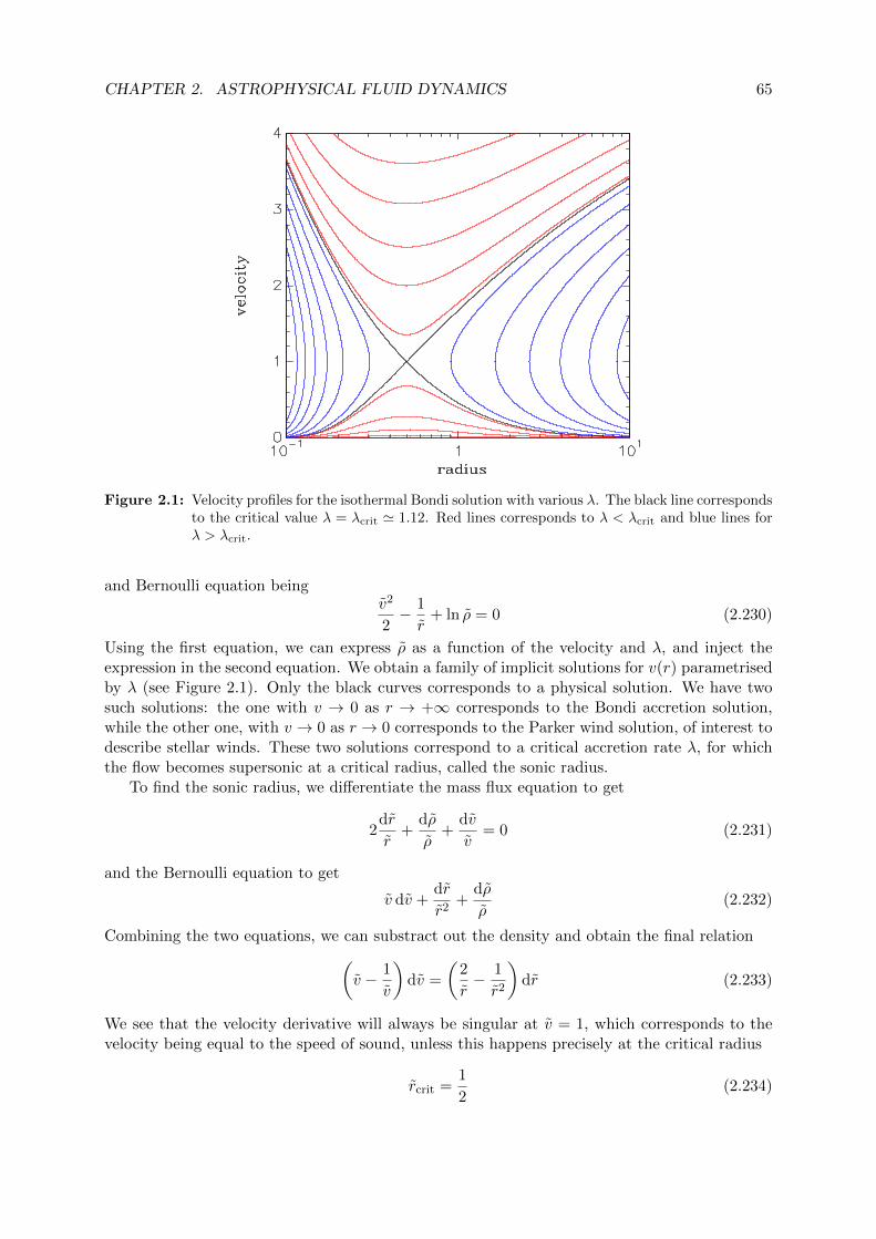
CHAPTER 2. ASTROPHYSICAL FLUID DYNAMICS 65
Figure 2.1: Velocity profiles for the isothermal Bondi solution with various λ. The black line correspondsto the critical value λ = λcrit ' 1.12. Red lines corresponds to λ < λcrit and blue lines forλ > λcrit.
and Bernoulli equation beingv2
2− 1
r+ ln ρ = 0 (2.230)
Using the first equation, we can express ρ as a function of the velocity and λ, and inject theexpression in the second equation. We obtain a family of implicit solutions for v(r) parametrisedby λ (see Figure 2.1). Only the black curves corresponds to a physical solution. We have twosuch solutions: the one with v → 0 as r → +∞ corresponds to the Bondi accretion solution,while the other one, with v → 0 as r → 0 corresponds to the Parker wind solution, of interest todescribe stellar winds. These two solutions correspond to a critical accretion rate λ, for whichthe flow becomes supersonic at a critical radius, called the sonic radius.
To find the sonic radius, we differentiate the mass flux equation to get
2dr
r+
dρ
ρ+
dv
v= 0 (2.231)
and the Bernoulli equation to get
v dv +dr
r2+
dρ
ρ(2.232)
Combining the two equations, we can substract out the density and obtain the final relation(v − 1
v
)dv =
(2
r− 1
r2
)dr (2.233)
We see that the velocity derivative will always be singular at v = 1, which corresponds to thevelocity being equal to the speed of sound, unless this happens precisely at the critical radius
rcrit =1
2(2.234)
CHAPTER 2. ASTROPHYSICAL FLUID DYNAMICS 66
If we inject this value in the Bernoulli equation, we find
ρ = exp
(3
2
)(2.235)
and finally, using the mass flux equation, we get
λcrit =1
4exp
(3
2
)' 1.12 (2.236)
Finally, the exact solution for the Bondi accretion rate is
M = λcritMB (2.237)
quite close to our initial guess. We can examine the corresponding density profile. For r rcrit = rB/2, the density is almost constant and equal to ρ∞. Inside the sonic radius, forr rB/2, the flow is supersonic. We can neglect the ln ρ term in the Bernoulli equation, andwe obtain the following singular velocity and density profiles
v ' 2a
(rB/2
r
)1/2
and ρ ' 2ρ∞
(rB/2
r
)3/2
(2.238)
This derivation is valid for an isothermal equation of state. As an exercise, we leave it to thereader to derive the Bondi solution for a polytropic equation of state, for which
P = P∞
(ρ
ρ∞
)Γ(2.239)
The solution is quite similar, with however some small interesting quantitative differences.
2.7 Sound waves
So far, we have studied static equilibrium and stationary solutions of the Euler equations withapplication to astrophysical fluid flows. We now need to check that these solutions are stable.The traditional approach to study the stability of equilibrium flows is to perturb slightly thesolution with deviations that are small enough to allow for a linearisation of the Euler equations.The resulting system of equations is much simpler to solve, and lead to particular propagatingsolutions called sound waves. If the amplitude of these waves remains constant (or decays withtime), the equilibrium solution is said to be stable. If, on the other hand, the amplitude increasesexponentially fast with time, we have an instability and the equilibrium solution is not viable.
2.7.1 Stable propagating waves
We consider the following simple equilibrium solution of the Euler equations ρeq = ρ0 constantand veq = 0, with an isothermal equation of state P = ρa2. We write the Euler equations in onespace dimension with v = (vx, 0, 0)
∂ρ
∂t+
∂
∂x(ρv) = 0 (2.240)
∂v
∂t+ v
∂v
∂x+
1
ρ
∂P
∂x= 0 (2.241)

CHAPTER 2. ASTROPHYSICAL FLUID DYNAMICS 67
where we dropped the index x in the velocity variable for simplicity. There is no energy equationto consider in the isothermal case. We define the perturbed solution as
ρ = ρ0 + δρ(x, t) (2.242)
v = 0 + δv(x, t) (2.243)
with |δρ| ρ0 and |δv| a. We can now linearise the two Euler equations by substitutingthese expressions and neglect the quadratic terms. We also assume that our perturbations aresmooth enough, so that their derivatives remain bound. For the mass conservation equation, weget
∂
∂t(δρ) + (ρ0 + δρ)
∂
∂x(δv) + δv
∂
∂x(δρ) = 0 (2.244)
∂
∂t(δρ) + ρ0
∂
∂x(δv) + δρ
∂
∂x(δv) + δv
∂
∂x(δρ) = 0 (2.245)
Neglecting the two rightermost quadratic terms in this equation, we obtain to leading order thelinear equation
∂
∂t(δρ) + ρ0
∂
∂x(δv) = 0 (2.246)
The momentum conservation equation becomes
∂
∂t(δv) + δv
∂
∂x(δv) +
a2
ρ
∂
∂x(ρ0 + δρ) = 0 (2.247)
The last term can be Taylor-expanded as
1
ρ' 1
ρ0
(1− δρ
ρ0
)so that
a2
ρ
∂
∂x(δρ) ' a2
ρ0
∂
∂x(δρ)− a2
ρ20
δρ∂
∂x(δρ) (2.248)
Neglecting again the quadratic terms, we obtain to leading order the linear form of the momen-tum conservation equation
∂
∂t(δv) +
a2
ρ0
∂
∂x(δρ) = 0 (2.249)
Now, if we take the time derivative of the first equation, and the space derivative of the secondequation, we combine the two equations and obtain the famous wave equation.
∂2
∂t2(δρ) = a2 ∂
2
∂x2(δρ) (2.250)
We are looking for planar wave solutions with the following Ansatz
δρ(x, t) ≡ ∆ρei(kx−ωt) (2.251)
δv(x, t) ≡ ∆v ei(kx−ωt) (2.252)
where ∆ρ and ∆v are the constant amplitude of the waves. Plugging this into the wave equation,we get
− ω2∆ρ+ a2k2∆ρ = 0 (2.253)
Since we are looking for non-trivial solutions with ∆ρ 6= 0, we get the dispersion relation of thewaves.
ω2 = a2k2 (2.254)
CHAPTER 2. ASTROPHYSICAL FLUID DYNAMICS 68
The wave speed is given by ωk = ±a. In this case, it is called the sound speed. From the second
linearized Euler equation, we get a relation between the amplitudes
− iω∆v + ika2
ρ∆ρ = 0 (2.255)
so that∆v
a= ±∆ρ
ρ0(2.256)
The particles of the fluid are moving with the velocity field δv, they are oscillating back and fortharound a fixed average position. So particles are not really moving away from the equilibriumsolution. Travelling waves are moving at the speed of sound, but only as a virtual feature.They don’t carry mass, only momentum and energy. Their amplitude is constant, so that thecorresponding equilibrium solution is said to be stable.
CHAPTER 2. ASTROPHYSICAL FLUID DYNAMICS 69
2.7.2 Thermal instability
We now consider the more general case of a polytropic equation of state, for which
P = P (ρ) = ρkBTeq(ρ)
m(2.257)
where the temperature is determined by a strict balance between heating and cooling processes.Figure 2.2 shows the equilibrium pressure within the interstellar medium of the Milky Way atdifferent distances from the centre of the Galaxy. Closer to the centre, the radiation field andthe cosmic ray flux are both stronger, and the corresponding equilibrium pressure higher. Atlow density, the gas settles into an isothermal equilibrium with T ' 104 K. At intermediatedensities, however, the pressure is dropping because cooling scales as n2 and it takes over thesevarious heating processes, lowering sharply the equilibrium temperature. At higher density, wereach an asymptotic isothermal regime with T ' 10 K and the pressure is rising again.
We consider here again a uniform equilibrium state with ρ = ρ0, v = 0 and T = Teq(ρ0).Starting again from the 1D Euler equations, with however a different equation of state, we getthe following linearized form
∂
∂t(δρ) + ρ0
∂
∂x(δv) = 0 (2.258)
∂
∂t(δv) +
P ′(ρ0)
ρ0
∂
∂x(δρ) = 0 (2.259)
with P ′(ρ) = ∂P∂ρ . Taking the time derivative of the first equation, swapping the time and space
derivative of the second term and replacing it by the the second equation, we get a new form ofthe wave equation
∂2
∂t2(δρ)− P ′(ρ0)
∂2
∂x2(δρ) = 0 (2.260)
We are considering here again solutions of the form δρ = ∆ρei(kx−ωt), where k is real but ω cannow be a complex number. Injecting the solution in the second order linear differential equationleads to the the dispersion relation
ω2 = P ′(ρ0)k2 (2.261)
Note that we can recover the isothermal case easily because for P = ρa2, P ′ = a2 and thedispersion relation leads to a real wave frequency with wave velocity ω
k = ±a. In the generalpolytropic case, however, we have to distinguish two different cases:
• P ′(ρ0) > 0In this case, both k and ω are real and we can define the sound speed as c2
s = P ′(ρ0) or
cs =√P ′(ρ0) (2.262)
We have propagating waves with a constant amplitude and wave velocities ±cs. Notethat if we include viscosity and/or thermal conduction, the wave amplitude will eventuallyslowly decay. In conclusion, it means our equilibrium solution is stable.
• P ′(ρ0) < 0In this case, we can find proper solutions only if k is real and ω is purely imaginary, becauseω2 < 0. We define the growth rate γ ∈ R as ω = iγ. The solutions are then defined by
γ = ±√−P ′(ρ0)k (2.263)
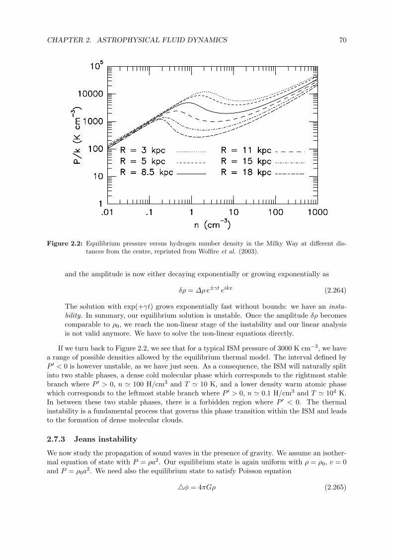
CHAPTER 2. ASTROPHYSICAL FLUID DYNAMICS 70
Figure 2.2: Equilibrium pressure versus hydrogen number density in the Milky Way at different dis-tances from the centre, reprinted from Wolfire et al. (2003).
and the amplitude is now either decaying exponentially or growing exponentially as
δρ = ∆ρe±γt eikx (2.264)
The solution with exp(+γt) grows exponentially fast without bounds: we have an insta-bility. In summary, our equilibrium solution is unstable. Once the amplitude δρ becomescomparable to ρ0, we reach the non-linear stage of the instability and our linear analysisis not valid anymore. We have to solve the non-linear equations directly.
If we turn back to Figure 2.2, we see that for a typical ISM pressure of 3000 K cm−3, we havea range of possible densities allowed by the equilibrium thermal model. The interval defined byP ′ < 0 is however unstable, as we have just seen. As a consequence, the ISM will naturally splitinto two stable phases, a dense cold molecular phase which corresponds to the rightmost stablebranch where P ′ > 0, n ' 100 H/cm3 and T ' 10 K, and a lower density warm atomic phasewhich corresponds to the leftmost stable branch where P ′ > 0, n ' 0.1 H/cm3 and T ' 104 K.In between these two stable phases, there is a forbidden region where P ′ < 0. The thermalinstability is a fundamental process that governs this phase transition within the ISM and leadsto the formation of dense molecular clouds.
2.7.3 Jeans instability
We now study the propagation of sound waves in the presence of gravity. We assume an isother-mal equation of state with P = ρa2. Our equilibrium state is again uniform with ρ = ρ0, v = 0and P = ρ0a
2. We need also the equilibrium state to satisfy Poisson equation
4φ = 4πGρ (2.265)
CHAPTER 2. ASTROPHYSICAL FLUID DYNAMICS 71
which is a problem, because the potential of an infinite uniform background is infinite. In orderto restore a viable equilibrium state, we appeal to the so-called Jeans swindle. The trick is tomodify Poisson equation into
4φ = 4πG(ρ− ρ0) (2.266)
so that the equilibrium solution is now φ = 0 when ρ = ρ0. The Jeans swindle is hard to justifyrigorously. In only two cases we can motivate the extra term in the right-hand side: in thepresence of rotation, the centrifugal force plays the role of an effective potential balancing gravity,and in cosmology, the expansion of the Universe cancels out exactly the mean backgrounddensity. In what follows, we just assume that this modification of Poisson equation is valid. Wethen augment the one-dimensional Euler equations with the modified one-dimensional Poissonequation
∂ρ
∂t+ ρ
∂v
∂x+ v
∂ρ
∂x= 0 (2.267)
∂v
∂t+ v
∂v
∂x+a2
ρ
∂ρ
∂x= −∂φ
∂x(2.268)
∂2φ
∂x2= 4πG(ρ− ρ0) (2.269)
We then consider perturbations of the form
ρ = ρ0 + δρ (2.270)
v = 0 + δv (2.271)
φ = 0 + δφ (2.272)
Injecting these perturbations into the previous system of equations, we can linearize them bydropping all high order quadratic terms and obtain the following system of linear differentialequations
∂
∂t(δρ) + ρ0
∂
∂x(δv) = 0 (2.273)
∂
∂t(δv) +
a2
ρ0
∂
∂x(δρ) = − ∂
∂x(δφ) (2.274)
∂2
∂x2(δφ) = 4πGδρ (2.275)
Here again, we take the time derivative of the mass conservation equation, swap the time andspace derivative of the velocity term and inject the momentum conservation equation. We obtainthe following relation
∂2
∂t2(δρ)− a2 ∂
2
∂x2(δρ)− ρ0
∂2
∂x2(δφ) = 0 (2.276)
Finally, we use the Poisson equation to replace the third term and obtain the final equation onthe density perturbation
∂2
∂t2(δρ)− a2 ∂
2
∂x2(δρ)− 4πGρ0(δρ) = 0 (2.277)
As always, we consider solutions of the form δρ = ∆ρei(kx−ωt) where k is real but ω can be acomplex number. Injecting this in the previous differential equation and requiring ∆ρ 6= 0, weobtain the following dispersion relation
ω2 = a2k2 − 4πGρ0 (2.278)
CHAPTER 2. ASTROPHYSICAL FLUID DYNAMICS 72
We can define a critical wave number that separates stable modes with ω2 > 0 from unstablemodes with ω2 < 0.
k2J =
4πGρ0
a2(2.279)
This critical wave number can be used to define the Jeans length as
λJ =2π
kJ= a
√π
Gρ0(2.280)
If k > kJ , we have stable propagating waves, which for k kJ are just normal sound waveswith ω
k = ±a.If k < kJ , we have ω2 < 0 and ω = iγ where γ is the growth rate. This is what we call Jeansinstability. For k kJ , we find γ =
√4πGρ0. This growth rate can be used to define the free
fall time as
tff =1
γ=
1√4πGρ0
(2.281)
This time is the e-folding time of the growth of the amplitude of the density fluctuations. Forvery long wavelengths, gravity wins over pressure forces and the sound waves collapse undertheir own weight within one free fall time. Beyond this time, the linearisation of the equationsis not valid anymore and we enter the non-linear regime of the gravitational instability. For veryshort wavelengths, on the other hand, pressure forces win against gravity and sound waves canpropagate freely without perturbing the initial equilibrium state.
2.8 Shock waves
Another type of waves plays a fundamental role in astrophysics, the shock waves. These arenot linear objects like sound waves. they are the product of the non-linear evolution of theEuler equations. Shock waves are discontinuities traveling in the fluid. Partial derivatives arenot defined across discontinuities, so we must rely on particular conservation laws, called theRankine-Hugoniot relations, to connect the two states on each side of the discontinuity. Shockwaves are also dissipative. Because all flow variables are discontinuous across shocks, the Eulerequations cease to be valid, as the scale of a discontinuity is obviously zero, much smaller thanthe collision mean free path. In fact, shock waves have a finite thickness, close to the meanfree path of the particles. This thickness is due to viscous effects at small scales. The Rankine-Hugoniot relations are powerful tools. Even if we ignore these small scale viscous effects, wecan still recover the correct relations connecting the upstream and downstream regions of theshock. After deriving these relations in the specific cases of adiabatic and isothermal shocks, wewill apply our findings to the theory of astrophysical blast waves, used in particular to describesupernova remnants in the interstellar medium.
2.8.1 Wave steepening and shock Formation
In order to describe the process of shock formation, we need to consider the full non-linear Eulerequations, with for the velocity in one dimension
∂v
∂t+ v
∂v
∂x+
1
ρ
∂P
∂x= 0 (2.282)
The second term is usually called the non-linear term because it features a quadratic term inthe velocity perturbation. In the previous sections, this term was dropped, leading to lineardifferential equations. We now want to keep this term and try to solve the previous equation in

CHAPTER 2. ASTROPHYSICAL FLUID DYNAMICS 73
Figure 2.3: Space time diagram showing the characteristics of the Burgers equation. The dotted linesshows the trajectories after characteristics crossings. The solid lines show the regularizedsingle valued solution and the formation of a shock front at x = 0.5 at time t = 0.16.
a slightly simplified setting. We consider here again an isothermal equation of state P = ρa2,but we restrict ourselves to the supersonic regime for which a v. In this case, we can write∣∣∣∣1ρ ∂P∂x
∣∣∣∣ =
∣∣∣∣a2
ρ
∂ρ
∂x
∣∣∣∣ ∣∣∣∣v ∂v∂x∣∣∣∣ (2.283)
and we can drop the pressure gradient and obtain the famous Burgers equation
∂v
∂t+ v
∂v
∂x= 0 (2.284)
We now want to solve this equation with the prescribed initial condition v0(x) = v(x, t = 0).For the sake of simplicity, we choose here a planar wave
v0(x) = ∆v sin
(2π
Lx
)(2.285)
consistent with the Ansatz used in the previous sections. We assume without loss of generalitythat ∆v = 1 and L = 1. Let us now consider fluid trajectories x(t) defined by
x = v(x(t), t) and x(0) = x0 (2.286)
We now define the scalar quantityα(t) ≡ v(x(t), t) (2.287)
attached to each trajectory x(t). Taking the time derivative and applying the chain rule gives
α(t) =∂v
∂xx+
∂v
∂t= 0 (2.288)
so that α(t) = α(0) = v0(x0) remains constant in time. This means that v = v0 along thetrajectory and the direct consequence is that trajectories are straight lines
x(t) = x0 + v0(x0) t (2.289)
The straight lines are called characteristic curves, or in short, characteristics.
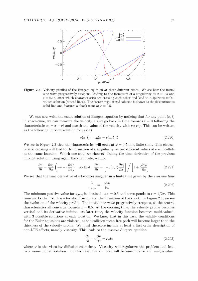
CHAPTER 2. ASTROPHYSICAL FLUID DYNAMICS 74
Figure 2.4: Velocity profiles of the Burgers equation at three different times. We see how the initialsine wave progressively steepens, leading to the formation of a singularity at x = 0.5 andt = 0.16, after which characteristics are crossing each other and lead to a spurious multi-valued solution (dotted lines). The correct regularized solution is shown as the discontinuoussolid line and features a shock front at x = 0.5.
We can now write the exact solution of Burgers equation by noticing that for any point (x, t)in space-time, we can measure the velocity v and go back in time towards t = 0 following thecharacteristic x0 = x− vt and match the value of the velocity with v0(x0). This can be writtenas the following implicit solution for v(x, t)
v(x, t) = v0(x− v(x, t)t) (2.290)
We see in Figure 2.3 that the characteristics will cross at x = 0.5 in a finite time. This charac-teristic crossing will lead to the formation of a singularity, as two different values of v will collideat the same location. Which one shall we choose? Taking the time derivative of the previousimplicit solution, using again the chain rule, we find
∂v
∂t=∂v0
∂x
(−v − t∂v
∂t
)so that
∂v
∂t=
[−v(x, t)
∂v0
∂x
]/[1 + t
∂v0
∂x
](2.291)
We see that the time derivative of v becomes singular in a finite time given by the crossing time
1
tcross= −∂v0
∂x(2.292)
The minimum positive value for tcross is obtained at x = 0.5 and corresponds to t = 1/2π. Thistime marks the first characteristic crossing and the formation of the shock. In Figure 2.4, we seethe evolution of the velocity profile. The initial sine wave progressively steepens, as the centralcharacteristics all converge towards x = 0.5. At the crossing time, the velocity profile becomesvertical and its derivative infinite. At later time, the velocity function becomes multi-valued,with 3 possible solutions at each location. We know that in this case, the validity conditionsfor the Euler equations are violated, as the collision mean free path will become larger than thethickness of the velocity profile. We must therefore include at least a first order description ofnon-LTE effects, namely viscosity. This leads to the viscous Burgers equation
∂v
∂t+ v
∂v
∂x= ν∆v (2.293)
where ν is the viscosity diffusion coefficient. Viscosity will regularize the problem and leadto a non-singular solution. In this case, the solution will become unique and single-valued

CHAPTER 2. ASTROPHYSICAL FLUID DYNAMICS 75
everywhere. This regularized solution is called the viscosity solution or the weak solution. Notethat the viscous Burgers equation has an exact solution based on the Hopf-Cole transform(not discussed here). The procedure is then to find the viscosity solution for a finite viscosityparameter ν and then make ν → 0, instead of setting ν = 0 in the equations before solvingthem, which leads to an ill-defined result.
2.8.2 Rankine-Hugoniot relations
Now that we are convinced that discontinuities form systematically after a finite time in as-trophysical fluid flows, we need a mathematical tool to deal with them. Indeed, the Eulerequations in Lagrangian or Eulerian forms feature many spatial derivatives which are obviouslynot defined across discontinuities. Shock fronts have to be considered as a singular surface sep-arating the flow in two regions: the pre-shock region that contains the unperturbed fluid andthe post-shock region with the shocked material. Inside these two regions, flow variables arecontinuous and differentiable, but not across the shock. In order to connect these two regionsacross the discontinuity, we need a new set of conservation laws in integral form, called theRankine-Hugoniot relations. To derive these famous relations, we write the Euler equations inthe following conservative form
∂U
∂t+∂F
∂x= 0 (2.294)
where the vector of conservative variables is defined by
U = (ρ, ρv,E) (2.295)
and the vector of the fluxes of the conserved variables is defined by
F = (ρv, ρv2 + P, (E + P )v) (2.296)
These equations are one-dimensional and represent the flow evolution in the direction normalto the shock surface. Note that many other equations can be expressed in this form: theisothermal Euler equations, without the energy equation, the ideal MHD equations that includethe magnetic field, the relativistic Euler equations, the traffic flow equations, the shallow waterequations, etc. The Rankine-Hugoniot relations can be derived similarly for all these differentsystem of conservation laws. We now integrate this system of equations in a square region inspace-time between times t1 and t2 and positions x1 and x2 chosen close enough from each otherso that the shock trajectory (or shock characteristic) can be approximated by its tangent line.The shock velocity S in the direction normal to the shock surface is therefore defined in thissmall region by x1 − x2 = S(t1 − t2).
We now write the integral both in time and space as∫ t2
t1
∫ x2
x1
(∂U
∂t+∂F
∂x
)dx dt = 0 (2.297)
The time derivative can be integrated immediately in time and the space derivative in space,leading to ∫ x2
x1
[U(x, t2)−U(x, t1)] dx+
∫ t2
t1
[F(x2, t)− F(x1, t)] dt = 0 (2.298)
We now label the pre-shock values on the right side of the shock front as UR and FR and thepost-shock region on the left as UL and FL. Since we consider a vanishingly small space-timeinterval, the pre-shock and post-shock values can be considered as constant both in time and
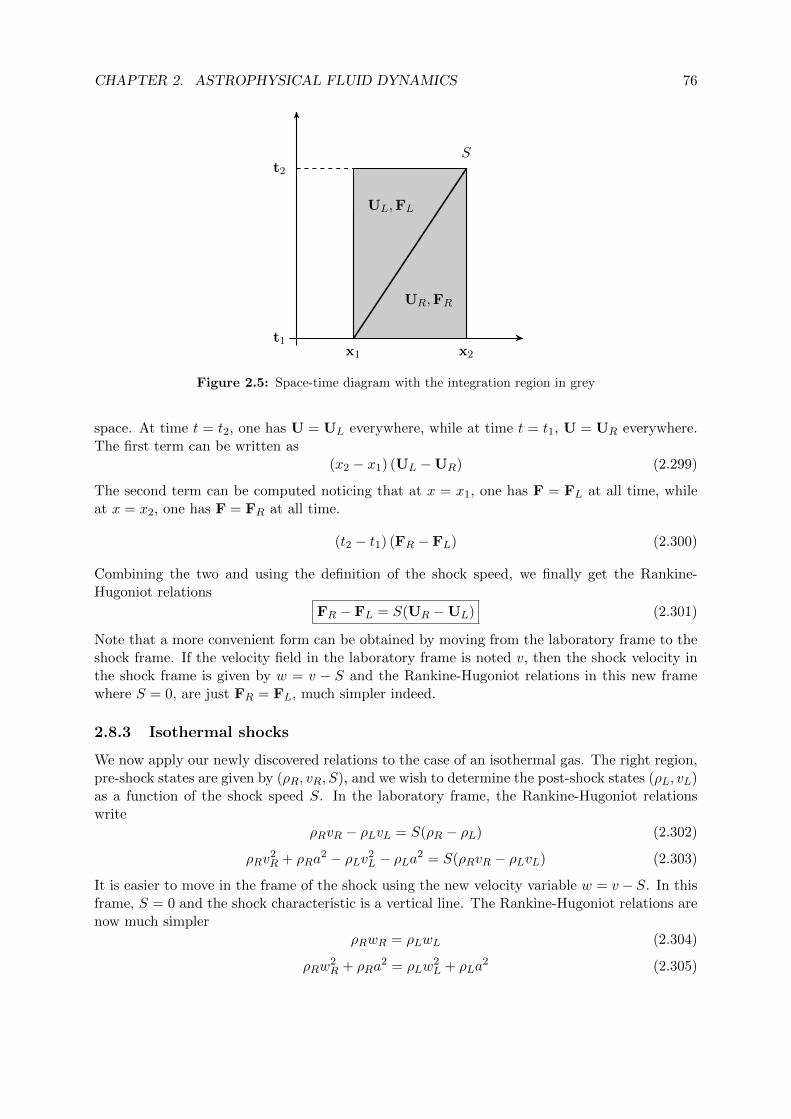
CHAPTER 2. ASTROPHYSICAL FLUID DYNAMICS 76
x1 x2
t1
t2
S
UL,FL
UR,FR
Figure 2.5: Space-time diagram with the integration region in grey
space. At time t = t2, one has U = UL everywhere, while at time t = t1, U = UR everywhere.The first term can be written as
(x2 − x1) (UL −UR) (2.299)
The second term can be computed noticing that at x = x1, one has F = FL at all time, whileat x = x2, one has F = FR at all time.
(t2 − t1) (FR − FL) (2.300)
Combining the two and using the definition of the shock speed, we finally get the Rankine-Hugoniot relations
FR − FL = S(UR −UL) (2.301)
Note that a more convenient form can be obtained by moving from the laboratory frame to theshock frame. If the velocity field in the laboratory frame is noted v, then the shock velocity inthe shock frame is given by w = v − S and the Rankine-Hugoniot relations in this new framewhere S = 0, are just FR = FL, much simpler indeed.
2.8.3 Isothermal shocks
We now apply our newly discovered relations to the case of an isothermal gas. The right region,pre-shock states are given by (ρR, vR, S), and we wish to determine the post-shock states (ρL, vL)as a function of the shock speed S. In the laboratory frame, the Rankine-Hugoniot relationswrite
ρRvR − ρLvL = S(ρR − ρL) (2.302)
ρRv2R + ρRa
2 − ρLv2L − ρLa2 = S(ρRvR − ρLvL) (2.303)
It is easier to move in the frame of the shock using the new velocity variable w = v− S. In thisframe, S = 0 and the shock characteristic is a vertical line. The Rankine-Hugoniot relations arenow much simpler
ρRwR = ρLwL (2.304)
ρRw2R + ρRa
2 = ρLw2L + ρLa
2 (2.305)
CHAPTER 2. ASTROPHYSICAL FLUID DYNAMICS 77
It is customary to define the compression ratio of the shock as
r =ρLρR
(2.306)
and the Mach number of the shock as
M =|wR|a
(2.307)
The mass conservation relation now writes
wL =1
rwR (2.308)
and the momentum conservation relation simplifies to
w2R + a2 = r
(w2L + a2
)(2.309)
Dividing by a2 and using the first relation, the second relation becomes
M2 + 1 = r
(M2
r2+ 1
)(2.310)
After some easy manipulations, we obtain a polynomial of degree 2 for the unknown compressionratio r
r2 − r(M2 + 1) +M2 = 0 (2.311)
Note r = 1 is always a solution of the Rankine-Hugoniot relations. It corresponds to a virtualshock wave moving through the fluid without affecting the flow. The physical solution is theother solution r = M2 > 1. One condition to get a shock wave is thus M > 1. Moving backto the laboratory frame, we obtain the post-shock values as a function of M and the pre-shockvalues
ρL =M2ρR (2.312)
vL =1
M2(vR − S) + S (2.313)
The strong shock limit is obtained forM→ +∞. In this case, we see that the compression ratiobecomes very large and that the post-shock velocity vL ' S. The fluid is therefore put in motionby the shock wave and immediately follows it. Let’s now consider two different examples.
• First example: Let’s assume that the pre-shock velocity is zero vR = 0 and the shockis moving from left to right with speed S > a. In this case, we have from the previousrelations M = S/a > 1. The compression ratio is fully specified by the shock speed with
r =M2 =S2
a2> 1 (2.314)
and the post-shock velocity is just
vL = S
(1− a2
S2
)(2.315)
• Second example: Let’s assume we don’t know the shock speed but we know that the fluidis initially moving from right to left with vR < 0 and is crashing onto the left wall ofthe laboratory. This sets the boundary conditions vL = 0. A shock will emerge from the
CHAPTER 2. ASTROPHYSICAL FLUID DYNAMICS 78
left wall with S > 0 and will propagate to the right, slowing down the incoming fluid.Using the previous relations, we deduce the shock speed value by solving the followingpolynomial of degree 2
S2 − SvR − a2 = 0 (2.316)
for which the only physical solution is
S =vR +
√v2R + 4a2
2> a (2.317)
The corresponding compression ratio is
r = 1 +v2R
4a2(2.318)
We see that in these two examples, the shock wave always travels supersonically with respect tothe fluid at rest. The compression ratio is always greater than 1, and scales as the Mach numbersquare, without bounds. In this isothermal case, the post-shock temperature remains constantand equal to the pre-shock temperature.
2.8.4 Adiabatic shocks
We now move to the more complex case of an ideal gas equation of state with P = (γ − 1)e.The Rankine-Hugoniot relations in the frame of the shock are
ρLwL = ρRwR (2.319)
ρLw2L + PL = ρRw
2R + PR (2.320)
wL(EL + PL) = wR(ER + PR) (2.321)
Using the definition of the total energy E = e + 12ρw
2 and injecting the mass conservationrelation, we can write the energy equation as
1
2w2L +
γ
γ − 1
PLρL
=1
2w2R +
γ
γ − 1
PRρR
(2.322)
In order to simplify the algebra, we consider the case where the fluid is initially at rest withvR = 0 so that wR = −S. We also assume that the Mach numberM = S/cs 1 with c2
s = γP/ρthe adiabatic sound speed. We also define the compression ratio as before r = ρL/ρR. The massconservation relation gives
wL = −Sr
(2.323)
The momentum conservation relation becomes
ρLw2L + PL ' ρRS2 which gives
PLρL
=S2
r− S2
r2(2.324)
where we have neglected the thermal pressure in the right-hand side owing to the strong shockcondition. Finally, the energy conservation relation becomes
1
2w2L +
γ
γ − 1
PLρL' 1
2S2 (2.325)

CHAPTER 2. ASTROPHYSICAL FLUID DYNAMICS 79
Combining all the previous results lead to the following relation between r and S
1
2
S2
r2+
γ
γ − 1
S2
r
(r − 1)
r=
1
2S2 (2.326)
which simplifies (as for the isothermal case) into the following polynomial of degree 2
r2 − 2γ
γ − 1r +
γ + 1
γ − 1= 0 (2.327)
which has the two solutions
r = 1 and r =γ + 1
γ − 1(2.328)
We thus get the post-shock density as a function of the pre-shock density using
ρL =γ + 1
γ − 1ρR (2.329)
The Maxwell-Boltzmann case with γ = 5/3 gives r = 4. The molecular equation of state withγ = 7/5 leads to r = 6 and relativistic fluids with γ = 4/3 have r = 7. Interestingly, one alsorecovers the isothermal limit with γ → 1 and r → +∞. The mass conservation relation gives usthe post-shock velocity with wL = −S/r and vL = S − S/r so that
vL =2
γ + 1S (2.330)
The post-shock pressure is obtained using the momentum conservation relation with
PL =2
γ + 1ρRS
2 (2.331)
and the post-shock temperature is given by
kBTLm
=PLρL
=2(γ − 1)
(γ + 1)2S2 (2.332)
We see that adiabatic shocks behave very differently than isothermal shocks. In the strong shocklimit, the compression ratio r is now finite and remains relatively small (from 4 to 7 dependingon the equation of state). On the other hand, the post-shock temperature scales as the squareof the shock speed and can become arbitrarily large, like the compression ratio in the isothermalcase. In the adiabatic case, energy is conserved and the kinetic energy of the pre-shock fluidis transferred into thermal energy in the post-shock region. Shocks are thus dissipative waveswhich generate entropy owing to viscous effects within the shock front.
2.8.5 Radiative shocks
In the general case, shocks are neither adiabatic, nor isothermal. We need to consider coolingand heating processes in the energy equation to describe how the fluid will return to its initialtemperature after the shock has passed through the fluid. Radiative processes will be describedin the next chapter. They are due to inelastic collisions between atoms and molecules that emitphotons. Since inelastic collisions have a probability lower than one to occur during an otherwiseelastic collision, radiative processes will always be slower than viscous processes. A shock waveis thus always adiabatic. Then, slowly, radiative processes cool down the gas in the post-shock
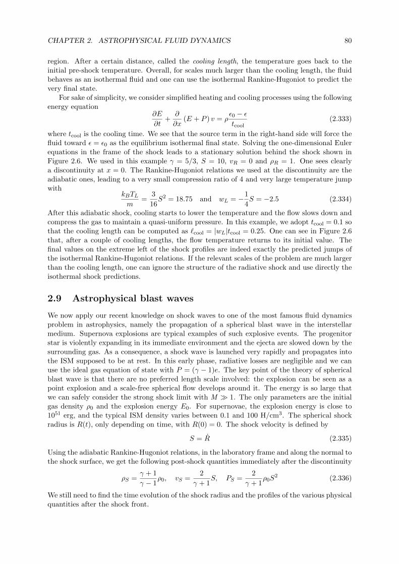
CHAPTER 2. ASTROPHYSICAL FLUID DYNAMICS 80
region. After a certain distance, called the cooling length, the temperature goes back to theinitial pre-shock temperature. Overall, for scales much larger than the cooling length, the fluidbehaves as an isothermal fluid and one can use the isothermal Rankine-Hugoniot to predict thevery final state.
For sake of simplicity, we consider simplified heating and cooling processes using the followingenergy equation
∂E
∂t+
∂
∂x(E + P ) v = ρ
ε0 − εtcool
(2.333)
where tcool is the cooling time. We see that the source term in the right-hand side will force thefluid toward ε = ε0 as the equilibrium isothermal final state. Solving the one-dimensional Eulerequations in the frame of the shock leads to a stationary solution behind the shock shown inFigure 2.6. We used in this example γ = 5/3, S = 10, vR = 0 and ρR = 1. One sees clearlya discontinuity at x = 0. The Rankine-Hugoniot relations we used at the discontinuity are theadiabatic ones, leading to a very small compression ratio of 4 and very large temperature jumpwith
kBTLm
=3
16S2 = 18.75 and wL = −1
4S = −2.5 (2.334)
After this adiabatic shock, cooling starts to lower the temperature and the flow slows down andcompress the gas to maintain a quasi-uniform pressure. In this example, we adopt tcool = 0.1 sothat the cooling length can be computed as `cool = |wL|tcool = 0.25. One can see in Figure 2.6that, after a couple of cooling lengths, the flow temperature returns to its initial value. Thefinal values on the extreme left of the shock profiles are indeed exactly the predicted jumps ofthe isothermal Rankine-Hugoniot relations. If the relevant scales of the problem are much largerthan the cooling length, one can ignore the structure of the radiative shock and use directly theisothermal shock predictions.
2.9 Astrophysical blast waves
We now apply our recent knowledge on shock waves to one of the most famous fluid dynamicsproblem in astrophysics, namely the propagation of a spherical blast wave in the interstellarmedium. Supernova explosions are typical examples of such explosive events. The progenitorstar is violently expanding in its immediate environment and the ejecta are slowed down by thesurrounding gas. As a consequence, a shock wave is launched very rapidly and propagates intothe ISM supposed to be at rest. In this early phase, radiative losses are negligible and we canuse the ideal gas equation of state with P = (γ − 1)e. The key point of the theory of sphericalblast wave is that there are no preferred length scale involved: the explosion can be seen as apoint explosion and a scale-free spherical flow develops around it. The energy is so large thatwe can safely consider the strong shock limit with M 1. The only parameters are the initialgas density ρ0 and the explosion energy E0. For supernovae, the explosion energy is close to1051 erg, and the typical ISM density varies between 0.1 and 100 H/cm3. The spherical shockradius is R(t), only depending on time, with R(0) = 0. The shock velocity is defined by
S = R (2.335)
Using the adiabatic Rankine-Hugoniot relations, in the laboratory frame and along the normal tothe shock surface, we get the following post-shock quantities immediately after the discontinuity
ρS =γ + 1
γ − 1ρ0, vS =
2
γ + 1S, PS =
2
γ + 1ρ0S
2 (2.336)
We still need to find the time evolution of the shock radius and the profiles of the various physicalquantities after the shock front.
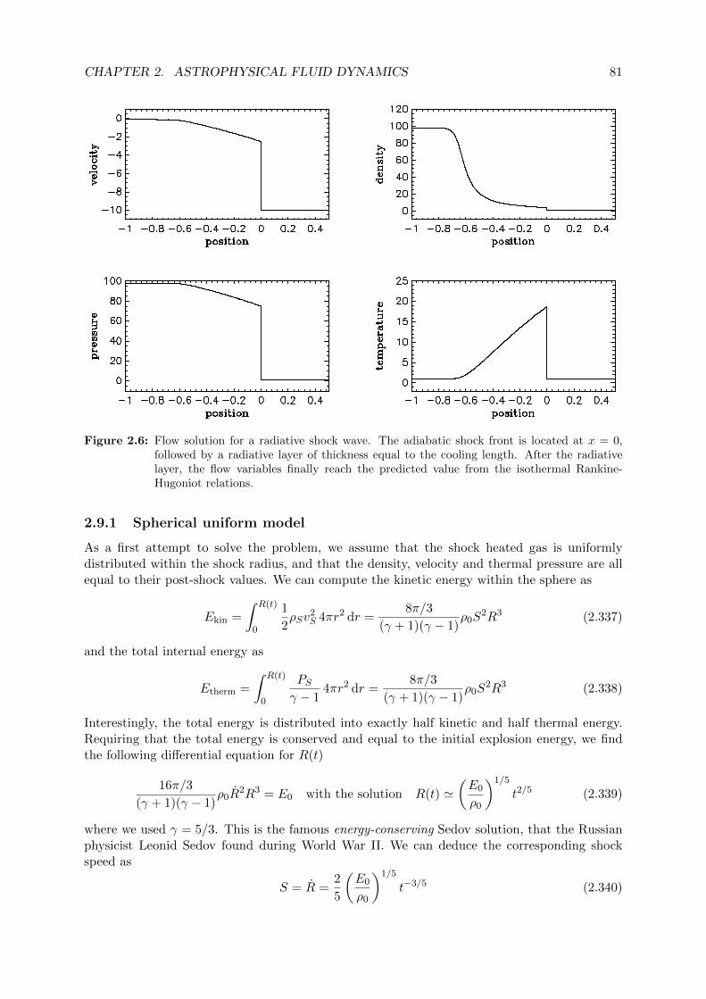
CHAPTER 2. ASTROPHYSICAL FLUID DYNAMICS 81
Figure 2.6: Flow solution for a radiative shock wave. The adiabatic shock front is located at x = 0,followed by a radiative layer of thickness equal to the cooling length. After the radiativelayer, the flow variables finally reach the predicted value from the isothermal Rankine-Hugoniot relations.
2.9.1 Spherical uniform model
As a first attempt to solve the problem, we assume that the shock heated gas is uniformlydistributed within the shock radius, and that the density, velocity and thermal pressure are allequal to their post-shock values. We can compute the kinetic energy within the sphere as
Ekin =
∫ R(t)
0
1
2ρSv
2S 4πr2 dr =
8π/3
(γ + 1)(γ − 1)ρ0S
2R3 (2.337)
and the total internal energy as
Etherm =
∫ R(t)
0
PSγ − 1
4πr2 dr =8π/3
(γ + 1)(γ − 1)ρ0S
2R3 (2.338)
Interestingly, the total energy is distributed into exactly half kinetic and half thermal energy.Requiring that the total energy is conserved and equal to the initial explosion energy, we findthe following differential equation for R(t)
16π/3
(γ + 1)(γ − 1)ρ0R
2R3 = E0 with the solution R(t) '(E0
ρ0
)1/5
t2/5 (2.339)
where we used γ = 5/3. This is the famous energy-conserving Sedov solution, that the Russianphysicist Leonid Sedov found during World War II. We can deduce the corresponding shockspeed as
S = R =2
5
(E0
ρ0
)1/5
t−3/5 (2.340)
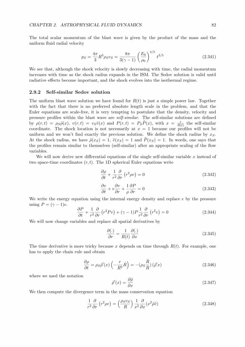
CHAPTER 2. ASTROPHYSICAL FLUID DYNAMICS 82
The total scalar momentum of the blast wave is given by the product of the mass and theuniform fluid radial velocity
pS =4π
3R3ρSvS =
8π
3(γ − 1)
(E0
ρ0
)4/5
t3/5 (2.341)
We see that, although the shock velocity is slowly decreasing with time, the radial momentumincreases with time as the shock radius expands in the ISM. The Sedov solution is valid untilradiative effects become important, and the shock evolves into the isothermal regime.
2.9.2 Self-similar Sedov solution
The uniform blast wave solution we have found for R(t) is just a simple power law. Togetherwith the fact that there is no preferred absolute length scale in the problem, and that theEuler equations are scale-free, it is very tempting to postulate that the density, velocity andpressure profiles within the blast wave are self-similar. The self-similar solutions are definedby ρ(r, t) = ρS ρ(x), v(r, t) = vS v(x) and P (r, t) = PSP (x), with x = r
R(t) the self-similarcoordinate. The shock location is not necessarily at x = 1 because our profiles will not beuniform and we won’t find exactly the previous solution. We define the shock radius by xS .At the shock radius, we have ρ(xS) = 1, v(xS) = 1 and P (xS) = 1. In words, one says thatthe profiles remain similar to themselves (self-similar) after an appropriate scaling of the flowvariables.
We will now derive new differential equations of the single self-similar variable x instead oftwo space-time coordinates (r, t). The 1D spherical Euler equations write
∂ρ
∂t+
1
r2
∂
∂r
(r2ρv
)= 0 (2.342)
∂v
∂t+ v
∂v
∂r+
1
ρ
∂P
∂r= 0 (2.343)
We write the energy equation using the internal energy density and replace e by the pressureusing P = (γ − 1)e.
∂P
∂t+
1
r2
∂
∂r
(r2Pv
)+ (γ − 1)P
1
r2
∂
∂r
(r2v)
= 0 (2.344)
We will now change variables and replace all spatial derivatives by
∂(.)
∂r=
1
R(t)
∂(.)
∂x(2.345)
The time derivative is more tricky because x depends on time through R(t). For example, onehas to apply the chain rule and obtain
∂ρ
∂t= ρS ρ
′(x)(− r
R2R)
= −(ρSR
R) (ρ′x) (2.346)
where we used the notation
ρ′(x) =∂ρ
∂x(2.347)
We then compute the divergence term in the mass conservation equation
1
r2
∂
∂r
(r2ρv
)=(ρSvS
R
) 1
x2
∂
∂x(x2ρv) (2.348)

CHAPTER 2. ASTROPHYSICAL FLUID DYNAMICS 83
Figure 2.7: Sedov solution: spherical profiles of the scaled flow variables, normalized to 1 at the shocklocation xS = 1.
and combine it with the time derivative to get
−
(ρSR
R
)(ρ′x)
+(ρSvS
R
) 1
x2
∂
∂x(x2ρv) = 0 (2.349)
Injecting the value of the post-shock velocity
vS =2
γ + 1R (2.350)
we see that all scaling variables cancel out and we are left with a dimensionless equation
− ρ′x+2
(γ + 1)
1
x2
∂
∂x(x2ρv) = 0 (2.351)
Developing the divergence term, we obtain our first differential equation
ρ′(
2
γ + 1v − x
)+ v′
(2
γ + 1
)ρ = − 4
γ + 1
ρv
x(2.352)
We now turn to the momentum equation, which writes in spherical coordinates
∂v
∂t+ v
∂v
∂r+
1
ρ
∂P
∂r= 0 (2.353)
We have to be careful because we use v = vS v(x) and the scaling variable vS now depends ontime. The time derivative thus writes
∂v
∂t= vS v + vS v
′
(−xR
R
)=
2
γ + 1R v − 2
γ + 1
R2
R(v′x) (2.354)
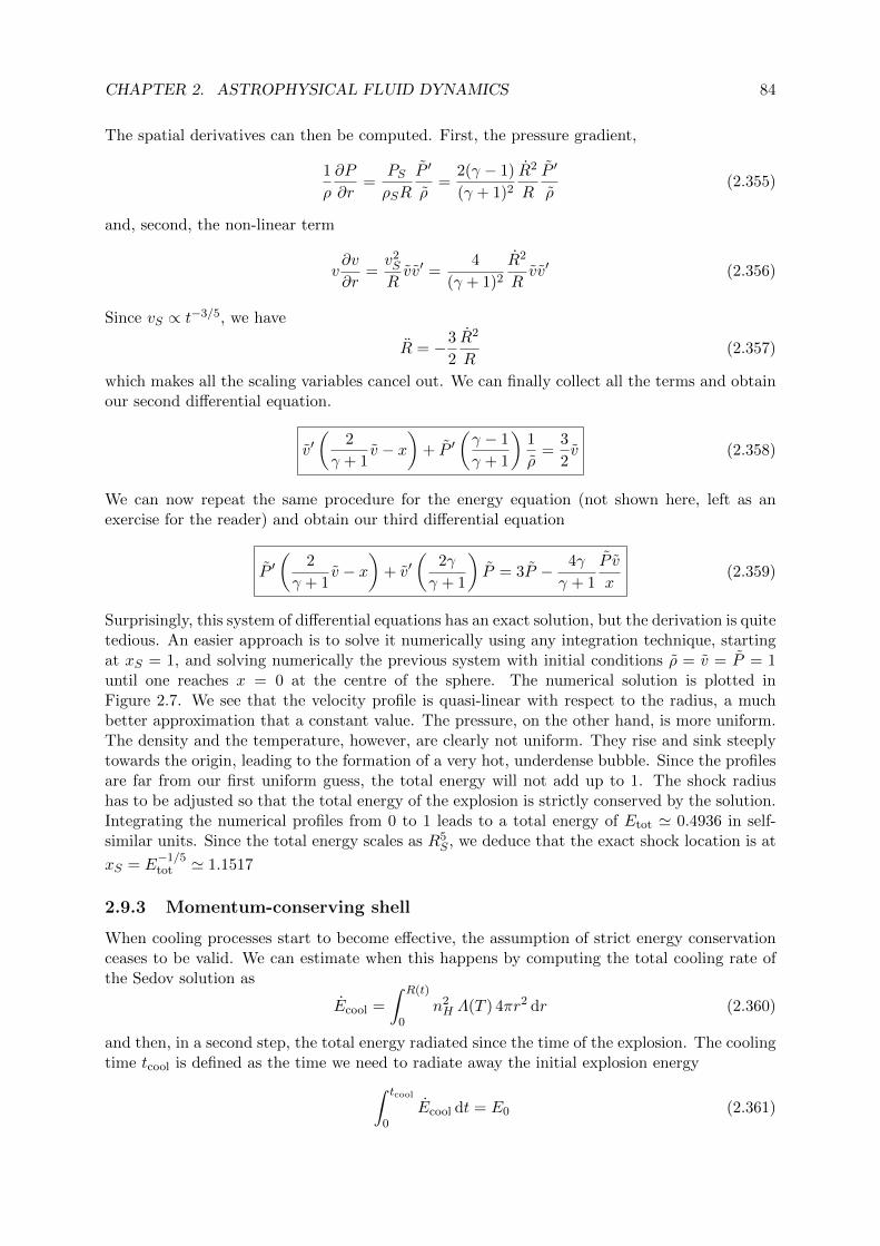
CHAPTER 2. ASTROPHYSICAL FLUID DYNAMICS 84
The spatial derivatives can then be computed. First, the pressure gradient,
1
ρ
∂P
∂r=
PSρSR
P ′
ρ=
2(γ − 1)
(γ + 1)2
R2
R
P ′
ρ(2.355)
and, second, the non-linear term
v∂v
∂r=v2S
Rvv′ =
4
(γ + 1)2
R2
Rvv′ (2.356)
Since vS ∝ t−3/5, we have
R = −3
2
R2
R(2.357)
which makes all the scaling variables cancel out. We can finally collect all the terms and obtainour second differential equation.
v′(
2
γ + 1v − x
)+ P ′
(γ − 1
γ + 1
)1
ρ=
3
2v (2.358)
We can now repeat the same procedure for the energy equation (not shown here, left as anexercise for the reader) and obtain our third differential equation
P ′(
2
γ + 1v − x
)+ v′
(2γ
γ + 1
)P = 3P − 4γ
γ + 1
P v
x(2.359)
Surprisingly, this system of differential equations has an exact solution, but the derivation is quitetedious. An easier approach is to solve it numerically using any integration technique, startingat xS = 1, and solving numerically the previous system with initial conditions ρ = v = P = 1until one reaches x = 0 at the centre of the sphere. The numerical solution is plotted inFigure 2.7. We see that the velocity profile is quasi-linear with respect to the radius, a muchbetter approximation that a constant value. The pressure, on the other hand, is more uniform.The density and the temperature, however, are clearly not uniform. They rise and sink steeplytowards the origin, leading to the formation of a very hot, underdense bubble. Since the profilesare far from our first uniform guess, the total energy will not add up to 1. The shock radiushas to be adjusted so that the total energy of the explosion is strictly conserved by the solution.Integrating the numerical profiles from 0 to 1 leads to a total energy of Etot ' 0.4936 in self-similar units. Since the total energy scales as R5
S , we deduce that the exact shock location is at
xS = E−1/5tot ' 1.1517
2.9.3 Momentum-conserving shell
When cooling processes start to become effective, the assumption of strict energy conservationceases to be valid. We can estimate when this happens by computing the total cooling rate ofthe Sedov solution as
Ecool =
∫ R(t)
0n2H Λ(T ) 4πr2 dr (2.360)
and then, in a second step, the total energy radiated since the time of the explosion. The coolingtime tcool is defined as the time we need to radiate away the initial explosion energy∫ tcool
0Ecool dt = E0 (2.361)
CHAPTER 2. ASTROPHYSICAL FLUID DYNAMICS 85
At that time, the supernova remnant has reached the cooling radius defined by
Rcool = RS(tcool) (2.362)
Beyond this radius, the flow will quickly become isothermal. In the strong shock limit, theRankine-Hugoniot relation will give us
ρS 'M2ρ0 =S2
a2ρ0 and vS ' S (2.363)
We see that, as in the isothermal shock case, the fluid after the shock immediately follows theshock front. The ISM will therefore accumulate in a very thin shell right behind the shock. Thetotal mass swept up by the shock is equal to the mass of ISM enclosed by the shock surface
MS =4π
3ρ0R
3(t) (2.364)
and is entirely located in a thin cold shell. The rest of the sphere is filled with the remnantof the Sedov phase, namely a bubble of low density hot gas. This hot gas is called the hotinterstellar medium and represents the third main phase of the ISM (after the warm neutralmedium and the cold molecular gas discussed in the thermal instability section). Obviously,during this isothermal evolution, the energy is not conserved. The shock is piling up gas likea snow-plow piling up snow on a piste and this thin shell conserves its momentum. The initialcondition of the snow-plow phase is the final state of the Sedov phase, so that the conservedmomentum is
pcool = pS(tcool) (2.365)
For t > tcool, we write that the momentum is constant as
MSR = pcool (2.366)
This gives us a new differential equation for the shock radius
R3R =3pcool
4πρ0(2.367)
Integrating this gives us a new solution for the time evolution of the shock radius.
R(t) =
(3pcool
πρ0
)1/4
t1/4 '(pcool
ρ0
)1/4
t1/4 (2.368)
We see that in this case, the shock is moving much slower. At some point, the shock velocitywill slow down so much that the shock front will become subsonic and the bubble will stopexpanding. The final stage is therefore a hot bubble surrounded by a dense shell of cold gas, inwhich new stars will form and after some time explode in supernovae, and the whole cycle willrepeat.
CHAPTER 2. ASTROPHYSICAL FLUID DYNAMICS 86
2.10 Astrophysical turbulence
We now turn to one of the most important topics in modern theory of astrophysical fluids, namelythe theory of turbulence. It plays a fundamental role in providing new mass, momentum andenergy transport phenomena. In engineering and climate modeling, the impact of turbulence ismajor, and various fluid instabilities that seed turbulence are responsible for many importantprocesses like the theory of flight, boundary layers, global energy transfer in the oceans orin the atmosphere, to name a few. In astrophysics, turbulence plays a fundamental role in theinterstellar medium and probably determines how stars acquire their mass. We have already seenthat turbulence controls the accretion rate in disks. It is also responsible for a very importantenergy transfer mechanism in stars and planets called convection.
2.10.1 Some fundamental fluid properties
Before we describe in greater details the theory of turbulence, we need to explain a few basicproperties of fluid flows that we will appeal to in the following section. It is therefore veryimportant to become familiar with these concepts, as they are the building blocks of whatfollows.
Adiabatic evolution
In absence of cooling and heating processes, and far away from shocks, the Euler equations aresaid to be adiabatic. In other words, as we will prove now, the entropy is srictly conserved alongtrajectories. If, on top of that, the initial entropy is homogeneous to start with, then it willremain homogeneous at all time. The flow is said to be isentropic. It is important to understandthat adiabatic is not equivalent to isentropic. The latter is a stronger condition on the flow thanthe former. Let’s write the Euler equations in Lagrangian form.
1
ρ
Dρ
Dt= −∇ · v , ρ
Dε
Dt= −P∇ · v , 1
ε
Dε
Dt= −(γ − 1)∇ · v (2.369)
where in the rightmost equation, we have used the equation of state of an ideal gas P = (γ−1)ρε.Combining the mass and energy conservation equations gives the following relation between themass density and the specific energy
1
ε
Dε
Dt= (γ − 1)
1
ρ
Dρ
Dt(2.370)
We define the pseudo-entropy (or the entropy for short), which is not the same as the trueentropy defined in the chapter on kinetic theory, as
S ≡ P
ργ= (γ − 1)
ε
ργ−1(2.371)
We compute the logarithmic Lagrange derivative of the entropy
1
S
DS
Dt=
1
ε
Dε
Dt− (γ − 1)
1
ρ
Dρ
Dt= 0 (2.372)
In conclusion, the adiabatic evolution of the fluid, in absence of cooling and heating, and faraway from shocks, is described by a very simple equation, namely
DS
Dt= 0 (2.373)

CHAPTER 2. ASTROPHYSICAL FLUID DYNAMICS 87
This simple equation just states that the entropy is conserved along the trajectory of each fluidelement. If xi is the initial location of the fluid element at time ti, and xf its final position attime tf , then one has for an adiabatic evolution Sf = Si or
P (xf , tf )
ρ(xf , tf )γ=P (xi, ti)
ρ(xi, ti)γ(2.374)
In contrast, isentropic flows have S(x, t) = S0 everywhere, or
P (x, t) = S0ργ(x, t) (2.375)
We see that isentropic flows are a particular case of a polytropic equation of state for whichP = AρΓ with A = S0 and Γ = γ. Note that in general the polytropic exponent Γ comes fromexternal processes, such as cooling or heating, while the ideal gas adiabatic exponent γ comesfrom microscopic processes describing the collisions.
Vorticity
A very important quantity used to describe turbulence is the vorticity. Vortices are fluid elementsfor which the vorticity, defined as ω = ∇× v, is constant and follows the displacements of thefluid element. Vortices are also called eddies. Examples of such vortices are cyclones in theatmosphere of the tropical regions. We now derive the famous vorticity equation, using themomentum conservation equation, including viscosity, as
Dv
Dt=∂v
∂t+ (v · ∇)v = −1
ρ∇P −∇φ+ ν4v (2.376)
with ν = µ/ρ = cst. The non-linear term, the one responsible for shock formation, can bedecomposed into
(v · ∇)v = ∇(v2
2
)+ (∇× v)× v (2.377)
which, after introducing the vorticity ∇× v = ω gives
∂v
∂t+∇
(v2
2
)+ ω × v = −1
ρ∇P −∇φ+ ν4v (2.378)
We now take the curl of the previous equation, using the two following vector relations: ∇ ×(∇φ) = 0 and ∇×4v = 4(∇× v), we obtain the vorticity equation
∂ω
∂t+∇× (ω × v) =
1
ρ2∇ρ×∇P + ν4ω (2.379)
This equation is among the most important results in fluid dynamics. It contains three termsgoverning the time evolution of the vorticity. The first term (that appears as the second term onthe left-hand side of the equation) corresponds to the transport of vorticity. Although it is notstrictly a Lagrange derivative, it still means that, aside from the effect of vortex-stretching, theeddies are basically following the Lagrangian flow. The second important term is the first on theright-hand side of the equation: this is the so called baroclinic term, which creates vorticity dueto the interaction between pressure and density gradients. This term is in most circumstanceszero. For example, an incompressible fluid has ρ = ρ0, so ∇ρ = 0 and the baroclinic termvanishes. An isothermal fluid or a fluid with a polytropic equation of state will have
∇P = P ′(ρ)∇ρ (2.380)

CHAPTER 2. ASTROPHYSICAL FLUID DYNAMICS 88
so that the pressure gradient is always colinear to the density gradient and the curl in thebaroclinic term will also vanish. In general, in order to create vorticity, one need to havemisaligned pressure and density gradients. This can happen if certain heating terms are presentin a localised region, or if two shock waves interact and create a triple point. These situations forwhich vorticity is created through the baroclinic term are usual associated to fluid instabilities.The third important term is the last one on the right-hand side: viscous dissipation. Onerecognizes the heat equation, this one for the vorticity. Since the molecular diffusion coefficientis very small ν = λcolla, the dissipation of eddies will take a long time, and they can be relativelylong-lived features in the flow. A strong consequence of this equation is that if the baroclinicterm is zero and no other source of vorticity are present, then vorticity will decay and remainzero for ever. We have a curl-free flow and it is justified to use the simple version of the secondBernoulli theorem.
Helmholtz decomposition theorem
This theorem is also known as the fundamental theorem of vector calculus. It states that anyvector field v can be decomposed into the sum of the gradient of a scalar potential and the curlof a vector potential
v = ∇ϕ+∇×A (2.381)
This decomposition is unique and both potentials can be found by solving two different Poissonequations
4ϕ = ∇ · v = θ (2.382)
4A = ∇× v = ω (2.383)
with the proper boundary conditions. We didn’t really simplify the problem, since now we haveone vector field and one scalar field instead of just one vector field. The added value of theHelmoltz decomposition will become clear now. Let’s consider two examples.
• Let us consider a curl-free flow, for which ω = 0. We also assume the boundary conditionat infinity is set to zero. Then, the corresponding vector potential is A = 0 and we havea pure potential flow with v = ∇ϕ.
• Let us now consider in addition that our flow is incompressible, so that θ = 0. Using themass conservation equation, we see that
1
ρ
Dρ
Dt= −∇ · v = −θ (2.384)
so that θ = 0 is equivalent to ρ = ρ0. In our study of sound waves, we have also seenthat the amplitude of the density perturbation is related to the amplitude of the velocityperturbation by
∆ρ
ρ0= ±∆v
a(2.385)
We conclude that incompressible flows are also subsonic flows for which v a. In thiscase, since θ = 0, we have a potential flow for which the scalar potential satisfies Laplaceequation: 4ϕ = 0.
CHAPTER 2. ASTROPHYSICAL FLUID DYNAMICS 89
Bernoulli theorem revisited
Since our incompressible flow is also a potential flow, we can go back to the second Bernoullitheorem, which was written as
∂v
∂t+∇
(v2
2+ φ+ π
)= v × ω (2.386)
and simplify it because with π = P/ρ0, ω = 0 and v = ∇ϕ. This gives us
∇(∂ϕ
∂t+v2
2+ φ+
P
ρ0
)= 0 (2.387)
If the gradient of a scalar quantity is zero everywhere, it means the quantity is uniform, so weobtain
∂ϕ
∂t+v2
2+ φ+
P
ρ0= C(t) (2.388)
where the Bernoulii constant C(t) is the same everywhere in the fluid but possibly depends ontime. This form of the Bernoulli theorem will prove very useful in what comes next.
Contact discontinuity and the kinematic condition
We now describe a new type of discontinuity which is not a shock but the interface between twofluids. This discontinuity is therefore not a wave that propagates through the fluid at a differentvelocity S but a material interface. The key point in describing a contact discontinuity is therequirement that the two fluids and the interface remain in contact. In the direction perpen-dicular to the interface, we can write the Rankine-Hugoniot relations for a general discontinuityas
ρ1v1 − ρ2v2 = S(ρ1 − ρ2) (2.389)(ρ1v
21 + P1
)−(ρ2v
22 + P2
)= S(ρ1v1 − ρ2v2) (2.390)
(E1 + P1) v1 − (E2 + P2) v2 = S(E1 − E2) (2.391)
where we have defined the normal component of the velocities using the unit vector normal tothe interface n as
v1 = v1 · n and v2 = v2 · n and S = vI · n (2.392)
The contact condition, also called the “no vacuum” condition, is just
v1 = v2 = S (2.393)
We see that the mass conservation relation is trivially satisfied. On the other hand, the momen-tum and total energy conservation relations require also pressure equality across the interfaceas
P1 = P2 (2.394)
These two conditions are the Rankine-Hugoniot relations for contact discontinuities. Note thatcontact discontinuities have in general a complex shape. In what follows, we restrict ourselvesto two dimensional flows, but it can be easily generalized to 3D. We will now derive what iscalled the kinematic condition on the interface. We are in a Cartesian coordinate system with

CHAPTER 2. ASTROPHYSICAL FLUID DYNAMICS 90
coordinates (x, z). If we represent the shape of the interface at any given time by the geometricalfunction z = η(x, t), we can define the interface position vector and its velocity by
rI = (x(t), η(x, t)) (2.395)
vI = (x,∂η
∂xx+
∂η
∂t) (2.396)
In the second equation, we have used the chain rule on the function η. The “no-vacuum”condition writes vI · n = v · n. Note for a contact discontinuity, we can authorize slippingmotions so that vI · t 6= v · t, where t is the tangent vector to the interface. We can computeeasily the unit tangent vector and the unit normal vector as
t =
(1,∂η
∂x
)/
√1 +
(∂η
∂x
)2
and n =
(−∂η∂x, 1
)/
√1 +
(∂η
∂x
)2
(2.397)
We now impose the contact condition for each fluid as v · n = vI · n which writes
− vx∂η
∂x+ vz = −x ∂η
∂x+ x
∂η
∂x+∂η
∂t(2.398)
which simplifies into the final kinematic condition on the interface
∂η
∂t+ vx
∂η
∂x= vz (2.399)
2.10.2 Rayleigh-Taylor instability
We consider two fluids with constant densities ρ1 and ρ2, separated by an interface initiallystrictly horizontal. Fluid 1 is initially below z = 0 and fluid 2 is above z = 0. The gravity fieldis constant and points downwards.
g = −gez with g > 0 (2.400)
Our initial state is described by the hydrostatic equilibrium equation with
− 1
ρ
∂P
∂z= g and v = 0 (2.401)
Integrating this equation in fluid 1 and 2 gives for the equilibrium pressure profile
P1 = P0 − ρ1gz and P2 = P0 − ρ2gz (2.402)
We see that our two fluids meet at z = 0 with P1 = P2 = P0.
Perturbations
Now that our equilibrium state has been specified, we consider small perturbations with velocitiesv1 a and v2 a so that, at least in the begining, the flow will remain subsonic and curl-free.We thus have two potential flows with
v1 = ∇ϕ1, 4ϕ1 = 0 and v2 = ∇ϕ2, 4ϕ2 = 0 (2.403)
We use for our scalar potential a general solution of the form
ϕ1(x, z, t) = ϕ1(z) ei(kx−ωt) and ϕ2(x, z, t) = ϕ2(z) ei(kx−ωt) (2.404)

CHAPTER 2. ASTROPHYSICAL FLUID DYNAMICS 91
where both ϕ1(z) and ϕ2(z) will be determined shortly. For the interface, we use a planar wavesolution of the form
η(x, t) = ∆η ei(kx−ωt) (2.405)
where ∆η is the fixed initial amplitude of the wave. Let’s first solve our two Laplace equationsin the two domains. For fluid 1, we have
4ϕ1 =∂2ϕ1
∂x2+∂2ϕ1
∂z2= −k2ϕ1(z) ei(kx−ωt) + ϕ1(z)′′ ei(kx−ωt) = 0 (2.406)
Dividing out the exponentials gives us the following diffential equation
ϕ1(z)′′ = k2ϕ1(z) (2.407)
for which the general solution is
ϕ1(z) = ∆ϕ+1 e
+kz +∆ϕ−1 e−kz (2.408)
where ∆ϕ+1 and ∆ϕ+
1 are fixed ampitude set by the initial conditions. Since fluid 1 is definedin the entire domain z < 0, we need to set ∆ϕ−1 = 0 to avoid a divergence at z → −∞. Inconclusion, the final form for our solution for ϕ1 reads
ϕ1(x, z, t) = ∆ϕ1 e+kzei(kx−ωt) (2.409)
where we dropped the index + for simplicity. Equivalently, we have for fluid 2
ϕ2(x, z, t) = ∆ϕ2 e−kzei(kx−ωt) (2.410)
for which we dropped the positive exponential to avoid a divergence at z → +∞. We havetherefore three unknown amplitudes to determine our complete solution ∆η, ∆ϕ1 and ∆ϕ2.
Kinematic condition
We now write the kinematic conditions between each fluid and the interface.
∂η
∂t+ vx
∂η
∂x= vz (2.411)
This equation is evaluated at z = η and linearized by Taylor expanding the exponential termand dropping all high-order (quadratic or higher) terms in the equation.
∂η
∂t' ∂ϕ1
∂zand
∂η
∂t' ∂ϕ2
∂z(2.412)
Using the adopted solutions, we get the following relations between the amplitudes
−iω∆η = +k∆ϕ1 and − iω∆η = −k∆ϕ2 (2.413)
Bernoulli theorem and pressure equality
We now write the second Bernoulli theorem in each domain as
∂ϕ1
∂t+v2
1
2+P1
ρ1+ gz = C1 (2.414)
∂ϕ2
∂t+v2
2
2+P2
ρ2+ gz = C2 (2.415)
CHAPTER 2. ASTROPHYSICAL FLUID DYNAMICS 92
The two Bernoulli constants can be found by noticing that the pressure at infinity matches theinitial equilibrium model. In other words, the perturbations vanish at infinity. We thus get
P1
ρ1+ gz → P0
ρ1= C1 as z → −∞ (2.416)
and similarlyP2
ρ2+ gz → P0
ρ2= C2 as z → +∞ (2.417)
We now linearize the two Bernoulli equations by dropping the kinetic energy term and evaluatethem at the interface z = η. This gives us
∂ϕ1
∂t+P1
ρ1+ gη =
P0
ρ1(2.418)
∂ϕ2
∂t+P2
ρ2+ gη =
P0
ρ2(2.419)
We finally require P1 = P2 at the interface, which gives the final relation between the amplitudes
ρ1 (−iω∆ϕ1 + g∆η) = ρ2 (−iω∆ϕ2 + g∆η) (2.420)
Injecting the two previous equations into the third one, we get the dispersion relation as
ρ1
(−ω2 + gk
)= ρ2
(+ω2 + gk
)(2.421)
and finally
ω2 =ρ1 − ρ2
ρ1 + ρ2gk (2.422)
• If ρ1 > ρ2, the previous dispersion relation yields stable propagating waves, with velocityω/k '
√g/k. This is the solution for deep sea water, with long wavelength perturbations
moving faster than small wavelength ones.
• If ρ1 < ρ2, on the other hand, the solutions are unstable. This is the Rayleigh-Taylorinstability. The amplitude of the interface will grow exponentially fast. In the non-linearregime, the low density fluid at the bottom generates bubbles that rise buoyantly in thehigh density fluid. The high density fluid on top will sink in the form of cold fingers thateventually break into droplets.
Note that the two fluids pressures at the interface are equal and a more general criterion for theinstability can be expressed as
S1 =P1
ργ1> S2 =
P2
ργ2(2.423)
This instability is also called the interchange instability, because the high entropy fluid at thebottom will change its position with the low entropy fluid on top. This instability is at theorigin of a fundamental process in stars and planets called convection. Once the amplitude ofthe perturbations are large, the instability enters the non-linear regime. Figure 2.8 shows a timesequence of the non-linear development of the Rayleigh-Taylor instability. Initially, the interfaceis almost perfectly horizontal. Once the amplitude of the instability is large enough, we can seeby eye the planar wave solution. Later on, the lighter fluid develops large bubble that rise, whilethe heavier fluid forms cold and dense fingers that sink in the direction of gravity. One can alsosee on the sides of the fingers small vortices due to a secondary Kelvin-Helmholtz instability.
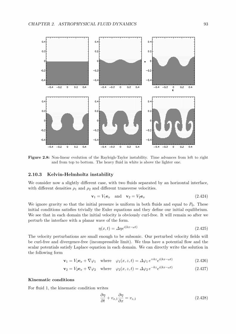
CHAPTER 2. ASTROPHYSICAL FLUID DYNAMICS 93
Figure 2.8: Non-linear evolution of the Rayleigh-Taylor instability. Time advances from left to rightand from top to bottom. The heavy fluid in white is above the lighter one.
2.10.3 Kelvin-Helmholtz instability
We consider now a slightly different case, with two fluids separated by an horizontal interface,with different densities ρ1 and ρ2 and different transverse velocities.
v1 = V1ex and v2 = V2ex (2.424)
We ignore gravity so that the initial pressure is uniform in both fluids and equal to P0. Theseinitial conditions satisfies trivially the Euler equations and they define our initial equilibrium.We see that in each domain the initial velocity is obviously curl-free. It will remain so after weperturb the interface with a planar wave of the form.
η(x, t) = ∆ηei(kx−ωt) (2.425)
The velocity perturbations are small enough to be subsonic. Our perturbed velocity fields willbe curl-free and divergence-free (incompressible limit). We thus have a potential flow and thescalar potentials satisfy Laplace equation in each domain. We can directly write the solution inthe following form
v1 = V1ex +∇ϕ1 where ϕ1(x, z, t) = ∆ϕ1 e+kzei(kx−ωt) (2.426)
v2 = V2ex +∇ϕ2 where ϕ2(x, z, t) = ∆ϕ2 e−kzei(kx−ωt) (2.427)
Kinematic conditions
For fluid 1, the kinematic condition writes
∂η
∂t+ vx,1
∂η
∂x= vz,1 (2.428)
CHAPTER 2. ASTROPHYSICAL FLUID DYNAMICS 94
with now
vx,1 = V1 +∂ϕ1
∂xand vz,1 =
∂ϕ1
∂z(2.429)
Linearizing this equation at the interface position z = η leads us to keep more terms than in theRayleigh-Taylor case
∂η
∂t+ V1
∂η
∂x=∂ϕ1
∂z(2.430)
We now inject our Ansatz and obtain our first relation between the perturbation amplitudes
(−iω + ikV1)∆η = +k∆ϕ1 (2.431)
Similarly, for fluid 2, we get
(−iω + ikV2)∆η = −k∆ϕ2 (2.432)
Bernoulli equation and pressure equilibrium
We now use Bernoulli equation in fluid 1 for which we have no gravity
∂ϕ1
∂t+
1
2v2x,1 +
1
2v2z,1 +
P1
ρ1= C1 (2.433)
We find the Bernoulli constant by requiring that the perturbations vanish at −∞ so that
1
2V 2
1 +P0
ρ1= C1 (2.434)
Finally, we linearize the Bernoulli equation, dropping all quadratic (or higher order) terms
∂ϕ1
∂t+
1
2V 2
1 + V1∂ϕ1
∂x+P1
ρ1=
1
2V 2
1 +P0
ρ1(2.435)
This lead to the pressure in fluid 1 at the interface to be
P1 = P0 − ρ1
(∂ϕ1
∂t+ V1
∂ϕ1
∂x
)(2.436)
and similarly for fluid 2, we have
P2 = P0 − ρ2
(∂ϕ2
∂t+ V2
∂ϕ2
∂x
)(2.437)
Imposing pressure equality at the interface and computing the time and space derivatives givesus our third relation
ρ1 (−iω + ikV1)∆ϕ1 = ρ2 (−iω + ikV2)∆ϕ2 (2.438)
Combining it with the two previously found relation leads to the dispersion relation
ρ1 (ω − kV1)2 = −ρ2 (ω − kV2)2 (2.439)
This is a problematic equation, because it states that a square is equal to minus another square.The solution is to introduce an imaginary component, which is, as we now know very well, aclear sign of instability. √
ρ1 (ω − kV1) = ±i√ρ2 (ω − kV2) (2.440)
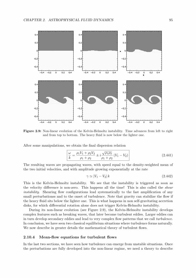
CHAPTER 2. ASTROPHYSICAL FLUID DYNAMICS 95
Figure 2.9: Non-linear evolution of the Kelvin-Helmoltz instability. Time advances from left to rightand from top to bottom. The heavy fluid is now below the lighter one.
After some manipulations, we obtain the final dispersion relation
ω
k=ρ1V1 + ρ2V2
ρ1 + ρ2± i√ρ1ρ2
ρ1 + ρ2(V1 − V2) (2.441)
The resulting waves are propagating waves, with speed equal to the density-weighted mean ofthe two initial velocities, and with amplitude growing exponentially at the rate
γ ' |V1 − V2| k (2.442)
This is the Kelvin-Helmoltz instability. We see that the instability is triggered as soon asthe velocity difference is non-zero. This happens all the time! This is also called the shearinstability. Shearing flow configurations lead systematically to the fast amplification of anysmall perturbationss and to the onset of turbulence. Note that gravity can stabilize the flow ifthe heavy fluid sits below the lighter one. This is what happens in non self-gravitating accretiondisks, for which differential rotation alone does not trigger Kelvin-Helmoltz instability.
During its non-linear evolution (see Figure 2.9), the Kelvin-Helmoltz instability developscomplex features such as breaking waves, that later become turbulent eddies. Larger eddies canin turn develop secondary eddies and lead to very complex flow patterns that we call turbulence.In conclusion, we have seen two classical equilibrium situations where turbulence forms naturally.We now describe in greater details the mathematical theory of turbulent flows.
2.10.4 Mean-flow equations for turbulent flows
In the last two sections, we have seen how turbulence can emerge from unstable situations. Oncethe perturbations are fully developed into the non-linear regime, we need a theory to describe
CHAPTER 2. ASTROPHYSICAL FLUID DYNAMICS 96
these fluctuations. The mean-flow equations are new fluid equations that can be used to describethe large-scale flow, averaging over the small-scale fluctuations. Density, velocity and pressurefluctuations are treated as random variables, whose exact values are not important. Only theaverage statistical properties of the fluctuations are important. The new mathematical keyconcept we introduce in this section is the averaging operator. For example, if you consider thedensity field ρ(x, t) as the variable of interest, you can define the space average within a fixedvolume V0 as
ρ(t) =1
V0
∫V0
ρ(x, t)dV (2.443)
with the overbar indicating the volume average. You can also use a small probe that recordsthe value of the density at a fixed location, and then you can perform the time average withina fixed time interval as
ρ(x) =1
T0
∫T0
ρ(x, t)dt (2.444)
These two averaging operators are easy to understand but they contain a fundamental flaw: Inboth cases, we have lost one independent variable, either time or space, so we won’t be ableto find new fluid equations. There is one more definition we can use to define the averagingoperator, namely the ensemble average, defined by
ρ(x, t) =1
N
∑i=1,N
ρi(x, t) (2.445)
Index i now stands for a parallel universe where we have the same exact fluid flow but withdifferent random properties, so we can now average over N parallel universes to get the averageand still keep both time and space as independent variables. Although this definition of theaveraging operator is practical in a mathematical sense, it is not realistic as one cannot designan experiment over parallel universes we don’t know how to explore. We nevertheless assumethat these three different definitions are equivalent and lead to the same value for the averagequantity. This is called the ergodic prinicple. In what follows, we will use the multiple universesviewpoint, but keep in mind that this can also mean time and/or space average within one singleexperiment.
Another interpretation of the averaging operator is related to the concept of smoothing. Wedefine a smoothing kernel of size R, say a Gaussian filter or a Top-Hat function W , and wedefine the average at time t and position x as the convolution of the original density field andthe filter function
ρ(x, t) =
∫R3
ρ(x′, t)W
(x− x′
R
)d3x′ (2.446)
The average density field is the smoothed density field at scales r > R, and the fluctuations aredefined as the small-scale perturbations for scales r < R. Whatever viewpoint we adopt, wealways define the fluctuating density as the different between the average and the original one.We thus have in each parallel universe
ρ(x, t) = ρ(x, t) + ρ′(x, t) (2.447)
v(x, t) = v(x, t) + v′(x, t) (2.448)
P (x, t) = P (x, t) + P ′(x, t) (2.449)
If we apply the averaging operator to the previous three equations, we find
ρ′ = 0 , v′ = 0 and P ′ = 0 (2.450)
CHAPTER 2. ASTROPHYSICAL FLUID DYNAMICS 97
Let’s now apply this operator to the mass conservation equation. We use in what follows Einsteinnotations, and start with
∂ρ
∂t+
∂
∂xj(ρvj) = 0 (2.451)
We decompose both the density and the velocity into the mean flow and the fluctuating flow asρ = ρ+ ρ′ and vj = vj + v′j and obtain
∂ρ
∂t+∂ρ′
∂t+
∂
∂xj
(ρ vj + ρv′j + ρ′vj + ρ′v′j
)= 0 (2.452)
We now apply the average operator on top of the entire equation. Already averaged quantitycan be considered as constant. Using the multiple universes interpretation, the average operatorobviously commutes with time and space derivatives. We therefore get
∂ρ
∂t+
∂
∂xj
(ρ vj + ρ′v′j
)= 0 (2.453)
We see that we have identified a new quantity ρ′v′j 6= 0 called the turbulent mass flux. Apartfrom this annoying term, we have derived a new mass conservation equation for the mean flowonly, that we can use to solve the mean flow evolution, ignoring the details of the turbulentfluctuations. We however need to come up with a model for the turbulent mass flux.
Another approach, more suited for compressible fluids, is based on the Favre average. Favreaveraging is based on a mass-weighted average of all specific quantities like the velocity, thespecific internal energy or the temperature. We have by definition
ρv = ρ v (2.454)
where the tilde means Favre average. We need to define new fluctuations with respect to thisnew average
v = v + v′′ and ε = ε+ ε′′ (2.455)
where now the double prime stands for fluctuations defined with respect to the mass-weighted,Favre average, and single prime for fluctuations with respect to the standard, volume-weightedaverage. Now we have for the fluctuating part the following property
ρv′′ = 0 and ρε′′ = 0 (2.456)
but of course we have unfortunately in this case
v′′ 6= 0 and ε′′ 6= 0 (2.457)
Let’s re-derive the mass conservation equation using the Favre average. This time, it is importantnot to develop the density inside the space derivative
∂ρ
∂t+∂ρ′
∂t+
∂
∂xj
(ρ vj + ρv′′j
)= 0 (2.458)
We now apply the average operator to the entire equation, which leads now to the much simplerform
∂ρ
∂t+
∂
∂xj(ρ vj) = 0 (2.459)
CHAPTER 2. ASTROPHYSICAL FLUID DYNAMICS 98
By adopting a new frame of reference, we have absorbed the turbulent mass flux in the Favreaverage. We can now relate the two different definitions of the mean flow velocity by simplyidentifying terms
vj = vj +ρ′v′jρ
(2.460)
We now move to the momentum conservation equation. We start as always with
∂
∂t(ρvi) +
∂
∂xj(ρvivj) +
∂P
∂xi= ρgi (2.461)
We decompose the velocity into vj = vj + v′′j but not the density
∂
∂t(ρvi) +
∂
∂t
(ρv′′i)
+∂
∂xj
(ρvivj + viρv
′′j + ρv′′i vj + ρv′′i v
′′j
)+∂P
∂xi= ρgi (2.462)
Now we apply the average operator over the entire equation. All terms with a ρv′′i = 0 vanishand we get the momentum conservation equation of the mean flow
∂
∂t(ρvi) +
∂
∂xj
(ρvivj + ρv′′i v
′′j
)+∂P
∂xi= ρgi (2.463)
This equation looks very much like the original one, but for one extra term, called the turbulentpressure tensor defined as
PT = ρv′′ ⊗ v′′ (2.464)
In analogy with the chapter on kinetic theory, we deconpose this tensor into a traceless tensorand an isotropic tensor as
PT = RT + PTI (2.465)
where the turbulent pressure is defined by
PT =1
3ρv′′2 =
2
3KT (2.466)
and we have introduced the turbulent kinetic energy KT. The Reynolds tensor is now definedby
RT = ρv′′ ⊗ v′′ − PTI (2.467)
and the momentum conservation equation for the mean flow can be modified as follows
∂
∂t(ρvi) +
∂
∂xj(ρvivj) +
∂
∂xj(RT,ij) +
∂P
∂xi+∂PT
∂xi= ρgi (2.468)
Finally, we derive the total energy equation for the mean flow. We start with the original energyequation in Eulerian form
∂E
∂t+
∂
∂xj(E + P ) vj = ρvjgj (2.469)
The total energy is decomposed into
E =1
2ρv2 + ρε =
1
2ρv2 + ρviv
′′i +
1
2ρv′′2 + ρε+ ρε′′ (2.470)
so that averaging the time derivative leads to
∂
∂t
(1
2ρv2 + 0 +
1
2ρv′′2 + ρε+ 0
)=∂Etot
∂t(2.471)
CHAPTER 2. ASTROPHYSICAL FLUID DYNAMICS 99
where now the total energy writes
Etot =1
2ρv2 + ρε+KT (2.472)
We see that this new total energy is equal to the kinetic energy of the mean flow, plus theinternal energy of the mean flow, plus the turbulent kinetic energy. Let’s now compute thespace derivatives. Using P = (γ − 1)ρε, we have
∂
∂xj(E + P ) vj =
∂
∂xj
(1
2ρv2vj + ρviv
′′i vj +
1
2ρv′′2vj + γρεvj + γρε′′vj
)(2.473)
We now decompose vj = vj + v′′j in the previous equation and apply immediately the averageoperator to obtain
∂
∂xj
(1
2ρv2vj + 0 + 0 + ρv′′i v
′′j vi +
1
2ρv′′2vj +
1
2ρv′′2v′′j + γρεvj + 0 + 0 + γρε′′v′′j
)(2.474)
We recognize the total energy flux due to the mean flow, the turbulence pressure tensor, that wedecompose into the Reynolds stress tensor plus the turbulent pressure, and a new term calledthe turbulent heat flux. The total energy equation for the mean flow finally writes
∂Etot
∂t+
∂
∂xj(Etot + Ptot) vj +
∂
∂xj(RT,ij vi) +
∂
∂xj(QT,j) = ρvjgj (2.475)
where the total pressure is defined by
Ptot = P + PT (2.476)
and the turbulent heat flux by
QT =1
2v′′2v′′ + γρε′′v′′ (2.477)
The analogy with kinetic theory is striking. We see that we have now introduced a new scalewhich captures mesoscopic processes such as turbulence, between the macroscopic scale of thesystem as a whole, described by the mean flow equations, and the microscopic processes suchas collisions. Turbulence is captured by the averaging operator in pretty much the same wayparticles are captured in phase space by integrating over velocity space. We are facing the sameproblem than in kinetic theory: We don’t know the exact form of the Reynolds stress tensorand the turbulent heat flux. We don’t know the value of the turbulent kinetic energy either. Wewill try to remedy for the latter in the next section.
2.10.5 Turbulent kinetic energy equation
We want to derive from first principles an equation governing the time evolution of the turbulentkinetic enrgy KT. For this, we start as always from the Euler equations,
∂ρ
∂t+
∂
∂xj(ρvj) = 0 (2.478)
ρ∂
∂tvi + ρvj
∂
∂xjvi +
∂P
∂xi= ρgi (2.479)
CHAPTER 2. ASTROPHYSICAL FLUID DYNAMICS 100
In the latter equation, we decompose vi = vi + v′′i but (very important!) not vj . We obtain
ρ∂
∂tvi + ρ
∂
∂tv′′i + ρvj
∂
∂xjvi + ρvj
∂
∂xjv′′i +
∂P
∂xi= ρgi (2.480)
We now multiply the previous equation by v′′i and sum over the three directions. If possible, wemake the specific kinetic energy appear. Otherwise, Einstein’s summation rules apply.
ρv′′i∂
∂tvi + ρ
∂
∂t
(1
2v′′2)
+ ρv′′i vj∂
∂xjvi + ρvj
∂
∂xj
(1
2v′′2)
= −v′′i∂P
∂xi+ ρv′′i gi (2.481)
We can now add to the previous equation
+1
2v′′2[∂ρ
∂t+
∂
∂xj(ρvj)
](2.482)
since it is exactly zero owing to the mass conservation equation. We get the sightly simpler form
ρv′′i∂
∂tvi +
∂
∂t
(1
2ρv′′2
)+ ρv′′i vj
∂
∂xjvi +
∂
∂xj
(1
2ρv′′2vj
)= −v′′i
∂P
∂xi+ ρv′′i gi (2.483)
Now comes the fateful moment: We at last decompose vj into vj + v′′j and apply immediatelythe averaging operator to the entire equation.
0 +∂
∂tKT + 0 + ρv′′i v
′′j
∂
∂xjvi +
∂
∂xj(KTvj) +
∂
∂xj
(1
2ρv′′2v′′j
)= −v′′i
∂P
∂xi+ 0 (2.484)
We recognize again the turbulent pressure tensor, that we decompose again into the isotropicturbulent pressure plus the Reynolds stress tensor. We also recognize one component of theheat flux, the one associated to the turbulent transport of turbulent kinetic energy. We noteit here Q′T. Finally, on the right-hand side, we have a new term called the convective term orthe turbulent work of the pressure fluctuations. In summary, we have for the turbulent kineticenergy equation
∂
∂tKT +
∂
∂xj(KTvj) + PT
∂vj∂xj
= −RT,ij∂vi∂xj− ∂
∂xj
(Q′T,j
)− v′′j
∂P
∂xj(2.485)
Here again, this equation looks very familiar. On the left-hand side, we have the transport ofturbulent kinetic energy by the mean flow, as well as the p dV work of the turbulent pressure dueto the mean flow. This is almost identical to the internal energy equation for the fluid. On theright-hand side, we have new terms that are associated to the production of turbulent kineticenergy. They are actually called the production terms. We will see in the next section how onecan compute these terms within some clever approximations. Qualitatively, however, these termswill inject turbulent kinetic energy in the system, but we have no way to dissipate this energy.In fact, viscous processes, not discussed here, will transform turbulent kinetic energy into heat(see the vorticity equation in one of the previous sections). To properly close the system, weneed to add a new term called the dissipation term, which encodes the viscous processes at smallscales and acts as a sink term in the turbulent kinetic energy equation
∂
∂tKT +
∂
∂xj(KTvj) + PT
∂vj∂xj
= −RT,ij∂vi∂xj− ∂
∂xj
(Q′T,j
)− v′′j
∂P
∂xj− εT (2.486)
This new term εT can also be computed using the averaging operator, if one includes viscosityin the Euler equations since the beginning of the present derivation. We leave the descriptionof turbulence dissipation to the last section of the chapter. This equation, sometimes called theK-equation, can be augmented by a similar equation for the dissipation term εT. The resultingmodel is very popular in engineering, and is called the K-ε model. In astrophysics, the mostpopular approach is probably the mixing length theory.
CHAPTER 2. ASTROPHYSICAL FLUID DYNAMICS 101
2.10.6 Eddy-viscosity and mixing length theory
We discuss now a model that gives an explicit form for the Reynolds tensor introduced above.This model is called the eddy-viscosity model or the Boussinesq approximation. The idea isto push the analogy with kinetic theory one step further and identifiy turbulent eddies withmicroscopic particles. In kinetic theory, particles move with random motions, at a typical speedgiven by the sound speed a and over a typical length scale given by the collision mean freepath λcoll. In the eddy-viscosity model, eddies also move with random motions, at a typicalspeed given by the the turbulent velocity dispersion σT and over a typical length scale calledthe mixing length and noted `.
The difference between particles and eddies is mostly the nature of the dissipation process.For turbulence, kinetic energy dissipation occur through secondary instabilities, similar to whatwe have seen in the Rayleigh-Taylor instability, that trigger a turbulent cascade to smaller andsmaller scales until the typical eddy size becomes comparable to the collision mean free path.The kinetic energy is then dissipated into heat through viscous processes. The analogy thenleads logically to adopt for the Reynold tensor the same form that the one we obtained usingChapman-Enskog theory, namely
RT = −µTS (2.487)
where the shear tensor is now defined for the mean flow as
Sij =∂vi∂xj
+∂vi∂xj− 2
3(∇ · v) δij (2.488)
The turbulent viscosity coefficient is given following the same analogy by
µT = ρ`σT (2.489)
We can then compute the production term associated to the Reynolds tensor using the dissipa-tion function of the mean flow (see chapter 1) which writes
Φ = µT
(S : ∇v
)= 2µT
∑ij
[1
2
(∂vi∂xj
+∂vj∂xi
)− 1
3(∇ · v) δij
]2
(2.490)
It is customary to write the dissipation function using Einstein’s summation rule as
Φ =1
2µT
∣∣∣Sij∣∣∣2 (2.491)
although this notation is only true for incompressible mean flows. We now consider a meanequilibrium flow dominated by strong shear and in absence of gravity. In this case, we can ignorethe mean pressure gradients, as it is usually a condition for equilibrium. More importantly, wecan also assume that the pressure fluctuations are also zero. If a small eddy or a low densitybubble in the fluid is over- or under-pressurised compared to the mean flow pressure, it willvery quickly expand or collapse until it reaches pressure equilibrium. Another viewpoint is toappeal to the Rankine-Hugoniot relations for a contact discontinuity which demand pressureequilibrium at the interface between the eddy or the bubble and the ambient gas. Given theseconditions, we can safely assume that the convective production term in the turbulent kineticenergy equation is zero. We also neglect the turbulent kinetic energy heat flux Q′T ' 0 as it isof higher order (third-order) in the velocity fluctuations than the shear production term. As aconsequence, the turbulent kinetic energy equation can be written as
∂
∂tKT +
∂
∂xj(KTvj) + PT
∂vj∂xj
=1
2µT
∣∣∣Sij∣∣∣2 − εT (2.492)
CHAPTER 2. ASTROPHYSICAL FLUID DYNAMICS 102
In the mixing length theory, we consider that eddies will travel over the mixing length at atypical velocity σT before releasing their kinetic energy to viscous processes and heat. We canthus write a simple model for εT as
εT =KT
τdisswith τdiss =
`
σT(2.493)
The mixing length theory then considers that there is a balance between production and dis-sipation of turbulence. Both terms exactly cancel out in the right-hand side of the turbulentkinetic energy equation. This is also called the Smagorinsky approximation. Using µT = ρ`σT,we get
1
2ρ`σT
∣∣∣Sij∣∣∣2 =KT
`σT which leads to σT = `
√∣∣∣Sij∣∣∣2 (2.494)
In conclusion, the turbulence velocity dispersion is fully specified as the result of the balancebetween injection of turbulence due to the mean shear flow (also known as the Kelvin-Helmoltzinstability) and dissipation of turbulence due to mixing and viscous processes. The only remain-ing free parameter is the mixing length, that can be adjusted to an experiment, or identifiedwith the smoothing scale of the corresponding averaging operator. In the latter case, the theoryis called subgrid-scale (SGS) turbulence.
Note that in presence of gravity, the present approach is not valid, as gravity will stabilisethe Kelvin-Helmoltz instability and prevent the production of turbulence, unless shear stressis strong enough to overcome gravity. In Keplerian disks, for example, the shear stress is theproduct of the differential rotation, so we know that gravity will always stabilise the flow. Thesource of turbulence has to be found elsewhere. Around supermassive black holes, the source ofturbulence is due to magnetic fields, In this case, although the eddy-viscosity model is a goodapproximation, one cannot apply the Smagorinsky model to determine σT, since the productionterm will be completely different. For protoplanetary disks, where magnetic fields are weak orabsent, the production term is unknown and could well be zero.
2.10.7 Convective heat flux in stars and planets
We now consider a different type of equilibrium for the mean flow, the hydrostatic equilibrium,for which we have in spherical systems like stars or planets
1
ρ
∂P
∂r= −g and v = 0 (2.495)
The gravity is purely radial and pointing downward. We assume that the equilibrium structureof the star follows a polytropic relation, as the result of an equilibrium between various heatingand cooling processes
P = AρΓ (2.496)
In the same time, the gas follows the ideal gas equation of state with
P = (γ − 1)e (2.497)
We now want to perturb slightly this perfect equilibrium, creating velocity, density and tem-perature fluctuations. Following the same argument used in the previous section, pressureequilibrium will be maintained within the fluctuations so that P ′ = 0, owing to the contactdiscontinuity jump relations. In this context dominated by gravity, fluctuations are closer tothe Rayleigh-Taylor picture and are not really eddies but underdense rising bubbles evolving

CHAPTER 2. ASTROPHYSICAL FLUID DYNAMICS 103
together with overdense sinking fingers. Since in this hydrostatic case the mean flow velocity iszero, we can write the fluctuating velocity equation as
ρ∂
∂tv′′i + ρvj
∂
∂rv′′i = ρ
D
Dtv′′i = −∂P
∂r− ρg (2.498)
The right-hand side can be decomposed into
ρD
Dtv′′i = −∂P
∂r− ρg − ρ′g (2.499)
where we use the fact that P ′ = 0. Since the mean flow is in hydrostatic equilibrium, we obtainfinally
ρD
Dtv′′i = −ρ′g (2.500)
We are left with only one force, namely the buoyancy of the fluid.
Convective instability
If we slightly perturb the fluid at some initial radius ri with ρ ' ρ(ri) but ρ′ < 0, then thebubble will rise owing to the buoyant force. Let’s assume that the bubble travels until somefinal radius rf . The evolution of the bubble is considered to be fast enough so that the thermalbalance between heating and cooling has not enough time to apply. The evolution of the bubblewill then be adiabatic and the entropy of the bubble will be conserved
Pfργf
=Piργi
(2.501)
Because of the pressure equilibrium condions, the final bubble density will be
ρf = ρ(ri)
(P (rf )
P (ri)
) 1γ
(2.502)
Writing ∆r = rf − ri ri, we can Taylor expand the previous equation and get
ρf = ρ(ri)
(1 +
1
γ
1
P
∂P
∂r∆r
)= ρ(ri)
(1− 1
γ
ρg
P∆r
)(2.503)
We used the hydrostatic equation to replace the pressure gradient in the rightmost equation.The equilibrium density, on the other hand, follows the polytopic relation, so we have
ρ(rf ) = ρ(ri)
(1− 1
Γ
ρg
P∆r
)(2.504)
The bubble will keep on rising due to buoyancy if ρf < ρ(rf ) or equivalently Γ > γ. This is thecriterion for the convective instability. The bubble will not travel and rise continuously towardsthe outskirts of the star. Following mixing length theory, we consider that after a length ∆r = `,the bubble will mix with its surroundings and dissipates its energy. We can finally compute thetypical density fluctuations due to rising and mixing bubbles as
ρ′ = ρf − ρ(rf ) = ρ
(1
Γ− 1
γ
)ρg`
P(2.505)
We see that we have indeed ρ′ < 0 for Γ > γ.

CHAPTER 2. ASTROPHYSICAL FLUID DYNAMICS 104
Convective heat flux
When we derived the total energy equation for the mean flow, we have obtained new termsfeaturing the Reynolds tensor and the turbulent heat flux. In the context of an hydrostaticmean flow, the shear tensor is zero everywhere ans we can ignore the Reynold stress. Theturbulent heat flux, on the other hand, is very important. In our spherically symmetric star, wehave a component only in the radial direction
QT =1
2v′′2v′′ + γρε′′v′′ (2.506)
In stellar interiors, the velocity fluctuations are highly subsonic. The specific internal energy isby far the dominant energy source. When our rising bubbles reach their terminal radius, set bythe mixing length, they deliver to their surroundings mostly internal energy, so that
QT 'γkB
(γ − 1)mρT ′′v′′ = CPρT ′′v′′ (2.507)
where CP is the well-known heat capacity at constant pressure. Computing the convective heatflux from first principle is not easy. In what follows, we assume that bubbles are rising untilthey reach exactly one mixing length, and that the temperature difference between the bubbleand the ambiant gas at that final radius will set the typical temperature fluctuation
T ′′ = Tf − T (rf ) (2.508)
Since our evolution is adiabatic, we can use exactly the same trick as before, Taylor expandingthe mean pressure and get
Tf = T (ri)
(1− γ − 1
γ
ρg
P∆r
)(2.509)
while the mean flow temperature follows the polytropic relation
T (rf ) = T (ri)
(1− Γ − 1
Γ
ρg
P∆r
)(2.510)
From this, we get for the typical temperature fluctuation
T ′′ = T
(1
γ− 1
Γ
)ρg`
P(2.511)
Note that T ′′ > 0 if Γ > γ. Otherwise, there is no instability and no temperature fluctuations.For the typical velocity fluctuations, we use as before v′′ ' σT the turbulence velocity dispersion.We finally get the convective heat flux
QT ' ρCP T σT
(1
γ− 1
Γ
)ρg`
Pif Γ > γ, otherwise QT = 0. (2.512)
Mixing length theory for convection
In order to determine the turbulent velocity dispersion, we need to solve the turbulent kineticenergy equation. The production term associated to the Reynolds tensor is again zero because ofour hydrostatic mean flow. What is important here is the convective production term. Exploitingthe hydrostatic mean flow equation and v = 0, we can write the turbulent kinetic energy equationsimply as
∂KT
∂t= −ρ′v′′g − εT (2.513)
CHAPTER 2. ASTROPHYSICAL FLUID DYNAMICS 105
Using the previously computed density fluctuations, we compute the source term for turbulenceas
− ρ′v′′g = ρσTg
(1
γ− 1
Γ
)ρg`
P= εT (2.514)
We use here again Smagorinsky approximation, imposing a strict balance between turbulenceproduction (through the Rayleigh-Taylor instability or buoyancy) and destruction (through vis-cosity and heat conduction) over one mixing length. The dissipation term can be written asbefore,
εT =KT
`σT (2.515)
which leads to the Smagorinsky prediction for the velocity dispersion of the convective flow
σT =ρg`
P
√2P
ρ
(1
γ− 1
Γ
)if Γ > γ, otherwise σT = 0. (2.516)
This completely specifies the convective heat flux. Inside stars and planets, heating and coolingprocesses can be very complex. For example, the core of the sun is the realm of nuclear reactions,while the radiative zone, as the name indicates, transports the released energy outside throughradiation transfer mechanisms. If for some reason, the resulting local polytropic inxex Γ (r)always remains smaller than γ, the star will be convectively stable. If, on the other hand,there exists a region r1 < r < r2 for which Γ (r) > γ, a strong convective flux will developand redistributes the energy so that Γ (r) ' γ within that region. These regions are calledconvective zones, and the main property of convective zones is a quasi-uniform entropy. Coolingand heating processes constantly fight against convection to have Γ > γ, but convection fightsback to restore Γ = γ. In the Sun, the convective zone occupies roughly half of the volumeand almost reaches the surface of the photosphere. In extreme cases, more massive stars can beentirely convective and turbulent.
2.10.8 Kolmogorov theory and Burgers turbulence
After describing in great details the dynamics of the mean flow, we now focus on the propertiesof the fluctuations themselves. We will present the probability distribution function (PDF) ofthe velocity and also of the density fluctuations, and more importantly derive the shape of theenergy spectrum of turbulence. The theory of Kolmogorov will allow us to derive the scale-dependant energy distribution of subsonic turbulence. In the interstellar medium, however, theturbulence is mostly supersonic and is better described using the theory of Burgers.
Gaussian and lognormal distributions
In what follows, we will use the isothermal Euler equations as our guiding model. We also usea frame of reference for which the mean flow velocity is zero. We will therefore drop the primeand double prime notations for the fluctuations. In Lagrangian form, the Euler equations writes
1
ρ
Dρ
Dt=D ln ρ
Dt= −∇ · v (2.517)
Dv
Dt= −1
ρ∇P = −a2∇ ln ρ (2.518)
Velocity and density fluctuations are considered as random processes. We can model the effectof these fluctuations on the flow by writing a sequence of time step of fixed size ∆t, so that
ln ρn+1 = ln ρn −∇ · vn∆t (2.519)

CHAPTER 2. ASTROPHYSICAL FLUID DYNAMICS 106
vn+1 = vn − a2∇ ln ρn∆t (2.520)
Summing up since the initial time, we get finally
ln ρn+1 = ln ρ0 −∆t∑i=1,n
∇ · vi (2.521)
vn+1 = v0 − a2∆t∑i=1,n
∇ ln ρi (2.522)
Both v and ln ρ can be seen as a large sum of independant random variables. We can apply thecentral limit theorem and conclude that both v and ln ρ are distributed according to a GaussianPDF. We define f(vx, vy, vz) the PDF of the velocity fluctuations, so that we can write theprobability to have a velocity fluctuation between vx and vx + dvx, vy and vy + dvy, vz andvz + dvz as
dP = f(vx, vy, vz)dvxdvydvz and
∫R3
f(v)d3v = 1 (2.523)
Similarly, we defines = ln ρ/ρ (2.524)
and f(s) so that we can write the probability to have a density fluctuation between s and s+ dsas
dP = f(s)ds and
∫Rf(s)ds = 1 (2.525)
The central limit theorem gave us the exact form of these distribution functions, with
f(v) =1
(2πσ2v)
3/2exp
(−(v − v)2
2σ2v
)(2.526)
f(s) =1
(2πσ2s)
1/2exp
(−(s− s)2
2σ2s
)(2.527)
Recall that if we are in the comoving frame of the mean flow, we have v = 0. Note that varianceσv, although related to the mean flow turbulent kinetic energy, is not the same quantitiy, becauseσT is a mass-weighted quantity, while σv is not. Only in the incompressible case do we have therelation
σ2T = 3σ2
v if ρ ≡ ρ (2.528)
Nevertheless, the analogy with kinetic theory is strenghtened, as the Gaussian PDF for thevelocity fluctuations is identical to the Maxwell-Boltzmann DF for particles in local thermody-namical equilibrium. The density PDF is called a lognormal distribution because the log followsa Gaussian distribution. The mean value s can be found by requiring
ρ =
∫Rρf(s)ds or
∫R
exps f(s)ds = 1 → s = −σ2s
2(2.529)
We need now to estimate the variance of the lognormal distribution σs. For this, we considerthat the velocity field can be decomposed into a collection of planar sine waves. In other words,we perform the Fourier transform of the velocity field. We know from a previous section thatthese planar waves will evolve into shocks in a finite amount of time. These isothermal shockswill compress the density of the fluid, with a compression ratio scaling as the square of the Mach
CHAPTER 2. ASTROPHYSICAL FLUID DYNAMICS 107
number. If we use the frame for which the mean flow velocity v = 0, we can use the compressionratio of the “isothermal shock on a wall” example from the previous sections, with
r = 1 +1
4
v2x
a2(2.530)
We define the Mach number of the turbulent flow using the 1D velocity dispersion
M =σva
(2.531)
Although the typical average shock compression ratio and the corresponding typical averagepost-shock density can be computed as
r = 1 +1
4M2 and ρ = ρ
(1 +
1
4M2
)(2.532)
shock front are usually followed by an exponential rarefaction wave, so that the variance of thelognormal distribution is reduced to
σs '
√ln
(1 +
1
4M2
)(2.533)
Both velocity and density PDFs are therefore fully specified using only one parameter, thevelocity dispersion σv. We see also that for a flow with a low Mach number, with M→ 0, thedensity PDF converges towards a delta function at ρ = ρ, which is consistent with the fact thatthe flow is incompressible. For very large Mach number, however, the lognormal PDF results ina very wide range of densities.
Subsonic turbulence and the energy spectrum
Subsonic turbulence is traditionally described using the theory of Kolmogorov. This theoryconsiders that the kinetic energy of turbulent eddies is injected on large scales, say the sizeof the system of interest, or the mixing length. These turbulent eddies then develop secondaryeddies, because of the Kelvin-Helmoltz instability for example, transferring the kinetic energy tosmaller and smaller scales. The process repeats itself with smaller and smaller eddies, buildingup a turbulent cascade. Once the smallest eddies reach the size of the collision mean free path,viscous processes finally dissipate the kinetic energy into heat.
In order to turn this qualitative vision into a quantitative theory, we need to introduce theconcept of Gaussian random fields. We start with our velocity perturbations, that follows aGaussian statistics. We define the Fourier transform of the velocity field by
v(k) =
∫R3
v(x) expik·x d3x (2.534)
Gaussian random fields follows strict properties in the Fourier domain. If we write the complexnumber v as
v(k) = r(k) expiϕ(k) where r = |v| , and ϕ = arg(v), (2.535)
the phase ϕ(k) is uniformly distributed in [0, 2π] and the modulus r(k) follows a Gaussiandistribution with zero mean and variance P (k) called the power spectrum. A fundamentalassumption is that turbulence is isotropic, so that the variance depends only on k but not onthe direction of k. Since the flow is incompressible, the turbulent kinetic energy is defined as
KT =
∫R3
1
2ρv2d3x (2.536)
CHAPTER 2. ASTROPHYSICAL FLUID DYNAMICS 108
Using Parseval theorem for the Fourier transform and ignoring the constant density ρ, we get∫R3
1
2v2d3x =
∫R3
1
2|v|2 d3k =
∫R
1
2|v|2 4πk2dk (2.537)
For the rightmost equation, we used the isotropy condition. The total turbulent kinetic energyis thus given be
KT =
∫RE(k)dk where E(k) = 2πk2 |v|2 (2.538)
The function E(k) is called the energy spectrum of turbulence.
Kolmogorov scaling relation
Kolmogorov main prediction was that the energy spectrum scales as k−5/3, in very good agree-ment with data. We will derive this result here using simple arguments. We start writing downthe viscous Euler eqaution for an incompressible fluid
∂
∂tv + (v · ∇) v +
1
ρ∇P = ν4v (2.539)
We then Fourier transform it
∂
∂tv(k, t) + T(k, t) = −νk2v(k, t) (2.540)
and introduce the vector field T that includes the Fourier transform of the non-linear term andof the pressure gradient. We then multiply by 4πk2v(k, t) to make the kinetic energy appear
∂
∂tE(k, t) + 4πk2v · T(k, t) = −2νk2E(k, t) (2.541)
We now define the spectral energy flux so that
∂
∂kΠ = 4πk2v · T (2.542)
and the energy spectrum equation becomes finally
∂
∂tE(k, t) +
∂
∂kΠ(k, t) = −2νk2E(k, t) (2.543)
The right-hand side stands for viscous dissipation of kinetic energy into heat, while the spectralenergy flux describes how kinetic energy flows through scales in Fourier space. The sum overk-space of the viscous term is equal to the dissipation term we have introduced in the mean flowturbulent kinetic energy equation
εT =
∫ +∞
02νk2E(k, t)dk (2.544)
We now consider three different scales.
• At small scales, the viscous term will dominates, owing to the k2 scaling of the Laplaceoperator. We can then ignore the flux term and solve the heat equation
∂
∂tE(k, t) = −2νk2E(k, t) with solution E(k, t) = E0(k) exp−2νk2t (2.545)
We have an exponential suppression of kinetic energy for all scale with k > kdiff = 1/√
2νt.This is the viscous diffusion regime.
CHAPTER 2. ASTROPHYSICAL FLUID DYNAMICS 109
• At intermediate scales, we can ignore the viscous effects and the spectral energy equationbecomes
∂
∂tE(k, t) +
∂
∂kΠ(k, t) = 0 (2.546)
The Kolmogorov spectrum can be obtained if we demand that turbulence reaches a sta-tionary state, for which
∂
∂tE(k, t) = 0 or equivalently Π = Π0 (2.547)
This is called the inertial regime.
• At large scales, we need to inject turbulent kinetic energy in the system, otherwise wewon’t be able to obtain a stationary solution. This injection is due to the productionterms that we have derived earlier. They can be modeled by a source term in the previousequation but for only one specific large scale kinj
∂
∂tE(k, t) +
∂
∂kΠ(k, t) = Einjδ(k − kinj) (2.548)
where δ is the Dirac-Delta function. Note that since for k < kinj, E = 0 and Π = 0,stationarity implies Π(kinj) = Π0 = Einj.
We will now model the inertial regime of the turbulent cascade, by writing the energy flux asΠ(k) = E(k)k where k is the Fourier space “velocity” of the turbulent cascade. This velocitycan be estimated using the so-called eddy turn-over time τeddy, which corresponds to the time ittakes for an eddy at scale k to develop secondary instabilities and produce smaller scale vortices.We know from previous sections that this time scale is related to the Kelvin-Helmoltz instabilitygrow rate γKH = |V1 − V2| k ' v(k)k, where v(k) is the typical velocity of eddies at scale k.Summing up all this, we have
Π = Ek = Ek
τeddy= EkγKH ' Evk2 (2.549)
In order to compute v(k), we need to use the energy spectrum and a high-pass filter. Indeed,if the total kinetic energy of the fluid is KT =
∫ +∞0 E(k′)dk′ and corresponds to the kinetic
energy of the largest eddies, the kinetic energy associated to eddies of scale k is the integral ofthe energy spectrum only for k′ > k.
1
2v(k)2 =
∫ +∞
kE(k′)dk′ =
1
α− 1E(k)k (2.550)
We have assumed that the energy spectrum follows a power law scaling E(k) ∝ k−α, whereα > 1 still needs to be determined. We obtain the following form for the flux
Π =
√2
α− 1E3/2k5/2 = Π0 → E(k) =
(1
3
)1/3
Π2/30 k−5/3 (2.551)
where we have found and used α = 5/3. If we integrate the stationary spectral energy equationbetween kinj and kdiff , we get ∫ kdiff
kinj
∂Π
∂k= Π(kdiff)−Π0 ' −εT (2.552)
CHAPTER 2. ASTROPHYSICAL FLUID DYNAMICS 110
At k ' kdiff , the exponential decay ensures that E ' 0 and Π ' 0, so we can write Π0 = εT.The final Kolmogorov spectrum is thus
E(k) ' 0.7 ε2/3T k−5/3 (2.553)
Note that in the Kolmogorov picture, we have Einj = Π0 = εT, which is also consistent with themixing length theory and Smagorinsky approximation.
Burgers turbulence and Larson scaling relation
Kolmogorov theory turned out to very succesfully explain subsonic turbulence on the Earth foratmospheric and oceanic modelling or engineering applications. What about the interstellarmedium ? A very famous observational study realized almost 4 decades ago by astrophysicistRichard Larson demonstrated that the 1D velocity dispersion in molecular clouds is stronglycorrelated with their size and scales as
σv(`) ' 1 km/s
(`
1 pc
)1/2
(2.554)
Using Kolmogorov theory, we can now compute the typical kinetic energy associated with eddiesof size ` = 2π/k as before
1
2v(k)2 =
∫ +∞
kE(k′)dk′ = 3E(k)k ∝ k−5/3k so that σv(`) ∝ `1/3 (2.555)
which obviously does not match the observational data. The problem is that Kolmogorov theoryonly applies to incompressible, subsonic turbulence, and molecular clouds, with a typical velocityof 1 km/s are obviously supersonic since the sound speed of the cold molecular gas is a '0.2 km/s. A better model for supersonic turbulence is given again by the Burgers equationand the formation of shocks. We have discussed already several times the unescapable fact thatshock waves form in finite time from initial random planar waves. A better description of thevelocity field, after the shock has formed, is a Heavyside function (see Figure 2.4). In order tosimpifiy the computations, we assume the velocity field is given by
vx(x, y, z) = −1 for x < 0 and vx(x, y, z) = +1 for x > 0 (2.556)
We also see that the velocity field is uniform in the y and z direction. The Fourier transform ofsuch a velocity field is highly anisotropic, and takes the form
vx = − i
kxδ(ky)δ(kz) (2.557)
where δ is the Dirac-Delta function. The kinetic energy associated to this profile is just
KT =
∫R3
1
2k−2x δ(ky)δ(kz)dkxdkydkz =
∫ +∞
0k−2x dkx (2.558)
For each planar wave, we have a similar energy spectrum. If we have enough random orientations,we can add up all these independant contributions and somewhat restore the isotropy condition.We finally get for Burgers turbulence
E(k) ∝ k−2 (2.559)
CHAPTER 2. ASTROPHYSICAL FLUID DYNAMICS 111
We can now compute the typical velocity dispersion at scale ` = 2π/k
1
2v(k)2 =
∫ +∞
kE(k′)dk′ = E(k)k ∝ k−2k so that σv(`) ∝ `1/2 (2.560)
in agreement with Larson relation. The transition between supersonic turbulence and subsonicturbulence occurs at the sonic scale `s defined by σv(`s) = a. Using Larson relation, we find`s ' 0.1 pc. For ` > 0.1 pc, the interstellar medium turbulence is supersonic, with a lognormaldensity PDF, while for ` < 0.1 pc, the turbulence is subsonic and the density remains almostconstant. Scales smaller than 0.1 pc are associated with dense molecular cores which are believedto be the sites of star formation. If a dense subsonic core is gravitationally unstable, it willeventually collapse and form one or two stars.
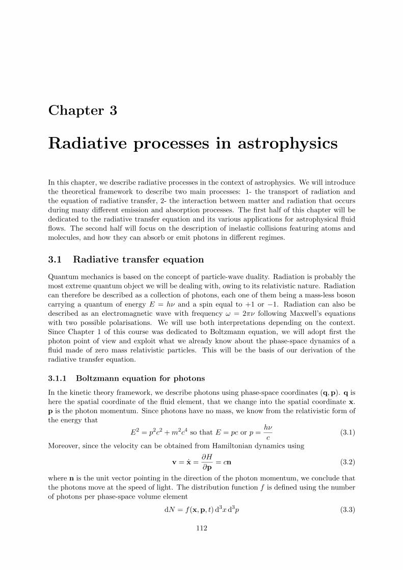
Chapter 3
Radiative processes in astrophysics
In this chapter, we describe radiative processes in the context of astrophysics. We will introducethe theoretical framework to describe two main processes: 1- the transport of radiation andthe equation of radiative transfer, 2- the interaction between matter and radiation that occursduring many different emission and absorption processes. The first half of this chapter will bededicated to the radiative transfer equation and its various applications for astrophysical fluidflows. The second half will focus on the description of inelastic collisions featuring atoms andmolecules, and how they can absorb or emit photons in different regimes.
3.1 Radiative transfer equation
Quantum mechanics is based on the concept of particle-wave duality. Radiation is probably themost extreme quantum object we will be dealing with, owing to its relativistic nature. Radiationcan therefore be described as a collection of photons, each one of them being a mass-less bosoncarrying a quantum of energy E = hν and a spin equal to +1 or −1. Radiation can also bedescribed as an electromagnetic wave with frequency ω = 2πν following Maxwell’s equationswith two possible polarisations. We will use both interpretations depending on the context.Since Chapter 1 of this course was dedicated to Boltzmann equation, we will adopt first thephoton point of view and exploit what we already know about the phase-space dynamics of afluid made of zero mass relativistic particles. This will be the basis of our derivation of theradiative transfer equation.
3.1.1 Boltzmann equation for photons
In the kinetic theory framework, we describe photons using phase-space coordinates (q,p). q ishere the spatial coordinate of the fluid element, that we change into the spatial coordinate x.p is the photon momentum. Since photons have no mass, we know from the relativistic form ofthe energy that
E2 = p2c2 +m2c4 so that E = pc or p =hν
c(3.1)
Moreover, since the velocity can be obtained from Hamiltonian dynamics using
v = x =∂H
∂p= cn (3.2)
where n is the unit vector pointing in the direction of the photon momentum, we conclude thatthe photons move at the speed of light. The distribution function f is defined using the numberof photons per phase-space volume element
dN = f(x,p, t) d3x d3p (3.3)
112

CHAPTER 3. RADIATIVE PROCESSES IN ASTROPHYSICS 113
n1n
dA1
dAdΩ
Figure 3.1: Schematics of a light ray impacting a detector surface element dA1 at an angle θ1 definedby cos θ1 = n · n1.
The resulting Boltzmann equation without collision term is written as (see Chapter 1 for thejustification).
∂f
∂t+ x · ∂f
∂x+ p · ∂f
∂p= 0 (3.4)
which simplifies in∂f
∂t+ cn · ∂f
∂x= 0 (3.5)
We have used again the fact that photons have no mass and thus cannot feel any Newtoniangravity. The situation is different if one considers general relativity but this is outside the scopeof this course. Since the last equation only features the angular variable (θ, φ) defining the unitvector n, it is customary to redefine the distribution function f the following way
f(x,p, t) = fν(x,n, t) (3.6)
where the degree of freedom associated to the norm of the momentum vector has been absorbedin the notation using the index ν. This is just a new notation without any deeper meaning.
3.1.2 Radiation specific intensity
Unfortunately, radiation is traditionally not described using the distribution function in phase-space, but using the radiation specific intensity Iν defined as
dE = Iν(x,n, t) dA1 cos θ1 dΩ dν dt = Iν(x,n, t) dAdΩ dν dt (3.7)
where dE is the energy absorbed by the surface element dA1 of a detector per units time dtin frequency range dν, coming from a beam pointing in direction n and of size dΩ. The anglecos θ1 = n1 · n is the angle between the unit normal vector on the detector n1 and the unitvector n pointing in the direction of the light ray. We can also use the rightmost formulationusing the projected surface perpendicular to the light ray dA = dA1 cos θ1. The units of Iν are[erg cm−2rad−1Hz−1s−1
].
It is straightforward to translate this new, more traditional definition into the kinetic theorydistribution function approach using our good-old collision cylinder. Indeed, during time stepdt, the photons along the light ray cover an infinitesimal volume
d3x = cdtdA (3.8)

CHAPTER 3. RADIATIVE PROCESSES IN ASTROPHYSICS 114
Using the definition of the photon momentum, we know that the momentum space volumeelement is
d3p = p2dpdΩ =h3ν2
c3dνdΩ (3.9)
Using the definition of the distribution function, we can compute the energy in the phase-spacevolume element as
dE = hνfνd3xd3p =h4ν3
c2fνdAdΩdνdt (3.10)
Identifying the terms, we finally get for the specific intensity
Iν =h4ν3
c2fν (3.11)
3.1.3 Bose-Einstein distribution and the Black Body spectrum
We know from the Chapter on kinetic theory that under local thermodynamical equilibrium(LTE) conditions, the distribution function must satisfy a well defined form. In the case ofphotons, which are mass-less bosons, we know detailed balance in phase-space leads to a newcollision invariant based on the occupation number N
lnN
1 +N= −βE = − hν
kBT(3.12)
In the previous equation, we state that the new collision invariant has to be proportional tothe existing ones following the microscopic conservation laws. Since photons have no mass,we do not have the coefficient related to mass conservation, namely the chemical potentialµ(x, t) = 0. We only have the multiplier associated to the total energy, which is noted hereβ(x, t)−1 = kBT (x, t). We also assume that we are in the comoving frame of the fluid, so thatthere is no term associated to the fluid bulk velocity. These terms will appear once we performa Lorentz transform from the comoving frame to the laboratory frame. In case of radiation, thiscomoving frame versus laboratory frame distinction is of crucial importance. We will first ignoreit, neglecting relativistic effects, but we will have to introduce them later to get a consistentdescription of radiation hydrodynamics.
Solving the previous equation for N , and using the relation between the distribution functionand the occupation number, we obtain the Bose-Einstein distribution function
fν =2
h3N =
2
h3
1
exp(hνkBT
)− 1
(3.13)
where we have multiplied the occupation number by 2 to account for the two possible spin states.Finally, using the previously derived relation between the specific radiation intensity and thedistribution function, we deduce the LTE specific intensity called the black body spectrum as
Bν(T ) =2hν3
c2
1
exp(hνkBT
)− 1
(3.14)
Note that for radiation, LTE is not reached through photon-photon collisions, but rather throughemission and absorption processes due to matter and radiation interactions. We will see howit works in details later. This radiation spectrum depends only on the frequency ν and on thetemperature T . Note that it does not depend on the angle variables, it is therefore an isotropic
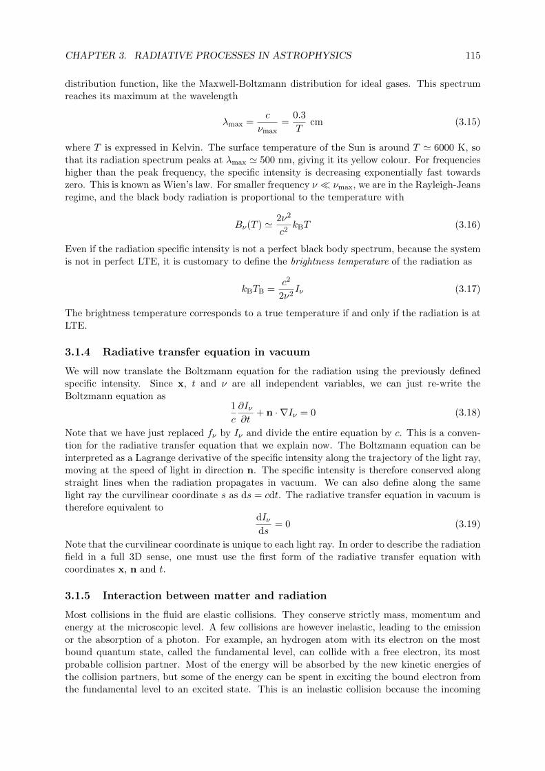
CHAPTER 3. RADIATIVE PROCESSES IN ASTROPHYSICS 115
distribution function, like the Maxwell-Boltzmann distribution for ideal gases. This spectrumreaches its maximum at the wavelength
λmax =c
νmax=
0.3
Tcm (3.15)
where T is expressed in Kelvin. The surface temperature of the Sun is around T ' 6000 K, sothat its radiation spectrum peaks at λmax ' 500 nm, giving it its yellow colour. For frequencieshigher than the peak frequency, the specific intensity is decreasing exponentially fast towardszero. This is known as Wien’s law. For smaller frequency ν νmax, we are in the Rayleigh-Jeansregime, and the black body radiation is proportional to the temperature with
Bν(T ) ' 2ν2
c2kBT (3.16)
Even if the radiation specific intensity is not a perfect black body spectrum, because the systemis not in perfect LTE, it is customary to define the brightness temperature of the radiation as
kBTB =c2
2ν2Iν (3.17)
The brightness temperature corresponds to a true temperature if and only if the radiation is atLTE.
3.1.4 Radiative transfer equation in vacuum
We will now translate the Boltzmann equation for the radiation using the previously definedspecific intensity. Since x, t and ν are all independent variables, we can just re-write theBoltzmann equation as
1
c
∂Iν∂t
+ n · ∇Iν = 0 (3.18)
Note that we have just replaced fν by Iν and divide the entire equation by c. This is a conven-tion for the radiative transfer equation that we explain now. The Boltzmann equation can beinterpreted as a Lagrange derivative of the specific intensity along the trajectory of the light ray,moving at the speed of light in direction n. The specific intensity is therefore conserved alongstraight lines when the radiation propagates in vacuum. We can also define along the samelight ray the curvilinear coordinate s as ds = cdt. The radiative transfer equation in vacuum istherefore equivalent to
dIνds
= 0 (3.19)
Note that the curvilinear coordinate is unique to each light ray. In order to describe the radiationfield in a full 3D sense, one must use the first form of the radiative transfer equation withcoordinates x, n and t.
3.1.5 Interaction between matter and radiation
Most collisions in the fluid are elastic collisions. They conserve strictly mass, momentum andenergy at the microscopic level. A few collisions are however inelastic, leading to the emissionor the absorption of a photon. For example, an hydrogen atom with its electron on the mostbound quantum state, called the fundamental level, can collide with a free electron, its mostprobable collision partner. Most of the energy will be absorbed by the new kinetic energies ofthe collision partners, but some of the energy can be spent in exciting the bound electron fromthe fundamental level to an excited state. This is an inelastic collision because the incoming

CHAPTER 3. RADIATIVE PROCESSES IN ASTROPHYSICS 116
particle kinetic energy is decomposed into excitation energy for the bound electron and kineticenergy for the outgoing particle. This excited state will later spontaneously decay back into thefundamental level, emitting a photon in the process. This leads to a net production of radiationemerging from the matter. The reverse situation is also possible, with an incoming photonabsorbed by an atom, leading to the ejection of the bound electron into the population of freeelectron. This process is called photo-ionisation and leads to a net absorption of radiation bythe matter. These 2 processes are just 2 examples of radiation and matter interaction, either theemission of radiation by matter or the absorption of radiation by matter. We will describe ingreat details all the classical processes that are relevant for astrophysical radiative fluids. Theseprocesses are described using jν , the emission coefficient and αν , the absorption coefficient, bothpresent in the right-hand side of the radiative transfer equation as
1
c
∂Iν∂t
+ n · ∇Iν = jν − ανIν (3.20)
These two new terms are the equivalent of the collision integral in the Boltzmann equation. Notethat the absorption term is proportional to the incoming radiation specific intensity. The unitsof jν are
[erg cm−3rad−1Hz−1s−1
], while the units of αν are simply
[cm−1
]. The emissivity
coefficient is traditionally decomposed into spontaneous emission and induced (or stimulated)emission, as
jν = jsν + ji
ν = jsν + αi
νIν (3.21)
where we used the fact that the induced emissivity coefficient is proportional to the incomingradiation specific intensity. Stimulated emission is due to the friendly nature of bosons who tendto gather together, with an enhanced probability of emission in phase-space volume elementsalready occupied by other bosons. We have described this effect using the Bose enhancementfactor 1+N . Here also, we have to multiply the emissivity coefficient by this Bose enhancementfactor, leading to the induced emission term. The induced emission term can in fact be absorbedinto the absorption coefficient, with a negative sign, leaving the original form of the radiativetransfer equation unchanged, just corrected from induced (or stimulated) emission.
The absorption coefficient αν can be also defined using either the mean free path λν , theopacity κν or the cross-section σν by
αν =1
λν= ρκν = nσν (3.22)
where λν is in [cm] and κν is in[cm2g−1
]. The opacity can be understood in term of cross-
section per particle of fluid. A particle can indeed be considered as a small sphere of radius awith a apparent cross-section σν = πa2 blocking the incoming light. The opacity is then definedas σν = mκν where m is the mass of the particle.
3.2 Formal solution of the radiative transfer equation
In this section, we will solve the radiative transfer equation in a formal sense. This means wewill have a full mathematical expression describing the evolution of the specific intensity alongthe light ray, but this expression is only of theoretical interest. We will however consider somesimplified cases where analytical expressions can be found and new insight on the propagationof radiation in a gaseous medium can be gained.
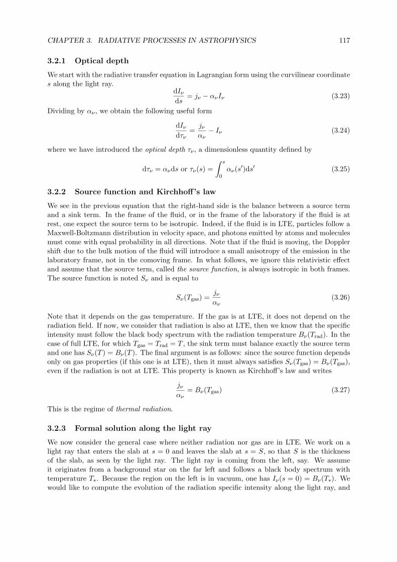
CHAPTER 3. RADIATIVE PROCESSES IN ASTROPHYSICS 117
3.2.1 Optical depth
We start with the radiative transfer equation in Lagrangian form using the curvilinear coordinates along the light ray.
dIνds
= jν − ανIν (3.23)
Dividing by αν , we obtain the following useful form
dIνdτν
=jναν− Iν (3.24)
where we have introduced the optical depth τν , a dimensionless quantity defined by
dτν = ανds or τν(s) =
∫ s
0αν(s′)ds′ (3.25)
3.2.2 Source function and Kirchhoff’s law
We see in the previous equation that the right-hand side is the balance between a source termand a sink term. In the frame of the fluid, or in the frame of the laboratory if the fluid is atrest, one expect the source term to be isotropic. Indeed, if the fluid is in LTE, particles follow aMaxwell-Boltzmann distribution in velocity space, and photons emitted by atoms and moleculesmust come with equal probability in all directions. Note that if the fluid is moving, the Dopplershift due to the bulk motion of the fluid will introduce a small anisotropy of the emission in thelaboratory frame, not in the comoving frame. In what follows, we ignore this relativistic effectand assume that the source term, called the source function, is always isotropic in both frames.The source function is noted Sν and is equal to
Sν(Tgas) =jναν
(3.26)
Note that it depends on the gas temperature. If the gas is at LTE, it does not depend on theradiation field. If now, we consider that radiation is also at LTE, then we know that the specificintensity must follow the black body spectrum with the radiation temperature Bν(Trad). In thecase of full LTE, for which Tgas = Trad = T , the sink term must balance exactly the source termand one has Sν(T ) = Bν(T ). The final argument is as follows: since the source function dependsonly on gas properties (if this one is at LTE), then it must always satisfies Sν(Tgas) = Bν(Tgas),even if the radiation is not at LTE. This property is known as Kirchhoff’s law and writes
jναν
= Bν(Tgas) (3.27)
This is the regime of thermal radiation.
3.2.3 Formal solution along the light ray
We now consider the general case where neither radiation nor gas are in LTE. We work on alight ray that enters the slab at s = 0 and leaves the slab at s = S, so that S is the thicknessof the slab, as seen by the light ray. The light ray is coming from the left, say. We assumeit originates from a background star on the far left and follows a black body spectrum withtemperature T∗. Because the region on the left is in vacuum, one has Iν(s = 0) = Bν(T∗). Wewould like to compute the evolution of the radiation specific intensity along the light ray, and

CHAPTER 3. RADIATIVE PROCESSES IN ASTROPHYSICS 118
especially how it emerges from the slab and appears to an observer located on the far right ofthe slab. We use the radiative transfer equation in its optical depth formulation as
dIνdτν
= Sν − Iν (3.28)
where τν is the integration variable. This is a first order linear ordinary differential equation.We apply the usual method, solving first the homogeneous equation
dIνdτν
= −Iν −→ Iν(τν) = Iν(0) exp−τν = Bν(T∗) exp−τν (3.29)
where, owing to the definition of τν , we have τν = 0 at s = 0. This homogeneous solutioncorresponds to the attenuation of the star radiation by the absorbing layer of gas. In this case,the observed radiation on the far right is just
Iobsν = Bν(T∗) exp−Tν (3.30)
where Tν is the total optical depth of the cloud calculated as
Tν =
∫ S
0αν(s′)ds′ (3.31)
In order to find the general solution, we use the technique of the variation of the constant withthe Ansatz
Iν = Jν exp−τν (3.32)
Injecting this Ansatz into the original differential equation, we obtain
dJνdτν
= Sν exp+τν −→ Jν =
∫ τν
0Sν exp+τ ′ν dτ ′ν +Bν(T∗) (3.33)
Note that we introduced τ ′ν as dummy integration variable. We finally get the complete andfinal formal solution to the radiative transfer problem along this single light ray
Iν (τν) =
∫ τν
0Sν(τ ′ν)
exp(τ ′ν−τν) dτ ′ν +Bν(T∗) exp−τν (3.34)
Let’s consider the particular case for which the source function is uniform throughout the gaseousslab Sν = Bν(Tgas) where Tgas is uniform. we can trivially integrate the previous equation andobtain
Iν (τν) = Bν(Tgas)(1− exp−τν
)+Bν(T∗) exp−τν (3.35)
We have two limiting cases:
• τν 1: this is the optically thick regime, for which the specific intensity converges expo-nentially fast towards the black body spectrum at the gas temperature. Since this spectrumis isotropic, we conclude that in the optically thick regime, the radiation is driven towardsLTE, with both an isotropic angular distribution, independent on the chosen light ray, anda black body spectrum with Trad = Tgas.
• τν 1: this is the optically thin regime. In this case, we can Taylor expand the twoexponentials and obtain Iν (τν) ' Bν(T∗) + (Bν(Tgas)−Bν(T∗)) τν . If T∗ > Tgas, theradiation in the slab is larger than the background stellar light. The radiation is said tobe in emission. In the opposite case, the stellar light is attenuated and the radiation issaid to be in absorption. Interestingly, the emergent optically thin radiation is directlyproportional to τν and can be used to infer physical properties of the absorbing gas.
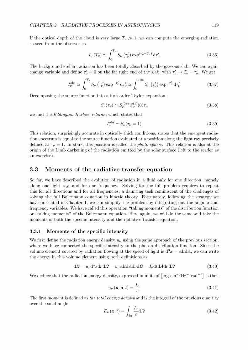
CHAPTER 3. RADIATIVE PROCESSES IN ASTROPHYSICS 119
If the optical depth of the cloud is very large Tν 1, we can compute the emerging radiationas seen from the observer as
Iν (Tν) '∫ Tν
0Sν(τ ′ν)
exp(τ ′ν−Tν) dτ ′ν (3.36)
The background stellar radiation has been totally absorbed by the gaseous slab. We can againchange variable and define τ ′ν = 0 on the far right end of the slab, with τ ′ν → Tν − τ ′ν . We get
Iobsν '
∫ Tν
0Sν(τ ′ν)
exp−τ′ν dτ ′ν '
∫ +∞
0Sν(τ ′ν)
exp−τ′ν dτ ′ν (3.37)
Decomposing the source function into a first order Taylor expansion,
Sν(τν) ' S(0)+ν S(1)
ν (0)τν (3.38)
we find the Eddington-Barbier relation which states that
Iobsν ' Sν(τν = 1) (3.39)
This relation, surprisingly accurate in optically thick conditions, states that the emergent radia-tion spectrum is equal to the source function evaluated at a position along the light ray preciselydefined at τν = 1. In stars, this position is called the photo-sphere. This relation is also at theorigin of the Limb darkening of the radiation emitted by the solar surface (left to the reader asan exercise).
3.3 Moments of the radiative transfer equation
So far, we have described the evolution of radiation in a fluid only for one direction, namelyalong one light ray, and for one frequency. Solving for the full problem requires to repeatthis for all directions and for all frequencies, a daunting task reminiscent of the challenges ofsolving the full Boltzmann equation in kinetic theory. Fortunately, following the strategy wehave presented in Chapter 1, we can simplify the problem by integrating out the angular andfrequency variables. We have called this operation “taking moments” of the distribution functionor “taking moments” of the Boltzmann equation. Here again, we will do the same and take themoments of both the specific intensity and the radiative transfer equation.
3.3.1 Moments of the specific intensity
We first define the radiation energy density uν using the same approach of the previous section,where we have connected the specific intensity to the photon distribution function. Since thevolume element covered by radiation flowing at the speed of light is d3x = cdtdA, we can writethe energy in this volume element using both definitions as
dE = uνd3xdνdΩ = uνcdtdAdνdΩ = IνdtdAdνdΩ (3.40)
We deduce that the radiation energy density, expressed in units of[erg cm−3Hz−1rad−1
]is then
uν (x,n, t) =Iνc
(3.41)
The first moment is defined as the total energy density and is the integral of the previous quantityover the solid angle.
Eν (x, t) =
∫4π
Iνc
dΩ (3.42)
CHAPTER 3. RADIATIVE PROCESSES IN ASTROPHYSICS 120
This new quantity depends only on the space and time coordinates. Its units are[erg cm−3Hz−1
].
It is customary to define also the mean radiation specific intensity as
Jν (x, t) =
∫4πIν
dΩ
4π=
c
4πEν (3.43)
We can finally integrate the total energy density over frequencies and obtain the total integratedradiation energy density, in units of
[erg cm−3
]Erad (x, t) =
∫ +∞
0Eνdν (3.44)
where we used index “rad” to avoid confusion with the fluid total energy. If the radiation is inLTE, we have Iν = Bν(T ) and strictly isotropic. The total energy radiation density is then
Eν (x, t) =4π
cBν(T ) =
8πhν3
c3
1
exp(hνkBT
)− 1
(3.45)
We can easily integrate this over frequencies and get the black body integrated energy as
Erad(T ) =8πh
c3
∫ +∞
0
ν3
exp(hνkBT
)− 1
dν =8πh
c3
(kBT
h
)4 ∫ +∞
0
x3
expx−1dx (3.46)
Since everyone knows that ∫ +∞
0
x3
expx−1dx =
π4
15(3.47)
we finally get for the black body radiation
Erad(T ) = aT 4 where Stefan′s constant is a =8π5
15
k4B
h3c3(3.48)
The striking feature of the black body is that the radiation energy depends only on temperature,as opposed to a Maxwell-Boltzmann gas, for which the internal energy depends also on density,or even only on density if it is degenerate. This is a consequence of photons having zero mass.
In analogy to kinetic theory, we now define more moments of the specific intensity that willprove useful later. The radiation flux is defined as a vector field
Fν (x, t) =
∫4πIνndΩ (3.49)
While the radiation energy density is considered as a zeroth order moment of the specific in-tensity, the radiation flux is the first order moment, because it comes with a polynomial of nof degree 1. If the radiation field is isotropic, like black body radiation, Iν can be taken out ofthe integral and the flux is trivially zero. Note that we can also define the momentum densityof the radiation by noticing that the momentum of a photon is given by its amplitude
p =hν
cso that pν =
uνc
=Iνc2
and pν =Iνc2
n (3.50)
Finally, integrating over the solid angle, we get the total radiation momentum density as
Pν (x, t) =Fν
c2(3.51)

CHAPTER 3. RADIATIVE PROCESSES IN ASTROPHYSICS 121
This is the radiation equivalent to the fluid momentum ρv. We can follow the analogy with afluid even more and define the radiation pressure tensor as the following second-order momentover the solid angle
Pν =
∫4π
Iνc
n⊗ ndΩ (3.52)
Note that the pressure tensor has the property
Tr Pν =
∫4π
Iνc
dΩ = Eν (3.53)
In case of isotropic black body radiation, the tensor is also isotropic and can be written as
Pν = PνI where Pν =1
3Eν (3.54)
The scalar quantity Pν is called the radiation pressure, and make sense only under opticallythick conditions. Note that we find that isotropic radiation behaves like a γ = 4/3 fluid, similarto a relativistic Maxwell-Boltzmann gas.
3.3.2 Radiation energy conservation equation
We now move to the task of taking the moments of the radiative transfer equation, integratingit over the solid angles. We first write the radiative transfer equation using time, space andangle coordinates
1
c
∂Iν∂t
+ n · ∇Iν = jν − ανIν (3.55)
We then perform the integration over 4π, bearing in mind that t, x and n are independentvariables. ∫
4π
1
c
∂Iν∂t
dΩ +
∫4π
n · ∇IνdΩ =
∫4πjνdΩ −
∫4πανIνdΩ (3.56)
(1) (2) ( 3) (4)
The first term, labelled (1) can be computed by taking the time derivative out of the integral,owing to the independence of t and n. This reveals the time derivative of the total radiationenergy density as
∂
∂t
∫4π
Iνc
dΩ =∂Eν∂t
(3.57)
The second term can be computed using the famous vector relation
n · ∇Iν = ∇ · (Iνn)− Iν∇ · n (3.58)
Since ∇ ·n = 0, owing to the independence of x and n, we can take the divergence operator outof the integral as
∇ ·[∫
4πIνndΩ
]≡ ∇ · Fν (3.59)
where we recognise the previously defined radiation flux
Fν =
∫4πIνndΩ (3.60)
We now deal with the source and sink terms on the right-hand side. The emissivity and absorp-tion coefficients jν and αν are considered here as isotropic in the laboratory frame. This is in
CHAPTER 3. RADIATIVE PROCESSES IN ASTROPHYSICS 122
fact true only in the comoving frame, but we will correct for the relativistic Doppler effect inthe following sections. They can thus be taken out of the integral, leading to the final form ofthe radiation energy conservation equation
∂Eν∂t
+∇ · Fν = 4πjν − ανcEν (3.61)
3.3.3 Radiation flux conservation equation
We then follow the same procedure, this time multiplying the radiative transfer equation by ni,each component of the direction vector n.∫
4πni
1
c
∂Iν∂t
dΩ +
∫4πnin · ∇IνdΩ −
∫4πnijνdΩ −
∫4πniανIνdΩ (3.62)
(1) (2) ( 3) (4)
The first term can be written as the time derivative of the first component of the radiation flux
(1) =1
c
∂Fi∂t
(3.63)
The second term, using the same vector relation as before, gives
(2) = ∇ ·(∫
4πIνnindΩ
)(3.64)
We recognise the first row of the previously defined radiation pressure tensor
Pν =
∫4π
n⊗ nIνc
dΩ (3.65)
The remaining terms of the right-hand side are respectively (3) zero, owing to the isotropy ofthe emissivity coefficient, and (4) proportional to the radiation flux. We finally get in full vectorand tensor notations
1
c
∂Fν
∂t+ c∇ · Pν = −ανFν (3.66)
3.3.4 Eddington tensor and closure relations
In the context of radiation transfer, it is customary to define the Eddington tensor as
Pν = DνEν (3.67)
The Eddington tensor is a dimensionless tensor that fully encodes the geometry of the radiationfield and its effect in the radiation flux conservation equation. In order to solve the previoussystem of equations, we need a model for the Eddington tensor. There are various approxima-tions one can use to close the otherwise infinite moments hierarchy. If we adopt a model for theEddington tensor, the moment hierarchy is closed at second-order.
The first and simplest model is to assume that the radiation is isotropic in angular space,like for example in the black body case, for which we have
Dν =1
3I and Pν =
1
3EνI (3.68)
Note that the radiation is not isotropic, we only assume the Eddington tensor is isotropic, whichis obviously a very rough approximation, except in the optically thick limit.
CHAPTER 3. RADIATIVE PROCESSES IN ASTROPHYSICS 123
The second simple case is when we have only one bright source, say a star, in the opticallythin limit. At each point in space, we have
Iν(n) = I∗νδ(n− n0) (3.69)
where n0 is the unit vector in the direction of the source. In this limit, the total radiation energyis just
Eν =
∫4π
Iνc
dΩ =I∗νc
(3.70)
and the radiation flux is
Fν =
∫4πIνndΩ = I∗νn0 = cEνn0 (3.71)
In the optically thin limit, with only one source, the radiation flux is just the radiation energytimes the speed of light in the direction of the source. We can also compute the Eddingtontensor in the same regime,
Pν =
∫4π
Iνc
n⊗ ndΩ =I∗νc
n0 ⊗ n0 = Eνn0 ⊗ n0 (3.72)
A third slightly more complicated model, called the M1 closure, was proposed by Levermore(1984) and interpolate the previous two regime based on the magnitude of the flux Fν comparedto its maximum allowed value of cEν . The M1 closure uses the following form for the Eddingtontensor
Dν =1− χ
2I +
3χ− 1
2n⊗ n (3.73)
where n = Fν/Fν and the function χ(f), not shown here, depends on f = Fν/(cEν), a quantitycalled the reduced flux, and reproduces the two previously discussed asymptotic cases χ = 1/3(isotropic) for f = 0 and χ = 1 (single optically thin source) for f = 1
More complex closure models are possible. The Optically Thin Variable Eddington Tensormodel, for example, assume that the Eddington tensor comes from the collective radiation of acollection of N sources in an optically thin medium. The corresponding radiation field is usedonly for the computation of the Eddington tensor, and writes
Iν(n) =
N∑i=1
Iiνδ(n− ni) (3.74)
Another method, called the Stationary Variable Eddington Tensor model, solves first for thestationary radiative transfer equation
n · ∇Iν = jν − ανIν (3.75)
without the time derivative, and then compute the corresponding Eddington tensor. These twomethods require a proper numerical integration scheme and quite expensive calculations, butare still simpler and cheaper than solving the full time dependent radiative transfer equation.

CHAPTER 3. RADIATIVE PROCESSES IN ASTROPHYSICS 124
3.4 Radiation hydrodynamics
We can now integrate the two previous moments equations over the frequency. We obtain thefrequency integrated radiation energy equation as
∂Erad
∂t+∇ · Frad = 4π
∫ +∞
0jνdν −
∫ +∞
0ανcEνdν (3.76)
The first term on the right-hand side is called the cooling function, and it represents the emissionof radiation from matter. It is noted here Crad and is given by
Crad = 4π
∫ +∞
0jνdν (3.77)
If and only if the gas is in LTE (regime of thermal radiation), one can write the cooling functionas
Crad = 4π
∫ +∞
0ανBν(Tgas)dν = αPcaT
4gas (3.78)
where we have defined the Planck mean for the absorption coefficient αP as
αP(Tgas) =
∫ +∞0 ανBν(Tgas)dν∫ +∞
0 Bν(Tgas)dν(3.79)
The second term on the right-hand side is called the heating function. It represents the radiationabsorbed by matter. It is noted Hrad and is given by
Hrad =
∫ +∞
0ανcEνdν = αEcErad (3.80)
where we have defined the energy mean for the absorption coefficient αE as
αE =
∫ +∞0 ανEνdν∫ +∞
0 Eνdν(3.81)
If and only if the radiation is in LTE (black body regime), one has Erad = aT 4rad and αE =
αP(Trad). Obviously, if Trad = Tgas, we are in full LTE and the two terms exactly cancel out.Integrating the radiation flux conservation equation over frequency, we get
1
c
∂Frad
∂t+ c∇ · Prad = −
∫ +∞
0ανFνdν = −αFFrad (3.82)
where we have defined the flux mean for the absorption coefficient αF as
αF =
∫ +∞0 ανFνdν∫ +∞
0 Fνdν(3.83)
Dividing by c, we can write the radiation momentum conservation equation as
1
c2
∂Frad
∂t+∇ · Prad = −
∫ +∞
0
ανFν
cdν = −αFFrad
c(3.84)
Note that the radiation energy emitted by the gas must correspond to thermal energy lost bythe gas during inelastic collisions. The same applies for the momentum lost by radiation: It

CHAPTER 3. RADIATIVE PROCESSES IN ASTROPHYSICS 125
must correspond to a net gain of momentum by the gas. We therefore have to modify the gasmomentum and energy equation to account for the total energy and momentum balance. Wetherefore have modified Euler equations for the gas. We start with the momentum conservationequation which now reads
∂
∂t(ρv) +∇ · (ρv ⊗ v) +∇P = ρa + ρarad (3.85)
where the radiative force (or the radiative acceleration) reads
arad =
∫ +∞
0
ανFν
ρcdν =
αFFrad
ρc(3.86)
For the fluid total energy equation, we have to account for two effects: First, we now have anew external force, in addition to gravity, namely the radiative force. The modified momentumconservation equation, when combined with the unmodified mass conservation, will lead to anadditional term in the energy equation due to the work of the radiative force. Second, we havealso to add source and sink of energy corresponding to the cooling and heating functions.
∂E
∂t+∇ · (E + P ) v = ρa · v + ρarad · v +Hrad − Crad (3.87)
We at last derived the cooling and heating terms that we used multiple times in the Chapteron astrophysical fluid dynamics. We see that they both originates from radiation and matterinteraction. The radiative force, however, is a new concept that we have not introduced earlier. Itplays a very important role in many astrophysical objects where the radiation flux is particularlyintense, mostly around massive stars or accretion disk around black holes. We will see later thatit also plays a fundamental role when the fluid is close to LTE, in the so-called diffusion limit.
These 4 equations define the radiation hydrodynamics system of equations. It features con-servation of mass, only for the fluid, conservation of momentum for both radiation and fluid,and conservation of energy for both radiation and fluid. Note that we can also add up the twomomentum (and energy) conservation equations and obtain new conservation laws for the fullsystem radiation + fluid.
3.5 Diffusion limit
We have seen in the previous section that under optically thick conditions, the specific intensityconverges towards the black body spectrum. The resulting isotropic angular distribution of theradiation leads to a vanishing radiation flux. This corresponds to strict LTE conditions for theradiation. Like for kinetic theory, we would like to study the regime when radiation is close toLTE but not quite there yet, so that the radiation field is close to a black body, but not strictlyisotropic. We expect a small but non zero radiation flux. It is in fact possible to computethe flux in that regime, following a methodology close to the Chapman-Enskog derivation forviscosity in non-ideal fluids.
We assume that the radiation specific intensity is close to a black body but not strictly equal,so that we have a small perturbation
Iν(x,n, t) = Bν(T ) + δIν(n) where δIν Iν (3.88)
The resulting total radiation energy can be written as
Eν(x, t) =4π
cBν(T ) + δEν(x, t) where δEν Eν (3.89)
CHAPTER 3. RADIATIVE PROCESSES IN ASTROPHYSICS 126
and the radiation flux as
Fν(x, t) = 0 + δFν(x, t) where δFν cEν (3.90)
We now follow the Chapman-Enskog methodology, introducing the reduced flux, so that onecan write
Fν(x, t) = fνcEν where fν 1 (3.91)
We now inject this form into the radiation flux conservation equation
1
c
∂
∂t(fνcEν) +∇ · (DνcEν) = −ανfνcEν (3.92)
where we have used the Eddington tensor form of the radiation pressure tensor. We now performan order of magnitude analysis of the previous equation, introducing the typical system size L,the typical fluid time-scale T and the typical fluid velocity V = L/T . The previous equationcan be written as an order of magnitude estimate[
fνcEνcT
]+
[DνcEνL
]= −
[fνcEνλν
](3.93)
The Eddington tensor is a dimensionless tensor whose magnitude is always of order unity withDν ∼ 1, actually between 1/3 and 1, as explained in the previous sections. In our optically thicklimit, since the radiation is close to isotropic, we have quite accurately
Dν '1
3I (3.94)
We define the light crossing time of the system as
tcross =L
c T =
L
V(3.95)
We see that the first term in the left-hand side is quite small, because cT L and fν 1. Inthis limit, we can safely ignore it in the momentum conservation equation, an approximationcalled the stationary flux limit. The term on the right-hand side, on the other hand, cannotbe ignored. It is true that fν 1 but in the same time, we have λν L, since we are inthe optically thick regime. Following the Chapman-Enskog method, we just consider the tworemaining terms have to be of the same order. This leads to the diffusion approximation, forwhich we have
c
3∇ · (IEν) =
c
3∇Eν = −ανFν or Fν = − c
3αν∇Eν (3.96)
The radiation energy conservation equation becomes
∂Eν∂t
= ∇ ·(
c
3αν∇Eν
)(3.97)
which is nothing but the good old heat equation. We see another analogy with kinetic theoryhere, where energy transport is dominated by a diffusion process, and the diffusion coefficientν = cλν . The other source terms in the radiation energy equation vanished because we haveIν ' Bν(T ). Since we have
Eν '4π
cBν(T ) (3.98)
we can write
∇Eν '4π
c
∂Bν∂T∇T (3.99)
CHAPTER 3. RADIATIVE PROCESSES IN ASTROPHYSICS 127
We can also integrate the previous equation over frequencies, and obtain
∂Erad
∂t+∇ · Frad = 0 (3.100)
where the frequency integrated radiative flux write
Frad = − c
3αR4aT 3∇T = −κrad∇T (3.101)
where we introduce the Rosseland mean as
1
αR=
(∫ +∞
0
1
αν
∂Bν∂T
dν
/∫ +∞
0
∂Bν∂T
dν
)(3.102)
Recall that we have for the black body radiation∫ +∞
0
4π
cBνdν = aT 4 (3.103)
It is worth stressing that the radiative flux in the diffusion limit is very close to the heat fluxwe derived from kinetic theory, with a radiative heat coefficient
κrad =4acT 3
3αR(3.104)
that can be added directly to the electron conduction coefficient, since both processes are pro-portional to the temperature gradient.
We can also compute the radiation force in the diffusion limit. It writes
ρarad =
∫ +∞
0
ανFν
cdν = −1
3
∫ +∞
0∇Eνdν = −1
3∇Erad = −∇Prad (3.105)
We conclude that in the diffusion limit, the radiation force is independent of the opacity, and isnothing but minus the radiation pressure gradient, completely analog to a fluid with γ = 4/3.Indeed, the momentum conservation equation for the fluid writes in the diffusion limit
∂
∂t(ρv) +∇ · (ρv ⊗ v) +∇ (P + Prad) = ρa (3.106)
In the limit of infinite opacity, however, the radiation flux in the diffusion limit converges tozero, and the energy equation writes
∂Erad
∂t= 0 (3.107)
which is not what we expect from a γ = 4/3 fluid. This inconsistency comes from the fact thatwe have ignored so far relativistic corrections to the equations, due to the Lorentz transformfrom the comoving (or rest) frame to the laboratory (or observer) frame. We will discuss theseinteresting aspects in the next section.
3.6 Relativistic corrections for radiative transfer
Our derivation of the radiative transfer equations ignored completely so far relativistic effects ofthe combined fluid of interacting photons and particles. This is problematic in multiple ways.First, we have assumed that the emissivity coefficient jν was isotropic, because the underlyingMaxwell-Boltzmann distribution of the particle velocities was isotropic. This is only true in
CHAPTER 3. RADIATIVE PROCESSES IN ASTROPHYSICS 128
the frame comoving with the bulk flow. In the laboratory frame, the particle velocities are thesum of the random thermal velocities and the average, fluid velocities that points in one specificdirection. If one defines the emissivity coefficient in the comoving frame as j0
ν , this is the trulyisotropic one. But the emissivity coefficient in the laboratory frame jν should be modified bythe Lorentz transformation bringing the emitted photon distribution to the lab frame.
The second problem arises when the radiation is close to LTE with matter. In this case,we have shown that the radiation specific intensity becomes isotropic, and equal to the sourcefunction, which, for thermal radiation, is equal to the black body distribution. Again, this isonly true in the comoving frame. One must therefore define radiation moments in the comovingframe, as E0
ν and F0ν , which differ from their equivalent in the laboratory frame Eν and Fν up
to a Lorentz transform. Note that here only photons are relativistic particles, but the fluid isnot, so we have v/c 1. The corrections are likely to be very small. But as we have seen inthe previous section, in the diffusion limit, the radiation flux is also very small. We thereforecan’t ignore these small relativistic corrections if we want to accurately describe the opticallythick limit of radiative hydrodynamics. In the optically thin limit, relativistic effects can beignored, at least for radiation transport. As we will see later, Doppler effects are important forline transfer and cannot be ignored, even in the optically thin limit.
3.6.1 Lorentz transform to first order in v/c
In order to change frame in the relativistic framework, we need to introduce the Lorentz trans-form. We however only keep terms up to first order in v/c, dropping all terms in (v/c)2 andhigher. This gives the following matrix
L =
1 −vx
c −vyc −vz
c−vx
c 1 0 0−vy
c 0 1 0−vz
c 0 0 1
(3.108)
Note that this modified Lorentz transform is not unitary anymore but only to first order so that|det(L)| = 1 +O
((v/c)2
). A 4-vector coordinate in space-time in the comoving frame is related
to the coordinate in the laboratory frame by
X0 = LX where X0 = (ct0, x0, y0, z0)T and X = (ct, x, y, z)T (3.109)
We obtain the classical Galilean transformation to the comoving frame, with however a first-order shift in the time coordinate
ct0 = ct− v · xc
and x0 = x− vt (3.110)
We can also apply the Lorentz transform to the photon 4-momentum
P0 = LP where P0 =
(hν0
c,hν0
cn0
)T
and P =
(hν
c,hν
cn
)T
(3.111)
where n0 and n (resp. ν0 and ν) are the unit vectors pointing in the direction of the radiation(resp. the photon frequency) in the comoving frame and in the laboratory frame. We obtainthe Doppler effect as
ν0 = ν(
1− v · nc
)(3.112)
and the angle aberration effect as
ν0n0 = ν(n− v
c
)(3.113)
CHAPTER 3. RADIATIVE PROCESSES IN ASTROPHYSICS 129
From our discussion in the previous chapter on relativistic kinetic theory, we have shown thatthe phase-space fluid element d3xd3p is a relativistic invariant, but d3p alone is not. We haveshown however that d3p/E is a relativistic invariant. Using the form of d3p derived at thebeginning of this chapter, and using E = hν for photons, we have
d3p
E=p2
EdpdΩ =
h2ν
c3dνdΩ (3.114)
we deduce thatν0dν0dΩ0 = νdνdΩ (3.115)
Using Liouville’s theorem, we have also deduced that the distribution function fν is a relativisticinvariant, but Iν , the radiation specific intensity, is not. Using the relation we have derivedbetween fν and Iν , namely
Iν =h4ν3
c2fν (3.116)
we deduce that Iν/ν3 is a relativistic invariant, so that
I0ν
ν30
=Iνν3
(3.117)
3.6.2 Moments equations in the laboratory frame
In order to account for the relativistic corrections for the emission and absorption coefficients,we need to consider the absorption along a light ray in the two frames. For simplicity, weassume that the velocity of the fluid is only along the z-axis with v = vez. We can write thetwo direction vectors n0 and n using the spherical coordinate system along the z axis. We have
ν0 sin θ0 cosφ0 = ν sin θ cosφ (3.118)
ν0 sin θ0 sinφ0 = ν sin θ sinφ
ν0 cos θ0 = ν(
cos θ − v
c
)The optical depth along the light ray can then be computed in the laboratory frame as
dτ = ανds = ανd`
sin θ(3.119)
where d` =√
dx2 + dy2 is the projected length of the light ray ds in the x − y plane. Thekey argument is as follows: the optical depth is a relativistic invariant, because it controls thenumber of photon absorbed by the slab along the light ray. We thus have dτ0 = dτ . Because theLorentz boost is only along the z direction, d`, perpendicular to the fluid motion, is not affectedby the change of frame. We then have d`0 = d`. On the other hand, the angle θ is affected bythe angle aberration. Combining the two first equations on the spherical coordinates, we get
ν0 sin θ0 = ν sin θ (3.120)
We finally get the relation between α0ν and αν in the two frames as
ν0α0ν = ναν (3.121)
The emissivity coefficient, jν can be treated similarly, by noticing that in the case of thermalradiation, one has jν = ανBν , where Bν is the specific intensity of the black body radiation. Ittherefore also satisfies
B0ν
ν30
=Bνν3
(3.122)

CHAPTER 3. RADIATIVE PROCESSES IN ASTROPHYSICS 130
Using the relation for αν , we deduce that
j0ν
ν20
=jνν2
(3.123)
We can write the radiative transfer equation in the laboratory frame as usual
1
c
∂
∂tIν + n · ∇Iν = jν − ανIν (3.124)
We then integrate this equation both in angle and in frequency, taking as usual the first andsecond moments. For the first moment, we get easily
∂
∂tErad +∇ · Frad =
∫ +∞
0
∫4πjνdνdΩ −
∫ +∞
0
∫4πανIνdνdΩ (3.125)
We need to express the two terms on the right-hand side as a function of the emissivity andabsorption coefficients in the comoving frame, the truly isotropic ones. The first term wasdefined as the cooling function. It can be written as
Crad =
∫ +∞
0
∫4πjνdνdΩ =
∫ +∞
0
∫4π
jνν2ν (νdνdΩ) =
∫ +∞
0
∫4π
j0ν
ν20
ν (ν0dν0dΩ0) (3.126)
Using both the Doppler effect and the angle aberration, we obtain to leading order in v/c
Crad '∫ +∞
0
∫4πj0ν
(1 +
v
c· n0
)dν0dΩ0 = C0
rad = α0PcaT
4gas (3.127)
where we assume thermal radiation for the emissivity coefficient in the comoving frame. TheDoppler contribution integrates to zero because j0
ν is isotropic in the comoving frame. Thesecond term on the right-hand side of the radiative energy equation was defined as the heatingfunction. It can be expressed as a function of the absorption coefficient in the comoving frameusing
Hrad =
∫ +∞
0
∫4πανIνdνdΩ =
∫ +∞
0
∫4π
(ανν)1
νIνdνdΩ =
∫ +∞
0
∫4πα0ν
ν0
νIνdνdΩ (3.128)
Using again the formula for the Doppler effect, we obtain
Hrad =
∫ +∞
0
∫4πα0ν
(1− v
c· n)IνdνdΩ = α0
EcErad − α0F
v
c· Frad (3.129)
We finally obtain the radiation energy equation in the laboratory frame as
∂
∂tErad +∇ · Frad = α0
PcaT4gas − α0
EcErad + α0F
v
c· Frad (3.130)
For the second moment of the radiation transfer equation, we obtain
1
c
∂
∂tFrad + c∇ · Prad =
∫ +∞
0
∫4πjνndνdΩ −
∫ +∞
0
∫4πανIνndνdΩ (3.131)
The first term on the right-hand side can be computed using like before the angle aberrationformula. We get to leading order in v/c (left to the reader as an exercise)∫ +∞
0
∫4πjνndνdΩ ' α0
PaT4gasv (3.132)
CHAPTER 3. RADIATIVE PROCESSES IN ASTROPHYSICS 131
We conclude that there is in fact a non-zero contribution of the emissivity coefficient to theradiation flux equation, entirely due to the Lorentz transform. The second term on the right-hand side is simpler to handle because we want to keep the radiation moments in the laboratoryframe. We find ∫ +∞
0
∫4πανIνndνdΩ =
∫ +∞
0
∫4πα0ν
(1− v
c· n)IνndνdΩ (3.133)
which can be simplified using the radiation flux and the radiation pressure tensor as∫ +∞
0
∫4πανIνndνdΩ = α0
FFrad − α0EPradv (3.134)
We finally obtain for the radiation momentum equation in the laboratory frame
1
c
∂
∂tFrad + c∇ · Prad = α0
PaT4gasv − α0
FFrad + α0EPradv (3.135)
We can check that if Frad ' cErad, then the new correction terms are vanishingly small, justifyingwhy we neglect them in the optically thin regime. In the optically thick regime, however, theyare required.
3.6.3 Moments equations in the comoving frame
In order to simplify the discussion, we will now consider that we have a grey material, meaningthat the opacity does not depend on frequency, so that all our different definitions (Rosseland,Planck, flux and energy means) for the frequency integrated opacities are equivalent. We canthen simplify the previous two equations as
∂
∂tErad +∇ · Frad = α0c
(aT 4
gas − Erad
)+ α0Frad ·
v
c(3.136)
1
c
∂
∂tFrad + c∇ · Prad = α0aT
4gasv − α0Frad + α0Pradv (3.137)
If one wants to properly converge to the diffusion limit, it is mandatory to define also thedifferent radiation moments in the comoving frame. We thus need to transform also Erad andFrad from the laboratory frame to the comoving frame. To perform this operation, we will usethe relativistic invariance of d3p/E and Iν/ν
3 and write
E0rad =
∫ +∞
0
∫4π
I0ν
cdν0dΩ0 =
∫ +∞
0
∫4π
ν30
ν3
Iνc
ν
ν0dνdΩ (3.138)
Taylor expanding the Doppler term to first order in v/c, we finally get
E0rad '
∫ +∞
0
∫4π
Iνc
(1− 2
v · nc
)dνdΩ (3.139)
We can perform the angular and frequency integration and obtain
E0rad = Erad −
2
cFrad ·
v
c(3.140)
Similarly, we can write the radiation flux in the comoving frame as
F0rad =
∫ +∞
0
∫4πI0νn0dν0dΩ0 =
∫ +∞
0
∫4π
ν30
ν3Iνν2
ν20
(n− v
c
)dνdΩ (3.141)
CHAPTER 3. RADIATIVE PROCESSES IN ASTROPHYSICS 132
and obtain
F0rad =
∫ +∞
0
∫4πIν
(1− v · n
c
)(n− v
c
)dνdΩ (3.142)
Performing the angular and frequency integration and neglecting a quadratic term in v/c, wefinally get
F0rad = Frad − Eradv − Pradv (3.143)
Injecting these two equations into the frequency integrated radiation energy and momentumconservation equations and dropping all quadratic terms in v/c leads to
∂
∂tErad +∇ · Frad ' α0c
(aT 4
gas − E0rad
)− α0F
0rad ·
v
c(3.144)
1
c
∂
∂tFrad + c∇ · Prad ' α0
(aT 4
gas − E0rad
)v − α0F
0rad (3.145)
where now we have only comoving variables in the right-hand side of these equations. We seenow that the optically thick limit corresponds to E0
rad ' aT 4gas and F0
rad ' 0 both expressed inthe comoving frame.
We need to derive now the diffusion limit in term of the comoving radiation energy and flux,writing
E0rad = aT 4
gas (1 + e) and F0rad = caT 4
gas (0 + f) (3.146)
where the reduced energy and the reduced flux are both small, with |e| 1 and |f | 1 but,very importantly, both small deviations are of the same order, with |e| ∼ |f |. We performthe same order of magnitude estimate as before, on our new radiation momentum conservationequation, with typical fluid length scale L and time scale T = L/V ,[
fcaT 4
gas
cT
]+
[Drad
caT 4gas
L
]= −
[eV aT 4
gas
λ0
]−
[fcaT 4
gas
λ0
](3.147)
The first term in the left-hand side can be dropped because we have Drad = 1/3I and tcross Tas before. The first term in the right-hand side can also be ignored, because V c. In thisChapman-Enskog approach, we obtain for the diffusion limit the two relations
F0rad ' −
c
3α0∇E0
rad and E0rad ' aT 4
gas (3.148)
exactly as before, but now valid in the comoving frame. In the diffusion limit, we can also writethe transformation between the laboratory frame and the comoving frame as
E0rad ' Erad and F0
rad ' Frad −4
3E0
radv (3.149)
We now inject these relations to obtain the radiation energy equation fully formulated in thecomoving frame and in the diffusion limit as
∂
∂tE0
rad +∇ · F0rad +∇ ·
(4
3E0
radv
)= α0c
(aT 4
gas − E0rad
)+
1
3v · ∇E0
rad (3.150)
which can be re-arranged as
∂
∂tE0
rad +∇ ·(E0
radv)
+1
3E0
rad∇ · v = ∇ ·(
c
3α0E0
rad
)+ α0c
(aT 4
gas − E0rad
)(3.151)
CHAPTER 3. RADIATIVE PROCESSES IN ASTROPHYSICS 133
Note that the left-hand side of the radiation energy equation is strictly equivalent to the internalenergy equation of a γ = 4/3 fluid. Relativistic corrections have thus repaired the inconsistencywe have detected in the previous section. We can now study the infinite opacity limit α0 → +∞.We have in this case E0
rad = aT 4gas and F0
rad = 0. We also have Trad = Tgas = T . Combining thematter internal energy equation with the radiation energy equation, we can obtain the full LTEradiation hydrodynamics equations
∂ρ
∂t+∇ · v = 0 (3.152)
∂
∂t(ρv) +∇ · (v ⊗ v) +∇Ptot = ρa (3.153)
∂Etot
∂t+∇ · (Etot + Ptot) v = ρa · v (3.154)
where the total pressure is defined as
Ptot = Pgas + Prad =ρkBT
m+
1
3aT 4 (3.155)
and the total energy is defined as
Etot =1
2ρv2 +
3
2
ρkBT
m+ aT 4 (3.156)
We see that the equation of state for the coupled radiation + matter fluid is highly non-trivial.If the gas pressure dominates, we have γ ' 5/3, but if the radiation pressure dominates, thefluid behaves as if γ ' 4/3. We see that the transition occurs at a critical temperature given by
Tcrit =
(3ρkB
am
)1/3
' 3.2× 10⁷
(ρ
1 g/cc
)1/3
K (3.157)
The centre of the Sun has a density of 150 g/cc and a temperature of 1.6 × 10⁷ K, so that thegas pressure dominates over the radiation pressure. In higher mass stars, on the other hand,the temperature is much higher and the radiation pressure dominates. It is quite interesting torealise that the full LTE gas + radiation fluid follows the original Euler equations, so that mostof the conclusion of the previous chapter on astrophysical fluid dynamics apply.

CHAPTER 3. RADIATIVE PROCESSES IN ASTROPHYSICS 134
3.7 Matter and radiation interaction
We now switch to the second part of the Chapter on radiation. The goal is to describe themain emission and absorption processes encountered in astrophysics. We will use extensivelythe wave-particle duality of radiation. While in the first part, we have adopted mainly the pointof view of photons and light rays, we will now focus more on the point of view of electromagneticwaves. At a few rare occasions, we will also adopt a more quantum mechanics approach withdiscrete particles and/or energy levels. The emission and absorption processes in astrophysicscan be decomposed into three main groups: bound-bound radiation with atomic and molecularlines, bound-free radiation due to atomic ionisation processes, and finally free-free radiation dueto free electrons interacting with radiation or with ions. We will describe all these processes indetails, obtaining in each case detailed equations describing the associated phenomenon.
3.8 Larmor formula
The most important ingredient we need in this course is the radiation emitted by an acceleratedcharged particle, in most cases an electron. Note that this electron can be bound to an atomor freely moving in the continuum. In order to compute the emitted radiation from movingcharges, we need to rely on the theory of electromagnetism and the use of Maxwell’s equationsand retarded potentials. In this section, we use a much simpler derivation due to Thomson.
ct
cΔt
Δvt
θ
Δvt sin θ
Figure 3.2: Field lines around an accelerated charge used in the derivation of Larmor formula.
We consider a point particle of charge q = −e, namely an electron. If this electron is at rest,it creates around itself a purely radial electric field given by Coulomb’s law
Er =q
r2(3.158)
We now give a kick in the x-direction to this particle, so that it acquires a small velocityvx = ∆v c during a small time step ∆t. The corresponding impulsive acceleration at time
CHAPTER 3. RADIATIVE PROCESSES IN ASTROPHYSICS 135
t = 0 is therefore
a =∆v
∆t(3.159)
Once the particle reaches its terminal velocity ∆v, it develops again a Coulomb potential, butthe information about the new particle position propagates at finite speed (the speed of light)along the field lines.We see in Figure 3.2 a schematic of these field lines. The information aboutthe start of the accelerating pulse reach a given point along a field line at distance r = ct.The new configuration of the field line is in place at a distance c∆t later. In order to connectproperly the field line before and after the pulse, the electrical field has to adjust, so that asmall transverse component is created, whose amplitude has to be, for geometrical reasons (seeFig. 3.2),
E⊥Er
=∆vt sin θ
c∆t(3.160)
Injecting the value of Er and replacing t by r/c, we get
E⊥ =qa sin θ
rc2(3.161)
A distant observer will see this transverse component as a time-dependant electric field, in otherwords, an electromagnetic wave. Electromagnetic waves are solution of Maxwell’s equations invacuum, with E and B evolving as two coupled vector fields with E = B. The energy fluxcarried by the electromagnetic wave is the Poynting flux, in units of
[erg cm−2 s−1
]S =
c
4πE×B (3.162)
In the case of our accelerating charge, the Poynting vector is directed in the radial direction,and its norm is
S =c
4πE2 =
1
4π
q2a2 sin2 θ
r2c3(3.163)
We see that the radiation is not isotropic. The sin2 θ dependance is typical of dipolar radiation.The total power (in units of
[erg s−1
]) emitted by the accelerating charge can be computed by
integrating the flux through the surface of a distant sphere at r = R. Using spherical coordinates,we obtain
dW
dt=q2a2
4πc3
∫4π
sin2 θ
R2R2dΩ =
q2a2
2c3
∫ π
0sin3 θdθ (3.164)
where quite logically the radius dependence drops out. We used the surface element on thesphere dS = r2dΩ = r2 sin θdθdφ. Solving the simple integral over θ and replacing q = −e, weobtain the formula of Larmor for the total emitted power by the accelerating electron
dW
dt=
2
3
e2
c3|a(t)|2 (3.165)
We derived this famous formula for the simple case of an impulsive acceleration, but this formulais more general and can be used for any acceleration profile a(t).
3.8.1 Radiation spectrum of an electromagnetic wave
In order to define the radiation spectrum of an electromagnetic wave, we need to use Fourieranalysis. The Fourier transform of the electric field is defined as
E(ω) =1
2π
∫ +∞
−∞E(t) expiωt dt (3.166)
CHAPTER 3. RADIATIVE PROCESSES IN ASTROPHYSICS 136
and the inverse Fourier transform is defined as
E(t) =
∫ +∞
−∞E(ω) exp−iωt dω (3.167)
We now use (again) Parseval’s theorem to define the total energy of the wave as∫ +∞
−∞E(t)2dt = 2π
∫ +∞
−∞
∣∣∣E(ω)∣∣∣2 dω (3.168)
Since the electric field is a real signal, we have∣∣∣E(−ω)
∣∣∣ =∣∣∣E(ω)
∣∣∣, so we have
∫ +∞
−∞E(t)2dt = 4π
∫ +∞
0
∣∣∣E(ω)∣∣∣2 dω (3.169)
We now use the Poynting vector to obtain the energy flux carried by the wave S(t) = c4πE(t)2.
Integrating this in time and using Parseval’s theorem, we obtain the total energy per unit areaas
dW
dA= c
∫ +∞
0
∣∣∣E(ω)∣∣∣2 dω (3.170)
We see that the right-hand side represents the spectral energy decomposition of the electromag-netic waves, also called the radiation spectrum, in
[erg cm−2 Hz−1
]with
dW
dAdω= c
∣∣∣E(ω)∣∣∣2 (3.171)
3.8.2 Emitted radiation spectrum
Using the relation between the electric field and the acceleration we derived earlier, we get forour accelerated electron
dW
dAdω=e2 sin2 θ
r2c3|a(ω)|2 (3.172)
where we introduce the Fourier transform of the acceleration
a(ω) =1
2π
∫ +∞
−∞a(t) expiωt dt (3.173)
Integrating this flux spectrum over the sphere at r = R, we get
dW
dω=e2
c3|a(ω)|2 1
R2
∫4π
sin2 θR2dΩ = 2πe2
c3|a(ω)|2
∫ π
0sin3 θdθ (3.174)
The emitted radiation spectrum in[erg Hz−1
]can be finally written as
dW
dω=
8π
3
e2
c3|a(ω)|2 (3.175)
This radiation spectrum is emitted by one particle being accelerated during one event, usuallya collision between an electron and a proton. Another collision will give rise to another pulse ofradiation, with probably a different dipole direction (the x-axis defined before) and a differentspectrum. In order to obtain the total emissivity of the fluid, one need to multiply by therate of these events per unit volume nevent. Assuming that the direction of these events is
CHAPTER 3. RADIATIVE PROCESSES IN ASTROPHYSICS 137
isotropically distributed, like for a Maxwell-Boltzmann distribution of particles, we can obtainthe final emissivity coefficient by multiplying by nevent and by dividing by 4π as
jω =nevent
4π
dW
dω(3.176)
in units of[erg cm−3 s−1 Hz−1 str−1
], which is exactly the definition of the emissivity coefficient
we gave in the previous sections, except it was noted jν with ω = 2πν
3.9 Bremsstrahlung
We now have all the necessary tools to compute our first emission process, Bremsstrahlung,also called free-free radiation. It corresponds to Larmor radiation during collisions between freeelectrons and ions (mostly protons), interacting through the Coulomb interaction. Coulombcollisions have been studied in details in the first Chapter. Because ions are much more massivethan electrons, the frame of the center of mass corresponds to the rest frame of the ion, whilethe relative velocity corresponds to the velocity of the electron. We assume that the ions havea charge q = +Ze, where Z = 1 for protons, while electrons have a charge q = −e.
We choose the x-axis aligned with the velocity of the incoming electron, while its y-coordinateat infinity is the impact parameter b. We use the small deflection angle approximation, so thatthe electron follows a straight line with y ' b and x ' vt. The time coordinate is chosen so thatt = 0 corresponds to the collision itself, where the radius between the electron and the ion isminimum with r = b, while before or after the collision the radius is r2 = x2 + y2 ' (vt)2 + b2.
The acceleration that matters here is the acceleration in the y-direction. The accelerationin the x-direction changes sign at t = 0 and averages to zero. For the Coulomb force, it writes
mea(t) = −Ze2
r3y ' −Ze
2
b2
[1 +
(t
τ
)2]−3/2
where τ =b
v(3.177)
The total velocity kick in the y-direction is obtained by integrating the acceleration as
∆v =
∫ +∞
−∞a(t)dt = −2Ze2
mebv(3.178)
We see that the acceleration has a typical bell shape, with a maximum at t = 0 and a thicknessof τ = b/v. The Fourier transform a(ω) has also a typical bell shape with its maximum at ω = 0.We have
a(ω) ' ∆v
2πfor ω ≤ 1
τand a(ω) ' 0 for ω ≥ 1
τ(3.179)
Using Larmor formula, we compute the radiation energy spectrum of this single collision
dW
dω=
8π
3
e2
c3|a(ω)|2 =
2
3π
e2
c3∆v2 =
8
3π
Z2e6
c3m2eb
2v2for ω ≤ v
b(3.180)
Using the collision cylinder, we can compute the number of collisions between incoming electronswith impact parameter between b and b+ db and velocity at infinity v and v + dv as
dncoll
dt= ni (ne(v)dv) (2πbdb) v (3.181)
where ne(v) is given by the Maxwell-Boltzmann distribution. In order to compute the totalemissivity coefficient, we need to integrate the single collision energy spectrum over all possibleimpact parameters and all possible incoming electron velocities.
4πjω =
∫ +∞
0nine(v)vdv
∫ +∞
02πb
dW
dωdb (3.182)
CHAPTER 3. RADIATIVE PROCESSES IN ASTROPHYSICS 138
We first perform the integration with respect to the impact parameter. The functional form ofthe integrand is db/b, which integrates into a logarithm, and therefore, as always, diverges forboth small and large impact parameters. Since the spectrum is approximately zero for b ≥ v/ω,we use as upper bound of the integral bmax = v/ω. For the lower bound, we use the usualvalue bmin = b90, the impact parameter corresponding to a 90-degrees deflection angle. We thenobtain
4πjω =16
3
Z2e6
c3m2e
∫ +∞
0nine(v) ln
(bmax
bmin
)dv
v(3.183)
The logarithm is absorbed in a slowly varying quantity called the free-free Gaunt factor anddefined by
gff(v, ω) =
√3
πln
(bmax
bmin
)(3.184)
The factor√
3/π was introduced in the Gaunt factor to account for the exact form of theFourier transform of the acceleration. The Gaunt factor is a slowly varying function of v andω. The emitted spectrum from a single collision is therefore almost flat. This cannot be truefor arbitrary high photon frequencies. Indeed, radiation during the collision will be emitted intodiscrete photons. Since the maximum available energy in the collision is the kinetic energy ofthe electron, we conclude that the maximum photon energy that can be emitted corresponds toone single photon with energy hν = 1
2mev2. This semi-classical argument allows us to derive
the spectral shape of the emitted radiation. The electron distribution function derives fromMaxwell-Boltzmann with
ne(v) =ne(
2π kBTme
)3/2exp−mev
2
2kBT 4πv2 (3.185)
We can integrate our almost flat radiation spectrum in velocity space, only including electronsfor which the kinetic energy is larger than the radiation energy
1
2mev
2 ≥ hν (3.186)
This set the lower bound of the integral, and we obtain
4πjω =32π
3√
3
Z2e6
c3m2e
nine(2π kBT
me
)1/2exp− hνkBT gff(ν) (3.187)
The average Gaunt factor gff(ν) corresponds to the previously defined Gaunt factor but averagedover the Maxwellian distribution. Finally, using jν = 2πjω, we get the emissivity coefficient ofBremsstrahlung
4πjν =32π
3√
3
Z2e6
c3m2e
nine
(2πme
kBT
)1/2
exp− hνkBT gff(ν) (3.188)
We can integrate over the frequencies to compute the corresponding cooling function,
Cff =
∫ +∞
04πjνdν =
32π
3√
3
Z2e6
hc3m2e
nine (2πmekBT )1/2 gff (3.189)
Numerically, we obtain the final and famous result
Cff = 1.42× 10⁻²⁷gffZ2nine
√T (3.190)
CHAPTER 3. RADIATIVE PROCESSES IN ASTROPHYSICS 139
The frequency average of the average Gaunt factor encodes the slow variations of the Gauntfactor gff(v, ω). This Gaunt factor is also used to include possible quantum corrections to oursimple semi-classical treatment. It is usually close to unity and traditionally set to be gff ' 1.2
In order to obtain the corresponding absorption coefficient, we invoke Kirchhoff’s relationfor thermal radiation
αν =jν
Bν(T )(3.191)
where Bν(T ) is the black body specific intensity. Note that the Bremsstrahlung emission hasa characteristic spectral shape, with an exponential cut-off for hν kBT and a flat spec-trum for hν kBT . The cooling function has a characteristic
√T temperature dependence.
Bremsstrahlung is the only remaining cooling process for hot ionised gas with T > 107 K. At highphoton frequencies, because of the exponential cut-off, the only remaining absorption process isThomson scattering.
3.10 Thomson scattering
Thomson scattering describes the interaction between a planar electromagnetic wave with afree electron in the plasma. It can be described fully classically, as long as the energy of theincoming photons satisfies hν mec
2. In short, the incoming electromagnetic wave couplesto the electron that starts to oscillate. The resulting electron acceleration is transformed intoLarmor radiation, emitted in a dipole pattern. The corresponding energy is removed to theincident wave, leading to the absorption of the incident radiation, and, simultaneously, to theemission of radiation in the same frequency but in a different direction. This is why this processis called scattering. Before we describe in details the interaction between the planar wave andthe free electron, we first need to introduce planar electromagnetic waves.
3.10.1 Planar electromagnetic waves
A planer wave propagating in the direction of a unit vector n0is described by the followingelectrical field
E(x, t) = E0 expi(k0x−ω0t) (3.192)
where the x-axis is chosen aligned with n0. The wave is monochromatic with frequency ω0 andsatisfies the dispersion relation of waves propagating in vacuum ω0 = ck0. The magnetic fieldfollows a similar form with E = B. The energy flux carried by the wave is given by the Poyntingflux
S(x, t) =c
4πE×B (3.193)
We see that its norm can be written as
S(x, t) =c
4πE2(x, t) (3.194)
It is a space- and time-dependent quantity, that oscillates at twice the frequency of the electricfield. Planar waves are analogues to the light-rays we used in the previous chapter. The radiationspecific intensity of a light ray propagating in vacuum is however constant, and not oscillatory.The usual way of solving this conundrum is to define the intensity of the planar wave as theaverage Poynting flux over one period T0 = 2π/ω0 and at some fixed location x. Adoptingwithout loss of generality x = 0, we have up to a constant phase
E(x = 0, t) = E0 cos (ω0t) (3.195)
CHAPTER 3. RADIATIVE PROCESSES IN ASTROPHYSICS 140
The average Poynting flux is a constant along the planar wave and its value is
S0 =1
T0
∫ T0
0
c
4πE2
0 cos2 (ω0t) dt =c
8πE2
0 (3.196)
We can now relate the specific radiation intensity along the light ray to the planar wave energyflux as
Iω = S0δ(ω − ω0)δ(n− n0) (3.197)
We see that although S0 has units of[erg cm−2s−1
], Iω has units of
[erg cm−2s−1Hz−1str−1
].
3.10.2 Thomson cross section
We now consider the Lorentz force due to the electromagnetic wave acting on the free electron.The equation of motion for the electron writes
mex = −e(E +
v
c×B
)' −eE so that x = − e
meE0 cos(ω0t)n0 (3.198)
because the electron velocity is non relativistic v c and B = E. From the previous sections,we know that this acceleration will be transformed into Larmor radiation, where the poweremitted per solid angle is
dW
dtdΩ(t) =
e2x2(t)
4πc3sin2 θ (3.199)
The new electromagnetic wave has the same frequency of the incoming one, it is therefore alsomonochromatic, and the radiation intensity is defined using the average Poynting flux over oneperiod. We therefore obtain
dW0
dtdΩ=
e4E20
8πc3m2e
sin2 θ (3.200)
The angle θ is defined with respect to the direction of the incoming wave n0. Integrating oversolid angle, we get the power emitted by the oscillating electron in all direction averaged overone period
dW0
dt=
e4E20
3c3m2e
(3.201)
In order to get the corresponding emissivity coefficient, we have to multiply by the numberdensity of electrons, and by the Dirac delta function to account for the monochromaticity,which gives
4πjω = nedW0
dtδ(ω − ω0) (3.202)
This energy emitted per unit time corresponds to the energy lost by the incoming wave. Thisallows us to compute the cross section as
dW0
dt= σT
c
8πE2
0 (3.203)
which leads to the Thomson cross-section
σT =8π
3
e4
c4m2e
(3.204)
The corresponding absorption coefficient is obtained using
αν = neσT (3.205)
CHAPTER 3. RADIATIVE PROCESSES IN ASTROPHYSICS 141
There is a simple way to obtain this result, using the electron classical radius, which can bedefined by
e2
re= mec
2 (3.206)
which states that the electron electrostatic energy is equal to the energy associated to theelectron rest mass. Although this has no particular physical meaning, Thomson scattering canbe pictured as electrons of finite size blocking the light, like small dust grains, giving the crosssection
σT ' πr2e = π
e4
c4m2e
(3.207)
We are just missing the factor 8/3.
CHAPTER 3. RADIATIVE PROCESSES IN ASTROPHYSICS 142
3.11 Atomic and molecular excitation levels
We now move to the description of what is called bound-bound radiation, namely absorption andemission processes associated to bound states of atoms and molecules. The atomic structure isusually described using quantum mechanics. This is not the goal of these lectures to give anaccurate account of quantum processes. We will just review the main results of quantum physicstheory, outlining a few well-known results using very rough derivations. We will use like in theprevious section a semi-classical approach of the theory of radiation and matter interaction,leaving again the more rigorous derivations to quantum mechanics books.
3.11.1 Electronic, vibrational and rotational states
We consider bound states of the Hydrogen atom, with an electron orbiting around a proton. Sofar we have considered only free electrons and naked protons. What we know from quantummechanics is that the electron orbital structure around the proton is quantized into a discreteset of states, called electronic states. The same is true for molecular processes, with vibrationaland rotational states. We would like to estimate the energy of these electronic, vibrational androtational states.
We can write the electron orbital energy as the sum of the potential energy and the kineticenergy.
E =p2
2me− e2
r(3.208)
If the electron is on a bound orbit, it must have E < 0. We know from quantum mechanics thatwe cannot adopt a classical approach. The trick is to use Heisenberg uncertainty principle toderive an order of magnitude estimate of the electron momentum with pr ' h. Injecting thisrelation for a marginally bound orbit with E = 0, we obtain the Bohr radius with
e2
rB=
p2B
2mewith pB =
~rB
(3.209)
This gives for the Bohr radius (note that we dropped the factor 2)
rB =~2
mee2(3.210)
This is the typical radius for the electron orbit around the proton. The corresponding energy is(note that we keep now the factor 2)
Eelec =p2
B
2me=
~2
2mer2B
=mee
4
2~2(3.211)
The total energy for the bound electronic state for the Hydrogen atom is given by
Eelec,n = −Eelec
n2= −13.6 eV
n2(3.212)
Using a similar approach, we can estimate the vibrational energy levels for molecules, moreimportantly the Hydrogen molecule. The idea is to consider the Hydrogen molecule as anharmonic oscillator, like a spring, whose equation of motion is given by mpx = −kex where thespring constant ke corresponds to the potential of the molecular bound, estimated here to beroughly equal to the electrostatic potential e2/rB, and the typical spring length is given by theBohr radius rB. The harmonic oscillator energy in quantum mechanics is given by
Evib = hω where ω =
√kemp
(3.213)

CHAPTER 3. RADIATIVE PROCESSES IN ASTROPHYSICS 143
The spring constant can be determined requiring that the spring potential energy is equal tothe electrostatic energy
1
2ker
2B = EB =
~2
2mer2B
which gives ke =~2
mer4B
and ω =~
√mempr2
B
(3.214)
We finally find the typical energy for vibrational levels as
Evib =~2
√mempr2
B
=
√me
mpEelec (3.215)
and the corresponding discrete energy levels are given
Evib,n = Evib
(n+
1
2
)= 0.31 eV
(n+
1
2
)(3.216)
Finally, the third category of bound states are molecular rotational energy levels, correspondingto the balance between the centrifugal force and the molecular bound. The kinetic energyassociated to the rotation is now K = 1
2IΩ2 = 1
2L2/I where I = mpr
2B is the moment of inertia
of the molecule and L = IΩ its angular momentum. We can estimate roughly the typical angularmomentum using the Heisenberg uncertainty principle L ' ~, which gives the typical energy forrotational levels
Erot =L2
2mpr2B
=~2
2mpr2B
=me
mpEelec (3.217)
and the corresponding discrete energy levels
Erot,n = ErotJ (J + 1) = 7.4× 10⁻⁴ eVJ (J + 1) (3.218)
We can compute the corresponding wavelength of the radiation associated to each process. UsingE = hν, we obtain λ = 912A for Eelec = 13.6 eV, which corresponds to ultraviolet radiation.Vibrational levels have λ ' 4 µm for Evib ' 0.3 eV and emits infrared radiation, while rotationallevels have λ ' 0.2mm for Etot ' 10−3 eV and are detected in the sub-mm range. Using E = kBT(a temperature of 11605 K corresponds to 1 eV), we see that atomic transitions are excited fortemperature T ' 105 K, while molecular vibrational levels are excited for T ' 3000 K and thelower rotational levels corresponds to T ' 10 K.
3.11.2 Collisional excitation
The first and most simple process that drives the bound electron from a lower to a higherexcited state are collisions. We have studied collisions quite extensively in the first Chapter.These collisions were elastic collisions, leading to a redistribution of the collision partners inmomentum space, but without changing the nature of the involved particles. In this Chapter,we consider inelastic collisions, between say an electron and an atom in excited level i, leadingto the excitation of the bound electron to a higher level j. In chemistry notations, this can bewritten as
e− +H0i←−−−→ e− +H0
j (3.219)
The upper index usually refers to the charge of the particle, where the Hydrogen atom with thebound electron has zero net charge. The free electron, on the other hand, has a negative chargeequal to −e, hence the upper index with a single negative sign. The double arrow in the centremean that the reaction is reversible. One collision can promote the bound electron to the higherlevel j, but another later collision can demote the electron to the lower level i. In what follows,
CHAPTER 3. RADIATIVE PROCESSES IN ASTROPHYSICS 144
for sake of simplicity, we will use a two levels atom model. The generalisation to a multiple levelsatom is conceptually straightforward but computational more involving. We can now computethe creation rate of the Hydrogen atom in state j = 1 as
dn1
dt= n2ne 〈σ21v〉 − n1ne 〈σ12v〉 (3.220)
where the electron number density, and the number density of atoms in state 1 and 2 arecomputed as
ne(x, t) =
∫R3
fed3p and n1(x, t) =
∫R3
f1d3p and n2(x, t) =
∫R3
f2d3p (3.221)
The two velocity-averaged cross sections are defined as the reaction cross section averaged overthe distribution function of the relative velocity v, which is in most cases the distribution functionof the electron. These collision rates are traditionally defined as
C21 = ne 〈σ21v〉 and C12 = ne 〈σ12v〉 (3.222)
so that the rate equation can now be written as
dn1
dt= C21n2 − C12n1 = −dn2
dt(3.223)
Note that when the system is in chemical equilibrium, we have the relation
C21n2 = C12n1 (3.224)
We will see in the following sections that this purely collisional description in only valid at highelectron densities. At lower densities, we must also include radiative processes.
3.11.3 Level population at LTE
We now want to compute the distribution of the excited states of the Hydrogen atom at LTE.For this, we need first to define the energy of the Hydrogen atom occupying excitation level i as
E =1
2mpv
2 +1
2mev
2 + Eelec,i (3.225)
where Eelec,i represents to total orbital energy of the bound electron, namely the sum of theorbital kinetic energy and the orbital electrostatic energy. In the previous equation, the firsttwo terms represent the translational kinetic energy of the bound system, in which the velocity ofthe proton and the electron are the same. We can clearly neglect the contribution of the latter,because mp = 1833me. We derived the LTE distribution function through reversible, elasticcollisions imposing detailed balance in phase-space. We can do the same thing here, leading todistribution function for each species, with
fe =2
h3exp(µe− p2
2me)/kBT (3.226)
for free electrons, and
fi =gih3
exp(µi− p2
2mp−Ei)/kBT (3.227)
for the Hydrogen atoms in different excitation levels, where gi is the maximum number ofdegenerate states of particle of type i that can occupy the same position in phase-space. Note
CHAPTER 3. RADIATIVE PROCESSES IN ASTROPHYSICS 145
that we ignored here the Fermi suppression factor 1 −N : We deal here with a non-degeneratefluid. We use the same detailed balance argument, but now for the inelastic collisions betweendifferent species, ln fe+ln fi = ln f ′e+ln f ′j . Note that here detailed balance is performed for eachindividual degenerate state individually. Degenerate states have the same chemical potential, aslong as they are indistinguishable. This translates into the condition
µe + µi = µe + µj or equivalently µi = µj (3.228)
because the total energy is conserved during the collision. Note that this additive property ofthe chemical potentials of reactants and products of a chemical reaction is quite general and ofcourse true only at LTE. Integrating over momentum space, we get the total number density ofatoms species i
ni(x, t) =
∫R3
fi(x,p, t)d3p = gi exp−Ei/kBT
expµi/kBT
h3
∫R3
exp− p2
2mp/kBT d3p (3.229)
The last integral over momentum space can be readily integrated (it is a Gaussian), and weobtain
ni(x, t) = gi exp−Ei/kBTexpµi/kBT
h3(2πmpkBT )3/2 (3.230)
Dividing the number densities of two different levels i and j, we see that the temperature and thechemical potential terms disappear (because µi = µj). We obtain the Boltzmann distributionof level populations at LTE
ninj
=gigj
exp−(Ei−Ej)/kBT (3.231)
We can also define the total number density of Hydrogen atoms, summing up over all possibleexcited states
ntot(x, t) =
+∞∑i=1
ni(x, t) =
(+∞∑i=1
gi exp−Ei/kBT
)expµ1/kBT
h3(2πmpkBT )3/2 (3.232)
where we used the fact that µi = µ1 for all levels. We can thus rewrite the level population atLTE as
nintot
=gi exp−Ei/kBT
Z(T )where Z(T ) =
+∞∑i=1
gi exp−Ei/kBT (3.233)
The function Z(T ) is called the partition function of the level population. The first level i = 1,also called the ground state or the fundamental level has energy E1 = −Eelec = −13.6 eV.For gas temperature kBT Eelec, we see that for all levels i > 1, the exponential term inthe Boltzmann relation will be zero. In this regime, ntot ' n1 and the level population issaid to be in the ground state. In the opposite regime, if kBT Eelec, then the exponentialbecomes one. The partition function now diverges. The Hydrogen atom has indeed multipledegenerate states for each electronic level with gi = i2, these degenerate states corresponding toangular momentum and spin degrees of freedom. In this limit, at high temperature, we get theinconsistent result that
Z(T ) '+∞∑i=1
i2 → +∞ (3.234)
We can solve this inconsistency with an analogy to the orbital model of the electron orbitingthe proton. If we write that each energy level Ei corresponds to an orbital radius ri, we find
Ei = −Eelec
i2= −e
2
riwe find ri = rBi
2 (3.235)

CHAPTER 3. RADIATIVE PROCESSES IN ASTROPHYSICS 146
We now can compute the mean interparticle seperation for the atoms and identify it as the lastorbit the atom can have without having its bound electron being captured by another nearbyatom.
rmax =1
n1/3tot
= rBi2max (3.236)
The partition function is then computed using only surviving bound states
Z(T ) 'imax∑i=1
i2 where imax =1√
rBn1/3tot
(3.237)
The partition function and the level population will converge properly, at the expense of havingmore and more free electrons ejected from the higher energy levels. This process is called pressureionisation. Coming back to our simple two levels atom, we can compare the chemical equilibriumrelation to the LTE level population
n2
n1=C12
C21versus
n2
n1=g2
g1exp−(E2−E1)/kBT (3.238)
We know that at LTE, both relations are valid. Since C12 and C21 only depend on the micro-scopic cross section and on the electron Maxwell-Boltzmann distribution, we conclude that thecollisional rates must satisfy this at all time (even in non-LTE conditions) the following relation
C12
C21=g2
g1exp−(E2−E1)/kBT (3.239)
In many astrophysical databases, only 〈σ21v〉 is given, the collision rate from a higher to a lowerlevel, in units of
[cm3s−1
]. It usually depends quite weakly on the temperature. We can evaluate
the collisional excitation cross section, using the hard sphere model with σ0 ' 10−15 cm2 andrequiring the incoming electron to have a kinetic energy at least equal to the excitation energy∆E21 = E2 − E1. This leads to the formula
C12 = ne 〈σ12v〉 = σ0
∫ +∞
∆E21
vfe(v)dv ' neσ0
(kBT
me
)1/2
exp−(E2−E1)/kBT (3.240)
We can evaluate numerically the collision rate of this simple hard sphere model
〈σ12v〉 ' 3.9× 10⁻¹⁰T 1/2 exp−(E2−E1)/kBT cm3 s−1 (3.241)
The inverse reaction rate, from the lower to the higher level, can then be computed using theprevious LTE-based relation. We obtain easily
C21 = neg1
g2σ0
(kBT
me
)1/2
(3.242)
where the exponential term nicely cancels out. The corresponding collision deexcitation ratewrites
〈σ21v〉 = 3.9× 10⁻¹⁰ g1
g2T 1/2 cm3 s−1 (3.243)
It is usually weakly dependent on the gas temperature.
CHAPTER 3. RADIATIVE PROCESSES IN ASTROPHYSICS 147
3.12 Line absorption and emission
We now describe the absorption of radiation by atoms on the ground state. A bound electroncan be promoted to an excited state by absorbing an incoming photon. The correspondingchemical reaction can be written as
hν +H01←−−−→ H0
2 (3.244)
The reverse reaction is called spontaneous emission. Because of energy conservation, the ab-sorbed or emitted photons must have hν = E2 − E1. Note that at LTE, because the chemicalpotential of photons is zero, detailed balance for radiative absorption and emission also gives
µν + µ1 = µ2 or equivalently µν = 0 and µ1 = µ2 (3.245)
3.12.1 Emission from a damped harmonic oscillator
The classical treatment of line emission and absorption was due to Lorentz. The idea is toconsider the excited state as an harmonic oscillator, where coordinate x represents the orbitalradius difference of the electron with respect to the ground state. In this classical view, onewrites
x+k
mex = 0 where ω2
21 =k
xand ~ω21 = E2 − E1 (3.246)
Without surprise, we obtain the solution of the harmonic oscillator
x(t) = x0 cosω21t (3.247)
Using Larmor formula, we compute the power emitted by this accelerated electron as
P (t) =2
3
e2
c3x2 =
2
3
e2
c3ω4
21x20 cos2(ω21t) (3.248)
As before, we average this power over one period to get the corresponding radiation energyemitted per unit time as
P0 =1
3
e2ω421
c3x2
0 (3.249)
We see immediately a problem. Because the initial available energy, namely E2 − E1 is finite,this radiation cannot last forever. This is in contradiction with the fact that the energy of theharmonic oscillator is conserved, A better model for the excited atom is the damped harmonicoscillator whose equation of motion is
x+ Γ x+ ω221x = 0 (3.250)
We can compute the drag coefficient by imposing that the work done by the friction force perunit time is equal to the radiated power, and this for the original harmonic oscillator. In otherwords, we neglect the effect of the drag over one oscillator period. This leads to
Pdrag = −Fdragx = meΓ x2 = meΓω
221x
20 sin2(ω21t) (3.251)
Here again, we average over one period, and impose that the energy dissipated by friction isequal to the energy radiated away. This gives
1
2meΓω
221x
20 =
1
3
e2ω421
c3x2
0 (3.252)
CHAPTER 3. RADIATIVE PROCESSES IN ASTROPHYSICS 148
The corresponding drag coefficient writes
Γ =2
3
e2ω221
mec3(3.253)
This frequency Γ is much smaller than the harmonic oscillator frequency ω21 for most photonenergies. Indeed, one recognises in the previous equation the electron classical radius re
Γ =2
3
recω2
21 (3.254)
The corresponding light crossing frequency is very high, with c/re ' 1021 Hz. We see forexample for visible light, we have ω21 ' 1014 Hz, so that Γ ' 10−7ω21, justifying our previousapproach of neglecting the effect of the drag in the harmonic oscillator solution. Using ourestimation of the drag coefficient, we now compute the true solution for x(t). We use the Ansatzx(t) = x0 exp(iωt) with now ω 6= ω21, and inject in the equation of motion for the dampedoscillator. This leads to the dispersion relation
− ω2 + iΓω + ω221 = 0 (3.255)
We can solve this second order polynomial equation with
∆ = −Γ 2 + 4ω221 ' 4ω2
21 (3.256)
because, as we just discussed, the drag frequency is much smaller than the radiation frequencyin most cases. The general solution is therefore
ω = ±ω21 + iΓ
2(3.257)
Since the orbital coordinate is real and peaks at t = 0, we have
x(t) = x0 exp−Γt/2 cos(ω21t) (3.258)
The corresponding radiated energy, averaged over one period, and using again Γ ω21 writes
P0 =1
3exp−Γt
e2ω421
c3x2
0 (3.259)
Integrating in time this power, we get the total radiated energy and we impose it to be equal tothe excitation energy
E0 =1
3Γ
e2ω421
c3x2
0 = E2 − E1 = ~ω21 = hν21 (3.260)
This way, we obtain the initial coordinate of the harmonic oscillator x0 and the entire emissionprocess is described by
P0 = hν21Γ exp−Γt (3.261)
This model can be used to model the spontaneous emission of light from an excited atomthat falls back to the ground state. In order to get the spectrum of this quasi-monochromaticradiation, we need to Fourier transform the orbital motion of the decaying electron.
x(ω) =x0
2π
∫ +∞
0
1
2
(expiω21t + exp−iω21t
)exp−Γt/2 expiωt dt (3.262)

CHAPTER 3. RADIATIVE PROCESSES IN ASTROPHYSICS 149
The dominant term is the second one,
x(ω) ' x0
4π
∫ +∞
0exp[i(ω−ω21)−(Γ/2)]t dt =
x0
4π
1
Γ/2− i(ω − ω21)(3.263)
Using Parseval theorem and Larmor formula, we get the radiation spectrum
dW
dω=
8π
3
e2
c3ω4 |x(ω)|2 (3.264)
We are mostly interested in the spectral distribution close to the oscillator frequency, so weapproximate ω ' ω21. We have
dW
dω' 1
2π
1
3
e2ω421
c3x2
0
1
(Γ/2)2 + (ω − ω21)2 (3.265)
Injecting the value we determined earlier for x0, we find
dW
dω' 1
2πhν21
Γ
(Γ/2)2 + (ω − ω21)2 (3.266)
We express the emitted radiation spectrum as a function of ν with ω = 2πν. We have
dW
dω=
dW
2πdν(3.267)
so thatdW
dν= hν21
Γ/4π2
(Γ/4π)2 + (ν − ν21)2 (3.268)
Finally, since the emitted radiation is isotropic, multiplying by the rate of these deexcitationevents, we get
jν =dn21
dt
hν21
4π
Γ/4π2
(Γ/4π)2 + (ν − ν21)2 =dn21
dt
hν21
4πφ(ν) (3.269)
The spectral energy distribution φ(ν) of the emitted radiation is called the line profile. In thiscase, it is the Lorentz profile that describe spontaneous emission due to the radiative decay ofthe excited level. We still need to estimate the deexcitation rate. It will come later.
3.12.2 Line absorption cross-section
We now move to the description of the interaction of our damped harmonic oscillator with anincoming monochromatic electromagnetic field. The electric field of the planar wave is similarto the Thomson scattering case with
E(t) = E0 expiωt (3.270)
The electron is now subject to the electromagnetic field of the incoming wave, and the equationof motion writes, neglecting the contribution of the magnetic field to the Lorentz force,
x+ Γ x+ ω221x =
eE0
meexpiωt (3.271)
This equation corresponds now a forced harmonic oscillator. We are looking for solutions of theform x(t) = x0 exp(iωt), where ω is the same frequency as the incoming electromagnetic wave.Injecting this into the equation of motion, we obtain(
−ω2 + iΓω + ω221
)x0 =
eE0
me(3.272)

CHAPTER 3. RADIATIVE PROCESSES IN ASTROPHYSICS 150
We find after some manipulations
x0 =eE0
me
ω221 − ω2 − iωΓ(
ω221 − ω2
)2+ ω2Γ 2
(3.273)
The power emitted by the accelerated electron, average over one period, writes
P0 =1
3
e4E20
m2ec
3
ω4(ω2
21 − ω2)2
+ ω2Γ 2(3.274)
We know that the incoming electromagnetic wave has for radiation intensity, using the Poyntingvector averaged over one period,
S0 =c
8πE2
0 (3.275)
We conclude that the emitted radiation is P0 = σ(ω)S0 where the absorption cross section is
σ21(ω) = σTω4(
ω221 − ω2
)2+ ω2Γ 2
(3.276)
We can discuss several regimes for the previous important result.
• For ω → +∞, we see that σ21 → σT. The electromagnetic wave is so energetic that thebound electron behaves like a free electron.
• For ω → 0, we have σ21 ' σT
(ω4/ω4
21
). This regime is called Rayleigh scattering. This
is the reason why the sky is blue, as more energetic (blue) photons are absorbed andre-emitted isotropically (in other words, scattered) more than less energetic (red) photons.
• For ω ' ω21, we can Taylor expand the previous equation using ∆ω = ω− ω21 ω21 andobtain the Lorentz absorption profile
σ21(ω) ' σTω2
21
4 (ω21 − ω)2 + Γ 2(3.277)
We will use this profile from now on to describe the absorption cross section close to theexcitation frequency.
For reasons that will become obvious later, we prefer to use the frequency integrated crosssection, called the equivalent width of the line
σ0 =
∫ +∞
0σ21(ω)dω ' σT
ω221
2Γ
∫ +∞
−∞
dx
1 + x2= σT
πω221
2Γ(3.278)
where we used the change of variable
x =2 (ω − ω21)
Γ(3.279)
Injecting the value we found for Γ , we obtain a value independent of the transition frequency
σ0 = 2π2 e2
mec(3.280)
CHAPTER 3. RADIATIVE PROCESSES IN ASTROPHYSICS 151
We can finally write the cross section as σ21(ω) = σ0φ(ω), where the line profile is now normalisedto 1.
φ(ω) =1
2π
Γ
(ω21 − ω)2 +(Γ2
)2 with
∫ +∞
0φ(ω)dω = 1 (3.281)
Note that the absorption cross section is expressed as a function of the wave frequency ω. If weexpress it as a function of the photon frequency ν, we have instead σ21(ν) = σ0φ(ν) with
σ0 =πe2
mecand φ(ν) =
Γ/4π2
(ν21 − ν)2 + (Γ/4π)2 with
∫ +∞
0φ(ν)dν = 1 (3.282)
The integrated cross section is a constant, with σ0 ' 0.027 cm2 Hz and independent on theenergy level. The shape of the Lorentz line profile has a typical width in photon frequency givenby ∆ν = Γ/2π. Interestingly, the width of the line profile expressed as a function of the photonwavelength is
∆λ =λ21
ν21∆ν =
cΓ
2πν221
=4π
3re (3.283)
which is the electron classical radius, also independent on the transition frequency. The linecan become wider due to the random thermal or turbulent velocities of the emitting atoms.This effect is called Doppler broadening and modifies strongly the line profile but does notchange the equivalent width σ0. The absorption coefficient can finally be computed as usualby multiplying by the number density of the absorbing atoms, in this case, the population ofatoms in the ground state n1. Note that this derivation used a semi-classical approach. Inorder to account for quantum mechanical effect, one introduces a correction factor f12 called theoscillator strength, which depends on each radiative transition. In conclusion, we have for theabsorption coefficient due to radiative excitations from level 1 to level 2
αν = n1πe2
mecf12φ(ν) (3.284)
Most of the atomic lines are said to be “authorised”, and the oscillator strength is close to 1, withvalues typically larger than 10−2. A few lines are “forbidden lines”, because of specific quantummechanical rules. In this case, the oscillator strengths can be very small, with f12 ' 10−10,and the corresponding optical depth also much smaller than that of a normal line. Molecularlines have typical oscillator strength f12 ' 10−5. This is because the effective charge that entersLarmor formula is much smaller for most molecules. For H2, for example, the dipole momentthat measures the strength of the Larmor emission is zero. For CO, the asymmetry of the chargedistribution leads to a larger dipole moment, but still two to three orders of magnitude smallerthan the one of the first excited level of the Hydrogen atom.
3.13 Einstein relations
We have seen in the previous sections that the emissivity of the spontaneous radiative decay ofthe atomic excited states depends on the unknown rate of deexcitation. This rate is encoded bythe first Einstein coefficient noted A21 so that
dn21
dt= n2A21 (3.285)
The emissivity coefficient then writes
jν = n2hν21
4πA21φ(ν) (3.286)

CHAPTER 3. RADIATIVE PROCESSES IN ASTROPHYSICS 152
Following the same convention, Einstein introduced the second Einstein coefficient in the ab-sorption coefficient as
αν = n1hν21
4πB12φ(ν) (3.287)
He also introduced the third Einstein coefficient to describe induced (or stimulated) emission, aprocess we have already discussed and associated to the Bose enhancement factor.
jinducedν = n2
hν21
4πB21Iνφ(ν) (3.288)
We already know that this term is associated to the quantum correction of the spontaneousemission
jν = n2hν21
4πA21φ(ν) (1 +Nν) (3.289)
We already know from our previous semi-classical derivation that the different line profiles areall given by the same Lorentz profile. We also know that the second Einstein coefficient is givenby
hν21
4πB12 =
πe2
mecf12 (3.290)
We now derive the famous Einstein relations. If the radiation and the fluid are both at LTE,then we have to fullfill 3 conditions. First, the level population are given by the Boltzmannrelation we have derived earlier
n2
n1=g2
g1exp−(E2−E1)/kBT =
g2
g1exp−hν21/kBT (3.291)
Second, emission and absorption must balance each other perfectly.
jν + jinducedν = ανIν (3.292)
or equivalently
n2hν21
4πA21φ(ν) + n2
hν21
4πB21Iνφ(ν) = n1
hν21
4πB12Iνφ(ν) (3.293)
Third, the radiation specific intensity must be equal to the black body spectrum
Iν = Bν(T ) (3.294)
The second equation simplifies into
n2 (A21 +B21Bν(T )) = n1B12Bν(T ) (3.295)
and finally we getn2A21 = (n1B12 − n2B21)Bν(T ) (3.296)
which leads toA21/B21
(n1B12/n2B21 − 1)= Bν(T ) =
2hν321/c
2
exp (hν21/kBT )− 1(3.297)
Note that we have evaluated the black body spectrum at the exact line position. Since the leftequation must match the right one, we deduce the following two relations between the Einsteincoefficients.
A21 =2hν3
21
c2B21 (3.298)
andg1B12 = g2B21 (3.299)
CHAPTER 3. RADIATIVE PROCESSES IN ASTROPHYSICS 153
These are known as the Einstein relations. The first relation is indeed nothing else than theBose enhancement factor multiplied to the spontaneous emission. As discussed before, inducedemission can be considered as negative absorption. Let’s assume we know the second Einsteincoefficient using the semi-classical theory.
B12 =4π2e2
mechν21f12 (3.300)
We deduce the third coefficient
B21 =g1
g2B12 =
4π2e2
mechν21
g1
g2f12 (3.301)
and the first coefficient
A21 =2hν3
21
c2B21 =
8π2e2ν221
mec3
g1
g2f12 = 3Γ
g1
g2f12 (3.302)
We can find in astrophysical database the first Einstein coefficient, in units of[s−1]. We then
have to deduce the second and third using the previous relations. We can also find the oscillatorstrength f21 which defines the second Einstein coefficient. We then deduce the first and thirdusing the previous relations. Using the semi-classical theory, we find for visible light withν21 ' 1014 Hz that Γ ' 2.4 × 10⁶ sec−1. This frequency is associated to the inverse of the lifetime of the excited state, which we find to be for visible light very short, namely around 4×10⁻⁷ s.For sub-mm wavelengths associated to molecular lines, the lifetime is much longer, of the order ofseveral years, because of the much smaller oscillator strength. Although we derived the Einsteinrelations under LTE conditions, since the various coefficients are microscopic properties of theatoms, we conclude that these relations are true even in the non-LTE case. In the general case,the intensity is not necessarily a black body, the level populations do not follow the Boltzmannrelations, and emission does not strictly balance absorption, but the Einstein relations still holds.We can summarise our results by writing the emissivity coefficient as
jν =πe2
mecf12
2hν321
c2
g2
g1n2φ(ν) (3.303)
and the absorption coefficient as
αν =πe2
mecf12
(n1 −
g2
g1n2
)φ(ν) (3.304)
It is left as an exercise to the reader to show that under LTE conditions, the two previousquantities satisfy Kirchhoff’s theorem. Under most conditions, the second level is much lesspopulated than the ground state. The absorption coefficient remains therefore positive. Butin some rare cases, we can have an inversion of the level population. The resulting negativeabsorption coefficient leads to the laser or maser effect.
3.14 Non-LTE level population
We have determined the absorption rates of the radiative reactions leading to the excitationof an atom from level 1 to level 2, and the emission rate of the radiative reactions leading tothe deexcitation of an atom from level 2 to level 1. These radiative reaction rates can now be
CHAPTER 3. RADIATIVE PROCESSES IN ASTROPHYSICS 154
added to the collision reactions rates we have already presented. We have already dealt withspontaneous emission, for which
dn21
dt= n2A21 (3.305)
owing to the definition of the first Einstein coefficient. We then want to compute the numberof transitions from 1 to 2 due to absorption of the incoming radiation. We just need to dividethe absorbed energy by the energy of one photon, and then integrate over all solid angles andall frequencies. This gives
dn12
dt=
∫ +∞
0
∫4παν
Iνhν
dΩdν (3.306)
where
αν = (n1B12 − n2B21)hν21
4πφ(ν) (3.307)
Since the line profile is very narrow at ν ' ν21, we have
dn12
dt' (n1B12 − n2B21)
∫ +∞
0
φ(ν)
4π
∫4πIνdΩdν (3.308)
We recognise the mean radiation intensity Jν , which is then weighted by the line profile andintegrated over frequency. We define
J21 =
∫ +∞
0Jνφ(ν)dν (3.309)
We can finally add this up in the rate equation for level 1 as
dn1
dt= n2C21 − n1C12 + n2A21 − (n1B12 − n2B21) J21 = −dn2
dt(3.310)
We have seen that the first Einstein coefficient is usually quite large, with corresponding lifetimes much smaller than the typical astrophysical time scales. In this case, we can safely assumethat the system will reach chemical equilibrium, which can be written as
n2
(C21 +A21 +B21J21
)= n1
(C12 +B12J21
)(3.311)
We conclude that in the general case Jν 6= Bν(T ), we don’t get the LTE level population, whichcan be defined by n2C21 = n1C12. Using the definitions C21 = ne 〈σ21v〉 and C12 = ne 〈σ12v〉, wesee that we converge towards the LTE limit only if the electron density is high enough, namely
ne ncrit =A21 +B21J21
〈σ21v〉(3.312)
This critical density depends on the radiation field, which makes the overall coupled problemof finding the level population and the corresponding radiation field a daunting task in general.This requires complex iterative numerical methods and is still a field on intense research. Notethat when the level population is not at LTE, it is customary to define the excitation temperatureas
kBTexc = hν12/ lnn1g2
n2g1(3.313)
Only at LTE do we recover Texc = T . The stronger the radiation field, the larger the deviationfrom LTE. The most optimistic case is to consider J21 = 0. This gives
ncrit =A21
〈σ21v〉(3.314)
CHAPTER 3. RADIATIVE PROCESSES IN ASTROPHYSICS 155
For atomic lines, we have A21 ' 107 Hz. We have also computed previously the collisionaldeexcitation cross section as
〈σ21v〉 = 3.9× 10⁻¹⁰ g1
g2T 1/2 cm3 s−1 (3.315)
We therefore find for the critical density
ncrit ' 2.5× 10¹⁶T−1/2 cm−3 (3.316)
This is the typical density of the Sun photosphere. LTE conditions can thus be found mostly instellar interiors. In all the other environments, we are in what is called coronal equilibrium. Inthis case, we see that chemical equilibrium writes as
n2 = n1ne〈σ12v〉A21
(3.317)
In this regime, line emission is therefore proportional to n2. At LTE, on the other hand, lineemission is proportional to n. For molecular lines, we have A21 ' 10−7 Hz. Using the same crosssection, we find ncrit ' 103 cm−3. This corresponds to typical conditions inside dense molecularclouds, in which modelling properly the transition from non-LTE to LTE is crucial.
3.15 Ionisation and recombinaison
This last section will be dedicated to bound-free radiation. This corresponds to inelastic colli-sions leading to the absorption of a energetic enough photon and the ejection of a bound electroninto the continuum, or to the capture of a free electron from the continuum and the emission ofa photon. We can write these chemical reactions as
hν +H0 ←−−−→ e− +H+ (3.318)
Note that the bound electron can be in any of the previously discussed bound states. Forsimplicity, however, we assume that the level population of the neutral Hydrogen atom is entirelyin the ground state.
3.15.1 Saha relation
In LTE, we can write the relation between the chemical potential. Using the fact that µν = 0,we have
µ0 = µe + µ+ (3.319)
For each of the three species, at LTE, the distribution function follows the Maxwell-Boltzmannwith
f0 =g0
h3expµ0/kBT exp−E1/kBT exp
− p202mp
/kBT (3.320)
f+ =g+
h3expµ+/kBT exp
−p2+
2mp/kBT (3.321)
fe =2
h3expµe/kBT exp−
p2e2me
/kBT (3.322)
Integrating over momentum space leads to
nH0(x, t) =
∫R3
f0(x,p0, t)d3p0 =
g0
h3exp−E1/kBT expµ0/kBT
∫R3
exp− p20
2mp/kBT d3p0 (3.323)
CHAPTER 3. RADIATIVE PROCESSES IN ASTROPHYSICS 156
We can integrate the Gaussian, leading to
nH0(x, t) =g0
h3exp−E1/kBT expµ0/kBT (2πmpkBT )3/2 (3.324)
We can write a similar equation for the number densities of the free electrons and of the nakedprotons with
nH+(x, t) =g+
h3expµ+/kBT (2πmpkBT )3/2 (3.325)
and
ne−(x, t) =2
h3expµe/kBT (2πmekBT )3/2 (3.326)
The additive relation between the chemical potential forces us to combine the three numberdensities into
nH+ne−
nH0
=
(2πmekBT
h2
)3/2 2g+
g0exp−χI/kBT (3.327)
where we introduced the ionisation potential for the ground state χI = −E1 = 13.6 eV. Notethat E1 < 0 and χI > 0. This relation, known as Saha relation, together with charge neutralityand proton conservation allows us to determine the ionisation state of the gas at LTE.
nH+ = ne− and nH =ρ
mp= nH+ + nH0 (3.328)
3.15.2 Einstein-Milne relation
The previous chemical reactions lead to the absorption or the emission of a photon. Energyconservation during the inelastic collision writes
1
2mev
2e +
1
2mpv
2+ = hν +
1
2(mp +me)v
20 + E1 (3.329)
Because the proton is so much more massive than the electron, the centre of mass velocity canbe considered equal to the proton and neutral Hydrogen velocity, while the relative velocity isequal to the electron velocity.
v+ = v0 = V and ve = v (3.330)
We then obtain the collision invariant, valid both for the emission or the absorption processes,
1
2mev
2 = hν − χI (3.331)
We define the absorption cross-section, called the photo-ionisation cross-section σion(ν), so thatthe number of collisions per unit time and per unit volume between neutral Hydrogens andincoming photons leading to by a photo-ionisation event is
dNion = σion(ν)cfνf0d3pνd3p0dtd3x (3.332)
We define the emission cross-section, called the recombination cross-section σrec(v), so that thenumber of collisions per unit time and per unit volume between protons and free electronsleading to a recombination event is
dNrec = σrec(v)vfef+ (1 +Nν) d3ped3p+dtd3x (3.333)
Note that in the last equation, we have properly multiply the cross-section by the Bose enhance-ment factor for photons, which leads to the induced emission process for recombination. We
CHAPTER 3. RADIATIVE PROCESSES IN ASTROPHYSICS 157
now write the detailed balance condition for LTE, with dNion = dNrec. We already know thatd3p+ = d3p0, From energy conservation, we also get
mevdv = hdν (3.334)
The photon and electron momentum are defined as
pν =hν
cand pe = mev (3.335)
At LTE, we also know that the photon distribution function follows the black-body spectrum,with
fν =2
h3Nν and
Nν1 +Nν
= exp−hν/kBT (3.336)
Injecting the various LTE distribution functions in the detailed balance equation leads to
σion(ν)cg0d3pν = σrec(v)vg+d3pe (3.337)
Using mevdv = hdν together with
d3pν =h3
c3ν2dνdΩ and d3pe = m3
ev2dvdΩ (3.338)
we find the Einstein-Milne relation
σion(ν)h2ν2
c2g0 = σrec(v)m2
ev2g+ (3.339)
We have derived this relation at LTE, but since both cross section are microscopic properties ofthe particles, they are valid all the time, even far from equilibrium. Interestingly, if we derivethe recombination cross section σrec(v), we can deduce immediately the photo-ionisation crosssection σion(ν).
3.16 Bound-free radiation
We now write the absorbed energy due to photo-ionisation events by multiplying the number ofevents by the absorbed photon energy hν and integrate over Hydrogen atoms momentum space
dEion = nH0hνσion(ν)cfνd3pνdtd3x = nH0σion(ν)h4ν3
c2fνdνdΩdtd3x (3.340)
We recognise the specific intensity
Iν =h4ν3
c2fν (3.341)
We deduce that the absorption coefficient for photoionisation is
αν = nH0σion(ν) (3.342)
As before, we consider the induced emission as a negative absorption. We can do this thanks toEinstein-Milne relation. Indeed, the energy emitted by induced emission during recombinationevents can be written, after multiplying by the photon energy hν and integrating over protonsmomentum space
dEinducedrec = nH+hνσrec(v)vfeNνd3pedtd
3x = nH+hνσrec(v)vfeNνm3ev
2dvdΩdtd3x (3.343)
CHAPTER 3. RADIATIVE PROCESSES IN ASTROPHYSICS 158
We use the connection between the free electron and the emitted photon with
1
2mev
2 = hν − χI and mevdv = hdν (3.344)
and assume that electrons are in LTE, but not photons, so that
fe =ne
(2πmekBT )3/2exp−
12mev2/kBT (3.345)
Injecting this into the induced emission energy and using the Einstein-Milne relation, we get
dEinducedrec =
g0
g+
nH+ne expχI/kBT
(2πmekBT )3/2σion(ν) exp−hν/kBT
h4ν3
c2NνdνdΩdtd3x (3.346)
Assuming that the ionisation state is at LTE, we can use Saha relation and we get
dEinducedrec = nH0
2
h3σion(ν) exp−hν/kBT
h4ν3
c2NνdνdΩdtd3x (3.347)
dEinducedrec = nH0σion(ν) exp−hν/kBT
h4ν3
c2fνdνdΩdtd3x (3.348)
We recognise again Iν . Adding this, with a negative sign, to the absorption coefficient, we finallyget
αν = nH0σion(ν)(
1− exp−hν/kBT)
(3.349)
Note that if electrons are at LTE, but the ionisation state is not at LTE, then we cannot performthe last simplification. In the general case, the absorption coefficient writes
αν = nH0σion(ν)
(1−
n∗H0
nH0
exp−hν/kBT
)(3.350)
where the ∗ value refer to the H0 density computed assuming LTE. It can be obtained byinverting Saha relation as
n∗H0 = nH+ne−g0
2g+
(expχI/kBT
/(2πmekBT
h2
)3/2)
(3.351)
Because this inverse Saha relation is quite complicated, it is customary to write it as
n∗H0 = nH+ne−f(T ) (3.352)
In order to compute the emissivity coefficient of recombination radiation, we will use the trickof invoking Birchhoff’s relation, which is valid if the gas is at LTE, namely
jν = ανBν(T ) (3.353)
Since again the microscopic properties of the gas are valid also outside of LTE, we get for theemissivity coefficient
jν = n∗H0σion(ν)2hν3
c2exp−hν/kBT (3.354)
where again the ∗ symbol refers to the value of the neutral Hydrogen density calculated assumingthat Saha relation holds, which is different than the true nH0 .
CHAPTER 3. RADIATIVE PROCESSES IN ASTROPHYSICS 159
3.17 Recombination and photo-ionisation cross sections
We follow here the semi-classical derivation proposed by Kramers in 1923. The scenario wepresent now is based on a free electron approaching a naked proton at rest on a Coulomb orbitwith impact parameter b and velocity v. We have already computed the emitted power to derivethe emissivity of Bremsstrahlung. We found the spectrum due to one single electron to be beingdecelerated by the proton
dW
dω=
8
3π
e6
c3m2eb
2v2for ω ≤ v
b(3.355)
and zero otherwise. Most of the electrons will just walk by without being captured by theproton, and contribute to the free-free, Bremsstrahlung radiation. We are interested in thoseelectrons that will land in one of the bound states of the Hydrogen atom. Since the classicalspectrum is flat, we can identify each photon emitted by an electron captured by level n withthe band of energy in between two consecutive bound states. The highest energy photon willcorrespond to a recombination to the ground state, while lower and lower energy photons willcorrespond to a recombination to less and less bound states. Following Kramers’ original idea,we write each energy level as
En = −χI
n2= hν = ~ω (3.356)
The frequency band between two consecutive states is
∆ω =χI
~
(1
n2− 1
(n+ 1)2
)' χI
~2
n3(3.357)
The cross section for the free electrons captured to a given bound state can be obtained byrequiring
dW
dω∆ω = hν (3.358)
We use for the ionising potential
χI =1
2
e2
rB=mee
4
2~2with rB =
~2
mee2(3.359)
We finally obtain using σrec(v) = πb2
σrec(v) =64π3
3
e10
c3h4me
1
n3νv2(3.360)
Using the Einstein-Milne relation with g0/g+ = n2, we immediately obtain the photoionisationcross section as
σion(ν) =64π3
3
e10me
ch6
1
n5ν3(3.361)
Here again, like for Bremsstrahlung, we can introduce a Gaunt factor gbf to account for possiblequantum correction. Like for Bremsstrahlung, a factor π/
√3 can then be introduced to account
for the exact shape of the acceleration profile. We have now computed the photo-ionisation crosssection and can therefore deduce the corresponding values for αν and jν , as explained in theprevious section. We leave to the reader as an exercise the direct computation of the emissivitycoefficient using the recombination cross section, without invoking Birchhoff’s law. The resultshould be identical.
CHAPTER 3. RADIATIVE PROCESSES IN ASTROPHYSICS 160
We now use the photo-ionisation cross section to compute recombination cooling. We restrictourselves to recombinations to the ground state with n = 1.
Crec =
∫ +∞
χI
4πjνdν = 4πnH+ne−f(T )
∫ +∞
χI
σion(ν)2hν3
c2exp−hν/kBT (3.362)
We see that the 1/ν3 dependance of the cross-section cancels out with the ν3 dependance of theblack body spectrum. We are left only with a simple integral over the exponential. Injectingthe function f(T ) from the Saha relation, we obtain
Crec = nH+ne−128π3
3
e10
c3h3(2πmekBT )−1/2 (3.363)
If we multiply by π/√
3 to account for the Gaunt factor, we obtain finally
Crec = 2.24× 10⁻²²gbfnH+ne−T−0.5 (3.364)
If we compare this value to Bremsstrahlung cooling, we find that Hydrogen recombination coolingdominates only for T < 105 K.
3.18 Non-LTE recombination and ionisation
In order to compute the ionisation state of the gas when it is not in LTE, we need to derive rateequations for the ionisation/recombination balance. A very important chemical reaction needsto be introduced first, namely collisional ionisation. It features a free electron that collides witha neutral Hydrogen atom and manages to eject the bound electron into the continuum. It canbe written as follows
e− +H0 ←−−−→ e− + e− +H+ (3.365)
Note that it does not involve any photon. It is a pure collisional process. The reverse reactionis called three-body recombination. In this case, the energy released by the capture of a freeelectron is not provided to the system as radiation, but as an increase in the kinetic energyof the second collision partner. This process is quite rare at low density, because it requiresto bring together 3 particles instead of 2 for binary collisions. At high density, however, it isof primary importance, and in the absence of radiation, this is the process that will drive thesystem towards LTE. We can now enumerate the 5 processes involved in the detailed ionisationbalance.
• photo-ionisation
• radiative recombination
• stimulated radiative recombination
• collisional ionisation
• three-body collisional recombination
We now compute each reaction rate one by one.
CHAPTER 3. RADIATIVE PROCESSES IN ASTROPHYSICS 161
3.18.1 Photo-ionisation rate
The total number of photo-ionisation is obtained by integrating the absorbed radiation overangle and frequency. Only photons with hν > χI will contribute to photo-ionisations.
dnH0
dt= −
∫ +∞
χI
∫4παν
Iνhν
dνdΩ (3.366)
where we divided by hν to get the number of photon absorbed per unit time. We use for αν ourprevious result, which leads to
dnH0
dt= −nH0
∫ +∞
χI
∫4πσion(ν)
Iνhν
dνdΩ = −nH0Γion (3.367)
where the photo-ionisation rate is traditionally used and defined as
Γion =
∫ +∞
χI
4πσion(ν)Jνhν
dν (3.368)
where we replaced the specific intensity by the angle average intensity Jν .
3.18.2 Radiative and stimulated recombination rates
We now compute the radiative recombination rate. We have seen earlier that it was describedby the emissivity coefficient
jν = n∗H0σion(ν)2hν3
c2exp−hν/kBT (3.369)
where n∗H0 = nH+ne−f(T ). The recombination rate is just the total number of radiative recom-binations, leading to
dnH0
dt=
∫ +∞
χI
4πjνhν
dν = nH+ne−f(T )
∫ +∞
χI
4πσion(ν)2ν2
c2exp−hν/kBT dν (3.370)
It is customary to write this asdnH0
dt= nH+ne−αrec(T ) (3.371)
with
αrec(T ) = f(T )
∫ +∞
χI
4πσion(ν)2ν2
c2exp−hν/kBT dν (3.372)
A good approximation for the recombination rate is to divide the recombination cooling rate bythe ionisation potential χI = 13.6 eV. This leads to
αrec(T ) ' 1.02× 10⁻¹¹T−0.5cm3s−1 (3.373)
The stimulated recombination coefficient can be computed following a similar procedure. Usingthe corresponding cross section derived before, we have
dnH0
dt=
∫ +∞
χI
∫4παν
Iνhν
dνdΩ (3.374)
withαν = n∗H0σion(ν) exp−hν/kBT (3.375)
CHAPTER 3. RADIATIVE PROCESSES IN ASTROPHYSICS 162
This leads todnH0
dt= nH+ne−f(T )
∫ +∞
χI
∫4πσion(ν) exp−hν/kBT
Iνhν
dνdΩ (3.376)
We write this asdnH0
dt= nH+ne−Γrec(T ) (3.377)
where
Γrec(T ) = f(T )
∫ +∞
χI
4πσion(ν) exp−hν/kBTJνhν
dν (3.378)
3.18.3 Collisional ionisation and three-body recombination rates
The last two rates are computed using the newly presented chemical reactions, namely ionisationand recombination featuring no photon but only free electron. These are the equivalent of thecollisional excitations and deexcitations for line transitions. We write the collisional ionisationrate between a free electron and an Hydrogen atom as
dnH0
dt= −nH0ne− 〈σionv〉 = −nH0ne−αion(T ) (3.379)
Note that this is not the photo-ionisation cross section σion(ν) that depends on photon frequency.This one depends on the electron velocity σion(v). Usually, this collision cross section is similar tothe elastic cross section we have computed for a Coulomb gas, times a small probability computedin a quantum mechanical framework. Many astrophysical databases provide tabulated values forthis αion(T ). We can estimate it using a simple hard sphere model with constant cross sectionσ0 ' 10−15 cm2, together with the requirement that the electron energy has to be larger thanthe ionisation potential to be able to ionise the atom. This leads to
ne 〈σionv〉 ' σ0
∫ +∞
χI
vfe(v)dv ' neσ0
(kBT
me
)1/2
exp−χI/kBT (3.380)
We finally obtain the collisional ionisation cross section
αion(T ) = σ0
(kBT
me
)1/2
exp−χI/kBT (3.381)
The numerical value can be estimated as
αion = 3.9× 10⁻¹⁰T 1/2 exp−χI/kBT (3.382)
The reverse reaction, three-body recombination, is more tricky to compute. For the time being,we write it formally as a three body collision, using
dnH0
dt= nH+n2
e−δrec(T ) (3.383)
Note that we don’t need to compute this rate from first principle. We will use the same argumentas before, requiring that at LTE, if the electron density is high enough, we can neglect all theother processes and write at chemical equilibrium
dnH0
dt= 0 so that nH+n2
e−δrec(T ) = nH0ne−αion(T ) (3.384)
CHAPTER 3. RADIATIVE PROCESSES IN ASTROPHYSICS 163
We see that we have the relation
nH+ne−
nH0
=αion(T )
δrec(T )=
(2πmekBT
h2
)3/2 2g+
g0exp−χI/kBT (3.385)
where the right-hand side comes from Saha relation. Since the two coefficients are microscopicproperties of the plasma, this relation is valid at all time, not only at LTE. If we know αion, wecan therefore deduce δrec. Using the just derived form for the collisional ionisation coefficient,we find for the ground state n = 1
δrec(T ) =σ0h
3
√8πme
(2πmekBT )−1 (3.386)
Using our simple hard sphere model, we found the following numerical form
δrec = 2.02× 10⁻²⁵T−1 cm6 s−1 (3.387)
3.18.4 Ionisation rate equation
We can now combine these 5 processes into a rate equation for the formation or destruction ofH0, with
dnH0
dt= δrec(T )nH+n2
e− + nH+ne−αrec(T ) + nH+ne−Γrec(T )− αion(T )nH0ne− − nH0Γion (3.388)
We see that the first 3 terms are all recombination processes. At high density, they will bedominated by the three-body term because it scales as n3, while the others scale as n2. The last2 terms are all ionisation processes, and here again the first one will dominate at high densitybecause it scales as n2, while the other scales only as n. The high density regime will be reachedif the electron density exceed a critical density. The most optimistic case is to consider noradiation, which leads to
ncrit =αrec(T )
δrec(T )(3.389)
Using the numerical values we have computed in the previous sections for these rates, we findthe critical electron density
ncrit ' 5.05× 10¹³T 1/2 cm−3 (3.390)
The high density regime with ne > ncrit will ensure most of the time that conditions are close toLTE, and one can then use the Saha relation. This regime is reached in dense stellar interiors.The low density regime with ne < ncrit is for everything else. It is called coronal equilibriumbecause it applies to stellar corona. This regime is of course valid in the interstellar mediumand even more in the intergalactic medium. In the very low density regime, ionisation equilib-rium may not be reached. This means one has to solve the full time-dependant ionisation rateequation.