theoretical computer science - isimapailloux/publis/rql_tcs2017.pdfb. chardin et al. / theoretical...
TRANSCRIPT
Theoretical Computer Science 658 (2017) 357–374
Contents lists available at ScienceDirect
Theoretical Computer Science
www.elsevier.com/locate/tcs
RQL: A Query Language for Rule Discovery in Databases
Brice Chardin a, Emmanuel Coquery b, Marie Pailloux c, Jean-Marc Petit d,∗a LIAS, ISAE-ENSMA, Franceb Univ. Lyon, University Lyon 1, CNRS, LIRIS, Francec Université Clermont Auvergne, CNRS, LIMOS, Franced Univ. Lyon, INSA Lyon, CNRS, LIRIS, France
a r t i c l e i n f o a b s t r a c t
Article history:Received 18 March 2015Received in revised form 19 July 2016Accepted 4 November 2016Available online 14 November 2016
Keywords:Query languagesFormal concept analysisImplicationsFunctional dependenciesQuery optimizationRelational calculus
Promoting declarative approaches in data mining is a long standing theme, the main idea being to simplify as much as possible the way data analysts interact with their data. This paper goes into this direction by proposing a well-founded logical query language, Saf eRL, allowing the expression of a wide variety of rules to be discovered against a database. By rules, we mean statements of the form “if . . . then . . . ”, as defined in logics for “implications” between boolean variables. As a consequence, Saf eRL extends and generalizes functional dependencies to new and unexpected rules. We provide a query rewriting technique and a constructive proof of the main query equivalence theorem, leading to an efficient query processing technique. From Saf eRL, we have devised RQL, a user-friendly SQL-like query language. We have shown how a tight integration can be performed on top of any relational database management system. Every RQL query turns out to be seen as a query processing problem, instead of a particular rule mining problem. This approach has been implemented and experimented on sensor network data. A web prototype has been released and is freely available (http://rql.insa-lyon.fr). Data analysts can upload a sample of their data, write their own RQL queries and get answers to know whether or not a rule holds (if not, a counterexample from the database is displayed) and much more.
© 2016 Elsevier B.V. All rights reserved.
1. Introduction
The relational database management systems (DBMS) market is already huge and continues to grow since it is expected to nearly double by 2016 [41]. As a trivial consequence for the data mining community, it makes sense – more than ever – to query the data in-place when using state of the art database technologies.
While a lot of techniques have been proposed over the last 20 years for pattern mining, only a few of them are tightly coupled with a DBMS. Most of the time, some pre-processing has to be performed before the use of pattern mining tech-niques and the data have to be formatted and exchanged between different systems, turning round-trip engineering into a nightmare.
In this paper, we provide a logical view for a certain class of pattern mining problems. More precisely, we propose a well-founded logical query language, Saf eRL, based on tuple relational calculus (TRC), allowing the expression of a wide
* Corresponding author.E-mail addresses: [email protected] (B. Chardin), [email protected] (E. Coquery), [email protected] (M. Pailloux), [email protected]
(J.-M. Petit).
http://dx.doi.org/10.1016/j.tcs.2016.11.0040304-3975/© 2016 Elsevier B.V. All rights reserved.
358 B. Chardin et al. / Theoretical Computer Science 658 (2017) 357–374
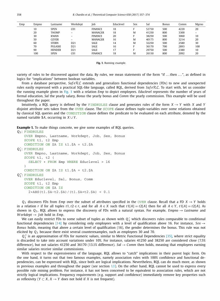
Emp Empno Lastname Workdept Job Educlevel Sex Sal Bonus Comm Mgrno
10 SPEN C01 FINANCE 18 F 52750 500 4220 2020 THOMP – MANAGER 18 M 41250 800 3300 –30 KWAN – FINANCE 20 F 38250 500 3060 1050 GEYER – MANAGER 16 M 40175 800 3214 2060 STERN D21 SALE 14 M 32250 500 2580 3070 PULASKI D21 SALE 16 F 36170 700 2893 10090 HENDER D21 SALE 17 F 29750 500 2380 10100 SPEN C01 FINANCE 18 M 26150 800 2092 20
Fig. 1. Running example.
variety of rules to be discovered against the data. By rules, we mean statements of the form “if . . . then . . . ”, as defined in logics for “implications” between boolean variables.
From a database perspective, Saf eRL extends and generalizes functional dependencies (FDs) to new and unexpected rules easily expressed with a practical SQL-like language, called RQL, derived from Saf eRL. To start with, let us consider the running example given in Fig. 1 with a relation Emp to depict employees. Educlevel represents the number of years of formal education, Sal the yearly salary, Bonus the yearly bonus and Comm the yearly commission. This example will be used throughout the paper.
Intuitively, a RQL query is defined by the FINDRULES clause and generates rules of the form X → Y with X and Ydisjoint attribute sets taken from the OVER clause. The SCOPE clause defines tuple-variables over some relations obtained by classical SQL queries and the CONDITION clause defines the predicate to be evaluated on each attribute, denoted by the named variable $A, occurring in X ∪ Y .
Example 1. To make things concrete, we give some examples of RQL queries.Q 1: FINDRULES
OVER Empno, Lastname, Workdept, Job, Sex, BonusSCOPE t1, t2 EmpCONDITION ON $A IS t1.$A = t2.$A
Q ′1: FINDRULES
OVER Empno, Lastname, Workdept, Job, Sex, BonusSCOPE t1, t2 (
SELECT * FROM Emp WHERE Educlevel > 16)CONDITION ON $A IS t1.$A = t2.$A
Q ′′1 : FINDRULES
OVER Educlevel, Sal, Bonus, CommSCOPE t1, t2 EmpCONDITION ON $A IS
2*ABS(t1.$A-t2.$A)/(t1.$A+t2.$A) < 0.1
Q 1 discovers FDs from Emp over the subset of attributes specified in the OVER clause. Recall that a FD X → Y holds in a relation r if for all tuples t1, t2 ∈ r, and for all A ∈ X such that t1[A] = t2[A] then for all A ∈ Y , t1[A] = t2[A]. As shown in Q 1, RQL allows to express the discovery of FDs with a natural syntax. For example, Empno → Lastname and W orkdept → Job hold in Emp.
We can easily restrict FDs to some subset of tuples as shown with Q ′1 which discovers rules comparable to conditional
functional dependencies [14] by considering only employees with a level of qualification above 16. For instance, Sex →Bonus holds, meaning that above a certain level of qualification (16), the gender determines the bonus. This rule was not elicited by Q 1 because there exist several counterexamples, such as employees 30 and 70.
Q ′′1 is an approximation of FDs for numeric values, similar to Metric Functional Dependencies [35], where strict equality
is discarded to take into account variations under 10%. For instance, salaries 41250 and 38250 are considered close (7.5% difference), but not salaries 41250 and 36170 (13.1% difference). Sal → Comm then holds, meaning that employees earning similar salaries receive similar commissions.
With respect to the expressiveness of the language, RQL allows to “catch” implications in their purest logic form. On the one hand, it turns out that two famous examples, namely association rules with 100% confidence and functional de-pendencies, can be expressed with RQL, since both are logical implications. Nevertheless, RQL can do much more, as shown in previous examples and throughout the paper (see section 1.1). On the other hand, RQL cannot be used to express every possible rule mining problem. For instance, it has not been conceived to be equivalent to association rules, which are not strictly logical implications. Frequency requirements (e.g. support and confidence) immediately remove key properties such as reflexivity (Y ⊂ X, X → Y does not hold if X is not frequent).
B. Chardin et al. / Theoretical Computer Science 658 (2017) 357–374 359
RQL has been devised as a user-friendly SQL-like query language, which can be integrated on top of any DBMS support-ing SQL. RQL query processing is seen as a classical query processing problem in databases. We provide a query rewriting technique and a constructive proof of the main query equivalence theorem, leading to an efficient query processing tech-nique.
This approach has been implemented and experimentally evaluated on sensor network data. A web prototype has been released and is freely available (http://rql.insa-lyon.fr http://rql.insa-lyon.fr). Data analysts can upload a sample of their data, write their own RQL queries and get answers to know whether or not a rule holds (if not, a counterexamplefrom the database is displayed) and much more.
This contribution is an attempt to bridge the gap between pattern mining and databases to facilitate the use of data mining techniques by SQL-aware analysts. The ultimate goal of this work is to integrate pattern mining techniques into core DBMS technologies.
1.1. More RQL examples
Conveniently, we have reused so far RQL examples related to FDs. Nevertheless, RQL does much more and is not restricted to FDs at all.
Example 2. null values in Dept.
Q 2: FINDRULESOVER Empno, Lastname, Workdept, Job, Sex, Bonus, MgrnoSCOPE t1 EmpCONDITION ON $A IS t1.$A IS NULL
Q 2 discovers rules between null values of the relation Emp. In most databases, null values are common and knowing relationships between attributes with respect to null values could be useful. For instance, Mgrno → W orkdept holds in Emp, meaning that when Mgrno is null, then Workdept is also null for the same tuple (only employee No. 20 in Example 1).
Example 3. Assume we are interested in a kind of sequential dependencies [27], i.e. dependencies showing similar behavior of attribute values. Q 3 discovers numerical attributes that vary together (i.e., X → Y means that if X increases then Y also increases).
Q 3: FINDRULESOVER Educlevel, Sal, Bonus, CommSCOPE t1, t2 EmpCONDITION ON $A IS t1.$A >= t2.$A
Using Q 3, Sal → Comm and Comm → Sal hold in Emp, which means that a higher salary is equivalent to a higher commission.
Example 4. Tuple-variables can also be defined on different relations. For instance, the following query searches for inequal-ities between tuple-variables from two views, referred to as managers and managees in the query.
FINDRULES OVER Educlevel, Sal, Bonus, CommSCOPEmanagers (SELECT * FROM Emp WHERE Empno IN (
SELECT Mgrno FROM Emp)),managees (SELECT * FROM Emp WHERE Empno NOT IN (
SELECT Mgrno FROM Emp WHERE Mgrno IS NOT NULL))CONDITION ON $A IS managers.$A > managees.$A
The rule ∅ → Educlevel then holds, meaning that managers always have a higher education levels than non-managers.
The interested reader may find more intricate examples in [18].
1.2. RQL query processing in a nutshell
This section unfolds one of the provided examples to convey the core ideas underlying RQL query processing, for which a general architecture is given in Fig. 3, section 5. To do so, we consider the following query Q (simplified from query Q ′
1given in Example 1):
360 B. Chardin et al. / Theoretical Computer Science 658 (2017) 357–374
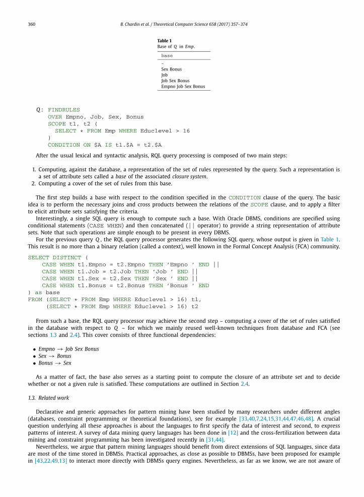
Table 1Base of Q in Emp.
base
–Sex BonusJobJob Sex BonusEmpno Job Sex Bonus
Q : FINDRULESOVER Empno, Job, Sex, BonusSCOPE t1, t2 (
SELECT * FROM Emp WHERE Educlevel > 16)CONDITION ON $A IS t1.$A = t2.$A
After the usual lexical and syntactic analysis, RQL query processing is composed of two main steps:
1. Computing, against the database, a representation of the set of rules represented by the query. Such a representation is a set of attribute sets called a base of the associated closure system.
2. Computing a cover of the set of rules from this base.
The first step builds a base with respect to the condition specified in the CONDITION clause of the query. The basic idea is to perform the necessary joins and cross products between the relations of the SCOPE clause, and to apply a filter to elicit attribute sets satisfying the criteria.
Interestingly, a single SQL query is enough to compute such a base. With Oracle DBMS, conditions are specified using conditional statements (CASE WHEN) and then concatenated (|| operator) to provide a string representation of attribute sets. Note that such operations are simple enough to be present in every DBMS.
For the previous query Q , the RQL query processor generates the following SQL query, whose output is given in Table 1. This result is no more than a binary relation (called a context), well known in the Formal Concept Analysis (FCA) community.
SELECT DISTINCT (CASE WHEN t1.Empno = t2.Empno THEN ’Empno ’ END ||CASE WHEN t1.Job = t2.Job THEN ’Job ’ END ||CASE WHEN t1.Sex = t2.Sex THEN ’Sex ’ END ||CASE WHEN t1.Bonus = t2.Bonus THEN ’Bonus ’ END
) as baseFROM (SELECT * FROM Emp WHERE Educlevel > 16) t1,
(SELECT * FROM Emp WHERE Educlevel > 16) t2
From such a base, the RQL query processor may achieve the second step – computing a cover of the set of rules satisfied in the database with respect to Q – for which we mainly reused well-known techniques from database and FCA (see sections 1.3 and 2.4). This cover consists of three functional dependencies:
• Empno → Job Sex Bonus• Sex → Bonus• Bonus → Sex
As a matter of fact, the base also serves as a starting point to compute the closure of an attribute set and to decide whether or not a given rule is satisfied. These computations are outlined in Section 2.4.
1.3. Related work
Declarative and generic approaches for pattern mining have been studied by many researchers under different angles (databases, constraint programming or theoretical foundations), see for example [33,40,7,24,15,31,44,47,46,48]. A crucial question underlying all these approaches is about the languages to first specify the data of interest and second, to express patterns of interest. A survey of data mining query languages has been done in [12] and the cross-fertilization between data mining and constraint programming has been investigated recently in [31,44].
Nevertheless, we argue that pattern mining languages should benefit from direct extensions of SQL languages, since data are most of the time stored in DBMSs. Practical approaches, as close as possible to DBMSs, have been proposed for example in [43,22,49,13] to interact more directly with DBMSs query engines. Nevertheless, as far as we know, we are not aware of
B. Chardin et al. / Theoretical Computer Science 658 (2017) 357–374 361
systems similar to RQL since it targets a very specific class of rules, i.e. those rules verifying Armstrong axioms and thus classical implication in logics. In other words, association rules systems such as MINE RULE [43] or data mining extensions of SQL systems (e.g. Oracle, IBM) cannot be fairly compared to RQL. Moreover, RQL cannot be compared to association rules systems due to the frequency requirement.
The Saf eRL language, inspired from the logical language proposed in [15], goes into this direction by providing a formal semantic based on the tuple relational calculus (TRC), underpinning SQL. FDs, association rules with 100% confidence and the ad-hoc language proposed in [6] are special cases of our Saf eRL language but none of them has a logical query language foundation. In this paper, we provide a logical view on the ad-hoc language proposed in [6] for gene expression data. The language of [6] was defined using a BNF grammar with no clear logical foundation and hence no practical SQL-like query language. From a technical point of view, the paper can be seen as a generalization of the approach proposed in [39,20,38] to discover functional dependencies (FD). Indeed, the machinery introduced in this paper generalizes the computation of agree sets (a base of the closure system associated with FD) to every RQL query. Moreover, the paper is a major extension of [5,17]: [5] provides a logical view on the ad-hoc language proposed in [6], with some restrictions (e.g. only one relation schema). Theoretical results on decidability problems are also given. We do not reproduce all the results in this paper. [17] introduces the practical query language RQL for the first time. Moreover, RQL has been used as a core building block to build a complete suite for genomics-data analysis in the RulNet prototype [52]. In RulNet, RQL is used with a slightly different syntax but with the same query engine to process the queries. Many options are provided to conveniently display a set of rules as gene regulatory network and to assess the quality of rules with different interestingness measures. Interestingly, other applications such as [3] exist for data analysis in biomedical studies with implications, for which RQL could also be useful.
Many dependencies different from functional dependencies have been studied such as implications in formal concept analysis (FCA) [38,42,9], conditional FDs [14], sequential dependencies [27], metric FDs [35], denial constraints [19] or constraint-generating dependencies [10]. They can partially be represented with RQL (cf. examples in Section 1) with some restrictions though. Nevertheless, RQL widens the scope of dependencies and lets the data analysts decide their patterns of interest with respect to their background knowledge, without any presupposition on the dependencies to be discovered.
1.4. Paper organization
Section 2 introduces some notations and recalls important notions on relational calculus and closure systems. Section 3presents the syntax and semantics of the Saf eRL language, while section 4 presents some results used for computing the answer to Saf eRL queries. Section 5 presents experimental results, section 6 presents the web prototype for RQL and section 7 concludes.
2. Preliminaries
This section introduces main definitions and notations used throughout the paper for the relational model, safe TRC, rules and closure systems.
2.1. Relational model
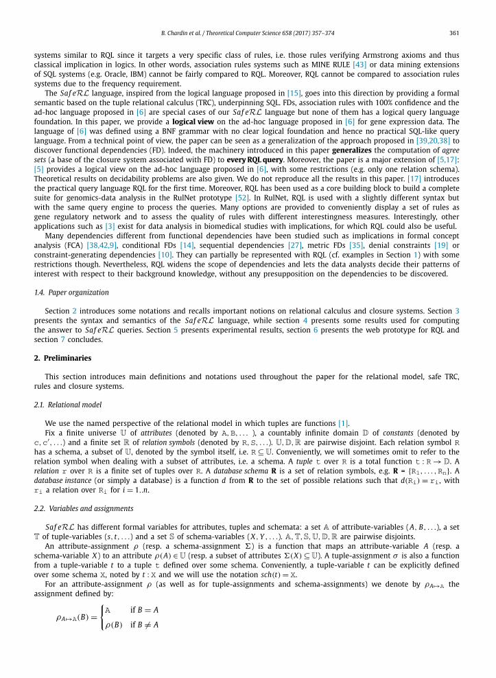
We use the named perspective of the relational model in which tuples are functions [1].Fix a finite universe U of attributes (denoted by A, B, . . . ), a countably infinite domain D of constants (denoted by
c, c′, . . .) and a finite set R of relation symbols (denoted by R, S, . . .). U, D, R are pairwise disjoint. Each relation symbol Rhas a schema, a subset of U, denoted by the symbol itself, i.e. R ⊆ U. Conveniently, we will sometimes omit to refer to the relation symbol when dealing with a subset of attributes, i.e. a schema. A tuple t over R is a total function t : R → D. A relation r over R is a finite set of tuples over R. A database schema R is a set of relation symbols, e.g. R = {R1, . . . , Rn}. A database instance (or simply a database) is a function d from R to the set of possible relations such that d(Ri) = ri , with ri a relation over Ri for i = 1..n.
2.2. Variables and assignments
Saf eRL has different formal variables for attributes, tuples and schemata: a set A of attribute-variables (A, B, . . .), a set T of tuple-variables (s, t, . . .) and a set S of schema-variables (X, Y , . . .). A, T, S, U, D, R are pairwise disjoints.
An attribute-assignment ρ (resp. a schema-assignment �) is a function that maps an attribute-variable A (resp. a schema-variable X) to an attribute ρ(A) ∈ U (resp. a subset of attributes �(X) ⊆ U). A tuple-assignment σ is also a function from a tuple-variable t to a tuple t defined over some schema. Conveniently, a tuple-variable t can be explicitly defined over some schema X, noted by t : X and we will use the notation sch(t) = X.
For an attribute-assignment ρ (as well as for tuple-assignments and schema-assignments) we denote by ρA →A the assignment defined by:
ρA →A(B) ={A if B = A
ρ(B) if B �= A
362 B. Chardin et al. / Theoretical Computer Science 658 (2017) 357–374
2.3. Safe TRC
Since TRC is a core component of Saf eRL, we recall here the syntax and semantics of the TRC in its simplest form (see [1] for more details). TRC formulas noted ψ, ψ1, ψ2, . . . are defined inductively as usual, where A, B ∈ U, X ⊆ U, c ∈D, R ∈R, t, t1, t2 ∈ T:
R(t) | t1.A= t2.B | t.A= c | ¬ψ | ψ1 ∧ ψ2 | ∃t : X (ψ)
Given a database d over R and a tuple assignment σ , the satisfaction of a TRC formula ψ is inductively defined as follows:
• 〈d, σ 〉 |= R(t) if σ(t) ∈ d(R), R ∈ R• 〈d, σ 〉 |= t1.A = t2.B if σ(t1)(A) = σ(t2)(B)
• 〈d, σ 〉 |= t.A = c if σ(t)(A) = c• 〈d, σ 〉 |= ¬ψ if 〈d, σ 〉 �|= ψ
• 〈d, σ 〉 |= ψ1 ∧ ψ2 if 〈d, σ 〉 |= ψ1 and 〈d, σ 〉 |= ψ2• 〈d, σ 〉 |= ∃t : X (ψ) if there exists a tuple t over X such that 〈d, σt →t〉 |= ψ
A TRC query is an expression of the form
q = {t | ψ}where ψ is a TRC formula with exactly one free variable t . The set of answers ans(q, d) of q w.r.t. a database d is
ans(q,d) = {σ(t) | 〈d,σ 〉 |= ψ}In the sequel, we consider safe TRC, the fragment of TRC known to always provide finite answers [1].Moreover, we shall admit several tuple variables in TRC formulas: Let ψ(t1, . . . , tn) be a safe TRC formulas with t1, . . . , tn
free variables, i.e. q = {(t1, . . . , tn) | ψ(t1, . . . , tn)}. Then the answer is just a set of tuple assignment σ defined for each ti, i = 1..n, i.e. ans(q, d) = {σ{t1,...,tn} | 〈d, σ 〉 |= ψ(t1, . . . , tn)}.
2.4. Rules and closure systems
Rules or implications, closure systems and closure operators have been widely studied in many branches of applied mathematics and computer sciences, with applications in databases for functional dependencies [8] and in formal concept analysis for implications [26]. The interested reader should refer to [16,11] for a comprehensive survey. We summarize the main results that are useful for the rest of the paper.
Let U ⊆ U and X, Y ⊆ U. A rule is a syntactic expression of the form X → Y . C ⊆ 2U is a closure system if U ∈ C and X, Y ∈ C ⇒ X ∩ Y ∈ C [26].
Let F be a set of rules on U . A rule X → A is implied by F , denoted by F � X → A, if there is a derivation (or a proof) from F using Armstrong’s axiom system (reflexivity, augmentation, transitivity) ending to X → A. The closure of a set X ⊆ Uis defined by X+
F = {A ∈ U | F � X → A}. A closure system can be defined for F , noted C L(F ) = {X ⊆ U |X = X+F }.
Let I R R(F ) be the set of meet-irreducible elements of C L(F ), i.e. X ∈ I R R(F ) iff for all Y , Z ∈ C L(F ), (X = Y ∩ Z) ⇒(X = Y or X = Z).
The notion of base of a closure system is now defined as follows:
Definition 1. Let C L(F ) be a closure system. A base B of C L(F ) is such that I R R(F ) ⊆ B ⊆ C L(F ).
A base is called a context in FCA terminology [26].It is worth noting that whenever a base has been computed from a given relation r, we can address the following
problems:
1. Given a set of attributes, compute its closure with respect to the rules satisfied in r.2. Given a rule, say whether or not this rule is satisfied. If not, give a counterexample from r.3. Compute a cover of non-satisfied rules in r.4. Compute a cover (or basis) of satisfied rules in r.
Let us consider the well-known functional dependencies. Given a relation r over R , a base of the closure system associ-ated to satisfied FDs in r is known as the set of agree sets. Given the agree sets ag(r), each problem listed above has been studied extensively in database and formal concept analysis communities [38]:
1. Compute the closure of a set of attributes: let X ⊆ R . X+ = ⋂{Y ∈ ag(r)|X ⊆ Y }.2. Verify a rule: let X → Y be a rule, r |= X → Y iff Y ⊆ X+ .
B. Chardin et al. / Theoretical Computer Science 658 (2017) 357–374 363
3. Compute a cover of approximate FDs, known as the Gottlob and Libkin cover [29]: X → A is given whenever X ∈max(A, r) = max⊆{X ∈ ag(r)|A �∈ X}.
4. Compute the canonical cover1 for satisfied FDs [39,20,38]: X → A is given whenever X is a minimal transversal of the hypergraph {R \ X |X ∈ max(A, r)}.
From a complexity point of view, steps 1 to 3 described above are polynomial while the fourth one is incremental quasi-polynomial in the size of the input and the output due to the enumeration of minimal transversal [25].
The rest of this paper proposes a generalization of this approach. Indeed, each Saf eRL query defines a closure system and therefore, in order to reuse previous results, the problem turns out to be on the computation against the database of a base with respect to a given Saf eRL query. In this paper, we will focus on this problem only. Other problems listed above such as the generation of a canonical cover will not be detailed.
3. A query language for rule mining
In the introduction, we have illustrated RQL – an SQL-like friendly language – through examples. This section formally defines the syntax and semantics of Saf eRL from which RQL is derived. We have introduced safe TRC for expressing SQL-like queries. Before defining Saf eRL, it remains to precisely define the notion of mining formulas, denoted in RQL (cf. previous examples) as:
CONDITION ON $A IS δ($A, t1, ... , tn)
3.1. Mining formulas
Mining formulas, denoted by δ, δ1, δ2, . . . , are defined over tuple-variables T, attribute-variables A and constants D only. Their syntax and their semantics are defined as follows.
Definition 2. Let t, t1, t2 ∈ T, A, B ∈ A and c ∈ D. A mining formula is of the form: t1.A = t2.B | t.A = c | ¬δ | δ1 ∧ δ2 where δ, δ1, δ2 are mining formulas.
The satisfaction of a mining formula δ w.r.t. a tuple-assignment σ and an attribute-assignment ρ , denoted by 〈σ , ρ〉 |= δ, is inductively defined as follows:
• 〈σ , ρ〉 |= t1.A = t2.B iff σ(t1)(ρ(A)) = σ(t2)(ρ(B))
• 〈σ , ρ〉 |= t.A = c iff σ(t)(ρ(A)) = c• 〈σ , ρ〉 |= ¬δ iff 〈σ , ρ〉 �|= δ
• 〈σ , ρ〉 |= δ1 ∧ δ2 iff 〈σ , ρ〉 |= δ1 and 〈σ , ρ〉 |= δ2
Such formulas are very simple and relatively restrictive to keep the presentation simple. In practice, we shall use other binary operators such as ≤, <, ≥, >, . . . . Details are omitted.
3.2. Saf eRL queries
The Saf eRL query language can now be defined.
Definition 3. A Saf eRL query over a database schema R is an expression of the form:
Q = { X → Y | ∀t1 . . .∀tn[ψ(t1, . . . , tn) →(∀A ∈ X(δ(A, t1, ..., tn)) → ∀A ∈ Y (δ(A, t1, ..., tn))
)] }where:
• X and Y are schema-variables,• ψ is a TRC-formula over R with n free tuple-variables t1, . . . , tn ,• δ is a mining formula with t1, . . . , tn free tuple-variables and A a single free attribute-variable.
When clear from context, a Saf eRL query Q may also be simply denoted by Q = 〈ψ(t1, ..., tn), δ(A, t1, ..., tn)〉, or even Q = 〈ψ, δ〉.
1 Also called canonical direct basis [11].
364 B. Chardin et al. / Theoretical Computer Science 658 (2017) 357–374
Example 5. Continuing Example 1, query Q 1 is formalized in Saf eRL as follows:
Q 1 = { X → Y | ∀t1, t2[(EMP(t1) ∧ EMP(t2)
) →(∀A ∈ X(t1.A = t2.A) → ∀A ∈ Y (t1.A = t2.A))] }
More succinctly, Q 1 is also noted 〈EMP(t1) ∧ EMP(t2), (t1.A = t2.A))〉.
The attributes appearing in the result of ψ are equal to ⋃n
i=1 sch(ti) whereas the schema of Q , denoted by sch(Q ), is defined by: sch(Q ) = ⋂n
i=1 sch(ti). Indeed, only common attributes of tuple-variables are meaningful to discover rules.To specify the result of the evaluation of a Saf eRL query against a database, we define the notion of satisfaction.
Definition 4. A Saf eRL query 〈ψ, δ〉 is satisfied in a database d and w.r.t. a schema-assignment �, denoted by 〈d, �〉 |=〈ψ, δ〉, if the following holds:
For all tuple-assignment σ such that (1)
〈d,σ 〉 |= ψ :if for all A ∈ �(X), 〈σ ,ρA →A〉 |= δ (2)
then for all A ∈ �(Y ), 〈σ ,ρA →A〉 |= δ (3)
Intuitively, this definition generalizes the definition of FD satisfaction in a relation: instead of only 2 tuples in a relation, we may have n tuples from the database d satisfying ψ (cf. (1)); and instead of the condition “for all A ∈ X, t1[A] = t2[A]”, we have “for all A ∈ �(X), δ(A, t1, . . . , tn)” (cf. (2) and (3)).
Definition 5. The answer of a Saf eRL query Q = 〈ψ, δ〉 in a database d over R, denoted by ans(Q , d), is defined as:
ans(Q ,d) = {�(X) → �(Y ) | 〈d,�〉 |= 〈ψ,δ〉,�(X) ∪ �(Y ) ⊆ sch(Q )}
3.3. RQL: a practical language for Saf eRL
RQL is a practical SQL-like declarative language to express Saf eRL queries. Let us consider a Saf eRL query Q =〈ψ(t1, . . . , tn), δ(A, t1, . . . , tn)〉 and its associated RQL query:
FINDRULESOVER A1, ... ,An
SCOPE t1(SQL1), ... , tn(SQLn)WHERE condition(t1, ... , tn)
CONDITION ON $A IS δ($A, t1, ... , tn)
The FINDRULES clause identifies RQL queries. The OVER clause specifies the set of attributes to be used for rule discov-ery. Those attributes have to be included in sch(Q ). The SCOPE clause specifies every tuple to be used to discover the rules and corresponds to the tuple-variables of ψ . Each tuple-variable is associated with an SQL query (which can be factorized if they refer to the same SQL query). The WHERE clause is borrowed from the SQL WHERE clause to specify relationships between tuple variables. The CONDITION ON $A IS specifies the mining formula δ.
Note that RQL allows much more flexibility than Saf eRL since more advanced conditions available in SQL – such as regular expressions, user-defined functions or built-in functions of the underlying DBMS – can be used for free, as in query Q ′′
1 of Example 1.
4. Theoretical results
In [5], a slightly different language for rule mining has been proposed. One of the main results was to point out that every query was “Armstrong-compliant”, meaning basically that Armstrong axioms are sound and that each query defines a closure system. The same result holds for Saf eRL queries as we shall see.
This result means that for query processing, we can adopt a strategy that generalizes the process of FD inference through agree sets [39,37].
Given a database d and a Saf eRL query Q , the basic idea is to compute a base of the closure system associated with Q from d. Let us start by introducing the closure system associated with Q , then the notion of base.
B. Chardin et al. / Theoretical Computer Science 658 (2017) 357–374 365
4.1. Closure system and bases for Saf eRL queries
Given a query Q against a database d, the definitions of a base and a closure system given in Section 2.4 are extended to ans(Q , d).
Definition 6. We say that Z ⊆ U satisfies ans(Q , d) if for all X → Y ∈ ans(Q , d), X �⊆ Z or Y ⊆ Z. The closure system of Q in d, denoted by C L Q (d), is defined by: C L Q (d) = {Z ⊆ sch(Q ) | Z satisfies ans(Q ,d)}.
Lemma 1. Let Q be a Saf eRL query and d a database.Then, C L Q (d) is a closure system on sch(Q ).
Proof. We have to show that sch(Q ) ∈ C L Q (d) and for all X, Y ∈ C L Q (d), X ∩ Y ∈ C L Q (d).
• sch(Q ) satisfies ans(Q , d) since for every X → Y ∈ ans(Q , d), we have Y ⊆ sch(Q ).• Let X, Y ∈ C L Q (d). We have to show that X ∩Y ∈ C L Q (d), i.e. X ∩Y satisfies ans(Q , d). By hypothesis, we have X ∈ C L Q (d)
and Y ∈ C L Q (d), implying for every V → W ∈ ans(Q , d), (V �⊆ X or W ⊆ X) and (V �⊆ Y or W ⊆ Y). We deduce that V �⊆ X ∩Yor W ⊆ X ∩ Y and the result follows. �
Corollary 1. Let Q be a Saf eRL query and d a database.Then, Q and d define a unique closure system.
It turns out that for every RQL query, there exists a closure system and thus, the main problem is to effectively compute a representation of the closure system, i.e. a base (cf. Definition 1).
In our setting, the definition of the base is:
Definition 7. Let Q = 〈ψ, δ〉 be a Saf eRL query over R and d a database over R. We assume that the attribute variable in δ is A. The base of Q in d, denoted by B Q (d), is defined by:
B Q (d) =⋃σ s.t.〈d,σ 〉|=ψ
{{A ∈ sch(Q ) | 〈σ ,ρA →A〉 |= δ}
}
That is, B Q (d) is the set of all Z ⊆ sch(Q ) for which there exists σ such that 〈d, σ 〉 |= ψ and 〈σ , ρA →A〉 |= δ for all A ∈ Z. Note that since A is the only attribute variable in δ, using ρA →A fully determines the attribute assignment in the evaluation of δ.
Proposition 1. B Q (d) is a base of the closure system C L Q (d).
Proof. We have to show that B Q (d) ⊆ C L Q (d) and I R R(C L Q (d)) ⊆ B Q (d).Let Z ∈ B Q (d) i.e. there exists a set of tuples t1 over sch(t1), . . . , tn over sch(tn) with 〈d, σt1 →t1,...,tn →tn 〉 |= ψ(t1, . . . , tn)
such that:
• ∀A ∈ Z, 〈σt1 →t1,...,tn →tn , ρA →A〉 |= δ(A, t1, . . . , tn), and• ∀A ∈ sch(Q )\Z, 〈σt1 →t1,...,tn →tn , ρA →A〉 �|= δ(A, t1, . . . , tn).
We have to show that Z ∈ C L Q (d). Suppose Z �∈ C L Q (d). In that case, there exists X ⊆ Z and Y �⊆ Z such that X → Y ∈ans(Q , d). It implies that: ∀A ∈ Y, 〈σt1 →t1,...,tn →tn , ρA →A〉 |= δ(A, t1, . . . , tn) since X ⊆ Z, there is a contradiction since Y �⊆ Z.
Let Z ∈ I R R(C L Q (d)), we have to show that Z ∈ B Q (d). We know that Z ∈ C L Q (d). Then, we have for all A ∈sch(Q )\Z, Z → A �∈ ans(Q , d). This means there exists some σA such that 〈σA, ρA →A〉 �|= δ(A, t1, . . . , tn) and for all B ∈ Z, 〈σA, ρA →B〉 |= δ(A, t1, . . . , tn). In other words, for all A ∈ sch(Q )\Z, there exists X ∈ B Q (d) such that Z ⊆ X and A �∈ X. Since Z = ⋂
A∈sch(Q )\Z{X ∈ B Q (d)|Z ⊆ X and A �∈ X} and Z ∈ I R R(C L Q (d)), we have the result, i.e. Z ∈ B Q (d). �4.2. Computing the base of a Saf eRL query using query rewriting
The naive approach consists in executing n SQL queries against the database, caching all intermediary results, keeping only the right combination of tuples with respect to the WHERE clause and then computing the base of the closure system. We can do much better: the basic idea is to transform the query in order to push as much as possible the processing into the SQL query engine.
For every RQL query Q = 〈ψ, δ〉 involving n tuple-variables, there exists another query Q ′ = 〈ψ ′, δ′〉 with a unique tuple-variable. The practical consequence of this remark is that the computation of the base can be done in a single SQL
366 B. Chardin et al. / Theoretical Computer Science 658 (2017) 357–374
query, i.e. the computation of the base of 〈ψ ′, δ′〉 can be delegated to the SQL query engine which was not the case in the former formulation.
By means of a rewriting function rw, we have to transform Q = 〈ψ(t1, . . . , tn), δ(A, t1, . . . , tn)〉 into Q ′ = 〈ψ ′(t), δ′(A, t)〉.The idea of rw is that the unique tuple-variable t appearing in Q ′ takes its values in the schema built from the disjoint
union of sch(ti), i = 1..n and is essentially the concatenation of the initial ti ’s.Let R be the new schema built as follows: R = ⋃
i∈1..n{〈A, i〉 | A ∈ sch(ti)}. Let t be a fresh tuple variable with sch(t) = Rand A1, . . . , An be n fresh attribute variables.
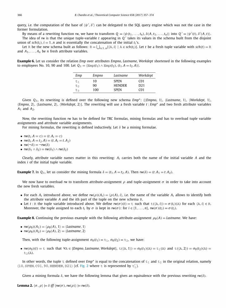
Example 6. Let us consider the relation Emp over attributes Empno, Lastname, Workdept shortened in the following examples to employees No. 10, 90 and 100. Let Q 1 = 〈Emp(t1) ∧ Emp(t2), (t1.A = t2.A)〉.
Emp Empno Lastname Workdept
t1 10 SPEN C01t2 90 HENDER D21t3 100 SPEN C01
Given Q 1, its rewriting is defined over the following new schema Emp∗: {〈Empno, 1〉, 〈Lastname, 1〉, 〈Workdept, 1〉, 〈Empno, 2〉, 〈Lastname, 2〉, 〈Workdept, 2〉}. The rewriting will use a fresh variable t : Emp∗ and two fresh attribute variables A1 and A2.
Now, the rewriting function rw has to be defined for TRC formulas, mining formulas and has to overload tuple variable assignments and attribute variable assignments.
For mining formulas, the rewriting is defined inductively. Let δ be a mining formulae.
• rw(ti .A = c) = (t.Ai = c)
• rw(ti .A = t j .A) = (t.Ai = t.A j)
• rw(¬δ) = ¬rw(δ)
• rw(δ1 ∧ δ2) = rw(δ1) ∧ rw(δ2)
Clearly, attribute variable names matter in this rewriting: Ai carries both the name of the initial variable A and the index i of the initial tuple variable.
Example 7. In Q 1, let us consider the mining formula δ = (t1.A = t2.A). Then rw(δ) = (t.A1 = t.A2).
We now have to overload rw to transform attribute-assignment ρ and tuple-assignment σ in order to take into account the new fresh variables.
• For each Ai introduced above, we define rw(ρ)(Ai) = 〈ρ(A), i〉, i.e. the name of the variable Ai allows to identify both the attribute variable A and the ith part of the tuple on the new schema R.
• Let t : R the tuple variable introduced above. We define rw(σ )(t) = t such that t(〈A, i〉) = σ(ti)(A) for each 〈A, i〉 ∈ R. Moreover, the tuple assigned to each ti by σ is kept in rw(σ ): for i ∈ {1, . . . , n}, rw(σ )(ti) = σ(ti).
Example 8. Continuing the previous example with the following attribute-assignment ρ0(A) = Lastname. We have:
• rw(ρ0)(A1) = 〈ρ0(A), 1〉 = 〈Lastname, 1〉• rw(ρ0)(A2) = 〈ρ0(A), 2〉 = 〈Lastname, 2〉
Then, with the following tuple-assignment σ0(t1) = t1 , σ0(t2) = t2 , we have:
• rw(σ0)(t) = t such that ∀A ∈ {Empno, Lastname, Workdept}, t(〈A, 1〉) = σ0(t1)(A) = t1(A) and t(〈A, 2〉) = σ0(t2)(A) =t2(A).
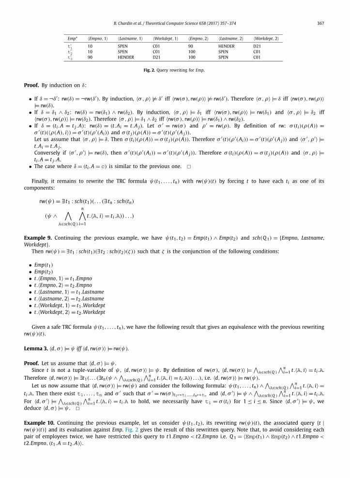
In other words, the tuple t defined over Emp∗ is equal to the concatenation of t1 and t2 in the original relation, namely 〈10, SPEN, C01, 90, HENDER, D21〉 (cf. Fig. 2 where t is represented by t′
1).
Given a mining formula δ, we have the following lemma that gives an equivalence with the previous rewriting rw(δ).
Lemma 2. 〈σ , ρ〉 |= δ iff 〈rw(σ ), rw(ρ)〉 |= rw(δ).
B. Chardin et al. / Theoretical Computer Science 658 (2017) 357–374 367
Emp∗ 〈Empno,1〉 〈Lastname,1〉 〈Workdept,1〉 〈Empno,2〉 〈Lastname,2〉 〈Workdept,2〉t′1 10 SPEN C01 90 HENDER D21t′2 10 SPEN C01 100 SPEN C01t′3 90 HENDER D21 100 SPEN C01
Fig. 2. Query rewriting for Emp.
Proof. By induction on δ:
• If δ = ¬δ′: rw(δ) = ¬rw(δ′). By induction, 〈σ , ρ〉 �|= δ′ iff 〈rw(σ ), rw(ρ)〉 �|= rw(δ′). Therefore 〈σ , ρ〉 |= δ iff 〈rw(σ ), rw(ρ)〉|= rw(δ).
• If δ = δ1 ∧ δ2: rw(δ) = rw(δ1) ∧ rw(δ2). By induction, 〈σ , ρ〉 |= δ1 iff 〈rw(σ ), rw(ρ)〉 |= rw(δ1) and 〈σ , ρ〉 |= δ2 iff 〈rw(σ ), rw(ρ)〉 |= rw(δ2). Therefore 〈σ , ρ〉 |= δ1 ∧ δ2 iff 〈rw(σ ), rw(ρ)〉 |= rw(δ1) ∧ rw(δ2).
• If δ = (ti .A = t j .A): rw(δ) = (t.Ai = t.A j). Let σ ′ = rw(σ ) and ρ ′ = rw(ρ). By definition of rw: σ(ti)(ρ(A)) =σ ′(t)(〈ρ(A), i〉) = σ ′(t)(ρ ′(Ai)) and σ(t j)(ρ(A)) = σ ′(t)(ρ ′(A j)).Let us assume that 〈σ , ρ〉 |= δ. Then σ(ti)(ρ(A)) = σ(t j)(ρ(A)). Therefore σ ′(t)(ρ ′(Ai)) = σ ′(t)(ρ ′(A j)) and 〈σ ′, ρ ′〉 |=t.Ai = t.A j .Conversely if 〈σ ′, ρ ′〉 |= rw(δ), then σ ′(t)(ρ ′(Ai)) = σ ′(t)(ρ ′(A j)). Therefore σ(ti)(ρ(A)) = σ(t j)(ρ(A)) and 〈σ , ρ〉 |=ti .A = t j .A.
• The case where δ = (ti .A = c) is similar to the previous one. �Finally, it remains to rewrite the TRC formula ψ(t1, . . . , tn) with rw(ψ)(t) by forcing t to have each ti as one of its
components:
rw(ψ) = ∃ t1 : sch(t1)(. . . (∃ tn : sch(tn)
(ψ ∧∧
A∈sch(Q )
n∧i=1
t.〈A, i〉 = ti .A)) . . .)
Example 9. Continuing the previous example, we have ψ(t1, t2) = Emp(t1) ∧ Emp(t2) and sch(Q 1) = {Empno, Lastname, Workdept}.
Then rw(ψ) = ∃ t1 : sch(t1)(∃ t2 : sch(t2)(ζ )) such that ζ is the conjunction of the following conditions:
• Emp(t1)
• Emp(t2)
• t.〈Empno, 1〉 = t1.Empno• t.〈Empno, 2〉 = t2.Empno• t.〈Lastname, 1〉 = t1.Lastname• t.〈Lastname, 2〉 = t2.Lastname• t.〈Workdept, 1〉 = t1.Workdept• t.〈Workdept, 2〉 = t2.Workdept
Given a safe TRC formula ψ(t1, . . . , tn), we have the following result that gives an equivalence with the previous rewriting rw(ψ)(t).
Lemma 3. 〈d, σ 〉 |= ψ iff 〈d, rw(σ )〉 |= rw(ψ).
Proof. Let us assume that 〈d, σ 〉 |= ψ .Since t is not a tuple-variable of ψ , 〈d, rw(σ )〉 |= ψ . By definition of rw(σ ), 〈d, rw(σ )〉 |= ∧
A∈sch(Q )
∧ni=1 t.〈A, i〉 = ti .A.
Therefore 〈d, rw(σ )〉 |= ∃t1(. . . (∃tn(ψ ∧ ∧A∈sch(Q )
∧ni=1 t.〈A, i〉 = ti .A)) . . .), i.e. 〈d, rw(σ )〉 |= rw(ψ).
Let us now assume that 〈d, rw(σ )〉 |= rw(ψ) and consider the following formula: ψ(t1, . . . , tn) ∧ ∧A∈sch(Q )
∧ni=1 t.〈A, i〉 =
ti .A. Then there exist t1, . . . , tn and σ ′ such that σ ′ = rw(σ )t1 →t1,...,tn →tn and 〈d, σ ′〉 |= ψ ∧ ∧A∈sch(Q )
∧ni=1 t.〈A, i〉 = ti .A.
For 〈d, σ ′〉 |= ∧A∈sch(Q )
∧ni=1 t.〈A, i〉 = ti .A to hold, we necessarily have ti = σ(ti) for 1 ≤ i ≤ n. Since 〈d, σ ′〉 |= ψ , we
deduce 〈d, σ 〉 |= ψ . �Example 10. Continuing the previous example, let us consider ψ(t1, t2), its rewriting rw(ψ)(t), the associated query {t |rw(ψ)(t)} and its evaluation against Emp. Fig. 2 gives the result of this rewritten query. Note that, to avoid considering each pair of employees twice, we have restricted this query to t1.Empno < t2.Empno i.e. Q 1 = 〈Emp(t1) ∧ Emp(t2) ∧ t1.Empno <
t2.Empno, (t1.A = t2.A)〉.
368 B. Chardin et al. / Theoretical Computer Science 658 (2017) 357–374
Interestingly, for every Saf eRL query Q = 〈ψ(t1, . . . , tn), δ((t1, . . . , tn, A)〉, rw(ψ) gives an intermediate representation allowing to compute the mining formula δ(t1, . . . , tn, A) on each tuple of the answer set.
Example 11. Let us consider the second tuple, denoted by t′2 , given in Example 10. The attribute Lastname (resp.
Workdept) satisfies rw(δ) since t′2(〈Lastname, 1〉) = t′
2(〈Lastname, 2〉) (resp. t′2(〈Workdept, 1〉) = t′
2(〈Workdept, 2〉)). The at-tribute Empno does not since t′
2(〈Empno, 1〉) �= t′2(〈Empno, 2〉). From t′
2 , the maximal set of attributes verifying rw(δ) is {Lastname, Workdept}, which is a closed set associated to the initial query Q 1. The closed set associated with t′
1 (resp t′3)
is empty since ∀ A ∈ sch(Q 1), t′1(〈A, 1〉) �= t′
1(〈A, 2〉) (resp. t′3(〈A, 1〉) �= t′
3(〈A, 2〉)).
We can now give an important result of the paper, i.e. how a base of the closure system associated to every Saf eRLquery can be computed.
Proposition 2.
B Q (d) =⋃
rw(σ )s.t.〈d,rw(σ )〉|=rw(ψ)
{{A ∈ sch(Q ) | ∃ρ : ρ(A) = A∧ 〈rw(σ ), rw(ρ)〉 |= rw(δ)}
}
Proof. By definition:
B Q (d) =⋃
σ s.t. 〈d,σ 〉|=ψ
{{A ∈ sch(Q ) | 〈σ ,ρA →A〉 |= δ}
}
Since A is the only attribute-variable in δ:
B Q (d) =⋃
σ s.t. 〈d,σ 〉|=ψ
{{A ∈ sch(Q ) | ∃ρ : ρ(A) = A∧ 〈σ ,ρ〉 |= δ}
}
By Lemma 2:
B Q (d) =⋃
σ s.t. 〈d,σ 〉|=ψ
{{A ∈ sch(Q ) | ∃ρ : ρ(A) = A∧ 〈rw(σ ), rw(ρ)〉 |= rw(δ)}
}
By Lemma 3:
B Q (d) =⋃
σ s.t.〈d,rw(σ )〉|=rw(ψ)
{{A ∈ sch(Q ) | ∃ρ : ρ(A) = A∧ 〈rw(σ ), rw(ρ)〉 |= rw(δ)}
}
We conclude by remarking that rw is bijective for σ . �The main theorem can now be given.
Theorem 1. Let Q be a Saf eRL query and d a database.Then
1. ans(Q , d) defines a unique closure system on sch(Q ), denoted by C L(ans(Q , d)).2. There exists an SQL query Q ′ over d such that I R R(ans(Q , d)) ⊆ ans(Q ′, d) ⊆ C L(ans(Q , d)).
Proof. The first item follows from Lemma 1. The second one follows from Proposition 1 and 2 for safe TRC formula. Since SQL is at least as expressive as safe TRC, the result holds. �
Therefore B Q (d) is computable by running only one SQL query, corresponding exactly to the safe TRC query {t | rw(ψ)}with only one difference: the SELECT part has to evaluate the satisfaction of rw(δ). From a practical point of view, it means that the base can be computed with only one SQL statement for all Saf eRL queries, pushing query processing as much as possible into the DBMS.
5. Implementation and experiments
Given a RQL query Q, the query processing engine consists of a Java/JavaCC application to:
1. Compute the base of the closure system of Q using the generated SQL query provided by Theorem 1.
B. Chardin et al. / Theoretical Computer Science 658 (2017) 357–374 369
Fig. 3. RQL query processing overview.
Samples
id DECIMAL(20,0)
timestamp TIMESTAMPtype DECIMAL(3,0)
value DECIMAL(10,0)
Descriptions
id DECIMAL(20,0)
type VARCHAR(12)location VARCHAR(18)description VARCHAR(78)
Fig. 4. PlaceLab database schema.
Time bathroom_light kitchen_humidity_0 ... bedroom_temperature_5
2006-08-22 00:00:00 0.4971428 4344 ... 21.432006-08-22 00:01:00 0.6685879 4344 ... 21.432006-08-22 00:02:00 0.4985673 4344 ... 21.465...2006-09-18 23:58:00 1567.7822 5324 ... 22.532006-09-18 23:59:00 1563.5891 5276 ... 22.50
Fig. 5. Sensors data after SQL preprocessing.
2. From the base, compute the canonical cover for exact rules and a Gottlob and Libkin cover for approximate rules [29]. Details are out of the scope of this paper, we mainly reused the code of T. Uno [45] for the most expensive part of the rule generation process, i.e. the enumeration of minimal transversal of hypergraphs.
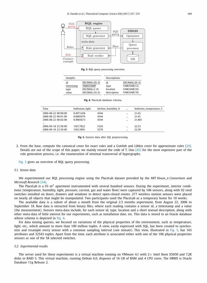
Fig. 3 gives an overview of RQL query processing.
5.1. Sensor data
We experimented our RQL processing engine using the PlaceLab dataset provided by the MIT House_n Consortium and Microsoft Research [34].
The PlaceLab is a 93 m2 apartment instrumented with several hundred sensors. During the experiment, interior condi-tions (temperature, humidity, light, pressure, current, gas and water flow) were captured by 106 sensors, along with 92 reed switches installed on doors, drawers and windows to detect open-closed events. 277 wireless motion sensors were placed on nearly all objects that might be manipulated. Two participants used the PlaceLab as a temporary home for 10 weeks.
The available data is a subset of about a month from the original 2.5 months experiment, from August 22, 2006 to September 18. Raw data is extracted from binary files, where each reading contains a sensor id, a timestamp and a value (the measurement). Sensors meta-data include, for each sensor id, type, location and a short textual description, along with other meta-data of little interest for our experiments, such as installation date, etc. This data is stored in an Oracle database whose schema is depicted in Fig. 4.
For data mining queries, we focused on variations of the physical properties of the environment, such as temperature, light, etc., which amount to more than 100 million tuples. A view, easily expressed with SQL, has been created to synchro-nize and resample every sensor with a common sampling interval (one minute). This view, illustrated in Fig. 5, has 165 attributes and 32543 tuples. Apart from the time, each attribute is associated either with one of the 106 physical properties sensors or one of the 58 selected switches.
5.2. Experimental results
The server used for these experiments is a virtual machine running on VMware 4.1 with 2× Intel Xeon X5650 and 7.2K disks in RAID 5. This virtual machine, running Debian 6.0, disposes of 16 GB of RAM and 4 CPU cores. The DBMS is Oracle Database 11g Release 2.
370 B. Chardin et al. / Theoretical Computer Science 658 (2017) 357–374
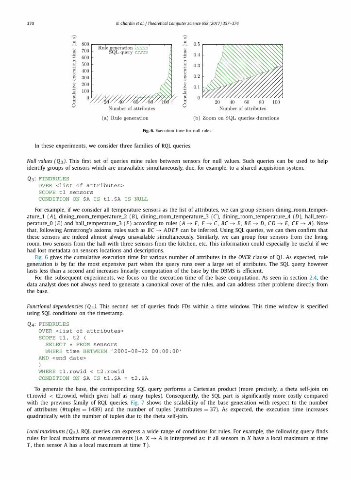
Fig. 6. Execution time for null rules.
In these experiments, we consider three families of RQL queries.
Null values (Q 3). This first set of queries mine rules between sensors for null values. Such queries can be used to help identify groups of sensors which are unavailable simultaneously, due, for example, to a shared acquisition system.
Q 3: FINDRULESOVER <list of attributes>SCOPE t1 sensorsCONDITION ON $A IS t1.$A IS NULL
For example, if we consider all temperature sensors as the list of attributes, we can group sensors dining_room_temper-ature_1 (A), dining_room_temperature_2 (B), dining_room_temperature_3 (C ), dining_room_temperature_4 (D), hall_tem-perature_0 (E) and hall_temperature_3 (F ) according to rules (A → F , F → C , BC → E , B E → D , C D → E , C E → A). Note that, following Armstrong’s axioms, rules such as BC → AD E F can be inferred. Using SQL queries, we can then confirm that these sensors are indeed almost always unavailable simultaneously. Similarly, we can group four sensors from the living room, two sensors from the hall with three sensors from the kitchen, etc. This information could especially be useful if we had lost metadata on sensors locations and descriptions.
Fig. 6 gives the cumulative execution time for various number of attributes in the OVER clause of Q1. As expected, rule generation is by far the most expensive part when the query runs over a large set of attributes. The SQL query however lasts less than a second and increases linearly: computation of the base by the DBMS is efficient.
For the subsequent experiments, we focus on the execution time of the base computation. As seen in section 2.4, the data analyst does not always need to generate a canonical cover of the rules, and can address other problems directly from the base.
Functional dependencies (Q 4). This second set of queries finds FDs within a time window. This time window is specified using SQL conditions on the timestamp.
Q 4: FINDRULESOVER <list of attributes>SCOPE t1, t2 (
SELECT * FROM sensorsWHERE time BETWEEN ’2006-08-22 00:00:00’
AND <end date>)WHERE t1.rowid < t2.rowidCONDITION ON $A IS t1.$A = t2.$A
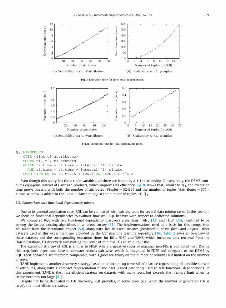
To generate the base, the corresponding SQL query performs a Cartesian product (more precisely, a theta self-join on t1.rowid < t2.rowid, which gives half as many tuples). Consequently, the SQL part is significantly more costly compared with the previous family of RQL queries. Fig. 7 shows the scalability of the base generation with respect to the number of attributes (#tuples = 1439) and the number of tuples (#attributes = 37). As expected, the execution time increases quadratically with the number of tuples due to the theta self-join.
Local maximums (Q 5). RQL queries can express a wide range of conditions for rules. For example, the following query finds rules for local maximums of measurements (i.e. X → A is interpreted as: if all sensors in X have a local maximum at time T , then sensor A has a local maximum at time T ).
B. Chardin et al. / Theoretical Computer Science 658 (2017) 357–374 371
Fig. 7. Execution time for functional dependencies.
Fig. 8. Execution time for local maximums rules.
Q 5 : FINDRULESOVER <list of attributes>SCOPE t1, t2, t3 sensorsWHERE t2.time = t1.time + interval ’1’ minute
AND t3.time = t2.time + interval ’1’ minuteCONDITION ON $A IS t1.$A < t2$.A AND t2$.A > t3$.A
Even though this query has three tuple-variables, all three are bound by a 1:1 relationship. Consequently, the DBMS com-putes equi-joins instead of Cartesian products, which improves its efficiency. Fig. 8 shows that, similar to Q 3, the execution time grows linearly with both the number of attributes (#tuples = 32433) and the number of tuples (#attributes = 37) – a time window is added to the SCOPE clause to adjust the number of tuples, cf. Q 4.
5.3. Comparison with functional dependencies miners
Due to its general application case, RQL can be compared with existing tools for several data mining tasks. In this section, we focus on functional dependencies to evaluate how well RQL behaves with respect to dedicated solutions.
We compared RQL with two functional dependency discovery algorithms: TANE [32] and FDEP [23], identified to be among the fastest existing algorithms in a recent survey [51]. The implementations used as a basis for this comparison are taken from the Metanome project [50], along with five datasets: ncvoter, fdreduced30, plista, flight and uniprot. Other datasets used in this experiment are provided by the UCI machine learning repository [36]. Table 2 gives an overview of these datasets and the corresponding execution times for RQL, FDEP and TANE, which includes: data retrieval from the Oracle database, FD discovery and writing the cover of minimal FDs to an output file.
The execution strategy of RQL is similar to FDEP, where a negative cover of maximal non-FDs is computed first. During this step, both algorithms have to compare records pair-wise, which is integrated in FDEP and delegated to the DBMS by RQL. Their behaviors are therefore comparable, with a good scalability on the number of columns but limited on the number of rows.
TANE implements another discovery strategy based on a bottom-up traversal of a lattice representing all possible subsets of attributes, along with a compact representation of the data (called partitions) used to test functional dependencies. In this experiment, TANE is the most efficient strategy on datasets with many rows, but exceeds the memory limit when its lattice becomes too large [51].
Despite not being dedicated to FDs discovery, RQL provides, in some cases (e.g. when the number of generated FDs is large), the most efficient strategy.
372 B. Chardin et al. / Theoretical Computer Science 658 (2017) 357–374
Table 2Execution times in seconds for functional dependency discovery.
Dataset Columns (#) Rows (#) Size (KB) FDs (#) RQL FDEP TANE
iris 5 150 4 4 <0.1 0.1 0.3balance-scale 5 625 6 1 0.1 0.2 0.4chess 7 28,056 519 1 214.6 71.6 1.0abalone 9 4,177 187 137 5.9 3.7 2.3nursery 9 12,960 1,036 1 60.9 25.1 6.4breast-cancer 11 699 19 46 0.4 0.5 0.9bridges 13 108 6 142 0.2 0.1 0.6echocardiogram 13 132 6 536 0.1 0.2 0.5adult 15 48,842 3,881 66 1661.7 784.3 127.1letter 17 20,000 696 61 327.7 158.0 MLncvoter 19 1,000 151 758 1.1 1.0 1.7hepatitis 20 155 7 8,250 0.6 0.5 5.2horse 28 368 28 156,723 2.9 6.1 MLfdreduced30 30 250,000 69,580 89,571 TL ML 132.9plista 63 1,001 575 178,152 11.2 16.4 MLflight 109 1,000 569 982,631 9.3 139.3 MLuniprot 223 1,000 2439 unknown TL ML ML
TL: time limit of 4 hours exceeded. ML: memory limit of 10 GB exceeded.
Fig. 9. Main web interface.
Fig. 10. Counterexamples with RQL.
6. A web prototype for RQL
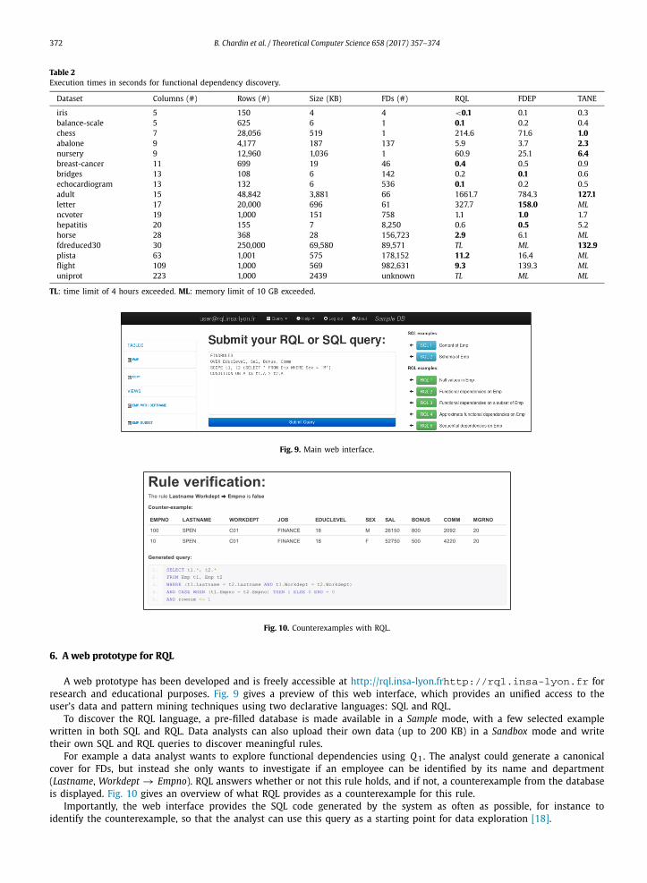
A web prototype has been developed and is freely accessible at http://rql.insa-lyon.frhttp://rql.insa-lyon.fr for research and educational purposes. Fig. 9 gives a preview of this web interface, which provides an unified access to the user’s data and pattern mining techniques using two declarative languages: SQL and RQL.
To discover the RQL language, a pre-filled database is made available in a Sample mode, with a few selected example written in both SQL and RQL. Data analysts can also upload their own data (up to 200 KB) in a Sandbox mode and write their own SQL and RQL queries to discover meaningful rules.
For example a data analyst wants to explore functional dependencies using Q 1. The analyst could generate a canonical cover for FDs, but instead she only wants to investigate if an employee can be identified by its name and department (Lastname, Workdept → Empno). RQL answers whether or not this rule holds, and if not, a counterexample from the database is displayed. Fig. 10 gives an overview of what RQL provides as a counterexample for this rule.
Importantly, the web interface provides the SQL code generated by the system as often as possible, for instance to identify the counterexample, so that the analyst can use this query as a starting point for data exploration [18].
B. Chardin et al. / Theoretical Computer Science 658 (2017) 357–374 373
7. Conclusion
In this paper, we have introduced Saf eRL, a logical query language based on the tuple relational calculus and de-voted to rule discovery in databases. The rule mining problem is seen as a query processing problem, for which we have proposed a query rewriting technique allowing the delegation of as much processing as possible to the underlying DBMS engine. RQL, the concrete language of Saf eRL, is an SQL-like rule mining language which allows SQL developers to extract precise information without specific knowledge in data mining. A system has been developed and tested against a real-life database provided by the MIT House_n Consortium and Microsoft Research. These experiments show both the feasibility and the efficiency of the proposed language.
RQL is an important contribution toward declarative pattern mining whose ambition is to simplify the way data analysts interact with their data. Through a convenient query language, close to SQL, they can focus on scientific discovery instead of spending considerable time switching data between different systems.
As future work, we could generate other covers for rules with RQL, typically optimal covers, namely the Duquenne and Guigues basis [30] or ordered direct implicational basis [4] (see [2] for a recent survey). The scalability of RQL to Big Data remains a quite challenging issue. Even if there is still room for improvements, we believe that alternative approaches should be conducted to guide the search towards interesting rules without enumerating all possible satisfied rules, for example by taking advantage of the knowledge brought by counterexamples. From an application point of view, the potential of RQLcould also be studied to express temporal dependencies [53] and more generally for data cleaning [28,21].
Acknowledgement
This work has been partially funded by the French national research agency (DAG project, ANR-09-EMER, 2009–2013) and CNRS Mastodons projects (PETASKY 2012-2015 and QualiSky 2016).
References
[1] Serge Abiteboul, Richard Hull, Victor Vianu, Foundations of Databases, Addison-Wesley, 1995.[2] Kira V. Adaricheva, James B. Nation, On implicational bases of closure systems with unique critical sets, Discrete Appl. Math. 162 (2014) 51–69.[3] Kira V. Adaricheva, James B. Nation, Gordon Okimoto, Vyacheslav Adarichev, Adina Amanbekkyzy, Shuchismita Sarkar, Alibek Sailanbayev, Nazar
Seidalin, Kenneth Alibek, Measuring the implications of the d-basis in analysis of data in biomedical studies, in: Formal Concept Analysis – 13th International Conference, ICFCA 2015, Proceedings, Nerja, Spain, June 23–26, 2015, 2015, pp. 39–57.
[4] Kira V. Adaricheva, James B. Nation, Robert Rand, Ordered direct implicational basis of a finite closure system, Discrete Appl. Math. 161 (6) (2013) 707–723.
[5] Marie Agier, Christine Froidevaux, Jean-Marc Petit, Yoan Renaud, Jef Wijsen, On Armstrong-compliant Logical Query Languages, in: George H.L. Fletcher, Slawek Staworko (Eds.), 4th International Workshop on Logic in Databases (LID 2011) in Conjunction with EDBT/ICDT Conference, ACM, March 2011, pp. 33–40.
[6] Marie Agier, Jean-Marc Petit, Einoshin Suzuki, Unifying framework for rule semantics: application to gene expression data, Fund. Inform. 78 (4) (2007) 543–559.
[7] Hiroki Arimura, Takeaki Uno, Polynomial-delay and polynomial-space algorithms for mining closed sequences, graphs, and pictures in accessible set systems, in: SDM, 2009, pp. 1088–1099.
[8] William Ward Armstrong, Dependency structures of data base relationships, in: Proceedings of the IFIP Congress, 1974, pp. 580–583.[9] Mikhail A. Babin, Sergei O. Kuznetsov, Computing premises of a minimal cover of functional dependencies is intractable, Discrete Appl. Math. 161 (6)
(2013) 742–749.[10] Marianne Baudinet, Jan Chomicki, Pierre Wolper, Constraint-generating dependencies, J. Comput. System Sci. 59 (1) (1999) 94–115.[11] Karell Bertet, Bernard Monjardet, The multiple facets of the canonical direct unit implicational basis, Theoret. Comput. Sci. 411 (22–24) (2010)
2155–2166.[12] Hendrik Blockeel, Toon Calders, Elisa Fromont, Bart Goethals, Adriana Prado, Céline Robardet, A practical comparative study of data mining query
languages, in: Sašo Džeroski, Bart Goethals, Pance Panov (Eds.), Inductive Databases and Constraint-Based Data Mining, Springer, New York, 2010, pp. 59–77.
[13] Hendrik Blockeel, Toon Calders, Élisa Fromont, Bart Goethals, Adriana Prado, Céline Robardet, An inductive database system based on virtual mining views, Data Min. Knowl. Discov. 24 (1) (2012) 247–287.
[14] Philip Bohannon, Wenfei Fan, Floris Geerts, Xibei Jia, Anastasios Kementsietsidis, Conditional functional dependencies for data cleaning, in: Proceedings of the 23rd International Conference on Data Engineering, ICDE ’07, 2007, pp. 746–755.
[15] Calders Toon, Jef Wijsen, On monotone data mining languages, in: Proceedings of the 8th International Workshop on Database Programming Languages, DBPL ’01, 2001, pp. 119–132.
[16] Nathalie Caspard, Bernard Monjardet, The lattices of closure systems, closure operators, and implicational systems on a finite set: a survey, Discrete Appl. Math. 127 (2) (2003) 241–269.
[17] Brice Chardin, Emmanuel Coquery, Benjamin Gouriou, Marie Pailloux, Jean-Marc Petit, Query rewriting for rule mining in databases, in: Bruno Crémilleux, Luc De Raedt, Paolo Frasconi, Tias Guns (Eds.), Languages for Data Mining and Machine Learning (LML) Workshop@ECML/PKDD 2013, September 2013, pp. 1–16.
[18] Brice Chardin, Emmanuel Coquery, Marie Pailloux, Jean-Marc Petit, RQL: an SQL-like query language for discovering meaningful rules (demo), in: IEEE ICDM 2014, Shengzen, China, December 2014.
[19] Xu Chu, Ihab F. Ilyas, Paolo Papotti, Discovering denial constraints, Proc. VLDB Endow. 6 (13) (August 2013) 1498–1509.[20] János Demetrovics, Vu Duc Thi, Some remarks on generating Armstrong and inferring functional dependencies relation, Acta Cybernet. 12 (2) (1995)
167–180.[21] Wenfei Fan, Floris Geerts, Uniform dependency language for improving data quality, IEEE Data Eng. Bull. 34 (3) (2011) 34–42.[22] Lujun Fang, Kristen LeFevre, Splash: ad-hoc querying of data and statistical models, in: Proceedings of the 13th International Conference on Extending
Database Technology, EDBT ’10, 2010, pp. 275–286.[23] Peter A. Flach, Iztok Savnik, Database dependency discovery: a machine learning approach, AI Commun. 12 (3) (1999) 139–160.
374 B. Chardin et al. / Theoretical Computer Science 658 (2017) 357–374
[24] Frédéric Flouvat, Fabien De Marchi, Jean-Marc Petit, The iZi project: easy prototyping of interesting pattern mining algorithms, in: New Frontiers in Applied Data Mining, in: Lecture Notes in Comput. Sci., vol. 5669, Springer, 2010, pp. 1–15.
[25] Michael L. Fredman, Leonid Khachiyan, On the complexity of dualization of monotone disjunctive normal forms, J. Algorithms 21 (3) (1996) 618–628.[26] Bernhard Ganter, Rudolf Wille, Formal Concept Analysis, Springer, 1999.[27] Lukasz Golab, Howard J. Karloff, Flip Korn, Avishek Saha, Divesh Srivastava, Sequential dependencies, Proc. VLDB Endow. 2 (1) (2009) 574–585.[28] Lukasz Golab, Howard J. Karloff, Flip Korn, Divesh Srivastava, Data auditor: exploring data quality and semantics using pattern tableaux, Proc. VLDB
Endow. 3 (2) (2010) 1641–1644.[29] Georg Gottlob, Leonid Libkin, Investigations on Armstrong relations, dependency inference, and excluded functional dependencies, Acta Cybernet. 9 (4)
(1990) 385–402.[30] Jean-Louis Guigues, Vincent Duquenne, Familles minimales d’implications informatives résultant d’un tableau de données binaires, Math. Sci. Hum.
24 (95) (1986) 5–18.[31] Tias Guns, Siegfried Nijssen, Luc De Raedt, Itemset mining: a constraint programming perspective, Artificial Intelligence 175 (12–13) (2011) 1951–1983.[32] Ykä Huhtala, Juha Kärkkäinen, Pasi Porkka, Hannu Toivonen, TANE: an efficient algorithm for discovering functional and approximate dependencies,
Comput. J. 42 (2) (1999) 100–111.[33] Tomasz Imielinski, Heikki Mannila, A database perspective on knowledge discovery, Commun. ACM 39 (11) (1996) 58–64.[34] Stephen S. Intille, Kent Larson, Emmanuel Munguia Tapia, Jennifer S. Beaudin, Pallavi Kaushik, Jason Nawyn, Randy Rockinson, Using a live-in laboratory
for ubiquitous computing research, in: PERVASIVE ’06, 2006, pp. 349–365.[35] Nick Koudas, Avishek Saha, Divesh Srivastava, Suresh Venkatasubramanian, Metric functional dependencies, in: ICDE, 2009, pp. 1275–1278.[36] Moshe Lichman, UCI Machine Learning Repository, 2016.[37] Stéphane Lopes, Jean-Marc Petit, Lotfi Lakhal, Efficient discovery of functional dependencies and Armstrong relations, in: EDBT 2000, 2000, pp. 350–364.[38] Stéphane Lopes, Jean-Marc Petit, Lotfi Lakhal, Functional and approximate dependency mining: database and FCA points of view, J. Exp. Theor. Artif.
Intell. 14 (2–3) (2002) 93–114.[39] Heikki Mannila, Kari-Jouko Räihä, Algorithms for inferring functional dependencies from relations, Data Knowl. Eng. 12 (1) (1994) 83–99.[40] Heikki Mannila, Hannu Toivonen, Levelwise search and borders of theories in knowledge discovery, Data Min. Knowl. Discov. 1 (3) (1997) 241–258.[41] MarketResearch.com, Worldwide relational database management systems 2012–2016 forecast, Aug 2012.[42] Raoul Medina, Lhouari Nourine, A unified hierarchy for functional dependencies, conditional functional dependencies and association rules, in: ICFCA,
in: Lecture Notes in Comput. Sci., vol. 5548, Springer, 2009, pp. 98–113.[43] Rosa Meo, Giuseppe Psaila, Stefano Ceri, An extension to SQL for mining association rules, Data Min. Knowl. Discov. 2 (2) (1998) 195–224.[44] Jean-Philippe Métivier, Patrice Boizumault, Bruno Crémilleux, Mehdi Khiari, Samir Loudni, A constraint-based language for declarative pattern discovery,
in: Declarative Pattern Mining Workshop, ICDM 2011, 2011, pp. 1112–1119.[45] Keisuke Murakami, Takeaki Uno, Efficient algorithms for dualizing large-scale hypergraphs, CoRR, arXiv:1102.3813, 2011.[46] Benjamin Négrevergne, Alexandre Termier, Marie-Christine Rousset, Jean-François Méhaut, Para Miner: a generic pattern mining algorithm for multi-
core architectures, Data Min. Knowl. Discov. 28 (3) (2014) 593–633.[47] Lhouari Nourine, Jean-Marc Petit, Extending set-based dualization: application to pattern mining, in: ECAI 2012, IOS Press, August 2012.[48] Lhouari Nourine, Jean-Marc Petit, Extended dualization: application to maximal pattern mining, Theoret. Comput. Sci. 618 (2016) 107–121.[49] Carlos Ordonez, Sasi K. Pitchaimalai, One-pass data mining algorithms in a DBMS with UDFs, in: SIGMOD Conference, 2011, pp. 1217–1220.[50] Thorsten Papenbrock, Tanja Bergmann, Moritz Finke, Jakob Zwiener, Felix Naumann, Data profiling with metanome, Proc. VLDB Endow. 8 (12) (2015)
1860–1871.[51] Thorsten Papenbrock, Jens Ehrlich, Jannik Marten, Tommy Neubert, Jan-Peer Rudolph, Martin Schönberg, Jakob Zwiener, Felix Naumann, Functional
dependency discovery: an experimental evaluation of seven algorithms, Proc. VLDB Endow. 8 (10) (2015) 1082–1093.[52] Jonathan Vincent, Pierre Martre, Benjamin Gouriou, Catherine Ravel, Zhanwu Dai, Jean-Marc Petit, Marie Pailloux, RulNet: a web-oriented platform for
regulatory network inference, application to wheat –omics data, PLoS ONE 10 (5) (May 2015) 20.[53] Jef Wijsen, Temporal dependencies, in: Encyclopedia of Database Systems, 2009, pp. 2960–2966.