theoretical network models - jackson state university

Theoretical Network Models

Dr. Natarajan Meghanathan

Professor of Computer Science

Jackson State University, Jackson, MS

E-mail: [email protected]

Theoretical Network Models• In this module, we will see the theoretical models using

which one could generate complex networks resembling those of real-world networks.

• The theoretical models we will see are as follows– Random Networks

• Erdos Renyi Model (ER Model)

– Scale-Free Networks

• Barabasi Albert Model (BA Model)

• Bianconi-Barabasi (BB Model)

– Small-World Networks

• Watts-Strogatz Model (WS Model)

• We will see the generation of the networks based on the above models and analyze their characteristics.

Random Networks• A random network is the one in which there is a

certain probability for a link between any two nodes in the network.

• Erdos-Renyi Model (ER) Model

– The probability for a link between any two nodes is the

same.

– Called the G(N, p) model where N is the number of nodes

and ‘p’ is the probability for a link between any two nodes

– Highly theoretical model and it is primarily used to

determine whether the links in a real-world network are

formed due to random interactions of nodes or due to the

preference of nodes to communicate or attach to certain

nodes.

ER Model• Step 1: Start with N

isolated nodes• Step 2: For a particular

node pair (u, v), generate a random number r. If r ≤ p, then, add the link (u, v) to the network.

• Repeat Step 2 for each of the N(N-1)/2 node pairs.

• Each random network we generate with the same parameters (N, p) will look slightly different.– The number of links L

is likely to be different.

N = 12 nodes, p = 1/6

L = 8 L = 10 L = 7

N = 100 nodes, p = 1/6

Source: Figure 3.3a: Barabasi

Generation of ER-Random Network

Let plink = 0.524

Index Pairs Random Val Edge1 0, 1 0.6335 N2 0, 2 0.7478 N

3 0, 3 0.1721 Y4 0, 4 0.9234 N5 0, 5 0.8563 N6 0, 6 0.3141 Y7 1, 2 0.1594 Y8 1, 3 0.2945 Y9 1, 4 0.2227 Y10 1, 5 0.0343 Y11 1, 6 0.7621 N12 2, 3 0.8595 N

13 2, 4 0.3091 Y14 2, 5 0.5312 N15 2, 6 0.1834 Y16 3, 4 0.4194 Y17 3, 5 0.2549 Y18 3, 6 0.6974 N19 4, 5 0.0968 Y20 4, 6 0.4486 Y21 5, 6 0.2983 Y

03

6

1

2 4

5Avg. Degree <K> = (2 + 4 + 3 + 4 + 5 + 4 + 4) / 7

= 3.71

ER Model: Poisson Degree Distribution

• In a network of N nodes, the maximum number of links for a node with its neighbors is N-1 and each of these links can occur with a probability p.– Average degree of a node <K> = (N-1)p

– Standard deviation for the degree of a node σk = sqrt(<K>)

• There could be a maximum N(N-1)/2 links in a random network of N nodes and each of these links can occur with a probability p.– Average number of links <L> = {N(N-1)/2}*p

• From the above, we can easily see that<K> = 2 * <L> / N

Poisson degree distribution

K ��

<K>

For larger networks, we simplyuse: <K> ~ Np

Generating a Poisson Degree Distribution

N = 10, p = 0.3�<k> = p(N-1)�<k> = 0.3*9 = 2.7

K ��

pk��

Generating a Poisson Degree Distribution

N = 10, p = 0.7�<k> = p(N-1)�<k> = 0.7*9 = 6.3

K ��

pk��

K ��

pk��

ER Model

Poisson Distribution

Random NetworkN = 100 Nodes; plink = 0.1

Average Degree <K>9.9 (Poisson); 9.93 (ER)

Standard Deviation SD(K)3.14 (Poisson); 3.28 (ER)

Degree Distribution: ER Model vs. Poisson

SD(K)

Sqrt(<K>)

Clustering Coefficient• In a random network evolved under the ER: G(N, p) model:

– For a node i with ki neighbors, the expected number of links connecting the neighbors is p*ki(ki -1)/2.

– Clustering coefficient is the ratio of the actual (also the expected value) number of links to that of the maximum number of links connecting the neighbors.

– Thus, the average clustering coefficient for an ER: G(N, p)-based random network is simply ‘p’ = <K> / N.

– Unlike real-world networks, the clustering coefficient is not dependent on degree distribution.

• Networks Actual Random: ER-G(N, p)Prison

Friendships 0.31 0.0134

Co-authorshipsMath 0.15 0.00002

Biology 0.09 0.00001

Economy 0.19 0.00002

WWWWeb links 0.11 0.002

Clustering Coefficients for Real Networks

Each circle corresponds to a real

network.

Directed networks were made

undirected to calculate C.

For ER-random networks, the average

clustering coefficient decreases as

1/N. In contrast, for real networks,

<C> has only a weak dependence

on N.

Real networks have a much higher

Clustering coefficient than expected

for a ER-random network of similar N

and L.

<C

> /

<K

>

Clustering for Real Networks

C(k) is measured by averaging the local clustering coefficient of all nodes

with the same degree k.

According to the ER-Random Network theory model, C(k) is independent of the

individual node degrees. However, we find that C(k) decreases as k increases.

Nodes with fewer neighbors have larger local clustering coefficients and vice-versa

Real Networks are not ER-Random

• Degree distribution: – ER-Random networks –Poisson distribution, esp. for k << N.

• Highly connected nodes (hubs) are effectively forbidden.

– Real networks: More highly connected nodes, compared to that predicted with random model.

• Connectedness:– ER-Random networks: One single giant component exists only if

<k> > ln N.

– Real networks: One single giant component exists for several networks with <k> < ln N.

• Average Path Length (small world property):– For both ER-random and real networks, the average path length

scales as ln N / ln <k>.

• Clustering coefficient:– ER-Random model: Local clustering coefficient is independent of

the node’s degree and <C> depends on the system size as 1/N.

– Real networks: <C> decreases with increase in node degrees and is largely independent of the system size.

Real Networks are not ER-Random

• Except for the small world property (avg. path length ~ lnN/ln<K>), the properties observed for real-world networks are not matching with that observed for ER-random networks.

• Then why study random graph theory (ER-model)?

• If a certain property is observed for real-world networks, we can refer to the random graph theory and analyze whether the property is observed by chance (like the small world property).

• If the property observed does not coincide with that of the random networks (like the local clustering coefficient), we need to further analyze the real-world network for the existence of the property because it did not just happen by chance.

• Establish useful benchmarks (e.g., diameter, degree distribution)

Generation of ER-Random Network0

1 2

3 4

5

6

Avg. Degree <K>= (2 + 3 + 3 + 5 + 3 + 4 + 2) / 7= 3.14

ER Model plink = <K> / (N-1)plink = 3.14 / 6 = 0.524

Index Pairs Random Val Edge1 0, 1 0.6335 N2 0, 2 0.7478 N3 0, 3 0.1721 Y4 0, 4 0.9234 N5 0, 5 0.8563 N6 0, 6 0.3141 Y7 1, 2 0.1594 Y

8 1, 3 0.2945 Y9 1, 4 0.2227 Y10 1, 5 0.0343 Y11 1, 6 0.7621 N12 2, 3 0.8595 N13 2, 4 0.3091 Y14 2, 5 0.5312 N15 2, 6 0.1834 Y16 3, 4 0.4194 Y17 3, 5 0.2549 Y

18 3, 6 0.6974 N19 4, 5 0.0968 Y20 4, 6 0.4486 Y21 5, 6 0.2983 Y

03

6

1

2 4

5Avg. Degree <K> = (2 + 4 + 3 + 4 + 5 + 4 + 4) / 7

= 3.71

Generation of ER-Random Network (contd…)

0

1 2

3 4

5

6

03

6

1

2 4

5

Given Network

ER-RandomNetwork

Degree #Nodes Prob.2 2 2/7 = 0.2863 3 3/7 = 0.428

4 1 1/7 = 0.1435 1 1/7 = 0.143

Degree #Nodes Prob.2 1 1/7 = 0.1433 1 1/7 = 0.143

4 4 4/7 = 0.5715 1 1/7 = 0.143

Degree Nodes LCC Avg <LCC>2 0, 6 1, 1 1.03 1, 2, 4 2/3, 2/3, 2/3 0.67

4 5 3/6 0.55 3 4/10 0.4

Degree Nodes LCC Avg <LCC>

2 0 0.0 0.03 2 2/3 0.674 1, 3, 5, 6 4/6, 3/6 0.542

4/6, 2/6 5 4 6/10 0.6

Problem Example 1

• Consider a random network generated according to the G(N, p) model where the total number of nodes is 12 and the probability that there are links between any two nodes is 0.20. Determine the following:

– The average number of links in the network

– The average node degree

– The standard deviation of the node degree

– The average path length (distance between any two nodes in the network)

– The average local clustering coefficient for any node in the network.

– The expected local clustering coefficient for a node that has exactly 5 neighbors.

Problem Example 1: Solution• There are N = 12 nodes

• Prob[link between any two nodes] = p = 0.2

Max. possible number of links between any two nodes is (N)(N-1)/2 = (12*11/2) = 66

(2) The average number of links in the network = p * N(N-1)/2

= 0.2 * 66 = 13.2

(3) Average node degree = p*(N-1) = 0.2 * 11 = 2.2

(4) Standard deviation of node degree = sqrt(<K>)

= sqrt(2.2) = 1.48

(5) Average path length = ln N / ln <k> = ln(12) / ln(2.2) = 3.15

(6) Avg. Local clustering coefficient for any node in the network = p = 0.2.

(7) The expected local clustering coefficient for a node in a random network is independent of its number of neighbors. Hence, the answer is 0.2

Scale-Free Networks


Professor

Department of Computer Science



Scale-Free Networks• Scale-free networks follows a Power-law distribution.

• P(k) ~ k-γ, where γ is the degree exponent (> 1)

• P(k) = Ck-γ, where C is the proportionality constant

ζ(γ) = ∑∞

=

−

1k

kγ ζ(γ) is called the

Riemann-Zeta

Function

Assuming the degree distribution is discrete

K

P(K)

Proportionality Constant (Discrete)γ

K-γγγγ

C

Computation of P(K) = CK–γ Values

γC

K

Power-Law Distribution (Discrete)

K ��

P(K

) ��

γ = 3

γ = 2

For larger values of the Degree exponent (γ), thechances of observing

a hub with a larger degreedecreases.

Example (Let N = 100)Kmin = 1γ Kmax

1.5 10,000 (ruled out)2.0 1002.5 21.553.0 103.5 6.31

Power Law (Discrete): Avg. Degreeγ

<K>

C

K

K*P

(K)

Why Power-Law is said to be scale-free?• Kurtosis is a measure of

how “heavy-tailed” a distribution is.

• A probability distribution is generally said to be scale-free (i.e., heavy-tailed) if its kurtosis is quite high (typically larger than 3).

• Scale-free distributions also have a standard deviation that is comparable or even larger than the mean.

22

][

4][

][

><−

><−=

KKE

KKEKKurtosis

K is the degree;

<K> is the mean degree

The Kurtosis and SD formula are applied for all values (# samples: N) of K for which there is a non-zero probability of finding a vertex with the particular degree

Standard Deviation, SD (K) =

( )∑>

><−N

KPK

KKN 0)(;

21

∑ ><−K

KKKP2

)(*)(SD(K) =

Kurtosis(K) =

4

4)(*)(

SD

KKKP

K

∑ ><−

Power-Law (Discrete): Degree (Avg. and SD)

γ��

<K>

SD(K)

Example 0: Power-law• Consider a network modeled using the power-law, P(K) =

CK-γ. Determine the power-law exponent γ and the constant C if the network has approximately 4% of nodes with degree 4 and 10% of nodes with degree 3.

• Solution:

• P(K) = CK-γ� ln P(K) = lnC + (-γ)lnK

• Given that P(3) = 0.10 and P(4) = 0.04

ln(0.10) = lnC + (-γ)ln(3) � -2.303 = lnC + (-γ)*1.098

ln(0.04) = lnC + (-γ)ln(4) � -3.219 = lnC + (-γ)*1.386 Solving for γ, we get γ = (3.219 – 2.303)/(1.386 – 1.098) = 3.18

Substituting for γ = 3.18 in the Power-law equation for one of the two degrees, we get C = P(4) / 4-γ. = 0.04 / 4–3.18

We get C = 3.286

Example 1: Generating a Discrete Power-

Law Distribution and Analyzing it• Generate a power-law distribution with degree exponent γ = 2.45.

Determine the power-law constant and the average degree.

KK-γγγγ

KK-γγγγ

Power-law Constant C = = 1/1.353 = 0.739

Power-Law: P(K) = CK–γγγγ = (0.739)K-2.45

KK-γγγγ

P(K)K*P(K)

Example 1 (1): Generating a Discrete

Power-Law Distribution and Analyzing itKK-γγγγ

P(K)K*P(K)

Average Degree <K> = = 1.670∑k

KPK )(*

KP(K)

(K-<K>)4

P(K)*(K-<K>)4

(K-<K>)2

P(K)*(K-<K>)2

Example 1 (2): Generating a Discrete

Power-Law Distribution and Analyzing it

KP(K)

(K-<K>)4

P(K)*(K-<K>)4

(K-<K>)2

P(K)*(K-<K>)2

337.3)(*)(2 =><−∑

K

KKKPSD(K) =

∑ ><−K

KKKP4

)(*)( = 377.4

Kurtosis(K) =

4

4)(*)(

SD

KKKP

K

∑ ><−

= 1.827

= -------------- = 33.9377.4

(1.827)4

Example 2: Analyzing a Degree Distribution for Scale-Free Property

Given the following adjacency list for the vertices, determine whether theDegree distribution could be classified to exhibit “scale-free” property.

0 10 20 3

0 40 50 70 81 31 51 61 93 44 6

4 75 97 8

0 �� 1, 2, 3, 4, 5, 7, 81 �� 0, 3, 5, 6, 92 �� 03 �� 0, 1, 44 �� 0, 3, 6, 75 �� 0, 1, 9

6 �� 1, 47 �� 0, 4, 88 �� 0, 79 �� 1, 5

ID Degree0 71 52 13 34 4

5 36 27 38 29 2

Degree #Nodes P(K)1 1 1/10 = 0.12 3 3/10 = 0.33 3 3/10 = 0.34 1 1/10 = 0.15 1 1/10 = 0.1

7 1 1/10 = 0.1

Avg. Degree = ∑

k

KPK )(*

Avg. Degree, <K>= (1)(0.1) + (2)(0.3) + (3)(0.3)+ (4)(0.1) + (5)(0.1) + (7)(0.1)= 3.2

Example 2(1): Analyzing a Degree Distribution for Scale-Free Property

Degree (K) P(K) (K-<K>)2 (K-<K>)4 P(K)*(K-<K>)2 P(K)*(K-<K>)4

1 0.1 4.84 23.43 0.484 2.343 2 0.3 1.44 2.07 0.432 0.6213 0.3 0.04 0.0016 0.012 0.000484 0.1 0.64 0.4096 0.064 0.040965 0.1 3.24 10.498 0.324 1.04987 0.1 14.44 208.51 1.444 20.851

<K> = 3.2

76.2)(*)(2 =><−∑

K

KKKPSD(K) =

∑ ><−K

KKKP4

)(*)( = 24.906

Kurtosis(K) =

4

4)(*)(

SD

KKKP

K

∑ ><−

= 1.661

= -------------- = 3.2724.906

(1.661)4

Since the Kurtosis (K) = 3.27is greater than 3, we say the Degree distribution is heavy-tailed.

Example 3: Analyzing a Degree Distribution for Scale-Free Property

Given the following adjacency list for the vertices, determine whether theDegree distribution could be classified to exhibit “scale-free” property.

0 10 20 3

0 40 51 21 41 61 92 32 83 63 8

4 54 74 95 7

0 �� 1, 2, 3, 4, 51 �� 0, 2, 4, 6, 92 �� 0, 1, 3, 83 �� 0, 2, 6, 84 �� 0, 1, 5, 7, 95 �� 0, 4, 7

6 �� 1, 37 �� 4, 58 �� 2, 39 �� 1, 4

ID Degree0 51 52 43 44 5

5 36 27 28 29 2

Degree #Nodes P(K)2 4 4/10 = 0.43 1 1/10 = 0.14 2 2/10 = 0.25 3 3/10 = 0.3

Avg. Degree = ∑

k

KPK )(*

Avg. Degree, <K>= (2)(0.4) + (3)(0.1) + (4)(0.2)+ (5)(0.3) = 3.4

Example 3(1): Analyzing a Degree Distribution for Scale-Free Property

Degree (K) P(K) (K-<K>)2 (K-<K>)4 P(K)*(K-<K>)2 P(K)*(K-<K>)4

2 0.4 1.96 3.842 0.784 1.53683 0.1 0.16 0.0256 0.016 0.002564 0.2 0.36 0.1296 0.072 0.025925 0.3 2.56 6.5536 0.768 1.9661

<K> = 3.4

64.1)(*)(2 =><−∑

K

KKKPSD(K) =

∑ ><−K

KKKP4

)(*)( = 3.5313

Kurtosis(K) =

4

4)(*)(

SD

KKKP

K

∑ ><−

= 1.281

= -------------- = 1.313.5313

(1.281)4

Since the Kurtosis (K) = 1.31Is lower than 3, we say the Degree distribution is NOT heavy-tailed.

Example 4: Predicting the Nature of Degree Distribution

Given the following probability degree distribution:1) Draw a plot of the degree distribution and determine if the degree distribution follows a power-law or Poisson? 2) Determine the parameters of the degree distribution you decided.

K P(K)1 0.7942 0.119

3 0.0394 0.0185 0.0106 0.0067 0.0048 0.0039 0.00210 0.001

K ��

P(K

) ��

It looks clearly like a power-law distribution.

Example 4(1): Predicting the Nature of Degree Distribution

K P(K) lnK lnP(K)1 0.794 0 -0.232 0.119 0.69 -2.13

3 0.039 1.10 -3.244 0.018 1.39 -4.025 0.010 1.61 -4.616 0.006 1.79 -5.127 0.004 1.95 -5.528 0.003 2.08 -5.819 0.002 2.20 -6.2110 0.001 2.30 -6.91

P(K) = C*K–γγγγ

lnP(K) = lnC + (-γ*lnK) : Compared to Y = (slope)*X + constant; slope = - γ ; constant = lnC;

We will use curve (line) fitting in Excel to find the slope and constant

lnK

lnP

(K)

Constant = lnC = –0.1873

C = e–0.1873 = 2.718–0.1873

C = 0.829lnP(K) = (-γ*lnK) + lnC

γ = 2.7755P(K) = 0.829*K–2.7755

Example 5: Predicting the Nature of Degree Distribution

Given the following probability degree distribution:1) Draw a plot of the degree distribution and determine if the degree distribution follows a power-law or Poisson? 2) Determine the parameters of the degree distribution you decided.

K P(K)0 0.0151 0.163

2 0.1323 0.1854 0.1945 0.1636 0.1147 0.0688 0.0369 0.01710 0.007

P(K

) ��

It looks clearly like a Poisson distribution.

K ��

Avg. Degree <K> = = 4.154∑k

KPK )(*

981.3)(*)(2 =><−∑

K

KKKPSD(K) = = 1.995

Kurtosis(K) =

4

4)(*)(

SD

KKKP

K

∑ ><−= -------------- = 2.852

45.181

(1.995)4

Kurtosis of Poisson distribution is expected to be close to 3Kurtosis of Heavy-tailed Power-law distribution is expected to be (much) larger than 3.

Where does the Power-Law distribution start for real networks?

• If P(x) = C X–γ, then Xmin needs to be certainly greater than 0, because X–γ is infinite at X = 0.

• Some real-world distributions exhibit power-law only from a minimum value (xmin).

Source:MEJ �Newman, Power laws, Pareto distributions and Zipf’s law, Contemporary Physics 46,

323–351 (2005)

Some Power-Law Exponents of Real-World Data

Power-Law Distribution (Discrete)

K ��

P(K

) ��

γ = 3

γ = 2

For larger values of the Degree exponent (γ), thechances of observing

a hub with a larger degreedecreases.

Example (Let N = 100)Kmin = 1γ Kmax

1.5 10,000 (ruled out)2.0 1002.5 21.553.0 103.5 6.31

Average Distance: Power-Law

Anomalous regime: Hub and

spoke configuration; average

distance independent of N.

Ultra small world regime

Hubs still reduce the path length

the lnN dependence on N (as

in random networks) starts

Small world property: Hubs are

not sufficiently large and numerous

to have impact on path length

The scale-free property shrinks the average path lengths as well as changes

the dependence of <d> on the system size. The smaller γ, the shorter are the

distances between the nodes.

Distances in

Scale-free

networks

Source:

Figure 4.12 Barabasi

Network Regimes based on SD(K)

γ��

SD(K)

<K>

Scale-Free Regime

An

om

alo

us

Reg

ime

Ran

do

m

Reg

ime

SD(K) ≤ Sqrt(<K>)

We refer to the regime as scale-freeif γ ≥ 2 and SD(K) > Sqrt(<K>)We also say the second moment

<K2> ~ [SD(K)]2 diverges in this regime

Source: Figure 4.14 Barabasi

Scale-free networks lack an

intrinsic scale

• For any bounded distribution (e.g. a Poisson or• a Gaussian distribution) the degree of a randomly chosen node

will be in the vicinity of <k>. Hence <k> serves as the network’s scale.

• In a scale-free network the second moment diverges, hence the degree of a randomly chosen node can be arbitrarily different from <k>. Thus, a scale-free network lacks an intrinsic scale (and hence gets its name).


Large Standard

Deviation for

Real Networks


Example: Power-Law, Avg. Path Length

• Consider a scale-free network of N = 100 nodes modeled

using the power-law, P(K) = CK-γ. The minimum and maximum degrees of the nodes in the network are kmin = 3

and kmax = 60 respectively. Find the power-law exponent

(γ), the power-law constant C and the average path length.

60 = 3 * (100)(1/γγγγ-1)

1/(γ-1) = ln(60/3) / ln(100)γ-1 = ln(100) / ln(20) = 1.54γ = 2.54

In this case:

∑=

−

=60

3

1

k

k

Cγ

Using an Excel Spreadsheet to calculate the valueof the summation, we get:

∑=

−60

3k

kγ

= 0.15333

C = 1/0.1533 = 6.52

Avg. Path Length= ln ln(N) / ln (γ-1)= ln ln(100) / ln(2.54-1)

= 3.54

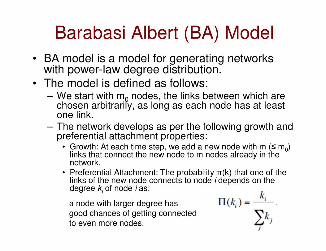
Barabasi Albert (BA) Model

• BA model is a model for generating networks with power-law degree distribution.

• The model is defined as follows:– We start with m0 nodes, the links between which are

chosen arbitrarily, as long as each node has at least one link.

– The network develops as per the following growth and preferential attachment properties:

• Growth: At each time step, we add a new node with m (≤ m0) links that connect the new node to m nodes already in the network.

• Preferential Attachment: The probability π(k) that one of the links of the new node connects to node i depends on the degree ki of node i as:

a node with larger degree has

good chances of getting connected

to even more nodes.

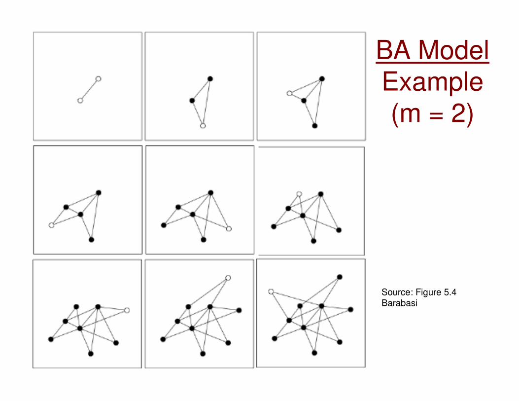
BA ModelExample (m = 2)

Source: Figure 5.4Barabasi

BA Model: Time-dependent Degree of a Node

• In the BA model, a node has a chance to increase its degree

each time a new node enters the network.

• Let ki be a time-dependent continuous real variable (ki is the

degree of node i that enters the network at time ti)

• The degree of node i at any time instant t ≥ ti is given by:

where β = ½ is called

the network’s dynamical exponent.

Observations:

1) The degree of each node increases following the above power law.

2) Each new node has more nodes to link than the previous nodes.

In other words, with time, each node competes for links with an increasing

pool of nodes.

Time Dependent Degree of a Node• The earlier node i was added, the higher is its degree

ki(t). – Hence, hubs are large not because they grow faster, but

because they arrived earlier.

– The growth in the degrees is sub linear (β < 1).

• The rate at which node i acquires new links is given by the derivative:

• Indicating that older nodes acquire more links in a unit time (as they have smaller ti), as well as that the rate at which a node acquires links decreases with time as t-1/2. Hence, less and less links go to a node with time.

• Thus, the BA model offers a dynamical description of a network’s evolution: in real networks, nodes arrive one after the other, connecting to the earlier nodes.– This sets up a competition for links during which the older nodes

have an advantage over the younger nodes, eventually turning into hubs.

Time-Dependent Variation of Degree Centrality

Concave Down

Increasing

Nature of Functions

Concave Up (the rate of increase or decrease increases with time)

Concave Down (the rate of increase or decrease decreases with time)

Time-Dependent Variation of Betweenness Centrality

Concave Up

Increasing

N. Meghanathan, "Time-Dependent Variation of the Centrality Measures of the Nodes during the

Evolution of a Scale-Free Network," Journal of Networks, vol. 10, no. 7, pp. 431-442, July 2015.http://ojs.academypublisher.com/index.php/jnw/article/view/jnw1007431442/10670

Bianconi-Barabasi (BB) ModelMotivation

• The Barabasi-Albert model leads to a scenario where the late nodes can never turn into the largest hubs.

• In reality, a node’s growth does not depend on the node’s age only.– Instead web pages, companies or actors have intrinsic qualities

that influence the rate at which they acquire links.

• Some show up late and nevertheless grab most links within a short timeframe.

• Example: Though, Facebook came later than Google, Facebook is the most linked node in the Internet.

• The goal of this model is to understand how the differences in the node’s ability to acquire links, and other processes not captured by the Barabasi-Albert model, like node and link deletion or aging, affect the network topology.

Bianconi-Barabasi (BB) Model • Fitness – the intrinsic property of a node that propels

more nodes towards it.

• The Barabasi-Albert model assumed that a node’s growth rate is determined solely by its degree.

• The BB model incorporates the role of fitness and assumes that preferential attachment is driven by the product of a node’s fitness, η, and its degree k.

• Growth: In each timestep, a new node j with m links and fitness ηj is added to the system, where ηj is a random number chosen from a distribution ρ(η) [for example: uniform distribution].– Once assigned, a node’s fitness does not change.

• Preferential Attachment: The probability that a link of a new node connects to a pre-existing node i is proportional to the product of node i’s degree ki and its fitness ηi.

BA Model vs. BB Model

BB Model

where β(ηi) is a fitness-dependent

dynamic exponent of node i.

A node with a

higher fitness will

increase its

degree faster.

Example-1: BA & BB Model• Consider the following degree distribution of the nodes and their

fitness.

• Determine the probability with which each node is likely to get the first link with a newly joining node under the BA and BB models.

• Let a new node join the network with 2 links under the BA and BBmodels. Determine which nodes are likely to get connected to thenew node.

ID De

gre

e

Fit

ne

ss

ID De

gre

e

Probability of a node getting the first link

CumulativeProbability

BA Model

(First Link)

Generate a random numberI got 0.2429 using the Random number generator

Program I gave you.

Node 2 gets selected forthe first link

Example-1: BA & BB Model

ID De

gre

e

Fit

ne

ss

ID De

gre

e

Probability of a node getting the second link


BA Model

(Second Link)

Generate a random numberI got 0.0022 using the Random number generatorProgram I gave you.

Node 1 gets selected forthe second link

The newly joining node gets connected nodes 2 and 1 (first and second linkrespectively)


ID De

gre

e

Fit

ne

ss

ID De

gre

e



BB Model

(First Link)

Fit

ne

ss

De

gre

e *

Fit

ne

ss

Generate a random numberI got 0.2584 using the Random number generator

Program I gave you.

Node 3 gets selected forthe first link


ID De

gre

e

Fit

ne

ss

ID De

gre

e



BB Model

(Second Link)

Fit

ne

ss

De

gre

e *

F

itn

es

sGenerate a random numberI got 0.4885 using the Random number generator

Program I gave you.

Node 4 gets selected forthe second link

The newly joining node gets connected nodes 3 and 4 (first and second linkrespectively)

Example-2: BA Model

• At some time unit t, if the degree of a node

that joined the network at time 10 units is 50,

compute the degree of the node that joined

the network at time 100 units.

• Solution:

• K10(t) = m(t/10)1/2 = 50

� m*t1/2 = 50 * 101/2 = 158.11

• K100(t) = m(t/100)1/2 = mt1/2 / 1001/2

= 158.11/10 = 15.81

Example-3: BA Model• Consider a scale-free network that has evolved according to

the BA model. Let there be two nodes P and Q such that the rate at which node P acquires new links is twice the rate at which node Q acquires new links. If node P joined the network at time 100 units, find the time at which node Q joined the network.

• Solution:

dKi(t)-------

dtP

=

dKi(t)2* -------

dtQ Time at which node

Q joined the networkis 400 units.

Example-4: BB Model• Consider the BB model for scale-free networks .

• Let the parameter β(ηi) for any node i be equal to the fitness of node i, ηi.

Consider two nodes A and B such that the fitness of node B is twice the

fitness of node A.

• Node A joins the network at time 10 units and node B joins the network at

time 100 units.

• If the degree of the nodes increase for every time unit (when a new node

joins), what is the minimum value of the time unit starting from

which the degree of node B would always be greater than the

degree of node A? KA (t, 10) = m (t/10)ηηηηA

KB (t, 100) = m (t/100)ηηηηB

Given that: ηB = 2*ηA

We want to find the minimum value of time instant t for which KB(t,100) > KA(t,10)

m (t/100)ηηηηB > m (t/10)ηηηηA

tηηηηB / 100ηηηηB > tηηηηA / 10ηηηηA

tηηηηB / tηηηηA > 100ηηηηB / 10ηηηηA

t2ηηηηA / tηηηηA > 1002ηηηηA / 10ηηηηA = 104ηηηηA / 10ηηηηA

tηηηηA > 103ηηηηA

Hence, t > 103�� t > 1000 time units

Example-5: BB Model• Consider the BB model for scale-free networks .

• Let the degree of a node A be 50 at time 100 units. If the fitness of node

A is 2, compute the degree of node A at time 400 units.

KA(100, tA) = 50 = m ( 100 / tA)2

KA(400, tA) = ?

KA(400, tA) = m ( 400 / tA)2

From KA(100, tA) = 50We get,

22100

50=

At

m

KA(400, tA) = 2

2400*

At

m

KA(400, tA) = 2

2400*

100

50

KA(400, tA) = 50*16 = 800

Example-6: BA Model• At time 500 units, the following is the degree distribution of the nodes that

joined at the time units indicated below. Determine the number of links added per node introduction (m) and the network’s dynamical exponent (β). Estimate the degree of a node that joined the network at time 40 units.

Node joining Degree at ln(t/ti) ln{ki(t)}Time, ti Time t = 500 ln(500/ti)10 28 3.912 3.332

25 18 2.996 2.89050 13 2.302 2.56575 10 1.897 2.302100 9 1.609 2.197125 8 1.386 2.079150 7 1.204 1.946

ln{ki(t)} = lnm + β*{ln(t/ti)}

Y = Q + (slope)*X

Example-6 (1): BA Model

ln(t/ti)

ln{k

i(t)

}

lnm = 1.3651

m = 2.718^1.361 = 3.9 ~ 4 links

β = 0.5067

ln{ki(t)} = lnm + β*{ln(t/ti)}

At time t = 500 units,Degree of the node that joined the network at ti = 40 units= 4 * (500/40)^0.5067 = 14.38 ~ 14.

Example-7: BB Model• A node joined the network at time 10 units. Given below is the degree of the node

at various time units. Determine the number of links added per node introduction and the fitness of the node. Under the BB model of evolution, assume the dynamical exponent value for a node is equal to the fitness of the node itself. Estimate the degree of the node at time 250 units.

Time Unit Degree at ln(t/ti) ln{ki(t)}t Time t ln(t/10)50 52 1.609 3.951

75 93 2.015 4.533100 142 2.302 4.956125 196 2.526 5.278150 256 2.708 5.545175 320 2.862 5.768200 388 2.996 5.961

ln{ki(t)} = lnm + ηi*{ln(t/ti)}

Y = Q + (slope)*X

Given ti = 10β(ηi) = ηi

Example-7 (1): BB Model

ln(t/ti)

ln{k

i(t)

} ln{ki(t)} = lnm + β*{ln(t/ti)}

lnm = 1.6116

m = 2.718^1.6116 = 5.0 ~ 5 links

ηi = 1.452

At time t = 250 units,Degree of the node that joined the network at ti = 10 units= 5 * (250/10)^1.452 = 535.5 ~ 536.

Small World Networks


Professor of Computer Science



Small-World Networks

• A small-world network is a type of graph in which most

nodes are not neighbors of one another, but most nodes can be reached from every other by a small number of hops.

• Specifically, a small-world network is defined to be a

network where the typical distance L (the number of hops)

between two randomly chosen nodes grows proportionally to the logarithm of the number of nodes in the network.

• Examples of Small-World Networks:

– Road maps, food chains, electric power grids, metabolite processing

networks, networks of brain neurons, voter networks, telephone call

graphs, gene regulatory networks.

Small Worlds

0 1Randomness

(Regular graph) (Small-world network) (Random graph)

• Two major properties of small world networks– High average clustering coefficient

• The neighbors of a node are connected to each other

• Nodes’ contacts in a social network tend to know each other.

– Short average shortest path length• Shorter paths between any two nodes in the network

Small Worlds• Note that for the same number of nodes and edges, we

could create:– Random graphs (with edges arbitrarily inserted between any two

nodes) and

– Regular graphs (with some specific pattern of how edges are inserted between nodes)

• Regular graphs tend to have relatively high average clustering coefficient

• Random graphs tend to have relatively low average shortest path length

• We could bring the best of the two graphs by generating a small world network as follows:– Remove a small fraction of the edges in a regular graph and re-insert

them between any two randomly chosen nodes. This will not appreciably affect the average clustering coefficient of the nodes; but would significantly lower the average lengths of the shortest paths.

WS Model • Watts and Strogatz (WS) Model: The WS model interpolates between an ER graph and a regular ring lattice.– Let N be the number of nodes and

K (assumed to be even) be the mean degree.

– Assume N >> K >> ln(N) >> 1.

– There is a rewiring parameter β (0 ≤ β ≤ 1).

– Initially, let there be a regular ring lattice of N nodes, with K neighbors (K/2 neighbors on each side).

– For every node ni = n0, n1, …, nN-1, rewire the edge (ni, nj), where i < j, with probability β. Rewiring is done by replacing (ni, nj) with (ni, nk) where nk is chosen uniform-randomly among all possible nodes that avoid self-looping and link duplication.

β = 0 �� Regular ring latticeβ = 1 �� Random network

WS Model for Grid Lattice (2-dim)

We have a nxn two-dimensional grid.

The nodes are identified with lattice points

i.e., a node v is identified with the

lattice point (i, j) with i, j = {1, 2, …, n}

For every node u, we remove one of

its associated edges to the neighbor

nodes with a probability β and connect

the node to a randomly chosen node

v, as long as there is no self-loops

and link duplication.

WS Model Illustration

1

23

4

56

Given NetworkLinks (u, v): u < v1 – 21 – 62 – 33 – 4

4 – 55 – 6

Let the rewiringProbability (β) be 0.7

Link Random # Selected1 – 2 0.933 NO 1 – 6 0.907 NO

2 – 3 0.541 YES 3 – 4 0.346 YES4 – 5 0.835 NO5 – 6 0.361 YES

We select a link for rewiringif the random number generated for the link is less

than or equal tothe rewiring probability

Rewiring (#1): Link 2 – 3

1

23

4

56

We cannot pick vertices 3 and 1as they are connected to vertex 2 in the original graph.

The candidates are: 4, 5, 6There is a 1/3 probability for each of them to be considered.

Cand. Prob. Cum Prob.4 1/3 1/3 = 0.335 1/3 2/3 = 0.676 1/3 3/3 = 1.00

Generate a randomNumber = 0.422

Vertex 2 is rewiredto Vertex 5.

WS Model Illustration (1)

1

23

4

56

Given Network

After Rewiring # 1


2 – 3 0.541 YES 3 – 4 0.346 YES4 – 5 0.835 NO5 – 6 0.361 YES




1

23

4

56

We cannot pick vertices 4 and 2as they are connected to vertex 3 in the original graph.

The candidates are: 1, 5, 6There is a 1/3 probability for each of them to be considered.

Cand. Prob. Cum Prob.1 1/3 1/3 = 0.335 1/3 2/3 = 0.676 1/3 3/3 = 1.00

Generate a randomNumber = 0.665


1

23

4

56

WS Model Illustration (2)

1

23

4

56

Given Network

After Rewiring # 2


2 – 3 0.541 YES 3 – 4 0.346 YES4 – 5 0.835 NO5 – 6 0.361 YES




1

23

4

56

We cannot pick vertices 6 and 4as they are connected to vertex 5 in the original graph as well cannot

pick vertices 2 and 3 as they are connected to vertex 5 in the rewiredgraph. Hence, the only candidatevertex available is vertex 1.

Cand. Prob. Cum Prob.1 1/1 1/1 = 1.0Generate a random

Number = 0.763


1

23

4

56

1

23

4

56

Given Network Rewiring # 1

1

23

4

56

Rewiring # 2

1

23

4

56

Rewiring # 3

1

23

4

56

1

23

4

56

1 2 3 4 5 61 0 1 2 3 2 12 1 0 1 2 3 2

3 2 1 0 1 2 34 3 2 1 0 1 25 2 3 2 1 0 16 1 2 3 2 1 0

Sum9

99999

Avg. PathLength= 54/ (6*5)= 1.8

1

23

4

56

1 2 3 4 5 61 0 1 2 2 1 12 1 0 2 2 1 2

3 2 2 0 2 1 34 2 2 2 0 1 35 1 1 1 1 0 26 1 2 3 3 2 0

Sum7

81010611

Avg. PathLength= 52/ (6*5)

= 1.73

Limitations of the WS Model• The WS model introduced the notion of random edges to infuse shorter

path lengths amidst larger clustering coefficient.

• However, the long-range edges span between any two nodes in the network and do not mimic the edges of different lengths seen in real-world networks (like in the US road map or airline map).– Path lengths could not be as small as they are in real networks.

– Need some edges to nodes that are few hops away, rather than edges to some arbitrarily chosen nodes.

1

23

4

56

Given Network After Rewiring # 1

1

23

4

56

Vertex 5 is chosen for rewiring to Vertex 2 even though the two verticesare three hops away. There were two

Candidate Vertices (4 and 6) two hops away.

1

23

4

56

Avg. PathLength= 52/ (6*5)= 1.73

After Rewiring # 3

The number of paths of length 3(i.e., 3 hops) reduced from 3 to 2Original Net: (1, 4); (2, 5); (3, 6)

Rewired Net: (3, 6); (4, 6)

Small-World Network: WS Model• The underlying lattice structure of the model produces a

locally clustered network, and the random links dramatically reduce the average path lengths

• The algorithm introduces about (βNK/2) non-lattice edges.

• Average Path Length (β):– Ring lattice L(0) = (N/2K) >> 1

– Random graph L(1) = (ln N / ln K)

– For 0 < β < 1, the average path length reduces significantly even for smaller values of β.

• Clustering Coefficient (β):

– For 0 < β < 1, the clustering coefficient remains close to that of the regular lattice for low and moderate values of β and falls only at relatively high β.

• For low-moderate values of β, we thus capture the small-world phenomenon where the average path length falls rapidly, while the clustering coefficient remains fairly high.

)1(4

)2(3)0(

−

−=

K

KC ( )3

1*)0()(' ββ −= CC

Avg. Path Length and Clus. Coeff.N = 20 nodes; K = 4

Avg. Path Length

Ring Lattice (Regular Net)

= N / 2K = 20 / (2*4) = 2.5

Random Network= ln N / ln K = ln(20)/ln(4) = 2.16

)1(4

)2(3)0(

−

−=

K

KC

( )31*)0()(' ββ −= CC

3 (4 – 2) C(0) = ---------------

4 (4 – 1)

3 * 2 C(0) = --------- = 0.5

4 * 3

C’(0.1) = 0.5 * (1 – 0.1)3 = 0.3645C’(0.2) = 0.5 * (1 – 0.2)3 = 0.256C’(0.5) = 0.5 * (1 – 0.5)3 = 0.0625C’(0.9) = 0.5 * (1 – 0.9)3 = 0.0005

Rewiring Prob. Vs. Clus. Coeff.

Rewiring Probability, β

Clu

ste

rin

g C

oeff

icie

nt,

C’(β

)

C(0)

Enhancement to the WS Model• In addition to the re-wiring parameter β, another

parameter called the clustering exponent (q) is introduced.

• An (u, v) edge is selected for re-wiring with a probability β. After being selected, we do not randomly re-wire u with a node w. Instead, we pick a pair (u, w) for re-wiring with a probability of [d(u, w)-q] / 2logn, where – For optimal results, q must be the dimensionality of the

network modeled. For a ring lattice, q = 1.

– n is the number of nodes in the network.

– d(u, w) is the minimum number of hops between u and w in the original network layout (before enhancement)

• The ring lattice is a single-dimension network

• A grid is a two-dimensional network.

Example 1: Small-World Model• Consider a regular ring lattice of degree 8 for every node.

This regular graph is transformed to a small-world network by arbitrarily re-wiring the edges with probability β. Let the clustering coefficient of the small-world network generated out of this re-wiring be 0.4. Determine the re-wiring probability β.

3 (8 – 2) 3*6C(0) = --------------- = ------ = 0.643

4 (8 – 1) 4*7

C’(β) = 0.4 = 0.643 * (1 – β)3

(1 – β)3 = 0.4/0.643 = 0.622

1 – β = (0.622)1/3

1 – β = 0.854

β = 0.146

)1(4

)2(3)0(

−

−=

K

KC

( )31*)0()(' ββ −= CC

1 2 3

7 8 9

4 5 6

1 2 3 4 5 6 7 8 91 0 1 2 1 2 3 2 3 42 0 1 2 1 2 3 2 3 3 0 3 2 1 4 3 2 4 0 1 2 1 2 35 0 1 2 1 2

6 0 3 2 17 0 1 2 8 0 19 0

Dist. Orig. Prob. Pairs1 0.524 (1, 2); (1, 4); (2, 3); (2, 5); (3, 6); (4, 5);

(4, 7); (5, 6); (5, 8); (6, 9); (7, 8); (8, 9)2 0.131 (1, 3); (1, 5); (1, 7); (2, 4); (2, 6); (2, 8);

(3, 5); (3, 9); (4, 6); (4, 8); (5, 7); (5, 9);

(6, 8); (7, 9)3 0.058 (1, 6); (1, 8); (2, 7); (2, 9); (3, 4); (3, 8);

(4, 9); (6, 7)4 0.033 (1, 9); (3, 7)

Prob. for a pair (u, w)at a distance d(u, w) is

[d(u, w)-q] / 2logn

We have q = 2 and n = 9

d(u, w) [d(u, w)-q] / 2logn1 (1^-2) / (2 * log 9) = 0.5242 (2^-2) / (2 * log 9) = 0.131

3 (3^-2) / (2 * log 9) = 0.058

4 (4^-2) / (2 * log 9) = 0.033

Ex -2: Enhanced Small-World Model

1 2 3

7 8 9

4 5 6

Dist. Orig. Prob.Pairs1 0.524 (1, 2); (1, 4); (2, 3); (2, 5);

(3, 6); (4, 5); (4, 7); (5, 6); (5, 8); (6, 9); (7, 8); (8, 9)

2 0.131 (1, 3); (1, 5); (1, 7); (2, 4); (2, 6); (2, 8); (3, 5); (3, 9);

(4, 6); (4, 8); (5, 7); (5, 9); (6, 8); (7, 9)

3 0.058 (1, 6); (1, 8); (2, 7); (2, 9); (3, 4); (3, 8); (4, 9); (6, 7)

4 0.033 (1, 9); (3, 7)

Assume we want to rewire the edge 1 – 2The pairs that could be considered are (everything except (1, 2) and (1, 4)):

(1, 3); (1, 5); (1, 6); (1, 7); (1, 8); (1, 9)

Pair Orig. Prob. Scaled Prob. Cum. Scaled Prob.

1 – 3 0.131 0.242 0.2421 – 5 0.131 0.242 0.4841 – 6 0.058 0.107 0.5911 – 7 0.131 0.242 0.8331 – 8 0.058 0.107 0.9401 – 9 0.033 0.060 1.000Sum 0.542

Scaled Prob. = Orig. Prob. / 0.542

Generate a random number: 0.2525

We will rewire node 1to node 5.

1 2 3 4 5 6 7 81 0 1 2 1 2 2 2 32 0 1 1 1 2 2 2 3 0 2 1 3 2 2 4 0 2 1 1 25 0 2 1 1

6 0 1 27 0 1 8 0


(4, 6); (4, 7); (5, 7); (5, 8); (6, 7); (7, 8)2 0.277 (1, 3); (1, 5); (1, 6); (1, 7); (2, 6); (2, 7);

(2, 8); (3, 4); (3, 7); (3, 8); (4, 5); (4, 8);

(5, 6); (6, 8)3 0.185 (1, 8); (3, 6)


[d(u, w)-q] / 2logn

We have q = 1 and n = 8

d(u, w) [d(u, w)-q] / 2logn1 (1^-1) / (2 * log 8) = 0.5542 (2^-1) / (2 * log 8) = 0.277

3 (3^-1) / (2 * log 8) = 0.185

Ex -3: Enhanced Small-World Model

1

2

3

6

7

8

4

5

Assume we want to rewire the edge 3 – 5 The pairs that could be considered are (1, 3); (3, 4); (3, 6); (3, 7); (3, 8)

Pair Orig. Prob. Scaled Prob. Cum. Scaled Prob.1 – 3 0.277 0.214 0.214

3 – 4 0.277 0.214 0.4283 – 6 0.185 0.143 0.5713 – 7 0.277 0.214 0.7853 – 8 0.277 0.214 0.999Sum 1.293




1

2

3

6

7

8

4

5


(4, 6); (4, 7); (5, 7); (5, 8); (6, 7); (7, 8)2 0.277 (1, 3); (1, 5); (1, 6); (1, 7); (2, 6); (2, 7);

(2, 8); (3, 4); (3, 7); (3, 8); (4, 5); (4, 8); (5, 6); (6, 8)

3 0.185 (1, 8); (3, 6)

Assume we want to rewire the edge 5 – 7The pairs that could be considered are (1, 5); (4, 5); (5, 6)

Pair Orig. Prob. Scaled Prob. Cum. Scaled Prob.1 – 5 0.277 0.333 0.333

4 – 5 0.277 0.333 0.6675 – 6 0.277 0.333 1.000Sum 0.831




1

2

3

6

7

8

4

5


(4, 6); (4, 7); (5, 7); (5, 8); (6, 7); (7, 8)2 0.277 (1, 3); (1, 5); (1, 6); (1, 7); (2, 6); (2, 7);

(2, 8); (3, 4); (3, 7); (3, 8); (4, 5); (4, 8); (5, 6); (6, 8)

3 0.185 (1, 8); (3, 6)

Ex-4: Enhanced WS Model• Consider the enhanced WS model for small-world networks.

Let there be a regular graph that is transformed to a small-world network. For every edge (u, v) selected for re-wiring, the probability that a node w of distance 2 hops to u is picked for re-wiring is 0.2 and the probability that a node w' of distance 4 hops to u is picked for re-wiring is 0.08. Find the value for the parameter q in the enhanced WS model.


[d(u, w)-q] / 2logn

Given: P(u, w) = 0.2 = 2–q / 2logn …… (1)P(u, w’) = 0.08 = 4–q / 2logn …. (2)

(1) 0.2 2-q 4q

----- �� ------- = -------- �� -------- = 2.5

(2) 0.08 4-q 2q

(22)q 22q

---------- = -------- = 2q

2q 2q

= 2.5

q = ln(2.5) / ln (2) = 1.322

theoretical network models - jackson state university

Documents