theoretical neuroanatomy - university of sussex

Theoretical Neuroanatomy:Analyzing the Structure, Dynamics,and Function of Neuronal Networks

Anil K. Seth and Gerald M. Edelman

The Neurosciences Institute, 10640 John Jay Hopkins Drive, San Diego, CA 92121USA

Abstract. The mammalian brain is an extraordinary object: its networks give riseto our conscious experiences as well as to the generation of adaptive behavior for theorganism within its environment. Progress in understanding the structure, dynamicsand function of the brain faces many challenges. Biological neural networks change overtime, their detailed structure is difficult to elucidate, and they are highly heterogeneousboth in their neuronal units and synaptic connections. In facing these challenges, graph-theoretic and information-theoretic approaches have yielded a number of useful insightsand promise many more.

1 Introduction

The human cerebral cortex contains a network consisting of approximately 30billion neurons and about 1x1015 connections. The state of each neuron varies incomplex ways over time, and neurons are diverse in their intrinsic properties andin the number of connections they make. Moreover, the structure of the braincontinuously changes as a result of ongoing interactions among neural substrates,neural activity, and the embodied action of the organism within an environment[1–3].

The aim of this chapter is to describe some recent developments in under-standing structural, dynamical and functional aspects of neural networks fromthe perspective of network theory. We focus our analysis on vertebrate corticalnetworks (the cortex is the heavily folded outer layer of the brain). Given this fo-cus, our coverage is not intended to be comprehensive, and we present a mixtureof previous results and new modeling data.

The structure of a neural network is reflected by the set of synaptic connec-tions among neurons at a given time. These synapses have different strengths(weights) which may vary over time as a result of plasticity processes. Dynamicshere refers to the neural firing patterns that a neural network supports. This isthe level of effective connectivity in the brain [4], and there is now substantialevidence that cognitive and perceptual states are closely related to dynamicalpatterns of neural activity [5–7]. Finally, we use the term ‘function’ to refer to therole of these firing patterns within the context of a larger system [8], in this casethe generation of adaptive behavior for the organism within its environment.

Structural and neuroanatomical analyses are most directly related to currentnetwork theory. Representing neural networks as directed graphs allows the ap-

A.K. Seth and G.M. Edelman, Theoretical Neuroanatomy: Analyzing the Structure, Dynamics, andFunction of Neuronal Networks, Lect. Notes Phys. 650, 483–511 (2004)http://www.springerlink.com/ c© Springer-Verlag Berlin Heidelberg 2004

484 A.K. Seth and G.M. Edelman

plication of a broad range of analytical tools from graph theory and statisticalcluster analysis [9–14]. At present, much less is known about the detailed con-nectivity of the vertebrate cortex in comparison to artificial networks such as theinternet (see, for example, [15]). However, the topology of biological neural net-works can be described at many different spatial scales, and graph-theoretic anal-ysis at the level of interconnected brain regions has revealed distinctive featuresof structural organization including so-called ‘small-world’ characteristics [16].

Network structure is particularly important inasmuch as it provides a sub-strate for dynamic processes [17,18]. Most dynamical data recorded from neuraltissue consist of sequences of discrete action potentials — or ‘spikes’ — withvarying inter-spike-intervals, and there is increasing evidence that precise spiketiming is significant for normal neural operations [19,20]. Statistical informa-tion theory provides a very general means of characterizing these dynamics, andwhile there is a growing literature concerning the measurement of the informa-tion content of single neural spike trains [21–24], we focus here on the dynamicsgenerated by networks of neuronal elements. We describe several information-theoretic measures appropriate for this task, including entropy, ‘integration’ and‘neural complexity’ [25,14]. Theoretical models show that networks optimized togenerate each kind of dynamics possess distinctive structural motifs [14]. Of par-ticular interest is neural complexity [25], which is maximized for networks thatshow an even balance between dynamical segregation and dynamical integra-tion. Networks that generate high complexity contain dense local clusters thatare linked by reciprocal bridges. Intriguingly, cortical connection matrices havevery similar structural properties, suggesting that they may be near-optimal forgenerating complex dynamics [14].

To be useful, a network-theoretic approach to neuroscience must take func-tion into account. Since biological neural networks are embodied in organismswhich are themselves embedded within environments, the most general functionof a biological neural network is to generate action for the organism that isadaptive within the current environment. It has been suggested [14] that adap-tation to rich sensory environments and motor demands may require complexneural dynamics. In this chapter we describe results that support this hypothe-sis, based on a model of target fixation by a simulated agent that is controlledby an artificial neural network [26].

While neuroscience has its specific explanatory targets and sources of data,the problem of understanding interactions among network structure, dynamics,and function is a very general one. Some aspects of the analyses presented in thischapter will prove useful for elucidating these interactions in network systems ofmany different kinds.

2 Structure

The anatomical or structural connectivity of a neuronal system is determinedby the network of connections linking its elements at a given time. This net-work can be described at a variety of spatial scales, from synaptic connections

Theoretical Neuroanatomy 485

among individual neurons, to fiber bundles linking local neuronal groups, to themassively parallel pathways connecting distributed areas of the brain.

In the vertebrate (and especially the human) cortex, global connectivity pat-terns at the level of individual neurons remain largely unknown [27]. Most recentanalyses of brain connectivity have made use of datasets such as those describ-ing connectivity at the level of segregated brain regions in the macaque monkeyvisual cortex [28,29] and the cat cortex [30,31]. While these datasets have provenvery useful, they are far from complete. Recent efforts to combine results acrossmany anatomical studies are improving this situation and have resulted in thedevelopment of online databases with increasingly detailed connectivity informa-tion [32]. For example, as of December 5, 2003 the CoCoMac database (accessibleat www.cocomac.org) contained details of 33,850 connections among 6,466 dis-tinct sites in the macaque brain [33]. Future analyses using this database, andothers like it, may reveal many presently unknown features of neuroanatomicalorganization.

2.1 Graph Theoretic Analysis

Neural networks can be described as directed graphs (digraphs) GNK with Nvertices (nodes) and K edges. The connection matrix Cij(G) of G contains el-ements cij holding the connection strength between node j (source) and nodei (target). If no information is available about relative connection strengths,as is often the case, then Cij(G) is written as a binary matrix, with entries 1(connection present) and 0 (connection not present). Paths within GNK refer toany ordered sequence of distinct nodes linking a source j to a target i with thecondition that no node is visited more than once, unless i = j, in which case thepath is a cycle.

Given GNK and the corresponding Cij(G) matrix, many standard tools ofgraph theory can be applied to yield insights into the structure of a neuralnetwork system [9–14].

The average connectivity of a digraph is the total number of connectionspresent divided by the total number of connections possible. For the humancerebral cortex, this value appears to be very small, perhaps as low as 9.7 x 10−7

[34]. However, most synapses in the brain are between neurons that share thesame local neighborhood, so that locally defined average connectivity values aremuch higher. For example, Nicoll and Blakemore estimate that neurons locatedwithin 300µm of each other in rat visual cortex are connected with a probabilityof 0.09 [35]. Average connectivity also increases at larger spatial scales; at thelevel of cortical areas, connection densities may be as high as 0.36 [28].

Average connectivity by itself does not give much insight into the structuralorganization of the brain. More useful are local measures such as the ‘matchingindex’ which gives the proportion of connections shared by two nodes i and j,normalized by the total number of connections belonging to both nodes [36]. Ahigh matching index between two nodes suggests a possible functional overlap.For example, primate cortical areas FST and MSTd have a matching index of


0.71 [12], and electrophysiological studies indicate that cells in these areas doindeed have similar response properties [37].1

Another useful local measure is the cluster index fclust, which is defined for anode i as the number of connections present among i and its immediate neighborsdivided by the maximal number of connections possible among this subset [16].The (global) cluster index for a graph G is the mean of fclust for all nodes.A high global cluster index indicates a ‘cliquish’ graph in which neighboringnodes connect mainly among each other. Since most synaptic connections aremade locally, neural networks may be expected to have high cluster indices, andindeed the macaque visual cortex has a cluster index fclust = 0.57, much higherthan the value for a randomly connected network with equivalent N and K(fclust � 0.36) [12].

The cluster index fclust is often measured in conjunction with the ‘charac-teristic path length’ of a graph, lpath, which is a measure of the mean separationbetween any two nodes [16]. Formally, lpath(G) is the global average of the dis-tance matrix Dij(G) whose elements dij hold the shortest path between nodesj and i. Highly clustered networks usually have high values for lpath, whereasrandom networks have low fclust and low lpath. In a widely cited paper, Watts &Strogatz [16] identified a class of networks which combine high clustering withshort characteristic path lengths; these ‘small-world’ networks consist mainlyof local connections with a small proportion of randomly rewired edges. Small-world characteristics are present in networks of many different kinds [16,39],and analysis of cortical connection matrices also reveals high cluster indices incombination with comparatively short path lengths [14,12]; for example, themacaque visual cortex has fclust = 0.57 (see above) and lpath = 1.64 (lpath foran equivalent random network � 1.60).

‘Scale-free’ networks have the property that the probability P (k) that a nodeconnects to k other nodes follows a power law, i.e. P (k) = k−γ , where typically2 < γ < 3. Such power-law degree distributions contrast with randomly con-nected networks which have Poissonian distributions with a characteristic av-erage degree [40]. As with small-world networks, scale-free characteristics havebeen found in a wide variety of networks, including the internet, the world-wideweb, and biological systems such as metabolic reaction networks [41,42]. As yet,however, no data have been found to indicate the existence of scale-free networksin the brain [12], although of course this does not rule out their discovery in thefuture.

It has been suggested that a distinctive feature of neurobiological structureand dynamics is reentry ; the ongoing recurrent exchange of signals along mas-sively parallel reciprocal pathways among neural areas [43–47]. The possibilityof reentrant activity in a network can be estimated to a first approximation bythe fraction of reciprocal connectivity among areas, i.e. the relative abundance

1 Areas FST (floor of the superior temporal sulcus) and MSTd (dorsomedial superiortemporal cortex) are visual areas whose cells show selective responses to the cor-relations in visual input that result from movement through a visual environment(optic flow) [38,37].


of cycles of length two. This quantity, designated as frecip, is high for mostcortical connection matrices [14]. For example, the macaque visual cortex hasfrecip = 0.77, a fraction much higher than the expected value of 0.3 for equivalentrandom networks [28,12].

A more general measure of reentry is provided by the quantity pcyc(q), whichcaptures the relative abundance of cycles of length q in a network (note thatpcyc(2) is equivalent to frecip) [14]. Both macaque visual cortex and cat cortexhave values for pcyc(q), for cycles of lengths up to at least q = 5, that aresignificantly above those obtained for equivalent random networks [14].

2.2 Optimal Wiring

None of the measures presented so far take into account the physical separationsamong neurons. Yet biological neural networks exist within the three-dimensionalconfines of the skull. Moreover, neural material is metabolically expensive, bothto develop and to sustain in operation. These considerations have led some re-searchers to propose that neuroanatomical structure is arranged in such a wayas to minimize the total wiring length among neural structures [48–51].

While some evidence exists in support of these ideas from studies of inver-tebrate nervous systems [49], analyses of cortical connection matrices are lessconvincing. Both the macaque visual cortex and the cat cortex have minimalwiring lengths that are significantly shorter than those of equivalent random net-works; however there exist many other networks with equivalent N and K thathave even shorter wiring lengths [14]. In any case, it seems improbable that thesole selection pressure during brain evolution was minimization of wiring length.More likely, anatomical arrangements evolved primarily to support dynamicalactivity patterns that contributed to the generation of adaptive behavior by theorganism, with metabolic and developmental constraints playing a secondaryrole.

2.3 Statistical Analysis

Statistical techniques complement graph-theoretic analyses by detecting consis-tent patterns in complex data sets, usually by some form of dimensionality re-duction. A constellation of techniques is currently available; here we briefly men-tion only one: non-metric multidimensional scaling (NMDS) [52,53,12]. NMDSrearranges objects in a low dimensional space (usually 2D or 3D) so that therank-ordering of the original (high-dimensional) distances among them are bestpreserved. Proximity in a NMDS diagram indicates that two nodes are stronglyinterconnected and/or share a relatively large proportion of their connections.

Young et al. [54] applied NMDS to the connection matrix of the macaquevisual system. They found that the resulting 2D configuration showed a clearseparation between two distinct groups of nodes. This separation correspondsto the commonly accepted distinction between ‘dorsal’ and ‘ventral’ streams of


visual processing [55].2 Alternative methods, which give results that are largelyconsistent with the NMDS analysis, are reviewed by Hilgetag et al. [56,12].

3 Dynamics

The networks of the brain support the exchange of signals among neurons. Thereis now substantial evidence that the resulting activity patterns are closely re-lated to our cognitive and perceptual states [5–7]. A central challenge for anetwork-theoretic approach to neuroscience is to relate structural descriptionsto dynamical patterns of activity at different spatial and temporal scales. In thissection we focus on the application of statistical information theory as a meansof characterizing neural network dynamics [25,14].

3.1 Information-Theoretic Analysis

The dynamical – or effective – connectivity of a neuronal system consists of thepattern of temporal correlations, or deviations from statistical independence,in the activities of neuronal elements that are generated by their interactions[4]. It has been suggested that cortical networks exhibit a balance between twomain principles of dynamical organization, segregation and integration [25,14,57,58]. Cortical networks contain many kinds of specialized neuronal units that areanatomically segregated from each other; for example, cells in different regions ofvisual cortex are specialized to respond to color, orientation, motion and so forth[59,60]. At the same time, in order to support globally coherent cognitive andperceptual states, the activity of these segregated elements has to be integratedacross space and over time.

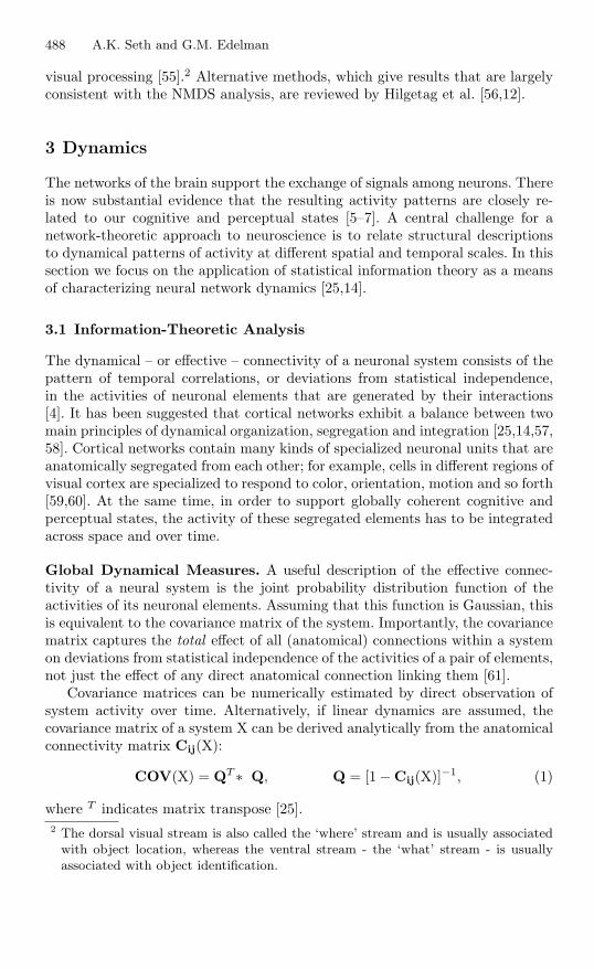
Global Dynamical Measures. A useful description of the effective connec-tivity of a neural system is the joint probability distribution function of theactivities of its neuronal elements. Assuming that this function is Gaussian, thisis equivalent to the covariance matrix of the system. Importantly, the covariancematrix captures the total effect of all (anatomical) connections within a systemon deviations from statistical independence of the activities of a pair of elements,not just the effect of any direct anatomical connection linking them [61].

Covariance matrices can be numerically estimated by direct observation ofsystem activity over time. Alternatively, if linear dynamics are assumed, thecovariance matrix of a system X can be derived analytically from the anatomicalconnectivity matrix Cij(X):

COV(X) = QT ∗ Q, Q = [1−Cij(X)]−1, (1)

where T indicates matrix transpose [25].2 The dorsal visual stream is also called the ‘where’ stream and is usually associated

with object location, whereas the ventral stream - the ‘what’ stream - is usuallyassociated with object identification.


Once the covariance matrix is obtained, a number of global dynamical mea-sures can be calculated. Three such measures, which are based on the founda-tions of statistical information theory, are entropy H(X), ‘integration’ I(X) and‘neural complexity’ Cn(X) [25,14].

For a system X, the entropy H(X) measures the system’s overall degree ofstatistical independence. Assuming stationarity, H(X) can be calculated usingthe standard formula

H(X) = 0.5ln((2πe)N |COV(X)|), (2)

where COV(X) is the N x N covariance matrix of X, and |.| denotes the matrixdeterminant [25,62].

The integration I(X) measures the system’s overall deviation from statisticalindependence. All elements in a highly integrated neural system are tightly cou-pled in their activity. With xi denoting the i’th element, I(X) can be calculatedusing

I(X) =N∑

i=1

H(xi)−H(X). (3)

Perhaps the most interesting global dynamical measure is neural complex-ity Cn(X), which measures the extent to which a system balances dynamicalsegregation and dynamical integration [25]. The component parts of a neurallycomplex system are differentiated; however, as larger and larger subsets of ele-ments are considered they become increasingly integrated (see Fig. 1). The term‘complexity’ may be considered appropriate for such systems since they are in-termediate between the two relatively simple extremes of disorder (maximalstatistical independence) and order (maximal statistical dependence).

The neural complexity Cn(X) of a system X is calculated by summing the av-erage Mutual Information (MI) between subsets of different sizes, for all possiblebipartitions of the system:

Cn(X) =nt/2∑

k=1

〈MI(Xkj ; X−Xk

j )〉, (4)

where nt is the total number of ways of bipartitioning X, Xkj is the j’th bipartition

of size k, and 〈.〉 is the average across index j. The MI between two subsets (Aand B) measures the uncertainty about A that is accounted for by the state ofB, and is defined as MI(A; B) = H(A) +H(B)−H(AB) [63] (see Fig. 1).

Another, closely related measure of complexity expresses the portion of en-tropy that is accounted for by interactions among all the elements of a sys-tem [58]:

C(X) = H(X)−N∑

k=1

H(xi|X− xi). (5)


S=1 S=N/2S=2

Fig. 1. Neural complexity is defined as the ensemble average MI between subsets of agiven size and their complement, summed over all subset sizes (adapted from Fig. 2 in[64]). Small circles represent neuronal elements and bold arrows indicate MI betweensubsets and the remainder of the system. Shown in the figure are a selection of subsets ofsize 1 (S=1), size 2 (S=2), and size N/2 for system size N (S=N/2). A neurally complexsystem is one in which small subsets of the system show high statistical independence,but large subsets show low statistical independence.

This measure takes on high values if single elements are highly informative aboutthe system to which they belong, without being overly alike. It has the advantageof being easier to compute than the first formulation Cn(X), and all resultsdescribed in this chapter use this formulation.

Dynamical Cluster Analysis. In Sect. 2.3 we described how statistical tech-niques such as NMDS could be used to identify clusters of highly interconnectednodes from high dimensional connectivity data. Cluster analysis can also per-formed at the level of network dynamics, where a dynamical cluster correspondsto a strongly interactive subset of elements. Note that dynamically identifiedclusters need not correspond to structurally identified clusters, although in manycases they may do so.

A dynamical cluster is characterized by a high level of statistical dependenceamong its elements and, at the same time, a low level of statistical dependencewith elements outside the cluster. Clusters can be identified by calculating thecluster index Cl(Xi

k), which is defined as follows [65]:

Cl(Xik) = I(Xi

k)/MI((Xik); X− (Xi

k)), (6)


where Xik denotes the i’th subset of size k, I(Xi

k) indicates its integration, andMI((Xi

k); X−(Xik)) denotes its mutual information with the rest of the system.

Note that Tononi et al. [65] describe this cluster index as a measure of func-tional clustering rather than dynamical clustering. However, as we remarkedin the introduction, function here refers to the role of a particular pattern ofdynamics in the context of the behavior of the organism.

Graph Selection. To explore the relationship between network structure andnetwork dynamics, Sporns et al. [14] applied an evolutionary search procedure tolook for distinct anatomical motifs associated with different measures of effectiveconnectivity. This procedure uses a global dynamical measure as a fitness (orcost) function, and it is implemented as follows. First, an initial population of Urandom graphs is created, each with N nodes and K edges with fixed identicalpositive weights wij . The ‘fitness’ of each graph is then assessed by deriving thecorresponding covariance matrix and calculating the global dynamical measure,eitherH(X), I(X) or C(X). After all members of U have been assessed, the graphwith highest fitness is selected and all others are discarded. The selected graphis then replicated U − 1 times to create the next generation. Each replicationintroduces a small amount of variation by randomly rewiring r edges of theselected graph. After a sufficient number of generations (these authors typicallyused 3,000 generations, a population size U = 10 and a rewiring rate r = 1) themembers of U should have near-optimal structures for generating the particulardynamical measure used as the selection criterion.3

Sporns et al. selected separately for graphs with high entropy H(X), highintegration I(X), and high neural complexity C(X). In each case they foundthat the resulting graphs (N = 32,K = 256) had distinctive structural features,as revealed both by simple visual inspection and by analysis using the graph-theoretic measures described in Sect. 2.1. Graphs optimized for high entropycontained mostly reciprocal connections without any apparent local clustering;they had high frecip, low fclust, as well as a short diameter (diamG) and a shortcharacteristic path length (lpath). Graphs optimized for integration, by contrast,were highly clustered (high fclust), had low values for frecip, large diameters andlarge characteristic path lengths. Visual inspection of these graphs revealed avery large central cluster loosely connected to an outlying mesh of nodes. Graphsoptimized for neural complexity were the most similar to the ‘small-world’ classof networks. These graphs usually are comprised of a number of dense groups ofnodes linked by a relatively small number of reciprocal bridges; they had highvalues for frecip and fclust, as well as low values for lpath and diamG.

3 Sporns et al. [14] applied three neurobiologically motivated constraints during graphselection. First, the number of incoming edges to each node was kept constant (8).Second, all graphs were required to be ‘strongly connected’ such that at least onepath exists between all pairs {i, j} of nodes. Third, small self-inhibitory weights wii

were applied to each graph such that the total variance – given by the sum of thediagonal terms in COV(X) – remained constant.


3.2 Dynamical Properties of Cortical Networks

To relate these theoretical observations to empirical data, Sporns et al. [14] an-alyzed the complexity of the connection matrices of the macaque visual cortexand the cat cortex. They assumed linear dynamics, equal connection strengths,and used equation (1) to derive covariance matrices corresponding to the respec-tive connection matrices. They found that both connection matrices gave rise toeffective connectivity with high neural complexity C(X) as compared to randomnetworks with equivalent N and K. Indeed, the matrices seemed to be near-optimal for generating highly complex dynamics. Random rewiring of edges, invirtually all cases, led to a reduction in the complexity of the correspondingeffective connectivity.

To identify the sets of anatomical areas responsible for these complex dy-namics, these authors applied dynamical cluster analysis (see Sect. 3.1) to themacaque visual cortex connection matrix. This analysis revealed an hierarchi-cal organization which separated into two distinct streams corresponding to the‘dorsal’ and ‘ventral’ visual processing streams [55], together with a small subsetof areas which were strongly interactive with both streams (these authors suggestthat these areas are strong candidates for mediating inter-stream interactions).Overall, this dynamical analysis was highly consistent with the structural clusteranalyses of Young et al. [54] and Hilgetag et al. [56].

Another application of dynamical cluster analysis compared PET4 data ob-tained from normal and schizophrenic subjects performing a set of cognitivetasks [65]. This study found significant differences in cluster profiles betweenthese two groups, despite the absence of differences in overall levels of activity.Future application of this analysis using imaging methods with higher temporalresolution (for example magnetoencephalography, see [67]) may be extremelyrevealing.

3.3 Matching Complexity and Degeneracy

While entropy, integration and neural complexity provide measures of the intrin-sic dynamics of a neural system, it is also of interest to characterize the dynamicsof neural systems as they interact with a surrounding environment. Measures of‘matching complexity’ [68] and ‘degeneracy’ [69,70] fulfil this role respectivelyfor systems connected to an input or to an output.

The matching complexity between system X and input S is defined as thetotal complexity when the input is present C(X)T minus the intrinsic complexityC(X)I and the complexity C(X)S that is directly attributable to the input S [68]:

M(X;S) = C(X)T − C(X)I − C(X)S . (7)

A high level of matching complexity indicates that there is strong match betweenthe statistical structure of the system and that of the input. A low value indicatesstatistical ‘novelty’.4 Positron Emission Tomography: A brain imaging technique based on measurement

of metabolic activity [66].


Degeneracy refers to the ability of elements (or sets of elements) that arestructurally different to perform the same function or yield the same output [69,70]. Degeneracy can be expressed as the mutual information between the varioussubsets of a system and the system’s output [69]:

D(X;O) = MIP (X, O)−∑

MIP (xi;O|X− xi;O), (8)

where MIP (xi;O|X − xi;O) refers to the conditional mutual information be-tween each element and O, given the mutual information between the rest of thesystem and O. Degeneracy is high for systems in which many different elementsaffect the output in a similar ways but at the same time can have independenteffects. This property contributes to the robustness of a system [70].

Sporns et al. [14] extended their graph selection method (see Sect. 3.1) toselect for graphs that exhibited high matching complexity with respect to aninput, and, separately, high degeneracy with respect to an output. In the formercase, a subset of 8 nodes was connected to an 8-node sensory sheet S that had aparticular input pattern described by a covariance matrix COVs. In the lattercase, a subset of nodes was chosen as a representation of output, and selectionwas carried out based on the global measure of degeneracy with respect to aparticular output pattern.

In all cases, selection for matching or degeneracy resulted in graphs with highneural complexity C(X) [14]. This suggests that high C(X) may reflect not onlyan intrinsic balance between dynamical integration and segregation, but mayalso correspond to the ability of a network rapidly to distribute input signalsand robustly generate output signals.

4 Function

As we remarked in the introduction, the most general function of a biologicalneural network is to generate adaptive behavior for the organism within its en-vironment [71]. The analysis of graphs with high degeneracy and high matchingcomplexity begins to address this issue of function. However, in the studies de-scribed above, there is no behavior as such: networks are coupled either to astatic input or a static output, and there is no sense in which the output at agiven time affects the input at a subsequent time.

In this section, we tackle these concerns by describing a relatively simplemodel of target fixation by a simulated head/eye system that is controlled by anartificial neural network. This model explicitly involves behavior, and its analy-sis provides support for the hypothesis that complex neural dynamics facilitateadaptation to rich sensory environments and motor demands [14]. An extendedanalysis of this model is given in Seth & Edelman [26].

As in the studies described above, the present model makes use of the tech-nique of evolutionary graph selection. However, instead of using a global dy-namical measure as a fitness function, in this case the fitness of a network is


G

H

T

Fig. 2. Simulation model of target fixation, depicting projections onto a plane (100u x100u, where u denotes an arbitrary spatial unit), of head direction H and gaze directionG. Also shown are target position T, and maximum offset of G from H (circle, radius35u). The position of G is calculated as a vector sum of H and an eye direction (E, notshown).

determined by its ability to support adaptive behavior when employed as a con-trol mechanism for a simulated head/eye system engaged in a target fixationtask. To explore how network structure, dynamics, and function interact, weselect networks for their target fixation ability in a variety of conditions thatdiffer in the (qualitative) complexity of the environment and the phenotype (thehead/eye system). Networks which evolved in different conditions are then an-alyzed in terms of their behavioral properties, their structural properties, andtheir dynamical properties.

4.1 Methods

Model Outline. This section describes basic properties of the model; specificsare provided in Appendix A. The simulated environment is a simple planar area,100x100 arbitrary units u, within which a target (T) can appear. The simulatedhead/eye system, or phenotype, is represented by the projection onto the planeof a head direction (H) and a gaze direction (G), which is the combination ofthe head direction (H) and an eye direction (E) relative to the head (Fig. 2).

The velocities of H and E in the x, y plane, and thus the position of G, arecontrolled by a neural network (N = 32, K = 256). The edges of this networkhave real-valued weights, and certain nodes are specified as sensory inputs andothers as motor outputs (see below). The remainder are ‘interneurons’ mediatingthe transformation of input signals into output signals. Evolutionary algorithmsare used to specify the connectivity and weight distribution of networks so thatthey give rise to adaptive behavior, which in this case consists of maximizingthe time for which G and T are aligned (i.e. keeping the target fixated) whilesimultaneously minimizing the offset between H and G (i.e. keeping the head


Table 1. Phenotype parameters in the four conditions (ES , ET , EH , and EC).VmaxH , VmaxE : maximum velocity of head and eye, AH , AE : motor gain of head andeye, mH , mE : momentum of head and eye, lag: the time-lag between head motor nodeoutput and head movement.

Condition VmaxH VmaxE AH AE mH mE lag

ES 7.0 7.0 1.0 1.0 0.0 0.0 0ET 7.0 7.0 1.0 1.0 0.0 0.0 0EH 5.0 10.0 0.33 1.0 0.75 0.05 10EC 5.0 10.0 0.33 1.0 0.75 0.05 10

and eye aligned). A constraint on the system is that G must remain within 35uof H, as indicated by the circle in Fig. 2.

Environment/Phenotype Conditions. We specify four conditions which aredistinguished by properties of the target and the head/eye phenotype. The phe-notype is defined by seven parameters: VmaxE specifies the maximum velocityof H, VmaxH specifies the maximum velocity of E with respect to H; motor gainparameters AH and AE specify scaling factors relating motor node output to Hand E velocity; momentum parameters mH and mE specify the inertial resis-tance of H and E, and lag specifies a time-lag between head motor node outputand head movement. These parameters constrain the movements of H, E and Gas described in Appendix A (which also describes how T is updated).

The values taken by the parameters in the four conditions are shown inTable 1. In condition ES (for ‘simple’) both the head and eye have the samemaximum velocity, identical motor gains, and zero momentum; the target is sta-tionary. Condition ET (for ‘tracking’) presents a more complex environment inwhich the target may occasionally jump to a different random location and/ordrift at a slow speed in a random direction; the phenotype is the same in condi-tion ES . Condition EH (for ‘head’) keeps the simple environment of conditionES but introduces a more complex phenotype in which E can move twice as fastas H, has a higher motor gain, a much lower momentum, and in which there is anon-zero time-lag. Finally, condition EC (for ‘complex’) combines the propertiesof both conditions ET and EH and is therefore the richest of the four.

Network Implementation. Each behavioral trial begins with the head and eyealigned and pointing to the center of the plane. The target position is initializedat a randomly selected location within 20u of this point. All trials last for 600time steps, each of which involves updating the state of the network controller(X) as well as the positions of E, G, H, and, in conditions ET and EC only, T.The network is updated using, for all nodes j,

sj(t) = f

(sin(j, t) +

K∑

i=1

Cij(X)si(t− 1)

), sj(0) = 0.0, (9)


where sj(t) is the output of node j at time t, sin(j, t) denotes the sensory inputto node j at time t (if any), f is a sigmoid function with input range ±10.0 andoutput range ±1.0, and Cij(X) is the connection matrix of X.

Six nodes are specified as ‘sensory’ inputs, two responding to the x, y dis-placement of G from T (with a maximum range of ±50.0u), and four delivering‘proprioceptive’ information, two of which reflect the displacement of H from thecenter of the plane (range ±50.0u), and two of which reflect the displacementof G from H (range ±35.0u). In all cases, input values are linearly scaled to therange ±1.0. Four nodes are specified as output nodes, two influencing H velocityin the x, y plane, and two influencing the velocity of E. Appendix A describeshow the activities of these nodes, along with the values in Table 1, are used toupdate the positions of E, G, and H.

Network Structure. Evolutionary algorithms (EAs) were used to specify theconnectivity and weight distribution of networks so that they supported targetfixation behavior.5 We ran a total of 40 separate EAs: 10 replications of theselection process for each of the four environment/phenotype conditions.

Each EA evolved a population of 64 networks over 2000 generations, witheach network initialized (generation 0) by randomly allocating K connections(each connection strength assigned randomly in the range ±1.0), subject tothe constraint that each node had 8 incoming connections. Each generation in-volved evaluating the fitness of each network, as described below, and then usingstochastic rank-based selection to replace low-fitness networks with mutated ver-sions of high-fitness networks. Each mutation of a network involved randomlyrewiring 1 connection (preserving in-degree) and also modifying the strength ofeach connection (probability 0.05 per connection) in the range ±0.1.

The fitness of a network was calculated as the mean of four separate behav-ioral trials, with the fitness of each trial (φ) given by

φ =tfttot

+ c0(1.0− c1d), (10)

where tf denotes the number of time steps for which the target was fixated(within a tolerance of 3u), ttot the total number of time steps in the trial (600),and d the mean offset for the trial between H and G. The constants c0 and c1were selected in order to balance the fitness contributions due to target fixationand those due to minimizing the offset between H and G (c0 = 1

4 , c1 = 135 ).

5 We used a distributed evolutionary algorithm [72]: Each EA was initialized by ar-ranging the population on an 8x8 toroidal grid and evaluating the fitness of eachnetwork. Each subsequent generation involved 64 repeats of the following: A randomgrid position was chosen determining a 3x3 sub-grid. Stochastic rank-based selec-tion was then used to select a weak member of this sub-grid for replacement, anda strong member as the ‘parent’. A mutated copy of the parent then replaced theweak member and was evaluated (the parent was also re-evaluated with probability0.75).


Table 2. Summary of target fixation performance. Shown are mean percentage of eachbehavioral trial for which T was fixated (within a tolerance of 3u), and mean displace-ment of G from H, for each network type. Average values were calculated from 10behavioral trials of each evolved network in the corresponding environment/phenotypecondition. Standard errors are given in parentheses.

Network type fixation % |G-H| (u)S-network 98.81 (0.01) 0.28 (0.07)T-network 92.43 (0.51) 0.92 (0.08)H-network 96.15 (0.79) 1.94 (0.19)C-network 84.76 (1.23) 15.41 (0.50)

4.2 Results

For convenience, networks which evolved in condition ES will be referred to asS-networks, with the same nomenclature for conditions ET (T-networks), EH(H-networks) and EC (C-networks).

Behavioral Analysis. The target fixation behavior of evolved networks wasassessed by measuring the percentage of each behavioral trial for which the targetwas fixated (i.e. the fraction of time steps for which the displacement betweenH and G was less than 3u). Table 2 shows that average fixation performancewas very high for S-networks, T-networks, and H-networks, and slightly lowerfor C-networks.

Figure 3 shows representative examples of successful fixation behavior forS-networks and C-networks in the corresponding conditions (ES and EC respec-tively). Inspection of the trajectories of the head and the eye indicates that thebehavioral dynamics for C-networks were qualitatively more complex than forS-networks. A non-trivial coordination of head and eye is needed in EC con-ditions in order to maintain consistent fixation of the target. Table 2 affirms

ss

5u

cc

25u

Fig. 3. Typical successful fixation behavior for S-networks in condition ES (left) andfor C-networks in condition EC (right), showing trajectories of G (solid line), H (dottedline) and T (dashed line, EC only), gray circle indicates initial positions of G and H,gray arrows indicate initial positions of T. Successful target tracking by C-networks isindicated by the overlap of the trajectories of G and T.


S C0

2

4

6

8

10

12

mea

n T

-G

*

5u 7u

(a) Robustness to perturbation (b) S-network (c) C-network

Fig. 4. Robustness of S-networks and C-networks to a novel perturbation: (a) Meandisplacement of G from T during enforced H movement, calculated over the 20 timesteps of enforced movement and the 10 time steps following for 10 S-networks and 10C-networks. Asterisk indicates statistical significance (p < 0.001, two-tailed t test).(b,c) trajectories generated by a typical (b) S-network and (c) C-network during thisoperation (solid line G, dotted line H, gray circles indicates initial positions of G andH, gray arrows indicate positions of T). For the S-network, fixation is lost (both H andG are displaced from the target), whereas for the C-network, fixation is maintained (Gremains close to the target even though H is displaced).

that the average displacements between H and G were considerably larger in forC-networks than for all other network types, while target fixation was achievedreliably in all cases.

To better compare the behavioral properties of S-networks and C-networks,they were reevaluated in a novel condition involving unexpected perturbations.As in condition ES , the environment was initialized with a stationary target T.An evolved S-network or C-network was then introduced and allowed to fixate.After 100 time steps, a head velocity (Vhx, Vhy) of between 1.0 and 3.0 (u pertime step) was induced for 20 time steps in a random direction. Importantly,neither network type had been selected to respond adaptively to this pertur-bation. Nevertheless, Fig. 4 illustrates that C-networks were generally able tomaintain fixation, whereas S-networks were not. These results show that net-work optimization in a rich environmental/phenotypic context can facilitate theemergence of robust behavior.

Structural Analysis. To assay reliable structural differences between networktypes, connectivity matrices were transformed into binary adjacency matricesAij(X) by replacing all non-zero elements in Cij(X) with the value 1 (we alsotried various thresholds, see below). We calculated four graph-theoretic quanti-ties from each Aij(X): frecip, diamG, lpath, and fclust (see Sect. 2.1).

Table 3 shows the results of applying these metrics to the fittest networksfrom each EA in each condition. Values were also calculated for an additional64 random networks (R-networks) with equivalent N and K (and a per-node in-degree of 8). The table indicates that there are no significant differences betweennetwork types (including random) in any of the metrics.


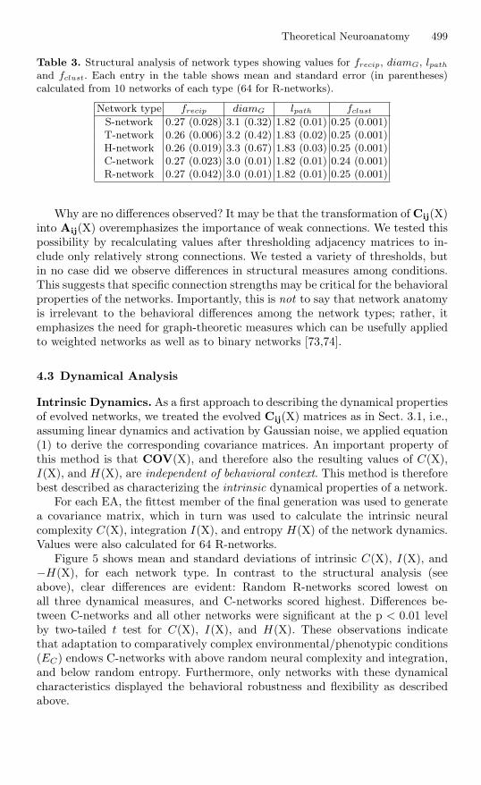
Table 3. Structural analysis of network types showing values for frecip, diamG, lpath

and fclust. Each entry in the table shows mean and standard error (in parentheses)calculated from 10 networks of each type (64 for R-networks).

Network type frecip diamG lpath fclust

S-network 0.27 (0.028) 3.1 (0.32) 1.82 (0.01) 0.25 (0.001)T-network 0.26 (0.006) 3.2 (0.42) 1.83 (0.02) 0.25 (0.001)H-network 0.26 (0.019) 3.3 (0.67) 1.83 (0.03) 0.25 (0.001)C-network 0.27 (0.023) 3.0 (0.01) 1.82 (0.01) 0.24 (0.001)R-network 0.27 (0.042) 3.0 (0.01) 1.82 (0.01) 0.25 (0.001)

Why are no differences observed? It may be that the transformation of Cij(X)into Aij(X) overemphasizes the importance of weak connections. We tested thispossibility by recalculating values after thresholding adjacency matrices to in-clude only relatively strong connections. We tested a variety of thresholds, butin no case did we observe differences in structural measures among conditions.This suggests that specific connection strengths may be critical for the behavioralproperties of the networks. Importantly, this is not to say that network anatomyis irrelevant to the behavioral differences among the network types; rather, itemphasizes the need for graph-theoretic measures which can be usefully appliedto weighted networks as well as to binary networks [73,74].

4.3 Dynamical Analysis

Intrinsic Dynamics. As a first approach to describing the dynamical propertiesof evolved networks, we treated the evolved Cij(X) matrices as in Sect. 3.1, i.e.,assuming linear dynamics and activation by Gaussian noise, we applied equation(1) to derive the corresponding covariance matrices. An important property ofthis method is that COV(X), and therefore also the resulting values of C(X),I(X), and H(X), are independent of behavioral context. This method is thereforebest described as characterizing the intrinsic dynamical properties of a network.

For each EA, the fittest member of the final generation was used to generatea covariance matrix, which in turn was used to calculate the intrinsic neuralcomplexity C(X), integration I(X), and entropy H(X) of the network dynamics.Values were also calculated for 64 R-networks.

Figure 5 shows mean and standard deviations of intrinsic C(X), I(X), and−H(X), for each network type. In contrast to the structural analysis (seeabove), clear differences are evident: Random R-networks scored lowest onall three dynamical measures, and C-networks scored highest. Differences be-tween C-networks and all other networks were significant at the p < 0.01 levelby two-tailed t test for C(X), I(X), and H(X). These observations indicatethat adaptation to comparatively complex environmental/phenotypic conditions(EC) endows C-networks with above random neural complexity and integration,and below random entropy. Furthermore, only networks with these dynamicalcharacteristics displayed the behavioral robustness and flexibility as describedabove.


S T H C R0.02

0.03

0.04C(X)

*

S T H C R0.5

0.75

1

1.25

I(X)

*

S T H C R22

22.4

22.8

23.2

−H(X)

*

Fig. 5. Mean and standard error intrinsic C(X), I(X), and −H(X) for S-networks(S), T-networks (T), H-networks (H), C-networks (C), and R-networks (R). Asterisksindicate that the value for C-networks is significantly higher than for all other networktypes (p < 0.01, two-tailed t tests). Values of C(X), I(X) and −H(X) for S-networks,T-networks, and H-networks are significantly lower than the corresponding values forC-networks, and significantly higher than the corresponding values for R-networks (p <0.01, two-tailed t tests). There are no significant differences in C(X), I(X) or −H(X)among S-networks, T-networks, and H-networks. All distributions are normal (p <0.05, Bera-Jarques test).

Figure 5 also shows that S-networks, H-networks, and T-networks scored atintermediate levels on all measures. Values of C(X), I(X) and −H(X) for thesenetworks are significantly lower than the corresponding values for C-networks,and significantly higher than the corresponding values for R-networks (p < 0.01,two-tailed t tests); there are no significant differences in C(X), I(X) or −H(X)among S-networks, T-networks, and H-networks. Changes in intrinsic dynamics,therefore, depend both on properties of the environment (condition ET ) and onproperties of the phenotype (condition EH).

While these results show that neurally complex network dynamics can accom-pany adaptive behavior in rich environmental/phenotypic conditions, intrinsicneural complexity is not unique in this respect, since similar patterns of resultsare apparent for both intrinsic integration I(X) and entropy H(X).

Interactive Dynamics. An alternative approach to characterizing network dy-namics is to derive covariance matrices directly from recordings of node activitiesduring behavior, i.e. while the network is actively transforming input signals intooutput signals. We define the resulting dynamics as ‘interactive’ since they arerelative to a particular behavior, environment, and phenotype. One importantproperty of interactive dynamics, as compared to intrinsic dynamics, is thatthey enable comparison of dynamics generated by the same network in differentbehavioral regimes or in different environments/phenotypes.

Each behavioral trial yields a (N x 600) matrix F which contains the indi-vidual activity records of each node for all 600 time steps. This matrix can beused to generate a covariance matrix according to:


RC

35u

RS

15u

SC

25u

CS

7u

Fig. 6. Representative behavior for various network-environment/phenotype combina-tions, showing trajectories of G (solid line), H (dotted line) and T (dashed line), graycircles indicate initial positions of G and H, gray arrows indicate initial positions ofT. RC: R-network in condition EC , RS: R-network in condition ES , SC: S-network incondition EC , CS: C-network in condition ES . Trajectories of a C-network in conditionEC and an S-network in condition ES are shown in Fig. 3.

COV(X) = cov(F), (11)

where F is the first derivative (with respect to time) of the activity matrix andcov() is a standard covariance function. This approach was chosen because ratesof change of node activities are more likely to reflect interactions between thenetwork and its phenotype and environment, than are absolute activity levels.COV(X) can then be used to calculate corresponding values of interactive C(X),I(X) and H(X) in just the same way as for the calculation of intrinsic dynamics.Note that calculation of interactive dynamics does not require equation (1) andso does not assume linear system dynamics.

We compared interactive dynamics for C-networks, S-networks, and randomR-networks evaluated in both EC and ES conditions, recording both networkactivities and behavioral trajectories. Figure 6 shows representative trajectoriesfrom the various combinations (trajectories of a C-network in condition ECand an S-network in condition ES are shown in Fig. 3). R-networks in EC andES conditions never achieve fixation, and their behavior is highly variable. S-networks in EC conditions are unable to achieve or maintain fixation despite ageneral tendency to track towards the target, and C-networks in ES conditionsrapidly achieve fixation despite some persistent oscillation in the head direction.Notice that in all except the last of these cases, the behavioral dynamics arerich, even though the behavior itself is not adaptive.


CC SC CS SS RS RC

0.4

0.5

0.6

0.7

0.8

C(X

)

*

CC SC CS SS RS RC20

25

30

35

40

I(X

)

CC SC CS SS RS RC0

20

40

60

-H(X

)

***

*

Fig. 7. Interactive C(X), I(X), and −H(X) calculated from covariance matrices derivedfrom recorded neural activity during behavior. CC: C-network in condition EC , SC:S-network in condition EC , CS: C-network in condition ES , SS: S-network in conditionES , RS: R-network in condition ES , RC: R-network in condition EC . Each columnshows mean and standard error calculated from 10 repetitions of each combination ofnetwork and condition. There is a significant correlation between the rank ordering ofcombination (from ‘CC’ to ‘RC’) and mean C(X) (r = 0.97, p < 0.01; Spearman’s rankcorrelation). No significant correlations exist for I(X) or −H(X) (p > 0.1). Asterisksindicate statistically significant differences between combinations ((*) p < 0.01, (**)p < 0.05, two-tailed t tests; only adjacent combinations were tested). All distributionsare normal (p < 0.05, Bera-Jarques test).

Figure 7 shows the interactive dynamics generated in each combination ofnetwork and condition. The top row shows a clear gradient in interactive C(X)proceeding from C-networks in condition EC (‘CC’; high), to R-networks inconditions ES and EC (‘RS’, ‘RC’; low). Intermediate values of C(X) were ob-served for simple networks in rich environmental/phenotypic conditions (‘SC’),and for complex networks in simple conditions (‘CS’). C-networks in conditionEC (‘CC’) have significantly higher C(X) than all other combinations. The re-maining significant differences among combinations are also consistent with thesteady gradient in interactive C(X).

Strikingly, only C(X) shows a pattern of values reflecting rich adaptive be-havior. Neither I(X) (Fig. 7, middle row) nor H(X) (bottom row) show any


such sensitivity. This is in contrast to the intrinsic analysis, in which all threedynamical measures behaved in a similar way (Fig. 5).

It is also notable that R-networks evoke low interactive C(X) despite dis-playing the rich behavioral patterns shown in Fig. 6. The contrast between R-networks and C-networks, together with the steady gradient in interactive C(X)across combinations (Fig. 7, top row), suggests that C(X) is indeed selectivelysensitive to the dynamics of rich adaptive behavior. Figure 7 also suggests thathigh interactive C(X) depends on a combination of environmental and pheno-typic properties. The intermediate values of C(X) in Fig. 7 (‘SC’ and ‘CS’) areconsistent with the intermediate values of intrinsic C(X) associated with richenvironments (condition ET ) and complex phenotypes (condition EH) shown inFig. 5.

4.4 Summary

In this model, evolutionary algorithms were used to generate neural networksable to support target fixation in environment/phenotype combinations of qual-itatively different levels of complexity. Not surprisingly for a selectional sys-tem, we found that those networks which evolved under rich environmen-tal/phenotypic conditions exhibited (qualitatively) more complex behavior thannetworks which evolved in comparatively simple conditions (Fig. 3). When com-pared in a condition involving a novel perturbation, networks which evolved inrich conditions showed greater robustness than networks which evolved in simpleconditions (Fig. 4).

This robustness was reflected by significantly higher neural complexity C(X)for networks in evolved in rich conditions, than for networks which evolved inrelatively simple conditions, or for equivalent random networks (figs. 5 and 7).This was true for both intrinsic and interactive methods of calculating dynam-ics, where the former are derived analytically from network connectivity, and thelatter are computed from observed network activity during behavior. However,while intrinsic dynamics did not differentiate between neural complexity C(X),integration I(X) or entropy H(X) (Fig. 5), interactive dynamics revealed thatonly C(X) consistently associated with adaptive behavior in rich environmen-tal/phenotypic conditions (Fig. 7).

Both types of dynamical analysis indicate that the magnitude of neural com-plexity depended on a combination of environmental, phenotypic, and mecha-nistic properties. Networks evolved in conditions of intermediate richness (ETand EH) generated intermediate values of intrinsic C(X) (Fig. 5). Networksevolved in rich environmental/phenotypic conditions, and tested in simple condi-tions, and vice-versa, generated intermediate values of interactive C(X) (Fig. 7).Taken together these results show that, in the present target fixation task, neuralcomplexity is selectively sensitive to the dynamics of adaptive behavior in richenvironmental and phenotypic conditions.


5 General Discussion

This chapter has surveyed a network-theoretic approach to neuroscience at thelevels of structure, dynamics and function. While the coverage has not beencomprehensive, we have described some key results and techniques that can beapplied not just to vertebrate cortical networks but to the analysis of complexnetwork systems of many different kinds. For example, the new results describedin the previous section show the importance of drawing a sharp distinction be-tween the dynamical patterns a network may support, and the functional appli-cations that these patterns may serve.

5.1 Structure

Structure provides the most basic level of analysis of cortical networks. Manyinteresting features are revealed by the application of graph-theoretic and sta-tistical analytical tools, most notably the presence of small-world characteristicsas well as the prevalence of reentrant connectivity [14].

However, current structural analysis has certain important limitations. De-tailed structural information is hard to obtain, especially at the microscopic levelof neuron-to-neuron connectivity, especially with regard to the human brain.Moreover, this fine structure is continually changing as a result of a host ofactivity-dependent plasticity processes. Also, most methods of structural analy-sis assume unweighted, binary networks (although see [73–75]) and also assumethat all nodes are essentially identical. Neither assumption is remotely satis-fied in the case of the brain, and it is certain that both neuronal diversity anddifferences among synaptic strengths are essential for normal brain function.

Nonetheless, the rapid development of novel graph-theoretic methods [41,18],together with the accelerating accumulation of detailed neuroscientific data sets[32,33], promises that future structural analyses will reveal further importantfeatures of the structural organization of neural systems.

5.2 Dynamics

Anatomical structure gives rise to neural dynamics. The tools of statistical in-formation theory are well suited to the analysis of these dynamics. It bearsemphasizing that the global dynamical measures described in this chapter applyequally well to dynamics generated by both binary and weighted networks; inthis sense, at least, dynamical analysis may be more generally applicable thanstructural analysis.

However, some assumptions have to be made in the application of thesemeasures. For example, the analytical derivation of a covariance matrix from aconnectivity matrix requires that linear dynamics be assumed. At least in somecases, linear and non-linear systems behave similarly with respect to effectiveconnectivity [58], and it has also been argued that large-scale dynamics of in-teracting brain areas are accurately represented by linear systems [76,77]. Also,


one may drop assumptions of linear dynamics by deriving covariances directlyfrom recorded activity (see Sect. 4.3).

Calculation of entropy from covariance further assumes that network activitycan be described as a stationary Gaussian process. This condition is by definitionsatisfied for calculation of intrinsic dynamics (see Sect. 3.1), but may not bestrictly satisfied in the calculation of interactive dynamics from network activityduring behavior. Indeed, it is a fact that many natural processes are not wellmodeled as stationary. Information-theoretic treatment of non-stationary signalshas been widely discussed [78,79,62], and as long as deviations from stationarityare not too extreme, such techniques remain well placed to provide insight intothe structure of dynamical interactions that a network produces.

More generally, the present methods are cross-sectional: Covariance matricesare derived from observations of network activity at successive time slices, so thatcorrelations over time exhibited in the activity profiles of single nodes are over-looked (by definition, the analytical calculation of intrinsic dynamics assumesthat there are no such correlations). A contrasting approach, which focuses onthese correlations, is provided by a growing literature concerned with measur-ing the information content of single spike trains [21–24]. Integrating these twoapproaches stands out as an important challenge for theoretical neuroscience.

Notably absent from this chapter has been any mention of neural synchrony.Some of the most obvious features of human brain dynamics are the promi-nent oscillations in different frequency bands known as the delta (3-5Hz), alpha(8-13Hz), beta (10-20Hz) and gamma (35-80Hz) rhythms. Different functionalroles have been proposed (but not proven) for these rhythms; for example, deltaoscillations have been associated with the maintenance of items in short-termmemory [80], and alpha oscillations are strongest during sleep and relaxed wake-fulness [81], and may represent an ‘idling state’ of the brain.

Gamma oscillations have a controversial interpretation: it has been suggestedthat gamma oscillations serve to ‘bind’ together disparate neural processes intoglobally integrated activity patterns [45,82,83]. In support of this idea, detailedcomputer simulations of visual cortical areas have shown that reentrant inter-actions can synchronize the activity of anatomically segregated neural areas,leading to coherent perceptual performance and behavior in visually complex en-vironments [44,47]. Computer simulations have also suggested that small-worldarchitectures may be particularly suitable for facilitating neural synchrony [84].

5.3 Function

Linking dynamic patterns to functional roles is perhaps the least visited of thetasks facing a science of networks. However, it is at least as important as under-standing structural and dynamical features by themselves. Many structural anddynamical features of brains have been selected by evolution precisely becauseof the adaptive functions they provide for the organism. Functional criteria canalso be described for networks of many other kinds, for example power grids(the transmission of power from source to consumer) and telephone networks(the maintenance of uninterrupted service for clients).


As for the brain, we remarked above that neural synchrony may play an es-sential role in binding disparate neural processes to a common purpose. Moregenerally, the results described in this chapter support the view that the brain isa selectional system [43], in which complex neural dynamics may facilitate adap-tation to rich sensory environments and motor demands by providing a specialkind of flexibility in the balance between dynamical integration and dynamicalsegregation. It has even been suggested that neurally complex dynamics in thethalamocortical system constitute the neural correlates of conscious states inhumans and other animals [64,46,85]. Further empirical research and theoreticalanalysis of the interactions between dynamics and function are therefore likelyto be valuable for neuroscience in the broader context of modeling the situatedorganism [86].

5.4 Summary

While important insights can be, and have been gained by analyses at the lev-els of structure, dynamics, and function separately, it must be recognized thatin biological systems these levels are in complex and continuous interaction.Structure is continually changing as a result of activity-dependent plasticityprocesses. These structural changes evoke dynamical changes which shape thebehavior of the organism, and behavior itself determines the correlations in thesensory signals that impinge on these networks, triggering further dynamicalchanges and structural alterations. Finding a language in which to articulatethese complex couplings is the major challenge for a network-theoretic approachto neuroscience. Success in this task will advance not just neuroscience, but alsoour understanding of many other network systems in which interactions amongstructure, dynamics, and function are important.

Acknowledgements

This research was supported by the Neurosciences Research Foundation. Spe-cial thanks to Bruno van Swinderen for Fig. 2, and to George Reeke and ouranonymous reviewers for helpful comments.Address correspondence to Anil K. Seth ([email protected]).

Appendix A: Implementation Details

Motor node outputs (shx, shy, sex, sey) are used to update E, H and G according to:

Vhx(t) = mHVhx(t − 1) + AH(1 − mh)shx(t − lag), (12)

Vhy(t) = mHVhy(t − 1) + AH(1 − mh)shy(t − lag), (13)

Vex(t) = mEVex(t − 1) + AE(1 − mE)sex(t), (14)

Vey(t) = mEVey(t − 1) + AE(1 − mE)sey(t), (15)

where Vhx(t), Vhy(t) represent the velocity of H in the x, y directions respectively attime t, and Vex(t), Vey(t) represent the velocity of E. In all cases, V (t) is bounded by


the corresponding value of Vmax. These values, as well as those of AH , AE , mH , mE ,and lag, are specified for each condition in the text. The positions of E, H and G inthe x, y plane are then updated using:

H(t) = H(t − 1) + Vhx(t) + Vhy(t), (16)

E(t) = E(t − 1) + Vex(t) + Vey(t), (17)

G(t) = H(t) + E(t), (18)

where H(t) and G(t) represent the positions of H and G on the x, y plane at time t,and E(t) represents the position of the eye relative to H. If the distance between G andH exceeds 35.0u then G is not updated at that time step. In conditions EC and ET thetarget position (T) is also updated at each time step, alternating between 50 time stepsof drift and 50 time steps without drift. Each period of drift is in a random directionat a random speed in the range 0.5 to 1.5 (u per time step). During the interveningperiods T is stationary except for occasional jumps (with a probability of 0.025 pertime step), each to a randomly chosen location within a radius of 25u to 31u of itsprevious location. The target cannot leave the 1002u2 area: If drift is leading it out ofbounds the appropriate velocity component is reversed at the boundary.

References

1. G.M. Edelman. The remembered present. Basic Books, Inc., New York, NY, 1989.2. A. Clark. Being there: Putting brain, body, and world together again. MIT Press,

Cambridge, MA, 1997.3. D. Buonomano and M. Merzenich. Cortical plasticity: From synapses to maps.

Annual Review of Neuroscience, 21:149–186, 1998.4. K. Friston. Functional and effective connectivity in neuroimaging: A synthesis.

Human Brain Mapping, 2:56–78, 1994.5. S.L. Bressler. Large-scale cortical networks and cognition. Brain Research Reviews,

20:288–304, 1995.6. R.S.J. Frackowiak, K.J. Friston, C.D. Frith, R.J. Dolan, and J.C. Mazziotta. Hu-

man brain function. Academic Press, San Diego, CA, 1997.7. F. Varela, J.-P Lachaux, E. Rodriguez, and J. Martiniere. The brainweb: Phase

synchronization and large-scale integration. Nature Reviews Neuroscience, 2:229–239, 2001.

8. R. Cummins. Functional analysis. Journal of Philosophy, 72:741–764, 1975.9. F. Harary. Graph theory. Addison-Wesley, Reading, MA, 1969.

10. B. Bollobas. Random graphs. Academic Press, London, 1985.11. B. Jouve, P. Rosentiehl, and M. Imbert. A mathematical approach to the connec-

tivity between the cortical visual areas of the macaque monkey. Cerebral Cortex,8:28–39, 1998.

12. C.C. Hilgetag, R. Kotter, K.E. Stephan, and O. Sporns. Computational methodsfor the analysis of brain connectivity. In G.A. Ascoli, editor, Computational neu-roanatomy: Principles and methods, pages 295–331. Humana Press, Totowa, NJ,2002.

13. O. Sporns. Graph theory methods for the analysis of neural connectivity patterns.In R. Kotter, editor, Neuroscience Databases. A Practical Guide, pages 169–183.Kluwer Publishers, Boston, MA, 2002.


14. O. Sporns, G. Tononi, and G.M. Edelman. Theoretical neuroanatomy: Relatinganatomical and functional connectivity in graphs and cortical connection matrices.Cerebral Cortex, 10:127–141, 2000.

15. R. Albert, H. Jeong, and A.-L. Barabasi. Diameter of the world wide web. Nature,401:130–131, 1999.

16. D.J. Watts and S.H. Strogatz. Collective dynamics of ‘small world’ networks.Nature, 393:440–442, 1998.

17. S.H. Strogatz. Exploring complex networks. Nature, 410:268–276, 2001.18. M.E.J. Newman. The structure and function of complex networks. SIAM Review,

45(2):167–256, 2003.19. G.Q. Bi and M.M. Poo. Synaptic modifications in cultured hippocampal neurons:

dependence on spike timing, synaptic strength, and postsynaptic cell type. Journalof Neuroscience, 18:10464–10472, 1998.

20. Y.X. Fu, K. Djupsund, H. Gao B. Hayden, K. Shen, and Y. Dan. Temporal speci-ficity in the cortical plasticity of visual space representation. Science, 296:1999–2003, 2002.

21. W. Bialek, I. Nemenman, and N. Tishby. Predictability, complexity, and learning.Neural Computation, 13:2409–2463, 2001.

22. M. Costa, A.L. Goldberger, and C.K. Peng. Multiscale entropy analysis of complexphysiological time series. Physical Review Letters, 89:681–682, 2002.

23. L. Paninski. Estimation of entropy and mutual information. Neural Computation,15:1191–1253, 2003.

24. G.N. Reeke and A.D. Coop. Estimating the temporal interval entropy of neuronaldischarge. Neural Computation, in press.

25. G. Tononi, O. Sporns, and G.M. Edelman. A measure for brain complexity: Re-lating functional segregation and integration in the nervous system. Proceedingsof the National Academy of Science (USA), 91:5033–5037, 1994.

26. A.K. Seth and G.M. Edelman. Environment and behavior influence the complexityof evolved neural networks. Adaptive Behavior, in press.

27. F. Crick and E. Jones. Backwardness of human neuroanatomy. Nature, 361:109–110, 1993.

28. D.J. Felleman and D.C. Van Essen. Distributed hierarchical processing in theprimate cerebral cortex. Cerebral Cortex, 1:1–47, 1991.

29. M.P. Young. The organization of neural systems in the primate cerebral cortex.Philosophical Transactions of the Royal Society of London: Series B, 252:13–18,1993.

30. J.W. Scannell, C. Blakemore, and M.P. Young. Analysis of connectivity in the catcerebral cortex. Journal of Neuroscience, 15, 1995.

31. J.W. Scannell, G.A.P.C. Burns, C.C. Hilgetag, M.A. O’Neil, and M.P. Young.The connectional organization of the cortico-thalamic system of the cat. CerebralCortex, 9:277–299, 1999.

32. R. Kotter. Neuroscience databases: Tools for exploring brain structure-functionrelationships. Philosophical Transactions of the Royal Society of London: SeriesB, 356:1111–1120, 2001.

33. K.E. Stephan, L. Kamper, A. Bokzurt, G.A.P.C. Burns, M.P. Young, andR. Kotter. Advances in database methodology for the collation of connectivitydata on the macaque brain (CoCoMac). Philosophical Transactions of the RoyalSociety of London: Series B, 356:1159–1186, 2001.

34. J.M.J. Murre and D.P.F. Sturdy. The connectivity of the brain: Multi-level quan-titative analysis. Biological Cybernetics, 73:529–545, 1995.


35. A. Nicoll and C. Blakemore. Patterns of local connectivity in the neocortex. NeuralComputation, 5:665–680, 1993.

36. C.C. Hilgetag. Mathematical approaches to the analysis of neural connectivity inthe mammalian brain. PhD thesis, Faculty of Medicine, University of Newcastleupon Tyne, 1999.

37. L. Lagae, D.K. Xiao, S. Raiquel, H. Maes, and G.A. Orban. Position invarianceof optic flow component selectivity differentiates monkey MST and FST cells fromMT cells. Invest. Ophthamol. Vis. Sci., 32:823, 1991.

38. J.J. Gibson. The ecological approach to visual perception. Houghton-Mifflin,Boston, 1979.

39. D.J. Watts. Small worlds. Princeton University Press, Princeton, NJ, 1999.40. P. Erdos and A. Renyi. On random graphs. Publicationes Mathematicae, 6:290–

297, 1959.41. R. Albert and A.-L. Barabasi. Statistical mechanics of complex networks. Reviews

of Modern Physics, 74:47–97, 2002.42. H. Jeong, B. Tombor, R. Albert, Z. Oltvai, and A.-L. Barabasi. The large-scale

organization of metabolic networks. Nature, 407:651–654, 2000.43. G.M. Edelman. Neural Darwinism. Basic Books, New York, 1987.44. G. Tononi, O. Sporns, and G.M. Edelman. Reentry and the problem of integrating

multiple cortical areas: Simulation of dynamic integration in the visual system.Cerebral Cortex, 2(4):31–35, 1992.

45. G.M. Edelman. Selection and reentrant signaling in higher brain function. Neuron,10:115–125, 1993.

46. G.M. Edelman and G. Tononi. A universe of consciousness: How matter becomesimagination. Basic Books, New York, 2000.

47. A.K. Seth, J.L. McKinstry, G.M. Edelman, and J.L. Krichmar. Visual bindingthrough reentrant connectivity and dynamic synchronization in a brain-based de-vice. Cerebral Cortex, in press.

48. G. Mitchison. Neuronal branching patterns and the economy of cortical wiring.Proceedings of the Royal Society of London: Series B. Biological Sciences., 245:151–158, 1991.

49. C. Cherniak. Component placement optimization in the brain. Journal of Neuro-science, 14:2418–2427, 1994.

50. C. Cherniak. Optimal-wiring models of neuroanatomy. In G.A. Ascoli, editor, Com-putational neuroanatomy: Principles and methods, pages 71–83. Humana Press,Totowa, NJ, 2002.

51. C. Cherniak, Z. Mokhtarzada, R. Rodriguez-Esteban, and K. Changizi. Globaloptimization of cerebral cortex layout. Proceedings of the National Academy ofSciences, USA, 101(4):1081–1086, 2004.

52. J.B. Kruskal. Nonmetric multidimensional scaling: A numerical method. Psy-chometrika, 29:115–129, 1964.

53. J.B. Kruskal. Multidimensional scaling by optimizing goodness of fit to a nonmetrichypothesis. Psychometrika, 29:1–27, 1964.

54. M.P. Young, J.W. Scannell, M.A. O’Neill, C.C. Hilgetag, G.A.P.C. Burns, andC. Blakemore. Non-metric multidimensional scaling in the analysis of neu-roanatomical connection data and the organization of the primate visual system.Philosophical Transactions of the Royal Society of London: Series B, 348:281–308,1995.

55. L.G. Ungerleider and J.V. Haxby. ‘what’ and ‘where’ in the human brain. CurrentOpinion in Neurobiology, 4:157–165, 1994.


56. C.C. Hilgetag, G.A.P.C. Burns, M.A. O’Neill, and M.P. Young. Cluster structureof cortical systems in mammalian brains. In J.M. Bower, editor, Computationalneuroscience, pages 41–46. Plenum Press, New York, 1998.

57. G. Tononi, G.M. Edelman, and O. Sporns. Complexity and coherency: Integratinginformation in the brain. Trends in Cognitive Science, 2:474–484, 1998.

58. O. Sporns and G. Tononi. Classes of network connectivity and dynamics. Com-plexity, 7(1):28–38, 2002.

59. S. Zeki. Functional specialization in the visual cortex of the Rhesus monkey. Na-ture, 274:423–428, 1978.

60. S. Zeki. A vision of the brain. Blackwell, Oxford, 1993.61. W. Vanduffel, B.R. Payne, S.G. Lomber, and G.A. Orban. Functional impact

of cerebral connections. Proceedings of the National Academy of Science (USA),94:7617–7620, 1997.

62. A. Papoulis and S.U. Pillai. Probability, random variables, and stochastic processes.McGraw-Hill, New York, NY, 2002. 4th edition.

63. D.S. Jones. Elemenary information theory. Clarendon Press, 1979.64. G. Tononi and G.M. Edelman. Consciousness and complexity. Science, 282:1846–

1851, 1998.65. G. Tononi, A.R. McIntosh, D.P. Russell, and G.M. Edelman. Functional clustering:

identifying strongly interactive brain regions in neuroimaging data. Neuroimage,7:133–149, 1998.

66. S.E. Petersen, P.T. Fox, M.I. Posner, M. Mintun, and M. Raichle. Positron emissiontomographic studies of the cortical anatomy of single-word processing. Nature,331:585–589, 1988.

67. R. Hari, S. Levanen, and T. Raij. Timing of human cortical functions duringcognition: role of MEG. Trends in Cognitive Science, 4(12):455–461, 2000.

68. G. Tononi, O. Sporns, and G.M. Edelman. A complexity measure for selectivematching of signals by the brain. Proceedings of the National Academy of Science(USA), 93:3422–3427, 1996.

69. G. Tononi, O. Sporns, and G.M. Edelman. Measures of degeneracy and redundancyin biological networks. Proceedings of the National Academy of Science (USA),96:3257–3262, 1999.

70. G.M. Edelman and J. Gally. Degeneracy and complexity in biological systems.Proceedings of the National Academy of Sciences, USA, 98(24):13763–13768, 2001.

71. A.K. Seth. On the relations between behaviour, mechanism, and environment:Explorations in artificial evolution. PhD thesis, University of Sussex, 2000.

72. M. Mitchell. An introduction to genetic algorithms. MIT Press, Cambridge, MA,1997.

73. V. Latora and M. Marchiori. Efficient behavior of small-world networks. PhysicalReview Letters, 87(19):198701–4, 2001.

74. C. Cannings and C. Penman. Random graphs. In C.R. Rao and D.N. Shanbhag, ed-itors, Stochastic processes: Modelling and simulation, Vol. 21. Handbook of Statis-tics series. Elsevier, 2002.

75. M. E. J. Newman Who is the best connected scientist? A study of scientificcoauthorship networks Physical Review E, 64:016131, 2001.

76. A.R. McIntosh and F. Gonzalez-Lima. Structural equation modeling and its ap-plication to network analysis in functional brain imaging. Human Brain Mapping,2:2–22, 1994.

77. A.R. McIntosh, C.L. Grady, L.G. Ungerleider, J.V. Haxby, S.I. Rapoport, andB. Horwitz. Network analysis of cortical visual pathways mapped with PET. Jour-nal of Neuroscience, 14:655–666, 1994.


78. M.S. Pinsker. Information and information stability of random variables and pro-cesses. Holden-Day, San Francisco, 1964.

79. R.M. Gray. Probability, random processes, and ergodic properties. Springer-Verlag,Berlin, 1988.

80. M. Doppelmayr, W. Klimesch, J. Schwaiger, and T. Winkler. Theta synchro-nization in human EEG and episodic retrieval. Neuroscience Letters, 257(1):41–4,1998.

81. J.L. Cantero, M. Atienza, and R.M. Salas. Human alpha oscillations in wakefulness,drowsiness period, and REM sleep: different electroencephalographic phenomenawithin the alpha band. Neurophysiol. Clin., 32(1):54–71, 2002.

82. W. Singer and C. Gray. Visual feature integration and the temporal correlationhypothesis. Annual Review of Neuroscience, 18:555–586, 1995.

83. C. Gray. The temporal correlation hypothesis: still alive and well. Neuron, 24:31–47, 1999.

84. L.F. Lago-Fernandez, R. Huerta, F. Corbacho, and J. Siguenza. Fast response andtemporal coherent oscillations in small-world networks. Physical Review Letters,84:2758–2761, 2000.

85. G.M. Edelman. Naturalizing consciousness: A theoretical framework. Proceedingsof the National Academy of Sciences, USA, 100(9):5520–5524, 2003.

86. J.L. Krichmar and G.M. Edelman. Machine psychology: Autonomous behavior,perceptual categorization and conditioning in a brain-based device. Cerebral Cor-tex, 12(8):818–30, 2002.

theoretical neuroanatomy - university of sussex

Documents