arX

iv:1

712.

0479

5v2

[qu

ant-

ph]

18

Dec

201

7

Quaternionic Wavefunction

Pavel A. Bolokhov

Theoretical Physics Department, St.Petersburg State University, Ulyanovskaya 1,

Peterhof, St.Petersburg, 198504, Russia

Abstract

We argue that quaternions form a natural language for the description of

quantum-mechanical wavefunctions with spin. We use the quaternionic spinor for-

malism which is in one-to-one correspondence with the usual spinor language. No

unphysical degrees of freedom are admitted, in contrast to the majority of literature

on quaternions. In this paper we first build a Dirac Lagrangian in the quater-

nionic form, derive the Dirac equation and take the non-relativistic limit to find the

Schrodinger’s equation. We show that the quaternionic formalism is a natural choice

to start with, while in the transition to the non-interacting non-relativistic limit

the quaternionic description effectively reduces to the regular complex wavefunction

language. We provide an easy to use grammar for switching between the ordinary

spinor language and the description in terms of quaternions. As an illustration of

the broader range of the formalism, we also derive the Maxwell’s equation from the

quaternionic Lagrangian of Quantum Electrodynamics. In order to derive the equa-

tions of motion, we develop the variational calculus appropriate for this formalism.

1 Introduction

The list of literature on the role of quaternions in physics is so vast that it is hardly

possible to enlist it [1]–[23]. The most of the literature touches base on the use

of quaternions in three-dimensional rotations and Lorentz transformations. Other

works include their applications in Electrodynamics and Quantum Mechanics. The

attractive feature of quaternions is that whenever a solution is possible in the quater-

nionic form, it is much more compact than that in the customary form of Lorentz

vectors and tensors.

For the majority of theorists, however, quaternions are seen as a somewhat exotic

subject, which neither has proven to be exceedingly effective, nor has lead to any

new insights or new formalisms.

The other drawback, as it is perceived, is a somewhat “strange” mathematical

language, often accompanied by strange results following from it [16]. While from

learning Quantum Mechanics and Gauge Theories we are used to non-commutative

operators, and non-commutative objects in general, when we see an operator of

multiplication “from the right” | ı (an example of the so-called “barred” operators)

it immediately induces a certain degree of skepsis. That is, mathematically this

formalism may be interesting, but physically this seems to be driven away from

reality and therefore deemed unnecessary.

In the literature, quaternionic wavefunction is usually introduced ad hoc. The

wavefunction is named quaternionic just as an attempt of a generalization of Quan-

tum Mechanics [1], [6] Quantum Electrodynamics [17], Gravity [22] and so on. Even

though such a theory may involve a new form of analysis, new operator formalisms,

and other attractive mathematical features, it is not warranted by experiment in

any sense. The resulting Dirac or Schrodinger equations often include unobserved

degrees of freedom. This is the consequence of the fact that quaternions are multi-

component numbers, with a bit too many components than needed for Quantum

Mechanics. These aspects of using quaternions in theoretical physics are enough to

discourage the interest in the majority of theorists.

Recently, a series of works have been published [18]–[20] where a formalism has

been developed for constructing the quaternionic analogues of spinors, based on the

determination of the so-called maximally totally isotropic subspaces which project

the desired minimal ideals from the complex quaternionic algebra C ⊗ H. This

construction has a direct physical interpretation in terms of chirality of spinors,

1

which we actively exploit in this paper. This way we are able to ensure that the

content of the theory we are writing does not include any exotic or non-observed

degrees of freedom.

Our main goal is to cast a bridge from the regular algebraic language of physics

(which is, dominantly based on complex numbers) to the language of quaternions.

We argue that quaternions have always been around, and we just neglected to ac-

knowledge them. There is no need or necessity for any new degrees of freedom or

new physics to arise. We would like to present a concise dictionary, so that any

theorist could connect to and appreciate the quaternionic formalism, which appears

to be quite capacious.

The omnipresence of quaternions is easy to observe. We know that Quantum

Mechanics is based solely on complex numbers. Complex numbers provide a compact

and meaningful way of both formulating and solving quantum-mechanical problems.

With some exceptions, it would be very awkward to split the Schrodinger equation

into its real and imaginary parts, and then to attempt to solve the resulting system

of equations. Quantum mechanical operators of momentum, angular momentum are

inherently complex. That is, to say, that the wavefunction is complex too.

But as soon as the relativistic effects are included into Quantum Mechanics, it

turns out that particles have spin. The way to incorporate spin into the wavefunction

is just to turn it into a spinor. The spin operator itself is then given by the Pauli

matrices. This is where quaternions get involved. The algebra of Pauli matrices is

the same as that of quaternionic units, loosely speaking. We argue that there is

no inherent need to having introduced matrices. Quaternionic units are all that is

needed, and implicitly the wavefunction in Quantum Mechanics is quaternionic.

So, how does one include spin into the wavefunction by means of quaternions?

We proceed in a very conservative way, essentially expanding on the development

originally presented in [24]: we start out from the Dirac Lagrangian, carefully taking

into account the spin degrees of freedom, and then derive the Schrodinger equa-

tion. Spin naturally appears as a consequence of the fact that the wavefunction is

quaternionic. Quaternionic derivations, while a bit unusual for some, are simpler

than spinor derivations. This way we argue that quaternionic language is natural for

Quantum Mechanics.

A well-known peculiar property of physics is that physical objects are actually

described by complex quaternions, which are also known as complexified quater-

nions, and not by the regular quaternions. This does not change our main argument,

2

however. Quaternionic structure allows one pass from the matrix formulation of the

theory to the algebraic description. In order to work with spinors one normally has to

involve Dirac or Pauli matrices, which often conceal the underlying algebraic struc-

ture of the solution. Needless to say, that the equations take a lot more attractive

look when such matrices are not involved.

It is not just for these reasons that we believe quaternions play a fundamental

role in physics. There are hints that quaternions are part of the natural language for

the entire Standard Model [20]. We view this work as one of the steps towards the

description of the Standard Model in such a language.

* * *

Let us talk about our notations first, while gradually introducing the subject

matter. The reader eager to see the physical results may choose to skip to the next

section, returning here to clarify the notations when necessary. Here we overview

the known facts which are easy to pick up and use, while their proof can be found

in the literature [15]. We denote the quaternionic units as

ı2 = 2 = k2 = − 1 , (1.1)

and we do not distinguish them from the three-dimensional spatial unit vectors. That

is, any three-dimensional vector is a quaternion

~a = a1 ı + a2 + a3 k . (1.2)

Complex quaternions are defined as

a = a0 + a1 ı + a2 + a3k , (1.3)

where all components

a0 = b0 + i b0 , a1 = b1 + i b1 , . . . , (1.4)

are complex numbers. Here i denotes a regular imaginary complex unit, which

commutes with ı, , k.

Let us introduce the conjugation operations. We denote the quaternionic conju-

gation (q.c.) by a,

a = a0 − a1 ı − a2 − a3k . (1.5)

3

We remember that the quaternionic conjugation switches the order of factors in a

product:

a b = b a . (1.6)

Since the components are complex numbers, we also have the complex conjugation

(c.c.) a∗

a∗ = (a0)∗ + (a1)∗ ı + (a2)∗ + (a3)∗ k . (1.7)

It is convenient to introduce the composition of these two conjugations, which we

call a hermitean conjugation (h.c.) (not without a reason),

a† = (a0)∗ − (a1)∗ ı − (a2)∗ − (a3)∗ k . (1.8)

By itself it does not give anything new, as it is merely a combination of ˜ and ∗operations, but it is important to have it, as we will see. Hermitean conjugation also

interchanges the order of terms in a product, obviously

(a b)† = b† a† . (1.9)

It is this plentitude of conjugations that give richness to the quaternionic language,

when applied to physics.

Now we can define a true four-dimensional vector

v = v0 + i ( v1 ı + v2 + v3 k ) ≡ v0 + i ~v (1.10)

in Minkowski space. Note that it is precisely the combination i ~v that gives a true

vector. Oppositely,

v = i v0 + ~v (1.11)

describes a pseudo-scalar and a pseudo-vector, with respect to inversion. Together,

the two objects (1.10) and (1.11) span the entire space of complex quaternions (1.3).

In other words, a generic complex quaternion a can be split into two four-vectors.

Their time components will represent a true- and a pseudo-scalar, while their three-

dimensional parts will represent a true and an axial vector, correspondingly. Notice,

how multiplication by the complex i turns a true vector into an axial vector, and the

same for scalars.

With four-dimensional vectors in Minkowski space, one has to be careful to always

keep in mind whether a vector is contravariant or covariant. Complex conjugation ∗turns a contravariant vector v into a covariant vector v∗.

v∗ = v0 − i ~v . (1.12)

4

This actually is equivalent to quaternionic conjugation v∗ = v†.

The derivative operator ∂

∂ = ∂0 + i ~∇ (1.13)

is by definition a covariant vector, while obviously

∂∗ = ∂0 − i ~∇ (1.14)

is a contravariant vector.

To make these identifications more meaningful, let us talk about Lorentz transfor-

mations. Lorentz transformations are generated by a purely-imaginary quaternionic

parameter

Λ = ~κ + i ~λ . (1.15)

We are not going to explicitly treat it as a vector, so we are not putting a vector

sign on this parameter. Parameter ~κ generates three-dimensional rotations, while

parameter ~λ generates boosts. These are “generators” in the sense that the actual

finite transformations are performed by the exponent

eΛ . (1.16)

It is important to be careful here, as ~κ can be interpreted as a three-dimensional

rotation only when ~λ = 0, and the same for ~λ — it can be interpreted as a boost

only when ~κ = 0. This is because in general ~κ and ~λ do not commute, and therefore

e~κ + i ~λ 6= e~κ · ei ~λ , (1.17)

where each individual exponent on the right-hand side is treated as a rotation and

a boost, correspondingly. Notice that since Λ is purely imaginary, Λ = − Λ, and

therefore

(eΛ) = e−Λ . (1.18)

A contravariant vector v transforms under Λ as

v → eΛ v eΛ†

. (1.19)

Any covariant vector then should transform the same way that v∗ does:

v∗ → eΛ∗

v∗ eΛ . (1.20)

5

As a special case of these, a three-dimensional vector ~v rotates as

~v → e~κ ~v e−~κ . (1.21)

This concludes our basic discussion of vectors for now.

Another way a complex quaternion (1.3) can be split up, is by separating its

zeroth component a0 ≡ φ and its vector part ~a. The zeroth component φ is a

complex number whose real and imaginary parts are identified as a true and axial

scalar fields, correspondingly. The remaining vector part is then identified as a field

strength:~F = ~B + i ~E . (1.22)

Notice that this agrees with the identifications of (1.10) and (1.11) as polar and

axial vectors. While both ~B and ~E are vectors in the three-dimensional sense, one

does not view the object (1.22) as a four-dimensional vector in any way. This is an

entirely different split up of a complex quaternion.

Both φ and ~F transform the same way under Lorentz transformations:

p → eΛ p eΛ . (1.23)

For the scalar φ this obviously does not do anything, since φ is just a complex

number:

eΛ φ eΛ = φ eΛ eΛ = φ ,

so it is indeed a scalar. While for the field strength, this dictates that

~F → eΛ ~F eΛ . (1.24)

Note that for the case of pure rotations, when Λ = ~κ, this agrees with Eq. (1.21),

as Λ = − Λ = − ~κ. That is, both the electric and magnetic fields rotate as

three-vectors.

Finally, we introduce spinors. Here we give a very brief overview of spinors neces-

sary for Section 2, while a more detailed discussion is postponed until Appendix A.

We begin with stating that the space of complex quaternions C ⊗ H can be split

in two halves in a yet another way, namely using chirality projectors, PL and PR.

This construction is based on identifying the projectors corresponding to the maxi-

mally totally isotropic subspaces of the quaternion algebra [24]. In the case of C ⊗Hsuch spaces are one-dimensional each, and are given by the projectors PL and PR.

6

A left-handed spinor is defined as an arbitrary complex quaternion multiplied by a

projector PL on the right:

ψL = aPL . (1.25)

Here PL is a complex quaternion

PL =1 + ik

2, (1.26)

and we call it a projector because

P 2L = PL .

All accompanying details of these definitions can be found in Appendix A. For an

ordinary reader ψL should be precisely viewed as a left-handed chiral spinor. A

convenient basis for ψL is formed by elements PL and PL, which are geometrically

orthogonal to each other:

ψL = ξL PL + χL PL . (1.27)

Complex numbers ξL and χL are precisely the “spin-up” and “spin-down” compo-

nents of ψL viewed as a Weyl spinor:

ψL =

ξLχL

. (1.28)

Left-handed spinors span one half of the complex quaternion space, while the

other half is spanned by the right-handed spinors:

ψR = aPR , (1.29)

where

PR =1 − ik

2. (1.30)

These two halves are related by complex conjugation ∗, and the projectors are related

as

PR = P ∗L , PL + PR = 1 . (1.31)

7

The basis for ψR is similarly given by PR and PR, but the components are identified

slightly differently

ψR = − ξR PR + χR PR . (1.32)

Defined like so,

ψR =

ξRχR

(1.33)

is precisely identified as a right-handed Weyl spinor. The basis (1.27) and especially

so (1.32) may seem a bit awkward, but they are convenient for doing algebra. The fact

that the projectors are part of the bases allows us to perform various manipulations

and conjugations on spinors quite effectively.

Under Lorentz transformations, left spinors by definition transform as

ψL → eΛ ψL , (1.34)

while the right-handed ones transform in the conjugate representation

ψR → eΛ∗

ψR . (1.35)

It is interesting to observe and compare how spinors and three-dimensional vectors

transform under three dimensional rotations. Consider a rotation around axis a

(a2 = − 1) through angle α. Vector ~v rotates as

~v → eα a/2 ~v e−α a/2 , (1.36)

while spinors transform as

ψL,R → eα a/2 ψL,R . (1.37)

In particular, if we perform a rotation through 2π, then e±2π a/2 = − 1, and a

vector is unchanged, while a spinor changes its sign, as it should be. Of course, this

is because of the factor of 1/2 in the exponent (the famous “Rodrigues’ two”), which

is just the reflection of the fact that SU(2) is a double cover of the rotation group

SO(3).

The action of discrete symmetries on spinors is presented in Appendix A.1.

8

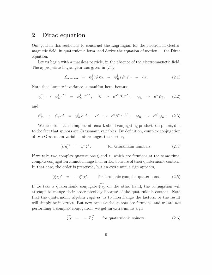
2 Dirac equation

Our goal in this section is to construct the Lagrangian for the electron in electro-

magnetic field, in quaternionic form, and derive the equation of motion — the Dirac

equation.

Let us begin with a massless particle, in the absence of the electromagnetic field.

The appropriate Lagrangian was given in [24],

Lmassless = ψ†L i∂ ψL + ψ†

R i ∂∗ ψR + c.c. (2.1)

Note that Lorentz invariance is manifest here, because

ψ†L → ψ†

L eˆ

= ψ†L e

−Λ∗

, ∂ → eΛ∗

∂ e−Λ , ψL → eΛ ψL , (2.2)

and

ψ†R → ψ†

R eΛ = ψ†

R e−Λ , ∂∗ → eΛ ∂∗ e−Λ∗

, ψR → eΛ∗

ψR . (2.3)

We need to make an important remark about conjugating products of spinors, due

to the fact that spinors are Grassmann variables. By definition, complex conjugation

of two Grassmann variable interchanges their order,

(ζ η)∗ = η∗ ζ∗ , for Grassmann numbers. (2.4)

If we take two complex quaternions ξ and χ, which are fermions at the same time,

complex conjugation cannot change their order, because of their quaternionic content.

In that case, the order is preserved, but an extra minus sign appears,

(ξ χ)∗ = − ξ∗ χ∗ , for fermionic complex quaternions. (2.5)

If we take a quaternionic conjugate ξ χ, on the other hand, the conjugation will

attempt to change their order precisely because of the quaternionic content. Note

that the quaternionic algebra requires us to interchange the factors, or the result

will simply be incorrect. But now because the spinors are fermions, and we are not

performing a complex conjugation, we get an extra minus sign

ξ χ = − χ ξ for quaternionic spinors. (2.6)

9

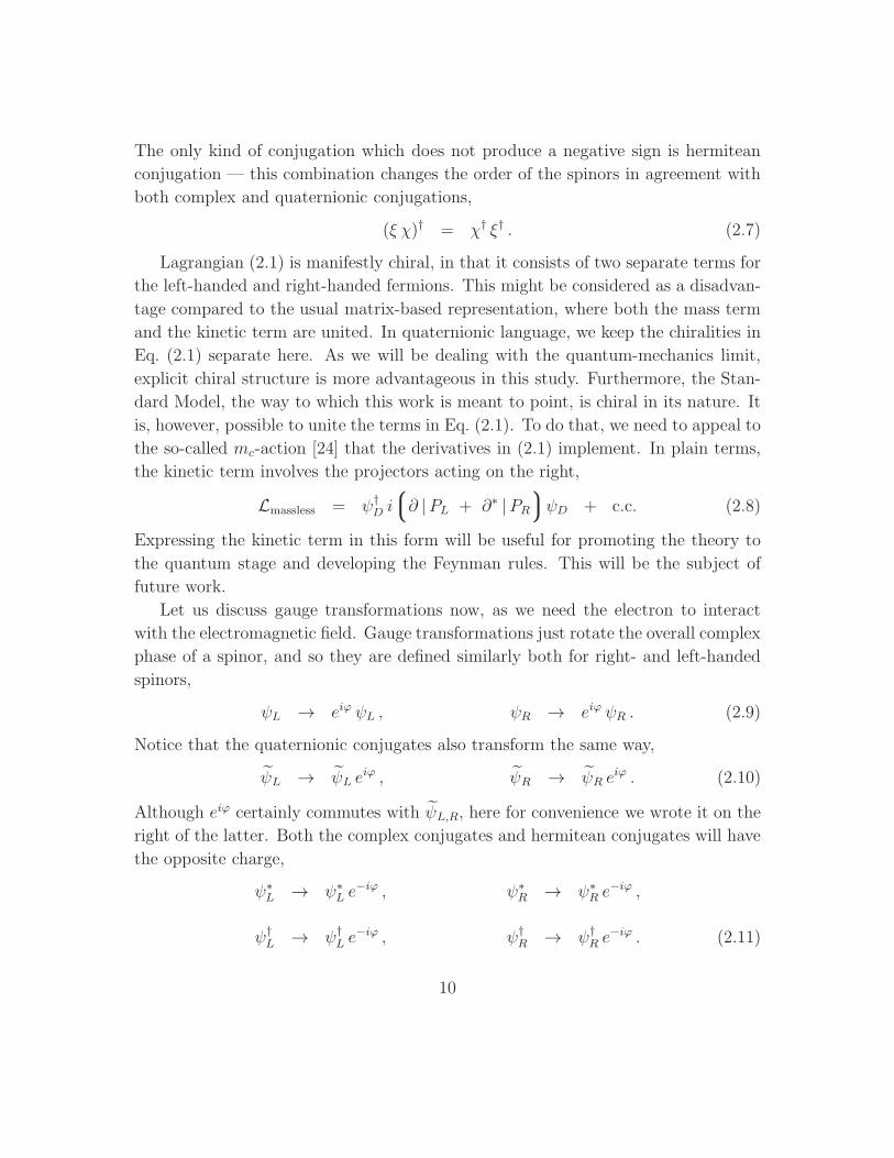
The only kind of conjugation which does not produce a negative sign is hermitean

conjugation — this combination changes the order of the spinors in agreement with

both complex and quaternionic conjugations,

(ξ χ)† = χ† ξ† . (2.7)

Lagrangian (2.1) is manifestly chiral, in that it consists of two separate terms for

the left-handed and right-handed fermions. This might be considered as a disadvan-

tage compared to the usual matrix-based representation, where both the mass term

and the kinetic term are united. In quaternionic language, we keep the chiralities in

Eq. (2.1) separate here. As we will be dealing with the quantum-mechanics limit,

explicit chiral structure is more advantageous in this study. Furthermore, the Stan-

dard Model, the way to which this work is meant to point, is chiral in its nature. It

is, however, possible to unite the terms in Eq. (2.1). To do that, we need to appeal to

the so-called mc-action [24] that the derivatives in (2.1) implement. In plain terms,

the kinetic term involves the projectors acting on the right,

Lmassless = ψ†D i

∂ |PL + ∂∗ |PR

ψD + c.c. (2.8)

Expressing the kinetic term in this form will be useful for promoting the theory to

the quantum stage and developing the Feynman rules. This will be the subject of

future work.

Let us discuss gauge transformations now, as we need the electron to interact

with the electromagnetic field. Gauge transformations just rotate the overall complex

phase of a spinor, and so they are defined similarly both for right- and left-handed

spinors,

ψL → eiϕ ψL , ψR → eiϕ ψR . (2.9)

Notice that the quaternionic conjugates also transform the same way,

ψL → ψL eiϕ , ψR → ψR e

iϕ . (2.10)

Although eiϕ certainly commutes with ψL,R, here for convenience we wrote it on the

right of the latter. Both the complex conjugates and hermitean conjugates will have

the opposite charge,

ψ∗L → ψ∗

L e−iϕ , ψ∗

R → ψ∗R e

−iϕ ,

ψ†L → ψ†

L e−iϕ , ψ†

R → ψ†R e

−iϕ . (2.11)

10

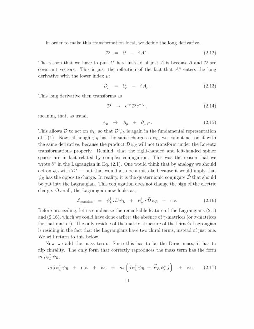
In order to make this transformation local, we define the long derivative,

D = ∂ − i A∗ . (2.12)

The reason that we have to put A∗ here instead of just A is because ∂ and D are

covariant vectors. This is just the reflection of the fact that Aµ enters the long

derivative with the lower index µ:

Dµ = ∂µ − i Aµ . (2.13)

This long derivative then transforms as

D → eiϕD e−iϕ , (2.14)

meaning that, as usual,

Aµ → Aµ + ∂µ ϕ . (2.15)

This allows D to act on ψL, so that D ψL is again in the fundamental representation

of U(1). Now, although ψR has the same charge as ψL, we cannot act on it with

the same derivative, because the product D ψR will not transform under the Lorentz

transformations properly. Remind, that the right-handed and left-handed spinor

spaces are in fact related by complex conjugation. This was the reason that we

wrote ∂∗ in the Lagrangian in Eq. (2.1). One would think that by analogy we should

act on ψR with D∗ — but that would also be a mistake because it would imply that

ψR has the opposite charge. In reality, it is the quaternionic conjugate D that should

be put into the Lagrangian. This conjugation does not change the sign of the electric

charge. Overall, the Lagrangian now looks as,

Lmassless = ψ†L iD ψL + ψ†

R i D ψR + c.c. (2.16)

Before proceeding, let us emphasize the remarkable feature of the Lagrangians (2.1)

and (2.16), which we could have done earlier: the absence of γ-matrices (or σ-matrices

for that matter). The only residue of the matrix structure of the Dirac’s Lagrangian

is residing in the fact that the Lagrangians have two chiral terms, instead of just one.

We will return to this below.

Now we add the mass term. Since this has to be the Dirac mass, it has to

flip chirality. The only form that correctly reproduces the mass term has the form

m ψ†L ψR,

m ψ†L ψR + q.c. + c.c = m

ψ†

L ψR + ψR ψ∗L

+ c.c. (2.17)

11

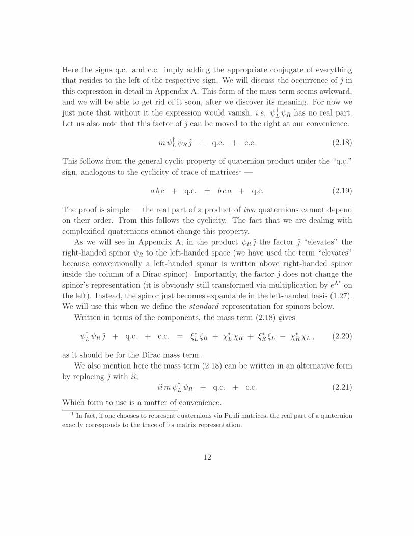
Here the signs q.c. and c.c. imply adding the appropriate conjugate of everything

that resides to the left of the respective sign. We will discuss the occurrence of in

this expression in detail in Appendix A. This form of the mass term seems awkward,

and we will be able to get rid of it soon, after we discover its meaning. For now we

just note that without it the expression would vanish, i.e. ψ†L ψR has no real part.

Let us also note that this factor of can be moved to the right at our convenience:

mψ†L ψR + q.c. + c.c. (2.18)

This follows from the general cyclic property of quaternion product under the “q.c.”

sign, analogous to the cyclicity of trace of matrices1 —

a b c + q.c. = b c a + q.c. (2.19)

The proof is simple — the real part of a product of two quaternions cannot depend

on their order. From this follows the cyclicity. The fact that we are dealing with

complexified quaternions cannot change this property.

As we will see in Appendix A, in the product ψR the factor “elevates” the

right-handed spinor ψR to the left-handed space (we have used the term “elevates”

because conventionally a left-handed spinor is written above right-handed spinor

inside the column of a Dirac spinor). Importantly, the factor does not change the

spinor’s representation (it is obviously still transformed via multiplication by eΛ∗

on

the left). Instead, the spinor just becomes expandable in the left-handed basis (1.27).

We will use this when we define the standard representation for spinors below.

Written in terms of the components, the mass term (2.18) gives

ψ†L ψR + q.c. + c.c. = ξ∗L ξR + χ∗

L χR + ξ∗R ξL + χ∗R χL , (2.20)

as it should be for the Dirac mass term.

We also mention here the mass term (2.18) can be written in an alternative form

by replacing with iı,

iı mψ†L ψR + q.c. + c.c. (2.21)

Which form to use is a matter of convenience.

1 In fact, if one chooses to represent quaternions via Pauli matrices, the real part of a quaternion

exactly corresponds to the trace of its matrix representation.

12

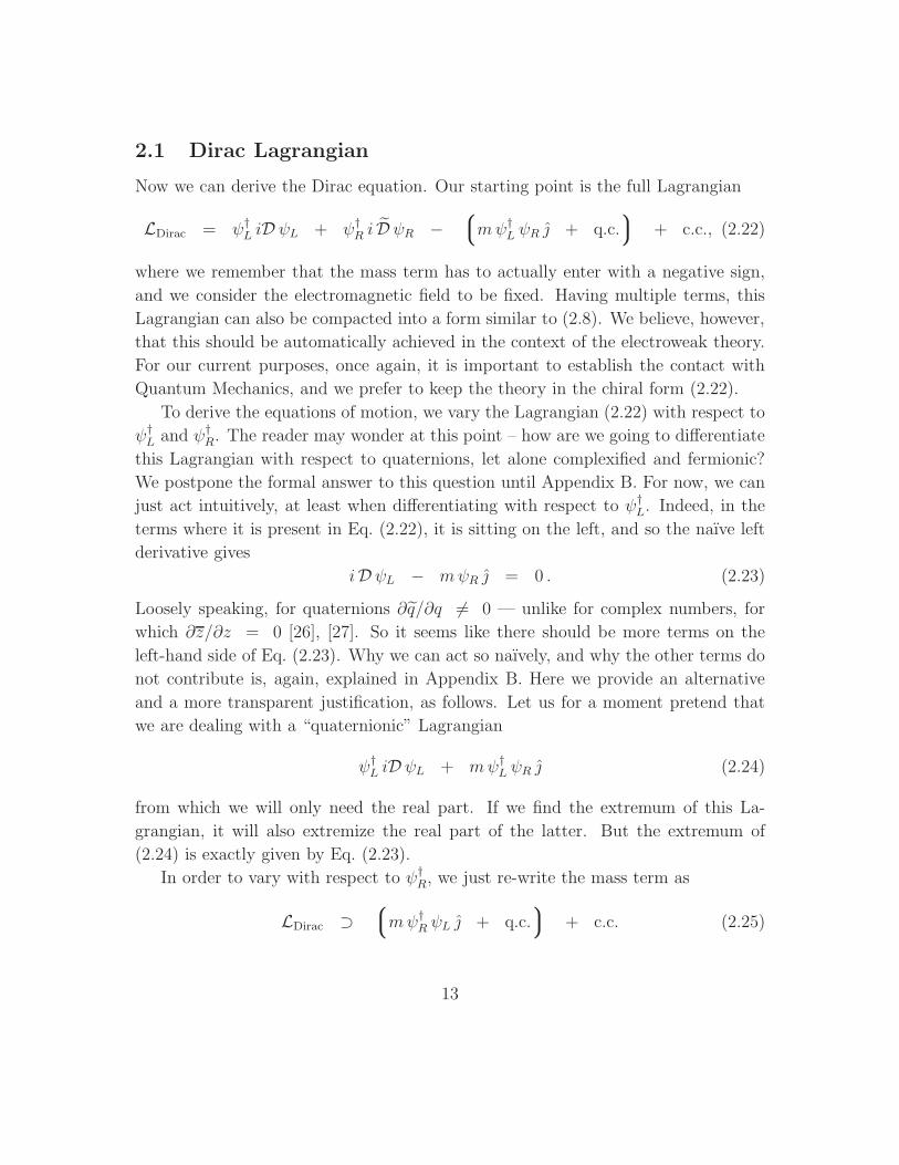
2.1 Dirac Lagrangian

Now we can derive the Dirac equation. Our starting point is the full Lagrangian

LDirac = ψ†L iD ψL + ψ†

R i D ψR −mψ†

L ψR + q.c. + c.c., (2.22)

where we remember that the mass term has to actually enter with a negative sign,

and we consider the electromagnetic field to be fixed. Having multiple terms, this

Lagrangian can also be compacted into a form similar to (2.8). We believe, however,

that this should be automatically achieved in the context of the electroweak theory.

For our current purposes, once again, it is important to establish the contact with

Quantum Mechanics, and we prefer to keep the theory in the chiral form (2.22).

To derive the equations of motion, we vary the Lagrangian (2.22) with respect to

ψ†L and ψ†

R. The reader may wonder at this point – how are we going to differentiate

this Lagrangian with respect to quaternions, let alone complexified and fermionic?

We postpone the formal answer to this question until Appendix B. For now, we can

just act intuitively, at least when differentiating with respect to ψ†L. Indeed, in the

terms where it is present in Eq. (2.22), it is sitting on the left, and so the naıve left

derivative gives

iD ψL − mψR = 0 . (2.23)

Loosely speaking, for quaternions ∂q/∂q 6= 0 — unlike for complex numbers, for

which ∂z/∂z = 0 [26], [27]. So it seems like there should be more terms on the

left-hand side of Eq. (2.23). Why we can act so naıvely, and why the other terms do

not contribute is, again, explained in Appendix B. Here we provide an alternative

and a more transparent justification, as follows. Let us for a moment pretend that

we are dealing with a “quaternionic” Lagrangian

ψ†L iD ψL + mψ†

L ψR (2.24)

from which we will only need the real part. If we find the extremum of this La-

grangian, it will also extremize the real part of the latter. But the extremum of

(2.24) is exactly given by Eq. (2.23).

In order to vary with respect to ψ†R, we just re-write the mass term as

LDirac ⊃mψ†

R ψL + q.c. + c.c. (2.25)

13

We did not introduce anything new, as the first term here was just hidden inside

the “q.c.” and “c.c.” in Eq. (2.22). Notice that this term enters with a positive sign.

Now we can vary the Lagrangian with respect to ψ†R, finding

i D ψR + mψL = 0 . (2.26)

The two expressions (2.23) and (2.26) are the quaternionic Dirac equations.

2.2 Non-relativistic limit

Now let us derive the Schrodinger equation. We do it in the classical way [28], by

taking the large-mass limit. First, we open up the long derivatives in Eqs. (2.23),

(2.26),

i ∂0 ψL + A0 ψL − (~∇ + i ~A)ψL − mψR = 0 ,

i ∂0 ψR + A0 ψR + (~∇ + i ~A)ψR + mψL = 0 . (2.27)

We can make one consistency check. For a free particle, the time derivative gives

the energy, i ∂0 → E. If at the same time, it has zero momentum, then E = m,

and we find

mψL − mψR = 0 =⇒ ψL = + ψR ,

mψR + mψL = 0 =⇒ ψR = − ψL . (2.28)

The two equations are consistent. What does the equality ψL = ψR mean? As

we already mentioned, and as we shall see in Appendix A, multiplying by on the

right rotates the components of ψL and ψR into each other. That is, in Dirac spinor

language, for a spinor

ψchiral =

ψαL

ψRα

(2.29)

this operation turns

ψαL → − ψRα , ψRα → ψαL . (2.30)

Equation (2.28) then simply implies that the two spinors ψαL and ψRα are equal. This

is correct, as a particle at rest is described by a single two-component spinor.

14

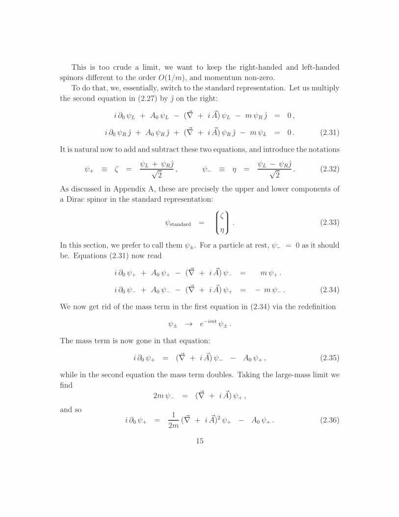
This is too crude a limit, we want to keep the right-handed and left-handed

spinors different to the order O(1/m), and momentum non-zero.

To do that, we, essentially, switch to the standard representation. Let us multiply

the second equation in (2.27) by on the right:

i ∂0 ψL + A0 ψL − (~∇ + i ~A)ψL − mψR = 0 ,

i ∂0 ψR + A0 ψR + (~∇ + i ~A)ψR − mψL = 0 . (2.31)

It is natural now to add and subtract these two equations, and introduce the notations

ψ+ ≡ ζ =ψL + ψR √

2, ψ− ≡ η =

ψL − ψR √2

. (2.32)

As discussed in Appendix A, these are precisely the upper and lower components of

a Dirac spinor in the standard representation:

ψstandard =

ζ

η

. (2.33)

In this section, we prefer to call them ψ±. For a particle at rest, ψ− = 0 as it should

be. Equations (2.31) now read

i ∂0 ψ+ + A0 ψ+ − (~∇ + i ~A)ψ− = mψ+ .

i ∂0 ψ− + A0 ψ− − (~∇ + i ~A)ψ+ = − mψ− . (2.34)

We now get rid of the mass term in the first equation in (2.34) via the redefinition

ψ± → e−imt ψ± .

The mass term is now gone in that equation:

i ∂0 ψ+ = (~∇ + i ~A)ψ− − A0 ψ+ , (2.35)

while in the second equation the mass term doubles. Taking the large-mass limit we

find

2mψ− = (~∇ + i ~A)ψ+ ,

and so

i ∂0 ψ+ =1

2m(~∇ + i ~A)2 ψ+ − A0 ψ+ . (2.36)

15

The final step now is to transform the quaternionic square

(~∇ + i ~A)2

into the usual vector operators — scalar and vector products. Denoting the scalar-

product square of a vector by figure brackets { }, one finds

(~∇ + i ~A)2 = −{~∇ + i ~A

}2+ i ~B ,

in the operator form. We thus get

i ∂0 ψ+ = − 1

2m

{~∇ + i ~A

}2ψ+ +

i ~B

2mψ+ − A0 ψ+ . (2.37)

Rescaling Aµ → eAµ, and switching to the Gaussian units, we arrive to

i ~ ∂t ψ+ =

1

2m

{~p +

e

c~A}2 − eA0 +

ie~

2mc~B

ψ+ , (2.38)

which is nothing but the Pauli equation. Notice once again that the σ-matrices

are absent from equations (2.37) and (2.38). Spin is the intrinsic property of the

wavefunction.

The factor of i in the magnetic moment term in Eq. (2.38) has a double role.

First, it is needed by the correspondence

~σ → i ı , i , i k ,

because the σ-matrices are hermitean, and the quaternionic units are not. Second

(and actually the same), by multiplying the magnetic field ~B, it turns it from an

axial vector into a polar vector i ~B. In the regular spinor formalism, one yet has to

argue that the product (~σ · ~B) yields a true scalar when acting on ψ.

It is precisely the form of equation (2.38) that establishes both the quaternionic

form of the Schrodinger equation and the fact that the Dirac Lagrangian (2.22) is

correct. Equation (2.38) involves a single two-component spinor ψ+. As a complex

quaternion, ψ+ only occupies a half of the quaternionic space, and in the most general

form it can be written as

ψ+ = ψ PL .

In fact this restriction can always be imposed in the end. The Schrodinger equation

(2.38) can be solved for an arbitrary ψ, and then projector PL can be applied. The

16

fact that the set of left-handed spinors forms an ideal guarantees that the projection

will be a solution too.

The right-handed projection ψ PR will also be a solution, of course. It may

either represent the same solution, or a different one, depending on the number of

solutions with a given energy. It can always be “moved” to the left-handed space by

multiplying by on the right.

The magnetic moment term in Eq. (2.38) is the only signature of quaternions in

that equation. Without it, the equation looks exactly like the ordinary Schrodinger

equation,

i ~ ∂t ψ =

p2

2m+ V

ψ , (2.39)

where we have dropped the gauge field for simplicity. For a complexified quater-

nion ψ, this equation falls apart into four identical complex equations. So the non-

relativistic Quantum Mechanics essentially only needs complex numbers. We stress

again that it is the spin of the particle that calls for the quaternionic appearance of

the wavefunction.

2.3 Current

Let us now find an expression for the electromagnetic current. It can be easily read

off the Lagrangian. Indeed, the current by definition is whatever the gauge field

couples to,

L ⊃ jµAµ =

j A + A j

2=

A j + j A

2. (2.40)

We can differentiate (i.e. vary) the latter quaternionic expression using equations

(B.45) and (B.46). The last fraction in Eq. (2.40) suggests differentiating with respect

to A in order to get current j,

∂A L ⊃ 4 j + (−2˜j)

2= j . (2.41)

We could now apply the same variational derivative to Lagrangian (2.22). Only this

is not necessary — it is enough to re-write the interacting part of (2.22) in the form

17

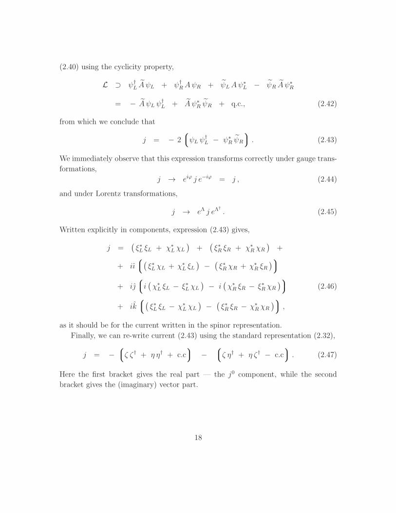
(2.40) using the cyclicity property,

L ⊃ ψ†L A ψL + ψ†

RAψR + ψLAψ∗L − ψR A ψ

∗R

= − A ψL ψ†L + A ψ∗

R ψR + q.c., (2.42)

from which we conclude that

j = − 2ψL ψ†

L − ψ∗R ψR

. (2.43)

We immediately observe that this expression transforms correctly under gauge trans-

formations,

j → eiϕ j e−iϕ = j , (2.44)

and under Lorentz transformations,

j → eΛ j eΛ†

. (2.45)

Written explicitly in components, expression (2.43) gives,

j =(ξ∗L ξL + χ∗

L χL)

+(ξ∗R ξR + χ∗

R χR)

+

+ iı(

ξ∗L χL + χ∗L ξL

)−

(ξ∗R χR + χ∗

R ξR)

+ ii

(χ∗L ξL − ξ∗L χL

)− i

(χ∗R ξR − ξ∗R χR

) (2.46)

+ ik(

ξ∗L ξL − χ∗L χL

)−

(ξ∗R ξR − χ∗

R χR) ,

as it should be for the current written in the spinor representation.

Finally, we can re-write current (2.43) using the standard representation (2.32),

j = −ζ ζ† + η η† + c.c

−

ζ η† + η ζ† − c.c

. (2.47)

Here the first bracket gives the real part — the j0 component, while the second

bracket gives the (imaginary) vector part.

18

3 Maxwell’s equation

Although not the main subject of our discussion, we can add the kinetic term for the

gauge field, and derive the resulting Maxwell’s equation. This section mainly serves

the purpose of illustration of differentiating with respect to quaternionic vectors. One

has to be particularly careful about the targets of differentiation of various involved

derivatives.

The gauge field strength is easily found to be

Φ = ~B + i ~E = − ∂ A − A ∂

2. (3.48)

This expression becomes particularly simple in the Lorentz gauge:

ΦLorentz = − ∂ A , (3.49)

although we will not use it for deriving the equations of motion.

The relevant part of the Lagrangian looks as,

LMaxwell =12Φ2 + A j

4+ q.c. + c.c. (3.50)

As we know from Section 2.3, varying the current part of the Lagrangian with respect

to A expectably gives us the current,

∂A Lcurrent = ∂AA j + j A

2= j . (3.51)

Now we need to vary the gauge part of the Lagrangian,

Lgauge =1

4Φ2 + c.c. (3.52)

Explicitly,

∂A (∂ A − A ∂) (∂ A − A ∂) =

∂A (∂ A − A ∂) (∂ A − A ∂) + ∂A (∂ A − A ∂) (∂ A − A ∂) . (3.53)

In the latter expression, we have underlined the particular instances of field A which

are acted upon by ∂A with a double line. All other occurrences of A are considered

19

constant for the matter of variation. The space-time derivatives ∂ here act on the

factors of A that are closest to them. We need to free the underlined variables A from

the space-time derivatives, by integrating the latter by parts. This will change the

sign in front of each of these derivatives, but will not move them anywhere because

they are quaternionic. To indicate that they are now acting on different targets, we

will underline them, as well as their targets, using a single line,

∂A(− ∂ A + A ∂

)(. . . ) + ∂A

(. . . )

(− ∂ A + A ∂

). (3.54)

Here the dots symbolize the term

∂ A − A ∂ . (3.55)

For the sake of variation, the space-time derivatives are now just constants. In fact,

everything is constant in Eq. (3.54) in regards to varying with respect to A— except

for the doubly-underlined A factors. Applying identities (B.45) and (B.46), we get,

explicitly

2 ∂(

. . . ) + 4 ∂(

. . . ) + 2 ∂(

. . . ) + 4(

. . . )0 ∂ . (3.56)

The third term here involves the quaternionic conjugate of (3.55), while the last term

involves the real component of the (3.55). Since (3.55) is purely imaginary, applying

quaternionic conjugation just changes its sign, while taking the real part annihilates

it,

4 ∂(∂ A − A ∂

)= − 8 ∂ Φ . (3.57)

Although a fair exercise in differentiation, the derivative of the conjugate term

Φ2 will actually give the same contribution. The reason we can guess that is that

the two terms Φ2 and Φ2 only differ by their complex-imaginary part

Im Φ2 ∝ ~E ◦ ~B , (3.58)

which is a boundary term and thus does not affect the equations of motion.

Altogether, we arrive to,

∂A LMaxwell = j − ∂ Φ , (3.59)

or,

∂ Φ = j , (3.60)

which is the quaternionic Maxwell’s equation. Notice that, because it is a complex-

quaternionic equation, it includes all eight real Maxwell’s equations. The reader is

encouraged to check that they are reproduced correctly in Eq. (3.60).

20

4 Conclusions

We have demonstrated the construction of Dirac and Weyl spinors in the complex

quaternionic space C ⊗ H. The spinors become part of the algebra, on the same

grounds as the kinetic operators acting on them. This allows for finding purely-

algebraic solutions of the Dirac equation in various settings, without resorting to

the matrix form. Different types of conjugation of spinors (2.5), (2.6) and (2.7) are

what particularly distinguishes the quaternionic formalism from the regular matrix

description. For example, the discrete transformations (A.19)–(A.22) have a simpler

appearance. In addition we notice that these complex and quaternionic conjugations

are not as easy to implement in the regular spinor formalism.

After building the Lagrangian, we have been able to develop a scheme of using

the variational calculus to consistently derive the equations of motion. This calculus

is well applicable to spinors and to vectors, which we have demonstrated by deriving

the (single) Maxwell’s equation.

An important result is the digression of the algebra in the non-relativistic limit.

By taking this limit, we have established the form of the Schrodinger’s equation

in the quaternionic formulation. Quantum Mechanics in the quaternionic form has

been a subject of long study with various success. We show that it is possible

to uniquely fix this form by starting from the Dirac equation. No extra degrees

off freedom appear. Furthermore, the existence of the spin of the wavefunction

is the natural consequence of the latter being quaternionic. The solution can be

sought in the algebraic form. Then, by applying the correct projector one finds

the quantum-mechanical wavefunction. Such solutions will be the subject of further

study. Once the spin is discarded, the Schrodinger’s equation takes the usual complex

form. The quaternionic algebra reduces to the complex one in the non-relativistic

limit. Extending this hypothesis, we hope to expect that addition of the strong and

weak interactions grows the algebra to a unifying O ⊗H⊗ C ⊗R.

In this context, we can address the length of the Lagrangian of electrodynamics

(2.22). As we have mentioned, it is possible to write it in a more compact way. There

have been multiple reasons we have not done this in this paper. Besides the desired

non-relativistic limit, we note that the Standard Model itself treats the chiralities

differently. Finally, we believe, that the right answer to a compact form is given by

placing the theory into the framework of electroweak interactions [20], [24]. This

comprises a promising direction for future work.

21

Acknowledgements

The author would like to thank Cohl Furey for valuable discussions during vari-

ous stages of this work, and the Institute of Nuclear Theory at the University of

Washington where part of this work was done for kind hospitality.

22

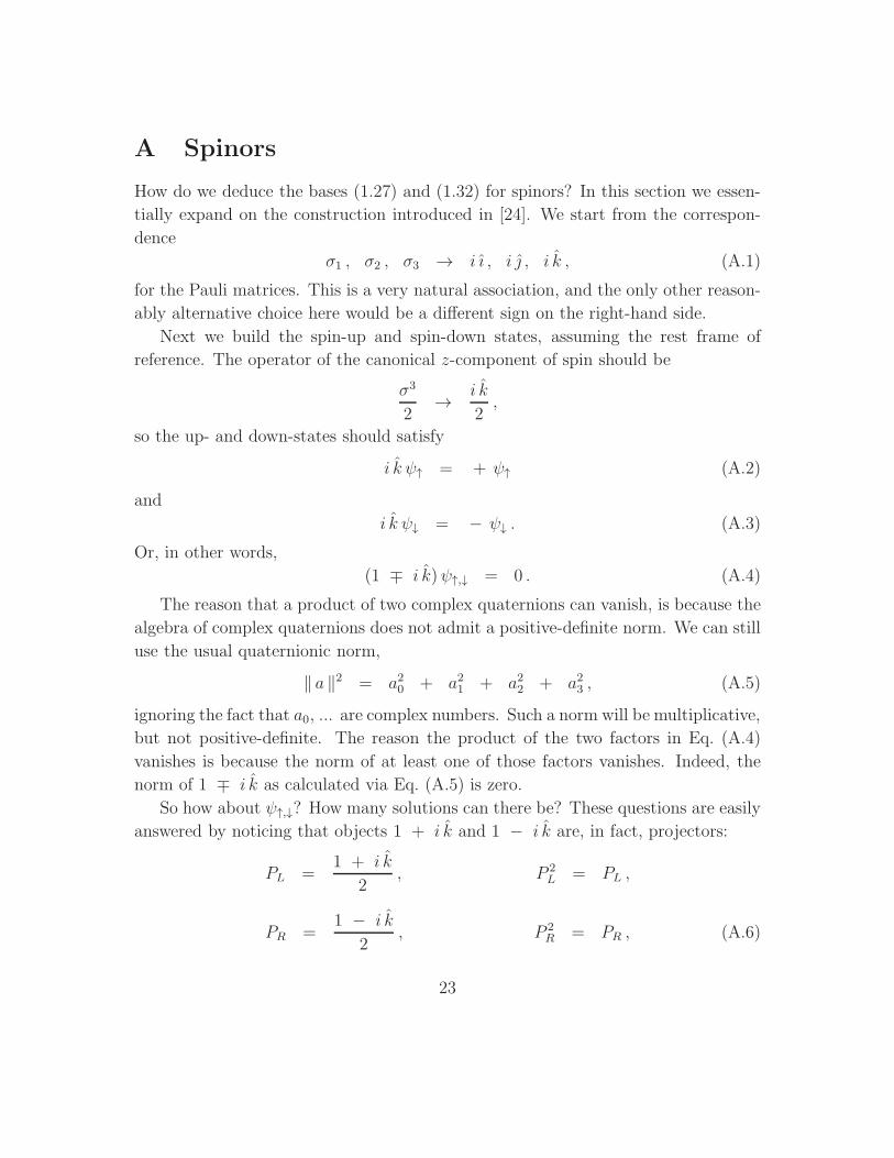
A Spinors

How do we deduce the bases (1.27) and (1.32) for spinors? In this section we essen-

tially expand on the construction introduced in [24]. We start from the correspon-

dence

σ1 , σ2 , σ3 → i ı , i , i k , (A.1)

for the Pauli matrices. This is a very natural association, and the only other reason-

ably alternative choice here would be a different sign on the right-hand side.

Next we build the spin-up and spin-down states, assuming the rest frame of

reference. The operator of the canonical z-component of spin should be

σ3

2→ i k

2,

so the up- and down-states should satisfy

i k ψ↑ = + ψ↑ (A.2)

and

i k ψ↓ = − ψ↓ . (A.3)

Or, in other words,

(1 ∓ i k)ψ↑,↓ = 0 . (A.4)

The reason that a product of two complex quaternions can vanish, is because the

algebra of complex quaternions does not admit a positive-definite norm. We can still

use the usual quaternionic norm,

‖ a ‖2 = a20 + a21 + a22 + a23 , (A.5)

ignoring the fact that a0, ... are complex numbers. Such a norm will be multiplicative,

but not positive-definite. The reason the product of the two factors in Eq. (A.4)

vanishes is because the norm of at least one of those factors vanishes. Indeed, the

norm of 1 ∓ i k as calculated via Eq. (A.5) is zero.

So how about ψ↑,↓? How many solutions can there be? These questions are easily

answered by noticing that objects 1 + i k and 1 − i k are, in fact, projectors:

PL =1 + i k

2, P 2

L = PL ,

PR =1 − i k

2, P 2

R = PR , (A.6)

23

which we judiciously have named the left- and right-handed projectors. Indeed, by

multiplying a quaternion on the left (or equally well, on the right) by PL, we are

obviously performing a linear operation upon the components of that quaternion.

The square of such an operation equals the operation itself ⇒ the operation is a

projection. Obviously the same is true for PR.

That means that if we run ψ through all values of complex quaternions, the prod-

uct PLψ will span only a portion of the quaternionic space — an ideal. What fraction

of the entire algebra does it span? We notice that PL and PR are complementary

projectors:

PR = P ∗L , PL + PR = 1 . (A.7)

Because they are symmetric, they can only project equal-size subsets of the algebra.

And since they are complementary to each other, the union of those subsets must

comprise the entire algebra. In other words, PL and PR split the algebra in two

halves.

Now, equation (A.4) can re-written as,

PR,L ψ↑,↓ = 0 , (A.8)

meaning that the most general ψ↑ must sit in one half of the algebra, while the most

general ψ↓ must sit in the other half. Since a generic complex quaternion has four

complex components, there are two complex solutions for ψ↑ and as many for ψ↓.

We have to stress here that these halves are not identified with the left- and right-

handed chiral spaces. For this reason we have not given names to these subspaces,

other than “spin-up” and “spin-down” spaces.

The easiest solution to (A.8) is given by the orthogonality of the projectors:

PR PL = 0 , PL PR = 0 . (A.9)

So, seemingly PL could be identified with a spin-up state, and PR — with the corre-

sponding spin-down state. However, these are states of different chiralities. Indeed,

since PL = P ∗R, such “spinors” transform in the mutually-conjugate representations

of the Lorentz group. This fact puts them into the opposite chirality spaces.

Let us summarize our goal and achievements now. We are looking for four com-

plex states ψL↑, ψL↓, ψR↑ and ψR↓. We have already found

ψL↑ = PL , ψR↓ = PR . (A.10)

24

It is not difficult to find the other two states. For example, if one wishes to avoid

pure guessing, which would perfectly work here too, we know that matrix −iσ2 turns

a spin-up state into a spin-down state:

−i σ2

1

0

=

0 −1

1 0

1

0

=

0

1

.

This exactly corresponds to multiplying by on the left, and we arrive to

ψL↓ = PL , ψR↑ = − PR . (A.11)

So we recap that the left-handed spinors can be written as

ψL = ξL PL + χL PL , (A.12)

while the right-handed spinors are represented as

ψR = − ξR PR + χR PR . (A.13)

A few important comments are in order here. The chiral subspaces are defined

here by multiplying arbitrary quaternions by projectors PL or PR on the right. In

other words, ψ PL spans the set of all left-handed spinors, and ψ PR of all right-

handed. This way, right multiplication splits the set of quaternions into the two

chirality subspaces. Whereas, left multiplication splits the quaternions into spin-up

and spin-down subspaces, because e.g.

PR (PL ψ) = 0 .

It is a trivial fact now that a set of the type{PL ψ } or

{ψ PL } forms a left (right)

ideal, since for an arbitrary quaternion a, the product, say,

a (ψ PL) = (aψ)PL ,

resides in the same subspace as ψ PL.

The other important remark is about the amount of freedom that we have in

defining the bases via Eqs. (A.12), (A.13). We have freedom in choosing the com-

ponent of the spin to be measurable — for which we chose k. The other freedom

was in parametrizing the spin-down component of ψL, for which we chose as an

25

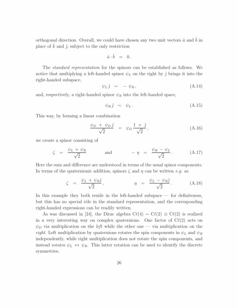
orthogonal direction. Overall, we could have chosen any two unit vectors a and b in

place of k and , subject to the only restriction

a · b = 0 .

The standard representation for the spinors can be established as follows. We

notice that multiplying a left-handed spinor ψL on the right by brings it into the

right-handed subspace,

ψL ∼ − ψR , (A.14)

and, respectively, a right-handed spinor ψR into the left-handed space,

ψR ∼ ψL . (A.15)

This way, by forming a linear combination

ψD + ψD √2

= ψD1 + √

2, (A.16)

we create a spinor consisting of

ζ =ψL + ψR√

2and − η =

ψR − ψL√2

. (A.17)

Here the sum and difference are understood in terms of the usual spinor components.

In terms of the quaternionic addition, spinors ζ and η can be written e.g. as

ζ =ψL + ψR√

2, η =

ψL − ψR√2

. (A.18)

In this example they both reside in the left-handed subspace — for definiteness,

but this has no special role in the standard representation, and the corresponding

right-handed expressions can be readily written.

As was discussed in [24], the Dirac algebra Cℓ(4) ∼ Cℓ(2) ⊗ Cℓ(2) is realized

in a very interesting way on complex quaternions. One factor of Cℓ(2) acts on

ψD via multiplication on the left while the other one — via multiplication on the

right. Left multiplication by quaternions rotates the spin components in ψL and ψRindependently, while right multiplication does not rotate the spin components, and

instead rotates ψL ↔ ψR. This latter rotation can be used to identify the discrete

symmetries.

26

A.1 Discrete symmetries

Here we will discuss the action of C, P and T symmetries on fermions. These

symmetries can be conveniently written for an entire Dirac fermion ψD. We use here

the phase conventions of [28].

· Charge conjugation C is realized by complex conjugation of the fermion,

ψD(x) → i ψ∗D(x) . (A.19)

· Parity transformation P is given by right multiplication by −ı,

ψD(t, ~x) → − ψD(t, −~x) ı , (A.20)

which interchanges the chiral components as,

ψL → i ψR , ψR → i ψL . (A.21)

· Time inversion T is performed by complex conjugation and multiplying by i

on the right,

ψD(t, ~x) → i ψ∗D(−t, ~x) . (A.22)

All three transformations result in

C P T ψD(x) = ψD(−x) k . (A.23)

Right-multiplying by ik preserves the sign of the left-handed spinor, while flips the

sign of the right-handed part. Therefore, multiplying by k = (−i)ik corresponds to

multiplying by iγ5 in the spinor representation. Notice that the above transforma-

tions have a significantly simpler form than they do in the γ-matrix representation.

B Differentiation

Derivation of the equations of motion from the Lagrangian involves one crucial step

— variation, which we will loosely call differentiation. Indeed, the problem of extrem-

izing the action essentially reduces to differentiating with respect to a quaternion.

As soon as we are able to differentiate, variational calculus sets in place. We start

with regular quaternions.

27

B.1 Ordinary quaternions

It is well known that there is no existing analyticity theory of quaternions analogous

to that of complex numbers. Even the notion of a derivative is not well established.

While complex analyticity rests on holomorphic functions that depend on z and are

independent of z,

f(z, z) = f(z) ,

this property cannot be extended to quaternions.

There is one crucial reason for this: if a complex function depends on z, there

is no way that it can be represented as a function of z. In other words, variable z

cannot be converted into z by multiplying it by any constants. This is not so with

quaternions. For, given a quaternion q, we find that a combination

− q + ı q ı + q + k q k

2= q (B.24)

is exactly the conjugate of q. Any other type of conjugation that can be introduced

for quaternions (say, the one that only flips the sign of a single imaginary unit ı)

can also be represented in such an “arithmetic” form. That means that any function

f(q) can be viewed as a function of q, just with different coefficients. So the notion

of holomorphy cannot be applied to quaternions, at least directly.

It is, however, possible to define a convenient notion of a derivative. It works

especially well if the function being differentiated is real (although it does not have

to be).

Let us say that f(q) is a function of variable q,

q ≡ t + ~r = t + x ı + y + z k. (B.25)

We introduce a derivative ∂,

∂ ≡ ∂t + ~∇ = ∂t + ı ∂x + ∂y + k ∂z . (B.26)

Strictly speaking, in analogy to complex numbers, we should call this quantity a

conjugate derivative 2 ∂ multiplied by a factor of two or so, as we will see below.

However, to keep notations flat and straightforward, we just call it ∂, and we define

a conjugate derivative as

∂ ≡ ∂t − ~∇ = ∂t − ı ∂x − ∂y − k ∂z . (B.27)

28

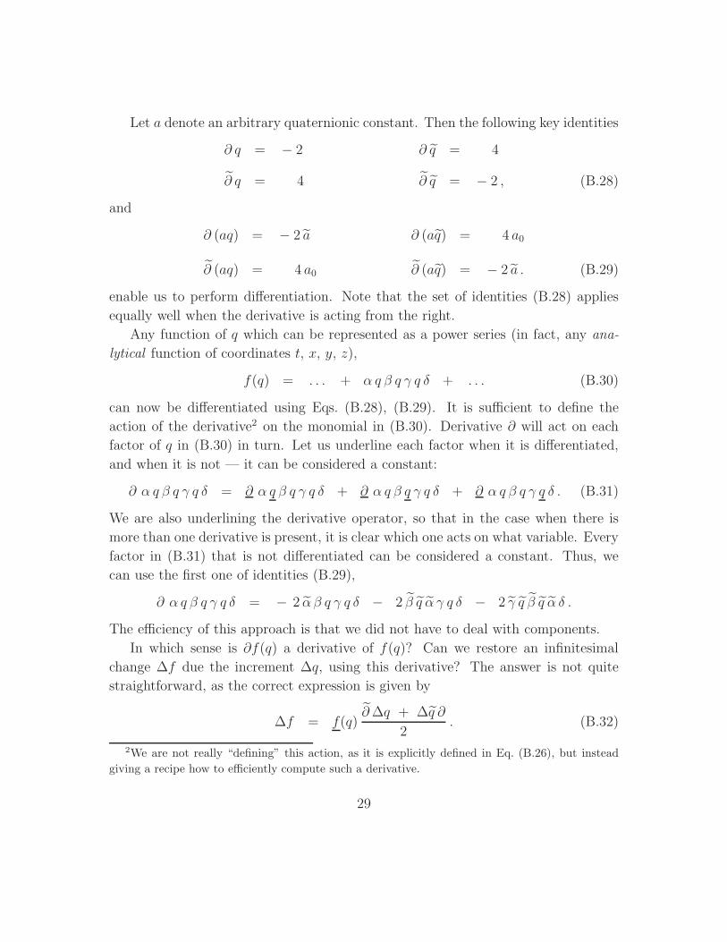
Let a denote an arbitrary quaternionic constant. Then the following key identities

∂ q = − 2 ∂ q = 4

∂ q = 4 ∂ q = − 2 , (B.28)

and

∂ (aq) = − 2 a ∂ (aq) = 4 a0

∂ (aq) = 4 a0 ∂ (aq) = − 2 a . (B.29)

enable us to perform differentiation. Note that the set of identities (B.28) applies

equally well when the derivative is acting from the right.

Any function of q which can be represented as a power series (in fact, any ana-

lytical function of coordinates t, x, y, z),

f(q) = . . . + α q β q γ q δ + . . . (B.30)

can now be differentiated using Eqs. (B.28), (B.29). It is sufficient to define the

action of the derivative2 on the monomial in (B.30). Derivative ∂ will act on each

factor of q in (B.30) in turn. Let us underline each factor when it is differentiated,

and when it is not — it can be considered a constant:

∂ α q β q γ q δ = ∂ α q β q γ q δ + ∂ α q β q γ q δ + ∂ α q β q γ q δ . (B.31)

We are also underlining the derivative operator, so that in the case when there is

more than one derivative is present, it is clear which one acts on what variable. Every

factor in (B.31) that is not differentiated can be considered a constant. Thus, we

can use the first one of identities (B.29),

∂ α q β q γ q δ = − 2 α β q γ q δ − 2 β q α γ q δ − 2 γ q β q α δ .

The efficiency of this approach is that we did not have to deal with components.

In which sense is ∂f(q) a derivative of f(q)? Can we restore an infinitesimal

change ∆f due the increment ∆q, using this derivative? The answer is not quite

straightforward, as the correct expression is given by

∆f = f(q)∂∆q + ∆q ∂

2. (B.32)

2We are not really “defining” this action, as it is explicitly defined in Eq. (B.26), but instead

giving a recipe how to efficiently compute such a derivative.

29

This result is obvious because the fraction here actually equals ∂µ∆qµ. Being a

scalar, it can be written on either side of f(q). The problem here is that one of

the two terms in that fraction will necessarily have a derivative operator ∂ sitting

furthest away from f(q),

f(q)∆q ∂ ,

and so will not form a derivative in our sense. In other words, here the derivative

has to depend on the increment ∆q in order to correctly reproduce ∆f .

Instead of engaging with this problem, let us switch to real functions f(q) — our

prime subject of interest — since the Lagrangian is real. For real f(q), the rightmost

term in the fraction in (B.32) commutes with f(q), and so

∆f =1

2

∆q ∂ f(q) + f(q) ∂∆q

,

where we also have replaced f(q) with f(q) in the first term in the bracket. The

extremum of f(q) is obviously achieved when

∂ f(q) = 0 , (B.33)

since this also implies that f(q) ∂ = 0.

Let us see how this works in practice. Let us apply a derivative operator ∂ on a

real function f(q). Even if we do not know the form of f(q), when viewed as a series

it can always be represented as

f(q) = . . . + q a + a q + . . . , (B.34)

since when we differentiate a particular factor of q in a given monomial term, all

the other factors of q in that term can be considered constant and absorbed into a.

Applying identities (B.28), (B.29) to function (B.34), we get

∂ f(q) ⊃ − 2 a + 4 a0 = 2 a . (B.35)

Note that we would have arrived to the same result had we written q and a in

Eq. (B.34) in a different order,

f(q) = . . . + a q + q a + . . . , (B.36)

only now the other identities in (B.28), (B.29) would have been involved.

30

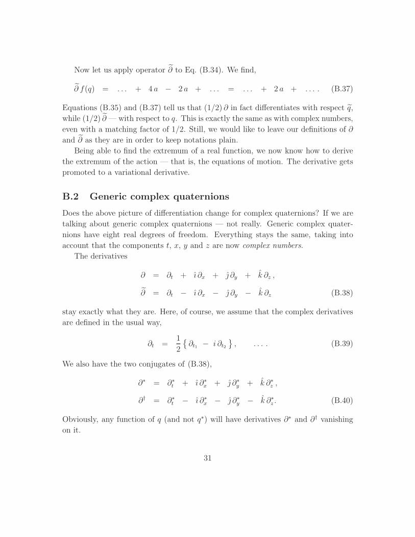
Now let us apply operator ∂ to Eq. (B.34). We find,

∂ f(q) = . . . + 4 a − 2 a + . . . = . . . + 2 a + . . . . (B.37)

Equations (B.35) and (B.37) tell us that (1/2) ∂ in fact differentiates with respect q,

while (1/2) ∂ —with respect to q. This is exactly the same as with complex numbers,

even with a matching factor of 1/2. Still, we would like to leave our definitions of ∂

and ∂ as they are in order to keep notations plain.

Being able to find the extremum of a real function, we now know how to derive

the extremum of the action — that is, the equations of motion. The derivative gets

promoted to a variational derivative.

B.2 Generic complex quaternions

Does the above picture of differentiation change for complex quaternions? If we are

talking about generic complex quaternions — not really. Generic complex quater-

nions have eight real degrees of freedom. Everything stays the same, taking into

account that the components t, x, y and z are now complex numbers.

The derivatives

∂ = ∂t + ı ∂x + ∂y + k ∂z ,

∂ = ∂t − ı ∂x − ∂y − k ∂z (B.38)

stay exactly what they are. Here, of course, we assume that the complex derivatives

are defined in the usual way,

∂t =1

2

{∂t1 − i ∂t2

}, . . . . (B.39)

We also have the two conjugates of (B.38),

∂∗ = ∂∗t + ı ∂∗x + ∂∗y + k ∂∗z ,

∂† = ∂∗t − ı ∂∗x − ∂∗y − k ∂∗z . (B.40)

Obviously, any function of q (and not q∗) will have derivatives ∂∗ and ∂† vanishing

on it.

31

Relations (B.28) and (B.29) are valid in our complex case verbatim. There is

also a complex conjugated copy of them. We are not going to pay much attention to

these relations.

We are able to re-use literally all the formulas applicable to the differentiation with

respect to regular quaternions, because complex quaternions have all eight degrees

of freedom occupied.

The story becomes more interesting when we have to address constrained quater-

nions — e.g. vectors or spinors. We call them constrained, because not all eight

components in them are independent (or non-zero). Thus, the derivatives (B.38),

(B.40) cannot be applied to them verbatim to produce a meaningful result.

There is also the field strength Φ which is a constrained quaternion, but we

normally do not vary with respect field strengths.

B.3 Constrained complex quaternions — vectors

Vectors open up quite an interesting story, as the only physical vector field variables

are gauge fields. Thus, differentiation with respect to vectors enables us to derive an

expression for the current, as well as to formally derive the form of the quaternionic

Maxwell’s equation.

Formally vectors can be defined by the constraint condition

q† = q , (B.41)

which means that only four real components of it are non-zero:

q ≡ t + i ~r = t + i(ı x + y + k z

). (B.42)

In relation to it we define the derivative operators

∂ ≡ ∂t + i ~∇ = ∂t + i(ı ∂x + ı ∂y + k ∂z

)(B.43)

and

∂ = ∂∗ = ∂t − i(ı ∂x + ı ∂y + k ∂z

). (B.44)

Relations (B.28) and (B.29) are valid but now their right-hand sides are inter-

changed vertically,

∂ q = 4 ∂ q = − 2

∂ q = − 2 ∂ q = 4 , (B.45)

32

and

∂ (aq) = 4 a0 ∂ (aq) = − 2 a

∂ (aq) = − 2 a ∂ (aq) = 4 a0 . (B.46)

Other than that, there is no difference from differentiating with respect to regular

quaternions, and these formulas are enough to derive the equations of motion.

B.4 Constrained complex quaternions — spinors

Full Dirac spinors are just complex quaternions, and so differentiation with respect

to them is in fact addressed by operators (B.38). There is nothing new from that

perspective. One only has to keep in mind that spinors are Grassmann numbers.

Weyl spinors, however are constrained. Even though a single Weyl spinor ψL or

ψR has all eight components non-zero, it only has four independent ones.

Let us take a left-handed fermion ψL,

ψL = ξL PL + χL PL . (B.47)

It turns out, that differentiation with respect to ψL is only meaningful when done

from the right. The reason behind is that when multiplying by anything from the

left, it is not possible to “cancel” the projectors PL. We have,

ψL

∂ξL − ∂χL

= PL + PR = 1 . (B.48)

Again, we have underlined ψL to show that the derivatives act to the left. Here ∂ξLand ∂χL

are the usual Grassmann derivatives with respect to the complex components

ξL and χL correspondingly. Analogously we find

ψR

∂ξR + ∂χR

= ψR

∂ξR − ∂χR

= 1 . (B.49)

So we essentially have identified the spinor derivatives, we just need to re-write them

in terms of the quaternionic components t, x, y and z. Although we are really

considering ψL and ψR separately, let us combine them both into a single Dirac

fermion. This is only done for the sake of completeness — a derivative with respect

33

to ψL does not touch ψR in any sense, because the components of the two spinors

are independent complex numbers. We have,

ψD =ξL + χR

2+ ı i

ξR + χL2

+ −ξR + χL

2+ k i

ξL − χR2

= t + ı x + y + k z . (B.50)

Knowing this, we can express derivatives ∂ξL , etc in terms of the derivatives with re-

spect to components t, x, y and z. Plugging them into the expressions in parentheses

in equations (B.48) and (B.49) we find,

∂ψL∝ ∂t − i ∂x − ∂y + i ∂z

2,

∂ψR∝ ∂t + i ∂x − ∂y − i ∂z

2. (B.51)

Although we could write equality signs in these equations, we postpone this until we

do the last extra step. Namely, equations (B.51) do not seem to be very aesthetic,

or easy to remember. Notice, that the action of these derivatives will not change if

we multiply them by the projectors PL and PR on the left, correspondingly. Indeed,

these projectors will carve out ψL or ψR from Eq. (B.50), before the actual derivatives

will hit them. It is then a matter of a simple multiplication to observe that the right-

hand sides of Eq. (B.51) when multiplied by the corresponding projectors, match a

regular derivative ∂ multiplied by the same projectors

∂ψL=

1

2PL ∂ ,

∂ψR=

1

2PR ∂ . (B.52)

where ∂ is the derivative (B.38) with respect to the components (B.50) of ψD viewed

as a complex quaternion,

∂ = ∂t − ı ∂x − ∂y − k ∂z . (B.53)

From Eq. (B.52),

∂ψL+ ∂ψR

=1

2∂ . (B.54)

34

We remind that all derivatives in Eqs. (B.52) and (B.54) act to the left.

Quite analogously, we consider the hermitean-conjugate spinors ψ†L and ψ†

R, for

which

∂ψ†L

∝ ∂ξ∗L

+ ∂χ∗L,

∂ψ†R

∝∂ξ∗

R+ ∂χ∗

R

(−) , (B.55)

where the derivatives now act to the right. Notice that the expressions in (B.55) are

precisely the hermitean conjugates of those in Eqs. (B.48) and (B.49). Proceeding

the same way as we arrived to Eq. (B.51) and past it, we, now unsurprisingly, find

∂ψ†L

=1

2∂∗ PL ,

∂ψ†R

=1

2∂∗ PR . (B.56)

We stress again that here the derivatives act to the right. Operator ∂∗ is the derivative

with respect to the complex conjugates of the components (B.50) of ψD, the latter

viewed as a complex quaternion,

∂∗ = ∂t∗ − ı ∂x∗ − ∂y∗ − k ∂z∗ ,

ψ∗D = t∗ + ı x∗ + y∗ + k z∗ . (B.57)

Equations (B.52) and (B.56) is our final answer for the spinor derivatives. The

reason is that we already now how to apply a differential operator ∂ or its conjugates

in an efficient way — we have equations (B.28) and (B.29) at our disposal.

If an expression is linear, say in ψL, then differentiation simply “erases” the latter

from the expression (since the Lagrangian is real, one can always arrange ψL to

stand on the right of the expression). Fermionic expressions are almost always linear

in spinors (ψ†L or ψ∗

L is an independent variable from ψL), except for four-fermion

interactions. Even then, Appendix B.1 explains how to deal with such functions.

As was shown in Appendix B.1, an extremum of a real function is attained when

∂ f = 0 . (B.58)

Whether the quaternions are ordinary or complex, does not change this. As we saw

above, such a derivative can be split into left- and right-handed parts, each of which

35

provides an independent equation — for ψL and ψR correspondingly. To see that, it

is enough to multiply Eq. (B.58) on the right by a left- or right-handed projector.

Thus, we have a recipe for deriving the equations of motion for Weyl spinors as well

as for Dirac spinors.

Let us give simple example that we use — a Lagrangian of a Dirac fermion,

L = ψ†L iD ψL + ψ†

R i D ψR −mψ†

L ψR + q.c. + c.c. (B.59)

We will need this Lagrangian in the full form,

L = ψ†L iD ψL + ψ†

R i D ψR + ψL iD∗ ψ∗L + ψR iD† ψ∗

R −

− mψ†

L ψR + ψR ψ∗L

+ m

ψL ψ∗

R + ψ†R ψL

. (B.60)

Caution must be executed with respect to signs when conjugating fermions. It is

advisable that the reader should take a moment to understand why the signs in front

of the conjugated terms are as they are shown in Eq. (B.60).

Let us begin with the kinetic terms first. Because of Lorentz transformations

(and of gauge transformations, if applicable), ψL and ψR are traditionally written on

the right, and their hermitean conjugates — on the left. So it is only straightforward

for us to apply operator ∂†ψLfrom (B.56) on the left. By construction, operators in

(B.56) erase the fermions directly neighbouring them. The first kinetic term gives us

iD ψL. What about ψL iD∗ ψ∗L ? Equation (B.55) seems to imply that the derivative

of ψ∗L with respect to ψ†

L maybe non-zero. While this is actually true, the kinetic term

for ψ∗L simply gets filtered out by the projector PL from (B.56). The same happens

to the mass term containing ψ∗L, so that only the first mass term contributes, and

we arrive to,

iD ψL − mψR = 0 . (B.61)

Analogously, the derivative with respect to ψ†R of the right-handed kinetic terms

is i D ψR. As for the mass term bracket containing ψ†R, one can proceed with it in two

ways. The first, and perhaps the easiest way, is to re-write it in the form identical

to that of the left-handed mass term. That is, please observe that the last bracket

in Eq. (B.60) is the “zeroth” quaternionic component of ψ†R ψL, and as such, is

invariant to cyclic permutations of the latter. Using this cyclic symmetry we can

pull ψ†R to the left,

mψL ψ∗

R + ψ†R ψL

= m

ψ†

R ψL + ψL ψ∗R

. (B.62)

36

The problem of differentiating with respect to ψ†R becomes trivial for the first term

in the bracket, giving us mψL . The second mass term again gets projected out.

Altogether, we have

i D ψR + mψL = 0 . (B.63)

The second way of differentiating the mass term with respect to ψ†R is to use

Eq. (B.56) directly. This would involve applying derivative ∂∗ with the help of

identities (B.29). The result will of course be the same.

We have mentioned here that the derivative ∂ψ†L

ψ∗L (along with the corresponding

right-handed one) is non-zero. What is it then? Let us see,

∂ψ†L

ψ∗L = ∂ψ†

L

(ψD PL)∗ = ∂ψ†

L

ψ∗D PR =

1

2∂∗ PL ψ

∗D PR . (B.64)

Using the first identity in (B.29) (for, ∂∗ for ψ∗D plays the same role as ∂ does for q),

we find,

∂ψ†L

ψ∗L = − PL PR = − PR . (B.65)

It is because of the other factors containing projectors that this derivative did not

contribute to the equation of motion (B.61) (and, correspondingly, the analogous

right-handed derivative did not contribute to Eq. (B.63)).

References

[1] S. L. Adler, New York, USA: Oxford Univ. Pr. (1995) 586 p. (International series of

monographs on physics, 88)

[2] J. C. Maxwell, A Treatise on Electricity and Magnetism, Oxford, Clarendon Press

(1873)

[3] P. G. Tait, An Elementary Treatise on Quaternions, Cambridge University Press

(1890)

[4] D. Finkelstein, J. M. Jauch and D. Speiser, J. Math. Phys. 3, 207 (1962).

doi:10.1063/1.1703794

[5] D. Finkelstein, J. M. Jauch, S. Schminovich and D. Speiser, J. Math. Phys. 4, 788

(1963). doi:10.1063/1.1724320

[6] J. D. Edmonds, Int. J. Theor. Phys. 6, 205 (1972). doi:10.1007/BF00672074

[7] J. D. Edmonds, Lett. Nuovo Cim. 7S2, 398 (1973) [Lett. Nuovo Cim. 7, 398 (1973)].

doi:10.1007/BF02735143

37

[8] J. D. Edmonds, Int. J. Theor. Phys. 10, 115 (1974). doi:10.1007/BF01810397

[9] M. Gunaydin and F. Gursey, J. Math. Phys. 14, 1651 (1973). doi:10.1063/1.1666240

[10] M. Gunaydin and F. Gursey, Phys. Rev. D 9, 3387 (1974).

doi:10.1103/PhysRevD.9.3387

[11] W. Gough, Eur. J. Phys. 7, 35 (1986). doi:10.1088/0143-0807/7/1/007

[12] W. Gough, Eur. J. Phys. 10, 188 (1989). doi:10.1088/0143-0807/10/3/005

[13] S. De Leo, Int. J. Mod. Phys. A 11, 3973 (1996) doi:10.1142/S0217751X96001863

[hep-th/9508010].

[14] S. De Leo and P. Rotelli, Mod. Phys. Lett. A 11, 357 (1996)

doi:10.1142/S0217732396000400 [hep-th/9509059].

[15] S. De Leo and W. A. Rodrigues, Jr., Int. J. Theor. Phys. 37, 1707 (1998)

doi:10.1023/A:1026692508708 [hep-th/9806058].

[16] S. De Leo and W. A. Rodrigues, Jr., Int. J. Theor. Phys. 37, 1511 (1998)

doi:10.1023/A:1026611718277 [hep-th/9806057].

[17] S. De Leo, Found. Phys. Lett. 14, no. 1, 37 (2001) doi:10.1023/A:1012077227985

[hep-th/0103129].

[18] C. Furey, Phys. Rev. D 86, 025024 (2012) doi:10.1103/PhysRevD.86.025024

[arXiv:1002.1497 [hep-th]].

[19] C. Furey, JHEP 1410, 046 (2014) doi:10.1007/JHEP10(2014)046 [arXiv:1405.4601

[hep-th]].

[20] C. Furey, Phys. Lett. B 742, 195 (2015) doi:10.1016/j.physletb.2015.01.023

[arXiv:1603.04078 [hep-th]].

[21] P. S. Bisht and O. P. S. Negi, Int. J. Theor. Phys. 47, 3108 (2008) doi:10.1007/s10773-

008-9744-8 [arXiv:0709.0088 [hep-th]].

[22] A. S. Rawat and O. P. S. Negi, Int. J. Theor. Phys. 51, 738 (2012) doi:10.1007/s10773-

011-0953-1 [arXiv:1107.0916 [physics.gen-ph]].

[23] B. C. Chanyal, P. S. Bisht, T. Li and O. P. S. Negi, Int. J. Theor. Phys. 51, 3410

(2012) doi:10.1007/s10773-012-1222-7 [arXiv:1204.0242 [physics.gen-ph]].

[24] C. Furey, arXiv:1611.09182 [hep-th].

[25] P. Girard, Quaternions, Clifford algebras and relativistic physics, Birkhauser Verlag

(2007).

[26] A. Sudbery, Quaternionic Analysis, Math. Proc. Camb. Math. Soc. 85 (1979), 199-

225.

38

[27] I. Frenkel, M. Libine, Quaternionic analysis, representation theory and physics, Adv.

Math. 218 (2008), 1806-1877 doi:10.1016/j.aim.2008.03.021

[28] V. B. Berestetskii, E. M. Lifshitz and L. P. Pitaevskii, Quantum Electrodynamics, 2nd

ed., Oxford, New York: Pergamon Press, 1982.

39