theoretical study on learning curve and
TRANSCRIPT

Theoretical Study on "Learning Curve and
Evaluation" for Problem-Solving-
Learning of Mathematics
by
Itsusuke KAWABATA
(Received October 31. 1978)
CONTENTS
CHAPTER I INTRODUCTION CHAPTER 11 MODELS AND ITS LEARNlNG CURVE IN PROBLEM-
SOLVlNG-LEARNlNG OF MATHEMATICS Section l. Interpretation of Learning as Viewed from Topological Psychology
Section 2. Mechanism of Problem-Solving
Section 3. Various Conditions to Affect Either Formation of Set or Transfer of
Set
Section 4. Models of Problem-Solving of Mathematics
Section 5. Learning Curve of Problem-Solving-Learning of Mathematics
CHAPTER 111 GENERALIZATION
SUMMARY LITERATURES
CHAPTER I INTRODUCTION
Society of the present age expends effort to educate the youths with expectation and
hope that the effort will be linked with the prosperity of human race, even when the
prospect thereof is not clear as to what development by the next generation will result.
Education is, originally, purposeful activities, and is intended in having individual
person grow up to his fullest extent of possibility. In school education, students should
be directed to grow up as much as possible according to his possibility irrespective of an
able boy or dull boy. Therefore, evaluation and test result of his should better be utiliz-
ed as the instruments for attaining better formation and better objectives, rather than
-1-

Proceedings of the Institute of Natural Sciences (1979)
usmg them merely as selectmg measures
The evaluation is usually made through "observation", and "paper test" in order to
judge the effect of learning which is one major item among various efiects of school
education activities.
In the meanwhile, two features, one is "to cultivate the attitude", and the other is
"to develop the ability", are set as the teaching objective in the existing course of study
of Ministry of Education for elementary school, Iower secondary school, and upper sec-
ondary schooll),2),3). The latter teaching objective constitutes in that the ability to cope
or deal with mathematically needs be cultivated and expanded through exercising more
10gical consideration and more integrative and expansive contemplation, so far as arith-
metic or mathematics in elementary school, Iower secondary school, and upper secondary
school is concerned. Generally applied evaluative procedures towards this objective for
ascertaining the learning effectiveness are as follows :
(1) To find out to what extent the children or students are conversant with the
knowledge required for the arithmetic or mathematic task for which the forthcom-
ing teaching arrangements are under preparation. In short, so-called readiness
test shall be exercised for a number of times, then the results thereof shall be
reflected immediately in the ensuing lesson.
(2) Find out better teaching methods and whether or not any points for improve-
ment exists through the post-evaluation that is worked upon completion of a series
of learning on the teaching materials.
(3) Execute formative evaluation in order to estimate how far the teaching objective
has actually been substantiated, then the evaluation result shall be made use of
for adoption, rejection, and selection of teaching materials and for improving
teaching methods.
It is important during these (1), (2) and (3) processes that the children or students
have their volition to learn stimulated through such feeding-back motivations as being
advised as to what part should be how studied with simultaneous information about the
state of the learning he has acquired so far. In this connection, it may be noted as a
matter of course that any proper evaluation cannot be attained so far as the task has
not been presented in a way matching with the development stage by the age and con-
templative faculty of the children or students.
Each of the foregoing term "evaluation" is the evaluation to result from the extent
up to which the number of arithmetic tasks presented have been solved. Usually, the
effect of learning is estimated from the evaluation of this evaluation.
From the afore-mentioned standpoint, writer has discovered some theoretical results
~2-

Theoretical Study on "Learning Curve and Evaluation" far Problem-Solving Learnmg of Mathematrcs
in this paper concerning the effect of mathematical learning. At the same time, he ex-
plains with respect to the evaluation of problem-solving-learning of mathematics.
CHAPTER 11 MODELS AND ITS LEARNlNG CURVE IN PROBLEM-SOLVlNG-LEARNlNG OF MATHEMATICS
Section 1. Interpretation of Learning as Viewed from Topological Psychology
When viewed2s) from the standpoint of K. Lewin (1936), a scholar of the school of
Gestalt psychology and at the same time the originator of topological psychology, the
whole factors that regulate the behavior of an organism (a person) at a certain moment
is termed as life space of the person at that moment4). In addition, the behavior (B)
of a person takes place depending on the structure of the life space (L), which is the
reciprocal action of the person (P) and environment (E). Here is established the fol-
lowing formula :
B=f(P, E)=F(L) Now, the processes, in which the structure of an environment having underfone cognition
of an organism, resulting into a state of a cognitive structure, is differentiated still higher
extent into restructuring (reorganization), constitutes learning effort27). As a result, a
person's trend to shift smoothly among various regions in a constant sequence at all
times within his life space (in other words, unity of specially selected path) increases.
that is, his behavior is set into custom as a result of learning.
From all these factors, it can be said that learning is a general term of phenomena
in which a change still more suitable to purpose and having comparatively lasting effect
on his behavior arises on the basis of some type of experience.
Section 2. Mechanism of Problem-Solving
The phenomena that the result of experience or learning of some kind or other af-
fects lator learnmg rs termed "transfer of learnmg" It needs no saying that this trans-
fer of learning is closely related with the unity of specially selected path explained in
the preceding Section.
When viewed from the standpoint 0L H. F. Harlow5) (1949), in the meantime, it is
conceivable that "learning how to learn" is accomplished simultaneously with the repetit-
ion of trial and error. This process is termed formation process for "learning set".
There exists three types of transfer-effect as given in the following as described in the
transfer-surface suggested by C. F. Osgood28) (1949) :
(1) When the past experience or learning has promotive effects to the learning in
-3-

Proceedings of the Institute of Natural Sciences (1979)
a new situation. (The transfer seen in this case is termed a positive transfer.).
(2) When the past experience or learning has prohibitive effects to the learning in
a new situation. (The transfer seen in this case is termed a negative transfer.).
(3) When the activities under a new situation is least affected whatsoever by the
prior experience or learning. (The situation in this case is termed zero transfer.).
A situation under which an organism holds an objective, yet he cannot achieve the
objective soon is generally termed a "Problem". The problem solvmg was confirmed to
be either promoted or obstructed according to the learning set being exerted by the con-
cerned person, from the result of study by H.F. Harlow6) (1959), H.G. Birch7),8)(1945),
A.S. Luchins9) (1942), and N.R.F. Maierlo) (1930).
Based on all these factors, problem-solving mechanism can be considered as follows :
As a number of problem-solving have been experienced through repetition of trial and
error (irrespective of whether it be a past experience or an unconsciously obtained ex-
perience), the concerned person is made able to assume a certain set for new problem-
solving (disregard of whether this set promotes or obstructs the problem-solving). When
this learning set, that was formed after the trial and error, attains a positive transfer
in the new problem-situation, problem-solving advances ; however, no advance is made
when a negative transfer is attained. The phenomenon with which this newly formed
learning set attains a positive transfer in the new problem-situation is termed insight.
Simple problems can be solved by the insight.
Section 3. Various Conditions to Affect Either Formation
of Set or Taansfer of Set
(1) Formation of set or positive transfer of ・_et, in general arises in a good deal
with learners of high intelligence. (G. Ulmerl5) (1939), I. Bialerl2) (1961), J. J.
Rayi3) (1936)).
(2) Positive transfer of set in a large amount is seen with growing generation,
while, negative transfer of set in a large amount is seen with the aged. That
is, the aged takes an unadvantageous persisting set for problem-solving. (H. T.
Heglinl4) (1956)).
(3) With the people of high trend of uncertainty, negative transfer of set arises.
(M.S. Mayzner and M.E. Tresseltl5) (1956)).
(4) When the motivation is low, positive transfer of set is difiicult to arise, while,
positive transfer of set arises when medium grade motivation is made. When
the motivation is made very high negative transfer of set arises. (H.G. Birch?),8)
(1945)).
-4-
1,

Theoretical Study on " Learning Curve and Evaluation" for Problem-Solving-Learning of Mathematics
(5) When positive transfer is in an easy to arise relation with prior learning and
posterior learning, Iarge amount positive transfer arises in proportion with the
extent of prior learning. When negative transfer is in an easy to arise relation
with prior and posterior learning, negative transfer arises so far as the extent of
prior learning is maintained low. If, however, increased extent of prior learning
is maintained in continuance, shift from negative transfer to positive transfer
will take place at a certain increased extent onward. (R.W. Brucel7) (1933), E.
M. Siipola and H.E. Israell8) (1933)).
(6) Greater amount of positive transfer arises in problem-solving learning through
having persons understand general principles. (C. H. Juddl9) (1908)).
~l( (7) When the contents of prior learning and posterior learning can be interrelated
by means of a medium, arising of positive transfer is made easier. (J. Bastian20)
(1961)).
(8) Greater positive transfer effect is attained through exercising the method of
whole learning than exercising the method of part learning. (A.K.P. Sinha and
M.B. Prasad21) (1962)).
(9) As the similarity between the structures of problem and structures of solving
is greater, positive transfer tends to arise with more ease. (M. S. Mayzner and
M.E. Tresselt22) (1958)).
(10) Offer of clever hints or instruction in problem-situation produces positive trans-
fer. (N.R.F. Maierlo) (1930)).
(ll) Extinction of a set once formed is very difficult so that the formed set causes
negative transfer in a new problem-solving often. (A. S. Luchins9) (1942)).
(12) The way how a problem is presented affects production of transfer of a set.
(13) When a means of limited uses is made use of in a situation, in which the
means is hardly used, negative transfer arises. (K. Duncker23) (1935)).
(14) Positive transfer is dif~cult to arise when a good number of material infor-
mation is used or a good number of series of responses are required for problem-
solving.
Main cases that affect formation of set or transfer of set have been described in the
foregoing. Among them all, (1), (2), (3), and (11) are inborn condition cases, while,
all the others are artificial condition cases.
,Section 4. Models of Problem-Solving of Mathematics
The fact that a person exercises to learn is to increase the unity of specially select-
,ed path of his life space, as will be understood from Sections 1. and 2. of this Chapter.
-5-

Proceedings of the Institute of Natural Sciences (1979)
The ratio of increase (probability) of this unity of specially selected path is a value in-
nate (proper) to each person, and is generally considered to depend upon both his age
and passage of time on year unit. Therefore, the value (innate to each person) may
be regarded to be a constant in any smaller period of time. Also, in the thinking ac-
tivity worked for the problem presented each time for ploblem-solving-learning of mathe-
matics, the ratio of transfer (probability) of the set (in which inborn conditions to affect
the transfer of set is taken into consideration) is nothing else than the ratio of increase
(probability) of the unity of specially selected path for the set. In reference with the
forego ng both the "learning gradient" and "transfer gradient" (both are explained
later), at a small interval period of time and in an ideal experimental situation, in which
the artifical conditions to affect transfer of set are maintained at a constant, ought to
be a constant, respectively in view of the problem-solving mechanism.
Now, the following experimental situations E1 and E2 Shall be established as the
experimental situation.
"Experimental Situation El"
For conducting the test, experimenter shall present each time mathematically dif-
ferent problems (a constant number of problems, three problems for instance) of a same
level (to be construed as "the same difficulty level in the problem-solving through a
number of tests") to the specified subjects (for a number of subjects simultaneously) for
a certain period of time (60 minutes as example). Each of the series of test shall be
conducted at a certain interval (of 24 hours, for instance). The subjects, in addition,
shall be kept free from any external stimulus affecting transfer of set such as giving
hint for problem-solving throughout the experimentation period.
"Experimental Situation E2"
In addition to execution of an entirely equal tests as those conducted in experimental
situation E1' the subjects in this situation are given immediately after each test a speci-
fic reinforcement such as teaching whether correct or erroneous on various points and of
correct solving method, or giving hints toward problem-solving.
In these experimental situations E1 and E2, the problem presentation each time is a
trial each time. Therefore, the subjects will accunrulate their experience in problem-
solving through each of the trials. Therefore, the subjects are subjected to learning by
going through the experience, after all. Decision criterion as to completion of learning
shall be that all the problems presented in a trial are solved. (Generally, the subjects
will become able to solve all the problems presented later or sooner while they repeat
going through the trials. )
In the meantime, all imaginable cases of transition state to take place during the
-6-

~
Theoretical Study on "Learning Curve and Evaluation" for Problem-Solving-Learning of Mathematics
problem-solving-process of mathematics are the following four cases :
( i ) The model of this case shall be expressed as S2 - KM in which two types of
state are imagined, i.e. ; 1. solution state B of the problem ; 2. non-solution
state ~ of the problem.
( ii) The model of this case shall be expressed as S3 - KMI in which three types
of state are imagined, i,e. ; 1. state A at the time of problem presentation ; 2.
solution state B of the problem ; 3. non-solution state ~ of the problem.
(iii) The model of this case shall be expressed as S4 - KM in which four types of
state are imagined, i.e. ; 1. state A at the time of problem presentation ; 2.
solution state B of the problem ; 3. state C in which the problem is unsolved
despite the problem-solving is still in process ; 4, state D in which neither the
problem-solving is proceeding nor the problem is solved.
(iv) The model of this case shall be expressed as S3 - KM2 in which three types
of state are imagined, i.e. ; 1, state S+ in which the set for a problem makes
a positive transfer when the problem is presented ; 2. state So in which the set
for a problem makes a zero transfer when the problem is presented ; 3. state
S_ in which the set for a problem makes a negative transfer when the problem
is presented.
Here, Iet us make it a rule that we consider in experimental situation E1 each of
the models in the afore-mentioned (i), (ii), and (iii) cases, and consider in experimental
situation E2 the model in the afore-mentioned (iv) case.
In this connection, however, it is clear for all (i), (ii), and (iii) cases that it is
impossible to come out of B state once when the B state has been realized in the ex-
perimental situation E1' Also in the case of (iv) in the experimental situation E2, rt
is impossible to come out of S+ State once when the S+ state has been realized. Such
types of state B, and state S+, are termed absorbing state (or trapping state).
Also, due to the reason already explained why the learning gradient in experimetal
situation El and transfer gradient in experimental situation E2, respectively, are constant
values unconcerned with trials, the conditional probability of transfer response in ex-
perimental situation E1 and conditional probability of problem-solving response in ex-
perimental situation E2, respectively, be necessarily constant values (as are explained
later) unconcerned with trials.
Now, when we let S^ denote the state of the n-th trial (the state at the time of
starting the n-th trial, in more details) :
In the case of (i), S~=(either of B or ~), (n=1, 2......)
In the case of (ii), S~=(any one out of A, B, and ~), (n=1. 2,......)
-7-

Proceedings of the Institute of Natural Sciences (1979)
In the case of (iii), S~=(any one out of A, B, C, and D), (n=1, 2,......)
In the case of (iv), S,,=(any one out of S+' So, and S_), (n=1, 2,......)
and in any case of (i), (ii), (iii), or (iv) the state series {S1' S2,"""} is a stochastic
process. In addition, the transition in this stochastic process from the state at the time
Of starting the n-th trial to the state at the time of starting the (n+1)-th trial depends
,only upon the state at the time of starting the n-th trial and has least bearing with any
state prior thereof. (This can be understood from the already explained reason that
learning gradient and transfer gradient are constant values, respectively, irrespective as
to trials. )
Stochastic process that possesses such property is termed Markov process (or Markov
chain). From all these, it is clear that any case of (i), (ii), (iii), and (iv) is an ab-
sorbing Markov model.
Now, Iet us find transition matrix M in each case of (i), (ii), (iii), and (iv) in
the following :
In the case of (i) (S2-KM)
Let a capital letter T represent the state that a subject is in set after having been
presented with a problem and is about to transfer. (Hereinafter, the capital letter T
shall be used to represent this type of the state.) In addition, Iet symbol B~ represent
the state B being present at the time of starting the n-th trial, and also let P(B~+1 B~)
,
1 ~(~i~:(/~3~~els~/ti~;/ebtt~L~s'tetBn+1
~n T ~~~L_b ~n+1 Zero transfer or negative transfer
Fig' I Transition from i~
Each of 1' b' and 1-b shown above an
arrow mark is a probability'
~n I T I Bn+1 Positive transfer
Fig. 2 Transition from B The figure I shown above each
arrow mark is a probability.
CO I b Fig' 3 Transition of the state
under S2-KM
- 8 -

Theoretical Study on "Learning Curve and Evaluation" for Problem-Solving-Learning of Mathematics
represent the conditional probability towards a state B~+1 to arise from state B This
way of notation will be used hereinafter to represent other states.
P(~~+11~~), P(B~+11~~), P(~~+11B~), and P(B~+11B~) are called "learning gradi-
ent". For the models, S3-KM1' and S4-KM for (ii) and (iii) cases, respectively, deflne
in the like manner the learning gradient.
As already explained, Iearning gradient is, at a smaller interval period 0L time, a
<:onstant value proper (least concerned with n) to a subject (in experimental situation
El)'
In the case experimental situation E1 is not an ideal situation, mean value E {P(B~+1
l ~~) } for random variable P(B~+11~~) with respect to n, for instance, may be regarded
as a constant value to correspond to P(B^+1l~~~). The same consideration may be ap-
plied to others. Apply the same consideration to modles S3 - KM1' and S4 - KM.
Tree diagram expression of the transition of state makes Figs. I and 2.
Wherein : P(~~+11~~~)=b
P(B~+1 1 ~~) = I - b
P(~~+1 1 B~) = O
P(B~+1 1 B~) = 1
Accordingly, transition of state becomes as mentioned in Fig. 3. Consequently, transition
matrix M of the state is shown below :
~~"+1 B B ~f ~~ b 1-b ^ B O l
In the next place, if we let (i, j)-component of matrix M be pij (i, j=1, 2), 1>pij~0
,(i, j=1, 2), ~pij=1 (i=1, 2) are obtained, therefore, M is a stochastic matrix having
j=1
figure I as the sum of components in a row.
Likewise, when we let ul~' and u2~ denote the probability for the cases of Sn = ~,
and of S~ = L~, respectively, while the state S~ = (either of ~ or B) exists at the time
of the start of the n-th trial, the row vector u~=(ul~' u2~) is a vector of state probabi-
lities for the n-th trial (in more details, at the starting time of the n-th trial), therefore,
1>u*~~0 (i=1, 2), ~ui~=1 are attained to prove that u~ is a stochastic vector.
i=1
~¥"+1 ~ B Besides the matnx M :~ pn pl2 allows the following to be attainable :
B p21 p22 { = ul'"pn + u2~p21 ul'~+1
u2, ~+ I = ul~pl2 + u2~p22
~ 9 -

Proceedings of the Institute of Natural Sciences (1979)
uj,n+1=i~1uinpij (j=1, 2)
un+1=u,eM (n=1, 2,......)
un+1=ulM", where ul=(ull' u21) is a vector of initial state probabilities.
rbn 1-b"I When actual calculation of Mn is made, M" = is obtained as the answer-LO I J
As will be noted from Fig. 3, this chain is an irreversible chain of a state, while M is
a triangular matrix. Transition matrix of an irreversible chain is generally a triangular
matrix.
In addition, the sum of components is a row of Mn is I (one), while each com-
ponent is non-negative, and under I (one). Therefore, M" is a stochastic matrix-
Product of a stochastic matrix is generally a stochastic matrix, too.
In the next place, the initial state is ul=(1,0) and ul=(0,1) when the start is
made from ~ and B, respectively. Therefore, when started from ~, the following ex-
pression applies :
un=(ul ' u2n) (1 O) b I (b -1 1 bn-1) n = , [ I ", -n~ l-b"-1
O 1 When started from B, the following expression applies :
un=(ul ' u2n) (O 1) b I (O, 1) n~ I - b"-1 n = , [ l O 1
The distribution of state probabilities at the time of start of the n th tnal rs ul~ bn 1
u2n=1-bn~1 and uln O, u2n I when the start rs made from B and B, respectively.
In other words, the first and second rows of Mn~1 express the vector u~ of the state
probability at the time 0L beginning of the n-th trial started respectively from ~ and B.
When the equalities Ji~) un=u=(u, u), ~ u=1 are given, the equality lim un=u
- 1 2 i=1 i n-= (~ ~) (O 1) rrrespectrve as to whethe the start was made from ~~ or from B, is
established. Where O < b < 1.
[] = u, It rs therefore understood that equalities lim Mn = u (u u) = (O, 1) are n-eo u
vector indicating the limiting distribution of state probabilities.
Markov chain (Markov process) at the time u (or the vector indicating the limiting
distribution 0L state probability) converge towards a certain vector, no matter in general
what initial state it made a start (or least concerned with the state of starting), is cal-
led regular ergodic chain (completely ergodic process). u is then called the vector of
limiting state probabilities (the vector of absolute state probabilities).
- 10 -

Theoretical Study on "Learning Curve and Evaluation" for Problem-Solving-Learning of Mathematics
In other words, when M is a (N, N)-type transition probability matrix, generally,
the Markov chain that satisfies the under-mentioned equalities is called a regular ergodic
chain :
" [ i J , ・-u
lim M = , u=(u, u .., u), ~u=1 n-- 1 2 N i=1 i
u In the meanwhile, the transition of state in problem-solving-learning, is considered
to be as follows :
Let S~ denote the state at the time of the start of the n-th trial, T denote the
state a subject in set after having been presented with a problem is going to transfer,
and Xn denote the response (in more details, the transfer response toward execution of
the n-th trial). Now , Xn consists of three alternatives. When we suppose the value of
each alternative to be xln' x2n' and x3n' any one of the three response values is made
to arise each time a trial is conducted with the following contents :
(See the next mentioned "Model of State-Movement")
Model of State-Movement
S~
J
Problem presentation (Stimulus)
!
In set toward transfer (response X~) subject to inclusion also of the
transfer created by the self-reinforcement the subject has achieved
through the problem-solving-training by means of the test itself.
!
Sn+1
xln (PositiVe transfer) f x3n (NegatiVe transfer)
Xn =: x2n (zero transfer)
can assign their values
f 1 xln ::; l
for instance ; Xn= x2n:=0
x3n=::: ~
Xn(n=:1' 2, ......) rs a random quantrty and rs considered to be a randOm
- 11 -
iJ'
We
variable,

Proceedings of the Institute of Natural Sciences (1979)
while series of response {Xi, X2,"'...} rs a stochastic process
Now, we can formulate as follows, then term them "conditional probability of trans-
fer response"
{ P(xilel~n)=gil (i=1, 2, 3)
P(xif~lBn)=gi2 (i=1, 2, 3)
Define "conditional probability of transfer response" also m the like manner wrth
respect to S3-KM1' and S4-KM models of (ii) and (iii) cases, respectively. As has
been explained, conditional probability of transfer response is a constant value proper
(1east concerned with n) to a subject in the experimental situation E1 at a smaller in-
terval period of time.
In the case the experimental situation E1 is not an ideal situation, the mean value
E{P(xln [Bn)} for the random variable P(xl~IBn)=gl2 relative to n, for instance, may
be regarded as a constant value to correspond to P(xll~ I B7~)' Similar consideration may
be applied to others. In addiuon apply the same consideration to models S3 - KMI and
S4-KM.
b Positive 1 1~n+1 ~L/
1 ~>~・i/:/11~:C'fl :r:::fer
~'n~~'p T transf er
n+1 Negative transf er
Fig' 4 g21+g31=:b The figure I shown above an arrow
mark is a probability'
Positive n T~~~::.___,Ft~¥¥¥; B 1 transfer ¥<¥ 1~ ~ zero ---1lb
n+1 transf er
Negative transf er
Fig' 5 Each figure o' and I shown above
an arrow mark iS a probability'
~¥" :~ B + gll gl2
Now, a matrix G = O g21 g22 is called a transfer response matrix, therefore.
- g31 g32 two equalities e~31 gil=1, and ~ gi2=1 are obtained, i.e. the sum of components in a
= i=1 column in G makes I (one), and every component thereof is less than I and non-
negative.
When we let u~, and G! denote, respectively, state probability at the time the n-th
trial is started, and the transposed matrix of G, a row vector t~=u~G' =(ul~' u2~)
( gll g21 g31J is called a stochastic vector for transfer response of the n-th trial, there-X
gl2 g22 g32
fore the component of t~, ti~ (i=1, 2, 3) becomes ti~=P(X~=xi~) =P(xi~ ~~)P(~~)
- 12 -

Theoretical Study on "Learning Curve and Evaluation" far Problem-Solving-Learning of Mathematics
+p(xi~lB~)P(1~~)=gilul~+g*2u2 (1 1 2 3) tl~' t2~, and t3~ are the probabilities of positive, zero, and negative transfer to take
place, respectively, during the n-th trial, (We may call these probabilities as, mean
probability of positive, zero, and negative transfer response, respectively. ) and the relat-
ion existing among them is expressed by an equality : i~:1 ti~ = 1.
Further details of Figs. l, and 2 are given in Figs. 4, and 5, respectively.
From the foregoings, the following transfer matrix G is obtained :
Fig' 6. Bn +1 A ,e +1
~e~ )~/~~~~s~:9~es An I T¥/fV/~V~~' Z ~o b -Positive transfer or Negative Bn+1
negative transfer transfer Transition from A. A iS in a state others else
than A. Each of 1' a, 1-a, and 1-b shown above
arrow mark iS a probability'
Fig. 7.
B,e I T I Bn+] Positive transf er
Transition from ~.
The figure I shown above the
arrow mark is a probabilify.
Fig. 8. Bn+1 e~a~~~ e ¥'/' C ielr or t~ tl~a~L9tet
~n I T ILeto t~9'n:s I B c C Positive n ~i transf er
Transition from B C is in a state others else than ~ and ~: Each of l, c, and 1-c shown above arrow mark is a probability.
1-a
~ c a(1 b)
1-c
Fig. 9. Transition of the state under
Ss~ KM1'
~¥" ~~ B + l-b, l
G= O g21 O , g21+g31=b
- g31' O In the case of (ii) (S3-KM1)
Tree diagram expression of the transition of state makes Figs. 6, 7, and 8.
are obtained the following six equalities :
P(A^+11A~) I a P(B~+11A) ab P(B~+1 1 A ~) = a(1 - b), P(1~~+1 1 ~~) = l
Here
- 13 -

Proc d ee ings of the Institute of Natural Sciences (1979)
P(Bn+1 1 ~~) = I - c, P(B1~+1 ~n) =c
From the equalities, Fig. 9 illustrating the transition of state is drawn. Conse-
quently, the following transition matrix M pertaining to the state is obtamed
n¥n+1 A ~ B A I - a, ab, a(1 - b)
M= ~~ O, I - c, c
B O, O, 1
The following are sufficed when we let the components (1, j) of the matrix M de-
note pij (i, j=1, 2, 3) : 1~pij;~O (i, j=1, 2, 3), ~pij=1 (i=1, 2, 3).
j=1
Because of this, M is a triangular matrix, and in addition, it is a stochastic matrix
possessing value I (one) as the sum of components in a row. In other words, the case
of S3 - KMI is also an irreversible absorbing-Markove-model.
In the next place, when we let uln, u2n' and u3n denote the probability for the cases
of S~=A, of Sle=~, and of S~=C, respectively, while the state Sn=(any one out of
A, ~, and C) exists at the time of the start of the n-th trial, the row vector un=(ul~'
u2';, u3~) is a vector of the state probabilities for the n-th trial (in more details, at the
starting time of the n-th trial) where 1~ui~~:O (i=1 2 3) ~ u =1 are obtained
, - - , , , t~ , i=1
therefore, un is a stochastic vector.
~¥n+1A ~ B A pll pl2 pl3
From matrix, M=~ p21 p22 p23 , the follo~iiving are attained :
B p31 p32 p33
uJ,n+1 i~=1utnpsJ (j=1, 2, 3)
un+1=(ul'n+1' u2,n+1' u3,~+1)=unM (n=1, 2,......) ........(~)
Wherein :
ul=(ull' u21' u31) is a vector of initial state probabilities.
In the next place, Iet us consider about z-transformation t(z) in order to calculate
Mn.
In the first place, replace the suffix figure to the main letter with another figure so
that ul' u2, u3, and so on are made to read uo, ul' u2, respectively, and so on, as fol-
lows ;
ul uo (ulo u20, u30)
u2 u (ull' u21' u31)
- 14 -

1,
l
Theoretical Study on "Learning Curve and Evaluation" L0r Problem-Solvjng-Learning of Mathematics
u3 ~ u2 = (ul2, u22, u32)
Therefore, expression ~) is rewritten as follows :
un+1 u M (n=0, 1, 2 ~) At the same time, ul=uoM, u2=ulM=uoMM=uoM2, u3=u2M=uoM2M=uoM3,.....
uM (n O 1 2,......).....・・-
Expression @ is an expression to correspond to expression @.
Now, we put t(z) = ~0f(n)zn supposing that ~0f(n)z" converges concerning f(n)
(n=0, 1, 2,......), then transform the function f(n) into t(z). We may call this a z-
transformation t(z). The relation between f(n) and t(z) is unique, therefore f(n) (n
= , , , " " ") can be obtained through inverse transformation of z-transformation t(z). 012 For example, when t(z)= ~f(n)z t (z)= 1-z 1+z +z +"'=~1'zn. 1-z ' n=0 '~=0 f(n)=1 (n=0, 1, 2,......)
In addition when t(z) = I = I _ I + az + a2z2 + a3z3 + , ~of(n)zn=t(z)= 1 - az = I - az
' = ~_o(rnzn
j~n)=an (n=0, 1, 2,......)
Besides, ~_of(n+1) zn=~f(n) z"~1 =z~1~_If(n)z" n=1
= z~1 [ _ f(O)z o + f(O)zo + f(1)z + f(2)z2 + . . . . . . J
= z~1 [t(z) - f(O)]
~=0 f(n +1)zn=z~1(t(z) -f(O)) ' " " """"' " " " " """' """"'~)
For z-transformation of vector or a matrix, z-transform each component.
When z-transformation of vector un is expressed as U(z), from expression C,
~0un+1zn =(~0ul'n+1z", ~0u2,n+1zn, ~0u3,?~+1z")
= (z~1(tl(z)-ulo), z~1(t2(z)-u20), z~1(t3(z) -u30))
=z~1(tl(z) -ulo, t2(z) -u20, t3(z) -u30) =z~1(U(z) -uo)
however, ti(z) =~0uinzn (i=1, 2, 3)
On the other hand, from expression R, ~ un+1zn = ~ znu?~M
n=0 n=0 U(z)M z (U(z)-uo)
- 15 -

Proceedings of the Institute of Natural Sciences (1979)
U(z) - z U(z)M= uo
U(z) = uo(E- zM)-1 " ' " " ' . . . . . . . .C However, E is a unit matrix.
Now, when started from state A, u0=(1. O. O), therefore from expression C, the
components of the vector U(z), tl(z), t2(z), and t3(z) are each of the components of
the first row of matrix (E - zM)-1. Therefore, the coeflicients of z" in each component
of the first row of (E-zM)-1 are equal to uln' u2n' and u3n' which are the coefficients
of zn in tl(z), t2(z), and t3(z), respectively. Nevertheless, from expression C, each
component in the first row of Mn is uln' u2~, and u3n' As a result, each component of
the first row of Mn is equal to the coefficient of zn in the each component of the first
row of (E-zM)-1. When consideration is made also on u0=(O, 1, O), and u0=(O, O,
l), it will be understood on the same logic that each component of the second and third
rows of Mn is equal to the coefficient of z" in the each component of the second and
third rows, respectively, of (E-zM)-1.
1 - a, ab, a(1 - b)
In the meantime, from M= O, I - c, c
O, O, 1 (E - zM)-l
1 abz abcz2 + a(1 - b) (1 - (1 - c)z)z 1: - (1 Ia)z ' (1 - (1 -a)z)(1 - (1 -c)z) ' (1-z)(1 - (1 -a)z)(1 - (1 -c)z):
l ~~ (1 i~b~)z (1 - z) (1 - (1 - c)z)
O 1-z
1 _= Moreover -' l-(1-a)~~ ~(1-a)"zn, *=0
- = ~ (1 - c)nzn, I = ~1 ' zn, 1 - (1 - c)z n=0 1 - z ,s=0
abz - a b 1 (1 - (1 - a)z) (1 - (1 - c)z) (a - c) (1 - (1 - a)z)
+ (a-c) >< (1-(11 c)z) =~ a-c ((1-c)n_(1-a)n)zn,
_ _ I _ cz ~0(1 - (1 - c)n)zn, (1-z)(1-(1-c)z) ~ l-z ~fl'(r-c)z n=
abcz2 + a(1 - b) (1 - (1 - c)z )z (a - ab - c) 1
= + (1 - z) (1 - (1 - a)z) (1 - (1 - c)z) I - z (c - a)
ab 1 1 (1-(1-a)z) + (c-a) X (1-(1-c)z) X
- 16 -
,r
1,

,
Theoretical Study on "Learning Curve and Evaluation" for Problem Solvmg Learmng of Mathematrcs
=r a-ab-c (1 a)"+-ab (1-c)"]z" = ~OLI +
c-a c-a M"=
(1-a)" ab {(1-c) (1 a) } " ab (1-c) 1+a-ab-c(1-a) + c-a
O , (1 - c)" I - (1 - c)" It is known from these expressions that M" is a triangular matrix having flgure 1
(one) as its sum of components in a row.
Now, from expression R, u~=ulM"-1 (n = 1, 2, ・ ・ ・ ・ ・ ・). Therefore, when the start is
made from state A in its initial state, ul=(1, O, O), than ul~' u2~, and u3~, which are
the distribution of state probabilities at the time of the start of the n-th trial, are each
of the components of the first row of M"-1. When the start is made from state ~~, and
state B in initial state, the distribution of state probabilities at the time of the start of
the n-th trial is, on the same logic, each of the components in the second row and third
row, respectively, of M"-1.
When lim u~=u=(u, u, u), ~ u=1,
~-- 1 2 3 i=1 i we obtain
u
lim M"= u , u=(u, u, u)=(O, O, l),
~~= 1 2 3 u therefore, the vector to indicate the limiting ~ distribution of state probabilities is (O, O,
1), no matter from which state of A, ~, or B the start is made in the initial state.
As it is, the Markov chain of model S3 - KMI is a regular ergodic chain.
In the next place, when with respect to the transfer response of the n-th trial
xl~ (Positive transfer)
X~ = x2~ (Zero transfer)
x3~ (Negative transfer) ,
P(xi~ I A^) =gil
expressrons p(x*~ I B ) =gi2 (i = 1, 2, 3) are ~iven,
P(xi~ I B~) =gi3
we obtain
~:lgij=1 (j=1, 2 3)
- 17 -

Proceedings of the Institute of Natural Sciences (1979)
~¥" A B B + gll gl2 gl3
Transfer matrix G = O g21 g22 g23 is a stochastic matrix having I (one) as sum of
- g31 g32 g33 components in a column.
When we let un, and G/ denote the vector of the state probabilities at the time of
the start of the n-th trial, and the transposed matrix of G, respectively, the row vector
of transfer probability tn = (tl"' t2~, t3n) is
gl I g21 g3 1
tn=unG (uln, u2^, . u3n) gl2 g22 g32
gl3 g23 g33 tl~' t2~, and t3n are the probabilities to take place of positive transfer, zero transfer.
and negative transfer, respectively, in the n-th trial,
and is ~ tin= 1.
i=1
Further details concerning Figs. 6, 7, and 8, are given in Figs. 10, 11, and 12.
respectively.
From all the above-mentioned, the transfer matrix G is expressed as follows :
?~¥" A ~ B + a(1 - b) , c, 1
G= O 1-a, g22, O , g22+g32=1-c
ab , g32 O
1 /OJ Zero A,~+1 . //¥/ transfer
1 ~:~~/~:1~~:rgll positive 1 An~~lF T J - -!b Positive -dFE;~+1
¥1~s! 1~s¥ transfer transf er Negative ~)A-~/1~/¥~ Negative_=~l'l ~,+1
transf er transf er
Fig' 10' gll a(1-b)' g31 :::ab
Positive n T ~~~~;;~,F¥f j~/¥¥:Negative B I transfer ¥
== Zero -~-'P J~n~l transf er
transf er
Figl 11'
- 18 -

Theoretical Study on "Learning Curve and Evaluation" for Problem-Solving-Learning of Mathematics
Negative transf er ~:/g~ 2 Zero
¥~e~;l~' ¥¥(, transfer I C I B
Positive ~~HP transfer n +1
Fig. 12. g22 +g32 ::::1- c
In the case of (iii) (S4-KM)
Tree diagram expression of the transition of state makes Figs, 13, 14, 15 and 16
Here are obtained the following equalities :
A ~ 1~~~+s'I~es ¥~://~~ ~~k Bn+1 /~~;s(¥/~v/'~so ~;';~:~ JL)~//o~'/U'~::~1e~e'~s:'LP~ef; ¥/~~/o~~;~:C/~:~~~~'~~ens+1
A B Positive transfer or Negative Positive transfer or
negative transfer negative transfer transfer Fig' 13. Transition from A. A iS in a state others else than A.
B is in a state others else than A, and B. Each of l' a' 1-a,
b, l- b, c, and 1-c showh above an arrow mark is a probability'
ill(e C n I f~,e~ ol.t;~/a:~en:~/s;ttessaxL:ossiel9Sos; ¥/~~~~s'~//o~a~;~;~~:eves$:~~~en~+1
T B Zero transfer negative transfer or ' ' ' Negat]ve transfer n+1 Positive transfer
Transition from C' B iS in .a state others else than A and B'
1' d' 1-d' e' and 1-e above the arrow mark are probabilities'
Bn I T I Bn+1 Positive transf er
Fig. 15. Transition from B.
The numeral I above arrow mark is probability.
Fig' 16. Dn+1 j 10:eg;t~:~. ~n~1 ~/ ^ .: ta:lp:s'tt~::~e"Ictr~L:~:p D ~~?1/~~~~~a;~:c~:::
1!'et o f -1 n~~' T D transf er Positive
TransitiOn from D' D is in a state others else
than A and D'
1, f, l-f, g, and 1-g above arrow mark are
probability'
- 19 -

Proceedings of the Institute of Natural Sciences (1979)
P(A~+1 A,,) I a P(B~+1 A~) =a(1-b),
P(C^+1 1 A~) = ab(1 - c). P(D~+1 1 A~) =abc,
P(B~+1 1 C~) =1 -d, P(C~+1 1 C~) =d(1 -e),
P(D~+11C ) de P(B~+11B~)=1, P(D~+1[D~)=1-f
P(1~~+11D ) f(1 g) P(C~+1 D~)=fg
From all these, the transition of state is illustrated in Fig. 17.
1-a
o'$0/ ~~~qrl¥ 1 - f lo'$0c' fl¥~dj 1
f(1-g) ~ /~:~~¥o q~ ~'~'1'J/~¥/ ~
Fig' 17' d( I - e)
Transition of state under S4-KM
Therefore, transition matrix M of the state is given below :
B C ~¥"+1 A D A l-a, abc, ab(l-c), a(1-b)
D O, I -f fg, f(1 -g) M=C O, de, d(1-e), 1-d ";.....~
1 B O O, O
When we let (i, j)-components of M be pij (i, j=1, 2 3 4) M rs a stochastic
matrix from which the following are obtained :
1>p*J>0 (i, j=1, 2, 3, 4), ~pij=1
j=1
In the next place, when we let ul~' u2*, u3^, and u4~ denote the probability for the
cases of S~=A, of S~=D, of S~=C, and of S~=B, respectively, while the state S~
= (any one out of A, D, C, and B) exists at the time of the start of the n-th trial, the
- 20 -
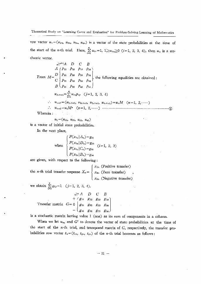
Theoretical Study on "Learning Curve and Evaluation" for Problem-Solving-Learning of Mathematrcs
row vector
the start
chastic
un = (ul
of the
vector.
From M=
u2n, u3?},
n-th trial.
~¥"+1A
A pu D p21
C p31
B p41
D pl2
p22
p32
p4 2
u4n)
Here,
C pl3
p2 3
p33
p43
4 uJ,n+1 = ~ uinpij
~=1
( u?e+1= ul'n+1'
un+1 = ulMn
is a vector of the state probabilities
~ uin=1, I~:uin:~0 (i=1, 2, 3, 4),
i=1 ~ ~ ~ pl4
p24
p34
p44
at the
then
the following equalities are obtained
(j=1, 2, 3, 4)
u2,~+1' u3,~+1' u4,~+1) u M (n 1 2,・・・・・・)
(n=1, 2,・.....)
Wherein :
ul=(ull' u21' u31' u41)
is a vector of initial state probabilities.
In the next place,
P(xi~ I A~) =gil
when P(xi~lD~)=gi2 (i=1, 2, 3)
P(xi~ I C~) =gi3
P(xin I B~) =gi4
are given, with respect to the following :
xl~ (Positive transfer)
the n-th trial transfer response X~ = x2~ (Zero transfer) ,
x3~ (Negative transfer)
we obtain ~gij=1 (j=1, 2, 3, 4).
i=1
n¥n A D C B + gu gl2 gl3 gl4
Transfer matrix G= O g21 g22 g23 g24
- g31 g32 g33 g34 is a stochastic matrix having value I (one) as its sum of components in a
When we let un, and G/ to denote the vector of state probabilities at
the start of the n-th trial, and transposed matrix of G, respectively, the
babilities row vector tn = (tl~' t2~, t3~) of the n-th trial becomes as follows :
time of
un is a Sto-
・R
column.
the time of
transfer pro-
- 21 -

Proceedings of the Institute of Natural Sciences (1979)
gn g21 g31
t unG (ul~' u2la, u3n, u4n) gl2 g22 g32
gl3 g23 g33
gl4 g24 g34 Wherein :
tln, t21~, t3~ are the probabilities of positive, zero, and negative transfers, respectively,
to take place in the n-th trial, and ~ ti~=1.
i=1
Further detailed illustration concerning Figs. 13, 14, 15, and 16, are shown in Figs.
18, 19, 20, and 21.
¥/ O tZrearnosfer ~pA'n+1 positive 1
A i_ Tg~/// tproasnl:t}evre___1 C;E+1 10 transfer~~~lPE;$+1 ' n POsitive ¥;¥;~1;F transf er
¥ Nega ~ _ Positive ¥:~1c A ~r?¥ Liransferlb¥/r ~~~a- _1__EH)Dn+1
¥N.ega J~'/ ~ transfer tive transfer ~ trve
Fig' 18. transfer gn +g31 =a' gn =:a(1- b) +ab(1- c), g31 :=abc
Positive 1 Fig. 19. transfer~Bn+1 Positive/,_._~positive positive
transf er ~¥_ Il-e Cs trans- I -g'l3 1 / transfer j ~L// +1 /~~2~~j/~( f er
Zero g2s Zero T ~¥Negative B ¥Negative I Dn+1 --~) transf er
transfer transfer g~3 and l-g~3 under arrow mark
are probability. gl3 g'l3 =1-~ ~~3 =de. gi3(1-gl3)+g23+g33=d, gl3(1-gl3)+g23=d(1 e)
Fig. 20. positive l/~/ transfer ¥1
1 ~'~"///g;4~ ' ~P~~~Oero ¥
~s T ~~+i ¥~,C'~~~~~ ¥¥atransfer /
Nega-tive transf er
Zero 1~~ ~~i transfer
D4+1 D I ~ie~/g~sNegativeJ)/ Positive I ~;s
n~T~transfer ~ +1 ~ transfer ~;// ~?¥¥ ¥~~~~~/positive
transfer ~ ~ ~g tproaSnlst~ve~ IFC;,+1
Fig. 21. ~~ +g~2 :::1-f, gl2 =f
- 22 -

Theoretical Study on "Learning Curve and Evaluation" for Problem-Solving-Learning of Mathematics
From the foregoings, the transfer matrix G becomes as follows :
D C J; f}¥ n A + a(1-b) +ab(1-c), f , gl3, l
, g22, g23, O 1-a G=0 abc , g32, de, O
g22 + g32 = I - f gl3 + g23 = I - de
In addition, there is obtained expression R, i,e., u,~+1=ulMn (n=1, 2, ・・・・・・) with
respect to vector un of the state probabilities at the time of the start of the n-th trial
and transition matrix M. When we let ul' u2, u3 replace therr sufiix so that they
become uo, ul' u2, ' " " ', respectively, in order to calculate Mn the same as n the case
'of (ii), as follows :
ul~~u0=(ulo, u20, u30, u40)
u2~~ul=(ull' u21' u31' u41)
u3~~u2=(ul2, u22, u32, u42)
then, expression C becomes u~=uoM" (n=0, 1, 2,......). Let us calculate M" by means
crf z-transformation t(z) in the same logic as in the case of (ii).
Firstly, from expression @ determinant I E-zMl (however, E is a unit matrix of
4th degree) becomes as follows :
1-z(1-a), , -zab(1-c), -za(1-b) - zabc
, I = z(1 -f ), -zfg , -zf(1 -g) O l E - ZMI , _ zde , I - zd (1 - e), - z(1 - d)
O
O
(1 z(1 a))(1 z) I ~(d(1-e)+(1-f) = - - - { ~-+ v(d(1 e) (1 f)) +4defg)z}
>< {1-~(d(1 e)+(1 f) V(d(1 e) (1 f)) +4defg)z} 1
here, by plitting as follows :
Q E E - zM,
1 = ~(d (1 - e) + (1 f ))2 + 4defg), -f) + v(d(1 -e) - (1 -
p E ~(d (1 - e) + (1 -f ) - V(d(1 - e) - (1 - f ))2 +4defg)
determinant Q becomes as follows :
I Q = (1- (1-a)z)(l-z)(1- ~z)(1- pz).
Also, when cofactor matrix R of Q is put
~ 23 -

Proceedings of the Institute of Natural Sciences (1979)
41 A21 A31 A41
R = A12 A22 A32 A42
A13 A23 A33 A43
A14 A24 A34 A44
41=(1-z)(1-1z)(1-/tz), A12=0, A13=0, A14=0
A21 = (1 - z) {abcz + abd (e - c)z2} ,
A22 = (1 - (1 - a)z) (1 - d(1 - e)z) (1 - z),
A23 =dez(1 -z)(1 - (1 -a)z), d24 =0,
A31 = (1 - z) {ab(1 - c)z + ab pz2}
here, p E cfg - (1 - f ) (1 - c)
A32 = (1 - z) U~gz - fg(1 - a)z2} ,
A33= (1- (1-a)z)(1 - (1 -j)z)(1 -z), A34=0
A41 = a(1 - b)z + apzz + aaz3
here, p ~ b(1 - c) (1 - d) + bcf(1 -g) - d (1 - e) (1 -b) - (1 - b)(1 - f),
a =bcfg(1 - d) + b(1 - c)f(1 -g)de + d (1 - e) (1 - b) (1 - f ) - (1 - b)fgde
- (1 - f )b(1 - c) (1 - d) - d (1 - e)bcf(1 - g)
A42 = (1 - (1 - a)z) (fi(1 -g)z+fez2)
here, e =g(1 - d) - (1 -g)d(1 - e)
A43 = (1 - (1 -a)z)((1 - d)z + 6z2)
here, ~ =def(1 -g) - (1 - d) (1 - f )
A44 = (1 - (1 - a)z) (1 - I z)(1 - pz)
Therefore mverse matnx Q~1 of Q becomes as follows :
l , A/ oo Al A! 1-(1-a)z ' ~~l a)nzn A 21 d 31 A/41 21 ' 31 41
- I R O , , A/ , A122' A/ , A'42 Al , A! O 22 32 42 Q = 1 32
I Q I O A/ ~ A/ A/ A' Al A' O , 23 , 43 , 23, 43 , 33 33'
, O , O O , O, ;e=0
here,
here,
_ ab cz+ abd (e - c)z2 B21 A2 1
l-(1-a)z +1 = (1-(1-a)z)(1-1z)(1-pz) = -1z+1-pz
=~=0{A21(1 - a)" + B211 ~ + C~l P"} z"
A21~ ab{c(1-a)+d(e-c)} ~ (1 - a - 1)(1 - a - p) '
B21~ ab{d(e-c)+cl} C21~ ~ab{d(e-c)+cp} ~ (1=a-1)(p-1) ' ~ (1-a-p)(p-1)
- 24 -

The。reticalStudy。n“LeamingCurveandEvaluati・n’7f・rPr・blem・S・lving・Leaming・fMathematics
here,
here,
here,
here,
here,
∠’・・一(1一(鑑建離μ2)一1一(豊α)2+、隻2+・集
謡Σ{z431(1一σ)π+B31λη+Cき1μπ}が
%=O
A31一α6{(1一α)(1-6)+β},
(1一α一λ)(1一α一μ)
B・・一(呈禦元鶴・C・・そ控麦嚇甥
α(1-6)之+αρ22+ασ23』4/41コ (1一(1一σ)之)(1-2)(1一λ之)(1一μ之)
一且4・+ B4・ +C4・+D4・ 1-2 1一(1一α)之 1一λ之 1一μ之
=Σ{A41+B41(1-4)π+C41λπ+P41μπ}が π=O
A41」一6+ρ+σ_一∫(1-4+4ε一489)一・, (1一λ)(1一μ) ∫(1-4十46-48g)
恥(わ毛鴇三蹴聖≡ll一σ・
α{(1一ゐ)λ2+ρえ+σ}C41= , (1一‘z一λ)(1一λ)(λ一μ)
一α{(1-6)μ2÷ρμ+σ}正)41= (1一‘z一μ)(1一μ)(λ一μ)
∠・22一(1矯1識2)一1集+、至鴛之一慧{A22λ・+B22μπ}2π
A22一λヲ撃・B22一μ書48
∠・32一(1一λ蕊一μ之)r聾2+、弩之一温{A32λ・+B32μπ}が
A32一∫9,B32一∫9 λ一μ μ一λ
∠・4 (、碧諜携.)一、全隻+、袈+・集
=Σ{且42+B42λπ+C42μπ}9π 飢=O
A・・一て告留)一・・
B42一馨ヲ契鍔・α・一誰坊8響
∠ノ23一 伽 一A23+B23一量{A23桝B23μ牌 (1一λ2)(1一μ2) 1一λ2 1一μ之 π=o
-25一

Proceedings of the Institute of Natural Sciences (1979)
here, A23- de B23- de ~ 1-p ' p-~
_ I - (1 - f )z = A/33 A33 + = ~ {A33 1 n + I~33 pn} zn B3 3
~ (1-1z)(1-pz) ~ 1-1z 1-pz n=0 here, - I~1+pf , B33= P-1+f A33
p-1
_ (1 - d )z + ~z2 C43 B4 3 A43 A/4B_ (1-z)(1-1z)(l-pz) = l-z + l-1z + 1-pez
=~=0{A43 + B43 1 ~ + C43 pn} zn
1-d+a here A43 = =1 ' (1 - I )(1 - p) ' B43- (fl~d))(~+ i) , C43- ~ {(1-d);/+ a}
- - ~ (1-p)(p-A) Therefore, Mn becomes as follows :
(1-a)n, A21(1-a)"+B21ln+C2lpn, A31(1-a)n+B31~n+C3lpn,
O A221 n + B22 pen , A32 ~ n + B32/en , Mn=
A23 ~ n + B23 p " , O , A33 1 " + B33 pn ,
O O
1 + B41(1 - a)" + C411 n + D4l pn
1 + B421 n + C42 pn
1 + B431 n + C43 pn
1
Mn is a stochastic matrix having value I (one) as the sum of components in a row.
When 0<1-a<1, 0<1<1, and 0<p<1, and
lim un=u=(u, u, u, u), ~u=1
n-" 1 2 3 4 i=1 i with respect to row vector un of the state probabilities at the time of the starting of
the n-th trial,
u
u lim Mn=
n-= u ¥u
u = (~, ~' ~ ~) = (O, O, O, 1). Therefore, the vector to indicate the limiting distribution
of state possibilities becomes (O. O, O, 1) irrespective as to from which out of A, D, C,
and B the start is made at the initial state. From this, the Markov chain of model S4
- KM is a regular ergodic chain.
- 26 -

Theoretical Study on "Learning Curve and Evaluation" for Problem-Solving-Learning of Mathematics
t
1,
In the case of (iv) (S3-KM2)
The following are termed "transfer-gradient."
P(S ~+11S ^), P(So~+11S_~), P(S+"+1tS ~),
P(S_~+11So~), P(S IS ) P(S IS ) +"+1 o~ ' o~+1 o~ '
P(S_ IS ) P(So~+11S+")' P(S+"+1tS+") "+1 +" '
As have been explained, the transfer gradient is, in a smaller interval period of
time, a constant value proper (unrelated with n) to a subject (under experimental situa-
tion E2)' When the experimental situation E2 is not an ideal situation, for instanc.e,
mean value E{P(S ^+11S+")} of random var able P(S ~+11S+") wrth respect to n may
be regarded as a constant value to correspond to P(S_^+ilS+")' Same consideration may
be employed to others.
Now, tree diagram expression of the transition of state makes Figs. 22, 23, and 24.
as follows :
Fig' 22. S-n+1
S ~ +n+1 1 ~~~~~r~~l~~J S 1~)o/b son+1
a -S -n~ forcernent
Transition from S_' S is in a state others
else than S_ 1, a, b, and l-b above arrow
mark are probability'
Fig. 24. Son+1 Ve
Son S I S + n+1 1 ~~~r~lc -U~~E~~1 Transition from So. S is in a state others else than S_ and So. c, l- c, and I above arrow mark are probability.
Fig. 23.
l S+nlp ~~-S+n+1 Transition from S+ '
The numeral I above the arrow mark is a probability.
*=*. ,= I - ~
' r)
1_. / ~¥"
Transiticn of state under S 3-KM2'
Here, P(S_~+11S ) I a P(S+n+11S_~)=a(1-b), P(So~+11S_~)=db,
P(S+"+11S+")=1 P(Son+11So~)=1-c P(S IS )=c ' ' +"+1 o~ ' When we let the components of transition matrix M of state denote pij (i, j=1, 2.
3),
- 27 -

Proceedings of the Institute of Natural Sciences (1979)
n¥n+1S_ So S+ n¥n+1S_ So S+ S_ [pll pl2 pl31 S_ [1-a, ab, a(1-b) M=S Lp21 p22 p23J J
=S [ O , 1=c, c S+ p31 p32 p33 S+ O , O , 1
This M is entirely the same in its from as the transition matrix M of states in S3 -
KM1' Therefore. Mn becomes as follows :
ab a - ab - c ab (1 - a) n, {(1-c)n_(1-a)"}, 1+ (1 - a) n + (1 - c) "
a-c c-a c-a M"= O , (1 - c) n , 1 - (1 - c)n
O , 1
In the next place, we let Sn denote the state at the time of the start of the n-th
trial. Also, the process, in which presentation of problems is made, the response whether
or not the problem be solved arises and an external reinforcement is extended by the
experimenter, is considered to be a process of reinforcement. Now, we let T denote
this process. In addition, we let Xn denote the response in the n-th trial (in more
details, the problem-solving-response whether or not the problems be solved after the set
and transfer are made in execution of the n-th trial).
Model of State-Movement
Sn !
Problem
presentation
f (Stimulus)
J
Res ponse
Provided
means of
X~ whether or not the problems be solved after a set and transfer.
that the subject's transfer attained through self-reinforcement by
the problem-solving-training of the test itself be included.
J
External reinf orcement extended by the experimenter
Problem-solving-response
and x3n denote the value of
values is made to arise each
!
i S~+1
Xn consists of three alternatives.
the three alternatives, respectively,
time a trial is conducted with the
- 28 -
When we let xl~' x2n,
any one of the response
following contents :
f

~~
,
~t
Theoretical Study on "Learning Curve and Evaluation" for Problem-Solving-Learning of Mathematics
l xln (When problems are solved. )
X,1 = I x2n (When problems are not solved despite the problem-solving going on. )
x3?s (When neither problem-solving goes on nor the problems are solved. )
X., (n=1, 2,......) rs a random vanable while senes of response {X1' X2""-'} is a
stochastic process.
P(x,nlS_n)=hil (i=1, 2, 3)
Now P(x~nlSon)=hi2 (i=1, 2, 3)
P(x~nlS+n) hi3 (i=1, 2, 3)
are put, and are called "conditional probability of problem-solving-response." As have
been explained, conditional probability of problem-solving-response is, in a smaller inter-
val period of time, a constant value proper (unconcerned with n) to the subject (under
'experimental situation E2)' When the experimental situation E2 is not an ideal situat-
ion, for instance, the mean value E {P(xlnlS+n) } of the random variable P(xln I S+") = hl3
relative to n may be regarded as a constant value to correspond to P(xln S+")' Same
consideration may be employed concerning others.
n¥n S_ So S+ (Sol.) [hn hl2 hl3 J
Now, H= (Pro. ) L h21 h22 h23 is called a "problem-solving-response matrix. "
(Non.) h31 h32 h33
~]i3 Ihij=1 (j=1, 2, 3), in other words, the sum of components in a column of H is 1
(one), and its every component is less than I and non-negative.
In the meanwhile, when we let v~=(vlf}' v2n' v3~), and H/ denote row vector of
state probabilities at the time of the start of the n-th trial, and the transposed matrix
hll h21 h31 of H, respectively, row vector s (sln' s2~' s3n) = vnH! = (v J f
1~' v2?~' v3n)[hl2 h22 h32
hl3 h23 h33 is called a stochastic vector of problem-solving response for the n-th trial.
The component sin (i = 1, 2, 3) of sn is
= P(Xn = xin) = P(xin I S_n) P(S_?~) + p(x~'e I So~) P(Son) + (x~n I S+n) P(S+?~) st?~
=htlvln+ht2v2n+hi3v3n (i=1, 2, 3)
I)rovided that the probability that the state Sn at the time of the start of the n-th trial
is S_ is expressed as P(S_n) = vln' when the same is So rs expressed as P(Son) = v2?~' and
when the same is S+ is expressed as P(S+n) = v3n'
It needs no saying that vln' v2n' and v3n are non negative and hold i~*i vi?}=1.
sln' s2?}' s3n are, respectively the probability for problem-solution, solving-progress,
- 29 -

Proceedings of the Institute of Natural Sciences (1979)
and non-solution (These are called, mean probability of solution response, mean probabili-
ty of solving-progress response, and mean probability of non-solution response, respectively.
of problem-solving. ) to take place in the n-th trial. Of course, ~ sin = I is held.
i=1
hn = P(xln I S_n) hl2 = P(xln I So~) hl3 = P(xll} i S+n) = 1 f
Now, I h21=P(x2nlS_?e)' h22=P(xznlSo~), h23=P(x2nlS+n) =0 hB1=P(x37~ IS_1~) h32=P(x3n Son) I h33=P(x3?~ S+n) =0
hll + h21 + h31 = 1, h 12 + h22 + h32 = 1.
n¥n S_ So S+ (Sol.)fhll hl2 Il
Therefore, H=(Pro.)Lh21 h22 OJ ~ hil=1, ~ hi2=1
I i-1 i=1 (Non.) h31 h32 O
Section 5. Learning Curve of Problem-Solving-Learning of Mathematics
Mean probability of positive transfer response tl'e in problem-solving-learning of
mathematics can be considered as follows : As it can be considered to be the response
that the ability of problem-solving (in problem-solving) takes positive transfer, it can be
construed that the probability tl~ of the response thereto is expressed by the probability
of the ability of problem-solving. The curve expressed by tln is termed problem-solving-
ability curve. Also, mean probability of solution response sl~ is considered to express the
probability of the response that problems are solved. The curve expressed by sln is
termed problem- solution-curve. Here, n is assumed to be a non-negative real number of
1 (one) or more when the curves of tl~ and sln are taken into consideration.
In the following, there are explained about the equations of the curves of tln and
sl~' and the evaluating method from the curves :
(1) In the case of S2-KM
Here, in this case, the symbols and results explained in the case of (i) (S2 - KM).
in the foregoing 4th Section, are employed as they are.
When a start is made from non-solution state ~~ of the problem with respect to
vector u~ of state probabilities at the time of the start of the n-th trial, and transition
matrix M of state,
b"-1 1 - bn-l -1 = , [ : l n=ulM" (1 O) u I =(bn-1, 1-b"-1). O
Now, when a start is made from solution state B of the problem.
bn-1 1 - bn-1 ' J 1 -= , [ , un=uMn I (O 1) I (O, l) O
- 30 -
,,
li
~~

Theoretical Study on "Learning Curve and Evaluation" for Problem-Solving-Learning of Mathematics
Therefore, model S2 - KM is a model applicable to a case of starting from ~.
Now, Iet us suppose that a start is made from B. The stochastic vector tn of trans-
fer response in the n-th trial with respect to transposed matrix G/ of transfer matrix G
is,
tn=(t t t3n)=uG (bn 1 1 bn-1) 1-b, g21' g3l] = -, - [ In' 2n' n 1 , O, O
=(1-bn, g2lbn-1, g3lbn-1), g21+g31=b.
f tln = I - bn (Mean probability of positive transfer response. )
t2n=g2ibn-1 (Mean probability of zero transfere response. )
1 t3l~ =g3ibn-1 (Mean probability of negative transfer response.)
g21+g31=b (Provided that 0<b<1) Here, Iet us consider the following three functions :
y+(x) ~ I - bx (O~x) ' " " " ' ' " " - ' (~) yo(x) ~~g2lbx-1 (o~:x) " " " ' ' " " " "~ y-(x) ~~g3lbx-1 (O~x) " " " " - " " -@ g21+g31=b (0<b<1)
The curve in the expression (~) is called a mean positive-transfer-response curve
(This is a problem-solving-ability curve. ). Also, the curve in the expression R is called
a mean zero-transfer-response curve, while the curve in the expression @ is called a
mean negative-transfer-response curve. In the meantime, t2n is considered to be the
probability for guessing to work in the n-th trial. The probabilities for the guessing
both to work and not to work are ~t2n' respectively. Therefore, tln+~t2n is the ap-
parent probability with which positive transfer response takes place in the n-th trial.
Also, t3n+ ~ t2n is the apparent probability with which negative transfer response takes
place in the n-th trial. Let us consider, at this moment, the following two functions
from expressions (~), ~, and @ :
z+(x) ~~y+(x) + ~ yo(x) =1 -bs;+ ~ g2lbx-1 = I - 1 - g21)bx-1 = I - abx-1 ( b ~'
z_(x) ~y-(x) + 12 yo(x) =g3lb~r-1 + ~g2lbx-1 = I g21)bx-1 ( g31+ ~
= (b I ¥ - g21)bx-1 = crbx-1 ~~
provided that a ~ b - ~g21'
z+ is considered to be a probability, O~z+~1. Therefore, a~0. Also, b and
g21 are probabilities, therefore, (~ has its maximum value when b = l, g21=0, then (~~1,
therefore O~o(~1. From all these,
- 31 -

Proceedings of the Institute of Natural Sciences (1979)
!z+(x)=1-abx-1 .........'............"""""""""""""""""""""""'~)
z_(x)=abx-1 "_"""""_""_"' la=b-~g21' O~a~1
The curve in expression ~ is called an apparent mean-positive-transfer-response-curve,
while the curve in expression C is called an app~trent mean-negative-transfer-response-
curve.
Also,
1 z+ ~y+ = (b - a)b;~-1 = ~g2lbx-1
1 y+(x) = z+(x) - (b-a)bx-1= * (x) -~g2lbx-1 ".' """"'@
z_ - y- = ((~ -g31)bx-1 = ~ g2lbx-1
y- (x) =z_ (x) - (b - (r)bx-1 = z_(x) - ~g2lbx-1 " " " " _ _ 'C
l (b-a)bx-1, Tg2lbx-1 are called a correctron term
In addition, when we express the values of y+' yo, y z+' and z_ in per cent, the
following are obtained :
! Y+ E~ 100y+ = 100(1 - bx)
Yo ~ 100yo = 100g2lbx-1
l Y_ ~ 100y- = 100g3lbx-1
+ ~~ 100z+ = 100(1 - abx-1) Z _ ~ 100z_ = 100cYbx-1 Z
What thinking-training is to thinking-learning is what reinforcement (for example,
to inform correct answer after each trial in paired-associates learning) is to rote learning.
Therefore, the expressions of y+' yo, y-, z+' z_, Y+' Yo, Y_, Z+' and Z_ of the above-
mentioned can be applied to rote learning. In addition, it is easy to experiment in rote
learning because to transfer positively is equal to make a true answer, while, to transfer
negatively is to make a Lalse answer directly.
Now, Iet us suppose that one hundred subjects of almost same brain level are sub-
jected to have paired-associates learning. (In the case of only one subiect, consideration
may be made in which the number of paired associates is taken for 100. )
In the n-th trial, when we express the rate of the subjects who make true answer
as Pn (true-answer), and express the rate of the subjects who make false answer as P7'
(false-answer), the following expressions are obtained :
~ 32 -

Theoretical Study on "Learning Curve and Evaluatlon for Problem Solvmg Learnmg of Mathemat cs
Px (true-answer) =z+(x) =1 - abx-1 .....
Px (false-answer) = z_(x) = (rbx-1 . .. . . . . . ........@
0~(x~:~1 ; x=1, 2,......
In 1966, R.E. Hilgard and G.H. Bower24) proved through experiments provided that ((
- ~ the correctness of the expressions of both R and @. Nevertheless, the two expre-
ssions C and R are the expressions which indicate to the last the probability
concerning apparent true-answer and apparent false-answer, respectively. The probability
of both genuine true-answer and genuine false-answer can be obtained as follows from
expressions @ and C, respectively :
y+=Px (true-answer)-(b-a)bx-1
=P(e (true-answer)- ~g2lbx-1 (x=1, 2,......) ........C/
y-= Px (false-answer) - (b-of)bx-l
=Px (false-answew)- ~g2lbx-1 (x=1, 2,・.・...) ........................ @l
Generally, the test problems that are scored by an electronic computer are essentially
O - X type test problems. In addition, to observe the learning-effect (indicated by pro-
babilities) from O - x type test is in itself considered to be an observation of the learn-
ing-effect (indicated by probabilities) in paired-associates learning. Therefore, an ap-
parent learning-effect is obtained without genuine learning-effect when a learning-effect
(indicated by probabilities) is observed by means of a result scored by an electronic
computer.
The genuine learning-effect (indicated by probabilities) is the remnant after sub-
1 traction of the correction term, (b - a)bx-1, or -g2lbx-1 from this apparent learning-effect 2
(indicated by probabilities). This is calculated by expressions R! and @/.
In the next place, explanation is made on evaluation 0L problem-solving-ability in
the following :
Firstly, as will be understood from Figs. 1, 2, 4, and 5, with model S2 - K.~4:, prob-
lem-solving-response corresponds to positive transfer response and problem-unsolving-res-
ponse corresponds to other else transfer responses (zero transfer and negative transfer
responses) than positive transfer responses. Then, in this problem-unsolving responses,
there are included problem-unsolving-responses that corresponds to zero transfer responses.
In other words, the problem-unsolving-response (expressed in probability) that corresponds
to this zero transfer response (expressed in probability) can be construed as that "The
subjects' probability to make guessing has mixed into the problem-unsolving-response
- 33 -

Proceedings of the Institute of I~]Tatural Sciences (1979)
(expressed in probability) corresponding to other else transfer responses than positive
transfer responses in a form of problem-unsolving-response (expressed in probability)
corresponding to zero transfer response (expressed in probability) taking the chance in
which model S2-KM was used. ".
From the foregoing, the following can be considered when model S2 - KM rs used
in the x-th trial :
"Apparent mean-positive-transfer-response (expressed in probability) z+(x) " = "ap-
parent mean-problem-solving-response (expressed in probability) Px (true-answer)", while.
"apparent mean-negative-transfer-response (expressed in probability) z_(x)" = "apparent
mean-problem-unsolving-response (expressed in probability) P* (false-answer)". As a
result, so far as model S2-KM is used, expressions, R, R, R', and @' hold, respecti-
vely, in an identical form both to problem-solving-learning of mathematics and to paired-
associates learning. (Provided the values of the constants, b, (x, and g21' that are used
in the four expressions are generally different by the learning type thereof. )
dy d2y+ Now, with expression (~), i,e. y+(x)=1-b" (0<b<1), + = _b"logb, dx dx2 = - (log b)2bx
O (x = O) y+(x)= 1-b (x=1)
(x~> + co) 1
- Iogb > o (x = O) d 2 y d y :L<0 (O~(x) + = _blogb>0 (x=1) d x
O (x~+oo) Therefore, the curve (i.e., problem-solving-ability curve) L expressed by y+(x)
- 34 -

Theoratical Study on "Learning Curve and Evaluation" for Problem-Solving-Learning of Mathematics
= I - b" becomes as mentioned in Fig. 26.
W(X)~~ 'jO y~Cx)dx I Cx ~ ~ JO (1 - b")dx
1 1 - b" 1-b x+ =1+ =1+ y+(x) = ( *) 10gb x xlogb xlogb w(x)=1+ 1-b" y+(x) xlogb =1+ xlogb "~~ """"C
w(x) is considered to be the average of the problem-solving-ability that have been
accumulated prior to the x-th trial, and is called mean faculty of solving problem in the
x-th trial.
d 1 - b" ~(1 - bx) limw(x)=1im(1+ =1+1im dx =1-limbx=0, )
xlog"b *~o dx (x logb)
lim w(x)=1, dw b xb logb-1 r-+* dx ~ x210gb
x ddx x b" lim xb" b- = d b-ie logb =0 = Iim * Iim lim *-+* "-+- *-+~ '-+- ~
d x
d (b~-xbxlogb-1) lxl_,moddwx =1im b~;-xb"logb-1 =1im dx
x2 Iog b d *~o x-o - -(x2 Iog b ) d x
d ( - xb x log b) =1im ~xb"logb =1imJlx .-o 2x .~o d (2x)
d x
- (logb) Iim(b' + xb"log b) = -x-o
lim dw = Iim b"-xb'logb-1 _O '-+- dx x-+= x210g b
Therefore, the curve (or the mean-faculty-curve of solving problm) L/ expressed by
w(x) becomes as shown in Fig. 26.
Percentage expression of the value of w(x) is, from O < w(x) < 1, as follows :
W(x)~100w(x)=100(1+ 1-bx _ y+(x) ) ) 100(1 + x log b ~ x log b
Now, b in expressions R and C, and accordingly the problem-solving-ability curve
L, and mean-faculty-curve of solving problem L! depend upon the difficulty level of the
problems presented to a subiect. Therefore, b is determined by the experiment to be
conducted using a number of basic problems arranged in one same difficulty level (This
is called "criterion problems".).
- 35 -

Proceedings of the Institute of Natural Sciences (1979)
With respect to b that is determined in this way, expressions ~) and C (or curves
L and L') to correspond to a subject are determined. Therefore, a subject is evaluated
with the value y+(1r) (or w(1F)) of y+(or w) in the trial x=1T (constant). (Refer to
Fig. 26.) In the actual case, Y+(1T)=100y+(1T), W(1c)=100w(It) are used, then
Y+(1~), and W(1r) are called problem-solving-ability with respect to trial It, and mean
faculty of solving problem with respect to trial lz, respectively. Also, 1~ is called "cn
terion trial".
(2) In the case of S3-KM1
Here in this case, the symbols and results explained in the case of (ii) (S3 - KM1)
in the preceding Section 4, are used as they are.
When a start is made from state A of the time 0L presenting problems with respect
to vector u~ of the state probabilities at the time of the start of the n-th trial, and
transition matrix M of state,
u =uMn-1_ (1-a)n-1, aabc { }, n I ~( _ (1 - c)n-1 _ (1 - a)n-1
a-ab-c ab ) (1-a)n-1+ c -a (l-c)n-l 1+ c-a
It is clear that model S3 - KMI is the model applicable for a case in which start is
made from state A.
Now, suppose that a start is made from state A. The stochastic vector tn Of trans-
fer response in the n-th trial with respect to transposed matrix G/ of transfer response
matrix G is,
t =(t t t3n)=u G n In' 2?e' n =(1+c-a+ab ab (1-c)'e, (1 - a)1~ _
a-c a-c 1 a abg22 (1 a)n-1+ a-c abg22 (1 - c)n-1 ( ~ ~a-c) ~
ab abg32 (1 a)n-1+ aabg3c2(1-c)n-1 ( ~ a-c ) ~ - ) g22 +g32 = I - c
Theref ore,
c-a+ab ab tln = I + a - c (1 - a)n_ (1 - c)n a- c
. . . . . .Mean probability of positive transfer response
t2n= 1-a- abg22 (1-a)n-1+ a-c abg22 (1 - c)n-1 - ) (
a c ......Mean probability of zero transfer response
- 36 -

Theoretical Study on "Learning Curve and Evaluation " for Problem-Solving-Learning of Mathematics
t3n= ab- abg32 (1-a)n-1+ a-c a bg32 (1 - c)n-1 - ) (
a c . . . . . .Mean probability of negative transfer response
g22 +g3z= I - c
Here, Iet us take the following three functions into consideration :
! + , e ~ e ex_ ab r~e (O~x) """ """"'C y (x) 1+ c a+ab a-c a- c
abg22 x-1+aabgc22Tx-1 (O~x) "" ( ) yo(x) -a-c
f y (x)- ab aabg3c2 x 1+ aabg3c2rx-1 (0<x) ' """ " ""' _ =( - _ )e ~ _ = " ' """ ' ...~
where, eEl-a, rE1-c, 0<e<1, 0<T<1, g22+g32=r. The curve in expression C is called mean positive-transfer-response curve. (This is
a problem-solving-ability curve).
The curve in expression ~) is called a mean zero-transfer-response curve. Also, the
curve in expression ~ is called a mean negative-transfer-response curve. yo(x) is the
probability to make guessing. The probabilities for the guessing both to work and not
to work are equally ~ yo(x), respectively.
Therefore, from expressions, C, ~), and ~), the equation of 'capparent mean-positive-
transfer-response-curve" is as follows :
z+(x) ~~~ y+(x) + ~ yo(x)
=1+ e (c - a+2ab)- abg22 ex-1 ab(r +g32) rx-1 """"~) 2(a - c) ~ 2(a - c)
Also, the equation of "apparent mean-negative-transfer-response-curve" is as follows :
z_ (x) s y_(x) + ~ yo(x)
x 1+ ab(r+g32) rx-1 """~) = (a-c)(e+2ab)-ab(r+g32) e ~ 2(a - c) 2(a - c)
Also,
1 y+ (x) = z+ (x) - ~ yo (x)
1 y_(x) = z_(x) - ~yo(x) " " " ~; Here,
ly (x) I e abg22 ex-1+ abg22 rx-1 o = (~ ) ~ ~ a- c 2(a - c) 1 yo(x) rs called a correction term
~ - 37 -

Proceedings of the Institute of Natural Sciences (1979)
As will be understood from Figs. 10, 11, and 12, with model S3-KM1' the mean
positive-transfer-response y+ (expressed in probability) added with the probability ~ yo
for the guessing to work becomes mean problem-solving-response (expressed in probabili-
ty) P* (true-answer), as the problem-solving-response is corresponding directly to positive
transfer response.
Theref ore,
"apparent mean-positive-transfer-response (expressed in probability) z~(x) "
= "apparent mean-problem-solving-response (expressed in probability) P* (true-answer)".
From this and expression ~),
~ (c - a+2ab) - abg22 ex-1_ P* (true-answer) =1+ ab(r +g32) fc-1 ........~/ 2(a - c) 2(a - c)
Now, the curve L expressed by expression C or
y (x) 1+ c-a+ab e" ab a-c r" a-c
is a problem-solving-ability curve.
Here. O~x, y+(O) =0, Iimy+(x) =1. *~ "
Theref ore,
mean faculty of solving problem w(x) in the x-th trial is
IC" l+c-a+abax ab rx)dx 1_~x = ( w(x) = x Jo y+(x)dx x Jo a- c a- c
_lJ c-a+abC" ab C;~ lx+- a-c Jo exdx a-c Jo rxdx} x
_ (c - a + ab)(ex_1) ab(r"-1) x(a - c) Iog e x(a - c) Iog T
_ (c -a+ ab~(~'-1) _ ab(rx_1) (0<x) """"~~~ w(x) - I + x(a - c) Iog a x(a - c) Iog r
Here, Iimw(x) =0, Iim w(x) =1.
*-o *-+-The curve L! expressed in expression ~) is a mean-faculty-curve of solving problem.
With respect to criterion problems and criterion trial IT, the values of the problem-
solving-ability Y+(1T), and of mean faculty of solving problem W(11:) are determined
from expressions R, and ~), respectively, so that evaluation of the subject is made pos-
sible. Here are Y+(1c)~~lOOy+(1T), and W(1T)~~100w(1r), in which both the y+(I~),
and w(1T) are expressed in per cent, respectively.
(3) In the case of S4-KM
Here in this case, the symbols and results explained in the case of (iii) (S4 - KM)
in the foregoing Section 4 are employed as they are. When a start is made from state
- 38 -

Theoretical Study on‘‘Leaming Curve and Evaluation・・for Problem-Solving・Leaming of Mathematics
A of the time of presenting problems with respect to vector%箆of the state probabilities
at the time of the start of theπ一th tria1,and transition matrix M of state,
砺一窃、1ゆ一1一((1一α)%一1,∠42、(1一σ)π一1+B2、2π一1+C2、μπ一1,
・43・(1一α)%一1+B3、λπ一1+C3、〆1,1+B4、(1一α)刺+C4、λ“1+D4、〆ユ)
It is clear that model S4一κM is the model applicable for a case in which start is
made from state A。
Now,suppose that a starHs made from state且.
The stochastic vector砺of transfer response in the n・th trial with respect to trans・
posed matrix C/of transfer matrix G:is,
命一(翫,孟2η,餓)一砺Gノ
ー(1+(α一⑳o+∫五2、+9、3且3、+B4、)(1一α)π一1
÷(∫B2、÷9、3B3、+C4、)λ%一1+(∫C、、+9、3C3、+D4、)μπ一1,
(1一α+922A2、+923A3、)(1一α)箆一1
+(922B2、+923B3、)え%一1+(922C2、+923C3、)〆1,
(妨o+932.42、+4話3、)(1-4)η一1
+(932B2、+46B3、)λ隅一1+(932C2、+46C3、)μπ一1)
Here,922+932=1一∫,9、3+923-1-48
Therefore,
娠一1+(α一⑳6+∫A2、+9、3A3、+B4、)(1一α)烈
+(∫B2・+9・3B3、+C4、)許一1+(fC2、+9、3C3、+P4、)μ魍
≠2ず(1一α+922A2、+923/13、)(1一α)%一1
+(922B2・+923B3、)λη一1+(922C2、+923C3、)μπ一1
輸一(励6+932A2、+48!13、)(1-4)π一1
+(932B2、+ノθB3、)λπ一1+(932C2、+づ8C3、)μπ一1
Here,孟1π,渉2児,and診3πare mean probability of positive transfer response,mean pro・
bability of zero transfer response,and mean probability of negative transfer sesponse,
τespecti▽ely.
Here,1et us take the following three funct圭ons into consideration:
ツ+(灘)…1+ε一1(α一α60+μ2、+9、3且3、+B4、)εの
+λ一1(∫B2、+9、3B3、+C4、)君+μ一1(fC2、+9、3C3、+D4、)グ……⑳
ツ・(詔)≡(1一α+922且2、+923且3、》一工+(922B2、+923B3、)λ坦
+(922C2、+923C3、)μの一1・………一……・……一………ひ……一⑳
』y一(躍)≡(⑳o+932A2、+48z43、)εの一1+(932B2、+48.B3、)λの一1
+(932C2・+46C3、)μ詔一1…・一…一一…・一……………・…・⑳
Hereシ0≦z,ε≡1一α,0<ε<1,0<λ<1,0〈μ<1,922+932-1-f,
913+923-1一‘!8.
一39一

Proceedings of the Institute of Natural Sciences (1979)
The curves in expressions, ~}, ~, and ~) are called mean positive-transfer-response
curve, mean zero-transfer-response curve, and mean negative-transfer-response curve,
respectively. The mean positive-transfer-response curve is problem-solving-ability curve
L. yo(x) is the probability to make guessing. The probability of guessing both to
work and not to work is 1.=2 yo(x), signifying that the probabilities for the guessing both
to work and not to work are equally ~ yo(x), respectively.
Therefore, from expressions, ~), ~~, and ~, the equation of "apparent mean-positsve-
transfer-response-curve" is as follows :
1+a 22abc + 2f~g22 A21 z (x) y (x)+~yo(x)=1+{ --I
+ l-de+gl3 l A31+ B41J ex-1 2
+ 2f~g22B21+ l-de+gl3 B31+C41}1x-1 {
2
f 2f +g I -d e +gl3 + 1~L:~~C21+ C31+D41} px-1 """" """"'~ t 2 2 --
Also, the equation of "apparent mean-negative-transfer-response-curve" is as follows :
z_ (x) ~~ y_(x) + ~yo(x)
1 a~2abc + 1-f2+g32 A21+ 2de +g23 l ={ - A3lf e :~'~1
2
+ 1-f+g32B21+ 2de+g23 B31J1'e-1 {
+ 1-f+g32C21+ 2de+g23 C31}px I ........~ {
2 2
In addition,
y+(x) =z+ (x) - I yQ(x)
~ y_(x) =z_ (x) - I yo(x) " " " "~) ~
Here I yo(x) = ~(1 - a + g22A21 + g23A31) e ~;-1 ' ~~
+ ~(g22B21 + g23B31) I x-1 + ~(g22C21 + g23C31) px-1
1 ~yo(x) is called a correction term.
As will be understood from Figs. 18, 19, 20, and 21, with model S4 - I~4:, none out
of positive, aero, and negative transfer responses do correspond direct (or at I : l) to any
of problem-solving-response, problem-solving-progress-response, and problem-unsolving-res-
- 40 -

Theoretrcal Study on Learnmg Curve and Evaluation" for Problem-Solving-Learning of Mathematics
ponse, i.e. , it is impossible to obtain any of mean positive-transfer-response (expressed
in probability), mean zero-transfer-response (expressed in probability), or mean negative-
transefer-response (expressed in probability) from the result of a test conducted with a
subject by use of model S4 - KM. Nevertheless, should the values of the constants con-
tained in expression ~ be obtained by some methods so that the value of every constant
is made known, the curve expressed by expression ~ is a problem-solving-ability curve
L. Therefore, the mean faculty of solving problem w(x) in the x-th trial becomes from
expression ~} as follows :
w(x) (a - a b c + fA21 + gl3A31 + B41)( e "- 1) = *iO x g log e y+ (x)d x = I +
+(fB21+gi3B31+C41)(1x_1) + (fC21+gl3C31+D41)(p'-1) ...R
XA Iog A x p log p Provided O <x.
The curve expressed by expression (3J2~ is a mean-faculty-curve of solving problem L/.
With respect to criterion problems and criterion trial lr, the values of the problem-solv-
ing-ability Y+(1r), and of mean faculty of solving problem W(1r) are determined from
expressions ~, and ~), respectively, so that evaluation of the subject is made possible.
Here are Y+(1:)~IOOy+(1r), and W(1r)~100w(1r), in which both the y+(I~), and w(It)
are expressed in per cent, respectively.
(4) In the case of S3-KM2
In this paragraph, the symbols and results explained in the case of (iv) (S3 -KM2)
in the foregoing Section 4 are employed as they are. If the state is S_ at the time of
starting the flrst trial and problems are presented simultaneously with respect to vector
v~ of state probabilities at the time of the start of the n-th trial and to transition
matrix M of state, the start is made, of course, from state S_, therefore, vector vn be-
comes as follows :
v^=(vl~' v2~, v3~)=vlM"-1=(1, O, O)Mn-l
=( "-1 ab {(1-c)"~1_(1-a)n-l}, (1 - a) ' a-c
_ ab 1+ a-ab-c_(1-a)" l+ (1-c)n-1)
c-a c-a Theref ore,
vll~ = (1 - a)"~1
ab v2~= {(1 - c)"~1 _ (1 - a)"~l} a- c
v3n = I + a - ab - c a b n-1 (1- c) (1-a)"~1+ c-a c-a
- 41 -

Proceedlngs of the Institute of Natural Sciences (1979)
Each of these three expressions expresses the probability of transferring from the
state at the starting of the n -th trial into negative, zero, and positive transfers, respect-
ively.
Now, in case various external events are assum.ed to cause generally undesirable in-
ner (or, for thinking action toward problem-solving of mathematics) effects, the subject
at the starting of the first trial is considered to be in S_-state, therefore it is appropriate
to start from S_ when model S3 - KM2 is used. The following three functions are, from
the afore-mentioned three expressions, taken into consideration, on the assumption that
the start is made from state S_, under the circumstances.
That is,
V-(x) ~s e (~;~1 '
~ (x) ab {rx-i ~ 1} *.'.*...R
a-c lv+(x)~l+ c-a+ab _x-1 aabc rx-1 ....................................~
a-c -Here, e~~l-a, TE1-c
In the mean while, the stochastic vector s n of the problem-solving-response in the
n-th trial with respect to the transposed matrix H/ of problem-solving-response matrix
H is as follows :
sn=(sln' s2T~' s3n)=vf;H/
1+ hll+ c-a+ab(1 hl2) (1 a) (l-c)n-1 =( { - - - Is-1 a b (1 - hl2) }
flh21 ~bh2c2 }(1 a)n-1+ a-c (1 c)n-l _ _ _ _ abh22 _ , {h31 ~bh~2 } (1 a)n-1+ (1- c)n-1) _ _ _ abh32
a-c h ll T h21 ~ h31 = 1, hl2 + h22 + h32 = l
theref ore,
sln=1+ hll+ c-a+ab(1-hl2) (1-a) 1~-1 ab(1 - hl2) (1 - c)n-1 { }
a-c a-c s 2f} = {h21 a b h22} (1 - a)n-1 + a b h22
(1 - c)n-1
a-c a-c -{h31 ~bh~2 }(1 a)n-1+ a-c (1 c)n-1 n ~ ~ _ ~ a b h32 _ s3
Each of s In' s2n' and s3n is mean probability of solution response, mean probability
of solving-progress response, and mean probability of non-solution response, respectively
in the n-th trial.
From the afore-mentioned three expressions, the following three functions are taken
- 42 -

,
Theoretical Study on "Learning Curve and Evaluation" for Problem-Solving-Learning of Mathematics
into consideration :
~l(x) ~1+ {hll+ c - a+ ab(1 - hl2) ab(1- hl2) rx-1 ~~i~~ }g x-1 ""'~~!~
~2(x) ~ {h21 a b h22 e a b h22 . . . . . . . .~ ~ } r$'~1 ... x-1 +
a-c a-c ~3(x) ~~ {h31 abh32 e abh32 . . . . . . . .R= - } rx-1 ... x-1 +
a-c a-c Here, hll+h21+h31=1 ; hl2+h22+h32=1 ;
e~1-a; r~1-c ; x=1, 2, 3,・-
Each of ~1(x), ~2(x), and ~3(x) is the probability of mean solution-response, mean_
solving-progress-response, and mean non-solution-response, respectively, of mathematics-
probleln in the x-th trial to be conducted. The curves expressed by expressions ~, R,
and ~) are called mean solution-response curve (this is a (an apparent) problem-solution-
curve K//), mean solving-progress-response curve, and mean non-solution-response curve,
respectively. The values of ~ 1(x), ~2(x), and ~3(x) are the probability including that
solved, that solution is proceeding on, and that unsolved, respectively by the guessing.
Therefore, each value of ~1(x), ~2(x), and ~3(x) can be obtained actually through
experiment. On account of this, the values of the constants such as a b c hil h21 h31
hl2 h22 h32, e , and r can be found from expressions ~), @, and ~). Therefore, the
transition matrix M of states, and problem-solving-response matrix H can be actually
found. In addition, the values of the constants included in expressions ~3)), R, and R
can be actually found. In the meanwhile, the probabilities of making, at the time of
starting the (x + 1)-th trial, negative transfer, zero transfer, and positive transfer, from
expressions ~_.'~3), R, and ~, respectively, are as follows :
~_(x)~~:~-(x+1)=8x ...,................. """R/ ab ~0(x) E ~o(x + l) = " " " "R/ {rx_ ex} ・・-a-c
c-a+ab ab ~+(x)~~~(x+1)=1+ ex_ a- c rx ........R a-c
Here, e~:~l-a, r~l-c, O~x
~_(x), r~/o(x), and ~+ (x) are the probabilities pertaining to "the state immediately
after completion of the x-th trial". Also, each of y+(x), yo(x), and y_(x) explained
with respect to models S2-KM, S3-KM1' and S4-KM in the foregoing paragraphs-
(1), (2), and (3) is the probabilities in the "responses that transfer in the x-th trial
(that is, in conducting the x-th trial)". Each of ~_(x), ~0(x), and ~+(x) is called
probability of posterior mean-negutive-transfer, probability of posterior mean-zero-transfer,
and probability of posterior mean-positive-transfer, respectively. In addition, the curves
- 43 -
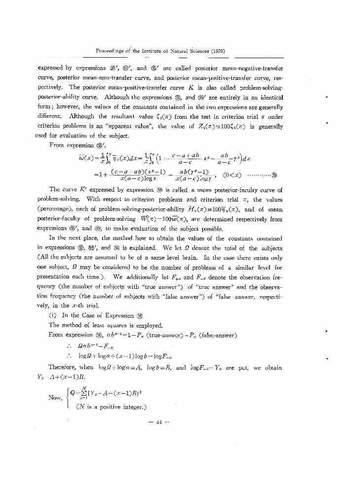
Proceedings of the Institute of Natural Sciences (1979)
expressed by expressions R/, R', and R/ are called posterior mean-negative-transfer
curve, posterior mean-zero-transfer curve, and posterior mean-positive-transfer curve, res-
pectively. The posterior mean-positive-transfer curve K is also called problem-solving-
posterior-ability curve. Although the expressions C, and ~/ are entirely in an identical
form ; however, the values of the constants contained in the two expressions are generally
different. Although the resultant value C l(I~) from the test in criterion trial 1~ under
criterion problems is an "apparent value", the value of Zl(1~)~~IOO~1(1c) is generally
used for evaluation of the subject.
From expression ~/.
w~(x)=~i0~+(x)dx 1+ c-a+ab ex ab rc)dx 1 ~* = ( ~ JO
a-c a-c =1+ (c -a+ ab)(e"-1) ab(r"-1) (0<x) ""-";-'~)
x(a- c)10g e x(a- c)logr '
The curve K/ expressed by expression R is called a mean posterior-faculty curve of
problem-solving. With respect to criterion problems and criterion trial -,, , the values
(percentage), each of problem-solving-posterior-ability ~+(1r)~sI00~+(1T), and of mean
posterior-faculty of problem-solving W~=~(1T)~IOOw~(I~), are determined respectively from
expressions ~)/, and R, to make evaluation of the subject possible.
In the next place, the method how to obtain the values of the constants contained
in expressions C, ~)', and R is explained. We let 9 denote the total of the subjects
(A11 the subjects are assumed to be of a same level brain. In the case there exists only
one subject, O may be considered to be the number of problems of a similar level for
presentation each time.). We additionally let F+" and F_. denote the observation fre-
quency (the number of subJects with "true answer") of "true answer" and the observa-
tion frequency (the number of subjects with "false answer") of "false answer, respecti-
vely, in the x-th ~rial.
(i) In the Case of Expression R
The method of least squares is employed.
From expression C, ab"-1=1-P.." (true-answer) =P* (false-answer)
Oa b"-1 = F_*
10g9 + Ioga + (x - 1) Iog b = IogF_x
Therefore, when logrl+10goi~A, Iogb~B, and logF_.~~~YX are put, we obtam
Y. = A+ (x - 1)B.
N Q E ~ { Y*-A- (x - l)B} 2 _Now, "=1
(N is a positive integer.)
- 44 -
t

,
Theoretical Study on "Learning Curve and Evaluation" for Problem-Solving-Learning of Mathematics
iS Put.
From aQ =0 aQ aA=0, and aB '
AN+ B~ (x - 1) = ~ Y(1' x=1 ~7=1
1 A~(x - 1) + 1;~v (x - 1)2 = ~(x- 1) Yx
x-1 x=1 x=1
theref ore,
theref ore,
A - (~Y*) {~(x-1)2} - {~(x-1)} {~(x-1)Y.} f -N~(x - l)2 - {~(x - 1)} 2
l B - N~(x-1)Y.- (~] Y.) {~(x-1)] ~ N~(x - l)2 - {~(x - 1)} 2
10g(x- (~Yx) {~(x-1)2} - {~(x-1)} {~(x-1)Yx} _log9 f - N~(x- 1)2 - {~(x- 1)} 2
1 Iogb - N~(x-1) Yx~ (~ Yx) {~(x-1)}
~ N~(x- l)2 - {~(x- 1)} 2
N (Here, ~ signifies ~.)
x=1
From these two expressions, the values of (~, and b are to be determined.
(ii) In the Case of Expression ~)/
The minimum x2 method used by Atkinson and Crothers25) (1964) will be used.
From expression ~/, the following expression is put :
_ (1- a)(c - a+2ab) - abg22 (1- a)x-1 P (true answer) -1+ 2(a-c)
ab {2(1 - c) - g22} _ 2(a-c) (1 c)x I p(x; a, b, c, g22)
Then,
F+x=QPx (true-answer) =QP(x ; a, b, c, g22)
= "expectation frequency for true answer m the x th tnal"
Here,
f~ {F+x~9P(x; a, b, c, g22)}2 =x (a b c, g22) N x=1 PP(x ; a, b, c, g2z) ~
Wherein : 0<a, b c g22<1
N is a positive integer.
is put, then change the possible values of parameters a, b, c , and g22 so that the
value of x2 (a, b, c, g22) is minimized, then the values of a, b, c, and g22 are deter-
mined.
- 45 -

Proceedings of the Institute of Natural Sciences (1979)
(iii) In the Case of Expression ~,.~~
The minimum X2 method will be used. From expression ~{i<_6', the following expres-
sion is put :
~1(x) =1+ {hn+ c - a+ ab(1 -hl2) .-1 } (1 - a)
a-c ab(1-hl2) (1-c)' I P(x a b c hll hl2) a-c
Then,
F+" g2~(x) !2P(x ; a, b, c h hl2) ' 11'
= "expectation frequency for problem-solving in the x-th trial"
Here,
N ~ {F+"~g~p(x; a, b, c, hll' hl2)}2 ~~ 2 X (a b, c, hn, hl2)
.=1 OP(x a, b, c, hll' hl2)
Wherein : 0<a, b, c, hll' hl2<1,
N is a positive integer.
is put, then change the possible values of parameters a, b, c, hn, and hl2 so that
the value of X2 (a b c h h 2) is minimized then the values of a b c hll and
hl2, are determined.
CHAPTER 111 GENERALIZATION
In this CHAPTER, conclusion is explained by using the symbols and results that
have been used in all the foregoing description in their original form without a change-
(1) In the case Model S2-KM is used
The case begins with non-solution state ~ of problem.
The equation for apparent mean-problem-solving-response curve L" is :
P*(true-answer) = I - ab"-1 (x = 1, 2, ・ ・ ・ ・ ・ ・)
(Here, 0<a<1, 0<b<1)
From this expression, determine the actual values of a and b.
The equation for problem-solving-ability curve L is :
y+(x)=1-b" (O~(x) The equation for mean-faculty-curve of solving problem L' is :
1 - b" w(x) = I + (O < x)
x log b
This model is suitable for problem-solving-learning that is close to paired-associates
learning.
(2) In the case Model S3-KMI rs used
- 46 -
lb

,
Theoretical Study on "Learning Curve and Evaluation" L0r Problem-Solving-Learning of Mathematics
The case begins with state A of the time of problem-presentation.
The equation for apparent mean-problem-solving-response curve L/! is :
P (true answer)=1+ e(c-a+2ab)-abg22 e"~1 ab(r+g32) rx-1 2(a - c) ~ 2(a- c)
(x=1, 2,......)
(Here 0<a b, c, e, r, g22, g32<1 e I a g22+g32 1 c r )
From this expression, the actual values of a, b, c , e , r , g22, g32 will be deter-
mined.
The equation for problem-solving-ability curve L is :
y+(x)=1+ c-a+ab e" ab rx (o~:x) a c
The equation for mean-faculty-curve of solving problem L/ is :
w(x) = I + (c - a + ab)( e "- 1) _ ab(rx_ 1) (O <x) x(a - c ) Iog r x(a - c) Iog e
(3) In the case Model S4-KM is used
The case begins with state A at the time of problem-presentation.
The equation for problem-solving-ability curve L is :
y+(x) = I + e ~1(a - a b c + fA21 + gl3A31 + B41) e "
+ 1-1(fB21+gl3B31+C41)1"+ p~1(fC21+gl3C31+D41)px (0<x)
here, 0<a, b, c, f, e, 1, p, gl3<1, eE1-a.
The equation for mean-faculty-curve of solving problem L/ is :
w(x) = I + I (a - ab c + fA21 + gl3A31 + B41)( e " - 1) x e log e
+ I ( f B21 + gl3B31 + C41) ( ~ " ~ 1) xl log 1
+ I ( fC21 + gl3C31 + D41) ( p" - 1) (O < x) x plog p
However, the values of the constants contained in the above-mentioned two expres-
sions which were introduced from the Model cannot be determined actually by the
method of using ordinary tests.
(4) In the case Model S3 - KM2 is used
The case begins with state S_ which make negative transfer.
The equation for (apparent) problem-solution-curve K/' is :
C1(x)=1+ flhu+ c - a+ ab(1-hl2) ab(1-hl2) rx-1 }e *-1
(x=1, 2,.・・・・・)
here, 0<a, b, c, e, r, hll' hl2<1 eEl-a, r~~1-c.
From this expression, the actual values of a, b, c, e, r, hll' and hl2 will be
- 47 -

Proceedings of the Institute of Natural Sciences (1979)
determined.
The equation for problem-solving-posterior-ability curve K is :
~ (x) 1+ c-a+ab e' ab r' (0<x)
a-c a-c The equation for mean posterior-faculty curve of problem-solving K' is :
w(x)=1+ (c-a+ab)(e"-1) _ ab(r"-1) (0<x) x(a - c)16g e x(a - c)log r
Throughout the above-mentioned cases of (1), (2), (3), and (4), with respect to criterion
problems and criterion trial lr, it becomes possible to evaluate the subject with the
values (in per cent) of Y+(1r)=100y+(1T), W(I~)=100w(1r), ~+(1r)=100~+(1~), '~~W(1T)
=100:~(1c), ~p* (true-answer) =100P. (true-answer), Z1(1T)=100~l(1T)' (However, it is
impossible to determine the values of the constants which are contained in the expres-
sions y+(x) and w(x) in the case (3).) Y+(~) and W(1~) are termed evaluation, ~H+(1T)
and ~W(I~) are termed post-evaluation, and ~5. (true-answer) and Z1(1T) are termed ap-
parent evaluation.
In the case models S2-KM, S3-KMl' and S3-KM2 are used, the L0110wing are
the methods to determine the values of the constants contained in the equations of ap-
parent mean-problem-solving-response curve L", and of (apparent) problem-solution-curve
K" '
Let !2 denote the total of subjects. Also, Iet F+" and F_* denote the number of
subjects of true answer in the x-th trial, and the number of subjects of false answer in
the x-th trial, respectively.
(i) In the case S2-KM is used
logoe=(~_Y){~(x l) } {~(x 1)}{~(x 1)Y} Iogl2
log b =
N~(x- 1)2 - {~(x - 1)} 2
N~(x - 1) Y. - (~ Y.) {~(x- 1)} N~(x - 1)2 - {~(x- 1)} 2
Wherein,
N ~ represents ~ Y* = IogF_.,
*=1'
N is a positive integer.
The values of a and b will be determmed from the above-mentioned two expres:
sions.
(ii) In the case S3-KMI rs used
N ~~ {F+"~QP(x; a, b, c, g22)} X (a b c, g22) (2P(x ; a J, b, c, g22) ~~
*=1
Here,
- 48 -
,

Theoretical Study on "Learning Curve and Evaluation" for Problem-Solving-Learning of Mathematics
P(x ; a, b, c, g22)E1
+ (1-a)(c-a+2ab)-abg22 (1-a)~'~l 2(a - c)
ab {2(1 - c) - g22}
-- (1 - c)x-1 2(a - c)
0<a, b, c, g22<1, N is a positive integer.
Determine the values of a, b, c, and g22 so that the value of x2 (a, b, c,
minimized through changing the values of the parameters a, b, c , and g22
within possible range.
(iii) In the case S3-KM2 is used
N {F+"~QP(x ; a, b, c, hn, hl2)}2 ~ ~X2(a, b, c, hll' hl2) pp(x , x=1 ' a, b, c, hll' hl2)
Here,
P(x ; a, b, c, hll' hl2)~l
c - a + ab(1 - hl2) (1-a)'~1 ab(1-hl2) (1- c) + {hll+ } ~-1
a- c a-c 0<a, b, c, hll' hl2<1, N is a positive integer.
Determine the values of a, b, c, hll' and hl2 so that the value of x2(a, b,
hl2) is minimized through changing the values of the parameters a b c hll'
to ones within possible range.
g22) is
to ones
c, h 11'
and h 12
SUMMARY
When the formed learning set is positively transfered to a new situation where a mathema-
tical problem is given, problem-solving will proceed ; when it is transfered negatively, problem
-solving won't proceed. Some subjects are in a state where a problem is going to be solved,
others are not in such a state. The learning sets formed by subjects may transfered positively
in some cases or negatively in other cases.
The author Inducted the concept of probablllty to Transfer and "State", and constructed
four models of S2-KM, S3-KM1' S4-KM and S"~-KM2 about problem-solving-learning of
mathematics from the theory of Markov chain. After that the author deducted equations of
important learning curves for these four models, and devised the method of evaluating learning
faculty (evaluation of problem-solving faculty to standard problems and criterion traial lr) from
these learning curves.
The theory that was titled "Models of Problem-Solving-Learning of Mathematics and Theore-
tical Study on its Learning Curves" and that was pre-'ented (through a lecture on 5th August,
1977) by Itsusuke KAWABATA as the results of his study at th 59th Grand Meeting of Japan
Society of Mathematical Education in Kanagawa, are explained in this paper. (15th April, 1978).
49

Proceedings of the Institute of Natural Sciences(1979)
LITERATURES
1)Ministry of Education,The course of study of an elementary schoo1,Printing Bureau of
Ministry of Finance,(July,1968).
2)Ministry of Education・The course of study of a lower secondary schoo1,Printing Bureau
of Ministry of Finance,(1969).
3)Ministry of Educat圭on,The course of study of an upper secondary school,P血ting Bureau.
of Ministry of Finance,(1970).
4)K Lewin,Princ1ples of Topological Psychology.New York,Mc Graw・Hi11,(1936).
5) H、F.Harlow,The formation of learning sets、PsychoL Rev.,56,51-65,(1949)。
6)H・F・Harlow,Leamingsetanderrorfactortheory,lnKoch,S.(Ed.),Psychology二A study of a science,VoL II.New York,Mc Graw・Hill,(1959).
7) HG,Birch,The role of motivational factors in ins孟ghtful problem・solving. J.comp.phy-
sioL PsychoL,38,295-317,(1945).
8) H・G・Birch・The relation of previous experience to ins圭ghtful problem-solving・ J.comp・
PsychoL,38,367-383,(1945).
9)A.S,Luchins,Mechanization in problem-solving: The e狂ect of Einstellung. Psycho1.
MonogL,54, No,248, (1942),
10) N.R F。Maier,Reasoning in human:1.On direction。J.comp。Psycho1.,10,115-143,
(1930).
11) G.Ulmer,Teaching geometry to cultivate reHect呈ve thinking:An experimental study with
1239}1igh school pupils. J.exp.E(luc.,8,18-25,(1939).
12) 1.B主aler,Primary and secondary stimulus generahzation as related to intelligence leveL J,
exp,PsychoL,62,395-402,(1961).
13) J、J,Ray,The general重zing ability of dull,bright,and superior children, Peabody ContL
Educ.,No,175,(1936).
14) H。T.Heglin,Problem・solving set in different age groups. J.Geront.,11,310-316.
(1956),
15)M S,Mayzner and M,E,Tresselt,The e鉦ect of the competition and generalization of
sets with respect to manifest anxiety.J。gen。PsychoL,55,241-247,(1956),
16)L Maltzman and L Morrisett,Effects of task instructions of d置erent classes of anagrams.
J.exp.PsychoL,45,351-354, (1953).
17)R.W.Bruce,Conditions of transfer of training、J.exp.Psychol.,16,343-361,(1933).
18)E.M.Siipola and H.E.Israe1,Habit-interference as dependent upon stage of training・
Amer、J,PsychoL,45,205-227,(1933).
19) C.H,Judd,The relation of spec主al training to general intelligence・ Educ・Rev・,36,28-
42, (1908)。
20) J.Bastian,Associative factors in verbal transfer. J.exp.PsychoL,62,70-79,(1961).
21) A,K.P.Sinha and B.Prasad,Transfer as a function of the method of丘rst・task learning,
J.gen.PsychoL,66,311-314,(1962).
22)M.S・Mayzner and M E・Tresselt,Anagram solution times:A function of letter order
and word frequency. J.exp。Psychol.,56,376-379,(1958).
23) K.Dunker,Zur Psychologie des produktiven Denkens。 Berlin,Springer,(1935).
24) R.E.Hilgard and G.H.Bower,Theories of leaming.3rd ed.Appleton-Century-Crofts.
一50一

Theoretical Study on‘‘Leaming Curve and Evaluation”for Problem-Solving-Leaming of Mathematics
(1966)。
25) R.C,Atkinson and EエCrothers,A comparison of paired・associate leaming models hav-
ing di狂erent acquisition and retention axioms,」.math.psychoL,1,285-315,(1964),
26)R R Skemp,The Psychology of Leaming Mathematics.Penguin Press,(1971).
27) K Lewin・Field Theory and Leaming. In the Psychology of Leaming.Natl.Soc.Stud.
Educ・,41stYearb・・k,PartII,215-242,(1942).
28) C.E。Osgood,The similarity paradox in human leaming:A resolution.PsychoL Rev,,
56ン 132-143, (1949).
銚%5威6KAWAB.AT且z)o,αプかπθπ診げハ4αオん6醒α≠1‘5,
ColZ6goげH謝zαπ漉θ5απ43‘∫6π‘05,MhoπU勉麗プ5勿,
3-25-40,Sα肋吻・5漉,S伽9αツα・ゑ㍑,丁吻・,」砂伽.
一51一