THEORY AND NUMERICS OF

THREE–DIMENSIONAL BEAMS WITH

ELASTOPLASTIC MATERIAL BEHAVIOUR ∗

F. Gruttmann1, R. Sauer2, W. Wagner3

1 Institut fur Statik, Technische Universitat Darmstadt, 64283 Darmstadt, Germany ,2 Ingenieurburo Jager, 01445 Radebeul, Germany,

3 Institut fur Baustatik, Universitat Karlsruhe, 76128 Karlsruhe, Germany

Keywords:Three-dimensional beams, finite deformations, torsion warping deformation, arbitrarycross sections, elastoplastic material behaviour, finite elements

ABSTRACT

A theory of space curved beams with arbitrary cross–sections and an associated finiteelement formulation is presented. Within the present beam theory the reference point,the centroid, the center of shear and the loading point are arbitrary points of the cross–section. The beam strains are based on a kinematic assumption where torsion–warpingdeformation is included. Each node of the derived finite element possesses seven de-grees of freedom. The update of the rotational parameters at the finite element nodes isachieved in an additive way. Applying the isoparametric concept the kinematic quantitiesare approximated using Lagrangian interpolation functions. Since the reference curve liesarbitrarily with respect to the centroid the developed element can be used to discretizeeccentric stiffener of shells. Due to the implemented constitutive equations for elastoplas-tic material behaviour the element can be used to evaluate the load carrying capacity ofbeam structures.

1 INTRODUCTION

Three–dimensional beam–like structures undergoing finite deformations occur in differentareas of engineering practice. Here motions of flexible beams like helicopter blades, rotorblades, robot arms or beams in space–structure technology are mentioned. Furthermore,the analysis of load carrying capacities requires the implementation of constitutive equa-tions for inelastic material behaviour. Numerous papers have been published up to nowusing different approaches. Some of them are discussed in the following.Due to the non–commutativity of successive finite rotations about fixed axes, Argyriset al.1 introduced the so–called semi–tangential rotations to circumvent this difficulty.Bathe and Bolourchi2 developed an updated and a total Lagrangian formulation for beamswith large displacements. Thin structures undergoing finite deformations are usuallycharacterized by significant rigid body motions. This motivates the so–called co–rotational

∗dedicated to F.G. Kollmann on the occasion of his 65th birthday

1

formulation where the rigid body motions are separated from the total deformation (e.g.see Belytschko and Hsieh,3 Crisfield4 or Nour–Omid5). Applying this procedure existinglinear elements can be used for nonlinear computations.Several authors developed finite element formulations for three–dimensional beams usingbeam strains derived from the internal virtual work, see Reissner.6 Here we mention thepapers of Simo and Vu–Quoc7,8 and Cardona and Geradin.9 The authors in [7] showthat the linearization of the virtual work principle yields a non–symmetric geometrictangent stiffness matrix when applying a multiplicative update of the rotation tensor. Thetangent matrix is only symmetric at a point of equilibrium assuming conservative loads.Ibrahimbegovic10 derived symmetric tangent matrices when using an additive update ofthe axial vector.Most of the finite element formulations are concerned with beams where centroid andcenter of shear coincide. The problem of coupled bending torsion deformation of beams hasbeen studied theoretically e.g. by Reissner.11,12 In Ref. [8] torsion–warping deformationhas been incorporated within the theory and the associated finite element formulation.

In this paper we derive a three–dimensional finite beam–element with arbitrary spacecurved reference axis. The novel aspects and essential features of the formulation aresummarized as follows:

(i) The introduced beam strains based on a kinematic assumption including torsion–warping deformation are conform with the strains in Ref. [8]. Here, we additionallyderive the relation to the Green–Lagrangian strains and the associated variations.In our formulation the matrix which relates the variation of the Green–Lagrangianstrains to the variational beam strains depends on the deformation. Thus the com-plete nonlinearity within the underlying kinematic assumption is considered in thepresent theory. Due to this fact the numerical results show a good agreement withthe results of higher valued models like shell discretizations for thin–walled struc-tures.

(ii) The constitutive equations for elastoplastic material behaviour are implemented.Within the present beam theory the normal stress and the shear stresses enterinto the von Mises yield condition and the associated flow rule. Thus interactionbetween the different stress components is included. The nonlinear stress–strainrelations requires a numerical integration over the cross–sections. The developedelement can be used to analyze the carrying capacity of beam structures.

(iii) For linear elasticity and small strains the material matrix can be integrated ana-lytically. For this purpose one has to apply the equations of Saint–Venant torsiontheory along with Green’s formula to integrate the so–called warping coordinates.This yields a material matrix in terms of section quantities which describes the cou-pling effects. In contrast to Ref. [8] the reference point is an arbitrary point of thecross–section.

(iv) The finite element formulation is presented using Lagrangian interpolation functions.Each node possesses seven degrees of freedom at the nodes. The update of thenodal rotation quantities is performed in an additive way. Within this procedureadditional storage of the rotation matrix with nine parameters can be avoided. Thelinearization yields a symmetric tangent matrix. However, due to the chosen finite

2

element approximation the expressions are essentially simpler compared with Ref.[10]. The external loading can be applied at an arbitrary point of the cross–section.The contribution of the loads to the stiffness matrix is derived. Loading with stresscouple resultants leads to a symmetric load stiffness matrix. This is in contrast tothe multiplicative procedure, see Ref. [7].

The contents of the paper is outlined as follows:In the next section we present the kinematics of a space curved beam. The beam strainsare defined and the relation to the Green–Lagrangian strains is shown. In section 3 theunderlying variational formulation of the boundary value problem is given using a La-grangian representation. The associated Euler–Lagrange equations are derived. Further-more the linearized variational formulation is described. In section 4 the basic equationsfor elastoplastic material behaviour are given. For linear elasticity and small strains thematerial matrix which describes the torsion bending coupling is derived in terms of sectionquantities. The associated finite element formulation is given in section 5. The applica-bility of the developed formulation is demonstrated in section 6 with several examples.Comparisons with results obtained with shell discretizations are given.

2 KINEMATIC DESCRIPTION OF THE BEAM

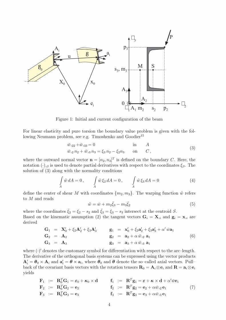
A beam with reference configuration denoted by B0 according to Fig. 1 is considered.Assuming arbitrary cross–sections the centroid S and the center of shear M are inde-pendent of the reference point O. An orthogonal basis system Ai with local coordinatesξ1, ξ2, ξ3 is introduced. The axis of the beam is initially along A1 with the arc–lengthparameter S = ξ1 ∈ [0, L] of the spatial curve. The cross–sections of the beam thereforelie in planes described by the basis vectors A2,A3. Accordingly the frame ai is definedin the current configuration which is characterized by the time parameter t. Note, thatwithin the underlying beam kinematic the vector a1 is not tangent vector of the deformedreference curve.The basis vectors Ai and ai follow from the orthogonal transformations

Ai(S) = R0(S) ei , ai(S, t) = R(S, t) ei with R0,R ∈ SO(3) . (1)

Several parametrizations of orthogonal tensor using Eulerian angles, Cardan angles, quater-nions etc. have been discussed in the literature, see e.g. Geradin and Rixen,13 Betsch etal.14

The position vectors of the undeformed and deformed cross–sections are given with thefollowing kinematic assumption

X(ξ2, ξ3, S) = X0(S) + ξ2A2(S) + ξ3A3(S)

x(ξ2, ξ3, S, t) = x0(S, t) + ξ2a2(S, t) + ξ3a3(S, t) + α(S, t) w(ξ2, ξ3) a1(t)(2)

where a1 is assumed to be piecewise constant. The given warping function w(ξ2, ξ3) isdefined within the Saint–Venant torsion theory for bars. This is a basic assumption whichrestricts the present formulation to a certain class of problems. Our numerical investi-gations however showed good agreement of the results for thin–walled beam structuresobtained with the present beam model compared with a higher valued shell model.

3

0B

B

X0x0

ei

Aiaiu

p3

3

2

1

s , m3 3

s2m2 p2A1

A3

0A2

M S

P

Figure 1: Initial and current configuration of the beam

For linear elasticity and pure torsion the boundary value problem is given with the fol-lowing Neumann problem, see e.g. Timoshenko and Goodier15

w,22 +w,33 = 0 in A

w,2 n2 + w,3 n3 = ξ3 n2 − ξ2n3 on C ,(3)

where the outward normal vector n = [n2, n3]T is defined on the boundary C. Here, the

notation (·),β is used to denote partial derivatives with respect to the coordinates ξβ. Thesolution of (3) along with the normality conditions∫

A

w dA = 0 ,∫A

w ξ2 dA = 0 ,∫A

w ξ3 dA = 0 (4)

define the center of shear M with coordinates m2, m3. The warping function w refersto M and reads

w = w + m2ξ3 − m3ξ2 (5)

where the coordinates ξ2 = ξ2 − s2 and ξ3 = ξ3 − s3 intersect at the centroid S.Based on the kinematic assumption (2) the tangent vectors Gi = X,i and gi = x,i arederived

G1 = X′0 + ξ2A

′2 + ξ3A

′3

G2 = A2

G3 = A3

g1 = x′0 + ξ2a

′2 + ξ3a

′3 + α′ wa1

g2 = a2 + α w,2 a1

g3 = a3 + α w,3 a1

(6)

where (·)′ denotes the customary symbol for differentiation with respect to the arc–length.The derivative of the orthogonal basis systems can be expressed using the vector productsA′

i = θ0 × Ai and a′i = θ × ai, where θ0 and θ denote the so–called axial vectors. Pull–

back of the covariant basis vectors with the rotation tensors R0 = Ai⊗ei and R = ai⊗ei

yields

F1 := RT0 G1 = ε0 + κ0 × d

F2 := RT0 G2 = e2

F3 := RT0 G3 = e3

f1 := RTg1 = ε + κ × d + α′we1

f2 := RTg2 = e2 + αw,2 e1

f3 := RTg3 = e3 + αw,3 e1

(7)

4

with d = ξ2e2 + ξ3e3. The strain vectors of the current configuration are defined with

ε := RTx′0 =

x′0 · a1

x′0 · a2

x′0 · a3

κ := RT θ =

a′2 · a3

a′3 · a1

a′1 · a2

. (8)

The corresponding quantities of the reference configuration read ε0 = RT0 X′

0 and κ0 =RT

0 θ0.Eqs. (6) are inserted into the Green–Lagrangian strain tensor E = EijG

i ⊗ Gj, wherethe dual basis vectors Gi are defined in a standard way Gi · Gj = δj

i . The componentswhich contribute to the virtual work read

E =

E11

2E12

2E13

=

12(g11 − G11)g12 − G12

g13 − G13

(9)

with the metric coefficients

Gij = Gi · Gj = Gi · R0RT0 Gj = Fi · Fj

gij = gi · gj = gi · RRTgj = fi · fj(10)

of the reference configuration and current configuration, respectively.

3 VARIATIONAL FORMULATION OF THE BOUNDARY VALUEPROBLEM

In this section the virtual work of the stresses and the external forces are derived consid-ering the beam kinematic. For this purpose stress resultants are defined. The associatedEuler–Lagrange equations and the linearization of the virtual work expressions are given.

3.1 Internal Virtual Work and Definition of Stress Resultants

Volume forces ρ0b and applied surface loads t are acting on the considered body. Hencethe equilibrium is given here in weak form

g(v, δv) =∫B0

S · δE dV −∫B0

ρ0b · δu dV −∫

∂B0

t · δu dΩ = 0 . (11)

The independent kinematic quantities of the beam are v = [u,R, α]T , where u = x0 −X0

and R = ai ⊗ ei denote the displacement vector and the rotation tensor of the referencecurve according to (2), respectively. The space of kinematically admissible variations isintroduced by

V := δv = [δu, δw, δα]T : [0, L] −→ R3| δv = 0 on Su (12)

where Su describes the boundaries with prescribed displacements and rotations. Here,the axial vector δw is defined by δai = δRRT ai = δw × ai.The Green–Lagrangian strain tensor is work conjugate to the Second Piola–Kirchhoffstress tensor S = Sij Gi⊗Gj. Within the present beam theory the components S22, S33, S23

5

are neglected. Using matrix notation the vector of non–vanishing stress components isdefined

S =[S11, S12, S13

]T. (13)

The variation of the work conjugate Green–Lagrangian strains (9) yields with (7) – (10)

δE =

δE11

2δE12

2δE13

=

f1 · δf1f2 · δf1 + f1 · δf2f3 · δf1 + f1 · δf3

(14)

whereδf1 = δε + δκ × d + δα′ we1

δf2 = δα w,2 e1

δf3 = δα w,3 e1 .

(15)

IntroducingF = [f1, f2, f3]

Wd = skewd =

0 −ξ3 ξ2

ξ3 0 0

−ξ2 0 0

a = (f1 · e1) (w,2 e2 + w,3 e3)

(16)

one obtains

δE = A δE

A = [FT , FTWTd , a, w FTe1] δE =

δε

δκ

δα

δα′

.

(17)

The variation of the beam strains (8) yields

δε = RT δx′0 + δRTx′

0 = RT (δx′0 − δw × x′

0)

δκ = RT δθ + δRT θ = RT δw′ .(18)

Eq. (18)1 is evident, whereas a proof of (18)2 is given e.g. in [17]. Furthermore arepresentation of the components yields

δε =

a1 · δu′ + x′0 · δa1

a2 · δu′ + x′0 · δa2

a3 · δu′ + x′0 · δa3

δκ =

a3 · δa′2 + a′

2 · δa3

a1 · δa′3 + a′

3 · δa1

a2 · δa′1 + a′

1 · δa2

. (19)

Using (17) the internal virtual work in (11) can be rewritten with dV = dA dS as

gint(v, δv) =∫B0

δET S dV =∫S

δET S dS

=∫S

(F · δε + M · δκ + Fwδα + Mwδα′) dS(20)

6

with the vector of stress resultants

S =∫A

AT S dA =

FMFw

Mw

=

∫A

TLTw

Lw

dA (21)

where T = [T 11, T 12, T 13]T = FS and L = Wd T. Finally a component representation ofthe vector of stress resultants yields

S =

F 1

F 2

F 3

M1

M2

M3

Fw

Mw

=∫A

T 11

T 12

T 13

T 13ξ2 − T 12ξ3

T 11ξ3

−T 11ξ2

T 12w,2 +T 13w,3

T 11w

dA (22)

with T 1α = (f1 · e1)S1α and α = 2, 3. Herein, F 1 is the normal force, F 2 and F 3 the shear

forces, M1 the torsion moment, M2 and M3 the bending moments, Fw the bi–shear andMw the bi–moment, respectively.

3.2 External Virtual Work and Euler–Lagrange Equations

In this paper the volume forces ρ0b and the surface loads t according to (11) are consideredwith the load p = p(S) acting at the coordinates p2, p3, see Fig.1. The vector of theloading point in the current configuration reads xp = x0+rp with rp = p2a2+p3a3+α wp a1

and wp = w(p2, p3).Hence the external virtual work reads

gext(v, δv) = −∫S

p · δxp dS

= −∫S

p · (δx0 + p2δa2 + p3δa3 + αwpδa1 + δαwpa1) dS

= −∫S

(p · δx0 + m · δw + p1δα) dS

(23)

with m = rp × p and p1 = wp (p · a1) .

The weak form of equilibrium (11) is now reformulated using the expressions (20), (18)and (23). This yields

g(v, δv) =∫S

[f · (δx′0 − δw × x′

0) + m · δw′ + Fwδα + Mwδα′ − (p · δx0 + m · δw + p1δα)] dS = 0

(24)

7

with f := RF and m := RM. Next, integration by parts yields with homogeneous stressboundary conditions

g(v, δv) = −∫S

[(f ′ + p) · δx0 + (m′ + x′0 × f + m) · δw + (Mw ′ − Fw + p1) δα] dS = 0 .

(25)Applying standard arguments from variational calculus we obtain

f ′ + p = 0

m′ + x′0 × f + m = 0

Mw ′ − Fw + p1 = 0 .

(26)

These are the Euler–Lagrange equations of the variational formulation. The first twoequations in (26) are well–known equilibrium equations of a three–dimensional beam usinga vector notation. The third equation is identical to that of the linear theory. Reissner12

derived (26)3 in the context of a second–order geometrical nonlinear theory.

3.3 Linearization of the Virtual Work Expressions

For the subsequent finite element formulation we need to derive the linearization of theweak form of equilibrium (11). This is formally achieved using the directional derivative

L [g(v, δv)] = g + Dg · ∆v , Dg · ∆v =d

dε[G(v + ε∆v)]ε=0 (27)

where ∆v = [∆u, ∆w, ∆α]T . The linearization of the internal virtual work yields amaterial part and a geometrical part

Dgint(v, δv) · ∆v =∫S

(δET D∆E + ∆δET S) dS . (28)

Here the linearized beam strains ∆E = [∆ε, ∆κ, ∆α, ∆α′]T are obtained from (19) re-placing the operator δ by ∆. Furthermore the linearized virtual strains are expressed by∆δE = [∆δε, ∆δκ, 0, 0]T with

∆δε =

δu′ · ∆a1 + δa1 · ∆u′ + x′0 · ∆δa1

δu′ · ∆a2 + δa2 · ∆u′ + x′0 · ∆δa2

δu′ · ∆a3 + δa1 · ∆u′ + x′0 · ∆δa3

∆δκ =

δa′2 · ∆a3 + δa3 · ∆a′

2 + a3 · ∆δa′2 + a′

2 · ∆δa3

δa′3 · ∆a1 + δa1 · ∆a′

3 + a1 · ∆δa′3 + a′

3 · ∆δa1

δa′1 · ∆a2 + δa2 · ∆a′

1 + a2 · ∆δa′1 + a′

1 · ∆δa2

.

(29)

Next the linearization of the stress resultants (21) applying the product rule leads to

D =d S

d E=

d

d E[∫A

AT S dA] =∫A

(ATCTA + G) dA . (30)

The first part follows from differentiation of the stress vector S and the incrementalGreen–Lagrangian strains dE = A dE. The tangential matrix CT := dS/dE is specified

8

for elastic–plastic material behaviour in the next section. The second part follows fromdifferentiation of the matrix product ATS where the stress vector S is held fixed. With

T

L

Tw

Lw

=

S11f1 + S12f2 + S13f3

Wd(S11f1 + S12f2 + S13f3)

S(f1 · e1)

S11w(f1 · e1) + Sαw

(31)

where S = S12w,2 +S13w,3 and fi according to (7) one obtains

G =

∂T∂ε

∂T∂κ

∂T∂α

∂T∂α′

∂L∂ε

∂L∂κ

∂L∂α

∂L∂α′

(∂T w

∂ε )T (∂T w

∂κ )T ∂T w

∂α∂T w

∂α′

(∂Lw

∂ε )T (∂Lw

∂κ )T ∂Lw

∂α∂Lw

∂α′

=

S111 S11WTd Se1 S11we1

S11Wd −S11W2d Sd S11wd

SeT1 SdT 0 Sw

S11weT1 S11wdT Sw S11w2

(32)

where d = Wde1 = ξ3e2 − ξ2e3. The integration over the cross–section in (21) and (30) isperformed numerically. The warping function w is determined for arbitrary cross–sectionsin a separate computing process using the finite element method as is discussed in [16].The finite element mesh for the computation of w is used here to perform the numericalGauss integration. In case of small strains F ≈ 1 holds, A becomes independent of thedisplacement field and G vanishes.Finally we derive the linearization of the external virtual work as

Dgext(v, δv) · ∆v = −∫S

p · ∆δxp dS (33)

with ∆δxp = p2∆δa2 + p3∆δa3 + αwp∆δa1 + δαwp∆a1 + ∆αwpδa1.

4 MATERIAL LAW AND STRESS RESULTANTS

In this section we present the constitutive equations for elastoplastic material behaviour.We consider metallic materials which can be described by the von Mises yield criterionwith isotropic hardening and associated flow rule. For elasticity the section integrals arereformulated using the equations of Saint–Venant’s torsion theory and Green’s theorem.This yields an elasticity matrix where for the general case torsion bending coupling occurs.

4.1 Elastic–Plastic Stress Analysis

The Green–Lagrangian strains (9) are decomposed in an elastic and plastic part

E = Eel + Epl (34)

which holds for small elastic and plastic strains. The elastic part is described by theso–called St.Venant–Kirchhoff material law. Thus, a quadratic strain energy function ispostulated where the stresses are obtained by partial derivatives

Ws(Eel) =

1

2EelTCEel , S =

∂Ws

∂Eel= CEel. (35)

9

Since the stresses S22, S33 and S23 are neglected the constitutive matrix reads

C =

E 0 0

0 G 00 0 G

.

(36)

Here, E and G denote Young’s modulus and shear modulus, respectively.The plastic flow of metals can be described using the von Mises yield condition withisotropic hardening

F (S, epl) = h(S) − y0 + r(epl) (37)

where

h(S) =√

STPS , P =

1 0 00 3 00 0 3

.

(38)

Assuming strain hardening the yield stress y is given here with the equivalent plasticstrain epl using a linear hardening function r(epl) = −K epl, thus

y = y0 + K epl . (39)

The initial yield stress y0 and the hardening parameter K are material constants.The rates of the plastic strains and of the equivalent plastic strain are described using anassociated flow rule

Epl = λ∂F

∂Sepl = λ

∂F

∂r, (40)

where the gradient of the yield condition can be expressed as

∂F

∂S=

1

hPS := N

∂F

∂r= 1 . (41)

In (40) the loading–unloading conditions

λ ≥ 0 , F ≤ 0 , λ F = 0 (42)

must hold.Hence, a backward Euler integration algorithm within a time step tn+1 = tn +∆t leads to

Epln+1 = Epl

n + γNn+1

epln+1 = epl

n + γ(43)

where γ =∫ tn+1tn λ dt. Inserting (35)2 and (43)1 into (34) at time tn+1 yields

Sn+1(γ) = C(γ)Etr Etr := En+1 − Epln (44)

with

C(γ) = (C−1 +γ

yP)−1 =

E1+Eγ/y

0 0

0 G1+3Gγ/y

0

0 0 G1+3Gγ/y

.

(45)

To express Sn+1 as an explicit function of γ we replaced h(S) by y(γ) in (45) usingF (S, epl) = 0. The consistency parameter γ is obtained with the solution of the yield

10

condition F (Sn+1, epln+1) = 0. This is achieved iteratively within a Newton iteration pro-

cedure

γ(l+1) = γ(l) − F (l)

dF (l)

dγ

F (l) = h[Sn+1(γ

(l))]− y

[epl

n+1(γ(l))

]dF (l)

dγ= −

[h

y(1 − γ

y

dy

depl)NT CN +

dy

depl

] (46)

where l denotes the iteration number and dy/depl = K. As starting value we takeγ(0) = 0. The equivalent plastic strain follows from (43)2. Note, that during the iterationy = h holds. The elastoplastic stresses at each integration point are evaluated using awell–known operator split method. The predictor step yields the so–called trial stressesStr = CEtr. If above yield condition is not fulfilled the stresses are given with thecorrector step according to (44), thus

Sn+1 =

CEtr if F (Str, epln ) ≤ 0

CEtr if F (Str, epln ) > 0 .

(47)

The consistency parameter γ depends on the strains E via eq. (46)2. This has to beconsidered when linearizing the stress vector (47). One obtains

dS

dE

∣∣∣∣∣n+1

=

C if F (Str, epln ) ≤ 0

C − CNNT C

NT CN + βif F (Str, epl

n ) > 0(48)

with β = K/(1 − γK/y).

4.2 Elastic Stress Analysis

In case of small strains the transformation matrix F according to (16) is approximatelythe identity matrix, thus F ≈ 1. In this case A is given with (17)

A =

1 0 0 0 ξ3 −ξ2 0 w

0 1 0 −ξ3 0 0 w,2 0

0 0 1 ξ2 0 0 w,3 0

.

(49)

One can see that A does not depend on the deformation and E = AE holds. Forelasticity the stress vector is obtained from S = CAE. Now the matrix of the linearizedstress resultants (30) can be reformulated using (48), (36), (49) and G = 0

D =∫A

E 0 0 0 Eξ3 −Eξ2 0 EwG 0 −Gξ3 0 0 Gw,2 0

G Gξ2 0 0 Gw,3 0G(ξ2

2 + ξ23) 0 0 G(ξ2w,3 −ξ3w,2 ) 0

Eξ23 −Eξ2ξ3 0 Ewξ3

Eξ22 0 −Ewξ2

sym G(w,22 +w,23 ) 0Ew2

dA . (50)

11

The centroid of the cross–section with coordinates s2, s3 is denoted by S, see Fig. 1.Furthermore we denote the area of the cross–section by A, the moments of inertia relativeto the centroid by I22, I33, I23, the Saint–Venant torsion modulus by IT and the warpingconstant by Iw. The following definitions are given with α, β = 2, 3

Sα :=∫A

ξαdA = Asα

Iαβ :=∫A

ξαξβ dA Iαβ :=∫A

ξαξβ dA = Iαβ + Asαsβ

I0 := I22 + I33

IT :=∫A

[ξ2(w,3 +ξ2) − ξ3(w,2 −ξ3)] dA = I0 +∫A

(ξ2w,3 −ξ3w,2 ) dA

Iw :=∫A

w2 dA .

(51)

Using the equations of Saint–Venants torsion theory (3) and application of Green’s theo-rem yields after some algebra the missing quantities, see appendix A.1∫

A

w,2 dA = As3

∫A

w,3 dA = −As2∫A

(w,22 +w,23 ) dA = I0 − IT∫A

wξ2 dA = I22m3 − I23m2 := Iw2

∫A

wξ3 dA = −I33m2 + I23m3 := Iw3∫A

w2 dA = Iw + I33m22 + I22m

23 − 2I23m2m3 := Iw .

(52)A numerical computation of w(ξ2, ξ3) which fulfills

∫A w dA = 0 and above section quan-

tities for arbitrary cross–sections using the finite element method is discussed in e.g. [16].In fact (52)4 and (52)5 are two equations which can be solved for the coordinates m2 andm3 if Iw2 and Iw3 are known, see Ref. [16].Now, (50) can be expressed inserting the section quantities (51) and (52) as follows

D =

EA 0 0 0 EAs3 −EAs2 0 0GA 0 −GAs3 0 0 GAs3 0

GA GAs2 0 0 −GAs2 0GI0 0 0 −G(I0 − IT ) 0

EI33 −EI23 0 EIw3

EI22 0 −EIw2

sym G(I0 − IT ) 0EIw

.

(53)

The elasticity matrix (53) is constant and symmetric. Hence, considering (30) the vectorof stress resultants follows from

S = D E E =

ε − ε0

κ − κ0

αα′

.

(54)

12

As can be seen torsion–bending coupling occurs if the reference point O and the shearcenter M with coordinates m2, m3 do not coincide. If the coordinates ξ2, ξ3 de-fine principal axes of the cross–section and if S = M = O all off–diagonal terms ex-cept −G(I0 − IT ) are zero. Furthermore, if the contribution of the bi–moment andof the bi–shear to the strain energy is neglectable a formulation with six stress resul-tants can be derived, see.17 In this case one obtains the well–known elasticity matrixD = diag [EA, GA, GA, GIT , EI33, EI22] .

5 FINITE ELEMENT FORMULATION

According to the isoparametric concept, the following kinematic variables are interpo-lated using standard Lagrangian shape functions NI(ξ) where ξ ∈ [−1, +1]. Within atypical element the position vector of the reference curve Sh

0 , the curve Sh of the currentconfiguration and the parameter α are interpolated by

Xh0 =

nel∑I=1

NI(ξ)XI , xh0 =

nel∑I=1

NI(ξ)(XI + uI) , αh =nel∑I=1

NI(ξ)αI . (55)

Here nel denotes the number of nodes at the element. For nel ≥ 3 the reference curve ofa space–curved beam is approximated by polynomial functions.Furthermore the basis systems of the reference configuration and the current configurationare approximated using the same interpolation functions

Ahm =

nel∑I=1

NI(ξ)AmI , ahm =

nel∑I=1

NI(ξ) amI . (56)

Thus the orthogonality condition of the basis systems Ahm and ah

m is only fulfilled at thenodes. Numerical investigations however show that no significant loss of accuracy followsfrom this approximation. The initial basis system AmI is generated within the input ofthe finite element mesh whereas the current basis system at the finite element nodes iscomputed using the so–called Rodrigues formula

RI = amI ⊗ em = 1 +sin ωI

ωI

ΩI +1 − cos ωI

ω2I

Ω2I (57)

with ωI = |ωI |. Note, that formula (57) is singularity free for 0 ≤ ωI < 2π. Thesingularity at n2π (n = 1, 2, 3, ...) can be overcome by a multiplicative update of therotation tensor after a certain number of load steps. The skew–symmetric tensor ΩI

follows from the independent rotational parameters by ΩI = skew ωI . The basic equationreads ΩI h = ωI × h for all h ∈ R3, thus the components are given by

ωI =

ω1I

ω2I

ω3I

,

ΩI =

0 −ω3I ω2I

ω3I 0 −ω1I

−ω2I ω1I 0

.

(58)

The finite element approximations of the virtual displacements, basis vectors and theassociated linearization are expressed as follows

δuh =nel∑I=1

NI(ξ)δuI , δαh =nel∑I=1

NI(ξ)δαI ,

δahm =

nel∑I=1

NI(ξ)δamI , ∆δahm =

nel∑I=1

NI(ξ)∆δamI .(59)

13

The derivative of the shape function NI(ξ) with respect to the arc–length S is obtainedusing the chain rule N ′

I(ξ) = NI(ξ),ξ /|Xh0 ,ξ |. Hence, the tangential vectors X′

0 and x′0,

the derivatives of the basis vectors A′m and a′

m and associated variations and linearizationsare given replacing NI by N ′

I in (55), (56) and (59).The variation of the orthogonal basis system amI yields for all h ∈ R3

δamI = δwI × amI = WTmIδwI ,

h · δamI = bmI(h) · δwI , bmI(h) = amI × h(60)

and

h · δam =nel∑I=1

NI bmI(h) · δwI h · δa′m =

nel∑I=1

N ′I bmI(h) · δwI . (61)

Thus, the virtual beam strains δE considering (19) can be expressed as follows

δEh =nel∑I=1

BI δvI , BI =

N ′I RT NI BT

εI 0

0 N ′I BT

κI + NI B′TκI 0

0 0 NI

0 0 N ′I

(62)

with the virtual nodal displacement vector δvI = [δuI , δwI , δαI ]T and

R := [a1, a2, a3] BεI := [b1I(x′0), b2I(x

′0), b3I(x

′0)]

BκI := [b2I(a3), b3I(a1), b1I(a2)] B′κI := [b3I(a

′2), b1I(a

′3), b2I(a

′1)] .

(63)

Next the finite element interpolation (55) – (63) is inserted into the linearized boundaryvalue problem (27)

L[g(vh, δvh)] = Ae=1

numel nel∑I=1

nel∑K=1

δvTI (f e

I + KeIK∆vK) . (64)

Here, A denotes the standard assembly operator, numel the total number of elementsto discretize the problem and ∆vK = [∆uK , ∆wK , ∆αK ]T the incremental displacementvector. Furthermore f e

I and KeIK denote the sum of the internal and external nodal forces

of node I and the tangential stiffness matrix of element e related to nodes I and K,respectively. Considering (62) one obtains

f eI =

∫S

(BTI S − NI q) dS , Ke

IK =∫S

(BTI DBK + GIK + PIK) dS (65)

withq = [p, mI , p1I ]

T

mI = rI × p rI = p2 a2I + p3 a3I + α wp a1I

p1I = wp p · a1I .(66)

For linear elasticity the vector of stress resultants follows from the constitutive equation(54). For elastoplastic material behaviour S and D are obtained by numerical integrationaccording to (22) and (30), respectively.

14

Next the geometric matrix GIK is derived with the linearized virtual strains (29). Forthis purpose the second variation of the current basis system is derived as

h · ∆δamI = δwI · M(amI ,h)∆wI

M(amI ,h) =1

2(amI ⊗ h + h ⊗ amI) +

1

2(tmI ⊗ ωI + ωI ⊗ tmI) + c10 1

(67)

where tmI and c10 are specified in appendix A.3. This yields

h · ∆δam =nel∑I=1

NI δwI · M(amI ,h) ∆wI

h · ∆δa′m =

nel∑I=1

N ′I δwI · M(amI ,h) ∆wI

(68)

for all h ∈ R3. As can be seen, the linearization of the basis system leads to a symmetricbi–linear form. One obtains

GIK =

0 N ′INK WT

fK 0

NIN′K WfI Gww

IK 0

0 0 0

,

(69)

where

GwwIK = N ′

INKW1IK + NIN

′KW2

IK + δIK [M(a1I ,h1I) + M(a2I ,h2I) + M(a3I ,h3I)]

h1I = NI F 1x′0 + NI M2a′

3 + N ′I M3a2

h2I = NI F 2x′0 + NI M3a′

1 + N ′I M1a3

h3I = NI F 3x′0 + NI M1a′

2 + N ′I M2a1

W1IK = M1W2IW

T3K + M2W3IW

T1K + M3W1IW

T2K

W2IK = M1W3IW

T2K + M2W1IW

T2K + M3W2IW

T3K

WfI = skew (F 1a1I + F 2a2I + F 3a3I) .(70)

The external loading yields a contribution to the stiffness matrix if rI = 0. Considering(33) one obtains

PIK = −

0 0 0

0 NI δIK M(rI , p) NINK m1I

0 NINK mT1K 0

(71)

where m1I = wp a1I × p.Application of the chain rule yields the differential arc–length dS = |Xh

0 ,ξ | dξ. The inte-gration of the element residual and element stiffness matrix with respect to the coordinateS is performed numerically. To avoid shear locking uniform reduced integration is appliedto all quantities. Finally the transformations of the axial vectors are introduced as follows

δwI = HI δωI ∆wK = HK ∆ωK (72)

where the tensor H is specified in appendix A.2. This leads to

L[g(vh, δvh)] = Ae=1

numel nel∑I=1

nel∑K=1

δvTI (f e

I + KeIK∆vK)

δvI = [δuI , δωI , δαI ]T ∆vK = [∆uK , ∆ωK , ∆αK ]T

f eI = TT

I f eI Ke

IK = TTI Ke

IKTK TI = diag[1, HI , 1] .

(73)

15

From eq. (73) one obtains a linear system of equations for the incremental nodal degreesof freedom. It is emphasized, that the update of the nodal displacements as well as of therotational parameters is performed in an additive way. Thus, the equilibrium configurationis computed iteratively within the Newton iteration procedure.

Remark:Within an alternative procedure one keeps ∆wI as unknown incremental rotational pa-rameters. Thus the transformation (73) is not necessary anymore. However ωI must beknown for the finite element interpolation (57) – (71). It can be obtained within thefollowing simple update procedure

ω(n+1)K = ω

(n)K + ∆ωK ∆ωK = H−1

K ∆wK

H−1K = 1 − 1

2Ω

(n)K + 1

2c3 Ω

2(n)K

(74)

where n denotes the index of the Newton iteration procedure. One can easily show thatabove expression fulfills H−1

K HK = 1. Again, the advantage of (74) compared with (73) is,that the transformation δwI = HI δωI drops out. However, the algorithm (74) requires

additional storage of the parameters ω(n)K .

6 NUMERICAL EXAMPLES

The element scheme has been implemented in an enhanced version of the program FEAPdocumented in Ref. [18]. In this section three examples with finite deformations andelastic–plastic material behaviour are presented. With the first example we investigatethe stability behaviour of a beam assuming linear elastic material behaviour. The lasttwo examples are concerned with the load carrying capacity of beam structures. Thesecond example is a channel–section beam, where centroid, center of shear and loadingpoint are not identical. With the last example we solve a coupled beam–shell problem.For comparison the investigated thin–walled beam structures are discretized using four–noded shell elements. These elements possess six nodal degrees of freedom which areidentical to the first six degrees of freedom of the beam.

6.1 Lateral Torsional Buckling of a Single Span Girder

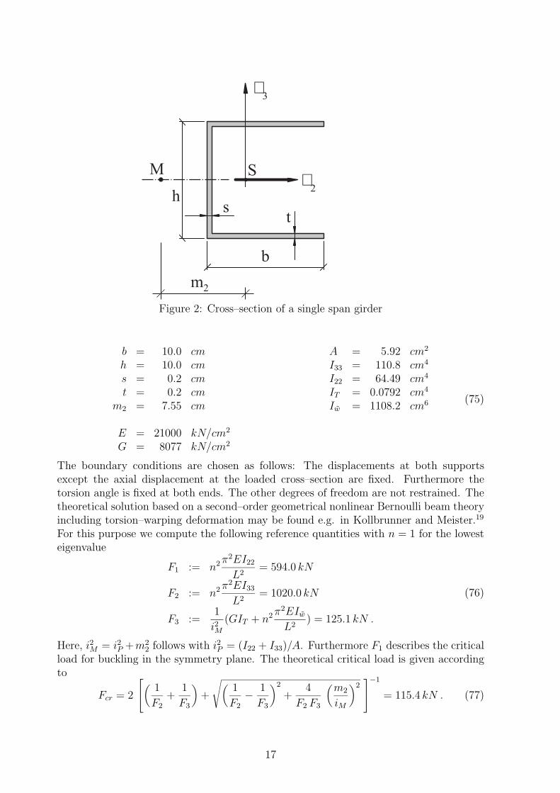
The first example is a single span girder with length L = 150 cm where an axial force Fis applied at the centroid. Fig. 2 shows the cross–section of the channel section beam.The ratio of the width of the flange to the height of the web is relatively large. Thistype of cross–section is fairly sensitive against torsional buckling. The geometrical andmaterial data are given in (75), where the moments of inertia are denoted according to thedefinitions in (51). The section quantities are determined with the finite element programas is described in [16].

16

t

b

sh

3

2

m2

M S

Figure 2: Cross–section of a single span girder

b = 10.0 cm A = 5.92 cm2

h = 10.0 cm I33 = 110.8 cm4

s = 0.2 cm I22 = 64.49 cm4

t = 0.2 cm IT = 0.0792 cm4

m2 = 7.55 cm Iw = 1108.2 cm6

E = 21000 kN/cm2

G = 8077 kN/cm2

(75)

The boundary conditions are chosen as follows: The displacements at both supportsexcept the axial displacement at the loaded cross–section are fixed. Furthermore thetorsion angle is fixed at both ends. The other degrees of freedom are not restrained. Thetheoretical solution based on a second–order geometrical nonlinear Bernoulli beam theoryincluding torsion–warping deformation may be found e.g. in Kollbrunner and Meister.19

For this purpose we compute the following reference quantities with n = 1 for the lowesteigenvalue

F1 := n2 π2EI22

L2= 594.0 kN

F2 := n2 π2EI33

L2= 1020.0 kN

F3 :=1

i2M(GIT + n2 π2EIw

L2) = 125.1 kN .

(76)

Here, i2M = i2P +m22 follows with i2P = (I22 + I33)/A. Furthermore F1 describes the critical

load for buckling in the symmetry plane. The theoretical critical load is given accordingto

Fcr = 2

(

1

F2

+1

F3

)+

√(1

F2

− 1

F3

)2

+4

F2 F3

(m2

iM

)2−1

= 115.4 kN . (77)

17

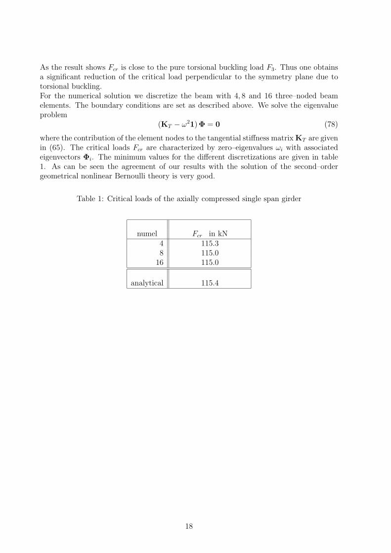
As the result shows Fcr is close to the pure torsional buckling load F3. Thus one obtainsa significant reduction of the critical load perpendicular to the symmetry plane due totorsional buckling.For the numerical solution we discretize the beam with 4, 8 and 16 three–noded beamelements. The boundary conditions are set as described above. We solve the eigenvalueproblem

(KT − ω21)Φ = 0 (78)

where the contribution of the element nodes to the tangential stiffness matrix KT are givenin (65). The critical loads Fcr are characterized by zero–eigenvalues ωi with associatedeigenvectors Φi. The minimum values for the different discretizations are given in table1. As can be seen the agreement of our results with the solution of the second–ordergeometrical nonlinear Bernoulli theory is very good.

Table 1: Critical loads of the axially compressed single span girder

numel Fcr in kN4 115.38 115.0

16 115.0

analytical 115.4

18

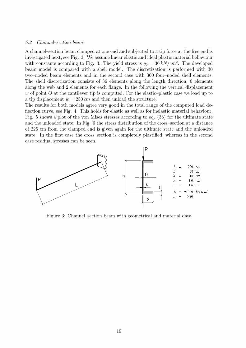
6.2 Channel–section beam

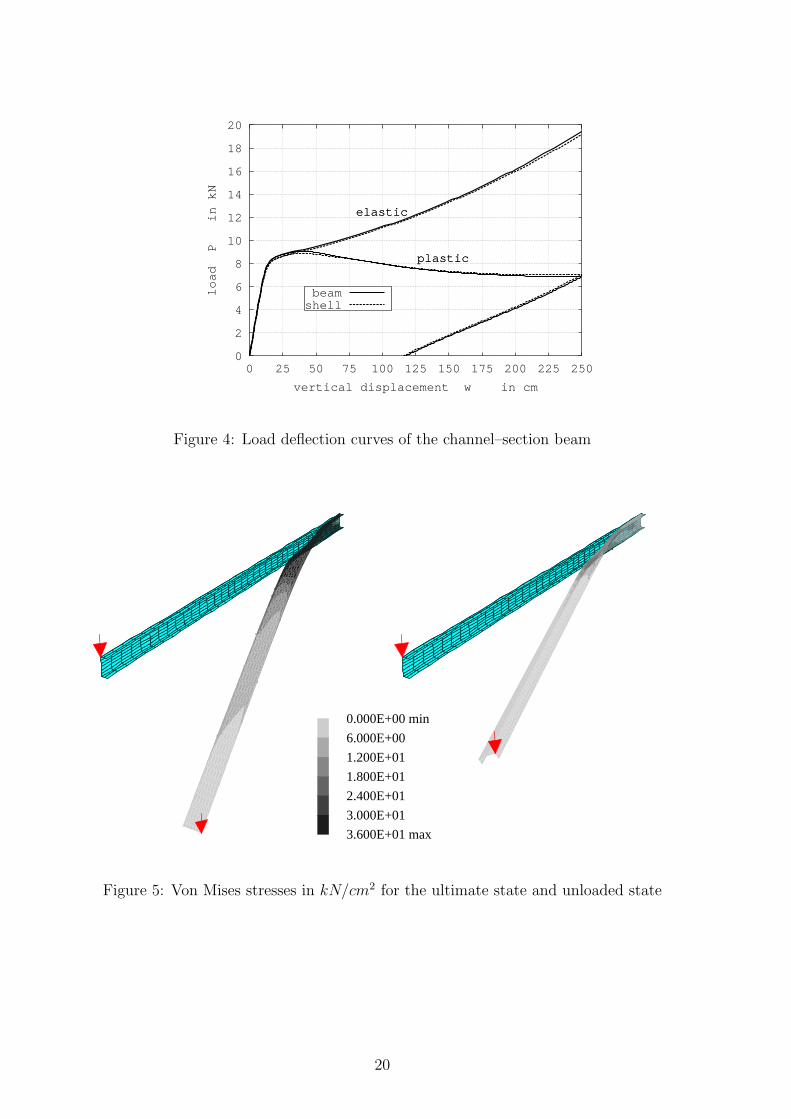
A channel–section beam clamped at one end and subjected to a tip force at the free end isinvestigated next, see Fig. 3. We assume linear elastic and ideal plastic material behaviourwith constants according to Fig. 3. The yield stress is y0 = 36 kN/cm2. The developedbeam model is compared with a shell model. The discretization is performed with 30two–noded beam elements and in the second case with 360 four–noded shell elements.The shell discretization consists of 36 elements along the length direction, 6 elementsalong the web and 2 elements for each flange. In the following the vertical displacementw of point O at the cantilever tip is computed. For the elastic–plastic case we load up toa tip displacement w = 250 cm and then unload the structure.The results for both models agree very good in the total range of the computed load de-flection curve, see Fig. 4. This holds for elastic as well as for inelastic material behaviour.Fig. 5 shows a plot of the von Mises stresses according to eq. (38) for the ultimate stateand the unloaded state. In Fig. 6 the stress distribution of the cross–section at a distanceof 225 cm from the clamped end is given again for the ultimate state and the unloadedstate. In the first case the cross–section is completely plastified, whereas in the secondcase residual stresses can be seen.

PL

t

b

s

h

P

0

L cm

h cmb cm

s cm

t cm

E kNcm

Figure 3: Channel–section beam with geometrical and material data

19

0

2

4

6

8

10

12

14

16

18

20

0 25 50 75 100 125 150 175 200 225 250

load P in kN

vertical displacement w in cm

elastic

plastic

elastic

plastic

beamshell

Figure 4: Load deflection curves of the channel–section beam

0.000E+00 min

6.000E+00

1.200E+01

1.800E+01

2.400E+01

3.000E+01

3.600E+01 max

Figure 5: Von Mises stresses in kN/cm2 for the ultimate state and unloaded state

20

0.000E+00 min

6.000E+00

1.200E+01

1.800E+01

2.400E+01

3.000E+01

3.600E+01 max

Figure 6: Von Mises stresses in kN/cm2 of the cross–section at a distance of 225 cm fromthe clamped end for the ultimate state and unloaded state

21

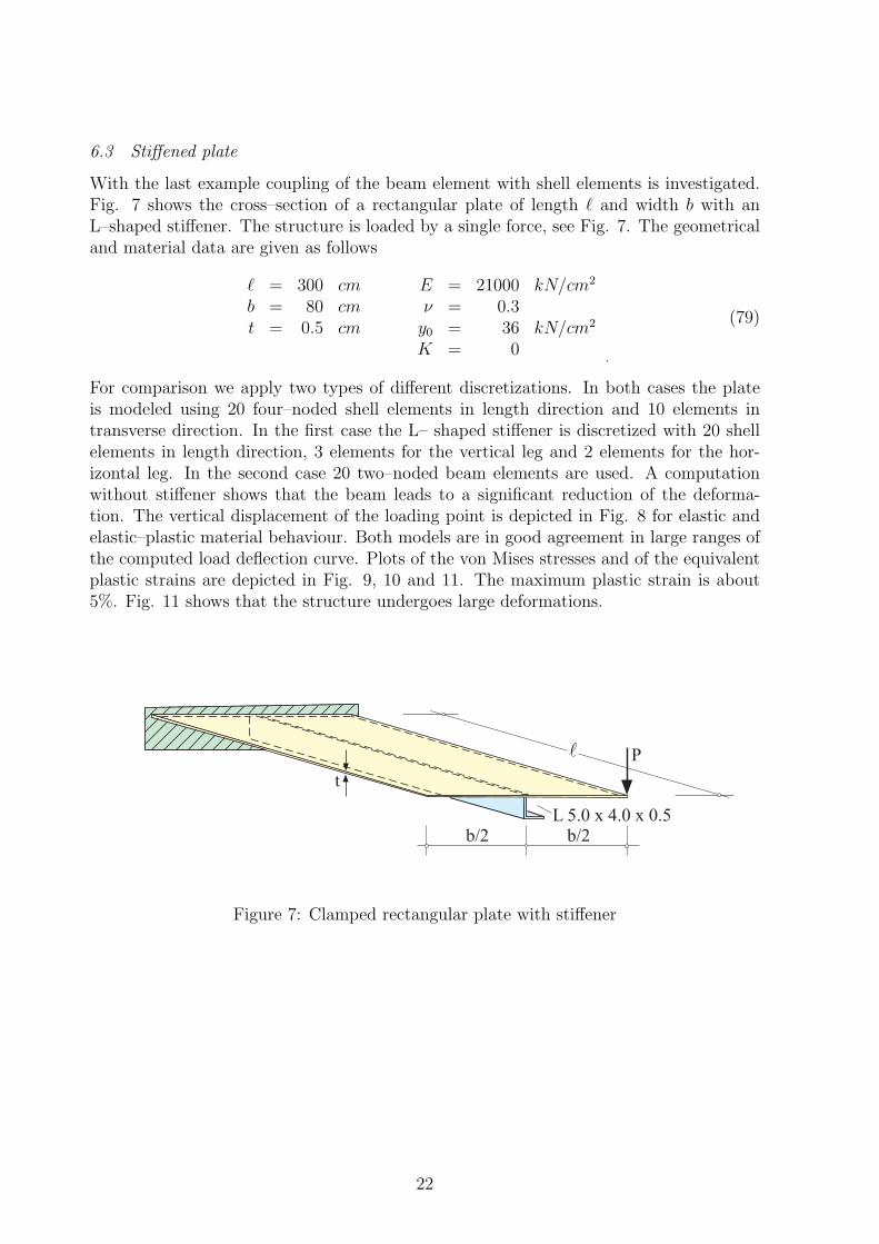
6.3 Stiffened plate

With the last example coupling of the beam element with shell elements is investigated.Fig. 7 shows the cross–section of a rectangular plate of length and width b with anL–shaped stiffener. The structure is loaded by a single force, see Fig. 7. The geometricaland material data are given as follows

= 300 cmb = 80 cmt = 0.5 cm

E = 21000 kN/cm2

ν = 0.3y0 = 36 kN/cm2

K = 0.

(79)

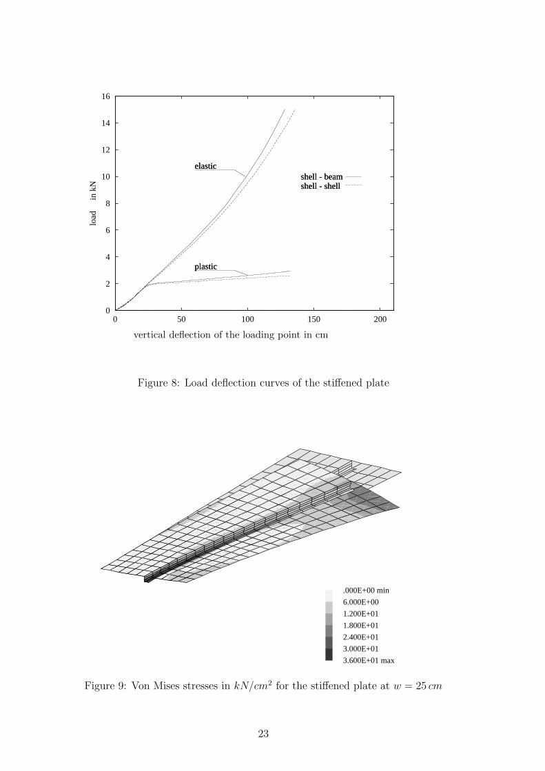
For comparison we apply two types of different discretizations. In both cases the plateis modeled using 20 four–noded shell elements in length direction and 10 elements intransverse direction. In the first case the L– shaped stiffener is discretized with 20 shellelements in length direction, 3 elements for the vertical leg and 2 elements for the hor-izontal leg. In the second case 20 two–noded beam elements are used. A computationwithout stiffener shows that the beam leads to a significant reduction of the deforma-tion. The vertical displacement of the loading point is depicted in Fig. 8 for elastic andelastic–plastic material behaviour. Both models are in good agreement in large ranges ofthe computed load deflection curve. Plots of the von Mises stresses and of the equivalentplastic strains are depicted in Fig. 9, 10 and 11. The maximum plastic strain is about5%. Fig. 11 shows that the structure undergoes large deformations.

t

b/2 b/2

P

L 5.0 x 4.0 x 0.5

Figure 7: Clamped rectangular plate with stiffener

22

0

2

4

6

8

10

12

14

16

0 50 100 150 200

load

i

n kN

shell - beamshell - shell

elastic

plastic

shell - beamshell - shell

elastic

plastic

vertical deflection of the loading point in cm

Figure 8: Load deflection curves of the stiffened plate

.000E+00 min

6.000E+00

1.200E+01

1.800E+01

2.400E+01

3.000E+01

3.600E+01 max

Figure 9: Von Mises stresses in kN/cm2 for the stiffened plate at w = 25 cm

23

.000E+00 min

6.000E+00

1.200E+01

1.800E+01

2.400E+01

3.000E+01

3.600E+01 max

Figure 10: Von Mises stresses in kN/cm2 for the stiffener at the clamped cross–section atw = 25 cm

.000E+00 min

1.000E-02

2.000E-02

3.000E-02

4.000E-02

5.029E-02 max

Figure 11: Equivalent plastic strains of the stiffened plate

24

7 CONCLUSIONS

In this paper a theory for three–dimensional beams with arbitrary cross–sections and anassociated finite element formulation is developed. The beam strains are derived from theGreen–Lagrangian strain tensor. Elastoplastic material behaviour applying the von Misesyield condition and associated flow rule is considered. Due to the nonlinear stress–strainrelations the stress resultants and associated linearizations are obtained by numerical in-tegration over the cross–sections. A finite beam element is developed using Lagrangianinterpolation functions to approximate the kinematic quantities. Each node of the ele-ment possesses seven degrees of freedom. The basis systems at the nodes are evaluatedusing orthogonal transformations. Due to the chosen finite element approximation the lin-earization yields relative simple expressions for the symmetric tangent matrix. Examplesshow the applicability of the developed beam element applied to geometrical and physicalnonlinear problems. Alternative discretizations of thin–walled cross–sections with shellelements show good agreement between the different models. Thus, the derived elementcan effectively be used to analyze the load–carrying capacities of spatial beam structures.

25

A APPENDIX

A.1 Proof of integrals (52)

Using (3)1 the following integral is reformulated such that Green’s formula can be applied.Hence inserting boundary condition (3)2 yields∫

A

w,2 dA =∫A

[(ξ2w,2 ),2 +(ξ2w,3 ),3 ] dA =∮C

[ξ2(w,2 n2 + w,3 n3)] dC

=∮C

[ξ2(ξ3n2 − ξ2n3)] dC .(80)

Again application of Green’s formula and considering (51)1 leads to∮C

[ξ2(ξ3n2 − ξ2n3)] dC =∫A

[(ξ2ξ3),2 −ξ22 ,3 ] dA =

∫A

ξ3 dA = A s3 (81)

which proves (52)1. Proceeding in an analogous way leads to (52)2.

The following integral is reformulated in the same way as done above. Thus, we apply(3)1, Green’s formula and boundary condition (3)2∫

A

(w,22 +w,23 ) dA =∫A

[(w w,2 ),2 +(w w,3 ),3 ] dA

=∮C

[w(w,2 n2 + w,3 n3)] dC =∮C

w (ξ3n2 − ξ2n3) dC .(82)

Again application of Green’s formula and considering the definition of Saint–Venant tor-sion modulus (51)4 yields∮

C

w(ξ3n2 − ξ2n3) dC =∫A

(w,2 ξ3 − w,3 ξ2) dA = I0 − IT (83)

which proves (52)3.

Next using (4) and (5) we get∫A

wξ2 dA =∫A

(ξ2 + s2)(w − m2ξ3 + m3ξ2) dA = I22m3 − I23m2 = Iw2 (84)

which yields (52)4. The expression for Iw3 is obtained in an analogous way. Finally eq.(52)6 can be derived considering the orthogonality conditions (4) and definition (5).

A.2 First Variation of the Orthogonal Basis System

The current orthogonal basis system can be written using the Rodrigues formula (57)

ai = Rei R = 1 +sin ω

ωΩ +

1 − cos ω

ω2Ω2 (85)

where ω = |ω| and Ω = skew ω. To alleviate the notation the node index is omitted. Thefirst variation, denoted here by the symbol δ, yields

δai = δRei = δRRTai = δw × ai (86)

26

with

δR =sin ω

ωδΩ +

1 − cos ω

ω2(δΩΩ + ΩδΩ)

+[ω cos ω − sin ω

ω2Ω +

ω sin ω + 2 cos ω − 2

ω3Ω2

]δω

RT = 1 − sin ω

ωΩ +

1 − cos ω

ω2Ω2

(87)

with δω = (ω · δω)/ω. Inserting the identities

Ω2 = ω ⊗ ω − ω21 Ω3 = −ω2Ω δΩΩ = ω ⊗ δω − (ω · δω)1 (88)

yields after some lengthy algebraic manipulation the skew–symmetric tensor

δRRT = (1 − c2ω2)δΩ + c1 (ΩδΩ − δΩΩ) + c2 (ω · δω)Ω

c1 =1 − cos ω

ω2, c2 =

ω − sin ω

ω3.

(89)

The associated axial vector reads

δw = H δω , H = 1 + c1 Ω + c2 Ω2 . (90)

A.3 Second Variation of the Orthogonal Basis System

The second variation of the orthogonal basis system is denoted by ∆. One obtains for allh ∈ R3

h · ∆δai = h · ∆(δw × ai)

= h · [δw × (∆w × ai) + ∆H δω × ai]

= δw · [ai ⊗ h − (ai · h)1] ∆w + bi · ∆H δω

(91)

where bi = ai × h. The second part in (91) yields with ∆ω = (ω · ∆ω)/ω

bi · ∆H δω = bi · [(∂c1

∂ωΩ +

∂c2

∂ωΩ2)∆ω + c1∆Ω + c2(∆ΩΩ + Ω∆Ω)] δω

= δω · [(−c4Ω + c5Ω2)bi ⊗ ω] ∆ω + c1bi × ∆ω + c2(∆ΩΩ + Ω∆Ω)bi

(92)with

c3 =ω sin ω + 2 cos ω − 2

ω2(cos ω − 1)

c4 =1

ω

∂c1

∂ω= −c1 c3 , c5 =

1

ω

∂c2

∂ω= c6 − c2 c3 , c6 =

c3 − c2

ω2.

(93)

Considering∆ΩΩbi = (bi × ω) × ∆ω

Ω∆Ωbi = [(bi · ω)1 − bi ⊗ ω] ∆ω

Di := c1Bi + c2Ci

Bi := h ⊗ ai − ai ⊗ h

Ci := ω ⊗ bi − bi ⊗ ω

si := (−c2 1 − c4 Ω + c5 Ω2)bi

(94)

27

we getbi · ∆H δω = δω · [si ⊗ ω + Di + c2(bi · ω)1] ∆ω . (95)

Inserting this result into (91) yields

h · ∆δai = δw · Mi ∆w

Mi = ai ⊗ h − (ai · h)1 + HT−1 [si ⊗ ω + Di + c2(bi · ω)1]H−1 .(96)

Within a multiplicative update procedure as is applied in [7] or [8] the last term in(96) is missing and one obtains a non–symmetric tangent operator. It follows if δw =δω is chosen, thus H = 1. However, this is justified for a multiplicative procedurewith unknown rotation increments ∆ω since H(∆ω) approaches the unit tensor at anequilibrium configuration.The symmetry of Mi is shown in the following. For this purpose Mi is split in a symmetricand a skew–symmetric part, thus Mi = MS

i +MAi where we show that the skew–symmetric

part cancels out. We introduce

wi := HT−1si = −c3bi + c6 (bi · ω) ω

HT−1 ω = ω(97)

where the first eq. follows immediately by multiplying (97)1 with HT , comparing thecoefficients and considering (93). The second equation is evident with (74) and Ωω = 0.One obtains

MAi =

1

2(Mi − MT

i )

=1

2(ai ⊗ h − h ⊗ ai) − 1

2c3(bi ⊗ ω − ω ⊗ bi) + HT−1 Di H

−1

= −1

2Bi +

1

2c3Ci + HT−1 Di H

−1 .

(98)

Considering (74) we get

HT−1 Di H−1 = Di + 1

2(ΩDi − DiΩ) + 1

2c3(Ω

2Di + DiΩ2)

+14c3(ΩDiΩ

2 − Ω2DiΩ) − 14ΩDiΩ + 1

4c23Ω

2DiΩ2

(99)

withDiΩ = ω ⊗ di − (di · ω)1

ΩDiΩ = −(di · ω)Ω

ΩDiΩ2 = Ω2DiΩ = −(di · ω)Ω2

Ω2Di + DiΩ2 = −(di · ω)Ω − ω2Di

Ω2DiΩ2 = ω2(di · ω)Ω

(100)

thusHT−1 Di H

−1 = c7 Di + 12(ΩDi − DiΩ) + c8(di · ω)Ω

c7 = 1 − 12c3ω

2 c8 = 14− 1

2c3 + 1

4c23ω

2(101)

with di = c1 bi + c2 bi × ω.Using di · ω = c1bi · ω, (94)3 and

1

2(ΩDi − DiΩ) = −1

2c2(bi · ω)Ω +

1

2c2ω

2 Bi − 1

2c1 Ci (102)

28

one obtains the final version of the skew–symmetric part as

MAi = (c1c8 − 1

2c2) (bi · ω)Ω + (−1

2+ c1c7 +

1

2c2ω

2)Bi + (1

2c3 + c2c7 − 1

2c1)Ci , (103)

where one can easily show that the coefficients vanish, and thus MAi ≡ 0.

The symmetric part of Mi reads

MSi = 1

2(Mi + MT

i )

= 12(ai ⊗ h + h ⊗ ai) − (ai · h)1 + 1

2(wi ⊗ ω + ω ⊗ wi) + c2(bi · ω)HT−1 H−1

(104)and with H−1 according to (74) and (88)

HT−1H−1 = 1 + c9Ω2 c9 = −1

4+ c3 − 1

4ω2c2

3 (105)

we may express (104) as follows

MSi = 1

2(ai ⊗ h + h ⊗ ai) + 1

2(ti ⊗ ω + ω ⊗ ti) + c101

ti = −c3 bi + (c6 + c2c9) (bi · ω) ω

c10 = c2(1 − c9 ω2) (bi · ω) − (ai · h) .

(106)

Applying a multiplicative update procedure the rotational parameters ω are replaced by∆ω which vanish in the Newton iteration process. Thus all terms in ω in eq. (106) cancelout. This again shows that M becomes symmetric at an equilibrium configuration withinthe multiplicative procedure.7

29

References

1. J.H. Argyris, O. Hilpert, G.A. Malejannakis and D.W. Scharpf, On the geometricalstiffness of a beam in space– A consistent v.w. approach, Comp. Meth. Appl. Mech.Engrg. 20 (1979) 105–131.

2. K.J. Bathe and S. Bolourchi, Large displacement analysis of three–dimensional beamstructures, Int. J. Num. Meth. Engng. 14 (1979) 961–986.

3. T. Belytschko and B.J. Hsieh, Non–linear finite element analysis with convected co-ordinates, Int. J. Num. Meth. Engng. 7 (1973) 255–271.

4. M.A. Crisfield, A consistent co–rotational formulation for non–linear three–dimensional beam elements, Comp. Meth. Appl. Mech. Engrg. 81 (1990) 131–150.

5. B. Nour–Omid and C.C. Rankin, Finite rotation analysis and consistent linearizationusing projectors, Comp. Meth. Appl. Mech. Engrg. 93 (1991) 353–384.

6. E. Reissner, On finite deformations of space–curved beams, J. Appl. Math. Phys.(ZAMP) 32 (1981) 734–744.

7. J.C. Simo and L. Vu–Quoc, A three–dimensional finite–strain rod model. Part II:Computational aspects, Comp. Meth. Appl. Mech. Engrg. 58(1) (1986) 79–116.

8. J.C. Simo and L. Vu–Quoc, A geometrically–exact rod model incorporating shear andtorsion–warping deformation, Int. J. Solids Structures 27(3) (1991) 371–393.

9. A. Cardona and M. Geradin, A beam finite element non–linear theory with finiterotations, Int. J. Num. Meth. Engng. 26 (1988) 2403–2438.

10. A. Ibrahimbegovic, Computational aspects of vector–like parametrization of three–dimensional finite rotations, Int. J. Num. Meth. Engng. 38 (1995) 3653–3673.

11. E. Reissner, Some considerations on the problem of torsion and flexure of prismaticalbeams, Int. J. Solids Structures 15 (1979) 41–53.

12. E. Reissner, On a simple variational analysis of small finite deformations of prismaticalbeams, J. Appl. Math. Phys. (ZAMP) 34 (1983) 642–648.

13. M. Geradin and D. Rixen, Parametrization of finite rotations in computational dy-namics: a review, Revue europeenne des elements finis, 4 (1995) 497–553

14. P. Betsch, A. Menzel, E. Stein, On the parametrization of finite rotations in com-putational mechanics A classification of concepts with application to smooth shells,Comp. Meth. Appl. Mech. Engrg. 155 (1998) 273–305.

15. S.P. Timoshenko and J.N. Goodier, Theory of Elasticity, 3rd edition, McGraw–HillInternational Book Company, 1984.

16. F. Gruttmann, W. Wagner and R. Sauer, Zur Berechnung von Wolbfunktion und Tor-sionskennwerten beliebiger Stabquerschnitte mit der Methode der finiten Elemente,Bauingenieur 73(3) (1998) 138–143.

30

17. F. Gruttmann, R. Sauer and W. Wagner W, A geometrical nonlinear eccentric 3D–beam element with arbitrary cross–sections, Comp. Meth. Appl. Mech. Engrg. 160(1998) 383–400.

18. O.C. Zienkiewicz and R.L. Taylor, The Finite Element Method, 4th edition, Volume1 (McGraw Hill, London, 1988).

19. C.F. Kollbrunner and M. Meister, Knicken, Biegedrillknicken, Kippen : Theorie undBerechnung von Knickstaben; Knickvorschriften, 2nd edition (Springer, Berlin, 1961).

31