theory of polarization: a modern approachdhv/pubs/local_preprint/dv_fchap.pdf · theory of...

To be published in Physics of Ferroelectrics: a Modern PerspectiveC.H. Ahn, K.M. Rabe, and J.M. Triscone, Eds.

Springer-Verlag, 2007

Theory of Polarization: A Modern Approach

Raffaele Resta1 and David Vanderbilt2

1 INFM–DEMOCRITOS National Simulation Center, Via Beirut 4, I–34014Trieste, Italy,and Dipartimento di Fisica Teorica, Universita di Trieste, Strada Costiera 11,I–34014 Trieste, Italy

2 Department of Physics and Astronomy, Rutgers University, 136 FrelinghuysenRoad, Piscataway, NJ 08854-8019, USA

Abstract. In this Chapter we review the physical basis of the modern the-ory of polarization, emphasizing how the polarization can be defined in termsof the accumulated adiabatic flow of current occurring as a crystal is mod-ified or deformed. We explain how the polarization is closely related to aBerry phase of the Bloch wavefunctions as the wavevector is carried acrossthe Brillouin zone, or equivalently, to the centers of charge of Wannier func-tions constructed from the Bloch wavefunctions. A resulting feature of thisformulation is that the polarization is formally defined only modulo a “quan-tum of polarization” – in other words, that the polarization may be regardedas a multi-valued quantity. We discuss the consequences of this theory forthe physical understanding of ferroelectric materials, including polarizationreversal, piezoelectric effects, and the appearance of polarization charges atsurfaces and interfaces. In so doing, we give a few examples of realistic cal-culations of polarization-related quantities in perovskite ferroelectrics, illus-trating how the present approach provides a robust and powerful foundationfor modern computational studies of dielectric and ferroelectric materials.

1 Why is a modern approach needed?

The macroscopic polarization is the most essential concept in any phenomeno-logical description of dielectric media [1]. It is an intensive vector quantitythat intuitively carries the meaning of electric dipole moment per unit vol-ume. The presence of a spontaneous (and switchable) macroscopic polariza-tion is the defining property of a ferroelectric (FE) material, as the name itselfindicates (“ferro-electric” modeled after ferro-magnetic), and the macroscopicpolarization is thus central for the whole physics of FEs.

Despite its primary role in all phenomenological theories and its over-whelming importance, the macroscopic polarization has long evaded micro-scopic understanding, not only at the first-principles level, but even at thelevel of sound microscopic models. What really happens inside a FE and,more generally, inside a polarized dielectric? The standard picture is almostinvariably based on the venerable Clausius-Mossotti (CM) model [2], in whichthe presence of identifiable polarizable units is assumed. We shall show that

2 R. Resta and D. Vanderbilt

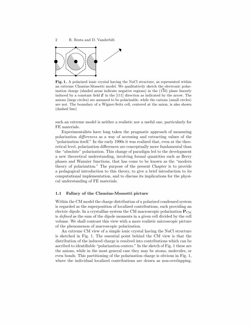
Fig. 1. A polarized ionic crystal having the NaCl structure, as represented withinan extreme Clausius-Mossotti model. We qualitatively sketch the electronic polar-ization charge (shaded areas indicate negative regions) in the (110) plane linearlyinduced by a constant field E in the [111] direction as indicated by the arrow. Theanions (large circles) are assumed to be polarizable, while the cations (small circles)are not. The boundary of a Wigner-Seitz cell, centered at the anion, is also shown(dashed line)

such an extreme model is neither a realistic nor a useful one, particularly forFE materials.

Experimentalists have long taken the pragmatic approach of measuringpolarization differences as a way of accessing and extracting values of the“polarization itself.” In the early 1990s it was realized that, even at the theo-retical level, polarization differences are conceptually more fundamental thanthe “absolute” polarization. This change of paradigm led to the developmenta new theoretical understanding, involving formal quantities such as Berryphases and Wannier functions, that has come to be known as the “moderntheory of polarization.” The purpose of the present Chapter is to providea pedagogical introduction to this theory, to give a brief introduction to itscomputational implementation, and to discuss its implications for the physi-cal understanding of FE materials.

1.1 Fallacy of the Clausius-Mossotti picture

Within the CM model the charge distribution of a polarized condensed systemis regarded as the superposition of localized contributions, each providing anelectric dipole. In a crystalline system the CM macroscopic polarization PCM

is defined as the sum of the dipole moments in a given cell divided by the cellvolume. We shall contrast this view with a more realistic microscopic pictureof the phenomenon of macroscopic polarization.

An extreme CM view of a simple ionic crystal having the NaCl structureis sketched in Fig. 1. The essential point behind the CM view is that thedistribution of the induced charge is resolved into contributions which can beascribed to identifiable “polarization centers.” In the sketch of Fig. 1 these arethe anions, while in the most general case they may be atoms, molecules, oreven bonds. This partitioning of the polarization charge is obvious in Fig. 1,where the individual localized contributions are drawn as non-overlapping.

Theory of Polarization 3

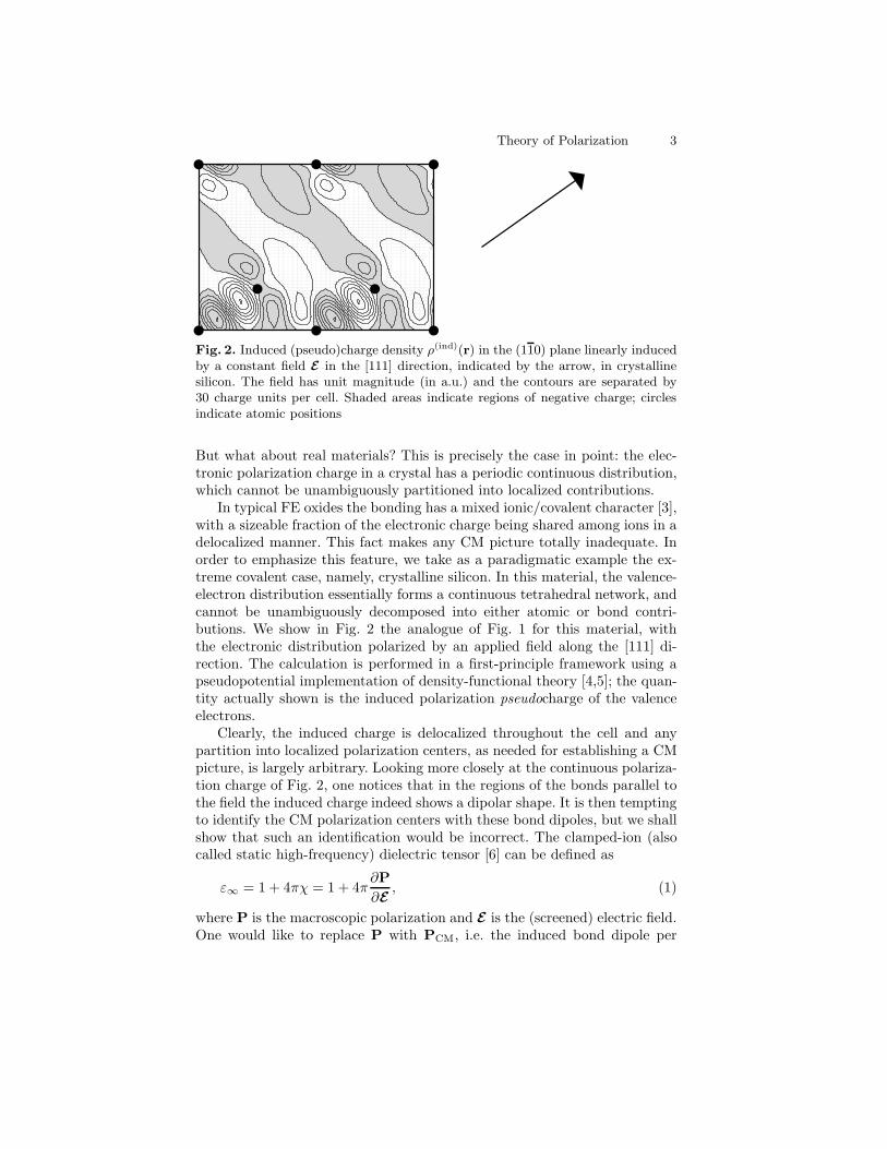
Fig. 2. Induced (pseudo)charge density ρ(ind)(r) in the (110) plane linearly inducedby a constant field E in the [111] direction, indicated by the arrow, in crystallinesilicon. The field has unit magnitude (in a.u.) and the contours are separated by30 charge units per cell. Shaded areas indicate regions of negative charge; circlesindicate atomic positions

But what about real materials? This is precisely the case in point: the elec-tronic polarization charge in a crystal has a periodic continuous distribution,which cannot be unambiguously partitioned into localized contributions.

In typical FE oxides the bonding has a mixed ionic/covalent character [3],with a sizeable fraction of the electronic charge being shared among ions in adelocalized manner. This fact makes any CM picture totally inadequate. Inorder to emphasize this feature, we take as a paradigmatic example the ex-treme covalent case, namely, crystalline silicon. In this material, the valence-electron distribution essentially forms a continuous tetrahedral network, andcannot be unambiguously decomposed into either atomic or bond contri-butions. We show in Fig. 2 the analogue of Fig. 1 for this material, withthe electronic distribution polarized by an applied field along the [111] di-rection. The calculation is performed in a first-principle framework using apseudopotential implementation of density-functional theory [4,5]; the quan-tity actually shown is the induced polarization pseudocharge of the valenceelectrons.

Clearly, the induced charge is delocalized throughout the cell and anypartition into localized polarization centers, as needed for establishing a CMpicture, is largely arbitrary. Looking more closely at the continuous polariza-tion charge of Fig. 2, one notices that in the regions of the bonds parallel tothe field the induced charge indeed shows a dipolar shape. It is then temptingto identify the CM polarization centers with these bond dipoles, but we shallshow that such an identification would be incorrect. The clamped-ion (alsocalled static high-frequency) dielectric tensor [6] can be defined as

ε∞ = 1 + 4πχ = 1 + 4π∂P∂E , (1)

where P is the macroscopic polarization and E is the (screened) electric field.One would like to replace P with PCM, i.e. the induced bond dipole per


cell. However, in order to actually evaluate PCM, one must choose a recipefor truncating the integration to a local region, which is largely arbitrary.Even more important, no matter which reasonable recipe one adopts, themagnitude of PCM is far too small (by at least an order of magnitude) toreproduce the actual value ε∞ ' 12 in silicon. The magnitude of the localdipoles seen in Fig. 2 may therefore account for only a small fraction of theactual P value for this material. In fact, as we shall explain below, it isgenerally impossible to obtain the value of P from the induced charge densityalone.

1.2 Fallacy of defining polarization via the charge distribution

Given that P carries the meaning of electric dipole moment per unit volume,it is tempting to try to define it as the dipole of the macroscopic sampledivided by its volume, i.e.,

Psamp =1

Vsamp

∫samp

dr rρ(r). (2)

We focus, once more, on the case of crystalline silicon polarized by an externalfield along the [111] direction. In order to apply (2), we need to assume amacroscopic but finite crystal. But the integral then has contributions fromboth the surface and the bulk regions, which cannot be easily disentangled.In particular, suppose that a cubic sample of dimensions L×L×L has itssurface preparation changed in such a way that a new surface charge density∆σ appears on the right face and −∆σ on the left; this will result in a changeof dipole moment scaling as L3, and thus, a change in the value of Psamp,despite the fact that the conditions in the interior have not changed. Thus,(2) is not a useful bulk definition of polarization; and even if it were, therewould be no connection between it and the induced periodic charge densityin the sample interior that is illustrated in Fig. 2.

A second tempting approach to a definition of the bulk polarization is via

Pcell =1Vcell

∫cell

dr rρ(r), (3)

where the integration is carried out over one unit cell deep in the interiorof the sample. However, this approach is also flawed, because the result of(3) depends on the shape and location of the unit cell. (Indeed, the averageof Pcell over all possible translational shifts is easily shown to vanish.) Itis only within an extreme CM model—where the periodic charge can bedecomposed with no ambiguity by choosing, as in Fig. 1, the cell boundaryto lie in an interstitial region of vanishing charge density—that Pcell is welldefined. However, in many materials a CM model is completely inappropriate,as discussed above.


As a third approach, one might imagine defining P as the cell average ofa microscopic polarization Pmicro defined via

∇ ·Pmicro(r) = −ρ(r). (4)

However, the above equation does not uniquely define Pmicro(r), since anydivergence-free vector field, and in particular any constant vector, can beadded to Pmicro(r) without affecting the left-hand side of (4).

The conclusion to be drawn from the above discussion is that a a knowl-edge of the periodic electronic charge distribution in a polarized crystallinesolid cannot, even in principle, be used to construct a meaningful definitionof bulk polarization. This has been understood, and similar statements haveappeared in the literature, since at least 1974 [7]. However, this importantmessage has not received the wide appreciation it deserves, nor has it reachedthe most popular textbooks [6].

These conclusions may appear counterintuitive and disturbing, since onereasonably expects that the macroscopic polarization in the bulk region ofa solid should be determined by what “happens” in the bulk. But this isprecisely the basis of a third, and finally rewarding, approach to the problem,in which one focuses on the change in Psamp that occurs during some processsuch as the turning on of an external electric field. The change in internalpolarization ∆P that we seek will then be given by the change ∆Psamp of(2), provided that any charge that is pumped to the surface is not allowedto be conducted away. (Thus, the sides of the sample must be insulating,there must be no grounded electrodes, etc.) Actually, it is preferable simplyto focus on the charge flow in the interior of the sample during this process,and write

∆P =∫dt

1Vcell

∫cell

dr j(r, t). (5)

This equation is the basis of the modern theory of polarization that will besummarized in the remainder of this Chapter. Again, it should be emphasizedthat the definition (5) has nothing to do with the periodic static chargedistribution inside the bulk unit cell of the polarized solid.

So far, we have avoided any experimental consideration. How is P mea-sured? Certainly no one relies on measuring cell dipoles, although inducedcharge distributions of the kind shown in Fig. 2 are accessible to x-ray crystal-lography. A FE material sustains, by definition, a spontaneous macroscopicpolarization, i.e., a non-vanishing value of P in the absence of any pertur-bation. But once again, while the microscopic charge distribution inside theunit cell of a FE crystal is experimentally accessible, actual measurements ofthe spontaneous polarization are based on completely different ideas, moreclosely related to (5). As we will see below in Sec. 2, this approach definesthe observable P in a way that very naturally parallels experiments, both forspontaneous and induced polarization. We also see that the theory vindicatesthe concept that macroscopic polarization is an intensive quantity, insensitive


to surface effects, whose value is indeed determined by what “happens” inthe bulk of the solid and not at its surface.

2 Polarization as an adiabatic flow of current

2.1 How is induced polarization measured?

Most measurements of bulk macroscopic polarization P of materials do notaccess its absolute value, but only its derivatives, which are expressed asCartesian tensors. For example, the permittivity

χαβ =dPα

dEβ(6)

appearing in (1) is defined as the derivative of polarization with respect tofield. Here, as throughout this Chapter, Greek subscripts indicate Cartesiancoordinates. Similarly, the pyroelectric coefficient

Πα =dPα

dT, (7)

the piezoelectric tensor

γαβδ =∂Pα

∂εβδ(8)

of Sec. 4.3, and the dimensionless Born (or “dynamical” or “infrared”) charge

Z∗s,αβ =Ωe

∂Pα

∂us,β(9)

of Sec. 4.2, are defined in terms of derivatives with respect to temperatureT , strain εβδ, and displacement us of sublattice s, respectively. Here e>0is the charge quantum, and from now on we use Ω to denote the primitivecell volume Vcell. (In the above formulas, derivatives are to be taken at fixedelectric field and fixed strain when these variables are not explicitly involved.)

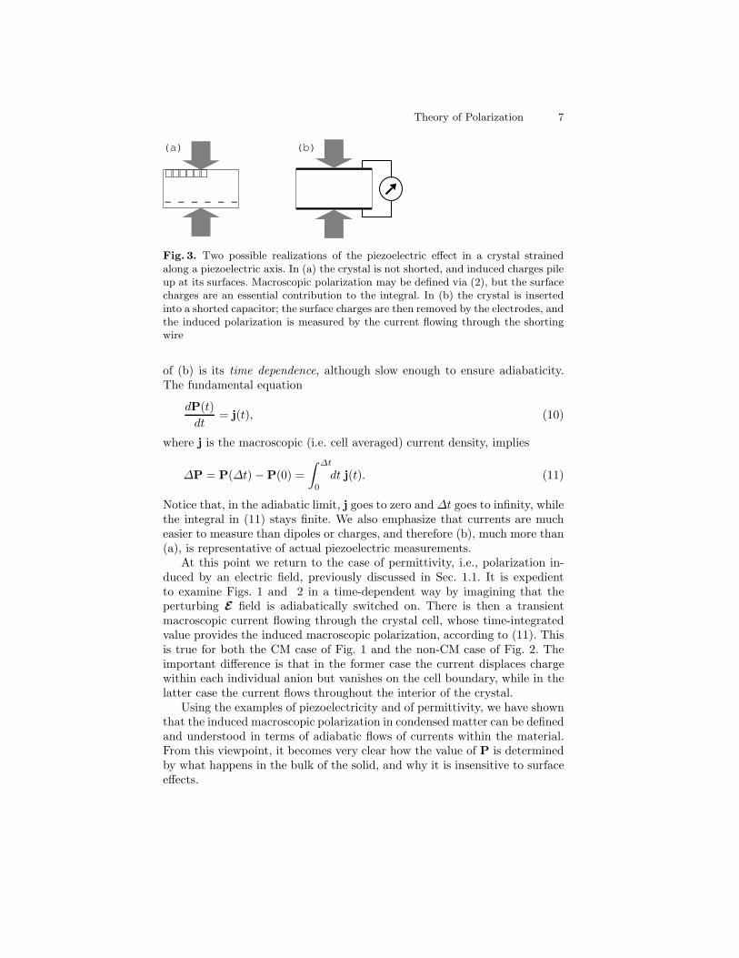
We start by illustrating one such case, namely, piezoelectricity, in Fig. 3.The situation depicted in (a) is the one where (2) applies. Supposing thatP is zero in the unstrained state (e.g. by symmetry), then the piezoelectricconstant is simply proportional to the value of P in the final state. Thedisturbing feature is that piezoelectricity appears as a surface effect, andindeed the debate whether piezoelectricity is a bulk or a surface effect lastedin the literature until rather recently [8]. The modern theory parallels thesituation depicted in (b) and provides further evidence that piezoelectricityis a bulk effect, if any was needed. While the crystal is strained, a transientelectrical current flows through the sample, and this is precisely the quantitybeing measured; the polarization of the final state is not obtained from ameasurement performed on the final state only. In fact, the essential feature


(a)

+ + + + + +

− − − − − −

(b)

Fig. 3. Two possible realizations of the piezoelectric effect in a crystal strainedalong a piezoelectric axis. In (a) the crystal is not shorted, and induced charges pileup at its surfaces. Macroscopic polarization may be defined via (2), but the surfacecharges are an essential contribution to the integral. In (b) the crystal is insertedinto a shorted capacitor; the surface charges are then removed by the electrodes, andthe induced polarization is measured by the current flowing through the shortingwire

of (b) is its time dependence, although slow enough to ensure adiabaticity.The fundamental equation

dP(t)dt

= j(t), (10)

where j is the macroscopic (i.e. cell averaged) current density, implies

∆P = P(∆t) −P(0) =∫ ∆t

0

dt j(t). (11)

Notice that, in the adiabatic limit, j goes to zero and ∆t goes to infinity, whilethe integral in (11) stays finite. We also emphasize that currents are mucheasier to measure than dipoles or charges, and therefore (b), much more than(a), is representative of actual piezoelectric measurements.

At this point we return to the case of permittivity, i.e., polarization in-duced by an electric field, previously discussed in Sec. 1.1. It is expedientto examine Figs. 1 and 2 in a time-dependent way by imagining that theperturbing E field is adiabatically switched on. There is then a transientmacroscopic current flowing through the crystal cell, whose time-integratedvalue provides the induced macroscopic polarization, according to (11). Thisis true for both the CM case of Fig. 1 and the non-CM case of Fig. 2. Theimportant difference is that in the former case the current displaces chargewithin each individual anion but vanishes on the cell boundary, while in thelatter case the current flows throughout the interior of the crystal.

Using the examples of piezoelectricity and of permittivity, we have shownthat the induced macroscopic polarization in condensed matter can be definedand understood in terms of adiabatic flows of currents within the material.From this viewpoint, it becomes very clear how the value of P is determinedby what happens in the bulk of the solid, and why it is insensitive to surfaceeffects.


2.2 How is ferroelectric polarization measured?

FE materials are insulating solids characterized by a switchable macroscopicpolarization P. At equilibrium, a FE material displays a broken-symmetry,noncentrosymmetric structure, so that a generic vector property is not re-quired to vanish by symmetry. The most important vector property is indeedP, and its equilibrium value is known as the spontaneous polarization.

However, the value of P is never measured directly as an equilibrium prop-erty; instead, all practical measurements exploit the switchability of P. Inmost crystalline FEs, the different structures are symmetry-equivalent; thatis, the allowed values of P are equal in modulus and point along equivalent(enantiomorphous) symmetry directions. In a typical experiment, applicationof a sufficiently strong electric field switches the polarization from P to −P,so that one speaks of polarization reversal.

The quantity directly measured in a polarization reversal experiment isthe difference in polarization between the two enantiomorphous structures;making use of symmetry, one can then equate this difference to twice thespontaneous polarization. This pragmatic working definition of spontaneouspolarization has, as a practical matter, been adopted by the experimentalcommunity since the early days of the field. However, it was generally con-sidered that this was done only as an expedient, because direct access to the“polarization itself” was difficult to obtain experimentally. Instead, with thedevelopment of modern electronic-structure methods and the application ofthese methods to FE materials, it became evident that the previous “text-book definitions” [6] of P were also unworkable from the theoretical point ofview. It was found that such attempts to define P as a single-valued equilib-rium property of the crystal in a given broken-symmetry state, in the spiritof (3), were doomed to failure because they could not be implemented in anunambiguous way.

In response to this impasse, a new theoretical viewpoint emerged in theearly 1990s and was instrumental to the development of a successful mi-croscopic theory [9–11]. As we shall see, this modern theory of polarizationactually elevates the old pragmatic viewpoint to the status of a postulate.Rather than focusing on P as an equilibrium property of the crystal in agiven state, one focuses on differences in polarization between two differentstates [9]. From the theoretical viewpoint, this represents a genuine change ofparadigm, albeit one that is actually harmonious with the old experimentalpragmatism.

We illustrate a polarization reversal experiment by considering the caseof the perovskite oxide PbTiO3, whose equilibrium structure at zero temper-ature is tetragonal. There are six enantiomorphous broken-symmetry struc-tures; two of them, having opposite nuclear displacements and opposite valuesof P, are shown in Fig. 4.

A typical measurement of the spontaneous polarization, performed throughpolarization reversal, is schematically shown in Fig. 5. The hysteresis cy-


Fig. 4. Tetragonal structure of PbTiO3: solid, shaded, and empty circles representPb, Ti, and O atoms, respectively. The arrows indicate the actual magnitude of theatomic displacements, where the origin has been kept at the Pb site (the Ti dis-placements are barely visible). Two enantiomorphous structures, with polarizationalong [001], are shown here. Application of a large enough electric field (coercivefield) switches between the two and reverses the polarization

cle is in fact the primary experimental output. The transition between thetwo enantiomorphous FE structures A and B of Fig. 4 is driven by an ap-plied electric field; the experimental setup typically measures the integratedmacroscopic current flowing through the sample, as in (11). One half of thedifference PB − PA defines the magnitude Ps of the spontaneous polariza-tion in the vertical direction. From Fig. 5, it is clear that Ps can also bedefined as the polarization difference ∆P between the broken-symmetry Bstructure and the centrosymmetric structure (where the displacements areset to zero). Notice that, while a field is needed to induce the switching inthe actual experiment, ideally one could evaluate ∆P along the vertical axisin Fig. 5, where the macroscopic field is identically zero. We stress that theexperiment measures neither PA nor PB, but only their difference. It is onlyan additional symmetry argument which allows one to infer the value of eachof them from the actual experimental data.

P

εB

A

Fig. 5. A typical hysteresis loop; the magnitude of the spontaneous polarizationis also shown (vertical dashed segment). Notice that spontaneous polarization is azero-field property


2.3 Basic prescriptions for a theory of polarization

For both induced and spontaneous polarization, we have emphasized therole of adiabatic currents in order to arrive at a microscopic theory of P,which by construction must be an intensive bulk property, insensitive to theboundaries. The root of this theory is in (11), whose form we simplify byintroducing a parameter λ having the meaning of a dimensionless adiabatictime: λ varies continuously from zero (corresponding to the initial system)to 1 (corresponding to the final system). Then we can write (11) as

∆P =∫ 1

0

dλdPdλ

. (12)

In general, “initial” and “final” refer to the state of the system before andafter the application of some slow sublattice displacements, strains, electricfields, etc. The key feature exploited here is that dP/dλ is a well-definedbulk vector property. We notice, however, that an important condition for(12) to hold is that the system remain insulating for all intermediate valuesof λ, since the transient current is otherwise not uniquely defined. Note thatfor access to the response properties of (6-9), no integration is needed; thephysical quantity of interest coincides by definition with dP/dλ evaluated atan appropriate λ.

In order to specialize the discussion to the spontaneous polarization of aFE, we now let λ scale the sublattice displacements (the lengths of the arrowsin Fig. 4) leading from a centrosymmetric reference structure (λ=0) to thespontaneously polarized structure (λ=1). Then the spontaneous polarizationmay be written [9]

Peff =∫ 1

0

dλdPdλ

(λ = 0 : centrosymmetric reference). (13)

For later reference, note that this is the “effective” and not the “formal”definition of polarization as given later in (20) and discussed in the laterparts of Sec. 3.

The current-carrying particles are electrons and nuclei; while the quantumnature of the former is essential, the latter can be safely dealt with as classicalpoint charges, whose current contributions to (11) and to (12) are trivial. Wefocus then mostly on the electronic term in the currents and in P, althoughit has to be kept in mind that the overall charge neutrality of the condensedsystem is essential. Furthermore, from now on we limit ourselves to a zero-temperature framework, thus ruling out the phenomenon of pyroelectricity.

We refer, once more, to Fig. 2, where the quantum nature of the electronsis fully accounted for. As explained above, in order to obtain P via (11), oneneeds the adiabatic electronic current which flows through the crystal whilethe perturbation is switched on. Within a quantum-mechanical descriptionof the electronic system, currents are closely related to the phase of the wave-function (for instance, if the wavefunction is real, the current vanishes every-where). But only the modulus of the wavefunction has been used in drawing


the charge distribution of Fig. 2; any phase information has been obliterated,so that the value of P cannot be retrieved. Interestingly, this argument isin agreement with the general concept, strongly emphasized above, that theperiodic polarization charge inside the material has nothing to do with thevalue of macroscopic polarization.

Next, it is expedient to discuss a bit more thoroughly the role of theelectric field E. A direct treatment of a finite electric field is subtle, becausethe periodicity of the crystal Hamiltonian, on which the Bloch theorem de-pends, is absent unless E vanishes (see Sec. 5.1). However, while E is bydefinition the source inducing P in the case of permittivity in (6), a sourceother than electric field is involved in the cases of pyroelectricity (7), piezo-electricity (8), dynamical effective charges (9), and spontaneous polarization(13). While it is sometimes appropriate to take these latter derivatives underelectrical boundary conditions other than those of vanishing field, we shallrestrict ourselves here to the most convenient and fundamental definitions inwhich the field E is set to zero. For example, piezoelectricity, when measuredas in Fig. 3(b), is clearly a zero-field property, since the sample is shorted atall times. Spontaneous polarization, when measured as in Fig. 5, is obviouslya zero-field property as well. Born effective charges, which will be addressedbelow, are also defined as zero-field tensors. Then, as an example of two dif-ferent choices of boundary conditions to address the same phenomenon, wemay consider again the case of piezoelectricity, Fig. 3. While in (b) the fieldis zero, in (a) a non-vanishing (“depolarizing”) field is clearly present insidethe material. The two piezoelectric tensors, phenomenologically defined inthese two different ways, are not equal but are related in a simple way (infact, they are proportional via the dielectric tensor).

Thus, it is possible to access many of the interesting physical properties,including piezoelectricity, lattice dynamics, and ferroelectricity, with calcula-tions performed at zero field. We will restrict ourselves to this case for mostof this chapter. As for the permittivity, it is theoretically accessible by meansof either the linear-response theory (see [12] for a thorough review), or viaan extension of the Berry-phase theory to finite electric field that will bedescribed briefly in Sec. 5.1.

3 Formal description of the Berry-phase theory

In this Section, we shall give an introduction to the modern theory of po-larization that was developed in the 1990s. Following important preliminarydevelopments of Resta [9], the principal development of the theory was in-troduced by King-Smith and Vanderbilt [10] and soon afterwards reviewedby Resta [11]. This theory is sometimes known as the “Berry-phase theory ofpolarization” because the polarization is expressed in the form of a certainquantum phase known as a Berry phase [13].


In order to deal with macroscopic systems, both crystalline and disor-dered, it is almost mandatory in condensed matter theory to assume periodic(Born-von Karman) boundary conditions [6]. This amounts to considering thesystem in a finite box which is periodically repeated, in a ring-like fashion,in all three Cartesian directions. Eventually, the limit of an infinitely largebox is taken. For practical purposes, the thermodynamic limit is approachedwhen the box size is much larger than a typical atomic dimension. Amongother features, a system of this kind has no surface and all of its propertiesare by construction “bulk” ones. When the system under consideration is amany-electron system, the periodic boundary conditions amount to requir-ing that the wavefunction and the Hamiltonian be periodic over the box. Asindicated previously, our discussion will be restricted to the case of vanishingelectric field unless otherwise stated.

We give below only a brief sketch of the derivation of the central formulasof the theory; interested readers are referred to Refs. [10,11,14] for details.

3.1 Formulation in continuous k-space

If we adopt for the many-electron system a mean-field treatment, such as theKohn-Sham one [4], the self-consistent one-body potential is periodic overthe Born-von Karman box, provided the electric field E vanishes, for anyvalue of the parameter λ. Furthermore, if we consider a crystalline system,the selfconsistent potential also has the lattice periodicity. The eigenfunctionsare of the Bloch form ψnk(r) = eik·r unk(r), where u is lattice-periodical, andobey the Schrodinger equation H |ψnk〉 = Enk |ψnk〉, where H = p2/2m+ V .Equivalently, the eigenvalue problem can be written Hk|unk〉 = Enk |unk〉where

Hk =(p + hk)2

2m+ V. (14)

All of these quantities depend implicitly on a parameter λ that changes slowlyin time, such that the wavefunction acquires, from elementary adiabatic per-turbation theory, a first-order correction

|δψnk〉 = −ih λ∑m 6=n

〈ψmk|∂λψnk〉Enk − Emk

|ψmk〉 (15)

where λ = dλ/dt and ∂λ is the derivative with respect to the parameter λ.The corresponding first-order current arising from the entire band n is then1

jn =dPn

dt=

iheλ

(2π)3m

∑m 6=n

∫dk

〈ψnk|p|ψmk〉〈ψmk|∂λψnk〉Enk − Emk

+ c.c. (16)

1 In this and subsequent formulas, we assume that n is a really a composite indexfor band and spin. Alternatively, factors of two may be inserted into the equationsto account for spin degeneracy.


where “c.c.” denotes the complex conjugate. Time t can be eliminated byremoving λ from the right-hand side and replacing dP/dt → dP/dλ onthe left-hand side above. Then, making use of ordinary perturbation theoryapplied to the dependence of Hk in (14) upon k, one obtains, after somemanipulation,

dPn

dλ=

ie

(2π)3

∫dk 〈∇kunk|∂λunk〉 + c.c. . (17)

It is noteworthy that the sum over “unoccupied” states m has disappearedfrom this formula, corresponding to our intuition that the polarization is aground-state property. Summing now over the occupied states, and insertingin (12), we get the spontaneous polarization of a FE. The result, after anintegration with respect to λ, is that the effective polarization (13) takes theform

Peff = ∆Pion + [Pel(1)−Pel(0) ] (18)

where the nuclear contribution ∆Pion has been restored, and

Pel(λ) =e

(2π)3Im

∑n

∫dk 〈unk|∇k|unk〉. (19)

Here, the sum is over the occupied states, and |unk〉 are understood to beimplicit functions of λ. In the case that the adiabatic path takes a FE crystalfrom its centrosymmetric reference state to its equilibrium polarized state,Peff of (18) is just exactly the spontaneous polarization.

Equation (19) is the central result of the modern theory of polariza-tion. Those familiar with Berry-phase theory [13] will recognize A(k) =i〈unk|∇k|unk〉 as a “Berry connection” or “gauge potential”; its integral overa closed manifold (here the Brillouin zone) is known as a “Berry phase”. It isremarkable that the result (19) is independent of the path traversed throughparameter space (and of the rate of traversal, as long as it is adiabaticallyslow), so that the result depends only on the end points. Implicit in the anal-ysis is that the system must remain insulating everywhere along the path, asotherwise the adiabatic condition fails.

To obtain the total polarization, the ionic contribution must be added to(19). The total polarization is then P = Pel + Pion or

P =e

(2π)3Im

∑n

∫dk 〈unk|∇k|unk〉+

e

Ω∑

s

Z ions rs (20)

where the first term is (19) and the second is Pion, the contribution arisingfrom positive point charges eZ ion

s located at atomic positions rs. In principle,the band index n should run over all bands, including those made from corestates, and Z ion should be the bare nuclear charge. However, in the frozen-core approximation that underlies pseudopotential theory, we let n run over


0 π2 /a

k0

π2 /a

k

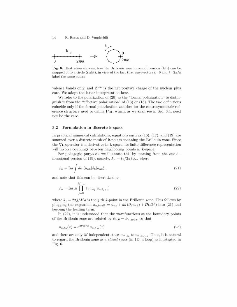
Fig. 6. Illustration showing how the Brillouin zone in one dimension (left) can bemapped onto a circle (right), in view of the fact that wavevectors k=0 and k=2π/alabel the same states

valence bands only, and Z ion is the net positive charge of the nucleus pluscore. We adopt the latter interpretation here.

We refer to the polarization of (20) as the “formal polarization” to distin-guish it from the “effective polarization” of (13) or (18). The two definitionscoincide only if the formal polarization vanishes for the centrosymmetric ref-erence structure used to define Peff , which, as we shall see in Sec. 3.4, neednot be the case.

3.2 Formulation in discrete k-space

In practical numerical calculations, equations such as (16), (17), and (19) aresummed over a discrete mesh of k-points spanning the Brillouin zone. Sincethe ∇k operator is a derivative in k-space, its finite-difference representationwill involve couplings between neighboring points in k-space.

For pedagogic purposes, we illustrate this by starting from the one-di-mensional version of (19), namely, Pn = (e/2π)φn, where

φn = Im∫dk 〈unk|∂k|unk〉 , (21)

and note that this can be discretized as

φn = Im lnM−1∏j=0

〈un,kj |un,kj+1〉 (22)

where kj = 2πj/Ma is the j’th k-point in the Brillouin zone. This follows byplugging the expansion un,k+dk = unk + dk (∂kunk) + O(dk2) into (21) andkeeping the leading term.

In (22), it is understood that the wavefunctions at the boundary pointsof the Brillouin zone are related by ψn,0 = ψn,2π/a, so that

un,k0(x) = e2πix/a un,kM (x) (23)

and there are only M independent states un,k0 to un,kM−1 . Thus, it is naturalto regard the Brillouin zone as a closed space (in 1D, a loop) as illustrated inFig. 6.


Equation (22) makes it easy to see why this quantity is called a Berry“phase.” We are instructed to compute the global product of wavefunctions

...〈uk1 |uk2〉〈uk2 |uk3〉〈uk3 |uk4〉... (24)

across the Brillouin zone, which in general is a complex number; then theoperation ‘Im ln’ takes the phase of this number. Note that this global phaseis actually insensitive to a change of the phase of any one wavefunction uk,since each uk appears once in a bra and once in a ket. We can thus view the“Berry phase” φn, giving the contribution to the polarization arising fromband n, as a global phase property of the manifold of occupied one-electronstates.

In three dimensions (3D), the Brillouin zone can be regarded as a closed3-torus obtained by identifying boundary points ψnk = ψn,k+Gj , where Gj isa primitive reciprocal lattice vector. The Berry phase for band n in directionj is φn,j = (Ω/e)Gj ·Pn, where Pn is the contribution to (19) from band n,so that

φn,j = Ω−1BZ Im

∫BZ

d3k 〈unk|Gj · ∇k|unk〉. (25)

We then have

Pn =12π

e

Ω

∑j

φn,j Rj (26)

where Rj is the real-space primitive translation corresponding to Gj . Tocompute the φn,j for a given direction j, the sampling of the Brillouin zone isarranged as in Fig. 7, where k‖ is the direction along Gj and k⊥ refers to the2D space of wavevectors spanning the other two primitive reciprocal latticevectors. For a given k⊥, the Berry phase φn,j(k⊥) is computed along thestring of M k-points extending along k‖ as in (22), and finally a conventionalaverage over the k⊥ is taken:

φn,j =1

Nk⊥

∑k⊥

φn(k⊥). (27)

Note that a subtlety arises in regard to the “choice of branch” when takingthis average, as discussed in the next subsection. Moreover, in 3D crystals,it may happen that some groups of bands must be treated using a many-band generalization of (22) due to degeneracy at high-symmetry points inthe Brillouin zone; see Refs. [10,11] for details.

The computation of P according to (26) is now a standard option in sev-eral popular electronic-structure codes (abinit [15], crystal [16], pwscf [17],siesta [18], and vasp [19]).


k

k

Fig. 7. Arrangement of Brillouin zone for computation of component of P alongk‖ direction

3.3 The quantum of polarization

It is clear that (22), being a phase, is only well-defined modulo 2π. We cansee this more explicitly in (21); let

|unk〉 = e−iβ(k) |unk〉 (28)

be a new set of Bloch eigenstates differing only in the choice of phase as afunction of k. Here β(k) is real and obeys β(2π/a) − β(0) = 2πm, where mis an integer, in order that ψn,0 = ψn,2π/a. Then plugging into (22) we findthat

φn = φn +∫ 2π/a

0

dk

(dβ

dk

)dk = φn + 2πm . (29)

Thus, φn is really only well-defined “modulo 2π.”In view of this uncertainty, care must be taken in the 3D case when

averaging φn(k⊥) over the 2D Brillouin zone of k⊥ space: the choice of branchcut must be made in such a way that φn(k⊥) remains continuous in k⊥. Inpractice, a conventional mesh sampling is used in the k⊥ space, and theaverage is computed as in (27). Consider, for example, Fig. 7, where Nk⊥=4.If the branch cut is chosen independently for each k⊥ so as to map φn(k⊥)to the interval [−π, π], and if the four values were found to be 0.75π, 0.85π,0.95π, and −0.95π, then the last value must be remapped to become 1.05πbefore the average is taken in (27). That is, the correct average is 0.90π,or equivalently −1.10π, but not 0.40π as would be obtained by taking theaverage blindly.

In other words, care must be taken to make a consistent choice of phaseson the right-hand side of (27). However, it is still permissible to shift all ofthe Nk⊥ phases by a common amount 2πmj. Thus, each φn,j in (26) is onlywell-defined modulo 2π, leading to the conclusion that Pn is only well-definedmodulo eR/Ω, where R =

∑j mjRj is a lattice vector. The same conclusion

results from generalizing the argument of (28)-(29) to 3D, showing that aphase twist of the form |unk〉 = exp[−iβ(k)] |unk〉 results in

Pn = Pn +eRΩ

(30)


where R is a lattice vector.These arguments are for a single band, but the same obviously applies

to the sum over all occupied bands. We thus arrive at a central result of themodern theory of polarization: the formal polarization, defined via (20) orcalculated through (26), is only well defined modulo eR/Ω, where R is anylattice vector and Ω is the primitive-cell volume.

At first sight the presence of this uncertainty modulo the quantum eR/Ωmay be surprising, but in retrospect it should have been expected. Indeed,the ionic contribution given by the second term of (20) is subject to preciselythe same uncertainty, arising from the arbitrariness of the nuclear locationrs modulo a lattice vector R. The choice of one particular value of P fromamong the lattice of values related to each other by addition of eR/Ω will bereferred to as the “choice of branch.”

Summarizing our results so far, we find that the formal polarization P,defined by (20), is only well-defined modulo eR/Ω, where R is any latticevector. Moreover, we have found that the change in polarization ∆P along anadiabatic path, as defined by (12), is connected with this formal polarizationby the relation

∆P :=(Pλ=1 −Pλ=0

)modulo

eRΩ

. (31)

This central formula, embodying the main content of the modern theoryof polarization, requires careful explanation. For a given adiabatic path, thechange in polarization appearing on the left-hand side of (31), and defined by(12), is given by a single-valued vector quantity that is perfectly well definedand has no “modulus” uncertainty. On the right-hand side, Pλ=0 and Pλ=1

are, respectively, the formal polarization of (20) evaluated at the start andend of the path. The symbol “:=” has been introduced to indicate that thevalue on the left-hand side is equal to one of the values on the right-handside. Thus, the precise meaning of (31) is that the actual integrated adiabaticcurrent flow ∆P is equal to (Pλ=1 −Pλ=0) + eR/Ω for some lattice vectorR.

It follows that (31) cannot be used to determine ∆P completely; it onlydetermines∆P within the same uncertainty modulo eR/Ω that applies to Pλ.Fortunately, the typical magnitude of Peff , and of polarization differences ingeneral, is small compared to this “quantum.” For cubic perovskites, a ' 4 A,so that the effective quantum for spin-paired systems is 2e/a2 ' 2.0 C/m2.In comparison, the spontaneous polarization of perovskite ferroelectrics istypically in the range of about 0.3 to 0.6C/m2, significantly less than thisquantum. Thus, this uncertainty modulo eR/Ω is rarely a serious concern inpractice. If there is doubt about the correct choice of branch for a given path,this doubt can usually be resolved promptly by computing the polarizationat several intermediate points along the path; as long as ∆P is small foreach step along the path, the correct interpretation of the evolution of thepolarization will be clear.


Px

Py(a)

Px

Py(b)

Px

Py(c)

Fig. 8. Polarization as a lattice-valued quantity, illustrated for a 2D square-latticesystem. Here (a) and (b) illustrate the two possible states of polarization consistentwith full square-lattice symmetry, while (c) illustrates a possible change in polar-ization induced by some symmetry-lowering change of the Hamiltonian. In (c), thearrows show the “effective polarization” as defined in (13)

Table 1. Atomic positions τ and nominal ionic charges Z for KNbO3 in its cen-trosymmetric cubic structure with lattice constant a

Atom τx τy τz Zion

K 0 0 0 +1Nb a/2 a/2 a/2 +5O1 0 a/2 a/2 −2O2 a/2 0 a/2 −2O3 a/2 a/2 0 −2

3.4 Formal polarization as a multivalued vector quantity

A useful way to think about the presence of this “modulus” is to regard theformal polarization as a multivalued vector quantity, rather than a conven-tional single-valued one. That is, the question “What is P?” is answered notby giving a single vector, but a lattice of vector values related by translationseR/Ω. Here, we explain how this viewpoint contributes to an understandingof the role of symmetry and provides an alternative perspective on the centralresult (31) of the previous subsection.

Let us begin with symmetry considerations, where we find some surprisingresults. Consider, for example, KNbO3 in its ideal cubic structure. Because ofthe cubic symmetry, one might expect that P as calculated from (20) wouldvanish; or more precisely, given the uncertainty expressed by (30), that itwould take on a lattice of values (m1,m2,m3)e/a2 that includes the zerovector (mj are integers). This expected situation is sketched (in simplified2D form) in Fig. 8(a).

However, when the result is actually calculated from (20) using first-principles electronic-structure methods, this is not what one finds. Instead,one finds that

P =(m1 + 1

2 , m2 + 12 , m3 + 1

2

) e

a2(integer mj) , (32)


which is indeed a multivalued object, but corresponding to the situationsketched in Fig. 8(b), not Fig. 8(a)!

While this result emerges above from a fully quantum-mechanical calcula-tion, it is not essentially a quantum-mechanical result. Indeed, it could havebeen anticipated based on purely classical arguments as applied to an idealionic model of the KNbO3 crystal. In such a picture, the formal polarizationis written as

P =e

Ω

∑s

Z ions τ s (33)

where τ s is the location, and Z ions is the nominal (integer) ionic charge, of ion

s. Evaluating (33) using the values given in Table 1 yields P = ( 12 ,

12 ,

12 )e/a

2.However, each vector τ s is arbitrary modulo a lattice vector. For example,it is equally valid to replace τK = (0, 0, 0) by τK = (a, a, a), yielding P =( 3

2 ,32 ,

32 )e/a2, which is again consistent with (32). Similarly, since each Z ion

s

is an integer,2 the shift of any τ s by a lattice vector ∆R simply generates ashift to one of the other vectors on the right-hand side of (32). This heuristicionic model then leads to the same conclusion expressed in (32), i.e., thatFig. 8(b) and not Fig. 8(a) is appropriate for the case of cubic KNbO3.

This may appear to be a startling result. We are saying that the polar-ization as defined by (20) does not necessarily vanish for a centrosymmetricstructure (or more precisely, that the lattice of values corresponding to Pdoes not contain the zero vector). Is this in conflict with the usual observa-tion that a vector-valued physical quantity must vanish in a centrosymmetriccrystal? No, because this theorem applies only to a normal (that is, single-valued) vector quantity. Instead, the formal polarization is a multi-valuedvector quantity. The constraint of centrosymmetry requires that the polar-ization must get mapped onto itself by the inversion operation. This would beimpossible for a non-zero single-valued vector, but it is possible for a latticeof vector values, as illustrated in Fig. 8(b). Indeed, the lattice of values shownin Fig. 8(b) is invariant with respect to all the operations of the cubic sym-metry group, as are those of Fig. 8(a). Actually, for a simple cubic structurewith full cubic symmetry, these are the only two possibilities consistent withsymmetry. It is not possible to know, from symmetry alone, which of theserepresentations of the formal polarization is correct. A heuristic argument ofthe kind leading to (32) can be used to guess the correct result, but it shouldbe confirmed by actual calculation. The heuristic arguments suggest, andfirst-principles calculations confirm, that the formal polarizations of BaTiO3

and KNbO3 are not equal, even though they have identical symmetry; theycorrespond to Fig. 8(a) and Fig. 8(b), respectively!

How should we understand the spontaneous polarization Ps of ferroelec-trically distorted KNbO3 in the present context? Recall that Ps is defined2 For precisely this reason, it is necessary to use an ionic model with formal integer

ionic charges for arguments of this kind. This requirement can be justified usingarguments based on a Wannier representation.


as the effective polarization Peff of (13) for the case of an adiabatic pathcarrying KNbO3 from its unstable cubic to its relaxed FE structure. Supposethat one were to find that this adiabatic evolution carried the polarizationalong the path indicated by the arrows in Fig. 8(c). In this case, the effec-tive polarization Peff of (13) is definitely known to correspond to the vectorsketched repeatedly in Fig. 8(c). However, when one evaluates ∆P from (31),using only a knowledge of the endpoints of the path, the knowledge of thecorrect branch is lost. For example, one could not be certain that the actual∆P associated with this path is the one shown in Fig. 8(c), rather than onepointing from from an open circle in one cell to a closed one in a neighbor-ing cell (and differing by the “modulus” eR/Ω). This is, of course, just thesame uncertainty attached to (31) and discussed in detail in the previoussubsection, now expressed from a more graphical point of view.

3.5 Mapping onto Wannier centers

Another way of thinking about the meaning of the Berry-phase polarization,and of the indeterminacy of the polarization modulo the quantum eR/Ω, isin terms of Wannier functions. The Wannier functions are localized functionswnR(r), labeled by band n and unit cell R, that span the same Hilbertsubspace as do the Bloch states ψnk. In fact, they are connected by a Fourier-transform-like expression

|wnR〉 =Ω

(2π)3

∫dk eik·R |ψnk〉 , (34)

where the Bloch states are normalized to one over the crystal cell. Once wehave the Wannier functions, we can locate the “Wannier centers” rnR =〈wnR|r|wnR〉. It turns out that the location of the Wannier center is nothingother than

rnR =Ωe

Pn + R . (35)

That is, specifying the contribution of band n to the Berry-phase polarizationis really just equivalent to specifying the location of the Wannier center inthe unit cell. Because the latter is indeterminate modulo R, the former isindeterminate modulo eR/Ω.

Thus, the Berry-phase theory can be regarded as providing a mapping ofthe distributed quantum-mechanical electronic charge density onto a latticeof negative point charges of charge −e, as illustrated in Fig. 9. While theCM picture obviously cannot be applied to the situation of Fig. 9(a), becausethe charge density vanishes nowhere in the unit cell, it can be applied tothe situation of Fig. 9(b) without problem. The only question is whether thenegative charge located at z = (1 − γ)c in this figure should be regardedas “living” in the same unit cell as the positive nucleus at the origin or the


(a) (b)γ c

(1−γ ) c

Fig. 9. Illustrative tetragonal crystal (cell dimensions a× a× c) having one mono-valent ion at the cell corner (origin) and one occupied valence band. (a) The dis-tributed quantum-mechanical charge distribution associated with the electron band,represented as a contour plot. (b) The distributed electron distribution has beenreplaced by a unit point charge −e located at the Wannier center rn, as given bythe Berry-phase theory

(a) (b)

Fig. 10. Possible evolution of positions of Wannier centers (−), relative to latticeof ions (+), as Hamiltonian evolves adiabatically around a closed loop. Wannierfunctions must return to themselves, but can do so either (a) without, or (b) with,a coherent shift by a lattice vector

one at z = c; this uncertainty corresponds precisely to the “quantum ofpolarization” eR/Ω for the case R = cz.

It therefore appears that, by adopting the Wannier-center mapping, theCM viewpoint has been rescued. We are in fact decomposing the charge(nuclear and electronic) into localized contributions whose dipoles determineP. However, one has to bear in mind that the phase of the Bloch orbitals isessential to actually perform the Wannier transformation. Knowledge of theirmodulus is not enough, while we stress once more that the modulus uniquelydetermines the periodic polarization charge, such the one shown in Fig. 9(a).

Before leaving this discussion, it is amusing to consider the behavior ofthe Wannier centers rn under a cyclic adiabatic evolution of the Hamiltonian.That is, we want to integrate the net adiabatic current flow as the system istaken around a closed loop in some multidimensional parameter space. (Forexample, one atomic sublattice might be displaced by 0.1 A first along +x,


then +y, then −x, and then −y.) Referring to (12) and (13), we have for thiscase

∆Pcyc =∮ 1

0

dλdPdλ

(cyclic evolution: Hλ=0 = Hλ=1) . (36)

From (31), it follows that∆Pcyc is either exactly zero or else exactly eR/Ω forsome non-zero lattice vector R. The latter case corresponds to the “quantizedcharge transport” (or “quantum pumping”) first discussed by Thouless [20].

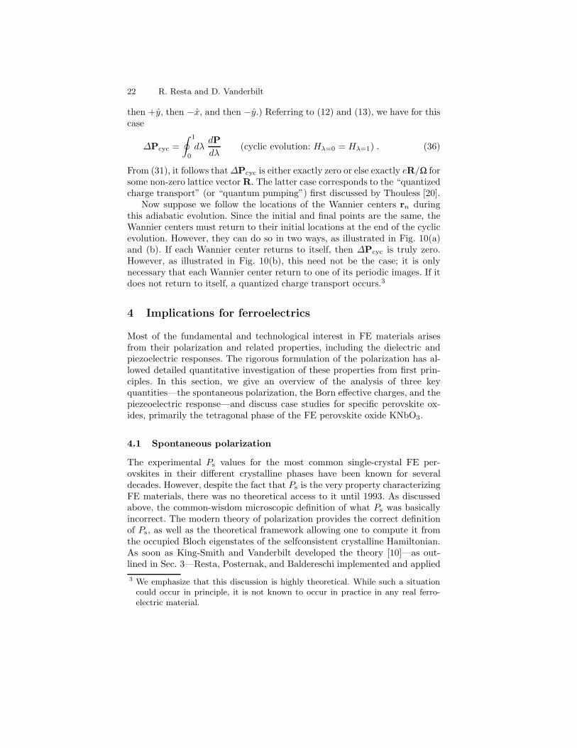
Now suppose we follow the locations of the Wannier centers rn duringthis adiabatic evolution. Since the initial and final points are the same, theWannier centers must return to their initial locations at the end of the cyclicevolution. However, they can do so in two ways, as illustrated in Fig. 10(a)and (b). If each Wannier center returns to itself, then ∆Pcyc is truly zero.However, as illustrated in Fig. 10(b), this need not be the case; it is onlynecessary that each Wannier center return to one of its periodic images. If itdoes not return to itself, a quantized charge transport occurs.3

4 Implications for ferroelectrics

Most of the fundamental and technological interest in FE materials arisesfrom their polarization and related properties, including the dielectric andpiezoelectric responses. The rigorous formulation of the polarization has al-lowed detailed quantitative investigation of these properties from first prin-ciples. In this section, we give an overview of the analysis of three keyquantities—the spontaneous polarization, the Born effective charges, and thepiezeoelectric response—and discuss case studies for specific perovskite ox-ides, primarily the tetragonal phase of the FE perovskite oxide KNbO3.

4.1 Spontaneous polarization

The experimental Ps values for the most common single-crystal FE per-ovskites in their different crystalline phases have been known for severaldecades. However, despite the fact that Ps is the very property characterizingFE materials, there was no theoretical access to it until 1993. As discussedabove, the common-wisdom microscopic definition of what Ps was basicallyincorrect. The modern theory of polarization provides the correct definitionof Ps, as well as the theoretical framework allowing one to compute it fromthe occupied Bloch eigenstates of the selfconsistent crystalline Hamiltonian.As soon as King-Smith and Vanderbilt developed the theory [10]—as out-lined in Sec. 3—Resta, Posternak, and Baldereschi implemented and applied3 We emphasize that this discussion is highly theoretical. While such a situation

could occur in principle, it is not known to occur in practice in any real ferro-electric material.


it to compute the spontaneous polarization of a prototypical perovskite oxidefrom first principles [21].

The case study was KNbO3 in its tetragonal phase, in a frozen-nucleigeometry taken from crystallographic data. The reciprocal cell is tetragonal:the integral in (19) was computed according to Sec. 3.2 (see Fig. 7), using theoccupied Kohn-Sham orbitals [4]. The electronic phase so evaluated dependson the choice of the origin in the crystalline cell, but translational invarianceis restored when the nuclear contribution is accounted for.

The computed phase turns out to be approximately π/3. This is largeenough that it is advisable to check whether the correct choice of branchhas been made for the multi-valued function “Im ln” in (22), in order to getrid of the 2π ambiguity discussed in Sec. 3.3. This is done by repeating thecalculation for smaller amplitudes of the FE distortion and making sure thatthe phase is a continuous function of the amplitude, as discussed earlier atthe end of Sec. 3.3.

The first-principle calculation of [21] for tetragonal KNbO3 yielded a valuePs = 0.35 C/m2, to be compared to a best experimental value of 0.37 C/m2.A similar level of agreement was later found for other perovskites and usingcomputational packages with different technical ingredients.

One aspect of the calculation deserves some comment. As stated abovewe have adopted a frozen-nuclei approach, which in principle is appropriatefor describing the polarization of the zero-temperature structure only. In thecalculation for KNbO3 discussed above, as well as in other calculations inthe literature, one addresses instead the spontaneous polarization of a finite-temperature crystalline phase. In fact, the tetragonal phase of KNbO3 onlyexists between 225 and 418 oC, while the equilibrium structure at zero tem-perature is rhombohedral and not tetrahedral. Crystallographic data providethe time-averaged crystalline structure, while polarization-reversal experi-ments provide the time-averaged spontaneous polarization. The question isthen whether the time-averaged polarization is equal, to a good approxima-tion, to the polarization of the time-averaged structure, as the latter is infact the quantity that is actually computed. The answer to this question isessentially ‘yes’, supported by the finding that the macroscopic polarizationis roughly linear, at the ±10-20% level, in the amplitude of the structuraldistortion. This essential linearity could not have been guessed from modelarguments, and in fact has only been discovered from the ab-initio calcula-tions [21,22].

4.2 Anomalous dynamical charges

The Born effective-charge tensors measure the coupling of a macroscopic fieldE with relative sublattice displacements (zone-center phonons) in the crystal;they also go under the name of dynamical charges or infrared charges. Withinan extreme rigid-ion model the Born charge coincides with the static chargeof the model ion (“nominal” value), while in a real material the Born charges


account for electronic polarization as well. Before the advent of the moderntheory of polarization in the 1990’s, the relevance of dynamical charges tothe phenomenon of ferroelectricity had largely been overlooked.

There are two equivalent definitions of the Born tensor Z∗s . (i) Z∗s,αβ ,as defined in (9), measures the change in polarization P in the α directionlinearly induced by a sublattice displacement us in the β direction in zeromacroscopic electric field. (Other kinds of effective charge can be definedusing other electrical boundary conditions [23], but this choice of E=0 is the“Born charge” one.) (ii) Alternatively, Z∗s,αβ measures the force F linearlyinduced in the α direction on the s-th nucleus by a uniform macroscopicelectric field E in the β direction (at zero displacement):

Fs,α = −e∑β

Z∗s,βα Eβ . (37)

Notice that, in low-symmetry situations, Z∗s is not symmetric in its Carte-sian indices. Since any rigid translation of the whole solid does not inducemacroscopic polarization, the Born effective-charge tensors obey∑

s

Z∗s,αβ = 0, (38)

a result that is generally known as the “acoustic sum rule” [24].The Berry-phase theory of polarization naturally leads to an evaluation

of the derivative in (9) as a finite difference, and this is the way most Z∗s cal-culations are performed for FE perovskites. However, expressions (9) or (37)based on linear response approaches [12] can be used whenever an electronic-structure code implementing such an approach (e.g., [15,17]) is available.

The Born effective-charge tensors are a staple quantity in the theory oflattice dynamics for polar crystals [25], and their experimental values havelong been known to a very good accuracy for simple materials such as bi-nary ionic crystals and simple semiconductors. As for FE materials, someexperimentally-derived values for BaTiO3 were proposed long ago [26]. How-ever, the subject remained basically neglected until 1993, when [21] appeared.This ab-initio calculation demonstrated that in FE perovskites the Borncharges are strongly “anomalous”, and that this anomaly has much to dowith the phenomenon of ferroelectricity. Since then, ab-initio investigationsof the Z∗s have become a standard tool for the study of FE oxides, and haveprovided invaluable insight into ferroelectric phenomena [3,23,27].

For most FE ABO3 perovskites the nominal static charges are either 1 or2 for the A cation, either 5 or 4 for the B cation, and −2 for oxygen. On thecontrary, modern calculations have demonstrated that in these materials theBorn charges typically assume much larger values. We discuss this featureusing as a paradigmatic example the case of KNbO3, which was the first tobe investigated in 1993 [21]. The paraelectric prototype structure is cubic,and the cations sit at cubic sites, thus warranting isotropic Z∗s tensors. The


oxygens sit instead at noncubic sites so that Z∗O has two independent com-ponents: one (called O1) for displacements pointing towards the Nb ion, andthe other (called O2) for displacements in the orthogonal plane. The resultsof [21] are that Z∗s takes values of 0.8 for K, 9.1 for Nb, −6.6 for O1, and−1.7 for O2. Both the Nb and O1 values are thus strongly anomalous, beingmuch larger (in modulus) than the corresponding nominal values.

Such a finding appears counterintuitive, since one would expect that theextreme ionic picture provides an upper bound on the ionic charges. In partlycovalent oxides one would naively guess values smaller, and not larger, thanthe nominal ones, for all ions. Instead, anomalous values for the transitionelement and for O1 ions have been later confirmed by all subsequent calcula-tions, using quite different technical ingredients and/or for other perovskiteoxides [28,29,23]. The physical origin of the giant dynamical charges is pre-cisely the borderline ionic-covalent character of ABO3 oxides, specificallyowing to the hybridization of 2p oxygen orbitals with the 4d or 5d orbitals ofthe B cation. A thorough discussion of this issue can be found in [3,27].

4.3 Piezoelectric properties

Piezoelectricity has been an intriguing problem for many years. Even the for-mal proof that piezoelectricity is a well-defined bulk property—independentof surface termination—is relatively recent (1972), and is due to R. M. Mar-tin. This proof was challenged, and the debate lasted for two decades [8].The piezoelectric tensor γ measures the coupling of a macroscopic field Ewith macroscopic strain. The root of the problems with understanding piezo-electricity is in the fact that—within periodic Born-von Karman boundaryconditions—strain is not a perturbing term in the Hamiltonian; instead, itamounts to a change of boundary conditions.

As in the case of the Born effective charges, there are two equivalentdefinitions of γ, which is a third-rank Cartesian tensor. (i) γδαβ measures thepolarization linearly induced in the δ direction by macroscopic strain εαβ atzero field:

γδαβ =∂Pδ

∂εαβ. (39)

(ii) Alternatively, γδαβ measures the stress σαβ linearly induced by a macro-scopic field in the δ direction at zero strain:

σαβ =∑

δ

γδαβ Eδ. (40)

The very first ab-initio calculation of piezoelectric constants appearedin 1989 [30]; therein, the III-V semiconductors were chosen as case studies.This work exploited (40), linear-response theory [12], and the Nielsen-Martinstress theorem [31]. Nowadays, most calculations of the piezoelectric effectin FE materials are based on the finite-difference approximation to (39), in


conjunction with a Berry-phase calculation. The first such calculation, forPbTiO3, was performed in 1998 [32,33]; other calculations for other ma-terials, including some ordered models of FE alloys, were performed soonafterwards [34,35].

Macroscopic strain typically induces internal strain as well. That is, whenthe cell parameters are varied, the internal coordinates relax to new equilib-rium positions, in general not mandated by symmetry. This effect is charac-terized by a set of material-dependent constants known as internal-strain pa-rameters. In principle, there is no need to deal with internal strain separately;(39) is in fact exact, provided that the internal coordinates are continually re-laxed to their equilibrium values as the strain is applied. However, it is oftenmore convenient to exploit linearity and to compute the piezoelectric tensorγ as the sum of two separate terms. The first term is the “clamped-nuclei”one, evaluated by applying a homogeneous macroscopic strain without includ-ing internal strain (i.e., without allowing any internal coordinates to relax).The second term accounts only for the change in polarization induced bythe internal strain, and can easily be evaluated—knowing the internal-strainparameters and the Born charges—as the change in polarization associatedwith induced displacements associated with polar zone-center phonons.

Whenever the crystal has a nonvanishing spontaneous polarization, thedefinition of the piezoelectric response becomes more subtle. The simplestand most natural definition, usually called the “proper” piezoelectric re-sponse [36], is based on the current density flowing through the bulk of asample in adiabatic response to a slow strain deformation, as in Fig. 3(b).The proper response corresponds in most circumstances to the actual exper-imental setup, and furthermore is the one having the most direct link to themodern theory. In order to evaluate a proper piezoelectric coefficient as afinite difference, it is enough to adopt a Berry-phase formulation in scaledcoordinates as in (26) and evaluate derivatives of the φn,j [11,36]. It is worthemphasizing that the arbitrary quantum of polarization, Sec. 3.3, does notgive rise to any ambiguity in the proper piezoelectric response, since its strainderivative is zero [36].

5 Further theoretical developments

In this Section, we very briefly introduce a few advanced topics associatedwith the theory of polarization, providing references to the literature for thosereaders who desire a fuller treatment.

5.1 Polarization in an applied electric field

Up to this point, our treatment has been limited to the case of insulators ina vanishing macroscopic electric field. Clearly there are many situations inwhich it is very desirable to treat the application of an electric field directly,


especially for FEs and for other types of dielectric materials. However, theusual theory of electron states in crystals is based on Bloch’s theorem, whichrequires that the crystal potential be periodic. This rules out the presence ofa macroscopic electric field E, since this would imply a change by eE ·R ofthe electron potential under a translation by a lattice vector R.

Indeed, the difficulties in treating the case of finite electric field are quitesevere. Even a small field changes the qualitative nature of the energy eigen-states drastically, and a theory based on such energy eigenstates is no longeruseful. Even more seriously, because the potential is unbounded from below,there is no well-defined ground state of the electron system! The “state” thatone has in mind is one in which all “valence” states are occupied and all“conduction” states are empty. However, for an insulator of gap Eg in a fieldE, it is always possible to lower the energy of the system by transferring elec-trons from the valence band in one region to the conduction band in a regiona distance Lt = Eg/E down-field. This “Zener tunneling” is analogous tothe auto-ionization that also occurs, in principle, for an atom or molecule ina finite electric field.

Nevertheless, we expect that if we start with an insulating crystal in itsground state and adiabatically apply a modest electric field, there should bereasonably well-defined “state” that we can solve for. Indeed, perturbativetreatments of the application of an electric field have long been known, andare a standard feature of modern electronic structure theory (for a review, see[12]). In 1994, Nunes and Vanderbilt [37] proposed a Wannier-function basedsolution to the finite-field problem which, while successful in principle, wasnot very useful in practice. Transforming back to Bloch functions, Nunes andGonze showed in 2001 [38] how the known perturbative treatments could beobtained (and, in some cases, extended) by deriving them from a variationalprinciple based on minimizing an energy functional F of the form

F = EKS(ψnk)− E ·P(ψnk) . (41)

Here EKS(ψnk) is the usual Kohn-Sham energy per unit volume expressedas a function of all occupied Bloch functions, and similarly P(ψnk) is theusual zero-field Berry-phase expression for the electronic polarization. Thisequation is to be minimized with respect to all ψnk in the presence of agiven field E ; thus, the Bloch functions at minimum become functions of E ,so that the first term in (41) also acquires an implicit E-dependence.

Subsequently, Souza, Iniguez and Vanderbilt [39] and Umari and Pasqua-rello [40] demonstrated that (41) was suitable for use as an energy functionalfor a variational approach to the finite field problem as well. The justificationfor such a procedure is not obvious, in view of the fact that the occupiedwavefunction solutions ψnk are not eigenstates of the Hamiltonian. Instead,they can be regarded as providing a representation of the one-particle densitymatrix, which can then be shown to remain periodic in the presence of a field[39,41], or by treating the system from a time-dependent framework [41] inwhich the field is slowly turned on from zero.


P1 P2

Fig. 11. Sketch of epitaxial interface between two different FE crystals, or betweenFE domains of a single crystal. The difference in the interface-normal componentsof P1 and P2 leads to an interface bound charge given by (43)

Because the “state” of interest is, in principle, only a long-lived resonancein the presence of a field, there should be some sense in which the abovetheory fails to produce a perfectly well-defined solution. This is so, and itcomes about in an unfamiliar way: the variational solution breaks down ifthe k-point sampling is taken to be too fine. Indeed, if ∆k << 1/Lt, whereLt = Eg/E is the Zener tunneling length mentioned above, the variationalprocedure fails [39,40]. The theory is thus limited to modest fields (moreprecisely, to E Eg/a, where a is a lattice constant).

In any case, it is interesting to discover that the problem of computing P inan electric field provides, in a sense, the solution to the problem of computingany property of an insulator in finite field: it is precisely the introduction ofthe Berry-phase polarization into (41) that solves the problem.

5.2 Interface theorem and the definition of bound charge

It is well known from elementary electrostatics that the bound charge densityin the presence of a spatially varying polarization field is

ρb(r) = −∇ ·P(r) , (42)

where ρb(r) and P(r) are macroscopic fields (i.e., coarse-grained over a lengthscale much larger than a lattice constant). As long as the polarization changesgradually over space, as in response to a gradual strain field or compositiongradient, there is no difficulty in associating P(r) with the Berry-phase po-larization of Sec. 3.3 computed for a crystal whose global structure matchesthe local structure at r. There is no difficulty with respect to the “choice ofbranch” (see Sec. 3.3) since the gradual variation of P allows the choice ofbranch to be followed from one region to another, and the bound charge of(42) is clearly independent of branch.


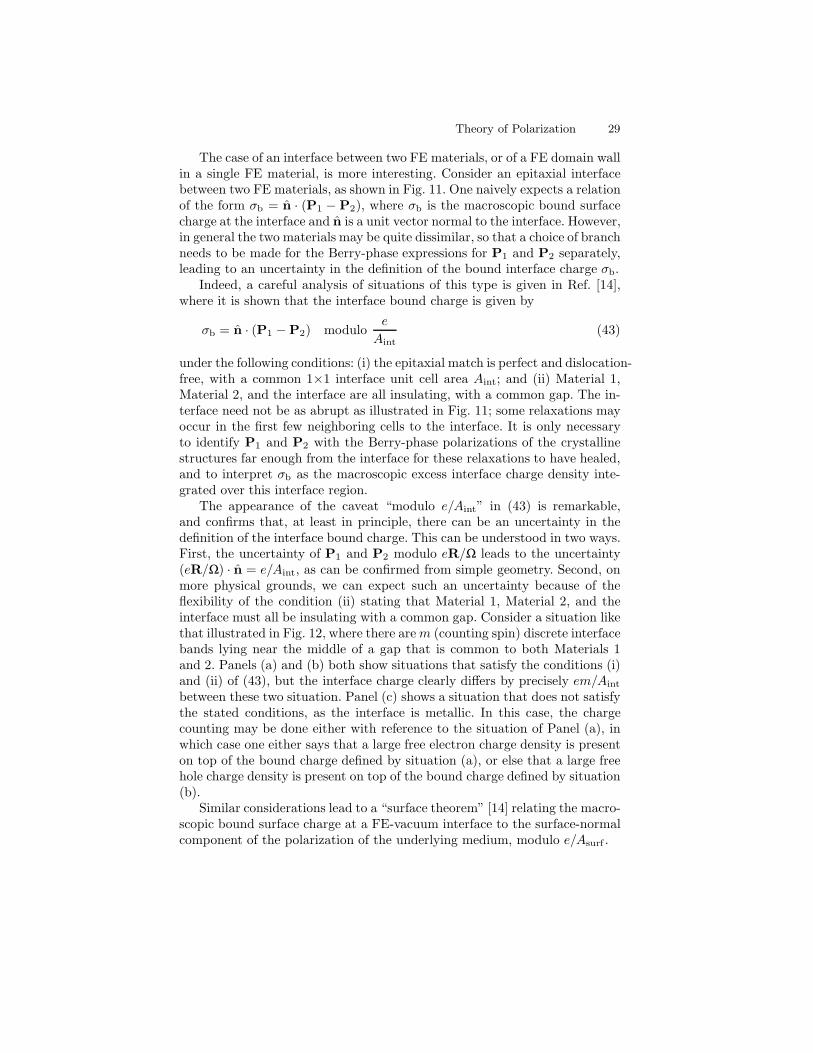
The case of an interface between two FE materials, or of a FE domain wallin a single FE material, is more interesting. Consider an epitaxial interfacebetween two FE materials, as shown in Fig. 11. One naively expects a relationof the form σb = n · (P1 − P2), where σb is the macroscopic bound surfacecharge at the interface and n is a unit vector normal to the interface. However,in general the two materials may be quite dissimilar, so that a choice of branchneeds to be made for the Berry-phase expressions for P1 and P2 separately,leading to an uncertainty in the definition of the bound interface charge σb.

Indeed, a careful analysis of situations of this type is given in Ref. [14],where it is shown that the interface bound charge is given by

σb = n · (P1 −P2) moduloe

Aint(43)

under the following conditions: (i) the epitaxial match is perfect and dislocation-free, with a common 1×1 interface unit cell area Aint; and (ii) Material 1,Material 2, and the interface are all insulating, with a common gap. The in-terface need not be as abrupt as illustrated in Fig. 11; some relaxations mayoccur in the first few neighboring cells to the interface. It is only necessaryto identify P1 and P2 with the Berry-phase polarizations of the crystallinestructures far enough from the interface for these relaxations to have healed,and to interpret σb as the macroscopic excess interface charge density inte-grated over this interface region.

The appearance of the caveat “modulo e/Aint” in (43) is remarkable,and confirms that, at least in principle, there can be an uncertainty in thedefinition of the interface bound charge. This can be understood in two ways.First, the uncertainty of P1 and P2 modulo eR/Ω leads to the uncertainty(eR/Ω) · n = e/Aint, as can be confirmed from simple geometry. Second, onmore physical grounds, we can expect such an uncertainty because of theflexibility of the condition (ii) stating that Material 1, Material 2, and theinterface must all be insulating with a common gap. Consider a situation likethat illustrated in Fig. 12, where there arem (counting spin) discrete interfacebands lying near the middle of a gap that is common to both Materials 1and 2. Panels (a) and (b) both show situations that satisfy the conditions (i)and (ii) of (43), but the interface charge clearly differs by precisely em/Aint

between these two situation. Panel (c) shows a situation that does not satisfythe stated conditions, as the interface is metallic. In this case, the chargecounting may be done either with reference to the situation of Panel (a), inwhich case one either says that a large free electron charge density is presenton top of the bound charge defined by situation (a), or else that a large freehole charge density is present on top of the bound charge defined by situation(b).

Similar considerations lead to a “surface theorem” [14] relating the macro-scopic bound surface charge at a FE-vacuum interface to the surface-normalcomponent of the polarization of the underlying medium, modulo e/Asurf .


(a) (b) (c)

Fig. 12. Sketch of density of states that could be associated with the epitaxialinterface of Fig. 11. Valence bands of Materials 1 and 2 are hashed; conductionbands are unfilled; and a band of interface states may either be (a) entirely empty;(b) entirely filled; or (c) partially filled (i.e., metallic)

In practice, the change in polarization (P1−P2) between two FE materialsis usually much smaller than the quantum, in which case there is a “natural”choice of branch for the definition of the interface bound charge σint in (43).However, for materials with large polarizations, such as certain Pb and Bi-based perovskites [42], the ambiguity in the definition of interface boundcharge may need to be considered with care.

5.3 Many-body and noncrystalline generalizations

The treatment given so far is based on the 1993 paper by King-Smith andVanderbilt [10] and assumes an independent-particle scheme, where polar-ization is evaluated as a Berry phase of one-electron orbitals, typically theKohn-Sham ones [4], which in a crystalline material assume the Bloch form.Shortly after the appearance of [10], Ortiz and Martin [43] provided themany-body generalization of the theory, where polarization is expressed as aBerry phase of the many-body wavefunction.

A subsequent development, by Resta [44], provides a unified treatment ofmacroscopic polarization, dealing on the same footing with either independent-electron or correlated systems, and with either crystalline or disordered sys-tems. This approach is based on a novel viewpoint, which goes under the(apparently oxymoronic) name of “single-point Berry phase”. On practicalgrounds, such single-point Berry phase is universally adopted in order to eval-uate macroscopic polarization within first-principle simulations of disorderedsystems [45].

Here we give a flavor of the approach, while we refer to the literaturefor more complete accounts [44,46,47]. Let us consider, for the sake of sim-plicity, a system of N one-dimensional spinless electrons. The many-bodyground wavefunction is then Ψ(x1, x2, . . . xj , . . . xN ), and all the electrons areconfined to a segment of length L. Eventually, we will be interested in thethermodynamic limit, defined as the limit N → ∞ and L → ∞, while the


density N/L is kept constant. The wavefunction Ψ is Born-von Karman peri-odic, with period L, over each electronic variable xj separately. Equivalently,one can imagine the electrons to be confined in a circular rail of length L: thecoordinates xj are then proportional to the angles 2πxj/L, defined modulo2π.

The key quantity is the ground-state expectation value

zN = 〈Ψ |U |Ψ〉 =∫ L

0

dx1 . . .

∫ L

0

dxN |Ψ(x1, . . . xN )|2U(x1, . . . xN ), (44)

where the unitary operator U , called “twist operator”, is defined as

U(x1, . . . xN ) = exp

i2π

L

N∑j=1

xj

, (45)

and clearly is periodic with period L. The expectation value zN is a dimen-sionless complex number, whose modulus is no larger than one. The electroniccontribution to the macroscopic polarization of the system can be expressedin the very compact form [44,47]:

Pel = − e

2πlim

N→∞Im ln zN , (46)

Notice that, for a one-dimensional system, the polarization has the dimen-sions of a charge (dipole per unit length). The essential ingredient in (46)is Im ln zN , i.e. the phase of the complex number zN . This phase can beregarded as a very peculiar kind of Berry phase.

So far, we have assumed neither independent electrons nor crystallineorder; (46) is in fact a very general definition of macroscopic polarization. Inthe special case of a crystalline system of independent electrons, the many-body wavefunction Ψ is a Slater determinant of single-particle orbitals. Forany finite N , (44) and (46) can be shown to be equivalent to a discretizedBerry phase of the occupied bands, of the same kind as those addressed inSec. 3.2.

5.4 Polarization in Kohn-Sham density-functional theory

Suppose we are given the ground-state interacting electron density n(r) of aninsulating crystal. From this, the Kohn-Sham theory [4] gives a unique pre-scription for determining a non-interacting system, with an effective Kohn-Sham potential, having the same ground-state electron density. The followingquestion then arises: If one computes the Berry-phase polarization from thisnon-interacting Kohn-Sham system, does one arrive, in principle, at the cor-rect many-body polarization?

As shown by Gonze, Ghosez, and Godby [48], the answer to this questionis that, in general, one does not obtain the correct polarization.


There are three ways to approach this issue. First, one may restrict one’sconsiderations to a strictly infinite crystalline system with a given cell shapeand with a uniform macroscopic electric field E [48]. One can then demon-strate a generalized Hohenberg-Kohn theorem stating that a given periodicdensity n(r) and macroscopic polarization P together uniquely determine aperiodic external potential Vper(r) and electric field E. Moreover, the cor-responding Kohn-Sham construction involves finding an effective periodicpotential V KS

per (r) and effective electric field EKS which yield, for a non-interacting system, the same n(r) and P. In this theory of Gonze et al.[48],the polarization is correct by construction, but at the expense of introduc-ing a correction EKS − E which they referred to as an “exchange-correlationelectric field.” The reader is directed to Ref. [48] for details.

A second approach is to consider conventional Kohn-Sham theory in thecontext of finite macroscopic sample geometries, surrounded by vacuum, andhaving particular surfaces, interfaces, or FE domain configurations. An anal-ysis of this type [49] again leads to the conclusion that the local polarizationobtained from exact Kohn-Sham theory is not, in general, the correct one.In general, one finds that the longitudinal part of the polarization field P(r)must be correct (since the corresponding charge density −∇ · P must becorrect), but the transverse part of the polarization field need not be correct.

A third approach is suggested by (44). The wavefunction ΨKS of the non-interacting Kohn-Sham system is a Slater determinant and is necessarilydifferent from Ψ , despite sharing the same single-particle density. Since thetwist operator U is a genuine many-body operator, its expectation value overΨKS is in general different from the one over Ψ . The polarization (46), isdifferent as well.

5.5 Localization, polarization, and fluctuations

An insulator is distinguished from a metal by its vanishing dc conductivityat low temperature. In contrast to what happens in metals, the electroniccharge in insulators (and quite generally nonmetals) cannot flow freely underan applied dc field; instead it undergoes static polarization. As first pointedout in 1964 by W. Kohn, this fact stems from a basic qualitative difference inthe organization of the electrons in their ground state [50]. The modern theoryof polarization has provided much insight into such different organization.

An insulator sustains a nontrivial, material-dependent, macroscopic po-larization, which is nonvanishing whenever the Hamiltonian is noncentrosym-metric. Instead, the polarization of a metallic sample is determined by theFaraday-cage effect and therefore is not a well defined property of the bulkmaterial. At the independent-electron level, the polarization of a crystallineinsulator can be expressed in terms of Wannier functions, as discussed inSec. 3.5. The key feature is that, in insulators, a set of well localized orbitals(the Wannier functions) spans the same Hilbert space as do the Bloch orbitals


of the occupied bands. This is indeed a qualitative difference in the organiza-tion of the electrons between insulators and metals. In the latter, in fact, itis impossible to span the Hilbert space of the occupied Bloch orbitals usingwell-localized orbitals. This statement can be made more precise by address-ing the spherical second moments of the charge distributions of the localizedorbitals [51]. Such second moments can be made finite in insulators, whilethey necessarily diverge in metals, as discussed below. It therefore emergesthat the key qualitative feature differentiating the ground state of an insula-tor from that of a metal is electron localization. This applies well beyond theindependent-electron level; in fact, as emphasized already by Kohn in 1964,the ground wavefunction of any insulator is localized. The modern theory ofpolarization leads to a simple and elegant measure of such localization [47].

It is expedient to refer, as in Sec. 5.3, to a system of N one-dimensionalspinless electrons. From (46) it is clear that macroscopic polarization is a well-defined quantity whenever the modulus of zN is nonvanishing in the large Nlimit. In the latter case, the second moment of the electron distribution canbe defined, following Resta and Sorella [52], as

〈x2〉c = − limN→∞

1N

(L

2π

)2

ln |zN |2, (47)

where the subscript “c” stands for “cumulant.” The same concept generalizesto a Cartesian tensor 〈rαrβ〉c in three dimensions. This localization tensor,having the dimension of a squared length, is an intensive property and applieson the same footing to ordered/disordered and correlated/uncorrelated many-electron systems; it is finite in any insulator and divergent in any metal. Inthe special case of an insulating crystalline system of independent electrons,the meaning of 〈rαrβ〉c becomes more perspicuous. In fact, the trace of thistensor is a lower bound to the average spherical second moment of the chargedistributions of the Wannier functions of the occupied bands [51]; in themetallic case, the lower bound is formally divergent.

Two important questions were left unanswered by Resta and Sorella.Given that in any insulator the localization tensor 〈rαrβ〉c is, at least in prin-ciple, a well-defined ground-state observable, the first question is whetherthis can be measured, and by which kind of experiments. The second ques-tion is whether 〈rαrβ〉c can be related in some way to dc conductivity, giventhat the vanishing of the latter characterizes—in addition to macroscopicpolarization—the insulating state of matter. Both questions received a posi-tive answer owing to the work of Souza, Wilkens and Martin [46]. They beganby showing that 〈rαrβ〉c measures the mean-square fluctuation of the polar-ization; then, by exploiting a fluctuation-dissipation theorem, they explicitlylinked 〈rαrβ〉c to the conductivity of the system.


6 Summary

In this Chapter we have reviewed the physical basis of the modern theoryof polarization. From a physical viewpoint, we have emphasized that thepolarization may be defined in terms of the accumulated adiabatic flow ofcurrent occurring as a crystal is modified or deformed, and have discussedthe consequences of this picture for the theory of polarization reversal andpiezoelectric effects in FE materials. From a mathematical viewpoint, wehave explained how the polarization is closely related to a Berry phase of theBloch wavefunctions as the wavevector traverses the Brillouin zone, and tothe centers of charge of the Wannier functions that may be constructed fromthe Bloch wavefunctions. An essential feature of the theory is the fact thatthe polarization is formally defined only modulo a “quantum of polarization,”or equivalently, that it must be regarded as a multi-valued quantity. We havealso attempted to clarify how piezoelectric effects and surface and interfacecharges are to be understood in terms of the modern theory.

The capability of computing polarization is now available in almost allcommonly-used software packages for bulk electronic-structure calculations.While initially formulated in vanishing electric field, the case of finite fieldcan be treated by letting the external electric field couple to the polarizationwhile retaining the Bloch form of the wavefunctions. These methods allowfor the computation of numerous quantities of interest, including spontaneouspolarization, Born effective charges, linear piezoelectric coefficients, nonlineardielectric and piezoelectric responses, and the like. Indeed, taken together,they provide a robust and powerful foundation for modern computationalstudies of the polarization-related properties of FE materials.

References

1. L. D. Landau, E. M. Lifshitz: Electrodynamics of Continuous Media (PergamonPress, Oxford, 1984)

2. O. F. Mossotti: Azioni e deformazioni nei dielettrici, Memorie di Matematicae di Fisica della Societa Italiana delle Scienze Residente in Modena, 24, 49(1850)R. Clausius: Die Mechanische Behandlung der Electrica (Vieweg, Berlin, 1879)

3. M. Posternak, R. Resta, A. Baldereschi: Role of covalent bonding in the polar-ization of perovskite oxides: The case of KNbO3, Phys. Rev. B 50, 8911 (1994)

4. Theory of the Inhomogeneous Electron Gas, edited by S. Lundqvist and N. H.March (Plenum, New York, 1983)

5. W. E. Pickett: Pseudopotential methods in condensed matter applications, Com-puter Phys. Reports 9, 115 (1989)

6. C. Kittel: Introduction to Solid State Physics, 7th. edition (Wiley, New York,1996)N. W. Ashcroft, N. D. Mermin: Solid State Physics (Saunders, Philadelphia,1976)


7. R. M. Martin: Comment on calculations of electric polarization in crystals,Phys. Rev. B 9, 1998 (1974)

8. R. M. Martin: Piezoelectricity, Phys. Rev. B 5, 1607 (1972)R. M. Martin: Comment on “Piezoelectricity under Hydrostatic Pressure”,Phys. Rev. B 6, 4874 (1972)W. F. Woo, W. Landauer: Comment on “Piezoelectricity under HydrostaticPressure”, Phys. Rev. B 6, 4876 (1972)R. Landauer: Pyroelectricity and piezoelectricity are not true volume effects,Solid St. Commun. 40, 971 (1981)C. Kallin, B. J. Halperin: Surface-induced charge disturbances and piezoelec-tricity in insulating crystals, Phys. Rev. B 29, 2175 (1984)R. Landauer: Introduction to Ferroelectric Surfaces, Ferroelectrics 73, 41 (1987)A. K. Tagantsev: Electric polarization in crystals and its response to thermaland elastic perturbations, Phase Transitions 35, 119 (1991)

9. R. Resta: Theory of the electric polarization in crystals, Ferroelectrics 136, 51(1992)

10. R.D. King-Smith, D. Vanderbilt: Theory of Polarization of Crystalline Solids,Phys. Rev. B 47, 1651 (1993)

11. R. Resta: Macroscopic polarization in crystalline dielectrics: the geometricphase approach, Rev. Mod. Phys. 66, 899 (1994)

12. S. Baroni, S. de Gironcoli, A. Dal Corso, P. Giannozzi: Phonons and relatedcrystal properties from density-functional perturbation theory, Rev. Mod. Phys.73, 515 (2001)

13. Geometric Phases in Physics, edited by A. Shapere, F. Wilczek (World Scien-tific, Singapore, 1989)R. Resta: Manifestations of Berry’s phase in molecules and condensed matter,J. Phys.: Condens. Matter 12, R107 (2000)

14. D. Vanderbilt, R.D. King-Smith: Electric polarization as a bulk quantity andits relation to surface charge, Phys. Rev. B 48, 4442 (1993)

15. http://www.abinit.org/

16. http://www.crystal.unito.it/

17. http://www.pwscf.org

18. http://www.uam.es/departamentos/ciencias/fismateriac/siesta

19. http://cms.mpi.univie.ac.at/vasp/

20. D. J. Thouless: Quantization of particle transport, Phys. Rev. B 27, 6083 (1983)21. R. Resta, M. Posternak, A. Baldereschi: Towards a quantum theory of polar-

ization in ferroelectrics: The case of KNbO3, Phys. Rev. Lett. 70, 1010 (1993)22. S. Dall’Olio, R. Dovesi, R. Resta: Spontaneous polarization as a Berry phase of

the Hartree-Fock wave function: The case of KNbO3, Phys. Rev. B, 56, 10105(1997)

23. Ph. Ghosez, J.-P. Michenaud, X. Gonze: Dynamical atomic charges: The caseof ABO3 compounds, Phys. Rev. B 58, 6224 (1998)

24. R. Pick, M. H. Cohen, R. M. Martin: Microscopic Theory of Force Constantsin the Adiabatic Approximation, Phys. Rev. B 1, 910 (1970)

25. M. Born, K. Huang, Dynamical Theory of Crystal Lattices (Oxford UniversityPress, Oxford, 1954)

26. J. D. Axe: Apparent Ionic Charges and Vibrational Eigenmodes of BaTiO3 andOther Perovskites, Phys. Rev. 157, 429 (1967)

27. R. Resta: Dynamical charges in oxides: recent advances, J. Phys. Chem. Solids61, 153 (1999)


28. W. Zhong, R. D. King-Smith, D. Vanderbilt: Giant LO-TO splittings in per-ovskite ferroelectrics, Phys. Rev. Lett. 72, 3618 (1994)

29. Ph. Ghosez, X. Gonze, Ph. Lambin, J.-P. Michenaud: Born effective chargesof barium titanate: Band-by-band decomposition and sensitivity to structuralfeatures, Phys. Rev. B 51, 6765 (1995)

30. S. de Gironcoli, S. Baroni, R. Resta: Piezoelectric properties of III-V semicon-ductors from first-principles linear-response theory, Phys. Rev. Lett. 62, 2853(1989)

31. O. H. Nielsen, R. M. Martin: First-Principles Calculation of Stress, Phys. Rev.Lett. 50, 697 (1983)O. H. Nielsen, R. M. Martin: Quantum-mechanical theory of stress and force,Phys. Rev. B 32, 3780 (1985)O. H. Nielsen, R. M. Martin: Stresses in semiconductors: Ab initio calculationson Si, Ge, and GaAs, Phys. Rev. B 32, 3792 (1985)

32. G. Saghi-Szabo, R. E. Cohen, H. Krakauer: First-Principles Study of Piezoelec-tricity in PbTiO3, Phys. Rev. Lett. 80, 4321 (1998)

33. H. Fu, R. E. Cohen: Polarization rotation mechanism for ultrahigh electrome-chanical response in single-crystal piezoelectrics, Nature 403, 281 (2000)

34. G. Saghi-Szabo, R. E. Cohen, H. Krakauer: First-principles study of piezo-electricity in tetragonal PbTiO3 and PbZr1/2Ti1/2O3, Phys. Rev. B 59, 12771(1999)

35. L. Bellaiche, D. Vanderbilt: Intrinsic Piezoelectric Response in Perovskite Al-loys: PMN-PT versus PZT, Phys. Rev. Lett. 83, 1347 (1999)

36. D. Vanderbilt: “Berry-phase theory of proper piezoelectric response,” J. Phys.Chem. Solids 61, 147 (2000)

37. R. W. Nunes, D. Vanderbilt: Real-Space Approach to Calculation of ElectricPolarization and Dielectric Constants, Phys. Rev. Lett. 73, 712 (1994)

38. R. W. Nunes, X. Gonze: Berry-phase treatment of the homogeneous electricfield perturbation in insulators, Phys. Rev. B, 63, 155107 (2001)

39. I. Souza, J. Iniguez, D. Vanderbilt: First-Principles Approach to Insulators inFinite Electric Fields, Phys. Rev. Lett. 89, 117602 (2002)

40. P. Umari, A. Pasquarello: Ab initio Molecular Dynamics in a Finite Homoge-neous Electric Field, Phys. Rev. Lett. 89, 157602 (2002)

41. I. Souza, J. Iniguez, D. Vanderbilt: Dynamics of Berry-phase polarization intime-dependent electric fields, Phys. Rev. B 69, 085106 (2004)

42. See, e.g., J. Iniguez, L. Bellaiche, D. Vanderbilt: First-principles study of(BiScO3)1−x(PbTiO3)x piezoelectric alloys, Phys. Rev. B 67, 224107 (2003).

43. G. Ortiz, R. M. Martin: Macroscopic polarization as a geometric quantumphase: Many-body formulation, Phys. Rev. B 49, 14202 (1994)

44. R. Resta: Quantum-Mechanical Position Operator in Extended Systems, Phys.Rev. Lett. 80, 1800 (1998)

45. http://www.cpmd.org/

46. I. Souza, T. Wilkens, R. M. Martin: Polarization and localization in insulators:Generating function approach, Phys. Rev. B 62, 1666 (2000)

47. R. Resta: Why are insulators insulating and metals conducting?, J. Phys.: Con-dens. Matter 14, R625 (2002)

48. X. Gonze, Ph. Ghosez, R.W. Godby: Density-Polarization Functional Theoryof the Response of a Periodic Insulating Solid to an Electric Field, Phys. Rev.Lett. 74, 4035 (1995)


X. Gonze, Ph. Ghosez, R.W. Godby: Density-Functional Theory of Polar In-sulators, Phys. Rev. Lett. 78, 294 (1997)

49. D. Vanderbilt: Nonlocality of Kohn-Sham Exchange-Correlation Fields in Di-electrics, Phys. Rev. Lett. 79, 3966 (1997)

50. W. Kohn: Theory of the Insulating State, Phys. Rev. 133, A171 (1964)51. N. Marzari, D. Vanderbilt: Maximally localized generalized Wannier functions

for composite energy bands, Phys. Rev. B 56, 12847 (1997)52. R. Resta, S. Sorella: Electron Localization in the Insulating State, Phys. Rev.

Lett. 82, 370 (1999)

theory of polarization: a modern approachdhv/pubs/local_preprint/dv_fchap.pdf · theory of...

Documents