theory of production and - elearn.moe.gov.et
TRANSCRIPT

0
10
5
15
1 2 3 4 5 6
1 2 3 4 5 6 7
7
6
12
18
24
30
27
Unit ObjectivesAfter completing this unit, you will be able to:
� comprehend and evaluate how firms combine economic resources so
as to maximize output;
� realize stages and economic regions of production;
� explain the meanings and behaviours of various types of costs and
integrate the relationship with production costs; and
� recognize the short run and long run production cost.
Main Contents
4.1 THEORY OF PRODUCTION
4.2 THEORY OF COST
4.3 RELATIONSHIP BETWEEN PRODUCTION AND COST
� Unit Summary
� Review Exercise
U n i tTheory of Production and
Cost

Grade 11 Economics
144
4.1 THEORY OF PRODUCTION
INTRODUCTION
Based on our discussion in Unit 2, we know that the supply price of a given
level of output depends upon the cost of production of the corresponding level of
output. Cost of production, in turn, depends upon:
� the physical relation between inputs and output and
� prices of inputs.
Assuming that the prices of inputs are given, cost of production will depend upon
the physical relationship between inputs and output. A study of the relationship
between inputs and output is known as the ‘theory of production’. A study of the
relationship between output and cost of production is what we call as ‘theory
of costs’. In the present unit we discuss various aspects and elements of these
two theories with a view to understand better the behaviour of firms (producer
behaviour) in the production of goods and services.
4.1 THEORY OF PRODUCTION At the end of this section, you will be able to:
� define production, input, and output;
� distinguish the differences between short-run and long-run production period;
� define production function;
� explain the concepts of production function with one variable input;
� distinguish the difference between total, average, and marginal product;
� show the relationship between average product and marginal product;
� describe the law of diminishing marginal product;
� identify and analyze the steps of productions;
� explain the concepts of production function with two variable input;
� define Isoquant curve schedule and map;
� state the basic characteristics of Isoquant;
� identify the economic region of production; and
� show the effects of technological change on production.
Key Terms and Concepts
³ Input
³ Short-run
³ Long-run
³ Production function
³ Isoquant

Unit 4: THEORY OF PRODUCTION AND COST145
4.1 THEORY OF PRODUCTION
Start up Activity Discuss on the factors that affect production, pay a visit to the nearby farmland or
factory and assess the factors that affect production.
Meaning of Production
Production is the transformation of resources (or inputs) into commodities (or
outputs). For example, when we get wheat on a plot of land with the help of inputs
like labour, capital and seeds, it is termed as production of wheat. Similarly,
when, in a cloth mill, inputs like labour, capital and threads are transformed into
cloth, it is called production of cloth. Similarly, in an economy, services are also
produced. For instance, services of a teacher, an advocate, a doctor, a singer and
servants are also called production in economics.
Input Output
Factors Affecting Production
Technology
A firm’s production behaviour is fundamentally determined by the state of
technology. Existing technology sets upper limits for the production of the firm,
irrespective of the nature of output and size of the firm.
Inputs
Definition:
Inputs are economic resources that can be used in the production of goods
and services.
There are wide variety of inputs used by the firms, like various raw materials,
labour services of different kinds, machine tools, buildings, etc. All inputs used
in production are broadly classified into four categories: land, labour, capital and
entrepreneurship. The inputs can also be divided into two main groups – fixed
and variable inputs. A fixed input is one whose quantity cannot be varied during
the period under consideration. Plant and equipment are examples of fixed inputs.
An input whose quantity can be changed during the period under consideration
is known as a variable input. Raw materials, labour, power, transportation, etc.,
whose quantity can often be increased or decreased on short notice, are examples
of variable inputs.
Production
Grade 11 Economics
146
4.1 THEORY OF PRODUCTION
Definition:
Outputs are outcomes of the production process.
Period of Production
The variability of an input depends on the length of the time period under
consideration. The shorter the time period, the more difficult it becomes to vary
the inputs. Economists classify time periods into two categories: the short-run
and the long-run.
i Short-Run: Short-run refers to the period of time over which the amount
of some inputs, called the ‘fixed inputs’, cannot be changed. For example,
the amount of plant and equipment, etc., is fixed in the short-run. This
implies that an increase in output in the short-run can be brought about by
increasing those inputs that can be varied, known as ‘variable inputs’. For
example, if a producer wishes to increase output in the short-run, she/he
can do so by using more of variable factors like labour and raw material.
ii Long-Run: Long-run is defined as the time period during which all factors
of production can be varied. A firm can install a new plant or raise a new
factory building. Long-run is the period during which the size of the plant
can be changed. Thus, all the factors are variable in the long-run.
It may be noted that the distinction between the short-run and the long-run does
not correspond to a specific calendar period, such as a month or a year. It is rather
based on the possibility of input adjustments.
Activity 4.1Make a visit to about 2-3 production centres in your locality and collect information
about their products, inputs and other factors of production. Prepare a detailed report
on your field-survey based project.
Production Function
Meaning of Production Function
The production function is purely a technological relationship which expresses
the relationship between the output of a good and the different combinations of
inputs used in its production. It indicates the maximum amount of output that can
be produced with the help of each possible combination of inputs.

Unit 4: THEORY OF PRODUCTION AND COST147
4.1 THEORY OF PRODUCTION
The production function is written mathematically as:
Q = f (x1, x
2, x
3, ....., x
n) (4. 1)
where x1, x
2, x
3, ....., x
n
are different inputs and Q is amount of output.
The production function is based on two main assumptions,
� Technology does not change,
� Producers utilise their inputs at maximum levels of efficiency.
Production Function with One Variable Input
Before we take up a detailed analysis of production function with one variable
input, certain key terms used in the analysis must be clarified. These are total
product (TP), marginal product (MP) and average product (AP). The total product
(TP) is the total amount of output resulting from the use of different quantities of
inputs. If we assume labour (L) to be the variable input assuming (capital, etc.,
held constant) then marginal product of labour (MPL) is defined as the change in
total product (TP) per unit change in variable input, say labour (L), that is,
MPL =
TP.
L
∆∆
(4.2)
Where, ΔTP stands for change in total production ΔL stands for change in labour input
Similarly, average product of labour may be defined as
APL =
TP.
L (4.3)
Where, TP stands for total production.
APL stands for average product for lobor.
Now let us consider a case where, for inputs like plant, machinery, floor space,
etc., of a firm are all fixed, while only the amount of labour services (L) vary.
That means that any increase or decrease in output is achieved with the help of
changes in the amount of L. When the firm changes only the amount of labour, it
alters the proportion between the fixed input and the variable input.
We go ahead with a hypothetical production schedule as shown in Table 4.1
below. Assume that capital is fixed at 1 unit, while L increases. Table 4.1 shows
that the total product reaches a maximum of 27 when 6 units of labour are used.

Grade 11 Economics
148
4.1 THEORY OF PRODUCTION
The MP of labour for the 2nd unit of labour is 6. It then increases to 7 and ultimately
becomes negative. Average product of labour also first increases and then falls.
Table 4.1: Hypothetical Schedule of TP, MP and AP
Variable Input (L) Total Product (TP) Marginal Product (MP) Average Product (AP)
0 0 — —
1 5 5 5
2 11 6 5.5
3 18 7 6
4 24 6 6
5 27 3 5.4
6 27 0 4.5
7 25 -2 3.5
The above schedule can also be expressed graphically by drawing TP, MP and
AP curves.
Figure 4.1: TP, MP and AP Curves Showing Three Stages of Production
0
10
5
15
1 2 3 4 5 6
1 2 3 4 5 6 7
7
6
12
18
24
30
27

Unit 4: THEORY OF PRODUCTION AND COST149
4.1 THEORY OF PRODUCTION
Relationship Between Total Product, Marginal Product, and Average Product
The relationship between MP and AP:
� When MP > AP, this means that AP is rising,
� When MP = AP, this means that AP is maximum,
� When MP < AP, this means that AP is falling.
Graphically, the relationships between the MP curve and AP curve are as follows
(see Figure 4.1):
� So long as the MP curve lies above the AP curve, the AP curve is a
positively sloping curve, AP rises
� When the MP curve intersects the AP curve, AP is at maximum,
� When the MP curve lies below the AP curve, the AP curve slopes
downward, i.e., AP declines.
The relationship between TP and MP:
� When TP increases at an increasing rate, marginal product increases,
� While TP increases at a diminishing rate, MP declines,
� When total product reaches its maximum, marginal product becomes
zero,
� When TP begins to decline, MP becomes negative.
Stages of Production
The short-run production function (with one variable input) can be divided into
three distinct stages of production. We may use Figure 4.1 to explain these stages.
Stage I runs from zero units of variable input to the level where AP of labour is
maximum. Stage II follows stage I and then proceeds to the point where MPL of
labour is zero (i.e., TPL
is maximum). Stage III continues on from that point. In
Figure 4.1, Stage I ranges from zero to 4 units of labour, Stage II begins from 4
units to 6 units of labour and Stage III lies beyond 6 units of labour.
It is obvious that no ‘rational’ firm will choose to operate either in Stage I or in
Stage III. In Stage I the firm is underutilising its fixed capacity, so in this stage
marginal product of variable input rises (i.e., each additional unit of the variable
factor contributes more to output than the earlier units). It is therefore profitable
for the firm to keep on employing additional units of the input. In Stage III, the
Grade 11 Economics
150
4.1 THEORY OF PRODUCTION
firm over utilises its fixed capacity. In other words, it would have so little fixed
capacity relative to the variable input it uses that the marginal contribution of each
additional unit of the variable is negative. It is therefore inadvisable to use any
additional units. Even if the cost of variable input is zero, it is still unprofitable
to move into Stage III. It can, thus, be concluded that Stage II is the only relevant
range for a rational firm.
For the sake of convenience, we can represent the three stages of production in
tabular form as follows:
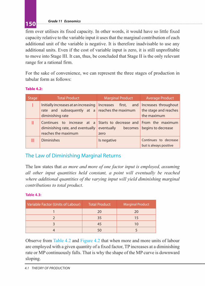
Table 4.2:
Stage Total Product Marginal Product Average Product
I Initially increases at an increasing
rate and subsequently at a
diminishing rate
Increases first, and
reaches the maximum
Increases throughout
the stage and reaches
the maximum
II Continues to increase at a
diminishing rate, and eventually
reaches the maximum
Starts to decrease and
eventually becomes
zero
From the maximum
begins to decrease
III Diminishes Is negative Continues to decrease
but is always positive
The Law of Diminishing Marginal Returns
The law states that as more and more of one factor input is employed, assuming
all other input quantities held constant, a point will eventually be reached
where additional quantities of the varying input will yield diminishing marginal
contributions to total product.
Table 4.3:
Variable Factor (Units of Labour) Total Product Marginal Product
1 20 20
2 35 15
3 45 10
4 50 5
Observe from Table 4.2 and Figure 4.2 that when more and more units of labour
are employed with a given quantity of a fixed factor, TP increases at a diminishing
rate or MP continuously falls. That is why the shape of the MP curve is downward
sloping.

Unit 4: THEORY OF PRODUCTION AND COST151
4.1 THEORY OF PRODUCTION
Figure 4.2: Marginal product curve
Note that:
� the law operates only if technology does not change
� the law starts to operate after the MP curve reaches its maximum (see
Figure 4.1)
� the law is universal because the tendency of diminishing return is all
pervading, and so it applies sooner or later in every field of production.
Production Function with Two Variable Inputs
We now discuss a more general case where the firm increases its output by using
more of two inputs that are substitutes for each other, say, labour and capital.
The two-variable-input case may be taken either as a short-run or a long-run
analysis of a production process, depending on what assumption is made about
the nature of the firm’s inputs. If the firm uses only two inputs and both of them
are variable, then this is a case of long-run analysis. In contrast, if more than two
inputs are used but only two of them are variable (and the others fixed), then this
would be taken as a short-run analysis.
Let us assume a firm wants to produce 20 units of output by using two variable
inputs, X and Y (say labour and capital respectively). It can do so by employing
different combinations of X and Y. We show these combinations in Table 4.4.
Grade 11 Economics
152
4.1 THEORY OF PRODUCTION
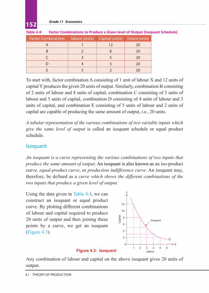
Table 4.4: Factor Combinations to Produce a Given level of Output (Isoquant Schedule)
Factor Combinations labour (units) Capital (units) Output (units)
A 1 12 20
B 2 8 20
C 3 5 20
D 4 3 20
E 5 2 20
To start with, factor combination A consisting of 1 unit of labour X and 12 units of
capital Y produces the given 20 units of output. Similarly, combination B consisting
of 2 units of labour and 8 units of capital, combination C consisting of 3 units of
labour and 5 units of capital, combination D consisting of 4 units of labour and 3
units of capital, and combination E consisting of 5 units of labour and 2 units of
capital are capable of producing the same amount of output, i.e., 20 units.
A tabular representation of the various combinations of two variable inputs which
give the same level of output is called an isoquant schedule or equal product
schedule.
Isoquant
An isoquant is a curve representing the various combinations of two inputs that
produce the same amount of output. An isoquant is also known as an iso-product
curve, equal-product curve, or production indifference curve. An isoquant may,
therefore, be defined as a curve which shows the different combinations of the
two inputs that produce a given level of output.
Using the data given in Table 4.4, we can
construct an isoquant or equal product
curve. By plotting different combinations
of labour and capital required to produce
20 units of output and then joining these
points by a curve, we get an isoquant
(Figure 4.3).
Figure 4.3: Isoquant
Any combination of labour and capital on the above isoquant gives 20 units of
output.

Unit 4: THEORY OF PRODUCTION AND COST153
4.1 THEORY OF PRODUCTION
Isoquant (or Equal-Product) Map
For each level of output, there is a
different isoquant. When the whole array
of isoquants is represented on a graph, it
is called an Isoquant Map (Figure 4.4). It
shows how outputs vary as the factor inputs
are changed. A higher isoquant represents
a higher level of output. However, the
distance between any two isoquants does
not measure the absolute difference in the
volume of output they represent. Figure 4.4: Isoquant Map
Properties of Isoquants
� An isoquant is downward-sloping to the right, (i.e., negatively
inclined), implying that if more of one factor is used, less of the other
factor is needed for producing the same level of output.
� No two isoquants intersect or touch each other. If two isoquants
intersect or touch each other it means that there is a common point on
the two curves (point A in Figure 4.6). This common point would imply
that the same amount of labour and capital can produce two levels of
outputs (example, 60 and 70 units, here), which is impossible.
� Isoquants are convex to the origin. The property of convexity implies
that the slope of the isoquant diminishes from left to right along the curve.
Convexity of an isoquant is the result of the principle of diminishing
Figure 4.5: Higher Isoquant vs. Lower Isoquant
Figure 4.6: Intersection of Isoquants (impossible condition)

Grade 11 Economics
154
4.1 THEORY OF PRODUCTION
marginal rate of technical substitution (MRTS) of one factor in place of
the other. We discuss MRTS more in a later sub-section.
Economic Region of Production
Economic theory states that the producer operates on the efficient ranges of
output. These are the ranges over which the marginal products of the inputs are
diminishing but positive. When the marginal products of inputs are negative, the
methods of production are considered inefficient. The efficient range of output
is represented by the portion of an isoquant that has a negative slope, while
the inefficient combinations of inputs are represented by the positively sloped
portions of an isoquant. A positive slope of an isoquant means that merely to
maintain the same level of output, the firm must use more of both of the inputs.
What is happening in this situation is that the marginal product of one of the
inputs is negative (i.e., its additional use will lead to a fall in output), so in order
to maintain the output at the same level, more of the other inputs (having positive
marginal product) must be used.
Figure 4.7: Economic Region of Production (Ridge Line)
In order to separate the efficient ranges of output from the inefficient ranges,
we need to draw lines between the negatively sloped and the positively sloped
portions of the isoquants. Such lines are known as ridge lines. A ridge line is the
locus of points of isoquants where marginal product of input is zero. In Figure 4.7,
the upper ridge line joins all such points (for example, a, b, etc.) where marginal
product of capital (MPk) is zero, while the lower ridge line joins points where
marginal product of labour (MPL) is zero (points c, d, etc.). The production
techniques are technically efficient inside the ridge lines. Outside the ridge lines,
the marginal products of inputs are negative, i.e., more of both inputs are required
MPx = 0

Unit 4: THEORY OF PRODUCTION AND COST155
4.1 THEORY OF PRODUCTION
to produce a given level of output. Obviously, no rational producer would like
to operate outside the ridge line. Thus, the economic region of production is the
region bounded by the ridge lines.
Marginal Rate of Technical Substitution (MRTS)
Marginal rate of technical substitution in the theory of production is similar to
the concept of marginal rate of substitution in the indifference curve analysis of
consumer behaviour. A marginal rate of technical substitution is the rate at which
factors can be substituted at the margin without altering the level of output. More
precisely, marginal rate of technical substitution of labour for capital may be
defined as the number of units of capital which can be replaced by one unit of
labour, the level of output remaining unchanged. The concept of marginal rate of
technical substitution can be easily understood from Table 4.5.
Table 4.5: Marginal Rate of Technical Substitution
Factor Combinations Units of Labour (L) Units of Capital (K) MRTS of L for K
A 1 12 —
B 2 8 4
C 3 5 3
D 4 3 2
E 5 2 1
Each of the input combinations, A, B, C, D and E, yields the same level of
output. Moving down the table from combination A to combination B, 4 units
of capital are replaced by 1 unit of labour in the production process without any
change in the level of output. Therefore, MRTS of labour for capital is 4 at this
stage. Switching from input combination B to input combination C involves the
replacement of 3 units of capital by an additional unit of labour, to keep output
remaining the same. Thus, MRTS is now 3. Likewise, MRTS between factor
combinations C and D is 2, and between factor combinations D and E is 1.
MRTS of labour for capital = K
L
∆∆
Amount of capital given up
Amount of labor used= (4.4)
ΔK represents change in units of capital and ∆L, change in units of labour.

Grade 11 Economics
156
4.1 THEORY OF PRODUCTION
An important observation that we can make from the above discussion is that
marginal rate of technical substitution diminishes
as more and more labour is substituted for
capital. In other words, as the quantity of labour
used is increased and the quantity of capital
employed is reduced, the amount of capital that
must to be replaced by an additional unit of
labour, so as to keep the output constant,
diminishes. This is known as the Principle of
Diminishing Marginal Rate of Technical
Substitution.
Returns to Scale (Production with all Variable Inputs)
In the previous sections we have discussed how output varies with a change in
one or two variable inputs. What happens if all inputs (factors of production) are
made to change?
In the short run, some factor inputs can be varied while the others remain fixed.
But in the long run, time is sufficient enough to vary all the factor inputs. In other
words, no input or factor is fixed in the long run. When all factor inputs can be
varied, keeping their proportion constant, it is called a change in the scale of
operations. The behaviour of output consequent to such changes in the quantities
of all factor inputs in the same proportion (i.e., keeping the factor proportions
unaltered) is known as ‘returns to scale’. Alternatively when all the factors
required for production of a commodity are increased in a given proportion, the
scale of production increases and the change caused in return (output) is called
return to scale. In such a situation, three types or stages of returns are usually
noticed.
� Increasing Returns to Scale. It occurs when output increases by a
greater proportion than the proportion of increase in all the inputs.
� Constant Returns to Scale. It happens when output increases by the
same proportion as of inputs increase.
� Diminishing Returns to Scale. It occurs when output increases by a
smaller proportion than the proportion of in input increases.
We illustrate these three stages with the help of following hypothetical schedule.
Note:
� MRTS at a point on an
isoquant = the slope of the
isoquant at that point.
� The property of diminishing
MRTS results in convexity of
the isoquant.

Unit 4: THEORY OF PRODUCTION AND COST157
4.1 THEORY OF PRODUCTION
Table 4.6: Returns to Scale
Sr. No. Scale of Inputs Total Product
(mts)
Marginal
Product (mts) Returns to Scale
1 2 labourers + 1 machine 200 200
Increasing2 4 labourers + 2 machines 500 300
3 6 labourers + 3 machines 900 400
4 8 labourers + 4 machines 1400 500
Constant5 10 labourers + 5 machines 1900 500
6 12 labourers + 6 machines 2400 500
7 14 labourers + 7 machines 2800 400
Decreasing 8 16 labourers + 8 machines 3100 300
9 18 labourers + 9 machines 3300 200
10 20 labourers + 10 machines 3400 100
We assume here that the firm is employing only two factors, namely, labour and
capital. Labour is measured in man-hours, capital in machine-hours, and output
in metres. As shown in the table, 2 units of labour and 1 unit of machine produce
200 metres of cloth in the beginning.
We can also represent the three stages of returns diagramatically by converting
the above Table 4.6 into the following diagram.
Figure 4.8: Returns to Scale

Grade 11 Economics
158
4.1 THEORY OF PRODUCTION
Reasons for Increasing and Decreasing Returns
Reasons for operation of increasing returns to scale are:
� Greater division of labour and specialisation which increases productivity.
� Use of more productive specialised machinery.
Reasons for operation of diminishing returns to scale are:
� The main reason for operation of diminishing return to scale is difficulty
in management and coordination when scale of operation becomes
bigger and bigger.
Effect of Technological Change on Production Function
Technological change refers to a change in the underlying techniques of production,
as occurs when a new process of production is invented or an old process is
improved. In such situations, the same output is produced with fewer inputs or
more output is produced with the same inputs. These changes in technology are
called technological progress or innovation in processes.
Figure 4.9: Technological Progress Shifts Production Function Upward
Graphically, the effect of innovation in processes is shown with an upward
shift of the production function. This shift shows that the same output may be
produced by using fewer factor inputs, or more output may be obtained with the
same inputs.

Unit 4: THEORY OF PRODUCTION AND COST159
4.1 THEORY OF PRODUCTION
Activity 4.21 Discuss the effect of technological change on the production function.
2 Complete the following table:
Units of Labour Total Product Marginal Product Average Product
1 50
2 90
3 120
4 140
5 150
6 150
7 140
8 120
3 Copy and complete the following table:
Units of Capital Total Product Average Product Marginal Product
1 20
2 16
3 12
4 8
5 4
4 Using the information given in the following table, express graphically the
behaviour of the TP, MP, and AP curves.
Land Fixed
Factor (units)
Labour Variable
Factor (units)
Total Product
(units)
Marginal
Product (units)
Average
Product (units)
1 0 0 — —
1 1 20 20 20
1 2 50 30 25
1 3 90 40 30
1 4 120 30 30
1 5 140 20 28
1 6 150 10 25
1 7 150 0 21.43
1 8 140 –10 17.5
1 9 120 –20 13.33
5 Identify the different output levels which mark the three stages of production
in the following data:

Grade 11 Economics
160
4.2 THEORY OF COST
Units of Variable Total Product (TP)
Input (units)
0 –
1 100
2 220
3 360
4 520
5 650
6 750
7 840
8 880
9 880
10 830
11 770
6 Calculate MRTS for each combination given in the following table:
Combination Units of Capital (K) Units of Labour (L)
A 1 15
B 2 10
C 3 6
D 4 3
E 5 1
Do you observe that MRTS diminishes as more and more capital is substituted
for labour?
4.2 THEORY OF COST At the end of this section, you will be able to:
� define cost;
� differentiate private and social cost;
� distinguish the difference between explicit and implicit cost;
� differentiate short-and long-run costs of production period;
� distinguish the differences among fixed, variable, and total costs;
� define marginal cost; and
� explain the long-run cost of production.

Unit 4: THEORY OF PRODUCTION AND COST161
4.2 THEORY OF COST
Key Terms and Concepts
³ Production
³ Cost
³ Input
³ Entrepreneurship
³ Short run
³ Long run
³ Fixed cost
³ Variable cost
³ Total cost
³ Marginal cost
Start-up Activity Assume an old fashioned tannery which purchases hides and skins from near by
society. The tannery discharges hazardous chemicals to human health and peasants
have no means to mitigate its effects. Discuss what society gain and loss due to the
presence of this tannery.
For producing a commodity, a firm requires various factor inputs as well as non-
factor inputs. The expenditures the firm incurs on these inputs refers to the cost
of production. However, in economics, we use different concepts relating to cost.
There are different types of cost. Some of the important ones are discussed in the
following paragraphs. Costs are the monetary values of expenditures that have
been used to produce something.
Private Cost and Social Cost
In economic analysis we often distinguish between private cost and social
cost. Private cost refers to cost of production incurred by an individual firm in
producing a commodity. Social cost, on the other hand, refers to the cost that
the society has to bear on account of production of a commodity. Social cost
is a wider concept than private cost. It is the sum total of the cost incurred by
the producers of goods and services (private cost) and the cost experienced by
those who have to suffer because of the production of the commodity in terms of
external cost.
Thus,
Social Cost = Private Cost + External Cost (4. 5)
‘External cost’ is the cost that is not borne by the firm, but is incurred by other
members of the society or the entire society. Such costs are termed external costs
from the firm’s point of view and social costs from society’s point of view. For
instance, an oil refinery discharges its wastes into a river, causing water pollution;

Grade 11 Economics
162
4.2 THEORY OF COST
mills and factories located in a city cause air pollution by emitting smoke; and
buses and trucks and other vehicles cause both air and noise pollution. Such
water, air and noise pollution cause health hazards and thereby produce pervasive
costs to the entire society. These costs are not taken into account by the individual
producers and, therefore, they are not part of the private cost. But the true cost
to the society must include all such costs, regardless of who bears them. Thus,
social cost differs from private cost to the extent of external cost.
Explicit Cost and Implicit Cost
Actual payments made by a firm for purchasing or hiring resources (or factor-
services) from the factor-owners or other firms are called explicit costs. In other
words, explicit costs are actual money expenses directly incurred for purchasing
the resources. These are the costs which a cost accountant includes under the head
expenses of the firm and are also known as accounting costs. Thus, examples of
explicit costs are: payments for raw materials and power; wages to the hired
workers; rent for the factory building; interest on borrowed money; expenses on
transport and publicity, etc.
Besides purchasing resources from other firms, a producer uses his/her own
factor services in the process of production. He/she generally does not take into
account the costs of his/her own factors while calculating the expenses of the
firm. The cost of using such factors is called implicit costs or imputed costs.
Thus, implicit costs refer to the imputed costs of the factors of production owned
by the producer himself/herself. They are called implicit costs because producers
do not make payment to others for them. For instance, rent of his/her own land,
interest on his/her own capital, and salary for his/her own services as manager,
etc. are implicit costs.
The main difference between explicit costs and implicit costs is that in the former
case, payment is made to others, while in the latter case payment is not made to
others but the payments become due to the producer’s own factors of production.
Economists define cost of production in a wider sense, i.e., in the sense of
economic cost, which includes both explicit cost and implicit cost. Thus economic
cost is the sum total of explicit cost and implicit cost.
Economic Cost = Explicit Cost + Implicit Cost (4.6)

Unit 4: THEORY OF PRODUCTION AND COST163
4.2 THEORY OF COST
Activity 4.31 Identify two production units (producing goods or services) in your local
area and list your economics workgroup, their explicit and implicit costs of
production.
2 In discuss various production activities from the point of view of their social
costs and private costs, and try to identify the cases where social costs could be
lower than private costs. Make a list of some examples where social costs are
higher than private costs and vice-versa.
Time Element and Cost
Time element has an important place in the analysis of cost of production. We
usually consider two kinds of time periods. They are:
� Short Run: Short run is defined as a period of time during which
production can be varied only by changing the quantities of variable
factors and not of fixed factors. Land, factory buildings, heavy capital
equipment, and services of high-category management are some of the
factors that cannot be varied in a short period. That is why they are
called fixed factors.
On the other hand, there are some factor inputs that can be varied as
and when required – for instance, power, fuel, labour, raw materials, etc.
They are called variable factors. Accordingly, in short-run production,
we have two types of costs - fixed costs and variable costs.
� Long Run. Long run is defined as a period which is long enough for the
inputs of all factors of production to be varied. In this period, no factor
is fixed, and all are variable factors. Accordingly, in the long run, all
costs are variable costs.
Short-Run Cost of Production
Total Costs in the Short Run
There are three concepts concerning total cost in the short period: Total Fixed
Cost, Total Variable Cost, and Total Cost. Fixed cost is that cost which is incurred
for fixed factors. Fixed costs consist of salary of the permanent staff, interest
on borrowed capital, rent of the factory buildings, depreciation of machinery,
expenses for maintenance of buildings, property tax and license fees etc.
Grade 11 Economics
164
4.2 THEORY OF COST
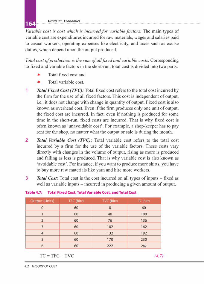
Variable cost is cost which is incurred for variable factors. The main types of
variable cost are expenditures incurred for raw materials, wages and salaries paid
to casual workers, operating expenses like electricity, and taxes such as excise
duties, which depend upon the output produced.
Total cost of production is the sum of all fixed and variable costs. Corresponding
to fixed and variable factors in the short-run, total cost is divided into two parts:
� Total fixed cost and
� Total variable cost.
1 Total Fixed Cost (TFC): Total fixed cost refers to the total cost incurred by
the firm for the use of all fixed factors. This cost is independent of output,
i.e., it does not change with change in quantity of output. Fixed cost is also
known as overhead cost. Even if the firm produces only one unit of output,
the fixed cost are incurred. In fact, even if nothing is produced for some
time in the short-run, fixed costs are incurred. That is why fixed cost is
often known as ‘unavoidable cost’. For example, a shop-keeper has to pay
rent for the shop, no matter what the output or sale is during the month.
2 Total Variable Cost (TVC): Total variable cost refers to the total cost
incurred by a firm for the use of the variable factors. These costs vary
directly with changes in the volume of output, rising as more is produced
and falling as less is produced. That is why variable cost is also known as
‘avoidable cost’. For instance, if you want to produce more shirts, you have
to buy more raw materials like yarn and hire more workers.
3 Total Cost: Total cost is the cost incurred on all types of inputs – fixed as
well as variable inputs – incurred in producing a given amount of output.
Table 4.7: Total Fixed Cost, Total Variable Cost, and Total Cost
Output (Units) TFC (Birr) TVC (Birr) TC (Birr)
0 60 0 60
1 60 40 100
2 60 76 136
3 60 102 162
4 60 132 192
5 60 170 230
6 60 222 282
TC = TFC + TVC (4.7)

Unit 4: THEORY OF PRODUCTION AND COST165
4.2 THEORY OF COST
Since total cost has total variable cost as
one of the components which varies with
change in output, the total cost will also
change positively with change in output.
Also, since total fixed cost, by definition,
remains constant, the changes in total cost
are entirely due to changes in total variable
cost. Table 4.7 and Figure 4.10 explain the
behaviour of various types of total cost in
the short run.
TFC curve: As Table 4.7 shows, total fixed cost remains constant at Birr 60 for
the entire range of output from 0 to 6 units. It does not change with change in
output. The TFC curve is a straight line parallel to the horizontal axis, indicating
the same amount of fixed cost at every level of output. Note that, in Figure 4.10,
the TFC curve starts from point A on the Y-axis, indicating that the total fixed
cost is incurred even if output is zero.
TVC curve: Total variable cost changes with change in output. Initially,
it increases at a decreasing rate as total output increases (up to 3 units), and
subsequently it increases at an increasing rate with increases in output (from the
4th unit onwards). The TVC curve is a positively sloping curve, showing that,
as output increases, total variable cost also increases. But the rate of increase
of TVC is not the same throughout. The TVC curve is concave downward, up
to the OQ level of output, indicating that the total variable cost increases at a
decreasing rate, and subsequently (beyond the OQ level of output) it is concave
upward, indicating that total variable cost increases at an increasing rate. Also
note that the TVC curve starts from the origin, which shows that when output is
zero, total variable cost is also zero.
TC curve: Since total cost is the sum of total fixed cost and total variable cost, it
is calculated in Table 4.7 by adding figures of column 2 and column 3 at different
levels of output. The total cost varies directly with output because of increases
in variable costs with increases in output. The TC curve has been obtained by
adding up vertically the TFC curve and the TVC curve. Since a constant fixed
cost is added to the total variable cost, the shape of the TC curve is the same as
that of the TVC curve. Note that the TC curve originates not from 0, but from A
because, at zero level of output, total cost equals fixed cost. The vertical distance
between the TVC and TC curves equals the amount of the total fixed cost.
Figure 4.10: Behaviour of Short-Run
Total Costs

Grade 11 Economics
166
4.2 THEORY OF COST
Average Costs in the Short Run
Average cost is simply the total cost divided by the number of units produced.
Corresponding to the three types of total costs in the short run, there are three
types of average costs. Average Fixed Cost, Average Variable Cost, and Average
Total Cost.
� Average Fixed Cost (AFC): Average fixed cost is the per-unit cost of
the fixed factors. It is obtained by dividing the fixed cost by the total
units of output.
TFC
AFC = Q
(4.8)
Where Q represents the total units of output produced.
� Average Variable Cost (AVC): Average variable cost is the per-unit
cost of the variable factors of production. It is obtained by dividing the
total variable cost by the total units of output.
TVCAVC =
Q
(4.9)
� Average Cost (AC) or Average Total Cost (ATC): Average total cost
or simply average cost is the per-unit cost of both fixed and variable
factors of production. It is obtained by dividing total cost by the total
units of output.
TCAC or ATC =
Q
(4.10)
Also, TCAC =
Q
= TFC + TVC
[Since TC = TFC + TVC]Q
= TFC TVC
+ Q Q
= AFC + AVC
AC or ATC = AFC + AVC (4.11)
The following schedule (based on Table 4.8) , together with the corresponding
average cost curves, explain the behaviour of various types of average costs in
the short run.

Unit 4: THEORY OF PRODUCTION AND COST167
4.2 THEORY OF COST
Table 4.8: Behaviour of average cost
Output
(Units)
TFC
(Birr)
TVC
(Birr) TC (Birr)
AFC
(Birr)
AVC
(Birr) ATC (Birr) MC (Birr)
= (∆TC/∆Q)
(1) (2) (3) (4) (2 + 3) (5) (2÷1) (6) (3÷1) (7) (4÷1)
or (5+6) (8) (TCn – TCn – 1)
0 60 0 60 – – – – 1 60 40 100 60 40 100 40 2 60 76 136 30 38 68 36 3 60 102 162 20 34 54 26 4 60 132 192 15 33 48 30 5 60 170 230 12 34 46 38 6 60 222 282 10 37 47 52
Figure 4.11: Behaviour of Average Costs
AFC Curve
It slopes downward throughout its length, from left to right, showing a continuous
fall in average fixed cost with increases in output. For very small outputs, the
average fixed cost is high, and for large outputs it is low. The curve approaches
the X-axis but never touches it because the average fixed cost cannot be zero since
total fixed cost is positive. Similarly, the AFC curve never touches the Y-axis
because total fixed cost has a positive value even at very low levels of output.
AVC Curve
The behaviour of the average variable cost is derived from the behaviour of
the total variable cost. The AVC curve slopes downward, up to output OQ2
(the optimum capacity level of output), showing decreases in average variable
cost, and it slopes upward beyond output OQ2, indicating increases in average
variable cost. In other words, the AVC curve is U-shaped. It is minimum at A,
corresponding to optimum capacity level of output, OQ2.

Grade 11 Economics
168
4.2 THEORY OF COST
Why is the AVC Curve U-shaped? The U-shape of the AVC curve follows directly
from the law of variable proportions. The average variable cost falls up to the
optimum capacity level of output due to increasing returns, and it increases
thereafter due to diminishing returns to the variable factor.
ATC Curve
Geometrically, the ATC Curve (or AC curve) can be obtained by adding the AFC
and AVC curves. An ATC curve is the vertical summation of the AFC and AVC
curves. Therefore, at each level of output, the ATC curve lies above the AVC
curve at a distance equal to the value (height) of the AFC curve.
Following are some important observations about the ATC curve.
� The distance between the average cost curve and the average variable
cost curve gets smaller as production increases. The ATC curve is far
above the AVC curve at early levels of output because the average fixed
cost is a high percentage of the average total cost. But the ATC curve
tends to come closer to AVC at higher levels of output because average
fixed cost now accounts for a relatively small percentage of average
total cost. Notice that the ATC curve never touches AVC the curve
because average fixed cost is always positive.
� The ATC curve is U-shaped, indicating that average total cost falls
initially, then reaches the minimum point, and then starts rising. It is
U-shaped for the same reasons for which the AVC curve is U-shaped.
Marginal Cost in the Short Run
Marginal cost is the addition to total cost as one more unit of output is produced.
In other words, marginal cost is the addition to total cost of producing n units
instead of n – 1 units.
MCn = TC
n – TC
n–1 (4.12)
Since the marginal cost is the change in total cost as a result of the change in
output by one unit, it can be written as:
TC
MC = Q
∆∆ (4.13)
Where, ΔTC is change in total cost, and ΔQ is change in the quantity of output.
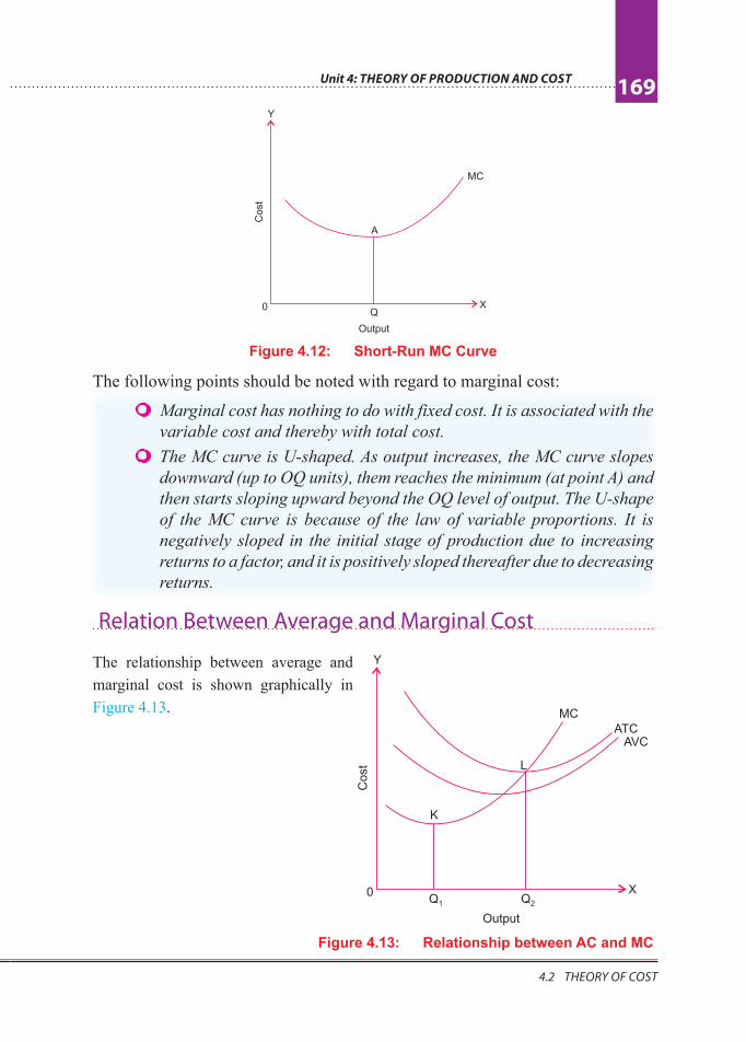
In Figure 4.12, the MC curve is the marginal cost curve.
Unit 4: THEORY OF PRODUCTION AND COST169
4.2 THEORY OF COST
Figure 4.12: Short-Run MC Curve
The following points should be noted with regard to marginal cost:
� Marginal cost has nothing to do with fixed cost. It is associated with the
variable cost and thereby with total cost.
� The MC curve is U-shaped. As output increases, the MC curve slopes
downward (up to OQ units), them reaches the minimum (at point A) and
then starts sloping upward beyond the OQ level of output. The U-shape
of the MC curve is because of the law of variable proportions. It is
negatively sloped in the initial stage of production due to increasing
returns to a factor, and it is positively sloped thereafter due to decreasing
returns.
Relation Between Average and Marginal Cost
The relationship between average and
marginal cost is shown graphically in
Figure 4.13.
Figure 4.13: Relationship between AC and MC

Grade 11 Economics
170
4.3 RELATIONSHIP BETWEEN PRODUCTION AND COST
Some notable points are:
The average variable cost is the total variable cost divided by the total product,
whereas marginal cost is the added cost involved for producing one more unit
of product.
� When the marginal cost is less than the average cost, the average cost
falls with increases in output. It will be seen from Figure 4.13 that, as
long as the MC curve lies below the ATC curve (up to OQ2 amount of
output), the ATC curve falls. Note the same relationship exists between
the MC curve and the AVC curve.
� When the marginal cost is greater than the average cost, the average
cost is rising. In Figure 4.13, the MC curve lies above the ATC curve
beyond the OQ2 level of output, and during this range the ATC curve is
rising.
� When marginal cost is equal to average cost, the average cost is
minimum. In Figure 4.13, the average cost is minimum for a while at
point L on the ATC curve, and the MC curve cuts the ATC curve at this
minimum point, showing that the marginal cost equals the average cost.
4.3 RELATIONSHIP BETWEEN PRODUCTION
AND COST At the end of this section, you will be able to:
� show the relationship between production and cost.
Key Terms and Concepts
³ Marginal cost
³ Marginal product
³ Total variable cost
³ Average product
³ Average cost
³ Explicit cost
³ Implicit cost
Start-up ActivityState the relationship between cost and production. State the various factor inputs in
which a firm requires to expend in the process of production in your locality.

Unit 4: THEORY OF PRODUCTION AND COST171
4.3 RELATIONSHIP BETWEEN PRODUCTION AND COST
Analyses of production and cost are closely related. We can even say that the cost
function is simply the production function expressed in money units. The basic
rule that governs this relationship is that when marginal product is increasing,
marginal cost is decreasing and vice versa. We illustrate the relationship between
production and cost in the short run, through the following table.
Table 4.9: Production and Cost in the Short Run
Units of
Variable Input,
Labour (L)
Total
Product
(Q)
Total Variable
Cost (L × wage
rate of Birr 100)
Marginal
Cost (Birr)
(∆TVC/∆Q)
Marginal
Product
(∆Q/∆L)
0 0 0 — —
1 10 100 10.00 10
2 22 200 8.33 12
3 40 300 5.55 18
4 55 400 6.67 15
5 62 500 14.33 7
6 65 600 33.33 3
7 60 700 (–)20.00 (–)5
The cost of using variable input is determined by multiplying the units of variable
input (labour) by its price. The table reveals that the total product (Q) first
increases at an increasing rate and later on at a decreasing rate. Correspondingly,
the total variable cost (TVC) first increases at a decreasing rate and then at an
increasing rate. By plotting the data of the first three columns of Table 4.9, we
get Figure 4.14, which reveals that the total variable cost and total product curves
are mirror images of each other: points A1, B
1, C
1, etc. match with points A
2, B
2,
C2, etc.
Figure 4.14: Cost and Production Short Run

Grade 11 Economics
172
4.3 RELATIONSHIP BETWEEN PRODUCTION AND COST
We may restate the relationship between cost and production (shown in Figure 4.14) in terms of marginal products and marginal cost. Comparison of columns 4 and 5 reveals that when MP is increasing, MC is decreasing, and while MP is decreasing, MC is increasing. MC increases in the ranges where production experiences diminishing returns. Note that just as the TVC and TP curves are mirror images of each other (as shown in Figure 4.14), MC and AVC curves are also mirror images of the MP and AP curves (as shown below).
Figure 4.15: Relationship Between Production and Cost
We may conclude that there is an inverse relationship between production and
cost.
� TVC and TP of labour are inversely related.
� AVC and AP of labour are inversely related.
� MC and MP of labour are inversely related. Assuming that labour is the
variable input and that the wage rate (W) is given, we give below an
algebraic proof for the relationship between MC and MP.
ΔTVC = ΔL × W
Since MC = ΔTVC/ΔQ
∴ MC = L L
L W L 1 W = W = W =
Q Q MP MP
∆ × ∆ ∆ ∆
(4.13)
Where, MPL = ΔQ/ΔL

Unit 4: THEORY OF PRODUCTION AND COST173
4.3 RELATIONSHIP BETWEEN PRODUCTION AND COST
Thus, assuming that the wage rate is given, MC and MP move in opposite
directions, or are inversely related to each other.
Practical Work
1 Complete the following table:
Output (Units) Total Cost (birr) TFC (birr) TVC (birr) MC (birr)
0 20
1 38
2 50
Solution:
TC - TVC = TFC TC - TFC = TVC TC
Q
DD
Output
(Units)
Total Cost
(birr) TFC (birr) TVC (birr) MC (birr)
0 20 20 0 —
1 38 20 18 38 – 20 = 18
2 50 20 30 50 – 38 = 12
2 The following table shows the total cost of production of a firm at different
levels of output. Find out the average variable cost and the marginal cost at
each level of output.
Output (Units) 0 1 2 3
Total Cost (birr) 60 100 130 150
Solution:
Output
(Units)
TC
(birr)
TFC
(birr)
TVC =TC – TFC
(birr)
AVC =TVC/Q
(birr)
MC = ∆TC/∆Q
(birr)
0 60 60 0 — —
1 100 60 40 40 100 – 60 = 40
2 130 60 70 35 130 – 100 = 30
3 150 60 90 30 150 – 130 = 20
Grade 11 Economics
174
4.3 RELATIONSHIP BETWEEN PRODUCTION AND COST
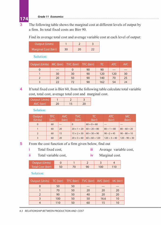
3 The following table shows the marginal cost at different levels of output by
a firm. Its total fixed costs are Birr 90.
Find its average total cost and average variable cost at each level of output:
Output (Units) 1 2 3
Marginal Cost (birr) 30 20 22
Solution:
Output (Units) MC (birr) TVC (birr) TFC (birr) TC ATC AVC
0 — 0 90 90 — —
1 30 30 90 120 120 30
2 20 50 90 140 70 25
3 22 72 90 162 54 24
4 If total fixed cost is Birr 60, from the following table calculate total variable
cost, total cost, average total cost and marginal cost.
Output (Units) 1 2 3
AVC (birr) 20 15 20
Solution:
Output (Units)
TFC (birr)
AVC (birr)
TVC (birr)
TC (birr)
ATC (birr)
MC (birr)
0 60 — 0 60 + 0 = 60 — —
1 60 20 20 × 1 = 20 60 + 20 = 80 80 ÷ 1 = 80 80 – 60 = 20
2 60 15 15 × 2 = 30 60 + 30 = 90 90 ÷2 = 45 90 – 80 = 10
3 60 20 20 × 3 = 60 60 + 60 = 120 120 ÷ 3 = 40 120 – 90 = 30
5 From the cost function of a firm given below, find out
i Total fixed cost,
ii Total variable cost,
iii Average variable cost,
iv Marginal cost.
Output (Units) 0 1 2 3 4
Total Cost (birr) 50 70 90 100 110
Solution:
Output (Units) TC (birr) TFC (birr) TVC (birr) AVC (birr) MC (birr)
0 50 50 — — —
1 70 50 20 20 20
2 90 50 40 20 20
3 100 50 50 16.6 10
4 110 50 60 15 10

Unit 4: THEORY OF PRODUCTION AND COST175
4.3 RELATIONSHIP BETWEEN PRODUCTION AND COST
Activity 4.4 1 Assume that the MC of a firm is Birr 40 and its AVC is Birr 50. Identify the stage
of production in which the firm is operating.
2 Given the cost function of a firm as: C = 128 – 6Q + 2Q2, Compute the following:
a TFC
b TVC of producing 4 units
c AVC of producing 4 units
d ATC of producing 4 units
e MC of producing the 4th unit
3 The following data refer to the production department of a firm:
a Number of workers: 1000
b Wage rate per worker: Birr 25
c Cost of raw materials used: Birr 15000
d Rent of factory building: Birr 5000
e Interest paid: Birr 2000
f Expenses for fuel: Birr 2000
g Number of units produced: 700
Compute AVC and AC for the firm.
4 From the data given below, calculate:
a Average fixed cost
b Average variable cost
c Marginal cost
Output (Units) 0 1 2 3 4 5
Total Cost (birr) 30 90 110 120 140 180
5 Cost function of a firm is given below:
Output (Units) 0 1 2 3 4 5 6
Total Cost (birr) 60 80 100 111 116 130 150
Find out the following:
a Total fixed cost
b Total variable cost
c Average fixed cost
d Average variable cost
e Marginal cost

Grade 11 Economics
176
4.3 RELATIONSHIP BETWEEN PRODUCTION AND COST
6 Is it correct to say that, when output is zero, total cost equals total variable cost?
Discuss with your friends.
7 Is it correct to say that, when output changes, the change in total cost is greater
than the change in total variable cost? Discuss in a group.
Long-Run Cost of Production
In the long runs all factors are variable,
and thus there are no fixed costs. For the
analysis of the long-run cost of production,
we use only three types of curves: Long-
Run Total Cost Curve (LTC), Long-Run
Average Cost Curve (LAC), and Long-
Run Marginal Cost Curve (LMC). Here
also, LAC and LMC curves are U-shaped,
but they are flatter than the short-run cost
curves.
Why is the LAC Curve U-shaped?
The U-shape of the LAC curve is because of returns to scale. As we increase the
scale of operation in the initial stages, we get increasing returns to scales (IRS) as
a result of economies of scale. Increasing returns to scale means that the increase
in output is more than proportionate to the increase in factor inputs. Hence the
LAC falls as output is increased (in the output range, to M in the diagram). But
then, beyond a certain point, we get decreasing returns to scale (DRS) as a result
of diseconomies of scale, and hence now LAC rises with increase in output. This
happens at output levels higher than M in the diagram. When economies and
diseconomies of scale offset each other, it is the stage of constant returns to scale
(CRS). It happens at M level of output.
Note that the LMC curve is also U-shaped, for the same reasons, and that it cuts
the LAC curve at its minimum point.
The Least Cost Rule
In the long run, cost of a product is the least cost of producing each level of
output when all factors of production, including the plant, are variable.
Figure 4.16: Relation Between Production and Cost
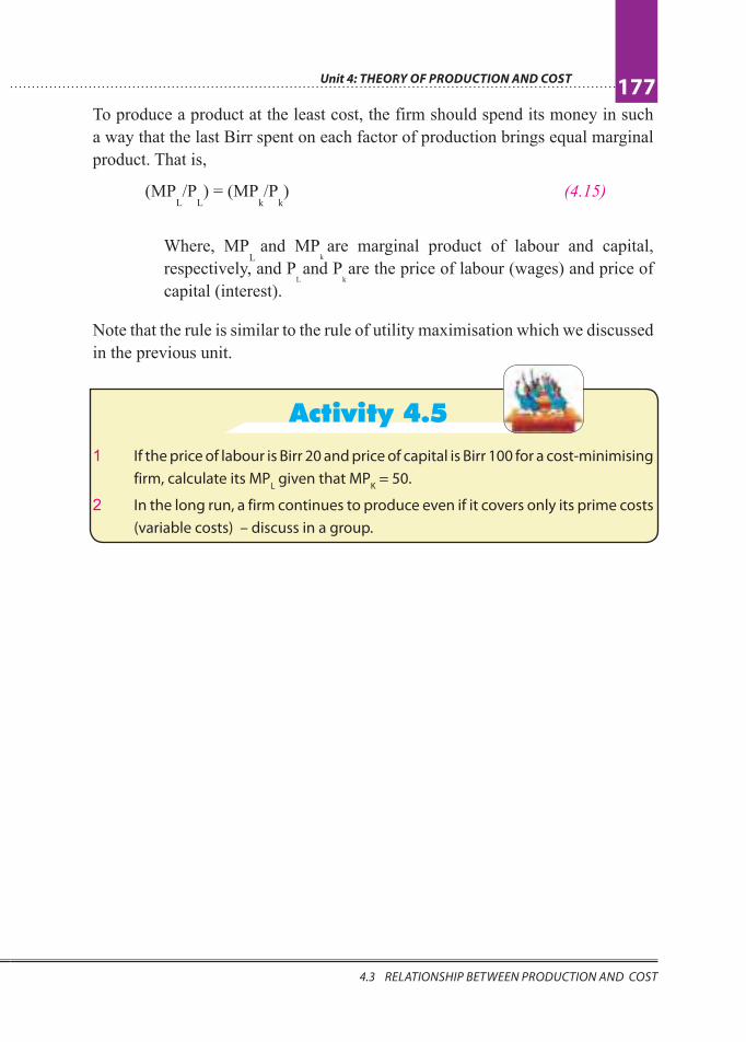
Unit 4: THEORY OF PRODUCTION AND COST177
4.3 RELATIONSHIP BETWEEN PRODUCTION AND COST
To produce a product at the least cost, the firm should spend its money in such
a way that the last Birr spent on each factor of production brings equal marginal
product. That is,
(MPL/P
L) = (MP
k/P
k) (4.15)
Where, MPL
and MPk
are marginal product of labour and capital,
respectively, and PL and P
k
are the price of labour (wages) and price of
capital (interest).
Note that the rule is similar to the rule of utility maximisation which we discussed
in the previous unit.
Activity 4.5
1 If the price of labour is Birr 20 and price of capital is Birr 100 for a cost-minimising
firm, calculate its MPL given that MP
K = 50.
2 In the long run, a firm continues to produce even if it covers only its prime costs
(variable costs) – discuss in a group.

U n i t R e v i e w
Grade 11 Economics
178
4.3 RELATIONSHIP BETWEEN PRODUCTION AND COST
UNIT SUMMARY � Production function shows the maximum quantity of a commodity
that can be produced per unit of time, with given amounts of inputs,
when the best production technique is used. The nature of production
function depends upon the time period allowed for adjustment of the
inputs.
� Short run refers to the period of time in which the amount of some
inputs cannot be changed.
� Long run is defined as the time period in which all factors of production
can be varied.
� Fixed factors are those factors which remain unchanged at all levels
of output.
� Variable factors are those factors whose quantity changes with
change in output level.
� Short run production function refers to a situation where we study the
change in output when only one input is variable and all other inputs
are fixed. In this case, factor proportion is changed. This is the subject
matter of the Law of Variable Proportions.
� Long-run production function studies the change in output when all the
inputs used in the production of a good are changed simultaneously
and in the same proportion. In this case, the scale of production is
changed. This is the subject matter of returns to scale.
� Total Product (TP) refers to the total amount of a commodity produced
during some period of time by combining different factors of production.
� Average Product (AP) of a variable factor refers to the output per unit
of variable factor. Thus,
L
L
TPAP =
L
� Marginal Product (MP) of a variable factor may be defined as the
change in total product resulting from the additional unit of a variable
factor.
� Returns to a factor means change in physical output of a good when
the quantity of one factor is increased while the quantity of other
factors remains constant.
� Law of Diminishing Marginal Returns states that in all production
processes, adding more of one factor of production, while holding
one or more of other inputs constant, will at some point yield lower per
L
L
TPMP =
L
∆
∆
Unit 4: THEORY OF PRODUCTION AND COST179
4.3 RELATIONSHIP BETWEEN PRODUCTION AND COST
unit returns. Diminishing returns occurs in the short run when at list one
factor is fixed.
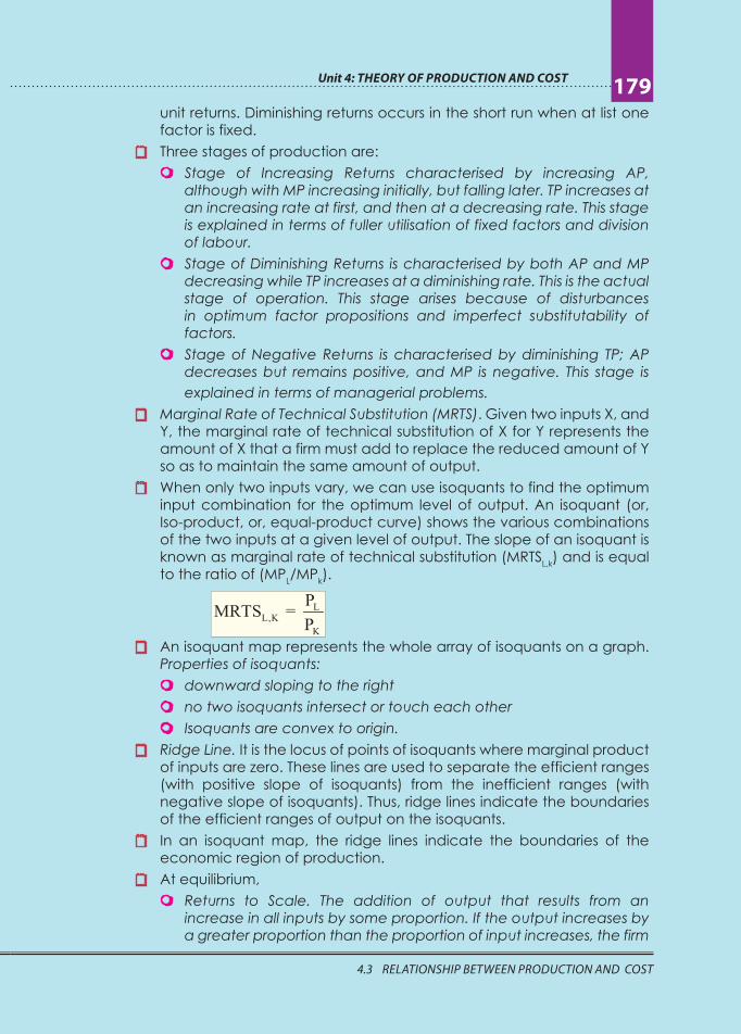
� Three stages of production are:
� Stage of Increasing Returns characterised by increasing AP,
although with MP increasing initially, but falling later. TP increases at
an increasing rate at first, and then at a decreasing rate. This stage
is explained in terms of fuller utilisation of fixed factors and division
of labour.
� Stage of Diminishing Returns is characterised by both AP and MP
decreasing while TP increases at a diminishing rate. This is the actual
stage of operation. This stage arises because of disturbances
in optimum factor propositions and imperfect substitutability of
factors.
� Stage of Negative Returns is characterised by diminishing TP; AP
decreases but remains positive, and MP is negative. This stage is
explained in terms of managerial problems.
� Marginal Rate of Technical Substitution (MRTS). Given two inputs X, and
Y, the marginal rate of technical substitution of X for Y represents the
amount of X that a firm must add to replace the reduced amount of Y
so as to maintain the same amount of output.
� When only two inputs vary, we can use isoquants to find the optimum
input combination for the optimum level of output. An isoquant (or,
Iso-product, or, equal-product curve) shows the various combinations
of the two inputs at a given level of output. The slope of an isoquant is
known as marginal rate of technical substitution (MRTSL,k
) and is equal
to the ratio of (MPL/MP
k).
� An isoquant map represents the whole array of isoquants on a graph.
Properties of isoquants:
� downward sloping to the right
� no two isoquants intersect or touch each other
� Isoquants are convex to origin.
� Ridge Line. It is the locus of points of isoquants where marginal product
of inputs are zero. These lines are used to separate the efficient ranges
(with positive slope of isoquants) from the inefficient ranges (with
negative slope of isoquants). Thus, ridge lines indicate the boundaries
of the efficient ranges of output on the isoquants.
� In an isoquant map, the ridge lines indicate the boundaries of the
economic region of production.
� At equilibrium,
� Returns to Scale. The addition of output that results from an
increase in all inputs by some proportion. If the output increases by
a greater proportion than the proportion of input increases, the firm
LL,K
K
PMRTS = .
P

Grade 11 Economics
180
4.3 RELATIONSHIP BETWEEN PRODUCTION AND COST
is experiencing increasing returns to scale. If the output increases
by the same proportion as the inputs, the firm is experiencing
constant returns to scale. Finally, if the output increases by a smaller
proportion than the increases in inputs, the firm is experiencing
decreasing returns to scale.
� Technological change shifts the production function upward.
� Private cost refers to the cost incurred by an individual firm in
producing a commodity.
� Social cost refers to the cost that society has to bear because of
the production of a commodity.
� Explicit cost refers to money expenses incurred in purchasing or
hiring the factor services.
� Implicit cost refers to the imputed value of the inputs owned by the
firm and used by it in its own production.
� Economic cost consists of explicit cost and implicit cost.
� Total fixed cost is the total cost incurred on fixed factors. It does not
change with change in output.
� Total variable cost is the total cost incurred on variable factors. It
changes with change in output.
� TFC curve is a straight-line curve parallel to the horizontal axis.
� TVC curve is concave downward, up to some level of output, then
concave upward.
� TC curve increases at a decreasing rate first and then at an
increasing rate.
� AFC is the per-unit cost of the fixed factors.
� AFC curve slopes downward continuously from left to right.
� AVC curve is the per-unit cost of the variable factors.
� AVC curve is U-shaped due to the law of variable proportions.
� ATC (or simply AC) is the per-unit cost of all factors of production
used in production.
� ATC curve is the vertical summation of the AVC and AFC curves. It
is U-shaped.
� Marginal cost is the addition to total cost as one more unit of output
is produced.
� MC curve is U-shaped due to the law of variable proportions.
� The relationship between AC and MC is:
^ when, MC < AC, AC falls;
^ when MC > AC, AC rises;
^ when MC = AC, AC is minimum.
� Long-run cost is the least cost of producing each level of output
when all factors of production are variable. To produce a product
at the least cost, the firm should spend its money in such a way
that the last Birr spent on each factor of production brings equal
marginal product.
Unit 4: THEORY OF PRODUCTION AND COST181
4.3 RELATIONSHIP BETWEEN PRODUCTION AND COST
� There is an inverse relationship between production and cost: TVC
and TP are inversely related; AVC and AP are inversely related; MC
and MP are inversely related.
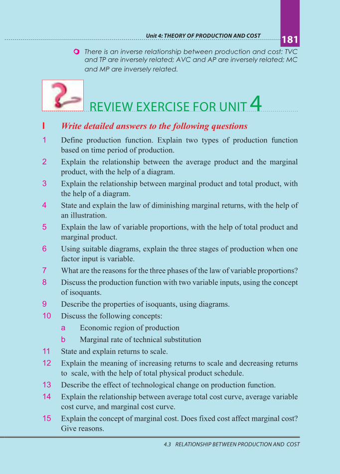
REVIEW EXERCISE FOR UNIT 4I Write detailed answers to the following questions
1 Define production function. Explain two types of production function
based on time period of production.
2 Explain the relationship between the average product and the marginal
product, with the help of a diagram.
3 Explain the relationship between marginal product and total product, with
the help of a diagram.
4 State and explain the law of diminishing marginal returns, with the help of
an illustration.
5 Explain the law of variable proportions, with the help of total product and
marginal product.
6 Using suitable diagrams, explain the three stages of production when one
factor input is variable.
7 What are the reasons for the three phases of the law of variable proportions?
8 Discuss the production function with two variable inputs, using the concept
of isoquants.
9 Describe the properties of isoquants, using diagrams.
10 Discuss the following concepts:
a Economic region of production
b Marginal rate of technical substitution
11 State and explain returns to scale.
12 Explain the meaning of increasing returns to scale and decreasing returns
to scale, with the help of total physical product schedule.
13 Describe the effect of technological change on production function.
14 Explain the relationship between average total cost curve, average variable
cost curve, and marginal cost curve.
15 Explain the concept of marginal cost. Does fixed cost affect marginal cost?
Give reasons.

Grade 11 Economics
182
4.3 RELATIONSHIP BETWEEN PRODUCTION AND COST
16 Explain the relationship between average cost and marginal cost, with the
help of an appropriate diagram. Can the average cost rise when the marginal
cost is diminishing?
17 Explain the relationship between total cost, average cost, and marginal
cost, with the help of a cost schedule.
18 Why is the short-run average cost curve (SAC) U shaped?
19 Explain the shape of the long-run average cost curve (LAC).
20 Discuss the relationship between production and cost.
II Distinguish between the following:
21 Returns to a variable factor and returns to scale
22 Increasing returns to a variable factor and increasing returns to scale
23 Diminishing returns to a variable factor and diminishing returns to scale
24 Fixed costs and variable costs
25 Private cost and social cost
III Write ‘True’ or ‘False’ for each of the following:
26 When MP > AP, this means that AP is falling.
27 When MP = AP, this means that AP is minimum.
28 When TP increases at an increasing rate, MP increases.
29 An isoquant is a curve representing the various combinations of two inputs
that produce different amounts of output.
30 Higher isoquants represents larger output.
31 MRTS increases as more and more labour is substituted for capital.
32 Technological progress shifts the production function downward.
33 Economic cost is the sum total of explicit cost and implicit cost.
34 In the short run, the AVC curve is U-shaped.
35 Production and cost are directly related to each other in the short run.
IV For each of the following, four choices are given, but only one of them is correct. Choose the correct one.
36 The process of using different factors of production in order to make goods
and services available is known as:
A Investment
B Production
C Consumption
D Resource

Unit 4: THEORY OF PRODUCTION AND COST183
4.3 RELATIONSHIP BETWEEN PRODUCTION AND COST
37 Any good or service that comes out of a production process, is known as:
A Output
B Input
C Labour
D Economic resource
38 When the short-run average product of labour is declining but positive, the
marginal product of labour is:
A Negative
B Declining
C Zero
D Any of these is possible
39 When the short-run marginal product of labour is greater than the average
product of labour:
A APL is increasing
B APL decreasing
C APL is equal to zero
D None of these
40 When the short-run, MPL is negative:
A TP is also negative
B TP is declining
C TP is rising at a constant rate
D TP is rising but at a diminishing rate
41 Suppose the average product of 6 workers is 150 units of a good and that of
7 workers is 170 units. The MP of the seventh worker equals:
A 200 B 270 C 290 D 220
V Write very short answers to the following questions
42 What do you call the period in which:
a the scale of plant cannot be altered;
b the scale of plant can be altered?
43 Give two examples of variable factors.
44 Give two examples of fixed factors.
45 When the total physical product of a variable factor reaches its maximum,
what will be the marginal physical product?
46 How does marginal physical product behave when total physical product
starts to decline?
47 What will be the direction of marginal physical product when total
physical product increases at an increasing rate?
48 When marginal physical product declines but it is neither zero nor negative,
does total physical product also decline?

Grade 11 Economics
184
4.3 RELATIONSHIP BETWEEN PRODUCTION AND COST
49 What will be the total physical product when:
a marginal physical product rises
b marginal physical product declines but remains positive
c marginal physical product is zero
d marginal physical product is negative
50 In which stage of the law of variable proportions will a producer produce?
51 When total product increases at a decreasing rate, what happens to marginal
product?
52 Can average product be zero or negative?
53 Can marginal product be zero or negative?
54 When production increases in the same proportion as the increase in a
variable factor, what do you call it?
55 When does scale of operation change?
56 Name the law expressing the relationship between the quantities of a
variable factor and the quantities of output.
57 State whether the law of variable proportions operates in the short run or
in the long run.
58 How many stages are there in the law of variable proportions?
59 What will be the shape of marginal product curve in the case of diminishing
returns to a factor?
60 Give two examples of:
a explicit costs
b implicit costs
c fixed costs
d variable costs
61 What is the shape of the total fixed-cost curve?
62 When the AC curve is falling, what will be the position of the MC curve?
63 Can the AFC curve touch the X-axis?
64 What does the difference between total cost and total variable cost indicate
in the short run?
65 Why are the TC and TVC curves parallel to each other?
66 Why do TC and TFC become equal at the zero level of output?
67 If TFC and TVC are given, how will you estimate the TC?
68 What does the difference between total cost and total fixed cost indicate in
the short run?
Unit 4: THEORY OF PRODUCTION AND COST185
4.3 RELATIONSHIP BETWEEN PRODUCTION AND COST
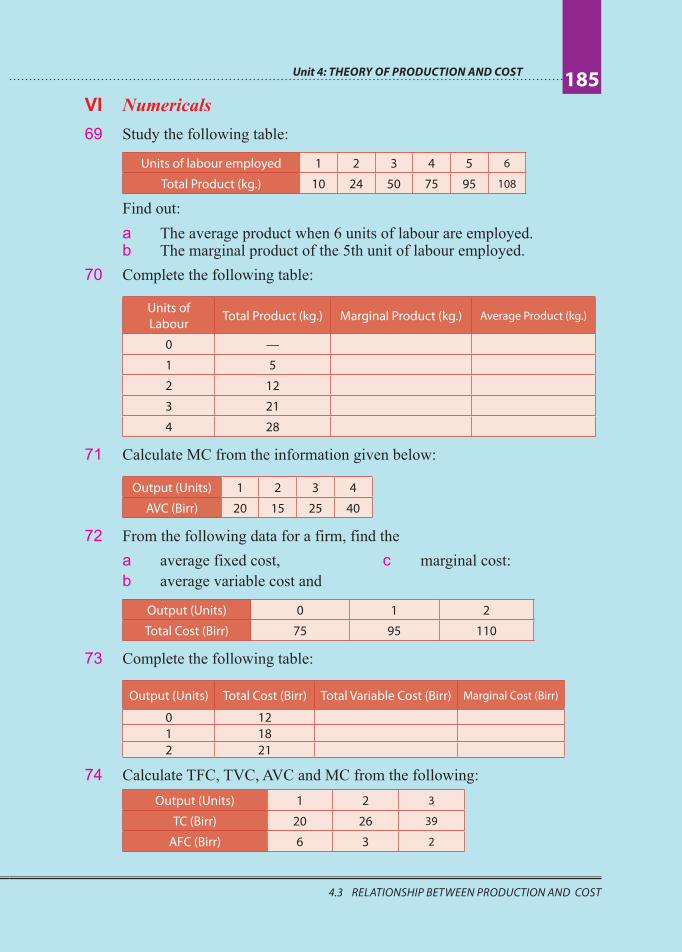
VI Numericals
69 Study the following table:
Units of labour employed 1 2 3 4 5 6
Total Product (kg.) 10 24 50 75 95 108
Find out:
a The average product when 6 units of labour are employed. b The marginal product of the 5th unit of labour employed.
70 Complete the following table:
Units of
Labour Total Product (kg.) Marginal Product (kg.) Average Product (kg.)
0 —
1 5
2 12
3 21
4 28
71 Calculate MC from the information given below:
Output (Units) 1 2 3 4
AVC (Birr) 20 15 25 40
72 From the following data for a firm, find the
a average fixed cost,
b average variable cost and
c marginal cost:
Output (Units) 0 1 2
Total Cost (Birr) 75 95 110
73 Complete the following table:
Output (Units) Total Cost (Birr) Total Variable Cost (Birr) Marginal Cost (Birr)
0 12
1 18
2 21
74 Calculate TFC, TVC, AVC and MC from the following:
Output (Units) 1 2 3
TC (Birr) 20 26 39
AFC (Birr) 6 3 2
Grade 11 Economics
186
4.3 RELATIONSHIP BETWEEN PRODUCTION AND COST
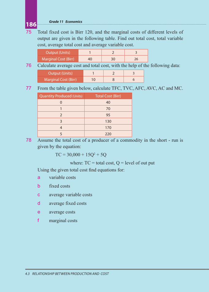
75 Total fixed cost is Birr 120, and the marginal costs of different levels of
output are given in the following table. Find out total cost, total variable
cost, average total cost and average variable cost.
Output (Units) 1 2 3
Marginal Cost (Birr) 40 30 26
76 Calculate average cost and total cost, with the help of the following data:
Output (Units) 1 2 3
Marginal Cost (Birr) 10 8 6
77 From the table given below, calculate TFC, TVC, AFC, AVC, AC and MC.
Quantity Produced (Units) Total Cost (Birr)
0 40
1 70
2 95
3 130
4 170
5 220
78 Assume the total cost of a producer of a commodity in the short - run is
given by the equation:
TC = 30,000 + 15Q2 + 5Q
where: TC = total cost, Q = level of out put
Using the given total cost find equations for: a variable costs
b fixed costs
c average variable costs
d average fixed costs
e average costs
f marginal costs