there goes gravity: how ebay reduces trade costs · there goes gravity: how ebay reduces trade...
TRANSCRIPT

There Goes Gravity:How eBay Reduces Trade Costs∗
Andreas Lendle†
Marcelo Olarreaga‡
Simon Schropp§
Pierre-Louis Vezina¶
August 2012
Abstract
We compare the impact of distance, a standard proxy for trade costs, on eBay andoffline international trade flows. We consider the same set of 62 countries and the samebasket of goods for both types of transactions. We find the effect of distance to be onaverage 65 percent smaller on the eBay online platform than offline. Using interactionvariables, we show this difference is explained by a reduction of information and trustfrictions enabled through online technology. We estimate the welfare gains from areduction in offline frictions to the level prevailing online at 29 percent on average.
JEL CODES: F10, F13, L81.Key Words: Trade costs, gravity, online trade, eBay.
∗We are grateful to Richard Baldwin, Christine Barthelemy, Mathieu Crozet, Anne-Celia Disdier,Jonathan Eaton, Peter Egger, Phil Evans, Simon Evenett, Lionel Fontagne, Gordon Hanson, Torfinn Harding,Beata Javorcik, Bertin Martens, Thierry Mayer, Hanne Melin, Marc Melitz, Peter Neary, Emanuel Ornelas,Cristian Ugarte, Tony Venables, and seminar participants at Oxford, the Villars PEGGED workshop, theWTO’s Trade and Development Workshop, the University of Neuchatel, the Paris Trade Seminar, the RIEFmeeting at Bocconi University, ERWIT, the XIII Conference on International Economics, and the GTAPconference in Geneva for their constructive comments and suggestions. We also thank Daniel Bocian, SteveBunnel, and Sarka Pribylova at eBay for their time, patience and efforts with our data requests, and eBayfor funding. All errors are the sole responsibility of the authors.†Graduate Institute, Geneva. email : [email protected]‡University of Geneva and CEPR. email: [email protected]§Sidley Austin LLP. email: [email protected]¶University of Oxford. email: [email protected]

1 Introduction
In the 1990s advances in transportation and communication technologies led many
commentators to believe that geographic distance between countries would soon no longer
encumber international transactions (e.g. Cairncross 1997). Despite some anecdotal evidence
in support of the “death of distance” hypothesis (e.g. Friedman 2005), a large number of
academic papers suggests that distance is “thriving”, not “dying”. Disdier and Head (2008),
using a meta-analysis based on 1,000 gravity equations, found that the estimated coefficient
on distance has been slightly on the rise since 1950. Chaney (2011) argues that the need
for direct interactions between trading partners, resulting from information frictions first
highlighted by Rauch (1999), explains why distance still matters for international trade
today. Similarly, Allen (2011) suggests information frictions account for 93 percent of the
distance effect. This would suggest that advances in technology in recent decades have failed
to reduce information frictions. Is this the death knell for the “death of distance” hypothesis?
In this paper we breathe new life into the “death of distance” hypothesis. We argue
that the right place to look is in online markets which, as opposed to “offline” markets,
make full use of technologies that can reduce information frictions. Indeed, as argued by
Hortacsu et al. (2009) and Goldmanis et al. (2010), the main benefit of the internet as a
trade facilitator is to reduce search costs, and it is reasonable to think of online marketplaces
as “frictionless” in this regard. Exporters no longer need to make multiple phone calls, send
faxes, write emails, attend trade fairs and networking events. And while importers still incur
some search costs, these are typically brought down to a simple internet search. In any event,
online search costs are not necessarily correlated with how remote markets are.
The heart of our paper is a dataset on cross-border transactions conducted over eBay,
the world’s largest online marketplace. This dataset allows us to examine the effect of
distance on international online trade. Our approach is similar to that of Hortacsu et al.
(2009) who, using a sample of within-US eBay transactions, showed that the coefficient on
distance on trade was much smaller online than offline. However, as noted by the authors,
several caveats make their comparison with offline trade imperfect. One is that the products
traded on eBay are mainly household durables, and thus comparison with total offline trade
2
is problematic. Another is that the demographic characteristics of the eBay users may
be online-specific and not representative of the offline world. A further shortcoming is that
international search costs may be very different from those within the US. Hence their sample
may not be fully appropriate to study the “death of distance” in international trade.1 Our
dataset allows us to overcome these criticisms and compare the distance effect on eBay and
offline trade considering the same set of countries and goods. It covers all eBay transactions,
disaggregated into 40 product categories, between 62 countries (representative of 92% of total
world trade) during 2004-2007. To create the best-possible comparison groups, we match
eBay product categories to product descriptions from the 6-digit level HS classification to
build comparable basket of goods. We also drop from our eBay data all transactions that
were concluded via auctions (60 percent of eBay traded value), as well as those sold by
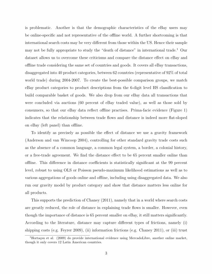
consumers, so that our eBay data reflect offline practises. Prima-facie evidence (Figure 1)
indicates that the relationship between trade flows and distance is indeed more flat-sloped
on eBay (left panel) than offline.
To identify as precisely as possible the effect of distance we use a gravity framework
(Anderson and van Wincoop 2004), controlling for other standard gravity trade costs such
as the absence of a common language, a common legal system, a border, a colonial history,
or a free-trade agreement. We find the distance effect to be 65 percent smaller online than
offline. This difference in distance coefficients is statistically significant at the 99 percent
level, robust to using OLS or Poisson pseudo-maximum likelihood estimations as well as to
various aggregations of goods online and offline, including using disaggregated data. We also
run our gravity model by product category and show that distance matters less online for
all products.
This supports the prediction of Chaney (2011), namely that in a world where search costs
are greatly reduced, the role of distance in explaining trade flows is smaller. However, even
though the importance of distance is 65 percent smaller on eBay, it still matters significantly.
According to the literature, distance may capture different types of frictions, namely (i)
shipping costs (e.g. Feyrer 2009), (ii) information frictions (e.g. Chaney 2011), or (iii) trust
1Hortacsu et al. (2009) do provide international evidence using MercadoLibre, another online market,though it only covers 12 Latin American countries.
3

frictions.2 In order to appreciate what is driving the distance-reducing effect brought about
by eBay, we need to isolate these frictions.
We start by controlling for bilateral shipping costs, which are included in our eBay
dataset. Somewhat surprisingly, we find that adding shipping costs barely affects the distance
coefficient. As seen in Figure 4, this is because shipping costs are uncorrelated with distance.
Furthermore, ad-valorem shipping costs seem higher online than offline, probably as there
are less bulk-shipping scale economies for online shipments. It is thus highly unlikely that a
reduction in shipping costs is driving the online death of distance.
To explore the trust and information channels we interact the distance coefficient with
indicators of corruption and information frictions at the country level. We find that the
distance-effect reduction is largest for exporting countries with high levels of corruption
and which are relatively unknown to consumers, as measured by Google search results.
This suggests that online markets reduce the distance effect by providing both both trust
and information.3 We obtain the same result when we interact distance with indices of
information intensity at the product level, namely Broda and Weinstein’s (2006) trade
elasticities as well as indices we build using the WIPO Global Brand Database and eBay’s
trademark-infringement alert system. We also test whether the distance effect is reduced by
the eBay seller-rating mechanism, which increases importer trust in exporters. As predicted,
we find that distance matters significantly less for sellers with higher ratings. This confirms
that distance captures trust and information frictions which are reduced by technology.
As highlighted earlier, different demographics could also be driving the different distance
effects. To control for these differences, all our specifications include importer and exporter
fixed effects that are specific to online and offline flows. Yet it could be argued that country
characteristics that drive the selection of eBay traders are correlated with the distance effect.
For example, in highly unequal societies only a few privileged buyers may have access to the
internet. This type of buyers may be more ‘international’, i.e. may have a preference
for purchases from remote countries, and hence this selection may explain why distance
2An alternative explanation are taste differences. Blum and Goldfarb (2006) showed that gravity holdsin the case of website visits and argued this was because distance proxies for taste similarity.
3We also find that the distance differential is highest for country pairs that do not share a language, i.e.when information and trust frictions are high.
4
matters less online. A selection of ‘international’ exporters on eBay could also be driving the
difference. In countries with low barriers to export and high internet penetration exporters
should be most similar online and offline. Using interaction terms, we show that even in the
extreme scenario in which all countries would be as equal as Sweden and as easy to export
from as Hong Kong, eBay would still significantly reduce the distance effect.
We conclude with an estimate of the gains from trade brought about by internet
technologies. We use the formula proposed by Arkolakis, Costinot and Rodrıguez-Clare
(2012) to calculate the welfare gains that would result from a drop in offline search costs to
the online level, as captured by the difference in distance effects. We find that in the average
country, real income would increase by 29 percent.
The reminder of the paper is organized as follows. In section 2 we provide some descriptive
statistics regarding international trade flows on eBay. Section 3 presents our empirical
strategy and section 4 the results. Section 5 presents the trade gains from world flattening.
Section 6 concludes.
2 International trade on eBay: Descriptive statistics
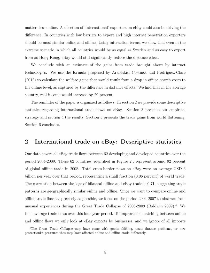
Our data covers all eBay trade flows between 62 developing and developed countries over the
period 2004-2009. These 62 countries, identified in Figure 2 , represent around 92 percent
of global offline trade in 2008. Total cross-border flows on eBay were on average USD 6
billion per year over that period, representing a small fraction (0.06 percent) of world trade.
The correlation between the logs of bilateral offline and eBay trade is 0.71, suggesting trade
patterns are geographically similar online and offline. Since we want to compare online and
offline trade flows as precisely as possible, we focus on the period 2004-2007 to abstract from
unusual experiences during the Great Trade Collapse of 2008-2009 (Baldwin 2009).4 We
then average trade flows over this four-year period. To improve the matching between online
and offline flows we only look at eBay exports by businesses, and we ignore of all imports
4The Great Trade Collapse may have come with goods shifting, trade finance problems, or newprotectionist pressures that may have affected online and offline trade differently.
5
purchased via auctions, which are prevalent on eBay but quite uncommon offline.5
Our dataset also allows us to focus on the same goods traded online and offline. It covers
all eBay transactions disaggregated into 40 product categories that we match with product
codes at the 6-digit level of the HS classification using information on sub-categories from
the eBay website (see our matching table (9)). Since it is impossible to match some eBay
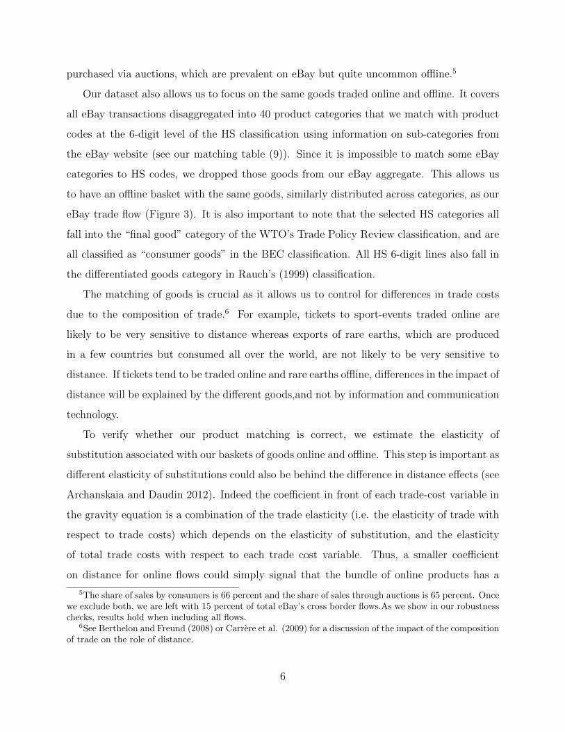
categories to HS codes, we dropped those goods from our eBay aggregate. This allows us
to have an offline basket with the same goods, similarly distributed across categories, as our
eBay trade flow (Figure 3). It is also important to note that the selected HS categories all
fall into the “final good” category of the WTO’s Trade Policy Review classification, and are
all classified as “consumer goods” in the BEC classification. All HS 6-digit lines also fall in
the differentiated goods category in Rauch’s (1999) classification.
The matching of goods is crucial as it allows us to control for differences in trade costs
due to the composition of trade.6 For example, tickets to sport-events traded online are
likely to be very sensitive to distance whereas exports of rare earths, which are produced
in a few countries but consumed all over the world, are not likely to be very sensitive to
distance. If tickets tend to be traded online and rare earths offline, differences in the impact of
distance will be explained by the different goods,and not by information and communication
technology.
To verify whether our product matching is correct, we estimate the elasticity of
substitution associated with our baskets of goods online and offline. This step is important as
different elasticity of substitutions could also be behind the difference in distance effects (see
Archanskaia and Daudin 2012). Indeed the coefficient in front of each trade-cost variable in
the gravity equation is a combination of the trade elasticity (i.e. the elasticity of trade with
respect to trade costs) which depends on the elasticity of substitution, and the elasticity
of total trade costs with respect to each trade cost variable. Thus, a smaller coefficient
on distance for online flows could simply signal that the bundle of online products has a
5The share of sales by consumers is 66 percent and the share of sales through auctions is 65 percent. Oncewe exclude both, we are left with 15 percent of total eBay’s cross border flows.As we show in our robustnesschecks, results hold when including all flows.
6See Berthelon and Freund (2008) or Carrere et al. (2009) for a discussion of the impact of the compositionof trade on the role of distance.
6

lower elasticity of substitution than the offline bundle. To estimate these elasticities of
substitution we assume that trade costs online and offline are Gamma distributed with
shape parameter kf , where f is the type of flow, but an identical scale parameter. Then
using existing estimates of the elasticity of substitution for aggregate trade flows, we can
back up consistent estimates of the elasticity of substitution online and offline using the fact
that the variance of a gamma distributed variable is proportional to the mean by a factor
equal to the scale parameter. For a detailed description of the methodology to estimate the
online and offline elasticities of substitution, see section 5.1.
Our results suggest that for an estimate of the aggregate elasticity of substitution of 5
(see Eaton and Kortum 2012), the online elasticity of substitution equals 4.5, whereas the
offline elasticity of substitution equals 5.6. The online estimate is within the [3.6 ; 5.9] range
estimated by Einav et al. (2012) using intra-US trade flows and identified with differences in
sales tax across states.7 The offline estimate is quite close to the Broda and Weinstein (2006)
median estimate of 5.9 in our bundle of HS-6 digit goods. Moreover, while the online and
offline elasticities of substitution are statistically different from zero at the 5 percent level,
they are not statistically different from each other. This comforts us in our matching of online
and offline products, and suggests that statistical differences in the estimated coefficients of
the gravity equation will be due to the contribution of these variables to trade costs, rather
than to differences in the elasticity of substitution.
Our eBay data also includes data on average bilateral ad-valorem shipping costs. While
we do not have an equivalent for bilateral offline flows, in the case of US imports we do have
data on freight and insurance costs from USITC. When plotting these costs against distance
(see Figure 4) we find that for both online and offline flows, shipping costs are uncorrelated
with distance, even though shipping costs seem to be much higher online.8 This suggests
that the introduction of observable shipping costs in the gravity equation, which are often
omitted due to lack of data, is not going to explain the importance of distance in the gravity
equation. But this is a testable hypothesis at least in the online sample.
7They are significantly lower than the estimates of De los Santos et al. (forthcoming) but these correspondto price elasticites of particular book varieties, and therefore we would expect them to be higher than ouraggregated bundle of goods.
8Using data on all country pairs online gives a similar picture.
7

Offline trade data and trade cost variables come from the usual sources and are described
in the Data Appendix.
3 The empirical model
To examine the impact of trade costs online and offline, our starting point is the gravity
model. It suggests that bilateral trade between two countries is proportional to their
economic mass and the multilateral resistance indices of the importer and the exporter,9
and inversely proportional to trade costs between the two countries, often proxied by the
geographic distance between them (see Anderson and Van Wincoop (2003) for an elegant
derivation):
(1) mij =yiyjyw
(tijPiΠj
)εwhere mij are imports of country i from country j, yi is total income in importing country
i, yj is total income in exporting country j, yw is total world income, tij are trade costs
between country i and country j, ε is the trade cost elasticity of bilateral imports,10 and
Pi and Πj are the multilateral resistance terms in the importing (inward) and exporting
(outward) country, respectively.11
We follow the literature and model bilateral trade costs (tij) as a function of geographic
distance and other trade cost variables:
(2) tij = DαDij e
NBijαNBeNCijαNCeNCLijαNCLeNCLSijαNCLSeNFTAijαNFTA
where all αs are parameters, Dij is the geographic distance between countries i and j, NBij
9The multilateral resistance terms are weighted averages of price indices in the importer’s and exporter’strading partners.
10Given by 1 - σ in Anderson and Van Wincoop (2003) where σ is the elasticity of substitution betweendifferent import sources in the importing country.
11The expressions for the inward and outward multilateral resistance terms are Pi =[∑
j (tij/Πj)ε yjyw
]1/εand Πj =
[∑i (tij/Pi)
ε yiyw
]1/ε.
8

is a dummy variable taking the value 1 when countries i and j do not share a border, NCij
is a dummy variable taking the value 1 when countries i and j did not share a colonial link,
NCLij is a dummy variable taking the value 1 when countries i and j do not share a common
language, NCLSij is a dummy variable taking the value 1 when countries i and j do not
share a common legal system, and NFTAij is a dummy variable taking the value 1 when
countries i and j are not part of the same Free Trade Agreement.12
We then substitute (2) into (1) and take logs on both sides to obtain:13
ln (mij) = ln(yi) + ln(yj)− ln(yw) + βDln(Dij) + βNBNBij +
βNCNCij + βNCLNCLij + βNCLSNCLSij + βNFTANFTAij +(3)
−εln(Pi)− εln(Πi)
where all βs are parameters to be estimated and βk = εαk, where k is the subscript indicating
the different trade cost variables. Because we are interested in understanding the variation
of different βs offline and online, and because Pi and Πi are not observable (and difficult to
estimate) we proceed as in much of the empirical literature and control for the multilateral
resistance terms (and yi and yj) including importer i and exporter j fixed effects.
A stochastic fixed-effect version of equation (3) is our baseline specification to understand
the importance of different trade costs offline and online. We estimate it separately for online
and offline flows, but also append the offline and online data so that we can test whether
coefficients are statistically different online and offline by introducing an eBay dummy that
we interact with each of the trade cost variables. If the interaction term is statistically
significant then the offline and online coefficients are statistically different. In both cases we
allow for importer and exporter fixed effects to be different online and offline. This captures
differences in prices for online and offline products, and can also correct for a selection of
buyers and sellers into online and offline platforms that could bias our estimate as argued
12Note that we measure the absence of common language, common legal system, colonial links ortrade agreements, rather than their presence as in most of the literature. This has no consequencesfor the estimates, but it allows to interpret these variables as trade costs (like distance) rather than astrade-enhancing variables.
13Since some of our left-hand side variables were zeros (21 percent on eBay, less than 1 percent offline),we added a dollar the the import value before taking the logs.
9

by Goolsbee (2000). We use a least-square dummy-variable estimator (LSDV), but also a
Poisson estimator to control for heteroscedasticity (see Santos-Silva and Tenreyro 2006). To
make sure results are not subject to aggregation bias, we also run the same specifications as
in equation (3) but at the product level and using exporter-product and importer-product
fixed effects, which also vary for online and offline flows.
To uncover what drives the difference in distance coefficients online and offline we use
interaction terms between distance and country or product characteristics that capture
information asymmetries and trust problems. The idea is that if results are partly driven by
technologies that reduce information asymmetries and trust problems, the differences in the
distance coefficients online and offline should be larger for countries and products affected
by information asymmetries.
4 Results
Table 1 provides the results of the estimation of (3) using distance as the only trade costs
in columns (1) and (5). The elasticity of distance is 61 percent smaller online than offline.
In columns (2) and (6) of Table 1 we provide the estimates of (3) including the other usual
trade costs variables. When we introduce these additional trade costs, the coefficient on
distance declines both online and offline. Still it remains around 65 percent smaller online,
suggesting a flatter world on the eBay platform.
Some interesting patterns emerge regarding the other trade-cost variables. Common legal
systems, trade agreements, colonial links and borders seem to matter much more offline. On
the other hand the absence of a common language seem to matter more online than offline.
We test for the statistical significance of these differences by appending the online and offline
datasets and estimating the gravity equation including interactions of each trade costs with
an eBay dummy which takes a value of one if the flow on the left-hand side is the eBay
flow and zero if it is the offline flow. As argued above we also include importer-eBay and
exporter-eBay fixed effects that control for any country-level differences between importers
and exporters online and offline. As seen in Table 2, we find that the difference in the effect
10

of distance is statistically significant. What’s more, we find that the absence of colonial links
and common legal systems also matter significantly less online, though only at the 90 percent
level. Hence technology may also reduce the distortions caused by historical legacies. We
find no significant difference in the effect of free-trade agreements, borders, or languages.
Columns (3) and (7) of Table 1 add shipping costs to the set of explaining variables. Since
these are not available for offline data, they are not usually included in gravity equations.
But since our eBay data includes shipping costs, we include this bilateral ad-valorem average
as a control both online and offline where it may also be a valid proxy for shipping costs.
Surprisingly, we find no significant effect for shipping costs,14 and our results are unaffected
by this inclusion, which can be explained by the fact that shipping costs are not necessarily
correlated with distance.15
Columns (4) and (8) provide the results using the Poisson pseudo-maximum likelihood
estimator which was suggested for gravity models by Santos Silva and Tenreyro (2006)
to control for heteroscedasticity. Again we find that distance matters more offline. The
estimated distance elasticity is around 55 percent smaller online.
To check that our result is not driven by a composition effect within the online and
offline bundles, we estimate gravity equations for each eBay category using the specification
of column (2) of Table 1 . The estimated coefficients, using both LSDV and Poisson
pseudo maximum likelihood estimators, are summarized in Figure 5 which shows that
distance always has a bigger effect offline. It is on average 2.5 times bigger. Pooling the
product regressions together and estimating an average effect using importer-category and
exporter-category fixed effects yields distance coefficients of -0.287 online and -1.167 offline
(columns 1-2 of Table 5).
In Table 3 we include the results of various robustness checks. As an important part of
eBay trade is in used goods (25 percent) or occurs through auctions (65 percent) we replicate
Table 1 disaggregating imports into used vs. new goods (this is done on a 2008 cross section
14This could be explained by endogeneity problems, as larger trade flows create incentives for investmentin transport infrastructure along those routes, or measurement error problems.
15This result also suggests that the death of distance online is not due to a reduction in shipping costs.Adding other controls such as bilateral average tariffs or trade-restrictiveness indices does not affect theresults (not shown).
11

because it is the only year for which we have the used versus new good information) and
auctions vs. direct sales. We also report results when looking at all trade flows reported
on comtrade, i.e. not just the eBay image, as well as all eBay trade flows and not only
those that match offline products. Results are consistent across aggregations suggesting that
across all types of eBay flows distance matters less. Interestingly, the distance coefficient is
smaller for new than for used goods, and for goods sold through auctions than for goods
sold through set-price transactions. Thus when information is more difficult to obtain
regarding the quality of the goods or the price at which it will be sold (i.e. in the case
of used goods and auction transactions) distance seems to matter more, suggesting that the
reason the distance coefficient declines for eBay may be because it helps reducing information
asymmetries regarding product or seller characteristics.16
The final two columns of Table 3 verify whether eBay seller reputation matters for the
impact of distance on trade flows. Online platforms adopt mechanisms to overcome the
incentives for opportunistic behavior in global markets where buyers and sellers do not
necessarily meet repeatedly. The eBay PowerSeller status is one of these mechanisms.17
It certifies that the seller has received 98% positive feedback, has been active for more
than 90 days, has completed at least 100 transactions or transactions worth at least $3000
during the past year, and complies with eBay policies.18 Seller reputation is in principle
much more important than buyer reputation on eBay as transactions are usually of the
“cash-in-advance” type where the buyer pays first and waits for the seller to send the goods.19
The last two columns of Table 2 look at whether the impact of distance on trade flows is
different for PowerSellers and non-PowerSellers. If the distance coefficient partly captures
the costs of trust in exporters, and if the PowerSeller mechanism were to be effective, then
we would expect a smaller distance coefficient for transactions undertaken by PowerSellers.
16We also run the same specification for sales by non-business exporters (e.g. consumers) and perhapssurprisingly found a similar distance elasticity as for B2C flows of around -0.5.
17Another important mechanism is the disclosure of information through photos and text. Lewis (2011)shows that they strongly influence auction prices on eBay motors as they help define the terms of the contractbetween sellers and buyers who cannot directly observed the goods they are buying.
18See eBay’s website for more details here:http://pages.ebay.com/sellerinformation/sellingresources/powerseller.html.19See Cabral and Hortacsu (2010) for a recent analysis of the consequences of seller reputation on eBay.
12
As predicted, we find that distance affects non-PowerSellers significantly more. We test for
the statistical significance of the difference on the distance coefficient of PowerSellers by
appending the PowerSeller and non-PowerSeller data and interacting each of the trade cost
variables with a dummy indicating whether the flow involves PowerSeller or not. The only
statistically-different coefficient at the 5 percent level is the distance one as shown in Table
4.
To examine whether eBay reduces search costs associated with product information as
suggested by Rauch (1999), we use three measures of information asymmetries at the product
level. First, we use Broda and Weinstein’s (2006) estimates of elasticity of substitution.20
The median of their HS-6 digit estimates measures the need for information, or the level of
product differentiation, within each category. Indeed as substitution among import sources
is smaller there is a stronger need for product information. Next, we construct two measures
of trademark intensity that also capture the presence of product information in each sector.
Our first measure of trademark intensity uses data from the WIPO Global Brand Database
which contains around 660,000 records relating to internationally protected trademarks. We
base our trademark intensity measure on the number of registered brands per keyword search,
where the keyword is the eBay category. For example, there are 605 registered brands that
match the keyword ’music’, and 284 that match ’electronics’. We suggest that the lower
this number, the higher the need for information gathering and diligence by importers.
If the search costs lowered by eBay are related to product information, we should find
eBay to reduce the role of distance most in categories with low trademark intensity for
which asymmetric information regarding product characteristics is stronger. Our second
indicator of trademark intensity comes from our eBay data and measures the intensity of
complaints by trademark owners to eBay about potentially-illegal transactions. We take the
share of companies who complain per category as an indicator of trademark intensity. We
then suggest that the more complaints there are, the more branded the product category
should be. We then interact these product-information indices with distance in our gravity
regressions. The results are summarized in Figure 6 (drawn from coefficients found in Table
20The use of Rauch’s (1999) classification into homogenous and differentiated goods is not possible in oursample as all categories fall within the differentiated-good category.
13

5). It shows that the distance-effect difference is much larger for products with low elasticities
of substitution or low trademark-intensity. As suggested above, it seems eBay is particularly
efficient at reducing the distance effect for products that require more information and trust,
and hence may be reducing information asymmetries.
To further understand the mechanisms through which eBay reduces the impact of distance
on bilateral trade flows, we interact distance with measures of exporter corruption and
information-availability. Our corruption measure is from the World Governance Indicators.
Our measure of country information-availability is the number of Google search results for
the country name. The idea is that there is more available information about countries that
have more Google results. The marginal effects of distance as a function of corruption and
country popularity are reported in Figure 7 (drawn from Table 6). The higher the level of
corruption in the importing or the exporting country, the larger the distance-effect difference
between online and offline flows. Similarly, the lower the degree of country information, the
larger the difference in distance coefficients. Furthermore, these differences in distance effects
are largest when exporters, rather than importers, are corrupt or unpopular. This confirms
that due to eBay’s ’cash-in-advance’ system, it is trust in the exporter that matters most.
Finally, as noted earlier, the difference in the effect of distance could be due to a selection
of ’international’ buyers rather than a ’technology’ effect. While the appended model
including importer-eBay and exporter-eBay fixed effects partly corrects for these selection
effects, buyer and seller characteristics might also affect the impact of distance. For example,
online buyers may tend to be richer and rich individuals may prefer purchasing goods from
faraway countries. Ideally, we would like to observe individual characteristics of buyers online
and offline, but we do not have access to that data. Thus, we check whether distance matters
less online at different levels of income inequality and internet penetration in the importing
country. The idea is that in highly unequal societies with low internet penetration only
a few privileged ’international’ buyers have access to internet and buy on eBay. In these
countries buyers on eBay and offline are likely to be most different. As reported in Figure 8
(drawn from Table 7), we find the biggest differences in distance effects in unequal countries
and in countries with low internet penetration, suggesting part of the difference may reflect
14
a selection of ’international’ buyers online. Still, we find that even for the most equal or
most internet-penetrated countries, where the online and offline buyers are plausibly most
similar, the distance effect is still statistically smaller online. This reinforces the idea that
technology has a distance-reducing impact beyond importer selection. A similar selection of
’international’ exporters could also be driving the difference. To check for this we interact
distance with the number of days required to export from each country, as well as exporter
internet penetration. The idea here is that in countries with low barriers to exports and high
internet penetration, exporters should be most similar offline. If a selection of ’international’
sellers on eBay explains the difference, the latter should be bigger in countries from which
it is hard to export. This is indeed what we find (Figure 8 (drawn from Table 7). Still, the
distance effect is statistically smaller in all countries. Hence, even in the extreme scenario in
which eBay exporters would be as international as Hong Kong’s and importers all a country
as equal as Sweden, distance would still matter less online.
5 Welfare gains
We have seen that the distance-reducing effect of online markets is larger where most
needed, i.e., in countries which are little known, with weak institutions, high levels of income
inequality, inefficient ports, and low internet penetration. But how large are these effects in
terms of welfare gains?
In order to estimate the welfare gains that would result from search costs being reduced
to the level on online platforms, i.e. if distance mattered offline as little as online, we first
need to calculate the change in intranational trade shares in each country using our gravity
estimates. We can then compute the changes in real income following Arkolakis, Costinot
and Rodrıguez-Clare (2012). Indeed, according to their proposition 1, assuming that trade
is balanced, that the ratio of profits to total income is constant, and that the import demand
system is such that bilateral trade flows are given by a gravity specification consistent with
the presence of a single production factor (labor), we can express the welfare change as:21
21Trade balance implies that imports cannot be larger than GDP which is inconsistent with what weobserved in the data for some of the countries in our sample. We therefore drop these countries from the
15

(4) Wi =
[mii
yi
]1/εwhere, for any variable x, x = x′/x, and x′ is the value of x after the shock. The change
in intranational trade as a share of income is given by (see Proposition 2 in Arkolakis et al.
2012):
(5)mii
yi=
1∑nj=1
mijyi
(wj tij
)εHence, in order to calculate the change in welfare associated with a partial ’death of
distance’ offline, we need an estimation of the change in trade costs (tij), as well as an
estimation of the change in wages (wj) in all n countries. The former can be obtained using
the estimates of the distance coefficient online and offline:
(6) tij = e1ε (βonline
D −βofflineD )lnDij
We use the βD coefficients reported in columns (4) and (8) of Table 1 which have been
consistently estimated using importer and exporter fixed effects specific to online and offline
flows and a Poisson estimator to control for heteroscedasticity. We can then easily compute
tij using an estimate of ε for aggregate trade flows from the existing literature. Eaton and
Kortum (2012) suggest that the current best estimate sets ε = −4.
The estimation of wj requires solving the general equilibrium wages of all countries in
our sample. Taking the change in wages in the United States as numeraire (wUSA = 1), the
change in wages in all other countries are implicitly given by (see Arkolakis et al. 2012):
welfare calculations.
16
(7) wj =n∑
i′=1
mi′jwi′(wj ti′j
)εyj∑n
j′=1mi′j′/y′i
(wj′ ti′j′
)εWe solve the n non-linear equations for the changes in wages (wj) numerically using the
Matlab solver. Substituting these and the estimates of the changes in trade costs in equation
(6) into (5) and the result into (4) yields the changes in real income following a drop in the
distance effect offline to the level prevailing online.
One important assumption we have been making is that the elasticity of substitution
online is not different from that offline. Without this assumption, the percentage changes
in trade costs cannot be approximated by the difference in β coefficients as βD = εαD.
Differences in ε would therefore be contaminating differences in βD. We test this assumption
below.
5.1 Estimates of the elasticity of substitution online and offline
Let us assume that offline trade costs ln(tij) are generated by a Gamma distribution with
scale parameter θ and shape parameter k:
(8) ln(tij) ∼1
θkΓ(k)(ln(tij))
k−1e−ln(tij)
θ
The empirical distribution of−εln(tij) can be consistently estimated using a log-linearized
version of equation (1) estimated with importer and exporter fixed effects. Since ln(tij) ∼
Γ(k, θ)↔ −εln(tij) ∼ Γ(k,−εθ), we can estimate k using the third moment of the empirical
distribution of −εln(tij). Indeed, the skewness of the Gamma distribution is given by 2/√k.
It yields k = 5.0. Then to obtain an estimate of θ we use the closed-form solution for the
mode of the Gamma distribution which is given by (k − 1)θ. Using the mode calculated
from the empirical distribution of −εln(tij), we can then back up θ using our estimate of k
and existing estimates in the literature for ε (equal to -4). Using the mode of the empirical
17

distribution of −εln(tij) we have θ = mode/ [(k − 1) ∗ (−ε)] = 0.04.
Assuming that the log of trade costs online and their offline image are also drawn from
a Gamma distribution with the same scale parameter θ, we can estimate the online and
offline elasticities of substitution, recalling that the variance-to-mean ratio of a Gamma
distribution is given by its scale parameter. Thus, for online and offline flows θε =
var(−εln(tij))/mean(−εln(tij)). For both online and offline flows we can solve for σ = 1− ε :
(9) σ = 1 +Var [−εln(tij)]
mean [−εln(tij)] θ
This procedure yields an estimate of the elasticity of substitution for online flows equal
to 4.5, and an estimate for the offline image flow equal to 5.6. The current best estimate of
σ is around 5 (if ε = −4), i.e., in between our online and matched offline estimates.
To check that our elasticities of substitution are statistically different from zero, but
not statistically different from each other we construct bootstrapped standard errors taking
into account the sampling error as well as the error associated with the offline aggregate
elasticity-of-substitution estimates. For the latter, we assume that ε is normally distributed
with mean -4 and a variance equal to 1. The bootstrapping yields a standard error equal
to 0.9 for the estimate of σonline = 4.5 and a standard error equal to 1.1 for an estimate of
σonline = 5.6. These elasticities are not statistically different from each other or from the
estimated σ = 5 for aggregate offline flows.
Finally, we can perform an additional external test of our assumption that ln(tij) is
Gamma distributed with coefficient equal to θ. Indeed, with an estimate of ε = −4, we
can easily construct ln(tij). Using a Kolmogorov-Smirnov test of equality-of-distributions
we check whether ln(tij) ∼ Γ(k = 5.00, θ = 0.04).22 The value of the Kolmogorov-Smirnov
statistic (D) is close to zero and therefore we cannot reject at the 5 percent level the null
hypothesis that ln(tij) is Gamma distributed with shape parameter k = 5.00 and scale
parameter θ = 0.04.
22For a discussion of the Kolmogorov-Smirnov test see Chakravarti, Laha, and Roy (1967).
18

5.2 Results
We could estimate the welfare gains only for 56 of the 62 countries in our sample. The
reason is that for some countries imports are larger than GDP which is inconsistent with
the assumptions used to derive the welfare gains. Other countries were dropped because we
didn’t have the full square matrix of trade costs which is necessary for the simulation.23.
The welfare-gains gains per country are given in Table 8.
The increase in real income associated with a reduction in the distance-effect for all trade
flows is on average equal to 29 percent, ranging from over 80 percent for Brazil to -0.9 percent
for Belgium, which currently gains from information frictions. Hence, our results suggest
that potential gains from the reduction in information asymmetries brought about by online
platforms are quite large. Unsurprisingly, as shown in Figure 9, the largest welfare gains
would occur in remote countries.
6 Concluding Remarks
Using a dataset on eBay cross-border transactions and comparable offline trade flows, we
estimated a distance effect on trade flows about 65 percent smaller online than offline. Using
various measures of information asymmetries at the product and country level, we argued
this difference in distance effects was due to online technologies that reduce information and
trust frictions associated with geographic distance. The largest distance reducing effects are
observed where they are most needed, i.e., in countries which are little known, have corrupt
governments, high levels of income inequality, little internet penetration and inefficient ports.
This is promising in terms of the potential for technology to render trade more efficient and
development friendly. Importantly, the welfare gains from the reduction in distance related
trade costs are large. If information frictions offline were reduced to the level prevailing
online, real income would increase by 29 percent on average.
23Omitted countries are ALB, ARM, HKG, SGP, SRB, and TWN
19
References
Allen, Treb (2011). Information Frictions in Trade, Job-Market paper, Yale University.
Anderson, James and Eric van Wincoop (2003). Gravity with gravitas: a solution to the
border puzzle, American Economic Review 93, 170-92.
Arkolakis, Costas, Arnaud Costinot and Andres Rodrıguez-Clare (2012). New Trade Models,
Same Old Gains?, American Economic Review, forthcoming.
Archanskaia, Elizaveta and Guillaume Daudin (2012). Heterogeneity and the Distance
Puzzle, FREIT Working Paper 448
Baldwin, Richard (2009). The great trade collapse. VoxEU.org Publication.
Berthelon, Matıas and Caroline Freund (2008). On the Conservation of Distance in
International Trade. Journal of International Economics 75(2), 310-310.
Blum, Bernardo, and Avi Goldfarb (2006). Does the internet defy the law of gravity? Journal
of International Economics 70, 384-405.
Broda, Christian and David Weinstein (2006). Globalization and the Gains from Variety,
The Quarterly Journal of Economics 121(2), 541-585.
Cabral, L. and A. Hortacsu (2010). The dynamics of seller reputation: evidence from eBay.
The Journal of Industrial Economics, 58(1), 54-78.
Cairncross, Frances (1997). The Death of Distance. Cambridge: Harvard Business School
Press.
Carrere, Celine, Jaime de Melo and John Wilson (2009). The Distance Effect and the
Regionalization of the Trade of Developing Countries. CEPR Discussion Paper 7458.
Chakravarti, Laha, and Roy (1967). Handbook of Methods of Applied Statistics, Volume I,
John Wiley and Sons, 392-394.
20

Chaney, Thomas (2011). ”The Gravity Equation in International Trade: an Explanation”,
mimeo.
De los Santos, Babur, Ali Hortacsu and Matthijs Wildenbeest (forthcoming). Testing models
of consumer search using data on web browsing and purchasing behavior. American Economic
Review.
Disdier, Anne-Celia and Keith Head (2008). The Puzzling Persistence of the Distance Effect
on Bilateral Trade. Review of Economics and Statistics 90(1), 37-48.
Eaton, Jonathan and Samuel Kortum (2012). Putting Ricardo to work. Journal of Economic
Perspectives 26(2), 65-90.
Einav, Liran, Dan Knoepfle, Jonathan Levin and Neel Sundaresan (2012). Sales taxes and
internet commerce. NBER Working paper 18018, National Bureau of Economic Research,
Boston.
Feyrer, James (2009). Distance, Trade, and Income : The 1967 to 1975 Closing of the Suez
Canal as a Natural Experiment. NBER Working Paper 15557, National Bureau of Economic
Research, Boston.
Friedman, Thomas L. (2005). The world is flat. Farrar, Straus & Giroux.
Goldmanis, M., Hortacsu, A., Syverson, C., and Emre, O (2010). E-Commerce and the
Market Structure of Retail Industries. Economic Journal 120, 651-682.
Goolsbee, Austan (2000). In a world without borders: the impact of taxes on internet
commerce. Quarterly Journal of Economics 115(2), 561-576.
Hortacsu, Ali, A. Martinez Jerez, and Jason Douglas (2009). The geography of trade in
online transactions: Evidence from eBay and MercadoLibre”, American Economic Journal:
Microeconomics 1(1), 53-74.
Lewis, Gregory (2011). Asymmetric information, adverse selection and online discolsure:
The case of eBay motors. American Economic Review 101(4), 1535-1546.
21
Rauch, James E. (1999). Networks versus markets in international trade. Journal of
International Economics 48(1), 7-35.
Santos Silva, J. M. C. and Silvana Tenreyro (2006). The Log of Gravity. The Review of
Economics and Statistics 88(4), 641-658
22

Data Appendix
Below we discuss variable construction and data sources for all variables used in the empirical
sections. The appendix Table provides descriptive statistics for each variable.
• Distance (D): Distance between two countries based on bilateral distances between
the largest cities of those two countries, those inter-city distances being weighted by
the share of the city in the overall country’s population. Source: CEPII Distances
database.
• Shipping cost (T ): Ad-valorem shipping costs as a share of product price (logged).
Source: eBay.
• No Border (NB): dummy variable indicating whether the two partners share a border.
Takes the value 1 when the two partners do not share a border. Source: CEPII
Distances database.
• No Colony (NC): dummy variable indicating whether the two countries have ever had
a colonial link. It takes the value 1 when the two trading partners do not share a
colonial link. Source: CEPII Distances database.
• No Common Language (NCL): dummy variable indicating whether the two countries
share a common official language. It takes the value 1 when the two trading partners
do not share a common language. Source: CEPII Distances database.
• No Common Legal System (NCLS): dummy variable indicating whether the two
countries have the same legal origin. It takes the value 1 when the two partners do not
share a legal origin. Source: CEPII Gravity database.
• No FTA (NFTA): dummy variable indicating whether the two countries have a
free-trade agreement declared at the WTO. It takes the value 1 when the two partners
do not have a free-trade agreement. Source: WTO.
• Corruption (C): Negative of control-of-corruption which captures perceptions of the
extent to which public power is exercised for private gain, including both petty and
23

grand forms of corruption, as well as ”capture” of the state by elites and private
interests. Source: Kaufmann et al. (2010).
• Google coverage (G): Log of the number of results of a Google search for the country
name in English . Source: Google.
• Trademark Intensity (VERO) (V ERO): Share of companies who complain about
parallel imports on eBay. Source: eBay.
• Trademark Intensity (WIPO) (WIPO): Log of the number of registered brands per
keyword search, where the keyword is the eBay category. Source: WIPO Global Brands
Database.
• Trade elasticity (sigma): Elasticity of substitution within HS-6 product categories.
Source: Broda and Weinstein (2006).
• eBay imports: Total eBay imports in current US dollars. Source: eBay.
• eBay-image imports: Total bilateral imports in HS codes corresponding to eBay
categories in current US dollars. Source: Comtrade
• Offline imports: Total bilateral imports in current US dollars. Source: Comtrade
• PowerSeller status (PS): Dummy indicating whether the exporters had a power seller
status on eBay. Source: eBay.
• Internet penetration (@): Number of internet users over population. Source: World
Bank World Development Indicators.
• Gini (Gini): Gini coefficient of income inequality. Source: World Bank World
Development Indicators.
• Days to export: Number of days required to go through export procedures and port
handling. Ocean transport time is not included. Source: Doing Business.
24

Figure 1The importance of distance with and without search costs
Note: Offline bilateral trade data is from UN Comtrade for 62 countries which representmore than 92 percent of world trade and is restricted to the set of goods which are tradedon the eBay platform. eBay bilateral trade data is from eBay for the same set of countries.Distance is from CEPII and is measured as the bilateral distance between the capitals of thetwo trading partners weighted by the share of the capital’s population in the total populationof the country.
Figure 2Country coverage
Note: The intensity of the red color signals the value of the log of eBay exports
25

Figure 3 Distribution across eBay categories
Note: The lines are quadratic fits.
Figure 4Distance and shipping costs offline and online
Sources: USITC and eBay
26

Figure 5Distance coefficient by eBay category
Note: The left panel reports estimates using an OLS estimator and the right panel reportsestimates using a poisson estimator. Each distance coefficient is estimated in a separateregression with a specification identical to the one reported in column (2) of Table 1.
27
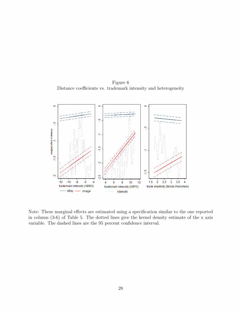
Figure 6Distance coefficients vs. trademark intensity and heterogeneity
Note: These marginal effects are estimated using a specification similar to the one reportedin column (3-6) of Table 5. The dotted lines give the kernel density estimate of the x axisvariable. The dashed lines are the 95 percent confidence interval.
28

Figure 7Corruption, Google popularity and the distance effect on trade
Note: The dotted lines give the kernel density estimate of the x axis variable. The dashedlines are the 95 percent confidence interval.
29
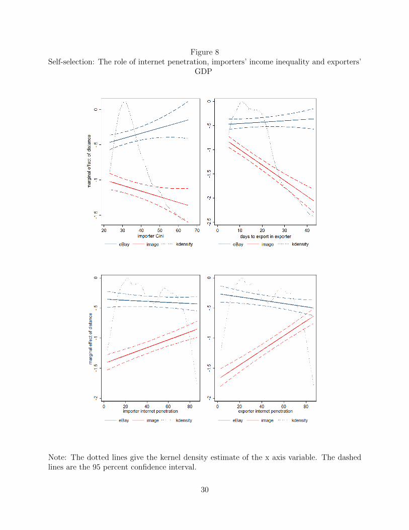
Figure 8Self-selection: The role of internet penetration, importers’ income inequality and exporters’
GDP
Note: The dotted lines give the kernel density estimate of the x axis variable. The dashedlines are the 95 percent confidence interval.
30
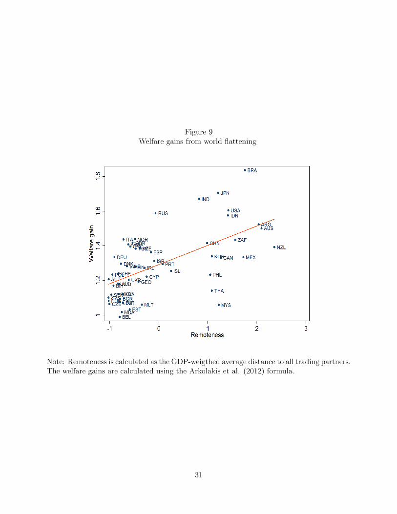
Figure 9Welfare gains from world flattening
Note: Remoteness is calculated as the GDP-weigthed average distance to all trading partners.The welfare gains are calculated using the Arkolakis et al. (2012) formula.
31

Tab
le1
Tra
de
cost
and
grav
ity
online
and
offlin
e(1
)(2
)(3
)(4
)(5
)(6
)(7
)(8
)eB
ayeB
ayeB
ayeB
ayoffl
ine
offlin
eoffl
ine
offl
ine
Dis
tance
-0.5
49**
*-0
.383
***
-0.3
82**
*-0
.299
***
-1.3
93***
-1.1
07***
-1.0
92***
-0.6
63**
*(0
.032
3)(0
.041
9)(0
.043
5)(0
.092
5)(0
.035
3)
(0.0
475)
(0.0
483)
(0.0
456)
No
com
mon
lega
lsy
s.-0
.304
***
-0.2
37**
*-0
.272
***
-0.5
77***
-0.5
78***
-0.3
79***
(0.0
547)
(0.0
536)
(0.1
02)
(0.0
536)
(0.0
537)
(0.0
591)
No
colo
ny
0.14
60.
0940
-0.2
87**
-0.4
18*
**
-0.4
22***
0.0
300
(0.1
35)
(0.1
33)
(0.1
25)
(0.1
58)
(0.1
57)
(0.1
09)
No
com
mon
langu
age
-0.4
75**
*-0
.486
***
-0.9
33**
*-0
.195
*-0
.200*
0.2
18**
(0.0
937)
(0.0
938)
(0.1
39)
(0.1
06)
(0.1
05)
(0.0
956)
No
bor
der
-0.1
53-0
.137
-0.7
62**
*-0
.366*
*-0
.333**
-0.2
85***
(0.1
24)
(0.1
22)
(0.1
37)
(0.1
44)
(0.1
44)
(0.0
895)
No
FT
A-0
.161
**-0
.181
**-0
.359
**-0
.320*
**
-0.2
97***
-0.4
30***
(0.0
796)
(0.0
795)
(0.1
51)
(0.0
872)
(0.0
876)
(0.0
830)
Ship
pin
gco
sts
0.05
27-0
.0835
(0.0
708)
(0.0
687)
Obse
rvat
ions
3,76
33,
763
3,73
33,
763
3,763
3,7
63
3,733
3,7
63
R-s
quar
ed0.
874
0.87
70.
882
0.8
51
0.85
90.
859
Note
:A
llre
gre
ssio
ns
are
esti
mate
du
sin
gan
imp
orte
ran
dex
por
ter
fixed
effec
tli
nea
rm
od
el,
exce
pt
for
colu
mn
s(4
)an
d(8
)w
hic
hu
sea
poi
sson
pse
ud
om
axim
um
like
lih
ood
esti
mat
or.
Th
efi
gure
sin
bra
cket
sar
ero
bu
stst
and
ard
erro
rs,
and
*st
an
ds
for
stati
stic
al
signifi
can
ce
atth
e10
per
cent
level
,**
for
stati
stic
al
sign
ifica
nce
atth
e5
per
cent
leve
lan
d**
*fo
rst
atis
tica
lsi
gnifi
can
ceat
the
1p
erce
nt
leve
l.
32

Tab
le2
Tes
ting
diff
eren
ces
ingr
avit
yco
effici
ents
Dis
tance
No
com
mon
No
colo
ny
No
com
mon
No
bor
der
No
FT
Ale
gal
syst
emla
ngu
age
Gra
vit
yco
effici
ent
-1.1
19**
*-0
.584
***
-0.4
08*
-0.2
10-0
.353
*-0
.314
***
(0.1
00)
(0.0
945)
(0.2
22)
(0.1
75)
(0.2
06)
(0.1
10)
Inte
ract
ion
wit
heB
aydum
my
0.71
1***
0.31
8*0.
596*
-0.2
390.
231
0.10
7(0
.136
)(0
.167
)(0
.318
)(0
.240
)(0
.273
)(0
.204
)
Not
e:T
he
dep
end
ant
vari
able
islo
gim
por
ts.
Reg
ress
ion
esti
mat
edusi
ng
imp
orte
r-eB
ayan
dex
port
er-e
Bay
fixed
effec
t
lin
ear
mod
el.
Th
efi
gure
sin
bra
cket
sar
ero
bu
stst
and
ard
erro
rs,an
d*
stan
ds
for
stat
isti
calsi
gnifi
can
ceat
the
10
per
cent
leve
l,**
for
stat
isti
cal
sign
ifica
nce
atth
e5
per
cent
leve
lan
d**
*fo
rst
atis
tica
lsi
gnifi
can
ceat
the
1p
erce
nt
leve
l.
33

Tab
le3
Rob
ust
nes
sch
ecks:
Tra
de
cost
and
grav
ity
for
diff
eren
tty
pes
ofeB
ayflow
s(1
)(2
)(3
)(4
)(5
)(6
)(7
)(8
)(9
)eB
ayto
tal
offlin
eto
tal
New
goods
Use
dgoods
Auct
ions
Non
-auct
ions
Consu
mer
seller
sP
ower
Sel
lers
Non-P
ower
Sel
lers
Dis
tance
-0.4
46**
*-1
.352
***
-0.4
08***
-0.5
73***
-0.4
90*
**-0
.335*
**
-0.5
35***
-0.3
55***
-0.4
61***
(0.0
306)
(0.0
495)
(0.0
393)
(0.0
470)
(0.0
287)
(0.0
327)
(0.0
574)
(0.0
362)
(0.0
393)
No
com
mon
lega
lsy
s.-0
.143
***
-0.5
69**
*0.0
295
-0.1
65*
**
-0.1
14**
*-0
.0567
-0.4
60***
-0.2
51***
-0.3
24***
(0.0
372)
(0.0
554)
(0.0
475)
(0.0
580)
(0.0
343)
(0.0
397)
(0.0
703)
(0.0
456)
(0.0
481)
No
colo
ny
-0.3
41**
*-0
.325
*0.
00399
-0.2
38*
-0.3
75*
**-0
.131
-0.1
80
-0.3
30***
-0.2
69**
(0.0
937)
(0.1
70)
(0.1
22)
(0.1
31)
(0.0
851)
(0.1
02)
(0.1
75)
(0.1
23)
(0.1
13)
No
com
mon
langu
age
-0.3
66**
*-0
.340
***
-0.4
32*
**-0
.245
***
-0.3
39***
-0.3
79***
-0.4
98***
-0.2
68***
-0.2
97***
(0.0
656)
(0.1
13)
(0.0
850)
(0.0
936)
(0.0
587)
(0.0
728
)(0
.128)
(0.0
738)
(0.0
868)
No
bor
der
-0.2
75**
*-0
.243*
-0.3
62**
*-0
.102
-0.2
65**
*-0
.345
***
-0.1
33
-0.2
58**
-0.2
68***
(0.0
845)
(0.1
46)
(0.1
07)
(0.1
24)
(0.0
752)
(0.0
936
)(0
.156)
(0.1
07)
(0.1
04)
No
FT
A-0
.122
**-0
.191
**-0
.0598
-0.2
28**
-0.0
546
-0.1
26**
0.0
337
-0.2
64***
-0.0
681
(0.0
545)
(0.0
932)
(0.0
728)
(0.0
895)
(0.0
566)
(0.0
588)
(0.1
01)
(0.0
699)
(0.0
716)
Obse
rvat
ions
3,77
83,
778
3,7
403,
740
3,7
403,
740
3,7
63
3,7
78
3,7
78
R-s
quar
ed0.
913
0.79
90.
881
0.81
80.
920
0.91
00.7
91
0.8
93
0.8
71
Note
:A
llre
gre
ssio
ns
are
esti
mate
du
sin
gan
imp
orte
ran
dex
por
ter
fixed
effec
tli
nea
rm
od
el.
Th
efi
gu
res
inb
rack
ets
are
imp
ort
er-
an
d
exp
orte
r-cl
ust
ered
stan
dard
erro
rs,
and
*st
and
sfo
rst
atis
tica
lsi
gnifi
can
ceat
the
10p
erce
nt
leve
l,**
for
stati
stic
al
sign
ifica
nce
at
the
5p
erce
nt
leve
lan
d**
*fo
rst
atis
tica
lsi
gn
ifica
nce
atth
e1
per
cent
level
.
34

Tab
le4
Tes
ting
diff
eren
ces
ingr
avit
yco
effici
ents
for
Pow
erSel
lers
Dis
tance
No
com
mon
No
colo
ny
No
com
mon
No
bor
der
No
FT
Ale
gal
syst
emla
ngu
age
Gra
vit
yco
effici
ent
-0.4
61**
*-0
.324
***
-0.2
69**
-0.2
97**
*-0
.268
***
-0.0
681
(0.0
393)
(0.0
481)
(0.1
13)
(0.0
868)
(0.1
04)
(0.0
716)
Inte
ract
ion
wit
hP
ower
Sel
ler
dum
my
0.10
6**
0.07
31-0
.061
10.
0291
0.00
982
-0.1
95*
(0.0
534)
(0.0
663)
(0.1
67)
(0.1
14)
(0.1
49)
(0.1
00)
Not
e:T
he
dep
end
ant
vari
able
islo
gof
eBay
imp
orts
.R
egre
ssio
nes
tim
ated
usi
ng
imp
ort
er-P
San
dex
port
er-P
Sfi
xed
effec
tli
nea
rm
od
el.
Th
efigu
res
inbra
cket
sar
ero
bu
stst
and
ard
erro
rs,
and
*st
and
sfo
rst
ati
stic
al
sign
ifica
nce
at
the
10
per
cent
leve
l,**
for
stati
stic
al
sign
ifica
nce
atth
e5
per
cent
leve
lan
d**
*fo
rst
atis
tica
lsi
gn
ifica
nce
at
the
1p
erce
nt
leve
l.
35

Tab
le5
Pro
duct
info
rmat
ion
and
dis
tance
effec
tson
line
and
offlin
e(1
)(2
)(3
)(4
)(5
)(6
)(7
)(8
)eb
ayoffl
ine
ebay
offlin
eeb
ayoffl
ine
ebay
offl
ine
Dis
tance
-0.2
99**
*-1
.552
***
-0.3
80**
*-2
.045
***
-0.2
40***
-0.1
23***
-0.3
56*
**
-0.9
99***
(0.0
105)
(0.0
306)
(0.0
118)
(0.0
322)
(0.0
117
)(0
.0280
)(0
.0126)
(0.0
279)
No
com
mon
lega
lsy
s.-0
.279*
**-0
.988
***
-0.2
87**
*-0
.907
***
-0.2
80*
**
-0.8
57**
*-0
.315***
-0.7
90***
(0.0
138)
(0.0
409)
(0.0
150)
(0.0
412)
(0.0
148
)(0
.0351
)(0
.0161)
(0.0
361)
No
colo
ny
-0.0
419
-0.7
58**
*-0
.046
0-0
.814
***
-0.0
650*
-0.8
34*
**
-0.0
297
-0.8
48***
(0.0
359)
(0.0
885)
(0.0
390)
(0.0
901)
(0.0
388
)(0
.0804
)(0
.0421)
(0.0
830)
No
com
mon
langu
age
-0.6
38*
**1.
198*
**-0
.715
***
0.71
0***
-0.7
29*
**
0.3
74***
-0.7
28***
-0.1
70***
(0.0
268)
(0.0
725)
(0.0
297)
(0.0
745)
(0.0
293
)(0
.0657
)(0
.0326)
(0.0
656)
No
bor
der
-0.6
19**
*-0
.300
***
-0.6
17**
*-0
.442
***
-0.6
05**
*-0
.629*
**
-0.5
59***
-0.6
88***
(0.0
320)
(0.0
746)
(0.0
351)
(0.0
764)
(0.0
342
)(0
.0676
)(0
.0371)
(0.0
699)
No
FT
A0.
0165
0.38
8***
0.01
470.
259*
**0.
0074
10.
105**
0.0
00187
-0.2
11***
(0.0
176)
(0.0
535)
(0.0
191)
(0.0
534)
(0.0
188
)(0
.0467
)(0
.0200)
(0.0
466)
Dis
tance×
TM
-com
pla
int
-0.0
145*
**-0
.071
1***
(0.0
0037
5)(0
.001
04)
Dis
tance×
TM
-WIP
O-0
.006
04*
**
-0.1
43**
*(0
.000
336
)(0
.000
740)
Dis
tance×
sigm
a0.0
272
***
-0.1
48***
(0.0
0107)
(0.0
0200)
Const
ant
6.2
65***
20.8
1***
6.03
9***
20.6
6***
6.2
92*
**
20.
07***
6.1
10***
19.1
6***
(0.0
795)
(0.2
23)
(0.0
871)
(0.2
28)
(0.0
861)
(0.1
98)
(0.0
940)
(0.2
02)
Obse
rvat
ions
107,3
0210
7,30
288
,744
88,7
4490
,977
90,9
77
76,4
10
76,4
10
R-s
quar
ed0.
055
0.04
60.
069
0.09
70.0
610.3
020.0
65
0.138
Note
:A
llre
gres
sion
sare
esti
mate
du
sin
gd
evia
tion
sfr
omth
eim
por
ter-
cate
gory
and
exp
ort
er-c
ateg
ory
mea
ns.
Th
efi
gu
res
inb
rack
ets
are
rob
ust
stan
dard
erro
rs,
an
d*
stan
ds
for
stat
isti
cal
sign
ifica
nce
atth
e10
per
cent
leve
l,**
for
stati
stic
al
sign
ifica
nce
at
the
5p
erce
nt
leve
lan
d
***
for
stat
isti
cal
sign
ifica
nce
at
the
1p
erce
nt
leve
l.
36

Tab
le6
Dis
enta
ngl
ing
the
mec
han
ism
s(1
)(2
)(3
)(4
)(5
)(6
)(7
)(8
)eb
ayeb
ayeb
ayeb
ayoffl
ine
offl
ine
offl
ine
offl
ine
Dis
tan
ce-0
.353
***
-0.3
53**
*-0
.225
0.24
6-1
.342*
**-1
.227***
-4.3
56**
*-2
.836***
(0.0
478)
(0.0
482)
(0.4
71)
(0.5
23)
(0.0
531
)(0
.0493)
(0.5
72)
(0.5
72)
No
com
mon
lega
lsy
s.-0
.320
***
-0.3
20**
*-0
.306
***
-0.3
11**
*-0
.456*
**-0
.514***
-0.5
41***
-0.5
58***
(0.0
555)
(0.0
548)
(0.0
555)
(0.0
555)
(0.0
545)
(0.0
542)
(0.0
543)
(0.0
544)
No
colo
ny
0.13
80.
138
0.14
20.
130
-0.3
54*
*-0
.386**
-0.3
37**
-0.3
74*
*(0
.135
)(0
.136
)(0
.136
)(0
.136
)(0
.155
)(0
.157)
(0.1
58)
(0.1
59)
No
com
mon
lan
gu
age
-0.4
60**
*-0
.460
***
-0.4
74**
*-0
.472
***
-0.3
15*
**-0
.256**
-0.2
14**
-0.2
04*
(0.0
938)
(0.0
939)
(0.0
945)
(0.0
948)
(0.1
04)
(0.1
04)
(0.1
06)
(0.1
06)
No
bord
er-0
.162
-0.1
62-0
.152
-0.1
47-0
.297
**-0
.331**
-0.3
91***
-0.3
82***
(0.1
24)
(0.1
24)
(0.1
25)
(0.1
25)
(0.1
33)
(0.1
38)
(0.1
42)
(0.1
43)
No
FT
A-0
.156
*-0
.156
*-0
.160
**-0
.158
**-0
.362
***
-0.3
42***
-0.3
39***
-0.3
30***
(0.0
807)
(0.0
806)
(0.0
805)
(0.0
804)
(0.0
860)
(0.0
880)
(0.0
876)
(0.0
882)
Dis
tan
ce×
exp
ort
erco
rru
pti
on0.
0399
-0.3
06*
**(0
.027
5)(0
.026
2)D
ista
nce×
imp
ort
erco
rru
pti
on
0.04
03-0
.157***
(0.0
260)
(0.0
238)
Dis
tan
ce×
exp
ort
erG
oog
lep
op
ula
rity
-0.0
0787
0.1
61***
(0.0
231)
(0.0
280)
Dis
tan
ce×
imp
orte
rG
oogl
ep
opu
lari
ty-0
.031
20.0
859
***
(0.0
258)
(0.0
282)
Con
stan
t-1
.178
**-1
.185
**-0
.757
-0.8
14*
13.
69**
*12.
08***
10.7
0***
10.5
4***
(0.5
96)
(0.5
97)
(0.4
89)
(0.4
88)
(0.5
51)
(0.5
17)
(0.4
52)
(0.4
49)
Ob
serv
ati
ons
3,76
33,
763
3,76
33,
763
3,76
33,7
63
3,7
63
3,7
63
R-s
qu
ared
0.91
00.
910
0.91
00.
910
0.90
50.9
02
0.9
020.9
01
Note
:A
llre
gre
ssio
ns
are
esti
mate
du
sin
gan
imp
orte
ran
dex
por
ter
fixed
effec
tli
nea
rm
od
el.
Th
efi
gure
sin
bra
cket
sare
rob
ust
stan
dard
erro
rs,
and
*st
an
ds
for
stat
isti
cal
sign
ifica
nce
atth
e10
per
cent
leve
l,**
for
stat
isti
cal
sign
ifica
nce
at
the
5p
erce
nt
leve
lan
d***
for
stati
stic
al
sign
ifica
nce
atth
e1
per
cent
leve
l.
37

Tab
le7
Sel
ecti
oneff
ects
?(1
)(2
)(3
)(4
)(5
)(6
)(7
)(8
)eb
ayeb
ayeb
ayeb
ayoffl
ine
offl
ine
offl
ine
offl
ine
Dis
tan
ce-0
.383
***
-0.4
85**
*-0
.354
***
-0.2
62*
**-1
.107*
**
-0.6
74***
-1.4
18***
-1.6
87***
(0.0
423
)(0
.0666
)(0
.0690
)(0
.070
4)(0
.047
9)
(0.0
711)
(0.0
672)
(0.0
762)
No
com
mon
lega
lsy
s.-0
.304
***
-0.3
17**
*-0
.290*
**
-0.3
28*
**-0
.577
***
-0.4
72***
-0.5
47***
-0.5
28***
(0.0
552
)(0
.0576
)(0
.0556
)(0
.055
8)(0
.054
1)
(0.0
568)
(0.0
552)
(0.0
555)
No
colo
ny
0.1
460.1
79
0.1
60
0.102
-0.4
18*
**
-0.3
43**
-0.3
75**
-0.3
80**
(0.1
36)
(0.1
38)
(0.1
39)
(0.1
34)
(0.1
59)
(0.1
56)
(0.1
60)
(0.1
56)
No
com
mon
lan
guag
e-0
.475
***
-0.5
07**
*-0
.514*
**
-0.4
48*
**-0
.195*
-0.2
66**
-0.2
52**
-0.2
81***
(0.0
946
)(0
.100
)(0
.0955
)(0
.096
1)(0
.107)
(0.1
08)
(0.1
08)
(0.1
07)
No
bor
der
-0.1
53-0
.102
-0.1
75
-0.2
04-0
.366*
*-0
.254*
-0.3
26**
-0.2
85**
(0.1
25)
(0.1
07)
(0.1
27)
(0.1
25)
(0.1
45)
(0.1
37)
(0.1
42)
(0.1
38)
no
FT
A-0
.161
**-0
.107
-0.1
63**
-0.1
54*
-0.3
20***
-0.3
23***
-0.3
19***
-0.3
18***
(0.0
804
)(0
.0837
)(0
.0810
)(0
.081
6)(0
.088
0)
(0.0
876)
(0.0
882)
(0.0
873)
Dis
tan
ce×
imp
orte
rG
ini
0.12
1***
0.1
67***
(0.0
0922
)(0
.00697)
Dis
tan
ce×
exp
orte
rd
ays
toex
por
t0.
002
91
-0.0
321***
(0.0
033
3)(0
.0036)
Dis
tan
ce×
imp
orte
rin
tern
etp
enet
rati
on-0
.000
892
0.0
0652***
(0.0
011
0)
(0.0
0107)
Dis
tan
ce×
exp
orte
rin
tern
etp
enet
rati
on-0
.002
74*
*0.0
121***
(0.0
011
9)(0
.00115)
Con
stan
t-4
.910
***
-0.5
29
-0.8
86-1
.462*
*4.
565
***
12.0
1***
12.2
2***
13.9
6***
(0.6
70)
(0.5
26)
(0.6
18)
(0.6
18)
(0.5
51)
(0.4
82)
(0.5
61)
(0.5
87)
Ob
serv
atio
ns
3,7
633,5
19
3,64
13,
641
3,7
63
3,5
19
3,6
41
3,6
41
R-s
qu
ared
0.9
10
0.9
080.9
11
0.910
0.901
0.9
06
0.9
02
0.9
04
Note
:A
llre
gre
ssio
ns
are
esti
mate
du
sin
gan
imp
orte
ran
dex
por
ter
fixed
effec
tli
nea
rm
od
el.
Th
efi
gure
sin
bra
cket
sare
rob
ust
stan
dard
erro
rs,
and
*st
an
ds
for
stat
isti
cal
sign
ifica
nce
atth
e10
per
cent
leve
l,**
for
stat
isti
cal
sign
ifica
nce
at
the
5p
erce
nt
leve
lan
d***
for
stati
stic
al
sign
ifica
nce
atth
e1
per
cent
leve
l.
38
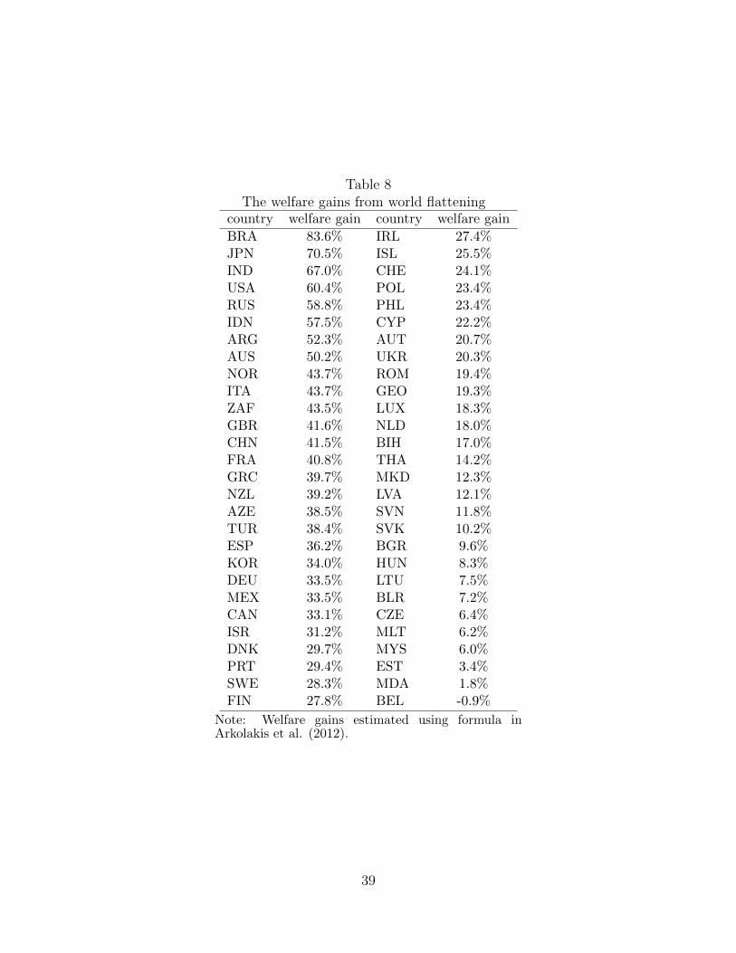
Table 8The welfare gains from world flattening
country welfare gain country welfare gain
BRA 83.6% IRL 27.4%JPN 70.5% ISL 25.5%IND 67.0% CHE 24.1%USA 60.4% POL 23.4%RUS 58.8% PHL 23.4%IDN 57.5% CYP 22.2%ARG 52.3% AUT 20.7%AUS 50.2% UKR 20.3%NOR 43.7% ROM 19.4%ITA 43.7% GEO 19.3%ZAF 43.5% LUX 18.3%GBR 41.6% NLD 18.0%CHN 41.5% BIH 17.0%FRA 40.8% THA 14.2%GRC 39.7% MKD 12.3%NZL 39.2% LVA 12.1%AZE 38.5% SVN 11.8%TUR 38.4% SVK 10.2%ESP 36.2% BGR 9.6%KOR 34.0% HUN 8.3%DEU 33.5% LTU 7.5%MEX 33.5% BLR 7.2%CAN 33.1% CZE 6.4%ISR 31.2% MLT 6.2%DNK 29.7% MYS 6.0%PRT 29.4% EST 3.4%SWE 28.3% MDA 1.8%FIN 27.8% BEL -0.9%
Note: Welfare gains estimated using formula inArkolakis et al. (2012).
39
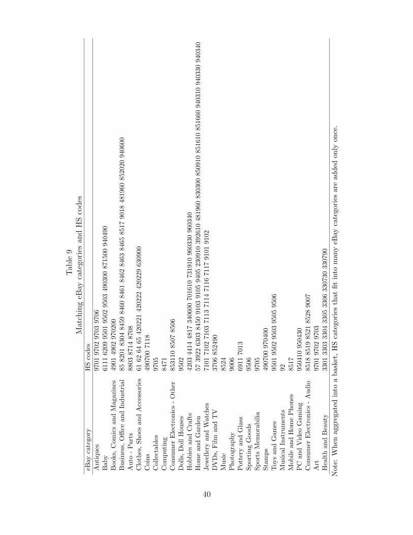
Tab
le9
Mat
chin
geB
ayca
tego
ries
and
HS
codes
eBay
cate
gory
HS
codes
Anti
ques
9701
9702
9703
9706
Bab
y61
1162
0995
0195
0295
0349
0300
8715
0094
0490
Book
s,C
omic
san
dM
agaz
ines
4901
4902
9702
00B
usi
nes
s,O
ffice
and
Indust
rial
8582
0183
0484
5984
6084
6184
6284
6384
6585
1790
1848
1960
852020
940600
Auto
-P
arts
8803
8714
8708
Clo
thes
,Shoes
and
Acc
esso
ries
6162
6465
4202
2142
0222
4202
2963
0900
Coi
ns
4907
0071
18C
olle
ctab
les
9705
Com
puti
ng
8471
Con
sum
erE
lect
ronic
s-
Oth
er85
3110
850
785
06D
olls
,D
oll
Hou
ses
9502
Hob
bie
san
dC
raft
s42
0344
1448
1734
0600
7016
1073
1910
9603
3096
0340
Hom
ean
dG
arden
5739
2263
0384
5091
0391
0594
0523
0910
3926
1048
1960
83030
0850910
851610
851660
940310
940330
940340
Jew
elle
ryan
dW
atch
es71
0171
0271
0371
1371
1471
1671
1791
0191
02D
VD
s,F
ilm
and
TV
3706
8524
90M
usi
c85
24P
hot
ogra
phy
9006
Pot
tery
and
Gla
ss69
1170
13Sp
orti
ng
Goods
9506
Sp
orts
Mem
orab
ilia
9705
Sta
mps
4907
00970
400
Toy
san
dG
ames
9501
9502
9503
9505
9506
Musi
cal
Inst
rum
ents
92M
obile
and
Hom
eP
hon
es85
17P
Can
dV
ideo
Gam
ing
9504
10950
430
Con
sum
erE
lect
ronic
s-
Audio
8518
8519
8521
8528
9007
Art
9701
9702
9703
Hea
lth
and
Bea
uty
3301
3303
3304
3305
3306
3307
3033
0790
Note
:W
hen
agg
rega
ted
into
ab
ask
et,
HS
cate
gori
esth
atfi
tin
tom
any
eBay
cate
gori
esar
ead
ded
on
lyon
ce.
40