I~CNNIC^L INFOIIMA’iiON I~iSION

UCRL-12409

University of California

Ernest O.Radiation

LawrenceLaboratory

THERMAL EFFECTS IN DIMENSIONAL METROLOGY

Livermore, California

UCRL- 12409

UNIVERSITY OF CALIFORNIA

Lawrence Radiation Laboratory

Livermore~ Californla

AEC Contract No. W-7405-eng-48

THERMAL EFFECTS IN DIMENSIONAL METROLOGY

Win. Brewer

,. Jarr~es B. Bryan

Eldon R. McClure

J.:.W. Pdarson

February 22, 1965

DISC’/LAI M RR

Thi~ document was prepm’ed a~ an account of work sponsored by m~ agency of the United StatesGovernment. Neither the United States GnvernLuont nor the University uf California aor m~y of theiremployees, makes any warranty, express or implied, pr assumea any legal liability or responsibility forthe accuracy, completeness, or usefulness of any information, apparatus, product, or process disclosed,or represents that its use wouk[ not infringe privately owned rights. Reference herein to any specificcommercial product, process, or service by trade name~ trademark~ mamtfitcturet9 or ofl~erwise, doesnot necessarily ~mstitut~ or imply its endorsement, recommendation, or favoring by the United StatesGovernment or the University 0f California. The views and opinions of authors expressed herein donot necessarily stale or t~flect those of the United States Government or the University of Calihmda,and shall not be used for advertising or product endorsement purposes.

This report has been rep~ducexidirectly from tile best available copy.

Available to DOE and DOE contrac|ors from theOffice of Scientific and Technical Inhmnation

P,O. Box 62, Oak Ridge, TN 3783~Prices aw~ilable flXHtx (615) 576-8401~ PTS 626-840I

Available to the public from theNational Tedmical Information Service

U.S. Department of Commerce5285 Port Royal Rd.,

Springfield, VA 22161

Work performed tinder Lhe atmpices of tile U,S. Depilrimei~t of llriergy by Lawrence Liveriuore NationalLaboratory under Contract W-Td05-ENG-41t.

TI.IE[~MAL EFFECTS.IN DIMENSIONAL METROLOGY1

Win. Brewer~~" James B, Br~an, 3 Eldon R. M.cCture, 4 and J. W. Pear,on5

ABSTRACT

A Lawrence Radiation Laboratory investigation of thermal effect in

dimensional metrology shows that, in the field of close tolerance work,

thermal effect is the largest single source of ~rror, large enough to make

correctiv~ action necessary if modern measurement systems and machine

tools are to attain their potential accuracies. This paper is .an effort to

create an awareness of the thermal environment problem and to suggest some

solutions. A simple, quantitative, s.emiexperimental method of thermal

error evaluation is developed. It is shown, experimentally and theoretica].ly,

that the fr.equegc.y .of temperature variation is..as important as the absolute

limits of the temperature variation, and that the sensitivity of machine

structures to thermal vibration, can be minimized by selecting environmental

frequencies to avoid resonant conditions. A relatively .si.mple device to monitor

the thermal environment and automatically effect error compensation is

proposed.

1Work performed under the auspices of the U. S. Atomic Energy Commission.

2Graduate Student of Mechanical Engineering, Michigan State University,East Lansing, Michigan.

3Chief Metrologist, Lawrence Radiation Laboratory, University of California,Livermore, California.

4Assistant Professor’ of Mecltanical Engineering, Oregon State University,Corvallis, Oregon.

5Mechanical Engineer, Lawrence Radiation Laboratory, University of California,Livermore, California. ’

-2-

I. INTRODUCTION

During a routine test of a measuring machine at the Lawrence Radiation

Laboratory (LRL), it was observed that the measurements varied significantly

with time. It was thought, at first, that the electronic gage used to make the

measurements was the cause, but a careful check showed that the electronic

drift was negligible. The measurement system was then monitored by means

of a sensitive temperature pickup mounted in the air near the gage. Tempera-

ture and gage output were recorded over long time periods. The results showed

a high degree of correlation between temperature variation and measurement

variation.

Similar tests were conducted on many different types of measurement

systems with similar results.¯ ¯Figure 1 is an example of such results. The

significance of this effect is clear when the observed drift is compared with the

working tolerance of the gage. The drift is 100 microinches and the working

tolerance of the gage is only 10.0 microinches. In the case shown, the drift

accounts for 10070 of the tolerance of the gage.

As a result of this distur.bing development, the Metrology Section of LRL

began an investigation of thermal effect in Dimensional Metrology. As the

investigation progressed, it became increasingly clear that:

1. In the field of dlose tolerance work, thermal effect is the greatest

si..ngle source of error.

2. The ugu....a.1 efforts to correct for thermal error by’ applying expansion

" correction," or by air conditioning the working area do not always

solve the problem and are based on an incomplete understanding of

the problem.

-3-

3. The specified accuracies of modern precision tools and gages are

attainable only if the thermal environment matches the require-

ments of each measurement system.

~t has been helpful to think of the temperature problem in terms of (1)

the effects of average temperatures other than 68 degrees, (2) the effects

temperature’variation about tltis avei-age. The paper ttrgariization reflects

this arbitrary division of theproblem. There is also a discussion of ways

and means of reducing thermal errors. Appendix A is a glossary of terms

used to discuss thermal effects problems. Appendix B is a detailed procedure

of a " drift ’’¯ check and Append.ix C is an outline of a method¯ to determine the

thermal frequency response o.f, a measuring system.

II. EFFECTS OF AVERAGE TEMPERATURES OTHER THAN 68°F

An inch is the distance between two fixed points in space. It is defined

as 41,929.398742 wavelengths of the orange-red radiation of krypton-86 when .

propagated in vacuum. An inch does not vary with temperature. This fact

is obscured because the lengths of the more common representations of the

inch such as gage blocks, lead screws, and scales do vary with temperature.

The lengths of most of the materials we deal with also change with tempera-

ture. In April, 1931, the International Committee of Weights and Measures

Meeting in Paris agreed that when we describe the length of an object we

automatically mean its length when it is at a temperature of .6_~_de_g.rees. This

agreement was preceded by intensive international debate and negotiation

[ 1, 2, 3, 4, 5, 11 ]6. This agreement., means that ..... it is not necessary to specify

t_h..e...m....e_.~..s.~.r..e.ment temperature on every drawing (no more necessary than it

is to define the inch on every drawing).

6Numbers in brackets designate Bibliography at end of paper.0

-4-

If dimensions are only correct at 68 degrees, how have we been getting

by a. ll these years by measuring at warmer temperatures? The answer is

that i~ o~t~ wo~,l~ i~ s~.e~t and out- ~eate is steer ~he two expand ~ogethex. a~td ~he

¯ resultant errors tend to cancel. If, however, the work is another material

such as aluminum, the errors are ~tifferent and they don,t cancel. We refer

to this error as " differential expansion." We can get :i.nto the same trouble

if our work is steel, but we are measuring with the " honest" inches that come

from an interferometer. As a result of the discovery of the laser and the

development of practical laser fringecoun.ting interferometers, .we expect to

be using more of these " honest" inches and will have to be very careful of

this problem. ,

Knowledgeable machinistp have always made differential expansion

corrections. The thing that is sometimes overlooked, however, is that these

corrections are not exact. Our knowledge about average coefficients of ex-

pansion is meager and we can never know the exact coefficient of each part,

This inexactness we call "u.ncertainty of differential expansion."

This inexactness or uncertainty is zero when the average temperature is

68 degrees, and increases according to the thermal distance from 68 degrees.

Its magnitude varies for different materials. We have reason to think that it

is at least 5~]o for gage steel and on up to 25~]0 for other materials. One

metallurgist, consulted in the course of our investigatiop, stated that the co-

efficient of expansion of cast iron may vary as much as 4Y0 between thin and

thick sections. This uncertainty factor also includes the possibility of differences

in expansion of a material in different directions. Diffe.Fences between the actual

thermal expansion and the handbook or ’~ nominal" expansion occur because of

experimental errors and because of dissimilarities between the experimental

materiat and the material of our workpiece.

Coml~lete studies of the errors introduced in the e~timates of thermal

e×pai~sion are notably absent. The data presented by Goldsmith et al. [ 9]

the coefficient of expansion of common materials. This disagreement might

be expected for some of the more exotic materials~ but intuition would indicate

that the knowledge of the properties of steel would be m~e e~act. Not

necessarily so, as ~chard K. Kfrby of the National Bureau of Standards

port s7:

" The accuracy of a tabulated value of a coefficient of thermal

expansion is about ~5 percent if the heat and mechanical treatment

of the steel ~s indicated. The .precision of the coefficient (a) among

many heats of steel of nominally the same chemical content is about

~3 percent, (b) among several heat treatments of the same steel

about ~10 percent, and (c). among samples cut from different locations

in a large part of steel that has been fully annealed, is about ~2 percent

(hot or cold roll~ng will cause a difference of about:~5 percent)."

Corrections for uncertainty of d~fferential expansion cannot be made. The

error can be reduced by establishing more accurate nominal coefficients of

thermal expansion, by improving the uniformity.of coefficient of expansion from

part to part through better chemical and metallurgical controls, by determining

indiv~dua~ part and gage expansions, ~d by limiting the room temperature

deviation from 68 degrees. ..

Control of uncertainty of ~ifferential expansion is the primary reason for

maintaining a ~68 degree averag~ temperature." Even ifwe had an exact knowl-

edge of all coefficients, the con~usion and pdssibility of mistakes in making

7A personal comm~ication from Richard K. Kirby, In charge, Thermal’Expansion Laboratory, Len~h Section, Metrology Division, U. S. NationalBureau of Standards, Washington, D. C.

-6-

corrections is a second reason for maintaining 68 degrees. As our study

progressed, it became necessary to establish a more exact definition of

.refer ~o Appendix A’. O~ossary of Terms, definitions No. 15 through

which are pe~’tinent to the discussion in this section.

Three examples are given below to illustrate the Consequences of

average temperatures other than 68 degrees. Possible errors are shown.to

be 13~o, 37~0, and ~.0~/0 of the working tolerance. These errors do not include

the effect of temperature variation which is covered in the next section.

They do not include the other errors of measurement such as accuracy of

standards and comparison technique. The traditional rule of ten to one allows

only 10~/~ of the working tolerance for all measurement error.

Example No, 1

A 10 inch long steel part with a tolerance of plus or minus a half-

thousandth (500/~in.) is measured in a C-frame comparator by comparing

to a 10 inch gage block in a room which averages 75 degrees. A handbook lists

the Nominal Coefficient of Expansion (K) for the gage block as 6.5/~in./in./deg.

The K for the steel part is assumed to have the same value. The Uncertainty

of Nominal Coefficient of Expansion (UNCE) for the gage block is estimated

at plus or minus 5~’. and for the part at 10~o (its exact comPosition is unknown).

For this case, the Nominal Differential Expansion (NDE) is zero. The

Uacertainty of Nominal Differential Expansion (UNDE) is, however, significant.

It is the sum of the two Uncertainty of Nominal Expansion (UNE) values.

-7-

NDE

UNE gage block

UNE part

~. No correction necessary ffi 0

"- 10 in. × 6.5/~in./in./deg

ffi 10 in. × 6.5/~in./in./deg × 7 deg × 10~o ffi 44 ~in.

UNDE = 86 ~in,

66 ,~ × 100 -" 13~/0 0.f working tolerance ~

Example No...2

A 10 inch long plastic part with a tolerance of plus or minus 0.002 inch

is measured on a surface plate using an indicator stand.to compare it to the

readings of a Cadillac gage. The room temperature averages 75 degrees (7

degree Temperature Offset)..A handbook lists the Nominal Coefficient of

Expansion (K) for the gage steel assUmed to be used in the Cadillac gage

6.5 pin./in./deg.. The K value for the plasti6 is listed by the manufactuger

as 40/~in./in./deg. The Uncertainty of Nominal Coefficient of Expansion

(UNCE) for the gage steel is estimated at 10~0 since we do not’ know the exact

composition nor heat treatment. Because of past experience with plastics and

a lack of any information to the contrary the UNCE for the plastic is estimated

at 25~]o. The inspector making the measurement is thoroughly familiar with

differential expansion. He computes the NDE correctly and applies it in the

proper direction to the dial indicator reading which is used to transfer the

Cadillac gage reading. A correction for UNDE cannot be made.

value is computed below:

NDE ffi Corrections are made = 0

UNEgage -- 10 in. × 6.5/~in./in./deg )< 7 deg × 1070 ffi 46/~in.

UNEpart = 10 in. ~< 40 ~in./in./deg × 7 deg )< 25~]o ffi 700.. pin.

UNDE = 746

746 ~< 100 = 37~of working tolerance

Its possible

-8-

Example No. 3

A 10 inch long aluminum part with a tolerance of plus or minus 0,001

inch is measured on a surface plate using an indicator stand to compare it to

the readings of a Cadillac gage. The room temperature averages 70 degrees.

(2 degree Temperature Offset.) As in the previous example, the NCE for the

gage is assumed to be 6.5 Bin./in./deg. The NCE for the aluminum part is

assumed to be 13.5 Bin./in./deg. The UNCE for the gage is estimated at 1070

and for the aluminum part at 2070. The inspector in this case does no_./t appreciate

the magnitude of NDE, and arbitrarily decides that 70 degrees is " close enough,"

he does " not bother" with an NDE correction to his readings. The possible

error is computed as follows:

-- 10in.NDE

UNDE:

UNEgage --

UNEpart --

2051000

(13.5 - 6.5) × 2 deg

10in, XS.5X2 deg× i07o = 13 Bin.

i0 in. X 13.5 X2 degX2070 = 52/~in.

UNDE =

NDE plus UNDE =

X 100 = 207~ of working tolerance

140/~in.

65 ~in,

205 ~in.

In the above examples we assumed that the average temperature of the

gage and part were the same as the average temperature of the room. If

adequate time has been allowed for the gage and part to " soak out" and reach

thermal equilibrium this is a reasonable assumption. Unfortunately, this

assumption does not apply to the instantaneous.temperatu~.e of these components.

Instead, the environment is continually varying around some mean value. The

result is that differences in temperature in the various components are dyh~mically

i.9-

induced in the system. The next section ,discusses the errors caused by

.v~nriation in thermal environment.

III..E.FFECTS OF VAI~,,IATIO~ IN THERMAL E ..NVIR.0NMENT

The Two-Element System.

All length measuring apparatus can be viewed as consisting of a number

of individual elements arranged to form a "C." Figure 2 shows a schematic

of a C-frame comparator.measuring the diameter of a short section of hollow

tubing. The comparator frame and the part form two elements. If the co-

efficient of expansion of the comparator is exactly the same as the part, the

gage head will read zero after ~oak-out at any uniform temperature that we

might select. If we induce a change in temperature, however, the relatively

thin section of the tubing will react sooner than the thick section of the

comparator frame and the gage head will show a temporary deviation. The

amount of the deviation will depend on the rate Of change of temperature. If

the rate is slow enough to allow both parts to keep up with the temperature

changes, there will be a small change in gage head reading. If the rate is so

fast that even the thin tubing can’~ respond, there will again be a small change

in reading. Somewhere in between these extremes there will be a frequency

of temperature change that results in a maximum change in reading. This is

somewhat similar to resonance in.vibration work,

To confirm our intuition on the nature of ~hese effects the above model was

further simplified to that shown in Fig. 3. Sample heat transfer calculations

were made for this model and programmed on an analog computer. The"

-10-

cylind~,r with the displacement pickup can be considered the comparator.

Both cylinders are made of steel and are 4 inches long. Cylinder A is 2 inches

i.’] diameter and Cylinder B is 1/2 inch in diameter. Figure 4 shows the

computer-predicted changes in length of the two cylinders as a result of a plus

and miaus one degree sinusoidal change in air temperature having a frequency

of one cycle per hour. The thick cylinder shows less than one-third of the

temperature change of the thin cylinder and its temperature lags the thin

cylinder by 3 or 4 minutes. The do{ted line in Fig. 4 shows the predicted gage

head reading which is the same as the instantaneous difference in the lengths of

the two cylinders. We call this ~he " Thermal Drift" (definition 24) of the system.

The effect of varying the " Thermal Vibration" frequency is plotted in Fig. 5.

As our intuition predicted, the drift is small for very high or low frequencies

and reaches a maximum amplitude at a point in between which we call resonance.

Figure 5 is called the " Frequency Response" (definition 14) of the system. In

this case resonance occurs at 1/2 cycle per hour and has a value of 15 pin.

This error would occur even if the Time Average Temperature of the environment

and .all mechanical elements was 68° exactly.

Fir.teen pin. may appear to be a negligible magnitude, but real measuring

machines and machine tools, of course, don’t have uniform coefficients through-

out, and real workpieces can have quite different coefficients. This makes the

effects of temperature variation much worse. If the part were Lucitc, for

example, these responses would be much more severe. Real systems generally

have much longer overall lengths and more severe differences in mass between

elements. Magnitudes of 150 ~in. per degree at resonant frequency are not

unusual. Rather than mass ~lone, the more significant factor is the ratio of

cubic inches of volume to the square inches of surface exposed to the air.. This

-11-

ratio is proportional to the " Time Constant" (definition 13) of the element. The

%in%e constant is discussed in the following heat transfer calculations, which

necessary, because the important conclusions have been presented above.

~e have used a ga~e frame %o illus~ra%e the effect of temperature variation,

but i~ should be emphasized that %he same %hin~ happens ~Q m~chine ~ooI fr~es.

Deflection due ~o temperature variations is common %o all machine s~ruc%~es

~e%her ~hey be measuring machines or machine tools.

Calculations for Fr..equency Response of Two-Element System Model

To simplify the calculations, the following assumptions have been made:

a. The bodies always have uniform temperatures, i.e., there is no

resistance to heat transmission between the parts of the body and any heat

added simply raises the temperature at all points uniformly and instantaneously.

Te

The temperature of the air surrounding the bodies ts uniform at

c. All heat transmission to and from the body is governed by Newton’s

law of cooling:

q = hA(T - e)

where A is the surface area of the body in ft p’, h is a film coefficient defining

the ability of heat to pass from air to the body, in Btu/hr-ft 9" OF, and q is the

rate of heat in-flux, Btu/hr.

d. The heat store.d in the’body is proportional to the thermal

capacitance of the body or that

qs = Cp ;~V dT/dt

8~eeping in mind that radiative and conductive envi.ronments can exist, we

shall limit the follo .wing discussion to the effect of a convective environmenton the measurement process and the resulting error.

-12-

where qs is the rate of heat storage, Cp is the specific heat in Btu/lb ¯ F,

V is the volume of the body in ft 3 p is the density’, pounds-mass per ft3

and dT/dt is the rate of change of body. temperature with time. Since the heat

ini’lux must equal the heat stored in any interval of time

q "-’ hA(T - Te) -- qs -- CpVp dT/dt,solving for Te yields the differential equation describing the system:

T+’r dT/dt -- Te (1)

where

Thermal capacitanceThermal resistance

Because of assumption (a), equation (I) is only approxim:ately correct. How-

ever, for metallic objects the thermal conductivity is high enough to make the

approximation reasonable.

Equation (i) is well known in the literature on the analy’sis of linear

systems [10] in which all elements i~ represents are called " time-constant

elements" and 7 is called " time constant" of the element.

Given that ’re varies sinusoidally around some mean’ Te00 i.e.,

Te = (Temax - Te0) sin ~t " (2)

where ~ is the frequency,of osciliation in radians per unit time, the solution to

equation (1) gives:

T = (Temax - Te0) sin (~t + ~,)(1+ ~2 v2)’l/2 (3)

where the phase lag .angle

-1~ = tan

isgiven by

-13-

\.Vhcn this solution is applied to the two-element system we obtain the

relationships between the temperatures of the tw.o elements and the

Di’ift Check

Measurement of the drift in a measurement system is called a " drift

check" (definition 26). To make a drift check it is merely necessary

indicate from the comparator to the master, or part as the case may be, ~nd

record the relative motion between the elements under the normal conditions

of the measurement process. ¯ This procedure has been made possible by the

development of high sensitivity, drift-free displacement transducers and

recorders. The electronics drift check (definition 25) provides a simple

means of proving the stability of these devices. Our exper{ence indicates that

"electronics drifts" of less than 3 ~in. per day for ±3° environments can be

expected. Details of drift-check procedures are given in¯Appendix B.

Predicting the Effects of Temperature Variation

The mathematical approac,.h given above allows us to make quantitative

observations about the effects of thermal vibration in sys.t.ems for which we

know all the time constants. The drift check provides us’with a practical

means of error evaluation on real systems in a given environment regardless

of their complexity. Neither of these approaches can provide us with a means

of determining how large the errors will be in real systems before they are

installed in a given environment.

design decisions are to be made.

Such information is necessarY if rational

Therefore, our investigation included a

study of the means to ~xperimentally determine the dynamic response of measure-

ment systems and to find ways to predict, from this information, what the "drift

will be for any ¯system in’ any environment.

-14-

A su:dy o~ the literature [ I0 1 on the analysis of linear systems shows that

it is possible to conduct "step input" tests, the results of which provide a

f~asib~lity ofapplyin~ this procedure %o a real measurement process, a series

of exporimonts was conducted in an L,~L inspection shop. [n these experiments

th~ apparatus consisted of a 15 .~nch Sheffield rotary con~gur ~a~e measurin~ a

hollow steel hemispherical part, as shown in F[~. S.

The Sheffield ~age chosen was particularly suited ~o these experiments

because i% was loca~ed in a room ~hat had a particul~rly good air-conditioning

system. Room-air temperatures in the vicinity of the gage responded to a one

de~ree chan~e in the set point of ~he air-conditioning controller within several

minutes.

Linearit~ of the system ~as established in three experiments which con-

sisted of suddenly raisin~ the s£t point of the controller I degree in the first,

lowerin~ it i de~ree in the second, and raisin~ it 2 de~rees.inthe third. Air

temperature a~ a point just above the par% was recorded usin~ a thermister

magnetically held in contact with a I0 inch piece of 0.010,inch shim stock. Re-

sulting drift was recorded by the equipment on the gage.

The results from this series of experiments were compared. All three

drift curves showed the effects of a high de~ree of linearity. They differed only

in magnitude and this disagreement was less than I0~.

Subsequently, an arbitrary temperature fluctuation was imposed on the

room by driving the controller set point with a motor-driven cam mechanism.

Temperature and drift were recorded as before.

The recorded drift and the correspondin~ recorded temperature chan~es

for the one-degree step input change experiment were used as shown in Appendix

C to compute a theoretical drift from the forced-drift temperature data. Figure

-15-

7 shows the step i~put temperature change and drift profiles and Fig. 8 the

recorded and computed drift. Considering the fact that the experiment con-

tinued over a period of about 6 weeks, we think the results fully justify the

applicability of this type of system testing.

These results encouraged .us to use the computation method to calculate

the frequency’i’esponse of the s~stem ~ith the results shown i’~ Fig. 9. Com-

paring these data with those in Fig. 5, we see the typical pattern as well as the

distorting effect of additional time-.constant elements,

The next question to be answered is: "Can data obtained on a system in

one environment be applied to a similar system in another environment?" If

the answer is yes, this means that a gage manufacturer, by conducting these

simple step input tests in his lal~pratory, can provide information that will

allow the customer to decide whether or not his environment is suitable for

the gage. ..

To answer the question, w.e conducted a normal dri.~t check (shown in

Fig. 1} on a second 15 inch Sheffield rotary contour gage located in a different

room with a different environmental control system. We used the recorded

temperature variation from this ~ystem and the frequency-response information

obtained from the first system to. compute a predicted drift. The results of

this experiment are shown in Fig. 10. The correspondence between the computed

and actual drift is impressive, and though the method used must be tried for a

large variety of. cases before we.know how general it is, we feel confident that

the affirmative answer has been obtained.

Application of this method require. s a high quality, temperature controlled

room large enough to house the completed machine.. The room must have the

ability to hold a given temperature to a tolerance that makes the step input’ change

slgnificaat. Tlm lime r(:quired /’or the room ¢o stabilize at the new tempera-

tu~’e should be a smal~ fraction of the ~oak-out time of the machine.

II w~.~ild l~.~ ~.1~ (~tlv~.~ll~.oai: I~~ w~.~ ~ui.ll.d al,~’,tve at a method i’o~, making

these predictions by analyzing the results of an ordinary drift check taken in

to be difficult, bul;possible. ~ ,~h.e difficulty is the depend:ence.~f the micro..

inch drift on the frequency of temperature variation as well. as i~s amplitude.

Work on the soiuti.on of this problem, is now underway.

All. length measurement systems can be discus~.~ed in terms of three

elements, a part, amaster, and a compa~ator usedto compare the part with

the master. The master i.s sometimes obscured because it is combined with

the comparator, as in a micrometer. In a ~nicrometer, the screw is the

master and the rest of the device is the cornparator. If the master and the

comparator are not combined, a ti~ne element is introduced into the measure-’i

merit process because the comparator, such as apair of calipers, cannot be

mastered, or set, at the same time it is used to J.ndicate on a part. This time

lapse is the difference between a two-clement r~ystem and a three-.element

system. We have already seen that the different response of part and compara~or

in a two.., element system cau~es a drift error. A simiiar error will.occur

tween mas~er and comparator. This means that, in athree...element system,

there is a master-comparator drift crror that must also be coasidcred to get

the maximum temperature variation error. The two drift curves, betweenpar~

and compara~or and between master and comparator, can be used to approximatc

this temperature variation error .in a ~hre, e-.e].ex~ent system for any mastering

time cycle.

-17.-

I~" lhe mastcring time is zero or insignificantly small, then ~he compa-

rator is slaved to the master and the temperalure variation error is the

drift between part and mas~er over a representative ~ims periocl, This is

equivalent to the two-element system discussed previously. The represen-

tative time period is usually a working day, but may be shorter or longer

pending on environment control,and work habits. It should be long enough to

cover the entire temperature cycle of each measurement situation. The

of part and master cannot usually be compared directly but can be compared

indirectly by comparing the par~-comparator drift curve wi~h the master-

comparator drift curve. The rr~aximum excursion of ~he two curves for the

same temperature phase and am: plitude over the representative time period

will provide the maximum partr.to-master drift error. This error is an

approximation because the temperature conditions of the two drif.t checks will

never be identical.

Figure 11 shows part and master drift curves. For simplicity they are

made sinusoidal and in phase..The curves show absolute drif.t ’in length from

an average temperature of 68° at which point they are equal length. It can be

seen that measuring the part at any time other than when the part and master

curves are at the same point will result in an error reading. The maximum

error will occur when the part i.s measured at the point of maximum difference.

The part is, of course, measured with the comparator, but with zero mastering

time, the comparator length is held to the master length at measuring time.

If the co.mparator cannot be used to indicate on a part at the same time

it is mastered, then the drift of the comparator with respect to part and master

becomes an additional source of error. I~ can be shown.that ,the maximum

possible temperature variation~¢rror for a finite mastering cycle time will not be

greater than the already determined maximum error from part-to-maste~ drift

.i

’,:nlcss eilhe~- tl:e I.(~I.~.[ lmvt..to..coml)arator drift or the total maatet-to-

coml)aralor (Iri~’(. (lu~’ing the maE~tcrin5 cyc].e time is more than twice

maxin%unt i)arl...io...mastc~r drift et-t-oP.

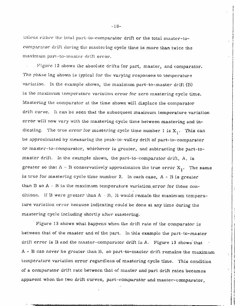
]t~tlre I~ ~.~hows the ab~olutc drifts Cot part, master, and comparator,

The phase lag shown is I.ypical for 1:he varyJ.ll~l’ responses to temperature

variation. In the example shown, the. maximum part.-to-ma.ster drift (B)

is the laaaximu~l temperature var’iatJo~l error for zero mastering cycl.e time.

Mastering the comparator at the time shown wi].l displace the comparator

drift curve. I~ can be seen that the subsequent maximum temperature variation

error will now vary with the mastering cycle time between mastering and

dicating. ’1’he true error for mastering cycle time number 1 is X1. This can

be approximated by measuring the peak-.Co..val].ey drift of part.-to-.comparator

or master.-to...coml)arator, whichever is {~rcater, and subtracting the part-to-

master drift. In the example shown, the par’t-.to..comparator drift, A, is

greater so that A .- B conservatively approximates the trae error X1. The same

is true for mas~eri.ng cycl.e time rmmber 2. In each case, A -. B is greater

than B so A .. B is the maximum temperature variation.error for those con-.

ditions, If B were greater ~.han A B, ]-~ would remain the maximum tcmpera-.

lure variation error because indicating could be done at any time during the

mastering cyc]e including shortl.y after mastering.

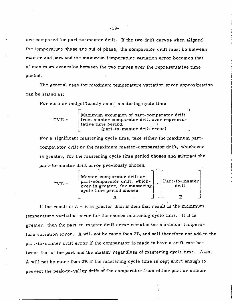
Figure 13 shows what happens when the drift rate of the comparator is

between that of the master and of the ~)art. In this example the part..to-.master

drift error is B and the rnaster.-comparator drift is A. Figure 13 shows’ that

A -. B can never be greater ~;han B, so part..to-.master drift remains the maximum

temperature variation error regardle~)s of mastering eycle time. This condition

of a comparator drift rate betwe.en l:hag of master and part drift rates becomes

apparent when the two drift curves, pari:.,eomt)arator and master-.comparator,

-19-

arc compared for part-to-master drift, If the two drift curves when aligned

for temperature phase are out of phase, the comparator drift must be between

and part and the maximum temperature variation error becomes ~hat

of maximum excursion between tl~e two curves over the representative time

period.

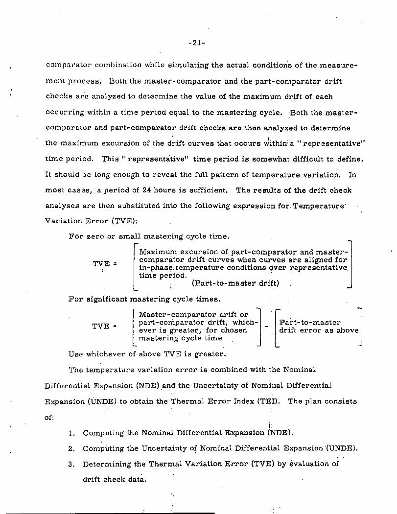
The general case for maximum .temperature variation error approximation

can be stated as:

For zero or insignificantly small, mastering cycle time

~[-’Maximum excursion of part-comparator driftTVE =

Lfr°mtativemastertime(part_to.masterperiod.c°mparat°r driftdrift oVererror), repre sen-

For a significant mastering cycle time, take either the maximum part-

comparator drift or the maximum master-comparator drift, whichever

is greater, for the mastering cycle time period chosen and subtract the

part-to-master drift error previously chosen.

rMaster-comparator drift or

part-comparator drift, which-| _TVE I ever is greater, for mastering iI cycle time period chosen!

Part-to-masterIdrift

.J

If the rbsult of A - B is greater than B then that result is the maximum

temperature variation error for the chosen mastering cycle time. If B is

greater, then the part-to-master drift.error remains the maximum tempera-

ture variation error. A will not be more than 2B, and will therefore not add. to the

part-to-master drift error if the comparator is made to have a drift rate be-

tween that of the part and the master regardless of mastering .cycle time. Also,

A will not be more than 2B if the mastering cycle time is kept. short enough to

prevent the peak-to-valley drift o~ the comparator from either part or ma’s~er

-21-

comparator combination while simula{ing the actual condition’s of the measure-

rncnt process. Both the master-comparator and the part-comparator drift

checks are analyzed to determine the value of the maximum drift of each

occurring within a time period equal to the mastering cycle..Both the master-

comparator and part-comparator drift checks are then analyzed to determine

the maximum excursion of the drift curves that occurs wxthin"a " representative"

time period. This " representative" time period is somewhat difficult to define.

It should be long enough to reveal the full pattern of temperature variation. In

most cases, a period of 24 hours is sufficient. The results of the drift check

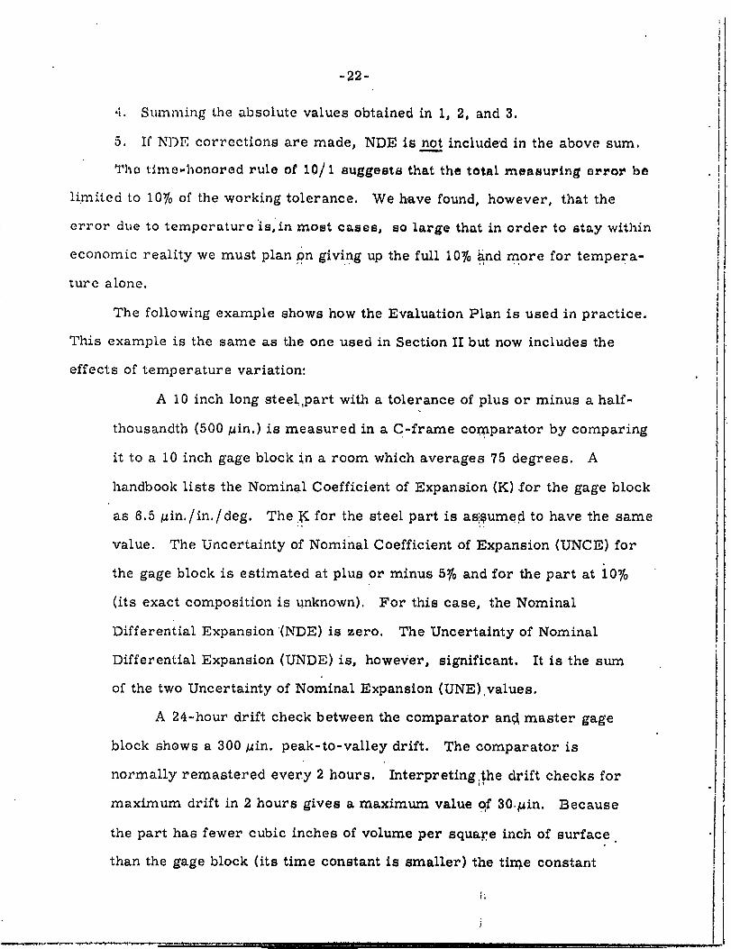
analyses are then substituted in~o the following expression for. Temperature’

Variation Error (TVE):

For zero or small masteri.ng cycle time.

~Maximum excu..rsion of part-comparat0r and master-

Icomparator drift curves when curves are aligned for

TVE = in-phase, temperature conditions .over representative.time period.

:: (l~art-to-master dri.ft)

For significant mastering .cycle times.

Master-c°mparat°rdrift°r ~ ~Part’t°’masterpart-con~parator drift, which- 1 -.~drift error as above.J

TVE = ever is greater., for chosen |mastering cycle time .]

Use whichever of above TVE is greater.

The temperature variation error is combined with the Nominal

Differential Expansion (NDE).and the Uncertainty of Nominal Differential

Expansion (UN. DE) to obtain the Thermal Error Index (TE:I). The plan consists

of:

1, Computing the Nominal Differential Expansion (NDE).

2. Computing the Uncertainty of Nominal Differential Expansion(UNDE).

3. Determining the Thermal Variation Error (TVE). by ,evaluation

drift check dat~. : "

-22-

4. Summing the absolute values obtained in 1, 2, and 3.

5. If NDE corrections are made, NDE is not include’d in the above sum.

2’he tlme-honored rule of 10/1 suggests that the ~otal measu~ing e~o~ be

limited to 10~0 of the working tolerance. We have found, however, that the

error due to temperatureis, lnmost c~ses, so large that in order to stay within

economic reality we must plan :~n giving up the full i0~o ~nd ~ore for tempera-

zure alone.

The following example shows how the Evaluation P~an is used in practice.

This example is the same as the one used in Section II but now includes the

effects of temperature variation:

A i0 inch long steel,part with a tolerance of plus or minus a half-

thousandth (500 pin.) is measured in a C-frame co~parator by comparing

it to a i0 inch gage block in a room which averages 75 degrees. A

handbook lists the Nominal Coefficient of Expansion (K) ~or the gage block

as 6,5 pin./in./deg. The.K for the steel part is as~$umed to have the same

value. The Uncertainty of Nominal Coefficient of Expansion (UNCE) for

~he gage block is estimated at plus or minus 5~ and for the part at ~0~

(its exact composition is unknown). For this case, the Nominal

Differential Expansion {NDE) is zero. The Uncertainty of Nominal

Differential Expansion {UNDE) is, howe~er, significant. It is the s~

of the two Uncertainty of Nomina~ Expansion (UNE}.vaiues,

A 24-hour drift check between the comparator an~ master gage

block shows a 300 pin. peak-to-valley drift. The comparator is

normally remastered eveny 2 hours. Interpreting.,~he drift checks for

maximum drift in 2 hours gives a maxim~ value qf 30.~in. Because

the part has fewer cubic inches of volume per square inch of surface

than the gage block (its time constant i~ smaller} the ti~e constant

-23-

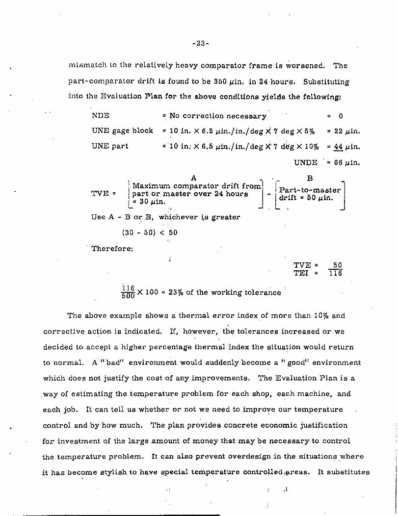
mismatch to the relatively heavy comparator frame is Worsened. The

part-comparator drift is found to be 350 ~in. in 24:hour:s, Substituting

into the Evaluation l~lan for the above conditions yields the following:

NDE = No correction necessary = 0

UNE gage block = 10 in. × 6.5 ~in./in./deg >~ 7 deg × 5~0 = 22 ~in.

UNE part --10 in.’ X 6.5 ~in./in./deg X:7 d~g X 10~o = 44 pin.

UNDE = 66/~in.

A! Maximum comparator drift from-

TVE = !part or master over 24 hours I

Use A - B or B, wl~ichever ~s greater

(30-50) <

Therefore:

B

! Part-to-master" j drift = 50 ~in.

TVE = 50

~165’00 X 100 = 23~ of the working tolerance

The above example shows a thermal error index of more than 1070 and

corrective action is indicated. If, however, the tolerances increased or we

decided to accept a higher percentage thermal index the situation would return

to normal. A" bad" environme:nt would suddenly become a " good" environment

whidh does not justify the cost o’f any impro.vements. The Evaluation Plan is a

.way of estimating the temperature problem for each shop, each machine, and

each job. It can tell us whether or not we need to improye our temperature

control and by how much. The plan provides concrete economic justification

for investment of the large .amount of money that may be necessary to control

the temperature problem. It can also prevent overdesign in the situations where

it has become stylish, to have special temperature controlled :~reas. It substitutes

-24-

an o.~’dc,’ly ~hinking process for emotion or arbitrarily set rules. Natural

priorities are established to indicate where our improvement efforts should

be made. Should we try to move closer to S8 degrees, or shoul~i we ~r~,~o

reduce our temperature variation? The plan not only answers these questions,

i~ gives a positive response to any improvements that may be made.

In spite of the advantages.of the plan, some objections have been raised.

One objection is that the plan p~etends to be an exact pr~cedd’re when obviously

we are still estimating. Our answer to this objection is to agree that the plan

is not perfect and not exact. It may be in error by 2S~/~ or more and still be a

significant advancement over no plan at all. No plan at all means that we must

depend on the opinion of experts who arbitrarily decide that this or that en-

vironment is, or is not, accept.able.

V. METHODS FOR DECREASING THERMAL ERROR INDEX

~verage Temperature Other Than 68~

The possibilities for controlling the error resulting from average temper-

atures other than 68° are limited. They can be summarized in one sentence~

The error can be reduced by making nominal differential expansion corrections,

by establishing more ac.curate nominal coefficients of expansion, by improving

the uniformity of coefficient of expansion frompart to part through better

chemical and metallurgical controls, by determining individual part expansio’ns,

and by limiting the room temperature deviation from 68 degrees.

Temperature Variation Error

What are some of the th~ngs we can do to improve the ability of a gaging

system to withstandtemperature variation? Our first reaction is to make the

thermal response of the master and comparator equal. This will result in zero

drift between the master and comParator. Shortening the mastering c’ycle has

-25-

the same effect, This is a false goal, however, because we may create an

increased mismatch to the part, "A worthwhile goal is to make the thermal

z,c.~spm~se of a~l th~e e~ement~ ~he ~ame, This completely ellmtnat~ ~he

problem but is not a practical approach because most gages are used for more

than one part. Tho best compromise ~s to destgntho aompa~htor dr~ft to be

about half-way between the part:drlft and the master drift (th~s ~s discussed in

more detail in Section III). Adjustment of thermal response can be accomplished

in several ways. The use of Invar i~ quite practical. Invar is readily obtain-

able at a reasonable cost and has a coefficient of only 1 ptn./in. Time constants

can be controlled by use of insulation and by proper design of wall thickness.

Unfortunately, none of these .solutions can be applied to the part itself.

We can’t insulate it; we can’t change its coefflcient; we can’t change ~ts wall

thickness. The only thing we can do is improve the env~ro~ent.

What are some of the things that can be done to improve the environment?

Our first reaction is to simply reduce the temperature excursion of the whole

room. This is effective, but also expensive. It maybe cheaper to control the

temperature excursion in a small area around the machine. The ~oore

Special Tool Co. of Bridgeport, Conn., uses th~s approach in comparing and

calibrating thelr ultraprecise step gages to an accuracy of one part in ten million.

Another approach is the possibillty of increasing the rate of cycling of the

room. The frequency response diagram of the rotary contour gage (Fig. 9) shows

the advantage of mismatching the environmental frequency and the resonant

frequency of the gage. Because the resonant frequencles of real gaging systems "

are so slow (in this case 14 hours per c~cle), this mismatching is best accomp-

lished by increasing the enviro~ental frequency. Interpreting Flg. 9 we see

that a plus or mlnus 1 degree temperature control at 0.07 cycle per hour glves

the same drift as a plus or minus 4 degree control.w&uld g~ve at one cycle per

-26-

hour. In some cases it is possible to increase the rate of room cycling by a

simple readjustment of the thermostat. The results can be quite dramatic.

High cycling rates are generally achieved by circulating large velumes

of air. High volume air circulation is not too expensive and offers several

advantag’es. A greater volume of air requirQs a smaller temperature dlffercnce

between the inlet and outlet to maintain the same room average. This is simply

a matter of removing the same number of Btu’s with more pounds of air at a

smaller temperature difference. Another advantage of air volume is that the

increased velocity tends to scrub the whole gaging system and remove the hea~

that may be coming from external point sources of heat such as motors, lights,

people, and radiation from the sun. Stated more exactly, the increased air

velocity increases the convective heat transfer coefficient and decreases the

thermal resistance between the gage and the room air, which is the thing that

is being controlled. Still another advantage of high air flow is increased

operator comfort. The decreased difference between inlet and outlet air

temperatures means fewer cold drafts which are the real source of discomfort.

The benefits of high air flow, high cycling rates, and close containment

of sensitive equipment have recently been demonstrated at LRL. A new rotary

contour gage has ~ust gone into service which is completely enclosed in a

plexiglass box. Air is admitted through a plenum chamber at the top and leaves

through a plenum chamber at the bottom. The circulation rate is one complete

change of air every 3 seconds. The cycling rate is 2B cycles per hour. The room

temperature variation is 0.7 degrees, but a 24-hour drift check shows less

than 3 ~in. of drift~

The problem of standardization of room air temperature measurement is

illustra~ed by the different values obtained on. this system with three different ways

of measuring. High sensitivity mercury thermometers show less than 0.05 degree

-27-

vari:uion. The thermister recorder-controller for the enclosure shows a 0.4

degree vnriatlon and a high frequency response thermo~raph shows 0.7 de~ree.

An Automatic Error Correctin~ Device

In reviewing our experiences with computing ~hermal drift from k~owlod~

of system frequency response and measurement of temperature variation,

J. W. Routh, of LRL, suggested that we consider the possibility of automatic

error correction. Preliminary investigation of ~his idea has convinced us

that it should be possible to design a thermal model of the system that can

sense the room temperature and provide an electrical output equal to the drift.

This output can be used to zero shift the coordinate system of the gage and

provide direct, on line, compensation for ~hermal error. As it is now

visualized, ~his device would be completely automatic once set for the specified

part to be measured. The operationat settings required would be nominal co-

efficien~ of expansion, time constant, and size of the part. The response of

the gage wouid be built into the device. Some’adjustment might be req~red

for different setups that might be enco~tered. If ~he time constan~ of the

master could be tailored to match the gage, the bulk of the thermai error could

be eliminated. Error due to uncertainty of nominai differential expansion woutd

still remain.

~£le this manuscript was being prepared, a report of a feasibility study

by a graduate student at the University of California, Berkeley [12) concerning

~he practicabiiity of such a device became available. This study was made at

our request and has shown that:

(i) A simple analog, consisting of on.ly two time-constant elements in

parallel, provides an adequate model of the system.

(2) The main problem enco~tered in constructing the compensating

device was in finding practical, Iong-~ime-constant elements.

-28-

This device, if realizable, will have far-reaching effects on the use and

design of machine tools and measuring machines.

VI. CONCLUSIONS

In conclusion tl%e following gcncrallzod approach to the problem of

thermal effects in dimensional metroloEy is suggested:

A. Evaluate existin~ conditions to determine whether or not a problem

exists. This,is acclo~nplished by substituting existin~ conditions

into the Evaluation Plan. If the thermal error index is more than

i0~o of the part tolerance, it is likely that a problem does exist.

B. Review the workin E tolerances to be sure they are economically

and functionally realistic.

C. If necessary, take corrective action to reduce the thermal error

index as follows:

To reduce error resulting from average temperatures other than

I.

9..

iV~ake corrections for nominal differential.expansion.

Establish more accurate coefficients of expansion so as to

increase the accuracy, of the corrections.

3. l’VIinimize average temperature deviations from 68°F.

To reduce error resulting from temperature variation:

I. Improve procedures for soaking out workpieces and masters

so they are in thermal equilibritun with the environment.

Shorten the mastering cycle time if indicated by the Evaluation

Plan.

3. Increase rate of air flow and improve its distribution.

4. Increase the frequency of temperature variation.

-29-

Dccrease the amplitude of temperature variation.

Redo.~ign ma~ters and temperature sO thoi~ time constants and

coefficients of expansion are in better balance with those of tl~e

parts to be measured.

" APPENDIX 2k: GLOSSARY OF TERMS ..

Part or Work]~iece: In every length determination process, there is some

physical object for which a linear dimension is to be determined. This

object is called the part or workp.i.ece.

Master: In the length measuring process, the unknown or desired dimension

of the part is compared with a known length called the master. This length

may be the wavelength of light, the length of a gage block, line standard,

lead screw, etc.

Comparatoz:: Any device used to perform the comparison of the part and

master is called a compar~/~or. {!

Mastering: The action o~ n,ulling ~ comparator with a master is called

mastering,

Mastering. Cycle Time: The time between successive master,rigs of the

process is called the mastering cy.cle time of the process.

Measurement Process: All of the activities of which.~a measurement is .

composed is called the measurement process. ~ ..

Measurement System’. The entire apparatus used in making a measure-

ment is called the measurement system.0

Thermal .Environment: Any!physical object is expose.d to various sources

(and sinks:) of heat energy which influence its thermal state. Taken in tote

all such sources and sinks form the thermal environment of the object." In

-30-

i.e., by convection, conduction, and radiation.

found in the laboratory are:

the laboratory or shop, the thermal enviro.nmen~_..of any object can c6nsist

of all other objects with which the object is in ~hermai communication,

Sources and sinks commonly

Convection sources and sinks:

Air atmosphere,~including the air-conditi~nin~ ~ system and

distribution or flow of the air. The air constitutes the medium

of convection heat transfer.

2) Radiant sources:

a) Sun (if ~vindQws exist)

b) Walls, floor..,:, and ceiling

c) Illuminating .lights

d) Electric motors

e) People

3) Conductive sources are usually the most olbvio.~s. , and include

all objects in direct contact.

In this sense, then, an obje~¢t in an air-conditioned room is in thermal

communication with the air-conditioner by, usually, convection. It may

also be in communication with an electric motor by convection, conduction,

and radiation.

Although, in the general case, it is probable that all types of thermal

communication exist between the environment and a given object, perhaps

the most common environment is the one in which the only significant

communication is by convec£ion. In this case, the effect ’of the environ-

ment on the object can be de’scribed in terms of thermal state of the

volume of air surrounding tl~e object.

8(b)

8(e)

TO = Te - 68°

Variations of Thermal Environments

9(a)

9(b)

9(c)

Convective environment,

When all environmental influences are convective in nature

and a single temperature describes the environment, the

environment is.called a convective environment. The response

of an object (changes in length) in such an environment can

directly correl~.ted with the environment" ten~perature,

Environment temperature, Te.

The temperature by which the thermal sta~e of a convective

environment is measured is called the environment temperatuz~e.

T__sm_m__perature offset.

The difference between the time average, of th.e environment

temperature .and 68° F is called .t.e,mpera:ture offset.

Stationary environment. !: [!

When the envigonment is invariable in time, it is called

stationary. ..

Periodic environment. :.

An environment in which every variable changes in a cyclic

manner .is called a periodic environmen,t..

Aperiodic environment. !: ..

(1) Transient environment: ¯

When the environment change is not periodic but has a

’ well-defined pattern, such as a constant:rate of increase’

of temperature in a convective envi.~’onment, it is called

a transient environment. ""

-32-

i00

ii.

(2) Random environment.

Whe.u the environment changes in a random manner, it is

called a random environment. Influences due to the

presence of human beings or weather tend to be random.

Although all environments have some random characteris.-

" tics, deliberate attempts at envirorfinen~l control, e.g.,

by refrigerant air conditioning, tend to introduce dominant

periodic characteristics. Also, in uncontrolled environments

transient characteristics may be found to dominate. For

example, t.he outside air temperature may dominate in a

room which is well ventilated.

Standard Temperature~ f__or, i.L.ength Measurements: Unless otherwise

specified, the dimensions of an object given in drawings or specifications

shall be for an object with a uniform temperature of. 68°F (20 ° C).

length of an object at stand:ard temperature is called:the standard length of

the object. This procedure follows the April 1931, resolution of the

International Committee of Weights and Measures that the temperature of

20° C (68 ° F) sh6uld be universally adopted as the normal temperature of

adjustment for all industrial standards of length. Also, Recommendation

No. 1 of the International Organization for Standardization, issued in 1954,

promulgates the standard temperature of 20° C among the 40 participating

countrieS.

_T...emperatures of a Bqd_y_

ll(a) Temperature (a.t a poi.nt).

When discussin~ a body which does not have a single uniform

temperature, it is necessary to refer in.~ome manner to ’the

distribution of temperature throughout the body. Temperature

12.

-33-

at a point in a body is assumed to be th@ temperature of a

very small volume of the body centered’at t~at point. The

continuum.

ll(b) The temD~ratur@ 9f abody.

When the differences between the temperatures at all point~

in a body are negligible, the body is said to be at a ~iform

temperature. This temperature is then the temperat~e of the

body.

11(c) Instantaneous a~verage temperature of a ~ody~

When the body .~s not at a uniform temperature at all points,

but it is desirable to identify the thermal state of the body by

a single temperature, the temperature which represents the

total heat storq~ in the body may be used. ~en the body is

homogeneous this temperature is the ave.rag¢., over the vol~e

of the body, of.all point temperatures. This’,iS called the

average temperature of the body.

ll(d) Time-mean temperature of a body.

The time average of the average temperature of a body is called

the time-mean t.emperature of the body. :

Soak Out: One of the characteristics of a thermal system is that it has.a

" memory." In other words, when a complete change in enviro~ent is

experienced, such as occuzs when an object is transported from one room

to another, there will be some period of time before~he object completely

" forgets" about its previous enviro~ent and exhibits a response dependent

only on its current environment. The time elapsed from .a change in

environment until the object.is influenced only by the new environment

is called soak-out time. After " soak out"the objec}~is said to be in

-34-

equilib,-ium with the new environment. In cases where an

environment is time-variant the response of the object is also a

variable in time, "vVhen the object exhibits a response dependent only

on the environment it is said to be in dynamic equilibrium with its

environment.

13, TAme Constant of a Body: ¯ Tile tlmo constant of a body Is a measure of the

response of the body %o envi, ronmental temperature ehan~es. It is defined

as the time required for a body to achieve ~3.2~0 of its total chan~e after

a sudden step chan~e in the environment,

14..~req%lency Res~5onse: The frequency ~esp0nse of a,measurement systsm

is defined as the ratio of the amplitude of the drift in microinches %o the

amplitude of a sinusoidal environment temperature oscillation in de~rees

Fahrenheit for all frequencies of temperature oscillation.

15. Thermal Expansion: The difference between the len~h of a body at one

the thermaltemperat,,ure and its length at another temperature is .called

expansion of the body. :

Coefficient of Expansion’,16.

The true coefficient of.expansion, ~, at a temperat.u, re., ’t_, of

of a body is the! rate of change of length of the. body with respect

to temperature ,at the given temperature divided by the length

at the given temperature.

I dL~ = L dt

The average true coefficient of expansion of a body over the

range of temper’atur’es from S8°F to t is defined as the ratio

of the fractional change of length of the body to the change in

temperature, .

-35-

17,

18.

Fractional chnnge of length is based on the length of the body

L- L68

a68, t - L68 (t - 68)

Hereinafter the term ~’ coefficient of expansion’.’ shall refer only to,, .,, ’,~ :.: ’ :

the average value over the range from 68=F to another temperature, t:

Nominal Coefficient of Expansion: The e~9}ir~.a.te....of....t..h e coefficient of

expansion of a body sha}! ,bg. ca!l..ed .th.e..no.~i.nal_. c.oeffic’ient. _. of expansion,

To distinguish this value from the average true coefficient Of expansion(K88’ t ) it shall be denoted by the symbol K,

{

Uncertainty of Nominal coefficient of Expansion: The maximum possible

percentage difference between the.actual coefficient of expansion, a, and

the nominal coefficient of e~,pansi~n shall be denoted by the s~..y~.b.o~..~, andexpressed as...~ ..p~.r..c.e..nt.age’ of the t.r..U.e. 9o.effic~.n..t o.f..exp.an,~i0.n,

- K "

Variations in material composition, formin, g processes, and heat treatment

as well as .inherent anisotro, pic properties and effects of preferred

orientation cause objects of suppo,s.edly identical composition to exhibit

different Shermal expansion.lcharacteristics, Also, d~fferences in ex-

perimental technique cause, disagreement among thermal¯expansion measure-

ments. As a result, it is difficul~, solely from published information, to

obtain an exact coefficient of expansi.on for any given:pbjec.t.

This value like that of K itse,lf must be an estimate. Various methods can

be used to make this estimate, For e,.~..a....mp.!e.:

18(a) The estimate may be based on the dispersion fDund among

published data. .

-36-

18(b) The estimate may be based on the dispersion found among

results of actual experiments conducted on a number of like

objects.

Of the two possibilities given above, (b) is the recommended

procedure.

Because the effects of inaccuracy of the estimate of the

uncertainty are of second order, it is considered sufficient

that good judgment be used.

19. Nominal Expansion: The estimate of the expansion of an object from 68°F

to its time-mean ternperatu~-e at the time of the measurement shall’be

called the nominal expansion and it shall be determined from the following

relationship.

NE = L(t -.68)(I~)

20..Uncertainty of Nominal Expansion: The maximum difference between the

true thermal expansion and.the nomiflal expansion is ,called the uncertainty

of nominal expansion. It is determined from:

21. Differenti"al Expansion~ Differential expansion is def.ined as the difference

between the expansion of the part from 68° F to its time-mean temperature

at the time of the measurement and the expansion of the master from 68° F

to its time-mean temperature at the time of the measurement.

22. Nominal Differential Expansion: The difference between the nominal

expansion of the part and of the master is called the inominal differential

expansion.

NDE -- (NE)part - (NE)master

-37-

,,3. l~jnce,’,’tainty of Nominal Differential Expan. s.ion.: The sum of the un-

certaintics of nominal expansion of the part an~l ma~er is calle~

uncertainty of nominal differential expansion.

UNDE = (UNE)I~,~ + (UNE)~

24, Thermal D~ift’. Drift is de~ned a~: the differential ~9ve~;enf of the part..

or f}~e master and the comparafor in microinches caused by time-variations

in fl~e thermal environment,

25. Electronics Drift Check: An experiment conducted to determine the drift

in a displacement transducer and its associated amplifiers and recorders

when it is subjected fo a thermal environment similar to that being

evaluatedby the drift check itself. The electronics ~rift ~s the s~ of the

" pure" electronics drift an~~ the effect of the enviro~ent on the sensing

head, amplifier, etc. The ~’lectronics drift check is performed by blocking

the ~ransducer and observin8 the output over a perio~ of time at least as

long as the duration of the drift test fo be performed.. Blocking a transducer

involves making a transducer effectively indicate on its own frame, base,

o~ cartridge... In the case of.a cartridge-f~e gage head, this is accomplished

by mounting a small cap ove.r the end of the cartridge so the plunger registers

against the inside of the cap., Finger t~e gage heads can be blocked with

similar devices, Care must:be exercised to see fhaffhe b~locking is done

in a direct ~manner so that fh~ influence of temperature on the blocking de-

vice is negIigible. ..

26, Drift Check... An experiment conducted to determine t~e a~tual drift inherent

in a measurement system ~der normal operating conditions is called a drift

check. Since the usual method of monitorin~ the envinonm’ent (see definition

28) involves the correlation of one or more temperatune recordings with

27.

28,

29.

drift, a drill cheek will usually consist of simultaneous recordings of

drift and cnviromnental temperatures. The recommended procedure for

the conduct of a drift check is given in Appendix B.

.Temperat.urc Variation Err~p~i .TVE: An emtimate of the maximum possible

measurement error induced solely b~ deviation of the environment from

average conditions is called the tem..__P..SAa_tDr_e_y_a.._ria_dg..n...e__rror. TVE is

determined from the results of two drift checks; on~ of the master and

comparator, and the other of the part and the comparator.

For zero or small mastering cyele time.

TVE =

Maximum .e.xcursion of part-comparator and master-comparator drift curves when curve~ are aligned for in-phase temperature conditions over representative timeperiod. (Part-to-master drift)

For significant mastering cycle times.

~ Master-cor~para~or drift or

TVE =~ part-comparator drift, which-i

i ever is greater, for chosenmastering c:ycle time

Use whichever of above TVE is greater.

Part-to-masterdrift error as above l

Total Thermal Error: Total thermal error is defined as the maximum possible

measurement error resulting from temperatures other than a uniform, con-

stant temperature of exactly 68°F. It is, of course, ~desirable to determine

the total thermal error induced in any measurement. :~ However, this is

usually not practical to do, and in many cases, not even possible. Therefore,

an alternative procedure is outlined below.

Thermal Error Index: The evaluation technique proposed in this section

does nothing more than estimate the maximum possible error caused by

thermal environment conditions affecting a particular measurement process.

It does not establish the actual magnitude of any error. It serves to remove

doubt about the existence of ~he errors and to establish a system of rewards

] :,and penalties to processes which are combinations of tech’nzques, some.of

which may be " good" and some "bad."

The The1"mal Error Index shall apply only so long as conditions do

not change,

Th~ proposed plan consists o~

(4).

Computing the nominal differential expansion, NDE.

In this computation (and in %he next), the temperature offse~

is assumed to be the average difference...’betw:een 68=i ? and

the air temperature in %he vicinity of the process over ~he

mastering cycle of ~he process.

Computing the uncertainty of NbE, UNDE.

Determining the thermal variation error,, TVE, by means

of a drift check.

Summing ~he absolute values obtained in i, 2,

an index related to the quality of.the process,

~emperature error index.

TEl = NDE + UNDE + TVE

If an effort is made to correct the meas~rem’en~

and 3 to obtain

yields the

(5) by computing

the NDE, part’l is to be deleted.

The plan penalizes a measJrement process on two c’ounts:

(i) Existence of er~vironment temperature o~fset’~ resulting in

differential exl~ansion.

(2) Existence of environment variations. "

The plan rewards good technique by reducing the thermal error index for:

(I) Attempting a. correction for differential .expansion.

(2) Keeping envirof~mental variations to a minimum.

Thermal error index can be used as an adminis~ratiye tool for certification

of measurement processes. ,as is discussed in the next section. It can also

be used as an absolute index of accep~abili%y of the ~roce.ss. For example,

a good rule of thumb for establishing the accep~abil~y of’a measurement

-40-

30.

process with respect to ti]ermal errors is to limit the acceptable thermal

error index to l O~/0 of the working tolerance of the part.

Monilorin~ To perpetuate the thermal error index it will be necessary

to monitor the process in such a way that significant changes in operating

conditions are recognizable.

The recoi/amended procedu’~e is to establish a parti~’ular"temperature

recording station which has a demonstrable

of the drift. In a " convective environment"

" environment temperature."

correlation with the magnitude

this could simply be the

¯The temperature of the selected station should be r~corded continuously

during any measurement pi’ocess to which the index~ls to be applied. If

the temperature shows a significant change of condlt~ons, the index is

null and void for that process, and a reevaluation should be accomplished,

or the conditions corrected to those for which the index applies.

In addition to continuous monitoring of environmental conditions, it is

recommended that efforts 5e made to establish that ~he process is

properly soaked out.- This may be done by checking the temperature of

all elements before and after the execution of the measurements.

APPENDIXB: DRIFT-CHECK PROCEDUI~E

The following is the recommended procedure for the conduci of a drift

check for a process in which the proposed monitoring m.e, thod is based on the

measurement of environment temperatures.

A. Equipme,~t

The major equipment necessary includes very sensitive displacement

transducers and sensitive, drift-free temperature s~nsors’with associated

-41-

,a~p~1~lers and recorders. A linear variable differential transformer

with provision for r~corder output has proven quite successful. Also,

variou~ resistance-bulb thermometers with rec~din~ provi~i~

proven successful as temperature monitoring devices.

The required sensitivity of the displacement transducers used may be,

adjusted according to the r~ted accuracy of the meas~rer~ent system.

B. ~ment Testing

The temperature measuring and recording ~ apparatus should be thoroughly

tested for accuracy of calibration, respbnse and drift. The availability

of sensitivities of at least 0.1 °F is desirable. Time constants of sensing

.elements of about 30 sec az:e recommended.

Before the displacement transducers and associated apparatus are used

they should be calibrated and checked for drift in the environment. ’An

" electron{cs drift Check" should b’e performed by blocking the transducer

and observing the ¯output over a period of time at least as long as the

duration of the drift test to be performed. "Blocking" a transducer in-

volves making a transduce~ effectively indicate on its ov~ frame, base,

or cartridge. .

C. Preparation of the System for Test

An essential feature of the drift check is that conditions during the check

must duplicate the " normal" ....conditions for the process as closely as

possible. "Therefore, before the check is started, "..normal" conditions

must be determined. The gctual step-by-step proce~lurefollowed in the

subject process must be followed in the same sequence and with the same

timing in the drift check. This is especially importaht in terms of the

actions of any human opera~ors in’mastering and all :lSreliminary setup steps.

-42-

With as little deviation from normal procedure as possible, the displace-

ment 1.ransducers should be introduced between the part {or master,

depe~d~g on the type of dz.~t checl¢~ and the rest of the ~-f~ame ~uah

that it measures relatively displacement ~ the line of action of the

subjcc~ measurement process.

The temperature sensing pickup must be placed to ~easdre a temperature

which is correiatable with the drift. Some trial and error may be

necessary. In the extreme case, temperature pickups may have to be

placed to measure the temperature of all of the active elements of the

measurement loop. .. ’

Representative Time Period For a Drif~ Check

Once set up the drift check should be allowed to continue as long as

possible, with a minimum of deviation from " normal" operating conditions.

In situations where a set pattern of activity is observed its duration should

be over some period of time during which most events are repeated. When

a 7-day work week is observed in the area, and each day is much like any

other, a 24-hour duration fs recommended. If a 5-day work week is ob-

served, then either a full-week cycle should be used or checks performed

during the first and last days of the week.

Postcheck Procedure

After the drift test, the displacement ~ransducers and the temperature

recording" apparatus should be recalibrated. "

Evaluation of the Drift Check (Drift-Check Report)_

Following the drift check, the data should be assessed for ~he following

values.

-43-

(a) Nonperiodic Effects - the effects of the operator tend to

disappear with elapsed time. These and similar effects

should be described and the portion of this error not

compensated by soak out should be included in the TVE .

(b) Temperature Variation Error (TVE) -

For zero or small masterii~g cycI~ time. ": "’

[’Maximum ex.cursion of part-comparator and master-,I comparator drift curves when curves are aligned for

TVE -- ] ¯~ in-phase temperature conditions over representative

Ltime period.(Part-to-master drift) -

For significant mastering cycle times.

i Master-co ,mparator drift or~ part-comparator drift, which-TVE = I

~ ever is gre. ater, for chosen

i mastering cycle time

Use whichever of above Tv:E is greater.

]Part-to-master!

Ldrift error as above

A complete report of the drift, check finding’s should.inclu.de the following:

Thermal Drift-Check Reports 0htline

Items in parenthesis are s~gested as a guide to what might be pertinent

under a heading. .:

I. Description of System

a)

b)

Identification

(Mfgs., model, . {pertinent specifications, .and dimensions)

Component Mo{ions

c)

(Active element’.s, lines of action)

Operati6ns ’:

1) Type of op6ration

-44-

2) Typical workpiece

Sizes

Materials

Minimum tolerances

3) Method of n~asterlng

.. 4) Cycle tima~

(Operating, mastering)

Environment Description

a)

b)

c)

floor,

Room Features

(Size; solar exposure; exits; wall,

heat sources)

System Features

I)

2) Internal heat sources

(Motors, l.a.mps, electronics)

Air Circulation

(Inlet-outlet locations, sizes, numbers,

circulated)

Temperature monitoring and control

Location with respect to " room features"

d)

Test Apparatus Description

a) Temperature monitoring

(Identification, response,

b) Displacement m..onitoring

(Identification, response,

Procedure

a)

ceiling, and other

sensitivity, lo~¢ation)

sensitivity, location)

Stepwise description of testing

drafts, air volume

-4"3-

Results

(Displacement-temperature vs time graphs; ~’naximum displacements

and temperature variations; cycle times; causes if known)

TVE

7. R, ecommendatlons

APPENDIX C: A METHOD FOR DETERMINING FREQUENCY

I~ESPONSE OF A MEASUREMENT SYSTEM

Data obtained from step-change experiments performed on the 15 inch

Sheffield rotary contour gige gave: (i) an indication that the.system was

linear with respect to thermal variations, and (2) the set of data correlating

temperature variation with drift.

The basic characteristic of a linear system is that the output (in this

case, drift) c.orresponding to any input (temperature variation) is the

of outputs correspondin~ to the.’, components of the input,:, :.

This characteristic permits the use of the data of Fig. 71 in computing

a predicted drift for a variation of ~emperature in the ~nvironment of

the Sheffield gage as follows: . .~

Suppose ~that the temperat.uTe variation isrecorded~as shown in Fig. C-i.

This record can be approximated by straight lines over 7-minute increments.

This procedure decomposes th.e temperature variation into a series of

components similar to that of F~ig. 7.

The drift corresponding t0. any one of these components, can be determined

by scaling th.e data of Fig. 7.

Figure Q-2 shows the resulting set of drift components and their sums

which is an approximation to the drift caused by the temperature variation

-48-

This computation procedure is cumbersome when done by hand but ’is

easily and quickly done by a digital computer, The results shown in Figs,

8 nnd I0 of the paper were computed’using an IBM 7094 digital computer at

in making

It must be possible to make an accurate approximation to the

temperature ~ata. For example, in the case described above,

a temper,~ture variation consisting of a sine-wave with a period

of less than ? minutes cannot be approximated.by the data

available.

(2) Because of the " memory" of the system, the computed drift is

in error until a perio d of time equal to the soak-out time has

elapsed. For example, in computin~ the data.for Fig. 8, the

drift computed for the first 12 hours of ~emperatur’.e variation

record was inaccdrate and was omitted.

ACKNOWLEDGMENTS

The authors wish to express special gratitude to Mr.

tl~e Lawrence Radiation Laboratory.

There are two practical considerations to be observed

computations of this kind: ’.

of NBS for his aid in assembling bibliographical material, and to Mr. T.

Young of NBS for suggestions concerning the uncertainties of thermal ex-

pansion properties.

I. H. Fullmer

R.

-47-

BIBLIOGRAPHY

1. Ch. Cochet, "On th~ Choice of a Uniform Temperature for ~he

Calibration of Measuring Instruments (Sur le choix .~l’un degre uniforme

¯ ’ de temperature pour l’etalonnage des instruments d’~ mesure)," Rev.

Gen. de l’Electricite, Vol. 4, Nov. 16, 1918, pp. 740-2. Report of

Commiss’ion de Normalisa{~on de’~ Ingenieurs des A~Tts e{’ Metiers de

Boulogne-sur-Seine recommending adoption of 0 degree centigrade as

standard.

2. A.Pcrard, " Temperature of Adjustment of Industrial Gages

temperature d’adjustage des calibres industriels)," Genie Civil, Vol. 90,

June 25, 1927,. pp. 621-4. ~,Plea to German Industri:,al Standards.

Committee to readopt adjus~tment of 0 degree insteac~ of 20 ¯degree

centrigrade; discusses req.~isite precision for indus.t.rial;gages and

necessity for standardization of temperature of adjus.tme,nt.

3. L. Graux, " Temperature ~djustment Of Length Stan:.dard~ (La

temperature d’adjustage des etalons industriels, des ver.ificateurs et

des pieces mecaniques)," Genie Civil, Vol... 91, Sept, 10, 1927,

pp. 250-2, Discusses adjustment on basis of standard m..~eter at 0 degree

or at +20 degree centigrades: .. ~ ,:

4. G.E. Guillaume, " Temperature of Standardization ef In,dustrial Gages

(La temperature de definition des calibres industrie~s),’",Rev. Gen.

1,Electric%te, Vol. 23, Jan~, 14, 1928, pp. 73-6. Object .el article is to

emphasize importance of de.cision made by German C:omm. ission fixing 20

degree c~ntigrade as temp¢..rature of standardization;:, after stating

necessity of unification 0f t~.mperature in all countrie..s an, d difficulties .

which have arisen, author gives some reasons which.have, moved hin~ ih

stating tr.oublesome effect Qerman decision can have :on d~sired unificat.£.on.

-48-

5. A. Petard. " Concerning Standardization Temperature of Industrial

Gages (A propos de la temperature de definition des calibres industriels),

I "~ ~

Discussion of reasons for not considering temperature of 20 degree

centigrade as temperature for standardization ~ather than 0 degree

ccntigrade~ takes into account coefficient of expansion. .

6. P. Grand, "Contribution a la metropole industrielle des longueurs,"

Rev. Gen. Mecanique, Vol. 36, Nos. 41,42, 45, May 1952, pp. i35-40:

Jm~e, pp. 167-70; Sept., pp. 293-6. Contribution to industrial measure-

ments of length, with reference to parts of large dimension; influence

of ambient temperature in ~orkshops; permissible deviation between

temperature of gage and object being measured~ measurement of steel

par~s with steel and wooden gages, and light alloy p~rts with steel,

light alloy, and wooden gages: diagrams. .: .~

7. P. Grand, " Influence de la.temperature sur l’etalon:nage, des jauges,"

Rev. Gen. de Mecanique, Vol. 39, Nos. 74, 79, 83, :84, Feb. 1855,

pp. 39-4~; July, pp. 247-54; Nov., pp. 395-400~ Dec.., pp. 445-50~

Voi. 40, Nos. 86, 88, Feb., :.1956,.pp. 81-7; Apr., pp. 15.9-64. Influence

of temperature on calibrati.en of gages’, environmental temperature in

measuring shop: temperature of materials subjected.to d~fferent

environments; calibration on measuring machine: comparator calibration:

9errors of calibration due to temperature variations. (UCRL Translation-

9This reference %vas not received until after the completio ~ of this paper’.~r. Grand has covered much of the same material presented.here. Hisapproach to the problem is different, however, and the doplidations do notjustify ~ithdrawal of this paper..

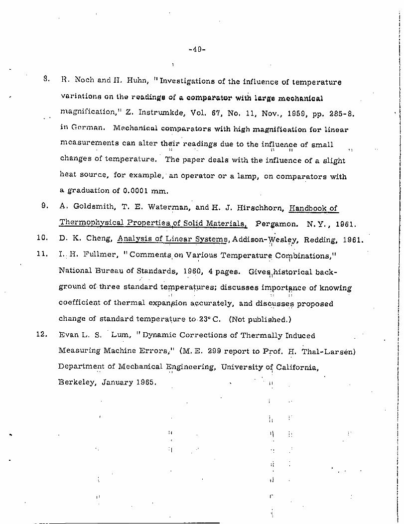
i0.

ii.

12.

-40-

R. Noah and I.I. Huhn, " Investigaiions of the influence of temperature

variations on ~h~ r~din~ of ~ ~ompa~ wi~h l~z m~h~ni~l

mag’nification," Z. Instr~kde, Vol. 67, No. ii, Nov., 1959, pp. 285-8.

in G(~rman. ~e~h~ni~l ~omp~ra~o~s with high ma~nifia~i~n for ~ine~r

measurements can alter their readings due to the influenoe of small

changes of temperature. The paper deals with the influence of a slight

heat source, for example, an operator or a lamp, on comparators with

a ~’~aduation of 0.0001 ram.

A. Goldsmith, T. E. Waterman , and H. J. Hitschhotn, Handbook of

ThermoPhysical Ptoperties..of Solid Materials~ Pergamon. N.Y., 19Sl.

D. K. Cheng, Analysis of Linear Systems, Addison-Wesley, Redding, 1961.

I.. H. Fullmer, " Comments on Various Temperature Combinations,"

National Bureau of Standards, 1960, 4 pages. Give~historical back-

ground of. three standard te~pera~gres; discusses importance of knowin~

coefficieD% of thermal expansion ~¢cutately, and disq~sse.@ proposed

chan~e of standard temperature to.28 oC. (Not published.)

Evan L. S. Lmn, " Dynamic Corrections of Thermally Induced

Measurin~ Machine Errors,." (M. E. 209 report to Prof. H. Thal-Lars4n)

Department of Mechanical Epgineering, University o~ California,

Berkeley, January 1965. ~,

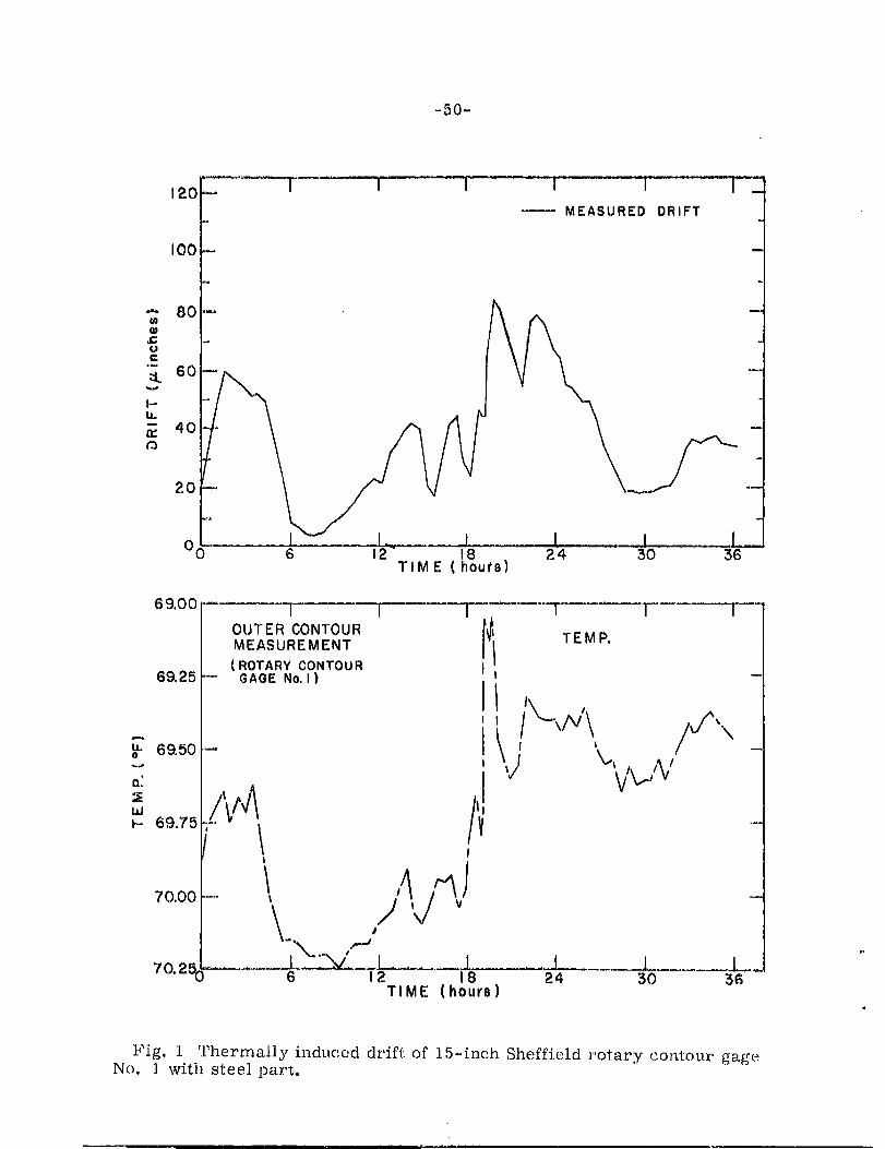
-50-

120

I00

] i i i i ]-- "_.

MEASURED DRIFT

0 0 6 12 18 2 4 30 36TIME (hours)

69.00

69.25

u= 69.50

~.- 69.7,5

70.00

I i i I TOU’r ER CONTOURMEASUREMENT(ROTARY CONTOURGAGE No, I )

TEMP.

I

,.,,,v

6 12 18TIME (hours)

f,,,/"’\/

-0 30 36

Fi.g, 1 ’.l.’hermal.ly induc,.ed drift of 15-inch Sheffield ~"otary co)~tour gageNo, ] with steel

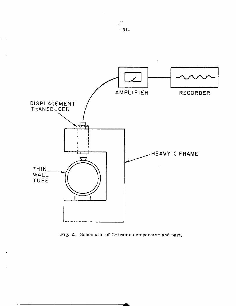
DISPLACEMENTTRANSDUCER

THINWALLTUBE

MPLIFIER

!

!

RECORDER

HEAVY C FRAME

:~,’ig. 2. Schematic of C-frame comparator and part.

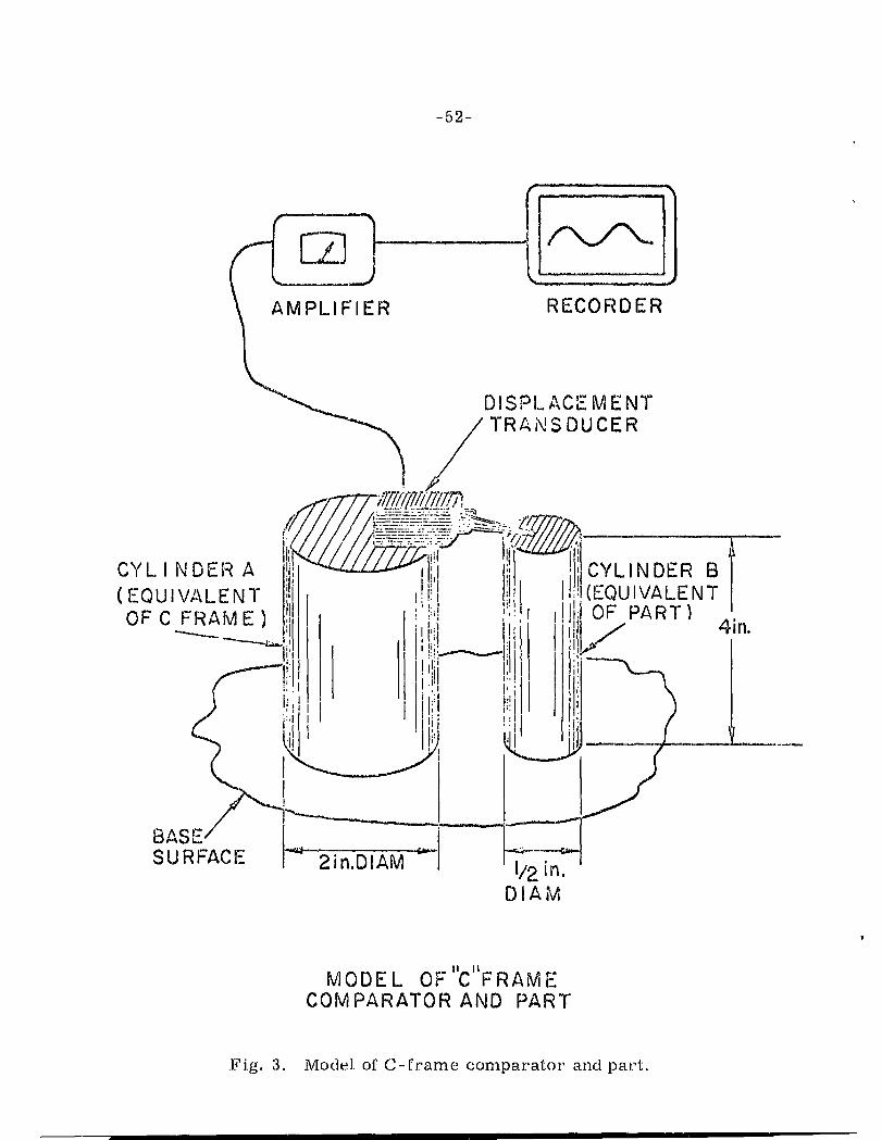
-52-

~. DISPI_ACEMENT

~ / TRANS DUCER

’i’,’1<//////’-/-/-/"~,,~ ) i’l’~zz~i!ilc¥~ ~ NDER_ A ~’, " Iili~, ", ’l’,i CYLI N DER~ B" -- -OF C FRAME I !’,

~ )’ I I~--’-----~’-’., )’ ~.: =’ ;ll .~irl,

Ii , =,~ IiiI ,,"-’--’1 : I l,

SURFACE I "~ ~[n.DIA-----~ ~" | 17-in~-2

DIAM

MODEL OF "C"FRAM ECOMPARATOR AND PART

.l?iig. 3. Model. of (]--frame compar’atot’ and pa).’t.

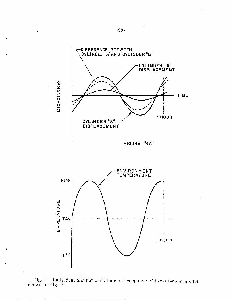
L~J

0

~,,,~~% ~D1FFERENCE BETWEEN

L I N DER IIKI AN D CYL I N DER IIBII

/" CYLINDERDISPLACEMENT

__./>----A.

CYLINDERDISPLACEMENT

FIGURE

TIME

+IOF

D

~ TAV

-IOF

ENVIRONMENTTEMPERATURE

I HOU R

I,:i.~. 4. InclJvitlLm]. and net (|z’fl’t thermal r’esl.)Or~sp. (~" two-t;](-;m(mt lu()de]..~hown .in I,’i.R’, :~.

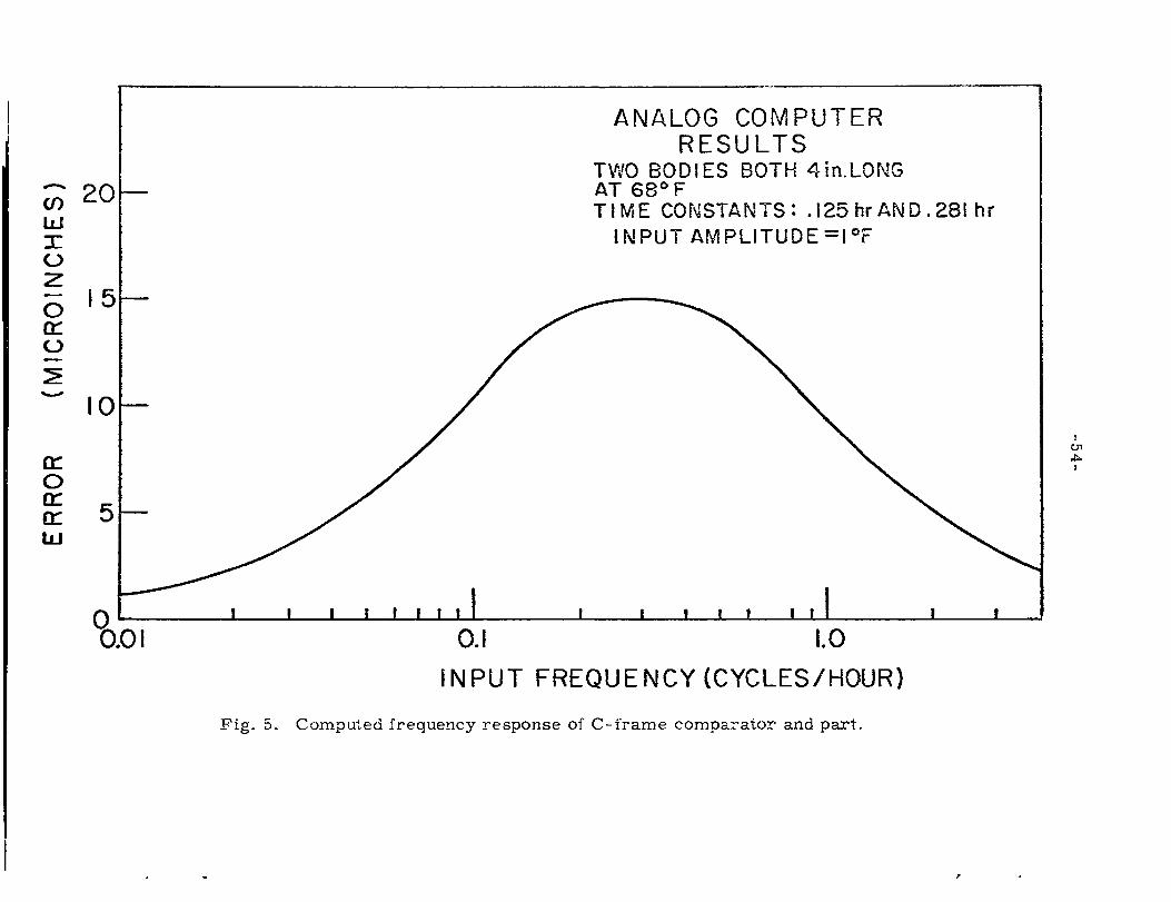
0

20

15

I0

ANALOG COMPUTERRESULTS

TWO BODIES BOTH Z~in.LONGAT 68° FTIME CONSTANTS: .125 brAND.281 hr

INPUT AMPLITUDE =l°F

Fig. 5.

I i I ! !

INPUT FREQUENCY (CYCLES/HOUR)

Computed frequency response of C-frame comoarator and part.

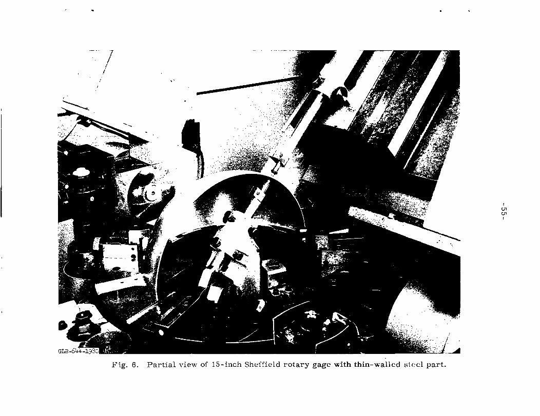
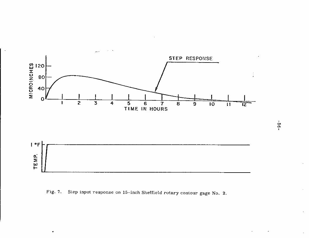
STEP RESPONSE

20

z. 80

TIME IN HOURS

Fig. 7. Step input response on 15-inch Sheffield rotary contour gage No. 2.

~-ACTUAL DRIFT

¯

/fCOMPUTED DRIFT8°1

o 1~.~-40~ II !

0 I 2 3 zl 5 6 7TIME (HOURS)

8! I i I

9 ¯ I0 . II 12,

TEMPERATURE VARIATION

INDUCED BY MOTOR DRIVEN CAMON SET POINT OF CONTROLLER

Fig. 8. Forced drift check on 15-inch Sheffield rotary gage No. 2.

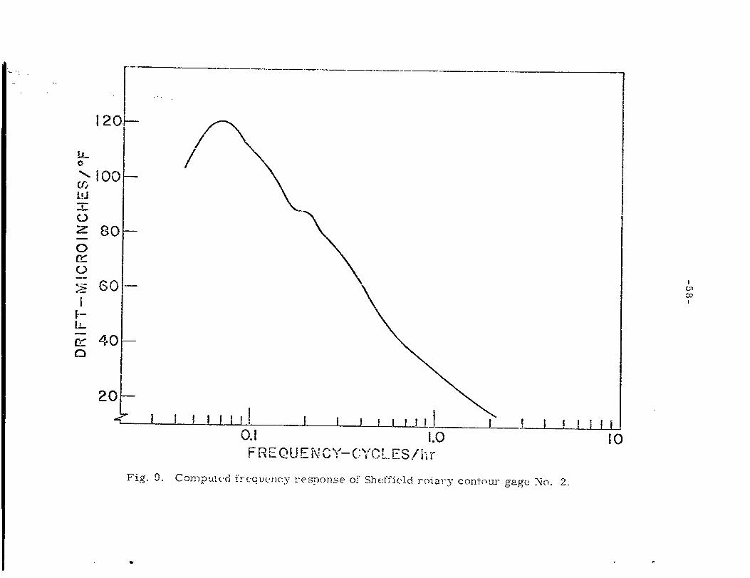
"- iO0 --

z 80--0

!|.--

~ 4.0,

20--

I ! I ! I!, ! i ~ ~ I__J.Jj I0.1 1.0FREQU ~- rt.C,,_ .,,,-,. ._"’ . C ~t.,L.ES/hi"

Computed +..~"eque,qcy response of SheFfield ga,R’e

li

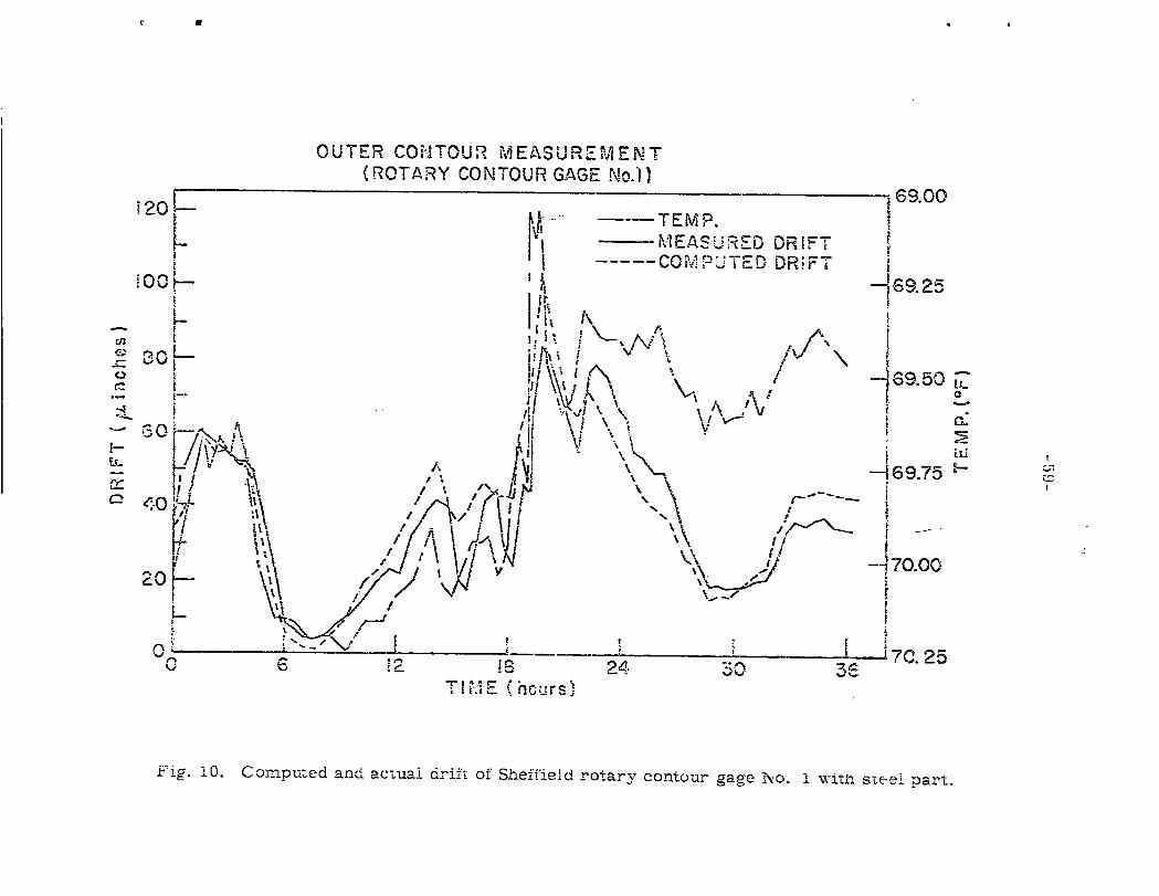
OUTER CONTOUR MEASUREMENT~’ ROTARY CONTOUR GAGE No.l )

69.00

t

----~ .$9. 25

-4 69.50 t,-...

--169.75 ~!

- 7o.oo

’ L._j 70. 250, i2 !$ 24. 50 5,¢,

TI ’" - r hours)i.i C ~.

I

Fig. i0. Conupuzed and ac’~ual drifi of She÷:~ie’;d rotary contour gage ho. ! ~i~ s%eei part.

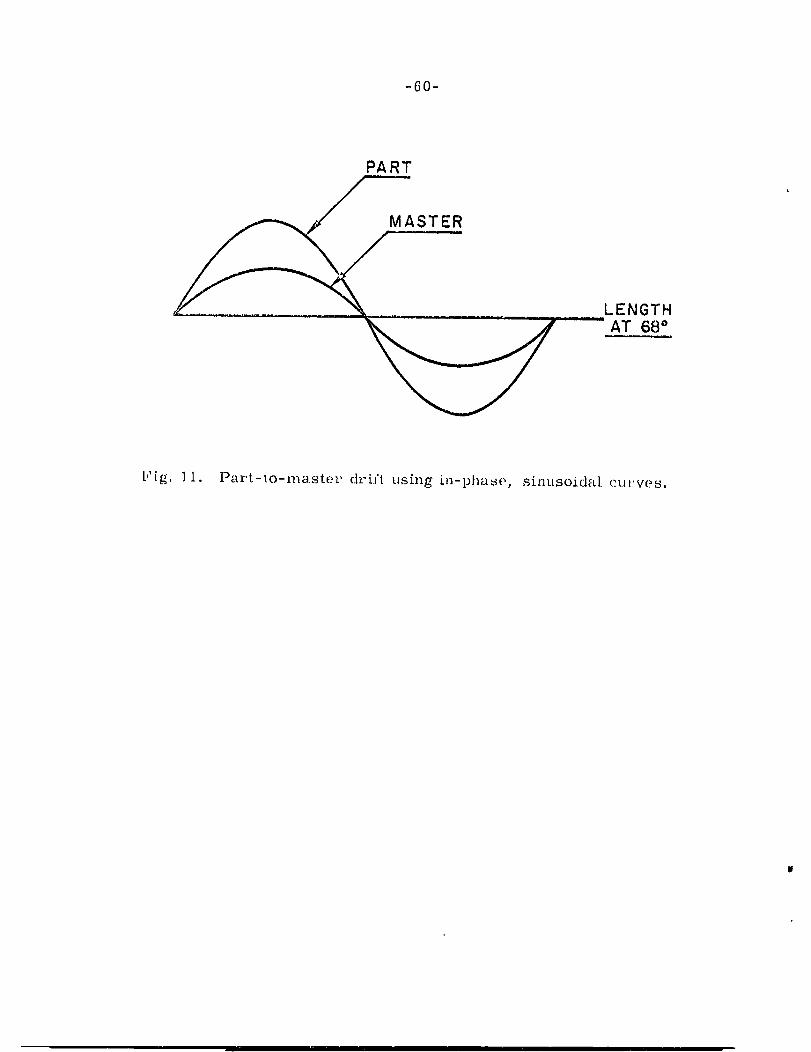
-60-

PART

LENGTHAT.___~8~

lri~, 1.1. o I~ar’t-to-masteP dPi..~’t using in-phase, sinusoi.dal, eu~’ves,

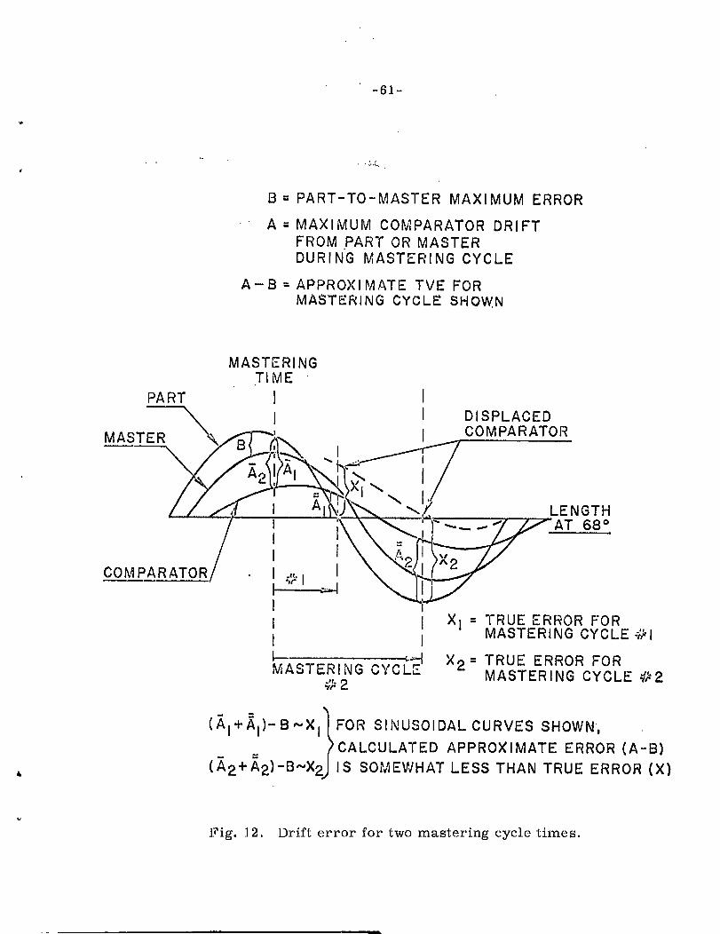
-61-

PART-TO-MASTER MAXIMUM ERROR

MAXIMUM COMPARATOR DRIFTFROM PART OR MASTERDURING MASTERING CYCLE

A- B = APPROXI MATE TVE FORMASTERING CYCLE 8HOW.N

MASTERINGTIME

PART I

~"k I DISPLACED

M A_S__TE R ~F"" COMPARATOR

COM PARATOR/ . ~g’l ~

I X1 = TRUE ERROR FORI MASTERING CYCLE -#1

’,H X ---MASTERING CYCLE TRUE ERROR FOR

MASTERING CYCLE

(~I+~I)-B~XI|FOR S!NUSOIDALCURVES SHOWN.

OCALCULATED APPROXIMATE ERROR (A-B}(~,2+~,2)-B~X2~J IS SOMEWHAT LESS THAN TRUE ERROR (X)

.l?i.g. ]2. Drift error for two mastering cycle times.

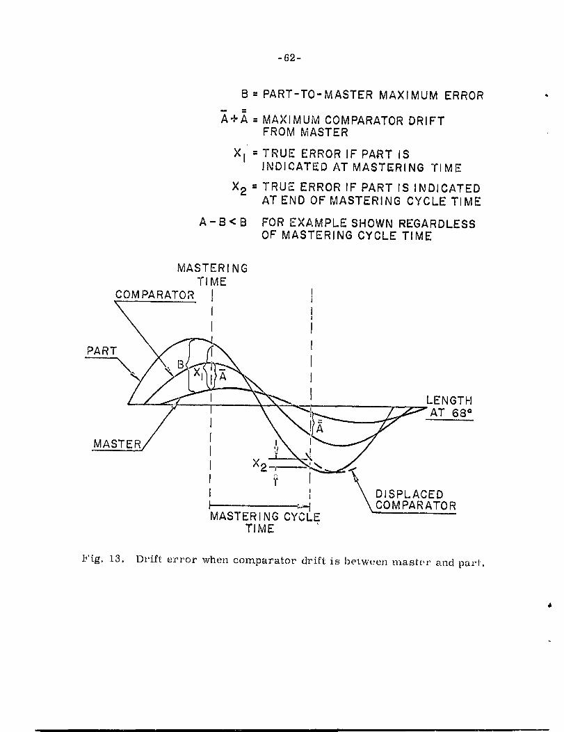
-62-

B = PART-TO-MASTER MAXIMUM ERROR

A+A-- MAXIMUM COMPARATOR DRIFTFROM MASTER

XI ;TRUE ERROR IF PART ISINDICATED AT MASTERING "rIME

X2-" TRUE ERROR IF PART IS INDICATEDAT END OF MASTERING CYCLE TIME

A-B<B FOR EXAMPLE SHOWN REGARDLESSOF MASTERING CYCLE TIME

MASTERINGTIME

COM PARATOR I

-~--~~~ z~AT 68°

-1 DISPLACED

~.--.[ COM PARATORMASTERING CYCLE

TIME

Fig. 13. Dl’ift error when comparator drift is betwt:en mast(,~’ and pa.r’l.

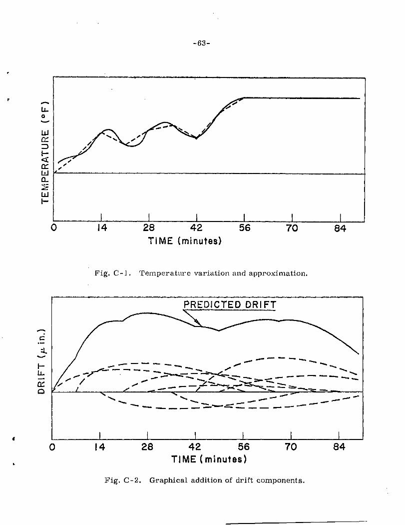
-63-

28 42 56 70 84TIME (minutes)

Fig’. C-I. Temperatul’e var’iation and approximation.

PREDICTED DRIFT

/ _ ~-,----.- __ ~ ...~-..._~....~._.,.../_~ _ "-....../ .. --; -- . _.....- ~---..~--~ ~.._~.~._. ~._-- .-- ..... ._ ....

! I I I 1 I0 14 28 42 56 70 84

TIME (minutes)

Fig. C-2. Graphical addition of drift components.

LEGAL NOTICE

This report was prepared as an account of Government sponsored work.Neither the United States, nor the Commission, nor any person acting onbehalf of the Commission."

A. Makes any warranty or representation, expressed or implied, withrespect to the accuracy, completeness, or usefulness of the information con-tained in this report, or that the use of any information, apparatus, method,or process disclosed in this report may not infringe privately owned rights; or

B. Assumes any liabilities with respect to the use of, or for dama.qesresulting from the use of any information, apparatus, method or process dis-closed in this report.

As used in the above, Ir person acting on behalf of the Commission i~includes any employee or contractor of the commission, or employee of suchcontractor, to the extent that such employee or contractor of the Commission,or employee of such contractor prepares, disseminates, or provides accessto, any information pursuant to his employment or contract with the Commis-sion, or his employment with such contractor.