thermal plasma processing -...

THERMAL PLASMA PROCESSING

OF FINE GRAINED

MATERIALS

by

MURALIDHARAN RAMACHANDRAN

RAMANA G. REDDY, COMMITTEE CHAIR

GARRY W. WARREN MARK L. WEAVER

YUEBIN GUO UDAY K. VAIDYA

A DISSERTATION

Submitted in partial fulfillment of the requirements for the degree of Doctor of Philosophy

in the Department of Metallurgical and Materials Engineering in the Graduate School of

The University of Alabama

TUSCALOOSA, ALABAMA

2012

ii

ABSTRACT

Synthesis of advanced ceramic materials has been systematically investigated using non-

transferred thermal plasma reactor. Low cost oxide feed materials has been used as the solid feed

to the reactor while methane (CH4) and argon (Ar) were used as reducing and carrier gases,

respectively.

A 2D computational fluid dynamics (CFD) based mathematical model was developed to

understand the flow and temperature profiles inside the reactor. The concept was extended to a

3D model and a comparison was made with the results from 2D model. The velocity increases

linearly with increase in the pressure in both the 2D and the 3D models while the maximum

velocity from 3D model is lower by about 35-40 m/s at any given pressure. A decrease in the

residence time was observed in the 3D model compared to the 2D model. An intermediate

plasma gas pressure of 45 psi was used in experiments to ensure high temperatures and residence

times in the reactor.

Thermochemical calculations have been carried out to determine the molar ratio of the

reducing gas to be used in TiO2-B2O3-CH4 and SiO2-CH4 system. The maximum theoretical

yield of TiB2 of about 82 mol% was obtained at a molar ratio of TiO2:B2O3:CH4 = 1:1:5.

Maximum theoretical yield of SiC of about 97 mol% was obtained at a molar ratio of

SiO2:CH4=1:3 at a temperature of 1520ºC.

Experiments were carried out using thermal plasma reactor to synthesize TiB2 and SiC.

The maximum yield of TiB2 of about 40 mol% was obtained with a feed molar ratio of

iii

TiO2:B2O3:CH4 = 1:1:5 and a power of 23.4 kW. Relatively higher solid feed rates increased the

yield of TiB2. The TiB2 spherical particles formed are in the range of 20-100 nm. A change in

crystal structure was observed in TiO2 from anatase to rutile.

Experiments using a molar ratio of SiO2:CH4 = 1:2 produced maximum yield of SiC of

about 65 mol% at a solid feed rate of 5 g/min. Mostly spherical morphology with some nanorods

have been observed. The presence of Si had been observed and was quantified using XRD, HR-

TEM, Raman and XPS.

iv

DEDICATION

This dissertation is dedicated to my mom, dad and brother.

v

LIST OF ABBREVIATIONS AND SYMBOLS

Density

r Radius

t Time

Velocity vector

Sm Source of any mass added from dispersed second phase

x

and r

Axial and radial velocities respectively

p Static pressure

τ Stress tensor

g Gravitational force

F External body forces

t Turbulent (or Eddy) viscosity

Gk Generation of turbulent kinetic energy (TKE) due to mean velocity gradients

Gb Generation of TKE due to buoyancy

YM Contribution of fluctuating dilatation in compressible turbulence to the overall dissipation rate

k Turbulent kinetic energy

Turbulence dissipation rate

keff Effective thermal conductivity.

vi

kt Turbulent thermal conductivity

Jj Diffusion flux of species j

Sh Heat of chemical reaction or any other volumetric heat source

h Sensible enthalpy

Yj Mass fraction of species j

hj Sensible enthalpy of species j

Specific dissipation rate

G Generation of

Yk and Y Dissipation of k and due to turbulence respectively

Sk and S User-defined sources terms for k and respectively

k and Turbulent Prandtl numbers for k and respectively

* Coefficient

Intermittency

S Strain rate magnitude

Flength Empirical correlation that controls the length of the transition length

Vorticity magnitude

G Total Gibbs energy of the system

Gi0 Standard molar Gibbs energy of species i at temperature T and pressure P

ni Number of moles of species i

Pi Partial pressure of species i

Xi Mole fraction of species i

i Activity coefficient of species i.

ITiB2 Intensity of TiB2

vii

ITiO2 Intensity of TiO2

IB2O3 Intensity of B2O3

IC Intensity of C

cTiB2 Volume fraction of TiB2

cTiO2 Volume fraction of TiO2

cB2O3 Volume fraction of B2O3

cC Volume fraction of C

RTiB2 Volume of inverse unit cell lattices of TiB2

RTiO2 Volume of inverse unit cell lattices of TiO2

RB2O3 Volume of inverse unit cell lattices of B2O3

RC Volume of inverse unit cell lattices of C

viii

ACKNOWLEDGMENTS

I would like to take this opportunity to express my sincere gratitude to my advisor and

chairman of this dissertation committee, Dr. Ramana G. Reddy, for his constant support and

guidance throughout my graduate study and research work at the University of Alabama.

I would like to thank Dr. Garry W. Warren, Dr. Mark L. Weaver, Dr. Yuebin Guo, and

Dr. Uday K. Vaidya for serving on my dissertation committee and providing valuable

suggestions and insights.

I’m thankful to the faculty, staff and students at the Metallurgical and Materials

Engineering department for their timely help. Special thanks to Dr. Divakar Mantha, research

engineer, for extensive technical discussions, comments and encouragement. I would like to

thank Dr. Muhammad Ali Rob Sharif for his help with the computational fluid dynamic

modeling of the plasma reactor. I thank the members of the central analytical facility (CAF) for

their constant help during characterization.

Thanks to ACIPCO and the University of Alabama for the financial support.

A special thanks to my parents, brother, and all my friends for their constant moral

support in all my endeavors.

ix

CONTENTS

ABSTRACT ................................................................................................ ii

DEDICATION ........................................................................................... iv

LIST OF ABBREVIATIONS AND SYMBOLS ........................................v

ACKNOWLEDGMENTS ....................................................................... viii

LIST OF TABLES ................................................................................... xiii

LIST OF FIGURES ...................................................................................xv

1. INTRODUCTION ...................................................................................1

2. LITERATURE REVIEW AND RESEARCH OBJECTIVES ................8

2.1 Plasma synthesis ..............................................................................8

2.2 Plasma sources for material synthesis..............................................9

2.3 Advanced material synthesis using thermal plasma ......................11

2.4 Properties and synthesis of titanium diboride ................................11

2.5 Properties and synthesis of silicon carbide ....................................12

2.6 Research objectives ........................................................................15

3. MATHEMATICAL MODEL ................................................................17

3.1 2D plasma reactor model ...............................................................17

3.2 Defining equations in 2D model ....................................................18

3.3 Grid refinement in 2D model .........................................................21

3.4 Results from 2D plasma reactor model ..........................................25

x

3.5 3D plasma reactor model ...............................................................31

3.6 Defining equations in 3D model ....................................................32

3.7 Turbulence and grid refinement in 3D model ................................34

3.8 Results from 3D plasma reactor model ..........................................44

4. EXPERIMENTAL SETUP ....................................................................49

4.1 Plasma power source ......................................................................49

4.2 Plasma reactor system ....................................................................54

4.2.1 Reaction zone ........................................................................54

4.2.2 Quench zone..........................................................................56

4.2.3 Filter zone .............................................................................57

4.3 Powder feeder ................................................................................58

4.4 Water source ..................................................................................59

4.5 Gas source ......................................................................................62

4.6 Raw materials.................................................................................63

4.7 Characterization of product powders .............................................66

4.7.1 X-Ray Diffraction (XRD) ....................................................66

4.7.2 Scanning Electron Microscope (SEM) ................................66

4.7.3 Transmission Electron Microscopy (TEM) .........................66

4.7.4 Differential Scanning Calorimetry (DSC) ...........................67

4.7.5 Raman Spectra .....................................................................67

4.7.6 X-Ray Photoelectron Spectroscopy (XPS) ..........................68

4.7.7 Thermo-Gravimetric and Differential Thermal Analyzer (TG-DTA) ............................................................................68

5. SYNTHESIS OF TITANIUM DIBORIDE ...........................................69

xi

5.1 Thermochemical calculations ........................................................69

5.2 Synthesis and characterization of titanium diboride ......................75

5.2.1 Phase and morphology of solid feed ....................................75

5.2.2 Phase, composition and morphology of product powders ...76

5.2.3 Phase transformation ............................................................83

5.2.4 Particle size reduction ..........................................................84

6. SYNTHESIS OF SILICON CARBIDE.................................................85

6.1 Thermochemical calculations ........................................................85

6.2 Synthesis and characterization of silicon carbide ..........................89

6.2.1 Phase and composition of product powders.........................89

6.2.2 Morphology of product powders .........................................98

6.2.3 Particle size reduction ........................................................103

6.2.4 Qualitative analysis of product powders ............................103

6.2.5 Post-processing of product powders ..................................106

7. CONCLUSIONS AND FUTURE WORK ..........................................108

7.1 CFD modeling of plasma reactor .................................................108

7.2 Synthesis of titanium diboride .....................................................109

7.3 Synthesis of silicon carbide .........................................................110

7.4 Future work ..................................................................................111

7.4.1 Modeling of plasma reactor ..........................................111

7.4.2 Synthesis of TiB2 ..........................................................112

7.4.3 Separation of Si, SiC and SiO2 .....................................112

REFERENCES ........................................................................................114

xii

APPENDIX ..............................................................................................121

A.1 INSTRUCTIONS FOR THE OPERATION OF PLASMA POWER SOURCE IN NON-TRANSFERRED MODE ............121

A.2 PROPERTIES OF GASES USED IN MODELING ..................125

A.3 CALCULATION OF VOLUME FRACTION USING DIRECT COMPARISON METHOD .........................................128

xiii

LIST OF TABLES

3.1 Initial and boundary condition values used during grid refinement studies .........................................................................23

3.2 Values of pressures used in determining the velocity and temperature profiles ............................................................................25

3.3 Average residence time in the plasma reactor as a function of plasma inlet pressure ...........................................................................30

3.4 Average residence time in the plasma reactor using 3D model as a function of plasma inlet pressure .....................................................48

4.1 Flow rate of cooling water for various parts of the plasma reactor system ..........................................................................61

4.2 Programmable gas controller set points in the thermal plasma power source for various types of torch ..................................63

5.1 Theoretical Yield of TiB2 and by-products in mol% as a function of molar ratio of methane in feed ........................................................72

5.2 Experimental design for the production of TiB2 using thermal plasma reactor ........................................................................75

5.3 Yield of product powders at different feed rates with a methane molar ratio of 5 in the feed ...................................................................78

6.1 Experimental Conditions for the production of SiC using thermal plasma .....................................................................................89

6.2 Weight fraction of product powders from experiment 1 .....................96

A.2.1 Viscosity (piecewise-linear) of argon ............................................125

A.2.2 Thermal conductivity (piecewise-linear) of argon .........................125

A.2.3 Heat capacity, CP (piecewise-linear) of methane ...........................126

xiv

A.2.4 Viscosity (piecewise-linear) of methane ........................................127

A.2.5 Thermal conductivity (piecewise-linear) of methane ....................127

A.3.1 The values of diffraction constants used in the calculation of volume fraction of product powders from TiB2 experiments ........129

xv

LIST OF FIGURES

1.1 Conceptual diagram of aerosol combustion process [3] ........................2

2.1 Schematic temperature distribution in a DC plasma arc (a) and RF discharge (b). ..................................................................................10

3.1 Schematic of the thermal plasma reactor. ............................................21

3.2 Grid of the plasma reactor with 4154 nodes (X=30; Y=133). .............21

3.3 Grid of the plasma reactor with 7257 nodes (X=40; Y=176). .............21

3.4 Grid of the plasma reactor with 11322 nodes (X=50; Y=221). ...........21

3.5 Velocity (a), stream function (b) and temperature (c) at a distance of X=1.8 cm from the plasma source for various

grid configurations. ..............................................................................22

3.6 Contour of temperature (a) and velocity (b) at a plasma inlet pressure of 45 psi. ................................................................................26

3.7 Effect of pressure on the inlet velocity of the plasma. .........................27

3.8 Profiles obtained from different areas of the reactor denoted by the line numbers. ........................................................................................28

3.9 Velocity profile along radial (a) and axial (b) directions at inlet pressure of 45 psi. ........................................................................29

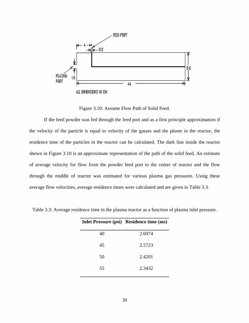
3.10 Assume Flow Path of Solid Feed .......................................................30

3.11 Various grid sizes for grid refinement studies in 3D thermal plasma reactor: (a) 8013 nodes, (b) 11516 nodes and (c) 18936 nodes .........34

3.12 Velocity profile at the cross-section of the feed port: (a) standard k- model, (b) standard k- model and (c) Transition SST model ...35

xvi

3.13 Velocity profile at the symmetry of the reactor: (a) standard k- model, (b) standard k- model and (c) Transition SST model ..........36

3.14 Line profiles created in the reactor to compare the modeling results from various case studies ........................................................37

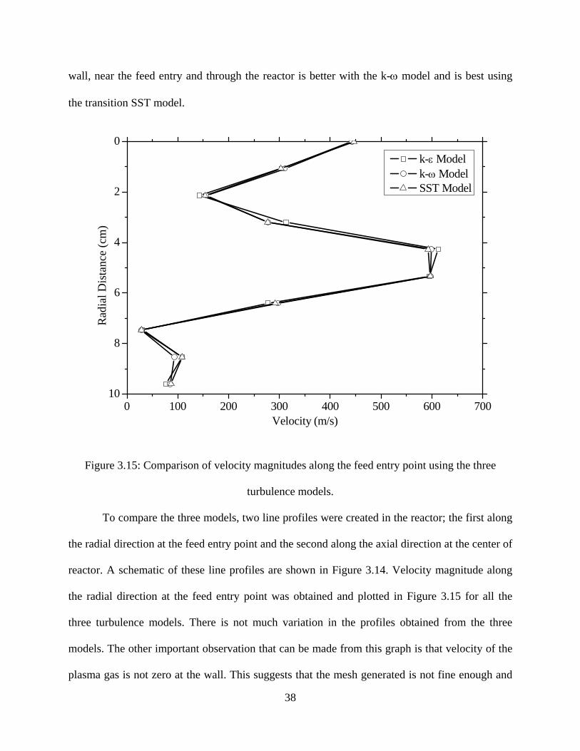
3.15 Comparison of velocity magnitudes along the feed entry point using the three turbulence models .....................................................38

3.16 Comparison of velocity magnitudes along the center of reactor using the three turbulence models .....................................................39

3.17 Velocity profile at the cross-section of the feed port: (a) 8013 nodes, (b) 11516 nodes and (c) 18936 nodes ....................................40

3.18 Velocity profile at the symmetry of the reactor: (a) 8013 nodes, (b) 11516 nodes and (c) 18936 nodes ...............................................41

3.19 Comparison of velocity magnitudes along the feed entry point using three different grid sizes ..........................................................42

3.20 Comparison of velocity magnitudes along the center of reactor using three different grid sizes ..........................................................43

3.21 Comparison of velocity magnitudes along the feed entry point using five different plasma inlet gas pressures ..................................45

3.22 Comparison of velocity magnitudes along the center of the reactor using five different plasma inlet gas pressures ..................................46

3.23 Effect of pressure on the inlet velocity of the plasma and comparison between the 2D model and the 3D model ......................47

3.24 Assume flow path for solid feed in 3D model ...................................48

4.1 Schematic of thermal plasma processing system .................................50

4.2 Schematic of non-transferred (left) and transferred (right) plasma arc torches ............................................................................................50

4.3 Photograph of plasma power source control panel ..............................51

4.4 Photograph of the new (left) and used (right) electrode assembly in a non-transferred plasma torch .............................................................52

xvii

4.5 Photograph of the electronic gas flow rate monitor on the plasma source ..................................................................................................53

4.6 Photograph of non-transferred thermal plasma reactor system ...........54

4.7 Photograph of the reaction zone ..........................................................55

4.8 Photograph of the two concentric copper quenching coils in the quench zone .........................................................................................56

4.9 Photograph of cloth filter in filter zone ................................................57

4.10 Photograph of the powder feeder (left) and the circuit of the control panel (right) ...........................................................................58

4.11 Photograph of cooling water system and roughing pump assembly ............................................................................................60

4.12 Flow meters controlling the flow rate of cooling water to various parts of the plasma reactor system ....................................................61

4.13 Photograph of gas supply system consisting of plasma, carrier and reducing gases .............................................................................62

4.14 Calibration of powder feeder for the mixture of TiO2 and B2O3 as the solid feed .................................................................................64

4.15 Calibration of powder feeder using SiO2 as the solid feed ................65

5.1 Formation of various product phases at a molar ratio of (a) TiO2:B2O3:CH4=1:1:4 and (b) TiO2:B2O3:CH4=1:1:5 ...................70

5.2 Formation of various product phases at a molar ratio of (a) TiO2:B2O3:CH4=1:1:6 and (b) TiO2:B2O3:CH4=1:1:7 ...................71

5.3 Theoretical yield of TiB2 and C at various molar ratio’s of methane to solid feed .......................................................................74

5.4 X-Ray diffraction pattern of 1:1 molar TiO2:B2O3 ..............................75

5.5 SEM images of solid feed powder at a molar ratio of TiO2:B2O3 = 1:1 ...................................................................................76

5.6 XRD patterns of product powders obtained from different experiments ..........................................................................................77

xviii

5.7 SEM images of product powders obtained from experiment 4 ...........79

5.8 SEM electron image (top) of the product powders obtained from experiment 4 and the corresponding EDS spectra (bottom) ................80

5.9 TEM image of the product powder obtained from experiment 4 ........81

5.10 HRTEM of product powders showing lattice fringes of hexagonal B2O3 in the (1 0 0) plane obtained from experiment 4 ......................82

5.11 STEM image (left) of product powders obtained from experiment 4 and the corresponding EDS spectra (right) .................83

6.1 Thermochemical calculations to determine stable phases at 1220⁰C as a function of molar ratio of methane to solid feed .........................85



6.4 Thermochemical calculations to determine stable phases at 3010⁰C as a function of molar ratio of methane to solid feed ..........................88

6.5 XRD pattern of product powders formed at various molar ratios of methane to solid feed and at a solid feed rate of 5g SiO2/min .............90

6.6 XRD patterns of product powders formed at various molar ratios of methane to solid feed and at a solid feed rate of 4g SiO2/min .............91

6.7 Experimental yield of product powders formed at various molar ratios of methane to solid feed and a solid feed rate of 5g/min ...........92

6.8 Experimental yield of product powders formed at various molar ratios of methane to solid feed and a solid feed rate of 4g/min ...........92

6.9 Effect of plasma power on the experimental yield at a feed rate of 5 g/min SiO2 and a molar ratio of SiO2:CH4 = 1:1 ..............................93

6.10 Effect of SiO2 feed rate on experimental yield at a power of 21.6 kW and a molar ratio of SiO2:CH4 = 1:2 ...................................94

6.11 Comparison of theoretical yield of SiC at various temperatures to experimental yield at a solid feed rate of 5g/min ................................94

xix

6.12 Heat capacity, sample heat flow and baseline heat flow for product powders from experiment 1 using DSC ...............................97

6.13 Comparison of heat capacity measured experimentally with those calculated using equation (29) ..........................................................98

6.14 SEM image showing the morphology of the product powders from experiment 1 ..............................................................................99

6.15 SEM image showing the morphology of the product powders from experiment 5 ..............................................................................99

6.16 SEM image showing the morphology of the product powders from experiment 7 ............................................................................100

6.17 TEM image showing the morphology of the product powders from experiment 1 ............................................................................101

6.18 (a) TEM image showing the morphology of the product powders from experiment 2; (b) and (c) HRTEM showing presence of Si and (d) SiO2 single crystal with insets of magnified image and electron diffraction pattern ...............................................................102

6.19 Raman spectra of product powders from experiments 1, 2 and 3 using a solid feed rate of 5g/min .....................................................104

6.20 XPS spectra of product powders from experiment 1 showing the Si 2p peak resolved into SiO2, SiC and Si peaks ............................105

6.21 Weight loss and heat flow curves from TG-DTA for the product powders from experiment 1 ...............................................106

1

CHAPTER 1

INTRODUCTION

Advanced ceramic materials are of enormous interest due to a wide variety of

applications in many key engineering fields such as electrical and electronics, optical,

mechanical, and chemical, to name a few. There are a number of commercial production

techniques that are in use depending on the size, shape and type of material. These ceramic

materials, in general, can be classified into three different categories namely, oxide ceramics,

non-oxide ceramics and ceramic based composites. Some of the most commonly used oxide

ceramics include but not limited to titanium dioxide, nickel oxide, cobalt oxide, molybdenum

oxide, yttria, zirconia, silica, etc. Other mixed oxides such as barium titanate, doped lanthanum

gallate, yttria stabilized zirconia, strontium doped LaMnO3 (LSM), yttrium barium copper oxide

(YBCO, commonly known as the 1-2-3 compound), are some of the examples of other oxide

based advanced ceramic materials.

One of the traditional ways of synthesizing mixed oxide is using high temperature ‘heat

and beat’ solid state synthesis route. The oxides are mixed together, heated to a temperature

followed by crushing / milling. This is done in cycles with increasing temperature in each cycle

till the final product is the desired single phase mixed oxide. This process is very time and

energy consuming and due to the extensive high temperature treatment of the material, the final

product size is in tens to hundreds of microns. Flux and hydrothermal synthesis routes [1] have

been reported to have relatively lower processing temperature between 200 and 600ºC.

2

Synthesis of Sr- and Li- doped lanthanum orthogallate is reported in literature [2] using

glycine- metal nitrate soft chemistry route. Stoichiometric metal nitrates were dissolved in water

and mixed with glycine, as fuel for combustion, and ammonium nitrate, as an initiator. The

initial synthesis temperature was very low, about 200ºC. The calcined powders were about 100-

200 nm in size and the crystallites in sintered pellets were about 0.5-1 m. In spite of low

temperature synthesis and finer grain sizes, the cost of starting materials, requirement of large

reactor volumes and batch processing make its commercial feasibility questionable.

Figure 1.1: Conceptual diagram of aerosol combustion process [3].

Aerosol combustion synthesis of MgO, ZrO2 and Yttria Stabilized Zirconia (YSZ) has

been reported in literature [3]. This concept has been patented [4-6] with the modification of the

actual apparatus. Similar to the metal nitrate-glycine soft chemistry route mentioned earlier, the

aerosol combustion synthesis route uses magnesium nitrate for MgO, zirconium nitrate for ZrO2,

3

and zirconyl chloride and yttrium nitrate for YSZ. These raw materials are mixed with sucrose

and the thus formed aerosol is sprayed into the reactor. It is a relatively high temperature process

and the temperature is in the range of 1000-1500 K. In spite of high temperature processing, due

to low residence time in the reactor, the particle size is small of the order of tens of nanometers.

The drawbacks of this processing technique are the low through-put and scalability to

commercial applications.

Yttria stabilized zirconia is one of the widely used solid electrolytes in solid oxide fuel

cells. It has good oxygen ion conductivity at about 1000ºC. Several researchers [7-12] have

studied the synthesis of YSZ to obtain small grain size, spherical morphology and sinterability at

relatively low temperatures. Thin film deposition of YSZ on -alumina substrate has also been

reported [13]. Electrochemical deposition of CeO2 thin films [14], microemulsion mediated

synthesis of mixed oxide powders [15], sol-gel synthesis of nano-TiO2 [16] and polyacrylamide

gel synthesis of -alumina [17], are some of the other techniques used in the synthesis of nano

scale oxide ceramic materials.

Carbides are an important class of non-oxide ceramics. Traditionally, carbides are made

by carbothermic reduction of corresponding metal oxide by carbon at relatively high

temperatures of about 1500-2000ºC. Transition metal carbide synthesis using alkalide reduction

[18] has been reported at low temperature with an annealing temperature varying between 950-

1200ºC for various carbides such as Fe3C, VC, TaC, and TiC nanocrystals. Low temperature

synthesis and shorter annealing time maintains the fine crystallite size in the range of 2-25 nm

with a relatively high surface area.

Carbon nanotubes have excellent properties. It is one of the most used materials in fiber-

reinforced polymer or metal composites. A synthesis procedure has been published [19] where

4

the carbon nanotube is reacted with volatile metal oxide or a volatile metal halide to form

nanorods of corresponding metal carbides. Synthesis of narrow rods with diameters ranging

between 2-30 nm and lengths up to 20 m has been reported. It is interesting to note that bulk

properties of the carbides (TiC – metal; NbC – superconductor; Fe3C – ferromagnetic; SiC –

semiconductor; BCx – insulator) are still maintained in the nanorod structures.

Precious metal catalysts are usually used as anode catalysts for hydrogen oxidation in

polymer electrolyte fuel cells. These were replaced by a nanoscale WC catalyst by Yang et. al.

[20]. They obtained high current densities of 0.9 A/cm2 at 80ºC and 3 atm at a relatively low WC

catalyst loading of about 0.5 mg/cm2. The nanoscale tungsten carbide was synthesized by

chemically reduced ball milling. A mixture of WO3, Mg and C powders were mixed in 1:6:1

ratio and ball milled for about 2 days. MgO formed as a byproduct is removed using HCl acid

solution.

Ceramic composites are a class of materials where the ceramic material is dispersed in a

matrix. The matrix can be a metal, alloy, polymer or another ceramic. The advantage of the

ceramic composites is that the dispersed ceramic material increases the strength and hardness of

the composite. The presence of matrix, on the other hand, can also influence the ceramic

material. It is shown that the photocatalytic activity of a TiO2/activated carbon composite is more

than that of pure TiO2 [21]. It is reported that the presence of activated carbon reduces the grain

growth of TiO2 particles during the sol-gel synthesis while a phase transformation from anatase

to rutile phase is observed.

Composites of Ag/YBCO superconductors have been reported in the literature [22]. It is

important to have a composite as the mechanical strength of pure superconductors is poor.

Synthesis of Y123 (YBa2Cu3O7) and Y123 + 40% Y211 (Y2BaCuO5) were carried out using

5

Y2O3, BaCO3 and CuO using solid state synthesis at a calcination temperature of 900ºC for 30h.

The product from the previous step was mixed with 0.5 wt% Pt and 3-30 wt% Ag2O. The

synthesis of Ag/YBCO composite was carried out using a melt growth method by partially

melting the sample and varying the maximum and the hold temperatures. Silver free regions

were observed in some of the samples. The effect of the starting material (Y123 or Y123 + 40

wt% Y211), maximum temperature, and holding temperature on the dispersion of silver in the

melt was made.

A multi-walled carbon nanotube (CNT) – alumina composite has been synthesized [23]

with the CNT’s highly ordered inside the alumina matrix. A three step synthesis method was

used. First, nano-channel alumina (NCA) template was developed on aluminum at 650ºC with

the diameter of the hexagonal close-packed pore controlled by the experimental anodization

conditions. Cobalt catalyst was deposited in the nano pores as a second step. This is followed in

the third step by the growth of parallel, highly-ordered carbon nanotubes by the pyrolysis of

acetylene. The removal of NCA template using a mixture of acids revealed that nanotubes were

parallel with a diameter distribution within 5% of mean diameter.

Iron-cementite nanocomposite was synthesized [24] using mechanosynthesis technique

from elemental iron and graphite powders. Finer grain sizes (about 7-8 nm) of iron and cementite

were obtained by ball-milling for 10 hours. The consolidated material also had relatively smaller

grain size of about 40 nm due to use of intermediate temperature and high pressure. While the

material had increased hardness, the magnetic properties were unaltered due to presence of finer

grains.

One of the widely used techniques for the production of nanoscale materials is the

conventional metal – catalytic vapor-liquid-solid (VLS) process [25]. This method is

6

implemented in different forms for the production of a variety of materials. Carbon nanotubes

using arc discharge [26], silicon nanowires [27] using a solution method, hot filament chemical

vapor deposition and laser ablation of a target [28,29] for large scale production, thermal

evaporation are some of the other processing techniques for the synthesis of nanoscale materials.

Oxide-assisted growth (OAG) [29-33] has been used for some materials (silicon nanowires) for

its large scale production. Some of the early synthesis methods include photolithography [34]

and scanning tunneling microscopy (STM) [35]. Some of the high temperature processes such as

solid state processing of B4C-Al composite is done at high temperature (1180⁰C) and high

pressure (20 MPa) [36], but yields coarse grained material.

There are two major factors in the synthesis of nanoscale materials. The thermodynamics

of a process determines the feasibility of a process. Among all the competing reactions in the

process, the one with the least Gibbs energy will be the one that will be the most favorable

reaction. The nucleation and growth are specific to the production technique and will depend on

a lot of process control variables.

The research objective of this project is to synthesize fine grained advanced ceramic

materials such as TiB2, and SiC in a thermal plasma reactor using low cost oxide feed materials

such as TiO2, B2O3 and SiO2 and methane as a reducing gas. Thermochemical calculations will

be performed on individual feed material-reducing gas system to evaluate the feasibility of

desired product formation and to obtain an estimate of optimum conditions and composition of

starting materials. Several experimental process parameters such as the molar ratio of the solid

feed to the reducing gas, the solid feed rate and the plasma power on the size, shape and amount

of the product powders will be systematically examined. A computational fluid dynamics (CFD)

based mathematical model will be developed to understand the flow inside the reactor. Several

7

characterization techniques such as XRD, SEM, TEM and EDS will be used in characterizing the

size, morphology, amount and orientation of the product powders. Thermal properties and

weight loss measurements will be done using TG-DTA and DSC to understand the constituents

of the product powders. Raman and XPS spectroscopic techniques will be used to determine the

presence of bonds and substantiation of the chemical binding energies, respectively.

8

CHAPTER 2

LITERATURE REVIEW AND RESEARCH OBJECTIVES

2.1 Plasma synthesis

Plasma synthesis is one of the methods of producing nanoscale materials. Plasma is

defined, in general, as a gas that is partially or fully ionized containing electrons, ions, neutral

atoms and/or molecules. There can be two possible states of plasma, either thermal or non-

thermal. Non-thermal plasmas are characterized by their low temperature while thermal plasmas

have relatively very high temperatures. Both the types of plasmas have been used successfully in

the synthesis of fine grained materials and thin films. In the case of thermal plasma, partial

thermal equilibrium is attained between the electrons and the heavy particles of the plasma

plume. In the mid to late twentieth century, thermal plasmas have been tested and used

extensively in many applications such as, extractive metallurgy, process metallurgy, plasma

spray coatings, plasma welding and cutting, synthesis of advanced materials, toxic and hazardous

waste treatment, etc. Plasma spray coating was an $800 million industry as reported in 1990 [37]

and rose up to a $1.35 billion in 1997 [38].

Synthesis of advanced materials has become one of the most important applications of

thermal plasma due to its high temperature, clean reaction environment, and use of inexpensive

feed materials. High purity products are obtained faster due to the enhanced reaction kinetics.

Rapid quenching from very high temperatures creates a steep temperature gradient aiding the

formation of fine sized particles. These fine particles can reach near-theoretical density on

9

sintering leading to improved mechanical properties. In spite of the numerous advantages of the

thermal plasma processing technique, there are some inherent drawbacks, such as engineering

and design difficulties, that can be overcome only with a detailed understanding of specific

reaction mechanisms. High installation and power consumption costs, recycling costs of the

process (off) gases from the plasma reactor are some of the other major concerns that need to be

addressed for an efficient operation of the process. The processes taking place inside the reactor

and reaction mechanisms are also difficult to understand and are specific to the reactor system.

2.2 Plasma sources for material synthesis

Material synthesis using thermal plasma can be done using various types of plasma

sources. The most used plasma sources in practice fall under the following categories: (1) high

intensity ac/dc arcs; (2) high frequency discharges; (3) Hybrid plasmas; (4) Reactive Submerged

Arc (RSA) plasma. In the high intensity DC arc plasma, both transferred and non-transferred

torches are used in material synthesis. In non-transferred arc plasma, the plasma arc is generated

between two electrodes and the chemical reaction occurs downstream. Transferred arc plasma is

originated using two electrodes, but the arc is transferred from one of the electrodes to the

material to be heated. There are two types of high frequency discharges used in the material

synthesis, namely, Radio Frequency (RF) inductively coupled plasma (ICP) and microwave

generated plasma (MWP). The ICP works in the range of kHz to MHz while the MWP works at

GHz and are generally called as electrodeless discharges. Hybrid plasmas are useful in various

applications. The ICP can be used in conjunction with either DC plasma or ICP plasma. DC

plasma has high temperature at the core of the plasma stream, while the ICP has an offset from

the center. A schematic of the temperature distribution in DC thermal plasma and RF plasma is

shown in Figure 2.1. The combination of these two plasmas will generate high temperatures

10

across the cross-section of the reactor. The combination of ICP-ICP plasmas is useful in

maintaining high temperatures in longer reactors. In reactive submerged arc (RSA) plasma, the

electrodes are immersed in a dielectric fluid. The arc formed between the electrodes vaporizes

the electrode and is quenched in liquid to form desired products.

Figure 2.1: Schematic temperature distribution in a DC plasma arc (a) and RF discharge (b).

(a)

(b)

11

2.3 Advanced material synthesis using thermal plasma

Literature is abundant on the types of plasma arcs and their uses and advantages in

materials production [39-41]. Production of AlN [42], ”-Al2O3 and diamond [43] have been

reported in the literature. Metallic and ceramic compounds such as magnesium, titanium carbide,

silicon carbide, boron carbide and zinc ferrite have been synthesized using this processing

technique [39-49]. Several composite materials such as Fe-TiN, Fe-TiC, Fe(Ti)-TiC, Al(Ti)-TiC,

and Al-SiC [50-52] have also been successfully synthesized. The use of thermal plasma for the

production of fine and ultrafine powders has been patented by Celik et al. in 2002 [53]. The

process variables such as plasma power, powder feed rate, and molar ratio of the reactants

influence the product phases and their yield.

2.4 Properties and synthesis of titanium diboride

The transition metal boride, TiB2, is of interest due to its exceptional

characteristics. The melting temperature of TiB2 is 3498 ±20 K [54-56]. The hardness of titanium

diboride is 25 GPa at a Vickers indentation load of 5N while the thermal and electrical

conductivity are 96 W/m.K and ~107 S/m, respectively, at 293 K [57]. Along with the high

melting point, high hardness, good electrical and thermal conductivity, titanium diboride also

exhibits good corrosion resistance and good oxidation resistance or high thermal resistance in

different media, making it an excellent candidate for parts requiring high wear resistance [58]. A

material with such excellent properties has been the focus of production using various techniques

such as electrodeposition from fused salt [59], induction plasma [60], plasma spray synthesis

[61] and many others [62-64]. The production of TiB2 using thermal plasma has been carried out

earlier by other researchers from ilmenite concentrates with a TiB2 yield of about 33% [65] and

from TiO2 and B2O3 with a yield of about 92% [66]. The high yield in the latter literature was

12

obtained by a series of post processing techniques used to remove the by-products. Titanium

diboride can also be synthesized using various high-temperature techniques such as direct

reaction between titanium and boron (Spark Plasma Sintering (SPS) of elemental powders) [67],

carbothermic reduction (thermite reaction using a pyrolant also known as Self-propagating High-

temperature Synthesis-SHS) between titanium dioxide and boron oxide [68], hydrogen reduction

of boron and titanium halides, etc. One of the classic solid state reactions to produce titanium

diboride is the borothermic reduction of titanium dioxide explained in reaction (1) below:

2TiO2 + B4C + 3C 2TiB2 + 4CO (1)

Even though the above mentioned synthesis method is well established, the titanium

diboride produced is larger in size and requires subsequent milling to reduce the particle size.

The sinterability of TiB2 [69] using sintering aids and properties of sintered material [70] have

also been reported in literature. Several synthesis procedures have been proposed by researchers

for the production of nano-crystalline TiB2 such as solution phase reaction of NaBH4 and TiCl4

at 1173-1373 K [71], Mechanical alloying of Ti and B powders [72], and solvothermal reaction

in benzene using amorphous boron powder, TiCl4 and Na at 673 K [73].

2.5 Properties and synthesis of silicon carbide

Silicon carbide is another material of interest due to is excellent properties. Some of the

properties include high strength, hardness and elastic modulus. This low density ceramic also

possesses high thermal conductivity, lower thermal expansion coefficient and excellent

resistance to thermal shock. It also has chemical inertness to numerous corrosive media. Such

excellent properties of silicon carbide make it a good candidate for application in numerous

13

fields. It is also a good semiconductor material with its conductivity dependant on the type and

amount of dopant used.

Silicon carbide can be synthesized using one of the oldest methods known as Acheson

method [74]. In this process silica, carbon, sawdust and common salt are mixed and heated in a

resistive heating furnace at 2700⁰C [75]. After allowing reaction to occur, the temperature is

slowly decreased. The final product of this process is mainly 6H-SiC. The product yield and

process reproducibility are not conducive for commercial production of SiC.

Lely method [76] followed later by improved Lely method [77-78] use carbon crucible

concentrically covered with a porous layer of SiC. The charge is loaded into the crucible and

heated in a furnace to about 2500⁰C. SiC platelets form on the inner side of the porous SiC layer.

The predominant phase of SiC is still 6H-SiC similar to Acheson method. The lack of control

over spontaneous nucleation and low yield are major drawbacks of the Lely and improved Lely

processes. Hence this process is also not commercially viable.

Seeded sublimation growth technique, also known as the modified Lely method [79],

uses a seed, and source material in a graphite crucible at temperatures between 1800 – 2600⁰C in

argon atmosphere at 10-4 to 760 Torr. In one configuration, the seed is at the bottom and source

material is on the top separated by a cylindrical graphite diaphragm [80]. Diffusion controls the

kinetics of species transport and the difference in temperature between the seed and the source

acts as a driving force, where the seed temperature is maintained slightly lower than the source

temperature. In the second configuration [81], seed is at the top and the source is at the bottom

and there is no graphite diaphragm used. Due to the high yield of this process [82], it is used

extensively today as a commercial production technique for SiC.

14

Sublimation sandwich method [83], Chemical Vapor Deposition (CVD) [84], and Liquid

Phase Epitaxy (LPE) [80,85] are some of the other techniques by which SiC can be synthesized.

As SiC is also used as a semiconductor material, doping is usually done during the synthesis of

the material. Aluminum for p-type and N2/Si3N4 for n-type are the most commonly used dopants.

Vanadium doping is used to make semi-insulating SiC. SiC exists in three major polymorphs,

3C-SiC (also known as -SiC), 4H-SiC and 6H-SiC (also known as -SiC). -SiC exists in

hexagonal crystal structure while -SiC is in cubic – zinc blende structure.

The current research work will concentrate on the production of fine grained materials

using thermal plasma processing technique. A 2D mathematical model will be developed to

determine the flow parameters inside the reactor. The model will be used to determine the effect

of plasma gas inlet pressure on the peak velocity of the flow inside the reactor. The concept will

be extended to obtain a 3D model to predict more accurate flow parameters. This will be

followed by thermochemical calculations to predict the optimum conditions for maximum yield

of product, synthesis experiments using thermal plasma reactor and characterization of the

product powders for phase, morphology and any properties, if possible.

15

2.6 Research objectives

The following are the specific research objectives of this research:

(i) Mathematical Model:

(a) To develop a two-dimensional (2D) mathematical model of the plasma reactor to

predict the flow and temperature profiles inside the reactor which is otherwise

difficult to determine experimentally.

(b) To refine the grid for specific reactor conditions and reaction parameters and to

optimize the grid size to obtain accurate results at a nominal time.

(c) To investigate the effect of the inlet pressure of the plasma gas on the velocity

profile inside the reactor.

(d) To obtain a three-dimensional (3D) mathematical model to determine, more

accurately, the flow profile inside the reactor.

(e) To investigate the effect of the inlet plasma gas pressure on the flow inside the

reactor.

16

(ii) Synthesis and Characterization of Materials:

(a) Thermochemical Calculations: To estimate the feasibility of synthesis of two

specific materials (TiB2 and SiC) from low cost oxide feed (B2O3, TiO2 and

SiO2) and methane as reducing gas using the concept of minimization of

Gibbs energy. These calculations enable the prediction of formation of

feasible products including the types and amounts of by-products.

(b) Thermal Plasma Synthesis: To run the thermal plasma experiments using the

low cost oxide feed and reducing gas to synthesize ceramic materials. To

investigate the effect of process parameters such as plasma input power (or the

processing temperature), the feed rate of the solid feed, and molar ratio of the

solid feed to the reducing gas, on the product yield. To optimize the process

parameters for higher product yield, and lower by-products.

(c) Characterization: To characterize the product powders using techniques such

as X-Ray Diffraction (XRD), Scanning Electron Microscopy (SEM), Energy

Dispersive Spectroscopy (EDS), and Transmission Electron Microscopy

(TEM). These techniques will characterize the products and by-products (if

present) for phase and morphology. Further characterization techniques such

as Thermo-Gravimetric and Differential Thermal Analysis (TG-DTA),

Differential Scanning Calorimetry (DSC), X-ray Photoelectron Spectroscopy

(XPS), etc, will be used to further substantiate the phase, morphology and post

processing of product powders.

17

CHAPTER 3

MATHEMATICAL MODEL

3.1 2D plasma reactor model:

The flow properties of plasma inside the reactor such as temperature and velocity at

various regions of the reactor are difficult to determine experimentally in a D. C. thermal plasma

jet. Some of the initial and the boundaries conditions, on the other hand, are well defined. These

conditions can be used in a mathematical model to determine the flow properties of plasma

inside the reactor. Estimation of flow properties of plasma is important as the particulate matter

injected into the reactor is surrounded by the plasma plume and hence the properties of particles

will be determined by the properties of plasma.

A systematic approach was used in determining the flow properties of plasma inside the

reactor. A two dimensional model of the reactor was developed using Fluent 6.3® [86]

considering the mass, momentum and energy conservation within the bounds of the reactor. A

2D grid was generated using Gambit [87]. A simple 2D model was generated using the plasma

gas Ar and reducing gas CH4 at the feed port. It is assumed that there is no solid feed at this point

(no species transport). A pressure based solver was used. The convergence was checked for the

conservation of mass, momentum, energy, turbulence and radiation. A simple 2-equation k-

model was used as an initial solver setting as it has been proven effective for thermal plasma

modeling [88-90]. A model using higher order turbulence equation such as the transition k- or

the transition shear stress transport (SST) model would give more accurate turbulence flow

18

profiles. This modification will be incorporated in the 3D model of the system. A P1 radiation

model was used to solve for the convergence of radiation.

The mathematical results obtained from modeling have to be validated using the results

obtained from experiments. These properties such as temperature and velocity, as mentioned

earlier, are difficult to measure and hence validation of the results becomes difficult. The

modeling results, while not helpful in the validation of results, can help in the design of

experiments and also in studying the effect of change of various well-established initial and

boundary conditions.

In this study, turbulent D. C. plasma jets will be considered during modeling, as it is the

type of plasma employed in the plasma synthesis of materials. The following assumptions are

made:

1. The plasma is in local thermodynamic equilibrium (LTE)

2. All the gases inside the reactor are considered to be ideal at all temperatures.

3. All the solid walls are immovable at all temperatures.

4. The solution obtained to the mathematical problem is at steady state in all the cases. No

time-dependant processes are considered.

5. The fluid flow formulation used in all the cases is compressible flow.

6. No species transport (or) secondary dispersed phase considered in the plasma flow.

3.2 Defining equations in 2D model:

The defining equations for the conservation of mass, or the continuity equation, are given

in the following equations. The general form of the equation is given in equation (2).

)2(. mSt

19

Sm – Source of any mass added from dispersed second phase. x

and r

are the axial and the

radial velocities.

The conservation of momentum in an inertial reference frame is given by

Where, p is the static pressure, τ is the stress tensor, g is the gravitational force and F is

the external body forces (also contains other sources). For the angular momentum, r or r2 =

constant and hence the conservation of angular momentum is given by

A standard k- turbulence model was used in the 2D model. More accurate higher order

turbulence models will be used in 3-D model of the plasma reactor. The transport equations for

the turbulent kinetic energy, k, and the turbulence dissipation rate, , are defined in the following

equations.

)4(mr

rx Srrx

)5(.. Fgpt

)6(2

rr

)7(kMbkjk

t

ji

i

SYGGx

k

xku

xk

t

)8(2

231

Sk

CGCGk

Cxx

uxt bk

j

t

ji

i

)3(0)(0.

t

oru

20

In the above equations, the turbulent (or Eddy) viscosity is defined as

Gk is generation of turbulent kinetic energy (TKE) due to mean velocity gradients; Gb is

generation of TKE due to buoyancy; YM is contribution of fluctuating dilatation in compressible

turbulence to the overall dissipation rate. C1, C2, C3, C are all constants. Standard values can

be used for the constants as a first approximation as follows. C1 =1.44, C2 = 1.92, C = 0.09, k

= 1.0, = 1.3. k and are the turbulent Prandtl numbers for k and , respectively.

The heat transfer (or the energy) equation for dissipation of energy through the reactor is

defined as

Where,

Effective conductivity, keff = k + kt,

kt is the turbulent thermal conductivity,

Jj is the diffusion flux of j,

Sh is the heat of chemical reaction or any other volumetric heat source,

h is the sensible enthalpy, Yj is the mass fraction of j and hj is the sensible enthalpy of j.

)9(2

kCt

)10(... hj

effjjeff SJhTkpEEt

Conduction Species

Diffusion

Viscous Dissipation

jjjhYh

phE

2

2

21

3.3 Grid refinement in 2D model:

Figure 3.1: Schematic of the thermal plasma reactor

Figure 3.2: Grid of the plasma reactor with 4154 nodes (X=30; Y=133)



1.8

22

Figure 3.5: Velocity (a), stream function (b) and temperature (c) at a distance of X=1.8 cm from

the plasma source for various grid configurations.

0100200300400500600700800

0.00 0.01 0.02 0.03 0.04 0.05 0.06 0.07 0.08 0.09 0.10

Vel

ocit

y M

agn

itu

de

(m/s

)

Distance in Y-Direction (m)

30 X 13340 X 17650 X 221

0

5

10

15

20

25

30

0.00 0.01 0.02 0.03 0.04 0.05 0.06 0.07 0.08 0.09 0.10

Str

eam

Fu

nct

ion

(k

g/s)


30 X 13340 X 17650 X 221

0

1000

2000

3000

4000

5000

6000

7000

0.00 0.01 0.02 0.03 0.04 0.05 0.06 0.07 0.08 0.09 0.10

Tem

per

atu

re (

ºC)


30 X 13340 X 17650 X 221

(a)

(b)

(c)

23

Table 3.1: Initial and boundary condition values used during grid refinement studies.

Position/Variable Value

Plasma inlet pressure 50 psi

Plasma gas Ar

Powder feeder gas pressure 14.6932 psi

Reducing gas CH4

Reactor outlet pressure Atmospheric

Solver Pressure based

Turbulence model Standard k-

Turbulence Specification Intensity and length scale*

- Plasma inlet 10% and 3.2 cm

- Powder feed inlet 10% and 1.6 cm

- Outlet 10% and 19.2 cm

Radiation model P1

Species Transport No

Gravity No

*length scale defined by hydraulic diameter, Dh = 4A/PW; A – Cross sectional area; PW – Wetted

perimeter

A schematic of the thermal plasma reactor is shown in Figure 3.1. The plasma plume

enters the reactor through the plasma port on the left side of the reactor. The port is located at the

center of the left side wall of the reactor. The feed enters the reactor through the feed port along

24

with carrying and reducing gases. All the products exit the reactor through the right side wall of

the reactor.

The geometry of 2D reactor and grid of various sizes were generated using Gambit [87].

Three different grid sizes were generated for grid refinement studies. The generated grids are

shown in Figures 3.2, 3.3 and 3.4 corresponding to 30x133 (4154 nodes), 40x176 (7257 nodes),

and 50x221 (11322 nodes), respectively. As can be seen from these figures, narrow grid spacing

was used at the plasma port and feed port to account for higher velocity at these places and a

smoother transition to lower velocity regions within the reactor. The initial and boundary

conditions used for grid refinement studies are listed in Table 3.1.

The solution to the CFD problem was obtained using Fluent [86]. Velocity, temperature

and stream function within the reactor was obtained for the three grid configurations used in the

study. An important cross-section in the reactor was chosen to analyze the results obtained from

the grid refinement studies. A distance of 1.8 cm from the plasma entry wall and across the

diameter of the reactor was chosen as it will account for the high velocity from the plasma

stream and any backflow from the feed stream. The results obtained from various grid sizes on

the velocity, stream function and temperature profiles at a distance of 1.8 cm are shown in Figure

3.5. As can be seen from the results, the size of the grid doesn’t affect the results while it

increases the number of iterations from 272, 375, and 641 with the increase in the number of

nodes from 4154, 7257, and 11322, respectively. Hence the processing time increases with the

increase in the number of nodes. Therefore, the grid with 7257 nodes was chosen to continue the

modeling to obtain as many data points (minimal intervals) at a nominal processing time.

25

3.4 Results from 2D plasma reactor model

Table 3.2: Values of pressures used in determining the velocity and temperature profiles.

Pressure (psi) Pressure (Pa) Temperature (K)

40 275790 6000

45 310264 7000

50 344737 8000

55 379211 9000

The change in pressure of the plasma gas, namely Ar, allows the increase in current

which in turn increases the power of the plasma plume. Increasing the current without a

corresponding increase in the pressure of gas will result in instability of the plasma plume. As a

first approximation, the pressure is increased in 5 psi segments as shown in Table 3.2 and

assumed that the corresponding increase in the temperature is 1000 K. Hence, at the plasma

entry, the pressures used were 40, 45, 50 and 55 psi and the corresponding inlet temperatures

used were 6000, 7000, 8000 and 9000 K. This is not accurate but will be a good starting point to

determine the initial flow and temperature profiles. Figure 3.6 shows the contours of temperature

and velocity inside the plasma reactor at inlet plasma pressure of 45 psi. The powder being fed

along with the carrying gas enters the reactor at ambient temperature. The images show that the

temperature at the outlet of reaction chamber is at least 4000 K. This is important information as

it determines the state of the feed powder before it enters the quenching chamber. The velocity

contour within the reactor at a plasma inlet pressure of 45 psi shows that velocity is a maximum

at the center of the reactor near plasma inlet. Due to the incoming flow from feed port, the

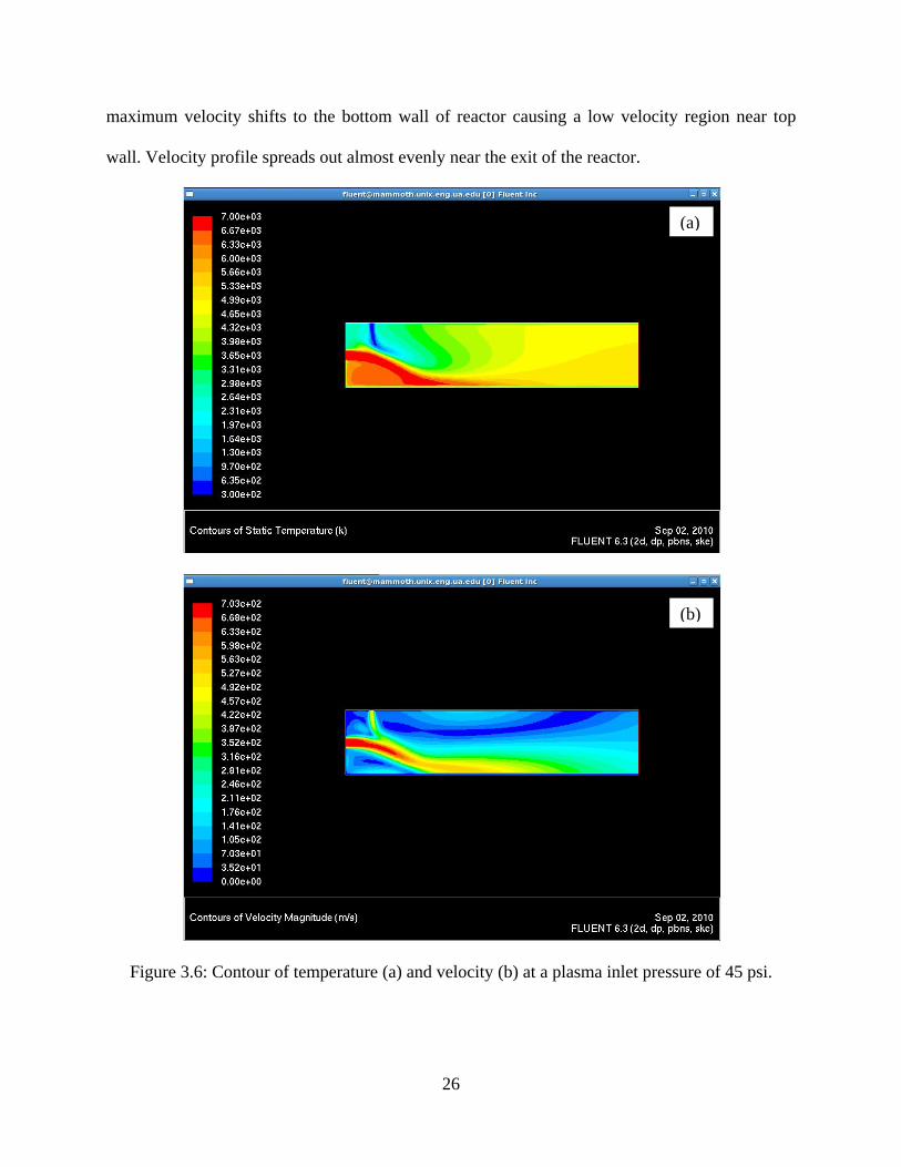
26

maximum velocity shifts to the bottom wall of reactor causing a low velocity region near top

wall. Velocity profile spreads out almost evenly near the exit of the reactor.

Figure 3.6: Contour of temperature (a) and velocity (b) at a plasma inlet pressure of 45 psi.

(a)

(b)

27

660

680

700

720

740

760

780

800

5000 6000 7000 8000 9000 10000

Vel

ocit

y (m

/s)

Temperature (K)

35 40 45 50 55 60Pressure of the plasma gas at inlet (psi)

Figure 3.7: Effect of pressure on the inlet velocity of the plasma.

The velocity profile inside the reactor is quite important as that of the temperature. This

determines the average residence time of the particles in the reactor. While the temperature

profile can be combined with thermodynamics of the reaction to determine its feasibility, the

velocity profile along with the physical properties of the powder such as its density, particle size,

etc, can be used in determining the residence time in the reactor. This when compared with the

vaporization time required for a given type of particle of a given size will determine the

feasibility and feed particle size range. Figure 3.7 shows the increase in the inlet velocity of the

plasma plume as a function of pressure of the plasma gas (Ar), plotted in the secondary x-axis.

28

As assumed earlier that the temperature is higher with increase in the plasma gas pressure, the

effect of temperature, plotted in the primary x-axis, is also shown on the inlet velocity.

Figure 3.8: Profiles obtained from different areas of the reactor denoted by line numbers.

To better understand the flow through the reactor chamber, sections were made at

different parts in the reactor as shown in the Figure 3.8. There are sections at a distance half way

to the solid feed point, at the solid feed entrance, half way of the entire reactor and at the end of

the reactor chamber, labeled as line 5, 6, 7 and 8 respectively. There is also a section made at the

center of the reactor along the flow of the plasma labeled as line 9. The flow profiles along these

labeled sections were obtained. The velocity along the radial lines 5, 6, 7 and 8 are plotted in

Figure 3.9 (a).

As can be seen, the velocity of plasma at the center is highest closer to the plasma entry.

At half way of the reactor length, the velocity is biased more towards the bottom of the reactor

which is an effect of the incoming carrying gas from the solid feed port. At the end of the

reactor, the velocity varies linearly along the radius of the reactor from about 100 m/s at the top

to about 230 m/s at the bottom. At the center of the reactor the velocity is very high closer to the

plasma torch and it starts to decrease exponentially right after the entry of the carrying gas from

Line 9

Line 5 Line 6

Line 7 Line 8

29

the solid feed inlet. It reaches a minimum and stabilizes at about a 140 m/s all the way to the end

of the reactor as can be seen from Figure 3.9 (b).

Figure 3.9: Velocity profile along radial (a) and axial (b) directions at inlet pressure of 45 psi.

0

0.012

0.024

0.036

0.048

0.06

0.072

0.084

0.096

0 100 200 300 400 500 600 700 800

Rad

ial D

ista

nce

(m

)

Velocity (m/s)

line 5line 6line 7line 8

0

100

200

300

400

500

600

700

800

0 0.044 0.088 0.132 0.176 0.22 0.264 0.308 0.352 0.396 0.44

Vel

ocit

y (m

/s)

Axial Distance (m)

line 9

(a)

(b)

30

Figure 3.10: Assume Flow Path of Solid Feed.

If the feed powder was fed through the feed port and as a first principle approximation if

the velocity of the particle is equal to velocity of the gasses and the plume in the reactor, the

residence time of the particles in the reactor can be calculated. The dark line inside the reactor

shown in Figure 3.10 is an approximate representation of the path of the solid feed. An estimate

of average velocity for flow from the powder feed port to the center of reactor and the flow

through the middle of reactor was estimated for various plasma gas pressures. Using these

average flow velocities, average residence times were calculated and are given in Table 3.3.

Table 3.3: Average residence time in the plasma reactor as a function of plasma inlet pressure.

Inlet Pressure (psi) Residence time (ms)

40 2.6974

45 2.5723

50 2.4201

55 2.3432

31

This residence times can be taken as the most conservative estimate as it does not take

into consideration the increase in density of the particulate matter compared to gasses and the

plasma plume. An estimate of the vaporization time of various feed materials of different sizes

and a comparison with residence time in the reactor will provide information on whether the feed

particles are completely vaporized.

3.5 3D plasma reactor model:

The flow properties of plasma plume in a three dimensional space is more accurate and is

a closer representation of actual plasma reactor. Hence a three-dimensional grid was generated

using Ansys 13.0® workbench [91] which is an integrated software that can generate the grid,

setup the computational fluid dynamics (CFD) problem, generate solution and compare results

from different case studies. A 3D axisymmetric geometry was generated using DesignModeler®.

Meshes of various sizes were created on the geometry using Meshing®. Fluent® 3d, pressure-

based, realizable k-epsilon version was used in the setup and solution of the CFD problem. The

results and post-processing of the obtained results such as generation of contours, and graphs,

etc., were done using CFD-Post®. DesignModeler®, Meshing®, Fluent® and CFD-Post® are all

parts of the Ansys 13.0 workbench®.

Assumptions similar to those made in the 2D model were used in the 3D model as a first

approximation. As the first step no species transport was considered in generating the flow field

of plasma plume inside reactor. This will help understand the velocity and temperature profiles

inside the reactor. The effect of particulate feed type and the solid feed rate into the reactor is a

separate case study.

32

3.6 Defining equations in 3D model:

Three different turbulent models were used in the 3D model, namely, k-, k- and

transition SST model. The transport equations for turbulent kinetic energy, k, and turbulence

dissipation rate, , for standard k- model are defined in equations (7) – (9) in section 3.2.

The transport equations for the standard k- model describing the turbulent kinetic

energy k and the specific dissipation rate are given below:

Where,

Gk - Generation of turbulence kinetic energy due to mean velocity gradients; G - Generation of

; Yk and Y – Dissipation of k and due to turbulence; Sk and S – User-defined sources terms

for k and .

Effective diffusivities for the k- model are defined in equations (13) and (14) while the

turbulent viscosity, t, using k and is defined in equation (15).

)11(kkkj

kj

ii

SYGx

k

xku

xk

t

)12( SYGxx

uxt jj

ii

)13(k

tk

)14(

t

)15(* k

t

33

)17(Rek

t

Where, k and are the turbulent Prandtl numbers for k and respectively.

At low Reynolds numbers, the coefficient, * defined in equation (16), helps in

damping the turbulent viscosity. At high Reynolds numbers, the coefficient is 1* * .

Model constants for the standard k- model are Rk = 6; *0 = i/3; i = 0.072; k = 2.0; = 2.0.

The following equations represent the transport equations for transition SST model for

intermittency, , given in equation (18). Defining equation for transition and destruction sources

are given in equations (19) and (20) respectively.

192 3

1

Consetlength FSFP

2011 PE

Where, S - Strain rate magnitude; Flength - Empirical correlation that controls the length of the

transition length.

212 12 turbFcP

22222 PcE

Where, is the vorticity magnitude. The constants for the intermittency equations are c1=0.03;

c2=50; c3=0.5; =1.0.

)18(2211

j

t

jj

j

xxEPEP

x

U

t

)16(/Re1

/Re*

*0*

kt

kt

R

R

34

3.7 Turbulence and grid refinement in 3D model:

Figure 3.11: Various grid sizes for grid refinement studies in 3D thermal plasma reactor: (a)

8013 nodes, (b) 11516 nodes and (c) 18936 nodes.

(a)

(b)

(c)

35

Figure 3.12: Velocity profile at the cross-section of the feed port: (a) standard k- model, (b)

standard k- model and (c) Transition SST model.

(a) (b)

(c)

36

Figure 3.13: Velocity profile at the symmetry of the reactor: (a) standard k- model, (b) standard

k- model and (c) Transition SST model.

(a)

(b)

(c)

37

A grid containing 5 turbulence layers and 8013 nodes was generated using Meshing

console of the Ansys Workbench as shown in Figure 3.11 (a). Three identical problems were

setup with the variation of the turbulence model and were solved using the Fluent console.

Figure 3.12 shows the velocity contours at the cross-section of feed port for three turbulence

models. Not much variation was observed in the velocity of plasma at the center of reactor in all

three cases. The major difference observed was in the velocity profile due to turbulence near the

wall. The standard k- model does not resolve the turbulence near the wall as well as the

standard k- model and is best resolved using the transition SST model.

Figure 3.14: Line profiles created in the reactor to compare the modeling results from various

case studies.

Contours of velocity magnitude were also obtained at the symmetry plane of the plasma

reactor. As can be seen from Figure 3.13 (a), the velocity profile is not well resolved in the case

of standard k- model, not only by the wall but also in the entire reactor. A comparison with the

standard k- and the transition SST models show that the resolution of turbulent velocity at the

38

wall, near the feed entry and through the reactor is better with the k- model and is best using

the transition SST model.

0 100 200 300 400 500 600 70010

8

6

4

2

0

Rad

ial D

ista

nce

(cm

)

Velocity (m/s)

k- Model k- Model SST Model

Figure 3.15: Comparison of velocity magnitudes along the feed entry point using the three

turbulence models.

To compare the three models, two line profiles were created in the reactor; the first along

the radial direction at the feed entry point and the second along the axial direction at the center of

reactor. A schematic of these line profiles are shown in Figure 3.14. Velocity magnitude along

the radial direction at the feed entry point was obtained and plotted in Figure 3.15 for all the

three turbulence models. There is not much variation in the profiles obtained from the three

models. The other important observation that can be made from this graph is that velocity of the

plasma gas is not zero at the wall. This suggests that the mesh generated is not fine enough and

39

needs to be refined to obtain consistent and acceptable results. A plot of the velocity magnitude

at the center line of the reactor is shown in Figure 3.16. All the three models have approximately

similar velocity profile until the feed entry point near 4 cm. A variation, even though, small was

observed in the profiles after the powder feed point. The standard k- model shows highest

velocity along the center of the reactor while the standard k- model shows the lowest. Grid

refinement becomes necessary to obtain accurate and consistent results and the four equation

transition SST model will be used to refine the grids and to further solve the problem of effect of

plasma gas pressure on flow through the plasma reactor.

0 5 10 15 20 25 30 35 40 450

100

200

300

400

500

600

700

800

Vel

ocit

y (m

/s)

Axial Direction (cm)

k- Model k- Model SST Model

Figure 3.16: Comparison of velocity magnitudes along the center of reactor using the three

turbulence models.

40

Grid refinement was done using three different grids as shown in Figure 3.11 using the

transition SST turbulence model. The first mesh with 8013 nodes was created with 5 layers by

the wall. The second mesh was created with 5 layers as well, but with reduced grid size, thus has

11516 nodes. The third mesh with 18936 nodes was created with same grid size as the second

mesh but with 10 layers near the wall.

Figure 3.17: Velocity profile at the cross-section of the feed port: (a) 8013 nodes, (b) 11516

nodes and (c) 18936 nodes.

(a) (b)

(c)

41

Figure 3.18: Velocity profile at the symmetry of the reactor: (a) 8013 nodes, (b) 11516 nodes and

(c) 18936 nodes.

(a)

(b)

(c)

42

Figure 3.17 shows the contours of velocity magnitude at the cross-section of the feed port

using various grid sizes. The contour using the mesh with 8013 nodes (grid 1) shows the shape of

the contour is a function of shape of the mesh. This is especially the case at the center of the

reactor where the velocity is relatively high. As the grid size is reduced, as in the case of 11516

nodes (grid 2) and 18936 nodes (grid 3), the shape of the contour is much smoother. The increase

in the number of turbulence layers from 5 in grid 2 to 10 in grid 3 creates a high velocity regime

in the top and the bottom of the reactor and restricts the flow of the mainstream fluid to the

center of the reactor.

0 100 200 300 400 500 600 70010

8

6

4

2

0

Rad

ial D

ista

nce

(cm

)

Velocity (m/s)

8013 Nodes 11516 Nodes 18936 Nodes

Figure 3.19: Comparison of velocity magnitudes along the feed entry point using three different

grid sizes.

43

The contours of velocity magnitude along the symmetry of the reactor are shown in

Figure 3.18 for the three grid sizes. The increase in the grid size from grid 1 to grid 2 improves

the shape of the contours obtained. On the other hand, increasing the number of turbulence layers

from 5 to 10 (grid 2 to grid 3) creates a high velocity regime at the top and the bottom of the

reactor along the feed entry port.

0 5 10 15 20 25 30 35 40 450

100

200

300

400

500

600

700

800

Vel

ocit

y (m

/s)


8013 Nodes 11516 Nodes 18936 Nodes

Figure 3.20: Comparison of velocity magnitudes along the center of reactor using three different

grid sizes.

A comparison of the velocity profiles along the radial and the axial directions using the

three grid sizes is shown in Figures 3.19 and 3.20, respectively. It is seen from the radial velocity

profile that the increase in grid size from grid 1 to grid 2 updates the velocity at the wall to zero.

The velocity profile, otherwise, is similar to that obtained from grid 1. The increase in the

44

turbulence layers from 5 to 10 (from grid 2 to grid 3), creates a high velocity regime at the top

and the bottom of the reactor near the feed entry. This also reduces the mainstream velocity.

Similar observation is made using the velocity profile at the center line. The mainstream velocity

of grid 2 is higher than that of grid 1 and grid 3, the latter being lower due to increased

turbulence layers. Hence to obtain a conservative model, a grid with higher velocity will be

chosen for further analysis, which will lead to a smaller particle residence time in the reactor.

Hence grid 2 was chosen along with the transition SST turbulence model to determine the effect

of plasma inlet pressure on the velocity profile in the reactor.

3.8 Results from 3D plasma reactor model:

A grid with 11516 nodes and 5 turbulence layers and transition SST turbulence model

was used in the determination of effect of pressure of plasma gas. Five different plasma gas

pressures were considered, i.e. 35, 40, 45, 50 and 55 psi. Assumption similar to the 2D model

was made that a 5 psi increase in the plasma gas pressure can allow for an increase of plasma

temperature by 1000 K. Hence the temperatures used in the calculation were 5000 K, 6000 K,

7000 K, 8000 K, and 9000 K corresponding to the plasma gas pressures of 35, 40, 45, 50, and 55

psi, respectively.

The problem setup and solution was done using Fluent varying the inlet plasma gas

pressure and holding the rest of the parameters constant. Axial and radial line profiles were

created similar to that shown in Figure 3.14 for all the cases. The velocity profile for the radial

line along the feed entry is shown in Figure 3.21 for the five different gas pressures.

45

Figure 3.21: Comparison of velocity magnitudes along the feed entry point using five different

plasma inlet gas pressures.

The increase in the plasma gas pressure has an effect on the velocity in almost all places

in the reactor other than the wall. The increase in pressure from 35 psi to 55 psi, increases the

velocity at the feed entry point from about 440 m/s to about 493 m/s. The effect on the velocity

of mainstream is rather high and the velocity varies from about 493 m/s for a pressure of 35 psi

to about 624 m/s at 55 psi. Such increase in velocity will have enormous effect on the residence

time of particles in the reactor and will restrict the size of particle that can be used in

experiments.

0

2

4

6

8

100 100 200 300 400 500 600 700

Rad

ial D

irec

tion

(cm

)

Velocity (m/s)

SST model 35 psiSST model 40 psiSST model 45 psiSST model 50 psiSST model 55 psi

46

Figure 3.22: Comparison of velocity magnitudes along the center of the reactor using five

different plasma inlet gas pressures.

Similar observation was made when the velocity magnitude along the center of the

reactor was plotted as a function of the axial direction as shown in Figure 3.22. The velocity

increased from about 590 m/s at 35 psi to about 740 at 55 psi. The increase in the velocity at any

given point in the reactor seems to vary linearly as a function of the plasma inlet gas pressure.

The velocity at the exit of the reactor varies from 68 m/s to 86 m/s for a corresponding variation

in gas pressure from 35 psi to 55 psi.

0

100

200

300

400

500

600

700

800

0 5 10 15 20 25 30 35 40 45

Vel

ocit

y (m

/s)


SST model 35 psiSST model 40 psiSST model 45 psiSST model 50 psiSST model 55 psi

47

580

600

620

640

660

680

700

720

740

760

780

800

5000 6000 7000 8000 9000

2D Model 3D Model

Temperature (K)

Vel

ocity

(m

/s)

35 40 45 50 55

Pressure (psi)

Figure 3.23: Effect of pressure on the inlet velocity of the plasma and comparison between the

2D model and the 3D model.

The maximum velocity at the inlet of the plasma torch is plotted as a function of the inlet

plasma gas pressure in Figure 3.23. Results from the 2D model were also plotted along with that

from the 3D model. Similar to the 2D model, the increase in velocity with the increase in the

inlet plasma gas pressure was observed to be almost linear. While the trend is similar to the 2D

model, the velocity at any given pressure was found to be lower by about 35 – 40 m/s in the 3D

model.

48

Figure 3.24: Assume flow path for solid feed in 3D model.

An assumed flow path of the solid feed similar to the 2D model was generated in the 3D

model as shown in Figure 3.24. Based on the average velocities from the powder feed port to the

center of the reactor and the flow through the center of the reactor, average residence times were

calculated for various plasma inlet gas pressures. The values of the residence times using the 3D

model is given in Table 3.4.

Table 3.4: Average residence time in the plasma reactor using 3D model as a function of plasma

inlet pressure.

Inlet Pressure (psi) Residence Time (ms)

35 2.1396

40 1.9919

45 1.8694

50 1.7639

55 1.6732

The residence time in the reactor is a strong function of the plasma inlet pressure. Hence

during experiments, a low enough plasma inlet gas pressure must be used to ensure a longer

residence time inside the reactor.

49

CHAPTER 4

EXPERIMENTAL SETUP

The non-transferred arc D. C. plasma reactor system was used in the synthesis of

materials. A detailed schematic of the reactor system is shown in Figure 4.1. The plasma reactor

system consists of the following parts:

(i) Plasma power source

(ii) Plasma reactor system

(iii) Powder feeder

(iv) Water source

(v) Gas source

4.1 Plasma power source

The plasma source, Model PT96 was manufactured by Plasma Energy Corporation. The

power source has a non-transferred plasma torch, Model PT-50C with a maximum power rating

of 45 kW and a transferred arc plasma torch that can be used with the transferred arc reactor

setup.

The two common types of plasma torches, namely, the transferred and the non-

transferred, vary in the positioning of the electrodes and hence, the way material is heated in the

reactor system. A schematic of the two different torches is shown in Figure 4.2.

50

Figure 4.1: Schematic of thermal plasma processing system.

Figure 4.2: Schematic of non-transferred (left) and transferred (right) plasma arc torches.

51

In the non-transferred type of plasma torch, anode and cathode are both parts of the torch

and the plasma arc is formed between them and is sustained till the current and voltage are

applied to the torch. The formed plasma plume and the hot gases travel through the plasma

reactor. The non-transferred mode is usually used in the synthesis of powders using a solid

powder feed.

Transferred plasma torch has a cathode similar to the non-transferred torch. The anode in

the transferred plasma torch is a collimator which helps in the formation of the plasma arc but

the plasma is eventually transferred to the material to be used and the work piece acts as an

anode during the operation of the reactor. The ionization and the principle of operation of the

plasma torch are otherwise similar to the non-transferred torch. Unlike the non-transferred torch,

a transferred plasma torch is used in melting and refining of materials. In case of solid powder

feed, the powder has to be made into a pellet before using the transferred torch.

Figure 4.3: Photograph of plasma power source control panel.

52

The plasma power source can be operated in the range of 15 kW – 90 kW, with a

maximum expandable power of up to 150 kW. Figure 4.3 shows the control panel of the plasma

power source. The controller can be used to operate both the transferred and the non-transferred

plasma torches. If the transfer mode is set to “DISABLE” as shown in the figure, the controller is

set to non-transferred mode of operation and “ENABLE” sets the controller to the transferred

mode of operation.

Figure 4.4: Photograph of the new (left) and used (right) electrode assembly in a non-transferred

plasma torch.

The non-transferred torch consists of a cathode and a consumable copper anode as shown

in Figure 4.4. The plasma arc is formed in between the anode and the cathode and moves through

the reactor. The size and the shape of the plasma formed and the temperature distribution inside

the plasma reactor is dependent on the shape of the anode. As the anode is consumable, it needs

to be replaced on a regular basis. The photograph on the right of Figure 4.4 shows an anode that

has been consumed as a result of regular use. Anode wear can also lead to instability of the

plasma plume during the operation of the plasma reactor.

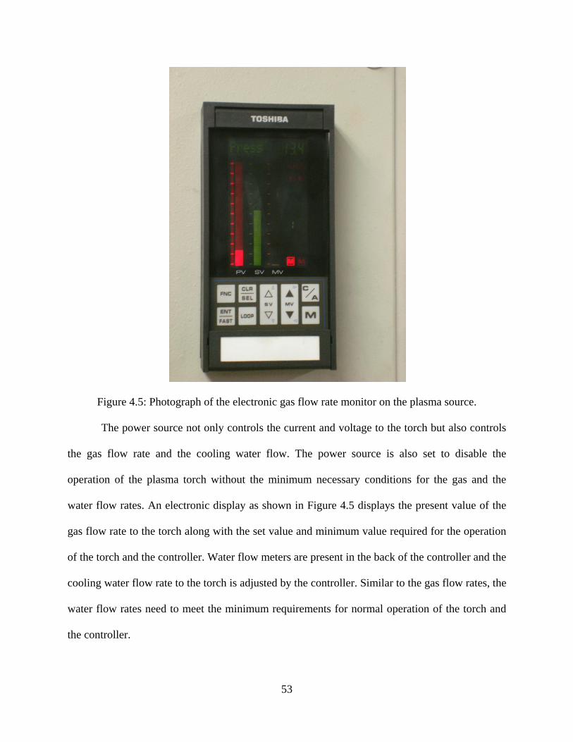
53

Figure 4.5: Photograph of the electronic gas flow rate monitor on the plasma source.

The power source not only controls the current and voltage to the torch but also controls

the gas flow rate and the cooling water flow. The power source is also set to disable the

operation of the plasma torch without the minimum necessary conditions for the gas and the

water flow rates. An electronic display as shown in Figure 4.5 displays the present value of the

gas flow rate to the torch along with the set value and minimum value required for the operation

of the torch and the controller. Water flow meters are present in the back of the controller and the

cooling water flow rate to the torch is adjusted by the controller. Similar to the gas flow rates, the

water flow rates need to meet the minimum requirements for normal operation of the torch and

the controller.

54

4.2 Plasma reactor system

The non-transferred and the transferred thermal plasma reactor systems are both in-house

built systems. The photograph in Figure 4.6 shows the reactor setup for the non-transferred mode

of operation. It consists of the following zones: Reaction zone, Quench zone and Filter zone.

Figure 4.6: Photograph of non-transferred thermal plasma reactor system.

4.2.1 Reaction zone

The reaction zone is the most important part of the plasma reactor system. The solid

powder feed fed into the reactor evaporates in this part of the reactor. The reaction by which final

product powders are formed is in vapor phase. The reactor, hence, is designed and fabricated in-

55

house to ensure all the solid feed is vaporized. The outer jacket of the reaction zone is made of

316L stainless steel which is water cooled. The inner part of the reaction zone where the

interaction between the plasma plume and the solid feed occurs and vaporization takes place is

made of graphitic carbon. A heat balance, assuming the maximum temperature to be as high as

5000 – 6000 K, was made to determine the thickness and the outer diameters of the inner carbon

lining. Several layers of insulating alumina felt were placed in between the graphite tube and the

water-cooled stainless steel jacket.

Figure 4.7: Photograph of the reaction zone.

A photograph of the reaction zone is shown in Figure 4.7. The reactor system is set up

horizontally with the solid feed, carrying gas and the reducing gas entering the reactor through a

water-cooled feed port that is set up perpendicular to the circumference of the reactor. There are

numerous k-type thermocouples in the reaction zone that are set to read the temperature in the

alumina felt. During experiments, the temperatures at various spots in the reaction zone are

56

allowed to stabilize. This will ensure most of the heat from the plasma stream is utilized in

heating the powder feed and minimum heat loss occurs. One end of the reaction zone is

connected to the plasma torch while the other is attached to the quench zone.

4.2.2 Quench zone

Figure 4.8: Photograph of the two concentric copper quenching coils in the quench zone.

Second most important part of the plasma reactor system is the quench zone. The vapors

from the reaction chamber enter into the quenching chamber and the product powders nucleate

and grow on two water-cooled concentric copper coils as shown in Figure 4.8. The outer jacket is

made of 316L stainless steel and is not water-cooled. Two k-type thermocouples are inserted into

the outer jacket of the quench zone to obtain the temperature of hot gases. The water inlet and

57

the outlet are monitored constantly using thermocouples to ensure the temperature of the cooling

water doesn’t rise more than 2⁰C. Unlike the plasma power source the cooling water for the

reactor jacket and the quench tubes are obtained from the common laboratory water source and

the used cooling water is not recycled.

4.2.3 Filter zone

Figure 4.9: Photograph of cloth filter in filter zone.

The outer jacket of the filter zone is made of 316L stainless steel and contains two

thermocouples to measure the temperature of the outgoing gases. It also consists of a cloth filter

that helps in retaining any solid products that are not accumulated on the quenching coils. A

photograph of the cloth filter assembly in the filter zone is shown in Figure 4.9. While the

quenching coils help in the nucleation and growth of powders, it also serves to reduce the

58

temperature of outgoing flue gases. Hence, the flue gases do not affect the cloth filter and the

temperature of the flue gases is about 100⁰C.

4.3 Powder feeder

Figure 4.10: Photograph of the powder feeder (left) and the circuit of the control panel (right).

A computerized powder feeder, model 1270, was used to feed the reactor with the solid

powder feed. It was manufactured by Praxair Surface Technologies, Inc. The powder feeder is

loaded with the solid powder feed and gases are connected to it. The raw materials were sieved

through a 325 mesh (~45 m) and heated to 200ºC to get rid of any adsorbed moisture. A

photograph of the powder feeder and the circuit of the control panel are shown in Figure 4.10. It

has a wheel assembly that rotates during the operation of the powder feeder at particular preset

rotations per minute (RPM). This pushes the powder into a chamber where it is mixed with the

59

gases and the gases carry the solid particles out of the feeder and into the reactor. There are two

types of gases used, namely, the carrier gas and the reducing/reacting gas. The carrier gas used in

the experiments is argon. As the solid feed is oxide material in all of the experiments, methane is

used as a reducing gas.

The rate of solid feed depends on the type and of solid material used, the flow rate of the

carrying/reducing gas mixture and the RPM of the powder feeder wheel. The type and the size of

the starting material are fixed for experiments using similar raw materials. The flow rate of the

gas mixture (argon + methane) is set to 6 LPM. The only unfixed parameter is the RPM of the

powder feeder wheel. A calibration chart is made for each raw material type for the solid feed

rate as a function of RPM.

The powder feeder is also attached with a heating element that surrounds the container

with solid feed to remove any adsorbed moisture in the material with a maximum temperature

limit of 150⁰F. The maximum allowed pressure in the powder feeder chamber is 20 psi. If the

exit of the powder feeder is blocked due to agglomeration or other reasons, a built-in security

feature releases a safety valve reducing the pressure inside the chamber.

4.4 Water source

The cooling water to the plasma torch is regulated by the plasma power source. The water

supply to the plasma power source comes from a 500 gallon high density poly ethylene tank. A

photograph of the tank and a booster pump is shown in Figure 4.11, the latter being used in

pumping water to the plasma power source. The pressure of water is maintained no less than

200 psi on the controller while the controller controls the flow rate to the plasma torch and is

about 28 GPM. The requirement for the cooling water is to be less than 38⁰C above which a

60

safety circuit turns off the power to the plasma torch. The cooling water is returned to the tank

through the plasma power source and is re-circulated. Due to the large volume of the tank, the

water temperature never exceeds the upper limit of the instrument.

Figure 4.11: Photograph of cooling water system and roughing pump assembly.

61

Figure 4.12: Flow meters controlling the flow rate of cooling water to various parts of the plasma

reactor system.

Table 4.1: Flow rate of cooling water for various parts of the plasma reactor system

Part of reactor Flow rate (LPM)

Copper feed tube 1

Stainless steel reactor jacket 2

Copper quench coils 4.5

The cooling water to the reactor jacket, the feed tube and the quenching coils are supplied

by the common laboratory water supply. Due to geometric restrictions and cooling requirement

62

for each of these parts, various flow rates were designed based on heat transfer calculations.

Table 1 gives the values of cooling water set at various places in the plasma reactor system. A

photograph of the flow meters set to the required flow rates is shown in Figure 4.12.

4.5 Gas source

Figure 4.13: Photograph of gas supply system consisting of plasma, carrier and reducing gases.

The plasma gas used in the experiments is high purity argon. Other gases can be used as

the plasma gas such as nitrogen or helium. The volume of gas used for the operation of the

reactor per unit time is less for argon and hence was used for the experiments.

Figure 4.13 shows the gas supply system that supplies argon to the plasma power source

and the gas mixture of argon and methane to the powder feeder. Two cylinders of argon are

connected to the plasma source to ensure constant uninterrupted flow of gas to the torch. Digital

flow meters are connected to manifolds to obtain the flow rates of gases. One argon cylinder for

the carrying gas and one methane cylinder for the reducing gas are connected to the powder

63

feeder. The flow rate to the powder feeder is small compared to that of the plasma gas flow rate

and hence one cylinder each will suffice the gas requirement of powder feeder. During

experimentation, the pressure of plasma argon gas at the cylinder outlet was maintained between

60 – 100 psi. The flow rate in LPM varies on the requirement at the plasma power source. There

are certain requirements on the starting, minimum and maximum pressure limits for the

programmable gas controller in the plasma power source to operate the torch and varies with the

type of torch. These values are given in the Table 2.

Table 4.2: Programmable gas controller set points in the thermal plasma power source for

various types of torch.

Type of torch Start Low High

Non-transferred 10 30 60

Transferred 20 30 60

4.6 Raw materials

Experiments for the synthesis of TiB2 were conducted using equi-molar quantities of

TiO2 (anatase, 99.9%, metals basis, Alfa-Aesar, MA, USA) and B2O3 (99.98%, metals basis,

Alfa-Aesar, MA, USA) that were mixed together and used as a powder feed to the plasma

reactor. Using argon as the carrying gas, methane as the reducing gas, 1:1 molar ratio TiO2:B2O3,

and total gas flow rate of 6 LPM, the powder feeder was calibrated for the solid feed rate in

g/min as a function of the powder feeder rotation speed in RPM as shown in Figure 4.14. A

linear fit for the graph was obtained and the two different solid feed rates, 2.15 g/min and 3.22

g/min were used for experiments. After the calibration of the powder feeder, the feed material is

fed to the reactor which is set to the required power level and the product powders are collected.

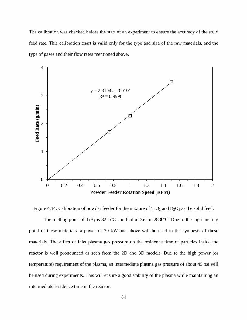
64

The calibration was checked before the start of an experiment to ensure the accuracy of the solid

feed rate. This calibration chart is valid only for the type and size of the raw materials, and the

type of gases and their flow rates mentioned above.

Figure 4.14: Calibration of powder feeder for the mixture of TiO2 and B2O3 as the solid feed.

The melting point of TiB2 is 3225ºC and that of SiC is 2830ºC. Due to the high melting

point of these materials, a power of 20 kW and above will be used in the synthesis of these

materials. The effect of inlet plasma gas pressure on the residence time of particles inside the

reactor is well pronounced as seen from the 2D and 3D models. Due to the high power (or

temperature) requirement of the plasma, an intermediate plasma gas pressure of about 45 psi will

be used during experiments. This will ensure a good stability of the plasma while maintaining an

intermediate residence time in the reactor.

y = 2.3194x - 0.0191R² = 0.9996

0

1

2

3

4

0 0.2 0.4 0.6 0.8 1 1.2 1.4 1.6 1.8 2

Fee

d R

ate

(g/m

in)

Powder Feeder Rotation Speed (RPM)

65

Experiments for the synthesis of SiC were conducted using SiO2 (99.9%, metals

basis, Alfa-Aesar, MA, USA) as a powder feed to the plasma reactor. The carrying gas used with

the powder feeder was ultra high purity Ar (AR UHP300 Gr 5.0, Airgas) and the reducing gas

was ultra high purity methane (ME UHP300 Gr 4.0, Airgas). The powder feeder was calibrated

to obtain the solid feed rate as a function of RPM as shown in Figure 4.15. The flow rate of gas

mixture, i.e. argon and methane, was maintained at 6 LPM. Two different solid feed rates, 4 and

5 g of SiO2/min were used in experiments. The calibration was checked before every experiment.

Figure 4.15: Calibration of powder feeder using SiO2 as the solid feed.

y = 2.8318xR² = 0.9989

0

2

4

6

8

10

12

14

0 0.5 1 1.5 2 2.5 3 3.5 4 4.5

Fee

d R

ate

(g/m

in)

Powder Feeder Rotation Speed (RPM)

66

4.7 Characterization of product powders

4.7.1 X-Ray Diffraction (XRD)

The product powders obtained were characterized using X-Ray Diffraction (XRD),

model Phillips PW-1710 (TiB2 experiments) and model Phillips X’Pert MPD (SiC experiments),

for phase analysis and volume fraction calculation using direct comparison method. Both the

instruments use a monochromated Cu-K radiation with a wavelength of 1.54056 Å. The Phillips

PW-1710 was operated at 40kV and 35 mA while the Phillips X’Pert MPD was operated at 45

kV and 35 mA. SiO2 slide was used to hold the sample. Vacuum grease was applied to the slide

and the product powders were dispersed on it.

4.7.2 Scanning Electron Microscope (SEM)

Scanning Electron Microscope (SEM) fitted with Energy Dispersive Spectroscopy

(EDS), model JOEL 7000 FE SEM was used to determine the morphology and elemental

composition of the product powders. The product powders were dispersed in acetone and

ultrasonicated for 5 minutes. A flat top SEM sample stub was used with a double-sided Cu tape

attached to it for holding the sample. Two drops of the ultrasonicated liquid was added to the Cu

tape and allowed to air dry and then was analyzed using SEM and EDS for morphology and

elemental analysis.

4.7.3 Transmission Electron Microscopy (TEM)

Transmission Electron Microscopy (TEM), model Tecnai F-20 TEM was used to

determine the morphology of the product powders, while the Scanning Tunneling Electron

Microscopy (STEM) was used in elemental composition analysis. High Resolution TEM

67

(HRTEM) was used in observing the lattice fringes and subsequent calculation of d-spacing. The

product powders were dispersed in acetone and ultrasonicated for 5 minutes. One drop of the

liquid containing the sample was added to a 200-mesh holy carbon Cu TEM grid. The grid was

allowed to air dry and then analyzed for morphology, elemental analysis and lattice fringes.

4.7.4 Differential Scanning Calorimetry (DSC)

Differential Scanning Calorimetry (DSC), model Perkin Elmer Diamond, was used to

determine the heat capacity of the sample. The DSC instrument was calibrated using Indium as

standard before the measurement of heat capacity. The powder sample was homogenized and

about 5-10 mg was added to a aluminum DSC sample pan. It was covered with a aluminum lid

and crimped to maintain a air tight environment for measurements. The baseline heat flow was

measured using empty sample and reference pans. The sample side was loaded with the crimped

powder sample and reference side was loaded with an empty pan. An ‘Iso-Scan-Iso’ temperature

scan with an interval of 50ºC and a heating rate of 10ºC/min was used to determine the heat flow

curves of the sample and baseline. The calculation of heat capacity of sample is done by the

difference in the heat flow between the sample and the baseline.

4.7.5 Raman Spectra

Raman spectra of product powders were obtained with a Bruker Senterra Raman

microscope, using 785 nm wavelength, 1 mW laser source at a 50x magnification. The sample

powders were added to a glass slide and surface was flattened. Using a 50x lens, the sample was

focused. Using the above mentioned laser source settings, the spectra was obtained with three

repetitions per sample. The final spectrum of a sample is the average of three repetitions.

68

4.7.6 X-Ray Photoelectron Spectroscopy (XPS)

X-Ray Photoelectron Spectroscopy (XPS), model KRATOS AXIS 165 XPS/Auger, was

used to determine the chemical binding states of the product powders. Powder sample was

dispersed on a glass slide using vacuum grease. The sample was then focused with a CCD

camera and the XPS spectra were obtained. The sample was analyzed for C-1s, O-1s, Si-2s and

Si-2p binding energies.

4.7.7 Thermo-Gravimetric and Differential Thermal Analyzer (TG-DTA)

Perkin Elmer Diamond Thermo-Gravimetric and Differential Thermal Analyzer (TG-

DTA) was used to measure the weight change and the heat flow to or from the sample. Platinum

sample and reference pans were used during analysis. The instrument was calibrated using

indium, aluminum and tin for heat flow. The product powders were homogenized and about 15-

20 mg was added to the sample pan. The reference pan was added with approximately same

amount of alumina. The experiment was conducted in air atmosphere. A temperature ramp from

50ºC to 1100ºC was done at a heating rate of 10ºC/min. The weight gain/loss with corresponding

heat loss/gain was recorded as a function of temperature of the sample.

69

CHAPTER 5

SYNTHESIS OF TITANIUM DIBORIDE

5.1 Thermochemical calculations

Thermodynamic calculations were made on the TiO2-B2O3-CH4 system using HSC

Chemistry 5.1® [92]. In the TiO2-B2O3-CH4 system, the molar ratio of the solid feed TiO2 and

B2O3 was maintained a constant at 1:1. The reducing gas used was methane and the molar ratio

of reducing gas to that of the solid feed was varied between 4 and 7. The calculations are based

on the principle of minimization of Gibb’s energy [93] for a set of reactants at a given

temperature and pressure. The equation describing this principle is given in equation 23.

∑ ∑ ∑ (23)

G is the total Gibbs energy of the system, Gi0 is standard molar Gibbs energy of species i at

temperature T and pressure P, ni is number of moles of species i, Pi is the partial pressure of

species i, Xi is mole fraction of species i, and i is activity coefficient of species i.

Formation of various elements and compounds in different phases can be determined

using the thermochemical calculations as a function of temperature if pressure is maintained a

constant. Figure 5.1 and Figure 5.2 shows the stability of phases as a function of temperature

between 0 and 7000⁰C for molar ratio of solid feed to methane (TiO2:B2O3:CH4) varying from

1:1:4 to 1:1:7. It is observed in all the cases that the formation of TiB2 in various quantities

occurs between the temperatures of about 1000 – 3500⁰C.

70

Figure 5.1: Formation of various product phases at a molar ratio of (a) TiO2:B2O3:CH4=1:1:4 and

(b) TiO2:B2O3:CH4=1:1:5.

(a)

(b)

71

Figure 5.2: Formation of various product phases at a molar ratio of (a) TiO2:B2O3:CH4=1:1:6 and

(b) TiO2:B2O3:CH4=1:1:7.

(a)

(b)

72

If complete reduction of oxides takes place in the presence of methane to form elemental

titanium and boron in vapor phase with subsequent reaction of the elements to form titanium

diboride, the following stoichiometric reactions (equations 24-27) can be written for varying

molar ratio of methane.

4 4 8 (24)

5 5 10 (25)

6 5 12 (26)

7 5 2 14 (27)

Table 5.1: Theoretical yield of TiB2 and by-products in mol% as a function of molar ratio of

methane in feed.

Molar ratio

of Methane TiB2 TiO2 B2O3 B2O3(g) TiB B TiC TiO C

4 54.69 5.47 5.47 13.28 6.25 3.13 0.00 11.72 0.00

5 82.51 0.00 0.00 1.35 7.17 4.48 0.00 0.00 4.48

6 47.06 0.00 0.00 0.00 1.96 1.96 0.00 0.00 49.02

7 31.15 0.00 0.00 0.00 1.31 1.97 0.33 0.00 65.25

The results from thermochemical calculations are shown in Table 5.1 for the

TiO2:B2O3:CH4 system. At lower molar ratios of methane especially at 4, the conversion to TiB2

is not complete with the formation of some of the oxide phases such as TiO, TiO2 and B2O3

along with some boron and titanium boride (TiB) in the product. There is no carbon observed in

the systems with a methane molar ratio of 4 in the feed. At 4 moles of methane in the feed, the

73

formation of about 5 mol% of TiO2 and B2O3 each, about 13 mol% B2O3 (g), 6 mol% TiB, 3

mol% B and about 12 mol% TiO, was observed.

The formation of oxides, at 4 moles of methane in the feed, such as TiO2, TiO and B2O3

in the final products is attributed to the fact that the amount of carbon in the reactants is low and

is not sufficient to reduce the reactants in the reactor. With the increase in the molar ratio of

methane to 5, the oxide phases such as TiO2 and B2O3 disappear while TiB and B along with

some carbon are observed. It is also notable that the amount of TiB2 increased from about 55

mol% at a molar ratio of 4 to about 82 mol% at a molar ratio of 5. Subsequent increase in the

molar ratio of methane to 6 and 7 shows no oxide phases and the amount of TiB and B were

almost minimum in the final product. On the contrary, the only two major phases observed are

TiB2 and carbon, with substantial increase in the amount carbon to about 50 mol% at a molar

ratio of 6 and about 65 mol% at a molar ratio of 7. While 5 moles of methane has just sufficient

enough carbon to reduce the oxides, an increase in the moles of methane to 6 and 7 increases the

amount of carbon in the product powder. The formation of TiC in very small quantities is

observed at 7 moles of methane. The formation of TiB and B is seen in the products using higher

molar ratio of methane in the feed but are in significantly smaller quantities and can be

neglected.

Theoretical recovery of TiB2 and other phases as a function of varying methane mole

fraction shows that the yield of TiB2 is maximum (>80 mol %) when the molar ratio is 5 and at a

temperature of 1770⁰C (2043 K). The amount of TiB2 increases with the increase in molar ratio

of CH4 up to 5 moles as shown in Figure 5.3. Further increase in the molar ratio of CH4 increases

the amount of carbon formed in the final product. The yield of TiB2 decreases with increase in

methane content above 5 moles.

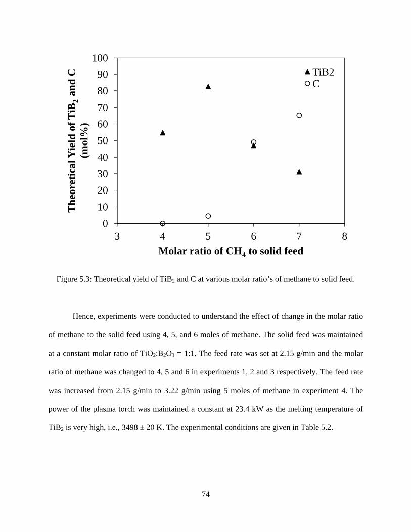
74

Figure 5.3: Theoretical yield of TiB2 and C at various molar ratio’s of methane to solid feed.

Hence, experiments were conducted to understand the effect of change in the molar ratio

of methane to the solid feed using 4, 5, and 6 moles of methane. The solid feed was maintained

at a constant molar ratio of TiO2:B2O3 = 1:1. The feed rate was set at 2.15 g/min and the molar

ratio of methane was changed to 4, 5 and 6 in experiments 1, 2 and 3 respectively. The feed rate

was increased from 2.15 g/min to 3.22 g/min using 5 moles of methane in experiment 4. The

power of the plasma torch was maintained a constant at 23.4 kW as the melting temperature of

TiB2 is very high, i.e., 3498 ± 20 K. The experimental conditions are given in Table 5.2.

0

10

20

30

40

50

60

70

80

90

100

3 4 5 6 7 8

Th

eore

tica

l Yie

ld o

f T

iB2

and

C

(mol

%)

Molar ratio of CH4 to solid feed

TiB2C

75

Table 5.2: Experimental design for the production of TiB2 using thermal plasma reactor.

Expt. # Raw Materials Molar Ratio Plasma Power (kW) Feed Rate (g/min)

1 TiO2:B2O3:CH4 1:1:4 23.4 2.15

2 TiO2:B2O3:CH4 1:1:5 23.4 2.15

3 TiO2:B2O3:CH4 1:1:6 23.4 2.15

4 TiO2:B2O3:CH4 1:1:5 23.4 3.22

5.2 Synthesis and characterization of titanium diboride

5.2.1 Phase and morphology of solid feed

The molar ratio of the solid feed TiO2:B2O3 was maintained at 1:1, consistent with the

thermochemical calculations. The mixture of the two oxides in the solid feed was analyzed using

XRD and the resulting pattern is shown in Figure 5.4.

Figure 5.4: X-Ray diffraction pattern of 1:1 molar TiO2:B2O3.

76

Figure 5.5: SEM images of solid feed powder at a molar ratio of TiO2:B2O3 = 1:1.

The morphology of the solid feed material in the molar ratio of TiO2:B2O3 = 1:1 was

analyzed using SEM. The images shown in Figure 5.5 show that the starting material was in the

size range of 20 – 50 m.

5.2.2 Phase, composition and morphology of product powders

Figure 5.6 shows the XRD patterns from the experiments conducted at different molar

ratio of methane and the feed rates. The amount of TiB2 in the final product in the case of

experiments 1 (4 moles of CH4 in feed) and 3 (6 moles of CH4 in feed), are relatively very less

compared to TiO2, B2O3 and C. Another important observation from the diffraction pattern is that

titanium dioxide in the product powder has changed from its original crystal structure of anatase

to its high temperature crystal structure, namely rutile. The anatase oxide phase was also present

in the product powders from experiments 1 and 3 but the amount was relatively small. This

suggests that the powders were vaporized and/or heated to very high temperatures and due to the

rapid quenching that takes place in the reactor TiO2 was condensed in its high temperature

structure. The experiments conducted with a methane molar ratio of 5 in feed yielded more TiB2

77

compared to those with molar ratios of 4 and 6 moles as can be seen from the XRD pattern

shown in Figure 5.6 (Expt-2).

20 30 40 50 60 70 80

*

0 Expt - 1

Expt - 2

Expt - 3

*

*

Inte

nsit

y (a

.u.)

Angle, 2 (degrees)

^

^

* *

*

x

0 0

0 - TiB2

* - TiO2 (a)

x - TiO2 (r)

^ - B2O

3

+ - C

^

x

0

0

+0

0 0 +

^

^

+ 0

*

*x* 0

*

*

^x

0

+ 0 +Expt - 4

Figure 5.6: XRD patterns of product powders obtained from different experiments.

Similar results were observed with increased solid feed rate of 3.22 g/min and a methane

molar ratio of 5 (Expt-4). The product phases such as TiC, TiB, and TiO that were obtained from

the thermodynamic simulation were not observed in the XRD patterns of product powders from

any of the experiments. Thus, we can conclude that all the phases that are thermodynamically

stable in a given system of reactions cannot be formed in the actual experiment using the thermal

78

plasma processing technique, but will serve as a good starting point for choosing experimental

conditions.

The volume fraction of the product powders were calculated using direct comparison

method from the XRD patterns. The volume fraction calculation was done on the product

powders in the condensed phase. Any products that escaped the reaction chamber in gaseous

phases are not accounted for. Similarly, amorphous phases that are present in the product

powders will not show peaks in the XRD pattern. They will rather add to the background and

hence, are not accounted for in these calculations. Some of the constants required to solve for the

volume fraction were obtained from Cullity [97]. The atomic positions of the elements in unit

cell were obtained from Pearson’s Handbook of Crystallographic Data [98]. The direct

comparison method was used in the calculation of the volume fractions of the product powders.

Equation (28) describes the equations for the product powders.

; ; ; 1 (28)

where, ITiB2, ITiO2, IB2O3 and IC represent the intensities of TiB2, TiO2, B2O3 and C respectively;

cTiB2, cTiO2, cB2O3 and cC represent the volume fractions of TiB2, TiO2, B2O3 and C respectively;

and RTiB2, RTiO2, RB2O3 and RC represent the volumes of inverse unit cell lattices of TiB2, TiO2,

B2O3 and C respectively.

Table 5.3: Yield of product powders at different feed rates with a methane molar ratio of 5 in the

feed.

Feed Rate (g/min) Yield TiB2 TiO2(r) B2O3 C

2.15 mol% 23.63 8.72 4.07 63.58

3.22 mol% 39.44 11.33 7.58 41.65

79

The values of the calculated volume fractions are reported in Table 5.3. With the increase

in the feed rate from 2.15 g/min to 3.22 g/min, the amount of TiB2 formed increased from about

24 mol% to about 40 mol%. It was also accompanied by the reduction in the amount of carbon in

the product powders from about 64 mol% to about 40 mol%.

Figure 5.7: SEM images of product powders obtained from experiment 4.

80

Figure 5.8: SEM electron image (top) of the product powders obtained from experiment 4 and

the corresponding EDS spectra (bottom).

The SEM micrograph of the product powders from experiment 4 is shown in Figure 5.7.

The particle sizes of these powders are in the range of 50-100 nm. The morphology of the

particles is about spherical and is uniform though out the sample. The Energy Dispersive Spectra

(EDS) and the corresponding electron image of the material are shown in Figure 5.8. The EDS

shows the presence of only titanium in the sample. The absence of oxygen and carbon in the

81

EDS proves that the titanium is not present as titanium oxide, titanium dioxide or titanium

carbide. Also, the absence of elemental titanium or boron from the XRD pattern of the sample

shows that the titanium is present either in the form of titanium boride (TiB) or titanium diboride

(TiB2) in the sample, as boron is not detectable using EDS. The absence of TiB phase from XRD

confirms the presence of only TiB2 in the sample.

Figure 5.9: TEM image of the product powder obtained from experiment 4.

The morphology of the material produced from experiment 4 was analyzed using TEM.

Figure 5.9 shows that the particles formed are in the range of 20-100 nm and are mostly spherical

as observed from the SEM images. A high resolution TEM image of the powder is shown in

Figure 5.10. The lattice fringes from the image were used in determining the d-spacing of the

crystal structure. From the calculations, it was found that the d-spacing was 3.75 Å, which

corresponds to the d-spacing of hexagonal boron oxide in the (1 0 0) plane.

82

Figure 5.10: HRTEM of product powders showing lattice fringes of hexagonal B2O3 in the (1 0

0) plane obtained from experiment 4.

STEM image of product powders from experiment 4 is shown in Figure 5.11. As the

major phases in the product powder (other than C) is TiB2 and TiO2, which have closer atomic

weight, phase contrast due to different phases is not as pronounced in the image. A spot EDS

was obtained from one of the brightest spots in the image which would correspond to a high

atomic number phase. It is marked in the STEM image with a red circle. The EDS corresponding

to the spot is shown on the right in Figure 5.11. Cu and Si are observed in the EDS which are

from the grid used to disperse the powders. Titanium is detected from the elemental analysis

similar to the EDS obtained from SEM-EDS. On the basis of a similar argument made earlier in

the SEM-EDS section, it can be concluded that the particle is titanium diboride.

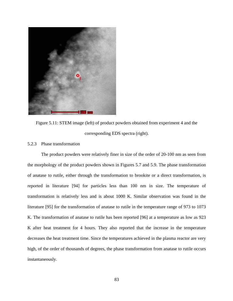
83

Figure 5.11: STEM image (left) of product powders obtained from experiment 4 and the

corresponding EDS spectra (right).

5.2.3 Phase transformation

The product powders were relatively finer in size of the order of 20-100 nm as seen from

the morphology of the product powders shown in Figures 5.7 and 5.9. The phase transformation

of anatase to rutile, either through the transformation to brookite or a direct transformation, is

reported in literature [94] for particles less than 100 nm in size. The temperature of

transformation is relatively less and is about 1000 K. Similar observation was found in the

literature [95] for the transformation of anatase to rutile in the temperature range of 973 to 1073

K. The transformation of anatase to rutile has been reported [96] at a temperature as low as 923

K after heat treatment for 4 hours. They also reported that the increase in the temperature

decreases the heat treatment time. Since the temperatures achieved in the plasma reactor are very

high, of the order of thousands of degrees, the phase transformation from anatase to rutile occurs

instantaneously.

84

5.2.4 Particle size reduction

Another important observation can be made from the morphology of the product

powders. The initial particle size of the solid feed as shown in Figure 5.5 is about 45 m or less.

A high resolution TEM (HRTEM) image of unreacted boron oxide is shown in Figure 5.10. It is

seen that particle size of the chemically unreacted boron oxide has reduced to about tens of

nanometers from submicron scale in the raw material. This observation can be used to conclude

that thermal plasma can be used in reduction of particle size of materials. The actual mechanism

in which the size reduction takes place is unknown at this time. As mentioned earlier the

temperature inside the reactor is of the order of thousands of degrees. One of mechanism that is

proposed here, by which the size reduction takes place, might be complete vaporization of the

feed and re-condensation of the unreacted boron oxide. The second reaction proposed is that the

surface of the particle melts and vaporizes at high temperatures, but complete vaporization

doesn’t take place leading to the reduction in the particle size.

85

CHAPTER 6

SYNTHESIS OF SILICON CARBIDE

6.1 Thermochemical calculations

Thermodynamic calculations were made on the SiO2-CH4 system using HSC Chemistry

5.1® [92]. In the SiO2-CH4 system, the molar ratio was varied between 0.8 and 5. The

calculations are based on the principle of minimization of Gibb’s energy [93] for a set of

reactants at a given temperature and pressure as explained in equation (23) in chapter 5.

Figure 6.1: Thermochemical calculations to determine stable phases at 1220⁰C as a function of

molar ratio of methane to solid feed.

0.00.10.20.30.40.50.60.70.80.91.01.11.21.31.41.5

0

10

20

30

40

50

60

70

80

90

100

0 1 2 3 4 5 6

Th

eoretical Yield

(mol%

)T

heo

reti

cal Y

ield

(m

ol%

)

Molar Ratio of Methane to Solid Feed

SiO2

C

SiC

Si

T = 1220ºC

86

The amount of theoretical product formation as a function of molar ratio of methane in

the feed at various temperatures was calculated and is shown in Figure 6.1. At 1220⁰C, the

temperature is relatively low and the amount of SiO2 reduced is relatively small as well. The

amount of carbon at 1220⁰C increases with increase in the amount of methane consistent with

the small amount of SiO2 reduced.



The equilibrium composition at 1520⁰C (Figure 6.2) shows an increase in the amount of

SiC with increase in the molar ratio of methane in the feed from 0.8 and reaches a maximum at

3. The SiC formation decreases with subsequent increase of molar ratio of methane from 3 to 5

with a corresponding increase in the amount of carbon and almost no SiO2 present.

0

10

20

30

40

50

60

70

80

90

100

0.5 1.5 2.5 3.5 4.5 5.5

Th

eore

tica

l Yie

ld (

mol

%)


SiO2

C

SiC

SiO(g)

Si

T = 1520ºC

87



When the temperature is increased to 2120⁰C, SiO2 is converted to SiO in gaseous phase

(Figure 6.3). Silicon forms when molar ratio of methane was increased above 1 and is a

maximum at 2. SiC forms only when the molar ratio of methane is 3. The amount of C increases

and SiO decreases with the increase in the amount of methane. At extremely high temperature,

for example at 3010⁰C, there is no formation of SiC, with Si forming after a methane molar ratio

of 1 and has a maximum at 2 (Figure 6.4). The amount of SiO decreases and the amount of C

increases with the increase in the methane concentration in feed.

It is concluded from thermochemical calculations that formation of SiC is favorable at

lower molar ratios of methane and is a maximum at 3. Favorable temperatures for the formation

of SiC are from about 1500⁰C to 2100⁰C. Formation of Si is favored at lower molar ratios of

0

20

40

60

80

100

120

0.0 1.0 2.0 3.0 4.0 5.0 6.0

Th

eore

tica

l Yie

ld (

mol

%)


SiO2SiCSiCSiO(g)

T = 2120ºC

88

methane as well but is a maximum at a molar ratio of 2. Formation temperatures favorable for Si

are from about 2100⁰C to 3000⁰C. Formation of carbon increases steadily with the increase of

methane in the feed. Relatively very low amount of SiC is formed at very low (<1500⁰C) and at

very high (>2100⁰C) temperatures. These observations led to the design of experiments with the

variation in the moles of methane between 0.8 and 3, two different plasma powers 18.9 and 21.6

kW and two different solid feed rates, 4 and 5 g of SiO2/min. The experimental conditions are

given in Table 6.1.



0

20

40

60

80

100

120

0.0 1.0 2.0 3.0 4.0 5.0 6.0

Th

eore

tica

l Yie

ld (

mol

%)


Si

C

SiO(g)

T = 3010ºC

89

Table 6.1: Experimental Conditions for the production of SiC using thermal plasma

Expt. # Raw Materials Molar Ratio Plasma Power (kW) Feed Rate (g/min)

1 SiO2:CH4 1:1 21.6 5

2 SiO2:CH4 1:0.8 21.6 5

3 SiO2:CH4 1:1.5 21.6 5

4 SiO2:CH4 1:1 18.9 5

5 SiO2:CH4 1:2 21.6 5

6 SiO2:CH4 1:2.5 21.6 5

7 SiO2:CH4 1:1 21.6 4

8 SiO2:CH4 1:2 21.6 4

9 SiO2:CH4 1:3 21.6 4

6.2 Synthesis and characterization of silicon carbide

6.2.1 Phase and composition of product powders

X-ray diffraction was done on the product powders from the experiment to determine the

product phases. The XRD patterns from experiments using a constant plasma power of 21.6 kW

and a constant feed rate of 5 g/min are shown in Figure 6.5. SiC is the major phase in all the

experiments with the variation of molar ratio of methane, while the amount of Si, C and SiO2

varies. Figure 6.6 shows the XRD patterns of the product powders from experiments with a

constant feed rate of 4 g/min and a constant power of 21.6 kW. The amount of SiC is more in the

case of 1:1 molar ratio of SiO2:CH4 but decreases with increase in the amount of methane with a

corresponding increase in the amount of SiO2 and carbon in the product powders.

90

20 40 60 80 100 120

0

2000

4000

6000

8000

10000

12000

(1 0

1)#

(0 0

2)^

SiO2:CH

4 = 1:2.5

SiO2:CH

4 = 1:2

SiO2:CH

4 = 1:1.5

SiO2:CH

4 = 1:1

Inte

nsity

(a.

u.)

Angle, 2 (degrees)

SiO2:CH

4 = 1:0.8

Feed Rate = 5g SiO2/min

Power = 21.6 kW(1 1

1)*

(2 0

0)*

(2 2

0)*

(3 1

1)*

(2 2

2)*

(3 3

1)*

(4 2

0)*

(1 1

1)0

(2 2

0)0

* SiC0 Si ̂C

# SiO2

(3 1

1)0

(1 0

2)^

(1 0

0)^

(1 0

0)#

Figure 6.5: XRD pattern of product powders formed at various molar ratios of methane to solid

feed and at a solid feed rate of 5g SiO2/min.

The volume fractions were calculated using the direct comparison method as described

earlier and was converted to corresponding mole percent and is presented in Figure 6.7 for the

experimental yield of products at a feed rate of 5 g/min and a power of 21.6 kW. As can be seen

SiC is the major phase formed with a minimum of about 40 mol% and a maximum of about 65

mol% at corresponding methane molar ratios of 0.8 and 2 in the feed, respectively. The amount

of Si is a maximum at a methane molar ratio of 1 and is determined to be about 40 mol%. SiO2 in

the product powder varies between a minimum of about 5 mol% and a maximum of about 35

mol%. The amount of C is relatively low in the experiments using a feed rate of 5 g of SiO2/min

and is a maximum of about 20 mol% at a methane molar ratio of 2.5. It can be concluded that

91

relatively lower molar ratios of methane favors formation of Si while relatively higher molar

ratios of methane favors the formation of SiC at a feed rate of 5g SiO2/min.

20 40 60 80 100 120

0

1000

2000

3000

4000

5000* SiC0 Si ̂C

# SiO2

Feed Rate = 4g SiO2/min

Power = 21.6 kW

SiO2:CH

4 = 1:3

SiO2:CH

4 = 1:2

SiO2:CH

4 = 1:1

Inte

nsi

ty (

a.u

.)

Angle, 2 (degrees)

(1 0

0)#

(0 0

2)^

(1 0

1)#

(1 1

1)0

(1 1

1)*

(2 0

0)*

(2 2

0)*

(3 1

1)*

(2 2

2)*

(3 3

1)*

(4 2

0)*

(1 0

0)^

(1 0

2)^

(3 1

1)0

Figure 6.6: XRD patterns of product powders formed at various molar ratios of methane to solid

feed and at a solid feed rate of 4g SiO2/min.

Similar calculations were done on the product powders from the experiments conducted

at a solid feed rate of 4 g of SiO2/min. It can be seen from Figure 6.8 that the amount of SiC and

Si are both a maximum at a methane molar ratio of 1. The experimental yield of SiC and Si were

found to be about 55 mol% and 35 mol% respectively. The amount of SiO2 in the product

powders seemed to be almost a constant with change in the molar ratio of methane and is about

10 mol%.

92

Figure 6.7: Experimental yield of product powders formed at various molar ratios of methane to

solid feed and a solid feed rate of 5g/min.

Figure 6.8: Experimental yield of product powders formed at various molar ratios of methane to

solid feed and a solid feed rate of 4g/min.

0

10

20

30

40

50

60

70

0.5 1 1.5 2 2.5 3

Yie

ld (

mol

%)


SiC ProductionFeed Rate 5 g/min

Power 21.6 kW

SiO2SiSiCC

0

10

20

30

40

50

60

70

0 1 2 3 4

Yie

ld (

mol

%)


SiC ProductionFeed Rate 4 g/min

Power 21.6 kW

SiO2SiSiCC

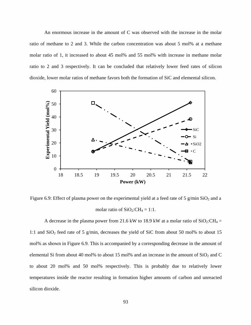
93

An enormous increase in the amount of C was observed with the increase in the molar

ratio of methane to 2 and 3. While the carbon concentration was about 5 mol% at a methane

molar ratio of 1, it increased to about 45 mol% and 55 mol% with increase in methane molar

ratio to 2 and 3 respectively. It can be concluded that relatively lower feed rates of silicon

dioxide, lower molar ratios of methane favors both the formation of SiC and elemental silicon.

Figure 6.9: Effect of plasma power on the experimental yield at a feed rate of 5 g/min SiO2 and a

molar ratio of SiO2:CH4 = 1:1.

A decrease in the plasma power from 21.6 kW to 18.9 kW at a molar ratio of SiO2:CH4 =

1:1 and SiO2 feed rate of 5 g/min, decreases the yield of SiC from about 50 mol% to about 15

mol% as shown in Figure 6.9. This is accompanied by a corresponding decrease in the amount of

elemental Si from about 40 mol% to about 15 mol% and an increase in the amount of SiO2 and C

to about 20 mol% and 50 mol% respectively. This is probably due to relatively lower

temperatures inside the reactor resulting in formation higher amounts of carbon and unreacted

silicon dioxide.

0

10

20

30

40

50

60

18 18.5 19 19.5 20 20.5 21 21.5 22

Exp

erim

enta

l Yie

ld (

mol

%)

Power (kW)

SiC

Si

SiO2

C

94

Figure 6.10: Effect of SiO2 feed rate on the yield of SiC at a power of 21.6 kW and a molar ratio

of SiO2:CH4 = 1:2.

Figure 6.11: Comparison of theoretical yield of SiC at various temperatures to experimental yield

at a solid feed rate of 5g/min.

0

10

20

30

40

50

60

70

3 4 5 6

Exp

erim

enta

l Yie

ld (

mol

%)

Feed Rate of SiO2 (g/min)

SiC

Si

SiO2

C

-10

0

10

20

30

40

50

60

70

80

90

100

0.5 1 1.5 2 2.5 3 3.5 4 4.5 5 5.5

Yie

ld (

mol

%)

Molar Ratio of CH4 to Solid Feed

1220 C - Theoretical1520 C - Theoretical2120 C - Theoretical3010 C - TheoreticalExperimental

95

The effect of SiO2 solid feed rate on the formation of product phases from experiments at

a molar ratio of SiO2:CH4 = 1:2 and a power of 21.6 kW is shown in Figure 6.10. Decrease in the

feed rate results in decreased amount of SiC and is almost half the amount formed at 5 g/min

feed rate. The amount of carbon, on the other hand, increased with the decrease in feed rate and

is almost twice as much compared to 5 g/min feed rate. The amount of elemental silicon in the

product powders remain almost the same while the amount of unreacted silicon dioxide has

doubled in quantity. A comparison with the yield at a molar ratio of SiO2:CH4 = 1:1 from

Figures 6.7 and 6.8 shows that the yield of product phases are almost similar. Hence, it can be

concluded that relatively higher molar ratios of methane and lower feed rate favors the formation

of carbon and unreacted SiO2, thus decreasing the yield of SiC.

A comparison of theoretical yield at various temperatures to the experimental yield of

product powders formed at various amounts of methane in feed and a solid feed rate of 5 g/min

was made. It is seen from Figure 6.11 that the experimental yield of SiC closely follows the

theoretical yield at 1520⁰C and is in between 1520⁰C to 2100⁰C. This observation suggests that

the temperature of the plasma reactor is about 1500⁰C where the formation of SiC takes place.

Theoretical calculation suggests the formation of elemental silicon at relatively higher

temperatures between 2100ºC and 3000ºC and at molar ratio of methane more than 1. But

experiments show the formation of Si at methane molar ratio of 1 or less. The formation of

SiO(g) is favorable at lower molar ratios as can be seen from Figures 6.3 and 6.4. Hence it is

possible that SiO2 vaporizes inside the reactor and reduces to SiO (g) at higher temperatures

which is subsequently reduced to Si (g). The gaseous Si condenses and nucleates on the quench

coils which are seen in the XRD patterns shown in Figure 6.5 and 6.6.

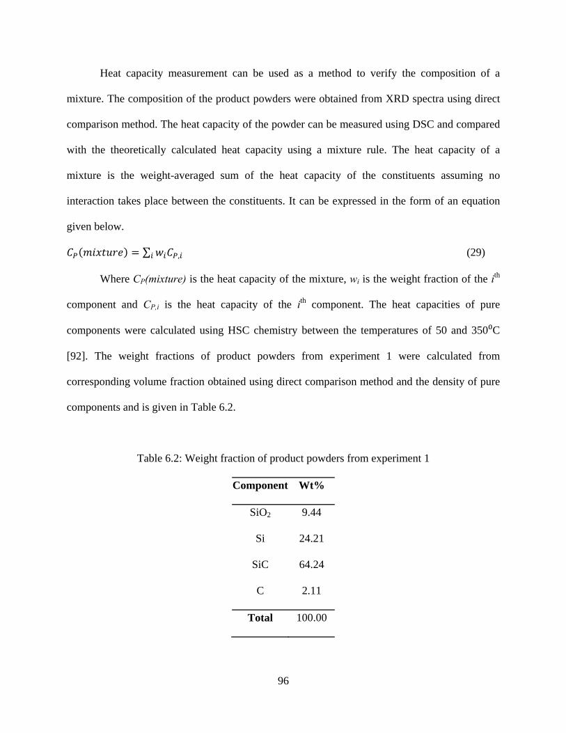
96

Heat capacity measurement can be used as a method to verify the composition of a

mixture. The composition of the product powders were obtained from XRD spectra using direct

comparison method. The heat capacity of the powder can be measured using DSC and compared

with the theoretically calculated heat capacity using a mixture rule. The heat capacity of a

mixture is the weight-averaged sum of the heat capacity of the constituents assuming no

interaction takes place between the constituents. It can be expressed in the form of an equation

given below.

∑ , (29)

Where CP(mixture) is the heat capacity of the mixture, wi is the weight fraction of the ith

component and CP,i is the heat capacity of the ith component. The heat capacities of pure

components were calculated using HSC chemistry between the temperatures of 50 and 350⁰C

[92]. The weight fractions of product powders from experiment 1 were calculated from

corresponding volume fraction obtained using direct comparison method and the density of pure

components and is given in Table 6.2.

Table 6.2: Weight fraction of product powders from experiment 1

Component Wt%

SiO2 9.44

Si 24.21

SiC 64.24

C 2.11

Total 100.00

97

Heat capacity measurement of product powders from experiment 1 was carried out using

a Perkin-Elmer Diamond DSC. The sample and the baseline heat flow, along with the heat

capacity of the material are shown in Figure 6.12. An ‘Iso-Scan-Iso’ temperature scan with an

interval of 50ºC and a heating rate of 10ºC/min was used to determine the heat flow curves of the

sample and baseline. The calculation of heat capacity of sample is done by the difference in the

heat flow between the sample and the baseline.

50 100 150 200 250 300 350

0

1

2

3

Hea

t Cap

acity

(J/

g*o C

)

Temperature (oC)

Specific Heat (J/g*°C)

-10

0

10

20

30

40

50

60

70

80

Sample Heat Flow Endo Up (mW) Baseline Heat Flow Endo Up (mW)

Hea

t Flo

w E

ndo

Up

(mW

)

Figure 6.12: Heat capacity, sample heat flow and baseline heat flow for product powders from

experiment 1 using DSC.

98

The experimentally measured heat capacity was compared with that calculated using

equation (29) as shown in Figure 6.13. The measured heat capacities match quite well with the

theoretically calculated heat capacity. This further substantiates the accuracy of the composition

of the phases present in the sample calculated using the direct comparison method.

Figure 6.13: Comparison of heat capacity measured experimentally with those calculated using

equation (29).

6.2.2 Morphology of product powders

Scanning electron microscopy was used to determine the morphology of the product

powders from the experiments. Figure 6.14 shows the morphology of the products from

experiment 1 with methane molar ratio of 1, solid feed rate of 5 g/min and a power of 21.6 kW.

0.0

0.5

1.0

1.5

2.0

2.5

3.0

50 100 150 200 250 300 350

Hea

t C

apac

ity,

CP

(J/g

*⁰C

)

Temperature (⁰C)

Cp (mix)Experimental

99

Figure 6.14: SEM image showing the morphology of the product powders from experiment 1.


100


The particles are almost spherical with an average diameter varying between 200 and 500

nm. It can also be seen from the micrographs that formation of nanorods are observed in the

morphology. Figure 6.15, on the other hand, shows the morphology of powders from experiment

5 with a methane molar ratio of 2 and 5 g/min solid feed. Mostly spherical particulates are

observed in this case with an average particle size distribution between 200 and 500 nm.

It was also observed that with the increase in the amount of methane in the feed above 1,

the amount of nanorods observed were less. Correlating with the phases formed from the XRD

patterns, it is speculated that the formation of nanorods is due to the presence of Si in the product

powders. This speculation is further justified by the morphology of the product powders from

experiment 7 with 1 mole of methane and 4 g/min solid feed rate in Figure 6.16. There is about

35 mol% Si present in the product powder which might have favored the formation of the

101

nanorods. Particulate matter of spherical morphology was also observed with an average particle

size between 200 nm and 500 nm.

Figure 6.17: TEM image showing the morphology of the product powders from experiment 1.

Product powders from experiment 1 at a molar ratio of SiO2: CH4 = 1:1 and a feed rate of

5g/min were further analyzed using TEM for its morphological features. Nanorods of about 20 -

30 nm in diameter are observed as can be seen from Figure 6.17. Similar observation was made

from the powders obtained from experiment 2 at a molar ratio of SiO2: CH4 = 1:0.8. Figure 6.18

(a) shows nanorods with an average diameter of 20-30 nm. High resolution TEM images from

the same experiment show the presence of Si at the tip of a nanorod as seen in Figure 6.18 (b).

Further evidence for the presence of Si is shown in Figure 6.18 (c) with a small inclusion of SiO2

of about 5nm in size. There is substantial amount (about 25 mol%) of unreacted SiO2 present in

the product powders from experiment 2 with a methane molar ratio of 0.8 as seen from the XRD

102

analysis. A small single crystal SiO2 particle was observed in the TEM analysis shown in Figure

6.18 (d) with insets of a magnified image and the corresponding diffraction pattern.

Figure 6.18: (a) TEM image showing the morphology of the product powders from experiment

2; (b) and (c) HRTEM showing presence of Si and (d) SiO2 single crystal with insets of

magnified image and electron diffraction pattern.

(a) (b)

(c) (d)

103

6.2.3 Particle size reduction

An observation similar to that in the synthesis of titanium diboride can be made here. The

particle size of the initial solid feed was 45 m or less. Figure 6.18 (d) shows a high resolution

image of silicon dioxide particle from experiment 2. As can be seen from the image, the size of

the unreacted silicon dioxide particle is in tens of nanometers. While the actual mechanism is

unknown at this time, the two mechanisms proposed earlier, namely, vaporization and re-

condensation of unreacted solid feed and surface vaporization, are assumed to be a possible way

in which the particle size reduction takes place.

6.2.4 Qualitative analysis of product powders

Inelastic or Raman scattering using a laser source was used to qualitatively substantiate

the presence of various components in the product powders. Raman spectra of product powders

from experiments 1, 2 and 3 (methane molar ratios varying from 0.8 to 1.5 at 5 g/min feed rate)

were obtained as shown in Figure 6.19. Presence of carbon in all the samples is substantiated by

the peaks at wavenumbers 1302.17, 1573.89 and 2593.51 cm-1. The peaks at wavenumbers 789

and 925.63 cm-1 correspond to SiC. It is reported in the literature that these wavenumbers

correspond to SiC in nanorod form [99]. The peaks corresponding to SiC are observed only in

experiments 1 and 2 at methane molar ratios of 0.8 and 1 and not in experiment 3 which

corresponds to a methane molar ratio of 1.5.

104

500 1000 1500 2000 2500 3000 35000

50

100

150

200

250

300

350

400

450

500

550

600

650

700

Experiment 3

Experiment 2

Experiment 1

512.

49, S

i

Ram

an I

nten

sity

Wavenumber (cm-1)

Experiment 1 (1:1) Experiment 2 (1:0.8) Experiment 3 (1:1.5)

300.

32

925.

63, S

iC N

R

1302

.17,

car

bon

1573

.89,

car

bon

2593

.51,

car

bon

789,

SiC

NR

Feed Rate 5g/min

Figure 6.19: Raman spectra of product powders from experiments 1, 2 and 3 using a solid feed

rate of 5g/min.

Presence of Si in the samples from experiment 1 and 2 are substantiated by the presence

of peak at a wavenumber of 512.49 cm-1. The composition calculation using XRD pattern shows

relatively high amounts of Si in experiments with methane molar ratio of 1 or less. This not only

corroborates the volume fraction calculation from XRD using direct comparison method, but

also accounts for presence of higher amounts of nanorods at lower molar ratios of methane as

seen from SEM and TEM.

105

92 94 96 98 100 102 104 106 108 110 112 114500

1000

1500

2000

2500

3000

3500

4000

4500

5000

XPS Raw Data XPS Raw Data - Gaussian Fit SiO

2 Peak - Gaussian Fit

SiC Peak - Gaussian Fit Si Peak - Gaussian Fit

Binding Energy (eV)

Inte

nsity

(C

PS

)

Figure 6.20: XPS spectra of product powders from experiment 1 showing the Si 2p peak resolved

into SiO2, SiC and Si peaks.

XPS spectra measures the elemental composition of a material based on its binding

energy. The difference in the binding energies can be used to substantiate the presence of

specific compounds. Si 2p XPS spectra of product powders from experiment 1 were obtained as

shown in Figure 6.20. A peak at binding energy of about 101.6 eV corresponds to elemental Si

bonding, while the peak at about 104.8 eV corresponds to the SiC bonding. The peak at about

108 eV corresponds to SiO2 in the product powders. The peaks positions for SiO2 and SiC have

also been reported in the literature [100,101]. A small change in the peak positions of about 2-4

106

eV was observed which might be due to the fluorescence effect of the powders used to determine

the binding energy. This provides further substantiation for the presence of Si, SiC and SiO2 in

the product powders.

6.2.5 Post-processing of product powders

100 200 300 400 500 600 700 800 900 1000 1100-800

-700

-600

-500

-400

-300

-200

-100

0

100

200

300

400

500100 200 300 400 500 600 700 800 900 1000 1100

Onset = 536.870C

W = 0.052 mg

W = 2.005 mg

Temperature (0C)

Hea

t Flo

w E

ndo

Dow

n (m

W)

Temperature (0C)

Heat Flow Endo Down (mW)

W = 0.548 mg

Onset = 1005.130C

15

16

17

18

19

20

Wei

ght (

mg)

Weight (mg)

Figure 6.21: Weight loss and heat flow curves from TG-DTA for the product powders from

experiment 1.

107

The product powders from thermal plasma synthesis experiments contain many phases

such as SiC, Si, SiO2 and C. Post processing or phase separation of these powders become

important in obtaining high quality powders useful in various applications. One of the easiest

ways of removing carbon is by calcining the material in oxygen or air atmosphere where carbon

reacts with oxygen to form carbon dioxide gas and leaves the system. To determine the

feasibility of this process the powders from experiment 1 were heated from room temperature to

1100⁰C in atmospheric air in a TG-DTA experiment (Figure 6.18). A weight loss (3.09 wt%)

was observed at a temperature of 536.87⁰C. It is accompanied by an exothermic heat. It is

speculated that the weight loss is due to the reaction of carbon and oxygen to form carbon

dioxide.

An 11.3 wt% weight gain was observed between the temperatures of 536.87⁰C and

1100⁰C. It is also accompanied by a steady drop in the heat flow. This could be due to the

oxidation of Si that is present in the sample due to the presence of atmospheric air. A small

weight gain (about 0.3 wt%) was observed at a temperature of 1005.13⁰C with an accompanying

exothermic heat. This is probably due to a phase transformation reaction that might be taking

place and is speculated to be the transformation of high quartz to tridymite. Hence it is possible

to remove carbon from product powders by calcining it at a temperature of about 550ºC in air. It

should also be noted that any increase in temperature might lead to the oxidation of elemental Si

to SiO2.

108

CHAPTER 7

CONCLUSIONS AND FUTURE WORK

7.1 CFD modeling of plasma reactor

A two dimensional (2D) model depicting the flow profile inside the plasma reactor was

developed using Fluent. Grid refinement studies were performed and an optimum grid size was

chosen for analysis. The velocity and temperature profiles inside the reactor were obtained. The

effect of inlet plasma pressure on the inlet velocity of the plasma gas was studied. It was

observed that velocity increases almost linearly with the increase in pressure. An assumed flow

path was generated inside the reactor. A conservative estimate of the residence time inside the

reactor was calculated as a function of plasma inlet gas pressure.

A three dimensional (3D) model was developed extending the 2D model. Transition SST

turbulence model was used with various grid sizes and turbulence layers to perform grid

refinement study. An optimum grid size was chosen and the effect of plasma inlet pressure on

the inlet velocity of the plasma gas was estimated. It was observed that the variation in velocity

was almost linear with change in the inlet pressure similar to the 2D model. The velocity at any

given pressure was found to be lower by about 35-40 m/s in the 3D model compared to that of

the 2D model. While the maximum velocity is lower than the 2D model, the residence time in

the 3D model is lower as well. Based on the requirements for experimental synthesis an

intermediate plasma gas pressure of 45 psi was used to ensure high temperature and a moderate

residence time in the reactor.

109

7.2 Synthesis of titanium diboride

The production of TiB2 using thermal plasma was carried out using TiO2 and B2O3 as

solid feed and CH4 as the reducing gas holding the molar ratio of the solid feed at 1:1.

Thermodynamic simulation based on the minimization of Gibbs energy shows that maximum

yield of TiB2 was obtained at a methane molar ratio of 5 with solid feed molar ratio of TiO2:B2O3

= 1:1. The experiments using 4, 5 and 6 moles of CH4 at a power of 23.4 kW and a solid feed

rate of 2.15 g/min showed that the yield of TiB2 was more using 5 moles of CH4 and was about

24 mol%. The increase in the solid feed rate from 2.15 g/min to 3.22 g/min at a feed composition

of TiO2:B2O3:CH4 = 1:1:5 increased the yield of TiB2 to about 40 mol%. The product yield

obtained in thermodynamic simulations in a reaction system may not be obtained in a thermal

plasma reactor. Hence, it is concluded that a relatively higher solid feed rate and a molar ratio of

TiO2:B2O3:CH4 = 1:1:5 yielded the maximum yield of TiB2. The as-formed product yield of TiB2

in a thermal plasma reactor is higher than that obtained in an earlier research. A change in crystal

structure was observed in TiO2 from anatase to rutile. While increase in feed rate from 2.15

g/min to 3.22 g/min increased the TiB2 yield from about 24 mol% to about 40 mol%, it also

reduced the amount of carbon from ~64 mol% to ~40 mol%. The TiB2 spherical particles formed

are in the range of 20-100 nm. Particle size reduction of boron oxide was observed in final

product powder from submicron sizes in solid feed to tens of nanometers in final product.

110

7.3 Synthesis of silicon carbide

SiC was successfully produced using thermal plasma using SiO2 as the solid feed and

methane as the reducing gas. Thermochemical calculations suggest that the yield of SiC is a

maximum at a temperature of 1520⁰C and a molar ratio of SiO2:CH4 = 1:3. Formation of Si and

SiO(g) was also observed from the calculations. Experiments using a molar ratio of SiO2:CH4 =

1:2 produced maximum yield of SiC with a solid feed rate of 5 g/min and a power of 21.6 kW.

Average heat capacity of the product powders was about 0.75 – 1.00 J/g*⁰C in the temperature

range of 50-350⁰C as determined by the DSC experiments, which is consistent with the

theoretical heat capacity calculated using mixture rule on the heat capacities of pure components.

This confirms the mole fractions of the product phases calculated using XRD. The size and shape

of the final products changed with the change in the process parameters. Spherical particulate

matter of no greater than 500 nm and nanorods of about 20-30 nm in diameter were observed. It

was speculated from HRTEM that Si acts as a nucleating agent for the nanorods to grow.

Reduction in particle size of unreacted silicon dioxide was observed in the final product

powders. The size of silicon dioxide in the final product powder is in tens of nanometers which is

very less compared to the submicron size of the starting powder. Raman spectra confirm the

presence of elemental Si in the samples and the presence of SiC nanorods. XPS confirms the

presence of Si, SiO2 and SiC in the samples. TG-DTA experiments in air show that the carbon

present in the sample can be removed when calcined at a temperature less than 600⁰C, thus,

preventing the oxidation of Si.

111

7.4 Future work

7.4.1 Modeling of plasma reactor

The flow properties of the plasma gas inside the reactor were obtained using both a 2D

model and a 3D model. It is seen that the 3D model more accurately predicts the flow inside the

reactor. An analysis of effect of various turbulence models on the flow properties in the reactor

showed that the transition SST model was the best for use in the thermal plasma reactors. Grid

refinement study was done on the meshes generated considering the total number of nodes and

the number of turbulence layers. An optimum grid size was chosen and the flow properties

determined inside the plasma reactor. Based on the model generated, a secondary solid phase can

be added to the system and the following information can be generated.

(i) Effect of solid feed on the flow properties in the reactor.

(ii) Effect of particle size on the residence time in the reactor.

(iii) Effect of solid feed rate on the residence time in the reactor.

This information can be generated for various systems, such as, TiO2, B2O3, SiO2, MgO,

etc. As the physical and the chemical properties of these compounds and their mixtures differ

from each other, the modeling results will give a good starting point for experiments with

different starting materials. After the experiments, the validation of the model can be performed

by comparing the theoretical weight of products and that obtained from the experiments.

112

7.4.2 Synthesis of TiB2

In the current research project, the synthesis of titanium diboride was carried out using a

constant molar ratio of TiO2:B2O3 = 1:1 in the solid feed. Due to the low melting and the

vaporization temperatures of boron oxide, some of it might have left the reactor in gaseous

phase. Standard data shows that the melting point of boron oxide is 450ºC. This might have been

a reason for the low (about 40 mol%) yield of TiB2 compared to about 82 mol% yield from the

theoretical calculations. This could be overcome by using higher molar ratios of boron oxide in

the feed materials. Experiments can be setup to use similar conditions such as a plasma power of

23.4 kW, molar ratio of methane to solid feed at 5 and a solid feed rate of 3.22 g/min, but the

molar ratio of TiO2:B2O3 can be increased to 1:1.5 and 1:2. This will increase the amount of

boron in the system and thus an increase in the yield of titanium diboride.

7.4.3 Separation of Si, SiC and SiO2

The synthesis of SiC using thermal plasma has been carried out successfully. The final

powders from the experiments contain four major phases, namely, silicon, silicon carbide, silicon

dioxide and carbon. The carbon present in the material can be removed by calcining the powders

in air atmosphere at about 600⁰C. The rest of the phases can be separated using the concepts of

electrophoresis and gravitational settling. Zeta-potential is the defined as the potential difference

between the surface of the particle and the bulk liquid. Electrophoresis uses the concept the zeta

potential to move solid suspension in a liquid. The zeta potential and the electro-osmotic velocity

of silica as a function of pH were determined as early as 1991 [102]. Isoelectric point (i.e.p) is

defined as the point at which zeta potential is zero. The particles dispersed in the solution

become unstable and start to agglomerate near the i.e.p. It is shown in the literature that the zeta

113

potential of silica varies with pH and the type of solvent but never reaches zero. Zeta potential

also has medical applications [103]. It varies with the change in the surface ion group. Silicon

and silicon carbide, unlike silica has i.e.p. and is very close to each other at low pH values of

around 3. Hence a higher pH was used to separate silicon from silicon carbide from waste slurry

obtained from sawing silicon wafers using silicon carbide wheels [104-106]. The isoelectric

points (IEP) for commercial SiC of various grit sizes, G800, G1000 and G1200 are at pH values

of 4.8, 4.2 and 3.3 respectively [107]. Thus using the difference in the particle shape and size,

difference in the zeta potential and varying pH, the three phases, namely, Si, SiC, and SiO2 can

be separated using a setup combining electrophoresis and gravitational settling.

114

REFERENCES

[1] A. Stein, S. W. Keller, T. E. Mallouk, Science, 259 (1993) 1558-1564.

[2] A-M Azad, M. Ramachandran, N. Schweitzer, Solid State Ionics, 178 (2007) 1476–1486.

[3] Helble, J. J., Journal of Aerosol Science, 29 [5/6] (1998) 721-736,

[4] Helble, J. J., Moniz, G. A. and Morency, J. R. (1994) United States Patent number 5,358,695.

[5] Helble, J. J., Moniz, G. A. and Morse, T.F. (1995) United States Patent number 5,447,708.

[6] Helble, J. J., Moniz, G. A. and Morse, T.F. (1997) United States Patent number 5,599,511.

[7] P. Duran, J. Tartaj, J. F. Fernandez, M. Villegas, and C. Moure, Ceramics International, 25 (1999) 125-135.

[8] P. Duran, M. Villegas, F. Capel, P. Recio, and C. Moure, Journal of European Ceramic Society, 16 (1996) 945-952.

[9] M. Mazaheri, A. Simchi, M. Dourandish, F. Golestani-Fard, Ceramics International, 35 (2009) 547–554.

[10] G. S. A. M. Theunissen, A. J. A. Winnubst, and A. J. Burggraaf, Journal of the European Ceramic Society 11 (1993) 315-324.

[11] O. Vasylkiv, and Y. Sakka, Journal of American Ceramic Society, 84 [11] (2001) 2489-2494.

[12] D. S. Patil, K. Prabhakaran, C. Durgaprasad, N. M. Gokhale, A. B. Samui, and S. C. Sharma, Ceramics International, 35 (2009) 515–519.

[13] L. G. J. de Haart, Y. S. Lin, K. J. de Vries, and A. J. Burggraaf, Journal of the European Ceramic Society 8 (1991) 59-70.

[14] Y. Zhou, J. A. Switzer, Journal of Alloys and Compounds, 237 (1996) 1-5.

115

[15] H. Herrig and R. Hempelmann, Nano Structured Materials, 9 (1997) 241-244.

[16] B. Li, X. Wang, M. Yan, and L. Li, Materials Chemistry and Physics, 78 (2002) 184–188.

[17] H. Wang, L. Gao, W. Li, and Q. Li, Nano Structured Materials, 11 [8] (1999) 1263–1267.

[18] J. A. Nelson and M. J. Wagner, Chemistry of Materials, 14 (2002) 4460-4463.

[19] Dai H., Wong E. W., Lu Y. Z., Fan S., and Lieber C. M., Nature, 375 (1995) 769-772.

[20] X. G. Yang and C. Y. Wang, Applied Physics Letters, 86 (2005) 224104.

[21] Y. Li, S. Zhang, Q. Yu, and W. Yin, Applied Surface Science, 253 (2007) 9254–9258.

[22] Y. Nakamura, K. Tachibana, and H. Fujimoto, Physica C, 306 (1998) 259–270.

[23] J. Li, C. Papadopoulos, J. M. Xu, and M. Moskovits, Applied Physics Letters, 75 [3] (1999) 367-369.

[24] T. J. Goodwin, S. H. Yoo, P. Matteazzi, and J. R. Groza, Nano Structured Materials, 8 [5] (1991) 559-566.

[25] R. S. Wagner, W. C. Ellis, Applied Physics Letters, 4 (1964) 89.

[26] S. Iijima, Nature, 354 (1991) 56.

[27] J. D. Holmes, K. P. Johnston, R. C. Doty, B. A. Korgel, Science, 287 (2000) 1471.

[28] A. M. Morales, C. M. Lieber, Science, 279 (1998) 208.

[29] Y. F. Zhang, Y. H. Tang, N. Wang, D. P. Yu, C. S. Lee, I. Bello, S. T. Lee, Applied Physics Letters, 72 (1998) 1835.

[30] N. Wang, Y. F. Zhang, Y. H. Tang, C. S. Lee, S. T. Lee, Physical Review B, 58 (1998) R16024.

[31] S. T. Lee, Y. F. Zhang, N. Wang, Y. H. Tang, I. Bello, C. S. Lee, Y. W. Chung, Journal of Materials Research, 14 (1999) 4503.

[32] S. T. Lee, N. Wang, C. S. Lee, Material Science and Engineering A, 286 (2000) 16.

[33] S. T. Lee, N. Wang, Y. F. Zhang, Y. H. Tang, MRS Bulletin, 24 (1999) 36.

116

[34] H. I. Liu, N. I. Maluf, R. F. W. Pease, Journal of Vacuum Science and Technology B, 10 (1992) 2846.

[35] T. Ono, H. Saitoh, M. Esashi, Applied Physics Letters, 70 (1997) 1852.

[36] D. C. Halverson, A. J. Pyzik, I. A. Aksay, and W. E. Snowden, Journal of American Ceramic Society, 72 [5] (1989) 775-80.

[37] D. Apelian, (1992). Materials Synthesis: A New Horizon for Plasma Processing. International Symposium on Thermal Plasma Applications in Materials and Metallurgical Processing, San Diego, California, USA, TMS, pp. 3-12.

[38] Thermal Spray Application for the Next Millennium – A Business Development Perspective: KASSABJI F., JACQ G., EDF, Direction des Etudes et Recherches, Dept. Systèmes Energétiques; MORET SUR LOING, FRANCE; DURAND, J., P., Magetex, France: Thermal Spray – Meeting the challenges of 21st century, Proceedings of the 15th International Thermal Spray Conference, Nice, France, 25-29 May 1998, pp. 1677-1680.

[39] P. R. Taylor, and S. A. Pirzada, Advanced Performance Materials, 1 (1994) 35.

[40] M. I. Boulos, IEEE Transactions on Plasma Science, 19[6] (1991) 1078.

[41] E. Pfender, Plasma Chemistry and Plasma Processing, 19[1] (1999) 1.

[42] S-M. Oh, and D-W. Park, Thin Solid Films, 316 (1998) 189.

[43] O. Fukumasa and S. Sakiyama, Surface and Coatings Technology, 131 (2000) 493.

[44] S. W. White and R. G. Reddy, Waste Processing of MgO Bag House Dust Using Plasma Arc Technology, in: EPD Congress, TMS, 1999, pp. 687-697.

[45] R. G. Reddy and L. V. M. Antony, JOM, 55 [3] (2003) 19.

[46] R. G. Reddy and L. V. M. Antony, Processing of SiC Nano Powders using Thermal Plasma Technique, in: Proceedings of the 2003 international conference on Nanotechnology: Scientific challenges and commercial opportunities, Rhode Island, 2003, pp. 47-54.

[47] I. Mohai, J. Szépvölgyi, I. Bertóti, M. Mohai, J. Gubicza, and T. Ungár, Solid State Ionics, 141-142 (2001) 163.

[48] L. Tong and R. G. Reddy, Scripta Materialia, 52 (2005) 1253.

[49] N. R. Thakkar, and R. G. Reddy, (2003): Thermal Plasma Processing of Boron Carbide Fine Powders. In Powder Materials: Current Research and Industrial Practices III. Ed. Marquis, F.D.S., TMS, Warrendale, PA, pp. 47 - 60.

117

[50] S. Niyomwas, B. Wu, and R. G. Reddy, Synthesis and Modeling of Fe-TiN Composites by Thermal Plasma Processing, in: C.Suryanarayana, N. N. Thadhani, and T. C. Lowe (Eds.), Ultrafine Grained Materials, TMS, 2000, pp. 89-98.

[51] L. V. M. Antony, Thermal Plasma Processing of Al-SiC Ultrafine Composites: Master’s Thesis, The University of Alabama, 2004.

[52] L. Tong and R. G. Reddy, Metallurgical and Materials Transactions B, 37B (2006) 531.

[53] U. S. Patent No. 6,379,419 B1, Date of Patent: Apr. 30, 2002.

[54] E. Rudy, Ternary Phase Equilibria in Transition Metal-Boron-Carbon-Silicon Systems, in: Part V, Compendium of Phase Diagram Data, Technical Report AFML-TR-65-2, Wright-Patterson Air Force Base, Ohio (1969) p. 198.

[55] A. E. McHale, (Ed.), Phase Equilibria Diagrams, American Ceramic Society, 10 (1994) 140.

[56] H. Duschanek, P. Rogl, and H. L. Lukas, Journal of Phase Equilibria, 16 (1995) 46.

[57] Munro R. G., Journal of Research of NIST, 105 (2000) 709.

[58] U.S. Patent No. 4,673,550, Date of Patent: Jun. 16, 1987.

[59] M. Makyta, V. Danek, G. M. Haarberg, J. Thonstad, Journal of Applied Electrochemistry, 26 (1996) 319.

[60] M. Shigeta, T. Watanabe, Thin Solid Films, 515 (2007) 4217.

[61] S. Dallaire, and B. Champagne, Thin Solid Films, 118 (1984) 477.

[62] T. Kodama, Y. Ikeda, and H. Tamura, Journal of Thermal Spray Technology, 8(4) (1999) 537.

[63] I. Song, L. Wang, M. Wixom, and L. T. Thompson, Journal of Materials Science, 35 (2000) 2611.

[64] A. M. Locci, R. Orru, G. Cao and Z. A. Munir, Journal of American Ceramic Society, 89(3) (2006) 848.

[65] P. R. Taylor, M. Manrique and S. A. Pirzada, Proceedings of the EPD Congress, TMS Annual Meeting, Las Vegas, Nevada, 1995, pp. 49-59.

[66] G. L. Watt, P. R. Taylor and S. A. Pirzada, Proceedings of the EPD Congress, TMS Annual Meeting, Las Vegas, Nevada, 1995, pp. 61-73.

118

[67] J. Schmidt et al., Science and Technology Advanced Materials, 8 (2007) 376.

[68] A. K. Khanra et al., Materials Letters, 58 (2004) 733.

[69] U. S. Patent No. 6,420,294 B1, Date of Patent: Jul. 16, 2002.

[70] B. Basu et al., International Materials Reviews, 51 (2006) 352.

[71] S. E. Bates et al., Journal of Materials Research, 10 (1995) 2599.

[72] A. Y. Hwang and J. K. Lee, Materials Letters, 54 (2002) 1.

[73] Y. Gu et al., Journal of Alloys and Compounds, 352 (2003) 325.

[74] Acheson A. G., British Patent 17:911, (1892).

[75] Knippenberg W. F., “Growth Phenomena in Silicon Carbide: Preparative Procedures.” Philips Research Reports, 18 (1966) 170–179.

[76] Lely J. A., Darstellung von Einkristallen von Siliziumcarbid und Beherrschung von Art und Menge der eingbauten Verunreinigungen. Berichte Deutche Keramik Geselshaft, 32 (1955) 229–231.

[77] Hamilton D. R., “The Growth of Silicon Carbide by Sublimation.” In: Connor JR, Smilestens J (eds.) Silicon Carbide, A High Temperature Semiconductor. Pergamon, Oxford, (1960) pp 45–51.

[78] Novikov V. P. and Ionov V. I., Growth of Crystals, 6b (1968) 9–21.

[79] Tairov Y. M. and Tsvetkov V. F., Journal of Crystal Growth, 43 (1978) 209–212.

[80] Ziegler G., Lanig P., Theis D. and Weyrich C., IEEE Transactions on Electron Device ED-30 (1983) 277–281.

[81] Glass R. C., Henshall D., Tsvetkov V. F. and Carter Jr C. H., MRS Bulletin 22 [3] (1997) 30–35.

[82] Tairov Yu. M., Materials Science and Engineering B, 29 (1995) 83–89.

[83] Karpov S. Yu., Makarov Yu. N., Mokhov E. N., Ramm M. G., Ramm M. S., Roenkov A. D., Talalaev R. A. and Vodakov Yu. A., Journal Crystal Growth 173 (1997) 408–416.

[84] Matsunami H. and Kimoto T., Materials Science and Engineering R, 20 (1997) 125–166.

[85] Epelbaum B. M., Hofmann D., Muller M. and Winnacker A., Materials Science Forum 338–342 (2000) 107–110.

119

[86] Fluent, version 6.3, Fluid Dynamics International, Fluid Dynamics Analysis Package. Fluent Inc. two-dimensional double precision (2ddp), pressure-based solver with standard k- model for turbulence.

[87] Gambit, Fluid Dynamics International, Fluid Dynamics Analysis Package, Evanston, IL.

[88] Li H-P. and Chen X., Journal of Physics D Applied Physics 34 (2001) L99–L102.

[89] Li H-P., Chen X., and Pfender E., Journal of Physics D Applied Physics 36 (2003) 1084–1096.

[90] Park J. M., Kim K. S., Hwang T. H., and Hong S. H., IEEE Transactions on Plasma Science, 32 (2004) 479–487.

[91] Ansys Workbench, version 13.0.

[92] HSC Chemistry Ver. 5.1, Copyright © Outokumpu Research Oy, Pori, Finland, A.Roine

[93] N. A. Gokcen, and R. G. Reddy, Thermodynamics, second ed., Plenum Publications, New York, 1996, pp. 203-243.

[94] H. Zhang and J. F. Banfield, Journal of Physical Chemistry B, 104 [15] (2000) 3481.

[95] N. Wetchakun, and S. Phanichphant, Current Applied Physics, 8 (2008) 343.

[96] W. Ma, Z. Lu, and M. Zhang, Applied Physics A, 66 (1998) 621.

[97] B. D. Cullity, Elements of X-Ray Diffraction, second ed., Addison-Wesley Publishing Co., 1978.

[98] P. Villars, Pearson's Handbook of Crystallographic Data for Intermetallic Phases, second ed., ASM International, Ohio, 1991.

[99] S. L. Zhang, B. F. Zhub, F. Huanga, Y. Yana, E. Y. Shangb, S. Fanc, and W. Hanc, Solid State Communications, 111 (1999) 647–651.

[100] Y. Ryu, Y. Tak, and K. Yong, Nanotechnology, 16 (2005) S370–S374.

[101] A. A. Galuska, J. C. Uht, and N. Marquez, Journal of Vacuum Science and Technology A, 6 [1] (1988) 110-122.

[102] C. Schwer and E. Kenndler, Analytical Chemistry, 63 (1991) 1801-1807.

[103] Y. Nitta, K. Okamoto, T. Nakatani, H. Hoshi, A. Homma, E. Tatsumi, and Y. Taenaka, Diamond & Related Materials, 17 (2008) 1972-1976.

120

[104] Y-F. Wu, and Y-M. Chen, Separation and Purification Technology, 68 (2009) 70-74.

[105] T-H. Tsai, Journal of Hazardous Materials, 189 (2011) 526-530.

[106] T-H. Tsai, Separation and Purification Technology, 78 (2011) 16-20.

[107] R. R. Rao, H. N. Roopa, and T. S. Kannan, Ceramics International, 25 (1999) 223-230.

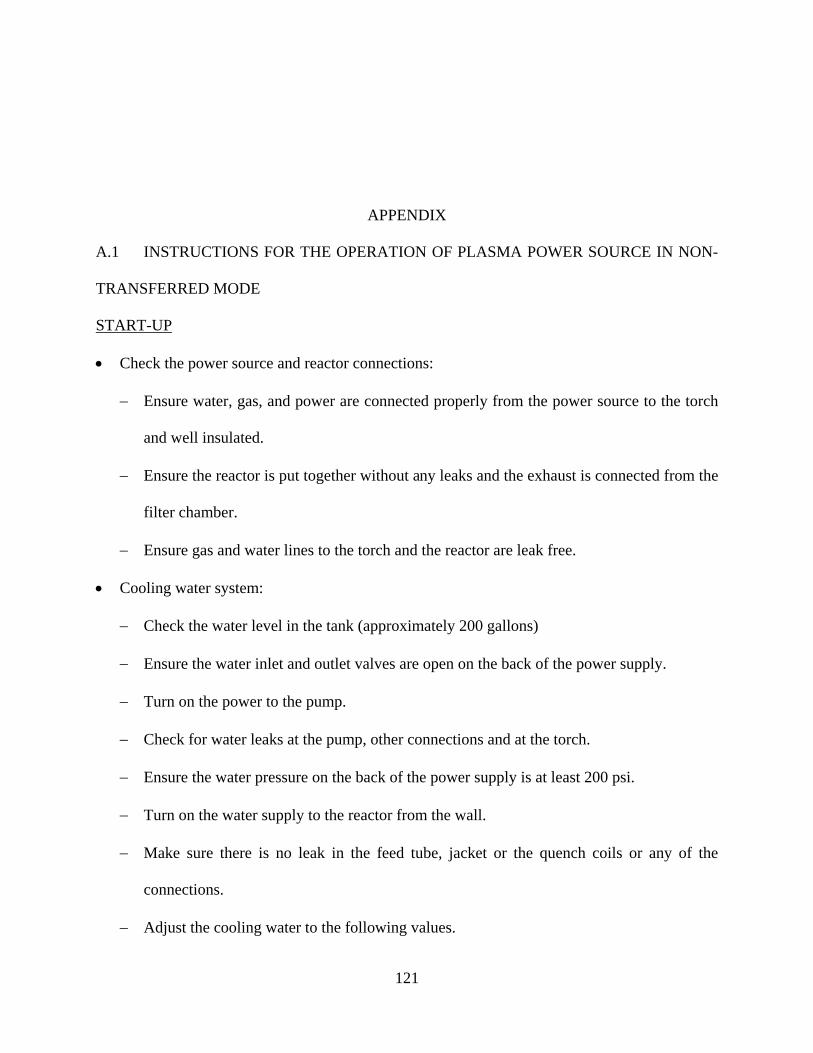
121

APPENDIX

A.1 INSTRUCTIONS FOR THE OPERATION OF PLASMA POWER SOURCE IN NON-

TRANSFERRED MODE

START-UP

Check the power source and reactor connections:

Ensure water, gas, and power are connected properly from the power source to the torch

and well insulated.

Ensure the reactor is put together without any leaks and the exhaust is connected from the

filter chamber.

Ensure gas and water lines to the torch and the reactor are leak free.

Cooling water system:

Check the water level in the tank (approximately 200 gallons)

Ensure the water inlet and outlet valves are open on the back of the power supply.

Turn on the power to the pump.

Check for water leaks at the pump, other connections and at the torch.

Ensure the water pressure on the back of the power supply is at least 200 psi.

Turn on the water supply to the reactor from the wall.

Make sure there is no leak in the feed tube, jacket or the quench coils or any of the

connections.

Adjust the cooling water to the following values.

122

Table 3.1: Flow rate of cooling water for various parts of the plasma reactor system

Part of reactor Flow rate (LPM)

Copper feed tube 1

Stainless steel reactor jacket 2

Copper quench coils 4.5

Gas Supply:

Open the plasma (argon) gas cylinder and check for a minimum of 500 psig tank pressure

on the regulator gauge.

Always connect a second argon cylinder to ensure uninterrupted gas supply to the torch.

Set the outlet pressure at the regulator to a minimum of 60 psig.

Open the gas inlet valve on the power supply’s gas manifold and check for approximately

3 scfm flow rate.

The above mentioned flow rate will correspond to a minimum outlet pressure of 10 psig

at the torch. The following table gives the minimum gas pressures for the operation of the

power supply and the plasma torch.

Table 3.2: Programmable gas controller set points in the thermal plasma power source for

various types of torch.

Type of torch Start Low High

Non-transferred 10 30 60

Transferred 20 30 60

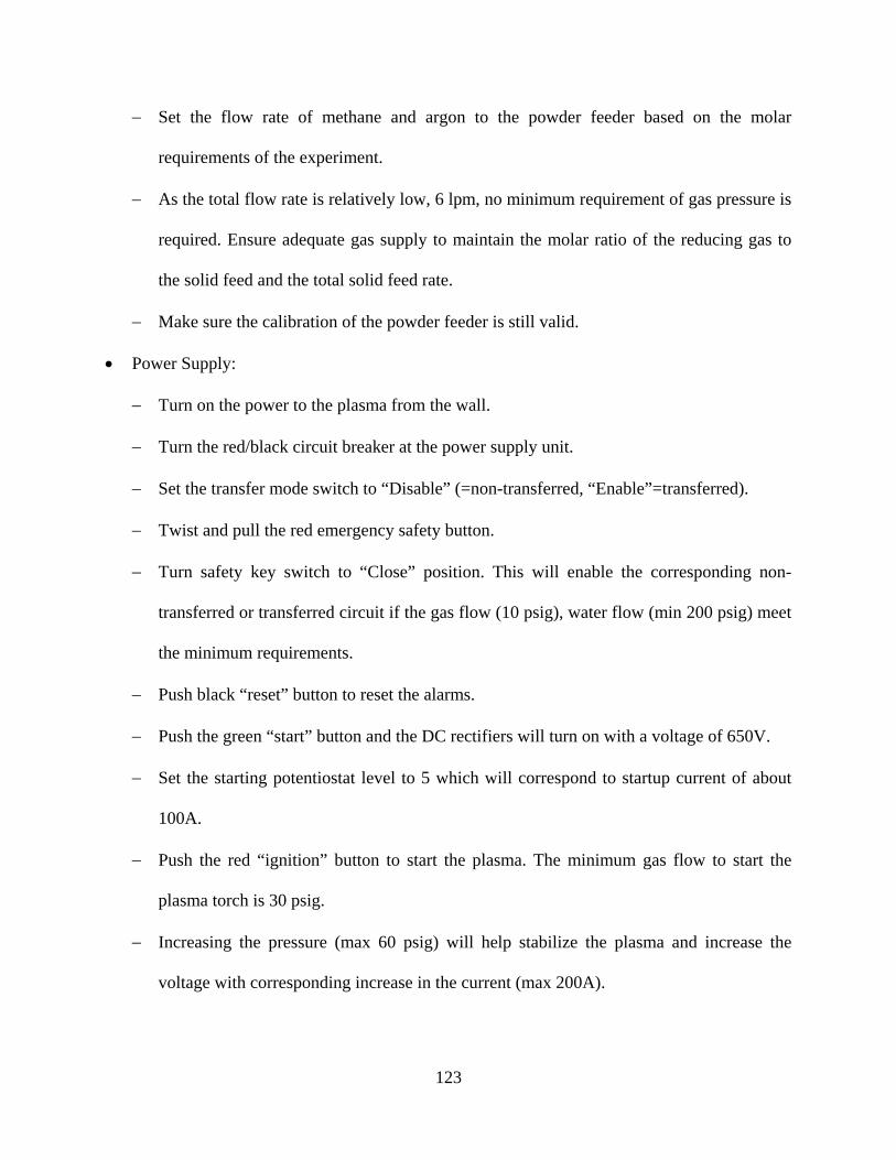
123

Set the flow rate of methane and argon to the powder feeder based on the molar

requirements of the experiment.

As the total flow rate is relatively low, 6 lpm, no minimum requirement of gas pressure is

required. Ensure adequate gas supply to maintain the molar ratio of the reducing gas to

the solid feed and the total solid feed rate.

Make sure the calibration of the powder feeder is still valid.

Power Supply:

Turn on the power to the plasma from the wall.

Turn the red/black circuit breaker at the power supply unit.

Set the transfer mode switch to “Disable” (=non-transferred, “Enable”=transferred).

Twist and pull the red emergency safety button.

Turn safety key switch to “Close” position. This will enable the corresponding non-

transferred or transferred circuit if the gas flow (10 psig), water flow (min 200 psig) meet

the minimum requirements.

Push black “reset” button to reset the alarms.

Push the green “start” button and the DC rectifiers will turn on with a voltage of 650V.

Set the starting potentiostat level to 5 which will correspond to startup current of about

100A.

Push the red “ignition” button to start the plasma. The minimum gas flow to start the

plasma torch is 30 psig.

Increasing the pressure (max 60 psig) will help stabilize the plasma and increase the

voltage with corresponding increase in the current (max 200A).

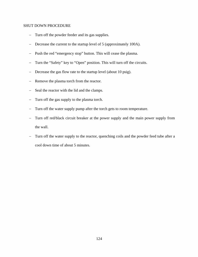
124

SHUT DOWN PROCEDURE

Turn off the powder feeder and its gas supplies.

Decrease the current to the startup level of 5 (approximately 100A).

Push the red “emergency stop” button. This will cease the plasma.

Turn the “Safety” key to “Open” position. This will turn off the circuits.

Decrease the gas flow rate to the startup level (about 10 psig).

Remove the plasma torch from the reactor.

Seal the reactor with the lid and the clamps.

Turn off the gas supply to the plasma torch.

Turn off the water supply pump after the torch gets to room temperature.

Turn off red/black circuit breaker at the power supply and the main power supply from

the wall.

Turn off the water supply to the reactor, quenching coils and the powder feed tube after a

cool down time of about 5 minutes.

125

A.2 PROPERTIES OF GASES USED IN MODELING

ARGON

Heat capacity, CP = 0.520 J/g/K = 20.786 J/mol/K. (constant)

Molecular Weight = 39.948 g/mol.

Density = 1.633 g/L (ideal gas)

Table A.2.1: Viscosity (piecewise-linear) of argon

Temperature (K) Viscosity * 106 (kg/m-s)

100 8.1

200 15.9

300 22.7

400 28.6

500 33.9

600 38.8

Table A.2.2: Thermal conductivity (piecewise-linear) of argon

Temperature (K) Thermal Conductivity (W/m/K)

100 6.3

200 12.4

300 17.7

400 22.4

500 26.5

600 30.3

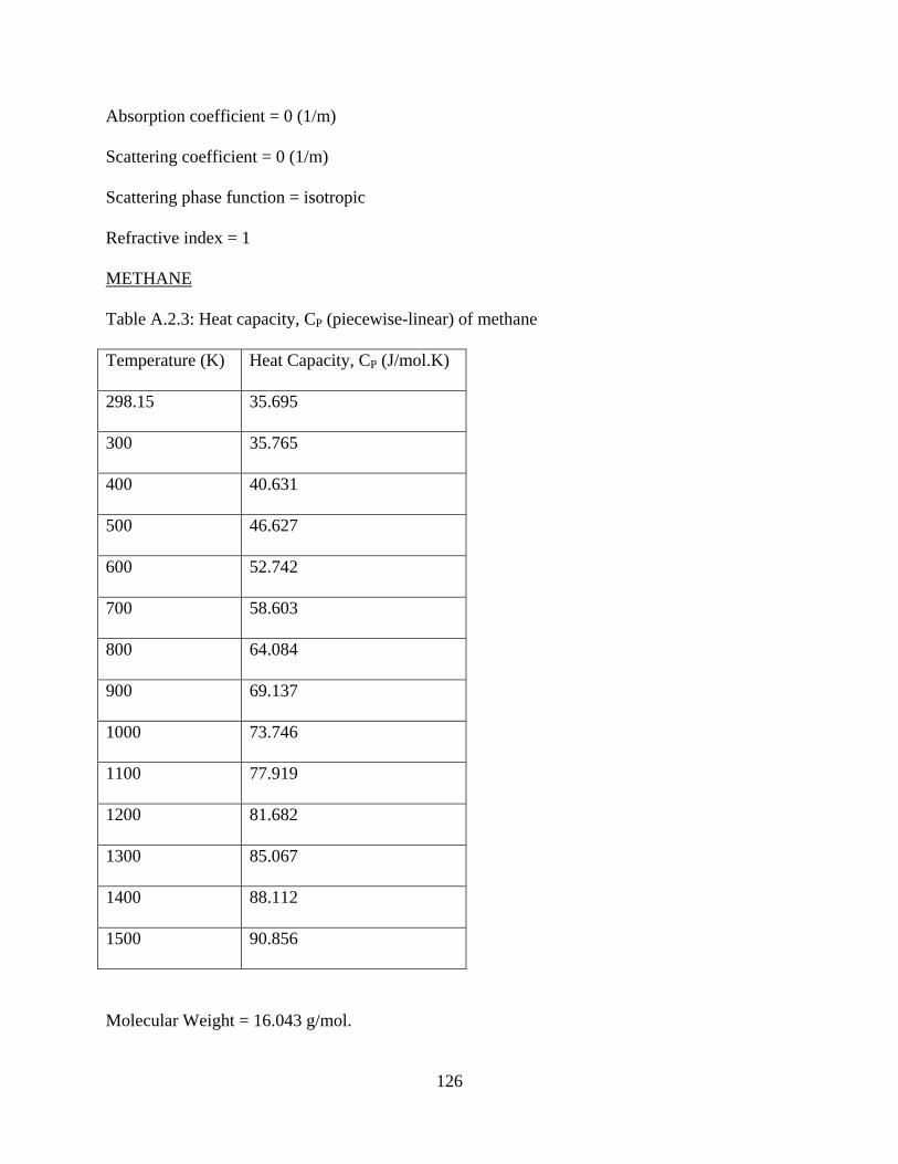
126

Absorption coefficient = 0 (1/m)

Scattering coefficient = 0 (1/m)

Scattering phase function = isotropic

Refractive index = 1

METHANE

Table A.2.3: Heat capacity, CP (piecewise-linear) of methane

Temperature (K) Heat Capacity, CP (J/mol.K)

298.15 35.695

300 35.765

400 40.631

500 46.627

600 52.742

700 58.603

800 64.084

900 69.137

1000 73.746

1100 77.919

1200 81.682

1300 85.067

1400 88.112

1500 90.856

Molecular Weight = 16.043 g/mol.

127

Density = 1.633 g/L (ideal gas)

Table A.2.4: Viscosity (piecewise-linear) of methane

Temperature (K) Viscosity * 106 (kg/m-s)

100 3.9

200 7.7

300 11.1

400 14.2

500 17.0

600 19.5

Table A.2.5: Thermal conductivity (piecewise-linear) of methane

Temperature (K) Thermal Conductivity (W/m/K)

100 10.4

200 21.8

300 34.4

400 50.0

500 68.4

600 88.6

Absorption coefficient = 0 (1/m)

Scattering coefficient = 0 (1/m)

Scattering phase function = isotropic

Refractive index = 1

128

A.3 CALCULATION OF VOLUME FRACTION USING DIRECT COMPARISON

METHOD

Phase analysis of the material was done using XRD. The volume fraction calculation was

done using direct comparison method [97]. The following equation is used in the determination

of the volume fractions of individual phases.

)30(1;; CBABB

CC

B

C

BB

AA

B

A ccccR

cR

I

I

cR

cR

I

I

IA, IB and IC – Intensities of A, B and C respectively

cA, cB and cC – Volume fractions of A, B and C respectively

RA, RB and RC – Volumes of inverse unit cell lattices of A, B and C respectively.

R depends on q, hkl and the kind of substance.

V is the volume of unit cell.

F is the Structure factor calculated using the atomic scattering factor, f, the hkl and the fractional

coordinates of the atoms uvw.

P is the Multiplicity factor for powder method.

e-2M is the temperature factor which is taken as 1 as the XRD was done at room temperature.

The values of F, f, fractional coordinates, L-P factor, and P were obtained from standard

literature [97].

)31(cossin

2cos11 22

22

2MePF

VR

)32(.cossin

2cos12

2

FactoronPolarizatiLorentz

129

Table A.3.1: The values of diffraction constants used in the calculation of volume fraction of

product powders from TiB2 experiments.

Material 2 hkl R

B2O3 26.006 011 3.280

TiO2(r) 27.911 110 4.485

C 41.859 100 1.192

TiB2 44.463 101 2.187

Table 5.3: Yield of product powders at different feed rates with 5 moles of methane in the feed.

Feed Rate (g/min) Yield TiB2 TiO2(r) B2O3 C

2.15 mol% 23.63 8.72 4.07 63.58

3.22 mol% 39.44 11.33 7.58 41.65

The volume fraction calculated using direct comparison method was converted to

corresponding mole fractions using the density and molecular weights of individual pure phases.

The converted result in mol% is shown in Table 5.3 for the synthesis of TiB2.

thermal plasma processing -...

Documents