thermal shape factor the impact of the building shape and
TRANSCRIPT
EN1630
Master Thesis in Energy Engineering, 30 credits
Thermal Shape Factor — the impact of the
building shape and thermal properties on
the heating energy demand in Swedish
climates
Martin Olsson

i
Abstract
In the year 2006, the energy performance directive 2002/91/EG was passed by the European Union,
according to this directive the Swedish building code was supplemented by a key measure of energy use
intensity (EUI). The implemented EUI equals some energy use within a building divided by its floor
area and must be calculated in new housing estate and shown when renting or selling housing property.
In order to improve the EUI, energy efficiency refurbishments could be implemented. Building energy
simulation tools enables a virtual view a building model and can estimate the energy use before
implementing any refurbishments. They are a powerful resource when determine the impact of the
refurbishment measure. In order to obtain a correct model which corresponds to the actual energy use,
some adjustments of the model are often needed. This process refers to as calibration.
The used EUI has been criticized and thus, the first objective in this work was to suggest an alternative
key measure of a buildings performance. The results showed that the currently used EUI is disfavoring
some districts in Sweden. New housing estate in the far north must take more refined actions in order to
fulfill the regulation demand, given that the users are behaving identical regardless where the house is
located. Further, the suggested measure is less sensitive to the users’ behavior than the presently used
EUI. It also has a significance meaning in building design as it relating the building shape and thermal
properties and stating that extreme building shapes must undergo a stricter thermal construction rather
than buildings that are more compact. Thus, the suggested key measure also creates a communication
link between architects and the consultant constructors.
The second objective of this thesis has been to investigate a concept of calibration using the data
normally provided by energy bills, i.e. some monthly aggregated data. A case study serves to answer
this objective, by using the building energy simulation tool IDA ICE 4.7 and a building located in Umeå,
Sweden. The findings showed that the used calibration approach yielded a model considered as
calibrated in eleven of twelve months. Furthermore, the method gives a closer agreement to the actual
heat demand rather than using templates and standardized values. The major explanation of the deviation
was influence of the users, but also that the case study building burden with large heat losses by domestic
hot water circulation and thus, more buildings should be subjected to this calibration approach.
Keywords: Heat loss coefficient, Building shape, Thermal properties, Calibration
ii
Sammanfattning (in Swedish)
År 2006 trädde Lagen om energideklarationer för byggnader i kraft, i enlighet med Europaparlamentets
och rådets direktiv 2002/91/EG om byggnaders energiprestanda. Lagen innebär bland annat att
byggnader ska genomgå energideklarationer vid försäljning och uthyrning. För att jämföra byggnader
infördes nyckeltalet Energiprestanda (Engelsk förkortning: EUI) vilket ska presenteras i deklarationen,
Boverket har definerat nyckeltalet som delar av energianvändningen i byggnader. Vidare ställer
Boverket krav på nybyggnationer genom att sätta en övre gräns för nybyggnationens energiprestanda-
tal. Ägaren till en befintlig byggnad kan förbättra energiprestanda-talet genom att genomföra olika
energieffektiviserande åtgärder och för att uppskatta energibesparingen med åtgärderna kan
energisimuleringsverktyg användas. För att erhålla tillförlitliga resultat är det av yttersta vikt att
simuleringsmodellen motsvarar den verkliga byggnaden. I denna process kommer olika metoder av
kalibriering till god nytta.
Energiprestanda-talet fått kritik från olika håll och därför har ett mål med arbetet varit att undersöka
alternativa prestandamått för byggnader. Resultatet visar på en inkonsitens i byggreglerna. Om en fix
nybyggnation brukas på samma vis så måste konstruktionen längst norrut vidta fler
energieffektiviserande åtgärder än längre söderut. Det föreslagna prestandatalet visar sig vara mindre
känsligt för brukarnas beteenden än vad Energiprestanda är. Talet medför även ett designkrav eftersom
det relaterar byggnadens form och termiska egenskaper och medför att mer arkitekturiskt avancerade
byggnader måste isoleras mer än byggnader av mer kompakt design.
Det andra målet med arbetet har varit att undersöka en kalibrieringsmetod, vilken baseras på
månadsaggregerad data som normalt sett tillhandahålls av energifakturor. Enbart IDA ICE 4.7 har
använts som simuleringsprogram i arbetet, mätdata har tillhandahållits från ett flerbostadshus i Umeå.
Metoden visar på god potential, då simuleringsmodellen anses kalibrierad under elva av tolv månader.
Vidare visar metoden ett bättre resultat än det erhållna resultat från schabloner och standardiserade
värden. Dock är den aktuella byggnaden försatt med stora varmvattencirkulationsförluster, varför fler
byggnader med fördel kan vidare utsättas för den föreslagna kalibrieringsmetoden för att erhålla fler
slutsatser.
Nyckelord: Värmeförlustkoefficient, Byggnadsform, Termiska egenskaper, Kalibriering

iii
Acknowledgments
This thesis of 30 credits has been written during the spring semester of 2016 and completes my Master
of Science in Energy Engineering at Umeå University. The project has been conducted in cooperation
with the Faculty of Applied Physics and Electronics.
First, I would like to thank my job requestor and supervisor, Staffan Andersson, for an interesting
research topic and furthermore, a steady support, numerous feedback sessions and great teaching
throughout my work. I would also thank my faculty supervisor, Ronny Östin, for your advisement and
comments during the project and writing of the report.
I would also like to thank Jimmy Vesterberg, for sharing processed data, knowledge about the case study
building at Ålidhem and the simulation tool IDA ICE. I am also thankful to Thomas Olofsson for your
opinions and guidance.
Lastly, I would like to thank friends and family for all your support throughout my education.
Umeå, August 2016
Martin Olsson

iv
Table of Contents
1. Introduction ..................................................................................................................................... 1
1.1 Background ............................................................................................................................. 1
1.1.1 Regulations, limits and climate zones ............................................................................. 2
1.1.2 Previous work .................................................................................................................. 3
1.2 Problem formulation ................................................................................................................ 5
1.3 Objectives ................................................................................................................................ 5
1.4 Constraints ............................................................................................................................... 5
2. Theory ............................................................................................................................................. 6
2.1 System boundaries ................................................................................................................... 6
2.2 Heat losses ............................................................................................................................... 8
2.3 Annual energy use for heating ............................................................................................... 10
2.4 Thermal Shape Factor, TSF ................................................................................................... 10
3. Case studied building .................................................................................................................... 12
4. Method........................................................................................................................................... 13
4.1 Part 1: Calibration ................................................................................................................. 13
4.1.1 General model ............................................................................................................... 13
4.1.2 Calibration process ........................................................................................................ 16
4.2 Part 2: Energy Performance Indicator ................................................................................... 18
4.2.1 Studied buildings ........................................................................................................... 18
5. Results and discussion ................................................................................................................... 20
5.1 Part 1: Calibration ................................................................................................................. 20
5.1.1 According to SVEBY .................................................................................................... 20
5.1.2 TSF approach ................................................................................................................ 21
5.2 Part 2: Energy Performance Indicator ................................................................................... 28
5.2.1 Shape area factor ........................................................................................................... 28
5.2.2 Thermal shape factor ..................................................................................................... 29
5.3 Summarized discussion ......................................................................................................... 38
5.3.1 Part 1: Calibration.......................................................................................................... 38
5.3.2 Part 2: Energy Performance Indicator ........................................................................... 38
5.3.3 Future work ................................................................................................................... 39
6. Conclusions ................................................................................................................................... 40
7. Bibliography ................................................................................................................................. 41

v
Nomenclature and definitions
Energy performance certificate Declaration of the annual energy use of a building
Building energy use The energy to include when conducting an energy performance
certificate.
Primary energy Non-transformed energy, i.e. biomass, coal, etc.
Building envelope Comprising area of a building, i.e. external walls, floor and
roof.
U-value A measure of the insolation level of the envelope, i.e. it
expresses the heat flux through a construction and the unit is
W/m2K.
Atemp Indoor floor area heated above 10°C.
Ktot Overall heat transfer coefficient, i.e. a factor describing the heat
losses associated to a specific building.
G-value The solar transmittance of windows, a g-value of 0.0 meaning
no solar energy passing the window and 1.0, all solar energy
passes.
Heating season The months when the outdoor temperature falls below the
balance temperature, i.e. when a heating system is required.
IDA ICE IDA Indoor Climate and Energy is a 3D simulation tool,
operating at a zonal level calculating, among others, energy
demand, daylight and air quality.
Specific-heat-energy-use The amount of heat needed in order to maintain the set-point
temperature inside a building.

vi
Abbreviations
Energy Performance EP
Energy Performance Certificate EPC
Energy Conservation Measure ECM
Building Energy Simulation program BES
Thermal Shape Factor TSF
Air Handling Unit AHU
Heating, Ventilating and Air Conditioning HVAC
Standardization and verifications of buildings SVEBY
National Board of Housing, Building and Planning Boverket
Domestic Hot Water DHW
Domestic Hot Water Circulation DHWC
District Heating DH
Specific-Heat-Energy-Use SHEU

Master Thesis in Energy Engineering
Thermal Shape Factor
Page 1
1. Introduction
The building sector uses nearly 40 % of the primary energy in Europe [1] and the residential buildings
are responsible for two-thirds of this usage. In Sweden, the major heating system for new apartment
blocks is district heating (89 %) [2]. The new detached houses use primarily a separate electric heater
(30 %) or district heating (47 %). The average annual energy utilization of a detached house [3] is 15.9
MWh (2014) and corresponding number for an apartment block [4] is 10.3 MWh. In 2002 the European
Union (EU) adopted the directive of Energy performance of buildings [5], stating the member states to
set a maximum level for energy utilization in buildings. In 2006 the Swedish parliament passed the law
of energy performance certificate of buildings, in accordance with the EU directive, compelling the
building owner to conduct an energy performance certification process when
The building exceed 250 square meters floor area and visited by public, or;
The building is sold or rented
To enable a process of benchmark buildings, the National Board of Housing, Building and Planning
(Boverket) has introduced a key measure of energy use intensity called energy performance (EP) [6].
EP is the quote of the energy used in a building and the heated floor area; it is expressed in kilowatt-
hours per square meter and year. The energy included is space heating and cooling, domestic hot water
and facility electricity.
To improve the EP, energy conservation measures (ECMs) could be implemented. An effective tool for
determine the effects of different ECMs is to use a building energy simulation (BES) program. Opposed
to actual field experiments, BES program give the possibility to predict energy savings in advance, and
thus the possibility to choose the most cost-effective ECMs.
1.1 Background
Questions’ has been raised if EP is a suitable key measure. The industry association Swedish District
heating claims that EP is disfavoring some energy sources [7], heat pumps yields a lower supplied
energy demand, than if the building where heated by district heating, although the physical properties
of the building is unmodified. Furthermore, Swedish District heating claims that EP excludes the
influence of the residents.
Research by academics confirms this latter problem. In the article Building performance based on
measured data [8] the authors makes an attempt to filter out the parameters, associated with user
behavior and also solar radiation, in measured energy utilizations of an existing building. The problem
is also mentioned in an investigation by the Swedish Government [9], suggesting that the impact on
heating demand which origins from the user behavior, should be consider with methods built on
empirical surveys and measurements.
Predicting the heat demand of a building is a complicated task, expected energy savings by
implementing ECMs from a BES model tends to not correspond [10] to the measured utilization.
Empirical studies [11] comparing the ECM savings from the BES with actual measurements shows a
large variance. Moreover, Mahapatra, K. [12] investigated deviations in predicted and actual energy use
in a set of some new residential buildings in Växjö, Sweden. The study covered 180 buildings, mainly

Master Thesis in Energy Engineering
Thermal Shape Factor
Page 2
one or two family houses and the major conclusions from the study was that; 13 % of the building did
not fulfill the requirements of the energy performance, where there were a significant difference between
the predicted and actual specific energy use. Moreover, the author recommends EP to be excluded as an
EUI, since EP do not consider a system perspective including losses associated with different energy
production technologies.
1.1.1 Regulations, limits and climate zones
The directive of the energy performance certificate (EPC) was establish by the European Union
influenced by the Kyoto Protocol [13]. The Swedish Government adapted the Swedish EPC to promote
ECMs, by making the yearly cost of energy usage visible. The quality of EPC has been evaluated by
Claesson et al. [14], concluding that EPCs include uncertainties since they are associated with many
assumptions.
Boverket has defined the building energy use as the energy required,
during normal user conditions, for a building at a normal year. If there
is any variation, in new housing estate, between the obtained energy use
and the calculated, it is to be corrected. Likewise, if the temperature
differs from the normal conditions the buildings energy use must be
corrected. The Swedish Meteorological and Hydrological Institute
provide such correction term.
Figure 1: The climate zones
of Sweden. Source: NIBE
Energy Systems [15].
Building energy use
includes:
Space heating energy
Space cooling energy
Domestic hot water (DHW)
Facility electricity
Building energy use
do not include:
o Internal heat gains (i.e.
equipment, occupants and
sun)
o Heat/electricity gained from
solar collectors/panels

Master Thesis in Energy Engineering
Thermal Shape Factor
Page 3
Sweden is divided into four zones; Figure 1 shows the geographical divisions of the zones. Where zone
I represent the coldest counties of Sweden, zone II the second coldest counties and so on. Each climate
zone has its own limit of allowed specific heat demand (also denoted as EP) for new housing estate, see
Table 1, defined as the ratio of the building energy use and the heated floor area, Atemp. Atemp, is defined
as all the floor area that is heated above 10°C and encased by the building envelope, according to the
Swedish Building Code. The Atemp do not includes some areas, such as the unheated and adjacent
garages. Mangold et al. [13] investigate the uncertainties of accomplished EPCs, showing the Atemp is
calculated differently depending methods applied by the performer.
Table 1: The limits of annual specific heat demand (kWh/m2) for new construction of detached houses and
apartment blocks according to the Swedish building code, first value represent if the building not uses electric
heating and value within the parenthesis if it is heated by electricity.
Type of building Zone I Zone II Zone III Zone IV
Detached houses 130 (95) 110 (75) 90 (55) 80 (50)
Apartment
blocks
115 (85) 100 (65) 80 (50) 75 (45)
The limit of the average heat transfer coefficient, U0, in the residential building category is constant and
applied to all climate zones. It is to not exceed 0.4 W/m2K, according to the Swedish building code.
1.1.2 Previous work
Many different studies focus on the two critical stages, design of a new building and choose of ECMs
for an existing building. For the design stage, a common parameter to analyze is the shape factor (SF).
By changing design parameters like shape, orientation and envelope assembly, a well-designed building
can reduce the energy usage with up to 40% [16], relative a poorly designed. For the stage of selecting
ECMs, numerous researches have put efforts in finding new and refined methods in how to calibrate
BES program, in order to obtain an accurate BES model.
Design factors
The shape factor is defined as the ratio between external envelope area and the inner volume of a
building and thereby a measure of buildings compactness, i.e. a building with high SF has a larger
envelope area for a given building volume. Danielski [17] analyses the SF and the specific heat demand
in a Swedish climate. The author confirms the finding of Rodrigues et al. [18] that states a strong
correlation between SF and energy usage in cold climates. The methodology was to use the BES
program VIP Energy together with measured data from 22 buildings in Stockholm. The author
recommends SF to be considered in future building codes. Danielski et al. [19] has further analyzed the
impact on the correlation between SF and the specific heat demand with shifted insulation level and
window-to-floor-area ratio of the envelope. The conclusion drawn was that a low SF is preferable and
the SF sensitive to the insulation level, as the impact of SF varies significantly in buildings with different
level of thermal insulation and the SF has a higher impact on buildings with a low thermal insulation.

Master Thesis in Energy Engineering
Thermal Shape Factor
Page 4
The concept of SF was challenged by Granadeiro et al. [20]. The authors aimed to find a more elaborated
design indicator, due to the findings of Depecker et al. [21] which concluded that in mild and sunny
climates there is no correlation between SF and heating demand. The design indicator, called envelope-
related energy demand (ERED), was defined as the sum of the heat transfer by transmission and the
solar gains, expressed in kWh/m2 (total floor area). The indicator was validated with simulations of
1 000 buildings, of different envelope shapes containing one or two floors, using the BES program
EnergyPlus. Their results showed a strong correlation between ERED and energy demand, further the
authors suggested that the absolute value of the ERED is an indicator of energy demand and thus ERED
should be considered as an adequate design tool.
A review of international regulations of thermal insulation [1] proposes a new methodology to regulate
the thermal insulation to harmonize the energy losses in the envelope of a building. The methodology
consists of four steps; (i) regulate the envelope energy losses by a supranational organization, (ii) create
a world map of degree-days, at equal indoor temperature and thus ensure the energy losses are
comparable between countries, (iii) calculate the overall heat transfer coefficient of the building that
complies with a maximum defined value and (iv) the U-values are to be selected of each part of the
envelope surface so that it comply to the limit in (iii). In the proposal for future research, the authors
suggest a maximum limit of envelope energy losses, according to the international directives.
Catalina et al. [22] made a regression analysis in order to determine the main factors influencing the
building’s heat demand. The best-fitted model was given by a polynomial function including three
parameters; the heat loss coefficient (W/m3K), the south equivalent surface and the temperature
difference of indoor and sol-air1 temperature. The model was validated with 17 apartment blocks located
in Romania, resulted in an average error of 20.2 %.
BES calibration
“The process of fitting the model to the observed data by adjusting the parameters is known as calibration
[23].” A calibrated BES model is usually very helpful to predict the savings of ECMs and to find how
much effort needed to generate a reliable BES model, a methodology were developed by Pedrini et al.
[24] dividing the process into three steps; (i) Simulation from building design plans and documentation,
(ii) auditing and lastly, (iii) energy-end-use measurements. By comparing the actual energy use from an
existing building with the simulation results, the enhancement in each step is detected. The first BES
model resulted in an annual energy demand 114 % higher than the measurements, the second showed a
dramatic enhancement as the annual difference was reduced to 0.1 %. The third step yielded the annual
difference of 0.2 %. The increased difference between step two and three is explained by overestimations
of energy use in the first steps. The results indicated that although the step two is well fitted with the
measured data, it is not reliable at an energy-end-use level.
Vesterberg et al. [25] proposed a BES calibration approach, using short-term detailed measurements and
a regression analysis. The regression approach was also compared with a conventional step-by-step BES
calibration approach and the best agreement was obtained with the regression approach. A drawback
with the regression approach is the need of conducting detailed site measurements. The method provides
an air-to-air heat loss coefficient that also was suggested as a candidate to serve as an EPI.
1 Sol-air temperature is an expression incorporates the parameters; air temperature and solar radiation.

Master Thesis in Energy Engineering
Thermal Shape Factor
Page 5
Mihai el al. [26] summarizes different validation approaches, whereas an approach was to let BES
models hold as calibrated when the monthly difference is less than 10 % between the predicted and
actual energy use.
1.2 Problem formulation
The present measure of energy performance in buildings includes impact from the residents of the
building. Thus, it is of interest to elaborate and investigate other measures of energy performance that
focus on the building itself and thus minimizes the influence from the users.
Previous studies put effort in calibrating with different approaches, Vesterberg et al. uses measurements
and regression analyses to achieve a well-calibrated BES model. A disadvantage of this calibration
method is the time-consuming process of collecting daily data. Hence, it could be of interest to determine
the robustness and accuracy using building information provided from the bills sent from energy
companies.
1.3 Objectives
The purpose of this thesis was to highlight a concept of relating the shape, and thermal properties, of a
building to the annual heating demand. The objectives were to
Evaluate how monthly measured data could be of usage to calibrate a simulation model
Suggest one alternative indicator of building energy performance
1.4 Constraints
In all simulations and calculations the DHW have been assumed to not contribute to the heat balance in
the studied buildings. This assumption was drawn since the hot water is believed to usually be spilled
out by waste pipes. Further, the heat gained by flush the hot water to the tap is seemed as being reduced
by the flush of cold water.
In the first part, the simulations was only conducted with Umeå as location and due to the far north
location of Umeå the solar radiation has been assumed as negligible during winter months.
The number of locations in the second part was limited to five locations; Kiruna (zone I), Umeå (zone
I), Sundsvall (zone II), Stockholm (zone III) and Malmö (zone IV). The buildings included in the second
part only detached residential houses created in a BES environment, in order to save time.

Master Thesis in Energy Engineering
Thermal Shape Factor
Page 6
2. Theory
The first part of this chapter briefly describes the heat losses associated to the building envelope and the
air handling unit (AHU), the following parts are to define the thermal shape factor (TSF).
2.1 System boundaries
When performing calculations to determine the energy demand, different system boundaries can be
used. When selecting the boundary of an energy certification system, it is of concern that the major
included factors are effectible for the ones the certification systems refers to, i.e. the constructor2 cannot
guarantee how the building is used, which heating system implemented etc. Recommendation of
Erlandsson et al. [27] remarking a distinction in energy certifications as (i) Building performance and
(ii) Energy system performance.
This work solely focuses at (i) the building performance. One selection could be the primary energy.
The usage of primary energy is a proper indicator of quantifying the use of the energy resources in a
specific process. The primary energy shifts the focus from an energy-end-use perspective to amount of
energy conversion of the energy resources [28]. In other words, when calculating the primary energy
use, one needs to consider all the steps required to acquire the final product. This approach is well-
known in life cycle assessments. In order to simplify these calculations primary energy factors for
different included processes can be of use; the primary energy factor is simply the conversion efficiency
of a process and can be obtained by administrative authorities.
Another approach is to only consider the net energy use and with the building envelope as boundary.
This system is in accordance with (i) as it centers the building and thus it is simple to obtain the
effectiveness of the envelope, i.e. how low the heat losses are. Figure 2 illustrates the concept of this
system, the figure also includes the system boundary used by Boverket. Boverket treat buildings similar
to the net energy approach but has chosen to enlarge the boundary to include the gained solar power by
collectors/panels. They have further chosen to only include some of the supplied energy within the
expression of EP, i.e. the bought energy for heating/cooling-system, facility electricity and DHW. This
amount of energy often denoted as the purchased energy. This is the most figuring in international
comparisons, and is beneficial in sense of reliability in the energy quantification [29].
2 The constructor is referred, in this work, to the business firm ordered to compute the energy use within a building
and/or further also assembly the building components.

Master Thesis in Energy Engineering
Thermal Shape Factor
Page 7
Figure 2: The net energy system of a building, seen as the building envelope, the grey box points the system
boundary used by Boverket [30]. The main heat fluxes in and out denoted as different arrows. The two grey
stars are pointing out the supplied energy included in the EP. Source: Created by the author.
Seen from Figure 2, some disadvantages are that the EP not includes the household electricity and power
supplied from solar collectors/panels is within the boundary according to Boverket. Throughout this
thesis the net energy is only considered with the building envelope as boundary. The heat losses and
gains of this system are explained below, also seen in Figure 2.
The heat loss from a building occurs in three different ways [20]:
Transmission losses through the building envelope, i.e. walls, windows, roof, floor etc.;
Ventilation, i.e. exhaust air leaving building to the surrounding; and
Infiltration, due to leaks in the building envelope and user behavior (opening and closing of
windows)
A building gains heat from [31]:
Heating system, i.e. furnace, heat exchanger and/or heating coils in AHU, etc.;
Solar radiation; and
Internal heat, i.e. electric components, occupants, etc.
The gained heat considers all supplied heat to the system, however the gained heat from DHW use is
assumed as negligible and only gained heat from circulating DHW (DHWC) is considered. For the use
of electricity not all of the energy is gained as heat in the system, since for instance, hot water from
boiling is being spilled out in the drains. Thus, a weighting factor is of relevance. According to
Standardization and verifications of buildings (SVEBY3) [32] several surveys recommend a utilization
factor as 70 %.
3 SVEBY is a Swedish building industry norm financed by the construction and real estate business.

Master Thesis in Energy Engineering
Thermal Shape Factor
Page 8
A static power balance of the building can be expressed as [20] [31];
𝑃𝑠𝑢𝑛 + 𝑃𝑜𝑐𝑐𝑢𝑝𝑎𝑛𝑡𝑠 + 𝛼𝑃𝑒𝑙𝑒𝑐𝑡𝑟𝑖𝑐𝑖𝑡𝑦 + 𝑃ℎ𝑒𝑎𝑡𝑖𝑛𝑔 𝑠𝑦𝑠𝑡𝑒𝑚 = 𝑃𝑡𝑟𝑎𝑛𝑠 + 𝑃𝑣𝑒𝑛𝑡 + 𝑃𝑖𝑛𝑓𝑖𝑙𝑡 1
where 𝑃𝑠𝑢𝑛, 𝑃𝑜𝑐𝑐𝑢𝑝𝑎𝑛𝑡𝑠, 𝑃𝑒𝑙𝑒𝑐𝑡𝑟𝑖𝑐𝑖𝑡𝑦, 𝑃ℎ𝑒𝑎𝑡𝑖𝑛𝑔 𝑠𝑦𝑠𝑡𝑒𝑚 are the supplied heat from the sun, occupants,
electricity and heating system, respectively, (W). The 𝑃𝑡𝑟𝑎𝑛𝑠, 𝑃𝑣𝑒𝑛𝑡 and 𝑃𝑖𝑛𝑓𝑖𝑙𝑡 are the heat loss through
transmission, ventilation and infiltration, respectively, (W). 𝛼 (-) is the utilization factor, compensating
heat by electrical equipment no being supplied to the building.
2.2 Heat losses
The term of heat losses due to transmission in equation (eq.) 1, 𝑃𝑡𝑟𝑎𝑛𝑠 (W), of the envelope can by
expressed as [33]
𝑃𝑡𝑟𝑎𝑛𝑠 = ∑ 𝑈𝑎.𝑔,𝑖𝐴𝑎.𝑔,𝑖 (𝑇𝑖𝑛 − 𝑇𝑜𝑢𝑡) + 𝑈𝑔𝐴𝑔(𝑇𝑖𝑛 − 𝑇𝑔)
2
where 𝑈𝑎.𝑔,𝑖 is the U-value of envelope component i above the ground, (W/(m2K))
𝐴𝑎.𝑔,𝑖 is the area of envelope component i above the ground, (m2)
𝑈𝑔 is the U-value of component facing the ground, (W/(m2 K))
𝐴𝑔 is the area of the component facing the ground, (m2)
𝑇𝑖𝑛 and 𝑇𝑜𝑢𝑡 are the indoor and outdoor temperature, respectively, (K)
𝑇𝑔 is the ground temperature, (K)
Due to constructions parts with low thermal resistance the so called thermal bridges occur, they are
usually separated in linear and point bridges. Where the linear bridges often is caused by beams or balks
in the building construction and the point bridges originates in corners where balks etc. are jointed. The
thermal bridges, 𝑃𝑡ℎ𝑒𝑟𝑚𝑎𝑙 𝑏𝑟𝑖𝑑𝑔𝑒 (W), can be expressed as [33]
𝑃𝑡ℎ𝑒𝑟𝑚𝑎𝑙 𝑏𝑟𝑖𝑑𝑔𝑒 = (∑ 𝜗𝑘𝑙𝑘 + ∑ 𝛾𝑗) (𝑇𝑖𝑛 − 𝑇𝑜𝑢𝑡)
3
where 𝜗𝑘 is the linear coefficient of thermal bridge k, (W/(m K))
𝑙𝑘 is the length of the linear thermal bridge k, (m)
𝛾𝑗 is the point coefficient of thermal bridge j, (W/K)
By adding the expressions of transmission heat loss, i.e. eq. 2 and eq. 3, the 𝑃𝑡𝑜𝑡.𝑡𝑟𝑎𝑛𝑠 (W) is achieved
as
𝑃𝑡𝑜𝑡.𝑡𝑟𝑎𝑛𝑠 = (∑ 𝑈𝑎.𝑔,𝑖𝐴𝑎.𝑔,𝑖 + ∑ 𝜗𝑘𝑙𝑘 + ∑ 𝛾𝑗) (𝑇𝑖𝑛 − 𝑇𝑜𝑢𝑡) + 𝑈𝑔𝐴𝑔(𝑇𝑖𝑛 − 𝑇𝑔)
4
Merging the thermal bridges with the heat losses above ground, eq. 4 could be rewritten to
𝑃𝑡𝑜𝑡.𝑡𝑟𝑎𝑛𝑠 = 𝑈´𝑎.𝑔𝐴𝑎.𝑔(𝑇𝑖𝑛 − 𝑇𝑜𝑢𝑡) + 𝑈𝑔𝐴𝑔(𝑇𝑖𝑛 − 𝑇𝑔) 5

Master Thesis in Energy Engineering
Thermal Shape Factor
Page 9
where 𝑈´𝑎.𝑔 is the overall U-value of the envelope components above ground, including thermal
bridges (W/(m2 K)).
𝐴𝑎.𝑔 is the total area of the envelope above ground, (m2)
Eq. 5 includes heat losses separated above and below the ground level, in order to avoid this separation,
an approach of normalizing the ground heat loss transmission by multiplying with the ratio 𝑇𝑖𝑛−𝑇𝑜𝑢𝑡
𝑇𝑖𝑛−𝑇𝑜𝑢𝑡, to
the ground transmission losses. This gives
𝑃𝑡𝑜𝑡.𝑡𝑟𝑎𝑛𝑠 = 𝑈´𝑎.𝑔𝐴𝑎.𝑔(𝑇𝑖𝑛 − 𝑇𝑜𝑢𝑡) + 𝑈𝑔𝐴𝑔
𝑇𝑖𝑛 − 𝑇𝑔
𝑇𝑖𝑛 − 𝑇𝑜𝑢𝑡
(𝑇𝑖𝑛 − 𝑇𝑜𝑢𝑡) 6
This approach is of relevance to archive an expression operating towards one single temperature
difference. From eq. 6 an overall U-value, 𝑈0 (W/(m2 K)), is expressed as
𝑈0 =𝑈´𝑎.𝑔𝐴𝑎.𝑔 + 𝑈𝑔𝐴𝑔 (
𝑇𝑖𝑛 − 𝑇𝑔
𝑇𝑖𝑛 − 𝑇𝑜𝑢𝑡)
𝐴0
7
where 𝐴0 is the total envelope area, (m2)
By using eq. 7 in eq. 6 an overall expression of the thermal transmission losses, 𝑃𝑡𝑟𝑎𝑛𝑠 (W), could be
expressed as
𝑃𝑡𝑟𝑎𝑛𝑠 = 𝑈0𝐴0 (𝑇𝑖𝑛 − 𝑇𝑜𝑢𝑡)
8
where 𝑈0 is the overall U-value in the envelope of the building, (W/(m2K))
𝐴0 is the total comprising area of the building, (m2)
The buildings ventilation system can be of two different types; Pressure driven flow or a mechanical
flow. The later always includes a pressure driven flow due to leakage in the envelope. The heat losses
by ventilation and infiltration, 𝑃𝑣𝑒𝑛𝑡 (W), is expressed as [33]
𝑃𝑣𝑒𝑛𝑡 = 𝜌𝑐𝑝 (�̇�𝑙𝑒𝑎𝑘 + �̇�𝑣𝑒𝑛𝑡(1 − 𝜂)) (𝑇𝑖𝑛 − 𝑇𝑜𝑢𝑡) 9
where 𝜌 is the density of air, (kg/m3), assumed as 1.2 kg/m3
𝑐𝑝 is the specific heat capacity, (kJ/ (kg K)), assumed as1 kJ/(kg K)
�̇�𝑣𝑒𝑛𝑡 and �̇�𝑙𝑒𝑎𝑘 are the volume flow of the ventilation and infiltration, (m3/s)
𝜂 is the efficiency coefficient of the heat recovery system in the AHU, (-)
According to SS-EN ISO 13789, the air leakage is determined at a pressure gradient of 50 Pa between
indoor and outdoor conditions, and is general normalized to the envelope area.
By adding eq. 8 with eq. 9, an expression of the total heat losses is formed as
𝑃𝑙𝑜𝑠𝑠 = (𝑈0𝐴0 + 𝜌𝑐𝑝(�̇�𝑣𝑒𝑛𝑡(1 − 𝜂) + �̇�𝑙𝑒𝑎𝑘)) (𝑇𝑖𝑛 − 𝑇𝑜𝑢𝑡) 10

Master Thesis in Energy Engineering
Thermal Shape Factor
Page 10
The factor (𝑈0𝐴0 + 𝜌𝑐𝑝(�̇�𝑣𝑒𝑛𝑡(1 − 𝜂) + �̇�𝑙𝑒𝑎𝑘)) in eq. 10 is hereby referred to as the overall heat
transfer coefficient, Ktot.
2.3 Annual energy use for heating
The degree-day method holds as a rather simplified expression for a buildings heating demand. The
method is accurate [34] if the building parameters, indoor temperature and internal heat loads are relative
constant. The heat losses from the building operate with the indoor temperature towards the outdoor
temperature, the degree-days, DD (°C day), is defined as
𝐷𝐷 = ∑(𝑇𝑖𝑛,𝑖 − 𝑇𝑜𝑢𝑡,𝑖)∆𝑡
𝑖
, 𝑖 = 1, 2, 3 … , 365 11
where 𝑇𝑖𝑛,𝑖 and 𝑇𝑜𝑢𝑡,𝑖 (°C) are the average daily indoor and outdoor temperature, respectively.
∆𝑡 (day) is the time resolution.
In order to determine the need of supplied heat from a heating system, the heat gains are to be considered.
The heat gains, 𝑃𝐻𝐺 (W), implies the heat sources within the building which is not a part of the primary
heating system, i.e. electrical components, occupants and solar radiation. It could be expressed as
𝑃𝐻𝐺 = 𝛼𝑃𝑒𝑙𝑒𝑐𝑡𝑟𝑖𝑐𝑖𝑡𝑦 + 𝑃𝑜𝑐𝑐𝑢𝑝𝑎𝑛𝑡𝑠 + 𝑃𝑠𝑢𝑛 12
This amount of heat yields a surplus in the need of heating power during heating season. By expressing
the heat balance, 𝑃𝐻𝐺 = 𝑃𝑙𝑜𝑠𝑠 using eq. 10 and eq. 12, and using the temperature difference of indoor
temperature and a balance temperature, 𝑇𝑏𝑎𝑙𝑎𝑛𝑐𝑒 (°C), the number of heating degrees gained from 𝑃𝐻𝐺
can be determined.
𝑇𝑏𝑎𝑙𝑎𝑛𝑐𝑒 = 𝑇𝑖𝑛𝑑𝑜𝑜𝑟 −𝑃𝐻𝐺
𝐾𝑡𝑜𝑡
13
Knowing the balance temperature, the number of heating degree-days, HDD (°C day), is defined as
𝐻𝐷𝐷 = ∑(𝑇𝑏𝑎𝑙𝑎𝑛𝑐𝑒,𝑖 − 𝑇𝑜𝑢𝑡,𝑖)
𝑖
∆𝑡, 𝑖 = 1, 2, 3 … , 365 14
where 𝑇𝑏𝑎𝑙𝑎𝑛𝑐𝑒,𝑖 (°C) is the balance temperature.
∆𝑡 (day) is the time resolution.
2.4 Thermal shape factor, TSF
As mentioned previous in chapter 1.1.1 Regulations, limits and climate zones, Boverket currently using
some purchased energy in order to determine the performance of buildings, however according to
chapter 2.2 Heat losses, there is a more suited indicator for the heat losses associate with a building, i.e.
the factor Ktot. Hence, it holds as interest to develop this factor. The general unit of expressing ventilation
flow is l/(m2s) (Atemp), thus Ktot is rewritten to adjust to this unit. Furthermore, the infiltration flow is
also expressed using Atemp instead of the envelope area. By assuming a constant air volume (CAV)
system is used, the following expression is formed.

Master Thesis in Energy Engineering
Thermal Shape Factor
Page 11
𝐾𝑡𝑜𝑡 = (𝑈0 [𝑊
𝑚2 , 𝐾] 𝐴0[𝑚2]
+ 1,2 [𝑘𝑔
𝑚3] 103 [𝐽
𝑘𝑔 𝐾] (�̇�𝑣𝑒𝑛𝑡 [
𝑙
s, 𝑚2] 10−3 [𝑚3
𝑙] 𝐴𝑡𝑒𝑚𝑝[𝑚2](1
− 𝜂) [−] + �̇�𝑙𝑒𝑎𝑘 [𝑙
s, 𝑚2] 10−3 [𝑚3
𝑙] 𝐴𝑡𝑒𝑚𝑝[𝑚2]))
= (𝑈0𝐴0 + 1,2𝐴𝑡𝑒𝑚𝑝(�̇�𝑣𝑒𝑛𝑡(1 − 𝜂) + �̇�𝑙𝑒𝑎𝑘))
15
It is preferable to normalize the eq. 15 against Atemp, in order to make the expression compatible to the
current representation of energy performance.
𝐾𝑡𝑜𝑡
𝐴𝑡𝑒𝑚𝑝= 𝑈0
𝐴0
𝐴𝑡𝑒𝑚𝑝+ 1,2(�̇�𝑣𝑒𝑛𝑡(1 − 𝜂) + �̇�𝑙𝑒𝑎𝑘)
16
let the ratio of 𝐾𝑡𝑜𝑡
𝐴𝑡𝑒𝑚𝑝 in eq. 16 be denoted as the thermal shape factor and
𝐴0
𝐴𝑡𝑒𝑚𝑝 be denoted as the shape
area factor (SF*), yielding the expression
𝑇𝑆𝐹 = 𝑈0𝑆𝐹∗ + 1,2(�̇�𝑣𝑒𝑛𝑡(1 − 𝜂) + �̇�𝑙𝑒𝑎𝑘) 17
The TSF can also be determined by using information of the internal heat gains. From eq. 10 and eq. 14
the annual heating demand, 𝐸𝐻𝐷 (Wh/m2), of a building is expressed as
𝐸𝐻𝐷 = 𝑇𝑆𝐹 ∙ 𝐻𝐷𝐷 18
By using eq. 11 and eq. 13, eq. 18 can be rewritten to
𝑇𝑆𝐹 =𝐸𝐻𝐷 + 𝐸𝐻𝐺
𝐷𝐷
19
where 𝐸𝐻𝐺 (Wh/m2) is the annual gained heat from the heat gains.

Master Thesis in Energy Engineering
Thermal Shape Factor
Page 12
3. Case studied building
The building involved in the BES calibration work is located at Matematikgränd 7, the building is hereby
referred as M7. The neighborhood was built during 1970-1971 and is at this moment leased for
residential rental by the housing company AB Bostaden i Umeå. The geographical position of M7 is
shown in Figure 3.
The building is enclosed by a black rectangle in Figure 3. M7 is a two-story residential building, where
each floor consists of two one-room apartments and three three-room apartments.
The measurements were conducted during the period of 2010-07-01 and 2011-06-30 and have been a
part of the energy efficiency project Sustainable Ålidhem4, where measurements has been conducted,
before and after implementing different ECMs, to enable a further analysis of the result of different
measures.
During the years 2010 and 2011, no refurbishments were implemented and so the building was assumed
to equal the original documentation from 1970. The heating system consists of radiators and heating
coils in the AHU, the heat was supplied by district heat and no cooling or air conditioning unit was used.
4 The sustainable Ålidhem is a pilot project aimed to reduce the energy use within the some neighborhoods of the
city district Ålidhem, financed by AB Bostaden i Umeå, Umeå University, Umeå municipality and the energy
company Umeå Energi [50]. The projected included new housing estate, a photovoltaic plant, a winter garden,
district heat supplied washing machines, individual energy monitoring in the apartments and energy efficiency
refurbishments.
Figure 3: The neighborhood of the case study building, Matematikgränd 7 is enclosed by a rectangle.
Source: Google Maps [35].

Master Thesis in Energy Engineering
Thermal Shape Factor
Page 13
4. Method
This chapter includes the methodology of this project. The work has been divided in two parts; Part 1
serves to answer the first objective, the measured data used and analyzed originates from the doctoral
thesis “Improved building energy simulations and verifications by regression” [36]. Part 2 examines
the field of using TSF as an energy performance indicator.
All simulations were carried out using the software IDA Indoor Climate and Energy 4.7 (IDA ICE).
This software allows the user to separate a building into multiple zones, each with individual ventilation,
set point temperatures, internal loads etc. It is a suitable tool when study energy performance of buildings
[37] [38]. IDA ICE has been developed by the division of Building Services Engineering at the KTH
Royal Institute of Technology. Validation of IDA ICE [39] and comparison [40] has been made to other
simulation software, a report from the International Energy Agency [41] concluding IDA ICE as a well
performing simulation tool. Furthermore, the major information used in this thesis has been obtained by
scientific databases and websites sponsored by authorities and the construction business. The primarily
database of usage was Web of Science [42] and Scopus [43], where reports and publications were
collected.
4.1 Part 1: Calibration
During the beginning of this thesis data from energy measurements was provided by the department of
TFE, along with drawings of the building. Further, field inspections were conducted in order to
determine different dimensions of M7. The gathered information provided an initial and general BES
model of M7 created in IDA ICE, by modification of this general BES model a comparison between the
cases of calibration and uncalibrated were possible.
The energy utilization in a building can be quantified in mainly two ways [44]; calculated or measured.
The calculations could be perform with a BES tool or steady-state calculations, measured data is
obtained from installed monitoring equipment or by a simplified approach; read directly from the energy
bills.
4.1.1 General model
The general model was constructed by using one building body in IDA ICE for the entire building where
each apartment was assigned as an individual zone, as well as the spaces of hallways and stairwells. The
doors were assumed to thermally equal the adjacent walls. Windows closely sited was approximated as
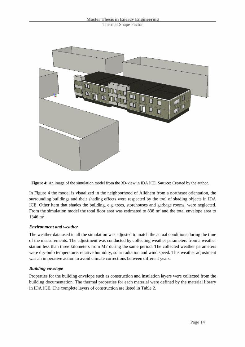
one unit and no opening schedule was used. Figure 4 visualizes the model.
Master Thesis in Energy Engineering
Thermal Shape Factor
Page 14
In Figure 4 the model is visualized in the neighborhood of Ålidhem from a northeast orientation, the
surrounding buildings and their shading effects were respected by the tool of shading objects in IDA
ICE. Other item that shades the building, e.g. trees, storehouses and garbage rooms, were neglected.
From the simulation model the total floor area was estimated to 838 m2 and the total envelope area to
1346 m2.
Environment and weather
The weather data used in all the simulation was adjusted to match the actual conditions during the time
of the measurements. The adjustment was conducted by collecting weather parameters from a weather
station less than three kilometers from M7 during the same period. The collected weather parameters
were dry-bulb temperature, relative humidity, solar radiation and wind speed. This weather adjustment
was an imperative action to avoid climate corrections between different years.
Building envelope
Properties for the building envelope such as construction and insulation layers were collected from the
building documentation. The thermal properties for each material were defined by the material library
in IDA ICE. The complete layers of construction are listed in Table 2.
Figure 4: An image of the simulation model from the 3D-view in IDA ICE. Source: Created by the author.

Master Thesis in Energy Engineering
Thermal Shape Factor
Page 15
Table 2: The constructions detail of M7.
Orientation Roof External floor Long side wall Gable wall
Outside 25 cm
sawdust
10 cm concrete 12 cm Half brick stone 12 cm Half brick
stone
6 cm sand
6 cm concrete
1.2 cm asphalt board
10 cm mineral wool
Vapor barrier
10 cm mineral wool
Inside 14 cm
concrete
0.5 cm floor coating 1.3 cm gypsum board 15 cm concrete
In Table 2 the construction details of M7 are listed, the corresponding U-values for each construction
are further listed in Table 3, by using the built-in material properties in IDA ICE. The building is built
on a slab on ground, the ground material was assumed as a default soil in the list of materials in IDA
ICE. The method for the calculation of the ground heat losses was done according to ISO 13370. The
roofs weather protection-layer was neglected, due to ventilation openings providing the surrounding air
to circulate underneath.
The sizes and placements of the windows were obtained by floor plans and front elevations, all the
windows are assumed to equal the same type, i.e. glass and frame construction. The windows consist of
double panels, with a U-value (default material in IDA ICE) of 2.00 W/m2K and 2.20 W/m2K for the
frame and glass, respectively. The ratio between window-to-total-envelope-area was determined to
23.46 %.
Table 3: The U-values of the elements of the envelope, separated in walls, floor, roof and windows.
Building element U-value (W/m2K)
Long side walls 0.291
Gable walls 0.304
External floor 2.648
Roof 0.296
Windows 2.18
HVAC-system
M7 has one central AHU for all the apartments, using a CAV-system with no heating recovery. In all
simulations every zone was provided with an ideal heater, dimensioned to manage the maximum heating
demand.
Occupants
The amount of occupants in M7 were assumed to agree with the template recommended by SVEBY
[32], a one-room and a three-room apartment are resided by 1.42 and 2.18 occupants, respectively. This
resulted in the total number of 18.76 occupants in M7. The time of stay for residents and their activity

Master Thesis in Energy Engineering
Thermal Shape Factor
Page 16
level was also set in accordance to SVEBY [32], occupancy of 14 hours per day with an activity level
correspond to 80 W per occupant.
4.1.2 Calibration process
The idea of the calibration process was to adjust the BES model in order to obtain a fitted model. First,
a basic BES model was adapted to the templets recommended by the SVEBY. Thereafter, the TSF
approach was conducted to calibrate the BES model.
Input parameter according to the Swedish building industry norm
The SVEBY model was constructed with input parameters primary taken from recommendations from
the Boverket, the Swedish Energy Agency and SVEBY, and consequently not calibrated with the TSF
approach. The recommendations from SVEBY [32], Boverket [45] and the Swedish Energy Agency
[46] include measurements and different surveys in order to state the general input parameter when
performing energy calculations. The following input parameters were approximated by these templates.
Window; G-value and shading coefficient
Thermal bridges
Ventilation, supply and return air flow
Indoor set point temperature
Domestic hot water circulation (DHWC) heat losses
The electricity usage
Input parameter according using the TSF approach
The central idea of this calibration concept was to enable a calibration tool based on monthly energy
reports, like energy bills with the energy usage for the actual building to analyze. Thereby, all the
measured data was deal with as average monthly values.
The TSF calibration process uses the fact that one knows all the variables of eq. 19 or using a template
for approximation of the parameters, yielding a value of TSF. Further, by using the other expression of
TSF, i.e. eq. 17, and export the overall U-value and the AHU properties from IDA ICE, the last unknown
in eq. 17, i.e. infiltration, was adjusted to obtain equivalence of the two expressions for TSF.
The calibration uses the energy balance during December and January, since the contribution from the
solar radiation is small and may thus be neglected. This approach has also been taken by previous
researches Andersson et al. [8] and Vesterberg [25].
Table 4 summarizes the measured parameters in M7. Assumptions were made that the pattern of the
residents equals the template of SVEBY [32], since no measurement of the occupancy level was
provided. Further, the electricity utilization factor (𝛼) was assumed as 70 % and all of the DHWC heat
losses were assumed to supply the building by 100 %.

Master Thesis in Energy Engineering
Thermal Shape Factor
Page 17
Table 4: The measured parameters of M7 in the period of 2010 – 2011, including a description how the
measurement been carried out.
Measured parameter Description
District heat delivery Radiators
Heat coils in AHU
DHW
DHWC
Electricity Household electricity
Facility electricity
Ventilation flow Average flow of the exhaust air
Indoor temperature Average temperature of the exhaust air
The TSF calibration approach is to give a simplified calibration to use in existing buildings, in order to
maintain the simple approach, it is of interest to start the process with some less detailed data. The
energy bill usually includes information regarding the accumulated energy usage, first level (Level 1)
was provided from the knowledge about the total monthly delivered electricity (sum of house-hold and
facility electricity) and district heat, no information about the end-use and thus it corresponds to the
monthly information provided by energy bills. The second level (Level 2) extends with the information
about the heat delivered for the DHW and DHWC. Lastly, the final level (Level 3) was further provided
with the most information from the measurements. A summary of the levels is found in Table 5.
Table 5: The four calibration levels of the work within Part 1. The parameter has either been estimated by a
Template (T) or, as in the refined calibration approaches (Level 1 – 3) the template information is switched to
Monthly Measured Data (MMD).
Utilization
factor, 𝜶
HE,
FE
DH DHW,
DHWC
Indoor
temperature
Ventilation
flow
Occupants
SVEBY T T - T T T T
Level 1 T MMD MMD T T T T
Level 2 T MMD MMD MMD T T T
Level 3 T MMD MMD MMD MMD MMD T

Master Thesis in Energy Engineering
Thermal Shape Factor
Page 18
4.2 Part 2: Energy performance indicator
The next field of review is Part 2 which serves to investigate if TSF could be of use as an EPI. Some
more simulations have been conducted to analyze TSF of several buildings and their performance. The
follow simulations are theoretical and are not related to the data provided in Part 1 and the measurements
from Sustainable Ålidhem.
4.2.1 Studied buildings
The simulated buildings were considered as detached houses and in order to demonstrate different design
of such buildings the BES models have only been constructed as simple boxes, each with an individual
assemble. The value of the thermal shape factor varies with shape of envelope according to eq. 17, as
illustrated in Figure 5, where all buildings have similar volume and Atemp.
(a) (b) (c) (d)
Figure 5: The treated shapes within Part 2, the building consisting of three identical rectangular parallelepipeds,
from the left; (a) building 1 (b) building 2 (c) building 3 and (d) building 4. The buildings are hereby denoted
as B1, B2, B3 and B4, respectively. The buildings are seen from an east-south perspective. Source: Created by
the author.
All the buildings in Figure 5 were constructed by three identical rectangular parallelepipeds assemble,
all with the dimensions 5 meters x 5 meters x 2.5 meters (m3), each external wall was supplied with a
window of size 1.5 meters x 1.2 meters (m2). The insulation layer and the thermal bridges of the envelope
were by simplicity set as the default values used by IDA ICE. The ventilation system consists of one
CAV-system for the building with a heat exchange efficiency of 0.6 (-) and the air flow was set to 0.35
l/(m2s). The infiltration was set as default value in IDA ICE as 0.10 l/(m2s) (external surface) at a
pressure difference of 50 Pa, the average infiltration flow was then calculated according to the SS-EN
ISO 13789. No internal loads were included within the buildings such as occupants and electrical
equipment; this was made in order to obtain a simple model corresponding solely to the heat demand to
maintain the indoor temperature of 21°C. Furthermore, the buildings are not equipped with any cooling
units and the heat systems consist of the AHU and radiators, and were assumed as ideal heaters in all
three zones. The area of the envelope, U-value and the resulting TSF could be seen in Table 6. The room
heights are equal for B1 – B4 and thus the SF and SF* are equivalent expressions, separated by a factor
of the room height.

Master Thesis in Energy Engineering
Thermal Shape Factor
Page 19
Table 6: Building parameters of design, overall U-values and corresponding TSF-values of B1, B2, B3 and B4.
Building 1 Building 2 Building 3 Building 4
Atemp (m2) 75 75 75 75
Atowards ground (m2) 75 50 75 25
A0 (m2) 250 225 300 200
Volume (m3) 187.50 187.50 187.50 187.50
SF* (m2/ m2) 3.33 3.00 4.00 2.67
U0 (W/(m2K)) 0.42 0.50 0.48 0.61
- UFloor
- UWalls
- URoof
- UWindows
0.26
0.54
0.17
1.91
0.26
0.54
0.17
1.91
0.26
0.54
0.17
1.91
0.26
0.54
0.17
1.91
TSF (W/(m2K)) 1.58 1.69 2.10 1.80
The overall U-value, U0, for the buildings in Table 6 is adopting different numbers, because of different
envelope design and the fact of different U-value and thermal bridges of each envelope section.
The simulations of the buildings were carried out with climate data of a whole year, January to
December, where the climate files were downloaded from database IWEC 2 in IDA ICE. The used
geographical locations were primarily Kiruna, Sundsvall (Midlanda airport), Stockholm (Arlanda
airport) and Malmö (Sturup airport) since they all are located in different climate zones.
As mentioned earlier the buildings are not occupied. Hence, the simulated heat demand to maintain the
indoor temperature corresponds to all the supplied heat in the net energy system, and is hereby referred
to as the specific-heat-energy-use (SHEU).

Master Thesis in Energy Engineering
Thermal Shape Factor
Page 20
5. Results and discussion
In this chapter, the results from the conducted simulations are presented. The first subchapter treats the
calibration, where the SVEBY assumptions are compared to the TSF calibration approach. The second
part analyses how TSF could serve as an EPI. Lastly, the obtained results in Part 1 and Part 2 are treated
in a summarized discussion.
5.1 Part 1: Calibration
The calibration method was, as mentioned in chapter 4.1.2 Calibration process, separated into different
levels of knowledge concerning the measured data. According to Mihai et al. [26], the simulation models
have been considered as calibrated if the monthly simulated data is within 10 % of the measured data.
The comparison of the measured data and the corresponding simulation includes space heat, heat losses
from DHWC and gained heat from electricity. Any additional heat from DHW was, as mentioned before,
assumed as negligible.
5.1.1 According to SVEBY
The first calibration approach was to solely use templates, the following text describes the used input
parameters. The solar transmittance of the glass, i.e. the G-value, was set to 0.71 with a correction factor,
due to shadings like curtains and blinds, of 0.5. This selection was made according to the
recommendations of SVEBY [32].
The building documentation was lacking information regarding the contributing heat losses due to
thermal bridges. Boverket stated in their handbook [30] an additional factor of 20 % to multiply the
overall U-value of the envelope, compensating for the linear thermal bridges. The point thermal bridges
were assumed as negligible. This approach resulted in the overall U-value (including linear thermal
bridges) 0.46 W/(m2K).
The CAV-system was assumed to use the minimum ventilation flow of 0.35 l/(m2s) in residential
building as stated by the Swedish Building Code [45]. No information regarding the infiltration was
provided by the building documentation, thus the default value in IDA ICE of 0.5 Air Change per Hour
(ACH), at 50 Pa, was used. The unit of ACH is simply the ratio of volume flow and room volume, and
thus a measure of how fast the air is changed in a room. The set point of the indoor temperature was set
as 21°C, by the SVEBY recommendation [32].
The domestic hot water use was assumed to apply to the SVEBY template [32], which recommends a
usage of 25 kWh/m2 (Atemp) annually. In a report from Swedish Energy agency [46], one could read that
DHWC losses are approximately 8 % of the total delivered energy for domestic hot water. The
household electricity for equipment and lighting were acquired from the recommendations of SVEBY,
as 30 kWh/m2 annually and the facility electricity as 15 kWh/m2 annually. For both household and
facility electricity in M7, a utilization factor of 70 % was used in order to follow the recommendations
of SVEBY [32]. In Figure 6 the result of using the SVEBY approach is shown, the result is presented
as the difference between the simulation and the measured data and thus directly comparable with the
±10 % limit.

Master Thesis in Energy Engineering
Thermal Shape Factor
Page 21
Figure 6: The difference of the simulation and the measured data, monthly calculated. Positive value represents
an overestimation by the simulation and a negative corresponds to an underestimation. The upper and lower
limit are represented by the two thick lines and corresponds to ±10 % of the measured energy demand.
In Figure 6 the monthly difference between the predicted value and the measure data is presented, i.e.
the required number for a perfect match is the zero difference. As the SVEBY model gives a negative
difference, the simulated building uses less heat than the real case. The SVEBY model is within the
limits during November to March and exceeds the limits during spring, summer and autumn and thus
the SVEBY model is considered as uncalibrated.
5.1.2 TSF approach
Based on the measured energy use TSF was determined, according to eq. 19, using data from December
and January, the period when Psun is very small in Umeå. Based on this obtained value of TSF, the IDA
ICE model adjusted to yield the same value for TSF, i.e. according to eq. 17. This was mainly done by
adjusting the infiltration flow.
As mentioned in 2.2 Heat losses, transmission losses occur both to ground and to ambient air. When
adjusting the IDA ICE model to the desired TSF value, eq. 7 was used determine the overall U-value.
To investigate the importance of the losses to ground the temperature correction (𝑇𝑖𝑛−𝑇𝑔
𝑇𝑖𝑛−𝑇𝑜𝑢𝑡) was omitted.
These two cases are referred to as (A) and (B), respectively. For case (A) 𝑇𝑔 was adjusted to obtain best
agreement between the simulated and monitored energy use at the calibration period.
Level 1
During summer the outdoor temperature in Umeå exceeds the balance temperature, thus all the delivered
district heat during July was assumed to equal the heat required for the DHW and DHWC. Figure 7a
and Figure 7b represents purchased energy to M7 divided in to total district heat delivery and electricity
usage, respectively.
-3000
-2000
-1000
0
1000
2000
3000
Dif
fera
nce
fro
m m
eas
ure
d d
ata
(kW
h)
IDA SVEBYmodel

Master Thesis in Energy Engineering
Thermal Shape Factor
Page 22
(a) (b)
Figure 7: The monthly delivered district heat to M7 (a) and the total electricity usage per month (b) divided into
household electricity and facility electricity. The timescale starting in July 2010 ending in June 2011.
The total energy delivery of district heat (DH) varies from the minimum load 4 200 kWh in July to peak
load 23 800 kWh in December. According to Figure 7a, the heat required for DHW and DHWC were
estimated to equal 4 200 kWh per month, since the space heating demand was assumed as negligible
during July. The amount of DHWC losses were assumed to follow the recommendation of the Swedish
Energy Agency [46], the obtained distribution could be seen in Figure 8. Figure 7b shows the energy
usage of electricity, the facility electricity is fairly at the constant level of 0.7 kWh/m2 (Atemp). The peak
demand of house-hold electricity occurred in December, with 2.8 kWh/m2 (Atemp). To handle this in IDA
ICE, a user schedule was implemented compensating for the lower demand during the rest of the year.
The remaining parameters were chosen to correspond with the templets used in the previous chapter,
5.1.1 According to SVEBY, see page 20.
Figure 8: The monthly delivered district heat divided into space heating, DHW and DHWC.
05000
10000150002000025000
Ene
rgy
(kW
h/m
on
th)
District heat
DHW DHWC Space Heating
0
5000
10000
15000
20000
25000
July
Au
gust
Sep
tem
be
r
Oct
ob
er
No
vem
be
r
De
cem
ber
Jan
uar
y
Feb
ruar
y
Mar
ch
Ap
ril
May
Jun
e
Ene
rgy
(kW
h/m
on
th)
District heat
(Space Heating, DHW, DHWC)
0500
100015002000250030003500
July
Au
gust
Sep
tem
be
r
Oct
ob
er
No
vem
be
r
De
cem
ber
Jan
uar
y
Feb
ruar
y
Mar
ch
Ap
ril
May
Jun
eEne
rgy
(kW
h/m
on
th)
Electricity
Facility electricity House-hold electricity

Master Thesis in Energy Engineering
Thermal Shape Factor
Page 23
In Figure 8 the total delivered DH is separated into space heating, DHW and DHWC. From assumptions
stated above, the DHW and DHWC equals roughly 3 850 kWh and 350 kWh per month, respectively.
This resulted in a contribution from DHWC of 0.57 W/m2 (Atemp).
By using the given heat gains of Level 1, the case of (A) yield the TSF parameters as ventilation flow
0.35 l/(m2s), infiltration flow 0.09 l/(m2s) and the overall U-value of 0.48 W/(m2K). When neglecting
the temperature correction, case (B) gave a ventilation flow as 0.35 l/(m2s), infiltration flow 0.00 l/(m2s)
and the overall 0.48 W/(m2K). The result of Level 1 is shown in Figure 9. The above mentioned overall
U-value refers to its regular expression, i.e. the one operating towards both to ambient air and the ground.
This representation is also used in IDA ICE.
Figure 9: The difference of the simulation result and the measured data, monthly calculated. Positive value
represents an overestimation by the simulation and a negative corresponds to an underestimation. The upper and
lower limit represents ±10 % of the measured energy demand. In the series of (A) means that the ground heat
loss been considered according to the eq. 7, (B) implies no arrangement of the ground heat losses been taken.
In order to obtain best agreement with the measured data for case (A), Tg was simply estimated by
performing simulations using ±annual outdoor temperature (2.7°C in Umeå) and further choosing the
Tg reaching the best agreement during the calibration period. For Level 1 (A) the ground temperature
was determined as 6.4°C. As the calibration was conducted during some of the coldest months these
results should be consider with low credibility. However, the result of 6.4°C indicates there are some
uncertainties in the extraction of TSF. The error could be derived from failure in determine the heat
gains, and/or failure in creating the building envelope, i.e. wrong U-value input. As seen in Figure 9 the
largest difference occurs in the summertime, which also indicates there is some idling heat loads or an
overestimation of the envelope properties. Thus, the templates used when determine the DHWC heat
loss could be underestimating the real case scenario. However, simulations of Level 1 results as an
uncalibrated model as both approaches (A) and (B) exceeds the lower limit during summer.
-3000
-2000
-1000
0
1000
2000
3000
Dif
fera
nce
fro
m m
eas
ure
d d
ata
(kW
h)
Months
Level 1(A)
Level 1(B)

Master Thesis in Energy Engineering
Thermal Shape Factor
Page 24
Level 2
Level 2 uses the information provided in Level 1 and further includes information regarding the
measurements of the heat losses in the DHWC, this gives the true distribution of the DHW and DHWC,
see Figure 10.
Figure 10: The monthly delivered district heat separated into space heating, DHW and DHWC.
In Figure 10 the total delivered DH is separated into space heating, DHW and DHWC. From
measurements the DHW and DHWC could both be observed as approximately 2 500 kWh per month,
during the heating season. The heat loss due to the DHWC used in IDA ICE was set to 4.07 W/m2 (Atemp)
according to the measurements, compared to 0.57 W/m2 for Level 1. The extremely high value of
DHWC loss is explained by the unusual installation of circulation pipes through the floor slab and
bathroom radiators. Hence, Level 1 was lacking heat gained from the DHWC. In case (A) the optimal
ground temperature during calibration period of December to January was determined as -3.2°C,
resulted in; ventilation flow 0.35 l/(m2s), infiltration flow 0.08 l/(m2s) and the overall 0.48 W/(m2K).
For Level 2 (B) ventilation flow 0.35 l/(m2s), infiltration flow 0.04 l/(m2s) and the overall U-value 0.48
W/(m2K). Figure 11 illustrates the result of Level 2.
The optimal ground temperature in Level 2 is particular interesting as it is close to a dimensioning
ground temperature, used by Erlandsson et al. [47] when determine a heat loss parameter for zero energy
buildings. According to the report, the dimensioning ground temperature for Umeå is -2.8°C.
0
5000
10000
15000
20000
25000
Ene
rgy
(kW
h/m
on
th)
District heat
DHW DHWC Space Heating

Master Thesis in Energy Engineering
Thermal Shape Factor
Page 25
Figure 11: The difference between the simulation setup and the measured data, monthly calculated. Positive
value represents an overestimation by the simulation and a negative corresponds to an underestimation.
As seen in Figure 11, by knowing the losses from the DHWC the model Level 2 is a more accurate than
the Level 1. Compensating for the ground heat losses the Level 2 (A) is within the limits with reservation
of September.
Level 3
The third level of the calibration was to apply the correct indoor temperature and ventilation flow. The
air flow was measured during 2010 – 2011, yielding an average ventilation flow of 0.24 l/(m2s), further
the average indoor temperature during December and January was observed as 20.6°C. According to
the TSF approach the parameters of Level 3 (A) the ground temperature during calibration period of
December to January was determined as -1.0°C yielding a ventilation flow 0.24 l/(m2s), infiltration flow
0.21 l/(m2s) and the overall 0.48 W/(m2K). Level 3 (B), ventilation flow 0.24 l/(m2s), infiltration flow
0.16 l/(m2s) and the overall U-values as 0.48 W/(m2K). Figure 12 shows the result of the final level.
-3000
-2000
-1000
0
1000
2000
3000
Dif
fera
nce
fro
m m
eas
ure
d d
ata
(kW
h)
Months
Level 2(A)
Level 2(B)

Master Thesis in Energy Engineering
Thermal Shape Factor
Page 26
Figure 12: The difference between the simulation setup and the measured data, monthly calculated. Positive
value represents an overestimation by the simulation and a negative corresponds to an underestimation.
The results of Level 1 – 3 showing a relatively good heat demand prediction during winter and by
knowing the internal load of DHWC, the Level 2 and 3 gives a better prediction during the year around.
Nevertheless, it occurs two minimum points in the plots seen in Figure 11 and Figure 12, which could
be explained by the user behavior. According to the surveys by SVEBY [32], an approximatively value
of the airing behavior holds as 4 kWh/m2 which would give an additional 3 350 kWh for M7. This
amount of extra heating demand would contribute to a better prediction. Another source of error which
contributes to form these minimum points could be the assumption of the gain factors, i.e. if the heat
gained from electricity is lower than 70 % and the heat from DHWC is not 100 %, the heat demand
would increase and lower the difference. As seen in September in Figure 12, Level 3 (A) inferiors the
lower limit by roughly 700 kWh, yielding an average difference of 0.99 kW. This corresponds to
approximately 30 % of the heat loss by the DHWC.
The idea of normalizing the ground U-value with the ratio of the temperature difference Tin – Tg and Tin
– Tout is of relevance in order to achieve an expression operating against a single temperature difference.
However, the process of finding the ground temperature of use is questionable as it is to be optimized
to fit the measured results, as seen by the results of Level 2 (A) and Level 3 (A) showing closely results
while using different indoor temperatures. Making a situation where the approach could use wide sets
of indoor temperature, since it is always corrected to the measurements. Thus, it would be preferable to
further review how to find correct ground temperature without the need of measured data, or further
elaborate TSF with further consideration to the ground losses. In further research it could be of interest
to apply the regression approach by Vesterberg [36] only using data provided from the energy bills and
separate the TSF expression into air and ground heat losses, respectively.
Presented in Table 7 are the results from all the simulations in Part 1. As shown in Figure 6, Figure 9,
Figure 11 and Figure 12, all simulations are falling below the lower calibration limit and thus none could
be considered as calibrated. However, the calibration based on the TSF approach yields a much better
agreement than a calibration based on SVEBY and especially for the winter months. One should keep
-3000
-2000
-1000
0
1000
2000
3000
Dif
fera
nce
fro
m m
eas
ure
d d
ata
(kW
h)
Months
Level 3(A)
Level 3(B)

Master Thesis in Energy Engineering
Thermal Shape Factor
Page 27
in mind that the M7 is a special case, as it uses large amount of district heat circulating the DHW. The
knowledge of the DHWC heat supply is key information in order to obtain reasonably simulation results
during summer, as seen between the results of Level 1 and Level 2. If the M7 would comply with the
templates of [46], the given results obtained in Level 1 should be comparable to Level 2. Thus, for the
normal building case the Level 1, the energy-bill-level, could be a tool to obtain a first approximate BES
model.
Table 7: The result of Part 1, the absolute error is summarized during the simulation period, where L1 is Level 1,
L2 is Level 2 etc.
SVEBY L1 (A) L1 (B) L2 (A) L2 (B) L3 (A) L3 (B)
Cumulative
error
(kWh)
17 600 10 900 13 500 6 200 9 500 6 800 12 400
Calibrated?
(Yes/No)
No No No No No No No
The cumulative error is largest for the SVEBY approach and smallest for the Level 2 approach. The
SVEBY, Level 1, Level 2 and Level 3 holds as calibrated for five, seven, eleven and eleven months,
respectively. But as all the approaches exceed the limit of calibration (10 %), none of them may be
considered as calibrated.

Master Thesis in Energy Engineering
Thermal Shape Factor
Page 28
5.2 Part 2: Energy Performance Indicator
In the following subchapter TSF is related to the buildings energy use. The energy utilization was
calculated as the specific-heat-energy-use. The energy within the SHEU corresponds to the total required
heat demand to maintain the set-point indoor temperature. The heat gain from solar radiation was not
included within the SHEU when extracting data from IDA ICE.
5.2.1 Shape area factor
The impact of the SF* to the SHEU is pictured by Figure 13, including the four buildings and an
additional case where B1 is improved with additional envelope insulation (hereby referred as B1*),
located in the Swedish climate zones.
B4 B2 B1/B1* B3
Figure 13: The annual specific-heat-energy-use related to the shape area factor in four cities, each located in
different climate zones. The order of the buildings is, from the left, B4, B2, B1 (B1* below) and B3.
In Figure 13 the SHEU demand hold as approximately linear in the SF* interval of 2.5 to 3.5, when the
thermal performance remains equivalent. However, with thermal improvement of B1 (i.e. better overall
U-value) the SHEU-value is lowered and the previous linearization with B4 and B2 is disfigured. This
result agrees with Danielski et al. [19], concluding a large variation of the impact of SF* when varying
the envelope properties. The B3 is the most diverging building from linear pattern, using roughly 50
kWh/m2 more than the other buildings. The zones of B3 are max-exposed to the surroundings, thus
yielding higher heat demand. The default settings in IDA ICE set the U-value of the external walls as
higher than the floor and roof, probably explains the decreasing SHEU as with a reduced external wall
area within SF* interval 2.5 to 3.5.
In order to further analyze the relation between SF* and SHEU, and the impact of the thermal properties
of the envelope, improvements of the external walls were conducted. This resulted in Uwalls of 0.1136
W/(m2K), i.e. improved by 79 %. Figure 14 graphically show how the relation is changed by adjusting
0
50
100
150
200
250
300
0 1 2 3 4 5
SHEU
(kW
h/m
^2)
SF* (-)
Kiruna
Sundsvall
Stockholm
Malmö

Master Thesis in Energy Engineering
Thermal Shape Factor
Page 29
U-values, simulated with the single location of Stockholm. The buildings with improved walls are
marked with an asterisk (*).
B4 B2 B1 B3
Figure 14: The annual SHEU as a function of the SF*, all buildings are located in Stockholm. The series
Stockholm* represent the buildings with improved wall insulation.
The specific-heat-energy-use highly depends on the insulation level of the building envelope, as seen in
Figure 14, as the heat losses by the walls decreases the heat losses by ground and roof becomes of greater
impact. Thus, finding a relation between a geometrical shape factor and the specific-heat-energy-use is
more of a coincidence of finding a set of some corresponding buildings rather than state a general
relationship. Rodrigues et al [18] also concluded this, stating a significant correlation of heat demand
and geometrical indicator only within a certain design programs or climate regions.
5.2.2 Thermal shape factor
Figure 15, using the identical building setting as in Figure 14, illustrates the impact of TSF on SHEU.
B4 B2 B1 B3 B1 B2 B4 B3
Figure 15: The annual SHEU as a function of the TSF, all buildings are located in Stockholm. The series
Stockholm* represent the buildings with improved wall insulation.
Figure 15 presents the annual specific-heat-energy-use for the default and improved buildings. It is seen
that there is a relation between the TSF and the SHEU as the coefficient of determination, R2, could be
020406080
100120140160180
0 1 2 3 4 5
SHEU
(kW
h/m
2)
SF* (-)
Stockholm
Stockholm*
y = 90,563x - 19,393R² = 0,9829
020406080
100120140160180
0 0,5 1 1,5 2 2,5
SHEU
(kW
h/m
2 )
TSF (W/(m2K))
Stockholm
Stockholm*
Linear

Master Thesis in Energy Engineering
Thermal Shape Factor
Page 30
considered as high. The variance within the correlation could be explained by different window
exposure, i.e. there is a difference between the numbers of windows attached to the buildings, as seen
in Figure 5, which could lead to a varied heat gain from solar radiation.
To examine the solar impact, all the north-facing windows were moved to the south façade; follow by
the opposite arrangement, i.e. no windows pointing south. The result of these actions is seen in Figure
16. The buildings with no windows mounted on the north and south facade are marked with two (**)
and three (***) asterisks, respectively.
Figure 16: The annual SHEU against TSF, with a varied placement of the windows. The data series of
Stockholm** and Stockholm*** represents the buildings with no windows orientated orthogonally towards
north and south, respectively.
In Figure 16 the TSF is unchanged since the number of windows attached to the envelope is held
constant. The results from shifting the window orientation shows that the relation between SHEU and
TSF is being reformed and thus stating the influence of the solar radiation. Furthermore, one could
observe the relation become linear as the solar exposure of the windows decreases. In order to examine
how the solar radiation affects the SHEU, a solar factor was defined influenced by Catalina et al. [22]
and their defined south equivalent surface. The solar factor was defined as
𝑠𝑜𝑙𝑎𝑟 𝑓𝑎𝑐𝑡𝑜𝑟 =
𝐴𝑠𝑜𝑢𝑡ℎ 𝑓𝑎𝑐𝑎𝑑𝑒
𝐴𝑒𝑛𝑣𝑒𝑙𝑜𝑝𝑒+
𝐴𝑠𝑜𝑢𝑡ℎ
𝐴𝑡𝑜𝑡𝑎𝑙+ 𝜑
(𝐴𝑒𝑎𝑠𝑡 + 𝐴𝑤𝑒𝑠𝑡)
𝐴𝑡𝑜𝑡𝑎𝑙 20
where Asouth facade is the south pointing façade area and Aenvelope is the building envelope area. Atotal is the
total window area, Asouth, Aeast and Awest are the window area facing directely towards south, east and west,
respectively, 𝜑 is a weighting factor and was chosen to 0.5. The buildings B1 – B4 were simulated
completely covered from solar radiation in order to state the solar impact. The relation of the solar impact
and eq. 20, i.e. solar factor, is seen in Figure 17.
0
20
40
60
80
100
120
140
160
180
200
0 0,5 1 1,5 2 2,5
SHEU
(kW
h/m
2 )
TSF (W/(m2K))
Stockholm
Stockholm**
Stockholm***
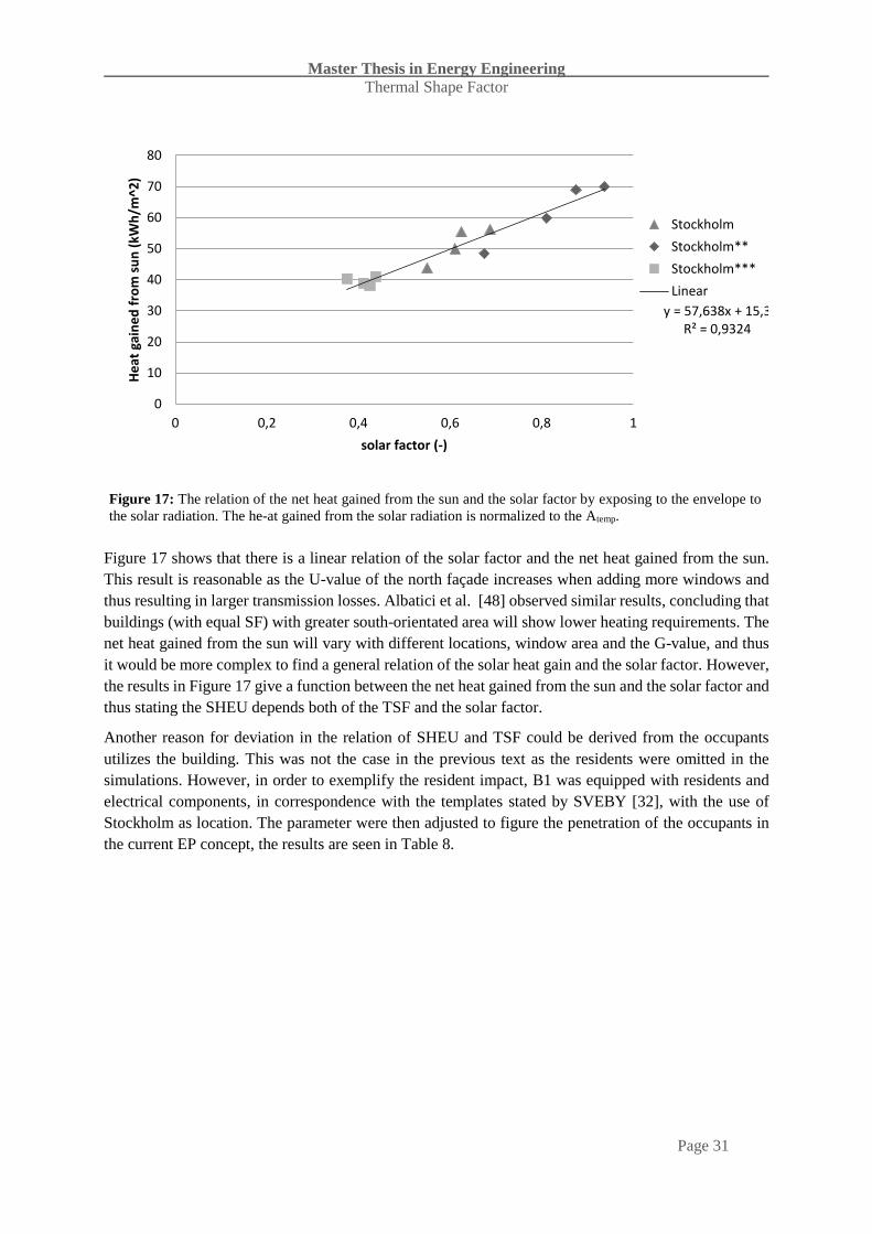
Master Thesis in Energy Engineering
Thermal Shape Factor
Page 31
Figure 17: The relation of the net heat gained from the sun and the solar factor by exposing to the envelope to
the solar radiation. The he-at gained from the solar radiation is normalized to the Atemp.
Figure 17 shows that there is a linear relation of the solar factor and the net heat gained from the sun.
This result is reasonable as the U-value of the north façade increases when adding more windows and
thus resulting in larger transmission losses. Albatici et al. [48] observed similar results, concluding that
buildings (with equal SF) with greater south-orientated area will show lower heating requirements. The
net heat gained from the sun will vary with different locations, window area and the G-value, and thus
it would be more complex to find a general relation of the solar heat gain and the solar factor. However,
the results in Figure 17 give a function between the net heat gained from the sun and the solar factor and
thus stating the SHEU depends both of the TSF and the solar factor.
Another reason for deviation in the relation of SHEU and TSF could be derived from the occupants
utilizes the building. This was not the case in the previous text as the residents were omitted in the
simulations. However, in order to exemplify the resident impact, B1 was equipped with residents and
electrical components, in correspondence with the templates stated by SVEBY [32], with the use of
Stockholm as location. The parameter were then adjusted to figure the penetration of the occupants in
the current EP concept, the results are seen in Table 8.
y = 57,638x + 15,3R² = 0,9324
0
10
20
30
40
50
60
70
80
0 0,2 0,4 0,6 0,8 1
He
at g
ain
ed
fro
m s
un
(kW
h/m
^2)
solar factor (-)
Stockholm
Stockholm**
Stockholm***
Linear

Master Thesis in Energy Engineering
Thermal Shape Factor
Page 32
Table 8: The impact of the occupants when determine the energy performance.
Energy efficient
occupants
Default
according to
template
Not energy
efficient
occupants
Set point temperature (°C) 20 21 22
Airing (kWh/m2) -10 % 4 +10 %
DHW (kWh/m2) -10 % 20 +10 %
Number of residents 3 2 1
Household electricity (kWh/m2) -10 % 30 +10 %
Obtained EP (kWh/m2) 117.6 (11 %) 131.7 146.7 (11 %)
As seen in Table 8 the obtained EP is diverging, changing some user influenced parameters the range of
EP is extended to ±15 kWh/m2. If this scenario holds as believable is not decided, but it do serve to
indicate the influence of the residents. This problem has been considered by the Boverket by using the
term of normal use, corresponding to the energy use if the building is used as it was intended to. If the
usage varies from the normal case corrections are allowed apply when verifying energy calculations of
buildings [30].
As mentioned above B1 – B4 are not occupied in the simulations. Thus, in order to benchmark the
buildings with the concept of EP adjustment had to be implemented; as the EP is not corresponding to
the SHEU. The SVEBY templates [32] were used to determine the heat gains and to convert the EP to
SHEU, these heat gains are submitted in Table 9.
Table 9: The internal loads inside the buildings according to templates in [32].
Template of internal loads Value
DHW 20 kWh/m2
Household electricity 30 kWh/m2
Facility electricity 15 kWh/m2
Electricity utilization factor 70 %
Number of occupants 2.79 (assuming four-room house)
Activity level 80 W
Attendance 14 h/day
The conversion from EP limits, as seen in Table 1, to SHEU limits was done (assuming the DHW do
not contribute to the heat balance) by subtracting the EP number by DHW and facility electricity, add
the gained heat from electricity and occupants, this yields a limit of all the supplied heat to a building.
The result of this action is seen in Table 10, where the EP limit was adjusted with an additional 12
kWh/m2 in order to meet the SHEU limit.

Master Thesis in Energy Engineering
Thermal Shape Factor
Page 33
Table 10: The EP limit and the corresponding specific-heat-energy-use limit.
Type of building Zone I Zone II Zone III Zone IV
EP limit 130 110 90 80
SHEU limit 142 122 102 92
The present system of EP and the division of the climate zones could be, as seen in Table 10, rewritten
to correspond to the SHEU concept. The buildings B1 – B4 are simulated in a city of each climate zone,
using the default window placement, the results are presented in Figure 18. The zone IV SHEU-limit
has been marked out as a thick line.
B1* B1 B2 B4 B3
Figure 18: The annual specific-heat-energy-use against TSF, the SHEU limit for new buildings in zone IV is marked
as a thick black line.
In Figure 18 SHEU is related to TSF of the four building shapes, the improved insulation in B1*
obviously lowers the SHEU. As mentioned in chapter 2. Theory, SHEU could be expressed as a linear
function of TSF according to eq. 19, given that the degree-days are held constant. Thus, if the other
buildings are improved with ECMs they will follow the linearization in Figure 18. Further seen in Figure
18 is that the buildings located in Malmö intersect the SHEU limit of zone IV at a TSF value of 1.27
W/(m2K), the same procedure was carried out for all the four climate zones. The results for the other
cities are presented in Table 11.
y = 131,9x + 4,9248R² = 0,9891
y = 100,29x - 4,8251R² = 0,9869
y = 76,595x + 6,7617R² = 0,9873
y = 79,615x - 8,7739R² = 0,9897
0
50
100
150
200
250
300
0 0,5 1 1,5 2 2,5
SHEU
(kW
h/m
^2)
TSF (W/K)
Kiruna
Sundsvall
Stockholm
Malmö
Linear(Kiruna)
Linear(Sundsvall)
Linear(Stockholm)
Linear(Malmö)

Master Thesis in Energy Engineering
Thermal Shape Factor
Page 34
Table 11: Comparison of the EP limits of detached houses in cites of the climate zones and the corresponding TSF
value needed for the buildings not to exceed the EP limits.
Zone I
(Kiruna)
Zone II
(Sundsvall)
Zone III
(Stockholm)
Zone IV
(Malmö)
SHEU limit (kWh/m2) 142 122 102 92
Corresponding TSF limit (W/(m2K)) 1.03 1.26 1.24 1.27
In Table 11 the limits of the TSF are presented for four cities. Building constructors in Kiruna must take
the most refined actions in order to generate the lowest TSF number, whereas the others could build
with less strictness regarding the heat losses. Same calculations can be made for Umeå. For Umeå,
located in the south of zone I, the required TSF is 1.15 W/(m2K) and thus there is also a large variation
within zone I and also in the other zones in the same reasoning. Furthermore, if a building is built
somewhere in an area that overlaps two zones; it could be constructed with a lower performance if
situated in the northern zone. According to these results, the division of climate zones is shortcoming.
A consequence to the present climate zone concept is that a building in most northern of a climate zone
probably is more expensive than if it is sited in the south region. However, as the present performance
indicator (EP) consist of purchased energy, the residents’ behavior could prevent this gap, i.e. for a fix
building the residents in Kiruna could lower EP by using less DHW, increasing the load supplied with
household electricity, etc.
The national limit of the overall U-value holds as 0.4 W/(m2K), which could be considering as a signal
for equal thermal properties of residential buildings throughout the entire nation. As discussed in the
above paragraph, the current EP system put limits in how a building must be constructed in different
parts of Sweden, i.e. if a household is assumed to act as the templates of SVEBY, they will have to take
different energy saving measures in order to fulfill the EP limit depending of where their building is
sited. Thus, this part of the building code understands as inconsistent. A reform of the current EPI would
thereby be preferable; using a distinct division between (i) the building itself and (ii) how the building
behave when being used.
Thermal shape factor could serve as an alternative EPI in terms of heat losses. The expression of TSF
also includes SF* and thus becomes a combined design and heat loss limit, providing a tool of easy
communication between constructors and architects. From construction papers and drawings it is easily
to determine the TSF in new housing estate making the TSF a measure rather easy to guarantee for the
building constructor, given that the verification of the outcome could be performed accurate enough.
Two approaches to determine the TSF from measurements are (i) the regression approach, used by
Vesterberg [38] and (ii) the degree-day approach, used in Part 1 of this thesis and will further used in
this section. As discussed earlier, Figure 17 shows that the solar impact on the annual SHEU is
significant when varying the solar factor. Andersson et al. [8] showed that the solar impact during the
winter solstice could be neglected in Umeå, but since Sweden covers several of latitudes, one could ask
if it could be neglected in the southern parts.
In order to determine the solar impact in the south of Sweden some further simulation was made using
Malmö as location. Only B3 was included in these simulations since this layout was most influenced by
the solar radiation. The winter solstice take place between 21-22st of December, thus the simulation was

Master Thesis in Energy Engineering
Thermal Shape Factor
Page 35
conducted during 30 days including covering this date. The result is shown in Figure 19, where a shaded
B3 is compared to an unshaded B3.
Figure 19: The daily SHEU for building B3 during the winter solstice in Malmö as a function of the temperature
difference. The shaded building is fully covered from the solar radiation and the non-shaded building is
uncovered, using the tool of shading objects in IDA ICE.
As seen in Figure 19 when B3 is solar exposed, SHEU is clearly effected, the relation of the SHEU-to-
temperature difference is being deformed. In order to determine the magnitude of the solar impact during
the simulation period, the SHEU of B3 with south point windows (B3**) and north pointing windows
(B3***) was simulated and compared to their corresponding shaded version. The result of this action is
seen in Table 12.
Table 12: The impact of the solar radiation, the SHEU of the solar exposed building is compared to a shaded
version giving the solar impact in percent.
B3 B3** B3***
SHEU (kWh/m2) solar exposed 32 31 33
Solar impact (%) 4.7 7.6 1.4
y = 0,0282x + 0,4172R² = 0,8338
y = 0,0275x + 0,3841R² = 0,7297
0
0,2
0,4
0,6
0,8
1
1,2
1,4
1,6
0 10 20 30 40
SHEU
(kW
h/m
2 , d
ay)
Tin-Tout (K)
B3 - Shaded
B3 - Unshaded
Linear (B3 -Shaded)
Linear (B3 -Unshaded)

Master Thesis in Energy Engineering
Thermal Shape Factor
Page 36
The result shown in Table 12 indicates that the solar factor is of matter when determine the solar impact
in the heat balance during winter solstice in the most south district of Sweden. However, excluding the
solar impact from the TSF could generate an incitement for constructor to maximize the solar factor in
order to obtain a TSF as low as possible. In order to determine sources of errors, a brief sensitivity
analysis was conducted, similar to the previous shown in Table 8. The analysis is seen in Table 13.
Table 13: Sensitivity analysis of different parameters included in the heat balance, the bottom rows includes
information on how the EP and TSF number are affected by adjusting of some parameters.
Recessed Default Improved
Solar factor (-) 0.38 0.63 0.88
Electricity utilization factor, α (%) - 10 % 70 + 10 %
Number of residents - 10 % 2.79 + 10 %
Airing (kWh/m2,a) - 10 % 4 + 10 %
Indoor temperature (°C) + 1°C 21 - 1°C
DHW (kWh/m2,a) + 10 % 20 - 10 %
Household electricity (kWh/m2,a) - 10 % 30 + 10 %
Resulting EP (kWh/m2, month) + 11 % 30.5 - 11 %
Resulting TSF (W/(m2K)) + 4 % 2.1 - 4 %
Seen in Table 13 is that when shifting the parameters towards Recessed and Improved mode, the impact
on EP and TSF is ±11 % and ±4 %, respectively. If the uncertainty in the solar factor is omitted, the
variation of the TSF reduces to ±1 % and EP to ±8 %.
Lastly, regarding a verification process the ground heat losses have to be mentioned. As said earlier,
ground losses has been considered by a ratio of temperature differences. However, in a verification
process it could be difficult to determine the true ground temperature without extensive measurements.
Instead, one could try to bypass the problem by using the annual temperature at the given location as an
approximation of the ground temperature. By using the default properties of B3 and Malmö as location,
yielding a monitored TSF number of 1.86 W/(m2K) by eq. 19. By correcting the ground U-value, i.e.
using eq. 7 with the ground temperature of 7.9° C (annual average outdoor temperature in Malmö), the
projected TSF number received from constructions papers is reduced from 2.10 to 1.99 W/(m2K). This
approach gives an error of 6.5 % between the monitored and projected TSF number. The verified TSF
becomes lower than the projected, which gives the building construction an error margin when
assembling the building.
In order to apply this concept to the future building code some adjustments are necessary. All buildings
should measure the total electricity utilization, all the supplied heat with a separate meter of the DHW
and the indoor temperature. The rise of investment of such surveying equipment could be assumed as
low in the context of a new building construction, but still assumptions have to be made regarding the
occupancy and the utilization factor (α). Furthermore, the verification process demands a period of low
solar impact. The proposed method could be summarized by eq. 21, where the first terms represents the
projected TSF number and is solved with data from the construction papers, and the last term
representing the monitored TSF number and is determined in the verification process. By subtracting

Master Thesis in Energy Engineering
Thermal Shape Factor
Page 37
the projected value by the monitored, a difference is formed which should be smaller than some defined
Limit.
|𝑈𝑎.𝑔𝐴𝑎.𝑔 + 𝑈𝑏.𝑔𝐴𝑎.𝑔 (
𝑇𝑖𝑛 − 𝑇𝑔
𝑇𝑖𝑛 − 𝑇𝑜𝑢𝑡)
𝐴0
𝑆𝐹∗ + 1,2 ∙ (�̇�𝑣𝑒𝑛𝑡(1 − 𝜂) + �̇�𝑙𝑒𝑎𝑘) −𝐸𝐻𝐷 + 𝐸𝐻𝐺
𝐷𝐷| ≤ 𝐿𝑖𝑚𝑖𝑡
21
As no construction data is available from any actual building cases, it is for future studies to determine
the reality-based use of this approach.

Master Thesis in Energy Engineering
Thermal Shape Factor
Page 38
5.3 Summarized discussion
This chapter includes a discussion considering the method, the results and sources of error. First, a
general discussion is carried out, followed by more specific discussion of two parts within the thesis.
Lastly, a recommendation of future prospects and work are presented.
The need of reliable energy data is of importance for both parts in this thesis, future homes could be
assumed to adapt to the so-called Smart homes including measuring equipment for distance control
among other things. This would surely also provide the property owner more detail energy data
regarding the building which could be of use detecting the outcome of different ECMs and would also
enable a more detailed verification of the building. However, the present building code could be refined
by claiming individual measurement of supplied heat, facility and household electricity in order to
simplify verification processes and understanding the heat balance of a building. Such measurements
would also provide unique data for the facility owner to use in calculations of new housing estate or
refurbishment projects.
5.3.1 Part 1: Calibration
The study of Part 1 investigates a calibration approach for a BES model. The case study building was
not an optimal choice, since M7 uses nearly eight times more energy for circulating the DHW than the
average building. Despite this fact, the TSF approach demonstrates a possibility to work as a calibration
tool. When the DHWC is known (Level 2 and 3), the BES model is considered as calibrated in eleven
of twelve months of the year.
In the TSF approach used in this study, the author put most effort in adjusting the ground heat losses
and infiltration in order to obtain a well-fit BES model. The expression of TSF also includes other
parameters, like thermal bridges. If the ground temperature is known, another TSF approach would be
to alter the other parameters, due to limited time within this work the author recommends this for future
research.
The advantage of the TSF approach is that it uses monthly aggregated data, with less information of
how the building is assembled, yielding a BES model nearly corresponding to the measured data. It is
in the author’s opinion that this could be the case when refurbishment project is implemented in the
existing building stock. One drawback of the approach is the estimations of parameters included in TSF,
e.g. the calculations of a more efficient AHU with incorrect ventilation flow do not give an accurate
result. Thus, it is of relevance to conduct specific measurements according to the considered ECM, i.e.
air ventilation flow, in order to achieve correct results.
5.3.2 Part 2: Energy Performance Indicator
According to the European Union directive 2010/31/EU, all new buildings must adapt to the concept of
nearly zero energy buildings (NZEB). In Sweden, Boverket was assigned by the government to suggest
how to implement the directive in the Swedish building code. The resulting report [49] suggest to keep
the handling of purchased energy, but to include weighting factors for the electric energy use in the
expression of energy performance. A major concept of NZEBs is to utilize the secondary heat gains (i.e.
solar radiation, equipment, occupant etc.) as main heat source. Thus, the suggestion of further using the
purchased energy becomes more of irrelevance as the purpose of the NZEB is to minimize this amount

Master Thesis in Energy Engineering
Thermal Shape Factor
Page 39
of energy. Hence, a measure of the heat losses associated with the building is of more relevance in this
context.
When determine an indicator of performance, it of great importance to address the indicator to the one
able to affect the outcome. The constructor should have an indicator solely addressed to the building
regardless how it is manage by the residents. Vesterberg explained the deviation between calculated and
measured EP [36] in a certain neighborhood as a combination of the chosen area of normalization and
the solar gain, and consequently not as a variance of the heat loss coefficient. Previous work [19] has
recommended the shape factor to be included in a future building code, but such limitation would restrict
the architects to draw buildings of certain compactness. As a result, it could lead in a direction where
less spectacular buildings are constructed. By adding the heat losses to the building shape, i.e. the
thermal shape factor, such limitation would not appear. The extreme building designs would instead be
forced towards a stricter construction to prevent heat losses. Furthermore, this representation of a key
measure would also enable a simple communication link between architects and building constructors.
In the study of Part 2, TSF was investigated as an EPI candidate. TSF is less sensitive to the user behavior
than EP and the use of TSF as an EPI throughout all regions of Sweden would benefit building
construction equality in the nation.
Furthermore, the solar factor has been defined and the results indicate a relation between the net solar
heat gain and building design, i.e. shape and window placement. However, the study only uses a fix
number of windows and the building is not rotated. Results from a work by Fallahtafti et al. [31]
indicates there is an optimal angel how a building is orientated, but according to the results of this study
it would be preferable to further research in how the windows is orientated, as it strongly affects the heat
gained from the sun. Furthermore, the expression of the solar factor could be reformed and improved,
as the present expression solely depends of the size of certain wall components and their orientation
towards the south.
5.3.3 Future work
The first calibration in the TSF approach, Level 1, is provided with information normally included
within an energy bill. As the DHWC highly diverge from the templates, it could be of interest to examine
Level 1 for a larger number of buildings to confirm whether this approach holds as an applicable tool.
This work has not put effort in determine the primary energy utilization instead the focus has covered
the net energy system. In future researches it would be of interest to determine how a national limit of
the TSF affects the primary energy usage throughout Sweden, perhaps it could be more energy efficient
to insulate buildings in some weather-exposed regions in order to decrease the energy utilization within
the Swedish building sector. Furthermore, it could be of interest to analyze how the society and
government-subventions contribute in such system.
The presented model for verification of the TSF number is limited to be conducted during the winter
solstice in order to minimize the solar impact of the heat balance. In order to extend the period of
verification some further work could elaborate a model for predicting the solar impact for a certain
building envelope, without the need of dynamic simulation tools.

Master Thesis in Energy Engineering
Thermal Shape Factor
Page 40
6. Conclusions
The main conclusions drawn from this thesis work is presented below.
None of the introduced calibration methods could fulfill the calibration limit for the case study
building. However, the results could differ if the M7 was not associated with large heat losses
by DHWC.
The present system of measuring energy performance of buildings is inconsistent, as the used
system boundary excludes elements from the heat balance. Furthermore, the use of four climate
zones brings inequalities regarding terms of the buildings energy efficiency, e.g. Building
constructors in the northern part of a zone must take more refined actions in making buildings
energy efficient than in the southern part.
TSF is a more robust EPI than EP and thus should be further investigated to be applicable in the
building code.

Master Thesis in Energy Engineering
Thermal Shape Factor
Page 41
7. Bibliography
[1] B. Rodríguez-Soria, J. Domínguz-Hernández and J. M.Pérez-Bella, "Review of international regulations governing the thermal insulation requirments of residential buildings and the harmnization of envelope energy loss," vol. 34, pp. 78-90, 2014.
[2] Statistics Sweden, "Yearbook of Housing and Building Statistics 2012," Statistics Sweden, Construction, Rents and Real Estate Statistics Unit, Stockholm, 2012.
[3] P. Westin and L. Nilsson, "Energy statistics for one- and two-dwelling buildings in 2014," Swedish Energy Agency, Eskilstuna, 2015.
[4] P. Westin and L. Nilsson, "Energy statistics for multi-dwelling buildings in 2014," Swedish Energy Agency, Eskilstuna, 2015.
[5] "EUR-Lex," European Union, 14 02 2007. [Online]. Available: http://eur-lex.europa.eu/legal-content/EN/TXT/?uri=URISERV%3Al27042. [Accessed 23 02 2016].
[6] National Board of Housing, Building and Planning, "Vad är en energideklaration? (In Swedish)," National Board of Housing, Building and Planning, 08 08 2014. [Online]. Available: http://www.boverket.se/sv/byggande/energideklaration/vad-ar-en-energideklaration/. [Accessed 22 02 2016].
[7] A. Sjöström, "Ändra Boverkets byggregler (In Swedish)," Swedish District Heating, [Online]. Available: http://www.svenskfjarrvarme.se/Asikter/Viktiga-fragor1/Viktiga-fragor/. [Accessed 22 01 2016].
[8] S. Andersson, J.-U. Sjögren, R. Östin and T. Olofsson, "Building performance based on measured data," in World Renewable Energy Congress - Sweden, Linköping, 2011.
[9] Departement of Enviroment and Energy, "Government Office," 2004. [Online]. Available: http://www.regeringen.se/contentassets/56e0c6645a054a5bbbd85646f53d20f0/sou-2004109---kapitel-5-t.o.m.-kapitel-9. [Accessed 23 02 2016].
[10] Z. Yang and B. Becerik-Gerber, "A model calibration framework for simultaneous multi-level building energy simulation," Applied Energy, vol. 149, pp. 415-431, 2015.
[11] P. Raftery, M. Kaene and M. Costa, "Calibrating whole building energy models: Detailed case study using hourly measured data.," Energy Buildings, vol. 43, no. 12, pp. 3666-3679, 2011.
[12] K. Mahapatra, "Energy use and CO2 emission of new residential buildings built under specific requirements - The case of Växjö municipality, Sweden," Applied Energy, vol. 152, pp. 31-38, 2015.
[13] M. Mangold, M. Österbring and H. Wallbaum, "Handling data uncertainties when using Swedish energy performance certificate data to describe energy usage in the building stock," Energy and Buildings, vol. 102, pp. 328-336, 2015.

Master Thesis in Energy Engineering
Thermal Shape Factor
Page 42
[14] J. Claesson, "Utfall och metodutvärdering av energideklaration av byggnader (In Swedish)," CERBOF Projekt no. 72, Stockholm, 2011.
[15] NIBE, "NIBE - Boverkets byggregler (In Swedish)," NIBE Energy Systems, [Online]. Available: http://www.nibe.se/support/BBR---Boverkets-byggregler/. [Accessed 30 04 2016].
[16] W. Wang, H. Rivard and R. Zmeureanu, "Floor shape optimization for green building design," vol. 20, pp. 363-378, 2006.
[17] I. Danielski, "Energy variations in apartment buildings due to different shape factors and relative size of common areas," in Energy End-Use Efficiency Issues (EEE), Linköping, Sweden, 2011.
[18] E. Rodrigues, A. Amaral, A. Rodrigues Gaspar and Á. Gomes, "How reliable are geometry-based building indices as thermal performance indicators?," Energy Conversion and Management, vol. 101, pp. 561-578, 2015.
[19] I. Danielski, A. Joelsson and M. Fröling, "The Impact of the shape factor on final energy demand in residential buildings in Nordic climates," in World Renewable Energy Congress, Denver, 2012.
[20] V. Granadeiro, J. R. Correia, V. M. Leal and J. P. Duarte, "Envelope-related energy demand: A design indicator of energy performance for residential buildings in early design stages," vol. 61, pp. 215-223, 2013.
[21] P. Depecker, C. Menezo, J. Virgone and S. Lepers, "Design of buildings shape and energetic consumption," Building and Enviroment, vol. 36, pp. 627-635, 2000.
[22] T. Catalina, V. Iordache and B. Caracaleanu, "Multiple regression model for fast prediction of the heating energy demand," Energy and Buildings, vol. 57, pp. 302-312, 2012.
[23] M. C. Kennedy and A. O'hagan, "Bayesian calibration of computer models," Journal of the Royal Statistical Society Series B-Statistical Methodology, vol. 63, no. 2, pp. 425-450, 2001.
[24] A. Pedrini, F. Westphal and R. Lamberts, "A methodology for building energy modelling and calibration in warm climates," Building and Environment, vol. 37, pp. 903-912, 2002.
[25] J. Vesterberg, "Calibration of low-rise multifamily residential simulation models using regressed estimations of transmission losses," Journal of Building Performance Simulation, vol. 9, no. 3, pp. 304-315, 2016.
[26] A. Mihai and R. Zmeureanu, "Bottom-up evidence-based calibration of the HVA air-side loop of a building energy model," Journal of Building Performance Simulation, pp. 1940-1507, 2016.
[27] M. Erlandsson, "Bedömning av resurseffektiva byggnader: Faktorer för olika energiformer och energislag (In Swedish)," Swedish Energy Agency, 2009.
[28] M. Wilby, A. Rodríguez Gonzalez and J. Vinagre Díaz, "Empirical and dynamic primary energy factors," Energy, vol. 73, pp. 771-779, 2014.

Master Thesis in Energy Engineering
Thermal Shape Factor
Page 43
[29] A. Person, C. Rydstrand and P. Hedenskog, "Allt eller inget - Systemgränser för byggnaders uppvärmning (In Swedish)," ÅF- Energi och miljö AB, Stockholm, 2005.
[30] National Board of Housing, Building and Planning, "Handbook of energy balance according to the Swedish building code, ISBN:978-91-87131-31-8," National Board of Housing, Building and Planning, Karlskrona, 2012.
[31] R. Fallahtafti and M. Mahdavinejad, "Optimisation of building shape and orientation for better energy efficient architecture," International Journal of Energy Sector Management, vol. 9, no. 4, pp. 593-618, 2015.
[32] P. e. a. Levin, "Brukarindata bostäder (In Swedish)," Sveby, Stockholm, 2012.
[33] M. D. Catarina Warfvinge, Projektering av VVS-installationer (In Swedish), Lund: Studentlitteratur AB, 2010.
[34] M. Christenson, H. Manz and D. Gyalistras, "Climate warming impact on degree-days and building energy demand in Switzerland," Energy Conversion and Management, no. 47, pp. 671-686, 2006.
[35] Google, "Google Maps," Google, [Online]. Available: https://www.google.se/maps/place/Matematikgr%C3%A4nd+7/@63.8061563,20.3107937,17.21z/data=. [Accessed 02 05 2016].
[36] J. Vesterberg, "Improved building energy simulations and verifications by regression," Umeå University, Department of Applied physics and electronics, Umeå, 2016.
[37] J. Jokisalo and J. Kurnitski, "Performance of EN ISO 13790 utilisation factor heat demand calculation method in a cold climate," Energy and Buildings, vol. 39, no. 2, pp. 236-247, 2007.
[38] J. Vesterberg, "A regression approach for assessment of building energy performance, ISBN: 978-91-7601-125-6," Umeå University, Umeå, 2014.
[39] Equa Simulation AB, "Validation of IDA Indoor Climate and Energy 4.0 with respect to CEN Standards EN 15255-2007 and EN 15265-2007," Equa Simulation AB, Stockholm, 2010.
[40] D. B. Crawley, J. W. Hand, M. Kummert and B. T. Griffith, "Contrasting the capabilities of building energy performance simulation programs," Building and Enviroment, vol. 43, pp. 661-673, 2008.
[41] A. Bring, P. Sahlin and M. Vuolle, "Models for Building Indoor Climate and Energy Simulation," International Energy Agency, Stockholm, 1999.
[42] Thomson Reuters, "Web of Science," Thomson Reuters, [Online]. Available: https://apps.webofknowledge.com/UA_GeneralSearch_input.do?product=UA&search_mode=GeneralSearch&SID=S1KR9bziC5NjNaSXehG&preferencesSaved=. [Accessed 22 06 2016].
[43] Elsevier, "Scopus," Elsevier, 2016. [Online]. Available: https://www.scopus.com/. [Accessed 22 06 2016].

Master Thesis in Energy Engineering
Thermal Shape Factor
Page 44
[44] S. Wang, C. Yan and F. Xiao, "Quantitative energy performance assessment methods for existing buildings," Energy and Buildings, vol. 55, pp. 873-888, 2012.
[45] National Board of Housing, Building and Planning, "Building Code," 19 04 2011. [Online]. Available: http://www.boverket.se/contentassets/a9a584aa0e564c8998d079d752f6b76d/bbr-bfs-2011-6-tom-bfs-2015-3-konsoliderad.pdf. [Accessed 14 04 2016].
[46] Swedish Energy Agency, "Domestic water utilization, ISSN 1403-1892," Swedish Energy Agency, Eskilstuna, 2012.
[47] M. Erlandsson, S. Ruud, E. Sandberg, Å. Blomsterberg, H. Eek and O. Ingulf, "Kravspecifikation för nollenergihus, passivhus och minienergihus (In Swedish)," Swedish association of Zero Energy Buildings, 2012.
[48] R. Albatici and F. Passerini, "Bioclimatic design of buildings considering heating requirements in Italian climatic conditions. A simplified approach," Building and Environment, vol. 46, pp. 1624-1631, 2011.
[49] National Board of Housing, Building and Planning, "Förslag till svensk tillämpning av nära-nollenergibyggnader, Rapportnummer: 2015:26 (In Swedish)," National Board of Housing, Building and Planning, Karlskrona, 2015.
[50] AB Bostaden i Umeå, "Hållbara Ålidhem - Om projektet (In Swedish)," AB Bostaden i Umeå, [Online]. Available: http://www.bostaden.umea.se/hallbara-alidhem/om-projektet. [Accessed 22 06 2016].