thermochemical non-equilibrium entry flows in mars in three-dimensions … · · 2014-11-20on the...

Abstract—This work describes a numerical tool to perform

thermochemical non-equilibrium simulations of reactive flow in

three-dimensions. The Van Leer and Liou and Steffen Jr. schemes, in

their first- and second-order versions, are implemented to accomplish

the numerical simulations. The Euler and Navier-Stokes equations,

on a finite volume context and employing structured and unstructured

spatial discretizations, are applied to solve the “hot gas” hypersonic

flow around a blunt body, in three-dimensions. The second-order

version of the Van Leer and Liou and Steffen Jr. schemes are

obtained from a “MUSCL” extrapolation procedure in a context of

structured spatial discretization. In the unstructured context, only

first-order solutions are obtained. The convergence process is

accelerated to the steady state condition through a spatially variable

time step procedure, which has proved effective gains in terms of

computational acceleration. The reactive simulations involve a Mars

atmosphere chemical model of nine species: N, O, N2, O2, NO, CO2,

C, CO, and CN, based on the work of Kay and Netterfield. Fifty-three

chemical reactions, involving dissociation and recombination, are

simulated by the proposed model. The Arrhenius formula is

employed to determine the reaction rates and the law of mass action

is used to determine the source terms of each gas species equation.

The results have indicated the Van Leer TVD scheme as presenting

good solutions, both inviscid and viscous cases.

Keywords— Thermochemical non-equilibrium, Mars entry, Nine

species model, Hypersonic “hot gas” flow, Finite volume, Euler and

Navier-Stokes equations, Three-dimensions.

I. INTRODUCTION

HERE has been significant interest in recent years in a

mission to Mars. One such proposal is the MARSNET

assessment study [1] concerning the potential contribution of

ESA (European Space Agency) to a Mars Network mission in

cooperation with NASA. NASA is currently studying a

network mission MESUR (Mars Environmental Survey),

involving the placement of up twenty small scientific stations

Edisson S. G. Maciel works as a post-doctorate researcher at ITA

(Aeronautical Technological Institute), Aeronautical Engineering Division –

Praça Marechal do Ar Eduardo Gomes, 50 – Vila das Acácias – São José dos

Campos – SP – Brazil – 12228-900 (corresponding author, phone number:

+55 012 99165-3565; e-mail: [email protected]).

Amilcar P. Pimenta teaches at ITA (Aeronautical Technological Institute),

Aeronautical Engineering Division – Praça Marechal do Ar Eduardo Gomes,

50 – Vila das Acácias – São José dos Campos – SP – Brazil – 12228-900 (e-

mail: [email protected])

Nikos E. Mastorakis is with WSEAS (World Scientific and Engineering

Academy and Society), A. I. Theologou 17-23, 15773 Zografou, Athens,

Greece, E-mail: [email protected] as well as with the Technical University

of Sofia, Industrial Engineering Department, Sofia, 1000, Bulgaria

mailto:[email protected]

on the surface of Mars. The objective of the proposed ESA

activities is the provision of three of these stations to perform a

variety of scientific experiments. The intended entry scenario

is an unguided ballistic entry at a typical velocity of 6 km/s

using a blunt sphere/cone configuration in which deceleration

is provided predominantly by hypersonic aero-braking. It is

important that the mass of the vehicle structure and thermal

protection system (TPS) be minimized such that the payload

delivered to the surface may be maximized.

The trajectory for a ballistic Martian entry takes the vehicle

through regions where thermochemical non-equilibrium effects

in the surrounding shock layer may be significant. For typical

entry velocities (> 5 km/s) the temperature in the shock layer

will be sufficiently high for dissociation of the freestream

species to occur. The energy removed through such reactions

may be released at the vehicle surface via recombination

leading to significantly enhanced heat transfer rates. In order

to design the TPS for minimum mass the heat transfer rate

needs to be accurately predicted. This requires that any

catalytic properties of the TPS material are accounted for in

the heat transfer rate calculation since these will determine the

extent of wall recombination.

As aforementioned, missions to other planets remain an

objective for the ESA, and such missions generally involve the

entry of a space vehicle into the atmospheres of those planets.

In the context of such entry, aerothermodynamics is one of the

critical technologies. While the thermochemical behavior of

air under re-entry conditions has been studied extensively, and

is to some degree understood, the same is not true for entries

into other atmospheres. The atmospheres of Mars and Venus,

for example, contain significant amounts of carbon dioxide. In

particular, the Mars atmosphere is a mixture of approximately

96% CO2 and 4% N2, with pressures much lower than the

Earth’s atmosphere, so for any entry into the Martian

atmosphere the non-equilibrium behavior of CO2 is likely to be

of importance for a typical blunt body entry vehicle. This

includes not just the influence of thermochemistry on the

forebody heatshield flowfield, but also the influence on the

shoulder expansion, base flow, and base heating environment.

Analyzing the reentry flows in Earth, [2] have proposed a

numerical tool implemented to simulate inviscid and viscous

flows employing the reactive gas formulation of thermal and

chemical non-equilibrium in two-dimensions. The [3]

numerical algorithm was implemented to perform the

numerical experiments. The Euler and Navier-Stokes

equations, employing a finite volume formulation, on the

context of structured and unstructured spatial discretizations,

Thermochemical Non-Equilibrium Entry Flows

in Mars in Three-Dimensions – Part I

Edisson S. G. Maciel, Amilcar P. Pimenta, and Nikos E. Mastorakis

T

INTERNATIONAL JOURNAL OF MATHEMATICAL MODELS AND METHODS IN APPLIED SCIENCES Volume 8, 2014

ISSN: 1998-0140 329





were solved. These variants allowed an effective comparison

between the two types of spatial discretization aiming verify

their potentialities: solution quality, convergence speed,

computational cost, etc. The aerospace problem involving the

hypersonic flow around a blunt body, in two-dimensions, was

simulated. The reactive simulations involved an air chemical

model of five species: N, O, N2, O2 and NO. Seventeen

chemical reactions, involving dissociation and recombination,

were simulated by the proposed model. The Arrhenius formula

was employed to determine the reaction rates and the law of

mass action was used to determine the source terms of each

gas species equation. A spatially variable time step was

employed aiming to obtain gains in terms of convergence

acceleration. Such gains were demonstrated in [4-5]. Good

results were obtained with such code.

[6] have presented a numerical tool implemented to

simulate inviscid and viscous flows employing the reactive gas

formulation of thermal and chemical non-equilibrium in three-

dimensions. The [3] numerical algorithm was implemented to

perform the numerical experiments. The Euler and Navier-

Stokes equations, employing a finite volume formulation, on

the context of structured and unstructured spatial

discretizations, were solved. The aerospace problem involving

the hypersonic “hot gas” flow around a blunt body, in three-

dimensions, was simulated. The reactive simulations involved

an air chemical model of five species: N, O, N2, O2 and NO.

Seventeen chemical reactions, involving dissociation and

recombination, were simulated by the proposed model. The

Arrhenius formula was employed to determine the reaction

rates and the law of mass action was used to determine the

source terms of each gas species equation. A spatially variable

time step was employed aiming to obtain gains in terms of

convergence acceleration. Such gains were demonstrated in [4-

5]. In that first part, only the structured solutions were

presented. The unstructured solutions will be shown in the

second part of such study.

[7] have proposed a numerical tool implemented to

simulate inviscid and viscous flows employing the reactive gas

formulation of thermochemical non-equilibrium in three-

dimensions. The [3] and [8] numerical algorithms were

implemented to perform the numerical experiments. The Euler

and Navier-Stokes equations, employing a finite volume

formulation, on the context of structured and unstructured

spatial discretizations, are solved. The aerospace problem

involving the hypersonic flow around a blunt body, in three-

dimensions, was simulated. The reactive simulations involved

an air chemical model of seven species: N, O, N2, O2, NO,

NO+ and e

-. Eighteen chemical reactions, involving

dissociation, recombination and ionization, were simulated by

the proposed model. Such model was suggested by Blottner

([9]). The Arrhenius formula was employed to determine the

reaction rates and the law of mass action was used to

determine the source terms of each gas species equation. A

spatially variable time step was employed aiming to obtain

gains in terms of convergence acceleration. Such gains were

demonstrated in [4-5]. In this work, it was only presented the

structured formulation and solutions. The unstructured

formulation and solutions will be presented in the second part

of this study, which treats exclusively the unstructured context.

This work, first part of this study, describes a numerical

tool to perform thermochemical non-equilibrium simulations

of reactive flows in three-dimensions in Mars atmosphere. The

[3; 8] schemes, in their first- and second-order versions, are

implemented to accomplish the numerical simulations. The

Euler and Navier-Stokes equations, on a finite volume context

and employing structured and unstructured spatial

discretizations, are applied to solve the “hot gas” hypersonic

flow around a blunt body, in three-dimensions. The second-

order version of the [3; 8] schemes are obtained from a

“MUSCL” extrapolation procedure (details in [10]) in a

context of structured spatial discretization. In the unstructured

context, only first-order solutions are obtained. The

convergence process is accelerated to the steady state

condition through a spatially variable time step procedure,

which has proved effective gains in terms of computational

acceleration (see [4-5]).

The reactive simulations involve a Mars atmosphere

chemical model of nine species: N, O, N2, O2, NO, CO2, C,

CO, and CN. Fifty-three chemical reactions, involving

dissociation and recombination, are simulated by the proposed

model. The Arrhenius formula is employed to determine the

reaction rates and the law of mass action is used to determine

the source terms of each gas species equation.

The results have demonstrated that the most conservative

scheme is due to [8], although the [3] scheme is more robust,

providing results to the second-order viscous case. Moreover,

the [3] scheme presents the best mass fraction profiles at the

stagnation line, characterizing discrete dissociation of CO2 and

formation of CO.

II. FORMULATION TO REACTIVE FLOW IN THERMOCHEMICAL

NON-EQUILIBRIUM

A. Reactive Equations in Three-Dimensions

The reactive Navier-Stokes equations in thermal and

chemical non-equilibrium were implemented on a finite

volume context, in the three-dimensional space. In this case,

these equations in integral and conservative forms can be

expressed by:

V V

CV

S

dVSdSnFQdVt

, with

kGGjFFiEEF veveve

, (1)

where: Q is the vector of conserved variables, V is the volume

of a computational cell, F

is the complete flux vector, n

is the

unity vector normal to the flux face, S is the flux area, SCV is

the chemical and vibrational source term, Ee, Fe and Ge are the

convective flux vectors or the Euler flux vectors in the x, y and

z directions, respectively, Ev, Fv and Gv are the viscous flux

vectors in the x, y and z directions, respectively. The i

, j


ISSN: 1998-0140 330

and k

unity vectors define the Cartesian coordinate system.

Fourteen (14) conservation equations are solved: one of

general mass conservation, three of linear momentum

conservation, one of total energy, eight of species mass

conservation and one of the vibrational internal energy of the

molecules. Therefore, one of the species is absent of the

iterative process. The CFD (“Computational Fluid Dynamics”)

literature recommends that the species of biggest mass fraction

of the gaseous mixture should be omitted, aiming to result in a

minor numerical accumulation error, corresponding to the

biggest mixture constituent (in this case, the Mars

atmosphere). To the present study, in which is chosen a

chemical model to the Mars atmosphere composed of nine (9)

chemical species (N, O, N2, O2, NO, CO2, C, CO, and CN) and

fifty-three (53) chemical reactions, this species is the CO2. The

vectors Q, Ee, Fe, Ge, Ev, Fv, Gv and SCV can, hence, be defined

as follows ([11]):

V

9

8

7

5

4

3

2

1

e

e

w

v

u

Q ,

ue

u

u

u

u

u

u

u

u

Hu

uw

uv

pu

u

E

V

9

8

7

5

4

3

2

1

2

e ; (2)

ve

v

v

v

v

v

v

v

v

Hv

vw

pv

vu

v

F

V

9

8

7

5

4

3

2

1

2

e ;

we

w

w

w

w

w

w

w

w

Hw

pw

wv

wu

w

G

V

9

8

7

5

4

3

2

1

2

e ; (3)

in which: is the mixture density; u, v and w are Cartesian

components of the velocity vector in the x, y and z directions,

respectively; p is the fluid static pressure; e is the fluid total

energy; 1, 2, 3, 4, 5, 7, 8, and 9 are densities of the N,

O, N2, O2, NO, C, CO and CN, respectively; H is the mixture

total enthalpy; eV is the sum of the vibrational energy of the

molecules; the ’s are the components of the viscous stress

tensor; qf,x, qf,y and qf,z are the frozen components of the

Fourier-heat-flux vector in the x, y and z directions,

respectively; qv,x, qv,y and qv,z are the components of the

Fourier-heat-flux vector calculated with the vibrational thermal

conductivity and vibrational temperature; svsx, svsy and svsz

represent the species diffusion flux, defined by the Fick law;

x, y and z are the terms of mixture diffusion; v,x, v,y and

v,z are the terms of molecular diffusion calculated at the

vibrational temperature; s is the chemical source term of

each species equation, defined by the law of mass action; *ve is

the molecular-vibrational-internal energy calculated with the

translational/rotational temperature; and s is the translational-

vibrational characteristic relaxation time of each molecule.

z,vz,v

z99

z88

z77

z55

z44

z33

z22

z11

zz,vz,fzzyzxz

zz

yz

xz

v

q

v

v

v

v

v

v

v

v

qqwvu

0

Re

1G

, (6)

mols

s,vs

mols

ss,v*

s,vs

9

8

7

5

4

3

2

1

CV

eee

0

0

0

0

0

S

. (7)

The viscous stresses, in N/m2, are determined, according to

a Newtonian fluid model, by:


ISSN: 1998-0140 331

z

w

y

v

x

u

3

2

x

u2xx ; (8)

x

v

y

uxy and

x

w

z

uxz ; (9)

z

w

y

v

x

u

3

2

y

v2yy ; (10)

y

w

z

vyz ; (11)

z

w

y

v

x

u

3

2

z

w2zz , (12)

in which is the fluid molecular viscosity.

The frozen components of the Fourier-heat-flux vector,

which considers only thermal conduction, are defined by:

x

Tkq fx,f

,

y

Tkq fy,f

; (13)

z

Tkq fz,f

, (14)

where kf is the mixture frozen thermal conductivity, calculated

conform presented in section C. The vibrational components

of the Fourier-heat-flux vector are calculated as follows:

x

Tkq v

vx,v

,

y

Tkq v

vy,v

; (15)

z

Tkq v

vz,v

, (16)

in which kv is the vibrational thermal conductivity and Tv is the

vibrational temperature, what characterizes this model as of

two temperatures: translational/rotational and vibrational. The

calculation of Tv and kv are presented in section C.

The terms of species diffusion, defined by the Fick law, to a

condition of thermal non-equilibrium, are determined by

([11]):

x

YDv

s,MFssxs

,

y

YDv

s,MF

ssys

; (17)

z

YDv

s,MFsszs

, (18)

with “s” referent to a given species, YMF,s being the molar

fraction of the species, defined as:

ns

1k

kk

sss,MF

M

MY (19)

and Ds is the species-effective-diffusion coefficient.

The diffusion terms x, y and z which appear in the energy

equation are defined by ([12]):

ns

1s

ssxsx hv ,

ns

1s

ssysy hv ; (20)

ns

1s

sszsz hv , (21)

being hs the specific enthalpy (sensible) of the chemical

species “s”. The specific enthalpy is calculated as function of

the several modes of internal energy as follows:

TR2/3e strans,i ;

molecules,TR

atoms,0e

srot,i ;

molecules,1e

R

atoms,0

e

vs,v T/

s,vsvib,i ;

refss,f0,i TRhe ;

0,ivib,irot,itrans,ii eeeee ;

TReh sis . (22)

The molecular diffusion terms calculated at the vibrational

temperature, v,x, v,y and v,z, which appear in the vibrational-

internal-energy equation are defined by ([11]):

mols

s,vsxsx,v hv ,

mols

s,vsysy,v hv ; (23)

mols

s,vszsz,v hv , (24)

Table 1. Molecular mass and enthalpy formation of each

species.

Species M (g/g-mol) hf,s (J/g-mol)

N 14.0 472,680.0

O 16.0 249,180.0

N2 28.0 0.0

O2 32.0 0.0

NO 30.0 90,290.0

CO2 44.0 -393,510.0

C 12.0 716,680.0

CO 28.0 -110,530.0

CN 26.0 435,100.0

with hv,s being the specific enthalpy (sensible) of the chemical

species “s” calculated at the vibrational temperature Tv. The

sums of the Eqs. (23-24), as also those present in Eq. (7),

considers only the molecules of the system, namely: N2, O2,


ISSN: 1998-0140 332

NO, CO2, CO and CN.

The molecular mass and the formation enthalpy of each

constituent of the Mars atmosphere are given in Tab. 1. Note

that to have hf,s in J/kg, it is only necessary to multiply it by

103 and to divide it by the molecular mass.

B. Chemical Model and Reaction Data

The following species are considered for entry into the

Martian atmosphere:

N, O, N2, O2, NO, CO2, C, CO, and CN.

These species represent the main constituents of a high

temperature mixture of carbon dioxide and nitrogen. The CN

molecule is included for assessment purposes though is not

expected to be present in large mass fractions. For the

moderate entry velocities considered in this work ionization is

assumed to be unimportant, thus no ionic species are

considered. This chemical model is based on the work of [13].

The reaction set used for these calculations is given in Tab. 2.

Reverse reaction rate data are specified directly in Tab. 3. It is

assumed that both the forward and reverse reaction rate

coefficients have the following Arrhenius temperature

dependence:

T/CeATk , (25)

Table 2. Reactions and forward coefficients.

Reaction A C

O2+M O+O+M 9.1x1018

-1.0 59,370

N2+M N+N+M 2.5x1019

-1.0 113,200

NO+M N+O+M 4.1x1018

-1.0 75,330

CO+M C+O+M 4.5x1019

-1.0 128,900

CO2+M CO+O+M 3.7x1014

0.0 52,500

N2+O NO+N 7.4x1011

0.5 37,940

NO+O O2+N 3.0x1011

0.5 19,460

CO+O C+O2 2.7x1012

0.5 69,540

CO2+O CO+O2 1.7x1013

0.0 26,500

CO+N NO+C 2.9x1011

0.5 53,630

CN+O NO+C 1.6x1013

0.1 14,600

CO+N CN+O 2.0x1014

0.0 38,600

N2+C CN+N 2.0x1014

0.0 23,200

where the pre-exponential factor A, the temperature exponent

and the activation energy C are obtained from experiment

and are given in Tabs. 2 and 3. M is a third body of collision

and can be any species. Data for the forward reactions 1 to 4

and 6 to 10 are taken from [14]. Reaction 5 and 11 to 13 are

taken from [15]. Data for the reverse reactions are taken from

[14], except for reactions 5 and 9 for which data are from

reference [16], and reactions 11 to 13 where data are from

[17]. For dissociation reactions the preferential model of Park

is used whereby the forward rates are governed by an average

temperature va T.TT . With all combinations to M, a total

of fifth-three (53) reactions are obtained.

Table 3. Reactions and reverse coefficients.

Reaction A C

O2+M O+O+M 9.0x1015 -0.5 0.0

N2+M N+N+M 1.5x1018 -1.0 0.0

NO+M N+O+M 3.5x1018 -1.0 0.0

CO+M C+O+M 1.0x1018 -1.0 0.0

CO2+M CO+O+M 2.4x1015 0.0 2,184

N2+O NO+N 1.6x1011 0.5 0.0

NO+O O2+N 9.5x1009 1.0 0.0

CO+O C+O2 9.4x1012 0.25 0.0

CO2+O CO+O2 2.5x1012 0.0 24,000

CO+N NO+C 2.6x1010 0.5 0.0

CN+O NO+C 3.8x1012 0.5 4,500

CO+N CN+O 6.3x1011 0.5 4,500

N2+C CN+N 4.4x1014 0.0 4,500

C. Transport Properties

For species N, O, N2, O2 and NO curve fits for viscosity as a

function of temperature have been developed by [18] which

are of the form

CTlnBTlnAexp1.0 . (26)

[19] develops equivalent curve fits for CO and CO2, while C

behaves as O. CN data are from [20]. Data for these curve fits

are given in Tab. 4.

Table 4. Coefficients for viscosity curve fits.

Species A B C

N 0.0115572 0.4294404 -12.4327495

O 0.0203144 0.4294404 -11.6031403

N2 0.0268142 0.3177838 -11.3155513

O2 0.0449290 -0.0826158 -9.2019475

NO 0.0436378 -0.0335511 -9.5767430

CO2 -0.0195274 1.0132950 -13.9787300

C 0.0203144 0.4294404 -11.6031403

CO -0.0195274 1.0478180 -14.3221200

CN -0.0025000 0.6810000 -12.4914000

The thermal conductivity of translational and rotational

energies for each species is derived from species viscosities

using an Eucken relation:

i,r,vi,t,vi,tr cc2/5k , (27)

where:


ISSN: 1998-0140 333

RTc

.atomsfor,0.0

moleculesfor,RT2/3c

r,v

t,v

(28)

The total viscosity and conductivity of the gas mixture are

calculated using the semi-empirical rule of [21]. To the

viscosity, for instance:

ns

1i i

iiX, (29)

where Xi is the mole fraction of species i and

ns

1j

j

i

24/1

i

j

j

ij

i

M

M18

M

M1X

. (30)

Xi can be calculated from

i

ii

M

McX , (31)

with:

ns

1j j

j

M

c1M ; (32)

j

jc (Mass fraction). (33)

Diffusion coefficients are computed as outlined by [22]. The

species diffusion coefficients are calculated from

i

ii

iX1

Dc1M

M

D

. (34)

The diffusion coefficient D is calculated from the Schmidt

number:

D

Sc

. (35)

The Schmidt number is set to 0.5 for neutral species and 0.25

for ions.

The species vibrational conductivities are also calculated by

the species viscosity and the Eucken formula:

iii,v Rk . (36)

The vibrational temperature is determined from the

definition of the internal vibrational energy of the mixture, on

an iterative process, and uses the Newton-Raphson method to

find the root, which is merely the approximate vibrational

temperature. Three steps are suffices to obtain a good

approximation.

D. Source Terms

The source terms for the species mass fractions in the

chemically reacting flow are giving by:

nr

1r

'r,i

''r,iii M

maxj

1j

jji,r

maxj

1j

jji,f

''r,j

'r,j MkMk . (37)

The reaction rate coefficients kf and kr are calculated as a

function of a rate controlling temperature Ta, as given in

section B.

E. Vibrational Relaxation Model

The vibrational internal energy of a molecule, in J/kg, is

defined by:

1e

Re

Vs,V T

s,vs

s,v

, (38)

and the vibrational internal energy of all molecules is given by:

mols

s,vsV ece . (39)

The heat flux due to translational-vibrational relaxation,

according to [23], is given by:

s

vs,v*

s,vss,VT

)T(e)T(eq

, (40)

where: *

s,ve is the vibrational internal energy calculated at the

translational temperature to the species “s”; and s is the

translational-vibrational relaxation time to the molecular

species, in s. The relaxation time is the time of energy

exchange between the translational and vibrational molecular

modes.

Vibrational characteristic time of [24]. According to [25], the

relaxation time of molar average of [24] is described by:

ns

1l

WMl,sl

ns

1l

lWM

ss , (41)


ISSN: 1998-0140 334

with:

WMl,s is the relaxation time between species of [24];

WMs is the vibrational characteristic time of [24];

lAVll mNc and AVll NMm . (42)

Definition of WM

l,s . For temperatures inferior to or equal to

8,000 K, [24] give the following semi-empirical correlation to

the vibrational relaxation time due to inelastic collisions:

42.18015.0TA

l

WMl,s

41l,s

31l,se

p

B

, (43)

where:

B = 1.013x105Ns/m

2 ([26]);

pl is the partial pressure of species “l” in N/m2;

34s,v

21l,s

3l,s 10x16.1A ([26]); (44)

ls

lsl,s

MM

MM

, (45)

being the reduced molecular mass of the collision partners:

kg/kg-mol;

T and s,v in Kelvin.

The values of the characteristic vibrational temperature are

given in Tab. 5. In the absence of specific vibrational

relaxation data for CN the molecule has been assumed to

behave as CO.

Table 5. Vibrational energy constants.

Species v (K)

N2 3395.0

O2 2239.0

NO 2817.0

CO 3074.0

CN 3074.0

[27] correction time. For temperatures superiors to 8,000 K,

the Eq. (43) gives relaxation times less than those observed in

experiments. To temperatures above 8,000 K, [27] suggests

the following relation to the vibrational relaxation time:

svs

Ps

n

1

, (46)

where:

TR8 s

s , (47)

being the molecular average velocity in m/s;

220

vT

000,5010

, (48)

being the effective collision cross-section to vibrational

relaxation in m2; and

sss mn , (49)

being the density of the number of collision particles of

species “s”. s in kg/m3 and ms in kg/particle, defined by Eq.

(42).

Combining the two relations, the following expression to the

vibrational relaxation time is obtained:

Ps

WMss . (50)

[27] emphasizes that this expression [Eq. (50)] to the

vibrational relaxation time is applicable to a range of

temperatures much more vast.

III. STRUCTURED VAN LEER AND LIOU AND STEFFEN JR.

ALGORITHMS TO THERMOCHEMICAL NON-EQUILIBRIUM

As shown in [8], the discrete convective flux calculated by the

AUSM scheme (“Advection Upstream Splitting Method”) can

be interpreted as a sum involving the arithmetical average

between the right (R) and the left (L) states of the (i+1/2,j,k)

cell face, related to cell (i,j,k) and its (i+1,j,k) neighbour,

respectively, multiplied by the interface Mach number, and a

scalar dissipative term. [28] have suggested that the flux

integrals could be calculated defining each part, dynamic,

chemical and vibrational, separately. Hence, to the (i+1/2,j,k)

interface, considering the dynamical part of the formulation:

RL

k,j,2/1ik,j,2/1ik,j,2/1i

aH

aw

av

au

a

aH

aw

av

au

a

M2

1SR

k,j,2/1i

z

y

x

LR

k,j,2/1i

0

pS

pS

pS

0

aH

aw

av

au

a

aH

aw

av

au

a

2

1

. (51)

The components of the unity vector normal to the flux

interface, the flux area of each interface and the cell volume

are defined in [6; 29].

The “a” quantity represents the frozen speed of sound.

Mi+1/2,j,k defines the advection Mach number at the


ISSN: 1998-0140 335

(i+1/2,j,k) face of the (i,j,k) cell, which is calculated according

to [8] as:

RLl MMM , (52)

where the separated Mach numbers M+/-

are defined by the [3]

formulas:

;1

;1Mif,0

Mif,1M25.0

;1Mif,M

M2

;1

.1Mif,M

Mif,1M25.0

;1Mif,0

M2

(53)

ML and MR represent the Mach number associated with the left

and right states, respectively. The advection Mach number is

defined by:

aSwSvSuSM zyx . (54)

The pressure at the (i+1/2,j,k) face of the (i,j,k) cell is

calculated by a similar way:

RLl ppp ,

(55)

with p+/-

denoting the pressure separation defined according to

the [3] formulas:

;1Mif,0

;1Mif,M21Mp25.0

;1Mif,p

p2

.1Mif,p

1Mif,M21Mp25.0

;1Mif,0

p2

; (56)

The definition of the dissipative term determines the

particular formulation of the convective fluxes. According to

[30], the choice below corresponds to the [3] scheme:

;0M1if,1M5.0M

;1M0if,1M5.0M

;1Mif,M

k,j,2/1i2

Lk,j,2/1i

k,j,2/1i2

Rk,j,2/1i

k,j,2/1ik,j,2/1i

k,j,2/1i (57)

and the choice below corresponds to the [8] scheme:

k,j,2/1ik,j,2/1i M ; (58)

the discrete-chemical-convective flux is defined by:

R9

8

7

5

4

3

2

1

L9

8

7

5

4

3

2

1

k,j,2/1ik,j,2/1ik,j,2/1i

a

a

a

a

a

a

a

a

a

a

a

a

a

a

a

a

M2

1SR

L9

8

7

5

4

3

2

1

R9

8

7

5

4

3

2

1

k,j,2/1i

a

a

a

a

a

a

a

a

a

a

a

a

a

a

a

a

2

1, (59)

and the discrete-vibrational-convective flux is determined by:

RvLvk,j,2/1ik,j,2/1ik,j,2/1i aeaeM2

1SR

LvRvk,j,2/1i aeae2

1. (60)

The time integration is performed employing the Runge-

Kutta explicit method of five stages, second-order accurate, to

the three types of convective flux.

To the dynamic part, this method can be represented in

general form by:

)k(k,j,i

)1n(k,j,i

k,j,i)1k(

k,j,ik,j,ik)0(k,j,i

)k(k,j,i

)n(k,j,i

)0(k,j,i

QQ

VQRtQQ

QQ

, (61)

to the chemical part, it can be represented in general form by:

)m(

k,j,i

)1n(

k,j,i

)1m(

k,j,iCk,j,i)1m(

k,j,ik,j,im)0(

k,j,i

)m(

k,j,i

)n(

k,j,i

)0(

k,j,i

QQ

QSVQRtQQ

QQ

, (62)

where the chemical source term SC is calculated with the

temperature Ta. Finally, to the vibrational part:


ISSN: 1998-0140 336

)m(

k,j,i

)1n(

k,j,i

)1m(

k,j,ivk,j,i)1m(

k,j,ik,j,im)0(

k,j,i

)m(

k,j,i

)n(

k,j,i

)0(

k,j,i

QQ

QSVQRtQQ

QQ

, (63)

in which:

mols

s,vs,C

mols

s,VTv eSqS ; (64)

m = 1,...,5; 1 = 1/4, 2 = 1/6, 3 = 3/8, 4 = 1/2 and 5 = 1.

This scheme is first-order accurate in space and second-order

accurate in time. The second-order of spatial accuracy is

obtained by the “MUSCL” procedure.

The viscous formulation follows that of [31], which adopts

the Green theorem to calculate primitive variable gradients.

The viscous vectors are obtained by arithmetical average

between cell (i,j,k) and its neighbours. As was done with the

convective terms, there is a need to separate the viscous flux in

three parts: dynamical viscous flux, chemical viscous flux and

vibrational viscous flux. The dynamical part corresponds to

the first five equations of the Navier-Stokes ones, the chemical

part corresponds to the following eight equations and the

vibrational part corresponds to the last equation.

IV. MUSCL PROCEDURE

Second order spatial accuracy can be achieved by introducing

more upwind points or cells in the schemes. It has been noted

that the projection stage, whereby the solution is projected in

each cell face (i-1/2,j,k; i+1/2,j,k) on piecewise constant states,

is the cause of the first order space accuracy of the Godunov

schemes ([10]). Hence, it is sufficient to modify the first

projection stage without modifying the Riemann solver, in

order to generate higher spatial approximations. The state

variables at the interfaces are thereby obtained from an

extrapolation between neighboring cell averages. This method

for the generation of second order upwind schemes based on

variable extrapolation is often referred to in the literature as

the MUSCL approach. The use of nonlinear limiters in such

procedure, with the intention of restricting the amplitude of the

gradients appearing in the solution, avoiding thus the

formation of new extrema, allows that first order upwind

schemes be transformed in TVD high resolution schemes with

the appropriate definition of such nonlinear limiters, assuring

monotone preserving and total variation diminishing methods.

Details of the present implementation of the MUSCL

procedure, as well the incorporation of TVD properties to the

schemes, are found in [10]. The expressions to calculate the

fluxes following a MUSCL procedure and the nonlinear flux

limiter definitions employed in this work, which incorporates

TVD properties, are defined as follows.

The conserved variables at the interface (i+1/2,j,k) can be

considered as resulting from a combination of backward and

forward extrapolations. To a linear one-sided extrapolation at

the interface between the averaged values at the two upstream

cells (i,j,k) and (i+1,j,k), one has:

k,j,1ik,j,ik,j,iL

k,j,2/1i QQ2

QQ

, cell (i,j,k); (65)

k,j,1ik,j,2ik,j,1iR

k,j,2/1i QQ2

QQ

, cell (i+1,j,k), (66)

leading to a second order fully one-sided scheme. If the first

order scheme is defined by the numerical flux

k,j,1ik,j,ik,j,2/1i Q,QFF

(67)

the second order space accurate numerical flux is obtained

from

R

k,j,2/1iL

k,j,2/1i)2(

k,j,2/1i Q,QFF . (68)

Higher order flux vector splitting methods, such as those

studied in this work, are obtained from:

R

k,j,2/1iL

k,j,2/1i)2(

k,j,2/1i QFQFF

. (69)

All second order upwind schemes necessarily involve at least

five mesh points or cells.

To reach high order solutions without oscillations around

discontinuities, nonlinear limiters are employed, replacing the

term in Eqs. (65) and (66) by these limiters evaluated at the

left and at the right states of the flux interface. To define such

limiters, it is necessary to calculate the ratio of consecutive

variations of the conserved variables. These ratios are defined

as follows:

k,j,1ik,j,ik,j,ik,j,1ik,j,2/1i QQQQr

k,j,ik,j,1ik,j1ik,j,2ik,j,2/1i QQQQr , (70)

where the nonlinear limiters at the left and at the right states of

the flux interface are defined by k,j,2/1i

L r and

k,j,2/1i

R r1 . In this work, five options of nonlinear

limiters were considered to the numerical experiments. These

limiters are defined as follows:

l

lll

VLl

r1

rr)r(

, [32] limiter; (71)

2l

2ll

lVAl

r1

rr)r(

, Van Albada limiter; (72)

llllMINl signal,rMIN,0MAXsignalr , minmod

limiter; (73)

2,rMIN,1,r2MIN,0MAXr lllSBl , “Super Bee”


ISSN: 1998-0140 337

limiter, due to [33]; (74)

,rMIN,1,rMIN,0MAXr lllL

l , -limiter,

(75)

with “l” varying from 1 to 14 (three-dimensional space), signal

being equal to 1.0 if rl 0.0 and -1.0 otherwise, rl is the ratio

of consecutive variations of the lth

conserved variable and is

a parameter assuming values between 1.0 and 2.0, being 1.5

the value assumed in this work.

With the implementation of the numerical flux vectors

following this MUSCL procedure, second order spatial

accuracy and TVD properties are incorporated in the

algorithms.

V. DEGENERACY OF CO2, VIBRATIONAL ENERGY, FROZEN

SPEED OF SOUND AND TOTAL ENERGY EQUATION

The CO2 presents three levels of degeneracy, each one

corresponding to a characteristic vibrational mode. The

characteristic vibrational temperature and the respective

degeneracy weights are given in Tab. 6.

Table 6. Values of g’s and v’s.

Degeneracy g v

1 1 1,903.0

2 2 945.0

3 1 3,329.0

Hence, the vibrational energy is determined by:

2,vCO21,vCO1

ns

1s

ns

6s1s

s,vss,vsv ecgecgecece22

3,vCO3 ecg2

, (76)

with ev given by Eq. (39). The frozen speed of sound is given

by the following equation:

mix,vc

R

and

p)1(a , (77)

with:

R being the universal gas constant;

ns

1s s

s

M; (78)

ns

1s

s,vsmix,v ccc , (79)

cv,s being the specific heat at constant volume for each species.

The total energy is given by:

222

vrefmixmix,fmix,v wvu2

1eTRhTce , (80)

where:

ns

1s

s,fsmix,f hch ; (81)

ns

1s

ssmix RcR ; (82)

Tref = 298.15K.

VI. INITIAL AND BOUNDARY CONDITIONS

A. Initial Condition

As initial conditions, the following flow properties are given:

init, uinit, , Ttr,init, Tv,init, cs(1), cs(2), cs(3), cs(4), cs(5), cs(7) ,

cs(8), and cs(9), in which: is the flow attack angle, Ttr,init is

the initial translational/rotational temperature, Tv,init is the

initial vibrational temperature, and the cs’s are the initial mass

fractions of the N, O, N2, O2, NO, C, CO and CN. In this way,

the cs(6) is easily obtained from:

ns

6s1s

ss c1)6(c (83)

Initially, Tv,init = Ttr,init. The dimensionless variables which will

compose the initial vector of conserved variables are

determined as follows:

dim = init/, udim = uinit/achar, vdim = udim/tg();

Ttr,dim = Ttr,init/achar and Tv,dim = Tv,init/achar, (84)

with:

defining the freestream density;

is the flow attack angle;

achar obtained from tables of the Mars atmosphere

properties.

Considering the species mass fractions and with the values

of the species specific heat at constant volume, it is possible to

obtain the mixture specific heat at constant volume. The

mixture formation enthalpy is also obtained from the mass

fractions and from the species formation enthalpies. The

dimensionless internal vibrational energy to each species is

obtained from:

1eRe dim,V2N,V

222

T

N,vNNdim,,v

;

1eRe dim,V2O,V

222

T

O,vOOdim,,v

;

1eRe dim,VNO,V T

NO,vNONOdim,,v

;


ISSN: 1998-0140 338

;1eR)1(ge dim,V)1(2CO,V

222

T

)1(CO,vCO)1(COdim,,v


222

T



222

T


;1eRe dim,VCO,V T

CO,vCOCOdim,,v

1eRe dim,VCN,V T

CN,vCNCNdim,,v

. (85)

The total internal vibrational energy of the system is

determined by Eq. (39). Finally, the dimensionless total energy

is determined by Eq. (80). The initial vector of conserved

variables is, therefore, defined by:

dim,vdim

sdim

sdim

sdim

sdim

sdim

sdim

sdim

sdim

dim

dimdim

dimdim

dimdim

dim

e

)9(c

)8(c

)7(c

)5(c

)4(c

)3(c

)2(c

)1(c

e

w

v

u

Q . (86)

B. Boundary Conditions

(a) Dynamical Part:

The boundary conditions are basically of three types: solid

wall, entrance and exit. These conditions are implemented in

special cells, named ghost cell.

(a.1) Wall condition: To inviscid flow, this condition imposes

the flow tangency at the solid wall. This condition is satisfied

considering the wall tangent velocity component of the ghost

volume as equals to the respective velocity component of its

real neighbor cell. At the same way, the wall normal velocity

component of the ghost cell is equaled in value, but with

opposite signal, to the respective velocity component of the

real neighbor cell. It results in:

rzxryxr2xg wnn2vnn2un21u ; (87)

rzyr2yrxyg wnn2vn21unn2v ; (88)

r2zryzrxzg wn21vnn2unn2w ; (89)

with “g” related with ghost cell and “r” related with real cell.

To the viscous case, the boundary condition imposes that the

ghost cell velocity components be equal to the real cell

velocity components, with the negative signal:

rfrfrf wwandvv,uu . (90)

The pressure gradient normal to the wall is assumed be equal

to zero, following an inviscid formulation and according to the

boundary layer theory. The same hypothesis is applied to the

temperature gradient normal to the wall, considering adiabatic

wall. The ghost volume density and pressure are extrapolated

from the respective values of the real neighbor volume (zero

order extrapolation), with these two conditions. The total

energy is obtained by the state equation of a perfect gas.

(a.2) Entrance condition:

(a.2.1) Subsonic flow: Four properties are specified and one is

extrapolated, based on analysis of information propagation

along characteristic directions in the calculation domain ([34]).

In other words, four characteristic directions of information

propagation point inward the computational domain and

should be specified. Only the characteristic direction

associated to the “(qn-a)” velocity cannot be specified and

should be determined by interior information of the calculation

domain. The total energy was the extrapolated variable from

the real neighbor volume, to the studied problems. Density and

velocity components had their values determined by the initial

flow properties.

(a.2.2) Supersonic flow: All variables are fixed with their

initial flow values.

(a.3) Exit condition:

(a.3.1) Subsonic flow: Four characteristic directions of

information propagation point outward the computational

domain and should be extrapolated from interior information

([34]). The characteristic direction associated to the “(qn-a)”

velocity should be specified because it penetrates the

calculation domain. In this case, the ghost volume’s total

energy is specified by its initial value. Density and velocity

components are extrapolated.

(a.3.2) Supersonic flow: All variables are extrapolated from

the interior domain due to the fact that all five characteristic

directions of information propagation of the Euler equations

point outward the calculation domain and, with it, nothing can

be fixed.

(b) Chemical Part:

The boundary conditions to the chemical part are also of three

types: solid wall, entrance and exit.

(b.1) Wall condition: In both inviscid and viscous cases, the

non-catalytic wall condition is imposed, which corresponds to

a zero order extrapolation of the species density from the

neighbor real cells.

(b.2) Entrance condition: In this case, the species densities of


ISSN: 1998-0140 339

each ghost cell are fixed with their initial values (freestream

values).

(b.3) Exit condition: In this case, the species densities are

extrapolated from the values of the neighbor real cells.

(c) Vibrational Part:

The boundary conditions in the vibrational part are also of

three types: solid wall, entrance and exit.

(c.1) Wall condition: In both inviscid and viscous cases, the

internal vibrational energy of the ghost cell is extrapolated

from the value of its neighbor real cell.

(c.2) Entrance condition: In this case, the internal vibrational

energy of each ghost cell is fixed with its initial value

(freestream value).

(c.3) Exit condition: In this case, the internal vibrational

energy is extrapolated from the value of the neighbor real cell.

VII. SPATIALLY VARIABLE TIME STEP

The basic idea of this procedure consists in keeping constant

the CFL number in all calculation domain, allowing, hence, the

use of appropriated time steps to each specific mesh region

during the convergence process. According to the definition of

the CFL number, it is possible to write:

k,j,ik,j,ik,j,i csCFLt , (83)

where CFL is the “Courant-Friedrichs-Lewy” number to

provide numerical stability to the scheme;

k,j,i

5.022k,j,i avuc

is the maximum characteristic

speed of information propagation in the calculation domain;

and k,j,is is a characteristic length of information transport.

On a finite volume context, k,j,is is chosen as the minor

value found between the minor baricenter distance, involving

the (i,j,k) cell and a neighbor, and the minor cell side length.

VIII. CONFIGURATIONS AND EMPLOYED MESHES

Figures 1 and 2 present the employed meshes to the structured

simulations in three-dimensions for the reactive flow around

the blunt body. Figure 1 shows the structured mesh to inviscid

simulations, whereas Fig. 2 presents the structured mesh to

viscous simulations. The viscous case mesh exhibits an

exponential stretching in the direction with a value of 7.5%.

The inviscid case mesh has 33,984 hexahedral cells and

39,000 nodes, which corresponds in finite differences to a

mesh of 65x60x10 points. The viscous case mesh has the same

number of hexahedral cells and nodes.

Figure 1. 3D structured mesh for inviscid flow.

Figure 2. 3D structured mesh for viscous flow.

IX. RESULTS

Tests were performed in a notebook with INTEL Core i7

processor of 2.0GHz and 8GBytes of RAM memory. As the

interest of this work is steady state problems, it is necessary to

define a criterion which guarantees the convergence of the

numerical results. The criterion adopted was to consider a

reduction of no minimal three (3) orders of magnitude in the

value of the maximum residual in the calculation domain, a

typical CFD-community criterion. In the simulations, the

attack angle was set equal to zero.

A. Blunt Body Problem

The initial conditions are presented in Tab. 7. The Reynolds

number is obtained from data available in the Mars atmosphere

tables [35]. The geometry of this problem is a blunt body with

0.85m of nose radius and rectilinear walls with 10º inclination.

The far field is located at 20.0 times the nose radius in relation

to the configuration nose.


ISSN: 1998-0140 340

Table 7. Initial conditions to the blunt body problem.

Property Value

M 31.0

0.0002687 kg/m3

p 8.3039 Pa

U 6,155 m/s

T 160.9 K

Altitude 41,700 m

cN 0.00

cO 0.00

2Nc

0.03

2Oc

0.00

cNO 0.00

2COc

0.97

cC 0.00

cCO 0.00

cCN 0.00

L 1.7 m

Re 3.23x105

Inviscid, first order, structured results. Figures 3 and 4

exhibit the pressure contours obtained by the [3] and the [8]

schemes, respectively. As can be observed, the [8] pressure

field is more severe than the [3] pressure field. Good

symmetry characteristics are observed in both figures.

Figures 7 and 8 show the translational / rotational

temperature contours obtained by the [3] and the [8] schemes,

respectively. As can be observed, the temperatures are very

high in comparison with the temperatures observed in reentry

flows in Earth ([6]). The [3] scheme captures a temperature

peak of 20,839K, whereas the [8] scheme captures a

temperature peak of 22,962K. Hence, the [8] algorithm

captures a more severe temperature field.

Figure 3. Pressure contours ([3]).


Figure 5. Mach number contours ([3]).


Figures 5 and 6 present the Mach number contours

captured by the [3] and the [8] algorithms, respectively. Good

symmetry properties are observed in both figures. The Mach


ISSN: 1998-0140 341

number field captured by the [3] scheme is more severe than

that captured by the [8] scheme. Both peaks are very high and

an appropriate thermal protection is necessary to guarantee the

integrity of the spatial vehicle. This thermal protection should

be located mainly in the blunt nose, which receives the main

contribution of the heating. To this range of temperature, the

main heating contribution is due to radiation and a blunt

slender profile is recommended to reduce such effect, as was

used in this example.

Figure 7. Translational/rotational temperature contours ([3]).


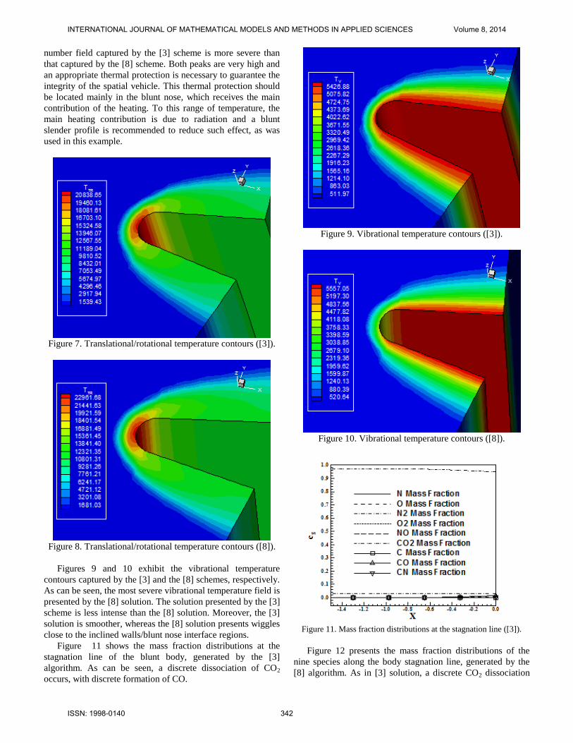
Figures 9 and 10 exhibit the vibrational temperature

contours captured by the [3] and the [8] schemes, respectively.

As can be seen, the most severe vibrational temperature field is

presented by the [8] solution. The solution presented by the [3]

scheme is less intense than the [8] solution. Moreover, the [3]

solution is smoother, whereas the [8] solution presents wiggles

close to the inclined walls/blunt nose interface regions.

Figure 11 shows the mass fraction distributions at the

stagnation line of the blunt body, generated by the [3]

algorithm. As can be seen, a discrete dissociation of CO2

occurs, with discrete formation of CO.

Figure 9. Vibrational temperature contours ([3]).


Figure 11. Mass fraction distributions at the stagnation line ([3]).

Figure 12 presents the mass fraction distributions of the

nine species along the body stagnation line, generated by the

[8] algorithm. As in [3] solution, a discrete CO2 dissociation


ISSN: 1998-0140 342

occurs close to the body. The formation of CO, in relation to

the [3] solution, is more discrete, almost indistinguishable


Viscous, first order, structured results. Figures 13 and 14

exhibit the pressure contours obtained by the [3] and the [8]

schemes, respectively, in the viscous case. As can be observed,

the pressure field generated by the [3] scheme is more severe

than that generated by the [8] scheme. Moreover, the shock

region generated by the [8] scheme is slightly closer to the

blunt nose than the same region generated by the [3] scheme.

This behavior suggests that the shock profile of the [8] scheme

is more realistic, closer to the blunt nose. The shock is

accurately generated by both schemes and with better

characteristics than the inviscid shock.


Figures 15 and 16 present the Mach number contours

obtained by the [3] and the [8] schemes, respectively. The [3]

solution is more dissipative, generating bigger regions of

supersonic flow, close to the wall. The [3] solution is more

severe.





ISSN: 1998-0140 343


Figure 18. Translational/Rotational temperature contours ([8]).


Figures 17 and 18 exhibit the translational/rotational

temperature contours generated by the [3] and the [8] schemes,

respectively. In this viscous case, temperatures peaks above

21,000K are observed. In this range, the radiation heat transfer

phenomenon is predominant and justifies the use of a blunt

slender body to fly at the Mars atmosphere. The normal shock

wave generated by the [3] scheme is more symmetrical and

heater than the [8] one. The [8] solution presents problems

with the shock formation and the contours are severely

damaged.

Figures 19 and 20 show the vibrational temperature

contours obtained by the [3] and the [8] algorithms,

respectively. The vibrational temperature field generated by

the [3] scheme is more strength than the respective one due to

[3]. Moreover, the [8] shock layer is confined to a smaller

region, close to the wall, than the [3] shock layer region.



Figure 21 exhibits the mass fraction distributions of the

nine species obtained from the [3] scheme. A discrete

dissociation of the CO2 is observed. As also noted the

formation of CO is very discrete.

Figure 22 shows the mass fraction distributions of the nine

species obtained from the [8] scheme. A discrete dissociation

of CO2, close to the blunt nose, is seen. It is not perceptible the

formation of CO.


ISSN: 1998-0140 344


Inviscid, second order, structured results. Figures 23 and 24

show the pressure contours obtained by the [3] and the [8]

schemes, respectively. The most strength pressure field is due

to [8]. Both solutions present good symmetry properties. The

pressure peak due to [3] reaches a value of 715 unities,

whereas this peak due to [8] reaches a value of 738,

identifying the latter as more conservative.

Figures 29 and 30 show the vibrational temperature

contours obtained by [3] and by [8] schemes, respectively. The

hot shock layer of the [8] solution is confined to a smaller

region than the hot shock layer of the [3] solution. The [3]

solution is smoother than the [8] one. Moreover, the [8]

solution is more intense than the respective one of [3].


Figures 25 and 26 present the Mach number contours due

to [3] and [8], respectively. The two Mach number fields are

very similar, quantitatively and qualitatively.

Figures 27 and 28 show the translational/rotational

temperature contours obtained by [3] and [8], respectively.

The temperature fields due to [3] and [8] reach maximum

peaks of 22,644K and 22,610K, less intense than in the

inviscid results. Again these peaks are concentrated in the

blunt nose region.





ISSN: 1998-0140 345




Figure 31 exhibits the mass fraction distributions along the

body stagnation line obtained by the [3] scheme. Again a very

discrete dissociation of the CO2 is observed. The formation of

CO and O are also almost non-perceptible.




Figure 32 presents the mass fraction distributions generated

by the [8] algorithm. It is possible to note a discrete CO2

dissociation than in the [3] case. As a consequence, the CO

and O formations are also almost non-perceptible. The

production of C and CN is less pronounced.


ISSN: 1998-0140 346

Viscous, second order, structured results. In this case, only

the [3] scheme has produced converged results. Figure 33

exhibits the pressure contours obtained by the [3]. The shock

wave is well captured. Good symmetry properties are observed

in the [3] solution.


Figure 34. Mach number field ([3]).

Figure 34 shows the Mach number contours generated by

[3] algorithm. As can be observed, the [3] scheme is more

dissipative, spreading the low supersonic region around the

body. The contours of Mach number due to [3] are

symmetrical enough. The shock wave develops correctly,

passing from a normal shock wave, going to oblique shock

waves and finishing with Mach waves.

Figure 35 shows the translational/rotational temperature

contours obtained by [3] scheme. The [3] temperature field is

close to 26,000K. It is clear the high temperature at the body

nose.

Figure 36 presents the vibrational temperature contours

obtained from [3] scheme. The [3] solution presents a more

severe temperature field in relation to its inviscid counterpart.

The shock layer of [3] is confined to a small region.




Figure 37 exhibits the mass fraction distributions along the

stagnation line of the blunt body, generated by [3] scheme. As

can be seen, a meaningful dissociation of CO2 is captured by

the [3] scheme, with significant formation of CO.


ISSN: 1998-0140 347

Computational data. The computational data of the present

simulations are shown in Tab. 8. The best performance,

converging in a minor number of iterations and wasting minor

time, is due to the [3] scheme, first-order and inviscid case.

The [8] did not present converged results to the second-order

viscous case. The convergence to 3 o.r.r. is the minimum

acceptable to consider a converged result. This happens in

three cases. All solutions are of good quality.

Table 8. Computational data.

Case CFL Iterations o.r.r.(1)

[3] – 1st – Inviscid 0.2 1,387 4

[8] – 1st – Inviscid 0.1 3,951 4

[3] – 1st – Viscous 0.2 3,960 4

[8] – 1st – Viscous 0.1 6,225 3

[3] – 2nd – Inviscid 0.1 3,114 4

[8] – 2nd – Inviscid 0.1 4,105 3

[3] – 2nd – Viscous 0.2 2,414 3 (1)

: o.r.r. = order of residual reduction.

X. CONCLUSIONS

This work, first part of this study, describes a numerical tool to

perform thermochemical non-equilibrium simulations of

reactive flow in three-dimensions. The [3] and [8] schemes, in

their first- and second-order versions, are implemented to

accomplish the numerical simulations. The Euler and Navier-

Stokes equations, on a finite volume context and employing

structured and unstructured spatial discretizations, are applied

to solve the “hot gas” hypersonic flow around a blunt body, in

three-dimensions. The second-order version of the [3] and [8]

schemes are obtained from a “MUSCL” extrapolation

procedure (details in [10]) in a context of structured spatial

discretization. In the unstructured context, only first-order

solutions are obtained. The convergence process is accelerated

to the steady state condition through a spatially variable time

step procedure, which has proved effective gains in terms of

computational acceleration (see [4-5]).

The reactive simulations involve a Mars atmosphere

chemical model of nine species: N, O, N2, O2, NO, CO2, C,

CO, and CN. Fifty-three chemical reactions, involving

dissociation and recombination, are simulated by the proposed

model. The Arrhenius formula is employed to determine the

reaction rates and the law of mass action is used to determine

the source terms of each gas species equation.

The results have demonstrated that the most conservative

scheme is due to [8], although the [3] scheme is more robust,

providing results to the second-order viscous case. Moreover,

the [3] scheme presents the best mass fraction profiles at the

stagnation line, characterizing discrete dissociation of CO2 and

formation of CO.

REFERENCES

[1] ESA, MARSNET – Assessment Study Report, ESA Publication SCI

(91) 6, January, 1991.

[2] E. S. G. Maciel, and A. P. Pimenta, Thermochemical Non-Equilibrium

Reentry Flows in Two-Dimensions – Part I, WSEAS TRANSACTIONS

ON MATHEMATICS, Vol. 11, Issue 6, June, 2012, pp. 520-545.

[3] B. Van Leer, Flux-Vector Splitting for the Euler Equations, Lecture

Notes in Physics. Springer Verlag, Berlin, Vol. 170, 1982, pp. 507-512.

[4] E. S. G. Maciel, Analysis of Convergence Acceleration Techniques

Used in Unstructured Algorithms in the Solution of Aeronautical

Problems – Part I, Proceedings of the XVIII International Congress of

Mechanical Engineering (XVIII COBEM), Ouro Preto, MG, Brazil,

2005. [CD-ROM]

[5] E. S. G. Maciel, Analysis of Convergence Acceleration Techniques

Used in Unstructured Algorithms in the Solution of Aerospace Problems

– Part II, Proceedings of the XII Brazilian Congress of Thermal

Engineering and Sciences (XII ENCIT), Belo Horizonte, MG, Brazil,

2008. [CD-ROM]

[6] E. S. G. Maciel, and Pimenta, A. P., Thermochemical Non-Equilibrium

Reentry Flows in Three-Dimensions – Part I – Structured Solutions,

WSEAS TRANSACTIONS ON APPLIED AND THEORETICAL

MECHANICS, Vol. 8, Issue 1, January, 2013, pp. 1-25.

[7] E. S. G. Maciel, and Pimenta, A. P., Thermochemical Non-Equilibrium

Reentry Flows in Three-Dimensions: Seven Species Model – Part I –

Structured Solutions, WSEAS TRANSACTIONS ON MATHEMATICS

(under review).

[8] M. Liou, and C. J. Steffen Jr., A New Flux Splitting Scheme, Journal of

Computational Physics, Vol. 107, 1993, pp. 23-39.

[9] F. G. Blottner, Viscous Shock Layer at the Stagnation Point With

Nonequilibrium Air Chemistry, AIAA Journal, Vol. 7, No. 12, 1969, pp.

2281-2288.

[10] C. Hirsch, Numerical Computation of Internal and External Flows –

Computational Methods for Inviscid and Viscous Flows. John Wiley &

Sons Ltd, 691p, 1990.

[11] R. K. Prabhu, An Implementation of a Chemical and Thermal

Nonequilibrium Flow Solver on Unstructured Meshes and Application

to Blunt Bodies, NASA CR-194967, 1994.

[12] S. K. Saxena and M. T. Nair, An Improved Roe Scheme for Real Gas

Flow, AIAA Paper 2005-587, 2005.

[13] R. D. Kay, and M. P. Netterfield, Thermochemical Non-Equilibrium

Computations for a Mars Entry Vehicle, AIAA Paper 93-2841, July,

1993.

[14] J. Evans, W. L. Grose, and C. J. Schexnayder, Effects of

Nonequilibrium Ablation Chemistry on Viking Radio Blackout, AIAA

Paper 73-0260, 1973.

[15] C. Park, G. V. Candler, J. T. Howe, and R. L. Jaffe, Chemical-Kinetic

Problems of Future NASA Missions, AIAA Paper 91-0464, 1991.

[16] Table of Recommended Rate Constants for Chemical Reactions

Occurring in Combustion, NSRDS-NBS 67, April, 1980.

[17] G. F. Mitchell, and T. J. Deveau, Effects of a Shock on Diffuse

Interstellar Cloud, J. Astrophysics, No. 266, 1983, pp. 646-661.

[18] F. G. Blottner, M. Johnson, and M. Ellis, Chemically Reacting Viscous

Flow Program for Multi-Component Gas Mixtures, SC-RR-70-754,

Sandia Laboratories, December, 1971.

[19] G. V. Candler, Computation of Thermochemical Non-Equilibrium

Martian Atmospheric Entry Flows, AIAA Paper 90-1695, 1990.

[20] R. N. Gupta, K. P. Lee, J. N. Moss, and K. Sutton, Viscous Shock Layer

Solutions with Coupled Radiation and Ablation Injection for Earth

Entry, AIAA Paper 90-1697, 1990.

[21] C. R. Wilke, A Viscosity Equation for Gas Mixtures, J. Chem. Phys.,

Vol. 18, No. 4, 1950, p. 517.

[22] G. V. Candler, and R. W. MacCormack, The Computation of

Hypersonic Ionized Flows in Chemical and Thermal Non-Equilibrium,

AIAA Paper 88-0511, 1988.

[23] L. Landau, and E. Teller, Theory of Sound Dispersion, Physikalische

Zeitschrift Der Sowjetunion, Vol. 10, 1936, pp. 34-43.

[24] R. C. Millikan and D. R. White, Systematics of Vibrational Relaxation,

The Journal of Chemical Physics, Vol. 39, No. 12, 1963, pp. 3209-

3213.

[25] R. Monti, D. Paterna, R. Savino, and A. Esposito, Experimental and

Numerical Investigation on Martian Atmosphere Entry, AIAA Paper

2001-0751, 2001.

[26] A. F. P. Houwing, S. Nonaka, H. Mizuno, and K. Takayama, Effects of

Vibrational Relaxation on Bow Shock Stand-off Distance for

Nonequilibrium Flows, AIAA Journal, Vol. 38, No. 9, 2000, pp. 1760-

1763.


ISSN: 1998-0140 348

[27] C. Park, Assessment of Two-Temperature Kinetic Model for Ionizing

Air, Journal of Thermophysics and Heat Transfer, Vol. 3, No. 13, pp.

233-244, 1989.

[28] D. Ait-Ali-Yahia, and W. G. Habashi, Finite Element Adaptive Method

for Hypersonic Thermochemical Nonequilibrium Flows, AIAA Journal

Vol. 35, No. 8, 1997, 1294-1302.

[29] E. S. G. Maciel, TVD Algorithms Applied to the Solution of the Euler

and Navier-Stokes Equations in Three-Dimensions, WSEAS

TRANSACTIONS ON MATHEMATICS, Vol. 11, Issue 6, June, 2012,

pp. 546-572.

[30] R. Radespiel, and N. Kroll, Accurate Flux Vector Splitting for Shocks

and Shear Layers, Journal of Computational Physics, Vol. 121, 1995,

pp. 66-78.

[31] L. N. Long, M. M. S. Khan, and H. T. Sharp, Massively Parallel Three-

Dimensional Euler / Navier-Stokes Method, AIAA Journal, Vol. 29, No.

5, 1991, pp. 657-666.

[32] B. Van Leer, Towards the Ultimate Conservative Difference Scheme. II.

Monotonicity and Conservation Combined in a Second-Order Scheme,

Journal of Computational Physics, Vol. 14, 1974, pp. 361-370.

[33] P. L. Roe, In Proceedings of the AMS-SIAM Summer Seminar on

Large-Scale Computation in Fluid Mechanics, Edited by B. E. Engquist

et al, Lectures in Applied Mathematics, Vol. 22, 1983, p. 163.

[34] E. S. G. Maciel, Simulação Numérica de Escoamentos Supersônicos e

Hipersônicos Utilizando Técnicas de Dinâmica dos Fluidos

Computacional, Doctoral Thesis, ITA, CTA, São José dos Campos,

SP, Brazil, 258p, 2002.

[35] NASA, Models of Mars' Atmosphere [1974], NASA SP-8010.

Edisson S. G. Maciel (F’14), born in

1969, february, 25, in Recife,

Pernambuco. He is a Mechanical

Engineering undergraduated by UFPE

in 1992, in Recife, PE, Brazil; Mester

degree in Thermal Engineering by

UFPE in 1995, in Recife, PE, Brazil;

Doctor degree in Aeronautical

Engineering by ITA in 2002, in São

José dos Campos, SP, Brazil; and

Post-Doctor degree in Aeronautical

Engineering by ITA in 2009, in São José dos Campos, SP, Brazil

Actually, he is doing a new post-doctorate curse in Aerospace Engineering

at ITA. The last researches are based on thermochemical non-equilibrium

reentry simulations in Earth and thermochemical non-equilibrium entry

simulations in Mars. They are: Maciel, E. S. G., and Pimenta, A. P.,

“Thermochemical Non-Equilibrium Reentry Flows in Two-Dimensions – Part

I’, WSEAS Transactions on Mathematics, Vol. 11, Issue 6, June, pp. 520-545,

2012; Maciel, E. S. G., and Pimenta, A. P., “Thermochemical Non-

Equilibrium Entry Flows in Mars in Two-Dimensions – Part I’, WSEAS

Transactions on Applied and Theoretical Mechanics, Vol. 8, Issue 1, January,

pp. 26-54, 2013; and he has three published books, the first one being:

Maciel, E. S. G., “Aplicações de Algoritmos Preditor-Corretor e TVD na

Solução das Equações de Euler e de Navier-Stokes em Duas Dimensões”,

Recife, PE, Editor UFPE, 2013. He is interested in the Magnetogasdynamic

field with applications to fluid dynamics and in the use of ENO algorithms.


ISSN: 1998-0140 349

thermochemical non-equilibrium entry flows in mars in three-dimensions … · · 2014-11-20on the...

Documents