thermodynamic modeling of complex systems · thermodynamic modeling of complex systems liang,...
TRANSCRIPT

General rights Copyright and moral rights for the publications made accessible in the public portal are retained by the authors and/or other copyright owners and it is a condition of accessing publications that users recognise and abide by the legal requirements associated with these rights.
Users may download and print one copy of any publication from the public portal for the purpose of private study or research.
You may not further distribute the material or use it for any profit-making activity or commercial gain
You may freely distribute the URL identifying the publication in the public portal If you believe that this document breaches copyright please contact us providing details, and we will remove access to the work immediately and investigate your claim.
Downloaded from orbit.dtu.dk on: Jun 25, 2020
Thermodynamic modeling of complex systems
Liang, Xiaodong
Publication date:2014
Document VersionPublisher's PDF, also known as Version of record
Link back to DTU Orbit
Citation (APA):Liang, X. (2014). Thermodynamic modeling of complex systems. Technical University of Denmark, Departmentof Chemical and Biochemical Engineering.

Xiaodong LiangPh.D. ThesisAugust 2014
Thermodynamic modeling of complex systems

Thermodynamic modeling of complex systems
PhD Thesis
Xiaodong LiangAugust 2014
Center for Energy Resources Engineering
Department of Chemical and Biochemical EngineeringTechnical University of DenmarkDK-2800 Kgs. Lyngby, Denmark
1

2
Copyright©: Xiaodong Liang
August 2014
Address: Center for Energy Resources Engineering
Department of Chemical and
Biochemical Engineering
Technical University of Denmark
Søltofts Plads, Building 229
DK-2800 Kgs. Lyngby
Denmark
Phone: +45 4525 2800
Fax: +45 4525 4588
Web: www.cere.dtu.dk
Print: J&R Frydenberg A/S
København
December 2014
ISBN: 978-87-93054-46-2

Preface
This thesis is submitted to fulfill the partial requirements for the Ph.D. degree at the Technical
University of Denmark (DTU). The work has been carried out at the Department of Chemical and
Biochemical Engineering and Center for Energy Resources Engineering (CERE), from August 2011
to August 2014, under the supervision of Professor Georgios M. Kontogeorgis, Associate Professor
Kaj Thomsen, and Senior Scientist Wei Yan. The project was funded by the Danish National
Advanced Technology Foundation (DNATF) and the Department of Chemical and Biochemical
Engineering, Technical University of Denmark.
I would like to express my most sincere gratitude to my supervisors for their full support throughout
the project. I would like to thank my main supervisor Professor Georgios M. Kontogeorgis, firstly
for offering me such a dream project, secondly for inspiring me so many exciting ideas, thirdly for
allowing me so much research freedom, fourthly for encouraging me all the time, fifthly for putting
me in the CHIGP meetings/giving me many presentation opportunities/improving my language, and
last but not least for your enthusiasm of thermodynamics. I would like to thank my supervisor
Associate Professor Kaj Thomsen for many help on revising articles and understanding the
electrolyte solution thermodynamics. I would like to thank my supervisor Senior Scientist Wei Yan
for many fruitful discussions on both the technical level, especially on oil characterization methods,
and the life side, especially for giving me so many help on different aspects.
I would like to thank all the colleagues, from top managements to secretaries to IT managers, and
from professors to researchers to Ph.D. students. I thank Associate Professor Nicolas von Solms for
the opportunity of teaching assistance of the course “Chemical Engineering Thermodynamics”, and
many inspirations on the association theory. I appreciate many suggestions and critical opinions on
various projects and general applied thermodynamics from Professor Michael L. Michelsen.
Computational details are rarely mentioned in this thesis, but there is no doubt that they are the
corner stone for most of the presented results. I thank my fellow colleagues in the CHIGP project,
Ioannis, Bjørn, Michael and Martin, for coauthoring publications, co-participating international
conferences, and for many fruitful discussions during the meetings. I thank Louise and Patricia for
preparing various documents, booking flight tickets and hotels for travels, and organizing different
events, etc. I thank Michael and Christine for improving the Danish Summary. I would also very
much like to thank many people in the lunch and running clubs – I have been having a great time.
iii
3

I would like to express my special thanks to my former officemate – Dr. Peter Jørgensen Herslund.
It is a fate to meet some people in the life, and Peter is one of mine. Peter gave me tremendous help
on many things – Danish letter translations from different organizations, delicious Danish food,
fruitful discussions about family, about life, about work. Peter, I wish all best for you and your
friendly family – Hélène, Marius and Iris.
I would like to thank many professionals around the world, some of whom I even did not meet, for
their constructive suggestions, ideas and explanations, and sending me inaccessable experimental
data, especially Dr. Ilya Polishuk from Ariel University, Israel.
I would like to thank my master supervisor Professor Honglai Liu at ECUST, China, for bringing
me into this old but energetic field, for explaining/sharing me many concepts/theories in details, for
such a long contribution to the molecular thermodynamics community – one of the most important
concepts of PC-SAFT is actually from the works of Professor Honglai Liu and Professor Ying Hu. I
would like to thank my former lead at HONEYWELL, Dr. Ensheng Zhao, for teaching me so many
things – research and development skills of applied thermodynamics in such a large commercial
process simulator, behaviors, languages, encouragements, managements, and very importantly for
inspiring me how amazing applied thermodynamics is, which is the most important reason why I
am at DTU.
We arrived in Copenhagen on August 11th, 2011. In the past three years, I mentally spent more than
necessary time on the project. Without the accompanying of my family, it would have been a tough
time, both mentally and physically.
“It is only in the mysterious equations of love that any logic or reasons can be found.”
Thank you for your love. I love you and our coming ‘little princess’ till “ ”.
iv
4

Dedicated to
Lijuan, Peishi and Anni
My parents and my brothers
5

6

Summary
Offshore reservoirs represent one of the major growth areas of the oil and gas industry, and
environmental safety is one of the biggest challenges for the offshore exploration and production.
The oil accidents in the Gulf of Mexico in 1979 and 2010 were two of the biggest disasters in
history. Contrary to earlier theories, the oil is not only present on the surface, but also in great
volumes both in the water column and on the seafloor, which indicates that we do not know enough
about how oil behaves in water and interacts with it. Sonar detection is one of the most important
and necessary technologies to reduce the environmental effects of offshore oil exploration. It could
be used (1) to detect oil and gas leaks around the subsea well head enabling faster responses,
especially in deep water and/or ice covered areas; (2) to detect and map the oil in the seawater
column during cleanup process after an oil spill. Engineering thermodynamics could be applied in
the state-of-the-art sonar products through advanced artificial technology, if the speed of sound,
solubility and density of oil-seawater systems could be satisfactorily modelled.
The addition of methanol or glycols into unprocessed well streams during subsea pipelines is
necessary to inhibit gas hydrate formation, and the offshore reservoirs often mean complicated
temperature and pressure conditions. Accurate description of the phase behavior and thermal-
physical properties of complex systems containing petroleum fluids and polar compounds are
extremely important from viewpoints of the economical operation and environmental safety.
The classical thermodynamic models used by the oil industry are semi-empirical and not suitable
for mixtures containing water and other polar chemicals. The complex nature of water, its
anomalous properties due to hydrogen bonding and the hydrophobic interactions with hydrocarbons
(oils), are not described well by such simple models. The perturbation theory based models have an
explicit term to account for the hydrogen bonding, and these models are also believed to have better
performance for derivative properties, e.g. speed of sound, and for density under extreme conditions.
This PhD thesis studies the capabilities and limitations of the Perturbed-Chain Statistical
Association Fluid Theory (PC-SAFT) equation of state. It consists of three parts. In the first part,
the PC-SAFT EOS is successfully applied to model the phase behaviour of water, chemical and
hydrocarbon (oil) containing systems with newly developed pure component parameters for water
and chemicals and characterization procedures for petroleum fluids. The performance of the PC-
SAFT EOS on liquid-liquid equilibria of water with hydrocarbons has been under debate for some
vii
7

years. An interactive step-wise procedure is proposed to fit the model parameters for small
associating fluids by taking the liquid-liquid equilibrium data into account. It is still far away from a
simple task to apply PC-SAFT in routine PVT simulations and phase behaviour of petroleum fluids.
It has been extensively studied on how to develop general petroleum fluid characterization
approaches for PC-SAFT. The performance of the newly developed parameters and characterization
procedures for the description of the phase equilibria of well- and ill-defined binary and ternary
systems containing water, chemicals and/or hydrocarbons (oils) is quite satisfactory, if compared to
the models available in literature. The modeling of petroleum fluid-water-MEG systems provides
further information to develop simpler and more robust characterization approaches.
In the second part, the speed of sound data and their correlations of various systems are reviewed.
Two approaches are proposed to improve the speed of sound description within the PC-SAFT
framework by putting speed of sound data into the parameter estimation and/or the universal
constant regression. The first approach works only for short associating fluids, while the second
approach significantly improves the speed of sound description for various systems both
qualitatively and quantitatively. The possibility of simultaneous modeling of phase behavior and
speed of sound, including the effects of parameter estimation approaches for 1-alcohol containing
systems, are also investigated.
In the third part, the fundamentals of PC-SAFT are investigated based on the universal constant
regression. The PC-SAFT EOS has been criticized for some numerical pitfalls during the recent
years. A new variant of universal constants has been developed, which has avoided the numerical
pitfalls of having more than three volume roots in the real application range. It has been shown that
it is possible to directly use the original PC-SAFT parameters with the new universal constants for
the systems considered in this thesis. Finally, the salt effects on the solubility of hydrocarbons, the
speed of sound, and the static permittivity of aqueous solutions are briefly discussed. It is still an
open question how to estimate the model parameters for associating fluids with pure component
properties only. The possibility of using the static permittivity data in the parameter estimation is
discussed by adopting a newly developed theory of static permittivity and association theory based
EOS.
viii
8

Resumé
Offshore reservoirer repræsenterer et af de store vækstområder i olie- og gasindustrien, og
miljøsikkerhed er en af de største udfordringer for offshore efterforskning og produktion. Olie
ulykkerne i Den Mexicanske Golf i 1979 og 2010 var to af de største katastrofer i historien. I
modsætning til tidligere teorier findes olien ikke kun på overfladen, men også i store mængder både
i vandsøjlen og på havbunden, hvilket indikerer, at vi ikke ved nok om, hvordan olien opfører sig i
vand og interagerer med det. Sonarlyde er en af de vigtigste og mest nødvendige teknologier til at
mindske miljøvirkningerne af offshore olieefterforskning . Det vil kunne bruges (1) til at detektere
olie og gas lækager omkring den undersøiske brønd overbygning, hvilketmuliggøre hurtigere svar,
især i dybt vand og / eller isdækkede områder; (2) til at registrere og kortlægge olie i havvandsøjlen
under rensningen efter et olieudslip. Engineering termodynamik vil kunne anvendes i state-of-the-
art sonar produkter gennem avanceret kunstig teknologi, hvis lydens hastighed, opløselighed og
massefyldeaf olie-havvand-systemer kan blive modelleret tilfredsstillende.
Tilsætning af methanol eller glycoler i uforarbejdede brøndstrømme i undersøiske rørledninger er
nødvendig for at hæmme gashydratdannelse, og offshore reservoirer betyder ofte ekstreme og
komplicerede temperatur og trykforhold. For den økonomisk drift og den miljømæssige sikkerheds
synsvinkel er det ekstremt vigtigt med en præcis beskrivelse af fase opførsel og termisk-fysiske
egenskaber af komplekse systemer, der indeholder petroleumsvæsker og polære forbindelser. .
De klassiske termodynamiske modeller, som olieindustrien anvender, er semi-empiriske og ikke
egnet til blandinger, der indeholder vand og andre polære kemiske stoffer. Den komplekse karakter
af vand, dets unormale egenskaber på grund af hydrogenbinding og hydrofobe interaktioner med
kulbrinter (olie), er ikke velbeskrevet af sådanne simple modeller. De perturbationsteori baserede
modeller har et eksplicit ledtilat tage højde for hydrogenbinding, og disse modeller menes også at
have bedre ydeevne for afledte egenskaber, fx lydens hastighed og for massefyldenunder ekstreme
forhold.
Denne ph.d.-afhandling undersøger de begrænsninger og muligheder i den perturberede-kæde
Statistical Association Fluid Teori (PC-SAFT) tilstandsligning. Den består af tre dele. I den første
del er PC-SAFT EOS anvendt med succes til at modellere vands opførsel, kemikalier og kulbrinter
(olier) der indeholder systemer mednyudviklede rene komponent parametre for vand og kemikalier,
og karakteriserings procedurer for petroleumsvæsker. PC-SAFT EOS ydeevne på væske-væske
ix
9

ligevægte af vand med kulbrinter har været under debat i nogle fåår. En interaktiv trinvis procedure
er foreslået til at tilpasse modelparametrene for små associerende væsker ved at tage
ligevægtsdataene for væske-væske i betragtning. Det er stadig langt fra en simpel opgave at
anvende PC-SAFT i rutinemæssige PVT simuleringer og til petroleumsvæskers fase opførsel. Det
er blevet undersøgt grundigt, hvordan man skal udvikle generelle petroleumsvæske karakteriserings
tilgange til PC-SAFT. Ydeevnen af de nyudviklede parametre og karakteriserings procedurer til
beskrivelsen af faseligevægte veldefineret og dårligt definerede binære og ternære systemer, der
indeholder vand, kemikalier og / eller kulbrinter (olier), er ganske lovende, hvis der sammenlignes
med tilgængelige litteratur parametre og / eller CPA EOS. Modelleringen af petrolium væske-vand-
MEG-systemer giver yderligere information til at udvikle enklere og mere robuste karakteriserings
tilgange.
I den anden del er lydhastighedsdata og deres korrelationer af forskellige systemer revideret. Der
foreslås to tilgange til at forbedre beskrivelsen af lydens hastighedinden for PC-SAFT rammen ved
at sætte lydhastighedsdata ind i parameterestimering og / eller den universelle konstant regression.
Den første fremgangsmåde fungerer kun i korte associerende væsker, mens den anden strategi
forbedrer beskrivelsen af lydens hastighed for forskellige systemer fra både kvalitative og
kvantitative synspunkter. Muligheden for samtidig modellering af fase opførslenog lydens
hastighed, herunder virkningerne af parameterestimerings tilgangene for systemer indeholdene 1-
alkohol, er også undersøgt.
I tredje del er de grundlæggende elementer i PC-SAFT undersøgt baseret på universel konstant
regression. PC-SAFT EOS er blevet kritiseret for nogle numeriske faldgruber i løbet af de seneste år.
En ny variant af universelle konstanter er blevet udviklet, som har undgået de numeriske faldgruber
ved at have mere end tre volumen rødder i den virkelige anvendelsesområde. Det er blevet påvist, at
det er muligt direkte at anvende de oprindelige PC-SAFT parametre med de nye universelle
konstanter for de systemer, der behandles i denne afhandling. Til sidst er salt indvirkningen på
opløseligheden af carbonhydrider, lydens hastighed og den statiske permittivitet for vandige
opløsninger kort diskuteret. Det er stadig et åbent spørgsmål, hvordan man kan estimere
modelparametrene til inddragelse af væsker med kun rene egenskaber. Muligheden for at anvende
de statiske permittivitet data i parameterestimering diskuteres ved at anvende en nyudviklet teori for
statisk permittivitet og associations teori baseret på EOS.
x
10

Table of Contents
Preface.............................................................................................................................................iii
Summary ........................................................................................................................................vii
Resumé............................................................................................................................................ix
Table of Contents ............................................................................................................................xi
Chapter 1. Introduction ........................................................................................................................1
1.1 Background ................................................................................................................................1
1.2 Thermodynamic models.............................................................................................................2
1.2.1 Phase behavior ....................................................................................................................2
1.2.2 Physical properties ..............................................................................................................3
1.3 Scope and outline .......................................................................................................................5
Chapter 2. Phase behavior of well-defined systems ............................................................................7
2.1 Models........................................................................................................................................7
2.1.1 PC-SAFT EoS.....................................................................................................................8
2.1.2 CPA EOS ..........................................................................................................................11
2.1.3 Deviations .........................................................................................................................12
2.2 Water parameters .....................................................................................................................13
2.2.1 Literature review ...............................................................................................................13
2.2.2 Comparison of literature parameters.................................................................................15
2.2.3 2B versus 4C .....................................................................................................................21
2.2.4 New water pure component parameters............................................................................25
2.2.5 Comments on free site (monomer) fraction ......................................................................31
2.2.6 Summary ...........................................................................................................................34
2.3 Parameters for 1-alcohols and MEG........................................................................................35
xi
11

2.4 Phase behavior .........................................................................................................................36
2.4.1 Associating + Inert binary mixtures..................................................................................36
2.4.2 Associating + Associating binary mixtures ......................................................................44
2.4.3 Water + Chemical + Inert ternary mixtures ......................................................................51
2.5 Conclusions..............................................................................................................................54
Chapter 3. Petroleum fluid characterization ......................................................................................55
3.1 Introduction..............................................................................................................................55
3.2 Entire C7+ characterization procedure......................................................................................58
3.3 Model parameter estimation for pseudo-components..............................................................61
3.3.1 Model parameters..............................................................................................................61
3.3.2 PNA estimations ...............................................................................................................63
3.3.3 Binary interaction parameters (BIP) kij.............................................................................64
3.3.4 Candidate methods (CM) ..................................................................................................64
3.4 Results and discussion .............................................................................................................65
3.4.1 Petroleum fluids database .................................................................................................65
3.4.2 Saturation pressure and density.........................................................................................67
3.4.3 A compromise method (CM7) ..........................................................................................74
3.4.4 Applications ......................................................................................................................76
3.5 Conclusions..............................................................................................................................83
Chapter 4. Modeling oil-water-chemical systems..............................................................................87
4.1 Introduction..............................................................................................................................87
4.2 Data ..........................................................................................................................................88
4.3 Results and Discussions ...........................................................................................................88
4.3.1 Live Oil 1 + Water ............................................................................................................88
4.3.2 Live Oil 2 + Water + Methanol.........................................................................................92
4.3.3 Dead Oils + MEG .............................................................................................................94
xii
12

4.3.4 Dead Oils + Water + MEG ...............................................................................................99
4.4 Conclusions............................................................................................................................102
Chapter 5. Data and correlations of speed of sound ........................................................................105
5.1 Introduction............................................................................................................................105
5.2 Data ........................................................................................................................................106
5.2.1 Pure fluids .......................................................................................................................106
5.2.2 Binary systems ................................................................................................................112
5.2.3 Multicomponent systems ................................................................................................119
5.3 Correlations............................................................................................................................122
5.4 Conclusions............................................................................................................................125
Chapter 6. Modeling speed of sound ...............................................................................................127
6.1 Introduction............................................................................................................................127
6.2 Comparison of SRK, CPA and PC-SAFT .............................................................................131
6.3 Improve PC-SAFT for modeling speed of sound ..................................................................134
6.3.1 Approaches......................................................................................................................134
6.3.2 Objective function and data ............................................................................................136
6.4 Results and discussion on speed of sound .............................................................................136
6.4.1 Pure substances ...............................................................................................................136
6.4.2 Binaries ...........................................................................................................................148
6.4.3 Ternary ............................................................................................................................158
6.4.4 Petroleum fluids ..............................................................................................................158
6.5 Beyond speed of sound ..........................................................................................................161
6.5.1 Properties ........................................................................................................................161
6.5.2 Phase behavior ................................................................................................................162
6.6 Conclusions............................................................................................................................168
Chapter 7. A new variant of the Universal Constants......................................................................171
xiii
13

7.1 Introduction............................................................................................................................171
7.2 Analysis of the Original PC-SAFT EOS................................................................................172
7.2.1 Temperature and density dependences ...........................................................................172
7.2.2 Isothermal curves ............................................................................................................175
7.3 New universal constants.........................................................................................................178
7.3.1 A practical way ...............................................................................................................179
...................................................................................................................180
7.3.3 Parameters and physical properties.................................................................................181
7.3.4 Application ranges ..........................................................................................................184
7.3.5 A real example ................................................................................................................185
7.4 Possibility to use the original PC-SAFT parameters .............................................................186
7.4.1 Binary hydrocarbon systems...........................................................................................186
7.4.2 1-Alcohol + n-alkane mixtures .......................................................................................186
7.4.3 Water containing systems ...............................................................................................188
7.4.4 Polymer containing systems............................................................................................190
7.4.5 Natural gas systems.........................................................................................................191
7.4.4 Petroleum fluid-water-MEG systems..............................................................................192
7.5 Conclusions............................................................................................................................193
Chapter 8. Salt effects ......................................................................................................................195
8.1 Introduction............................................................................................................................195
8.2 Salt effects..............................................................................................................................195
8.2.1 Phase equilibria ...............................................................................................................195
8.2.2 Speed of sound ................................................................................................................196
8.2.3 Static permittivity............................................................................................................200
8.3 Static permittivity and association models.............................................................................202
8.4 Conclusions............................................................................................................................205
xiv
14

Chapter 9. Conclusions and future work..........................................................................................207
9.1 Conclusions............................................................................................................................207
9.1.1 Phase behavior ................................................................................................................207
9.1.2 Speed of sound ................................................................................................................208
9.1.3 Fundamentals ..................................................................................................................209
9.2 Future work ............................................................................................................................209
Reference .........................................................................................................................................211
List of Symbols ................................................................................................................................229
List of Figures ..................................................................................................................................232
List of Tables ...................................................................................................................................241
APPENDICES .................................................................................................................................243
Appendix A. Petroleum fluid database ........................................................................................245
Appendix B. Detailed results for Chapter. 4 ................................................................................247
Appendix C. Speed of sound database.........................................................................................253
Appendix D. Detailed results for Chapter. 7................................................................................261
Appendix E. Academic activities.................................................................................................267
Peer reviewed journal articles ..................................................................................................267
Conference presentations .........................................................................................................267
Teaching assistance..................................................................................................................268
xv
15

16

Chapter 1. Introduction
1.1 Background
As the offshore reservoirs represent one of the major growth areas of the oil and gas industry for
decades, the complex phase behavior between petroleum fluids and polar compounds such as water,
methanol or glycols has gained increasing attention. For instance, the addition of methanol or
glycols into unprocessed well streams in subsea pipelines is necessary to inhibit gas hydrate
formation. Since the mutual solubility of petroleum fluids and water will considerably increase
when chemicals are involved, the phase behavior modeling of oil-water-chemicals is very important
from the viewpoints of economical operation and environmental safety. The offshore reservoirs
often mean extreme temperature and pressure conditions, accurate description of fluid properties at
such conditions are far from a simple task.
Environmental safety is one of the biggest challenges for the offshore exploration and production.
In 1979, an oil accident occurred in Mexico with a total of approximate three million barrels oil
poured into the ocean. In more than 30 years, the marine life after the incident is still affected [Ixtoc
I oil spill]. In 2010, the oil accident in the Gulf of Mexico was one of the biggest oil disasters in
history [Deepwater Horizon oil spill]. More than 4.9 million barrels crude oil were leaked into the
ocean and this could be an environmental disaster for many years. Contrary to earlier theories, the
oil is not only present on the surface, but also in great volumes both in the water column and on the
seafloor. This may in part be attributed to the use of dispersing agents, but a lot indicates that we do
not know enough about how oil behaves in water and interacts with it, when the oil leak occurs at
great depths as the case with Deepwater Horizon. In order to reduce the environmental impact of
the offshore oil exploration and production, sonar detection is one of the most important and
necessary technologies, which could be used to: (1) detect oil and gas leaks around the subsea well
head enabling faster responses, especially in deep water and/or ice covered areas, (2) detect and
map the oil in the seawater column during cleanup process after an oil spill. It would be possible to
detect or even classify the presence of oil in the seawater column, by combining the knowledge
from engineering thermodynamics, geophysical inversion and underwater acoustics into the design
of an optimal detection/classification algorithm. It is sketched in Figure 1.1 how to apply
1
17

Thermodynamic modeling of complex systems
thermodynamic models in such an artificial intelligence technology system. The required properties
are mainly acoustic properties, solubility and density of oil-seawater systems.
Model predictionSonar detection
Sender
TARGET
Receiver
Inspectingdata
Images
Thermodynamic models
Oils, Seawater, Chemicals
Solubility,, u, Z, ...
Mathematical models
Images
T, P,Flow info
Model parametersOil CharacterizationDerivative propertiesSalt effects
Figure 1.1 Applying thermodynamic models in sonar subsea detection
1.2 Thermodynamic models
The main purpose of this PhD project is to develop thermodynamic models capable of describing
the phase behavior, density and speed of sound for complex systems, involved in the oil and gas
industry, over a wide range of conditions (temperature, pressure, oil types and origins).
1.2.1 Phase behavior
The classical thermodynamic models used by the oil industry are semi-empirical and not suitable
for mixtures containing water and other polar chemicals. The complex nature of water, its
anomalous properties due to hydrogen bonding and the polar and hydrophobic interactions with
hydrocarbons (oil) are not described well by such simple models.
In the early 1990's the theory of Wertheim emerged from statistical thermodynamics. It turned out
to be a useful tool for describing chemical substances and their mixtures when hydrogen bonding is
significant. This theory has been implemented into a new generation of engineering equations of
state (EOS) such as SAFT and CPA [Kontogeorgis et al. (2010a)]. CPA stands for Cubic-Plus-
Association and SAFT is the Statistical Association Fluid Theory. Both equations contain
2
18
Chapter 1. Introduction
essentially the same association term but different ways of accounting for the short range physical
interactions. The CPA model uses a conventional cubic EOS for the physical interactions whereas
SAFT uses theoretically-based terms for the repulsive and attractive contributions as well as a
separate "chain" term to account for the macromolecular effects in large molecules. These models
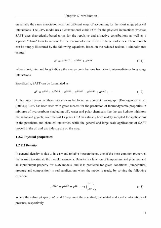
can be simply illustrated by the following equations, based on the reduced residual Helmholtz free
energy: = + + (1.1)
where short, inter and long indicate the energy contributions from short, intermediate or long range
interactions.
Specifically, SAFT can be formulated as:= + + + + + + (1.2)
A thorough review of these models can be found in a recent monograph [Kontogeorgis et al.
(2010a)]. CPA has been used with great success for the prediction of thermodynamic properties in
mixtures of hydrocarbons (including oil), water and polar chemicals like the gas hydrate inhibitors
methanol and glycols, over the last 15 years. CPA has already been widely accepted for applications
in the petroleum and chemical industries, while the general and large scale applications of SAFT
models in the oil and gas industry are on the way.
1.2.2 Physical properties
1.2.2.1 Density
In general, density is, due to its easy and reliable measurements, one of the most common properties
that is used to estimate the model parameters. Density is a function of temperature and pressure, and
an input/output property for EOS models, and it is predicted for given conditions (temperature,
pressure and composition) in real applications when the model is ready, by solving the following
equation:
= = (1.3)
Where the subscript spec, calc and id represent the specified, calculated and ideal contributions of
pressure, respectively.
3
19

Thermodynamic modeling of complex systems
SAFT models are believed to have potentially better description for density at extreme conditions,
e.g. high pressure, than traditional cubic EOS models, even with volume-translation, due to their
more theoretical sound reference term.
1.2.2.2 Speed of sound
Speed of sound, by definition, equals to the distance that a sound wave propagates through an
elastic medium in a unit of time. It is a thermo-physical property, which can be accurately
determined in wide ranges of temperature and pressure. In classic mechanics, speed of sound can be
calculated by the following equation:
= (1.4)
where u is the speed of sound, P is the pressure, is the mass density, and subscript S denotes the
derivative taken adiabatically. Since
= (1.5)
where CP and CV are isobaric and isochoric heat capacities, respectively.
By inserting equation (1.5) into equation (1.4), we get:
= (1.6)
If replacing with the total volume V, speed of sound is given by [Michelsen and Mollerup (2007)]:
= (1.7)
The and are calculated by the following equations:
= + = , + , , (1.8)
= + = , (1.9)
4
20

Chapter 1. Introduction
The ideal gas heat capacity could be found from various databases, and the DIPPR database (2012)
is used in this PhD thesis. SAFT models are also believed to have a better description for speed of
sound than cubic EOS models, due to their more theoretical sound reference term. Speed of sound
modeling may gain wide applications for petroleum fluids in geophysics for seismic interpretations.
1.3 Scope and outline
The Perturbed-Chain Statistical Associating Fluid Theory (PC-SAFT) equation of state is selected
as the working model in this project, mainly for two reasons: (1) we have extensively used this
model for various research projects in the past decade; (2) this model, as mentioned in the previous
sections, is believed to have better performance for physical properties over wide ranges of
temperature and pressure. Besides, our selection is also motivated by some challenges for PC-SAFT,
including how to apply this model into the routine modeling and simulation in the oil and gas
industry in a general manner, how to estimate the five PC-SAFT parameters for certain associating
compouds like water, and whether it is possible to simultaneously model phase behaviour and speed
of sound with only three parameters for non-associating fluids. In addition, PC-SAFT has been
criticized for its numerical pitfalls in recent years, and we would like to see if they can be resolved.
This PhD project is going to address the above challenges, and the thesis is outlined as follows:
Chapter 2 discusses the parameter estimation of water, which in general has five parameters within
the association theory based models, and proposes a general optimization procedure, by taking
account of the liquid-liquid equilibrium data of water and non-aromatic hydrocarbons into the
estimation process. The same procedure is also adopted for other chemicals like mono-ethylene
glycol. This chapter presents the performance of these parameters on the properties of pure
substances and the phase equilibria of binary and ternary systems containing water, hydrocarbons
and chemicals, by comparing to the literature available parameters and/or the CPA EOS. This
chapter also presents how to setup the binary interaction schemes and parameters, which provides
solid foundation for applying PC-SAFT into oil-water-chemical systems.
Chapter 3 studies the influence of different options for developing general oil characterization
methods with PC-SAFT. These options include the molar composition distribution function, the
density correlation, the number of pseudo-components, the estimation method of PNA contents, the
binary interaction parameters, the significance of fitting parameters and of the fitting strategy.
Based on the performance of the characterization approaches for predicting saturation pressure and
5
21

Thermodynamic modeling of complex systems
density of various petroleum fluids, and the activity coefficients of pseudo-components, two of
them are selected for further study.
Chapter 4 applies the newly developed parameters and interaction schemes from Chapter 2 and the
two characterization approaches from Chapter 3 to model oil-water-chemical systems. The overall
results are quite promising, when compared to the published results in the literature. It also provides
more information to develop simpler and more robust characterization approaches.
Chapter 5 reviews and analyzes the speed of sound data of hydrocarbons, alcohols and their binary
and multi-component mixtures, including petroleum fluids, and it reviews the correlations of the
speed of sound in various systems, and develops the correlation coefficients for the speed of sound
in pure hydrocarbons and 1-alcohols within one general framework.
Chapter 6 proposes two approaches to improve the speed of sound description with the PC-SAFT
framework, after a brief comparison of SRK, CPA and PC-SAFT for normal hydrocarbons. The
performance of these two approaches has been evaluated on predicting the speed of sound in wide
range of mixtures – binary hydrocarbons, binary hydrocarbon + alcohol, binary alcohols, ternary
hydrocarbons and petroleum fluids. The possibility of simultaneous phase behavior and speed of
sound modeling has been investigated, including the effects of parameter estimation approaches for
1-alcohol containing systems.
Chapter 7 analyzes the temperature and volume dependence of the PC-SAFT EOS in a somewhat
deterministic way, and develops a new variant of universal constants with focus on vapor pressure
and density. It then evaluates the performance of the new variant on the properties of pure normal
hydrocarbons, and on the behavior of isothermal curves and critical points, by comparing with the
original universal constants. It finally investigates the possibility of using the original PC-SAFT
parameters with the new universal constants.
Chapter 8 briefly discusses the salt effects on the solubility of hydrocarbons, the speed of sound,
and the static permittivity of aqueous solutions. It also discusses the possibility to use the newly
developed theory of calculating the static permittivity from the association theory based EOS to
simplify the parameter estimation for associating fluids.
Chapter 9 presents the conclusions and future work.
6
22

Chapter 2. Phase behavior of well-defined systems
The Statistical Associating Fluid Theory (SAFT) and Cubic Plus Association (CPA) equations of
state (EOS), with an association term based on the first-order thermodynamic perturbation theory,
are two of the most successful and widely used model families. In the past three decades, numerous
SAFT variants have been proposed, among which the perturbed-chain SAFT (PC-SAFT) has gained
widespread acceptance with great successes in the fields of polymers, chemical, biochemical,
pharmaceutical, and so on.
It is well-known that crude oils from petroleum reservoirs are made up of a large number of highly
diversified chemical compounds, which in general are only partially miscible at normal temperature
and pressure conditions. In order to develop thermodynamic models, which can describe the phase
behavior and physical properties of these complex mixtures, model parameters and binary
interaction parameters have to be setup for the relevant pure substances and binary mixtures. The
relevant ternary or multicomponent mixtures are very helpful on validating the model and its
predictive capabilities.
The purpose of this study is to develop new parameters for relevant associating fluids with the PC-
SAFT EOS, and then to investigate the performance of these parameters, by comparing to PC-
SAFT with the available parameters in the literature and/or the CPA EOS, on the properties of pure
substances and the phase equilibria of binary and ternary systems containing water, hydrocarbons
and chemicals, along which the binary interaction schemes and parameters will be setup.
2.1 Models
Over the past two decades, the popularity of SAFT EOS, based on a perturbation theory for
associating fluids proposed by Wertheim (1984a, 1984b, 1986a, 1986b), has grown very fast. The
model appeared in the form known today due to the work of Chapman et al. [Chapman et al. (1988,
1990); Jackson et al. (1988)] and of Huang and Radosz (1990, 1991) and for this reason both of
these models are often referred to as ‘original’ SAFT. After this, many different versions of SAFT
have followed, some of the successful ones being the SAFT-VR from 1997 by Gil-Villegas et al.
[Gil-Villegas et al. (1997); Galindo et al. (1998)], the soft-SAFT from 1997 by Blas and Vega
7
23

Thermodynamic modeling of complex systems
(1997, 1998), and the PC-SAFT in both its original version from 2001 by Gross and Sadowski
(2001, 2002) and the simplified version from 2003 by von Solms et al. (2003), the SAFT-VR Mie
by Lafitte et al. (2006, 2007, 2013), and the SWCF-VR by Li et al. (2009, 2011)
In SAFT EOS, molecules are modeled as chains of covalently bonded spheres. The models are
typically written as a sum of the contributions to the reduced residual Helmholtz free energy as in
the form:
= = + + (2.1)
where is the part of the Helmholtz energy due to segment-segment interactions, is the
term due to chain formation, and represents the contribution due to association, i.e. hydrogen
bonding, between different molecules. The biggest differences in the different SAFT variants are
the dispersion term and the choice of reference fluid. Almost all of the different SAFT variants
more or less use the same expressions for the chain formation and association terms, and include in
most cases five pure component parameters with well-defined physical meanings (the number of
segments, the segment size and energy, and the association volume and energy).
Nowadays this theoretical SAFT-type approach is very popular due to its versatility and the good
results obtained for different applications [Kontogeorgis et al. (2010a)]. However, while SAFT’s
ability to describe the phase equilibria of chain and associating pure fluids and mixtures is well-
established, its performance for the simultaneous description of phase equilibria and second-order
derivative properties is still limited and not sufficiently explored [Lafitte et al. (2006)].
2.1.1 PC-SAFT EoS
The PC-SAFT EoS was developed by Gross and Sadowski (2001) by extending the perturbation
theory of Barker and Henderson (1967) to a hard-chain reference. The reduced residual Helmholtz
free energy for mixtures containing associating fluids in PC-SAFT can be formulated as:= + + + (2.2)
where and are the contributions from hard sphere segment-segment interaction and chain
formation, of which the summation is the reference to build the dispersion force . The term
represents the contributions of association forces of sites.
8
24

Chapter 2. Phase behavior of well-defined systems
Instead of accounting the dispersion force among hard spheres first and then forming chains in other
SAFT variants, hard-sphere chain is formed first and then the dispersion force is accounted among
chains in PC-SAFT. So it has the same hard sphere, hard chain terms and quite similar association
term as those of other SAFT variants, and a fundamental difference on the dispersion term.
In this work, the simplified PC-SAFT version proposed by von Solms et al. (2003) will be used. It
is not a new EOS, rather a simplified version in terms of mixing rules of the original PC-SAFT
EOS, which aims to simplify and reduce the computational time of the PC-SAFT EOS. All details
can be found in the original literature [Gross and Sadowski (2001, 2002), von Solms et al. (2003)]
or the book of Kontogeorgis and Folas [Kontogeorgis et al. (2010a)]. The dispersion and association
terms, however, will be extensively studied, so brief introductions are presented below.
2.1.1.1 Dispersion term
The reduced residual Helmholtz free energy for the dispersion term is given as the sum of a first-
order and a second-order term: = + (2.3)
= 2 ( ) ( ; ) (2.4)
= 1 + + ( ) ( ; ) (2.5)
Where,1 + + = 1 + 8 2(1 ) + (1 ) 20 27 + 12 2[(1 )(2 )] (2.6)
Where x is the reduced radial distance around a segment ( = ), ( ) = ( ) denotes the
reduced potential function, and ( ; ) is the average segment-segment radial distribution
function of the hard-chain fluid with temperature-dependent segment diameter d T .
The reduced density or packing fraction and temperature-dependent segment diameter are given as:= 6 (2.7)= [1 0.12 ( 3 )] (2.8)
9
25

Thermodynamic modeling of complex systems
A novel idea in PC-SAFT is to use polynomials to represent the two integrals, inspired by the work
of Liu and Hu (1996), which are given by:
( , ) = ( ) ( ; ) = (2.9)
( , ) = ( ) ( ; ) = (2.10)
With the power series in reduced density being given by the equations:= , + 1 , + 1 2 , (2.11)
= , + 1 , + 1 2 , (2.12)
By applying the van der Waals one-fluid mixing rules to the perturbation terms, it gives:= 2 ( , ) (2.13)
= 1 + + ( , ) (2.14)
The mixing rules for the parameters are needed:
= 12 + (2.15)= 1 (2.16)
2.1.1.2 Association term
The association term , which represents the contributions of association forces of sites, is
formulated as:
= ( 2) + 2 (2.17)
where is the association site number of molecule i, and is the fraction of molecules i not
bonded at site A, given by:
10
26

Chapter 2. Phase behavior of well-defined systems
= 1 + (2.18)
The original and the simplified PC-SAFT have the same pure component parameters, while a
simple conversion is needed for the association volume parameter due to a slightly different
expression for the association strength employed in the simplified PC-SAFT:
= 6 1 (2.19)
In other words, the association volume from the original PC-SAFT should be divided /6
when used into the simplified PC-SAFT.
In this project, the following combing rules are used for cross-associating mixtures:
= 12 ( + ) (2.20)
= (2.21)
More details can be found in the literature [von Solms et al. (2003), Grenner et al. (2006),
Kontogeorgis et al. (2010a)].
2.1.2 CPA EOS
The CPA EOS, proposed by Kontogeorgis et al. (1996), is a combination of the SRK (or other
cubic) EOS, widely used in the petroleum industry (e.g. for mixtures with gases and hydrocarbons),
and of the association term of the SAFT type models. The CPA model reduces to SRK in the
absence of hydrogen bonding compounds (water, alcohols, acids, etc.), thus achieving a balance
between accuracy and simplicity and gaining acceptance in the oil, gas and chemical industries.
The CPA EOS can be expressed for mixtures in terms of pressure P as:
= ( )( + ) 12 1 + (1 ) (2.22)
Where is the molar density ( = 1 ), and = 1 (1 0.475 ). More details of CPA can be
found in the literature [Kontogeorgis et al. (1996, 2010a)].
11
27

Thermodynamic modeling of complex systems
For non-associating components, the main difference of CPA and SRK comes from the
parameterization. The critical properties and acentric factor are used in the SRK, while the pure
component parameters of CPA are regressed from vapor pressure and liquid density. Besides
simplicity and accuracy, the numerical implementation of the association term ensures that the
computation time is not much higher than that of SRK and other simple models [Michelsen et al.
(2001, 2006)].
CPA is a useful EOS in modeling aqueous systems [Kontogeorgis et al. (2010a)]. It can predict
satisfactorily multicomponent, multiphase equilibria for mixtures containing water, hydrocarbons
and chemicals, e.g. alcohols or glycols [Kontogeorgis et al. (1996, 2006a, 2006b, 2010a, 2011)].
More specifically, the CPA EOS has been previously shown to perform very well in correlating
with one adjustable parameter (per binary) LLE for water-alkanes [Yakoumis et al. (1998)] and with
two adjustable parameters (as cross association is accounted for) LLE and VLE for water-aromatics
[Folas et al. (2005)]. A characteristic application of the model that reveals its predictive capabilities
is the LLE aqueous multicomponent systems with glycols and hydrocarbons [Kontogeorgis et al.
(2011)]. The CPA EOS is a well established model for associating fluids containing mixtures, and it
is used in many cases for comparing the results obtained with the PC-SAFT model in this project.
2.1.3 Deviations
The percentage (average) absolute deviation will be used to evaluate the quantitative performance
in this work, defined as:
% ( ) = 1 1 × 100% (2.23)
% ( ) = 1 × 100% (2.24)
where is vapor pressure, liquid molar volume, speed of sound, residual isochoric and isobaric heat
capacities, or composition in LLE.
The following equation is used for temperature:
% = 1 T T (2.25)
12
28

Chapter 2. Phase behavior of well-defined systems
And for vapor composition, it is:
% = 1 y y × 100% (2.26)
The percentage (average) relative deviation is also used in certain cases, and it gives the information
to show if the deviations are positive or negative, and if the modeling results qualitatively match the
experimental data well. It is defined as:
% ( ) = 1 1 × 100% (2.27)
% ( ) = 1 × 100% (2.28)
2.2 Water parameters
Modeling water is a vital part of this project, and it is also very important in research and industrial
applications. Water is, in many respects, a unique molecule and it is a challenge for any EOS to
simultaneously model the physical properties and phase equilibria of water containing systems with
satisfactory accuracy [Kontogeorgis et al. (2010a)].
Hydrogen-bonding and the associated tetrahedral structure are considered to be the dominant factors
for the unusual and complex behavior of water containing systems [Nezbeda et al. (1999)]. The
association models, which explicitly account for hydrogen bonding interactions, show advantages
over the classical ones, especially from a predictive point of view [Kontogeorgis et al. (2010a)].
2.2.1 Literature review
Water has been modeled as a two-site (2B), three-site (3B) or four-site (4C) molecule within the
SAFT framework [Huang et al. (1990)]. Numerous water containing systems have been studied
with PC-SAFT in the past decade, and more than 20 sets of pure component parameters have been
published with emphasis on different applications. This is because, as clearly demonstrated by
Clark et al. (2006), the five pure component parameters have a degeneracy when fitted solely to
vapor pressure and saturated liquid density.
13
29

Thermodynamic modeling of complex systems
In the work of extending PC-SAFT to associating systems, Gross and Sadowski (2002) published a
2B parameter set for water along with other associating fluids, i.e. alcohols, amines and one acid. In
order to have a better description of experimental data in a narrow temperature range, Cameretti et
al. (2005) refitted the pure component parameters with the 2B scheme. Later, Cameretti et al. (2008)
proposed to use a temperature dependent segment diameter to obtain an excellent description of the
density of water. This new water parameter set has been recently applied for biological systems
[Held et al. (2011, 2013, 2014)]. In order to find an appropriate association scheme for water,
Kleiner (2008) fitted the pure component parameters using the 3B and 4C schemes as well, which
were tested for the binary systems of water with different hydrocarbons along with the 2B
parameters from Gross and Sadowski (2002). It was found that the mutual solubility of water and
hydrocarbons could be described only with the 4C scheme.
In order to investigate the performance of PC-SAFT for describing spectroscopy data, seven 4C
parameter sets with gradually fixed segment number (m=2.00-3.50) were proposed by von Solms et
al. (2006b), where they are compared with the 2B parameters of Gross and Sadowski (2002). The
4C scheme was found to be more appropriate by using the spectroscopy data as a guide in finding
suitable model parameters. Using physically justified values for the association energy and the
dispersion energy, Grenner et al. (2006) proposed a 4C parameter set with a fixed segment number
(m=1.5). They showed that in this way good results are obtained for the phase equilibria of water
containing systems [Grenner et al. (2008), Tsivintzelis et al. (2008)]. To comment on parameter
estimation of water, Grenner et al. (2007b) published a new 4C parameter set by fitting to vapor
pressure, liquid density and enthalpy of vaporization data. They pointed out that the use of mixture
data, especially LLE data for mixtures of associating and inert compounds, is possibly the ultimate
test for obtaining optimum parameters. Kontogeorgis et al. (2010b) published three parameter sets
for 2B, 3B and 4C directly using monomer fraction in the parameter estimation, and it was found
that 4C scheme is the best choice for water. Meanwhile it is still an open question whether the phase
behavior calculations could be improved by including monomer fraction data in the parameter
estimation [Kontogeorgis et al. (2010b), Tsivintzelis et al. (2014)].
Aparicio-Martínez and Hall (2007) fitted the PC-SAFT parameters of water to vapor pressure and
saturated liquid data with the consideration of hydrogen-bonding energy for the association schemes
2B, 3B and 4C. They found that the 3B scheme seems to be the most appropriate choice from the
structural point of view. They also commented that the experimental spectroscopic data may be
14
30

Chapter 2. Phase behavior of well-defined systems
helpful for selecting the most adequate association scheme. Then the 3B parameters were further
rescaled to match the critical points with the association parameters retained, and with this new
parameter set, promising results were shown for modeling aqueous mixtures with CO2, N2 and n-
alkanes.
Diamantonis and Economou (2010) published a PC-SAFT 4C parameter set which shows overall
satisfactory results for the physical properties of pure water, and has found applications in carbon
capture and sequestration (CCS) related systems.
2.2.2 Comparison of literature parameters
Eight of the PC-SAFT parameter sets for pure water reviewed above will be compared in this work.
The parameters are listed in Table 2.1, and the association volume parameter has been converted to
those used in the simplified PC-SAFT EOS [von Solms et al. (2003), Grenner et al. (2006)]. It can
be readily seen that the five pure component parameters cover wide ranges, e.g. the segment
number from 1 to 3, the dispersion energy from 140K to 372K, and the association energy from
1259K to 2501K. These parameter sets are selected because, besides the wide ranges, they are
reported from different groups, and are optimized from different criteria, e.g. best pure properties,
including monomer fractions, and LLE of water containing binaries. Also, we can reproduce the
published deviations for the vapor pressure and the liquid density.
Table 2.1 The water pure component parameters with the simplified PC-SAFT EOS
Set name* m HB/k (K) HB scheme T range(K)GS 1.0656 3.0007 366.51 2501.00 0.06659 2B 273-647
W2B 1.3112 2.7613 372.37 2123.10 0.09356 2B 273-634W3B 1.7960 2.4697 327.62 1558.40 0.1304 3B 273-634
W3B_C 2.3753 2.5609 275.81 1558.40 0.1304 3B 273-634AG 1.5 2.6273 180.30 1804.22 0.1800 4C 324-583DE 2.1945 2.2290 141.66 1804.17 0.3894 4C 275-640
NVS 3.0 2.0135 182.92 1259.00 0.8188 4C 275-640W4C 1.5725 2.6270 291.13 1334.20 0.1420 4C 273-634XL 2.0 2.3449 171.67 1704.06 0.3048 4C 280-620
* The names are based on the authors, GS, AG, DE, NVS and XL are parameters from Gross and Sadowski (2002), Grenner et al. (2006), Diamantonis and Economou (2010), von Solms et al. (2006b) and this work, respectively. While the names starting with the letter ‘W’ followed by the association schemes are from Aparicio-Marínez et al. (2007), since there are four parameter sets from the same work. The parameter set W3B_C represents the set with non-associating parameters matched to critical points with scheme 3B.
15
31

Thermodynamic modeling of complex systems
Table 2.2 %AADs for pure water properties using the parameters of Table 2.1
Sets%AAD of different properties against NIST data in 280-620K [REFPROP (2010)]
Vap. Pres. Density Res. CV Res. CPSpeed of
sounddP/dV
sum (%AAD)
GS 2.30 6.22 22.8 25.9 41.0 94.4 193W2B 0.82 4.28 19.8 14.5 55.3 137 232W3B 0.71 4.02 29.1 14.2 66.9 156 271
W3B_C 3.92 61.1 18.4 26.4 55.7 29.0 195AG 1.85 3.50 20.1 29.7 19.1 61.1 135DE 2.03 0.86 23.8 20.1 7.20 16.9 70.9
NVS 0.30 1.41 34.5 9.33 45.6 89.5 181W4C 0.70 4.85 18.9 13.8 63.3 176 278XL 1.46 2.14 21.8 20.6 21.1 49.7 117
CPA 0.75 1.16 15.1 11.0 9.05 18.4 55.5
Note: (1) The Bold and Italic values are the smallest %AAD; (2) The Italic values are slightly worse than the best ones, but they are quite satisfactory; (3) The Highlight (gray) values are the largest %AAD; (4) If the result of CPA is best, it is also marked; (5) The same marks are used in the following tables.
As found in Table 2.1, a name is given to each parameter set. In general, these names are based on
the authors, for instance, GS, AG, DE and NVS are parameters from Gross and Sadowski (2002),
Grenner et al. (2006), Diamantonis and Economou (2010) and von Solms et al. (2006b). The
parameters from Aparicio-Marínez et al. (2007), however, are based on the association scheme,
since there are four parameter sets from the same work. Their names start with the letter ‘W’
followed by the association schemes. The parameter set W3B_C represents the set with non-
associating parameters matched to critical points with scheme 3B. In the following discussion, the
association scheme will be attached in many cases as well for clearer explanation.
Firstly, the physical properties of pure water are calculated using these eight parameter sets with the
simplified PC-SAFT EOS. The %AADs of the predictions against from the NIST data [REFPROP
(2010)], in the temperature range of 280-620K, are listed in Table 2.2. Almost all parameter sets
give quite reasonable and similar deviations for the vapor pressure, while they show different
deviations for the saturated liquid density. The set W3B_C, as expected, presents worst deviations
for these two properties, since the parameters are forced to match the critical properties. Most of the
sets fail to represent the second-order derivative properties within 10%. It is shown in Figure 2.1 (a)
that none of the parameter sets satisfactorily describes the residual isochoric heat capacity from
16
32

Chapter 2. Phase behavior of well-defined systems
either the quantitative or the qualitative points of view. This property is directly related to the
derivatives of Helmholtz free energy with respect to temperature as shown in equation (1.9). Table
2.2 also shows that the parameter set DE presents the smallest deviation for the speed of sound. As
seen in Figure 2.1 (b), however, all sets fail to capture the curvature of speed of sound against
temperature, especially the maximum around 350K. The results of residual isochoric heat capacity
and speed of sound indicate that the temperature dependences of the model must be improved for
water. The parameter sets with the 4C association scheme tend to provide an overall better
description of pure water properties from a quantitative point of view, as seen in Table 2.2.
Figure 2.1 Experimental and calculated properties with PC-SAFT using different model parameters (a) residual isochoric heat capacity of saturated water and (b) speed of sound in saturated water. The experimental data are from NIST [REFPROP (2010)].
The calculated percentage monomer fractions using the eight parameter sets are plotted in Figures
2.2 (a). It can be seen that the predictions from the sets NVS (4C) and W4C are closest to the
experimental data at the low and high temperature regions, respectively. The parameters with both
2B and 3B association schemes over-predict the monomer fractions. In the original article [Luck
(1980)] and a later publication [Luck (1991)], as discussed and verified by von Solms et al. (2006b),
Luck assumed four sites on water to calculate the monomer fractions. So it might be unfair to
compare the monomer fractions predicted from 2B or 3B schemes to the ‘experimental 4C data’. It
is, however, possible to obtain the ‘experimental’ free site fraction from monomer fraction by
applying the following equation, which was given by von Solms et al. (2006b):
= (2.29)
where is the monomer fraction, is the free site fraction, S is the total site number.
15
25
35
45
55
280 360 440 520 600
Resid
ual C
v (J/
mol
-K)
Temperture (K)
(a) NIST
GS (2B)
W3B
W3B_C
AG (4C)
NVS (4C)
500
1000
1500
2000
2500
3000
280 360 440 520 600
Spee
d of
soun
d (m
/s)
Temperture (K)
(b) NISTGS (2B)W2BW3B_CDE (4C)NVS (4C)
17
33

Thermodynamic modeling of complex systems
The free site fraction can be directly calculated from the association models using equation (2.18).
This indicates that it is more straightforward to compare the free site fractions instead of monomer
fractions if different association schemes are to be compared at the same conditions, so the free site
fractions will be used hereafter in the following discussions. As shown in Figure 2.2 (b), the two 2B
parameter sets under-predict the free site fractions.
Figure 2.2 Calculated percentage (a) monomer fractions and (b) free site fractions of saturated water with PC-SAFT. In Figure 2.2 (a), the experimental monomer fractions were obtained assuming four sites on water (4C scheme), and the corresponding free site fractions in Figure 2.2 (b) are converted by applying equation (2.25). Data are taken from Luck (1980, 1991).
The investigations on properties of pure water discussed above show that the parameter sets with
the 4C scheme present better performance, but none of them seems to be clearly superior to the
others. The binary systems of water with non-aromatic hydrocarbons are perfect candidate systems
to study the associating interactions of water, as the non-aromatic hydrocarbons are considered to
be inert compounds. The solubility of water in the hydrocarbon rich phase is a few orders of
magnitude higher than the solubility of hydrocarbon in the water rich phase, mainly due to the self-
associating interactions of water.
The prediction and correlation of LLE of binary systems of water with n-hexane, n-octane or cyclo-
hexane [Tsonopoulos et al. (1983, 1985)] are shown in Table 2.3, in which both %ARD and %AAD
are reported for the mutual solubility of water and hydrocarbons. The pure component parameters
of these hydrocarbons are taken from Gross and Sadowski (2001). The %ARD is helpful to
distinguish a positive or negative deviation, and give an intuitive idea about how good or bad the
results are. Typical prediction and correlation results of the binary system of water with n-hexane
0.001
0.01
0.1
1
10
100
280 360 440 520 600
% m
onom
er fr
actio
n
Temperture (K)
(a)
Exp. (4C)
GS (2B) W2B
W3B W3B_C
AG (4C) DE (4C)
NVS (4C) W4C0
0.2
0.4
0.6
280 360 440 520 600
Free
site
frac
tion
Temperture (K)
(b)
Exp.
GS (2B) W2B
AG (4C) DE (4C)
NVS (4C) W4C
18
34

Chapter 2. Phase behavior of well-defined systems
are presented in Figures 2.3 (a) and (b), respectively. A temperature independent binary interaction
parameter (kij) is fitted to the solubilities in both phases. The fitted kij values are sorted from
smallest to largest, and plotted against the parameter sets in Figure 2.4. It can be concluded that:
(1) The behavior for the three binary systems is quite similar for all the parameter sets as shown by
the %AAD in Table 2.3, and also indicated by the kij values in Figure 2.4;
(2) The correlations of the solubilities of hydrocarbons in the water rich phase show a weak
dependence on the parameters within the same association scheme, i.e. different parameters
with the same association scheme have quite similar results; the minimum in the solubilities of
hydrocarbons in water are not captured by any set;
(3) The parameter sets with the 2B or 3B association schemes over-predict the solubility of water in
the hydrocarbon rich phase;
(4) The two parameter sets AG (4C) and DE (4C) are the only ones able to simultaneously describe
the solubilities in both phases, and AG (4C) gives the best results (at the slight cost of the
density prediction shown in Table 2.2);
(5) The parameter set NVS (4C), which has the best representation of vapor pressure and quite
accurate description of liquid density for pure water, shows difficulties in simultaneously
capturing the solubility in both phases of the binary mixtures. This is mainly because it
significantly under-predicts the solubility of hydrocarbon in the water rich phase.
(6) The parameter set W3B_C over-predicts the solubility of water in the hydrocarbon rich phase
most.
As seen from Table 2.3 and Figure 2.3, the two solubility lines move in the same direction, and the
sign of kij value is determined by the solubility of hydrocarbon in the water rich phase for the
parameters discussed above. Figure 2.3 also shows that the solubility lines of hydrocarbons in the
water rich phase have quite similar slopes for association schemes 2B and 3B, while they are
significantly different from those of the scheme 4C. This leads to large differences on the deviations
of the solubility of hydrocarbons in the water rich phase for the schemes 2B and 3B, as listed in
Table 2.3. Based on this fact, it can also be anticipated that quite different results might be obtained
when the data in different temperature ranges are used to fit the kij values.
19
35

Thermodynamic modeling of complex systems
Table 2.3 %AADs (%ARD)s for the mutual solubility of water and hydrocarbons with PC-SAFT and CPA*
Model Prediction Correlationx(HC) in H2O x(H2O) in HC kij x(HC) in H2O x(H2O) in HC
n-Hexane (Experimental data from Tsonopoulos et al. (1983) in 270-490K)GS 517 (+) 568 (+) 0.0349 86.6 (49.2) 385 (+)
W2B 43.6 (-) 671 (+) -0.0239 104 (60.3) 864 (+)W3B 94.6 (-) 678 (+) -0.0732 89.0 (44.5) 1482 (+)
W3B_C 1513 (+) 1339 (+) 0.0590 110 (64.0) 609 (+)AG 636 (+) 14.2 (13.3) 0.0488 49.4 (16.5) 13.2 (-11.0)DE 80.6 (65.4) 31.5 (-) 0.0088 46.4 (16.5) 34.6 (-)
NVS 99.4 (-) 43.3 (+) -0.1087 42.3 (6.39) 248 (+)W4C 85.8 (-) 312 (+) -0.0503 58.8 (20.1) 505 (+)XL 52.3(24.5) 9.83 (+) 0.0021 46.2 (14.1) 8.67 (+)
CPA 75.8 (54.9) 15.8 (11.5) 0.0355 35.6 (-14.9) 11.7(1.67)n-Octane (Experimental data from Tsonopoulos et al. (1985) in 270-530K)
GS 680 (+) 470 (+) 0.0319 101 (64.6) 325 (+)W2B 46.9 (-) 568 (+) -0.0255 130 (88.6) 753 (+)W3B 96.3 (-) 572 (+) -0.0739 110 (67.3) 1308 (+)
W3B_C 2592 (+) 1116 (+) 0.0560 152 (108) 509 (+)AG 955 (+) 5.74 (-2.88) 0.0461 49.5 (11.8) 23.2 (-)DE 77.8 (54.2) 43.1 (-) 0.0067 45.1 (9.72) 45.1 (-)
NVS 99.7 (-) 22.8 (15.4) -0.1095 38.6 (2.53) 189 (+)W4C 90.6 (-) 252 (+) -0.0517 63.6 (25.7) 427 (+)XL 44.0 (8.93) 8.37(-) 0.0001 43.7 (8.34) 8.42 (-)
CPA 30.8 (-13.0) 10.4 (-) -0.0165 47.3 (18.3) 6.40 (-)Cyclohexane (Experimental data from Tsonopoulos et al. (1983) in 270-520K)
GS 1236 (+) 984 (+) 0.0656 59.3 (22.4) 422 (+)W2B 122 (92.7) 1091 (+) 0.0112 70.8 (26.7) 952 (+)W3B 71.6 (-) 1041 (+) -0.0349 58.0 (11.4) 1585 (+)
W3B_C 2789 (+) 2358 (+) 0.0869 84.8 (36.7) 583 (+)AG 886 (+) 31.6 (+) 0.0647 25.3 (3.80) 10.5 (-8.9)DE 198 (+) 26.4 (-) 0.0279 24.0 (5.85) 37.6 (-)
NVS 95.5 (-) 65.5 (+) -0.0714 17.9 (-10.8) 221 (+)W4C 48.4 (-) 450 (+) -0.0170 34.4 (-2.17) 537 (+)XL 152 (+) 25.7 (+) 0.0243 21.2 (0.84) 8.73 (7.19)
CPA 230 (+) 38.8 (+) 0.0510 59.6 (46.1) 22.7(18.1)* The values in parentheses are %ARD. For simplicity and clarity, if |% | > 0.95% , using plus and minus to denote its sign only, i.e. positive or negative corresponding to %AAD.
20
36

Chapter 2. Phase behavior of well-defined systems
Figure 2.3 Experimental and calculated mutual solubilities of water and n-hexane with PC-SAFT, (a) model predictions, and (b) correlations with kij shown in the parentheses. The data are taken from Tsonopoulos et al (1983).
Figure 2.4 Water-HC binary interaction parameter kij for the considered parameter sets.
2.2.3 2B versus 4C
As shown in Table 2.1 and discussed above, the model parameters from different sources cover
wide ranges, thus it is of interest to compare the association schemes in some systematic ways from
both qualitative and quantitative viewpoints. We have decided to investigate the water parameters
with fixed values of association energy. The assumed ranges 1000-2500K and 1000-2000K are,
respectively, chosen for 2B and 4C for the association energy. The other four parameters are fitted
to vapor pressure and saturated liquid density of water in the temperature range 280-620K based on
the data from NIST [REFPROP (2010)] using the following objective function:
( , , , ) = (m, , , , )(2.30)
where, is vapor pressure or saturated liquid density.
1.E-7
1.E-6
1.E-5
1.E-4
1.E-3
1.E-2
1.E-1
1.E+0
270 340 410 480
Solu
bilit
y
Temperature (K)
(a)
Exp. x GS (2B) W3B W3B_C AG (4C) DE (4C)
1.E-7
1.E-6
1.E-5
1.E-4
1.E-3
1.E-2
1.E-1
1.E+0
270 340 410 480
Solu
bilit
y
Temperature (K)
(b)
Exp. x GS (2B, 0.0349) W3B (-0.0732)W3B_C (0.0589) AG (4C, 0.0488) DE (4C, 0.0088)
-0.12
-0.05
0.02
0.09
k ij
nC6
nC8
cC6
21
37

Thermodynamic modeling of complex systems
The %AADs for vapor pressure and liquid density are plotted against association energy in Figure
2.5 (a). It can be seen that 2B and 4C have quite similar performance for vapor pressure from the
qualitative point of view, but 2B gives smaller deviations in the range close to the experimental
association energy value (~1800K). The parameters with 4C association scheme present smaller
deviations for saturated liquid densities in the whole range. The %AADs for residual isochoric and
isobaric heat capacities are presented against association energy in Figure 2.5 (b). It is revealed that
the 4C scheme sets show smaller deviations for residual isochoric heat capacity, while the 2B
scheme sets seem to give better description of the residual isobaric heat capacity, again in the region
close to the experimental value of the association energy (~1800K). The %AADs for speed of
sound and dP/dV are presented in Figure 2.5 (c), which clearly shows that the 4C scheme sets
present smaller deviations for both properties. As discussed in some previous works [de Villiers et
al. (2011, 2013), Liang et al. (2012)], the speed of sound is dominated by the derivative property
dP/dV when density is described well.
Figure 2.5 %AADs for vapor pressure (Pres), liquid density (LiqD), residual isochoric (Res. CV)and isobaric (Res. CP) heat capacities, speed of sound (SoS) and the derivative dP/dV (dP/dV) calculated with PC-SAFT using the 2B and 4C schemes.
0
1
2
3
1000 1500 2000 2500
%AA
D
Association Energy ( HB/k) (K)
(a)Pres (4C)
Pres (2B)
LiqD (4C)
LiqD (2B)
0
10
20
30
40
50
1000 1500 2000 2500
%AA
D
Association Energy ( HB/ ) (K)
(b)
Res. Cv (4C)
Res. Cv (2B)
Res. Cp (4C)
Res. Cp (2B)
0
30
60
90
120
1000 1500 2000 2500
%AA
D
Association Energy ( HB/k) (K)
(c)SoS (4C)SoS (2B)dP/dV (4C)dP/dV (2B)
22
38

Chapter 2. Phase behavior of well-defined systems
In order to further study the relationship of water properties on association energy, five parameter
sets are chosen for each association scheme. The selected parameter sets cover wide association
energy ranges and have enough differences, e.g. larger than 200K, to distinguish each other. The
ratios of the calculated and experimental vapor pressure of water are presented in Figures 2.6 (a)
and (b) for these two association schemes. Though the best representation of vapor pressure locates
at different association energy regions, it can be readily seen that the relationships of this property
against association energy are quite similar for these two schemes. The calculated and experimental
speed of sound in saturated water are plotted in Figures 2.7 (a) and (b). Figure 2.7 shows that the
slope of the calculated speed of sound curve can be slightly changed for both association schemes
by changing the parameters, but none of the sets can capture the curvature of speed of sound against
temperature. This fact suggests that it is not feasible to put speed of sound directly in parameter
estimation as the curvature change occurs in a wide temperature range.
The free site fractions that are predicted using these five parameter sets are presented in Figures 2.8
(a) and (b) for both association schemes. It can be seen that these two association schemes perform
quite similarly for this property as well. The same trends, as seen here for vapor pressure, speed of
sound and free site fractions against association energy, are also observed for other properties, e.g.
liquid density, residual heat capacities. This observation reveals that it is hard to determine which
association scheme is superior to the others, in terms of describing the properties of pure water.
Figure 2.6 Ratio of correlated and experimental vapor pressure values against temperature, (a) 2B and (b) 4C. The label _ = 2000 denotes the parameters with fixed association energy equal to 2000K. The experimental data is from NIST [REFPROP (2010)].
0.95
1.00
1.05
280 360 440 520 600
Pcalc
/Pex
p
Temperature (K)
(a)ass=1200
ass=1500
ass=1800
ass=2000
ass=2500
0.95
1.00
1.05
1.10
280 360 440 520 600
Pcalc
/Pex
p
Temperature (K)
(b)ass=1000
ass=1300
ass=1500
ass=1700
ass=2000
23
39

Thermodynamic modeling of complex systems
Figure 2.7 Speed of sound prediction with PC-SAFT, (a) 2B and (b) 4C. The label _ = 2000denotes the parameters with fixed association energy equal to 2000K. The experimental data is from NIST [REFPROP (2010)].
Figure 2.8 Free site fractions predicted with PC-SAFT, (a) 2B and (b) 4C. The label _ = 2000denotes the parameters with fixed association energy equal to 2000K. The experimental data are taken from Luck (1980, 1991).
Figure 2.9 Mutual solubilities of water and n-hexane. Calculations with PC-SAFT using the (a) 2B and (b) 4C schemes. The label _ = 2000 denotes the parameters with fixed association energy equal to 2000K. The data are taken from Tsonopoulos et al. (1983).
500
1000
1500
2000
2500
3000
280 360 440 520 600
Spee
d of
soun
d (m
/s)
Temperature (K)
(a)NISTass=1200ass=1500ass=1800ass=2000ass=2500
500
1000
1500
2000
2500
3000
280 360 440 520 600
Spee
d of
soun
d (m
/s)
Temperature (K)
(b)NISTass=1000ass=1300ass=1500ass=1700ass=2000
0
0.2
0.4
0.6
280 360 440 520 600
Free
site
frac
tion
Temperature (K)
(a)Exp.
ass=1200ass=1500ass=1800ass=2000ass=2500
0
0.2
0.4
0.6
280 360 440 520 600
Free
site
frac
tion
Temperature (K)
(b)Exp.
ass=1000ass=1300ass=1500ass=1700ass=2000
1.E-7
1.E-6
1.E-5
1.E-4
1.E-3
1.E-2
1.E-1
1.E+0
270 320 370 420 470
Solu
bilit
y
Temperature (K)
(a)
Exp. x ass=1200ass=1500 ass=1800ass=2000 ass=2500
1.E-7
1.E-6
1.E-5
1.E-4
1.E-3
1.E-2
1.E-1
1.E+0
270 320 370 420 470
Solu
bilit
y
Temperature (K)
(b)
Exp. x ass=1000
ass=1300 ass=1500
ass=1700 ass=2000
24
40

Chapter 2. Phase behavior of well-defined systems
The correlated LLE for water with n-hexane is shown in Figure 2.9 for these five parameter sets, for
both 2B and 4C. It confirms that it is relatively easy to tune the solubility of hydrocarbons in the
water rich phase for both association schemes, while with the 2B scheme some difficulties in
describing the solubility of water in the hydrocarbon rich phase are observed without strongly
deteriorating the description of the other phase.
If we consider the liquid-liquid equilibria of associating and inert compound mixtures to be the
ultimate test for obtaining optimum parameters,
There is no doubt that the 4C scheme is a better choice.
2.2.4 New water pure component parameters
The two parameter sets AG (4C) and DE (4C) have almost the same association energy, but the
other four parameters are quite different. They show comparable performance for the phase
behaviors of binary systems investigated in this work. Inspired by this fact, following the analysis
of association scheme above, we propose a procedure to take the LLE of water and hydrocarbons
into account for the estimation of water pure component parameters with the PC-SAFT EOS. This
procedure may also be suitable for other SAFT variants.
According to the works of Gupta et al. (1994) and Pfohl et al. (2001), the association energy can be
approximately connected to the hydrogen bonding energy: = = (2.31)
where is the hydrogen bonding energy, while is the association energy in perturbation
theory based models.
The experimental hydrogen bonding energy is reported as 3.7 kcal/mol from IR measurements
[Luck (1980, 1991)], while Luck reported 3.4±0.1 kcal/mol from the two-state theory [Luck (1980)].
If taking the hydrogen bonding energy range 3.3-3.7 kcal/mol, the corresponding association energy
range will be 1660-1860K by applying equation (2.31). Therefore the parameters with association
energy in the range 1660-1860K will be investigated in this work.
The five pure component parameters are obtained with the following objective function:
25
41

Thermodynamic modeling of complex systems
( , , ) = (m, , , , )(2.32)
where is vapor pressure or saturated liquid density.
The estimation procedure is as follows: with a given fixed association energy and another fixed
parameter, the other three parameters are fitted to vapor pressure and liquid density. The segment
e three parameters segment number (m), dispersion
energy ( ) and association volume ( ) are fixed sequentially, which means that the fitting
parameters and could be the combinations { , } if m is fixed, { , } if is fixed, or { , } if is fixed. The association energy is taken gradually from 1660K to 1860K with an
HB=[0.1, 0.6]. A quite similar procedure was adopted in the work of Clark et al. (2006),
in which the association energy and the dispersion energy were fixed in wide ranges. This approach
makes the optimization procedure be more or less of global character in a rather manual way.
Figure 2.10 The comparison of obtained PC-SAFT parameters using three combinations of fixing two of them. The parameters being fixed are shown in the parentheses.
The parameters from these three different combinations are presented in Figure 2.10. It can be seen
that the parameters are consistent with each other. This indicates that a unique solution can be
obtained for the three parameters to match the two properties, i.e. vapor pressure and saturated
liquid density, when the other two model parameters are fixed. The scenario that both the
association energy and association volume are fixed is preferable according to our experience. So
0
1
2
3
4
120 140 160 180 200 220
m,
(Å),
Dispersion energy ( /k) (K)
m (fixed fixed fixed
m (fixed m) fixed m) fixed m)
m (fixed fixed fixed
26
42

Chapter 2. Phase behavior of well-defined systems
the parameters are refitted with this scenario in the range of association energy from 1660K to
1860K with an interval 10K, and association volume from 0.1 to 0.6 with an interval 0.01.
The final parameters are manually chosen for each given association energy based on the deviations
of the solubilities of water in the hydrocarbon rich phase. The main criteria are:
(1) If it is possible to keep the deviations of the solubility of water in all three systems less than
10%, the parameter set is chosen with the smallest sum of the deviations of water with n-octane
and with cyclohexane;
(2) Otherwise, the parameter set with smaller sum of the deviations in either the systems of water
with n-hexane and with cyclohexane, or the systems of water with n-octane and cyclohexane is
chosen, but the later one is given a higher priority. This is because n-hexane and cyclohexane
both have six carbon numbers, and quite similar results are obtained for the systems of water
with n-hexane and with n-octane, while the correlated ‘experimental’ data of the system with n-
The %AADs for vapor pressure and saturated liquid density of pure water, and the %AAD for the
solubilities of water in the n-hexane, n-octane and cyclohexane rich phases are presented in Figure
2.11. With this parameter estimation strategy, the %AADs for vapor pressure and saturated liquid
density increase linearly with the association energy, while the changes of the %AAD for vapor
pressure are smoother. It is also readily seen that the solubility of water in all three systems can be
correlated with quite good accuracy, i.e. less than 15%, using either small or large kij values, in the
investigated association energy range.
Figure 2.11 %AADs for the solubility of water in hydrocarbon rich phases, vapor pressure and liquid density against the association energy for parameters obtained using the procedure developed in this work for PC-SAFT.
%AAD (P or ) = 3
%AAD (x(H2O)) = 10
0
3
6
9
12
15
1660 1700 1740 1780 1820 1860
%AA
D
Association Energy HB/k (K)nC6 nC8 cC6 Pres LiqD
27
43

Thermodynamic modeling of complex systems
It is noticed that the parameters with association energy below 1740K can present the %AAD for
water solubility in the hydrocarbon rich phases less than 10% and the %AADs for vapor pressure
and saturated liquid density less than 2% and 3%, respectively. The kij values are relatively small
for the parameters with association energy in the range of 1660-1740K, as presented in Figure 2.12
(a). These kij values increase linearly with the association energy. Moreover, very good linear
correlations can be obtained between the other four parameters and association energy in this range,
as shown in Figure 2.12 (b).
All these results indicate that it is hard to determine a unique parameter set if only based on the
information available here. Even if the prediction of the mutual solubility of water and
hydrocarbons is used as an extra constraint, it is still a difficult decision to make, since mixtures
with different hydrocarbons (n-hexane, n-octane or cyclohexane) are described better with different
parameter sets. As shown in Figure 2.12 (a), the sets giving better predictions for mixtures of water
with n-octane or n-hexane have much higher association energy (around 1700K) than the sets which
present better predictions for water with cyclohexane (less than 1660K).
Figure 2.12 (a) The binary interaction parameters of water-hydrocarbons using the water parameters obtained by the procedure developed for PC-SAFT. (b) Linear correlations for the PC-SAFT parameter trends against the association energy in the range of 1660-1740K.
As shown in Figure 2.12 (a), the parameter sets with association energy around 1700K give best
predictions for the LLE of water with n-hexane and n-octane, while the corresponding segment
number is around 2. So without loss of generality, we have decided to assume the segment number
m to be equal to 2, instead of assuming association energy to be equal to 1700K. The association
energy can be reversely calculated by the correlation of m, and then the other parameters can be
calculated sequentially using the correlations shown in Figure 2.12 (b). The pure component
kij = 0
-0.02
0
0.02
0.04
1660 1680 1700 1720 1740
k ij
Association Energy ( HB/k) (K)
(a)kij (nC6)
kij (nC8)
kij (cC6)
m = -6.4405 x HB/1000+ 12.975 (R² = 0.999)
(Å) = 3.1117 x HB/1000 - 2.9576 (R² = 0.999)
/100(K) = 2.1923x HB/1000 - 2.0191 (R² = 0.998)
HB = -2.1656 x HB/1000 + 3.9949 (R² = 0.992)
0
0.5
1
1.5
2
2.5
1660 1680 1700 1720 1740
m,
(Å),
/100
(K),
HB
Association Energy ( HB/k) (K)
(b)
m
HB)
28
44

Chapter 2. Phase behavior of well-defined systems
parameters ( Å, =171.67K, HB=1704.06K, HB=0.3048) will be used hereafter in
this work. Again, here the association volume HB is based on the simplified PC-SAFT EOS, and it
should be multiplied by /6 (thus =0.1596) if it is used with the original PC-SAFT EOS. It needs
to be pointed out that it would not be surprising that equally good LLE correlation results could be
obtained using the parameter sets with association energy 1690K, 1700K or 1710K. The calculated
deviations of the properties of water from this new water parameter set are also given in Table 2.2.
As seen from Table 2.2, with the new water parameters, the PC-SAFT EOS gives 1.45% and 2.12%
deviations for vapor pressure and saturated liquid density, respectively, against from the NIST data
[REFPROP (2010)], in the temperature range of 280-620K, which are satisfactory compared to
those from the literature available parameters. The deviations of CPA EOS predictions for the
properties of water are also reported in Table 2, which are calculated with the water parameters
from Kontogeorgis et al. (1999). It is worth noticing that the CPA EOS gives smallest deviations for
description of pure water properties.
The calculated and experimental residual isochoric and isobaric heat capacities are compared in
Figures 2.13 (a) and (b). Even though CPA gives much smaller %AAD values, we cannot conclude
that CPA performs better than PC-SAFT for these two properties, apparently from the qualitative
point of view.
The calculated and experimental speed of sound in liquid water at saturated, isobaric and isothermal
conditions are presented in Figures 2.14 (a), (b) and (c), respectively. It is shown, on one hand, that
both models have apparent difficulties in describing the temperature dependence of speed of sound,
even though CPA gives much smaller quantitative deviations. On the other hand, PC-SAFT
describes the pressure dependence of speed of sound at constant temperature quite well from a
qualitative point of view, which can be demonstrated using a simple translation strategy, as shown
in Figure 2.14 (c). The whole calculated line could successfully match the experimental data if a
multiplying factor was used. The factor, in this case, equals to the ratio of the experimental and the
calculated speed of sound at atmospheric pressure, i.e. the starting point of the line.
29
45

Thermodynamic modeling of complex systems
Figure 2.13 Modeling results of PC-SAFT with the new proposed water parameters and CPA for the (a) residual isochoric heat capacity and (b) the residual isobaric heat capacity. The experimental data are taken from NIST [REFPROP (2010)].
Figure 2.14 Experimental and calculated speed of sound in pure water with PC-SAFT using the new proposed water parameters and CPA at (a) saturated, (b) isobaric and (c) isothermal conditions. The solids lines are correlations obtained if the PC-SAFT results (red-dot lines) are multipled by the ratio of the experimental and the caculated speed of sound from PC-SAFT at the starting points. The experimental data are taken from NIST [REFPROP (2010)].
20
30
40
50
280 360 440 520 600
Resid
ual C
v (J/
mol
-K)
Temperature (K)
(a)NIST
PCSAFT (XL, 21.8%)
CPA (15.1%)
20
40
60
80
100
280 360 440 520 600
Resid
ual C
p (J/
mol
-K)
Temperature (K)
(b)
NIST
PCSAFT (XL, 20.5%)
CPA (11.1%)
500
1000
1500
2000
280 360 440 520 600
Spee
d of
soun
d (m
/s)
Temperature (K)
(a)
NIST
PCSAFT (XL)
CPA
1000
1400
1800
2200
280 360 440 520 600
Spee
d of
soun
d (m
/s)
Temperature (K)
(b)
30MPa 100MPa
PCSAFT (XL) CPA
1300
1600
1900
2200
0 20 40 60 80 100
Spee
d of
soun
d (m
/s)
Pressure (MPa)
(c)
300K 400K
PCSAFT (XL) CPA
Corr. (PCSAFT)
30
46

Chapter 2. Phase behavior of well-defined systems
The prediction and correlation LLE results for water-hydrocarbon systems from the simplified PC-
SAFT with the new parameters and CPA are also reported in Table 2.3. The results obtained with
the new parameters proposed in this work are denoted as XL. Typical correlation results are shown
in Figures 2.15 (a) and (b) for the binary systems of water with n-octane and with cyclohexane,
respectively. The two models apparently show quite satisfactory deviations for both phases for these
systems. They give similar results for the systems of water with n-hexane and with n-octane, while
PC-SAFT seems to have a better description of mutual solubility of water and cyclohexane. The
two models also show slightly different slopes of the solubility of hydrocarbons in the water rich
phase. Compared to the results in Figure 2.3 (b), this indicates that the association term plays a
more important role than the physical (non-association) terms in describing the solubility of
hydrocarbons in the water rich phase.
Figure 2.15 Mutual solubilities of water with (a) n-octane and (b) cyclohexane. Experimental data [Tsonopoulos et al. (1983, 1985)], PC-SAFT (with the new proposed water parameters) and CPA.
2.2.5 Comments on free site (monomer) fraction
The calculated and experimental monomer fractions are presented in Figure 2.16 for CPA and PC-
SAFT with the new parameters. Similar results are obtained, while predictions from both models
show large deviations from the experimental data. However, the predicted results, multiplied by a
factor (Kf) 1.3 and 1.4 respectively for CPA and PC-SAFT, match the experimental data quite well,
as shown in Figure 2.16.
Comparing Figures 2.8 and 2.9, it can be seen that all five 2B parameter sets under- and over-
predict the free site fractions and the solubility of water in the n-hexane rich phase, respectively.
However, the watershed happens around association energy 1700K for the 4C parameter sets, from
1.E-8
1.E-7
1.E-6
1.E-5
1.E-4
1.E-3
1.E-2
1.E-1
1.E+0
270 320 370 420 470 520
Solu
bilit
y
Temperature (K)
(a)
x(H2O)
x(nC8)
PCSAFT (XL, 1.0e-4)
CPA (-0.0165) 1.E-6
1.E-5
1.E-4
1.E-3
1.E-2
1.E-1
1.E+0
270 320 370 420 470 520
Solu
bilit
y
Temperature (K)
(b)
x(H2O)
x(cC6)
PCSAFT (XL, 0.0243)
CPA (0.051)
31
47

Thermodynamic modeling of complex systems
where the parameter sets under-predict both the free site fraction and the solubility of water. The
same behavior is also observed in the binary system of water with n-octane.
The results presented above suggest, on one hand, that either the experimental free site fraction
could be much smaller than what are currently being used, or the current association framework
prevents them from a simultaneous satisfactory description of the free site fractions and LLE of
water-hydrocarbon systems. On the other hand, reinterpretation of the connection between the
association models and the experimental free site or monomer fractions may be needed, as we show
above, i.e. with multiplying factors.
Figure 2.16 Free site fractions of saturated water with PC-SAFT (using the new proposed water parameters) and CPA. Correlations obtained if the PC-SAFT predictions (red dot line) are multiplied by a factor equal to 1.4 (X), and if the CPA predictions (blue dash line) are multiplied by a factor equal to 1.3 (+) are also shown. The experimental data (o) is taken from Luck (1980, 1991).
Figure 2.17 Different trends of free site fraction of pure saturated water below and above 450K. The experimental data is taken from Luck (1980, 1991).
0
0.2
0.4
0.6
280 360 440 520 600
Free
site
frac
tion
Temperature (K)
Exp.
PCSAFT (XL)
CPA
PCSAFT (XL, Kf=1.4)
CPA (Kf=1.3)
0
0.2
0.4
0.6
280 360 440 520 600
Free
site
frac
tion
Temperature (K)
Exp.
Below 450K
Above 450K
32
48

Chapter 2. Phase behavior of well-defined systems
Figure 2.18 Water free site fractions with PC-SAFT using different parameters. The experimental data were converted by applying equation (13) from the monomer fraction data of Luck (1980, 1991). The parameter sets 1660K, 1760K and 1860K were obtained in this work with when considering LLE of water with hydrocarbons, and the parameter set W4C_1 is taken from Grenner et al. (2006).
It is also interesting to note that the trends of the experimental free site fractions are slightly
different from below and above 450K, as shown in Figure 2.17, based on the experimental data of
Luck (1980, 1991). This indicates that, to some extent, the water may not be stabilized in one
structure over a wide range of temperature.
The free site fractions calculated from the three parameter sets with association energies of 1660K,
1760K, 1860K and the set AG (4C) are presented in Figure 2.18. It can be seen that these four
parameter sets perform quite similarly from both the quantitative and qualitative points of view.
This reveals that the predicted values for the free site fractions or monomer fractions are insensitive
to the pure component parameters, when they are estimated under the same constraints, e.g. equally
good description of the mutual solubility of water and non-aromatic hydrocarbons in this work.
Therefore it may not be surprising that free site fractions or monomer fractions could not provide
much help to find a unique parameter set for associating fluids, especially when the experimental
uncertainties are not reported.
More systematically experimental investigations are needed based on these discussions, especially
due to the fact the LLE of water and hydrocarbons have been measured and critically evaluated by
several groups [Tsonopoulos et al. (1983, 1985), et al. (2004)]. Tsivintzelis et al. (2014)
also suggested that the data for the monomer fractions of methanol and ethanol from the same study
of Luck (1980) have to be validated from other groups.
0
0.2
0.4
0.6
280 360 440 520 600
Free
site
frac
tion
Temperature (K)
Exp.
1660K
1760K
1860K
AG (4C)
33
49

Thermodynamic modeling of complex systems
2.2.6 Summary
In this section, the performance of eight parameter sets from the literature is investigated on
properties of pure water and LLE of water with non-aromatic hydrocarbons. Then in order to
investigate which association scheme is a better choice for water, the pure component parameters
are obtained for the 2B and 4C association schemes by fitting to vapor pressure and saturated liquid
density with fixed association energies in a wide range. These parameters are subsequently studied
for the properties of pure water and the LLE of water with n-hexane from both qualitative and
quantitative aspects. The results show that it is hard to determine which scheme (2B or 4C)
performs better if we compare them based only on the properties of pure water. This is because 2B
tends to have smaller deviations for vapor pressure and residual isobaric heat capacity in the
‘experimentally’ reasonable association energy ranges, while 4C shows smaller deviations of liquid
density, residual isochoric heat capacity and speed of sound. The most important finding is that the
two association schemes perform quite similarly from the qualitative point of view for all the
properties investigated in this work. For neither scheme do we get parameters able to yield
acceptable deviations for the residual isochoric heat capacity, nor could they capture the maximum
of speed of sound in water against temperature.
It is shown, however, that the association scheme 4C presents definitely better performance than 2B
on phase equilibria of water with non-aromatic hydrocarbons. These binary systems represent a
good way to investigate the effect of the self-association interactions of water. An interactive
optimization procedure is proposed to take LLE of water with non-aromatic hydrocarbons into
account when estimating the water pure component parameters with the simplified PC-SAFT EOS.
It is found that numerous parameter sets could give comparably good results in wide parameter
ranges. A new parameter set is obtained with the segment number being fixed to 2, which
coincidentally presents kij values close to 0.0 for the systems of water with n-hexane and with n-
octane. The new parameter set gives 1.45% and 2.12% deviations for vapor pressure and saturated
liquid density, respectively, from NIST data [REFPROP (2010)] in the temperature range of 280-
620K, and it represents the description for the mutual solubility of water and hydrocarbons with
very high accuracy, which is superior to the other parameter sets available in literature. Finally, the
investigations of the free site fractions of water reveal that more systematically experimental and
theoretical studies are needed for measuring and explaining the free site fractions or monomer
fractions of water, and their relationships with the hydrogen-bonding structure of liquid water.
34
50

Chapter 2. Phase behavior of well-defined systems
2.3 Parameters for 1-alcohols and MEG
Chemicals are extensively used in the oil and gas industry [Kontogeorgis et al. (2010a)]. In order to
model these compounds, and to compare the water and chemical parameters in a more complete
sense, it is crucial to investigate the phase equilibria of binary or ternary mixtures of water,
chemicals and hydrocarbons. In this work, methanol, ethanol, 1-propanol, 1-butanol, 1-pentanol and
mono-ethylene glycol (MEG) are chosen, because of, besides their industrial importance, the wide
variations of molecular interaction strength and the variety of phase equilibrium types. In these
systems, VLE, LLE and VLLE types of phase equilibria are observed, and azeotropic behavior also
appears in some cases.
Table 2.4 PC-SAFT model parameters of 1-alcohols and MEG and %AADs for vapor pressure and liquid density
Comp. m HB/k (K) HB Name* %AADPres. Dens.
Methanol1.5255 3.2300 188.90 2899.50 0.06718 GS 1.89 0.521.8824 3.0020 181.77 2738.03 0.1044 XL 1.42 0.23
2.0 2.9392 180.28 2721.93 0.1071 XL2 2.23 0.32
Ethanol 2.3827 3.1771 198.24 2653.40 0.06185 GS 1.02 0.552.6351 3.0577 191.90 2574.01 0.07885 XL 0.37 0.13
1-propanol 2.9997 3.2522 233.40 2276.80 0.02916 GS 1.06 1.213.2802 3.1234 214.45 2230.20 0.06260 AG 0.37 0.14
1-butanol 2.7515 3.6139 259.50 2544.60 0.01278 GS 0.99 0.792.8317 3.5574 252.15 2504.00 0.01845 IK 1.22 0.81
1-pentanol 3.6260 3.4508 247.28 2252.10 0.01971 GS 0.74 0.362.6048 3.9001 282.31 2811.02 0.006303 AG 3.20 0.34
MEG 1.9088 3.5914 325.23 2080.03 0.04491 AG 1.06 2.272.4064 3.2913 277.13 2000.00 0.09100 XL 1.74 1.73
* The explanations of the names are seen from the content just above the table.
The pure component parameters of these associating fluids are listed in Table 2.4. The parameter
sets of all primary alcohols (methanol to 1-pentanol), named as GS, are taken from Gross and
Sadowski (2002). The parameter sets of methanol and ethanol, named as XL, are from Liang et al.
(2012, 2013), for which the speed of sound were used in the parameter estimation, The parameter
sets of 1-propanol and 1-pentanol, named as AG, are from Grenner et al. (2007a), but the
‘optimized’ set is used for 1-propanol, while the ‘generalized’ set is used for 1-pentanol. The
parameter set of 1-butanol, named as IK, is from Kouskoumvekaki et al. (2004), where they
successfully applied the simplified PC-SAFT for complex polymer systems. The parameter set of
35
51

Thermodynamic modeling of complex systems
MEG, also named as AG, is from Tsivintzelis et al. (2008). Finally the parameter sets XL2 of
methanol and XL of MEG are obtained by using the same procedure developed for water in this
work. Association schemes 2B and 4C are assumed for 1-alcohols and MEG, respectively.
The %AADs for the vapor pressure and liquid density against from DIPPR database (2012) in the
reduced temperature range Tr=[0.5, 0.9] are also given, which show they have noticeable deviations.
2.4 Phase behavior
2.4.1 Associating + Inert binary mixtures
2.4.1.1 Vapor-liquid equilibria (solubility)
The VLE correlations of water with methane and with ethane are presented in Figures 2.19-2.22. It
can be seen that the correlations from the parameters with the 4C scheme (AG and XL) are better
than those of the parameters with the 2B scheme (GS), especially for the water composition in the
vapor phase. The two 4C scheme parameter sets AG and XL have similar performance in describing
the both phases. It is also clearly shown that a temperature dependent kij is necessary for describing
the solubility of methane or ethane in water, while kij has very limited impacts on the correlation of
water fraction in the vapor phase, i.e. the composition of water is mainly determined by its
parameters. As shown in Figures 2.20 (c) and 2.22 (c), the kij is not a simple function of temperature,
e.g. linear with temperature or reciprocal temperature.
Figure 2.19 Correlations of water + methane with a temperature independent (constant) kij. The experimental data are from Olds et al. (1942), Culberson et al. (1951), Lekvam (1997), Wang et al. (2003), Chapoy et al. (2004, 2005a, 2005b), Mohammadi et al. (2004), and Frost et al. (2014). GS, AG and XL denote the PC-SAFT parameters of water are from Gross and Sadowski (2002), Grenner et al. (2006) and this work, respectively.
0.0E+0
2.0E-3
4.0E-3
6.0E-3
8.0E-3
1.0E-2
1.2E-2
0 100 200 300 400 500 600 700
Solu
bilit
y of
met
hane
in w
ater
Pressure (Bar)
(a) Exp. (310.93K)
Exp. (344.26K)
Exp. (444.26K)
GS (0.03157)
AG (0.03166)
XL (-0.04235)
1.E-04
1.E-03
1.E-02
1.E-01
1.E+00
0 100 200 300 400 500 600 700
Mol
e fr
actio
n of
wat
er in
vap
or p
hase
Pressure (Bar)
(b) Exp. (310.93K) GS (0.03157)
Exp. (344.26K) AG (0.03166)
Exp. (444.26K) XL (-0.04235)
36
52

Chapter 2. Phase behavior of well-defined systems
Figure 2.20 Correlations of water + methane with a temperature dependent kij. The experimental data are from Olds et al. (1942), Culberson et al. (1951), Lekvam (1997), Wang et al. (2003), Chapoy et al. (2004, 2005a, 2005b), Mohammadi et al. (2004), and Frost et al. (2014).
Figure 2.21 Correlations of water + ethane with a temperature independent (constant) kij. The experimental data are from Culberson et al. (1950), Coan et al. (1971), and Dhima et al. (1998). GS, AG and XL denote the PC-SAFT parameters of water are from Gross and Sadowski (2002), Grenner et al. (2006) and this work, respectively.
0.E+0
1.E-3
2.E-3
3.E-3
4.E-3
5.E-3
6.E-3
7.E-3
8.E-3
0 100 200 300 400 500 600 700
Solu
bilit
y of
met
hane
in w
ater
Pressure (Bar)
(a) Exp. (310.93K)
Exp. (344.26K)
Exp. (444.26K)
xC1 (GS)
xC1 (AG)
xC1 (XL)
1.E-04
1.E-03
1.E-02
1.E-01
1.E+00
0 100 200 300 400 500 600 700
Mol
e fr
actio
n of
wat
er in
vap
or p
hase
Pressure (Bar)
(b) Exp. (310.93K) xH2O (GS)
Exp. (344.26K) xH2O (AG)
Exp. (444.26K) xH2O (XL)
-0.1
-0.05
0
0.05
0.1
280 330 380 430
K ij v
alue
s
Temperature (K)
(c)
GS AG XL
0.E+0
1.E-3
2.E-3
3.E-3
4.E-3
0 100 200 300 400 500 600 700
Solu
bilit
y of
eth
ane
in w
ater
Pressure (Bar)
(a)Exp. (310.93K)Exp. (344.26K)Exp. (444.26K)GS (0.07991)AG (0.07836)XL (0.02801)
1.E-04
1.E-03
1.E-02
1.E-01
1.E+00
0 100 200 300 400 500 600 700
Mol
ar fr
actio
n of
wat
er in
vap
or p
hase
Pressure (Bar)
(b)Exp. (310.93K) GS (0.07991)
Exp. (344.26K) AG (0.07836)
Exp. (444.26K) XL (0.02801)
37
53

Thermodynamic modeling of complex systems
Figure 2.22 Correlations of water + ethane with a temperature dependent kij. The experimental data are from Culberson et al. (1950), Coan et al. (1971), and Dhima et al. (1998).
The correlations of VLE of methanol with methane are presented in Figures 2.23 and 2.24. The
results show that the three parameter sets give similar correlations for the solubility of methane in
the polar phase, and the methanol composition in the vapor phase under 20MPa, from which all
parameter sets start to present significant deviations, which indicate that the interactions of this
system at high pressure are not described satisfactorily with the model, for instance, the 2B scheme
may not be appropriate anymore. As for the binary mixture of water with methane, a temperature
dependent kij has significant and limited impacts on the solubility of methane in the polar phase and
the methanol composition in the vapor phase, respectively. In this case, a simple correlation of kij
against reciprocal temperature could be found as shown in Figure 2.24 (c). From a quantitative
point of view, however, the temperature dependent kij gives comparable results to those from a
constant kij. As shown in Figures 2.23 (a) and 2.24 (a), the experimental data seems to show some
uncertainties, so the constant kij values will be used in this work.
0.E+0
1.E-3
2.E-3
3.E-3
4.E-3
0 100 200 300 400 500 600 700
Solu
bilit
y of
eth
ane
in w
ater
Pressure (Bar)
(a) Exp. (310.93K)
Exp. (344.26K)
Exp. (444.26K)
xC2 (GS)
xC2 (AG)
xC2 (XL)
1.E-4
1.E-3
1.E-2
1.E-1
1.E+0
0 100 200 300 400 500 600 700
Mol
ar fr
actio
n of
wat
er in
vap
or p
hase
Pressure (Bar)
(b) Exp. (310.93K) xH2O (GS)
Exp. (344.26K) xH2O (AG)
Exp. (444.26K) xH2O (XL)
0.0E+0
2.0E-2
4.0E-2
6.0E-2
8.0E-2
1.0E-1
1.2E-1
300 350 400 450
K ijv
alue
s
Temperature (K)
(c)
GS AG XL
38
54

Chapter 2. Phase behavior of well-defined systems
Figure 2.23 Correlations of methanol + methane with a temperature independent (constant) kij. The experimental data are from Hong et al. (1987), Wang et al. (2003) and Frost et al. (2014). GS, XLand XL2 denote the PC-SAFT parameters of water are from Gross and Sadowski (2002), Liang et al. (2012) and this work, respectively.
Figure 2.24 Correlations of water + methane with a temperature dependent kij. The kij values are plotted in (c). The experimental data are from Hong et al. (1987), Wang et al. (2003) and Frost et al. (2014).
0
0.05
0.1
0.15
0.2
0.25
0 10 20 30 40
x (C 1
)
Pressure (MPa)
(a)
Exp. (273.15K)
Exp. (298.87K)
Exp. (310K)
GS (0.04190)
XL (0.01494)
XL2 (0.00436)0.0E+0
5.0E-3
1.0E-2
1.5E-2
2.0E-2
2.5E-2
0 10 20 30 40
y (M
EOH)
Pressure (MPa)
(b)Exp. (273.15K)
Exp. (298.87K)
Exp. (310K)
GS (0.04190)
XL (0.01494)
XL2 (0.00436)
0
0.05
0.1
0.15
0.2
0.25
0 10 20 30 40
x (C 1
)
Pressure (MPa)
(a)
Exp. (273.15K)
Exp. (298.87K)
Exp. (310K)
xC1 (GS)
xC1 (XL)
xC1 (XL2)0.0E+0
5.0E-3
1.0E-2
1.5E-2
2.0E-2
2.5E-2
0 10 20 30 40
y (M
EOH)
Pressure (MPa)
(b)Exp. (273.15K)
Exp. (298.87K)
Exp. (310K)
xMEOH (GS)
xMEOH (XL)
xMEOH (XL2)
-0.02
0.00
0.02
0.04
0.06
0.003 0.0032 0.0034 0.0036
K ijv
alue
s
1/T (1/K)
(c)
GS XL XL2
39
55

Thermodynamic modeling of complex systems
The correlations of the VLE of methanol and propane with a constant kij are presented in Figure
2.25, which reveals that almost the same results are obtained for the three parameter sets. The
correlations of the VLE of MEG and methane with the AG and XL parameter sets using constant kij
values are presented in Figure 2.26. They are reasonably good, and the two sets give similar results.
Figure 2.25 Correlations of methanol + propane with the parameters from Gross and Sadowski (2002), and Liang et al. (2012). The parameter set XL2 is from this work. The experimental data are from Galivel-Solastiouk et al. (1986) and Lev et al. (1992).
Figure 2.26 The correlations of the MEG + methane with the MEG parameters from Tsivintzelis and Grenner (2008) and this work. The experimental data are from Wang et al. (2003) and Folas et al. (2007).
3
6
9
12
15
0 0.2 0.4 0.6 0.8 1
Vapo
r pre
ssur
e (B
ar)
y(MEOH)
Exp. X
Exp. Y
GS (0.04788)
XL (0.03829)
XL2 (0.03373)
0
0.005
0.01
0.015
0.02
0.025
50 150 250 350
xC1in
aqu
eous
pha
se
Pressure (Bar)
Exp. (283.2K)
Exp. (303.2K)
AG (0.06855)
XL (0.05531)
40
56

Chapter 2. Phase behavior of well-defined systems
2.4.1.2 Liquid-liquid equilibria
The predictions and correlations of the mutual solubilities of water with normal hydrocarbons are
presented in Figures 2.27-2.28. The predictions of the solubility of water from the two parameter
sets present quite high accuracy, and the predictions of the solubility of normal hydrocarbons with
the new proposed parameters are quite satisfactory. A simply linear kij correlation against carbon
number (or molecular weight) could make the AG parameters give almost the same accuracy of the
solubility of normal alkanes in water with a noticeable deterioration of the solubility of water in
hydrocarbons, especially at the low to medium temperature range.
Figure 2.27 The prediction of the mutual solubility of water and n-alkanes. The water parameters AG and XL are respectively from the parameters of Grenner et al. (2006) and Liang et al. (2014). The experimental data are from et al. (2004).
Figure 2.28 The mutual solubility of water and n-alkanes, correlations and predictions from the water parameters AG of Grenner et al. (2006) and XL of Liang et al. (2014), respectively. The experimental data are from et al. (2004).
1.E-8
1.E-7
1.E-6
1.E-5
1.E-4
1.E-3
270 320 370 420 470
HC in
H2O
rich
pha
se
Temperature (K)
(a)
nC5nC6nC7nC8nC9AGXL
1.E-4
1.E-3
1.E-2
1.E-1
270 320 370 420 470
H 2O
in H
C ric
h ph
ase
Temperature (K)
(b)
nC5nC6nC7nC8nC10AGXL
kij (AG) = 0.0488 - 1.35/1000 X CN
1.E-8
1.E-7
1.E-6
1.E-5
1.E-4
1.E-3
270 320 370 420 470
HC in
H2O
rich
pha
se
Temperature (K)
(a)
nC5
nC6
nC7
nC8
1.E-4
1.E-3
1.E-2
1.E-1
270 320 370 420 470
H 2O
in H
C ric
h ph
ase
Temperature (K)
(b)
nC5nC6nC7nC8nC10AGXL
41
57

Thermodynamic modeling of complex systems
The correlations of LLE of methanol + nC6, nC8 and nC10 are presented in Figure 2.29. It is shown
that the XL and XL2 parameters perform better than GS on correlating the hydrocarbon rich branch.
As shown in Figure 2.30, a constant kij could be used for the binary mixtures of methanol and
normal hydrocarbons heavier than n-butane, which will be very useful for modeling oil and
methanol containing systems.
Figure 2.29 Correlations of the methanol + nC6, nC8 and nC10 with the parameters from Gross and Sadowski (2002), and Liang et al. (2012). The parameter set XL2 is from this work. The experimental data are from Matsuda et al. (2002, 2004), Kurihara et al. (2002).
Figure 2.30 The kij values for the correlations of the methanol + n-alkanes with the parameters from Gross and Sadowski (2002), and Liang et al. (2012). The parameter set XL2 is from this work.
260
285
310
335
360
0 0.2 0.4 0.6 0.8 1
Tem
pera
ture
(K)
x (MEOH)
C6 C8 C10
GS XL XL2
kij = 0.0272
kij = 0.0212
kij = 0.018
0.01
0.015
0.02
0.025
0.03
50 70 90 110 130 150
k ijv
alue
s
Molecular weight (g/mol)
GS XL XL2
42
58

Chapter 2. Phase behavior of well-defined systems
The correlations of the LLE of water with nC6 and with nC7 are presented in Figures 2.31, which
show that the parameter set XL performs better than the parameter set AG on describing the mutual
solubility. Similar results have been seen for the binary mixture of water and nC9. As shown in
Figure 2.32, a simple linear correlation of the kij values against molecular weight could be found for
both parameter sets, which is very useful in modeling oil/MEG containing systems.
Figure 2.31 The correlations of the (a) MEG + nC6 and (b) MEG + nC7. The MEG parameters AGand XL are respectively from Tsivintzelis and Grenner (2008) and this work. The experimental data are from Derawi et al. (2002).
Figure 2.32 Linear correlations of the kij values against molecular weight for the systems of MEG +n-alkanes with the MEG parameters of AG from Tsivintzelis and Grenner (2008) and XL from this work.
0.0E+0
5.0E-4
1.0E-3
1.5E-3
2.0E-3
307 313 319 325 331
Solu
bilit
y
Temperature (K)
(a)
xC6
xMEG
AG (0.04173)
XL (0.03842)
0.0E+0
5.0E-4
1.0E-3
1.5E-3
2.0E-3
315 325 335 345
Solu
bilit
y
Temperature (K)
(b)
xC7
xMEG
AG (0.03675)
XL (0.03430)
kij (AG) = -3.4129E-04 x Mw + 7.1063E-02R² = 0.9998
kij (XL) = -3.0798E-04 x Mw + 6.5040E-02R² = 0.9997
0.025
0.027
0.029
0.031
0.033
0.035
0.037
0.039
0.041
0.043
0.045
85 95 105 115 125
k ijv
alue
s
Molecular weight (g/mol)
AG XL
43
59

Thermodynamic modeling of complex systems
2.4.1.3 Summary
A temperature dependent kij is crucial for correlating the solubility of light hydrocarbons (methane
and ethane) in water, while a constant kij could be used for the binary mixtures of methane with
methanol or with MEG.
The predictions of water and normal hydrocarbon series from the new water parameters are quite
satisfactory, so kij is not needed for these binaries. A simply linear kij correlation against carbon
number (or molecular weight) has been introduced for the water parameter set AG to improve the
description of the solubility of normal alkanes in the water rich phase.
The model parameters of methanol having speed of sound data and LLE data of methanol with
normal hydrocarbons considered in the parameter estimations, i.e. XL and XL2, give almost the
same performance for the systems investigated in this study. So the parameter set XL, which has
been published [Liang et al. (2012)], will be used hereafter. It has been found that constant kij
values could be used to model the LLE of methanol with hydrocarbons heavier than butane, and
simple linear correlations of the kij values against molecular weight have been developed for both
MEG parameter sets (AG and XL). These findings are very useful in modeling oil/chemical
containing systems.
2.4.2 Associating + Associating binary mixtures
2.4.2.1 Impacts of water parameters
In order to investigate the water parameters in a more complete way, the phase equilibria of binary
mixtures of water and primary alcohols are extensively studied with the alcohol parameters from the
same group, i.e. Gross and Sadowski (2002).
The prediction and correlation of VLE or VLLE of water and 1-alcohols are reported in Tables 2.5
and 2.6. Quite large deviations from the predictions are seen for some cases, for which incorrect
phase behavior is predicted. These large deviations are still reported simply because the same
calculation procedures are used for both prediction and correlation, which are good examples to
show the deficiencies of the corresponding parameter sets and the significances of correlation, i.e.
using the binary interaction parameter kij.
44
60

Chapter 2. Phase behavior of well-defined systems
As reported in Table 2.5, the parameter sets AG (4C) and W3B_C give the best predictions for VLE
of binary systems of water with methanol and with ethanol, respectively. The parameter sets GS
(2B) and AG (4C) give the best predictions for VLE of water with 1-propanol. It can be seen from
Table 2.6 that the parameter sets GS (2B) and W3B_C show comparable and better predictions than
the other sets for the VLLE of water with 1-butanol, while GS (2B) has best predictions for the
system of water with 1-pentanol. It is surprising to see that the parameter sets with the best
description of vapor pressure of water, i.e. NVS (4C), show worst predictions for all of these
systems. It is worth noticing that the predictions of parameter sets W3B and W4C, both from
Aparicio-Marínez et al. (2007), are not satisfactory, while the set W3B_C, with rescaling to the
critical point and poor description of vapor pressure and liquid density, show comparably good
prediction results.
Comparing the results in Tables 2.3, 2.5 and 2.6, the phase equilibria of water and 1-alcohols are
easier to tune than the LLE of water and hydrocarbons, using either large or small kij values. The
most obvious example is the parameter set NVS (4C), as indicated by the large kij values and simply
demonstrated in Figure 2.33 (a), in which relatively large kij values are used to correlate the VLE of
water and methanol for the parameter sets that show poor predictions for this system. The results
from these two tables reveal that the parameters with 4C association schemes do perform better than
those with 2B and 3B on correlating VLE of water with 1-alcohols if taking the deviations of the
pressure or temperature and vapor composition into account.
As seen from Table 2.6, even though the parameters with the 2B and 3B schemes show acceptable
deviations for the 1-alcohols rich phases, they have difficulties in describing this phase from the
qualitative point of view, as shown in Figure 2.33 (b). Meanwhile the 4C sets, which have
satisfactory description for the LLE of water with hydrocarbons, e.g. AG, DE and XL, could
describe the 1-alcohols rich phases very well, but have difficulties in matching the water rich phase
in the LLE of water with 1-alcohols, especially with 1-butanol. It is again surprising to see that the
set NVS (4C) gives best results in balancing three phases with relatively large kij values. Lastly, it is
interesting to note that the parameter set GS (2B) presents close to zero positive kij values, for water
with 1-propanol and with 1-pentanol, while all of other sets give negative values.
In general, the new water parameter set (XL) shows quite satisfactory correlations for both VLE and
VLLE of the binary systems of water with 1-alcohols, if compared to the results from the literature
available parameters.
45
61

Thermodynamic modeling of complex systems
Table 2.5 %AAD for the VLE of water with methanol, ethanol or 1-propanol*
ModelsdP (%) / dT (K) dY (H2O, %) kij dP (%) / dT (K) dY (H2O, %)
Methanol (Experimental data in 298.15-373.15K)Butler et al. (1933), Griswold et al. (1952)
GS 29.2 9.63 -0.0716 4.87 1.75W2B 74.6 17.8 -0.1118 5.06 2.10W3B 169 24.5 -0.1429 6.72 2.44
W3B_C 33.4 11.0 -0.0680 5.00 2.44AG 17.3 6.30 -0.0585 3.81 0.99DE 29.2 10.4 -0.0863 3.52 0.79
NVS 217 26.7 -0.1660 3.71 1.42W4C 83.3 19.0 -0.1216 4.23 1.94XL 32.0 11.1 -0.0852 3.62 1.01
XL (XL)+ 24.2 8.90 -0.0657 3.48 0.97CPA 10.6 4.27 -0.0748 3.10 1.03
Ethanol (Experimental data in 298.14-363.15K)Phutela et al. (1979), Kurihara et al. (1995), Pemberton et al. (1978)
GS 10.3 4.88 -0.0304 3.19 2.10W2B 30.3 10.3 -0.0628 2.86 1.50W3B 61.6 15.5 -0.0845 4.04 2.36
W3B_C 6.25 2.93 -0.0146 2.64 1.42AG 9.87 3.70 -0.0359 1.83 0.86DE 15.4 5.92 -0.0541 1.46 0.53
NVS 108 19.7 -0.1212 1.65 0.72W4C 46.3 13.4 -0.0877 2.00 0.75XL 16.5 6.34 -0.0532 1.46 0.47
XL (XL) 14.0 5.50 -0.0456 1.31 0.52CPA 4.48 2.52 -0.0409 1.68 1.40
1-Propanol (at atmospheric pressure, Udovenko et al. (1972)GS 1.10 3.69 0.0022 1.12 3.43
W2B 3.68 8.19 -0.0240 1.05 3.18W3B 9.45 17.0 -0.0452 1.43 4.03
W3B_C 2.67 7.37 0.0239 0.71 2.74AG 1.87 1.77 -0.0148 1.06 2.24DE 3.96 5.89 -0.0334 1.08 2.23
NVS 21.4 27.1 -0.0874 0.44 1.31W4C 9.13 14.8 -0.0512 0.46 2.12XL 3.66 5.29 -0.0287 0.85 1.86
XL (AG) 2.65 3.74 -0.0215 0.69 1.55CPA 0.99 3.10 -0.0300 1.37 4.08
* The mark for smallest (Bold and Italic) and largest (Highlight) deviations based on the sum.+ TW_1 denotes the simplified PC-SAFT with the new proposed water parameters from this work and the 1-alcohol parameters from another source.
46
62

Chapter 2. Phase behavior of well-defined systems
Table 2.6 %AAD for the VLE and LLE of water with 1-butanol or 1-pentanol*
Models%AAD of x (H2O) in each phase %AAD of x (H2O) in each phase
dT (K) vapor water alcohol kij dT (K) vapor water alcohol1-Butanol (at atmospheric pressure) [Boublik (1960), Sørensen et al. (1995)]
GS 1.41 3.69 1.39 21.7 -0.0170 2.56 5.47 0.91 6.03W2B 5.87 11.5 1.92 51.6 -0.0559 3.16 6.15 0.97 7.69W3B 18.4 22.1 1.98 64.0 -0.0830 3.42 6.74 1.18 6.20
W3B_C 1.39 4.23 0.93 24.7 -0.0141 2.73 6.24 1.94 9.88AG 2.81 3.62 0.53 46.1 -0.0360 0.83 2.54 8.38 3.81DE 6.45 9.97 1.58 64.0 -0.0629 1.12 3.32 8.84 9.61
NVS 30.4 29.3 1.99 84.8 -0.1250 0.87 2.42 2.52 2.29W4C 13.1 19.1 1.95 71.1 -0.0887 2.44 4.88 2.91 8.87XL 5.96 9.22 1.64 61.3 -0.0585 0.85 2.40 6.31 4.15
XL (IK) 5.11 8.11 1.59 59.1 -0.0556 1.05 2.25 6.07 2.98CPA 2.21 3.76 1.44 28.4 -0.0650 2.95 5.61 0.70 3.64
1-Pentanol (at atmospheric pressure) [Beregovykh et al. (1971), Sørensen et al. (1995)]GS 1.97 4.34 0.20 15.6 0.0094 1.69 4.82 0.29 10.9
W2B 5.04 9.38 0.39 23.5 -0.0251 2.23 5.43 0.29 12.8W3B 16.4 16.4 0.43 40.4 -0.0477 3.07 7.02 0.34 11.4
W3B_C 2.84 5.61 0.71 26.1 0.0137 0.92 3.17 0.28 13.2AG 6.46 4.48 0.19 39.0 -0.0373 2.90 2.48 3.89 3.47DE 10.4 9.81 0.24 56.0 -0.0603 3.40 2.85 4.37 1.64
NVS 33.2 24.7 0.43 76.8 -0.1060 1.64 1.01 0.50 5.63W4C 15.5 16.9 0.41 57.5 -0.0692 0.77 3.02 0.48 13.1XL 9.39 9.03 0.27 51.2 -0.0518 2.65 2.05 2.52 2.82
XL (AG) 11.4 12.2 0.36 54.0 -0.0640 2.25 1.53 1.44 3.12CPA 0.81 2.34 0.30 8.42 -0.0370 1.44 3.62 0.15 6.16
* The mark for smallest (Bold and Italic) and largest (Highlight) deviations based on the sum.
Figure 2.33 Experimental data and PC-SAFT correlations (kij shown in the parentheses) for the phase behavior of water with (a) methanol and (b) 1-butanol. The experimental data are taken from Butler et al. (1933), Griswold et al. (1952), Boublik et al. (1960), and DECHEMA data series [Sørensen et al. (1995)]. The names are explained in section 1.2.2 and Table 2.1.
2
6
10
14
18
0 0.2 0.4 0.6 0.8 1
Vapo
r pre
ssur
e (k
Pa)
x (methanol)
(a) Exp. XExp. YW2B (-0.1118)W3B (-0.1429)NVS (-0.1660)W4C (-0.1216)
270
310
350
390
0 0.2 0.4 0.6 0.8 1
Tem
pera
ture
(K)
x (1-butanol)
(b)
VLELLEGS (-0.0170)W3B (-0.0830)AG (-0.0360)NVS (-0.1250)
47
63

Thermodynamic modeling of complex systems
2.4.2.2 Impacts of 1-alcohol parameters
The modeling of water and primary alcohols with PC-SAFT presented above has been conducted
using the alcohol parameters from Gross and Sadowski (2002). There are some other parameters
available for the 1-alcohols in the literature, which have shown good performance for some
applications. In order to investigate if it is possible to have better description of water-alcohol
systems, the same calculations are conducted for the alcohol parameters from other sources with the
new proposed water parameters.
One result is reported for each system in Tables 2.5 and 2.6, using the name XL with the name of
the alcohol parameters in the parentheses. The parameter values of each set can be found in Table
2.4. It can be seen that it is possible to have better the results with the new combinations than the
original ones in terms of correlations, while it is worth pointing out that these alcohol parameters
are obtained in different ways.
A typical example of correlating water and methanol mixtures with different parameter
combinations is given in Table 2.7. These results deliver an important message that systematic
investigations are needed to be conducted on alcohols as well. In the meantime, it is possible to
conduct similar investigation as done for water above, since alcohols, as associating fluids, are
modeled using five pure component parameters with the SAFT models.
Table 2.7 Correlation kij and %AAD of water + methanol*
Models (parameter sets) kij %AADWater Methanol Sat. Press. yH2O in vapor
GS GS -0.0716 3.81 2.37GS XL -0.0628 3.42 2.30GS XL2 -0.0585 3.36 2.33AG GS -0.0585 2.69 1.81AG XL -0.0539 2.56 1.80AG XL2 -0.0504 2.57 1.87XL GS -0.0852 2.61 1.48XL XL -0.0661 2.44 1.47XL XL2 -0.0594 2.40 1.51
* Experimental data are from Butler et al. (1933), Griswold(1952), Kurihara et al. (1995).
48
64

Chapter 2. Phase behavior of well-defined systems
2.4.2.3 PC-SAFT versus CPA
The prediction and correlation of VLE and VLLE results for the binary mixtures of water and
alcohols from CPA are also presented in Tables 2.5 and 2.6. Typical correlation results, from PC-
SAFT with the new water parameters and from CPA, are compared in Figures 2.34 (a) and (b) for
the systems of water with ethanol and with 1-pentanol, respectively.
In terms of predictions, on one hand, CPA shows much better accuracy than the simplified PC-
SAFT with the new parameters for all systems, and with literature parameters for most of the
systems as well. On the other hand, in terms of temperature or pressure in VLE correlations, PC-
SAFT presents better results for the systems of water with ethanol, 1-propanol or 1-butanol, while
CPA shows better performance for the systems of water with methanol and 1-pentanol. PC-SAFT
with the new parameters, however, gives smaller deviations for vapor composition for all systems.
CPA results in better LLE correlations of water with 1-butanol on both phases, while the two
models describe best one of the two sides of the binodal for the LLE of water with 1-pentanol.
Figure 2.34 Phase behavior of water with (a) ethanol at 343.15K and (b) 1-pentanol at 1 atm.Experimental data from Pemberton et al. (1978), Beregovykh et al. (1971), and DECHEMA data series [Sørensen et al. (1995)]. The new proposed water parameters are used for PC-SAFT.
2.4.2.4 Water + MEG
The VLE correlation results of water and MEG are presented in Table 2.8 and Figure 2.35 from
different parameter combinations. The correlations are all quite satisfactory. Though the AG-AG
combination could give slightly better results than the XL-XL, the differences in the results are even
smaller than experimental uncertainties.
30
40
50
60
70
0 0.2 0.4 0.6 0.8 1
Vapo
r pre
ssur
e (k
Pa)
x (ethanol)
(a)
Exp. X
Exp. Y
PCSAFT (XL, -0.0532)
CPA (-0.0409)
280
320
360
400
0 0.2 0.4 0.6 0.8 1
Tem
pera
ture
(K)
x (1-pentanol)
(b)
VLE
LLE
PCSAFT (XL, -0.0518)
CPA (-0.0370)
49
65

Thermodynamic modeling of complex systems
Figure 2.35 VLE of water and MEG. The experimental data are from Chiavone-Filho et al. (1993).
Table 2.8 Correlation kij and %AAD of water + MEG*
Models (parameter sets) kij %AADWater MEG Sat. Press. yH2OAG AG -0.0497 2.55 0.304AG XL -0.0461 2.30 0.299XL AG -0.0674 4.61 0.304XL XL -0.0559 3.40 0.296
* Experimental data are from Chiavone-Filho et al. (1993).
2.4.2.5 Summary
With PC-SAFT, the phase behavior of binary aqueous systems with 1-alcohols is easier to be
described (using one adjustable parameter) than the phase behavior of water-hydrocarbon mixtures.
The PC-SAFT water parameters with the 4C association scheme seem to be more effective in
obtaining better correlations of the phase equilibrium for aqueous 1-alcohols mixtures. It is
necessary, however, to point out that for the 4C parameter sets presenting good description of the
LLE for water with hydrocarbons, there is some space left for improving the descriptions of the
water rich phase for the LLE of water with 1-butanol and with 1-pentanol. The fact that different
results could be obtained by using different alcohol parameters suggest that systematic investigation
needs to be conducted on alcohols as well, since they, as associating fluids, are also described using
five pure component parameters with the SAFT theory. In general, CPA gives better predictions on
the water and 1-alcohol binary systems studied in this section, but PC-SAFT with the new water
parameters present comparably satisfactory VLE and VLLE correlations.
0
20
40
60
80
0 0.2 0.4 0.6 0.8 1
Vapo
r pre
ssur
e (k
Pa)
xH2O
343.15K
363.15K
AG-AG
XL-XL
50
66

Chapter 2. Phase behavior of well-defined systems
2.4.3 Water + Chemical + Inert ternary mixtures
2.4.3.1 Vapor-liquid equilibria
The prediction of the ternary systems of water, methanol and methane using the combinations of the
water parameter sets AG and XL, and the methanol parameter sets GS and XL are presented in
Figure 2.36. The results show that the three combinations from different parameter sets give equally
reasonable results. As in the binaries, the composition of water and methanol in the vapor phase is
mainly determined by the their parameters, e.g. the methanol parameter set GS predicts slightly
lower composition of methanol in the vapor phase, while the water parameter set XL predicts
slightly higher composition of water in the vapor phase, which is more close to the experimental
data.
Figure 2.36 The predictions of the ternary systems of water + methanol + methane using the combinations of the water parameters from Grenner et al. (2006) and this work, and the methanol parameters from Gross and Sadowski (2002) and Liang et al. (2012). The data are taken from Wang et al. (2003) and Frost et al. (2014).
0
3
6
9
12
0 100 200 300 400
xC1
in a
queo
us p
hase
Pressure (Bar)
(a)283.2K (20%wt MEOH)
293.2K (40%wt MEOH)
AG-GS
AG-XL
XL-XL
0
20
40
60
80
0 100 200 300 400
xC1
in a
queo
us p
hase
Pressure (Bar)
(b)283.2K (60%wt MEOH)
303.2K (80%wt MEOH)
AG-GS
AG-XL
XL-XL
0.1
1
10
50 70 90 110 130
yMEO
H in
vap
or p
hase
Pressure (bar)
(c)
280.25K 313.45K AG-GS AG-XL XL-XL
0.1
1
50 70 90 110 130
yH2O
in v
apor
pha
se
Pressure (Bar)
(d)
280.25K 313.45K AG-GS AG-XL XL-XL
51
67

Thermodynamic modeling of complex systems
The predictions of the ternary mixture of water-MEG-methane using the combinations of the water
and MEG parameter sets AG and XL are presented in Figure 2.37. The performance of these
combinations is quite similar to what has been seen in the ternary mixture of water-methanol-
methane, e.g. the MEG parameter set AG predicts slightly lower composition of MEG in the vapor
phase, while the water parameter set XL predicts slightly higher composition of water in the vapor
phase. There is no obvious evidence clarifying which combination is best.
Figure 2.37 The predictions of the ternary systems of water + MEG + methane using the combinations of the water parameters from Grenner et al. (2006) and this work, and the MEG parameters from Tsivintzelis and Grenner (2008) and this work. The data are taken from Wang et al. (2003) and Folas et al. (2007).
2.4.3.2 Liquid-liquid equilibria
The prediction of the LLE of the ternary mixture water-methanol-heptane is presented in Figure
2.38. The combinations of water parameter sets AG and XL, and the methanol parameter sets GS
and XL give similar prediction for the solubility of heptane in the polar phase, while the methanol
parameter set XL presents higher prediction for the solubility of methanol in the organic phase than
the parameter set GS. As shown in Figure 2.38 (b), if the experimental data is fully reliable, the
0
3
6
9
12
50 150 250 350
xC1
(x10
00) i
n aq
ueou
s pha
se
Pressure (Bar)
(a)80wt% (283.2K)
60%wt (293.2K)
40%wt (303.2K)
AG-AG
AG-XL
XL-XL
0
0.5
1
1.5
2
2.5
50 100 150 200
xMEG
(ppm
mol
) in
vapo
r pha
se
Pressure (Bar)
(b)278.15K
298.15K
AG-AG
AG-XL
XL-XL
0
0.2
0.4
0.6
50 100 150 200 250 300 350
xH2O
(x10
00) i
n va
por p
hase
Pressure (Bar)
(c)288.13K
298.13K
AG-AG
AG-XL
XL-XL
52
68

Chapter 2. Phase behavior of well-defined systems
parameter set XL shows better performance in the high solubility region and the parameter set GS
performs better in the low solubility region.
Figure 2.38 The predictions of the ternary systems of water + methanol + heptane using the combinations of the water parameters from Grenner et al. (2006) and this work, and the methanol parameters from Gross and Sadowski (2012) and Liang et al. (2012). The experimental data are taken from Letcher et al. (1986).
Figure 2.39 The predictions of the ternary systems of water + MEG + hexane using the combinations of the water parameters from Grenner et al. (2006) and this work, and the MEG parameters from Tsivintzelis and Grenner (2008) and this work. The data are taken from Razzouk et al. (2010).
0
0.02
0.04
0.06
0.08
0 0.1 0.2 0.3 0.4 0.5
x (nC
7) in
aqu
eous
pha
se
x (H2O) in aqueous phase
(a) xC7 (293.15K)
AG-GS
AG-XL
XL-XL
0
0.02
0.04
0.06
0.08
0 0.1 0.2 0.3 0.4 0.5
x (M
EOH)
in n
C 7ric
h ph
ase
x (H2O) in aqueous phase
(b) xMEOH (293.15K)
AG-GS
AG-XL
XL-XL
1.E-6
1.E-5
1.E-4
1.E-3
0.1 0.3 0.5 0.7 0.9
xC6
in a
queo
us p
hase
xMEG in aqueous phase
(a) xC6 (283.15K)
xC6 (323.15K)
AG-AG
AG-XL
XL-XL
0.E+0
1.E-4
2.E-4
3.E-4
4.E-4
0.1 0.3 0.5 0.7 0.9
xMEG
in H
C ph
ase
xMEG in aqueous phase
(b) xMEG (283.15K)
xMEG (323.15K)
AG-AG
AG-XL
XL-XL
0.0E+0
3.0E-4
6.0E-4
9.0E-4
1.2E-3
0.1 0.3 0.5 0.7 0.9
xH2O
in H
C ph
ase
xMEG in aqueous phase
(c)xH2O (283.15K)
xH2O (323.15K)
AG-AG
AG-XL
XL-XL
53
69

Thermodynamic modeling of complex systems
The prediction of the LLE of the ternary mixture water-MEG-hexane is presented in Figure 2.39.
As expected, the combinations of water and MEG parameter sets AG and XL give quite similar
prediction for the solubility of hexane in the polar phase. Both water and MEG parameters from this
work show better predictions of the solubility of water and MEG in the organic phase than the AG
parameter set. This might be due to the usage of the relevant LLE data in the parameter estimation.
2.5 Conclusions
The binary systems of water and hydrocarbons, without accounting for cross association (solvation),
present a good way to investigate the effect of the self-association interactions of water. An
interactive step-wise optimization procedure has been developed to take LLE of water with non-
aromatic hydrocarbons into account when estimating the pure component parameters for water with
the simplified PC-SAFT EOS. This approach is similar to the one used for CPA.
The PC-SAFT EOS with the newly developed parameters and the CPA EOS, on one hand, give
equally good description of the vapor pressure and saturated liquid density of water, and present
quite satisfactory VLE/LLE/VLLE correlations for binary and ternary systems containing water,
hydrocarbons, and chemicals. On the other hand, both models have difficulties in describing the
second-order derivative properties, e.g. residual isochoric heat capacity and speed of sound. The
significant deficiency of these perturbation theory based models on residual isochoric heat capacity
indicates that the temperature dependency is not described well within the current frameworks. The
temperature dependency of the speed of sound in saturated water on temperature is abnormal –
there is a maximum around 350K, and different approaches give quite similar results. These
observations suggest that it is not recommended to directly put these two properties in the parameter
estimation for water.
54
70

Chapter 3. Petroleum fluid characterization
The PC-SAFT EOS has shown promising results for describing complex phase behaviors and high
pressure properties of various systems. It has been proposed as an alternative to the classical cubic
equations of state in the petroleum industry. However, it is far from a simple task to develop
successful oil characterization methods for the PC-SAFT EOS.
The purpose of this study is: (1) to discuss the influence of different options in the characterization
procedure, including the molar composition distribution, the density correlation, the number of
pseudo-components, the estimation method of PNA contents and the binary interaction parameters,
on PVT calculations; (2) to investigate the significance of fitting model parameters during
characterization, and how to choose the fitting parameters for accurate descriptions of saturation
pressure and density; (3) to propose general petroleum characterization methods with the PC-SAFT
EOS; (4) to show the advantages and limitations of the PC-SAFT EOS.
3.1 Introduction
Characterization is always needed for applying thermodynamic models for phase behavior and
property calculations of petroleum fluids. This is due to the facts that (1) a complete identification
and quantification of all the species in the petroleum fluids is not feasible; (2) the properties to be
used as model parameters, e.g. critical properties for cubic EOS models, are largely missing for
most species; (3) it is impractical to perform phase equilibrium calculations for thousands of
substances in process and/or reservoir simulations or online control [Pedersen et al. (2007a),
Whitson et al. (2000), Riazi (2005)]. The characterization procedure is to represent the petroleum
fluids with a reasonable number of pseudo-components and to find the EOS model parameters for
each of them. In this way, we have an engineering solution that enables the application of
theoretical thermodynamic models to ill-defined petroleum fluid mixtures. Fluid characterization is
now an indispensable part in simulations involved in both upstream and downstream scenarios of
the oil industry.
55
71

Thermodynamic modeling of complex systems
The most widely used characterization procedures in the petroleum industry are those proposed by
Pedersen et al. (1983, 1984) and Whitson et al. (1983, 1989), which were originally developed in
connection with the Soave-Redlich-Kwong (SRK) EOS [Soave (1972)] and the Peng-Robinson (PR)
EOS [Peng and Robinson (1976)]. These two cubic EOS are the standard models for pressure-
volume-temperature (PVT) modeling of reservoir fluids and compositional reservoir simulations,
and they have been so for decades. Recently, the PC-SAFT EOS has been proposed as a potential
next generation model, because of its performance for phase equilibrium calculations of highly
asymmetric systems, high pressure density and second-order derivative properties, for instance
compressibility and speed of sound, are superior to what are calculated from cubic EOS [Gross and
Sadowski (2001), von Solms et al. (2006a), Pedersen et al. (2007b), Kontogeorgis et al. (2010a), de
Villiers (2011), de Hemptinne et al. (2012)].
Pedersen and Sørensen (2007b) proposed to use linear functions of molecular weight to represent m
and m / for the paraffinic-naphthenic and the aromatic parts of single carbon number (SCN)
fractions heavier than n-hexane, and then these two parts are combined by using the paraffinic-
naphthenic-aromatic (PNA) estimation with the procedure of van Nes and van Western (1951). The
adjustable coefficients are regressed to match the saturation points of 10 different reservoir fluids
and the experimental asphaltenes precipitation onset pressures for 3 different oils. The segment
diameter parameter ( ) is fitted to match the specific gravity (SG, liquid density) of the SCN
fraction at atmospheric pressure and 288.15K. The C50+ SCN fractions are split into two asphaltene
and non-asphaltene pseudo-components when modeling behaviors of asphaltene, such as
precipitation. Recently, Pedersen et al. (2012) updated the characterization method by introducing
molecular weight and liquid density of each SCN fraction directly in expressions of m and m /k.
The PNA content estimations only went into the C7 fraction, which is assumed to be composed of
n-heptane, cyclo-hexane and benzene. This characterization procedure has been used to model
enhanced-oil-recovery (EOR) PVT data [Pedersen et al. (2012)], and high pressure phase behavior
and asphaltene precipitation onsets of Gulf of Mexico (GoM) oil mixed with nitrogen [Hustad et al.
(2013)]. Leekumjorn et al. (2013) commented that reliable and generally applicable petroleum fluid
characterization methods are still needed to be developed for the PC-SAFT EOS.
Yan et al. (2010) developed a characterization method for the PC-SAFT EOS by combining the
procedure proposed by Pedersen et al. (1983, 1984) with a set of new correlations for the model
parameters. The new correlations are developed in a two-step perturbation approach: first, the
56
72

Chapter 3. Petroleum fluid characterization
reference parameters are calculated from the linear correlation functions of molecular weight for the
corresponding normal alkane; then, the parameters of the SCN fraction are estimated using a
perturbation relation of SG. The correlations for these parameters were developed using 29 normal
alkanes and 210 other hydrocarbons from the DIPPR database (2012).
Chapman and coworkers have shown promising results for asphaltene modeling with the PC-SAFT
EOS [Ting (2003), Gonzaléz (2008), Vargas (2010), Panuganti et al. (2012, 2013), Punnapala et al.
(2013)]. Their characterization method was based on saturates-aromatics-resins-asphaltene (SARA)
analysis. Only three pseudo-components, i.e. saturates, aromatics + resins and asphaltene, were
proposed to represent the stock tank oil (STO), and well-behaved correlation sets between pure
component parameters and molecular weight were developed for saturates, aromatics and resins.
The aromatics and resins were then combined by introducing an extra aromaticity parameter ,
which is fitted to the saturation pressure and STO density of the reservoir fluids. The parameters of
asphaltene are considered to be adjustable, and are in general fitted to the measured precipitation
onset data with or without gas injection.
The characterization methods for the PC-SAFT EOS discussed above can be summarized: (1) well-
behaved correlations between model parameters and molecular weights could be established for
different homologous series; (2) PNA or SARA analysis could be used to combine the parameters
for each SCN fraction or pseudo-component; (3) SG could be used to correct or tune the parameters;
(4) one extra pseudo-component could be introduced if necessary when modeling asphaltene.
In this study, it is assumed that only molecular weight and SG and/or true boiling point (Tb) are
directly used in the characterization. We will review firstly the two widely used petroleum fluid
characterization procedures, and in the meantime propose a third one by combining these two. Then,
the well-behaved linear correlations for model parameters, the binary interaction parameters and the
estimation method of PNA contents will be discussed, and six candidate methods will be proposed
to estimate the model parameters by combining simple correlations with the PNA content
estimations, and/or by fitting model parameters. Thirdly, the performance of these six candidate
methods is investigated for predicting the saturation pressure and density of various petroleum
fluids, and a new compromise general method is proposed. Finally, the behavior of the best four
methods is further studied on PVT simulation, phase envelope and activity coefficients.
57
73

Thermodynamic modeling of complex systems
3.2 Entire C7+ characterization procedure
The petroleum fluid characterization procedures aim to provide the necessary information for EOS
calculations from limited experimental data. In a full petroleum characterization, the components
are normally classified into three categories [Pedersen et al. (2007a)]: (1) defined components
whose properties are well known, such as N2, CO2, H2S, C1, C2, C3, iC4, nC4, iC5, nC5 and C6; (2)
Tb fractions, whose molecular weight and SG are either measured or estimated within a given
temperature interval; (3) the plus (CN+) fraction whose average molecular weight and SG are
normally available. The characterization is in general used for the fractions in categories (2) and (3),
which involve mainly C7+ fractions, so the petroleum fluid characterization procedure is sometimes
called C7+ characterization procedure.
The characterization procedure proposed by Pedersen et al. (1983, 1984) is based on an exponential
decay distribution of molar composition against molecular weight of SCN fractions, and in general
C80 is the heaviest SCN fraction considered. The SCN fraction lumping is needed. This procedure
consists of four steps: (1) calculating the mole fraction of SCN fraction by assuming a linear
relationship between the logarithm of molar composition and the carbon number for SCN heavier
than CN+ depending on users’ specification; (2) calculating the liquid density of SCN fractions by
assuming a linear relationship between the liquid density and the logarithm of carbon number; (3)
estimating the required properties or parameters of the chosen EOS model for each SCN fraction,
e.g. critical properties for cubic EOS; (4) lumping the SCN fractions and their properties into a user-
specified number of pseudo-components with some given rules, for instance, approximate equal
mass fraction.
Another well-known characterization procedure, which was developed by Whitson is based on a
gamma type distribution of molar composition against molecular weight [Whitson et al. (1983,
1989)]. It consists of the following four steps: (1) calculating the characteristic parameters of the
gamma distribution function, which is used to describe the relationship between molar composition
and molecular weight in a continuous space; (2) creating a user-specified number of pseudo-
components with either the equal mass fraction or the Gaussian quadrature approach; (3) calculating
the SG by using a sophisticated correlation whose characteristic coefficient is fitted to the property
of C7+ fraction [Søreide (1989), Whitson et al. (2000)]; (4) estimating the required properties or
parameters of the chosen EOS model for each pseudo-component.
58
74

Chapter 3. Petroleum fluid characterization
These two characterization procedures are compared in Table 3.1, and they are named as the
exponential and gamma characterization procedures in the following discussions. It can be seen that
there are two adjustable parameters in describing molar composition distribution in both
characterization procedures if the experimental MC7+ is used in gamma characterization procedure,
while there are one or two adjustable coefficients for the liquid density function or the SG
correlation. Ghasemi et al. (2011) showed that the exponent constant in the Søreide correlation
[Søreide (1989)] can also be used as an additional adjustable parameter. The known molecular
weight and SG information of the C7+ fractions is used to estimate these parameters. The fitting
makes little meaning when the CN+ fraction dominates the C7+ fraction, i.e. > 0.95, in
the gamma characterization procedure, so the recommended values of characteristic parameters ( = 1; = 90) will be used to create pseudo-components for these cases.
Table 3.1 Comparison of the exponential and gamma characterization procedures
Property or rule Exponential Gamma
molecular weight = 14 × 4 = ( ) ( )( ) ( )mole composition = + × = ( ) ( )
specific gravity = + × = 0.2855 + ( 66) .combining rule (Exp)
ORcharacteristic function
(Gamma)
= = ( ) = ( ) (( ) )( ) =
function
Pedersen et al. (1992, 2007) showed that the performance of these two procedures was very similar
based on an analysis of the mathematical expressions and the extended compositional analysis. Zuo
and Zhang (2000), however, stated that the characterization procedure proposed by Pedersen et al.
(1983, 1984) usually gives better predictions than those of Whitson et al. (1983, 1989) if no EOS
tuning is undertaken.
In this study, both characterization procedures have been implemented and used with the PC-SAFT
EOS. In order to investigate the individual influence from different options in the first two steps of
59
75

Thermodynamic modeling of complex systems
characterization, i.e. the molar composition distribution and the SG correlation strategy, a third
characterization procedure has also been implemented – the Søreide correlation is used to calculate
the SG for the lumped pseudo-components in the exponential characterization procedure. The entire
flowchart is shown in Figure 3.1. All of these three characterization procedures are so general that
only the step of estimating model parameters should be changed for different EOS models or
different approaches for the same EOS model. In many cases, it is common or necessary to tune the
model parameters to match experimental data, such as saturation pressure, oil density and
precipitation onset pressure of asphaltene [Pedersen et al. (2007a)].
Read in user specifications: option for Exp. or Gamma; option for params/props estimation; experimental data;
Estimate the coefficients of composition vs. CN
Estimate the coefficients of composition vs. Mw
Estimate the coefficients of density vs. CN
Create pseudo-components
Estimate model parameters Estimate SG & TB for given Mw (Søreide correlation)
Estimate model parametersLump SCN fractions into pseudo-component
Exp. or Gamma
Søreide correlation
RETURN model parameters
Exp. Gamma
Yes
No
Lump SCN fractions into pseudo-component
Figure 3.1 Entire C7+ characterization procedure
60
76

Chapter 3. Petroleum fluid characterization
3.3 Model parameter estimation for pseudo-components
3.3.1 Model parameters
As discussed in the Chapter 2, the PC-SAFT EOS has three model parameters, i.e. the number of
segments (m), the diameter of the se - for
each non-associating compound. Two other parameters are needed for the associating fluids. The
pseudo-components are normally assumed to be non-associating in petroleum fluid characterization.
When using the PC-SAFT EOS with the general characterization procedures discussed above,
correlations or fitting approaches are needed to estimate the model parameters m, for SCN
fractions or pseudo-components. Simple correlations between the model parameters and molecular
weight for n-alkanes or other homologous hydrocarbon series
al. (2006, 2008), Yan et al. (2010)], which provide a feasible basis to apply the PC-SAFT EOS for
the petroleum fluids. It is most common to express the model parameters or their combinations m, 3 and m k as lin
Based on the model parameters given by Gross and Sadowski (2001), Tihic et al. (2006) and Yan et
al. (2010), linear correlations for n-alkanes, cyclo-alkanes and benzene derivatives are refitted and
listed in Table 3.2 and shown in Figure 3.2. The model parameters of methane are not used in the
regression.
Table 3.2 Correlations of PC-SAFT model parameters against molecular weight for different homologous hydrocarbons families*
Propertiesn-alkanes
(Paraffins)
cyclo-alkanes
(Naphthenes)
benzene series
(Aromatics)
m 0.02569Mw + 0.8709 0.02254Mw + 0.6827 0.02576Mw + 0.25883 (Å3) 1.7284Mw + 18.787 1.7115Mw + 1.9393 1.7539Mw - 21.324
m k (K) 6.8248Mw + 141.14 6.4962Mw + 154.53 6.6756Mw + 172.40
*
There are alternatives for estimating the model parameters of ill-defined SCN fractions or pseudo-
components. Based on the analysis of the relationships between different combinations of
parameters and properties, Yan et al. (2010) proposed the following equation to correlate 3 using
a kind of perturbation expansion procedure.
61
77

Thermodynamic modeling of complex systems ( ) 1 = 0.86381 × ( ) 1 (3.1)
where subscript 0 denotes the parameter ( 3) or property (SG) of the corresponding n-alkanes
which have the same molecular weight or Tb of the SCN fraction or pseudo-component being
estimated for the parameters. The details of the calculation procedure can be found in the work of
Twu (1984) or Yan et al. (2010).
In this study, a further analysis has been conducted for 310 hydrocarbons heavier than benzene, and
it is found that a very good linear relationship exists for m k and Mw, as shown in Figure 3.3.= 6.8311 × + 124.42 (3.2)
The properties of these hydrocarbons are taken from DIPPR database (2012), and the three model
parameters are regressed to the correlated vapor pressure and saturated liquid density data available
in DIPPR database (2012).
Figure 3.2 3 -alkanes, (b) cyclo-alkanes, and (c) benzene derivatives.
0
5
10
15
30 130 230 330 430
m, m
3 (Å3 )
, m/k
(K)
Molecular weight (g/mol)
(a)
mmm k / 1000
0
2
4
6
40 90 140 190 240
m, m
3 (Å3 )
, m/k
(K)
Molecular weight (g/mol)
(b)
mmm k / 1000
0
3
6
9
70 120 170 220 270 320
m, m
3 (Å3 )
, m/k
(K)
Molecular weight (g/mol)
(c)
m
m
m k / 1000
62
78

Chapter 3. Petroleum fluid characterization
Figure 3.3database (2012).
3.3.2 PNA estimations
For the prediction of thermodynamic properties of ill-defined petroleum fractions, knowledge of the
PNA distribution of each SCN fraction or pseudo-component is usually helpful if it is available. In
this study, two estimation methods of the PNA contents have been implemented. One method was
developed by van Nes and van Western (1951), which is normally called as n-d-M method. The
other one is from the work of Riazi and Daubert (1986), which will be denoted as Riazi method
hereafter. The detailed calculation procedures of these two methods can be found in the book of
Riazi (2005).
The PC-SAFT EOS model parameters can be combined using the following equation. = × + × + × (3.3)
where represents m, m 3 or m /k, and , , are the percentages of P, N and A contents in
each SCN fraction or pseudo-component, which fulfill the following summation constraint.+ + = 1 (3.4)
The model parameters of the P, N and A contents are represented, respectively, by n-alkanes, cyclo-
alkanes and benzene derivatives in this study, for which the correlations are given in Table 3.2.
m /k = 6.8311 x Mw + 124.42R² = 0.9795
0
1
2
3
4
0 200 400 600
m/k
(K)/1
000
Molecular weight (g/mol)
63
79

Thermodynamic modeling of complex systems
3.3.3 Binary interaction parameters (BIP) kij
In general, a binary interaction parameter (kij) is needed for polar or highly asymmetric binaries to
correct the segment-segment interactions when using the PC-SAFT EOS. The kij values for the
same binary mixtures are different for the original and simplified versions [von Solms et al. (2003)].
Fortunately, a lot of work has been done for the simplified PC-SAFT EOS in the past decade. Yan
et al. (2010) reported an optimal kij table for the possibly most important binary pairs in reservoir
fluids. These pairs include N2-X, CO2-X and C1-X, where X is another compound in the reservoir
-liquid equilibria of binary systems of heavy
hydrocarbons and light alkanes or gases. In this work, the kij values are mainly taken from the work
of Yan et al. (2010), while the following three changes are made: (1) negative kij values of
hydrocarbon pairs, which are not common, have been removed or replaced by the values from
ij between H2S and other components are added; and
(3) the kij of N2-C7+, CO2-C7+, and C1-C7+ are taken the reasonable values in the middle of those
from Yan et al. (2010) considered the n-
alkanes only up to n-decane. The modified kij values are compared with the old ones in Table 3.3,
and the kij for other pairs could be found in the work of Yan et al. (2010). More discussions will be
given for the modification (3) in the following section.
Table 3.3 The modified kij values from the kij table reported in work of Yan et al. (2010)
Comp. 1 Comp. 2 kij (old) kij (new)N2 C7+ 0.055 0.08
CO2 C7+ 0.07 0.06H2S iC4 0.00 0.026H2S nC4 0.00 0.045H2S nC6 0.00 0.048H2S C7+ 0.00 0.03C1 C2 -0.0058 0.0C1 nC4 -0.0159 0.0041C1 C7+ 0.016 0.02
3.3.4 Candidate methods (CM)
It is shown earlier that simple correlations for the model parameters can be readily established for
homologous series, and the PNA contents can be easily estimated as well. Therefore, it is possible
to develop approaches for estimating model parameters based on combining the simple correlations
64
80

Chapter 3. Petroleum fluid characterization
with the estimated PNA contents. In order to investigate the feasibility of using linear correlations
for model parameters, and/or the significances of fitting approaches, six methods are proposed to
estimate the model parameters during the characterization procedure.
The brief descriptions of the main ideas of these six candidate methods are presented in Table 3.4.
The basic procedure is to choose homologous series with well-behaved correlations to represent the
PNA contents, and to combine the models parameters with the estimated PNA contents, and then to
fit zero, one or two parameters to the known physical properties, i.e. SG and/or Tb, of each SCN
fraction or pseudo-component. The details of how they are implemented are shown in the flowchart
Figure 3.4, and more discussions are given for each method in the following sections.
Table 3.4 Description of the candidate methods for estimating model parameters
Candidate Method Description
CM1 combination of correlations from Table 3.2 using equations (3.3 and 3.4)
CM2 P and N percentages are tuned to match Tb and SG with equation (3.4)
CM3 3.1)
CM4 are tuned to match Tb and SG with from equation (3.1)
CM5 is tuned (3.2)
CM6 are tuned to match Tb and SG and (3.2)
3.4 Results and discussion
3.4.1 Petroleum fluids database
In order to investigate and compare the overall performance of different candidate methods, a
petroleum fluid database covering wide ranges of composition, temperature and pressure is needed.
In this work, 80 petroleum fluids have been collected from different sources [Wu et al. (1999),
Jaubert et al. (2002), Al-Ajmi et al. (2011), Yan et al. (2013), CERE Internal Databank (2013)]. As
listed in Appendix Table A, it can be seen that different types of petroleum fluids, from gas
condensate to quite heavy oil, are included. It is readily seen that the plus fractions are starting from
C7, C11 or C20 for most of the fluids. Various experimental data from different measurements, such
as Constant Mass Expansion (CME), Differential Liberation (DL), and/or separator test, are
available for many of the fluids in this database.
65
81

Thermodynamic modeling of complex systems
Figure 3.4 Implementation flowchart of the six candidate characterization methods
66
82
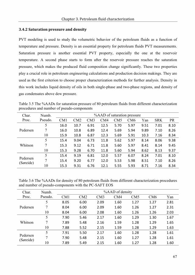
Chapter 3. Petroleum fluid characterization
3.4.2 Saturation pressure and density
PVT modeling is used to study the volumetric behavior of the petroleum fluids as a function of
temperature and pressure. Density is an essential property for petroleum fluids PVT measurements.
Saturation pressure is another essential PVT property, especially the one at the reservoir
temperature. A second phase starts to form after the reservoir pressure reaches the saturation
pressure, which makes the produced fluid composition change significantly. These two properties
play a crucial role in petroleum engineering calculations and production decision makings. They are
used as the first criterion to choose proper characterization methods for further analysis. Density in
this work includes liquid density of oils in both single-phase and two-phase regions, and density of
gas condensates above dew pressure.
Table 3.5 The %AADs for saturation pressure of 80 petroleum fluids from different characterization procedures and number of pseudo-components
Char.Proc.
Numb.Pseudo.
%AAD of saturation pressureCM1 CM2 CM3 CM4 CM5 CM6 Yan SRK PR
Pedersen5 16.0 10.7 6.91 12.5 5.70 5.97 9.51 7.01 8.10 7 16.0 10.8 6.89 12.4 5.69 5.94 9.89 7.10 8.26 10 15.9 10.8 6.87 12.3 5.69 5.91 10.3 7.16 8.34
Whitson5 15.4 9.04 6.73 11.8 5.62 5.97 8.14 8.06 9.38 7 15.3 9.12 6.71 11.8 5.60 5.97 8.41 8.14 9.45 10 15.3 9.28 6.70 11.8 5.60 5.94 8.62 8.13 9.37
Pedersen(Søreide)
5 15.4 9.19 6.81 12.0 5.57 6.07 8.24 7.01 8.10 7 15.4 9.20 6.77 12.0 5.53 5.98 8.51 7.10 8.26 10 15.3 9.31 6.76 12.1 5.55 5.93 8.71 7.16 8.34
Table 3.6 The %AADs for density of 80 petroleum fluids from different characterization procedures and number of pseudo-components with the PC-SAFT EOS
Char.Proc.
Numb.Pseudo.
%AAD of densityCM1 CM2 CM3 CM4 CM5 CM6 Yan
Pedersen5 8.05 6.00 2.09 1.60 1.27 1.27 2.81 7 8.04 6.00 2.09 1.60 1.26 1.27 2.31
10 8.04 6.00 2.08 1.60 1.26 1.26 2.03
Whitson5 7.90 5.46 2.17 1.60 1.29 1.30 1.67 7 7.89 5.48 2.16 1.59 1.28 1.29 1.65
10 7.88 5.52 2.15 1.59 1.28 1.29 1.63
Pedersen(Søreide)
5 7.91 5.50 2.17 1.60 1.28 1.28 1.61 7 7.90 5.48 2.15 1.60 1.27 1.28 1.61
10 7.89 5.49 2.15 1.60 1.27 1.28 1.60
67
83

Thermodynamic modeling of complex systems
Table 3.7 The percent deviations of saturation pressure for individual fluids
Fluid CM1 CM2 CM3 CM4 CM5 CM5(Whit.)
CM5(nc=10)
CM5(Riazi) CM6 Yan SRK
F01 6.08 0.15 2.43 9.69 2.37 5.05 0.53 2.00 2.38 10.6 9.23F02 2.01 3.10 2.45 3.02 2.08 3.12 4.30 3.06 2.18 6.52 0.57F03 2.58 9.72 6.69 3.32 7.71 8.06 10.1 10.1 6.25 15.6 4.90F04 10.2 1.15 6.69 11.4 5.51 7.17 0.16 2.68 6.97 10.4 4.30F05 0.45 9.45 5.16 4.54 6.67 4.96 12.1 9.79 4.53 23.2 0.08F06 18.3 9.04 6.64 23.8 3.44 2.87 2.87 2.83 3.91 3.73 19.3F07 12.0 6.83 4.15 10.4 2.78 2.01 2.44 1.76 2.97 4.98 2.52F08 6.58 0.14 1.47 4.87 2.99 1.40 3.49 7.07 2.55 22.4 1.59F09 1.52 4.78 2.11 0.11 1.38 4.29 1.07 3.03 1.51 30.0 5.35F10 1.88 3.05 0.29 1.71 0.62 1.48 0.95 1.57 0.70 13.1 5.28F11 0.24 3.36 0.67 0.57 0.18 1.81 0.47 2.00 0.26 15.9 3.95F12 9.30 4.06 1.09 3.91 0.19 1.57 0.27 4.97 0.07 5.19 1.64F13 16.5 11.5 8.51 11.0 7.22 5.97 7.13 2.75 7.42 2.02 1.63F14 16.4 11.7 8.31 11.0 7.00 5.75 6.91 2.49 7.19 1.78 2.22F15 17.9 13.5 9.45 15.1 8.05 6.92 7.95 3.70 8.22 1.95 4.45F16 17.6 13.2 10.7 12.9 9.58 8.42 9.43 5.76 9.85 4.83 4.12F17 20.4 15.8 12.9 15.7 11.7 10.5 11.5 7.65 12.0 7.24 6.70F18 15.4 10.6 7.07 12.6 5.65 4.41 5.50 1.48 5.94 0.03 2.70F19 19.5 14.9 12.3 14.8 11.1 9.93 11.0 7.24 11.5 6.81 6.43F20 13.2 8.27 4.86 10.9 3.40 2.19 3.25 0.69 3.78 2.12 1.94F21 14.9 10.2 6.50 12.4 5.00 3.75 4.85 0.87 5.39 0.71 2.71F22 3.01 3.29 4.99 0.59 6.50 7.62 6.64 10.4 5.75 10.7 9.19F23 5.11 0.64 4.98 1.72 6.94 8.27 7.09 11.8 6.24 13.5 8.10F24 18.9 13.8 10.1 12.6 8.40 7.07 8.29 3.62 9.02 2.43 0.11F25 19.9 14.2 12.2 14.4 10.6 9.6 10.5 6.73 11.6 6.51 4.63F26 14.1 1.11 5.74 7.21 3.99 4.58 3.99 1.21 4.50 0.43 4.88F27 7.94 2.07 1.71 2.98 0.78 0.62 0.54 3.53 1.34 14.5 9.15F28 34.1 26.9 20.4 25.4 17.8 17.5 17.8 10.7 18.3 2.28 1.28F29 17.4 4.55 4.11 8.55 1.33 1.44 1.33 4.26 2.04 10.0 3.48F30 13.1 6.76 4.51 13.8 3.05 2.75 2.78 1.17 3.52 6.96 8.88F31 19.5 13.4 10.8 20.8 9.54 9.41 9.35 6.15 10.1 1.42 11.9F32 13.2 2.05 2.26 3.01 5.56 5.26 5.57 11.6 4.25 19.5 9.10F33 12.4 6.15 2.80 11.8 1.47 1.11 1.33 2.14 2.16 6.14 0.39F34 19.8 10.2 3.79 9.91 0.41 0.11 0.40 7.43 1.08 16.1 7.53F35 20.6 12.7 10.3 21.7 8.37 8.27 8.13 4.98 9.31 1.02 13.0F36 22.6 14.0 7.90 21.1 4.92 4.76 4.68 0.76 5.73 8.58 6.09F37 21.9 13.0 10.5 23.8 8.14 8.22 7.92 5.02 9.19 0.68 16.6F38 30.5 23.1 15.3 24.2 12.0 12.7 11.9 4.44 12.6 4.78 5.28F39 18.3 13.2 9.33 12.9 7.69 6.96 7.45 1.57 8.24 9.36 7.18F40 23.2 14.6 8.22 21.1 5.04 4.87 4.82 0.72 6.05 8.89 6.48F41 18.1 8.49 4.74 18.2 2.06 2.07 1.86 2.20 3.26 8.56 5.83
68
84

Chapter 3. Petroleum fluid characterization
F42 24.8 16.8 9.34 23.3 6.09 5.78 5.84 0 7.02 8.73 7.47F43 31.9 26.8 16.9 27.3 13.9 13.2 13.8 6.37 14.8 2.83 0.70F44 23.7 14.0 9.68 22.8 6.62 6.56 6.44 2.03 7.90 4.40 9.54F45 19.4 13.3 3.66 14.0 0.56 0.44 0.42 6.63 1.54 14.7 10.4F46 27.8 21.4 7.56 21.3 3.06 3.13 2.95 8.16 4.14 24.1 5.69F47 37.2 29.5 23.4 33.3 20.2 20.6 20.1 14.5 21.4 6.67 20.9F48 29.7 23.2 10.3 23.1 5.77 6.14 5.66 4.45 6.96 18.0 0.10F49 26.2 20.7 9.82 19.6 6.41 6.34 6.28 1.87 7.35 13.2 6.86F50 30.0 23.0 10.8 24.3 6.28 6.79 6.15 3.14 7.66 16.0 2.47F51 17.4 10.8 6.36 10.2 4.08 3.56 4.01 0.91 5.20 4.36 6.62F52 8.34 2.35 1.67 5.91 0.26 0.19 0.13 1.73 1.75 2.98 2.04F53 29.7 24.7 13.2 22.7 9.38 9.06 9.24 1.42 10.7 8.64 4.10F54 5.95 4.62 5.19 2.6 8.21 7.63 8.28 10.8 5.51 12.2 8.81F55 13.1 6.37 2.54 5.04 6.24 6.18 6.28 13.0 4.86 20.7 14.7F56 28.1 23.0 10.3 20.0 6.08 5.67 5.90 2.88 7.58 13.7 9.14F57 39.0 35.8 19.2 27.4 14.4 11.9 14.4 2.23 15.6 15.8 11.3F58 35.9 32.0 14.7 21.8 9.11 9.58 9.07 5.45 10.6 25.0 19.4F59 11.5 3.85 0 5.86 3.14 4.01 3.18 6.44 0.67 11.5 0.02F60 26.2 22.4 2.66 4.71 3.71 7.51 3.72 21.1 2.01 45.1 44.7F61 22.1 16.7 7.02 8.21 2.74 1.11 2.70 4.03 5.23 12.3 17.8F62 10.0 5.38 7.14 10.8 7.68 7.79 7.79 6.79 7.85 6.61 12.3F63 10.3 2.64 2.85 9.72 1.00 1.18 0.69 1.14 2.14 4.42 9.56F64 8.10 1.76 0.16 9.44 1.32 1.26 1.66 4.03 0.59 8.51 5.77F65 7.24 1.31 1.17 8.29 0.90 0.89 1.10 2.73 0.83 4.87 15.6F66 4.09 1.61 4.27 4.83 5.17 4.21 5.33 4.22 4.94 17.1 5.86F67 0.03 9.01 8.17 1.08 10.5 10.3 11.0 13.5 9.07 18.0 0.39F68 7.66 0.21 0.60 5.07 2.62 3.06 3.03 5.96 1.74 9.86 0.28F69 19.8 14.4 10.8 15.2 8.92 8.17 8.54 4.94 9.39 0.13 3.82F70 5.87 2.48 4.22 7.26 6.63 6.37 6.95 9.74 4.33 15.4 2.88F71 11.6 4.74 6.54 9.06 5.29 5.41 5 3.41 6.12 1.23 10.1F72 7.66 1.31 2.14 6.19 0.84 0.92 0.57 1.28 2.01 3.74 6.35F73 11.1 2.3 0.73 11.8 1.87 1.65 2.27 4.64 1.05 13.2 9.81F74 8.21 0.55 0.42 6.47 3.19 2.81 3.58 5.75 1.66 10.5 8.25F75 22.2 16.4 14.5 18.8 12.4 12.1 12.2 10.3 14.1 6.99 13.0F76 9.81 4.26 1.32 5.65 1.25 1.72 1.52 3.24 0.53 6.57 1.49F77 8.10 2.21 0.87 3.34 1.82 3.46 2.26 2.49 0.58 0.38 FAILF78 23.3 15.6 10.4 19.7 7.73 6.89 7.59 1.86 8.35 2.82 3.19F79 19.0 14.3 8.17 14.4 5.21 4.76 5.03 1.04 6.81 3.34 0.94F80 21.0 16.6 9.28 20.3 6.09 6.14 5.75 1.55 7.45 4.75 11.0avg 16.0 10.7 6.91 12.5 5.70 5.62 5.69 4.87 5.97 9.51 7.01>10* 57 41 21 47 10 8 12 11 12 32 17
* Number of cases whose calculated saturation pressure deviation is larger than 10%.
69
85

Thermodynamic modeling of complex systems
The %AADs for saturation pressure and density are respectively listed in Tables 3.5 and 3.6 for
these 80 petroleum fluids. The comparisons are made in four aspects, i.e. molar composition
distributions, SG correlations, numbers of pseudo-components and EOS models or estimation
methods of model parameters for the same EOS. The PNA distributions are estimated by the n-d-M
method. The second column indicates how many pseudo-components are used to represent the C7+
fraction. The results from SRK and PR are also presented as references, for which the critical
properties are calculated by the method developed by Twu (1984) and the acentric factor is
calculated from the Lee-Kesler correlations [Lee et al. (1975), Kesler et al. (1976)].
The %AAD of saturation pressure for individual fluids are presented in Table 3.7. The results with
different characterization procedures, number of pseudo-components and PNA content estimation
methods are given for the candidate method CM5, while the standard exponential characterization
procedure [Pedersen et al. (1983, 1984, 2007a)] is used for other methods. Both of the average
values of %AAD and the number of cases with deviation larger than 10% are given for comparison.
As seen from Table 3.5 and the work of Yan et al. (2010), SRK and PR perform quite similarly, and
SRK gives slightly smaller overall deviations of saturation pressure. Thus the results of individual
fluids from SRK are presented here for comparison.
It can be seen from Tables 3.5 and 3.6 that there are small variations of the overall %AAD of both
saturation pressure and density among different characterization procedures, and these differences
mainly come from different SG approaches, rather than from the molar composition distributions.
The further comparison of these two characterization procedures, however, as presented in Table
3.7, shows that they have noticeable differences for individual oil fluids with plus fractions starting
from seven or with extremely heavy plus fraction, for example F57, F60, F61 and F77. This is
because default characteristic parameters are used for these fluids in the gamma characterization
procedure. However, the overall %AADs for vapor pressure of fluids F57, F60, F61, F77 and those
with plus fraction starting from seven are, respectively, 5.73% and 5.52% for the exponential and
the gamma characterization procedures. All of these results confirm the conclusion made by
Pedersen et al. (2007a) that the exponential and gamma characterization procedures perform quite
similarly. Tables 3.5 and 3.6 also show that the variations of overall %AADs for saturation pressure
and density among different number of pseudo-components are even smaller compared to those
from different characterization procedures. However, the number of pseudo-components has
significant impact on the dew points of gas condensate fluids as shown in Table 3.7. This could
70
86

Chapter 3. Petroleum fluid characterization
probably be explained that the more pseudo-components used to represent the plus fraction, the
heavier the last component would be, and the easier it would get condensed. The results indicate
that five pseudo-components for the plus fraction seem to be enough to get satisfactory predictions
of saturation pressure and density for oils, which is consistent to the statements about how many
components to group from Whitson et al. (2000) and Riazi (2005). It is also meaningful for
modeling and simulation of petroleum fluids, since the overall computational load increases
significantly with the total component numbers.
The results from CM1 have much larger %AAD than those from other candidate methods in terms
of both saturation pressure and density, which means that it is not the correct way to produce the
model parameters. In order to eliminate the effects of PNA content estimations, the percentages of P
and N are tuned to match the SG and Tb of the SCN fractions or pseudo-components in CM2. It can
be seen that the predictions of both saturation pressure and density are much improved, while they
are still unsatisfactory. This reveals that combination of the correlations of n-alkanes, cyclo-alkane
and benzene derivatives are not good enough for producing all of the model parameters. Meanwhile
it also indicates that it would not be generally applicable to have simple linear correlations for the
three model parameters suitable for all different types of petroleum fluids.
The correlation equation (3.1) is used in CM3, CM4 and Yan’s method [Yan et al. (2010)]. As
shown in Tables 3.5 and 3.6, CM3 and Yan’s method yield comparable descriptions of saturation
pressure to those given by SRK and PR. The results of %AAD of density are also acceptable. In
order to investigate if it is possible to further improve the descriptions of density within this
framework, the parameters m and in CM4 are tuned to match the SG and Tb of SCN fractions and
pseudo-
shows significant deterioration of the predictions of saturation pressure with small improvements on
density descriptions.
to match SG in CM5, while both parameters m and
PR EOS, the results from these two methods are quite promising, with the %AADs for saturation
pressure and density less than 6.0% and 1.3%, respectively, and more than 85% possibility to
match SG in CM3. The %AADs for saturation pressure and density are respectively 5.67% and
71
87

Thermodynamic modeling of complex systems
1.28%, which are very close to those from CM5. This confirms to some extent that it is possible to
feasible to use linear correlations for one or two of these parameters, while the remaining one(s)
is/are tuned to SG and/or Tb.
The results and discussions presented above suggest on one hand that it is crucial to tune the model
parameters to SG and/or Tb to have precise description of density, which could simultaneously
improve the descriptions of saturation pressure further. On the other hand, it is very important to
choose the right parameters for fitting purposes.
Since the percentages of PNA contents are used directly or indirectly in the process of estimating
model parameters, it is useful to compare the two PNA content estimation methods themselves.
The %AADs for saturation pressure and density are compared in Figures 3.5 (a) and (b) for all the
candidate methods. The results of individual fluids are also given for CM5 in Table 3.7. The
exponential characterization procedure [Pedersen et al. (1983, 1984, 2007a)] with five pseudo-
components is used here, which will be the default procedure for the following discussions. It is
clearly shown that the results from these two estimation methods are quite different. The
comparisons in Figures 3.5 (a) and (b) show that the Riazi method [Riazi et al. (1986)] gives
slightly smaller overall %AADs for both saturation pressure and density, while it can be seen from
Table 3.7 that it really depends on the fluids under investigation. It is not surprising to see that these
two PNA estimation methods give quite close results for CM4 and CM6. This is because the same
and Tb), only with different initial guesses
from these two PNA estimation methods.
Figure 3.5 Comparison of the impacts of the estimations methods of PNA contents on the %AADs for (a) saturation pressure and (b) density of 80 petroleum fluids
0
4
8
12
16
CM1 CM2 CM3 CM4 CM5 CM6
%AA
D of
satu
ratio
n pr
essu
re
Candidate method
(a)n-d-MRiazi
0
2
4
6
8
CM1 CM2 CM3 CM4 CM5 CM6
%AA
D of
den
sity
Candidate method
(b)
n-d-MRiazi
72
88

Chapter 3. Petroleum fluid characterization
It is quite demanding to investigate the effects of binary interaction parameters for these candidate
methods. The %AADs for saturation pressure and density are compared in Figures 3.6 (a) and (b)
for all candidate methods with the two available kij sets. It can be seen that kij values have,
respectively, large and negligible impacts on the description of the saturation pressure and density.
This is because kij values are mainly for the pairs containing light gases and/or methane, and these
light components have large impacts on the saturation pressures of petroleum fluids, which makes
kij values a powerful tool to tune the EOS model to match the saturation pressure. Most of the fluids
considered in this work are oil samples, and the light components are too light to affect the oil
density.
Figure 3.6 Comparison of the effects of binary interaction parameters on the %AADs for (a) saturation pressure and (b) density of 80 petroleum fluids.
As seen from Table 3.7, the saturation pressures of the N2 and/or CO2 rich fluids are predicted with
satisfactory accuracy, which indicates, to some extent, that the kij values for pairs containing N2 or
CO2 are reasonable. These kij values will not be further investigated in this work also because of
lack of enough cases. It is, however, a good opportunity to study the influence of the kij of pairs
containing C1 on PVT calculations. We proposed to conduct the investigations with the scenarios by
sequentially setting kij(C1,C2-6)=0.0, kij(C1,C7+)=0.01, kij(C1,C7+)=0.03, or using the following
correlation: 1000×kij( , ) = 0.070199 × + 5.4229 (3.5)
This correlation is regressed from the values published by Yan et al. (2010) and
2008). The difference between the %AAD of these kij values and the one with kij(C1,C7+)=0.02 are
plotted against the fluid number in Figure 3.7, where the %AAD from each scenario are also given.
0
6
12
18
CM1 CM2 CM3 CM4 CM5 CM6
%AA
D of
satu
ratio
n pr
essu
re
Candidate method
(a)new kij old kij
0
2
4
6
8
CM1 CM2 CM3 CM4 CM5 CM6
%AA
D of
den
sity
Candidate method
(b)new kij old kij
73
89

Thermodynamic modeling of complex systems
It is readily seen that the kij(C1,C2-6) and kij(C1,C7+) have, respectively, quite small and fairly
significant impacts on prediction of saturation pressure, even though quite close %AAD are
obtained by using 0.02, 0.03 and equation (3.5) for kij(C1,C7+). The results suggest that more
extensive investigations should be further conducted if the kij values are indirectly used to develop
‘general’ correlations for new characterization methods, as in the work of Pedersen et al. (2007b).
Figure 3.7 The difference between the %AAD of these kij values and the one with kij(C1,C7+) = 0.02. The average %AAD values of each kij are also listed in the legend for comparison.
3.4.3 A compromise method (CM7)
The candidate methods CM5 and CM6 have better overall performance on the prediction of
saturation pressure and density. The two PNA content estimation methods (n-d-M and Riazi) have
overall comparable performance for CM5, and the one with the Riazi method will be denoted as
CM5 (R) hereafter.
As listed in Table 3.7, the candidate methods give comparable average deviations of the saturation
pressure prediction, while the predictions for the individual case are quite different. It inspires us to
investigate if it is possible to have simple (linear) correlations for m and m 3 as well. The strategy
is to put the parameters which give the best prediction for each case together, and to analyze their
relationships with molecular weight. The results are presented in Figure 3.8. It can be seen that the
correlation of m is quite satisfactory, while the correlation of m 3 shows a bit more scatter for
heavy pseudo-components.
-20
-10
0
10
20
0 20 40 60 80
Diffe
renc
es o
f %AA
D
Fluid number
kij(C1,C2-C6)=0 (5.86%)
kij(C1,C7+)=0.01 (9.17%)
kij(C1,C7+)=0.03 (5.58%)
kij(C1,C7+)=eq5 (6.02%)
74
90

Chapter 3. Petroleum fluid characterization
The prediction of the saturation pressure of the aforementioned 80 fluids from this new method is
compared with the ones from CM5 and CM6 in Table 3.8. Since the correlation of m 3 is not
satisfactory at the heavy component ends, fitting to the specific density, as done before, has also
for accurate description of density, and then the new method performs as satisfactory as the other
ones.
In order to test the predictive capability of these methods, the predictions of the saturation pressure
of the 55 fluids from Elsharkawy (2003) are conducted for these methods. The results are also
reported in Table 3.8. The results for the additional 55 fluids, reported in this work, are assuming to
use nC4 and nC5 for C4 and C5, but as we have found that there are no observable differences to use
normal-hydrocarbons or iso-hydrocarbons. It can be seen that these methods show equally good
predictions. The new method is named CM7, and it will be investigated, along with the other
methods, further for three fluids for which extensive PVT experimental data is available.
Figure 3.8 Correlations of m and m 3 from the best candidate methods for each fluid
Table 3.8 Comparison of the new method with CM5 and MC6 on saturation pressure and density
fluid
numberCM5 CM5 (R) CM6
CM7
no fitting
80 5.70 4.87 5.97 5.12 (1.27)* 6.69 (2.49)
80+55 6.33 6.79 6.44 6.60 7.31
* The values in the parentheses are the deviations of density.
m = 0.0233982 x Mw + 0.941006R² = 0.995
0
10
20
30
0 200 400 600 800 1000
m
Molecualr weight (g/mol)
(a)
m 3 = 1.408578 x Mw + 52.6004R² = 0.985
0
300
600
900
1200
1500
1800
0 200 400 600 800 1000
m3
Molecular weight (g/mol)
(b)
75
91

Thermodynamic modeling of complex systems
3.4.4 Applications
3.4.4.1 PVT simulations
The methods CM5, CM5 (R), CM6 and CM7 are further tested using the three fluids from the book
of Pedersen and Christensen (2007a) without tuning against the experimental PVT data. The first
fluid is a gas condensate, and three experimental CME data sets are available. The second fluid is
an oil sample, for which there are three CME data sets and five DL data sets available. The third
fluid is also an oil sample, and four-stage separator test experimental data are available. The
definitions of these experiments and associated properties, composition and experimental data can
be found in the chapter 3 of the book [Pedersen et al. (2007a)].
The characterized fluid composition and model parameters of C7+ pseudo-components can be found
in Tables 3.9 and 3.10. The model parameters of the defined components are taken from the work of
Gross and Sadowski (2001). The model parameters of the first four pseudo-components of fluid F04
are the same in CM5 and CM6 as listed in Table 3.10, which means that no further fitting is needed
to match SG and Tb for them.
Table 3.9 Mole composition of the three fluids (F04, F63, F64) after characterization
Comp.Fluid F04 Fluid F63 Fluid F64
Mw (g/mol) z% Mw (g/mol) z% Mw (g/mol) z%N2 0.60 0.39 0.59
CO2 3.34 0.30 0.36C1 74.167 40.2 40.81C2 7.901 7.61 7.38C3 4.15 7.95 7.88iC4 0.71 1.19 1.20C4 1.44 4.08 3.96iC5 0.53 1.39 1.33C5 0.66 2.15 2.09C6 0.81 2.79 2.84P1 97.36 2.35 111.00 14.14 117.58 14.44P2 125.19 1.13 173.58 7.66 175.40 6.21P3 161.09 1.06 253.29 4.815 239.32 5.483P4 218.25 0.681 392.91 3.439 379.43 3.433P5 362.00 0.471 674.59 1.896 665.62 1.994
76
92

Chapter 3. Petroleum fluid characterization
The simulated CME results of fluid F04 from these four methods are compared with the
experimental data in Figures 3.9 (a), (b) and (c). It can be seen that these characterization methods
give quite similar overall results for these three CME measurements, except for the starting point of
the drop liquid volume percentage. The simulated and experimental relative volumes agree very
well in the whole pressure range, and the simulated Z factor matches the experimental data nicely
with some small deviations in the high pressure range. The simulated percent liquid dropout
volumes seem to be much lower than the experimental data in the low pressure range. These results,
however, are comparable to those from SRK and PR with volume translations, for which simulation
results are available in the chapter 7 of the book [Pedersen et al. (2007a)].
Table 3.10 Model parameters of C7+ pseudo-components for the three fluids (F04, F63, F64)
Fluid F04 Fluid F63 Fluid F64
m (Å) (K) m (Å) (K) m (Å) (K)CM5
3.0956 3.7943 255.04 3.5110 3.8159 251.41 3.7341 3.8293 248.423.8148 3.8244 256.80 5.0837 3.8671 257.73 5.1551 3.8721 256.564.7700 3.8590 256.79 7.0736 3.9035 262.20 6.7153 3.8973 261.976.1859 3.8958 261.13 10.6916 3.8904 262.68 10.3516 3.8836 262.419.8645 3.9181 263.30 17.3748 3.9121 272.38 17.1599 3.8982 272.23
CM5 (R)3.1334 3.7755 251.96 3.4770 3.8310 253.87 3.6572 3.8619 253.643.7573 3.8480 260.73 4.9420 3.9115 265.11 4.9598 3.9331 266.674.6126 3.9117 265.55 7.0323 3.9128 263.74 6.6856 3.9043 263.146.1425 3.9069 262.97 10.3733 3.9386 270.74 10.0264 3.9345 270.929.7006 3.9450 267.74 17.1037 3.9373 276.70 16.8016 3.9319 278.03
CM63.0956 3.7943 255.04 3.5110 3.8159 251.41 3.8172 3.7950 243.013.8148 3.8244 256.80 5.0973 3.8629 257.03 5.2882 3.8323 250.104.7700 3.8590 256.79 7.1122 3.8949 260.78 6.7133 3.8978 262.066.1859 3.8958 261.13 10.7823 3.8770 260.47 10.4212 3.8730 260.669.9855 3.8986 260.11 17.9459 3.8604 263.71 17.7040 3.8484 263.86
CM73.2191 3.7339 245.26 3.5383 3.8038 249.47 3.6921 3.8470 251.243.8703 3.8020 253.12 5.0025 3.8924 261.90 5.0451 3.9061 262.164.7103 3.8787 260.04 6.8676 3.9505 270.06 6.5407 3.9391 268.976.0477 3.9316 267.10 10.1344 3.9762 277.12 9.8190 3.9680 276.649.4112 3.9939 275.98 16.7251 3.9736 282.96 16.5154 3.9598 282.85
77
93

Thermodynamic modeling of complex systems
Figure 3.9 Simulation CME results of fluid F04 with characterization methods CM5, CM5 (R),CM6 and CM7. (a) Relative volume; (b) Z factor above dew point; (c) Liquid dropout volume (%). The experimental data are from the book of Pedersen et al. (2007a).
The simulated DL and CME results of fluid F63 are presented in Figure 3.10. It can be seen from
Figure 3.10 (a) that these methods represent the oil density perfectly at all pressure steps. As seen
from Figure 3.10 (b), however, they have difficulties in describing the liberated gas phase
compressibility factor (Z factor) at high pressures.
The simulated Y-factor is compared with the experimental data in Figure 3.10 (c), which shows that
the different methods do not predict as similar results as those they do for oil density and Z factor.
The method CM6 gives best match to the experimental data. The simulated compressibility results
are presented in Figure 3.10 (d). The similar scatter results as for Y-factor are seen, but the method
CM6 presents the largest deviation from the experimental data for this property.
The simulated compressibility from PR are also plotted in Figure 3.10 (d), which is taken from the
book of Pedersen and Christensen (2007a), where they showed that PR gave much better results
0.7
1
1.3
1.6
1.9
2.2
100 200 300 400 500 600
V/Vsa
t
Pressure (bar)
(a)
Exp.
CM5
CM5 (R)
CM6
CM7
1
1.1
1.2
1.3
1.4
1.5
380 450 520 590
Z Fa
ctor
Pressure (bar)
(b)Exp.
CM5
CM5 (R)
CM6
CM7
0
3
6
9
12
100 200 300 400
Liqu
id v
olum
e (%
)
Pressure (bar)
(c)
Exp.
CM5
CM5 (R)
CM6
CM7
78
94

Chapter 3. Petroleum fluid characterization
than SRK for this case. There is no doubt that PC-SAFT significantly improves the descriptions of
compressibility. Similar results were reported by Pedersen et al. (2007b) and Leekumjorn et al.
(2013), and this seems to be natural since cubic EOS have inherent deficiency in the compressibility
description. However, the simulated compressibility values from PC-SAFT still show some
deviations from the experimental data at high pressure range, from both quantitative and qualitative
points of view. This phenomenon is consistent to what was seen in previous works [Pedersen
(2007b), de Villiers (2011), Liang et al. (2012), Leekumjorn et al. (2013)], and it is because PC-
SAFT EOS has difficulties in describing the derivatives of pressure with respect to volume in wide
range of temperature, which can be somehow improved by refitting the universal constants [Liang
et al. (2012)].
Figure 3.10 Simulation DL and CME results of fluid F63 with characterization methods CM5, CM5 (R), CM6 and CM7. (a) Oil density; (b) Z factor of liberated gas; (c) Y-Factor; (d) Compressibility above saturation pressure. The experimental data is from Pedersen et al. (2007a).
0.6
0.65
0.7
0.75
0.8
0 100 200 300
Oil
dens
ity (g
/cm
3 )
Pressure (bar)
(a)Exp.
CM5
CM5 (R)
CM6
CM7
0.8
0.85
0.9
0.95
1
0 50 100 150 200
Z fa
ctor
Pressure (bar)
(b) Exp.
CM5
CM5 (R)
CM6
CM7
1.5
2
2.5
3
3.5
50 100 150 200
Y-fa
ctor
Pressure (bar)
(c)
Exp.
CM5
CM5 (R)
CM6
CM7
0.18
0.21
0.24
0.27
200 250 300 350
Com
pres
sibili
ty (1
000/
bar)
Pressure (bar)
(d)
Exp. PR
CM5 CM5 (R)
CM6 CM7
79
95

Thermodynamic modeling of complex systems
The %AAD of simulation results from the properties measured in CME and DL for fluids F04 and
F63 are presented in Table 3.11. It can be seen that the simulation deviations are reasonably
satisfactory except for the percent liquid dropout volume.
Table 3.11 %AADs for properties measured in CME and DL for fluid F04 and fluid F63
Methods
%AAD of properties
Fluid F04 CME Fluid F63 CME Fluid F63 DL
Rel. V Liq. V Z fact. Rel. V Y Fact. Com. c0 Bo Rs Bg Z fact. G.G.
CM5 3.47 25.7 1.62 0.48 2.78 2.31 3.51 4.77 0.20 2.47 2.34 0.93
CM5 (R) 1.85 19.8 1.67 0.28 4.91 2.21 2.84 5.82 0.25 2.46 2.36 0.86
CM6 4.31 28.4 1.61 0.67 1.28 3.16 3.63 4.42 0.28 2.41 2.28 0.90
CM7 0.45 32.7 1.62 0.37 6.59 2.33 3.46 5.61 0.26 2.57 2.23 0.86
It has been shown that these methods have quite similar quantitative and qualitative behaviors for
CME and DL results, and the same conclusion is true for the separator test experiments here. So the
separator test results calculated only by the candidate method CM5 (R) and CM7 will be presented.
The simulated separator test results of fluid F64 from both the simplified PC-SAFT and SRK EOS
are presented in Table 3.12 along with the experimental data. Simulation results with both five and
ten pseudo-components are available for the simplified PC-SAFT EOS. Since SRK and PR EOS
give quite close results, which can be also seen from the Pedersen et al. (2007a), only the ones from
SRK are presented. It can be seen that the simulated results from these two EOS models are quite
close except for the composition of C7+, if the same number of pseudo-components is used. It shows
that the composition of C7+ could be largely affected by the number of pseudo-components for the
plus fraction. This might be explained that the more pseudo-components are used to represent the
plus fraction, the lighter the first C7+ component would be, and the tendency to enter the vapor
phase would be easier. However, there is really small impact on the composition of the defined
components when changing the number of pseudo-components for the plus fraction. This is
consistent with the aforementioned statement that the number of pseudo-component has little effect
on bubble points of oil samples. It is also seen that the simulated compositions of C5 and C6 are
larger than the experimental results at the final stage for both EOS models, which might be tuned by
binary interaction parameters.
80
96

Chapter 3. Petroleum fluid characterization
Table 3.12 Comparison of simulated and experimental composition at each stage in separator test
Comp. stage 1 stage 2 stage 3 stage 4 stage 1 stage 2 stage 3 stage 4Experimental data* SRK (nc=5)
N2 1.07 0.42 0.01 0.00 1.32 0.61 0.16 0.02CO2 0.49 0.62 0.60 0.28 0.57 0.69 0.65 0.29C1 77.43 64.63 36.04 8.89 78.44 65.40 37.45 8.89C2 9.56 14.42 20.23 16.19 9.13 14.14 20.02 15.68C3 6.70 12.01 24.89 35.52 6.21 11.49 23.32 33.69iC4 0.71 1.30 3.13 5.74 0.64 1.23 2.84 5.52nC4 2.01 3.65 9.02 17.22 1.80 3.42 8.20 17.32iC5 0.44 0.74 1.86 3.77 0.39 0.70 1.73 4.23nC5 0.59 0.98 2.31 4.61 0.52 0.93 2.34 5.86C6 0.47 0.66 1.28 2.92 0.38 0.62 1.52 4.01C7+ 0.53 0.57 0.63 4.86 0.59 0.78 1.76 4.50
CM5 (R) (nc=5) CM5 (R) (nc=10)N2 1.31 0.53 0.12 0.01 1.31 0.53 0.12 0.01
CO2 0.59 0.68 0.62 0.27 0.59 0.68 0.61 0.26C1 78.31 65.79 38.09 9.36 78.18 65.60 37.74 9.06C2 9.13 14.13 20.31 16.59 9.13 14.12 20.21 16.20C3 6.32 11.41 23.07 33.77 6.33 11.41 23.02 33.26iC4 0.68 1.24 2.84 5.48 0.68 1.24 2.84 5.43nC4 1.84 3.38 8.06 17.13 1.84 3.39 8.07 17.02iC5 0.40 0.71 1.76 4.29 0.40 0.71 1.76 4.28nC5 0.54 0.93 2.32 5.83 0.54 0.93 2.33 5.83C6 0.40 0.62 1.53 4.03 0.40 0.62 1.53 4.04C7+ 0.48 0.58 1.28 3.25 0.59 0.77 1.78 4.61
CM7 (nc=5) CM7 (nc=10)N2 1.30 0.52 0.12 0.01 1.30 0.52 0.12 0.01
CO2 0.59 0.68 0.62 0.26 0.59 0.68 0.61 0.26C1 78.24 65.68 37.90 9.24 78.11 65.49 37.56 8.95C2 9.15 14.16 20.32 16.50 9.16 14.15 20.22 16.13C3 6.34 11.44 23.12 33.71 6.35 11.44 23.07 33.21iC4 0.68 1.25 2.85 5.49 0.68 1.25 2.85 5.44nC4 1.84 3.39 8.09 17.15 1.85 3.40 8.09 17.04iC5 0.40 0.71 1.76 4.30 0.40 0.71 1.77 4.29nC5 0.54 0.94 2.33 5.84 0.54 0.94 2.34 5.84C6 0.40 0.62 1.53 4.04 0.40 0.62 1.54 4.06C7+ 0.50 0.61 1.36 3.45 0.62 0.80 1.84 4.77
* The experimental data is taken from Pedersen et al. (2007a).
81
97

Thermodynamic modeling of complex systems
3.4.4.2 Phase envelope
The phase envelopes of fluids F04 and F63 from the PC-SAFT EOS with the characterization
methods CM5, CM5(R), CM6 and CM7, and the PR EOS are presented in Figure 3.11. It can be
seen that PC-SAFT predicts a bit larger phase envelopes for these two fluids than PR, among which
the method CM7 gives the largest ones. These characterization methods present similar predictions
around the experimental points, so it is hard to say which characterization method is superior to
others if based on one saturation pressure data point only.
Both PC-SAFT and PR predict liquid-liquid like phase split at the low temperature regions for fluid
F04, though temperature regions are much different, i.e. the liquid-liquid like phase split from PC-
SAFT appears 80K higher than those from PR. PC-SAFT predicts liquid-liquid like phase split for
fluid F63 as well, however, PR does not give the same prediction. The experimental data are
extremely scarce at these temperature ranges, e.g. below 250K, so it is hard to determine whether
this is a physical or non-physical prediction.
Figure 3.11 Phase envelopes of F04 (a) and F63 (b) from the PC-SAFT and PR EOS
3.4.4.3 Activity coefficients
The activity coefficients are good measures to roughly indicate the solution behavior of the heavy
components. The activity coefficients of the pseudo-components have been calculated for 55 fluids,
for which the DL/CME experimental data is available. The calculations have been conducted under
the same temperature, pressure and composition conditions as those in the DL/CME experiments,
and the results are shown in Table 3.13.
0
200
400
600
100 200 300 400 500 600
Pres
sure
(bar
)
Temperature (K)
(a)
Exp.PRCM5CM5 (R)CM6CM7
0
50
100
150
200
250
200 400 600 800
Pres
sure
(bar
)
Temperature (K)
(b)
Exp.PRCM5CM5 (R)CM6CM7
82
98

Chapter 3. Petroleum fluid characterization
On one hand, the average activity coefficients for all the pseudo-components from different
characterization methods are not far from unity, indicating that our models predict a near-ideal
solution behavior for the pseudo-components in the tested systems. On the other hand, as the
pseudo-component becomes heavier, the activity coefficient generally decreases, showing a shift
towards the athermal solution behavior, which to some extent largely depends on the oil types, as
indicated by the increasing standard deviations.
Table 3.13 Average activity coefficients of pseudo-components from four characterization methods
Comp. CM5 CM5 (R) CM6 CM7
P1 1.03 (0.038)* 1.03 (0.036) 1.02 (0.038) 1.02 (0.031)
P2 1.03 (0.050) 1.04 (0.059) 1.04 (0.051) 1.03 (0.049)
P3 0.98 (0.095) 1.00 (0.083) 0.99 (0.098) 1.01 (0.087)
P4 0.88 (0.125) 0.96 (0.127) 0.87 (0.132) 0.98 (0.133)
P5 0.82 (0.151) 0.91 (0.215) 0.74 (0.144) 0.92 (0.205)
* The numbers in the parentheses are standard deviations along with the averages
3.5 Conclusions
In this work, six candidate methods are proposed for estimating model parameters during petroleum
fluid characterization procedures for the PC-SAFT EOS, in which the model parameters are
produced by combining well-behaved simple correlations of homologous series with the estimated
PNA contents, and/or by using different approaches fitted to match SG and/or Tb. The performance
of these candidate methods is investigated for predicting the saturation pressure and density of 80
petroleum fluids over wide temperature, pressure and composition conditions, along with different
options in characterization procedures, including the molar composition distribution function, the
SG correlation, the number of pseudo-components, the PNA content estimation method and the
binary interaction parameters.
The results show that the characterization procedures have small impact on saturation pressure and
density for all of the proposed candidate methods, so does the number of pseudo-components for oil
fluids. However, the number of pseudo-components has significant impact on saturation pressure of
the gas condensates. The investigations of PNA content estimation methods reveal that they could
lead to quite different results, which suggests that precautions should be taken when the PNA
content estimations are directly used in producing model parameters. The binary interaction
83
99

Thermodynamic modeling of complex systems
parameters have significant effects on saturation pressure and quite small impact on density, and
more extensive investigations are recommended if the kij values are indirectly used to develop
‘general’ correlations for new characterization methods. The candidate methods CM5 and CM6
show better overall performance than other methods, with %AAD less than 6.0% and 1.3% of
saturation pressure and density, respectively, and with 85% possibility to predict saturation pressure
within 10%.
A further analysis has been conducted for the generated parameters from the best candidate methods
for each fluid, and a new compromise method is proposed with a simple linear correlation for the
model parameter m, named as CM7, which gives quite similar predictions for saturation pressure
and density as those from CM5 and CM6.
The methods CM5, CM6 and CM7 are further studied on simulating experimental CME, DL and
separator test data for three petroleum fluids. These methods show overall similar performance. The
simulated relative volumes and density of both gas condensate and oil fluids match the experimental
data quite well. These methods, however, have difficulties in describing the percent volumes of
dropped liquid from gas condensate, Z factor of liberated gas from oil, and the compressibility of
oils at high pressure range from the qualitative point of view. The simulated separator test results
from the simplified PC-SAFT EOS and the SRK EOS are quite close except for the composition of
C7+, which seem to be largely influenced by using different number of pseudo-components for the
plus fraction. Compared to the simulation results available in the literature with volume corrected
cubic EOS models [Pedersen et al. (2007a)] or the PC-SAFT EOS [Pedersen et al. (2007b)], the
results presented in this work are quite promising.
This work provides valuable information for developing general characterization methods for the
PC-SAFT EOS, i.e. (1) simple linear correlations could be used for model parameter m and the
an accurate description of
density, and improve the prediction of saturation pressure further.
As seen in previous works [de Villiers (2011), Liang et al. (2012)], the PC-SAFT EOS has
difficulties in describing the speed of sound in fluids, especially for those containing long-chain
components. In this work, the similar deficiency of the PC-SAFT EOS has been seen in the
description of isothermal compressibility. Both properties are directly linked to the derivative of
pressure with respect to the total volume, when the density could be accurately modeled. Liquid-
84
100

Chapter 3. Petroleum fluid characterization
liquid phase split has been predicted by PC-SAFT, but not by cubic EOS for some cases, at low
temperature region, which needs to be further investigated.
Based on the feedback from one of the reviewers of the published article [Liang et al. (2014)] who
stated that the pseudo-components in oils show near-ideal solution behavior, the methods CM5 (R)
and CM7 are proposed for further use in modeling oil-water-chemical systems in the next chapter.
85
101

86
102

Chapter 4. Modeling oil-water-chemical systems
Compared to other applications, the PC-SAFT EOS has not been extensively applied to model
petroleum fluids, which might be due to the complex and ill-defined nature of oils. It is a critical
test for PC-SAFT to model the systems of oil plus water and/or chemicals, since sophisticated
characterization methods and robust parameters are needed for oils and polar compounds.
The purpose of this work is to apply the PC-SAFT EOS into modeling oil-water-chemical systems,
with the newly developed model parameters of polar compounds, interaction schemes from well-
defined mixtures, and the characterization methods in the previous chapters.
4.1 Introduction
The complex phase behavior between petroleum fluids and polar compounds such as water,
methanol and glycols has become more and more important as the offshore reservoirs represent one
of the major growth areas of the oil and gas industry, which often mean extreme and complicated
conditions, the use of hydrate inhibitors, etc. It is a reasonable approximation to deal with water and
petroleum fluids as totally immiscible systems at low to moderate temperature and pressure
conditions. However, the mutual solubility of petroleum fluid and water will considerably increases
when chemicals are involved, the petroleum fluid is highly aromatic, or at high temperature and
pressure regions. For instance, the addition of methanol or glycols into unprocessed well streams
during subsea pipelines is necessary to inhibit gas hydrate formation, for which modeling the phase
behavior of oil-water-chemicals is very important for the viewpoints of economical operation and
environmental safety.
It is hard and often unreliable to use conventional cubic EOS, which have been standard models for
the oil and gas industry for decades, for such complex systems containing petroleum fluids, water
and/or chemicals, even with quite large binary interaction coefficients for water and hydrocarbons.
The association models, explicitly accounting for hydrogen bonding interactions, show advantages
over cubic EOS, especially for predictive calculations [Kontogeorgis et al. (2010a)]. In this chapter,
the developments from the previous chapters will be applied to model the phase behavior of oil plus
water and/or chemical systems.
87
103

Thermodynamic modeling of complex systems
4.2 Data
Seven petroleum fluids, two live oils and five dead oils, are studied in this work. The compositions
of these fluids are listed in Table 4.1, and it can be seen that the fluid Light-1 is a quite heavy oil.
The composition of N2, CO2 and hydrocarbons up to six carbon numbers in general are kept no
change during the characterization procedure, and the model parameters of these components are
taken from the original literature [Gross et al. (2001)], so the related information will not be
duplicated in the characterization results hereafter.
Table 4.1 Composition of petroleum fluids
Comp. Live Oil 1* Live Oil 2+ Cond-1# Cond-2# Cond-3# Light-1# Light-2#
N2 0. 369 0.64 0.0 0.0 0.0 0.0 0.0CO2 4.113 3.10 0.0 0.0 0.0 0.0 0.0C1 69.242 72.733 0.0 0.0 0.0 0.04 0.0C2 8.732 8.009 0.004 0.0 0.0 0.30 0.17C3 4.27 4.26 0.0896 0.0 1.04 0.81 2.35iC4 0.877 0.73 2.382 0.015 5.23 0.41 1.83nC4 1.641 1.49 7.813 0.527 6.33 1.02 6.47iC5 0.625 0.53 5.502 10.2 5.86 0.74 4.13nC5 0.720 0.64 7.275 12.174 5.55 0.90 5.73C6 0.972 0.81 10.292 14.289 13.98 1.92 8.41C7 2.499 1.08 16.046 20.837 26.65 4.92 13.69C8 0.732 1.20 16.632 18.433 21.81 6.21 14.27C9 0.637 1.08 8.903 8.558 6.69 6.09 8.38
C10+ 4.571 3.70 24.254 14.966 6.86 76.64 34.57
Data are from * Pedersen et al. (1996); + Pedersen et al. (2001); # Riaz M. (2011).
4.3 Results and Discussions
4.3.1 Live Oil 1 + Water
The characterization results of Live Oil 1 with the PC-SAFT EOS, using the two characterization
methods CM5 (R) and CM7 are plotted in Figure 4.1. The detailed information, i.e. molar fraction,
molecular weight and model parameters, of each pseudo-component are reported in Table B.1
(Appendix B).
It can be seen that these two methods produce considerably different parameters, i.e. CM5 (R) gives
smaller segment number, larger segment size and larger dispersion energy, respectively, but similar
trends are observed for all three parameters. The quantities (m 3) and (m ) are reported in Figures
4.1 (c) and (e). These two characterization methods show quite similar values for the quantity (m 3),
88
104

Chapter 4. Modeling oil-water-chemical systems
and almost identical results for the quantity (m ). The later one is expected, since the same linear
correlation = 6.8311 × + 124.42 is used in both methods (see in Chapter 3), so it will
not be reported for other cases hereafter. These similar trends lead to similar phase envelopes, as
shown in Figure 4.2, from the qualitative point of view. CM7 presents a bit larger phase envelope
than CM5 (R), as discussed in Chapter 3.
Figure 4.1 Characterized PC-SAFT parameters of pseudo-components for Live Oil 1. (a) Segment number (m), (b) segment size ( ), (c) quantity (m 3), (d) segment energy ( ), (e) quantity (m ).
m = 0.021635 Mw + 1.055469R² = 0.9996
m = 0.023398 Mw + 0.941006R² = 1.0000
0
3
6
9
12
90 190 290 390 490
m
Molecular weight (g/mol)
(a)
m (CM5 (R))
m (CM7)
3.6
3.7
3.8
3.9
4
90 190 290 390 490
(Å)
Molecular weight (g/mol)
(b)
CM5 (R))
CM7)
m 3 (Å3) = 1.1282 Mw + 78.246R² = 0.9962
m 3 (Å3) = 1.1083 Mw + 79.445R² = 0.9963
150
300
450
600
90 190 290 390 490
m3
(Å3 )
Molecular weight (g/mol)
(c)
m CM5 (R))
m CM7)
240
260
280
300
90 190 290 390 490
/k(K
)
Molecular weight (g/mol)
(d)
k (CM5 (R))
k (CM7)500
1500
2500
3500
90 190 290 390 490
m/k
(K)
Molecular weight (g/mol)
(e)
m k (CM5 (R))
m k (CM7)
89
105

Thermodynamic modeling of complex systems
Figure 4.2 Phase envelopes of Live Oil 1 with PC-SAFT using characterization methods CM5 (R) and CM7
The modeling results with PC-SAFT are reported in Table 4.2. Two water parameter sets are used
in the calculations. One is from Grenner et al. (2006), which is named as AG, and the other one is
developed in Chapter 2, which is given the name XL. These two sets will be used throughout this
chapter. The temperature dependent kij of methane-water are applied in both cases. The simple
linear correlation of kij against molecular weight (carbon number) between pseudo-components and
water is used for the AG parameters, and zero kij is used for the XL parameters. The details of these
binary mixtures are available in Chapter 2.
As shown in Table 4.2, in general, this system could be satisfactorily modeled with both water
parameter sets AG and XL, while the set XL performs better on predicting the mutual solubility of
the Live Oil 1 and water, especially the solubility of hydrocarbons in the polar phase. The parameter
set AG over-predicts the solubility of hydrocarbons in the polar phase at all conditions, while the
XL set presents predictions cross the experimental points. Both parameter sets noticeably under-
predict the solubility of water in organic phase at all conditions.
The method CM5 (R) predicts three liquid phases at 308.15K and 100MPa, as presented in Table
4.3. This is a non-physical prediction, though the phase fraction is quite small. It can be seen that
the new small amount phase is rich in heavy ends. It could be anticipated that the three phase split
might be due to the high dispersion energy produced by method CM5 (R) for these heavy pseudo-
components, as seen from Figure 4.1 (d) and Table B.1.
0
300
600
900
300 350 400 450 500 550 600 650 700
Pres
sure
(Bar
)
Temperature (K))
CM5 (R)
CM7
90
106

Chapter 4. Modeling oil-water-chemical systems
Table 4.2 The experimental and calculated composition (×1000) of Live Oil 1 + Water
T(K)
P(MPa)
Char.Method
xC1 xHC yH2OExp. AG* XL* Exp. AG XL Exp. AG XL
308.15 100CM5 (R)
3.424.09 3.73
5.676.20 5.50
0.550.298 0.366
CM7 4.09 3.73 6.18 5.49 0.300 0.370
393.15 100CM5 (R)
4.314.49 4.22
6.286.73 6.26
7.535.05 5.51
CM7 4.48 4.21 6.71 6.24 5.07 5.61
473.15 100CM5 (R)
7.469.35 8.48
10.0212.5 11.4
46.8335.2 35.6
CM7 9.32 8.46 12.4 11.3 35.4 36.2
473.15 70CM5 (R)
6.017.85 7.25
8.1910.5 9.72
57.2545.1 46.6
CM7 7.83 7.23 10.5 9.69 45.2 47.2
%AADCM5 (R) 20.0 11.3 17.3 8.91 31.2 25.7
CM7 19.7 11.2 16.8 8.86 30.9 24.5* AG denotes the results are calculated using the water parameters from Grenner et al. (2006), and XL is using the water parameters developed in Chapter 2.
Table 4.3 Phase equilibrium results of the Live Oil 1 + Water at 308.15K and 100MPa *
Comp. feed CM7 CM5 (R)organic polar organic 1 organic 2 polar
phase fraction 4.03E-01 5.97E-01 2.00E-03 4.01E-01 5.97E-01Composition
H2O 5.93E-01 3.70E-04 9.95E-01 4.06E-04 3.66E-04 9.94E-01N2 1.50E-03 3.70E-03 1.35E-05 1.80E-03 3.71E-03 1.36E-05
CO2 1.67E-02 3.91E-02 1.61E-03 3.60E-02 3.91E-02 1.63E-03C1 2.82E-01 6.92E-01 3.73E-03 4.38E-01 6.94E-01 3.73E-03C2 3.55E-02 8.78E-02 1.18E-04 7.82E-02 8.79E-02 1.18E-04C3 1.74E-02 4.30E-02 1.38E-05 4.00E-02 4.30E-02 1.39E-05iC4 3.57E-03 8.84E-03 3.96E-07 7.72E-03 8.85E-03 3.97E-07nC4 6.67E-03 1.65E-02 1.23E-06 1.63E-02 1.65E-02 1.23E-06iC5 2.54E-03 6.30E-03 7.81E-08 6.46E-03 6.30E-03 7.84E-08nC5 2.93E-03 7.26E-03 1.06E-07 7.49E-03 7.25E-03 1.06E-07nC6 3.95E-03 9.80E-03 3.62E-08 1.08E-02 9.79E-03 3.63E-08P1 1.02E-02 2.52E-02 1.99E-07 3.52E-02 2.51E-02 2.00E-07P2 2.98E-03 7.38E-03 5.13E-09 1.05E-02 7.36E-03 5.19E-09P3 2.59E-03 6.42E-03 1.27E-09 9.76E-03 6.40E-03 1.30E-09P4 6.35E-03 1.57E-02 1.50E-09 2.98E-02 1.57E-02 1.59E-09P5 2.98E-03 7.38E-03 1.02E-10 1.88E-02 7.30E-03 1.11E-10P6 3.16E-03 7.84E-03 2.02E-11 2.77E-02 7.71E-03 2.40E-11P7 2.60E-03 6.45E-03 1.91E-12 3.55E-02 6.25E-03 2.43E-12P8 2.17E-03 5.39E-03 8.46E-14 5.76E-02 5.02E-03 1.14E-13P9 1.31E-03 3.25E-03 2.22E-16 1.32E-01 2.36E-03 2.59E-16
* The results presented here are calculated with the XL water parameters, and the same three liquid phase split is obtained with the AG water parameters.
91
107

Thermodynamic modeling of complex systems
In general the two characterization methods present very close modeling results, especially for the
solubility of hydrocarbons in the aqueous phase. As compared in Figure 4.3, there are, however,
systematic differences between these two methods – CM7 predicts the solubility of petroleum fluid
in polar phase smaller and the solubility of water in organic phase larger, respectively, than CM5
(R). They have larger impacts on the solubility of water in the organic phase than on the solubility
of petroleum fluid in the polar phase, and on the XL parameter set than on the AG one, with 1.0%
larger on average.
The following quantity is used for comparison of these two characterization methods through this
chapter: ( 5 ( ) – 7) 7 = ( ) × 100% (4.1)
where, x1 and x2 are the solubilities from characterization method CM5 (R) or CM7, respectively.
Figure 4.3 Comparisons of the two characterization methods on the solubilities with both AG and XL water parameter sets (see explanation in content or Table 4.2). The quantity (CM5 (R) –CM7)/CM7 is defined in equation (4.1).
4.3.2 Live Oil 2 + Water + Methanol
The characterization results of Live Oil 2 are plotted in Figure 4.4, and the detailed results can be
found in Table B.2. In this case, the parameters from the two characterization methods are closer to
each other, if compared to those of Live Oil 1, but the trends of individual segment energy and
segment size parameters are not as similar as what seen in Live Oil 1. The segment number and
quantity (m 3) are following quite similar trends, and the quantity (m ) of course has the same
function of molecular weight.
-2.5
-1.5
-0.5
0.5
1 2 3 4
(CM
5 (R
) -CM
7)/C
M7
Case no.
xOil (AG) xOil (XL)
xH2O (AG) xH2O (XL)
92
108

Chapter 4. Modeling oil-water-chemical systems
Figure 4.4 Characterized PC-SAFT parameters of pseudo-components for Live Oil 2. (a) Segment number (m), (b) segment energy ( ), (c) segment size ( ), (d) quantity (m 3).
The modeling results are presented in Table 4.4. The CPA modeling results are taken from Yan et al.
(2009). The calculations with PC-SAFT are performed by applying two parameter combinations.
One combination is the water parameter set AG and the methanol parameters from Gross and
Sadowski (2002), so the combination is named as AG-GS. The other combination is the parameters
of both components from this work, named as XL-XL. The temperature independent kij of methane-
methanol and water-methanol are used for both parameter combinations as discussed in Chapter 2,
and the same interaction strategy of normal hydrocarbon-water kij is adopted here. Almost the same
results are obtained for the two characterization methods.
It can be seen that the experimental solubility data are only available for methanol in the vapor and
organic liquid phases. CPA predicts closer results, especially for the solubility of methanol in the
organic phase. As shown in Table 4.4, some amounts of water are predicted from both CPA and
PC-SAFT in the two phases, and as discussed in Chapter 2, water will be presented in the vapor
phase in the methane-water binary, and in the organic phase in the normal hydrocarbon-water
binaries. Therefore the deviations of the results with PC-SAFT from those with CPA are calculated,
3
5
7
9
90 180 270 360
m
Molecular weight (g/mol)
(a)
m (CM5 (R))
m (CM7)
240
250
260
270
280
90 180 270 360
/k(K
)
Molecular weight (g/mol)
(b)
CM5 (R))
CM7)
3.7
3.8
3.9
4
90 180 270 360
(Å)
Molecular weight (g/mol)
(c)
CM5 (R))
CM7)150
300
450
600
90 180 270 360
m3
(Å3 )
Molecular weight (g/mol)
(d)
m CM5 (R))
m CM7)
93
109
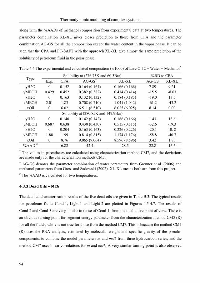
Thermodynamic modeling of complex systems
along with the %AADs of methanol composition from experimental data at two temperatures. The
parameter combination XL-XL gives closer prediction to those from CPA and the parameter
combination AG-GS for all the composition except the water content in the vapor phase. It can be
seen that the CPA and PC-SAFT with the approach XL-XL give almost the same prediction of the
solubility of petroleum fluid in the polar phase.
Table 4.4 The experimental and calculated composition (×1000) of Live Oil 2 + Water + Methanol*
TypeSolubility at (276.75K and 60.3Bar) %RD to CPA
Exp. CPA AG-GS+ XL-XL AG-GS XL-XLyH2O 0 0.152 0.164 (0.164) 0.166 (0.166) 7.89 9.21
yMEOH 0.429 0.452 0.382 (0.382) 0.414 (0.414) -15.5 -8.63xH2O 0 0.163 0.132 (0.132) 0.184 (0.185) -19.0 13.5
xMEOH 2.01 1.83 0.708 (0.710) 1.041 (1.042) -61.2 -43.2xOil 0 6.02 6.511 (6.510) 6.025 (6.025) 8.14 0.00
Solubility at (280.85K and 149.9Bar)yH2O 0 0.140 0.142 (0.142) 0.166 (0.166) 1.43 18.6
yMEOH 0.687 0.638 0.430 (0.430) 0.515 (0.515) -32.6 -19.3xH2O 0 0.204 0.163 (0.163) 0.226 (0.226) -20.1 10. 8
xMEOH 1.88 1.99 0.814 (0.815) 1.174 (1.176) -58.8 -40.7xOil 0 8.76 9.065 (9.064) 8.596 (8.596) 3.42 1.83
%AAD # 6.82 42.4 28.5 22.8 16.6* The values in parentheses are calculated using characterization method CM7, and the deviations are made only for the characterization methods CM7.+ AG-GS denotes the parameter combination of water parameters from Grenner et al. (2006) and methanol parameters from Gross and Sadowski (2002). XL-XL means both are from this project.# The %AAD is calculated for two temperatures.
4.3.3 Dead Oils + MEG
The detailed characterization results of the five dead oils are given in Table B.3. The typical results
for petroleum fluids Cond-1, Light-1 and Light-2 are plotted in Figures 4.5-4.7. The results of
Cond-2 and Cond-3 are very similar to those of Cond-1, from the qualitative point of view. There is
an obvious turning-point for segment energy parameter from the characterization method CM5 (R)
for all the fluids, while is not true for those from the method CM7. This is because the method CM5
(R) uses the PNA analysis, estimated by molecular weight and specific gravity of the pseudo-
components, to combine the model parameters m and from three hydrocarbon series, and the
method CM7 uses linear correlations for m and . A very similar turning-point is also observed
94
110

Chapter 4. Modeling oil-water-chemical systems
for the segment size parameter from the method CM5 (R). The turning-point in these two
parameters indicates that they are to some extent coupling with each other, especially the quantity
(m 3) shows quite similar values from the two characterization methods, as seen from the two live
oils above.
The modeling results of the mutual solubility of petroleum fluids and MEG with PC-SAFT, using
the characterization method CM7, are plotted in Figure 4.8, and the detailed results with the two
characterization methods can be found in Appendix B.4. The %AAD results with PC-SAFT and
CPA are presented in Table 4.5. The CPA modeling results are taken from Riaz et al. (2011a, 2011b,
2014), and Frost et al. (2013). Two MEG parameter sets are applied for PC-SAFT. One is from
Tsivintzelis and Grenner (2008), which is named as AG as well. The other one from this thesis is
named as XL. Linear correlations of kij between pseudo-components and MEG against molecular
weight, developed in Chapter 2, with 0.0 as the truncation are used for the both MEG parameter sets.
Figure 4.5 Characterized PC-SAFT parameters of pseudo-components for petroleum fluid Cond-1. (a) Segment number (m), (b) segment energy ( ), (c) segment size ( ), (d) quantity (m 3).
3
5
7
9
90 180 270 360
m
Molecular weight (g/mol)
(a)
m (CM5 (R))
m (CM7)
240
250
260
270
280
90 180 270 360
/k(K
)
Molecular weight (g/mol)
(b)
CM5 (R))
CM7)
3.7
3.8
3.9
4
90 180 270 360
(Å)
Molecular weight (g/mol)
(c)
CM5 (R))
CM7)150
300
450
600
90 180 270 360
m3
(Å3 )
Molecular weight (g/mol)
(d)
m CM5 (R))
m CM7)
95
111

Thermodynamic modeling of complex systems
Figure 4.6 Characterized PC-SAFT parameters of pseudo-components for petroleum fluid Light-1.(a) Segment number (m), (b) segment energy ( ), (c) segment size ( ), (d) quantity (m 3).
In general, both CPA and PC-SAFT could reasonably model the petroleum fluid + MEG systems,
except for the petroleum fluid Light-1, for which the models significantly under-predict the
solubility of MEG in the organic phase. It can be seen from Table 4.5 that in general the CPA
predicts the solubility of the petroleum fluids in the polar phase better, but PC-SAFT wins the other
side, i.e. the solubility of MEG in the organic phase.
Though the parameter set XL correlates the LLE of MEG and normal hydrocarbons better as
discussed in Chapter 2, the two parameter sets give similar prediction of the solubility of the
petroleum fluids in the MEG rich phase, as seen from Figure 4.8 (a) and Table 4.5. The parameter
set XL presents smaller overall deviation for the prediction of the solubility of MEG in the organic
phase, as presented in Table 4.5. As shown in Figure 4.8 (b), however, the performance largely
depends on the type of petroleum fluids. In general, the results from Table 4.5 reveal that the
parameter set XL performs better for the condensate gas, while the MEG parameter set AG gives
better predictions for oils on the solubility of MEG in organic phases. This might be because the
3
9
15
21
90 360 630 900
m
Molecular weight (g/mol)
(a)
m (CM5 (R))
m (CM7)
240
260
280
300
90 360 630 900
/k(K
)
Molecular weight (g/mol)
(b)
CM5 (R))
CM7)
3.7
3.8
3.9
4
90 360 630 900
(Å)
Molecular weight (g/mol)
(c)
CM5 (R))
CM7)150
400
650
900
1150
90 360 630 900
m3
(Å3 )
Molecular weight (g/mol)
(d)
m CM5 (R))
m CM7)
96
112

Chapter 4. Modeling oil-water-chemical systems
parameter set AG always predicts higher solubility of MEG in the organic phase than those from the
parameter set XL, as seen in Figure 4.8.
Figure 4.7 Characterized PC-SAFT parameters of pseudo-components for petroleum fluid Light-2.(a) Segment number (m), (b) segment energy ( ), (c) segment size ( ), (d) quantity (m 3).
Figure 4.8 Modeling results of the mutual solubility of petroleum fluids and MEG with PC-SAFT using the two characterization methods. The experimental data are taken from Riaz et al. (2011a, 2011b, 2014), and Frost et al. (2013). The detailed modeling results can be found in Appendix B.4.
3
5
7
9
11
13
90 190 290 390 490
m
Molecular weight (g/mol)
(a)
m (CM5 (R))
m (CM7)
240
250
260
270
280
90 190 290 390 490
/k(K
)
Molecular weight (g/mol)
(b)
CM5 (R))
CM7)
3.7
3.8
3.9
4
90 190 290 390 490
(Å)
Molecular weight (g/mol)
(c)
CM5 (R))
CM7)150
350
550
750
90 190 290 390 490
m3
(Å3 )
Molecular weight (g/mol)
(d)
m CM5 (R))
m CM7)
900
2900
4900
6900
900 2900 4900 6900
Calc
. sol
ubili
ty o
f oil
in p
olar
pha
se
Exp. solubility of oil in polar phase
(a)Cond-1 (AG) Cond-1 (XL)
Cond-2 (AG) Cond-2 (XL)
Cond-3 (AG) Cond-3 (XL)
Light-1 (AG) Light-1 (XL)
Light-2 (AG) Light-2 (XL)
0
1000
2000
3000
0 1000 2000 3000
Calc
. sol
ubili
ty o
f MEG
in o
rgan
ic p
hase
Exp. solubility of MEG in organic phase
(b)Cond-1 (AG) Cond-1 (XL)
Cond-2 (AG) Cond-2 (XL)
Cond-3 (AG) Cond-3 (XL)
Light-1 (AG) Light-1 (XL)
Light-2 (AG) Light-2 (XL)
97
113

Thermodynamic modeling of complex systems
Table 4.5 %AADs for the mutual solubility of petroleum fluids and MEG from different models*
Fluid Oil fluids in polar phase MEG in organic phaseCPA AG + XL + CPA AG XL
Cond-1 11.0 7.12 (8.18) 5.77 (6.66) 12.0 33.9 (33.6) 8.57 (8.47)Cond-2 17.0 35.5 (36.2) 34.6 (34.6) None 18.6 (18.5) 8.99 (8.99)Cond-3 None 24.9 (23.4) 27.4 (26.2) None 27.2 (26.7) 11.0 (10.9)
LightOil-1 1.00 5.77 (4.13) 7.42 (5.95) 82.0 60.3 (60.0) 70.5 (70.3)LightOil-2 13.0 14.6 (13.9) 15.8 (15.3) 21.0 5.02 (5.13) 17.8 (17.7)
avg. %AAD 10.3 17.6 (17.2) 18.2 (17.7) 36.7 29.0 (28.8) 23.4 (23.3)* Values in parentheses are from CM7.+ AG denotes that the PC-SAFT parameters of MEG from are Tsivintzelis and Grenner (2008), and XL means that the parameters are from this thesis.
As seen from Table 4.5 and Appendix B.4, the two characterization methods present similar overall
modeling results, especially for the solubility of MEG in the organic phase. The similar systematic
differences, as seen from the case Live Oil 1 + Water, are observed in this case for the solubility of
petroleum fluid in polar phase – CM7 predicts smaller solubility than CM5 (R). They have slightly
larger impacts on the AG parameter set than on the XL one for this solubility. There seem no
systematic differences for the solubility of MEG in the organic phase, but the impacts on it are
smaller than on the solubility of petroleum fluid in the polar phase from the two characterization
methods. Largest impacts are seen for Light-1. These results are demonstrated in Figure 4.9.
Figure 4.9 Comparisons of the two characterization methods on the solubilities from both AG and XL MEG parameter sets. The quantity (CM5 (R) – CM7)/CM7 is defined in equation (4.1). The x-axis ‘Case no.’ can be found in Table Appendix B.4, which is corresponding to the conditions of each petroleum fluid.
0.4
0.8
1.2
1.6
0 8 16 24
(CM
5 (R
) -CM
7)/C
M7
of xO
il in
MEG
Case no.
(a)
AG (Cond-1) AG (Cond-2) AG (Cond-3) AG (Light-1) AG (Light-2)XL (Cond-1) XL (Cond-2) XL (Cond-3) XL (Light-1) XL (Light-2)
-0.9
-0.6
-0.3
0
0.3
0.6
0 8 16 24
(CM
5 (R
) -CM
7)/C
M7
of xM
EG in
Oil
Case no.
(b)
AG (Cond-1) AG (Cond-2) AG (Cond-3) AG (Light-1) AG (Light-2)XL (Cond-1) XL (Cond-2) XL (Cond-3) XL (Light-1) XL (Light-2)
98
114

Chapter 4. Modeling oil-water-chemical systems
4.3.4 Dead Oils + Water + MEG
The modeling results of petroleum fluid + water + MEG systems with the PC-SAFT EOS, using the
characterization method CM7, are presented in Figure 4.10, and the detailed results with the two
characterization methods are given in Table Appendix B.5. The calculations with the PC-SAFT
EOS are performed with two options of the parameters: (1) the parameters of water and MEG are
from Grenner et al. (2006) and Tsivintzelis and Grenner (2008), which option is denoted as AG; and
(2) the parameters of both compounds are from this project, which option is denoted as XL.
The %AADs for the modeling results from CPA and PC-SAFT are compared in Table 4.6. The
CPA modeling results are taken from Riaz et al. (2011a, 2011b, 2014), and Frost et al. (2013). The
percentage relative deviations (%RD) are reported for each case, and the calculations of PC-SAFT
are using the characterization method CM7. The %AADs for all the conditions are presented at the
end of the table, for which the results from both characterization methods are reported.
Figure 4.10 Modeling results of the solubility of petroleum fluids, MEG and water from CPA and PC-SAFT with the characterization method CM7. Figure (b) is rescaled from Figure (a), and the legend is the same in all four figures. The experimental data are taken from Riaz et al. (2011a, 2011b, 2014), and Frost et al. (2013). The detailed modeling results can be found in Appendix B.5.
0
400
800
1200
1600
2000
0 400 800 1200 1600 2000
Calc
. sol
ubili
ty o
f Oil
in p
olar
pha
se
Exp. solubility of Oil in polar phase
(a)Cond-1 (CPA) Cond-1 (AG) Cond-1 (XL)Cond-2 (CPA) Cond-2 (AG) Cond-2 (XL)Cond-3 (CPA) Cond-3 (AG) Cond-3 (XL)Light-1 (CPA) Light-1 (AG) Light-1 (XL)Light-2 (CPA) Light-2 (AG) Light-2 (XL)
0
200
400
600
800
0 200 400 600 800
Calc
. sol
ubili
ty o
f Oil
in p
olar
phas
e
Exp. solubility of Oil in polar phase
(b)
0
200
400
600
0 200 400 600
Calc
. sol
ubili
ty o
f MEG
in o
rgan
ic p
hase
Exp. solubility of MEG in organic phase
(c)
0
300
600
900
1200
1500
0 300 600 900 1200 1500
Calc
. sol
ubili
ty o
f H2O
in o
rgan
ic ph
ase
Exp. solubility of H2O in organic phase
(d)
99
115

Thermodynamic modeling of complex systems
Table 4.6 Deviations of the solubility of petroleum fluids, MEG and water from different models
Case no. T (K) Oil in polar phase MEG in organic phase H2O in organic phaseCPA* AG# XL# CPA AG XL CPA AG XL
Cond-11 323.15 -43 123 5 70 108 76 -10 -29 -102 323.15 -26 47 6 61 107 68 -19 -37 -203 323.15 -1 21 12 27 66 32 -10 -30 -10
Cond-24 303.15 -78 -10 -59 27 21 4 -45 -55 -415 303.15 -61 -14 -47 27 27 6 -43 -54 -406 303.15 -2 18 -5 61 64 34 -39 -52 -367 323.15 -72 -10 -54 55 44 23 -17 -34 -178 323.15 -63 -30 -54 61 55 28 -21 -37 -219 323.15 -41 -35 -45 37 35 9 -25 -41 -25
Cond-310 313.15 -29 34 9 -3 30 7 -23 -35 -1411 313.15 -35 84 17 10 44 21 -19 -33 -1212 313.15 -50 135 15 -6 22 6 -16 -30 -9
LightOil-113 313.15 -18 17 -3 -58 11 -16 -37 -48 -3914 313.15 -58 -19 -49 -61 0 -23 -23 -36 -2615 323.15 -22 7 -11 -43 43 7 -28 -40 -3116 323.15 -49 -10 -39 -46 32 1 -29 -41 -32
LightOil-217 323.15 -4 59 30 -36 0 -21 -32 -48 -3518 323.15 -47 40 -11 -62 -43 -54 -30 -47 -3419 323.15 -66 38 -33 -54 -37 -48 -34 -49 -37
%AAD (CM7) 40.3 39.5 26.5 42.4 41.5 25.5 26.3 40.9 25.7%AAD (CM5 (R)) 40.0 26.3 41.6 25.5 41.5 26.5* The CPA results are from Riaz et al. (2011a, 2011b, 2014) and Frost et al. (2013). The kij of MEG and HC are 0.0 and 0.4 for Cond-2 and Cond-3, respectively, and it is 0.02 for other cases.# AG uses the PC-SAFT parameters of water and MEG from Grenner et al. (2006) and Tsivintzelis and Grenner (2008). XL uses the parameters of both components from this project.
The prediction of the mutual solubility of petroleum fluids and polar compounds, i.e. water and
MEG, highly depend on the types of petroleum fluids and the conditions, as seen from Figure 4.10,
Tables 4.6 and Appendix B.5. As shown in Table 4.6, PC-SAFT with the parameter option XL
presents generally the best overall predictions. It predicts the solubility of petroleum fluids in the
polar phase and the solubility of MEG in the organic phase better than both CPA and PC-SAFT
with the parameter option AG. The parameter option XL gives quite similar prediction of the water
solubility to CPA, and much better prediction than the parameter option AG for all the cases. It is
interesting to see that the prediction of the solubility of MEG in the organic phase for Light-1 is
100
116

Chapter 4. Modeling oil-water-chemical systems
quite reasonable, where the models have difficulties in predicting this solubility in the systems of
Light-1 + MEG, as discussed above.
It is worth noticing that both CPA and PC-SAFT under-predict the solubility of water in the organic
phase. This is because the water parameters are obtained by taking account the LLE data of water
with non-aromatic hydrocarbons into the estimation procedure. Very recently, it has been shown
internally the prediction from CPA could be improved by using different binary interaction
parameter approach, but it is not true for PC-SAFT if good prediction of the solubility of petroleum
fluid in the polar phase needs to be kept. This is because, as discussed in Chapter 3, the solubility
lines of hydrocarbons and water always go the same direction by tuning the interaction parameter.
As a feasible solution, the prediction is anticipated to be improved for heavy oils by taking the
aromatic compounds into accounts explicitly, for which the solvation interactions will bring more
water into the organic phase. The solubility of water in normal hexane, cyclo-hexane and benzene
are presented in Figure 4.11, which shows that the solubility of water in benzene is much higher
than those in non-aromatic hydrocarbons, especially at low temperature ranges.
Figure 4.11 Comparison the solubility of water in different hydrocarbons. The dash-dot line is the prediction from PC-SAFT for water-nC6 binary system.
The two characterization methods present very similar modeling results, especially for the solubility
of the petroleum fluids in the polar phase and the MEG solubility in the organic phase, as seen from
Table Appendix B.5. The method CM7 presents slightly better results than CM5 on the water
solubility in the organic phase. The similar systematic differences, as seen from previous cases,
appear in this case as well – CM7 predicts the solubility of petroleum fluid in polar phase smaller
and the solubility of water in organic phase larger, respectively, than CM5 (R). These results are
demonstrated in Figure 4.12. It shows that the impacts, respectively, are largest for the water
1.E-4
1.E-3
1.E-2
1.E-1
1.E+0
270 350 430 510
Solu
bilit
y of
H2O
in h
ydro
carb
ons
Temperature (K)
nC6
cC6
C6H6
PC-SAFT (nC6, kij=0.0)
101
117

Thermodynamic modeling of complex systems
solubility and smallest for the MEG solubility. In this case, the differences of the impacts on the
water solubility between these two water parameters are not as large as what have been seen in the
case Live Oil 1 + Water. The two characterization methods show larger impacts on the solubility of
petroleum fluids in the polar phase for this case than for the case Live Oil 1 + Water.
Figure 4.12 Comparisons of the two characterization methods on the solubilities from both AG and XL parameter combinations. The quantity (CM5 (R) – CM7)/CM7 is defined in equation (4.1). The x-axis ‘Case no.’ can be found in Table Appendix B.5, which is corresponding to the conditions of each petroleum fluid.
4.4 Conclusions
In this work, the PC-SAFT EOS with the newly developed parameters of water, methanol and MEG,
and the general petroleum fluid characterization methods is applied to model the phase behavior of
oil plus water and/or chemical systems. The modeling results for most systems are satisfactory. The
PC-SAFT EOS with the newly developed water and MEG parameters give quite promising
prediction on the mutual solubility of the oil-water-MEG systems, compared to those from CPA and
PC-SAFT with other literature available parameters. The results also show that the current PC-
0
0.5
1
1.5
0 6 12 18
(CM
5 (R
) -CM
7)/C
M7
of xO
il in
pol
ar
Case no.
(a)
AG (Cond-1) AG (Cond-2) AG (Cond-3) AG (Light-1) AG (Light-2)
XL (Cond-1) XL (Cond-2) XL (Cond-3) XL (Light-1) XL (Light-2)
-1
-0.5
0
0.5
0 6 12 18
(CM
5 (R
) -CM
7)/C
M7
of xM
EG in
Oil
Case no.
(b)
AG (Cond-1) AG (Cond-2) AG (Cond-3) AG (Light-1) AG (Light-2)
XL (Cond-1) XL (Cond-2) XL (Cond-3) XL (Light-1) XL (Light-2)
-2
-1.5
-1
-0.5
0
0 6 12 18
(CM
5 (R
) -CM
7)/C
M7
of xH
2O in
Oil
Case no.
(c)
AG (Cond-1) AG (Cond-2) AG (Cond-3) AG (Light-1) AG (Light-2)
XL (Cond-1) XL (Cond-2) XL (Cond-3) XL (Light-1) XL (Light-2)
102
118

Chapter 4. Modeling oil-water-chemical systems
SAFT parameters under-predict the water solubility in the organic phase, which suggest that the
explicit inclusion of the aromatic compounds might improve the modeling results by introducing
the solvation interactions.
The two characterization methods CM5 (R) and CM 7, developed in the Chapter 3, on one hand,
produce quite different PC-SAFT model parameters (segment number, segment size and segment
energy) of pseudo-components for individual cases. On the other hand, they show quite similar
trends for the segment number and the quantity (m 3) against molecular weight. In the meantime,
the same linear equation is used for the quantity (m ) in both characterization methods. These
similar or same trends lead to quite similar overall modeling results for almost all of the considered
systems in this work, but systematic differences are observed between these two characterization
methods. CM7 predicts the solubility of petroleum fluid in the polar phase smaller and the solubility
of water in the organic phase larger, respectively, than CM5 (R). It is also found that both these two
characterization methods have, respectively, largest and smallest impacts for the water solubility
and for the MEG solubility. These systematic differences lead the method CM7 to give slightly
better overall predictions, but these differences are much smaller than experimental uncertainties.
So the modeling of the mutual solubility of oil plus water and/or chemicals would still not be the
excellent criterion to select the characterization methods from the quantitative point of view. It is
worth pointing out that, however, these two characterization methods predict different phase splits
at some specific conditions. For instance, non-physical liquid-liquid-liquid phase equilibrium is
predicted by CM5 (R) for the case Live Oil 1 + Water at low temperature. The characterization
method CM7 might be recommended as the default method, but other alternative approaches for
model parameters are possible, especially for segment size, which will be the future work due to the
time limitation.
103
119

104
120

Chapter 5. Data and correlations of speed of sound
Volumetric properties and phase equilibria data are commonly used to tune the thermodynamic
models. It is preferable, however, to include the derivative properties into the parameter fitting
procedures, if the model is going to be extended to calculate derivative properties, e.g. speed of
sound, as in this project.
The purpose of this work is (1) to review and analyze the speed of sound data of hydrocarbons,
alcohols and their mixtures including petroleum fluids; (2) to review correlations for the speed of
sound data, and develop general correlations for speed of sound in pure hydrocarbons and 1-alcohol.
5.1 Introduction
Speed of sound is a thermo-physical property that can be accurately determined in wide temperature
and pressure ranges. The usage of ultrasound has been moving from the exploratory stage to
systematic applications in various fields, such as fundamental researches on intermolecular
interactions, and online monitor of industrial processes. In oil industry, acoustic measurements are
helpful on obtaining phase behavior and physical properties of reservoir fluids, e.g. estimating the
density of downhole reservoir fluids, and on in-situ measurement or characterization of the
heterogeneous or homogenous mixtures in reservoirs [Meng et al. (2005, 2006), Goodwin (2003),
Machefer et al. (2007), Durackova (1995)]. Specifically SONAR (Sound Navigation and Ranging)
uses sound propagation to navigate, communicate with or detect objects on or under the surface of
the water, and it can even provide some measurements of the echo characteristics of the “targets”
[Automatic Leak Detection Sonar (2012)].
As discussed in Chapter 1, within the framework of general thermodynamic rules, on one hand,
speed of sound is related with other thermodynamic properties such as density, isobaric and
isochoric heat capacities, and isothermal compressibility. Moreover, speed of sound measurements
have found wide acceptance as a satisfactory and relatively simple method to obtain thermodynamic
data of liquids, since it is possible to derive equations of state for liquids from these experimental
results. As the direct determination of properties such as density and heat capacity can be quite
difficult at elevated pressures, some people claim that it is more reliable to calculate these properties
105
121

Thermodynamic modeling of complex systems
from the speed of sound data by combining direct measurements of density and heat capacity at
atmospheric pressure. Moreover, speed of sound is a valuable property for developing
thermodynamic model as a supplement property or a discriminating reference quantity, since it can
be measured to a high degree of accuracy, even in high pressure regions.
5.2 Data
The following sections will be organized based on pure fluids, binary mixtures, ternary mixtures,
and oil or gas mixtures.
5.2.1 Pure fluids
5.2.1.1 Normal hydrocarbons
Hydrocarbons are the primary constituents of reservoir fluids, and are commonly categorized as
paraffins, naphthenes and aromatics. They range from the lightest components, which at normal
conditions are gases, such as methane and ethane, to extremely heavy components, for instance
asphaltenes or bituminous residues [Pedersen et al. (2007a)].
Normal hydrocarbons are very important constituents in crude oils, and extensive speed of sound
measurements have been done, especially for the short chain ones. Comprehensive data reviews can
be found in the works of Khasanshin et al. (2001), Oakley et al. (2003) and Padilla-Victoria et al.
(2013). The speed of sound database for pure hydrocarbons from this work is given in Appendix C
(Table C.1). Detailed reviews will not be duplicated anymore, but more efforts will be put to show
that the high degree of accuracy of speed of sound measurements, the impacts of temperature,
pressure and chain length on speed of sound, and the performance of NIST [REFPROP (2010)]
reference equations of state for speed of sound in short chain n-alkanes.
Methane (C1) is probably the most important single compound in the oil and gas mixtures. The
speed of sound in gaseous and liquid methane had been extensively measured in wide temperature
and pressure ranges since 1960s because of the petroleum industry development [van Itterbeek et al.
(1967), Straty (1974), Gammon et al. (1976), Baidakov et al. (1982), Kortbeek et al. (1990)]. The
speed of sound in saturated liquid methane and compressed liquid methane are shown in Figure 5.1.
On one hand, it is shown that the speed of sound measurements are highly reproduced among
different groups, indicating the high degree of experimental accuracy. On the other hand, the NIST
reference equation of state [REFPROP (2010)] represents the speed of sound in C1 very well.
106
122

Chapter 5. Data and correlations of speed of sound
Normal hexane (nC6) is another extensively studied hydrocarbon, an important constituent of fuel,
and a widely in-use solvent. Many groups conducted speed of sound measurements for n-hexane
[Boelhouwer (1967), Daridon et al. (1998), Ball et al. (2001), Khasanshin et al. (2001), Plantier et al.
(2003/2004)]. It can be seen from Figure 5.2 (a) that high reproducibility is again shown for the
speed of sound in liquid n-hexane, but the NIST [REFPROP (2010)] reference equation of state
does not seems to perform as well as for methane. The speed of sound in n-nonane is supplemented
in Figure 5.2 (b) to show that the accuracy of NIST [REFPROP (2010)] reference equations of state
are compound dependent rather than a systematic error along with chain length. The speed of sound
in both n-hexane and n-nonane show similarly smooth functionalities of temperature and pressure.
Figure 5.1 (a) The speed of sound in saturated methane. Data are taken from van Itterbeek et al. (1967), Straty (1974), and Baidakov et al. (1982), respectively. (b) The speed of sound in condensed liquid methane. Data are taken from Straty (1974). Lines are data from NIST [REFPROP (2010)].
Figure 5.2 (a) The speed of sound in liquid nC6. Data are taken from Daridon et al. (1998a), Khasanshin et al. (2001), and Ball et al. (2001). (b) The speed of sound in liquid nC9. Data are taken from Boelhouwer (1967) and Lago et al. (2006). Lines are data from NIST [REFPROP (2010)].
300
600
900
1200
1500
90 110 130 150 170 190
Spee
d of
soun
d (m
/s)
Temperature (K)
(a)
Straty, G.C.
van Dæl, A.l
Baidakov, V.G.
NIST
200
600
1000
1400
1800
0 10 20 30
Spee
d of
soun
d (m
/s)
Pressure (MPa)
(b)
100K_GCS 150K_GCS150K_VGB 170K_GCS170K_AVI 170K_VGB300K_GCS NIST
800
1000
1200
1400
1600
0 20 40 60 80 100
Spee
d of
soun
d (m
/s)
Pressure (MPa)
(a)
303.15K_JLD 303.15K_TSK
323.15K_JLD 323.15K_SJB
373.15K_JLD 373.15K_TSK
373.15K_SJB NIST 950
1150
1350
1550
0 20 40 60 80 100
Spee
d of
soun
d (m
/s)
Pressure (MPa)
(b)
293.15K_SL 293.15K_JWMB313.15K_SL 313.15K_JWMB333.15K_SL 333.15K_JWMB353.15K_SL 353.15K_JWMBNIST
107
123

Thermodynamic modeling of complex systems
Khasanshin et al. (2001, 2002, 2003, 2009) made many speed of sound measurements for n-alkanes,
shorter than n-hexadecane. During the same period, Daridon et al. (2000, 2002) and Dutour et al.
(2000, 2001a, 2001b, 2002) systematically measured the speed of sound in n-alkanes up to n-
hexatriacontane. The pressure dependence of the speed of sound in n-dodecane, n-octadecane, n-
tetracosane and n-hexatriacontane at 373.15K is plotted in Figure 5.3. It can be seen that the speed
of sound in n-alkanes increase as the chains get longer, and show qualitatively similar functions of
pressure, which makes it possible to use a generalized expression to correlate the speed of sound as
a function of chain length [Khasanshin et al. (2000, 2001), Padilla-Victoria et al. (2013)].
Figure 5.3 The speed of sound in liquid nC12, nC18, nC24 and nC36 at 373.15K. Data are taken from Khasanshin et al. (2003) and Dutour et al. (2000, 2001b, 2002).
Figure 5.4 The speed of sound in liquid nC16. Data are taken from Boelhouwer (1967), Ye et al. (1990), Ball et al. (2001), and Khasanshin et al. (2001).
1000
1200
1400
1600
0 20 40 60 80 100
Spee
d of
soun
d (m
/s)
Pressure (MPa)
nC12
nC18
nC24
nC36
800
1000
1200
1400
1600
0 20 40 60 80 100
Spee
d of
soun
d (m
/s)
Pressure (MPa)
303.15K_JWMB 303.15K_SY 303.15K_TSK
373.15K_JWMB 373.15K_SY 373.15K_TSK
373.15K_SJB 433.15K_JWMB 433.15K_TSK
108
124

Chapter 5. Data and correlations of speed of sound
The speed of sound measurements have high degree of accuracies, which can be seen from high
reproducibility of the experimental results from different groups. It is, however, not always true.
Figure 5.4 presents that the speed of sound in n-hexadecane at 373.15K measured by Ball et al.
(2001) deviate from other three sets [Boelhouwer (1967), Khasanshin et al. (2001, 2009)] under
elevated pressures, which suggest that careful selections or evaluations of experimental data should
be undertaken when more than one data sets are available.
5.2.1.2 Cyclohexane, Benzene and Toluene
Cyclohexane, benzene and toluene are common constituents of petroleum fluids. Cyclohexane and
toluene are important solvents, while benzene is one of the most elementary petrochemicals.
Sun et al. (1987) measured the speed of sound in cyclohexane in the temperature range from 283.15
to 323.06 K and pressure range up to 85 MPa. Takagi et al. (2002) reported the speed of sound in
cyclohexane at temperatures between 283.15K and 333.15K and pressures up to 20 MPa. The speed
of sound in cyclohexane at three temperatures is plotted in Figure 5.5 (a) together with the data
calculated from NIST [REFPROP (2010)] reference equation of state. It shows again that the NIST
[REFPROP (2010)] reference equation of state does not perform very well for cyclohexane from the
qualitative point of view, especially for those above room temperature.
Bobik (1978) measured the speed of sound in benzene at temperatures between 283K and 463 K
and pressures from the coexistence region up to 62 MPa. Takagi et al. (1984, 1987, 2004c) reported
the speed of sound in benzene in temperature ranges 283.15-333.15K and pressure ranges 0.1-
170MPa in three works. Sun et al. (1987) also reported the speed of sound in benzene in
temperature range from 283.143 to 323.125 K and pressure up to 170 MPa in the same work in
which they published the data for cyclohexane. In Figure 5.5 (b), it can be seen that the
experimental data from different groups are consistent to each other, and NIST [REFPROP (2010)]
reference equation of state gives perfect description of the speed of sound in benzene.
Hawley et al. (1970) reported the speed of sound in nine liquids, in which the data of toluene were
measured at temperatures 303 to 348 K and pressures between 0.1 to 522 MPa. Takagi et al. (1984)
measured the speed of sound in toluene at temperatures 293.15K, 298.15K and 303.15K and in the
pressure range from 0.1 to 160 MPa. Muringer et al. (1985) measured the speed of sound in toluene
up to 263.5 MPa and at temperatures from 173.18 to 320.3 K. Comprehensive speed of sound
measurements in toluene were carried out very recently by Meier et al. (2013) at the temperatures
109
125

Thermodynamic modeling of complex systems
between 240 and 420 K with the pressure range from 0.1 to 100 MPa, in which they summarized
the reference of experimental works on speed of sound measurements for toluene. Figure 5.5 (c)
shows the data from different groups and NIST [REFPROP (2010)] reference equation of state.
Figure 5.5 (a) The speed of sound in cyclo-C6. Data are taken from Sun et al. (1987) and Takagi et al. (2002). (b) The speed of sound in benzene. Data are taken from Sun et al. (1987), Bobik (1978), and Takagi et al. (1987). (c) The speed of sound in toluene. Data are taken from Takagi et al. (1984), Hawley et al. (1970), Muringer et al. (1985), and Meier et al. (2013). Lines are data from NIST [REFPROP (2010)].
5.2.1.3 1-Alcohols
1-Alcohols are important biologically and industrially amphiphilic additives in the oil production
and petrochemical industries [Abida et al. (2003), Dubey et al. (2008c)]. They are also very good
candidates to investigate the association phenomena.
1100
1200
1300
1400
1500
1600
0 20 40 60 80
Spee
d of
soun
d (m
/s)
Pressure (MPa)
(a)
298.123K_TFS 298.15K_TT
313.15K_TFS 313.15K_TT
323.06K_TFS NIST700
900
1100
1300
1500
1700
0 20 40 60 80 100Sp
eed
of so
und
(m/s
)Pressure (MPa)
(b)
303.15K_TFS 303.15K_TT
323.125K_TFS 323.15K_TT
433.15K_MB NIST
1200
1400
1600
1800
2000
2200
0 50 100 150 200 250
Spee
d of
soun
d (m
/s)
Pressure (MPa)
(c)
248.11K_MJPM 303.0K_SH
303.15K_TT 320.3K_MJPM
320K_KM NIST
110
126

Chapter 5. Data and correlations of speed of sound
There were some systematic investigations on acoustic properties of monatomic saturated alcohols.
Wilson et al. (1964) measured the speed of sound in four primary alcohols, i.e. methanol, ethanol,
1-propanol and 1-butanol, at temperatures from 273.15 to 323.15 K and pressures up to 96.5 MPa.
Sun et al. (1988, 1991) measured the speed of sound in methanol and ethanol, respectively, at
temperatures from 274.74 to 332.95 K and from 193.4 to 263.05 K up to 280 MPa. Khasanshin et al.
(1992) proposed a correlation expression for the speed of sound in the series of normal alcohols
from C4 to the higher homologs in the region of liquid state within temperatures range 303-405K
and pressures below 100 MPa. The speed of sound in methanol, 1-butanol and 1-octanol was
reported in the temperature range from 303.15 to 373.15 K and pressure range up to 50 MPa by
Plantier et al. (2002b), which data was used to determine the nonlinear acoustic parameter. In their
systematic work of thermodynamics properties of organic liquids using the acoustic methods,
Dzida et al. (2000, 2007, 2009a, 2013) reported the speed of sound data for 1-propanol, 1-pentanol
to 1-decanol in the temperature range from 293 to 318 K and pressures up to above 100 MPa.
The speed of sound in 1-alkanols, from methanol to 1-decanol, at 313.15K are presented in Figure
5.6 (a). It can be seen that a similar trend is obtained as the speed of sound in n-alkanes. The speed
of sound, on one hand, shows a simple and smooth function of temperature and pressure, and on the
other hand, the slower the speed of sound increases as the chains get longer. Figure 5.6 (b) shows
that the NIST [REFPROP (2010)] reference equation of state represents the speed of sound in
methanol with a perfect accuracy.
Figure 5.6 (a) The speed of sound in 1-alkanols at 313.15K. Data are taken from Sun et al. (1988), Marczak et al. (2000), Plantier et al. (2002b), Dzida et al. (2005, 2007, 2009a, 2013 ); (b) The speed of sound in methanol. Data are taken from Sun et al. (1988), and Plantier et al. (2002b). Lines are data from NIST [REFPROP (2010)].
1000
1200
1400
1600
1800
0 20 40 60 80 100
Spee
d of
soun
d (m
/s)
Pressure (MPa)
(a)
C1OH C2OH
C3OH C4OH
C5OH C6OH
C7OH C8OH
C9OH C10OH 1000
1100
1200
1300
1400
1500
1600
0 20 40 60 80 100
Spee
d of
soun
d (m
/s)
Pressure (MPa)
(b)
NIST 283.17K_TFS
303.15K_TFS 303.15K_FP
323.05K_TFS 323.15K_FP
111
127

Thermodynamic modeling of complex systems
5.2.2 Binary systems
The investigation on physical and transport properties of binary mixtures are of considerable
interest to fundamental researches and industrial applications. On one hand, the experimental excess
properties (deviations from ideal mixing) provides information about intermolecular interactions,
e.g. packing efficiencies taking place when mixing the pure compounds into a solution, effects of
temperature and pressure, and changes with respect to composition. The phase behavior information,
on the other hand, can be used to validate the predictive capabilities of thermodynamic models or
adjust the binary interaction parameters for engineering applications [Dubey et al. (2008a, 2008c),
Dzida et al. (2008)].
There is no ideal mixing concept for speed of sound, but in order to analyze the limit of the speed of
sound in mixtures, the following equation is used for representing the ideal limit (ideal mixing):
= (5.1)
where x and u are the molar fraction of and speed of sound in the pure compound i. In the meantime,
the concepts of positive and negative deviations from this ideal limit will be introduced for binary
and ternary mixtures.
5.2.2.1 Hydrocarbon + hydrocarbon
Thermodynamic and acoustic properties of binary hydrocarbons mixtures are very important to
petroleum industries. Meanwhile binary mixtures of hydrocarbons, especially alkanes, are very
important systems to investigate the impacts of temperature and pressure on the thermodynamic
properties through the effects of short-range interactions, such as dispersion force, chain length and
mixing behaviors of asymmetric molecules, from a theoretical point of view.
A summary of temperature range, pressure range and references of the experimental speed of sound
data in binary hydrocarbons mixtures, available in our data base, is given in Appendix C, Table C.2.
The impacts of temperature, pressure and molecular asymmetry on speed of sound will be
investigated through the discussions of speed of sound for some typical systems.
Figure 5.7 presents the speed of sound in two gaseous binary systems dominated by methane at
three temperatures [Lagourette et al. (1994)]. It can be seen that the speed of sound curves at low
112
128

Chapter 5. Data and correlations of speed of sound
pressure regions are intersecting each other or having a minimum against pressure, which is because
the gaseous mixtures are moving from a vapor-like state to a liquid-like state. This behavior might
introduce difficulties in correlating speed of sound as a function of pressure by a universal form.
Figure 5.8 presents the speed of sound in binary series of n-hexane with moderate (n-heptane) to
long chain (n-hexadecane) normal alkanes at 298.15 K and atmospheric pressure [Tourino et al.
(2004), Bolotnikov et al. (2005)]. The speed of sound in these systems show positive deviations
from ideal limit, and as expected, the deviations increase as the asymmetry of the corresponding
pure compounds become larger.
Figure 5.7 The speed of sound in gaseous binary systems of (a) {0.8998 methane + 0.1002 propane} and (b) {0.98 methane + 0.02 nC8}. Data are taken from Lagourette et al. (1994).
Figure 5.8 The speed of sound in binary systems of n-hexane + n-heptane, n-nonane, n-dodecane or n-hexadecane at 298.15K and atmospheric pressure. Data are taken from Tourino et al. (2004) and Bolotnikov et al. (2005). Lines are from equation (5.1).
300
500
700
900
1100
1300
10 30 50 70
Spee
d of
soun
d (m
/s)
Pressure (MPa)
(a)
273.75K
333.55K
393.75K500
700
900
1100
1300
25 50 75 100
Spee
d of
soun
d (m
/s)
Pressure (MPa)
(b)
293.15K
333.55K
373.15K
1050
1100
1150
1200
1250
1300
1350
0 0.2 0.4 0.6 0.8 1
Spee
d of
soun
d (m
/s)
x (n-Hexane)
nC7 nC7 (id)nC9 nC9 (id)nC12 nC12 (id)nC16 nC16 (id)
113
129

Thermodynamic modeling of complex systems
In order to investigate the impacts of temperature, pressure and compound asymmetry on deviation
from ideal limit, three speed of sound data sets are presented in Figure 5.9 for each binary system,
(a) methane + n-hexadecane at 298.15K [Ye et al. (1992b)], (b) n-hexane + n-hexadecane at
323.15K [Ye et al. (1992b)], (c) n-hexane + n-hexadecane at 10 MPa [Ye et al. (1992b)], and (d) n-
heptane + n-dodecane at 298.15K [Dzida et al. (2008)]. It can be known from these figures that
asymmetry plays a better important role than temperature and pressure on deviations from ideal
limit, which are positive and become smaller as temperature and/or pressure increase. The ideal
limit gives satisfactory description of the speed of sound in the binary mixture of n-hexane and n-
hexadecane at high temperature and pressure, as shown in Figure 5.9 (b) and (c). It performs very
well for the speed of sound in the binary mixture of n-heptane and n-dodecane, as seen from Figure
5.9 (d). These results tell us that, for such kinds of binary systems, good prediction results can be
obtained if correlations of speed of sound in the corresponding pure fluids are available.
Figure 5.9 The speed of sound in binary systems (a) methane + n-hexadecane at 313.25K; (b) n-hexane + n-hexadecane at 323.15K; (c) n-hexane + n-hexadecane at 10MPa; (d) n-heptane + n-dodecane at 298.15K. Data are taken from Ye et al. (1992b), Bolotnikov et al. (2005) and Dzida et al. (2008). Lines are from equation (5.1).
500
800
1100
1400
0 0.2 0.4 0.6 0.8 1
Spee
d of
soun
d (m
/s)
x (Methane)
(a)
20.6MPa 20.6MPa (id)
40.6MPa 40.6MPa (id)
60.6MPa 60MPa (id)900
1100
1300
1500
0 0.2 0.4 0.6 0.8 1
Spee
d of
soun
d (m
/s)
x (n-Hexane)
(b)
0.1MPa 0.1MPa (id)
30MPa 30MPa (id)
70MPa 70MPa (id)
800
1000
1200
1400
0 0.2 0.4 0.6 0.8 1
Spee
d of
soun
d (m
/s)
x (n-Hexane)
(c)
313K 313K (id)
333K 333K (id)
373K 373K (id)1050
1250
1450
1650
0 0.2 0.4 0.6 0.8 1
Spee
d of
soun
d (m
/s)
x (n-Heptane)
(d)
0.1MPa 0.1MPa (id)46MPa 46MPa (id)101MPa 101MPa (id)
114
130

Chapter 5. Data and correlations of speed of sound
Figure 5.10 (a) presents the speed of sound in binary mixtures of n-hexane + cyclohexane at
303.15K [Oswal et al. (2002)] and n-hexane or cyclohexane + benzene or toluene at 313.15K
[Calvar (2009a, 2009b)]. All measurements are made at atmospheric pressure. The speed of sound
in these binary systems shows negative deviations from the ideal limit. The negative deviations in
the binary mixture of n-hexane and cyclohexane are smaller than those in the systems with benzene
or toluene, which compounds have similar performance on the systems when they are mixing with
n-alkanes or cyclohexane. The speed of sound in binary series of benzene with n-hexane to n-
nonane is shown in Figure 5.10 (b), which indicates that the deviations from ideal limit become
more negative when the normal alkane gets heavier.
Figure 5.10 (a) The speed of sound in binary systems of n-hexane + cyclohexane at 303.15K and n-hexane or cyclohexane + benzene or toluene at 313.15K and atmospheric pressure. Data are taken from Oswal et al. (2002) and Calvar et al. (2009a, 2009b). (b) The speed of sound in binary systems of benzene + n-hexane, n-heptane, n-octane and n-nonane at 313.15K and atmospheric pressure. Data are taken from Calvar et al. (2009b). Lines are from equation (5.1).
5.2.2.2 Hydrocarbon + 1-alcohol
Systematic studies have been made extensively on binary mixtures of 1-alkanols with hydrocarbons,
especially with alkanes. This is mainly because binary mixtures of alcohols and alkanes, as pointed
by many researchers [Nath (1998b), Dubey et al. (2008c, 2008d), Dzida (2009b)], are convenient
model systems for studying association phenomena, solvation and nonspecific physical interactions,
which are essential for developing and testing of advanced general theoretical models, such as
SAFT models [Chapman et al. (1988, 1990), Jackson et al. (1988)], considering intermediate range
forces, e.g. hydrogen bonding, in an explicit way.
1000
1050
1100
1150
1200
1250
0 0.2 0.4 0.6 0.8 1
Spee
d of
soun
d (m
/s)
x (n-Hexane/cyclo-Hexane)
(a)
nC6-cycloC6
nC6-benzene
nC6-toluene
cycloC6-benzene
cycloC6-toluene
Ideal Limit1000
1050
1100
1150
1200
1250
0 0.2 0.4 0.6 0.8 1
Spee
d of
soun
d (m
/s)
x (Benzene)
(b)
nC6 nC6 (id)
nC7 nC7 (id)
nC8 nC8 (id)
nC9 nC9 (id)
115
131

Thermodynamic modeling of complex systems
During their systematic investigations on the volumetric properties of binary mixtures of 1-alkanol
+ n-alkane, Benson and co-workers [Kiyohara et al. (1979), Benson et al. (1981), Handa et al.
(1981)] measured the speed of sound in binary mixtures of methanol to 1-hexanol, 1-octanol and 1-
decanol with n-heptane, in binary mixtures of 1-hexanol with n-pentane, n-hexane, n-octane and n-
decane, and in binary mixtures of 1-decanol with n-pentane, n-hexane, n-octane, n-decane and n-
hexadecane, over the whole molar composition range at 298.15K and atmospheric pressure. In their
measurements, special attention was paid to the high dilute regions with respect to 1-alkanols.
In their systematic studies on thermodynamics of alcohol + alkane binary mixtures by measuring
scarcely available physical and transport properties, such as dielectric constants, refractive indices
and viscosities, Sastry et al. (1996a, 1996b) reported the speed of sound in binary mixtures of 1-
propanol or 1-butanol + n-heptane at 298.15K and 308.15K, and 1-heptanol + n-hexane or n-
heptane at 303.15K and 313.15K, all at atmospheric pressure.
During the continuous work series of the program on thermodynamic properties and phase behavior
of binary and ternary nonelectrolyte systems related to homogeneous and heterogeneous extractive
distillation, Orge et al. (1995, 1999) reported the speed of sound, as a function of mole fraction, in
binary mixtures of (benzene or cyclo-hexane) with 1-pentanol at 298.15K, (methanol, ethanol or 1-
propanol) with (n-pentane, n-hexane, n-heptane or n-octane) at 298.15K, and (methanol or ethanol)
with (hexane, heptane or octane) at temperatures from 303.15 to 318.15 K. All are at atmospheric
pressure. Recently, new speed of sound data in binary mixtures of ethanol with (n-hexane, n-
heptane, n-octane or n-nonane) at temperatures from 288.15 to 323.15K over the whole composition
range was reported by Gaycol et al. (2007), with co-authors of the works presented above.
Oswal et al. (1998) measured the speed of sound in ten binary mixtures of ethanol to 1-decanol, and
1-dodecanol with cyclo-hexane over the whole composition range at temperature 303.15K and
atmospheric pressure.
To study intermolecular interactions predominated by hydrogen bonding, chain length and
temperature dependence of excess thermodynamic properties, Nath (1997, 1998a, 2000, 2002a,
2002b) carried out systematic measurements on the speed of sound in binary mixtures of (1-butanol,
1-hexanol, 1-heptanol and 1-octanol) with (n-pentane to n-octane) at temperature range from 288.15
to 303.15K and atmospheric pressure.
116
132

Chapter 5. Data and correlations of speed of sound
The speed of sound in binary mixtures of 1-pentanol and n-nonane was reported at temperature
from 293.15 to 313.15K over the whole composition range by Gepert et al. (2003)
Recently, along with density and viscosity, speed of sound in binary mixtures (1-butanol, 1-hexanol,
1-octanol or 1-decanol) with (n-hexane, n-octane or n-decane), and (1-butanol or 1-octanol) with (n-
hexadecane or squalane) were measured at temperatures 298.15K, 303.15K and 308.15K and
atmospheric pressure in the series of work by Dubey et al. (2008a-f). They adopted the Redlich–
Kister type mathematical formula to correlate the excess properties, and used the Prigogine-Flory-
Patterson (PFP) theory to analyze excess volume and to estimate the speed of sound and the
isentropic compressibilities in these systems.
Experimental speed of sound data of 1-alkanol and alkanes binary mixtures at high pressures is
rather scarce. To fill this gap and to provide a way to calculate properties such as density and heat
capacity at high pressures, Dzida et al. (2003, 2005, 2009b) measured the speed of sound in binary
systems of (ethanol, 1-propanol and 1-decanol) with n-heptane at the temperatures from 293 to
318K and pressures up to over 90MPa. These experimental results provide valuable information to
study both the temperature and pressure dependence of excess properties and to test theoretical
models [Dzida et al. (2003)].
The speed of sound in binary mixtures of, respectively, methanol + n-hexane at 298.15K, 308.15K
and 318.15K at atmospheric pressure, and 1-propanol + n-heptane at 298.15K at 0.1MPa, 46MPa
and 101MPa pressures are presented in Figure 5.11. It could be seen that these systems show
negative deviations from ideal limit, and temperature and pressure do not show significant impacts.
Figure 5.11 The speed of sound in binary system of (a) methanol + n-hexane at 298.15K, 308.15K and 318.15K and atmospheric pressure; (b) 1-propanol + n-heptane at 298.15K under 0.1MPa, 46MPa and 101MPa pressures. Data are taken from Orge et al. (1997, 1999) and Dzida et al. (2003). Lines are from equation (5.1).
950
1000
1050
1100
0 0.2 0.4 0.6 0.8 1
Spee
d of
soun
d (m
/s)
x (Methanol)
(a) 298.15K 298.15K (id)
308.15K 308.15K (id)
318.15K 318.15K (id)
1100
1300
1500
1700
0 0.2 0.4 0.6 0.8 1
Spee
d of
soun
d (m
/s)
x (1-Propanol)
(b)
0.1MPa 0.1MPa (id)
46MPa 46MPa (id)
101MPa 101MPa (id)
117
133

Thermodynamic modeling of complex systems
The speed of sound in binary systems of, respectively, 1-butanol + (n-hexane, n-decane, n-
hexadecane or squalane) at 298.15K, n-heptane + (ethanol, 1-propanol, 1-heptanol or 1-decanol) at
293.15K, and cyclo-hexane + (ethanol, 1-propanol, 1-heptanol or 1-dodecanol) at 303.15K is
presented in Figures 5.12 (a), (b) and (c), all at atmospheric pressure. These figures all show that the
deviations of the speed of sound in 1-alkanol + hydrocarbon binary systems change from negative
to positive as the chain differences become larger. Figure 5.12 (d) presents the speed of sound in
binary systems of 1-pentanol with benzene or cyclo-hexane at 298.15K and atmospheric pressure,
which shows similar negative deviations.
Figure 5.12 The speed of sound in binary systems of (a) 1-butanol + n-hexane, n-decane, n-hexadecane or squalane at 298.15K; (b) n-heptane + ethanol, 1-propanol, 1-heptanol or 1-decanol at 293.15K; (c) cyclo-hexane + ethanol, 1-propanol, 1-heptanol or 1-dodecanol at 303.15K. All are at atmospheric pressure. Data are taken from Dubey et al. (2008b, 2008c). (d) The speed of sound in binary systems of 1-pentanol and benzene or cyclo-hexane at 298.15K and atmospheric pressure. Data are taken from Orge et al. (1995). Lines are from equation (5.1).
1000
1100
1200
1300
1400
0 0.2 0.4 0.6 0.8 1
Spee
d of
soun
d (m
/s)
x (1-Butanol)
(a)
nC6 nC6 (id)nC10 nC10 (id)nC16 nC16 (id)nC30 nC30 (id) 1100
1200
1300
1400
0 0.2 0.4 0.6 0.8 1
Spee
d of
soun
d (m
/s)
x (n-Heptane)
(b)C2OH C2OH (id)
C3OH C3OH (id)
C7OH C7OH (id)
C10OH C10OH (id)
1100
1200
1300
1400
0 0.2 0.4 0.6 0.8 1
Spee
d of
soun
d (m
/s)
x (cyclo-Hexane)
(c) C2OH C2OH (id)C3OH C3OH (id)C7OH C7OH (id)C12OH C12OH (id)
1230
1250
1270
1290
1310
0 0.2 0.4 0.6 0.8 1
Spee
d of
soun
d (m
/s)
x (1-Pentanol)
(d) benzene bezene (id)
cyclo-hexane cyclo-hexane (id)
118
134

Chapter 5. Data and correlations of speed of sound
5.2.2.3 1-Alcohol + 1-Alcohol
The speed of sound measurements in binary mixtures containing only 1-alkanols are scarce, at least
not as extensive as other mixtures presented above. Gepert et al. (2003, 2006) reported the speed of
sound in binary mixtures of 1-pentanol with 1-octanol at temperature from 293K to 313K, binary
mixtures of 1-propanol with 1-hexanol, 1-pentanol with 1-nonanol, and 1-pentanol with 1-decanol
at 298.15K, all over whole composition range, which are shown in Figure 5.13.
Figure 5.13 The speed of sound in the binary 1-alcohols. Data are taken from Gepert et al. (2006).
5.2.3 Multicomponent systems
5.2.3.1 Ternary mixtures
It is a common and economically attractive practice to add a new compound in azeotropic mixture
separations. To study the capability of using 1-pentanol as such a candidate for benzene and
cyclohexane mixture, Orge et al. (1995) measured different properties, including speed of sound,
for this ternary system at 298.15K over wide composition ranges.
To explore molecular interactions in ternary liquid mixtures using empirical, semi-empirical and
statistical theories, Rai et al. (1989) measured the speed of sound in ternary mixtures of (n-pentane
+ n-hexane + benzene), (n-hexane + cyclohexane + benzene), and (cyclohexane + n-heptane +
toluene) at 298.15 K and atmospheric pressure. Later, Pandey et al. (1999) adopted these theories
to predict the speed of sound in ternary mixtures of (toluene + n-heptane + n-hexane), (cyelohexane
+ n-heptane + n-hexane) and (n-hexane + n-heptane + n-deeane), which were compared with their
experimental results.
1200
1250
1300
1350
1400
0 0.2 0.4 0.6 0.8 1
Spee
d of
soun
d (m
/s)
x1
C3OH (1) + C6OH (2)C5OH (1) + C9OH (2)C5OH (1) + C10OH (2)C3OH + C6OH (id)C5OH + C9OH (id)C5OH + C10OH (id)
119
135

Thermodynamic modeling of complex systems
In order to possess experimental information covering the temperature and pressure conditions
encountered at all stages in petroleum production, Daridon, Lagourette and their co-workers carried
out systematic acoustic measurements for synthetic mixtures in wide temperature and pressure
ranges. They measured the speed of sound in ternary mixtures of (0.88methane + 0.10propane +
0.02n-octane) at the temperatures from 293.15 to 373.15K and pressures from 25 to 100MPa
[Lagourette et al. (1995)]. They also measured the speed of sound in ternary mixtures of (carbon
dioxide + methane + n-hexadecane) in the temperature range 313.15 to 393.15K and pressure up to
70MPa for three composition {0.12, 0.10, 0.78}, {0.10, 0.46, 0.44} and {0.44, 0.11, 0.45} [Daridon
et al. (1996a)]. Later, they reported the speed of sound in four synthetic systems which were
representative of distillation cuts with high bubble points in even wider temperature and pressure
ranges. The speed of sound data, together with the density data at atmospheric pressure, were used
to calculate densities and isentropic and isothermal compressibilities under evaluated pressures.
[Daridon et al. (1998b, 1999)]
It is not easy to show the deviations from ideal limit in a two-dimension figure for a ternary system,
so the average relative deviations of some typical systems are calculated and reported in Appendix
C (Table C.3). It can be seen that the ideal limit can describe well for systems consisting of similar
compounds, such as n-hexane, n-heptane and cyclo-hexane, but it gives unsatisfactory results for
some other systems depending on the composition, temperature and pressure.
Figure 5.14 shows the speed of sound in ternary systems of methane + propane + n-octane with
fixed composition {0.88, 0.10 and 0.02} as a function of pressure, which shows similar behaviors in
the low pressure region as those in binary mixtures predominated by methane in Figure 5.7.
Figure 5.14 The speed of sound in a ternary mixture {0.88 methane + 0.10 propane + 0.02 n-octane} as a function of pressure at 293.15K, 323.15K, 343.15K and 363.15K. Data are taken from Lagourette et al. (1995).
500
700
900
1100
1300
25 50 75 100
Spee
d of
soun
d (m
/s)
Pressure (MPa)
293.15K
323.15K
343.15K
363.15K
120
136

Chapter 5. Data and correlations of speed of sound
5.2.3.2 Oils and gases
To fill the void of experimental data of acoustic properties in crude oils, Wang et al. (1990)
measured the speed of sound in three light oils, two refined oils, five heavy oils and one live oil,
covering a wide API gravity range from 5 to 62 degrees, in wide temperature and pressure ranges.
They made correlations between speed of sound, temperature, pressure and API gravity, so
empirical equations were available to calculate the speed of sound in oils with known API gravities.
To meet the challenges from the increasing number of hyperbaric oil reservoirs, Daridon and co-
workers [Labes et al. (1994), Daridon et al. (1996b, 1998c), Barreau et al. (1997), Lagourette et al.
(1999), Plantier et al. (2008)] made systematic studies on the thermodynamic properties and fluid
behaviors of reservoir fluids by speed of sound measurements in the wide ranges of temperature,
pressure and petroleum fluid types. They conducted a series of systematic acoustic measurements
on pure, binary, ternary and other synthetic hydrocarbons mixtures, as discussed above, and also
they measured the speed of sound in reservoir fluids from condensate gases to heavy oils. The
composition, temperature and pressure information of the speed of sound measurements in oils,
available in our data base, is summarized in Appendix C (Table C.4).
Figure 5.15 (a) presents the speed of sound in one condensate gas, one hyperbaric oil and one heavy
oil as a function of pressure at 313.15K, which shows that the speed of sound in heavy oil are
higher, but they show a similar trend versus pressure from the qualitative point of view. Figure 5.15
(b) presents the speed of sound in two extremely heavy oils, which show very close values above
room temperature, but they get diverged at low temperatures.
Figure 5.15 (a) The speed of sound in a condensate gas, a hyperbaric oil and an under-saturated heavy oil as a function of pressure at 313.15K. Data are taken from Daridon et al. (1998c). (b) The speed of sound in two very heavy oils. Data are taken from Plantier et al. (2008).
800
1000
1200
1400
10.0 30.0 50.0 70.0
Spee
d of
soun
d (m
/s)
Pressure (MPa)
(a)
Cond. Gas
HP Oil
Heavy Oil1200
1400
1600
1800
2000
0 5 10 15 20
Spee
d of
soun
d (m
/s)
Pressure (MPa)
(b)283.15K_A 283.15K_B 313.15K_A 313.15K_B
343.15K_A 343.15K_B 373.15K_A 373.15K_B
121
137

Thermodynamic modeling of complex systems
5.3 Correlations
In order to interpolate and extrapolate experimental data to given conditions, and also for compact
and smooth representations, it is a common practice to correlate the measured speed of sound data
to mathematical expressions. This also makes it possible for people to compare their own data with
the published values at the exactly same conditions, i.e. temperature, pressure and/or composition.
Depending on the number of free variables, different mathematical expressions are used to correlate
the experimental data, among which the combination of polynomials are most popular.
Equation (5.2) is a general expression for one free variable situation.
= (5.2)
are coefficients.
This equation can be used to represent the speed of sound as a function of temperature along
isobaric or co-existence lines, a function of pressure along isothermal lines for pure fluids or
mixtures with fixed composition, or a function of the concentration of one compound in binary
mixtures at constant temperature and pressure [Del Grosso et al. (1972), Straty (1974), Bobik
(1978), Oswal et al. (2002)]. Oakley et al. (1991) used this type expression up to third degree for the
speed of sound as a function of pressure for 68 different organic liquids. Wang et al. (1991) even
correlated the speed of sound as a linear function of temperature for 26 pure hydrocarbons samples
at atmospheric pressure with satisfactory accuracy. It is also common to express the pressure as a
function of speed of sound using the same type formula [Sun et al. (1987), Muringer et al. (1985)].
Besides equation (5.2), many researchers [Nath (1997), Oswal et al. (2002), Dzida et al. (2003),
Dubey et al. (2008e)] have expressed the speed of sound deviation from the ideal limit as a function
of concentration, which makes it clear to show the non-ideality of the binary mixtures from the
viewpoint of speed of sound.
= (1 ) (2 1) (5.3)
= × + × (5.4)
where x could be molar composition or volume fraction.
122
138

Chapter 5. Data and correlations of speed of sound
Several mathematical formulas were proposed by different researchers to express the speed of
sound in pure fluids or mixtures with fixed composition as a function of temperature and pressure.
The most popular one is the following equation [Wilson (1959), Bobik (1978), Niepmann et al.
(1987), Takagi et al. (1992, 1997 et al. (2000), Khasanshin et al. (2002)]:
= ( ) ( ) (5.5)
where are correlation coefficients, and T0 and P0 are arbitrarily chosen independent constants. T
and P could be absolute or reduced variables over critical values or some given constants, such as
1000 for temperature and 100 for pressure.
while -2 was used by ak et al. (2000) for the speed of sound in water.
As done for the one variable situation, Sun, Biswas and their co-workers [Marczak et al. (2000),
Sun et al. (1987, 1988, 1991)], Dzida and co-workers [Dzida et al. (2003, 2005, 2008, 2009b)] have
extensively used the following expressions to correlate the experimental speed of sound data.
= ( ) (5.6)
where P0 normally is an arbitrarily chosen constant, but the most common one is 0.1MPa, and u0 is
the corresponding speed of sound.
A more complex expression, ratio of two polynomials, was adopted by Lainez, Zollweg and their
co-workers [Lainez et al. (1989, 1990), Guedes et al. (1992)], Takagi et al. (2002, 2004a-c).
= ( ) ( )( ) ( ) (5.7)
whe could be 1 or 2. If
0 would usually be set to 1.
The same idea of equation (5.7) was adopted in the works of Daridon, Lagourette and their co-
workers [Daridon et al. (1998a, 1998b, 2000, 2002), Dutour et al. (2000, 2001), Lagourette et al.
(1999)], but the cross terms of temperature and pressure were not considered and only linear terms
were in the denominator. This expression could lead to a straightforward and analytical form of the
123
139

Thermodynamic modeling of complex systems
integral of 1/u2, which is useful when calculating the density and/or heat capacity under high
pressures.
= + (1 + × + × ) (5.8)
where ai, bj, c and d are adjustable coefficients.
Recently, the following more complex expression, not a combination of pure polynomials anymore,
was adopted by Khasanshin et al. (2006, 2009) to correlate the speed of sound in 1-hexadecene and
n-hexadecane, in which it was used to calculate other properties under high pressures as well.10 = + + 100 + + 100 (5.9)
= + 100 (5.10)
= + 100 (5.11)
= + 100 + 100 (5.12)
where A, B, c0, c1, d0, d1, e0, e1, e2 and
In order to calculate the speed of sound in binary mixtures of ethanol or 1-decanol + n-heptane at
atmospheric pressure for any given temperature and composition, equation (5.3) were extended by
Dzida et al. (2005, 2009) to include temperature dependence in a straight forward way.
= (1 ) (2 1) (5.13)
Hasanov (2012) successfully correlated the speed of sound in the binary mixture of n-heptane and
n-octane in wide ranges of temperature and pressure, over the whole composition range by the
following equation.
= (100 ) (5.14)
124
140

Chapter 5. Data and correlations of speed of sound
Khasanshin et al. (1992, 2000, 2001) attempted to develop generalized correlations to predict the
speed of sound in n-alkanes and 1-alkanols.( ) = ( ) + × (5.15)
where ln(u0) and A is expressed by equation (5.5), N -1 or -1/2.
Very recently, Padilla-Victoria et al. (2013) proposed the following Tait type expression to correlate
the speed of sound in normal alkanes and their binary mixtures with carbon number 5.
= × ++ (5.16)
D is a function of temperature, pressure and carbon number, while E is a function of temperature
and carbon number only. The detailed mathematical expressions will not be duplicated here.
5.4 Conclusions
The experimental speed of sound data of pure hydrocarbons, pure 1-alcohols, binary mixtures,
ternary systems, oil and gas mixtures have been reviewed and analyzed. The results have shown
that the speed of sound measurements have high accuracy, and the speed of sound in binary
mixtures to some extent are good candidates to show the deviations from ‘ideal solution’, even
though there is no real ideal mixing or excess property concept for speed of sound.
The empirical correlations for the speed of sound data have been collected as well, most of which
are suitable for fixed composition or simple binary mixtures. The only one that is used to correlate
the speed of sound, composition, temperature and pressure simultaneously for the binary mixture of
nC7 and nC8 needs 90 coefficients. These results indicate that it is not very realistic to use speed of
sound to build general equations of state for predictive purpose over wide ranges of compounds,
temperature and pressure.
Based on equation (5.8), the correlations for the speed of sound in pure normal hydrocarbons up to
nC36, cyclo-hexane, benzene, toluene and 1-alcohols are developed. The coefficients are given in
Appendix C (Table C.5), and the corresponding temperature and pressure conditions and statistics
are given in Appendix C (Table C.6).
125
141

126
142

Chapter 6. Modeling speed of sound
Within the thermodynamics framework, speed of sound is directly related to the density or volume,
heat capacities, and isothermal compressibility. As a second-order derivative property, it is one of
the most demanding tests to check the performance limits for a thermodynamic model. The speed of
sound, on one hand, is a valuable property for thermodynamic model developments as a supplement
property or a discriminating reference quantity, since it can be measured to a high degree of
accuracy, even in high pressure regions. On the other hand, an EOS model that can describe the
speed of sound for a wide range of mixtures accurately would be very helpful on in-situ
characterization of the research objects, for example, in the petroleum industry, by combining the
acoustic measurements and seismic data analysis.
The purposes of this work are (1) to compare SRK, CPA and PC-SAFT on modeling speed of
sound in pure substances; (2) to propose approaches to improve the speed of sound description
within the PC-SAFT framework; (3) to evaluate the performance of the new approach on predicting
speed of sound in a wide range of mixtures; (4) to investigate the possibility or cost of simultaneous
modeling phase behavior and speed of sound; (5) to study the association term of the PC-SAFT
framework using pure 1-alcohols and 1-alcohol + hydrocarbon binary systems as research objects.
6.1 Introduction
The calculation of speed of sound needs first and second order derivatives of Helmholtz free energy
with respect to both temperature and total volume, so it is a second-order derivative property. As
pointed out by Gregorowicz et al. (1996), the precise description of the second derivative properties
is a challenge for any EOS model. For instance, most of the classical EOS, such as SRK [Soave
(1972)] and PR [Peng and Robinson (1976)], fail in describing speed of sound reliably in wide
temperature and pressure ranges [Gregorowicz et al. (1996), Ye et al. (1992b), Faradonbeh et al.
(2014)]. This may be due to the intrinsic nature of these EOS, usually applied only to phase
equilibria calculations, to the sensitivity of the second-order derivative properties performed to a
given function, or to the physics behind these models and properties. A way to discern some of
these uncertainties could be to use a molecular-based EOS – these equations retain the microscopic
contributions considered when building the equation. Meanwhile it needs to be kept in mind that the
127
143

Thermodynamic modeling of complex systems
second-order derivative properties should not be improved at the expense of significant
deterioration of the primary properties, such as vapor pressure and liquid density. Some of the
applications of the SAFT family EOS for speed of sound calculations are reviewed below.
Lafitte et al. (2006, 2007) proposed the SAFT-VR Mie approach to simultaneously describe phase
equilibria and derivative properties. In the first paper, they preliminarily checked the performance
of the models PC-SAFT, SAFT-VR, and SAFT-VR LJC [Davies et al. (1998)] to describe the
derivative properties with molecular parameters fitted to the vapor-liquid equilibrium data only, i.e.
vapor pressure and saturated liquid densities, which aims to identify the limitations of these models.
Poor agreement of the results from these models with the experimental data made them conclude
that all these models fail to describe the speed of sound. As discussed in the article, a feasible
solution might be to recalculate molecular parameters for these models by taking into consideration
isothermal compressibility data (or speed of sound) in the fitting procedure to overcome this
problem. The reported results of these tests indicated a slight improvement on isothermal
compressibility estimation results with an important deterioration of the vapor-liquid equilibrium
curve. Hence, by assuming that the problem in accurately describing the derivative properties was
the choice of the intermolecular potential used to model the repulsion and dispersion interactions
between the monomers forming the chain, they modified the potential term in the SAFT-VR
approach, and proposed the SAFT-VR Mie model. The new model introduces an extra compound
specific parameter related to the shape of the repulsive part of the potential. In addition, they
proposed new fitting procedures to include two types of properties, vapor-liquid equilibrium data,
i.e. vapor pressure and liquid density, and the speed of sound in the condensed liquid phase. The
results of both first and second derivative properties were shown better agreements with the
experimental data than the other SAFT models with original parameters. The mentioned %AAD for
speed of sound was around 2%. This work showed the capability of the SAFT-type models for
describing both first and second derivative properties with good accuracy simultaneously. In the
second article [Lafitte et al. (2007)], they extended this approach to model vapor-liquid equilibria
behavior and second-order derivative properties of alcohols and 1-alcohol + n-alkanes mixtures
simultaneously. The extra nonconformal parameter characterizing the repulsive interaction between
the monomer segments greatly enhanced the performance of the SAFT-VR theory for the prediction
of second derivative properties of the 1-alcohol substances with around 2.5%AAD for speed of
sound. This was due to the fact that in SAFT theory the contact segment-segment radial distribution
128
144

Chapter 6. Modeling speed of sound
function plays a fundamental role not only in the chain contribution but also in the association
contribution with the free energy [Lafitte et al. (2007)].
In order to get a more precise speed of sound prediction for mixtures from the SAFT-VR Mie
model, Khammar and Shaw (2010) translated isentropic compressibility estimations for a mixture at
a specific composition by adding the molar average error of the predicted pure components
isentropic compressibility to the isentropic compressibility of the mixture predicted from SAFT-VR
Mie EOS, which has been tested for binary mixtures of 1-alcohol and n-alkane.
Llovell et al. (2006a, 2006b) argued that inclusion of properties other than vapour pressure and
saturated liquid density data in the fitting procedure would reduce the predictive capability of the
model. So they performed calculations with soft-SAFT [Blas et al. (1997, 1998)] on second
derivative properties with the pure component parameters fitted to vapour pressure and saturated
liquid density data only to show the physical soundness of the theory and to address specifically the
transferability of the parameters. In addition, the soft-SAFT is able to accurately capture the density
singularities related to the critical region by using a crossover treatment which explicitly
incorporates a renormalization group term with two extra parameters [Llovell et al. (2004)]. Pure n-
alkanes and 1-alkanols were modeled in their first article [Llovell et al. (2006b)]. Their work
provided a clear insight into the capability of the SAFT theory to capture simultaneously the vapor-
liquid and derivative properties of an associating fluid, but the %AADs for speed of sound in n-
hexane and n-heptane at Tr=1.1 are around 20%. In the later work [Llovell et al. (2006a)], the
%AADs of speed of sound for n-heptane at 0.1MPa and 101.3MPa is about 6%.
Diamantonis et al. (2010) evaluated the performance of SAFT and PC-SAFT on derivative
properties in a wide range of conditions for six fluids that are of interest to the Carbon Capture and
Sequestration (CCS) technology. They used a similar approach, as that proposed by Llovell et al.
(2006b), to predict the second-order derivative properties using the pure component parameters
fitted to VLE data only. The results revealed that both models performed well, especially away
from the critical region. PC-SAFT was shown to be more accurate than SAFT for CO2, H2S and
H2O, while two models give comparable accuracies for other components. The average %AAD of
the PC-SAFT model on the speed of sound for the six fluids is 2%. These results are not consistent
with the point of view of Lafitte et al. (2006), who said that PC-SAFT was not able to describe the
speed of sound well, but the author argued that direct comparisons are difficult, since the fluids and
129
145

Thermodynamic modeling of complex systems
conditions examined are not the same. We agree partly with this argument, and also want to point
out that the studied six fluids are all composed of small molecules.
Very recently, to address the numerical pitfalls, unphysical predictions and wrong estimations of the
pure components’ critical properties of the SAFT approaches, Polishuk (2011b) proposed a SAFT
plus Cubic approach, where in SAFT the attractive term of cubic EoS is attached. As pointed out by
the author, unlike other SAFT variants, SAFT + Cubic relies on generalizing the regularities
exhibited by experimental data rather than approximating the results of molecular simulations. The
authors concluded several merits of this approach: (1) free of the well-known disadvantages
characteristic for several SAFT approaches, such as the inability to correlate the critical and
subcritical pure compound data simultaneously and generating artificial unrealistic phase equilibria;
(2) free of numerical pitfalls; (3) the smaller number of the pure compound adjustable parameters
due to solving the critical conditions to obtain three of the five parameters (for most pure alkanes,
one more parameter could be estimated by a empirical expression) when critical properties are
available; (4) relatively modest numerical contribution. This approach demonstrated its superiority
on speed of sound calculation compared to SAFT-VR Mie, PC-SAFT and SBWR for the selected
systems both on curvature and accuracy from the figures in their published articles [Polishuk et al.
(2011a-d)]. Unfortunately, they presented very limited %AAD data explicitly, and also there is very
little information about the vapor pressure prediction accuracy. This SAFT + Cubic approach has
five parameters for non-associating compounds and seven for associating ones.
In order to provide a comprehensive understanding of the potentials and limitations of the advanced
SAFT family EOS and their improvements over classical models, de Villiers et al. (2011, 2013)
have studied the performance of SRK, PR, CPA, SAFT and PC-SAFT on derivative properties for
different component families, i.e., non-polar, polar non-associating, and associating, in both the
compressed liquid and near-critical regions. Based on the fact that the total Helmholtz free energy is
expressed as summation of separate contributions and all of the derivative properties could be
calculated explicitly from one or more Helmholtz free energy derivatives with respect to
temperature or total volume, they analyzed the contributions of individual terms on the final
derivative properties and single derivatives. They concluded that, in general, the performance of
PC-SAFT is superior in correlating most of the second-order derivative properties of investigated
alkanes. A major improvement of the SAFT and PC-SAFT over CPA is its ability to give a better
description of the dP/dV derivative. However, as pointed out by the authors, this improvement is
130
146

Chapter 6. Modeling speed of sound
still not sufficiently significant and is the primary reason why the models are not able to correlate
the speed of sound accurately. They further pointed out that a similar approach as SAFT-VR Mie
[Lafitte et al. (2006, 2007)] seems to be necessary in order to accurately predict speed of sound,
since the dP/dV derivative is predominantly influenced by the hard-sphere term and its incorrect
slope with respect to pressure is possibly caused by the chain term, both of which are largely
influenced by the radial distribution function. The similar incorrect slope of residual isochoric heat
capacity and isothermal compressibility with respect to molar density from the chain term
contribution were shown in the work of Llovell and Vega (2006b), in which they conducted the
same term contribution analysis for these two properties for short and long, non-associating and
associating chain compounds. They concluded from this analysis that association played a dominant
role in heat capacities (and other energetic properties) for relatively short associating chains.
Based on the literature investigations above, the SAFT-type models (the SAFT framework) seem to
provide a ‘theoretically correct’ approach to describe the first and second-order derivative
properties simultaneously. The differences depend mostly on segment potentials, parameter
estimation procedures and the number of adjustable parameters used.
6.2 Comparison of SRK, CPA and PC-SAFT
Although some calculations of SRK, CPA and PC-SAFT EOS have been reported for speed of
sound for alkanes [de Villiers (2011)], it is worth performing an extensive comparison for these
models over wide temperature and pressure ranges. In this work, the performance of these three
models on speed of sound is evaluated for normal paraffins from methane to n-eicosane (n-C20), n-
tetracosane (n-C24) and n-hexatriacontane (n-C36) over wide temperature and pressure ranges
against the experimental or correlation data based on the available literature. The pure component
parameters of CPA can be found in the book of Kontogeorgis and Folas (2010), and those of PC-
SAFT can be found in the original literature [Gross et al. (2001), Ting et al. (2003)]. The vapor
pressure and saturated liquid density data are taken from the DIPPR correlations [DIPPR Database
(2012)] in the reduced temperature range Tr=[0.45, 0.9] for consistency and easy comparison with
other models, while the speed of sound data of methane to n-decane is taken from the NIST
database [REFPROP (2010)], and those of other long chain molecules are taken from the literature.
The typical shapes of the isothermal speed of sound curves from the three models are shown in
Figure 6.1, from which it can be seen that PC-SAFT performs better on capturing the curvature.
131
147

Thermodynamic modeling of complex systems
According to the investigation of de Villiers et al. (2011, 2013), it is due to the fact that PC-SAFT
provides a good description of the derivative of pressure with respect to total volume, which is the
dominant term in the speed of sound calculation. Not surprisingly, CPA performs significantly
better to SRK as liquid density is used in the parameter fitting procedure. This is because density is
directly used in the speed of sound calculation, as expressed in equation (1.7). It is shown in Figure
6.1 (d), however, that the superiority of CPA over SRK is much smaller than that of PC-SAFT over
CPA, which indicates that the model itself is more important than the parameter fitting. The detailed
%AAD information of vapor pressure, liquid density and speed of sound of these three models are
supplied in Table 6.1. It is worth pointing out that SRK or CPA could have a smaller %AAD in
narrow low pressure ranges for some cases, such as hexane at 300K in Figure 6.1 (b), because the
cancellation of the errors from the under-predicted to over-predicted regions.
Figure 6.1 Speed of sound in (a) methane (C1) at T=200K (Tr=1.05), (b) nC6 at T=300K (Tr=0.59), (c) nC15 at T=313.15K (Tr=0.44). (d) The %AAD of speed of sound from SRK, CPA and PC-SAFT against carbon number. Dash line, dash dot line and solid line are results of SRK, CPA and PC-SAFT, respectively, and data for C1 and nC6 are taken from NIST [REFPROP (2010)], and data of nC15 are from Daridon et al. (2002).
250
750
1250
1750
0 30 60 90 120 150
Spee
d of
soun
d (m
/s)
Pressure (MPa)
(a) NIST
PCSAFT (2.44%)
CPA (6.34%)
SRK (6.61%)
800
1200
1600
2000
2400
0 30 60 90 120 150
Spee
d of
soun
d (m
/s)
Pressure (MPa)
(b) NIST
PCSAFT (10.7%)
CPA (12.7%)
SRK (16.5%)
1000
1900
2800
3700
0 50 100 150
Spee
d of
Sou
nd (m
/s)
Pressure (MPa)
(c)Daridon et al.
PCSAFT (17.6%)
CPA (39.2%)
SRK (52.5%)
0
20
40
60
80
100
1 6 11 16 21 26 31 36
%AA
D of
spee
d of
soun
d
Carbon Number
(d)PCSAFT
CPA
SRK
132
148

Chapter 6. Modeling speed of sound
Table 6.1 %AADs for vapor pressure, liquid density and speed of sound from different models
Comp SRK CPA PC-SAFT T of u (K)P
of u (MPa)
np +
P u P u P uC1*,1 1.67 2.73 5.51 0.51 1.77 5.55 0.21 0.49 2.36 100-350 0.1-150 25C2 1 1.87 5.18 7.36 0.32 1.23 7.77 0.25 0.68 5.80 150-500 0.1-150 30C3 1 1.20 6.81 10.7 3.43 1.90 9.75 0.19 0.51 7.92 150-500 0.1-150 30C4 1 1.79 8.04 10.7 0.63 4.07 9.31 0.33 0.50 7.66 200-550 0.1-150 30C5 1 1.66 9.91 11.2 0.63 0.75 9.52 0.29 1.35 8.18 250-550 0.1-150 30C6 1 1.94 11.6 13.9 2.61 0.55 11.1 1.05 0.66 7.92 250-600 0.1-150 30C7 1 1.13 13.0 17.1 1.65 0.60 13.6 0.26 0.94 9.34 250-600 0.1-150 30C8 1 1.76 14.5 17.2 0.77 0.77 12.8 0.44 0.82 8.40 300-600 0.1-150 30C9 1 1.60 15.5 20.5 1.54 0.92 15.2 0.77 0.62 9.69 300-600 0.1-150 30
C10 1 2.03 16.5 23.6 1.92 0.99 17.1 0.84 0.61 10.1 300-650 0.1-150 30C11 2 1.36 17.8 24.1 2.07 1.34 17.3 1.79 0.67 13.6 303.15-413.15 0.1-118 91C12 3 1.79 18.6 26.9 1.79 1.53 19.4 1.29 0.79 13.6 293.15-433.15 0.1-140 112C13 4 1.05 20.1 41.0 1.92 2.26 29.4 1.89 1.18 15.1 293.15-433.15 0.1-150 294C14 4 1.34 21.7 42.8 1.75 2.19 30.4 2.69 0.74 15.7 293.15-433.15 0.1-150 269C15 5 0.46 22.3 45.6 1.16 2.07 33.2 2.24 0.79 16.4 293.15-383.15 0.1-150 170C16 6 1.42 23.0 41.8 2.97 2.43 30.1 2.51 0.63 15.2 303.15-433.15 0.1-140 58C17 5 1.56 22.8 50.5 1.41 2.27 37.0 2.95 0.58 16.9 303.15-383.15 0.1-150 151C18 7 1.91 23.4 53.2 1.49 2.52 38.8 3.01 0.51 17.1 313.15-383.15 0.1-150 141C19 7 1.91 23.9 55.7 2.74 2.70 41.0 3.71 0.51 17.3 313.15-383.15 0.1-150 134C20 8 4.90 23.5 58.6 3.08 2.79 42.8 4.17 0.79 17.2 323.15-393.15 0.1-150 129C24 9 8.84 25.4 68.4 2.52 3.34 49.5 1.28 0.41 17.5 333.15-393.15 0.1-150 105C3610 22.1 26.6 91.0 33.3 5.07 68.3 19.43 1.49 18.7 363.15-403.15 0.1-151 76Avg. 2.97 16.9 33.5 3.19 2.00 25.0 2.34 0.74 12.4
* The reduced temperature ranges of vapor pressure and liquid density is Tr=[0.45, 0.9], while for methane it starting from 100K.+ np denotes the number of evenly spread vapor pressure and liquid density data used to evaluate the %AAD. The same data is used in parameter estimation and universal constants regression.
The vapor pressure and liquid density of C1 to C10 and C11 to C36 are from NIST [REFPROP
(2010)] and DIPPR Database (2012) , respectively.
Speed of sound reference: (1) REFPROP (2010); (2) Badalyan et al. (1971); (3) Khasanshin et al.
(2003); (4) Daridon et al. (2000); (5) Daridon et al. (2002); (6) Boelhouwer (1967); (7) Dutour et al.
(2000); (8) Dutour et al. (2001a); (9) Dutour et al. (2001b); (10) Dutour et al. (2002).
133
149

Thermodynamic modeling of complex systems
6.3 Improve PC-SAFT for modeling speed of sound
6.3.1 Approaches
As discussed above, PC-SAFT could be taken as a good start to calculate the speed of sound due to
its capability of capturing the curvature as discussed above, but the quantitative performance is not
good enough. By inspired the fact shown in Figure 6.1 (b), in order to improve the description of
speed of sound with PC-SAFT, an intuitively feasible approach is to take the speed of sound data
into consideration in the parameter fitting procedure, as discussed by Laffite et al. (2006). This is
named as OrgSS (original one with speed of sound).
The speed of sound calculated from the PC-SAFT model does not deviate qualitatively very much
from the experimental data curve. Thus, it is speculated whether it is possible to ‘rotate’ or ‘move’
somewhat the calculated curve in order to match the experimental results better by putting the speed
of sound data into the universal constants regression, and the pure component parameters are then
estimated with the new universal constants. This is named as NewUC, and the original one with
literature available parameters is given the name OrgUC.
It can be seen from equations (2.11) and (2.12) that 14 numbers, i.e. { } and { }, of the 42
universal constants need to be fitted for methane if its segment number is fixed to 1. On the other
hand, as shown Figure 6.1 (a), PC-SAFT can predict the speed of sound for methane with good
accuracy. So we propose to fit the universal constants and pure component parameters in two steps.
In the first step, the universal constants and pure component parameters are regressed for methane
using an iterative procedure as shown below:
(1) Estimate the pure component parameters with original universal constants
(2) Regress the coefficients { } and { } for each component(3) Estimate the pure component parameters with the new universal constants
(4) Repeat steps (2) to (3) until convergence is obtained
The original { } and { } provide good initial estimates for the regression. In the second step,
only the differences of the coefficients from those of methane need to be regressed, i.e., the sum of
the last two terms of equations (2.11) and (2.12). The same procedure is applied for ethane to n-
decane, but an additional step is needed to fit the coefficients to segment number m after getting the
individual coefficients, in which step 28, i.e. { , } and { , } in equations (2.11) and (2.12),
134
150

Chapter 6. Modeling speed of sound
of the 42 universal constants can be fitted. This procedure makes it possible to use the original
universal constants as initial values.
Convergence here means that the changes of overall %AAD of the three properties or the changes
of the pure component parameters are smaller than given tolerance. It is unavoidable to arrive to
multiple local minimum points when the problem has several parameters, as discussed later. Thus it
is a good strategy to decrease the tolerance in the convergence criteria error gradually and to keep
the curves on reasonable trends which can be controlled by carefully choosing boundaries for the
coefficients. The new universal constants are reported in Table 6.2.
Table 6.2 The newly developed universal constants with speed of sound in regression*
First dispersion term universal constants (I1)
i a0i a1i a2i
0 0.836215101666 -0.411727190935913 0.03198676729162121 2.201683842453 2.37426400571265 -2.751377561555032 -11.25210310939 -21.0620603419144 25.75811753343973 37.841836899902 105.65718855671 -103.0827371630444 -68.035304263396 -298.665894225644 239.5698563656225 69.952369867326 468.695983731173 -320.6220854305066 -42.828905226651 -316.673589664169 186.50494276364
Second dispersion term universal constants (I2)
b0i b1i b2i
0 0.627209841336118 -0.622507280536237 -0.03030612753201691 4.02517816132384 1.86478114256654 2.595542094153712 -22.6660554011051 -22.5660800172653 11.58035888172893 70.0153445172765 153.069895818654 -145.9153052883524 -129.548046066679 -321.710866534244 354.9010711744015 150.197401680241 453.083735030445 -151.6759702002326 -86.9664928046989 -233.232187026907 -282.837925415568
* The vapor pressure, liquid density and speed of sound data of saturated methane to decane are used in the regression.
135
151

Thermodynamic modeling of complex systems
6.3.2 Objective function and data
The objective function used in this work is:
= + + (6.1)
Where P, and u are vapor pressure, liquid density and speed of sound respectively; N and w with
the corresponding subscript are total experimental points and weights of the objective function
respectively.
This objective function is minimized by applying a Levenberg-Marquardt algorithm [Móre (1977)]
for both universal constant regression and pure component parameter estimation. Equal points of
vapor pressure, liquid density and speed of sound of saturated methane to n-decane are used for
both universal constants regression and pure component parameters estimation. Equal weights,
i.e. = = = 1 , are used for the three properties, although Laffite et al. (2006, 2007)
suggested using half weight for the speed of sound in their parameter fitting procedure. The
information of data points can be found in Table 6.1.
For other components, the number points of experimental vapor pressure and liquid density data
used in the pure component parameter estimations depend on the available compressed liquid speed
of sound data, for which the ranges of temperature and pressure and how many data points can be
found in Table 6.1 as well.
6.4 Results and discussion on speed of sound
6.4.1 Pure substances
6.4.1.1 Hydrocarbons
The pure component parameters from these two approaches OrgSS and NewUC are compared with
the original ones (OrgUC) in Table 6.3. Due to their sound physical meanings and the same
framework of PC-SAFT, it can be seen that the three pure component parameters obtained from all
three approaches follow similar trends against molecular weight. As shown in Figure 6.2, the 3 linear functions of molecular
weight, as the original ones discussed in other works [ Yan et al. (2010)].
136
152

Chapter 6. Modeling speed of sound
Table 6.3 PC-SAFT pure component parameters estimated from different approaches
Alkanes OrgUC OrgSS NewUCm m m
C1 1.0 3.7039 150.03 1.0 3.7040 150.07 1.0 3.7030 149.98C2 1.6069 3.5206 191.42 1.63742 3.4994 189.26 1.61691 3.5225 190.52C3 2.002 3.6184 208.11 2.03288 3.5938 206.27 2.01124 3.6106 207.51C4 2.3316 3.7086 222.88 2.41443 3.6633 218.20 2.32230 3.7129 223.40C5 2.6896 3.7729 231.20 2.83126 3.6936 224.64 2.68579 3.7666 231.41C6 3.0576 3.7983 236.77 3.29163 3.7014 227.18 3.04140 3.8083 237.15C7 3.4831 3.8049 238.40 3.67278 3.7374 231.17 3.52812 3.7800 236.67C8 3.8176 3.8373 242.78 4.23567 3.7096 229.48 3.89759 3.8137 239.76C9 4.2079 3.8448 244.51 4.25860 3.8174 243.24 4.14894 3.8713 246.14
C10 4.6627 3.8384 243.87 4.90831 3.7797 237.26 4.62216 3.8560 244.73C11 4.9082 3.8893 248.82 5.13150 3.8375 243.25 5.01574 3.8706 245.86C12 5.3060 3.8959 249.21 5.48676 3.8548 245.09 5.36078 3.8888 247.74C13 5.6877 3.9143 249.78 5.93966 3.8553 244.53 5.75866 3.8981 248.13C14 5.9002 3.9396 254.21 6.26516 3.8737 246.61 6.06497 3.9194 250.39C15 6.2855 3.9531 254.14 6.59888 3.8927 248.09 6.36243 3.9441 252.37C16 6.6485 3.9552 254.70 6.95948 3.8986 249.12 6.74213 3.9457 252.77C17 6.9809 3.9675 255.65 7.36130 3.9032 249.42 7.07933 3.9592 253.97C18 7.3271 3.9668 256.20 7.73947 3.9077 249.59 7.43336 3.9661 254.25C19 7.7175 3.9721 256.00 8.18528 3.8975 249.10 7.86483 3.9567 253.66C20 7.9849 3.9869 257.75 8.53672 3.9155 249.90 8.19382 3.9759 254.60C24 9.8220 3.9370 253.18 9.86769 3.9474 252.69 9.41287 4.0195 258.08C36 13.86 4.0140 256.37 15.5707 3.8376 245.21 14.8457 3.9188 250.19
Figure 6.2 The parameter groups m (cycle), 3 (square) and (triangle) from the approach NewUC as linear functions of molecular weight for n-alkanes up to n-C36.
m = 0.0270 Mw + 0.7107 (R² = 0.9973)
m 3/100 = 0.01738 Mw + 0.1947 (R² = 0.9998)
m /k/1000 = 7.0663e-3 Mw + 0.1052 (R² = 0.9990)
0
4
8
12
16
0 100 200 300 400 500
m/k
/100
0(K)
m
3 /10
0 (Å
3 )
m
Molecular weight (g/mol)
m m m k/1000
137
153

Thermodynamic modeling of complex systems
The %AAD of vapor pressure (Psat), density ( ), speed of sound (u) are reported in Table 6.4. There
are two columns for speed of sound in Table 6.4, and the one with u(s) presents that the %AAD is
calculated for saturated speed of sound data, since this data is used to fit the parameters for methane
to n-decane. The two Avg. rows in Table 6.4 are for methane to n-decane and for methane to n-
hexatriacontane, respectively, since the data of methane to n-decane are used to readjust the
universal constants. The large %AAD vapor pressure of n-hexatriacontane is mainly because its
vapor pressure from DIPPR correlation is very low, about 4.0E-4 Pa at Tr=0.45. Similar results
were reported for SAFT-VR and SAFT-VR Mie [Lafitte et al. (2006)]. The speed of sound in
saturated and compressed nC6, and in compressed nC15 are shown in Figures 6.3 and 6.4 with the
three approaches.
Table 6.4 %AADs for vapor pressure, liquid density and speed of sound from different approaches
Comp. OrgUC * OrgSS NewUCP u(s)+ u P u(s) u P u(s) u
C1 0.21 0.49 2.38 2.36 0.26 0.50 2.33 2.35 0.52 0.83 1.26 2.52C2 0.25 0.68 7.83 5.80 0.50 0.40 7.79 5.75 0.68 1.75 0.90 3.69C3 0.19 0.51 8.69 7.92 0.62 0.39 8.59 8.00 0.65 1.90 1.54 3.55C4 0.33 0.50 8.55 7.66 1.62 0.72 8.57 7.73 0.72 1.80 1.34 3.32C5 0.29 1.35 8.84 8.18 1.86 0.69 8.58 8.42 0.58 1.59 1.68 3.51C6 1.05 0.66 7.04 7.92 2.74 1.25 6.79 7.99 1.74 1.49 0.58 2.97C7 0.26 0.94 8.40 9.34 2.61 1.73 8.44 9.42 1.13 1.63 1.52 3.47C8 0.44 0.82 7.33 8.40 4.32 2.48 6.78 8.34 1.16 1.56 0.41 2.69C9 0.77 0.62 8.73 9.69 0.99 0.61 8.56 9.82 1.40 1.82 2.30 2.91
C10 0.84 0.61 8.42 10.1 3.02 1.91 8.23 10.1 1.28 1.59 1.54 3.93C11 1.79 0.67 13.6 1.32 1.44 13.3 1.52 1.41 2.03C12 1.29 0.79 13.6 1.25 1.40 13.3 1.52 1.41 2.07C13 1.89 1.18 15.1 1.29 1.70 14.8 1.37 1.37 2.24C14 2.69 0.74 15.7 1.43 1.70 15.1 1.43 1.37 2.52C15 2.24 0.79 16.4 1.13 1.78 16.0 1.11 1.37 2.94C16 2.51 0.63 15.2 1.39 1.54 14.8 1.77 1.33 2.79C17 2.95 0.58 16.9 1.26 1.80 16.4 1.54 1.29 3.26C18 3.01 0.51 17.1 1.20 1.82 16.5 1.49 1.28 3.47C19 3.71 0.51 17.3 1.70 1.73 16.7 2.21 1.26 3.66C20 4.17 0.79 17.2 1.86 1.82 16.4 2.71 1.24 3.46C24 1.28 0.41 17.5 1.09 1.76 17.3 2.57 1.25 4.25C36 19.4 1.49 18.7 16.5 2.23 17.5 17.2 1.91 5.10
Avg.1 0.46 0.72 7.62 7.74 1.85 1.07 7.47 7.79 0.99 1.60 1.31 3.26Avg.2 2.34 0.74 12.4 2.27 1.43 12.1 2.10 1.48 3.20
* The original parameters are from Gross and Sadowski (2001) and Ting et al. (2003).+u with s in parentheses denote the %AAD value only for saturated data of C1 to C10. Avg.1 and Avg.2 denote the average deviations from C1 to C10 and from C1 to C36, respectively. The ranges of temperature and pressure; and the references can be found in Table 6.1.
138
154

Chapter 6. Modeling speed of sound
Figure 6.3 Speed of sound in liquid nC6 at saturated state (a) and 300K (b) with parameters from different approaches. Triangles mark data are from NIST [REFPROP (2010)]. The solid lines, dash dot lines and dash lines are the results of the approaches OrgUC, OrgSS and NewUC, respectively.
Figure 6.4 Speed of sound in nC15 from different approaches, (a) OrgUC, (b) OrgSS and (c) NewUC. The experimental data are from Daridon et al. (2002).
400
600
800
1000
1200
1400
228 278 328 378 428
Spee
d of
soun
d (m
/s)
Tempearture (K)
(a)NISTOrgUC (7.0%)OrgSS (6.8%)NewUC (0.6%)
900
1200
1500
1800
0 30 60 90 120 150
Spee
d of
soun
d (m
/s)
Pressure (MPa)
(b)
NIST
OrgUC (10.7%)
OrgSS (10.3%)
NewUC (0.6%)
800
1100
1400
1700
2000
0 30 60 90 120 150
Spee
d of
soun
d (m
/s)
Pressure (MPa)
(a)
303.15K (18.3%)323.15K (17.0%)343.15K (16.0%)363.15K (15.0%)383.15K (14.1%)
800
1100
1400
1700
2000
0 30 60 90 120 150
Spee
d of
soun
d (m
/s)
Pressure (MPa)
(b)
303.15K (17.8%)323.15K (16.6%)343.15K (15.6%)363.15K (14.7%)383.15K (13.8%)
800
1100
1400
1700
2000
0 30 60 90 120 150
Spee
d of
soun
d (m
/s)
Pressure (MPa)
(c)
303.15K (4.29%)323.15K (3.00%)343.15K (2.57%)363.15K (2.27%)383.15K (2.00%)
139
155

Thermodynamic modeling of complex systems
As shown in Table 6.4 and Figures 6.3-6.4, the approach OrgSS offers small improvements on
speed of sound, but yields poor vapor pressures and liquid densities. Similar results were obtained
in the works of de Villiers (2011, 2013) and Laffite et al. (2006). However, with the approach
NewUC, significant improvements are obtained both in terms of accuracy and reproducing the
curvature of the speed of sound with a reasonable loss in accuracy for vapor pressures and liquid
densities. Compared to the SAFT-VR Mie model [Lafitte et al. (2006)], our approach is slightly
inferior on both saturated liquid density and speed of sound based on the limited data from their
work, but is better on vapor pressures. The average %AAD of vapor pressure and liquid density of
the same n-alkanes from SAFT-VR Mie model are 5.0% and 0.6% respectively, while the reported
average %AAD of speed of sound was close to 2%. (The condensed liquid density data was used in
parameter estimation SAFT-VR Mie). Our approach captures the speed of sound curvature quite
well with only three pure component parameters for non-associating fluids.
6.4.1.2 1-Alcohols
1-Alcohols are good candidates to investigate the association phenomena, and to check the
capability of the association models, so it is worth investigating the impact of the new universal
constants on the speed of sound in 1-alcohols. The performance of PC-SAFT on modeling 1-
alcohols containing systems has been extensively studied by different researchers. It is also a good
opportunity to thoroughly compare the pure component parameters from different sources.
The parameters of methanol to 1-nonanol from Gross and Sadowski (2002), the methanol
parameters of Avlund (2010), and the two parameter sets of ethanol to 1-decanol from Grenner et
al. (2007a) are investigated along with the two sets obtained in this work. As done for
hydrocarbons, on one hand, we use OrgUC, OrgSS and NewUC to present the parameters from
different fitting methods when it is clear to distinguish parameter sets. On the other hand, since
there are four or five parameter sets for each 1-alcohol, when it is necessary, we use #1 to designate
the pure component parameters from Gross and Sadowski (2002), #2 and #3 for the two new sets
fitted in this work with the original (OrgSS) and new universal constants (NewUC), respectively,
and #4 or #5 for the parameters from other sources for easy reference.
More specifically, the methanol parameters of Avlund (2010) will be denoted as #4. The optimized
and general parameters of ethanol to 1-decanol from Grenner et al. (2007a) will be labeled as #4
and #5, respectively. Only four parameter sets for methanol and 1-decanol are discussed in this
140
156

Chapter 6. Modeling speed of sound
work, since methanol was not included in the work of Grenner et al. (2007a) and 1-decanol was not
included in the work of Gross and Sadowski (2002). The parameter sets of methanol and 1-decanol
fitted by the approaches OrgSS (#2) and NewUC (#3) are presented in Table 6.5. Readers are
referred to the original literature for the detailed values of other parameter sets.
Table 6.5 Simplified PC-SAFT parameters for methanol to 1-decanol fitted to vapor pressure, liquid density and speed of sound data with the original and new universal constants.
1-Alkanols Approach (#set) pure component parameters (2B)m
C1OH OrgSS (#2) 1.88238 3.0023 181.77 2738.03 0.1044NewUC (#3) 1.55166 3.2335 190.66 2864.78 0.06861
C2OH OrgSS (#2) 2.63505 3.0577 191.90 2574.01 0.07885NewUC (#3) 2.35339 3.1692 186.65 2798.79 0.06446
C3OH OrgSS (#2) 2.71906 3.3512 231.50 2464.16 0.03183NewUC (#3) 3.08888 3.1645 191.02 2650.96 0.08001
C4OH OrgSS (#2) 2.49226 3.7399 270.25 2697.72 0.009106NewUC (#3) 3.47445 3.2843 201.87 2560.02 0.085351
C5OH OrgSS (#2) 4.11911 3.2902 235.95 2023.36 0.02862NewUC (#3) 3.46732 3.5058 223.66 2419.99 0.07999
C6OH OrgSS (#2) 5.10492 3.1827 229.55 2321.46 0.005552NewUC (#3) 2.99576 3.9046 265.71 2760.01 0.016547
C7OH OrgSS (#2) 5.84139 3.1989 225.25 2750.51 0.001318NewUC (#3) 3.21685 4.0278 278.17 2979.98 0.006001
C8OH OrgSS (#2) 6.13366 3.2477 228.96 2750.00 0.001162NewUC (#3) 3.50513 4.0364 280.88 2950.02 0.006099
C9OH OrgSS (#2) 6.16014 3.3524 236.73 3397.23 2.3176e-4NewUC (#3) 3.89104 4.0105 282.08 3079.98 0.003519
C10OH OrgSS (#2) 6.45578 3.4215 238.95 3460.17 1.9464e-4NewUC (#3) 4.26982 4.0240 280.00 3091.77 0.003339
Pure component parameters from all these sets are plotted against molecular weight in Figure 6.5, in
which segment size and dispersion energy are expressed as m 3 and m /k, respectively. The
parameters of methanol are not shown for sets #4 and #5, and the parameters of 1-decanol are not
shown for set #1, for reasons explained above. In general, the pure component parameters show
similar overall trends. The segment number (m), segment size (m 3), and segment dispersion
energy (m /k) increase with the molecular weight. The association energy ( ) and association
volume ( ), except those from parameter sets #2 (OrgSS), show small variations for heavy 1-
alkanols, e.g. starting from 1-heptanol. To some extent, the phenomena indicate that the association
term does not play as important role for heavy 1-alkanols as for light ones.
141
157

Thermodynamic modeling of complex systems
Figure 6.5 Relationships of pure component parameters against molecular weight for all parameter sets (#1, #2, #3, #4, #5). (a) segment number (m), (b) segment number times cubic segment size (m 3), (c) segment number times dispersion energy (m /k), (d) association energy ( /k), (e) association volume ( ). Pure component parameters of methanol are not shown for sets #4 and #5, and those of 1-decanol are not included in parameter set #1.
1
3
5
7
30 60 90 120 150
m
Molecular weight (g/mol)
(a)#1
#2
#3
#4
#5
50
100
150
200
250
300
30 60 90 120 150
m3
(Å3 )
Molecular weight (g/mol)
(b)#1
#2
#3
#4
#5
100
600
1100
1600
30 60 90 120 150
m/
(K)
Molecular weight (g/mol)
(c) #1
#2
#3
#4
#5
2000
2500
3000
3500
30 60 90 120 150
A iB j/(K
)
Molecular weight (g/mol)
(d) #1
#2
#3
#4
#5
0.0001
0.001
0.01
0.1
30 60 90 120 150
A iB j
Molecular weight (g/mol)
(e)
#1
#2
#3
#4
#5
142
158

Chapter 6. Modeling speed of sound
It is also noticed that different sets show quite different parameter values or trends for 1-butanol to
1-hexanol. The segment number (m) of 1-butanol is smaller than that of 1-propanol in both
parameter set #1 and #2 (OrgSS). This could be attributed to the coupling of parameters, i.e. the
non-association and association terms are competing to dominate the interactions, which makes the
parameter fitting more difficult, e.g. more sensitive to the input data.
As expressed in equation (2.17), association energy and association volume only appear in the
association strength term, which means that these two association parameters are highly coupled
from a mathematical point of view. Figure 6.6 presents the relationship between the quantity
, the combination of segment size, association energy and association volume, and
temperature for ethanol and 1-octanol. Parameter set #2 (OrgSS) gives values very close to those
from parameter set #1 for ethanol, while larger differences result from other parameter sets for 1-
octanol. This suggests again that, as expected, the association term plays a more important role for
small associating fluids than for long chain associating ones. Figure 6.6 also shows that parameter
sets #4 and #5 give values very close to each other for 1-octanol, but not for ethanol. However, the
quantity shows, as expected, qualitative similarity as a function of temperature for all
parameter sets.
Figure 6.6 Relationships of the combinations of segment size, association energy and association volume (i.e. ) against temperature for parameter sets (#1, #2, #3, #4, #5). (a) ethanol, (b) 1-octanol. Square dot (dense dash line), dash dot line, solid line, dash line and dot line are for parameter sets #1, #2, #3, #4 and #5 respectively.
The clear trends of pure component parameters combinations m 3, m /k and might
provide ideas to simplify the parameter fitting procedure for a specific class of compounds. One
such example was the work of Grenner et al. (2007a), in which constant association energy and
1.E-05
1.E-04
1.E-03
1.E-02
1.E-01
250 300 350 400 450 500
A iB j/g
Temperature (K)
(a)#1#2#3#4#5
1.0E-06
1.0E-05
1.0E-04
1.0E-03
1.0E-02
1.0E-01
250 300 350 400 450 500
A iB j/g
Temperature (K)
(b)#1#2#3#4#5
143
159

Thermodynamic modeling of complex systems
association volume values were used for all the 1-alkanols (except for methanol) in the parameter
estimation. This strategy help avoiding the sensitivities of the parameter estimation to the input data
when association and non-association compete to dominate the contributions, since as shown in
Chapter 2, there is a unique solution for three parameters fitted to vapor pressure and liquid density.
According to the investigations above, however, there would be other alternatives for the starting
points and association parameters.
Table 6.6 %AAD of vapor pressure, liquid density and speed of sound from different parameter sets
C.N.+Percentage Average Absolute Deviation (%AAD)
Vapor Pressure (P) Liquid Density ( ) Speed of Sound (u)
#1 #2 #3 #4 #5 #1 #2 #3 #4 #5 #1 #2 #3 #4 #5
1 1.86 1.39 1.54 0.76 NA 0.53 0.22 0.58 0.10 NA 5.52 1.19 0.73 23.4 NA
2 1.01 0.37 1.15 0.38 0.86 0.55 0.13 1.00 0.69 2.23 2.44 1.56 0.8 5.04 6.83
3 1.02 0.38 2.21 0.36 0.84 1.21 0.53 0.88 0.14 1.27 4.58 1.97 0.53 2.38 2.21
4 0.97 0.41 3.65 0.30 2.30 0.78 0.75 0.94 0.64 0.89 2.14 1.80 0.90 4.27 1.86
5 0.74 0.50 3.59 0.86 3.19 0.36 0.69 1.02 0.17 0.33 2.96 2.02 1.53 4.02 7.39
6 1.74 1.45 3.97 1.49 3.55 0.50 1.85 1.36 0.30 0.23 7.38 2.56 2.60 8.76 9.56
7 2.16 2.41 2.45 1.81 2.71 2.06 0.46 2.80 2.58 2.72 7.14 4.02 3.27 8.99 11.2
8 3.43 2.59 1.29 3.33 4.07 0.56 1.27 1.81 0.40 0.38 10.4 6.64 1.95 12.3 12.4
9 1.63 3.08 1.21 1.54 2.24 0.98 1.83 0.92 0.50 1.33 12.1 9.02 1.57 14.2 13.8
10 NA 3.02 0.23 1.24 1.17 NA 1.48 1.00 0.52 0.47 NA 10.6 0.71 14.0 14.6
Avg.* 1.59 1.58 2.19 1.26 2.33 0.88 1.00 1.30 0.66 1.09 6.14 4.47 1.54 8.22 8.87+ C.N. designates Carbon Number of 1-Alkanols.* Average is for ethanol to 1-decanol, since the parameter set #4 is taken from a different source.Reference: the vapor pressure and liquid density are from DIPPR Database (2012); the speed of sound data are from Sun et al. (1991); Wilson et al. (1964), Marczak et al. (2000), Plantier et al. (2002), Dzida (2007, 2009b) and Chorazewski et al. (2013).
The %AAD of vapor pressure, liquid density and speed of sound with the different parameter sets
are compared in Table 6.6. It can be seen that different parameter sets give overall comparable
%AAD results in vapor pressure and liquid density. The parameter set #3 (NewUC) reproduces
these two properties well, as shown in Figure 6.7. The correlations of the speed of sound in the 1-
alcohols with parameter set #3 (NewUC) are quite satisfactory. However, it has difficulties in
simultaneously reproducing the vapor pressure, liquid density and speed of sound for 1-butanol to
144
160

Chapter 6. Modeling speed of sound
1-heptanol. Along with the observation that the association volumes of 1-butanol to 1-hexanol from
parameter set #3 (NewUC) are much larger than those from other parameter sets, as shown in
Figure 6.5 (e), it can be concluded that, to balance the non-association and association terms,
parameterization should be carried out carefully for 1-butanol to 1-heptanol. The parameterization
could be pure component parameters fitting, and/or further changes of universal constants in
dispersion term or other parts of the model.
Figure 6.7 Vapor pressure and liquid volumes of saturated 1-alkanols (ethanol to 1-decanol) with new universal constant PC-SAFT (parameter set #3). Data are taken from DIPPR database (2012).
The speed of sound calculated with parameter set #3 (NewUC) shows the smallest %AAD among
all sets in Table 6.6. This is further confirmed in Figure 6.8, which presents the speed of sound in
methanol at four temperatures from the approaches OrgUC, OrgSS and NewUC, and the speed of
sound in 1-propanol and 1-nonanol at 308.15 K, and 1-decanol at 30 MPa. The approach NewUC
(parameter set #3) remarkably improves the description of speed of sound from both quantitative
and qualitative points of view.
It is seen from Table 6.6 that parameter set #2 (OrgSS) gives satisfactory description of the three
properties, i.e. vapor pressure, liquid density and speed of sound, for methanol, as observed by de
Villiers (2011). These results are comparable to those calculated from SAFT-VR Mie model
[Lafitte et al. (2007)], with one more model parameter. Similarly, the parameter sets #2 (OrgSS), #4
and #5 give acceptable deviations for these three properties of ethanol to 1-pentanol. As concluded
in the work of Llovell and Vega (2006b), the association plays an important role in the derivative
properties for short associating compounds. From the parameter estimation point of view, two
additional parameters give significant flexibility to fit the experimental data. As shown in Table 6.6,
parameter set #2 (OrgSS) yields better overall %AAD than those of parameter set #1 (OrgUC) and
-4
-2
0
2
4
6
8
0.0015 0.002 0.0025 0.003 0.0035 0.004
ln(P
/kPa
)
1/T (K-1)
(a)
C2OHC3OHC4OHC5OHC6OHC7OHC8OHC9OHC10OHPC-SAFT
50
100
150
200
250
300
0.5 0.6 0.7 0.8 0.9
Liqu
id v
olum
e (c
m3 /
mol
)
Tr
(b)
145
161

Thermodynamic modeling of complex systems
parameter set #3 (NewUC) for methanol to 1-pentanol. In the Chapter 2, it has been shown that the
parameters of methanol from parameter set #2 (OrgSS) could improve the description of LLE of
methanol with normal hydrocarbons. These results reveal that it is possible to find a better
compromise of parameters by using more inherently different constraints, for instance by putting
second-order derivative properties into the parameter estimation, when there are extra parameters
and they play important role, such as association energy and association volume in SAFT EOS.
Figure 6.8 The speed of sound in methanol with parameters from different approaches, (a) OrgUC,(b) OrgSS and (c) NewUC; and the speed of sound in (d) 1-propanol at 308.15K; (e) 1-nonanol at 308.15K; (f) 1-decanol at 30 MPa with different parameters. Comparison to the experimental data from Plantier et al. (2002).
800
1000
1200
1400
0 10 20 30 40 50
Spee
d of
soun
d (m
/s)
Pressure (MPa)
(a)
303.15K (6.1%)
323.15K (5.9%)
343.15K (5.8%)
363.15K (4.9%)800
1000
1200
1400
0 10 20 30 40 50
Spee
d of
soun
d (m
/s)
Pressure (MPa)
(b)
303.15K (1.0%)
323.15K (1.2%)
343.15K (1.2%)
363.15K (1.3%)
800
1000
1200
1400
0 10 20 30 40 50
Spee
d of
soun
d (m
/s)
Pressure (MPa)
(c)
303.15K (1.2%)323.15K (0.5%)343.15K (0.6%)363.15K (0.8%) 1100
1300
1500
1700
0 30 60 90 120
Spee
d of
soun
d (m
/s)
Pressure (MPa)
(d)
Exp.#1 (4.69%)#2 (1.98%)#3 (0.32%)#4 (2.46%)#5 (2.13%)
1100
1300
1500
1700
1900
0 20 40 60 80 100
Spee
d of
soun
d (m
/s)
Pressure (MPa)
(e) Exp.#1 (12.0%)#2 (9.00%)#3 (1.64%)#4 (14.0%)#5 (13.7%)
1250
1350
1450
1550
292 297 302 307 312 317
Spee
d of
soun
d (m
/s)
Tempereature (K)
(f)
Exp.#2 (10.3%)#3 (0.33%)#4 (13.9%)#5 (14.5%)
146
162

Chapter 6. Modeling speed of sound
As argued by Lafitte et al. (2007), however, any theory with a certain degree of complexity
including several characteristic parameters must face the presence of several local minima for the
fitted parameters. The resulting values after any correlation depend to a great extent on a priori
conditions imposed on the parameters, as their physical meanings and the choice of the objective
functions. Hence, the values of the parameters will depend strongly on what we want to estimate
and to the expected degree of accuracy. Similar discussions were reported by Avlund (2011). As
shown in Figure 6.8 (d) for the speed of sound in 1-propanol, none of the sets performs correctly
from a qualitative point of view, even with quite satisfactory accuracy for some sets. Moreover, the
pressure dependence is not as good as what has been seen for alkanes from the qualitative point of
view, which is seen for the long chain fluids as well, as presented in Figure 6.8 (e) for the speed of
sound in 1-nonanol.
As listed in Table 6.6 and shown in Figure 6.5, parameter set #2 (OrgSS) is characterized by the
pure component parameters that are very different from other parameter sets for 1-alkanols heavier
than 1-pentanol. As shown in Figures 6.8 (e) and (f), the results also reveal that the predictions by
PC-SAFT can not be improved by including the speed of sound data into the common parameter
estimation procedure for considerable long chain 1-alcohols, for which the chain term becomes the
dominant contribution. This is the same conclusion as we arrived to for normal hydrocarbons. This
is because the dominant contribution is turned to be the chain length for long chain molecules,
which is consistent with the results of Llovell and Vega (2006b).
6.4.1.3 Water
The speed of sound in saturated water has been calculated with different approaches, and the results
are presented in Figure 6.9. The data show a complicated temperature dependence of the speed of
sound, i.e. there is a maximum around 350K, and the results reveal that none of the approaches or
models is able to capture the curvature correctly, though they could give comparable quantitative
deviations. The parameters of OrgUC are taken from Diamantonis and Economou (2010), as these
parameters give smallest deviation of the speed of sound in saturated water as shown in Chapter 2.
The two approaches OrgSS and NewUC give similar results. As the curves intersect the data, PC-
SAFT is able to satisfactorily predict the speed of sound around some specific temperature points.
The liquid-liquid equilibria of water containing systems are of high interest to this project, so the
same procedure, developed for estimating water parameters by taking LLE data into account, is also
147
163

Thermodynamic modeling of complex systems
applied to the new universal constants. The speed of sound from the parameters with both original
and new universal constant are quite similar, as compared in Figure 6.9 (b). The performance on
phase behavior will be discussed later in this chapter.
Figure 6.9 Speed of sound in saturated pure water, (a) comparison of the three approaches and CPA, and (b) comparison of parameters with LLE data in parameter estimation. The water parameters with OrgUC are taken from Diamantonis and Economou (2010), and the data are taken from NIST [REFPROP (2010)]
6.4.2 Binaries
In this work, the speed of sound in most pure fluids are used to fit the pure component parameters,
so it is very demanding to test the predictive capability of the approach by applying it to mixtures.
6.4.2.1 Hydrocarbon + Hydrocarbon
The speed of sound in hydrocarbon binaries have been calculated using the original parameters and
the two approaches proposed in this work. The binary mixtures cover normal hydrocarbons, cyclic
hydrocarbons and aromatic hydrocarbons. The speed of sound data are, for most of the binary
mixtures, measured at atmospheric pressure. The deviations are reported in Table 6.7. As an
example, the speed of sound in the binary of nC6 and nC16 are presented in Figure 6.10.
It can be seen from Table 6.7 and Figure 6.10 that the approach NewUC significantly improves the
description of speed of sound for all of these mixtures – deviations are more than 4 times smaller.
The Figures 6.10 (a) and (b) show the speed of sound against pressure at temperature 323.15K and
373.15K, respectively. The prediction from the approach NewUC at high temperature is quite
satisfactory, but it deviates from the experimental data noticeably in the nC16 rich mixtures,
especially at low temperatures. While the temperature dependence of the speed of sound at different
600
1000
1400
1800
280 360 440 520 600
Spee
d of
soun
d (m
/s)
Temperture (K)
(a)
NIST
OrgUC
OrgSS
NewUC
CPA
600
1000
1400
1800
280 360 440 520 600Sp
eed
of so
und
(m/s
)Temperture (K)
(b)
NIST
OrgUC (LLE)
NewUC (LLE)
148
164

Chapter 6. Modeling speed of sound
pressures are quite similar, as shown in Figures 6.10 (c) and (d), which present the speed of sound
at 5MPa and 40MPa, respectively. From the qualitative point of view, the results also show that the
approach NewUC significantly improves the pressure dependence of the speed of sound to a
satisfactory degree, while it does not improve the temperature dependence enough, especially in the
nC16 rich ends. This might be due to the temperature dependence of the framework of PC-SAFT,
which will be discussed more in the later chapter.
It is worth pointing out that the description of the speed of sound in nC6 or cC6 containing binary
mixtures might be able to be slightly improved by using the experimental speed of sound data in the
parameter estimation, since the speed of sound in these fluids from NIST [REFPROP (2010)] do
not match the experimental data perfectly, as discussed in Chapter 5.
Table 6.7 %AADs for speed of sound in binary hydrocarbons from different approaches
Comp1 Comp2 OrgUC OrgSS NewUC T range (K) P range (MPa) np Ref.nC6 nC7 11.9 11.5 1.53 298.15 0.1 11 1nC6 nC8 12.5 11.9 1.88 298.15 0.1 11 1nC6 nC9 13.2 12.8 2.30 298.15 0.1 11 1nC6 nC10 13.9 13.1 2.53 298.15 0.1 11 1nC6 nC11 14.3 13.8 2.86 298.15 0.1 11 1nC6 nC12 14.5 14.1 2.99 298.15 0.1 11 1nC6 nC16 14.3 13.9 2.49 298.15-373.15 0.1-70 340 2nC7 nC12 14.2 12.5 2.05 293-318 0.1-100 485 3nC6 Benzene 10.2 9.68 0.59 313.15 0.1 12 4nC7 Benzene 10.9 10.5 0.59 313.15 0.1 13 4nC8 Benzene 11.7 10.9 0.98 313.15 0.1 13 4nC9 Benzene 12.3 11.9 1.39 313.15 0.1 13 4nC6 Toluene 10.6 10.2 0.49 313.15 0.1 11 4nC7 Toluene 11.4 11.2 0.64 313.15 0.1 12 4nC8 Toluene 12.2 11.6 1.09 313.15 0.1 13 4nC9 Toluene 12.8 12.5 1.53 313.15 0.1 12 4cC5 Benzene 11.5 11.0 1.72 313.15 0.1 13 5cC5 Toluene 12.0 11.7 1.75 313.15 0.1 13 5cC6 Benzene 13.0 12.2 2.48 313.15 0.1 13 5cC6 Toluene 13.4 12.8 2.43 313.15 0.1 13 5
Reference: (1) Tourino et al. (2004), (2) Ye et al. (1992), (3) Dzida et al. (2008), (4) Calvar et al. (2009b), (5) Calvar et al. (2009a)
149
165

Thermodynamic modeling of complex systems
Figure 6.10 The speed of sound in the binary of nC6 and nC16 at (a) 323.15K and (b) 373.15K, (c) 5MPa and (d) 40MPa. Solid line and dash lines are from the parameters with the original and new universal constants, respectively. The experimental data are from Ye et al. (1992).
6.4.2.2 Hydrocarbon + 1-Alcohol
The prediction of the speed of sound in 29 binary systems of 1-alkanol and n-alkanes at atmospheric
pressure are presented in Table 6.8. The calculations of the speed of sound in the binary systems of
ethanol, 1-propanol and 1-decanol with n-heptane are performed in the temperature range of 293-
318K, and pressure ranges of 0.1-91MPa, 0.1-122MPa and 15-101MPa, respectively, and the
deviations at constant 1-alkanol composition are summarized in Table 6.9. The modeling results of
the speed of sound in the binary mixtures of 1-alkanol and cC6 are reported in Table 6.10. All these
results show that the approach NewUC (parameter set #3) considerably improves the description of
speed of sound.
1000
1100
1200
1300
1400
1500
1600
0 10 20 30 40 50 60 70
Spee
d of
soun
d (m
/s)
Pressure (MPa)
(a) Exp. (x1=0.2) Exp. (x1=0.4)
Exp. (x1=0.6) Exp. (x1=0.8)
OrgUC NewUC
800
900
1000
1100
1200
1300
1400
0 10 20 30 40 50 60 70
Spee
d of
soun
d (m
/s)
Pressure (Mpa)
(b)
Exp. (x1=0.2) Exp. (x1=0.4)
Exp. (x1=0.6) Exp. (x1=0.8)
OrgUC NewUC
800
1000
1200
1400
298 318 338 358 378
Spee
d of
soun
d (m
/s)
Temperature (K)
(c) Exp. (x1=0.2) Exp. (x1=0.4)
Exp. (x1=0.6) Exp. (x1=0.8)
OrgUC NewUC
1000
1200
1400
1600
298 318 338 358 378
Spee
d of
soun
d (m
/s)
Temperature (K)
(d) Exp. (x1=0.2) Exp. (x1=0.4)
Exp. (x1=0.6) Exp. (x1=0.8)
OrgUC NewUC
150
166

Chapter 6. Modeling speed of sound
Table 6.8 %AADs for the speed of sound in binary systems of 1-alkanol + n-alkane *
1-Alcohol n-AlkaneDeviations with different sets
T (K) Data Points Ref.#1 #2 #3 #4 #5
C1OH
nC5 6.67 4.49 2.02 14.0 NA 298.15 12 1nC6 7.44 5.01 1.49 13.6 NA 298.15-318.15 54 1,2nC7 8.32 5.95 1.71 17.6 NA 298.15-318.15 43 1,2nC8 9.28 6.75 1.95 18.7 NA 298.15-318.15 42 1,2
C2OH
nC5 3.86 4.15 2.15 6.04 6.43 298.15 12 1nC6 4.74 4.68 1.23 6.16 6.73 298.15-318.15 56 1,2nC7 6.08 5.91 0.89 6.72 7.29 298.15-318.15 55 1,2nC8 7.41 6.80 1.13 7.53 8.14 298.15-318.15 55 1,2
C3OH
nC5 6.93 4.49 2.55 5.78 4.16 298.15 12 1nC6 7.23 5.04 1.68 6.19 5.00 298.15 11 1nC7 6.76 5.51 1.40 6.09 5.64 298.15 12 1nC8 7.96 6.38 1.39 7.36 6.82 298.15 11 1
C4OHnC6 4.24 3.98 2.18 5.03 4.19 298.15-308.15 48 3nC8 6.38 6.32 1.32 6.6 6.74 298.15-308.15 48 3
nC10 7.99 8.23 1.71 7.81 8.46 298.15-308.15 48 3
C6OHnC6 6.41 3.92 2.40 7.35 7.91 298.15-308.15 48 4nC8 8.65 5.72 1.73 9.49 9.99 298.15-308.15 48 4
nC10 10.2 7.43 1.91 10.9 11.4 298.15-308.15 48 4
C7OH
nC5 4.94 2.53 3.44 6.33 8.07 293.15 26 5nC6 6.23 3.85 2.72 7.59 9.27 293.15 27 5nC7 7.47 5.28 2.06 8.79 10.4 293.15 27 5nC8 8.37 5.93 1.71 9.67 11.3 293.15 27 5
C8OHnC6 8.18 5.42 1.97 9.52 9.66 298.15-308.15 48 6nC8 10.2 7.53 1.30 11.4 11.5 298.15-308.15 48 6
nC10 11.6 9.28 1.56 12.7 12.8 298.15-308.15 48 6
C10OH
nC6 NA 8.05 1.16 10.8 11.2 298.15-308.15 47 7nC7 NA 9.17 0.99 11.3 11.7 298.15-308.15 66 8nC8 NA 9.86 0.66 12.5 12.9 298.15-308.15 48 7
nC10 NA 11.3 1.25 13.6 14.0 298.15-308.15 48 7Avg. # 7.34 6.17 1.71 8.53 8.87 293.15-318.15 1123
* All measurements are made at atmospheric pressure.#Averages for parameter sets #4 and #5 cover ethanol to 1-decanol.
Reference: (1) Orge et al. (1997), (2) Orge et al. (1999), (3) Dubey et al. (2008c), (4) Dubey et al. (2008e), (5) Nath (1998), (6) Dubey et al. (2008d), (7) Dubey et al. (2008f), (8) Dzida (2009b).
151
167

Thermodynamic modeling of complex systems
Table 6.9 %AADs for the speed of sound in binary systems of C2OH, C3OH or C10OH + nC7
x1Deviations with different sets T range (K) &
P range (MPa)Data
Points#1 #2 #3 #4 #5C2OH (1) + nC7 (2) [Dzida et al. (2005)]
0.1214 11.6 11.3 0.95 11.3 11.4
293.0-318.2K0.1-91MPa
900.2279 10.9 10.6 0.85 10.3 10.5 900.3054 10.4 9.98 0.75 9.42 9.75 900.4045 9.63 9.12 0.65 8.20 8.6 890.4966 9.06 8.45 0.79 7.15 7.58 900.7016 6.65 5.73 0.41 3.47 3.7 900.8123 5.18 4.05 0.31 1.71 1.58 750.9157 3.76 2.57 0.41 1.94 2.81 89
avg. 8.40 7.73 0.64 6.69 6.99 703C3OH (1) + nC7 (2) [Dzida et al. (2003)]
0.1008 11.2 11.2 0.79 11.3 11.6
293.2-318.2K0.1-122MPa
590.3008 8.66 9.38 0.47 9.07 9.91 540.4992 5.71 7.27 0.47 6.52 8.00 540.6027 4.14 6.01 0.51 5.00 6.83 540.7016 2.91 4.8 0.57 3.82 5.67 540.7986 1.97 3.78 0.62 2.69 4.50 54
avg. 5.77 7.07 0.57 6.40 7.75 329C10OH (1) + nC7 (2) [Dzida (2009b)]
0.0111
NA
12.1 1.05 12.4 12.4
292.8-318.2K15-101MPa
450.0147 12.1 0.93 12.3 12.4 430.0508 11.8 0.73 12.3 12.3 430.153 11.3 0.45 12.1 12.1 44
0.2911 10.9 0.66 12.1 12.3 430.5159 10.6 1.12 12.5 12.8 440.6924 10.5 1.17 13.0 13.4 430.8616 10.4 0.72 13.6 14.1 30
avg. 11.2 0.85 12.5 12.7 335
Table 6.10 The speed of sound in binary of cC6 + 1-alcohol at 303.15K and atmospheric pressure
1-Alochol OrgUC OrgSS NewUC 1-Alochol OrgUC OrgSS NewUCC2OH 8.76 7.88 2.49 C3OH 8.23 7.12 2.45C4OH 7.25 7.41 2.27 C5OH 6.9 6.21 2.11C6OH 9.62 6.02 2.29 C7OH 9.2 6.72 2.34C8OH 11.7 8.66 1.85 C9OH 12.5 9.8 1.76
C10OH 13.9 10.9 1.76 Experimental data are from Oswal et al. (1998)
152
168

Chapter 6. Modeling speed of sound
Figure 6.11 Speed of sound in the binary mixture of ethanol and n-alkanes at (a) 298.15K and (b) 318.15K. Filled square, diamond, triangle and circle markers indicate the speed of sound in nC5, nC6, nC7 and nC8, respectively (from top to bottom). Dash line and solid line represent the results from the approach OrgUC (first number in the parentheses is the corresponding %AAD) and the approach NewUC (second number in the parentheses is the corresponding %AAD), respectively. The experimental data are from Orge et al. (1997, 1999).
Figure 6.11 shows the measured and predicted speed of sound in the binary system of ethanol with
n-alkanes at 298.15K (a) and 318.15K (b) at atmospheric pressure. The speed of sound results from
the parameter sets using the original universal constants are qualitatively similar, as illustrated in
Figure 6.8, and quantitatively comparable, as summarized in Table 6.6, so only one result from the
approach OrgUC are compared with those from the new approach NewUC. Both parameter sets
capture to some extent the local minimum in the variation of the speed of sound with the
composition. The deviation from the approach OrgUC becomes larger as the n-alkane gets heavier,
but the approach NewUC does not show the same trend. Even though there is no doubt that the
approach NewUC shows better quantitative speed of sound description, it does not perform very
well from a qualitative point of view. This is mainly because the approach NewUC fails to describe
the speed of sound in pure ethanol and n-alkanes with high accuracy, especially in nC8.
This can be improved by the approach proposed by Khammar and Shaw (2010), which is to
translate the isentropic compressibility estimation for a mixture by adding the molar average error
of the pure component isentropic compressibility predicted from an EOS model, more specifically,
SAFT-VR Mie in their work. This ‘translation’ approach was applied to the simplified PC-SAFT
models with the parameters from approaches OrgUC and NewUC for the speed of sound in the
binary mixtures of ethanol + n-octane, by using the correlations developed in Chapter 5. Figure 6.12
shows that this strategy works well for both appraoches. The root mean square deviations of this
900
1000
1100
1200
0 0.2 0.4 0.6 0.8 1
Spee
d of
soun
d (m
/s)
x (ethanol)
(a)
nC5 (3.86% vs. 2.15%)nC6 (4.89% vs. 1.41%)nC7 (6.08% vs. 1.16%)nC8 (7.07% vs. 1.33%)OrgUCNewUC 850
950
1050
1150
0 0.2 0.4 0.6 0.8 1
Spee
d of
soun
d (m
/s)
x (ethanol)
(b)
nC6 (4.24% vs. 1.16%)
nC7 (5.67% vs. 0.71%)
nC8 (7.08% vs. 0.94%)
OrgUC
NewUC
153
169

Thermodynamic modeling of complex systems
system are 13.9 m/s and 3.69 m/s, respectively, for the approach OrgUC and the approach NewUC
in the temperature range from 298.15 to 318.15K over the whole composition range. These
deviations are comparable to the results 6.4 to 7.1 m/s reported by Khammar and Shaw (2010) for
the same system under the same conditions with SAFT-VR Mie. This ‘translation’ strategy,
however, needs experimental density and speed of sound data, or reliable correlations, of the pure
substances at the same temperature and pressure as inputs, which are not always available.
Figure 6.12 Speed of sound in the binary mixtures of ethanol + nC8 at 298.15K and 0.1MPa. The suffix ‘-Trans’ represent the results calculated from the ‘Translation’ approach proposed by Khammar and Shaw (2010). The experimental data are from Orge et al. (1997).
Some typical results of the speed of sound in the binary systems of 1-propanol and 1-decanol with
n-heptane at different temperature and pressure conditions are plotted in Figures 6.13 and 6.14. It is
clearly seen that the approach NewUC leads to a significantly improved prediction of the speed of
sound both qualitatively and quantitatively, and the improvements become more pronounced as the
chain length gets longer.
By comparing Figure 6.14 with Figure 6.13, it can be seen that the approach OrgUC results in better
qualitative behavior in the systems with 1-decanol than in the systems with 1-propanol, due mainly
to overestimation and underestimation of speed of sound in the two pure compounds. This behavior
also because to some extent the association term plays a more important role for 1-propanol, while
different combining rules are used for the parameters in the association and dispersion terms.
1000
1050
1100
1150
1200
0 0.2 0.4 0.6 0.8 1
Spee
d of
soun
d (m
/s)
x (ethanol)
Exp.
OrgUC (7.07%)
OrgUC-Trans (0.99%)
NewUC (1.33%)
NewUC-Trans (0.32%)
154
170

Chapter 6. Modeling speed of sound
For the speed of sound in the binary system of 1-propanol with n-heptane, as shown in Figure 6.13,
the deviations from the approach NewUC become smaller as the pressure increases at constant
temperature, but this is not the case for the approach OrgUC. The speed of sound in the binary
system of 1-decanol with n-heptane is shown in Figure 6.14. The deviations from calculations with
the approach OrgUC become smaller and those from the approach NewUC become larger as the
temperature increases at constant pressure. However, the deviations do not vary very much with
temperature and pressure. It can be anticipated that the approach NewUC can predict the speed of
sound in other mixtures of 1-alcohols and n-alkanes with equally good accuracy.
Figure 6.13 Temperature effects on speeds of sound in the binary mixtures of 1-propanol + n-heptane. (a) 293.15K; (b) 303.15K; (c) 313.15K. Filled triangle, square and circle mark indicate the speeds of sound at 0.1MPa, 46MPa and 101MPa at constant temperatures respectively (from bottom to top). Same curves and %AAD designations as Figure 6.11 are used. The experimental data are from Dzida et al. (2003).
900
1100
1300
1500
1700
0 0.2 0.4 0.6 0.8 1
Spee
d of
soun
d (m
/s)
x (1-propanol)
(a)
0.1MPa (6.58% vs. 1.39%)
46MPa (6.41% vs. 0.62%)
101MPa (6.78% vs. 0.60%)900
1100
1300
1500
1700
0 0.2 0.4 0.6 0.8 1
Spee
d of
soun
d (m
/s)
x (1-propanol)
(b)
0.1 Mpa (6.58% vs. 1.31%)
46 Mpa (6.17% vs. 0.52%)
101 Mpa (6.56% vs. 0.41%)
900
1100
1300
1500
1700
0 0.2 0.4 0.6 0.8 1
Spee
d of
soun
d (m
/s)
x (1-propanol)
(c)
0.1 Mpa (6.57% vs. 1.25%)46 Mpa (5.94% vs. 0.57%)101 Mpa (6.35% vs. 0.23%)
155
171

Thermodynamic modeling of complex systems
Figure 6.14 Pressure effects on speeds of sound in binary mixtures of 1-decanol + n-heptane, (a) 0.1MPa, (b) 30MPa, (c) 61MPa. Filled triangle, square and circle mark the speeds of sound at 293.15K, 308.15K and 318.15K at constant pressures respectively (from top to bottom). Same curves and %AAD designations as Figure 6.11 are used. The experimental data are from Dzida et al. (2009b).
With SAFT-VR Mie, having an extra pure component parameter, Lafitte et al. (2007) correlated
vapor pressure and liquid density of saturated pure 1-alkanols from ethanol to 1-decanol with
average %AAD 1.35% and 0.81%. These deviations are smaller than those from parameter sets #1,
#2, #3 and #5 studied in this work. The speed of sound in binary mixtures of methanol + n-pentane,
methanol + n-hexane, 1-propanol + n-pentane and ethanol + n-octane were predicted with
deviations 4.07%, 4.10%, 3.45% and 4.96% respectively in the temperature range 298-318K at
atmospheric pressure. The %AAD of the speed of sound in the binary mixture of ethanol + n-
heptane was 1.83% in the temperature and pressure range of 293-318K and 0.1-90MPa. As seen
from Tables 6.8 and 6.9, the parameter #3 (NewUC) presents smaller deviations of the speed of
sound in the same systems. As discussed above, the ‘translation’ strategy proposed by Khammar
and Shaw (2010) can be generalized to PC-SAFT as well, and even smaller deviations are obtained
for the binary systems of ethanol + n-octane.
900
1000
1100
1200
1300
1400
0 0.2 0.4 0.6 0.8 1
Spee
d of
soun
d (m
/s)
x (1-decanol)
(a)
293.15K (12.5% vs. 0.75%)
308.15K (11.3% vs. 1.01%)
318.15K (10.6% vs. 1.22%)1100
1200
1300
1400
1500
0 0.2 0.4 0.6 0.8 1
Spee
d of
soun
d (m
/s)
x (1-decanol)
(b)
293.15K (13.3% vs. 0.86%)
308.15K (12.5% vs. 0.96%)
318.15K (11.9% vs. 1.06%)
1200
1300
1400
1500
1600
1700
0 0.2 0.4 0.6 0.8 1
Spee
d of
soun
d (m
/s)
x (1-decanol)
(c)
293.15K (13.4% vs. 0.70%)308.15K (12.7% vs. 0.84%)318.15K (12.2% vs. 0.94%)
156
172

Chapter 6. Modeling speed of sound
6.4.2.3 1-Alcohol + 1-Alcohol
The experimental results of the speed of sound in the binary 1-alcohol + 1-alcohol mixtures are
scare. The prediction for three such binary systems from the three approaches is reported in Table
6.11. It can be seen again that the approach NewUC improves the description of speed of sound, but
not as pronounced as those seen for other systems discussed above. However, it is worth pointing
out that, as shown in Figure 6.15 (a), the results from the approach OrgUC are qualitatively
incorrect. This is because the investigated 1-alcohols parameters with the approach OrgUC did not
predict the trend of speed of sound against chain length of 1-alcohols correctly, as presented in
Figure 6.15 (b). The results also suggest more investigations for the approach NewUC.
Table 6.11 Speed of sound in binary 1-alcohol + 1-alcohol at 298.15K and atmospheric pressure*
Binary OrgUC OrgSS NewUC
C3OH + C6OH 4.21 3.39 2.03
C5OH + C9OH 6.45 3.57 1.47
C5OH + C10OH 7.90 4.76 0.73
*The experimental data are from Gepert et al. (2006).
Figure 6.15 (a) The speed of sound in 1-alcohol binaries. Black and blue data and lines are speed of sound in C3OH + C6OH and C5OH + C10OH, respectively. The experimental data are from Gepert et al. (2006). (b) The speed of sound versus carbon number at 298.15K and atmospheric pressure.
1150
1200
1250
1300
1350
1400
0 0.2 0.4 0.6 0.8 1
Spee
d of
soun
d (m
/s)
x1
(a)
C3OH (1) + C6OH (2) C5OH (1) + C10OH (2)OrgUC (C3OH + C6OH) OrgUC (C5OH + C10OH)NewUC (C3OH + C6OH) NewUC (C5OH + C10OH) 1150
1200
1250
1300
1350
1400
3 4 5 6 7 8 9 10
Spee
d of
soun
d (m
/s)
Carbon number
(b)
Exp. OrgUC NewUC
157
173

Thermodynamic modeling of complex systems
6.4.3 Ternary
The speed of sound in ternary mixtures have been predicted with PC-SAFT, and the deviations are
reported in Table 6.12. The approach NewUC considerably improves the description of the speed of
sound in most of the systems, except in the methane rich (xC1=0.88) mixture. As shown above, the
original PC-SAFT has already had good description of the speed of sound in methane.
Table 6.12 %AADs for speed of sound in ternary mixtures from different approaches
Comp1 Comp2 Comp3 OrgUC OrgSS NewUC T (K) P (Mpa) np Ref.
C1 C3 nC8 3.12 3.08 3.62 293.15-373.15 25-100 144 1
nC6 nC7 nC10 9.59 9.04 1.87 298.15 0.1 15 2
nC6 nC7 cC6 12.9 12.5 2.43 298.15 0.1 15 2
nC6 nC7 Tol 11.8 11.5 0.97 298.15 0.1 15 3
cC6 Ben C5OH 7.36 6.07 1.05 298.15 0.1 41 5
Reference: (1) Lagourette et al. (1995), (2) Pandy et al. (1999), (3) Ria et al. (1989), (4) Orge et al. (1995).
Figure 6.16 The speed of sound in the ternary mixture C1 (0.88) + C3 (0.10) + nC8 (0.02) from the three approaches. The data are taken from Lagourette and Daridon (1995).
6.4.4 Petroleum fluids
The speed of sound prediction is performed for the petroleum fluids for which basic information of
composition and molecular weight, necessary for petroleum fluid characterization, is available. The
composition information and the molecular weight of the plus fraction are listed in Table 6.13. Data
for one condensate gas, one light oil and three heavy oils are available.
500
700
900
1100
1300
20 40 60 80 100
Spee
d of
soun
d (m
/s)
Pressure (MPa)
293.15K
353.15K
OrgUC
OrgSS
NewUC
158
174

Chapter 6. Modeling speed of sound
In order to calculate the speed of sound with the new universal constants, it is necessary to have
characterization methods to estimate the model parameters. The petroleum fluid characterization
methods discussed and developed in Chapter 3, however, are for the original PC-SAFT. Since in
general the speed of sound data is not available or not measured as commonly as density, it is not
straightforward to develop similar general characterization procedures for such a new model. So we
propose a procedure to convert the model parameters from the original universal constants to the
new ones, based on the fact that linear correlations against molecular weight are used for m and
in the characterization method CM7.
(1) Calculating the differences of the parameters m and of normal hydrocarbons from the original (OrgUC) and new universal constants (NewUC);
(2) Adding these differences to the correlations of m and in the characterization method CM7;(3) Calculating the speed of sound in normal hydrocarbons with the same molecular weight of the
pseudo-component by using the correlation developed in Chapter 5;(4)
The prediction results with both OrgUC and NewUC are presented in Table 6.14, and two examples
are plotted in Figure 6.17. Different characterization methods have been tested, which show that
both the number of pseudo-components and characterization methods have small impact.
Table 6.13 Molar composition and molecular weight of the plus fraction of the petroleum fluids
Comp. mole composition (%)Condensate Gas * Light Oil * Heavy Oil 1 * Heavy Oil 2 # Heavy Oil 3 #
N2 0.497 0.556 0.506 0.000 0.000CO2 2.13 2.897 1.337 0.000 0.000C1 61.886 69.129 29.96 0.000 0.000C2 9.35 8.156 6.845 0.000 0.012C3 5.792 4.011 5.317 0.008 0.028iC4 0.737 0.875 0.96 0.031 0.016nC4 2.128 1.596 2.89 0.161 0.014iC5 0.794 0.829 1.629 0.280 0.080nC5 1.063 0.737 1.682 0.241 0.037C6 2.316 1.521 4.672 0.867 0.245C7 2.349 1.755 3.208 1.131 0.927C8 1.716 1.563 3.445 0.994 1.229C9 1.223 1.16 3.19 1.146 0.246
C10 0.675 0.909 3.248 1.404 0.878
C11+ 7.34(Mw=275)
4.305(Mw=237.5)
31.11(Mw=323)
93.737(Mw=525)
96.288(Mw=525)
Reference: * Daridon et al. (1998c), # Plantier et al. (2008)
159
175

Thermodynamic modeling of complex systems
It can be seen that the approach OrgUC performs even better than the approach NewUC for the
condensate gas, which might be because it has considerably high methane concentration, as
demonstrated above. Meanwhile the predictions for live oils from the approach NewUC are
reasonably acceptable. Significant improvements for the prediction of the speed of sound have been
seen in the extremely heavy oils, however, the results are not satisfactory enough. This is mainly
because the correction being used is based only on the difference from normal hydrocarbons (for
both parameters and fitting speed of sound data), and aromatic compounds generally appear
considerable amounts in the quite heavy oils. So more sophisticated characterization procedures are
needed for the approach NewUC for extremely heavy oils. It is a feasible engineering solution to
predict the speed of sound in condensate gas with high methane content by the original PC-SAFT
EOS, and the speed of sound in other live petroleum fluids by the procedures proposed here with
the new universal constants (NewUC).
Table 6.14 %AADs for speed of sound prediction in petroleum fluids
Petroleum type %AAD of speed of sound T Range (T) P Range (MPa)OrgUC NewUCCondensate Gas 3.03 5.40 273.05-373.45 40-70
Light Oil 2.96 2.97 313.15-469.15 40-120Heavy Oil 1 11.1 1.45 273.75-413.45 16-70Heavy Oil 2 25.7 12.4 283.15-373.15 0.1-20Heavy Oil 3 26.5 13.4 283.15-373.15 0.1-20
Figure 6.17 The speed of sound in the (a) condensate gas and (b) heavy oil from the two approaches OrgUC and NewUC. The data are taken from Daridon and Lagourette (1998).
700
900
1100
1300
40 50 60 70
Spee
d of
soun
d (m
/s)
Pressure (MPa)
(a) Exp (323.15K) Exp (363.20K)
OrgUC (323.15K,2.56%) OrgUC (363.20K,4.41%)
NewUC (323.15K,5.48%) NewUC (363.20K,5.27%)
900
1100
1300
1500
1700
16 34 52 70
Spee
d of
soun
d (m
/s)
Pressure (MPa)
(b) Exp (293.65K) Exp (373.65K)
OrgUC (293.65K,14.7%) OrgUC (373.65K,8.92%)
NewUC (293.65K,1.77%) NewUC (373.65K,1.16%)
160
176

Chapter 6. Modeling speed of sound
6.5 Beyond speed of sound
As demonstrated above, the approach NewUC significantly improves the description of the speed of
sound in various systems. Modeling speed of sound is a challenge for any equation of state, so it is
demanding to investigate the possibility of simultaneous modelling the first- and second-order
derivative properties within one framework, and to see what kind of price we have to pay if this is
not possible. These investigations are valuable for further improvements of the framework.
6.5.1 Properties
6.5.1.1 Pure substances
In order to test the overall performance of the approach NewUC, we calculated the molar volumes,
isochoric and isobaric heat capacity and the derivative of pressure with respect to volume in the
same temperature and pressure ranges of speed of sound as in Table 6.1 for methane to n-decane.
These properties are directly involved in the speed of sound calculation, i.e. the equations (1.7).
Table 6.15 %AADs for different properties with the approaches OrgUC and NewUC over wide temperature and pressure ranges
AlkanesOrgUC NewUC
u CV CP dP/dV u CV CP dP/dVC1 0.99 2.36 3.42 1.36 3.62 1.2 2.52 3.40 1.99 5.82C2 1.74 5.80 4.77 1.23 4.76 1.85 3.69 5.05 3.65 11.15C3 1.44 7.95 5.24 1.43 9.32 2.33 3.55 5.54 4.28 10.9C4 1.40 7.66 4.91 1.44 9.47 2.23 3.32 4.76 3.37 9.72C5 1.11 8.18 4.38 1.06 11.1 2.10 3.51 4.15 3.17 8.27C6 1.35 7.92 3.82 1.25 10.4 2.14 2.99 3.48 3.14 8.82C7 1.29 9.34 3.22 1.06 13.6 2.21 3.47 2.86 3.74 7.48C8 1.31 8.40 1.99 0.82 12.0 1.69 2.69 1.70 3.43 6.59C9 1.73 9.69 2.73 0.89 13.0 2.02 2.91 2.26 3.86 5.80
C10 1.63 10.12 2.60 0.96 14.5 2.10 3.93 2.13 3.62 5.39Avg. 1.40 7.74 3.71 1.15 10.2 1.99 3.26 3.53 3.43 7.99
Reference: the data are from NIST [REFPROP (2010)].
As shown in Table 6.15, the approach NewUC improves the speed of sound and the derivative of
pressure with respect to volume while deteriorating the molar volume and isobaric heat capacity.
Both models give comparable isochoric heat capacity, which reveals that the new approach does
have impact on the derivatives of Helmholtz free energy with respect to the volume, but less so on
161
177

Thermodynamic modeling of complex systems
the derivatives with respect to the temperature. It is worth noticing that the approach OrgUC
describes the isobaric heat capacity for hydrocarbons quite well, but it can be shown that that the
new approach gives comparable isobaric heat capacity results as SAFT-VR Mie [Lafitte and
Bessieres (2006)], as reported in Table 6.16.
Table 6.16 %AADs for isobaric heat capacity from different models
Comp.OrgUC NewUC SAFT-VR Mie
T range (K) P range (MPa)PC r
PC PC rPC PC r
PCnC6 * 0.51 2.23 4.29 18.5 5.40 22.8 298.15-403.15 10-100
nC12 # 0.45 2.11 6.61 31.1 6.78 31.2 313.15-373.15 0.1-100nC13 + 0.39 1.85 6.55 30.9 7.01 32.2 313.15-373.15 0.1-100
Reference: * Randzio et al. (1994), # Bessieres et al. (2000a), + Bessieres et al. (2000b)
6.5.1.2 Density of hydrocarbon + alcohol
The liquid density in 29 binary systems of 1-alkanol and n-alkanes are calculated at atmospheric
pressure by the same various parameter sets, as done for the speed of sound above. The results are
presented in Table 6.17.
It can be readily seen that the approach NewUC (parameter set #3) gives noticeably worse liquid
density than the other parameter sets for the systems containing heavy 1-alkanols. The main reason
is that, as illustrated in Figure 6.7 (b), the deviations of liquid density of pure 1-alkanols get larger
at lower temperatures. However, the model accuracy for the liquid density of the systems containing
light 1-alkanols is quite satisfactory. The parameter sets #4 and #5 show overall comparable
accuracies of liquid density and speed of sound.
6.5.2 Phase behavior
6.5.2.1 VLE of hydrocarbon + alcohol
Vapor-liquid equilibria (VLE) of 35 binary systems of 1-alkanols and n-alkanes with total 1533
experimental data points were calculated in a predictive manner (i.e. binary interaction parameter
kij=0) over the temperature range from 273 to 493K. The %AADs for the saturation pressure are
summarized in Table 6.18. It can be seen that in general the prediction results are reasonably
satisfactory with deviations lower than 10% for most of the systems.
162
178

Chapter 6. Modeling speed of sound
Table 6.17 %AADs for liquid densities of the binary systems of 1-alkanol + n-alkane*
n-Alkanols n-AlkanesDeviations with different sets
T (K) Data Points Ref.#1 #2 #3 #4 #5
C1OH
nC5 0.88 0.46 0.74 1.33 NA 298.15 12 1nC6 0.59 0.82 0.32 1.29 NA 298.15-318.15 54 1,2nC7 0.68 0.93 0.32 1.05 NA 298.15-318.15 43 1,2nC8 0.59 1.17 0.73 0.79 NA 298.15-318.15 42 1,2
C2OH
nC5 0.95 0.29 0.97 0.70 1.24 298.15 12 1nC6 0.72 0.69 0.54 0.49 0.94 298.15-318.15 56 1,2nC7 1.01 1.11 0.50 0.81 1.26 298.15-318.15 55 1,2nC8 0.97 1.50 0.71 0.80 1.2 298.15-318.15 55 1,2
C3OH
nC5 1.12 0.40 0.50 0.63 1.01 298.15 12 1nC6 0.95 0.76 0.23 0.42 0.8 298.15 11 1nC7 1.17 1.06 0.24 0.65 0.99 298.15 12 1nC8 1.15 1.4 1.01 0.62 0.94 298.15 11 1
C4OHnC6 1.11 1.12 0.82 0.27 0.63 298.15-308.15 48 3nC8 1.15 1.65 1.48 0.39 0.69 298.15-308.15 48 3nC10 1.27 1.69 2.13 0.57 0.83 298.15-308.15 48 3
C6OHnC6 0.43 1.46 1.70 0.34 0.26 298.15-308.15 48 4nC8 0.45 1.6 2.32 0.38 0.30 298.15-308.15 48 4nC10 0.50 1.55 2.89 0.44 0.40 298.15-308.15 48 4
C7OH
nC5 0.77 0.63 3.35 0.56 0.54 293.15 26 5nC6 0.71 0.59 3.87 0.50 0.30 293.15 27 5nC7 0.68 0.71 3.93 0.49 0.45 293.15 27 5nC8 0.64 0.87 4.61 0.45 0.33 293.15 27 5
C8OHnC6 0.23 1.40 2.56 0.27 0.44 298.15-308.15 48 6nC8 0.28 1.50 3.14 0.31 0.46 298.15-308.15 48 6nC10 0.39 1.43 3.64 0.42 0.56 298.15-308.15 48 6
C10OH
nC6 NA 1.42 2.71 0.42 0.26 298.15-308.15 47 7nC7 NA 1.56 2.72 0.61 0.48 298.15-308.15 28 8nC8 NA 1.47 3.20 0.45 0.29 298.15-308.15 48 7nC10 NA 1.41 3.67 0.49 0.37 298.15-308.15 48 7
Avg.# 0.78 1.13 1.92 0.50 0.64 293.15-318.15 1085* The measurements are made at atmospheric pressures.# Averages for parameter sets #4 and #5 cover ethanol to 1-decanol.
Reference: (1) Orge et al. (1997), (2) Orge et al. (1999), (3) Dubey et al. (2008c), (4) Dubey et al. (2008e), (5) Nath (1998), (6) Dubey et al. (2008d), (7) Dubey et al. (2008f), (8) Sastry et al.(1996c).
163
179

Thermodynamic modeling of complex systems
Table 6.18 Prediction of vapor-liquid equilibria of the binary systems of 1-alkanol + n-alkane
1-Alkanol n-AlkaneDeviations with different sets
T range (K) DataPoints Ref.
#1 #2 #3 #4 #5
C1OHC3 28.1 26.1 27.5 19.1 NA 310.7-373.15 55 1,2
nC5 9.02 7.39 8.61 2.39 NA 372.7- 422.6 33 3nC6 11.3 10.1 10.8 4.80 NA 293.15- 333.15 74 4
C2OH
nC5 13.9 12.9 15.2 12.4 8.72 273.15-303.15 47 4nC6 6.39 5.55 6.22 6.20 3.55 298.15-333.15 50 4nC7 6.84 5.48 7.40 6.14 2.78 303.15-343.15 92 4nC8 7.12 6.46 7.95 6.35 3.66 313.15-348.15 56 4nC9 6.14 5.21 6.09 4.70 2.47 343.15 27 4
C3OH
nC6 5.09 5.31 3.91 2.83 4.77 298.15-313.15 36 4nC7 5.90 5.35 5.71 3.27 5.44 278.16-333.15 54 4,5nC8 6.17 6.80 5.33 3.34 5.44 313.15-363.15 63 4nC9 6.49 6.89 5.55 3.73 5.69 333.15-363.15 47 4nC11 8.70 8.64 6.87 4.88 8.14 333.15-353.15 34 4
C4OH
nC4 12.0 9.13 3.59 10.9 10.9 333.01-493.28 145 6nC5 6.99 6.73 8.37 3.16 6.71 303.15 15 4nC6 6.14 5.75 4.24 5.45 5.34 288.15-333.15 87 7,8nC7 7.24 5.71 4.90 6.72 7.34 313.15-363.15 69 4nC8 5.01 9.27 3.58 4.81 6.51 283.16-308.09 52 4,9nC10 4.73 4.79 5.15 4.64 5.72 358.15-388.15 42 4
C5OH
nC5 5.21 4.14 10.8 6.30 6.99 303.15 15 4nC6 7.17 6.72 8.47 7.73 7.61 303.15-323.15 30 4nC7 6.66 5.73 4.75 6.42 5.32 313.15- 368.15 65 4nC8 6.84 8.42 3.85 6.56 5.53 313.15-373.15 30 4nC10 5.19 5.81 3.93 4.81 3.54 363.27 13 4
C6OH nC6 5.69 6.73 5.02 5.34 4.99 298.23-342.82 33 4
C8OH
nC6 5.83 8.06 5.01 4.09 3.81 313.15-333.15 34 4nC7 4.32 5.83 6.84 3.19 3.10 293.15-313.15 48 4nC8 8.77 11.1 3.72 6.55 6.06 373.15-383.15 27 10nC10 8.21 9.72 3.69 6.21 6.05 373.15-413.15 64 4,11nC11 10.7 12.0 6.87 9.08 9.29 393.15-413.15 32 4nC12 10.2 11.1 6.64 8.67 9.20 393.15-413.15 32 4
C10OH nC6 NA 5.74 7.51 3.67 3.64 283.15- 323.15 32 4avg. 7.13 7.28 6.11 5.80 5.80 273-493 1533
Reference: (1) Galivel-Solastiouk et al. (1986), (2) Lev et al. (1992), (3) Wilsak et al. (1987), (4) Góral et al. (2002), (5) Lee et al. (1967), (6) Deak et al. (1995), (7) Rodriguez et al. (1993), (8) Heintz et al. (1986), (9) Gracia et al. (1992), (10) Plesnar et al. (1988), (11) Plesnar et al. (1989).
164
180

Chapter 6. Modeling speed of sound
The predictions with parameter sets #3 (NewUC), #4 and #5, for which the same pure component
experimental vapor pressure data is used in the parameter estimation, are generally giving
lower %AAD than those with parameter set #1 from Gross and Sadowski (2002). However, this
does not mean that one of the parameter sets performs clearly better than the others for all systems.
It is shown from Table 6.18 that the parameter set #4 of methanol from Avlund (2011) gives much
better VLE results, while it performs worse for both speed of sound and liquid density as reported in
Tables 6.8 and 6.17.
Figure 6.18 Predictions of vapor-liquid equilibria of 1-alcohols and n-hexane with parameters fitted in different ways. (a) ethanol at 333.15K [Góral et al. (2002)]; (b) 1-propanol at 313.15K [Góral et al. (2002)]; (c) 1-butanol at 333.15K [Rodriguez et al. (1993), Heintz et al. (1986)]; (d) 1-pentanol at 303.15K [Góral et al. (2002)].
Some typical VLE (Pxy) diagrams of 1-alkanols with n-hexane are given in Figure 6.18. Parameter
set #5 shows much better results for the system of ethanol with n-hexane at 333.15K especially on
the ethanol rich side, as shown in Figure 6.18 (a). It is shown in Figure 6.18 (b) that the parameter
sets #3 (NewUC) and #4 perform better for the systems of 1-propanol with n-hexane at 313.15K, on
40
65
90
115
0 0.2 0.4 0.6 0.8 1
P (k
Pa)
x (ethanol)
(a)
Exp#1 (6.15%)#2 (5.07%)#3 (5.60%)#4 (6.45%)#5 (4.17%)
5
15
25
35
45
0 0.2 0.4 0.6 0.8 1
P (k
Pa)
x (1-propanol)
(b)
Exp
#1 (5.39%)
#2 (5.14%)
#3 (3.56%)
#4 (3.09%)
#5 (4.80%)
0
20
40
60
80
0 0.2 0.4 0.6 0.8 1
P (k
Pa)
x (1-butanol)
(c)
Exp#1 (6.89%)#2 (5.47%)#3 (2.57%)#4 (6.70%)#5 (6.28%) 0
5
10
15
20
25
0 0.2 0.4 0.6 0.8 1
P (k
Pa)
x (1-pentanol)
(d)
Exp#1 (6.73%)#2 (6.31%)#3 (7.46%)#4 (7.58%)#5 (7.89%)
165
181
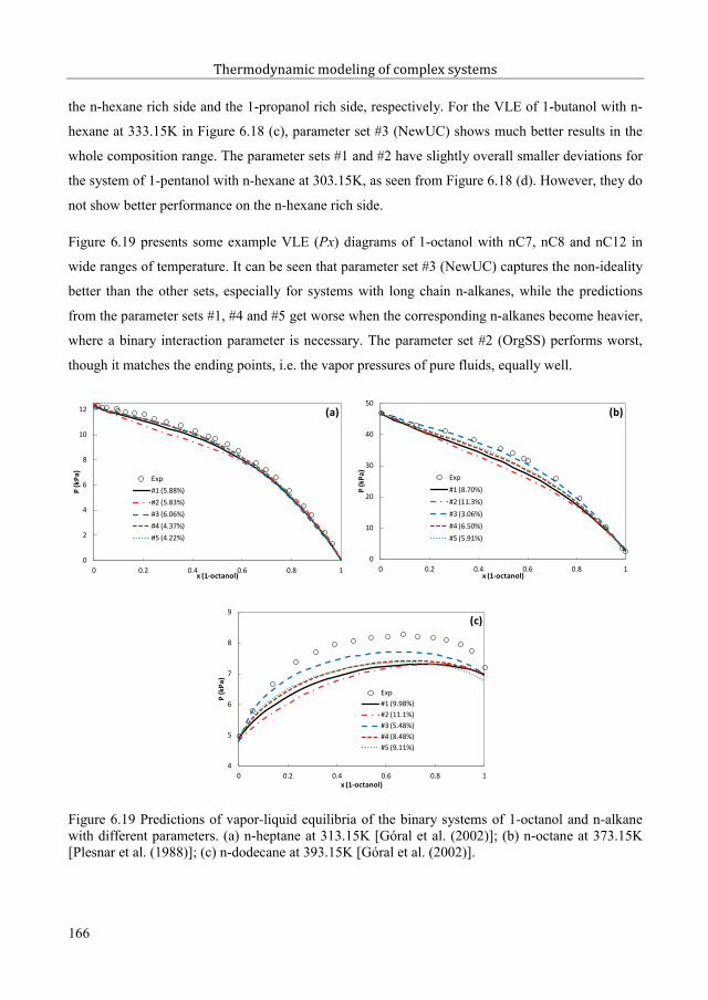
Thermodynamic modeling of complex systems
the n-hexane rich side and the 1-propanol rich side, respectively. For the VLE of 1-butanol with n-
hexane at 333.15K in Figure 6.18 (c), parameter set #3 (NewUC) shows much better results in the
whole composition range. The parameter sets #1 and #2 have slightly overall smaller deviations for
the system of 1-pentanol with n-hexane at 303.15K, as seen from Figure 6.18 (d). However, they do
not show better performance on the n-hexane rich side.
Figure 6.19 presents some example VLE (Px) diagrams of 1-octanol with nC7, nC8 and nC12 in
wide ranges of temperature. It can be seen that parameter set #3 (NewUC) captures the non-ideality
better than the other sets, especially for systems with long chain n-alkanes, while the predictions
from the parameter sets #1, #4 and #5 get worse when the corresponding n-alkanes become heavier,
where a binary interaction parameter is necessary. The parameter set #2 (OrgSS) performs worst,
though it matches the ending points, i.e. the vapor pressures of pure fluids, equally well.
Figure 6.19 Predictions of vapor-liquid equilibria of the binary systems of 1-octanol and n-alkane with different parameters. (a) n-heptane at 313.15K [Góral et al. (2002)]; (b) n-octane at 373.15K[Plesnar et al. (1988)]; (c) n-dodecane at 393.15K [Góral et al. (2002)].
0
2
4
6
8
10
12
0 0.2 0.4 0.6 0.8 1
P (k
Pa)
x (1-octanol)
(a)
Exp#1 (5.88%)#2 (5.83%)#3 (6.06%)#4 (4.37%)#5 (4.22%)
0
10
20
30
40
50
0 0.2 0.4 0.6 0.8 1
P (k
Pa)
x (1-octanol)
(b)
Exp#1 (8.70%)#2 (11.3%)#3 (3.06%)#4 (6.50%)#5 (5.91%)
4
5
6
7
8
9
0 0.2 0.4 0.6 0.8 1
P (k
Pa)
x (1-octanol)
(c)
Exp#1 (9.98%)#2 (11.1%)#3 (5.48%)#4 (8.48%)#5 (9.11%)
166
182

Chapter 6. Modeling speed of sound
The parameter sets #4 and #5 show overall comparable predictions of the VLE, liquid density and
speed of sound of the binary mixtures of 1-alcohols and normal hydrocarbons. This could be
explained by the fact that they are fitted to the same experimental data. These observations reveal
that it is possible to perform the pure component parameter fitting in a dimension-reduced space for
a regular compound series during parameter estimation. For example, Grenner et al. (2007a) and
Llovell et al. (2006b) used constant association energy and association volume for all of the 1-
alkanols (except for very short molecules) to obtain the pure component parameters.
6.5.2.2 Water containing systems
As discussed in Chapter 2, water is a unique molecule, and it is not an easy task to model water with
any thermodynamic model. The same procedure of fitting water parameters developed in Chapter 2
is applied to the new universal constants. The correlation results of the liquid-liquid equilibira of
water with nC8 and with cC6 are presented in Figure 6.20. These two sets of the universal constants
have almost identical correlation capability.
Figure 6.20 Correlations of the liquid-liquid equilibria of (a) water with nC8 and (b) water with cC6 from the approaches OrgUC and NewUC. The experimental data are from Tsonopoulos et al. (1983, 1985).
The prediction and correlation of the phase behavior of water and 1-alochols, as done in Chapter 2,
are performed with the approach NewUC as well. The results are compared to those from the
approach OrgUC in Table 6.19. The results show that these two approaches OrgUC and NewUC
have comparable results, which is mainly due to the robustness of the association framework. It is
worth pointing out that the vapor phase correlation of water + 1-butanol mixture from the approach
NewUC is not satisfactory, which is mainly due to the poor performance for the vapor pressure
description of pure 1-butanol, as shown in Table 6.6.
1.E-8
1.E-7
1.E-6
1.E-5
1.E-4
1.E-3
1.E-2
1.E-1
1.E+0
270 320 370 420 470 520
Solu
bilit
y
Temperature (K)
(a)
x(H2O)
x(nC8)
OrgUC
NewUC 1.E-6
1.E-5
1.E-4
1.E-3
1.E-2
1.E-1
1.E+0
270 320 370 420 470 520
Solu
bilit
y
Temperature (K)
(b)
x(H2O)
x(cC6)
OrgUC (0.0243)
NewUC (0.0244)
167
183

Thermodynamic modeling of complex systems
Table 6.19 VLE and VLLE of water with 1-alcohols from the approaches OrgUC and NewUC
Approach dP (%)dT (K)
%AAD of x (H2O) kijdP (%)dT (K)
%AAD of x (H2O)vapor water alcohol vapor water alcohol
Methanol (T=298.15-373.15K)[Butler et al. (1933), Griswold et al. (1952)]
OrgUC 32.0 11.1 -0.0852 3.62 1.01NewUC 26.7 7.39 -0.0847 2.38 1.42
Ethanol (T=298.14-363.15K)[Phutela et al. (1979), Kurihara et al. (1995), Pemberton et al. (1978)]
OrgUC 16.5 6.34 -0.0532 1.46 0.47NewUC 18.0 6.84 -0.0581 1.34 0.51
1-Propanol (at atmospheric pressure)[Udovenko et al. (1972)]
OrgUC 3.66 5.29 -0.0287 0.85 1.86NewUC 3.29 5.82 -0.0296 0.52 1.41
1-Butanol (at atmospheric pressure)[Boublik (1960), Sørensen et al. (1995)]
OrgUC 5.96 9.22 1.64 61.3 -0.0585 0.85 2.40 6.31 4.15NewUC 5.11 8.11 1.59 59.1 -0.0597 2.36 2.99 5.36 3.44
1-Pentanol (at atmospheric pressure)[Beregovykh et al. (1971), Sørensen et al. (1995)]
OrgUC 3.82 7.09 1.62 56.8 -0.0518 2.65 2.05 2.52 2.82NewUC 8.44 10.1 0.35 46.9 -0.0640 0.70 1.58 0.92 8.35
6.6 Conclusions
In this work, firstly, the performance of the SRK, CPA and PC-SAFT EOS is evaluated for the
speed of sound in normal alkanes. The results reveal that (1) none of the models could describe the
speed of sound with satisfactory accuracy, over wide ranges of temperature, pressure and chain-
length; (2) fitting parameters to experimental data could improve the description of the speed of
sound for chain molecules, i.e. CPA performs better than SRK; (3) PC-SAFT is superior to SRK
and CPA from both the accuracy and the curvature points of view over wide pressure ranges due to
its theoretically more sound physical term. This indicates that the functional form of the model is
more important than the parameter fitting strategy.
Secondly, the PC-SAFT model was chosen as the starting point to develop approaches for modeling
speed of sound. The first approach is to include the speed of sound data into pure component
parameters. The second approach is to integrate the speed of sound data into both the universal
constants regression and the pure component parameters estimation. The new universal constants
168
184

Chapter 6. Modeling speed of sound
regression was based on the data of saturated methane to decane. As the original parameters of
normal hydrocarbons, the new ones exhibit good linear correlation functions for m, 3 and
against molecular weight due to the same framework. These two approaches have been applied to
model the speed of sound in pure hydrocarbons, pure 1-alcohols, pure water, binary mixtures of
hydrocarbons, binary mixtures of hydrocarbon + 1-alcohol, ternary mixtures and petroleum fluids.
The first approach could not improve the description of speed of sound for normal alkanes and
heavy 1-alcohols, even at the cost of accuracy loss for vapor pressure and liquid density, but it does
improve the speed of sound description for the short 1-alcohols, for which the association term
plays an important role, from the quantitative point of view. This is mainly due to the significant
improvements of the flexibility of parameter estimation with two extra parameters. As discussed in
Chapter 2, the parameters with speed of sound data in estimation could improve the description of
the liquid-liquid equilibria of methanol with normal hydrocarbons, which reveals that better
compromise might be obtained by putting the second derivative properties into the parameter
estimation if there are extra fitting parameters, i.e. association energy and volume here, when the
association term plays an important role.
The second approach significantly improves the description of the speed of sound in most of the
defined systems except for methane rich fluids and water, from both qualitative and quantitative
points of view. For the methane rich fluids, the original PC-SAFT has already had good description
of the speed of sound in methane, but it has to be pointed out that it is possible to have alternatives
to offer better description of speed of sound in such fluids. The current PC-SAFT framework,
however, is not able to model the speed of sound in water in wide temperature and pressure ranges,
because the temperature dependence is complex. In this project, general petroleum fluid
characterization methods have been developed for the original PC-SAFT EOS, but it is still far
away to have such procedures for the new universal constants. This is because the speed of sound
data is not available as commonly as density, which is necessary to characterize the model
parameters with the new universal constants. A simple conversion procedure is proposed to connect
the model parameters of the pseudo-components from the original PC-SAFT EOS to the new
universal constants. It shows considerably improvements for the description of the speed of sound
in heavy oils, but the results are not satisfactory enough for extremely heavy oils.
The new universal constants have been applied to model the phase equilibria of the binary systems
containing n-alkanes, 1-alkanols and water, in which VLE, LLE and VLLE are covered. In general,
169
185

Thermodynamic modeling of complex systems
comparable results are obtained as those given by the original universal constants. This fact reveals
that it is possible to have simultaneously satisfactory description of phase equilibria and speed of
sound within the same PC-SAFT framework.
The two sets of universal constants present similar isochoric heat capacity results for the considered
normal hydrocarbons, which show that the second approach has little impact on the derivatives of
residual Helmholtz free energy with respect to temperature. However, the new universal constants
perform less satisfactorily than the original ones for the isobaric heat capacity for the investigated
normal hydrocarbons. The new universal constants have difficulties in simultaneously describing
the vapor pressure, liquid density and speed of sound in the associating fluids with chain length
around m=3, and they also have difficulties in reproducing the liquid density for both associating
and non-associating long chain fluids. The results indicate that more systematic research needs to be
done in the universal constants regression, if excellent accuracy in both first- and second-order
derivative properties is desired.
The pure component parameters from different sources, fitted in different ways, are investigated
with the original universal constants for 1-alcohols. They perform differently for specific systems,
but they present overall comparable performance in terms of describing vapor-liquid equilibria,
liquid densities, speed of sound for various systems in wide ranges of temperature and pressure. The
results confirm that it is possible to use generalized parameter estimation schemes for 1-alcohols,
but they also suggest that further systematic studies are needed.
Lastly, an important message from this chapter is that changing the universal constants is possible!
170
186

Chapter 7. A new variant of the Universal Constants
As a popular and promising model, the PC-SAFT EOS has been applied into many different fields,
including chemicals, polymers, biochemicals, pharmaceuticals, and so on. It has also been shown in
the previous chapters that the PC-SAFT EOS is capable of modeling the phase behavior of oil and
water containing systems, if appropriate parameters could be found for both well- and ill-defined
systems. The PC-SAFT EOS has, however, been criticized for some numerical pitfalls especially
during the recent years.
The purposes of this chapter are (1) to analyze the temperature and volume dependence of the PC-
SAFT EOS in a somehow deterministic way; (2) to propose a new variant of universal constants
which can avoid the numerical pitfalls; (3) to compare the universal constant sets and to investigate
the possibility of using the original PC-SAFT parameters with the new universal constant set.
7.1 Introduction
As denoted by its name, the dispersion term of the PC-SAFT EOS is a perturbation for hard chains
instead of hard spheres, but in fact it is represented by the interaction energy fitted to the real fluids
in the form of 6th degree polynomials of reduced density. There are in total 42 empirical coefficients
in these 6th degree polynomials, which are the so-called universal constants. In Chapter 6, the
universal constants are readjusted because the original ones could not provide satisfactory
correlation and/or prediction for the speed of sound in most systems, even with the pure component
parameters fitted to the speed of sound data. The universal constants were obtained by including the
vapor pressure, liquid density and speed of sound data of saturated methane to decane in the
regression.
On one hand, it has been found that these new universal constants improve the description of the
speed of sound in most systems from both qualitative and quantitative points of view, while keeping
satisfactory description of phase equilibrium. Very recently, Polishuk et al (2013) have found that
the universal constants, developed in our previous work, could practically avoid the numerical
pitfalls of the additional fictitious critical point of the pure components.
171
187

Thermodynamic modeling of complex systems
On the other hand, it has also been found that these new universal constants perform worse for the
density of long chain fluids and isobaric heat capacity. Polishuk showed, in a later article (2014),
that these new universal constants give poor prediction for virial coefficients, even negative third
virial coefficients at high temperatures. Moreover, it is not convenient to develop general
characterization procedures for modeling ill-defined systems, e.g. petroleum fluids, since speed of
sound used in the parameter estimation. Equally importantly, unrealistic phase behavior can be
predicted by the original PC-SAFT EOS. All these inspired us to revisit the fundamentals of this
model.
7.2 Analysis of the Original PC-SAFT EOS
7.2.1 Temperature and density dependences
The PC-SAFT EOS can be expressed as:= + = + + (7.1)
If it is assumed, for a given temperature and density, that the reduced residual Helmholtz free
energy can be calculated from a well-established model, for instance from NIST reference equations
[REFPROP (2010)], and the hard-sphere chain contribution is calculated from PC-SAFT, the
reduced dispersion term can be calculated:= (7.2)
First, the following variables are introduced for easy mathematic manipulations.= = ( ) ( ) (7.3)
= ( ) = ( ) ( ) ( ) (7.4)
= ( ) = ( ) ( ) ( ) (7.5)
Furthermore, a new function F is defined as:
= ( 12 ) × + ( ) × ( 6 ) × (7.6)
Where the constant factor is ignored here, so
172
188

Chapter 7. A new variant of Universal Constants
= 1(7.7)
= ( ) = 1 ( ) = 1( ) ( ) (7.8)
= ( ) = 1( ) + ( ) 2 × (7.9)
Then, = ( ) × (7.10)
= {( ) × + } × ( ) (7.11)
= ( ) × ( ) + 2 × × (7.12)
If F is further formulated as: = + (7.13)= ( 12 ), = (7.14)
= ( ), = ( 6 ), = (7.15)
Then,
+ 1 = (7.16)
+ 1( ) + 1 = 1(7.17)
+ 2( ) + 1( ) + 2( ) + 1= 1 (7.18)
For a pure fluid,
173
189

Thermodynamic modeling of complex systems
= (7.19)
The following three variables should be all linear functions of 1/T.1 , 1 , 1(7.20)
In this way, it is possible to have a deterministic procedure to obtain the universal constants, as long
as the framework and the assumed pure component parameters could fulfill the requirements that
the three properties in equation (7.20) are all linear functions of 1/T. The procedure is documented
in detail as below:
(1) Setup NIST and PC-SAFT for the specified compound
(2) Specify reduced density and temperature T
(3) Setup PC-SAFT for temperature dependent parameters/variables, and calculate V from and T
by =(4) Call NIST to calculate the required properties ( , , )
(5) Call PC-SAFT to calculate the contributions of the hard-chain term
(6) Calculate the dispersion term from NIST and hard-chain term from PC-SAFT (equation 7.3-7.5)
(7) Calculate , , from equations 7.10-7.12
(8) Calculate linear coefficients of , , as a function of 1/T for the given
(9) If we assume = + , we could get = ; =(10) If we assume = + , we could get = ; = + ( )(11) If we assume = + , we could get= ; = ( ) + ( ) + ( )(12) When all the information is available, the sixth polynomial coefficients could be fitted to be the
universal constants
The examples of the converted dispersion term (eq. 7.16) of methane and propane are demonstrated
for the volume dependence and temperature dependence, respectively, in Figures 7.1 and 7.2. It can
be seen that the reduced density dependence, 6th degree polynomials, is sufficient, but the
174
190

Chapter 7. A new variant of Universal Constants
temperature dependence is only valid either at low density region, or in a narrow range of
temperature. This explains why PC-SAFT has difficulties in describing the highly temperature
dependent properties, e.g. residual isochoric heat capacity, which solely depends on the derivatives
of residual Helmholtz free energy with respect to temperature.
Figure 7.1 Volume (density) dependence of the converted dispersion term (eq. 7.16) for methane and propane. The reduced residual Helmholtz free energy is calculated by NIST [REFPROP (2010)].
Figure 7.2 Temperature dependence of the converted dispersion term (eq. 7.16) for methane and propane. The reduced residual Helmholtz free energy is calculated by NIST [REFPROP (2010)].
7.2.2 Isothermal curves
It has been criticized that the original PC-SAFT EOS can give more than three volume roots at
some temperature and pressure conditions. Privat et al. (2010) stated that it is a problem to have
more than three volume roots, since the classical volume-root solvers only search for three roots. It
could be argued that this issue can be solved by developing sophisticated volume-root solvers, e.g.
setting limit values or checking the derivatives. The isothermal curves of C10 at 135K and C20 at
F (180K) = -932.8 6 + 1130.6 5 - 298.54 4 - 63.77 3 + 19.78 2 + 3.10 - 14.25R² = 0.9995
F (300K) = -561.63 6 + 556.99 5 - 143.45 4 + 22.73 3 - 15.04 2 + 1.19 - 12.64R² = 1
-15
-14
-13
-12
0 0.2 0.4 0.6
Conv
t. Di
sp. T
erm
(F/S
S 1, e
q 7.
16)
Packing fraction (
(a)
180K 300K
F (250K) = -11132 6 + 19745 5 - 12659 4 + 3407.4 3 - 294.24 2 - 4.04 - 14.70R² = 0.9999
F(305K) = -2834 6 + 4280.4 5 - 2107.5 4 + 352.34 3 - 7.65 2 + 1.78 - 12.97R² = 0.9997
F (500K) = -707.32 6 + 661.08 5 - 72.73 4 - 12.32 3 - 16.47 2 + 0.80 - 10.83R² = 1
-16
-14
-12
-10
0 0.2 0.4 0.6
Conv
t. Di
sp. T
erm
(F/S
S 1, e
q 7.
16)
Packing fraction ( )
(b)
250K 305K 500K
-15
-14
-13
3 4 5 6 7
Conv
t. Di
sp. T
erm
(F/S
S 1, e
q 7.
16)
1000/T (1/K)
(a) e=1e-4 e=0.1
e=0.2 e=0.3
e=0.4 e=0.5
-14.0
-13.0
-12.0
-11.0
2 3 4 5 6
Conv
. Disp
. Ter
m (F
/SS 1
, eq.
16)
1000/T (1/K)
(b)e=1e-4 e=0.25
e=0.35 e=0.4
e=0.5
175
191

Thermodynamic modeling of complex systems
150K from the original PC-SAFT EOS are presented in Figure 7.3. The one of C10 was firstly
reported by Privat et al. (2010), in which the detailed information of its curve shape in the low
reduced density region can be found. It can be seen that it is possible to have two stable liquid
volume roots in some pressure ranges, and there is only one single volume root locating in the very
heavy reduced density region. More severely, the volume roots are not continuous as the pressure
increases, so the volume-root solver will probably not be an appropriate solution anymore.
Figure 7.3 Isothermal curves of (a) C10 at 135K and (b) C20 at 150K from the original PC-SAFT EOS [Gross and Sadowski (2001)]. The curve of C10 was firstly reported by Privat et al (2010).
In order to have a more complete picture of the isothermal curves, the parameters and temperature
are screened to test how many volume roots the original PC-SAFT EOS will have at most by using
the following procedure.
(1) Produce the parameters from {m=[1:1:200 =3.8Å, 10:1000]K}
(2) Produce the temperature from {T=[100:20:2000]K}
(3) Check the number of volume roots at P=0Bar, NVR(P=0), and P( 0)
(4) If [NVR(P=0)] is zero, check the number of volume roots of dP/dV=0, NVR(dP/dV=0)
(5) If [NVR(P=0)] is two, check the number of volume roots of dP/dV=0, NVR(dP/dV=0) for P > 0
(6) LOOP step (1) to (5) until testing all the parameters
According to the work of Polishuk et al. (2013), the parameter is arbitrarily set to 3.8Å, which is a
typical value for hydrocarbons. When the isothermal curve has zero or two volume roots at P=0 Bar,
it does not mean it is free from the numerical pitfalls, simply because the working pressure is not
zero Bar. This is why it is checked in steps (4) and (5) for the number of volume roots of dP/dV=0.
= 0.74048
-6000
-4000
-2000
0
2000
4000
6000
0 0.2 0.4 0.6 0.8
Pres
sure
(Bar
)
Reduced density (packing fraction )
C10 at 135K
C20 at 150K
176
192

Chapter 7. A new variant of Universal Constants
Figure 7.4 presents the examples of the parameter combinations with which the original PC-SAFT
EOS has one or three volume roots at P=0 Bar when ( 0) > 0 Bar. It can be seen that it is
probably that no single solution will be found in most of the interested pressure ranges, while it
could be argued that the dispersion energy ( ) has been too large and temperature has been too
low for real applications, but this examination gives the limitations of the feasible ranges of the
parameters, which is very useful for automatic parameter tuning in large scale simulations.
Figure 7.4 Isothermal curves from PC-SAFT (GS) with different parameter combinations. Red dash-dot line is for one root and blue dash line is for three roots at P=0 bar with ( 0) > 0.
Figure 7.5 (a) and (b) present the examples of the parameter combinations with which the original
PC-SAFT EOS has four volume roots at P=0 Bar, and more than two volume roots satisfying
dP/dV=0 when the NVR(P=0) is two, respectively. It can be seen that the functionalities of pressure
versus reduced density from these two situations are quite similar to those shown in Figure 7.3 for
C10 and C20, i.e. two stable liquid volume roots exist at some ranges of pressure and the only valid
liquid volume root locates in very high reduced density region for higher pressures. It can be also
seen that some combinations have already located in the real application ranges. It is possible to use
this procedure to define the application ranges of the original PC-SAFT EOS. For example, the
ranges of segment number and dispersion energy parameters, with which these phenomena of
Figure 7.5 will occur, are given in Figure 7.6 for the given segment size (3.8Å) and temperature
(300K). Figure 7.6 (a) indicates that it is not recommended to use the dispersion energy higher than
460K if the segment number is larger than 10 at temperature 300K.
-9000
-6000
-3000
0
0 0.2 0.4 0.6 0.8
Pres
sure
(Bar
)
Reduced density (packing fraction )
m=10; Å; k=700K; T=140K, NVP(P=0)=1m=3; Å; k=700K; T=120K; NVP(P=0)=3
177
193

Thermodynamic modeling of complex systems
Figure 7.5 Isothermal curves from the original PC-SAFT EOS with different parameter combinations for the situations. (a) Four volume roots at P=0Bar, and (b) more than two volume roots satisfying dP/dV=0 when two volume roots at P=0Bar.
Figure 7.6 The ranges of m and for the original PC-SAFT EOS to have the same type of P-curve as those presented Figure 7.5, with fixed =3.8Å at 300K.
7.3 New universal constants
On one hand, as discussed by Polishuk et al. (2013), it is a feasible approach to fix the numerical
pitfalls by changing the universal constants. On the other hand, the PC-SAFT EOS has already been
successfully applied into modeling various types of systems. It will fundamentally extend the
application ranges of the PC-SAFT EOS if a new set of universal constants can avoid the numerical
pitfalls and reuse the original parameters as much as possible.
-20000
-10000
0
10000
0 0.2 0.4 0.6 0.8
Pres
sure
(Bar
)
Reduced density (packing fraction )
(a)
m=5; Å; k=500K; T=260K
m=10; Å; k=500K; T=300K
m=15; Å; k=500K; T=340K
m=15; Å; k=440K; T=300K
m=15; Å; k=400K; T=260K
P = 2000 Bar
-1000
1000
3000
5000
0 0.2 0.4 0.6 0.8
Pres
sure
(Bar
)
Reduced density (packing fraction )
(b)
m=10; Å; k=300K; T=200K
m=20; Å; k=350K; T=250K
m=15; Å; k=420K; T=290K
400
500
600
700
0 20 40 60 80 100
/k (K
)
m
(a)
350
450
550
650
0 20 40 60 80 100
/k (K
)
m
(b)
178
194

Chapter 7. A new variant of Universal Constants
7.3.1 A practical way
In Chapter 6, the universal constants are regressed with a step-wise procedure by assuming that the
methane (C1) has a segment number parameter m=1. It is further assumed that propane (C3) has a
segment number parameter m=2 to develop the following practical procedure.
(1) Estimate the pure component parameters for C1 to C10 with the original universal constants
(2) Regress the coefficients { } and { } from the properties of C1 with m = 1
(3) Regress the coefficients { } and { } from the properties of C3 with m = 2
(4) Regress the coefficients { } and { } from the properties of C4 to C10
(5) Estimate the pure component parameters for C1 to C10 with the new universal constants
In the previous work [Liang et al. (2012)], the universal constant regression and pure component
parameter estimation are iterated, but the steps (2) and (5) are not repeated in this work, because we
want to keep the most possibility of reusing the original PC-SAFT EOS parameters.
The following objective function is employed:
= 1 (7.21)
Where is vapor pressure and density (both saturated and isothermal-isobaric conditions), and
second-order derivative property dP/dV.
For pure component parameter estimation, vapor pressure and saturated liquid density are the only
properties used, but for the regression of the universal constants, dP/dV is included with a weight
factor = 0.01, as the objective function with vapor pressure and density only has a very flat
respond surface. As demonstrated above, that the current PC-SAFT framework are not good enough
for simultaneously accurate description of the first- and second-order derivative properties over
wide ranges of temperature with the associated pure component parameters. This is one of the
reasons why a small number (0.01) is used, and the other reason is to keep the possibility to reuse
the original PC-SAFT parameters. The data are the same ones from NIST [REFPROP (2010)], and
the details of the temperature and pressure ranges can be found in Chapter 6.
179
195
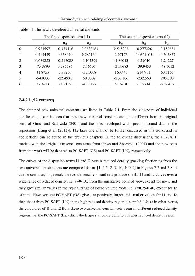
Thermodynamic modeling of complex systems
Table 7.1 The newly developed universal constants
iThe first dispersion term (I1) The second dispersion term (I2)
a0i a1i a2i b0i b1i b2i
0 0.961597 -0.333416 -0.0632483 0.548398 -0.277226 -0.1506841 0.414449 0.358440 0.287134 2.07176 0.0621105 -0.5078772 0.689253 -0.219088 -0.105309 -1.84013 4.29640 1.242273 -7.43899 0.285586 7.16607 -29.9683 -39.9453 -48.70524 31.8755 5.88256 -37.5008 160.445 214.911 63.11555 -54.8833 -22.4931 68.8002 -206.106 -232.563 205.3806 27.3613 21.2109 -40.3177 51.6201 60.9734 -262.437
7.3.2 I1/I2 versus
The obtained new universal constants are listed in Table 7.1. From the viewpoint of individual
coefficients, it can be seen that these new universal constants are quite different from the original
ones of Gross and Sadowski (2001) and the ones developed with speed of sound data in the
regression [Liang et al. (2012)]. The later one will not be further discussed in this work, and its
applications can be found in the previous chapters. In the following discussions, the PC-SAFT
models with the original universal constants from Gross and Sadowski (2001) and the new ones
from this work will be denoted as PC-SAFT (GS) and PC-SAFT (LK), respectively.
two universal constant sets are compared for m=[1, 1.5, 2, 3, 10, 10000] in Figures 7.7 and 7.8. It
can be seen that, in general, the two universal constant sets produce similar I1 and I2 curves over a
-1.0, from the qualitative point of view, except for m=1, and
they give similar values in th -0.40, except for I2
of m=1. However, the PC-SAFT (GS) gives, respectively, larger and smaller values for I1 and I2
than those from PC- -1.0, or in other words,
the curvatures of I1 and I2 from these two universal constant sets occur in different reduced density
regions, i.e. the PC-SAFT (LK) shifts the larger stationary point to a higher reduced density region.
180
196

Chapter 7. A new variant of Universal Constants
Figure 7.7 Comparison of dispersion term I1 from the two universal constant sets from (a) this work and (b) Gross and Sadowski (2001).
Figure 7.8 Comparison of dispersion term I2 from the two universal constant sets from (a) this work and (b) Gross and Sadowski (2001).
7.3.3 Parameters and physical properties
In order to have a fair comparison, the pure component parameters of normal hydrocarbons are
refitted to the same vapor pressure and saturated liquid densitydata with both universal constant sets.
The fitted parameters and corresponding deviations are listed in Appendix D, Tables D.1 and D.2,
respectively. It is known from Table D.2 that PC-SAFT (GS) gives deviations 0.65% and 0.35%,
respectively, for vapor pressure and density of the normal hydrocarbons from C1 to C20, and PC-
SAFT (LK) gives deviations 0.30% and 0.27% for the corresponding properties. This illustrates that
both universal constant sets provide very good correlating capabilities for the vapor pressure and
saturated liquid density.
0
1
2
0 0.2 0.4 0.6 0.8 1
Disp
ersio
n te
rm I1
Reduced density (packing fraction )
(a) m=1 m=1.5
m=2 m=3
m=10 m=10000
0
1
2
0 0.2 0.4 0.6 0.8 1
Disp
ersio
n te
rm I1
packing fraction ( )
(b)
m=1 m=1.5
m=2 m=3
m=10 m=10000
0
2
4
6
8
10
0 0.2 0.4 0.6 0.8 1
Disp
ersio
n te
rm I2
packing fraction ( )
(a)
m=1 m=1.5
m=2 m=3
m=10 m=10000
-6
-4
-2
0
2
4
0 0.2 0.4 0.6 0.8 1
Disp
ersio
n te
rm I2
packing fraction ( )
(b)
m=1 m=1.5
m=2 m=3
m=10 m=10000
181
197

Thermodynamic modeling of complex systems
The differences of the pure component parameters from PC-SAFT with the two universal constants
are compared in Figure 7.9 (a), which is defined as:
% = × 100% (7.22)
GS and LK are used instead of PC-SAFT (GS) and PC-SAFT (LK) just for simplicity, which will
also be used in the following figures.
It can be seen that the PC-SAFT (LK) gives larger parameter m and smaller parameters
for all the investigated n-alkanes, except C1, but the differences are smaller than 1%, and the
differences themselves have small variations for n-alkanes longer than C10.
Figure 7.9 Comparisons of the PC-SAFT parameters and the corresponding %AADs for vapor pressure and liquid density of normal hydrocarbons (from C1 to C20). The experimental data are taken from NIST [REFPROF (2010)] for C1 to C10 and from DIPPR (2012) for C11 to C20.
The differences of the deviations for vapor pressure and saturated liquid density from PC-SAFT
with the two universal constants are compared in Figure 7.9 (b), which is defined by:% = (7.23)
It is shown in Figure 7.9 (b) that PC-SAFT (LK) presents a slightly better correlation for vapor
pressure than the PC-SAFT (GS), whereas the two sets perform quite similarly for density.
The second-order derivative properties, speed of sound (u), dP/dV, residual isochoric and isobaric
heat capacities (CV (r) and CP (r)), and Joule-Thomson (JT) coefficients are calculated from PC-
SAFT with the two universal constants, and compared with the data from NIST [REFPROP(2010)].
The detailed deviations for all the properties are reported in Appendix D, Tables D.3 and D.4. The
-1.0
-0.5
0.0
0.5
1.0
0 100 200 300
%RD
of p
aram
eter
s
Molecular weight (g/mol)
(a)
m k
-1.5
-1
-0.5
0
0.5
0 100 200 300
%AA
D di
ffere
nce
(New
UC -
Org
UC)
Molecular weight (g/mol)
(b)
P
182
198

Chapter 7. A new variant of Universal Constants
deviations are compared for speed of sound and dP/dV in Figure 7.10 (a), and for residual and total
isochoric and isobaric heat capacities in Figure 7.10 (b) by using equation (7.23) as well. It can be
seen that the PC-SAFT (LK) gives better description of speed of sound and dP/dV, except for C1,
and the PC-SAFT (GS) gives better prediction of residual isochoric heat capacity for short chain
molecules. They present quite similar performance for residual isobaric heat capacities as well as
the total heat capacities, both isochoric and isobaric ones.
The deviations of Joule-Thomson coefficients are compared in Figure 7.11 (a). It can be seen, from
Figure 7.11 (a) and Tables S3 and S4, that the PC-SAF (LK) predicts quite large deviations for
Joule-Thomson coefficients of saturated nC8. This is because one ‘experimental’ datum has a very
small value, i.e. just around the point when the sign changes. The whole Joule-Thomson coefficient
curves of saturated nC8 from these two models are plotted in Figure 7.11 (b), from which the two
universal constant sets present quite similar results.
As discussed above, it is possible for different universal constants to have equally good correlations
for vapor pressure and density, and it is possible to obtain different universal constants by taking
different property combinations into account, which will give different balances on describing the
properties depending on the designed objective function. To best of our experience, it seems not
possible to find a unique set of universal constants, within the current framework, which is able to
give absolutely better description for all the properties. It could be anticipated that it is a
fundamental deficiency that the current PC-SAFT framework is not able to simultaneously describe
all of the first- and second-order derivative properties, based on this work and the previous one.
Figure 7.10 Comparisons of the %AADs from the two universal constants using equation (7.23). (a) speed of sound (u) and dP/dV, and (b) residual and total heat capacities of C1 to C10, over wide ranges of temperature and pressure. The experimental data are taken from NIST [REFPROP(2010)].
-5
-4
-3
-2
-1
0
1
1 2 3 4 5 6 7 8 9 10
%AA
D di
ffere
nces
Carbon number (C.N.)
(a)
u
dP/dV
-1
0
1
2
3
4
5
1 2 3 4 5 6 7 8 9 10
%AA
D di
ffere
nces
Carbon number (C.N.)
(b)
Cv (r)
Cp (r)
Cv
Cp
183
199

Thermodynamic modeling of complex systems
Figure 7.11 (a) Comparisons of the %AADs for Joule-Thomson (JT) coefficients of C1 to C10 over wide ranges of temperature and pressure using equation (7.23), and (b) Joule-Thomson coefficients of saturated nC8 from the two universal constants. GS and LK denote the universal constants from Gross and Sadowski (2001) and this work, respectively. The experimental data are taken from NIST[REFPROP (2010)].
7.3.4 Application ranges
The same procedure proposed in Section 7.2.2 is also conducted for the new universal constants.
The results show that the behavior of having one or three volume roots at P=0 Bar when (0) > 0 Bar have not been observed, as those presented in Figure 7.4. It has also been found that it is
possible to have at most two volume roots satisfying dP/dV=0 when there are zero or two volume
roots at P=0 Bar, which means these are typical cubic-like P- curves, so there will be no numerical
pitfalls for these two situations as well.
In the entire investigated ranges of parameters and temperature, all possible combinations, with
which the new universal constants give four volume roots at P=0 Bar, are shown in Figure 7.12. It
can be seen that it is not possible to have more than three roots, or two stable liquid volume roots, in
the entire pressure range if the dispersion energy is not larger than 780K, or if the working
temperature is higher than 120K. In another word, the PC-SAFT EOS with the new universal
constants is practically free of numerical pitfalls of the presence of more than three volume roots.
However, it has to be pointed out that it is possible for the PC-SAFT (LK) to give at most six
volume roots at P=0 Bar if the working temperature is very low, e.g. smaller than 55K, which could
be argued that it is out of the real application ranges for most interested processes. This can be
improved by tuning the universal constants to obtain the I1 and I2 curves as those from our previous
work [Liang et al. (2012)] or Polishuk (2014), but the ultimate solution is believed to use a fewer
-1
0
1
2
3
4
5
6
7
1 2 3 4 5 6 7 8 9 10
%AA
D di
ffere
nces
Carbon number (C.N.)
(a)
JT
-0.05
-0.03
-0.01
0.01
0.03
0.05
250 350 450 550
Joul
e-Th
omso
n co
effic
ient
s (K/
Bar)
Temperature (K)
(b)
Exp. (NIST)
GS
LK
184
200

Chapter 7. A new variant of Universal Constants
degree polynomials, e.g. 4th degree, or other types of functions to represent the dispersion
interactions. In this case, however, the model parameters are probably needed to be refitted.
Figure 7.12 The ranges of m and for the PC-SAFT EOS with the new universal constants to have four volume roots at P=0Bar, which presents the potential risk to have more than three volume roots and discontinuity of the volume roots versus temperature or pressure when the parameters locate in these ranges.
7.3.5 A real example
It is a common practice to use large parameter values for dispersion energy and/or segment number
when modeling asphaltene. For instance, Hustad et al. (2013) used the parameters {m=11, =4.53Å,
/k=500K} for asphaltene. The isothermal curve of this asphaltene at 280K is shown in Figure 7.13
(a), and the one from the PC-SAFT (GS) has the typical behavior of four volume roots at P=0 Bar.
It can be seen that the discontinuity of the volume roots occurs when the pressure exceeds 600Bar,
and the volume root will then locate in the very heavy reduced density area ( ).
In order to study the relationship of isothermal curve and phase equilibrium, the isobaric-isothermal
flash calculations have been conducted for the original reservoir fluid, i.e. without nitrogen injection,
from 200 to 1000Bar at 280K. All the parameters, including the binary interaction parameters, are
taken from Hustad et al. The molar numbers of the asphaltene in its rich phase are presented in
Figure 7.13 (b). It can be seen that the two models give similar prediction below 600Bar, and the
PC-SAFT (GS) predicts non-physical phase split results when the pressure exceeds 600Bar, i.e. one
pure asphaltene phase, whereas the PC-SAFT (LK) gives a smooth prediction. The discontinuity of
the volume roots versus pressure is believed to the reason for the discontinuous phase equilibrium
results along the pressure curve.
750
800
850
900
950
1000
0 50 100 150 200
/k (K
)
m
100K 120K
185
201

Thermodynamic modeling of complex systems
Figure 7.13 (a) Isothermal curves of asphaltene at 280K with the parameters from Hustad et al.(2013); (b) the molar numbers of asphaltene in its rich phase versus pressure. GS and LK denote the universal constants from Gross and Sadowski (2001) and this work, respectively.
7.4 Possibility to use the original PC-SAFT parameters
As discussed above, the same pure component parameters from the original universal constants are
used when fitting the new universal constants, and the differences of the final pure component
parameters of n-alkanes from these two universal constant sets are less than 1%. In this section, we
will investigate the possibility of reusing the parameters from the original PC-SAFT EOS with the
new universal constants.
7.4.1 Binary hydrocarbon systems
The VLE of the binary mixtures of C2 + nC10 and C3 + C6H6 have been modeled by PC-SAFT
with both universal constant sets using the parameters from Gross and Sadowski. The results are
presented in Figure 7.14. The kij is 0.0 in both cases. It can be seen that the phase diagrams from the
two universal constant sets are quite similar to each other.
7.4.2 1-Alcohol + n-alkane mixtures
The VLE of the binary mixtures of ethanol + nC6 and 1-octanol + nC12 have been modeled by PC-
SAFT with both universal constants. The results are presented in Figure 7.15. The kij is fitted to the
data for the original parameters with the PC-SAFT (GS). Again it can be readily seen that the phase
diagrams are almost identical.
The possibility of using the original parameters with the new universal constants is also checked for
the LLE of methanol + n-alkanes (nC6, nC8 or nC10). The results with the same model parameters
= 0.74048
-2000
-1000
0
1000
2000
0 0.2 0.4 0.6 0.8
Pres
sure
(Bar
)
Reduced density (packing fraction )
(a)
m=11; =4.53Å; /k=500K; T=280K
GS LK
0.5
0.6
0.7
0.8
200 400 600 800 1000
Mol
ar n
umbe
rs o
f asp
halte
ne
Pressure (Bar)
(b)
GS LK
186
202

Chapter 7. A new variant of Universal Constants
and kij are presented in Figure 7.16 (a). The model parameters of methanol are from Liang et al.
(2012), with speed of sound data in the parameter estimation. The kij is fitted to the data for the
original parameters with the PC-SAFT (GS). It can be seen that the phase diagrams are similar, but
the differences from the two universal constants are not as small as what have been seen in the
aforementioned VLE modeling results. It is demonstrated in Figure 7.16 (b) that a slightly different
kij could give almost identical phase diagrams.
Figure 7.14 P-x diagrams of (a) ethane + n-decane. Data are from Reamer et al. (1962) and (b) propane + benzene. Data are from Glanville et al. (1950) The model parameters of all hydrocarbons are from Gross and Sadowski (2001). GS and LK denote the universal constants from Gross and Sadowski (2001) and this work, respectively.
Figure 7.15 P-x diagrams of (a) ethanol + n-hexane and (b) 1-octanol + n-dodecane. The data are both from Góral et al. (2002), The ethanol and 1-octanol parameters are from Gross and Sadowski (2001) and Grenner et al. (2007a), respectively. The kij values are shown in the parenthesis. GS and LK denote the universal constants from Gross and Sadowski (2001) and this work, respectively.
0
40
80
120
0 0.2 0.4 0.6 0.8 1
Pres
sure
(Bar
)
x (ethane)
(a)Exp. (340F)
Exp. (460F)
GS (0.0)
LK (0.0)
0
20
40
60
0 0.2 0.4 0.6 0.8 1
Pres
sure
(Bar
)
x (propane)
(b)Exp. (160F)
Exp. (280F)
GS (0.0)
LK (0.0)
0
10
20
30
40
50
0 0.2 0.4 0.6 0.8 1
Pres
sure
(kPa
)
x (ethanol)
(a)
Exp. (298.15K)
Exp. (313.15K)
GS (0.0162)
LK (0.0162)0
5
10
15
20
0 0.2 0.4 0.6 0.8 1
Pres
sure
(kPa
)
x (octanol)
(b)
Exp. (393.15K)
Exp. (413.15K)
GS (0.0162)
LK (0.0162)
187
203

Thermodynamic modeling of complex systems
Figure 7.16 LLE of methanol with n-hexane, n-octane or n-decane, (a) same model parameters and kij, (b) same model parameters and different kij. The methanol parameters are from Liang et al.(2012) The experimental data are from Matsuda et al. (2002), Kurihara et al. (2002), and Matsuda et al. (2004) The kij values are shown in the parenthesis. GS and LK denote the universal constants from Gross and Sadowski (001) and this work, respectively.
Figure 7.17 Phase equilibria of (a) water + n-hexane, data are from Tsonopoulos et al. (1983) and water parameters are from Gross and Sadowski (2002); (b) water + cyclo-hexane, data are from Tsonopoulos et al. (1985) and parameters from Liang et al. The kij values are shown in the parenthesis. GS and LK denote the universal constants from Gross and Sadowski (2001) and this work, respectively.
7.4.3 Water containing systems
From the phase equilibrium modeling point of view, the water containing systems are good
candidates in order to investigate the possibility of using the original PC-SAFT parameters with the
new universal constants, since water is a challenging molecule for any EOS. The PC-SAFT
modeling results of the LLE of water + non-aromatic hydrocarbon (nC6 or cyclo-C6), VLE of water
+ mono-ethylene glycol (MEG), VLE and LLE of water + 1-butanol, and LLE of water + methanol
+ nC7 are presented in Figures 7.17-7.19 with both universal constants. All of the model parameters
260
285
310
335
360
0 0.2 0.4 0.6 0.8 1
Tem
pera
ture
(K)
x (MEOH)
(a)
C6 C8 C10
GS (0.0212) LK (0.0212)260
285
310
335
360
0 0.2 0.4 0.6 0.8 1
Tem
pera
ture
(K)
x (MEOH)
(b)
C6 C8 C10
GS (0.0212) LK (0.0228)
1.E-7
1.E-6
1.E-5
1.E-4
1.E-3
1.E-2
1.E-1
1.E+0
270 320 370 420 470
Solu
bilit
y
Temperature (K)
(a)
x(H2O)x(nC6)OrgUC (0.0349)NewUC (0.0349) 1.E-6
1.E-5
1.E-4
1.E-3
1.E-2
1.E-1
1.E+0
270 320 370 420 470 520
Solu
bilit
y
Temperature (K)
(b)
x(H2O)
x(cC6)
GS (0.0243)
LK (0.0243)
188
204

Chapter 7. A new variant of Universal Constants
and binary interaction parameters are based on the PC-SAFT (GS). The combining rule CR-1 is
used for cross associations. It can be seen that the two models give similar results for all the systems,
except for the 1-butanol rich phase in the water + 1-butanol binary mixture and the methanol
solubility in the hydrocarbon rich phase of the ternary mixture, which can be tuned by the binary
interaction parameters as discussed above for the methanol + n-alkane binary mixtures. It could be
argued, however, that the deviations from these two universal constant sets are much smaller than
the deviations of modeling results from the experimental data.
Figure 7.18 Phase equilibria (a) water with MEG. Data are from Chiavone-Filho et al. (1993) The model parameters of water and MEG are from Grenner et al. (1996) and Tsivintzelis et al. (2008),respectively. (b) water + 1-butanol. Data are from Boublik (1960) and Sørensen et al. (1995) The model parameters of water and 1-butanol are from Gross and Sadowski (2002). The kij values are shown in the parenthesis. GS and LK denote the universal constants from Gross and Sadowski(2001) and this work, respectively.
Figure 7.19 LLE of water + methanol + n-heptane, (a) the solubility of n-heptane in aqueous phase; (b) the solubility of methanol in n-heptane rich phase. The data are from Letcher et al. (1986) The model parameters of water and methanol are from Liang et al. (2012, 2014) GS and LK denote the universal constants from Gross and Sadowski (2001) and this work, respectively.
0
20
40
60
0 0.2 0.4 0.6 0.8 1
Vapo
r pre
ssur
e (k
Pa)
xH2O
(a)343.15K
363.15K
GS (-0.0497)
LK (-0.0497)
270
310
350
390
0 0.2 0.4 0.6 0.8 1
Tem
pera
ture
(K)
x (1-butanol)
(b)
VLE
LLE
GS (-0.017)
LK (-0.017)
0
0.02
0.04
0.06
0.08
0 0.1 0.2 0.3 0.4 0.5
x (nC
7) in
aqu
eous
pha
se
x (H2O) in aqueous phase
(a)
xC7 (293.15K)
GS
LK
0
0.02
0.04
0.06
0.08
0 0.1 0.2 0.3 0.4 0.5
x (m
etha
nol)
in n
C 7ric
h ph
ase
x (H2O) in aqueous phase
(b)
xMEOH (293.15K)
GS
LK
189
205
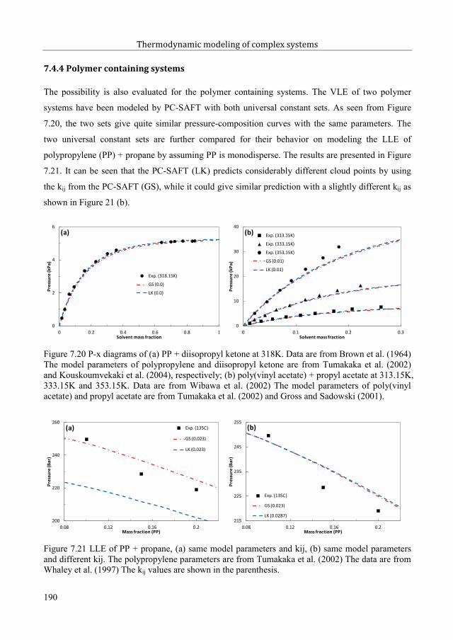
Thermodynamic modeling of complex systems
7.4.4 Polymer containing systems
The possibility is also evaluated for the polymer containing systems. The VLE of two polymer
systems have been modeled by PC-SAFT with both universal constant sets. As seen from Figure
7.20, the two sets give quite similar pressure-composition curves with the same parameters. The
two universal constant sets are further compared for their behavior on modeling the LLE of
polypropylene (PP) + propane by assuming PP is monodisperse. The results are presented in Figure
7.21. It can be seen that the PC-SAFT (LK) predicts considerably different cloud points by using
the kij from the PC-SAFT (GS), while it could give similar prediction with a slightly different kij as
shown in Figure 21 (b).
Figure 7.20 P-x diagrams of (a) PP + diisopropyl ketone at 318K. Data are from Brown et al. (1964) The model parameters of polypropylene and diisopropyl ketone are from Tumakaka et al. (2002)and Kouskoumvekaki et al. (2004), respectively; (b) poly(vinyl acetate) + propyl acetate at 313.15K, 333.15K and 353.15K. Data are from Wibawa et al. (2002) The model parameters of poly(vinyl acetate) and propyl acetate are from Tumakaka et al. (2002) and Gross and Sadowski (2001).
Figure 7.21 LLE of PP + propane, (a) same model parameters and kij, (b) same model parameters and different kij. The polypropylene parameters are from Tumakaka et al. (2002) The data are from Whaley et al. (1997) The kij values are shown in the parenthesis.
0
2
4
6
0 0.2 0.4 0.6 0.8 1
Pres
sure
(kPa
)
Solvent mass fraction
(a)
Exp. (318.15K)
GS (0.0)
LK (0.0)
0
10
20
30
40
0 0.1 0.2 0.3
Pres
sure
(kPa
)
Solvent mass fraction
(b) Exp. (313.15K)
Exp. (333.15K)
Exp. (353.15K)
GS (0.01)
LK (0.01)
200
220
240
260
0.08 0.12 0.16 0.2
Pres
sure
(Bar
)
Mass fraction (PP)
(a) Exp. (135C)
GS (0.023)
LK (0.023)
215
225
235
245
255
0.08 0.12 0.16 0.2
Pres
sure
(Bar
)
Mass fraction (PP)
(b)
Exp. (135C)
GS (0.023)
LK (0.0287)
190
206

Chapter 7. A new variant of Universal Constants
7.4.5 Natural gas systems
Since it is based on mean-field theory, the PC-SAFT EOS is believed to have difficulties in
predicting the critical points when the model parameters are fitted to the vapor pressure and liquid
density only. The critical points of 50 multicomponent systems are predicted from PC-SAFT with
both universal constants using the model parameters from the PC-SAFT (GS), which are compared
in Figure 7.22. It can be seen that the two models predict quite similar critical points.
The phase envelope of two natural gas systems are investigated with both universal constant sets by
using the original model parameters in a predictive way, i.e. no binary interaction parameter is used.
As shown in Figure 7.23, it can be seen that the shapes of the phase envelopes are quite similar.
Figure 7.22 Critical temperature and pressure of 50 natural gas systems. The collections of the detailed data, including mixture composition, critical temperature and pressure, and literature can be found in Sørensen (2008). GS and LK denote the universal constants from Gross and Sadowski (2001) and this work, respectively.
Figure 7.23 Phase envelope of (a) the Gas 2 from the work of Avila et al. (2002); (b) 60.0C1 + 31.0nC4 + 9.0nC10, from Urlic et al. (2003)
200
280
360
440
200 280 360 440
Crit.
Tem
p. T c
(K) f
rom
PC-
SAFT
(LK)
Crit. Temp. Tc (K) from PC-SAFT (GS)
(a)
%AAD Tc (GS) = 2.29%
%AAD Tc (LK) = 2.57%
40
60
80
100
120
140
40 60 80 100 120 140
Crit.
Pre
ss. P
c(B
ar) f
rom
PC-
SAFT
(LK)
)
Crit. Press. Pc (Bar) from PC-SAFT (GS)
(b)
%AAD Pc (GS) = 5.44%
%AAD Pc (LK) = 5.30%
0
20
40
60
80
180 200 220 240
Pres
sure
(Bar
)
Temperature (K)
(a)
Exp. GS LK
0
50
100
150
200
200 300 400 500
Pres
sure
(Bar
)
Temperature (K)
(b)
Exp. GS LK
191
207

Thermodynamic modeling of complex systems
7.4.4 Petroleum fluid-water-MEG systems
It has been shown in Chapter 4 that the PC-SAFT EOS is able to successfully model the petroleum
fluid-water-MEG systems by using the newly developed parameters of water and MEG, and
petroleum fluid characterization procedures. These ternary mixtures are modelled with PC-SAFT
(LK) by using the same characterization procedure CM7, i.e. directly replacing the universal
constants with the new ones during calculations. The overall deviations from these two universal
constant sets are compared in Table 7.2, and the modeling results of individual cases are compared
in Figure 7.24.
It is readily seen from Table 7.2 that the overall deviations from the two universal constant sets are
almost identical. The solubilities of water from the two models are almost identical, and the
solubilities of MEG from PC-SAFT (LK) are almost identical to and slightly smaller than those
from PC-SAFT (GS), respectively, for gas condensates (case 1 to case 12) and heavy oils (case 13
to case 19). PC-SAFT (LK) predicts larger solubilities of petroleum than PC-SAFT (GS), but the
differences are lower than 5%.
Table 7.2 %AADs for the petroleum fluid-water-MEG systems from two universal constant sets
Model Oil in polar phase MEG in organic phase H2O in organic phasePC-SAFT (LK) 26 25 26PC-SAFT (GS) 27 25 26
Figure 7.24 The ratios of solubility of petroleum fluid, water and MEG from PC-SAFT (LK) and PC-SAFT (GS) with the same characterization procedure.
0.99
1
1.01
1.02
1.03
1.04
1.05
1 3 5 7 9 11 13 15 17 19
Solu
bilit
y ra
tio (L
K/GS
)
Case no.
xH2O xMEG xHC
192
208

Chapter 7. A new variant of Universal Constants
7.5 Conclusions
Based on the total residual Helmholtz free energy calculated from well-established models, such as
NIST reference models in this work, the temperature and volume dependences of the PC-SAFT
EOS have been analyzed. The results reveal that the 6th degree polynomials are sufficient for
representing the volume dependence of the model, but the temperature dependence is only valid at
low density region or in a narrow range of temperature. Moreover, this will lead to a deterministic
procedure for obtaining the universal constants of the dispersion term if the framework and assumed
pure component parameters could correctly represent the temperature dependences.
The behavior of isothermal curves, i.e. pressure versus reduced density at a given temperature, is
investigated by screening the parameters and temperature over wide ranges. The results show that it
is possible for the original universal constants to have more than three volume roots, or two stable
liquid volume roots, and the discontinuity of volume roots can occur as the pressure increases,
which will lead to unrealistic prediction of phase behavior. This investigation gives the limitation of
the feasible parameter ranges, in which the PC-SAFT EOS will be free of numerical pitfalls.
Based on the step-wise procedure developed in the former work, a practical way is proposed to
obtain the 42 universal constants by further assuming that propane has a fixed m=2. The same pure
component parameters from the original PC-SAFT EOS are used. The new universal constants are
compared with the original ones on the properties of n-alkanes from methane to decane. The results
show that the new universal constants perform better on speed of sound and dP/dV, while the
original ones have better description for the residual isochoric heat capacity of short chain n-alkanes
and Joule-Thomson coefficients of long chain n-alkanes, and they show similar performance on
vapor pressure, density and isobaric heat capacities. Different universal constants could give equally
good correlations for vapor pressure and density, but it does not seem possible to obtain a unique set
having the best description for all properties.
More importantly, the PC-SAFT EOS with the new universal constants is free of numerical pitfalls
of the presence of more than three volume roots or the discontinuity of volume roots versus pressure
in the real application conditions. The investigation on various types of mixtures reveals that it is
feasible to use the original PC-SAFT model parameters with the new universal constants. It is even
possible to use the original binary interaction parameter for the VLE modeling, while it might be
necessary to tune the binary interaction parameter for some LLE systems.
193
209

Thermodynamic modeling of complex systems
From the author:
“The possibility of using the original PC-SAFT parameters with the new universal constants has
been shown for the hydrocarbon, water, chemical, polymer, petroleum fluid containing systems. It
is also believed that the new universal constants have the correlation capability as good as the
original ones, if not better. It is still recommended that the pure component parameters and binary
interaction parameter are refitted to the new universal constants if the users have the expertise and
the experimental data are available. ”
194
210

Chapter 8. Salt effects
Electrolyte solutions are believed to be more difficult to model than non-electrolyte mixtures. This
is because the charged particles introduce much longer range interactions and more complex
interaction schemes than neutral molecules, which in general results to more non-ideal mixtures
than non-electrolyte solutions. In this chapter, the salt effects on the solubility of hydrocarbon in,
speed of sound in and static permittivity of the aqueous phase are discussed. The relationship of the
static permittivity and free site fraction from association theory is also briefly discussed, which is
important for developing general electrolyte equation of state models within the primitive approach.
8.1 Introduction
In the oil and gas industry, the study of electrolyte solutions is significant in various aspects – oil
recovery enhancement, gas hydrate inhibition enhancement and pipeline corrosion prevention. On
on hand, the presence of salts will generally reduce the solubility of hydrocarbons in the aqueous
phase from the viewpoint of phase equilibrium. On the other hand, the presence of salts will
increase the speed of sound and decrease the static permittivity of fluids.
8.2 Salt effects
8.2.1 Phase equilibria
The salting out effects of the solubility of methane in aqueous phase are demonstrated in Figure 8.1,
in which the temperature effects are also reported for one salt concentration. The experimental data
are taken from O’Sullivan et al. (1970). It can be seen that the salt effects are significant, and much
larger than the temperature effects on the solubility of methane, and that the salt effects get larger as
the pressure increases.
Salt effects on the solubility of pentane and hexane in the aqueous phase are plotted in Figure 8.2.
The data are taken from Shaw et al. (2006). Again, the salt shows significant impact on the
solubility of hydrocarbons in the electrolyte solution, especially at the low salt concentration region.
195
211

Thermodynamic modeling of complex systems
Figure 8.1 Salt effects on the solubility of methane in aqueous solution. Data are from O’Sullivan et al. (1970).
Figure 8.2 Salt effects on the solubility of hydrocarbons (a) n-pentane and (b) n-hexane in aqueous solution at 298.15K. Data are taken from Shaw et al. (2006).
8.2.2 Speed of sound
8.2.2.1 Water and seawater
The speed of sound in water has been extensively measured by many researchers [Wilson (1959),
Del Grosso et al. (1972), Kroebel et al. (1976), Fujii et al. (1993), Bilaniuk et al. (1993), Plantier et
al. (2002), Lampreia et al. (2005) and Benedetto et al. (2005)]. Figure 8.3 shows the speed of sound
in saturated and compressed water. The speed of sound in saturated water reaches a miximum
around 350K. This can be observed also for the speed of sound in compressed water at 343.15K and
363.15K. The quantities of the speed of sound are very closeto each other at these two temperatures,
and they intersect each other.
0
10
20
30
40
100 200 300 400 500 600
Solu
bilit
y of
met
hane
(X 1
04 )
Pressure (atm)
Pure H2O (51.5C)
1m NaCl (51.5C)
4m NaCl (51.5C)
1m NaCl (102.5C)
1m NaCl (125C)
0
3
6
9
12
0 100 200 300 400
Solu
bilit
y nC
5 (p
pm m
ol)
Salinity (g/kg)
(a)
x(C5)
0
1
2
3
0 50 100 150
Solu
bilit
y nC
5 (p
pm m
ol)
Salinity (g/kg)
(b)
x(C6)
196
212

Chapter 8. Salt effects
Speed of sound measurements for seawater have been of great interest to oceanographers for many
years, and numerous experimental data has been published in the past 90 years. Among them, the
most cited ones are those of Wilson (1960), Del Grosso et al. (1972) and Chen et al. (1977). As
discussed in the previous chapters, none of the models can describe the speed of sound in water
over wide temperature and pressure ranges. As an engineering solution, the speed of sound in water
and seawater will be calculated by the sophisticated tool TEOS-10. TEOS-10 is an international
standard package for calculating the thermodynamic properties of seawater [IOC, SCOR and
IAPSO (2010)]. Experimental and calculated (with TEOS-10) speed of sound data of seawater are
presented in Figure 8.4 for different salinity and temperature conditions, which a perfect match can
be seen.
Figure 8.3 The speed of sound in (a) saturated water against temperature, and data are from Chávez et al. (1985); and (b) compressed water against pressure at constant temperature, and data are from Wilson (1959) and Plantier et al. (2002). Lines are data from NIST.
Figure 8.4 The speed of sound in seawater, comparison of experimental data and calculations from TEOS-10 [IOC, SCOR and IAPSO (2010)]. S denotes salinity (mol/kg).
1000
1200
1400
1600
270 320 370 420 470 520
Spee
d of
soun
d (m
/s)
Temperature (K)
(a)
Exp
NIST
1500
1550
1600
1650
1700
1750
0 20 40 60 80 100
Spee
d of
soun
d (m
/s)
Pressure (MPa)
(b)T=303.1K_WDW T=303.15K_FPT=322.72K_WDW T=323.15K_FPT=342.81K_WDW T=343.15K_FPT=364.42K_WDW T_363.15K_FPNIST
1400
1490
1580
1670
0 200 400 600 800 1000
Spee
d of
soun
d (m
/s)
Pressure (Bar)
TEOS (S=5.493, T=10C) Exp. (S=5.493, T=10C)
TEOS (S=10.618, T=20C) Exp. (S=10.618, T=20C)
TEOS (S=33.323, T=5C) Exp. (S=33.323, T=5C)
197
213

Thermodynamic modeling of complex systems
8.2.2.2 Salt solutions
The speed of sound in electrolyte solutions could be very useful for fundamental research, for
instance, it can be used a discriminate property to check the new electrolyte thermodynamic models.
The speed of sound in various aqueous salt solutions has been measured by many researchers.
Millero and co-workers have made extensive and systematic studies on major sea salts solutions in
wide ranges of temperature, pressure and composition. More than 99.98% of seawater by mass is
composed of elements oxygen, hydrogen, chloride, sodium, magnesium, sulfur, calcium and
potassium. Millero et al. (1977) measured the speed of sound in aqueous solutions containing
compounds with different combinations of these elements in the molality range 0.01 to 1.0 mol/kg
at 298.15K. Chen et al. (1978a) measured the speed of sound in four major sea salts NaCl, Na2SO4,
MgCl2, and MgSO4 aqueous solutions over molality 0 to 1.0 mol/kg, temperature 273.15 to
328.15K, and pressure 0.1-100MPa. Later, Millero et al. (1982, 1987) reported the speed of sound
in the aqueous solutions with the same four major sea salts from diluted to saturate solutions, from
273.15 to 318.15K and from 298.15 to 368.15K in two separate works. Besides single salt solutions,
Millero et al. (1985a, 1985b) determined the speed of sound in possible combinations of the major
sea salt ions (Na+, Mg2+, Cl-, and SO42- ) at constant ionic strength (I=0.1, 0.5 or 3.0) and
temperatures up to 298.15K, pressures up to 100MPa. They also proposed a method using the
additivity principle to estimate the speed of sound from binary solutions.
It is commonly to use the relative concept to discuss the impact of salts on speed of sound in water
solutions. The relative speed of sound is defined as the speed of sound in the salt solution minus
that in the pure water at the same temperature and pressure conditions:= (8.1)
where the subscripts sw and pw denote the seawater (salt water) and pure water, respectively.
Figure 8.5 presents the relative speed of sound in NaCl solution up to molality 6 mol/kg at four
temperatures and atmospheric pressure, which shows that the salt concentration has considerable
impacts on speed of sound in the solution, and that, as expected, the speed of sound increases as the
salt concentration. Figure 8.6 shows the relative speed of sound in seven electrolyte solutions versus
concentrations at 298.15K and atmospheric pressure. The results show that the sodium and
magnesium ions seem to have similar and slightly larger impact on the speed of sound than the
potassium ion at the same concentration (mass fraction).
198
214
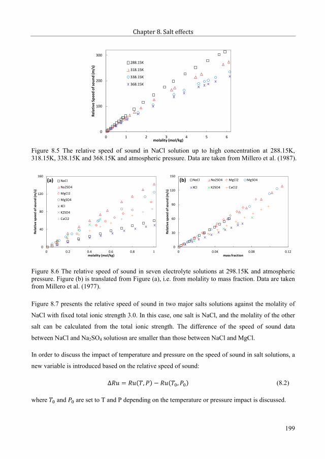
Chapter 8. Salt effects
Figure 8.5 The relative speed of sound in NaCl solution up to high concentration at 288.15K, 318.15K, 338.15K and 368.15K and atmospheric pressure. Data are taken from Millero et al. (1987).
Figure 8.6 The relative speed of sound in seven electrolyte solutions at 298.15K and atmospheric pressure. Figure (b) is translated from Figure (a), i.e. from molality to mass fraction. Data are taken from Millero et al. (1977).
Figure 8.7 presents the relative speed of sound in two major salts solutions against the molality of
NaCl with fixed total ionic strength 3.0. In this case, one salt is NaCl, and the molality of the other
salt can be calculated from the total ionic strength. The difference of the speed of sound data
between NaCl and Na2SO4 solutiosn are smaller than those between NaCl and MgCl.
In order to discuss the impact of temperature and pressure on the speed of sound in salt solutions, a
new variable is introduced based on the relative speed of sound:= ( , ) ( , ) (8.2)
where and are set to T and P depending on the temperature or pressure impact is discussed.
0
100
200
300
0 1 2 3 4 5 6
Rela
tive
Spee
d of
soun
d (m
/s)
molality (mol/kg)
288.15K
318.15K
338.15K
368.15K
0
40
80
120
160
0 0.2 0.4 0.6 0.8 1
Rela
tive
spee
d of
soun
d (m
/s)
molality (mol/kg)
(a) NaCl
Na2SO4
MgCl2
MgSO4
KCl
K2SO4
CaCl2
0
30
60
90
120
150
0 0.04 0.08 0.12
Rela
tive
spee
d of
soun
d (m
/s)
mass fraction
(b) NaCl Na2SO4 MgCl2 MgSO4
KCl K2SO4 CaCl2
199
215

Thermodynamic modeling of complex systems
Figure 8.8 shows the temperature and pressure dependence of relative speed of sound in NaCl
solution at different concentrations. It reveals that pressure and temperature, respectively, have
minor and moderate impacts on speed of sound.
Figure 8.7 The relative speed of sound in two major salts solutions against the molality of NaCl with fixed the total ionic strength 3.0. Data are taken from Millero et al. (1985b).
Figure 8.8 Temperature dependence of the speed of sound in NaCl solution (a) at molality 0.4906, 1.0399, 3.8718 and 6.1469 mol/kg at atmospheric pressure, minus that at 368.15K; (b) pressure dependence of the speed of sound at molality 0.010, 0.095, 0.502 and 0.999 mol/kg at 298.15K, minus that at atmospheric pressure. Data are from Chen et al (1978a) and Millero et al. (1987).
8.2.3 Static permittivity
Static permittivity plays a very important role in modeling the electrolyte solutions when the
primitive approach is used, and it depends on the temperature, molar density, electric dipole
moment and optical polarizability. Figure 8.9 (a) and (b) present the static permittivity of saturated
water and the binary mixtures of water with methanol and ethanol. It can be seen from Figure 8.9 (a)
90
120
150
180
0 1 2 3
Rela
tive
spee
d of
soun
d (m
/s)
molality of NaCl (mol/kg)
MgCl2
Na2SO4
MgSO4
0
20
40
60
80
298 318 338 358
Delta
spee
d of
soun
d (m
/s)
Temperature (K)
(a)
b=0.4906 b=1.0399
b=3.8718 b=6.1469
-4
-3
-2
-1
0
1
0 20 40 60 80 100
Delta
spee
d of
soun
d (m
/s)
Pressure (MPa)
(b)
b=0.010 b=0.095
b=0.502 b=0.999
200
216

Chapter 8. Salt effects
that, as expected, the static permittivity of saturated water decreases as the temperature increases. It
is known from Figure 8.9 (b) that the static permittivity of water is higher than that of methanol,
which is larger than that of ethanol. The static permittivity of these binary mixtures shows quite
linear dependence on mass fraction in a relative large concentration range, i.e. from 20% to 100%.
Figure 8.9 (a) Static permittivity of saturated water and (b) static permittivity of binary mixtures of water with methanol or ethanol. The experimental data are taken from NIST [REFPROP (2010)] and Åkerlöf (1932).
Figure 8.10 presents the static permittivity of NaCl solution at different temperatures. The static
permittivity decreases as the solution gets concentrated at constant temperature, but the temperature
dependence of the static permittivity at constant concentration is a bit more complex. The static
permittivity decreases as the temperature increases if the concentration is smaller than 3mol/L, and
temperature has very small impact on the static permittivity when the temperature is higher than
20C and the concentration is larger than 3.5mol/L.
Figure 8.10 Static permittivity of NaCl solution at different temperatures. The experimental data are taken from Buchner et al. (1999).
10
30
50
70
90
280 360 440 520 600
Stat
ic p
erm
ittiv
ity
Temperature (K)
(a)
static permittivity
15
35
55
75
0 20 40 60 80 100
Stat
ic p
erm
ittiv
ity
Mass fraction of water (%)
(b)
MEOH (20C) ETOH (20C)
MEOH (40C) ETOH (40C)
MEOH (60C) ETOH (60C)
40
50
60
70
80
90
0 1 2 3 4 5
Stat
ic p
erm
ittiv
ity
c (mol/L)
5C
20C
25C
35C
201
217

Thermodynamic modeling of complex systems
8.3 Static permittivity and association models
Very recently, Maribo-Mogensen et al. (2013a, 2013b) developed a method to model the static
permittivity with the association theory based equations of state. The key equation to connect the
static permittivity and the association theory is the following one:(2 + )( )( + 2) = 9 , (8.3)
where the variable is the Kirkwood g-factor, which is given by:
= 1 + + 1 ,, (8.4)
where is the possibility of two molecules to be bonded, and is given by definition:= 1 (8.5)
is the non-bonded site fraction, which can be directly calculated from association theory-based
equations of state.
The details can be found in the original articles of Maribo-Mogensen et al. (2013a, 2013b).
As discussed in the previous chapters, it is still an open question how to estimate the pure
component parameters for associating fluids using pure properties only. Here we are interested at
how to employ the static permittivity data in the parameter estimation by directly calculating the
free site fraction with this newly developed theory.
For pure component system, equation (8.3) could be rewritten as below: (2 + )( )( + 2) = 9 (8.6)
where can be calculated from the following equation:1+ 2 = 13 (8.7)
Equation (8.6) can be further arranged to be:
202
218

Chapter 8. Salt effects
= 1 (2 + )( )( + 2) 9(8.8)
While from the definition of Kirkwood g-factor, i.e. equation (8.4) and (8.5), we can get:
= 1 + × (1 ) × ( )(1 ) × ( ) + 1 (8.9)
It can be reformulated as:
(1 ) = 1( ) ( 1) ( ) (8.10)
This means that it is possible to calculate the free site fraction from experimental static permittivity
data, from equation (8.8) to (8.10), if the molecular structure information is known.
Let’s take water as an example, the component specific parameters are:= 1.855 , = 109.47°, = 69.4°, = 1.613 × 10 (8.11)
The calculated free site fractions are compared in Figure 8.11 with the experimental data [Luck
(1980, 1991)] and the PC-SAFT results using the newly developed parameters from Chapter 2. The
experimental density and static permittivity data are taken from NIST [REFPROP (2010)]. It can be
seen that the two calculated results are in good agreement with each other and both lower than the
experimental data.
Figure 8.11 The free site fractions of saturated water from experimental work of Luck (1980, 1991), equation (8.10), and the PC-SAFT EOS with the newly developed parameters from Chapter 2.
0
0.2
0.4
0.6
280 360 440 520 600
Free
site
frac
tion
Temperature (K)
Exp.
Calc. (eq. 8.10)
PCSAFT
203
219

Thermodynamic modeling of complex systems
When the free site fraction is known, it is possible to calculate the association strength for the pure
component with a given association scheme. As discussed in Chapter 2, 4C is possibly the best
association scheme option for water, and the association strength can be calculated as:
= 1 + 1 + 84 = 12 ( ) (8.12)
The calculated association strengths from static permittivity and experimental free site fraction data
[Luck (1980, 1991)] are compared in Figure 8.12 versus temperature. It is readily seen that the
association strengths calculated in this way show very good linear functions against reciprocal
temperature below certain temperature, i.e. 450K, and they show quite different qualitative behavior
above this temperature.
Figure 8.12 Association strength calculated from static permittivity of saturated water.Experimental data are from Luck (1980, 1991).
There are three ways to employ equation (8.12) in parameter estimation of associating fluids. The
first way is to assume the temperature dependence of the radial distribution function is weak enough
and ( ) 1 ( ). As seen from the definition of the association strength
(equation 2.19), the association energy could be read from the correlations 1500.4K from equation
(8.10) or 1971.8K from experimental data. It is known from Kontogeorgis et al (2010a) that the
experimental association energy is 1813K, so the association energy values from different sources
varies over a large range.1502 ( ) < 1704 ( ) < 1813 ( . ) < 1920 ( . 8.12) < 2003 ( )
= 1501.8/T - 12.212R² = 0.9998
ln( ) = 1920.4/T - 13.920R² = 0.9994
-12
-11
-10
-9
-8
-7
-6
0.0015 0.002 0.0025 0.003 0.0035 0.004Reciprocal temperature (1/K)
XA from r (eq. 8.10)
XA from Luck data
204
220

Chapter 8. Salt effects
For the given pure component parameters , , , the association volume parameter can be
directly calculated from the truncation values, so, in this way, there will only be three parameters
left for fitting.
The second way is to combine the radial distribution function into the association strength and to
assume ( ) 1 ( ), as follows:
= + (8.13)
where contains the contants and temperature-independent parameters.
During parameter estimation, the parameters and could be directly calculated by linear
regression as the other parameters are given, so there are also only three adjustable parameters left
for fitting in this way.
The third way does not introduce any assumptions, but employ equation (8.12) as an additional
constraint in the parameter estimation by using the experimental free site fraction data or calculating
the free site fraction from the experimental static permittivity data.
8.4 Conclusions
The salt effects on the solubility of hydrocarbons and the speed of sound in water have been briefly
discussed. The salts will decrease the solubility of hydrocarbons and increase the speed of sound in
water. The effects of salts are larger than the effects of temperature on the solubility of
hydrocarbons in water. The temperature and pressure have, respectively, moderate and minor
effects on the speed of sound in salt solutions.
Based on the newly developed theory of Maribo-Mogensen et al. (2013a, 2013b), the feasibility of
its usage in the parameter estimation has been discussed. With two simple approximations, there are
three adjustable parameters left for fitting, and the two association parameters could be directly
calculated before or during the parameter estimation. It has to be pointed out that the structure
information angle(s) is/are used as adjustable parameters in the works of Maribo-Mogensen et al.
(2013a, 2013b), and it is a question if the structure is stable over wide ranges of temperature and
pressure, so more systematic experimental investigations are needed, and quantum chemistry
computations would also provide valuable information on the aspects of molecular structure.
205
221

Thermodynamic modeling of complex systems
206
222

Chapter 9. Conclusions and future work
9.1 Conclusions
This PhD project belongs to a broader project which was initiated because of the oil spill in the Gulf
of Mexico. The main purpose of the broader project is to integrate thermodynamic models into
sophisticated mathematic modelings, from which a self-learning loop is constructed together with
the-state-of-the-art sonar products. This advanced self-learning technology can be used to detect
subsea targets. The most important properties from the thermodynamic models are speed of sound,
solubility and density of oil-seawater systems.
From the viewpoint of knowledge exploration, this thesis is about the capabilities and limitations of
the PC-SAFT framework, from the studies on phase behavior, speed of sound and fundamentals.
9.1.1 Phase behavior
Firstly, we have answered the question of which association scheme is a better choice for water
within the PC-SAFT framework, and have developed an interactive step-wise optimization
procedure, having a global character via a rather manual way, to estimate the model parameters for
associating fluids by taking the liquid-liquid equilibrium data into account. The same procedure has
been used for methanol and mono-ethylene-glycol (MEG). These newly estimated parameters have
been applied to the phase equilibrium modeling of systems containing water, hydrocarbons and/or
chemicals. Satisfactory results have been obtained when compared to calculations using other
parameters or models. It has also been found that the parameters of methanol estimated with speed
of sound data in consideration show equally good performance as the parameters obtained by the
abovementioned procedure. These parameters and the corresponding binary interaction parameters
(schemes) provide solid basis for modeling oil-water-chemical systems.
Secondly, in order to apply PC-SAFT into petroleum fluids, we have performed a comprehensive
analysis on developing simple and reliable parameter estimation methods for ill-defined systems.
The results show that the general characterization procedures and the number of pseudo-
components give quite similar influence as for the traditional cubic EOS. The paraffinic-
naphthenic-aromatic (PNA) estimation methods show quite different performance, so care should
207
223

Thermodynamic modeling of complex systems
be excercised when the PNA estimation is directly used in producing the PC-SAFT parameters. The
binary interaction parameters between C1 and C2 to C6, in general, have small impacts on predicting
the saturation pressure, while the binary interaction parameter between C1 and C7+ shows quite
significant influence on individual cases. From an overall point of view, however, different binary
interaction schemes between C1 and C7+ give similar deviations for an oil databank considered in
this project, so a compromise method has been proposed to combine the best results of each case,
by using linear correlations for m and m /k, and fitting the remaining parameter to specific
gravity. Two candidate methods, including the compromise one, have been used to model the oil-
water-chemical systems.
Finally, the overall modeling results of oil-water-chemical systems, with the estimated parameters
of water and chemicals and proposed characterization methods, are quite satisfactory, if compared
to the results using the avialble parameters and/or models in the literature, The two characterization
methods give similar prediction from the quantitative point of view, but they produce different
parameters, which lead to some systematic differences. The results reveal that the approach used in
the compromise method is more attractive.
9.1.2 Speed of sound
Firstly, we have collected and reviewed the experimental speed of sound data of pure compounds
(hydrocarbons and 1-alcohols), binary systems (hydrocarbon + hydrocarbon, hydrocarbon + 1-
alcohol, and 1-alcohol + 1-alcohol), ternary hydrocarbons with or without 1-alcohol, and petroleum
fluids. The conclusions are that speed of sound could be measured with very high accuracy, though
small inconsistencies have been seen for some systems. The NIST reference models represent the
speed of sound in most pure fluids, i.e. hydrocarbons and 1-alcohols available in the database, quite
satisfactorily, but some deviations are seen for normal hexane and cyclo-hexane, depending on the
temperature and pressure ranges. The correlations of speed of sound in different systems are also
reviewed, and a single expression has been used to correlate the speed of sound in pure
hydrocarbons and pure 1-alcohols.
Secondly, two approaches were proposed to improve the speed of sound description within the PC-
SAFT framework. The first approach is to use the speed of sound data in the pure component
parameter estimation, and the second approach is to firstly readjust the universal constants using the
speed of sound data of saturated methane to decane, and then fit the pure component parameters
208
224

Chapter 9. Conclusions and future work
with vapor pressure, liquid density and speed of sound. These two approaches have been evaluated
for the previously reviewed systems. The results show that the first approach works only for small
associating fluids, due to the two extra association parameters, where the association term plays a
very important role, while the second approach significantly improves the description of the speed
of sound from both qualitative and quantitative points of view. Further investigations show that the
second approach could give equally good phase equilibria for the considered systems, but it would
deteriorate the density, especially for the systems containing long-chain molecules.
9.1.3 Fundamentals
The investigations of the temperature and density dependences of PC-SAFT reveal that the sixth
polynomials are sufficient to represent the reduced density dependence, while the temperature
dependence of the model is only valid at low density region or in a narrow range of temperature,
with the given pure component parameters.
Following a similar procedure as that with the modeling of speed of sound, a new variant of the 42
universal constants has been developed with focus on vapor pressure and density. The results show
that the new variant performs better than the original one for the vapor pressure, speed of sound and
dP/dV, similar on density and heat capacities, but worse for the Joule-Thomson coefficients. The
new universal constants give only three volume roots where the original ones show four or five
volume roots, and more surprisingly, the new universal constants have almost completely avoided
the most criticized issue, i.e. presence of more than three volume roots, in the real application range.
Further investigations reveal that it is possible to directly apply the new universal constants into the
systems considered in this PhD thesis without changing the model parameters and even the binary
interaction parameter.
9.2 Future work
There is a clear degeneracy of the five pure component parameters for associating fluids during the
parameter estimation. The approach of considering the liquid-liquid equilibrium data with inert
compound in the parameter estimation works well for the phase behavior of the investigated water
and/or mono-ethylene glycol systems, but its performance must be further investigated for other
systems or properties. Putting speed of sound data in the parameter estimation of short-chain 1-
alcohols improved the overall description, but does not work for long-chain 1-alcohols. It is still an
open question how to develop a general parameter estimation procedure for all 1-alochols. In
209
225

Thermodynamic modeling of complex systems
Chapter 8, it is pointed out that, by applying the newly developed theory of calculating static
permittivity from association theory based EOS, it is possible to fit only three or four pure
component parameters for associating fluids with the given molecular structure, and to calculate the
remaining parameters by using the experimental static permittivity data as input. But more
systematic experimental investigations and/or quantum chemistry computations are needed to
provide valuable information on the molecular structure, of which the monomer fractions or free
site fractions of systems under consideration are extremely important.
Comprehensive analysis has been conducted on developing general oil characterization approaches
for PC-SAFT. It is recommended to evaluate these approaches for routine PVT simulations over
wide ranges of temperature, pressure and composition, phase equilibrium of oil and water, gas
injections and asphaltene modeling. This could help developing even simpler and more robust
characterization procedures, and then facilitate the acceptance of PC-SAFT in the upstream oil
industry.
A new variant of the 42 universal constants has been developed with focus on vapor pressure and
density. It has been shown that the new universal constants have practically avoided the most
criticized numerical pitfalls, i.e. existence of more than three volume roots. In the meantime,
equally good performance of phase behavior modeling has been obtained. It is recommended to
extensively evaluate the new universal constants for various systems over wide ranges of
temperature and pressure.
It would be very interesting to investigate what kind of fundamental changes could make the PC-
SAFT framework sufficient enough to represent the temperature dependence of the Helmholtz free
energy, e.g. residual isochoric heat capacity, speed of sound and Joule-Thomson coefficients
simultaneously. An even more challenging problem is how to model the special properties of water,
e.g. maximum points for density, speed of sound and isothermal compressibility versus temperature.
210
226

Reference
Reference
[1]. Abida, A.; Nain, A.K.; Hyder, S. J. Sol. Chem. 32 (2003) 865-877.
[2]. Al-Ajmi, M.F.; Tybjerg, P.; Rasmussen, C.P.; Azeem, J. SPE Middle East Oil and Gas Show
and Conference, Manama, Bahrain, Sep. 25-28, 2011, (SPE 141241).
[3]. Albo, P.A.G.; Lago, S.; Romeo, R.; Lorefice, S. J. Chem. Thermodyn. 58 (2013) 95-100.
[4]. Aparicio-Martínez, S.; Hall, K.R. Fluid Phase Equilib. 254 (2007) 112-125.
[5]. Automatic Leak Detection Sonar, Sonardyne. http://www.sonardyne.com/ (accessed June 2012).
[6]. Avila, S.; Blanco, S.T.; Velasco, I.; Rauzy, E.; Otín, S. Energy & Fuels, 16 (2002) 928-934.
[7]. Avlund, A.S. Extension of Association Models to Complex Chemicals. PhD Dissertation,
Technical University of Denmark, Kgs. Lyngby, Denmark, 2011.
[8]. Badalyan, A.L.; Otpuschennikov, N.F. Izv. Akad. Nauk. SSSR, Fiz. Zemli. 6 (1971) 207.
[9]. Baidakov, V.G.; Kaverin, A.M.; Skripov, V.P. J. Chem. Thermodyn. 14 (1982) 1003-1010.
[10]. Ball, S.J.; Trusler, J.P.M. Int. J. Thermophys. 22 (2001) 427-443.
[11]. Ball, S.J.; Goodwin, A.R.H.; Trusler, J.P.M. J. Petro. Sci. Eng. 34 (2002) 1-11.
[12]. Barker, J.A.; Henderson, D. J. Chem. Phys. 47 (1967) 2856-2861.
[13]. Barreau, A.; Gaillard, K.; Behar, E.; Daridon, J.L.; Lagourette, B.; Xans. P. Fluid Phase
Equilib. 127 (1997) 155-171.
[14]. Batzle, M.; Wang, Z.J. Geophysics 57 (1992) 1396-1408.
[15]. Benedetto, G.; Gavioso, R.M; Albo, P.A.G.; Lago, S.; Ripa, D.M.; Spagnolo, R. Int. J.
Thermophys. 26 (2005) 1667-1680.
[16]. Benson, G.C.; Handa, Y.P. J. Chem. Thermodyn. 13 (1981) 887-896.
[17]. Beregovykh, V.V.; Timofeev, V.S.; Lukyanova, R.N. Uch. Zap. Mosk. Inst. Tonkoi Khim.
Tekhol. 1 (1971) 31-38.
[18]. Bessieres, D.; Saint-Guirons, H.; Daridon, J.L. High Press. Res. 18 (2000a), 279.
[19]. Bessieres, D.; Saint-Guirons, H.; Daridon, J.L. J. Therm. Anal. Calorim. 62 (2000b) 621.
[20]. Bilaniuk, N.; Wong, G.S.K. J. Acoust. Soc. Am. 93 (1993) 1609-1612.
[21]. Blandamer, M.J.; Davis, M.I.; Douhéret, G.; Reis, J.C.R. Chem. Soc. Rev. 30 (2001) 8-15.
[22]. Blas, F.J.; Vega, L.F. Mol. Phys. 92 (1997) 135.
[23]. Blas, F.J.; Vega, L.F. Ind. Eng. Chem. Res. 37 (1998) 660.
211
227

Thermodynamic modeling of complex systems
[24]. Bobik, M. J. Chem. Thermodyn. 10 (1978) 1137-1146.
[25]. Boelhouwer, J.W.M. Physica. 34 (1967) 484-492.
[26]. Bolotnikov, M.F.; Verveyko, V.N.; Verveyko, M.V. J. Chem. Eng. Data, 49 (2004) 631-634.
[27]. Bolotnikov, M.F.; Neruchev, Y.A.; Melikhov, Y.F.; Verveyko, V.N.; Verveyko, M.V. J.
Chem. Eng. Data, 50 (2005) 1095-1098.
[28]. Boublik, T. Collect. Czech. Chem. Commun. 25 (1960) 285-287.
[29]. Brown W.B.; Gee, G.; Taylor, W.D. Polymer, 5 (1964) 362-367.
[30]. Buchner, R.; Hefter, G.T.; May, P.M. J. Phys. Chem. A, 103 (1999) 1-9.
[31]. Butler, J. A.V.; Thomson, D.W.; Maclennan, W.H. J. Chem. Soc. 1933, 674-686.
[32]. Calvar, N.; González, B.; Gómez, E.; Canosa, J. J. Chem. Eng. Data, 54 (2009a) 1334-1339.
[33]. Calvar, N.; Gómez, E.; González, B.; Domínguezm, Á. J. Chem. Thermodyn. 41 (2009b)
939-944.
[34]. Cameretti, L.F.; Sadowski, G.; Mollerup, J.M. Ind. Eng. Chem. Res. 44 (2005) 3355-3362.
[35]. Cameretti, L.F.; Sadowski, G. Chem. Eng. Process. 47 (2008) 1018-1025.
[36]. CERE Internal Databank, Technical University of Denmark, 2013.
[37]. Chapman, W.G.; Jackson, G.; Gubbins, K.E. Mol. Phys. 65 (1988) 1057-1079.
[38]. Chapman, W.G.; Gubbins, K.E.; Jackson, G.; Radosz, M. Ind. Eng. Chem. Res. 29 (1990)
1709-1721.
[39]. Chapoy, A.; Mohammadi, A.H.; Richon, D.; Tohidi, B. Fluid Phase Equilib. 220 (2004) 113-
121.
[40]. Chapoy, A.; Coquelet, C.; Richon, D. Fluid Phase Equilib. 230 (2005a) 210-214.
[41]. Chapoy, A.; Mohammadi, A.H.; Tohidi, B.; Richon, D. J. Chem. Eng. Data, 50 (2005b)
1157-1161.
[42]. Chávez, M.; Palaclos, J.M.; Tsumura, E. J. Chem. Eng. Data, 27 (1982) 350-351.
[43]. Chávez, M.; Sosa, V.; Tsumura, R. J. Acoust. Soc. Am. 77 (1985) 420-423.
[44]. Chen, C.T.; Millero, F.J. J. Acoust. Soc. Am. 62 (1977) 1129-1135.
[45]. Chen, C.T.; Chen, L.S.; Millero, F.J. J. Acoust. Soc. Am. 63 (1978a) 1795-1800.
[46]. Chen, C.T.; Millero, F.J.; J. Marine. Res. 36 (1978b) 657-691.
[47]. Chorazewski, M.; Dzida, M.; Zorebski, E.; Zorebski, M. J. Chem. Thermodyn. 58 (2013)
389-397.
[48]. Chiavone-Filho, O.; Proust, P.; Rasmussen, P. J. Chem. Eng. Data, 38 (1993) 128-131.
[49]. Clark, G.N.I.; Haslam, A.J.; Galindo, A.; Jackson, G. Mol. Phys. 104 (2006) 3561-3581.
212
228

Reference
[50]. Coan, C.R.; King, A.D. J. Am. Chem. Soc. 93 (1971) 1857-1862.
[51]. Culberson, O.L.; Mcketta, J.J. Trans. AMIE. 189 (1950) 319-322.
[52]. Culberson, O.L.; Mcketta, J.J. Trans. AMIE. 192 (1951) 223-226.
[53]. Daridon, J.L.; Lagourette, B.; Xans, P. Fluid Phase Equilib. 100 (1994) 269-282.
[54]. Daridon, J.L.; Lagourette, B.; Labes, P. Int. J. Thermophys. 17 (1996a) 851-871.
[55]. Daridon, J.L.; Lagourette, B.; Gaubert, J.F.; Xans, P.; Montel, F. Ultrasonics, 34 (1996b)
447-449.
[56]. Daridon, J.L.; Lagourette, B.; Grolier, J.P.E. Int. J. Thermophys. 19 (1998a) 145-160.
[57]. Daridon, J.L.; Lagrabette, A.; Lagourette, B. J. Chem. Thermodyn. 30 (1998b) 607-623.
[58]. Daridon, J.L.; Lagourette, B.; Xans, P.; Montel, F. J. Petroleum Sci. Eng. 19 (1998c) 281-
293.
[59]. Daridon, J.L.; Lagourette, B.; Lagrabette, A. Phys. Chem. Liq. 37 (1999) 137-160.
[60]. Daridon, J.L.; Lagourette, B. High Temp. - High Pressures. 32 (2000) 83-87.
[61]. Daridon, J.L.; Pauly, J.; Coutinho, J.A.P.; Montel, F. Energy & Fuels, 15 (2001) 730-735.
[62]. Daridon, J.L.; Carrier, H.; Lagourette, B. Int. J. Thermophys. 23 (2002) 697-708.
[63]. Davies, L.A.; Gil-Villegas, A.; Jackson, G. Int. J. Thermophys. 19 (1998), 675-686.
[64]. Davis, L.A.; Gordon, R.B. J. Chem. Phys. 46 (1967) 2650-2660.
[65]. de Hemptinne, J. C.; Ledanois, J. M.; Mougin, P.; Barreau, A. Select Thermodynamic Models
for Process Simulation. Editions Technip: Paris, France, 2012.
[66]. de Villiers, A. J. Evaluation and improvement of the sPC-SAFT equation of state for complex
mixtures. PhD Dissertation, Stellenbosch University, Stellenbosch, South Africa, 2011.
[67]. de Villiers, A.J.; Schwarz, C.E.; Burger A.J.; Kontogeorgis, G.M. Fluid Phase Equilib. 338
(2013) 1-15.
[68]. Deak, A.; Victorov, A.I.; de Loos, Th.W. Fluid Phase Equilib. 107 (1995) 277-301.
[69]. Deepwater Horizon oil spill, http://en.wikipedia.org/wiki/Deepwater_Horizon_oil_spill,
(accessed June 2014).
[70]. Del Grosso, V.A.; Mader, C.W. J. Acoust. Soc. Am. 52 (1972a) 961-974.
[71]. Del Grosso, V.A.; Mader, C.W. J. Acoust. Soc. Am. 52 (1972b) 1442-1446.
[72]. Derawi, S.O.; Kontogeorgis, G.M.; Stenby, E.H.; Haugum, T.; Fredheim, A.O. J. Chem. Eng.
Data, 47 (2002) 169-173.
[73]. Dhima, A.; de Hemptinne, J.C.; Moracchini, G. Fluid Phase Equilib. 145 (1998) 129-150.
[74]. Diamantonis, N. I.; Economou, I. G. Energy & Fuels, 25 (2010) 3334.
213
229

Thermodynamic modeling of complex systems
[75]. Ding, Z.S.; Alliez, J.; Boned, C.; Xans, P. Meas. Sci. Technol. 8 (1997) 154-161.
[76]. DIPPR Database, Design Institute for Physical Property Data; DIADEM, Information and
Data Evaluation Manager, version 6.0.1, 2012.
[77]. Douhéret, G.; Davis, M.I.; Reis, J.C.R. “The measurements, interpretation and prediction of
speeds of sound in liquids and liquid mixtures” Focus on Lasers and Electro-Optics Research
(Ed by W.T. Akin), Nova Science, Hauppauge, NY, 2004.
[78]. Dovnar, D.V.; Lebedinskii, Y.A.; Khasanshin, T.S.; Shchemelev, A.P. High Temperature, 39
(2001) 835-839.
[79]. Dubey, G.P.; Sharma, M. Int. J. Thermophys. 29 (2008a) 1361-1375.
[80]. Dubey, G.P.; Sharma, M. J. Chem. Eng. Data, 53 (2008b) 1032-1038.
[81]. Dubey, G.P.; Sharma, M.; Dubey, N. J. Chem. Thermodyn. 40 (2008c) 309-320.
[82]. Dubey, G.P.; Sharma, M. J. Chem. Thermodyn. 40 (2008d) 991-1000.
[83]. Dubey, G.P.; Sharma, M. J. Mol. Liq. 142 (2008e) 124-129.
[84]. Dubey, G.P.; Sharma, M. J. Mol. Liq. 143 (2008f) 109-114.
[85]. Durackova, S., Apostolo, M.; Canegallo, S.; Morbidelli, M. J. Appl. Polym. Sci. 57 (1995)
639-644.
[86]. Dutour, S.; Daridon, J.L.; Lagourette, B. Int. J. Thermophys. 21 (2000) 173-184.
[87]. Dutour, S.; Daridon, J.L.; Lagourette, B. High Temp. - High Pressures. 33 (2001a) 371-378.
[88]. Dutour, S.; Lagourette, B.; Daridon, J.L. J. Chem. Thermodyn. 33 (2001b) 765-774.
[89]. Dutour, S.; Lagourette, B.; Daridon, J.L. J. Chem. Thermodyn. 34 (2002) 475-484.
[90]. Dzida, M.; Ernst, S. J. Chem. Eng. Data, 48 (2003) 1453-1457.
[91]. Dzida, M.; Zak, A.; Ernst, S. J. Chem. Thermodyn. 37 (2005) 405-414.
[92]. Dzida, M. J. Chem. Eng. Data, 52 (2007) 521-531.
[93]. Dzida, M.; Cempa, M. J. Chem. Thermodyn. 40 (2008) 1531-1541.
[94]. Dzida, M. J. Chem. Eng. Data, 54 (2009a) 1034-1040.
[95]. Dzida, M. J. Phys. Chem. B 113 (2009b) 11649-11661.
[96]. Elsharkawy, A.M. J. Petro. Sci. Eng. 38 (2003) 57-77.
[97]. Ekiner, O.; Thodos, G. J. Chem. Eng. Data, 11 (1966) 457-460.
[98]. Ekiner, O.; Thodos, G. J. Chem. Eng. Data, 13 (1968) 304-306.
[99]. Estrada-Alexanders, A.F.; Trusler, J.P.M.; Zarari, M.P. Int. J. Thermophys. 16 (1995) 663-
667.
[100]. Estrada-Alexanders, A.F.; Trusler, J.P.M. J. Chem. Thermodyn. 29 (1997) 991-1015.
214
230

Reference
[101]. Etter, D.O.; Kay, W.B. J. Chem. Eng. Data, 6 (1961) 409-414.
[102]. Faradonbeh, M. R.; Abede, J.; Harding, T. G. Can. J. Chem. Eng. 91 (2013) 101-110.
[103]. Folas, G.K.; Gabrielsen, J.; Michelsen, M.L.; Stenby, E.H.; Kontogeorgis, G.M. Ind. Eng.
Chem. Res. 44 (2005) 3823-3833.
[104]. Folas, G.K.; Berg, O.J.; Solbraa, E.; Fredheim, A.O.; Kontogeorgis, G.M.; Michelsen, M.L.;
Stenby, E.H. Fluid Phase Equilib. 251 (2007) 52-58.
[105]. Formann, J.C.; Thodos, F. AIChE J. 8 (1962) 209-213.
[106]. Frost, M.; Karakatsani, E.; von Solms, N.; Richon, D.; Kontogeorgios, G.M. J. Chem. Eng.
Data, 59 (2014) 961-967.
[107]. Frost, M.; Kontogeorgis, G.M.; Stenby, E.H.; Yussuf, M.A.; Haugum, T.; Christensen, K.O.;
Solbraa, E.; Løkken, T.V. Fluid Phase Equilib. 340 (2013) 1-6.
[108]. Fujii, K.I.; Masui, R. J. Acoust. Soc. Am. 93 (1993) 276-282.
[109]. Galindo, A.; Davies, L. A.; Gil-Villegas, A.; Jackson, G. Mol. Phys. 93 (1998) 241-252.
[110]. Galivel-Solastiouk, F.; Laugier, S.; Richon, D. Fluid Phase Equilib. 28 (1986) 73-85.
[111]. Gammon, B.E.; Douslin, D.R. J. Chem. Phys. 64 (1976) 203-218.
[112]. Gapta, R. B.; Johnston, K. P. Fluid Phase Equilib. 99 (1994) 135-151.
[113]. Gayol, A.; Iglesias, M.; Goenaga, J.M.; Concha, R.G.; Resa, J.M. J. Mol. Liq. 135 (2007)
105-114.
[114]. Gepert, M.; Ernst, S. J. Sol. Chem. 32 (2003) 831-852.
[115]. Gepert, M.; Stachowska, B. J. Sol. Chem. 35 (2006) 425-454.
[116]. Ghasemi, M.; Alavian, S.A.; Whitson, C.H. SPE Heavy Oil Conference and Exhibition held
in Kuwait City, Kuwait, Dec. 12-14, 2011 (SPE 148906)
[117]. Gil-Villegas, A.; Galinda, A.; Whitehead, P.J.; Mills, S.J.; Jackson, G.; Burgess, A.N. J.
Chem. Phys. 106 (1997) 4168-4186.
[118]. Glanville, J.W.; Sage, B.H.; Lacey, W.N. Ind. Eng. Chem. 42 (1950) 508-513.
[119]. Gonzalez, M.H.; Lee, A.L. J. Chem. Eng. Data, 13 (1968) 172-176.
[120]. Gonzaléz, D.L. Modeling of Asphaltene Precipitation and Deposition Tendency using the
PC-SAFT Equation of State. PhD Thesis, Rice University, 2008.
[121]. Goodwin, A. R. H. Method and apparatus for measuring fluid density downhole. U.S.
Patent 6640625, 2003.
[122]. J. Phys. Chem. Ref. Data, 31
(2002) 701-748.
215
231

Thermodynamic modeling of complex systems
[123]. Gracia, M.; Sánchez, F.; Pérez, P.; Valero, J.; Losa, C.G. J. Chem. Thermodyn. 24 (1992)
843-849.
[124]. Gregorowicz, J.; O'Conell, J.P.; Peters, C.J. Fluid Phase Equilib. 116 (1996) 94-101.
[125]. Grenner, A.; Schmelzer, J.; von Solms, N.; Kontogeorgis, G.M. Ind. Eng. Chem. Res. 45
(2006) 8170-8179.
[126]. Grenner, A.; Kontogeorgis, G.M.; von Solms, N.; Michelsen, M.L. Fluid Phase Equilib.
258 (2007a) 83-94.
[127]. Grenner, A.; Kontogeorgis, G.M.; Michelsen, M.L.; Folas, G.K. Mol. Phys. 105 (2007b)
1797-1801.
[128]. Grenner, A.; Tsivintzelis, I.; Economou, I.G.; Panayiotou, C.; Kontogeorgis, G.M. Ind. Eng.
Chem. Res. 47 (2008) 5636-5650.
[129]. Griswold, J.; Wong, S. Y. Chem. Eng. Prog. Symp. Ser. 48 (1952) 18-34.
[130]. Gross, J.; Sadowski, G. Ind. Eng. Chem. Res. 40 (2001) 1244-1260.
[131]. Gross, J.; Sadowski, G. Ind. Eng. Chem. Res. 41 (2002) 5510-5515.
[132]. Guedes, H.J.R.; Zollweg, J.A. Int. J. Refrigeration, 15 (1992) 381-385.
[133]. Handa, Y.P.; Halpin, C.J.; Benson, G.C. J. Chem. Thermodyn. 13 (1981) 875-886.
[134]. Hasanov, V.H. High Temperatures, 50 (2012) 44-51.
[135]. Hauptamann, P.; Hoppe, N.; Püttmer, A. Meas. Sci. Technol. 13 (2002) 73-83.
[136]. Hawley, S.; Allegra, J.; Holton, G. J. Acoust. Soc. Am. 47 (1970) 137-142.
[137]. He, C.C.; Li, J.L.; Peng, C.J.; Liu, H.L.; Hu, Y. Fluid Phase Equilib. 302 (2011) 139-152.
[138]. Heintz, A.; Dolch, E.; Lichtenthaler, R.N. Fluid Phase Equilib. 27 (1986) 61-79.
[139]. Held, C.; Neuhaus, T.; Sadowski, G. Biophys. Chem. 152 (2010) 28-39.
[140]. Held, C.; Cameretti, L. F.; Sadowski, G. Ind. Eng. Chem. Res. 50 (2011) 131-141.
[141]. Held, C.; Reschke, T.; Müller, R.; Kunz, W.; Sadowski, G. J. Chem. Thermodyn. 68 (2014)
1-12.
[142]. Held, C.; Sadowski, G.; Carneiro, A.; Rodríguez, O.; Macedo E.A. AIChE J. 59 (2013)
4794-4805.
[143]. Hong, J.H.; Malone, P.V.; Jett, M.D.; Kobayashi, R. Fluid Phase Equilib. 38 (1987) 83-96.
[144]. Huang, S. H.; Radosz, M. Ind. Eng. Chem. Res. 29 (1990) 2284-2294.
[145]. Huang, S. H.; Radosz, M. Ind. Eng. Chem. Res. 30 (1991) 1994-2005.
216
232

Reference
[146]. Hustad, O.S.; Jia, N.J.; Pedersen, K.S.; Memon, A.; Leekumjorn, S. SPE Annual Technical
Conference and Exhibition, New Orleans, Louisiana, USA. Sep. 30 – Oct. 2, 2013 (SPE
166097).
[147]. IOC, SCOR and IAPSO, 2010: The international thermodynamic equation of seawater –
2010: Calculation and use of thermodynamic properties. Intergovernmental Oceanographic
Commission, Manuals and Guides No.56, UNESCO.
[148]. Ixtoc I oil spill, http://en.wikipedia.org/wiki/Ixtoc_I_oil_spill (accessed June 2014).
[149]. Jackson, G.; Chapman, W.G.; Gubbins, K.E. Mol. Phys. 65 (1988) 1-31.
[150]. Jaubert, J.N.; Avaullee, L.; Souvay, J.F. J. Petro. Sci. Eng. 34 (2002) 65-107.
[151]. Junquera, E.; Tardajos, G.; Aicart. E. J. Chem. Thermodyn. 20 (1988) 1461-1467.
[152]. Kesler, M.G.; Lee, B.I. Hydrocarbon Processing, 55 (1976) 153-158.
[153]. Khammar, M.; Shaw, J.M. Fluid Phase Equilib. 288 (2010) 145-154.
[154]. Khasanshin, T.S. High Temperature, 29 (1992) 554-559.
[155]. Khasanshin, T.S.; Shchemelev, A.P. High Temp. – Hihg Pressures, 32 (2000) 663-668.
[156]. Khasanshin, T.S.; Shchemelev, A.P. High Temperature, 39 (2001) 60-67.
[157]. Khasanshin, T.S.; Shchemelev, A.P. High Temperature, 40 (2002) 207-211.
[158]. Khasanshin, T.S.; Shchamialiou, A.P.; Poddubskij, O.G. Int. J. Thermophys. 24 (2003)
1277-1289.
[159]. Khasanshin, T.S.; Shchamialiou, O.G.A.P.; Samuilov, V.S. Fluid Phase Equilib. 245 (2006)
26-31.
[160]. Khasanshin, T.S.; Samuilov, V.S.; Shchemelev, A.P. J. Eng. Phys. Thermophys. 82 (2009)
149-156.
[161]. Kiyohara, O.; Benson, G.C. J. Chem. Thermodyn. 11 (1979) 861-873.
[162]. Kleiner, M. Thermodynamic Modeling of Complex Systems: Polar and Associating Fluids
and Mixtures. PhD Dissertation, Technical University of Dortmund, Dortmund, Germany, 2008.
[163]. Kontogeorgis, G.M.; Voutsas, E.C.; Yakoumis, I.V.; Tassios, D.P. Ind. Eng. Chem. Res. 35
(1996) 4310-4318.
[164]. Kontogeorgis, G.M.; Yakoumis, I.V.; Meijer H.; Hendriks, E.; Moorwood, T. Fluid Phase
Equilib. 158-160 (1999) 201-209.
[165]. Kontogeorgis, G.M.; Michelsen, M.L.; Folas, G.K.; Derawi, S.; Von Solms, N.; Stenby, E.H.
Ind. Eng. Chem. Res. 45 (2006a) 4855-4868.
217
233

Thermodynamic modeling of complex systems
[166]. Kontogeorgis, G.M.; Michelsen, M.L.; Folas, G.K.; Derawi, S.; Von Solms, N.; Stenby, E.H.
Ind. Eng. Chem. Res. 45 (2006b) 4869-4878.
[167]. Kontogeorgis, G.M; Folas, G. K. Thermodynamic models for industrial applications – from
classical and advanced mixing rules to association theories. John Wiley and Sons: New York,
(2010a).
[168]. Kontogeorgis, G.M.; Tsivintzelis, I.; von Solms, N.; Grenner, A.; Bøgn, D.; Frost, M.;
Knage-Rasmussen, A.; Economou, I.G. Fluid Phase Equilib. 296 (2010b) 219-229.
[169]. Kontogeorgis, G.M.; Tsivintzelis, I.; Michelsen, M.L.; Stenby, E.H. Fluid Phase Equilib.
301 (2011) 244-256.
[170]. Kortbeek, P.J.; Schouten, J.A. Int. J. Thermophys. 11 (1990) 455-466.
[171]. Kouskoumvekaki, I.A.; von Solms, N.; Michelsen, M.L.; Kontogeorgis, G.M. Fluid Phase
Equilib. 215 (2004) 71-78.
[172]. Kroebel, W.; Mahrt, K.H. Acustica, 35 (1976) 154-164.
[173]. Kumar, A. J. Chem. Eng. Data, 48 (2003) 388-391.
[174]. Kurihara, K.; Minoura, T.; Takeda, K.; Kojima, K. J. Chem. Eng. Data, 40 (1995) 679-684.
[175]. Kurihara, K.; Midorikawa, T.; Hashimoto, T.; Kojima, K.; Ochi, K. J. Chem. Eng. (of
Japan), 35 (2002) 360-364.
[176]. Kushare, S.K.; Kolhapurkar, R.R.; Dagade, D.H.; Patil, K.J. J. Chem. Eng. Data, 51 (2006)
1617-1623.
[177]. Labes, P.; Daridon, J.L.; Lagourette, B.; Saint-Guirons, H. Int. J. Thermophys. 15 (1994)
803-819.
[178]. Lafitte, T.; Bessieres, D.; Pineiro, M. M.; Daridon, J. L. J. Chem. Phys. 124 (2006) 024509
(1-16).
[179]. Lafitte, T.; Pineiro, M.M.; Daridon, J.L.; Bessieres, D.A. J. Phys. Chem. B. 111 (2007)
3447-3461.
[180]. Lafitte, T.; Apostolakou, A.; Avendaño, C.; Galindo, A.; Adjiman, C.S.; Müller, E.A.;
Jackson, G. J. Chem. Phys. 139 (2013) 154504-154537.
[181]. Lago, S.; Albo, P.A.G; Ripa, D.M. Int. J. Thermophys. 27 (2006) 1083-1094.
[182]. Lagourette, B.; Daridon, J.L.; Gaubert, J.F.; Xans, P. J. Chem. Thermodyn. 26 (1994)
1051-1061.
[183]. Lagourette, B.; Daridon, J.L.; Gaubert, J.F.; Saint-Guiron, H. J. Chem. Thermodyn. 27
(1995) 259-266.
218
234

Reference
[184]. Lagourette, B.; Daridon, J.L. J. Chem. Thermodyn. 31 (1999) 987-1000.
[185]. Lainez, A.; Gopal, P.; Zollweg, J.A.; Streett, W.B. J. Chem. Thermody. 21 (1989) 773-777.
[186]. Lainez, A.; Zollweg, J.A.; Streett, W.B. J. Chem. Thermodyn. 22 (1990) 937-948.
[187]. Lampreia, I.M.S.; Mendonca, A.F.S.S. Meas. Sci. Technol. 16 (2005) 2391-2395.
[188]. Lee, B.I.; Kesler, M.G. AIChE J. 21 (1975) 510-527.
[189]. Lee, L.L.; Scheller, W.A. J. Chem. Eng. Data, 12 (1967) 497-499.
[190]. Leekumjorn, S.; Krejbjerg, K. Fluid Phase Equilib. 359 (2013) 17-23.
[191]. Lekvam, K.; Bishnoi, P.R. Fluid Phase Equilib. 131 (1997) 297-309.
[192]. Letcher, T.M.; Wootton, S.; Shuttleworth, B.; Heyward, C. J. Chem. Thermodyn. 18 (1986)
1037-1042.
[193]. Lev, A.D.; Robinson, D.B.; Chung, S.Y.K.; Chen, C.J. Can. J. Chem. Eng. 70 (1992) 330-
334.
[194]. Li, J.L.; He, H.H.; Peng, C.J.; Liu, H.L.; Hu, Y. Fluid Phase Equilib. 276 (2009) 57-68.
[195]. Liang, X.D.; Thomsen, K.; Yan, W.; Kontogeorgis, G.M. Fluid Phase Equilib. 360 (2013)
222-232.
[196]. Liang, X.D.; Maribo-Mogensen, B.; Thomsen, K.; Yan, W.; Kontogeorgis, G.M. Ind. Eng.
Chem. Res. 51 (2012) 14903-14914.
[197]. Liang, X.D.; Tsivintzelis, I.; Kontogeorgis, G.M. Ind. Eng. Chem. Res. 53 (2014) 14493-
14503.
[198]. Liu, H.L.; Hu, Y. Fluid Phase Equilib. 122 (1996) 75-97.
[199]. Llovell, F.; Pamies, J.C.; Vega, L.F. J. Chem. Phys. 121 (2004) 10715-10724.
[200]. Llovell, F.; Peters, C.J.; Vega, L.F. Fluid Phase Equilib. 248 (2006a) 115-122.
[201]. Llovell, F.; Vega, L.F. J. Phys. Chem. B. 110 (2006b) 11427-11437.
[202]. Luck, W.A.P. Angew. Chem. Int. Ed. Engl. 19 (1980) 28-41.
[203]. Luck, W.A.P.; Zeegers-Huyskens, T. Intermolecular forces: an introduction to modern
methods and results. Chapter IX, Water – The Most Anomalous Liquid. Springer-Verlag: Berlin,
Germany, 1991.
[204]. Lundstrøm, C.; Michelsen, M.L.; Kontogeorgis, G.M.; Pedersen, K.S.; Sørensen, H. Fluid
Phase Equilib. 247 (2006)149-157.
[205]. Machefer, S.; Schnitzlein, K. Chem. Eng. Technol. 30 (2007) 1381-1390.
[206]. - al, M. J. Phys. Chem. Ref. Data, 33 (2004)
549-577.
219
235

Thermodynamic modeling of complex systems
[207]. Marczak, W.; Dzida, M.; Ernst, S. High Temp. - High Pressures, 32 (2000) 283-292.
[208]. Maribo-Mogensen, B.; Kontogeorgis, G.M.; Thomsen, K. J. Phys. Chem. B, 117 (2013a)
3389-3397.
[209]. Maribo-Mogensen, B.; Kontogeorgis, G.M.; Thomsen, K. J. Phys. Chem. B, 117 (2013b)
10523-10533.
[210]. Matsuda, H.; Kurihara, K.; Ochi, K.; Kojima, K. Fluid Phase Equilib. 203 (2002) 269-284.
[211]. Matsuda, H.; Ochi, K. Fluid Phase Equilib. 224 (2004) 31-37.
[212]. Mehra V.S.; Thodos, G. J. Chem. Eng. Data, 8 (1963) 1-8.
[213]. Meier, K.; Kabelac, S. J. Chem. Eng. Data, 58 (2013) 1398-1406.
[214]. Meng, G.T.; Jaworski, A.J.; Dyakowski, T.; Hale J.M.; White, N.M. Meas. Sci. Technol. 16
(2005) 942-954.
[215]. Meng, G.T.; Jaworski, A.J.; White, N.M. Chem. Eng. Process, Proc. Intens. 45 (2006) 383-
391.
[216]. Michelsen, M.L.; Hendriks, E.M. Fluid Phase Equilib. 180 (2001) 165-174.
[217]. Michelsen, M.L. Ind. Eng. Chem. Res. 45 (2006) 8449-8453.
[218]. Michelsen, M.L.; Mollerup, J.M. Thermodynamic Models: Fundamentals & Computational
Aspects; Tie-Line Technology: Holte, Denmark, 2007. ISBN-89-989961-3-4.
[219]. Millero, F.J.; Ward, G.K.; Chetirkin, P.V. J. Acoust. Soc. Am. 61 (1977) 1492-1498.
[220]. Millero, F.J.; Ricco, J.; Schreiber, D.R. J. Sol. Chem. 11 (1982) 671-686.
[221]. Millero, F.J.; Chen, C.A. J. Sol. Chem. 14 (1985a) 301-310.
[222]. Millero, F.J.; Lampreia, M.I.; J. Sol. Chem. 14 (1985b) 853-864.
[223]. Millero, F.J.; Vinokurova, F.; Fernandez, M.; Hershey, J.P. J. Sol. Chem. 16 (1987) 269-
284.
[224]. Mohammadi, A.H.; Chapoy, A.; Richon, D.; Tohidi, B. Ind. Eng. Chem. Res. 43 (2004)
7148-7162.
[225]. More, J.J. Levenberg-Marquardt algorithm: implementation and theory. Technical Report,
CONF-770636-1, Contract W-31-109-ENG-38; Argonne National Lab., IL, 1977.
[226]. Morrison, G.; Kincaid, J.M. AIChE J. 30 (1984) 257-262.
[227]. Muringer, M.J.P.; Trappeniers, N.J.; Biswas, S.N. Phys. Chem. Liq. 14 (1985) 273-296.
[228]. Mørch, Ø.; Nasrifar, K.; Bolland, O.; Solbraa, E.; Fredheim, A.O.; Gjertsen, L.H. Fluid
Phase Equilib. 239 (2006) 138-145.
[229]. Nath, J. J. Chem. Thermodyn. 29 (1997) 853-863.
220
236

Reference
[230]. Nath, J. J. Chem. Thermodyn. 30 (1998a) 1385-1392.
[231]. Nath, J. J. Chem. Thermodyn. 30 (1998b) 885-895.
[232]. Nath, J. Fluid Phase Equilib. 175 (2000) 63-73.
[233]. Nath, J. Fluid Phase Equilib. 203 (2002a) 261-268.
[234]. Nath, J. J. Chem. Thermodyn. 34 (2002b) 1857-1872.
[235]. Nezbeda, I.; Kolafa, J. Mol. Phys. 97 (1999) 1105-1116.
[236]. Niepmann, R. J. Chem. Thermodyn. 16 (1984) 851-860.
[237]. Niepmann, R.; Esper, G.J.; Riemann, K.A. J. Chem. Thermodyn. 19 (1987) 741-749.
[238]. Oakley, B.A; Hanna, D.; Shillor, M.; Barber, G. J. Phys. Chem. Ref. Data, 32 (1991) 1535-
1544.
[239]. Oakley, B.A.; Barber, G.; Worden, T.; Hanna, D. J. Phys. Chem. Ref. Data, 32 (2003)
1501-1534.
[240]. Olds, R.H.; Sage, B.H.; Lacey, W.N. Ind. Eng. Chem. 34 (1942) 1223-1227.
[241]. Orge, B.; Iglesias, M.; Tojo, J. J. Chem. Eng. Data, 40 (1995) 260-263.
[242]. Orge, B.; Iglesias, M.; Rodriguez, A.; Canosa, J.M.; Tojo, J. Fluid Phase Equilib. 133
(1997) 213-227.
[243]. Orge, B.; Rodriguez, A.; Canosa, J.M.; Marino, G.; Iglesias, M.; Tojo, J. J. Chem. Eng.
Data, 44 (1999) 1041-1047.
[244]. Oswal, S.L.; Prajapati, K.D. J. Chem. Eng. Data, 43 (1998) 367-372.
[245]. Oswal, S.L.; Maisuria, M.M. J. Mol. Liq. 109 (2002) 91-112.
[246]. Oswal, S.L.; Maisuria, M.M.; Gardas, R.L. J. Mol. Liq. 109 (2004) 155-166.
[247]. Outcalt, S.; Laesecke, A.; Fortin, T.J. J. Chem. Thermodyn. 42 (2010) 700-706.
[248]. O’Sullivan, T.D.; Smith, N.O. J. Phys. Chem. 74 (1970) 1460-1466.
[249]. Padilla-Victoria, H.; Iglesias-Silva, G.A.; Ramos-Estrada, M.; Hall, K.R. Fluid Phase
Equilib. 338 (2013) 119-127.
[250]. Pandey, J.D.; Vyas, V.; Jain, P.; Dubey, G.P.; Tripathi, N.; Dey, R. J. Mol. Liq. 81 (1999)
123-133.
[251]. Panuganti, S.R.; Vargas, F.M.; Gonzalez, D.L.; Kurup, A.S.; Chapman, W.G. Fuel, 93
(2012) 658-669.
[252]. Panuganti, S.R.; Tavakkoli, M.; Vargas, F.M.; Gonzalez, D.L.; Chapman, W.G. Fluid
Phase Equilib. 359 (2013) 2-16.
221
237

Thermodynamic modeling of complex systems
[253]. Parikh, J.S.; Bukacek, R.F.; Graham, L.; Leipziger, S. J. Chem. Eng. Data, 29 (1984) 301-
303.
[254]. Parke, S.A.; Birch, G.G. Food Chemistry 67 (1999) 241-246.
[255]. Pedersen, K.S.; Thomassen, P.; Fredenslund, A. Fluid Phase Equilib. 14 (1983) 209-218.
[256]. Pedersen, K.S.; Thomassen, P.; Fredenslund, A. Ind. Eng. Chem. Process Des. Dev. 23
(1984) 163-170.
[257]. Pedersen, K.S.; Blilie, A.L.; Meisingset, K.K. Ind. Eng. Chem. Res. 31 (1992) 1378-1384.
[258]. Pedersen, K.S.; Christensen, P.L. Phase Behavior of Petroleum Reservoir Fluids, Second
Edition: CRC Press, Taylor & Francis, Boca Raton, Florida, USA, 2007a. ISBN 0-8247-0694-3.
[259]. Pedersen, K.S.; Sørensen, C.H. SPE Annual Technical Conference and Exhibition, 2007b,
Anaheim, California, U.S.A.
[260]. Pedersen, K.S.; Leekumjorn, S.; Krejbjerg, K.; Azeem, J. Abu Dhabi International
Petroleum Exhibition & Conference, Abu Dhabi, UAE, Nov. 11-14, 2012 (SPE 162346).
[261]. Pemberton, R.C.; Mash, C.J. J. Chem. Thermodyn. 10 (1978) 867-888.
[262]. Peng, D.Y.; Robinson, D.B. Ind. Eng. Chem. Fundam. 15 (1976) 59-65.
[263]. Peng, D.Y.; Robinson, D.B. AIChE J. 23 (1977) 127-144.
[264]. Pfohl, O.; Budich, M. Fluid Phase Equilib. 189 (2001) 179-185.
[265]. Phutela, R.C.; Kooner, Z.S.; Fenby, D.V. Austra. J. Chem. 32 (1979) 2353-2359.
[266]. Plantier, F.; Daridon, J.L.; Lagourette, B. J. Acoust. Soc. Am. 111 (2002a) 707-715.
[267]. Plantier, F.; Daridon, J.L.; Lagourette, B. J. Phys. D: Appl. Phys. 35 (2002b) 1063-1067.
[268]. Plantier, F.; Daridon, J.L.; Lagourette, B. High Temp.– High Pressures, 35/36 (2003/2004)
109-116.
[269]. Plantier, F.; Bessieres, D.; Daridon, J.L.; Montel, F. Fuel, 87 (2008) 196-201.
[270]. Plesnar, Z.; Gierycz, P.; Bylicki, A. Thermochim. Acta 128 (1988) 93-98.
[271]. Plesnar, Z.; Gierycz, P.; Gregorowicz, J.; Bylicki, A. Thermochim. Acta 150 (1989) 101-
109.
[272]. Privat, R.; Gani, R.; Jaubert, J.N. Fluid Phase Equilib. 295 (2010) 76-92.
[273]. Privat, R.; Conte, E.; Jaubert, J.N.; Gani, R. Fluid Phase Equilib. 318 (2012) 61-76.
[274]. Polishuk, I.; Katz, M.; Levi Y.; Lubarsky, H. Fluid Phase Equilib. 316 (2011a) 66-73.
[275]. Polishuk, I. Ind. Eng. Chem. Res. 50 (2011b) 4183-4198.
[276]. Polishuk, I. Ind. Eng. Chem. Res. 50 (2011c) 11422-11431.
[277]. Polishuk, I. J. Supercrit. Fluids. 58 (2011d) 204-215.
222
238

Reference
[278]. Polishuk, I.; Privat, R.; Jaubert, J.N. Ind. Eng. Chem. Res. 52 (2013) 13875-13885.
[279]. Polishuk, I. Ind. Eng. Chem. Res. 53 (2014) 14127-14141.
[280]. Punnapala, S.; Vargas, F.M. Fuel, 108 (2013) 417-429.
[281]. Rai, R.D.; Shukla, R.K.; Shukla, A.K.; Pandey, J.D. J. Chem. Thermodyn. 21 (1989) 125-
129.
[282]. Randzio, S.L.; Grolier, J.P.E.; Quint, J.R.; Eatough, D.J.; Lewis, E.A.; Hansen, L.D. Int. J.
Thermophys. 15 (1994) 415-441.
[283]. Razzouk, A.; Naccoul, R.A.; Mokbel, I.; Duchet-Suchaux, P.; Jose, J.; Rauzy, E.; Berro, C.
J. Chem. Eng. Data, 55 (2010) 1468-1472.
[284]. Reamer, H.H.; Sage, B.H. J. Chem. Eng. Data, 7 (1962) 161-168.
[285]. REFPROP, NIST Standard Reference Database 23, Version 9.0, 2010.
[286]. Riaz, M.; Kontogeorgis, G.M.; Stenby, E.H.; Yan, W.; Haugum, T.; Christensen, K.O.;
Solbraa, E.; Løkken, T.V. Fluid Phase Equilib. 300 (2011a) 172-181.
[287]. Riaz, M.; Kontogeorgis, G.M.; Stenby, E.H.; Yan, W.; Haugum, T.; Christensen, K.O.;
Løkken, T.V.; Solbraa, E. J. Chem. Eng. Data, 56 (2011b) 4342-4351.
[288]. Riaz, M.; Yussuf, M.A.; Kontogeorgis, G.M.; Stenby, E.H.; Yan, W.; Solbraa, E. Fluid
Phase Equilib. 337 (2013) 298-310.
[289]. Riaz, M.; Yussuf, M.A.; Frost, M.; Kontogeorgis, G.M.; Stenby, E.H.; Yan, W.; Solbraa, E.
Energy & Fuels. 28 (2014) 3530-3538.
[290]. Riazi, M.R.; Daubert, T.E. Ind. Eng. Chem. Process Des. Dev. 25 (1986) 1009-1015
[291]. Riazi, M.R. Characterization and Properties of Petroleum Fractions, First Edition: ASTM
stock number: MNL50, 2005. ISBN 0-8031-3361-8.
[292]. Rodriguez, V.; Pardo, J.; López, M.C.; Royo, F.M.; Urieta, J.S. J. Chem. Eng. Data, 38
(1993) 350-352.
[293]. Ruether, F.; Sadowski, G. J. Pharm. Sci. 98 (2009) 4205-4215.
[294]. Sastry, N.V.; Raj, M.M. J. Chem. Eng. Data, 41 (1996a) 612-618.
[295]. Sastry, N.V.; Valand, M.K. J. Chem. Eng. Data, 41 (1996b) 1421-1425.
[296]. Sastry, N.V.; Valand, M.K. J. Chem. Eng. Data, 41 (1996c) 1428-1428.
[297]. Sehgal, C.M.; Porter, B.R.; Greenleaf, J.F. J. Acoust. Soc. Am. 79 (1986) 566-570.
[298]. Shaw, D.G.; Maczynski, A.; Hefter, G.T.; Kleinschmidt, M.; Mackay, D.; Meyers, P.A.;
Miyamoto, H.; Shiu, W.Y. J. Phys. Chem. Ref. Data, 35 (2006) 785-837.
[299]. Soave, G. Chem. Eng. Sci. 27 (1972) 1197-1203.
223
239
Thermodynamic modeling of complex systems
[300]. Søreide, I. Improved Phase Behavior Prediction of Petroleum Reservoir Fluids from a Cubic
Equation of State. PhD Thesis, Norwegian Inst. of Technology, Trondheim, Norway, 1989.
[301]. Sørensen, C.H. Thermodynamic Modeling of Hydrocarbon Mixtures with the PC-SAFT
Model. Msc Thesis, Technical University of Denmark, Kgs. Lyngby, Denmark, 2008.
[302]. Sørensen, J.M.; Arlt, W. Liquid-liquid equilibrium data collection (Binary Systems);
DECHEMA Chemistry Data Series: Frankfurt/Main, Germany, 1995, Vol. V, Part 1.
[303]. Straty, G.C. Cryogenics, 14 (1974) 367-370.
[304]. Sun, T.F.; Kortbeek, P.J.; Trappeniers, N.J.; Biswas, S.N. Phys. Chem. Liq. 16 (1987) 163-
178.
[305]. Sun, T.F.; Biswas, S.N.; Trappeniers, N.J.; Ten Seldam, C.A. J. Chem. Eng. Data, 33
(1988a) 395-398.
[306]. Sun, T.F.; Ten Seldam, C.A.; Kortbeek, P.J.; Trappeniers, N.J.; Biswas, S.N. Phys. Chem.
Liq. 18 (1988b) 107-116.
[307]. Sun, T.F.; Schouten, J.A.; Biswas, S.N. Int. J. Thermophys. 12 (1991) 381-395.
[308]. Takagi, T. J. Chem. Thermodyn. 12 (1980) 1183-1190.
[309]. Takagi, T.; Teranishi, H. J. Soc. Mater. Sci. (in Japanese) 33 (1984) 134-139.
[310]. Takagi, T.; Teranishi, H. Fluid Phase Equilib. 20 (1985) 315-320.
[311]. Takagi, T.; Teranishi, H. J. Chem. Thermodyn. 19 (1987) 1299-1304.
[312]. Takagi, T.; Kusunokl, M.; Hongo, M. J. Chem. Eng. Data, 37 (1992) 39-41.
[313]. Takagi, T. J. Chem. Eng. Data, 42 (1997) 1129-1132.
[314]. Takagi, T.; Sakura, T.; Guedes, H.J.R. J. Chem. Thermodyn. 34 (2002) 1943-1957.
[315]. Takagi, T.; Sawada, K.; Urakawa, H.; Ueda, M.; Cibulka, I. J. Chem. Eng. Data, 49 (2004a)
1652-1656.
[316]. Takagi, T.; Sawada, K.; Urakawa, H.; Tsuji, T.; Cibulka, I. J. Chem. Eng. Data, 49 (2004b)
1657-1660.
[317]. Takagi, T.; Sawada, K.; Urakawa, H.; Ueda, M.; Cibulka, I. J. Chem. Thermodyn. 36
(2004c) 659-664.
[318]. Tamura, K.; Ohomuro, K.; Murakami, S. J. Chem. Thermodyn. 15 (1983) 859-868.
[319]. Tamura, K.; Murakami, S. J. Chem. Thermodyn. 16 (1984) 33-38.
[320]. Tihi , A.; Kontogeorgis, G.M.; von Solms, N.; Michelsen, M.L. Fluid Phase Equilib. 248
(2006) 29-43.
224
240

Reference
[321]. Tihi , A.; Group Contribution sPC-SAFT Equation of State. PhD Thesis, Technical
University of Denmark, 2008.
[322]. Ting, P.D.; Joyce, P.C.; Jog, P.K.; Chapman, W.G.; Thies, M.C. Fluid Phase Equilib. 206
(2003) 267-286.
[323]. Ting, P.D. Thermodynamic Stability and Phase Behavior of Asphaltenes in Oil and of Other
Highly Asymmetric Mixtures. PhD Thesis, Rice University, 2003b.
[324]. Tourino, A.; Hervello, M.; Moreno, V.; Iglesias, M.; Marino, G. Phys. Chem. Liq. 42 (2004)
37-51.
[325]. Tsivintzelis, I.; Grenner, A.; Economou, I. G.; Kontogeorgis, G.M. Ind. Eng. Chem. Res. 47
(2008) 5651-5659.
[326]. Tsivintzelis, I.; Bøgh, D.; Karakatsani, E.; Kontogeorgis, G.M. Fluid Phase Equilib. 365
(2014) 11-122.
[327]. Tsonopoulos, C.; Wilson, G.M. AIChE J. 29 (1983), 990-999.
[328]. Tsonopoulos, C.; Wilson, G.M. AIChE J. 31 (1985), 376-384.
[329]. Tsumura, R.; Straty, G.C. Cryogenics, 17 (1977) 195-200.
[330]. Tumakaka, F.; Gross, J.; Sadowski, G. Fluid Phase Equilib. 194-197 (2002) 541-551.
[331]. Twu, C.H. Fluid Phase Equilib. 16 (1984) 137-150.
[332]. Udovenko, V.V.; Mazanko, T.F.; Ya Plyngeu, V. Liquid-vapor equilibrium in normal propyl
alcohol-water and normal propyl alcohol benzene systems. Zh. Fiz. Khim. 1972, Vol. 46, 218.
[333]. Urlic, L.E.; Florusse, L.J.; Straver, E.J.M.; Degrange, S.; Peters, C.J. Transport in Porous
Media, 52 (2003) 141-157.
[334]. van Itterbeek, A.; Thoen, J.; Cops, A.; van Dael, W. Physica, 35 (1967) 162-166.
[335]. van Nes, K.; van Western, H.A. Aspects of the Constitution of Mineral Oils. Elsevier. New
York, 1951.
[336]. van Poolen, L.J.; Holcomb, C.D. Fluid Phase Equilib. 165 (1999) 157-168.
[337]. Vargas, F.M. Modeling of Asphaltene Precipitation and Arterial Deposition. PhD Thesis,
Rice University, 2010.
[338]. von Solms, N.; Michelsen, M.L.; Kontogeorgis, G.M. Ind. Eng. Chem. Res. 42 (2003)
1098-1105.
[339]. von Solms, N.; Kouskoumvekaki, I.A.; Michelsen,M.L.; Kontogeorgis, G.M. Fluid Phase
Equilib. 241 (2006a) 344-353.
225
241

Thermodynamic modeling of complex systems
[340]. von Solms, N.; Michelsen, M.L.; Passos, C.P.; Derawi, S.O. Kontogeorgis, G.M. Ind. Eng.
Chem. Res. 45 (2006b) 5368-5374.
[341]. Wang, L.K.; Chen, G.J.; Han, G.H.; Guo, X.Q.; Guo, T.M. Fluid Phase Equilib. 207 (2003)
143-154.
[342]. Wang, Z.J.; Nur, A. Geophysics, 55 (1990a) 723-733.
[343]. Wang, Z.J.; Nur, A.M.; Batzle, M.L. J. Pet. Tech. 42 (1990b) 192-200.
[344]. Wang, Z.J.; Nur, A. J. Acoust. Soc. Am. 89 (1991) 2725-2730.
[345]. Wertheim, M. S. J. Stat. Phys. 35 (1984a) 19-34.
[346]. Wertheim, M. S. J. Stat. Phys. 35 (1984b) 35-47.
[347]. Wertheim, M. S. J. Stat. Phys. 42 (1986a) 459-476.
[348]. Wertheim, M. S. J. Stat. Phys. 42 (1986b) 477-492.
[349]. Whaley, P.D.; Winter, H.H.; Ehrlich, P. Macromolecules, 30 (1997) 4882-4886.
[350]. Whitson, C.H. SPE J. 23 (1983) 683-694.
[351]. Whitson, C.H.; Andersen, T.F.; Søreide, I. C7+ Characterization of Related Equilibrium
Fluids Using the Gamma Distribution. C7+ Fraction Characterization, Advances in
Thermodynamics, Taylor & Francis, New York, 1989.
[352]. Whitson, C.H.; Brulé, M.R. Phase Behavior, Monograph Volume 20, Society of Petroleum
Engineers Inc., Richardson, Texas, 2000. ISBN 1-55563-087-1.
[353]. Wibawa, G.; Hatano, R.; Sato, Y.; Takishima, S.; Masuoka, H. J. Chem. Eng. Data, 47
(2002) 1022-1029.
[354]. Wiese, H.C.; Jacob, J.; Sage, B.H. J. Chem. Eng. Data, 15 (1970) 82-91.
[355]. Wilsak, R.A.; Campbell, S.W.; Thodos, G. Fluid Phase Equilib. 33 (1987) 157-171.
[356]. Wilson, W.D. J. Acoust. Soc. Am. 31 (1959) 1067-1072.
[357]. Wilson, W.D. J. Acoust. Soc. Am. 32 (1960) 641-644.
[358]. Wilson, W.D.; Bradley, D. J. Acoust. Soc. Am. 36 (1964) 333-337.
[359]. Wolf, B.A.; Enders, S. Polymer Thermodynamics – Liquid Polymer-Containing Mixtures.
Spinger-Verlag Berlin Heidelberg, 2011.
[360]. Wu, R.; Rosenegger, L. J. Can. Petro. Technol. 38 (1999) 1-10 (97-05).
[361]. Yakoumis, I.V.; Kontogeorgis, G.M.; Voutsas, E.C.; Hendriks, E.M.; Tassios, D.P. Ind.
Eng. Chem. Res. 37 (1998) 4175-4182.
[362]. Yan, W.; Stenby, E.H. Presented at International conference on Properties and Phase
Equilibria for Product and Process Design (PPEPPD), Suzhou, Jiangsu, China, May 16-21, 2010.
226
242

Reference
[363]. Yan, W.; Liang, X.D. Heptane plus characterization, Private communication, 2013.
[364]. Yarborough, L.; Smith, L.R. Soc. Petro. Eng. J. 10 (1970) 298-310.
[365]. Ye, S.; Alliez, J.; Lagourette, B.; Saint-Guirons, H.; Arman, J.; Xans, P. Revue. Phys. Appl.
25 (1990) 555-565.
[366]. Ye, S.; Lagourette, B.; Alliez, J.; Saint-Guirons, H.; Xans, P. Fluid Phase Equilib. 74
(1992a) 157-175.
[367]. Ye, S.; Lagourette, B.; Alliez, J.; Saint-Guirons, H.; Xans, P. Fluid Phase Equilib. 74
(1992b) 177-202.
[368]. Yelash, L.; Müller, M.; Paul, W.; Binder, K. J. Chem. Phys. 123 (2005) 14908 (1-15).
[369]. Yelash, L.; Müller, M.; Paul, W.; Binder, K. Phys. Chem. Chem. Phys. 7 (2005) 3728-3732.
[370]. Zuo, J.Y.; Zhang, D. Presented at the SPE Asia Pacific Oil and Gas Conference in Brisbane,
Australia, Oct. 16-18, 2000 (SPE 64520-MS).
[371]. Åkerlöf, G. J. Am. Chem. Soc. 54 (1932) 4125-4139.
[372]. Rev. Sci. Instrum. 71 (2000) 1756-1765.
227
243

Thermodynamic modeling of complex systems
228
244

List of Symbols
List of Symbols
Physical constants= Avogadro’s number
= Boltzmann constant
R = Gas Constant
= Vacuum permittivity
Physical properties
T = Temperature
P = Pressure
V = Total volume
= Molar density
Z = Compressibility factor
u = Speed of Sound
= Isochoric heat capacity
= Isobaric heat capacity
Equation of state
EoS = Equation(s) of State
CPA = Cubic Plus Association
SAFT = Statistical Associating Fluid Theory
PC-SAFT = Perturbed-Chain Statistical Associating Fluid Theory
sPC-SAFT = Simplified-Perturbed-Chain Statistical Associating Fluid Theory
= Residual Helmholtz free energy
= Molar residual Helmholtz free energy
hs (seg) = Hard sphere (segment) term of reduced residual Helmholtz free energy
hc = Chain term of reduced residual Helmholtz free energy
disp = Dispersion term of reduced residual Helmholtz free energy
229
245

Thermodynamic modeling of complex systems
assoc = Association term of reduced residual Helmholtz free energy
OrgUC = sPC-SAFT with the original universal constants and parameters
OrgSS = sPC-SAFT with the original universal constants and new parameters fitted to the
speed of sound containing data
NewUC = sPC-SAFT with the new universal constants and parameters readjusted to the the
speed of sound containing data
PC-SAFT (GS)= sPC-SAFT with the original universal constants
PC-SAFT (LK)= sPC-SAFT with the new universal constants with fitting focus on vapor pressure
and density
N = molar numbers
= Molar fraction
m = Segment number
= Segment diameter
= Segment energy
or = Association energy
or = Association volume
= Temperature-dependent segment diameter
= Packing fraction (reduced density)
= Radial distribution function of hard sphere fluid
= Association strength between site Ai and site Bj
= Non-bonded site fraction of association site A of component i
= Binary interaction parameter
GS = Gross and Sadowski
DE = Diamantonis and Economou
XL = Xiaodong Liang
AG = Andreas Grenner
NVS = Nicolas von Solms
W2B = Water parameters with 2B association scheme
W3B = Water parameters with 3B association scheme
W3B_C = Water parameters with 3B association scheme, rescaled to critical points
W4C = Water parameters with 4C association scheme
230
246

List of Symbols
Others
%AAD = Percentage average absolute deviation
%ARD = Percentage average relative deviation
%AD = Percentage absolute deviation
%RD = Percentage relative deviation
VLE = Vapor-Liquid Equilibria
LLE = Liquid-Liquid Equilibria
VLLE = Vapor-Liquid-Liquid Equilibria
MEG = Mono-Ethylene Glycol
SCN = Single Carbon Number
PNA = Paraffins, Naphthenes, Aromatics
CM = Candidate Method
231
247

Thermodynamic modeling of complex systems
List of Figures
Figure 1.1 Applying thermodynamic models in sonar subsea detection .............................................2
Figure 2.1 Experimental and calculated properties with PC-SAFT using different model parameters
(a) residual isochoric heat capacity of saturated water and (b) speed of sound in saturated water.. .17
Figure 2.2 Calculated percentage (a) monomer fractions and (b) free site fractions of saturated water
with PC-SAFT....................................................................................................................................18
Figure 2.3 Experimental and calculated mutual solubilities of water and n-hexane with PC-SAFT, (a)
model predictions, and (b) correlations with kij shown in the parentheses.. ......................................21
Figure 2.4 Water-HC binary interaction parameter kij for the considered parameter sets. ................21
Figure 2.5 %AADs for vapor pressure (Pres), liquid density (LiqD), residual isochoric (Res. CV)
and isobaric (Res. CP) heat capacities, speed of sound (SoS) and the derivative dP/dV (dP/dV)
calculated with PC-SAFT using the 2B and 4C schemes. .................................................................22
Figure 2.6 Ratio of correlated and experimental vapor pressure values against temperature, (a) 2B
and (b) 4C...........................................................................................................................................23
Figure 2.7 Speed of sound prediction with PC-SAFT, (a) 2B and (b) 4C. ........................................24
Figure 2.8 Free site fractions predicted with PC-SAFT, (a) 2B and (b) 4C. .....................................24
Figure 2.9 Mutual solubilities of water and n-hexane. Calculations with PC-SAFT using the (a) 2B
and (b) 4C schemes. ...........................................................................................................................24
Figure 2.10 The comparison of obtained PC-SAFT parameters using three combinations of fixing
two of them. .......................................................................................................................................26
Figure 2.11 %AADs for the solubility of water in hydrocarbon rich phases, vapor pressure and
liquid density against the association energy. ....................................................................................27
Figure 2.12 (a) The binary interaction parameters of water-hydrocarbons using the water parameters
obtained by the procedure developed for PC-SAFT. (b) Linear correlations for the PC-SAFT
parameter trends against the association energy in the range of 1660-1740K...................................28
Figure 2.13 Modeling results of PC-SAFT with the new proposed water parameters and CPA for
the (a) residual isochoric heat capacity and (b) the residual isobaric heat capacity. .........................30
Figure 2.14 Experimental and calculated speed of sound in pure water with PC-SAFT using the new
proposed water parameters and CPA at (a) saturated, (b) isobaric and (c) isothermal conditions. ...30
232
248

List of Figures
Figure 2.15 Mutual solubilities of water with (a) n-octane and (b) cyclohexane ..............................31
Figure 2.16 Free site fractions of saturated water with PC-SAFT (using the new proposed water
parameters) and CPA .........................................................................................................................32
Figure 2.17 Different trends of free site fraction of pure saturated water below and above 450K. ..32
Figure 2.18 Water free site fractions with PC-SAFT using different parameters..............................33
Figure 2.19 Correlations of water + methane with a temperature independent (constant) kij. ..........36
Figure 2.20 Correlations of water + methane with a temperature dependent kij................................37
Figure 2.21 Correlations of water + ethane with a temperature independent (constant) kij. .............37
Figure 2.22 Correlations of water + ethane with a temperature dependent kij...................................38
Figure 2.23 Correlations of methanol + methane with a temperature independent (constant) kij .....39
Figure 2.24 Correlations of water + methane with a temperature dependent kij................................39
Figure 2.25 Correlations of methanol + propane ...............................................................................40
Figure 2.26 The correlations of the MEG + methane ........................................................................40
Figure 2.27 The prediction of the mutual solubility of water and n-alkanes.. ...................................41
Figure 2.28 The mutual solubility of water and n-alkanes, correlations and predictions ..................41
Figure 2.29 Correlations of the methanol + nC6, nC8 and nC10 ......................................................42
Figure 2.30 The kij values for the correlations of the methanol + n-alkanes .....................................42
Figure 2.31 The correlations of the (a) MEG + nC6 and (b) MEG + nC7 ........................................43
Figure 2.32 Linear correlations of the kij values against molecular weight for the systems of MEG +
n-alkanes ............................................................................................................................................43
Figure 2.33 Experimental data and PC-SAFT correlations (kij shown in the parentheses) for the
phase behavior of water with (a) methanol and (b) 1-butanol. ..........................................................47
Figure 2.34 Phase behavior of water with (a) ethanol at 343.15K and (b) 1-pentanol at 1 atm. .......49
Figure 2.35 VLE of water and MEG..................................................................................................50
Figure 2.36 The predictions of the ternary systems of water + methanol + methane........................51
Figure 2.37 The predictions of the ternary systems of water + MEG + methane..............................52
Figure 2.38 The predictions of the ternary systems of water + methanol + heptane .........................53
Figure 2.39 The predictions of the ternary systems of water + MEG + hexane. ...............................53
Figure 3.1 Entire C7+ characterization procedure ..............................................................................60 3 -alkanes, (b)
cyclo-alkanes, and (c) benzene derivatives........................................................................................62
233
249

Thermodynamic modeling of complex systems
Figure 3.3 Simple correlat
database. .............................................................................................................................................63
Figure 3.4 Implementation flowchart of the six candidate characterization methods .......................66
Figure 3.5 Comparison of the impacts of the estimations methods of PNA contents on the %AADs
for (a) saturation pressure and (b) density of 80 petroleum fluids.....................................................72
Figure 3.6 Comparison of the effects of binary interaction parameters on the %AADs for (a)
saturation pressure and (b) density of 80 petroleum fluids. ...............................................................73
Figure 3.7 The difference between the %AAD of these kij values and the one with kij(C1,C7+) = 0.02.
The average %AAD values of each kij are also listed in the legend for comparison.........................74 3 from the best candidate methods for each fluid ....................75
Figure 3.9 Simulation CME results of fluid F04 with different characterization methods, (a)
Relative volume; (b) Z factor above dew point; (c) Liquid dropout volume (%)..............................78
Figure 3.10 Simulation DL and CME results of fluid F63 with different characterization methods, (a)
Oil density; (b) Z factor of liberated gas; (c) Y-Factor; (d) Compressibility above saturation
pressure. .............................................................................................................................................79
Figure 3.11 Phase envelopes of F04 (a) and F63 (b) from the PC-SAFT and PR EOS ....................82
Figure 4.1 Characterized PC-SAFT parameters of pseudo-components for Live Oil 1. (a) Segment 3
............................................................................................................................................................89
Figure 4.2 Phase envelopes of Live Oil 1 with PC-SAFT with different characterization methods .90
Figure 4.3 Comparisons of the two characterization methods on the solubilities .............................92
Figure 4.4 Characterized PC-SAFT parameters of pseudo-components for Live Oil 2. (a) Segment 3). .............................93
Figure 4.5 Characterized PC-SAFT parameters of pseudo-components for petroleum fluid Cond-1. 3). .........95
Figure 4.6 Characterized PC-SAFT parameters of pseudo-components for petroleum fluid Light-1.
(a) Segmen 3). .........96
Figure 4.7 Characterized PC-SAFT parameters of pseudo-components for petroleum fluid Light-2.3). .........97
Figure 4.8 Modeling results of the solubility of petroleum fluids and MEG with PC-SAFT. ..........97
Figure 4.9 Comparisons of the two characterization methods on the solubilities. ............................98
234
250

List of Figures
Figure 4.10 Modeling results of the solubility of petroleum fluids, MEG and water with PC-SAFT
............................................................................................................................................................99
Figure 4.11 Comparison the solubility of water in different hydrocarbons.....................................101
Figure 4.12 Comparisons of the two characterization methods on the solubilities .........................102
Figure 5.1 (a) The speed of sound in saturated methane. (b) The speed of sound in condensed liquid
methane ............................................................................................................................................107
Figure 5.2 (a) The speed of sound in liquid nC6. (b) The speed of sound in liquid nC9.. ..............107
Figure 5.3 The speed of sound in liquid nC12, nC18, nC24 and nC36 at 373.15K. .......................108
Figure 5.4 The speed of sound in liquid nC16.................................................................................108
Figure 5.5 (a) The speed of sound in cyclo-C6. (b) The speed of sound in benzene. (c) The speed of
sound in toluene. ..............................................................................................................................110
Figure 5.6 (a) The speed of sound in 1-alkanols at 313.15K. (b) The speed of sound in methanol.111
Figure 5.7 The speed of sound in gaseous binary systems of (a) {0.8998 methane + 0.1002 propane}
and (b) {0.98 methane + 0.02 nC8}.................................................................................................113
Figure 5.8 The speed of sound in binary systems of n-hexane + n-heptane, n-nonane, n-dodecane or
n-hexadecane at 298.15K and atmospheric pressure. ......................................................................113
Figure 5.9 The speed of sound in binary systems (a) methane + n-hexadecane at 313.25K; (b) n-
hexane + n-hexadecane at 323.15K; (c) n-hexane + n-hexadecane at 10MPa; (d) n-heptane + n-
dodecane at 298.15K........................................................................................................................114
Figure 5.10 (a) The speed of sound in binary systems of n-hexane + cyclohexane at 303.15K and n-
hexane or cyclohexane + benzene or toluene at 313.15K and atmospheric pressure. (b) The speed of
sound in binary systems of benzene + n-hexane, n-heptane, n-octane and n-nonane at 313.15K and
atmospheric pressure........................................................................................................................115
Figure 5.11 The speed of sound in binary system of (a) methanol + n-hexane at 298.15K, 308.15K
and 318.15K and atmospheric pressure; (b) 1-propanol + n-heptane at 298.15K under 0.1MPa,
46MPa and 101MPa pressures.. .......................................................................................................117
Figure 5.12 The speed of sound in binary systems of (a) 1-butanol + n-hexane, n-decane, n-
hexadecane or squalane at 298.15K; (b) n-heptane + ethanol, 1-propanol, 1-heptanol or 1-decanol at
293.15K; (c) cyclo-hexane + ethanol, 1-propanol, 1-heptanol or 1-dodecanol at 303.15K. All are at
atmospheric pressure. (d) The speed of sound in binary systems of 1-pentanol and benzene or cyclo-
hexane at 298.15K and atmospheric pressure.. ................................................................................118
Figure 5.13 The speed of sound in the binary 1-alcohols ................................................................119
235
251
Thermodynamic modeling of complex systems
Figure 5.14 The speed of sound in a ternary mixture {0.88 methane + 0.10 propane + 0.02 n-octane}
as a function of pressure at 293.15K, 323.15K, 343.15K and 363.15K. .........................................120
Figure 5.15 (a) The speed of sound in a condensate gas, a hyperbaric oil and an under-saturated
heavy oil as a function of pressure at 313.15K (b) The speed of sound in two very heavy oils......121
Figure 6.1 Speed of sound in (a) methane (C1) at T=200K (Tr=1.05), (b) nC6 at T=300K (Tr=0.59),
(c) nC15 at T=313.15K (Tr=0.44). (d) The %AAD of speed of sound from SRK, CPA and PC-
SAFT against carbon number. .........................................................................................................132
Figure 6.2 The parameter groups m (cycle), 3 (square) and (triangle) from the approach
NewUC as linear functions of molecular weight for n-alkanes up to n-C36. ...................................137
Figure 6.3 Speed of sound in liquid nC6 at saturated state (a) and 300K (b) with parameters from
different approaches. ........................................................................................................................139
Figure 6.4 Speed of sound in nC15 from different approaches. ......................................................139
Figure 6.5 Relationships of pure component parameters against molecular weight for all parameter
sets (#1, #2, #3, #4, #5). (a) segment number (m), (b) segment number times cubic segment size 3 /k), (e)
association volume ( ). ..............................................................................................................142
Figure 6.6 Relationships of the combinations of segment size, association energy and association
volume (i.e. / ) against temperature for parameter sets (#1, #2, #3, #4, #5). (a) ethanol, (b)
1-octanol...........................................................................................................................................143
Figure 6.7 Vapor pressure and liquid volumes of saturated 1-alkanols (ethanol to 1-decanol) with
new universal constant PC-SAFT (parameter set #3).. ....................................................................145
Figure 6.8 The speed of sound in methanol with parameters from different approaches, (a) OrgUC,
(b) OrgSS and (c) NewUC; and the speed of sound in (d) 1-propanol at 308.15K; (e) 1-nonanol at
308.15K; (f) 1-decanol at 30 MPa with different parameters.. ........................................................146
Figure 6.9 Speed of sound in saturated pure water, (a) comparison of the three approaches and CPA,
and (b) comparison of parameters with LLE data in parameter estimation.....................................148
Figure 6.10 The speed of sound in the binary of nC6 and nC16 at (a) 323.15K and (b) 373.15K, (c)
5MPa and (d) 40MPa. ......................................................................................................................150
Figure 6.11 Speed of sound in the binary mixture of ethanol and n-alkanes at (a) 298.15K and (b)
318.15K............................................................................................................................................153
Figure 6.12 Speed of sound in the binary mixtures of ethanol + nC8 at 298.15K and 0.1MPa. .....154
236
252

List of Figures
Figure 6.13 Temperature effects on speeds of sound in the binary mixtures of 1-propanol + n-
heptane. (a) 293.15K; (b) 303.15K; (c) 313.15K.............................................................................155
Figure 6.14 Pressure effects on speeds of sound in binary mixtures of 1-decanol + n-heptane, (a)
0.1MPa, (b) 30MPa, (c) 61MPa.......................................................................................................156
Figure 6.15 (a) The speed of sound in 1-alcohol binaries................................................................157
Figure 6.16 The speed of sound in the ternary mixture C1 (0.88) + C3 (0.10) + nC8 (0.02) from the
three approaches...............................................................................................................................158
Figure 6.17 The speed of sound in the (a) condensate gas and (b) heavy oil from the two approaches
OrgUC and NewUC.........................................................................................................................160
Figure 6.18 Predictions of vapor-liquid equilibria of 1-alcohols and n-hexane with parameters fitted
in different ways. (a) ethanol at 333.15K; (b) 1-propanol at 313.15K; (c) 1-butanol at 333.15K; (d)
1-pentanol at 303.15K......................................................................................................................165
Figure 6.19 Predictions of vapor-liquid equilibria of the binary systems of 1-octanol and n-alkane
with different parameters. (a) n-heptane at 313.15K; (b) n-octane at 373.15K; (c) n-dodecane at
393.15K............................................................................................................................................166
Figure 6.20 Correlations of the liquid-liquid equilibria of (a) water with nC8 and (b) water with cC6
from the approaches OrgUC and NewUC. ......................................................................................167
Figure 7.1 Volume (density) dependence of the converted dispersion term for methane and propane.
..........................................................................................................................................................175
Figure 7.2 Temperature dependence of the converted dispersion term for methane and propane.. 175
Figure 7.3 Isothermal curves of (a) C10 at 135K and (b) C20 at 150K from the original PC-SAFT
EOS [Gross and Sadowski (2001)]. .................................................................................................176
Figure 7.4 Isothermal curves from PC-SAFT (GS) with different parameter combinations. Red
dash-dot line is for one root and blue dash line is for three roots at P=0 bar with 0 > 0......177
Figure 7.5 Isothermal curves from the original PC-SAFT EOS with different parameter
combinations for the situations. (a) Four volume roots at P=0Bar, and (b) more than two volume
roots satisfying dP/dV=0 when two volume roots at P=0Bar..........................................................178
Figure 7.6 The ranges of m and for the original PC-SAFT EOS to have the same type of P-
curve as those presented Figure 7.5, with fixed =3.8Å at 300K. ...................................................178
Figure 7.7 Comparison of dispersion term I1 from the two universal constant sets from (a) this work
and (b) Gross and Sadowski (2001). ................................................................................................181
237
253

Thermodynamic modeling of complex systems
Figure 7.8 Comparison of dispersion term I2 from the two universal constant sets from (a) this work
and (b) Gross and Sadowski (2001). ................................................................................................181
Figure 7.9 Comparisons of the PC-SAFT parameters and the corresponding %AADs for vapor
pressure and liquid density of normal hydrocarbons (from C1 to C20). T......................................182
Figure 7.10 Comparisons of the %AADs from the two universal constants, (a) speed of sound (u)
and dP/dV, and (b) residual and total heat capacities of C1 to C10 ................................................183
Figure 7.11 (a) Comparisons of the %AADs for Joule-Thomson (JT) coefficients of C1 to C10, and
(b) Joule-Thomson coefficients of saturated nC8 from the two universal constants.......................184
Figure 7.12 The ranges of m and for the PC-SAFT EOS with the new universal constants to have
four volume roots at P=0Bar............................................................................................................185
Figure 7.13 (a) Isothermal curves of asphaltene at 280K with the parameters from Hustad et al.
(2013); (b) the molar numbers of asphaltene in its rich phase versus pressure.. .............................186
Figure 7.14 P-x diagrams of (a) ethane + n-decane, and (b) propane + benzene.. ..........................187
Figure 7.15 P-x diagrams of (a) ethanol + n-hexane and (b) 1-octanol + n-dodecane.. ..................187
Figure 7.16 LLE of methanol with n-hexane, n-octane or n-decane, (a) same model parameters and
kij, (b) same model parameters and different kij...............................................................................188
Figure 7.17 Phase equilibria of (a) water + n-hexane, (b) water + cyclo-hexane............................188
Figure 7.18 Phase equilibria (a) water with MEG, (b) water + 1-butanol. ......................................189
Figure 7.19 LLE of water + methanol + n-heptane, (a) the solubility of n-heptane in aqueous phase;
(b) the solubility of methanol in n-heptane rich phase.....................................................................189
Figure 7.20 P-x diagrams of (a) PP + diisopropyl ketone at 318K, (b) poly(vinyl acetate) + propyl
acetate at 313.15K, 333.15K and 353.15K. .....................................................................................190
Figure 7.21 LLE of PP + propane, (a) same model parameters and kij, (b) same model parameters
and different kij.................................................................................................................................190
Figure 7.22 Critical temperature and pressure of 50 natural gas systems........................................191
Figure 7.23 Phase envelope of (a) the Gas 2 from the work of Avila et al. (2002); (b) 60.0C1 +
31.0nC4 + 9.0nC10, from Urlic et al. (2003)...................................................................................191
Figure 7.24 The ratios of solubility of petroleum fluid, water and MEG. .......................................192
Figure 8.1 Salt effects on the solubility of methane in aqueous solution. .......................................196
Figure 8.2 Salt effects on the solubility of hydrocarbons (a) n-pentane and (b) n-hexane in aqueous
solution at 298.15K. .........................................................................................................................196
238
254

List of Figures
Figure 8.3 The speed of sound in (a) saturated water against temperature, and (b) compressed water
against pressure at constant temperature..........................................................................................197
Figure 8.4 The speed of sound in seawater, comparison of experimental data and calculations from
TEOS-10 ..........................................................................................................................................197
Figure 8.5 The relative speed of sound in NaCl solution up to high concentration at 288.15K,
318.15K, 338.15K and 368.15K and atmospheric pressure.............................................................199
Figure 8.6 The relative speed of sound in seven electrolyte solutions at 298.15K and atmospheric
pressure. ...........................................................................................................................................199
Figure 8.7 The relative speed of sound in two major salts solutions against the molality of NaCl
with fixed the total ionic strength 3.0. .............................................................................................200
Figure 8.8 Temperature dependence of the speed of sound in NaCl solution (a) at molality 0.4906,
1.0399, 3.8718 and 6.1469 mol/kg at atmospheric pressure, minus that at 368.15K; (b) pressure
dependence of the speed of sound at molality 0.010, 0.095, 0.502 and 0.999 mol/kg at 298.15K,
minus that at atmospheric pressure. .................................................................................................200
Figure 8.9 (a) Static permittivity of saturated water and (b) static permittivity of binary mixtures of
water with methanol or ethanol........................................................................................................201
Figure 8.10 Static permittivity of NaCl solution at different temperatures. ....................................201
Figure 8.11 The free site fractions of saturated water......................................................................203
Figure 8.12 Association strength calculated from static permittivity of saturated water. ...............204
239
255

Thermodynamic modeling of complex systems
240
256

List of Tables
List of Tables
Table 2.1 The water pure component parameters with the simplified PC-SAFT EOS .....................15
Table 2.2 %AADs for pure water properties using the parameters of Table 2.1...............................16
Table 2.3 %AADs (%ARDs) for the mutual solubility of water and hydrocarbons with PC-SAFT
and CPA .............................................................................................................................................20
Table 2.4 PC-SAFT model parameters of 1-alcohols and MEG and %AADs for vapor pressure and
liquid density......................................................................................................................................35
Table 2.5 %AAD for the VLE of water with methanol, ethanol or 1-propanol ................................46
Table 2.6 %AAD for the VLE and LLE of water with 1-butanol or 1-pentanol ...............................47
Table 2.7 Correlation kij and %AAD of water + methanol................................................................48
Table 2.8 Correlation kij and %AAD of water + MEG......................................................................50
Table 3.1 Comparison of the exponential and gamma characterization procedures .........................59
Table 3.2 Correlations of PC-SAFT model parameters against molecular weight for different
homologous hydrocarbons families ...................................................................................................61
Table 3.3 The modified kij values from the kij table reported in work of Yan et al. (2010) ..............64
Table 3.4 Description of the candidate methods for estimating model parameters...........................65
Table 3.5 The %AADs for saturation pressure of 80 petroleum fluids from different characterization
procedures and number of pseudo-components.................................................................................67
Table 3.6 The %AADs for density of 80 petroleum fluids from different characterization procedures
and number of pseudo-components with the PC-SAFT EOS............................................................67
Table 3.7 The percent deviations of saturation pressure for individual fluids...................................68
Table 3.8 Comparison of the new method with CM5 and MC6 on saturation pressure and density 75
Table 3.9 Mole composition of the three fluids (F04, F63, F64) after characterization....................76
Table 3.10 Model parameters of C7+ pseudo-components for the three fluids (F04, F63, F64)........77
Table 3.11 %AADs for properties measured in CME and DL for fluid F04 and fluid F63 ..............80
Table 3.12 Comparison of simulated and experimental composition at each stage in separator test 81
Table 3.13 Average activity coefficients of pseudo-components from four characterization methods
............................................................................................................................................................83
Table 4.1 Composition of petroleum fluids .......................................................................................88
241
257

Thermodynamic modeling of complex systems
Table 4.2 The experimental and calculated composition (×1000) of Live Oil 1 + Water ................91
Table 4.3 Phase equilibrium results of the Live Oil 1 + Water at 308.15K and 100MPa .................91
Table 4.4 The experimental and calculated composition (×1000) of Live Oil 2+Water+Methanol.94
Table 4.5 %AADs for the mutual solubility of petroleum fluids and MEG from different models..98
Table 4.6 Deviations of the solubility of petroleum fluids, MEG and water from different models
..........................................................................................................................................................100
Table 6.1 %AAD of vapor pressure, liquid density and speed of sound from different models .....133
Table 6.2 The newly developed universal constants with speed of sound in regression .................135
Table 6.3 PC-SAFT pure component parameters estimated from different approaches .................137
Table 6.4 %AADs for vapor pressure, liquid density and speed of sound from different approaches
..........................................................................................................................................................138
Table 6.5 Simplified PC-SAFT parameters for methanol to 1-decanol fitted to vapor pressure, liquid
density and speed of sound data with the original and new universal constants. ............................141
Table 6.6 %AADs for vapor pressure, liquid density and speed of sound from different parameter
sets....................................................................................................................................................144
Table 6.7 %AADs for speed of sound in binary hydrocarbons from different approaches.............149
Table 6.8 %AADs for the speed of sound in binary systems of 1-alkanol + n-alkane ....................151
Table 6.9 %AADs for the speed of sound in binary systems of C2OH, C3OH or C10OH + nC7 .152
Table 6.10 The speed of sound in binary of cC6 + 1-alcohol at 303.15K and atmospheric pressure
..........................................................................................................................................................152
Table 6.11 Speed of sound in binary 1-alcohol + 1-alcohol at 298.15K and atmospheric pressure 157
Table 6.12 %AADs for speed of sound in ternary mixtures from different approaches .................158
Table 6.13 Molar composition and molecular weight of the plus fraction of the petroleum fluids 159
Table 6.14 %AADs for speed of sound prediction in petroleum fluids...........................................160
Table 6.15 %AADs for different properties with the approaches OrgUC and NewUC over wide
temperature and pressure ranges ......................................................................................................161
Table 6.16 %AADs for isobaric heat capacity from different models.............................................162
Table 6.17 %AADs for liquid densities of the binary systems of 1-alkanol + n-alkane .................163
Table 6.18 Prediction of vapor-liquid equilibria of the binary systems of 1-alkanol + n-alkane ....164
Table 6.19 VLE and VLLE of water with 1-alcohols from the approaches OrgUC and NewUC ..168
Table 7.1 The newly developed universal constants with focus on vapor pressure and density .....180
Table 7.2 %AADs for the petroleum fluid-water-MEG systems from OrgUC and NewUC ..........192
242
258

APPENDICES
APPENDICES
243
259

Thermodynamic modeling of complex systems
244
260
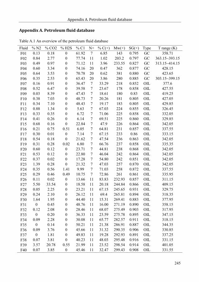
Appendix A. Petroleum fluid database
Appendix A. Petroleum fluid database
Table A.1 An overview of the petroleum fluid database
Fluid % N2 % CO2 % H2S % C1 N+ % C(+) Mw(+) SG(+) Type T range (K)F01 0.13 0.18 0 61.92 7 6.85 143 0.795 GC 358.71F02 0.84 2.77 0 77.74 11 1.02 203.2 0.797 GC 363.15~393.15F03 0.49 0.97 0 71.12 11 3.96 233.55 0.827 GC 313.15~414.15F04 0.60 3.34 0 74.16 20 0.47 362 0.877 GC 428.15F05 0.64 3.53 0 70.78 20 0.62 381 0.880 GC 423.65F06 0.35 2.53 0 65.43 20 3.86 280 0.885 GC 303.15~399.15F07 0.16 0.91 0 36.47 7 33.29 218 0.852 OIL 377.6F08 0.52 6.47 0 39.58 7 23.67 178 0.858 OIL 427.55F09 0.03 8.39 0 47.43 7 18.61 180 0.83 OIL 419.25F10 0.38 7.03 0 48.73 7 20.26 181 0.805 OIL 427.05F11 0.34 7.10 0 48.43 7 19.17 183 0.805 OIL 429.85F12 0.88 1.34 0 5.63 7 67.03 224 0.855 OIL 326.45F13 0.33 0.35 0 6.72 7 71.06 225 0.858 OIL 332.05F14 0.41 0.26 0 6.14 7 69.51 225 0.860 OIL 329.85F15 0.68 0.16 0 22.84 7 47.9 226 0.864 OIL 342.05F16 0.21 0.75 0.51 6.05 7 64.81 231 0.857 OIL 337.55F17 0.30 0.01 0 7.14 7 67.15 233 0.86 OIL 333.15F18 0.54 0.18 0 21.62 7 47.54 236 0.863 OIL 342.05F19 0.31 0.28 0.02 6.80 7 66.76 237 0.858 OIL 335.35F20 0.60 0.12 0 23.71 7 44.81 238 0.868 OIL 342.05F21 0.53 0.12 0 22.80 7 46.04 242 0.864 OIL 342.05F22 0.37 0.02 0 17.28 7 54.80 242 0.851 OIL 342.05F23 1.39 0.28 0 21.32 7 47.03 257 0.870 OIL 342.05F24 0.35 0.56 1.41 9.99 7 71.03 258 0.872 OIL 337.55F25 0.29 0.46 0.49 10.75 7 72.86 261 0.861 OIL 335.95F26 0.11 0.02 0 13.66 11 83.83 232.93 0.857 OIL 311.15F27 5.50 33.54 0 18.58 11 20.18 244.84 0.866 OIL 409.15F28 0.05 2.25 0 23.21 11 67.15 245.65 0.931 OIL 329.75F29 0.24 2.10 0 26.12 11 69.4 265.81 0.894 OIL 318.35F30 1.64 1.95 0 44.40 11 15.31 269.41 0.883 OIL 377.95F31 0 0.45 0 48.76 11 16.00 271.19 0.890 OIL 358.15F32 0.12 2.08 0 28.46 11 68.07 275.49 0.903 OIL 317.95F33 0 0.20 0 36.33 11 23.59 275.78 0.895 OIL 347.15F34 0.09 2.28 0 30.08 11 65.77 282.57 0.911 OIL 318.15F35 0 0.14 0 50.21 11 21.38 286.91 0.887 OIL 344.35F36 0.09 3.76 0 45.66 11 31.32 290.35 0.906 OIL 330.85F37 0 1.81 0 49.83 11 19.28 292.93 0.891 OIL 337.25F38 0.07 3.81 0 40.23 11 48.03 295.48 0.916 OIL 331.15F39 3.57 20.78 0.55 21.99 11 23.52 298.54 0.914 OIL 401.05F40 0.07 3.85 0 45.46 11 32.47 299.43 0.908 OIL 331.55
245
261

Thermodynamic modeling of complex systems
F41 0.17 0.08 0 44.72 11 24.78 299.83 0.905 OIL 335.25F42 0.1 3.84 0 46.77 11 30.24 301.41 0.912 OIL 331.15F43 0.16 0.23 0 39.45 11 36.02 305.16 0.949 OIL 346.15F44 0.08 0.27 0 49.71 11 28.61 305.28 0.910 OIL 337.85F45 0.23 0.05 0 37.62 11 38.27 314.09 0.930 OIL 342.15F46 0 4.70 0 38.64 11 43.17 314.99 0.946 OIL 318.15F47 0.24 2.54 0 40.82 11 41.27 317.89 0.916 OIL 323.35F48 0 2.65 0 41.99 11 45.64 318.03 0.934 OIL 319.55F49 0.07 3.59 0 35.53 11 40.33 319.42 0.943 OIL 339.85F50 0 2.25 0 44.66 11 42.68 321.5 0.932 OIL 322.65F51 0.66 0.11 0 19.54 11 50.82 322.87 0.908 OIL 351.65F52 0.38 0.14 0 18.79 11 32.09 324.25 0.876 OIL 362.25F53 0.13 0.09 0 41.32 11 41.53 343.32 0.943 OIL 344.95F54 0.23 0.16 0 35.13 11 41.73 344.49 0.876 OIL 318.75F55 0.5 0.04 0.88 21.50 11 49.53 345.5 0.929 OIL 331.15F56 0.81 0.08 0 42.14 11 43.14 347.49 0.946 OIL 346.05F57 0.32 0.97 0 30.17 11 53.69 371.28 0.987 OIL 329.15F58 0.15 0.82 0 32.81 11 59.41 375.01 0.984 OIL 329.15F59 0.12 1.94 0.96 13.15 11 45.85 380.92 0.913 OIL 312.15F60 0 2.25 0 18.38 11 76.78 400.21 1.001 OIL 323.15F61 0.12 0.02 0 3.90 11 70.45 427.41 0.958 OIL 332.15F62 0.37 0.751 0 56.31 11 13.92 286.32 0.865 OIL 408.15~418.15F63 0.39 0.30 0 40.20 20 6.64 453 0.918 OIL 370.65F64 0.59 0.36 0 40.81 20 6.25 458 0.926 OIL 370.95F65 0.25 3.60 2.32 47.64 20 6.02 411 0.881 OIL 303.25~417.85F66 0.35 3.14 0 54.26 20 4.08 418 0.905 OIL 388.15F67 0.40 2.55 0.36 47.24 20 6.01 434 0.917 OIL 394.25F68 0 0.77 0 36.20 20 8.15 442 0.938 OIL 383.15F69 0.45 2.07 0.38 26.58 20 12.96 450 0.956 OIL 394.25F70 0.67 0.86 0 46.63 20 6.55 450 0.927 OIL 373.75F71 0 2.13 0 31.28 20 6.33 455 0.915 OIL 393.15F72 0.083 1.82 0 32.17 20 6.70 455 0.915 OIL 393.15F73 0.32 2.80 1.49 45.29 20 6.04 460 0.939 OIL 299.85~394.25F74 0.45 1.64 0 45.85 20 6.18 474 0.925 OIL 387.35F75 0.20 1.34 0 23.64 20 12.03 530 0.949 OIL 372.05F76 0.18 0.82 0 22.92 20 11.44 560 0.951 OIL 374.85F77 1.25 0.90 0 37.54 20 13.17 678 0.900 OIL 377.55F78 0.49 0.31 0 44.01 30 9.96 449 0.989 OIL 347.15F79 0.29 0.22 0 21.66 36 6.66 291 0.895 OIL 350.4F80 0.27 0.32 0 36.08 36 3.48 262 0.880 OIL 335.7min 0 0.01 0 3.90 7 0.47 143 0.795 299.85max 5.5 33.54 2.32 77.74 36 83.83 678 1.001 429.85
246
262

Appendix B. Detailed results for Chapter. 4
Appendix B. Detailed results for Chapter. 4
Table B.1 Characterization results of Live Oil 1
Comp. z Mw CM5 (R) CM7m m
P1 0.02499 94.70 3.10526 3.77873 248.40 3.15682 3.75318 244.34P2 0.00732 114.20 3.56668 3.85154 253.61 3.61308 3.83129 250.35P3 0.00637 128.30 3.87375 3.87700 258.37 3.94300 3.84923 253.83P4 0.01563 148.70 4.27839 3.86920 266.51 4.42038 3.81850 257.95P5 0.00732 184.51 5.07438 3.85849 272.91 5.25827 3.80351 263.37P6 0.00778 218.70 5.73639 3.87103 282.13 6.05825 3.78685 267.14P7 0.00640 266.57 6.74654 3.85876 288.36 7.17833 3.76341 271.01P8 0.00534 338.31 8.30894 3.82789 293.12 8.85694 3.73022 274.98P9 0.00323 495.03 11.84171 3.75204 296.08 12.52390 3.66736 279.95
Table B.2 Characterization of Live Oil 2
Comp. z Mw CM5 (R) CM7m m
P1 0.02824 106.42 3.43905 3.84784 247.56 3.43100 3.85158 248.14P2 0.01694 148.42 4.34333 3.91174 262.08 4.41372 3.88639 257.90P3 0.01016 190.42 5.34204 3.91121 266.79 5.39645 3.89523 264.10P4 0.00874 243.29 6.64231 3.88982 268.94 6.63356 3.89189 269.29P5 0.00651 365.37 9.24731 3.90470 283.36 9.49007 3.86383 276.11
247
263

Thermodynamic modeling of complex systems
Table B.3 Characterization results of the five dead oils
PseudoComp. z Mw
CM5 (R) CM7m m
Cond-1P1 0.16046 91.40 3.02720 3.76347 247.35 3.07960 3.73690 243.14P2 0.16632 103.60 3.26702 3.79478 254.70 3.36506 3.74917 247.28P3 0.08903 118.50 3.61186 3.83754 258.57 3.71369 3.79440 251.48P4 0.05038 136.00 4.01464 3.87201 262.40 4.12316 3.83042 255.50P5 0.03992 150.00 4.33481 3.88937 265.08 4.45074 3.84811 258.18P6 0.03162 164.00 4.65829 3.90188 267.21 4.77831 3.86201 260.50P7 0.02506 178.00 4.98502 3.91064 268.88 5.10589 3.87303 262.51P8 0.01985 192.00 5.31486 3.91652 270.19 5.43346 3.88180 264.29P9 0.02819 212.19 5.95940 3.87717 264.11 5.90584 3.89134 266.50
P10 0.01769 240.19 6.60332 3.89027 267.32 6.56099 3.90040 269.04P11 0.01808 278.99 7.48585 3.90365 271.21 7.46879 3.90726 271.83P12 0.01176 371.40 9.58049 3.91728 277.80 9.63102 3.90890 276.34
Cond-2P1 0.20837 91.00 3.00568 3.75710 248.22 3.07031 3.72424 243.00P2 0.18433 104.33 3.29076 3.80001 254.37 3.38202 3.75773 247.51P3 0.08558 119.32 3.65308 3.84986 257.17 3.73276 3.81622 251.68P4 0.02695 136.00 4.04361 3.88732 260.52 4.12316 3.85676 255.50P5 0.02210 150.00 4.36993 3.91006 262.95 4.45074 3.88120 258.18P6 0.03297 170.31 4.84627 3.93465 265.73 4.92589 3.90884 261.44P7 0.01218 192.00 5.35813 3.95353 268.00 5.43346 3.93131 264.29P8 0.00999 206.00 5.92732 3.89768 258.40 5.76104 3.94283 265.86P9 0.01490 226.31 6.42081 3.90994 260.15 6.23619 3.95639 267.85
P10 0.01372 260.16 7.24020 3.92551 262.65 7.02826 3.97305 270.56P11 0.00924 307.56 8.38755 3.93937 265.33 8.13745 3.98806 273.48P12 0.00762 409.74 10.85822 3.95141 269.23 10.52814 4.00142 277.67
Cond-3P1 0.26650 90.18 2.97766 3.75008 248.67 3.05106 3.71257 242.69P2 0.21810 103.79 3.28496 3.80086 253.71 3.36951 3.76155 247.34P3 0.06690 117.24 3.57143 3.82935 259.09 3.68421 3.78125 251.15P4 0.02005 136.00 4.01814 3.87385 262.17 4.12316 3.83359 255.50P5 0.01419 150.00 4.34902 3.89772 264.22 4.45074 3.86146 258.18P6 0.01004 164.00 4.68106 3.91692 265.91 4.77831 3.88453 260.50P7 0.00711 178.00 5.01418 3.93250 267.31 5.10589 3.90384 262.51P8 0.00503 192.00 5.34829 3.94526 268.50 5.43346 3.92019 264.29P9 0.00356 206.00 5.91248 3.89304 259.05 5.76104 3.93413 265.86
P10 0.00252 220.00 6.25596 3.90305 260.11 6.08861 3.94612 267.26P11 0.00178 234.00 6.59974 3.91157 261.06 6.41618 3.95649 268.52P12 0.00432 281.90 7.77067 3.93305 263.82 7.53681 3.98210 272.01
248
264

Appendix B. Detailed results for Chapter. 4
Light-1P1 0.04920 92.14 3.04376 3.76662 247.67 3.09692 3.73981 243.42P2 0.06210 107.14 3.39291 3.82489 252.38 3.44789 3.79983 248.36P3 0.06090 123.24 3.78280 3.87846 255.44 3.82460 3.86117 252.65P4 0.19315 155.74 4.50680 3.91639 263.67 4.58505 3.88923 259.17P5 0.14476 211.74 5.93998 3.89957 264.45 5.89535 3.91148 266.46P6 0.08423 261.33 7.12028 3.90135 268.19 7.05560 3.91578 270.65P7 0.08740 309.74 8.20072 3.91116 273.18 8.18837 3.91355 273.59P8 0.07913 371.99 9.57300 3.91844 278.44 9.64481 3.90656 276.37P9 0.05518 441.99 11.11420 3.92029 282.85 11.28268 3.89635 278.63
P10 0.05039 523.98 12.96963 3.91133 285.57 13.20120 3.88317 280.56P11 0.04203 644.01 15.61781 3.90333 289.65 16.00974 3.86389 282.56P12 0.03012 865.23 20.37698 3.89292 296.16 21.18581 3.83106 284.86
Light-2P1 0.1369 91.82 3.03797 3.76578 247.42 3.08943 3.73977 243.30P2 0.1427 104.45 3.30540 3.80521 253.50 3.38495 3.76837 247.55P3 0.0838 118.10 3.60110 3.83586 258.58 3.70433 3.79204 251.38P4 0.08781 142.49 4.17363 3.88650 263.03 4.27497 3.84896 256.79P5 0.03515 164.00 4.67793 3.91485 266.08 4.77831 3.88144 260.50P6 0.05658 184.49 5.16247 3.93335 268.22 5.25770 3.90444 263.36P7 0.04221 212.49 6.04881 3.89176 260.54 5.91285 3.92772 266.53P8 0.03149 240.49 6.72452 3.90700 262.80 6.56800 3.94442 269.07P9 0.03289 274.64 7.54476 3.92071 265.15 7.36703 3.95876 271.55
P10 0.02119 316.64 8.55596 3.93141 267.35 8.34975 3.97053 273.95P11 0.02246 375.10 9.96249 3.93981 269.69 9.71756 3.97990 276.48P12 0.01593 518.27 13.39703 3.94484 273.55 13.06756 3.98519 280.45
249
265

Thermodynamic modeling of complex systems
Table B.4 Mutual solubility of petroleum fluids and MEG*
T (K) Caseno.
Solubility of oil in polar phase Solubility of MEG in organic phase
Exp.AG XL
Exp.AG XL
CM5(R) CM7 CM5
(R) CM7 CM5(R) CM7 CM5
(R) CM7
Cond-1 [Riaz, et al. (2011a)]275.15 1 None 3306 3277 3198 3172 53 70 70 57 57283.15 2 None 3510 3477 3436 3407 74 113 113 92 92303.15 3 4590 4083 4039 4097 4060 250 336 335 269 268308.15 4 None 4242 4195 4279 4240 335 431 430 344 343313.15 5 4524 4408 4358 4468 4426 431 549 548 436 436318.15 6 5170 4582 4529 4665 4620 None 694 692 549 549323.15 7 4937 4764 4707 4870 4823 722 871 869 687 686326.55 8 None 4892 4832 5015 4965 711 1012 1009 797 796
Cond-2 [Riaz, et al. (2011b)]275.15 9 None 2483 2463 2420 2406 51 64 64 53 53283.15 10 None 2672 2649 2635 2620 87 104 104 85 85303.15 11 4879 3210 3178 3243 3221 290 310 310 249 249308.15 12 None 3360 3326 3412 3389 355 399 398 319 319313.15 13 5325 3518 3481 3588 3563 470 509 508 405 406318.15 14 5860 3683 3643 3772 3746 None 643 643 511 512323.15 15 6084 3856 3813 3965 3936 581 808 807 640 641
Cond-3 [Riaz, et al. (2014)]303.15 16 3485 4452 4400 4497 4455 196 273 272 222 221313.15 17 3906 4826 4766 4925 4877 337 449 447 362 361323.15 18 4239 5235 5165 5389 5334 654 714 711 574 572
Light-1 [Frost et al. (2013)]303.15 19 973 1081 1065 1088 1073 1931 638 643 478 482313.15 20 1106 1153 1135 1172 1155 2630 1036 1044 769 776323.15 21 1210 1234 1215 1265 1248 3488 1631 1643 1203 1213
Light-2 [Frost et al. (2013)]303.15 22 3433 3786 3765 3790 3773 385 390 390 307 308313.15 23 3477 4062 4037 4106 4087 612 636 637 498 498323.15 24 3738 4363 4334 4449 4427 916 1006 1007 782 783* No decimal is used for the values.
250
266

Appendix B. Detailed results for Chapter. 4
Table B.5 Solubility of petroleum fluids, MEG and water from PC-SAFT with different parameters
Char.Method
Caseno.
Oil in polar phase MEG in organic phase H2O in organic phaseExp AG XL Exp AG XL Exp AG XL
Cond-1 (323.15K) [Riaz, et al. (2011a)]CM5 (R)
1* 69155 73
61127 108
1218855 1079
CM7 154 73 127 108 865 1092CM5 (R)
2* 417616 443
172357 289
946586 747
CM7 611 441 356 289 593 757CM5 (R)
3 17932194 2029
381634 504
402277 356
CM7 2173 2013 633 504 280 361Cond-2 (303.15K) [Riaz, et al. (2011b)]
CM5 (R)4 67
60 2836
44 38806
358 471CM7 60 28 44 38 361 474
CM5 (R)5 189
163 10073
93 77635
287 380CM7 163 100 92 77 289 383
CM5 (R)6 508
603 486103
169 138394
187 250CM7 599 484 169 138 188 252
Cond-2 (323.15K) [Riaz, et al. (2011b)]CM5 (R)
7 9182 42
82118 101
1309860 1082
CM7 82 42 118 101 867 1091CM5 (R)
8 311219 145
158245 202
1119695 880
CM7 218 144 245 202 701 887CM5 (R)
9 1181776 656
328442 356
784457 584
CM7 770 653 442 356 461 589Cond-3 (313.15K) [Riaz, et al. (2014)]
CM5 (R)10 711
960 777178
232 191480
309 409CM7 952 772 231 190 312 413
CM5 (R)11 180
334 21291
132 111673
449 588CM7 332 210 131 110 454 595
CM5 (R)12 62
147 7253
65 56796
550 717CM7 146 71 65 56 556 725
Light-1 (313.15K) [Frost et al. (2013)]CM5 (R)
13 230272 226
493545 410
722367 431
CM7 268 223 549 413 374 438CM5 (R)
14 11796 61
270268 207
908571 662
CM7 94 60 270 209 581 675
251
267

Thermodynamic modeling of complex systems
Light-1 (323.15K) [Frost et al. (2013)]CM5 (R)
15 239259 215
568806 603
1023605 694
CM7 256 213 812 608 615 706CM5 (R)
16 129118 80
363475 362
1443842 958
CM7 116 79 478 365 857 976Light-2 (323.15K) [Frost et al. (2013)]
CM5 (R)17* 686
1092 897549
548 432917
473 594CM7 1088 895 548 433 475 596
CM5 (R)18+ 270
379 240529
301 2431351
719 894CM7 378 240 301 243 722 898
CM5 (R)19+ 125
173 84238
147 1231744
886 1095CM7 172 84 148 123 889 1099
The calculation pressure is 1.01325bar, except (*) 1.21325bar and (+) 1.31325bar.
252
268

Appendix C. Speed of sound database
Appendix C. Speed of sound database
Table C.1 Temperature and pressure ranges of speed of sound measurements in pure n-alkane fluids
Comp. T (K) P (MPa) Ref. Comp. T (K) P (MPa) Ref.C1 113.15-323.15 0.11-25 1 nC11 271.15-394.15 0.101325 16
91-186 saturated 2 278-318 1-100 25100-300 1.6-35 2 nC12 273.15-473.15 0.1-140 14
111.33 – 190 0.11-20 3 277.15-392.15 0.101325 16150-183 1.6-4.0 4 303.15-433.15 0.1-49 18
148.15-295.15 0.1-1000 5 293.15-433.15 0.1-140 26C2 91-303 saturated 6 nC13 303.15-433.15 0.1-49 18
100-323.15 4.1-37 6 293.15-373.15 0.1-150 27220-450 0.014-10.5 7 nC14 283.15-393.15 0.101325 16
C3 200-340 0.02-60 8 303.15-433.15 0.1-49 18nC4 200-375 0.002-60 8 293.15-373.15 0.1-150 27nC5 205.67-308.4 saturated 9 293.15-433.15 0.1-140 28
185.65-310.65 0.1-263 10 nC15 287.15-394.15 0.101325 16263.15-433.24 0.22-210 11 303.15-433.15 0.1-49 18293.15-373.15 5-100 12 303.15-433.15 0.1-140 29293.15-313.15 0.1-600 13 293.15-383.15 0.1-150 30
nC6 253.15-333.15 0.1-140 14 nC16 293.15-473.15 0.1-140 14303 0.1-392 15 303.15-393.15 0.1-70 24
263.15-341.15 0.101325 16 296.15-392.15 0.101325 16293.15-373.15 0.1-150 17 303.15-433.15 0.1-49 18298.15-433.15 0.1-49 18 298.3-373.15 0.1-100 19298.3-373.15 0.1-100 19 293.15-333.15 0.101325 31
293.15-333.15 0.101325 20 298.15-433.15 0.1-140 32nC7 253.15-453.15 0.1-140 14 209.65-343.15 0.083 33
265.15-368.15 0.101325 16 nC17 303.15-383.15 0.1-150 30293.15-373.15 0.1-150 21 nC18 301.15-395.15 0.101325 16298.15-523.15 0.1-59 22 313.15-383.15 0.1-150 34
nC8 253.15-393.15 0.1-140 14 nC19 313.15-383.15 0.1-150 34265.15-392.15 0.101325 16 nC20 323.15-393.15 0.1-150 35293.15-363.15 5-90 12 nC22 323.15-393.15 0.1-150 35303.15-433.15 0.1-49 18 317.15-393.15 0.101325 16298.15-523.15 0.1-59 22 nC23 333.15-393.15 0.1-150 36
nC9 253.15-413.15 0.1-140 14 nC24 333.15-393.15 0.1-150 36293.15-393.15 0.1-100 23 nC28 334.15-393.15 0.101325 16
nC10 300.15-413.15 0.1-60 24 353.15-403.15 0.1-150 37268.15-391.15 0.101325 16 nC36 347.15-405.15 0.101325 16298.15-433.15 0.1-49 18 363.16-403.15 0.1-151 37
253
269

Thermodynamic modeling of complex systems
Reference for Table C.1: (1) Itterbeek et al. 81967), (2) Straty (1974), (3) Gammon et al. (1976), (4) Baidakov et al. (1982), (5) Kortbeek et al. (1990), (6) Tsumura et al. (1977), (7) Estrada-Alexanderset al. (1997), (8) Niepmann (1984), (9) Chávez et al. (1982), (10) Muringer et al. (1985), (11) Lainez et al. (1990), (12) Ding et al. (1997), (13) Bolotnikov et al. (2004), (14) Boelhouwer et al. (1967), (15) Hawley et al. (1970), (16) Wang et al. (1991), (17) Daridon et al. (1998a), (18) Khasanshin et al. (2001), (19) Ball et al. (2001), (20) Bolotnikov et al. (2005), (21) Daridon et al. (1999), (22) Hasanov (2012), (23) Lago et al. (2006), (24) Ye et al. (1990), (25) Giuliano Albo et al. (2013), (26) Khasanshin et al. (2003), (27) Daridon et al. (2000), (28) Khasanshin et al. (2002), (29) Dovnar et al. (2001), (30) Daridon et al. (2002), (31) Bolotnikov et al. (2005), (32) Khasanshin et al. (2009), (33) Outcalt et al. (2010), (34) Dutour et al. (2000), (35) Dutour et al. (2001a), (36) Dutour et al. (2001b), (37) Dutour et al. (2002).
254
270

Appendix C. Speed of sound database
Table C.2 The speed of sound database for binary hydrocarbon systems *
System T (K) P (MPa) Ref. System T (K) P (MPa) Ref.C1 + C3 262.75-413.45 10-70 (a) 1 nC6 + cC6 303.15 0.101325 9
C1 + nC8 293.15-373.15 25-100 (b) 1 nC6 + C6H6 313.15 0.101325 10C1 + nC16 292.15-413.15 6.3-66 (c) 2 nC6 + C7H8 313.15 0.101325 10nC6 + nC7 298.15 0.101325 3 nC7 + cC6 303.15 0.101325 9nC6 + nC8 298.15 0.101325 3 nC7+ C6H6 298.15 0.101325 11nC6 + nC9 298.15 0.101325 3 nC7 + C6H6 313.15 0.101325 10
293.16-313.73 0.101325 4 nC7 + C7H8 313.15 0.101325 10nC6 + nC10 298.15 0.1-100 5 nC8 + cC6 303.15 0.101325 9
298.15 0.101325 3 nC8 + C6H6 313.15 0.101325 10nC6 + nC11 298.15 0.101325 3 nC8 + C7H8 313.15 0.101325 10nC6 + nC12 298.15 0.101325 3 nC9 + C6H6 313.15 0.101325 10nC6 + nC16 298.15-373.15 0.1-70 (d) 2 nC9 + C7H8 313.15 0.101325 10
293.15-373.15 0.101325 6 cC6+ C6H6 293.15-303.15 0.1-200 12nC7 + nC8 298.15-523.15 0.1-59 7 298.15 0.101325 11
nC7 + nC12 293-318 0.1-101 8 293.15-303.15 0.101325 13nC10 + nC12 298.15 0.1-100 5 298.15 0.101325 14nC10 + nC14 298.15 0.1-100 5 303.15 0.101325 15
313.15 0.101325 16cC6+ C7H8 313.15 0.101325 16
* The composition range is mole fraction from 0 to 1 by default, except (a) x1 = 0.8998; (b) x1 = 0.98; (c) x1 = 0.323, 0.51, 0.679; (d) x1 = 0.2, 0.4, 0.6, 0.8
Reference of Table C.2: (1) Lagourette et al. (1994), (2) Ye et al. (1992), (3) Tourino et al. (2004), (4) Gepert et al. (2003), (5) Takagi et al. (1985), (6) Bolotnikov et al. (2005), (7) Hasanov et al. (2012), (8) Dzida et al. (2008), (9) Oswal et al. (2002), (10) Calvar et al. (2009b), (11) Tamura et al. (1983), (12) Takagi et al. (1980), (13) Tamura et al. (1984), (14) Junquera et al. (1988), (15) Oswal et al. (2004), (16) Calvar et al. (2009a).
255
271

Thermodynamic modeling of complex systems
Table C.3 The speed of sound database for ternary systems at 298.15K and atmospheric pressure
Comp. 1 Comp. 2 Comp. 3 Mole Fraction Range %ARD Points Ref.
n-hexane n-heptane n-decane x1=[0.1735-0.4500]x2=[0.2759-0.5179] -3.17 15 1
n-hexane n-heptane cyclo-hexane x1=[0.1533-0.6988]x2=[0.1823-0.4103] -0.61 15 1
n-hexane n-heptane toluene x1=[0.1522-0.6952]x2=[0.1838-0.4045] -0.97 15 1
n-pentane n-hexane benzene x1=[0.0966-0.4082]x2=[0.2877-0.4665] -4.19 10 2
n-hexane cyclo-hexane benzene x1=[0.0771-0.3448]x2=[0.3342-0.4851] -2.62 10 2
n-heptane cyclo-hexane toluene x1=[0.2837-0.4393]x2=[0.1124-0.4525] -6.78 10 2
cyclo-hexane benzene 1-pentanol x1=[0.0401-0.7091]x2=[0.0572-0.8998] 2.36 41 3
Reference of Table C.3: (1) Pandey et al. (1999), (2) Rai et al. (1989), (3) Orge et al. (1995).
256
272

Appendix C. Speed of sound database
Table C.4 The speed of sound database for oils
System Temp. range (K) Press. range (MPa) API or C1 composition C11+ composition ref.Oil A 297.15-378.15 0.1-44 5° (API) 1Oil B 296.15-375.15 0.1-44 7° (API) 1Oil C 303.15-385.15 0.1-44 10° (API) 1Oil D 294.15-387.15 0.1-44 10.5° (API) 1Oil E 296.15-390.15 0.1-44 12° (API) 1Oil F 298.15-380.15 0.1-44 34° (API) 1Oil G 297.15-359.15 0.1-44 43° (API) 1Oil H 296.15-363.15 0.1-44 57° (API) 1Oil I 317.15-382.15 0.1-44 62° (API) 1Oil J 296.15-345.15 0.8-44 23° (API) 1Oil K 296.15-345.15 8.8-44 live oil 1Oil L 262.40-354.00 12-70 x~88.4% 2Oil M 272.90-413.60 20-70 x~89.6% 2Oil N 313.15-453.15 40-120 x=68.4% 4.88% 3Oil O 293.15-373.15 40-100 x=76.6% 1.73% 4Oil P 273.05-373.45 40-70 x=61.9% 7.30% 5Oil Q 313.15-453.15 40-120 x=69.1% 4.30% 5Oil R 273.75-413.45 10-70 x=30.0% 31.1% 5Oil S 293.15-373.15 0.1-150 synthetic system 100% 6Oil T 293.15-373.15 0.1-150 distillation cut 100% 6Oil U 335.10-402.10 12.6-70 x=34.3% 20.8% 7Oil V 283.15-373.15 0.1-20 None 93.7% 8Oil W 283.15-373.15 0.1-20 None 96.3% 8
Reference of Table C.4: (1) Wang et al. (1990b), (2) Labes et al. (1994), (3) Daridon et al. (1996b), (4) Barreau et al. (1997), (5) Daridon et al. (1998c), (6) Lagourette et al. (1999), (7) Ball et al. (2002), (8) Plantier et al. (2008).
257
273

Thermodynamic modeling of complex systems
Table C.5 Coefficients of correlation for the speed of sound in pure hydrocarbons and 1-alcohols with equation (5.8)
Comp. Coefficient for temperaturea0 a1 a2 a3 c
nC5 0.212068 7.57345e-3 1.347817 -2.058622 -1.912743nC6 0.327610 -2.074676 10.71832 -12.91560 -2.112133nC7 0.343941 -2.045490 9.842795 -11.13332 -2.009931nC8 0.655236 -4.637980 16.67994 -16.52105 -1.887652nC9 1.503543 -12.46010 40.81211 -40.87069 -1.732812
nC10 0.568900 -3.765328 13.79155 -13.90872 -1.805046nC11 0.192076 -0.500779 4.346802 -4.808256 -1.748128nC12 0.299330 -1.502390 7.371681 -7.810305 -1.708618nC13 0.165173 -0.303609 3.861754 -5.014875 -1.749733nC14 0.147974 -0.122435 3.183280 -4.329440 -1.741384nC15 0.270360 -1.204313 6.262105 -6.770369 -1.652112nC16 0.250287 -1.034741 5.738589 -6.132522 -1.614573nC17 0.0293568 0.935828 -0.119980 -0.908207 -1.681083nC18 0.0132357 1.083803 -0.625768 -0.473679 -1.689141nC19 0.190218 -0.493966 4.035938 -4.998633 -1.661775nC20 -1.256293 11.90259 -31.28656 28.28115 -1.675184nC22 -0.022899 1.341533 -1.289403 0.139508 -1.624181nC23 -0.167505 2.531357 -4.594079 3.051720 -1.642080nC24 0.112948 0.200237 1.832853 -2.861589 -1.636320nC28 -0.469255 5.205791 -12.49757 10.59317 -1.628044nC32 1.221912 -8.509352 24.48875 -22.55682 -1.602115nC36 -1.772879 14.88992 -36.33291 30.30698 -1.518427cC6 -0.876113 9.263434 -26.13995 24.15456 -2.288684
Benzene 0.438767 -3.047202 11.68608 -11.67896 -1.880101Toluene 0.227227 -1.080297 6.216340 -7.852064 -1.931299C1OH -2.085638 22.16740 -68.11488 70.77175 -1.953617C2OH 0.488784 -3.780596 18.27565 -23.46797 -1.755921C3OH -5.598469 56.90094 -183.3801 206.2862 -0.759965C4OH 0.212071 7.54197e-3 1.347913 -2.058722 -1.912743C5OH 1.104831 -9.590740 35.34638 -39.42883 -1.488062C6OH -0.131744 2.655069 -5.297635 4.468302 -1.605447C7OH 1.499865 -13.22723 46.44495 -48.40760 -0.981517C8OH 0.047158 1.035350 -1.142850 -1.053466 -1.976260C9OH 0.862893 -6.991803 25.68677 -26.88268 -1.174164
C10OH -0.464308 5.754787 -15.73310 14.53866 -1.833814
258
274

Appendix C. Speed of sound database
Comp. Coefficients for pressureb1 b2 b3 d
nC5 0.150526 -0.164302 0.157367 0.587264nC6 0.232235 -0.0972733 0.0248121 0.857459nC7 0.250922 -0.103857 0.0249824 0.886224nC8 0.333414 -0.202573 0.0939259 0.992887nC9 0.266674 -0.168712 0.0715825 0.922512
nC10 0.236484 -0.0573302 -0.0323692 0.871618nC11 0.237099 -0.103164 0.0291584 0.863294nC12 0.229912 -0.0914951 0.0221359 0.855233nC13 0.161167 -0.0554454 0.0126638 0.719217nC14 0.145632 -0.0470097 0.0101635 0.685614nC15 0.189874 -0.0689852 0.0156544 0.782491nC16 0.206872 -0.0798097 0.0196817 0.813228nC17 0.142272 -0.0452343 9.65593e-3 0.677207nC18 0.128265 -0.0392626 8.45507e-3 0.643371nC19 0.129197 -0.0393608 8.32487e-3 0.647980nC20 0.118483 -0.0351406 7.66272e-3 0.618130nC22 0.129621 -0.0395939 8.34839e-3 0.646879nC23 0.111381 -0.0300290 5.70816e-3 0.606004nC24 0.111395 -0.0318087 6.74247e-3 0.602092nC28 0.084579 -0.0176640 2.89094e-3 0.548891nC32 0.093346 -0.0208488 3.45463e-3 0.563780nC36 0.111325 -0.0322675 6.91334e-3 0.610190cC6 -3.30997e-3 0.0397137 -0.0182198 0.317615
Benzene 0.195281 -0.0273543 -0.0169796 0.690872Toluene 0.0928646 -0.0111089 -0 2.77118e-3 0.508280C1OH 0.143815 -0.0312255 3.98001e-3 0.646859C2OH 0.178722 -0.0435911 6.05255e-3 0.775934C3OH 0.696505 -0.312281 0.0824123 1.863796C4OH 0.150526 -0.164302 0.157367 0.587263C5OH 0.237466 -0.0851677 0.0203957 0.887607C6OH 0.153811 -0.0390488 5.24194e-3 0.708279C7OH 0.384709 -0.152258 0.0395031 1.276415C8OH 0.0261175 0.0150605 -8.12289e-3 0.365628C9OH 0.251068 -0.0857784 0.0197680 0.976948
C10OH 0.0412392 0.0122681 -0.0114725 0.414458
259
275
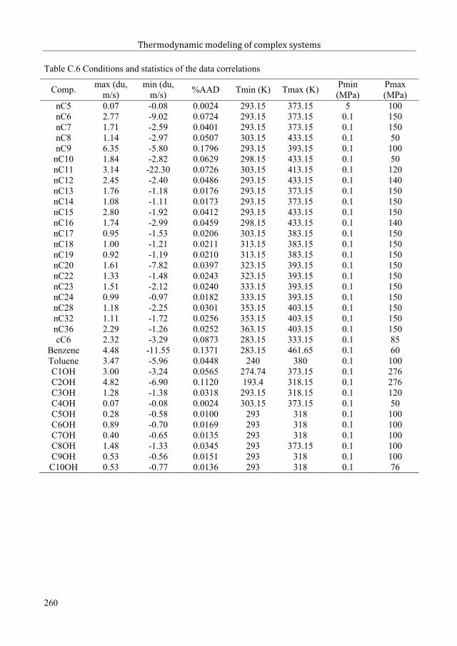
Thermodynamic modeling of complex systems
Table C.6 Conditions and statistics of the data correlations
Comp. max (du, m/s)
min (du, m/s) %AAD Tmin (K) Tmax (K) Pmin
(MPa)Pmax (MPa)
nC5 0.07 -0.08 0.0024 293.15 373.15 5 100nC6 2.77 -9.02 0.0724 293.15 373.15 0.1 150nC7 1.71 -2.59 0.0401 293.15 373.15 0.1 150nC8 1.14 -2.97 0.0507 303.15 433.15 0.1 50nC9 6.35 -5.80 0.1796 293.15 393.15 0.1 100
nC10 1.84 -2.82 0.0629 298.15 433.15 0.1 50nC11 3.14 -22.30 0.0726 303.15 413.15 0.1 120nC12 2.45 -2.40 0.0486 293.15 433.15 0.1 140nC13 1.76 -1.18 0.0176 293.15 373.15 0.1 150nC14 1.08 -1.11 0.0173 293.15 373.15 0.1 150nC15 2.80 -1.92 0.0412 293.15 433.15 0.1 150nC16 1.74 -2.99 0.0459 298.15 433.15 0.1 140nC17 0.95 -1.53 0.0206 303.15 383.15 0.1 150nC18 1.00 -1.21 0.0211 313.15 383.15 0.1 150nC19 0.92 -1.19 0.0210 313.15 383.15 0.1 150nC20 1.61 -7.82 0.0397 323.15 393.15 0.1 150nC22 1.33 -1.48 0.0243 323.15 393.15 0.1 150nC23 1.51 -2.12 0.0240 333.15 393.15 0.1 150nC24 0.99 -0.97 0.0182 333.15 393.15 0.1 150nC28 1.18 -2.25 0.0301 353.15 403.15 0.1 150nC32 1.11 -1.72 0.0256 353.15 403.15 0.1 150nC36 2.29 -1.26 0.0252 363.15 403.15 0.1 150cC6 2.32 -3.29 0.0873 283.15 333.15 0.1 85
Benzene 4.48 -11.55 0.1371 283.15 461.65 0.1 60Toluene 3.47 -5.96 0.0448 240 380 0.1 100C1OH 3.00 -3.24 0.0565 274.74 373.15 0.1 276C2OH 4.82 -6.90 0.1120 193.4 318.15 0.1 276C3OH 1.28 -1.38 0.0318 293.15 318.15 0.1 120C4OH 0.07 -0.08 0.0024 303.15 373.15 0.1 50C5OH 0.28 -0.58 0.0100 293 318 0.1 100C6OH 0.89 -0.70 0.0169 293 318 0.1 100C7OH 0.40 -0.65 0.0135 293 318 0.1 100C8OH 1.48 -1.33 0.0345 293 373.15 0.1 100C9OH 0.53 -0.56 0.0151 293 318 0.1 100
C10OH 0.53 -0.77 0.0136 293 318 0.1 76
260
276

Appendix D. Detailed results for Chapter. 7
Appendix D. Detailed results for Chapter. 7
Table D.1 The model parameters of n-alkanes*
Alkanes PC-SAFT (GS)+ PC-SAFT (LK)#
m mC1 1.0 3.6997 150.18 1.0 3.7075 149.85C2 1.60640 3.5258 191.41 1.62319 3.5055 189.90C3 1.98464 3.6270 209.21 2.00185 3.6098 207.87C4 2.30312 3.7218 224.55 2.32014 3.7077 223.35C5 2.67703 3.7650 232.04 2.69409 3.7544 231.00C6 3.03141 3.8046 237.88 3.04588 3.7967 237.11C7 3.45837 3.8066 239.48 3.47284 3.8006 238.86C8 3.86157 3.8179 241.42 3.88157 3.8110 240.73C9 4.21311 3.8422 244.39 4.23554 3.8348 243.73
C10 4.59397 3.8562 245.91 4.62638 3.8481 245.07C11 5.04849 3.8445 245.40 5.07409 3.8428 244.87C12 5.40389 3.8608 247.08 5.43101 3.8595 246.60C13 5.82782 3.8635 247.01 5.85874 3.8621 246.54C14 6.14811 3.8817 249.06 6.18361 3.8797 248.56C15 6.46509 3.9023 250.74 6.50012 3.9009 250.33C16 6.85832 3.9024 251.02 6.90210 3.8996 250.51C17 7.22541 3.9099 251.81 7.26950 3.9076 251.38C18 7.60403 3.9127 251.84 7.65229 3.9100 251.42C19 8.05710 3.9008 251.09 8.11613 3.8967 250.59C20 8.41319 3.9160 251.76 8.47251 3.9123 251.31
* For a fair comparison, the model parameters are estimated or re-estimated to the same data with the same procedure for the new and original universal constants. The experimental data are taken from NIST [REFPROP (2010)] for C1 to C10 and from DIPPR Database (2012) for C11 to C20. The data for pure component parameter estimation are from the saturated line only.+ PC-SAFT (GS) denotes the PC-SAFT model with the original universal constants from Gross and Sadowski. # PC-SAFT (LK) denotes the PC-SAFT model with the new universal constants from this work, Liang and Kontogeorgis.
261
277

Thermodynamic modeling of complex systems
Table D.2 %AADs for vapor pressure (P), liquid density ( ) and speed of sound (u) *
Comp. PC-SAFT (GS) PC-SAFT (LK)P P
C1 0.39 0.95 0.21 0.47C2 0.10 0.28 0.13 0.31C3 0.18 0.17 0.14 0.31C4 0.33 0.24 0.28 0.29C5 0.23 0.25 0.26 0.21C6 0.46 0.37 0.54 0.34C7 0.23 0.36 0.18 0.19C8 0.46 0.43 0.13 0.19C9 0.63 0.36 0.12 0.30
C10 0.66 0.36 0.08 0.21C11 0.93 0.46 0.39 0.25C12 0.83 0.46 0.25 0.23C13 0.72 0.42 0.07 0.20C14 0.91 0.41 0.06 0.20C15 0.45 0.42 0.69 0.20C16 1.14 0.32 0.08 0.20C17 0.64 0.26 0.55 0.22C18 0.62 0.23 0.72 0.27C19 1.43 0.16 0.31 0.39C20 1.57 0.14 0.74 0.42
Avg.+ 0.65 0.35 0.30 0.27Avg.# 0.90 0.31 0.34 0.28
* The data of C1 to C10 are from NIST [REFPROP (2010)], and the vapor pressure and liquid density data of C11 to C20 are from DIPPR Database (2012).
Avg. +, and Avg. # denote the average %AAD from C1 to C20, and from C1 to C24, respectively.
262
278

Appendix D. Detailed results for Chapter. 7
Table D.3 %AADs for residual heat capacities, dP/dV and Joule-Thomson (JT) coefficients*
Comp.PC-SAFT (GS) PC-SAFT (LK)
u dP/dV JT u dP/dV JTC1 4.17 18.7 11.1 19.1 8.90 6.47 26.5 6.14 24.4 8.49C2 8.26 33.6 3.92 9.01 5.04 8.08 39.9 3.14 8.08 3.97C3 9.97 40.2 2.51 13.4 3.41 8.93 43.9 3.05 10.9 3.99C4 9.58 49.3 3.22 14.4 7.02 8.13 51.0 4.05 11.0 3.62C5 9.27 44.5 1.97 14.6 6.57 7.63 44.7 3.24 10.9 3.01C6 8.89 45.2 3.80 14.6 6.93 6.76 45.9 4.92 9.54 5.52C7 10.8 32.4 2.21 20.2 5.63 8.57 32.8 2.46 14.4 8.72C8 10.2 23.6 2.29 20.3 9.14 7.74 24.4 2.74 13.6 53.8C9 11.2 33.8 3.07 21.6 7.46 8.73 34.0 3.32 14.9 18.7
C10 10.7 33.8 2.71 19.8 7.47 8.32 34.4 3.36 13.7 12.6Avg. 9.30 35.5 3.68 16.7 6.76 7.94 37.8 3.64 13.1 12.2
* The used data are only at saturated lines.
Table D.4 %AADs for density, speed of sound, residual heat capacities, dP/dV and Joule-Thomson (JT) coefficients *
Comp.OrgUC NewUC
u dP/dV JT u dP/dV JTC1 1.15 2.79 19.0 5.82 7.02 8.01 0.70 3.30 24.1 5.20 7.43 6.73C2 1.33 6.02 30.9 4.62 5.53 10.1 1.26 5.83 34.4 4.55 4.67 10.2C3 1.40 8.28 37.2 4.91 9.63 13.0 1.30 7.41 40.4 4.78 7.33 13.4C4 1.41 7.96 46.1 5.92 9.73 8.55 1.34 6.99 47.3 5.50 7.52 8.78C5 1.55 9.35 45.6 6.40 12.1 7.17 1.38 7.94 46.7 5.73 9.21 7.38C6 1.49 8.14 42.5 7.78 10.5 7.95 1.41 6.87 42.8 7.37 7.91 8.83C7 1.55 9.60 33.8 6.67 13.6 6.33 1.43 8.08 34.0 6.08 10.5 7.69C8 1.34 8.65 24.2 6.52 12.9 6.98 1.29 7.25 24.3 6.25 10.0 14.0C9 1.60 9.89 34.5 6.87 14.0 6.78 1.61 8.32 34.2 6.36 10.7 10.3
C10 1.66 10.2 33.0 8.08 15.6 6.70 1.60 8.66 33.2 7.48 11.6 8.77Avg. 1.45 8.08 34.7 6.36 11.0 8.16 1.33 7.07 36.1 5.93 8.69 9.61
* The used data are over wide temperature and pressure ranges, which can be found in Chapter 6.
263
279

Thermodynamic modeling of complex systems
Table D.5 Critical points from both original and new universal constants *
Exp. data Tc and Pc with %RD from PC-SAFT (GS)
Tc and PC with %RD from PC-SAFT (LK) Ref.
Tc (K) Pc (bar) Tc (K) Pc (bar) %RD Tc (K) Pc (bar) %RDTc Pc Tc Pc
345.37 70.12 356.99 67.59 3.36 -3.60 355.75 67.46 3.01 -3.79 1336.48 73.43 354.14 70.79 5.25 -3.60 353.01 70.77 4.91 -3.63 1327.59 77.08 347.19 74.27 5.98 -3.64 346.27 74.42 5.70 -3.45 1380.37 68.40 388.11 64.56 2.04 -5.62 386.45 64.03 1.60 -6.38 1362.04 83.98 378.35 73.53 4.51 -12.4 376.91 73.26 4.11 -12.8 1318.71 117.20 343.93 98.25 7.91 -16.2 344.14 98.39 7.98 -16.1 1377.59 82.53 383.06 81.73 1.45 -0.97 381.73 81.43 1.10 -1.33 2344.26 100.53 347.47 100.54 0.93 0.01 347.66 100.50 0.99 -0.03 2310.26 121.62 311.87 125.89 0.52 3.51 315.48 125.03 1.68 2.80 2277.59 123.14 279.60 129.23 0.72 4.95 285.15 129.24 2.72 4.95 2438.15 66.13 445.06 67.57 1.58 2.18 442.31 66.36 0.95 0.35 3385.92 76.06 392.41 78.83 1.68 3.64 390.70 78.28 1.24 2.92 3400.37 62.79 408.77 66.23 2.10 5.48 406.64 65.43 1.57 4.20 3391.49 89.01 397.68 87.40 1.58 -1.80 395.96 86.81 1.14 -2.48 4421.48 71.57 429.81 74.72 1.98 4.40 427.09 73.85 1.33 3.18 4415.93 70.61 424.60 73.53 2.09 4.14 421.99 72.74 1.46 3.01 4224.21 68.50 224.56 69.62 0.16 1.63 227.60 73.30 1.51 7.01 5397.15 56.02 409.38 59.18 3.08 5.63 407.20 58.46 2.53 4.35 6428.81 41.88 437.75 45.96 2.08 9.74 435.47 44.89 1.55 7.18 6450.20 38.80 459.00 42.51 1.96 9.57 456.51 41.24 1.40 6.29 6405.87 51.13 416.30 54.48 2.57 6.56 414.16 53.60 2.04 4.84 6417.92 45.06 426.24 48.45 1.99 7.53 424.09 47.41 1.48 5.22 6423.15 74.12 428.92 78.29 1.36 5.63 426.29 77.27 0.74 4.25 6387.03 72.20 396.87 72.62 2.54 0.59 395.00 72.19 2.06 -0.01 6385.42 56.24 393.56 59.30 2.11 5.44 391.67 58.62 1.62 4.24 6366.44 67.20 378.00 69.63 3.16 3.61 376.21 69.29 2.67 3.12 7366.44 66.20 377.46 68.71 3.01 3.80 375.69 68.38 2.53 3.29 7366.44 63.80 377.10 67.54 2.91 5.87 375.38 67.21 2.44 5.34 7366.44 61.20 376.89 65.50 2.85 7.02 375.18 65.09 2.39 6.36 7394.22 61.00 402.81 63.05 2.18 3.35 400.70 62.39 1.64 2.28 7421.99 60.70 430.12 59.33 1.93 -2.25 427.67 58.51 1.35 -3.62 7421.99 51.90 429.46 53.49 1.77 3.06 427.17 52.51 1.23 1.18 7310.53 137.48 312.09 146.58 0.50 6.62 316.62 144.52 1.96 5.12 8376.42 65.36 384.32 67.53 2.10 3.32 382.61 67.08 1.64 2.63 8322.03 86.75 326.97 85.12 1.53 -1.88 326.72 85.93 1.46 -0.95 9322.03 92.05 326.89 89.50 1.51 -2.77 326.60 90.50 1.42 -1.69 9313.70 92.32 320.20 89.34 2.07 -3.23 320.29 90.25 2.10 -2.24 9313.70 97.98 320.10 92.87 2.04 -5.21 320.18 93.91 2.07 -4.16 9303.60 72.56 312.03 78.92 2.78 8.77 308.00 77.00 1.45 6.11 10
264
280

Appendix D. Detailed results for Chapter. 7
303.90 72.51 311.37 79.62 2.46 9.80 307.67 77.94 1.24 7.49 10303.20 72.63 310.23 79.36 2.32 9.27 306.74 77.87 1.17 7.22 10302.00 69.37 312.38 76.74 3.44 10.6 307.76 74.47 1.91 7.35 10306.10 72.12 312.40 76.92 2.06 6.66 307.83 74.67 0.56 3.54 10309.10 72.31 312.41 76.93 1.07 6.39 307.84 74.67 -0.41 3.27 10304.50 72.79 312.60 80.72 2.66 10.9 308.68 78.84 1.37 8.31 10305.20 72.78 313.80 80.88 2.82 11.1 309.66 78.80 1.46 8.28 10304.35 72.62 312.40 80.41 2.64 10.7 308.52 78.56 1.37 8.18 10199.44 53.40 201.40 54.52 0.98 2.09 203.17 57.48 1.87 7.64 11196.72 51.81 199.27 53.02 1.30 2.33 201.12 55.99 2.23 8.06 11199.72 54.58 201.93 56.16 1.11 2.89 204.21 59.65 2.25 9.30 11%AAD 2.29 5.44 1.96 4.83* The collection of the mixture composition can be found in Sørensen (2008).
Reference: (1) Formann et al. (1962); (2) Wiese et al. (1970); (3) Ekiner et al. (1966); (4) Ekiner et al. (1968); (5) Parikh et al. (1984); (6) Etter et al. (1961); (7) Mehra et al. (1963); (8) Peng et al. (1977); (9) Yarborough et al. (1970); (10) Morrison et al. (1984); (11) Gonzalez et al. (1968).
265
281

Thermodynamic modeling of complex systems
266
285

Appendix E. Academic activities
Appendix E. Academic activities
Peer reviewed journal articles
1. Xiaodong Liang; Bjørn Maribo-Mogensen; Kaj Thomsen; Wei Yan; Georgios M. Kontogeorgis. Approach to Improve Speed of Sound Calculation within PC-SAFT Framework. Ind. Eng. Chem. Res. 2012, Vol. 51(45), pp.14903-14914.
2. Xiaodong Liang; Kaj Thomsen; Wei Yan; Georgios M. Kontogeorgis. Prediction of the vapor-liquid equilibria and speed of sound in binary systems of 1-alkanols and n-alkanes with the simplified PC-SAFT equation of state. Fluid Phase Equilib. 2013, Vol. 360, pp.222-232.
3. Xiaodong Liang; Wei Yan; Kaj Thomsen; Georgios M. Kontogeorgis. On petroleum fluid characterization with PC-SAFT equation of state. Fluid Phase Equilib. 2014, Vol. 375, pp.254-268.
4. Xiaodong Liang; Ioannis Tsivintzelis; Georgios M. Kontogeorgis. Modeling water containing systems with the CPA and the simplified PC-SAFT equation of state. Ind. Eng. Chem. Res. 2012, Vol. 53 (45), pp.14493-14507.
5. Xiaodong Liang; Georgios M. Kontogeorgis. A New Variant of the Universal Constants in thePerturbed-Chain Statisical Association Fluid Theory Equation of State. Submitted to Ind. Eng. Chem. Res.
Conference presentations
1. Xiaodong Liang; Georgios M. Kontogeorgis. Speed of sound from SAFT-Family Equations of state (Poster), Study Trip, Houston TX, USA, March 17-23, 2012.
2. Xiaodong Liang; Georgios M. Kontogeorgis. Speed of Sound from Equations of State (Oral), CERE Annual Discussion Meeting, Hillerød, Denmark, June 13-15, 2012.
3. Xiaodong Liang; Georgios M. Kontogeorgis. What Can We Learn from Putting Speed of Sound Data into the Universal Constants Regression in PC-SAFT (Poster), 26th ESAT, Potsdam, Germany, Oct. 7-10, 2012.
4. Xiaodong Liang; Georgios M. Kontogeorgis. Investigation on pure component parameters of water with simplified PC-SAFT (Oral), CERE Annual Discussion Meeting, Snekkersten, Denmark, June 19-21, 2013.
5. Xiaodong Liang; Georgios M. Kontogeorgis. Phase equilibria and speed of sound from PC-SAFT approach (Poster), CERE Annual Discussion Meeting, Snekkersten, Denmark, June 19-21, 2013.
6. Xiaodong Liang; Georgios M. Kontogeorgis. Comparison of the pure component parameters of water with the simplified PC-SAFT EOS (Poster), Thermodynamics 2013, Manchester, UK, Sep. 3-6, 2013.
267
283

Thermodynamic modeling of complex systems
7. Xiaodong Liang; Kaj Thomsen; Wei Yan; Georgios M. Kontogeorgis. PC-SAFT in modeling speed of sound (Oral), SAFT 2014, Tróia, Portugal, April 22-24, 2014.
8. Xiaodong Liang; Ioannis Tsivintzelis; Georgios M. Kontogeorgis. Modeling water containing systems with the simplified PC-SAFT and the CPA equations of state (Poster), SAFT 2014, Tróia, Portugal, April 22-24, 2014.
9. Xiaodong Liang; Wei Yan; Kaj Thomsen; Georgios M. Kontogeorgis. Thermodynamic modeling of complex systems (Oral), CERE Annual Discussion Meeting, Snekkersten, Denmark, June 25-27, 2014.
10. Xiaodong Liang; Wei Yan; Kaj Thomsen; Georgios M. Kontogeorgis. Speed of sound modeling within PC-SAFT framework (Poster), CERE Annual Discussion Meeting,Snekkersten, Denmark, June 25-27, 2014.
11. Xiaodong Liang; Ioannis Tsivintzelis; Georgios M. Kontogeorgis. Water – a parameter study with the simplified PC-SAFT and the CPA equations of state (Poster), CERE Annual Discussion Meeting, Snekkersten, Denmark, June 25-27, 2014.
Teaching assistance
1. Assistant in Chemical Engineering Thermodynamics (2012, 2013).
2. Assistant in Thermodynamic Models – Fundamentals and Computational Aspects (2014).
268
284


Center for Energy Resources Engineering
Department of Chemical and
Biochemical Engineering
Technical University of Denmark
Søltofts Plads, Building 229
DK-2800 Kgs. Lyngby
Denmark
Phone: +45 4525 2800
Fax: +45 4525 4588
Web: www.cere.dtu.dk
ISBN : 978-87-93054-46-2