thermodynamic modelling of surfactant solutions · correlated and predicted successfully with the...
TRANSCRIPT

General rights Copyright and moral rights for the publications made accessible in the public portal are retained by the authors and/or other copyright owners and it is a condition of accessing publications that users recognise and abide by the legal requirements associated with these rights.
Users may download and print one copy of any publication from the public portal for the purpose of private study or research.
You may not further distribute the material or use it for any profit-making activity or commercial gain
You may freely distribute the URL identifying the publication in the public portal If you believe that this document breaches copyright please contact us providing details, and we will remove access to the work immediately and investigate your claim.
Downloaded from orbit.dtu.dk on: Feb 27, 2020
Thermodynamic Modelling of Surfactant Solutions
Cheng, Hongyuan
Publication date:2004
Document VersionPublisher's PDF, also known as Version of record
Link back to DTU Orbit
Citation (APA):Cheng, H. (2004). Thermodynamic Modelling of Surfactant Solutions. Kgs. Lyngby: Technical University ofDenmark.

The high energy demands in our society pose great challenges if
we are to avoid adverse environmental effects. Increasing energy
efficiency and the reduction and/or prevention of the emission
of environmentally harmful substances are principal areas of focus
when striving to attain a sustainable development. These are the
key issues of the CHEC (Combustion and Harmful Emission Control)
Research Centre at the Department of Chemical Engineering of the
Technical University of Denmark. CHEC carries out research in
fields related to chemical reaction engineering and combustion,
with a focus on high-temperature processes, the formation and
control of harmful emissions, and particle technology.
In CHEC, fundamental and applied research, education and know-
ledge transfer are closely linked, providing good conditions for the
application of research results. In addition, the close collabora-
tion with industry and authorities ensures that the research activ-
ities address important issues for society and industry.
CHEC was started in 1987 with a primary objective: linking funda-
mental research, education and industrial application in an inter-
nationally orientated research centre. Its research activities are
funded by national and international organizations, e.g. the Tech-
nical University of Denmark.
technical university of denmarkdepartment of chemical engineering
Ph.D. Thesis
Thermodynamic Modelling of Surfactant Solutions
Hongyuan Cheng
Hongyuan Cheng
Thermodynamic Modelling of Surfactant Solutions
Hongyuan Cheng Therm
odynamic M
odelling of Surfactant Solutions2003
2003
704172_omslag 26/01/04 13:04 Side 1
ISBN: 87-91435-00-5
Thermodynamic Modelling of Surfactant Solutions
Hongyuan Cheng
2003
Department of Chemical Engineering
Technical University of Denmark
DK-2800 Kongens Lyngby, Denmark
Copyright © Hongyuan Cheng, 2004, ISBN 87-91435-00-5
Printed by BookPartnerMedia, Copenhagen, Denmark

Preface i
Preface
This thesis is submitted as a partial fulfilment of the Ph.D. degree at the Technical
University of Demark.
The project, granted by the Danish Environmental Research Programme, has been
carried out from January 2000 to June 2003 at the Department of Chemical Engineering,
Technical University of Denmark under the supervision of Professor Erling Stenby and
associate Professor Georgios Kontogeorgis. I wish to thank my supervisors for their
guidance, their ideas, and their ability to encourage me.
My thanks also extend to Professors Peter Rasmussen, Jørgen Mollerup, Michael
Michelsen, Simon Andersen and Kaj Thomsen in IVC-SEP for discussions on the new
research topic.
I would also like to thank Dr. Chau-Chyun Chen for our many discussions on matters of
modelling surfactant solutions through email and during his visit in Denmark.
My thanks also give to my family, my wife Hongwen Li and my son Fan Cheng for
their support and understanding during the past years.
Finally, I wish to thank all members of the IVC-SEP for making the past years so
successful.
Hongyuan Cheng Kongens Lyngby, October 2003

Preface ii
Summary iii
Summary
In this work, the key physical properties of non-ionic and ionic surfactant solutions,
such as the critical micelle concentration (CMC) and the octanol-water partition coefficient
(Kow), are studied by molecular thermodynamic methods based on UNIFAC. The mean
activity coefficients of the aqueous electrolyte and organic electrolyte solutions are modelled
by a modified Achard’s UNIFAC model proposed in this work. Some of important properties
in the surfactant solutions, such as the hydrophilic-lipophilic balance (HLB), the Krafft point
(KP), the cloud point (CP), the aggregation number (ng), the toxicity (EC50) and the bio-
concentration factor (BCF) are also investigated. And suitable correlations have been
developed.
Surfactant solutions are unique systems because the surfactant molecules form micelles
in aqueous and non-aqueous solvents by self-assembly under the hydrophobic interaction
with solvent molecules. Surfactant solutions have attracted much attention from academia
and industry because they play important role in different industrial areas, e.g. chemical and
oil industry, pharmaceutical and bio-industries, paper, food and film industries.
In this work, different thermodynamic frameworks for the micelle formation of
surfactant molecules in aqueous solution are systematically reviewed and compared. The
method proposed by Chen et al. (Chen, C.-C., AIChE J., 42, 3231, 1996; Chen, C.-C., C. P.
Bokis, and P. Mathias, AIChE J., 47, 2593, 2001) is selected for studying the micelle
formation of surfactant molecules in aqueous solutions.
Based on the method of Chen (1996), the CMC of non-ionic surfactant solutions is
correlated and predicted successfully with the UNIFAC method. In this step, a new UNIFAC
functional group is introduced. The necessary interaction parameters for the new group are
obtained from vapour-liquid equilibrium data.
In order to correlate the CMC of ionic surfactant solutions, an electrolyte UNIFAC
model proposed by Achard et al. (Achard C., C. G. Dussap, and J. B. Gros, AIChE J., 40,
1210 , 1994a; Achard C., C. G. Dussap, and J. B. Gros, Fluid Phase Equilibria, 98, 71,
1994b) is modified and used to correlate the mean ionic activity coefficient of aqueous
electrolyte and organic electrolyte solutions. It was found that the structural parameters (Q,
Summary iv
R) of ions used in the work of Achard and others do not follow Flory-Huggins assumption
(Q/R 1). Thus, a new method is developed to calculate the Q, R of ions from ionic radii
using the condition Q/R<1. The mean activity coefficients of some aqueous electrolyte
solutions are correlated with the modified Achard method and compared with the electrolyte
NRTL and the extended UNIQUAC models. The mean activity coefficients of five sodium
carboxylate systems are correlated simultaneously with the modified Achard model. The
correlation results show a good agreement with the experimental values.
Based on the work of Chen et al. (2001), the CMC of sodium alkyl sulphates, sodium
alkyl sulfonates and potassium carboxylates are successfully correlated using the modified
Achard model.
Furthermore, the Kow of phthalates and non-ionic surfactants are predicted with
different UNIFAC methods and commercial software. The prediction results are compared
with the few experimental data available.
Finally, some correlations for properties of surfactant solutions, i.e. HLB, KP, CP, ng,
EC50 and BCF are presented.
Summary v
Summary in Danish – Resume på dansk
I Ph.D arbejdet er de vigtige fysiske egenskaber af ikke-ioniske og ioniske
surfaktantopløsninger, så som kritisk micelle koncentration (CMC) og oktanol-vand
fordelingskoefficient (Kow), undersøgt ved molekylære termodynamiske metoder baseret på
UNIFAC. Middel-ion-aktivitetskoefficienter for vandige elektrolytopløsninger og organiske
elektrolytopløsninger er modelleret vha. en modificeret Achard’s UNIFAC model foreslået i
denne afhandling. Nogle vigtige egenskaber for surfaktantopløsninger, som hydrofil-lipofil
balance (HLB), Krafft punkt (KP), ”cloud”-punkt (CP), aggregationstal (ng), toksisitet
(EC50) og bio-koncentrationsfaktor (BCF) er ligeledes bestemt og passende korrelationer er
udviklet.
Surfaktantopløsninger er unikke systemer, fordi surfaktantmolekyler i vandige og ikke-
vandige opløsningsmidler danner miceller ved selvorganisening ved hydrofob vekselvirkning
med solventmolekyler. Surfaktantopløsninger har fået megen akademisk og industriel
opmærksomhed, fordi de spiller en vigtig rolle på forskellige industrielle områder, f.eks. olie-
og kemisk-industri, farmaceutisk- og bio-industri, papir, fødevare og film industri.
I Ph.D. arbejdet, er forskellige termodynamiske metoder for micelledannelse af
surfaktantmolekyler i vandig opløsning systematisk undersøgt og sammenlignet. Metoden
foreslået af Chen et al. (Chen, C.-C., AIChE J., 42, 3231, 1996; Chen, C.-C., C. P. Bokis, and
P. Mathias, AIChE J., 47, 2593, 2001) er udvalgt for yderligere at undersøge micelledannelse
af surfaktantmolekyler i vandige opløsninger.
Baseret på Chens metode (1996), er CMC af ikke-ioniske sufaktantopløsninger korreleret
og forudsagt med succes ved anvendelse af UNIFAC metoden. I dette trin er en ny funktionel
gruppe introduceret i UNIFAC. De nødvendige interaktionsparametre for denne nye gruppe
er hentet fra damp-væske ligevægtsdata.
For at korrelere CMC for ioniske surfaktantopløsninger, er en elektrolyt UNIFAC model,
foreslået af Archard et al. (Achard C., C. G. Dussap, and J. B. Gros, AIChE J., 40, 1210 ,
1994a; Achard C., C. G. Dussap, and J. B. Gros, Fluid Phase Equilibria, 98, 71, 1994b),
blevet modificeret og anvendt til at korrelere middel-ion-aktivetetskoefficienten af vandige
elektrolyt- og organiske elektrolytopløsninger. Det viste sig, at ion strukturparametrene (Q,R)
brugt i Achards og andres arbejde ikke følger Flory-Hugggins antagelse (Q/R 1). Derfor er
Summary vi
en ny metode udviklet til at beregne Q, R ud fra ionradiier ved brug af antagelsen (Q/R<1).
Middel-ion-aktivitetskoefficienterne for nogle vandige elektrolytopløsninger er korreleret
med den modificerede Achard metode og sammenlignet med elektrolyt NRTL og Extended
UNIQUAC modellen. Middel-ion-aktivitetskoefficienterne for fem natriumcarboxylat-
systemer er korreleret samtidig med den modificerede Achard model.
Korrelationsresultaterne viser god overensstemmelse med eksperimentelle data.
Baseret på Chen et al.’s arbejde (2001), er CMC af natriumalkylsulfater,
natriumalkylsulfonater og kaliumcarboxylater, korreleret med succes ved brug af den
modificerede Achard model.
Ydermere, er Kow for phthalater og ikke-ioniske surfaktanter forudsagt ved anvendelse af
forskellige UNIFAC metoder og kommercielt software. De forudsagte resultater er
sammenlignet med de få eksperimentelle data, der er til rådighed.
Sluttelig er nogle korrelationer for surfaktantopløsningers egenskaber, f.eks. HLB, KP,
CP, ng, EC50 and BCF, præsenteret.

Table of Contents vii
Table of Contents
Preface .........................................................................................................................i
Summary...................................................................................................................................iii
Summary in Danish-Resume på dansk......................................................................................v
Table of Contents ....................................................................................................................vii
Chapter 1 Introduction ....................................................................................................1
Chapter 2 Surfactant Solutions .....................................................................................7
2.1 Surfactants and Classification .........................................................................................7
2.2 Consumption, Application, Environmental and Health Assessment of Surfactants .....11
2.3 Micelle Formation .........................................................................................................14
2.4 Phase Behaviour of Surfactant Solutions ......................................................................16
Chapter 3 Thermodynamics of Surfactant Solutions ....................................21
3.1 Outline ...........................................................................................................................21
3.2 The Pseudo-phase Separation Model ............................................................................24
3.3 The Mass-action Model .................................................................................................27
3.4 Molecular Thermodynamic Models ..............................................................................28
3.4.1 Tanford’s Approach................................................................................................28
3.4.2 Israelachvili’s Method ............................................................................................31
3.4.3 Nagarajan’s Method ...............................................................................................35
3.4.4 Blankschtein’s Method...........................................................................................37
3.4.5 Chen’s Method .......................................................................................................38
3.5 Mixed Surfactant Systems .............................................................................................43
3.6 Thermodynamic Functions of Surfactant Solutions .....................................................46
3.7 Summary........................................................................................................................49

Table of Contents viii
Chapter 4 Octanol-water Partition Coefficient for Nonionic Surfactant
Solutions...............................................................................................................................53
4.1 Introduction ...................................................................................................................53
4.2 Octanol-water Partition Coefficient and its Calculation................................................56
4.3 Experimental Kow Data for Alcohol Ethoxylates and Phthalates.................................57
4.4 Results and Discussions ................................................................................................57
4.5 Conclusions ...................................................................................................................66
Chapter 5 Critical Micelle Concentration of Nonionic Surfactant Solutions
.................................................................................................................................................67
5.1 Recent Progress .............................................................................................................67
5.2 Prediction of CMC with Existing UNIFAC Models .....................................................69
5.3 Towards a UNIFAC Model for Surfactant Solutions....................................................72
5.3.1 The New Oxyethylene Group (OCH2CH2) for UNIFAC.......................................73
5.3.2 Existing Interaction Parameters for the Oxyethylene Group..................................73
5.3.3 Summary.................................................................................................................74
5.4 Correlation of CMC Using UNIFAC ............................................................................75
5.5 Prediction of CMC Using UNIFAC ..............................................................................75
5.6 Discussion and Conclusions ..........................................................................................79
Chapter 6 The UNIFAC Model for Aqueous Electrolyte Solutions...............81
6.1 Modelling of Aqueous Electrolyte Solutions ................................................................81
6.1.1 Definitions of Electrolyte Solutions .......................................................................81
6.1.2 Activity Coefficient Models ...................................................................................83
6.2 Efforts in Extending the UNIQUAC/UNIFAC Method to Electrolyte Solutions .........84
6.3 Achard’s Electrolyte UNIFAC Model and its Modifications........................................88
6.3.1 Achard’s Electrolyte UNIFAC Model....................................................................88
6.3.2 Modifications for Achard’s Method.......................................................................91
6.4 Structural Parameter Calculation for Ions .....................................................................95

Table of Contents ix
6.4.1 Structural Parameter Calculation............................................................................95
6.4.2 Effects of Structural Parameters on UNIQUAC/UNIFAC ....................................96
6.4.3 A New Estimation Method for the Structural Parameters of Ions........................100
6.4.4 Effects of New Structural Parameters .................................................................105
6.5 Application of the Modified Achard Method to Solutions of Single Electrolytes ......108
6.5.1 Correlation of Mean Activity Coefficient Data....................................................108
6.5.2 Temperature Effects .............................................................................................114
6.5.3 Correlation for Organic Electrolytes ....................................................................116
6.6 Summary......................................................................................................................119
Chapter 7 Critical Micelle Concentration of Ionic Surfactant Solutions...121
7.1 Recent Progress for Modelling Ionic Surfactant Solutions .........................................121
7.2 Equations for the CMC Correlation ...........................................................................122
7.2.1 Activity Coefficient Calculations ........................................................................122
7.2.2 Interaction Parameters ..........................................................................................123
7.2.3 Objective Function ...............................................................................................124
7.3 CMC Correlation .........................................................................................................125
7.3.1 CMC Correlation with the Modified Acahrd Model ............................................125
7.3.2 Prediction of CMC for Sodium Carboxylates .....................................................133
7.4 CMC Calculation of Surfactant Mixtures....................................................................135
7.5 Summary......................................................................................................................138
Chapter 8 Correlations of Important Properties of Surfactant Solutions .141
8.1 Introduction .................................................................................................................141
8.2 The Hydrophilic-Lipophilic Balance (HLB) ...............................................................142
8.3 Correlations of the Krafft Point ...................................................................................146
8.4 Correlations of the Cloud Point ...................................................................................148
8.5 Correlations of the Detergency....................................................................................151
8.6 New Developed Correlations ......................................................................................152
8.6.1 Correlation of HLB with CMC.............................................................................153
Table of Contents x
8.6.2 Correlation of CMC with the Krafft Point ...........................................................154
8.6.3 Correlation of Aggregation Number with CMC ..................................................155
8.6.4 Correlation of Kow with HLB..............................................................................157
8.6.5 Correlation of Kow with Environmental Properties .............................................160
8.7 Conclusions .................................................................................................................166
Chapter 9 Conclusions and Future Work .............................................................167
9.1 Conclusions .................................................................................................................167
9.2 Future Work.................................................................................................................168
Appendix A The UNIFAC Method ..........................................................................171
A.1 Basic Equations ..........................................................................................................171
A.2 Existing UNIFAC Models ..........................................................................................172
Appendix B Micelle Formation Equation in Ionic Surfactant Solutions ...175
Appendix C Van der Waals Parameters in Local Composition Models ...179
Appendix D Structure Parameters of Ions............................................................181
References .........................................................................................................................185
List of Symbols ................................................................................................................199

Chapter 1 Introduction 1
Chapter 1 Introduction
Surfactants
Surface-active compounds (surfactants) are chemicals that show ability to adsorb at
interfaces. The surfaces (interfaces), at which surfactants adsorb, can be between two
immiscible liquids, the liquid-gas (air) surface or between a solid and a liquid. The
surfactants are also often called amphiphiles, surface-active agents or “soft-matter”.
Surfactant molecules have two parts: a hydrophilic (polar) part which likes water, and a
hydrophobic (non-polar) part which does not. The hydrophobic part of a surfactant molecule
is soluble in oil (non-polar solvents) but is not very soluble in water and other polar solvents.
The hydrophilic part, on the other hand, has a great affinity to water but is not very
compatible with non-polar solvents. The amphiphilic nature of these molecules results in
many unique phenomena when surfactants are dissolved in aqueous or non-aqueous
solutions. Although surfactants are often present in very small amounts in solution, they do
affect the overall properties of the system greatly, such as surface tension, osmotic pressure,
solubility, etc., because of their ability to adsorb at surfaces and to form micelles in the
solutions. The characteristics of solutions containing surfactants, such as detergency, wetting,
emulsification, dispersion and foaming, have been known for a long time and have many
practical applications in daily life and industry. Many industrial products, like soap,
shampoo, washing powders, etc. contain surfactants. The characteristics of surfactants have
attracted huge attention from the scientific community. For example, in 1991, de Gennes’s
Nobel Lecture was on “Soft Matter”, i.e. polymers, surfactants and liquid crystals.
When surfactants are dissolved in aqueous solutions, the surfactant solution has a
completely different behaviour. In the aqueous surfactant solution, at fairly well defined
concentration, abrupt changes occur in several physical properties, such as osmotic pressure,
electrical conductance and surface tension. This anomalous behaviour could be explained in
terms of formation of organised aggregates of the surfactant molecules (the micelles) in
which the hydrophobic hydrocarbon chains are orientated towards the interior of the micelle,
leaving the hydrophilic groups in contact with the aqueous medium. The concentration above
2 Chapter 1 Introduction
which micelle formation becomes appreciable is termed critical micelle concentration
(CMC).
Thermodynamic Modelling of the Surfactant Solutions
Understanding and modelling the surfactant solutions are focused on some suitable
properties. These are, for surfactant solutions, the surface tension, the aggregation number,
the CMC, the Krafft temperature, the cloud point, etc., all of which have been studied by both
experimental and theoretical methods. In surfactant solutions, the micelle formation (also
called self-association or self-assembly) is a unique phenomenon. All properties in surfactant
solutions are related to the micelle formation of surfactant molecules. Among these
properties, the CMC and the aggregation number are possibly the most important properties
for surfactant solutions. The CMC gives the condition of micelle formation. The aggregation
number, which is the number of surfactant molecules making up a micelle, describes the
initial ‘size’ of a micelle, the growth of the micelle and the phase separation of the surfactant
solution.
Many experimental and theoretical publications about micelle formation in surfactant
solutions are presented in the literature. Although great progress has been made in
experimental and theoretical aspects of surfactant solutions, there are still gaps between
understanding of surfactant solutions and practical applications. Research work on surfactant
solutions is somewhat limited to experimental study and documentation of the observed
behaviour (Hines, 2001). The theoretical understanding is still rather poor. A complete
thermodynamic or physical framework has not been established.
Several thermodynamic treatments or frameworks have been proposed for the micelle
formation in aqueous surfactant solutions. In these frameworks, the micelle formation is
treated as a pseudo-phase formation, a mass-action process, etc. in solution. These treatments
capture at least partly the phenomena of the micelle formation.
Working Strategy
The main purpose of this research project is not to set up a completely new
thermodynamic theory for micelle formation. Rather, the objective of this work is to develop

Chapter 1 Introduction 3
a thermodynamic method for the micelle formation and use it to correlate or predict the
important properties of surfactant solutions. The CMC of surfactant solutions is the main
property studied by molecular thermodynamic methods.
Recently, a thermodynamic framework was proposed by Chen et al. (1996, 2001) to
describe the micelle formation of non-ionic and ionic surfactant solutions. In Chen’s work,
the activities of components or ionic species are combined with a thermodynamic expression
for the micelle formation. A local composition based activity coefficient model, the NRTL
(nonrandom, two-liquid) equation, is used to calculate the activities.
From an industrial application viewpoint, it would be convenient to develop structure
activity models possibly based on group contributions, which can predict the important
properties of surfactant solutions. The universal functional activity coefficient (UNIFAC)
model is such a group contribution method for the estimation of activity coefficients.
Comprehensive studies of UNIFAC have been presented by several researchers (see
Appendix A), but not for the surfactant solutions until very recently (Cheng, et al. 2002,
Flores, et al. 2001). Several versions of UNIFAC with different group interaction parameters
are readily available in the literature. Due to the extensive use of UNIFAC in the chemical
industry and its large amount of group parameters, it is interesting to explore its applicability
to surfactant solutions. Therefore, the UNIFAC model will be used in this work to study the
CMC with the thermodynamic treatment of Chen et al. (1996, 2001).
Another property studied in this work is the octanol-water partition coefficient (Kow).
The Kow is a widely used property for assessing the hydrophobic and hydrophilic tendencies
of molecules in environmental and pharmaceutical applications. However, it is difficult to
measure for surfactants. Alternatively, Kow can be predicted from thermodynamic methods
such as UNIFAC and empirical correlations for these difficult chemicals.
Some special properties are often applied to surfactant solutions, e.g. the cloud point,
the Krafft point, the hydrophilic-lipophilic balance (HLB), the aggregation number (ng),
phase inversion temperature (PIT). Some of them, e.g. HLB, are not strictly defined, but are
convenient for certain practical applications and are widely used in practice to describe the
specific surfactant characteristics, such as emulsification, solubility, wetting, dispersing,
foaming, and detergency. These properties often provide a fast way to classify the abilities of
4 Chapter 1 Introduction
surfactants. For example, many producers report the HLB values for surfactant-based
products.
Some of these empirically-based properties, e.g. HLB and ng can be correlated with
CMC and Kow which can be measured and/or calculated from thermodynamic models. Such
correlations are useful in surfactant development and choice of new materials. Some relevant
correlations of this type are collected from the literature, and others are developed in this
work.
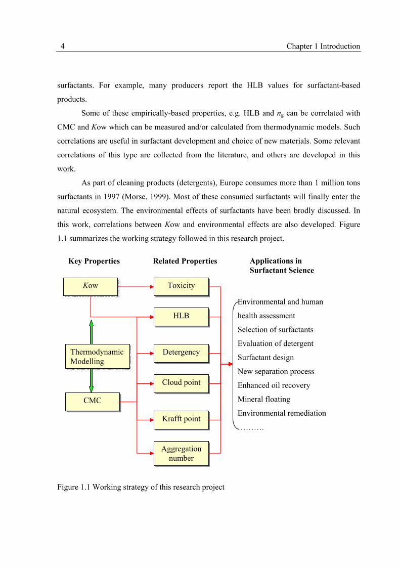
As part of cleaning products (detergents), Europe consumes more than 1 million tons
surfactants in 1997 (Morse, 1999). Most of these consumed surfactants will finally enter the
natural ecosystem. The environmental effects of surfactants have been brodly discussed. In
this work, correlations between Kow and environmental effects are also developed. Figure
1.1 summarizes the working strategy followed in this research project.
Figure 1.1 Working strategy of this research project
Key Properties
Kow
CMC
Related Properties Applications in
Surfactant Science
HLB
Toxicity
Detergency
Cloud point
Krafft point
Aggregation number
Environmental and human
health assessment
Selection of surfactants
Evaluation of detergent
Surfactant design
New separation process
Enhanced oil recovery
Mineral floating
Environmental remediation
……….
Thermodynamic Modelling
Chapter 1 Introduction 5
Priority Surfactants
Following the guidelines of the Danish environmental research programme (AMI
report, 2000, Madsen, et al. 2001, Danish EPA web page: www.mst.dk), the priority
surfactant families which were chosen for further studying in this work are sodium alkyl
sulphates, sodium alkyl ether sulphates and alcohol ethoxylates. Meanwhile, the octanol-
water partition coefficient of phthalates has been also studied as part of this environmental
program.
References
AMI report, “Review of the Knowledge Basis of Risk Evaluation of Air Pollutions in Relation to Lung Cancer and Respiratory System Allergy,” Center for Environmental and Respiratory System, National Institute of Occupational Health, Denmark, (2000) (in Danish).
Chen, C.-C., “Molecular Thermodynamic Model Based on the Polymer NRTL Model for Nonionic Surfactant Solutions,” AIChE J., 42, 3231 (1996)
Chen, C.-C., C. P. Bokis, and P. Mathias, “Segment-Based Excess Gibbs Energy Model for Aqueous Organic Electrolytes,” AIChE J., 47, 2593 (2001)
Cheng, H. Y., G. M. Kontogeorgis, and E. H. Stenby, “Prediction of Micelle Formation for Non-ionic Surfactants through UNIFAC Method,” Ind. Eng. Chem. Res., 41, 892 (2002).
Flores, M. V., E. C. Voutsas, N. Spiliotis, G. M. Eccleston, G. Bell, D. P. Tassios, and P. J. Halling, “Critical Micelle Concentrations of Non-ionic Surfactants in Organic Solvents: Approximate Prediction with UNIFAC,” Journal of Colloid and Interface Science, 240, 277 (2001).
Hines, J. D., “Theoretical Aspects of Micelllisation in Surfactant Mixtures,” Current
Opinion in Colloid & Interface Science, 6, 350 (2001). Madsen, T., H. B. Boyd, D. Nylén, A. R. Pedersen, G. I. Petersen and F. Simonsen,
“Environmental and Health Assessment of Substances in Household Detergents and Cosmetic Detergent Products,” Environmental Project No. 615, Danish Environmental Protection Agency (www.mst.dk), Copenhagen, (2001).
Morse, P. M. “Soaps & Detergents”, Chemical & Engineering News, 77, 35, Feb. 1,
(1999).

6 Chapter 1 Introduction

Chapter 2 Surfactant Solutions 7
Chapter 2 Surfactant Solutions
In this chapter, some basic characteristics of surfactant molecules and solutions are
briefly described. The environmental and health assessment of surfactants is discussed. The
micelle formation and phase diagrams of surfactant solution are outlined.
2.1 Surfactants and Classification Surfactant Molecules
Surfactant molecules have a dual nature. One part of the molecule is soluble in water (the
hydrophilic part or “head”), while the other part is not water-soluble (the hydrophobic part or
“tail”), as shown in Figure 2.1. The hydrophobic part is commonly a hydrocarbon chain
(branched or linear) that may contain aromatic structures. This part of the surfactant is
soluble in oil (non-polar solvents) but only sparingly soluble in water and other polar
solvents. The hydrophilic part on the other hand has a great affinity to water but is not very
soluble in non-polar solvents (oil). The hydrophilic part can be an ionic or strongly polar
group (such as ethylene oxide).
Figure 2.1 Structure of surfactant molecules
Despite being called the head-group, the hydrophilic part is not necessarily placed at the
end of the hydrocarbon chain. More than one hydrophilic or hydrophobic group can be
present in a surfactant molecule. A surfactant molecule is not fully compatible with either a
non-polar or a polar medium. There is always a conflict between the affinity of the head-
Hydrophilic head
Hydrophobic tail

8 Chapter 2 Surfactant Solutions
group and the tail. Their amphiphilic nature forces the surfactant molecules to adopt unique
orientations in an aqueous medium and to form suitably organized aggregates.
Classification of Surfactant Molecules
Surfactants are typically classified according to the nature (charge) of their head-
group. Four main types of surfactants exist: anionic, cationic, non-ionic and zwitterionic (or
amphoteric) surfactants, as shown in Figure 2.2 (Porter, 1994). The ionic surfactants carry a
net charge (positive or negative) located on the head-group, whereas the non-ionic surfactants
are neutral, but have polar head-groups e.g. ethylene oxide (EO). Zwitterionic surfactants can
be either anionic or cationic depending on the pH value of the solution.
Figure 2.2 The four different main types of surfactants Examples and Chemical Structures of Surfactant Molecules
Anionic Surfactants
Anionic surfactants are the most common surfactants in cleaning products with 0.6
million tons consumed in the U.S. in 1997. Anionics are the least expensive surfactants, at
0.6 cents to $2.00 per kg, and prices are generally stable (Morse, 1999). The hydrophilic part
of the molecules can be a carboxylate, sulphate, sulfonate or phosphate. Some examples are
given in Table 2.1 (de Guertechin, 1999, Huibers et al. 1997).
+
+
Non-ionic
Anionic
Cationic
Zwitterionic

Chapter 2 Surfactant Solutions 9
Table 2.1 Examples and chemical structures of anionic surfactants Carboxylates CH3CH2…CH2-COO-
C O-
O
Phosphates CH3CH2…CH2-PO4
-
OP O
-
O
O-
Alkylsulfates CH3CH2…CH2-OSO3
-
O S
O
O
O-
Alkyl sulfonates CH3CH2…CH2-SO3
-
S O-
O
O
Alkylbenzenesulfonates CH3CH2…CH2-C6H4-SO3
-
SO3-
Alkylethersulfonates CH3CH2…CH2-CHO-SO3
-
O O SO3-
Alkylethersulfates CH3CH2…CH2 CHO-OSO3
-
O OSO3-
Others
OHSO3
-
SO3-
NR R
Cationic Surfactants
Typical cationic surfactants are alkyl amines, alkylimidazolines, quaternary
ammonium compounds, ethoxylated alkyl amines and esterified quaternaries, as shown in
Table 2.2. The alkyl amines are not strictly cationic surfactant because they are uncharged in
solution (de Guertechin, 1999). Only a small amount of cationic surfactants are consumed per
year compared to anionic and non-ionic surfactants. Cationics are remain a small, specialized
part of cleaning product market (Morse, 1999).
10 Chapter 2 Surfactant Solutions
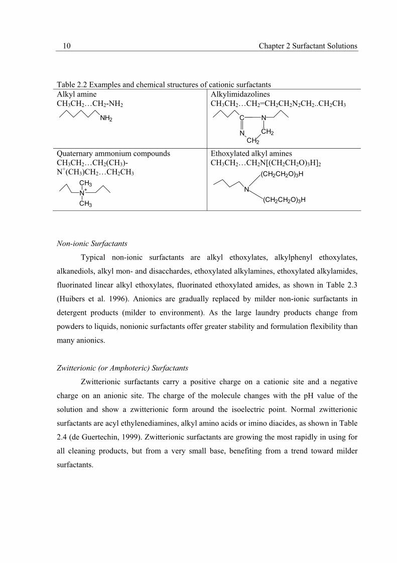
Table 2.2 Examples and chemical structures of cationic surfactants Alkyl amine CH3CH2…CH2-NH2
NH2
Alkylimidazolines CH3CH2…CH2=CH2CH2N2CH2..CH2CH3
C
NCH2
N
CH2
Quaternary ammonium compounds CH3CH2…CH2(CH3)-N+(CH3)CH2…CH2CH3
N+
CH3
CH3
Ethoxylated alkyl amines CH3CH2…CH2N[(CH2CH2O)3H]2
N
(CH2CH2O)3H
(CH2CH2O)3H
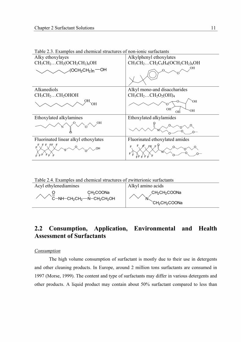
Non-ionic Surfactants
Typical non-ionic surfactants are alkyl ethoxylates, alkylphenyl ethoxylates,
alkanediols, alkyl mon- and disacchardes, ethoxylated alkylamines, ethoxylated alkylamides,
fluorinated linear alkyl ethoxylates, fluorinated ethoxylated amides, as shown in Table 2.3
(Huibers et al. 1996). Anionics are gradually replaced by milder non-ionic surfactants in
detergent products (milder to environment). As the large laundry products change from
powders to liquids, nonionic surfactants offer greater stability and formulation flexibility than
many anionics.
Zwitterionic (or Amphoteric) Surfactants
Zwitterionic surfactants carry a positive charge on a cationic site and a negative
charge on an anionic site. The charge of the molecule changes with the pH value of the
solution and show a zwitterionic form around the isoelectric point. Normal zwitterionic
surfactants are acyl ethylenediamines, alkyl amino acids or imino diacides, as shown in Table
2.4 (de Guertechin, 1999). Zwitterionic surfactants are growing the most rapidly in using for
all cleaning products, but from a very small base, benefiting from a trend toward milder
surfactants.
Chapter 2 Surfactant Solutions 11
Table 2.3. Examples and chemical structures of non-ionic surfactants Alky ethoxylayes CH3CH2…CH2(OCH2CH2)nOH
(OCH2CH2)n OH
Alkylphenyl ethoxylates CH3CH2…CH2C6H4(OCH2CH2)nOH
OO
OH
Alkanediols CH3CH2…CH2OHOH
OHOH
Alkyl mono-and disaccharides CH3CH2…CH2O2(OH)4
OO OH
OHOHOH
Ethoxylated alkylamines
NO
OOH
O
Ethoxylated alkylamides
N
OO
OO
OO O
Fluorinated linear alkyl ethoxylates
S
F F
FF F
F F
F F
F F
F FO
OOH
Fluorinated ethoxylated amides
NF
F
FFF
F F
F F
F FF
F F
FO
OO
O
OO O
Table 2.4. Examples and chemical structures of zwitterionic surfactants Acyl ethylenediamines
C
O
NH CH2CH2 N CH2CH2OH
CH2COONa
Alkyl amino acids
N
CH2CH2COONa
CH2CH2COONa
2.2 Consumption, Application, Environmental and Health Assessment of Surfactants
Consumption
The high volume consumption of surfactant is mostly due to their use in detergents
and other cleaning products. In Europe, around 2 million tons surfactants are consumed in
1997 (Morse, 1999). The content and type of surfactants may differ in various detergents and
other products. A liquid product may contain about 50% surfactant compared to less than
12 Chapter 2 Surfactant Solutions
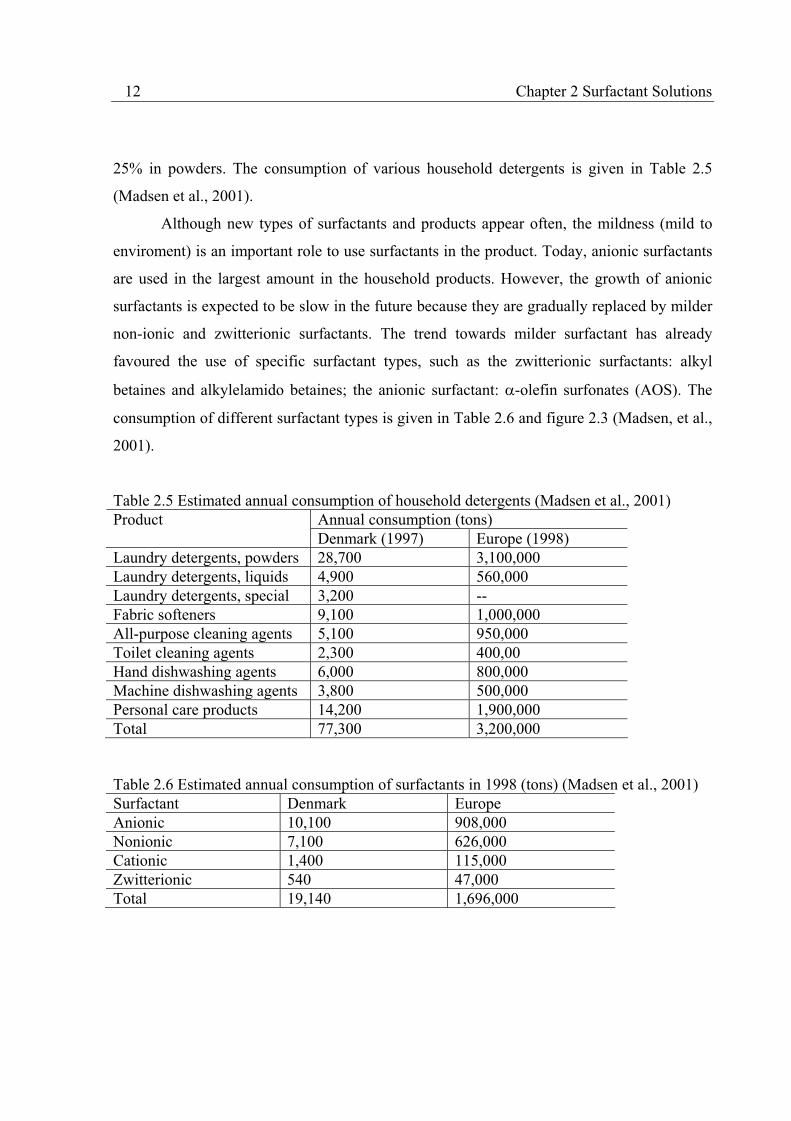
25% in powders. The consumption of various household detergents is given in Table 2.5
(Madsen et al., 2001).
Although new types of surfactants and products appear often, the mildness (mild to
enviroment) is an important role to use surfactants in the product. Today, anionic surfactants
are used in the largest amount in the household products. However, the growth of anionic
surfactants is expected to be slow in the future because they are gradually replaced by milder
non-ionic and zwitterionic surfactants. The trend towards milder surfactant has already
favoured the use of specific surfactant types, such as the zwitterionic surfactants: alkyl
betaines and alkylelamido betaines; the anionic surfactant: -olefin surfonates (AOS). The
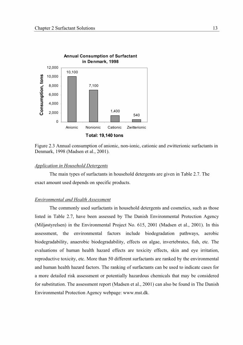
consumption of different surfactant types is given in Table 2.6 and figure 2.3 (Madsen, et al.,
2001).
Table 2.5 Estimated annual consumption of household detergents (Madsen et al., 2001) Annual consumption (tons) Product Denmark (1997) Europe (1998)
Laundry detergents, powders 28,700 3,100,000 Laundry detergents, liquids 4,900 560,000 Laundry detergents, special 3,200 -- Fabric softeners 9,100 1,000,000 All-purpose cleaning agents 5,100 950,000 Toilet cleaning agents 2,300 400,00 Hand dishwashing agents 6,000 800,000 Machine dishwashing agents 3,800 500,000 Personal care products 14,200 1,900,000 Total 77,300 3,200,000 Table 2.6 Estimated annual consumption of surfactants in 1998 (tons) (Madsen et al., 2001) Surfactant Denmark Europe Anionic 10,100 908,000 Nonionic 7,100 626,000 Cationic 1,400 115,000 Zwitterionic 540 47,000 Total 19,140 1,696,000
Chapter 2 Surfactant Solutions 13
Annual Consumption of Surfactant
in Denmark, 1998
10,100
7,100
1,400540
0
2,000
4,000
6,000
8,000
10,000
12,000
Anionic Nonionic Cationic Zwitterionic
Total: 19,140 tons
Co
nsu
mp
tio
n, to
ns
Figure 2.3 Annual consumption of anionic, non-ionic, cationic and zwitterionic surfactants in Denmark, 1998 (Madsen et al., 2001).
Application in Household Detergents
The main types of surfactants in household detergents are given in Table 2.7. The
exact amount used depends on specific products.
Environmental and Health Assessment
The commonly used surfactants in household detergents and cosmetics, such as those
listed in Table 2.7, have been assessed by The Danish Environmental Protection Agency
(Miljøstyrelsen) in the Environmental Project No. 615, 2001 (Madsen et al., 2001). In this
assessment, the environmental factors include biodegradation pathways, aerobic
biodegradability, anaerobic biodegradability, effects on algae, invertebrates, fish, etc. The
evaluations of human health hazard effects are toxicity effects, skin and eye irritation,
reproductive toxicity, etc. More than 50 different surfactants are ranked by the environmental
and human health hazard factors. The ranking of surfactants can be used to indicate cases for
a more detailed risk assessment or potentially hazardous chemicals that may be considered
for substitution. The assessment report (Madsen et al., 2001) can also be found in The Danish
Environmental Protection Agency webpage: www.mst.dk.
14 Chapter 2 Surfactant Solutions
Table 2.7 Overview the contents of household detergents (Morse, 1999) Household detergent Surfactant contents* Heavy-duty laundry powders Linear alkylbenzene sulfonates
- Sulfomethyl esters Alkyl polyglucosides Alcohol sulfates Linear alcohol ethoxylates
Heavy-duty laundry liquids Linear alkylbenzene sulfonates Linear alcohol ethoxylates
Light-duty liquid detergents Linear alkylbenzene sulfonates Light-duty liquid dish detergents Secondary alkane sulfonates
-Olefin sulfonates Fatty amine oxides Fatty alkanolamides Alkyl polyglucosides Linear alcohol ethoxylates
Liquid hand soaps -Olefin sulfonates, Shampoos -Olefin sulfonates
Fatty amine oxides Fatty alkanolamides Alcohol sulfates Linear alcohol ethoxylates
Toilet soaps Alkyl glyceryl ether sulfonates Specialty cleansers Linear alkylbenzene sulfonates
Fatty amine oxides *It is not necessary to have all the contents in one product.
2.3 Micelle Formation
When surfactants are dissolved in water, they are forced to adopt unique orientations
in the water medium because of their dual nature. The surfactant molecules become adsorbed
at an air-water or oil-water interface. They are able to locate their hydrophilic head groups in
the aqueous phase and allow the hydrophobic hydrocarbon chains to escape into the vapour
or oil phases, as shown in Figure 2.4. This situation is energetically more favourable than
complete solubilization in either phase. The strong adsorption of such molecules results in
the formation of an orientated mono-molecule layer at surface or interface. This surface
activity is a dynamic phenomenon, since the final state of a surface or interface represents a

Chapter 2 Surfactant Solutions 15
balance between the tendency towards adsorption and the tendency towards complete mixing
due to the thermal motion of the molecules.
Figure 2.4 Surface adsorption and micelle formation
The tendency of surfactants to pack into an interface favours an expansion of the
interface. Therefore, this must be balanced against the tendency for the interface to contract
under normal surface tension forces. The surface tension is thus lowered. If the interfacial
tension between two liquids is reduced to a sufficiently low value with the addition of a
surfactant, emulsification will readily take place, because only a relatively small increase in
the surface free energy of the system is involved (Shaw, 1992).
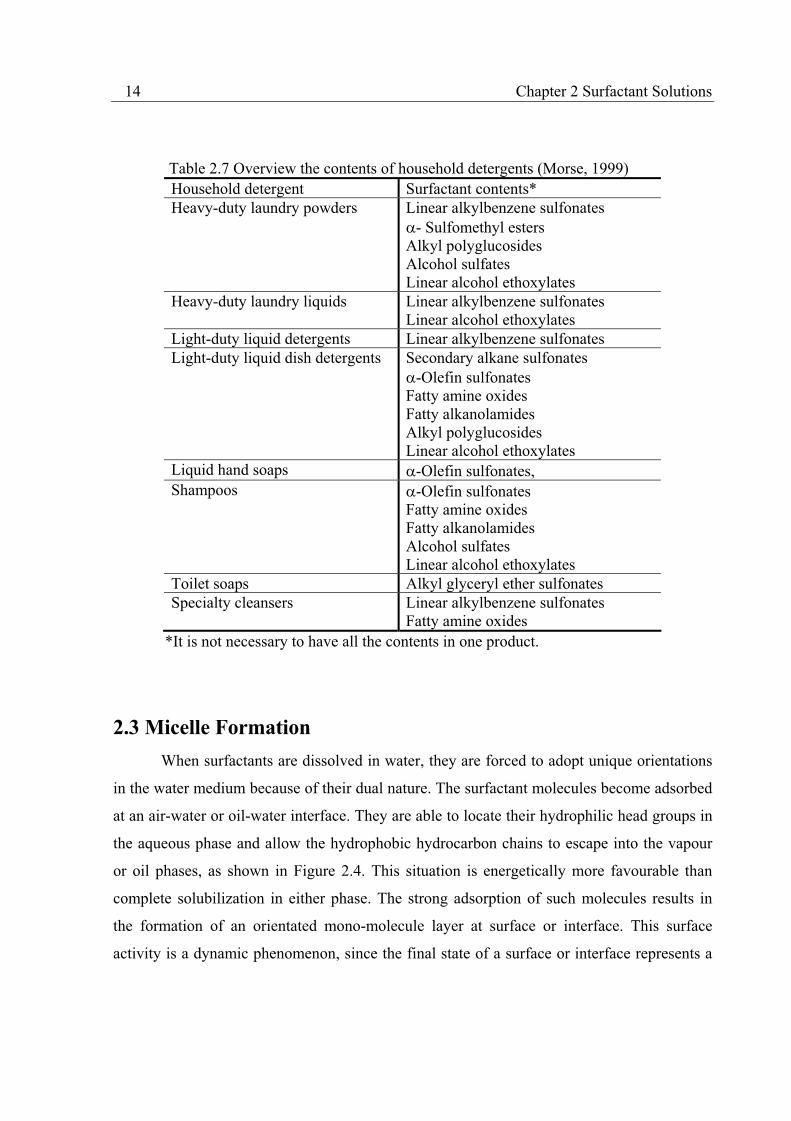
At fairly well defined concentrations, several physical properties (e.g. osmotic pressure,
electrical conductivity, surface tension, etc.) abruptly change their values in aqueous
surfactant solutions, as schematically shown in Figure 2.5. McBain and Swain (1936)
suggested that this seemingly anomalous behaviour could be explained in terms of the
formation of organised aggregates of the surfactant molecules, the micelles. The
concentration above which micelle formation becomes appreciable is termed “critical micelle
concentration (CMC)”. However, the CMC is a narrow concentration range, not a fixed value
as shown in figure 2.5. When the hydrophobic part of the surfactant is a hydrocarbon chain,
the micelle will consist of a hydrocarbon core, with hydrophilic groups at the surface serving
Surfactants
Micelle
Free surfactant molecule
Surface layer
16 Chapter 2 Surfactant Solutions
to maintain solubility in water. In such micelles, the hydrophobic core is, in effect, a small
volume of liquid hydrocarbon because the hydrocarbon chains are generally regarded as
disordered (Tanford, 1980).
CMC
Osmotic pressure
Conductivity
Density changeDetergency
Surface tension
Pro
pert
y
Surfactant concentration
Figure 2.5 Variation of various properties with surfactant concentration
2.4 Phase Behaviour of Surfactant Solutions
The phase behaviour of surfactant solutions is a basis to understand the properties of
these systems and is important for the numerous industrial applications of surfactants.
However, the phase diagram of surfactant solution is very complex because the surfactant
molecules undergo many different metastable states with changing temperature and
concentration. The metastable phases are characterized as irreversible colloid particles. Many
research aspects in phase studies of surfactant systems are summarized in book of Laughlin
(1994) and in some reviews (Chernik, 2000, Khan, 1996).
The basic phase behaviour of surfactant solutions and the commonly encountered
phase regions are shown in Figure 2.6 (Holland and Rubingh, 1992). In the temperature vs.
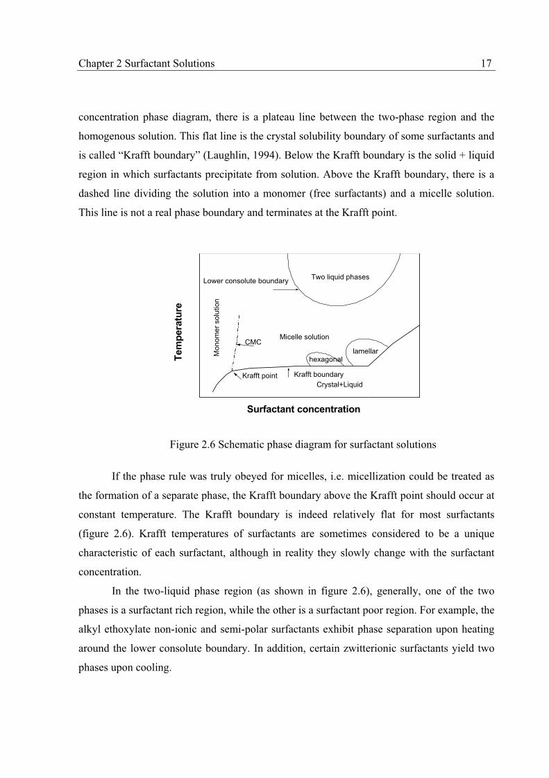
Chapter 2 Surfactant Solutions 17
concentration phase diagram, there is a plateau line between the two-phase region and the
homogenous solution. This flat line is the crystal solubility boundary of some surfactants and
is called “Krafft boundary” (Laughlin, 1994). Below the Krafft boundary is the solid + liquid
region in which surfactants precipitate from solution. Above the Krafft boundary, there is a
dashed line dividing the solution into a monomer (free surfactants) and a micelle solution.
This line is not a real phase boundary and terminates at the Krafft point.
Krafft boundary
lamellarhexagonal
Crystal+Liquid
Krafft point
Mo
no
me
r so
lutio
n
Micelle solutionCMC
Lower consolute boundaryTwo liquid phases
Tem
pera
ture
Surfactant concentration
Figure 2.6 Schematic phase diagram for surfactant solutions
If the phase rule was truly obeyed for micelles, i.e. micellization could be treated as
the formation of a separate phase, the Krafft boundary above the Krafft point should occur at
constant temperature. The Krafft boundary is indeed relatively flat for most surfactants
(figure 2.6). Krafft temperatures of surfactants are sometimes considered to be a unique
characteristic of each surfactant, although in reality they slowly change with the surfactant
concentration.
In the two-liquid phase region (as shown in figure 2.6), generally, one of the two
phases is a surfactant rich region, while the other is a surfactant poor region. For example, the
alkyl ethoxylate non-ionic and semi-polar surfactants exhibit phase separation upon heating
around the lower consolute boundary. In addition, certain zwitterionic surfactants yield two
phases upon cooling.
18 Chapter 2 Surfactant Solutions
0 20 40 60 80 100
wt% of C10E6
0
40
80
-20
20
60
100
Tem
pera
ture
, °C
V1
L
Liquid
2-liquid
H1
Liquid
C10E6+Scice+ Sc
ice+H1
C10E6+Lice+L
C10E6+H1
----Expt. data
C10E6+L
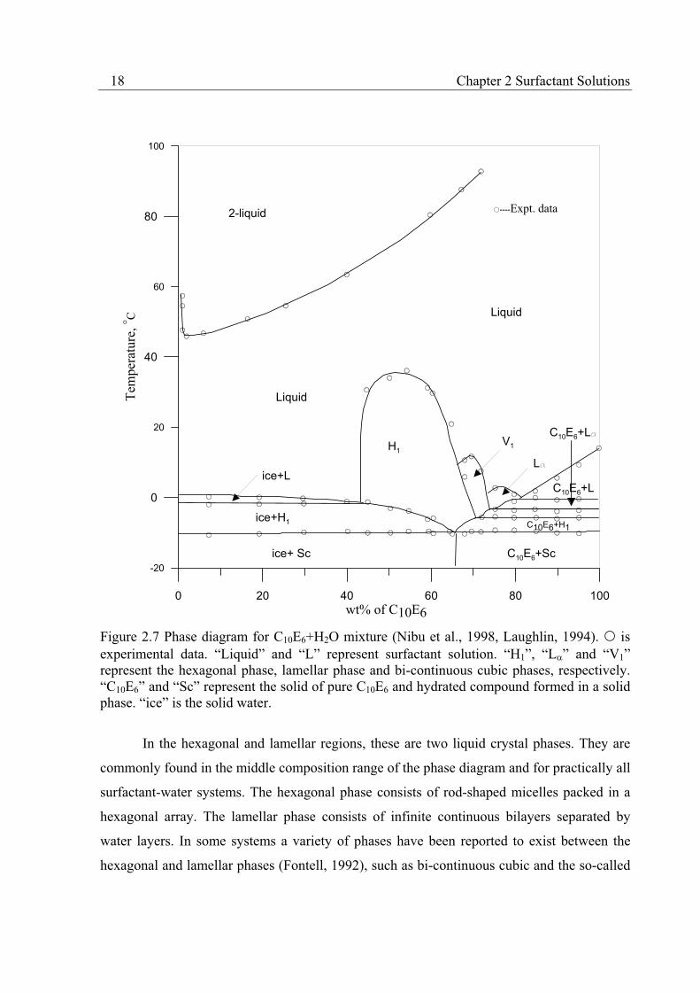
Figure 2.7 Phase diagram for C10E6+H2O mixture (Nibu et al., 1998, Laughlin, 1994). is experimental data. “Liquid” and “L” represent surfactant solution. “H1”, “L ” and “V1” represent the hexagonal phase, lamellar phase and bi-continuous cubic phases, respectively. “C10E6” and “Sc” represent the solid of pure C10E6 and hydrated compound formed in a solid phase. “ice” is the solid water.
In the hexagonal and lamellar regions, these are two liquid crystal phases. They are
commonly found in the middle composition range of the phase diagram and for practically all
surfactant-water systems. The hexagonal phase consists of rod-shaped micelles packed in a
hexagonal array. The lamellar phase consists of infinite continuous bilayers separated by
water layers. In some systems a variety of phases have been reported to exist between the
hexagonal and lamellar phases (Fontell, 1992), such as bi-continuous cubic and the so-called

Chapter 2 Surfactant Solutions 19
intermediate phases (Holmes, 1998). An example of phase diagram for hexaethylene glycol
decyl ether is given in figure 2.7.
Figure 2.7 shows a phase diagram for hexaethylene glycol decyl ether (C10E6) and
water system (Nibu, et al., 1998, Laughlin, 1994). In figure 2.7, “2-liquid phase” represents a
two liquid phase region. H1 and L represent the hexagonal and the lamellar phases,
respectively. C10E6 and Sc represent the solid of pure C10E6 and the hydrated compound
formed in a solid phase, respectively. V1 represents a bi-continuous cubic phase. Ice
represents the solid water. Liquid and L represent the C10E6+H2O solution.

20 Chapter 2 Surfactant Solutions
Chapter 3 Thermodynamics of Surfactant Solutions 21
Chapter 3 Thermodynamics of Surfactant Solutions
In this chapter, different thermodynamic treatments for micelle formation in
surfactant solutions are discussed. Although many efforts have been made towards
theoretical understanding of surfactant solutions, capturing the nature of such solutions is
still considered rather difficult. In contrast to the rigorous universal thermodynamic
treatment of fluid phase equilibrium, many thermodynamic formulations have been
proposed for micelle formation.
In this study, two types of thermodynamic methods are discussed: i)
phenomenological models, such as the pseudo-phase separation model and the mass-action
model and ii) molecular thermodynamic methods, such as those proposed by Tanford
(1980), Israelachvili (1992), Nagarajan (1991, 1997a), Blankschtein (1986), and Chen et al.
(1996, 2001).
3.1 Outline
The majority of research in the area of surfactant science focuses on experimental
studies and documentation of behaviour. The theoretical understanding is rather limited
(Hines, 2001). Blandamer et al. (1995), Blankschtein et al. (1997), Hines, (2001),
Nagarajan (1997b), and Zana (1995) have reviewed the theories for surfactant solutions.
Laughlin (1994) reviewed phase behaviours of surfactant solution and the history of
surfactant science. These reviews include many different theories and models for surfactant
solutions. However, only few of them have been applied to practice.
Theoretical approaches for surfactant solutions may be classified into molecular
thermodynamic and phenomenological methods (empirical, semi-empirical methods). The
molecular thermodynamic methods describe the physical properties of surfactant solutions
using molecular thermodynamic principles and molecular structure characteristics.
Empirical relations correlate experimental results via statistical methods. The semi-
empirical methods follow an intermediate road, employing empirical rules and combining
databases of physical properties with quantum chemical or topological descriptors. An
22 Chapter 3 Thermodynamics of Surfactant Solutions
important limitation of the semi-empirical and empirical approaches is that their
implementation relies exclusively on the availability of experimental data. In
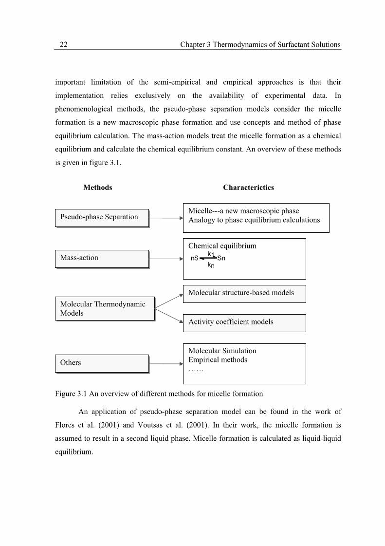
phenomenological methods, the pseudo-phase separation models consider the micelle
formation is a new macroscopic phase formation and use concepts and method of phase
equilibrium calculation. The mass-action models treat the micelle formation as a chemical
equilibrium and calculate the chemical equilibrium constant. An overview of these methods
is given in figure 3.1.
Figure 3.1 An overview of different methods for micelle formation
An application of pseudo-phase separation model can be found in the work of
Flores et al. (2001) and Voutsas et al. (2001). In their work, the micelle formation is
assumed to result in a second liquid phase. Micelle formation is calculated as liquid-liquid
equilibrium.
Pseudo-phase Separation
Mass-action
Molecular Thermodynamic Models
Others
Micelle---a new macroscopic phase Analogy to phase equilibrium calculations
Chemical equilibrium
nS Snkn
k1
Molecular Simulation Empirical methods ……
Molecular structure-based models
Activity coefficient models
Methods Characterictics
Chapter 3 Thermodynamics of Surfactant Solutions 23
Desnoyers and co-workers (1997) applied the mass-action approach to non-ionic
surfactants and extended it to ionic systems by correlating the data for the monomers with
the Debye-Hückel limiting law.
Two different methods are used in the molecular thermodynamic models: one is
based on detailed molecule structure information to calculate the properties of micelle
formation; the other depends on activity coefficient models.
The objective of molecular thermodynamic theories is to relate the chemical
potential of surfactant molecules in the micelle state to the chemical potential of the free
surfactant molecules in solution. These theories provide a way of relating the molecular
geometry, size and chemical nature of the hydrophilic and hydrophobic groups in surfactant
molecules to both macroscopic properties of the solutions and the size of the aggregated
micelles. Fundamental contributions in this area are the work by Tanford (1980) and
Israelachvili (1992).
Nagarajan (1991, 1997a), and Blankschtein (1997, 1998) developed two similar
molecular thermodynamic methods for surfactant solution (“molecular structure” branch in
figure 3.1). Detailed molecular and micelle structures descriptions are used to build up the
properties of micelle formation and surfactant solution. They have used their methods to
calculate CMC and other properties for nonionic, anionic, pure and binary surfactant
mixtures (Zoller, 1996).
Recently, Chen et al. (1996, 2001) proposed a thermodynamic framework for the
micelle formation combined with conventional local composition activity coefficient
models, such as NRTL (“activity coefficient” branch in figure 3.1). This method has been
applied to calculate CMC of non-ionic and ionic surfactant solutions. Based on Chen’s
proposal, Li et al. (1998, 2000) used UNIQUAC and SAFT equations to calculate CMC of
non-ionic and ionic surfactant solutions.
Some of these methods are briefly presented in following sections.
24 Chapter 3 Thermodynamics of Surfactant Solutions
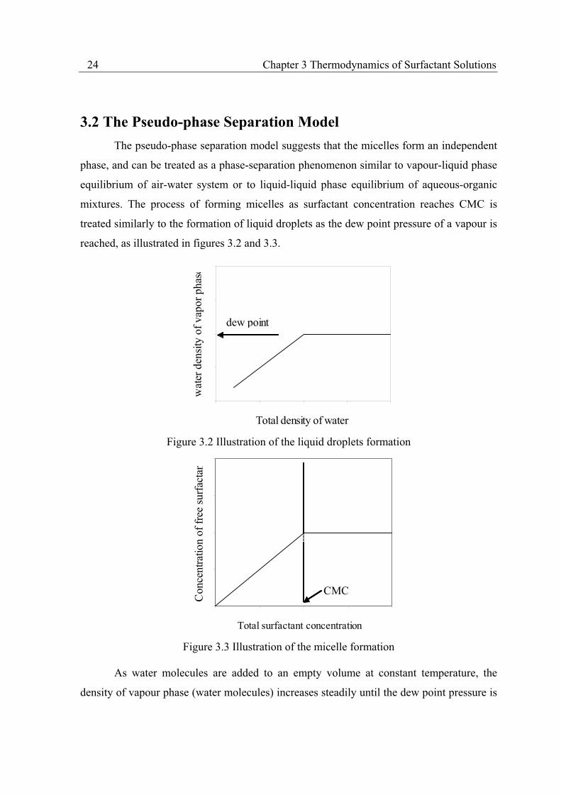
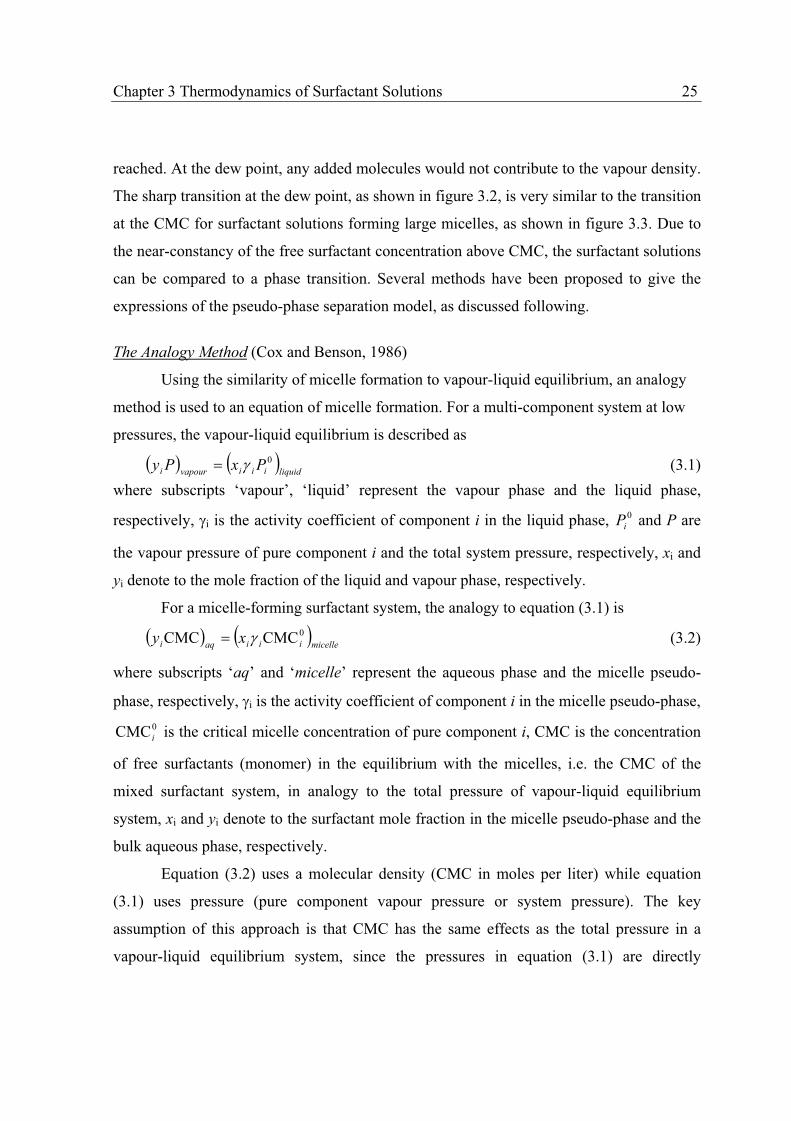
3.2 The Pseudo-phase Separation Model
The pseudo-phase separation model suggests that the micelles form an independent
phase, and can be treated as a phase-separation phenomenon similar to vapour-liquid phase
equilibrium of air-water system or to liquid-liquid phase equilibrium of aqueous-organic
mixtures. The process of forming micelles as surfactant concentration reaches CMC is
treated similarly to the formation of liquid droplets as the dew point pressure of a vapour is
reached, as illustrated in figures 3.2 and 3.3.
Total density of water
wat
er d
ensi
ty o
f va
por
phas
e
dew point
Figure 3.2 Illustration of the liquid droplets formation
Total surfactant concentration
Con
cent
ratio
n of
fre
e su
rfac
tan
CMC
Figure 3.3 Illustration of the micelle formation
As water molecules are added to an empty volume at constant temperature, the
density of vapour phase (water molecules) increases steadily until the dew point pressure is
Chapter 3 Thermodynamics of Surfactant Solutions 25
reached. At the dew point, any added molecules would not contribute to the vapour density.
The sharp transition at the dew point, as shown in figure 3.2, is very similar to the transition
at the CMC for surfactant solutions forming large micelles, as shown in figure 3.3. Due to
the near-constancy of the free surfactant concentration above CMC, the surfactant solutions
can be compared to a phase transition. Several methods have been proposed to give the
expressions of the pseudo-phase separation model, as discussed following.
The Analogy Method (Cox and Benson, 1986)
Using the similarity of micelle formation to vapour-liquid equilibrium, an analogy
method is used to an equation of micelle formation. For a multi-component system at low
pressures, the vapour-liquid equilibrium is described as
liquidiiivapouri PxPy 0 (3.1)
where subscripts ‘vapour’, ‘liquid’ represent the vapour phase and the liquid phase,
respectively, i is the activity coefficient of component i in the liquid phase, 0iP and P are
the vapour pressure of pure component i and the total system pressure, respectively, xi and
yi denote to the mole fraction of the liquid and vapour phase, respectively.
For a micelle-forming surfactant system, the analogy to equation (3.1) is
micelleiiiaqi xy 0CMCCMC (3.2)
where subscripts ‘aq’ and ‘micelle’ represent the aqueous phase and the micelle pseudo-
phase, respectively, i is the activity coefficient of component i in the micelle pseudo-phase,
0CMC i is the critical micelle concentration of pure component i, CMC is the concentration
of free surfactants (monomer) in the equilibrium with the micelles, i.e. the CMC of the
mixed surfactant system, in analogy to the total pressure of vapour-liquid equilibrium
system, xi and yi denote to the surfactant mole fraction in the micelle pseudo-phase and the
bulk aqueous phase, respectively.
Equation (3.2) uses a molecular density (CMC in moles per liter) while equation
(3.1) uses pressure (pure component vapour pressure or system pressure). The key
assumption of this approach is that CMC has the same effects as the total pressure in a
vapour-liquid equilibrium system, since the pressures in equation (3.1) are directly

26 Chapter 3 Thermodynamics of Surfactant Solutions
proportional to densities under ideal gas conditions (low pressures), where equation (3.1) is
valid.
The Flores and Voutsas Approach (Flores et al., 2001, Voutsas et al., 2001)
In this approach, micelles are assumed to form a new macroscopic phase, i.e. a
second liquid phase. Liquid-liquid equilibrium is assumed between water and micelle. Two
phases coexist: one solvent (water)-rich phase where the surfactant concentration is the
CMC, and one surfactant-rich phase approximated by the micelle phase. At CMC
(equilibrium) the activities of both solvent and surfactant are the same in the two phases.
Flores et al., (2001) and Voutsas et al., (2001) used the UNIFAC method for
describing liquid-liquid equilibrium. The CMC of non-ionic surfactants in aqueous and
non-aqueous solvent is predicted. The reported average deviation between predicted and
experimental values was about 0.1 log units.
Many researchers have used the “pseudo-phase separation” approach to calculate
CMC in different surfactant solutions, such as non-ionic, ionic, anionic and cationic
surfactant solutions (Cox and Benson, 1986; Hall, 1987; Holland and Rubingh, 1992;
Ogino and Abe, 1993).
From a thermodynamic point of view, however, the formation of micelles is not a
true phase transition, because the micelle formation does not create a new macroscopic
phase in solution. The sharp changes in properties occur over a range of concentration. The
“pseudo-phase separation” approach represents the case when the aggregation number in
the micelles is assumed to approach infinity. In practical, the aggregation number falls
down in the range of 20 to 2000 in surfactant solutions. Thus, the pseudo-phase model
cannot describe the size of micelles (aggregation number).
3.3 The Mass-action Model
In the mass-action model, the micelle formation is considered as a chemical
equilibrium between free surfactant and micelle. At low concentrations, the micelle
solution is the formation of aggregates from free surfactant, as shown in equation (3.3).

Chapter 3 Thermodynamics of Surfactant Solutions 27
nS Sn (3.3) where n free surfactant molecules (S) form a micelle (Sn) having an aggregation number of
ng. Both micelles and free surfactants are treated as solutes in an aqueous solution. In the
mass-action model, the thermodynamic formulations are slightly different for nonionic and
ionic surfactant solutions. One of the formulations (nonionic surfactant) is described as
follows (Blandamer et al. 1995):
For nonionic (neutral) surfactant solutions, at chemical equilibrium, we have:
micelleimonign ,, (3.4) where i,mon is the chemical potential of monomeric (free) surfactant i, i,micelle is the
chemical potential of surfactant i in the micelle form, ng is the aggregation number. The
chemical potentials of monomeric surfactant and surfactant in micelle are given as:
monimonimonimoni xRT ,,0,, ln (3.5)
micelleimicelleimicelleimicellei xRT ,,0,, ln (3.6)
Using equation (3.4), we have
micelleimicellei
g
monimonimonimicellei
g
imic xRTn
xRTn
G ,,,,0,
0,
0 ln1
ln1
(3.7)
where xi,mon and xi,micelle are the mole fraction of monomeric surfactant and surfactant in
micelle, respectively, i,mon and i,micelle are the activity coefficient of monomeric surfactant
and surfactant in micelle, respectively, 0,moni and 0
,micellei are the standard state chemical
potential for monomeric surfactant and surfactant in micelle, respectively, and 0imicG is the
difference of Gibbs energy.
For a dilute solution, the activity coefficients of monomeric surfactant and
surfactant in micelle are set equal to 1.0. Then equation (3.7) becomes
micellei
g
moniimic xRTn
xRTG ,,0 ln
1ln (3.8)
In surfactant solution, CMC is the total concentration of surfactant (xtot), which is a
sum of free surfactant (xi,mon) and surfactants in micelles (xi,micelle). Assuming a sufficiently
high value for ng, the second term in the above equation become very small and can be
neglected. Then xi,mon can be approximated to CMC.

28 Chapter 3 Thermodynamics of Surfactant Solutions
Based on the mass-action model, Amos et al. (1998) proposed a model for the
distribution of micelle sizes. The model of Amos et al. includes micelle-micelle interactions
as a function of the size for a multi-component solution consisting of micelle aggregates,
monomer, counterions, and added electrolytes. Surfactant solutions of sodium dodecyl
sulphate and cetylpridinum chloride with 0.01M NaCl are studied in their work.
3.4 Molecular Thermodynamic Models
3.4.1 Tanford’s Approach
The work of Tanford (1980) systematically investigated the micelle formation using
molecule thermodynamic method. In Tanford’s theory, the hydrophobic effect of molecules
in aqueous solutions provides the driving force for aggregation, whereas the repulsion
between head (hydrophilic) groups limits the size that a micelle can attain. However, both
factors vary with the micelle size. It is therefore evident that a theoretical treatment without
containing the size dependence may account for the occurrence of surfactant aggregation,
but it cannot explain why micelles are the statistical aggregates with a broad size
distribution.
Since at equilibrium, a mixture will normally contain micelles with a range of
different aggregation numbers ng, it is necessary for a rigorous approach to account for the
size dependent contributions in the chemical potential. The simplest procedure is to
consider micelles of different size as distinct components of the solution, each
characterized by the number ng of constituent monomer molecules and by a distinct value
of the standard potential. The dependence of the standard potential on the value of ng arises
from the dependence of surface area with micelle size.
A chemical potential expression, equation (3.9), is often expressed as a sum of a
standard state chemical potential, 0i , and the part including the mole fraction xi and the
activity coefficient i :
iiii xRT ln0 (3.9)
Chapter 3 Thermodynamics of Surfactant Solutions 29
Tanford suggests that the second part ( iixRT ln ) contribution to the chemical
potential per mole of micelle of size ng is RTln(mole fraction of micelles of size ng),
assuming a sufficiently dilute solution in micelles, thus neglecting nonideality. Thus, the
second part of equation (3.9) becomes gn nxRTg
/ln , and the contribution per mole of
surfactants is 1/ng. Based on this analysis, Tanford formulated the conditions for micelle
formation with the chemical potential of free monomeric surfactants and the surfactants in
the micelle state.
Thermodynamic Formulation of Micelle Formation
In a solution of a single surfactant, the chemical potential of a surfactant in a micelle
of size ng, gnmic, , is given by
g
n
g
nmicnmicn
x
n
RT g
ggln0
,, (3.10)
where 0
gmic,n is the standard state chemical potential of a surfactant in the micelle state, gnx
is the mole fraction of surfactant inside the micelle of size ng.
The chemical potential of free monomeric surfactant in aqueous solutions, mon, is:
nxRT momon0monmon ln (3.11)
where 0mon is the standard state chemical potential of the free monomeric surfactants in
aqueous solutions, xmon is the mole fraction of free monomeric surfactants in aqueous
solutions, and mon is the activity coefficient of free monomeric surfactants in aqueous
solutions.
At equilibrium:
monnmic g, (3.12)
then
monmonmon
g
n
g
nmic xRTn
x
n
RT g
glnln 00
, (3.13)

30 Chapter 3 Thermodynamics of Surfactant Solutions
We assume that all micelles have the same size ng in the surfactant solutions, and introduce
a new standard state chemical potential 0mic (without subscript ng) for surfactant in any
micelle. Thus, equation (3.13) becomes
gmonmongmonmic
gn nxnRT
nxg
lnlnln00
(3.14)
Critical Micelle Concentration (CMC)
Tanford says that the concept of a “critical concentration” for the formation of
micelles from free surfactant is, rigorously speaking, inexact but convenient. It would be
exact if micelle formation could be regarded as separation of a distinct phase, and free
surfactant in solution could coexist with the micelle phase at only a fixed concentration. An
important feature of micelle formation is that the free monomeric surfactant concentration
in equilibrium with micelles changes only slowly with the concentration of micelles.
By defining a parameter CMC/gnx , then
CMC)1(monx (3.15)
Here the CMC is the total concentration in the micelle solution as follow:
gnmontotal xxx CMC (3.16)
Thus, at CMC, equation (3.14) gives:
g
g
mon
g
gmonmicn
nn
n
RTln
11lnlnCMCln
100
(3.17)
The exact choice of varies from 0.01 to 0.10.
The Tanford’s method and analysis for the hydrophobic effect in aqueous solutions
have been widely used in research related to biological lipids, proteins, serum lipoproteins,
and biological membranes. This method has been extended to large lipid aggregates such as
bilayers, vesicles, other micelle phases and microemulsion droplets by Nagarajan and
Rukenstein (1991), Israellachivili (1992), Blanckstein (1986), Puvvada and Blankschtein
(1990).
Chapter 3 Thermodynamics of Surfactant Solutions 31
3.4.2 Israelachvili’s Method
Israelachvili (1992) developed a thermodynamic framework for micelle formation
and then investigated the relationship between intermolecular interaction and different
micelle shapes. Different intermolecular interactions determine the formed micelles with
varied structures. Molecular geometry has a crucial role in determining the structures of
formed micelles. From the molecular geometry, many of the physical properties of
surfactant solutions can be quantitatively understood without requiring a detailed
knowledge of the complex molecular forces.
Thermodynamic Equations of Micelle Formation
The micelle formation is expressed as a formation of surfactant aggregates with
different sizes:
S + S S2 dimers (3.18)
S + S +S S3 trimers
……..
S + S + S +… Sn n-mers
Equilibrium thermodynamics requires that when molecules form aggregated
structures in solution, the chemical potentials of all identical molecules in different
aggregates are the same. This is expressed as:
...3
1log
3
1
2
1log
2
1log 3
032
021
01 xTkxTkxTk BBB (3.19)
monomers dimers trimers
or
g
n
g
Bnn
n
x
n
Tk g
gglog0 constant, ng=1, 2, 3,…. (3.20)
where gn is the mean chemical potential of a molecule in a micelle of aggregation number
ng, 0
gn is the standard state of the chemical potential (the mean interaction free energy per
molecule) in an micelle of aggregation number ng, gnx is the concentration (more strictly the
32 Chapter 3 Thermodynamics of Surfactant Solutions
activity) of molecules in aggregates of number ng (ng=1, 01 and x1 correspond to isolated
molecules, or monomers, in solution), and kB is the Boltzmann constant. Using the law of
mass action, equation (3.19) can be derived as follows:
Rate of association = gnxk 11 (3.21)
Rate of dissociation = g
n
nn
xk
g
g (3.22)
where
Tk
n
k
kK
B
ng
n
g
g
01
0
1 exp (3.23)
This is the ratio of the two ‘reaction’ rates (equilibrium constants), k1 and gnk .
Equation (3.23) assumes ideal mixing and is restricted to dilute systems where inter-
aggregate interactions can be ignored.
Combining equations (3.19)-(3.23), we obtain:
Mn
B
nMM
g
n
g
gg
Tk
M
M
x
n
x/
00
exp (3.24)
If M=1, we have
g
gg
n
B
n
g
n
Tkx
n
x 001
1 exp (3.25)
where M is any arbitrary reference state of aggregates (or monomers) with aggregation
number M (or 1). The total solute concentration C is given by
1321 ...
g
g
n
nxxxxC (3.26)
Depending on how the standard state chemical potentials 01 and 0
gn are defined,
the dimensionless concentrations C and gnx can be expressed in volume fraction or mole
fraction. The C and gnx can never exceed unity. Equations (3.24)-(3.26) completely define
the system.
Chapter 3 Thermodynamics of Surfactant Solutions 33
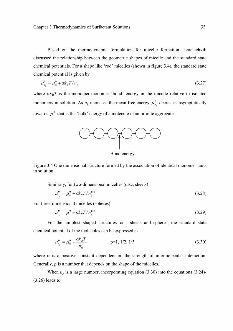
Based on the thermodynamic formulation for micelle formation, Israelachvili
discussed the relationship between the geometric shapes of micelle and the standard state
chemical potentials. For a shape like ‘rod’ micelles (shown in figure 3.4), the standard state
chemical potential is given by
gBn nTkg
/00 (3.27)
where kBT is the monomer-monomer ‘bond’ energy in the micelle relative to isolated
monomers in solution. As ng increases the mean free energy 0
gn decreases asymptotically
towards 0 that is the ‘bulk’ energy of a molecule in an infinite aggregate.
Figure 3.4 One dimensional structure formed by the association of identical monomer units in solution
Similarly, for two-dimensional micelles (disc, sheets)
2/100 / gBn nTkg
(3.28)
For three-dimensional micelles (spheres)
3/100 / gBn nTkg
(3.29)
For the simplest shaped structures-rods, sheets and spheres, the standard state
chemical potential of the molecules can be expressed as
p
g
Bn
n
Tkg
00 p=1, 1/2, 1/3 (3.30)
where is a positive constant dependent on the strength of intermolecular interaction.
Generally, p is a number that depends on the shape of the micelles.
When ng is a large number, incorporating equation (3.30) into the equations (3.24)-
(3.26) leads to
Bond energy
34 Chapter 3 Thermodynamics of Surfactant Solutions
gg
g
g
g
n
g
np
gg
n
B
n
gn exnnxnTk
xnx 11
001
1 /11expexp (3.31)
In equation (3.31), the limitation of x1 is RT
gn
001
exp or e . At this condition, the
monomer concentration x1 is the critical micelle concentration (CMC). Thus, in general
RTx
gn
001
crit1 expCMC)( (3.32)
or
ex CMC)( crit1 for all p (3.33)
where p is a number depended on the shape of the micelles. Equations (3.32) and (3.33)
define the CMC.
Critical Packing Parameter
Israelachvili (1992) proposed a critical packing parameter (cpp) to describe the
surfactant molecule structures as:
cla
v
0
cpp (3.34)
where v denotes to the tail chain (or chains) volume, lc is the critical tail chain length, a0 is
the headgroup area at the head-tail interface, as shown in figure 3.5. The v and lc can be
calculated by empirical equations (Tanford, 1980). a0 can be measured by experimental
method (Lantzsch et al., 1996).
Figure 3.5 The cpp of a surfactant molecule
chain length lc
headgroup area a0 tail volume v
Chapter 3 Thermodynamics of Surfactant Solutions 35
Table 3.1 shows the relationship of cpp values and micelle structures. Different cpp
values correspond to different micelles, as shown in Table 3.1. The cpp value of surfactants
can also indicate which phase exists in solution: lamellar, cubic or hexagonal phases.
Table 3.1 Relationship between cpp value and micelle structure cpp value Micelle structure Example*
<1/3 Spherical micelles SDS in low salt
1/3~1/2 Cylindrical micelles SDS and CTAB in high salt
1/2~1 Flexible bilayers Phosphatidyl choline
~1 Planar bilayers Phosphatidyl ethanolamine
>1 Reversed micelle Cardiolipin+Ca2+
*SDS: sodium dodecyl sulphate, CTAB: hexadecyl trimethylammonium bromide
Based on the thermodynamic framework, Israelachvili studied the relationships
between micelle size distribution, micelle structures and CMC, the aggregation of
surfactant molecules into micelles, bilayers, vesicles and biological membranes.
3.4.3 Nagarajan’s Method
Nagarajan and co-workers (1991, 1997a) developed a thermodynamic model to
calculate CMC, aggregation number and phase separation for non-ionic, anionic, cationic
and zwitterionic single and mixed surfactant solutions depending on information of
structures and interactions. The method, in details, described the relations between
chemical potential (Gibbs free energy) of surfactant solutions and different micelle
structures.
Using the condition of ideal mixing in dilute solutions, the chemical potential of
micelles with size ng is given by
gBgg xTk ln0 (3.35)
36 Chapter 3 Thermodynamics of Surfactant Solutions
where 0g is the standard state of the species g (micelle with aggregation number ng), xg is
the mole fraction of micelles in solution. The chemical potential of monomer surfactant, 1,
is given by setting ng=1 in equation (3.35):
1011 ln xTkB (3.36)
where 01 is the standard state of free (monomeric) surfactant in solution and x1 is the mole
fraction of free (monomeric) surfactant in solution.
At equilibrium, the chemical potentials:
1
g
g
n (3.37)
where ng is the aggregation number.
The micelles size distribution equation is derived from equation (3.37)
Tk
nx
Tk
nxx
B
ggn
B
ggn
ggg
0
1
01
0
1 expexp (3.38)
where 0g is the difference in the standard state chemical potentials between a surfactant
molecule present in a micelle of size ng and a monomeric surfactant in solution.
If an expression for 0g is available, then the micelle size distribution can be
calculated from equation (3.38).
Based on different contributions, Nagarajan developed an equation to calculate 0g
as:
ionicgdipolegstericggdefgtrgg
000
int
0000 (3.39)
where trg
0 is the contribution from surfactant tail, defg
0 is the contribution of the tail
local deformation, int
0g is the contribution of the formation of micelle core–water
interface, stericg
0 describes how polar head groups of surfactant molecules are brought to
the surface of the micelle and generate steric repulsion among the head groups, dipoleg
0
is the contribution of the head group dipole interactions and ionicg
0 is the head group
ionic interactions.
Chapter 3 Thermodynamics of Surfactant Solutions 37
The calculation methods for these terms in equation (3.39) can be found in reference
of Nagarajan (1997a).
3.4.4 Blankschtein’s Method
Puvvada and Blankschtein (1990) proposed an approach that is a blending of a
molecular model of micellization with a thermodynamic theory.
Using the principle of multiple chemical equilibria between micelles with different
size and monomers, we have
1gn n (3.40)
where n is the chemical potential of micelle with aggregation number ng and 1 is the
chemical potential of free monomeric surfactant in solution.
The micelle size distribution is given by
gmicg
n
n ngnxx g exp1 (3.41)
where TkB
1, x1 is the mole fraction of monomeric surfactant in the solution.
Using the surfactant mass balance relation, equation (3.41) is re-formulated to
represent the CMC of the surfactant solution, xcmc, as follows:
1)(exp * shgx miccmc (3.42)
where *micg is the free energy of micellization correlated to different micelle structures (sh),
sh is the shape variable of surfactant solution, such as sphere, cylinder and disk.
The free energy of micellization, *micg , represents the free energy change (per
monomer) required to form an n-mer, having core radius lc, and shape sh, from n individual
monomers in water. Its magnitude reflects many complex physical chemical factors such as
the hydrophobic effect, hydrogen bonding, conformation free energy changes associated
with hydrocarbon chain packing, and steric and electrostatic interactions between the
hydrophilic surfactant (head groups).
In the method of Blankschtein, the expression of CMC is similar to that of
Nagarajan, but with some variations in the free energy expressions. In this method, the
38 Chapter 3 Thermodynamics of Surfactant Solutions
molecular model incorporates the effects of solvent properties and surfactant molecular
architecture on physical factors which control micelle formation and growth. The method
has been utilized to predict a broad spectrum of micelle solution equilibrium properties as a
function of surfactant concentration and temperature. These properties include (1) the
critical micelle concentration, (2) the micelle size distribution, (3) the critical surfactant
concentration for the onset of phase separation (Puvvada and Blankschtein, 1990,
Blankschtein et al., 1997).
3.4.5 Chen’s Method
Chen et al. (1996, 2001) proposed a thermodynamic framework for describing the
micelle formation of aqueous surfactant solutions. The conventional NRTL activity
coefficient model is combined with the framework to correlate and predict the CMC of
non-ionic and ionic surfactant solutions. The thermodynamic treatments are slightly
different for non-ionic surfactant and ionic surfactant solutions.
Thermodynamic Framework for Non-ionic Surfactant Solutions
As shown in figure 3.6, when the surfactant molecules are dissolved in excess water
as free monomeric molecules, both head and tail parts are exposed to or surrounded by
water molecules. The physical interactions of the surfactant solution are characterized by
the hydrophilic part-water and hydrophobic part-water interactions. The hydrophilic part-
water interaction is attractive in nature, and the hydrophobic part-water interaction is
repulsive in nature.
When surfactant molecules form micelles, aggregated surfactant molecules can be
approximated as effectively removed from the aqueous environment. Only the surfactant
molecules stay inside the micelle with a specific orientation. Both head and tail groups are
now placed in an “idealized state” where head groups are surrounded by head groups and
tail groups are surrounded by tail groups. In such “idealized state” or specific orientation
state, the physical interactions of micellar surfactants are characterized by the head group-
head group and the tail group-tail group interactions. The “idealized state” is not a pure

Chapter 3 Thermodynamics of Surfactant Solutions 39
liquid surfactant state (a random mixing state), but a single surfactant system. In this
thermodynamic treatment, the “idealized state” corresponds to the reference state chosen
for the aggregated surfactant molecules.
Figure 3.6 Micelle formation and surfactant molecules
At CMC, the monomeric surfactant concentration is at the onset of micelle
formation, thus the chemical potential of monomeric surfactants ( s ) equals that
surfactants in micelles ( m ).
ms (at CMC) (3.43)
sss aRT ln0 (3.44)
mmm aRT ln0 (3.45)
where 0s is the reference state of monomeric surfactants, 0
m is the reference state of
surfactants in micelles, as is the activity of free surfactants (not in micelles) and am is the
activity of surfactant molecules in the “idealized state”. The “idealized state”, which is a
single surfactant system, is chosen as the reference state for free surfactants and surfactants
in micelles. Then we have 00ms .
At the micelle formation, the aggregated surfactant molecules (micelles) are
considered to be a single surfactant excluding solvent (water) from their interiors. For the
Free monomer Micelle
Hydrophobic tail
Hydrophilic head
=H2O
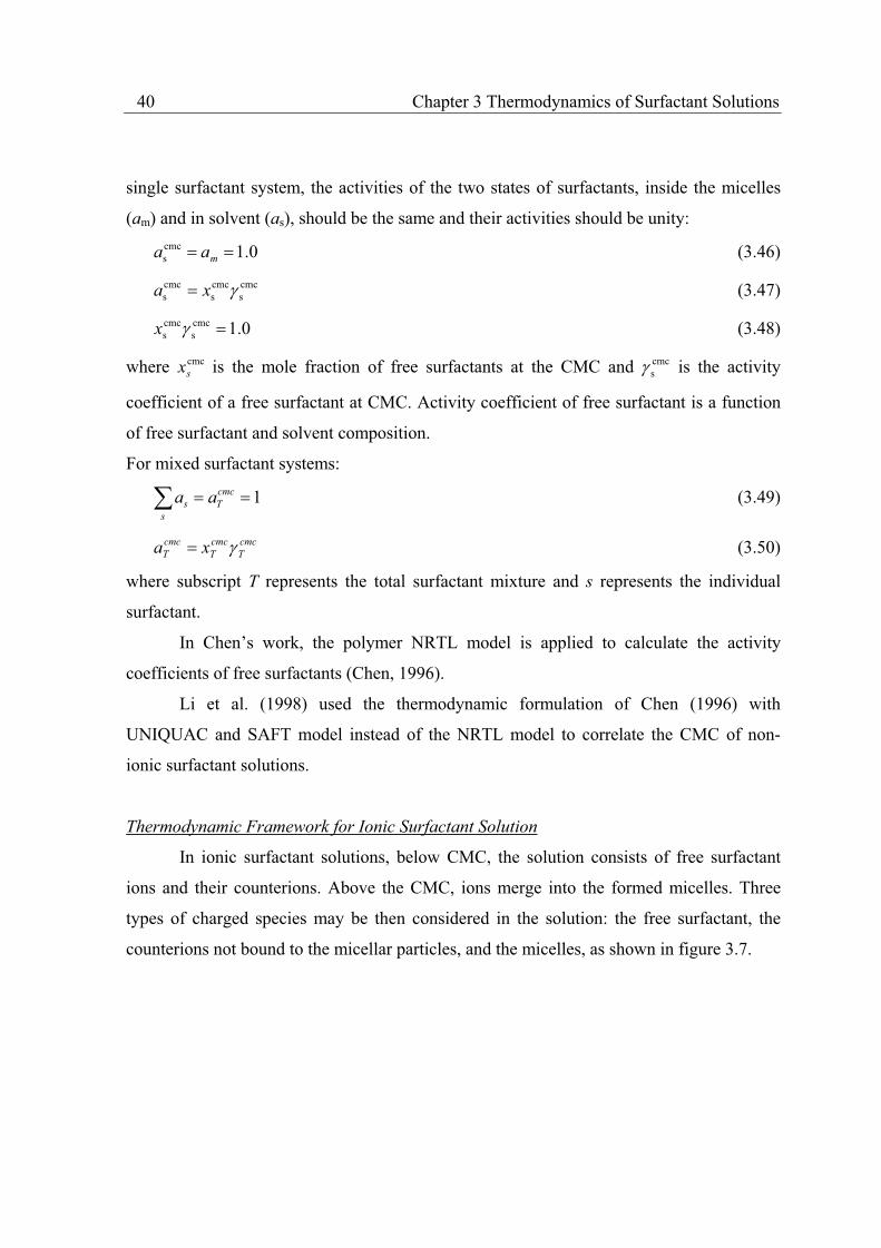
40 Chapter 3 Thermodynamics of Surfactant Solutions
single surfactant system, the activities of the two states of surfactants, inside the micelles
(am) and in solvent (as), should be the same and their activities should be unity:
0.1cmcs maa (3.46)
cmcs
cmcs
cmcs xa (3.47)
0.1cmcs
cmcsx (3.48)
where cmcsx is the mole fraction of free surfactants at the CMC and cmc
s is the activity
coefficient of a free surfactant at CMC. Activity coefficient of free surfactant is a function
of free surfactant and solvent composition.
For mixed surfactant systems:
s
cmc
Ts aa 1 (3.49)
cmc
T
cmc
T
cmc
T xa (3.50)
where subscript T represents the total surfactant mixture and s represents the individual
surfactant.
In Chen’s work, the polymer NRTL model is applied to calculate the activity
coefficients of free surfactants (Chen, 1996).
Li et al. (1998) used the thermodynamic formulation of Chen (1996) with
UNIQUAC and SAFT model instead of the NRTL model to correlate the CMC of non-
ionic surfactant solutions.
Thermodynamic Framework for Ionic Surfactant Solution
In ionic surfactant solutions, below CMC, the solution consists of free surfactant
ions and their counterions. Above the CMC, ions merge into the formed micelles. Three
types of charged species may be then considered in the solution: the free surfactant, the
counterions not bound to the micellar particles, and the micelles, as shown in figure 3.7.
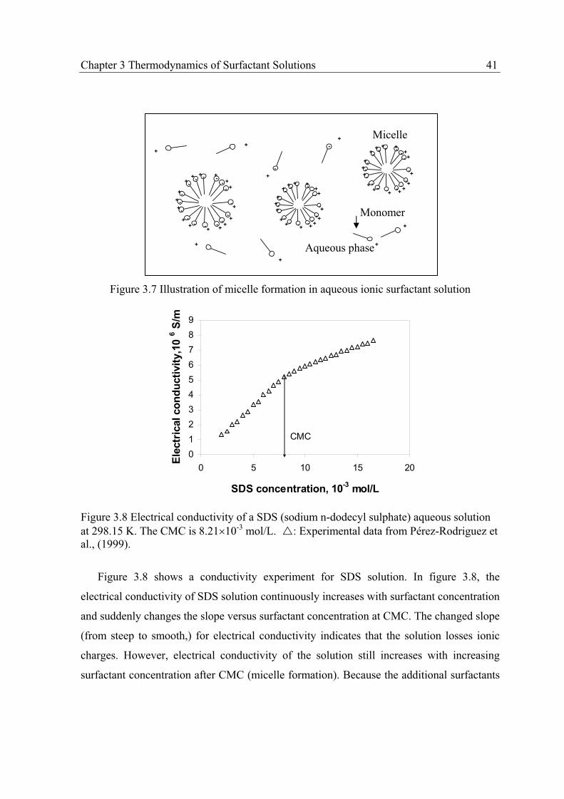
Chapter 3 Thermodynamics of Surfactant Solutions 41
Figure 3.7 Illustration of micelle formation in aqueous ionic surfactant solution
0
1
2
3
4
5
6
7
8
9
0 5 10 15 20
SDS concentration, 10-3
mol/L
Ele
ctr
ical co
nd
ucti
vit
y,1
0 6
S/m
CMC
Figure 3.8 Electrical conductivity of a SDS (sodium n-dodecyl sulphate) aqueous solution at 298.15 K. The CMC is 8.21 10-3 mol/L. : Experimental data from Pérez-Rodriguez et al., (1999).
Figure 3.8 shows a conductivity experiment for SDS solution. In figure 3.8, the
electrical conductivity of SDS solution continuously increases with surfactant concentration
and suddenly changes the slope versus surfactant concentration at CMC. The changed slope
(from steep to smooth,) for electrical conductivity indicates that the solution losses ionic
charges. However, electrical conductivity of the solution still increases with increasing
surfactant concentration after CMC (micelle formation). Because the additional surfactants
-+-+
-+
-+
-+
-+
-+-+ -
+-+-+
- +
- +
- + - + -+
-+-+
-+
-+
-+
-+
-+-+ -
+-+-+
-+
-+
- +- +-+
- + -
+
- +
- +
- +
- +
- + - + -
+ - +
- +
- +
- +
- + - +
- +
-++
-
+
+
+
+
+
+
Micelle
Aqueous phase
Monomer
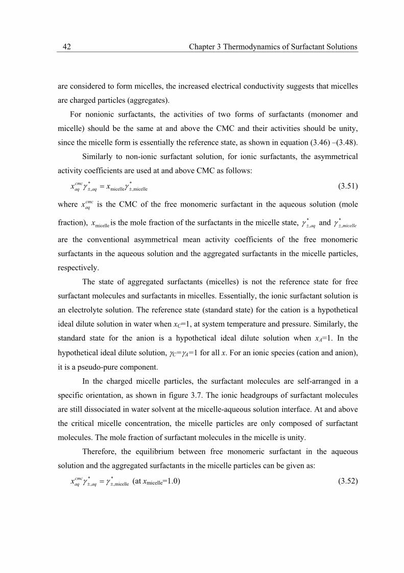
42 Chapter 3 Thermodynamics of Surfactant Solutions
are considered to form micelles, the increased electrical conductivity suggests that micelles
are charged particles (aggregates).
For nonionic surfactants, the activities of two forms of surfactants (monomer and
micelle) should be the same at and above the CMC and their activities should be unity,
since the micelle form is essentially the reference state, as shown in equation (3.46) –(3.48).
Similarly to non-ionic surfactant solution, for ionic surfactants, the asymmetrical
activity coefficients are used at and above CMC as follows:
*micelle,micelle
*, xx aq
cmc
aq (3.51)
where cmc
aqx is the CMC of the free monomeric surfactant in the aqueous solution (mole
fraction), micellex is the mole fraction of the surfactants in the micelle state, *,aq and *
,micelle
are the conventional asymmetrical mean activity coefficients of the free monomeric
surfactants in the aqueous solution and the aggregated surfactants in the micelle particles,
respectively.
The state of aggregated surfactants (micelles) is not the reference state for free
surfactant molecules and surfactants in micelles. Essentially, the ionic surfactant solution is
an electrolyte solution. The reference state (standard state) for the cation is a hypothetical
ideal dilute solution in water when xC=1, at system temperature and pressure. Similarly, the
standard state for the anion is a hypothetical ideal dilute solution when xA=1. In the
hypothetical ideal dilute solution, C= A=1 for all x. For an ionic species (cation and anion),
it is a pseudo-pure component.
In the charged micelle particles, the surfactant molecules are self-arranged in a
specific orientation, as shown in figure 3.7. The ionic headgroups of surfactant molecules
are still dissociated in water solvent at the micelle-aqueous solution interface. At and above
the critical micelle concentration, the micelle particles are only composed of surfactant
molecules. The mole fraction of surfactant molecules in the micelle is unity.
Therefore, the equilibrium between free monomeric surfactant in the aqueous
solution and the aggregated surfactants in the micelle particles can be given as:
*micelle,
*,aq
cmc
aqx (at xmicelle=1.0) (3.52)
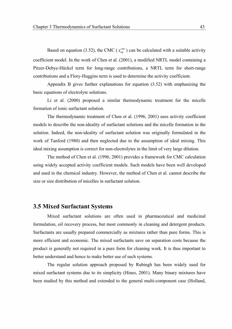
Chapter 3 Thermodynamics of Surfactant Solutions 43
Based on equation (3.52), the CMC ( cmc
aqx ) can be calculated with a suitable activity
coefficient model. In the work of Chen et al. (2001), a modified NRTL model containing a
Pitzer-Debye-Hückel term for long-range contributions, a NRTL term for short-range
contributions and a Flory-Huggins term is used to determine the activity coefficient.
Appendix B gives further explanations for equation (3.52) with emphasizing the
basic equations of electrolyte solutions.
Li et al. (2000) proposed a similar thermodynamic treatment for the micelle
formation of ionic surfactant solution.
The thermodynamic treatment of Chen et al. (1996, 2001) uses activity coefficient
models to describe the non-ideality of surfactant solutions and the micelle formation in the
solution. Indeed, the non-ideality of surfactant solution was originally formulated in the
work of Tanford (1980) and then neglected due to the assumption of ideal mixing. This
ideal mixing assumption is correct for non-electrolytes in the limit of very large dilution.
The method of Chen et al. (1996, 2001) provides a framework for CMC calculation
using widely accepted activity coefficient models. Such models have been well developed
and used in the chemical industry. However, the method of Chen et al. cannot describe the
size or size distribution of micelles in surfactant solution.
3.5 Mixed Surfactant Systems
Mixed surfactant solutions are often used in pharmaceutical and medicinal
formulation, oil recovery process, but most commonly in cleaning and detergent products.
Surfactants are usually prepared commercially as mixtures rather than pure forms. This is
more efficient and economic. The mixed surfactants save on separation costs because the
product is generally not required in a pure form for cleaning work. It is thus important to
better understand and hence to make better use of such systems.
The regular solution approach proposed by Rubingh has been widely used for
mixed surfactant systems due to its simplicity (Hines, 2001). Many binary mixtures have
been studied by this method and extended to the general multi-component case (Holland,

44 Chapter 3 Thermodynamics of Surfactant Solutions
1986). In calculating mixed CMC, the regular solution approach requires that the CMC of
both pure components (in the binary case) and one measured CMC for the mixed surfactant
system. A single adjustable parameter can, then, be obtained and used to calculate CMC of
wide composition range. In this method, regular solution assumption is used for micelles
other than the surfactant solution. Section 7.4 gives an example for the mixed CMC
calculation by this method.
Reviews for the theories of mixed surfactants can be found in the references of
Hines (2001) and Ogino et al (1993).
The Rubingh’s approach (Rubingh, 1979)
In Rubingh’s method, the chemical potential of monomeric surfactant 1, 1, in a
mixed surfactant solution can be written as:
monxRT 1011 ln (3.53)
where the activity coefficient of free monomer is assumed to be unity, 01 is a standard state
chemical potential of surfactant 1, monx1 is the monomer concentration of surfactant 1 (mol
fraction).
The chemical potential of surfactant 1 in the mixed micelle, M
1 , (two surfactant
components in the micelle) is given by
110
11 ln xRTMM (3.54)
where 01M is the chemical potential of surfactant 1 in pure micelle state, 1 and x1 are the
activity coefficient and mole fraction (solvent free) of surfactant 1 in the mixed micelle,
respectively.
For surfactant 1 in the pure micelle state, we have
101
01 CMClnRTM (3.55)
where CMC1 is the CMC of pure surfactant 1, 01 is a standard chemical potential of
monomeric surfactant 1.
At equilibrium, we have
M
11 (3.56)
Chapter 3 Thermodynamics of Surfactant Solutions 45
From equations (3.53) (3.55), we obtain that
1111 CMCxxmon (3.57)
Similar arguments can be used for surfactant 2 to derive the relation
2212 CMC1 xxmon (3.58)
At concentration below the concentration of mixed micelle formation, the concentration of
surfactant 1, monx1 , is simply given by
T
mon xx 11 (3.59)
where xT is the total concentration of surfactant 1 and 2, 1 is a fraction of surfactant 1 in
total mixed solute.
Similarly to component 2,
T
mon xx 12 1 (3.60)
At the mixed micelle formation, by continuity, equations (3.59)-(3.60) become
mix11 CMCmonx (3.61)
mix12 CMC1monx (3.62)
Combining equations (3.57), (3.58), (3.61), (3.62), we obtain
22
1
11
1
mix CMC
1
CMCCMC
1 (3.63)
Using the regular solution approximation, the activity coefficients in the mixed micelle are
given as:
2
11 1exp x (3.64)
212 exp x (3.65)
where is an adjustable interaction parameter, x1 is the mole fraction of surfactant 1 in the
mixed micelle.
Holland (1986) used this approach to correlate the interaction parameter for
different mixed surfactant solutions. Murphy et al. (2002) reported the interaction
parameter for several cationic surfactant solutions.
46 Chapter 3 Thermodynamics of Surfactant Solutions
3.6 Thermodynamic Functions of Surfactant Solutions
In previous sections of this chapter, some theoretical models of micelle formation
have been discussed. However, the thermodynamic functions, G, H and S, of
surfactant solutions are also very important for a quantitative understanding of the micelle
solution. Although one have acquired considerable knowledge of the surfactant solutions,
the thermodynamics of the solution is far from being completely understood. In this section,
some general considerations of the thermodynamic functions for surfactant solutions are
presented based on the work of Tanford (1980), Hoffmann et al. (1986) and Yaminsky et al.
(2001).
The thermodynamic functions, G, H and S, of surfactant solutions are the key
to quantitatively understand the behaviour of surfactant solutions. A large amount of
reliable experimental work has been carried out to measure these thermodynamic
parameters (van Os et al., 1993). Based on phenomenological rules, one may correlate and
predict some thermodynamic parameters. Different molecular interpretations of the
thermodynamic parameters have been proposed (Yaminsky et al., 2001).
In experimental techniques, G of micelle formation is measured through the
determination of the activity of the solute or of the solvent. H is determined by
microcalorimeters or precision solution calorimeters (Hoffmann et al., 1986). The S can
be obtained from thermodynamic relation: STHG .
In practice, H is the most commonly measured property for micelle solution by
microcalorimeters. Many commercial microcalorimeters are available. The CMC and
enthalpy can be determined directly from the same experiment. Using mass-action model or
pseudo-phase model, G can be calculated through measured H (Paula et al., 1995,
Garidel et al., 2000).
Using mass-action model, the enthalpy can be related to CMC through van’t Hoff
equation (Garidel et al., 2000) as follows:
van’t Hoff equation
2
ln
RT
H
dT
Kd (3.66)
Chapter 3 Thermodynamics of Surfactant Solutions 47
From thermodynamic relation: KRTG ln0 , the van’t Hoff equation can be
transformed to:
2
00
T
H
T
G
dT
d (3.67)
As discussed in section 3.3, assuming a sufficiently high value for aggregation number ng,
the second term of mass-action equation (3.8) becomes very small and can be neglected.
Thus, we have
CMCln0 RTGmic (3.68)
For a single surfactant system, combining equation (3.67) and (3.68), we obtain
2
0CMCln
RT
H
dT
d mic (3.69)
The first derivative of H with respect to temperature yields the change in heat capacity
Cp:
p
pT
HC (3.70)
The change in entropy S can be obtained by the Gibbs-Helmholtz equation:
TGHS / (3.71)
Based on equations (3.68)-(3.71), the relations between CMC and thermodynamic
functions can be obtained. In these equations, the Gibbs free energy model is a key factor to
give the relation of CMC and thermodynamic functions. As discussed in previous sections,
different theories have been proposed to calculate the G, such as pseudo-phase separation
model, mass-action model, molecular thermodynamic models, etc. However, in the
calorimetric experimental work the pseudo-phase separation model and mass-action model
are often used to get Gibbs free energy and entropy of micelle formation (Garidel et al.,
2000).
The effect of temperature on the micelle formation is small. For ionic surfactants,
the CMC increases with increasing temperature, for non-ionic surfactants, it decreases with
increasing temperature. It has been observed that CMC has a minimum value in
investigated temperature range for some surfactant systems, such as SDS, octyl glucoside,

48 Chapter 3 Thermodynamics of Surfactant Solutions
etc. (Garidel et al., 2000). However, the reason of the CMC minimum in a certain
temperature range is not clear at present.
In the micelle formation of surfactant solutions, the enthalpy values are often
positive at low temperatures and become negative at higher temperatures, while it is the
opposite for entropy. Thus, micelle formation is a entropy-controlled (or entropy-driven)
process at low temperatures. For high temperatures, the micelle formation is no longer
entropy but enthalpy controlled. Whether enthalpy or entropy dominates the hydrophobic
effect, the net is unfavourable dissolution. The aqueous environment remains hostile to
hydrocarbons.
The molecular interpretation of thermodynamic functions depends on the
understanding of ‘hydrophobic effect’ that controls hydrocarbon solubility in water. The
science of hydrophobic effect possible starts with the like-likes-like principle in explanation
of solubility that is a traditional part of chemistry. In the early part of 20th century,
Langmuir attributed the relatively low solubility of hydrocarbons in water to the strong
mutual interaction between hydrocarbon moieties. By contrast, Harkins suggested that the
slight solubility of hydrocarbons in water is due to the fact that water is strongly self-
associated. In 1960s, Hildebrand, Tanford in 1970s, and van Oss et al. in 1980s essentially
reclaimed Harkins’ analysis. Although the energy of water-water cohesion is substantially
greater than that of water-hydrocarbon adhesion, hydrocarbon-hydrocarbon interaction
energies are about the same as that between water and hydrocarbon (Yaminsky et al., 2001).
3.7 Summary
In this chapter, different thermodynamic treatments for the micelle formation in
surfactant solutions are briefly reviewed. Since the concept of micelle or aggregation was
first reported by McBain and Swain (1936), it has been widely accepted in research for
surfactant solutions. Many experimental results have proved the existence of self-organized
aggregates, and many different thermodynamic frameworks have been proposed to explain
the micelle formation in surfactant solution. The discussed methods in this chapter are those
often used in practice.

Chapter 3 Thermodynamics of Surfactant Solutions 49
In the pseudo-phase theory, the micelles or aggregates are assumed as a
macroscopic phase in surfactant solution. The calculation methods of vapour-liquid
equilibrium or liquid-liquid equilibrium are used to describe the micelle formation. Because
the assumed macroscopic phase (micelles) is corresponded to infinite aggregation number
in surfactant solution, this method cannot describe the aggregation number of surfactants.
The mass-action theory treats the micelle formation as the product of a chemical
reaction. The chemical equilibrium constants are studied by thermodynamic method.
However, this method cannot calculate the phase separation in the surfactant solution.
The molecular thermodynamic framework for micelle formation has two different
branches: one relays on detailed molecule descriptions to build up the properties of
surfactant solution, the other uses activity coefficient. Figure 3.7 shows the basic
characteristics of the two branches.
The thermodynamic frameworks of Tanford, Israelachvili, Blankschtein and
Nagarajan are based on molecular structure description (molecular structure method). Two
different formulation factors are employed in these methods:
1) The chemical potential of micelle is related to the size of micelle, or aggregation
number (the number of surfactant molecules making up a micelle). In the chemical
potential expression, the ideal mixing assumption is introduced because micelle formation
normally occurs in very dilute solutions.
2) The standard state chemical potential is related to the detailed structural
description of surfactant molecules or micelles, such as tail length, headgroup area, tail
volume, etc. Different molecular structures give different contributions to the changes of
chemical potential. Such changes result in the micelle formation in surfactant solutions. In
the approaches of Blankschtein and Nagarajan, the detailed molecule geometry calculation
methods have been proposed to estimate the free energy of different surfactants.

50 Chapter 3 Thermodynamics of Surfactant Solutions
Figure 3.7 Two branches in molecular thermodynamic methods for surfactant solution
As discussed previously, the ideal mixing assumption is correct for nonelectrolytes
at a very large dilution, but not for electrolyte solutions. Moreover, the dependence of the
chemical potential on the aggregation number, such as equation (3.37), (3.40), gives the
possibility of following the aggregation process in detail. But the equations (3.37) and (3.40)
cannot be used to calculate phase separation in surfactant system, because the aggregation
Molecular structure
Activity coefficient
New chemical potential expressions
Typical chemical potential expression
Detailed molecule descriptions: tail volume, extended tail length, head group area, packing parameter…….
0micelle calculation, then, CMC
Tanford (1980) Israleachvili (1992) Nagarajan (1991) Blankschtein (1990) ......
Activity coefficient calculation
CMC calculation
Chen (1996)
e.g. gg
micellemicellen
x
n
RTln0
ng-----aggregation number
xRTmicellemicelle ln0
Methods Characteristics
Chapter 3 Thermodynamics of Surfactant Solutions 51
number tends to infinite in a new surfactant phase formed. Therefore, a complete new set of
equations were used to calculate phase separation of surfactant solutions in the molecular
structure methods (Puvvada et al., 1990, Nagarajan 1997a).
It can be seen that the molecular structure methods do not take advantage of the
extensive work on activity coefficient models carried out in the past decades for solutions
of non-electrolytes, electrolytes and polymers in academic and chemical industry,
especially for the phase separation calculation.
Chen et al. (1996, 2001) and Li et al. (1998, 2000) proposed slightly
different thermodynamic treatments for the micelle formation in surfactant solutions using
activity coefficient models, e.g. NRTL and UNIQUAC, to calculate CMC of surfactant
solutions. Some typical surfactant solutions, such as alcohol ethoxylates, sodium alkyl
sulphates, etc., have been studied by their methods.

52 Chapter 3 Thermodynamics of Surfactant Solutions
Chapter 4 Octanol-water Partition Coefficient for Non-ionic Surfactant Solutions 53
Chapter 4 Octanol-water Partition Coefficients for Non-ionic Surfactant Solutions
In this chapter, the octanol-water partition coefficient (Kow) for non-ionic surfactant
molecules (alcohol ethoxylates) and phthalates are investigated with the UNIFAC method
and commercial software. The calculations are compared with a few experimental Kow data
for these compounds. In Chapter 8, the Kow results will be used to establish correlations of
toxicity and bio-concentration factor for alcohol ethoxylates.
4.1 Introduction
The n-octanol-water partition coefficient (Kow) is a widely used property in
environmental and biological applications, because it measures the hydrophobic and
hydrophilic nature of organic compounds. Kow has been used successfully in Quantitative
Structure Activity Relationships (QSAR) in various fields (Leo et al., 2003): drug and
pesticide design, pharmacokinetics, anaesthesiology, environmental transport and soil
binding, toxicology, bioaccumulation, protein folding, enzyme binding, enzymic reactions in
non-aqueous solvents, and host-guest complexation.
Many experimental methods have been developed to measure Kow for different
chemicals (Sangster, 1997). Experimental Kow data for more than 20,000 organic
compounds have been compiled (Sangster, 2001). However, these measurements are carried
out in a very dilute solute concentration region, i.e. in the ranges of part per million (ppm) or
parts per billion (ppb). Thus, such measurement can be of considerable uncertainty in some
cases and may reach errors up to a few orders of magnitude. At the same time, for many
newly released chemicals, Kow values have not been measured. Thus, methods for predicting
Kow are of interest.
Various Kow calculation methods have been systematically compiled and compared by
several researchers (Sangster, 1997, Buchwald et al., 1998, Derawi et al., 2001). A number of
54 Chapter 4 Octanol-water Partition Coefficient for Non-ionic Surfactant Solutions
commercial tools are also available for Kow prediction, such as ACD/LogP, KowWin and
ClogP.
ACD/LogP (ACD/LogP, 2003, www.acdlabs.com) is a method developed by Advanced
Chemistry Development, Inc. The method used in ACD has not been described in the
scientific literature (Sangster, 1997). The calculation in ACD/LogP is based on an algorithm
that uses the experimental Kow values for over 12,400 structures with more than 1,200
different functional groups. ACD/LogP's internal database contains over 18,400 compounds
with experimental Kow values collected from different sources.
KowWin (KowWin, 2003, esc.syrres.com) is a software developed by Syracuse Research
Corporation using the Meylan and Howard approach (Meylan et al., 1995). The program
estimates the octanol-water partition coefficient of organic chemicals using an atom/fragment
contribution method. Using a training set of 2,410 chemicals with 175 groups and 280
correction factors, a correlation coefficient of 0.98 was found between the experimental and
estimated logKow values. The method has been evaluated using a validation set of
experimental values for 10,550 chemicals other than those included in the training set with a
resulting correlation coefficient of 0.94 and a mean error of 0.35 in logKow. The complete
database in KowWin has experimental Kow values for 13,058 compounds.
Clog (ClogP, 2003, www.daylight.com) is developed by Daylight Chemical Information
Systems Inc. with the Hansch and Leo’s fragment approach (Hansch et al., 1995). The
method adds together contribution values for structural parts (fragments) of a solute molecule
and correction factors dependent upon the particular way the parts are put together. With the
use of a large database of reliable experimental Kow data, the contribution values of different
structural parts (fragments) to the total Kow of molecules have been obtained.
Surfactants, such as alcohol ethoxylates (or polyoxyethylene alcohol) R(CH2CH2O)nOH,
are amphiphilic molecules that include both a hydrophilic and a hydrophobic part. The
surfactant molecules are adsorbed at the interface between the two different fluids, e.g. in the
water-air, water-octanol interface. Thus, they can significantly change the surface or
interfacial tension. This property of surfactant molecules is useful for many different
industrial products, e.g. detergents, washing powders, etc. However, exactly because of this
surface adsorption, the Kow measurements are difficult for surfactants. In the Kow

Chapter 4 Octanol-water Partition Coefficient for Non-ionic Surfactant Solutions 55
measurements, the surfactant molecules accumulate at the octanol-water interface, which
results in lower surfactant concentration in the bulk solvent. At the same time, the surfactants
may also form emulsions and enhance the mutual solubility of octanol and water by strong
interaction with octanol even below their critical micelle concentration (Müller et al., 1999).
Thus, it is very useful to develop a predictive method to evaluate the Kow of surfactants since
the experimental data are often not available. This study is an effort towards this direction.
The UNIFAC method (Fredenslund et al., 1975) is a group contribution method based on
the local composition concept. This method has been successfully used to predict many
physical properties especially in chemical engineering applications, e.g. vapour-liquid
equilibrium (Fredenslund et al., 1975), liquid-liquid equilibrium (Magnussen et al., 1981), etc.
Kow has also been studied with the UNIFAC model by several researchers. (Chen et al.,
1993, Wienke et al., 1998, Derawi et al., 2001). UNIFAC has been proven in some cases to
be a good model for predicting Kow in the case of lack of experimental data. However there
has been no systematic attempt so far to estimate Kow for surfactants using UNIFAC.
In this work, the Kow of phthalates are first studied as a test because phthalates are often
used in different chemical products (plastics, paints, etc.) and are important in many
environmental studies (AMI report, 2000). Although phthalates are not surfactant molecules,
they have similar functional groups, e.g. –COO, as surfactants. Figure 4.1 illustrates the basic
chemical structure of phthalates, where the R1 and R2 may be alkyl or aryl groups, etc.
Then, the Kow values for alcohol ethoxylates (R(CH2CH2O)nOH) are evaluated using
UNIFAC model and the 3 commercial tools described previously (ClogP, ACD, KowWin) as
well as a recently developed group contribution solvation model (Lin et al., 1999). The
prediction results of the various models are compared to the limited experimental Kow data
for alcohol ethoxylates.
O
O
O
O
R1
R2
Figure 4.1 Structure of phthalates. R1 and R2 may be alkyl or aryl groups, etc.

56 Chapter 4 Octanol-water Partition Coefficient for Non-ionic Surfactant Solutions
4.2 Octanol-water Partition Coefficient and its Calculation
The partition coefficient of a single compound i between octanol (O) and water (W)
phases can be defined for dilute solutions (Sandler, 1999) at 25°C:
,
,
owO
i
W
W
i
O
C
CK (4.1)
where CO and CW represent the total molar concentrations of the octanol-rich and water-rich
phases at 25°C, respectively. Because only a small amount of solute is added to the octanol-
water mixture, the solute concentration is very small in both phases. Thus the activity
coefficients at infinite dilution, ,W
i , ,O
i are used. Using the solubility data of water and
octanol in water-rich phase and octanol-rich phase from the Handbook of Chemical Property
Estimation Methods (Lyman, 1982), the Kow expression in equation (4.1) becomes:
,
,
151.0owO
i
W
iK (4.2)
The solubility of water and octanol in the water-rich phase and octanol-rich phase at 25°C is,
respectively, 55.3 mol/liter for water, and 4.5×10⁻³ mol/liter for octanol in the water-rich
phase; 2.30 mol/liter for water, and 6.07mol/liter for octanol in the octanol-rich phase.
The activity coefficients at infinite dilution can be calculated from different activity
coefficient models, e.g. NRTL, UNIQUAC and UNIFAC. In this study the UNIFAC method
is chosen to calculate the activity coefficients because it is a predictive tool based on the
group contribution principle. Using UNIFAC method, Kow can be predicted from the
chemical structure information of a compound. The UNIFAC model is presented in
Appendix A.
Based on a comprehensive review of these different UNIFAC methods for Kow in
several chemical families (Derawi et al., 2001, Thomsen et al., 1999), the UNIFAC LLE1
and water-UNIFAC were recommended for predicting the Kow. A new UNIFAC model
(Micelle) has been also recently developed for predicting the critical micelle concentration
for non-ionic surfactants (Cheng et al., 2002). This model is presented in Chapter 5 of this
thesis. In “Micelle UNIFAC”, a new functional group (CH2CH2O) was introduced into
Chapter 4 Octanol-water Partition Coefficient for Non-ionic Surfactant Solutions 57
UNIFAC VLE1; the interaction parameters were obtained from vapor-liquid equilibrium data.
These different UNIFAC methods are used to calculate Kow in this work.
4.3 Experimental Kow Data for Alcohol Ethoxylates and Phthalates
Very few experimental octanol-water partition coefficient data have been reported for
alcohol ethoxylates (Morral, et al., 1996) due to the experimental difficulties discussed above.
For the same reason, existing Kow data for alcohol ethoxylates surfactants may not be very
reliable. Thus, Kow data for compounds with similar structures are helpful for testing the
UNIFAC group interaction parameters.
The alcohol ethoxylates (R(CH2CH2O)nOH) are often abbreviated as CiEj. Here i is the
number of alkyl carbon (CH3-, CH2-) in the R group and j is the number of oxyethylene
groups (CH2CH2O-) in the molecule. The alcohol ethoxylates also have an alcohol group
(-OH). Therefore, the Kow data from the same alcohol ethoxylate family, such as 2-
methoxyethanol (C1E1), 2-ethoxyethanol (C2E1), etc., are very useful in this work even
though the C1E1 and C2E1 are not actual surfactant molecules.
In this work, all Kow data for surfactants and phthalates are taken from the LOGKOW
databank (Sangster, 2001).
4.4 Results and Discussions
The various methods used in this work are summarized in Table 4.1. Using these
different methods, the Kow prediction results for phthalates are shown in Table 4.2, while the
Kow results for alcohol ethoxylates are presented in Tables 4.3 and 4.4. Based on these
results, the following points summarize our observations:

58 Chapter 4 Octanol-water Partition Coefficient for Non-ionic Surfactant Solutions
Table 4.1 Methods used for Kow calculations Method Abbreviation Reference Original UNIFAC VLE 1 VLE1 Hansen et al. 1991 UNIFAC LLE 1 LLE1 Magnussen et al., 1981 UNIFAC VLE 2 VLE2 Hansen et al., 1992 Modified UNIFAC VLE 3 VLE3 Larsen et al., 1987 Water-UNIFAC H2O Chen et al., 1993 UNIFAC for surfactants Micelle Cheng et al., 2002 ClogP ClogP www.daylight.com ACD/LogP ACD www.acdlabs.com KowWin Kwin esc.syrres.com Solvation model GCS Lin et al., 1999
Table 4.2 logKow prediction results for phthalates with UNIFAC VLE 1, GCS and 3 commercial software methods. All names for phthalates are given as substitute groups. Phthalate Exp.* VLE1 ACD ClogP KowWin GCS Dimethyl 1.6 1.74 1.62 1.56 1.66 -0.08 Diethyl 2.42 2.64 2.69 2.62 2.65 0.97 Dipropyl 3.64 3.53 3.75 3.68 3.63 2.03 di-iso-propyl 2.83 3.53 3.38 3.24 3.48 1.73 Dibutyl 4.50 4.43 4.81 4.73 4.61 3.09 di-iso-butyl 4.48 4.43 4.44 4.47 4.46 2.79 Dipentyl 5.62 5.32 5.87 5.79 5.59 4.15 Dihexyl 6.82 6.21 6.94 6.85 6.57 5.21 Dioctyl 8.18 8.00 9.06 8.97 8.54 7.34 Didecyl 8.83 9.79 11.19 11.08 10.5 9.46 di-sec-octyl 7.06 8.00 8.69 8.71 8.39 7.03 Ditridecyl 8.4 12.47 14.38 14.26 13.45 12.6 Diallyl 2.98 3.39 3.28 3.11 3.36 0.93 dutylbenzyl 4.73 4.79 4.99 4.98 4.84 2.37 dicyclohexyl 4.9 6.02 5.74 5.62 6.20 5.0 Mean Dev. % 12 14 13 13 37
* Exp.: Experimental data from Sangster (2001).

Chapter 4 Octanol-water Partition Coefficient for Non-ionic Surfactant Solutions 59
Table 4.3 logKow prediction results for alcohol ethoxylates with UNIFAC VLE 1, GCS and 3 commercial software methods Compound Exp.* ClogP Kwin ACD GCS Micelle VLE1 2-methoxethanol (C1E1) -0.77 -0.75 -0.91 -0.80 -1.56 -0.31 -0.83 2-ethoxyethanol (C2E1) -0.28 -0.22 -0.42 -0.27 -1.02 0.14 -0.38 3,6-dioxa-1-octanol (C2E2) -0.54 -0.15 -0.69 -0.26 -1.89 0.28 -0.75 iso-propoxyethanol (C3E1) 0.05 0.09 0.00 0.08 -0.65 0.58 0.07 2-butoxyethanol (C4E1) 0.8 0.84 0.57 0.80 0.03 1.03 0.51 3,6-dioxadecanol (C4E2) 0.56 0.91 0.29 0.81 -0.83 1.18 0.15 2-(hexyloxy) ethanol (C6E1) 1.86 1.90 1.55 1.86 1.09 1.92 1.41 3,6-dioxa-1-dodecanol (C6E2) 1.7 1.96 1.28 1.87 0.22 2.07 1.04 Mean Dev. % 33 39 22 311 199 36
* Exp.: Experimental data from Sangster (2001)
Table 4.4 logKow prediction results for alcohol ethoxylates with various UNIFAC methods Compound Exp.* VLE1 LLE1 H2O Micelle VLE2 VLE3 C1E1 -0.77 -0.83 -1.51 -0.96 -0.31 -0.78 -0.60 C2E1 -0.28 -0.38 -1.02 -0.52 0.14 -0.31 -0.06 C2E2 -0.54 -0.75 -1.93 -0.88 0.28 -0.72 -0.30 C3E1 0.05 0.07 -0.53 -0.07 0.58 0.15 0.47 C4E1 0.8 0.51 -0.04 0.38 1.03 0.62 1.01 C4E2 0.56 0.15 -0.95 0.01 1.18 1.55 2.08 C6E1 1.86 1.41 0.94 1.27 1.92 0.21 0.77 C6E2 1.7 1.04 0.03 0.90 2.07 1.14 1.84 Mean Dev.% 36 287 80 199 48 135
* Exp.: Experimental data from Sangster (2001)
In Table 4.2, 4.3 and 4.4,
%owlog
owlogowlog1Dev.%Mean
1Exp
Caln
Exp
K
KK
n, n is the total number of data.
(1) Kow Prediction for Phthalates From Table 4.2, it can be seen that the VLE1, ACD,
ClogP and KowWin methods perform similarly, with VLE1 being slightly more accurate.
The GCS method employed here has been originally developed for mono-functional
chemicals and yields large deviations for phthalates. Phthalate molecules have structures
containing alkyl carbon, aromatic and COO groups, which are multi-functional compounds
60 Chapter 4 Octanol-water Partition Coefficient for Non-ionic Surfactant Solutions
(similar to alcohol ethoxylates). It is not surprising that the GCS method cannot satisfactorily
predict the Kow values for phthalates. Based on these calculations, UNIFAC VLE 1 is
recommended for predicting Kow for phthalates.
(2) Kow Prediction for Alcohol Ethoxylates
It is useful to identify the surfactant molecules from the alcohol ethoxylates shown in
Table 4.3. D’Arrigo et al. (1991) suggested that the C4E1 molecule is the shortest alcohol
ethoxylate surfactant. Following D’Arrigo et al., four compounds of Table 4.3 (C4E1, C4E2,
C6E1 and C6E2) can be classified as surfactants. It will be of interest to investigate whether a
UNIFAC model can calculate the values of Kow for both non-surfactants (C1E1 ~ C3E1) and
surfactant molecules (C4E1 ~ C6E1) including both short chain and longer chain surfactants
(C4E1, C4E2 to C6E1, C6E2).
The Kow value can assist in interpreting the distribution trend of chemicals.
Hydrophilic chemicals with low Kow values will be largely partitioned into the water-rich
phase. Thus, the longer hydrophilic group chain a chemical has, the lower Kow value is
expected. In Table 4.3, it means that the C4E2 should have lower Kow value than C4E1
because the C4E2 has two hydrophilic oxyethylene groups. Similarly, longer hydrophobic
chains of a chemical indicate a larger Kow value, i.e. Kow must increase from C1E1 to
C6E1. All Kow data shown in Table 4.3 agree with these general considerations.
As shown in Table 4.3, the three commercial tools (ACD, ClogP, KowWin) and
UNIFAC VLE 1 perform similarly in the Kow prediction for the investigated compounds
with ACD showing the lowest deviation. UNIFAC VLE 1 is the best among the various
UNIFAC methods for Kow calculations, as shown in Table 4.4.
The GCS method for mono-functional chemicals and the UNIFAC micelle method
yield larger deviations. The plots of Kow prediction results with chain lengths are useful for
analysing the general behaviour of the models. Such plots are shown in Figures 4.2-4.4 for
three types of alcohol ethoxylate surfactants.

Chapter 4 Octanol-water Partition Coefficient for Non-ionic Surfactant Solutions 61
Figure 4.2 Experimental and predicted Kow values for CnE1
Fig 4.3 Experimental and predicted Kow values for C4En
1 2 3 4 5 6
-4
-3
-2
-1
0
1
log
KO
W
n in C4En
Exp.
VLE1
ACD
ClogP
KowWin
GCS
1 2 3 4 5 6-2
-1
0
1
2
log
KO
W
n in CnE1
Exp.
VLE1
ACD
ClogP
KowWin
GCS

62 Chapter 4 Octanol-water Partition Coefficient for Non-ionic Surfactant Solutions
Figure 4.4 Experimental and predicted Kow values for C6En.
Figure 4.2 shows that all methods predict the correct trend with increasing alkyl
group numbers n in CnE1. However, Figures 4.3 and 4.4 indicate the ACD and ClogP
methods exhibit different trends from the VLE1, KowWin and GCS models. It seems that
only VLE1, KowWin and GCS follow the experimental trend, i.e. decreasing Kow with
increasing oxyethylene group number n in C4En and C6En based on the few data available.
Based on these comparisons, it can be concluded that UNIFAC VLE 1 provides,
qualitatively, very good Kow prediction results for the investigated systems. This method
only uses group parameters based on vapour-liquid equilibrium data.
(3) Kow Prediction for alcohol ethoxylates in case no experimental data is available
The Kow values for alcohol ethoxylates, for which no reported experimental Kow
data is available, are calculated, as shown in Figures 4.5-4.10, using UNIFAC VLE 1,
commercial tools and the GCS solvation model. However, the Kow calculations of ACD,
ClogP and KowWin software produce unreliable results when the alkyl carbon number of
alcohol ethoxylates exceeds 12 (indicated by the messages of these three software). The
selected surfactants in the Kow prediction are currently used in industry.
1 2 3 4 5 6
-3
-2
-1
0
1
2
log
KO
W
n in C6En
Exp.
VLE1
ACD
ClogP
KowWin
GCS

Chapter 4 Octanol-water Partition Coefficient for Non-ionic Surfactant Solutions 63
Figure 4.5 Predicted Kow values for CnE4
Figure 4.6 Predicted Kow values for CnE6
0 2 4 6 8 10 12
-4
-2
0
2
4
6
log
KO
W
n in CnE4
VLE1
ACD
ClogP
KowWin
GCS
4 6 8 10 12
-4
-2
0
2
4
6
log
KO
W
n in CnE6
VLE1
ACD
ClogP
KowWin
GCS
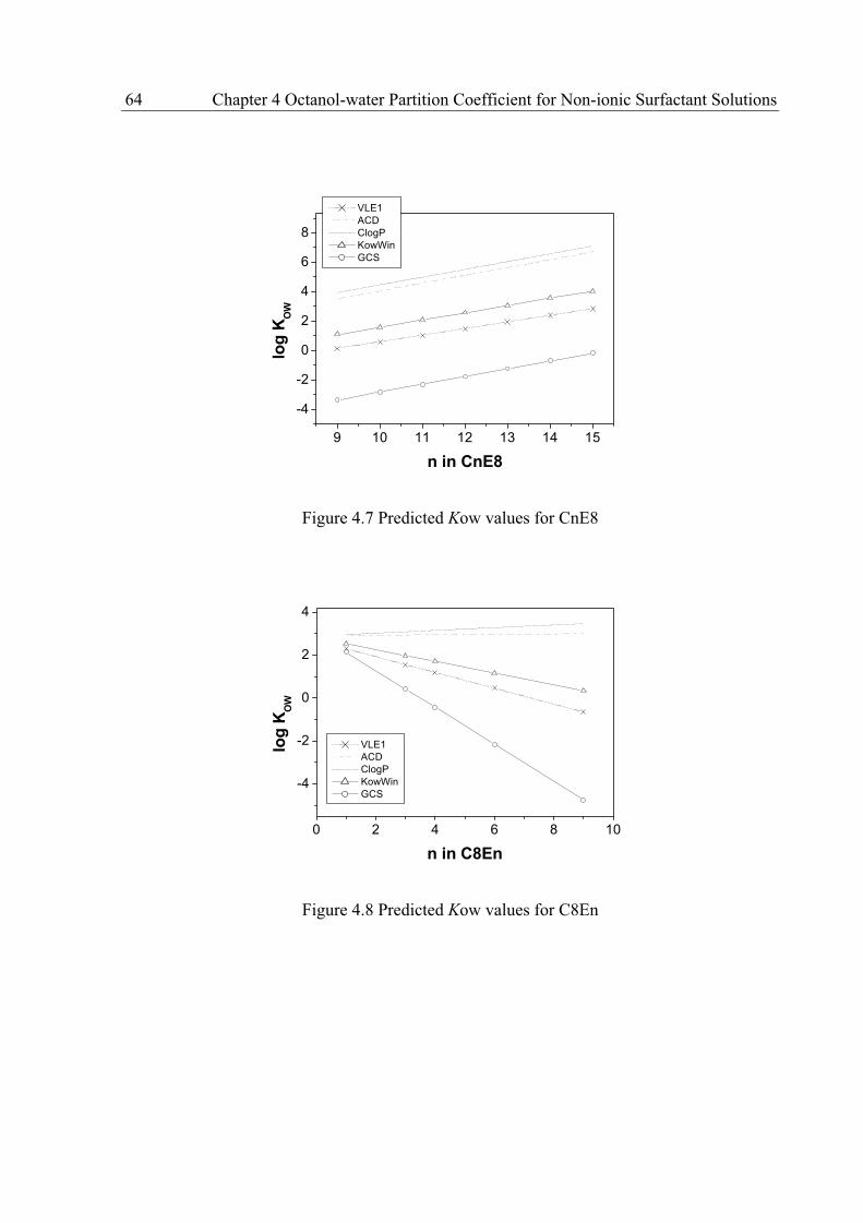
64 Chapter 4 Octanol-water Partition Coefficient for Non-ionic Surfactant Solutions
Figure 4.7 Predicted Kow values for CnE8
Figure 4.8 Predicted Kow values for C8En
9 10 11 12 13 14 15
-4
-2
0
2
4
6
8
log
KO
W
n in CnE8
VLE1
ACD
ClogP
KowWin
GCS
0 2 4 6 8 10
-4
-2
0
2
4
log
KO
W
n in C8En
VLE1
ACD
ClogP
KowWin
GCS

Chapter 4 Octanol-water Partition Coefficient for Non-ionic Surfactant Solutions 65
Figure 4.9 Predicted Kow values for C12En
Figure 4.10 Predicted Kow values for C16En
0 2 4 6 8
-2
0
2
4
6
log
KO
W
n in C12En
VLE1
ACD
ClogP
KowWin
GCS
5 10 15 20 25 30-12
-10
-8
-6
-4
-2
0
2
4
6
8
10
log
KO
W
n in C16En
VLE1
ACD
ClogP
KowWin
GCS

66 Chapter 4 Octanol-water Partition Coefficient for Non-ionic Surfactant Solutions
4.5 Conclusions
The original UNIFAC VLE 1 model (VLE1) can, at least qualitatively, satisfactorily
predict the octanol-water partition coefficients (Kow) of phthalates and yields similar results
to commercial methods like ACD, ClogP and KowWin that are specifically designed for
Kow.
Moreover, the VLE1 method can predict reasonably well Kow values of alcohol
ethoxylates, compared to the limited experimental data available. Again, the performance of
VLE1 is similar to the commercial methods. The mono-functional group contribution
solvation model (GCS) has the correct tendency with increasing numbers of oxyethylene
group (CH2CH2O) and alkyl group (CH2) in alcohol ethoxylates (R(CH2CH2O)nOH) but it
cannot be used for these complex compounds. The ACD and ClogP methods have slightly
lower deviations for small alcohol ethoxylates molecules but unlike VLE1, they do not yield
the correct trend with increasing oxyethylene group numbers for these compounds. The
UNIFAC for surfactant solution method (Micelle) is very similar to ACD and ClogP but has
larger deviation in Kow prediction for the alcohol ethoxylates. The KowWin can
satisfactorily follow the trend with increasing numbers of oxyethylene group and alkyl group
in alcohol ethoxylates and has similar deviations as UNIFAC VLE1. Extension of UNIFAC
VLE1 method to other classes of non-ionic surfactants is straightforward because the
interaction parameters of necessary groups, which may not available, can be estimated from
phase equilibrium data for the UNIFAC VLE 1 method. Overall, it can be concluded that the
UNIFAC VLE 1 method seems to be the best one among the investigated methods in Kow
prediction for non-ionic surfactants.
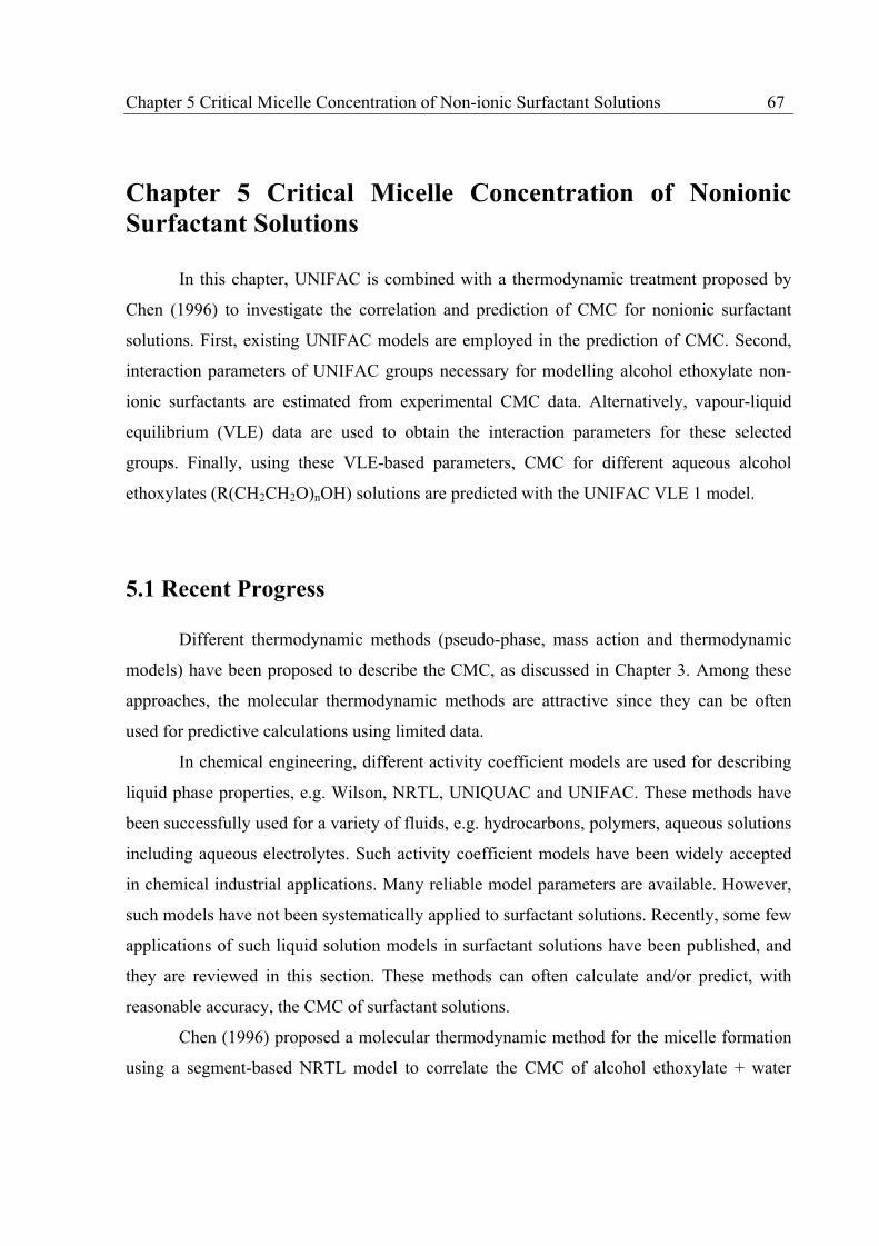
Chapter 5 Critical Micelle Concentration of Non-ionic Surfactant Solutions 67
Chapter 5 Critical Micelle Concentration of Nonionic Surfactant Solutions
In this chapter, UNIFAC is combined with a thermodynamic treatment proposed by
Chen (1996) to investigate the correlation and prediction of CMC for nonionic surfactant
solutions. First, existing UNIFAC models are employed in the prediction of CMC. Second,
interaction parameters of UNIFAC groups necessary for modelling alcohol ethoxylate non-
ionic surfactants are estimated from experimental CMC data. Alternatively, vapour-liquid
equilibrium (VLE) data are used to obtain the interaction parameters for these selected
groups. Finally, using these VLE-based parameters, CMC for different aqueous alcohol
ethoxylates (R(CH2CH2O)nOH) solutions are predicted with the UNIFAC VLE 1 model.
5.1 Recent Progress
Different thermodynamic methods (pseudo-phase, mass action and thermodynamic
models) have been proposed to describe the CMC, as discussed in Chapter 3. Among these
approaches, the molecular thermodynamic methods are attractive since they can be often
used for predictive calculations using limited data.
In chemical engineering, different activity coefficient models are used for describing
liquid phase properties, e.g. Wilson, NRTL, UNIQUAC and UNIFAC. These methods have
been successfully used for a variety of fluids, e.g. hydrocarbons, polymers, aqueous solutions
including aqueous electrolytes. Such activity coefficient models have been widely accepted
in chemical industrial applications. Many reliable model parameters are available. However,
such models have not been systematically applied to surfactant solutions. Recently, some few
applications of such liquid solution models in surfactant solutions have been published, and
they are reviewed in this section. These methods can often calculate and/or predict, with
reasonable accuracy, the CMC of surfactant solutions.
Chen (1996) proposed a molecular thermodynamic method for the micelle formation
using a segment-based NRTL model to correlate the CMC of alcohol ethoxylate + water

68 Chapter 5 Critical Micelle Concentration of Non-ionic Surfactnat Soluitons
systems. In his work, the temperature dependent interaction parameters of the NRTL model
are obtained from the correlation of binary VLE of water-polyethylene glycol systems and
LLE of water + hydrocarbons. CMC of some aqueous alcohol ethoxylate solutions are
successfully predicted by this method.
Li et al. (1998) used Chen’s thermodynamic treatment and employed the segment-
based UNIQUAC model and the statistical associating fluid theory (SAFT) to obtain the
activity coefficients of aqueous nonionic surfactant solutions. CMC of single aqueous
surfactant system was correlated and predicted for polyoxyethylene surfactant solutions. The
interaction parameters of segmented-based UNIQUAC are obtained from experimental CMC
data. Temperature dependent interaction parameters are employed in their work. To obtain
the SAFT parameters of water, the liquid densities and saturated vapour pressure of pure
water between 0-100ºC were correlated in their work. The segment parameters for surfactants
in SAFT are regressed by fitting the experimental CMC data at 25ºC.
Flores et al. (2001) and Voutsas, et al. (2001) used a phase separation thermodynamic
framework approach to describe the micelle formation of surfactant solutions, in which the
micelle phase is approximated as a second liquid phase resulting from the liquid-liquid
equilibrium between the solvent and surfactant. The necessary activity coefficients are
predicted by UNIFAC. The most promising UNIFAC model in their purpose was found to
be the UNIFAC-Lyngby (Larsen, et al. 1987). To improve the results for surfactants
containing oxyethylene chains, a new set of parameters was evaluated for a new group
(CH2CH2O), leading to better CMC prediction for both water and organic solvents, as well as
binary solvent systems.
From an application viewpoint, it would be convenient to use structure activity
models, possibly based on group contributions, in a thermodynamic treatment for micelle
formation, which can correlate and predict the important properties of surfactants, such as the
critical micelle concentration and the partition coefficients. The UNIFAC model
(Fredenslund et al., 1977) is such a group contribution method for the estimation of activity
coefficients. Based on UNIFAC, the CMC data of different surfactant molecules can be used
to estimate the interaction parameters of the necessary functional groups.

Chapter 5 Critical Micelle Concentration of Non-ionic Surfactant Solutions 69
5.2 Prediction of CMC with Existing UNIFAC Models
Chen (1996) used the original UNIFAC VLE1 (Hansen et al., 1991) to predict the
CMC for alcohol ethoxylate surfactant solutions. According to Chen, the predicted CMC
values using UNIFAC follow qualitatively the observed trend as the hydrophobic alkyl chain
part of surfactants increases. However, UNIFAC cannot (not even qualitatively) yield the
observed trend with respect to the hydrophilic chain. In this work, various existing UNIFAC
models (see Appendix A) will be evaluated for several aqueous nonionic surfactant systems.
The nonionic surfactants having a polyoxyethylene chain are among the most
extensively investigated systems in the literature. The alcohol ethoxylate surfactants are often
abbreviated as CiEj, where i is the number of alkyl carbon and j is the number of oxyethylene
group (OCH2CH2). Due to the fact that existing UNIFAC parameter tables do not contain a
separate oxyethylene group, it is necessary to investigate first how well the combination of an
ether group (CH2O) and an alkyl group (CH2) can represent the oxyethylene group
(CH2CH2O) for surfactant systems. In such combination, the values of group parameters Q
and R for the oxyethylene group (CH2CH2O) are estimated as follows:
OCHCH 22Q = OCH 2
Q +2CHQ =1.320 OCHCH 22
R = OCH2R +
2CHR =1.5927
Q and R values of group CH2O and CH2 are taken from the work of Hansen et al.
(1991). The ether main group (CH2O) interaction parameters are used in these calculations.
The values of the interaction parameters for different UNIFAC models are taken from the
references given in Appendix A and are listed in Table 5.1.
Table 5.1 UNIFAC interaction parameters for ether-alcohol and ether-water groups (in K) CH2(1)~CH2O(2) CH2O(1)~H2O(2) a1-2 a2-1 a1-2 a2-1 UNIFAC VLE 1 251.5 83.36 -314.7 540.5UNIFAC LLE 1 662.1001 1571. 212.8 64.42UNIFAC VLE 2 164.2
1.627251.2
-2.19782.42 5.0
-90.87 -2.218
UNIFAC VLE 3 230.5 -1.328 -2.476
369.8999 -1.542 -3.228
183.1 -2.507
0.0
19.54 1.293 -8.85
Water-UNIFAC 251.5 83.36 -314.7 540.5
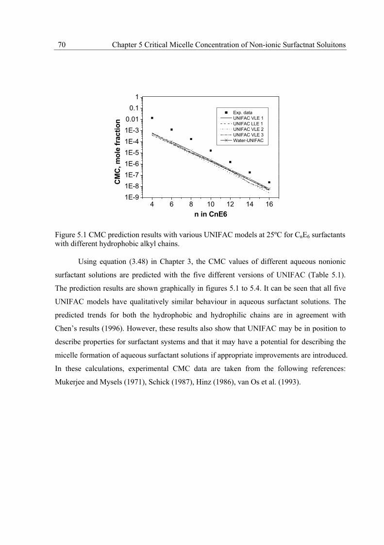
70 Chapter 5 Critical Micelle Concentration of Non-ionic Surfactnat Soluitons
Figure 5.1 CMC prediction results with various UNIFAC models at 25ºC for CnE6 surfactants with different hydrophobic alkyl chains.
Using equation (3.48) in Chapter 3, the CMC values of different aqueous nonionic
surfactant solutions are predicted with the five different versions of UNIFAC (Table 5.1).
The prediction results are shown graphically in figures 5.1 to 5.4. It can be seen that all five
UNIFAC models have qualitatively similar behaviour in aqueous surfactant solutions. The
predicted trends for both the hydrophobic and hydrophilic chains are in agreement with
Chen’s results (1996). However, these results also show that UNIFAC may be in position to
describe properties for surfactant systems and that it may have a potential for describing the
micelle formation of aqueous surfactant solutions if appropriate improvements are introduced.
In these calculations, experimental CMC data are taken from the following references:
Mukerjee and Mysels (1971), Schick (1987), Hinz (1986), van Os et al. (1993).
4 6 8 10 12 14 161E-9
1E-8
1E-7
1E-6
1E-5
1E-4
1E-3
0.01
0.1
1
CM
C, m
ole
fra
cti
on
n in CnE6
Exp. data
UNIFAC VLE 1
UNIFAC LLE 1
UNIFAC VLE 2
UNIFAC VLE 3
Water-UNIFAC
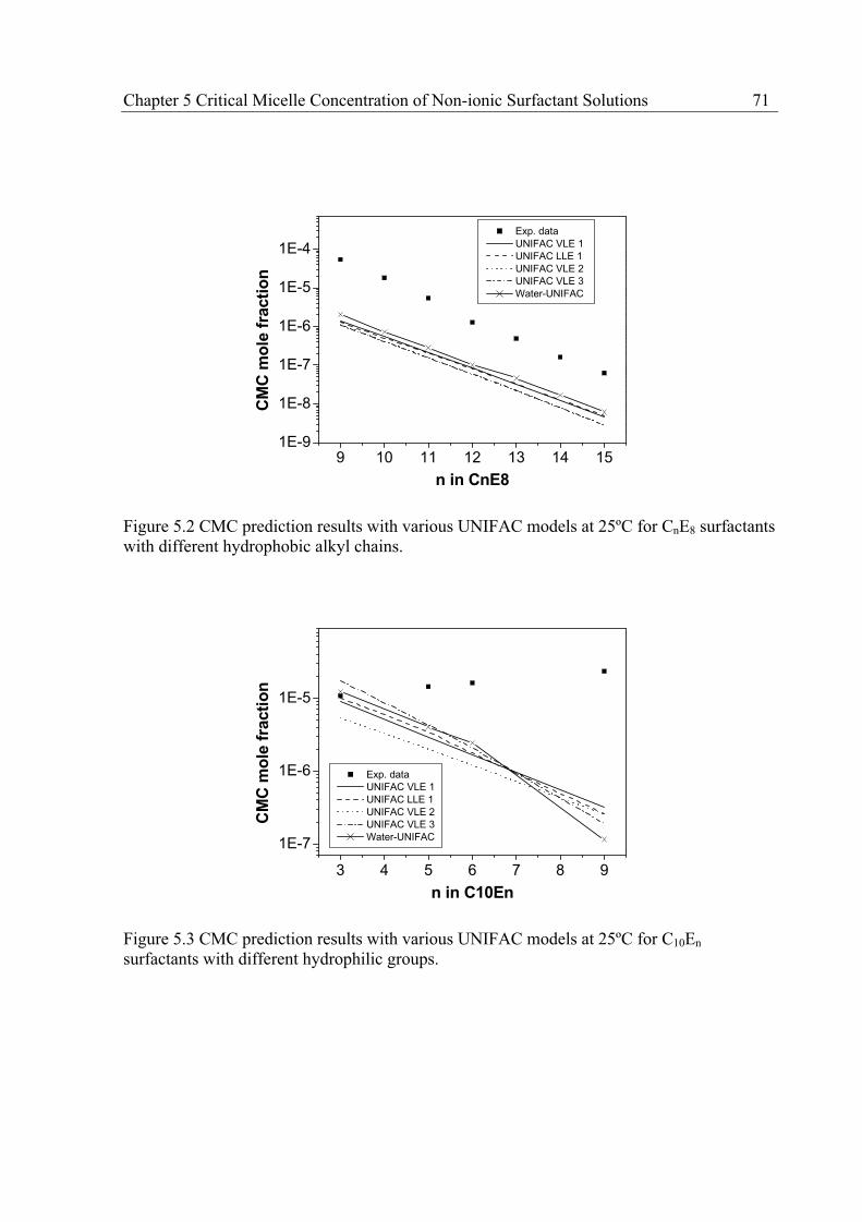
Chapter 5 Critical Micelle Concentration of Non-ionic Surfactant Solutions 71
Figure 5.2 CMC prediction results with various UNIFAC models at 25ºC for CnE8 surfactants with different hydrophobic alkyl chains.
Figure 5.3 CMC prediction results with various UNIFAC models at 25ºC for C10En surfactants with different hydrophilic groups.
9 10 11 12 13 14 151E-9
1E-8
1E-7
1E-6
1E-5
1E-4
CM
C m
ole
fra
cti
on
n in CnE8
Exp. data
UNIFAC VLE 1
UNIFAC LLE 1
UNIFAC VLE 2
UNIFAC VLE 3
Water-UNIFAC
3 4 5 6 7 8 9
1E-7
1E-6
1E-5
CM
C m
ole
fra
cti
on
n in C10En
Exp. data
UNIFAC VLE 1
UNIFAC LLE 1
UNIFAC VLE 2
UNIFAC VLE 3
Water-UNIFAC

72 Chapter 5 Critical Micelle Concentration of Non-ionic Surfactnat Soluitons
Figure 5.4 CMC prediction results with various UNIFAC models at 25ºC for C12En surfactants with different hydrophilic groups.
5.3 Towards a UNIFAC Model for Surfactant Solutions
As shown in figures 5.1-5.4, UNIFAC has the correct CMC tendency with varying
alkyl number in surfactant molecules, but not with varying oxyethylene number. Therefore it
is necessary to further investigate the applicability of UNIFAC to surfactant systems. Since
the selection of functional groups plays an important role in UNIFAC, a special new
oxyethylene group (CH2CH2O) is introduced and evaluated. New interaction parameters for
this group are first directly correlated from experimental CMC data. If results from this step
are found satisfactory, the CH2CH2O interaction parameters would be then estimated solely
from vapor-liquid phase equilibrium data. These interaction parameters from the second step
will give the possibility for direct CMC prediction through UNIFAC.
5 6 7 8 9
1E-7
1E-6
1E-5
CM
C m
ole
fra
cti
on
n in C12En
Exp. data
UNIFAC VLE 1
UNIFAC LLE 1
UNIFAC VLE 2
UNIFAC VLE 3
Water-UNIFAC

Chapter 5 Critical Micelle Concentration of Non-ionic Surfactant Solutions 73
5.3.1 The New Oxyethylene Group (OCH2CH2) for UNIFAC
Surfactant molecules have a wide range of structural features. For nonionic
surfactants alone, several typical structure families are among branched alkyl ethoxylates,
linear alkyl ethoxylates, octylphenol ethoxylates, alkanediols, alkyl mono- and disaccharides
ethers and esters, ethoxylated alkyl amines and amides, fluorinated linear ethoxylates and
amides (Huibers et al. 1996).
Most of these nonionic surfactants contain the oxyethylene group (ethylene oxide
oligomers) in the hydrophilic part of the molecule. These surfactants often contain a
distribution of polyethylene oxide chain lengths rather than a constant number of units. In
this work, two families are studied: the branched alkyl ethoxylates and the linear alkyl
ethoxylates, which are widely used in the chemical industry and are among the most
extensively investigated nonionic surfactants. They are also considered to be environmental
friendly chemicals (AMI report, 2000). These two classes can be represented as the sum of
oxyethylene groups, CH2CH2O and alkyl groups along with one alcohol group OH. Thus,
only one new main UNIFAC group, CH2CH2O, needs to be introduced in order to describe
these two classes of surfactants.
5.3.2 Existing Interaction Parameters for the Oxyethylene Group
In their study of phase equilibrium of aqueous polymer solutions, Rasmussen et al.
(1989) have introduced a special CH2CH2O (polyethylene oxide) group in the UNIFAC
model and successfully predicted the phase behaviour of aqueous polymer solutions with its
group interaction parameters. These group interaction parameters (shown in Table 5.2) have
been also used for investigating the applicability of UNIFAC model for predicting CMC
values of surfactant solutions. Some prediction results are shown in figure 5.5 (denoted as
“Rasmussen”). The calculation is the same as the various UNIFAC methods discussed in
section 5.2. As shown in figure 5.5, using the parameters from Rasmussen et al. (1989) , the
UNIFAC cannot satisfactorily predict the CMC trends of nonionic surfactants with both
increasing hydrophobic and hydrophilic chain-length.

74 Chapter 5 Critical Micelle Concentration of Non-ionic Surfactnat Soluitons
Figure 5.5 Prediction and correlation results of CMC of two CiEj surfactants (CnE6 and C10En) at 25ºC with different methods.
Another group selection for surfactant molecules could be the special glycolether
group, which has been published by Hansen et al. 1991. However, the glycolether-ether
interaction parameters are not available in this UNIFAC model. Thus, this special group was
not studied further.
5.3.3 Summary
This discussion and the previous calculations in section 5.2 indicate that the possible
way for applying UNIFAC to surfactant systems would be to estimate special group
interaction parameters. In figure 5.5, the prediction results of the UNIFAC from Rasmussen
show that the UNIFAC model with a new oxyethylene group may have the capability for
predicting satisfactorily the CMC values for different hydrocarbon chain length in aqueous
surfactant solutions. It is thus very valuable to further investigate the potential of the use of a
separate oxyethylene group. In order to predict the CMC of surfactant solutions,
experimental vapour liquid equilibrium data for non surfactant solutions will be used to
estimate the CH2CH2O group interaction parameters with the UNIFAC model. However, it is
2 4 6 8 10 12 14 161E-9
1E-8
1E-7
1E-6
1E-5
1E-4
1E-3
0.01
0.1
1
C10En
CnE6
CM
C, m
ole
fra
cti
on
n in CnE6, C10En
Exp. data
Correlation
NRTL
Rasmussen
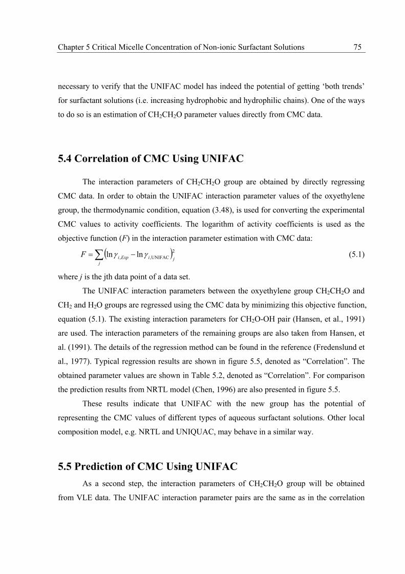
Chapter 5 Critical Micelle Concentration of Non-ionic Surfactant Solutions 75
necessary to verify that the UNIFAC model has indeed the potential of getting ‘both trends’
for surfactant solutions (i.e. increasing hydrophobic and hydrophilic chains). One of the ways
to do so is an estimation of CH2CH2O parameter values directly from CMC data.
5.4 Correlation of CMC Using UNIFAC
The interaction parameters of CH2CH2O group are obtained by directly regressing
CMC data. In order to obtain the UNIFAC interaction parameter values of the oxyethylene
group, the thermodynamic condition, equation (3.48), is used for converting the experimental
CMC values to activity coefficients. The logarithm of activity coefficients is used as the
objective function (F) in the interaction parameter estimation with CMC data:
jjiExpiF2
UNIFAC,, lnln (5.1)
where j is the jth data point of a data set.
The UNIFAC interaction parameters between the oxyethylene group CH2CH2O and
CH2 and H2O groups are regressed using the CMC data by minimizing this objective function,
equation (5.1). The existing interaction parameters for CH2O-OH pair (Hansen, et al., 1991)
are used. The interaction parameters of the remaining groups are also taken from Hansen, et
al. (1991). The details of the regression method can be found in the reference (Fredenslund et
al., 1977). Typical regression results are shown in figure 5.5, denoted as “Correlation”. The
obtained parameter values are shown in Table 5.2, denoted as “Correlation”. For comparison
the prediction results from NRTL model (Chen, 1996) are also presented in figure 5.5.
These results indicate that UNIFAC with the new group has the potential of
representing the CMC values of different types of aqueous surfactant solutions. Other local
composition model, e.g. NRTL and UNIQUAC, may behave in a similar way.
5.5 Prediction of CMC Using UNIFAC
As a second step, the interaction parameters of CH2CH2O group will be obtained
from VLE data. The UNIFAC interaction parameter pairs are the same as in the correlation
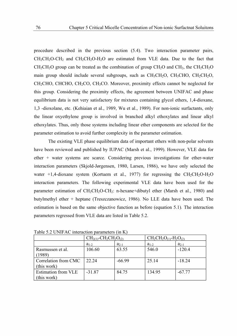
76 Chapter 5 Critical Micelle Concentration of Non-ionic Surfactnat Soluitons
procedure described in the previous section (5.4). Two interaction parameter pairs,
CH2CH2O-CH2 and CH2CH2O-H2O are estimated from VLE data. Due to the fact that
CH2CH2O group can be treated as the combination of group CH2O and CH2, the CH2CH2O
main group should include several subgroups, such as CH3CH2O, CH3CHO, CH2CH2O,
CH2CHO, CHCHO, CH2CO, CH3CO. Moreover, proximity effects cannot be neglected for
this group. Considering the proximity effects, the agreement between UNIFAC and phase
equilibrium data is not very satisfactory for mixtures containing glycol ethers, 1,4-dioxane,
1,3 -dioxolane, etc. (Kehiaian et al., 1989, Wu et al., 1989). For non-ionic surfactants, only
the linear oxyethylene group is involved in branched alkyl ethoxylates and linear alkyl
ethoxylates. Thus, only those systems including linear ether components are selected for the
parameter estimation to avoid further complexity in the parameter estimation.
The existing VLE phase equilibrium data of important ethers with non-polar solvents
have been reviewed and published by IUPAC (Marsh et al., 1999). However, VLE data for
ether + water systems are scarce. Considering previous investigations for ether-water
interaction parameters (Skjold-Jørgensen, 1980, Larsen, 1986), we have only selected the
water +1,4-dioxane system (Kortuem et al., 1977) for regressing the CH2CH2O-H2O
interaction parameters. The following experimental VLE data have been used for the
parameter estimation of CH2CH2O-CH2: n-hexane+dibutyl ether (Marsh et al., 1980) and
butylmethyl ether + heptane (Treszczanowicz, 1986). No LLE data have been used. The
estimation is based on the same objective function as before (equation 5.1). The interaction
parameters regressed from VLE data are listed in Table 5.2.
Table 5.2 UNIFAC interaction parameters (in K) CH2(1)-CH2CH2O(2) CH2CH2O(1)-H2O(2) a1-2 a2-1 a1-2 a2-1 Rasmussen et al. (1989)
106.60 63.55 546.0 -120.4
Correlation from CMC (this work)
22.24 -66.99 25.14 -18.24
Estimation from VLE (this work)
-31.87 84.75 134.95 -67.77

Chapter 5 Critical Micelle Concentration of Non-ionic Surfactant Solutions 77
Using the UNIFAC interaction parameters from vapour-liquid equilibrium data
(Table 5.2), CMC has been predicted using equation (3.48). The predicted results are shown
in the figures 5.6-5.10, and are also compared with the correlation results (section 5.4).
Figure 5.6 Predicted and correlated CMC values with UNIFAC VLE 1 model at 25ºC for two CiEj surfactants (CnE3 and CnE4) with different hydrophobic alkyl chains.
Figure 5.7 Predicted and correlated CMC values with UNIFAC VLE 1 model at 25ºC for two CiEj surfactants (CnE6 and CnE8) with different hydrophobic alkyl chains.
4 6 8 10 12 14 161E-9
1E-7
1E-5
1E-3
0.1 9 10 11 12 13 14 15
1E-7
1E-6
1E-5
1E-4
CnE6
n in CnE6,CnE8
CnE8
CM
C, m
ole
fra
cti
on
Exp. data
Prediction
Correlation
6 7 8 9 10 11 12
1E-6
1E-5
1E-4
1E-35 6 7 8 9 10 11 12
1E-6
1E-5
1E-4
1E-3
CnE3
n in CnE3,CnE4
CnE4
CM
C, m
ole
fra
cti
on
Exp. data
Prediction
Correlation
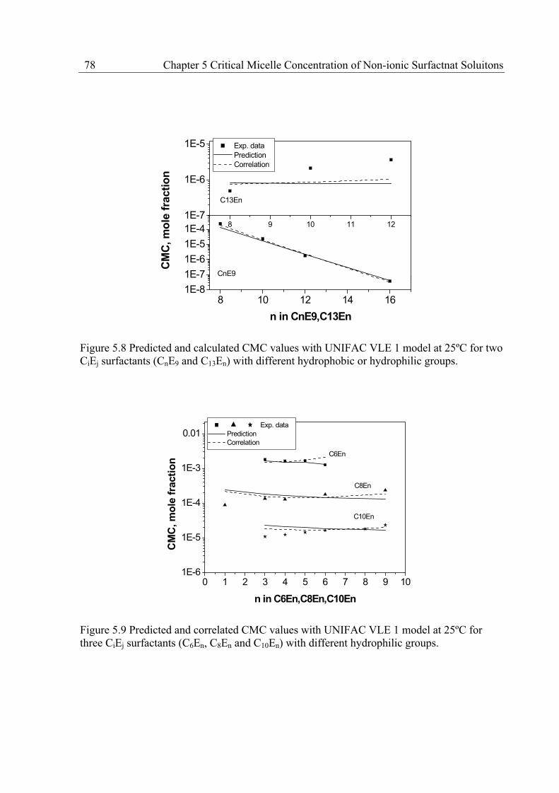
78 Chapter 5 Critical Micelle Concentration of Non-ionic Surfactnat Soluitons
Figure 5.8 Predicted and calculated CMC values with UNIFAC VLE 1 model at 25ºC for two CiEj surfactants (CnE9 and C13En) with different hydrophobic or hydrophilic groups.
Figure 5.9 Predicted and correlated CMC values with UNIFAC VLE 1 model at 25ºC for three CiEj surfactants (C6En, C8En and C10En) with different hydrophilic groups.
0 1 2 3 4 5 6 7 8 9 101E-6
1E-5
1E-4
1E-3
0.01
C10En
C8En
C6En
CM
C, m
ole
fra
cti
on
n in C6En,C8En,C10En
Exp. data
Prediction
Correlation
8 10 12 14 161E-8
1E-7
1E-6
1E-5
1E-48 9 10 11 12
1E-7
1E-6
1E-5
CnE9
n in CnE9,C13En
C13En
CM
C, m
ole
fra
cti
on
Exp. data
Prediction
Correlation

Chapter 5 Critical Micelle Concentration of Non-ionic Surfactant Solutions 79
Figure 5.10 Predicted and correlated CMC values with UNIFAC VLE 1 model at 25ºC for two CiEj surfactants (C12En and C16En) with different hydrophilic groups.
From these results, it can be seen that the UNIFAC model, with the interaction
parameter from VLE data, can quantitatively represent CMC for different aqueous non-ionic
surfactant solutions. Specifically, the UNIFAC model predicts well the observed trends of
hydrophobic alkyl and hydrophilic chain for these nonionic surfactant solutions. Slight
deviations in the hydrophilic tendencies could be attributed to the fact that interaction
parameters are estimated only from water+1,4-dioxane VLE data. The values of oxyethylene
group interaction parameters could be different in the linear and cyclical states. On the other
hand, the obtained CMC data are from different data sources; only part of them being from
the collection of Mukerjee et al. (1971) in which CMC data have been carefully reviewed.
Experimental CMC data may be subject to errors, which can be difficult to assess due to lack
of a method for testing the consistency of CMC data.
5.6 Discussion and Conclusions
Different UNIFAC methods have been systematically investigated for water + alcohol
ethoxylate systems. The results show that the original UNIFAC VLE 1, modified UNIFAC
0 5 10 15 20 25 30 351E-8
1E-7
1E-6
1E-5
C16En
C12EnC
MC
, m
ole
fra
cti
on
n in C12En, C16En
Exp. data
Prediction
Correlation

80 Chapter 5 Critical Micelle Concentration of Non-ionic Surfactnat Soluitons
VLE 3, UNIFAC LLE 1, the linear temperature dependent UNIFAC VLE 2 and water
UNIFAC methods predict qualitatively correct the observed trend of the CMC with
hydrophobic chain for aqueous nonionic surfactant solutions, but fail to predict the CMC
trend with the hydrophilic chain. By introducing a new group, the oxyethylene group
(CH2CH2O), and estimating its interaction parameters from vapour-liquid equilibrium data,
the original UNIFAC VLE 1 method can provide good prediction for micelle formation in
water + alcohol ethoxylate systems with both the hydrophobic and hydrophilic trends.
Because the UNIFAC model has a large amount of interaction parameters readily available in
reference (Hansen et al., 1991), it should be in principle applicable to other nonionic
surfactant solutions, e.g. alkyl phenol-oxyethylene, if (when required) new functional group
parameters are introduced and estimated from available phase equilibrium data.
Besides the phase equilibrium data, osmotic coefficient and enthalpy data can also be
applied to estimate the interaction parameters of the CH2CH2O group in the UNIFAC model.
Dearden et al. (1996), Sato et al. (1988), van Os et al. (1993), McGinnis et al. (1997) have
published these types of data. Because the osmotic coefficients are directly obtained from
vapour pressure measurement of aqueous surfactant solutions, the osmotic coefficient data
could be used to get the group interaction parameters in surfactant molecules, e.g. CH2CH2O
group. In this way, UNIFAC may give better prediction results. However, interaction
parameter estimation using osmotic coefficient data cannot completely overcome certain
limitations of UNIFAC, such as the proximity effects.
Modelling of micelle formation in mixed surfactant systems is at the beginning.
However, mixed surfactant systems are very important in industrial applications. In the
mixed aqueous surfactant solutions, more than one nonionic surfactant may exist in micelles.
In many cases, these solutions also contain salts and ionic surfactants as additives. Chen
(1996) has proposed a thermodynamic framework for mixed surfactant systems, but this has
not been applied to a specific mixed surfactant solution.

Chapter 6 The UNIFAC Model for Aqueous Electrolyte Solutions 81
Chapter 6 The UNIFAC Model for Aqueous Electrolyte Solutions
The purpose of this chapter is to select and evaluate a model to describe the mean
activity coefficients of electrolyte solutions, which will be applied to ionic surfactant
solution.
The ionic (cationic or anionic) surfactant molecules dissociate into cations and anions
in aqueous solutions. Such solutions exhibit typical electrolytic properties. The electrical
conductivity of the solution can be measured, and can be used experimentally to determine
the critical micelle concentrations (CMC) of ionic surfactant solutions (Mukerjee et al.,
1971); as shown in figure 2.5 (Chapter 2) and figure 3.8 (Chapter 3). Thus, a model for
organic electrolyte solutions is required to calculate the properties of ionic surfactant
solutions, such as mean activity coefficients.
In this chapter, the modelling of aqueous electrolyte solutions is first briefly
reviewed, emphasizing the efforts of extending the UNIQUAC or UNIFAC model to aqueous
electrolyte solutions. Achard’s electrolyte UNIFAC method (Achard et al. 1994a, b) is then
described and modified. It has been found that the structural parameter (Q, R) of ions used in
this model and other UNIQUAC based models did not follow Flory-Huggins assumption
(Q/R 1). Thus, structural parameters (Q, R) of ions for the UNIFAC model are estimated
from ionic radii based on the condition Q/R<1. Mean activity coefficients of some aqueous
and organic electrolyte solutions are studied with the modified Achard electrolyte UNIFAC
model using the new set of structural parameters.
6.1 Modelling of Aqueous Electrolyte Solutions
6.1.1 Definitions of Electrolyte Solutions
When dissolved in a high-dielectric-constant solvent like water, an electrically neutral
electrolyte Mv+Xv- is dissociated into v+ positive ions (cations) each with a charge z+, and v-
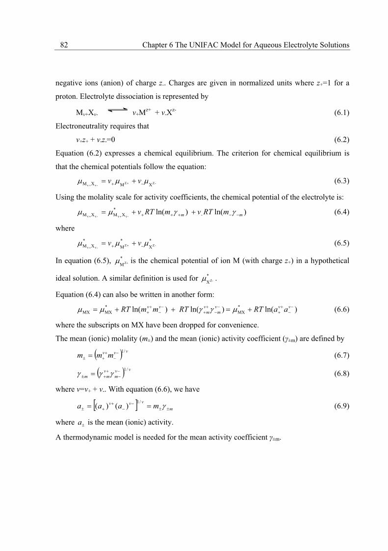
82 Chapter 6 The UNIFAC Model for Aqueous Electrolyte Solutions
negative ions (anion) of charge z-. Charges are given in normalized units where z+=1 for a
proton. Electrolyte dissociation is represented by
Mv+Xv- v+Mz+ + v-Xz- (6.1)
Electroneutrality requires that
v+z+ + v-z-=0 (6.2)
Equation (6.2) expresses a chemical equilibrium. The criterion for chemical equilibrium is
that the chemical potentials follow the equation:
-ZZ-vv X-MXM vv (6.3)
Using the molality scale for activity coefficients, the chemical potential of the electrolyte is:
)ln( )ln( -*
XMXM -vv-vv mm mRTvmRTv (6.4)
where
*
X-*
M
*XM -ZZ
-vv vv (6.5)
In equation (6.5), *
MZ is the chemical potential of ion M (with charge z+) in a hypothetical
ideal solution. A similar definition is used for *
X -Z .
Equation (6.4) can also be written in another form:
)ln( )ln( )ln( *MX
*MXMX
vvv
m
v
m
vv aaRTRTmmRT (6.6)
where the subscripts on MX have been dropped for convenience.
The mean (ionic) molality (m±) and the mean (ionic) activity coefficient ( ±m) are defined by
vvv mmm/1
(6.7)
vv
m
v
mm
/1 (6.8)
where v=v+ + v-. With equation (6.6), we have
m
vvv maaa/1
)()( (6.9)
where a is the mean (ionic) activity.
A thermodynamic model is needed for the mean activity coefficient ±m.

Chapter 6 The UNIFAC Model for Aqueous Electrolyte Solutions 83
6.1.2 Activity Coefficient Models
The work of Debye and Hückel in 1923 is one of the first theoretical attempts in
modelling electrolytes (Laidler, 1999). In Debye-Hückel theory, the water or solvent is
regarded as a dielectric continuum, the solvent molecules are not explicitly taken into
account. The ions are regarded as individual spheres. This is a simplified representation of a
very dilute solution. The Debye-Hückel theory only considers the energy of charging-up a
system. That implies the existence of an uncharged system of molecules that needs to be
charged. If the Debye-Hückel theory is used without any additional terms, it only represents
the behaviour of very dilute solutions. Starting with the Debye-Hückel theory, many
researchers have proposed their methods to represent concentrated electrolyte solutions.
Loehe and Donohue (1997) have reviewed modelling approaches for thermodynamic
properties of aqueous electrolyte solutions. Theoretical and engineering models for the
thermodynamic properties of strong electrolyte solutions have advanced significantly since
the 80’s. Significant progress has been made in the ability to calculate various properties of
single and mixed strong electrolyte solutions over a wide range of temperature and
composition, including effects of various non-electrolytes, solvents and supercritical
components. Engineering models for thermodynamic properties of electrolyte solutions may
be divided into three catalogues: (1) local composition and hydration models; (2) empirical
and semi-empirical equations of state for strong electrolytes; and (3) equations for mixed
solvents, mixed electrolytes, and mixtures of supercritical gases and electrolytes. In this
work, we focus on local composition models.
Many such semi-empirical local composition models have been proposed using a
Debye-Hückel type term for the long-range contribution, but different expressions for the
short-range contribution, e.g. UNIQUAC, NRTL, Wilson, van Laar and Margules equations
(Prausnitz et al., 1999). The models of Cruz and Renon (1978) and Chen et al. (1982, 1986),
use NRTL; the model of Zerres and Prausnitz (1994) uses an extended van Laar equation. In
Pitzer’s model (1973, 1980), a virial series is used for the short-range contribution.
The electrolyte NRTL model of Chen et al. is based on two important assumptions:
(1) the local composition of cations around cations is zero, and similarly for anions, which is
equivalent to assuming that repulsive forces between ions of like charge are extremely large
84 Chapter 6 The UNIFAC Model for Aqueous Electrolyte Solutions
(like-ion repulsion assumption); (2) the distribution of cations and anions around a central
solvent molecule is such that the net local ionic charge is zero (local electroneutrality
assumption). Based on these assumptions, Chen derived an expression for the short-range
contribution to the excess Gibbs energy that includes two adjustable parameters. Chen’s
model reproduces well the mean ionic activity coefficients of aqueous single electrolytes up
to a molality of six. For multi-salt systems, this model requires binary parameters obtained
from data of the corresponding binary systems. Recently, Chen et al. (2001) modified their
electrolyte NRTL model and extended it to aqueous organic electrolytes. The proposed
extension has three terms: the Pitzer-Debye-Hückel term, the local composition term from an
NRTL-type expression, and the Flory-Huggins term. This NRTL version for aqueous organic
electrolytes was then applied to micelle formation of aqueous sodium carboxylate solutions.
6.2 Efforts in Extending the UNIQUAC/UNIFAC Methods to Electrolyte Solutions
Many efforts have been reported for extending the UNIQUAC or UNIFAC models
(as short-range term) for electrolyte solutions. Only some of the efforts are discussed here.
Christensen et al. (1983 a, b)
Christensen et al. investigated aqueous electrolyte solutions with the UNIQUAC
model. In their work, the excess Gibbs energy of solution includes three terms: (1) a Debye-
Hückel term from Robinson and Stokes (1965); (2) a term of the Brøndsted-Guggenheim
type, which is an empirical expression given by Guggenheim referring to the interaction
between cations and anions; (3) a UNIQUAC term. It is assumed that the local composition
of cations around cations and anions around anions is very small, due to the strong repulsive
electrostatic interaction between charges of the same sign. This corresponds to a high
positive value for the interaction parameter between two cations or two anions. This
assumption is equivalent to the “like-ion repulsion assumption” of Chen et al. (1982).
Another assumption is to arbitrarily set the value of interaction parameters of water-water
Chapter 6 The UNIFAC Model for Aqueous Electrolyte Solutions 85
and cation-anion to zero. For ions, the structural parameters are calculated using the ionic
radii in crystals. The ionic radii in crystals can be found in CRC handbook (Lide, 2002). For
a single electrolyte system, three estimated parameters, i.e. ucation-H2O, uanion-H2O in the
UNIQUAC term and one cation-anion in the Brøndsted-Guggenheim term, are used to correlate
the activity coefficients of electrolyte solutions.
Sander et al. (1984, 1986)
To correlate and predict salt effects in vapour-liquid equilibria for water and
cosolvent mixtures, Sander et al. (1984, 1986) combined the Debye-Hückel term and a
modified UNIQUAC equation with concentration-dependent interaction parameters. The
model parameters are ion-specific, and no ternary parameters are required. In Sander’s
model, some of the interaction parameters between cations and anions are set to be zero.
Instead of using the “like-ion repulsion assumption” of Chen et al. (1982), the interaction
parameters between like ions are also set to zero. The volume (R) and surface area (Q)
parameters of cations were modified. This is because the very small values of the ionic radii
of the cations lead to Q-values of the order of 0.1 to 0.5. Q values of this magnitude reduce
the fitting capabilities of the UNIQUAC equation. For the anions, the R and Q are calculated
from ionic radii in crystals. However, a large number of parameters are needed: 7 for a
salt/solvent system and 14 for a salt/co-solvent system. Sander’s model suffers from
improper combination of Lewis-Randall and McMillan-Mayer formalisms. This deficiency
was later corrected by Macedo et al. (1990).
Kikic et al. (1991)
Kikic et al. developed a UNIFAC model for correlation of vapour liquid equilibria in
mixed solvent-salt systems. The model of Kikic et al. used the same thermodynamic
framework as Sander’s. UNIFAC is used for the short-range contribution term instead of
UNIQUAC. The Debye-Hückel expression is used for long-range interactions. The
assumptions for interaction parameters are the same as in Sander’s method. The volume and
surface area parameters of ions are taken from Sander’s work.
86 Chapter 6 The UNIFAC Model for Aqueous Electrolyte Solutions
Thomsen et al. (1996, 1997, 1999)
Thomsen et al. modified Sander’s model (1986) with a linear temperature dependence
of the binary interaction parameters and extended the UNIQUAC model to correlate and
predict the thermal properties and phase behaviours of aqueous electrolyte systems. The
interaction parameters are estimated from Gibbs energy of formation, enthalpy of formation
and heat capacities for electrolytes. Thomsen’s model sets the water-water and the like cation
interaction parameters to zero. The volume and surface area parameters of ions are regressed
from experimental data.
Li et al. (1994)
Li et al. proposed an excess Gibbs energy (GE) model for electrolyte systems based on
the results from statistical thermodynamics and took into account the interactions between all
species present in the electrolyte solution. In this model, the electrolyte solution is treated as
a non-electrolyte solution plus charge interactions. It is assumed that the charge interactions
are both direct and indirect: direct interactions between charges, indirect effects under the
influence of the electric field created by the charges. Both direct and indirect effects depend
on the ionic strength of the solution. The expression of excess Gibbs energy for electrolyte
solutions is:
ESR
EMR
ELR
E GGGG (6.10)
where the ELRG represents the long-range (LR) interaction due to the electrostatic forces, and
mainly describes the direct effects of charge interactions. ELRG is calculated with the Debye-
Hückel theory modified by Fowler and Guggenheim. EMRG represents the indirect effects
from the noncharge short-range interactions of the non-electrolyte solutions, and is called the
middle-range (MR) interaction contribution. EMRG is computed by an expression proposed by
Li et al. (1994), ESRG expresses the short-range interaction, and is calculated by the
UNIQUAC model. The volume and surface area parameters are fixed to 1.0 for ions. For a
single electrolyte solution, four parameters are required to describe the cation-anion
interactions; eight parameters are needed for ion-solvent interactions. Based on the
thermodynamic framework of Li et al. (1994), Yan et al. (1999) used the UNIFAC model,
Chapter 6 The UNIFAC Model for Aqueous Electrolyte Solutions 87
instead of UNIQUAC, to describe the short-range interaction contribution and introduced
group interaction parameters to the middle-range term. The volume and surface area
parameters of ions in the UNIFAC model are treated as adjustable parameters.
Lu and Maurer (1993)
Lu and Maurer combined ionic solvation equilibria and physical interaction forces for
mixed electrolyte solutions. In this model, the Debye-Hückel model is used for the long-
range term, and the UNIQUAC model is used for the short-range term to represent the excess
Gibbs energy. The UNIQUAC structural parameters of charged species are approximated by
the ionic radii of ions. Furthermore, for all ionic species the UNIQUAC size R and surface Q
parameters are set equal to each other. For the interaction parameters, it is assumed that: (1)
the interaction parameters are equal to 2000 K for ions carrying same sign charges, (2) the
interaction parameters between cation-anion are equal to that of anion-cation, (3) the
interaction parameters between any ion and a water molecule are zero since these interactions
are taken into account by the solvation reaction, and (4) the interaction parameter between
water molecules is set to zero. For the ions of a strong electrolyte, there remain only 3 “pure
component” parameters, which are, the unsolvated ionic radius, solvation number and
solvation equilibrium constant. There are two binary parameters for interactions between a
cation and an anion, that is, one size correction parameter and one energy parameter. Lu et al.
(1996) further extended this method to various temperatures.
Achard et al. (1994a, b)
Achard et al. (1994a, b) proposed a modified UNIFAC method to correlate and
predict salt effects on vapour-liquid equilibria of mixed solvent systems and extend the
method for weak electrolytes in aqueous solutions. The model of Achard et al. combined a
term of the Debye-Hückel type with a modified UNIFAC equation based on solvation
phenomena. In Achard’s method, the volume and surface area parameters of ions are
computed by combining the ionic radii in crystals with hydration numbers. The method has
been used to represent salt effects on vapour-liquid equilibrium of mixed solvent systems, the
pH in complex aqueous solutions, especially the water activity and osmotic pressure of

88 Chapter 6 The UNIFAC Model for Aqueous Electrolyte Solutions
organic electrolyte solutions, i.e. amino acids, carboxylic acids, phosphates and carbonates
(Achard et al. 1993, 1994a, b). This model was chosen for further study in this work.
6.3 Achard’s Electrolyte UNIFAC Model and its Modifications
6.3.1 Achard’s Electrolyte UNIFAC Model
In the electrolyte UNIFAC method proposed by Achard et al. (1994a, b), the excess
Gibbs energy (gE) is divided into two terms, one resulting from short-range (SR) interactions
(physical forces, solvation phenomena between water and ionic species), and the other from
long-range (LR) electrostatic interactions:
RT
g
RT
g
RT
g LRESREE ,,
(6.11)
or similarly for activity coefficients:
LR
i
SR
ii lnlnln (6.12)
The activity coefficient models used in equation (6.12) are the modified UNIFAC
method (Larsen et al., 1987) for the short-range interaction term and the extended form of the
Debye-Hückel expression given by Pitzer (1973, 1980) for the long-range interaction term. In
addition a set of solvation equations is also proposed to account for the hydration of ions by
water molecules (formation of clusters) in the activity coefficient calculations.
In UNIFAC, the interaction parameter is expressed as jjijij uua with jiij uu
following the work of Christensen et al. (1983). The uij interaction energies are used instead
of aij, as they are proportional to the interaction forces between species i and j. The
assumptions for the interaction parameters (energies) are:
(i) The repulsion forces between ions of like charge are very large and the resulting
interaction energies (ucc and uaa) are set equal to 2500K. The subscripts c, a
represent cations and anions, respectively.
(ii) The attractive forces between a cation and an anion (uca) are set to zero to
preserve the predictive capabilities of the model, so that it is not necessary to have
experimental data for every water-electrolyte system.
Chapter 6 The UNIFAC Model for Aqueous Electrolyte Solutions 89
(iii) The interaction energy between two water molecules is equal to 700K. This
value is calculated from the enthalpy of vaporization of water at 25ºC.
The alkyl group energy parameter ukk is calculated as follows:
wwwkkwkk uaau (6.13)
where w represents the water and k represents the hydrocarbon solvent group.
These assumptions for the interaction parameters are summarized in Table 6.1.
Table 6.1 Interaction parameters for a solution of a single electrolyte in Achard’s method (in K)*
Cation(c) Anion(a) H2O(w) Cation(c) ucc-ucc=0 uca-uaa=-2500 ucw-uww= ucw +700 Anion(a) uac-ucc=-2500 uaa-uaa=0 uaw-uww= uaw +700 H2O(w) uwc-ucc= uwc –2500 uwa-uaa= uwa-2500 uww-uww=0
* uwc=ucw, uaw=uwa, uca=uac
The unknown interaction parameters for a single electrolyte solution are ucw, uaw . In some
cases, the cation-anion interaction parameter, uca, is also used as an adjustable parameter to
improve model behaviours.
The solvation phenomena are considered in the model as chemical association
between water and ionic species. It is this behaviour that causes the non-ideality of
electrolyte solutions. To account for the solvation phenomena of aqueous electrolyte
solutions, two different standard states are proposed: one is the non-hydrated standard state,
which corresponds to the classical standard state; the other is the hydrated standard state.
In the hydrated standard state, water molecules are chemically bound to ionic species and to
form clusters. This is taken into account in the calculation of ionic structural parameters and
mole fractions of water and cluster with a set of solvation equations to get structural
parameters for hydrated species and mole fraction as follows.
Structural Parameters for Hydrated Species
1' RNhRR kkk (6.14)
1' QNhQQ kkk (6.15)
90 Chapter 6 The UNIFAC Model for Aqueous Electrolyte Solutions
where 'kR and '
kQ are the structural parameters of hydrated species k, Rk and Qk are the
structure parameter calculated by ionic radii in crystals, Nhk is the hydration number, and is
fitted simultaneously with interaction parameters, R1 and Q1 are the volume and surface area
parameters of water. For a single electrolyte system, there are two Nhk parameters: one for
cations, the other for anions. There are four unknown parameters for a single aqueous
electrolyte solution: two parameters for the interaction energy and two parameters for the
hydration number.
Mole Fractions Corresponding to the Hydrated Standard State (H)
The mole fraction of water, Hx1 , is given by:
N
j
jj
N
j
jj
H
xNh
xNhx
x
2
21
1
1
(6.16)
The mole fraction of ionic species, H
ix , is given by
N
j
jj
iH
i
xNh
xx
2
1
(6.17)
The structural parameters and mole fraction in the hydrated state are used in the
UNIFAC model. The activity coefficients in the hydrated standard state, HSR
i
, , and classical
standard state, SR
i , are related as follows:
1
1,11
x
xHHSRSR (6.18)
iNhHSR
i
H
iHSR
i
SR
i xx
x11
, (i 1) (6.19)
where subscript 1 is the water, the notation ‘H’ refers to the hydrated reference state,
HSR,1 and HSR
i
, are calculated with Larsen’s UNIFAC model (Larsen et al., 1987) using the
mole fractions and structural parameters of hydrated species. The SR
1 and SR
i are used as the
Chapter 6 The UNIFAC Model for Aqueous Electrolyte Solutions 91
short-range term activity coefficients. A complete activity coefficient expression can now be
obtained by combining the short-range and long-range terms.
6.3.2 Modifications of Achard’s Method
In aqueous electrolyte solutions, solvation phenomena have been studied
experimentally by mobility investigations (Robinson and Stokes, 1959). When an electrolyte,
Mv+Xv-, is dissolved into water, it completely (or partially) dissociates and attains ionic
solvation equilibria in the solution:
Mz+ + h+H2O MZ+·h+H2O (6.20)
Xz- + h-H2O Xz-·h-H2O (6.21)
Where h+ and h- are the number of water molecules in a solvation complex with cation and
anion, respectively. In the aqueous electrolyte solution, the polar solvent (water) can shield
the electric field originating from the point charge of an ion by forming a shell around it. In
solution, these ions permanently carry water molecules with them that are regarded as part of
the ion. The ions and water molecules are chemically associated. The solvation phenomena
determine the effective size of ions. As can be seen from the above equations, the solvation
equilibria depend on the concentration and temperature of the system. In Achard’s method,
the solvation phenomena are considered to be independent to concentration and temperature.
The hydration numbers are obtained by a regression of mean activity coefficient data for
electrolyte solutions.
To account for the hydration phenomena, different methods have been proposed by
Robinson and Stokes (1959), Lu and Maurer (1993), Chen et al. (1999) and the Achard’s
work. These methods can partly capture the complex hydration phenomena for electrolyte
solutions. However, in this research work, we focus on the micelle formation in ionic
surfactant solutions. Hydration equations may lead to additional complexity, thus they are not
used. Instead, we use ionic radii to calculate the structural parameters R and Q. All other
assumptions for group interaction parameters in the Achard’s model remain unchanged.
92 Chapter 6 The UNIFAC Model for Aqueous Electrolyte Solutions
Activity Coefficient for the Modified Achard Model
The asymmetrical convention activity coefficient ( *i ) is expressed:
UNIFAC*,PDH*,* lnlnln iii (6.22)
where the asymmetrical Pitzer-Debye-Hückel (PDH) (1973, 1980) expression is used to
account for the long-range ion-ion interaction term, UNIFAC is used for the short-range
interaction term for the completely dissociated electrolyte in aqueous solutions. Without
using the hydration number, the solvation equations for structural parameters and mole
fractions are not valid. The interaction parameters reported in Achard’s work cannot be used
in equation (6.22) because the hydration number variable is not used. In equation (6.22), the
reference state is the pure liquid for the solvent at the temperature and pressure of the
mixture. For a solute species, the reference sate is at infinite dilution in water at the system
temperature and pressure. Appendix B gives detailed descriptions for the reference state.
Because original UNIFAC is a symmetric expression, it is normalized using terms with
“infinite-dilution activity coefficient in water” for each ion, in order to obtain an expression
based on the asymmetric convention.
Long-range Interaction Term
The Pitzer-Debye-Hückel equation for any species is
2/1
2/32/122/1
22/1
*,
1
21ln
21000ln
x
xxix
i
s
PDH
iI
IIZI
ZA
M (6.23)
iix xZI 2
2
1 (6.24)
where Ix is the ionic strength on a mole fraction basis, Ms is the molecular weight of the
solvent, A is the usual Debye-Hückel parameter and is the ‘closest approach’ parameter.
The value of depends on the electrolyte as well as the expression used to represent the
short-range interactions. The value of 14.9 from Pitzer’s work (1980) is used for . The
Debye-Hückel parameter A is from Chen’s correlation (1982):
TTFTTETDTTCTTBTTAA / /ln/exp/exp 02
02
0
2
00 (6.25)

Chapter 6 The UNIFAC Model for Aqueous Electrolyte Solutions 93
where 0TTT , T0=273.15 K, A= 61.4453, B=2.864468, C=183.5379, D= 0.6820223,
E=7.875695×10⁻⁴, F=58.95788.
Short-range Interaction Term
For the UNIFAC model, the linear temperature-dependent UNIFAC method (Hansen
et al., 1992) is used instead of the UNIFAC model of Larsen et al. (1987) in Achard’s work.
The assumptions for the interaction parameters of UNIFAC are taken from Achard’s work
(Table 6.1). The interaction parameters of Hansen et al., (1992) are given by the temperature
dependent equation:
02,1, TTaaa ijijij , (T0=298.15 K) (6.26)
By using 1,1,1, jjijij uua , 2,2,2, jjijij uua , the linear temperature dependent parameter is
reformulated to:
02,1,02,1, TTuuTTuua jjjjijijij (6.27)
If the ujj can be treated as temperature independent, we have
jjijijij uTTuua 02,1, (6.28)
For a solution of single electrolyte, the interaction parameters between ions (i) and water (w)
(or other groups) are
wwiwiwwwiwiw uTTuuuua 02,1, (6.29)
where K 700wwu at 298.15 K from Achard’s work, uiw,1 and uiw,2 are two unknown
interaction parameters.
The interaction parameters between cation (c) and anion (a) are
K 2500aacaca uua , K 2500ccacac uua (6.30)
The interaction parameters are summarized in Table 6.2. The unknown interaction
parameters for a single electrolyte aqueous solution are ucw,1, ucw,2, uaw,1 and uaw,2.
The modified Achard model can be used to organic electrolyte. For organic
electrolytes, the cation or anion may contain alkyl groups, e.g. sodium butanoate. By using
the UNIFAC method, the anion C4H7O2- of sodium butanoate (C4H7O2
-Na+) can be divided
as one CH3, two CH2, and one COO- group. The interaction parameters between the alkyl
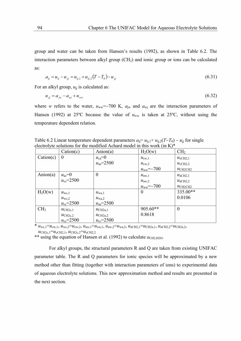
94 Chapter 6 The UNIFAC Model for Aqueous Electrolyte Solutions
group and water can be taken from Hansen’s results (1992), as shown in Table 6.2. The
interaction parameters between alkyl group (CH2) and ionic group or ions can be calculated
as:
jjijijjjijij uTTuuuua 02,1, (6.31)
For an alkyl group, ujj is calculated as:
wwwjjwjj uaau (6.32)
where w refers to the water, uww= 700 K, ajw and awj are the interaction parameters of
Hansen (1992) at 25ºC because the value of uww is taken at 25ºC, without using the
temperature dependent relation.
Table 6.2 Linear temperature dependent parameters aij= uij,1+ uij,2(T T0) ujj for single electrolyte solutions for the modified Achard model in this work (in K)*
Cation(c) Anion(a) H2O(w) CH2 Cation(c) 0 uca=0
uaa=2500 ucw,1 ucw,2 uww= 700
ucCH2,1 ucCH2,2 uCH2CH2
Anion(a) uac=0 ucc=2500
0 uaw,1 uaw,2 uww= 700
uaCH2,1 uaCH2,2 uCH2CH2
H2O(w) uwc,1 uwc,2 ucc=2500
uwa,1 uwa,2 uaa=2500
0 335.00** 0.0106
CH2 uCH2c,1 uCH2c,2 ucc=2500
uCH2a,1 uCH2a,2 ucc=2500
905.60** 0.8618
0
* uwc,1=ucw,1, uwc,2=ucw,2, uaw,1=uwa,1, uaw,2=uwa,2, uaCH2,1=uCH2a,1, uaCH2,2=uCH2a,2, uCH2c,1=ucCH2,1, uCH2c,2=ucCH2,2 ** using the equation of Hansen et al. (1992) to calculate aCH2,H2O.
For alkyl groups, the structural parameters R and Q are taken from existing UNIFAC
parameter table. The R and Q parameters for ionic species will be approximated by a new
method other than fitting (together with interaction parameters of ions) to experimental data
of aqueous electrolyte solutions. This new approximation method and results are presented in
the next section.

Chapter 6 The UNIFAC Model for Aqueous Electrolyte Solutions 95
6.4 Structural Parameter Calculation for Ions
6.4.1 Structural Parameter Calculation
Abrams and Prausnitz‘s Approach
Abrams and Prausnitz (1975) proposed the structural parameter calculation method
for the UNIQUAC model. The effects of molecular size and shape are evaluated by structural
parameters obtained from pure-component data. The structural parameters are, respectively,
the van der Waals volume and surface area of the molecule relative to those of a standard
segment:
ws
wkk
V
VR (6.33)
ws
wkk
A
AQ (6.34)
where Vwk and Awk are the van der Waals volume and area of the molecule given by Bondi
(1968), Vws and Aws are the van der Waals volume and area of a standard segment. The
methylene segment (-CH2-) was arbitrarily chosen as the standard segment. The volume of
the standard sphere in terms of its radius rws is given by
3 3
4wsws rV (6.35)
and the area by
2 4 wsws rA (6.36)
Based on these equations, Abrams and Prausnitz (1975) derived the following equations:
17.15/wkk VR (6.37)
)105.2/( 9wkk AQ (6.38)
where Rk and Qk are, respectively, the dimensionless volume and surface area parameters for
the UNIQUAC model, and 15.17 and 2.5 109 are normalization factors derived from CH2
group. The derivation of these equations is reproduced in Appendix C based on the work of
Abrams and Prausnitz (1975). In UNIFAC, the same method is used for the structural
parameters.
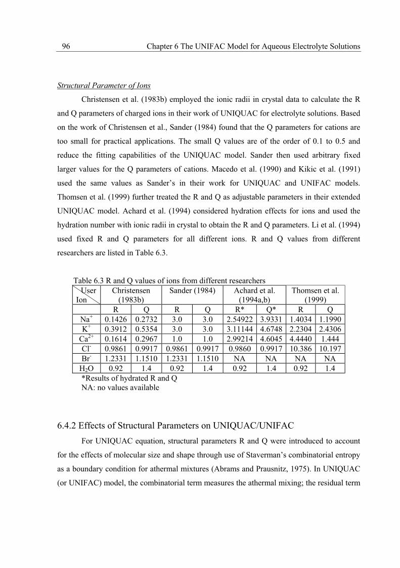
96 Chapter 6 The UNIFAC Model for Aqueous Electrolyte Solutions
Structural Parameter of Ions
Christensen et al. (1983b) employed the ionic radii in crystal data to calculate the R
and Q parameters of charged ions in their work of UNIQUAC for electrolyte solutions. Based
on the work of Christensen et al., Sander (1984) found that the Q parameters for cations are
too small for practical applications. The small Q values are of the order of 0.1 to 0.5 and
reduce the fitting capabilities of the UNIQUAC model. Sander then used arbitrary fixed
larger values for the Q parameters of cations. Macedo et al. (1990) and Kikic et al. (1991)
used the same values as Sander’s in their work for UNIQUAC and UNIFAC models.
Thomsen et al. (1999) further treated the R and Q as adjustable parameters in their extended
UNIQUAC model. Achard et al. (1994) considered hydration effects for ions and used the
hydration number with ionic radii in crystal to obtain the R and Q parameters. Li et al. (1994)
used fixed R and Q parameters for all different ions. R and Q values from different
researchers are listed in Table 6.3.
Table 6.3 R and Q values of ions from different researchers User Ion
Christensen (1983b)
Sander (1984) Achard et al. (1994a,b)
Thomsen et al. (1999)
R Q R Q R* Q* R Q Na+ 0.1426 0.2732 3.0 3.0 2.54922 3.9331 1.4034 1.1990K+ 0.3912 0.5354 3.0 3.0 3.11144 4.6748 2.2304 2.4306
Ca2+ 0.1614 0.2967 1.0 1.0 2.99214 4.6045 4.4440 1.444 Cl- 0.9861 0.9917 0.9861 0.9917 0.9860 0.9917 10.386 10.197Br- 1.2331 1.1510 1.2331 1.1510 NA NA NA NA
H2O 0.92 1.4 0.92 1.4 0.92 1.4 0.92 1.4 *Results of hydrated R and Q NA: no values available
6.4.2 Effects of Structural Parameters on UNIQUAC/UNIFAC
For UNIQUAC equation, structural parameters R and Q were introduced to account
for the effects of molecular size and shape through use of Staverman’s combinatorial entropy
as a boundary condition for athermal mixtures (Abrams and Prausnitz, 1975). In UNIQUAC
(or UNIFAC) model, the combinatorial term measures the athermal mixing; the residual term
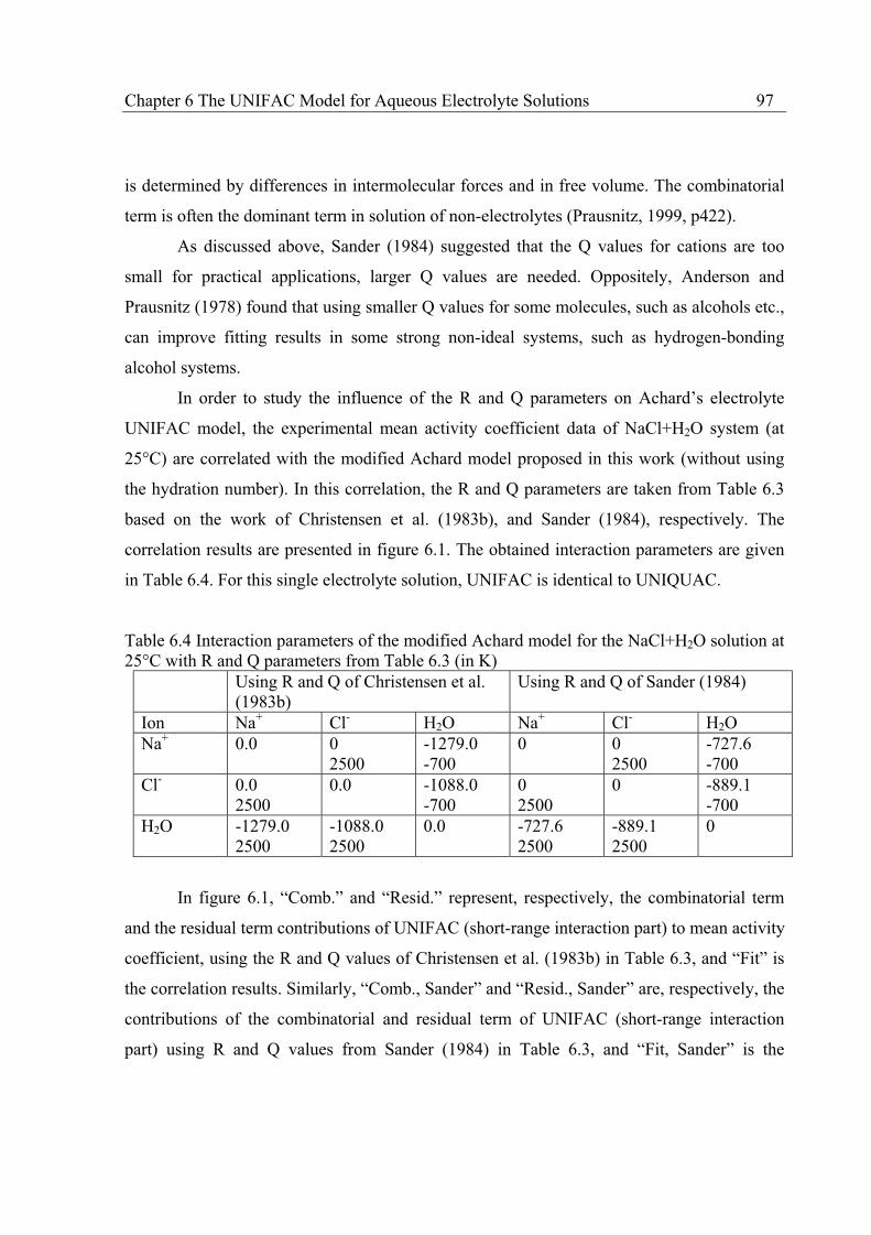
Chapter 6 The UNIFAC Model for Aqueous Electrolyte Solutions 97
is determined by differences in intermolecular forces and in free volume. The combinatorial
term is often the dominant term in solution of non-electrolytes (Prausnitz, 1999, p422).
As discussed above, Sander (1984) suggested that the Q values for cations are too
small for practical applications, larger Q values are needed. Oppositely, Anderson and
Prausnitz (1978) found that using smaller Q values for some molecules, such as alcohols etc.,
can improve fitting results in some strong non-ideal systems, such as hydrogen-bonding
alcohol systems.
In order to study the influence of the R and Q parameters on Achard’s electrolyte
UNIFAC model, the experimental mean activity coefficient data of NaCl+H2O system (at
25°C) are correlated with the modified Achard model proposed in this work (without using
the hydration number). In this correlation, the R and Q parameters are taken from Table 6.3
based on the work of Christensen et al. (1983b), and Sander (1984), respectively. The
correlation results are presented in figure 6.1. The obtained interaction parameters are given
in Table 6.4. For this single electrolyte solution, UNIFAC is identical to UNIQUAC.
Table 6.4 Interaction parameters of the modified Achard model for the NaCl+H2O solution at 25°C with R and Q parameters from Table 6.3 (in K)
Using R and Q of Christensen et al. (1983b)
Using R and Q of Sander (1984)
Ion Na+ Cl- H2O Na+ Cl- H2O Na+ 0.0 0
2500 -1279.0 -700
0 0 2500
-727.6 -700
Cl- 0.0 2500
0.0 -1088.0 -700
0 2500
0 -889.1 -700
H2O -1279.0 2500
-1088.0 2500
0.0 -727.6 2500
-889.1 2500
0
In figure 6.1, “Comb.” and “Resid.” represent, respectively, the combinatorial term
and the residual term contributions of UNIFAC (short-range interaction part) to mean activity
coefficient, using the R and Q values of Christensen et al. (1983b) in Table 6.3, and “Fit” is
the correlation results. Similarly, “Comb., Sander” and “Resid., Sander” are, respectively, the
contributions of the combinatorial and residual term of UNIFAC (short-range interaction
part) using R and Q values from Sander (1984) in Table 6.3, and “Fit, Sander” is the
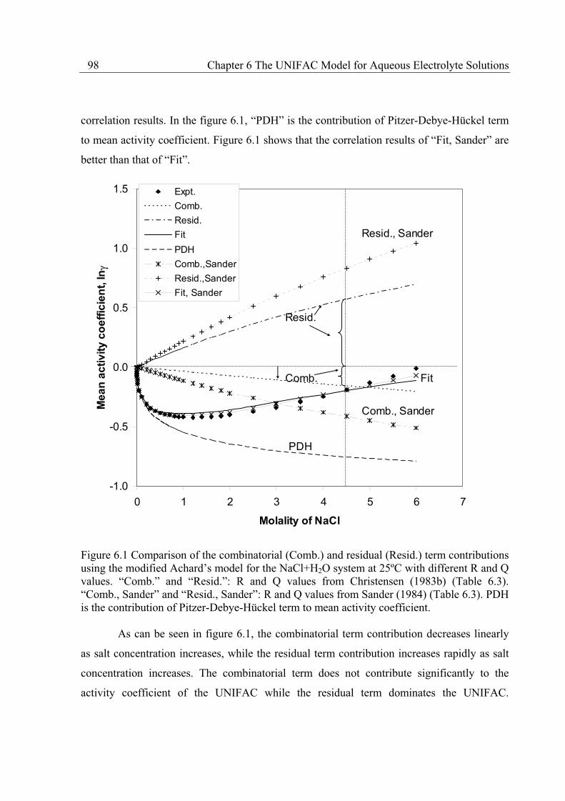
98 Chapter 6 The UNIFAC Model for Aqueous Electrolyte Solutions
correlation results. In the figure 6.1, “PDH” is the contribution of Pitzer-Debye-Hückel term
to mean activity coefficient. Figure 6.1 shows that the correlation results of “Fit, Sander” are
better than that of “Fit”.
-1.0
-0.5
0.0
0.5
1.0
1.5
0 1 2 3 4 5 6 7
Molality of NaCl
Me
an
ac
tiv
ity
co
eff
icie
nt,
ln
Expt.
Comb.
Resid.
Fit
PDH
Comb.,Sander
Resid.,Sander
Fit, Sander
Resid.
Comb.
PDH
Fit
Comb., Sander
Resid., Sander
Figure 6.1 Comparison of the combinatorial (Comb.) and residual (Resid.) term contributions using the modified Achard’s model for the NaCl+H2O system at 25ºC with different R and Q values. “Comb.” and “Resid.”: R and Q values from Christensen (1983b) (Table 6.3). “Comb., Sander” and “Resid., Sander”: R and Q values from Sander (1984) (Table 6.3). PDH is the contribution of Pitzer-Debye-Hückel term to mean activity coefficient.
As can be seen in figure 6.1, the combinatorial term contribution decreases linearly
as salt concentration increases, while the residual term contribution increases rapidly as salt
concentration increases. The combinatorial term does not contribute significantly to the
activity coefficient of the UNIFAC while the residual term dominates the UNIFAC.
Chapter 6 The UNIFAC Model for Aqueous Electrolyte Solutions 99
However, the combinatorial term of UNIFAC (or UNIQUAC) equation is often the dominant
term in non-electrolytes solutions (Prausnitz, 1999, p422). The PDH term dominates the
mean activity coefficient at dilute concentration range and has an almost constant
contribution at high concentrations.
Compare to the experimental curve in figure 6.1, the PDH term has a large negative
contribution to the mean activity coefficient, and cannot capture the mean activity coefficient
behaviour at high concentrations in which the short-range interaction has to be account for.
The UNIFAC is used to account for the short-range interaction and correct the large negative
contribution of PDH term to mean activity coefficient. At high concentration, the residual
term of UNIFAC corrects the negative contribution of PDH, but the combinatorial term of
UNIFAC increases the negative contribution of PDH. If the combinatorial term has lager
contribution than that of PDH term at high concentrations, the residual term will compete
with combinatorial term other than PDH term with increasing concentration. Because the
PDH term contribution is almost a constant, it does not reflect the changing of molecular
forces with increasing concentration of electrolytes. At high concentrations, the short-range
term should dominate the behaviour of activity coefficient model. Figure 6.1 shows that
using larger Q values in UNIFAC (Sander’s method) modifies the combinatorial term
contribution, then, improves the correlation results in this system. The Q parameter has a key
role in the model.
In UNIQUAC and UNIFAC models, the Q and R parameters are calculated from pure
component property and are used to describe molecule size and shape. Based on Sander’s
work, the Q parameter is very important to UNIQUAC fro electrolytes. However, the ratio
Q/R is the measure of the shape of molecules, not Q or R. Thus, it is necessary to further
investigate the limitations of these parameters from the physical derivation of UNIQUAC
(Abrams and Prausnitz, 1975, Maurer and Prausnitz, 1978).
Physical Interpretation of the Q/R ratio of ions
As can be seen from Table 6.3, the ratio Q/R as reported by several researchers
(Christensen, 1983b, Achard et al., 1994a, b) is greater than 1 for most R and Q values. The
work of Thomsen et al. (1999) represented an exception. However, based on the physical
100 Chapter 6 The UNIFAC Model for Aqueous Electrolyte Solutions
derivation of UNIQUAC model (Abrams and Prausnitz, 1975, Maurer and Prausnitz, 1978),
the Q/R>1.0 cannot be valid for UNIQUAC, because it does not follow the ‘physical’ upper
limit of Q/R=1 for the combinatorial entropy of mixing (and therefore Gibbs energy) in
UNQUAC.
The ratio Q/R is a measure of the shape of long-chain molecules, and was originally
applied to flexible chain molecules that differ significantly in size by Flory and Huggins.
Several researchers have investigated the effects of the ratio Q/R (Prausnitz et al., 1999,
p423, Donohue and Prausnitz, 1975). For a monomer, Q/R= 1. As R becomes very large for a
linear chain, Q/R 2/3 and for a sphere (or cube), Q/R 0. For globular molecules, the ratio
Q/R lies between zero and unity. Flory-Huggins assumed that Q/R=1.0, it gives an upper
limit for the combinatorial entropy of mixing, the Q/R=1 is the highest value of Q/R. The
combinatorial term (Staverman’s formula) of UNIQUAC (UNIFAC) is not exact but similar
to that of Flory-Huggins (Kikic et al., 1990). When Q/R>1 is used in UNQUAC (or
UNIFAC), the combinatorial term of the model is not physically correct.
Current R and Q parameters of UNIFAC and UNIQUAC follow Q/R<1 except for the
groups H2O, OH, HCOOH and FCH2O which are adjusted empirically to obtain better
agreement. In aqueous solutions, simple ions with hydrated water molecules can be
approximated as globular particles, and thus we would expect Q/R<1.
As mentioned above, Anderson et al. (1978) modified the Q parameter in UNIQUAC
to get better fitting results for systems containing hydrogen-bonding components, such as
water or lower alcohols. However, in this work, the Q/R is less than 1.0 for alcohols. Strong
molecular interactions do not change the Q/R ratio.
In order to keep the ‘physical’ upper limit, Q/R=1, for the combinatorial term in
UNIQUAC (UNIFAC), a new method is proposed to calculate the R and Q parameters for
ions.
6.4.3 A New Estimation Method for the Structural Parameters of Ions
Following the R and Q parameter calculation method for UNIQUAC model (Abrams
and Prausnitz, 1975, reproduced in Appendix C), the volume (Vi) and surface area (Ai) of an
ion i can be approximated by its radius (ri) as follows:

Chapter 6 The UNIFAC Model for Aqueous Electrolyte Solutions 101
3 3
4ii rV (6.39)
2 4 ii rA (6.40)
The Ri and Qi of the ion are calculated as following:
s
ii
V
VR (6.41)
s
ii
A
AQ (6.42)
where Vs and As are, respectively, the volume and surface area of a standard segment, which
are computed based on the radius (rs) of the standard segment. Applying the condition Q/R<
1.0, we have
0.1/
/
i
s
si
si
i
i
r
r
VV
AA
R
Q (6.43)
This equation suggests that the radius of a standard segment should be smaller than that of a
charged ion, rs< ri. For hydrocarbon fluids, the standard segment methylene group (-CH2-) is
indeed the smallest of all hydrocarbon groups, and has a radius of 1.818Å (Abrams and
Prausnitz, 1975).
However, if we compare the radius of this standard segment, 1.818Å, with the radii of
charged ions in crystals, as shown in Table 6.5, we see that the radius of the standard
segment (-CH2-) is larger than those of most ions, especially of the cations. In the work of
Christensen (1983b) and Sander (1984), the R and Q parameters are based on the value
1.818Å as the radius of a standard segment. Therefore, in the work of Christensen (1983b)
and etc., the obtained R and Q yield a Q/R ratio greater than 1, as shown in Table 6.3.
Table 6.5 Comparison of the ionic radii in crystal with the radius of -CH2-*
Ion/group -CH2- Na+ K+ Ca2+ Cl- Br-
Radius, Å 1.818 1.02 1.38 1.00 1.81 1.96
*Ionic radii are from CRC Handbook (Lide, 2002)

102 Chapter 6 The UNIFAC Model for Aqueous Electrolyte Solutions
If we follow the ‘physical’ limit for the R and Q parameters, a smaller radius for the
standard segment should be used in the R and Q calculation for ions, assuming that the R and
Q parameters of ions in aqueous solution could be approximated by the ionic radii in crystal.
Using the same method as Abrams and Prausnitz (1975), the radius of a standard
segment can be derived using a specific reference fluid.
The standard segment is defined as a sphere such that for a linear poly-segment
molecule of infinite length the identity
12
RQRZ
(6.44)
is satisfied. The coordination number Z is set equal to 10. The volume of the standard sphere
in terms of its radius rs is given by
3 3
4ss rV (6.45)
and the area by
2 4 ss rA (6.46)
The volume and area of an n-mer poly-segment molecule are n times the volume and
area of a reference molecule (ref);
refi nVV (6.47)
refi nAA (6.48)
Substitution of equations (6.41)-(6.42), (6.45)-(6.48) into (6.44) as n tends to infinity yields
the following equations:
12
10
s
ref
s
ref
s
ref
V
nV
A
nA
V
nV (6.49)
or
nV
V
A
A
V
V
s
ref
s
ref
s
ref 15 (6.50)
As n , 01
n and we obtain
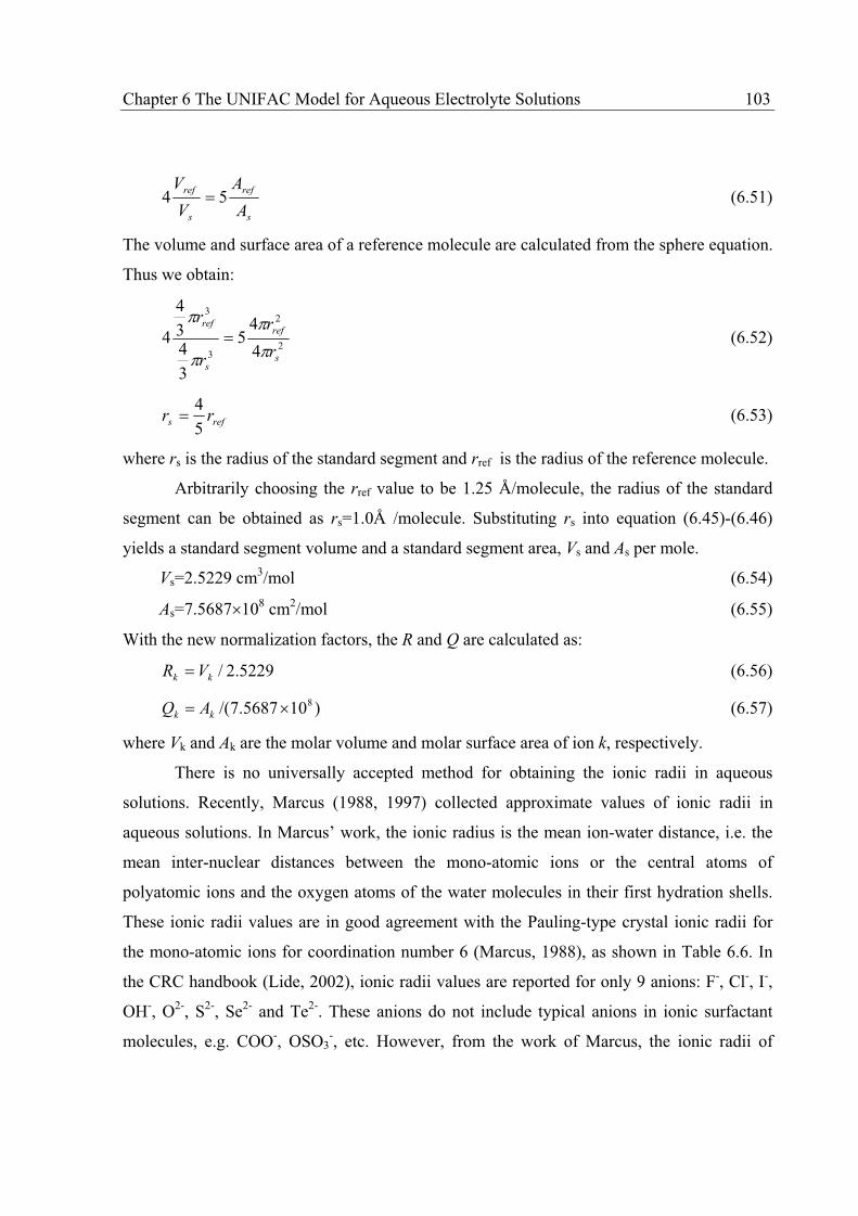
Chapter 6 The UNIFAC Model for Aqueous Electrolyte Solutions 103
s
ref
s
ref
A
A
V
V54 (6.51)
The volume and surface area of a reference molecule are calculated from the sphere equation.
Thus we obtain:
2
2
3
3
4
45
3
43
4
4s
ref
s
ref
r
r
r
r
(6.52)
refs rr5
4 (6.53)
where rs is the radius of the standard segment and rref is the radius of the reference molecule.
Arbitrarily choosing the rref value to be 1.25 Å/molecule, the radius of the standard
segment can be obtained as rs=1.0Å /molecule. Substituting rs into equation (6.45)-(6.46)
yields a standard segment volume and a standard segment area, Vs and As per mole.
Vs=2.5229 cm3/mol (6.54)
As=7.5687 108 cm2/mol (6.55)
With the new normalization factors, the R and Q are calculated as:
5229.2/kk VR (6.56)
)105687.7/( 8kk AQ (6.57)
where Vk and Ak are the molar volume and molar surface area of ion k, respectively.
There is no universally accepted method for obtaining the ionic radii in aqueous
solutions. Recently, Marcus (1988, 1997) collected approximate values of ionic radii in
aqueous solutions. In Marcus’ work, the ionic radius is the mean ion-water distance, i.e. the
mean inter-nuclear distances between the mono-atomic ions or the central atoms of
polyatomic ions and the oxygen atoms of the water molecules in their first hydration shells.
These ionic radii values are in good agreement with the Pauling-type crystal ionic radii for
the mono-atomic ions for coordination number 6 (Marcus, 1988), as shown in Table 6.6. In
the CRC handbook (Lide, 2002), ionic radii values are reported for only 9 anions: F-, Cl-, I-,
OH-, O2-, S2-, Se2- and Te2-. These anions do not include typical anions in ionic surfactant
molecules, e.g. COO-, OSO3-, etc. However, from the work of Marcus, the ionic radii of
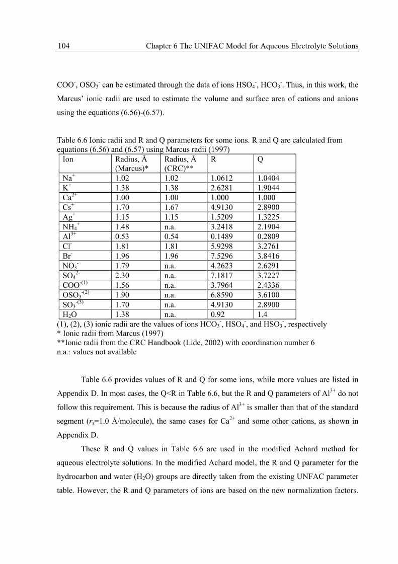
104 Chapter 6 The UNIFAC Model for Aqueous Electrolyte Solutions
COO-, OSO3- can be estimated through the data of ions HSO4
-, HCO3-. Thus, in this work, the
Marcus’ ionic radii are used to estimate the volume and surface area of cations and anions
using the equations (6.56)-(6.57).
Table 6.6 Ionic radii and R and Q parameters for some ions. R and Q are calculated from equations (6.56) and (6.57) using Marcus radii (1997)
Ion Radius, Å (Marcus)*
Radius, Å (CRC)**
R Q
Na+ 1.02 1.02 1.0612 1.0404 K+ 1.38 1.38 2.6281 1.9044 Ca2+ 1.00 1.00 1.000 1.000 Cs+ 1.70 1.67 4.9130 2.8900 Ag+ 1.15 1.15 1.5209 1.3225 NH4
+ 1.48 n.a. 3.2418 2.1904 Al3+ 0.53 0.54 0.1489 0.2809 Cl- 1.81 1.81 5.9298 3.2761 Br- 1.96 1.96 7.5296 3.8416 NO3
- 1.79 n.a. 4.2623 2.6291 SO4
2- 2.30 n.a. 7.1817 3.7227 COO-(1) 1.56 n.a. 3.7964 2.4336 OSO3
-(2) 1.90 n.a. 6.8590 3.6100 SO3
-(3) 1.70 n.a. 4.9130 2.8900 H2O 1.38 n.a. 0.92 1.4
(1), (2), (3) ionic radii are the values of ions HCO3-, HSO4
-, and HSO3-, respectively
* Ionic radii from Marcus (1997) **Ionic radii from the CRC Handbook (Lide, 2002) with coordination number 6 n.a.: values not available
Table 6.6 provides values of R and Q for some ions, while more values are listed in
Appendix D. In most cases, the Q<R in Table 6.6, but the R and Q parameters of Al3+ do not
follow this requirement. This is because the radius of Al3+ is smaller than that of the standard
segment (rs=1.0 Å/molecule), the same cases for Ca2+ and some other cations, as shown in
Appendix D.
These R and Q values in Table 6.6 are used in the modified Achard method for
aqueous electrolyte solutions. In the modified Achard model, the R and Q parameter for the
hydrocarbon and water (H2O) groups are directly taken from the existing UNFAC parameter
table. However, the R and Q parameters of ions are based on the new normalization factors.
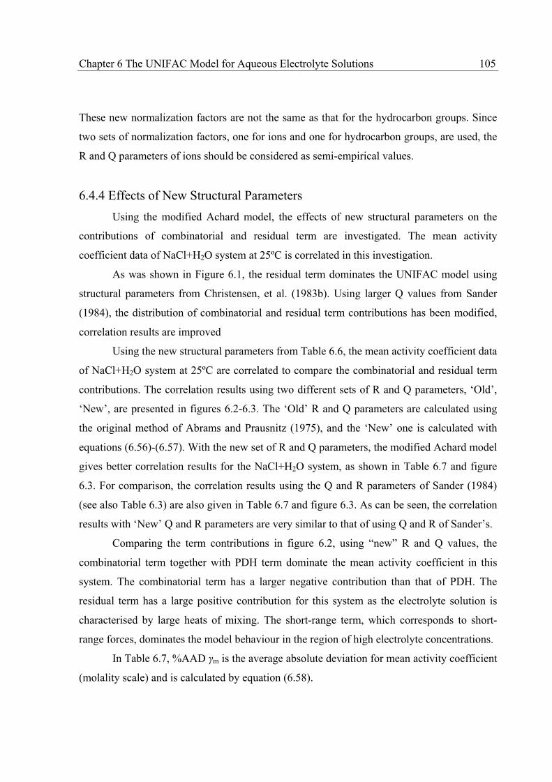
Chapter 6 The UNIFAC Model for Aqueous Electrolyte Solutions 105
These new normalization factors are not the same as that for the hydrocarbon groups. Since
two sets of normalization factors, one for ions and one for hydrocarbon groups, are used, the
R and Q parameters of ions should be considered as semi-empirical values.
6.4.4 Effects of New Structural Parameters
Using the modified Achard model, the effects of new structural parameters on the
contributions of combinatorial and residual term are investigated. The mean activity
coefficient data of NaCl+H2O system at 25ºC is correlated in this investigation.
As was shown in Figure 6.1, the residual term dominates the UNIFAC model using
structural parameters from Christensen, et al. (1983b). Using larger Q values from Sander
(1984), the distribution of combinatorial and residual term contributions has been modified,
correlation results are improved
Using the new structural parameters from Table 6.6, the mean activity coefficient data
of NaCl+H2O system at 25ºC are correlated to compare the combinatorial and residual term
contributions. The correlation results using two different sets of R and Q parameters, ‘Old’,
‘New’, are presented in figures 6.2-6.3. The ‘Old’ R and Q parameters are calculated using
the original method of Abrams and Prausnitz (1975), and the ‘New’ one is calculated with
equations (6.56)-(6.57). With the new set of R and Q parameters, the modified Achard model
gives better correlation results for the NaCl+H2O system, as shown in Table 6.7 and figure
6.3. For comparison, the correlation results using the Q and R parameters of Sander (1984)
(see also Table 6.3) are also given in Table 6.7 and figure 6.3. As can be seen, the correlation
results with ‘New’ Q and R parameters are very similar to that of using Q and R of Sander’s.
Comparing the term contributions in figure 6.2, using “new” R and Q values, the
combinatorial term together with PDH term dominate the mean activity coefficient in this
system. The combinatorial term has a larger negative contribution than that of PDH. The
residual term has a large positive contribution for this system as the electrolyte solution is
characterised by large heats of mixing. The short-range term, which corresponds to short-
range forces, dominates the model behaviour in the region of high electrolyte concentrations.
In Table 6.7, %AAD m is the average absolute deviation for mean activity coefficient
(molality scale) and is calculated by equation (6.58).

106 Chapter 6 The UNIFAC Model for Aqueous Electrolyte Solutions
1001
AAD%1
exp
exp
m
n
it
i
t
i
cal
i
n (6.58)
where n is the number of data points.
-4.0
-3.0
-2.0
-1.0
0.0
1.0
2.0
3.0
4.0
0 1 2 3 4 5 6 7
Molality of NaCl
Me
an
ac
tiv
ity
co
eff
., ln
Comb., New R & Q
Resid., new R & Q
PDH
Resid., old R & Q
Comb., old R & Q
Fit
Figure 6.2 Comparison of combinatorial (Comb.) and residual (Resid.) term contributions of UNIFAC using the modified Achard’s model for NaCl+H2O system at 25ºC. “New R & Q” and “Old R & Q”: see Table 6.7. : Experimental data. “Fit”: fitting results. PDH is the contribution of Pitzer-Debye-Hückel term to mean activity coefficient.
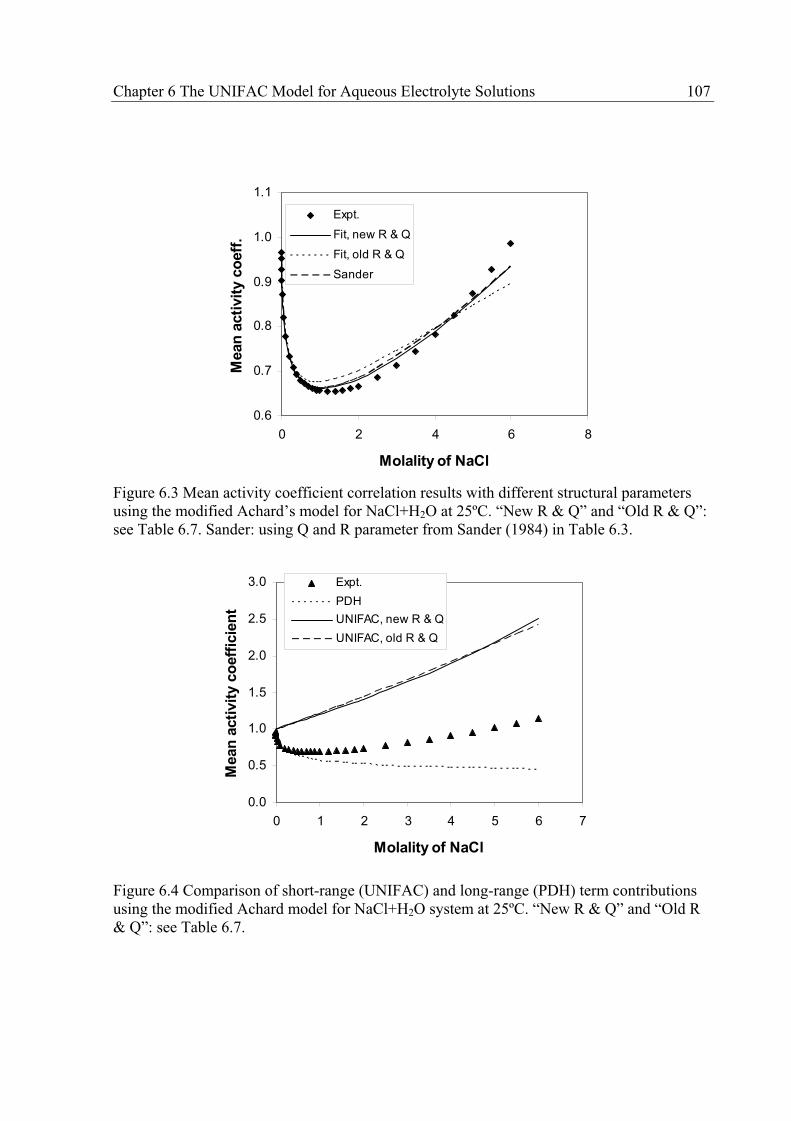
Chapter 6 The UNIFAC Model for Aqueous Electrolyte Solutions 107
0.6
0.7
0.8
0.9
1.0
1.1
0 2 4 6 8
Molality of NaCl
Mean
acti
vit
y c
oeff
.
Expt.
Fit, new R & Q
Fit, old R & Q
Sander
Figure 6.3 Mean activity coefficient correlation results with different structural parameters using the modified Achard’s model for NaCl+H2O at 25ºC. “New R & Q” and “Old R & Q”: see Table 6.7. Sander: using Q and R parameter from Sander (1984) in Table 6.3.
0.0
0.5
1.0
1.5
2.0
2.5
3.0
0 1 2 3 4 5 6 7
Molality of NaCl
Mean
acti
vit
y c
oeff
icie
nt
Expt.
PDH
UNIFAC, new R & Q
UNIFAC, old R & Q
Figure 6.4 Comparison of short-range (UNIFAC) and long-range (PDH) term contributions using the modified Achard model for NaCl+H2O system at 25ºC. “New R & Q” and “Old R & Q”: see Table 6.7.

108 Chapter 6 The UNIFAC Model for Aqueous Electrolyte Solutions
Table 6.7 Regression results for the NaCl+H2O solution at 25°C using different R and Q parameters New R & Q from
Table 6.6 Old R & Q from
Christensen in Table 6.3 R & Q from Sander in Table 6.3
Ion R Q R Q R Q Na+ 1.0612 1.0404 0.1426 0.2732 3.0 3.0 Cl- 5.9298 3.2761 0.9861 0.9917 0.9861 0.9917 Interaction parameter
uNa+,H2O= 1145.8 uCl-,H2O= 975.9
uNa+,H2O= 1279 uCl-,H2O= 1088
uNa+,H2O= 727.6 uCl-,H2O= 889.1
%AAD m 1.08 3.22 1.65
Short-range and Long-range Contributions
The excess Gibbs energy of electrolyte solutions consists of both short-range and
long-range contributions. The long-range contribution dominates in the dilute concentration
region. The short-range contribution becomes important at high concentrations. In figure 6.4,
a comparison of the short-range (UNIFAC) contribution and long-range (PDH) contribution
is shown using the modified Achard’s model for the NaCl+H2O system at 25ºC. The short-
range contribution increases almost linearly as ionic strength increases, while the long-range
contribution decreases rapidly in the very dilute region and then tends to a constant value at
high ionic strength.
In the short-range (UNIFAC) contribution calculation, the “new” and “old” R and Q
parameters are, respectively, used. As can be seen in figure 6.4, different R and Q parameters
do not significant change the short-range contribution, but the distribution of the
combinatorial and residual term contributions (shown in figure 6.2).
6.5 Application of the Modified Achard Method to Solutions of Single Electrolytes 6.5.1 Correlation of Mean Activity Coefficient Data
The modified Achard method as described previously is used to correlate the mean
activity coefficient data of single electrolyte systems. The objective function used is:
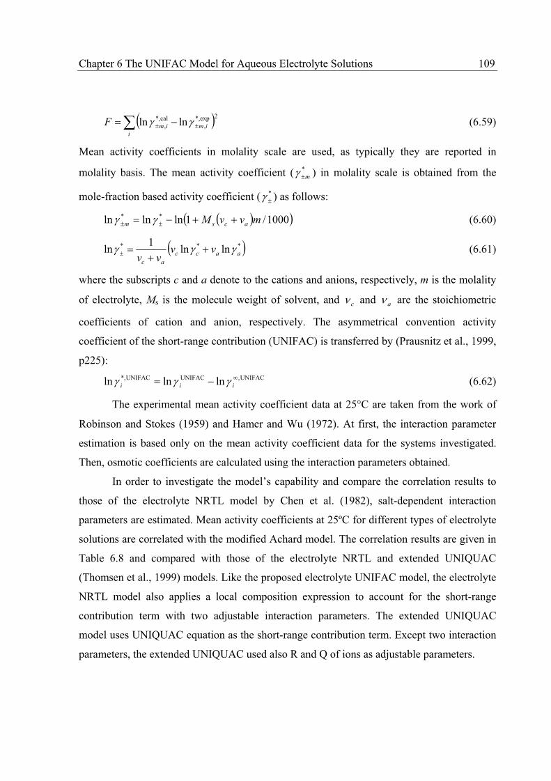
Chapter 6 The UNIFAC Model for Aqueous Electrolyte Solutions 109
2exp*,,
cal*,, lnln
i
imimF (6.59)
Mean activity coefficients in molality scale are used, as typically they are reported in
molality basis. The mean activity coefficient ( *m ) in molality scale is obtained from the
mole-fraction based activity coefficient ( * ) as follows:
1000/1lnlnln ** mvvM acsm (6.60)
*** lnln1
ln aacc
ac
vvvv
(6.61)
where the subscripts c and a denote to the cations and anions, respectively, m is the molality
of electrolyte, Ms is the molecule weight of solvent, and c and a are the stoichiometric
coefficients of cation and anion, respectively. The asymmetrical convention activity
coefficient of the short-range contribution (UNIFAC) is transferred by (Prausnitz et al., 1999,
p225):
UNIFAC,UNIFACUNIFAC*, lnlnln iii (6.62)
The experimental mean activity coefficient data at 25 C are taken from the work of
Robinson and Stokes (1959) and Hamer and Wu (1972). At first, the interaction parameter
estimation is based only on the mean activity coefficient data for the systems investigated.
Then, osmotic coefficients are calculated using the interaction parameters obtained.
In order to investigate the model’s capability and compare the correlation results to
those of the electrolyte NRTL model by Chen et al. (1982), salt-dependent interaction
parameters are estimated. Mean activity coefficients at 25ºC for different types of electrolyte
solutions are correlated with the modified Achard model. The correlation results are given in
Table 6.8 and compared with those of the electrolyte NRTL and extended UNIQUAC
(Thomsen et al., 1999) models. Like the proposed electrolyte UNIFAC model, the electrolyte
NRTL model also applies a local composition expression to account for the short-range
contribution term with two adjustable interaction parameters. The extended UNIQUAC
model uses UNIQUAC equation as the short-range contribution term. Except two interaction
parameters, the extended UNIQUAC used also R and Q of ions as adjustable parameters.
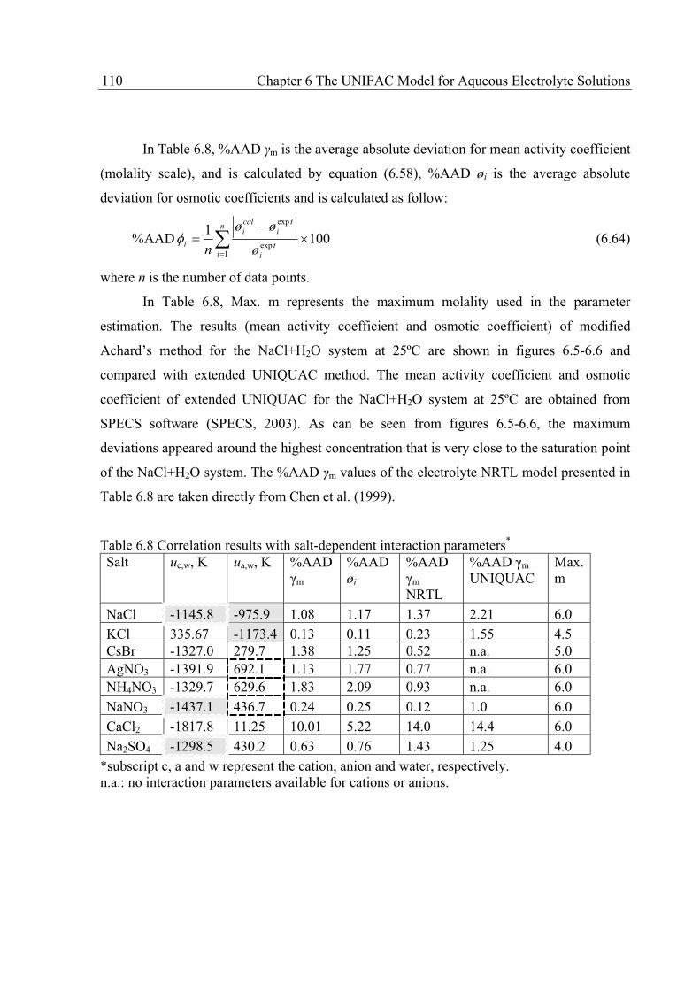
110 Chapter 6 The UNIFAC Model for Aqueous Electrolyte Solutions
In Table 6.8, %AAD m is the average absolute deviation for mean activity coefficient
(molality scale), and is calculated by equation (6.58), %AAD øi is the average absolute
deviation for osmotic coefficients and is calculated as follow:
1001
AAD%1
exp
expn
it
i
t
i
cal
i
iø
øø
n (6.64)
where n is the number of data points.
In Table 6.8, Max. m represents the maximum molality used in the parameter
estimation. The results (mean activity coefficient and osmotic coefficient) of modified
Achard’s method for the NaCl+H2O system at 25ºC are shown in figures 6.5-6.6 and
compared with extended UNIQUAC method. The mean activity coefficient and osmotic
coefficient of extended UNIQUAC for the NaCl+H2O system at 25ºC are obtained from
SPECS software (SPECS, 2003). As can be seen from figures 6.5-6.6, the maximum
deviations appeared around the highest concentration that is very close to the saturation point
of the NaCl+H2O system. The %AAD m values of the electrolyte NRTL model presented in
Table 6.8 are taken directly from Chen et al. (1999).
Table 6.8 Correlation results with salt-dependent interaction parameters* Salt uc,w, K
ua,w, K
%AAD m
%AAD øi
%AAD m
NRTL
%AAD m UNIQUAC
Max. m
NaCl -1145.8 -975.9 1.08 1.17 1.37 2.21 6.0
KCl 335.67 -1173.4 0.13 0.11 0.23 1.55 4.5 CsBr -1327.0 279.7 1.38 1.25 0.52 n.a. 5.0 AgNO3 -1391.9 692.1 1.13 1.77 0.77 n.a. 6.0 NH4NO3 -1329.7 629.6 1.83 2.09 0.93 n.a. 6.0
NaNO3 -1437.1 436.7 0.24 0.25 0.12 1.0 6.0
CaCl2 -1817.8 11.25 10.01 5.22 14.0 14.4 6.0
Na2SO4 -1298.5 430.2 0.63 0.76 1.43 1.25 4.0
*subscript c, a and w represent the cation, anion and water, respectively. n.a.: no interaction parameters available for cations or anions.
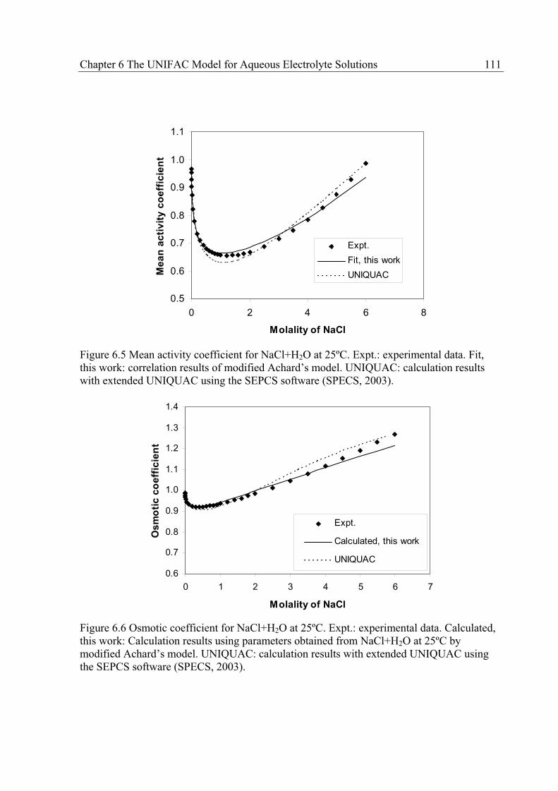
Chapter 6 The UNIFAC Model for Aqueous Electrolyte Solutions 111
0.5
0.6
0.7
0.8
0.9
1.0
1.1
0 2 4 6 8
Molality of NaCl
Me
an
ac
tiv
ity
co
eff
icie
nt
Expt.
Fit, this work
UNIQUAC
Figure 6.5 Mean activity coefficient for NaCl+H2O at 25ºC. Expt.: experimental data. Fit, this work: correlation results of modified Achard’s model. UNIQUAC: calculation results with extended UNIQUAC using the SEPCS software (SPECS, 2003).
0.6
0.7
0.8
0.9
1.0
1.1
1.2
1.3
1.4
0 1 2 3 4 5 6 7
Molality of NaCl
Os
mo
tic
co
eff
icie
nt
Expt.
Calculated, this work
UNIQUAC
Figure 6.6 Osmotic coefficient for NaCl+H2O at 25ºC. Expt.: experimental data. Calculated, this work: Calculation results using parameters obtained from NaCl+H2O at 25ºC by modified Achard’s model. UNIQUAC: calculation results with extended UNIQUAC using the SEPCS software (SPECS, 2003).

112 Chapter 6 The UNIFAC Model for Aqueous Electrolyte Solutions
The correlation results of Table 6.8 show that the mean activity coefficients of single
aqueous electrolyte solutions are successfully correlated with the modified Achard model
using two salt-dependent interaction parameters. The deviations of the correlation have the
same order as electrolyte NRTL model and smaller than that of extended UNIQUAC.
However, the extended UNIQUAC gives better results around saturation points, as shown in
figures 6.5 and 6.6. It was the purpose of the extended UNIQUAC to simulate electrolyte
solutions around saturation points (Thomsen et al., 1996, 1997, 1999).
The salt-dependent interaction parameters have some patterns, as shown in Table 6.8 the
highlight parts. The interaction parameters between Na+ and H2O (uNaH2O) have similar
values in different electrolyte solutions, i.e. NaCl+H2O, NaNO3+H2O and Na2SO4+H2O
where these values are -1145.82, -1437.08 and -1298.46 K, respectively. The interaction
parameters between NO3- and H2O are also close each other in the solutions AgNO3+H2O,
NH4NO3+H2O and NaNO3+H2O. However, the interaction parameter between Cl- and H2O in
CaCl2+H2O system is very different from other systems containing H2O and Cl- (NaCl+H2O,
KCl+H2O). In fact, the model cannot successfully correlate the mean activity coefficient of
the CaCl2+H2O system in which a particularly large non-ideality appears at the high
concentration range. Electrolyte NRTL and extended UNIQUAC exhibit the same as the
modified Achard model for CaCl2+H2O system. From these parameter similarities, it seems
that it is possible to use the assumption of group independence (group contribution concept)
for the ions interaction. Following the group contribution concept of the UNIFAC method, it
can be assumed that the interaction parameters between the ionic groups and the water group
do not depend on the electrolyte solutions. This means the interaction parameter between Na+
and H2O does not depend on the system NaCl+H2O or NaNO3+H2O system, but is merely
ion-dependent. The ions can be treated as separate UNIFAC functional groups. Based on the
group contribution concept, the Na+ H2O, Cl- H2O group interaction parameters obtained
from the NaCl+H2O solution are employed to the other electrolyte solutions.
Starting from the NaCl+H2O solution, the interaction parameters of different ions-water
are estimated. The mean activity coefficient data (25°C) of single electrolyte solutions are
used in the interaction parameter estimation with the modified Achard model. The results are
presented in Table 6.9.
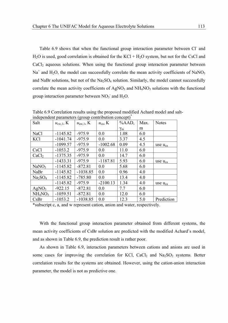
Chapter 6 The UNIFAC Model for Aqueous Electrolyte Solutions 113
Table 6.9 shows that when the functional group interaction parameter between Cl- and
H2O is used, good correlation is obtained for the KCl + H2O system, but not for the CsCl and
CaCl2 aqueous solutions. When using the functional group interaction parameter between
Na+ and H2O, the model can successfully correlate the mean activity coefficients of NaNO3
and NaBr solutions, but not of the Na2SO4 solution. Similarly, the model cannot successfully
correlate the mean activity coefficients of AgNO3 and NH4NO3 solutions with the functional
group interaction parameter between NO3- and H2O.
Table 6.9 Correlation results using the proposed modified Achard model and salt-independent parameters (group contribution concept)* Salt ucw,1, K uaw,1, K uca, K %AAD,
m Max. m
Notes
NaCl -1145.82 -975.9 0.0 1.08 6.0 KCl -1041.74 -975.9 0.0 3.37 4.5 -1099.57 -975.9 -1002.68 0.09 4.5 use uca CsCl -1053.2 -975.9 0.0 11.0 6.0 CaCl2 -1375.35 -975.9 0.0 14.7 6.0 -1433.31 -975.9 -1187.81 5.93 6.0 use uca NaNO3 -1145.82 -872.81 0.0 5.68 6.0 NaBr -1145.82 -1038.85 0.0 0.96 4.0 Na2SO4 -1145.82 -785.80 0.0 13.4 4.0 -1145.82 -975.9 -2100.13 1.34 4.0 use uca AgNO3 -922.15 -872.81 0.0 7.7 6.0 NH4NO3 -1059.51 -872.81 0.0 12.0 6.0 CsBr -1053.2 -1038.85 0.0 12.3 5.0 Prediction *subscript c, a, and w represent cation, anion and water, respectively.
With the functional group interaction parameter obtained from different systems, the
mean activity coefficients of CsBr solution are predicted with the modified Achard’s model,
and as shown in Table 6.9, the prediction result is rather poor.
As shown in Table 6.9, interaction parameters between cations and anions are used in
some cases for improving the correlation for KCl, CaCl2 and Na2SO2 systems. Better
correlation results for the systems are obtained. However, using the cation-anion interaction
parameter, the model is not as predictive one.
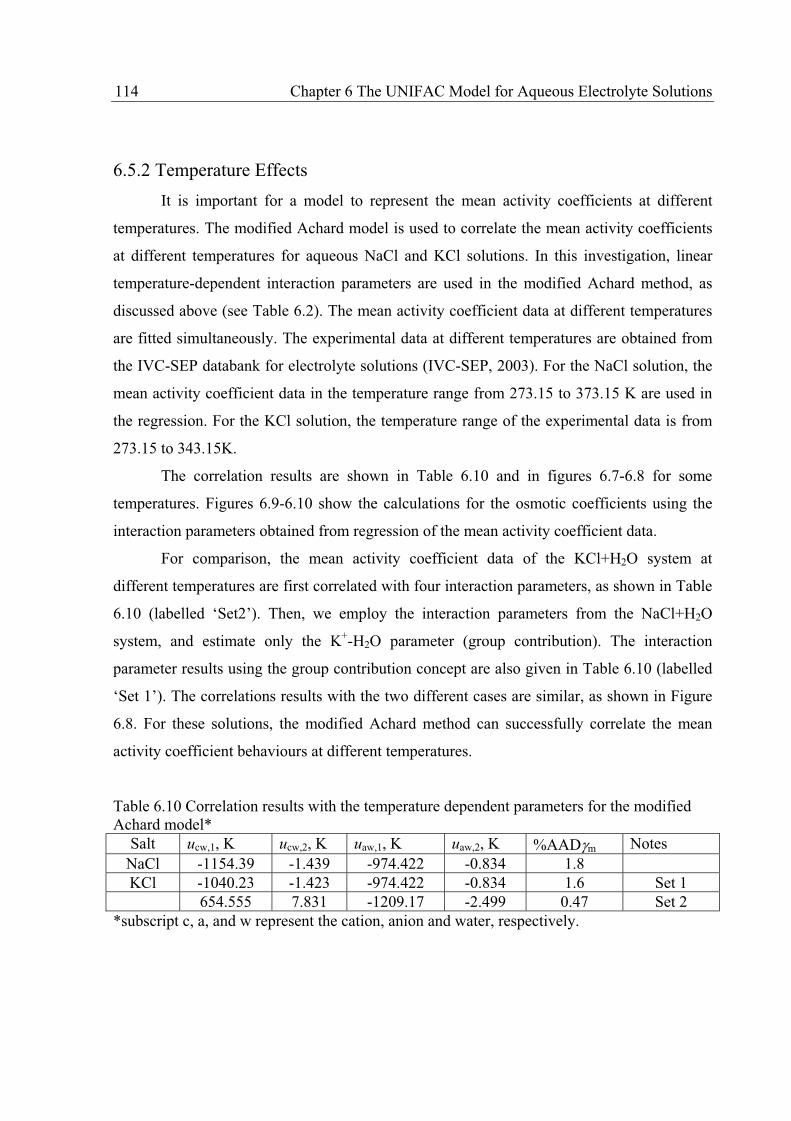
114 Chapter 6 The UNIFAC Model for Aqueous Electrolyte Solutions
6.5.2 Temperature Effects
It is important for a model to represent the mean activity coefficients at different
temperatures. The modified Achard model is used to correlate the mean activity coefficients
at different temperatures for aqueous NaCl and KCl solutions. In this investigation, linear
temperature-dependent interaction parameters are used in the modified Achard method, as
discussed above (see Table 6.2). The mean activity coefficient data at different temperatures
are fitted simultaneously. The experimental data at different temperatures are obtained from
the IVC-SEP databank for electrolyte solutions (IVC-SEP, 2003). For the NaCl solution, the
mean activity coefficient data in the temperature range from 273.15 to 373.15 K are used in
the regression. For the KCl solution, the temperature range of the experimental data is from
273.15 to 343.15K.
The correlation results are shown in Table 6.10 and in figures 6.7-6.8 for some
temperatures. Figures 6.9-6.10 show the calculations for the osmotic coefficients using the
interaction parameters obtained from regression of the mean activity coefficient data.
For comparison, the mean activity coefficient data of the KCl+H2O system at
different temperatures are first correlated with four interaction parameters, as shown in Table
6.10 (labelled ‘Set2’). Then, we employ the interaction parameters from the NaCl+H2O
system, and estimate only the K+-H2O parameter (group contribution). The interaction
parameter results using the group contribution concept are also given in Table 6.10 (labelled
‘Set 1’). The correlations results with the two different cases are similar, as shown in Figure
6.8. For these solutions, the modified Achard method can successfully correlate the mean
activity coefficient behaviours at different temperatures.
Table 6.10 Correlation results with the temperature dependent parameters for the modified Achard model*
Salt ucw,1, K ucw,2, K uaw,1, K uaw,2, K %AAD m Notes NaCl -1154.39 -1.439 -974.422 -0.834 1.8 KCl -1040.23 -1.423 -974.422 -0.834 1.6 Set 1
654.555 7.831 -1209.17 -2.499 0.47 Set 2 *subscript c, a, and w represent the cation, anion and water, respectively.
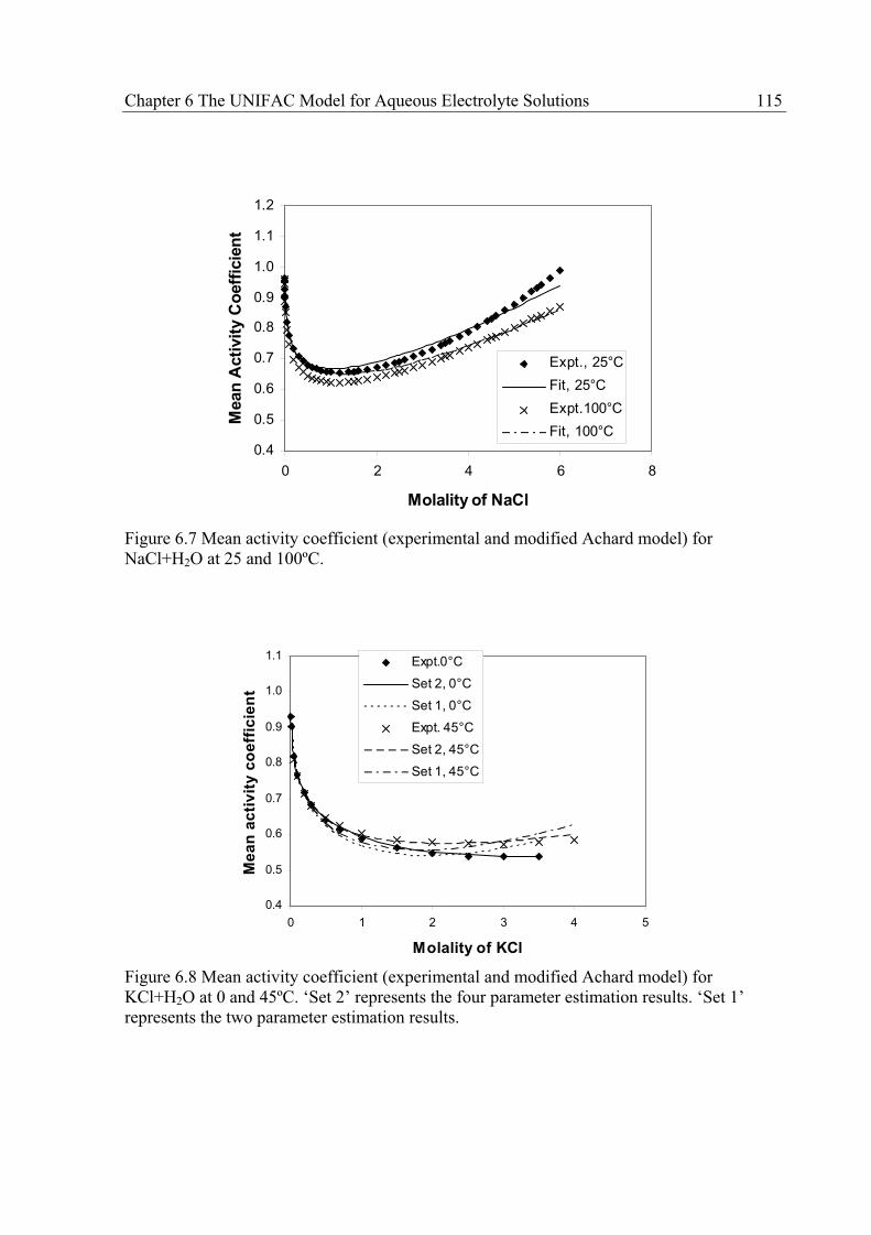
Chapter 6 The UNIFAC Model for Aqueous Electrolyte Solutions 115
0.4
0.5
0.6
0.7
0.8
0.9
1.0
1.1
1.2
0 2 4 6 8
Molality of NaCl
Mean
Acti
vit
y C
oeff
icie
nt
Expt., 25°C
Fit, 25°C
Expt.100°C
Fit, 100°C
Figure 6.7 Mean activity coefficient (experimental and modified Achard model) for NaCl+H2O at 25 and 100ºC.
0.4
0.5
0.6
0.7
0.8
0.9
1.0
1.1
0 1 2 3 4 5
Molality of KCl
Me
an
ac
tiv
ity
co
eff
icie
nt
Expt.0°C
Set 2, 0°C
Set 1, 0°C
Expt. 45°C
Set 2, 45°C
Set 1, 45°C
Figure 6.8 Mean activity coefficient (experimental and modified Achard model) for KCl+H2O at 0 and 45ºC. ‘Set 2’ represents the four parameter estimation results. ‘Set 1’ represents the two parameter estimation results.
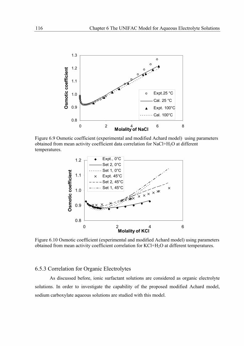
116 Chapter 6 The UNIFAC Model for Aqueous Electrolyte Solutions
0.8
0.9
1.0
1.1
1.2
1.3
0 2 4 6 8Molality of NaCl
Osm
oti
c c
oeff
icie
nt
Expt.25 °C
Cal. 25 °C
Expt. 100°C
Cal. 100°C
Figure 6.9 Osmotic coefficient (experimental and modified Achard model) using parameters obtained from mean activity coefficient data correlation for NaCl+H2O at different temperatures.
0.8
0.9
1.0
1.1
1.2
0 2 4 6Molality of KCl
Osm
oti
c c
oeff
icie
nt
Expt., 0°C
Set 2, 0°C
Set 1, 0°C
Expt. 45°C
Set 2, 45°C
Set 1, 45°C
Figure 6.10 Osmotic coefficient (experimental and modified Achard model) using parameters obtained from mean activity coefficient correlation for KCl+H2O at different temperatures.
6.5.3 Correlation for Organic Electrolytes
As discussed before, ionic surfactant solutions are considered as organic electrolyte
solutions. In order to investigate the capability of the proposed modified Achard model,
sodium carboxylate aqueous solutions are studied with this model.
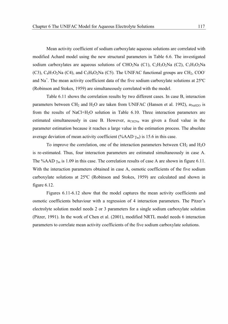
Chapter 6 The UNIFAC Model for Aqueous Electrolyte Solutions 117
Mean activity coefficient of sodium carboxylate aqueous solutions are correlated with
modified Achard model using the new structural parameters in Table 6.6. The investigated
sodium carboxylates are aqueous solutions of CHO2Na (C1), C2H3O2Na (C2), C3H5O2Na
(C3), C4H7O2Na (C4), and C5H9O2Na (C5). The UNIFAC functional groups are CH2, COO-
and Na+. The mean activity coefficient data of the five sodium carboxylate solutions at 25ºC
(Robinson and Stokes, 1959) are simultaneously correlated with the model.
Table 6.11 shows the correlation results by two different cases. In case B, interaction
parameters between CH2 and H2O are taken from UNIFAC (Hansen et al. 1992), uNaH2O is
from the results of NaCl+H2O solution in Table 6.10. Three interaction parameters are
estimated simultaneously in case B. However, uCH2Na was given a fixed value in the
parameter estimation because it reaches a large value in the estimation process. The absolute
average deviation of mean activity coefficient (%AAD m) is 15.6 in this case.
To improve the correlation, one of the interaction parameters between CH2 and H2O
is re-estimated. Thus, four interaction parameters are estimated simultaneously in case A.
The %AAD m is 1.09 in this case. The correlation results of case A are shown in figure 6.11.
With the interaction parameters obtained in case A, osmotic coefficients of the five sodium
carboxylate solutions at 25ºC (Robinson and Stokes, 1959) are calculated and shown in
figure 6.12.
Figures 6.11-6.12 show that the model captures the mean activity coefficients and
osmotic coefficients behaviour with a regression of 4 interaction parameters. The Pitzer’s
electrolyte solution model needs 2 or 3 parameters for a single sodium carboxylate solution
(Pitzer, 1991). In the work of Chen et al. (2001), modified NRTL model needs 6 interaction
parameters to correlate mean activity coefficients of the five sodium carboxylate solutions.

118 Chapter 6 The UNIFAC Model for Aqueous Electrolyte Solutions
0.4
0.6
0.8
1.0
1.2
1.4
1.6
0 1 2 3 4
Molality of sodium carboxylates
Mean
acti
vit
y c
oeff
icie
nt
Expt. C1
Cal. C1
Expt. C2
Cal. C2
Expt. C3
Cal. C3
Expt. C4
Cal. C4
Expt. C5
Cal. C5
Figure 6.11 Mean activity coefficient (experimental and modified Achard model) for five sodium carboxylate solutions at 25ºC. Correlation results of case A of Table 6.11.
0.7
0.8
0.9
1.0
1.1
1.2
1.3
1.4
0 1 2 3 4
Molality of sodium carboxylates
osm
oti
c c
oeff
icie
nt
Expt. C1
Cal. C1
Expt. C2
Cal. C2
Expt. C3
Cal. C3
Expt. C4
Cal. C4
Expt. C5
Cal. C5
Figure 6.12 Osmotic coefficient (experimental and modified Achard model) for five sodium carboxylate solutions at 25ºC. Calculation results of case A of Table 6.11
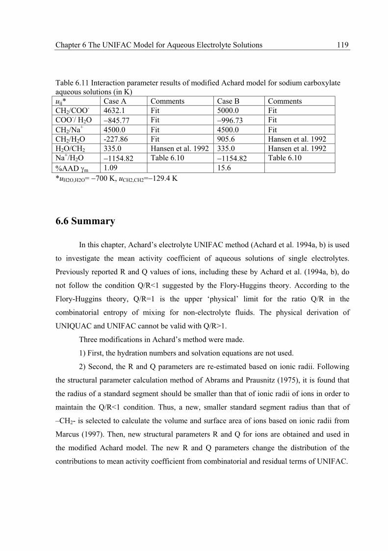
Chapter 6 The UNIFAC Model for Aqueous Electrolyte Solutions 119
Table 6.11 Interaction parameter results of modified Achard model for sodium carboxylate aqueous solutions (in K) uij* Case A Comments Case B Comments CH2/COO- 4632.1 Fit 5000.0 Fit COO-/ H2O 845.77 Fit 996.73 Fit CH2/Na+ 4500.0 Fit 4500.0 Fit CH2/H2O -227.86 Fit 905.6 Hansen et al. 1992 H2O/CH2 335.0 Hansen et al. 1992 335.0 Hansen et al. 1992 Na+/H2O 1154.82 Table 6.10 1154.82 Table 6.10
%AAD m 1.09 15.6
*uH2O,H2O= 700 K, uCH2,CH2= 129.4 K
6.6 Summary
In this chapter, Achard’s electrolyte UNIFAC method (Achard et al. 1994a, b) is used
to investigate the mean activity coefficient of aqueous solutions of single electrolytes.
Previously reported R and Q values of ions, including these by Achard et al. (1994a, b), do
not follow the condition Q/R<1 suggested by the Flory-Huggins theory. According to the
Flory-Huggins theory, Q/R=1 is the upper ‘physical’ limit for the ratio Q/R in the
combinatorial entropy of mixing for non-electrolyte fluids. The physical derivation of
UNIQUAC and UNIFAC cannot be valid with Q/R>1.
Three modifications in Achard’s method were made.
1) First, the hydration numbers and solvation equations are not used.
2) Second, the R and Q parameters are re-estimated based on ionic radii. Following
the structural parameter calculation method of Abrams and Prausnitz (1975), it is found that
the radius of a standard segment should be smaller than that of ionic radii of ions in order to
maintain the Q/R<1 condition. Thus, a new, smaller standard segment radius than that of
–CH2- is selected to calculate the volume and surface area of ions based on ionic radii from
Marcus (1997). Then, new structural parameters R and Q for ions are obtained and used in
the modified Achard model. The new R and Q parameters change the distribution of the
contributions to mean activity coefficient from combinatorial and residual terms of UNIFAC.

120 Chapter 6 The UNIFAC Model for Aqueous Electrolyte Solutions
3) The third modification concerns the interaction parameters. Instead of using the
modified UNIFAC method of Larsen et al. (1987), the linear T-dependent UNIFAC method
of Hansen et al. (1992) is adopted in this work. All other assumptions on interaction
parameters from Achard’s model remain unchanged.
Using the proposed modified Achard model, mean activity coefficients of single
electrolyte solutions are calculated for several systems. Using two salt-dependent interaction
parameters, the model shows similar deviation to those of the electrolyte NRTL model, and
give better results than that of extended UNIQUAC model for the mean activity coefficients.
Using the UNIFAC group contribution concept, ions are treated as functional groups.
With the ionic functional groups, the mean activity coefficient data for some single
electrolyte solutions are correlated with the modified Achard model. For some systems, the
model can successfully correlate the mean activity coefficient data with the ions treated as
functional groups. Problems occur for other systems.
In addition, the model can capture the mean activity coefficient of some aqueous
solutions of single electrolytes at different temperatures.
The modified Achard model can simultaneously and successfully correlate the mean
activity coefficient data of five sodium carboxylate solutions at 25ºC using four interaction
parameters.

Chapter 7 Critical Micelle Concentration of Ionic Surfactant Solutions 121
Chapter 7 Critical Micelle Concentration of Ionic Surfactant Solutions
In this chapter, recent progress in modelling the micelle formation of ionic surfactant
solutions is first outlined. The modified Achard model is applied to study the CMC of ionic
surfactant solutions based on the thermodynamic framework of Chen et al. (2001) for micelle
formation. The CMC of four surfactant families, i.e. sodium alkyl sulphates, sodium alkyl
sulfonates, sodium carboxylates and potassium carboxylates, is investigated. CMC values of
sodium alkyl sulphates (AS) and alkyl trimethylammonium bromides (TAB) ternary
surfactant mixtures are calculated by regular solution method.
7.1 Recent Progress for Modelling Ionic Surfactant Solutions
Recently, Hines (2001) reviewed the progress for modelling surfactant solutions. The
understanding for such solution at a theoretical level is still poor. Douheret and Viallard
(1982) proposed a mass action law model with a two-parameter expression for the activity
coefficients of ionic species to represent the micelle formation in ionic surfactant solutions.
Based on a mass-action model with a single micellar aggregate species, Burchfield and
Woolley (1984) suggested an activity coefficient model for aqueous ionic surfactant
solutions. The micellar solution is treated as mixed electrolytes by using the Guggenheim
equation. Huibers et al. (1997) investigated the relationship between the molecular structure
and the CMC of anionic surfactants using a quantitative structure-property relationship
approach. A linear regression model is constructed for 119 anionic surfactants. Amos et al.
(1998) proposed a model incorporating the distribution of micellar size. The model of Amos
et al. is based on a mass-action equilibrium approach that includes micelle-micelle
interactions as a function of size for multi-component surfactant solutions consisting of
micellar aggregates, monomer, counterions, and electrolytes.
Li et al. (2000) use SAFT (statistical associating fluid theory), together with the mean
spherical approximation (MSA), to calculate the activity coefficients of aqueous ionic
surfactant solutions. In Li’s method, the monomeric surfactant ions are assumed to be in a
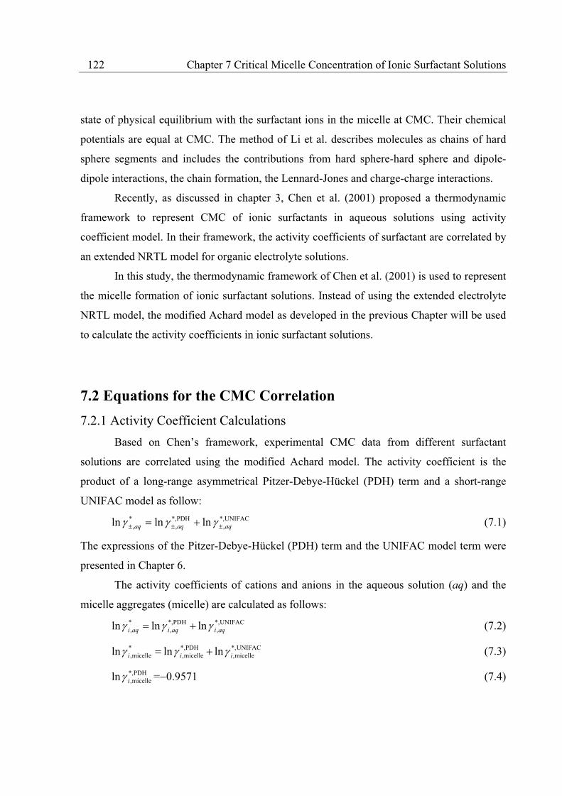
122 Chapter 7 Critical Micelle Concentration of Ionic Surfactant Solutions
state of physical equilibrium with the surfactant ions in the micelle at CMC. Their chemical
potentials are equal at CMC. The method of Li et al. describes molecules as chains of hard
sphere segments and includes the contributions from hard sphere-hard sphere and dipole-
dipole interactions, the chain formation, the Lennard-Jones and charge-charge interactions.
Recently, as discussed in chapter 3, Chen et al. (2001) proposed a thermodynamic
framework to represent CMC of ionic surfactants in aqueous solutions using activity
coefficient model. In their framework, the activity coefficients of surfactant are correlated by
an extended NRTL model for organic electrolyte solutions.
In this study, the thermodynamic framework of Chen et al. (2001) is used to represent
the micelle formation of ionic surfactant solutions. Instead of using the extended electrolyte
NRTL model, the modified Achard model as developed in the previous Chapter will be used
to calculate the activity coefficients in ionic surfactant solutions.
7.2 Equations for the CMC Correlation
7.2.1 Activity Coefficient Calculations
Based on Chen’s framework, experimental CMC data from different surfactant
solutions are correlated using the modified Achard model. The activity coefficient is the
product of a long-range asymmetrical Pitzer-Debye-Hückel (PDH) term and a short-range
UNIFAC model as follow:
UNIFAC*,,
PDH*,,
*, lnlnln aqaqaq (7.1)
The expressions of the Pitzer-Debye-Hückel (PDH) term and the UNIFAC model term were
presented in Chapter 6.
The activity coefficients of cations and anions in the aqueous solution (aq) and the
micelle aggregates (micelle) are calculated as follows:
UNIFAC*,,
PDH*,,
*, lnlnln aqiaqiaqi (7.2)
UNIFAC,*micelle,
PDH*,micelle,
*micelle, lnlnln iii (7.3)
PDH*,micelle,ln i = 0.9571 (7.4)

Chapter 7 Critical Micelle Concentration of Ionic Surfactant Solutions 123
UNIFAC,UNIFAC*,micelle, lnln ii (7.5)
where PDH*,micelle,ln i is set to 0.9571, which is the limiting value of the PDH term for univalent
ions as the electrolyte concentration approaches unity and UNIFAC,ln i is the infinite dilute
activity coefficient calculated by the UNIFAC model. The molality scale mean activity
coefficient ( *m ) is obtained from the mole fraction mean activity coefficient ( * ) by
equations (6.60)-(6.61) in Chapter 6. The asymmetrical activity coefficient of UNIFAC
model is calculated by equation (6.62) in Chapter 6.
7.2.2 Interaction Parameters
As discussed in Chapter 6, the interaction parameters (aij) between ions and other
groups of the modified Achard model depend on temperature as follows (Hansen et al.,
1992):
jjijijij uTTuua 02,1, (7.6)
For non-ionic groups, the interaction parameters are calculated by the original equation of
Hansen et al. (1992), i.e. equation (6.26) in Chapter 6.
For alkyl groups (CH3, CH2), ujj in equation (7.6) is calculated as:
wwwjjwjj uaau , T0=298.15 K (7.7)
where w refers to the water, uww= 700 K, ajw and awj are the interaction parameters between
water and hydrocarbon groups from Hansen et al. (1992). uww is computed only at 25ºC by
Achard et al. (1994b). The uCH2,CH2 interaction parameter at 25ºC is calculated from equation
(7.7) as follow:
K 4.129)700(0.3356.905H2OH2O,CH2H2O,H2OCH2,CH2CH2, uaau (7.8)
In the aqueous solution of sodium alkyl sulphates (CnH2n+1OSO3-Na+), for example,
there are groups H2O, CH3, CH2, and ions OSO3-, Na+. The interaction parameters between
these groups are summarized in Table 7.1. The groups CH3 and CH2 belong to the same
UNIFAC main functional group “CH2”.
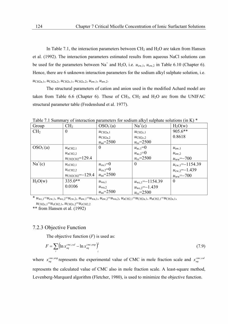
124 Chapter 7 Critical Micelle Concentration of Ionic Surfactant Solutions
In Table 7.1, the interaction parameters between CH2 and H2O are taken from Hansen
et al. (1992). The interaction parameters estimated results from aqueous NaCl solutions can
be used for the parameters between Na+ and H2O, i.e. ucw,1, ucw,2 in Table 6.10 (Chapter 6).
Hence, there are 6 unknown interaction parameters for the sodium alkyl sulphate solution, i.e.
uCH2a,1, uCH2a,2, uCH2c,1, uCH2c,2, uaw,1, uaw,2.
The structural parameters of cation and anion used in the modified Achard model are
taken from Table 6.6 (Chapter 6). Those of CH3, CH2 and H2O are from the UNIFAC
structural parameter table (Fredenslund et al. 1977).
Table 7.1 Summary of interaction parameters for sodium alkyl sulphate solutions (in K) * Group CH2 OSO3
-(a) Na+(c) H2O(w) CH2 0 uCH2a,1
uCH2a,2 uaa=2500
uCH2c,1 uCH2c,2 ucc=2500
905.6** 0.8618
OSO3-(a) uaCH2,1
uaCH2,2 uCH2CH2=129.4
0 uac,1=0 uac,2=0 ucc=2500
uaw,1 uaw,2 uww= 700
Na+(c) ucCH2,1 ucCH2,2 uCH2CH2= 129.4
uca,1=0 uca,2=0 uaa=2500
0 ucw,1= 1154.39 ucw,2= 1.439 uww= 700
H2O(w) 335.0** 0.0106
uwa,1 uwa,2 uaa=2500
uwc,1= 1154.39 uwc,2= 1.439 ucc=2500
0
* uwc,1=ucw,1, uwc,2=ucw,2, uaw,1=uwa,1, uaw,2=uwa,2, uaCH2,1=uCH2a,1, uaCH2,1=uCH2a,1, uCH2c,1=ucCH2,1, uCH2c,2=ucCH2,2 ** from Hansen et al. (1992)
7.2.3 Objective Function
The objective function (F) is used as:
2exp,, lnlnii
cmc
aq
calcmc
aq xxF (7.9)
where exp,cmc
aqx represents the experimental value of CMC in mole fraction scale and calcmc
aqx ,
represents the calculated value of CMC also in mole fraction scale. A least-square method,
Levenberg-Marquard algorithm (Fletcher, 1980), is used to minimize the objective function.

Chapter 7 Critical Micelle Concentration of Ionic Surfactant Solutions 125
The reported molality scale CMC values are converted to mole fractions. The critical
micelle concentration (CMC) data of Mukerjee et al. (1971) and Brandrup et al. (1975) are
used in the interaction parameter estimation.
7.3 CMC Correlation
7.3.1 CMC Correlation with the Modified Achard Model
The CMC of three surfactant families, sodium alkyl sulphates, sodium alkyl
sulfonates and potassium carboxylates, are studied with the modified Acahrd model. The
sodium alkyl sulphates, sodium alkyl sulfonates and potassium (sodium) carboxylates are,
respectively, abbreviated as CnOSO3Na, CnSO3Na and CnCOOK(Na), where Cn refers to
the carbon number of the alkyl chain. These surfactant solutions are widely used in practice
and extensively investigated in various applications. The group assignments for these
surfactant molecules are presented in Table 7.2. The structural parameters of the groups are
given in Table 7.3.
Table 7.2 Group assignments for surfactant molecules Surfactant family Abbreviation Group Assignment* Sodium alkyl sulphates CnOSO3Na CH3, CH2, Na+(c), OSO3
-(a) Sodium alkyl sulfonates CnSO3Na CH3, CH2, Na+(c), SO3
-(a) Potassium carboxylates CnCOOK CH3, CH2, K
+(c), COO-(a) Sodium carboxylates CnCOONa CH3, CH2, Na+(c), COO-(a) * c: cation, a: anion
Table 7.3 Structural parameter values Group R Q Comments CH3 0.9011 0.848 CH2 0.6744 0.540 Na+ 1.0612 1.0404 K+ 2.6281 1.9044 OSO3
- 6.8590 3.6100 From HSO4- data
SO3- 4.9130 2.8900 From HSO3
- data COO- 3.7964 2.4336 From HCO3
- data H2O 0.92 1.40
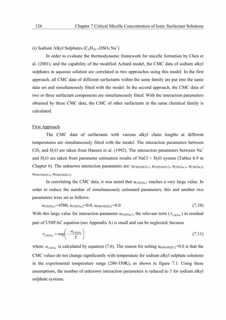
126 Chapter 7 Critical Micelle Concentration of Ionic Surfactant Solutions
(i) Sodium Alkyl Sulphates (CnH2n+1OSO3-Na+)
In order to evaluate the thermodynamic framework for micelle formation by Chen et
al. (2001), and the capability of the modified Achard model, the CMC data of sodium alkyl
sulphates in aqueous solution are correlated in two approaches using this model. In the first
approach, all CMC data of different surfactants within the same family are put into the same
data set and simultaneously fitted with the model. In the second approach, the CMC data of
two or three surfactant components are simultaneously fitted. With the interaction parameters
obtained by these CMC data, the CMC of other surfactants in the same chemical family is
calculated.
First Approach
The CMC data of surfactants with various alkyl chain lengths at different
temperatures are simultaneously fitted with the model. The interaction parameters between
CH2 and H2O are taken from Hansen et al. (1992). The interaction parameters between Na+
and H2O are taken from parameter estimation results of NaCl + H2O system (Tables 6.9 in
Chapter 6). The unknown interaction parameters are: uCH2OSO3,1, uCH2OSO3,2, uCH2Na,1, uCH2Na,2,
uOSO3H2O,1, uOSO3H2O,2.
In correlating the CMC data, it was noted that uCH2Na,1 reaches a very large value. In
order to reduce the number of simultaneously estimated parameters, this and another two
parameters were set as follows:
uCH2Na,1=4500, uCH2Na,2=0.0, uOSO3H2O,2=0.0 (7.10)
With this large value for interaction parameter uCH2Na,1, the relevant term ( CH2Na ) in residual
part of UNIFAC equation (see Appendix A) is small and can be neglected, because
T
aCH2NaCH2Na exp (7.11)
where CH2Naa is calculated by equation (7.6). The reason for setting uOSO3H2O,2=0.0 is that the
CMC values do not change significantly with temperature for sodium alkyl sulphate solutions
in the experimental temperature range (280-350K), as shown in figure 7.1. Using these
assumptions, the number of unknown interaction parameters is reduced to 3 for sodium alkyl
sulphate systems.

Chapter 7 Critical Micelle Concentration of Ionic Surfactant Solutions 127
All reported CMC data for sodium alkyl sulphates are simultaneously fitted. The solid
lines in Figure 7.1 and 7.2 show the fitting results. The parameter estimation results are given
Table 7.4. The results show that the thermodynamic expression of micelle formation
combined with the modified Achard method can describe satisfactorily both temperature and
chain length effects of CMC.
Table 7.4 Parameter estimation results (bold numbers) of two approaches for sodium alkyl sulphates (in K). All other parameters can be found in Table 7.1 CH2 OSO3
-(a) H2O OSO3-(a) CH2 Na+(c) Na+ H2O(w)
First approach
uaCH2,1= 46.29 uaCH2,2=1.449
uwa,1=556.19 uwa,2=0
uCH2c,1=4500* uCH2c,2=0
ucw,1= 1145.8 ucw,2=0
Second approach
uaCH2,1= 7.162 uaCH2,2=0.718
uwa,1=668.13 uwa,2=0
uCH2c,1=4500* uCH2c,2=0
ucw,1= 1154.39 ucw,2= 1.439
* fixed value
1.E-03
1.E-02
1.E-01
1.E+00
270 290 310 330 350 370
Temperature, K
CM
C, M
ola
lity
C8 fit
C10
C12
C14 fit
Figure 7.1 Results for C8OSO3Na (C8 fit), C10OSO3Na (C10), C12OSO3Na (C12), and C14OSO3Na(C14 fit) at different temperatures. Points: experimental CMC values. Solid lines: fitting results of first approach, dotted lines: fitting results of second approach, dashed lines: calculation results.
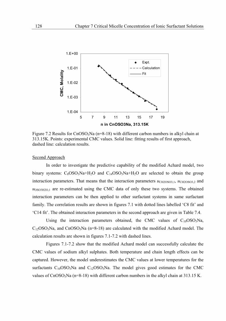
128 Chapter 7 Critical Micelle Concentration of Ionic Surfactant Solutions
1.E-04
1.E-03
1.E-02
1.E-01
1.E+00
5 7 9 11 13 15 17 19
n in CnOSO3Na, 313.15K
CM
C,
Mo
lali
tyExpt.
Calculation
Fit
Figure 7.2 Results for CnOSO3Na (n=8-18) with different carbon numbers in alkyl chain at 313.15K. Points: experimental CMC values. Solid line: fitting results of first approach, dashed line: calculation results.
Second Approach
In order to investigate the predictive capability of the modified Achard model, two
binary systems: C8OSO3Na+H2O and C14OSO3Na+H2O are selected to obtain the group
interaction parameters. That means that the interaction parameters uCH2OSO3,1, uCH2OSO3,2 and
uOSO3H2O,1 are re-estimated using the CMC data of only these two systems. The obtained
interaction parameters can be then applied to other surfactant systems in same surfactant
family. The correlation results are shown in figures 7.1 with dotted lines labelled ‘C8 fit’ and
‘C14 fit’. The obtained interaction parameters in the second approach are given in Table 7.4.
Using the interaction parameters obtained, the CMC values of C10OSO3Na,
C12OSO3Na, and CnOSO3Na (n=8-18) are calculated with the modified Achard model. The
calculation results are shown in figures 7.1-7.2 with dashed lines.
Figures 7.1-7.2 show that the modified Achard model can successfully calculate the
CMC values of sodium alkyl sulphates. Both temperature and chain length effects can be
captured. However, the model underestimates the CMC values at lower temperatures for the
surfactants C10OSO3Na and C12OSO3Na. The model gives good estimates for the CMC
values of CnOSO3Na (n=8-18) with different carbon numbers in the alkyl chain at 313.15 K.
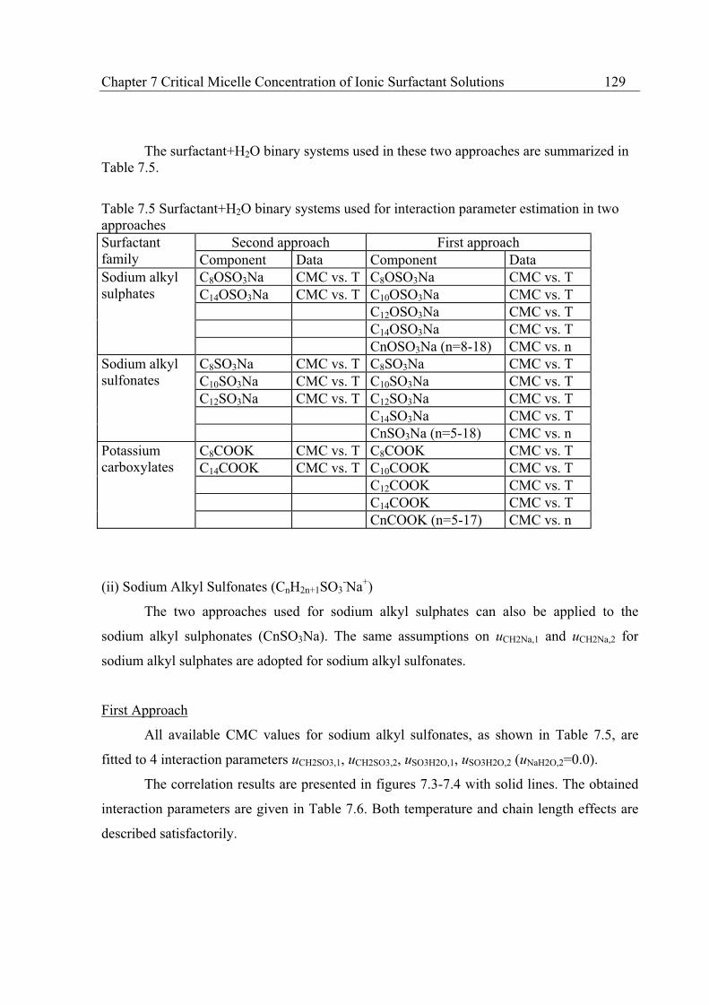
Chapter 7 Critical Micelle Concentration of Ionic Surfactant Solutions 129
The surfactant+H2O binary systems used in these two approaches are summarized in Table 7.5.
Table 7.5 Surfactant+H2O binary systems used for interaction parameter estimation in two approaches
Second approach First approach Surfactant family Component Data Component Data
C8OSO3Na CMC vs. T C8OSO3Na CMC vs. T C14OSO3Na CMC vs. T C10OSO3Na CMC vs. T C12OSO3Na CMC vs. T C14OSO3Na CMC vs. T
Sodium alkyl sulphates
CnOSO3Na (n=8-18) CMC vs. n C8SO3Na CMC vs. T C8SO3Na CMC vs. T C10SO3Na CMC vs. T C10SO3Na CMC vs. T C12SO3Na CMC vs. T C12SO3Na CMC vs. T C14SO3Na CMC vs. T
Sodium alkyl sulfonates
CnSO3Na (n=5-18) CMC vs. n C8COOK CMC vs. T C8COOK CMC vs. T C14COOK CMC vs. T C10COOK CMC vs. T C12COOK CMC vs. T C14COOK CMC vs. T
Potassium carboxylates
CnCOOK (n=5-17) CMC vs. n
(ii) Sodium Alkyl Sulfonates (CnH2n+1SO3-Na+)
The two approaches used for sodium alkyl sulphates can also be applied to the
sodium alkyl sulphonates (CnSO3Na). The same assumptions on uCH2Na,1 and uCH2Na,2 for
sodium alkyl sulphates are adopted for sodium alkyl sulfonates.
First Approach
All available CMC values for sodium alkyl sulfonates, as shown in Table 7.5, are
fitted to 4 interaction parameters uCH2SO3,1, uCH2SO3,2, uSO3H2O,1, uSO3H2O,2 (uNaH2O,2=0.0).
The correlation results are presented in figures 7.3-7.4 with solid lines. The obtained
interaction parameters are given in Table 7.6. Both temperature and chain length effects are
described satisfactorily.
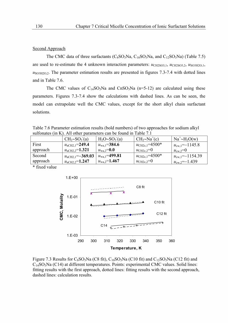
130 Chapter 7 Critical Micelle Concentration of Ionic Surfactant Solutions
Second Approach
The CMC data of three surfactants (C8SO3Na, C10SO3Na, and C12SO3Na) (Table 7.5)
are used to re-estimate the 4 unknown interaction parameters: uCH2SO3,1, uCH2SO3,2, uSO3H2O,1,
uSO3H2O,2. The parameter estimation results are presented in figures 7.3-7.4 with dotted lines
and in Table 7.6.
The CMC values of C14SO3Na and CnSO3Na (n=5-12) are calculated using these
parameters. Figures 7.3-7.4 show the calculations with dashed lines. As can be seen, the
model can extrapolate well the CMC values, except for the short alkyl chain surfactant
solutions.
Table 7.6 Parameter estimation results (bold numbers) of two approaches for sodium alkyl sulfonates (in K). All other parameters can be found in Table 7.1 CH2 SO3
-(a) H2O SO3-(a) CH2 Na+(c) Na+ H2O(w)
First approach
uaCH2,1=249.4 uaCH2,2=1.321
uwa,1=384.6 uwa,2=0.0
uCH2c,1=4500* uCH2c,2=0
ucw,1= 1145.8 ucw,2=0
Second approach
uaCH2,1= 369.03 uaCH2,2=1.247
uwa,1=499.81 uwa,2=1.467
uCH2c,1=4500* uCH2c,2=0
ucw,1= 1154.39 ucw,2= 1.439
* fixed value
1.E-03
1.E-02
1.E-01
1.E+00
290 300 310 320 330 340 350 360
Temperature, K
CM
C,
Mo
lali
ty
C8 fit
C10 fit
C12 fit
C14
Figure 7.3 Results for C8SO3Na (C8 fit), C10SO3Na (C10 fit) and C12SO3Na (C12 fit) and C14SO3Na (C14) at different temperatures. Points: experimental CMC values. Solid lines: fitting results with the first approach, dotted lines: fitting results with the second approach, dashed lines: calculation results.
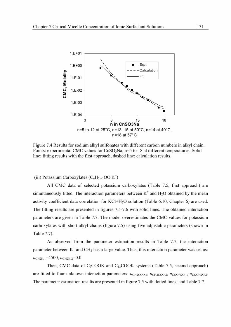
Chapter 7 Critical Micelle Concentration of Ionic Surfactant Solutions 131
1.E-04
1.E-03
1.E-02
1.E-01
1.E+00
1.E+01
3 8 13 18n in CnSO3Na
n=5 to 12 at 25°C, n=13, 15 at 50°C, n=14 at 40°C,
n=18 at 57°C
CM
C, M
ola
lity
Expt.
Calculation
Fit
Figure 7.4 Results for sodium alkyl sulfonates with different carbon numbers in alkyl chain. Points: experimental CMC values for CnSO3Na, n=5 to 18 at different temperatures. Solid line: fitting results with the first approach, dashed line: calculation results.
(iii) Potassium Carboxylates (CnH2n-1OO-K+)
All CMC data of selected potassium carboxylates (Table 7.5, first approach) are
simultaneously fitted. The interaction parameters between K+ and H2O obtained by the mean
activity coefficient data correlation for KCl+H2O solution (Table 6.10, Chapter 6) are used.
The fitting results are presented in figures 7.5-7.6 with solid lines. The obtained interaction
parameters are given in Table 7.7. The model overestimates the CMC values for potassium
carboxylates with short alkyl chains (figure 7.5) using five adjustable parameters (shown in
Table 7.7).
As observed from the parameter estimation results in Table 7.7, the interaction
parameter between K+ and CH2 has a large value. Thus, this interaction parameter was set as:
uCH2K,1=4500, uCH2K,2=0.0.
Then, CMC data of C7COOK and C13COOK systems (Table 7.5, second approach)
are fitted to four unknown interaction parameters: uCH2COO,1, uCH2COO,2, uCOOH2O,1, uCOOH2O,2.
The parameter estimation results are presented in figure 7.5 with dotted lines, and Table 7.7.

132 Chapter 7 Critical Micelle Concentration of Ionic Surfactant Solutions
Using the obtained interaction parameters, the CMC of C9COOK, C11COOK,
C15COOK, and CnCOOK (n=5-17) are calculated with the modified Achard method. The
calculations are shown in figures 7.5-7.6 with dashed lines. The model overestimates the
CMC of short alkyl chain potassium carboxylates.
Table 7.7 Parameter estimation results (bold numbers) of potassium carboxylates (in K). All other parameters can be found in Table 7.1 CH2 COO-(a) H2O COO-(a) CH2 K+(c) K+ H2O(w) First approach uaCH2,1= 176.47
uaCH2,2=15.35 uwa,1=289.56 uwa,2=8.962
uCH2c,1=3220 uCH2c,2=0
ucw,1= 654.555 ucw,2=7.831
Second approach
uaCH2,1= 91.75 uaCH2,2=5.846
uwa,1=420.83 uwa,2= 1.962
uCH2c,1=4500* uCH2c,2=0
ucw,1= 654.555 ucw,2=7.831
* fixed value
1.E-04
1.E-03
1.E-02
1.E-01
1.E+00
1.E+01
280 290 300 310 320 330 340 350
Temperature, K
CM
C, M
ola
lity
C7COOK
C9COOK C11COOK
C13COOK
C15COOK
Figure 7.5 Results for C7COOK, C9COOK, C11COOK, C13COOK and C15COOK at different temperatures. Points: experimental CMC values. Solid lines: fitting results with the first approach, dotted lines: fitting results with the second approach, dashed lines: calculation results.

Chapter 7 Critical Micelle Concentration of Ionic Surfactant Solutions 133
1.E-04
1.E-03
1.E-02
1.E-01
1.E+00
3 8 13 18
n in CnCOOK, 298.15K
CM
C, M
ola
lity
Expt.
Calculation
Fit
308.15K
328.15 K
Figure 7.6 Results for potassium carboxylates with different carbon numbers in alkyl chain. Points: experimental CMC values at 298.15 K. Solid line: fitting results with the first approach, dashed line: calculation results
7.3.2 Prediction of CMC for Sodium Carboxylates
With the interaction parameters obtained from the CMC data for potassium
carboxylates (CnCOOK) systems (Table 7.7) and the mean activity coefficient data
correlation for NaCl+H2O system (Table 6.10, Chapter 6), the CMC values of sodium
carboxylate (CnH2n-1COO-Na+, abbr. CnCOONa) solutions are predicted with the modified
Achard model, as shown in figure 7.7. As can be seen, the prediction results are rather poor.
But the prediction shows CMC increases with increasing temperature. The interaction
parameters used in the prediction are summarized in Table 7.8 labelled with ‘Pred.’. For
comparison, the CMC data of sodium carboxylates are also fitted with the modified Achard
model and presented in figure 7.7 and Table 7.8 labelled with ‘Fitting’.
As discussed in Chapter 6, the modified Achard method can simultaneously correlate
the mean activity coefficients of five short chain sodium carboxylate (CnCOONa, n=1-5)
solutions. The interaction parameters obtained for these sodium carboxylates can be used to
predict the CMC of long chain sodium carboxylates (CnCOONa, n=7-18) with the modified
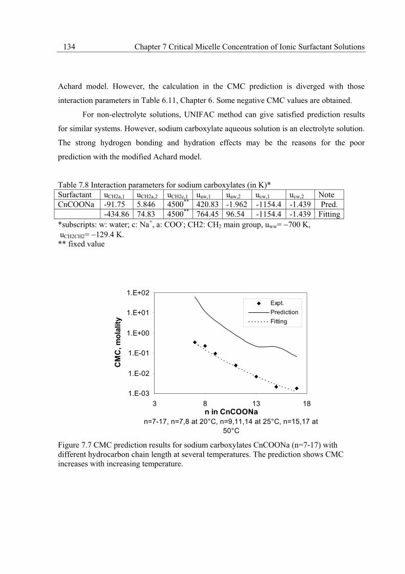
134 Chapter 7 Critical Micelle Concentration of Ionic Surfactant Solutions
Achard model. However, the calculation in the CMC prediction is diverged with those
interaction parameters in Table 6.11, Chapter 6. Some negative CMC values are obtained.
For non-electrolyte solutions, UNIFAC method can give satisfied prediction results
for similar systems. However, sodium carboxylate aqueous solution is an electrolyte solution.
The strong hydrogen bonding and hydration effects may be the reasons for the poor
prediction with the modified Achard model.
Table 7.8 Interaction parameters for sodium carboxylates (in K)* Surfactant uCH2a,1 uCH2a,2 uCH2c,1 uaw,1 uaw,2 ucw,1 ucw,2 Note CnCOONa -91.75 5.846 4500** 420.83 -1.962 -1154.4 -1.439 Pred. -434.86 74.83 4500** 764.45 96.54 -1154.4 -1.439 Fitting*subscripts: w: water; c: Na+, a: COO-; CH2: CH2 main group, uww= 700 K, uCH2CH2= 129.4 K. ** fixed value
1.E-03
1.E-02
1.E-01
1.E+00
1.E+01
1.E+02
3 8 13 18n in CnCOONa
n=7-17, n=7,8 at 20°C, n=9,11,14 at 25°C, n=15,17 at
50°C
CM
C, m
ola
lity
Expt.
Prediction
Fitting
Figure 7.7 CMC prediction results for sodium carboxylates CnCOONa (n=7-17) with different hydrocarbon chain length at several temperatures. The prediction shows CMC increases with increasing temperature.

Chapter 7 Critical Micelle Concentration of Ionic Surfactant Solutions 135
7.4 CMC Calculation of Surfactant Mixtures
As an example to use and evaluate regular solution method (Rubingh, 1979, Holland,
1986) discussed in Chapter 3, CMC of sodium alkyl sulphates (AS) and alkyl
trimethylammonium bromides (TAB) ternary surfactant mixtures were calculated in this
method based on the work of Murphy et al. (2002). This method is often applied to mixed
surfactant systems and treats the micelles or aggregates as a separated pseudo-phase. The
pseudo micelle phase is considered as non-ideal liquid mixtures. Regular solution method is
used to describe activity coefficient of surfactants in the non-ideal liquid mixtures (pseudo
micelle phase).
Extending equation (3.63) to ternary mixture of surfactants, CMC can be calculated
as:
33
3
22
2
11
1
mix CMCCMCCMCCMC
1 (7.12)
where CMCmix, CMC1, CMC2, CMC3 are the CMC values of the mixed surfactants,
surfactant 1, surfactant 2 and surfactant 3, respectively; 1, 2 and 3 are the mole fractions
of the respective surfactants in aqueous solution (aqueous phase) and 1, 2 and 3 are the
activity coefficients of surfactants 1, 2 and 3 in pseudo micelle phase. The activity
coefficients are calculated by:
RTxxxx /ln 322313122313
22121 (7.13)
RTxxxx /ln 311323122323
21122 (7.14)
RTxxxx /ln 211213232223
21133 (7.15)
where 12, 13 and 23 are the interaction parameters between surfactants 1 and 2, 1 and 3,
and 2 and 3, respectively, and they are obtained by fitting CMC of binary surfactant systems;
x1, x2 and x3 are the compositions of surfactants 1, 2 and 3 in pseudo micelle phase.
Based on these equations, CMC values of ternary surfactant mixtures are calculated
for cationic surfactants: octyl- (C8), decyl- (C10), dodecyl- (C12), tetradecyl- (C14) and
hexadecyl- (C16) trimethylammonium bromide (TAB), and anionc surfactants: sodium octyl-
(C8), decyl- (C10), dodecyl- (C12), tetradecyl- (C14) and hexadecyl- (C16) sulphates. The
interaction parameters between these surfactants are taken from Murphy et al. (2002). Based

136 Chapter 7 Critical Micelle Concentration of Ionic Surfactant Solutions
on the work of Murphy et al., compositions of surfactants 1, 2 and 3 in aqueous phase ( 1, 2
and 3) and pseudo micelle phase (x1, x2 and x3) are approximated as:
Aqueous phase composition: 3/1321
Pseudo micelle phase: 3/1321 xxx
because the three components in an experimental sample are very similar, as shown in Tables
7.9-7.10. If the compositions of surfactant in micelle phase are not available, a method
proposed by Holland (1986) can be used to calculate them.
By equations (7.12)-(7.15), CMC of ternary surfactant mixtures are calculated and
presented in Tables 7.9-7.10, and figure 7.8. In these tables, experimental CMC are from
conductivity measurements (Murphy et al. 2002). These results show that the regular solution
method can predict well the CMC of ternary surfactant mixture using experimental binary
interaction parameters. However, these calculations only show an ideal case because the
surfactant compositions in aqueous and micelle phase are equal for these ternary surfactant
systems through the special designed experiments in the work of Murphy et al. (2002).
Table 7.9 CMC calculation results using the regular solution method for alkyl trimethylammonium bromides at 303 K (Molality, 10-3)* Surfactants 1/2/3
CMC1 CMC2 CMC3 12 13 23 CMC, exp.
CMC, cal.
Dev.%
C12/C10/C8 16.03 48 290 -0.7 -1.4 -0.7 27.00 34.65 28.3 C14/C10/C8 3.08 48 290 -1.6 -2.4 -0.7 7.00 8.60 22.9 C16/C10C8 0.8 48 290 -3.1 -3.9 -0.7 1.90 2.36 24.0 C14/C12/C8 3.08 16.03 290 -0.8 -2.1 -2.7 6.77 7.69 13.6 C16/C12/C8 0.8 16.03 290 -3.3 -3.9 -2.9 1.89 2.28 20.7 C16/C14/C8 0.8 3.08 290 -1.0 -3.8 -2.4 1.83 1.90 4.0 C14/C12/C10 3.08 16.03 48 -0.9 -2.5 -0.8 6.80 7.36 8.2 C16/C12/C10 0.8 16.03 48 -3.2 -3.7 -0.6 1.70 2.25 32.4 C16/C14/C10 0.8 3.08 48 -0.9 -2.9 -2.1 1.90 1.88 1.0 Average Dev. 17.2 * experimental CMC, 12, 13 and 23: from Murphy et al. (2002)
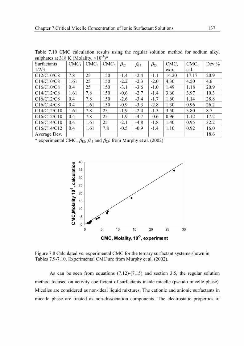
Chapter 7 Critical Micelle Concentration of Ionic Surfactant Solutions 137
Table 7.10 CMC calculation results using the regular solution method for sodium alkyl sulphates at 318 K (Molality, 10-3)* Surfactants 1/2/3
CMC1 CMC2 CMC3 12 13 23 CMC, exp.
CMC, cal.
Dev.%
C12/C10/C8 7.8 25 150 -1.4 -2.4 -1.1 14.20 17.17 20.9 C14/C10/C8 1.61 25 150 -2.2 -2.3 -2.0 4.30 4.50 4.6 C16/C10/C8 0.4 25 150 -3.1 -3.6 -1.0 1.49 1.18 20.9 C14/C12/C8 1.61 7.8 150 -0.6 -2.7 -1.4 3.60 3.97 10.3 C16/C12/C8 0.4 7.8 150 -2.6 -3.4 -1.7 1.60 1.14 28.8 C16/C14/C8 0.4 1.61 150 -0.9 -3.3 -2.8 1.30 0.96 26.2 C14/C12/C10 1.61 7.8 25 -1.9 -2.4 -1.3 3.50 3.80 8.7 C16/C12/C10 0.4 7.8 25 -1.9 -4.7 -0.6 0.96 1.12 17.2 C16/C14/C10 0.4 1.61 25 -2.1 -4.8 -1.8 1.40 0.95 32.2 C16/C14/C12 0.4 1.61 7.8 -0.5 -0.9 -1.4 1.10 0.92 16.0 Average Dev. 18.6 * experimental CMC, 12, 13 and 23: from Murphy et al. (2002)
0
5
10
15
20
25
30
35
40
0 5 10 15 20 25 30
CMC, Molality, 10-3
, experiment
CM
C,M
ola
lity
10-3
, calc
ula
tio
n
Figure 7.8 Calculated vs. experimental CMC for the ternary surfactant systems shown in Tables 7.9-7.10. Experimental CMC are from Murphy et al. (2002).
As can be seen from equations (7.12)-(7.15) and section 3.5, the regular solution
method focused on activity coefficient of surfactants inside micelle (pseudo micelle phase).
Micelles are considered as non-ideal liquid mixtures. The cationic and anionic surfactants in
micelle phase are treated as non-dissociation components. The electrostatic properties of

138 Chapter 7 Critical Micelle Concentration of Ionic Surfactant Solutions
ionic surfactants in aqueous and micelle phase are not taken into account, even the CMC of
mixed surfactants are obtained by conductive measurement (Murphy et al., 2002). In aqueous
phase, activity coefficients of surfactant are set to unity.
In sections 7.2 and 7.3, activity coefficients of surfactant in aqueous phase were
studied using modified Achard model. This model could be used to calculate the activity
coefficient in equation (7.12). However, in the framework of regular solution method for
mixed surfactants, ionic surfactants are treated as non-dissociated component. The necessary
interaction parameters of non-dissociated cations and anions are not available for the
modified Achard model. Therefore, the CMC of mixed surfactants are not calculated by the
modified Achard model. In aqueous phase, activity coefficient is set to 1.0 in the regular
solution method for mixed surfactants.
Using the modified Achard model, however, CMC of pure surfactants in aqueous
solution, such as sodium alkyl sulphates, can be extrapolate to different temperatures. Based
on the CMC of pure surfactants, the CMC of mixed surfactants at different temperatures can
be calculated using equation (7.12) if the binary interaction parameters of surfactants can be
used at different temperatures.
In principle, other activity coefficient model, such as UNQUAC and UNIFAC can be
used to calculate the activity coefficients of surfactant in micelle phase. But the necessary
interaction parameters of non-dissociated ionic surfactants or groups are not available for
these models.
7.5 Summary
Based on Chen’s thermodynamic treatment (Chen et al., 2001) for the micelle
formation of ionic surfactant solution, the modified Achard method can successfully correlate
the CMC values of three surfactant families. Using the CMC data of a few surfactant + H2O
systems (two or three systems), the group interaction parameters of the modified Achard
model are determined. Using these group interaction parameters, the modified Achard model
can calculate the CMC values of other ionic surfactants in the same surfactant family. The

Chapter 7 Critical Micelle Concentration of Ionic Surfactant Solutions 139
modified Achard model has some potential in predicting the CMC of ionic surfactant
solutions. However, the CMC prediction results for sodium carboxylates + H2O systems are
poor using the interaction parameters determined from potassium carboxylates+H2O systems
and NaCl+H2O system.
Using regular solution method (Rubingh, 1979, Holland, 1986), CMC values of alkyl
trimethylammonium bromides (at 303 K) and sodium alkyl sulphates (at 318 K) are predicted
successfully based on experimental binary interaction parameters reported by Murphy et al.
(2002).

140 Chapter 7 Critical Micelle Concentration of Ionic Surfactant Solutions
Chapter 8 Correlations for Important Properties of Surfactant Solutions 141
Chapter 8 Correlations of Important Properties of Surfactant Solutions
In this chapter, some correlations of important properties of surfactants and surfactant
solutions, e.g. the hydrophilic lipophilic balance (HLB), the Krafft point, the cloud point and
detergency are presented. Some new correlations for the aggregation number, the toxicity, the
bio-concentration factor and the HLB of specific surfactant families are developed in this
work. A calculation map of these properties is also presented.
8.1 Introduction
A number of properties are of interest to certain applications of surfactant solutions,
e.g. the cloud point, the Krafft point, the hydrophilic-lipophilic balance (HLB), the
aggregation number (ng), and the phase inversion temperature (PIT). They are often related to
emulsification and solubility, wetting, dispersing, foaming and detergency. Some of them, e.g.
HLB, have no solid thermo-physical origin, but are widely used in industrial applications.
These properties give a fast, less expensive and perhaps unique way to classify the abilities of
surfactants.
A lot of experimental investigations have been carried out for these important
properties. However, such data are scattered in many different journals and books and are
somewhat difficult to retrieve. van Os and co-workers (1993) have compiled many types of
physico-chemical properties for non-ionic, cationic and anionic surfactants during the period
1970-1991. Mukerjee and Mysels (1971) published a CMC data collection, and evaluated the
CMC values for hundreds of surfactants. Grieser and Drummond (1988) collected data on
micelle aggregation numbers. Hinz (1986) edited a thermodynamic data collection for
biochemistry and biotechnology which include a chapter on experimental data of surfactant
solutions.
142 Chapter 8 Correlations for Important Properties of Surfactant Solutions
Laughlin (1994) summarized the research history of surfactant solutions since the end
of the 19th century. In this book, different theoretical concepts are comprehensively
described and compared. The journal ‘Current Opinion in Colloid & Interface Science’
(Current Chemistry Ltd, London, UK) is now publishing review papers on different aspects
of surfactant solutions, including thermodynamic theories.
Empirical correlations are often of interest to engineers so that many important
properties of surfactant solutions can be estimated using one or two key properties (e.g. CMC,
Kow). The investigated properties in this chapter are HLB, Krafft point, cloud point,
aggregation number, detergency and toxicity.
In this study, many of the correlation results are directly collected from the literature.
Some new correlations have been also developed for certain surfactant families.
8.2 The Hydrophilic-Lipophilic Balance (HLB)
In 1949, Griffin introduced the parameter HLB (hydrophilic - lipopholic balance) to
characterise the effectiveness of polyoxyethylene surfactants as emulsifiers based on their
molecular structures (Laughlin, 1994). As a consequence, the HLB number is nowadays
mostly used as a parameter to compare one surfactant with others and to classify surfactants
in a scale that varies from 1 to 40. The lower numbers indicate high solubility in oil
(hydrophobic), while the higher numbers indicate high solubility in water (hydrophilic). The
HLB should be considered as an empirical selection method that provides some general
trends, but cannot be used for fine-tuning formulation. HLB value is often reported for the
various surfactant products.
The surfactant HLB number is calculated directly from the relative weight of the
hydrophilic and lipophilic parts of the surfactant. For instance, the HLB number of
polyethoxylate non-ionic surfactants is linearly related to the percent of ethylene oxide group,
EO (CH2CH2O), in the molecule. Using the Griffin’s equation (Schick, 1987), HLB of
polyethoxylate can be calculated as following.
5/%EOHLB (8.1)

Chapter 8 Correlations for Important Properties of Surfactant Solutions 143
Such a HLB number cannot take into account the formulation effects that are known to be
relevant, such as the nature, structure or branching of the hydrophobic group, the temperature
effect, etc. Moreover, surfactants with the same HLB number can sometimes exhibit quite
different behaviours.
The great importance of HLB is due to two practical uses (Bergen et al. 1998): first,
the numerical value of HLB permits one to predict the kind of emulsion that can be formed,
such as oil/water (O/W) if HLB>8 or water/oil (W/O) if HLB<8; second, the HLB values in
surfactant mixtures are additive as follows:
i
iiw HLBHLB (8.2)
where wi is the weight fraction of surfactant i, (HLB)i is the HLB value of surfactant i. The
HLB in a surfactant mixture is an average of all pure surfactant HLB numbers with a
numerical weight factor identical to the weight fraction wi. This is a useful equation in the
design of emulsions.
An alternative method for characterizing emulsifying agents is the phase inversion
temperature (PIT). With nonionic surfactants, below this temperature range the surfactant is
soluble in water and above this range it is soluble in oil (Marszall, 1987). Thus, the PIT is the
temperature at which the surfactant shifts its preferential solubility from water to oil, as the
temperature is increased.
Different methods have been developed to relate HLB to the properties of surfactants
or surfactant solutions. Most of them are empirical correlations. However, Bergen et al.
(1998) made an effort to examine the possible relation between HLB and the parameters of
equation of state of a lattice fluid. In our work, the relation between HLB and CMC is of
interest since CMC can be obtained from thermodynamic considerations. Some estimation
methods for HLB are presented here.
(1) Davies’s Method for Estimating HLB
Davies et al. (1963) suggested a group-contribution method for estimating HLB of
surfactants directly from their structure. The HLB is calculated from the following equation:

144 Chapter 8 Correlations for Important Properties of Surfactant Solutions
HLB=7 + (hydrophilic group numbers) + (lipophilic group numbers) (8.3)
where the summations are over all (hydrophobic and lipophilic) groups. Group numbers (i.e.
group contribution parameters) are estimated for various groups of surfactant molecules, e.g.,
CH3, -CH2, -COO-, -CH2CH2O-, etc., as listed in Table 8.1. For many cases, Davies has
shown that the HLB numbers calculated from this equation are in satisfactory agreement to
the experimental data. However, this equation is based on the assumption that each individual
group has the same hydrophilic or hydrophobic contribution in all situations, thus the
equation fails in some cases.
For a given structure, the HLB is calculated by substituting the group number (listed
Table 8.1) into equation (8.3). For example, the HLB of C12H25OSO3Na (SDS) is
0.400.475-1238.77HLB
The literature HLB number is also 40 for SDS (Becher, 1987).
Table 8.1 HLB group values (Davies et al., 1963) Hydrophilic group Group number Lipophilic group Group number -SO4Na+ 38.7 -CH- 0.475 -COO-H+ 21.1 -CH2- 0.475 -COO-Na+ 19.1 CH3- 0.475 N(tertiary amine) 9.4 =CH- 0.475 Ester (sorbitan ring) 6.8 -CF2- 0.870 Ester (free) 2.4 -CF3- 0.870 -COOH 2.1 Derived groups OH (free) 1.9 -(CH2-CH-O)- 0.33 -O- 1.3 -(CH2-CH-(CH3)-O)- 0.15 OH (sorbititan ring) 0.5 (2) General Correlations Between CMC and HLB
By regressing experimental data for ionic and nonionic surfactant solutions at 25ºC,
some researchers (Lin and Marszall, 1976, 1977, Wang, 1986) derived a series of
relationships for CMC and HLB or effective number of carbon atoms in chain (neff), as
shown in Table 8.2.
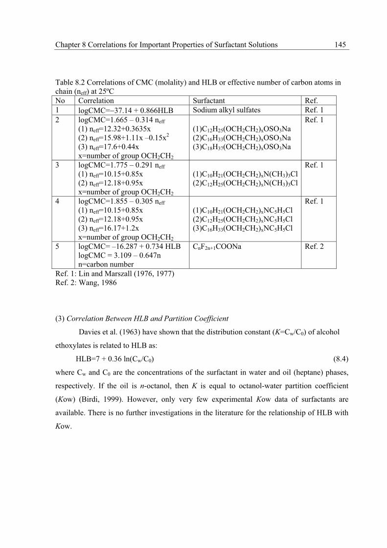
Chapter 8 Correlations for Important Properties of Surfactant Solutions 145
Table 8.2 Correlations of CMC (molality) and HLB or effective number of carbon atoms in chain (neff) at 25ºC No Correlation Surfactant Ref. 1 logCMC= 37.14 + 0.866HLB Sodium alkyl sulfates Ref. 1 2 logCMC=1.665 – 0.314 neff
(1) neff=12.32+0.3635x (2) neff=15.98+1.11x –0.15x2 (3) neff=17.6+0.44x x=number of group OCH2CH2
(1)C12H25(OCH2CH2)xOSO3Na (2)C16H33(OCH2CH2)xOSO3Na (3)C18H37(OCH2CH2)xOSO3Na
Ref. 1
3 logCMC=1.775 – 0.291 neff (1) neff=10.15+0.85x (2) neff=12.18+0.95x x=number of group OCH2CH2
(1)C10H21(OCH2CH2)xN(CH3)3Cl (2)C12H25(OCH2CH2)xN(CH3)3Cl
Ref. 1
4 logCMC=1.855 – 0.305 neff (1) neff=10.15+0.85x (2) neff=12.18+0.95x (3) neff=16.17+1.2x x=number of group OCH2CH2
(1)C10H21(OCH2CH2)xNC5H5Cl (2)C12H25(OCH2CH2)xNC5H5Cl (3)C16H33(OCH2CH2)xNC5H5Cl
Ref. 1
5 logCMC= –16.287 + 0.734 HLB logCMC = 3.109 – 0.647n n=carbon number
CnF2n+1COONa Ref. 2
Ref. 1: Lin and Marszall (1976, 1977) Ref. 2: Wang, 1986
(3) Correlation Between HLB and Partition Coefficient
Davies et al. (1963) have shown that the distribution constant (K=Cw/C0) of alcohol
ethoxylates is related to HLB as:
HLB=7 + 0.36 ln(Cw/C0) (8.4)
where Cw and C0 are the concentrations of the surfactant in water and oil (heptane) phases,
respectively. If the oil is n-octanol, then K is equal to octanol-water partition coefficient
(Kow) (Birdi, 1999). However, only very few experimental Kow data of surfactants are
available. There is no further investigations in the literature for the relationship of HLB with
Kow.
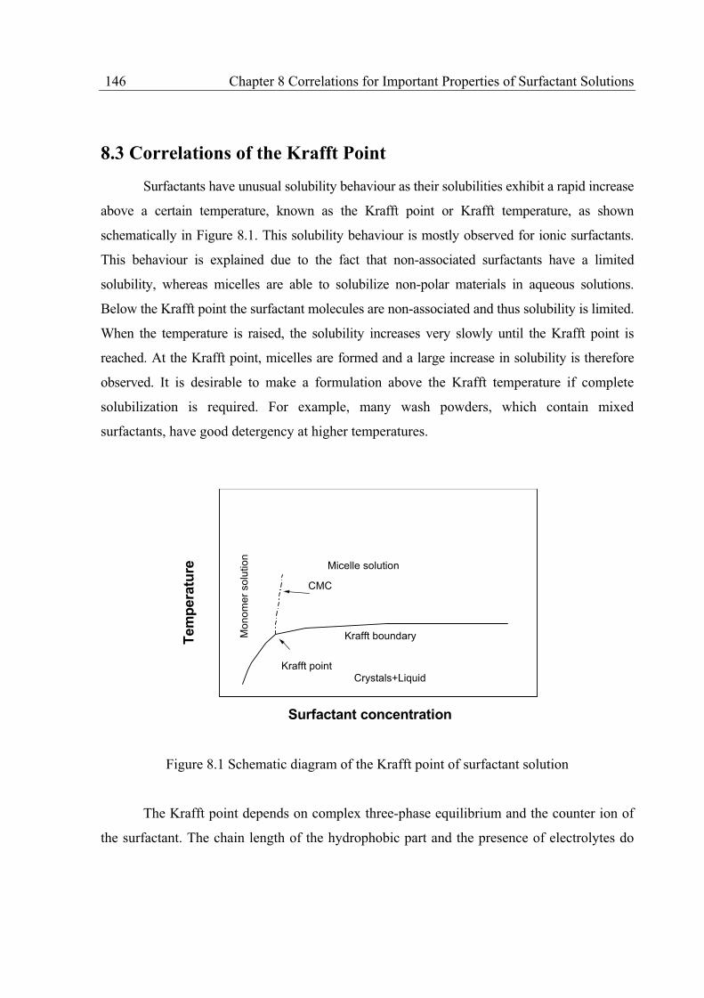
146 Chapter 8 Correlations for Important Properties of Surfactant Solutions
8.3 Correlations of the Krafft Point
Surfactants have unusual solubility behaviour as their solubilities exhibit a rapid increase
above a certain temperature, known as the Krafft point or Krafft temperature, as shown
schematically in Figure 8.1. This solubility behaviour is mostly observed for ionic surfactants.
This behaviour is explained due to the fact that non-associated surfactants have a limited
solubility, whereas micelles are able to solubilize non-polar materials in aqueous solutions.
Below the Krafft point the surfactant molecules are non-associated and thus solubility is limited.
When the temperature is raised, the solubility increases very slowly until the Krafft point is
reached. At the Krafft point, micelles are formed and a large increase in solubility is therefore
observed. It is desirable to make a formulation above the Krafft temperature if complete
solubilization is required. For example, many wash powders, which contain mixed
surfactants, have good detergency at higher temperatures.
Krafft boundary
Crystals+LiquidKrafft point
Mo
no
me
r so
lutio
n
Micelle solution
CMC
Tem
pera
ture
Surfactant concentration
Figure 8.1 Schematic diagram of the Krafft point of surfactant solution
The Krafft point depends on complex three-phase equilibrium and the counter ion of
the surfactant. The chain length of the hydrophobic part and the presence of electrolytes do
Chapter 8 Correlations for Important Properties of Surfactant Solutions 147
also influence the Krafft point of ionic surfactants. The addition of electrolytes increases the
Krafft point.
Surfactants with a high Krafft temperature have ionic head groups or have compact
highly polar head-groups and long straight alkyl chains. Lower Krafft point temperature can
be obtained with branched alkyl chains or bulkier hydrophobic groups (e.g. two alkyl chains).
If the surfactant solution exhibits surface-activity based characteristics, such as wetting, the
solution would be used below or near its Krafft point, whereas if high solubility is required,
the solution need to be used at temperatures above the Krafft point.
Several estimation methods have been proposed for Krafft point. Huibers (1996a)
used quantitative structure-property relationships (QSPR) to correlate the Krafft point with
molecule structure information and obtain a predictive relation for the Krafft points of 44
surfactants. In our study, correlations between Krafft point and molecular structure or CMC
are presented.
(1) Correlation of Gu et al. (1992)
In the work of Gu et al., (1992), the Krafft points (KP, ºC) are correlated with the
structure of different surfactant molecules. In the case of ionic ethoxylated surfactants of type
CnH2n+1(OCH2CH2)mSO4-Na+, the dependence between the KP and the molecular structure
units can be expressed as
iEOcc kmnk 9KP (8.5)
where nc is the number of hydrocarbon groups in alkyl chain, nc = 16, 18, mEO is the number
of ethylene oxide unit (OCH2CH2) in CnH2n+1(OCH2CH2)mSO4-Na+ molecule, mEO=1~4. In
the equation kc and ki are constants depending on the ionic headgroup, which are given in
Table 8.3.
For surfactants with a single straight hydrocarbon chain, the KP can also be related to
the number of hydrocarbon groups, nc (nc = 10~18) by
icc knkKP (8.6)
where ki and kc are the values listed in Table 8.3.
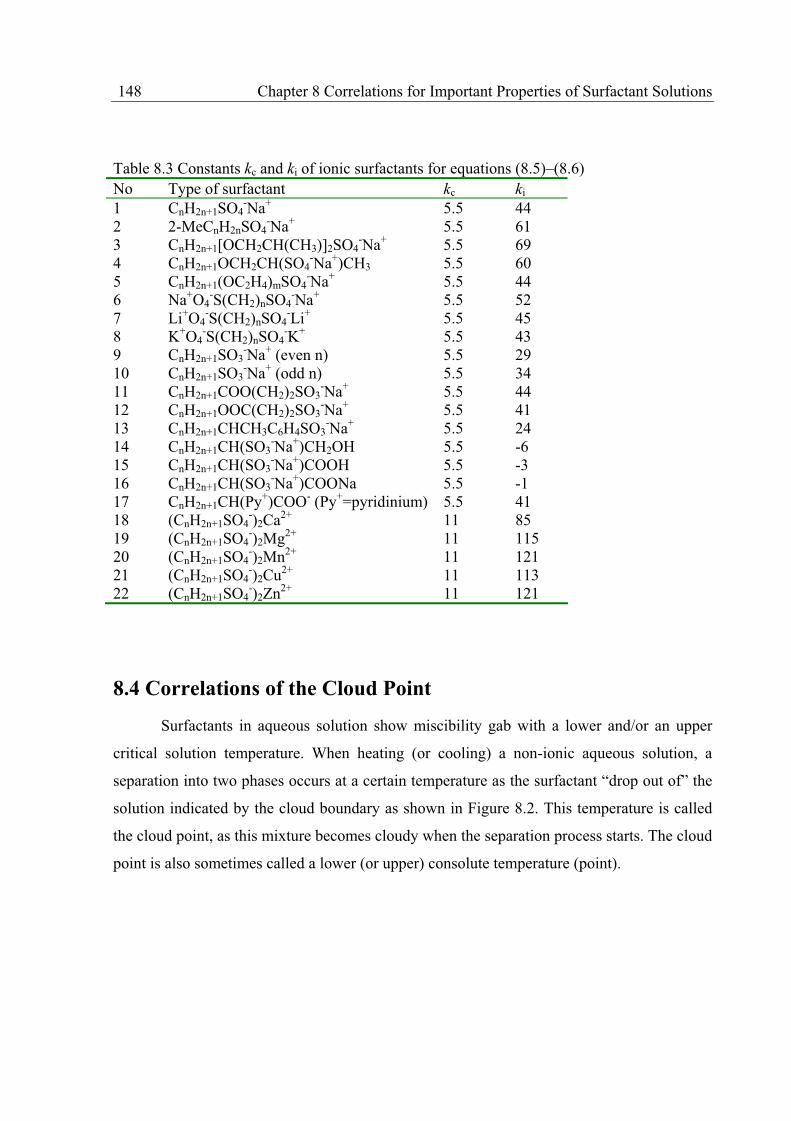
148 Chapter 8 Correlations for Important Properties of Surfactant Solutions
Table 8.3 Constants kc and ki of ionic surfactants for equations (8.5)–(8.6) No Type of surfactant kc ki 1 CnH2n+1SO4
-Na+ 5.5 44 2 2-MeCnH2nSO4
-Na+ 5.5 61 3 CnH2n+1[OCH2CH(CH3)]2SO4
-Na+ 5.5 69 4 CnH2n+1OCH2CH(SO4
-Na+)CH3 5.5 60 5 CnH2n+1(OC2H4)mSO4
-Na+ 5.5 44 6 Na+O4
-S(CH2)nSO4-Na+ 5.5 52
7 Li+O4-S(CH2)nSO4
-Li+ 5.5 45 8 K+O4
-S(CH2)nSO4-K+ 5.5 43
9 CnH2n+1SO3-Na+ (even n) 5.5 29
10 CnH2n+1SO3-Na+ (odd n) 5.5 34
11 CnH2n+1COO(CH2)2SO3-Na+ 5.5 44
12 CnH2n+1OOC(CH2)2SO3-Na+ 5.5 41
13 CnH2n+1CHCH3C6H4SO3-Na+ 5.5 24
14 CnH2n+1CH(SO3-Na+)CH2OH 5.5 -6
15 CnH2n+1CH(SO3-Na+)COOH 5.5 -3
16 CnH2n+1CH(SO3-Na+)COONa 5.5 -1
17 CnH2n+1CH(Py+)COO- (Py+=pyridinium) 5.5 41 18 (CnH2n+1SO4
-)2Ca2+ 11 85 19 (CnH2n+1SO4
-)2Mg2+ 11 115 20 (CnH2n+1SO4
-)2Mn2+ 11 121 21 (CnH2n+1SO4
-)2Cu2+ 11 113 22 (CnH2n+1SO4
-)2Zn2+ 11 121
8.4 Correlations of the Cloud Point
Surfactants in aqueous solution show miscibility gab with a lower and/or an upper
critical solution temperature. When heating (or cooling) a non-ionic aqueous solution, a
separation into two phases occurs at a certain temperature as the surfactant “drop out of” the
solution indicated by the cloud boundary as shown in Figure 8.2. This temperature is called
the cloud point, as this mixture becomes cloudy when the separation process starts. The cloud
point is also sometimes called a lower (or upper) consolute temperature (point).
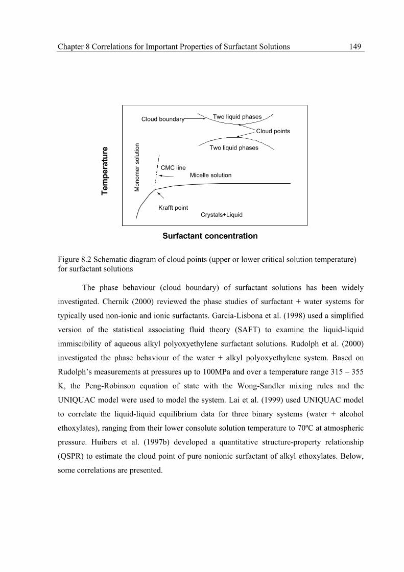
Chapter 8 Correlations for Important Properties of Surfactant Solutions 149
Cloud points
Two liquid phases
Crystals+LiquidKrafft point
Mo
no
me
r so
lutio
n
Micelle solution
CMC line
Cloud boundary Two liquid phases
Tem
pera
ture
Surfactant concentration
Figure 8.2 Schematic diagram of cloud points (upper or lower critical solution temperature) for surfactant solutions
The phase behaviour (cloud boundary) of surfactant solutions has been widely
investigated. Chernik (2000) reviewed the phase studies of surfactant + water systems for
typically used non-ionic and ionic surfactants. Garcia-Lisbona et al. (1998) used a simplified
version of the statistical associating fluid theory (SAFT) to examine the liquid-liquid
immiscibility of aqueous alkyl polyoxyethylene surfactant solutions. Rudolph et al. (2000)
investigated the phase behaviour of the water + alkyl polyoxyethylene system. Based on
Rudolph’s measurements at pressures up to 100MPa and over a temperature range 315 – 355
K, the Peng-Robinson equation of state with the Wong-Sandler mixing rules and the
UNIQUAC model were used to model the system. Lai et al. (1999) used UNIQUAC model
to correlate the liquid-liquid equilibrium data for three binary systems (water + alcohol
ethoxylates), ranging from their lower consolute solution temperature to 70ºC at atmospheric
pressure. Huibers et al. (1997b) developed a quantitative structure-property relationship
(QSPR) to estimate the cloud point of pure nonionic surfactant of alkyl ethoxylates. Below,
some correlations are presented.
150 Chapter 8 Correlations for Important Properties of Surfactant Solutions
(1) Correlation by Gu and Sjöblom (1992)
Gu and Sjöblom (1992) developed a linear relationship between the cloud point (CP)
and the logarithm of the ethylene oxide number for nonionic surfactants:
CBnnA CEO )log(CP (8.7)
where CP is the cloud point with unit in K, nEO is the ethylene oxide unit for alkyl
ethoxylates, alkylpenyl ethoxylates and methyl capped alkyl ethoxylate esters (nEO=5-8) and
nC is the alkyl carbon number for linear alkyl ethoxylates (nC=6-16). In the equation, A, B and
C are empirical constants depending on the surfactants as shown in Table 8.4.
Table 8.4 Constants A, B, C for equation (8.7)*
No Type of surfactant A B C
1 CnH2n+1(OC2H4)mOH 220 5.5 55
2 CnH2n+1C6H4(OC2H4)mOH 278 5.5 171
3 CnH2n+1COO(C2H4O)mCH3, n=9, 11 152 0.0 87
* subscript m: ethylene oxide unit nEO, subscript n: alkyl carbon number nC
(2) Correlation of Huibers et al. (1997b)
Huibers et al. (1997b) re-calculated the empirical relationship of equation (8.7) (Gu
and Sjöblom, 1992) with a larger data set and obtained a new set of coefficients for the linear
alkyl ethoxylates:
7.4078.5log1.87CP CEO nn (8.8)
Based on the correlation, it is found that the carbon number (nc) is an inadequate descriptor
for modelling the cloud point except for linear alkyl ethoxylates. Huibers et al. (1997b), thus
further developed a correlation using several topological descriptors from connectivity or
topology of molecules to get better regression results for the cloud point. The correlations of
topological method can be found in the work of Huibers et al. (1997b).

Chapter 8 Correlations for Important Properties of Surfactant Solutions 151
8.5 Correlations of the Detergency
The detergency is described as (Zimoch et al., 2000):
%CA
CYD (8.9)
where D is the detergency, Y and C are the average whiteness degree of the investigated test
fabric after and before washing, respectively, and A is the average whiteness of the
investigated fabric, not soiled.
Detergency is a complex physicochemical process, which occurs at the interface
between fabrics contaminated with soil and surfactant aqueous solutions. Many parameters
affect the detergency during a washing process. The efficiency of washing depends on the
properties of washed fabrics, type and composition of soil, composition of washing bath and
washing conditions. The wetting of the hydrophilic fabrics and emulsifications of soil
deposited on the fabrics play a crucial role in the effectiveness of washing.
In practice, the washing ability is measured using the standard, tedious and time-
consuming experiments in which swatches of standard soiled fabrics are washed in specially
designed washing device. Carroll (1993) investigated the physical characteristics of
detergency. Miller et al. (1993) studied the solubilization mechanism of detergency. But,
their investigations and theories cannot be generalized for complex washing system.
Correlation methods are often used to shorten the period of time to determine the
optimal formulations of washing agents. Zimoch et al. (2000) and Lindgren et al. (1994)
modelled the detergency with physical properties of surfactants. Some of their results are
presented here.
(1) Correlations of Zimoch et al. (2000)
Zimoch et al. investigated the relations of detergency with surface tension and HLB
using three standard test swatches: Krefeld 10C (cotton fabric), Krefeld 20C (65% polyester
and 35% cotton mixed cloth) and Krefeld 30C (polyester) for alcohol ethoxylate surfactants.
Correlation results are presented as follows:
Krefeld 10C:
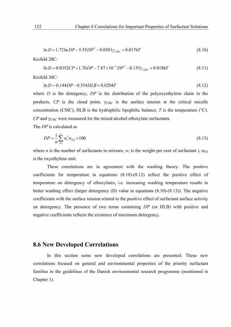
152 Chapter 8 Correlations for Important Properties of Surfactant Solutions
TDPDPD CMC 0176.00501.055.5ln72.1ln 2 (8.10)
Krefeld 20C:
TDPDPCPD CMC 0186.0135.01087.776.10352.0ln 23 (8.11)
Krefeld 30C:
THLBDPD 0204.0554.0144.0ln (8.12)
where D is the detergency, DP is the distribution of the polyoxyethylene chain in the
products, CP is the cloud point, CMC is the surface tension at the critical micelle
concentration (CMC), HLB is the hydrophilic lipophilic balance, T is the temperature (°C).
CP and CMC were measured for the mixed alcohol ethoxylate surfactants.
The DP is calculated as
n
i
EOi nwn
DP1
2 1001
(8.13)
where n is the number of surfactants in mixture, wi is the weight per cent of surfactant i, nEO
is the oxyethylene unit.
These correlations are in agreement with the washing theory. The positive
coefficients for temperature in equations (8.10)-(8.12) reflect the positive effect of
temperature on detergency of ethoxylates, i.e. increasing washing temperature results in
better washing effect (larger detergency (D) value in equations (8.10)-(8.13)). The negative
coefficients with the surface tension related to the positive effect of surfactant surface activity
on detergency. The presence of two terms containing DP (or HLB) with positive and
negative coefficients reflects the existence of maximum detergency.
8.6 New Developed Correlations
In this section some new developed correlations are presented. These new
correlations focused on general and environmental properties of the priority surfactant
families in the guidelines of the Danish environmental research programme (mentioned in
Chapter 1).

Chapter 8 Correlations for Important Properties of Surfactant Solutions 153
8.6.1 Correlation of HLB with CMC
(1) Correlations for Polyoxyethylene Sodium Alkyl Sulfates
The polyoxyethylene sodium alkyl sulfates (CnH2n+1(OC2H4)mSO4-Na+) are nontoxic,
biodegradeable, and industrial useful surfactants. However, no correlation between HLB and
CMC could be found in the literature. Such a correlation was developed in our work using
the experimental data presented in Table 8.5. An excellent linear relationship is obtained as
shown in equation (8.14) and figure 8.3.
HLB 666072628CMClog ..- , r2=0.999 (8.14)
where r2 is the correlation coefficient. Table 8.5 HLB and CMC data (Lin et al.,1976) CnH2n+1(OC2H4)mSO4
-Na+ CMC, 25ºC HLB No. n m Molality 1 12 0 8.10E-03 40 2 12 1 4.20E-03 39.57 3 12 2 3.10E-03 39.38 4 12 3 2.80E-03 39.24 5 12 5 1.90E-03 39.05 6 14 0 2.10E-03 39.05 7 16 0 4.00E-04 38.1 8 16 1 2.20E-04 37.62 9 16 2 1.40E-04 37.34 10 16 3 1.00E-04 37.15 11 16 4 1.00E-04 37.15 12 18 0 1.10E-04 37.15 13 18 1 1.10E-04 37.15 14 18 2 7.00E-05 36.91 15 18 3 5.00E-05 36.63 16 18 4 4.00E-05 36.53 * HLB and CMC data are from Lin et al. (1976)
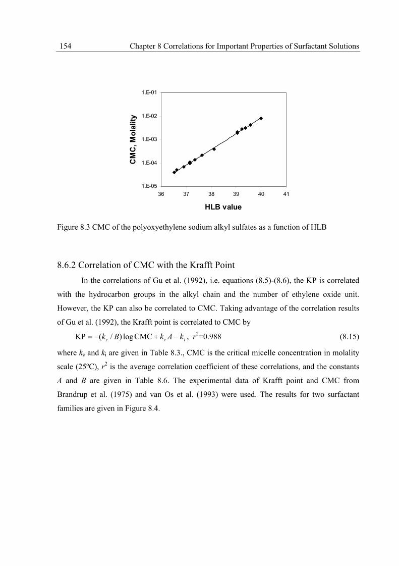
154 Chapter 8 Correlations for Important Properties of Surfactant Solutions
1.E-05
1.E-04
1.E-03
1.E-02
1.E-01
36 37 38 39 40 41
HLB value
CM
C, M
ola
lity
Figure 8.3 CMC of the polyoxyethylene sodium alkyl sulfates as a function of HLB
8.6.2 Correlation of CMC with the Krafft Point
In the correlations of Gu et al. (1992), i.e. equations (8.5)-(8.6), the KP is correlated
with the hydrocarbon groups in the alkyl chain and the number of ethylene oxide unit.
However, the KP can also be correlated to CMC. Taking advantage of the correlation results
of Gu et al. (1992), the Krafft point is correlated to CMC by
icc kAkBk CMClog)/(KP , r2=0.988 (8.15)
where kc and ki are given in Table 8.3., CMC is the critical micelle concentration in molality
scale (25ºC), r2 is the average correlation coefficient of these correlations, and the constants
A and B are given in Table 8.6. The experimental data of Krafft point and CMC from
Brandrup et al. (1975) and van Os et al. (1993) were used. The results for two surfactant
families are given in Figure 8.4.
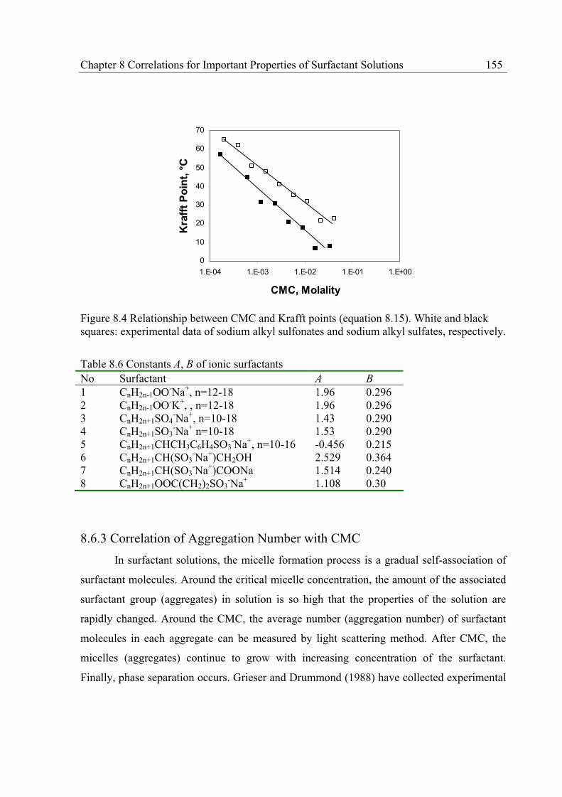
Chapter 8 Correlations for Important Properties of Surfactant Solutions 155
0
10
20
30
40
50
60
70
1.E-04 1.E-03 1.E-02 1.E-01 1.E+00
CMC, Molality
Kra
fft
Po
int,
°C
Figure 8.4 Relationship between CMC and Krafft points (equation 8.15). White and black squares: experimental data of sodium alkyl sulfonates and sodium alkyl sulfates, respectively.
Table 8.6 Constants A, B of ionic surfactants No Surfactant A B
1 CnH2n-1OO-Na+, n=12-18 1.96 0.296 2 CnH2n-1OO-K+, , n=12-18 1.96 0.296 3 CnH2n+1SO4
-Na+, n=10-18 1.43 0.290 4 CnH2n+1SO3
-Na+ n=10-18 1.53 0.290 5 CnH2n+1CHCH3C6H4SO3
-Na+, n=10-16 -0.456 0.215 6 CnH2n+1CH(SO3
-Na+)CH2OH 2.529 0.364 7 CnH2n+1CH(SO3
-Na+)COONa 1.514 0.240 8 CnH2n+1OOC(CH2)2SO3
-Na+ 1.108 0.30
8.6.3 Correlation of Aggregation Number with CMC
In surfactant solutions, the micelle formation process is a gradual self-association of
surfactant molecules. Around the critical micelle concentration, the amount of the associated
surfactant group (aggregates) in solution is so high that the properties of the solution are
rapidly changed. Around the CMC, the average number (aggregation number) of surfactant
molecules in each aggregate can be measured by light scattering method. After CMC, the
micelles (aggregates) continue to grow with increasing concentration of the surfactant.
Finally, phase separation occurs. Grieser and Drummond (1988) have collected experimental

156 Chapter 8 Correlations for Important Properties of Surfactant Solutions
aggregation number data. In our study, empirical relationships between aggregation number
and CMC are regressed for several surfactant families, as shown in Table 8.7 using the data
from van Os et al. (1993). The correlation results are also given in figures 8.5 and 8.6. In
figure 8.5, the regression line is extended to low CMC values reported by van Os et al. (1993)
to observe the extrapolated aggregation number. But no aggregation number data have been
reported for the low CMC values.
Table 8.7 Correlations for aggregation number (ng) vs. CMC (in molality, 25ºC)
No Surfactant Correlation r2
1 CnH2n+1SO4Na ng=8.333 21.92logCMC, n=8 18 0.986
2 C12H25(OCH2CH2)mOH logng= 3.2604 – 1.24597logCMC, m=4 12 0.96
3 C16H33(OCH2CH2)mOH logng= 9.25699 – 2.05724logCMC, m=7 21 0.975
4 C9H19C6H4(OCH2CH2)mOH logng= 4.160 – 1.553logCMC, m=10 50 0.98
* r2 is the correlation coefficient
0
10
20
30
40
50
60
70
80
90
100
1.E-04 1.E-03 1.E-02 1.E-01 1.E+00
CMC, Molality
Ag
gre
gati
on
nu
mb
er
CnOSO3Na
Figure 8.5 Correlation results for CnH2n+1SO4Na (CnOSO3Na). Points: experimental data from van Os et al. (1993) at 25°C. Line: regression result.

Chapter 8 Correlations for Important Properties of Surfactant Solutions 157
1.E+01
1.E+02
1.E+03
1.E-06 1.E-05 1.E-04 1.E-03
CMC, Molality
Ag
gre
gati
on
nu
mb
er
C16EnC12En
C9ØEOn
Figure 8.6 Correlation results for C12H25(OCH2CH2)mOH (C12En), C16H33(OCH2CH2)mOH (C16En), C9H19C6H4(OCH2CH2)mOH (C9ØEOn). Points: experimental data from van Os et al. (1993) at 25°C. Lines: regression results.
8.6.4 Correlation of Kow with HLB
The relationship of Kow and HLB is investigated in this section. Davies et al. (1963)
proposed a linear correlation for HLB and partition coefficient, i.e. equation (8.4). Birdi
(1999) suggested that this partition coefficient could be replaced by the octanol-water
partition coefficient (Kow). In chapter 4, the Kow has been investigated by UNIFAC and
commercial software. Because HLB can be easily obtained or calculated for surfactants, a
correlation for HLB and Kow is very helpful for practical applications even if Kow cannot be
easily measured for surfactants.
Both HLB and Kow are parameters to describe the hydrophobic and hydrophilic
properties of a chemical. HLB is an approximated parameter and often used for surfactants,
and Kow is a strict thermodynamic parameter. The HLB value is a summation of the
contributions from the hydrophobic and the hydrophilic groups. As can be seen from Table
8.1, hydrophilic groups have a positive contribution to HLB, and hydrophobic groups give a
negative contribution. The chemicals with longer hydrophilic chain will have larger HLB.
Oppositely, the longer hydrophilic group chain a chemical has, the lower Kow value a
chemical will have.
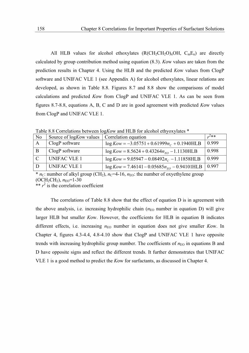
158 Chapter 8 Correlations for Important Properties of Surfactant Solutions
All HLB values for alcohol ethoxylates (R(CH2CH2O)nOH, CmEn) are directly
calculated by group contribution method using equation (8.3). Kow values are taken from the
prediction results in Chapter 4. Using the HLB and the predicted Kow values from ClogP
software and UNIFAC VLE 1 (see Appendix A) for alcohol ethoxylates, linear relations are
developed, as shown in Table 8.8. Figures 8.7 and 8.8 show the comparisons of model
calculations and predicted Kow from ClogP and UNIFAC VLE 1. As can be seen from
figures 8.7-8.8, equations A, B, C and D are in good agreement with predicted Kow values
from ClogP and UNIFAC VLE 1.
Table 8.8 Correlations between logKow and HLB for alcohol ethyoxylates * No Source of logKow values Correlation equation r
2** A ClogP software HLB1940.061999.005751.3log CnKow 0.999
B ClogP software HLB1130.143264.05624.8log EOnKow 0.998
C UNIFAC VLE 1 HLB11858.108492.005947.9log CnKow 0.999
D UNIFAC VLE 1 HLB94101.005685.046141.7log EOnKow 0.997
* nC: number of alkyl group (CH2), nC=4-16, nEO: the number of oxyethylene group (OCH2CH2), nEO=1-30 ** r2 is the correlation coefficient
The correlations of Table 8.8 show that the effect of equation D is in agreement with
the above analysis, i.e. increasing hydrophilic chain (nEO number in equation D) will give
larger HLB but smaller Kow. However, the coefficients for HLB in equation B indicates
different effects, i.e. increasing nEO number in equation does not give smaller Kow. In
Chapter 4, figures 4.3-4.4, 4.8-4.10 show that ClogP and UNIFAC VLE 1 have opposite
trends with increasing hydrophilic group number. The coefficients of nEO in equations B and
D have opposite signs and reflect the different trends. It further demonstrates that UNIFAC
VLE 1 is a good method to predict the Kow for surfactants, as discussed in Chapter 4.

Chapter 8 Correlations for Important Properties of Surfactant Solutions 159
0
1
2
3
4
5
6
7
8
9
10
0 2 4 6 8 10
logKow, model
log
Ko
w, C
log
P
Figure 8.7 Scatter plot of the equation A and B (model) vs. ClogP for logKow values of alcohol ethoxylates
-8.0
-6.0
-4.0
-2.0
0.0
2.0
4.0
6.0
-8 -6 -4 -2 0 2 4 6
logKow, model
log
Ko
w, U
NIF
AC
VL
E 1
Figure 8.8 Scatter plot of the equation C and D (model) vs. UNIFAC VLE 1 for logKow values of alcohol ethoxylates
Table 8.9 gives logKow calculation results for alcohol ethoxylates using the equations
in Table 8.8 and compares with few experimental Kow data. As can be seen, the equations C
and D produce very stable Kow values and are in good agreement with UNIFAC VLE 1.
Equations A and B match well ClogP values except for C3E1.

160 Chapter 8 Correlations for Important Properties of Surfactant Solutions
Based on these correlations, the logKow value can be easily calculated from HLB and
one structural parameter nC or nEO. These correlations provide the basis to set up correlation
for Kow and environmental properties which is given in the next section.
Table 8.9 logKow calculation results for alcohol ethoxylates using equations in Table 8.8 Compound Exp.* ClogP Eq. A Eq. B VLE1* Eq. C Eq. D C1E1 -0.77 -0.75 -0.74 -0.75 -0.83 -0.82 -0.83 C2E1 -0.28 -0.22 -0.21 -0.22 -0.38 -0.37 -0.39 C2E2 -0.54 -0.15 -0.15 -0.16 -0.75 -0.74 -0.75 C3E1 0.05 0.09 0.32 0.31 0.07 0.07 0.06 C4E1 0.8 0.84 0.84 0.84 0.51 0.52 0.51 C4E2 0.56 0.91 0.91 0.90 0.15 0.15 0.14 C6E1 1.86 1.90 1.90 1.89 1.41 1.41 1.40 C6E2 1.7 1.96 1.96 1.96 1.04 1.04 1.03 Mean Dev.% 33 91 87 36 36 35 *Exp.: experimental data from Sangster (2001), VLE1: original UNIFAC VLE 1 (Hansen et al., 1991).
In Table 8.9,
%owlog
owlogowlog1Dev.%Mean
1Exp
CalExpn
K
KK
n, n is the total number of data.
8.6.5 Correlation of Kow with Environmental Properties
As presented in Table 2.6 (Chapter 2), Denmark consumes about 20,000 tons
surfactants as cleaning products in 1998; Europe markets need 1.7 million tons surfactants
annually. All these consumed surfactants will finally enter our nature. Therefore, the
environmental effects of surfactants have been heavily debated in public. The Danish
Environmental Protection Agency (EPA) has systematically investigated and published
reports about the environmental effects of surfactants. Modelling work for the environmental
effects of surfactants will help EPA to evaluate the newly released surfactants. In our work,
the correlations of Kow and environmental effects are developed.
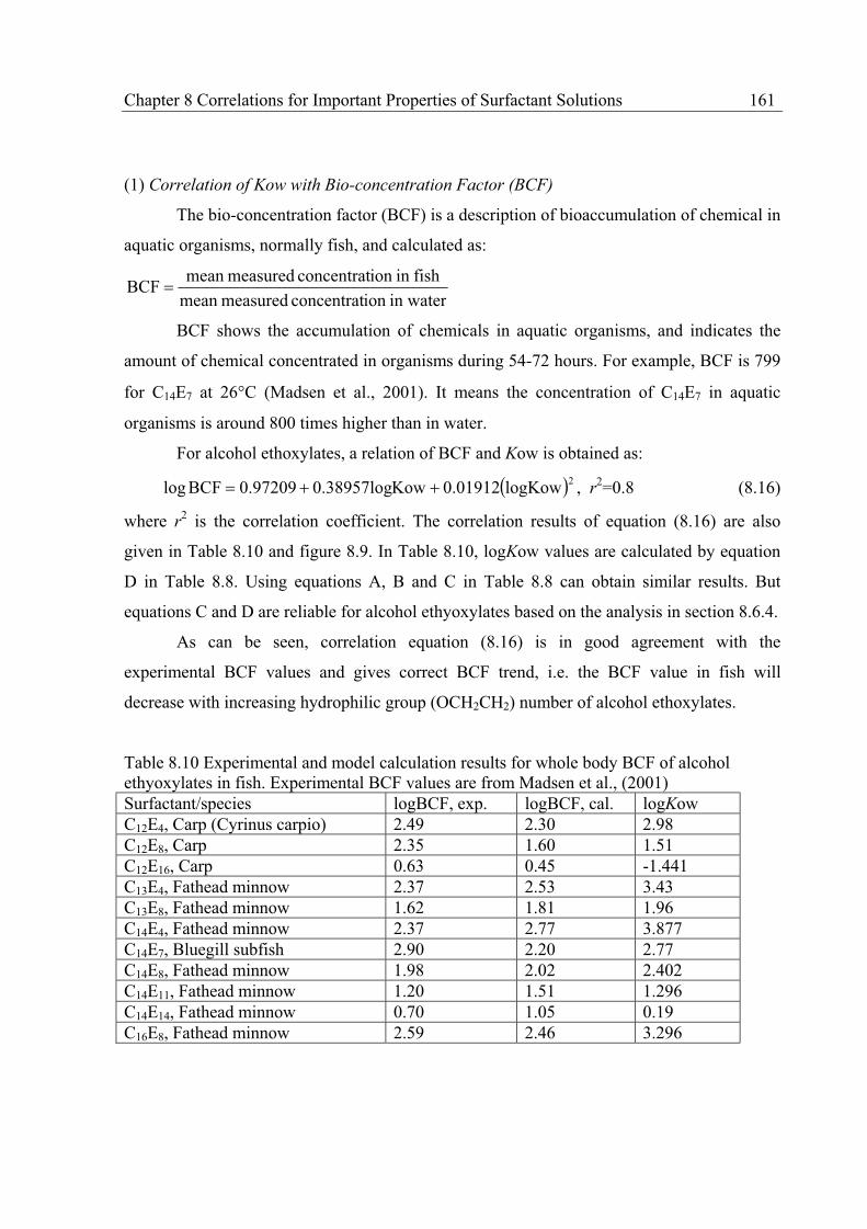
Chapter 8 Correlations for Important Properties of Surfactant Solutions 161
(1) Correlation of Kow with Bio-concentration Factor (BCF)
The bio-concentration factor (BCF) is a description of bioaccumulation of chemical in
aquatic organisms, normally fish, and calculated as:
in waterion concentrat measuredmean
fishin ion concentrat measuredmean BCF
BCF shows the accumulation of chemicals in aquatic organisms, and indicates the
amount of chemical concentrated in organisms during 54-72 hours. For example, BCF is 799
for C14E7 at 26 C (Madsen et al., 2001). It means the concentration of C14E7 in aquatic
organisms is around 800 times higher than in water.
For alcohol ethoxylates, a relation of BCF and Kow is obtained as:
2logKow0.01912Kow0.38957log0.97209BCFlog , r2=0.8 (8.16)
where r2 is the correlation coefficient. The correlation results of equation (8.16) are also
given in Table 8.10 and figure 8.9. In Table 8.10, logKow values are calculated by equation
D in Table 8.8. Using equations A, B and C in Table 8.8 can obtain similar results. But
equations C and D are reliable for alcohol ethyoxylates based on the analysis in section 8.6.4.
As can be seen, correlation equation (8.16) is in good agreement with the
experimental BCF values and gives correct BCF trend, i.e. the BCF value in fish will
decrease with increasing hydrophilic group (OCH2CH2) number of alcohol ethoxylates.
Table 8.10 Experimental and model calculation results for whole body BCF of alcohol ethyoxylates in fish. Experimental BCF values are from Madsen et al., (2001) Surfactant/species logBCF, exp. logBCF, cal. logKow C12E4, Carp (Cyrinus carpio) 2.49 2.30 2.98 C12E8, Carp 2.35 1.60 1.51 C12E16, Carp 0.63 0.45 -1.441 C13E4, Fathead minnow 2.37 2.53 3.43 C13E8, Fathead minnow 1.62 1.81 1.96 C14E4, Fathead minnow 2.37 2.77 3.877 C14E7, Bluegill subfish 2.90 2.20 2.77 C14E8, Fathead minnow 1.98 2.02 2.402 C14E11, Fathead minnow 1.20 1.51 1.296 C14E14, Fathead minnow 0.70 1.05 0.19 C16E8, Fathead minnow 2.59 2.46 3.296

162 Chapter 8 Correlations for Important Properties of Surfactant Solutions
-2 -1 0 1 2 3 4
0.5
1.0
1.5
2.0
2.5
3.0
log
BC
F, fi
sh
logKow
logBCF,Expt.
logBCF, Fit
Figure 8.9 Equation (8.16) calculation results for whole body BCF of alcohol ethoxylates in fish using the logKow as correlation parameter. Experimental BCF values are from Madsen et al. (2001).
(2) Correlation of Kow with Toxicity
Toxicity is a very important property and often used to establish regulations in
chemical management. Using Kow to correlate and predict toxicity has a long history
(Schultz, 2003). Kow is one of the standard parameters for EPA to evaluate the toxicity of
chemicals. In our work, a new correlation model for toxicity and Kow of alcohol ethoxylates
is developed.
Toxicity to algae, invertebrates, fish and rat data are taken from the collection of
Madsen et al. (2001) for alcohol ethoxylates which includes CiEj, i=9~18, j=1~30. Kow data
are calculated by UNIFAC VLE 1 (see Appendix A) and compared with correlation equation
D in Table 8.8. The comparison between UNIFAC VLE 1 and equation D is given in figure
8.10. Figure 8.10 shows the simple equation D can be used to replace UNIFAC VLE 1 in the
Kow calculation for alcohol ethoxylates. Based on the toxicity and Kow data, linear
correlations are obtained and given in Table 8.11 and figures 8.11-8.14.

Chapter 8 Correlations for Important Properties of Surfactant Solutions 163
-6
-4
-2
0
2
4
6
8
-6 -4 -2 0 2 4 6 8
logKow, equation D in Table 8.8
log
Ko
w, U
NIF
AC
VL
E1
Figure 8.10 Scatter plot of logKow values from the equation D in Table 8.8 and UNIFAC VLE 1 for alcohol ethoxylates used in toxicity correlations.
Table 8.11 Correlations of Kow and toxicity (EC50: mg/l, LD50: g/kg) Species Correlation equation Figures r
2 Algae ow0.4507logK1.13599EC50/1log 8.11 0.67
Invertebrates Kow0.18504log.719050EC50/1log 8.12 0.52
Fish ow0.1776logK.555710EC50/1log 8.13 0.76
Rat Kow0.18631log.043560LD50log 8.14 0.88
In the equations of Table 8.11, EC50 is the concentration of a chemical causing a
defined effect to 50% of a group of test organisms (e.g. immobilization or growth inhibition),
LD50 is the dosage causing death to 50% of the exposed animals after a single administration.
As can be seen in figures 8.11-8.14, experimental toxicity data are rather scattered
with plot against Kow. However, Kow does capture qualitatively the trend of the
experimental toxicity data. The scattered experimental data indicate this toxicity cannot be
correlated alone with Kow.
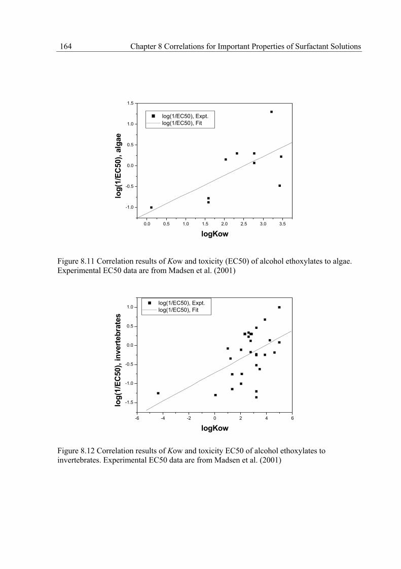
164 Chapter 8 Correlations for Important Properties of Surfactant Solutions
0.0 0.5 1.0 1.5 2.0 2.5 3.0 3.5
-1.0
-0.5
0.0
0.5
1.0
1.5
log
(1/E
C50),
alg
ae
logKow
log(1/EC50), Expt.
log(1/EC50), Fit
Figure 8.11 Correlation results of Kow and toxicity (EC50) of alcohol ethoxylates to algae. Experimental EC50 data are from Madsen et al. (2001)
-6 -4 -2 0 2 4 6
-1.5
-1.0
-0.5
0.0
0.5
1.0
log
(1/E
C50),
in
vert
eb
rate
s
logKow
log(1/EC50), Expt.
log(1/EC50), Fit
Figure 8.12 Correlation results of Kow and toxicity EC50 of alcohol ethoxylates to invertebrates. Experimental EC50 data are from Madsen et al. (2001)

Chapter 8 Correlations for Important Properties of Surfactant Solutions 165
-4 -2 0 2 4
-1.6
-1.4
-1.2
-1.0
-0.8
-0.6
-0.4
-0.2
0.0
0.2
0.4
log
(1/E
C50),
fis
h
logKow
log(1/EC50), Expt.
log(1/EC50), Fit
Figure 8.13 Correlation results of Kow and toxicity EC50 of alcohol ethoxylates to fish. Experimental EC50 data are from Madsen et al. (2001).
-1 0 1 2 3 4 5 6 7
0.0
0.2
0.4
0.6
0.8
1.0
1.2
1.4
log
LD
50, ra
t
logKow
logLD50, Expt.
logLD50, Fit.
Figure 8.14 Correlation results of Kow and toxicity LD50 of alcohol ethoxylates to rat. Experimental EC50 data are from Madsen et al. (2001).
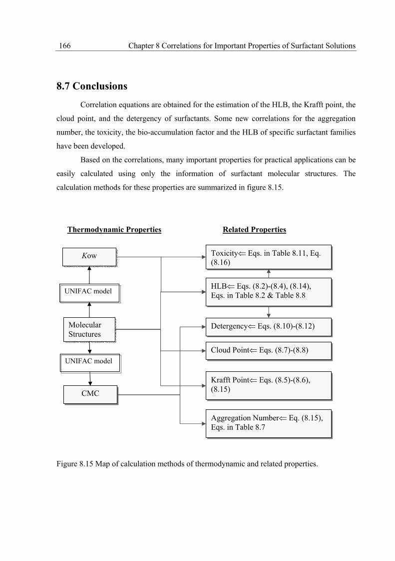
166 Chapter 8 Correlations for Important Properties of Surfactant Solutions
8.7 Conclusions
Correlation equations are obtained for the estimation of the HLB, the Krafft point, the
cloud point, and the detergency of surfactants. Some new correlations for the aggregation
number, the toxicity, the bio-accumulation factor and the HLB of specific surfactant families
have been developed.
Based on the correlations, many important properties for practical applications can be
easily calculated using only the information of surfactant molecular structures. The
calculation methods for these properties are summarized in figure 8.15.
Figure 8.15 Map of calculation methods of thermodynamic and related properties.
Thermodynamic Properties
Kow
CMC
Related Properties
HLB Eqs. (8.2)-(8.4), (8.14), Eqs. in Table 8.2 & Table 8.8
Toxicity Eqs. in Table 8.11, Eq. (8.16)
Detergency Eqs. (8.10)-(8.12)
Cloud Point Eqs. (8.7)-(8.8)
Krafft Point Eqs. (8.5)-(8.6), (8.15)
Aggregation Number Eq. (8.15), Eqs. in Table 8.7
Molecular Structures
UNIFAC model
UNIFAC model

Chapter 9 Conclusions and Future Work 167
Chapter 9 Conclusions and Future Work
9.1 Conclusions
This thesis has addressed the modelling of surfactant solutions. The main conclusions
are summarised here:
(1) The thermodynamic framework of Chen et al. (1996, 2001) for non-ionic and ionic
surfactant solutions is adopted. Based on this, the CMC of non-ionic and ionic surfactant
solutions is investigated with the UNIFAC model.
(2) The CMC of a specific family of non-ionic surfactant solutions (alcohol
ethoxylates) is first correlated and then predicted with the UNIFAC model. A new UNIFAC
functional group (OCH2CH2) is introduced and the necessary interaction parameters are
obtained directly from the CMC data (correlation) or from vapour-liquid equilibrium data
(prediction). The trends of CMC against both the hydrophobic and hydrophilic chain length
are well represented.
(3) The octanol-water partition coefficients of phthalates and non-ionic surfactant
(alcohol ethoxylates) are predicted with different UNIFAC models and three commercial
tools, known with the abbreviations ACD, ClogP and KowWin. UNIFAC VLE1 is the best
among the methods investigated and very close to some of these commercial tools.
(4) In order to describe the CMC of ionic surfactant solutions, an electrolyte UNIFAC
model proposed by Achard et al. (1994 a, b) is used and modified to correlate the mean ionic
activity coefficients of organic electrolyte solutions. The structural parameters of ions are
directly calculated with the ionic radii of Marcus’s without using hydration number.
(5) It has been found that the ratio of structural parameters (R and Q) for ions in the
Achard’s method (and other) is Q/R>1 and does not follow the physically correct limitation
Q/R 1 in the Flory-Huggins theory. The physical derivation of UNIQUAC/UNIFAC is not
correct with the ratio Q/R>1. The effects of Q/R for electrolyte UNIQUAC/UNIFAC have
been studied through comparing combinatorial and residual terms of UNIQUAC model. A
new set of normalization factors is derived to yield a ratio Q/R 1 for ions.

168 Chapter 9 Conclusions and Future Work
(6) Using the new structural parameters of ions, the mean activity coefficients of
electrolyte solutions and organic electrolyte solutions are successfully correlated with the
modified Achard model. Similar behaviour as the electrolyte NRTL model is observed. For
investigated systems, the model has better correlation results than that of the extended
UNIQUAC. For organic electrolyte solutions, the model simultaneously captures the mean
activity coefficients of five sodium carboxylate systems with four interaction parameters and
is in good agreement with experimental values.
(7) The modified Achard model was used for calculating the CMC of sodium alkyl
sulphates, sodium alkyl sulfonates and potassium carboxylates surfactant solutions. The
model can successfully capture the effects of different alkyl chain lengths and temperatures.
However, the CMC prediction results for sodium carboxylates are poor.
(8) Semi-empirical relationships for the hydrophilic-lipophilc balance (HLB), the Krafft
point, the cloud point and the detergency are presented.
(9) New correlations for the aggregation number, the HLB, the toxicity and bio-
concentration factor of some specific surfactants are developed.
9.2 Future Work
As described in Chapter 3, thermodynamic understanding of surfactant solutions is
rather limited. The work described so far is an effort toward such understanding. Based on
the work presented in previous chapters, it seems appropriate to suggest some directions for
future efforts as following.
As shown in chapters 5 and 7, CMC of alcohol ethoxylates, sodium alkyl sulphates,
sodium alkyl sulfonates and sodium (potassium) carboxylates can be correlated and predicted
by UNIFAC or modified Achard model. Thus, it is very interesting to extend the UNIFAC
and modified Achard model developed in this work to different single surfactant solutions,
especially for sodium alky ether sulphates and sodium alky benzene sulphates. In practical
applications, CMC of mixed surfactant solutions are very important. The correlation results
Chapter 9 Conclusions and Future Work 169
for different single surfactant solutions will help to establish a basis to extend these models to
mixed surfactant solutions.
As described in Chapter 6, the structural parameters (Q, R) of ions used by many
UNIQUAC or UNIFAC based electrolyte models do not follow Flory-Huggins theory, which
results in UNIQUAC and UNIFAC having no physical meanings. Based on this point, a new
method was proposed to calculate Q and R parameters of ions from ionic radii. The new Q
and R calculation method can be further investigated in several directions: (1) optimization of
standard segment for structural parameter estimation; (2) investigation of the effects of
different Q and R ratios in mean activity coefficient correlation of electrolyte solutions. From
these investigations, a new UNIQUAC or UNIFAC-based electrolyte model could be
developed for electrolytes, especially for organic electrolyte solutions or ionic liquids.
Based on the UNIFAC and modified Achard model for non-ionic and ionic surfactant
solutions, CMC of mixed surfactants could be investigated. In order to carry out this work,
mixing rule for mixed surfactant solutions should be first selected or developed based on
existing methods. Meanwhile, an electrolyte model for mixed solvents and multiple ions
should be found or developed.
In Chapter 7, environmental properties of surfactant, such as BCF, EC50 and LD50,
were correlated with Kow for alcohol ethoxylates. This correlation method can be extended
to other surfactant families, such as sodium alkyl sulphates, etc. As a necessary step, the
octanol-water partition coefficient of ionic surfactants should be first investigated using
modified Achard method proposed in this work.

170 Chapter 9 Conclusions and Future Work
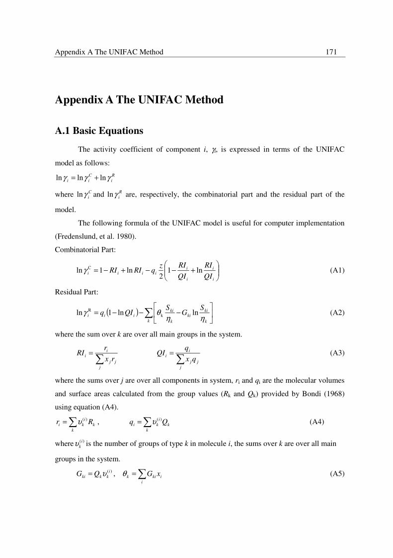
Appendix A The UNIFAC Method 171
Appendix A The UNIFAC Method
A.1 Basic Equations
The activity coefficient of component i, γi, is expressed in terms of the UNIFAC
model as follows:
Ri
Cii γγγ lnlnln +=
where Ciγln and R
iγln are, respectively, the combinatorial part and the residual part of the
model.
The following formula of the UNIFAC model is useful for computer implementation
(Fredenslund, et al. 1980).
Combinatorial Part:
+−−+−=i
i
i
iiiii QI
RI
QI
RIzqRIRI ln1
2ln1ln Cγ (A1)
Residual Part:
( ) −−−=k k
kiki
k
kiiii
SG
SQIq
ηηθγ lnln1ln k
R (A2)
where the sum over k are over all main groups in the system.
=
jjj
ii rx
rRI =
jjj
ii qx
qQI (A3)
where the sums over j are over all components in system, ri and qi are the molecular volumes
and surface areas calculated from the group values (Rk and Qk) provided by Bondi (1968)
using equation (A4).
=k
ki
ki Rr )(υ , =k
ki
ki Qq )(υ (A4)
where )(ikυ is the number of groups of type k in molecule i, the sums over k are over all main
groups in the system.
)(ikkki QG υ= , =
iikik xGθ (A5)

172 Appendix A The UNIFAC Method
=m
mkmiki GS τ , =i
ikik xSη (A6)
−=T
amkmk expτ (A7)
where the sum m is over all main groups in the system. In equation (A6), the unit of group
interaction parameter amk is in K. The coordination number z is set equal to 10.
A.2 Existing UNIFAC Models
Since the UNIFAC method has been introduced (Fredenslund et al., 1977), several
different versions (group interaction parameter tables and changing in the combinatorial and
residual part) have been proposed. Among these, the following five versions are used in this
work: the original UNIFAC VLE 1 (Hansen et al., 1991), UNIFAC LLE 1 (Magnussen et al.,
1981), UNIFAC VLE 2 (Hansen et al., 1992), Modified UNIFAC VLE 3 (Larsen et al., 1987)
and water-UNIFAC (Chen et al., 1993). They are summarised in Table A.1.
Table A.1 The five UNIFAC models considered in this work Model Volume fraction RIi
calculation in combinatorial part
Temperature dependency of the interaction parameters
Data used in parameter estimation
Refs.
Original UNIFAC VLE 1 =
jjj
ii rx
rRI
a ≠ f(T) VLE a
UNIFAC LLE 1 =
jjj
ii rx
rRI
a ≠ f(T) LLE b
UNIFAC VLE 2 =
jjj
ii rx
rRI
)( 02,1, TTaaa jijiji −+= VLE c
Modified UNIFAC VLE 3 =
jjj
ii rx
rRI
3/2
3/2
)ln(
)(
00
3,
02,1,
TTT
TTa
TTaaa
ji
jijiji
−+
+−+=
VLE & HE d
Water- UNIFAC =
jjj
ii rx
rRI
a ≠ f(T) VLE & γ∞,aq e
Appendix A The UNIFAC Method 173
In Table A.1, VLE indicates Vapor-Liquid Equilibrium, LLE denotes Liquid-Liquid
Equilibrium, HE is the Excess enthalpy, and γ∞,aq is the activity coefficient at infinite dilute
for aqueous solutions.
References for Table A. 1
a). Hansen, H. K., P. Rasmussen, A. Fredenslund, M. Schiller, and J. Gmehling, “Vapor-Lquid Equilibria by UNIFAC Group Contribution 5. Revision and Extension,” Ind. Eng. Chem. Res., 30, 2352 (1991). b). Magnussen, T., P. Rasmussen, and A. Fredenslund, “UNIFAC Parameters Table for Prediction of Liquid – Liquid Equilibria,” Ind. Eng. Chem. Process Des. Dev., 20, 133 (1981). c). Hansen, H. K., B. Coto, and B. Kuhlmann, UNIFAC with Linearly Temperature-dependent Group Interaction Parameters. SEP 9212 (Internal Report); Department of Chemical Engineering, Technical University of Denmark, Lyngby, Denmark, (1992). d). Larsen, B. L., P. Rasmussen, and A. Fredenslund, “A Modified UNIFAC Group Contribution Modle for Prediction of Phase Equilibria and Heats of Mixing,” Ind. Eng. Chem. Res., 26, 2274 (1987). e). Chen, F., J. H. Andersen, and H. Tyle, “New Developments of the UNIFAC Model for Environmental Application,” Chemosphere, 26, 1325 (1993).
174 Appendix A The UNIFAC Method
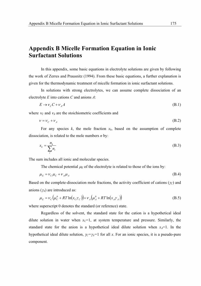
Appendix B Micelle Formation Equation in Ionic Surfactant Solutions 175
Appendix B Micelle Formation Equation in Ionic Surfactant Solutions
In this appendix, some basic equations in electrolyte solutions are given by following
the work of Zerres and Prausnitz (1994). From these basic equations, a further explanation is
given for the thermodynamic treatment of micelle formation in ionic surfactant solutions.
In solutions with strong electrolytes, we can assume complete dissociation of an
electrolyte E into cations C and anions A:
ACE AC (B.1)
where C and A are the stoichiometric coefficients and
AC (B.2)
For any species k, the mole fraction xk, based on the assumption of complete
dissociation, is related to the mole numbers n by:
l
l
kk
n
nx (B.3)
The sum includes all ionic and molecular species.
The chemical potential E of the electrolyte is related to those of the ions by:
AACCE (B.4)
Based on the complete-dissociation mole fractions, the activity coefficient of cations ( C) and
anions ( A) are introduced as:
AAAACCCCE xRTxRT lnln 00 (B.5)
where superscript 0 denotes the standard (or reference) state.
Regardless of the solvent, the standard state for the cation is a hypothetical ideal
dilute solution in water when xC=1, at system temperature and pressure. Similarly, the
standard state for the anion is a hypothetical ideal dilute solution when xA=1. In the
hypothetical ideal dilute solution, C= A=1 for all x. For an ionic species, it is a pseudo-pure
component.
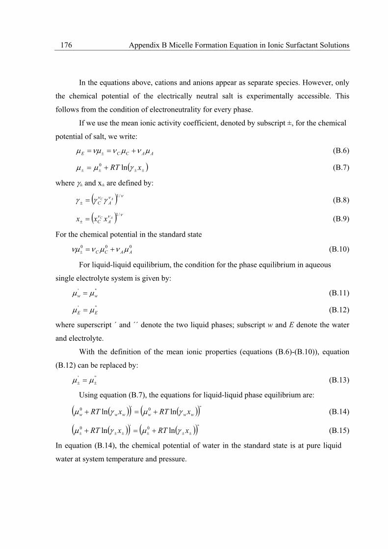
176 Appendix B Micelle Formation Equation in Ionic Surfactant Solutions
In the equations above, cations and anions appear as separate species. However, only
the chemical potential of the electrically neutral salt is experimentally accessible. This
follows from the condition of electroneutrality for every phase.
If we use the mean ionic activity coefficient, denoted by subscript ±, for the chemical
potential of salt, we write:
AACCE (B.6)
xRT ln0 (B.7)
where ± and x± are defined by:
/1AC
AC (B.8)
/1AC
AC xxx (B.9)
For the chemical potential in the standard state
000AACC (B.10)
For liquid-liquid equilibrium, the condition for the phase equilibrium in aqueous
single electrolyte system is given by:
'''ww (B.11)
'''EE (B.12)
where superscript ´ and ´´ denote the two liquid phases; subscript w and E denote the water
and electrolyte.
With the definition of the mean ionic properties (equations (B.6)-(B.10)), equation
(B.12) can be replaced by:
''' (B.13)
Using equation (B.7), the equations for liquid-liquid phase equilibrium are:
''0'0 lnln wwwwww xRTxRT (B.14)
''0'0 lnln xRTxRT (B.15)
In equation (B.14), the chemical potential of water in the standard state is at pure liquid
water at system temperature and pressure.
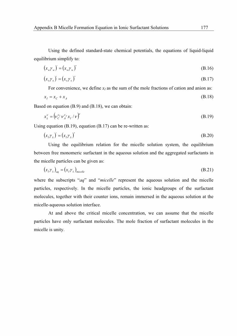
Appendix B Micelle Formation Equation in Ionic Surfactant Solutions 177
Using the defined standard-state chemical potentials, the equations of liquid-liquid
equilibrium simplify to:
'''
wwww xx (B.16)
'''xx (B.17)
For convenience, we define xI as the sum of the mole fractions of cation and anion as:
ACI xxx (B.18)
Based on equation (B.9) and (B.18), we can obtain:
/IAC xx AC (B.19)
Using equation (B.19), equation (B.17) can be re-written as:
'''
II xx (B.20)
Using the equilibrium relation for the micelle solution system, the equilibrium
between free monomeric surfactant in the aqueous solution and the aggregated surfactants in
the micelle particles can be given as:
micelleIaqI xx (B.21)
where the subscripts “aq” and “micelle” represent the aqueous solution and the micelle
particles, respectively. In the micelle particles, the ionic headgroups of the surfactant
molecules, together with their counter ions, remain immersed in the aqueous solution at the
micelle-aqueous solution interface.
At and above the critical micelle concentration, we can assume that the micelle
particles have only surfactant molecules. The mole fraction of surfactant molecules in the
micelle is unity.

178 Appendix B Micelle Formation Equation in Ionic Surfactant Solutions

Appendix C Evaluation of Pure Component Structural Parameters R and Q 179
Appendix C Van der Waals Parameters of Local Composition Models
This appendix is largely reported by the work of Abrams and Prausnitz (1975).
The structural parameters R and Q of UNIQUAC model are, respectively, the van der Waals
volume and area of the molecule relative to those of a standard segment.
ws
wkk
V
VR (C.1)
ws
wkk
A
AQ (C.2)
where Vwk and Awk are the van der Waals volume and area of the molecule given by Bondi
(1968), Vws and Aws are the van der Waals volume and area of a standard segment. The choice
of a standard segment is somewhat arbitrary. However, it is defined as a sphere such that for
a linear poly-methylene molecule of infinite length, the identity
12
RQRZ
(C.3)
is satisfied because Q/R=1.0 for the standard segment (monomer). The coordination number
Z is set equal to 10. The volume of the standard sphere in terms of its radius Rws is given by
3 3
4wsws RV (C.4)
and the area by
2 4 wsws RA (C.5)
The van der Waals volume and area of an n-mer of poly-methylene are n times the
volume and area of a methylene group as given by Bondi; that is
mole/cm10.23n 3wkV (C.6)
mole/cm101.35n 29wkA (C.7)
Substitution of equations (C.1), (C.2), and (C.4) to (C.7) into (C.3) yields:
12
10
ws
wk
ws
wk
ws
wk
V
V
A
A
V
V (C.8)

180 Appendix C Evaluation of Pure Component Structural Parameters R and Q
154ws
wk
ws
wk
A
A
V
V (C.9)
14
1035.15
3
423.10
42
9
3 wsws
R
n
R
n (C.10)
nRR ws
ws
1
4
1035.15
3
423.10
42
9
3
(C.11)
As n , 01
n and we obtain
2
9
3 4
1035.15
3
423.10
4ws
ws
RR
(C.12)
ecm/molecul1081867.1 8wsR
or cm/mole1010.95106.0231081867.1 15238wsR
Substitution the Rws value into equations (C.4) and (C.5) yields a standard segment volume
and area.
mole/cm 17.1510023.610818.13
4 32338wsV (C.13)
mole/cm10 50.210023.610818.14 292328wsA (C.14)
Equations (C.1) and (C.2) then become
17.15/wkk VR (C.15)
)105.2/( 9wkk AQ (C.16)
Equations (C.15) and (C.16) are the ones typically used in UNIQUAC and UNIFAC models.
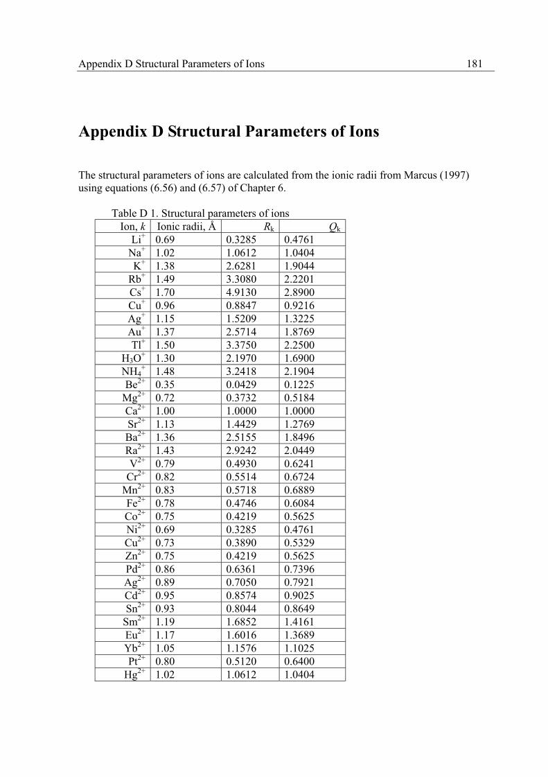
Appendix D Structural Parameters of Ions 181
Appendix D Structural Parameters of Ions The structural parameters of ions are calculated from the ionic radii from Marcus (1997) using equations (6.56) and (6.57) of Chapter 6. Table D 1. Structural parameters of ions
Ion, k Ionic radii, Å Rk Qk
Li+ 0.69 0.3285 0.4761 Na+ 1.02 1.0612 1.0404 K+ 1.38 2.6281 1.9044
Rb+ 1.49 3.3080 2.2201 Cs+ 1.70 4.9130 2.8900 Cu+ 0.96 0.8847 0.9216 Ag+ 1.15 1.5209 1.3225 Au+ 1.37 2.5714 1.8769 Tl+ 1.50 3.3750 2.2500
H3O+ 1.30 2.1970 1.6900
NH4+ 1.48 3.2418 2.1904
Be2+ 0.35 0.0429 0.1225 Mg2+ 0.72 0.3732 0.5184 Ca2+ 1.00 1.0000 1.0000 Sr2+ 1.13 1.4429 1.2769 Ba2+ 1.36 2.5155 1.8496 Ra2+ 1.43 2.9242 2.0449 V2+ 0.79 0.4930 0.6241
Cr2+ 0.82 0.5514 0.6724 Mn2+ 0.83 0.5718 0.6889 Fe2+ 0.78 0.4746 0.6084 Co2+ 0.75 0.4219 0.5625 Ni2+ 0.69 0.3285 0.4761 Cu2+ 0.73 0.3890 0.5329 Zn2+ 0.75 0.4219 0.5625 Pd2+ 0.86 0.6361 0.7396 Ag2+ 0.89 0.7050 0.7921 Cd2+ 0.95 0.8574 0.9025 Sn2+ 0.93 0.8044 0.8649
Sm2+ 1.19 1.6852 1.4161 Eu2+ 1.17 1.6016 1.3689 Yb2+ 1.05 1.1576 1.1025 Pt2+ 0.80 0.5120 0.6400
Hg2+ 1.02 1.0612 1.0404
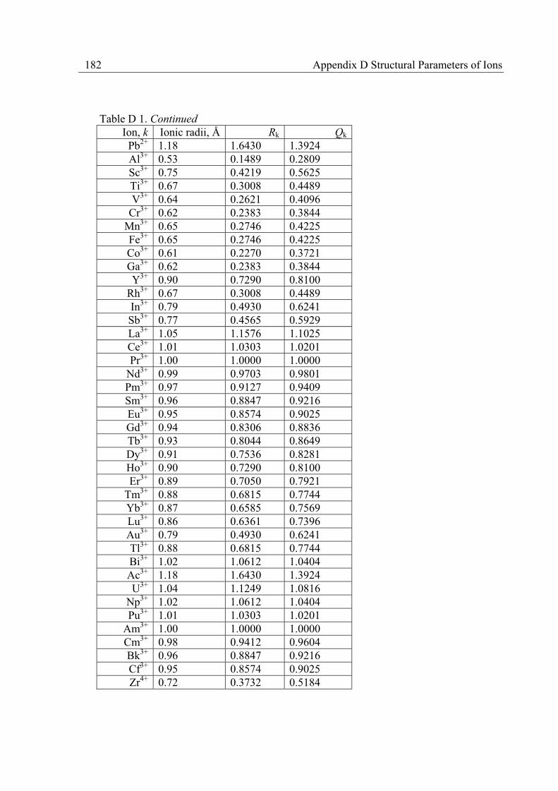
182 Appendix D Structural Parameters of Ions
Table D 1. Continued Ion, k Ionic radii, Å Rk Qk
Pb2+ 1.18 1.6430 1.3924 Al3+ 0.53 0.1489 0.2809 Sc3+ 0.75 0.4219 0.5625 Ti3+ 0.67 0.3008 0.4489 V3+ 0.64 0.2621 0.4096
Cr3+ 0.62 0.2383 0.3844 Mn3+ 0.65 0.2746 0.4225 Fe3+ 0.65 0.2746 0.4225 Co3+ 0.61 0.2270 0.3721 Ga3+ 0.62 0.2383 0.3844 Y3+ 0.90 0.7290 0.8100
Rh3+ 0.67 0.3008 0.4489 In3+ 0.79 0.4930 0.6241 Sb3+ 0.77 0.4565 0.5929 La3+ 1.05 1.1576 1.1025 Ce3+ 1.01 1.0303 1.0201 Pr3+ 1.00 1.0000 1.0000
Nd3+ 0.99 0.9703 0.9801 Pm3+ 0.97 0.9127 0.9409 Sm3+ 0.96 0.8847 0.9216 Eu3+ 0.95 0.8574 0.9025 Gd3+ 0.94 0.8306 0.8836 Tb3+ 0.93 0.8044 0.8649 Dy3+ 0.91 0.7536 0.8281 Ho3+ 0.90 0.7290 0.8100 Er3+ 0.89 0.7050 0.7921
Tm3+ 0.88 0.6815 0.7744 Yb3+ 0.87 0.6585 0.7569 Lu3+ 0.86 0.6361 0.7396 Au3+ 0.79 0.4930 0.6241 Tl3+ 0.88 0.6815 0.7744 Bi3+ 1.02 1.0612 1.0404 Ac3+ 1.18 1.6430 1.3924 U3+ 1.04 1.1249 1.0816
Np3+ 1.02 1.0612 1.0404 Pu3+ 1.01 1.0303 1.0201
Am3+ 1.00 1.0000 1.0000 Cm3+ 0.98 0.9412 0.9604 Bk3+ 0.96 0.8847 0.9216 Cf3+ 0.95 0.8574 0.9025 Zr4+ 0.72 0.3732 0.5184
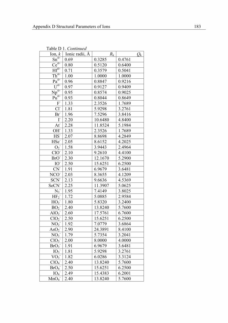
Appendix D Structural Parameters of Ions 183
Table D 1. Continued Ion, k Ionic radii, Å Rk Qk
Sn4+ 0.69 0.3285 0.4761 Ce4+ 0.80 0.5120 0.6400 Hf4+ 0.71 0.3579 0.5041 Th4+ 1.00 1.0000 1.0000 Pa4+ 0.96 0.8847 0.9216 U4+ 0.97 0.9127 0.9409
Np4+ 0.95 0.8574 0.9025 Pu4+ 0.93 0.8044 0.8649
F- 1.33 2.3526 1.7689 Cl- 1.81 5.9298 3.2761 Br- 1.96 7.5296 3.8416
I- 2.20 10.6480 4.8400 At- 2.28 11.8524 5.1984
OH- 1.33 2.3526 1.7689 HS- 2.07 8.8698 4.2849
HSe- 2.05 8.6152 4.2025 O2
- 1.58 3.9443 2.4964 ClO- 2.10 9.2610 4.4100 BrO- 2.30 12.1670 5.2900
IO- 2.50 15.6251 6.2500 CN- 1.91 6.9679 3.6481
NCO- 2.03 8.3655 4.1209 SCN- 2.13 9.6636 4.5369
SeCN- 2.25 11.3907 5.0625 N3
- 1.95 7.4149 3.8025 HF2
- 1.72 5.0885 2.9584 HO2
- 1.80 5.8320 3.2400 BO2
- 2.40 13.8240 5.7600 AlO2
- 2.60 17.5761 6.7600 ClO2
- 2.50 15.6251 6.2500 NO2
- 1.92 7.0779 3.6864 AsO2
- 2.90 24.3891 8.4100 NO3
- 1.79 5.7354 3.2041 ClO3
- 2.00 8.0000 4.0000 BrO3
- 1.91 6.9679 3.6481 IO3
- 1.81 5.9298 3.2761 VO3
- 1.82 6.0286 3.3124 ClO4
- 2.40 13.8240 5.7600 BrO4
- 2.50 15.6251 6.2500 IO4
- 2.49 15.4383 6.2001 MnO4
- 2.40 13.8240 5.7600

184 Appendix D Structural Parameters of Ions
Table D 1. Continued Ion, k Ionic radii, Å Rk Qk
TcO4- 2.50 15.6251 6.2500
ReO4- 2.60 17.5761 6.7600
BH4- 1.93 7.1891 3.7249
BF4- 2.30 12.1670 5.2900
B(OH)4- 2.30 12.1670 5.2900
Al(OH)4 - 2.90 24.3891 8.4100
HCO2- 2.04 8.4897 4.1616
HCO3- 1.56 3.7964 2.4336
HSO3- 1.70 4.9130 2.8900
HseO3- 2.10 9.2610 4.4100
HSO4- 1.90 6.8590 3.6100
HseO4- 2.10 9.2610 4.4100
H2PO4- 2.00 8.0000 4.0000
O2- 1.40 2.7440 1.9600 S2- 1.84 6.2295 3.3856
Se2- 1.98 7.7624 3.9204 Te2- 2.21 10.7939 4.8841 O2
2- 1.73 5.1777 2.9929 S2
2- 2.80 21.9521 7.8400 CO3
2- 1.78 5.6398 3.1684 C2O4
2- 2.10 9.2610 4.4100 SiO3
2- 2.14 9.8004 4.5796 SO3
2- 2.00 8.0000 4.0000 SeO3
2- 2.39 13.6520 5.7121 TeO3
2- 2.50 15.6251 6.2500 SO4
2- 2.30 12.1670 5.2900 SeO4
2- 2.43 14.3490 5.9049 TeO4
2- 2.60 17.5761 6.7600 CrO4
2- 2.40 13.8240 5.7600 MoO4
2- 2.54 16.3871 6.4516 WO4
2- 2.70 19.6831 7.2900 MnO4
2- 2.50 15.6251 6.2500 S2O3
2- 2.50 15.6251 6.2500 S2O4
2- 2.60 17.5761 6.7600 S2O6
2- 2.80 21.9521 7.8400 S4O6
2- 3.10 29.7911 9.6100 S2O8
2- 2.90 24.3891 8.4100 HPO4
2- 2.00 8.0000 4.0000 SiF6
2- 2.59 17.3740 6.7081 PO4
3- 2.38 13.4813 5.6644

References 185
References Abrams D. S. and J. M. Prausnitz, “Statistical Thermodynamics of Liquid Mixture: A New Expression for the Excess Gibbs Energy of Partly or Completely Miscible Systems,” AIChE J. 21, 116 (1975). ACD/LogP, version 4.5, Advanced Chemistry Development, Inc. (2003). webpage: www.acdlabs.com. Achard C., C. G. Dussap, and J. B. Gros, “Application of a Group-contribution Method to Biological Systems: Prediction of Water Activity, pH, and related Properties,” Computers &
Chemical Engineering, 17, Suppl, S159 (1993). Achard C., C. G. Dussap, and J. B. Gros, “Prediction of pH in Complex Aqueous Mixtures Using a Group-contribution Method,” AIChE J., 40, 1210 (1994a). Achard C., C. G. Dussap, and J. B. Gros, “Representation of Vapor-Liquid Equilibria in Water-alcohol-electrolyte Mixture with a Modified UNIFAC Group-contribution Method,” Fluid Phase Equilibria, 98, 71 (1994b). AMI report, “Review of the Knowledge Basis of Risk Evaluation of Air Pollutions in Relation to Lung Cancer and Respiratory System Allergy,” Center for Environmental and Respiratory System, National Institute of Occupational Health, Denmark, (2000) (in Danish). Amos, D. A., L. Scott, and C. J. Radke, “A Self-Consistent Multicomponenet Activity Coefficient Model for Ionic Micellar Surfactant Solutions,” Langmuir, 14, 2297 (1998). Anderson, T. F., and J. M. Prausnitz, “Application of the UNIQUAC Equation to Calculation of Multicomponent Phase Equilibria. 1. Vapor-Liquid Equilibria,” Ind. Eng. Chem. Process
Des. Dev., 17, 553 (1978). Barakat, Y., T. S. Gendy, I. K. Basily, and A. I. Mohamad “Polymeric Surfactants for Enhanced Oil Recovery. Part II- the HLB-CMC Relationship of Ethoxylated Alkylphenol-Formaldehyde Polymeric Surfactants,” British Polymer Journal, 21, 451 (1989). Becher, P., “Macromulsions,” in Schick, M. J., Nonionic Surfactants- Physical Chemistry, Marcel Dekker, New York, 1987. Bergen, V. R., and E. Rogel, “A Lattice Fluid Approach to the Concept of Hydrophile Lipophile Balance: Alkylethoxylated Surfactants,” Fluid Phase Equilibria, 153, 63 (1998).

186 References
Birdi, K. S. Self-assembly Monolayer Structures of Lipids and Macromolecules at Interfaces, Kluwer Academic / Plenum Publishers, New York, 1999, p336. Blandamer, M. J., P. M. Cullis, L. G. Soldi, J. B. F. N. Engberts, A. Kacperska, N. M. van Os, and M. C. S. Subha, “Thermodynamics of Micellar Systems: Comparison of Mass Action and Phase Equilibrium Models for the Calculation of Standard Gibbs Energies of Micelle Formation,” Adv. Colloid Interface Sci. 58, 171 (1995). Blankschtein, D., A. Shiloach, and N. Zoeller, “Thermodynamic Theories of Micelle and Vesicular Systems,” Current Opinion in Colloid & Interface Science, 2, 294 (1997). Blankschtein, D., G. M. Thurston, Benedek, G. B. “Phenomenological Theroy of Equilibrium Thermodynamic Properties and Phase Separation of Micellar Solutions,” J. Chem. Phys., 85, 7268 (1986). Bondi, A., Physical Properties of Molecular Crystals, Liquids and Glasses, Wiley, New York, (1968). Brandrup, J., and E. H. Immergut, Polymer Handbook, 2nd ed., Wiley, New York, pII483-497 (1975). Buchwald, P., and N. Bodor, “Octanol-Water Partition: Searching for Predictive Models,” Current Medicinal Chemistry, 5, 353 (1998). Burchfield, T. E., and E. M. Woolley, “Model for Thermodynamics of Ionic Surfactant Solutions: 1. Osmotic and Activity Coefficients,” J. of Phys. Chem., 88, 2149 (1984). Carroll, B. J., “Physical Aspects of Detergency,” Colloids Surfaces A: Phys. Eng. Asp. 74, 131 (1993). Chen, C.-C., H. I. Britt, J. F. Boston, and L. B. Evans, “Local Composition Model for Excess Gibbs Energy of Electrolyte Systems,” AIChE J., 28, 588 (1982). Chen, C.-C., and L. B. Evans, “A Local Composition Model for Excess Gibbs Energy of Aqueous Electrolyte Systems,” AIChE J., 32, 444 (1986). Chen, C.-C., “A Segment-Based Local Composition Model for the Gibbs Energy of Polymer Solutions,” Fluid Phase Equilibria, 83, 301 (1993). Chen, C.-C., “Molecular Thermodynamic Model Based on the Polymer NRTL Model for Nonionic Surfactant Solutions,” AIChE J., 42, 3231 (1996). Chen, C.-C., P. M., Mathias, and H. Orbey, “Use of Hydration and Dissociation Chemistries with the Electrolyte-NRTL Model,” AIChE J., 45, 1576 (1999).
References 187
Chen, C.-C., C. P. Bokis, and P. Mathias, “Segment-Based Excess Gibbs Energy Model for Aqueous Organic Electrolytes,” AIChE J., 47, 2593 (2001). Chen, F., J. H. Andersen, and H. Tyle, “New Developments of the UNIFAC Model for Environmental Application,” Chemosphere, 26, 1325 (1993). Cheng, H. Y., G. M. Kontogeorgis, and E. H. Stenby, “Prediction of Micelle Formation for Non-ionic Surfactants through UNIFAC Method,” Ind. Eng. Chem. Res., 41, 892 (2002). Chernik, G. G. “Phase Studies of Surfactant-Water Systems,” Current Opinion in colloid &
Interface Science, 4, 381 (2000). Christensen, C., “A New Model for Liquids Containing Strong Electrolytes, An Excess Enthalpy Data Collection,” Ph.D. Thesis, Department of Chemical Engineering, Technical University of Denmark, Lyngby, Denmark, (1983a). Christensen, C., B. Sander, A. Fredenslund, and P. Rasmussen, “Towards the Extension of UNIFAC to Mixtures with Electrolytes,” Fluid Phase Equilibria, 13, 297 (1983b). Cistola, D. P., and D. M. Small, “On Micelle Formation and Phase Separation,” J. Am. Chem.
Soc., 112, 3214 (1990). ClogP, Daylight Chemical Information systems, Inc. (2003), webpage: www.daylight.com. Cox, K. R., and H. L. Benson, “The Pseudo-phase Analogy: Application of Vapor-Liquid Equilibria Techniques to Micelle Solution,” Fluid Phase Equilibria, 30, 173 (1986). Cruz, J.-L., and H. Renon, “A New Thermodynamic Representation of Binary Electrolyte Solutions Nonideality in the Whole Range of Concentrations,” AIChE J., 24, 817 (1978). D’Arrigo, G., F. Mallamace, N. Micali, A. Paparelli, and C. Vasi, “Molecular Aggregations in Water-2-butoxyethanol Mixtures by Ultrasonic and Brillouin Light-scattering Measurements,” Physical Review A, 44, 2578 (1991). Davies, J. T., and E. K. Rideal, Interface Phenomena, Academic Press, New York, (1963), pp. 371-383. de Guertechin, L. O. “Surfactants: Classification” in G Broze (Ed.), Handbook of detergents
A, Properties, New York, N.Y. Dekker 1999. Dearden, L. V., and E. M. Woolley, “Osmotic Coefficients and Enthalpies of Dilution of Aqueous Sodium n-Alkane-1-sulphonates at the Temperatures (298.15, 313.15, 328.15, and 343.15) K,” J. Chem. Thermodynamics, 28, 1283 (1996).

188 References
Derawi, S. O., G. M. Kontogeorgis, and E. H. Stenby, “Application of Group Contribution Models to the Calculation of the Octanol-Water Partition Coefficient,” Ind. Eng. Chem. Res., 40, 434 (2001). Desnoyers, J. E., and G. Perron, “Thermodynamic Properties of Surfactant Solutions” in K.S. Birdi, (Ed.), Handbook of Surface and Colloid Chemistry, CRC Press, Boca Raton, (1997). Donohue, M. D., and J. M. Prausnitz, “Combinatorial Entropy of Mixing Molecules that Differ in Size and Shape-A Simple Approximation for Binary and Multicomponent Mixtures,” Can. J. Chem., 53, 1586 (1975). Douheret, G., and A. Viallard, “Activity Coefficients and Micellar Equilibria. I. the Mass Action Law Model Applied to Aqueous Solutions of Sodium Carboxylates at 298.15 K,” Fluid Phase Equilibria, 8, 233 (1982). Ellington, J. J., “Octanol/Water Partition Coefficients and Water Solubilities of Phthalate Esters,” J. Chem. Eng. Data, 44, 1414 (1999). Enders, S., and D. Häntzschel, “Thermodynamics of Aqueous Carbohydrate Surfactant Solutions,” Fluid Phase Equilibria, 153, 1 (1998). Fletcher, R. Practical Methods of Optimization, Wiley, New York, (1980). Flores, M. V., E. C. Voutsas, N. Spiliotis, G. M. Eccleston, G. Bell, D. P. Tassios, and P. J. Halling, “Critical Micelle Concentrations of Non-ionic Surfactants in Organic Solvents: Approximate Prediction with UNIFAC,” Journal of Colloid and Interface Science, 240, 277 (2001). Floriano, M. A., E. Cponetti, and A. Z. Panagiotopoulos, “Micellization in Model Surfactant Systems,” Langmuir, 15, 3143 (1999). Fontell, K., “Some Aspects on the Cubic Phases in Surfactant and Surfactant-like Lipid Systems,” Adv. Colloid Interface Sci., 41, 127 (1992). Fredenslund, A., R. L. Jones, and J. M. Prausnitz, “Group Contribution Estimation of Activity Coefficients in Nonideal Liquid Mixtures,” AIChE J., 21, 1086 (1975). Fredenslund, A., J. Gmehling, and P. Rasmussen, Vapor-Liquid Equilibria Using UNIFAC-a
Group-Contribution Method, Elsevier: Amsterdam, (1977). Fredenslund, A., P. Rasmussen, and M. L. Michelsen, “Recent Progress in The Computation of Equilibrium Ratios,” Chem. Eng. Commun., 4, 485 (1980).
References 189
Garcia-Lisbona, M. N., A. Galindo, G. Jackson, and A. N. Burgess, “An Examination of the Cloud curves of Liquid-Liquid Immiscibility in Aqueous Solutions of Alkyl Polyoxyethylene Surfactants Using the SAFT-HS Approach with Transferable parameters,” J. Am. Chem. Soc. 120, 4191 (1998). Garidel, P., A. Hildebrand, R. Neubert, and A. Blume, “Thermodynamic Characterization of Bile Salt Aggregation as a Function of Temperature and Ionic Strength Using Isothermal Titration Calorimetry,” Langmuir, 16, 5267 (2000). Gerrens, H., and G. Hirsch, “Critical Micelle Concentration” in Brandrup, J., and E.H. Immergut (Ed.) Polymer Handbook , John Wiley & Sons, New York (1975). Goldberg, R.N., “Evaluated Activity and Osmotic Coefficients for Aqueous Solutions: bi-Univalent Compounds of Zinc, Cadmium, and Ethylene bis (trimethylammonium) Chloride and Iodide,” J. Phys. Chem. Ref. Data, 10, 1 (1981). Grieser, F., and C. J. Drummond, “Physicochemical properties of self-assembled surfactant aggregates as determined by some molecular spectroscopic probe techniques,” Journal of
Physical Chemistry, 92, 5580 (1988). Gu, T., and J. Sjöblem, “Surfactant Structure and its Relation to the Krafft Point, Cloud Point and Micellization: Some empirical Relationships,” Colloids and Surface, 64, 39 (1992). Hall, D. G., “Thermodynamics of Micelle Formation,” in Schick, M. J. (Ed.), Nonionic
Surfactants, Marcel Dekker, New York, p233 (1987). Hamer, W.J., and Y.-C. Wu, “Osmotic Coefficients and Mean Activity Coefficients of Uni-univalent Electrolytes in Water at 25ºC,” J. Phys. Chem. Ref. Data, 1, 1047 (1972). Hansch, C., A. Leo, and D. Hoekman, Exploring QSAR: Fundamentals and Applications in
Chemistry and Biology, American Chemical Society: Washington, DC, (1995). Hansen, H. K., P. Rasmussen, A. Fredenslund, M. Schiller, and J. Gmehling, “Vapor-Lquid Equilibria by UNIFAC Group Contribution 5. Revision and Extension,” Ind. Eng. Chem. Res., 30, 2352 (1991). Hansen, H. K., B. Coto, and B. Kuhlmann, UNIFAC with Linearly Temperature-dependent
Group Interaction Parameters. SEP 9212 (Internal Report); Department of Chemical Engineering, Technical University of Denmark, Lyngby, Denmark, (1992). Hines, J. D., “Theoretical Aspects of Micelllisation in Surfactant Mixtures,” Current Opinion
in Colloid & Interface Science, 6, 350 (2001). Hinz, H.-J. ed., Thermodynamic Data for Biochemistry and Biotechnology, Springer-Verlag: Berlin, (1986).
190 References
Hoffmann, H., and W. Ulbricht, “The Formation of Micelles” in Hinz, H.-J. (Ed.), Thermodynamic Data for Biochemistry and Biotechnology, Springer-Verlag, Berlin, (1986). Holmes, M. C., “Intermediate phases of surfactant-water mixtures,” Curr. Opin. Colloid
Interface Sci., 3, 485 (1998). Holland, P. M., “Nonideal Mixed Micellar Solutions,” Advances in Colloid and Interface
Science, 26, 111 (1986). Holland, P. M., and D. N. Rubingh, “Mixed Surfactant Systems, An Overview,” in Mixed
Surfactant Systems, ACS Symposium Series 501, ACS, Washington, DC (1992). Horstmann, S., K. Fischer, and J. Gmehling, “PSRK Group Contribution Equation of State: Revision and Extension III.,” Fluid Phase Equilib., 167, 173 (2000). Huibers, P. D. T., “Surfactant Self-assembly, Kinetics and Thermodynamics of Micellar and Microemulsion System”, Ph.D. Dissertation, Department of Chemical Engineering, University of Florida, Gainesville, Florida (1996a). Huibers, P. D. T., V. S. Lobanov, A. R. Katritzky, D. O. Shah, and M. Karelson, “Prediction of Critical Micelle Concentration Using a Quantitative Structure-Property Relationship Approach 1.Nonionic Surfactants,” Langmuir, 12, 1462 (1996b). Huibers, P. D. T., V. S. Lobanov, A. R. Katritzky, D. O. Shah, and M. Karelson, “Prediction of Critical Micelle Concentration Using a Quantitative Structure-Property Relationship Approach 2. Anionic Surfactants,” J. of Colloid and Interface Science, 187, 113 (1997a). Huibers, P. D. T., and A. R. Katrizky, “Predicting Surfactant Cloud Point from Molecular Structure,” J. Colloid & Interface Science, 193, 132 (1997b). Israelachvili, J. N., Intermolecular and Surface Forces 2nd ed., Chapter 16, 17, Academic Press, London (1992). IVC-SEP, The IVC-SEP Data Bank for Electrolyte Solutions, IVC-SEP, Department of Chemical Engineering, Technical University of Denmark, Lyngby, Denmark (2003). Jackson, G., and J. S. Rowlinson “Phase Equilibria in Model Mixtures of Spherical Molecules of Different Sizes,” J. Chem. Soc. Faraday Trans. 1, 82, 3461 (1986). Kehiaian, H. V., and M.R. Tine, “Thermodynamics of Binary Mixtures Containing Oxaalkanes Parts. Monoethers, Plolyethers, Acetals, Orthoesters and Cyclic Monoethers+n-Alkanes or Cyclohexane,” Fluid Phase Equilib., 46, 131 (1989). Khan, A. “Phase Science of Surfactants,” Current Opinion in colloid & Interface Science, 6, 121 (1986).
References 191
Kikic, I., M. Fermeglia, and P. Rasmussen, “UNIFAC Prediction of Vapor-Liquid Equilibria in Mixed Solvent-Salt Systems,” Chemical Engineering Science, 46, 2775 (1991). Kikic, I., P. Alessi, P. Rasmussen, and Aa. Fredenslund, “On the Combinatorial Part of the UNIFAC and UNIQUAC Models,” Can. J. of Chem. Eng., 58, 253 (1990). Kortuem, G., and V. Valent, “Thermodynamic Mixing Effect in the Water(1)-1,4-dioxane(2) and Methanol(1)-1,4-dioxane(2) Systems; A Comparision,” Ber. Bunsen-Ges. Phys. Chem., 81, 752 (1977). KowWin, Syracuse Research Corporation, (2001). Webpage: esc.syrres.com. Kuramochi, H., H. Noritomi, D. Hoshino, K. Nagahama, “Representation of Activity Coefficients of Fundamental Biochemicals in Water by the UNIFAC Model,” Fluid Phase Equilibria, 130, 117 (1997). Lai, H.-H., and L.-J. Chen, “Liquid-Liquid Equilibrium Phase Diagram and Density of Three Water + Nonionic Surfactant CiEj Binary Systems,” J. Chem. Eng. Data, 44, 251 (1999). Laidler, K. J., and J. H. Meiser Physical Chemistry, Houghton Mifflin Company, Boston, (1999). Lantzsch, G., H. binder, H. Heerklotz, M. Wendling, G. Klose, “Surface Areas and Packing Constraints in POPC/C12EOn membranes. A Time-resolved Fluorescence Study,” Biophysical Chemistry, 58, 289 (1996). Larsen, B. L., P. Rasmussen, and A. Fredenslund, “A Modified UNIFAC Group Contribution Modle for Prediction of Phase Equilibria and Heats of Mixing,” Ind. Eng. Chem. Res., 26, 2274 (1987). Larsen, B. L., “Predictions of Phase Equilibria and Heat effects of Mixing with a modified UNIFAC Model,” Ph.D. Thesis, Department of Chemical Engineering, Technical University of Denmark, Lyngby, Denmark, (1986). Laughlin, R. G. The Aqueous Phase Behaviours of Surfactants, Academic Press, London (1994). Leo, A., and D. Weininger, CLOGP Reference Manual, Daylight Chemical Information Systems, Inc., Daylight Version 4.82 (2003) Li, J., H. M. Polka, and J. Gmehling, “A gE Model for Single and Mixed Solvent Electrolyte Systems,” Fluid Phase Equilibria, 94, 89 (1994). Li, S.X., J. F. Lu, Y. G. Li, and J. C. Liu, “Studies on UNIQUAC and SAFT Equations for Nonionic Surfactant Solutions,” Fluid Phase Equilibria, 153, 215 (1998).

192 References
Li, S.X., J. F. Lu, Y. G. Li, “Study on Ionic Surfactant Solutions by SAFT Equation Incorporated with MSA,” Fluid Phase Equilibria, 168, 107 (2000). Lide D. R. CRC Handbook of Chemistry and Physics, 83rd Edition, CRC Press, Boca Raton, 2002. Lin, I. J., and L. Marszall, “CMC, HLB, and Effective Chain Length of Surface-Active Anionic and Cationic Substances Containing Oxyethylene Groups,” J. Colloid & Interface
Sci., 57, 1 (1976). Lin, I. J., and L. Marszall, “The Effective Chain Length of Polyoxypropylated Ionic and Nonionic Surfactants,” Tenside Deterg., 14, 131 (1977). Lin, S-T, and S. I. Sandler, “Prediction of Octanol-Water Partition Coefficients Using a Group Contribution Solvation Model,” Ind. Eng. Chem. Res., 38, 4081 (1999). Lin, S-T, and S. I. Sandler, “Multipole Corrections to Account for Structure and Proximity Effects in Group Contribution Methods: Octanol-Water Partition Coefficients,” J. Phys. Chem. A, 104, 7099 (2000). Lindgren, A., and M. Sjostrom, “Multivariate Physicochemical Characterisation of Some Technical Non-ionic Surfactants,” Chemometrics and Intelligent Laboratory Systems, 23, 179 (1994). Loehe, J. R., and M. D. Donohue, “Recent Advances in Modelling Thermodynamic Properties of Aqueous Strong Electrolyte Systems,” AIChE J. 43, 180 (1997). Lu, X-H, and G. Maurer, “Model for Describing Activity Coefficients in Mixed Electrolyte Aqueous Solutions,” AIChE J., 39, 1527 (1993). Lu, X., L. Zhang, Y. Wang, J. Shi, and G. Maurer, “Prediction of Activity Coefficients of Electrolytes in Aqueous Solutions at High Temperature,” Ind. Eng. Chem. Res., 35, 1777 (1996). Lyman, W. J., W. F. Reehl, and D. H. Rosenblatt, Handbook of Chemical Property Estimation Methods, McGraw-Hill, New York, (1982). Macedo, E.A., P. Skovborg, and P. Rasmussen “Calculation of Phase Equilibria for Solutions of Strong Electrolytes in Solvent-Water Mixtures,” Chemical Engineering Science, 14, 875 (1990). Madsen, T., H. B. Boyd, D. Nylén, A. R. Pedersen, G. I. Petersen and F. Simonsen, “Environmental and Health Assessment of Substances in Household Detergents and Cosmetic Detergent Products,” Environmental Project No. 615, Danish Environmental Protection Agency (www.mst.dk), Copenhagen, (2001).

References 193
Magnussen, T., P. Rasmussen, and A. Fredenslund, “UNIFAC Parameters Table for Prediction of Liquid – Liquid Equilibria,” Ind. Eng. Chem. Process Des. Dev., 20, 133 (1981). Marcus, Y., “Ionic Radii in Aqueous Solutions,” Chemical Reviews, 88, 1475 (1988). Marcus, Y., Ion Properties, Marcel Dekker, Inc., New York, (1997). Marszall, L., “HLB of Nonionic surfactants: PIT and EIP Methods,” in Schick, M. J., Nonionic Surfactants- Physical Chemistry, Marcel Dekker, New York, 1987. Maurer, G., and J. M. Prausnitz, “On the Derivation and Extension of the UNIQUAC Equation,” Fluid Phase Equilibria, 2, 91 (1978). Marsh, K. N., J. B. Ott, and M. J. Costigan, “Excess Enthalpies, Excess Volumes, and Excess Gibbs Free Energies for n-Hexane + Di-n-Butyl Ether at 298.15 and 308.15 K,” J. Chem.
Thermodyn., 12, 857 (1980). Marsh, K. N., P. Niamskul, J. Gmehling, and R. Bölts, “Review of Thermophysical Property Measurements on Mixtures Conaining MTBE, TAME, and Other Ethers with Non-polar Solvents,” Fluid Phase Equilib., 156, 207 (1999). McBain, J. W., and R. C. Swain, “Measurements of Adsorption at the Air-Water Interface by the Microtome Method,” Proc. Roy. Soc. (London), A154, 608 (1936). McGinnis, T. P., and E. M. Woolley, “Thermodynamic properties of aqueous 1-n-alkanepyridinium chlorides at temperatures from 283.15 K to 343.15 K,” Journal of
Chemical Thermodynamics, 29, 401 (1997). Meylan, W.M., and P. H. Howard, “Atom/fragment Contritution Method for Estimating Octanol-Water Partition Coefficients,” J. Pharm. Sci., 84, 83 (1995). Miller, C. A., and K. H. Raney, “Solubilization-emulsification Mechanism of Detergency,” Colloids Surfaces A: Phys. Eng. Asp., 74, 169 (1993). Morral, S.W., P. P. Herzog, P. Kloepper-Sams, and M. J. Rosen, “Octanol/Water Partitioning of Surfactants and its Relevance to Toxicity and Environmental Behaviour,” Special
Publications of the Royal Society of Chemistry, 189, 220 (1996). Morse, P. M. “Soaps & Detergents”, Chemical & Engineering News, 77, 35, Feb. 1, (1999) Mukerjee, P., and K. J. Mysels, Critical Micelle Concentrations of Aqueous Surfactant
Systems; Nat. Stand. Ref. Data Ser. Nat. Bur. Stand., 36 (1971).
194 References
Müller, M. T., A. J. B. Zehnder, and B. I. Escher, “Liposome-Water and Octanol-Water Partitioning of Alcohol Ethoxylates,” Environmental Toxicology and Chemistry, 18, 2191 (1999). Murphy, A., and G. Taggart, “A Comparison of Predicted and Experimental Critical Micelle Concentration Values of Cationic and Anionic Ternary Surfactant Mixtures using molecular-thermodynamic Theory and Pseudophase Separation Theory,” Colloids and Surfaces A:
Physicochemical and Engineering Aspects, 205, 237 (2002). Nagarajan, R., and E. Ruckenstein, “Theory of Surfactant Self-Assembly: A Predictive Molecular Thermodynamic Approach,” Langmuir, 7, 2934 (1991). Nagarajan, R., “Micellization of binary surfactant mixtures: Theory,” in Holland, P. M., and D. N. Rubingh, (Ed.), Mixed Surfactant Systems, ACS Symposium Series 501, ACS, Washington, DC, (1992) p54. Nagarajan, R., “Theory of Micelle Formation: Quantitative Approach to Predicting Micellar properties from Surfactant Molecular Structure,” in Esumi, K., and M. Ueno (Ed.), Structure-
Performance Relationships in Surfactants, Marcel Dekker, Inc. New York, p1, (1997a). Nagarajan, R., “Solubilization by Amphiphilar Aggregates,” Current Opinion in Colloid &
Interface Science, 2, 282 (1997b). Nagata, I., and K. Katoh, “Effective UNIQUAC Equation in Phase Equilibrium Calculation,” Fluid Phase Equilibria, 5, 225 (1980). Nicolaisen, H., R. Rasmussen, and J. M. Sørensen, “Correlation and Prediction of Mineral Solubilities in the Reciprocal Salt System (Na+, K+) (Cl-, SO4
2-)-H2O at 0-100ºC,” Chemical
Engineering Science, 48, 3149 (1993). Nibu, Y., and T. Inoue, “Phase behaviour of Aqueous Mixtures of Some Polyethylene Glycol Decyl Ethers Revealed by DSC and FT-IR Measurements,” J. of Colloid and Interface
Science, 205, 305 (1998). van Os, N. M., J. R. Haak, and L. A. M. Rupert, Physical-Chemical Properties of Selected Anionic, Cationic and Nonionic Surfactants, Elsevier, Amsterdam, (1993). Ogion, K., and M. Abe, (Ed.), Mixed Surfactants Systems, Marcel Dekker, New York (1992). Paula, S., W. Süs, J. Tuchtenhagen, and A. Blume, “Thermodynamics of Micelle formation as a Function of Temperature: A high Sensitivity Titration Calorimetry Study,” J. Phys.
Chem., 99, 11742 (1995).
References 195
Pérez-Rodriguez, M., L. M. Varela, M. Garcia, V. Mosquera, and F. Sarmiento, “Conductivity and Relative Permittivity of Sodium n-Dodecyl Sulfate and n-Dodecyl Trimethylammonium Bromide,” J. Chem. Eng. Data, 44, 944 (1999). Pitzer, K. S., “Thermodynamics of Electrolytes. I. Theoretical Basis and General Equations,” J. Phys. Chem., 77, 268 (1973). Pitzer, K. S., “Thermodynamics of Electrolytes. II. Activity and Osmotic Coefficients for Strong Electrolytes with One or Both Ions Univalent,” J. Phys. Chem., 77, 2300 (1973). Pitzer, K. S., “Electrolytes: From Dilute Solutions to Fused Salts,” J. of Am. Chem. Soc. 102, 2902 (1980). Pitzer, K. S. (Ed.), Activity Coefficients in Electrolytes Solutions, 2nd Ed. Boca Raton: CRC Press, (1991). Pitzer, K. S., Thermodynamics, 3rd Ed., McGraw-Hill, Inc., New York (1995). Porter, M. R., “The Handbook of Surfactant”, 2nd Ed. Chapman & Hall, (1994). Prausnitz, J. M., R. N. Lichtenthaler, and E. G. de Azevedo, Molecular Thermodynamics of
Fluid-Phase Equilibria, 3rd Ed., Prentice Hall PTR, New Jersey, (1999). Puvvada, S., and D. Blankschtein, “Molecular Thermodynamic Approach to Predict Micellization, Phase Behavior and Phase Separation of Micellar Solutions. I. Application to Nonionic Surfactants,” J. Chem. Phys., 92, 3710 (1990). Rasmussen, D., and P. Rasmussen, “Phase Equilibria in Aqueous Polymer Solutions,” Chem.
Eng. Prog., 85, 50 (1989). Robinson, R. A., and R. H. Stokes, Electrolyte Solutions, 2nd Ed. Butterworth, London, (1965). Rosen, M. J. (Ed.), Structure/Performance Relationship in Surfactants, ACS Symposium series 253, ACS, Washington, DC (1984). Rosen, M. J., Surfactants and Interfacial Phenomena, 2nd ed., Wiely: NewYork, (1989). Rubingh D. N., “Mixed Micelle Solutions,” in: Mittal K. L. editor, Solution Chemistry of
Surfactants, Plenum Press, New York (1979). Rubingh, D.N., and P. M. Holland, (Eds.), Cationic Surfactants-Physical Chemistry, Marcel Dekker, New York (1990).

196 References
Rudolph, E. S. J., J. H. Langeveld, Th. W. de Loos, J. de Swaan Arons, “Phase Behaviour of Water + Non-ionic Surfactant Systems: experiments and Modelling Applying the Peng-Robinson Equation of State with the Wong-Sandler Mixing Rules and the UNIQUAC g
E- Model,” Fluid Phase Equilibria, 173, 81 (2000). Rusanov, A. I., “Thermodynamic Functions of Micelle Formation in a Quasichemical Model,” Colloid Journal of the USSR, 50, 513 (1988). Translated from Kolloidnyi Zhurnal. Sander, B., “Extended UNIFAC/UNIQUAC Models for (1) Gas Solubilities and (2) Electrolyte Solutions,” Ph.D. Thesis, Department of Chemical Engineering, Technical University of Denmark, Lyngby, Denmark, (1984). Sander, B., A. Fredenslund, and P. Rasmussen, ”Calculation of Vapor-liquid Equilibria in Mixed Solvent/salt System Using an Extended UNIQUAC Equation,” Chemical Engineering
Science, 41, 1171 (1986). Sandler, S.I. Chemical and Engineering Thermodynamic, 3rd ed., John Wiley & Sons, Inc., New York, (1999). Sangster, J. Octanol-Water partition Coefficients: Fundamentals and Physical Chemistry, Wiley & Sons: Chichester, (1997). Sangster, J., LOGKOW- A Databak of Evaluated Octanol-Water Partition Coefficients, Sangster Research Laboratories, Montreal, (2001). Sato, S., and H. Kishimoto, “Osmotic and Activity Coefficients of a Noninic Surfactant, Surfynol 465, at its Higher concentrations in Water,” Journal of Colloid and Interface
Science, 126, 109 (1988). Schick, M. J., Nonionic Surfactants- Physical Chemistry, Marcel Dekker: New York, p126 (1987). Schultz, T. W., M. T. D. Cronin, J. D. Walker and A. O. Aptula, “Quantitative Structure-activity Relationships (QSARSs) in Toxicology: A Historical Perspective,” Journal of
Molecular Structure (Theochem), 622, 1 (2003). Shaw, D. J., Introduction to Colloid and Surface Chemistry, 4th Ed., Butterworth-Heinemann, Oxford (1992). Shiloach, A., and D. Blankschtein, “Prediction of Critical Micelle Concentrations and Synergism of Binary Surfactant Mixtures Containing Zwitterionic Surfactants,” Langmuir, 13, 3968 (1997). Shiloach, A., and D. Blankschtein, “Predicting Micellar Solution Properties of Binary Surfactant Mixtures,” Langmuir, 14, 1618 (1998).
References 197
Simirnova, N. A. “Thermodynamic Study of the Micellar Solution-Solid Surfactant Equilibrium,” Fluid Phase Equlibria, 110, 1 (1995). Simirnova, N. A. “Modeling of the Micellar Solution-Solid Surfactant Equilibrium,” Fluid
Phase Equlibria, 117, 320 (1996). Skjold-Jørgensen, S., On the UNIFAC and UNIQUAC Models, Ph.D. Thesis, Department of Chemical Engineering, Technical University of Denmark, Lyngby, Denmark, (1980). SPECS, version 4.6, IVC-SEP, Department of Chemical Engineering, Technical University of Denmark, Lyngby, Denmark (2003). Staverman, A. J. “The Entropy of High Polymer Solution: Generalization of Formulae,” Rev.
Trav. Chim. Pays-Bas, 69, 163 (1950). Tanchuk, Yu. V. “Hydrophilic-lipophilic Balance of Surfactants,” Dopov. Akad. Nauk Ukr.
RSR, Ser. B: Geol., Khim Biol. Nauki, 2, 150 (1977). Tanford, C., The Hydrophobic Effect, Wiley: New York, (1980). Thomsen, M., A. G. Rasmussen, and L. Carlsen, “SAR/QSAR Approaches to Solubility, Partitioning and Sorption of Phthalates,” Chemosphere, 38, 2613 (1999). Thomsen, K., P. Rasmussen, and R. Gani, “Correlation and Predicition of Thermal Properties and Phase Behaviour for a Class of Aqueous Electrolyte Systems,” Chemical Engineering
Science, 51, 3675 (1996). Thomsen, K., Aqueous Electrolytes: Model Parameters and Process Simulation, Ph.D. Thesis, Department of Chemical Engineering, Technical University of Denmark, Lyngby, Denmark, (1997). Thomsen, K., and P. Rasmussen, “Modeling of Vapor-liquid-solid equilibrium in Gas-aqueous electrolyte Systems,” Chemical Engineering Science, 54, 1787 (1999). Treszczanowicz, T., B. C.-Y. Lu, “Isothermal Vapor-Liquid Equilibria for an Example of an Ether + a Hydrocarbon,” J.Chem. Thermodyn., 18, 213 (1986). van Os, N. M., J. R. Haak, and L. A. M. Rupert, Physical-Chemical Properties of Selected
Anionic, Cationic and Nonionic Surfactants, Elsevier, Amsterdam, (1993). Voutsas, E. C., M. V. Flores, N. Spiliotis, G. Bell, P. J. Halling, and D. P. Tassios, “Prediction of Critical Micelle Concentrations of Nonionic Surfactants in Aqueous and Nonaqueous Solvents with UNIFAC,” Ind. Eng. Chem. Res. 40, 2362 (2001).
198 References
Voutsas, E. C., and D. P. Tassios, “analysis of the UNIFAC-Type Group-Contribution Models at the highly Dilute Region. 1. Limitation of the Combinatorial and Residual Expressions,” Ind. Eng. Chem. Res. 36, 4965 (1997). Wienke, G., and J. Gmehling, “Prediction of Octanol-Water Partition Coefficients, Henry Coefficients and Water Solubilities Using UNIFAC,” Toxicol. Environ. Chem. 65, 57 (1998). Wang, Z. R. “Hydrophilic-lipophilic Balance of Surfactants,” Fine Chemical Technology
(China), 3, 7 (1986). Wu, H. S., and S. I. Sandler, “Proximity Effects on the Predictions of UNIFAC Model: I. Ethers,” J. AIChE, 35, 168 (1989). Yaminsky, V. V., and E. A. Vogler, “Hydrophobic Hydration,” Current Opinion in Colloid
& Interface Science, 6, 342 (2001). Yan, W., M. Topphoff, C. Rose, and J. Gmehling, “Prediction of Vapor-Liquid Equilibria in Mixed-Solvent Electrolyte Systems Using the Group Contribution Concept,” Fluid Phase
Equilibria, 162, 97 (1999). Zana, R., “Critical Micellization Concentration of Surfactants in Aqueous Solution and Free Energy of Micellization,” Langmuir, 12, 1208 (1996). Zana, R., “Aqueous Surfactan-Alcohol Systems: A Review,” Adv. Colloid Interface Sci., 57, 1 (1995). Zerres, H., and J. M. Prausnitz, “Thermodynamics of Phase Equilibria in Aqueous-Organic Systems with Salt,” AIChE J., 40, 676 (1994). Zimoch, J., J. Szymanowski, A. Borowiak-Resterna, and W. Apostoluk, “Modelling of Detergency of Oxyethylated Alcohols,” J. of Chemical Technology and Biotechnology, 75, 403 (2000). Zoeller, N.J., A. Shiloach, and D. Blankschtein, “Predicting Surfactant Solution Behavior,” Chemtech, 26, 24 (1996).
List of Symbols 199
List of Symbols
a Activity
a0 Head group area at the head-tail interface
aij Energy parameter in UNIFAC
A Average whiteness of the investigated fabric, not soiled
Aws van der Waals surface area
Aø Debye-Hückel parameter
BCF Bio-concentration factor
C Concentration; average whiteness degree, before washing
Ci Critical micelle concentration of pure surfactant i, in equation (3.6), (3.7)
C* Critical micelle concentration of mixed micelle solution
CCP Critical packing parameter
CMC Critical micelle concentration
0CMC Critical micelle concentration of pure component
CP Cloud point
CP Constant-pressure heat capacity
EC50 Concentration of a chemical causing a defined effect to 50% of a group of test
organisms (e.g. immobilization or growth inhibition)
D Detergency
DP Distribution of the polyoxyethylene chain in a product
ng Aggregation number
*micg Free energy of micellization
gE Molar excess Gibbs energy
G Gibbs energy
GE Molar excess Gibbs energy
h Hydration number
H Enthalpy
HLB Hydrophilic-lipophilic balance

200 List of Symbols
I Ionic strength
k Chemical reaction equilibrium constant
kB Boltzmann’s constant
K Chemical reaction equilibrium constant
Kow n-Octanol-water partition coefficient
KP Krafft point
lc Critical tail chain kength
LD50 Dosage causing death to 50% of the exposed animals after a single
administration
m Molality
M Cation
n Carbon number; group number
NRTL Nonrandom, two-liquid equation
Nhk Hydration number of ions k
P Pressure
P A number depends on the shape of micelles
PIT Phase inversion temperature
0P Vapour pressure of pure component
Qk Surface area parameter in UNIQUAC
'kQ Surface area parameter of hydrated species
r Radius
R Gas constant
Rk Volume parameter in UNIQUAC
'kR Volume parameter of hydrated species
Rws Radius standard sphere
T Absolute temperature
S Entropy; Free surfactant molecules
Sn Surfactant molecules in a micelle, having an aggregation number n
SATF Statistical association fluid theory
List of Symbols 201
sh Shape variable of surfactant solution
uij Energy parameter in UNIQUAC
UNIFAC Universal functional activity coefficient model
UNIQUAC Universal quasi-chemical equation
Vws van der Waals volume
v Tail chain volume
x Liquid phase mole fraction
X Anion
y Vapour phase mole fraction
Y Average whiteness degree, after washing
w Weight fraction
Z Ionic valence; coordination number
Greek Symbols
System dependent (adjustable) parameter; mole fraction of surfactant in
aqueous solution
Molecular interaction parameter; system parameter
Osmotic coefficient
Activity coefficient
* Unsymmetrically normalized activity coefficient
Chemical potential
01M Chemical potential of surfactant 1 in pure micelles
M
1 Chemical potential of surfactant 1 in mixed micelle
Ionic charge
‘Closet approach’ parameter in Pitzer-Debye-Hückel theory
Adjustable parameter
Superscripts 0 Standard state

202 List of Symbols
cmc Critical micelle concentration
H Hydrated standard state
mon Monomer
LR Long-range interaction
MR Middle range interaction
o Octanol
p Structure parameter of micelle
PDH Pitzer-Debye-Hückel equation
SR Short-range interaction
w Water
Infinite dilution
Subscripts
aq Aqueous solution
cmc Critical micelle concentration
crit Critical micelle concentration
g Aggregates
i Component i
liquid Liquid phase
m Surfactant molecule inside micelle
mic Micelle
micelle Micelle phase
mon Monomer
s Free surfactant molecule
T Total surfactant mixture
t Overall concentration
vapour Vapour phase
w Water
ws van der Waals
Infinite dilution

List of Symbols 203