thermodynamic properties of the us. . banking system · thermodynamic properties of the us. ....

Thermodynamic Properties of the U.S. Banking System

Bakhodir Ergashev Office of the Comptroller of the Currency

Economics Working Paper 2015-1

May 2015

Keywords: the U.S. banking system, thermodynamic systems, bank groups, herding, systemic risk, multi-objective portfolio optimization JEL classifications: C19, G11, G21 Bakhodir Ergashev is a senior financial economist at the Office of the Comptroller of the Currency. To comment, please contact Bakhodir Ergashev at the Office of the Comptroller of the Currency, 400 7th St. SW, Washington, DC 20219, or call (202) 649-6820; fax (703)-857-3526; or e-mail [email protected]. The views expressed in this paper are those of the author alone and do not necessarily reflect those of the Office of the Comptroller of the Currency. The author would like to thank Michael Carhill, Christopher Finger, Dennis Glennon, Akhtarur Siddique, and the participant of the 2014 Federal Regulatory Interagency Risk Quantification Forum for helpful comments and suggestions. Gheorghe Salahura provided excellent research assistance. The author also would like to thank Mark Gibbard and Jessica Scully for editorial assistance. The author takes responsibility for any remaining errors.

mailto:[email protected]

Thermodynamic Properties of the U.S. Banking System

Bakhodir Ergashev

May 2015

Abstract: We model the U.S. banking system as a thermodynamic system of interacting elements with individual banking firms representing those elements. Firms with similar asset and liability structures interact in the sense that they pursue similar objectives. These objectives include specialization in lending, processing, investing, etc. In this model of a thermodynamic system, each firm can pursue multiple objectives at the same time. The energy of a firm relative to a given objective determines to what extent the objective is achieved: the lower the energy, the closer the firm is to the objective. A firm’s total energy is determined as a weighted sum of its energies relative to individual objectives it is pursuing. As with any thermodynamic system, each firm’s overall objective is to reduce its total energy. The preliminary results of calibrating the model to the balance sheet structure of U.S. large banks using Uniform Bank Holding Company Performance Reports reveals that a slow buildup in herding (i.e., pursuing similar objectives) was occurring before the last crisis among some groups of banks. Significant change in the objectives is observed in the later stages of the crisis, however, especially in the direction of moving away from the objectives set before the crisis.

Economics Working Paper 2015-1 1

1. Introduction

The main purpose of this paper is to study the behavior of banks’ portfolios of assets and

liabilities. We do it in a dynamic setting by tracking changes in the portfolio structure of

individual banks, bank groups, and the banking system as a whole. For this purpose, the standard

approach to portfolio optimization—with the main objective of maximizing a portfolio’s

expected return while keeping its risk (i.e., the return’s volatility) below a certain level—may not

work well. In reality, bank managers face complex, multi-objective optimization problems

beyond the risk vs. return framework while managing their banks’ asset and liability portfolios.

For example, the desire to fail with the market turns out to have been an important objective for

some firms, which created a strong incentive to herd in the banking business, as the recent crisis

revealed. When other banks are taking more and more risk, any given bank may have incentives

to engage in similar risk-taking activities. Acharya and Yorulmazer (2005) show that limited

liability can induce profit-maximizing bank managers to herd and undertake correlated

investments to increase the likelihood of joint survival while not being concerned about the

associated increase in the likelihood of joint failure. Also, banks tend to herd ex ante to increase

the likelihood of being bailed out when they anticipate that the regulator will find it ex post

optimal to bail out some or all failed banks (Acharya and Yorulmazer [2007]). While analyzing

balance sheet data from Uniform Bank Holding Company Performance Reports (UBHCPR), we

have also documented cases when the structures of the asset portfolios of some banks belonging

to the same peer group exhibit high levels of correlation. These observations show that one needs

a framework that goes beyond the risk vs. return analysis to quantitatively capture the dynamics

of banks’ asset and liability portfolios.

The recent portfolio optimization literature acknowledges the level of complexity in portfolio

optimization and explores various multi-objective portfolio optimization strategies (see

Kosmidou and Zopounidis [2008] and Steuer, Qi, and Hirschberger [2008], among others). One

aspect of multi-objective portfolio optimization missing in this literature is the consideration that

some portfolio managers might target or try to replicate specific portfolio structures. As

mentioned previously, there is substantial evidence that banks tend to structure their portfolios

similarly to other banks they consider to be in their own peer group, whether by size or business


model. Some herding has also been captured in banks’ behavior, especially during the periods

preceding the last crisis (see, for example, Van den End and Tabbae [2012] and the literature

they cite). To our best knowledge, however, there are no studies focusing on exploring and

modeling portfolio optimization strategies based on targeting specific portfolio structures.

In this paper, we discuss our search for further evidence that bank portfolio managers may be

targeting specific portfolio structures. We also look for any evidence of changes in the banks’

portfolio targeting behavior as the banks were adjusting their portfolios because of the recent

crisis and associated changes in the regulatory regime. We focus mostly on bank holding

companies’ (BHC) portfolios because of the rich information on BHC portfolios available

through the quarterly submitted UBHCPR regulatory filings in the period from the first quarter

of 2002 through the last quarter of 2013. We cannot go further back because of the unavailability

of good-quality granular information. In these filings, BHCs report their detailed balance sheet

structure and income statements, among other information. This dataset also allows study of the

dynamics of both asset and liability structures jointly. The inclusion of the liability side is

important from the perspective of understanding banks’ funding decisions on their portfolio

structures.

Each BHC’s portfolio is presented as a vector consisting of several assets and liabilities items in

which liabilities also include equity. We normalize the portfolio vector to make sure the sum of

all assets (liabilities) equals one. By doing so, we abstract ourselves from the bank sizes to focus

on their portfolio structures. Because we implement the approach to large banks with total assets

exceeding $50 billion, the size effect is not strong.1 We aggregate granular balance sheet

information to a few balance sheet categories with special care to make sure that the resulting

configuration helps clearly identify five representative portfolio (RP) structures, each of which is

specific to one of the following five well-established bank types: commercial, investment,

universal, custody, and consumer credit. As a result, the structure of each representative portfolio

is different from the other representative portfolios by the portfolio weights being heavily

1 Although the methodology can be extended to cover the size effect as well, the current implementation is still capable of separating a group of universal banks with the largest sizes from the rest of the system just by focusing on the differences in their portfolio structures. See, for example, Laeven, Ratnovski, and Tong (2014) for a study of the relations between bank size, the complexity of bank activities, and systemic risk.


concentrated on a few bank-type-specific items. We identify five representative portfolios on the

liability side as well. These portfolios should represent the following types of funding: diverse,

retail core, retail non-core, wholesale, and stable.

We start with an our initial guess as to how the representative portfolios are structured using the

information we have gathered from various sources about how each bank type structures its asset

and liability portfolio. Then we calculate the Euclidean distance from each firm’s portfolio to

each representative portfolio. The firm is identified as belonging to the group formed with the

representative portfolio located within the smallest distance. Using this method, we effectively

identify bank groups that are concentrated around each representative portfolio. The approach

seems to correctly identify the firms traditionally considered to belong to one or another well-

established bank type. We also find the optimal representative portfolios, using an empirical

optimization technique called simulated annealing.

The approach to grouping banks we describe previously is essentially the k-means clustering

approach with a few additional tweaks to take advantage of some important specifics of bank

portfolio structures. In the standard k-mean clustering approach, the initial groups are identified

randomly and the group means are calculated, then the group means are used to rebuild the new

groups by assigning to each group the elements that are closest to the group mean. This process

is repeated until satisfactory results are achieved. Instead of randomly choosing the initial guess,

we choose it carefully using the available information about how bank types structure their

portfolios. Also, we find the optimal representative portfolios simultaneously by minimizing the

sum of the group-wide distances over a certain period of time, but not quarter by quarter. As a

result, the proposed approach is robust to reasonable fluctuations in the portfolio weights. When

we apply this approach to the BHC data, we are able to produce intuitively meaningful and stable

bank groups. Moreover, it turns out there exists a remarkable correspondence between the bank

types and the types of funding.

We then expand on the described grouping and propose a new approach to studying banks’

portfolio, targeting behavior based on the concepts of representative portfolio structures and

energy. Energy, as a much broader concept than distance, allows us to take into account the


possibility of bank managers pursuing multiple objectives. The main assumption is that the

banking system is treated as a thermodynamic system in which (1) banks are strongly attracted to

the representative portfolio structures that are closest to their own portfolio structure; (2) banks

can be attracted to other representative portfolio structures at the same time; and (3) the

attractiveness of a given portfolio structure to a bank is determined by the bank’s level of energy

relative to the representative portfolio structure: the lower the energy, the higher the level of

attraction. We still define a bank’s energy relative to a representative portfolio as the Euclidean

distance between the bank portfolio and the representative portfolio. The bank’s total energy is,

however, a weighted sum of its distances relative to each representative portfolio. The weights

are determined based on the distance: the farther the portfolio from a given RP, the lower the

weight assigned to the portfolio’s energy relative to the representative portfolio. We borrow the

weighting scheme from a well-known clustering algorithm for image recognition that is based on

exploring the thermodynamic properties of large datasets (Blatt, Wiseman, and Domany [1997]).

The preliminary results reveal strong evidence of a dynamic herding behavior among some

groups of banks.

The rest of the paper is structured as follows: In section 2 we describe the dataset we use in this

study and explain how we aggregate the balance sheet data to arrive at a handful of items on both

sides of the balance sheet. Appendix A presents a brief discussion of several identified data

issues and how they have been addressed. In section 3 we describe the well-known bank types.

Section 4 presents the results of grouping banks using the k-means clustering approach and the

representative portfolio structures. In section 5 we expand on the ideas of section 4 and present a

thermodynamic model of a banking system. Our additional findings regarding the dynamic

structural changes obtained using the thermodynamic model are presented in section 6. Section 7

covers several possible extensions of the model, and section 8 concludes.

2. Data: Uniform BHC Performance Reports

In the United States, BHCs report their quarterly performance in the Consolidated Financial

Statements using the form FR Y-9C. These reports are available to the public though the Board

of Governors of the Federal Reserve System’s and the Federal Deposit Insurance Corporation’s


(FDIC) Web sites. This database provides quarterly information on BHCs’ balance sheets and

income statements at a granular level. We first aggregate this information into several assets and

liabilities categories with special care, which we explain in the next paragraph. Then we use the

aggregated information to study the dynamic changes in the structure of the BHCs’ balance

sheets. Using the proportions of the chosen asset and liability categories in total assets, we study

dynamic structural changes at the individual firms, groups of firms, and aggregate portfolio

levels.

We decided to aggregate the granular balance sheet information to a few balance sheet categories

for a number of reasons. First, the aggregation simplifies the task of tracking the dynamic

structural changes in the balance sheets. Second, focusing on too granular information may not

allow one to detect higher-level emerging trends. Most importantly, we conduct the aggregation

with the purpose of creating a set of categories in which each category generates significant asset

or liability weight for at least some banks or bank groups. By doing so, we hope to separate the

behavior of different banking types, such as commercial, custody, or investment banking. It is

also important to be able to separate short-term assets (liabilities) from long-term assets

(liabilities) as well as liquid assets from illiquid ones. Such separations allow us to understand

how banks restructure their balance sheets as they go through various phases of a business cycle.

In this study, we aggregate each bank’s balance sheet into nine asset categories, seven liability

categories, and equity. We briefly describe each of these categories in the remaining part of this

section.

2.1. Asset Categories

Cash and interest-bearing assets: These are highly liquid assets, including cash, deposits at the

Federal Reserve, and interest-bearing bank balances, such as short-term certificates of deposit at

other banks.

Securities assets for sale (AFS) and held to maturity (HTM): Banks invest in AFS and HTM

securities for reasons ranging from a short-term investment of extra cash to earn some interest


(e.g., U.S. Treasuries and municipal securities) or appreciation in value (e.g., stocks) to holding

fractions of securities issued through securitizations.

Federal funds sold and reverse repos: These are very short-term loans, with maturities usually

varying from one day to several weeks. Federal funds sold are unsecured advances of excess

balances from the reserve account a bank has on deposit with the Federal Reserve. Reverse repos

are short-term loans provided through repurchase agreements and secured by the U.S. Treasuries

or agency securities. In a reverse repo, the supplier of funds buys a security by delivering funds

when the agreement is made and reselling the security for immediately available funds when the

contract matures.

Real estate loans: This category includes mortgages, commercial real estate loans, and

commercial and industrial (C&I) loans.

Loans to individuals: This category consists mostly of credit card loans and auto loans.

Other loans: This is the residual category for all loans. It consists of all remaining loans that are

not captured in the previous loan categories.

Trading assets: These are the total amount of assets held in trading accounts. Only universal and

investment banks are involved in significant trading activities. The other bank types do not hold

significant trading assets.

Goodwill and other intangible assets: This category includes identifiable (copyright, patent,

franchise, etc.) and unidentifiable (goodwill) assets that possess no physical substance. In a

merger and acquisition (M&A) activity, the price differential between what the acquiring bank

paid and the price of assets is accounted as goodwill. M&A activity before the financial crisis

resulted in an unprecedented accumulation of goodwill on the balance sheets of major U.S. and

European banks, because many banks paid a premium to acquire businesses when the economy

and growth forecasts seemed brighter (Standard & Poor’s [2012]).


All remaining assets: This is the residual category for assets, which is calculated as total assets

minus the sum of all other described categories of assets.

Table 1 includes additional information on the specific UBHCPR asset codes we use to extract

the balance sheet data for the presented asset categories.

Table 1. Aggregated Asset Categories of Consolidated BHC Performance Reports

Category Abbr. codes Comments

Category’s description in consolidated BHC performance report

1 A_CIB Cash due from banks and interest-bearing balances with banks A_CIB = BHCK0081 + BHCK0395 + BHCK0397

• Non-interest-bearing balances and currency and coin due from depository institutions

• Interest-bearing balances in U.S. offices • Interest-bearing balances in foreign

offices

2 A_SEC Securities: HTM and AFS A_SEC = BHCK1754 + BHCK1773

• Securities: held to maturity, amortized cost

• Securities: available for sale, fair value

3 A_RRP Reverse repos and fed funds sold A_RRP = BHDMB987 + BHCKB987

• Federal funds sold in domestic offices • Securities purchased under agreement to

resell

4 A_LRE Loans: Real estate and C&I A_LRE = BHDM1410 + BHDM1766

• Loans secured by real estate • C&I loans, all other

5 A_LIN Loans: To individuals (primarily credit cards)

Loans to individuals, personal

6 A_LOT Loans: Other A_LOT = BHCKB529 - A_LRE - A_LIN

Loans and leases, net of unearned income and allowance for loan and lease losses

7 A_TRD Trading assets Total assets held in trading accounts

8 A_GWO Goodwill and other intangibles A_GWO = BHCK3163 + BHCK0426

• Goodwill • Other intangible assets

9 A_RST A_RST = total assets - all above Residual category for consolidated total assets

2.2. Liability Categories

Core deposits: These are demand deposits that, because of deposit insurance, are considered to

be a more stable form of funding for banks compared with funding in wholesale markets.

Non-core deposits: These are interest-sensitive deposits, including time deposits, foreign

deposits, and brokered deposits. Brokered deposits are considered to be a less stable source of


funding because they are at risk of competitive offers by other providers, especially in an

environment of increasing interest rates. Also, a number of studies show that brokered deposits

are correlated with behaviors that increase the risk of failure (FDIC [2011]). Custodian banks

should be an exception because they hold large brokered deposits as a by-product of their core

activities.

Federal funds purchased and repos: This category consists of borrowings with very short-term

maturities, usually from one day to several weeks. Federal funds are borrowed to meet the

regulatory reserve requirements at the banks’ reserve accounts with the Federal Reserve. Repos

are short-term borrowing obtained through repurchase agreements that are secured by U.S.

Treasuries or agency securities. In a repo agreement, the borrower sells a security to obtain funds

when the agreement is made and buys the securities back when the contract matures.

Long-term borrowing: This category includes borrowings with maturities of more than one

year, long-maturity debentures, and trust-preferred securities.

Trading liabilities: As with the trading assets, only universal and investment banks, which are

involved in trading activities by the nature of their business models, held significant amounts of

trading loans. The remaining banks’ trading loans are insignificant.

Short-term borrowing: This category includes short-term wholesale funding, which is usually

not insured and is subject to rollover risk (Acharya, Gale, and Yorulmazer [2011]).

Remaining liabilities: This is the residual category.

Equity: This is the total equity capital.

Table 2 contains additional information on the specific UBHCPR liability codes we use to

extract balance sheet data for the previously presented liabilities categories and equity.


Table 2. Aggregated Liability Categories of Consolidated BHC Performance Reports

Category Abbr. code Comments

Category’s description in Consolidated BHC Performance Report

1 L_DCO Deposits, core • Demand deposits • Negotiable order of withdrawal accounts • Automatic transfer service accounts • Money market deposit accounts • Time deposits under $100K

2 L_DNC Deposits, non-core L_DNC = BHSR035 + BHSR036 + BHSR863

• Time deposits of $100K or more • Foreign deposits • Brokered deposits < $100K

3 L_FFP Fed funds purchased and repos Federal funds purchased and securities sold (repos)

4 L_BLT Borrowing, long term; long-maturity debentures and trust-preferred securities L_BLT= BHSR877 + BHSR878

• Other borrowed money with a remaining maturity of more than one year

• Sub notes & debentures + trust preferred securities

5 L_TRD Trading liabilities Total liabilities held in trading accounts 6 L_BST Borrowing, short term (including

commercial paper) L_BST= BHCK2309 + BHCK2332

• Commercial paper • Other borrowings with remaining maturity of

one year or less 7 L_RST L_RST = Total liabilities - all above Residual category for consolidated total liabilities 8 EQT Equity Total equity capital

3. Studying Banks by Groups

While studying dynamic changes in banks’ balance sheet structure, it is important to identify and

track homogeneous groups of banks because each group might react differently to changes in the

business and regulatory environments and restructure its balance sheet differently. Next we

discuss characteristics of various well-established bank types as a starting point for grouping.

Specifically, these are commercial banks, investment banks, universal banks, custody banks, and

consumer credit banks. We briefly describe each of these established bank types with the

emphasis on their main activities on both sides of the balance sheet. These main activities then

become the basis for building the representative portfolios structures in section 4 of this paper.

The representative portfolio structures play a key role in identifying bank groups from the

information available in the balance sheet.


3.1. Established Types of Banks and Sources of Their Funding

Commercial banks are deposit-taking institutions that use their funds primarily to make loans to

individuals and firms who have no access to other sources of funds. The main two sources of

funding for commercial banks are core deposits and non-core deposits.

Investment banks are primarily involved in a broad set of banking activities, including

underwriting and advisory services, trading and brokerage, and asset management. Investment

banks fund their activities through short trading positions, repos, and long-term debt, although

the long-term debt is typically a small fraction of the balance sheet for investment banks (see, for

instance, Adrian and Shin [2008]).

Universal banks are banks that perform both commercial and investment activities. Universal

banks have diverse sources of funding ranging from core deposits to trading liabilities (Iannotta

[2010]).

Custody banks specialize in the provision of safekeeping, settlement, asset administration, and

trust and banking services to institutional investor customers. Custody banks hold customers’

residual cash in deposits—custody deposits—as a necessary by-product of services they provide.

Custody deposits have proven to be stable, predictable, and a steady source of funding over the

long term. These qualities of custody deposits are mainly by the complexity and switching costs

of the operational services provided by custody banks. Custody banks, as trustees, hold customer

deposits for the life of the transactions, which can extend for years (Comptroller of the Currency

[2002]). Deposit data show that custody banks’ deposit base significantly increased immediately

following the Lehman Brothers crisis in 2008, the European sovereign debt crisis, and the recent

instability resulting from the U.S. debt ceiling debates in Congress. Custody banks hold

significant amounts of AFS and HTM (about 40 percent of total assets), as well as significant

amounts of interest-bearing balances (about 20 percent of total assets). Federal funds sold in

domestic offices and purchased under agreement to resell are about 5 percent of total assets.


Consumer credit banks specialize in providing consumer credit, such as credit card loans and

automobile loans. Our focus is on large consumer credit banks. They have access to diverse

funding sources since 2009 when these monoline banks have become BHCs and gained access to

deposit funding. Still, the main two sources of funding are securitization and deposits. Through

securitization, these banks can issue consumer credit asset-backed securities with maturities of

two, three, five, seven, or even 10 years (Lang, Mester, and Vermilyea [2008] and Opstal

[2013]).

3.2. Identifying Bank Groups From Balance Sheet Data: Challenges With Standard Approaches

In the previous section of this paper we describe five well-established types of banks and their

distinctive characteristics, which are reflected in the composition of their assets and liabilities.

Therefore, it is natural to look for approaches to analyzing the information reported in the BHCs’

quarterly balance sheets to support these well-established types. This analysis helps us to answer

the following questions: Does the reported balance sheet structure support the bank types with

clear consensus as to which banks belong to which groups? Or, more generally, what groupings

do the reported BHC balance sheet data support? It seems that the previously described types are

largely based on the main activities banks conduct on the asset side. Is such a grouping capable

of capturing differences on the funding side as well? If not, should we expect any

correspondence between the asset-based and liability-based groups? Should such a

correspondence be stable over time? In particular, what message does it convey when a bank

leaves one group and joins another?

One standard approach to building and studying bank groups is to use hierarchical clustering

techniques. These techniques did not, however, allow us to obtain a stable separation of banks by

their types. Slight changes in the positions of data points often led to significantly different

cluster compositions. Banks belonging to the same cluster in one quarter frequently ended up

belonging to separate clusters in the next quarter, although intuitively they were expected to

belong to the same cluster. Also, the configuration of clusters of larger sizes was completely

dependent on the configuration of smaller clusters that were formed in initial stages of clustering.

These findings are not surprising, given the widely known limitations of hierarchical cluster


analysis techniques, such as their sensitivity to the initial specifications, including the choice of a

distance measure and a linkage method from many alternatives, as well as their path dependence

(Jain and Dubes [1988]). Nevertheless, we should note that this technique works fine in many

other applications. As a recent example, Blei and Ergashev (2014) use the hierarchical clustering

approach to derive an indicator of systemic risk.

We also experimented with the correlation approach to finding bank groups from the information

embedded in the balance sheet, but this approach did not work either. The correlation

coefficients are always high. As a result, we could not observe any visible and stable clustering.

4. Identifying Bank Groups Using Representative Portfolio Structures

Another clustering technique, known as k-means clustering, seems more appropriate to grouping

banks using their asset and liability portfolios. For this technique to work, one has to

predetermine the number of clusters, k, in a dataset. It also requires the knowledge of an initial

configuration of clusters. Once these two inputs are known, the standard k-means algorithm

calculates the group means, then uses the group means to rebuild the new groups by assigning to

each group the elements that are closest to the group mean. This process is repeated until

satisfactory results are achieved.

To improve the performance of the k-means clustering, we introduce a few additional tweaks by

taking advantage of some important specifics of bank portfolio structures. First, we assign k the

value 5 to be able to separate five well-established bank types on the asset side: commercial,

investment, universal, custody, and consumer credit. We also use five different types on the

liability (i.e., funding) side: diverse, retail core, retail non-core, wholesale, and stable. Second,

instead of randomly choosing the initial cluster configuration, we choose it carefully using

available information about how banks structure their asset and liability portfolios. Because bank

specialization forces banks to load heavily on a few items on both sides of their balance sheet,

we should be able to capture such specialization-specific loadings using the concept of

representative portfolios as the group means. Third, we find the optimal representative portfolios

simultaneously by minimizing the sum of the group-wide distances over a certain period of time,


but not quarter by quarter. As a result, the proposed approach is robust to reasonable fluctuations

in the portfolio weights.

Using the proposed approach with the asset-based representative portfolios leads to a stable

clustering of the banks into the predefined five bank types that intuitively makes sense. When we

use the approach with the liability-based representative portfolios, we also notice a stable and

intuitively appealing relation between the bank types and the funding side. There are cases,

however, when banks belonging to one type sometimes switch to funding strategies that are

usually used by banks of another type, and vice versa. We pay special attention to such cases and

investigate them further.

4.1. Some Notations and the Grouping Rule

In this section we present a simple grouping rule and provide some technical details of how the

grouping rule works. Suppose a banking system consists of nt banks at time t. Each bank i’s

portfolio of assets and liabilities is represented by a vector of m assets and k+1 liabilities

including equity:

𝒗𝒗𝒊𝒊,𝒕𝒕 = (𝑎𝑎1,𝑖𝑖,𝑡𝑡, … ,𝑎𝑎𝑚𝑚,𝑖𝑖,𝑡𝑡, 𝑙𝑙1,𝑖𝑖,𝑡𝑡, … , 𝑙𝑙𝑘𝑘,𝑖𝑖,𝑡𝑡, 𝑒𝑒𝑖𝑖,𝑡𝑡)

For convenience, we also use the following notations:

𝒂𝒂𝒊𝒊,𝒕𝒕 = (𝑎𝑎1,𝑖𝑖,𝑡𝑡, … ,𝑎𝑎𝑚𝑚,𝑖𝑖,𝑡𝑡) and 𝒍𝒍𝒊𝒊,𝒕𝒕 = (𝑙𝑙1,𝑖𝑖,𝑡𝑡, … , 𝑙𝑙𝑘𝑘,𝑖𝑖,𝑡𝑡, 𝑒𝑒𝑖𝑖,𝑡𝑡)

Both assets and liabilities are normalized so that

� 𝑎𝑎𝑗𝑗,𝑖𝑖,𝑡𝑡

𝑚𝑚

𝑗𝑗=0= 1 and � 𝑙𝑙𝑗𝑗,𝑖𝑖,𝑡𝑡

𝑘𝑘

𝑗𝑗=0+ 𝑒𝑒𝑖𝑖,𝑡𝑡 = 1.

This normalization is achieved by dividing the dollar amount of each asset or liability item by the

dollar amount of the bank’s total assets.

We also assume that at any given time t, nt banks form ga ≥ 2 asset-based groups and gl ≥ 2

liability-based groups because of similarities in the asset and liability sides of their balance sheet

structures 𝒗𝒗 = (𝒂𝒂, 𝒍𝒍) within each group and distinct dissimilarities among the groups.


Each asset-based group is defined by an asset-based representative portfolio

𝒂𝒂�𝒈𝒈 = �𝑎𝑎�1,𝑔𝑔, … ,𝑎𝑎�𝑚𝑚,𝑔𝑔�,𝑔𝑔 = 1, … ,𝑔𝑔𝑎𝑎

and each liability-based group is defined by a liability-based representative portfolio

�̅�𝒍𝒈𝒈 = �𝑙𝑙1̅,𝑔𝑔, … , 𝑙𝑙�̅�𝑘,𝑔𝑔, �̅�𝑒𝑔𝑔�,𝑔𝑔 = 1, … ,𝑔𝑔𝑙𝑙.

As is clear from the notation, we assume that the number of representative portfolios is fixed

over time, and so are the structures of the representative portfolios.

Similarities in the portfolio structure among banks can be measured using the Euclidean distance

in a multidimensional space. The closer the distance is between two portfolios, the stronger the

similarities are between them. Using this notion, we use a simple criterion to define which group

a bank belongs to. Let us start with the definition of the distance.

The distance between bank 𝑖𝑖’s asset-based portfolio, 𝒂𝒂𝒊𝒊,𝒕𝒕, and an asset-based representative

portfolio, 𝒂𝒂�𝒈𝒈, is defined as

𝑑𝑑𝑎𝑎(𝑖𝑖,𝑔𝑔, 𝑡𝑡) = ��𝑎𝑎𝑗𝑗,𝑖𝑖,𝑡𝑡 − 𝑎𝑎�𝑗𝑗,𝑔𝑔�2

𝑚𝑚

𝑗𝑗=1

.

Similarly, the distance between bank 𝑖𝑖’s liability-based portfolio, 𝒍𝒍𝒊𝒊,𝒕𝒕, and a liability-based

representative portfolio, �̅�𝒍𝒈𝒈, is defined as

𝑑𝑑𝑙𝑙(𝑖𝑖,𝑔𝑔, 𝑡𝑡) = ��𝑙𝑙𝑗𝑗,𝑖𝑖,𝑡𝑡 − 𝑙𝑙�̅�𝑗,𝑔𝑔�2

+ �𝑒𝑒𝑖𝑖,𝑡𝑡 − �̅�𝑒𝑔𝑔�2

𝑘𝑘

𝑗𝑗=1

.

The grouping rule

(a) We assign bank 𝑖𝑖 to the asset-based group g at time t if the 𝑑𝑑𝑎𝑎(𝑖𝑖,𝑔𝑔, 𝑡𝑡) is the smallest among

all distances between the asset portfolio of bank i and each of the asset-based representative

portfolios:

𝑑𝑑𝑎𝑎(𝑖𝑖,𝑔𝑔, 𝑡𝑡) = 𝑚𝑚𝑖𝑖𝑚𝑚 {𝑑𝑑𝑎𝑎(𝑖𝑖, 1, 𝑡𝑡), … ,𝑑𝑑𝑎𝑎(𝑖𝑖,𝑔𝑔𝑎𝑎, 𝑡𝑡)}


(b) We assign bank 𝑖𝑖 to the liability-based group g at time t if the 𝑑𝑑𝑙𝑙(𝑖𝑖,𝑔𝑔, 𝑡𝑡) is the smallest

among all distances between the liability portfolio of bank i and each of the liability-based

representative portfolio:

𝑑𝑑𝑙𝑙(𝑖𝑖,𝑔𝑔, 𝑡𝑡) = 𝑚𝑚𝑖𝑖𝑚𝑚 {𝑑𝑑𝑙𝑙(𝑖𝑖, 1, 𝑡𝑡), … ,𝑑𝑑𝑙𝑙(𝑖𝑖,𝑔𝑔𝑙𝑙, 𝑡𝑡)}

In a nutshell, a bank is assigned to the group formed by the representative portfolio structure that

is closest to the bank’s own portfolio structure.

An important question remaining is how to determine the exact structure of each of the

representative portfolios. In the next section of this paper we suggest a simple solution that leads

to intuitively reasonable results. Namely, we start with our initial guess regarding how the

representative portfolios are structured, which surprisingly leads to intuitively well-justified bank

groups on both sides of the balance sheet. Then in section 6 we explore the possibility of

determining the optimal representative portfolios using numerical optimization techniques.

4.2. Asset-Based Representative Portfolios to Determine Bank Types—Initial Guess

We start with building our initial guess on representative portfolios based on the information we

have gathered from different sources about how each bank type builds its asset portfolio. We

focus on asset allocations that are representative for the earlier described five bank types. While

assigning percentages to each category, we keep the numbers proportional to 5 to avoid data-

mining concerns. The final outcome of this exercise is presented in table 3, and figure 1

represents the information contained in table 3 in a visual form.

Table 3. Asset-Based Representative Portfolio Structures—Initial Guess (in Percentages)

Type of banking A_CIB A_SEC A_RRP A_LRE A_LIN A_LOT A_TRD A_GWO A_RST

Universal 5 15 15 15 15 5 15 5 10

Commercial 5 20 0 50 10 0 0 5 10

Custody 30 30 10 10 0 10 0 0 10

Investment 5 0 40 0 5 0 40 0 10

Consumer credit 5 20 0 20 30 10 0 0 15


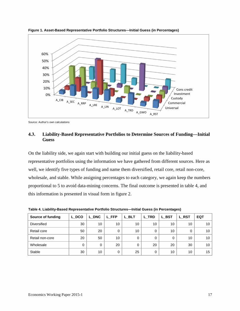
Figure 1. Asset-Based Representative Portfolio Structures—Initial Guess (in Percentages)

Source: Author’s own calculations

4.3. Liability-Based Representative Portfolios to Determine Sources of Funding—Initial Guess

On the liability side, we again start with building our initial guess on the liability-based

representative portfolios using the information we have gathered from different sources. Here as

well, we identify five types of funding and name them diversified, retail core, retail non-core,

wholesale, and stable. While assigning percentages to each category, we again keep the numbers

proportional to 5 to avoid data-mining concerns. The final outcome is presented in table 4, and

this information is presented in visual form in figure 2.

Table 4. Liability-Based Representative Portfolio Structures—Initial Guess (in Percentages)

Source of funding L_DCO L_DNC L_FFP L_BLT L_TRD L_BST L_RST EQT

Diversified 30 10 10 10 10 10 10 10

Retail core 50 20 0 10 0 10 0 10

Retail non-core 20 50 10 0 0 0 10 10

Wholesale 0 0 20 0 20 20 30 10

Stable 30 10 0 25 0 10 10 15

UniversalCommercial

CustodyInvestment

Cons credit0%

10%

20%

30%

40%

50%

60%

A_CIB A_SEC A_RRP A_LRE A_LIN A_LOT A_TRD A_GWO A_RST


Figure 2. Liability-Based Representative Portfolio Structures—Initial Guess (in Percentages)

Source: Author’s own calculations.

4.4. Grouping Results Based on Initially Guessed Representative Portfolios—Last Available Quarter

Here we report the results of applying the grouping rule of section 4.1 of this paper to the U.S.

BHCs’ quarterly balance sheet dataset we describe earlier.

Table 5. Bank Groups in Last Available Quarter (Based on Guessed Representative Portfolios)

Source: UBHCPR and author’s own calculations.

Diverse

Retail coreRetail non-core

WholesaleStable0%

10%20%30%40%50%

60%

L_DCOL_DNC

L_FFPL_BLT

L_TRDL_BST

L_RSTEQT

Banks Asset allocation Source of funding Banks Asset allocation Source of fundingBANK OF AMERICA Univiversal Diverse BANCWEST Commercial Retail coreCITIGROUP Univiversal Retail non-core BB&T Commercial Retail coreHSBC NORTH AMER Univiversal Diverse BBVA COMPASS BSHRS Commercial Retail coreJPMORGAN CHASE Univiversal Diverse BMO Commercial Retail coreUNITED SVC AUTO ASSN Univiversal Diverse COMERICA Commercial Retail core

FIFTH THIRD BC Commercial Retail coreGOLDMAN SACHS Investment Wholesale HUNTINGTON BSHRS Commercial Retail coreMORGAN STANLEY Investment Wholesale KEYCORP Commercial Retail coreTAUNUS Investment Wholesale M&T BK Commercial Retail core

NATIONAL CITY Commercial Retail coreBANK OF NY MELLON Custody Retail non-core PNC SVC Commercial Retail coreCHARLES SCHWAB Custody Retail core RBS CITIZENS Commercial Retail coreE TRADE Custody Retail core REGIONS Commercial Retail coreMETLIFE Custody Wholesale SUNTRUST BK Commercial Retail coreNORTHERN TR Custody Retail non-core TD BK US HC Commercial Retail coreSTATE STREET Custody Retail non-core U S BC Commercial Retail core

WELLS FARGO Commercial Retail coreALLY Consumer credit Stable ZIONS BC Commercial Retail coreAMERICAN EXPRESS Consumer credit StableCAPITAL ONE Consumer credit Retail core COUNTRYWIDE Commercial DiverseGENERAL ELEC CAP Consumer credit Stable WACHOVIA Commercial Stable


Table 5 summarizes the group structure for each firm based on the information of the last quarter

in which the data was available for the bank. Switching to the last quarter of the observations,

which is 2013Q4, leads to a grouping that is only slightly different from the grouping reported in

this table.

There are a few observations we would like to make. The universal banks group includes USAA

but not Wells Fargo, which belongs to the group of commercial banks based on its balance sheet

structure. All the universal banks have diverse funding structures except Citi, which, as figure 3

shows, has relied mainly on retail non-core funding since 2002Q1. All the investment banks rely

mainly on wholesale funding, while the custody banks do not exhibit homogeneity on their

funding side. The consumer credit banks group uses stable funding except for Capital One. The

vast majority of commercial banks use retail core funding as their main source of funding, except

for Wachovia and Countrywide. Wachovia’s case is unique. In the last quarter before being

acquired by Wells Fargo, Wachovia was losing its core deposits, and its total assets were

declining as well. In response, Wachovia was able to increase its long-term funding substantially

in nominal terms, which made its long-term funding even larger as a percentage of its total assets

and moved Wachovia to the stable funding group. Seemingly, a rapid deterioration in the quality

of Wachovia’s assets, which is not captured in our data, did not allow its continued existence as

an independent firm.

Table 5 identifies Taunus Corporation , which was renamed as DB USA Corporation in 2014, as

an investment bank. This is not surprising because Taunus is a holding company that operates as

a subsidiary of Deutsche Bank AG with two major subsidiaries of its own: Deutsche Bank Trust

Company Americas and Deutsche Bank Securities Inc. Taunus provides a wide range of

financial services and is especially noted for its wealth management and investment services. Its

Web site reports that the company is involved in trading and structuring a wide range of financial

market products, such as bonds, equities, and exchange-traded and over-the-counter derivatives,

and foreign exchange, money market, and securitized instruments. Deutsche Bank Securities Inc.

also includes advisory activities, such as portfolio management, pension consulting, and rating or

pricing securities.


Also, the grouping rule identifies the Charles Schwab Corporation as a custody bank (see table

4), which makes sense because Google Finance describes Charles Schwab as a savings and loan

holding company that is engaged, through its subsidiaries, in securities brokerage, banking, and

related financial services. The company provides financial services to individuals and

institutional clients through two segments, investor services and institutional services. The

investor services segment provides retail brokerage and banking services to individual investors.

The institutional services segment provides custodial, trading, and support services to

independent investment advisors.

4.5. Grouping Results Based on Initially Guessed Representative Portfolios—Dynamics

Table 5 depicts a static snapshot of how the proposed grouping rule works. That information is

not sufficient for determining whether the rule leads to a stable grouping over time, so we now

present the results of applying the grouping rule for all 48 quarters included in the dataset. We

summarize these results separately for asset-based and liability-based groupings in the form of

two graphs in figure 3. Thus, figure 3 shows, in a dynamic setting, how each bank’s asset-based

(top graph) and liability-based (bottom graph) group affiliation evolves over time. It is clear from

figure 3 that the proposed rule leads to fairly stable grouping. The group affiliations of most

banks change rarely.


Figure 3. Dynamics of Asset-Based (Top Graph) and Liability-Based (Bottom Graph) Bank Groups

Note: Dynamics are obtained using our initial guess on the representative portfolio structures.


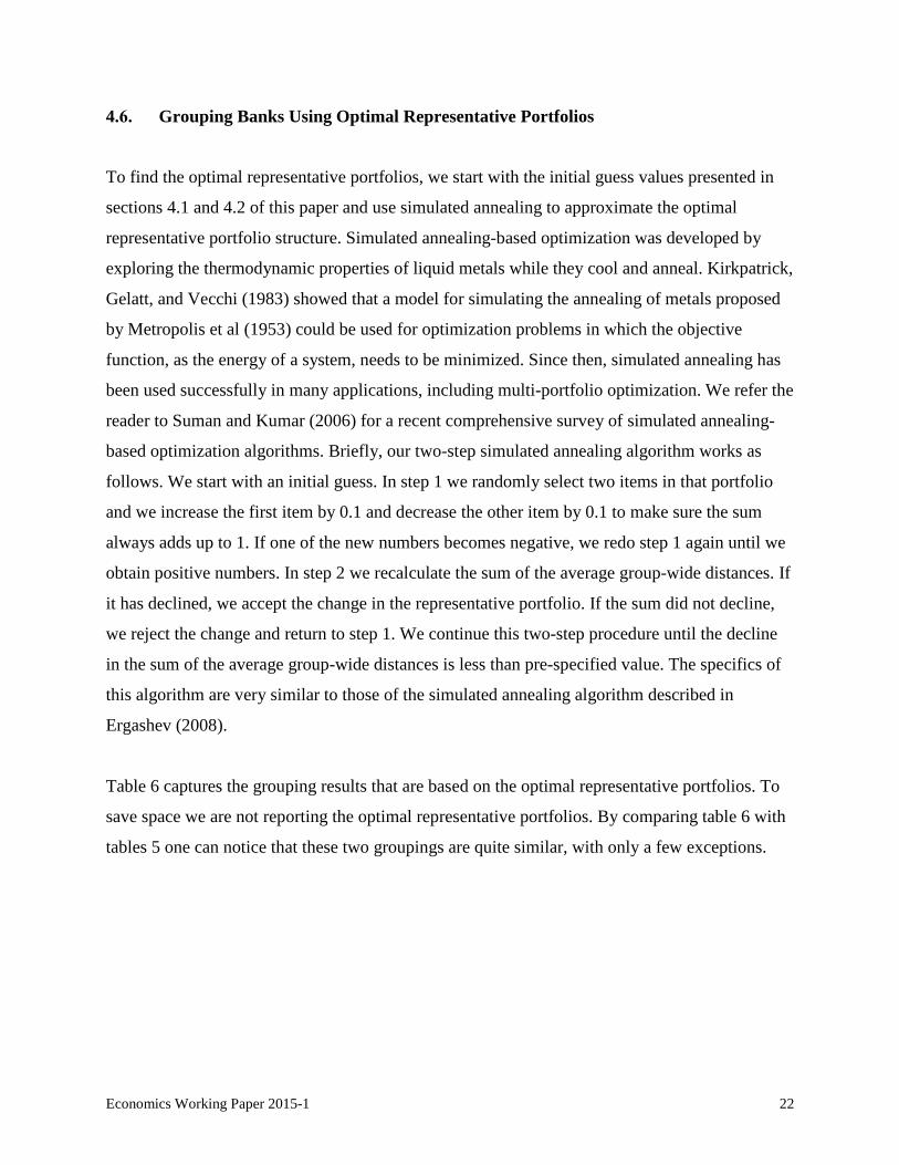
4.6. Grouping Banks Using Optimal Representative Portfolios

To find the optimal representative portfolios, we start with the initial guess values presented in

sections 4.1 and 4.2 of this paper and use simulated annealing to approximate the optimal

representative portfolio structure. Simulated annealing-based optimization was developed by

exploring the thermodynamic properties of liquid metals while they cool and anneal. Kirkpatrick,

Gelatt, and Vecchi (1983) showed that a model for simulating the annealing of metals proposed

by Metropolis et al (1953) could be used for optimization problems in which the objective

function, as the energy of a system, needs to be minimized. Since then, simulated annealing has

been used successfully in many applications, including multi-portfolio optimization. We refer the

reader to Suman and Kumar (2006) for a recent comprehensive survey of simulated annealing-

based optimization algorithms. Briefly, our two-step simulated annealing algorithm works as

follows. We start with an initial guess. In step 1 we randomly select two items in that portfolio

and we increase the first item by 0.1 and decrease the other item by 0.1 to make sure the sum

always adds up to 1. If one of the new numbers becomes negative, we redo step 1 again until we

obtain positive numbers. In step 2 we recalculate the sum of the average group-wide distances. If

it has declined, we accept the change in the representative portfolio. If the sum did not decline,

we reject the change and return to step 1. We continue this two-step procedure until the decline

in the sum of the average group-wide distances is less than pre-specified value. The specifics of

this algorithm are very similar to those of the simulated annealing algorithm described in

Ergashev (2008).

Table 6 captures the grouping results that are based on the optimal representative portfolios. To

save space we are not reporting the optimal representative portfolios. By comparing table 6 with

tables 5 one can notice that these two groupings are quite similar, with only a few exceptions.


Table 6. Bank Groups in Last Available Quarter (Based on Optimal Representative Portfolios)


In figure 4, we present the evolution of the asset-based and liability-based groups. Again, we

compare these results with those of figure 3 and notice that they are very similar.

Banks Asset allocation Source of funding Banks Asset allocation Source of fundingBANK OF AMERICA Univiversal Retail core BANCWEST Commercial Retail coreCITIGROUP Univiversal Retail non-core BB&T Commercial Retail coreHSBC NORTH AMER Univiversal Diverse BBVA COMPASS BSHRS Commercial Retail coreJPMORGAN CHASE Univiversal Diverse BMO Univiversal Retail coreUNITED SVC AUTO ASSN Univiversal Retail core COMERICA Commercial Retail core

FIFTH THIRD BC Commercial Retail coreGOLDMAN SACHS Investment Wholesale HUNTINGTON BSHRS Commercial Retail coreMORGAN STANLEY Investment Wholesale KEYCORP Commercial Retail core

TAUNUS Investment Wholesale M&T BK Commercial Retail coreNATIONAL CITY Commercial Retail core

BANK OF NY MELLON Custody Retail non-core PNC SVC Commercial Retail coreCHARLES SCHWAB Custody Retail core RBS CITIZENS Commercial Retail coreE TRADE Custody Retail core REGIONS Commercial Retail coreMETLIFE Custody Wholesale SUNTRUST BK Commercial Retail coreNORTHERN TR Custody Retail non-core TD BK US HC Commercial Retail coreSTATE STREET Custody Retail non-core U S BC Commercial Retail core

WELLS FARGO Commercial Retail coreALLY Consumer credit Stable ZIONS BC Commercial Retail coreAMERICAN EXPRESS Consumer credit StableCAPITAL ONE Consumer credit Retail core COUNTRYWIDE Commercial DiverseGENERAL ELEC CAP Univiversal Stable WACHOVIA Commercial Stable


Figure 4. Dynamics of Asset-Based (Top Graph) and Liability-Based (Bottom Graph) Bank Groups

Note: Dynamics were obtained using the optimal representative portfolios.


5. Thermodynamic Model of a Banking System

Encouraged by the positive results described in the previous section of this paper, which we

obtained using a simple idea of identifying bank groups based on predetermined representative

portfolio structures, we now explore the possibility of building a more general dynamic model of

a banking system. In this model, the banks interact with one another, as elements of a dynamic

system, by forming groups around each representative portfolio structure with the possibility of

weakly interacting with the other groups as well. To be able to capture such complex group

dynamics, we need a broader framework than the k-means clustering approach we employed in

the previous sections of this paper to identify various bank groups. This approach, like any other

clustering approach, is not designed to capture interactions among the groups. For example,

when within one group some banks start dynamically approaching another group (while other

things being equal) such a dynamic cannot be identified within a clustering approach. The

absence of an overall objective function to minimize is an important limitation of the clustering

techniques (Jain and Dubes [1988]).

In the previous section of this paper we use the Euclidean distance as the measure of the strength

of interaction. Now we would like to generalize this concept as well. To achieve the listed goals,

we turn to a model of a thermodynamic system that we borrow from statistical mechanics. We

apply this model to the U.S. banking system in section 6 with the hope of providing new insights

into how the banking system evolves over time.

5.1. Thermodynamic Systems

Thermodynamics is a general engineering tool used to model processes within a system of

interacting elements that exchange energy while interacting. Because a thermodynamic system is

a very general concept, there are no hypotheses regarding the structure of the system (see

Spakovszky [2009], among others). The concept of energy is used to measure the strength of

interaction among the elements of the system. Energy is also defined broadly, such as potential

energy measuring the strength of interactions through the distance between the elements, kinetic

energy measuring the strength of interaction through elements’ speeds, or a combination of both.


At any given moment, a thermodynamic system can take one of a usually continuum number of

states, and the state of the system is in equilibrium when its properties remain unchanged, so

long as the external conditions are unchanged. If the state of the system is changing, it is

undergoing a process of moving from one equilibrium to another. There are several important

laws of thermodynamics the elements follow while interacting with one another, such as the law

of conservation of energy in a closed system and the law of entropy, according to which entropy

(i.e., disorder) of the system tends to increase over time and reaches its maximum level at

equilibrium. Because we are not using many other thermodynamic concepts and laws, we now

switch from a discussion of a general thermodynamic system to a description of the

thermodynamic system we have developed to approximate the dynamic behavior of a banking

system.

There are a number of benefits of treating a banking system as a thermodynamic system. With

such a setup, we should be able to capture interactions among the banks without using

information that goes beyond what is available through banks’ balance sheets. There is a

growing body of literature on the network structure of banking systems, which uses information

on mutual exposures among the financial institutions (see Bech and Atalay [2008]; Cont,

Moussa, and Santos [2013]; and Upper [2011], among others). Data on interbank exposure

among the U.S. banks, however, is not readily available. The approach we take in this paper

allows us to model interactions among banks by treating the system as a thermodynamic one and

only using information embedded in balance sheet data. Also, we can separate banks into a few

stable groups based on specific activities each group specializes in.

The following concept helps the reader better follow the energy dynamics we are studying in the

paper: When there are no interactions among the groups, any increase (decrease) in a specific

energy means moving away from (moving toward) the representative portfolio is used to

calculate the energy. When the groups interact, however, some of the dynamics reflect the net

effects of compensating movements by various energies.

We also would like to emphasize the following caveats of using thermodynamics to describe

bank behavior: the banking system is not isolated—interactions with other participants of a


broader financial system are possible, portfolio managers face other influential factors

conflicting with the goal of building replicating portfolios, etc.

5.2. Model

The thermodynamic system we develop in this paper consists of many elements, which we call

banks. Each bank is determined by an 𝑚𝑚 + 𝑘𝑘 + 1 dimensional portfolio vector, which we also

call the bank’s portfolio structure, where 𝑚𝑚 is the number of asset categories and 𝑘𝑘 + 1 is the

number of liability categories that include equity as well. The portfolio vector is normalized so

that the sum of the assets (liabilities) equals 1. The number of banks within the system, 𝑚𝑚𝑡𝑡, may

vary over time 𝑡𝑡 for various reasons, such as M&A activity, but the number of groups the banks

belong to, 𝑔𝑔𝑎𝑎 + 𝑔𝑔𝑙𝑙, is fixed, where 𝑔𝑔𝑎𝑎 is the number of groups formed based on the banks’ asset

portfolios and 𝑔𝑔𝑙𝑙 is the number of groups formed based on the banks’ liability portfolios. Each

group is defined by its own RP structure. One might think of a RP as a portfolio structure

reflecting common features of banks with similar portfolio structures. A bank belongs to the

group of banks formed by the closest RP.

We define closeness between different portfolios through potential energy. We denote the

potential energy of bank 𝑖𝑖 relative to a given asset-based representative portfolio 𝒂𝒂�𝒈𝒈 as

𝐸𝐸𝑎𝑎(𝑖𝑖,𝑔𝑔, 𝑡𝑡). Similarly, we denote the potential energy of bank 𝑖𝑖 relative to a liability-based

representative portfolio �̅�𝒍𝒈𝒈 as 𝐸𝐸𝑙𝑙(𝑖𝑖,𝑔𝑔, 𝑡𝑡). In section 4 of this paper, closeness is determined by a

simple grouping rule based on the smallest Euclidian distance. In the next definition we use the

concept of potential energy, which is more general than distance.

Definition 1

(a) We assume that bank 𝑖𝑖 belongs to the asset-based group g at time t if the potential energy

𝐸𝐸𝑎𝑎(𝑖𝑖,𝑔𝑔, 𝑡𝑡) is the smallest among its potential energies relative to each of the asset-based

representative portfolios:

𝐸𝐸𝑎𝑎(𝑖𝑖,𝑔𝑔, 𝑡𝑡) = 𝑚𝑚𝑖𝑖𝑚𝑚 {𝐸𝐸𝑎𝑎(𝑖𝑖, 1, 𝑡𝑡), … ,𝐸𝐸𝑎𝑎(𝑖𝑖,𝑔𝑔𝑎𝑎, 𝑡𝑡)}


(b) We assume that bank 𝑖𝑖 belongs to the liability-based group g at time t if the potential energy

𝐸𝐸𝑙𝑙(𝑖𝑖,𝑔𝑔, 𝑡𝑡) is the smallest among its potential energies relative to each of the liability-based

representative portfolios:

𝐸𝐸𝑙𝑙(𝑖𝑖,𝑔𝑔, 𝑡𝑡) = 𝑚𝑚𝑖𝑖𝑚𝑚 {𝐸𝐸𝑙𝑙(𝑖𝑖, 1, 𝑡𝑡), … ,𝐸𝐸𝑙𝑙(𝑖𝑖,𝑔𝑔𝑙𝑙, 𝑡𝑡)}

The defined potential energies are the basis for calculating variety of other energies. Definition 2

introduces several useful ones.

Definition 2

(a) The total asset energy of bank 𝑖𝑖 at time 𝑡𝑡 is defined as

𝐸𝐸𝑎𝑎(𝑖𝑖, 𝑡𝑡) =1𝑐𝑐𝑎𝑎

� 𝐸𝐸𝑎𝑎(𝑖𝑖,𝑔𝑔, 𝑡𝑡) · exp{−𝜆𝜆 · 𝐸𝐸𝑎𝑎(𝑖𝑖,𝑔𝑔, 𝑡𝑡)} ,𝑔𝑔𝑎𝑎

𝑔𝑔=1

where 𝐸𝐸𝑎𝑎(𝑖𝑖,𝑔𝑔, 𝑡𝑡) = 𝑑𝑑2𝑎𝑎(𝑖𝑖,𝑔𝑔, 𝑡𝑡) is the square of the Euclidean distance defined in section 4

of this paper, 𝜆𝜆 ≥ 0 is the parameter determining the strength of interactions between the

groups, and 𝑐𝑐𝑎𝑎 > 0 is the normalizing constant.

(b) Likewise, the total funding energy of bank 𝑖𝑖 at time 𝑡𝑡 is defined as

𝐸𝐸𝑙𝑙(𝑖𝑖, 𝑡𝑡) =1𝑐𝑐𝑙𝑙

� 𝐸𝐸𝑙𝑙(𝑖𝑖,𝑔𝑔, 𝑡𝑡) · exp {−𝜆𝜆 · 𝐸𝐸𝑙𝑙(𝑖𝑖,𝑔𝑔, 𝑡𝑡)}.𝑔𝑔𝑙𝑙

𝑔𝑔=1

(c) The total energy of bank 𝑖𝑖 at time 𝑡𝑡 is defined as

𝐸𝐸(𝑖𝑖, 𝑡𝑡) = 𝐸𝐸𝑎𝑎(𝑖𝑖, 𝑡𝑡) + 𝐸𝐸𝑙𝑙(𝑖𝑖, 𝑡𝑡).

The normalizing constants in definitions 2(a) and 2(b) are chosen such that the sum of the

exponential weights is always equal to 1. We also use the concept of average energy, which is

derived by dividing each sum by the number of components in the summation.

We borrow the idea of introducing the strength of interactions among the energy groups using

the exponential form (see definitions 2(a) and 2(b)) from Blatt, Wiseman, and Domany (1997),

who jointly authored a well-known clustering algorithm based on exploring the thermodynamic

properties of large datasets. Their algorithm is very popular in image recognition. Our model is


different from their thermodynamic model in a number of ways. First, their algorithm is based on

a so-called Potts model, in which each element can take a fixed number of discrete values

ranging from 1 to, say q, where q is a positive integer. Therefore, q is the number of states each

element can possibly take. In our model, each element can take a continuum number of

multidimensional states. Another distinct feature of our model is the existence of centers of

attraction in the form of representative portfolios.

In the model, we use the concept of potential energy, instead of just the Euclidean (as in section

4 of this paper) or any other distance, because energy is a more general concept, which comes

with a number of advantages. Among them is its ability to capture group interactions, which we

incorporated in definitions 2(a) and 2(b) by the exponential weights and parameter λ. As one can

see from these definitions, energy also allows us to consider multi-objective optimization in

which it is possible to incorporate, in a unified setting, the possibility that banks may explore

multiple portfolio strategies at the same time.

5.3. Implications for Multi-Objective Portfolio Optimization

The latest asset and liability management techniques are being built under the assumption that

determining banks’ optimal asset and liability structure is a multi-objective optimization problem

with profit maximization playing a central role. For example, Kosmidou and Zopounidis (2008)

and Steuer, Qi, and Hirschberger (2008) present an overview of multi-objective linear as well as

stochastic programming techniques applied to asset and liability management and portfolio

optimization. An important challenge still facing this literature, however, is the uncertainty about

how portfolio managers weigh the importance of each objective.

In our approach, we postulate that firms are engaged in portfolio targeting strategies by

positioning their portfolios closer to specific representative portfolios or a set of representative

portfolios. This approach has a number of advantages relative to the existing approaches to

multi-objective portfolio optimization, such as linear programming or goal programming. In

particular, it does not require the knowledge of a bank portfolio manager’s preference on the

order of importance of optimization regarding each representative portfolio. In fact, this


approach actually provides a rank ordering among the objectives using the information

embedded in the balance sheet data. It also allows us to determine the relative weight of each

objective for each bank, with the main objective the bank is following being the one with the

smallest energy.

6. Implementation of Thermodynamic Model to U.S. Banking System

In this section we present the details of how we implement the model of section 4 of this paper to

U.S. banks using the data described in section 5 of this paper. For this exercise, we assume that

the parameter of the strength of interaction among the groups of banks, λ, is set to 2.5. We arrive

at λ = 2.5 based on the recommendation by Blatt, Wiseman, and Domany (1997) to choose this

parameter approximately as large as 1/(2z2) where z is the average distance between the groups.

The average distance between the representative portfolios that we guessed is about 0.47 for the

representative asset portfolios and 0.42 for representative liability portfolios. This leads us to the

value of 1/(2z2) 2.2 to 2.8. Thus, λ = 2.5 was chosen. One can notice from definition 2 that the

group interactions become stronger as λ → 0 and weaker as λ → ∞. We have experimented with

values of λ ranging between 0 and 4 with no significant qualitative changes in the results. For

values of λ exceeding 6, the properties of the system change dramatically and in a way that is

hard to explain. This observation supports the notion that various bank groups within the banking

system interact with each other.

We start with an initial guess on the representative portfolio structures. Based on the initial

guess, we then determine the bank groups. Next, we search for the optimal representative

portfolios using simulated annealing as our optimization tool, and we reevaluate the bank groups

based on the optimal representative portfolios. Once the final groups are established, using this

grouping we analyze the behavior of individual banks and bank groups throughout the period

2002Q1 to 2013Q4.


6.1. Herding Among Commercial Banks

The thermodynamic model allows us to detect a group-specific herding behavior in the system.

The type of herding we are looking for is a group of banks that dynamically restructure their

balance sheets in a similar manner over extended periods. We call this type of herding “portfolio

targeting.” This type of herding is different from herding studied in the recent literature. Several

papers study the herding behavior in mutual fund managers’ stock buying and selling decisions.

Wermers (1999), for example, finds there is greater herding in small, growth-oriented mutual

funds than among income funds. This and many other studies use a measure of herding proposed

by Lakonishok, Shleifer, and Vishny (1992). Our approach to measuring herding is different

because, in contrast with the previous studies, we focus on herding based on similarities in

portfolio composition rather than similarities in trading patterns.

Another well-studied type of herding is information cascades. An information cascade is a

situation in which every subsequent player observes the previous choices makes a choice

independent of his or her private signal. Models of information cascades by Banerjee (1992) and

Bikhchandani, Hirshleifer, and Welch (1992) that demonstrate how information cascades start in

investor behavior also show the unstable nature of those cascades. The cited models of

information cascades may not be directly applicable to types of herding taking place within the

banking system, because information cascades in those models appear and disappear quickly

while herding in the banking system seems to evolve slowly and revolve back slowly as well—

rebalancing bank portfolios takes time.

A natural starting point for studying portfolio targeting in the banking system is the within-a-

group joint behavior among some of the groups we identify in previous sections. After a careful

study of the energy dynamics of all the identified groups of banks, we noticed a herding behavior

of the commercial banks on the funding side. As can be seen from figure 5, the funding energy of

the commercial banks group shows a common behavior throughout the observation period.

Initially, the funding energy is high; it then starts to decline, reaching the lowest levels before or

at the onset of the last crisis. In the last quarter of 2008, the energy begins to increase again. The

funding energy for each bank is calculated as the weighted sum of all five liability-based


energies divided by 5. Also, one can notice that some banks lead these changes while others

follow. To understand the causes of this behavior, we decompose the funding energy into its five

components. Among them, wholesale energy and diverse energy show patterns similar to the

overall pattern (see figures 6 and 7), suggesting that these two types of energy played prominent

roles in shaping the funding energy. The economic interpretation of this behavior is as follows.

Before and in the initial stages of the crisis, the commercial banks were diversifying their

funding away from retail funding toward increasingly relying on wholesale funding. This is why

the levels of diverse and wholesale energy declined during this period. Since the end of the crisis,

commercial banks significantly moved away from that pattern of financing their activities in the

direction of increasing their reliance on retail funding.

Figure 5. Funding Energy of Commercial Banks



Figure 6. Wholesale Energy of Commercial Banks


Figure 7. Diverse Energy of Commercial Banks


6.2. Dynamics of Commercial Banks’ Asset and Funding Energies

Now we study the dynamics of the commercial banks’ asset and funding energies. For each

bank, the asset (funding) energy is defined as the weighted average of all five asset-based

(liability-based) energies.2 These individual bank energies then are averaged among the

commercial banks to arrive in the commercial banks’ asset and funding energies.

2 Our findings remain the same qualitatively if we replace the weighted average with the simple average of the five energies.


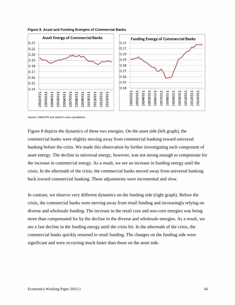
Figure 8. Asset and Funding Energies of Commercial Banks


Figure 8 depicts the dynamics of these two energies. On the asset side (left graph), the

commercial banks were slightly moving away from commercial banking toward universal

banking before the crisis. We made this observation by further investigating each component of

asset energy. The decline in universal energy, however, was not strong enough to compensate for

the increase in commercial energy. As a result, we see an increase in funding energy until the

crisis. In the aftermath of the crisis, the commercial banks moved away from universal banking

back toward commercial banking. These adjustments were incremental and slow.

In contrast, we observe very different dynamics on the funding side (right graph). Before the

crisis, the commercial banks were moving away from retail funding and increasingly relying on

diverse and wholesale funding. The increase in the retail core and non-core energies was being

more than compensated for by the decline in the diverse and wholesale energies. As a result, we

see a fast decline in the funding energy until the crisis hit. In the aftermath of the crisis, the

commercial banks quickly returned to retail funding. The changes on the funding side were

significant and were occurring much faster than those on the asset side.


6.3. Energy and Macroeconomic Factors

In this section of the paper we explore the possibility of various energies co-moving with

macroeconomic variables. For this purpose, we use quarterly reports on the following macro

variables: the growth rate of the real gross domestic product, the national unemployment rate,

and the house prices index (HPI). This information was downloaded from the Federal Reserve

Bank of Saint Louis’s FRED economic database.

We find that the funding energy of all the banks included in our study is negatively correlated

with the HPI. For each bank, the funding energy is defined as the weighted sum of all five

liability-based energies, as in definition 2. Specifically, the contemporaneous correlation

coefficient between the quarterly percentage changes in the HPI and the quarterly changes in the

average funding energy of all banks is –0.50. This relation is captured graphically in figure 9.

Figure 9. Negative of Quarterly Percent Changes in Funding Energy Vs. Quarterly Percent Changes in HPI

Source: UBHCPR, FRED, and author’s own calculations


The captured link between the funding energy and the HPI shows that the dynamics of the banks’

funding structure were strongly correlated with the dynamics of the housing prices throughout

the observed period.

7. Possible Extensions

7.1. Accounting for Negative Energy

The concept of energy is broader than the concept of distance for one very important reason:

energy can be negative while distance is always positive. While positive energy allows one to

study the attractiveness of various portfolio structures, or objectives from the portfolio

optimization perspective, with the inclusion of negative energy one can also study cases when

banks are forced to move away from specific portfolio structures or objectives.

As an example, we next discuss the following energy and study its implications. What we call

“diversify but avoid failing with the market” energy is calculated as the diversification energy

minus the fail with the market energy. Here, the diversification energy is the energy of each

bank’s asset portfolio relative to the most diversified portfolio structure, consisting of 1/9 in each

of its nine asset items. Therefore, this energy equals the square of the Euclidean distance

between the bank portfolio and the vector (1/9,…,1/9). The fail with the market energy of a bank

is measured as the square of the Euclidean distance between the bank portfolio and the aggregate

portfolio. Here the aggregate portfolio is built by adding all banks’ assets into one portfolio.

Figure 10 depicts the dynamics of the “diversify but avoid failing with the market” energy

individually for each bank. The dynamics of this energy for the commercial banks is captured by

the lines shaded gray. The remaining banks are the universal banks, which are the closest to the

average (captured by the bold black line), and the custody banks with the lowest energy levels.

The investment banks are not included in this figure because of data limitations. One clear

observation is that practically every bank started to follow the “diversify but avoid failing with

the market” objective starting from 2008Q4 following the collapse of Lehman Brothers.


Figure 10. Energy of the Diversify but Avoid Failing With the Market Objective


7.2. Other Possible Extensions

Allowing for the representative portfolio structures (as the centers of attraction) to change over

time would be another useful extension of the model. The model also can be expanded to capture

a varying number of groups, allowing detection of the birth of a new group of banks.

In this paper we use a very simple version of potential energy, the square of the Euclidean

distance. In general, though, potential energy of an element is not only proportional to the

distance, it is also proportional to the mass of the element. In this paper we made a simplifying

assumption that all the banks of the system have the same fixed mass. One can expand potential

energy to take into account each bank’s mass as, for instance, the dollar amount of its total

assets.

Although we did not include any discussion of entropy in this version, we would like to discuss it

in the next version. The entropy of the banking system plays an important role in measuring the

level of systemic risk of the entire banking system. Declining levels of entropy usually signal


increasing levels of systemic risk, because they mean the system is becoming more order driven.

Measuring entropy, however, is difficult. The exact analytical solutions for entropy are not

always available, although it can be approximately evaluated using simulation methods. Because

the entropy of the system is proportional to its energy (other things being equal), a decline in the

entropy is usually associated with a decline in the overall energy of the system. One policy

implication of this observation is that, if the overall energy of the system is declining,

policymakers could force an increase in energy by forcefully changing some of the

representative portfolio structures. For example, the Volcker Rule on proprietary trading forced a

change in the structure of the representative portfolios associated with investment banking by

reducing the weights of the trading assets and trading liabilities.

Another possible extension would be exploring the possibility of incorporating information

contained in the BHC’s income statements by introducing the concept of kinetic energy in the

model. Such an extension would allow one to incorporate the costs (including losses) and

benefits (i.e., return) of quarterly changes in the balance sheet structure.

8. Conclusion

The asset-based and liability-based bank groups we identify using our thermodynamic model of

a banking system are intuitively appealing and stable over time. Further explorations of the

dynamic properties of the U.S. banking system using the proposed model (with the main focus

being on the large banks) shed additional light on how the balance sheet structures of these banks

evolved throughout the crisis. In particular, we identify a herding behavior among the

commercial banks in the form of jointly targeting specific portfolio structures.

This paper’s findings have important implications for the annual regulatory stress tests of large

and midsize U.S. banks under the Dodd–Frank Wall Street Reform and Consumer Protection

Act. As an example, one can expand the group dynamics captured in figure 4 for nine more

quarters using the balance sheet forecasts submitted by the participating banks under different

scenarios and assess whether those projected dynamics make sense. For instance, if a bank

changes its group affiliation during the projected quarters on either side of the balance sheet, this


would require additional scrutiny to understand whether the bank’s balance sheet projections are

reasonable. As we saw earlier, banks’ group affiliations do not change frequently and most banks

kept their group affiliation intact throughout the last crisis.

The approach we develop in this paper has implications for multi-objective portfolio

optimization as well. In particular, our approach provides a rank ordering among the objectives

using the information embedded in balance sheet data. It also allows one for determining the

relative weight of each objective from the data.


References

Adrian, Tobias, and Hyun S. Shin, 2011. “Financial Intermediary Balance Sheet Management.” Federal Reserve Bank of New York Staff Reports No. 532.

Adrian, Tobias, and Hyun S. Shin, 2008. “Liquidity and Leverage.” Federal Reserve Bank of

New York Staff Report No. 328 (revised in 2010). Acharya, V. V., and T. Yorulmazer, 2005. “Limited Liability and Bank Herding.” London

Business School IFA Working Paper No. 445. Acharya, V. V., and T. Yorulmazer, 2007. “Too Many to Fail—An Analysis of Time

Inconsistency in Bank Closure Policies.” Journal of Financial Intermediation 16: 1–31. Banerjee, Abhijit, 1992. “A Simple Model of Herd Behavior.” Quarterly Journal of Economics,

107, pp. 797–818. Beck, Morten, and Enghin Atalay, 2008. “The Topology of the Federal Funds Markets.”

European Central Bank Working Paper No. 986. Bikhchandani, Sushil, David Hirshleifer, and Ivo Welch, 1992. “A Theory of Fads, Fashion,

Custom and Cultural Change As Information Cascades.” Journal of Political Economy, 100, pp. 992–1026.

Bikhchandani, Sushil, and Sunil Sharma, 2000. “Herd Behavior in Financial Market: A Review.”

IMF Working Paper WP/00/48. Blatt, Marcelo, Shai Wiseman, and Eytan Domany, 1997. “Data Clustering Using a Model

Granular Magnet.” Neural Computation, MIT, Vol. 9, pp.1805–1842. Blei, Sharon, and Bakhodir Ergashev, 2014. “Asset Commonality and Systemic Risk Among

Large Banks in the United States.” OCC Economics Working Papers WP 2014-3. Bonfim, Diana, and Moshe Kim, 2012. “Liquidity Risk in Banking: Is There Herding?”

European Banking Center Discussion Paper, 2012-024. Chandler, David, 1987. Introduction to Modern Statistical Mechanics, Oxford University Press. Cont, Rama, Amal Moussa, and Edson B. Santos, 2013. “Network Structure and Systemic Risk

in Banking Systems.” In Handbook of Systemic Risk, Cambridge University Press. Comptroller of the Currency, 2002. “Custody Services.” Comptroller’s Handbook, January 2002. Ergashev, B., 2008. “Should Risk Managers Rely on Maximum Likelihood Estimation Method

While Quantifying Operational Risk?” Journal of Operational Risk, 3, 2, 63–86.


https://www.bportugal.pt/pt-PT/BdP%20Publicaes%20de%20Investigao/wp201218.pdf

FDIC, 2011. “Study on Core Deposits and Brokered Deposits.” An FDIC Study Submitted to the U.S. Congress on July 8.

Iannotta, Giuliano, 2010. “Investment Banking: A Guide to Underwriting and Advisory

Services.” Springer Berlin Heidelberg Jain, Anil K., and Richard C. Dubes, 1988. “Algorithms for Clustering Data.” Prentice-Hall

Advanced Reference Series, Prentice-Hall. Kirkpatrick, S., C.D. Gelatt, and Jr., M.P. Vecchi, 1983. “Optimization by Simulated

Annealing.” Science, Vol. 220, No. 4598, pp. 671–680. Kosmidou, K., and C. Zopounidis, 2008. “Asset Liability Management Techniques.” Published

in Handbook of Financial Engineering, Springer Science, New York, pp. 281–300. Laeven, Luc, Lev Ratnovski, and Hui Tong, 2014. “Bank Size and Systemic Risk.” IMF Staff

Discussion Note SDN/14/04. Lang, William W., Loretta J. Mester, and Todd Vermilyea, 2008. “Competitive Effects of Basel

II on U.S. Bank Credit Card Lending.” Journal for Financial Intermediation, 17:4, pp. 478–508.

Metropolis, N., A.W. Rosenbluth, M.N. Rosenbluth, A.H. Teller, and E. Teller, 1953. “Equation

of State Calculations by Fast Computing Machines.” Journal of Chemical Physics 21 (6): 1087–1092.

Opstal, James, 2013. “Funding Credit Card Loans: Current and Future Considerations.”

Discussion Paper, Payment Cards Center, Federal Reserve Bank of Philadelphia Spakovszky, Z.S., 2009. “Thermodynamics and Propulsion Notes,” 2008–2009, MIT. Standard and Poor’s, 2012. “Why U.S. and European Banks’ Goodwill Assets Are Under

Pressure.” Steuer, Ralph E., Yue Qi, and Markus Hirschberger, 2008. “Portfolio Selection in the Presence

of Multiple Criteria.” Published in Handbook of Financial Engineering, Springer Science, New York, pp. 3–24.

Suman, B., and P. Kumar, 2006. “A Survey of Simulated Annealing As a Tool for Single and

Multiobjective Optimization.” Journal of the Operation Research Society, 57, pp. 1143–1160.

Upper, Christian, 2011. “Simulation Methods to Assess the Danger of Contagion in Interbank

Markets.” Journal of Financial Stability, 7, pp. 111–125.


Yorulmazer, Tanju, 2014. “Literature Review on the Stability of Funding Models.” FRBNY Economic Policy Review, February 2014.

Yorulmazer, Tanju, 2014. “Case Studies on Disruptions During the Crisis.” FRBNY Economic

Policy Review, February 2014. Van den End, Jan W., and M. Tabbae, 2012. “When Liquidity Risk Becomes a Systemic Issue:

Empirical Evidence of Bank Behavior.” Journal of Financial Stability, 8, 107–120. Wermers, Russ, 1999. “Mutual Fund Herding and the Impact on Stock Prices.” Journal of

Finance, Vol. LIV, No. 2, 581–622.


Appendix A: Brief Discussion of How Identified Data Issues Have Been Addressed

We removed several firms from the dataset because the quality of their submissions did not

allow us to include them. These are ABN AMRO, Barclays, and North Fork, which are relatively

small, with each one’s total assets representing less than 1 percent of the aggregate portfolio.

In TD Bank’s data there is a huge jump in core deposits as ratios of liabilities, from 60 percent in

2007Q2 to about 70 percent in 2007Q3 or higher till 2009Q1, then back to 63 percent in 2009Q2.

This could be related to TD’s acquisition of Commerce Bank, which was announced on October

2, 2007.

Among the CCAR 2015 participants, Discover Financial Services and Santander Holdings USA

Inc. are not included in this study. Deutsche Bank Trust Corporation’s subsidiary Taunus is

included for the period from 2002Q1 till the last quarter with available data, 2011Q4.

Several M&A activities occurred during the observation period, which resulted in significant

changes in the balance sheet structures in the quarters when the legacy institutions’ data were

reported jointly for the first time. We have noticed that the following M&A activities led to

significant changes in the combined firms’ balance sheet structure:

(1) The merger of Wells Fargo and North Fork is reflected in the 2006Q4 report.

(2) Bank of NY’s merger with Mellon Corporation (July 2, 2007) is reflected in the 2007Q3

report.

(3) Bank of America’s acquisition of Countrywide (August 23, 2007) is reflected in the 2007Q4

report.

(4) Bank of America’s acquisition of Merrill Lynch (September 14, 2008) is reflected in the

2009Q1 report.

(5) Wells Fargo’s acquisition of Wachovia (October 3, 2008) is reflected in the 2008Q4 report.

(6) PNC’s acquisition of National City (October 24, 2008) is reflected in the 2008Q4 report.


To assess the influence of these events on the final results, we separately repeated the analysis

with the combined data. The combined data were built by combining the balance sheet data of

the two legacy firms to created one report covering the period before the M&A activity. We were

able to build the combined data only for the following M&A activities listed: (3), (5), and (6). In

the case of M&A (2) and M&A (4), the firms being acquired were not BHCs. Therefore, they

were not required to submit consolidated BHC reports. In the case of M&A(1), the North Fork

data was of poor quality. Therefore, we removed this firm from our dataset. The results of the

analysis based on the combined data further reinforced the stability of our previous findings.


thermodynamic properties of the us. . banking system · thermodynamic properties of the us. ....

Documents