thermostats for the smart grid: models, benchmarks…faculty.haas.berkeley.edu/levine/papers/ej...
TRANSCRIPT
Name /ej334/ej334_04_Liang/Mp_61 03/08/2012 06:03PM Plate # 0 pg 61 # 1
61
* Corresponding author. Ph.D. Candidate of Department of Industrial Engineering and OperationResearch, U.C. Berkeley, CA, 94720; (510)-708-9909; E-mail: [email protected].
** Chair of the Economic Analysis and Policy Group, Chair of the Advisory Board of the Centeron Evaluation for Global Action and Eugene E. and Catherine M. Trefethen Professor of WalterA. Haas School of Business, U.C. Berkeley.
*** Chancellor’s Professor of Department of Industrial Engineering and Operations, U.C. Berkeley.
The Energy Journal, Vol. 33, No. 4. Copyright � 2012 by the IAEE. All rights reserved.
Thermostats for the Smart Grid:Models, Benchmarks, and Insights
Yong Liang*, David I. Levine**, and Zuo-Jun (Max) Shen***
We model two existing thermostats and one novel thermostat to see howwell they operate under dynamic pricing. The existing thermostats include a tra-ditional thermostat with set temperature goals and a rigid thermostat that mini-mizes cost while always keeping temperature within a rigid predetermined range.We contrast both with a novel optimizing thermostat that finds the optimal trade-off between comfort and cost. We compare the thermostats’ performance boththeoretically and via numerical simulations. The simulations show that, underplausible assumptions, the optimizing thermostat’s advantage is economicallylarge. Importantly, the electricity demand of the rigid thermostat (but not theoptimizing thermostat) ceases to respond to electricity prices on precisely thedays when the electricity grid tends to be near capacity. These are the times whendemand response is the most socially valuable to avoid massive price spikes. Thesocial benefits of the optimizing thermostat may provide incentives for utilitiesand regulators to encourage its adoption.
Keywords: Thermostat, Smart Grid, Dynamic Pricing
http://dx.doi.org/10.5547/01956574.33.4.4
1. INTRODUCTION
The electricity grid that we have been using for more than a century isbeing challenged. Occasional peaks in demand (for example, from air condition-ing on hot afternoons) require costly year-round ancillary services. Declines insupply due to maintenance at traditional plants and (increasingly) due to thevariability of renewable sources such as wind exacerbate the challenge (Joskow,
Name /ej334/ej334_04_Liang/Mp_62 03/08/2012 06:03PM Plate # 0 pg 62 # 2
62 / The Energy Journal
Copyright � 2012 by the IAEE. All rights reserved.
2011). Moreover, because users are charged flat-rate prices, they have little in-centive to reduce demand when the grid is nearing capacity. As a result, there hasbeen a great desire to move to a Smart Grid that can better coordinate the supplyand demand of electricity (Ipakchi, 2009).
Most visions of the Smart Grid include time-varying prices (also knownas real-time-pricing (RTP) or dynamic pricing) to balance supply and demand.Dynamic prices provide users with an incentive to use less electricity when theprice is high, helping match demand and supply. To quote from Schweppe et al.(1980): “Homeostatic Utility Control can offer a set of advantages of both supplyfollows demand and demand follows supply while avoiding the majority of theirpitfalls.” Although some emerging technologies allow for efficient data collectionand for bi-directional communication between users and the grid, dynamic pricesare only likely to have much effect on demand if users have automatic systemsto manage their electricity demand.
Heating, venting, and air conditioning (HVAC) is a prime candidate toprovide the needed price-elastic demand. HVAC accounts for about 31% of thetotal electricity usage in U.S. homes (DOEEIA, 2005). Deschenes and Greenstone(2008) predict a 33% increase in electricity consumed by HVAC appliances inthe U.S. due to climate change.
Meanwhile, demand for HVAC is more flexible than other residentialdemand because it is often possible to shift heating or cooling away from periodsof peak demand with little or no reduction in comfort. With this motivation, welook at the design of smart thermostats that can react to dynamic prices andschedule the use of HVAC appliances to maximize users’ total utility. While wefocus on HVAC, this optimal control strategy can easily accommodate other elec-tric appliances.
Unfortunately, the comprehensive survey conducted by Walker andMeier (2008) found no thermostat on the market that could react to dynamicprices. Recently, Livengood and Larson (2009) propose a conceptual energy-management system called “Energy Box” for residential and small-business build-ings. They show by simulations that using the Energy Box to control room tem-perature enhances users’ total utility in terms of both cost and comfort.
Early work on modeling users’ comfort involved purely empirical rela-tions between physical variables and comfort (also known as thermal sensationrating). For instance, the Predicted Percent Dissatisfied and Predicted Mean Voteproposed by Fanger (1972), which has been largely accepted for design and fieldassessment, measure how various factors such as air humidity, clothing, and users’activities affect the perceived comfort of a large group of users. However, it isdifficult to incorporate this model into the design of an optimal control strategythat takes into account both cost and comfort. Alternatively, some recent workmodels comfort/discomfort by using functions of the parameters of interest. Forinstance, Livengood and Larson (2009) uses a discretized function that maps theroom temperatures at discretized time points to numbers quantifying comfort;Liang and Shen (2011) model discomfort as two parts: delay in meeting demand
Name /ej334/ej334_04_Liang/Mp_63 03/08/2012 06:03PM Plate # 0 pg 63 # 3
Thermostats for the Smart Grid / 63
Copyright � 2012 by the IAEE. All rights reserved.
and failure to meet demand. We notice that users are usually risk-averse over thedeviation of room temperature from the preferred one; for example, a 2�F moveaway from the preferred temperature is barely noticeable, but a similar increasewhen the temperature is already 8�F causes a noticeable increase in discomfort.This paper attempts to use a comfort function that captures that characteristic.
While one of the objectives of the studies cited above and other relatedwork is to use price to reduce demand in peak hours, little has been done toanalyze what would happen in the off-peak periods. Black and Tyagi (2010) studythe rebound effect under critical-peak-pricing (CPP), which is a variant of time-of-use (TOU) pricing. They notice that when CPP is applied, a significant portionof the load is shifted from peak-pricing hours to subsequent hours. With deeppenetration of CPP in pilot studies, this effect is enlarged and results in new peaksright after the peak-pricing periods. Fortunately, the optimizing thermostat pro-posed in this paper mitigates the rebound effect.
Because HVAC appliances operate more efficiently when temperaturedifferences between inside and outside are small, in some cases pre-cooling canreduce costs even without dynamic pricing (Braun, 2003). Braun (2003) notesthat better control strategies are needed to optimize pre-cooling. Our optimizingthermostat provides optimal pre-cooling under flat-rate prices (see section 4.1).
This paper focuses on analyzing the economic impacts of having smarterthermostats for Smart Grid users. It contributes to the current literature in thefollowing ways. We first model the control problems of three types of thermostat;namely, the traditional thermostat, the rigid thermostat, and the optimizing ther-mostat. In particular, we formulate both the thermodynamics of room tempera-tures and users’ comfort. We further show by both analytical results and controlledsimulations that the optimizing thermostat gives users maximum overall benefit.We also illustrate the social value of the optimizing thermostat and discuss draw-backs of the traditional and the rigid thermostats.
The remainder of this paper is organized as follows. In section 2, weformulate the control problems of the three types of thermostat and analyze theirperformance. In section 3, we conduct computational studies to compare thesethermostats and obtain managerial insights. In section 4, we discuss an improvedthermal model and the uncertainties in forecasts. In section 5, we conclude thepaper and discuss the limitations and future research directions.
2. MODEL
2.1 Three Types of Thermostat
Users in most American homes program a traditional thermostat with atarget room temperature (or temperature range), which may vary by the time ofday. The traditional thermostat uses a trigger policy: HVAC is activated everytime the room temperature deviates from the target temperature (or falls out ofthe target range). Unfortunately, the traditional thermostat gives the same responseregardless of energy prices.
Name /ej334/ej334_04_Liang/Mp_64 03/08/2012 06:03PM Plate # 0 pg 64 # 4
64 / The Energy Journal
Copyright � 2012 by the IAEE. All rights reserved.
1. To numerically compare the performance of the thermostats, we tweak the inputs so the ther-mostats generate almost identical comfort and compare the costs.
2. In Appendix A, we study how the length of each period, the number of look-ahead periods,the length of the planning horizon, and the aggregation level of temperatures affect computationalrequirements (measured by CPU time) and the performance of the control algorithms.
To enable automatic management of electricity usage, a new generationof somewhat intelligent—or “rigidly smart”—thermostats have been proposed,which we name rigid thermostats. A rigid thermostat runs an optimization routinein the background that, given dynamic prices, finds the lowest-cost path to keeproom temperatures within a rigid range set by the user (such as the thermostatstudied by Oldewurtel et al. (2010)). The range, for instance, may be what theusers find tolerable. Unlike the traditional thermostat, the rigid thermostat shiftselectricity demand from high-price peak hours to lower-price hours. However,the rigid thermostat’s price-responsiveness disappears precisely when the socialvalue of lowering peak demand is highest. In addition, how users set their min-imum and maximum room temperatures is subtle. For instance, to save cost, usersmay set a temperature range broad enough to lead to extreme discomfort, suchas overcooling in summer.
To overcome the drawbacks of the rigid thermostat, we propose a noveloptimizing thermostat. The optimizing thermostat trades off comfort for cost sav-ing based on users’ preferences. Instead of indicating the acceptable range ofroom temperature, users set parameters to reflect their preferences on room tem-peratures and cost savings. The optimizing thermostat runs an optimization rou-tine in the background to maximize users’ total utility.
Both the rigid and the optimizing thermostats pre-cool, but the latter ismore flexible in how it treats high and low temperatures. For example, on a hotafternoon, the rigid thermostat will typically let the afternoon temperature rise toits rigid maximum. The optimizing thermostat might keep inside temperatureslower than that level if electricity prices are low, but permit the afternoon tem-peratures to rise higher if electricity prices are extremely high. Although theoptimizing thermostat sometimes costs its users more than the rigid one does, italways gives users the highest total utility in cost and comfort.
All three types of thermostat first ask users to input the necessary pa-rameters: a target temperature or range for the traditional thermostat, a tempera-ture range for the rigid thermostat, and preference parameters for the optimizingthermostat. Presumably, the users of the traditional and rigid thermostats wouldlike to set the inputs to maximize their total utility, but the control strategies ofthose thermostats do not help them achieve that goal.1 We discretize time intoperiods and assume that, at the beginning of each period, each thermostat runsits control algorithm to decide whether or not to run HVAC and, if so, what thetarget room temperature should be.2 The detailed model formulations for thecontrol problems are described in the following subsection.
Name /ej334/ej334_04_Liang/Mp_65 03/08/2012 06:03PM Plate # 0 pg 65 # 5
Thermostats for the Smart Grid / 65
Copyright � 2012 by the IAEE. All rights reserved.
2.2 Thermal Model and Users’ Utility
First we define the following notation:
• Parameters:▪ n: index of periods, n = 1,2, . . . ,N.▪ N: the number of (look-ahead) periods.▪ tn: time at the beginning of period n and the end of period n–1.▪ h: the length of each period.▪ pn: price of electricity in period n.▪ Tin,s: indoor/room temperature at time s.▪ Tini,n: initial indoor/room temperature in period n.▪ Tout,n: ambient temperature in period n. We assume the ambient tem-
perature remains unchanged throughout any period.▪ Tpfr,n: user-preferred room temperature in period n. This is the room
temperature at which users feel most comfortable.
• User’s decision variables:▪ Itra,n: the traditional thermostat users’ target room temperature in
period n.▪ Imin,n: the rigid thermostat users’ minimum acceptable room tem-
perature in period n.▪ Imax,n: the rigid thermostat users’ maximum acceptable room tem-
perature in period n.
• Thermostat’s decision variables:▪ Xtar,n: the target room temperature for HVAC at the beginning of
period n. (Xtar,n = Itra,n for the users of the traditional thermostat.)
There have been various models for how room temperature evolves.These models are typically functions of initial room temperatures, ambient tem-peratures and other factors such as construction materials, sources of internal gain(e.g., appliances and lighting), and the behavior of residents. Different factorsand parameters can lead to quite different models; for instance, models for housesin California can be quite different from those for apartments in New York.
However, because the focus of this paper is to investigate the perfor-mance of the optimizing thermostat in general, we use a simple but general model(as in Reddy et al. (1991)) instead of those ad-hoc models. Our model can describethe temperature-evolving process, which is necessary in order to measure users’comfort.
We model a building’s thermodynamics in the following way. The wholebuilding is treated as one object with room temperature Tin,s at time s. Let k1
denote the building’s projected heat capacity—the amount of electricity requiredby HVAC to change the building’s temperature by ; is smaller if HVAC is1�F k1
Name /ej334/ej334_04_Liang/Mp_66 03/08/2012 06:03PM Plate # 0 pg 66 # 6
66 / The Energy Journal
Copyright � 2012 by the IAEE. All rights reserved.
more efficient. At the beginning of period (that is, time )n s = t T = T =n in,s in,tn
. The amount of electricity required to change the temperature of theT Qini,n n
building in period is:n
Q = k X –T = k DT (1)⎪ ⎪n 1 tar,n ini,n 1
Let be the building material’s conductance and be the cross-sectionalk Aarea of the conducting surface. By Newton’s law of cooling, the rate of heat fluxfrom the ambience to the internal space of the building at time ( ),s s∈ [t ,t ]n n + 1
is described by the following Fourier differential equation:
dQrq = = kA(T –T ) = k (T –T ) (2)s out,n in,s 2 out,n in,sds
We call the projected conductance rate, the rate at which thek = kA2
building loses heat to or gains heat from the outside. A smaller indicates thatk2
the building is better insulated. Note that the heat transfer rate is proportional tothe temperature difference. Therefore, even if we allow air exchange between theinside of the building and its surroundings, the same model still works after asmall modification of .k2
When the HVAC is off, we assume that the only driving force for tem-perature change is conduction through the walls, windows, and ceilings. Accord-ing to Equations (1) and (2), the rate of change of room temperature at timeTin,s
( ) without HVAC is:s s∈ [t ,t ]n n + 1
dTin,sk = k (T –T ) (3)1 2 out,n in,sds
Let be the time at which HVAC is stopped and be the roomt Xstop,n tar,n
temperature at the end of the previous HVAC run, then the functioncalculates the room temperature at time ( ):T 3f : � r � T s s∈ [t ,t ]+ in,s stop,n n + 1
TT = f (T ,X ,s– t )in,s out,n tar,n stop,n (4)k2
(s t )� � stop,nk1= T + (X –T )eout,n tar,n out,n
Remark: In practice, the amount of energy required to cool the building is de-termined by outside temperatures, solar gain (and associated solar load), time-variant internal gain, the characteristics of the building (such as size, structure,building material, and furnishings), etc. In our model, we assume that capturesk1
all the factors that affect the difference in a building’s internal energy at differentequilibrium room temperatures. In addition, by treating the entire building as oneobject, we actually assume that the heat transfer processes among the objectsinside the building happen instantly. Thus, the electricity required by HVAC is
Name /ej334/ej334_04_Liang/Mp_67 03/08/2012 06:03PM Plate # 0 pg 67 # 7
Thermostats for the Smart Grid / 67
Copyright � 2012 by the IAEE. All rights reserved.
proportional to the change in room temperature. We further assume that isk2
constant over time, while in reality, increases when windows or doors are open.k2
Fortunately, relaxing these assumptions does not affect the main results of thispaper (see section 4.1).
Let be users’ total utility in period . We assume that it is separableU nn
into (1) the cost of heating and cooling, , and (2) the comfort of having anCn
inside temperature different from the users-preferred one, , both of which re-Dn
duce total utility (thus both take negative values):
U = C + Dn n n
Without loss of generality, we convert comfort to dollar values. InDn
particular, we assume that users have a total utility function that depends oncomfort and on heating and cooling cost. The unit of the utility function is arbi-trary up to a positive affine transformation. To save one more parameter, werescale comfort to be in dollar values. This normalization permits us to describethe comfort for which a user is willing to pay as “ worth of comfort”.$100 $100In particular, function calculates , the cost of changing the roomC 2F : � r � C+ + n
temperature by HVAC from to :T Xini,n tar,n
CC = F (T ,X ) = –p Q = –p k T –X (5)⎪ ⎪n ini,n tar,n n n 1 ini,n tar,n
For simplicity, we assume that changing room temperature by HVAC isinstantaneous: . For two reasons, the error generated by this assumptiont = tstop,n n
is believed to be small. First, because the conduction process that gradually gainsor loses heat to ambience after HVAC stops is much slower than the convectionprocess through which HVAC changes room temperature, users’ experience inthe former process dominates. Second, the cost is not related to how quickly theenergy is consumed, but to the total amount of energy used. Results are similarwithout these simplifying assumptions.
Because users usually become increasingly uncomfortable when theroom temperature deviates further from , we model their utility associatedTpfr,n
with comfort by a negative-valued concave function. In particular, we chooseto be concave quadratic to calculate , the comfort gain per unitD 4f : � r � d(s)+ –
time due to the temperature deviation at time in period :s n
Dd(s) = f (T ,T ,X ,s– t )out,n pfr,n tar,n n
2– T )pfr,n= a(T + b T –T⎪ ⎪in,s in,s pfr,n (6)T 2= a( f (T ,X ,s– t )–T )out,n tar,n n pfr,n
T+ b f (T ,X ,s– t )–T⎪ ⎪out,n tar,n n pfr,n
where the parameters and are the coefficients of the second-order and first-a border deviation terms. Specifically, measures how much the users’ comfortb
Name /ej334/ej334_04_Liang/Mp_68 03/08/2012 06:03PM Plate # 0 pg 68 # 8
68 / The Energy Journal
Copyright � 2012 by the IAEE. All rights reserved.
decreases with small deviations from the preferred room temperature, while aaccounts for the increasing decrement in comfort with each increment in thedeviation. For example, imagine that two users prefer the same room temperatureof . Let , for the first user and , for the second73�F a = –1 b = 0 a = 0 b = –11 1 2 2
user. According to Equation (6), the first user finds 4 hours of neither better74�Fnor worse than 3 hours of plus 1 hour of . On the other hand, the second73�F 75�Fuser has the same level of comfort with 4 hours of , and finds that neither74�Fbetter nor worse than 3 hours of plus 1 hour of . Hence, the second73�F 77�Fuser will be less uncomfortable by having 3 hours of plus 1 hour of ,73�F 75�Fwhich results from the fact that the first user is more sensitive to greater deviationin room temperature.
Because room temperatures keep changing between two consecutiveHVAC runs, let function calculate users’ utility associated withD 3F : � r �+ –
comfort, , by integrating Equation (6):Dn
h
D DD = F (T ,T ,X ) = f (T ,T ,X ,s)dsn out,n pfr,n tar,n out,n pfr,n tar,n�0 (7)
h
T 2 T= {a[ f (T ,X ,s)–T ] + b f (T ,X ,s)–T }ds⎪ ⎪out,n tar,n pfr,n out,n tar,n pfr,n�0
Total utility is the sum of Equation (5) and Equation (7):Un
U (T ,T ,T ,X ) = –p k T –X⎪ ⎪n out,n ini,n pfr,n tar,n n 1 ini,n tar,n
h
T 2+ a[ f (T ,X ,s)–T ] ds (8)out,n tar,n pfr,n�0
h
T+ b f (T ,X ,s)–T ds⎪ ⎪out,n tar,n pfr,n�0
Unless otherwise noted, we assume in the remainder of this paper thatthe users of the traditional thermostat set for all . In addition, ratherI = T ntra,n pfr,n
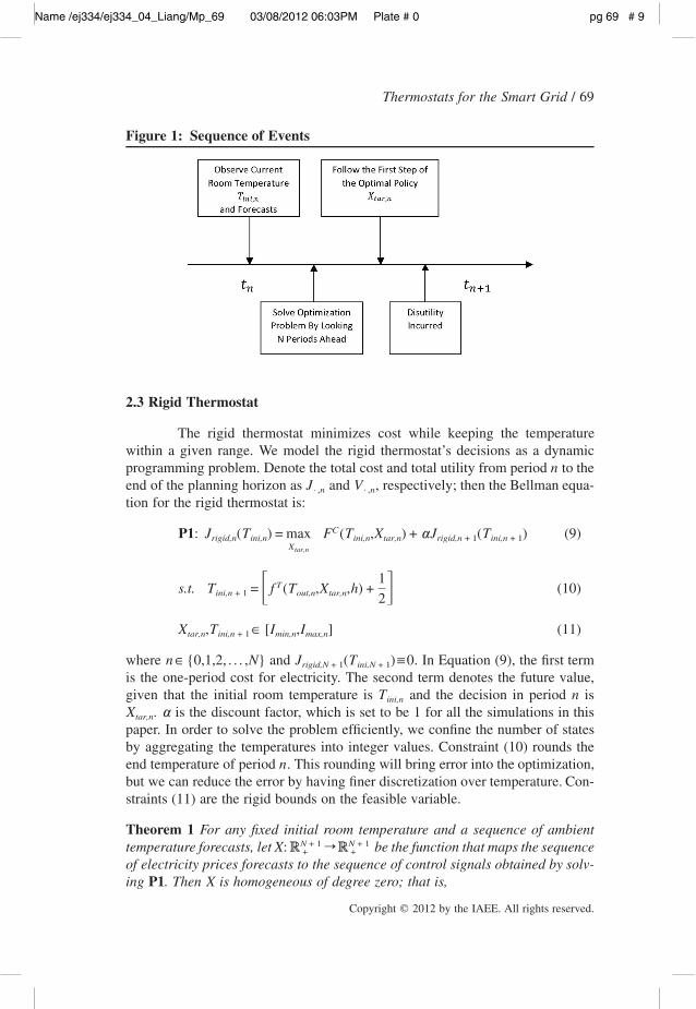
than using the trigger policy of the traditional thermostat, the other two thermo-stats work in the following way. As shown in Figure 1, at the beginning of period
, a thermostat reads the current room temperature and obtains forecasts on elec-ntricity prices and weather condition for the next periods. Then, by solving anNoptimization problem outlined in the next subsection, the thermostat generates asequence of target room temperatures and executes the first step. The room tem-perature is adjusted by the HVAC and the total utility is incurred. The ther-Un
mostat repeats this procedure in every period.
Name /ej334/ej334_04_Liang/Mp_69 03/08/2012 06:03PM Plate # 0 pg 69 # 9
Thermostats for the Smart Grid / 69
Copyright � 2012 by the IAEE. All rights reserved.
Figure 1: Sequence of Events
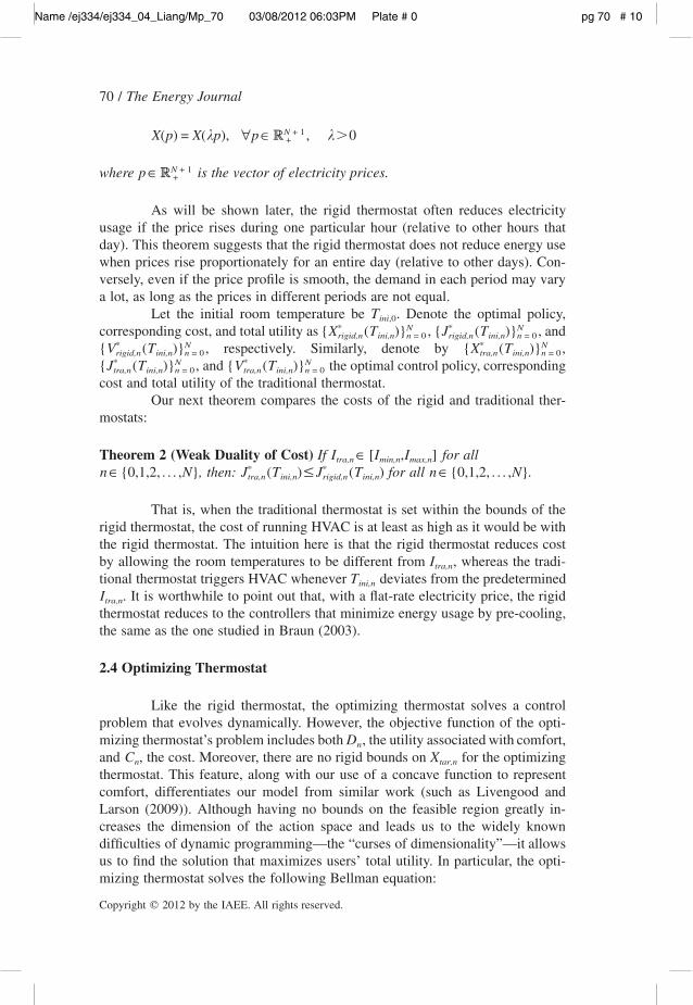
2.3 Rigid Thermostat
The rigid thermostat minimizes cost while keeping the temperaturewithin a given range. We model the rigid thermostat’s decisions as a dynamicprogramming problem. Denote the total cost and total utility from period to thenend of the planning horizon as and , respectively; then the Bellman equa-J V⋅ ,n ⋅ ,n
tion for the rigid thermostat is:
CP1: J (T ) = max F (T ,X ) + αJ (T ) (9)rigid,n ini,n ini,n tar,n rigid,n + 1 ini,n + 1Xtar,n
1Ts.t. T = f (T ,X ,h) + (10)ini,n + 1 out,n tar,n� �2
X ,T ∈ [I ,I ] (11)tar,n ini,n + 1 min,n max,n
where and . In Equation (9), the first termn∈{0,1,2, . . . ,N} J (T )≡0rigid,N + 1 ini,N + 1
is the one-period cost for electricity. The second term denotes the future value,given that the initial room temperature is and the decision in period isT nini,n
. is the discount factor, which is set to be 1 for all the simulations in thisX αtar,n
paper. In order to solve the problem efficiently, we confine the number of statesby aggregating the temperatures into integer values. Constraint (10) rounds theend temperature of period . This rounding will bring error into the optimization,nbut we can reduce the error by having finer discretization over temperature. Con-straints (11) are the rigid bounds on the feasible variable.
Theorem 1 For any fixed initial room temperature and a sequence of ambienttemperature forecasts, let be the function that maps the sequenceN + 1 N + 1X: � r �+ +
of electricity prices forecasts to the sequence of control signals obtained by solv-ing P1. Then is homogeneous of degree zero; that is,X
Name /ej334/ej334_04_Liang/Mp_70 03/08/2012 06:03PM Plate # 0 pg 70 # 10
70 / The Energy Journal
Copyright � 2012 by the IAEE. All rights reserved.
N + 1X(p) = X(kp), ∀p∈ � , k�0+
where is the vector of electricity prices.N + 1p∈ � +
As will be shown later, the rigid thermostat often reduces electricityusage if the price rises during one particular hour (relative to other hours thatday). This theorem suggests that the rigid thermostat does not reduce energy usewhen prices rise proportionately for an entire day (relative to other days). Con-versely, even if the price profile is smooth, the demand in each period may varya lot, as long as the prices in different periods are not equal.
Let the initial room temperature be . Denote the optimal policy,Tini,0
corresponding cost, and total utility as , , and* N * N{X (T )} {J (T )}rigid,n ini,n n = 0 rigid,n ini,n n = 0
, respectively. Similarly, denote by ,* N * N{V (T )} {X (T )}rigid,n ini,n n = 0 tra,n ini,n n = 0
, and the optimal control policy, corresponding* N * N{J (T )} {V (T )}tra,n ini,n n = 0 tra,n ini,n n = 0
cost and total utility of the traditional thermostat.Our next theorem compares the costs of the rigid and traditional ther-
mostats:
Theorem 2 (Weak Duality of Cost) If for allI ∈ [I ,I ]tra,n min,n max,n
, then: for all .* *n∈{0,1,2, . . . ,N} J (T )≤ J (T ) n∈{0,1,2, . . . ,N}tra,n ini,n rigid,n ini,n
That is, when the traditional thermostat is set within the bounds of therigid thermostat, the cost of running HVAC is at least as high as it would be withthe rigid thermostat. The intuition here is that the rigid thermostat reduces costby allowing the room temperatures to be different from , whereas the tradi-Itra,n
tional thermostat triggers HVAC whenever deviates from the predeterminedTini,n
. It is worthwhile to point out that, with a flat-rate electricity price, the rigidItra,n
thermostat reduces to the controllers that minimize energy usage by pre-cooling,the same as the one studied in Braun (2003).
2.4 Optimizing Thermostat
Like the rigid thermostat, the optimizing thermostat solves a controlproblem that evolves dynamically. However, the objective function of the opti-mizing thermostat’s problem includes both , the utility associated with comfort,Dn
and , the cost. Moreover, there are no rigid bounds on for the optimizingC Xn tar,n
thermostat. This feature, along with our use of a concave function to representcomfort, differentiates our model from similar work (such as Livengood andLarson (2009)). Although having no bounds on the feasible region greatly in-creases the dimension of the action space and leads us to the widely knowndifficulties of dynamic programming—the “curses of dimensionality”—it allowsus to find the solution that maximizes users’ total utility. In particular, the opti-mizing thermostat solves the following Bellman equation:
Name /ej334/ej334_04_Liang/Mp_71 03/08/2012 06:03PM Plate # 0 pg 71 # 11
Thermostats for the Smart Grid / 71
Copyright � 2012 by the IAEE. All rights reserved.
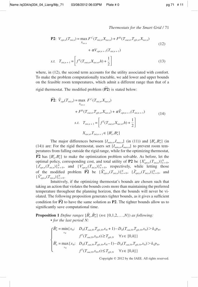
C DP2: V (T ) = max F (T ,X ) + F (T ,T ,X )opt,n ini,n ini,n tar,n out,n pfr,n tar,nXtar,n (12)
+ αV (T )opt,n + 1 ini,n + 1
1Ts.t. T = f (T ,X ,h) + (13)ini,n + 1 out,n tar,n� �2
where, in (12), the second term accounts for the utility associated with comfort.To make the problem computationally tractable, we add lower and upper boundson the feasible room temperatures, which admit a different range than that of a
rigid thermostat. The modified problem ( ) is stated below:�P2
� C˜P2: V (T ) = max F (T ,X )opt ini,n ini,n tar,nXtar,n
D ˜+ F (T ,T ,X ) + αV (T )out,n pfr,n tar,n opt,n + 1 ini,n + 1 (14)
1Ts.t. T = f (T ,X ,h) +ini,n + 1 out,n tar,n� �2
l uX ,T ∈ [B ,B ]tar,n ini,n + 1 n n
The major differences between (in (11)) and (inl u[I ,I ] [B ,B ]min,n max,n n n
(14)) are: For the rigid thermostat, users set to prevent room tem-[I ,I ]min,n max,n
peratures from falling outside the rigid range, while for the optimizing thermostat,has to make the optimization problem solvable. As before, let the
� l uP2 [B ,B ]n n
optimal policy, corresponding cost, and total utility of be ,* NP2 {X (T )}opt,n ini,n n = 0
, and , respectively, while letting those* N * N{J (T )} {V (T )}opt,n ini,n n = 0 opt,n ini,n n = 0
of the modified problem be , , and� * N * N˜ ˜P2 {X (T )} {J (T )}opt,n ini,n n = 0 opt,n ini,n n = 0
.* N˜{V (T )}opt,n ini,n n = 0
Intuitively, if the optimizing thermostat’s bounds are chosen such thattaking an action that violates the bounds costs more than maintaining the preferredtemperature throughout the planning horizon, then the bounds will never be vi-olated. The following proposition generates tighter bounds, as it gives a sufficient
condition for to have the same solution as . The tighter bounds allow us to�P2 P2
significantly save computational time.
Proposition 1 Define ranges as following:l u˜ ˜[B ,B ] (n∈{0,1,2, . . . ,N})n n
• for the last period :N
uB = min{x : D (T ,T ,x + 1)–D (T ,T ,x )�k p ,n N N out,N pfr,N N N out,N pfr,N N 1 NxN
Tf (T ,x ,s)≥ T ∀s∈ [0,h]}out,N N pfr,N
lB = max{x : D (T ,T ,x –1)–D (T ,T ,x )�k p ,n N N out,N pfr,N N N out,N pfr,N N 1 N�xN
Tf (T ,x ,s)≤ T ∀s∈ [0,h]}out,N N pfr,N

Name /ej334/ej334_04_Liang/Mp_72 03/08/2012 06:03PM Plate # 0 pg 72 # 12
72 / The Energy Journal
Copyright � 2012 by the IAEE. All rights reserved.
• for the other periods :n (n∈{0,1,2, . . . ,N–1})
uB = min{x : D (T ,T ,x + 1)–D (T ,T ,x )�k p ,n n n out,n pfr,n n n out,n pfr,n n 1 nxn
Tf (T ,x ,s)≥ T ∀s∈ [0,h],out,n n pfr,n
T uf (T ,x ,h)≥ B }out,n n n + 1
lB = max{x : D (T ,T ,x –1)–D (T ,T ,x )�k p ,n n n out,n pfr,n n n out,n pfr,n n 1 nxn
T� f (T ,x ,s)≤ T ∀s∈ [0,h],out,n n pfr,n
T lf (T ,x ,h)≤ B }out,n n n + 1
If the feasible region of satisfies , then the optimal� l u l u˜ ˜P2 [B ,B ]�[B ,B ]n n n n
solutions of are interior points of the feasible region of .�
P2 P2
The following theorem relates the total utilities of using the three typesof thermostat:
Theorem 3 (Weak Duality) If and for alll uI ≥ B I ≤ B n∈min,n n max,n n
, then the total utilities of using the three types of thermostat satisfy:{0,1,2, . . . N}
* * *˜V (T )≤ V (T )≤ V (T )tra,n ini,n opt,n ini,n opt,n ini,n
and
* * *˜V (T )≤ V (T )≤ V (T )rigid,n ini,n opt,n ini,n opt,n ini,n
The second inequalities are binding if the condition in Proposition 1 is met.
Note that the conditions in Theorem 3 are sufficient conditions. Theintuition behind Theorem 3 is that the optimizing thermostat penalizes deviationfrom the preferred temperature; in contrast, the rigid thermostat treats the pre-ferred and the other temperatures in as equally comfortable and the[I ,I ]min max
temperature outside as infinitely uncomfortable. Furthermore, it is[I ,I ]min max
straightforward to extend the results of Theorem 3 to obtain the following usefulcorollary.
Corollary 1 Compared with the rigid thermostat, the optimizing thermostat:• Creates more comfort for users if room temperatures are constrained
within (or if the generated room temperatures are bounded[I ,I ]min max
by ), and[I ,I ]min max
• Costs less when it generates lower or equal comfort.
The above results do not rely on the specific model for room tempera-tures that we assumed. More accurate models (for room temperatures and the
Name /ej334/ej334_04_Liang/Mp_73 03/08/2012 06:03PM Plate # 0 pg 73 # 13
Thermostats for the Smart Grid / 73
Copyright � 2012 by the IAEE. All rights reserved.
3. Source: http://www.ipm.ucdavis.edu/WEATHER/wxretrieve.html4. All figures use only data collected at the beginning and the end of each hourly period. In later
figures, data from distinct simulations are plotted with different markers and we connect the datapoints to make the results that come from different settings more distinguishable.
associated comfort calculations) are able to better describe room temperatures butdo not change the relationship among the regions of the feasible solutions in theBellman equations of the thermostats; thus, Theorem 2 and Theorem 3 still hold.Theorem 1 also holds because scaling the price does not affect the relationshipamong different solutions. In fact, as long as the model of interest possesses theMarkovian property, we can model the control problems of the rigid and theoptimizing thermostats by similar Bellman equations and the above theorems stillhold.
Our models also work when there are forecasting uncertainties. In par-ticular, the certainty equivalence control approach (Bertsekas, 1995) is applied.Although applying this approach is penalized when “bad” scenarios with lowprobability occur (Papavasiliou, 2011), the worst-case one-period total utility ofsetting at ( equals to or ) is bounded below by the summation* *X X X X Xtar,n rigid,n opt,n
of , , and . Sim-D C C T TF (T ,T ,X) F (T ,T ) F ( f (T ,X,h), f (T ,T ,h))out,n pfr,n ini,n pfr,n out,n out,n pfr,n
ulations that study the performance of this CEC approach are presented in section4.2. An alternative approach that also preserves the weak duality is to relax thefull-information assumption by setting prices and ambient temperatures as Mar-kov processes. This approach slightly increases the computational requirements,as the deterministic value-to-go functions need to be replaced by their expecta-tions.
3. SIMULATION AND MANAGERIAL INSGIHTS
Theorem 3 implies that a user’s total utility when using the optimizingthermostat, , is always better than or equal to those of using the traditional*Vopt,n
and the rigid thermostats. In this section, we conduct numerical studies to learnthe magnitude of the increase in comfort and/or reduction in cost of the optimizingthermostat relative to the other two. Then, we perform several controlled numer-ical experiments to examine how the different thermostats affect peak demandand how the different parameters influence the performance of these thermostats.
3.1 Summer Savings of the Rigid and Optimizing Thermostats
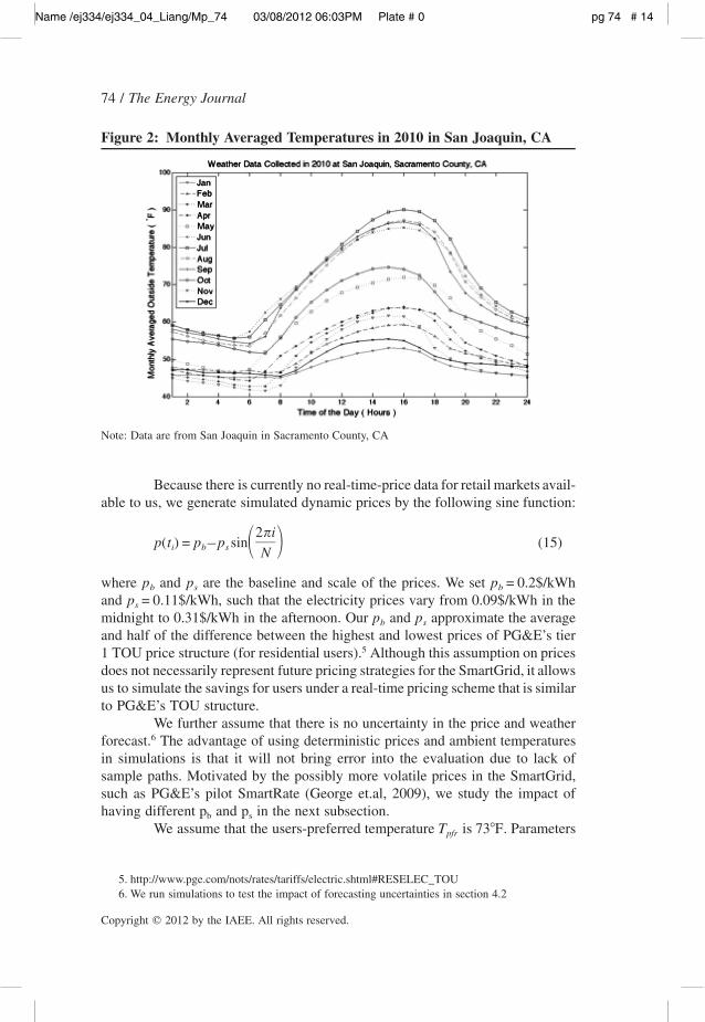
We first investigate how the optimizing and rigid thermostats benefitSmart Grid users in the summer. In order to get a realistic simulation, we choosethe ambient temperature data collected at San Joaquin in Sacramento County,California in 2010.3 The hour-by-hour monthly average ambient temperature pro-files are plotted in Figure 2.4 We simulate one entire summer (24 hourly datapoints per day on the 93 days from June 21 to September 21).
Name /ej334/ej334_04_Liang/Mp_74 03/08/2012 06:03PM Plate # 0 pg 74 # 14
74 / The Energy Journal
Copyright � 2012 by the IAEE. All rights reserved.
Figure 2: Monthly Averaged Temperatures in 2010 in San Joaquin, CA
Note: Data are from San Joaquin in Sacramento County, CA
5. http://www.pge.com/nots/rates/tariffs/electric.shtml#RESELEC_TOU6. We run simulations to test the impact of forecasting uncertainties in section 4.2
Because there is currently no real-time-price data for retail markets avail-able to us, we generate simulated dynamic prices by the following sine function:
2pip(t ) = p –p sin (15)i b s � �N
where and are the baseline and scale of the prices. We setp p p = 0.2$/kWhb s b
and , such that the electricity prices vary from in thep = 0.11$/kWh 0.09$/kWhs
midnight to in the afternoon. Our and approximate the average0.31$/kWh p pb s
and half of the difference between the highest and lowest prices of PG&E’s tier1 TOU price structure (for residential users).5 Although this assumption on pricesdoes not necessarily represent future pricing strategies for the SmartGrid, it allowsus to simulate the savings for users under a real-time pricing scheme that is similarto PG&E’s TOU structure.
We further assume that there is no uncertainty in the price and weatherforecast.6 The advantage of using deterministic prices and ambient temperaturesin simulations is that it will not bring error into the evaluation due to lack ofsample paths. Motivated by the possibly more volatile prices in the SmartGrid,such as PG&E’s pilot SmartRate (George et.al, 2009), we study the impact ofhaving different and in the next subsection.p pb s
We assume that the users-preferred temperature is . ParametersT 73�Fpfr
Name /ej334/ej334_04_Liang/Mp_75 03/08/2012 06:03PM Plate # 0 pg 75 # 15
Thermostats for the Smart Grid / 75
Copyright � 2012 by the IAEE. All rights reserved.
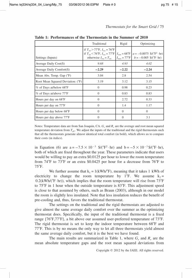
Table 1: Performances of the Thermostats in the Summer of 2010
Traditional Rigid Optimizing
Settings (Inputs)
if ,T �77�F I = 76�Fini tra
if ,T �76�F I = 77�Fini tra
otherwise I = Ttra ini
I = 68�Fmin
I = 77�Fmax
2a = –0.0075 $/(�F ⋅hr)b = –0.005 $/(�F ⋅hr)
Average Daily Cost($) 9.68 4.93 4.02
Average Daily Comfort($) –2.29 –2.22 –2.24
Mean Abs. Temp. Gap (�F) 3.04 2.8 2.54
Root Mean Squared Deviation: (�F) 3.19 3.12 3.15
of Days at/below% 68�F 0 0.98 0.23
of Days at/above% 77�F 0 0.83 0.83
Hours per day on 68�F 0 2.72 0.33
Hours per day on 77�F 0 1.4 1.17
Hours per day below 68�F 0 0 0
Hours per day above 77�F 0 0 3.1
Notes: Temperature data are from San Joaquin, CA. and are the average and root mean squaredG Re e
temperature deviation from . We adjust the inputs of the traditional and the rigid thermostats suchTpfr
that all the thermostats generate almost identical total comfort (in bold), which allows us to comparetheir costs (in italics).
in Equation (6) are and ,–3 2 –3a = –7.5�10 $/(�F ⋅hr) b = –5�10 $/(�F ⋅hr)both of which are fixed throughout the year. These parameters indicate that userswould be willing to pay an extra per hour to lower the room temperature$0.0125from to or an extra per hour for a decrease from to74�F 73�F $0.0425 76�F
.75�FWe further assume that , meaning that it takes ofk = 1(kWh/�F) 1 kWh1
electricity to change the room temperature by . We assume1�F k =2
, which implies that the room temperature will rise from0.2(kWh/(�F ⋅hr)) 73�Fto in 1 hour when the outside temperature is . This adjustment speed75�F 83�Fis close to that assumed by others, such as Braun (2003), although in our modelthe room is slightly less insulated. Note that less insulation reduces the benefit ofpre-cooling and, thus, favors the traditional thermostat.
The settings on the traditional and the rigid thermostats are adjusted togive almost the same average daily comfort over the summer as the optimizingthermostat does. Specifically, the input of the traditional thermostat is a fixedrange , a bit above our assumed user-preferred temperature of .[76�F,77�F] 73�FThe rigid thermostat is set to keep the indoor temperature between and68�F
. This is by no means the only way to let all three thermostats yield almost77�Fthe same average daily comfort, but it is the best we have found.
The main results are summarized in Table 1, where and are theG Re e
mean absolute temperature gaps and the root mean squared deviations from
Name /ej334/ej334_04_Liang/Mp_76 03/08/2012 06:03PM Plate # 0 pg 76 # 16
76 / The Energy Journal
Copyright � 2012 by the IAEE. All rights reserved.
, respectively. In this simulation, the rigid thermostat costs perT = 73�F $458.5pfr
summer, ( ) less than the traditional thermostat to achieve the same average49%comfort. Consistent with Theorem 3, the optimizing thermostat does even better,saving per summer ( ) relative to the traditional thermostat and$526.4 58%
( ) relative to the rigid thermostat. To put these savings in perspective,$84.63 18%an Internet-enabled thermostat costs less than at Home Depot. With the$100simulation results, we believe that, even if we ignore the costs of the other twothermostats, the setup cost of the optimizing thermostat can be more than com-pensated for by the cost saving in the first summer of use.
The advantage of the optimizing thermostat over the rigid thermostatcomes in part from keeping the indoor temperature on average closer to the users-preferred temperature; the mean absolute deviation is for the optimizingG 2.54�Fe
versus for the rigid thermostat. The rigid thermostat treats all temperatures2.80�Fbetween its lowest ( ) and highest ( ) permitted temperatures as equallyI Imin max
valuable. Thus, if the indoor temperature is anywhere within that range, the rigidthermostat makes no effort to keep the temperature any nearer to the users-pre-ferred temperature. Therefore, on any fairly hot day, the thermostat pre-cools allthe way down to the lowest rigid constraint , and also spends the warm partImin
of the afternoon at the highest rigid constraint . In our simulations, the rigidImax
thermostat pushes the temperature down to on 91 of the 93 days over theImin
summer, while the optimizing thermostat only pushes temperatures that low on21 days. Similarly, the rigid thermostat keeps the inside temperature within adegree of for hours per day over the summer, while the optimizingI 2.72min
thermostat only does so for 0.33 hours per day.At the same time, the rigid thermostat never permits temperatures above
, while the optimizing thermostat balances cost and comfort with few extremeImax
room temperatures. For instance, in the above simulation, the optimizing ther-mostat rises over for 3.1 hours per day during the simulated summer.Imax
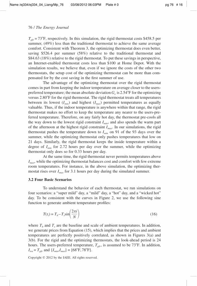
3.2 Four Basic Scenarios
To understand the behavior of each thermostat, we run simulations onfour scenarios: a “super mild” day, a “mild” day, a “hot” day, and a “wicked hot”day. To be consistent with the curves in Figure 2, we use the following sinefunction to generate ambient temperature profiles:
2piT(t ) = T –T sin (16)i b s � �N
where and are the baseline and scale of ambient temperatures. In addition,T Tb s
we generate prices from Equation (15), which implies that the prices and ambienttemperatures are perfectly positively correlated, as shown in Figures 3(a) and3(b). For the rigid and the optimizing thermostats, the look-ahead period is 24hours. The users-preferred temperature, , is assumed to be . In addition,T 73�Fpfr
and .I = T [I ,I ] = [68�F,78�F]tra pfr min max
Name /ej334/ej334_04_Liang/Mp_77 03/08/2012 06:03PM Plate # 0 pg 77 # 17
Thermostats for the Smart Grid / 77
Copyright � 2012 by the IAEE. All rights reserved.
Figure 3: Four Basic Scenarios
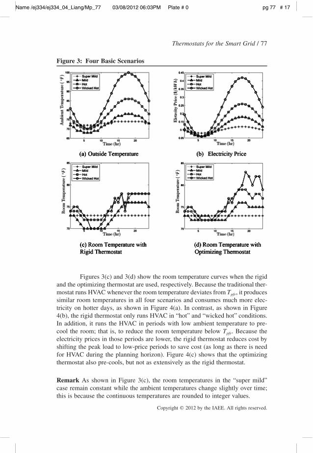
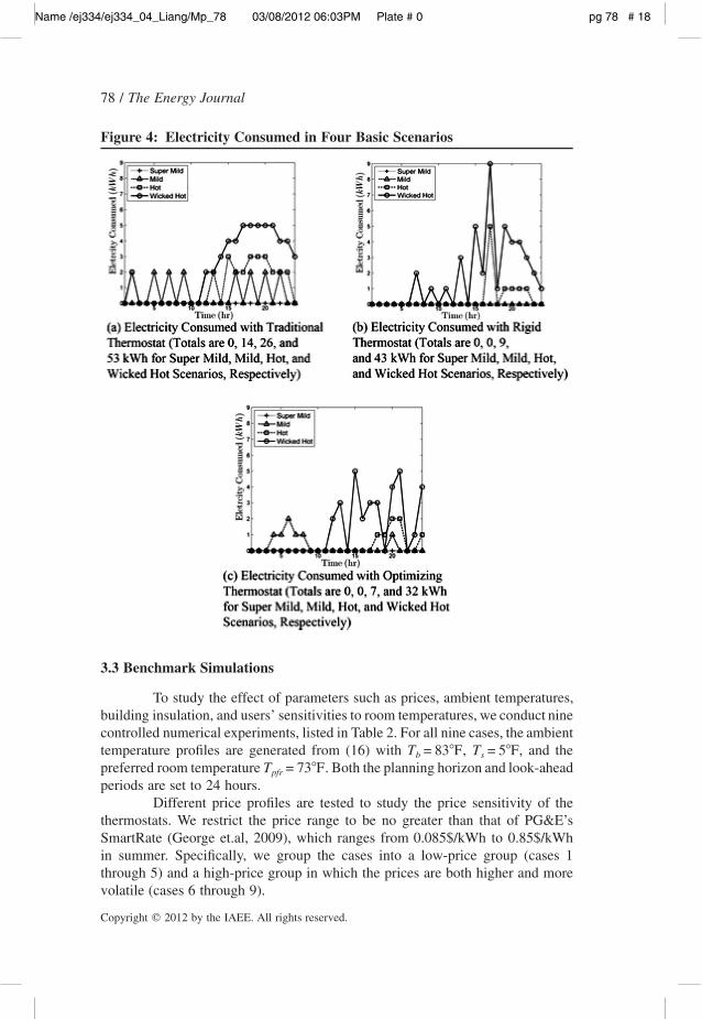
Figures 3(c) and 3(d) show the room temperature curves when the rigidand the optimizing thermostat are used, respectively. Because the traditional ther-mostat runs HVAC whenever the room temperature deviates from , it producesTpfr
similar room temperatures in all four scenarios and consumes much more elec-tricity on hotter days, as shown in Figure 4(a). In contrast, as shown in Figure4(b), the rigid thermostat only runs HVAC in “hot” and “wicked hot” conditions.In addition, it runs the HVAC in periods with low ambient temperature to pre-cool the room; that is, to reduce the room temperature below . Because theTpfr
electricity prices in those periods are lower, the rigid thermostat reduces cost byshifting the peak load to low-price periods to save cost (as long as there is needfor HVAC during the planning horizon). Figure 4(c) shows that the optimizingthermostat also pre-cools, but not as extensively as the rigid thermostat.
Remark As shown in Figure 3(c), the room temperatures in the “super mild”case remain constant while the ambient temperatures change slightly over time;this is because the continuous temperatures are rounded to integer values.
Name /ej334/ej334_04_Liang/Mp_78 03/08/2012 06:03PM Plate # 0 pg 78 # 18
78 / The Energy Journal
Copyright � 2012 by the IAEE. All rights reserved.
Figure 4: Electricity Consumed in Four Basic Scenarios
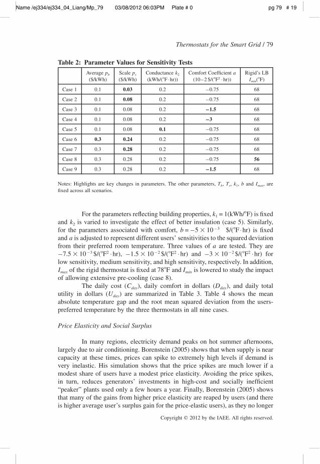
3.3 Benchmark Simulations
To study the effect of parameters such as prices, ambient temperatures,building insulation, and users’ sensitivities to room temperatures, we conduct ninecontrolled numerical experiments, listed in Table 2. For all nine cases, the ambienttemperature profiles are generated from (16) with , , and theT = 83�F T = 5�Fb s
preferred room temperature . Both the planning horizon and look-aheadT = 73�Fpfr
periods are set to 24 hours.Different price profiles are tested to study the price sensitivity of the
thermostats. We restrict the price range to be no greater than that of PG&E’sSmartRate (George et.al, 2009), which ranges from to0.085$/kWh 0.85$/kWhin summer. Specifically, we group the cases into a low-price group (cases 1through 5) and a high-price group in which the prices are both higher and morevolatile (cases 6 through 9).
Name /ej334/ej334_04_Liang/Mp_79 03/08/2012 06:03PM Plate # 0 pg 79 # 19
Thermostats for the Smart Grid / 79
Copyright � 2012 by the IAEE. All rights reserved.
Table 2: Parameter Values for Sensitivity Tests
Average pb
( )$/kWhScale ps
( )$/kWhConductance k2
(kWh/(�F ⋅hr))Comfort Coefficient a
2(10–2 $/(�F ⋅hr))Rigid’s LB
I (�F)min
Case 1 0.1 0.03 0.2 –0.75 68
Case 2 0.1 0.08 0.2 –0.75 68
Case 3 0.1 0.08 0.2 –1.5 68
Case 4 0.1 0.08 0.2 –3 68
Case 5 0.1 0.08 0.1 –0.75 68
Case 6 0.3 0.24 0.2 –0.75 68
Case 7 0.3 0.28 0.2 –0.75 68
Case 8 0.3 0.28 0.2 –0.75 56
Case 9 0.3 0.28 0.2 –1.5 68
Notes: Highlights are key changes in parameters. The other parameters, , , , and , areT T k b Ib s 1 max
fixed across all scenarios.
For the parameters reflecting building properties, is fixedk = 1(kWh/�F)1
and is varied to investigate the effect of better insulation (case 5). Similarly,k2
for the parameters associated with comfort, is fixed–3b = –5�10 $/(�F ⋅hr)and is adjusted to represent different users’ sensitivities to the squared deviationafrom their preferred room temperature. Three values of are tested. They area
, and for–3 2 –2 2 –2 2–7.5�10 $/(�F ⋅hr) –1.5�10 $/(�F ⋅hr) –3�10 $/(�F ⋅hr)low sensitivity, medium sensitivity, and high sensitivity, respectively. In addition,
of the rigid thermostat is fixed at and is lowered to study the impactI 78�F Imax min
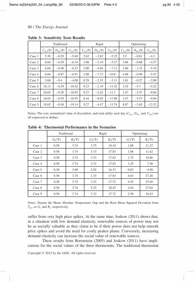
of allowing extensive pre-cooling (case 8).The daily cost ( ), daily comfort in dollars ( ), and daily totalC Dday day
utility in dollars ( ) are summarized in Table 3. Table 4 shows the meanUday
absolute temperature gap and the root mean squared deviation from the users-preferred temperature by the three thermostats in all nine cases.
Price Elasticity and Social Surplus
In many regions, electricity demand peaks on hot summer afternoons,largely due to air conditioning. Borenstein (2005) shows that when supply is nearcapacity at these times, prices can spike to extremely high levels if demand isvery inelastic. His simulation shows that the price spikes are much lower if amodest share of users have a modest price elasticity. Avoiding the price spikes,in turn, reduces generators’ investments in high-cost and socially inefficient“peaker” plants used only a few hours a year. Finally, Borenstein (2005) showsthat many of the gains from higher price elasticity are reaped by users (and thereis higher average user’s surplus gain for the price-elastic users), as they no longer
Name /ej334/ej334_04_Liang/Mp_80 03/08/2012 06:03PM Plate # 0 pg 80 # 20
80 / The Energy Journal
Copyright � 2012 by the IAEE. All rights reserved.
Table 3: Sensitivity Tests Results
Traditional Rigid Optimizing
Cday($) Dday($) Uday($) Cday($) Dday($) Uday($) Cday($) Dday($) Uday($)
Case 1 5.39 –0.29 –5.69 2.62 –2.62 –5.25 3.5 –0.81 –4.3
Case 2 6.04 –0.29 –6.34 3.08 –2.19 –5.27 3.68 –0.88 –4.57
Case 3 6.04 –0.48 –6.53 3.08 –4.04 –7.11 3.86 –1.33 –5.19
Case 4 6.04 –0.87 –6.91 3.08 –7.73 –10.8 4.98 –0.99 –5.97
Case 5 3.68 –0.4 –4.08 0.78 –2.33 –3.11 1.81 –0.27 –2.08
Case 6 18.13 –0.29 –18.42 9.23 –2.19 –11.42 3.52 –5.7 –9.22
Case 7 18.65 –0.29 –18.95 9.27 –2.42 –11.7 3.47 –5.57 –9.04
Case 8 18.65 –0.29 –18.95 8.44 –8.65 –17.08 3.47 –5.57 –9.04
Case 9 18.65 –0.48 –19.14 9.27 –4.47 –13.74 8.87 –3.65 –12.52
Notes: The cost, normalized value of discomfort, and total utility each day ( , ) areC D and Uday day day
all expressed in dollars.
Table 4: Thermostat Performance in the Scenarios
Traditional Rigid Optimizing
Ge(�F) Re(�F) Ge(�F) Re(�F) Ge(�F) Re(�F)
Case 1 0.58 3.74 3.75 19.18 1.88 11.27
Case 2 0.58 3.74 3.33 17.83 1.88 11.62
Case 3 0.58 3.74 3.33 17.83 1.75 10.86
Case 4 0.58 3.74 3.33 17.83 1.25 7.48
Case 5 0.38 3.00 2.92 16.31 0.83 4.90
Case 6 0.58 3.74 3.33 17.83 4.63 27.26
Case 7 0.58 3.74 3.33 17.72 4.54 27.04
Case 8 0.58 3.74 5.25 30.43 4.54 27.04
Case 9 0.58 3.74 3.33 17.72 2.58 16.43
Notes: Denote the Mean Absolute Temperature Gap and the Root Mean Squared Deviation from, as and , respectively.T G Rpfr e e
suffer from very high price spikes. At the same time, Joskow (2011) shows that,in a situation with low demand elasticity, renewable sources of power may notbe as socially valuable as they claim to be if their power does not help smoothprice spikes and avoid the need for costly peaker plants. Conversely, increasingdemand elasticity can increase the social value of renewable sources.
These results from Borenstein (2005) and Joskow (2011) have impli-cations for the social values of the three thermostats. The traditional thermostat
Name /ej334/ej334_04_Liang/Mp_81 03/08/2012 06:03PM Plate # 0 pg 81 # 21
Thermostats for the Smart Grid / 81
Copyright � 2012 by the IAEE. All rights reserved.
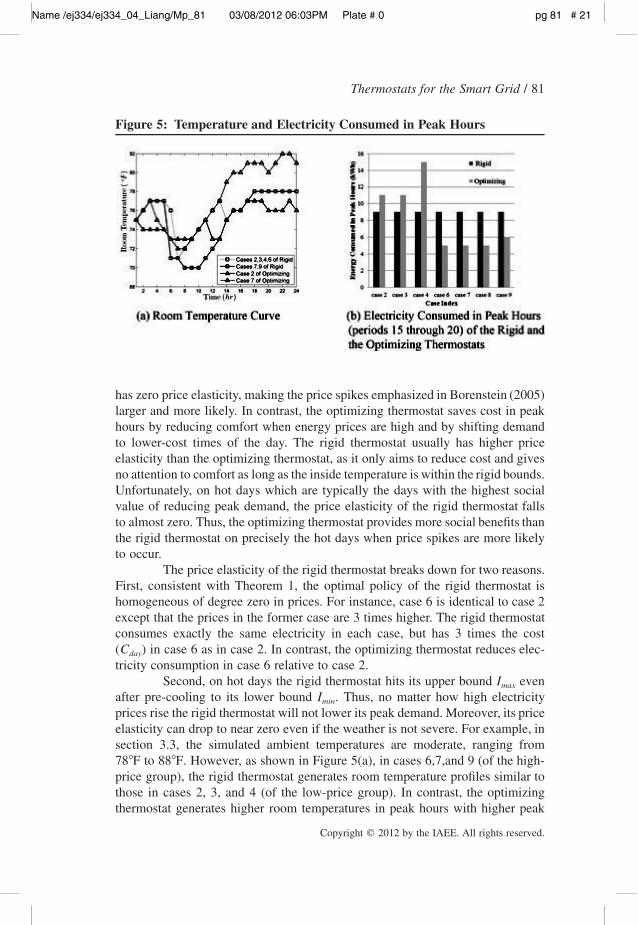
Figure 5: Temperature and Electricity Consumed in Peak Hours
has zero price elasticity, making the price spikes emphasized in Borenstein (2005)larger and more likely. In contrast, the optimizing thermostat saves cost in peakhours by reducing comfort when energy prices are high and by shifting demandto lower-cost times of the day. The rigid thermostat usually has higher priceelasticity than the optimizing thermostat, as it only aims to reduce cost and givesno attention to comfort as long as the inside temperature is within the rigid bounds.Unfortunately, on hot days which are typically the days with the highest socialvalue of reducing peak demand, the price elasticity of the rigid thermostat fallsto almost zero. Thus, the optimizing thermostat provides more social benefits thanthe rigid thermostat on precisely the hot days when price spikes are more likelyto occur.
The price elasticity of the rigid thermostat breaks down for two reasons.First, consistent with Theorem 1, the optimal policy of the rigid thermostat ishomogeneous of degree zero in prices. For instance, case 6 is identical to case 2except that the prices in the former case are 3 times higher. The rigid thermostatconsumes exactly the same electricity in each case, but has 3 times the cost( ) in case 6 as in case 2. In contrast, the optimizing thermostat reduces elec-Cday
tricity consumption in case 6 relative to case 2.Second, on hot days the rigid thermostat hits its upper bound evenImax
after pre-cooling to its lower bound . Thus, no matter how high electricityImin
prices rise the rigid thermostat will not lower its peak demand. Moreover, its priceelasticity can drop to near zero even if the weather is not severe. For example, insection 3.3, the simulated ambient temperatures are moderate, ranging from
to . However, as shown in Figure 5(a), in cases 6,7,and 9 (of the high-78�F 88�Fprice group), the rigid thermostat generates room temperature profiles similar tothose in cases 2, 3, and 4 (of the low-price group). In contrast, the optimizingthermostat generates higher room temperatures in peak hours with higher peak
Name /ej334/ej334_04_Liang/Mp_82 03/08/2012 06:03PM Plate # 0 pg 82 # 22
82 / The Energy Journal
Copyright � 2012 by the IAEE. All rights reserved.
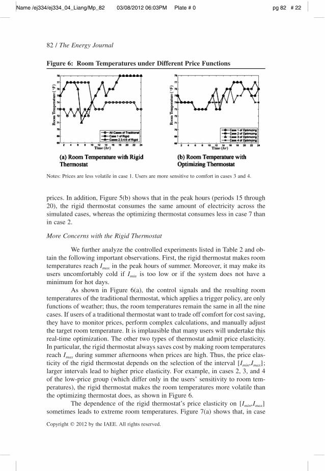
Figure 6: Room Temperatures under Different Price Functions
Notes: Prices are less volatile in case 1. Users are more sensitive to comfort in cases 3 and 4.
prices. In addition, Figure 5(b) shows that in the peak hours (periods 15 through20), the rigid thermostat consumes the same amount of electricity across thesimulated cases, whereas the optimizing thermostat consumes less in case 7 thanin case 2.
More Concerns with the Rigid Thermostat
We further analyze the controlled experiments listed in Table 2 and ob-tain the following important observations. First, the rigid thermostat makes roomtemperatures reach in the peak hours of summer. Moreover, it may make itsImax
users uncomfortably cold if is too low or if the system does not have aImin
minimum for hot days.As shown in Figure 6(a), the control signals and the resulting room
temperatures of the traditional thermostat, which applies a trigger policy, are onlyfunctions of weather; thus, the room temperatures remain the same in all the ninecases. If users of a traditional thermostat want to trade off comfort for cost saving,they have to monitor prices, perform complex calculations, and manually adjustthe target room temperature. It is implausible that many users will undertake thisreal-time optimization. The other two types of thermostat admit price elasticity.In particular, the rigid thermostat always saves cost by making room temperaturesreach during summer afternoons when prices are high. Thus, the price elas-Imax
ticity of the rigid thermostat depends on the selection of the interval ;[I ,I ]min max
larger intervals lead to higher price elasticity. For example, in cases 2, 3, and 4of the low-price group (which differ only in the users’ sensitivity to room tem-peratures), the rigid thermostat makes the room temperatures more volatile thanthe optimizing thermostat does, as shown in Figure 6.
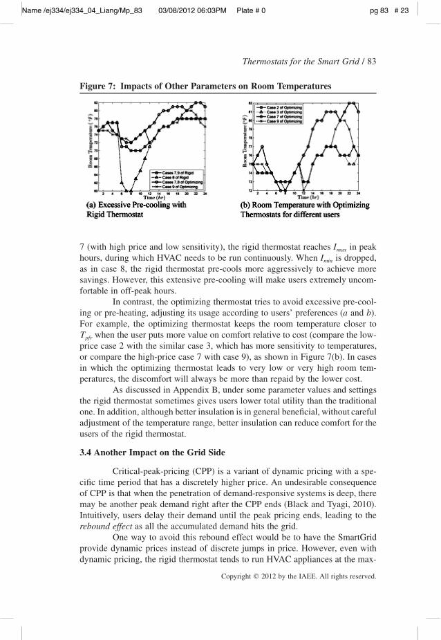
The dependence of the rigid thermostat’s price elasticity on [I ,I ]min max
sometimes leads to extreme room temperatures. Figure 7(a) shows that, in case
Name /ej334/ej334_04_Liang/Mp_83 03/08/2012 06:03PM Plate # 0 pg 83 # 23
Thermostats for the Smart Grid / 83
Copyright � 2012 by the IAEE. All rights reserved.
Figure 7: Impacts of Other Parameters on Room Temperatures
7 (with high price and low sensitivity), the rigid thermostat reaches in peakImax
hours, during which HVAC needs to be run continuously. When is dropped,Imin
as in case 8, the rigid thermostat pre-cools more aggressively to achieve moresavings. However, this extensive pre-cooling will make users extremely uncom-fortable in off-peak hours.
In contrast, the optimizing thermostat tries to avoid excessive pre-cool-ing or pre-heating, adjusting its usage according to users’ preferences ( and ).a bFor example, the optimizing thermostat keeps the room temperature closer to
when the user puts more value on comfort relative to cost (compare the low-Tpfr
price case 2 with the similar case 3, which has more sensitivity to temperatures,or compare the high-price case 7 with case 9), as shown in Figure 7(b). In casesin which the optimizing thermostat leads to very low or very high room tem-peratures, the discomfort will always be more than repaid by the lower cost.
As discussed in Appendix B, under some parameter values and settingsthe rigid thermostat sometimes gives users lower total utility than the traditionalone. In addition, although better insulation is in general beneficial, without carefuladjustment of the temperature range, better insulation can reduce comfort for theusers of the rigid thermostat.
3.4 Another Impact on the Grid Side
Critical-peak-pricing (CPP) is a variant of dynamic pricing with a spe-cific time period that has a discretely higher price. An undesirable consequenceof CPP is that when the penetration of demand-responsive systems is deep, theremay be another peak demand right after the CPP ends (Black and Tyagi, 2010).Intuitively, users delay their demand until the peak pricing ends, leading to therebound effect as all the accumulated demand hits the grid.
One way to avoid this rebound effect would be to have the SmartGridprovide dynamic prices instead of discrete jumps in price. However, even withdynamic pricing, the rigid thermostat tends to run HVAC appliances at the max-
Name /ej334/ej334_04_Liang/Mp_84 03/08/2012 06:03PM Plate # 0 pg 84 # 24
84 / The Energy Journal
Copyright � 2012 by the IAEE. All rights reserved.
Table 5: Maximum enegy use versus usage during peak hours
Traditional Rigid Opt
Emax Epeak Emax Epeak Emax Epeak
Case 1 3 3 4 1.5 5 1.83
Case 2 3 3 6 1.5 4 1.83
Case 3 3 3 6 1.5 4 1.83
Case 4 3 3 6 1.5 5 2.5
Case 5 2 2 5 0 2 0.67
Case 6 3 3 6 1.5 4 0.83
Case 7 3 3 7 1.5 3 0.83
Case 8 3 3 18 1.5 3 0.83
Case 9 3 3 7 1.5 5 1
Notes: Comparison of (the maximum electricity demand in per period) and (theE kWh Emax peak
average electricity consumed in per period in periods 15 through 20, the peak periods, with thekWhtraditional thermostat)
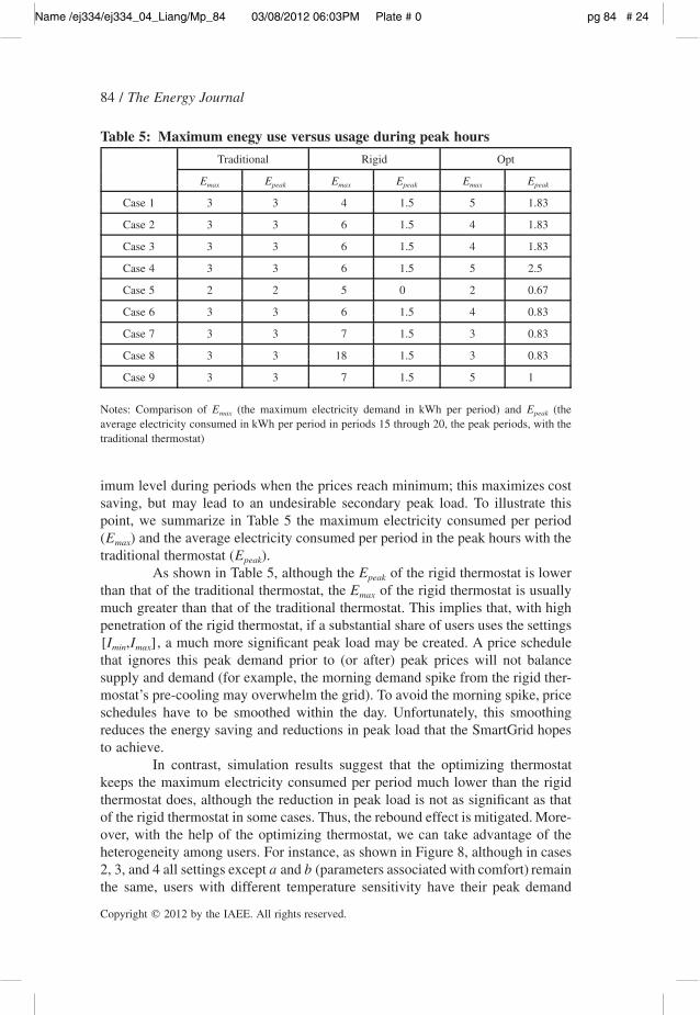
imum level during periods when the prices reach minimum; this maximizes costsaving, but may lead to an undesirable secondary peak load. To illustrate thispoint, we summarize in Table 5 the maximum electricity consumed per period( ) and the average electricity consumed per period in the peak hours with theEmax
traditional thermostat ( ).Epeak
As shown in Table 5, although the of the rigid thermostat is lowerEpeak
than that of the traditional thermostat, the of the rigid thermostat is usuallyEmax
much greater than that of the traditional thermostat. This implies that, with highpenetration of the rigid thermostat, if a substantial share of users uses the settings
, a much more significant peak load may be created. A price schedule[I ,I ]min max
that ignores this peak demand prior to (or after) peak prices will not balancesupply and demand (for example, the morning demand spike from the rigid ther-mostat’s pre-cooling may overwhelm the grid). To avoid the morning spike, priceschedules have to be smoothed within the day. Unfortunately, this smoothingreduces the energy saving and reductions in peak load that the SmartGrid hopesto achieve.
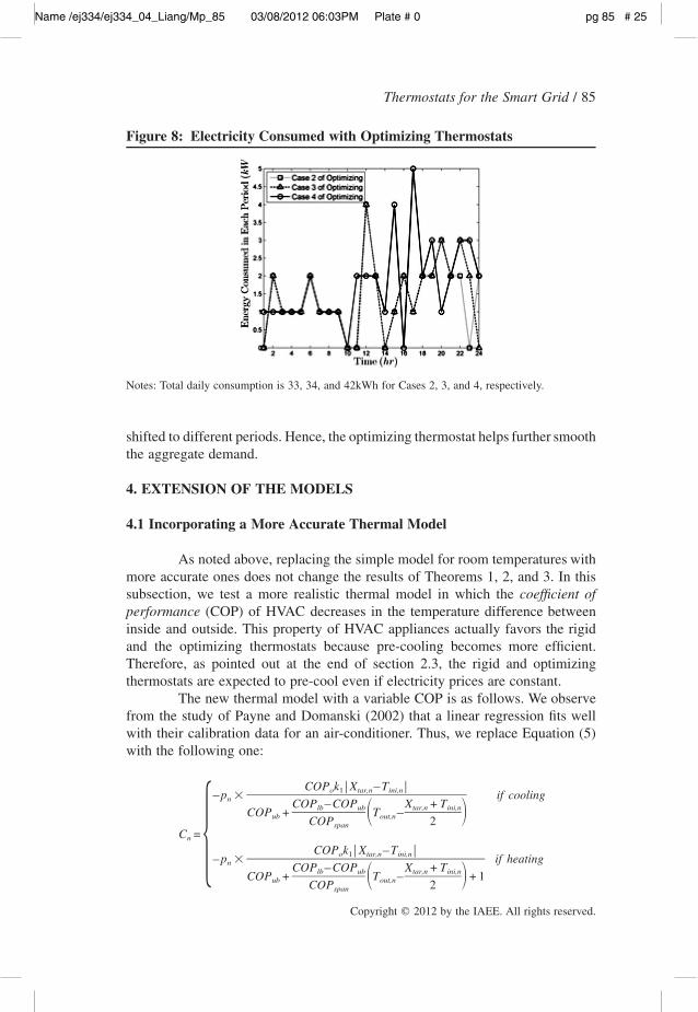
In contrast, simulation results suggest that the optimizing thermostatkeeps the maximum electricity consumed per period much lower than the rigidthermostat does, although the reduction in peak load is not as significant as thatof the rigid thermostat in some cases. Thus, the rebound effect is mitigated. More-over, with the help of the optimizing thermostat, we can take advantage of theheterogeneity among users. For instance, as shown in Figure 8, although in cases2, 3, and 4 all settings except and (parameters associated with comfort) remaina bthe same, users with different temperature sensitivity have their peak demand
Name /ej334/ej334_04_Liang/Mp_85 03/08/2012 06:03PM Plate # 0 pg 85 # 25
Thermostats for the Smart Grid / 85
Copyright � 2012 by the IAEE. All rights reserved.
Figure 8: Electricity Consumed with Optimizing Thermostats
Notes: Total daily consumption is , , and for Cases 2, 3, and 4, respectively.33 34 42kWh
shifted to different periods. Hence, the optimizing thermostat helps further smooththe aggregate demand.
4. EXTENSION OF THE MODELS
4.1 Incorporating a More Accurate Thermal Model
As noted above, replacing the simple model for room temperatures withmore accurate ones does not change the results of Theorems 1, 2, and 3. In thissubsection, we test a more realistic thermal model in which the coefficient ofperformance (COP) of HVAC decreases in the temperature difference betweeninside and outside. This property of HVAC appliances actually favors the rigidand the optimizing thermostats because pre-cooling becomes more efficient.Therefore, as pointed out at the end of section 2.3, the rigid and optimizingthermostats are expected to pre-cool even if electricity prices are constant.
The new thermal model with a variable COP is as follows. We observefrom the study of Payne and Domanski (2002) that a linear regression fits wellwith their calibration data for an air-conditioner. Thus, we replace Equation (5)with the following one:
COP k X –T⎪ ⎪o 1 tar,n ini,n–p � if coolingn COP –COP X + Tlb ub tar,n ini,nCOP + T –ub out,n� �COP 2span
C =n
COP k X –T⎪ ⎪o 1 tar,n ini,n–p � if heating� n COP –COP X + Tlb ub tar,n ini,nCOP + T – + 1ub out,n� �COP 2span
Name /ej334/ej334_04_Liang/Mp_86 03/08/2012 06:03PM Plate # 0 pg 86 # 26
86 / The Energy Journal
Copyright � 2012 by the IAEE. All rights reserved.
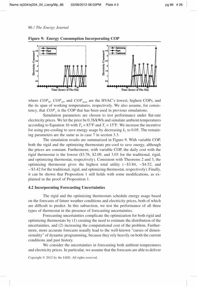
Figure 9: Energy Consumption Incorporating COP
where , , and are the HVAC’s lowest, highest COPs, andCOP COP COPlb ub span
the its span of working temperatures, respectively. We also assume, for consis-tency, that is the COP that has been used in previous simulations.COPo
Simulation parameters are chosen to test performance under flat-rateelectricity prices. We let the price be and simulate ambient temperatures0.3$/kWhaccording to Equation 16 with and . We increase the incentiveT = 83�F T = 15�Fb s
for using pre-cooling to save energy usage by decreasing to . The remain-k 0.052
ing parameters are the same as in case 7 in section 3.3.The simulation results are summarized in Figure 9. With variable COP,
both the rigid and the optimizing thermostats pre-cool to save energy, althoughthe prices are constant. Furthermore, with variable COP, the daily cost with therigid thermostat is the lowest ( , , and for the traditional, rigid,$3.76 $2.09 3.03and optimizing thermostat, respectively). Consistent with Theorems 2 and 3, theoptimizing thermostat gives the highest total utility ( , , and–$3.84 –$4.52
for the traditional, rigid, and optimizing thermostat, respectively). Finally,–$3.42it can be shown that Proposition 1 still holds with some modifications, as ex-plained in the proof of Proposition 1.
4.2 Incorporating Forecasting Uncertainties
The rigid and the optimizing thermostats schedule energy usage basedon the forecasts of future weather conditions and electricity prices, both of whichare difficult to predict. In this subsection, we test the performance of all threetypes of thermostat in the presence of forecasting uncertainties.
Forecasting uncertainties complicate the optimization for both rigid andoptimizing thermostats by (1) creating the need to estimate the distribution of theuncertainties, and (2) increasing the computational cost of the problem. Further-more, more accurate forecasts usually lead to the well-known “curses of dimen-sionality” of dynamic programming, because they rely heavily on both the currentconditions and past history.
We consider the uncertainties in forecasting both ambient temperaturesand electricity prices. In particular, we assume that the forecasts are able to deliver
Name /ej334/ej334_04_Liang/Mp_87 03/08/2012 06:03PM Plate # 0 pg 87 # 27
Thermostats for the Smart Grid / 87
Copyright � 2012 by the IAEE. All rights reserved.
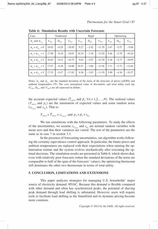
Table 6: Simulation Results with Uncertain Forecasts
Case Traditional Rigid Optimizing
andσ σe ep Tout
Cday Dday Uday Cday Dday Uday Cday Dday Uday
σ = σ = 0e ep Tout
18.65 –0.29 –18.95 9.27 –2.42 –11.70 3.47 –5.57 –9.04
σ = σ = 1e ep Tout
17.90 –0.10 –18.01 10.19 –3.10 –13.29 4.46 –5.78 –10.24
σ = σ = 2e ep Tout
16.63 –0.12 –16.75 9.62 –3.07 –12.70 5.18 –5.77 –10.95
σ = σ = 3e ep Tout
17.87 –0.20 –18.06 10.51 –3.06 –13.56 7.11 –5.73 –12.84
σ = σ = 5e ep Tout
17.55 –0.27 –17.82 8.56 –3.03 –11.59 5.90 –4.36 –10.27
Notes: and are the standard deviation of the noise of the forecasts of prices (¢/kWh) andσ σe ep Tout
ambient temperatures ( ). The cost, normalized value of discomfort, and total utility each day�F( , ) are all expressed in dollars.C D and Uday day day
the accurate expected values ( and ). The realized valuesT p ∀n = 1,2, . . . ,Nout,n n
( and ) are the summation of expected values and some random noiseT pout,n n
( and ). That is:e eT pout,n n
ˆT = T + e , and p = p + eout,n out,n T n n pout,n n
We run simulations with the following parameters. To study the effectsof the uncertainties, we assume and are normal random variables withe eT pout,n n
mean zero and that their variances are varied. The rest of the parameters are thesame as in case 7 in section 3.3.
In the presence of forecasting uncertainties, our algorithm works follow-ing the certainty equivalence control approach. In particular, the future prices andambient temperatures are replaced with their expectations when running the op-timization routine and the system evolves stochastically after executing the op-timal decisions. The simulation results are presented in Table 6, which shows that,even with relatively poor forecasts (when the standard deviations of the noise arecomparable to half of the span of the forecasts’ values), the optimizing thermostatstill dominates the other two thermostats in terms of total utility.
5. CONCLUSION, LIMITATIONS AND EXTENSIONS
This paper analyzes strategies for managing U.S. households’ majorsource of electricity demand: HVAC. Because this demand is flexible comparedwith other demand and often has synchronized peaks, the potential of shavingpeak demand through load shifting is substantial. However, users will requiretools to facilitate load shifting as the SmartGrid and its dynamic pricing becomemore common.
Name /ej334/ej334_04_Liang/Mp_88 03/08/2012 06:03PM Plate # 0 pg 88 # 28
88 / The Energy Journal
Copyright � 2012 by the IAEE. All rights reserved.
We model three types of thermostat—traditional, rigid, and optimiz-ing—and the corresponding control strategies. We compare the performance ofthese thermostats both theoretically and via numerical studies. Both the traditionaland the rigid thermostats have serious drawbacks and both deliver lower totalutility than the optimizing thermostat. The optimizing thermostat creates morevalue for its users because it balances cost saving and comfort. In addition, theoptimizing thermostat creates more value to society because it lowers peak elec-tricity usage on the hottest days.
Our model captures the main elements of the problem, but makes anumber of simplifying assumptions. It is straightforward to extend the currentmodel to incorporate more complex circumstances, such as users’ adaption tosustained high or low outdoor temperature (Angilletta (2009), see Appendix Cfor a preliminary analysis), forecasts (with uncertainty) of the number of peoplewho will soon be home (perhaps using input from GPS-enabled phones, onlinecalendars, motion sensors in burglar alarms, etc.), and multiple residents withdifferent preferences. Parameters such as the users-preferred temperature and will-ingness to pay for comfort ( , and ) can be learned by statistical learningT a bpfr
modules yet to be developed. It is also straightforward (1) to replace the modelfor room temperatures with one that accounts better for lags, humidity, solar gain,wind, and so forth, (2) to utilize an algorithm that uses each day’s data to updatethe parameters describing the building, and (3) to optimize multiple zones in ahome, each with different uses and occupancy. Other extensions include modelingthe time that HVAC appliances take to change inside temperatures, adding inother appliances that permit load shifting (such as dishwashers and clothes wash-ers), and dealing with forecasting uncertainties by more efficient techniques. Noneof these extensions should change the main results of the paper.
In addition, our simulations can be replicated with data on weather, pricevariation, and building parameters that are appropriate for different structures,regions, and (real and potential) electricity markets. Simulations in this paper canhelp users determine the potential savings from an optimizing thermostat.
When coupled with data on the elasticity of supply and demand forelectricity, these simulations can also inform policy makers about the potentialsocial value of optimizing thermostats. If these social gains are large, policy-makers may want to encourage adoption of optimizing thermostats and relatedproducts that increase the responsiveness of electricity demand to prices.
REFERENCES
Angilletta, M.J.(2009). “Thermal Adaptation: A Theoretical and Empirical Synthesis.” Oxford Uni-versity Press, Oxford.
Borenstein, S.(2005). “The Long-Run Efficiency of Real-Time Electricity Pricing.” The Energy Jour-nal, 26(3): 93–116. http://dx.doi.org/10.5547/ISSN0195-6574-EJ-Vol26-No3-5.
Bertsekas, D.P.(1995). Dynamic Programming and Optimal Control. Athena Scientific, New Hamp-shire.
Black, J.W. and R. Tyagi (2010). “Potential Problems with Large Scale Differential Pricing Programs.”Transmission and Distribution Conference and Exposition. IEEE PES.
Name /ej334/ej334_04_Liang/Mp_89 03/08/2012 06:03PM Plate # 0 pg 89 # 29
Thermostats for the Smart Grid / 89
Copyright � 2012 by the IAEE. All rights reserved.
Braun, J.E. (2003). “Load Control Using Building Thermal Mass.” Journal of Solar Energy Engi-neering 125: 292–302. http://dx.doi.org/10.1115/1.1592184.
Department of Energy Energy Information Administration (DOEEIA) (2005). “U.S. Household Elec-tricity Report.” Accessed at http://www.eia.doe.gov/emeu/reps/enduse/er01_us.html.
Deschenes, O., and M. Greenstone (2008). “Climate Change, Mortality and Adaptation: Evidencefrom Annual Fluctuations in Weather in the U.S.” Massachusetts Institute of Technology Depart-ment of Economics Working Paper Series.
Fanger, P.O. (1972). Thermal Comfort: Analysis and Applications in Environmental Engineering.McGraw-Hill, New York.
George, S.S., J. Bode, M. Perry, Z. Mayer and Freeman, Sullivan & Co. (2009). “2009 Load ImpactEvaluation for Pacific Gas and Electric Company’s Residential SmartRate Peak Day Pricing andTOU Tariffs and SmartAC Program Volume 1: Ex Post Load Impacts.”
Ipakchi, A. and F. Albuyeh (2009). “Grid of the Future.” Power and Energy Magazine, IEEE 7(2):52–62. http://dx.doi.org/10.1109/MPE.2008.931384.
Joskow, P.L. (2011). “Comparing the Costs of Intermittent and Dispatchable Electricity GeneratingTechnologies.” American Economic Review Papers and Proceedings 101(3): 238–241. http://dx.doi.org/10.1257/aer.101.3.238.
Liang, Y., and Z.-J. M. Shen (2011) . “Stochastic Control for Smart Grid Users with Flexible Demand.”working paper, University of California, Berkely, September.
Livengood, D., and R. Larson (2009). “The Energy Box: Locally Automated Optimal Control ofResidential Electricity Usage.” Service Science 1(1): 1–16.
Oldewurtel, F., A. Ulbig, A. Parisio, G. Andersson, M. Morari (2010). “Reducing Peak ElectricityDemand in Building Climate Control Using Real-time Pricing and Model Predictive Control.”Decision and Control, 2010 49th IEEE Conference: 1927–1932.
Papavasiliou, A., and S.S. Oren (2011). “Integration of Contracted Renewable Energy and SpotMarket Supply to Serve Flexible Loads.” 18th World Congress of the International Federation ofAutomatic Control, August 28-September 2, 2011, Milano, Italy.
Payne, W.V., and P.A. Domanski (2002). “A Comparison of an R22 and an R410A Air ConditionerOperating at High Ambient Temperatures, R2-1.” Proceedings of the International Refrigerationand Air Conditioning Conference, Purdue, West Lafayette, IN, 16–19 July 2002.
Reddy, T.A., L.K. Norford and W. Kempton (1991). “Shaving Residential Air-conditioner ElectricityPeaks by Intelligent Use of the Building Thermal Mass.” Energy 16(7): 1001–1010. http://dx.doi.org/10.1016/0360-5442(91)90060-Y.
Schweppe, F.C., R.D. Tabors, J.L. Kirtley, H.R. Outhred, F.H. Pickel and A.J. Cox (1980). “Home-ostatic Utility Control.” IEEE Transactions on Power Apparatus and Systems vol. PAS-99 (3):1151–1163. http://dx.doi.org/10.1109/TPAS.1980.319745.
Walker,I. S. and A. K. Meier (2008). “Residential Thermostats: Comfort Controls in CaliforniaHomes.” Lawrence Berkeley National Laboratory.
APPENDIX
A. On CPU Time and Aggregation
In our simulations, we aggregate temperatures into discretized valuesand make only one decision per period. In this appendix, we study how the lengthof each period, the number of look-ahead periods, the length of the planninghorizon, and the aggregation level of temperatures affect computational require-ments (measured by CPU time) and performance of the control algorithms. Let
denote the greatest common divider of the differences between any two dis-DTcretized temperatures and let denote the length of each period (in hours).Dt Nand denote the number of hours of the planning horizon and the look-aheadT

Name /ej334/ej334_04_Liang/Mp_90 03/08/2012 06:03PM Plate # 0 pg 90 # 30
90 / The Energy Journal
Copyright � 2012 by the IAEE. All rights reserved.
Table 7: CPU Time Tests
Rigid Thermostat Optimizing Thermostat
DT (�F), Dt (hr) N, T (hr) ttable (sec) ttotal (sec) ttable (sec) ttotal (sec)
DT = 0.5Dt = 0.5
,N = 24 T = 12
0.017
0.032
132.781
132.799
,N = 24 T = 24 0.043 132.811
,N = 24 T = 36 0.056 132.821
DT = 1.0Dt = 1.0
,N = 24 T = 12
0.008
0.01
30.109
30.112
,N = 24 T = 24 0.011 30.113
,N = 24 T = 36 0.012 30.114
Notes: CPU Time Required at Each Step ( is the length of the each interval of which the temperatureDTis aggregated and is the length of each period. and are the number of periods simulated andDt N Tthe number of look-ahead periods for making each decision. For all previous simulations, ,DT = 1.0
, , and .)Dt = 1.0 N = 24 T = 24
7. The rigid thermostat’s control algorithm only needs state transition, so constructing its look-uptable does not involve computing comfort.
periods at each step, respectively. summarizes the CPU time required tottotal
obtain control signals at each step.In general, the CPU time consumed by the traditional thermostat is neg-
ligible, for only one operation is required at each step. The other two controlalgorithms are coded in MATLAB R2008a and tested on a computer with IntelCore 2 Duo CPU at 2.26GHz and 3 GB of RAM running Windows XP. The CPUtime required for obtaining the control signals at the beginning of each period issummarized in Table 7. As expected, finer aggregation of temperatures and time,more look-ahead periods, and longer planning horizon increase CPU time. In ouralgorithms, we calculate look-up tables consisting of state transitions and thecorresponding comfort levels before applying backward recursion. Computingcomfort involves computing an integral, which takes much more effort than thebackward recursion does. records the time required to build the look-upttable
table.7 Hence, if the look-up tables are calculated in advance, the real-time com-putational requirement can be substantially reduced.
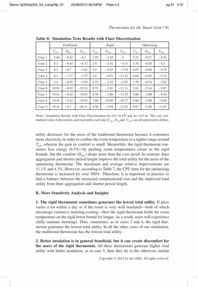
The aggregation of temperatures and the assumption of one decision perperiod reduce computational time, but at the cost of suboptimality, for two rea-sons. First, the feasible region may exclude the optimal solution. Second, round-ing state transitions may increase the error in approximating the value-to-go func-tion. Table 8 summarizes the total utilities of the three types of thermostat withfiner aggregation: and (compared to Table 3, in whichDT = 0.5�F Dt = 0.5 hr
and ). Surprisingly, the daily total utilities for the users ofDT = 1.0�F Dt = 1.0 hrthe traditional and rigid thermostats drop under finer aggregation. The daily total
Name /ej334/ej334_04_Liang/Mp_91 03/08/2012 06:03PM Plate # 0 pg 91 # 31
Thermostats for the Smart Grid / 91
Copyright � 2012 by the IAEE. All rights reserved.
Table 8: Simulation Tests Results with Finer Discretization
Traditional Rigid Optimizing
Cday Dday Uday Cday Dday Uday Cday Dday Uday
Case 1 5.68 –0.42 –6.1 2.55 –2.45 –5 3.52 –0.51 –4.03
Case 2 6.3 –0.42 –6.72 2.9 –2.41 –5.31 3.76 –0.55 –4.3
Case 3 6.3 –0.7 –7.01 2.9 –4.45 –7.35 4.07 –0.68 –4.75
Case 4 6.3 –1.27 –7.57 2.9 –8.53 –11.43 4.66 –0.65 –5.31
Case 5 3.4 –0.45 –3.85 0.72 –2.35 –3.07 1.78 –0.24 –2.02
Case 6 18.91 –0.42 –19.33 8.71 –2.41 –11.11 3.91 –5.16 –9.07
Case 7 19.41 –0.42 –19.83 8.58 –2.66 –11.25 5.06 –3.88 –8.94
Case 8 19.41 –0.42 –19.83 7.88 –10.89 –18.77 5.06 –3.88 –8.94
Case 9 19.41 –0.7 –20.11 8.58 –4.94 –13.52 9.67 –2.26 –11.93
Notes: Simulation Results with Finer Discretization for and . The cost, nor-DT = 0.5�F Dt = 0.5 hrmalized value of discomfort, and total utility each day ( , ) are all expressed in dollars.C D and Uday day day
utility decreases for the users of the traditional thermostat because it consumesmore electricity in order to confine the room temperature to a tighter range around
, whereas the gain in comfort is small. Meanwhile, the rigid thermostat con-Tpfr
sumes less energy ( ) by pushing room temperatures closer to the rigid6.5%bounds, but the comfort ( ) drops more than the cost saved. In contrast, finerDday
aggregation and shorter period length improve the total utility for the users of theoptimizing thermostat. The maximum and average relative improvements are
and . However, according to Table 7, the CPU time for the optimizing11.1% 4.3%thermostat is increased by over . Therefore, it is important in practice to300%find a balance between the increased computational cost and the improved totalutility from finer aggregation and shorter period length.
B. More Sensitivity Analysis and Insights
1. The rigid thermostat sometimes generates the lowest total utility. If pricevaries a lot within a day or if the room is very well insulated—both of whichencourage extensive morning cooling—then the rigid thermostat holds the roomtemperature on the rigid lower bound for longer. As a result, users will experiencechilly summer mornings. Thus, sometimes, as in cases 3 and 4, the rigid ther-mostat generates the lowest total utility. In all the other cases of our simulation,the traditional thermostat has the lowest total utility.
2. Better insulation is in general beneficial, but it can create discomfort forthe users of the rigid thermostat. All three thermostats generate higher totalutility with better insulation, as in case 5, than they do in the otherwise similar
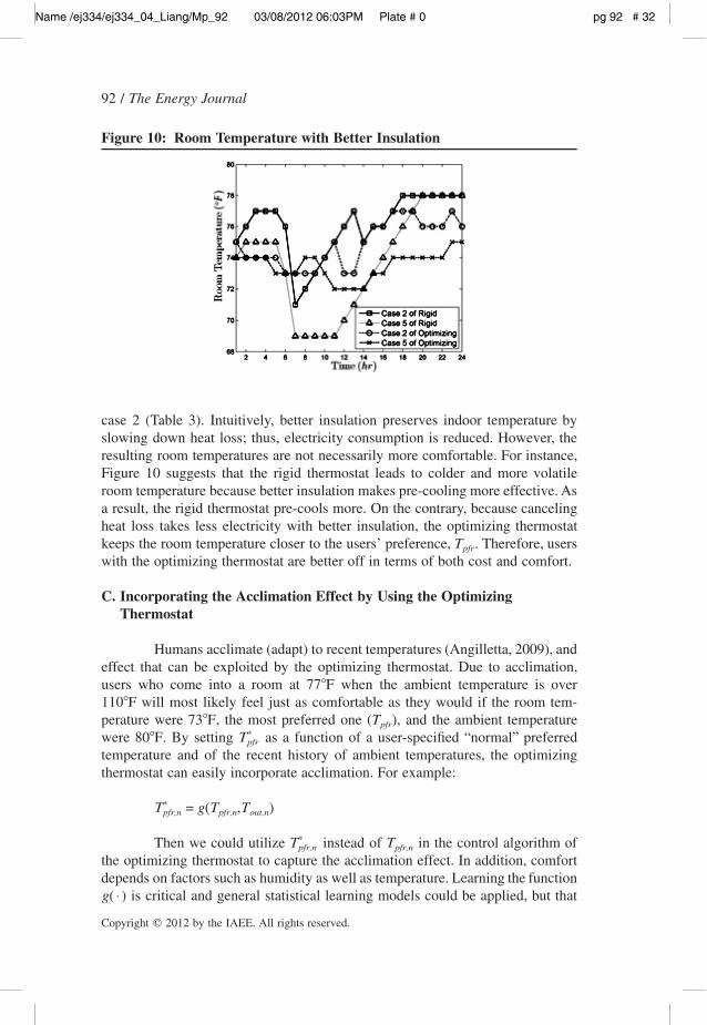
Name /ej334/ej334_04_Liang/Mp_92 03/08/2012 06:03PM Plate # 0 pg 92 # 32
92 / The Energy Journal
Copyright � 2012 by the IAEE. All rights reserved.
Figure 10: Room Temperature with Better Insulation
case 2 (Table 3). Intuitively, better insulation preserves indoor temperature byslowing down heat loss; thus, electricity consumption is reduced. However, theresulting room temperatures are not necessarily more comfortable. For instance,Figure 10 suggests that the rigid thermostat leads to colder and more volatileroom temperature because better insulation makes pre-cooling more effective. Asa result, the rigid thermostat pre-cools more. On the contrary, because cancelingheat loss takes less electricity with better insulation, the optimizing thermostatkeeps the room temperature closer to the users’ preference, . Therefore, usersTpfr
with the optimizing thermostat are better off in terms of both cost and comfort.
C. Incorporating the Acclimation Effect by Using the OptimizingThermostat
Humans acclimate (adapt) to recent temperatures (Angilletta, 2009), andeffect that can be exploited by the optimizing thermostat. Due to acclimation,users who come into a room at when the ambient temperature is over77�F
will most likely feel just as comfortable as they would if the room tem-110�Fperature were , the most preferred one ( ), and the ambient temperature73�F Tpfr
were . By setting as a function of a user-specified “normal” preferred*80�F Tpfr
temperature and of the recent history of ambient temperatures, the optimizingthermostat can easily incorporate acclimation. For example:
*T = g(T ,T )pfr,n pfr,n out,n
Then we could utilize instead of in the control algorithm of*T Tpfr,n pfr,n
the optimizing thermostat to capture the acclimation effect. In addition, comfortdepends on factors such as humidity as well as temperature. Learning the function
is critical and general statistical learning models could be applied, but thatg( ⋅ )
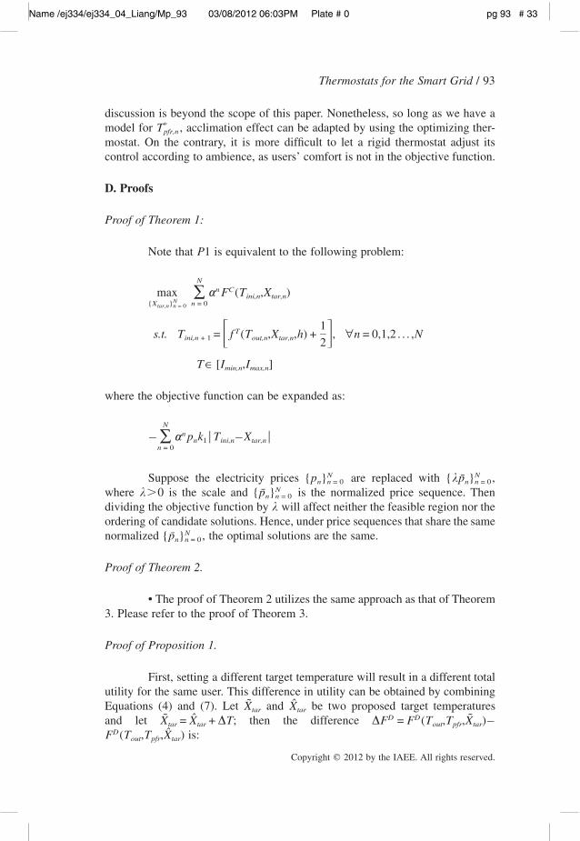
Name /ej334/ej334_04_Liang/Mp_93 03/08/2012 06:03PM Plate # 0 pg 93 # 33
Thermostats for the Smart Grid / 93
Copyright � 2012 by the IAEE. All rights reserved.
discussion is beyond the scope of this paper. Nonetheless, so long as we have amodel for , acclimation effect can be adapted by using the optimizing ther-*Tpfr,n
mostat. On the contrary, it is more difficult to let a rigid thermostat adjust itscontrol according to ambience, as users’ comfort is not in the objective function.
D. Proofs
Proof of Theorem 1:
Note that is equivalent to the following problem:P1
Nn Cmax α F (T ,X )∑ ini,n tar,n
N{X } n = 0tar,n n = 0
1Ts.t. T = f (T ,X ,h) + , ∀n = 0,1,2 . . . ,Nini,n + 1 out,n tar,n� �2
T∈ [I ,I ]min,n max,n
where the objective function can be expanded as:
Nn– α p k T –X∑ ⎪ ⎪n 1 ini,n tar,n
n = 0
Suppose the electricity prices are replaced with ,N N{p } {kp }n n = 0 n n = 0
where is the scale and is the normalized price sequence. ThenNk�0 {p }n n = 0
dividing the objective function by will affect neither the feasible region nor thekordering of candidate solutions. Hence, under price sequences that share the samenormalized , the optimal solutions are the same.N{p }n n = 0
Proof of Theorem 2.
• The proof of Theorem 2 utilizes the same approach as that of Theorem3. Please refer to the proof of Theorem 3.
Proof of Proposition 1.
First, setting a different target temperature will result in a different totalutility for the same user. This difference in utility can be obtained by combiningEquations (4) and (7). Let and be two proposed target temperatures˜ ˆX Xtar tar
and let ; then the difference D D˜ ˆ ˜X = X + DT DF = F (T ,T ,X )–tar tar out pfr tar
is:D ˆF (T ,T ,X )out pfr tar
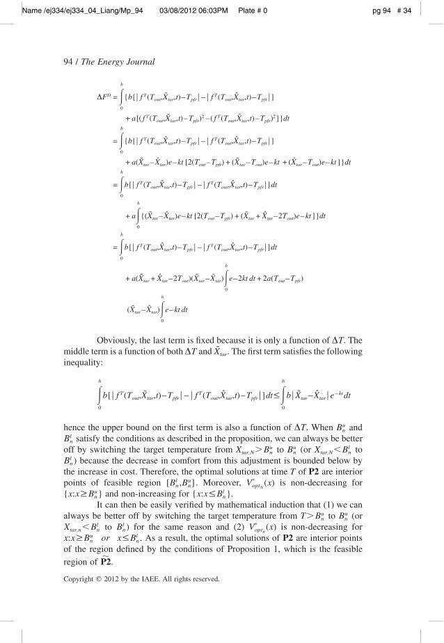
Name /ej334/ej334_04_Liang/Mp_94 03/08/2012 06:03PM Plate # 0 pg 94 # 34
94 / The Energy Journal
Copyright � 2012 by the IAEE. All rights reserved.
h
D T T˜ ˆDF = {b[ f (T ,X ,t)–T – f (T ,X ,t)–T ]⎪ ⎪ ⎪ ⎪out tar pfr out tar pfr�0
T 2 T 2˜ ˆ+ a[( f (T ,X ,t)–T ) –( f (T ,X ,t)–T ) ]}dtout tar pfr out tar pfr
h
T T˜ ˆ= {b[ f (T ,X ,t)–T – f (T ,X ,t)–T ]⎪ ⎪ ⎪ ⎪out tar pfr out tar pfr�0
˜ ˆ ˜ ˆ+ a(X –X )e–kt [2(T –T ) + (X –T )e–kt + (X –T )e–kt ]}dttar tar out pfr tar out tar out
h
T T˜ ˆ= b[ f (T ,X ,t)–T – f (T ,X ,t)–T ]dt⎪ ⎪ ⎪ ⎪out tar pfr out tar pfr�0
h
˜ ˆ ˜ ˆ+ a {(X –X )e–kt [2(T –T ) + (X + X –2T )e–kt ]}dttar tar out pfr tar tar out�0
h
T T˜ ˆ= b[ f (T ,X ,t)–T – f (T ,X ,t)–T ]dt⎪ ⎪ ⎪ ⎪out tar pfr out tar pfr�0
h
˜ ˆ ˜ ˆ+ a(X + X –2T )(X –X ) e–2kt dt + 2a(T –T )tar tar out tar tar out pfr�0
h
˜ ˆ(X –X ) e–kt dttar tar �0
Obviously, the last term is fixed because it is only a function of . TheDTmiddle term is a function of both and . The first term satisfies the following˜DT Xtar
inequality:
h h
T T – kt˜ ˆ ˜ ˆb[ f (T ,X ,t)–T – f (T ,X ,t)–T ]dt≤ b X –X e dt⎪ ⎪ ⎪ ⎪ ⎪ ⎪out tar pfr out tar pfr tar tar� �0 0
hence the upper bound on the first term is also a function of . When anduDT Bn
satisfy the conditions as described in the proposition, we can always be betterlBn
off by switching the target temperature from to (or tou u lX �B B X �Btar,N n n tar,N n
) because the decrease in comfort from this adjustment is bounded below bylBn
the increase in cost. Therefore, the optimal solutions at time of are interiorT P2points of feasible region . Moreover, is non-decreasing forl u *[B ,B ] V (x)n n optN
and non-increasing for .u l{x:x≥ B } {x:x≤ B }n n
It can then be easily verified by mathematical induction that (1) we canalways be better off by switching the target temperature from to (oru uT�B Bn n
to ) for the same reason and (2) is non-decreasing forl l *X �B B V (x)tar,n n n optn
. As a result, the optimal solutions of are interior pointsu lx:x≥ B or x≤ B P2n n
of the region defined by the conditions of Proposition 1, which is the feasible
region of .�P2
Name /ej334/ej334_04_Liang/Mp_95 03/08/2012 06:03PM Plate # 0 pg 95 # 35
Thermostats for the Smart Grid / 95
Copyright � 2012 by the IAEE. All rights reserved.
If we adopt the COP-based model for room temperatures, this proposi-
tion still holds after we replace with . In addition, if is decreasingCOP ko 1k COP1 xCOPlb
at and increasing at , then replacing with ( andCOP ko 1u l˜ ˜B B k j∈{u,l} n =n n 1
jCOPBn
) is sufficient to guarantee that the optimal solutions of are interior1,2, . . . ,N P2points of the region defined by the modified conditions.
Proof of Theorem 3.
• The following inequality:
* *˜V (T )≤ V (T )tra,n ini,n opt,n ini,n
that is, the first inequality in Theorem 3 holds, becaues the modified optimizingthermostat optimizes total utility from both cost and comfort over a broader fea-sible region, while the policy of the traditional thermostat is a feasible solutionto the former one.
• The other inequality:
* *˜V (T )≤ V (T )rigid,n ini,n opt,n ini,n
holds for the same reason as explained above.• The second inequalities in both equations comes from the fact that the
feasible region of the modified problem is a subset of that of the original�P2
problem .P2
Proof of Corollary 1.
The optimizing thermostat costs less than the rigid and traditional ther-mostats when it generates lower or equal comfort because the former creates thehighest total utility for its users, as stated in Theorem 3.
Compared with the rigid thermostat, the optimizing thermostat createsmore comfort for users when the obtained room temperatures are within
. Although not readily seen, this is also consistent with Theorem 3. If[I ,I ]min max
the obtained room temperatures of the optimizing thermostat are bounded by, the cost of using the optimizing thermostat is greater or equal to that[I ,I ]min max
of using the rigid thermostat, as the optimal solution generated by the optimizingthermostat is also a feasible solution to the rigid thermostat’s problem. Thereforeunder this condition, Theorem 3 implies that the optimizing thermostat is able toprovide greater comfort, as the optimizing thermostat creates the highest totalutility for its users.

Name /ej334/ej334_04_Liang/Mp_96 03/08/2012 06:03PM Plate # 0 pg 96 # 36