this page intentionally left blank - wordpress.com · 10.3 strict-sense and wide-sense stationary...
TRANSCRIPT


This page intentionally left blank

P R O B A B I L I T Y A N D R A N D O M P R O C E S S E S F O RE L E C T R I C A L A N D C O M P U T E R E N G I N E E R S
The theory of probability is a powerful tool that helps electrical and computerengineers explain, model, analyze, and design the technology they develop. Thetext begins at the advanced undergraduate level, assuming only a modest knowledgeof probability, and progresses through more complex topics mastered at the graduatelevel. The first five chapters cover the basics of probability and both discrete andcontinuous random variables. The later chapters have a more specialized coverage,including random vectors, Gaussian random vectors, random processes, MarkovChains, and convergence. Describing tools and results that are used extensively inthe field, this is more than a textbook: it is also a reference for researchers workingin communications, signal processing, and computer network traffic analysis. Withover 300 worked examples, some 800 homework problems, and sections for exampreparation, this is an essential companion for advanced undergraduate and graduatestudents.
Further resources for this title, including solutions, are available online atwww.cambridge.org/9780521864701.
John A. Gubner has been on the Faculty of Electrical and ComputerEngineering at the University of Wisconsin-Madison since receiving his Ph.D.in 1988, from the University of Maryland at College Park. His research interestsinclude ultra-wideband communications; point processes and shot noise; subspacemethods in statistical processing; and information theory. A member of the IEEE,he has authored or co-authored many papers in the IEEE Transactions, includingthose on Information Theory, Signal Processing, and Communications.


PROBABILITY AND RANDOMPROCESSES FOR ELECTRICAL AND
COMPUTER ENGINEERS
JOHN A. GUBNERUniversity of Wisconsin-Madison

cambridge university pressCambridge, New York, Melbourne, Madrid, Cape Town, Singapore, São Paulo
Cambridge University PressThe Edinburgh Building, Cambridge cb2 2ru, UK
First published in print format
isbn-13 978-0-521-86470-1
isbn-13 978-0-511-22023-4
© Cambridge University Press 2006
2006
Information on this title: www.cambridge.org/9780521864701
This publication is in copyright. Subject to statutory exception and to the provision ofrelevant collective licensing agreements, no reproduction of any part may take placewithout the written permission of Cambridge University Press.
isbn-10 0-511-22023-5
isbn-10 0-521-86470-4
Cambridge University Press has no responsibility for the persistence or accuracy of urlsfor external or third-party internet websites referred to in this publication, and does notguarantee that any content on such websites is, or will remain, accurate or appropriate.
Published in the United States of America by Cambridge University Press, New York
www.cambridge.org
hardback
eBook (EBL)
eBook (EBL)
hardback

To Sue and Joe


Contents
Chapter dependencies page x
Preface xi
1 Introduction to probability 1
1.1 Sample spaces, outcomes, and events 6
1.2 Review of set notation 8
1.3 Probability models 17
1.4 Axioms and properties of probability 22
1.5 Conditional probability 26
1.6 Independence 30
1.7 Combinatorics and probability 34
Notes 43
Problems 48
Exam preparation 62
2 Introduction to discrete random variables 63
2.1 Probabilities involving random variables 63
2.2 Discrete random variables 66
2.3 Multiple random variables 70
2.4 Expectation 80
Notes 96
Problems 99
Exam preparation 106
3 More about discrete random variables 108
3.1 Probability generating functions 108
3.2 The binomial random variable 111
3.3 The weak law of large numbers 115
3.4 Conditional probability 117
3.5 Conditional expectation 127
Notes 130
Problems 132
Exam preparation 137
4 Continuous random variables 138
4.1 Densities and probabilities 138
4.2 Expectation of a single random variable 149
4.3 Transform methods 156
4.4 Expectation of multiple random variables 162
4.5 Probability bounds 164
Notes 167
Problems 170
Exam preparation 183
5 Cumulative distribution functions and their applications 184
5.1 Continuous random variables 185
5.2 Discrete random variables 194
5.3 Mixed random variables 197
5.4 Functions of random variables and their cdfs 200
5.5 Properties of cdfs 205
5.6 The central limit theorem 207
5.7 Reliability 215
vii

viii Contents
Notes 219
Problems 222
Exam preparation 238
6 Statistics 240
6.1 Parameter estimators and their properties 240
6.2 Histograms 244
6.3 Confidence intervals for the mean – known variance 250
6.4 Confidence intervals for the mean – unknown variance 253
6.5 Confidence intervals for Gaussian data 256
6.6 Hypothesis tests for the mean 262
6.7 Regression and curve fitting 267
6.8 Monte Carlo estimation 271
Notes 273
Problems 276
Exam preparation 285
7 Bivariate random variables 287
7.1 Joint and marginal probabilities 287
7.2 Jointly continuous random variables 295
7.3 Conditional probability and expectation 302
7.4 The bivariate normal 309
7.5 Extension to three or more random variables 314
Notes 317
Problems 319
Exam preparation 328
8 Introduction to random vectors 330
8.1 Review of matrix operations 330
8.2 Random vectors and random matrices 333
8.3 Transformations of random vectors 340
8.4 Linear estimation of random vectors (Wiener filters) 344
8.5 Estimation of covariance matrices 348
8.6 Nonlinear estimation of random vectors 350
Notes 354
Problems 354
Exam preparation 360
9 Gaussian random vectors 362
9.1 Introduction 362
9.2 Definition of the multivariate Gaussian 363
9.3 Characteristic function 365
9.4 Density function 367
9.5 Conditional expectation and conditional probability 369
9.6 Complex random variables and vectors 371
Notes 373
Problems 375
Exam preparation 382
10 Introduction to random processes 383
10.1 Definition and examples 383
10.2 Characterization of random processes 388
10.3 Strict-sense and wide-sense stationary processes 393
10.4 WSS processes through LTI systems 401
10.5 Power spectral densities for WSS processes 403
10.6 Characterization of correlation functions 410
10.7 The matched filter 412
10.8 The Wiener filter 417

Contents ix
10.9 The Wiener–Khinchin theorem 421
10.10Mean-square ergodic theorem for WSS processes 423
10.11Power spectral densities for non-WSS processes 425
Notes 427
Problems 429
Exam preparation 440
11 Advanced concepts in random processes 443
11.1 The Poisson process 443
11.2 Renewal processes 452
11.3 The Wiener process 453
11.4 Specification of random processes 459
Notes 466
Problems 466
Exam preparation 475
12 Introduction to Markov chains 476
12.1 Preliminary results 476
12.2 Discrete-time Markov chains 477
12.3 Recurrent and transient states 488
12.4 Limiting n-step transition probabilities 496
12.5 Continuous-time Markov chains 502
Notes 507
Problems 509
Exam preparation 515
13 Mean convergence and applications 517
13.1 Convergence in mean of order p 518
13.2 Normed vector spaces of random variables 522
13.3 The Karhunen–Loeve expansion 527
13.4 The Wiener integral (again) 532
13.5 Projections, orthogonality principle, projection theorem 534
13.6 Conditional expectation and probability 537
13.7 The spectral representation 545
Notes 549
Problems 550
Exam preparation 562
14 Other modes of convergence 564
14.1 Convergence in probability 564
14.2 Convergence in distribution 566
14.3 Almost-sure convergence 572
Notes 579
Problems 580
Exam preparation 589
15 Self similarity and long-range dependence 591
15.1 Self similarity in continuous time 591
15.2 Self similarity in discrete time 595
15.3 Asymptotic second-order self similarity 601
15.4 Long-range dependence 604
15.5 ARMA processes 606
15.6 ARIMA processes 608
Problems 610
Exam preparation 613
Bibliography 615
Index 618

Chapter dependencies
1 Introduction to probability
2 Introduction to discrete random variables3 More about discrete random variables
6 Statistics
7 Bivariate random variables
10 Introduction to random processes
13 Mean convergence and applications14 Other modes of convergence15 Self similarity and long−range dependence
11.1 The Poisson process
11.2−11.4 Advanced concepts in random processes
5 Cumulative distribution functions and their applications
4 Continuous random variables
8 Introduction to random vectors
9 Gaussian random vectors
12.1−12.4 Discrete−time Markov chains
12.5 Continuous−time Markov chains
x

Preface
Intended audience
This book is a primary text for graduate-level courses in probability and random pro-
cesses that are typically offered in electrical and computer engineering departments. The
text starts from first principles and contains more than enough material for a two-semester
sequence. The level of the text varies from advanced undergraduate to graduate as the
material progresses. The principal prerequisite is the usual undergraduate electrical and
computer engineering course on signals and systems, e.g., Haykin and Van Veen [25] or
Oppenheim and Willsky [39] (see the Bibliography at the end of the book). However, later
chapters that deal with random vectors assume some familiarity with linear algebra; e.g.,
determinants and matrix inverses.
How to use the book
A first course. In a course that assumes at most a modest background in probability, the
core of the offering would include Chapters 1–5 and 7. These cover the basics of probability
and discrete and continuous random variables. As the chapter dependencies graph on the
preceding page indicates, there is considerable flexibility in the selection and ordering of
additional material as the instructor sees fit.
A second course. In a course that assumes a solid background in the basics of prob-
ability and discrete and continuous random variables, the material in Chapters 1–5 and 7
can be reviewed quickly. In such a review, the instructor may want include sections and
problems marked with a , as these indicate more challenging material that might not
be appropriate in a first course. Following the review, the core of the offering would
include Chapters 8, 9, 10 (Sections 10.1–10.6), and Chapter 11. Additional material from
Chapters 12–15 can be included to meet course goals and objectives.
Level of course offerings. In any course offering, the level can be adapted to the
background of the class by omitting or including the more advanced sections, remarks,
and problems that are marked with a . In addition, discussions of a highly technical
nature are placed in a Notes section at the end of the chapter in which they occur. Pointers
to these discussions are indicated by boldface numerical superscripts in the text. These
notes can be omitted or included as the instructor sees fit.
Chapter features
• Key equations are boxed:
P(A|B) :=P(A∩B)
P(B).
• Important text passages are highlighted:
Two events A and B are said to be independent if P(A∩B) = P(A)P(B).
xi

xii Preface
• Tables of discrete random variables and of Fourier transform pairs are found inside
the front cover. A table of continuous random variables is found inside the back cover.
• The index was compiled as the book was written. Hence, there are many cross-
references to related information. For example, see “chi-squared random variable.”
• When cumulative distribution functions or other functions are encountered that do not
have a closed form, MATLAB commands are given for computing them; see “Matlab
commands” in the index for a list. The use of many commands is illustrated in the
examples and the problems throughout most of the text. Although some commands
require the MATLAB Statistics Toolbox, alternative methods are also suggested; e.g.,
the use of erf and erfinv for normcdf and norminv.
• Each chapter contains a Notes section. Throughout each chapter, numerical super-
scripts refer to discussions in the Notes section. These notes are usually rather tech-
nical and address subtleties of the theory.
• Each chapter contains a Problems section. There are more than 800 problems through-
out the book. Problems are grouped according to the section they are based on, and
this is clearly indicated. This enables the student to refer to the appropriate part of
the text for background relating to particular problems, and it enables the instructor
to make up assignments more quickly. In chapters intended for a first course, the
more challenging problems are marked with a . Problems requiring MATLAB are
indicated by the label MATLAB.
• Each chapter contains an Exam preparation section. This serves as a chapter sum-
mary, drawing attention to key concepts and formulas.
Acknowledgements
The writing of this book has been greatly improved by the suggestions of many people.
At the University of Wisconsin–Madison, the sharp eyes of the students in my classes
on probability and random processes, my research students, and my postdocs have helped
me fix countless typos and improve explanations of several topics. My colleagues here have
been generous with their comments and suggestions. Professor Rajeev Agrawal, now with
Motorola, convinced me to treat discrete random variables before continuous random vari-
ables. Discussions with Professor Bob Barmish on robustness of rational transfer functions
led to Problems 38–40 in Chapter 5. I am especially grateful to Professors Jim Bucklew, Yu
Hen Hu, and Akbar Sayeed, who taught from early, unpolished versions of the manuscript.
Colleagues at other universities and students in their classes have also been generous
with their support. I thank Professors Toby Berger, Edwin Chong, and Dave Neuhoff, who
have used recent manuscripts in teaching classes on probability and random processes and
have provided me with detailed reviews. Special thanks go to Professor Tom Denney for his
multiple careful reviews of each chapter.
Since writing is a solitary process, I am grateful to be surrounded by many supportive
family members. I especially thank my wife and son for their endless patience and faith
in me and this book, and I thank my parents for their encouragement and help when I was
preoccupied with writing.

1
Introduction to probability
Why do electrical and computer engineers need to study proba-bility?
Probability theory provides powerful tools to explain, model, analyze, and design tech-
nology developed by electrical and computer engineers. Here are a few applications.
Signal processing. My own interest in the subject arose when I was an undergraduate
taking the required course in probability for electrical engineers. We considered the situa-
tion shown in Figure 1.1. To determine the presence of an aircraft, a known radar pulse v(t)
tXv( )t +
(
radar
v( )t
linearsystem
detector
Figure 1.1. Block diagram of radar detection system.
is sent out. If there are no objects in range of the radar, the radar’s amplifiers produce only a
noise waveform, denoted by Xt . If there is an object in range, the reflected radar pulse plus
noise is produced. The overall goal is to decide whether the received waveform is noise
only or signal plus noise. To get an idea of how difficult this can be, consider the signal
plus noise waveform shown at the top in Figure 1.2. Our class addressed the subproblem
of designing an optimal linear system to process the received waveform so as to make the
presence of the signal more obvious. We learned that the optimal transfer function is given
by the matched filter. If the signal at the top in Figure 1.2 is processed by the appropriate
matched filter, we get the output shown at the bottom in Figure 1.2. You will study the
matched filter in Chapter 10.
Computer memories. Suppose you are designing a computer memory to hold k-bit
words. To increase system reliability, you employ an error-correcting-code system. With
this system, instead of storing just the k data bits, you store an additional l bits (which are
functions of the data bits). When reading back the (k+ l)-bit word, if at least m bits are read
out correctly, then all k data bits can be recovered (the value of m depends on the code). To
characterize the quality of the computer memory, we compute the probability that at least m
bits are correctly read back. You will be able to do this after you study the binomial random
variable in Chapter 3.
1

2 Introduction to probability
−1
0
1
0
0.5
Figure 1.2. Matched filter input (top) in which the signal is hidden by noise. Matched filter output (bottom) in
which the signal presence is obvious.
Optical communication systems. Optical communication systems use photodetectors
(see Figure 1.3) to interface between optical and electronic subsystems. When these sys-
detectorphoto− photoelectronslight
Figure 1.3. Block diagram of a photodetector. The rate at which photoelectrons are produced is proportional to
the intensity of the light.
tems are at the limits of their operating capabilities, the number of photoelectrons produced
by the photodetector is well-modeled by the Poissona random variable you will study in
Chapter 2 (see also the Poisson process in Chapter 11). In deciding whether a transmitted
bit is a zero or a one, the receiver counts the number of photoelectrons and compares it
to a threshold. System performance is determined by computing the probability that the
threshold is exceeded.
Wireless communication systems. In order to enhance weak signals and maximize the
range of communication systems, it is necessary to use amplifiers. Unfortunately, amplifiers
always generate thermal noise, which is added to the desired signal. As a consequence of the
underlying physics, the noise is Gaussian. Hence, the Gaussian density function, which you
will meet in Chapter 4, plays a prominent role in the analysis and design of communication
systems. When noncoherent receivers are used, e.g., noncoherent frequency shift keying,
aMany important quantities in probability and statistics are named after famous mathematicians and
statisticians. You can use an Internet search engine to find pictures and biographies of them on
the web. At the time of this writing, numerous biographies of famous mathematicians and statisti-
cians can be found at http://turnbull.mcs.st-and.ac.uk/history/BiogIndex.html and at
http://www.york.ac.uk/depts/maths/histstat/people/welcome.htm. Pictures on stamps
and currency can be found at http://jeff560.tripod.com/.
Relative frequency 3
this naturally leads to the Rayleigh, chi-squared, noncentral chi-squared, and Rice density
functions that you will meet in the problems in Chapters 4, 5, 7, and 9.
Variability in electronic circuits. Although circuit manufacturing processes attempt to
ensure that all items have nominal parameter values, there is always some variation among
items. How can we estimate the average values in a batch of items without testing all of
them? How good is our estimate? You will learn how to do this in Chapter 6 when you
study parameter estimation and confidence intervals. Incidentally, the same concepts apply
to the prediction of presidential elections by surveying only a few voters.
Computer network traffic. Prior to the 1990s, network analysis and design was carried
out using long-established Markovian models [41, p. 1]. You will study Markov chains
in Chapter 12. As self similarity was observed in the traffic of local-area networks [35],
wide-area networks [43], and in World Wide Web traffic [13], a great research effort began
to examine the impact of self similarity on network analysis and design. This research has
yielded some surprising insights into questions about buffer size vs. bandwidth, multiple-
time-scale congestion control, connection duration prediction, and other issues [41, pp. 9–
11]. In Chapter 15 you will be introduced to self similarity and related concepts.
In spite of the foregoing applications, probability was not originally developed to handle
problems in electrical and computer engineering. The first applications of probability were
to questions about gambling posed to Pascal in 1654 by the Chevalier de Mere. Later,
probability theory was applied to the determination of life expectancies and life-insurance
premiums, the theory of measurement errors, and to statistical mechanics. Today, the theory
of probability and statistics is used in many other fields, such as economics, finance, medical
treatment and drug studies, manufacturing quality control, public opinion surveys, etc.
Relative frequency
Consider an experiment that can result in M possible outcomes, O1, . . . ,OM . For ex-
ample, in tossing a die, one of the six sides will land facing up. We could let Oi denote
the outcome that the ith side faces up, i = 1, . . . ,6. Alternatively, we might have a computer
with six processors, and Oi could denote the outcome that a program or thread is assigned to
the ith processor. As another example, there are M = 52 possible outcomes if we draw one
card from a deck of playing cards. Similarly, there are M = 52 outcomes if we ask which
week during the next year the stock market will go up the most. The simplest example we
consider is the flipping of a coin. In this case there are two possible outcomes, “heads” and
“tails.” Similarly, there are two outcomes when we ask whether or not a bit was correctly
received over a digital communication system. No matter what the experiment, suppose
we perform it n times and make a note of how many times each outcome occurred. Each
performance of the experiment is called a trial.b Let Nn(Oi) denote the number of times Oi
occurred in n trials. The relative frequency of outcome Oi,
Nn(Oi)
n,
is the fraction of times Oi occurred.
bWhen there are only two outcomes, the repeated experiments are called Bernoulli trials.

4 Introduction to probability
Here are some simple computations using relative frequency. First,
Nn(O1)+ · · ·+Nn(OM) = n,
and soNn(O1)
n+ · · ·+ Nn(OM)
n= 1. (1.1)
Second, we can group outcomes together. For example, if the experiment is tossing a die,
let E denote the event that the outcome of a toss is a face with an even number of dots; i.e.,
E is the event that the outcome is O2, O4, or O6. If we let Nn(E) denote the number of times
E occurred in n tosses, it is easy to see that
Nn(E) = Nn(O2)+Nn(O4)+Nn(O6),
and so the relative frequency of E is
Nn(E)
n=
Nn(O2)
n+
Nn(O4)
n+
Nn(O6)
n. (1.2)
Practical experience has shown us that as the number of trials n becomes large, the rel-
ative frequencies settle down and appear to converge to some limiting value. This behavior
is known as statistical regularity.
Example 1.1. Suppose we toss a fair coin 100 times and note the relative frequency of
heads. Experience tells us that the relative frequency should be about 1/2. When we did
this,c we got 0.47 and were not disappointed.
The tossing of a coin 100 times and recording the relative frequency of heads out of 100
tosses can be considered an experiment in itself. Since the number of heads can range from
0 to 100, there are 101 possible outcomes, which we denote by S0, . . . ,S100. In the preceding
example, this experiment yielded S47.
Example 1.2. We performed the experiment with outcomes S0, . . . ,S100 1000 times and
counted the number of occurrences of each outcome. All trials produced between 33 and 68
heads. Rather than list N1000(Sk) for the remaining values of k, we summarize as follows:
N1000(S33)+N1000(S34)+N1000(S35) = 4
N1000(S36)+N1000(S37)+N1000(S38) = 6
N1000(S39)+N1000(S40)+N1000(S41) = 32
N1000(S42)+N1000(S43)+N1000(S44) = 98
N1000(S45)+N1000(S46)+N1000(S47) = 165
N1000(S48)+N1000(S49)+N1000(S50) = 230
N1000(S51)+N1000(S52)+N1000(S53) = 214
N1000(S54)+N1000(S55)+N1000(S56) = 144
cWe did not actually toss a coin. We used a random number generator to simulate the toss of a fair coin.
Simulation is discussed in Chapters 5 and 6.

What is probability theory? 5
N1000(S57)+N1000(S58)+N1000(S59) = 76
N1000(S60)+N1000(S61)+N1000(S62) = 21
N1000(S63)+N1000(S64)+N1000(S65) = 9
N1000(S66)+N1000(S67)+N1000(S68) = 1.
This summary is illustrated in the histogram shown in Figure 1.4. (The bars are centered
over values of the form k/100; e.g., the bar of height 230 is centered over 0.49.)
0.3 0.4 0.5 0.6 0.70
50
100
150
200
250
Figure 1.4. Histogram of Example 1.2 with overlay of a Gaussian density.
Below we give an indication of why most of the time the relative frequency of heads is
close to one half and why the bell-shaped curve fits so well over the histogram. For now
we point out that the foregoing methods allow us to determine the bit-error rate of a digital
communication system, whether it is a wireless phone or a cable modem connection. In
principle, we simply send a large number of bits over the channel and find out what fraction
were received incorrectly. This gives an estimate of the bit-error rate. To see how good an
estimate it is, we repeat the procedure many times and make a histogram of our estimates.
What is probability theory?
Axiomatic probability theory, which is the subject of this book, was developed by A.
N. Kolmogorovd in 1933. This theory specifies a set of axioms for a well-defined math-
ematical model of physical experiments whose outcomes exhibit random variability each
time they are performed. The advantage of using a model rather than performing an exper-
iment itself is that it is usually much more efficient in terms of time and money to analyze
a mathematical model. This is a sensible approach only if the model correctly predicts the
behavior of actual experiments. This is indeed the case for Kolmogorov’s theory.
A simple prediction of Kolmogorov’s theory arises in the mathematical model for the
relative frequency of heads in n tosses of a fair coin that we considered in Example 1.1. In
the model of this experiment, the relative frequency converges to 1/2 as n tends to infinity;
dThe website http://kolmogorov.com/ is devoted to Kolmogorov.
6 Introduction to probability
this is a special case of the the strong law of large numbers, which is derived in Chapter 14.
(A related result, known as the weak law of large numbers, is derived in Chapter 3.)
Another prediction of Kolmogorov’s theory arises in modeling the situation in Exam-
ple 1.2. The theory explains why the histogram in Figure 1.4 agrees with the bell-shaped
curve overlaying it. In the model, the strong law tells us that for each k, the relative fre-
quency of having exactly k heads in 100 tosses should be close to
100!
k!(100− k)!
1
2100.
Then, by the central limit theorem, which is derived in Chapter 5, the above expression is
approximately equal to (see Example 5.19)
1
5√
2πexp
[−1
2
(k−50
5
)2].
(You should convince yourself that the graph of e−x2is indeed a bell-shaped curve.)
Because Kolmogorov’s theory makes predictions that agree with physical experiments,
it has enjoyed great success in the analysis and design of real-world systems.
1.1 Sample spaces, outcomes, and events
Sample spaces
To model systems that yield uncertain or random measurements, we let Ω denote the
set of all possible distinct, indecomposable measurements that could be observed. The set
Ω is called the sample space. Here are some examples corresponding to the applications
discussed at the beginning of the chapter.
Signal processing. In a radar system, the voltage of a noise waveform at time t can be
viewed as possibly being any real number. The first step in modeling such a noise voltage
is to consider the sample space consisting of all real numbers, i.e., Ω = (−∞,∞).Computer memories. Suppose we store an n-bit word consisting of all 0s at a particular
location. When we read it back, we may not get all 0s. In fact, any n-bit word may be read
out if the memory location is faulty. The set of all possible n-bit words can be modeled by
the sample space
Ω = (b1, . . . ,bn) : bi = 0 or 1.Optical communication systems. Since the output of a photodetector is a random
number of photoelectrons. The logical sample space here is the nonnegative integers,
Ω = 0,1,2, . . ..Notice that we include 0 to account for the possibility that no photoelectrons are observed.
Wireless communication systems. Noncoherent receivers measure the energy of the
incoming waveform. Since energy is a nonnegative quantity, we model it with the sample
space consisting of the nonnegative real numbers, Ω = [0,∞).Variability in electronic circuits. Consider the lowpass RC filter shown in Figure 1.5(a).
Suppose that the exact values of R and C are not perfectly controlled by the manufacturing
process, but are known to satisfy
95 ohms ≤ R ≤ 105 ohms and 300 µF ≤ C ≤ 340 µF.

1.1 Sample spaces, outcomes, and events 7
(a) (b)
95 105
300
340
r
c
C
R+
−
+−
Figure 1.5. (a) Lowpass RC filter. (b) Sample space for possible values of R and C.
This suggests that we use the sample space of ordered pairs of real numbers, (r,c), where
95 ≤ r ≤ 105 and 300 ≤ c ≤ 340. Symbolically, we write
Ω = (r,c) : 95 ≤ r ≤ 105 and 300 ≤ c ≤ 340,
which is the rectangular region in Figure 1.5(b).
Computer network traffic. If a router has a buffer that can store up to 70 packets, and
we want to model the actual number of packets waiting for transmission, we use the sample
space
Ω = 0,1,2, . . . ,70.Notice that we include 0 to account for the possibility that there are no packets waiting to
be sent.
Outcomes and events
Elements or points in the sample space Ω are called outcomes. Collections of outcomes
are called events. In other words, an event is a subset of the sample space. Here are some
examples.
If the sample space is the real line, as in modeling a noise voltage, the individual num-
bers such as 1.5, −8, and π are outcomes. Subsets such as the interval
[0,5] = v : 0 ≤ v ≤ 5
are events. Another event would be 2,4,7.13. Notice that singleton sets, that is sets
consisting of a single point, are also events; e.g., 1.5, −8, π. Be sure you understand
the difference between the outcome −8 and the event −8, which is the set consisting of
the single outcome −8.
If the sample space is the set of all triples (b1,b2,b3), where the bi are 0 or 1, then any
particular triple, say (0,0,0) or (1,0,1) would be an outcome. An event would be a subset
such as the set of all triples with exactly one 1; i.e.,
(0,0,1),(0,1,0),(1,0,0).
An example of a singleton event would be (1,0,1).

8 Introduction to probability
In modeling the resistance and capacitance of the RC filter above, we suggested the
sample space
Ω = (r,c) : 95 ≤ r ≤ 105 and 300 ≤ c ≤ 340,which was shown in Figure 1.5(b). If a particular circuit has R = 101 ohms and C = 327 µF,
this would correspond to the outcome (101,327), which is indicated by the dot in Figure 1.6.
If we observed a particular circuit with R≤ 97 ohms and C ≥ 313 µF, this would correspond
to the event
(r,c) : 95 ≤ r ≤ 97 and 313 ≤ c ≤ 340,which is the shaded region in Figure 1.6.
95 105
300
340
r
c
Figure 1.6. The dot is the outcome (101,327). The shaded region is the event (r,c) : 95 ≤ r ≤ 97 and 313 ≤ c ≤340.
1.2 Review of set notation
Since sample spaces and events use the language of sets, we recall in this section some
basic definitions, notation, and properties of sets.
Let Ω be a set of points. If ω is a point in Ω, we write ω ∈ Ω. Let A and B be two
collections of points in Ω. If every point in A also belongs to B, we say that A is a subset of
B, and we denote this by writing A ⊂ B. If A ⊂ B and B ⊂ A, then we write A = B; i.e., two
sets are equal if they contain exactly the same points. If A ⊂ B but A = B, we say that A is a
proper subset of B.
Set relationships can be represented graphically in Venn diagrams. In these pictures,
the whole space Ω is represented by a rectangular region, and subsets of Ω are represented
by disks or oval-shaped regions. For example, in Figure 1.7(a), the disk A is completely
contained in the oval-shaped region B, thus depicting the relation A ⊂ B.
Set operations
If A ⊂ Ω, and ω ∈ Ω does not belong to A, we write ω /∈ A. The set of all such ω is
called the complement of A in Ω; i.e.,
Ac := ω ∈ Ω : ω /∈ A.This is illustrated in Figure 1.7(b), in which the shaded region is the complement of the disk
A.
The empty set or null set is denoted by ∅; it contains no points of Ω. Note that for any
A ⊂ Ω, ∅ ⊂ A. Also, Ωc = ∅.

1.2 Review of set notation 9
( a )
A B A
Ac
( b )
Figure 1.7. (a) Venn diagram of A ⊂ B. (b) The complement of the disk A, denoted by Ac, is the shaded part of the
diagram.
The union of two subsets A and B is
A∪B := ω ∈ Ω : ω ∈ A or ω ∈ B.Here “or” is inclusive; i.e., if ω ∈ A∪B, we permit ω to belong either to A or to B or to
both. This is illustrated in Figure 1.8(a), in which the shaded region is the union of the disk
A and the oval-shaped region B.
B
( a )
A A B
( b )
Figure 1.8. (a) The shaded region is A∪B. (b) The shaded region is A∩B.
The intersection of two subsets A and B is
A∩B := ω ∈ Ω : ω ∈ A and ω ∈ B;
hence, ω ∈A∩B if and only if ω belongs to both A and B. This is illustrated in Figure 1.8(b),
in which the shaded area is the intersection of the disk A and the oval-shaped region B. The
reader should also note the following special case. If A ⊂ B (recall Figure 1.7(a)), then
A∩B = A. In particular, we always have A∩Ω = A and ∅∩B = ∅.
The set difference operation is defined by
B\A := B∩Ac,
i.e., B \A is the set of ω ∈ B that do not belong to A. In Figure 1.9(a), B \A is the shaded
part of the oval-shaped region B. Thus, B\A is found by starting with all the points in B and
then removing those that belong to A.
Two subsets A and B are disjoint or mutually exclusive if A∩B = ∅; i.e., there is no
point in Ω that belongs to both A and B. This condition is depicted in Figure 1.9(b).

10 Introduction to probability
BA
( a ) ( b )
B
A
Figure 1.9. (a) The shaded region is B\A. (b) Venn diagram of disjoint sets A and B.
Example 1.3. Let Ω := 0,1,2,3,4,5,6,7, and put
A := 1,2,3,4, B := 3,4,5,6, and C := 5,6.Evaluate A∪B, A∩B, A∩C, Ac, and B\A.
Solution. It is easy to see that A∪B = 1,2,3,4,5,6, A∩B = 3,4, and A∩C = ∅.
Since Ac = 0,5,6,7,
B\A = B∩Ac = 5,6 = C.
Set identities
Set operations are easily seen to obey the following relations. Some of these relations
are analogous to the familiar ones that apply to ordinary numbers if we think of union as
the set analog of addition and intersection as the set analog of multiplication. Let A,B, and
C be subsets of Ω. The commutative laws are
A∪B = B∪A and A∩B = B∩A. (1.3)
The associative laws are
A∪ (B∪C) = (A∪B)∪C and A∩ (B∩C) = (A∩B)∩C. (1.4)
The distributive laws are
A∩ (B∪C) = (A∩B)∪ (A∩C) (1.5)
and
A∪ (B∩C) = (A∪B)∩ (A∪C). (1.6)
De Morgan’s laws are
(A∩B)c = Ac ∪Bc and (A∪B)c = Ac ∩Bc. (1.7)
Formulas (1.3)–(1.5) are exactly analogous to their numerical counterparts. Formulas (1.6)
and (1.7) do not have numerical counterparts. We also recall that A∩Ω = A and ∅∩B = ∅;
hence, we can think of Ω as the analog of the number one and ∅ as the analog of the number
zero. Another analog is the formula A∪∅ = A.

1.2 Review of set notation 11
We next consider infinite collections of subsets of Ω. It is important to understand how
to work with unions and intersections of infinitely many subsets. Infinite unions allow us
to formulate questions about some event ever happening if we wait long enough. Infinite
intersections allow us to formulate questions about some event never happening no matter
how long we wait.
Suppose An ⊂ Ω, n = 1,2, . . . . Then
∞⋃n=1
An := ω ∈ Ω : ω ∈ An for some 1 ≤ n < ∞.
In other words, ω ∈ ⋃∞n=1 An if and only if for at least one integer n satisfying 1 ≤ n < ∞,
ω ∈ An. This definition admits the possibility that ω ∈ An for more than one value of n.
Next, we define∞⋂
n=1
An := ω ∈ Ω : ω ∈ An for all 1 ≤ n < ∞.
In other words, ω ∈⋂∞n=1 An if and only if ω ∈ An for every positive integer n.
Many examples of infinite unions and intersections can be given using intervals of real
numbers such as (a,b), (a,b], [a,b), and [a,b]. (This notation is reviewed in Problem 5.)
Example 1.4. Let Ω denote the real numbers, Ω = IR := (−∞,∞). Then the following
infinite intersections and unions can be simplified. Consider the intersection
∞⋂n=1
(−∞,1/n) = ω : ω < 1/n for all 1 ≤ n < ∞.
Now, if ω < 1/n for all 1 ≤ n < ∞, then ω cannot be positive; i.e., we must have ω ≤ 0.
Conversely, if ω ≤ 0, then for all 1 ≤ n < ∞, ω ≤ 0 < 1/n. It follows that
∞⋂n=1
(−∞,1/n) = (−∞,0].
Consider the infinite union,
∞⋃n=1
(−∞,−1/n] = ω : ω ≤−1/n for some 1 ≤ n < ∞.
Now, if ω ≤ −1/n for some n with 1 ≤ n < ∞, then we must have ω < 0. Conversely, if
ω < 0, then for large enough n, ω ≤−1/n. Thus,
∞⋃n=1
(−∞,−1/n] = (−∞,0).
In a similar way, one can show that
∞⋂n=1
[0,1/n) = 0,
as well as∞⋃
n=1
(−∞,n] = (−∞,∞) and
∞⋂n=1
(−∞,−n] = ∅.

12 Introduction to probability
The following generalized distributive laws also hold,
B∩( ∞⋃
n=1
An
)=
∞⋃n=1
(B∩An),
and
B∪( ∞⋂
n=1
An
)=
∞⋂n=1
(B∪An).
We also have the generalized De Morgan’s laws,( ∞⋂n=1
An
)c
=∞⋃
n=1
Acn,
and ( ∞⋃n=1
An
)c
=∞⋂
n=1
Acn.
Finally, we will need the following definition. We say that subsets An,n = 1,2, . . . , are
pairwise disjoint if An ∩Am = ∅ for all n = m.
Partitions
A family of nonempty sets Bn is called a partition if the sets are pairwise disjoint and
their union is the whole space Ω. A partition of three sets B1, B2, and B3 is illustrated in
Figure 1.10(a). Partitions are useful for chopping up sets into manageable, disjoint pieces.
Given a set A, write
A = A∩Ω
= A∩(⋃
n
Bn
)=
⋃n
(A∩Bn).
Since the Bn are pairwise disjoint, so are the pieces (A∩Bn). This is illustrated in Fig-
ure 1.10(b), in which a disk is broken up into three disjoint pieces.
B1
B2
B3
( a ) ( b )
B1
B2
B3
Figure 1.10. (a) The partition B1, B2, B3. (b) Using the partition to break up a disk into three disjoint pieces (the
shaded regions).
1.2 Review of set notation 13
If a family of sets Bn is disjoint but their union is not equal to the whole space, we can
always add the remainder set
R :=
(⋃n
Bn
)c
(1.8)
to the family to create a partition. Writing
Ω = Rc ∪R
=
(⋃n
Bn
)∪R,
we see that the union of the augmented family is the whole space. It only remains to show
that Bk ∩R = ∅. Write
Bk ∩R = Bk ∩(⋃
n
Bn
)c
= Bk ∩(⋂
n
Bcn
)= Bk ∩Bc
k ∩(⋂
n =k
Bcn
)= ∅.
Functions
A function consists of a set X of admissible inputs called the domain and a rule or
mapping f that associates to each x ∈ X a value f (x) that belongs to a set Y called the
co-domain. We indicate this symbolically by writing f :X → Y , and we say, “ f maps X
into Y .” Two functions are the same if and only if they have the same domain, co-domain,
and rule. If f :X → Y and g:X → Y , then the mappings f and g are the same if and only if
f (x) = g(x) for all x ∈ X .
The set of all possible values of f (x) is called the range. In symbols, the range is the set
f (x) : x ∈ X. Since f (x)∈Y for each x, it is clear that the range is a subset of Y . However,
the range may or may not be equal to Y . The case in which the range is a proper subset of Y
is illustrated in Figure 1.11.
f
range
Xdomain Yco−domain
x y
Figure 1.11. The mapping f associates each x in the domain X to a point y in the co-domain Y . The range is the
subset of Y consisting of those y that are associated by f to at least one x ∈ X . In general, the range is a proper
subset of the co-domain.

14 Introduction to probability
A function is said to be onto if its range is equal to its co-domain. In other words, every
value y ∈ Y “comes from somewhere” in the sense that for every y ∈ Y , there is at least one
x ∈ X with y = f (x).A function is said to be one-to-one if the condition f (x1) = f (x2) implies x1 = x2.
Another way of thinking about the concepts of onto and one-to-one is the following. A
function is onto if for every y ∈ Y , the equation f (x) = y has a solution. This does not rule
out the possibility that there may be more than one solution. A function is one-to-one if for
every y ∈Y , the equation f (x) = y can have at most one solution. This does not rule out the
possibility that for some values of y ∈ Y , there may be no solution.
A function is said to be invertible if for every y∈Y there is a unique x∈X with f (x) = y.
Hence, a function is invertible if and only if it is both one-to-one and onto; i.e., for every
y ∈ Y , the equation f (x) = y has a unique solution.
Example 1.5. For any real number x, put f (x) := x2. Then
f :(−∞,∞) → (−∞,∞)
f :(−∞,∞) → [0,∞)
f : [0,∞) → (−∞,∞)
f : [0,∞) → [0,∞)
specifies four different functions. In the first case, the function is not one-to-one because
f (2) = f (−2), but 2 = −2; the function is not onto because there is no x ∈ (−∞,∞) with
f (x) = −1. In the second case, the function is onto since for every y ∈ [0,∞), f (√
y) = y.
However, since f (−√y) = y also, the function is not one-to-one. In the third case, the
function fails to be onto, but is one-to-one. In the fourth case, the function is onto and one-
to-one and therefore invertible.
The last concept we introduce concerning functions is that of inverse image. If f :X →Y ,
and if B ⊂ Y , then the inverse image of B is
f−1(B) := x ∈ X : f (x) ∈ B,which we emphasize is a subset of X . This concept applies to any function whether or not
it is invertible. When the set X is understood, we sometimes write
f−1(B) := x : f (x) ∈ Bto simplify the notation.
Example 1.6. Suppose that f :(−∞,∞) → (−∞,∞), where f (x) = x2. Find f−1([4,9])and f−1([−9,−4]).
Solution. In the first case, write
f−1([4,9]) = x : f (x) ∈ [4,9]= x : 4 ≤ f (x) ≤ 9= x : 4 ≤ x2 ≤ 9= x : 2 ≤ x ≤ 3 or −3 ≤ x ≤−2= [2,3]∪ [−3,−2].

1.2 Review of set notation 15
In the second case, we need to find
f−1([−9,−4]) = x : −9 ≤ x2 ≤−4.Since there is no x ∈ (−∞,∞) with x2 < 0, f−1([−9,−4]) = ∅.
Remark. If we modify the function in the preceding example to be f : [0,∞)→ (−∞,∞),then f−1([4,9]) = [2,3] instead.
Countable and uncountable sets
The number of points in a set A is denoted by |A|. We call |A| the cardinality of A. The
cardinality of a set may be finite or infinite. A little reflection should convince you that if A
and B are two disjoint sets, then
|A∪B| = |A|+ |B|;use the convention that if x is a real number, then
x+∞ = ∞ and ∞+∞ = ∞,
and be sure to consider the three cases: (i) A and B both have finite cardinality, (ii) one has
finite cardinality and one has infinite cardinality, and (iii) both have infinite cardinality.
A nonempty set A is said to be countable if the elements of A can be enumerated or
listed in a sequence: a1,a2, . . . . In other words, a set A is countable if it can be written in
the form
A =∞⋃
k=1
ak,
where we emphasize that the union is over the positive integers, k = 1,2, . . . . The empty set
is also said to be countable.
Remark. Since there is no requirement that the ak be distinct, every finite set is countable
by our definition. For example, you should verify that the set A = 1,2,3 can be written in
the above form by taking a1 = 1,a2 = 2,a3 = 3, and ak = 3 for k = 4,5, . . . . By a countably
infinite set, we mean a countable set that is not finite.
Example 1.7. Show that a set of the form
B =∞⋃
i, j=1
bi j
is countable.
Solution. The point here is that a sequence that is doubly indexed by positive integers
forms a countable set. To see this, consider the array
b11 b12 b13 b14
b21 b22 b23
b31 b32
b41. . .

16 Introduction to probability
Now list the array elements along antidiagonals from lower left to upper right defining
a1 := b11
a2 := b21, a3 := b12
a4 := b31, a5 := b22, a6 := b13
a7 := b41, a8 := b32, a9 := b23, a10 := b14
...
This shows that
B =∞⋃
k=1
ak,
and so B is a countable set.
Example 1.8. Show that the positive rational numbers form a countable subset.
Solution. Recall that a rational number is of the form i/ j where i and j are integers with
j = 0. Hence, the set of positive rational numbers is equal to
∞⋃i, j=1
i/ j.
By the previous example, this is a countable set.
You will show in Problem 16 that the union of two countable sets is a countable set. It
then easily follows that the set of all rational numbers is countable.
A set is uncountable or uncountably infinite if it is not countable.
Example 1.9. Show that the set S of unending row vectors of zeros and ones is uncount-
able.
Solution. We give a proof by contradiction. In such a proof, we assume that what we
are trying to prove is false, and then we show that this leads to a contradiction. Once a
contradiction is obtained, the proof is complete.
In this example, we are trying to prove S is uncountable. So, we assume this is false;
i.e., we assume S is countable. Now, the assumption that S is countable means we can write
S =⋃∞
i=1ai for some sequence ai, where each ai is an unending row vector of zeros and
ones. We next show that there is a row vector a that does not belong to
∞⋃i=1
ai.
1.3 Probability models 17
To show how to construct this special row vector, suppose
a1 := 1 0 1 1 0 1 0 1 1 · · ·a2 := 0 0 1 0 1 1 0 0 0 · · ·a3 := 1 1 1 0 1 0 1 0 1 · · ·a4 := 1 1 0 1 0 0 1 1 0 · · ·a5 := 0 1 1 0 0 0 0 0 0 · · ·
.... . .
where we have boxed the diagonal elements to highlight them. Now use the following
diagonal argument. Take a := 01001 · · · to be such that kth bit of a is the complement
of the kth bit of ak. In other words, viewing the above row vectors as an infinite matrix, go
along the diagonal and flip all the bits to construct a. Then a = a1 because they differ in the
first bit. Similarly, a = a2 because they differ in the second bit. And so on. Thus,
a /∈∞⋃
i=1
ai = S.
However, by definition, S is the set of all unending row vectors of zeros and ones. Since a
is such a vector, a ∈ S. We have a contradiction.
The same argument shows that the interval of real numbers [0,1) is not countable. To
see this, write each such real number in its binary expansion, e.g., 0.11010101110 . . . and
identify the expansion with the corresponding row vector of zeros and ones in the example.
1.3 Probability models
In Section 1.1, we suggested sample spaces to model the results of various uncertain
measurements. We then said that events are subsets of the sample space. In this section, we
add probability to sample space models of some simple systems and compute probabilities
of various events.
The goal of probability theory is to provide mathematical machinery to analyze com-
plicated problems in which answers are not obvious. However, for any such theory to be
accepted, it should provide answers to simple problems that agree with our intuition. In this
section we consider several simple problems for which intuitive answers are apparent, but
we solve them using the machinery of probability.
Consider the experiment of tossing a fair die and measuring, i.e., noting, the face turned
up. Our intuition tells us that the “probability” of the ith face turning up is 1/6, and that the
“probability” of a face with an even number of dots turning up is 1/2.
Here is a mathematical model for this experiment and measurement. Let the sample
space Ω be any set containing six points. Each sample point or outcome ω ∈ Ω corresponds
to, or models, a possible result of the experiment. For simplicity, let
Ω := 1,2,3,4,5,6.

18 Introduction to probability
Now define the events
Fi := i, i = 1,2,3,4,5,6,
and
E := 2,4,6.The event Fi corresponds to, or models, the die’s turning up showing the ith face. Similarly,
the event E models the die’s showing a face with an even number of dots. Next, for every
subset A of Ω, we denote the number of points in A by |A|. We call |A| the cardinality of A.
We define the probability of any event A by
P(A) := |A|/|Ω|.In other words, for the model we are constructing for this problem, the probability of an
event A is defined to be the number of outcomes in A divided by the total number of pos-
sible outcomes. With this definition, it follows that P(Fi) = 1/6 and P(E) = 3/6 = 1/2,
which agrees with our intuition. You can also compare this with MATLAB simulations in
Problem 21.
We now make four observations about our model.
(i) P(∅) = |∅|/|Ω| = 0/|Ω| = 0.
(ii) P(A) ≥ 0 for every event A.
(iii) If A and B are mutually exclusive events, i.e., A∩B = ∅, then P(A∪B) = P(A)+P(B); for example, F3 ∩E = ∅, and it is easy to check that
P(F3 ∪E) = P(2,3,4,6) = P(F3)+P(E).
(iv) When the die is tossed, something happens; this is modeled mathematically by the
easily verified fact that P(Ω) = 1.
As we shall see, these four properties hold for all the models discussed in this section.
We next modify our model to accommodate an unfair die as follows. Observe that for a
fair die,e
P(A) =|A||Ω| = ∑
ω∈A
1
|Ω| = ∑ω∈A
p(ω),
where p(ω) := 1/|Ω|. For example,
P(E) = ∑ω∈2,4,6
1/6 = 1/6+1/6+1/6 = 1/2.
For an unfair die, we simply change the definition of the function p(ω) to reflect the likeli-
hood of occurrence of the various faces. This new definition of P still satisfies (i) and (iii);however, to guarantee that (ii) and (iv) still hold, we must require that p be nonnegative and
sum to one, or, in symbols, p(ω) ≥ 0 and ∑ω∈Ω p(ω) = 1.
Example 1.10. Construct a sample space Ω and probability P to model an unfair die
in which faces 1–5 are equally likely, but face 6 has probability 1/3. Using this model,
compute the probability that a toss results in a face showing an even number of dots.
eIf A = ∅, the summation is taken to be zero.

1.3 Probability models 19
Solution. We again take Ω = 1,2,3,4,5,6. To make face 6 have probability 1/3, we
take p(6) = 1/3. Since the other faces are equally likely, for ω = 1, . . . ,5, we take p(ω) = c,
where c is a constant to be determined. To find c we use the fact that
1 = P(Ω) = ∑ω∈Ω
p(ω) =6
∑ω=1
p(ω) = 5c+1
3.
It follows that c = 2/15. Now that p(ω) has been specified for all ω , we define the proba-
bility of any event A by
P(A) := ∑ω∈A
p(ω).
Letting E = 2,4,6 model the result of a toss showing a face with an even number of dots,
we compute
P(E) = ∑ω∈E
p(ω) = p(2)+ p(4)+ p(6) =2
15+
2
15+
1
3=
3
5.
This unfair die has a greater probability of showing an even numbered face than the fair die.
This problem is typical of the kinds of “word problems” to which probability theory is
applied to analyze well-defined physical experiments. The application of probability theory
requires the modeler to take the following steps.
• Select a suitable sample space Ω.
• Define P(A) for all events A. For example, if Ω is a finite set and all outcomes ω are
equally likely, we usually take P(A) = |A|/|Ω|. If it is not the case that all outcomes
are equally likely, e.g., as in the previous example, then P(A) would be given by some
other formula that must be determined based on the problem statement.
• Translate the given “word problem” into a problem requiring the calculation of P(E)for some specific event E.
The following example gives a family of constructions that can be used to model exper-
iments having a finite number of possible outcomes.
Example 1.11. Let M be a positive integer, and put Ω := 1,2, . . . ,M. Next, let p(1),. . . , p(M) be nonnegative real numbers such that ∑M
ω=1 p(ω) = 1. For any subset A ⊂ Ω, put
P(A) := ∑ω∈A
p(ω).
In particular, to model equally likely outcomes, or equivalently, outcomes that occur “at
random,” we take p(ω) = 1/M. In this case, P(A) reduces to |A|/|Ω|.
Example 1.12. A single card is drawn at random from a well-shuffled deck of playing
cards. Find the probability of drawing an ace. Also find the probability of drawing a face
card.

20 Introduction to probability
Solution. The first step in the solution is to specify the sample space Ω and the prob-
ability P. Since there are 52 possible outcomes, we take Ω := 1, . . . ,52. Each integer
corresponds to one of the cards in the deck. To specify P, we must define P(E) for all
events E ⊂ Ω. Since all cards are equally likely to be drawn, we put P(E) := |E|/|Ω|.To find the desired probabilities, let 1,2,3,4 correspond to the four aces, and let 41, . . . ,
52 correspond to the 12 face cards. We identify the drawing of an ace with the event A :=1,2,3,4, and we identify the drawing of a face card with the event F := 41, . . . ,52. It
then follows that P(A) = |A|/52 = 4/52 = 1/13 and P(F) = |F |/52 = 12/52 = 3/13. You
can compare this with MATLAB simulations in Problem 25.
While the sample spaces Ω in Example 1.11 can model any experiment with a finite
number of outcomes, it is often convenient to use alternative sample spaces.
Example 1.13. Suppose that we have two well-shuffled decks of cards, and we draw
one card at random from each deck. What is the probability of drawing the ace of spades
followed by the jack of hearts? What is the probability of drawing an ace and a jack (in
either order)?
Solution. The first step in the solution is to specify the sample space Ω and the probabil-
ity P. Since there are 52 possibilities for each draw, there are 522 = 2704 possible outcomes
when drawing two cards. Let D := 1, . . . ,52, and put
Ω := (i, j) : i, j ∈ D.Then |Ω|= |D|2 = 522 = 2704 as required. Since all pairs are equally likely, we put P(E) :=|E|/|Ω| for arbitrary events E ⊂ Ω.
As in the preceding example, we denote the aces by 1,2,3,4. We let 1 denote the ace of
spades. We also denote the jacks by 41,42,43,44, and the jack of hearts by 42. The drawing
of the ace of spades followed by the jack of hearts is identified with the event
A := (1,42),and so P(A) = 1/2704 ≈ 0.000370. The drawing of an ace and a jack is identified with
B := Baj ∪Bja, where
Baj :=(i, j) : i ∈ 1,2,3,4 and j ∈ 41,42,43,44
corresponds to the drawing of an ace followed by a jack, and
Bja :=(i, j) : i ∈ 41,42,43,44 and j ∈ 1,2,3,4
corresponds to the drawing of a jack followed by an ace. Since Baj and Bja are disjoint,
P(B) = P(Baj)+P(Bja) = (|Baj|+ |Bja|)/|Ω|. Since |Baj|= |Bja|= 16, P(B) = 2 ·16/2704 =2/169 ≈ 0.0118.
Example 1.14. Two cards are drawn at random from a single well-shuffled deck of play-
ing cards. What is the probability of drawing the ace of spades followed by the jack of
hearts? What is the probability of drawing an ace and a jack (in either order)?
1.3 Probability models 21
Solution. The first step in the solution is to specify the sample space Ω and the prob-
ability P. There are 52 possibilities for the first draw and 51 possibilities for the second.
Hence, the sample space should contain 52 ·51 = 2652 elements. Using the notation of the
preceding example, we take
Ω := (i, j) : i, j ∈ D with i = j,Note that |Ω| = 522 − 52 = 2652 as required. Again, all such pairs are equally likely, and
so we take P(E) := |E|/|Ω| for arbitrary events E ⊂ Ω. The events A and B are defined
as before, and the calculation is the same except that |Ω| = 2652 instead of 2704. Hence,
P(A) = 1/2652 ≈ 0.000377, and P(B) = 2 ·16/2652 = 8/663 ≈ 0.012.
In some experiments, the number of possible outcomes is countably infinite. For ex-
ample, consider the tossing of a coin until the first heads appears. Here is a model for such
situations. Let Ω denote the set of all positive integers, Ω := 1,2, . . .. For ω ∈ Ω, let p(ω)be nonnegative, and suppose that ∑∞
ω=1 p(ω) = 1. For any subset A ⊂ Ω, put
P(A) := ∑ω∈A
p(ω).
This construction can be used to model the coin tossing experiment by identifying ω = i
with the outcome that the first heads appears on the ith toss. If the probability of tails on a
single toss is α (0 ≤ α < 1), it can be shown that we should take p(ω) = αω−1(1−α) (cf.
Example 2.12). To find the probability that the first head occurs before the fourth toss, we
compute P(A), where A = 1,2,3. Then
P(A) = p(1)+ p(2)+ p(3) = (1+α +α2)(1−α).
If α = 1/2, P(A) = (1+1/2+1/4)/2 = 7/8.
For some experiments, the number of possible outcomes is more than countably infinite.
Examples include the duration of a cell-phone call, a noise voltage in a communication
receiver, and the time at which an Internet connection is initiated. In these cases, P is
usually defined as an integral,
P(A) :=∫
Af (ω)dω, A ⊂ Ω,
for some nonnegative function f . Note that f must also satisfy∫
Ω f (ω)dω = 1.
Example 1.15. Consider the following model for the duration of a cell-phone call. For
the sample space we take the nonnegative half line, Ω := [0,∞), and we put
P(A) :=∫
Af (ω)dω,
where, for example, f (ω) := e−ω . Then the probability that the call duration is between 5
and 7 time units is
P([5,7]) =∫ 7
5e−ω dω = e−5 − e−7 ≈ 0.0058.

22 Introduction to probability
Example 1.16. An on-line probability seminar is scheduled to start at 9:15. However,
the seminar actually starts randomly in the 20-minute interval between 9:05 and 9:25. Find
the probability that the seminar begins at or after its scheduled start time.
Solution. Let Ω := [5,25], and put
P(A) :=∫
Af (ω)dω.
The term “randomly” in the problem statement is usually taken to mean f (ω)≡ constant. In
order that P(Ω) = 1, we must choose the constant to be 1/length(Ω) = 1/20. We represent
the seminar starting at or after 9:15 with the event L := [15,25]. Then
P(L) =
∫[15,25]
1
20dω =
∫ 25
15
1
20dω =
25−15
20=
1
2.
Example 1.17. A cell-phone tower has a circular coverage area of radius 10 km. If a
call is initiated from a random point in the coverage area, find the probability that the call
comes from within 2 km of the tower.
Solution. Let Ω := (x,y) : x2 + y2 ≤ 100, and for any A ⊂ Ω, put
P(A) :=area(A)
area(Ω)=
area(A)
100π.
We then identify the event A := (x,y) : x2 +y2 ≤ 4 with the call coming from within 2 km
of the tower. Hence,
P(A) =4π
100π= 0.04.
1.4 Axioms and properties of probability
In this section, we present Kolmogorov’s axioms and derive some of their consequences.
The probability models of the preceding section suggest the following axioms that we
now require of any probability model.
Given a nonempty set Ω, called the sample space, and a function P defined on the
subsets1 of Ω, we say P is a probability measure if the following four axioms are satisfied.2
(i) The empty set ∅ is called the impossible event. The probability of the impossible
event is zero; i.e., P(∅) = 0.
(ii) Probabilities are nonnegative; i.e., for any event A, P(A) ≥ 0.
(iii) If A1,A2, . . . are events that are mutually exclusive or pairwise disjoint, i.e., An ∩Am = ∅ for n = m, then
P
( ∞⋃n=1
An
)=
∞
∑n=1
P(An). (1.9)

1.4 Axioms and properties of probability 23
The technical term for this property is countable additivity. However, all it says
is that the probability of a union of disjoint events is the sum of the probabilities of
the individual events, or more briefly, “the probabilities of disjoint events add.”
(iv) The entire sample space Ω is called the sure event or the certain event, and its
probability is one; i.e., P(Ω) = 1. If an event A = Ω satisfies P(A) = 1, we say that
A is an almost-sure event.
We can view P(A) as a function whose argument is an event, A, and whose value, P(A),is greater than or equal to zero. The foregoing axioms imply many other properties. In
particular, we show later that P(A) satisfies 0 ≤ P(A) ≤ 1.
We now give an interpretation of how Ω and P model randomness. We view the sample
space Ω as being the set of all possible “states of nature.” First, Mother Nature chooses a
state ω0 ∈Ω. We do not know which state has been chosen. We then conduct an experiment,
and based on some physical measurement, we are able to determine that ω0 ∈ A for some
event A ⊂ Ω. In some cases, A = ω0, that is, our measurement reveals exactly which state
ω0 was chosen by Mother Nature. (This is the case for the events Fi defined at the beginning
of Section 1.3). In other cases, the set A contains ω0 as well as other points of the sample
space. (This is the case for the event E defined at the beginning of Section 1.3). In either
case, we do not know before making the measurement what measurement value we will get,
and so we do not know what event A Mother Nature’s ω0 will belong to. Hence, in many
applications, e.g., gambling, weather prediction, computer message traffic, etc., it is useful
to compute P(A) for various events to determine which ones are most probable.
Consequences of the axioms
Axioms (i)–(iv) that characterize a probability measure have several important implica-
tions as discussed below.
Finite disjoint unions. We have the finite version of axiom (iii):
P
( N⋃n=1
An
)=
N
∑n=1
P(An), An pairwise disjoint.
To derive this, put An := ∅ for n > N, and then write
P
( N⋃n=1
An
)= P
( ∞⋃n=1
An
)=
∞
∑n=1
P(An), by axiom (iii),
=N
∑n=1
P(An), since P(∅) = 0 by axiom (i).
Remark. It is not possible to go backwards and use this special case to derive axiom (iii).
Example 1.18. If A is an event consisting of a finite number of sample points, say
A = ω1, . . . ,ωN, then3P(A) = ∑N
n=1 P(ωn). Similarly, if A consists of countably many

24 Introduction to probability
sample points, say A = ω1,ω2, . . ., then directly from axiom (iii), P(A) = ∑∞n=1 P(ωn).
Probability of a complement. Given an event A, we can always write Ω = A∪Ac,
which is a finite disjoint union. Hence, P(Ω) = P(A)+P(Ac). Since P(Ω) = 1, we find that
P(Ac) = 1−P(A). (1.10)
Monotonicity. If A and B are events, then
A ⊂ B implies P(A) ≤ P(B). (1.11)
To see this, first note that A ⊂ B implies
B = A∪ (B∩Ac).
This relation is depicted in Figure 1.12, in which the disk A is a subset of the oval-shaped
BA
Figure 1.12. In this diagram, the disk A is a subset of the oval-shaped region B; the shaded region is B∩Ac, and
B = A∪ (B∩Ac).
region B; the shaded region is B∩Ac. The figure shows that B is the disjoint union of the
disk A together with the shaded region B∩Ac. Since B = A∪ (B∩Ac) is a disjoint union,
and since probabilities are nonnegative,
P(B) = P(A)+P(B∩Ac)
≥ P(A).
Note that the special case B = Ω results in P(A) ≤ 1 for every event A. In other words,
probabilities are always less than or equal to one.
Inclusion–exclusion. Given any two events A and B, we always have
P(A∪B) = P(A)+P(B)−P(A∩B). (1.12)
This formula says that if we add the entire shaded disk of Figure 1.13(a) to the entire shaded
ellipse of Figure 1.13(b), then we have counted the intersection twice and must subtract off
a copy of it. The curious reader can find a set-theoretic derivation of (1.12) in the Notes.4
1.4 Axioms and properties of probability 25
B
( a )
A BA
( b )
Figure 1.13. (a) Decomposition A = (A∩Bc)∪ (A∩B). (b) Decomposition B = (A∩B)∪ (Ac ∩B).
Limit properties. The following limit properties of probability are essential to answer
questions about the probability that something ever happens or never happens. Using ax-
ioms (i)–(iv), the following formulas can be derived (see Problems 33–35). For any se-
quence of events An,
P
( ∞⋃n=1
An
)= lim
N→∞P
( N⋃n=1
An
), (1.13)
and
P
( ∞⋂n=1
An
)= lim
N→∞P
( N⋂n=1
An
). (1.14)
In particular, notice that if the An are increasing in the sense that An ⊂ An+1 for all n, then
the finite union in (1.13) reduces to AN (see Figure 1.14(a)). Thus, (1.13) becomes
P
( ∞⋃n=1
An
)= lim
N→∞P(AN), if An ⊂ An+1. (1.15)
Similarly, if the An are decreasing in the sense that An+1 ⊂ An for all n, then the finite
intersection in (1.14) reduces to AN (see Figure 1.14(b)). Thus, (1.14) becomes
P
( ∞⋂n=1
An
)= lim
N→∞P(AN), if An+1 ⊂ An. (1.16)
( a )
A1 A2 A3 A1 A2 A3
( b )
Figure 1.14. (a) For increasing events A1 ⊂ A2 ⊂ A3, the union A1 ∪A2 ∪A3 = A3. (b) For decreasing events
A1 ⊃ A2 ⊃ A3, the intersection A1 ∩A2 ∩A3 = A3.

26 Introduction to probability
Formulas (1.15) and (1.16) are called sequential continuity properties. Formulas (1.12)
and (1.13) together imply that for any sequence of events An,
P
( ∞⋃n=1
An
)≤
∞
∑n=1
P(An). (1.17)
This formula is known as the union bound in engineering and as countable subadditivity
in mathematics. It is derived in Problems 36 and 37 at the end of the chapter.
1.5 Conditional probability
A computer maker buys the same chips from two different suppliers, S1 and S2, in
order to reduce the risk of supply interruption. However, now the computer maker wants
to find out if one of the suppliers provides more reliable devices than the other. To make
this determination, the computer maker examines a collection of n chips. For each one,
there are four possible outcomes, depending on whether the chip comes from supplier S1
or supplier S2 and on whether the chip works (w) or is defective (d). We denote these
outcomes by Ow,S1, Od,S1, Ow,S2, and Od,S2. The numbers of each outcome can be arranged
in the matrix [N(Ow,S1) N(Ow,S2)N(Od,S1) N(Od,S2)
]. (1.18)
The sum of the first column is the number of chips from supplier S1, which we denote by
N(OS1). The sum of the second column is the number of chips from supplier S2, which we
denote by N(OS2).The relative frequency of working chips from supplier S1 is N(Ow,S1)/N(OS1). Sim-
ilarly, the relative frequency of working chips from supplier S2 is N(Ow,S2)/N(OS2). If
N(Ow,S1)/N(OS1) is substantially greater than N(Ow,S2)/N(OS2), this would suggest that
supplier S1 might be providing more reliable chips than supplier S2.
Example 1.19. Suppose that (1.18) is equal to[754 499
221 214
].
Determine which supplier provides more reliable chips.
Solution. The number of chips from supplier S1 is the sum of the first column, N(OS1)= 754 + 221 = 975. The number of chips from supplier S2 is the sum of the second col-
umn, N(OS2) = 499+214 = 713. Hence, the relative frequency of working chips from sup-
plier S1 is 754/975 ≈ 0.77, and the relative frequency of working chips form supplier S2 is
499/713 ≈ 0.70. We conclude that supplier S1 provides more reliable chips. You can run
your own simulations using the MATLAB script in Problem 51.
Notice that the relative frequency of working chips from supplier S1 can also be written
as the quotient of relative frequencies,
N(Ow,S1)
N(OS1)=
N(Ow,S1)/n
N(OS1)/n. (1.19)

1.5 Conditional probability 27
This suggests the following definition of conditional probability. Let Ω be a sample space.
Let the event S1 model a chip’s being from supplier S1, and let the event W model a chip’s
working. In our model, the conditional probability that a chip works given that the chip
comes from supplier S1 is defined by
P(W |S1) :=P(W ∩S1)
P(S1),
where the probabilities model the relative frequencies on the right-hand side of (1.19). This
definition makes sense only if P(S1) > 0. If P(S1) = 0, P(W |S1) is not defined.
Given any two events A and B of positive probability,
P(A|B) =P(A∩B)
P(B)(1.20)
and
P(B|A) =P(A∩B)
P(A).
From (1.20), we see that
P(A∩B) = P(A|B)P(B). (1.21)
Substituting this into the numerator above yields
P(B|A) =P(A|B)P(B)
P(A). (1.22)
We next turn to the problem of computing the denominator P(A).
The law of total probability and Bayes’ rule
The law of total probability is a formula for computing the probability of an event that
can occur in different ways. For example, the probability that a cell-phone call goes through
depends on which tower handles the call. The probability of Internet packets being dropped
depends on which route they take through the network.
When an event A can occur in two ways, the law of total probability is derived as follows
(the general case is derived later in the section). We begin with the identity
A = (A∩B)∪ (A∩Bc)
(recall Figure 1.13(a)). Since this is a disjoint union,
P(A) = P(A∩B)+P(A∩Bc).
In terms of Figure 1.13(a), this formula says that the area of the disk A is the sum of the
areas of the two shaded regions. Using (1.21), we have
P(A) = P(A|B)P(B)+P(A|Bc)P(Bc). (1.23)
This formula is the simplest version of the law of total probability.

28 Introduction to probability
Example 1.20. Due to an Internet configuration error, packets sent from New York to
Los Angeles are routed through El Paso, Texas with probability 3/4. Given that a packet is
routed through El Paso, suppose it has conditional probability 1/3 of being dropped. Given
that a packet is not routed through El Paso, suppose it has conditional probability 1/4 of
being dropped. Find the probability that a packet is dropped.
Solution. To solve this problem, we use the notationf
E = routed through El Paso and D = packet is dropped.With this notation, it is easy to interpret the problem as telling us that
P(D|E) = 1/3, P(D|E c) = 1/4, and P(E) = 3/4. (1.24)
We must now compute P(D). By the law of total probability,
P(D) = P(D|E)P(E)+P(D|E c)P(E c)
= (1/3)(3/4)+(1/4)(1−3/4)
= 1/4+1/16
= 5/16. (1.25)
To derive the simplest form of Bayes’ rule, substitute (1.23) into (1.22) to get
P(B|A) =P(A|B)P(B)
P(A|B)P(B)+P(A|Bc)P(Bc). (1.26)
As illustrated in the following example, it is not necessary to remember Bayes’ rule as
long as you know the definition of conditional probability and the law of total probability.
Example 1.21 (continuation of Internet Example 1.20). Find the conditional probabil-
ity that a packet is routed through El Paso given that it is not dropped.
Solution. With the notation of the previous example, we are being asked to find P(E|Dc).Write
P(E|Dc) =P(E ∩Dc)
P(Dc)
=P(Dc|E)P(E)
P(Dc).
From (1.24) we have P(E) = 3/4 and P(Dc|E) = 1−P(D|E) = 1− 1/3. From (1.25),
P(Dc) = 1−P(D) = 1−5/16. Hence,
P(E|Dc) =(2/3)(3/4)
11/16=
8
11.
fIn working this example, we follow common practice and do not explicitly specify the sample space Ω or the
probability measure P. Hence, the expression “let E = routed through El Paso” is shorthand for “let E be the
subset of Ω that models being routed through El Paso.” The curious reader may find one possible choice for Ω and
P, along with precise mathematical definitions of the events E and D, in Note 5.

1.5 Conditional probability 29
If we had not already computed P(D) in the previous example, we would have computed
P(Dc) directly using the law of total probability.
We now generalize the law of total probability. Let Bn be a sequence of pairwise disjoint
events such that ∑n P(Bn) = 1. Then for any event A,
P(A) = ∑n
P(A|Bn)P(Bn).
To derive this result, put B :=⋃
n Bn, and observe thatg
P(B) = ∑n
P(Bn) = 1.
It follows that P(Bc) = 1−P(B) = 0. Next, for any event A, A∩Bc ⊂ Bc, and so
0 ≤ P(A∩Bc) ≤ P(Bc) = 0.
Hence, P(A∩Bc) = 0. Writing (recall Figure 1.13(a))
A = (A∩B)∪ (A∩Bc),
it follows that
P(A) = P(A∩B)+P(A∩Bc)
= P(A∩B)
= P
(A∩
[⋃n
Bn
])= P
(⋃n
[A∩Bn]
)= ∑
n
P(A∩Bn). (1.27)
This formula is illustrated in Figure 1.10(b), where the area of the disk is the sum of the
areas of the different shaded parts.
To compute P(Bk|A), write
P(Bk|A) =P(A∩Bk)
P(A)=
P(A|Bk)P(Bk)
P(A).
In terms of Figure 1.10(b), this formula says that P(Bk|A) is the ratio of the area of the kth
shaded part to the area of the whole disk. Applying the law of total probability to P(A) in
the denominator yields the general form of Bayes’ rule,
P(Bk|A) =P(A|Bk)P(Bk)
∑n
P(A|Bn)P(Bn).
gNotice that since we do not require⋃
n Bn = Ω, the Bn do not, strictly speaking, form a partition. However,
since P(B) = 1 (that is, B is an almost sure event), the remainder set (cf. (1.8)), which in this case is Bc, has
probability zero.

30 Introduction to probability
In formulas like this, A is an event that we observe, while the Bn are events that we cannot
observe but would like to make some inference about. Before making any observations, we
know the prior probabilities P(Bn), and we know the conditional probabilities P(A|Bn).After we observe A, we compute the posterior probabilities P(Bk|A) for each k.
Example 1.22. In Example 1.21, before we learn any information about a packet, that
packet’s prior probability of being routed through El Paso is P(E) = 3/4 = 0.75. After we
observe that the packet is not dropped, the posterior probability that the packet was routed
through El Paso is P(E|Dc) = 8/11 ≈ 0.73, which is different from the prior probability.
1.6 Independence
In the previous section, we discussed how a computer maker might determine if one
of its suppliers provides more reliable devices than the other. We said that if the relative
frequency of working chips from supplier S1 is substantially different from the relative
frequency of working chips from supplier S2, we would conclude that one supplier is better
than the other. On the other hand, if the relative frequencies of working chips from both
suppliers are about the same, we would say that whether a chip works not does not depend
on the supplier.
In probability theory, if events A and B satisfy P(A|B) = P(A|Bc), we say A does not
depend on B. This condition says that
P(A∩B)
P(B)=
P(A∩Bc)
P(Bc). (1.28)
Applying the formulas P(Bc) = 1−P(B) and
P(A) = P(A∩B)+P(A∩Bc)
to the right-hand side yields
P(A∩B)
P(B)=
P(A)−P(A∩B)
1−P(B).
Cross multiplying to eliminate the denominators gives
P(A∩B)[1−P(B)] = P(B)[P(A)−P(A∩B)].
Subtracting common terms from both sides shows that P(A∩B) = P(A)P(B). Since this
sequence of calculations is reversible, and since the condition P(A ∩ B) = P(A)P(B) is
symmetric in A and B, it follows that A does not depend on B if and only if B does not
depend on A.
When events A and B satisfy
P(A∩B) = P(A)P(B), (1.29)
we say they are statistically independent, or just independent.

1.6 Independence 31
Caution. The reader is warned to make sure he or she understands the difference be-
tween disjoint sets and independent events. Recall that A and B are disjoint if A∩B = ∅.
This concept does not involve P in any way; to determine if A and B are disjoint requires
only knowledge of A and B themselves. On the other hand, (1.29) implies that independence
does depend on P and not just on A and B. To determine if A and B are independent requires
not only knowledge of A and B, but also knowledge of P. See Problem 61.
In arriving at (1.29) as the definition of independent events, we noted that (1.29) is
equivalent to (1.28). Hence, if A and B are independent, P(A|B) = P(A|Bc). What is this
common value? Write
P(A|B) =P(A∩B)
P(B)=
P(A)P(B)
P(B)= P(A).
We now make some further observations about independence. First, it is a simple exer-
cise to show that if A and B are independent events, then so are A and Bc, Ac and B, and Ac
and Bc. For example, writing
P(A) = P(A∩B)+P(A∩Bc)
= P(A)P(B)+P(A∩Bc),
we have
P(A∩Bc) = P(A)−P(A)P(B)
= P(A)[1−P(B)]
= P(A)P(Bc).
By interchanging the roles of A and Ac and/or B and Bc, it follows that if any one of the four
pairs is independent, then so are the other three.
Example 1.23. An Internet packet travels from its source to router 1, from router 1
to router 2, and from router 2 to its destination. If routers drop packets independently with
probability p, what is the probability that a packet is successfully transmitted from its source
to its destination?
Solution. A packet is successfully transmitted if and only if neither router drops it. To
put this into the language of events, for i = 1,2, let Di denote the event that the packet is
dropped by router i. Let S denote the event that the packet is successfully transmitted. Then
S occurs if and only if the packet is not dropped by router 1 and it is not dropped by router 2.
We can write this symbolically as
S = Dc1 ∩Dc
2.
Since the problem tells us that D1 and D2 are independent events, so are Dc1 and Dc
2. Hence,
P(S) = P(Dc1 ∩Dc
2)
= P(Dc1)P(Dc
2)
= [1−P(D1)] [1−P(D2)]
= (1− p)2.
32 Introduction to probability
Now suppose that A and B are any two events. If P(B) = 0, then we claim that A and B
are independent. We must show that
P(A∩B) = P(A)P(B) = 0.
To show that the left-hand side is zero, observe that since probabilities are nonnegative, and
since A∩B ⊂ B,
0 ≤ P(A∩B) ≤ P(B) = 0. (1.30)
We now show that if P(B) = 1, then A and B are independent. Since P(B) = 1, P(Bc) =1−P(B) = 0, and it follows that A and Bc are independent. But then so are A and B.
Independence for more than two events
Suppose that for j = 1,2, . . . , A j is an event. When we say that the A j are independent,
we certainly want that for any i = j,
P(Ai ∩A j) = P(Ai)P(A j).
And for any distinct i, j,k, we want
P(Ai ∩A j ∩Ak) = P(Ai)P(A j)P(Ak).
We want analogous equations to hold for any four events, five events, and so on. In general,
we want that for every finite subset J containing two or more positive integers,
P
(⋂j∈J
A j
)= ∏
j∈J
P(A j).
In other words, we want the probability of every intersection involving finitely many of
the A j to be equal to the product of the probabilities of the individual events. If the above
equation holds for all finite subsets of two or more positive integers, then we say that the A j
are mutually independent, or just independent. If the above equation holds for all subsets
J containing exactly two positive integers but not necessarily for all finite subsets of 3 or
more positive integers, we say that the A j are pairwise independent.
Example 1.24. Given three events, say A, B, and C, they are mutually independent if
and only if the following equations all hold,
P(A∩B∩C) = P(A)P(B)P(C)
P(A∩B) = P(A)P(B)
P(A∩C) = P(A)P(C)
P(B∩C) = P(B)P(C).
It is possible to construct events A, B, and C such that the last three equations hold (pairwise
independence), but the first one does not.6 It is also possible for the first equation to hold
while the last three fail.7

1.6 Independence 33
Example 1.25. Three bits are transmitted across a noisy channel and the number of
correct receptions is noted. Find the probability that the number of correctly received bits
is two, assuming bit errors are mutually independent and that on each bit transmission the
probability of correct reception is λ for some fixed 0 ≤ λ ≤ 1.
Solution. When the problem talks about the event that two bits are correctly received,
we interpret this as meaning exactly two bits are received correctly; i.e., the other bit is
received in error. Hence, there are three ways this can happen: the single error can be in the
first bit, the second bit, or the third bit. To put this into the language of events, let Ci denote
the event that the ith bit is received correctly (so P(Ci) = λ ), and let S2 denote the event that
two of the three bits sent are correctly received.h Then
S2 = (Cc1 ∩C2 ∩C3)∪ (C1 ∩Cc
2 ∩C3)∪ (C1 ∩C2 ∩Cc3).
This is a disjoint union, and so P(S2) is equal to
P(Cc1 ∩C2 ∩C3)+P(C1 ∩Cc
2 ∩C3)+P(C1 ∩C2 ∩Cc3). (1.31)
Next, since C1, C2, and C3 are mutually independent, so are C1 and (C2 ∩C3). Hence, Cc1
and (C1 ∩C2) are also independent. Thus,
P(Cc1 ∩C2 ∩C3) = P(Cc
1)P(C2 ∩C3)
= P(Cc1)P(C2)P(C3)
= (1−λ )λ 2.
Treating the last two terms in (1.31) similarly, we have P(S2) = 3(1−λ )λ 2. If bits are as
likely to be received correctly as incorrectly, i.e., λ = 1/2, then P(S2) = 3/8.
Example 1.26. If A1,A2, . . . are mutually independent, show that
P
( ∞⋂n=1
An
)=
∞
∏n=1
P(An).
Solution. Write
P
( ∞⋂n=1
An
)= lim
N→∞P
( N⋂n=1
An
), by limit property (1.14),
= limN→∞
N
∏n=1
P(An), by independence,
=∞
∏n=1
P(An),
where the last step is just the definition of the infinite product.
hIn working this example, we again do not explicitly specify the sample space Ω or the probability measure P.
The interested reader can find one possible choice for Ω and P in Note 8.

34 Introduction to probability
Example 1.27. Consider the transmission of an unending sequence of bits over a noisy
channel. Suppose that a bit is received in error with probability 0 < p < 1. Assuming errors
occur independently, what is the probability that every bit is received in error? What is the
probability of ever having a bit received in error?
Solution. We use the result of the preceding example as follows. Let Ω be a sample
space equipped with a probability measure P and events An,n = 1,2, . . . , with P(An) = p,
where the An are mutually independent.9 Thus, An corresponds to, or models, the event that
the nth bit is received in error. The event that all bits are received in error corresponds to⋂∞n=1 An, and its probability is
P
( ∞⋂n=1
An
)= lim
N→∞
N
∏n=1
P(An) = limN→∞
pN = 0.
The event of ever having a bit received in error corresponds to A :=⋃∞
n=1 An. Since
P(A) = 1−P(Ac), it suffices to compute the probability of Ac =⋂∞
n=1 Acn. Arguing exactly
as above, we have
P
( ∞⋂n=1
Acn
)= lim
N→∞
N
∏n=1
P(Acn) = lim
N→∞(1− p)N = 0.
Thus, P(A) = 1−0 = 1.
1.7 Combinatorics and probability
There are many probability problems, especially those concerned with gambling, that
can ultimately be reduced to questions about cardinalities of various sets. We saw several
examples in Section 1.3. Those examples were simple, and they were chosen so that it
was easy to determine the cardinalities of the required sets. However, in more complicated
problems, it is extremely helpful to have some systematic methods for finding cardinalities
of sets. Combinatorics is the study of systematic counting methods, which we will be using
to find the cardinalities of various sets that arise in probability. The four kinds of counting
problems we discuss are:
(i) ordered sampling with replacement;
(ii) ordered sampling without replacement;
(iii) unordered sampling without replacement; and
(iv) unordered sampling with replacement.
Of these, the first two are rather straightforward, and the last two are somewhat complicated.
Ordered sampling with replacement
Before stating the problem, we begin with some examples to illustrate the concepts to
be used.
Example 1.28. Let A, B, and C be finite sets. How many triples are there of the form
(a,b,c), where a ∈ A, b ∈ B, and c ∈C?

1.7 Combinatorics and probability 35
Solution. Since there are |A| choices for a, |B| choices for b, and |C| choices for c, the
total number of triples is |A| · |B| · |C|.
Similar reasoning shows that for k finite sets A1, . . . ,Ak, there are |A1| · · · |Ak| k-tuples of
the form (a1, . . . ,ak) where each ai ∈ Ai.
Example 1.29. Suppose that to send an Internet packet from the east coast of the United
States to the west coast, a packet must go through a major east-coast city (Boston, New York,
Washington, D.C., or Atlanta), a major mid-west city (Chicago, St. Louis, or New Orleans),
and a major west-coast city (San Francisco or Los Angeles). How many possible routes are
there?
Solution. Since there are four east-coast cities, three mid-west cities, and two west-coast
cities, there are 4 ·3 ·2 = 24 possible routes.
Example 1.30 (ordered sampling with replacement). From a deck of n cards, we draw
k cards with replacement; i.e., we draw each card, make a note of it, put the card back in the
deck and re-shuffle the deck before choosing the next card. How many different sequences
of k cards can be drawn in this way?
Solution. Each time we draw a card, there are n possibilities. Hence, the number of
possible sequences is
n ·n · · ·n︸ ︷︷ ︸k times
= nk.
Ordered sampling without replacement
In Example 1.28, we formed triples (a,b,c) where no matter which a ∈ A we chose,
it did not affect which elements we were allowed to choose from the sets B or C. We
next consider the construction of k-tuples in which our choice for the each entry affects the
choices available for the remaining entries.
Example 1.31. From a deck of 52 cards, we draw a hand of 5 cards without replace-
ment. How many hands can be drawn in this way?
Solution. There are 52 cards for the first draw, 51 cards for the second draw, and so on.
Hence, there are
52 ·51 ·50 ·49 ·48 = 311875200.
different hands
Example 1.32 (ordered sampling without replacement). A computer virus erases files
from a disk drive in random order. If there are n files on the disk, in how many different
orders can k ≤ n files be erased from the drive?

36 Introduction to probability
Solution. There are n choices for the first file to be erased, n−1 for the second, and so
on. Hence, there are
n(n−1) · · ·(n− [k−1]) =n!
(n− k)!
different orders in which files can be erased from the disk.
Example 1.33. Let A be a finite set of n elements. How may k-tuples (a1, . . . ,ak) of
distinct entries ai ∈ A can be formed?
Solution. There are n choices for a1, but only n−1 choices for a2 since repeated entries
are not allowed. Similarly, there are only n−2 choices for a3, and so on. This is the same
argument used in the previous example. Hence, there are n!/(n− k)! k-tuples with distinct
elements of A.
Given a set A, we let Ak denote the set of all k-tuples (a1, . . . ,ak) where each ai ∈ A. We
denote by Ak∗ the subset of all k-tuples with distinct entries. If |A|= n, then |Ak|= |A|k = nk,
and |Ak∗| = n!/(n− k)!.
Example 1.34 (the birthday problem). In a group of k people, what is the probability
that two or more people have the same birthday?
Solution. The first step in the solution is to specify the sample space Ω and the proba-
bility P. Let D := 1, . . . ,365 denote the days of the year, and let
Ω := (d1, . . . ,dk) : di ∈ D
denote the set of all possible sequences of k birthdays. Then |Ω| = |D|k. Assuming all
sequences are equally likely, we take P(E) := |E|/|Ω| for arbitrary events E ⊂ Ω.
Let Q denote the set of sequences (d1, . . . ,dk) that have at least one pair of repeated
entries. For example, if k = 9, one of the sequences in Q would be
(364,17,201,17,51,171,51,33,51).
Notice that 17 appears twice and 51 appears 3 times. The set Q is complicated. On the other
hand, consider Qc, which is the set of sequences (d1, . . . ,dk) that have no repeated entries.
Then
|Qc| =|D|!
(|D|− k)!,
and
P(Qc) =|Qc||Ω| =
|D|!|D|k (|D|− k)!
,
where |D| = 365. A plot of P(Q) = 1−P(Qc) as a function of k is shown in Figure 1.15.
As the dashed line indicates, for k ≥ 23, the probability of two more more people having
the same birthday is greater than 1/2.

1.7 Combinatorics and probability 37
0 5 10 15 20 25 30 35 40 45 50 550
0.1
0.2
0.3
0.4
0.5
0.6
0.7
0.8
0.9
1.0
Figure 1.15. A plot of P(Q) as a function of k. For k ≥ 23, the probability of two or more people having the same
birthday is greater than 1/2.
Unordered sampling without replacement
Before stating the problem, we begin with a simple example to illustrate the concept to
be used.
Example 1.35. Let A = 1,2,3,4,5. Then A3 contains 53 = 125 triples. The set of
triples with distinct entries, A3∗, contains 5!/2! = 60 triples. We can write A3∗ as the disjoint
union
A3∗ = G123 ∪G124 ∪G125 ∪G134 ∪G135
∪G145 ∪G234 ∪G235 ∪G245 ∪G345,
where for distinct i, j,k,
Gi jk := (i, j,k),(i,k, j),( j, i,k),( j,k, i),(k, i, j),(k, j, i).Each triple in Gi jk is a rearrangement, or permutation, of the same three elements.
The above decomposition works in general. Write Ak∗ as the union of disjoint sets,
Ak∗ =
⋃G, (1.32)
where each subset G consists of k-tuples that contain the same elements. In general, for a
k-tuple built from k distinct elements, there are k choices for the first entry, k−1 choices for
the second entry, and so on. Hence, there are k! k-tuples that can be built. In other words,
each G in (1.32) has |G| = k!. It follows from (1.32) that
|Ak∗| = (number of different sets G) · k!, (1.33)

38 Introduction to probability
and so the number of different subsets G is
|Ak∗|k!
=n!
k!(n− k)!.
The standard notation for the above right-hand side is(n
k
):=
n!
k!(n− k)!
and is read “n choose k.” In MATLAB,(
nk
)= nchoosek(n,k). The symbol
(nk
)is also called
the binomial coefficient because it arises in the binomial theorem, which is discussed in
Chapter 3.
Example 1.36 (unordered sampling without replacement). In many card games, we are
dealt a hand of k cards, but the order in which the cards are dealt is not important. From a
deck of n cards, how many k-card hands are possible?
Solution. First think about ordered hands corresponding to k-tuples with distinct en-
tries. The set of all such hands corresponds to Ak∗. Now group together k-tuples composed
of the same elements into sets G as in (1.32). All the ordered k-tuples in a particular G
represent rearrangements of a single hand. So it is really the number of different sets G that
corresponds to the number of unordered hands. Thus, the number of k-card hands is(
nk
).
Example 1.37. A new computer chip has n pins that must be tested with all patterns in
which k of the pins are set high and the rest low. How many test patterns must be checked?
Solution. This is exactly analogous to dealing k-card hands from a deck of n cards. The
cards you are dealt tell you which pins to set high. Hence, there are(
nk
)patterns that must
be tested.
Example 1.38. A 12-person jury is to be selected from a group of 20 potential jurors.
How many different juries are possible?
Solution. There are (20
12
)=
20!
12!8!= 125970
different juries.
Example 1.39. A 12-person jury is to be selected from a group of 20 potential jurors of
which 11 are men and nine are women. How many 12-person juries are there with five men
and seven women?
Solution. There are(
115
)ways to choose the five men, and there are
(97
)ways to choose
the seven women. Hence, there are(11
5
)(9
7
)=
11!
5!6!· 9!
7!2!= 16632
possible juries with five men and seven women.

1.7 Combinatorics and probability 39
Example 1.40. An urn contains 11 green balls and nine red balls. If 12 balls are chosen
at random, what is the probability of choosing exactly five green balls and seven red balls?
Solution. Since balls are chosen at random, the desired probability is
number of ways to choose five green balls and seven red balls
number of ways to choose 12 balls.
In the numerator, the five green balls must be chosen from the 11 available green balls, and
the seven red balls must be chosen from the nine available red balls. In the denominator,
the total of 5 + 7 = 12 balls must be chosen from the 11 + 9 = 20 available balls. So the
required probability is (11
5
)(9
7
)(
20
12
) =16632
125970≈ 0.132.
Example 1.41. Consider a collection of N items, of which d are defective (and N − d
work properly). Suppose we test n ≤ N items at random. Show that the probability that k of
the n tested items are defective is (d
k
)(N −d
n− k
)(
N
n
) . (1.34)
Solution. Since items are chosen at random, the desired probability is
number of ways to choose k defective and n− k working items
number of ways to choose n items.
In the numerator, the k defective items are chosen from the total of d defective ones, and the
n− k working items are chosen from the total of N −d ones that work. In the denominator,
the n items to be tested are chosen from the total of N items. Hence, the desired numerator
is(
dk
)(N−dn−k
), and the desired denominator is
(Nn
).
Example 1.42 (lottery). In some state lottery games, a player chooses n distinct num-
bers from the set 1, . . . ,N. At the lottery drawing, balls numbered from 1 to N are mixed,
and n balls withdrawn. What is the probability that k of the n balls drawn match the player’s
choices?
Solution. Let D denote the subset of n numbers chosen by the player. Then 1, . . . ,N=D∪Dc. We need to find the probability that the lottery drawing chooses k numbers from D
and n− k numbers from Dc. Since |D| = n, this probability is(n
k
)(N −n
n− k
)(
N
n
) .
40 Introduction to probability
Notice that this is just (1.34) with d = n. In other words, we regard the numbers chosen by
the player as “defective,” and we are finding the probability that the lottery drawing chooses
k defective and n− k nondefective numbers.
Example 1.43 (binomial probabilities). A certain coin has probability p of turning up
heads. If the coin is tossed n times, what is the probability that k of the n tosses result in
heads? Assume tosses are independent.
Solution. Let Hi denote the event that the ith toss is heads. We call i the toss index,
which takes values 1, . . . ,n. A typical sequence of n tosses would be
H1 ∩H c2 ∩H3 ∩·· ·∩Hn−1 ∩H c
n ,
where H ci is the event that the ith toss is tails. The probability that n tosses result in k heads
and n− k tails is
P
(⋃H1 ∩·· ·∩ Hn
),
where Hi is either Hi or H ci , and the union is over all such intersections for which Hi = Hi
occurs k times and Hi = H ci occurs n− k times. Since this is a disjoint union,
P
(⋃H1 ∩·· ·∩ Hn
)= ∑P
(H1 ∩·· ·∩ Hn
).
By independence,
P(H1 ∩·· ·∩ Hn
)= P
(H1
) · · ·P(Hn
)= pk(1− p)n−k
is the same for every term in the sum. The number of terms in the sum is the number of
ways of selecting k out of n toss indexes to assign to heads. Since this number is(
nk
), the
probability that k of n tosses result in heads is(n
k
)pk(1− p)n−k.
Example 1.44 (bridge). In bridge, 52 cards are dealt to four players; hence, each player
has 13 cards. The order in which the cards are dealt is not important, just the final 13 cards
each player ends up with. How many different bridge games can be dealt?
Solution. There are(
5213
)ways to choose the 13 cards of the first player. Now there
are only 52− 13 = 39 cards left. Hence, there are(
3913
)ways to choose the 13 cards for
the second player. Similarly, there are(
2613
)ways to choose the second player’s cards, and(
1313
)= 1 way to choose the fourth player’s cards. It follows that there are(
52
13
)(39
13
)(26
13
)(13
13
)=
52!
13!39!· 39!
13!26!· 26!
13!13!· 13!
13!0!
=52!
(13!)4≈ 5.36×1028

1.7 Combinatorics and probability 41
games that can be dealt.
Example 1.45. Traditionally, computers use binary arithmetic, and store n-bit words
composed of zeros and ones. The new m–Computer uses m-ary arithmetic, and stores n-
symbol words in which the symbols (m-ary digits) come from the set 0,1, . . . ,m − 1.
How many n-symbol words are there with k0 zeros, k1 ones, k2 twos, . . . , and km−1 copies
of symbol m−1, where k0 + k1 + k2 + · · ·+ km−1 = n?
Solution. To answer this question, we build a typical n-symbol word of the required
form as follows. We begin with an empty word,
( , , . . . , )︸ ︷︷ ︸n empty positions
.
From these n available positions, there are(
nk0
)ways to select positions to put the k0 zeros.
For example, if k0 = 3, we might have
( ,0, ,0, , . . . , ,0)︸ ︷︷ ︸n−3 empty positions
.
Now there are only n− k0 empty positions. From these, there are(
n−k0k1
)ways to select
positions to put the k1 ones. For example, if k1 = 1, we might have
( ,0,1,0, , . . . , ,0)︸ ︷︷ ︸n−4 empty positions
.
Now there are only n− k0 − k1 empty positions. From these, there are(
n−k0−k1k2
)ways to
select positions to put the k2 twos. Continuing in this way, we find that the number of
n-symbol words with the required numbers of zeros, ones, twos, etc., is(n
k0
)(n− k0
k1
)(n− k0 − k1
k2
)· · ·(
n− k0 − k1 −·· ·− km−2
km−1
),
which expands to
n!
k0!(n− k0)!· (n− k0)!
k1!(n− k0 − k1)!· (n− k0 − k1)!
k2!(n− k0 − k1 − k2)!· · ·
· · · (n− k0 − k1 −·· ·− km−2)!
km−1!(n− k0 − k1 −·· ·− km−1)!.
Canceling common factors and noting that (n− k0 − k1 −·· ·− km−1)! = 0! = 1, we obtain
n!
k0!k1! · · ·km−1!
as the number of n-symbol words with k0 zeros, k1 ones, etc.

42 Introduction to probability
We call (n
k0, . . . ,km−1
):=
n!
k0!k1! · · ·km−1!
the multinomial coefficient. When m = 2,(n
k0,k1
)=
(n
k0,n− k0
)=
n!
k0!(n− k0)!=
(n
k0
)becomes the binomial coefficient.
Unordered sampling with replacement
Before stating the problem, we begin with a simple example to illustrate the concepts
involved.
Example 1.46. An automated snack machine dispenses apples, bananas, and carrots.
For a fixed price, the customer gets five items from among the three possible choices. For
example, a customer could choose one apple, two bananas, and two carrots. To record
the customer’s choices electronically, 7-bit sequences are used. For example, the sequence
(0,1,0,0,1,0,0) means one apple, two bananas, and two carrots. The first group of zeros
tells how many apples, the second group of zeros tells how many bananas, and the third
group of zeros tells how many carrots. The ones are used to separate the groups of zeros.
As another example, (0,0,0,1,0,1,0) means three apples, one banana, and one carrot. How
many customer choices are there?
Solution. The question is equivalent to asking how many 7-bit sequences there are with
five zeros and two ones. From Example 1.45, the answer is(
75,2
)=(
75
)=(
72
).
Example 1.47 (unordered sampling with replacement). Suppose k numbers are drawn
with replacement from the set A = 1,2, . . . ,n. How many different sets of k numbers can
be obtained in this way?
Solution. Think of the numbers 1, . . . ,n as different kinds of fruit as in the previous
example. To count the different ways of drawing k “fruits,” we use the bit-sequence method.
The bit sequences will have n−1 ones as separators, and the total number of zeros must be
k. So the sequences have a total of N := n− 1 + k bits. How many ways can we choose
n−1 positions out of N in which to place the separators? The answer is(N
n−1
)=
(n−1+ k
n−1
)=
(k +n−1
k
).
Just as we partitioned Ak∗ in (1.32), we can partition Ak using
Ak =⋃
G,
where each G contains all k-tuples with the same elements. Unfortunately, different Gs may
contain different numbers of k-tuples. For example, if n = 3 and k = 3, one of the sets G
would be
(1,2,3),(1,3,2),(2,1,3),(2,3,1),(3,1,2),(3,2,1),

Notes 43
while another G would be
(1,2,2),(2,1,2),(2,2,1).How many different sets G are there? Although we cannot find the answer by using an
equation like (1.33), we see from the above analysis that there are(
k+n−1k
)sets G.
Notes
1.4: Axioms and properties of probability
Note 1. When the sample space Ω is finite or countably infinite, P(A) is usually defined
for all subsets of Ω by taking
P(A) := ∑ω∈A
p(ω)
for some nonnegative function p that sums to one; i.e., p(ω) ≥ 0 and ∑ω∈Ω p(ω) = 1. (It
is easy to check that if P is defined in this way, then it satisfies the axioms of a probability
measure.) However, for larger sample spaces, such as when Ω is an interval of the real
line, e.g., Example 1.16, and we want the probability of an interval to be proportional to
its length, it is not possible to define P(A) for all subsets and still have P satisfy all four
axioms. (A proof of this fact can be found in advanced texts, e.g., [3, p. 45].) The way
around this difficulty is to define P(A) only for some subsets of Ω, but not all subsets of
Ω. It is indeed fortunate that this can be done in such a way that P(A) is defined for all
subsets of interest that occur in practice. A set A for which P(A) is defined is called an
event, and the collection of all events is denoted by A . The triple (Ω,A ,P) is called a
probability space. For technical reasons discussed below, the collection A is always taken
to be a σ -field.
If A is a collection of subsets of Ω with the following properties, then A is called a
σσ -field or a σσ -algebra.
(i) The empty set ∅ belongs to A , i.e., ∅ ∈ A .
(ii) If A ∈ A , then so does its complement, Ac, i.e., A ∈ A implies Ac ∈ A .
(iii) If A1,A2, . . . belong to A , then so does their union,⋃∞
n=1 An.
Given that P(A) may not be defined for all sets A, we now list some of the technical
benefits of defining P(A) for sets A in a σ -field. First, since a σ -field contains ∅, it makes
sense in axiom (i) to talk about P(∅). Second, since the complement of a set in A is also in
A , we have Ω = ∅c ∈ A , and so it makes sense in axiom (iv) to talk about P(Ω). Third, if
A1,A2, . . . are in A , then so is their union; hence, it makes sense in axiom (iii) to talk about
P
(⋃∞n=1 An
). Fourth, again with regard to An ∈ A , by the indentity
∞⋂n=1
An =
( ∞⋃n=1
Acn
)c
,
we see that the left-hand side must also belong to A ; hence, it makes sense to talk about
P
(⋂∞n=1 An
).

44 Introduction to probability
Given any set Ω, let 2Ω denote the collection of all subsets of Ω. We call 2Ω the power
set of Ω. This notation is used for both finite and infinite sets. The notation is motivated by
the fact that if Ω is a finite set, then there are 2|Ω| different subsets of Ω.i Since the power
set obviously satisfies the three properties above, the power set is a σ -field.
Let C be any collection of subsets of Ω. We do not assume C is a σ -field. Define σ(C )to be the smallest σσ -field that contains C . By this we mean that if D is any σ -field with
C ⊂ D , then σ(C ) ⊂ D .
Example 1.48. Let A be a nonempty subset of Ω, and put C = A so that the collection
C consists of a single subset. Find σ(C ).
Solution. From the three properties of a σ -field, any σ -field that contains A must also
contain Ac, ∅, and Ω. We claim
σ(C ) = ∅,A,Ac,Ω.Since A∪Ac = Ω, it is easy to see that our choice satisfies the three properties of a σ -field.
It is also clear that if D is any σ -field such that C ⊂ D , then every subset in our choice for
σ(C ) must belong to D ; i.e., σ(C ) ⊂ D .
More generally, if A1, . . . ,An is a partition of Ω, then σ(A1, . . . ,An) consists of the
empty set along with the 2n −1 subsets constructed by taking all possible unions of the Ai.
See Problem 40.
For general collections C of subsets of Ω, all we can say is that (Problem 45)
σ(C ) =⋂
A :C⊂A
A ,
where the intersection is over all σ -fields A that contain C . Note that there is always at
least one σ -field A that contains C ; e.g., the power set.
Note 2. The alert reader will observe that axiom (i) is redundant. In axiom (iii), take
A1 = Ω and An = ∅ for n ≥ 2 so that⋃∞
n=1 An = Ω and we can write
P(Ω) = P(Ω)+∞
∑n=2
P(∅)
≥∞
∑n=2
P(∅),
By axiom (ii), either P(∅) = 0 (which we want to prove) or P(∅) > 0. If P(∅) > 0,
then the above right-hand side is infinite, telling us that P(Ω) = ∞. Since this contradicts
axiom (iv) that P(Ω) = 1, we must have P(∅) = 0.
iSuppose Ω = ω1, . . . ,ωn. Each subset of Ω can be associated with an n-bit word. A point ωi is in the subset
if and only if the ith bit in the word is a 1. For example, if n = 5, we associate 01011 with the subset ω2,ω4,ω5since bits 2, 4, and 5 are ones. In particular, 00000 corresponds to the empty set and 11111 corresponds to Ω itself.
Since there are 2n n-bit words, there are 2n subsets of Ω.

Notes 45
Since axiom (i) is redundant, why did we include it? It turns out that axioms (i)–(iii)
characterize what is called a measure. If the measure of the whole space is finite, then
the foregoing argument can be trivially modified to show that axiom (i) is again redundant.
However, sometimes we want to have the measure of the whole space be infinite. For exam-
ple, Lebesgue measure on IR takes the measure of an interval to be its length. In this case,
the length of IR = (−∞,∞) is infinite. Thus, axioms (i)–(iii) characterize general measures,
and a finite measure satisfies these three axioms along with the additional condition that the
measure of the whole space is finite.
Note 3. In light of Note 1, we see that to guarantee that P(ωn) is defined in Exam-
ple 1.18, it is necessary to assume that the singleton sets ωn are events, i.e., ωn ∈ A .
Note 4. Here is a set-theoretic derivation of (1.12). First note that (see Figure 1.13)
A = (A∩Bc)∪ (A∩B)
and
B = (A∩B)∪ (Ac ∩B).
Hence,
A∪B =[(A∩Bc)∪ (A∩B)
]∪ [(A∩B)∪ (Ac ∩B)].
The two copies of A∩B can be reduced to one using the identity F ∪F = F for any set F .
Thus,
A∪B = (A∩Bc)∪ (A∩B)∪ (Ac ∩B).
A Venn diagram depicting this last decomposition is shown in Figure 1.16. Taking proba-
BA
Figure 1.16. Decomposition A∪B = (A∩Bc)∪ (A∩B)∪ (Ac ∩B).
bilities of the preceding equations, which involve disjoint unions, we find that
P(A) = P(A∩Bc)+P(A∩B),
P(B) = P(A∩B)+P(Ac ∩B),
P(A∪B) = P(A∩Bc)+P(A∩B)+P(Ac ∩B).
Using the first two equations, solve for P(A∩Bc) and P(Ac ∩B), respectively, and then
substitute into the first and third terms on the right-hand side of the last equation. This
results in
P(A∪B) =[P(A)−P(A∩B)
]+P(A∩B)
+[P(B)−P(A∩B)
]= P(A)+P(B)−P(A∩B).

46 Introduction to probability
1.5: Conditional probability
Note 5. Here is a choice for Ω and P for Example 1.21. Let
Ω := (e,d) : e,d = 0 or 1,
where e = 1 corresponds to being routed through El Paso, and d = 1 corresponds to a
dropped packet. We then take
E := (e,d) : e = 1 = (1,0) , (1,1) ,
and
D := (e,d) : d = 1 = (0,1) , (1,1) .It follows that
E c = (0,1) , (0,0) and Dc = (1,0) , (0,0) .
Hence, E ∩D = (1,1), E ∩Dc = (1,0), E c ∩D = (0,1), and E c ∩Dc = (0,0).
In order to specify a suitable probability measure on Ω, we work backwards. First, if a
measure P on Ω exists such that (1.24) holds, then
P((1,1)) = P(E ∩D) = P(D|E)P(E) = 1/4,
P((0,1)) = P(E c ∩D) = P(D|E c)P(E c) = 1/16,
P((1,0)) = P(E ∩Dc) = P(Dc|E)P(E) = 1/2,
P((0,0)) = P(E c ∩Dc) = P(Dc|E c)P(E c) = 3/16.
This suggests that we define P by
P(A) := ∑ω∈A
p(ω),
where p(ω) = p(e,d) is given by p(1,1) := 1/4, p(0,1) := 1/16, p(1,0) := 1/2, and
p(0,0) := 3/16. Starting from this definition of P, it is not hard to check that (1.24) holds.
1.6: Independence
Note 6. Here is an example of three events that are pairwise independent, but not mu-
tually independent. Let
Ω := 1,2,3,4,5,6,7,and put P(ω) := 1/8 for ω = 7, and P(7) := 1/4. Take A := 1,2,7, B := 3,4,7,
and C := 5,6,7. Then P(A) = P(B) = P(C) = 1/2. and P(A∩B) = P(A∩C) = P(B∩C) = P(7) = 1/4. Hence, A and B, A and C, and B and C are pairwise independent.
However, since P(A∩B∩C) = P(7) = 1/4, and since P(A)P(B)P(C) = 1/8, A, B, and
C are not mutually independent. Exercise: Modify this example to use a sample space with
only four elements.

Notes 47
Note 7. Here is an example of three events for which P(A∩B∩C) = P(A)P(B)P(C)but no pair is independent. Let Ω := 1,2,3,4. Put P(1) = P(2) = P(3) = p and
P(4) = q, where 3p + q = 1 and 0 ≤ p,q ≤ 1. Put A := 1,4, B := 2,4, and C :=3,4. Then the intersection of any pair is 4, as is the intersection of all three sets. Also,
P(4) = q. Since P(A) = P(B) = P(C) = p+q, we require (p+q)3 = q and (p+q)2 = q.
Solving 3p+q = 1 and (p+q)3 = q for q reduces to solving 8q3 +12q2−21q+1 = 0. Now,
q = 1 is obviously a root, but this results in p = 0, which implies mutual independence.
However, since q = 1 is a root, it is easy to verify that
8q3 +12q2 −21q+1 = (q−1)(8q2 +20q−1).
By the quadratic formula, the desired root is q =(−5 + 3
√3)/4. It then follows that p =(
3−√3)/4 and that p+q =
(−1+√
3)/2. Now just observe that (p+q)2 = q.
Note 8. Here is a choice for Ω and P for Example 1.25. Let
Ω := (i, j,k) : i, j,k = 0 or 1,
with 1 corresponding to correct reception and 0 to incorrect reception. Now put
C1 := (i, j,k) : i = 1,C2 := (i, j,k) : j = 1,C3 := (i, j,k) : k = 1,
and observe that
C1 = (1,0,0) , (1,0,1) , (1,1,0) , (1,1,1) ,C2 = (0,1,0) , (0,1,1) , (1,1,0) , (1,1,1) ,C3 = (0,0,1) , (0,1,1) , (1,0,1) , (1,1,1) .
Next, let P((i, j,k)) := λ i+ j+k(1−λ )3−(i+ j+k). Since
Cc3 = (0,0,0) , (1,0,0) , (0,1,0) , (1,1,0) ,
C1∩C2∩Cc3 = (1,1,0). Similarly, C1∩Cc
2 ∩C3 = (1,0,1), and Cc1 ∩C2∩C3 = (0,1,1).
Hence,
S2 = (1,1,0) , (1,0,1) , (0,1,1) = (1,1,0)∪(1,0,1)∪(0,1,1),
and thus, P(S2) = 3λ 2(1−λ ).
Note 9. To show the existence of a sample space and probability measure with such
independent events is beyond the scope of this book. Such constructions can be found in
more advanced texts such as [3, Section 36].

48 Introduction to probability
Problems
1.1: Sample spaces, outcomes, and events
1. A computer job scheduler chooses one of six processors to assign programs to. Sug-
gest a sample space to model all possible choices of the job scheduler.
2. A class of 25 students is surveyed to find out how many own an MP3 player. Suggest
a sample space to model all possible results of the survey.
3. The ping command is used to measure round-trip times for Internet packets. Suggest
a sample space to model all possible round-trip times. What is the event that a round-
trip time exceeds 10 ms?
4. A cell-phone tower has a circular coverage area of radius 10 km. We observe the
source locations of calls received by the tower.
(a) Suggest a sample space to model all possible source locations of calls that the
tower can receive.
(b) Using your sample space from part (a), what is the event that the source location
of a call is between 2 and 5 km from the tower.
1.2: Review of set notation
5. For real numbers −∞ < a < b < ∞, we use the following notation.
(a,b] := x : a < x ≤ b(a,b) := x : a < x < b[a,b) := x : a ≤ x < b[a,b] := x : a ≤ x ≤ b.
We also use
(−∞,b] := x : x ≤ b(−∞,b) := x : x < b
(a,∞) := x : x > a[a,∞) := x : x ≥ a.
For example, with this notation, (0,1]c = (−∞,0]∪ (1,∞) and (0,2]∪ [1,3) = (0,3).Now analyze
(a) [2,3]c,
(b) (1,3)∪ (2,4),
(c) (1,3)∩ [2,4),
(d) (3,6]\ (5,7).
6. Sketch the following subsets of the x-y plane.
Problems 49
(a) Bz := (x,y) : x+ y ≤ z for z = 0,−1,+1.
(b) Cz := (x,y) : x > 0, y > 0, and xy ≤ z for z = 1.
(c) Hz := (x,y) : x ≤ z for z = 3.
(d) Jz := (x,y) : y ≤ z for z = 3.
(e) Hz ∩ Jz for z = 3.
(f) Hz ∪ Jz for z = 3.
(g) Mz := (x,y) : max(x,y) ≤ z for z = 3, where max(x,y) is the larger of x and y.
For example, max(7,9) = 9. Of course, max(9,7) = 9 too.
(h) Nz := (x,y) : min(x,y) ≤ z for z = 3, where min(x,y) is the smaller of x and
y. For example, min(7,9) = 7 = min(9,7).
(i) M2 ∩N3.
(j) M4 ∩N3.
7. Let Ω denote the set of real numbers, Ω = (−∞,∞).
(a) Use the distributive law to simplify
[1,4]∩([0,2]∪ [3,5]
).
(b) Use De Morgan’s law to simplify([0,1]∪ [2,3]
)c
.
(c) Simplify
∞⋂n=1
(−1/n,1/n).
(d) Simplify
∞⋂n=1
[0,3+1/(2n)).
(e) Simplify
∞⋃n=1
[5,7− (3n)−1].
(f) Simplify
∞⋃n=1
[0,n].
8. Fix two sets A and C. If C ⊂ A, show that for every set B,
(A∩B)∪C = A∩ (B∪C). (1.35)
Also show that if (1.35) holds for some set B, then C ⊂ A (and thus (1.35) holds for
all sets B).
9. Let A and B be subsets of Ω. Put
I := ω ∈ Ω : ω ∈ A implies ω ∈ B.
Show that A∩ I = A∩B.
50 Introduction to probability
10. Explain why f :(−∞,∞) → [0,∞) with f (x) = x3 is not well defined.
11. Consider the formula f (x) = sin(x) for x ∈ [−π/2,π/2].
(a) Determine, if possible, a choice of co-domain Y such that f : [−π/2,π/2] → Y
is invertible. Hint: You may find it helpful to sketch the curve.
(b) Find x : f (x) ≤ 1/2.
(c) Find x : f (x) < 0.
12. Consider the formula f (x) = sin(x) for x ∈ [0,π].
(a) Determine, if possible, a choice of co-domain Y such that f : [0,π]→Y is invert-
ible. Hint: You may find it helpful to sketch the curve.
(b) Find x : f (x) ≤ 1/2.
(c) Find x : f (x) < 0.
13. Let X be any set, and let A ⊂ X . Define the real-valued function f by
f (x) :=
1, x ∈ A,0, x /∈ A.
Thus, f :X → IR, where IR := (−∞,∞) denotes the real numbers. For arbitrary B⊂ IR,
find f−1(B). Hint: There are four cases to consider, depending on whether 0 or 1
belong to B.
14. Let f :X → Y be a function such that f takes only n distinct values, say y1, . . . ,yn.
Define
Ai := f−1(yi) = x ∈ X : f (x) = yi.Let B ⊂ Y . Show that if f−1(B) is not empty, then it can be expressed as a union of
the Ai. (It then follows that there are only 2n possibilities for f−1(B).)
15. If f :X → Y , show that inverse images preserve the following set operations.
(a) If B ⊂ Y , show that f−1(Bc) = f−1(B)c.
(b) If Bn is a sequence of subsets of Y , show that
f−1
( ∞⋃n=1
Bn
)=
∞⋃n=1
f−1(Bn).
(c) If Bn is a sequence of subsets of Y , show that
f−1
( ∞⋂n=1
Bn
)=
∞⋂n=1
f−1(Bn).
16. Show that if B =⋃
ibi and C =⋃
ici are countable sets, then so is A := B∪C.

Problems 51
17. Let C1, C2, . . . be countable sets. Show that
B :=∞⋃
i=1
Ci
is a countable set.
18. Show that any subset of a countable set is countable.
19. Show that if A ⊂ B and A is uncountable, then so is B.
20. Show that the union of a countable set and an uncountable set is uncountable.
1.3: Probability models
21. MATLAB. At the beginning of Section 1.3, we developed a mathematical model for
the toss of a single die. The probability of any one of the six faces landing up is
1/6 ≈ 0.167. If we toss a die 100 times, we expect that each face should land up
between 16 and 17 times. Save the following MATLAB script in an M-file and run it
to simulate the toss of a fair die. For now, do not worry about how the script works.
You will learn more about histograms in Chapter 6.
% Simulation of Tossing a Fair Die
%
n = 100; % Number of tosses.
X = ceil(6*rand(1,n));
minX = min(X); % Save to avoid re-
maxX = max(X); % computing min & max.
e = [minX:maxX+1]-0.5;
H = histc(X,e);
nbins = length(e) - 1;
bin_centers = [minX:maxX];
bar(bin_centers,H(1:nbins),’w’)
Did each face land up between 16 and 17 times? Modify your M-file to try again with
n = 1000 and n = 10000.
22. MATLAB. What happens if you toss a pair of dice and add the number of dots on each
face — you get a number from 2 to 12. But if you do this 100 times, how many times
do you expect each number to appear? In this problem you can investigate using
simulation. In the script for the preceding problem, replace the line
X = ceil(6*rand(1,n));
with the three lines
Y = ceil(6*rand(1,n));
Z = ceil(6*rand(1,n));
X = Y + Z;

52 Introduction to probability
Run the script with n = 100, n = 1000, and n = 10000. Give an intuitive explanation
of your results.
23. A letter of the alphabet (a–z) is generated at random. Specify a sample space Ωand a probability measure P. Compute the probability that a vowel (a, e, i, o, u) is
generated.
24. A collection of plastic letters, a–z, is mixed in a jar. Two letters are drawn at random,
one after the other. What is the probability of drawing a vowel (a, e, i, o, u) and a
consonant in either order? Two vowels in any order? Specify your sample space Ωand probability P.
25. MATLAB. Put the following MATLAB script into an M-file, and use it to simulate
Example 1.12.
% Simulation of Drawing an Ace
%
n = 10000; % Number of draws.
X = ceil(52*rand(1,n));
aces = (1 <= X & X <= 4);
naces = sum(aces);
fprintf(’There were %g aces in %g draws.\n’,naces,n)
In Example 1.12, we showed that the probability of drawing an ace is 1/13 ≈ 0.0769.
Hence, if we repeat the experiment of drawing a card 10000 times, we expect to see
about 769 aces. What do you get when you run the script? Modify the script to
simulate the drawing of a face card. Since the probability of drawing a face card is
0.2308, in 10000 draws, you should expect about 2308 face cards. What do you get
when you run the script?
26. A new baby wakes up exactly once every night. The time at which the baby wakes up
occurs at random between 9 pm and 7 am. If the parents go to sleep at 11 pm, what
is the probability that the parents are not awakened by the baby before they would
normally get up at 7 am? Specify your sample space Ω and probability P.
27. For any real or complex number z = 1 and any positive integer N, derive the geomet-
ric series formulaN−1
∑k=0
zk =1− zN
1− z, z = 1.
Hint: Let SN := 1+ z+ · · ·+ zN−1, and show that SN − zSN = 1− zN . Then solve for
SN .
Remark. If |z| < 1, |z|N → 0 as N → ∞. Hence,
∞
∑k=0
zk =1
1− z, for |z| < 1.
28. Let Ω := 1, . . . ,6. If p(ω) = 2 p(ω − 1) for ω = 2, . . . ,6, and if ∑6ω=1 p(ω) = 1,
show that p(ω) = 2ω−1/63. Hint: Use Problem 27.

Problems 53
1.4: Axioms and properties of probability
29. Let A and B be events for which P(A), P(B), and P(A∪B) are known. Express the
following in terms of these probabilities:
(a) P(A∩B).
(b) P(A∩Bc).
(c) P(B∪ (A∩Bc)).
(d) P(Ac ∩Bc).
30. Let Ω be a sample space equipped with two probability measures, P1 and P2. Given
any 0 ≤ λ ≤ 1, show that if P(A) := λP1(A)+(1−λ )P2(A), then P satisfies the four
axioms of a probability measure.
31. Let Ω be a sample space, and fix any point ω0 ∈ Ω. For any event A, put
µ(A) :=
1, ω0 ∈ A,0, otherwise.
Show that µ satisfies the axioms of a probability measure.
32. Suppose that instead of axiom (iii) of Section 1.4, we assume only that for any two
disjoint events A and B, P(A∪B) = P(A)+P(B). Use this assumption and inductionj
on N to show that for any finite sequence of pairwise disjoint events A1, . . . ,AN ,
P
( N⋃n=1
An
)=
N
∑n=1
P(An).
Using this result for finite N, it is not possible to derive axiom (iii), which is the
assumption needed to derive the limit results of Section 1.4.
33. The purpose of this problem is to show that any countable union can be written as a
union of pairwise disjoint sets. Given any sequence of sets Fn, define a new sequence
by A1 := F1, and
An := Fn ∩F cn−1 ∩·· ·∩F c
1 , n ≥ 2.
Note that the An are pairwise disjoint. For finite N ≥ 1, show that
N⋃n=1
Fn =N⋃
n=1
An.
Also show that∞⋃
n=1
Fn =∞⋃
n=1
An.
jIn this case, using induction on N means that you first verify the desired result for N = 2. Second, you assume
the result is true for some arbitrary N ≥ 2 and then prove the desired result is true for N +1.

54 Introduction to probability
34. Use the preceding problem to show that for any sequence of events Fn,
P
( ∞⋃n=1
Fn
)= lim
N→∞P
( N⋃n=1
Fn
).
35. Use the preceding problem to show that for any sequence of events Gn,
P
( ∞⋂n=1
Gn
)= lim
N→∞P
( N⋂n=1
Gn
).
36. The finite union bound. Show that for any finite sequence of events F1, . . . ,FN ,
P
( N⋃n=1
Fn
)≤
N
∑n=1
P(Fn).
Hint: Use the inclusion–exclusion formula (1.12) and induction on N. See the last
footnote for information on induction.
37. The infinite union bound. Show that for any infinite sequence of events Fn,
P
( ∞⋃n=1
Fn
)≤
∞
∑n=1
P(Fn).
Hint: Combine Problems 34 and 36.
38. First Borel–Cantelli lemma. Show that if Bn is a sequence of events for which
∞
∑n=1
P(Bn) < ∞, (1.36)
then
P
( ∞⋂n=1
∞⋃k=n
Bk
)= 0.
Hint: Let G :=⋂∞
n=1 Gn, where Gn :=⋃∞
k=n Bk. Now use Problem 35, the union bound
of the preceding problem, and the fact that (1.36) implies
limN→∞
∞
∑n=N
P(Bn) = 0.
39. Let Ω = [0,1], and for A ⊂ Ω, put P(A) :=∫
A 1dω . In particular, this implies P([a,b])= b−a. Consider the following sequence of sets. Put A0 := Ω = [0,1]. Define A1 ⊂A0
by removing the middle third from A0. In other words,
A1 = [0,1/3]∪ [2/3,1].
Now define A2 ⊂ A1 by removing the middle third of each of the intervals making up
A1. An easy way to do this is to first rewrite
A1 = [0,3/9]∪ [6/9,9/9].

Problems 55
Then
A2 =([0,1/9]∪ [2/9,3/9]
)∪([6/9,7/9]∪ [8/9,9/9]
).
Similarly, define A3 by removing the middle third from each of the above four inter-
vals. Thus,
A3 := [0,1/27]∪ [2/27,3/27]
∪ [6/27,7/27]∪ [8/27,9/27]
∪ [18/27,19/27]∪ [20/27,21/27]
∪ [24/27,25/27]∪ [26/27,27/27].
Continuing in this way, we can define A4, A5, . . . .
(a) Compute P(A0), P(A1), P(A2), and P(A3).
(b) What is the general formula for P(An)?
(c) The Cantor set is defined by A :=⋂∞
n=0 An. Find P(A). Justify your answer.
40. This problem assumes you have read Note 1. Let A1, . . . ,An be a partition of Ω. If
C := A1, . . . ,An, show that σ(C ) consists of the empty set along with all unions of
the form ⋃i
Aki
where ki is a finite subsequence of distinct elements from 1, . . . ,n.
41. This problem assumes you have read Note 1. Let Ω := [0,1), and for n = 1,2, . . . ,let Cn denote the partition
Cn :=[k−1
2n,
k
2n
),k = 1, . . . ,2n
.
Let An := σ(Cn), and put A :=⋃∞
n=1 An. Determine whether or not A is a σ -field.
42. This problem assumes you have read Note 1. Let Ω be a sample space, and let
X :Ω → IR, where IR denotes the set of real numbers. Suppose the mapping X takes
finitely many distinct values x1, . . . ,xn. Find the smallest σ -field A of subsets of Ωsuch that for all B ⊂ IR, X−1(B) ∈ A . Hint: Problems 14 and 15.
43. This problem assumes you have read Note 1. Let Ω := 1,2,3,4,5, and put A :=1,2,3 and B := 3,4,5. Put P(A) := 5/8 and P(B) := 7/8.
(a) Find F := σ(A,B), the smallest σ -field containing the sets A and B.
(b) Compute P(F) for all F ∈ F .
(c) Trick question. What is P(1)?44. This problem assumes you have read Note 1. Show that a σ -field cannot be count-
ably infinite; i.e., show that if a σ -field contains an infinite number of sets, then it
contains an uncountable number of sets.

56 Introduction to probability
45. This problem assumes you have read Note 1.
(a) Let Aα be any indexed collection of σ -fields. Show that⋂
α Aα is also a σ -field.
(b) Illustrate part (a) as follows. Let Ω := 1,2,3,4,
A1 := σ(1,2,3,4) and A2 := σ(1,3,2,4).
Find A1 ∩A2.
(c) Let C be any collection of subsets of Ω, and let σ(C ) denote the smallest σ -
field containing C . Show that
σ(C ) =⋂
A :C⊂A
A ,
where the intersection is over all σ -fields A that contain C .
46. This problem assumes you have read Note 1. Let Ω be a nonempty set, and let F
and G be σ -fields. Is F ∪G a σ -field? If “yes,” prove it. If “no,” give a counterex-
ample.
47. This problem assumes you have read Note 1. Let Ω denote the positive integers.
Let A denote the collection of all subsets A such that either A is finite or Ac is finite.
(a) Let E denote the positive integers that are even. Does E belong to A ?
(b) Show that A is closed under finite unions. In other words, if A1, . . . ,An are in
A , show that⋃n
i=1 Ai is also in A .
(c) Determine whether or not A is a σ -field.
48. This problem assumes you have read Note 1. Let Ω be an uncountable set. Let A
denote the collection of all subsets A such that either A is countable or Ac is countable.
Determine whether or not A is a σ -field.
49. The Borel σσ -field. This problem assumes you have read Note 1. Let B denote the
smallest σ -field containing all the open subsets of IR := (−∞,∞). This collection B
is called the Borel σσ -field. The sets in B are called Borel sets. Hence, every open
set, and every open interval, is a Borel set.
(a) Show that every interval of the form (a,b] is also a Borel set. Hint: Write (a,b]as a countable intersection of open intervals and use the properties of a σ -field.
(b) Show that every singleton set a is a Borel set.
(c) Let a1,a2, . . . be distinct real numbers. Put
A :=∞⋃
k=1
ak.
Determine whether or not A is a Borel set.
Problems 57
(d) Lebesgue measure λ on the Borel subsets of (0,1) is a probability measure
that is completely characterized by the property that the Lebesgue measure of
an open interval (a,b) ⊂ (0,1) is its length; i.e., λ((a,b)
)= b− a. Show that
λ((a,b]
)is also equal to b− a. Find λ (a) for any singleton set. If the set A
in part (c) is a Borel set, compute λ (A).
Remark. Note 5 in Chapter 5 contains more details on the construction of prob-
ability measures on the Borel subsets of IR.
50. The Borel σσ -field, continued. This problem assumes you have read Note 1.
Background: Recall that a set U ⊂ IR is open if for every x ∈ U , there is a positive
number εx, depending on x, such that (x− εx,x + εx) ⊂U . Hence, an open set U can
always be written in the form
U =⋃
x∈U
(x− εx,x+ εx).
Now observe that if (x− εx,x + εx) ⊂U , we can find a rational number qx close to x
and a rational number ρx < εx such that
x ∈ (qx −ρx,qx +ρx) ⊂ (x− εx,x+ εx) ⊂U.
Thus, every open set can be written in the form
U =⋃
x∈U
(qx −ρx,qx +ρx),
where each qx and each ρx is a rational number. Since the rational numbers form a
countable set, there are only countably many such intervals with rational centers and
rational lengths; hence, the union is really a countable one.
Problem: Show that the smallest σ -field containing all the open intervals is equal to
the Borel σ -field defined in Problem 49.
1.5: Conditional probability
51. MATLAB. Save the following MATLAB script in an M-file to simulate chips from
suppliers S1 and S2. Do not worry about how the script works. Run it, and based on
your output, tell which supplier you think has more reliable chips.
% Chips from suppliers S1 and S2.
%
NOS1 = 983; % Number of chips from S1
NOS2 = 871; % Number of chips from S2
NOWS1 = sum(rand(1,NOS1) >= 0.2); NODS1 = NOS1-NOWS1;
NOWS2 = sum(rand(1,NOS2) >= 0.3); NODS2 = NOS2-NOWS2;
Nmat = [ NOWS1 NOWS2; NODS1 NODS2 ]
NOS = [ NOS1 NOS2 ]
fprintf(’Rel freq working chips from S1 is %4.2f.\n’,...
NOWS1/NOS1)
fprintf(’Rel freq working chips from S2 is %4.2f.\n’,...
NOWS2/NOS2)

58 Introduction to probability
52. IfN(Od,S1)
N(OS1), N(OS1),
N(Od,S2)
N(OS2), and N(OS2)
are given, compute N(Ow,S1) and N(Ow,S2) in terms of them.
53. If P(C) and P(B∩C) are positive, derive the chain rule of conditional probability,
P(A∩B|C) = P(A|B∩C)P(B|C).
Also show that
P(A∩B∩C) = P(A|B∩C)P(B|C)P(C).
54. The university buys workstations from two different suppliers, Mini Micros (MM)
and Highest Technology (HT). On delivery, 10% of MM’s workstations are defec-
tive, while 20% of HT’s workstations are defective. The university buys 140 MM
workstations and 60 HT workstations for its computer lab. Suppose you walk into the
computer lab and randomly sit down at a workstation.
(a) What is the probability that your workstation is from MM? From HT?
(b) What is the probability that your workstation is defective? Answer: 0.13.
(c) Given that your workstation is defective, what is the probability that it came
from Mini Micros? Answer: 7/13.
55. The probability that a cell in a wireless system is overloaded is 1/3. Given that it is
overloaded, the probability of a blocked call is 0.3. Given that it is not overloaded, the
probability of a blocked call is 0.1. Find the conditional probability that the system is
overloaded given that your call is blocked. Answer: 0.6.
56. The binary channel shown in Figure 1.17 operates as follows. Given that a 0 is trans-
mitted, the conditional probability that a 1 is received is ε . Given that a 1 is transmit-
ted, the conditional probability that a 0 is received is δ . Assume that the probability
of transmitting a 0 is the same as the probability of transmitting a 1. Given that a 1
is received, find the conditional probability that a 1 was transmitted. Hint: Use the
notation
Ti := i is transmitted, i = 0,1,
and
R j := j is received, j = 0,1.
Remark. If δ = ε , this channel is called the binary symmetric channel.
101−δ
δ
0 11− ε
ε
Figure 1.17. Binary channel with crossover probabilities ε and δ . If δ = ε , this is called a binary symmetric
channel.

Problems 59
57. Professor Random has taught probability for many years. She has found that 80% of
students who do the homework pass the exam, while 10% of students who don’t do
the homework pass the exam. If 60% of the students do the homework, what percent
of students pass the exam? Of students who pass the exam, what percent did the
homework? Answer: 12/13.
58. A certain jet aircraft’s autopilot has conditional probability 1/3 of failure given that it
employs a faulty microprocessor chip. The autopilot has conditional probability 1/10
of failure given that it employs a nonfaulty chip. According to the chip manufacturer,
the probability of a customer’s receiving a faulty chip is 1/4. Given that an autopilot
failure has occurred, find the conditional probability that a faulty chip was used. Use
the following notation:
AF = autopilot failsCF = chip is faulty.
Answer: 10/19.
59. Sue, Minnie, and Robin are medical assistants at a local clinic. Sue sees 20% of the
patients, while Minnie and Robin each see 40% of the patients. Suppose that 60% of
Sue’s patients receive flu shots, while 30% of Minnie’s patients receive flu shots and
10% of Robin’s patients receive flu shots. Given that a patient receives a flu shot, find
the conditional probability that Sue gave the shot. Answer: 3/7.
60. You have five computer chips, two of which are known to be defective.
(a) You test one of the chips; what is the probability that it is defective?
(b) Your friend tests two chips at random and reports that one is defective and one is
not. Given this information, you test one of the three remaining chips at random;
what is the conditional probability that the chip you test is defective?
(c) Consider the following modification of the preceding scenario. Your friend takes
away two chips at random for testing; before your friend tells you the results,
you test one of the three remaining chips at random; given this (lack of) informa-
tion, what is the conditional probability that the chip you test is defective? Since
you have not yet learned the results of your friend’s tests, intuition suggests that
your conditional probability should be the same as your answer to part (a). Is
your intuition correct?
1.6: Independence
61. (a) If two sets A and B are disjoint, what equation must they satisfy?
(b) If two events A and B are independent, what equation must they satisfy?
(c) Suppose two events A and B are disjoint. Give conditions under which they are
also independent. Give conditions under which they are not independent.
62. A certain binary communication system has a bit-error rate of 0.1; i.e., in transmitting
a single bit, the probability of receiving the bit in error is 0.1. To transmit messages,

60 Introduction to probability
a three-bit repetition code is used. In other words, to send the message 1, 111 is
transmitted, and to send the message 0, 000 is transmitted. At the receiver, if two or
more 1s are received, the decoder decides that message 1 was sent; otherwise, i.e.,
if two or more zeros are received, it decides that message 0 was sent. Assuming bit
errors occur independently, find the probability that the decoder puts out the wrong
message. Answer: 0.028.
63. You and your neighbor attempt to use your cordless phones at the same time. Your
phones independently select one of ten channels at random to connect to the base unit.
What is the probability that both phones pick the same channel?
64. A new car is equipped with dual airbags. Suppose that they fail independently with
probability p. What is the probability that at least one airbag functions properly?
65. A dart is repeatedly thrown at random toward a circular dartboard of radius 10 cm.
Assume the thrower never misses the board. Let An denote the event that the dart
lands within 2 cm of the center on the nth throw. Suppose that the An are mutually
independent and that P(An) = p for some 0 < p < 1. Find the probability that the dart
never lands within 2 cm of the center.
66. Each time you play the lottery, your probability of winning is p. You play the lottery
n times, and plays are independent. How large should n be to make the probability of
winning at least once more than 1/2? Answer: For p = 1/106, n ≥ 693147.
67. Anne and Betty go fishing. Find the conditional probability that Anne catches no fish
given that at least one of them catches no fish. Assume they catch fish independently
and that each has probability 0 < p < 1 of catching no fish.
68. Suppose that A and B are independent events, and suppose that A and C are indepen-
dent events. If C ⊂ B, determine whether or not A and B\C are independent.
69. Consider the sample space Ω = [0,1) equipped with the probability measure
P(A) :=
∫A
1dω, A ⊂ Ω.
For A = [0,1/2), B = [0,1/4)∪ [1/2,3/4), and C = [0,1/8)∪ [1/4,3/8)∪ [1/2,5/8)∪[3/4,7/8), determine whether or not A, B, and C are mutually independent.
70. Given events A, B, and C, show that
P(A∩C|B) = P(A|B)P(C|B)
if and only if
P(A|B∩C) = P(A|B).
In this case, A and C are conditionally independent given B.
71. Second Borel–Cantelli lemma. Show that if Bn is a sequence of independent events
for which∞
∑n=1
P(Bn) = ∞,

Problems 61
then
P
( ∞⋂n=1
∞⋃k=n
Bk
)= 1.
Hint: The inequality 1−P(Bk) ≤ exp[−P(Bk)] may be helpful.k
1.7: Combinatorics and probability
72. An electronics store carries three brands of computers, five brands of flat screens, and
seven brands of printers. How many different systems (computer, flat screen, and
printer) can the store sell?
73. If we use binary digits, how many n-bit numbers are there?
74. A certain Internet message consists of four header packets followed by 96 data pack-
ets. Unfortunately, a faulty router randomly re-orders all of the packets. What is the
probability that the first header-type packet to be received is the 10th packet to arrive?
Answer: 0.02996.
75. Joe has five cats and wants to have pictures taken of him holding one cat in each
arm. How many pictures are needed so that every pair of cats appears in one picture?
Answer: 10.
76. In a pick-4 lottery game, a player selects four digits, each one from 0, . . . ,9. If the
four digits selected by the player match the random four digits of the lottery drawing
in any order, the player wins. If the player has selected four distinct digits, what is
the probability of winning? Answer: 0.0024.
77. How many 8-bit words are there with three ones (and five zeros)? Answer: 56.
78. A faulty computer memory location reads out random 8-bit bytes. What is the proba-
bility that a random word has four ones and four zeros? Answer: 0.2734.
79. Suppose 41 people enter a contest in which three winners are chosen at random. The
first contestant chosen wins $500, the second contestant chosen wins $400, and the
third contestant chosen wins $250. How many different outcomes are possible? If
all three winners receive $250, how many different outcomes are possible? Answers:
63 960 and 10 660.
80. From a well-shuffled deck of 52 playing cards you are dealt 14 cards. What is the
probability that two cards are spades, three are hearts, four are diamonds, and five are
clubs? Answer: 0.0116.
81. From a well-shuffled deck of 52 playing cards you are dealt five cards. What is the
probability that all five cards are of the same suit? Answer: 0.00198.
82. A finite set D of n elements is to be partitioned into m disjoint subsets, D1, . . . ,Dm in
which |Di| = ki. How many different partitions are possible?
kThe inequality 1−x ≤ e−x for x ≥ 0 can be derived by showing that the function f (x) := e−x −(1−x) satisfies
f (0) ≥ 0 and is nondecreasing for x ≥ 0, e.g., its derivative, denoted by f ′, satisfies f ′(x) ≥ 0 for x ≥ 0.

62 Introduction to probability
83. m-ary pick-n lottery. In this game, a player chooses n m-ary digits. In the lottery
drawing, n m-ary digits are chosen at random. If the n digits selected by the player
match the random n digits of the lottery drawing in any order, the player wins. If the
player has selected n digits with k0 zeros, k1 ones, . . . , and km−1 copies of digit m−1,
where k0 + · · ·+ km−1 = n, what is the probability of winning? In the case of n = 4,
m = 10, and a player’s choice of the form xxyz, what is the probability of winning;
for xxyy; for xxxy? Answers: 0.0012, 0.0006, 0.0004.
84. In Example 1.46, what 7-bit sequence corresponds to two apples and three carrots?
What sequence corresponds to two apples and three bananas? What sequence corre-
sponds to five apples?
Exam preparation
You may use the following suggestions to prepare a study sheet, including formulas men-
tioned that you have trouble remembering. You may also want to ask your instructor for
additional suggestions.
1.1. Sample spaces, outcomes, and events. Be able to suggest sample spaces to model
simple systems with uncertain measurements. Know the difference between an out-
come and an event. Understand the difference between the outcome ω , which is
a point in the sample space, and the singleton event ω, which is a subset of the
sample space.
1.2. Review of set notation. Be familiar with set notation, operations, and identities.
If required, be familiar with the precise definition of a function and the notions of
countable and uncountable sets.
1.3. Probability models. Know how to construct and use probability models for simple
problems.
1.4. Axioms and properties of probability. Know the axioms and properties of prob-
ability. Important formulas include (1.9) for disjoint unions, and (1.10)–(1.12). If
required, understand and know how to use (1.13)–(1.17); in addition, your instructor
may also require familiarity with Note 1 and related problems concerning σ -fields.
1.5. Conditional probability. What is important is the law of total probability (1.23) and
and being able to use it to solve problems.
1.6. Independence. Do not confuse independent sets with disjoint sets. If A1,A2, . . . are
independent, then so are A1, A2, . . . , where each Ai is either Ai or Aci .
1.7. Combinatorics and probability. The four kinds of counting problems are:
(i) ordered sampling of k out of n items with replacement: nk;
(ii) ordered sampling of k ≤ n out of n items without replacement: n!/(n− k)!;(iii) unordered sampling of k ≤ n out of n items without replacement:
(nk
); and
(iv) unordered sampling of k out of n items with replacement:(
k+n−1k
).
Know also the multinomial coefficient.
Work any review problems assigned by your instructor. If you finish them, re-work your
homework assignments.

2
Introduction to discrete random variables
In most scientific and technological applications, measurements and observations are
expressed as numerical quantities. Traditionally, numerical measurements or observations
that have uncertain variability each time they are repeated are called random variables. We
typically denote numerical-valued random quantities by uppercase letters such as X and Y .
The advantage of working with numerical quantities is that we can perform mathematical
operations on them such as
X +Y, XY, max(X ,Y ), and min(X ,Y ).
For example, in a telephone channel the signal X is corrupted by additive noise Y . In a
wireless channel, the signal X is corrupted by fading (multiplicative noise). If X and Y are
the traffic rates at two different routers of an Internet service provider, it is desirable to have
these rates less than the router capacity, say c; i.e., we want max(X ,Y ) ≤ c. If X and Y are
sensor voltages, we may want to trigger an alarm if at least one of the sensor voltages falls
below a threshold v; e.g., if min(X ,Y ) ≤ v. See Figure 2.1.
+ X+YX
Y
+ XYX
Y
X
Y
alarm
statusX
YX,Ymax( ) c<_
output status OKif
v<_Trigger alarmif min( )X,Y
Figure 2.1. Systems represented by operations on random variables.
In order to exploit the axioms and properties of probability that we studied in Chap-
ter 1, we technically define random variables as functions on an underlying sample space
Ω. Fortunately, once some basic results are derived, we can think of random variables in the
traditional manner, and not worry about, or even mention the underlying sample space.
This chapter introduces the student to random variables. Emphasis is on discrete random
variables and basic concepts and tools for working with them, such as probability mass
functions, expectation, and moments.
2.1 Probabilities involving random variables
A real-valued function X(ω) defined for points ω in a sample space Ω is called a ran-
dom variable. Random variables are important because they provide a compact way of
63

64 Introduction to discrete random variables
referring to events via their numerical attributes. For example, if X models the number of
visits to a website, it is much easier to write P(X > 1000) than to write
P(number of visits > 1000).
We now make this more precise and relate it all back to the properties of P that we developed
in Chapter 1.
Example 2.1. Let us construct a model for counting the number of heads in a sequence
of three coin tosses. For the underlying sample space, we take
Ω := TTT, TTH, THT, HTT, THH, HTH, HHT, HHH,
which contains the eight possible sequences of tosses. However, since we are only interested
in the number of heads in each sequence, we define the random variable (function) X by
X(ω) :=
⎧⎪⎪⎨⎪⎪⎩0, ω = TTT,1, ω ∈ TTH, THT, HTT,2, ω ∈ THH, HTH, HHT,3, ω = HHH.
This is illustrated in Figure 2.2.
IR
Ω
HHH HHT HTH THH
TTT TTH THT HTT
0
1
2
3
Figure 2.2. Illustration of a random variable X that counts the number of heads in a sequence of three coin tosses.
With the setup of the previous example, let us assume for specificity that the sequences
are equally likely. Now let us find the probability that the number of heads X is less than
2. In other words, we want to find P(X < 2). But what does this mean? Let us agree that
P(X < 2) is shorthand for
P(ω ∈ Ω : X(ω) < 2).Then the first step is to identify the event ω ∈ Ω : X(ω) < 2. In Figure 2.2, the only
lines pointing to numbers less than 2 are the lines pointing to 0 and 1. Tracing these lines
backwards from IR into Ω, we see that
ω ∈ Ω : X(ω) < 2 = TTT, TTH, THT, HTT.
2.1 Probabilities involving random variables 65
Since the sequences are equally likely,
P(TTT, TTH, THT, HTT) =|TTT, TTH, THT, HTT|
|Ω|=
4
8=
1
2.
Example 2.2. On the sample space Ω of the preceding example, define a random vari-
able to describe the event that the number of heads in three tosses is even.
Solution. Define the random variable Y by
Y (ω) :=
0, ω ∈ TTT, THH, HTH, HHT,1, ω ∈ TTH, THT, HTT, HHH.
Then Y (ω) = 0 if the number of heads is even (0 or 2), and Y (ω) = 1 if the number of heads
is odd (1 or 3).
The probability that the number of heads is less than two and odd is P(X < 2,Y = 1),by which we mean the probability of the event
ω ∈ Ω : X(ω) < 2 and Y (ω) = 1.
This is equal to
ω ∈ Ω : X(ω) < 2∩ω ∈ Ω : Y (ω) = 1,or just
TTT, TTH, THT, HTT ∩TTH, THT, HTT, HHH,which is equal to TTH, THT, HTT. The probability of this event, again assuming all
sequences are equally likely, is 3/8.
The shorthand introduced above is standard in probability theory. More generally, if
B ⊂ IR, we use the shorthand
X ∈ B := ω ∈ Ω : X(ω) ∈ B
and1
P(X ∈ B) := P(X ∈ B) = P(ω ∈ Ω : X(ω) ∈ B).If B is an interval such as B = (a,b],
X ∈ (a,b] := a < X ≤ b := ω ∈ Ω : a < X(ω) ≤ b
and
P(a < X ≤ b) = P(ω ∈ Ω : a < X(ω) ≤ b).Analogous notation applies to intervals such as [a,b], [a,b), (a,b), (−∞,b), (−∞,b], (a,∞),and [a,∞).

66 Introduction to discrete random variables
Example 2.3. A key step in manufacturing integrated circuits requires baking the chips
in a special oven in a certain temperature range. Let T be a random variable modeling the
oven temperature. Show that the probability the oven temperature is in the range a < T ≤ b
can be expressed as
P(a < T ≤ b) = P(T ≤ b)−P(T ≤ a).
Solution. It is convenient to first rewrite the desired equation as
P(T ≤ b) = P(T ≤ a)+P(a < T ≤ b). (2.1)
Now observe that
ω ∈ Ω : T (ω) ≤ b = ω ∈ Ω : T (ω) ≤ a∪ω ∈ Ω : a < T (ω) ≤ b.Since we cannot have an ω with T (ω)≤ a and T (ω) > a at the same time, the events in the
union are disjoint. Taking probabilities of both sides yields (2.1).
If B is a singleton set, say B = x0, we write X = x0 instead of
X ∈ x0
.
Example 2.4. A computer has three disk drives numbered 0,1,2. When the computer
is booted, it randomly selects a drive to store temporary files on. If we model the selected
drive number with the random variable X , show that the probability drive 0 or drive 1 is
selected is given by
P(X = 0 or X = 1) = P(X = 0)+P(X = 1).
Solution. First note that the word “or” means “union.” Hence, we are trying to find the
probability of X = 0∪X = 1. If we expand our shorthand, this union becomes
ω ∈ Ω : X(ω) = 0∪ω ∈ Ω : X(ω) = 1.Since we cannot have an ω with X(ω) = 0 and X(ω) = 1 at the same time, these events are
disjoint. Hence, their probabilities add, and we obtain
P(X = 0∪X = 1) = P(X = 0)+P(X = 1). (2.2)
2.2 Discrete random variables
We say X is a discrete random variable if there exist distinct real numbers xi such that
∑i
P(X = xi) = 1. (2.3)
For discrete random variables, it can be shown using the law of total probability that2
P(X ∈ B) = ∑i:xi∈B
P(X = xi). (2.4)

2.2 Discrete random variables 67
Integer-valued random variables
An integer-valued random variable is a discrete random variable whose distinct values
are xi = i. For integer-valued random variables,
P(X ∈ B) = ∑i∈B
P(X = i).
Here are some simple probability calculations involving integer-valued random variables.
P(X ≤ 7) = ∑i≤7
P(X = i) =7
∑i=−∞
P(X = i).
Similarly,
P(X ≥ 7) = ∑i≥7
P(X = i) =∞
∑i=7
P(X = i).
However,
P(X > 7) = ∑i>7
P(X = i) =∞
∑i=8
P(X = i),
which is equal to P(X ≥ 8). Similarly
P(X < 7) = ∑i<7
P(X = i) =6
∑i=−∞
P(X = i),
which is equal to P(X ≤ 6).
Probability mass functions
When X is a discrete random variable taking distinct values xi, we define its probability
mass function (pmf) by
pX (xi) := P(X = xi).
Since pX (xi) is a probability, it is a number satisfying
0 ≤ pX (xi) ≤ 1,
and, on account of (2.3),
∑i
pX (xi) = 1.
Example 2.5. Let X be the random variable of Example 2.1. Assuming all sequences
are equally likely, find the pmf of X .
Solution. From the definition of X or from Figure 2.2, we see that X takes the distinct
values 0,1,2,3. Hence, we must compute pX (0), pX (1), pX (2), and pX (3). We begin with

68 Introduction to discrete random variables
pX (0) = P(X = 0). The first step is to identify the outcomes ω that constitute the event
ω : X(ω) = 0. From the definition of X or from Figure 2.2, we see that
ω : X(ω) = 0 = TTT.Hence,
pX (0) = P(X = 0) = P(TTT) =|TTT|
|Ω| =1
8.
Similarly,
pX (1) = P(X = 1) = P(HTT,THT,TTH) =3
8,
pX (2) = P(X = 2) = P(HHT,HTH,HHT) =3
8,
and
pX (3) = P(X = 3) = P(HHH) =1
8.
This pmf is sketched in Figure 2.3.
1/8
3/8
0 1 2 3 4−1
ipX
( )
i
Figure 2.3. Pmf of the random variable X in Example 2.5.
Uniform random variables
When an experiment results in a finite number of “equally likely” or “totally random”
outcomes, we model it with a uniform random variable. We say that X is uniformly distrib-
uted on 1, . . . ,n if
P(X = k) =1
n, k = 1, . . . ,n.
In other words, its pmf takes only two values:
pX (k) =
1/n, k = 1, . . . ,n,
0, otherwise.
For example, to model the toss of a fair die we would use pX (k) = 1/6 for k = 1, . . . ,6sketched in Figure 2.4. To model the selection of one card from a well-shuffled deck of
playing cards we would use pX (k) = 1/52 for k = 1, . . . ,52. More generally, we can let k
vary over any subset of n integers. A common alternative to 1, . . . ,n is 0, . . . ,n− 1. For k
not in the range of experimental outcomes, pX (k) = 0.

2.2 Discrete random variables 69
0 1 2 3 4 5 6 7
1/6
k
pX
( )k
Figure 2.4. Uniform pmf on 1,2,3,4,5,6.
Example 2.6. Ten neighbors each have a cordless phone. The number of people using
their cordless phones at the same time is totally random. Find the probability that more than
half of the phones are in use at the same time.
Solution. We model the number of phones in use at the same time as a uniformly
distributed random variable X taking values 0, . . . ,10. Zero is included because we allow
for the possibility that no phones are in use. We must compute
P(X > 5) =10
∑i=6
pX (i) =10
∑i=6
1
11=
5
11.
If the preceding example had asked for the probability that at least half the phones are
in use, then the answer would have been P(X ≥ 5) = 6/11.
The Poisson random variable
The Poisson random variable is used to model many different physical phenomena rang-
ing from the photoelectric effect and radioactive decaya to computer message traffic arriving
at a queue for transmission. A random variable X is said to have a Poisson probability mass
function with parameter λ > 0, denoted by X ∼ Poisson(λ ), if
pX (k) =λ ke−λ
k!, k = 0,1,2, . . . .
A graph of pX (k) is shown in Figure 2.5 for λ = 10,30, and 50. To see that these prob-
abilities sum to one, recall that for any real or complex number z, the power series for ez
is
ez =∞
∑k=0
zk
k!.
Example 2.7. The number of hits to a popular website during a 1-minute interval is
given by a Poisson(λ ) random variable. Find the probability that there is at least one hit
between 3:00 am and 3:01 am if λ = 2. Then find the probability that there are at least 2
hits during this time interval.
aThe Poisson probability mass function arises naturally in this case, as shown in Example 3.7.

70 Introduction to discrete random variables
0 10 20 30 40 50 60 70 800
0.02
0.04
0.06
0.08
0.10
0.12
0.14
k
Figure 2.5. The Poisson(λ ) pmf pX (k) = λ ke−λ /k! for λ = 10,30, and 50 from left to right, respectively.
Solution. Let X denote the number of hits. Then
P(X ≥ 1) = 1−P(X = 0) = 1− e−λ = 1− e−2 ≈ 0.865.
Similarly,
P(X ≥ 2) = 1−P(X = 0)−P(X = 1)
= 1− e−λ −λe−λ
= 1− e−λ (1+λ )
= 1− e−2(1+2) ≈ 0.594.
2.3 Multiple random variables
If X and Y are random variables, we use the shorthand
X ∈ B,Y ∈C := ω ∈ Ω : X(ω) ∈ B and Y (ω) ∈C,which is equal to
ω ∈ Ω : X(ω) ∈ B∩ω ∈ Ω : Y (ω) ∈C.Putting all of our shorthand together, we can write
X ∈ B,Y ∈C = X ∈ B∩Y ∈C.We also have
P(X ∈ B,Y ∈C) := P(X ∈ B,Y ∈C)= P(X ∈ B∩Y ∈C).

2.3 Multiple random variables 71
Independence
If the events X ∈B and Y ∈C are independent for all sets B and C, we say that X and
Y are independent random variables. In light of this definition and the above shorthand,
we see that X and Y are independent random variables if and only if
P(X ∈ B,Y ∈C) = P(X ∈ B)P(Y ∈C) (2.5)
for all sets3 B and C.
Example 2.8. On a certain aircraft, the main control circuit on an autopilot fails with
probability p. A redundant backup circuit fails independently with probability q. The air-
craft can fly if at least one of the circuits is functioning. Find the probability that the aircraft
cannot fly.
Solution. We introduce two random variables, X and Y . We set X = 1 if the main
circuit fails, and X = 0 otherwise. We set Y = 1 if the backup circuit fails, and Y = 0
otherwise. Then P(X = 1) = p and P(Y = 1) = q. We assume X and Y are independent
random variables. Then the event that the aircraft cannot fly is modeled by
X = 1∩Y = 1.
Using the independence of X and Y , P(X = 1,Y = 1) = P(X = 1)P(Y = 1) = pq.
The random variables X and Y of the preceding example are said to be Bernoulli. To in-
dicate the relevant parameters, we write X ∼ Bernoulli(p) and Y ∼ Bernoulli(q). Bernoulli
random variables are good for modeling the result of an experiment having two possible out-
comes (numerically represented by 0 and 1), e.g., a coin toss, testing whether a certain block
on a computer disk is bad, whether a new radar system detects a stealth aircraft, whether a
certain Internet packet is dropped due to congestion at a router, etc. The Bernoulli(p) pmf
is sketched in Figure 2.6.
0 1 2 3 4−1
ipX
( )
i
p1−
p
Figure 2.6. Bernoulli(p) probability mass function with p > 1/2.

72 Introduction to discrete random variables
Given any finite number of random variables, say X1, . . . ,Xn, we say they are indepen-
dent if
P
( n⋂j=1
Xj ∈ B j)
=n
∏j=1
P(Xj ∈ B j), for all choices of the sets B1, . . . ,Bn. (2.6)
If X1, . . . ,Xn are independent, then so is any subset of them, e.g., X1, X3, and Xn.4 If
X1,X2, . . . is an infinite sequence of random variables, we say that they are independent
if (2.6) holds for every finite n = 1,2, . . . .
If for every B, P(Xj ∈ B) does not depend on j, then we say the Xj are identically
distributed. If the Xj are both independent and identically distributed, we say they are i.i.d.
Example 2.9. Let X , Y , and Z be the number of hits at a website on three consecutive
days. Assuming they are i.i.d. Poisson(λ ) random variables, find the probability that on
each day the number of hits is at most n.
Solution. The probability that on each day the number of hits is at most n is
P(X ≤ n,Y ≤ n,Z ≤ n).
By independence, this is equal to
P(X ≤ n)P(Y ≤ n)P(Z ≤ n).
Since the random variables are identically distributed, each factor has the same value. Since
the random variables are Poisson(λ ), each factor is equal to
P(X ≤ n) =n
∑k=0
P(X = k) =n
∑k=0
λ k
k!e−λ ,
and so
P(X ≤ n,Y ≤ n,Z ≤ n) =
(n
∑k=0
λ k
k!e−λ
)3
.
Example 2.10. A webpage server can handle r requests per day. Find the probability
that the server gets more than r requests at least once in n days. Assume that the number of
requests on day i is Xi ∼ Poisson(λ ) and that X1, . . . ,Xn are independent.
Solution. We need to compute
P
( n⋃i=1
Xi > r)
= 1−P
( n⋂i=1
Xi ≤ r)
= 1−n
∏i=1
P(Xi ≤ r)
= 1−n
∏i=1
(r
∑k=0
λ ke−λ
k!
)= 1−
(r
∑k=0
λ ke−λ
k!
)n
.

2.3 Multiple random variables 73
Max and min problems
Calculations similar to those in the preceding example can be used to find probabilities
involving the maximum or minimum of several independent random variables.
Example 2.11. For i = 1, . . . ,n, let Xi model the yield on the ith production run of an
integrated circuit manufacturer. Assume yields on different runs are independent. Find the
probability that the highest yield obtained is less than or equal to z, and find the probability
that the lowest yield obtained is less than or equal to z.
Solution. We must evaluate
P(max(X1, . . . ,Xn) ≤ z) and P(min(X1, . . . ,Xn) ≤ z).
Observe that max(X1, . . . ,Xn) ≤ z if and only if all of the Xk are less than or equal to z; i.e.,
max(X1, . . . ,Xn) ≤ z =n⋂
k=1
Xk ≤ z.
It then follows that
P(max(X1, . . . ,Xn) ≤ z) = P
( n⋂k=1
Xk ≤ z)
=n
∏k=1
P(Xk ≤ z),
where the second equation follows by independence.
For the min problem, observe that min(X1, . . . ,Xn) ≤ z if and only if at least one of the
Xi is less than or equal to z; i.e.,
min(X1, . . . ,Xn) ≤ z =n⋃
k=1
Xk ≤ z.
Hence,
P(min(X1, . . . ,Xn) ≤ z) = P
( n⋃k=1
Xk ≤ z)
= 1−P
( n⋂k=1
Xk > z)
= 1−n
∏k=1
P(Xk > z).

74 Introduction to discrete random variables
Geometric random variables
For 0 ≤ p < 1, we define two kinds of geometric random variables.
We write X ∼ geometric1(p) if
P(X = k) = (1− p)pk−1, k = 1,2, . . . .
As the example below shows, this kind of random variable arises when we ask how many
times an experiment has to be performed until a certain outcome is observed.
We write X ∼ geometric0(p) if
P(X = k) = (1− p)pk, k = 0,1, . . . .
This kind of random variable arises in Chapter 12 as the number of packets queued up at
an idealized router with an infinite buffer. A plot of the geometric0(p) pmf is shown in
Figure 2.7.
0 1 2 3 4 5 6 7 8 90
0.1
0.2
0.3
k
Figure 2.7. The geometric0(p) pmf pX (k) = (1− p)pk with p = 0.7.
By the geometric series formula (Problem 27 in Chapter 1), it is easy to see that the
probabilities of both kinds of random variable sum to one (Problem 16).
If we put q = 1− p, then 0 < q ≤ 1, and we can write P(X = k) = q(1− q)k−1 in the
geometric1(p) case and P(X = k) = q(1−q)k in the geometric0(p) case.
Example 2.12. When a certain computer accesses memory, the desired data is in the
cache with probability p. Find the probability that the first cache miss occurs on the kth
memory access. Assume presence in the cache of the requested data is independent for each
access.
Solution. Let T = k if the first time a cache miss occurs is on the kth memory access.
For i = 1,2, . . . , let Xi = 1 if the ith memory request is in the cache, and let Xi = 0 otherwise.
Then P(Xi = 1) = p and P(Xi = 0) = 1− p. The key observation is that the first cache miss
occurs on the kth access if and only if the first k−1 accesses result in cache hits and the kth
access results in a cache miss. In terms of events,
T = k = X1 = 1∩ · · ·∩Xk−1 = 1∩Xk = 0.Since the Xi are independent, taking probabilities of both sides yields
P(T = k) = P(X1 = 1∩ · · ·∩Xk−1 = 1∩Xk = 0)= P(X1 = 1) · · · P(Xk−1 = 1) ·P(Xk = 0)
= pk−1(1− p).

2.3 Multiple random variables 75
Example 2.13. In the preceding example, what is the probability that the first cache
miss occurs after the third memory access?
Solution. We need to find
P(T > 3) =∞
∑k=4
P(T = k).
However, since P(T = k) = 0 for k ≤ 0, a finite series is obtained by writing
P(T > 3) = 1−P(T ≤ 3)
= 1−3
∑k=1
P(T = k)
= 1− (1− p)[1+ p+ p2].
Joint probability mass functions
The joint probability mass function of X and Y is defined by
pXY (xi,y j) := P(X = xi,Y = y j). (2.7)
An example for integer-valued random variables is sketched in Figure 2.8.
0
1
2
3
4
5
6
7
8
01
23
45
6
0
0.02
0.04
0.06
ji
Figure 2.8. Sketch of bivariate probability mass function pXY (i, j).
It turns out that we can extract the marginal probability mass functions pX (xi) and
pY (y j) from the joint pmf pXY (xi,y j) using the formulas
pX (xi) = ∑j
pXY (xi,y j) (2.8)

76 Introduction to discrete random variables
and
pY (y j) = ∑i
pXY (xi,y j), (2.9)
which we derive later in the section.
Another important fact that we derive below is that a pair of discrete random variables
is independent if and only if their joint pmf factors into the product of their marginal pmfs:
pXY (xi,y j) = pX (xi) pY (y j).
When X and Y take finitely many values, say x1, . . . ,xm and y1, . . . ,yn, respectively, we
can arrange the probabilities pXY (xi,y j) in the m×n matrix⎡⎢⎢⎢⎣pXY (x1,y1) pXY (x1,y2) · · · pXY (x1,yn)pXY (x2,y1) pXY (x2,y2) pXY (x2,yn)
.... . .
...
pXY (xm,y1) pXY (xm,y2) · · · pXY (xm,yn)
⎤⎥⎥⎥⎦ .
Notice that the sum of the entries in the top row is
n
∑j=1
pXY (x1,y j) = pX (x1).
In general, the sum of the entries in the ith row is pX (xi), and the sum of the entries in the
jth column is pY (y j). Since the sum of either marginal is one, it follows that the sum of all
the entries in the matrix is one as well.
When X or Y takes infinitely many values, a little more thought is required.
Example 2.14. Find the marginal probability mass function pX (i) if
pXY (i, j) :=
⎧⎨⎩ 2[i/(i+1)] j
n(n+1), j ≥ 0, i = 0, . . . ,n−1,
0, otherwise.
Solution. For i in the range 0, . . . ,n−1, write
pX (i) =∞
∑j=−∞
pXY (i, j)
=∞
∑j=0
2[i/(i+1)] j
n(n+1)
=2
n(n+1)· 1
1− i/(i+1),

2.3 Multiple random variables 77
by the geometric series. This further simplifies to 2(i+1)/[n(n+1)]. Thus,
pX (i) =
⎧⎨⎩ 2i+1
n(n+1), i = 0, . . . ,n−1,
0, otherwise.
Remark. Since it is easily checked by induction that ∑ni=1 i = n(n+1)/2, we can verify
that ∑n−1i=0 pX (i) = 1.
Derivation of marginal formulas (2.8) and (2.9)
Since the shorthand in (2.7) can be expanded to
pXY (xi,y j) = P(X = xi∩Y = y j), (2.10)
two applications of the law of total probability as in (1.27) can be used to show that5
P(X ∈ B,Y ∈C) = ∑i:xi∈B
∑j:y j∈C
pXY (xi,y j). (2.11)
Let us now specialize (2.11) to the case that B is the singleton set B = xk and C is the
biggest set possible, C = IR. Then (2.11) becomes
P(X = xk,Y ∈ IR) = ∑i:xi=xk
∑j:y j∈IR
pXY (xi,y j).
To simplify the left-hand side, we use the fact that
Y ∈ IR := ω ∈ Ω : Y (ω) ∈ IR = Ω
to write
P(X = xk,Y ∈ IR) = P(X = xk∩Ω) = P(X = xk) = pX (xk).
To simplify the double sum on the right, note that the sum over i contains only one term, the
term with i = k. Also, the sum over j is unrestricted. Putting this all together yields.
pX (xk) = ∑j
pXY (xk,y j).
This is the same as (2.8) if we change k to i. Thus, the pmf of X can be recovered from the
joint pmf of X and Y by summing over all values of Y . The derivation of (2.9) is similar.
Joint PMFs and independence
Recall that X and Y are independent if
P(X ∈ B,Y ∈C) = P(X ∈ B)P(Y ∈C) (2.12)

78 Introduction to discrete random variables
for all sets B and C. In particular, taking B = xi and C = y j shows that
P(X = xi,Y = y j) = P(X = xi)P(Y = y j)
or, in terms of pmfs,
pXY (xi,y j) = pX (xi) pY (y j). (2.13)
We now show that the converse is also true; i.e., if (2.13) holds for all i and j, then (2.12)
holds for all sets B and C. To see this, write
P(X ∈ B,Y ∈C) = ∑i:xi∈B
∑j:y j∈C
pXY (xi,y j), by (2.11),
= ∑i:xi∈B
∑j:y j∈C
pX (xi) pY (y j), by (2.13),
=
[∑
i:xi∈B
pX (xi)
][∑
j:y j∈C
pY (y j)
]= P(X ∈ B)P(Y ∈C).
Computing probabilities with MATLAB
Example 2.15. If X ∼ geometric0(p) with p = 0.8, compute the probability that X takes
the value of an odd integer between 5 and 13.
Solution. We must compute
(1− p)[p5 + p7 + p9 + p11 + p13].
The straightforward solution is
p = 0.8;
s = 0;
for k = 5:2:13 % loop from 5 to 13 by steps of 2
s = s + pˆk;
end
fprintf(’The answer is %g\n’,(1-p)*s)
However, we can avoid using the for loop with the commandsb
p = 0.8;
pvec = (1-p)*p.ˆ[5:2:13];
fprintf(’The answer is %g\n’,sum(pvec))
The answer is 0.162. In this script, the expression [5:2:13] generates the vector [5
7 9 11 13]. Next, the “dot notation” p.ˆ[5 7 9 11 13] means that MATLAB
should do exponentiation on each component of the vector. In this case, MATLAB com-
putes [p5 p7 p9 p11 p13]. Then each component of this vector is multiplied by the scalar 1− p.
This new vector is stored in pvec. Finally, the command sum(pvec) adds up the com-
ponents of the vector.
bBecause MATLAB programs are usually not compiled but run through the interpreter, loops require a lot of
execution time. By using vectorized commands instead of loops, programs run much faster.

2.3 Multiple random variables 79
Example 2.16. A light sensor uses a photodetector whose output is modeled as a Pois-
son(λ ) random variable X . The sensor triggers an alarm if X > 15. If λ = 10, compute
P(X > 15).
Solution. First note that
P(X > 15) = 1−P(X ≤ 15) = 1− e−λ(
1+λ +λ 2
2!+ · · ·+ λ 15
15!
).
Next, since k! = Γ(k + 1), where Γ is the gamma function, we can compute the required
probability with the commands
lambda = 10;
k = [0:15]; % k = [ 0 1 2 ... 15 ]
pvec = exp(-lambda)*lambda.ˆk./gamma(k+1);
fprintf(’The answer is %g\n’,1-sum(pvec))
The answer is 0.0487. Note the operator ./ which computes the quotients of corresponding
vector components; thus,
pvec = e−λ [λ 0 λ 1 λ 2 · · ·λ 15 ] ./ [0! 1! 2! · · · 15! ]
= e−λ[
λ 0
0!
λ 1
1!
λ 2
2!· · · λ 15
15!
].
We can use MATLAB for more sophisticated calculations such as P(g(X) ≤ y) in many
cases in which X is a discrete random variable and g(x) is a function that MATLAB can
compute.
Example 2.17. Let X be a uniform random variable on 0, . . . ,100. Assuming that g(x):= cos(2πx/10), compute P(g(X) ≤ 1/2).
Solution. This can be done with the simple script
p = ones(1,101)/101; % p(i) = P(X=i) = 1/101, i = 0,...,100
k=[0:100];
i = find(cos(2*pi*k/10) <= 1/2);
fprintf(’The answer is %g\n’,sum(p(i)))
The answer is 0.693.
Remark. The MATLAB Statistics Toolbox provides commands for computing several
probability mass functions. In particular, we could have used geopdf(k,1-p) for the
geometric0(p) pmf and poisspdf(k,lambda) for the Poisson(λ ) pmf.
We next use MATLAB for calculations involving pairs of random variables.
Example 2.18. The input X and output Y of a system subject to random perturba-
tions are described probabilistically by the joint pmf pXY (i, j), where i = 1,2,3 and j =1,2,3,4,5. Let P denote the matrix whose i j entry is pXY (i, j), and suppose that
P =1
71
⎡⎣ 7 2 8 5 4
4 2 5 5 9
2 4 8 5 1
⎤⎦ .

80 Introduction to discrete random variables
Find the marginal pmfs pX (i) and pY ( j).
Solution. The marginal pY ( j) is obtained by summing the columns of the matrix. This is
exactly what the MATLAB command sum does with a matrix. Thus, if P is already defined,
the commands
format rat % print numbers as ratios of small integers
pY = sum(P)
yieldpY =
13/71 8/71 21/71 15/71 14/71
Similarly, the marginal pX (i) is obtained by summing the rows of P. Since sum computes
column sums, the easy way around this is to use the transpose of P instead of P. The apos-
trophe ’ is used to compute transposes. Hence, the command pX = sum(P’)’ computes
column sums on the transpose of P, which yields a row vector; the second transpose opera-
tion converts the row into a column. We find that
pX =26/7125/7120/71
Example 2.19. Let X and Y be as in the previous example, and let g(x,y) be a given
function. Find P(g(X ,Y ) < 6).
Solution. The first step is to create a 3×5 matrix with entries g(i, j). We then find those
pairs (i, j) with g(i, j) < 6 and then sum the corresponding entries of P. Here is one way to
do this, assuming P and the function g are already defined.
for i = 1:3
for j = 1:5
gmat(i,j) = g(i,j);
end
end
prob = sum(P(find(gmat<6)))
If g(x,y) = xy, the answer is 34/71. A way of computing gmat without loops is given in
the problems.
2.4 Expectation
The definition of expectation is motivated by the conventional idea of numerical average.
Recall that the numerical average of n numbers, say a1, . . . ,an, is
1
n
n
∑k=1
ak.
We use the average to summarize or characterize the entire collection of numbers a1, . . . ,an
with a single “typical” value.

2.4 Expectation 81
Example 2.20. The average of the 10 numbers 5,2,3,2,5,−2,3,2,5,2 is
5+2+3+2+5+(−2)+3+2+5+2
10=
27
10= 2.7.
Notice that in our collection of numbers, −2 occurs once, 2 occurs four times, 3 occurs two
times, and 5 occurs three times. In other words, their relative frequencies are
−2 : 1/10
2 : 4/10
3 : 2/10
5 : 3/10.
We can rewrite the average of the ten numbers in terms of their relative frequencies as
−2 · 1
10+2 · 4
10+3 · 2
10+5 · 3
10=
27
10= 2.7.
Since probabilities model relative frequencies, if X is a discrete random variable taking
distinct values xi with probabilities P(X = xi), we define the expectation or mean of X by
E[X ] := ∑i
xi P(X = xi),
or, using the pmf notation pX (xi) = P(X = xi),
E[X ] = ∑i
xi pX (xi).
Example 2.21. Find the mean of a Bernoulli(p) random variable X .
Solution. Since X takes only the values x0 = 0 and x1 = 1, we can write
E[X ] =1
∑i=0
iP(X = i) = 0 · (1− p)+1 · p = p.
Note that, since X takes only the values 0 and 1, its “typical” value p is never seen (unless
p = 0 or p = 1).
Example 2.22. When light of intensity λ is incident on a photodetector, the number of
photoelectrons generated is Poisson with parameter λ . Find the mean number of photoelec-
trons generated.
Solution. Let X denote the number of photoelectrons generated. We need to calculate
E[X ]. Since a Poisson random variable takes only nonnegative integer values with positive
probability,
E[X ] =∞
∑n=0
nP(X = n).

82 Introduction to discrete random variables
Since the term with n = 0 is zero, it can be dropped. Hence,
E[X ] =∞
∑n=1
nλ ne−λ
n!
=∞
∑n=1
λ ne−λ
(n−1)!
= λe−λ∞
∑n=1
λ n−1
(n−1)!.
Now change the index of summation from n to k = n−1. This results in
E[X ] = λe−λ∞
∑k=0
λ k
k!= λe−λ eλ = λ .
Example 2.23. If X is a discrete random variable taking finitely many values, say x1,. . . ,xn with corresponding probabilities p1, . . . , pn, then it is easy to compute E[X ] with
MATLAB. If the value xk is stored in x(k) and its probability pk is stored in p(k), then
E[X ] is given by x’*p, assuming both x and p are column vectors. If they are both row
vectors, then the appropriate expression is x*p’.
Example 2.24 (infinite expectation). Zipf random variables arise in the analysis of web-
site popularity and web caching. Here is an example of a Zipf random variable with infinite
expectation. Suppose that P(X = k) = C−1/k2, k = 1,2, . . . , wherec
C :=∞
∑n=1
1
n2.
Then
E[X ] =∞
∑k=1
kP(X = k) =∞
∑k=1
kC−1
k2= C−1
∞
∑k=1
1
k= ∞
as shown in Problem 48.
Some care is necessary when computing expectations of signed random variables that
take more than finitely many values. It is the convention in probability theory that E[X ]should be evaluated as
E[X ] = ∑i:xi≥0
xi P(X = xi)+ ∑i:xi<0
xi P(X = xi),
assuming that at least one of these sums is finite. If the first sum is +∞ and the second one
is −∞, then no value is assigned to E[X ], and we say that E[X ] is undefined.
cNote that C is finite by Problem 48. This is important since if C = ∞, then C−1 = 0 and the probabilities would
sum to zero instead of one.

2.4 Expectation 83
Example 2.25 (undefined expectation). With C as in the previous example, suppose that
for k = 1,2, . . . , P(X = k) = P(X = −k) = 12C−1/k2. Then
E[X ] =∞
∑k=1
kP(X = k)+−1
∑k=−∞
kP(X = k)
=1
2C
∞
∑k=1
1
k+
1
2C
−1
∑k=−∞
1
k
=∞2C
+−∞2C
= undefined.
Expectation of a function of a random variable, or the law of the unconsciousstatistician (LOTUS)
Given a random variable X , we will often have occasion to define a new random variable
by Z := g(X), where g(x) is a real-valued function of the real variable x. More precisely,
recall that a random variable X is actually a function taking points of the sample space,
ω ∈ Ω, into real numbers X(ω). Hence, the notation Z = g(X) is actually shorthand for
Z(ω) := g(X(ω)). If we want to compute E[Z], it might seem that we first have to find the
pmf of Z. Typically, this requires a detailed analysis of g. However, as we show below, we
can compute E[Z] = E[g(X)] without actually finding the pmf of Z. The precise formula is
E[g(X)] = ∑i
g(xi) pX (xi). (2.14)
Because it is so much easier to use (2.14) than to first find the pmf of Z, (2.14) is sometimes
called the law of the unconscious statistician (LOTUS) [23]. As a simple example of its
use, we can write, for any constant a,
E[aX ] = ∑i
axi pX (xi) = a∑i
xi pX (xi) = aE[X ].
In other words, constant factors can be pulled out of the expectation; technically, we say that
expectation is a homogeneous operator. As we show later, expectation is also additive. An
operator that is both homogeneous and additive is said to be linear. Thus, expectation is a
linear operator.
Derivation of LOTUS
To derive (2.14), we proceed as follows. Let X take distinct values xi. Then Z takes
values g(xi). However, the values g(xi) may not be distinct. For example, if g(x) = x2, and
X takes the four distinct values ±1 and ±2, then Z takes only the two distinct values 1 and
4. In any case, let zk denote the distinct values of Z and observe that
P(Z = zk) = ∑i:g(xi)=zk
P(X = xi).

84 Introduction to discrete random variables
We can now write
E[Z] = ∑k
zkP(Z = zk)
= ∑k
zk
(∑
i:g(xi)=zk
P(X = xi)
)
= ∑k
(∑
i:g(xi)=zk
zk P(X = xi)
)
= ∑k
(∑
i:g(xi)=zk
g(xi)P(X = xi)
)= ∑
i
g(xi)P(X = xi),
since the last double sum is just a special way of summing over all values of i.
Linearity of expectation
The derivation of the law of the unconscious statistician can be generalized to show that
if g(x,y) is a real-valued function of two variables x and y, then
E[g(X ,Y )] = ∑i
∑j
g(xi,y j) pXY (xi,y j).
In particular, taking g(x,y) = x + y, it is a simple exercise to show that E[X +Y ] = E[X ]+E[Y ]. Thus, expectation is an additive operator. Since we showed earlier that expectation
is also homogeneous, it follows that expectation is linear; i.e., for constants a and b,
E[aX +bY ] = E[aX ]+E[bY ] = aE[X ]+bE[Y ]. (2.15)
Example 2.26. A binary communication link has bit-error probability p. What is the
expected number of bit errors in a transmission of n bits?
Solution. For i = 1, . . . ,n, let Xi = 1 if the ith bit is received incorrectly, and let Xi = 0
otherwise. Then Xi ∼ Bernoulli(p), and Y := X1 + · · ·+ Xn is the total number of errors in
the transmission of n bits. We know from Example 2.21 that E[Xi] = p. Hence,
E[Y ] = E
[n
∑i=1
Xi
]=
n
∑i=1
E[Xi] =n
∑i=1
p = np.
Moments
The nth moment, n ≥ 1, of a real-valued random variable X is defined to be E[Xn]. The
first moment of X is its mean, E[X ]. Letting m = E[X ], we define the variance of X by
var(X) := E[(X −m)2]. (2.16)

2.4 Expectation 85
The variance is the average squared deviation of X about its mean. The variance character-
izes how likely it is to observe values of the random variable far from its mean. For example,
consider the two pmfs shown in Figure 2.9. More probability mass is concentrated near zero
in the graph at the left than in the graph at the right.
ipX
( )
0 1 2−1i
−2
1/6
1/3
Yip ( )
0 1 2−1i
−2
1/6
1/3
Figure 2.9. Example 2.27 shows that the random variable X with pmf at the left has a smaller variance than the
random variable Y with pmf at the right.
Example 2.27. Let X and Y be the random variables with respective pmfs shown in
Figure 2.9. Compute var(X) and var(Y ).
Solution. By symmetry, both X and Y have zero mean, and so var(X) = E[X2] and
var(Y ) = E[Y 2]. Write
E[X2] = (−2)2 16+(−1)2 1
3+(1)2 1
3+(2)2 1
6= 2,
and
E[Y 2] = (−2)2 13+(−1)2 1
6+(1)2 1
6+(2)2 1
3= 3.
Thus, X and Y are both zero-mean random variables taking the values ±1 and ±2. But Y
is more likely to take values far from its mean. This is reflected by the fact that var(Y ) >var(X).
When a random variable does not have zero mean, it is often convenient to use the
variance formula,
var(X) = E[X2]− (E[X ])2, (2.17)
which says that the variance is equal to the second moment minus the square of the first
moment. To derive the variance formula, write
var(X) := E[(X −m)2]
= E[X2 −2mX +m2]
= E[X2]−2mE[X ]+m2, by linearity,
= E[X2]−m2
= E[X2]− (E[X ])2.
The standard deviation of X is defined to be the positive square root of the variance. Since
the variance of a random variable is often denoted by the symbol σ2, the standard deviation
is denoted by σ .

86 Introduction to discrete random variables
Example 2.28. Find the second moment and the variance of X if X ∼ Bernoulli(p).
Solution. Since X takes only the values 0 and 1, it has the unusual property that X2 = X .
Hence, E[X2] = E[X ] = p. It now follows that
var(X) = E[X2]− (E[X ])2 = p− p2 = p(1− p).
Example 2.29. An optical communication system employs a photodetector whose out-
put is modeled as a Poisson(λ ) random variable X . Find the second moment and the vari-
ance of X .
Solution. Observe that E[X(X −1)]+E[X ] = E[X2]. Since we know that E[X ] = λ from
Example 2.22, it suffices to compute
E[X(X −1)] =∞
∑n=0
n(n−1)λ ne−λ
n!
=∞
∑n=2
λ ne−λ
(n−2)!
= λ 2e−λ∞
∑n=2
λ n−2
(n−2)!.
Making the change of summation k = n−2, we have
E[X(X −1)] = λ 2e−λ∞
∑k=0
λ k
k!
= λ 2.
It follows that E[X2] = λ 2 +λ , and
var(X) = E[X2]− (E[X ])2 = (λ 2 +λ )−λ 2 = λ .
Thus, the Poisson(λ ) random variable is unusual in that the values of its mean and variance
are the same.
A generalization of the variance is the nth central moment of X , which is defined to
be E[(X −m)n]. Hence, the second central moment is the variance. If σ2 := var(X), then
the skewness of X is defined to be E[(X −m)3]/σ3, and the kurtosis of X is defined to be
E[(X −m)4]/σ4.
Example 2.30. If X has mean m and variance σ2, it is sometimes convenient to intro-
duce the normalized random variable
Y :=X −m
σ.

2.4 Expectation 87
It is easy to see that Y has zero mean. Hence,
var(Y ) = E[Y 2] = E
[(X −m
σ
)2]=
E[(X −m)2]
σ2= 1.
Thus, Y always has zero mean and unit variance. Furthermore, the third moment of Y is
E[Y 3] = E
[(X −m
σ
)3]=
E[(X −m)3]
σ3,
which is the skewness of X , and similarly, the fourth moment of Y is the kurtosis of X .
Indicator functions
Given a set B ⊂ IR, there is a very special function of x, denoted by IB(x), for which
we will be interested in computing E[IB(X)] for various random variables X . The indicator
function of B, denoted by IB(x), is defined by
IB(x) :=
1, x ∈ B,0, x /∈ B.
For example I[a,b)(x) is shown in Figure 2.10(a), and I(a,b](x) is shown in Figure 2.10(b).
1
ba
(a)
1
ba
(b)
Figure 2.10. (a) Indicator function I[a,b)(x). (b) Indicator function I(a,b](x).
Readers familiar with the unit-step function,
u(x) :=
1, x ≥ 0,0, x < 0,
will note that u(x) = I[0,∞)(x). However, the indicator notation is often more compact. For
example, if a < b, it is easier to write I[a,b)(x) than u(x− a)− u(x− b). How would you
write I(a,b](x) in terms of the unit step?
Example 2.31 (every probability is an expectation). If X is any random variable and B
is any set, then IB(X) is a discrete random variable taking the values zero and one. Thus,
IB(X) is a Bernoulli random variable, and
E[IB(X)] = P(IB(X) = 1
)= P(X ∈ B).

88 Introduction to discrete random variables
We also point out that if X is a discrete random variable taking distinct values xi, then
∑i
IB(xi)P(X = xi) = ∑i:xi∈B
P(X = xi) = P(X ∈ B).
The advantage of using the left-hand expression is that the summation is over all i and is
not restricted by the set B. This can be useful when we want to interchange the order of
summation in more complicated expressions.
The Markov and Chebyshev inequalities
Many practical applications require knowledge of probabilities of the form P(X ≥ a) for
some threshold a. For example, an optical communication receiver may decide an incoming
bit is a 1 if the number X of photoelectrons detected exceeds a and decide 0 otherwise. Or
a could be the buffer size of an Internet router, and packets would be dropped if the packet
backlog X exceeds a. Unfortunately, it is often difficult to compute such probabilities when
X is the output of a complicated system. The Markov and Chebyshev inequalities provide
bounds on probabilities in terms of expectations that are more readily computable.
The Markov inequality says that if X is a nonnegative random variable, then for any
a > 0,
P(X ≥ a) ≤ E[X ]
a. (2.18)
Since we always have P(X ≥ a) ≤ 1, the Markov inequality is useful only when the right-
hand side is less than one. Following the next two examples, we derive the inequality
P(X ≥ a) ≤ E[Xr]
ar, r > 0. (2.19)
Taking r = 1 yields the Markov inequality.d
Example 2.32. A cellular company study shows that the expected number of simulta-
neous calls at a base station is Cavg = 100. However, since the actual number of calls is
random, the station is designed to handle up to Cmax = 150 calls. Use the Markov inequality
to bound the probability that the station receives more than Cmax = 150 calls.
Solution. Let X denote the actual number of calls. Then E[X ] = Cavg. By the Markov
inequality,
P(X > 150) = P(X ≥ 151) ≤ E[X ]
151=
Cavg
151= 0.662.
Example 2.33. In the preceding example, suppose you are given the additional infor-
mation that the variance of the number of calls is 50. Can you give a better bound on the
probability that the base station receives more than Cmax = 150 calls?
Solution. This time we use the more general result (2.19) with r = 2 to write
P(X ≥ 151) ≤ E[X2]
1512=
var(X)+(E[X ])2
22,801=
50+1002
22,801=
10,050
22,801= 0.441.
dWe have derived (2.18) from (2.19). It is also possible to derive (2.19) from (2.18). Since X ≥ a = Xr ≥ar, write P(X ≥ a) = P(Xr ≥ ar) ≤ E[Xr]/ar by (2.18).
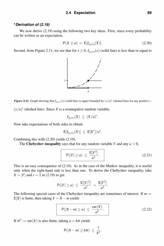
2.4 Expectation 89
Derivation of (2.19)
We now derive (2.19) using the following two key ideas. First, since every probability
can be written as an expectation,
P(X ≥ a) = E[I[a,∞)(X)]. (2.20)
Second, from Figure 2.11, we see that for x ≥ 0, I[a,∞)(x) (solid line) is less than or equal to
a
1
Figure 2.11. Graph showing that I[a,∞)(x) (solid line) is upper bounded by (x/a)r (dashed line) for any positive r.
(x/a)r (dashed line). Since X is a nonnegative random variable,
I[a,∞)(X) ≤ (X/a)r.
Now take expectations of both sides to obtain
E[I[a,∞)(X)] ≤ E[Xr]/ar.
Combining this with (2.20) yields (2.19).
The Chebyshev inequality says that for any random variable Y and any a > 0,
P(|Y | ≥ a) ≤ E[Y 2]
a2. (2.21)
This is an easy consequence of (2.19). As in the case of the Markov inequality, it is useful
only when the right-hand side is less than one. To derive the Chebyshev inequality, take
X = |Y | and r = 2 in (2.19) to get
P(|Y | ≥ a) ≤ E[|Y |2]a2
=E[Y 2]
a2.
The following special cases of the Chebyshev inequality are sometimes of interest. If m :=E[X ] is finite, then taking Y = X −m yields
P(|X −m| ≥ a) ≤ var(X)
a2. (2.22)
If σ2 := var(X) is also finite, taking a = kσ yields
P(|X −m| ≥ kσ) ≤ 1
k2.

90 Introduction to discrete random variables
These two inequalities give bounds on the probability that X is far from its mean value.
We will be using the Chebyshev inequality (2.22) in Section 3.3 to derive the weak law
of large numbers.
Example 2.34. A circuit is designed to handle a nominal current of 20 mA plus or minus
a deviation of less than 5 mA. If the applied current has mean 20 mA and variance 4 mA2,
use the Chebyshev inequality to bound the probability that the applied current violates the
design parameters.
Solution. Let X denote the applied current. Then X is within the design parameters if
and only if |X −20| < 5. To bound the probability that this does not happen, write
P(|X −20| ≥ 5) ≤ var(X)
52=
4
25= 0.16.
Hence, the probability of violating the design parameters is at most 16%.
Expectations of products of functions of independent random variables
We show that X and Y are independent if and only if
E[h(X)k(Y )] = E[h(X)]E[k(Y )] (2.23)
for all functions h(x) and k(y). In other words, X and Y are independent if and only if for
every pair of functions h(x) and k(y), the expectation of the product h(X)k(Y ) is equal to
the product of the individual expectations.6
There are two claims to be established. We must show that if (2.23) holds for every pair
of functions h(x) and k(y), then X and Y are independent, and we must show that if X and
Y are independent, then (2.23) holds for every pair of functions h(x) and k(y).The first claim is easy to show by taking h(x) = IB(x) and k(y) = IC(y) for any sets B
and C. Then (2.23) becomes
E[IB(X)IC(Y )] = E[IB(X)]E[IC(Y )]
= P(X ∈ B)P(Y ∈C).
Since IB(X)IC(Y ) = 1 if and only if X ∈ B and Y ∈ C, the left-hand side is simply P(X ∈B,Y ∈C). It then follows that
P(X ∈ B,Y ∈C) = P(X ∈ B)P(Y ∈C),
which is the definition of independence.
To derive the second claim, we use the fact that
pXY (xi,y j) := P(X = xi,Y = y j)
= P(X = xi)P(Y = y j), by independence,
= pX (xi) pY (y j).

2.4 Expectation 91
Now write
E[h(X)k(Y )] = ∑i
∑j
h(xi)k(y j) pXY (xi,y j)
= ∑i
∑j
h(xi)k(y j) pX (xi) pY (y j)
= ∑i
h(xi) pX (xi)
[∑
j
k(y j) pY (y j)
]= E[h(X)]E[k(Y )].
Example 2.35. Let X and Y be independent random variables with X ∼ Poisson(λ ) and
Y ∼ Poisson(µ). Find E[XY 2].
Solution. By independence, E[XY 2] = E[X ]E[Y 2]. From Example 2.22, E[X ] = λ , and
from Example 2.29, E[Y 2] = µ2 + µ . Hence, E[XY 2] = λ (µ2 + µ).
Correlation and covariance
The correlation between two random variables X and Y is defined to be E[XY ]. The cor-
relation is important because it determines when two random variables are linearly related;
namely, when one is a linear function of the other.
Example 2.36. Let X have zero mean and unit variance, and put Y := 3X . Find the
correlation between X and Y .
Solution. First note that since X has zero mean, E[X2] = var(X) = 1. Then write
E[XY ] = E[X(3X)] = 3E[X2] = 3. If we had put Y := −3X , then E[XY ] = −3.
Example 2.37. The input X and output Y of a system subject to random perturba-
tions are described probabilistically by the joint pmf pXY (i, j), where i = 1,2,3 and j =1,2,3,4,5. Let P denote the matrix whose i j entry is pXY (i, j), and suppose that
P =1
71
⎡⎣ 7 2 8 5 4
4 2 5 5 9
2 4 8 5 1
⎤⎦ .
Use MATLAB to compute the correlation E[XY ].
Solution. Assuming P is already defined, we use the script
s = 0;
for i = 1:3
for j = 1:5
s = s + i*j*P(i,j);
end
end
[n,d] = rat(s); % to express answer fraction
fprintf(’E[XY] = %i/%i = %g\n’,n,d,s)

92 Introduction to discrete random variables
and we find that E[XY ] = 428/71 = 6.02817.
An important property of correlation is the Cauchy–Schwarz inequality, which says
that ∣∣E[XY ]∣∣ ≤
√E[X2]E[Y 2], (2.24)
where equality holds if and only if X and Y are linearly related. This result provides an
important bound on the correlation between two random variables.
To derive (2.24), let λ be any constant and write
0 ≤ E[(X −λY )2] (2.25)
= E[X2 −2λXY +λ 2Y 2]
= E[X2]−2λE[XY ]+λ 2E[Y 2].
To make further progress, take
λ =E[XY ]
E[Y 2].
Then
0 ≤ E[X2]−2E[XY ]2
E[Y 2]+
E[XY ]2
E[Y 2]2E[Y 2]
= E[X2]− E[XY ]2
E[Y 2].
This can be rearranged to get
E[XY ]2 ≤ E[X2]E[Y 2]. (2.26)
Taking square roots yields (2.24). We can also show that if (2.24) holds with equality, then X
and Y are linearly related. If (2.24) holds with equality, then so does (2.26). Since the steps
leading from (2.25) to (2.26) are reversible, it follows that (2.25) must hold with equality.
But E[(X −λY )2] = 0 implies X = λY .7
When X and Y have different means and variances, say mX := E[X ], mY := E[Y ], σ2X :=
var(X) and σ2Y := var(Y ), we sometimes look at the correlation between the “normalized”
random variablesX −mX
σX
andY −mY
σY
,
which each have zero mean and unit variance.
The correlation coefficient of random variables X and Y is defined to be the correlation
of their normalized versions,
ρXY := E
[(X −mX
σX
)(Y −mY
σY
)].
2.4 Expectation 93
Furthermore, |ρXY | ≤ 1, with equality if and only if X and Y are related by a linear function
plus a constant. A pair of random variables is said to be uncorrelated if their correlation
coefficient is zero.
Example 2.38. For the random variables X and Y of Example 2.37, use MATLAB to
compute ρXY .
Solution. First note that the formula for ρXY can be expanded as
ρXY =E[XY ]−mX mY
σX σY
.
Next, except for the term E[XY ], the remaining quantities can be computed using marginal
pmfs, which can be computed easily with the sum command as done in Example 2.18. Since
E[XY ] was computed in Example 2.37 and was called s, the following additional script will
compute rhoxy.
format rat
pY = sum(P)
y = [ 1 2 3 4 5 ]
mY = y*pY’
varY = ((y-mY).ˆ2)*pY’
pX = sum(P’)
x = [ 1 2 3 ]
mX = x*pX’
varX = ((x-mX).ˆ2)*pX’
rhoxy = (s-mX*mY)/sqrt(varX*varY)
We find that mX = 136/71, mY = 222/71, var(X) = 412/643, var(Y ) = 1337/731, and
ρXY = 286/7963 = 0.0359161.
Example 2.39. If X and Y are zero mean, then σ2X = E[X2] and σ2
Y = E[Y 2]. It now
follows that
ρXY =E[XY ]√
E[X2]E[Y 2].
Example 2.40. Let U , W1, and W2 be independent with zero means. Put
X := U +W1,
Y := −U +W2.
Find the correlation coefficient between X and Y .
Solution. It is clear that mX = mY = 0. Now write
E[XY ] = E[(U +W1)(−U +W2)]
= E[−U2 +UW2 −W1U +W1W2]
= −E[U2],

94 Introduction to discrete random variables
using independence and the fact that U , W1, and W2 are all zero mean. We next calculate
E[X2] = E[(U +W1)2] = E[U2 +2UW1 +W 2
1 ] = E[U2]+E[W 21 ].
A similar calculation shows that E[Y 2] = E[U2]+E[W 22 ]. It then follows that
ρXY =−E[U2]√
(E[U2]+E[W 21 ])(E[U2]+E[W 2
2 ])
If W1 and W2 have the same variance, say E[W 21 ] = E[W 2
2 ] = σ2, then
ρXY =−E[U2]
E[U2]+σ2. (2.27)
If we define the signal-to-noise ratio (SNR) by
SNR :=E[U2]
σ2,
then
ρXY =−SNR
1+SNR.
As the signal-to-noise ratio goes to infinity, say by letting σ2 → 0, we have from (2.27) that
ρXY → −1. If 0 = σ2 = E[W 21 ] = E[W 2
2 ], then W1 = W2 ≡ 0. This means that X = U and
Y = −U , which implies Y = −X ; i.e., X and Y are linearly related.
It is frequently more convenient to work with the numerator of the correlation coefficient
and to forget about the denominators. This leads to the following definition.
The covariance between X and Y is defined by
cov(X ,Y ) := E[(X −mX )(Y −mY )].
With this definition, we can write
ρXY =cov(X ,Y )√var(X)var(Y )
.
Hence, X and Y are uncorrelated if and only if their covariance is zero.
Let X1,X2, . . . be a sequence of uncorrelated random variables; more precisely, for i = j,
Xi and Xj are uncorrelated. We show next that
var
(n
∑i=1
Xi
)=
n
∑i=1
var(Xi). (2.28)
In other words, for uncorrelated random variables, the variance of the sum is the sum of the
variances.

2.4 Expectation 95
Let mi := E[Xi] and m j := E[Xj]. Then uncorrelated means that
E[(Xi −mi)(Xj −m j)] = 0 for all i = j.
Put
X :=n
∑i=1
Xi.
Then
E[X ] = E
[n
∑i=1
Xi
]=
n
∑i=1
E[Xi] =n
∑i=1
mi,
and
X −E[X ] =n
∑i=1
Xi −n
∑i=1
mi =n
∑i=1
(Xi −mi).
Now write
var(X) = E[(X −E[X ])2]
= E
[(n
∑i=1
(Xi −mi)
)(n
∑j=1
(Xj −m j)
)]=
n
∑i=1
(n
∑j=1
E[(Xi −mi)(Xj −m j)]
).
For fixed i, consider the sum over j. When j = i, which is the case for n−1 values of j, the
expectation is zero because Xj and Xi are uncorrelated. Hence, of all the terms in the inner
sum, only the term with j = i survives. Thus,
var(X) =n
∑i=1
(E[(Xi −mi)(Xi −mi)]
)=
n
∑i=1
E[(Xi −mi)2]
=n
∑i=1
var(Xi).
Example 2.41. Show that X and Y are uncorrelated if and only if
E[XY ] = E[X ]E[Y ]. (2.29)
Solution. The result is obvious if we expand
E[(X −mX )(Y −mY )] = E[XY −mXY −XmY +mX mY ]
= E[XY ]−mXE[Y ]−E[X ]mY +mX mY
= E[XY ]−mX mY −mX mY +mX mY
= E[XY ]−mX mY .
From this we see that cov(X ,Y ) = 0 if and only if (2.29) holds.

96 Introduction to discrete random variables
From (2.29), we see that if X and Y are independent, then they are uncorrelated. Intu-
itively, the property of being uncorrelated is weaker than the property of independence. For
independent random variables, recall that
E[h(X)k(Y )] = E[h(X)]E[k(Y )]
for all functions h(x) and k(y), while for uncorrelated random variables, we only require
that this hold for h(x) = x and k(y) = y. For an example of uncorrelated random variables
that are not independent, see Problem 44. For additional examples, see Problems 20 and 51
in Chapter 7.
Notes
2.1: Probabilities involving random variables
Note 1. According to Note 1 in Chapter 1, P(A) is only defined for certain subsets
A ∈ A . Hence, in order that the probability
P(ω ∈ Ω : X(ω) ∈ B)
be defined, it is necessary that
ω ∈ Ω : X(ω) ∈ B ∈ A . (2.30)
To illustrate the problem, consider the sample space Ω := 1,2,3 equipped with the σ -field
A :=∅,1,2,3,Ω. (2.31)
Take P(1,2) = 2/3 and P(3) = 1/3. Now define two functions X(ω) := ω and
Y (ω) :=
2, ω = 1,2,3, ω = 3.
Observe that
ω ∈ Ω : X(ω) = 2 = 2 /∈ A ,
while
ω ∈ Ω : Y (ω) = 2 = 1,2 ∈ A .
Since 2 /∈A , P(ω ∈Ω : X(ω) = 2) is not defined. However, since 1,2 ∈A , P(ω ∈Ω : Y (ω) = 2) = 2/3.
In the general case, to guarantee that (2.30) holds, it is convenient to consider P(X ∈ B)only for sets B in some σ -field B of subsets of IR. The technical definition of a random
variable is then as follows. A function X from Ω into IR is a random variable if and only
if (2.30) holds for every B ∈ B. Usually B is taken to be the Borel σσ -field; i.e., B is the
smallest σ -field containing all the open subsets of IR. If B ∈B, then B is called a Borel set.
It can be shown [3, pp. 182–183] that a real-valued function X satisfies (2.30) for all Borel
sets B if and only if
ω ∈ Ω : X(ω) ≤ x ∈ A , for all x ∈ IR.

Notes 97
With reference to the functions X(ω) and Y (ω) defined above, observe that ω ∈ Ω :
X(ω) ≤ 1 = 1 /∈ A defined in (2.31), and so X is not a random variable. However,
it is easy to check that Y does satisfy ω ∈ Ω : Y (ω) ≤ y ∈ A defined in (2.31) for all y;
hence, Y is a random variable.
For B ∈ B, if we put
µ(B) := P(X ∈ B) = P(ω ∈ Ω : X(ω) ∈ B), (2.32)
then µ satisfies the axioms of a probability measure on IR. This follows because µ “inherits”
the properties of P through the random variable X (Problem 4). Once we know that µ is a
measure, formulas (2.1) and (2.2) become obvious. For example, (2.1) says that
µ((−∞,b]) = µ((−∞,a])+ µ((a,b]).
This is immediate since (−∞,b] = (−∞,a]∪ (a,b] is a disjoint union. Similarly, (2.2) says
that
µ(0∪1) = µ(0)+ µ(1).Again, since this union is disjoint, the result is immediate.
Since µ depends on X , if more than one random variable is under discussion, we write
µX (B) instead. We thus see that different random variables induce different probability mea-
sures on IR. Another term for measure is distribution. Hence, we call µX the distribution
of X . More generally, the term “distribution” refers to how probability is spread out. As we
will see later, for discrete random variables, once we know the probability mass function,
we can compute µX (B) = P(X ∈ B) for all B of interest. Similarly, for the continuous ran-
dom variables of Chapter 4, once we know the probability density function, we can compute
µX (B) = P(X ∈ B) for all B of interest. In this sense, probability mass functions, probabil-
ity density functions, and distributions are just different ways of describing how to compute
P(X ∈ B).
2.2: Discrete random variables
Note 2. To derive (2.4), we apply the law of total probability as given in (1.27) with
A = X ∈ B and Bi = X = xi. Since the xi are distinct, the Bi are disjoint, and (1.27) says
that
P(X ∈ B) = ∑i
P(X ∈ B∩X = xi). (2.33)
Now observe that if xi ∈ B, then X = xi implies X ∈ B, and so
X = xi ⊂ X ∈ B.
This monotonicity tells us that
X ∈ B∩X = xi = X = xi.
On the other hand, if xi /∈ B, then we cannot have X = xi and X ∈ B at the same time; in
other words
X ∈ B∩X = xi = ∅.

98 Introduction to discrete random variables
It now follows that
P(X ∈ B∩X = xi) =
P(X = xi), xi ∈ B,
0, xi /∈ B.
Substituting this in (2.33) yields (2.4).
2.3: Multiple random variables
Note 3. In light of Note 1 above, we do not require that (2.5) hold for all sets B and C,
but only for all Borel sets B and C.
Note 4. If X1, . . . ,Xn are independent, we show that any subset of them must also be
independent. Since (2.6) must hold for all choices of B1, . . . ,Bn, put B j = IR for the Xj that
we do not care about. Then use the fact that Xj ∈ IR = Ω and P(Ω) = 1 to make these
variables “disappear.” For example, if Bn = IR in (2.6), we get
P
([n−1⋂j=1
Xj ∈ B j]∩Xn ∈ IR
)=
[n−1
∏j=1
P(Xj ∈ B j)
]P(Xn ∈ IR)
or
P
([n−1⋂j=1
Xj ∈ B j]∩Ω
)=
[n−1
∏j=1
P(Xj ∈ B j)
]P(Ω),
which simplifies to
P
( n−1⋂j=1
Xj ∈ B j)
=n−1
∏j=1
P(Xj ∈ B j).
This shows that X1, . . . ,Xn−1 are independent.
Note 5. We show that
P(X ∈ B,Y ∈C) = ∑i:xi∈B
∑j:y j∈C
pXY (xi,y j).
Consider the disjoint events Y = y j. Since ∑ j P(Y = y j) = 1, we can use the law of total
probability as in (1.27) with A = X = xi,Y ∈C to write
P(X = xi,Y ∈C) = ∑j
P(X = xi,Y ∈C,Y = y j).
Now observe that
Y ∈C∩Y = y j =
Y = y j, y j ∈C,∅, y j /∈C.
Hence,
P(X = xi,Y ∈C) = ∑j:y j∈C
P(X = xi,Y = y j) = ∑j:y j∈C
pXY (xi,y j).
The next step is to use (1.27) again, but this time with the disjoint events X = xi and
A = X ∈ B,Y ∈C. Then,
P(X ∈ B,Y ∈C) = ∑i
P(X ∈ B,Y ∈C,X = xi).

Problems 99
Now observe that
X ∈ B∩X = xi =
X = xi, xi ∈ B,∅, xi /∈ B.
Hence,
P(X ∈ B,Y ∈C) = ∑i:xi∈B
P(X = xi,Y ∈C)
= ∑i:xi∈B
∑j:y j∈C
pXY (xi,y j).
2.4: Expectation
Note 6. To be technically correct, in (2.23), we cannot allow h(x) and k(y) to be com-
pletely arbitrary. We must restrict them so that
E[|h(X)|] < ∞, E[|k(Y )|] < ∞, and E[|h(X)k(Y )|] < ∞.
Note 7. Strictly speaking, we can only conclude that X = λY with probability one; i.e.,
P(X = λY ) = 1.
Problems
2.1: Probabilities involving random variables
1. On the probability space of Example 1.10, define the random variable X(ω) := ω .
(a) Find all the outcomes ω that belong to the event ω : X(ω) ≤ 3.
(b) Find all the outcomes ω that belong to the event ω : X(ω) > 4.
(c) Compute P(X ≤ 3) and P(X > 4).
2. On the probability space of Example 1.12, define the random variable
X(ω) :=
⎧⎨⎩2, if ω corresponds to an ace,1, if ω corresponds to a face card,0, otherwise.
(a) Find all the outcomes ω that belong to the event ω : X(ω) = 2.
(b) Find all the outcomes ω that belong to the event ω : X(ω) = 1.
(c) Compute P(X = 1 or X = 2).
3. On the probability space of Example 1.15, define the random variable X(ω) := ω .
Thus, X is the duration of a cell-phone call.
(a) Find all the outcomes ω that belong to the event ω : X(ω) ≤ 1.
(b) Find all the outcomes ω that belong to the event ω : X(ω) ≤ 3.
(c) Compute P(X ≤ 1), P(X ≤ 3), and P(1 < X ≤ 3).
4. This problem assumes you have read Note 1. Show that the distribution µ defined
in (2.32) satisfies the axioms of a probability measure on IR. Hints: Use the fact that
µ(B) = P(X−1(B)); use the inverse-image properties of Problem 15 in Chapter 1; the
axioms of a probability measure were defined in Section 1.4.
100 Introduction to discrete random variables
2.2: Discrete random variables
5. Let Y be an integer-valued random variable. Show that
P(Y = n) = P(Y > n−1)−P(Y > n).
6. Find the pmf of the random variable Y defined in Example 2.2 assuming that all
sequences in Ω are equally likely.
7. Find the pmf of the random variable of Problem 1.
8. Find the pmf of the random variable of Problem 2.
9. Consider the sample space Ω := −2,−1,0,1,2,3,4. For an event A ⊂ Ω, suppose
that P(A) = |A|/|Ω|. Define the random variable X(ω) := ω2. Find the probability
mass function of X .
10. Let X ∼ Poisson(λ ). Evaluate P(X > 1); your answer should be in terms of λ . Then
compute the numerical value of P(X > 1) when λ = 1. Answer: 0.264.
11. A certain photo-sensor fails to activate if it receives fewer than four photons in a
certain time interval. If the number of photons is modeled by a Poisson(2) random
variable X , find the probability that the sensor activates. Answer: 0.143.
2.3: Multiple random variables
12. A class consists of 15 students. Each student has probability p = 0.1 of getting an “A”
in the course. Find the probability that exactly one student receives an “A.” Assume
the students’ grades are independent. Answer: 0.343.
13. In a certain lottery game, the player chooses three digits. The player wins if at least
two out of three digits match the random drawing for that day in both position and
value. Find the probability that the player wins. Assume that the digits of the random
drawing are independent and equally likely. Answer: 0.028.
14. At the Chicago IRS office, there are m independent auditors. The kth auditor processes
Xk tax returns per day, where Xk is Poisson distributed with parameter λ > 0. The of-
fice’s performance is unsatisfactory if any auditor processes fewer than 2 tax returns
per day. Find the probability that the office performance is unsatisfactory.
15. An astronomer has recently discovered n similar galaxies. For i = 1, . . . ,n, let Xi
denote the number of black holes in the ith galaxy, and assume the Xi are independent
Poisson(λ ) random variables.
(a) Find the probability that at least one of the galaxies contains two or more black
holes.
(b) Find the probability that all n galaxies have at least one black hole.
(c) Find the probability that all n galaxies have exactly one black hole.
Your answers should be in terms of n and λ .

Problems 101
16. Show that the geometric0(p) pmf pX (k) = (1− p)pk,k = 0,1, . . . sums to one. Repeat
for the geometric1(p) pmf pX (k) = (1− p)pk−1,k = 1,2, . . . . Hint: Use the geometric
series formula from Problem 27 in Chapter 1.
17. There are 29 stocks on the Get Rich Quick Stock Exchange. The price of each stock
(in whole dollars) is geometric0(p) (same p for all stocks). Prices of different stocks
are independent. If p = 0.7, find the probability that at least one stock costs more
than 10 dollars. Answer: 0.44.
18. Suppose that X1, . . . ,Xn are independent, geometric1(p) random variables. Evaluate
P(min(X1, . . . ,Xn) > ) and P(max(X1, . . . ,Xn) ≤ ).
19. In a class of 25 students, the number of coins in each student’s pocket is uniformly
distributed between zero and twenty. Suppose the numbers of coins in different stu-
dents’ pockets are independent.
(a) Find the probability that no student has fewer than 5 coins in his/her pocket.
Answer: 1.12×10⁻³.
(b) Find the probability that at least one student has at least 19 coins in his/her
pocket. Answer: 0.918.
(c) Find the probability that exactly one student has exactly 19 coins in his/her
pocket. Answer: 0.369.
20. Blocks on a computer disk are good with probability p and faulty with probability
1− p. Blocks are good or bad independently of each other. Let Y denote the location
(starting from 1) of the first bad block. Find the pmf of Y .
21. Let X ∼ geometric1(p).
(a) Show that P(X > n) = pn.
(b) Compute P(X > n+ k|X > n). Hint: If A ⊂ B, then A∩B = A.
Remark. Your answer to (b) should not depend on n. For this reason, the geometric
random variable is said to have the memoryless property. For example, let X model
the number of the toss on which the first heads occurs in a sequence of coin tosses.
Then given a heads has not occurred up to and including time n, the conditional prob-
ability that a heads does not occur in the next k tosses does not depend on n. In other
words, given that no heads occurs on tosses 1, . . . ,n has no effect on the conditional
probability of heads occurring in the future. Future tosses do not remember the past.
22. From your solution of Problem 21(b), you can see that if X ∼ geometric1(p), then
P(X > n+ k|X > n) = P(X > k). Now prove the converse; i.e., show that if Y is
a positive integer-valued random variable such that P(Y > n+k|Y > n) = P(Y >k), then Y ∼ geometric1(p), where p = P(Y > 1). Hint: First show that P(Y > n) =P(Y > 1)n; then apply Problem 5.

102 Introduction to discrete random variables
23. Let X and Y be ternary random variables taking values 1, 2, and 3 with joint proba-
bilities pXY (i, j) given by the matrix⎡⎣ 1/8 0 1/8
0 1/2 0
1/8 0 1/8
⎤⎦ .
(a) Find pX (i) and pY ( j) for i, j = 1,2,3.
(b) Compute P(X < Y ).
(c) Determine whether or not X and Y are independent.
24. Repeat the previous problem if the pXY (i, j) are given by⎡⎣ 1/24 1/6 1/24
1/12 1/3 1/12
1/24 1/6 1/24
⎤⎦ .
25. Let X and Y be jointly discrete, integer-valued random variables with joint pmf
pXY (i, j) =
⎧⎪⎪⎪⎪⎨⎪⎪⎪⎪⎩3 j−1e−3
j!, i = 1, j ≥ 0,
46 j−1e−6
j!, i = 2, j ≥ 0,
0, otherwise.
Find the marginal pmfs pX (i) and pY ( j), and determine whether or not X and Y are
independent.
26. Let X and Y have joint pmf
pXY (k,n) :=
⎧⎪⎨⎪⎩(1− p)pk−1kne−k
n!, k ≥ 1,n ≥ 0,
0, otherwise.
(a) Compute pX (k) for k ≥ 1.
(b) Compute pY (0).
(c) Determine whether or not X and Y are independent.
27. MATLAB. Write a MATLAB script to compute P(g(X) ≥−16) if X is a uniform ran-
dom variable on 0, . . . ,50 and g(x) = 5x(x−10)(x−20)(x−30)(x−40)(x−50)/106.
Answer: 0.6275.
28. MATLAB. Let g(x) be as in the preceding problem. Write a MATLAB script to com-
pute P(g(X) ≥−16) if X ∼ geometric0(p) with p = 0.95. Answer: 0.5732.
29. MATLAB. Suppose x is a column vector of m numbers and y is a column vector of n
numbers and you want to compute g(x(i),y( j)), where i ranges from 1 to m, j ranges
from 1 to n, and g is a given function. Here is a simple way to do this without any
for loops. Store the following function in an M-file called allpairs.m
Problems 103
function [x1,y1] = allpairs(x,y)
lx = length(x);
ly = length(y);
x1 = kron(ones(ly,1),x);
y1 = kron(y,ones(lx,1));
(The MATLAB command kron computes the Kronecker product.) Then issue the
following commands and print out your results.
x = [ 1 2 3 ]’
y = [ 10 20 30 ]’
[x1,y1] = allpairs(x,y);
pairs = [x1 y1]
allsums = x1+y1
30. MATLAB. Let X and Y have the joint pmf of Example 2.18. Use the following script
to compute P(XY < 6).
i = [1:3]’;
j = [1:5]’;
[x,y]=allpairs(i,j);
prob = sum(P(find(x.*y<6)))
Do you get the same answer as in Example 2.19?
31. MATLAB. Write MATLAB scripts to solve Problems 23 and 24.
2.4: Expectation
32. Compute E[X ] if P(X = 2) = 1/3 and P(X = 5) = 2/3.
33. If X ∼ geometric0(1/2), compute E[I(2,6)(X)].
34. If X is Poisson(λ ), compute E[1/(X +1)].
35. A random variable X has mean 2 and variance 7. Find E[X2].
36. If X has mean m and variance σ2, and if Y := cX , find the variance of Y .
37. Compute E[(X +Y )3] if X ∼ Bernoulli(p) and Y ∼ Bernoulli(q) are independent.
38. Let X be a random variable with mean m and variance σ2. Find the constant c that best
approximates the random variable X in the sense that c minimizes the mean-squared
error E[(X − c)2].
39. The general shape of (x/a)r in Figure 2.11 is correct for r > 1. Find out how Fig-
ure 2.11 changes for 0 < r ≤ 1 by sketching (x/a)r and I[a,∞)(x) for r = 1/2 and
r = 1.
40. Let X ∼ Poisson(3/4). Compute both sides of the Markov inequality,
P(X ≥ 2) ≤ E[X ]
2.

104 Introduction to discrete random variables
41. Let X ∼ Poisson(3/4). Compute both sides of the Chebyshev inequality,
P(X ≥ 2) ≤ E[X2]
4.
42. Let X and Y be two random variables with means mX and mY and variances σ2X and
σ2Y . Let ρXY denote their correlation coefficient. Show that cov(X ,Y ) = σX σY ρXY .
Show that cov(X ,X) = var(X).
43. Let X and Y be two random variables with means mX and mY , variances σ2X and
σ2Y , and correlation coefficient ρ . Suppose X cannot be observed, but we are able to
measure Y . We wish to estimate X by using the quantity aY , where a is a suitable
constant. Assuming mX = mY = 0, find the constant a that minimizes the mean-
squared error E[(X −aY )2]. Your answer should depend on σX , σY , and ρ .
44. Show by counterexample that being uncorrelated does not imply independence. Hint:
Let P(X =±1) = P(X =±2) = 1/4, and put Y := |X |. Show that E[XY ] = E[X ]E[Y ],but P(X = 1,Y = 1) = P(X = 1)P(Y = 1).
45. Suppose that Y := X1 + · · ·+ XM , where the Xk are i.i.d. geometric1(p) random vari-
ables. Find E[Y 2].
46. Betting on fair games. Let X ∼ Bernoulli(p). For example, we could let X = 1
model the result of a coin toss being heads. Or we could let X = 1 model your
winning the lottery. In general, a bettor wagers a stake of s dollars that X = 1 with
a bookmaker who agrees to pay d dollars to the bettor if X = 1 occurs; if X = 0, the
stake s is kept by the bookmaker. Thus, the net income of the bettor is
Y := dX − s(1−X),
since if X = 1, the bettor receives Y = d dollars, and if X = 0, the bettor receives
Y = −s dollars; i.e., loses s dollars. Of course the net income to the bookmaker is
−Y . If the wager is fair to both the bettor and the bookmaker, then we should have
E[Y ] = 0. In other words, on average, the net income to either party is zero. Show
that a fair wager requires that d/s = (1− p)/p.
47. Odds. Let X ∼ Bernoulli(p). We say that the (fair) odds against X = 1 are n2 to
n1 (written n2 : n1) if n2 and n1 are positive integers satisfying n2/n1 = (1− p)/p.
Typically, n2 and n1 are chosen to have no common factors. Conversely, we say that
the odds for X = 1 are n1 to n2 if n1/n2 = p/(1− p). Consider a state lottery game
in which players wager one dollar that they can correctly guess a randomly selected
three-digit number in the range 000–999. The state offers a payoff of $500 for a
correct guess.
(a) What is the probability of correctly guessing the number?
(b) What are the (fair) odds against guessing correctly?
(c) The odds against actually offered by the state are determined by the ratio of the
payoff divided by the stake, in this case, 500 :1. Is the game fair to the bettor? If
not, what should the payoff be to make it fair? (See the preceding problem for
the notion of “fair.”)

Problems 105
48. These results are used in Examples 2.24 and 2.25. Show that the sum
Cp :=∞
∑k=1
1
kp
diverges for 0 < p ≤ 1, but is finite for p > 1. Hint: For 0 < p ≤ 1, use the inequality∫ k+1
k
1
t pdt ≤
∫ k+1
k
1
kpdt =
1
kp,
and for p > 1, use the inequality∫ k+1
k
1
t pdt ≥
∫ k+1
k
1
(k +1)pdt =
1
(k +1)p.
49. For Cp as defined in Problem 48, if P(X = k) = C−1p /kp for some p > 1, then X
is called a zeta or Zipf random variable. Show that E[Xn] < ∞ for n < p− 1, and
E[Xn] = ∞ for n ≥ p−1.
50. Let X be a discrete random variable taking finitely many distinct values x1, . . . ,xn.
Let pi := P(X = xi) be the corresponding probability mass function. Consider the
function
g(x) := − logP(X = x).
Observe that g(xi) = − log pi. The entropy of X is defined by
H(X) := E[g(X)] =n
∑i=1
g(xi)P(X = xi) =n
∑i=1
pi log1
pi
.
If all outcomes are equally likely, i.e., pi = 1/n, find H(X). If X is a constant random
variable, i.e., p j = 1 for some j and pi = 0 for i = j, find H(X).
51. Jensen’s inequality. Recall that a real-valued function g defined on an interval I is
convex if for all x,y ∈ I and all 0 ≤ λ ≤ 1,
g(λx+(1−λ )y
) ≤ λg(x)+(1−λ )g(y).
Let g be a convex function, and let X be a discrete random variable taking finitely
many values, say n values, all in I. Derive Jensen’s inequality,
E[g(X)] ≥ g(E[X ]).
Hint: Use induction on n.
52. Derive Lyapunov’s inequality,
E[|Z|α ]1/α ≤ E[|Z|β ]1/β , 1 ≤ α < β < ∞.
Hint: Apply Jensen’s inequality to the convex function g(x) = xβ/α and the random
variable X = |Z|α .

106 Introduction to discrete random variables
53. A discrete random variable is said to be nonnegative, denoted by X ≥ 0, if P(X ≥0) = 1; i.e., if
∑i
I[0,∞)(xi)P(X = xi) = 1.
(a) Show that for a nonnegative random variable, if xk < 0 for some k, then P(X =xk) = 0.
(b) Show that for a nonnegative random variable, E[X ] ≥ 0.
(c) If X and Y are discrete random variables, we write X ≥ Y if X −Y ≥ 0. Show
that if X ≥ Y , then E[X ] ≥ E[Y ]; i.e., expectation is monotone.
Exam preparation
You may use the following suggestions to prepare a study sheet, including formulas men-
tioned that you have trouble remembering. You may also want to ask your instructor for
additional suggestions.
2.1. Probabilities involving random variables. Know how to do basic probability calcu-
lations involving a random variable given as an explicit function on a sample space.
2.2. Discrete random variables. Be able to do simple calculations with probability mass
functions, especially the uniform and the Poisson.
2.3. Multiple random variables. Recall that X and Y are independent if P(X ∈ A,Y ∈B) = P(X ∈ A)P(Y ∈ B) for all sets A and B. However, for discrete random variables,
all we need to check is whether or not P(X = xi,Y = y j) = P(X = xi)P(Y = y j), or, in
terms of pmfs, whether or not pXY (xi,y j) = pX (xi) pY (y j) for all xi and y j. Remember
that the marginals pX and pY are computed using (2.8) and (2.9), respectively. Be
able to solve problems with intersections and unions of events involving independent
random variables. Know how the geometric1(p) random variable arises.
2.4. Expectation. Important formulas include LOTUS (2.14), linearity of expectation
(2.15), the definition of variance (2.16) as well as the variance formula (2.17), and
expectation of functions of products of independent random variables (2.23). For
sequences of uncorrelated random variables, the variance of the sum is the sum of the
variances (2.28). Know the difference between uncorrelated and independent. A list
of common pmfs and their means and variances can be found inside the front cover.
The Poisson(λ ) random variable arises so often that it is worth remembering, even
if you are allowed to bring a formula sheet to the exam, that its mean and variance
are both λ and that by the variance formula, its second moment is λ +λ 2. Similarly,
the mean p and variance p(1− p) of the Bernoulli(p) are also worth remembering.
Your instructor may suggest others to memorize. Know the Markov inequality (for
nonnegative random variables only) (2.18) and the Chebyshev inequality (for any
random variable) (2.21) and also (2.22).
A discrete random variable is completely characterized by its pmf, which is the
collection of numbers pX (xi). In many problems we do not know the pmf. However,
the next best things to know are the mean and variance; they can be used to bound
probabilities as in the Markov and Chebyshev inequalities, and they can be used for
approximation and estimation as in Problems 38 and 43.

Exam preparation 107
Work any review problems assigned by your instructor. If you finish them, re-work your
homework assignments.

3
More about discrete random variables
This chapter develops more tools for working with random variables. The probability
generating function is the key tool for working with sums of nonnegative integer-valued ran-
dom variables that are independent. When random variables are only uncorrelated, we can
work with averages (normalized sums) by using the weak law of large numbers. We empha-
size that the weak law makes the connection between probability theory and the every-day
practice of using averages of observations to estimate probabilities of real-world measure-
ments. The last two sections introduce conditional probability and conditional expectation.
The three important tools here are the law of total probability, the law of substitution, and,
for independent random variables, “dropping the conditioning.”
The foregoing concepts are developed here for discrete random variables, but they will
all be extended to more general settings in later chapters.
3.1 Probability generating functions
In many problems we have a sum of independent random variables, and we would like to
know the probability mass function of their sum. For example, in an optical communication
system, the received signal might be Y = X +W , where X is the number of photoelectrons
due to incident light on a photodetector, and W is the number of electrons due to dark
current noise in the detector. An important tool for solving these kinds of problems is
the probability generating function. The name derives from the fact that it can be used to
compute the probability mass function. Additionally, the probability generating function
can be used to compute the mean and variance in a simple way.
Let X be a discrete random variable taking only nonnegative integer values. The prob-
ability generating function (pgf) of X is1
GX (z) := E[zX ] =∞
∑n=0
znP(X = n). (3.1)
Readers familiar with the z transform will note that G(z−1) is the z transform of the proba-
bility mass function pX (n) := P(X = n).
Example 3.1. Find the probability generating function of X if it is Poisson with para-
meter λ .
Solution. Write
GX (z) = E[zX ]
=∞
∑n=0
znP(X = n)
=∞
∑n=0
zn λ ne−λ
n!
108

3.1 Probability generating functions 109
= e−λ∞
∑n=0
(zλ )n
n!
= e−λ ezλ
= eλ (z−1).
An important property of probability generating functions is that the pgf of a sum of
independent random variables is the product of the individual pgfs. To see this, let Y :=X1 + · · ·+Xn, where the Xi are independent with corresponding pgfs GXi
(z). Then
GY (z) := E[zY ]
= E[zX1+···+Xn ]
= E[zX1 · · ·zXn ]
= E[zX1 ] · · ·E[zXn ], by independence,
= GX1(z) · · ·GXn(z). (3.2)
We call this the factorization property. Remember, it works only for sums of independent
random variables.
Example 3.2. Let Y = X +W , where X and W are independent Poisson random vari-
ables with respective parameters λ and µ . Here X represents the signal and W the dark
current in the optical communication systems described at the beginning of the section.
Find the pgf of Y .
Solution. Write
GY (z) = E[zY ]
= E[zX+W ]
= E[zX zW ]
= GX (z)GW (z), by independence,
= eλ (z−1)eµ(z−1), by Example 3.1,
= e(λ+µ)(z−1),
which is the pgf of a Poisson random variable with parameter λ + µ .
The foregoing example shows that the pgf of Y is that of a Poisson random variable. We
would like to conclude that Y must have the Poisson(λ + µ) probability mass function. Is
this a justifiable conclusion? For example, if two different probability mass functions can
have the same pgf, then we are in trouble. Fortunately, we can show this is not the case.
We do this by showing that the probability mass function can be recovered from the pgf as
follows.

110 More about discrete random variables
Let GX (z) be a probability generating function. Since for |z| ≤ 1,∣∣∣∣ ∞
∑n=0
znP(X = n)
∣∣∣∣ ≤∞
∑n=0
|znP(X = n)|
=∞
∑n=0
|z|nP(X = n)
≤∞
∑n=0
P(X = n) = 1, (3.3)
the power series for GX has radius of convergence at least one. Writing
GX (z) = P(X = 0)+ zP(X = 1)+ z2P(X = 2)+ · · · ,
we immediately see that GX (0) = P(X = 0). If we differentiate the above expression with
respect to z, we get
G′X (z) = P(X = 1)+2zP(X = 2)+3z2
P(X = 3)+ · · · ,and we see that G′
X (0) = P(X = 1). Continuing in this way shows that
G(k)X (z)|z=0 = k!P(X = k),
or equivalently,
G(k)X (z)|z=0
k!= P(X = k). (3.4)
Example 3.3. If GX (z) =(
1+z+z2
3
)2, find P(X = 2).
Solution. First write
G′X (z) = 2
(1+ z+ z2
3
)(1+2z
3
),
and then
G′′X (z) = 2
(1+ z+ z2
3
)(2
3
)+2
(1+2z
3
)(1+2z
3
).
It follows that
P(X = 2) =G′′
X (0)
2!=
1
2!
(4
9+
2
9
)=
1
3.
The probability generating function can also be used to find moments. Starting from
GX (z) =∞
∑n=0
znP(X = n),
we compute
G′X (z) =
∞
∑n=1
nzn−1P(X = n).

3.2 The binomial random variable 111
Setting z = 1 yields
G′X (1) =
∞
∑n=1
nP(X = n) = E[X ].
Similarly, since
G′′X (z) =
∞
∑n=2
n(n−1)zn−2P(X = n),
setting z = 1 yields
G′′X (1) =
∞
∑n=2
n(n−1)P(X = n) = E[X(X −1)] = E[X2]−E[X ].
In general, since
G(k)X (z) =
∞
∑n=k
n(n−1) · · ·(n− [k−1])zn−kP(X = n),
setting z = 1 yields2
G(k)X (z)|z=1 = E
[X(X −1)(X −2) · · ·(X − [k−1])
]. (3.5)
The right-hand side is called the kth factorial moment of X .
Example 3.4. The probability generating function of X ∼ Poisson(λ ) was found in Ex-
ample 3.1 to be GX (z) = eλ (z−1). Use GX (z) to find E[X ] and var(X).
Solution. Since G′X (z) = eλ (z−1)λ , E[X ] = G′
X (1) = λ . Since G′′X (z) = eλ (z−1)λ 2,
E[X2]−E[X ] = λ 2, E[X2] = λ 2 +λ . For the variance, write
var(X) = E[X2]− (E[X ])2 = (λ 2 +λ )−λ 2 = λ .
3.2 The binomial random variable
In many problems, the key quantity of interest can be expressed in the form Y = X1 +· · ·+Xn, where the Xi are i.i.d. Bernoulli(p) random variables.
Example 3.5. A certain communication network consists of n links. Suppose that each
link goes down with probability p independently of the other links. Show that the number
of links that are down is a sum of independent Bernoulli random variables.
Solution. Let Xi = 1 if the ith link is down and Xi = 0 otherwise. Then the Xi are
independent Bernoulli(p), and Y := X1 + · · ·+Xn counts the number of links that are down.

112 More about discrete random variables
Example 3.6. A sample of radioactive material is composed of n molecules. Each mol-
ecule has probability p of emitting an alpha particle, and the particles are emitted indepen-
dently. Show that the number of particles emitted is a sum of independent Bernoulli random
variables.
Solution. Let Xi = 1 if the ith molecule emits an alpha particle, and Xi = 0 otherwise.
Then the Xi are independent Bernoulli(p), and Y := X1 + · · ·+ Xn counts the number of
alpha particles emitted.
There are several ways to find the probability mass function of Y . The most common
method uses a combinatorial argument, which we give in the next paragraph; following that,
we give a different derivation using probability generating functions. A third derivation
using techniques from Section 3.4 is given in the Notes.3
Observe that the only way to have Y = k is to have k of the Xi = 1 and the other n− k
Xi = 0. Let Bk denote the set of all sequences of zeros and ones, say (b1, . . . ,bn), in which
k of the bi = 1 and the other n− k bi = 0. Then
P(Y = k) = P((X1, . . . ,Xn) ∈ Bk)
= ∑(b1,...,bn)∈Bk
P(X1 = b1, . . . ,Xn = bn)
= ∑(b1,...,bn)∈Bk
P(X1 = b1) · · ·P(Xn = bn),
where the last step follows because the Xi are independent. Now each factor in the above
product is either p or 1− p according to whether each bi equals zero or one. Since the sum is
over (b1, . . . ,bn) ∈ Bk, there are k factors equal to p and n−k factors equal to 1− p. Hence,
P(Y = k) = ∑(b1,...,bn)∈Bk
pk(1− p)n−k
= |Bk|pk(1− p)n−k,
where |Bk| denotes the number of sequences in the set Bk. From the discussion in Sec-
tion 1.7,
|Bk| =
(n
k
)=
n!
k!(n− k)!.
We now see that
P(Y = k) =
(n
k
)pk(1− p)n−k, k = 0, . . . ,n.
Another way to derive the formula for P(Y = k) is to use the theory of probability
generating functions as developed in Section 3.1. In this method, we first find GY (z) and
then use the formula G(k)Y (z)|z=0/k! = P(Y = k). To find GY (z), we use the factorization
property for pgfs of sums of independent random variables. Write
GY (z) = E[zY ]
= E[zX1+···+Xn ]
= E[zX1 ] · · ·E[zXn ], by independence,
= GX1(z) · · ·GXn(z).
3.2 The binomial random variable 113
For the Bernoulli(p) random variables Xi,
GXi(z) := E[zXi ] = z0(1− p)+ z1 p = (1− p)+ pz.
Thus,
GY (z) = [(1− p)+ pz]n.
Next, we need the derivatives of GY (z). The first derivative is
G′Y (z) = n[(1− p)+ pz]n−1 p,
and in general, the kth derivative is
G(k)Y (z) = n(n−1) · · ·(n− [k−1]) [(1− p)+ pz]n−k pk.
It follows that
P(Y = k) =G
(k)Y (0)
k!
=n(n−1) · · ·(n− [k−1])
k!(1− p)n−k pk
=n!
k!(n− k)!pk(1− p)n−k
=
(n
k
)pk(1− p)n−k.
Since the formula for GY (z) is a polynomial of degree n, G(k)Y (z) = 0 for all k > n. Thus,
P(Y = k) = 0 for k > n.
The preceding random variable Y is called a binomial(n, p) random variable. Its prob-
ability mass function is usually written using the notation
pY (k) =
(n
k
)pk(1− p)n−k, k = 0, . . . ,n.
In MATLAB,(
nk
)= nchoosek(n,k). A graph of pY (k) is shown in Figure 3.1.
The binomial theorem says that for any complex numbers a and b,
n
∑k=0
(n
k
)akbn−k = (a+b)n.
A derivation using induction on n along with the easily verified identity(n
k−1
)+
(n
k
)=
(n+1
k
), k = 1, . . . ,n, (3.6)
can be given. However, for nonnegative a and b with a+b > 0, the result is an easy conse-
quence of our knowledge of the binomial random variable (see Problem 10).

114 More about discrete random variables
0 10 20 30 40 50 60 70 800
0.02
0.04
0.06
0.08
0.10
0.12
k
Figure 3.1. The binomial(n, p) pmf pY (k) =(
nk
)pk(1− p)n−k for n = 80 and p = 0.25,0.5, and 0.75 from left to
right, respectively.
On account of the binomial theorem, the quantity(
nk
)is sometimes called the binomial
coefficient. It is convenient to know that the binomial coefficients can be read off from the
nth row of Pascal’s triangle in Figure 3.2. Noting that the top row is row 0, it is immediately
seen, for example, that
(a+b)5 = a5 +5a4b+10a3b2 +10a2b3 +5ab4 +b5.
To generate the triangle, observe that except for the entries that are ones, each entry is equal
to the sum of the two numbers above it to the left and right. Thus, the triangle is a graphical
depiction of (3.6).
1
1 1
1 2 1
1 3 3 1
1 4 6 4 1
1 5 10 10 5 1
...
Figure 3.2. Pascal’s triangle.

3.3 The weak law of large numbers 115
Poisson approximation of binomial probabilities
If we let λ := np, then the probability generating function of a binomial(n, p) random
variable can be written as
[(1− p)+ pz]n = [1+ p(z−1)]n
=
[1+
λ (z−1)
n
]n
.
From calculus, recall the formula
limn→∞
(1+
x
n
)n
= ex.
So, for large n, [1+
λ (z−1)
n
]n
≈ exp[λ (z−1)],
which is the probability generating function of a Poisson(λ ) random variable (Example 3.4).
In making this approximation, n should be large compared to λ (z− 1). Since λ := np, as
n becomes large, so does λ (z− 1). To keep the size of λ small enough to be useful, we
should keep p small. Under this assumption, the binomial(n, p) probability generating func-
tion is close to the Poisson(np) probability generating function. This suggests the Poisson
approximationa (n
k
)pk(1− p)n−k ≈ (np)ke−np
k!, n large, p small.
Example 3.7. As noted in Example 3.6, the number of alpha particles emitted from
a radioactive sample is a binomial(n, p) random variable. However, since n is large, say
1023, even if the expected number of particles, np (Problem 8), is in the billions, say 109,
p ≈ 10−14 is still very small, and the Poisson approximation is justified.b
3.3 The weak law of large numbers
Let X1,X2, . . . be a sequence of random variables with a common mean E[Xi] = m for all
i. In practice, since we do not know m, we use the numerical average, or sample mean,
Mn :=1
n
n
∑i=1
Xi,
in place of the true, but unknown value, m. Can this procedure of using Mn as an estimate
of m be justified in some sense?
aThis approximation is justified rigorously in Problems 20 and 21(a) in Chapter 14. It is also derived directly
without probability generating functions in Problem 22 in Chapter 14.bIf the sample’s mass m is measured in grams, then the number of atoms in the sample is n = mA/w, where
A = 6.022× 10²³ is Avogadro’s number, and w is the atomic weight of the material. For example, the atomic
weight of radium is 226.

116 More about discrete random variables
Example 3.8. You are given a coin which may or may not be fair, and you want to
determine the probability of heads, p. If you toss the coin n times and use the fraction of
times that heads appears as an estimate of p, how does this fit into the above framework?
Solution. Let Xi = 1 if the ith toss results in heads, and let Xi = 0 otherwise. Then
P(Xi = 1) = p and m := E[Xi] = p as well. Note that X1 + · · ·+ Xn is the number of heads,
and Mn is the fraction of heads. Are we justified in using Mn as an estimate of p?
One way to answer these questions is with a weak law of large numbers (WLLN). A
weak law of large numbers gives conditions under which
limn→∞
P(|Mn −m| ≥ ε) = 0
for every ε > 0. This is a complicated formula. However, it can be interpreted as follows.
Suppose that based on physical considerations, m is between 30 and 70. Let us agree that if
Mn is within ε = 1/2 of m, we are “close enough” to the unknown value m. For example,
if Mn = 45.7, and if we know that Mn is within 1/2 of m, then m is between 45.2 and
46.2. Knowing this would be an improvement over the starting point 30 ≤ m ≤ 70. So, if
|Mn −m| < ε , we are “close enough,” while if |Mn −m| ≥ ε we are not “close enough.” A
weak law says that by making n large (averaging lots of measurements), the probability of
not being close enough can be made as small as we like; equivalently, the probability of
being close enough can be made as close to one as we like. For example, if P(|Mn −m| ≥ε) ≤ 0.1, then
P(|Mn −m| < ε) = 1−P(|Mn −m| ≥ ε) ≥ 0.9,
and we would be 90% sure that Mn is “close enough” to the true, but unknown, value of m.
Conditions for the weak law
We now give sufficient conditions for a version of the weak law of large numbers
(WLLN). Suppose that the Xi all have the same mean m and the same variance σ2. Assume
also that the Xi are uncorrelated random variables. Then for every ε > 0,
limn→∞
P(|Mn −m| ≥ ε) = 0.
This is an immediate consequence of the following two facts. First, by the Chebyshev
inequality (2.22),
P(|Mn −m| ≥ ε) ≤ var(Mn)
ε2.
Second, since the Xi are uncorrelated, a slight extension of (2.28) gives
var(Mn) = var
(1
n
n
∑i=1
Xi
)=(1
n
)2 n
∑i=1
var(Xi) =nσ2
n2=
σ2
n. (3.7)
Thus,
P(|Mn −m| ≥ ε) ≤ σ2
nε2, (3.8)

3.4 Conditional probability 117
which goes to zero as n → ∞. Note that the bound σ2/nε2 can be used to select a suitable
value of n.
Remark. The weak law was first proved around 1700 for Xi ∼ Bernoulli(p) random
variables by Jacob (a.k.a. James or Jacques) Bernoulli.
Example 3.9. Given ε and σ2, determine how large n should be so the probability that
Mn is within ε of m is at least 0.9.
Solution. We want to have
P(|Mn −m| < ε) ≥ 0.9.
Rewrite this as
1−P(|Mn −m| ≥ ε) ≥ 0.9,
or
P(|Mn −m| ≥ ε) ≤ 0.1.
By (3.8), it suffices to take
σ2
nε2≤ 0.1,
or n ≥ 10σ2/ε2.
Remark. In using (3.8) as suggested, it would seem that we are smart enough to know
σ2, but not m. In practice, we may replace σ2 in (3.8) with an upper bound. For example, if
Xi ∼ Bernoulli(p), then m = p and σ2 = p(1− p). Since, 0 ≤ p ≤ 1, it is easy to show that
σ2 ≤ 1/4.
Remark. If Z1,Z2, . . . are arbitrary, independent, identically distributed random vari-
ables, then for any set B ⊂ IR, taking Xi := IB(Zi) gives an independent, and therefore
uncorrelated, sequence of Bernoulli(p) random variables, where p = E[Xi] = P(Zi ∈ B).Hence, the weak law can be used to estimate probabilities as well as expected values. See
Problems 18 and 19. This topic is pursued in more detail in Section 6.8.
3.4 Conditional probability
We introduce two main applications of conditional probability for random variables.
One application is as an extremely powerful computational tool. In this connection, you
will learn how to use
• the law of total probability for random variables,
• the substitution law, and
• independence (if you have it).
The other application of conditional probability is as a tool that uses observational data to
estimate data that cannot be directly observed. For example, when data is sent over a noisy
channel, we use the received measurements along with knowledge of the channel statistics
to estimate the data that was actually transmitted.

118 More about discrete random variables
For conditional probabilities involving random variables, we use the notation
P(X ∈ B|Y ∈C) := P(X ∈ B|Y ∈C)=
P(X ∈ B∩Y ∈C)P(Y ∈C)
=P(X ∈ B,Y ∈C)
P(Y ∈C).
For discrete random variables, we define the conditional probability mass functions,
pX |Y (xi|y j) := P(X = xi|Y = y j)
=P(X = xi,Y = y j)
P(Y = y j)
=pXY (xi,y j)
pY (y j),
and
pY |X (y j|xi) := P(Y = y j|X = xi)
=P(X = xi,Y = y j)
P(X = xi)
=pXY (xi,y j)
pX (xi).
For future reference, we record these two formulas,
pX |Y (xi|y j) =pXY (xi,y j)
pY (y j)(3.9)
and
pY |X (y j|xi) =pXY (xi,y j)
pX (xi), (3.10)
noting that they make sense only when the denominators are not zero. We call pX |Y the con-
ditional probability mass function (pmf) of X given Y . Similarly, pY |X is called the condi-
tional pmf of Y given X . Notice that by multiplying through by the denominators, we obtain
pXY (xi,y j) = pX |Y (xi|y j) pY (y j) = pY |X (y j|xi) pX (xi). (3.11)
Note that if either pX (xi) = 0 or pY (y j) = 0, then pXY (xi,y j) = 0 from the discussion fol-
lowing Example 1.23.
Example 3.10. Find the conditional probability mass function pY |X ( j|i) if
pXY (i, j) :=
⎧⎨⎩ 2[i/(i+1)] j
n(n+1), j ≥ 0, i = 0, . . . ,n−1,
0, otherwise.

3.4 Conditional probability 119
Solution. Recall from Example 2.14 that
pX (i) =
⎧⎨⎩ 2i+1
n(n+1), i = 0, . . . ,n−1,
0, otherwise.
Hence, for i = 0, . . . ,n−1,
pY |X ( j|i) =
⎧⎨⎩1
i+1
( i
i+1
) j
, j ≥ 0,
0, j < 0.
In other words, given X = i for i in the range 0, . . . ,n− 1, we have that Y is conditionally
geometric0
(i/(i+1)
).
The general formula pY |X (y j|xi) = pXY (xi,y j)/pX (xi) shows that for fixed xi, pY |X (y j|xi)as a function of y j has the same shape as a slice of pXY (xi,y j). For the pmfs of Example 3.10
with n = 5, this is illustrated in Figure 3.3. Here we see that for fixed i, pXY (i, j) as a function
of j has the shape of the geometric0(i/(i+1)) pmf pY |X ( j|i).
01
23
4
0
5
10
0
0.01
0.02
0.03
0.04
0.05
0.06
0.07
j
i
Figure 3.3. Sketch of bivariate probability mass function pXY (i, j) of Example 3.10 with n = 5. For fixed i,
pXY (i, j) as a function of j is proportional to pY |X ( j|i), which is geometric0(i/(i + 1)). The special case i = 0
results in pY |X ( j|0) ∼ geometric0(0), which corresponds to a constant random variable that takes the value j = 0
with probability one.
Conditional pmfs are important because we can use them to compute conditional prob-
abilities just as we use marginal pmfs to compute ordinary probabilities. For example,
P(Y ∈C|X = xk) = ∑j
IC(y j)pY |X (y j|xk).
This formula is derived by taking B = xk in (2.11), and then dividing the result by P(X =xk) = pX (xk).

120 More about discrete random variables
Example 3.11 (optical channel). To transmit message i using an optical communication
system, light of intensity λi is directed at a photodetector. When light of intensity λi strikes
the photodetector, the number of photoelectrons generated is a Poisson(λi) random vari-
able. Find the conditional probability that the number of photoelectrons observed at the
photodetector is less than 2 given that message i was sent.
Solution. Let X denote the message to be sent, and let Y denote the number of photo-
electrons generated by the photodetector. The problem statement is telling us that
P(Y = n|X = i) =λ n
i e−λi
n!, n = 0,1,2, . . . .
The conditional probability to be calculated is
P(Y < 2|X = i) = P(Y = 0 or Y = 1|X = i)
= P(Y = 0|X = i)+P(Y = 1|X = i)
= e−λi +λie−λi .
Example 3.12. For the random variables X and Y used in the solution of the previous
example, write down their joint pmf if X ∼ geometric0(p).
Solution. The joint pmf is
pXY (i,n) = pX (i) pY |X (n|i) = (1− p)pi λ ni e−λi
n!,
for i,n ≥ 0, and pXY (i,n) = 0 otherwise.
The law of total probability
In Chapter 1, we used the law of total probability to compute the probability of an event
that can occur in different ways. In this chapter, we adapt the law to handle the case in which
the events we condition on are described by discrete random variables. For example, the
Internet traffic generated at a university depends on how many students are logged in. Even
if we know the number of students logged in, the traffic they generate is random. However,
the number of students logged in is a random variable. The law of total probability can help
us analyze these situations.
Let A ⊂ Ω be any event, and let X be any discrete random variable taking distinct values
xi. Then the events
Bi := X = xi = ω ∈ Ω : X(ω) = xi.are pairwise disjoint, and ∑i P(Bi) = ∑i P(X = xi) = 1. The law of total probability as in
(1.27) yields
P(A) = ∑i
P(A∩Bi) = ∑i
P(A|X = xi)P(X = xi).
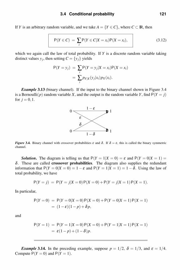
3.4 Conditional probability 121
If Y is an arbitrary random variable, and we take A = Y ∈C, where C ⊂ IR, then
P(Y ∈C) = ∑i
P(Y ∈C|X = xi)P(X = xi), (3.12)
which we again call the law of total probability. If Y is a discrete random variable taking
distinct values y j, then setting C = y j yields
P(Y = y j) = ∑i
P(Y = y j|X = xi)P(X = xi)
= ∑i
pY |X (y j|xi)pX (xi).
Example 3.13 (binary channel). If the input to the binary channel shown in Figure 3.4
is a Bernoulli(p) random variable X , and the output is the random variable Y , find P(Y = j)for j = 0,1.
101−δ
δ
0 11− ε
ε
Figure 3.4. Binary channel with crossover probabilities ε and δ . If δ = ε , this is called the binary symmetric
channel.
Solution. The diagram is telling us that P(Y = 1|X = 0) = ε and P(Y = 0|X = 1) =δ . These are called crossover probabilities. The diagram also supplies the redundant
information that P(Y = 0|X = 0) = 1− ε and P(Y = 1|X = 1) = 1− δ . Using the law of
total probability, we have
P(Y = j) = P(Y = j|X = 0)P(X = 0)+P(Y = j|X = 1)P(X = 1).
In particular,
P(Y = 0) = P(Y = 0|X = 0)P(X = 0)+P(Y = 0|X = 1)P(X = 1)
= (1− ε)(1− p)+δ p,
and
P(Y = 1) = P(Y = 1|X = 0)P(X = 0)+P(Y = 1|X = 1)P(X = 1)
= ε(1− p)+(1−δ )p.
Example 3.14. In the preceding example, suppose p = 1/2, δ = 1/3, and ε = 1/4.
Compute P(Y = 0) and P(Y = 1).

122 More about discrete random variables
Solution. We leave it to the reader to verify that P(Y = 0) = 13/24 and P(Y = 1) =11/24. Since the crossover probabilities are small, the effect of the channel on the data is
minimal. Since the input bit values are equally likely, we expect the output bit values to be
almost equally likely, which they are.
Example 3.15. Radioactive samples give off alpha-particles at a rate based on the size
of the sample. For a sample of size k, suppose that the number of particles observed is a
Poisson random variable Y with parameter k. If the sample size is a geometric1(p) random
variable X , find P(Y = 0) and P(X = 1|Y = 0).
Solution. The first step is to realize that the problem statement is telling us that as a
function of n, P(Y = n|X = k) is the Poisson pmf with parameter k. In other words,
P(Y = n|X = k) =kne−k
n!, n = 0,1, . . . .
In particular, note that P(Y = 0|X = k) = e−k. Now use the law of total probability to write
P(Y = 0) =∞
∑k=1
P(Y = 0|X = k) ·P(X = k)
=∞
∑k=1
e−k · (1− p)pk−1
=1− p
p
∞
∑k=1
(p/e)k
=1− p
p
p/e
1− p/e=
1− p
e− p.
Next,
P(X = 1|Y = 0) =P(X = 1,Y = 0)
P(Y = 0)
=P(Y = 0|X = 1)P(X = 1)
P(Y = 0)
= e−1 · (1− p) · e− p
1− p
= 1− p/e.
Example 3.16. A certain electric eye employs a photodetector whose efficiency occa-
sionally drops in half. When operating properly, the detector outputs photoelectrons ac-
cording to a Poisson(λ ) pmf. When the detector malfunctions, it outputs photoelectrons
according to a Poisson(λ/2) pmf. Let p < 1 denote the probability that the detector is op-
erating properly. Find the pmf of the observed number of photoelectrons. Also find the
conditional probability that the circuit is malfunctioning given that n output photoelectrons
are observed.

3.4 Conditional probability 123
Solution. Let Y denote the detector output, and let X = 1 indicate that the detector is
operating properly. Let X = 0 indicate that it is malfunctioning. Then the problem statement
is telling us that P(X = 1) = p and
P(Y = n|X = 1) =λ ne−λ
n!and P(Y = n|X = 0) =
(λ/2)ne−λ/2
n!.
Now, using the law of total probability,
P(Y = n) = P(Y = n|X = 1)P(X = 1)+P(Y = n|X = 0)P(X = 0)
=λ ne−λ
n!p+
(λ/2)ne−λ/2
n!(1− p).
This is the pmf of the observed number of photoelectrons.
The above formulas can be used to find P(X = 0|Y = n). Write
P(X = 0|Y = n) =P(X = 0,Y = n)
P(Y = n)
=P(Y = n|X = 0)P(X = 0)
P(Y = n)
=
(λ/2)ne−λ/2
n!(1− p)
λ ne−λ
n!p+
(λ/2)ne−λ/2
n!(1− p)
=1
2ne−λ/2 p
(1− p)+1
,
which is clearly a number between zero and one as a probability should be. Notice that as
we observe a greater output Y = n, the conditional probability that the detector is malfunc-
tioning decreases.
The substitution law
It is often the case that Z is a function of X and some other discrete random variable Y ,
say Z = g(X ,Y ), and we are interested in P(Z = z). In this case, the law of total probability
becomes
P(Z = z) = ∑i
P(Z = z|X = xi)P(X = xi).
= ∑i
P(g(X ,Y ) = z|X = xi)P(X = xi).
We claim that
P(
g(X ,Y ) = z∣∣X = xi
)= P
(g(xi,Y ) = z
∣∣X = xi
). (3.13)

124 More about discrete random variables
This property is known as the substitution law of conditional probability. To derive it, we
need the observation
g(X ,Y ) = z∩X = xi = g(xi,Y ) = z∩X = xi.From this we see that
P(g(X ,Y ) = z|X = xi) =P(g(X ,Y ) = z∩X = xi)
P(X = xi)=
P(g(xi,Y ) = z∩X = xi)P(X = xi)
= P(g(xi,Y ) = z|X = xi).
We can make further simplifications if X and Y are independent. In this case,
P(g(xi,Y ) = z|X = xi) =P(g(xi,Y ) = z,X = xi)
P(X = xi)
=P(g(xi,Y ) = z)P(X = xi)
P(X = xi)
= P(g(xi,Y ) = z).
Thus, when X and Y are independent, we can write
P(g(xi,Y ) = z|X = xi) = P(g(xi,Y ) = z), (3.14)
and we say that we “drop the conditioning.”
Example 3.17 (signal in additive noise). A random, integer-valued signal X is transmit-
ted over a channel subject to independent, additive, integer-valued noise Y . The received
signal is Z = X +Y as shown in Figure 3.5. To estimate X based on the received value Z, the
system designer wants to use the conditional pmf pX |Z . Find the desired conditional pmf.
+X
Y
Z=X+Y
Figure 3.5. Signal X subjected to additive noise Y .
Solution. Let X and Y be independent, discrete, integer-valued random variables with
pmfs pX and pY , respectively. Put Z := X +Y . We begin by writing out the formula for the
desired pmf
pX |Z(i| j) = P(X = i|Z = j)
=P(X = i,Z = j)
P(Z = j)

3.4 Conditional probability 125
=P(Z = j|X = i)P(X = i)
P(Z = j)
=P(Z = j|X = i)pX (i)
P(Z = j). (3.15)
To continue the analysis, we use the substitution law followed by independence to write
P(Z = j|X = i) = P(X +Y = j|X = i)
= P(i+Y = j|X = i)
= P(Y = j− i|X = i)
= P(Y = j− i)
= pY ( j− i). (3.16)
This result can also be combined with the law of total probability to compute the denomi-
nator in (3.15). Just write
pZ( j) = ∑i
P(Z = j|X = i)P(X = i) = ∑i
pY ( j− i)pX (i). (3.17)
In other words, if X and Y are independent, discrete, integer-valued random variables, the
pmf of Z = X +Y is the discrete convolution of pX and pY .
It now follows that
pX |Z(i| j) =pY ( j− i)pX (i)
∑k
pY ( j− k)pX (k),
where in the denominator we have changed the dummy index of summation to k to avoid
confusion with the i in the numerator.
The Poisson(λ ) random variable is a good model for the number of photoelectrons
generated in a photodetector when the incident light intensity is λ . Now suppose that an
additional light source of intensity µ is also directed at the photodetector. Then we expect
that the number of photoelectrons generated should be related to the total light intensity
λ + µ . The next example illustrates the corresponding probabilistic model.
Example 3.18 (Poisson channel). If X and Y are independent Poisson random variables
with respective parameters λ and µ , use the results of the preceding example to show
that Z := X + Y is Poisson(λ + µ). Also show that as a function of i, pX |Z(i| j) is a
binomial( j,λ/(λ + µ)) pmf.
Solution. To find pZ( j), we apply (3.17) as follows. Since pX (i) = 0 for i < 0 and since
pY ( j− i) = 0 for j < i, (3.17) becomes
pZ( j) =j
∑i=0
λ ie−λ
i!· µ j−ie−µ
( j− i)!
=e−(λ+µ)
j!
j
∑i=0
j!
i!( j− i)!λ iµ j−i
126 More about discrete random variables
=e−(λ+µ)
j!
j
∑i=0
(j
i
)λ iµ j−i
=e−(λ+µ)
j!(λ + µ) j, j = 0,1, . . . ,
where the last step follows by the binomial theorem.
Our second task is to compute
pX |Z(i| j) =P(Z = j|X = i)P(X = i)
P(Z = j)
=P(Z = j|X = i)pX (i)
pZ( j).
Since we have already found pZ( j), all we need is P(Z = j|X = i), which, using (3.16), is
simply pY ( j− i). Thus,
pX |Z(i| j) =µ j−ie−µ
( j− i)!· λ ie−λ
i!
/[e−(λ+µ)
j!(λ + µ) j
]=
λ iµ j−i
(λ + µ) j
(j
i
)=
(j
i
)[λ
(λ + µ)
]i[ µ(λ + µ)
] j−i
,
for i = 0, . . . , j.
Binary channel receiver design
Consider the problem of a receiver using the binary channel in Figure 3.4. The receiver
has access to the channel output Y , and must estimate, or guess, the value of X . What
decision rule should be used? It turns out that no decision rule can have a smaller probability
of error than the maximum a posteriori probability (MAP) rule.4 Having observed Y = j,
the MAP rule says to decide X = 1 if
P(X = 1|Y = j) ≥ P(X = 0|Y = j), (3.18)
and to decide X = 0 otherwise. In other words, the MAP rule decides X = 1 if the posterior
probability of X = 1 given the observation Y = j is greater than the posterior probability of
X = 0 given the observation Y = j.
Observe that since
P(X = i|Y = j) =P(X = i,Y = j)
P(Y = j)=
P(Y = j|X = i)P(X = i)
P(Y = j),
(3.18) can be rewritten as
P(Y = j|X = 1)P(X = 1)
P(Y = j)≥ P(Y = j|X = 0)P(X = 0)
P(Y = j).

3.5 Conditional expectation 127
Canceling the common denominator, we have
P(Y = j|X = 1)P(X = 1) ≥ P(Y = j|X = 0)P(X = 0). (3.19)
This is an important observation. It says that we do not need to compute the denominator to
implement the MAP rule.
Next observe that if the inputs X = 0 and X = 1 are equally likely, we can cancel these
common factors as well and get
P(Y = j|X = 1) ≥ P(Y = j|X = 0). (3.20)
Sometimes we do not know the prior probabilities P(X = i). In this case, we sometimes use
(3.20) anyway. The rule that decides X = 1 when (3.20) holds and X = 0 otherwise is called
the maximum-likelihood (ML) rule. In this context, P(Y = j|X = i) is called the likelihood
of Y = j. The maximum-likelihood rule decides X = i if i maximizes the likelihood of the
observation Y = j.
A final thing to note about the MAP rule is that (3.19) can be rearranged as
P(Y = j|X = 1)
P(Y = j|X = 0)≥ P(X = 0)
P(X = 1).
Since the left-hand side is the ratio of the likelihoods, this quotient is called the likelihood
ratio. The right-hand side does not depend on j and is just a constant, sometimes called a
threshold. The MAP rule compares the likelihood ratio against this specific threshold. The
ML rule compares the likelihood ratio against the threshold one. Both the MAP rule and
ML rule are sometimes called likelihood-ratio tests. The reason for writing the tests in
terms of the likelihood ratio is that the form of the test can be greatly simplified; e.g., as in
Problems 35 and 36.
3.5 Conditional expectation
Just as we developed expectation for discrete random variables in Section 2.4, including
the law of the unconscious statistician, we can develop conditional expectation in the same
way. This leads to the formula
E[g(Y )|X = xi] = ∑j
g(y j) pY |X (y j|xi). (3.21)
Example 3.19. The random number Y of alpha particles emitted by a radioactive sample
is conditionally Poisson(k) given that the sample size X = k. Find E[Y |X = k].
Solution. We must compute
E[Y |X = k] = ∑n
nP(Y = n|X = k),
where (cf. Example 3.15)
P(Y = n|X = k) =kne−k
n!, n = 0,1, . . . .

128 More about discrete random variables
Hence,
E[Y |X = k] =∞
∑n=0
nkne−k
n!.
Now observe that the right-hand side is exactly ordinary expectation of a Poisson random
variable with parameter k (cf. the calculation in Example 2.22). Therefore, E[Y |X = k] = k.
Example 3.20. Let Z be the output of the Poisson channel of Example 3.18, and let X
be the transmitted signal. Compute E[X |Z = j] using the conditional pmf pX |Z(i| j) found in
Example 3.18.
Solution. We must compute
E[X |Z = j] =j
∑i=0
iP(X = i|Z = j),
where, letting p := λ/(λ + µ),
P(X = i|Z = j) =
(j
i
)pi(1− p) j−i.
Hence,
E[X |Z = j] =j
∑i=0
i
(j
i
)pi(1− p) j−i.
Now observe that the right-hand side is exactly the ordinary expectation of a binomial( j, p)random variable. It is shown in Problem 8 that the mean of such a random variable is jp.
Therefore, E[X |Z = j] = jp = jλ/(λ + µ).
Substitution law for conditional expectation
For functions of two variables, we have the following conditional law of the unconscious
statistician,
E[g(X ,Y )|X = xi] = ∑k
∑j
g(xk,y j) pXY |X (xk,y j|xi).
However,
pXY |X (xk,y j|xi) = P(X = xk,Y = y j|X = xi)
=P(X = xk,Y = y j,X = xi)
P(X = xi).
Now, when k = i, the intersection
X = xk∩Y = y j∩X = xiis empty, and has zero probability. Hence, the numerator above is zero for k = i. When
k = i, the above intersections reduce to X = xi∩Y = y j, and so
pXY |X (xk,y j|xi) = pY |X (y j|xi), for k = i.

3.5 Conditional expectation 129
It now follows that
E[g(X ,Y )|X = xi] = ∑j
g(xi,y j) pY |X (y j|xi)
= E[g(xi,Y )|X = xi].
We call
E[g(X ,Y )|X = xi] = E[g(xi,Y )|X = xi] (3.22)
the substitution law for conditional expectation. Note that if g in (3.22) is a function of
Y only, then (3.22) reduces to (3.21). Also, if g is of product form, say g(x,y) = h(x)k(y),then
E[h(X)k(Y )|X = xi] = h(xi)E[k(Y )|X = xi].
Law of total probability for expectation
In Section 3.4 we discussed the law of total probability, which shows how to compute
probabilities in terms of conditional probabilities. We now derive the analogous formula for
expectation. Write
∑i
E[g(X ,Y )|X = xi] pX (xi) = ∑i
[∑
j
g(xi,y j) pY |X (y j|xi)
]pX (xi)
= ∑i
∑j
g(xi,y j) pXY (xi,y j)
= E[g(X ,Y )].
Hence, the law of total probability for expectation is
E[g(X ,Y )] = ∑i
E[g(X ,Y )|X = xi] pX (xi). (3.23)
In particular, if g is a function of Y only, then
E[g(Y )] = ∑i
E[g(Y )|X = xi] pX (xi).
Example 3.21. Light of intensity λ is directed at a photomultiplier that generates X ∼Poisson(λ ) primaries. The photomultiplier then generates Y secondaries, where given X =n, Y is conditionally geometric1
((n + 2)−1
). Find the expected number of secondaries and
the correlation between the primaries and the secondaries.
Solution. The law of total probability for expectations says that
E[Y ] =∞
∑n=0
E[Y |X = n] pX (n),
where the range of summation follows because X is Poisson(λ ). The next step is to compute
the conditional expectation. The conditional pmf of Y is geometric1(p), where, in this case,

130 More about discrete random variables
p = (n+2)−1, and the mean of such a pmf is, by Problem 4, 1/(1− p). Hence,
E[Y ] =∞
∑n=0
[1+
1
n+1
]pX (n) = E
[1+
1
X +1
].
An easy calculation (Problem 34 in Chapter 2) shows that for X ∼ Poisson(λ ),
E
[1
X +1
]= [1− e−λ ]/λ ,
and so E[Y ] = 1+[1− e−λ ]/λ .
The correlation between X and Y is
E[XY ] =∞
∑n=0
E[XY |X = n] pX (n)
=∞
∑n=0
nE[Y |X = n] pX (n)
=∞
∑n=0
n
[1+
1
n+1
]pX (n)
= E
[X
(1+
1
X +1
)].
Now observe that
X
(1+
1
X +1
)= X +1− 1
X +1.
It follows that
E[XY ] = λ +1− [1− e−λ ]/λ .
Notes
3.1: Probability generating functions
Note 1. When z is complex,
E[zX ] := E[Re(zX )]+ jE[Im(zX )].
By writing
zn = rne jnθ = rn[cos(nθ)+ j sin(nθ)],
it is easy to check that for |z| ≤ 1, the above expectations are finite (cf. (3.3)) and that
E[zX ] =∞
∑n=0
znP(X = n).
Note 2. Although GX (z) is well defined for |z| ≤ 1, the existence of its derivatives is
only guaranteed for |z| < 1. Hence, G(k)X (1) may have to be understood as limz ↑ 1G
(k)X (z).
By Abel’s theorem [32, pp. 64–65], this limit is equal to the kth factorial moment on the
right-hand side of (3.5), even if it is infinite.

Notes 131
3.4: Conditional probability
Note 3. Here is an alternative derivation of the fact that the sum of independent Ber-
noulli random variables is a binomial random variable. Let X1,X2, . . . be independent
Bernoulli(p) random variables. Put
Yn :=n
∑i=1
Xi.
We need to show that Yn ∼ binomial(n, p). The case n = 1 is trivial. Suppose the result is
true for some n ≥ 1. We show that it must be true for n+1. Use the law of total probability
to write
P(Yn+1 = k) =n
∑i=0
P(Yn+1 = k|Yn = i)P(Yn = i). (3.24)
To compute the conditional probability, we first observe that Yn+1 = Yn +Xn+1. Also, since
the Xi are independent, and since Yn depends only on X1, . . . ,Xn, we see that Yn and Xn+1 are
independent. Keeping this in mind, we apply the substitution law and write
P(Yn+1 = k|Yn = i) = P(Yn +Xn+1 = k|Yn = i)
= P(i+Xn+1 = k|Yn = i)
= P(Xn+1 = k− i|Yn = i)
= P(Xn+1 = k− i).
Since Xn+1 takes only the values zero and one, this last probability is zero unless i = k or
i = k−1. Returning to (3.24), we can writec
P(Yn+1 = k) =k
∑i=k−1
P(Xn+1 = k− i)P(Yn = i).
Assuming that Yn ∼ binomial(n, p), this becomes
P(Yn+1 = k) = p
(n
k−1
)pk−1(1− p)n−(k−1) + (1− p)
(n
k
)pk(1− p)n−k.
Using the easily verified identity,(n
k−1
)+
(n
k
)=
(n+1
k
),
we see that Yn+1 ∼ binomial(n+1, p).
Note 4. We show that the MAP rule is optimal for minimizing the probability of a
decision error. Consider a communication system whose input X takes values 1, . . . ,Mwith given probabilities pX (i) = P(X = i). The channel output is an integer-valued random
variable Y . Assume that the conditional probability mass function pY |X ( j|i) = P(Y = j|X =i) is also known. The receiver decision rule is ψ(Y ) = i if Y ∈ Di, where D1, . . . ,DM is
cWhen k = 0 or k = n+1, this sum actually has only one term, since P(Yn = −1) = P(Yn = n+1) = 0.
132 More about discrete random variables
a partition of IR. The problem is to characterize the choice for the partition sets Di that
minimizes the probability of a decision error, or, equivalently, maximizes the probability of
a correct decision. Use the laws of total probability and substitution to write the probability
of a correct decision as
P(ψ(Y ) = X) =M
∑i=1
P(ψ(Y ) = X |X = i)P(X = i)
=M
∑i=1
P(ψ(Y ) = i|X = i)pX (i)
=M
∑i=1
P(Y ∈ Di|X = i)pX (i)
=M
∑i=1
[∑
j
IDi( j)pY |X ( j|i)
]pX (i)
= ∑j
[M
∑i=1
IDi( j)pY |X ( j|i)pX (i)
].
For fixed j, consider the inner sum. Since the Di form a partition, the only term that is not
zero is the one for which j ∈ Di. To maximize this value, we should put j ∈ Di if and only
if the weight pY |X ( j|i)pX (i) is greater than or equal to pY |X ( j|i′)pX (i′) for all i′ = i. This is
exactly the MAP rule (cf. (3.19)).
Problems
3.1: Probability generating functions
1. Find var(X) if X has probability generating function
GX (z) = 16+ 1
6z+ 2
3z2.
2. If GX (z) is as in the preceding problem, find the probability mass function of X .
3. Find var(X) if X has probability generating function
GX (z) =
(2+ z
3
)5
.
4. Evaluate GX (z) for the cases X ∼ geometric0(p) and X ∼ geometric1(p). Use your
results to find the mean and variance of X in each case.
5. For i = 1, . . . ,n, let Xi ∼ Poisson(λi). Put
Y :=n
∑i=1
Xi.
Find P(Y = 2) if the Xi are independent.

Problems 133
6. Let a0, . . . ,an be nonnegative and not all zero. Let m be any positive integer. Find a
constant D such that
GX (z) := (a0 +a1z+a2z2 + · · ·+anzn)m/D
is a valid probability generating function.
7. Let X1,X2, . . . ,Xn be i.i.d. geometric1(p) random variables, and put Y := X1 + · · ·+Xn.
Find E[Y ], var(Y ), and E[Y 2]. Also find the probability generating function of Y .
Remark. We say that Y is a negative binomial or Pascal random variable with para-
meters n and p.
3.2: The binomial random variable
8. Use the probability generating function of Y ∼ binomial(n, p) to find the mean and
variance of Y .
9. Show that the binomial(n, p) probabilities sum to one. Hint: Use the fact that for any
nonnegative integer-valued random variable, GY (z)|z=1 = 1.
10. The binomial theorem says that
n
∑k=0
(n
k
)akbn−k = (a+b)n.
Derive this result for nonnegative a and b with a + b > 0 by using the fact that the
binomial(n, p) probabilities sum to one. Hint: Take p = a/(a+b).
11. A certain digital communication link has bit-error probability p. In a transmission
of n bits, find the probability that k bits are received incorrectly, assuming bit errors
occur independently.
12. A new school has M classrooms. For i = 1, . . . ,M, let ni denote the number of seats
in the ith classroom. Suppose that the number of students in the ith classroom is
binomial(ni, p) and independent. Let Y denote the total number of students in the
school. Find P(Y = k).
13. Let X1, . . . ,Xn be i.i.d. with P(Xi = 1) = 1− p and P(Xi = 2) = p. If Y := X1 + · · ·+Xn,
find P(Y = k) for all k.
14. Ten-bit codewords are transmitted over a noisy channel. Bits are flipped indepen-
dently with probability p. If no more than two bits of a codeword are flipped, the
codeword can be correctly decoded. Find the probability that a codeword cannot be
correctly decoded.
15. Make a table comparing both sides of the Poisson approximation of binomial proba-
bilities, (n
k
)pk(1− p)n−k ≈ (np)ke−np
k!, n large, p small,

134 More about discrete random variables
for k = 0,1,2,3,4,5 if n = 150 and p = 1/100. Hint: If MATLAB is available, the
binomial probability can be written
nchoosek(n,k)∗ p k∗ (1−p) (n−k)
and the Poisson probability can be written
(n∗p) k∗exp(−n∗p)/factorial(k).
3.3: The weak law of large numbers
16. Show that E[Mn] = m. Also show that for any constant c, var(cX) = c2var(X).
17. Student heights range from 120 to 220 cm. To estimate the average height, determine
how many students’ heights should be measured to make the sample mean within
0.25 cm of the true mean height with probability at least 0.9. Assume measurements
are uncorrelated and have variance σ2 = 1. What if you only want to be within 1 cm
of the true mean height with probability at least 0.9?
18. Let Z1,Z2, . . . be i.i.d. random variables, and for any set B ⊂ IR, put Xi := IB(Zi).
(a) Find E[Xi] and var(Xi).
(b) Show that the Xi are uncorrelated.
Observe that
Mn =1
n
n
∑i=1
Xi =1
n
n
∑i=1
IB(Zi)
counts the fraction of times Zi lies in B. By the weak law of large numbers, for large
n this fraction should be close to P(Zi ∈ B).
19. With regard to the preceding problem, put p := P(Zi ∈ B). If p is very small, and n
is not large enough, it is likely that Mn = 0, which is useless as an estimate of p. If
p = 1/1000, and n = 100, find P(M100 = 0).
20. Let Xi be a sequence of random variables, and put Mn := (1/n)∑ni=1 Xi. Assume that
each Xi has mean m. Show that it is not always true that for every ε > 0,
limn→∞
P(|Mn −m| ≥ ε) = 0.
Hint: Let Z be a nonconstant random variable and take Xi := Z for i = 1,2, . . . . To be
specific, try Z ∼ Bernoulli(1/2) and ε = 1/4.
21. Let X1,X2, . . . be uncorrelated random variables with common mean m and common
variance σ2. Let εn be a sequence of positive numbers with εn → 0. With Mn :=(1/n)∑n
i=1 Xi, give sufficient conditions on εn such that
P(|Mn −m| ≥ εn) → 0.

Problems 135
3.4: Conditional probability
22. If Z = X +Y as in the Poisson channel Example 3.18, find E[X |Z = j].
23. Let X and Y be integer-valued random variables. Suppose that conditioned on X = i,
Y ∼ binomial(n, pi), where 0 < pi < 1. Evaluate P(Y < 2|X = i).
24. Let X and Y be integer-valued random variables. Suppose that conditioned on Y = j,
X ∼ Poisson(λ j). Evaluate P(X > 2|Y = j).
25. Let X and Y be independent random variables. Show that pX |Y (xi|y j) = pX (xi) and
pY |X (y j|xi) = pY (y j).
26. Let X and Y be independent with X ∼ geometric0(p) and Y ∼ geometric0(q). Put
T := X −Y , and find P(T = n) for all n.
27. When a binary optical communication system transmits a 1, the receiver output is
a Poisson(µ) random variable. When a 2 is transmitted, the receiver output is a
Poisson(ν) random variable. Given that the receiver output is equal to 2, find the
conditional probability that a 1 was sent. Assume messages are equally likely.
28. In a binary communication system, when a 0 is sent, the receiver outputs a ran-
dom variable Y that is geometric0(p). When a 1 is sent, the receiver output Y ∼geometric0(q), where q = p. Given that the receiver outputs Y = k, find the condi-
tional probability that the message sent was a 1. Assume messages are equally likely.
29. Apple crates are supposed to contain only red apples, but occasionally a few green
apples are found. Assume that the number of red apples and the number of green ap-
ples are independent Poisson random variables with parameters ρ and γ , respectively.
Given that a crate contains a total of k apples, find the conditional probability that
none of the apples is green.
30. Let X ∼ Poisson(λ ), and suppose that given X = n, Y ∼ Bernoulli(1/(n + 1)). Find
P(X = n|Y = 1).
31. Let X ∼ Poisson(λ ), and suppose that given X = n, Y ∼ binomial(n, p). Find P(X =n|Y = k) for n ≥ k.
32. Let X and Y be independent binomial(n, p) random variables. Find the conditional
probability of X > k given that max(X ,Y ) > k if n = 100, p = 0.01, and k = 1. An-
swer: 0.576.
33. Let X ∼ geometric0(p) and Y ∼ geometric0(q), and assume X and Y are independent.
(a) Find P(XY = 4).
(b) Put Z := X +Y and find pZ( j) for all j using the discrete convolution formula
(3.17). Treat the cases p = q and p = q separately.
34. Let X and Y be independent random variables, each taking the values 0,1,2,3 with
equal probability. Put Z := X +Y and find pZ( j) for all j. Hint: Use the discrete
convolution formula (3.17) and pay careful attention to the limits of summation.

136 More about discrete random variables
35. Let X ∼ Bernoulli(p), and suppose that given X = i, Y is conditionally Poisson(λi),where λ1 > λ0. Express the likelihood-ratio test
P(Y = j|X = 1)
P(Y = j|X = 0)≥ P(X = 0)
P(X = 1)
in as simple a form as possible.
36. Let X ∼Bernoulli(p), and suppose that given X = i, Y is conditionally geometric0(qi),where q1 < q0. Express the likelihood-ratio test
P(Y = j|X = 1)
P(Y = j|X = 0)≥ P(X = 0)
P(X = 1)
in as simple a form as possible.
37. Show that if P(X = xi|Y = y j) = h(xi) for all j and some function h, then X and Y are
independent.
3.5: Conditional expectation
38. Let X and Y be jointly discrete, integer-valued random variables with joint pmf
pXY (i, j) =
⎧⎪⎪⎪⎪⎨⎪⎪⎪⎪⎩3 j−1e−3
j!, i = 1, j ≥ 0,
46 j−1e−6
j!, i = 2, j ≥ 0,
0, otherwise.
Compute E[Y |X = i], E[Y ], and E[X |Y = j].
39. Let X and Y be as in Example 3.15. Find E[Y ], E[XY ], E[Y 2], and var(Y ).
40. Let X and Y be as in Example 3.16. Find E[Y |X = 1], E[Y |X = 0], E[Y ], E[Y 2], and
var(Y ).
41. Let X ∼ Bernoulli(2/3), and suppose that given X = i, Y ∼ Poisson(3(i + 1)
). Find
E[(X +1)Y 2].
42. Let X ∼ Poisson(λ ), and suppose that given X = n, Y ∼ Bernoulli(1/(n + 1)). Find
E[XY ].
43. Let X ∼ geometric1(p), and suppose that given X = n, Y ∼ Pascal(n,q). Find E[XY ].
44. Let X and Y be integer-valued random variables, with Y being positive. Suppose
that given Y = k, X is conditionally Poisson with parameter k. If Y has mean m and
variance r, find E[X2].
45. Let X and Y be independent random variables, with X ∼ binomial(n, p), and let Y ∼binomial(m, p). Put V := X +Y . Find the pmf of V . Find P(V = 10|X = 4) (assume
n ≥ 4 and m ≥ 6).
46. Let X and Y be as in Example 3.15. Find GY (z).

Exam preparation 137
Exam preparation
You may use the following suggestions to prepare a study sheet, including formulas men-
tioned that you have trouble remembering. You may also want to ask your instructor for
additional suggestions.
3.1. Probability generating functions. Important formulas include the definition (3.1),
the factorization property for pgfs of sums of independent random variables (3.2), and
the probability formula (3.4). The factorial moment formula (3.5) is most useful in
its special cases
G′X (z)|z=1 = E[X ] and G′′
X (z)|z=1 = E[X2]−E[X ].
The pgfs of common discrete random variables can be found inside the front cover.
3.2. The binomial random variable. The binomial(n, p) random variable arises as the
sum of n i.i.d. Bernoulli(p) random variables. The binomial(n, p) pmf, mean, vari-
ance, and pgf can be found inside the front cover. It is sometimes convenient to
remember how to generate and use Pascal’s triangle for computing the binomial co-
efficient(
nk
)= n!/[k!(n− k)!].
3.3. The weak law of large numbers. Understand what it means if P(|Mn −m| ≥ ε) is
small.
3.4. Conditional probability. I often tell my students that the three most important things
in probability are:
(i) the law of total probability (3.12);
(ii) the substitution law (3.13); and
(iii) independence for “dropping the conditioning” as in (3.14).
3.5. Conditional expectation. I again tell my students that the three most important things
in probability are:
(i) the law of total probability (for expectations) (3.23);
(ii) the substitution law (3.22); and
(iii) independence for “dropping the conditioning.”
If the conditional pmf of Y given X is listed in the table inside the front cover (this
table includes moments), then E[Y |X = i] or E[Y 2|X = i] can often be found by in-
spection. This is a very useful skill.
Work any review problems assigned by your instructor. If you finish them, re-work your
homework assignments.

4
Continuous random variables
In Chapters 2 and 3, the only random variables we considered specifically were discrete
ones such as the Bernoulli, binomial, Poisson, and geometric. In this chapter we consider
a class of random variables allowed to take a continuum of values. These random vari-
ables are called continuous random variables and are introduced in Section 4.1. Continuous
random variables are important models for integrator output voltages in communication
receivers, file download times on the Internet, velocity and position of an airliner on radar,
etc. Expectation and moments of continuous random variables are computed in Section 4.2.
Section 4.3 develops the concepts of moment generating function (Laplace transform) and
characteristic function (Fourier transform). In Section 4.4 expectation of multiple random
variables is considered. Applications of characteristic functions to sums of independent
random variables are illustrated. In Section 4.5 the Markov inequality, the Chebyshev
inequality, and the Chernoff bound illustrate simple techniques for bounding probabilities
in terms of expectations.
4.1 Densities and probabilities
Introduction
Suppose that a random voltage in the range [0,1) is applied to a voltmeter with a one-
digit display. Then the display output can be modeled by a discrete random variable Y
taking values .0, .1, .2, . . . , .9 with P(Y = k/10) = 1/10 for k = 0, . . . ,9. If this same random
voltage is applied to a voltmeter with a two-digit display, then we can model its display
output by a discrete random variable Z taking values .00, .01, . . . , .99 with P(Z = k/100) =1/100 for k = 0, . . . ,99. But how can we model the voltage itself? The voltage itself, call
it X , can be any number in range [0,1). For example, if 0.15 ≤ X < 0.25, the one-digit
voltmeter would round to the tens place and show Y = 0.2. In other words, we want to be
able to write
P
( k
10−0.05 ≤ X <
k
10+0.05
)= P
(Y =
k
10
)=
1
10.
Notice that 1/10 is the length of the interval[ k
10−0.05,
k
10+0.05
).
This suggests that probabilities involving X can be computed via
P(a ≤ X < b) =∫ b
a1dx = b−a,
which is the length of the interval [a,b). This observation motivates the concept of a con-
tinuous random variable.
138

4.1 Densities and probabilities 139
Definition
We say that X is a continuous random variable if P(X ∈ B) has the form
P(X ∈ B) =∫
Bf (t)dt :=
∫ ∞
−∞IB(t) f (t)dt (4.1)
for some integrable function f .a Since P(X ∈ IR) = 1, the function f must integrate to one;
i.e.,∫ ∞−∞ f (t)dt = 1. Further, since P(X ∈ B) ≥ 0 for all B, it can be shown that f must be
nonnegative.1 A nonnegative function that integrates to one is called a probability density
function (pdf).
Usually, the set B is an interval such as B = [a,b]. In this case,
P(a ≤ X ≤ b) =∫ b
af (t)dt.
See Figure 4.1(a). Computing such probabilities is analogous to determining the mass of a
piece of wire stretching from a to b by integrating its mass density per unit length from a to
b. Since most probability densities we work with are continuous, for a small interval, say
[x,x+∆x], we have
P(x ≤ X ≤ x+∆x) =∫ x+∆x
xf (t)dt ≈ f (x)∆x.
See Figure 4.1(b).
(a) (b)
a b x+x x
Figure 4.1. (a) P(a ≤ X ≤ b) =∫ b
a f (t)dt is the area of the shaded region under the density f (t). (b) P(x ≤ X ≤x+∆x) =
∫ x+∆xx f (t)dt is the area of the shaded vertical strip.
Note that for random variables with a density,
P(a ≤ X ≤ b) = P(a < X ≤ b) = P(a ≤ X < b) = P(a < X < b)
since the corresponding integrals over an interval are not affected by whether or not the
endpoints are included or excluded.
Some common densities
Here are some examples of continuous random variables. A summary of the more com-
mon ones can be found on the inside of the back cover.
aLater, when more than one random variable is involved, we write fX (x) instead of f (x).

140 Continuous random variables
Uniform. The simplest continuous random variable is the uniform. It is used to model
experiments in which the outcome is constrained to lie in a known interval, say [a,b], and
all outcomes are equally likely. We write f ∼ uniform[a,b] if a < b and
f (x) =
⎧⎨⎩1
b−a, a ≤ x ≤ b,
0, otherwise.
This density is shown in Figure 4.2. To verify that f integrates to one, first note that since
ba
_____1
b−a
Figure 4.2. The uniform density on [a,b].
f (x) = 0 for x < a and x > b, we can write∫ ∞
−∞f (x)dx =
∫ b
af (x)dx.
Next, for a ≤ x ≤ b, f (x) = 1/(b−a), and so∫ b
af (x)dx =
∫ b
a
1
b−adx = 1.
This calculation illustrates an important technique that is often incorrectly carried out by
novice students: First modify the limits of integration, then substitute the appropriate for-
mula for f (x). For example, it is quite common to see the incorrect calculation,∫ ∞
−∞f (x)dx =
∫ ∞
−∞
1
b−adx = ∞.
Example 4.1. In coherent radio communications, the phase difference between the trans-
mitter and the receiver, denoted by Θ, is modeled as having a density f ∼ uniform[−π, π].Find P(Θ ≤ 0) and P(Θ ≤ π/2).
Solution. To begin, write
P(Θ ≤ 0) =∫ 0
−∞f (θ)dθ =
∫ 0
−πf (θ)dθ ,
where the second equality follows because f (θ) = 0 for θ < −π . Now that we have
restricted the limits of integration to be inside the region where the density is positive, we
can write
P(Θ ≤ 0) =∫ 0
−π
1
2πdθ = 1/2.
The second probability is treated in the same way. First write
P(Θ ≤ π/2) =∫ π/2
−∞f (θ)dθ =
∫ π/2
−πf (θ)dθ .

4.1 Densities and probabilities 141
It then follows that
P(Θ ≤ π/2) =∫ π/2
−π
1
2πdθ = 3/4.
Example 4.2. Use the results of the preceding example to compute P(Θ > π/2|Θ > 0).
Solution. To calculate
P(Θ > π/2|Θ > 0) =P(Θ > π/2∩Θ > 0)
P(Θ > 0),
first observe that the denominator is simply P(Θ > 0) = 1−P(Θ ≤ 0) = 1−1/2 = 1/2. As
for the numerator, note that
Θ > π/2 ⊂ Θ > 0.Then use the fact that A ⊂ B implies A∩B = A to write
P(Θ > π/2∩Θ > 0) = P(Θ > π/2) = 1−P(Θ ≤ π/2) = 1/4.
Thus, P(Θ > π/2|Θ > 0) = (1/4)/(1/2) = 1/2.
Exponential. Another simple continuous random variable is the exponential with para-
meter λ > 0. We write f ∼ exp(λ ) if
f (x) =
λe−λx, x ≥ 0,
0, x < 0.
This density is shown in Figure 4.3. As λ increases, the height increases and the width
decreases. It is easy to check that f integrates to one. The exponential random variable is
often used to model lifetimes, such as how long a cell-phone call lasts or how long it takes a
computer network to transmit a message from one node to another. The exponential random
variable also arises as a function of other random variables. For example, in Problem 4.3
you will show that if U ∼ uniform(0,1), then X = ln(1/U) is exp(1). We also point out
that if U and V are independent Gaussian random variables, which are defined later in this
section, then U2 +V 2 is exponential and√
U2 +V 2 is Rayleigh (defined in Problem 30).2
Example 4.3. Given that a cell-phone call has lasted more than t seconds so far, suppose
the conditional probability that the call ends by t +∆t is approximately λ∆t when ∆t is small.
Show that the call duration is an exp(λ ) random variable.
Solution. Let T denote the call duration. We treat the problem assumption as saying
that
P(T ≤ t +∆t|T > t) ≈ λ∆t.

142 Continuous random variables
exp(λ)λ
λ/2
0
0 ln(2)/λ
Laplace(λ)
λ/2
λ/4
0
0−ln(2)/λ ln(2)/λ
Cauchy(λ)
00−λ λ
N(m,σ2)
0mm−σ m+σ
√2π σ_______1
2πλ
πλ1
1_____
____
Figure 4.3. Several common density functions.
To find the density of T , we proceed as follows. Let t ≥ 0 and write
P(T ≤ t +∆t|T > t) =P(T ≤ t +∆t∩T > t)
P(T > t)
=P(t < T ≤ t +∆t)
P(T > t)
=
∫ t+∆t
tfT (θ)dθ
P(T > t).
For small ∆t, the left-hand side is approximately λ∆t, and the right-hand side is approxi-
mately fT (t)∆t/P(T > t); i.e.,
λ∆t =fT (t)∆t
P(T > t).
Now cancel ∆t on both sides and multiply both sides by P(T > t) to get λP(T > t) = fT (t).In this equation, write P(T > t) as an integral to obtain
λ∫ ∞
tfT (θ)dθ = fT (t).
Differentiating both sides with respect to t shows that
−λ fT (t) = f ′T (t), t ≥ 0.
The solution of this differential equation is easily seen to be fT (t) = ce−λ t for some constant
c. However, since fT (t) is a density and since its integral from zero to infinity must be one,
it follows that c = λ .

4.1 Densities and probabilities 143
Remark. In the preceding example, T was the duration of a cell-phone call. However,
if T were the lifetime or time-to-failure of a device or system, then in reliability theory, the
quantity
lim∆t→0
P(T ≤ t +∆t|T > t)
∆t
is called the failure rate. If this limit does not depend on t, then the calculation of the
preceding example shows that the density of T must be exponential. Time-varying failure
rates are considered in Section 5.7.
Laplace / double-sided exponential. Related to the exponential is the Laplace, some-
times called the double-sided exponential. For λ > 0, we write f ∼ Laplace(λ ) if
f (x) = λ2
e−λ |x|.
This density is shown in Figure 4.3. As λ increases, the height increases and the width
decreases. You will show in Problem 54 that the difference of two independent exp(λ )random variables is a Laplace(λ ) random variable.
Example 4.4. An Internet router can send packets via route 1 or route 2. The packet
delays on each route are independent exp(λ ) random variables, and so the difference in
delay between route 1 and route 2, denoted by X , has a Laplace(λ ) density. Find
P(−3 ≤ X ≤−2 or 0 ≤ X ≤ 3).
Solution. The desired probability can be written as
P(−3 ≤ X ≤−2∪0 ≤ X ≤ 3).Since these are disjoint events, the probability of the union is the sum of the individual
probabilities. We therefore need to compute
P(−3 ≤ X ≤−2) and P(0 ≤ X ≤ 3).
Since X has a Laplace(λ ) density, these probabilities are equal to the areas of the corre-
sponding shaded regions in Figure 4.4. We first compute
P(−3 ≤ X ≤−2) =∫ −2
−3
λ2
e−λ |x| dx = λ2
∫ −2
−3eλx dx,
y 2/
0 1 2 3−1−2−3
Figure 4.4. Laplace(λ ) density for Example 4.4.

144 Continuous random variables
where we have used the fact that since x is negative in the range of integration, |x| = −x.
This last integral is equal to (e−2λ − e−3λ )/2. It remains to compute
P(0 ≤ X ≤ 3) =∫ 3
0
λ2
e−λ |x| dx = λ2
∫ 3
0e−λx dx,
which is equal to (1− e−3λ )/2. The desired probability is then
1−2e−3λ + e−2λ
2.
Cauchy. The Cauchy random variable with parameter λ > 0 is also easy to work with.
We write f ∼ Cauchy(λ ) if
f (x) =λ/π
λ 2 + x2.
This density is shown in Figure 4.3. As λ increases, the height decreases and the width
increases. Since (1/π)(d/dx) tan−1(x/λ ) = f (x), and since tan−1(∞) = π/2, it is easy
to check that f integrates to one. The Cauchy random variable arises as the tangent of a
uniform random variable (Example 5.10) and also as the quotient of independent Gaussian
random variables (Problem 33 in Chapter 7).
Example 4.5. In the λ -lottery you choose a number λ with 1 ≤ λ ≤ 10. Then a random
variable X is chosen according to the Cauchy density with parameter λ . If |X | ≥ 1, then
you win the lottery. Which value of λ should you choose to maximize your probability of
winning?
Solution. Your probability of winning is
P(|X | ≥ 1) = P(X ≥ 1 or X ≤−1)
=∫ ∞
1f (x)dx+
∫ −1
−∞f (x)dx,
where f (x) = (λ/π)/(λ 2 + x2) is the Cauchy density. Since the Cauchy density is an even
function,
P(|X | ≥ 1) = 2
∫ ∞
1
λ/πλ 2 + x2
dx.
Now make the change of variable y = x/λ , dy = dx/λ , to get
P(|X | ≥ 1) = 2
∫ ∞
1/λ
1/π1+ y2
dy.
Since the integrand is nonnegative, the integral is maximized by minimizing 1/λ or by
maximizing λ . Hence, choosing λ = 10 maximizes your probability of winning.

4.1 Densities and probabilities 145
Gaussian / normal. The most important density is the Gaussian or normal. For σ2 > 0,
we write f ∼ N(m,σ2) if
f (x) =1√
2π σexp
[−1
2
(x−m
σ
)2], (4.2)
where σ is the positive square root of σ2. A graph of the N(m,σ2) density is sketched in Fig-
ure 4.3. It is shown in Problems 9 and 10 that the density is concave for x ∈ [m−σ ,m+σ ]and convex for x outside this interval. As σ increases, the height of the density decreases
and it becomes wider as illustrated in Figure 4.5. If m = 0 and σ2 = 1, we say that f is a
standard normal density.
σ = small
σ = large
m
0
Figure 4.5. N(m,σ2) densities with different values of σ .
As a consequence of the central limit theorem, whose discussion is taken up in Chap-
ter 5, the Gaussian density is a good approximation for computing probabilities involving a
sum of many independent random variables; this is true whether the random variables are
continuous or discrete! For example, let
X := X1 + · · ·+Xn,
where the Xi are i.i.d. with common mean m and common variance σ2. For large n, it is
shown in Chapter 5 that if the Xi are continuous random variables, then
fX (x) ≈ 1√2π σ
√n
exp[−1
2
(x−nm
σ√
n
)2],
while if the Xi are integer-valued,
pX (k) ≈ 1√2π σ
√n
exp[−1
2
(k−nm
σ√
n
)2].
In particular, since the macroscopic noise current measured in a circuit results from the sum
of forces of many independent collisions on an atomic scale, noise current is well-described
by the Gaussian density. For this reason, Gaussian random variables are the noise model of
choice in electronic communication and control systems.
To verify that an arbitrary normal density integrates to one, we proceed as follows.
(For an alternative derivation, see Problem 17.) First, making the change of variable t =(x−m)/σ shows that ∫ ∞
−∞f (x)dx =
1√2π
∫ ∞
−∞e−t2/2 dt.

146 Continuous random variables
So, without loss of generality, we may assume f is a standard normal density with m = 0
and σ = 1. We then need to show that I :=∫ ∞−∞ e−x2/2 dx =
√2π . The trick is to show
instead that I2 = 2π . First write
I2 =
(∫ ∞
−∞e−x2/2 dx
)(∫ ∞
−∞e−y2/2 dy
).
Now write the product of integrals as the iterated integral
I2 =
∫ ∞
−∞
∫ ∞
−∞e−(x2+y2)/2 dxdy.
Next, we interpret this as a double integral over the whole plane and change from Cartesian
coordinates x and y to polar coordinates r and θ . To integrate over the whole plane in polar
coordinates, the radius r ranges from 0 to ∞, and the angle θ ranges from 0 to 2π . The
substitution is x = r cosθ and y = r sinθ . We also change dxdy to r dr dθ . This yields
I2 =
∫ 2π
0
∫ ∞
0e−r2/2r dr dθ
=∫ 2π
0
(−e−r2/2
∣∣∣∣∞0
)dθ
=∫ 2π
01dθ
= 2π.
Example 4.6. The noise voltage in a certain amplifier has the standard normal density.
Show that the noise is as likely to be positive as it is to be negative.
Solution. In terms of the density, which we denote by f , we must show that∫ 0
−∞f (x)dx =
∫ ∞
0f (x)dx.
Since f (x) = e−x2/2/√
2π is an even function of x, the two integrals are equal. Furthermore,
we point out that since the sum of the two integrals is∫ ∞−∞ f (x)dx = 1, each individual
integral must be 1/2.
Location and scale parameters and the gamma densities
Since a probability density function can be any nonnegative function that integrates to
one, it is easy to create a whole family of density functions starting with just one density
function. Let f be any nonnegative function that integrates to one. For any real number c
and any positive number λ , consider the nonnegative function
λ f(λ (x− c)
).
Here c is called a location parameter and λ is called a scale parameter. To show that this
new function is a probability density, all we have to do is show that it integrates to one. In
the integral ∫ ∞
−∞λ f
(λ (x− c)
)dx

4.1 Densities and probabilities 147
0 1
2
(a)
2
c c+1
(b)
0
2y
y1/
(c)
Figure 4.6. (a) Triangular density f (x). (b) Shifted density f (x − c). (c) Scaled density λ f (λx) shown for
0 < λ < 1.
make the change of variable t = λ (x− c), dt = λ dx to get∫ ∞
−∞λ f(λ (x− c)
)dx =
∫ ∞
−∞f (t)dt = 1.
Let us first focus on the case λ = 1. Then our new density reduces to f (x− c). For
example, if f is the triangular density shown in Figure 4.6(a), then f (x− c) is the density
shown in Figure 4.6(b). If c is positive, then f (x− c) is f (x) shifted to the right, and if c is
negative, then f (x− c) is f (x) shifted to the left.
Next consider the case c = 0 and λ > 0. In this case, the main effect of λ is to shrink (if
λ > 1) or to expand (if λ < 1) the density. The second effect of λ is to increase or decrease
the height of the density. For example, if f is again the triangular density of Figure 4.6(a),
then λ f (λx) is shown in Figure 4.6(c) for 0 < λ < 1.
To see what happens both c = 0 and λ > 0, first put h(x) := λ f (λx). Then observe that
h(x− c) = λ f(λ (x− c)
). In other words, first find the picture for λ f (λx), and then shift
this picture by c.
In the exponential and Laplace densities, λ is a scale parameter, while in the Cauchy
density, 1/λ is a scale parameter. In the Gaussian, if we write f (x) = e−x2/2/√
2π , then
λ f(λ (x− c)
)= λ
e−(λ (x−c))2/2
√2π
.
Comparing this with (4.2) shows that c = m and λ = 1/σ . In other words for an N(m,σ2)random variable, m is a location parameter and 1/σ is a scale parameter. Note in particular
that as σ increases, the density becomes shorter and wider, while as σ decreases, the density
becomes taller and narrower (recall Figure 4.5).
An important application of the scale parameter arises with the basic gamma density
with parameter p > 0. This density is given by
gp(x) :=
⎧⎨⎩xp−1e−x
Γ(p), x > 0,
0, otherwise,
where
Γ(p) :=∫ ∞
0xp−1e−x dx, p > 0,

148 Continuous random variables
is the gamma function. In other words, the gamma function is defined to make the gamma
density integrate to one.3 (Properties of the gamma function are derived in Problem 14.)
Graphs of gp(x) for p = 1/2, p = 1, p = 3/2, p = 2, and p = 3 are shown in Figure 4.7. To
explain the shapes of these curves, observe that for x near zero, e−x ≈ 1, and so the behavior
is determined by the factor xp−1. For the values of p in the figure, this factor is x−1/2, x0,
x1/2, x, and x2. In the first case, x−1/2 blows up as x approaches the origin, and decreases
as x moves to the right. Of course, x0 = 1 is a constant, and in the remaining cases, xp−1
is zero for x = 0 and then increases. In all cases, as x moves to the right, eventually, the
decaying nature of the factor e−x dominates, and the curve decreases to zero as x → ∞.
Setting gp,λ (x) := λ gp(λx) defines the general gamma density, and the following spe-
cial cases are of great importance. When p = m is a positive integer, gm,λ is called an
Erlang(m,λ ) density (see Problem 15). As shown in Problem 55(c), the sum of m i.i.d.
exp(λ ) random variables is an Erlang(m,λ ) random variable. For example, if m customers
are waiting in a queue, and the service time for each one is exp(λ ), then the time to serve all
m is Erlang(m,λ ). The Erlang densities for m = 1,2,3 and λ = 1 are g1(x), g2(x), and g3(x)shown in Figure 4.7. When p = k/2 and λ = 1/2, gp,λ is called a chi-squared density with
k degrees of freedom. As you will see in Problem 46, the chi-squared random variable arises
as the square of a normal random variable. In communication systems employing nonco-
herent receivers, the incoming signal is squared before further processing. Since the thermal
noise in these receivers is Gaussian, chi-squared random variables naturally appear. Since
chi-squared densities are scaled versions of gk/2, the chi-squared densities for k = 1,2,3,4,and 6 are scaled versions of g1/2, g1, g3/2, g2, and g3 shown in Figure 4.7.
0 1 2 3 40
1
= 1/2
= 1
= 3/2
p
p
p
p = 2
p = 3
Figure 4.7. The gamma densities gp(x) for p = 1/2, p = 1, p = 3/2, p = 2, and p = 3.

4.2 Expectation of a single random variable 149
The paradox of continuous random variables
Let X be a continuous random variable. For any given x0, write
1 =
∫ ∞
−∞f (t)dt =
∫ x0
−∞f (t)dt +
∫ ∞
x0
f (t)dt
= P(X ≤ x0)+P(X ≥ x0)
= P(X ≤ x0)+P(X = x0)+P(X > x0).
Since P(X ≤ x0)+P(X > x0) = P(X ∈ IR) = 1, it follows that P(X = x0) = 0. We are thus
confronted with the fact that continuous random variables take no fixed value with positive
probability! The way to understand this apparent paradox is to realize that continuous ran-
dom variables are an idealized model of what we normally think of as continuous-valued
measurements. For example, a voltmeter only shows a certain number of digits after the
decimal point, say 5.127 volts because physical devices have limited precision. Hence, the
measurement X = 5.127 should be understood as saying that
5.1265 ≤ X < 5.1275,
since all numbers in this range round to 5.127. Now there is no paradox since P(5.1265 ≤X < 5.1275) has positive probability.
You may still ask, “Why not just use a discrete random variable taking the distinct val-
ues k/1000, where k is any integer?” After all, this would model the voltmeter in question.
One answer is that if you get a better voltmeter, you need to redefine the random variable,
while with the idealized, continuous-random-variable model, even if the voltmeter changes,
the random variable does not. Also, the continuous-random-variable model is often mathe-
matically simpler to work with.
Remark. If B is any set with finitely many points, or even countably many points, then
P(X ∈B) = 0 when X is a continuous random variable. To see this, suppose B = x1,x2, . . .where the xi are distinct real numbers. Then
P(X ∈ B) = P
( ∞⋃i=1
xi)
=∞
∑i=1
P(X = xi) = 0,
since, as argued above, each term is zero.
4.2 Expectation of a single random variable
For a discrete random variable X with probability mass function p, we computed expec-
tations using the law of the unconscious statistician (LOTUS)
E[g(X)] = ∑i
g(xi) p(xi).
Analogously, for a continuous random variable X with density f , we have
E[g(X)] =∫ ∞
−∞g(x) f (x)dx. (4.3)
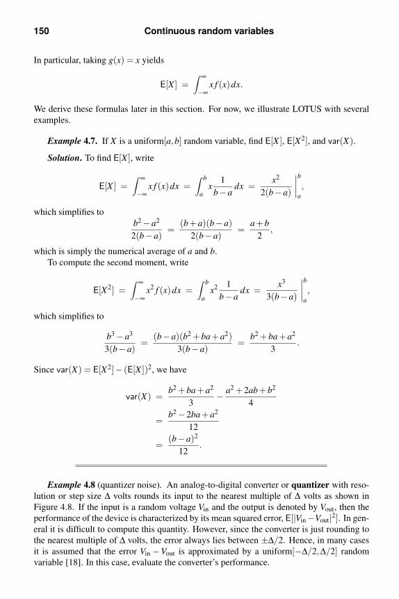
150 Continuous random variables
In particular, taking g(x) = x yields
E[X ] =∫ ∞
−∞x f (x)dx.
We derive these formulas later in this section. For now, we illustrate LOTUS with several
examples.
Example 4.7. If X is a uniform[a,b] random variable, find E[X ], E[X2], and var(X).
Solution. To find E[X ], write
E[X ] =∫ ∞
−∞x f (x)dx =
∫ b
ax
1
b−adx =
x2
2(b−a)
∣∣∣∣ba
,
which simplifies to
b2 −a2
2(b−a)=
(b+a)(b−a)
2(b−a)=
a+b
2,
which is simply the numerical average of a and b.
To compute the second moment, write
E[X2] =∫ ∞
−∞x2 f (x)dx =
∫ b
ax2 1
b−adx =
x3
3(b−a)
∣∣∣∣ba
,
which simplifies to
b3 −a3
3(b−a)=
(b−a)(b2 +ba+a2)
3(b−a)=
b2 +ba+a2
3.
Since var(X) = E[X2]− (E[X ])2, we have
var(X) =b2 +ba+a2
3− a2 +2ab+b2
4
=b2 −2ba+a2
12
=(b−a)2
12.
Example 4.8 (quantizer noise). An analog-to-digital converter or quantizer with reso-
lution or step size ∆ volts rounds its input to the nearest multiple of ∆ volts as shown in
Figure 4.8. If the input is a random voltage Vin and the output is denoted by Vout, then the
performance of the device is characterized by its mean squared error, E[|Vin−Vout|2]. In gen-
eral it is difficult to compute this quantity. However, since the converter is just rounding to
the nearest multiple of ∆ volts, the error always lies between ±∆/2. Hence, in many cases
it is assumed that the error Vin −Vout is approximated by a uniform[−∆/2,∆/2] random
variable [18]. In this case, evaluate the converter’s performance.

4.2 Expectation of a single random variable 151
/2Vin
outV
Figure 4.8. Input–output relationship of an analog-to-digital converter or quantizer with resolution ∆.
Solution. If X ∼ uniform[−∆/2,∆/2], then the uniform approximation allows us to
writeE[|Vin −Vout|2] ≈ E[X2]
= var(X), since X has zero mean,
=(∆/2− (−∆/2))2
12, by the preceding example,
=∆2
12.
Example 4.9. If X is an exponential random variable with parameter λ = 1, find all
moments of X .
Solution. We need to compute
E[Xn] =∫ ∞
0xne−x dx.
Use integration by parts (see Note 4 for a refresher) with u = xn and dv = e−xdx. Then
du = nxn−1dx, v = −e−x, and
E[Xn] = −xne−x
∣∣∣∣∞0
+n
∫ ∞
0xn−1e−x dx.
Using the fact that xne−x = 0 both for x = 0 and for x → ∞, we have
E[Xn] = n
∫ ∞
0xn−1e−x dx = nE[Xn−1], (4.4)
Taking n = 1 yields E[X ] = E[X0] = E[1] = 1. Taking n = 2 yields E[X2] = 2 ·1, and n = 3
yields E[X3] = 3 ·2 ·1. The general result is that E[Xn] = n!.
Observe that ∫ ∞
0xne−x dx =
∫ ∞
0x(n+1)−1e−x dx = Γ(n+1).
Hence, the preceding example shows that Γ(n + 1) = n!. In Problem 14(a) you will gener-
alize the calculations leading to (4.4) to show that Γ(p+1) = p ·Γ(p) for p > 0.

152 Continuous random variables
Example 4.10. Find the mean and variance of an exp(λ ) random variable.
Solution. Since var(X) = E[X2]−(E[X ]2), we need the first two moments of X . The nth
moment is
E[Xn] =∫ ∞
0xn ·λe−λx dx.
Making the change of variable y = λx, dy = λdx, we have
E[Xn] =∫ ∞
0(y/λ )ne−y dy =
1
λ n
∫ ∞
0yne−y dy.
Since this last integral is the nth moment of the exp(1) random variable, which is n! by the
last example, it follows that
E[Xn] =n!
λ n.
Hence,
var(X) = E[X2]− (E[X ])2 =2
λ 2−( 1
λ
)2
=1
λ 2.
Example 4.11. Let X be a continuous random variable with standard Gaussian density
f ∼ N(0,1). Compute E[Xn] for all n ≥ 1.
Solution. Write
E[Xn] =∫ ∞
−∞xn f (x)dx,
where f (x) = exp(−x2/2)/√
2π . Since f is an even function of x, the above integrand is
odd for n odd. Hence, all the odd moments are zero. For n ≥ 2, write
E[Xn] =∫ ∞
−∞xn e−x2/2
√2π
dx
=1√2π
∫ ∞
−∞xn−1 · xe−x2/2 dx.
Integration by parts shows that this last integral is equal to
−xn−1e−x2/2∣∣∣∞−∞
+(n−1)∫ ∞
−∞xn−2e−x2/2 dx.
Since e−x2/2 decays faster than any power of x, the first term is zero. Thus,
E[Xn] = (n−1)∫ ∞
−∞xn−2 e−x2/2
√2π
dx
= (n−1)E[Xn−2],
where, from the integral with n = 2, we see that E[X0] = 1. When n = 2 this yields E[X2] = 1,
and when n = 4 this yields E[X4] = 3. The general result is
E[Xn] =
1 ·3 · · ·(n−3)(n−1), n even,
0, n odd.

4.2 Expectation of a single random variable 153
At this point, it is convenient to introduce the double factorial notation,
n!! :=
1 ·3 · · ·(n−2) ·n, n > 0 and odd,2 ·4 · · ·(n−2) ·n, n > 0 and even.
In particular, with odd n = 2m−1, we see that
(2m−1)!! = 1 ·3 · · ·(2m−3)(2m−1)
=1 ·2 ·3 ·4 · · ·(2m−1)(2m)
2 ·4 · · ·(2m)
=(2m)!
(2 ·1) · (2 ·2) · (2 ·3) · · ·(2m)
=(2m)!
2m m!.
Hence, if X ∼ N(0,1),
E[X2m] = 1 ·3 · · ·(2m−3)(2m−1) = (2m−1)!! =(2m)!
2m m!. (4.5)
Example 4.12. If X has density f ∼ N(m,σ2), show that E[X ] = m and var(X) = σ2.
Solution. Instead of showing E[X ] = m, it is easier to show that E[X −m] = 0. Write
E[X −m] =∫ ∞
−∞(x−m) f (x)dx
=∫ ∞
−∞(x−m)
exp[− 1
2
(x−m
σ
)2]√
2π σdx
=∫ ∞
−∞
x−m
σ·
exp[− 1
2
(x−m
σ
)2]√
2πdx.
Make the change of variable y = (x−m)/σ , noting that dy = dx/σ . Then
E[X −m] = σ∫ ∞
−∞y
e−y2/2
√2π
dy,
which is seen to be zero once we recognize the integral as having the form of the mean of
an N(0,1) random variable Y .
To compute var(X), write
E[(X −m)2] =∫ ∞
−∞(x−m)2 f (x)dx
=∫ ∞
−∞(x−m)2
exp[− 1
2
(x−m
σ
)2]√
2π σdx
= σ∫ ∞
−∞
(x−m
σ
)2
·exp
[− 1
2
(x−m
σ
)2]√
2πdx.

154 Continuous random variables
Making the same change of variable as before, we obtain
E[(X −m)2] = σ2∫ ∞
−∞y2 e−y2/2
√2π
dy.
Now recognize this integral as having the form of the second moment of an N(0,1) random
variable Y . By the previous example, E[Y 2] = 1. Hence, E[(X −m)2] = σ2.
Example 4.13 (infinite expectation). Pareto densitiesb have been used to model packet
delay, files sizes, and other Internet characteristics. Let X have the Pareto density f (x) =1/x2, x ≥ 1. Find E[X ].
Solution. Write
E[X ] =∫ ∞
1x · 1
x2dx =
∫ ∞
1
1
xdx = lnx
∣∣∣∣∞1
= ∞.
Example 4.14. Determine E[X ] if X has a Cauchy density with parameter λ = 1.
Solution. This is a trick question. Recall that as noted following Example 2.24, for
signed discrete random variables,
E[X ] = ∑i:xi≥0
xi P(X = xi)+ ∑i:xi<0
xi P(X = xi),
if at least one of the sums is finite. The analogous formula for continuous random variables
is
E[X ] =∫ ∞
0x f (x)dx+
∫ 0
−∞x f (x)dx,
assuming at least one of the integrals is finite. Otherwise we say that E[X ] is undefined.
Since f is the Cauchy(1) density,
x f (x) = x · 1/π1+ x2
.
Since this integrand has anti-derivative
1
2πln(1+ x2),
we have
E[X ] =1
2πln(1+ x2)
∣∣∣∣∞0
+1
2πln(1+ x2)
∣∣∣∣0−∞
= (∞−0)+(0−∞)
= ∞−∞
= undefined.
bAdditional Pareto densities are considered in Problems 2, 23, and 26 and in Problem 59 in Chapter 5.
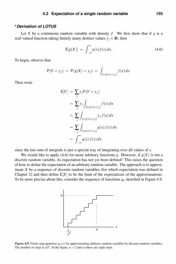
4.2 Expectation of a single random variable 155
Derivation of LOTUS
Let X be a continuous random variable with density f . We first show that if g is a
real-valued function taking finitely many distinct values y j ∈ IR, then
E[g(X)] =∫ ∞
−∞g(x) f (x)dx. (4.6)
To begin, observe that
P(Y = y j) = P(g(X) = y j) =∫x:g(x)=y j
f (x)dx.
Then write
E[Y ] = ∑j
y jP(Y = y j)
= ∑j
y j
∫x:g(x)=y j
f (x)dx
= ∑j
∫x:g(x)=y j
y j f (x)dx
= ∑j
∫x:g(x)=y j
g(x) f (x)dx
=∫ ∞
−∞g(x) f (x)dx,
since the last sum of integrals is just a special way of integrating over all values of x.
We would like to apply (4.6) for more arbitrary functions g. However, if g(X) is not a
discrete random variable, its expectation has not yet been defined! This raises the question
of how to define the expectation of an arbitrary random variable. The approach is to approx-
imate X by a sequence of discrete random variables (for which expectation was defined in
Chapter 2) and then define E[X ] to be the limit of the expectations of the approximations.
To be more precise about this, consider the sequence of functions qn sketched in Figure 4.9.
___1
2n
n
nx
nq ( )x
Figure 4.9. Finite-step quantizer qn(x) for approximating arbitrary random variables by discrete random variables.
The number of steps is n2n. In the figure, n = 2 and so there are eight steps.

156 Continuous random variables
Since each qn takes only finitely many distinct values, qn(X) is a discrete random variable
for which E[qn(X)] is defined. Since qn(X)→ X , we then define5E[X ] := limn→∞ E[qn(X)].
Now suppose X is a continuous random variable. Since qn(X) is a discrete random
variable, (4.6) applies, and we can write
E[X ] := limn→∞
E[qn(X)] = limn→∞
∫ ∞
−∞qn(x) f (x)dx.
Now bring the limit inside the integral,6 and then use the fact that qn(x) → x. This yields
E[X ] =
∫ ∞
−∞limn→∞
qn(x) f (x)dx =
∫ ∞
−∞x f (x)dx.
The same technique can be used to show that (4.6) holds even if g takes more than
finitely many values. Write
E[g(X)] := limn→∞
E[qn(g(X))]
= limn→∞
∫ ∞
−∞qn(g(x)) f (x)dx
=∫ ∞
−∞limn→∞
qn(g(x)) f (x)dx
=∫ ∞
−∞g(x) f (x)dx.
4.3 Transform methods
In Chapter 3, we made extensive use of probability generating functions to compute
moments and to analyze sums of independent random variables. However, probability gen-
erating functions apply only to nonnegative, integer-valued random variables. To handle
other kinds of random variables, we now introduce moment generating functions and char-
acteristic functions.
Moment generating functions
The moment generating function (mgf) of a real-valued random variable X is defined
by
MX (s) := E[esX ]. (4.7)
This generalizes the concept of probability generating function because if X is discrete
taking only nonnegative integer values, then
MX (s) = E[esX ] = E[(es)X ] = GX (es).
To see why MX is called the moment generating function, we differentiate (4.7) with respect
to s and obtain
M′X (s) =
d
dsE[esX ]
= E
[d
dsesX
]= E[XesX ].

4.3 Transform methods 157
Taking s = 0, we have
M′X (s)|s=0 = E[X ].
Differentiating k times and then setting s = 0 yields
M(k)X (s)|s=0 = E[Xk], (4.8)
assuming MX (s) is finite in a neighborhood of s = 0 [3, p. 278].
Example 4.15. If X ∼ N(0,1), find its moment generating function, and use it to find
the first four moments of X .
Solution. To begin, write
MX (s) =1√2π
∫ ∞
−∞esxe−x2/2 dx.
Combining the exponents in the above integral and completing the square we find
MX (s) = es2/2∫ ∞
−∞
e−(x−s)2/2
√2π
dx.
The above integrand is a normal density with mean s and unit variance. Since densities
integrate to one, MX (s) = es2/2.
For the first derivative of MX (s), we have M′X (x) = es2/2 · s, and so E[X ] = M′
X (0) = 0.
Before computing the remaining derivatives, it is convenient to notice that M′X (s) = MX (s)s.
Using the product rule,
M′′X (s) = MX (s)+M′
X (s)s = MX (s)+MX (s)s2.
Since we always have MX (0) = 1, we see that E[X2] = M′′X (0) = 1. Rewriting M′′
X (s) =MX (s)(1+ s2), we get for the third derivative,
M(3)X (s) = MX (s)(2s)+M′
X (s)(1+ s2) = MX (s)(3s+ s3).
Hence, E[X3] = M(3)X (0) = 0. For the fourth derivative,
M(4)X (s) = MX (s)(3+3s2)+M′
X (s)(3s+ s3).
Since we are stopping with the fourth moment, no further simplification is necessary since
we are going to set s = 0. We find that E[X4] = M(4)X (0) = 3.
It is now convenient to allow s to be complex. This means that we need to define the
expectation of complex-valued functions of X . If g(x) = u(x) + jv(x), where u and v are
real-valued functions of x, then
E[g(X)] := E[u(X)]+ jE[v(X)].

158 Continuous random variables
If X has density f , then
E[g(X)] := E[u(X)]+ jE[v(X)]
=
∫ ∞
−∞u(x) f (x)dx+ j
∫ ∞
−∞v(x) f (x)dx
=∫ ∞
−∞[u(x)+ jv(x)] f (x)dx
=∫ ∞
−∞g(x) f (x)dx.
It now follows that if X is a continuous random variable with density f , then
MX (s) = E[esX ] =∫ ∞
−∞esx f (x)dx,
which is just the Laplace transformc of f .
Example 4.16. If X is an exponential random variable with parameter λ > 0, find its
moment generating function.
Solution. Write
MX (s) =∫ ∞
0esxλe−λx dx
= λ∫ ∞
0ex(s−λ ) dx (4.9)
=λ
λ − s.
For real s, the integral in (4.9) is finite if and only if s < λ . For complex s, the analogous
condition is Res < λ . Hence, the moment generating function of an exp(λ ) random variable
is defined only for Res < λ .
If MX (s) is finite for all real s in a neighborhood of the origin, say for −r < s < r for
some 0 < r ≤∞, then X has finite moments of all orders, and the following calculation using
the power series eξ = ∑∞n=0 ξ n/n! is valid for complex s with |s| < r [3, p. 278]:
E[esX ] = E
[ ∞
∑n=0
(sX)n
n!
]=
∞
∑n=0
sn
n!E[Xn], |s| < r. (4.10)
Example 4.17. For the exponential random variable of the previous example, we can
obtain the power series as follows. Recalling the geometric series formula (Problem 27 in
Chapter 1), writeλ
λ − s=
1
1− s/λ=
∞
∑n=0
(s/λ )n,
cSignals and systems textbooks define the Laplace transform of f by∫ ∞−∞ e−sx f (x)dx. Hence, to be precise, we
should say that MX (s) is the Laplace transform of f evaluated at −s.

4.3 Transform methods 159
which is finite for all complex s with |s| < λ . Comparing the above sum with (4.10) and
equating the coefficients of the powers of s, we see by inspection that E[Xn] = n!/λ n. In
particular, we have E[X ] = 1/λ and E[X2] = 2/λ 2. Since var(X) = E[X2]− (E[X ])2, it
follows that var(X) = 1/λ 2.
In the preceding example, we computed MX (s) directly, and since we knew its power
series expansion, we could pick off the moments by inspection. As the next example shows,
the reverse procedure is sometimes possible; i.e., if we know all the moments, we can write
down the power series, and if we are lucky, we can find a closed-form expression for the
sum.
Example 4.18. If X ∼ N(0,1), sum the power series expansion for MX (s).
Solution. Since we know from Example 4.15 that MX (s) is finite for all real s, we can
use the power series expansion (4.10) to find MX (s) for all complex s. The moments of X
were determined in Example 4.11. Recalling that the odd moments are zero,
MX (s) =∞
∑m=0
s2m
(2m)!E[X2m]
=∞
∑m=0
s2m
(2m)!· (2m)!
2m m!, by (4.5),
=∞
∑m=0
(s2/2)m
m!
= es2/2.
Remark. Lest the reader think that Example 4.18 is redundant in light of Example 4.15,
we point out that the solution of Example 4.15 works only for real s because we treated s as
the mean of a real-valued random variable.7
Characteristic functions
In Example 4.16, the moment generating function was guaranteed finite only for Res <λ . It is possible to have random variables for which MX (s) is defined only for Res = 0; i.e.,
MX (s) is only defined for imaginary s. For example, if X is a Cauchy random variable, then
it is easy to see that MX (s) = ∞ for all real s = 0. In order to develop transform methods
that always work for any random variable X , we introduce the characteristic function of
X , defined by
ϕX (ν) := E[e jνX ]. (4.11)
Note that ϕX (ν) = MX ( jν). Also, since |e jνX | = 1, |ϕX (ν)| ≤ E[|e jνX |] = 1. Hence, the
characteristic function always exists and is bounded in magnitude by one.

160 Continuous random variables
If X is a continuous random variable with density f , then
ϕX (ν) =∫ ∞
−∞e jνx f (x)dx,
which is just the Fourier transformd of f . Using the Fourier inversion formula,
f (x) =1
2π
∫ ∞
−∞e− jνxϕX (ν)dν . (4.12)
Example 4.19. If X is an N(0,1) random variable, then by Example 4.18, MX (s) =
es2/2. Thus, ϕX (ν) = MX ( jν) = e( jν)2/2 = e−ν2/2. In terms of Fourier transforms,
1√2π
∫ ∞
−∞e jνxe−x2/2 dx = e−ν2/2.
In signal processing terms, the Fourier transform of a Gaussian pulse is a Gaussian pulse.
An alternative derivation of the N(0,1) characteristic function is given in Problem 50.
Example 4.20. If X has the gamma density gp(x) = xp−1e−x/Γ(p), x > 0, find the char-
acteristic function of X .
Solution. It is shown in Problem 44 that MX (s) = 1/(1− s)p. Taking s = jν shows that
ϕX (ν) = 1/(1− jν)p is the characteristic function.8 An alternative derivation is given in
Problem 51.
Example 4.21. As noted above, the characteristic function of an N(0,1) random vari-
able is e−ν2/2. Show that
ϕX (ν) = e jνm−σ2ν2/2, if X ∼ N(m,σ2).
Solution. Let f0 denote the N(0,1) density. If X ∼ N(m,σ2), then fX (x) = f0((x−m)/σ)/σ . Now write
ϕX (ν) = E[e jνX ]
=∫ ∞
−∞e jνx fX (x)dx
=∫ ∞
−∞e jνx · 1
σf0
(x−m
σ
)dx.
dSignals and systems textbooks define the Fourier transform of f by∫ ∞−∞ e− jωx f (x)dx. Hence, to be precise,
we should say that ϕX (ν) is the Fourier transform of f evaluated at −ν .

4.3 Transform methods 161
Then apply the change of variable y = (x−m)/σ , dy = dx/σ and obtain
ϕX (ν) =∫ ∞
−∞e jν(σy+m) f0(y)dy
= e jνm
∫ ∞
−∞e j(νσ)y f0(y)dy
= e jνme−(νσ)2/2
= e jνm−σ2ν2/2.
If X is an integer-valued random variable, then
ϕX (ν) = E[e jνX ] = ∑n
e jνnP(X = n)
is a 2π-periodic Fourier series. Given ϕX , the coefficients can be recovered by the formula
for Fourier series coefficients,
P(X = n) =1
2π
∫ π
−πe− jνnϕX (ν)dν . (4.13)
When the moment generating function is not finite in a neighborhood of the origin,
the moments of X cannot be obtained from (4.8). However, the moments can sometimes
be obtained from the characteristic function. For example, if we differentiate (4.11) with
respect to ν , we obtain
ϕ ′X (ν) =
d
dνE[e jνX ] = E[ jXe jνX ].
Taking ν = 0 yields ϕ ′X (0) = jE[X ]. The general result is
ϕ(k)X (ν)|ν=0 = jk
E[Xk], (4.14)
assuming E[|X |k] < ∞ [3, pp. 344–345].
Why so many transforms?
We have now discussed probability generating functions, moment generating functions,
and characteristic functions. Why do we need them all? After all, the characteristic function
exists for all random variables, and we can use it to recover probability mass functions and
densities and to find expectations.
In the case of nonnegative, integer-valued random variables, there are two reasons for
using the probability generating function. One is economy of notation. Since ϕX (ν) =GX (e jν), the formula for the probability generating function is simpler to derive and to
remember. The second reason is that it easier to compute the nth derivative P(X = n) =
G(n)X (0)/n! than the integral (4.13).

162 Continuous random variables
There are three reasons for using the moment generating function when it exists. First,
we again have economy of notation due to the fact that ϕX (ν) = MX ( jν). Second, for
computing moments, the formula E[Xn] = M(n)X (0) is easier to use than E[Xn] = jnϕ(n)
X (0),and is much easier to use than the factorial moment formulas, e.g., E[X(X − 1)(X − 2)] =
G(3)X (1). Third, the Chernoff bound, discussed later in Section 4.5, and importance sampling
(Section 6.8) require the use of MX (s) for positive values of s; imaginary values are not
useful.
To summarize, for some random variables, such as the Cauchy, the moment generating
function does not exist, and we have to use the characteristic function. Otherwise we should
exploit the benefits of the probability and moment generating functions.
4.4 Expectation of multiple random variables
In Chapter 2 we showed that for discrete random variables, expectation is linear and
monotone. We also showed that the expectation of a product of independent discrete random
variables is the product of the individual expectations. These properties continue to hold
for general random variables. Before deriving these results, we illustrate them with some
examples.
Example 4.22. Let Z := X +Y , were X and Y are independent, with X ∼ N(0,1) and
Y ∼ Laplace(1) random variables. Find cov(X ,Z).
Solution. Recall from Section 2.4 that
cov(X ,Z) := E[(X −mX )(Z−mZ)] = E[XZ]−mX mZ .
Since mX = 0 in this example,
cov(X ,Z) = E[XZ] = E[X(X +Y )] = E[X2]+E[XY ].
Since E[X2] = 1 and since X and Y are independent,
cov(X ,Z) = 1+E[X ]E[Y ] = 1.
Example 4.23. Let Z := X +Y , where X and Y are independent random variables. Show
that the characteristic function of Z is the product of the characteristic functions of X and Y .
Solution. The characteristic function of Z is
ϕZ(ν) := E[e jνZ ] = E[e jν(X+Y )] = E[e jνX e jνY ].
Now use independence to write
ϕZ(ν) = E[e jνX ]E[e jνY ] = ϕX (ν)ϕY (ν). (4.15)

4.4 Expectation of multiple random variables 163
An immediate consequence of the preceding example is that if X and Y are independent
continuous random variables, then the density of their sum Z = X +Y is the convolution of
their densities,
fZ(z) =∫ ∞
−∞fX (z− y) fY (y)dy. (4.16)
This follows by inverse Fourier transforming (4.15).9
Example 4.24. In the preceding example, suppose that X and Y are Cauchy with para-
meters λ and µ , respectively. Find the density of Z := X +Y .
Solution. The characteristic functions of X and Y are, by Problem 49, ϕX (ν) = e−λ |ν |and ϕY (ν) = e−µ|ν |. Hence,
ϕZ(ν) = ϕX (ν)ϕY (ν) = e−λ |ν |e−µ|ν | = e−(λ+µ)|ν |,
which is the characteristic function of a Cauchy random variable with parameter λ + µ .
Derivations
Recall that for an arbitrary random variable X , E[X ] := limn→∞ E[qn(X)], where qn(x)is sketched in Figure 4.9, qn(x) → x, and for each n, qn(X) is a discrete random variable
taking finitely many values.
To establish linearity, write
aE[X ]+bE[Y ] := a limn→∞
E[qn(X)]+b limn→∞
E[qn(Y )]
= limn→∞
aE[qn(X)]+bE[qn(Y )]
= limn→∞
E[aqn(X)+bqn(Y )]
= E[ limn→∞
aqn(X)+bqn(Y )]
= E[aX +bY ],
where the third equality is justified because expectation is linear for discrete random vari-
ables.
From E[X ] := limn→∞ E[qn(X)] and the definition of qn (Figure 4.9), it is clear that if
X ≥ 0, then so is E[X ]. Combining this with linearity shows that monotonicity holds for
general random variables; i.e., X ≥ Y implies E[X ] ≥ E[Y ].
Example 4.25. Show that
∣∣E[X ]∣∣ ≤ E[|X |].
Solution. We use the fact that for p > 0, the condition |t| ≤ p is equivalent to the
condition −p ≤ t ≤ p. Since X ≤ |X |,E[X ] ≤ E[|X |]. (4.17)
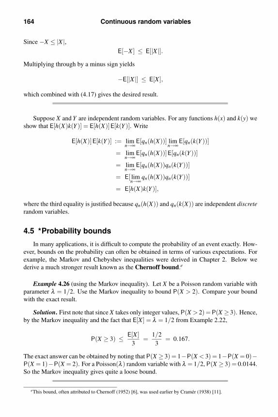
164 Continuous random variables
Since −X ≤ |X |,E[−X ] ≤ E[|X |].
Multiplying through by a minus sign yields
−E[|X |] ≤ E[X ],
which combined with (4.17) gives the desired result.
Suppose X and Y are independent random variables. For any functions h(x) and k(y) we
show that E[h(X)k(Y )] = E[h(X)]E[k(Y )]. Write
E[h(X)]E[k(Y )] := limn→∞
E[qn(h(X))] limn→∞
E[qn(k(Y ))]
= limn→∞
E[qn(h(X))]E[qn(k(Y ))]
= limn→∞
E[qn(h(X))qn(k(Y ))]
= E[ limn→∞
qn(h(X))qn(k(Y ))]
= E[h(X)k(Y )],
where the third equality is justified because qn(h(X)) and qn(k(X)) are independent discrete
random variables.
4.5 Probability bounds
In many applications, it is difficult to compute the probability of an event exactly. How-
ever, bounds on the probability can often be obtained in terms of various expectations. For
example, the Markov and Chebyshev inequalities were derived in Chapter 2. Below we
derive a much stronger result known as the Chernoff bound.e
Example 4.26 (using the Markov inequality). Let X be a Poisson random variable with
parameter λ = 1/2. Use the Markov inequality to bound P(X > 2). Compare your bound
with the exact result.
Solution. First note that since X takes only integer values, P(X > 2) = P(X ≥ 3). Hence,
by the Markov inequality and the fact that E[X ] = λ = 1/2 from Example 2.22,
P(X ≥ 3) ≤ E[X ]
3=
1/2
3= 0.167.
The exact answer can be obtained by noting that P(X ≥ 3) = 1−P(X < 3) = 1−P(X = 0)−P(X = 1)−P(X = 2). For a Poisson(λ ) random variable with λ = 1/2, P(X ≥ 3) = 0.0144.
So the Markov inequality gives quite a loose bound.
eThis bound, often attributed to Chernoff (1952) [6], was used earlier by Cramer (1938) [11].

4.5 Probability bounds 165
Example 4.27 (using the Chebyshev inequality). Let X be a Poisson random variable
with parameter λ = 1/2. Use the Chebyshev inequality to bound P(X > 2). Compare your
bound with the result of using the Markov inequality in Example 4.26.
Solution. Since X is nonnegative, we don’t have to worry about the absolute value signs.
Using the Chebyshev inequality and the fact that E[X2] = λ 2 +λ = 0.75 from Example 2.29,
P(X ≥ 3) ≤ E[X2]
32=
3/4
9≈ 0.0833.
From Example 4.26, the exact probability is 0.0144 and the Markov bound is 0.167.
We now derive the Chernoff bound. As in the derivation of the Markov inequality, there
are two key ideas. First, since every probability can be written as an expectation,
P(X ≥ a) = E[I[a,∞)(X)]. (4.18)
Second, from Figure 4.10, we see that for all x, I[a,∞)(x) (solid line) is less than or equal to
es(x−a) (dashed line) for any s ≥ 0. Taking expectations of
I[a,∞)(X) ≤ es(X−a)
yields
E[I[a,∞)(X)] ≤ E[es(X−a)] = e−saE[esX ] = e−saMX (s).
Combining this with (4.18) yields10
P(X ≥ a) ≤ e−saMX (s). (4.19)
Now observe that this inequality holds for all s ≥ 0, and the left-hand side does not depend
on s. Hence, we can minimize the right-hand side to get as tight a bound as possible. The
Chernoff bound is given by
P(X ≥ a) ≤ mins≥0
[e−saMX (s)
], (4.20)
where the minimum is over all s ≥ 0 for which MX (s) is finite.
a
1
Figure 4.10. Graph showing that I[a,∞)(x) (solid line) is upper bounded by es(x−a) (dashed line) for any positive s.
Note that the inequality I[a,∞)(x) ≤ es(x−a) holds even if s = 0.

166 Continuous random variables
Example 4.28. Let X be a Poisson random variable with parameter λ = 1/2. Bound
P(X > 2) using the Chernoff bound. Compare your result with the exact probability and
with the bound obtained via the Chebyshev inequality in Example 4.27 and with the bound
obtained via the Markov inequality in Example 4.26.
Solution. First recall that MX (s) = GX (es), where GX (z) = exp[λ (z− 1)] was derived
in Example 3.4. Hence,
e−saMX (s) = e−sa exp[λ (es −1)] = exp[λ (es −1)−as].
The desired Chernoff bound when a = 3 is
P(X ≥ 3) ≤ mins≥0
exp[λ (es −1)−3s].
We must now minimize the exponential. Since exp is an increasing function, it suffices to
minimize its argument. Taking the derivative of the argument and setting it equal to zero
requires us to solve λes − 3 = 0. The solution is s = ln(3/λ ). Substituting this value of s
into exp[λ (es −1)−3s] and simplifying the exponent yields
P(X ≥ 3) ≤ exp[3−λ −3ln(3/λ )].
Since λ = 1/2,
P(X ≥ 3) ≤ exp[2.5−3ln6] = 0.0564.
Recall that from Example 4.26, the exact probability is 0.0144 and the Markov inequality
yielded the bound 0.167. From Example 4.27, the Chebyshev inequality yielded the bound
0.0833.
Example 4.29. Let X be a continuous random variable having exponential density with
parameter λ = 1. Compute P(X ≥ 7) and the corresponding Markov, Chebyshev, and Cher-
noff bounds.
Solution. The exact probability is P(X ≥ 7) =∫ ∞
7 e−x dx = e−7 = 0.00091. For the
Markov and Chebyshev inequalities, recall that from Example 4.17, E[X ] = 1/λ and E[X2]= 2/λ 2. For the Chernoff bound, we need MX (s) = λ/(λ − s) for s < λ , which was de-
rived in Example 4.16. Armed with these formulas, we find that the Markov inequality
yields P(X ≥ 7) ≤ E[X ]/7 = 1/7 = 0.143 and the Chebyshev inequality yields P(X ≥ 7) ≤E[X2]/72 = 2/49 = 0.041. For the Chernoff bound, write
P(X ≥ 7) ≤ mins
e−7s/(1− s),
where the minimization is over 0 ≤ s < 1. The derivative of e−7s/(1− s) with respect to s is
e−7s(7s−6)
(1− s)2.
Setting this equal to zero requires that s = 6/7. Hence, the Chernoff bound is
P(X ≥ 7) ≤ e−7s
(1− s)
∣∣∣∣s=6/7
= 7e−6 = 0.017.

Notes 167
For sufficiently large a, the Chernoff bound on P(X ≥ a) is always smaller than the
bound obtained by the Chebyshev inequality, and this is smaller than the one obtained by
the Markov inequality. However, for small a, this may not be the case. See Problem 67 for
an example.
Notes
4.1: Densities and probabilities
Note 1. Strictly speaking, it can only be shown that f in (4.1) is nonnegative almost
everywhere; that is ∫t∈IR: f (t)<0
1dt = 0.
For example, f could be negative at a finite or countably infinite set of points.
Note 2. If U and V are N(0,1), then by Problem 46, U2 and V 2 are each chi-squared
with one degree of freedom (defined in Problem 15). By the Remark following Prob-
lem 55(c), U2 + V 2 is chi-squared with two degrees of freedom, which is the same as
exp(1/2).
Note 3. In the formula gp(x) = xp−1e−x/Γ(p), it is important that Γ(p) be finite; other-
wise gp(x) = 0 for all x and would not be a valid density. We claim that the gamma function
integral is finite for p > 0, but infinite for p ≤ 0. To begin, write
Γ(p) =∫ ∞
0xp−1e−x dx =
∫ 1
0xp−1e−x dx+
∫ ∞
1xp−1e−x dx.
The integral from zero to one is finite for p ≥ 1 since in this case the integrand xp−1e−x is
bounded. However, for p < 1, the factor xp−1 blows up as x approaches zero. Observe that∫ 1
0xp−1e−x dx ≤
∫ 1
0xp−1 dx
and ∫ 1
0xp−1e−x dx ≥ e−1
∫ 1
0xp−1 dx.
Now note that ∫ 1
0xp−1 dx = 1
pxp
∣∣∣∣10
is finite for 0 < p < 1 and infinite for p < 0. For p = 0, the anti-derivative is lnx, and the
integral is again infinite.
It remains to consider the integral from 1 to ∞. For p ≤ 1, this integral is finite because
it is upper bounded by∫ ∞
1 e−x dx < ∞. For p > 1, we use the fact that
ex =∞
∑k=0
xk
k!≥ xn
n!, x ≥ 0, n ≥ 0.

168 Continuous random variables
This implies e−x ≤ n!/xn. Then
xp−1e−x ≤ xp−1n!/xn = n!x(p−1)−n.
Now, for x > 1, if we take n > (p−1)+2, we can write xp−1e−x ≤ n!/x2. Hence,∫ ∞
1xp−1e−x dx ≤
∫ ∞
1n!/x2 dx < ∞.
We now see that of the two integrals making up Γ(p), the second integral is always
finite, but the first one is finite only for p > 0. Hence, the sum of the two integrals is finite
if and only if p > 0.
4.2: Expectation of a single random variable
Note 4. Integration by parts. The formula for integration by parts is∫ b
audv = uv
∣∣ba−∫ b
avdu.
This is shorthand for ∫ b
au(t)v′(t)dt = u(t)v(t)
∣∣ba−∫ b
av(t)u′(t)dt.
It is obtained by integrating the derivative of the product u(t)v(t) and rearranging the result.
If we integrate the formula
d
dtu(t)v(t) = u′(t)v(t)+u(t)v′(t),
we get
u(t)v(t)∣∣ba
=∫ b
a
d
dt
[u(t)v(t)
]dt =
∫ b
au′(t)v(t)dt +
∫ b
au(t)v′(t)dt.
Rearranging yields the integration-by-parts formula.
To apply this formula, you need to break the integrand into two factors, where you know
the anti-derivative of one of them. The other factor you can almost always differentiate. For
example, to integrate tne−t , take u(t) = tn and v′(t) = e−t , since you know that the anti-
derivative of e−t is v(t) = −e−t .
Another useful example in this book is tne−t2/2, where n ≥ 1. Although there is no
closed-form anti-derivative of e−t2/2, observe that
d
dte−t2/2 = −te−t2/2.
In other words, the anti-derivative of te−t2/2 is −e−t2/2. This means that to integrate
tne−t2/2, first write it as tn−1 · te−t2/2. Then take u(t) = tn−1 and v′(t) = te−t2/2 and use
v(t) = −e−t2/2.
Notes 169
Note 5. Since qn in Figure 4.9 is defined only for x ≥ 0, the definition of expectation in
the text applies only to arbitrary nonnegative random variables. However, for signed random
variables,
X =|X |+X
2− |X |−X
2,
and we define
E[X ] := E
[ |X |+X
2
]−E
[ |X |−X
2
],
assuming the difference is not of the form ∞−∞. Otherwise, we say E[X ] is undefined.
We also point out that for x ≥ 0, qn(x) → x. To see this, fix any x ≥ 0, and let n > x.
Then x will lie under one of the steps in Figure 4.9. If x lies under the kth step, then
k−1
2n≤ x <
k
2n,
For x in this range, the value of qn(x) is (k−1)/2n. Hence, 0 ≤ x−qn(x) < 1/2n.
Another important fact to note is that for each x ≥ 0, qn(x) ≤ qn+1(x). Hence, qn(X) ≤qn+1(X), and so E[qn(X)] ≤ E[qn+1(X)] as well. In other words, the sequence of real num-
bers E[qn(X)] is nondecreasing. This implies that limn→∞ E[qn(X)] exists either as a finite
real number or the extended real number ∞ [51, p. 55].
Note 6. In light of the preceding note, we are using Lebesgue’s monotone convergence
theorem [3, p. 208], which applies to nonnegative functions.
4.3: Transform methods
Note 7. If s were complex, we could interpret∫ ∞−∞ e−(x−s)2/2 dx as a contour integral in
the complex plane. By appealing to the Cauchy–Goursat theorem [9, pp. 115–121], one
could then show that this integral is equal to∫ ∞−∞ e−t2/2 dt =
√2π . Alternatively, one can
use a permanence of form argument [9, pp. 286–287]. In this approach, one shows that
MX (s) is analytic in some region, in this case the whole complex plane. One then obtains a
formula for MX (s) on a contour in this region, in this case, the contour is the entire real axis.
The permanence of form theorem then states that the formula is valid in the entire region.
Note 8. Problem 44(a) only shows that MX (s) = 1/(1− s)p for real s with s < 1. How-
ever, since MX (s) is analytic for complex s with Res < 1, the permanence of form argument
mentioned in Note 7 shows that MX (s) = 1/(1− s)p holds all such s. In particular, the
formula holds for s = jν , since in this case, Res = 0 < 1.
4.4: Expectation of multiple random variables
Note 9. We show that if X and Y are independent with densities fX and fY , then the
density of Z := X +Y is given by the convolution of fX and fY . We have from (4.15) that
the characteristic functions of X , Y , and Z satisfy ϕZ(ν) = ϕX (ν)ϕY (ν). Now write
fZ(z) =1
2π
∫ ∞
−∞e− jνzϕZ(ν)dν

170 Continuous random variables
=1
2π
∫ ∞
−∞e− jνzϕX (ν)ϕY (ν)dν
=1
2π
∫ ∞
−∞e− jνzϕX (ν)
[∫ ∞
−∞e jνy fY (y)dy
]dν
=∫ ∞
−∞
[1
2π
∫ ∞
−∞e− jν(z−y)ϕX (ν)dν
]fY (y)dy
=∫ ∞
−∞fX (z− y) fY (y)dy.
4.5: Probability bounds
Note 10. We note that (4.19) follows directly from the Markov inequality. Observe that
for s > 0,
X ≥ a = sX ≥ sa = esX ≥ esa.Hence,
P(X ≥ a) = P(esX ≥ esa) ≤ E[esX ]
esa= e−saMX (s),
which is exactly (4.19). The reason for using the derivation in the text is to emphasize the
idea of bounding I[a,∞)(x) by different functions of x. For (2.19), we used (x/a)r for x ≥ 0.
For (4.19), we used es(x−a) for all x.
Problems
4.1: Densities and probabilities
1. A certain burglar alarm goes off if its input voltage exceeds 5 V at three consecutive
sampling times. If the voltage samples are independent and uniformly distributed on
[0,7], find the probability that the alarm sounds.
2. Let X have the Pareto density
f (x) =
2/x3, x > 1,
0, otherwise,
The median of X is the number t satisfying P(X > t) = 1/2. Find the median of X .
3. Let X have density
f (x) =
cx−1/2, 0 < x ≤ 1,
0, otherwise,
shown in Figure 4.11. Find the constant c and the median of X .
4. Let X have an exp(λ ) density.
(a) Show that P(X > t) = e−λ t for t ≥ 0.
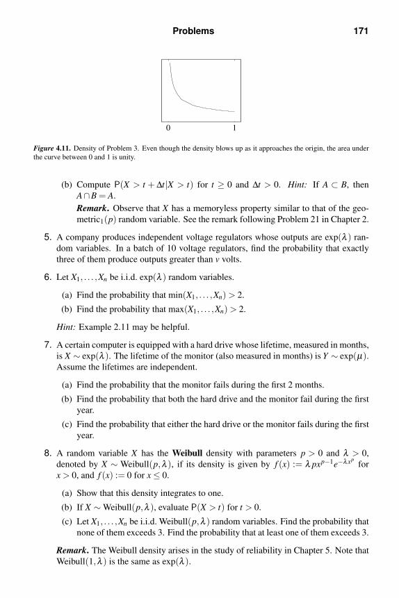
Problems 171
0 1
Figure 4.11. Density of Problem 3. Even though the density blows up as it approaches the origin, the area under
the curve between 0 and 1 is unity.
(b) Compute P(X > t + ∆t|X > t) for t ≥ 0 and ∆t > 0. Hint: If A ⊂ B, then
A∩B = A.
Remark. Observe that X has a memoryless property similar to that of the geo-
metric1(p) random variable. See the remark following Problem 21 in Chapter 2.
5. A company produces independent voltage regulators whose outputs are exp(λ ) ran-
dom variables. In a batch of 10 voltage regulators, find the probability that exactly
three of them produce outputs greater than v volts.
6. Let X1, . . . ,Xn be i.i.d. exp(λ ) random variables.
(a) Find the probability that min(X1, . . . ,Xn) > 2.
(b) Find the probability that max(X1, . . . ,Xn) > 2.
Hint: Example 2.11 may be helpful.
7. A certain computer is equipped with a hard drive whose lifetime, measured in months,
is X ∼ exp(λ ). The lifetime of the monitor (also measured in months) is Y ∼ exp(µ).Assume the lifetimes are independent.
(a) Find the probability that the monitor fails during the first 2 months.
(b) Find the probability that both the hard drive and the monitor fail during the first
year.
(c) Find the probability that either the hard drive or the monitor fails during the first
year.
8. A random variable X has the Weibull density with parameters p > 0 and λ > 0,
denoted by X ∼ Weibull(p,λ ), if its density is given by f (x) := λ pxp−1e−λxpfor
x > 0, and f (x) := 0 for x ≤ 0.
(a) Show that this density integrates to one.
(b) If X ∼ Weibull(p,λ ), evaluate P(X > t) for t > 0.
(c) Let X1, . . . ,Xn be i.i.d. Weibull(p,λ ) random variables. Find the probability that
none of them exceeds 3. Find the probability that at least one of them exceeds 3.
Remark. The Weibull density arises in the study of reliability in Chapter 5. Note that
Weibull(1,λ ) is the same as exp(λ ).

172 Continuous random variables
9. The standard normal density f ∼ N(0,1) is given by f (x) := e−x2/2/√
2π . The fol-
lowing steps provide a mathematical proof that the normal density is indeed “bell-
shaped” as shown in Figure 4.3.
(a) Use the derivative of f to show that f is decreasing for x > 0 and increasing for
x < 0. (It then follows that f has a global maximum at x = 0.)
(b) Show that f is concave for |x| < 1 and convex for |x| > 1. Hint: Show that the
second derivative of f is negative for |x| < 1 and positive for |x| > 1.
(c) Since ez = ∑∞n=0 zn/n!, for positive z, ez ≥ z. Hence, e+x2/2 ≥ x2/2. Use this fact
to show that e−x2/2 → 0 as |x| → ∞.
10. Use the results of parts (a) and (b) of the preceding problem to obtain the corre-
sponding results for the general normal density f ∼ N(m,σ2). Hint: Let ϕ(t) :=
e−t2/2/√
2π denote the N(0,1) density, and observe that f (x) = ϕ((x−m)/σ)/σ .
11. As in the preceding problem, let f ∼ N(m,σ2). Keeping in mind that f (x) depends
on σ > 0, show that limσ→∞ f (x) = 0. Using the result of part (c) of Problem 9, show
that for x = m, limσ→0 f (x) = 0, whereas for x = m, limσ→0 f (x) = ∞.
12. For n = 1,2, . . . , let fn(x) be a probability density function, and let pn be a sequence
of nonnegative numbers summing to one; i.e., a probability mass function.
(a) Show that
f (x) := ∑n
pn fn(x)
is a probability density function. When f has this form, it is called a mixture
density.
Remark. When the fn(x) are chi-squared densities and the pn are appropriate
Poisson probabilities, the resulting mixture f is called a noncentral chi-squared
density. See Problem 65 for details.
(b) If f1 ∼ uniform[0,1] and f2 ∼ uniform[2,3], sketch the mixture density
f (x) = 0.25 f1(x)+0.75 f2(x).
(c) If f1 ∼ uniform[0,2] and f2 ∼ uniform[1,3], sketch the mixture density
f (x) = 0.5 f1(x)+0.5 f2(x).
13. If g and h are probability densities, show that their convolution,
(g∗h)(x) :=∫ ∞
−∞g(y)h(x− y)dy,
is also a probability density; i.e., show that (g ∗ h)(x) is nonnegative and when inte-
grated with respect to x yields one.
Problems 173
14. The gamma density with parameter p > 0 is given by
gp(x) :=
⎧⎨⎩xp−1 e−x
Γ(p), x > 0,
0, x ≤ 0,
where Γ(p) is the gamma function,
Γ(p) :=∫ ∞
0xp−1 e−x dx, p > 0.
In other words, the gamma function is defined exactly so that the gamma density
integrates to one. Note that the gamma density is a generalization of the exponential
since g1 is the exp(1) density. Sketches of gp for several values of p were shown in
Figure 4.7.
Remark. In MATLAB, Γ(p) = gamma(p).
(a) Use integration by parts as in Example 4.9 to show that
Γ(p) = (p−1) ·Γ(p−1), p > 1.
Since Γ(1) can be directly evaluated and is equal to one, it follows that
Γ(n) = (n−1)!, n = 1,2, . . . .
Thus Γ is sometimes called the factorial function.
(b) Show that Γ(1/2) =√
π as follows. In the defining integral, use the change
of variable y =√
2x. Write the result in terms of the standard normal density,
which integrates to one, in order to obtain the answer by inspection.
(c) Show that
Γ(
2n+1
2
)=
(2n−1) · · ·5 ·3 ·12n
√π =
(2n−1)!!
2n
√π, n ≥ 1.
(d) Show that (gp ∗gq)(x) = gp+q(x). Hints: First show that for x > 0,
(gp ∗gq)(x) =
∫ x
0gp(y)gq(x− y)dy
=xp+q−1e−x
Γ(p)Γ(q)
∫ 1
0θ p−1(1−θ)q−1dθ . (4.21)
Now integrate this equation with respect to x; use the definition of the gamma
function and the result of Problem 13.
Remark. The integral definition of Γ(p) makes sense only for p > 0. However, the
recursion Γ(p) = (p− 1)Γ(p− 1) suggests a simple way to define Γ for negative,
noninteger arguments. For 0 < ε < 1, the right-hand side of Γ(ε) = (ε −1)Γ(ε −1)is undefined. However, we rearrange this equation and make the definition,
Γ(ε −1) := − Γ(ε)
1− ε.

174 Continuous random variables
Similarly writing Γ(ε −1) = (ε −2)Γ(ε −2), and so on, leads to
Γ(ε −n) =(−1)nΓ(ε)
(n− ε) · · ·(2− ε)(1− ε).
Note also that
Γ(n+1− ε) = (n− ε)Γ(n− ε)
= (n− ε) · · ·(1− ε)Γ(1− ε).
Hence,
Γ(ε −n) =(−1)nΓ(ε)Γ(1− ε)
Γ(n+1− ε).
15. Important generalizations of the gamma density gp of the preceding problem arise if
we include a scale parameter. For λ > 0, put
gp,λ (x) := λ gp(λx) = λ(λx)p−1e−λx
Γ(p), x > 0.
We write X ∼ gamma(p,λ ) if X has density gp,λ , which is called the gamma density
with parameters p and λ .
(a) Let f be any probability density. For λ > 0, show that
fλ (x) := λ f (λx)
is also a probability density.
(b) For p = m a positive integer, gm,λ is called the Erlang density with parameters
m and λ . We write X ∼ Erlang(m,λ ) if X has density
gm,λ (x) = λ(λx)m−1 e−λx
(m−1)!, x > 0.
What kind of density is g1,λ (x)?
(c) If X ∼ Erlang(m,λ ), show that
P(X > t) =m−1
∑k=0
(λ t)k
k!e−λ t , t ≥ 0.
In other words, if Y ∼ Poisson(λ t), then P(X > t) = P(Y < m). Hint: Use
repeated integration by parts.
(d) For p = k/2 and λ = 1/2, gk/2,1/2 is called the chi-squared density with k
degrees of freedom. It is not required that k be an integer. Of course, the chi-
squared density with an even number of degrees of freedom, say k = 2m, is the
same as the Erlang(m,1/2) density. Using Problem 14(b), it is also clear that
for k = 1,
g1/2,1/2(x) =e−x/2
√2πx
, x > 0.

Problems 175
For an odd number of degrees of freedom, say k = 2m+1, where m ≥ 1, show
that
g 2m+12 , 1
2(x) =
xm−1/2e−x/2
(2m−1) · · ·5 ·3 ·1√2πfor x > 0. Hint: Use Problem 14(c).
16. The beta density with parameters p > 0 and q > 0 is defined by
bp,q(x) :=Γ(p+q)
Γ(p)Γ(q)xp−1(1− x)q−1, 0 < x < 1,
where Γ is the gamma function defined in Problem 14. We note that if X ∼ gamma(p,λ ) and Y ∼ gamma(q,λ ) are independent random variables, then X/(X +Y ) has the
beta density with parameters p and q (Problem 42 in Chapter 7).
(a) Find simplified formulas and sketch the beta density for the following sets of
parameter values: (i) p = 1, q = 1. (ii) p = 2, q = 2. (iii) p = 1/2, q = 1.
(b) Use the result of Problem 14(d), including equation (4.21), to show that the beta
density integrates to one.
Remark. The fact that the beta density integrates to one can be rewritten as
Γ(p)Γ(q) = Γ(p+q)∫ 1
0up−1(1−u)q−1 du. (4.22)
This integral, which is a function of p and q, is usually called the beta function, and
is denoted by B(p,q). Thus,
B(p,q) =Γ(p)Γ(q)
Γ(p+q), (4.23)
and
bp,q(x) =xp−1(1− x)q−1
B(p,q), 0 < x < 1.
17. Use equation (4.22) in the preceding problem to show that Γ(1/2) =√
π . Hint: Make
the change of variable u = sin2 θ . Then take p = q = 1/2.
Remark. In Problem 14(b), you used the fact that the normal density integrates to one
to show that Γ(1/2) =√
π . Since your derivation there is reversible, it follows that
the normal density integrates to one if and only if Γ(1/2) =√
π . In this problem, you
used the fact that the beta density integrates to one to show that Γ(1/2) =√
π . Thus,
you have an alternative derivation of the fact that the normal density integrates to one.
18. Show that ∫ π/2
0sinn θ dθ =
Γ(
n+1
2
)√π
2Γ(
n+2
2
) .
Hint: Use equation (4.22) in Problem 16 with p = (n+1)/2 and q = 1/2, and make
the substitution u = sin2 θ .

176 Continuous random variables
19. The beta function B(p,q) is defined as the integral in (4.22) in Problem 16. Show that
B(p,q) =
∫ ∞
0(1− e−θ )p−1e−qθ dθ .
20. Student’s t density with ν degrees of freedom is given by
fν(x) :=
(1+ x2
ν
)−(ν+1)/2
√νB( 1
2, ν
2)
, −∞ < x < ∞,
where B is the beta function. Show that fν integrates to one. Hint: The change of
variable eθ = 1+ x2/ν may be useful. Also, the result of the preceding problem may
be useful.
Remark. (i) Note that f1 ∼ Cauchy(1).
(ii) It is shown in Problem 44 in Chapter 7 that if X and Y are independent with X ∼N(0,1) and Y chi-squared with k degrees of freedom, then X/
√Y/k has Student’s t
density with k degrees of freedom, a result of crucial importance in the study of
confidence intervals.
(iii) This density was reported by William Sealey Gosset in the journal paper,
Student, “The probable error of a mean,” Biometrika, vol. VI, no. 1, pp. 1–
25, Mar. 1908.
Gosset obtained his results from statistical studies at the Guinness brewery in Dublin.
He used a pseudonym because Guinness did not allow employees to publish.
21. As illustrated in Figure 4.12, Student’s t density fν(x) defined in Problem 20 con-
verges to the standard normal density as ν → ∞. In this problem you will demonstrate
this mathematically.
(a) Stirling’s formula says that Γ(x) ≈ √2π xx−1/2e−x. Use Stirling’s formula to
show that
Γ(
1+ν2
)√
ν Γ(
ν2
) ≈ 1√2.
(b) Use the fact that (1+ξ/n)n → eξ to show that(1+
x2
ν
)(ν+1)/2
→ ex2/2.
Then combine this with part (a) to show that fν(x) → e−x2/2/√
2π .
22. For p and q positive, let B(p,q) denote the beta function defined by the integral in
(4.22) in Problem 16. Show that
fZ(z) :=1
B(p,q)· zp−1
(1+ z)p+q, z > 0,
is a valid density (i.e., integrates to one) on (0,∞). Hint: Make the change of variable
t = 1/(1+ z).
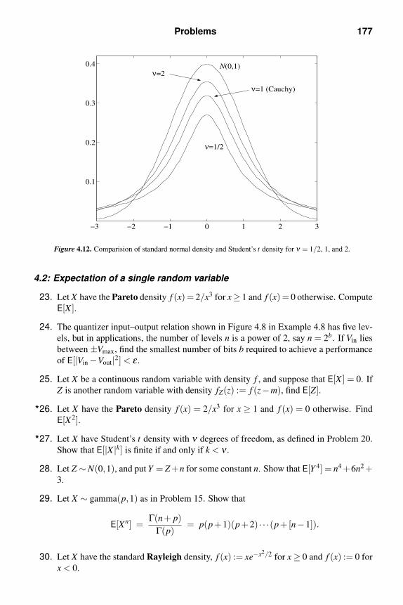
Problems 177
−3 −2 −1 0 1 2 3
0.1
0.2
0.3
0.4
ν=1/2
ν=1 (Cauchy)
ν=2N(0,1)
Figure 4.12. Comparision of standard normal density and Student’s t density for ν = 1/2, 1, and 2.
4.2: Expectation of a single random variable
23. Let X have the Pareto density f (x) = 2/x3 for x≥ 1 and f (x) = 0 otherwise. Compute
E[X ].
24. The quantizer input–output relation shown in Figure 4.8 in Example 4.8 has five lev-
els, but in applications, the number of levels n is a power of 2, say n = 2b. If Vin lies
between ±Vmax, find the smallest number of bits b required to achieve a performance
of E[|Vin −Vout|2] < ε .
25. Let X be a continuous random variable with density f , and suppose that E[X ] = 0. If
Z is another random variable with density fZ(z) := f (z−m), find E[Z].
26. Let X have the Pareto density f (x) = 2/x3 for x ≥ 1 and f (x) = 0 otherwise. Find
E[X2].
27. Let X have Student’s t density with ν degrees of freedom, as defined in Problem 20.
Show that E[|X |k] is finite if and only if k < ν .
28. Let Z ∼N(0,1), and put Y = Z +n for some constant n. Show that E[Y 4] = n4 +6n2 +3.
29. Let X ∼ gamma(p,1) as in Problem 15. Show that
E[Xn] =Γ(n+ p)
Γ(p)= p(p+1)(p+2) · · ·(p+[n−1]).
30. Let X have the standard Rayleigh density, f (x) := xe−x2/2 for x ≥ 0 and f (x) := 0 for
x < 0.

178 Continuous random variables
(a) Show that E[X ] =√
π/2.
(b) For n ≥ 2, show that E[Xn] = 2n/2Γ(1+n/2).
31. Consider an Internet router with n input links. Assume that the flows in the links are
independent standard Rayleigh random variables as defined in the preceding problem.
Suppose that the router’s buffer overflows if more than two links have flows greater
than β . Find the probability of buffer overflow.
32. Let X ∼ Weibull(p,λ ) as in Problem 8. Show that E[Xn] = Γ(1+n/p)/λ n/p.
33. A certain nonlinear circuit has random input X ∼ exp(1), and output Y = X1/4. Find
the second moment of the output.
34. High-Mileage Cars has just begun producing its new Lambda Series, which aver-
ages µ miles per gallon. Al’s Excellent Autos has a limited supply of n cars on its
lot. Actual mileage of the ith car is given by an exponential random variable Xi with
E[Xi] = µ . Assume actual mileages of different cars are independent. Find the prob-
ability that at least one car on Al’s lot gets less than µ/2 miles per gallon.
35. A small airline makes five flights a day from Chicago to Denver. The number of
passengers on each flight is approximated by an exponential random variable with
mean 20. A flight makes money if it has more than 25 passengers. Find the probability
that at least one flight a day makes money. Assume that the numbers of passengers
on different flights are independent.
36. The differential entropy of a continuous random variable X with density f is
h(X) := E[− log f (X)] =∫ ∞
−∞f (x) log
1
f (x)dx.
If X ∼ uniform[0,2], find h(X). Repeat for X ∼ uniform[0, 12] and for X ∼ N(m,σ2).
37. Let X have Student’s t density with ν degrees of freedom, as defined in Problem 20.
For n a positive integer less than ν/2, show that
E[X2n] = νn Γ(
2n+12
)Γ( ν−2n
2
)Γ(
12
)Γ( ν
2
) .
4.3: Transform methods
38. Let X have moment generating function MX (s) = eσ2s2/2. Use formula (4.8) to find
E[X2].
39. Recall that the moment generating function of an N(0,1) random variable es2/2. Use
this fact to find the moment generating function of an N(m,σ2) random variable.
40. If X ∼ uniform(0,1), show that Y = ln(1/X) ∼ exp(1) by finding its moment gener-
ating function for s < 1.

Problems 179
41. Find a closed-form expression for MX (s) if X ∼ Laplace(λ ). Use your result to find
var(X).
42. Let X have the Pareto density f (x) = 2/x3 for x ≥ 1 and f (x) = 0 otherwise. For
what real values of s is MX (s) finite? Hint: It is not necessary to evaluate MX (s) to
answer the question.
43. Let Mp(s) denote the moment generating function of the gamma density gp defined
in Problem 14. Show that
Mp(s) =1
1− sMp−1(s), p > 1.
Remark. Since g1(x) is the exp(1) density, and M1(s) = 1/(1− s) by direct calcula-
tion, it now follows that the moment generating function of an Erlang(m,1) random
variable is 1/(1− s)m.
44. Let X have the gamma density gp given in Problem 14.
(a) For real s < 1, show that MX (s) = 1/(1− s)p.
(b) The moments of X are given in Problem 29. Hence, from (4.10), we have for
complex s,
MX (s) =∞
∑n=0
sn
n!· Γ(n+ p)
Γ(p), |s| < 1.
For complex s with |s| < 1, derive the Taylor series for 1/(1− s)p and show
that it is equal to the above series. Thus, MX (s) = 1/(1− s)p for all complex s
with |s| < 1. (This formula actually holds for all complex s with Res < 1; see
Note 8.)
45. As shown in the preceding problem, the basic gamma density with parameter p, gp(x),has moment generating function 1/(1−s)p. The more general gamma density defined
by gp,λ (x) := λgp(λx) is given in Problem 15.
(a) Find the moment generating function and then the characteristic function of
gp,λ (x).
(b) Use the answer to (a) to find the moment generating function and the character-
istic function of the Erlang density with parameters m and λ , gm,λ (x).
(c) Use the answer to (a) to find the moment generating function and the character-
istic function of the chi-squared density with k degrees of freedom, gk/2,1/2(x).
46. Let X ∼ N(0,1), and put Y = X2. For real values of s < 1/2, show that
MY (s) =
(1
1−2s
)1/2
.
By Problem 45(c), it follows that Y is chi-squared with one degree of freedom.

180 Continuous random variables
47. Let X ∼ N(m,1), and put Y = X2. For real values of s < 1/2, show that
MY (s) =esm2/(1−2s)
√1−2s
.
Remark. For m = 0, Y is said to be noncentral chi-squared with one degree of
freedom and noncentrality parameter m2. For m = 0, this reduces to the result of
the previous problem.
48. Let X have characteristic function ϕX (ν). If Y := aX +b for constants a and b, express
the characteristic function of Y in terms of a,b, and ϕX .
49. Apply the Fourier inversion formula to ϕX (ν) = e−λ |ν | to verify that this is the char-
acteristic function of a Cauchy(λ ) random variable.
50. Use the following approach to find the characteristic function of the N(0,1) density
[62, pp. 138–139]. Let f (x) := e−x2/2/√
2π .
(a) Show that f ′(x) = −x f (x).
(b) Starting with ϕX (ν) =∫ ∞−∞ e jνx f (x)dx, compute ϕ ′
X (ν). Then use part (a) to
show that ϕ ′X (ν) = − j
∫ ∞−∞ e jνx f ′(x)dx.
(c) Using integration by parts, show that this last integral is − jνϕX (ν).
(d) Show that ϕ ′X (ν) = −νϕX (ν).
(e) Show that K(ν) := ϕX (ν)eν2/2 satisfies K′(ν) = 0.
(f) Show that K(ν) = 1 for all ν . (It then follows that ϕX (ν) = e−ν2/2.)
51. Use the method of Problem 50 to find the characteristic function of the gamma density
gp(x) = xp−1e−x/Γ(p), x > 0. Hints: Show that (d/dx)xgp(x) = (p− x)gp(x). Use
integration by parts to show that ϕ ′X (ν) = −(p/ν)ϕX (ν)+(1/ jν)ϕ ′
X (ν). Show that
K(ν) := ϕX (ν)(1− jν)p satisfies K′(ν) = 0.
4.4: Expectation of multiple random variables
52. Let Z := X +Y , where X and Y are independent with X ∼ exp(1) and Y ∼ Laplace(1).Find cov(X ,Z) and var(Z).
53. Find var(Z) for the random variable Z of Example 4.22.
54. Let X and Y be independent random variables with moment generating functions
MX (s) and MY (s). If Z := X −Y , show that MZ(s) = MX (s)MY (−s). Show that if
both X and Y are exp(λ ), then Z ∼ Laplace(λ ).
55. Let X1, . . . ,Xn be independent, and put Yn := X1 + · · ·+Xn.
(a) If Xi ∼ N(mi,σ2i ), show that Yn ∼ N(m,σ2), and identify m and σ2. In other
words, “The sum of independent Gaussian random variables is Gaussian.”
(b) If Xi ∼ Cauchy(λi), show that Yn ∼ Cauchy(λ ), and identify λ . In other words,
“The sum of independent Cauchy random variables is Cauchy.”
Problems 181
(c) If Xi is a gamma random variable with parameters pi and λ (same λ for all i),
show that Yn is gamma with parameters p and λ , and identify p. In other words,
“The sum of independent gamma random variables (with the same scale factor)
is gamma (with the same scale factor).”
Remark. Note the following special cases of this result. If all the pi = 1, then
the Xi are exponential with parameter λ , and Yn is Erlang with parameters n and
λ . If p = 1/2 and λ = 1/2, then Xi is chi-squared with one degree of freedom,
and Yn is chi-squared with n degrees of freedom.
56. Let X1, . . . ,Xr be i.i.d. gamma random variables with parameters p and λ . Let Y =X1 + · · ·+Xr. Find E[Y n].
57. Packet transmission times on a certain network link are i.i.d. with an exponential
density of parameter λ . Suppose n packets are transmitted. Find the density of the
time to transmit n packets.
58. The random number generator on a computer produces i.i.d. uniform(0,1) random
variables X1, . . . ,Xn. Find the probability density of
Y = ln
(n
∏i=1
1
Xi
).
59. Let X1, . . . ,Xn be i.i.d. Cauchy(λ ). Find the density of Y := β1X1 + · · ·+βnXn, where
the βi are given positive constants.
60. Two particles arrive at a detector at random, independent positions X and Y lying on
a straight line. The particles are resolvable if the absolute difference in their positions
is greater than two. Find the probability that the two particles are not resolvable if X
and Y are both Cauchy(1) random variables. Give a numerical answer.
61. Three independent pressure sensors produce output voltages U , V , and W , each
exp(λ ) random variables. The three voltages are summed and fed into an alarm that
sounds if the sum is greater than x volts. Find the probability that the alarm sounds.
62. A certain electric power substation has n power lines. The line loads are independent
Cauchy(λ ) random variables. The substation automatically shuts down if the total
load is greater than . Find the probability of automatic shutdown.
63. The new outpost on Mars extracts water from the surrounding soil. There are 13
extractors. Each extractor produces water with a random efficiency that is uniformly
distributed on [0,1]. The outpost operates normally if fewer than three extractors
produce water with efficiency less than 0.25. If the efficiencies are independent, find
the probability that the outpost operates normally.
64. The time to send an Internet packet is a chi-squared random variable T with one
degree of freedom. The time to receive the acknowledgment A is also chi-squared
with one degree of freedom. If T and A are independent, find the probability that the
round trip time R := T +A is more than r.

182 Continuous random variables
65. In this problem we generalize the noncentral chi-squared density of Problem 47.
To distinguish these new densities from the original chi-squared densities defined in
Problem 15, we refer to the original ones as central chi-squared densities. The non-
central chi-squared density with k degrees of freedom and noncentrality parameter
λ 2 is defined by f
ck,λ 2(x) :=∞
∑n=0
(λ 2/2)ne−λ 2/2
n!c2n+k(x), x > 0,
where c2n+k denotes the central chi-squared density with 2n + k degrees of freedom.
Hence, ck,λ 2(x) is a mixture density (Problem 12) with pn = (λ 2/2)ne−λ 2/2/n! being
a Poisson(λ 2/2) pmf.
(a) Show that∫ ∞
0 ck,λ 2(x)dx = 1.
(b) If X is a noncentral chi-squared random variable with k degrees of freedom and
noncentrality parameter λ 2, show that X has moment generating function
Mk,λ 2(s) =exp[sλ 2/(1−2s)]
(1−2s)k/2.
Hint: Problem 45 may be helpful.
Remark. When k = 1, this agrees with Problem 47.
(c) Use part (b) to show that if X ∼ ck,λ 2 , then E[X ] = k +λ 2.
(d) Let X1, . . . ,Xn be independent random variables with Xi ∼ cki,λ 2i. Show that
Y := X1 + · · ·+Xn has the ck,λ 2 density, and identify k and λ 2.
Remark. By part (b), if each ki = 1, we could assume that each Xi is the square
of an N(λi,1) random variable.
(e) Show that
e−(x+λ 2)/2
√2πx
· eλ√
x + e−λ√
x
2= c1,λ 2(x).
(Note that if λ = 0, the left-hand side reduces to the central chi-squared density
with one degree of freedom.) Hint: Use the power series eξ = ∑∞n=0 ξ n/n! for
the two exponentials involving√
x.
4.5: Probability bounds
66. Let X have the Pareto density f (x) = 2/x3 for x ≥ 1 and f (x) = 0 otherwise. For
a ≥ 1, compare P(X ≥ a) and the bound obtained via Markov inequality.
67. Let X be an exponential random variable with parameter λ = 1. Compute the Markov
inequality, the Chebyshev inequality, and the Chernoff bound to obtain bounds on
P(X ≥ a) as a function of a. Also compute P(X ≥ a).
fA closed-form expression is derived in Problem 25 of Chapter 5.

Exam preparation 183
(a) For what values of a is the Markov inequality smaller than the Chebyshev in-
equality?
(b) MATLAB. Plot the Markov bound, the Chebyshev bound, the Chernoff bound,
and P(X ≥ a) for 0 ≤ a ≤ 6 on the same graph. For what range of a is the
Markov bound the smallest? the Chebyshev? Now use MATLAB command
semilogy to draw the same four curves for 6 ≤ a ≤ 20. Which bound is the
smallest?
Exam preparation
You may use the following suggestions to prepare a study sheet, including formulas men-
tioned that you have trouble remembering. You may also want to ask your instructor for
additional suggestions.
4.1. Densities and probabilities. Know how to compute probabilities involving a random
variable with a density (4.1). A list of the more common densities can be found inside
the back cover. Remember, density functions can never be negative and must integrate
to one.
4.2. Expectation. LOTUS (4.3), especially for computing moments. The table inside the
back cover contains moments of many of the more common densities.
4.3. Transform methods. Moment generating function definition (4.7) and moment for-
mula (4.8). For continuous random variables, the mgf is essentially the Laplace trans-
form of the density. Characteristic function definition (4.11) and moment formula
(4.14). For continuous random variables, the density can be recovered with the in-
verse Fourier transform (4.12). For integer-valued random variables, the pmf can be
recovered with the formula for Fourier series coefficients (4.13). The table inside the
back cover contains the mgf (or characteristic function) of many of the more common
densities. Remember that ϕX (ν) = MX (s)|s= jν .
4.4. Expectation of multiple random variables. If X and Y are independent, then we
have E[h(X)k(Y )] = E[h(X)]E[k(Y )] for any functions h(x) and k(y). If X1, . . . ,Xn
are independent random variables, then the moment generating function of the sum
is the product of the moment generating functions, e.g., Example 4.23. If the Xi are
continuous random variables, then the density of their sum is the convolution of their
densities, e.g., (4.16).
4.5. Probability bounds. The Markov inequality (2.18) and the Chebyshev inequality
(2.21) were derived in Section 2.4. The Chernoff bound (4.20).
Work any review problems assigned by your instructor. If you finish them, re-work your
homework assignments.
5
Cumulative distribution functions and their
applications
In this chapter we introduce the cumulative distribution function (cdf) of a random
variable X . The cdf is defined bya
FX (x) := P(X ≤ x).
As we shall see, knowing the cdf is equivalent to knowing the density or pmf of a random
variable. By this we mean that if you know the cdf, then you can find the density or pmf,
and if you know the density or pmf, then you can find the cdf. This is the same sense
in which knowing the characteristic function is equivalent to knowing the density or pmf.
Similarly, just as some problems are more easily solved using characteristic functions in-
stead of densities, there are some problems that are more easily solved using cdfs instead of
densities.
This chapter emphasizes three applications in which cdfs figure prominently: (i) Finding
the probability density of Y = g(X) when the function g and the density of X are given; (ii)The central limit theorem; and (iii) Reliability.
The first application concerns what happens when the input of a system g is modeled as
a random variable. The system output Y = g(X) is another random variable, and we would
like to compute probabilities involving Y . For example, g could be an amplifier, and we
might need to find the probability that the output exceeds some danger level. If we knew
the probability mass function or the density of Y , we would know what to do next. It turns
out that we can easily find the probability mass function or density of Y if we know its cdf,
FY (y) = P(Y ≤ y), for all y. Section 5.1 focuses on the problem Y = g(X) when X has a
density and g is a fairly simple function to analyze. We note that Example 5.9 motivates a
discussion of the maximum a posteriori probability (MAP) and maximum likelihood (ML)
rules for detecting discrete signals in continuous noise. We also show how to simulate
a continuous random variable by applying the inverse cdf to a uniform random variable.
Section 5.2 introduces cdfs of discrete random variables. It is also shown how to simulate a
discrete random variable as a function of a uniform random variable. Section 5.3 introduces
cdfs of mixed random variables. Mixed random variables frequently appear in the form
Y = g(X) when X is continuous, but g has “flat spots.” For example, most amplifiers have a
linear region, say −v ≤ x ≤ v, wherein g(x) = αx. However, if x > v, then g(x) = αv, and
if x < −v, then g(x) = −αv. If a continuous random variable is applied to such a device,
the output will be a mixed random variable, which can be thought of as a random variable
whose “generalized density” contains Dirac impulses. The problem of finding the cdf and
generalized density of Y = g(X) is studied in Section 5.4. At this point, having seen several
aAs we have defined it, the cdf is a right-continuous function of x (see Section 5.5). However, we alert the
reader that some texts put FX (x) = P(X < x), which is left-continuous in x.
184

5.1 Continuous random variables 185
generalized densities and their corresponding cdfs, Section 5.5 summarizes and derives the
general properties that characterize arbitrary cdfs.
Section 5.6 contains our second application of cdfs, the central limit theorem. (This
section can be covered immediately after Section 5.1 if desired.) Although we have seen
many examples for which we can explicitly write down probabilities involving a sum of i.i.d.
random variables, in general, the problem is quite hard. The central limit theorem provides
an approximation of probabilities involving the sum of i.i.d. random variables — even when
the density of the individual random variables is unknown! This is crucial in parameter-
estimation problems where we need to compute confidence intervals as in Chapter 6.
Section 5.7 contains our third application of cdfs. This section, which is a brief diversion
into reliability theory, can be covered immediately after Section 5.1 if desired. With the
exception of the formula
E[T ] =∫ ∞
0P(T > t)dt
for nonnegative random variables, which is derived at the beginning of Section 5.7, the
remaining material on reliability is not used in the rest of the book.
5.1 Continuous random variables
If X is a continuous random variable with density f , thenb
F(x) = P(X ≤ x) =
∫ x
−∞f (t)dt.
Pictorially, F(x) is the area under the density f (t) from −∞ < t ≤ x. This is the area of
the shaded region in Figure 5.1. Since the total area under a density is one, the area of the
unshaded region, which is∫ ∞
x f (t)dt, must be 1−F(x). Thus,
1−F(x) =∫ ∞
xf (t)dt = P(X ≥ x).
F x( ) 1−F x( )
xt
( )f t
Figure 5.1. The area under the density f (t) from −∞ < t ≤ x is∫ x−∞ f (t)dt = P(X ≤ x) = F(x). Since the total
area under the density is one, the area of the unshaded region is 1−F(x).
bWhen only one random variable is under discussion, we simplify the notation by writing F(x) instead of FX (x).

186 Cumulative distribution functions and their applications
For a < b, we can use the cdf to compute probabilities of the form
P(a ≤ X ≤ b) =∫ b
af (t)dt
=∫ b
−∞f (t)dt −
∫ a
−∞f (t)dt
= F(b)−F(a).
Thus, F(b)−F(a) is the area of the shaded region in Figure 5.2.
t
( )f t
a b
F a( )bF( )−
Figure 5.2. The area of the shaded region is∫ b
a f (t)dt = F(b)−F(a).
Example 5.1. Find the cdf of a Cauchy random variable X with parameter λ = 1.
Solution. Write
F(x) =∫ x
−∞
1/π1+ t2
dt
=1
πtan−1(t)
∣∣∣∣x−∞
=1
π
(tan−1(x)− −π
2
)=
1
πtan−1(x)+
1
2.
A graph of F is shown in Figure 5.3.
Example 5.2. Find the cdf of a uniform[a,b] random variable X .
Solution. Since f (t) = 0 for t < a and t > b, we see that F(x) =∫ x−∞ f (t)dt is equal to
0 for x < a, and is equal to∫ ∞−∞ f (t)dt = 1 for x > b. For a ≤ x ≤ b, we have
F(x) =∫ x
−∞f (t)dt =
∫ x
a
1
b−adt =
x−a
b−a.
Hence, for a ≤ x ≤ b, F(x) is an affinec function of x. A graph of F when X ∼ uniform[0,1]is shown in Figure 5.3.
cA function is affine if it is equal to a linear function plus a constant.

5.1 Continuous random variables 187
−3 −2 −1 0 1 2 3
0
1Cauchy
−3 −2 −1 0 1 2 3
0
1uniform
−3 −2 −1 0 1 2 3
0
1
x
Gaussian
Figure 5.3. Cumulative distribution functions of Cauchy(1), uniform[0,1], and standard normal random variables.
We now consider the cdf of a Gaussian random variable. If X ∼ N(m,σ2), then
F(x) =∫ x
−∞
1√2π σ
exp[−1
2
( t −m
σ
)2]dt. (5.1)
Unfortunately, there is no closed-form expression for this integral. However, it can be com-
puted numerically, and there are many subroutines available for doing it. For example, in
MATLAB, the above integral can be computed with normcdf(x,m,sigma).
We next show that the N(m,σ2) cdf can always be expressed using the standard normal
cdf,
Φ(y) :=1√2π
∫ y
−∞e−θ 2/2 dθ ,
which is graphed in Figure 5.3. In (5.1), make change of variable θ = (t −m)/σ to get
F(x) =1√2π
∫ (x−m)/σ
−∞e−θ 2/2 dθ
= Φ(x−m
σ
).
It is also convenient to define the complementary cumulative distribution function (ccdf),
Q(y) := 1−Φ(y) =1√2π
∫ ∞
ye−θ 2/2 dθ .
Example 5.3 (bit-error probability). At the receiver of a digital communication system,
thermal noise in the amplifier sometimes causes an incorrect decision to be made. For
example, if antipodal signals of energy E are used, then the bit-error probability can be

188 Cumulative distribution functions and their applications
shown to be P(X >√
E ), where X ∼ N(0,σ2) represents the noise, and σ2 is the noise
power. Express the bit-error probability in terms of the standard normal cdf Φ and in terms
of Q.
Solution. Write
P(X >√
E ) = 1−FX (√
E )
= 1−Φ(√
E
σ
)= 1−Φ
(√E
σ2
)= Q
(√E
σ2
).
This calculation shows that the bit-error probability is completely determined by E /σ2,
which is called the signal-to-noise ratio (SNR). As the SNR increases, so does Φ, while Q
decreases, and the error probability as well. In other words, increasing the SNR decreases
the error probability. Hence, the only ways to improve performance are to use higher-
energy signals or lower-noise amplifiers.
Because every Gaussian cdf can be expressed in terms of the standard normal cdf Φ, we
can compute any Gaussian probability if we have a table of values of Φ(x) or a program to
compute Φ(x). For example, a small table of values of Φ(x) and Q(x) = 1−Φ(x) is shown
in Table 5.1. Fortunately, since Φ can be expressed in terms of the error function,1 which
is available in most numerical subroutine libraries, tables are rarely needed.
Example 5.4. Compute the bit-error probability in the preceding example if the signal-
to-noise ratio is 6 dB.
Solution. As shown in the preceding example, the bit-error probability is Q(√
E /σ2 ).The problem statement is telling us that
10log10
E
σ2= 6,
or E /σ2 = 106/10 ≈ 3.98 and√
E /σ2 ≈ 2.0. Hence, from Table 5.1, the error probability
is Q(2) = 0.0228.
For continuous random variables, the density can be recovered from the cdf by differen-
tiation. Since
F(x) =∫ x
−∞f (t)dt,
differentiation yields
F ′(x) = f (x).

5.1 Continuous random variables 189
x Φ(x) Q(x) x Φ(x) Q(x)
0.0 0.5000 0.5000 2.0 0.9772 0.0228
0.1 0.5398 0.4602 2.1 0.9821 0.0179
0.2 0.5793 0.4207 2.2 0.9861 0.0139
0.3 0.6179 0.3821 2.3 0.9893 0.0107
0.4 0.6554 0.3446 2.4 0.9918 0.0082
0.5 0.6915 0.3085 2.5 0.9938 0.0062
0.6 0.7257 0.2743 2.6 0.9953 0.0047
0.7 0.7580 0.2420 2.7 0.9965 0.0035
0.8 0.7881 0.2119 2.8 0.9974 0.0026
0.9 0.8159 0.1841 2.9 0.9981 0.0019
1.0 0.8413 0.1587 3.0 0.9987 0.0013
1.1 0.8643 0.1357 3.1 0.9990 0.0010
1.2 0.8849 0.1151 3.2 0.9993 0.0007
1.3 0.9032 0.0968 3.3 0.9995 0.0005
1.4 0.9192 0.0808 3.4 0.9997 0.0003
1.5 0.9332 0.0668 3.5 0.9998 0.0002
1.6 0.9452 0.0548 3.6 0.9998 0.0002
1.7 0.9554 0.0446 3.7 0.9999 0.0001
1.8 0.9641 0.0359 3.8 0.9999 0.0001
1.9 0.9713 0.0287 3.9 1.0000 0.0000
Table 5.1. Values of the standard normal cumulative distribution function Φ(x) and complementary cumulative
distribution function Q(x) := 1−Φ(x). To evaluate Φ and Q for negative arguments, use the fact that since the
standard normal density is even, Φ(−x) = Q(x).
Example 5.5. Let the random variable X have cdf
F(x) :=
⎧⎨⎩√
x, 0 < x < 1,1, x ≥ 1,0, x ≤ 0.
Find the density and sketch both the cdf and pdf.
Solution. For 0 < x < 1, f (x) = F ′(x) = 12x−1/2, while for other values of x, F(x) is
piecewise constant with value zero or one; for these values of x, F ′(x) = 0. Hence,2
f (x) :=
⎧⎨⎩1
2√
x, 0 < x < 1,
0, otherwise.
The cdf and pdf are sketched in Figure 5.4.
The observation that the density of a continuous random variable can be recovered from
its cdf is of tremendous importance, as the following examples illustrate.
Example 5.6. Consider an electrical circuit whose random input voltage X is first am-
plified by a gain µ > 0 and then added to a constant offset voltage β . Then the output

190 Cumulative distribution functions and their applications
0 1
0
1 cdf
0 10
1
2
3density
Figure 5.4. Cumulative distribution function F(x) (left) and density f (x) (right) of Example 5.5.
voltage is Y = µX + β . If the input voltage is a continuous random variable X , find the
density of the output voltage Y .
Solution. Although the question asks for the density of Y , it is more advantageous to
find the cdf first and then differentiate to obtain the density. Write
FY (y) = P(Y ≤ y)
= P(µX +β ≤ y)
= P(X ≤ (y−β )/µ), since µ > 0,
= FX ((y−β )/µ).
If X has density fX , thend
fY (y) =d
dyFX
(y−βµ
)=
1
µF ′
X
(y−βµ
)=
1
µfX
(y−βµ
).
Example 5.7. In wireless communications systems, fading is sometimes modeled by
lognormal random variables. We say that a positive random variable Y is lognormal if lnY
is a normal random variable. Find the density of Y if lnY ∼ N(m,σ2).
Solution. Put X := lnY so that Y = eX , where X ∼ N(m,σ2). Although the question
asks for the density of Y , it is more advantageous to find the cdf first and then differentiate
to obtain the density. To begin, note that since Y = eX is positive, if y ≤ 0, FY (y) = P(Y ≤y) = 0. For y > 0, write
FY (y) = P(Y ≤ y) = P(eX ≤ y) = P(X ≤ lny) = FX (lny).
By the chain rule,
fY (y) = fX (lny) 1y.
dRecall the chain rule,d
dyF(G(y)) = F ′(G(y))G′(y).
In the present case, G(y) = (y−β )/µ and G′(y) = 1/µ .
5.1 Continuous random variables 191
Using the fact that X ∼ N(m,σ2),
fY (y) =e−[(lny−m)/σ ]2/2
√2π σ y
, y > 0.
The functions g(x) = µx + β and g(x) = ex of the preceding examples are continuous,
strictly increasing functions of x. In general, if g(x) is continuous and strictly increasing (or
strictly decreasing), it can be shown3 that if Y = g(X), then
fY (y) = fX
(h(y)
)|h′(y)|, (5.2)
where h(y) := g−1(y). Since we have from calculus that h′(y) = 1/g′(g−1(y)
), (5.2) is
sometimes written as
fY (y) =fX
(g−1(y)
)∣∣g′(g−1(y))∣∣ .
Although (5.2) is a nice formula, it is of limited use because it only applies to continuous,
strictly-increasing or strictly-decreasing functions. Even simple functions like g(x) = x2 do
not qualify (note that x2 is decreasing for x < 0 and increasing for x > 0). These kinds of
functions can be handled as follows.
Example 5.8. Amplitude modulation in certain communication systems can be accom-
plished using various nonlinear devices such as a semiconductor diode. Suppose we model
the nonlinear device by the function Y = X2. If the input X is a continuous random variable,
find the density of the output Y = X2.
Solution. Although the question asks for the density of Y , it is more advantageous to
find the cdf first and then differentiate to obtain the density. To begin, note that since Y = X2
is nonnegative, for y < 0, FY (y) = P(Y ≤ y) = 0. For nonnegative y, write
FY (y) = P(Y ≤ y)
= P(X2 ≤ y)
= P(−√y ≤ X ≤√
y)
=∫ √
y
−√y
fX (t)dt.
The density ise
fY (y) =d
dy
∫ √y
−√y
fX (t)dt
=1
2√
y
[fX (
√y)+ fX (−√
y)], y > 0.
Since P(Y ≤ y) = 0 for y < 0, fY (y) = 0 for y < 0.
eRecall Leibniz’ rule,d
dy
∫ b(y)
a(y)f (t)dt = f (b(y))b′(y)− f (a(y))a′(y).
The general form is derived in Note 7 in Chapter 7.

192 Cumulative distribution functions and their applications
When the diode input voltage X of the preceding example is N(0,1), it turns out that Y
is chi-squared with one degree of freedom (Problem 11). If X is N(m,1) with m = 0, then
Y is noncentral chi-squared with one degree of freedom (Problem 12). These results are
frequently used in the analysis of digital communication systems.
The two preceding examples illustrate the problem of finding the density of Y = g(X)when X is a continuous random variable. The next example illustrates the problem of finding
the density of Z = g(X ,Y ) when X is discrete and Y is continuous.
Example 5.9 (signal in additive noise). Let X and Y be independent random variables,
with X being discrete with pmf pX and Y being continuous with density fY . Put Z := X +Y
and find the density of Z.
Solution. Although the question asks for the density of Z, it is more advantageous to
find the cdf first and then differentiate to obtain the density. This time we use the law of
total probability, substitution, and independence. Write
FZ(z) = P(Z ≤ z)
= ∑i
P(Z ≤ z|X = xi)P(X = xi)
= ∑i
P(X +Y ≤ z|X = xi)P(X = xi)
= ∑i
P(xi +Y ≤ z|X = xi)P(X = xi)
= ∑i
P(Y ≤ z− xi|X = xi)P(X = xi)
= ∑i
P(Y ≤ z− xi)P(X = xi)
= ∑i
FY (z− xi) pX (xi).
Differentiating this expression yields
fZ(z) = ∑i
fY (z− xi) pX (xi).
We should also note that FZ|X (z|xi) := P(Z ≤ z|X = xi) is called the conditional cdf
of Z given X . When FZ|X (z|xi) is differentiable with respect to z, we call this derivative
the conditional density of Z given X , and we denote it by fZ|X (z|xi). In the case of the
preceding example, fZ|X (z|xi) = fY (z− xi). In analogy with the discussion at the end of
Section 3.4, fZ|X (z|xi) is sometimes called the likelihood of Z = z.
Receiver design for discrete signals in continuous noise
Considering the situation in the preceding example, how should a receiver estimate or
guess the transmitted message X = xi based only on observing a value Z = z? The design
goal is to minimize the probability of a decision error. If we proceed as in the case of discrete
random variables,f we are led to the continuous analog of the Maximum A posteriori
fSee Note 4 in Chapter 3. The derivation there carries over to the present case if the sum using the conditional
pmf is replaced by an integral using the conditional density.

5.1 Continuous random variables 193
Probability (MAP) rule in (3.19); that is, we should decide X = xi if
fZ|X (z|xi)P(X = xi) ≥ fZ|X (z|x j)P(X = x j) (5.3)
for all j = i. If X takes only M values, and if they are equally likely, we can cancel the
common factors P(X = xi) = 1/M = P(X = x j) and obtain the maximum likelihood (ML)
rule, which says to decide X = xi if
fZ|X (z|xi) ≥ fZ|X (z|x j)
for all j = i. If X takes only two values, say 0 and 1, the MAP rule (5.3) says to decide
X = 1 if and only iffZ|X (z|1)
fZ|X (z|0)≥ P(X = 0)
P(X = 1).
The corresponding ML rule takes the ratio on the right to be one. As in the discrete case,
the ratio on the left is again called the likelihood ratio. Both the MAP and ML rules are
sometimes called likelihood-ratio tests. The reason for writing the tests in terms of the
likelihood ratio is that the form of the test can be greatly simplified; for example, as in
Problem 17.
Simulation
Virtually all computers have routines for generating uniformly distributed random num-
bers on (0,1), and most computers have routines for generating random numbers from the
more common densities and probability mass functions. What if you need random numbers
from a density or mass function for which no routine is available on your computer? There
is a vast literature of methods for generating random numbers, such as [15], [45], [47]. If
you cannot find anything in the literature, you can use the methods discussed in this section
and later in the text. We caution, however, that while the methods we present always work
in theory, they may not always be the most computationally efficient.
If X ∼ uniform(0,1), we can always perform a transformation Y = g(X) so that Y is
any kind of random variable we want. Below we show how to do this when Y is to have a
continuous, strictly increasing cdf F(y). In Section 5.2, we show how to do this when Y is
to be a discrete random variable. The general case is more complicated, and is covered in
Problems 37–39 in Chapter 11.
If F(y) is a continuous, strictly increasing cdf, it has an inverse F−1 such that for all
0 < x < 1, F(y) = x can be solved for y with y = F−1(x). If X ∼ uniform(0,1), and we put
Y = F−1(X), then
FY (y) = P(Y ≤ y) = P(F−1(X) ≤ y
).
Since
F−1(X) ≤ y = X ≤ F(y),we can further write
FY (y) = P(X ≤ F(y)
)=
∫ F(y)
01dx = F(y)
as required.
194 Cumulative distribution functions and their applications
Example 5.10. Find a transformation to convert X ∼ uniform(0,1) into a Cauchy(1)random variable.
Solution. We have to solve F(y) = x when F(y) is the Cauchy(1) cdf of Example 5.1.
From1
πtan−1(y)+
1
2= x,
we find that
y = tan[π(x−1/2)].
Thus, the desired transformation is Y = tan[π(X −1/2)].
In MATLAB, we can generate a vector of k Cauchy(1) random variables with the com-
mands
X = rand(1,k);
Y = tan(pi*(X-1/2));
where rand(1,k) returns a 1× k matrix of uniform(0,1) random numbers.
Other cdfs that can be easily inverted include the exponential, the Rayleigh, and the
Weibull.g If the cdf is not invertible in closed form, the inverse can be computed numerically
by applying a root-finding algorithm to F(y)− x = 0. The Gaussian cdf, which cannot be
expressed in closed form, much less inverted in closed form, is difficult to simulate with this
approach. Fortunately, there is a simple alternative transformation of uniform(0,1) random
variables that yields N(0,1) random variables; this transformation is given in Problem 24
of Chapter 8. In MATLAB, even this is not necessary since randn(1,k) returns a 1× k
matrix of N(0,1) random numbers.
5.2 Discrete random variables
For continuous random variables, the cdf and density are related by
F(x) =
∫ x
−∞f (t)dt and f (x) = F ′(x).
In this section we show that for a discrete random variable taking distinct values xi with
probabilities p(xi) := P(X = xi), the analogous formulas are
F(x) = P(X ≤ x) = ∑i:xi≤x
p(xi),
and for two adjacent values x j−1 < x j,
p(x j) = F(x j)−F(x j−1).
gIn these cases, the result can be further simplified by taking advantage of the fact that if X ∼ uniform(0,1),then 1−X is also uniform(0,1) (cf. Problems 6, 7, and 8).

5.2 Discrete random variables 195
For the cdf, the analogy between the continuous and discrete cases is clear: The density
becomes a pmf, and the integral becomes a sum. The analogy between the density and pmf
formulas becomes clear if we write the derivative as a derivative from the left:
f (x) = F ′(x) = limy↑x
F(x)−F(y)
x− y.
The formulas for the cdf and pmf of discrete random variables are illustrated in the
following examples.
Example 5.11. Find the cdf of a Bernoulli(p) random variable.
Solution. Since the Bernoulli random variable takes only the values zero and one, there
are three ranges of x that we need to worry about: x < 0, 0 ≤ x < 1, and x ≥ 1. Consider an
x with 0 ≤ x < 1. The only way we can have X ≤ x for such x is if X = 0. Hence, for such x,
F(x) = P(X ≤ x) = P(X = 0) = 1− p. Next consider an x < 0. Since we never have X < 0,
we cannot have X ≤ x. Therefore, F(x) = P(X ≤ x) = P(∅) = 0. Finally, since we always
have X ≤ 1, if x ≥ 1, we always have X ≤ x. Thus, F(x) = P(X ≤ x) = P(Ω) = 1. We now
have
F(x) =
⎧⎨⎩0, x < 0,1− p, 0 ≤ x < 1,1, x ≥ 1,
which is sketched in Figure 5.5. Notice that F(1)−F(0) = p = P(X = 1).
1− p
p
0 1
1
Figure 5.5. Cumulative distribution function of a Bernoulli(p) random variable.
Example 5.12. Find the cdf of a discrete random variable taking the values 0, 1, and 2
with probabilities p0, p1, and p2, where the pi are nonnegative and sum to one.
Solution. Since X takes three values, there are four ranges to worry about: x < 0,
0 ≤ x < 1, 1 ≤ x < 2, and x ≥ 2. As in the previous example, for x less than the minimum
possible value of X , P(X ≤ x) = P(∅) = 0. Similarly, for x greater than or equal to the
maximum value of X , we have P(X ≤ x) = P(Ω) = 1. For 0 ≤ x < 1, the only way we can
have X ≤ x is to have X = 0. Thus, F(x) = P(X ≤ x) = P(X = 0) = p0. For 1 ≤ x < 2, the
only way we can have X ≤ x is to have X = 0 or X = 1. Thus,
F(x) = P(X ≤ x) = P(X = 0∪X = 1) = p0 + p1.

196 Cumulative distribution functions and their applications
In summary,
F(x) =
⎧⎪⎪⎨⎪⎪⎩0, x < 0,p0, 0 ≤ x < 1,p0 + p1, 1 ≤ x < 2,1, x ≥ 2,
which is sketched in Figure 5.6. Notice that
F(1)−F(0) = p1,
and
F(2)−F(1) = 1− (p0 + p1) = p2 = P(X = 2).
Thus, each of the probability masses can be recovered from the cdf.
0 1 2
p1
p2
p0
p0 + p1
p0 + p1 + p2 = 1
Figure 5.6. Cumulative distribution function of the discrete random variable in Example 5.12.
Simulation
Suppose we need to simulate a discrete random variable taking distinct values yi with
probabilities pi. If X ∼ uniform(0,1), observe that
P(X ≤ p1) =∫ p1
01dx = p1.
Similarly,
P(p1 < X ≤ p1 + p2) =∫ p1+p2
p1
1dx = p2,
and P(p1 + p2 < X ≤ p1 + p2 + p3) = p3, and so on. For example, to simulate a Bernoulli(p)random variable Y , we would take y1 = 0, p1 = 1− p, y2 = 1, and p2 = p. This suggests the
following MATLAB script for generating a vector of n Bernoulli(p) random variables. Try
typing it in yourself!
p = 0.3
n = 5
X = rand(1,n)
Y = zeros(1,n)
i = find(X>1-p)
Y(i) = ones(size(i))

5.3 Mixed random variables 197
In this script, rand(1,n) returns a 1×n matrix of uniform(0,1) random numbers; zeros
(1,n) returns a 1×n matrix of zeros; find(X>1-p) returns the positions in X that have
values greater than 1-p; the command ones(size(i)) puts a 1 at the positions in Y that
correspond to the positions in X that have values greater than 1-p. By adding the command
Z = sum(Y), you can create a single binomial(n, p) random variable Z. (The command
sum(Y) returns the sum of the elements of the vector Y.)
Now suppose we wanted to generate a vector of m binomial(n, p) random numbers. An
easy way to do this is to first generate an m×n matrix of independent Bernoulli(p) random
numbers, and then sum the rows. The sum of each row will be a binomial(n, p) random
number. To take advantage of MATLAB’S vector and matrix operations, we first create an
M-file containing a function that returns an m×n matrix of Bernoulli(p) random numbers.
% M-file with function to generate an
% m-by-n matrix of Bernoulli(p) random numbers.
%
function Y = bernrnd(p,m,n)
X = rand(m,n);
Y = zeros(m,n);
i = find(X>1-p);
Y(i) = ones(size(i));
Once you have created the above M-file, you can try the following commands.
bernmat = bernrnd(.5,10,4)
X = sum(bernmat’)
Since the default operation of sum on a matrix is to compute column sums, we included the
apostrophe (’) to transpose bernmat. Be sure to include the semicolons (;) so that large
vectors and matrices will not be printed out.
5.3 Mixed random variables
We begin with an example. Consider the function
g(x) =
x, x ≥ 0,0, x < 0,
(5.4)
which is sketched in Figure 5.7. The function g operates like a half-wave rectifier in that if
a positive voltage x is applied, the output is y = x, while if a negative voltage x is applied,
the output is y = 0. Suppose Y = g(X), where X ∼ uniform[−1,1]. We now find the cdf of
0 1
1
Figure 5.7. Half-wave-rectifier transformation g(x) defined in (5.4).

198 Cumulative distribution functions and their applications
Y , FY (y) := P(Y ≤ y). The first step is to identify the event Y ≤ y for all values of y. As X
ranges over [−1,1], Y = g(X) ranges over [0,1]. It is important to note that Y is never less
than zero and never greater than one. Hence, we easily have
Y ≤ y =
∅, y < 0,Ω, y ≥ 1.
This immediately gives us
FY (y) = P(Y ≤ y) =
P(∅) = 0, y < 0,P(Ω) = 1, y ≥ 1.
It remains to compute FY (y) for 0 ≤ y < 1. For such y, Figure 5.7 tells us that g(x) is less
than or equal to some level y if and only if x ≤ y. Hence,
FY (y) = P(Y ≤ y) = P(X ≤ y).
Now use the fact that since X ∼ uniform[−1,1], X is never less than −1; i.e., P(X <−1) = 0.
Hence,
FY (y) = P(X ≤ y)
= P(X < −1)+P(−1 ≤ X ≤ y)
= P(−1 ≤ X ≤ y)
=y− (−1)
2.
In summary,
FY (y) =
⎧⎨⎩0, y < 0,(y+1)/2, 0 ≤ y < 1,1, y ≥ 1,
which is sketched in Figure 5.8(a). The derivative, fY (y), is shown in Figure 5.8(b). Its
formula is
fY (y) = fY (y)+1
2δ (y),
0 1
1
1/2
( a )
0 1
1
1/2
( b )
Figure 5.8. (a) Cumulative distribution function of a mixed random variable. (b) The corresponding impulsive
density.
5.3 Mixed random variables 199
where
fY (y) :=
1/2, 0 < y < 1,
0, otherwise.
Notice that we need an impulse functionh in fY (y) at y = 0 since FY (y) has a jump discon-
tinuity there. The strength of the impulse is the size of the jump discontinuity.
A random variable whose density contains impulse terms as well as an “ordinary” part is
called a mixed random variable, and the density, fY (y), is said to be impulsive. Sometimes
we say that a mixed random variable has a generalized density. The typical form of a
generalized density is
fY (y) = fY (y)+∑i
P(Y = yi)δ (y− yi), (5.5)
where the yi are the distinct points at which FY (y) has jump discontinuities, and fY (y) is
an ordinary, nonnegative function without impulses. The ordinary part fY (y) is obtained
by differentiating FY (y) at y-values where there are no jump discontinuities. Expectations
E[k(Y )] when Y has the above generalized density can be computed with the formula
E[k(Y )] =∫ ∞
−∞k(y) fY (y)dy =
∫ ∞
−∞k(y) fY (y)dy+∑
i
k(yi)P(Y = yi).
Example 5.13. Consider the generalized density
fY (y) =1
4e−|y| +
1
3δ (y)+
1
6δ (y−7).
Compute P(0 < Y ≤ 7), P(Y = 0), and E[Y 2].
Solution. In computing
P(0 < Y ≤ 7) =∫ 7
0+fY (y)dy,
the impulse at the origin makes no contribution, but the impulse at 7 does. Thus,
P(0 < Y ≤ 7) =
∫ 7
0+
[1
4e−|y| +
1
3δ (y)+
1
6δ (y−7)
]dy
=1
4
∫ 7
0e−y dy+
1
6
=1− e−7
4+
1
6=
5
12− e−7
4.
hThe unit impulse or Dirac delta function, denoted by δ , is defined by the two properties
δ (t) = 0 for t = 0 and
∫ ∞
−∞δ (t)dt = 1.
Using these properties, it can be shown that for any function h(t) and any t0,∫ ∞
−∞h(t)δ (t − t0)dt = h(t0).
200 Cumulative distribution functions and their applications
Similarly, in computing P(Y = 0) = P(Y ∈ 0), only the impulse at zero makes a contri-
bution. Thus,
P(Y = 0) =∫0
fY (y)dy =∫0
1
3δ (y)dy =
1
3.
To conclude, write
E[Y 2] =∫ ∞
−∞y2 fY (y)dy
=∫ ∞
−∞y2(1
4e−|y| +
1
3δ (y)+
1
6δ (y−7)
)dy
=∫ ∞
−∞
y2
4e−|y| +
y2
3δ (y)+
y2
6δ (y−7)dy
=1
4
∫ ∞
−∞y2e−|y| dy+
02
3+
72
6
=1
2
∫ ∞
0y2e−y dy+
49
6.
Since this last integral is the second moment of an exp(1) random variable, which is 2 by
Example 4.17, we find that
E[Y 2] =2
2+
49
6=
55
6.
5.4 Functions of random variables and their cdfs
Most modern systems today are composed of many subsystems in which the output
of one system serves as the input to another. When the input to a system or a subsystem
is random, so is the output. To evaluate system performance, it is necessary to take into
account this randomness. The first step in this process is to find the cdf of the system output
if we know the pmf or density of the random input. In many cases, the output will be a
mixed random variable with a generalized impulsive density.
We consider systems modeled by real-valued functions g(x). The system input is a
random variable X , and the system output is the random variable Y = g(X). To find FY (y),observe that
FY (y) := P(Y ≤ y) = P(g(X) ≤ y) = P(X ∈ By),
where
By := x ∈ IR : g(x) ≤ y.If X has density fX , then
FY (y) = P(X ∈ By) =∫
By
fX (x)dx.
The difficulty is to identify the set By. However, if we first sketch the function g(x), the
problem becomes manageable.

5.4 Functions of random variables and their cdfs 201
Example 5.14. Find the cdf and density of Y = g(X) if X ∼ uniform[0,4], and
g(x) :=
⎧⎪⎪⎨⎪⎪⎩x, 0 ≤ x < 1,1, 1 ≤ x < 2,
3− x, 2 ≤ x < 3,0, otherwise.
Solution. We begin by sketching g as shown in Figure 5.9(a). Since 0 ≤ g(x) ≤ 1, we
can never have Y = g(X) < 0, and we always have Y = g(X) ≤ 1. Hence, we immediately
have
FY (y) = P(Y ≤ y) =
P(∅) = 0, y < 0,P(Ω) = 1, y ≥ 1.
To deal with 0 ≤ y < 1, draw a horizontal line at level y as shown in Figure 5.9(b). Also
drop vertical lines where the level crosses the curve g(x). In Figure 5.9(b) the vertical lines
intersect the x-axis at u and v. Observe also that g(x) ≤ y if and only if x ≤ u or x ≥ v.
Hence, for 0 ≤ y < 1,
FY (y) = P(Y ≤ y) = P(g(X) ≤ y
)= P(X ≤ u∪X ≥ v).
Since X ∼ uniform[0,4],
P(X ≤ u∪X ≥ v) =u−0
4+
4− v
4.
It remains to find u and v. From Figure 5.9(b), we see that g(u) = y, and since 0 ≤ u < 1,
the formula for g(u) is g(u) = u. Hence, g(u) = y implies u = y. Similarly, since g(v) = y
and 2 ≤ v < 3, the formula for g(v) is g(v) = 3− v. Solving 3− v = y yields v = 3− y. We
can now simplify
FY (y) =y+(4− [3− y])
4=
2y+1
4=
y
2+
1
4, 0 ≤ y < 1.
The complete formula for FY (y) is
FY (y) :=
⎧⎨⎩0, y < 0,
y2+ 1
4, 0 ≤ y < 1,
1, y ≥ 1.
0
1
1 2 3 4
( a )
0
1
1 2 3 4u v
( b )
y
Figure 5.9. (a) The function g of Example 5.14. (b) Drawing a horizontal line at level y.

202 Cumulative distribution functions and their applications
Examination of this formula shows that there are jump discontinuities at y = 0 and y =1. Both jumps are of height 1/4. See Figure 5.10(a). Jumps in the cdf mean there are
corresponding impulses in the density. The complete density formula is
fY (y) = fY (y)+1
4δ (y)+
1
4δ (y−1),
where
fY (y) :=
1/2, 0 < y < 1,
0, otherwise.
Figure 5.10(b) shows fY (y).
0 1
1
( a )
1/2
1/4
3/4
0 1
1
1/2
1/4
3/4
( b )
Figure 5.10. (a) Cumulative distribution of Y in Example 5.14. (b) Corresponding impulsive density.
Example 5.15. Suppose g is given by
g(x) :=
⎧⎪⎪⎪⎪⎨⎪⎪⎪⎪⎩1, −2 ≤ x < −1,x2, −1 ≤ x < 0,x, 0 ≤ x < 2,2, 2 ≤ x < 3,0, otherwise.
If Y = g(X) and X ∼ uniform[−4,4], find the cdf and density of Y .
Solution. To begin, we sketch g in Figure 5.11. Since 0 ≤ g(x) ≤ 2, we can never have
Y < 0, and we always have Y ≤ 2. Hence, we immediately have
FY (y) = P(Y ≤ y) =
P(∅) = 0, y < 0,P(Ω) = 1, y ≥ 2.
To deal with 0 ≤ y < 2, we see from Figure 5.11 that there are two interesting places to
draw a horizontal level y: 1 ≤ y < 2 and 0 ≤ y < 1.
Fix any y with 1 ≤ y < 2. On the graph of g, draw a horizontal line at level y. At the
intersection of the horizontal line and the curve g, drop a vertical line to the x-axis. This
vertical line hits the x-axis at the point marked × in Figure 5.12. Observe that for all x to
the left of this point, and for all x ≥ 3, g(x) ≤ y. To find the x-coordinate of ×, we solve

5.4 Functions of random variables and their cdfs 203
−2 −1 0 1 2 3
0
1
2
x
Figure 5.11. The function g(x) from Example 5.15.
−2 −1 0 1 2 3
0
1
2
x
y
Figure 5.12. Drawing a horizontal line at level y, 1 ≤ y < 2.
g(x) = y for x. For the y-value in question, the formula for g(x) is g(x) = x. Hence, the
x-coordinate of × is simply y. Thus, g(x) ≤ y ⇔ x ≤ y or x ≥ 3, and so,
FY (y) = P(g(X) ≤ y)
= P(X ≤ y∪X ≥ 3)=
y− (−4)
8+
4−3
8
=y+5
8.
Now fix any y with 0 ≤ y < 1, and draw a horizontal line at level y as shown in Fig-
ure 5.13. This time the horizontal line intersects the curve g in two places, and there are two
points marked × on the x-axis. Call the x-coordinate of the left one x1 and that of the right
one x2. We must solve g(x1) = y, where x1 is negative and g(x1) = x21. We must also solve
g(x2) = y, where g(x2) = x2. We conclude that g(x)≤ y⇔ x <−2 or −√y≤ x≤ y or x≥ 3.
Thus,
FY (y) = P(g(X) ≤ y)
= P(X < −2∪−√y ≤ X ≤ y∪X ≥ 3)
=(−2)− (−4)
8+
y− (−√y)
8+
4−3
8
=y+
√y+3
8.

204 Cumulative distribution functions and their applications
−2 −1 0 1 2 3
0
1
2
x
y
Figure 5.13. Drawing a horizontal line at level y, 0 ≤ y < 1.
Putting all this together,
FY (y) =
⎧⎪⎪⎨⎪⎪⎩0, y < 0,(y+
√y+3)/8, 0 ≤ y < 1,
(y+5)/8, 1 ≤ y < 2,1, y ≥ 2.
In sketching FY (y), we note from the formula that it is 0 for y < 0 and 1 for y ≥ 2. Also
from the formula, there is a jump discontinuity of 3/8 at y = 0 and a jump of 1/8 at y = 1
and at y = 2. See Figure 5.14.
0 1 2
0
1
0 1 2
0
1
Figure 5.14. Cumulative distribution function FY (y) (top) and impulsive density fY (y) (bottom) of Example 5.15.
The strength of the impulse at zero is 3/8; the other two impulses are both 1/8.
From the observations used in graphing FY , we can easily obtain the generalized density,
fY (y) =3
8δ (y)+
1
8δ (y−1)+
1
8δ (y−2)+ fY (y),

5.5 Properties of cdfs 205
where
fY (y) =
⎧⎨⎩[1+1/(2
√y)]/8, 0 < y < 1,
1/8, 1 < y < 2,0, otherwise,
is obtained by differentiating FY (y) at non-jump points y. A sketch of fY is shown in Fig-
ure 5.14.
5.5 Properties of cdfs
Given an arbitrary real-valued random variable X , its cumulative distribution function is
defined by
F(x) := P(X ≤ x), −∞ < x < ∞.
We show below that F satisfies eight properties. For help in visualizing these properties, the
reader should consult Figures 5.3, 5.4(top), 5.8(a), 5.10(a), and 5.14(top).
(i) 0 ≤ F(x) ≤ 1.
(ii) For a < b, P(a < X ≤ b) = F(b)−F(a).(iii) F is nondecreasing, i.e., a ≤ b implies F(a) ≤ F(b).(iv) lim
x↑∞F(x) = 1.
Since this is a statement about limits, it does not require that F(x) = 1 for any finite
value of x. For example, the Gaussian and Cauchy cdfs never take the value one
for finite values of x. However, all of the other cdfs in the figures mentioned above
do take the value one for finite values of x. In particular, by properties (i) and (iii),
if F(x) = 1 for some finite x, then for all y ≥ x, F(y) = 1.
(v) limx↓−∞
F(x) = 0.
Again, since this is a statement about limits, it does not require that F(x) = 0 for
any finite value of x. The Gaussian and Cauchy cdfs never take the value zero for
finite values of x, while all the other cdfs in the figures do. Moreover, if F(x) = 0
for some finite x, then for all y ≤ x, F(y) = 0.
(vi) F(x0+) := limx↓x0
F(x) = P(X ≤ x0) = F(x0).
This says that F is right-continuous.
(vii) F(x0−) := limx↑x0
F(x) = P(X < x0).
(viii) P(X = x0) = F(x0)−F(x0−).This says that X can take the value x0 with positive probability if and only if the cdf
has a jump discontinuity at x0. The height of the jump is the value of P(X = x0).
We also point out that
P(X > x0) = 1−P(X ≤ x0) = 1−F(x0),
and
P(X ≥ x0) = 1−P(X < x0) = 1−F(x0−).
If F(x) is continuous at x = x0, i.e., F(x0−) = F(x0), then this last equation becomes
P(X ≥ x0) = 1−F(x0).

206 Cumulative distribution functions and their applications
Another consequence of the continuity of F(x) at x = x0 is that P(X = x0) = 0. Hence, if a
random variable has a nonimpulsive density, then its cumulative distribution is continuous
everywhere.
We now derive the eight properties of cumulative distribution functions.
(i) The properties of P imply that F(x) = P(X ≤ x) satisfies 0 ≤ F(x) ≤ 1.
(ii) First consider the disjoint union (−∞,b] = (−∞,a]∪ (a,b]. It then follows that
X ≤ b = X ≤ a∪a < X ≤ b
is a disjoint union of events in Ω. Now write
F(b) = P(X ≤ b)
= P(X ≤ a∪a < X ≤ b)= P(X ≤ a)+P(a < X ≤ b)
= F(a)+P(a < X ≤ b).
Now subtract F(a) from both sides.
(iii) This follows from (ii) since P(a < X ≤ b) ≥ 0.
(iv) We prove the simpler result limN→∞ F(N) = 1. Starting with
IR = (−∞,∞) =∞⋃
n=1
(−∞,n],
we can write
1 = P(X ∈ IR)
= P
( ∞⋃n=1
X ≤ n)
= limN→∞
P(X ≤ N), by limit property (1.15),
= limN→∞
F(N).
(v) We prove the simpler result, limN→∞ F(−N) = 0. Starting with
∅ =∞⋂
n=1
(−∞,−n],
we can write
0 = P(X ∈ ∅)
= P
( ∞⋂n=1
X ≤−n)
= limN→∞
P(X ≤−N), by limit property (1.16),
= limN→∞
F(−N).

5.6 The central limit theorem 207
(vi) We prove the simpler result, P(X ≤ x0) = limN→∞
F(x0 + 1N). Starting with
(−∞,x0] =∞⋂
n=1
(−∞,x0 + 1n],
we can write
P(X ≤ x0) = P
( ∞⋂n=1
X ≤ x0 + 1n)
= limN→∞
P(X ≤ x0 + 1N), by (1.16),
= limN→∞
F(x0 + 1N).
(vii) We prove the simpler result, P(X < x0) = limN→∞
F(x0 − 1N). Starting with
(−∞,x0) =∞⋃
n=1
(−∞,x0 − 1n],
we can write
P(X < x0) = P
( ∞⋃n=1
X ≤ x0 − 1n)
= limN→∞
P(X ≤ x0 − 1N), by (1.15),
= limN→∞
F(x0 − 1N).
(viii) First consider the disjoint union (−∞,x0] = (−∞,x0)∪x0. It then follows that
X ≤ x0 = X < x0∪X = x0is a disjoint union of events in Ω. Using Property (vii), it follows that
F(x0) = F(x0−)+P(X = x0).
Some additional technical information on cdfs can be found in the Notes.4,5
5.6 The central limit theorem
Let X1,X2, . . . be i.i.d. with common mean m and common variance σ2. There are many
cases for which we know the probability mass function or density of
n
∑i=1
Xi.
For example, if the Xi are Bernoulli, binomial, Poisson, gamma, or Gaussian, we know
the cdf of the sum (see Section 3.2, Problems 5 and 12 in Chapter 3, and Problem 55 in
Chapter 4). Note that the exponential and chi-squared are special cases of the gamma (see

208 Cumulative distribution functions and their applications
Problem 15 in Chapter 4). In general, however, finding the cdf of a sum of i.i.d. random
variables is not computationally feasible. Furthermore, in parameter-estimation problems,
we do not even know the common probability mass function or density of the Xi. In this
case, finding the cdf of the sum is impossible, and the central limit theorem stated below is
a rather amazing result.
Before stating the central limit theorem, we make a few observations. First note that
E
[n
∑i=1
Xi
]=
n
∑i=1
E[Xi] = nm.
As n → ∞, nm does not converge if m = 0. Hence, if we are to get any kind of limit result,
it might be better to considern
∑i=1
(Xi −m),
which has zero mean for all n. The second thing to note is that since the above terms are
independent, the variance of the sum is the sum of the variances (Eq. (2.28)). Hence, the
variance of the above sum is nσ2. As n → ∞, nσ2 → ∞. This suggests that we focus our
analysis on
Yn :=1√n
n
∑i=1
(Xi −m
σ
), (5.6)
which has zero mean and unit variance for all n (Problem 51).
Central limit theorem (CLT). Let X1,X2, . . . be independent, identically distributed
random variables with finite mean m and finite variance σ2. If Yn is defined by (5.6), then
limn→∞
FYn(y) = Φ(y),
where Φ(y) :=∫ y−∞ e−t2/2/
√2π dt is the standard normal cdf.
Remark. When the Xi are Bernoulli(1/2), the CLT was derived by Abraham de Moivre
around 1733. The case of Bernoulli(p) for 0 < p < 1 was considered by Pierre-Simon
Laplace. The CLT as stated above is known as the Lindeberg–Levy theorem.
To get some idea of how large n should be, we compare FYn(y) and Φ(y) in cases where
FYn is known. To do this, we need the following result.
Example 5.16. Show that if Gn is the cdf of ∑ni=1 Xi, then
FYn(y) = Gn(yσ√
n+nm). (5.7)
Solution. Write
FYn(y) = P
(1√n
n
∑i=1
(Xi −m
σ
)≤ y
)= P
(n
∑i=1
(Xi −m) ≤ yσ√
n
)

5.6 The central limit theorem 209
= P
(n
∑i=1
Xi ≤ yσ√
n+nm
)= Gn(yσ
√n+nm).
When the Xi are exp(1), Gn is the Erlang(n,1) cdf given in Problem 15(c) in Chapter 4.
With n = 30, we plot in Figure 5.15 FY30(y) (dashed line) and the N(0,1) cdf Φ(y) (solid
line).
−3 −2 −1 0 1 2 3
0
0.25
0.50
0.75
1.00
y
Figure 5.15. Illustration of the central limit theorem when the Xi are exponential with parameter 1. The dashed
line is FY30(y), and the solid line is the standard normal cumulative distribution, Φ(y).
A typical calculation using the central limit theorem is as follows. To approximate
P
(n
∑i=1
Xi > t
),
write
P
(n
∑i=1
Xi > t
)= P
(n
∑i=1
(Xi −m) > t −nm
)= P
(n
∑i=1
(Xi −m
σ
)>
t −nm
σ
)= P
(Yn >
t −nm
σ√
n
)≈ 1−Φ
(t −nm
σ√
n
). (5.8)
For example, if Xi ∼ exp(1), then the probability that ∑30i=1 Xi (whose expected value is
30) is greater than t = 35 is 0.177, while the central limit approximation is 1−Φ(0.91287)

210 Cumulative distribution functions and their applications
0 1 2 3 410
−5
10−4
10−3
10−2
10−1
100
y
Figure 5.16. Plots of log10(1−FY30(y)) (dashed line), log10(1−FY300
(y)) (dash-dotted line), and log10(1−Φ(y))(solid line).
= 0.181. This is not surprising since Figure 5.15 shows good agreement between FY30(y) and
Φ(y) for |y| ≤ 3. Unfortunately, this agreement deteriorates rapidly as |y| gets large. This is
most easily seen if we plot log10(1−FYn(y)) and log10(1−Φ(y)) as shown in Figure 5.16.
Notice that for y = 4, the n = 30 curve differs from the limit by more than an order of
magnitude.
These observations do not mean the central limit theorem is wrong, only that we need
to interpret it properly. The theorem says that for any given y, FYn(y) → Φ(y) as n → ∞.
However, in practice, n is fixed, and we use the approximation for different values of y. For
values of y near the origin, the approximation is better than for values of y away from the
origin. We must be careful not to use the central limit approximation when y is too far away
from the origin for the value of n we may be stuck with.
Example 5.17. A certain digital communication link has bit-error probability p. Use
the central limit theorem to approximate the probability that in transmitting a word of n
bits, more than k bits are received incorrectly.
Solution. Let Xi = 1 if bit i is received in error, and Xi = 0 otherwise. We assume the
Xi are independent Bernoulli(p) random variables. Hence, m = p and σ2 = p(1− p). The
number of errors in n bits is ∑ni=1 Xi. We must compute (5.8) with t = k. However, since
the Xi are integer valued, the left-hand side of (5.8) is the same for all t ∈ [k,k + 1). It
turns out we get a better approximation using t = k + 1/2. Taking t = k + 1/2, m = p, and
σ2 = p(1− p) in (5.8), we have
P
(n
∑i=1
Xi > k +1
2
)≈ 1−Φ
(k +1/2−np√
np(1− p)
). (5.9)
5.6 The central limit theorem 211
Let us consider the preceding example with n = 30 and p = 1/30. On average, we
expect that one out of 30 bits will be received incorrectly. What is the probability that more
than 2 bits will be received incorrectly? With k = 2, the exact probability is 0.077, and
the approximation is 0.064. What is the probability that more than 6 bits will be received
incorrectly? With k = 6, the exact probability is 5×10⁻⁵, and the approximation is 6×10⁻⁹.
Clearly, the central limit approximation is not useful for estimating very small probabilities.
Approximation of densities and pmfs using the CLT
Above we have used the central limit theorem to compute probabilities. However, we
can also gain insight into the density or pmf of X1 + · · ·+ Xn. In addition, by considering
special cases (Example 5.18 and Problem 54), we get Stirling’s formula for free.
Suppose FYn(y) ≈ Φ(y). Fix a small ∆y, and suppose FYn(y + ∆y) ≈ Φ(y + ∆y) as well.
Then
FYn(y+∆y)−FYn(y) ≈ Φ(y+∆y)−Φ(y)
=∫ y+∆y
y
e−t2/2
√2π
dt
≈ e−y2/2
√2π
∆y, (5.10)
since the Gaussian density is continuous.
If FYn has density fYn , the above left-hand side can be replaced by∫ y+∆y
y fYn(t)dt. If the
density fYn is continuous, this integral is approximately fYn(y)∆y. We are thus led to the
approximation
fYn(y)∆y ≈ e−y2/2
√2π
∆y,
and then
fYn(y) ≈ e−y2/2
√2π
. (5.11)
This is illustrated in Figure 5.17 when the Xi are i.i.d. exp(1). Figure 5.17 shows fYn(y) for
n = 1,2,5,30 along with the N(0,1) density.
In practice, it is not Yn that we are usually interested in, but the cdf of X1 + · · ·+ Xn,
which we denote by Gn. Using (5.7) we find that
Gn(x) = FYn
(x−nm
σ√
n
)≈ Φ
(x−nm
σ√
n
),
Thus, Gn is approximated by the cdf of a Gaussian random variable with mean nm and
variance nσ2. Differentiating Gn(x) and denoting the corresponding density by gn(x), we
have
gn(x) ≈ 1√2π σ
√n
exp[−1
2
(x−nm
σ√
n
)2], (5.12)
which is the N(nm,nσ2) density. Just as the approximation FYn(y) ≈ Φ(y) is best for y near
zero, the approximation of Gn(x) and gn(x) is best for x near nm.

212 Cumulative distribution functions and their applications
−3 −2 −1 0 1 2 30
0.25
0.50
0.75
1.00
y
Gaussian
n=1
n=2
n=5
n=30
Figure 5.17. For Xi i.i.d. exp(1), sketch of fYn (y) for n = 1,2,5,30 and the N(0,1) density.
Example 5.18. Let X1, . . . ,Xn be i.i.d. exp(1) so that in (5.12) gn is the Erlang(n,1)density (Problem 55(c) in Chapter 4). Since m = σ2 = 1, (5.12) becomes
xn−1e−x
(n−1)!≈ 1√
2πnexp
[−1
2
(x−n√n
)2]. (5.13)
Since the approximation is best for x close to n, let us take x = n to get
nn−1e−n
(n−1)!≈ 1√
2πn,
which we can rewrite as √2π nn−1/2e−n ≈ (n−1)!.
Multiplying through by n yields Stirling’s formula,
n! ≈√
2π nn+1/2e−n.
Remark. A more precise version of Stirling’s formula is [16, pp. 50–53]
√2π nn+1/2e−n+1/(12n+1) < n! <
√2π nn+1/2e−n+1/(12n).
Remark. Since in (5.13) we have the exact formula on the left-hand side, we can see
why the central limit theorem provides a bad approximation for large x when n is fixed. The
left-hand side is dominated by e−x, while the right-hand side is dominated by e−x2/2n. As
x increases, e−x2/2n decays much faster than e−x. Although in this case the central limit

5.6 The central limit theorem 213
theorem density decays more quickly than the true density gn, there are other examples in
which the central limit theorem density decays more slowly than gn. See Problem 55.
If the Xi are discrete, then
Tn := X1 + · · ·+Xn
is also discrete, and its cdf Gn has no density. However, if the Xi are integer valued, then so
is Tn, and we can write
P(Tn = k) = P(k−1/2 < Tn ≤ k +1/2)
= Gn(k +1/2)−Gn(k−1/2)
= FYn
(k + 12−nm
σ√
n
)−FYn
(k− 12−nm
σ√
n
).
Proceeding as in the derivation of (5.10), we have
FYn(y+δ/2)−FYn(y−δ/2) ≈ Φ(y+δ/2)−Φ(y−δ/2)
=∫ y+δ/2
y−δ/2
e−t2/2
√2π
dt
≈ e−y2/2
√2π
δ .
Taking y = (k−nm)/σ√
n and δ = 1/σ√
n shows that
P(Tn = k) ≈ 1√2π
exp[−1
2
(k−nm
σ√
n
)2] 1
σ√
n. (5.14)
Just as the approximation FYn(y) ≈ Φ(y) is best for y near zero, the above approximation of
P(Tn = k) is best for k near nm.
Example 5.19 (normal approximation of the binomial). Let Xi be i.i.d. Bernoulli(p)random variables. Since m = p and σ2 = p(1− p) (Example 2.28), (5.14) gives us the
approximation
P(Tn = k) ≈ 1√2π
exp[−1
2
( k−np√np(1− p)
)2] 1√np(1− p)
.
We also know that Tn is binomial(n, p) (Section 3.2). Hence, P(Tn = k) =(
nk
)pk(1− p)n−k,
and it follows that(n
k
)pk(1− p)n−k ≈ 1√
2πexp
[−1
2
( k−np√np(1− p)
)2] 1√np(1− p)
,
as claimed in Chapter 1. The approximation is best for k near nm = np. The approximation
can be bad for large k. In fact, notice that Tn = X1 + · · ·+Xn ≤ n since the Xi are either zero
or one. Hence, P(Tn = k) = 0 for k > n while the above right-hand side is positive.

214 Cumulative distribution functions and their applications
Derivation of the central limit theorem
It is instructive to consider first the following special case, which illustrates the key steps
of the general derivation. Suppose that the Xi are i.i.d. Laplace with parameter λ =√
2.
Then m = 0, σ2 = 1, and (5.6) becomes
Yn =1√n
n
∑i=1
Xi.
The characteristic function of Yn is
ϕYn(ν) = E[e jνYn ] = E
[e
j(ν/√
n)n
∑i=1
Xi
]=
n
∏i=1
E[e j(ν/
√n)Xi
].
Of course, E[e j(ν/
√n)Xi
]= ϕXi
(ν/
√n), where, for the Laplace
(√2)
random variable Xi,
ϕXi(ν) =
2
2+ν2=
1
1+ν2/2.
Thus,
E[e j(ν/√
n)Xi ] = ϕXi
( ν√n
)=
1
1+ ν2/2n
,
and
ϕYn(ν) =
(1
1+ ν2/2n
)n
=1(
1+ ν2/2n
)n .
We now use the fact that for any number ξ ,(1+
ξn
)n
→ eξ .
It follows that
ϕYn(ν) =1(
1+ ν2/2n
)n → 1
eν2/2= e−ν2/2,
which is the characteristic function of an N(0,1) random variable.
We now turn to the derivation in the general case. Letting Zi := (Xi − m)/σ , (5.6)
becomes
Yn =1√n
n
∑i=1
Zi,
where the Zi are i.i.d. zero mean and unit variance. Let ϕZ(ν) := E[e jνZi ] denote their
common characteristic function. We can write the characteristic function of Yn as
ϕYn(ν) := E[e jνYn ]
= E
[exp
(j
ν√n
n
∑i=1
Zi
)]

5.7 Reliability 215
= E
[n
∏i=1
exp
(j
ν√n
Zi
)]=
n
∏i=1
E
[exp
(j
ν√n
Zi
)]=
n
∏i=1
ϕZ
( ν√n
)= ϕZ
( ν√n
)n
.
Now recall that for any complex ξ ,
eξ = 1+ξ +1
2ξ 2 +R(ξ ).
Thus,
ϕZ
( ν√n
)= E[e j(ν/
√n)Zi ]
= E
[1+ j
ν√n
Zi +1
2
(j
ν√n
Zi
)2
+R(
jν√n
Zi
)].
Since Zi is zero mean and unit variance,
ϕZ
( ν√n
)= 1− 1
2· ν2
n+E
[R(
jν√n
Zi
)].
It can be shown that the last term on the right is asymptotically negligible [3, pp. 357–358],
and so
ϕZ
( ν√n
)≈ 1− ν2/2
n.
We now have
ϕYn(ν) = ϕZ
( ν√n
)n
≈(
1− ν2/2
n
)n
→ e−ν2/2,
which is the N(0,1) characteristic function. Since the characteristic function of Yn con-
verges to the N(0,1) characteristic function, it follows that FYn(y) → Φ(y) [3, p. 349, Theo-
rem 26.3].
5.7 Reliability
Let T be the lifetime of a device or system. The reliability function of the device or
system is defined by
R(t) := P(T > t) = 1−FT (t). (5.15)
The reliability at time t is the probability that the lifetime is greater than t.

216 Cumulative distribution functions and their applications
The mean time to failure (MTTF) is defined to be the expected lifetime, E[T ]. Since
lifetimes are nonnegative random variables, we claim that
E[T ] =∫ ∞
0P(T > t)dt. (5.16)
It then follows that
E[T ] =∫ ∞
0R(t)dt;
namely, the MTTF is the integral of the reliability. To derive (5.16), first recall that every
probability can be written as an expectation (Example 2.31). Hence,∫ ∞
0P(T > t)dt =
∫ ∞
0E[I(t,∞)(T )]dt = E
[∫ ∞
0I(t,∞)(T )dt
].
Next, observe that as a function of t, I(t,∞)(T ) = I(−∞,T )(t); just check the cases t < T and
t ≥ T . It follows that ∫ ∞
0P(T > t)dt = E
[∫ ∞
0I(−∞,T )(t)dt
].
To evaluate this last integral, observe that since T is nonnegative, the intersection of [0,∞)and (−∞,T ) is [0,T ). Hence,∫ ∞
0P(T > t)dt = E
[∫ T
0dt
]= E[T ].
The failure rate of a device or system with lifetime T is
r(t) := lim∆t↓0
P(T ≤ t +∆t|T > t)
∆t.
This can be rewritten as
P(T ≤ t +∆t|T > t) ≈ r(t)∆t.
In other words, given that the device or system has operated for more than t units of time,
the conditional probability of failure before time t +∆t is approximately r(t)∆t. Intuitively,
the form of a failure rate function should be as shown in Figure 5.18. For small values of t,
r(t) is relatively large when pre-existing defects are likely to appear. Then for intermediate
values of t, r(t) is flat indicating a constant failure rate. For large t, as the device gets older,
r(t) increases indicating that failure is more likely.
To say more about the failure rate, write
P(T ≤ t +∆t|T > t) =P(T ≤ t +∆t∩T > t)
P(T > t)
=P(t < T ≤ t +∆t)
P(T > t)
=FT (t +∆t)−FT (t)
R(t).

5.7 Reliability 217
Figure 5.18. Typical form of a failure rate function r(t).
Since FT (t) = 1−R(t), we can rewrite this as
P(T ≤ t +∆t|T > t) = −R(t +∆t)−R(t)
R(t).
Dividing both sides by ∆t and letting ∆t ↓ 0 yields the differential equation
r(t) = −R′(t)R(t)
.
Now suppose T is a continuous random variable with density fT . Then
R(t) = P(T > t) =∫ ∞
tfT (θ)dθ ,
and
R′(t) = − fT (t).
We can now write
r(t) = −R′(t)R(t)
=fT (t)∫ ∞
tfT (θ)dθ
. (5.17)
In this case, the failure rate r(t) is completely determined by the density fT (t). The converse
is also true; namely, given the failure rate r(t), we can recover the density fT (t). To see this,
rewrite the above differential equation as
−r(t) =R′(t)R(t)
=d
dtlnR(t).
Integrating the left and right-hand formulas from zero to t yields
−∫ t
0r(τ)dτ = lnR(t)− lnR(0).
Then
e−∫ t
0 r(τ)dτ =R(t)
R(0)= R(t), (5.18)

218 Cumulative distribution functions and their applications
where we have used the fact that for a nonnegative, continuous random variable, R(0) =P(T > 0) = P(T ≥ 0) = 1. If we differentiate the left and right-hand sides of (5.18) and use
the fact that R′(t) = − fT (t), we find that
fT (t) = r(t)e−∫ t
0 r(τ)dτ . (5.19)
Example 5.20. In some problems, you are given the failure rate and have to find the
density using (5.19). If the failure rate is constant, say r(t) = λ , then∫ t
0r(τ)dτ =
∫ t
0λ dτ = λ t.
It follows that
fT (t) = λe−λ t ,
and we see that T has an exponential density with parameter λ .
A more complicated failure rate is r(t) = t/λ 2. In this case,
∫ t
0r(τ)dτ =
∫ t
0
τλ 2
dτ =t2
2λ 2.
It then follows that
fT (t) =t
λ 2e−(t/λ )2/2,
which we recognize as the Rayleigh(λ ) density.
Example 5.21. In other problems you are given the density of T and have to find the
failure rate using (5.17). For example, if T ∼ exp(λ ), the denominator in (5.17) is∫ ∞
tfT (θ)dθ =
∫ ∞
tλe−λθ dθ = −e−λθ
∣∣∣∞t
= e−λ t .
It follows that
r(t) =fT (t)∫ ∞
t fT (θ)dθ=
λe−λ t
e−λ t= λ .
If T ∼ Rayleigh(λ ), the denominator in (5.17) is∫ ∞
t
θλ 2
e−(θ/λ )2/2 dθ = −e−(θ/λ )2/2∣∣∣∞t
= e−(t/λ )2/2.
It follows that
r(t) =fT (t)∫ ∞
t fT (θ)dθ=
tλ 2 e−(t/λ )2/2
e−(t/λ )2/2= t/λ 2.

Notes 219
Notes
5.1: Continuous random variables
Note 1. The normal cdf and the error function. We begin by writing
Q(y) := 1−Φ(y) =1√2π
∫ ∞
ye−θ 2/2 dθ .
Then make the change of variable ξ = θ/√
2 to get
Q(y) =1√π
∫ ∞
y/√
2e−ξ 2
dξ .
Since the complementary error function is given by
erfc(z) :=2√π
∫ ∞
ze−ξ 2
dξ ,
we can write
Q(y) = 12
erfc(y/√
2).
The MATLAB command for erfc(z) is erfc(z).
We next use the fact that since the Gaussian density is even,
Q(−y) =1√2π
∫ ∞
−ye−θ 2/2 dθ =
1√2π
∫ y
−∞e−t2/2 dt = Φ(y).
Hence,
Φ(y) = 12
erfc(−y/
√2).
The error function is defined by
erf(z) :=2√π
∫ z
0e−ξ 2
dξ .
It is easy to check that erf(z)+ erfc(z) = 1. Since erf is odd, Φ(y) = 12
[1 + erf
(y/√
2)]
.
However, this formula is not recommended because erf(z) is negative for z < 0, and this
could result in a loss of significant digits in numerical computation.
Note 2. In Example 5.5, the cdf has “corners” at x = 0 and at x = 1. In other words, left
and right derivatives are not equal at these points. Hence, strictly speaking, F ′(x) does not
exist at x = 0 or at x = 1.
Note 3. Derivation of (5.2). Let g(x) be a continuous, strictly-increasing function. By
strictly increasing, we mean that for x1 < x2, g(x2) < g(x2). Such a function always has an

220 Cumulative distribution functions and their applications
inverse g−1(y), which is also strictly increasing. So, if Y = g(X), we can find the cdf of Y
by writing
FY (y) = P(Y ≤ y)
= P(g(X) ≤ y
)= P
(X ≤ g−1(y)
)= FX
(g−1(y)
),
where the third equation follows because
g(X) ≤ y = X ≤ g−1(y). (5.20)
It is now convenient to put h(y) := g−1(y) so that we can write
FY (y) = FX
(h(y)
).
Differentiating both sides, we have
fY (y) = fX
(h(y)
)h′(y). (5.21)
We next consider continuous, strictly-decreasing functions. By strictly decreasing, we
mean that for x1 < x2, g(x1) > g(x2). For such functions, the inverse is also strictly de-
creasing. In this case, instead of (5.20), we have g(X) ≤ y = X ≥ g−1(y). This leads
to
FY (y) = P(Y ≤ y)
= P(g(X) ≤ y
)= P
(X ≥ g−1(y)
)= 1−FX
(g−1(y)
).
Again using the notation h(y) := g−1(y), we can write
FY (y) = 1−FX
(h(y)
).
Differentiating yields
fY (y) = − fX
(h(y)
)h′(y). (5.22)
We further note that if h is increasing, theni
h′(x) := lim∆x→0
h(x+∆x)−h(x)
∆x≥ 0, (5.23)
while if h is decreasing, h′(x) ≤ 0. Since densities are nonnegative, this explains the minus
sign in (5.22). We can combine (5.21) and (5.22) into the single expression
fY (y) = fX
(h(y)
)|h′(y)|.iIf h is increasing, then the numerator in (5.23) is nonnegative for ∆x > 0 and nonpositive for ∆x < 0. In either
case, the quotient is nonnegative, and so the limit is too.

Notes 221
5.5: Properties of cdfs
Note 4. So far we have discussed random variables that are discrete, continuous, or
mixed, noting that the discrete and continuous are special cases of the mixed. By allowing
density functions to contain impulses, any of the these cdfs can be expressed in the form
F(x) =∫ x
−∞f (t)dt. (5.24)
With this representation, if f is continuous at a point x0, then f (x0) = F ′(x0), while if f
has an impulse at x0, then F has a jump at x0, and the size of the jump, P(X = x0) =F(x0)−F(x0−), is magnitude of the impulse. This suffices for most applications. However,
we mention that it is possible to have a random variable whose cdf is continuous, strictly
increasing, but whose derivative is the zero function [3]. Such a cdf cannot be written
in the above form: Since F is continuous, f cannot have impulses; since F ′ is the zero
function, F ′(x) = f (x) is zero too; but then (5.24) would say F(x) = 0 for all x, contradicting
F(x) → 1 as x → ∞. A random variable whose cdf is continuous but whose derivative is the
zero function is said to be singular. Since both singular random variables and continuous
random variables have continuous cdfs, in advanced texts, continuous random variables are
sometimes called absolutely continuous.
Note 5. If X is a random variable defined on Ω, then µ(B) := P(ω ∈ Ω : X(ω) ∈B) satisfies the axioms of a probability measure on the Borel subsets of IR (Problem 4
in Chapter 2). (Also recall Note 1 and Problems 49 and 50 in Chapter 1 and Note 1 in
Chapter 2.) Taking B = (−∞,x] shows that the cdf of X is F(x) = µ((−∞,x]). Thus,
µ determines F . The converse is also true in the sense that if F is a right-continuous,
nondecreasing function satisfying F(x) → 1 as x → ∞ and F(x) → 0 as x →−∞, then there
is a unique probability measure µ on the Borel sets of IR such that µ((−∞,x]) = F(x) for all
x ∈ IR. A complete proof of this fact is beyond the scope of this book, but here is a sketch
of the main ideas. Given such a function F , for a < b, put µ((a,b]) := F(b)−F(a). For
more general Borel sets B, we proceed as follows. Suppose we have a collection of intervals
(ai,bi] such thatj
B ⊂∞⋃
i=1
(ai,bi].
Such a collection is called a covering of intervals. Note that we always have the covering
B ⊂ (−∞,∞). We then define
µ(B) := infB⊂⋃i(ai,bi]
∞
∑i=1
F(bi)−F(ai),
where the infimum is over all coverings of intervals. Uniqueness is a consequence of the
fact that if two probability measures agree on intervals, then they agree on all the Borel sets.
This fact follows from the π–λ theorem [3].
jIf bi = ∞, it is understood that (ai,bi] means (ai,∞).

222 Cumulative distribution functions and their applications
Problems
5.1: Continuous random variables
1. Find the cumulative distribution function F(x) of an exponential random variable X
with parameter λ .
2. The Rayleigh density with parameter λ is defined by
f (x) :=
⎧⎨⎩x
λ 2e−(x/λ )2/2, x ≥ 0,
0, x < 0.
Find the cumulative distribution function.
3. Find the cdf of the Weibull(p,λ ) density defined in Problem 8 of Chapter 4.
4. The Maxwell density with parameter λ is defined by
f (x) :=
⎧⎪⎨⎪⎩√
2
πx2
λ 3e−(x/λ )2/2, x ≥ 0,
0, x < 0.
Show that the cdf F(x) can be expressed in terms of the standard normal cdf
Φ(y) :=1√2π
∫ y
−∞e−θ 2/2 dθ .
5. If Z has density fZ(z) and Y = eZ , find fY (y).
6. If Y = 1−X , and X has density fX , show that fY (y) = fX (1− y). In particular, show
that if X ∼ uniform(0,1), then Y ∼ uniform(0,1).
7. If X ∼ uniform(0,1), find the density of Y = ln(1/X).
8. Let X ∼ Weibull(p,λ ). Find the density of Y = λX p.
9. If X is exponential with parameter λ = 1, show that Y =√
X is Rayleigh(1/√
2).
10. If X ∼ N(m,σ2), then Y := eX is said to be a lognormal random variable. Find the
moments E[Y n].
11. The input to a squaring circuit is a Gaussian random variable X with mean zero and
variance one. Use the methods of this chapter to show that the output Y = X2 has the
chi-squared density with one degree of freedom,
fY (y) =e−y/2
√2πy
, y > 0.

Problems 223
12. If the input to the squaring circuit of Problem 11 includes a fixed bias, say m, then
the output is given by Y = (X + m)2, where again X ∼ N(0,1). Use the methods of
this chapter to show that Y has the noncentral chi-squared density with one degree of
freedom and noncentrality parameter m2,
fY (y) =e−(y+m2)/2
√2πy
· em√
y + e−m√
y
2, y > 0.
Note that if m = 0, we recover the result of Problem 11.
13. Let X1, . . . ,Xn be independent with common cumulative distribution function F(x).Let us define Xmax := max(X1, . . . ,Xn) and Xmin := min(X1, . . . ,Xn). Express the cu-
mulative distributions of Xmax and Xmin in terms of F(x). Hint: Example 2.11 may be
helpful.
14. If X and Y are independent exp(λ ) random variables, find E[max(X ,Y )].
15. Let X ∼ Poisson(µ), and suppose that given X = m, Y ∼ Erlang(m,λ ). Find the
correlation E[XY ].
16. Let X ∼ Poisson(λ ), and suppose that given X = n, Y is conditionally an exponential
random variable with parameter n. Find P(Y > y) for y ≥ 0.
17. Digital communication system. The received voltage in a digital communication
system is Z = X +Y , where X ∼ Bernoulli(p) is a random message, and Y ∼ N(0,1)is a Gaussian noise voltage. Assume X and Y are independent.
(a) Find the conditional cdf FZ|X (z|i) for i = 0,1, the cdf FZ(z), and the density
fZ(z).
(b) Find fZ|X (z|1), fZ|X (z|0), and then express the likelihood-ratio test
fZ|X (z|1)
fZ|X (z|0)≥ P(X = 0)
P(X = 1)
in as simple a form as possible.
18. Fading channel. Let X and Y be as in the preceding problem, but now suppose
Z = X/A+Y , where A, X , and Y are independent, and A takes the values 1 and 2 with
equal probability. Find the conditional cdf FZ|A,X (z|a, i) for a = 1,2 and i = 0,1.
19. Generalized Rayleigh densities. Let Yn be chi-squared with n > 0 degrees of free-
dom as defined in Problem 15 of Chapter 4. Put Zn :=√
Yn.
(a) Express the cdf of Zn in terms of the cdf of Yn.
(b) Find the density of Z1.
(c) Show that Z2 has a Rayleigh density, as defined in Problem 2, with λ = 1.
(d) Show that Z3 has a Maxwell density, as defined in Problem 4, with λ = 1.

224 Cumulative distribution functions and their applications
(e) Show that Z2m has a Nakagami-m density
f (z) :=
⎧⎨⎩2
2mΓ(m)
z2m−1
λ 2me−(z/λ )2/2, z ≥ 0,
0, z < 0,
with λ = 1.
Remark. For the general chi-squared random variable Yn, it is not necessary that n
be an integer. However, if n is a positive integer, and if X1, . . . ,Xn are i.i.d. N(0,1),then the X2
i are chi-squared with one degree of freedom by Problem 11, and Yn :=X2
1 + · · ·+ X2n is chi-squared with n degrees of freedom by Problem 55(c) in Chap-
ter 4. Hence, the above densities usually arise from taking the square root of the
sum of squares of standard normal random variables. For example, (X1,X2) can be
regarded as a random point in the plane whose horizontal and vertical coordinates are
independent N(0,1). The distance of this point from the origin is
√X2
1 +X22 = Z2,
which is a Rayleigh random variable. As another example, consider an ideal gas. The
velocity of a given particle is obtained by adding up the results of many collisions
with other particles. By the central limit theorem (Section 5.6), each component
of the given particle’s velocity vector, say (X1,X2,X3) should be i.i.d. N(0,1). The
speed of the particle is
√X2
1 +X22 +X2
3 = Z3, which has the Maxwell density. When
the Nakagami-m density is used as a model for fading in wireless communication
channels, m is often not an integer.
20. Let X1, . . . ,Xn be i.i.d. N(0,1) random variables. Find the density of
Y := (X1 + · · ·+Xn)2.
21. Generalized gamma densities.
(a) For positive p and q, let X ∼ gamma(p,1), and put Y := X1/q. Show that
fY (y) =qypq−1e−yq
Γ(p), y > 0.
(b) If in part (a) we replace p with p/q, we find that
fY (y) =qyp−1e−yq
Γ(p/q), y > 0.
Evaluate limy→0
fY (y) for the three cases 0 < p < 1, p = 1, and p > 1.
(c) If we introduce a scale parameter λ > 0, we have the generalized gamma
density [60]. More precisely, we say that Y ∼ g-gamma(p,λ ,q) if Y has density
fY (y) =λq(λy)p−1e−(λy)q
Γ(p/q), y > 0.
Clearly, g-gamma(p,λ ,1) = gamma(p,λ ), which includes the exponential, Er-
lang, and the chi-squared as special cases. Show that

Problems 225
(i) g-gamma(p,λ 1/p, p) = Weibull(p,λ ).
(ii) g-gamma(2,1/(√
2λ ),2) is the Rayleigh density defined in Problem 2.
(iii) g-gamma(3,1/(√
2λ ),2) is the Maxwell density defined in Problem 4.
(d) If Y ∼ g-gamma(p,λ ,q), show that
E[Y n] =Γ((n+ p)/q
)Γ(p/q)λ n
,
and conclude that
MY (s) =∞
∑n=0
sn
n!· Γ((n+ p)/q
)Γ(p/q)λ n
.
(e) Show that the g-gamma(p,λ ,q) cdf is given by FY (y) = Gp/q((λy)q), where Gp
is the cdf of the gamma(p,1) random variable,k
Gp(x) :=1
Γ(p)
∫ x
0t p−1e−t dt. (5.25)
Remark. In MATLAB, Gp(x) = gamcdf(x,p). Hence, you can easily compute
the cdf of any gamma random variable such as the Erlang or chi-squared or any
g-gamma random variable such as the Rayleigh, Maxwell, or Weibull. Note,
however, that the Rayleigh and Weibull cdfs have closed forms (Problems 2
and 3). Note also that MATLAB provides the command chi2cdf(x,k) to
compute the cdf of a chi-squared random variable with k degrees of freedom.
22. In the analysis of communication systems, one is often interested in P(X > x) =1−F(x) for some voltage threshold x. We call Fc(x) := 1−F(x) the complementary
cumulative distribution function (ccdf) of X . Of particular interest is the ccdf of the
standard normal, which is often denoted by
Q(x) := 1−Φ(x) =1√2π
∫ ∞
xe−t2/2 dt.
Using the hints below, show that for x > 0,
e−x2/2
√2π
(1
x− 1
x3
)< Q(x) <
e−x2/2
x√
2π.
Hints: To derive the upper bound, apply integration by parts to∫ ∞
x
1
t· te−t2/2 dt,
and then drop the new integral term (which is positive),∫ ∞
x
1
t2e−t2/2 dt.
kThe integral in (5.25), as well as∫ ∞
x t p−1e−t dt, are sometimes referred to as incomplete gamma functions.
MATLAB actually uses (5.25) as the definition of the incomplete gamma function. Hence, in MATLAB, Gp(x) =gammainc(x,p).

226 Cumulative distribution functions and their applications
If you do not drop the above term, you can derive the lower bound by applying inte-
gration by parts one more time (after dividing and multiplying by t again) and then
dropping the final integral.
23. In wireless communications, it is often necessary to compute E[Q(Z)], where Q is the
complementary cdf (ccdf) of the standard normal defined in the previous problem, and
Z is some random variable that arises in the detector. The formulas in parts (c)–(f)
can be inferred from [65, eqs. (3.60), (3.65), (3.61), (3.64)], respectively. Additional
formulas can be found in [65, Section 3.3].
(a) If X and Z are continuous random variables, show that
E[FcX (Z)] = E[FZ(X)].
(b) If Z ∼ Erlang(m,λ ), show that
E[FZ(X)] = P(X ≥ 0)−m−1
∑k=0
λ k
k!E[Xke−λX I[0,∞)(X)].
Hint: Problem 15(c) in Chapter 4.
(c) If Z ∼ exp(λ ), show that
E[Q(Z)] =1
2− eλ 2/2Q(λ ).
Hint: This is a special case of part (b).
(d) If Y is chi-squared with 2m degrees of freedom, show that
E[Q(σ√
Y )] =1
2− 1
2√
1+σ−2
m−1
∑k=0
1 ·3 ·5 · · ·(2k−1)
k!2k(1+σ2)k.
(e) If Z ∼ Rayleigh(σ), show that
E[Q(Z)] =1
2
(1− 1√
1+σ−2
).
Hint: This is a special case of part (d).
(f) Let V1, . . . ,Vm be independent, exp(λi) random variables for distinct, positive
values of λi. Show that
E[Q(√
V1 + · · ·+Vm )] =m
∑i=1
ci
2[1− (1+2λi)
−1/2],
where ci := ∏k =i λk/(λk − λi). Hint: The first step is to put Y := V1 + · · ·+Vm, and find fY by first expanding its moment generating function using partial
fractions.
Remark. In applications, Vi arises as Vi = U2i +W 2
i , where Ui and Wi are in-
dependent N(0,σ2i /2), and represent the real and imaginary parts of a complex
Gaussian random variable Ui + jWi (Section 9.6). In this case, λi = 1/σ2i .
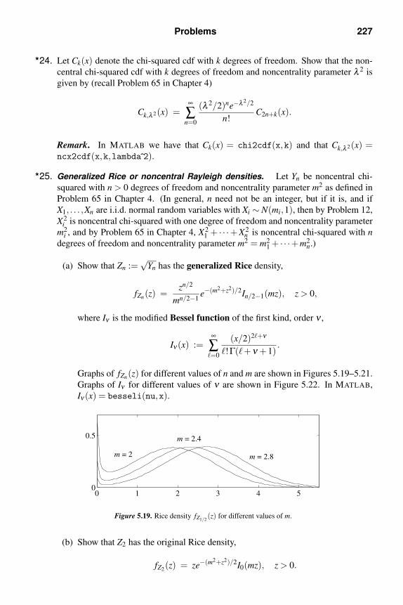
Problems 227
24. Let Ck(x) denote the chi-squared cdf with k degrees of freedom. Show that the non-
central chi-squared cdf with k degrees of freedom and noncentrality parameter λ 2 is
given by (recall Problem 65 in Chapter 4)
Ck,λ 2(x) =∞
∑n=0
(λ 2/2)ne−λ 2/2
n!C2n+k(x).
Remark. In MATLAB we have that Ck(x) = chi2cdf(x,k) and that Ck,λ 2(x) =ncx2cdf(x,k,lambda 2).
25. Generalized Rice or noncentral Rayleigh densities. Let Yn be noncentral chi-
squared with n > 0 degrees of freedom and noncentrality parameter m2 as defined in
Problem 65 in Chapter 4. (In general, n need not be an integer, but if it is, and if
X1, . . . ,Xn are i.i.d. normal random variables with Xi ∼ N(mi,1), then by Problem 12,
X2i is noncentral chi-squared with one degree of freedom and noncentrality parameter
m2i , and by Problem 65 in Chapter 4, X2
1 + · · ·+ X2n is noncentral chi-squared with n
degrees of freedom and noncentrality parameter m2 = m21 + · · ·+m2
n.)
(a) Show that Zn :=√
Yn has the generalized Rice density,
fZn(z) =zn/2
mn/2−1e−(m2+z2)/2In/2−1(mz), z > 0,
where Iν is the modified Bessel function of the first kind, order ν ,
Iν(x) :=∞
∑=0
(x/2)2+ν
!Γ(+ν +1).
Graphs of fZn(z) for different values of n and m are shown in Figures 5.19–5.21.
Graphs of Iν for different values of ν are shown in Figure 5.22. In MATLAB,
Iν(x) = besseli(nu,x).
0 1 2 3 4 50
0.5
m = 2
m = 2.4
m = 2.8
Figure 5.19. Rice density fZ1/2(z) for different values of m.
(b) Show that Z2 has the original Rice density,
fZ2(z) = ze−(m2+z2)/2I0(mz), z > 0.

228 Cumulative distribution functions and their applications
0 1 2 3 4 50
0.5
m = 1m = 2
m = 2.7
Figure 5.20. Rice density fZ1(z) for different values of m.
0 1 2 3 4 5 6 7 8 90
0.5 m = 1m = 3 m = 5
Figure 5.21. Rice density fZ2(z) for different values of m.
(c) Show that
fYn(y) =1
2
(√y
m
)n/2−1
e−(m2+y)/2In/2−1(m√
y), y > 0,
giving a closed-form expression for the noncentral chi-squared density. Recall
that you already have a closed-form expression for the moment generating func-
tion and characteristic function of a noncentral chi-squared random variable (see
Problem 65(b) in Chapter 4).
Remark. In MATLAB, the cdf of Yn is given by FYn(y) = ncx2cdf(y,n, m 2).
(d) Denote the complementary cumulative distribution of Zn by
FcZn
(z) := P(Zn > z) =∫ ∞
zfZn(t)dt.
Show that
FcZn
(z) =( z
m
)n/2−1
e−(m2+z2)/2In/2−1(mz)+FcZn−2
(z).
Hint: Use integration by parts; you will need the easily-verified fact that
d
dx
(xν Iν(x)
)= xν Iν−1(x).
(e) The complementary cdf of Z2, FcZ2
(z), is known as the Marcum Q function,
Q(m,z) :=∫ ∞
zte−(m2+t2)/2I0(mt)dt.

Problems 229
Show that if n ≥ 4 is an even integer, then
FcZn
(z) = Q(m,z)+ e−(m2+z2)/2n/2−1
∑k=1
( z
m
)k
Ik(mz).
(f) Show that Q(m,z) = Q(m,z), where
Q(m,z) := e−(m2+z2)/2∞
∑k=0
(m/z)kIk(mz).
Hint: [27, p. 450] Show that Q(0,z) = Q(0,z) = e−z2/2. It then suffices to prove
that∂
∂mQ(m,z) =
∂∂m
Q(m,z).
To this end, use the derivative formula in the hint of part (d) to show that
∂∂m
Q(m,z) = ze−(m2+z2)/2I1(mz);
you will also need the fact (derived in the next problem) that I−1(x) = I1(x).Now take the same partial derivative of Q(m,z) as defined in part (e), and then
use integration by parts on the term involving I1.
26. Properties of modified Bessel functions. In this problem you will derive some
basic properties of the modified Bessel functions of the first kind,
Iν(x) :=∞
∑=0
(x/2)2+ν
!Γ(+ν +1),
several of which are sketched in Figure 5.22.
(a) Show that
limx↓0
Iν(x)
(x/2)ν =1
Γ(ν +1),
and use result to evaluate
limz↓0
fZn(z),
where fZn is the Rice density of the previous problem. Hint: Remembering that
n > 0 need not be an integer, the three cases to consider are 0 < n < 1, n = 1,
and n > 1.
(b) Show that
I′ν(x) = 12[Iν−1(x)+ Iν+1(x)]
and that
Iν−1(x)− Iν+1(x) = 2(ν/x) Iν(x).
Note that the second identity implies the recursion,
Iν+1(x) = Iν−1(x)−2(ν/x) Iν(x).

230 Cumulative distribution functions and their applications
0 1 2 30
1
2
3
ν=−1/2
ν=0
ν=1/2 ν=1 ν=2
Figure 5.22. Graphs if Iν (x) for different values of ν .
Hence, once I0(x) and I1(x) are known, In(x) can be computed for n = 2,3, . . . .We also mention that the second identity with ν = 0 implies I−1(x) = I1(x).Using this in the first identity shows that I′0(x) = I1(x).
(c) Parts (c) and (d) of this problem are devoted to showing that for integers n ≥ 0,
In(x) =1
2π
∫ π
−πexcosθ cos(nθ)dθ .
To this end, denote the above integral by In(x). Use integration by parts and then
a trigonometric identity to show that
In(x) =x
2n[In−1(x)− In+1(x)].
Hence, in Part (d) it will be enough to show that I0(x) = I0(x) and I1(x) = I1(x).
(d) As noted in part (b), I′0(x) = I1(x). From the integral definition of In(x), it is
clear that I′0(x) = I1(x) as well. Hence, it is enough to show that I0(x) = I0(x).Since the integrand defining I0(x) is even,
I0(x) =1
π
∫ π
0excosθ dθ .
Show that
I0(x) =1
π
∫ π/2
−π/2e−xsin t dt.
Then use the power series eξ = ∑∞k=0 ξ k/k! in the above integrand and integrate
term by term. Then use the results of Problems 18 and 14 of Chapter 4 to show
that I0(x) = I0(x).

Problems 231
(e) Use the integral formula for In(x) to show that
I′n(x) = 12[In−1(x)+ In+1(x)].
5.2: Discrete random variables
27. MATLAB. Computing the binomial probability(n
k
)pk(1− p)n−k =
n!
k!(n− k)!pk(1− p)n−k
numerically can cause overflow problems if the factorials in the numerator and de-
nominator are computed separately. However, since the log of the right-hand side
is
ln(n!)− ln(k!)− ln[(n− k)!]+ k ln p+(n− k) ln(1− p),
this suggests an alternative way to calculate the probability. We can do even more to
reduce overflow problems. Since n! = Γ(n + 1), we use the built-in MATLAB func-
tion gammaln, which computes the log of the gamma function. Enter the following
MATLAB M-file containing the function binpmf(n,p) for computing the required
probability.
% M-file with function for computing the
% binomial(n,p) pmf.
%
function y = binpmf(k,n,p)
nk = n-k;
p1 = 1-p;
w = gammaln(n+1) - gammaln(nk+1) - gammaln(k+1) + ...
log(p)*k + log(p1)*nk;
y = exp(w);
Now type in the commands
n = 4
p = 0.75
k = [0:n]
prob = binpmf(k,n,p)
stem(k,prob,’filled’)
to generate a stem plot of the binomial(4,3/4) pmf.
28. Let X ∼ binomial(n, p) with n = 4 and p = 3/4. Sketch the graph of the cumulative
distribution function of X , F(x).

232 Cumulative distribution functions and their applications
5.3: Mixed random variables
29. A random variable X has generalized density
f (t) = 13e−tu(t)+ 1
2δ (t)+ 1
6δ (t −1),
where u is the unit step function defined in Section 2.1, and δ is the Dirac delta
function defined in Section 5.3.
(a) Sketch f (t).
(b) Compute P(X = 0) and P(X = 1).
(c) Compute P(0 < X < 1) and P(X > 1).
(d) Use your above results to compute P(0 ≤ X ≤ 1) and P(X ≥ 1).
(e) Compute E[X ].
30. If X has generalized density f (t) = 12[δ (t)+I(0,1](t)], evaluate E[eX ] and P(X = 0|X ≤
1/2).
31. Show that E[X ] = 7/12 if X has cdf
FX (x) =
⎧⎪⎪⎨⎪⎪⎩0, x < 0,x2, 0 ≤ x < 1/2,x, 1/2 ≤ x < 1,1, x ≥ 1.
32. Show that E[√
X ] = 49/30 if X has cdf
FX (x) :=
⎧⎪⎪⎪⎨⎪⎪⎪⎩0, x < 0,√x/4, 0 ≤ x < 4,
(x+11)/20, 4 ≤ x < 9,
1, x ≥ 9.
33. Find and sketch the cumulative distribution function of Example 5.13.
34. A certain computer monitor contains a loose connection. The connection is loose
with probability 1/2. When the connection is loose, the monitor displays a blank
screen (brightness = 0). When the connection is not loose, the brightness is uniformly
distributed on (0,1]. Let X denote the observed brightness. Find formulas and plot
the cdf and generalized density of X .
5.4: Functions of random variables and their cdfs
35. Let Θ ∼ uniform[−π,π], and put X := cosΘ and Y := sinΘ.
(a) Show that FX (x) = 1− 1π cos−1 x for −1 ≤ x ≤ 1.
(b) Show that FY (y) = 12+ 1
π sin−1 y for −1 ≤ y ≤ 1.

Problems 233
(c) Show that fX (x) = (1/π)/√
1− x2 and fY (y) = (1/π)/√
1− y2. Since X and
Y have the same density, they have the same cumulative distribution function.
Hence, both X and Y are called arcsine random variables.
(d) Show that Z = (Y +1)/2 has the beta density of Problem 16 in Chapter 4.
36. Find the cdf and density of Y = X(X +2) if X is uniformly distributed on [−3,1].
37. Let X ∼ uniform[−3,3], and suppose Y = g(X), where
g(x) =
⎧⎪⎨⎪⎩2, −1 ≤ x ≤ 1,
2/x2, 1 < |x| ≤ 2,
0, otherwise.
Find fY (y) for −∞ < y < ∞.
38. Consider the series RLC circuit shown in Figure 5.23. The voltage transfer function
R L
C+
−v ( t )c
+−
Figure 5.23. Series RLC circuit. The output is the capacitor voltage vc(t).
between the source and the capacitor is
H(ω) =1
(1−ω2LC)+ jωRC.
A plot of
|H(ω)|2 =1
(1−ω2LC)2 +(ωRC)2
is shown in Figure 5.24. The resonant frequency of the circuit, ω0, is the value of ω
0 1 20
1
2
3
Figure 5.24. Plot of |H(ω)|2 for L = 1, C = 1, and R =√
0.3.
that maximizes |H(ω)|2. It is not hard to show that
ω0 =
√1
LC− 1
2
(R
L
)2
.

234 Cumulative distribution functions and their applications
If these circuits are mass produced, then the actual values of R, L, and C in a particular
device vary somewhat from their design specifications, and hence, so does the reso-
nant frequency. Assuming L = 1, C = 1, and R∼ uniform[0,√
2], find the probability
density function of the resonant frequency Y =√
1−R2/2.
39. With the setup of the previous problem, find the probability density of the resonant
peak
Z = |H(ω0)|2 =1
R2(1−R2/4),
where R ∼ uniform[0,√
2], and we again take L = 1 and C = 1.
40. Suppose that a unit step voltage is applied to the circuit in Figure 5.23. When the
system is underdamped, the capacitor voltage has the form in Figure 5.25. When
0 5 10 150
1
maximumovershoot
Figure 5.25. Capacitor voltage vc(t) when a unit step source voltage is applied to the circuit in Figure 5.23 and the
circuit is underdamped. The horizontal dashed line is the limiting capacitor voltage vc(t) as t → ∞.
L = 1 and C = 1, the time at which the maximum overshoot occurs is
T =π√
1−R2/4.
If R ∼ uniform[0,√
2], find the probability density of T . Also find the probability
density of the maximum overshoot,
M = e−π(R/2)/√
1−R2/4.
41. Let g be as in Example 5.15. Find the cdf and density of Y = g(X) if
(a) X ∼ uniform[−1,1];
(b) X ∼ uniform[−1,2];
(c) X ∼ uniform[−2,3];
(d) X ∼ exp(λ ).
42. Let
g(x) :=
⎧⎨⎩0, |x| < 1,
|x|−1, 1 ≤ |x| ≤ 2,1, |x| > 2.
Find the cdf and density of Y = g(X) if
Problems 235
(a) X ∼ uniform[−1,1];
(b) X ∼ uniform[−2,2];
(c) X ∼ uniform[−3,3];
(d) X ∼ Laplace(λ ).
43. Let
g(x) :=
⎧⎪⎪⎨⎪⎪⎩−x−2, x < −1,−x2, −1 ≤ x < 0,x3, 0 ≤ x < 1,1, x ≥ 1.
Find the cdf and density of Y = g(X) if
(a) X ∼ uniform[−3,2];
(b) X ∼ uniform[−3,1];
(c) X ∼ uniform[−1,1].
44. Consider the function g given by
g(x) =
⎧⎨⎩ x2 −1, x < 0,x−1, 0 ≤ x < 2,
1, x ≥ 2.
If X is uniform[−3,3], find the cdf and density of Y = g(X).
45. Let X be a uniformly distributed random variable on the interval [−3,1]. Let Y =g(X), where
g(x) =
⎧⎪⎪⎨⎪⎪⎩0, x < −2,
x+2, −2 ≤ x < −1,x2, −1 ≤ x < 0,√
x, x ≥ 0.
Find the cdf and density of Y .
46. Let X ∼ uniform[−6,0], and suppose that Y = g(X), where
g(x) =
⎧⎪⎨⎪⎩|x|−1, 1 ≤ |x| < 2,
1−√|x|−2, |x| ≥ 2,
0, otherwise.
Find the cdf and density of Y .
47. Let X ∼ uniform[−2,1], and suppose that Y = g(X), where
g(x) =
⎧⎪⎪⎪⎨⎪⎪⎪⎩x+2, −2 ≤ x < −1,
2x2
1+ x2, −1 ≤ x < 0,
0, otherwise.
Find the cdf and density of Y .

236 Cumulative distribution functions and their applications
48. For x ≥ 0, let g(x) denote the fractional part of x. For example, g(5.649) = 0.649, and
g(0.123) = 0.123. Find the cdf and density of Y = g(X) if
(a) X ∼ exp(1);
(b) X ∼ uniform[0,1);
(c) X ∼ uniform[v,v + 1), where v = m + δ for some integer m ≥ 0 and some 0 <δ < 1.
5.5: Properties of cdfs
49. Show that G(x) := P(X < x) is a left-continuous function of x. Also show that P(X =x0) = G(x0+)−G(x0).
50. From your solution of Problem 4(b) in Chapter 4, you can see that if X ∼ exp(λ ),then P(X > t + ∆t|X > t) = P(X > ∆t). Now prove the converse; i.e., show that if
Y is a nonnegative random variable such that P(Y > t +∆t|Y > t) = P(Y > ∆t), then
Y ∼ exp(λ ), where λ = − ln[1−FY (1)], assuming that P(Y > t) > 0 for all t ≥ 0.
Hints: Put h(t) := lnP(Y > t), which is a right-continuous function of t (Why?).
Show that h(t +∆t) = h(t)+h(∆t) for all t,∆t ≥ 0.
5.6: The central limit theorem
51. Let X1, . . . ,Xn be i.i.d. with mean m and variance σ2. Show that
Yn :=1√n
n
∑i=1
(Xi −m
σ
)has zero mean and unit variance.
52. Packet transmission times on a certain Internet link are i.i.d. with mean m and variance
σ2. Suppose n packets are transmitted. Then the total expected transmission time for
n packets is nm. Use the central limit theorem to approximate the probability that
the total transmission time for the n packets exceeds twice the expected transmission
time.
53. To combat noise in a digital communication channel with bit-error probability p, the
use of an error-correcting code is proposed. Suppose that the code allows correct
decoding of a received binary codeword if the fraction of bits in error is less than or
equal to t. Use the central limit theorem to approximate the probability that a received
word cannot be reliably decoded.
54. If X1, . . . ,Xn are i.i.d. Poisson(1), evaluate both sides of (5.14). Then rearrange your
result to obtain Stirling’s formula, n! ≈√2π nn+1/2e−n.
55. Following Example 5.18, we remarked that when the Xi are i.i.d. exp(1), the central
limit theorem density decays faster than gn(x) as x → ∞. Here is an example in which
the central limit theorem density decays more slowly than gn(x). If the Xi are i.i.d.
uniform[−1,1], find xmax such that for x > xmax, gn(x) = 0, while the central limit
density is always positive.

Problems 237
56. Let Xi =±1 with equal probability. Then the Xi are zero mean and have unit variance.
Put
Yn =n
∑i=1
Xi√n.
Derive the central limit theorem for this case; i.e., show that ϕYn(ν) → e−ν2/2. Hint:
Use the Taylor series approximation cos(ξ ) ≈ 1−ξ 2/2.
5.7: Reliability
57. The lifetime T of a Model n Internet router has an Erlang(n,1) density, fT (t) =tn−1e−t/(n−1)!.
(a) What is the router’s mean time to failure?
(b) Show that the reliability of the router after t time units of operation is
R(t) =n−1
∑k=0
tk
k!e−t .
(c) Find the failure rate (known as the Erlang failure rate). Sketch the failure rate
for n = 2.
58. A certain device has the Weibull failure rate
r(t) = λ pt p−1, t > 0.
(a) Sketch the failure rate for λ = 1 and the cases p = 1/2, p = 1, p = 3/2, p = 2,
and p = 3.
(b) Find the reliability R(t).
(c) Find the mean time to failure.
(d) Find the density fT (t).
59. A certain device has the Pareto failure rate
r(t) =
p/t, t ≥ t0,
0, t < t0.
(a) Find the reliability R(t) for t ≥ 0.
(b) Sketch R(t) if t0 = 1 and p = 2.
(c) Find the mean time to failure if p > 1.
(d) Find the Pareto density fT (t).
60. A certain device has failure rate r(t) = t2 −2t +2 for t ≥ 0.
(a) Sketch r(t) for t ≥ 0.
(b) Find the corresponding density fT (t) in closed form (no integrals).

238 Cumulative distribution functions and their applications
61. Suppose that the lifetime T of a device is uniformly distributed on the interval [1,2].
(a) Find and sketch the reliability R(t) for t ≥ 0.
(b) Find the failure rate r(t) for 1 < t < 2.
(c) Find the mean time to failure.
62. Consider a system composed of two devices with respective lifetimes T1 and T2. Let
T denote the lifetime of the composite system. Suppose that the system operates
properly if and only if both devices are functioning. In other words, T > t if and only
if T1 > t and T2 > t. Express the reliability of the overall system R(t) in terms of
R1(t) and R2(t), where R1(t) and R2(t) are the reliabilities of the individual devices.
Assume T1 and T2 are independent.
63. Consider a system composed of two devices with respective lifetimes T1 and T2. Let
T denote the lifetime of the composite system. Suppose that the system operates
properly if and only if at least one of the devices is functioning. In other words,
T > t if and only if T1 > t or T2 > t. Express the reliability of the overall system
R(t) in terms of R1(t) and R2(t), where R1(t) and R2(t) are the reliabilities of the
individual devices. Assume T1 and T2 are independent.
64. Let Y be a nonnegative random variable. Show that
E[Y n] =
∫ ∞
0nyn−1
P(Y > y)dy.
Hint: Put T = Y n in (5.16).
Exam preparation
You may use the following suggestions to prepare a study sheet, including formulas men-
tioned that you have trouble remembering. You may also want to ask your instructor for
additional suggestions.
5.1. Continuous random variables. Know that a continuous random variable is com-
pletely characterized by its cdf because the density is given by the derivative of the
cdf. Be able to find the cdf of Y = g(X) in terms of FX when g is a simple function
such as g(x) = x2 or g(x) =√
x. Then use the formula fY (y) = (d/dy)FY (y). You
should be aware of the MAP and ML rules. You should also be aware of how to use
the inverse cdf to simulate a random variable starting with a uniform(0,1) random
variable.
5.2. Discrete random variables. Know that a discrete random variable is completely
characterized by its cdf since P(X = x j) = FX (x j)−FX (x j−1). Be aware of how to
simulate a discrete random variable starting with a uniform(0,1) random variable.
5.3. Mixed random variables. Know that a mixed random variable is completely charac-
terized by its cdf since the generalized density is given by (5.5), where fY (y) = F ′Y (y)
for y = yi, and P(Y = yi) is the size of the jump discontinuity in the cdf at yi.

Exam preparation 239
5.4. Functions of random variables and their cdfs. When Y = g(X), be able to use
graphical methods to find the cdf FY (y). Then differentiate to find fY (y), but be
careful to account for jumps in the cdf. Jumps in the cdf correspond to impulses in
the density.
5.5. Properties of cdfs. Be familiar with the eight properties.
5.6. The central limit theorem. When the Xi are i.i.d. with finite first and second mo-
ments, the key formulas are (5.8) for continuous random variables and (5.9) for
integer-valued random variables.
5.7. Reliability. Key formulas are the reliability function R(t) (5.15), the mean time to
failure formula for E[T ] (5.16), the differential equation for the failure rate function
r(t) and its representation in terms of the density fT (t) (5.17), and the density fT (t)in terms of the failure rate function (5.19).
Work any review problems assigned by your instructor. If you finish them, re-work your
homework assignments.

6
Statistics†
As we have seen, most problems in probability textbooks start out with random variables
having a given probability mass function or density. However, in the real world, problems
start out with a finite amount of data, X1,X2, . . . ,Xn, about which very little is known based
on the physical situation. We are still interested in computing probabilities, but we first
have to find the pmf or density with which to do the calculations. Sometimes the physical
situation determines the form of the pmf or density up to a few unknown parameters. For
example, the number of alpha particles given off by a radioactive sample is Poisson(λ ), but
we need to estimate λ from measured data. In other situations, we may have no information
about the pmf or density. In this case, we collect data and look at histograms to suggest
possibilities. In this chapter, we not only look at parameter estimators and histograms, we
also try to quantify how confident we are that our estimate or density choice is a good one.
Section 6.1 introduces the sample mean and sample variance as unbiased estimators of
the true mean and variance. The concept of strong consistency is introduced and used to
show that estimators based on the sample mean and sample variance inherit strong con-
sistency. Section 6.2 introduces histograms and the chi-squared statistic for testing the
goodness-of-fit of a hypothesized pmf or density to a histogram. Sections 6.3 and 6.4 focus
on how good a sample mean estimator is; namely, how confident we are that it is close to
the true mean. This is made precise through the notion of a confidence interval. Section 6.5
considers estimation of the mean and variance for Gaussian data. While the results of Sec-
tions 6.3 and 6.4 use approximations based on the central limit theorem, for Gaussian data,
no such approximation is required. Section 6.6 uses our knowledge of confidence intervals
to develop one-tailed and two-tailed hypothesis tests for the mean. Section 6.7 gives a quick
introduction to curve fitting under the name of regression. Although formulas are developed
using both variational arguments (derivatives) and the orthogonality principle, the empha-
sis is on using MATLAB to do the calculations. Section 6.8 provides a brief introduction
to the estimation of probabilities using Monte Carlo simulation. Confidence intervals are
used to assess the estimates. Particular attention is paid to the difficulties of estimating very
small probabilities, say 10−4 and smaller. The use of importance sampling is suggested for
estimating very small probabilities.
6.1 Parameter estimators and their properties
A sequence of observations or data measurements, say X1, . . . ,Xn, is called a sample. A
statistic is any function of the data. The sample mean,
Mn :=1
n
n
∑i=1
Xi, (6.1)
†The material in this chapter is not used elsewhere in the book, with the exception of Problem 16 in Chapter 11,
Problem 6 in Chapter 15, and Section 8.5. The present chapter can be covered at any time after Chapter 5.
240

6.1 Parameter estimators and their properties 241
is a statistic. Another useful statistic is the sample variance,
S2n :=
1
n−1
n
∑i=1
(Xi −Mn)2. (6.2)
The sample standard deviation is Sn :=√
S2n. In MATLAB, if X is a vector of data, try the
following commands to compute the sample mean, the sample standard deviation, and the
sample variance.
X = [ 5 2 7 3 8 ]
Mn = mean(X)
Sn = std(X)
Sn2 = var(X)
Now suppose that the Xi all have the same mean m and the same variance σ2. To distin-
guish between the sample mean Mn and the parameter m, m is called the population mean
or the ensemble mean. Similarly, σ2 is called the population variance or the ensemble
variance. Is there a relationship between the random variable Mn and the constant m? What
about the random variable S2n and the constant σ2? With regard to Mn and m, it is easy to
see that
E[Mn] = E
[1
n
n
∑i=1
Xi
]=
1
n
n
∑i=1
E[Xi] =1
n
n
∑i=1
m = m.
In other words, the expected value of the sample mean is the population mean. For this
reason, we say that the sample mean Mn is an unbiased estimator of the population mean m.
With regard to S2n and σ2, if we make the additional assumption that the Xi are uncorrelated,
then the formulaa
S2n =
1
n−1
[(n
∑i=1
X2i
)−nM2
n
], (6.3)
can be used to show that E[S2n] = σ2 (Problem 1). In other words, the sample variance S2
n is
an unbiased estimator of the ensemble variance σ2. To derive (6.3), write
S2n :=
1
n−1
n
∑i=1
(Xi −Mn)2
=1
n−1
n
∑i=1
(X2i −2XiMn +M2
n)
=1
n−1
[(n
∑i=1
X2i
)−2
(n
∑i=1
Xi
)Mn +nM2
n
]=
1
n−1
[(n
∑i=1
X2i
)−2(nMn)Mn +nM2
n
]=
1
n−1
[(n
∑i=1
X2i
)−nM2
n
].
Up to this point we have assumed only that the Xi are uncorrelated. However, to establish
the main theoretical results to follow, we need a stronger assumption. Therefore, in the
aFor Bernoulli random variables, since X2i = Xi, (6.3) simplifies to S2
n = Mn(1−Mn)n/(n−1).

242 Statistics
rest of this chapter, we make the assumption that the Xi are independent, identically
distributed (i.i.d.) with common mean m and common variance σ2. Then the strong law
of large numbers implies1
limn→∞
Mn = m and limn→∞
S2n = σ2. (6.4)
In other words, for large n, the random variables Mn and S2n are close to the constants m
and σ2, respectively. When an estimator converges to the desired parameter, the estimator
is said to be strongly consistent.
Example 6.1. Let X1, . . . ,Xn be i.i.d. with known mean m, but unknown variance σ2.
Determine whether or not1
n
n
∑i=1
(Xi −m)2.
is an unbiased estimator of σ2. Is it strongly consistent?
Solution. To see if the estimator is unbiased, write
E
[1
n
n
∑i=1
(Xi −m)2
]=
1
n
n
∑i=1
E[(Xi −m)2] =1
n
n
∑i=1
σ2 = σ2.
Hence, the proposed formula is an unbiased estimator of σ2. To assess consistency, write
1
n
n
∑i=1
(Xi −m)2 =n
∑i=1
(X2i −2Xim+m2)
=
(1
n
n
∑i=1
X2i
)−2m
(1
n
n
∑i=1
Xi
)+
1
n
n
∑i=1
m2
=
(1
n
n
∑i=1
X2i
)−2mMn +m2.
We already know that by the strong law of large numbers,
Mn =1
n
n
∑i=1
Xi → m.
Similarly,
1
n
n
∑i=1
X2i → E[X2
i ] = σ2 +m2,
since the X2i are i.i.d. on account of the fact that the Xi are i.i.d. Hence,
limn→∞
1
n
n
∑i=1
(Xi −m)2 = (σ2 +m2)−2m2 +m2 = σ2.
Thus, the proposed estimator is strongly consistent.

6.1 Parameter estimators and their properties 243
Example 6.2. Let X1, . . . ,Xn be i.i.d. with unknown mean m and unknown variance σ2.
Since we do not know m, we cannot use the estimator of the previous example. However, in
that estimator, let us replace m by the estimator Mn; i.e., we propose the estimator
S2n :=
1
n
n
∑i=1
(Xi −Mn)2
Determine whether or not S2n is an unbiased estimator of σ2. Is it strongly consistent?
Solution. It is helpful to observe that from (6.2)
S2n =
n−1
nS2
n.
Then
E[S2n] =
n−1
nE[S2
n] =n−1
nσ2 = σ2.
Thus, S2n is not an unbiased estimator of σ2 (we say that S2
n is a biased estimator of σ2).
However, since E[S2n]→ σ2, we say that S2
n is an asymptotically unbiased estimator of σ2.
We also point out that since S2n → σ2,
limn→∞
S2n = lim
n→∞
n−1
nlimn→∞
S2n = 1 ·σ2 = σ2.
Thus, both S2n and S2
n are strongly consistent estimators of σ2, with S2n being unbiased, and
S2n being only asymptotically unbiased.
Example 6.3. Let X1, . . . ,Xn be i.i.d. binomial(N, p) where N is known and p is not
known. Find an unbiased, strongly consistent estimator of p.
Solution. Since E[Xi] = N p (Problem 8 in Chapter 3),
p =E[Xi]
N.
This suggests the estimator
pn =Mn
N.
The estimator is unbiased because its expectation is N p/N = p. The estimator is strongly
consistent because Mn → N p implies Mn/N → N p/N = p.
Example 6.4. Let X1, . . . ,Xn be i.i.d. exp(λ ) where λ is not known. Find a strongly
consistent estimator of λ .
Solution. Recall that E[Xi] = 1/λ . Rewrite this as
λ =1
E[Xi].

244 Statistics
This suggests the estimator
λn =1
Mn
.
Since Mn → 1/λ , λn → λ , and we see that the estimator is strongly consistent as required.
6.2 Histograms
In the preceding section, we showed how to estimate various parameters from a collec-
tion of i.i.d. data X1, . . . ,Xn. In this section, we show how to estimate the entire probability
mass function or density of the Xi.
Given data X1, . . . ,Xn, we create a histogram as follows. We first select m intervals
called bins, denoted by [e j,e j+1), whereb
e1 < · · · < em+1,
and e1 and em+1 satisfy
e1 ≤ mini
Xi and maxi
Xi ≤ em+1.
When maxi Xi = em+1, we use the interval [em,em+1] instead of [em,em+1) so that no data is
lost. The sequence e is called the edge sequence. Notice that the number of edges is equal
to one plus the number of bins. The histogram count for bin j is
H j :=n
∑i=1
I[e j ,e j+1)(Xi).
In other words, H j is the number of data samples Xi that lie in bin j; i.e., the number of data
samples Xi that satisfy e j ≤ Xi < e j+1.
For each j, the term I[e j ,e j+1)(Xi) takes only the values zero and one. It is therefore a
Bernoulli random variable with parameter equal to its expectation,
E[I[e j ,e j+1)(Xi)] = P(e j ≤ Xi < e j+1). (6.5)
We assume that the Xi are i.i.d. to guarantee that for each j, the I[e j ,e j+1)(Xi) are also i.i.d.
Since H j/n is just the sample mean of the I[e j ,e j+1)(Xi), we have from the discussion in
Section 6.1 that H j/n converges to (6.5); i.e., for large n,
H j
n≈ P(e j ≤ Xi < e j+1). (6.6)
If the Xi are integer-valued random variables, it is convenient to use bins centered on the
integers, e.g., e j = j−1/2 and e j+1 = j +1/2. Then
H j
n≈ P(Xi = j).
Such an edge sequence and histogram counts are easily constructed in MATLAB with the
commands
bWe have used intervals of the form [a,b) because this is the form used by the MATLAB function histc.

6.2 Histograms 245
e = [min(X):max(X)+1]-0.5;
H = histc(X,e);
where X is a previously defined vector of integer-valued data. To plot the histogram H
normalized by the sample size n, use the commands
n = length(X);
nbins = length(e) - 1;
bin_centers = [min(X):max(X)];
bar(bin_centers,H(1:nbins)/n,’w’)
Remark. The reason we have to write H(1:nbins) instead of just H is that the vector
returned by histc has the length of e, which is one plus the number of bins.
After we plot the normalized histogram, it is convenient to overlay it with the corre-
sponding probability mass function. For example, if we know the data is i.i.d. binomial(10,0.3), we can use the function binpmf defined in Problem 27 of Chapter 5 to compute the
binomial pmf.
hold on % prevent erasure of last plot
k = [0:10]; % range for plotting pmf
prob = binpmf(k,10,0.3); % compute binomial(10,0.3) pmf
stem(k,prob,’filled’) % make stem plot of pmf
In a real situation, even if we have good reasons for believing the data is, say, binomial
(10, p), we do not know p. In this case, we can use the estimator developed in Example 6.3.
The MATLAB commands for doing this are
Mn = mean(X);
pn = Mn/10;
Example 6.5. Let us apply the above procedure to a sequence of n = 1000 binomi-
al(10,0.3) random variables. We use the function bernrnd defined in Section 5.2 to gen-
erate an array of Bernoulli random variables. The sum of each row gives one binomial
random variable.
n = 1000; % sample size
Bernmat = bernrnd(0.3,n,10); % generate n binomial
X = sum(Bernmat’); % random numbers in X
minX = min(X); % save to avoid re-
maxX = max(X); % computing min & max
e = [minX:maxX+1]-0.5;
H = histc(X,e);
nbins = length(e) - 1;
bin_centers = [minX:maxX];
bar(bin_centers,H(1:nbins)/n,’w’)
hold on
k = [0:10]; % range of pmf
Mn = mean(X);
pn = Mn/10; % estimate p
prob = binpmf(k,10,pn); % pmf w/ estimated p
stem(k,prob,’filled’)

246 Statistics
−1 0 1 2 3 4 5 6 7 8 9 100
0.1
0.2
0.3
Figure 6.1. Normalized histogram of 1000 i.i.d. binomial(10,0.3) random numbers. Stem plot shows pmf using
pn = 0.2989 estimated from the data.
fprintf(’Mn = %g pn = %g\n’,Mn,pn)
hold off
The command hold off allows the next run to erase the current figure. The plot is shown
in Figure 6.1. Notice that our particular realization of X1, . . . ,Xn did not have any occur-
rences of Xi = 9 or Xi = 10. This is not surprising since with N = 10 and p = 0.3, the
probability that Xi = 10 is 0.310 = 6×10⁻⁶, while we used only 1000 samples.
For continuous random variables Xi, the edge sequence, histogram counts, and bin cen-
ters are computed in MATLAB as follows, assuming that X and nbins have already been
defined.
minX = min(X);
maxX = max(X);
e = linspace(minX,maxX,nbins+1);
H = histc(X,e);
H(nbins) = H(nbins)+H(nbins+1); % explained below
H = H(1:nbins); % resize H
bw = (maxX-minX)/nbins; % bin width
a = e(1:nbins); % left edge sequence
b = e(2:nbins+1); % right edge sequence
bin_centers = (a+b)/2; % bin centers
Since we have set e(nbins+1) = max(X), histc will not count the value of max(X)
as belonging to the interval [e(nbins),e(nbins+1)). What histc does is use
H(nbins+1) is to count how many elements of X are exactly equal to e(nbins+1).
Hence, we add H(nbins+1) to H(nbins) to get the correct count for [e(nbins),

6.2 Histograms 247
0 0.2 0.4 0.6 0.8 1 1.2 1.40
1
2
3
4
5
Figure 6.2. Normalized histogram of 1000 i.i.d. exponential random numbers and the exp(λ ) density with the
value of λ estimated from the data.
e(nbins+1)]. For later use, note that a(j) is the left edge of bin j and b(j) is the
right edge of bin j.
We normalize the histogram as follows. If c j is the center of bin j, and ∆x j is the bin
width, then we want
H j
n≈ P(e j ≤ Xi < e j+1) =
∫ e j+1
e j
fX (x)dx ≈ fX (c j)∆x j.
So, if we are planning to draw a density function over the histogram, we should plot the
normalized values H j/(n∆x j). The appropriate MATLAB commands are
n = length(X);
bar(bin_centers,H/(bw*n),’hist’)
Example 6.6. You are given n = 1000 i.i.d. measurements X1, . . . ,Xn stored in a MAT-
LAB vector X. You plot the normalized histogram shown in Figure 6.2, and you believe the
Xi to be exponential random variables with unknown parameter λ . Use MATLAB to com-
pute the estimator in Example 6.4 to estimate λ . Then plot the corresponding density over
the histogram.
Solution. The estimator in Example 6.4 was λn = 1/Mn. The following MATLAB code
performs the desired task assuming X is already given and the normalized histogram already
plotted.
hold on
Mn = mean(X);
lambdan = 1/Mn;
t = linspace(minX,maxX,150); % range to plot pdf
plot(t,lambdan*exp(-lambdan*t))

248 Statistics
fprintf(’Mn = %g lambdan = %g\n’,Mn,lambdan)
hold off
The histogram and density are shown in Figure 6.2. The value of Mn was 0.206 and the
value of lambdan was 4.86.
The chi-squared test
So far we have been plotting histograms, and by subjective observation selected a pmf or
density that would overlay the histogram nicely, in our opinion. Here we develop objective
criteria, which are known as goodness-of-fit tests. The first step is to select a candidate
pmf or density that we subjectively think might be a good fit to the data. We refer to this
candidate as the hypothesis. Then we compute a statistic, call it Z, and compare it to a
threshold, call it zα . If Z ≤ zα , we agree that our hypothesis is a reasonable fit to the data.
If Z > zα , we reject our hypothesis and try another one. The threshold zα is chosen so that
if the data actually is i.i.d. pX or fX , then
P(Z > zα) = α.
Thus α is the probability of rejecting the hypothesis when it is actually correct. Hence, α is
usually taken to be a small number such as 0.01 or 0.05. We call α the significance level,
and specify it as a percentage, e.g., 1% or 5%.
The chi-squared testc is based on the histogram. The first step is to use the hypothesized
pmf or density to compute
p j := P(e j ≤ Xi < e j+1).
If our candidate pmf or density is a good one, then (6.6) tells us that
m
∑j=1
|H j −np j|2
should be small. However, as we shall see, it is advantageous to use the normalized statistic
Z :=m
∑j=1
|H j −np j|2np j
.
This normalization is motivated by the fact that (see Problem 16)
H j −np j√np j
has zero mean and variance 1− p j for all n and m, which implies E[Z] = m−1 for all n.
Example 6.7. In Example 6.5, we plotted a histogram and overlayed a binomial(10,0.2989) pmf, where 0.2989 was the estimated from the data. Compute the statistic Z.
Solution. This is easily done in MATLAB.
cOther popular tests include the Kolmogorov–Smirnov test and the Anderson–Darling test. However, they
apply only to continuous cdfs.

6.2 Histograms 249
p = binpmf(bin_centers,10,0.2989);
Z = sum((H(1:nbins)-n*p).ˆ2./(n*p))
We found that Z = 7.01.
Example 6.8. In Example 6.6, we plotted a histogram and fitted an exp(λ ) density. The
estimated value of λ was 4.86. Compute the statistic Z under this hypothesis.
Solution. Recall that for continuous random variables,
p j = P(e j ≤ Xi < e j+1) =
∫ e j+1
e j
fX (x)dx = FX (e j+1)−FX (e j).
Recalling the left and right edge sequences defined earlier, we can also write
p j = P(e j ≤ Xi < e j+1) =∫ b j
a j
fX (x)dx = FX (b j)−FX (a j).
Since the cdf of X ∼ exp(λ ) is FX (x) = 1− e−λx, we first create an M-file containing the
MATLAB function F to compute FX (x).
function y = F(x)
y = 1 - exp(-4.86*x);
The following MATLAB commands compute Z.
p = F(b) - F(a);
Z = sum((H-n*p).ˆ2./(n*p))
We found that Z = 8.33.
The only remaining problem is to choose α and to find the threshold zα , called the
critical value of the test. It turns out that for large n, the cdf of Z is approximately that of
a chi-squared random variable (Problem 15(d) in Chapter 4) with m−1 degrees of freedom
[3, p. 386, Problem 29.8]. However, if you use r estimated parameters, then Z has only
m−1− r degrees of freedom [12], [47, pp. 205–206].d Hence, to solve
P(Z > zα) = α
for zα we must solve 1−FZ(zα) = α or FZ(zα) = 1−α . This can be done by applying
a root-finding algorithm to the equation FZ(zα)− 1 + α = 0 or in MATLAB with the com-
mand chi2inv(1-alpha,k), where k is the number of degrees of freedom of Z. Some
solutions are also shown in Table 6.1.
Example 6.9. Find zα for α = 0.05 in Examples 6.5 and 6.6.
Solution. In the first case, the number of degrees of freedom is m− 1− 1, where m
is the number of bins, which from Figure 6.1, is 9, and the extra 1 is subtracted because
dThe basic Kolmogorov–Smirnov test does not account for using estimated parameters. If estimated parameters
are used, the critical value zα must be determined by simulation [47, p. 208].

250 Statistics
k zα(α = 5%) zα(α = 1%)
1 3.841 6.635
2 5.991 9.210
3 7.815 11.345
4 9.488 13.277
5 11.070 15.086
6 12.592 16.812
7 14.067 18.475
8 15.507 20.090
9 16.919 21.666
10 18.307 23.209
11 19.675 24.725
12 21.026 26.217
13 22.362 27.688
14 23.685 29.141
15 24.996 30.578
16 26.296 32.000
17 27.587 33.409
18 28.869 34.805
19 30.144 36.191
20 31.410 37.566
Table 6.1. Thresholds zα for the chi-squared test with k degrees of freedom and significance levels α = 5% and
α = 1%.
we used one estimated parameter. Hence, k = 7, and from Table 6.1, zα = 14.067. From
Example 6.7, the statistic Z was 7.01, which is well below the threshold. We conclude that
the binomial(10,0.2989) is a good fit to the data. In the second case, the number of degrees
of freedom is m−1−1, where m is the number of bins, and the extra 1 is subtracted because
we estimated one parameter. From Figure 6.2, m = 15. Hence, k = 13, and from Table 6.1,
zα = 22.362. From Example 6.8, Z was 8.33. Since Z is much smaller than the threshold,
we conclude that the exp(4.86) density is a good fit to the data.
6.3 Confidence intervals for the mean – known variance
As noted in Section 6.1, the sample mean Mn converges to the population mean m as
n → ∞. However, in practice, n is finite, and we would like to say something about how
close the random variable Mn is to the unknown constant m. One way to do this is with a
confidence interval. For theory purposes, we write
P(m ∈ [Mn −δ ,Mn +δ ]) = 1−α, (6.7)
where [Mn −δ ,Mn +δ ] is the confidence interval, and 1−α is the confidence level. Thus,
a confidence interval is a random set, and the confidence level 1−α is the probability that
the random set contains the unknown parameter m. Commonly used values of 1−α range

6.3 Confidence intervals for the mean – known variance 251
from 0.90 to 0.99. In applications, we usually write (6.7) in the form
m = Mn ±δ with 100(1−α)% probability.
The next problem we consider is how to choose δ so that equation (6.7) holds.e From
(6.7), the left-hand side depends on Mn = (X1 + · · ·+ Xn)/n. Hence, the first step would
be to find the pmf or density of the sum of i.i.d. random variables. This can only be done
in special cases (e.g., Problem 55 in Chapter 4). We need a more general approach. To
proceed, we first rewrite the condition m ∈ [Mn − δ ,Mn + δ ] as |Mn −m| ≤ δ . To see that
these conditions are equivalent, observe that m ∈ [Mn −δ ,Mn +δ ] if and only if
Mn −δ ≤ m ≤ Mn +δ .
Multiplying through by −1 yields
−Mn +δ ≥ −m ≥ −Mn −δ ,
from which we get
δ ≥ Mn −m ≥ −δ .
This is more compactly rewritten as f
|Mn −m| ≤ δ .
It follows that the left-hand side of (6.7) is equal to
P(|Mn −m| ≤ δ ). (6.8)
Now take
δ = σy/√
n
so that (6.8) becomes
P
(|Mn −m| ≤ σy√
n
),
or
P
(∣∣∣Mn −m
σ/√
n
∣∣∣≤ y). (6.9)
Setting
Yn :=Mn −m
σ/√
n,
we have2
P
(∣∣∣Mn −m
σ/√
n
∣∣∣≤ y)
= P(|Yn| ≤ y) = P(−y ≤ Yn ≤ y) = FYn(y)−FYn(−y).
eAlternatively, one could specify δ and then compute 1−α .fTo see that |t| ≤ δ is equivalent to −δ ≤ t ≤ δ , consider separately the two cases t ≥ 0 and t < 0, and note
that for t < 0, |t| = −t.

252 Statistics
By the central limit theorem (Section 5.6),g FYn(y)→Φ(y), where Φ is the standard normal
cdf,
Φ(y) =1√2π
∫ y
−∞e−t2/2 dt.
Thus, for large n,
P
(∣∣∣Mn −m
σ/√
n
∣∣∣≤ y)
≈ Φ(y)−Φ(−y) = 2Φ(y)−1, (6.10)
where the last step uses the fact that the standard normal density is even (Problem 17). The
importance of this formula is that if we want the left-hand side to be 1−α , all we have to
do is solve for y in the equation
1−α = 2Φ(y)−1,
or
Φ(y) = 1−α/2.
Notice that this equation does not depend on n or on the pmf or density of the Xi! We
denote the solution of this equation by yα/2. It can be found from tables, e.g., Table 6.2, or
numerically by finding the unique root of the equation Φ(y)+α/2−1 = 0, or in MATLAB
by yα/2 = norminv(1−alpha/2). h
We now summarize the procedure. Fix a confidence level 1−α . Find the corresponding
yα/2 from Table 6.2. Then write
m = Mn ±σyα/2√
nwith 100(1−α)% probability, (6.11)
and the corresponding confidence interval is[Mn −
σyα/2√n
,Mn +σyα/2√
n
]. (6.12)
Example 6.10. Let X1,X2, . . . be i.i.d. random variables with variance σ2 = 2. If M100 =7.129, find the 93 and 97% confidence intervals for the population mean.
Solution. In Table 6.2 we scan the 1−α column until we find 0.93. The corresponding
value of yα/2 is 1.812. Since yα/2σ/√
n = 1.812√
2/√
100 = 0.256, we write
m = 7.129±0.256 with 93% probability,
and the corresponding confidence interval is [6.873,7.385].
gThe reader should verify that Yn as defined here is equal to Yn as defined in (5.6).hSince Φ can be related to the error function erf (see Note 1 in Chapter 5), yα/2 can also be found using the in-
verse of the error function. Hence, yα/2 =√
2 erf−1(1−α). The MATLAB command for erf−1(z) is erfinv(z).

6.4 Confidence intervals for the mean – unknown variance 253
1−α yα/2
0.90 1.645
0.91 1.695
0.92 1.751
0.93 1.812
0.94 1.881
0.95 1.960
0.96 2.054
0.97 2.170
0.98 2.326
0.99 2.576
Table 6.2. Confidence levels 1−α and corresponding yα/2 such that 2Φ(yα/2)−1 = 1−α .
For the 97% confidence interval, we use yα/2 = 2.170. Then yα/2σ/√
n is equal to
2.170√
2/√
100 = 0.307, and we write
m = 7.129±0.307 with 97% probability,
and the corresponding confidence interval is [6.822,7.436].
This example illustrates the general result that if we want more confidence, we have to
use a wider interval. Equivalently, if we use a smaller interval, we will be less confident that
it contains the unknown parameter. Mathematically, the width of the confidence interval is
2 · σyα/2√n
.
From Table 6.2, we see that as 1−α increases, so does yα/2, and hence the width of the
confidence interval. It should also be noted that for fixed 1−α , we can reduce the width of
the confidence interval by increasing n; i.e., taking more measurements.
6.4 Confidence intervals for the mean – unknown variance
In practice, we usually do not know σ . Hence, we replace it by Sn. To justify this, first
observe that the argument showing the left-hand side of (6.7) is equal to (6.8) can be carried
out with δ = Snyα/2/√
n. Hence,
P
(m ∈
[Mn −
Snyα/2√n
,Mn +Snyα/2√
n
])is equal to
P
(|Mn −m| ≤ Snyα/2√
n
).
Now observe that this is equal to
P
(∣∣∣Mn −m
σ/√
n
∣∣∣≤ Snyα/2
σ
). (6.13)

254 Statistics
Recalling our definition Yn := (Mn −m)/(σ/√
n), the above probability is
P
(|Yn| ≤
Snyα/2
σ
).
Since Sn → σ , the ratio Sn/σ → 1. This suggests3 that for large n
P
(|Yn| ≤
Snyα/2
σ
)≈ P(|Yn| ≤ yα/2) (6.14)
≈ 2Φ(yα/2)−1, by the central limit theorem,
= 1−α, by the definition of yα/2. (6.15)
We now summarize the new procedure. Fix a confidence level 1−α . Find the corre-
sponding yα/2 from Table 6.2. Then write
m = Mn ±Snyα/2√
nwith 100(1−α)% probability, (6.16)
and the corresponding confidence interval is[Mn −
Snyα/2√n
,Mn +Snyα/2√
n
]. (6.17)
Example 6.11. Let X1,X2, . . . be i.i.d. Bernoulli(p) random variables. Find the 95%
confidence interval for p if M100 = 0.28 and S100 = 0.451.
Solution. Observe that since m := E[Xi] = p, we can use Mn to estimate p. From
Table 6.2, yα/2 = 1.960, S100 yα/2/√
100 = 0.088, and
p = 0.28±0.088 with 95% probability.
The corresponding confidence interval is [0.192,0.368].
Applications
Estimating the number of defective products in a lot. Consider a production run of
N cellular phones, of which, say d are defective. The only way to determine d exactly and
for certain is to test every phone. This is not practical if N is large. So we consider the
following procedure to estimate the fraction of defectives, p := d/N, based on testing only
n phones, where n is large, but smaller than N.
FOR i = 1 TO n
Select a phone at random from the lot of N phones;
IF the ith phone selected is defective
LET Xi = 1;
ELSE
LET Xi = 0;

6.4 Confidence intervals for the mean – unknown variance 255
END IF
Return the phone to the lot;
END FOR
Because phones are returned to the lot (sampling with replacement), it is possible to test
the same phone more than once. However, because the phones are always chosen from the
same set of N phones, the Xi are i.i.d. with P(Xi = 1) = d/N = p. Hence, the central limit
theorem applies, and we can use the method of Example 6.11 to estimate p and d = N p.
For example, if N = 1000 and we use the numbers from Example 6.11, we would estimate
that
d = 280±88 with 95% probability.
In other words, we are 95% sure that the number of defectives is between 192 and 368 for
this particular lot of 1000 phones.
If the phones were not returned to the lot after testing (sampling without replacement),
the Xi would not be i.i.d. as required by the central limit theorem. However, in sampling
with replacement when n is much smaller than N, the chances of testing the same phone
twice are negligible. Hence, we can actually sample without replacement and proceed as
above.
Predicting the outcome of an election. In order to predict the outcome of a presi-
dential election, 4000 registered voters are surveyed at random. In total, 2104 (more than
half) say they will vote for candidate A, and the rest say they will vote for candidate B.
To predict the outcome of the election, let p be the fraction of votes actually received by
candidate A out of the total number of voters N (millions). Our poll samples n = 4000, and
M4000 = 2104/4000 = 0.526. Suppose that S4000 = 0.499. For a 95% confidence interval
for p, yα/2 = 1.960, S4000 yα/2/√
4000 = 0.015, and
p = 0.526±0.015 with 95% probability.
Rounding off, we would predict that candidate A will receive 53% of the vote, with a margin
of error of 2%. Thus, we are 95% sure that candidate A will win the election.
Sampling with and without replacement
Consider sampling n items from a batch of N items, d of which are defective. If we
sample with replacement, then the theory above worked out rather simply. We also argued
briefly that if n is much smaller than N, then sampling without replacement would give
essentially the same results. We now make this statement more precise.
To begin, recall that the central limit theorem says that for large n, FYn(y)≈ Φ(y), where
Yn = (Mn −m)/(σ/√
n), and Mn = (1/n)∑ni=1 Xi. If we sample with replacement and set
Xi = 1 if the ith item is defective, then the Xi are i.i.d. Bernoulli(p) with p = d/N. When
X1,X2, . . . are i.i.d. Bernoulli(p), we know from Section 3.2 that ∑ni=1 Xi is binomial(n, p).
Putting this all together, we obtain the de Moivre–Laplace theorem, which says that if
V ∼ binomial(n, p) and n is large, then the cdf of (V/n− p)/√
p(1− p)/n is approximately
standard normal.
Now suppose we sample n items without replacement. Let U denote the number of de-
fectives out of the n samples. It was shown in Example 1.41 that U is a hypergeometric(N,

256 Statistics
d,n) random variable with pmf i
P(U = k) =
(d
k
)(N −d
n− k
)(
N
n
) , k = 0, . . . ,n.
In the next paragraph we show that if n is much smaller than d, N −d, and N, then P(U =k)≈ P(V = k). It then follows that the cdf of (U/n− p)/
√p(1− p)/n is close to the cdf of
(V/n− p)/√
p(1− p)/n, which is close to the standard normal cdf if n is large. (Thus, to
make it all work we need n large, but still much smaller than d, N −d, and N.)
To show that P(U = k) ≈ P(V = k), write out P(U = k) as
d!
k!(d − k)!· (N −d)!
(n− k)![(N −d)− (n− k)]!· n!(N −n)!
N!.
We can easily identify the factor(
nk
). Next, since 0 ≤ k ≤ n d,
d!
(d − k)!= d(d −1) · · ·(d − k +1) ≈ dk.
Similarly, since 0 ≤ k ≤ n (N −d),
(N −d)!
[(N −d)− (n− k)]!= (N −d) · · · [(N −d)− (n− k)+1] ≈ (N −d)n−k.
Finally, since n N,
(N −n)!
N!=
1
N(N −1) · · ·(N −n+1)≈ 1
Nn.
Writing p = d/N, we have
P(U = k) ≈(
n
k
)pk(1− p)n−k.
6.5 Confidence intervals for Gaussian data
In this section we assume that X1,X2, . . . are i.i.d. N(m,σ2).
Estimating the mean
If the Xi are i.i.d. N(m,σ2), then by Problem 30, Yn = (Mn −m)/(σ/√
n) is N(0,1).Hence, the analysis in Sections 6.3 shows that
P
(m ∈
[Mn − σy√
n,Mn +
σy√n
])= P(|Yn| ≤ y)
= 2Φ(y)−1.
The point is that for normal data there is no central limit theorem approximation. Hence,
we can determine confidence intervals as in Section 6.3 even if n is not large.
iSee the Notes4 for an alternative derivation using the law of total probability.
6.5 Confidence intervals for Gaussian data 257
Example 6.12. Let X1,X2, . . . be i.i.d. N(m,2). If M10 = 5.287, find the 90% confidence
interval for m.
Solution. From Table 6.2 for 1−α = 0.90, yα/2 is 1.645. We then have yα/2σ/√
10 =
1.645√
2/√
10 = 0.736,
m = 5.287±0.736 with 90% probability,
and the corresponding confidence interval is [4.551,6.023].
Unfortunately, formula (6.14) in Section 6.4 still involves the approximation Sn/σ ≈ 1
even if the Xi are normal. However, let us rewrite (6.13) as
P
(∣∣∣Mn −m
Sn/√
n
∣∣∣≤ yα/2
),
and put
T :=Mn −m
Sn/√
n.
As shown later, if the Xi are i.i.d. N(m,σ2), then T has Student’s t density with ν = n− 1
degrees of freedom (defined in Problem 20 in Chapter 4). To compute 100(1−α)% confi-
dence intervals, we must solve
P(|T | ≤ y) = 1−α
or
FT (y)−FT (−y) = 1−α.
Since the density fT is even, FT (−y) = 1−FT (y), and we must solve
2FT (y)−1 = 1−α,
or FT (y) = 1−α/2. This can be solved using tables, e.g., Table 6.3, or numerically by
finding the unique root of the equation FT (y) + α/2− 1 = 0, or in MATLAB by yα/2 =tinv(1−alpha/2,n−1).
Example 6.13. Let X1,X2, . . . be i.i.d. N(m,σ2) random variables, and suppose M10 =5.287. Further suppose that S10 = 1.564. Find the 90% confidence interval for m.
Solution. In Table 6.3 with n = 10, we see that for 1−α = 0.90, yα/2 is 1.833. Since
S10 yα/2/√
10 = 0.907,
m = 5.287±0.907 with 90% probability.
The corresponding confidence interval is [4.380,6.194].

258 Statistics
1−α yα/2(n = 10)
0.90 1.833
0.91 1.899
0.92 1.973
0.93 2.055
0.94 2.150
0.95 2.262
0.96 2.398
0.97 2.574
0.98 2.821
0.99 3.250
1−α yα/2(n = 100)
0.90 1.660
0.91 1.712
0.92 1.769
0.93 1.832
0.94 1.903
0.95 1.984
0.96 2.081
0.97 2.202
0.98 2.365
0.99 2.626
Table 6.3. Confidence levels 1−α and corresponding yα/2 such that P(|T | ≤ yα/2) = 1−α . The left-hand table
is for n = 10 observations with T having n− 1 = 9 degrees of freedom, and the right-hand table is for n = 100
observations with T having n−1 = 99 degrees of freedom.
Limiting t distribution
If we compare the n = 100 table in Table 6.3 with Table 6.2, we see they are almost
the same. This is a consequence of the fact that as n increases, the t cdf converges to the
standard normal cdf. We can see this by writing
P(T ≤ t) = P
(Mn −m
Sn/√
n≤ t
)= P
(Mn −m
σ/√
n≤ Sn
σt
)= P
(Yn ≤ Sn
σt)
≈ P(Yn ≤ t),
since3 Sn converges to σ . Finally, since the Xi are independent and normal, FYn(t) = Φ(t).We also recall from Problem 21 in Chapter 4 and Figure 4.12 there that the t density
converges to the standard normal density.
Estimating the variance – known mean
Suppose that X1,X2, . . . are i.i.d. N(m,σ2) with m known but σ2 unknown. We use
V 2n :=
1
n
n
∑i=1
(Xi −m)2 (6.18)
as our estimator of the variance σ2. It is easy to see that V 2n is a strongly consistent estimator
of σ2.
For determining confidence intervals, it is easier to work with
n
σ2V 2
n =n
∑i=1
(Xi −m
σ
)2
.

6.5 Confidence intervals for Gaussian data 259
1−α u
0.90 77.929 124.342
0.91 77.326 125.170
0.92 76.671 126.079
0.93 75.949 127.092
0.94 75.142 128.237
0.95 74.222 129.561
0.96 73.142 131.142
0.97 71.818 133.120
0.98 70.065 135.807
0.99 67.328 140.169
Table 6.4. Confidence levels 1−α and corresponding values of and u such that P(≤ nV 2n /σ2 ≤ u) = 1−α and
such that P(nV 2n /σ2 ≤ ) = P(nV 2
n /σ2 ≥ u) = α/2 for n = 100 observations.
Since (Xi −m)/σ is N(0,1), its square is chi-squared with one degree of freedom (Prob-
lem 46 in Chapter 4 or Problem 11 in Chapter 5). It then follows that nV 2n /σ2 is chi-squared
with n degrees of freedom (see Problem 55(c) and its Remark in Chapter 4).
Choose 0 < < u, and consider the equation
P
( ≤ n
σ2V 2
n ≤ u)
= 1−α.
We can rewrite this as
P
(nV 2
n
≥ σ2 ≥ nV 2
n
u
)= 1−α.
This suggests the confidence interval [nV 2
n
u,
nV 2n
]. (6.19)
Then the probability that σ2 lies in this interval is
F(u)−F() = 1−α,
where F is the chi-squared cdf with n degrees of freedom. We usually choose and u to
solve
F() = α/2 and F(u) = 1−α/2.
These equations can be solved using tables, e.g., Table 6.4, or numerically by root finding,
or in MATLAB with the commands
= chi2inv(alpha/2,n) and u = chi2inv(1−alpha/2,n).
Example 6.14. Let X1,X2, . . . be i.i.d. N(5,σ2) random variables. Suppose that V 2100 =
1.645. Find the 90% confidence interval for σ2.

260 Statistics
Solution. From Table 6.4 we see that for 1−α = 0.90, = 77.929 and u = 124.342.
The 90% confidence interval is[100(1.645)
124.342,
100(1.645)
77.929
]= [1.323,2.111].
Estimating the variance – unknown mean
Let X1,X2, . . . be i.i.d. N(m,σ2), where both the mean and the variance are unknown, but
we are interested only in estimating the variance. Since we do not know m, we cannot use
the estimator V 2n above. Instead we use S2
n. However, for determining confidence intervals,
it is easier to work with ((n− 1)/σ2)S2n. As argued below, (n− 1)S2
n/σ2 is a chi-squared
random variable with n−1 degrees of freedom.
Choose 0 < < u, and consider the equation
P
( ≤ n−1
σ2S2
n ≤ u)
= 1−α.
We can rewrite this as
P
((n−1)S2
n
≥ σ2 ≥ (n−1)S2
n
u
)= 1−α.
This suggests the confidence interval[(n−1)S2
n
u,(n−1)S2
n
]. (6.20)
Then the probability that σ2 lies in this interval is
F(u)−F() = 1−α,
where now F is the chi-squared cdf with n−1 degrees of freedom. We usually choose and
u to solve
F() = α/2 and F(u) = 1−α/2.
These equations can be solved using tables, e.g., Table 6.5, or numerically by root finding,
or in MATLAB with the commands = chi2inv(alpha/2,n−1) and u = chi2inv(1−alpha/2,n−1).
Example 6.15. Let X1,X2, . . . be i.i.d. N(m,σ2) random variables. If S2100 = 1.608, find
the 90% confidence interval for σ2.
Solution. From Table 6.5 we see that for 1−α = 0.90, = 77.046 and u = 123.225.
The 90% confidence interval is[99(1.608)
123.225,
99(1.608)
77.046
]= [1.292,2.067].

6.5 Confidence intervals for Gaussian data 261
1−α u
0.90 77.046 123.225
0.91 76.447 124.049
0.92 75.795 124.955
0.93 75.077 125.963
0.94 74.275 127.103
0.95 73.361 128.422
0.96 72.288 129.996
0.97 70.972 131.966
0.98 69.230 134.642
0.99 66.510 138.987
Table 6.5. Confidence levels 1−α and corresponding values of and u such that P(≤ (n−1)S2n/σ2 ≤ u) = 1−α
and such that P((n−1)S2n/σ2 ≤ ) = P((n−1)S2
n/σ2 ≥ u) = α/2 for n = 100 observations (n−1 = 99 degrees
of freedom).
Derivations
The remainder of this section is devoted to deriving the distributions of S2n and
T :=Mn −m
Sn/√
n=
(Mn −m)/(σ/√
n)√n−1
σ2S2
n
/(n−1)
under the assumption that the Xi are i.i.d. N(m,σ2).We begin with the numerator in T . By Problem 30, Yn := (Mn − m)/(σ/
√n) is ∼
N(0,1).For the denominator, we show that the density of (n−1)S2
n/σ2 is chi-squared with n−1
degrees of freedom. We begin by recalling the derivation of (6.3). If we replace the first line
of the derivation with
S2n =
1
n−1
n
∑i=1
([Xi −m]− [Mn −m])2,
then we end up with
S2n =
1
n−1
[(n
∑i=1
[Xi −m]2)−n[Mn −m]2
].
Using the notation Zi := (Xi −m)/σ , we have
n−1
σ2S2
n =n
∑i=1
Z2i −n
(Mn −m
σ
)2
,
orn−1
σ2S2
n +
(Mn −m
σ/√
n
)2
=n
∑i=1
Z2i .
262 Statistics
As we argue below, the two terms on the left are independent. It then follows that the density
of ∑ni=1 Z2
i is equal to the convolution of the densities of the other two terms. To find the
density of (n−1)S2n/σ2, we use moment generating functions. Now, the second term on the
left is the square of an N(0,1) random variable. It is therefore chi-squared with one degree
of freedom and has moment generating function is 1/(1−2s)1/2 (Problem 46 in Chapter 4).
The same holds for each Z2i . Since the Zi are independent, ∑n
i=1 Z2i is chi-squared with n
degrees of freedom and has moment generating function is 1/(1− 2s)n/2 (Problem 55(c)
in Chapter 4). It now follows that the moment generating function of (n− 1)S2n/σ2 is the
quotient
1/(1−2s)n/2
1/(1−2s)1/2=
1
(1−2s)(n−1)/2,
which is the moment generating function of a chi-squared random variable with n− 1 de-
grees of freedom.
It remains to show that S2n and Mn are independent. Observe that S2
n is a function of the
vector
W := [(X1 −Mn), . . . ,(Xn −Mn)]′.
In fact, S2n = W ′W/(n− 1). By Example 9.6, the vector W and the sample mean Mn are
independent. It then follows that any function of W and any function of Mn are independent.
We can now find the density of
T =(Mn −m)/(σ/
√n)√
n−1
σ2S2
n
/(n−1)
.
If the Xi are i.i.d. N(m,σ2), then the numerator and the denominator are independent; the
numerator is N(0,1), and in the denominator (n−1)S2n/σ2 is chi-squared with n−1 degrees
of freedom. By Problem 44 in Chapter 7, T has Student’s t density with ν = n−1 degrees
of freedom.
6.6 Hypothesis tests for the mean
Let X1,X2, . . . be i.i.d. with mean m and variance σ2. Consider the problem of deciding
between two possibilities such as
m ≤ m0 or m > m0,
where m0 is a threshold. Other pairs of possibilities include
m = m0 or m = m0
and
m = m0 or m > m0.
It is not required that each possibility be the negation of the other, although we usually do
so here.

6.6 Hypothesis tests for the mean 263
Example 6.16. A telecommunications satellite maker claims that its new satellite has a
bit-error probability of no more that p0. To put this information into the above framework,
let Xi = 1 if the ith bit transmitted is received in error, and let Xi = 0 otherwise. Then
p := P(Xi = 1) = E[Xi], and the claim is that p ≤ p0. For the other possibility, we allow
p > p0.
The problem of deciding which of several possibilities is correct is called hypothesis
testing. In this section we restrict attention to the case of two possibilities. In assessing two
competing claims, it is usually natural give the benefit of the doubt to one and the burden
of proof to the other. The possibility that is given the benefit of the doubt is called the null
hypothesis, and the possibility that is given the burden of proof is called the alternative
hypothesis.
Example 6.17. In the preceding example, the satellite maker claims that p ≤ p0. If the
government is considering buying such a satellite, it will put the burden of proof on the
manufacturer. Hence, the government will take p > p0 as the null hypothesis, and it will be
up to the data to give compelling evidence that the alternative hypothesis p ≤ p0 is true.
Decision rules
To assess claims about m, it is natural to use the sample mean Mn, since we know that
Mn converges to m as n → ∞. However, for finite n, Mn is usually not exactly equal to m.
In fact, Mn may be quite far from m. To account for this, when we test the null hypothesis
m ≤ m0 against the alternative hypothesis m > m0, we select δ > 0 and agree that if
Mn ≤ m0 +δ , (6.21)
then we declare that the null hypothesis m≤m0 is true, while if Mn > m0 +δ , we declare that
the alternative hypothesis m > m0 is true. Clearly, the burden of proof is on the alternative
hypothesis m > m0, since we do not believe it unless Mn is substantially greater than m0.
The null hypothesis m ≤ m0 gets the benefit of the doubt, since we accept it even if m0 <Mn ≤ m0 +δ .
Proceeding similarly to test the null hypothesis m > m0 against the alternative hypothesis
m ≤ m0, we agree that if
Mn > m0 −δ , (6.22)
then we declare m > m0 to be true, while if Mn ≤ m0 − δ , we declare m ≤ m0. Again, the
burden of proof is on the alternative hypothesis, and the benefit of the doubt is on the null
hypothesis.
To test the null hypothesis m = m0 against the alternative hypothesis m = m0, we declare
m = m0 to be true if
|Mn −m0| ≤ δ , (6.23)
and m = m0 otherwise.
264 Statistics
Acceptance and rejection regions
As in the case of confidence intervals, it is sensible to have δ depend on the variance
and on the number of observations n. For this reason, if the variance is known, we take δto be of the form δ = yσ/
√n, while if the variance is unknown, we take δ = ySn/
√n. This
amounts to working with the statistic
Mn −m0
σ/√
n(6.24)
if σ known, or the statisticMn −m0
Sn/√
n(6.25)
otherwise. If the appropriate statistic is denoted by Zn, then (6.21)–(6.23) become
Zn ≤ y, Zn > −y, and |Zn| ≤ y.
The value with which Zn or |Zn| is compared is called the critical value. The corresponding
acceptance regions are the intervals
(−∞,y], (−y,∞), and [−y,y].
In other words, if Zn lies in the acceptance region, we accept the null hypothesis as true. The
complement of the acceptance region is called the rejection region or the critical region.
If Zn lies in the rejection region, we reject the null hypothesis and declare the alternative
hypothesis to be true.
Types of errors
In deciding between the null hypothesis and the alternative hypothesis, there are two
kinds of erroneous decisions we can make. We say that a Type I error occurs if we declare
the alternative hypothesis to be true when the null hypothesis is true. We say that a Type II
error occurs if we declare the null hypothesis to be true when the alternative hypothesis is
true.
Since the burden of proof is on the alternative hypothesis, we want to bound the prob-
ability of mistakenly declaring it to be true. In other words, we want to bound the Type I
error by some value, which we denote by α . The number α is called the significance level
of the test.
Finding the critical value
We first treat the case of testing the null hypothesis m = m0 against the alternative hy-
pothesis m = m0. In this problem, we declare the alternative hypothesis to be true if |Zn|> y.
So, we need to choose the critical value y so that P(|Zn|> y)≤ α . If m = m0, then as argued
in Sections 6.3 and 6.4, the cdf of Zn in either (6.24) or (6.25) can be approximated by the
standard normal cdf Φ as long as the number of observations n is large enough. Hence,
P(|Zn| > y) ≈ 1− [Φ(y)−Φ(−y)] = 2[1−Φ(y)], (6.26)
since the N(0,1) density is even. The right-hand side is equal to α if and only if Φ(y) =1−α/2. The solution, which we denote by yα/2, can be obtained in MATLAB with the

6.6 Hypothesis tests for the mean 265
α yα/2 yα
0.01 2.576 2.326
0.02 2.326 2.054
0.03 2.170 1.881
0.04 2.054 1.751
0.05 1.960 1.645
0.06 1.881 1.555
0.07 1.812 1.476
0.08 1.751 1.405
0.09 1.695 1.341
0.10 1.645 1.282
Table 6.6. Significance levels α and corresponding critical values yα/2 such that Φ(yα/2) = 1−α/2 for a two-
tailed test and yα such that Φ(yα ) = 1−α for the one-tailed test of the hypothesis m ≤ m0. For the one-tailed test
m > m0, use −yα .
command norminv(1-alpha/2) or from Table 6.6. The formula P(|Zn| > yα/2) = αis illustrated in Figure 6.3; notice that the rejection region lies under the tails of the density.
For this reason, testing m = m0 against m = m0 is called a two-tailed or two-sided test.
y/2
y/2
−
( )fnZ
z
z
Figure 6.3. Illustration of the condition P(|Zn| > yα/2) = α . Each of the two shaded regions has area α/2.
Their union has total area α . The acceptance region is the interval [−yα/2,yα/2], and the rejection region is its
complement.
We next find the critical value for testing the null hypothesis m ≤ m0 against the alter-
native hypothesis m > m0. Since we accept the null hypothesis if Zn ≤ y and reject it if
Zn > y, the Type I error probability is P(Zn > y). To analyze this, it is helpful to expand
Zn into two terms. We treat only the unknown-variance case with Zn given by (6.25); the
known-variance case is similar. When Zn is given by (6.25), we have
Zn =Mn −m
Sn/√
n+
m−m0
Sn/√
n.
If the Xi have mean m, then we know from the discussion in Section 6.4 that the cdf of
the first term on the right can be approximated by the standard normal cdf Φ if n is large.
Hence,
P(Zn > y) = P
(Mn −m
Sn/√
n> y− m−m0
Sn/√
n
)

266 Statistics
≤ P
(Mn −m
Sn/√
n> y
), since m ≤ m0,
≈ 1−Φ(y). (6.27)
The value of y that achieves 1−Φ(y) = α is denoted by yα and can be obtained in MAT-
LAB with the command y = norminv(1-alpha) or found in Table 6.6. The formula
P(Zn > yα) = α is illustrated in Figure 6.4. Since the rejection region is the interval under
the upper tail, testing m ≤ m0 against m > m0 is called a one-tailed or one-sided test.
y
( )fnZ
z
z0
Figure 6.4. The shaded region has area α . The rejection region is (yα ,∞) under the upper tail of the density.
To find the critical value for testing the null hypothesis m > m0 against the alternative
hypothesis m ≤ m0, write
P(Zn ≤−y) = P
(Mn −m
Sn/√
n≤−y− m−m0
Sn/√
n
)≤ P
(Mn −m
Sn/√
n≤−y
), since m > m0,
≈ Φ(−y), (6.28)
Since the N(0,1) density is even, the value of y that solves Φ(−y) = α is the same as
the one that solves 1−Φ(y) = α (Problem 35). This is the value yα defined above. It
can be obtained in MATLAB with the command y = norminv(1-alpha) or found in
Table 6.6.
Example 6.18 (Zener diodes). An electronics manufacturer sells Zener diodes to main-
tain a nominal voltage no greater than m0 when reverse biased. You receive a shipment of
n diodes that maintain voltages X1, . . . ,Xn, which are assumed i.i.d. with mean m. You want
to assess the manufacturer’s claim that m ≤ m0. (a) Would you take Zn to be the statistic
in (6.24) or in (6.25)? (b) If the burden of proof is on the manufacturer, what should you
choose for the alternative hypothesis? For the null hypothesis? (c) For the test in (b), what
critical value is needed for a significance level of α = 0.05? What is the critical region?
Solution. (a) Since the variance of the Xi is not given, we take Zn as in (6.25).
(b) The manufacturer claims m ≤ m0. To put the burden of proof on the manufacturer,
we make m ≤ m0 the alternative hypothesis and m > m0 the null hypothesis.
(c) The acceptance region for such a null hypothesis is (−y,∞). To achieve a significance
level of α = 0.05, we should take y = yα from Table 6.6. In this case, yα = 1.645. The

6.7 Regression and curve fitting 267
critical region, or the rejection region, is the interval (−∞,−yα ] = (−∞,−1.645].
Small samples
The approximations in (6.26)–(6.28) are based on the central limit theorem, which is
valid only asymptotically as n → ∞. However, if the Xi are Gaussian with known variance
and Zn is given by (6.24), then Zn has the N(0,1) cdf Φ for all values of n. In this case, there
is no approximation in (6.26)–(6.28), and the foregoing results hold exactly for all values
of n. If the Xi are Gaussian with unknown variance and Zn is given by (6.25), then Zn has
Student’s t density with n−1 degrees of freedom. In this case, if Φ is replaced by Student’s t
cdf with n−1 degrees of freedom in (6.26)–(6.28), then there is no approximation and the
foregoing results are exact for all values of n. This can be accomplished in MATLAB if yαis computed with the command tinv(1-alpha,n-1) and if yα/2 is computed with the
command tinv(1-alpha/2,n-1).
6.7 Regression and curve fitting
In analyzing a physical system, we often formulate an idealized model of the form
y = g(x) that relates the output y to the input x. If we apply a particular input x to the system,
we do not expect the output we measure to be exactly equal to g(x) for two reasons. First,
the formula g(x) is only a mathematical approximation of the physical system. Second,
there is measurement error. To account for this, we assume measurements are corrupted
by additive noise. For example, if we apply inputs x1, . . . ,xn and measure corresponding
outputs Y1, . . . ,Yn, we assume that
Yk = g(xk)+Wk, k = 1, . . . ,n, (6.29)
where the Wk are noise random variables with zero mean.
When we have a model of the form y = g(x), the structural form of g(x) is often known,
but there are unknown parameters that we need to estimate based on physical measurements.
In this situation, the function g(x) is called the regression curve of Y on x. The procedure
of finding the best parameters to use in the function g(x) is called regression. It is also
called curve fitting.
Example 6.19. A resistor can be viewed as a system whose input is the applied current,
i, and whose output is the resulting voltage drop v. In this case, the output is related to
the input by the formula v = iR. Suppose we apply a sequence of currents, i1, . . . , in, and
measure corresponding voltages, V1, . . . ,Vn, as shown in Figure 6.5. If we draw the best
straight line through the data points, the slope of that line would be our estimate of R.
Example 6.20. The current–voltage relationship for an ideal diode is of the form
i = is(eav −1),
where is and a are constants to be estimated. In this example, we can avoid working with the
exponential function if we restrict attention to large v. For large v, we use the approximation
i ≈ iseav.

268 Statistics
Current
Vo
ltag
e
Figure 6.5. Scatter plot of voltage versus current in a resistor.
Taking logarithms and letting y := ln i and b := ln is suggests the linear model
y = av+b.
When we have measurements (xk,Yk) modeled by (6.29), and we have specified the
structural form of g up to some unknown constants, our goal is to choose those constants so
as to minimize the sum of squared errors,
e(g) :=n
∑k=1
|Yk −g(xk)|2. (6.30)
Example 6.21 (linear regression). To fit a straight line through the data means that g(x)has the form g(x) = ax+b. Then the sum of squared errors becomes
e(a,b) =n
∑k=1
|Yk − [axk +b])|2.
To find the minimizing values of a and b we could compute the partial derivatives of e(a,b)with respect to a and b and set them equal to zero. Solving the system of equations would
yield
a =SxY
Sxx
and b = Y −ax,
where
x :=1
n
n
∑k=1
xk, and Y :=1
n
n
∑k=1
Yk,
and
Sxx :=n
∑k=1
(xk − x)2, and SxY :=n
∑k=1
(xk − x)(Yk −Y ).
Fortunately, there is an easier and more systematic way of deriving these equations, which
we discuss shortly.

6.7 Regression and curve fitting 269
In many cases, such as in the preceding example, the set of all functions g(x) with a given
structure forms a subspace. In other words, the set is closed under linear combinations.
Example 6.22. Let Gp denote the set of all functions g(x) that are polynomials of degree
p or less. Show that Gp is a subspace.
Solution. Let g1(x) = a0 + a1x + · · ·+ apxp, and let g2(x) = b0 + b1x + · · ·+ bpxp. We
must show that any linear combination λg1(x)+µg2(x) is a polynomial of degree p or less.
Write
λg1(x)+ µg2(x) = λ (a0 +a1x+ · · ·+apxp)+ µ(b0 +b1x+ · · ·+bpxp)
= (λa0 + µb0)+(λa1 + µb1)x+ · · ·+(λap + µbp)xp,
which is a polynomial of degree p or less.
When we want to minimize e(g) in (6.30) as g ranges over a subspace of functions G ,
we can show that the minimizing g, denoted by g, is characterized by the property
n
∑k=1
[Yk − g(xk)]g(xk) = 0, for all g ∈ G . (6.31)
This result is known as the orthogonality principle because (6.31) says that the n-dimen-
sional vectors
[Y1 − g(x1), . . . ,Yn − g(xn)] and [g(x1), . . . ,g(xn)]
are orthogonal.
To show that (6.31) implies e(g) ≤ e(g) for all g ∈ G , let g ∈ G and write
e(g) =n
∑k=1
|Yk −g(xk)|2
=n
∑k=1
∣∣[Yk − g(xk)]+ [g(xk)−g(xk)]∣∣2
=n
∑k=1
|Yk − g(xk)|2 +2[Yk − g(xk)][g(xk)−g(xk)]+ |g(xk)−g(xk)|2.
Since G is a subspace, the function g− g ∈ G . Hence, in (6.31), we can replace the factor
g(xk) by g(xk)−g(xk). This tells us that
n
∑k=1
[Yk − g(xk)][g(xk)−g(xk)] = 0.
We then have
e(g) =n
∑k=1
|Yk − g(xk)|2 +n
∑k=1
|g(xk)−g(xk)|2
≥n
∑k=1
|Yk − g(xk)|2
= e(g).
We have thus shown that if g satisfies (6.31), then e(g) ≤ e(g) for all g ∈ G .

270 Statistics
Example 6.23 (linear regression again). We can use (6.31) to derive the formulas in Ex-
ample 6.21 as follows. In the linear case, (6.31) says that
n
∑k=1
[Yk − (axk + b)](axk +b) = 0 (6.32)
has to hold for all values of a and b. In particular, taking a = 0 and b = 1 implies
n
∑k=1
[Yk − (axk + b)] = 0.
Using the notation of Example 6.21, this says that
nY − anx−nb = 0,
or b = Y − ax. Now substitute this formula for b into (6.32) and take a = 1 and b = −x. We
then find thatn
∑k=1
[(Yk −Y )− a(xk − x)
](xk − x) = 0.
Using the notation of Example 6.21, this says that
SxY − aSxx = 0,
or a = SxY /Sxx. It is shown in Problem 39 that e(g) = SYY −S2xY /Sxx, where
SYY :=n
∑k=1
(Yk −Y )2.
In general, to find the polynomial of degree p that minimizes the sum of squared errors,
we can take a similar approach as in the preceding example and derive p + 1 equations in
the p + 1 unknown coefficients of the desired polynomial. Fortunately, there are MATLAB
routines that do all the work for us automatically.
Suppose x and Y are MATLAB vectors containing the data point xk and Yk, respectively.
If
g(x) = a1xp +a2xp−1 + · · ·apx+ap+1
denotes the best-fit polynomial of degree p, then the vector a = [a1, . . . ,ap+1] can be ob-
tained with the command
a = polyfit(x,Y,p).
To compute g(t) at a point t or a vector of points t = [t1, . . . ,tm], use the command,
polyval(a,t).
For example, these commands can be used to plot the best-fit straight line through the points
in Figure 6.5. The result is shown in Figure 6.6. As another example, at the left in Figure 6.7,
a scatter plot of some data (xk,Yk) is shown. At the right is the best-fit cubic polynomial.
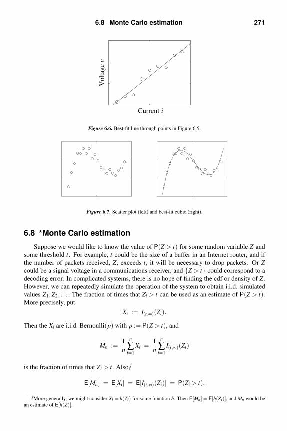
6.8 Monte Carlo estimation 271
Current i
Vo
ltag
e v
Figure 6.6. Best-fit line through points in Figure 6.5.
Figure 6.7. Scatter plot (left) and best-fit cubic (right).
6.8 Monte Carlo estimation
Suppose we would like to know the value of P(Z > t) for some random variable Z and
some threshold t. For example, t could be the size of a buffer in an Internet router, and if
the number of packets received, Z, exceeds t, it will be necessary to drop packets. Or Z
could be a signal voltage in a communications receiver, and Z > t could correspond to a
decoding error. In complicated systems, there is no hope of finding the cdf or density of Z.
However, we can repeatedly simulate the operation of the system to obtain i.i.d. simulated
values Z1,Z2, . . . . The fraction of times that Zi > t can be used as an estimate of P(Z > t).More precisely, put
Xi := I(t,∞)(Zi).
Then the Xi are i.i.d. Bernoulli(p) with p := P(Z > t), and
Mn :=1
n
n
∑i=1
Xi =1
n
n
∑i=1
I(t,∞)(Zi)
is the fraction of times that Zi > t. Also,j
E[Mn] = E[Xi] = E[I(t,∞)(Zi)] = P(Zi > t).
jMore generally, we might consider Xi = h(Zi) for some function h. Then E[Mn] = E[h(Zi)], and Mn would be
an estimate of E[h(Z)].

272 Statistics
Hence, we can even use the theory of confidence intervals to assess the quality of the prob-
ability estimate Mn, e.g.,
P(Z > t) = Mn ±Snyα/2√
nwith 100(1−α)% probability,
where yα/2 is chosen from Table 6.2.
Example 6.24. Suppose the Zi are i.i.d. exponential with parameter λ = 1, and we want
to estimate P(Z > 2). If M100 = 0.15 and S100 = 0.359, find the 95% confidence interval for
P(Z > 2).
Solution. The estimate is
P(Z > 2) = 0.15± 0.359(1.96)√100
= 0.15±0.07,
which corresponds to the interval [0.08,0.22]. This interval happens to contain the true
value e−2 = 0.135.
Caution. The foregoing does not work well if P(Z > t) is very small, unless n is cor-
respondingly large. The reason is that if P(Z > t) is small, it is likely that we will have
all X1, . . . ,Xn equal to zero. This forces both Mn and Sn to be zero too, which is not a
useful estimate. The probability that all Xi are zero is [1−P(Z > t)]n. For example, with
Z ∼ exp(1), P(Z > 7) = e−7 = 0.000912, and so [1−P(Z > 7)]100 = 0.9. In other words,
90% of simulations provide no information about P(Z > 7). In fact, using the values of Zi
of the preceding example to estimate P(Z > 7) did result in Mn = 0 and Sn = 0.
To estimate small probabilities without requiring n to be unreasonably large requires
more sophisticated strategies such as importance sampling [26], [47], [58]. The idea of
importance sampling is to redefine
Xi := I(t,∞)(Zi)fZ(Zi)
fZ(Zi)
,
where the Zi have a different density fZ
such that P(Z > t) is much bigger than P(Z > t).
If P(Z > t) is large, then very likely, many of the Xi will be nonzero. Observe that we still
have
E[Xi] =∫ ∞
−∞
[I(t,∞)(z)
fZ(z)
fZ(z)
]fZ(z)dz
=∫ ∞
−∞I(t,∞)(z) fZ(z)dz
= P(Z > t).
Thus, the Xi are no longer Bernoulli, but they still have the desired expected value. Our
choice for fZ
is
fZ(z) := esz fZ(z)/MZ(s), (6.33)

Notes 273
where the real parameter s is to be chosen later. This choice for fZ
is called a tilted or a
twisted density. Since integrating esz fZ(z) is just computing the moment generating func-
tion of Z, we need MZ(s) in the denominator above to make fZ
integrate to one. Our goal is
to adjust s so that a greater amount of probability is located near t. For Z ∼ exp(1),
fZ(z) =
esz fZ(z)
MZ(s)=
esze−z
1/(1− s)= (1− s)e−z(1−s).
In other words, Z ∼ exp(1− s). Hence, we can easily adjust s so that E[Z] = 7 by taking
s = 1−1/7 = 0.8571. We simulated n = 100 values of Zi and found M100 = 0.0007, S100 =0.002, and
P(Z > 7) = 0.0007± 0.002(1.96)√100
= 0.0007±0.0004.
This corresponds to the interval [0.0003,0.0011]. Thus, still using only 100 simulations, we
obtained a nonzero estimate and an informative confidence interval.
We also point out that even in the search for P(Z > 2), importance sampling can result
in a smaller confidence interval. In Example 6.24, the width of the confidence interval is
0.14. With importance sampling (still with n = 100), we found the width was only about
0.08.
Notes
6.1: Parameter estimators and their properties
Note 1. The limits in (6.4) are in the almost-sure sense of Section 14.3. By the first-
moment strong law of large numbers (stated following Example 14.15), Mn converges
almost surely to m. Similarly (1/n)∑ni=1 X2
i converges almost surely to σ2 + m2. Using
(6.3),
S2n =
n
n−1
[(1
n
n
∑i=1
X2i
)−M2
n
].
Then
limn→∞
S2n = lim
n→∞
n
n−1
[limn→∞
(1
n
n
∑i=1
X2i
)− lim
n→∞M2
n
]= 1 · [(σ2 +m2)−m2]
= σ2.
6.3: Confidence intervals for the mean – known variance
Note 2. The derivation of (6.10) used the formula
P(−y ≤ Yn ≤ y) = FYn(y)−FYn(−y),
which is valid when FYn is a continuous cdf. In the general case, it suffices to write
P(−y ≤ Yn ≤ y) = P(Yn = −y)+P(−y < Yn ≤ y) = P(Yn = −y)+FYn(y)−FYn(−y)
274 Statistics
and then show that P(Yn = −y) → 0. To do this fix any ε > 0 and write
P(Yn = −y) ≤ P(−y− ε < Yn ≤−y+ ε)
= FYn(−y+ ε)−FYn(−y− ε)
→ Φ(−y+ ε)−Φ(−y− ε), by the central limit theorem.
To conclude, write
Φ(−y+ ε)−Φ(−y− ε) = [Φ(−y+ ε)−Φ(−y)]+ [Φ(−y)−Φ(−y− ε)],
which goes to zero as ε → 0 on account of the continuity of Φ. Hence, P(−y ≤Yn ≤ y)→ 0.
6.4: Confidence intervals for the mean – unknown variance
Note 3. Since the Xi have finite mean and variance, they have finite second moment.
Thus, the X2i have finite first moment σ2 +m2. By the first-moment weak law of large num-
bers stated following Example 14.15, ∑ni=1 X2
i converges in probability to σ2 + m2. Using
(6.3), Example 14.2, and Problem 2 in Chapter 14, it follows that Sn converges in probabil-
ity to σ . Now appeal to the fact that if the cdf of Yn, say Fn, converges to a continuous cdf
F , and if Un converges in probability to 1, then
P(Yn ≤ yUn) → F(y).
This result, which is proved in Example 14.11, is a version of Slutsky’s theorem.
Note 4. The hypergeometric random variable arises in the following situation. We have
a collection of N items, d of which are defective. Rather than test all N items, we select at
random a small number of items, say n < N. Let Yn denote the number of defectives out the
n items tested. We show that
P(Yn = k) =
(d
k
)(N −d
n− k
)(
N
n
) , k = 0, . . . ,n.
We denote this by Yn ∼ hypergeometric(N,d,n).
Remark. In the typical case, d ≥ n and N − d ≥ n; however, if these conditions do
not hold in the above formula, it is understood that(
dk
)= 0 if d < k ≤ n, and
(N−dn−k
)= 0 if
n− k > N −d, i.e., if 0 ≤ k < n− (N −d).
For i = 1, . . . ,n, draw at random an item from the collection and test it. If the ith item
is defective, let Xi = 1, and put Xi = 0 otherwise. In either case, do not put the tested
item back into the collection (sampling without replacement). Then the total number of
defectives among the first n items tested is
Yn :=n
∑i=1
Xi.
We show that Yn ∼ hypergeometric(N,d,n).

Notes 275
Consider the case n = 1. Then Y1 = X1, and the chance of drawing a defective item at
random is simply the ratio of the number of defectives to the total number of items in the
collection; i.e., P(Y1 = 1) = P(X1 = 1) = d/N. Now in general, suppose the result is true
for some n ≥ 1. We show it is true for n+1. Use the law of total probability to write
P(Yn+1 = k) =n
∑i=0
P(Yn+1 = k|Yn = i)P(Yn = i). (6.34)
Since Yn+1 = Yn +Xn+1, we can use the substitution law to write
P(Yn+1 = k|Yn = i) = P(Yn +Xn+1 = k|Yn = i)
= P(i+Xn+1 = k|Yn = i)
= P(Xn+1 = k− i|Yn = i).
Since Xn+1 takes only the values zero and one, this last expression is zero unless i = k or
i = k−1. Returning to (6.34), we can write
P(Yn+1 = k) =k
∑i=k−1
P(Xn+1 = k− i|Yn = i)P(Yn = i). (6.35)
When i = k−1, the above conditional probability is
P(Xn+1 = 1|Yn = k−1) =d − (k−1)
N −n,
since given Yn = k−1, there are N −n items left in the collection, and of those, the number
of defectives remaining is d − (k−1). When i = k, the needed conditional probability is
P(Xn+1 = 0|Yn = k) =(N −d)− (n− k)
N −n,
since given Yn = k, there are N −n items left in the collection, and of those, the number of
nondefectives remaining is (N −d)− (n− k). If we now assume that Yn ∼ hypergeometric
(N,d,n), we can expand (6.35) to get
P(Yn+1 = k) =d − (k−1)
N −n·
(d
k−1
)(N −d
n− (k−1)
)(
N
n
)
+(N −d)− (n− k)
N −n·
(d
k
)(N −d
n− k
)(
N
n
) .
It is a simple calculation to see that the first term on the right is equal to
(1− k
n+1
)·
(d
k
)(N −d
[n+1]− k
)(
N
n+1
) ,
276 Statistics
and the second term is equal to
k
n+1·
(d
k
)(N −d
[n+1]− k
)(
N
n+1
) .
Thus, Yn+1 ∼ hypergeometric(N,d,n+1).
Problems
6.1: Parameter estimators and their properties
1. Use formula (6.3) to show that S2n is unbiased, assuming the Xi are uncorrelated.
2. (a) If X1,X2, . . . are i.i.d. Rayleigh(λ ), find an unbiased, strongly consistent estima-
tor of λ .
(b) MATLAB. Modify the MATLAB code below to generate n = 1000 Rayleigh(λ )random variables with λ = 3, and use your answer in part (a) to estimate λ from
the data.
n = 1000;
U = rand(1,n);
X = sqrt(-2*log(U)); % X is Rayleigh(1)
X = 3*X; % Make X Rayleigh(3)
(c) MATLAB. Since E[Xi] = λ√
π/2, and since we know the value of λ used to
generate the data, we can regard π as the unknown parameter. Modify your
code in part (b) to estimate π from simulation data with n = 100000. What is
your estimate of π?
3. (a) If X1,X2, . . . are i.i.d. gamma(p,λ ), where λ is known, find an unbiased, strongly
consistent estimator of p.
(b) MATLAB. Modify the MATLAB code below to generate n = 1000 chi-squared
random variables with k = 5 degrees of freedom, and use your answer in part (a)
to estimate k from the data. Remember, chi-squared with k degrees of freedom
is the same as gamma(k/2,1/2). Recall also Problems 46 and 55 in Chapter 4.
n = 1000;
U = randn(5,n); % U is N(0,1)
U2 = U.ˆ2; % U2 is chi-squared
% with one degree of freedom
X = sum(U2); % column sums are
% chi-squared with 5 degrees of freedom
Here the expression U.ˆ2 squares each element of the matrix U.
4. (a) If X1,X2, . . . are i.i.d. noncentral chi-squared with k degrees of freedom and non-
centrality parameter λ 2, where k is known, find an unbiased, strongly consistent
estimator of λ 2. Hint: Use Problem 65(c) in Chapter 4.

Problems 277
(b) MATLAB. Modify the following MATLAB code to generate n = 1000 noncentral
chi-squared random variables with k = 5 degrees of freedom, and noncentrality
parameter λ 2 = 4, and use your answer in part (a) to estimate λ 2 from the data.
n = 1000;
U = randn(5,n); % U is N(0,1)
U = U + 2/sqrt(5); % U is N(m,1)
% with m = 2/sqrt(5)
U2 = U.ˆ2; % U2 is noncentral
% chi-squared with one degree of freedom
% and noncentrality parameter 4/5
X = sum(U2); % column sums are
% noncentral chi-squared with 5 degrees
% of freedom and noncentrality parameter 4
Here the expression U.ˆ2 squares each element of the matrix U.
5. (a) If X1,X2, . . . are i.i.d. gamma(p,λ ), where p is known, find a strongly consistent
estimator of λ .
(b) MATLAB. Modify the following MATLAB code to generate n = 1000 gamma
random variables with p = 3 and λ = 1/5, and use your answer in part (a) to
estimate λ from the data. Recall Problem 55 in Chapter 4.
n = 1000;
U = rand(3,n); % U is uniform(0,1)
V = -log(U); % V is exp(1)
V = 5*V; % V is exp(1/5)
X = sum(V); % column sums are Erlang(3,1/5)
Remark. This suggests a faster method to simulate chi-squared random variables than
the one used in Problem 3. If k is even, then the chi-squared is Erlang(k/2,1/2). If k
is odd, then the chi-squared is equal to the sum of an Erlang(k/2−1/2,1/2) and the
square of a single N(0,1).
6. (a) If X1,X2, . . . are i.i.d. Laplace(λ ), find a strongly consistent estimator of λ .
(b) MATLAB. Modify the MATLAB code below to generate n = 1000 Laplace(λ )random variables with λ = 2, and use your answer in part (a) to estimate λ from
the data. Recall Problem 54 in Chapter 4.
n = 1000;
U1 = rand(1,n); % U1 is uniform(0,1)
V1 = -log(U1)/2; % V1 is exp(2)
U2 = rand(1,n); % U2 is uniform(0,1)
V2 = -log(U2)/2; % V2 is exp(2)
X = V1-V2; % X is Laplace(2)
7. (a) If X1,X2, . . . are i.i.d. gamma(p,λ ), find strongly consistent estimators of p and
λ . Hint: Consider both E[Xi] and E[X2i ].
(b) MATLAB. Modify the MATLAB code in Problem 5 to generate n = 1000 gamma
random variables with p = 3 and λ = 1/5, and use your answer in part (a) to
estimate p and λ from the data.

278 Statistics
8. If X1,X2, . . . are i.i.d. generalized gamma with parameters p, λ , and q, where p and
q are known, find a strongly consistent estimator of λ . (The generalized gamma was
defined in Problem 21 in Chapter 5.) Hint: Consider E[Xq].
9. In the preceding problem, assume that only q is known and that both p and λ are
unknown. Find strongly consistent estimators of p and λ .
6.2: Histograms
10. MATLAB. Use the following MATLAB code to generate n = 1000 N(0,1) random
variables, plot a histogram and the true density over it.
n = 1000;
X = randn(1,n); % X is N(0,1)
nbins = 15;
minX = min(X);
maxX = max(X);
e = linspace(minX,maxX,nbins+1);
H = histc(X,e);
H(nbins) = H(nbins)+H(nbins+1);
H = H(1:nbins); % resize H
bw = (maxX-minX)/nbins; % bin width
a = e(1:nbins); % left edge sequence
b = e(2:nbins+1); % right edge sequence
bin_centers = (a+b)/2; % bin centers
bar(bin_centers,H/(bw*n),’hist’)
hold on
t = linspace(min(X),max(X),150);
y = exp(-t.ˆ2/2)/sqrt(2*pi);
plot(t,y)
hold off
11. MATLAB. Modify the code in Problem 2 to plot a histogram of X, and using the
estimated parameter value, draw the density on top of the histogram. If you studied
the subsection on the chi-squared test, print out the chi-squared statistic Z, the critical
value zα for α = 0.05, and whether or not the test accepts the density as a good fit to
the data.
12. MATLAB. Modify the code in Problem 3 to plot a histogram of X, and using the
estimated parameter value, draw the density on top of the histogram. If you studied
the subsection on the chi-squared test, print out the chi-squared statistic Z, the critical
value zα for α = 0.05, and whether or not the test accepts the density as a good fit to
the data.
13. MATLAB. Modify the code in Problem 4 to plot a histogram of X, and using the esti-
mated parameter value, draw the density on top of the histogram. Use the noncentral
chi-squared density formula given in Problem 25(c) in Chapter 5. If you studied the
subsection on the chi-squared test, print out the chi-squared statistic Z, the critical
value zα for α = 0.05, and whether or not the test accepts the density as a good fit to
the data.

Problems 279
14. MATLAB. Modify the code in Problem 5 to plot a histogram of X, and using the
estimated parameter value, draw the density on top of the histogram. If you studied
the subsection on the chi-squared test, print out the chi-squared statistic Z, the critical
value zα for α = 0.05, and whether or not the test accepts the density as a good fit to
the data.
15. MATLAB. Modify the code in Problem 6 to plot a histogram of X, and using the
estimated parameter value, draw the density on top of the histogram. If you studied
the subsection on the chi-squared test, print out the chi-squared statistic Z, the critical
value zα for α = 0.05, and whether or not the test accepts the density as a good fit to
the data.
16. Show thatH j −np j√
np j
has zero mean and variance 1− p j.
6.3: Confidence intervals for the mean – known variance
17. Let F be the cdf any even density function f . Show that F(−x) = 1 − F(x). In
particular, note that the standard normal density is even.
18. If σ2 = 4 and n = 100, how wide is the 99% confidence interval? How large would n
have to be to have a 99% confidence interval of width less than or equal to 1/4?
19. Let W1,W2, . . . be i.i.d. with zero mean and variance 4. Let Xi = m +Wi, where m is
an unknown constant. If M100 = 14.846, find the 95% confidence interval.
20. Let Xi = m +Wi, where m is an unknown constant, and the Wi are i.i.d. Cauchy with
parameter 1. Find δ > 0 such that the probability is 2/3 that the confidence interval
[Mn −δ ,Mn +δ ] contains m; i.e., find δ > 0 such that
P(|Mn −m| ≤ δ ) = 2/3.
Hints: Since E[W 2i ] = ∞, the central limit theorem does not apply. However, you
can solve for δ exactly if you can find the cdf of Mn −m. The cdf of Wi is F(w) =1π tan−1(w)+1/2, and the characteristic function of Wi is E[e jνWi ] = e−|ν |.
21. MATLAB. Use the following script to generate a vector of n = 100 Gaussian random
numbers with mean m = 3 and variance one. Then compute the 95% confidence
interval for the mean.
n = 100
X = randn(1,n); % N(0,1) random numbers
X = X + 3; % Change mean to 3
Mn = mean(X)
sigma = 1
delta = 1.96*sigma/sqrt(n)
fprintf(’The 95%% confidence interval is [%g,%g]\n’, ...
Mn-delta,Mn+delta)

280 Statistics
6.4: Confidence intervals for the mean – unknown variance
22. Let X1,X2, . . . be i.i.d. random variables with unknown, finite mean m and variance
σ2. If M100 = 10.083 and S100 = 0.568, find the 95% confidence interval for the
population mean.
23. Suppose that 100 engineering freshmen are selected at random and X1, . . . ,X100 are
their times (in years) to graduation. If M100 = 4.422 and S100 = 0.957, find the 93%
confidence interval for their expected time to graduate.
24. From a batch of N = 10000 computers, n = 100 are sampled, and 10 are found de-
fective. Estimate the number of defective computers in the total batch of 10000, and
give the margin of error for 90% probability if S100 = 0.302.
25. You conduct a presidential preference poll by surveying 3000 voters. You find that
1559 (more than half) say they plan to vote for candidate A, and the others say they
plan to vote for candidate B. If S3000 = 0.500, are you 90% sure that candidate A will
win the election? Are you 99% sure?
26. From a batch of 100000 airbags, 500 are sampled, and 48 are found defective. Esti-
mate the number of defective airbags in the total batch of 100000, and give the margin
of error for 94% probability if S100 = 0.295.
27. A new vaccine has just been developed at your company. You need to be 97% sure
that side effects do not occur more than 10% of the time.
(a) In order to estimate the probability p of side effects, the vaccine is tested on 100
volunteers. Side effects are experienced by 6 of the volunteers. Using the value
S100 = 0.239, find the 97% confidence interval for p if S100 = 0.239. Are you
97% sure that p ≤ 0.1?
(b) Another study is performed, this time with 1000 volunteers. Side effects occur
in 71 volunteers. Find the 97% confidence interval for the probability p of side
effects if S1000 = 0.257. Are you 97% sure that p ≤ 0.1?
28. Packet transmission times on a certain Internet link are independent and identically
distributed. Assume that the times have an exponential density with mean µ .
(a) Find the probability that in transmitting n packets, at least one of them takes
more than t seconds to transmit.
(b) Let T denote the total time to transmit n packets. Find a closed-form expression
for the density of T .
(c) Your answers to parts (a) and (b) depend on µ , which in practice is unknown
and must be estimated. To estimate the expected transmission time, n = 100
packets are sent, and the transmission times T1, . . . ,Tn recorded. It is found that
the sample mean M100 = 1.994, and sample standard deviation S100 = 1.798,
where
Mn :=1
n
n
∑i=1
Ti and S2n :=
1
n−1
n
∑i=1
(Ti −Mn)2.
Find the 95% confidence interval for the expected transmission time.

Problems 281
29. MATLAB. Use the following script to generate n = 100 Gaussian random variables
with mean m = 5 and variance σ2 = 9. Compute the 95% confidence interval for the
mean.
n = 100
X = randn(1,n); % N(0,1) random numbers
m = 5
sigma = 3
X = sigma*X + m; % Change to N(m,sigmaˆ2)
Mn = mean(X)
Sn = std(X)
delta = 1.96*Sn/sqrt(n)
fprintf(’The 95%% confidence interval is [%g,%g]\n’, ...
Mn-delta,Mn+delta)
6.5: Confidence intervals for Gaussian data
30. If X1, . . . ,Xn are i.i.d. N(m,σ2), show that Yn = (Mn −m)/(σ/√
n) is N(0,1). Hint:
Recall Problem 55(a) in Chapter 4.
31. Let W1,W2, . . . be i.i.d. N(0,σ2) with σ2 unknown. Let Xi = m +Wi, where m is an
unknown constant. Suppose M10 = 14.832 and S10 = 1.904. Find the 95% confidence
interval for m.
32. Let X1,X2, . . . be i.i.d. N(0,σ2) with σ2 unknown. Find the 95% confidence interval
for σ2 if V 2100 = 4.413.
33. Let W1,W2, . . . be i.i.d. N(0,σ2) with σ2 unknown. Let Xi = m +Wi, where m is an
unknown constant. Find the 95% confidence interval for σ2 if S2100 = 4.736.
6.6: Hypothesis tests for the mean
34. In a two-sided test of the null hypothesis m = m0 against the alternative hypothesis
m = m0, the statistic Zn = −1.80 is observed. Is the null hypothesis accepted at the
0.05 significance level? If we are doing a one-sided test of the null hypothesis m > m0
against the alternative hypothesis m ≤ m0 and Zn = −1.80 is observed, do we accept
the null hypothesis at the 0.05 significance level?
35. Show that if Φ(−y) = α , then Φ(y) = 1−α .
36. An Internet service provider claims that a certain link has a packet loss probability of
at most p0. To test the claim, you send n packets and let Xi = 1 if the ith packet is
lost and Xi = 0 otherwise. Mathematically, the claim is that P(Xi = 1) = E[Xi] ≤ p0.
You compute the statistic Zn in (6.25) and find Zn = 1.50. (a) The Internet service
provider takes E[Xi] ≤ p0 as the null hypothesis. On the basis of Zn = 1.50, is the
claim E[Xi] ≤ p0 accepted at the 0.06 significance level? (b) Being skeptical, you
take E[Xi] > p0 as the null hypothesis. On the basis of the same data Zn = 1.50 and
significance level 0.06, do you accept the Internet service provider’s claim?

282 Statistics
37. A computer vendor claims that the average waiting time on its technical support hot-
line is at most m0 minutes. However, a consumer group claims otherwise based on the
following analysis. The consumer group made n calls, letting Xi denote the waiting
time on the ith call. It computed the statistic Zn in (6.25) and found that Zn = 1.30.
Assuming that the group used a significance level from Table 6.6, what critical value
did they use?
38. A drug company claims that its new medicine relieves pain for more than m0 hours
on average. To justify this claim, the company tested its medicine in n people. The
ith person reported pain relief for Xi hours. The company computed the statistic Zn
in (6.25) and found that Zn = −1.60. Can the company justify its claim if a 0.05
significance level is used? Explain your answer.
6.7: Regression and curve fitting
39. For the linear regression problem in Example 6.23, show that the minimum sum of
squared errors, e(g), is equal to SYY − S2xY /Sxx, where this notation is defined in Ex-
amples 6.21and 6.23.
40. Regression and conditional expectation. Let X and W be independent random
variables with W having zero mean. If Y := g(X)+W , show that E[Y |X = x] = g(x).
41. MATLAB. Use the script below to plot the best-fit polynomial of degree p = 2 to the
data. Note that the last two lines compute the sum of squared errors.
x = [ 1 2 3 4 5 6 7 8 9 ];
Y = [ 0.2631 0.2318 0.1330 0.6751 1.3649 1.5559, ...
2.3184 3.7019 5.2953];
p = 2;
a = polyfit(x,Y,p)
subplot(2,2,1); % Put multiple plots in same fig.
plot(x,Y,’o’) % Plot pnts only; do not connect.
axis([0 10 -1 7]); % Force plot to use this scale.
subplot(2,2,2)
t=linspace(0,10,50); % For plotting g from 0 to 10
gt = polyval(a,t); % at 50 points.
plot(x,Y,’o’,t,gt)
axis([0 10 -1 7]); % Use same scale as prev. plot.
gx = polyval(a,x); % Compute g(x_k) for each k.
sse = sum((Y-gx).ˆ2) % Compute sum of squared errors.
Do you get a smaller sum of squared errors with p = 3? What about p = 7 and p = 8?
Is it a good idea to continue increasing p?
42. MATLAB. You can use the methods of this section to find polynomial approximations
to nonpolynomial functions. Use the following script to plot the best-fit polynomial
of degree p = 4 to sin(x) on [0,2π] based on five equal-spaced samples.
T = 2*pi;
x = linspace(0,T,5);

Problems 283
Y = sin(x);
p = 4;
a = polyfit(x,Y,p);
t = linspace(0,T,50);
st = sin(t);
gt = polyval(a,t);
subplot(2,1,1)
plot(t,st,t,gt)
subplot(2,1,2)
plot(t,st-gt) % Plot error curve sin(t)-g(t).
Since the values of sin(x) for π/2 ≤ x ≤ 2π can be computed using values of sin(x)for 0 ≤ x ≤ π/2, modify the above code by setting T = π/2. Do you get a better
approximation now that you have restricted attention to [0,π/2]?
43. MATLAB. The data shown at the left in Figure 6.8 appears to follow a power law of
the form c/tq, where c and q are to be estimated. Instead of fitting a polynomial to
the data, consider taking logarithms to get
ln(c/tq) = lnc−q ln t.
Let us denote the points at the left in Figure 6.8 by (tk,Zk), and put Yk := lnZk and
xk := ln tk. A plot of (xk,Yk) and the best-fit straight line through it are shown at the
right in Figure 6.8. How would you estimate c and q from the best-fit straight line?
Use your answer to fill in the two blanks in the code below. Then run the code to see
a comparison of the best cubic fit to the data and a plot of c/t q. If you change from
a cubic to higher-order polynomials, can you get a better plot than with the log–log
method?
t = [ 1 1.4444 1.8889 2.3333 2.7778 3.2222 3.6667, ...
4.1111 4.5556 5 ];
Z = [ 1.0310 0.6395 0.3404 0.2873 0.2090 0.1147, ...
0.2016 0.1192 0.1297 0.0536 ];
x = log(t);
Y = log(Z);
subplot(2,2,1)
a = polyfit(t,Z,3); % Fit cubic to data (t_k,Z_k).
1 2 3 4 50
1
0 1 2
−3
−2
−1
0
Figure 6.8. Data (tk,Zk) for Problem 43 (left). Log of data (ln tk, lnZk) and best-fit straight line (right).

284 Statistics
u = linspace(1,5,50);
v = polyval(a,u);
plot(t,Z,’o’,u,v) % Plot (t_k,Z_k) & cubic.
axis([1 5 0 1.1])
title(’Best-fit cubic to data’)
subplot(2,2,2)
a = polyfit(x,Y,1); % Fit st. line to (x_k,Y_k).
u = linspace(0,2,2);
v = polyval(a,u);
plot(x,Y,’o’,u,v) % Plot (x_k,Y_k) & st. line.
title(’Best-fit straight line to (ln(t_k),ln(Z_k))’)
subplot(2,2,3)
qhat = _____
chat = _____
u = linspace(1,5,50);
v = chat./u.ˆqhat;
plot(t,Z,’o’,u,v)
axis([1 5 0 1.1]) % Plot (t_k,Z_k) & c/tˆq using estimates.
title(’(estimate of c)/t\ˆ(estimate of q)’)
6.8: Monte Carlo estimation
44. For the tilted density fZ(z) = esz fZ(z)/MZ(s), show that
fZ(z)
fZ(z)
= e−szMZ(s).
45. If Z ∼ N(0,1), find the tilted density fZ(z) = esz fZ(z)/MZ(s). How would you choose
s to make E[Z] = t?
46. If Z ∼ gamma(p,λ ), find the tilted density fZ(z) = esz fZ(z)/MZ(s). How would you
choose s to make E[Z] = t? Note that the gamma includes the Erlang and chi-squared
as special cases.
47. MATLAB. If Z ∼ N(0,1), use the following script to estimate P(Z > t) for t = 5 with
95% confidence.
t = 5;
s = t;
n = 100;
Z = randn(1,n); % N(0,1) random numbers
Zt = Z+s; % change mean to s
X = zeros(1,n);
i = find(Zt>t);
X(i) = exp(-s*Zt(i))*exp(sˆ2/2);
Mn = mean(X);
Sn = std(X);
delta = Sn*1.96/sqrt(n);
fprintf(’M(%7i) = %g +/- %g, Sn = %g\n’,...
Exam preparation 285
n,Mn,delta,Sn)
fprintf(’The 95%% confidence interval is [%g,%g]\n’, ...
Mn-delta,Mn+delta)
48. It is also possible to tilt probability mass functions. The formula for tilting the prob-
ability mass function of a discrete random variable taking values zi is
pZ(zi) := eszi pZ(zi)/MZ(s).
If Z ∼ Bernoulli(p), find the tilted pmf pZ(i) for i = 0,1.
Exam preparation
You may use the following suggestions to prepare a study sheet, including formulas men-
tioned that you have trouble remembering. You may also want to ask your instructor for
additional suggestions.
6.1. Parameter estimators and their properties. Know the sample mean (6.1) and sam-
ple variance (6.2). Know the meaning of unbiased and the fact that the sample mean
and sample variance are unbiased estimators of the population (or ensemble) mean
and variance. Know how to derive estimators of parameters that are related to mo-
ments.
6.2. Histograms. Understand how the pieces of code in the text can be collected to solve
problems in MATLAB. Be able to explain how the chi-squared test works.
6.3. Confidence intervals for the mean – known variance. Know formulas (6.11) and
(6.12) and how to find yα/2 from Table 6.2.
6.4. Confidence intervals for the mean – unknown variance. Know formulas (6.16)
and (6.17) and how to find yα/2 from Table 6.2. Know how to apply these results to
estimating the number of defective items in a lot.
6.5. Confidence intervals for Gaussian data. For estimating the mean with unknown
variance, use formulas (6.16) and (6.17), except that yα/2 is chosen from Table 6.3.
To estimate the variance when the mean is known, use (6.19) with and u chosen
from Table 6.4. To estimate the variance when the mean is unknown, use (6.20) with
and u chosen from Table 6.4.
6.6. Hypothesis tests for the mean. Know when to use the appropriate statistic (6.24)
or (6.25). For testing m = m0, use the critical value yα/2 in Table 6.6; accept the
hypothesis if |Zn| ≤ yα/2. For testing m ≤ m0, use the critical value yα in Table 6.6;
accept the hypothesis if Zn ≤ yα . For testing m > m0, use the critical value −yα ,
where yα is from Table 6.6; accept the hypothesis if Zn > −yα .
6.7. Regression and curve fitting. Regression is another name for curve fitting. In the
model (6.29), the Wk can account for either measurement noise or inaccuracies in g(x).To give an example of the latter case, consider approximating sin(x) by a polynomial
g(x). If we put Wk := sin(xk)−g(xk) and Yk := sin(xk), then (6.29) holds.
6.8. Monte Carlo estimation. If you are not using importance sampling or some sophis-
ticated technique, and you want to estimate a very small probability, you will need a

286 Statistics
correspondingly large number of simulations. Know the formula for the tilted density
(6.33).
Work any review problems assigned by your instructor. If you finish them, re-work your
homework assignments.

7
Bivariate random variables
The main focus of this chapter is the study of pairs of continuous random variables
that are not independent. In particular, conditional probability and conditional expectation
along with corresponding laws of total probability and substitution are studied. These tools
are used to compute probabilities involving the output of systems with two (and sometimes
three or more) random inputs.
7.1 Joint and marginal probabilities
Consider the following functions of two random variables X and Y ,
X +Y, XY, max(X ,Y ), and min(X ,Y ).
For example, in a telephone channel the signal X is corrupted by additive noise Y . In a
wireless channel, the signal X is corrupted by fading (multiplicative noise). If X and Y are
the traffic rates at two different routers of an Internet service provider, it is desirable to have
these rates less than the router capacity, say u; i.e., we want max(X ,Y ) ≤ u. If X and Y
are sensor voltages, we may want to trigger an alarm if at least one of the sensor voltages
falls below a threshold v; e.g., if min(X ,Y ) ≤ v. We now show that the cdfs of these four
functions of X and Y can be expressed in the form P((X ,Y ) ∈ A) for various sets1 A ⊂ IR2.
We then argue that such probabilities can be computed in terms of the joint cumulative
distribution function to be defined later in the section.
Before proceeding, you should re-work Problem 6 in Chapter 1.
Example 7.1 (signal in additive noise). A random signal X is transmitted over a channel
subject to additive noise Y . The received signal is Z = X +Y . Express the cdf of Z in the
form P((X ,Y ) ∈ Az) for some set Az.
Solution. Write
FZ(z) = P(Z ≤ z) = P(X +Y ≤ z) = P((X ,Y ) ∈ Az),
where
Az := (x,y) : x+ y ≤ z.Since x + y ≤ z if and only if y ≤ −x + z, it is easy to see that Az is the shaded region in
Figure 7.1.
Example 7.2 (signal in multiplicative noise). A random signal X is transmitted over a
channel subject to multiplicative noise Y . The received signal is Z = XY . Express the cdf
of Z in the form P((X ,Y ) ∈ Az) for some set Az.
287

288 Bivariate random variables
z
zx
y
Figure 7.1. The shaded region is Az = (x,y) : x+ y ≤ z. The equation of the diagonal line is y = −x+ z.
Solution. Write
FZ(z) = P(Z ≤ z) = P(XY ≤ z) = P((X ,Y ) ∈ Az),
where now Az := (x,y) : xy ≤ z. To see how to sketch this set, we are tempted to write
Az = (x,y) : y ≤ z/x, but this would be wrong because if x < 0 we need to reverse the
inequality. To get around this problem, it is convenient to partition Az into two disjoint
regions, Az = A+z ∪A−
z , where
A+z := Az ∩(x,y) : x > 0 and A−
z := Az ∩(x,y) : x < 0.
Thus, A+z and A−
z are similar to Az, but now we know the sign of x in each set. Hence, it is
correct to write
A+z := (x,y) : y ≤ z/x and x > 0
and
A−z := (x,y) : y ≥ z/x and x < 0.
These regions are sketched in Figure 7.2.
Az+
−Azx
y
Figure 7.2. The curve is y = z/x. The shaded region to the left of the vertical axis is A−z = (x,y) : y ≥ z/x, x < 0,
and the shaded region to the right of the vertical axis is A+z = (x,y) : y ≤ z/x, x > 0. The sketch is for the case
z > 0. How would the sketch need to change if z = 0 or if z < 0?
Example 7.3. Express the cdf of U := max(X ,Y ) in the form P((X ,Y ) ∈ Au) for some
set Au.

7.1 Joint and marginal probabilities 289
Solution. To find the cdf of U , begin with
FU (u) = P(U ≤ u) = P(max(X ,Y ) ≤ u).
Since the larger of X and Y is less than or equal to u if and only if X ≤ u and Y ≤ u,
P(max(X ,Y ) ≤ u) = P(X ≤ u,Y ≤ u) = P((X ,Y ) ∈ Au),
where Au := (x,y) : x ≤ u and y ≤ u is the shaded “southwest” region shown in Fig-
ure 7.3(a).
(a) (b)
v
vx
y
x
y
u
u
Figure 7.3. (a) Southwest region (x,y) : x ≤ u and y ≤ u. (b) The region (x,y) : x ≤ v or y ≤ v.
Example 7.4. Express the cdf of V := min(X ,Y ) in the form P((X ,Y ) ∈ Av) for some
set Av.
Solution. To find the cdf of V , begin with
FV (v) = P(V ≤ v) = P(min(X ,Y ) ≤ v).
Since the smaller of X and Y is less than or equal to v if and only either X ≤ v or Y ≤ v,
P(min(X ,Y ) ≤ v) = P(X ≤ v or Y ≤ v) = P((X ,Y ) ∈ Av),
where Av := (x,y) : x ≤ v or y ≤ v is the shaded region shown in Figure 7.3(b).
Product sets and marginal probabilities
The Cartesian product of two univariate sets B and C is defined by
B×C := (x,y) : x ∈ B and y ∈C.
In other words,
(x,y) ∈ B×C ⇔ x ∈ B and y ∈C.

290 Bivariate random variables
For example, if B = [1,3] and C = [0.5,3.5], then B×C is the rectangle
[1,3]× [0.5,3.5] = (x,y) : 1 ≤ x ≤ 3 and 0.5 ≤ y ≤ 3.5,
which is illustrated in Figure 7.4(a). In general, if B and C are intervals, then B×C is a
rectangle or square. If one of the sets is an interval and the other is a singleton, then the
product set degenerates to a line segment in the plane. A more complicated example is
shown in Figure 7.4(b), which illustrates the product([1,2]∪ [3,4]
)× [1,4]. Figure 7.4(b)
also illustrates the general result that × distributes over ∪; i.e., (B1 ∪B2)×C = (B1 ×C)∪(B2 ×C).
0
1
2
3
4
0 1 2 3 4
( a )
0
1
2
3
4
0 1 2 3 4
( b )
Figure 7.4. The Cartesian products (a) [1,3]× [0.5,3.5] and (b)([1,2]∪ [3,4]
)× [1,4].
Using the notion of product set,
X ∈ B,Y ∈C = ω ∈ Ω : X(ω) ∈ B and Y (ω) ∈C= ω ∈ Ω : (X(ω),Y (ω)) ∈ B×C,
for which we use the shorthand
(X ,Y ) ∈ B×C.We can therefore write
P(X ∈ B,Y ∈C) = P((X ,Y ) ∈ B×C).
The preceding expression allows us to obtain the marginal probability P(X ∈ B) as
follows. First, for any event E, we have E ⊂ Ω, and therefore, E = E ∩Ω. Second, Y is
assumed to be a real-valued random variable, i.e., Y (ω)∈ IR for all ω . Thus, Y ∈ IR= Ω.
Now write
P(X ∈ B) = P(X ∈ B∩Ω)
= P(X ∈ B∩Y ∈ IR)= P(X ∈ B,Y ∈ IR)
= P((X ,Y ) ∈ B× IR).
Similarly,
P(Y ∈C) = P((X ,Y ) ∈ IR×C). (7.1)

7.1 Joint and marginal probabilities 291
Joint cumulative distribution functions
The joint cumulative distribution function of X and Y is defined by
FXY (x,y) := P(X ≤ x,Y ≤ y).
We can also write this using a Cartesian product set as
FXY (x,y) = P((X ,Y ) ∈ (−∞,x]× (−∞,y]).
In other words, FXY (x,y) is the probability that (X ,Y ) lies in the southwest region shown in
Figure 7.5(a).
( , )x y
a( ) b( )
c
d
a b
Figure 7.5. (a) Southwest region (−∞,x]× (−∞,y]. (b) Rectangle (a,b]× (c,d].
The joint cdf is important because it can be used to compute P((X ,Y ) ∈ A) for any set
A. For example, you will show in Problems 3 and 4 that
P(a < X ≤ b,c < Y ≤ d),
which is the probability that (X ,Y ) belongs to the rectangle (a,b]× (c,d] shown in Fig-
ure 7.5(b), is given by the rectangle formula2
FXY (b,d)−FXY (a,d)−FXY (b,c)+FXY (a,c). (7.2)
Example 7.5. If X and Y have joint cdf FXY , find the joint cdf of U := max(X ,Y ) and
V := min(X ,Y ).
Solution. Begin with
FUV (u,v) = P(U ≤ u,V ≤ v).
From Example 7.3, we know that U = max(X ,Y ) ≤ u if and only if (X ,Y ) lies in the
southwest region shown in Figure 7.3(a). Similarly, from Example 7.4, we know that
V = min(X ,Y ) ≤ v if and only if (X ,Y ) lies in the region shown in Figure 7.3(b). Hence,
U ≤ u and V ≤ v if and only if (X ,Y ) lies in the intersection of these two regions. The form
of this intersection depends on whether u > v or u ≤ v. If u ≤ v, then the southwest region

292 Bivariate random variables
u
u
v
vx
y
Figure 7.6. The intersection of the shaded regions of Figures 7.3(a) and 7.3(b) when v < u.
in Figure 7.3(a) is a subset of the region in Figure 7.3(b). Their intersection is the smaller
set, and so
P(U ≤ u,V ≤ v) = P(U ≤ u) = FU (u) = FXY (u,u), u ≤ v.
If u > v, the intersection is shown in Figure 7.6. Since this region can be obtained by
removing the rectangle (v,u]× (v,u] from the southwest region (−∞,u]× (−∞,u],
P(U ≤ u,V ≤ v) = FXY (u,u)−P(v < X ≤ u,v < Y ≤ u).
This last probability is given by the rectangle formula (7.2),
FXY (u,u)−FXY (v,u)−FXY (u,v)+FXY (v,v).
Hence,
FUV (u,v) = FXY (v,u)+FXY (u,v)−FXY (v,v), u > v.
The complete joint cdf formula is
FUV (u,v) =
FXY (u,u), u ≤ v,
FXY (v,u)+FXY (u,v)−FXY (v,v), u > v.
Marginal cumulative distribution functions
It is possible to obtain the marginal cumulative distributions FX and FY directly from
FXY by setting the unwanted variable to ∞. More precisely, it can be shown that3
FX (x) = limy→∞
FXY (x,y) =: FXY (x,∞), (7.3)
and
FY (y) = limx→∞
FXY (x,y) =: FXY (∞,y). (7.4)

7.1 Joint and marginal probabilities 293
Example 7.6. Use the joint cdf FUV derived in Example 7.5 to compute the marginal
cdfs FU and FV .
Solution. To compute
FU (u) = limv→∞
FUV (u,v),
observe that as v becomes large, eventually it will be greater than u. For v ≥ u, FUV (u,v) =FXY (u,u). In other words, for v ≥ u, FUV (u,v) is constant and no longer depends on v.
Hence, the limiting value is also FXY (u,u).To compute
FV (v) = limu→∞
FUV (u,v),
observe that as u becomes large, eventually it will be greater than v. For u > v,
FUV (u,v) = FXY (v,u)+FXY (u,v)−FXY (v,v)
→ FX (v)+FY (v)−FXY (v,v)
as u → ∞.
To check the preceding result, we compute FU and FV directly. From Example 7.3,
FU (u) = P(max(X ,Y ) ≤ u) = P(X ≤ u,Y ≤ u) = FXY (u,u).
From Example 7.4,
FV (v) = P(X ≤ v or Y ≤ v).
By the inclusion–exclusion formula (1.12),
FV (v) = P(X ≤ v)+P(Y ≤ v)−P(X ≤ v,Y ≤ v)
= FX (v)+FY (v)−FXY (v,v).
The foregoing shows how to compute the cdfs of max(X ,Y ) and min(X ,Y ) in terms of
the joint cdf FXY . Computation of the cdfs of X +Y and XY in terms of FXY can only be
done in a limiting sense by chopping up the regions Az of Figures 7.1 and 7.2 into small
rectangles, applying the rectangle formula (7.2) to each rectangle, and adding up the results.
To conclude this subsection, we give another application of (7.3) and (7.4).
Example 7.7. If
FXY (x,y) =
⎧⎨⎩ y+ e−x(y+1)
y+1− e−x, x,y > 0,
0, otherwise,
find both of the marginal cumulative distribution functions, FX (x) and FY (y).
Solution. For x,y > 0,
FXY (x,y) =y
y+1+
1
y+1· e−x(y+1)− e−x.

294 Bivariate random variables
01
23
45
01
23
450
1
x−axisy−axis
Figure 7.7. Joint cumulative distribution function FXY (x,y) of Example 7.7.
(This surface is shown in Figure 7.7.) Hence, for x > 0,
limy→∞
FXY (x,y) = 1+0 ·0− e−x = 1− e−x.
For x ≤ 0, FXY (x,y) = 0 for all y. So, for x ≤ 0, limy→∞
FXY (x,y) = 0. The complete formula
for the marginal cdf of X is
FX (x) =
1− e−x, x > 0,
0, x ≤ 0,(7.5)
which implies X ∼ exp(1). Next, for y > 0,
limx→∞
FXY (x,y) =y
y+1+
1
y+1·0−0 =
y
y+1.
We then see that the marginal cdf of Y is
FY (y) =
y/(y+1), y > 0,
0, y ≤ 0.(7.6)
Independent random variables
Recall that X and Y are independent if and only if P(X ∈ B,Y ∈C) = P(X ∈ B)P(Y ∈C)for all sets B and C. In terms of product sets, this says that
P((X ,Y ) ∈ B×C) = P(X ∈ B)P(Y ∈C). (7.7)
In other words, the probability that (X ,Y ) belongs to a Cartesian-product set is the product
of the individual probabilities. In particular, if X and Y are independent, the joint cdf factors
into
FXY (x,y) = P(X ≤ x,Y ≤ y) = FX (x)FY (y).

7.2 Jointly continuous random variables 295
Example 7.8. Show that X and Y of Example 7.7 are not independent.
Solution. Using the results of Example 7.7, for any x,y > 0,
FX (x)FY (y) = (1− e−x)y
y+1= y+ e−x(y+1)
y+1− e−x.
As noted above, if X and Y are independent, then their joint cdf factors. The converse
is also true; i.e., if FXY (x,y) = FX (x)FY (y) for all x,y, then X and Y are independent in the
sense that (7.7) holds for all sets B and C. We prove this only for the case of B = (a,b] and
C = (c,d]. Since B×C = (a,b]× (c,d] is a rectangle, the left-hand side of (7.7) is given by
the rectangle formula (7.2). Since we are assuming the joint cdf factors, (7.2) becomes
FX (b)FY (d)−FX (a)FY (d)−FX (b)FY (c)+FX (a)FY (c),
which factors into
[FX (b)−FX (a)]FY (d)− [FX (b)−FX (a)]FY (c)
or
[FX (b)−FX (a)][FY (d)−FY (c)],
which is the product P(X ∈ (a,b])P(Y ∈ (c,d]) required for the right-hand side of (7.7).
We thus record here that X and Y are independent if and only if their joint cdf factors
into the product of the marginal cdfs,
FXY (x,y) = FX (x)FY (y).
7.2 Jointly continuous random variables
In analogy with the univariate case, we say that two random variables X and Y are
jointly continuous4 with joint density fXY (x,y) if
P((X ,Y ) ∈ A) =∫ ∫A
fXY (x,y)dxdy
for some nonnegative function fXY that integrates to one; i.e.,∫ ∞
−∞
∫ ∞
−∞fXY (x,y)dxdy = 1.
Sketches of several joint densities are shown in Figure 7.8 below and in Figures 7.9–7.11 in
Section 7.4.
Caution. It is possible to have two continuous random variables X and Y that are not
jointly continuous. In other words, X has a density fX (x) and Y has a density fY (y), but
there is no joint density fXY (x,y). An example is given at the end of the section.

296 Bivariate random variables
Example 7.9. Show that
fXY (x,y) = 12π e−(2x2−2xy+y2)/2
is a valid joint probability density.
Solution. Since fXY (x,y) is nonnegative, all we have to do is show that it integrates to
one. By completing the square in the exponent, we obtain
fXY (x,y) =e−(y−x)2/2
√2π
· e−x2/2
√2π
.
This factorization allows us to write the double integral∫ ∞
−∞
∫ ∞
−∞fXY (x,y)dxdy =
∫ ∞
−∞
∫ ∞
−∞
e−(2x2−2xy+y2)/2
2πdxdy
as the iterated integral ∫ ∞
−∞
e−x2/2
√2π
(∫ ∞
−∞
e−(y−x)2/2
√2π
dy
)dx.
The inner integral, as a function of y, is a normal density with mean x and variance one.
Hence, the inner integral is one. But this leaves only the outer integral, whose integrand is
an N(0,1) density, which also integrates to one.
Example 7.10 (signal in additive noise, continued). Suppose that a random, continuous-
valued signal X is transmitted over a channel subject to additive, continuous-valued noise
Y . The received signal is Z = X +Y . Find the cdf and density of Z if X and Y are jointly
continuous random variables with joint density fXY .
Solution. As in Example 7.1, write
FZ(z) = P(Z ≤ z) = P(X +Y ≤ z) = P((X ,Y ) ∈ Az),
where Az := (x,y) : x + y ≤ z was sketched in Figure 7.1. With this figure in mind, the
double integral for P((X ,Y ) ∈ Az) can be computed using the iterated integral
FZ(z) =∫ ∞
−∞
[∫ z−x
−∞fXY (x,y)dy
]dx.
Now carefully differentiate with respect to z. Writea
fZ(z) =∂∂ z
∫ ∞
−∞
[∫ z−x
−∞fXY (x,y)dy
]dx
=∫ ∞
−∞
∂∂ z
[∫ z−x
−∞fXY (x,y)dy
]dx
=∫ ∞
−∞fXY (x,z− x)dx.
aRecall that∂∂ z
∫ g(z)
−∞h(y)dy = h(g(z))g′(z).
If g(z) = z− x, then g′(z) = 1. See Note 7 for the general case.

7.2 Jointly continuous random variables 297
Example 7.11 (signal in multiplicative noise, continued). A random, continuous-valued
signal X is transmitted over a channel subject to multiplicative, continuous-valued noise Y .
The received signal is Z = XY . Find the cdf and density of Z if X and Y are jointly continu-
ous random variables with joint density fXY .
Solution. As in Example 7.2, write
FZ(z) = P(Z ≤ z) = P(XY ≤ z) = P((X ,Y ) ∈ Az),
where Az := (x,y) : xy ≤ z is partitioned into two disjoint regions, Az = A+z ∪ A−
z , as
sketched in Figure 7.2. Next, since
FZ(z) = P((X ,Y ) ∈ A−z )+P((X ,Y ) ∈ A+
z ),
we proceed to compute these two terms. Write
P((X ,Y ) ∈ A+z ) =
∫ ∞
0
[∫ z/x
−∞fXY (x,y)dy
]dx
and
P((X ,Y ) ∈ A−z ) =
∫ 0
−∞
[∫ ∞
z/xfXY (x,y)dy
]dx.
It follows thatb
fZ(z) =∫ ∞
0fXY (x, z
x) 1
xdx−
∫ 0
−∞fXY (x, z
x) 1
xdx.
In the first integral on the right, the range of integration implies x is positive, and so we can
replace 1/x with 1/|x|. In the second integral on the right, the range of integration implies x
is negative, and so we can replace 1/(−x) with 1/|x|. Hence,
fZ(z) =∫ ∞
0fXY (x, z
x) 1|x| dx+
∫ 0
−∞fXY (x, z
x) 1|x| dx.
Now that the integrands are the same, the two integrals can be combined to get
fZ(z) =∫ ∞
−∞fXY (x, z
x) 1|x| dx.
Joint and marginal densities
In this section we first show how to obtain the joint density fXY (x,y) from the joint cdf
FXY (x,y). Then we show how to obtain the marginal densities fX (x) and fY (y) from the
joint density fXY (x,y).
bRecall that∂∂ z
∫ ∞
g(z)h(y)dy = −h(g(z))g′(z).
If g(z) = z/x, then g′(z) = 1/x. See Note 7 for the general case.

298 Bivariate random variables
To begin, write
P(X ∈ B,Y ∈C) = P((X ,Y ) ∈ B×C)
=∫ ∫B×C
fXY (x,y)dxdy
=∫
B
(∫C
fXY (x,y)dy
)dx (7.8)
=∫
C
(∫B
fXY (x,y)dx
)dy.
At this point we would like to substitute B = (−∞,x] and C = (−∞,y] in order to obtain
expressions for FXY (x,y). However, the preceding integrals already use x and y for the vari-
ables of integration. To avoid confusion, we must first replace the variables of integration.
We change x to t and y to τ . We then find that
FXY (x,y) =∫ x
−∞
(∫ y
−∞fXY (t,τ)dτ
)dt,
or, equivalently,
FXY (x,y) =∫ y
−∞
(∫ x
−∞fXY (t,τ)dt
)dτ.
It then follows that
∂ 2
∂y∂xFXY (x,y) = fXY (x,y) and
∂ 2
∂x∂yFXY (x,y) = fXY (x,y). (7.9)
Example 7.12. Let
FXY (x,y) =
⎧⎨⎩ y+ e−x(y+1)
y+1− e−x, x,y > 0,
0, otherwise,
as in Example 7.7. Find the joint density fXY .
Solution. For x,y > 0,
∂∂x
FXY (x,y) = e−x − e−x(y+1),
and∂ 2
∂y∂xFXY (x,y) = xe−x(y+1).
Thus,
fXY (x,y) =
xe−x(y+1), x,y > 0,
0, otherwise.
This surface is shown in Figure 7.8.
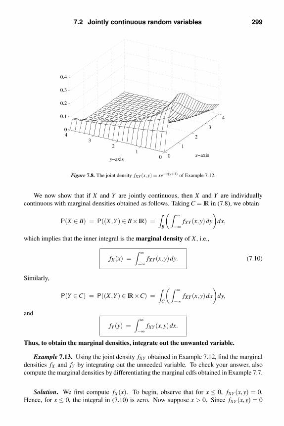
7.2 Jointly continuous random variables 299
0
1
2
3
4
01
23
40
0.1
0.2
0.3
0.4
x−axisy−axis
Figure 7.8. The joint density fXY (x,y) = xe−x(y+1) of Example 7.12.
We now show that if X and Y are jointly continuous, then X and Y are individually
continuous with marginal densities obtained as follows. Taking C = IR in (7.8), we obtain
P(X ∈ B) = P((X ,Y ) ∈ B× IR) =∫
B
(∫ ∞
−∞fXY (x,y)dy
)dx,
which implies that the inner integral is the marginal density of X , i.e.,
fX (x) =∫ ∞
−∞fXY (x,y)dy. (7.10)
Similarly,
P(Y ∈C) = P((X ,Y ) ∈ IR×C) =∫
C
(∫ ∞
−∞fXY (x,y)dx
)dy,
and
fY (y) =∫ ∞
−∞fXY (x,y)dx.
Thus, to obtain the marginal densities, integrate out the unwanted variable.
Example 7.13. Using the joint density fXY obtained in Example 7.12, find the marginal
densities fX and fY by integrating out the unneeded variable. To check your answer, also
compute the marginal densities by differentiating the marginal cdfs obtained in Example 7.7.
Solution. We first compute fX (x). To begin, observe that for x ≤ 0, fXY (x,y) = 0.
Hence, for x ≤ 0, the integral in (7.10) is zero. Now suppose x > 0. Since fXY (x,y) = 0

300 Bivariate random variables
whenever y ≤ 0, the lower limit of integration in (7.10) can be changed to zero. For x > 0,
it remains to compute ∫ ∞
0fXY (x,y)dy = xe−x
∫ ∞
0e−xy dy
= e−x.
Hence,
fX (x) =
e−x, x > 0,0, x ≤ 0,
and we see that X is exponentially distributed with parameter λ = 1. Note that the same
answer can be obtained by differentiating the formula for FX (x) in (7.5).
We now turn to the calculation of fY (y). Arguing as above, we have fY (y) = 0 for y ≤ 0,
and fY (y) =∫ ∞
0 fXY (x,y)dx for y > 0. Write this integral as∫ ∞
0fXY (x,y)dx =
1
y+1
∫ ∞
0x · (y+1)e−(y+1)x dx. (7.11)
If we put λ = y+1, then the integral on the right has the form∫ ∞
0x ·λe−λx dx,
which is the mean of an exponential random variable with parameter λ . This integral is
equal to 1/λ = 1/(y + 1), and so the right-hand side of (7.11) is equal to 1/(y + 1)2. We
conclude that
fY (y) =
1/(y+1)2, y > 0,
0, y ≤ 0.
Note that the same answer can be obtained by differentiating the formula for FY (y) in (7.6).
Independence
We now consider the joint density of jointly continuous independent random variables.
As noted in Section 7.1, if X and Y are independent, then FXY (x,y) = FX (x)FY (y) for all
x and y. If X and Y are also jointly continuous, then by taking second-order mixed partial
derivatives, we find∂ 2
∂y∂xFX (x)FY (y) = fX (x) fY (y).
In other words, if X and Y are jointly continuous and independent, then the joint density is
the product of the marginal densities. Using (7.8), it is easy to see that the converse is also
true. If fXY (x,y) = fX (x) fY (y), (7.8) implies
P(X ∈ B,Y ∈C) =∫
B
(∫C
fXY (x,y)dy
)dx
=∫
B
(∫C
fX (x) fY (y)dy
)dx

7.2 Jointly continuous random variables 301
=
∫B
fX (x)
(∫C
fY (y)dy
)dx
=
(∫B
fX (x)dx
)P(Y ∈C)
= P(X ∈ B)P(Y ∈C).
We record here that jointly continuous random variables X and Y are independent if and
only if their joint density factors into the product of their marginal densities: fXY (x,y) =fX (x) fY (y).
Expectation
If X and Y are jointly continuous with joint density fXY , then the methods of Section 4.2
can easily be used to show that
E[g(X ,Y )] =∫ ∞
−∞
∫ ∞
−∞g(x,y) fXY (x,y)dxdy.
For arbitrary random variables X and Y , their bivariate characteristic function is de-
fined by
ϕXY (ν1,ν2) := E[e j(ν1X+ν2Y )].
If X and Y have joint density fXY , then
ϕXY (ν1,ν2) =∫ ∞
−∞
∫ ∞
−∞fXY (x,y)e j(ν1x+ν2y) dxdy,
which is simply the bivariate Fourier transform of fXY . By the inversion formula,
fXY (x,y) =1
(2π)2
∫ ∞
−∞
∫ ∞
−∞ϕXY (ν1,ν2)e
− j(ν1x+ν2y)dν1 dν2.
Now suppose that X and Y are independent. Then
ϕXY (ν1,ν2) = E[e j(ν1X+ν2Y )] = E[e jν1X ]E[e jν2Y ] = ϕX (ν1)ϕY (ν2).
In other words, if X and Y are independent, then their joint characteristic function factors.
The converse is also true; i.e., if the joint characteristic function factors, then X and Y
are independent. The general proof is complicated, but if X and Y are jointly continuous,
it suffices to show that the joint density has product form. This is easily done with the
inversion formula. Write
fXY (x,y) =1
(2π)2
∫ ∞
−∞
∫ ∞
−∞ϕXY (ν1,ν2)e
− j(ν1x+ν2y)dν1 dν2

302 Bivariate random variables
=1
(2π)2
∫ ∞
−∞
∫ ∞
−∞ϕX (ν1)ϕY (ν2)e
− j(ν1x+ν2y)dν1 dν2
=
(1
2π
∫ ∞
−∞ϕX (ν1)e
− jν1x dx
)(1
2π
∫ ∞
−∞ϕY (ν2)e
− jν2y dy
)= fX (x) fY (y).
We summarize here that X and Y are independent if and only if their joint characteristic
function is a product of their marginal characteristic functions; i.e.,
ϕXY (ν1,ν2) = ϕX (ν1)ϕY (ν2).
Continuous random variables that are not jointly continuous
Let Θ ∼ uniform[−π,π], and put X := cosΘ and Y := sinΘ. As shown in Problem 35 in
Chapter 5, X and Y are both arcsine random variables, each having density (1/π)/√
1− x2
for −1 < x < 1.
Next, since X2 +Y 2 = 1, the pair (X ,Y ) takes values only on the unit circle
C := (x,y) : x2 + y2 = 1.
Thus, P((X ,Y ) ∈C
)= 1. On the other hand, if X and Y have a joint density fXY , then
P((X ,Y ) ∈C
)=
∫ ∫C
fXY (x,y)dxdy = 0
because a double integral over a set of zero area must be zero. So, if X and Y had a joint
density, this would imply that 1 = 0. Since this is not true, there can be no joint density.
Remark. Problem 44 of Chapter 2 provided an example of uncorrelated discrete ran-
dom variables that are not independent. The foregoing X = cosΘ and Y = sinΘ provide an
example of continuous random variables that are uncorrelated but not independent (Prob-
lem 20).
7.3 Conditional probability and expectation
If X is a continuous random variable, then its cdf FX (x) := P(X ≤ x) =∫ x−∞ fX (t)dt is a
continuous function of x.5 It follows from the properties of cdfs in Section 5.5 that P(X =x) = 0 for all x. Hence, we cannot define P(Y ∈ C|X = x) by P(X = x,Y ∈ C)/P(X = x)since this requires division by zero! Similar problems arise with conditional expectation.
How should we define conditional probability and expectation in this case?
Conditional probability
As a first step, let us compute
lim∆x→0
P(Y ∈C|x < X ≤ x+∆x).

7.3 Conditional probability and expectation 303
For positive ∆x, this conditional probability is given by
P(x < X ≤ x+∆x,Y ∈C)
P(x < X ≤ x+∆x).
If we write the numerator as P((X ,Y ) ∈ (x,x + ∆x]×C), and if we assume X and Y are
jointly continuous, the desired conditional probability can be written as∫ x+∆x
x
(∫C
fXY (t,y)dy
)dt∫ x+∆x
xfX (τ)dτ
.
Now divide the numerator and denominator by ∆x to get
1
∆x
∫ x+∆x
x
(∫C
fXY (t,y)dy
)dt
1
∆x
∫ x+∆x
xfX (τ)dτ
.
Letting ∆x → 0, we obtain the limit∫C
fXY (x,y)dy
fX (x)=
∫C
fXY (x,y)
fX (x)dy.
We therefore define the conditional density of Y given X by
fY |X (y|x) :=fXY (x,y)
fX (x), for x with fX (x) > 0, (7.12)
and we define the conditional probability
P(Y ∈C|X = x) :=∫
CfY |X (y|x)dy.
The conditional cdf is
FY |X (y|x) := P(Y ≤ y|X = x) =
∫ y
−∞fY |X (t|x)dt.
Note also that if X and Y are independent, the joint density factors, and so
fY |X (y|x) =fXY (x,y)
fX (x)=
fX (x) fY (y)
fX (x)= fY (y).
It then follows that P(Y ∈ C|X = x) = P(Y ∈ C); similarly FY |X (y|x) = FY (y). In other
words, we can “drop the conditioning.”

304 Bivariate random variables
Recall that for discrete random variables, conditional pmfs are proportional to slices
of the joint pmf (cf. Example 3.10 and Figure 3.3). Similarly, (7.12) shows that condi-
tional densities are proportional to slices of the joint density. For example, the joint density
fXY (x,y) = xe−x(y+1) was sketched in Figure 7.8. For fixed x, slices have the shape of an
exponential density, while for fixed y, slices have the shape of a gamma density with p = 2
shown in Figure 4.7.
We now show that our definition of conditional probability satisfies the following law
of total probability,
P(Y ∈C) =∫ ∞
−∞P(Y ∈C|X = x) fX (x)dx. (7.13)
Remark. Notice that although (7.12) only makes sense for those x with fX (x) > 0, these
are the only values of x used to evaluate the integral in (7.13).
To derive (7.13), first write∫ ∞
−∞P(Y ∈C|X = x) fX (x)dx =
∫ ∞
−∞
(∫C
fY |X (y|x)dy
)fX (x)dx.
Then from (7.12), observe that
fY |X (y|x) fX (x) = fXY (x,y).
Hence, the above double integral becomes∫ ∫IR×C
fXY (x,y)dxdy = P((X ,Y ) ∈ IR×C) = P(Y ∈C),
where the last step uses (7.1).
If we repeat the limit derivation above for P((X ,Y ) ∈ A|x < X ≤ x + ∆x), then we are
led to define (Problem 24)
P((X ,Y ) ∈ A|X = x) :=
∫ ∞
−∞IA(x,y) fY |X (y|x)dy.
It is similarly easy to show that the law of total probability
P((X ,Y ) ∈ A) =∫ ∞
−∞P((X ,Y ) ∈ A|X = x) fX (x)dx (7.14)
holds. We also have the substitution law,
P((X ,Y ) ∈ A|X = x) = P((x,Y ) ∈ A|X = x). (7.15)
Rather than derive these laws of total probability and substitution here, we point out that
they follow immediately from the corresponding results for conditional expectation that we
discuss later in this section.6

7.3 Conditional probability and expectation 305
Example 7.14 (signal in additive noise). Suppose that a random, continuous-valued sig-
nal X is transmitted over a channel subject to additive, continuous-valued noise Y . The re-
ceived signal is Z = X +Y . Find the cdf and density of Z if X and Y are jointly continuous
random variables with joint density fXY .
Solution. Since we are not assuming that X and Y are independent, the characteristic-
function method of Example 4.23 does not work here. Instead, we use the laws of total
probability and substitution. Write
FZ(z) = P(Z ≤ z)
=
∫ ∞
−∞P(Z ≤ z|Y = y) fY (y)dy
=∫ ∞
−∞P(X +Y ≤ z|Y = y) fY (y)dy
=∫ ∞
−∞P(X + y ≤ z|Y = y) fY (y)dy
=∫ ∞
−∞P(X ≤ z− y|Y = y) fY (y)dy
=∫ ∞
−∞FX |Y (z− y|y) fY (y)dy.
By differentiating with respect to z,
fZ(z) =∫ ∞
−∞fX |Y (z− y|y) fY (y)dy =
∫ ∞
−∞fXY (z− y,y)dy.
This is essentially the formula obtained in Example 7.10; to see the connection, make the
change of variable x = z−y. We also point out that if X and Y are independent, we can drop
the conditioning and obtain the convolution
fZ(z) =∫ ∞
−∞fX (z− y) fY (y)dy. (7.16)
This formula was derived using characteristic functions following Example 4.23.
Example 7.15 (signal in multiplicative noise). A random, continuous-valued signal X
is transmitted over a channel subject to multiplicative, continuous-valued noise Y . The
received signal is Z = XY . Find the cdf and density of Z if X and Y are jointly continuous
random variables with joint density fXY .
Solution. We proceed as in the previous example. Write
FZ(z) = P(Z ≤ z)
=∫ ∞
−∞P(Z ≤ z|Y = y) fY (y)dy
=∫ ∞
−∞P(XY ≤ z|Y = y) fY (y)dy
=∫ ∞
−∞P(Xy ≤ z|Y = y) fY (y)dy.

306 Bivariate random variables
At this point we have a problem when we attempt to divide through by y. If y is negative,
we have to reverse the inequality sign. Otherwise, we do not have to reverse the inequality.
The solution to this difficulty is to break up the range of integration. Write
FZ(z) =∫ 0
−∞P(Xy ≤ z|Y = y) fY (y)dy+
∫ ∞
0P(Xy ≤ z|Y = y) fY (y)dy.
Now we can divide by y separately in each integral. Thus,
FZ(z) =∫ 0
−∞P(X ≥ z/y|Y = y) fY (y)dy+
∫ ∞
0P(X ≤ z/y|Y = y) fY (y)dy
=∫ 0
−∞
[1−FX |Y
(zy
∣∣y)] fY (y)dy+∫ ∞
0FX |Y
(zy
∣∣y) fY (y)dy.
Differentiating with respect to z yields
fZ(z) = −∫ 0
−∞fX |Y
(zy
∣∣y) 1y
fY (y)dy+∫ ∞
0fX |Y
(zy
∣∣y) 1y
fY (y)dy. (7.17)
Now observe that in the first integral, the range of integration implies that y is always neg-
ative. For such y, −y = |y|. In the second integral, y is always positive, and so y = |y|.Thus,
fZ(z) =∫ 0
−∞fX |Y
(zy
∣∣y) 1|y| fY (y)dy+
∫ ∞
0fX |Y
(zy
∣∣y) 1|y| fY (y)dy
=∫ ∞
−∞fX |Y
(zy
∣∣y) 1|y| fY (y)dy
=∫ ∞
−∞fXY
(zy,y)
1|y| dy.
This is essentially the formula obtained in Example 7.11; to see the connection, make the
change of variable x = z/y in (7.17) and proceed as before.
Example 7.16. If X and Y are jointly continuous, find the density of Z := X2 +Y 2.
Solution. As always, we first find the cdf.
FZ(z) = P(Z ≤ z)
=
∫ ∞
−∞P(Z ≤ z|Y = y) fY (y)dy
=∫ ∞
−∞P(X2 +Y 2 ≤ z|Y = y) fY (y)dy
=∫ ∞
−∞P(X2 ≤ z− y2|Y = y) fY (y)dy.
At this point, we observe that for y2 > z, P(X2 ≤ z− y2|Y = y) = 0 since X2 cannot be
negative. We therefore write
FZ(z) =∫ √
z
−√zP(X2 ≤ z− y2|Y = y) fY (y)dy

7.3 Conditional probability and expectation 307
=∫ √
z
−√zP(−√z− y2 ≤ X ≤
√z− y2
∣∣Y = y)
fY (y)dy
=∫ √
z
−√z
[FX |Y
(√z− y2
∣∣y)−FX |Y(−√z− y2
∣∣y)] fY (y)dy.
Using Leibniz’ rule,7
d
dz
∫ b(z)
a(z)h(z,y)dy = −h
(z,a(z)
)a′(z)+h
(z,b(z)
)b′(z)+
∫ b(z)
a(z)
∂∂ z
h(z,y)dy,
we find that
fZ(z) =∫ √
z
−√z
fX |Y(√
z− y2∣∣y)+ fX |Y
(−√z− y2∣∣y)
2√
z− y2fY (y)dy.
Example 7.17. Let X and Y be jointly continuous, positive random variables. Find the
cdf and density of Z := min(X ,Y )/max(X ,Y ).
Solution. First note that since 0 < Z ≤ 1, we only worry about FZ(z) for 0 < z < 1.
(Why?) Second, note that if Y ≤ X , Z = Y/X , while if X < Y , Z = X/Y . Our analytical
approach is to write
P(Z ≤ z) = P(Z ≤ z,Y ≤ X)+P(Z ≤ z,X < Y )
= P(Y/X ≤ z,Y ≤ X)+P(X/Y ≤ z,X < Y ),
and evaluate each term using the law of total probability. We begin with
P(Y/X ≤ z,Y ≤ X) =∫ ∞
0P(Y/X ≤ z,Y ≤ X |X = x) fX (x)dx
=
∫ ∞
0P(Y ≤ zx,Y ≤ x|X = x) fX (x)dx.
Since 0 < z < 1, Y ≤ zx ⊂ Y ≤ x, and so
Y ≤ zx∩Y ≤ x = Y ≤ zx.Hence,
P(Y/X ≤ z,Y ≤ X) =∫ ∞
0P(Y ≤ zx|X = x) fX (x)dx
=∫ ∞
0FY |X (zx|x) fX (x)dx.
Similarly,
P(X/Y ≤ z,X < Y ) =∫ ∞
0P(X ≤ zy,X < y|Y = y) fY (y)dy
=∫ ∞
0P(X ≤ zy|Y = y) fY (y)dy
=∫ ∞
0FX |Y (zy|y) fY (y)dy.

308 Bivariate random variables
It now follows that
fZ(z) =∫ ∞
0x fY |X (zx|x) fX (x)dx+
∫ ∞
0y fX |Y (zy|y) fY (y)dy.
Conditional expectation
Since P(Y ∈C|X = x) is computed by integrating the conditional density fY |X (y|x) over
the set C, it is only natural to define8
E[g(Y )|X = x] :=∫ ∞
−∞g(y) fY |X (y|x)dy. (7.18)
To see how E[g(X ,Y )|X = x] should be defined so that suitable laws of total probability
and substitution can be obtained, write
E[g(X ,Y )] =∫ ∞
−∞
∫ ∞
−∞g(x,y) fXY (x,y)dxdy
=∫ ∞
−∞
(∫ ∞
−∞g(x,y) fXY (x,y)dy
)dx
=
∫ ∞
−∞
(∫ ∞
−∞g(x,y)
fXY (x,y)
fX (x)dy
)fX (x)dx
=∫ ∞
−∞
(∫ ∞
−∞g(x,y) fY |X (y|x)dy
)fX (x)dx.
Thus, defining
E[g(X ,Y )|X = x] :=∫ ∞
−∞g(x,y) fY |X (y|x)dy (7.19)
gives us the law of total probability
E[g(X ,Y )] =
∫ ∞
−∞E[g(X ,Y )|X = x] fX (x)dx. (7.20)
Furthermore, if we replace g(y) in (7.18) by gx(y) := g(x,y) and compare the result with
(7.19), we obtain the substitution law,
E[g(X ,Y )|X = x] = E[g(x,Y )|X = x]. (7.21)
Another important point to note is that if X and Y are independent, then fY |X (y|x) =fY (y). In this case, (7.18) becomes E[g(Y )|X = x] = E[g(Y )]. In other words, we can “drop
the conditioning.”
Example 7.18. Let X ∼ exp(1), and suppose that given X = x, Y is conditionally normal
with fY |X (·|x) ∼ N(0,x2). Evaluate E[Y 2] and E[Y 2X3].

7.4 The bivariate normal 309
Solution. We use the law of total probability for expectation. We begin with
E[Y 2] =∫ ∞
−∞E[Y 2|X = x] fX (x)dx.
Since fY |X (y|x) = e−(y/x)2/2/(√
2π x) is an N(0,x2) density in the variable y, E[Y 2|X = x] =
x2. Substituting this into the above integral yields
E[Y 2] =∫ ∞
−∞x2 fX (x)dx = E[X2].
Since X ∼ exp(1), E[X2] = 2 by Example 4.17.
To compute E[Y 2X3], we proceed similarly. Write
E[Y 2X3] =∫ ∞
−∞E[Y 2X3|X = x] fX (x)dx
=∫ ∞
−∞E[Y 2x3|X = x] fX (x)dx
=∫ ∞
−∞x3
E[Y 2|X = x] fX (x)dx
=∫ ∞
−∞x3x2 fX (x)dx
= E[X5]
= 5!, by Example 4.17.
7.4 The bivariate normal
The bivariate Gaussian or bivariate normal density is a generalization of the univari-
ate N(m,σ2) density. (The multivariate case is treated in Chapter 9.) Recall that the standard
N(0,1) density is given by ψ(x) := exp(−x2/2)/√
2π . The general N(m,σ2) density can
be written in terms of ψ as
1√2π σ
exp
[−1
2
(x−m
σ
)2]=
1
σ·ψ(
x−m
σ
).
In order to define the general bivariate Gaussian density, it is convenient to define a
standard bivariate density first. So, for |ρ| < 1, put
ψρ(u,v) :=exp
(−1
2(1−ρ2)[u2 −2ρuv+ v2]
)2π√
1−ρ2. (7.22)
For fixed ρ , this function of the two variables u and v defines a surface. The surface corre-
sponding to ρ = 0 is shown in Figure 7.9. From the figure and from the formula (7.22), we
see that ψ0 is circularly symmetric; i.e., for all (u,v) on a circle of radius r, in other words,
for u2 + v2 = r2, ψ0(u,v) = e−r2/2/2π does not depend on the particular values of u and v,

310 Bivariate random variables
−3−2
−10
12
3 −3−2
−10
12
3
0.05
0.10
0.15
v−axisu−axis
−3 −2 −1 0 1 2 3−3
−2
−1
0
1
2
3
u−axis
v−
ax
is
Figure 7.9. The Gaussian surface ψρ (u,v) of (7.22) with ρ = 0 (left). The corresponding level curves (right).
but only on the radius of the circle on which they lie. Some of these circles (level curves)
are shown in Figure 7.9. We also point out that for ρ = 0, the formula (7.22) factors into the
product of two univariate N(0,1) densities, i.e., ψ0(u,v) = ψ(u)ψ(v). For ρ = 0, ψρ does
not factor. In other words, if U and V have joint density ψρ , then U and V are independent if
and only if ρ = 0. A plot of ψρ for ρ =−0.85 is shown in Figure 7.10. It turns out that now
ψρ is constant on ellipses instead of circles. The axes of the ellipses are not parallel to the
coordinate axes, as shown in Figure 7.10. Notice how the major axis of these ellipses and
the density are concentrated along the line v =−u. As ρ →−1, this concentration becomes
more extreme. As ρ → +1, the density concentrates around the line v = u. We now show
−3 −2 −1 0 1 2 3 −3
−2
−1
0
1
2
30.1
0.2
0.3
v−axis
u−axis−3 −2 −1 0 1 2 3
−3
−2
−1
0
1
2
3
u−axis
v−
axis
Figure 7.10. The Gaussian surface ψρ (u,v) of (7.22) with ρ = −0.85 (left). The corresponding level curves
(right).

7.4 The bivariate normal 311
that the density ψρ integrates to one. To do this, first observe that for all |ρ| < 1,
u2 −2ρuv+ v2 = u2(1−ρ2)+(v−ρu)2.
It follows that
ψρ(u,v) =e−u2/2
√2π
·exp
(−1
2(1−ρ2)[v−ρu]2
)√
2π√
1−ρ2
= ψ(u) · 1√1−ρ2
ψ(
v−ρu√1−ρ2
). (7.23)
Observe that the right-hand factor as a function of v has the form of a univariate normal
density with mean ρu and variance 1− ρ2. With ψρ factored as in (7.23), we can write∫ ∞−∞∫ ∞−∞ψρ(u,v)dudv as the iterated integral∫ ∞
−∞ψ(u)
[∫ ∞
−∞
1√1−ρ2
ψ(
v−ρu√1−ρ2
)dv
]du.
As noted above, the inner integrand, as a function of v, is simply an N(ρu,1−ρ2) density,
and therefore integrates to one. Hence, the above iterated integral becomes∫ ∞−∞ ψ(u)du = 1.
We can now easily define the general bivariate Gaussian density with parameters mX ,
mY , σ2X , σ2
Y , and ρ by
fXY (x,y) :=1
σX σY
ψρ
(x−mX
σX
,y−mY
σY
). (7.24)
More explicitly, this density is
exp(
−12(1−ρ2)
[( x−mXσX
)2 −2ρ( x−mXσX
)( y−mY
σY)+( y−mY
σY)2])
2πσX σY
√1−ρ2
. (7.25)
It can be shown that the marginals are fX ∼ N(mX ,σ2X ) and fY ∼ N(mY ,σ2
Y ) and that
E
[(X −mX
σX
)(Y −mY
σY
)]= ρ
(see Problems 47 and 50). Hence, ρ is the correlation coefficient between X and Y . From
(7.25), we observe that X and Y are independent if and only if ρ = 0. A plot of fXY with
mX = mY = 0, σX = 1.5, σY = 0.6, and ρ = 0 is shown in Figure 7.11. The corresponding
elliptical level curves are shown in Figure 7.11. Notice how the level curves and density are
concentrated around the x-axis. Also, fXY is constant on ellipses of the form(x
σX
)2
+
(y
σY
)2
= r2.
To show that∫ ∞−∞∫ ∞−∞ fXY (x,y)dxdy = 1 as well, use formula (7.23) for ψρ and proceed
as above, integrating with respect to y first and then x. For the inner integral, make the
change of variable v = (y−mY )/σY , and in the remaining outer integral make the change
of variable u = (x−mX )/σX .

312 Bivariate random variables
−3−2
−10
12
3 −3−2
−10
12
3
0.05
0.10
0.15
y−axisx−axis
−3 −2 −1 0 1 2 3−3
−2
−1
0
1
2
3
x−axis
y−
ax
is
Figure 7.11. The bivariate normal density fXY (x,y) of (7.25) with mX = mY = 0, σX = 1.5, σY = 0.6, and ρ = 0
(left). The corresponding level curves (right).
Example 7.19. Let random variables U and V have the standard bivariate normal den-
sity ψρ in (7.22). Show that E[UV ] = ρ .
Solution. Using the factored form of ψρ in (7.23), write
E[UV ] =∫ ∞
−∞
∫ ∞
−∞uvψρ(u,v)dudv
=∫ ∞
−∞uψ(u)
[∫ ∞
−∞
v√1−ρ2
ψ(
v−ρu√1−ρ2
)dv
]du.
The quantity in brackets has the form E[V ], where V is a univariate normal random variable
with mean ρu and variance 1−ρ2. Thus,
E[UV ] =∫ ∞
−∞uψ(u)[ρu]du
= ρ∫ ∞
−∞u2 ψ(u)du
= ρ,
since ψ is the N(0,1) density.
Example 7.20. Let U and V have the standard bivariate normal density fUV (u,v) =ψρ(u,v) given in (7.22). Find the conditional densities fV |U and fU |V .
Solution. It is shown in Problem 47 that fU and fV are both N(0,1). Hence,
fV |U (v|u) =fUV (u,v)
fU (u)=
ψρ(u,v)
ψ(u),

7.4 The bivariate normal 313
where ψ is the N(0,1) density. If we now substitute the factored form of ψρ(u,v) given in
(7.23), we obtain
fV |U (v|u) =1√
1−ρ2ψ(
v−ρu√1−ρ2
);
i.e., fV |U (· |u) ∼ N(ρu,1−ρ2).To compute fU |V we need the following alternative factorization of ψρ ,
ψρ(u,v) =1√
1−ρ2ψ(
u−ρv√1−ρ2
)·ψ(v). (7.26)
It then follows that
fU |V (u|v) =1√
1−ρ2ψ(
u−ρv√1−ρ2
);
i.e., fU |V (· |v) ∼ N(ρv,1 − ρ2). To see the shape of this density with ρ = −0.85, look
at slices of Figure 7.10 for fixed values of v. Two slices from Figure 7.10 are shown in
Figure 7.12. Notice how the mean value of the different slices depends on v and ρ .
−3−2
−10
12
3 −3
−2
−1
0
1
2
3
0
0.1
0.2
0.3
v−axis
u−axis
Figure 7.12. Two slices from Figure 7.10.
Example 7.21. If U and V have standard joint normal density ψρ(u,v), find E[V |U = u].
Solution. Recall that from Example 7.20, fV |U (·|u) ∼ N(ρu,1−ρ2). Hence,
E[V |U = u] =∫ ∞
−∞v fV |U (v|u)dv = ρu.
It is important to note here that E[V |U = u] = ρu is a linear function of u. For arbitrary
random variables U and V , E[V |U = u] is usually a much more complicated function of

314 Bivariate random variables
u. However, for the general bivariate normal, the conditional expectation is either a linear
function or a linear function plus a constant, as shown in Problem 48.
7.5 Extension to three or more random variables
The ideas we have developed for pairs of random variables readily extend to any finite
number of random variables. However, for ease of notation, we illustrate the case of three
random variables. We also point out that the use of vector notation can simplify many of
these formulas as shown in Chapters 8 and 9.
Given a joint density fXY Z(x,y,z), if we need to find fXY (x,y), fXZ(x,z), or fY Z(y,z), we
just integrate out the unwanted variable; e.g.,
fY Z(y,z) =∫ ∞
−∞fXY Z(x,y,z)dx.
If we then need only fZ(z), we integrate out y:
fZ(z) =∫ ∞
−∞fY Z(y,z)dy.
These two steps can be combined into the double integral
fZ(z) =∫ ∞
−∞
∫ ∞
−∞fXY Z(x,y,z)dxdy.
With more variables, there are more possibilities for conditional densities. In addition
to conditional densities of one variable given another such as
fY |Z(y|z) :=fY Z(y,z)
fZ(z), (7.27)
we also have conditional densities of the form
fX |Y Z(x|y,z) :=fXY Z(x,y,z)
fY Z(y,z)(7.28)
and
fXY |Z(x,y|z) :=fXY Z(x,y,z)
fZ(z).
We also point out that (7.27) and (7.28) imply
fXY Z(x,y,z) = fX |Y Z(x|y,z) fY |Z(y|z) fZ(z).
Example 7.22. Let
fXY Z(x,y,z) =3z2
7√
2πe−zy exp
[− 1
2
(x−y
z
)2],
for y ≥ 0 and 1 ≤ z ≤ 2, and fXY Z(x,y,z) = 0 otherwise. Find fY Z(y,z) and fX |Y Z(x|y,z).Then find fZ(z), fY |Z(y|z), and fXY |Z(x,y|z).

7.5 Extension to three or more random variables 315
Solution. Observe that the joint density can be written as
fXY Z(x,y,z) =exp
[− 1
2
(x−y
z
)2]√
2π z· ze−zy · 3
7z2.
The first factor as a function of x is an N(y,z2) density. Hence,
fY Z(y,z) =∫ ∞
−∞fXY Z(x,y,z)dx = ze−zy · 3
7z2,
and
fX |Y Z(x|y,z) =fXY Z(x,y,z)
fY Z(y,z)=
exp[− 1
2
(x−y
z
)2]√
2π z.
Thus, fX |Y Z(·|y,z) ∼ N(y,z2). Next, in the above formula for fY Z(y,z), observe that ze−zy as
a function of y is an exponential density with parameter z. Thus,
fZ(z) =∫ ∞
0fY Z(y,z)dy = 3
7z2, 1 ≤ z ≤ 2.
It follows that fY |Z(y|z) = fY Z(y,z)/ fZ(z) = ze−zy; i.e., fY |Z(·|z) ∼ exp(z). Finally,
fXY |Z(x,y|z) =fXY Z(x,y,z)
fZ(z)=
exp[− 1
2
(x−y
z
)2]√
2π z· ze−zy.
The law of total probability
For expectations, we have
E[g(X ,Y,Z)] =∫ ∞
−∞
∫ ∞
−∞
∫ ∞
−∞g(x,y,z) fXY Z(x,y,z)dxdydz.
A little calculation using conditional probabilities shows that with
E[g(X ,Y,Z)|Y = y,Z = z] :=∫ ∞
−∞g(x,y,z) fX |Y Z(x|y,z)dx,
we have the law of total probability,
E[g(X ,Y,Z)] =∫ ∞
−∞
∫ ∞
−∞E[g(X ,Y,Z)|Y = y,Z = z] fY Z(y,z)dydz. (7.29)
In addition, we have the substitution law,
E[g(X ,Y,Z)|Y = y,Z = z] = E[g(X ,y,z)|Y = y,Z = z]. (7.30)

316 Bivariate random variables
Example 7.23. Let X , Y , and Z be as in Example 7.22. Find E[X ] and E[XZ].
Solution. Rather than use the marginal density of X to compute E[X ], we use the law of
total probability. Write
E[X ] =∫ ∞
−∞
∫ ∞
−∞E[X |Y = y,Z = z] fY Z(y,z)dydz.
From Example 7.22, fX |Y Z(·|y,z) ∼ N(y,z2), and so E[X |Y = y,Z = z] = y. Thus,
E[X ] =∫ ∞
−∞
∫ ∞
−∞y fY Z(y,z)dydz = E[Y ],
which we compute by again using the law of total probability. Write
E[Y ] =∫ ∞
−∞E[Y |Z = z] fZ(z)dz.
From Example 7.22, fY |Z(·|z) ∼ exp(z); hence, E[Y |Z = z] = 1/z. Since fZ(z) = 3z2/7,
E[Y ] =∫ 2
1
37zdz = 9
14.
Thus, E[X ] = E[Y ] = 9/14.
To find E[XZ], write
E[XZ] =∫ ∞
−∞
∫ ∞
−∞E[Xz|Y = y,Z = z] fY Z(y,z)dydz.
We then note that E[Xz|Y = y,Z = z] = E[X |Y = y,Z = z]z = yz. Thus,
E[XZ] =
∫ ∞
−∞
∫ ∞
−∞yz fY Z(y,z)dydz = E[Y Z].
In Problem 56 the reader is asked to show that E[Y Z] = 1. Thus, E[XZ] = 1 as well.
Example 7.24. Let N be a positive, integer-valued random variable, and let X1,X2, . . . be
i.i.d. Further assume that N is independent of X1, . . . ,Xn for every n. Consider the random
sum,N
∑i=1
Xi.
Note that the number of terms in the sum is a random variable. Find the mean value of the
random sum.
Solution. Use the law of total probability to write
E
[N
∑i=1
Xi
]=
∞
∑n=1
E
[n
∑i=1
Xi
∣∣∣∣N = n
]P(N = n).

Notes 317
By independence of N and the Xi sequence,
E
[n
∑i=1
Xi
∣∣∣∣N = n
]= E
[n
∑i=1
Xi
]=
n
∑i=1
E[Xi].
Since the Xi are i.i.d., they all have the same mean. In particular, for all i, E[Xi] = E[X1].Thus,
E
[n
∑i=1
Xi
∣∣∣∣N = n
]= nE[X1].
Now we can write
E
[N
∑i=1
Xi
]=
∞
∑n=1
nE[X1]P(N = n)
= E[N]E[X1].
Notes
7.1: Joint and marginal probabilities
Note 1. Comments analogous to Note 1 in Chapter 2 apply here. Specifically, the set A
must be restricted to a suitable σ -field B of subsets of IR2. Typically, B is taken to be the
collection of Borel sets of IR2; i.e., B is the smallest σ -field containing all the open sets of
IR2.
Note 2. While it is easily seen that every joint cdf FXY (x,y) satisfies
(i) 0 ≤ FXY (x,y) ≤ 1,
(ii) For fixed y, FXY (x,y) is nondecreasing in x,
(iii) For fixed x, FXY (x,y) is nondecreasing in y,
it is the rectangle formula
P(a < X ≤ b, c < Y ≤ d) = FXY (b,d)−FXY (a,d)−FXY (b,c)+FXY (a,c)
that implies the above right-hand side is nonnegative.
Given a function F(x,y) that satisfies the above three properties, the function may or
may not satisfy
F(b,d)−F(a,d)−F(b,c)+F(a,c) ≥ 0.
In fact, the function
F(x,y) :=
1, (x,y) ∈ quadrants I, II, or IV,0, (x,y) ∈ quadrant III,
satisfies the three properties, but for
(a,b]× (c,d] = (−1/2,1/2]× (−1/2,1/2],
it is easy to check that
F(b,d)−F(a,d)−F(b,c)+F(a,c) = −1 < 0.

318 Bivariate random variables
Note 3. We now derive the limit formula for FX (x) in (7.3); the formula for FY (y) can
be derived similarly. To begin, write
FX (x) := P(X ≤ x) = P((X ,Y ) ∈ (−∞,x]× IR).
Next, observe that IR =⋃∞
n=1(−∞,n], and write
(−∞,x]× IR = (−∞,x]×∞⋃
n=1
(−∞,n]
=∞⋃
n=1
(−∞,x]× (−∞,n].
Since the union is increasing, we can use the limit property (1.15) to show that
FX (x) = P
((X ,Y ) ∈
∞⋃n=1
(−∞,x]× (−∞,n]
)= lim
N→∞P((X ,Y ) ∈ (−∞,x]× (−∞,N])
= limN→∞
FXY (x,N).
7.2: Jointly continuous random variables
Note 4. As illustrated at the end of Section 7.2, it is possible to have X and Y each
be continuous random variables but not jointly continuous. When a joint density exists,
advanced texts say the pair is absolutely continuous. See also Note 4 in Chapter 5.
7.3: Conditional probability and expectation
Note 5. If the density fX is bounded, say by K, it is easy to see that the cdf FX (x) =∫ x−∞ fX (t)dt is continuous. Just write
|FX (x+∆x)−FX (x)| =
∣∣∣∣∫ x+∆x
xfX (t)dt
∣∣∣∣ ≤ K |∆x|.
For the general case, see Problem 6 in Chapter 13.
Note 6. To show that the law of substitution holds for conditional probability, write
P(g(X ,Y ) ∈C) = E[IC(g(X ,Y ))] =∫ ∞
−∞E[IC(g(X ,Y ))|X = x] fX (x)dx
and reduce the problem to one involving conditional expectation, for which the law of sub-
stitution is easily established.
Note 7. Here is a derivation of Leibniz’ rule for computing
d
dz
∫ b(z)
a(z)h(z,y)dy. (7.31)

Problems 319
Recall that by the chain rule from calculus, for functions H(u,v,w), a(z), b(z), and c(z),
d
dzH(a(z),b(z),c(z)
)=
∂H
∂ua′(z)+
∂H
∂vb′(z)+
∂H
∂wc′(z),
where occurrences of u, v, and w in the formulas for the partial derivatives are replaced by
u = a(z), v = b(z), and w = c(z). Consider the function
H(u,v,w) :=∫ v
uh(w,y)dy,
and note that
∂H
∂u= −h(w,u),
∂H
∂v= h(w,v), and
∂H
∂w=
∫ v
u
∂∂w
h(w,y)dy.
Now observe that (7.31) is the derivative of H(a(z),b(z),z
)with respect to z. It follows that
(7.31) is equal to
−h(z,a(z)
)a′(z)+h
(z,b(z)
)b′(z)+
∫ b(z)
a(z)
∂∂ z
h(z,y)dy.
Note 8. When g takes only finitely many distinct values, (7.18) and (7.19) can be de-
rived by conditioning on x < X ≤ x + ∆x and letting ∆x → 0. Then the case for general g
can be derived in the same way as the law of the unconscious statistician was derived for
continuous random variables at the end of Section 4.2.
Problems
7.1: Joint and marginal distributions
1. Express the cdf of Z := Y −X in the form P((X ,Y ) ∈ Az) for some set Az. Sketch
your set Az.
2. Express the cdf of Z := Y/X in the form P((X ,Y ) ∈ Az) for some set Az. Sketch your
set Az.
3. For a < b and c < d, sketch the following sets.
(a) R := (a,b]× (c,d].
(b) A := (−∞,a]× (−∞,d].
(c) B := (−∞,b]× (−∞,c].
(d) C := (a,b]× (−∞,c].
(e) D := (−∞,a]× (c,d].
(f) A∩B.

320 Bivariate random variables
4. Show that P(a < X ≤ b,c < Y ≤ d) is given by
FXY (b,d)−FXY (a,d)−FXY (b,c)+FXY (a,c).
Hint: Using the notation of the preceding problem, observe that
(−∞,b]× (−∞,d] = R∪ (A∪B),
and solve for P((X ,Y ) ∈ R).
5. For each of the following two-dimensional sets, determine whether or not it is a Carte-
sian product. If it is, find the two one-dimensional sets of which it is a product.
(a) (x,y) : |x| ≤ y ≤ 1.
(b) (x,y) : 2 < x ≤ 4, 1 ≤ y < 2.
(c) (x,y) : 2 < x ≤ 4, y = 1.
(d) (x,y) : 2 < x ≤ 4.
(e) (x,y) : y = 1.
(f) (1,1), (2,1), (3,1).
(g) The union of (1,3), (2,3), (3,3) and the set in (f).
(h) (1,0), (2,0), (3,0), (0,1), (1,1), (2,1), (3,1).
6. If c
FXY (x,y) =
⎧⎪⎪⎪⎪⎨⎪⎪⎪⎪⎩x−1− e−y − e−xy
y, 1 ≤ x ≤ 2, y ≥ 0,
1− e−y − e−2y
y, x > 2, y ≥ 0,
0, otherwise,
find the marginals FX (x) and FY (y) and determine whether or not X and Y are inde-
pendent.
7. If
FXY (x,y) =
⎧⎪⎪⎪⎨⎪⎪⎪⎩27(1− e−2y), 2 ≤ x < 3, y ≥ 0,
(7−2e−2y −5e−3y)
7, x ≥ 3, y ≥ 0,
0, otherwise.
find the marginals FX (x) and FY (y) and determine whether or not X and Y are inde-
pendent.
cThe quotients involving division by y are understood as taking their limiting values when y = 0.

Problems 321
7.2: Jointly continuous random variables
8. The joint density in Example 7.12 was obtained by differentiating FXY (x,y) first with
respect to x and then with respect to y. In this problem, find the joint density by
differentiating first with respect to y and then with respect to x.
9. Find the marginal density fX (x) if
fXY (x,y) =exp[−|y− x|− x2/2]
2√
2π.
10. Find the marginal density fY (y) if
fXY (x,y) =4e−(x−y)2/2
y5√
2π, y ≥ 1.
11. Let X and Y have joint density fXY (x,y). Find the marginal cdf and density of
max(X ,Y ) and of min(X ,Y ). How do your results simplify if X and Y are inde-
pendent? What if you further assume that the densities of X and Y are the same?
12. Let X ∼ gamma(p,1) and Y ∼ gamma(q,1) be independent random variables. Find
the density of Z := X +Y . Then compute P(Z > 1) if p = q = 1/2.
13. Find the density of Z := X +Y , where X and Y are independent Cauchy random
variables with parameters λ and µ , respectively. Then compute P(Z ≤ 1) if λ = µ =1/2.
14. In Example 7.10, the double integral for P((X ,Y ) ∈ Az), where Az is sketched in
Figure 7.1, was evaluated as an iterated integral with the inner integral with respect
to y and the outer integral with respect to x. Re-work the example if the inner integral
is with respect to x and the outer integral is with respect to y.
15. Re-work Example 7.11 if instead of the partition Az = A+z ∪A−
z shown in Figure 7.2,
you use the partition Az = B+z ∪B−
z , where
B+z := (x,y) : x ≤ z/y, y > 0 and B−
z := (x,y) : x ≥ z/y, y < 0.
16. If X and Y have joint density fXY , find the cdf and density of Z = Y −X .
17. If X and Y have joint density fXY , find the cdf and density of Z = Y/X .
18. Let
fXY (x,y) :=
Kxnym, (x,y) ∈ D,
0, otherwise,
where n and m are nonnegative integers, K is a constant, and D := (x,y) : |x| ≤ y≤ 1.
(a) Sketch the region D.
(b) Are there any restrictions on n and m that you need to make in order that fXY be
a valid joint density? If n and m are allowable, find K so that fXY is a valid joint
density.

322 Bivariate random variables
(c) For 0 < z < 1, sketch the region
Az := (x,y) : xy > z.(d) Sketch the region Az ∩D.
(e) Compute P((X ,Y ) ∈ Az).
19. A rectangle is drawn with random width being uniform on [0,w] and random height
being uniform on [0,h]. For fraction 0 < λ < 1, find the probability that the area of
the rectangle exceeds λ times the maximum possible area. Assume that the width and
the height are independent.
20. Let X := cosΘ and Y := sinΘ, where Θ ∼ uniform[−π,π]. Show that E[XY ] = 0.
Show that E[X ] = E[Y ] = 0. Argue that X and Y cannot be independent. This gives an
example of continuous random variables that are uncorrelated, but not independent.
Hint: Use the results of Problem 35 in Chapter 5.
21. Suppose that X and Y are random variables with the property that for all bounded
continuous functions h(x) and k(y),
E[h(X)k(Y )] = E[h(X)]E[k(Y )].
Show that X and Y are independent random variables.
22. If X ∼ N(0,1), then the complementary cumulative distribution function (ccdf) of X
is
Q(x0) := P(X > x0) =
∫ ∞
x0
e−x2/2
√2π
dx.
(a) Show that
Q(x0) =1
π
∫ π/2
0exp
( −x20
2cos2 θ
)dθ , x0 ≥ 0.
Hint: For any random variables X and Y , we can always write
P(X > x0) = P(X > x0,Y ∈ IR) = P((X ,Y ) ∈ D),
where D is the half plane D := (x,y) : x > x0. Now specialize to the case
where X and Y are independent and both N(0,1). Then the probability on the
right is a double integral that can be evaluated using polar coordinates.
Remark. The procedure outlined in the hint is a generalization of that used in
Section 4.1 to show that the standard normal density integrates to one. To see
this, note that if x0 = −∞, then D = IR2.
(b) Use the result of (a) to derive Craig’s formula [10, p. 572, Eq. (9)],
Q(x0) =1
π
∫ π/2
0exp
( −x20
2sin2 t
)dt, x0 ≥ 0.
Remark. Simon and Alouini [54] have derived a similar result for the Marcum
Q function (defined in Problem 25 in Chapter 5) and its higher-order general-
izations. See also [56, pp. 1865–1867].

Problems 323
7.3: Conditional probability and expectation
23. Using the definition (7.12) of conditional density, show that∫ ∞
−∞fY |X (y|x)dy = 1.
24. If X and Y are jointly continuous, show that
lim∆x→0
P((X ,Y ) ∈ A|x < X ≤ x+∆x) =∫ ∞
−∞IA(x,y) fY |X (y|x)dy.
25. Let fXY (x,y) be as derived in Example 7.12, and note that fX (x) and fY (y) were found
in Example 7.13. Find fY |X (y|x) and fX |Y (x|y) for x,y > 0. How do these conditional
densities compare with the marginals fY (y) and fX (x); is fY |X (y|x) similar to fY (y)and is fX |Y (x|y) similar to fX (x)?
26. Let fXY (x,y) be as derived in Example 7.12, and note that fX (x) and fY (y) were found
in Example 7.13. Compute E[Y |X = x] for x > 0 and E[X |Y = y] for y > 0.
27. Let X and Y be jointly continuous. Show that if
P(X ∈ B|Y = y) :=∫
BfX |Y (x|y)dx,
then
P(X ∈ B) =∫ ∞
−∞P(X ∈ B|Y = y) fY (y)dy.
28. Use the formula of Example 7.16 to compute fZ(z) if X and Y are independent
N(0,σ2).
29. Use the formula of Example 7.17 to compute fZ(z) if X and Y are independent exp(λ )random variables.
30. Find P(X ≤ Y ) if X and Y are independent with X ∼ exp(λ ) and Y ∼ exp(µ).
31. Let X and Y be independent random variables with Y being exponential with parame-
ter 1 and X being uniform on [1,2]. Find P(Y/ ln(1+X2) > 1).
32. Let X and Y be jointly continuous random variables with joint density fXY . Find fZ(z)if
(a) Z = eXY .
(b) Z = |X +Y |.33. Let X and Y be independent continuous random variables with respective densities fX
and fY . Put Z = Y/X .
(a) Find the density of Z. Hint: Review Example 7.15.
(b) If X and Y are both N(0,σ2), show that Z has a Cauchy(1) density that does not
depend on σ2.

324 Bivariate random variables
(c) If X and Y are both Laplace(λ ), find a closed-form expression for fZ(z) that
does not depend on λ .
(d) Find a closed-form expression for the density of Z if Y is uniform on [−1,1] and
X ∼ N(0,1).
(e) If X and Y are both Rayleigh random variables with parameter λ , find a closed-
form expression for the density of Z. Your answer should not depend on λ .
34. Let X and Y be independent with densities fX (x) and fY (y). If X is a positive random
variable, and if Z = Y/ ln(X), find the density of Z.
35. Let X , Z, and U be independent random variables with X and Z being independent
exp(1) random variables and U ∼ uniform[−1/2,1/2]. Compute E[e(X+Z)U ].
36. Let Y ∼ uniform[1,2], and given Y = y, suppose that X ∼ Laplace(y). Find E[X2Y ].
37. Let Y ∼ exp(λ ), and suppose that given Y = y, X ∼ gamma(p,y). Assuming r > n,
evaluate E[XnY r].
38. Let V and U be independent random variables with V being Erlang with parameters
m = 2 and λ = 1 and U ∼ uniform[−1/2,1/2]. Put Y := eVU .
(a) Find the density fY (y) for all y.
(b) Use your answer to part (a) to compute E[Y ].
(c) Compute E[Y ] directly by using the laws of total probability and substitution.
Remark. Your answers to parts (b) and (c) should be the same as your answer to
Problem 35. Can you explain why?
39. Use the law of total probability to solve the following problems.
(a) Evaluate E[cos(X +Y )] if given X = x, Y is conditionally uniform on [x−π,x+π].
(b) Evaluate P(Y > y) if X ∼ uniform[1,2], and given X = x, Y is exponential with
parameter x.
(c) Evaluate E[XeY ] if X ∼ uniform[3,7], and given X = x, Y ∼ N(0,x2).
(d) Let X ∼ uniform[1,2], and suppose that given X = x, Y ∼ N(0,1/x). Evaluate
E[cos(XY )].
40. The Gaussian signal X ∼N(0,σ2) is subjected to independent Rayleigh fading so that
the received signal is Y = ZX , where Z ∼ Rayleigh(1) and X are independent. Use
the law of total probability to find the moment generating function of Y . What is the
density of Y ?
41. Find E[XnY m] if Y ∼ exp(β ), and given Y = y, X ∼ Rayleigh(y).
42. Let X ∼ gamma(p,λ ) and Y ∼ gamma(q,λ ) be independent.

Problems 325
(a) If Z := X/Y , show that the density of Z is
fZ(z) =1
B(p,q)· zp−1
(1+ z)p+q, z > 0.
Observe that fZ(z) depends on p and q, but not on λ . It was shown in Problem 22
in Chapter 4 that fZ(z) integrates to one. Hint: You will need the fact that
B(p,q) = Γ(p)Γ(q)/Γ(p+q), which was shown in Problem 16 in Chapter 4.
(b) Show that
V :=X
X +Y
has a beta density with parameters p and q. In particular, if p = q = 1 so that X
and Y are exp(λ ), then V ∼ uniform(0,1). Hint: Observe that V = Z/(1 + Z),where Z = X/Y as above.
Remark. If W := (X/p)/(Y/q), then fW (w) = (p/q) fZ(w(p/q)). If further p = k1/2
and q = k2/2, then W is said to be an F random variable with k1 and k2 degrees of
freedom. If further λ = 1/2, then X and Y are chi-squared with k1 and k2 degrees of
freedom, respectively.
43. Let X1, . . . ,Xn be i.i.d. gamma(p,λ ) random variables, and put
Yi :=Xi
X1 + · · ·+Xn
.
Use the result of Problem 42(b) to show that Yi has a beta density with parameters p
and (n−1)p.
Remark. Note that although the Yi are not independent, they are identically distrib-
uted. Also, Y1 + · · ·+Yn = 1. Here are two applications. First, the numbers Y1, . . . ,Yn
can be thought of as a randomly chosen probability mass function on the integers 1 to
n. Second, if we let Z be the vector of length n whose ith component is√
Yi, then Z
has length √Z2
1 + · · ·+Z2n =
√Y1 + · · ·+Yn = 1.
In other words, Z is a randomly chosen vector that always lies on the surface of the
unit sphere in n-dimensional space.
44. Let X and Y be independent with X ∼ N(0,1) and Y being chi-squared with k degrees
of freedom. Show that the density of Z := X/√
Y/k has Student’s t density with k
degrees of freedom. Hint: For this problem, it may be helpful to review the results of
Problems 14–16 and 20 in Chapter 4.
45. The generalized gamma density was introduced in Problem 21 in Chapter 5. Recall
that X ∼ g-gamma(p,λ ,r) if
fX (x) =λ r(λx)p−1e−(λx)r
Γ(p/r), x > 0.
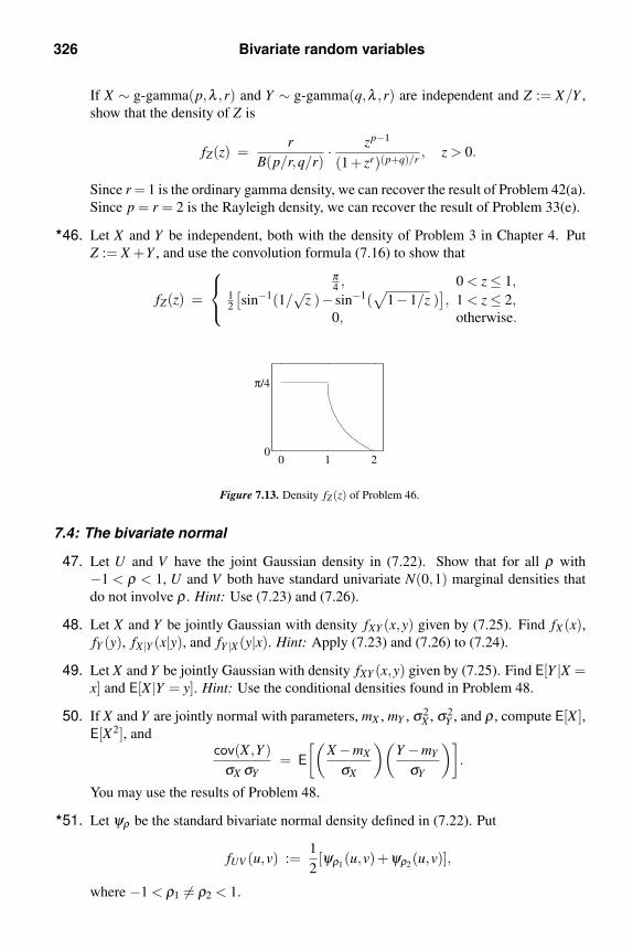
326 Bivariate random variables
If X ∼ g-gamma(p,λ ,r) and Y ∼ g-gamma(q,λ ,r) are independent and Z := X/Y ,
show that the density of Z is
fZ(z) =r
B(p/r,q/r)· zp−1
(1+ zr)(p+q)/r, z > 0.
Since r = 1 is the ordinary gamma density, we can recover the result of Problem 42(a).
Since p = r = 2 is the Rayleigh density, we can recover the result of Problem 33(e).
46. Let X and Y be independent, both with the density of Problem 3 in Chapter 4. Put
Z := X +Y , and use the convolution formula (7.16) to show that
fZ(z) =
⎧⎨⎩π4, 0 < z ≤ 1,
12
[sin−1(1/
√z )− sin−1(
√1−1/z )
], 1 < z ≤ 2,
0, otherwise.
0 1 20
π/4
Figure 7.13. Density fZ(z) of Problem 46.
7.4: The bivariate normal
47. Let U and V have the joint Gaussian density in (7.22). Show that for all ρ with
−1 < ρ < 1, U and V both have standard univariate N(0,1) marginal densities that
do not involve ρ . Hint: Use (7.23) and (7.26).
48. Let X and Y be jointly Gaussian with density fXY (x,y) given by (7.25). Find fX (x),fY (y), fX |Y (x|y), and fY |X (y|x). Hint: Apply (7.23) and (7.26) to (7.24).
49. Let X and Y be jointly Gaussian with density fXY (x,y) given by (7.25). Find E[Y |X =x] and E[X |Y = y]. Hint: Use the conditional densities found in Problem 48.
50. If X and Y are jointly normal with parameters, mX , mY , σ2X , σ2
Y , and ρ , compute E[X ],E[X2], and
cov(X ,Y )
σX σY
= E
[(X −mX
σX
)(Y −mY
σY
)].
You may use the results of Problem 48.
51. Let ψρ be the standard bivariate normal density defined in (7.22). Put
fUV (u,v) :=1
2[ψρ1
(u,v)+ψρ2(u,v)],
where −1 < ρ1 = ρ2 < 1.
Problems 327
(a) Show that the marginals fU and fV are both N(0,1). (You may use the results
of Problem 47.)
(b) Show that ρ := E[UV ] = (ρ1 +ρ2)/2. (You may use the result of Example 7.19.)
(c) Show that U and V cannot be jointly normal. Hints: (i) To obtain a contra-
diction, suppose that fUV is a jointly normal density with parameters given
by parts (a) and (b). (ii) Consider fUV (u,u). (iii) Use the following fact: If
β1, . . . ,βn are distinct real numbers, and if
n
∑k=1
αkeβkt = 0, for all t ≥ 0,
then α1 = · · · = αn = 0.
(d) By construction, U and V are jointly continuous. If ρ1 = −ρ2, then part (b)
shows that U and V are uncorrelated. However, they are not independent. Show
this by arguing as follows. First compute E[V 2|U = u] and show that even if
ρ1 = −ρ2, this conditional expectation is a function of u unless ρ1 = ρ2 = 0.
Then note that if U and V were independent, E[V 2|U = u] = E[V 2] = 1 and does
not depend on u. Hint: Example 7.20 will be helpful.
52. Let U and V be jointly normal with joint density ψρ(u,v) defined in (7.22). Put
Qρ(u0,v0) := P(U > u0,V > v0).
Show that for u0,v0 ≥ 0,
Qρ(u0,v0) =∫ tan−1(v0/u0)
0hρ(v2
0,θ)dθ +∫ π/2−tan−1(v0/u0)
0hρ(u2
0,θ)dθ ,
where
hρ(z,θ) :=
√1−ρ2
2π(1−ρ sin2θ)exp
[−z(1−ρ sin2θ)
2(1−ρ2)sin2 θ
].
This formula for Qρ(u0,v0) is Simon’s [55, eq. (78b)], [56, pp. 1864–1865] bivariate
generalization of Craig’s univariate formula given in Problem 22. Hint: Write P(U >u0,V > v0) as a double integral and convert to polar coordinates. It may be helpful to
review your solution of Problem 22 first.
53. Use Simon’s formula in Problem 52 to show that
Q(x0)2 =
1
π
∫ π/4
0exp
( −x20
2sin2 θ
)dθ .
In other words, to compute Q(x0)2, we integrate Craig’s integrand (Problem 22) only
half as far [55, p. 210], [56, p. 1865] !

328 Bivariate random variables
7.5: Extension to three or more random variables
54. If
fXY Z(x,y,z) =2exp[−|x− y|− (y− z)2/2]
z5√
2π, z ≥ 1,
and fXY Z(x,y,z) = 0 otherwise, find fY Z(y,z), fX |Y Z(x|y,z), fZ(z), and fY |Z(y|z).55. Let
fXY Z(x,y,z) =e−(x−y)2/2e−(y−z)2/2e−z2/2
(2π)3/2.
Find fXY (x,y). Then find the means and variances of X and Y . Also find the correla-
tion, E[XY ].
56. Let X , Y , and Z be as in Example 7.22. Evaluate E[XY ] and E[Y Z].
57. Let X , Y , and Z be as in Problem 54. Evaluate E[XY Z].
58. Let X , Y , and Z be jointly continuous. Assume that X ∼ uniform[1,2]; that given
X = x, Y ∼ exp(1/x); and that given X = x and Y = y, Z is N(x,1). Find E[XY Z].
59. Let N denote the number of primaries in a photomultiplier, and let Xi be the number
of secondaries due to the ith primary. Then the total number of secondaries is
Y =N
∑i=1
Xi.
Express the characteristic function of Y in terms of the probability generating func-
tion of N, GN(z), and the characteristic function of the Xi, assuming that the Xi are
i.i.d. with common characteristic function ϕX (ν). Assume that N is independent of
the Xi sequence. Find the density of Y if N ∼ geometric1(p) and Xi ∼ exp(λ ).
Exam preparation
You may use the following suggestions to prepare a study sheet, including formulas men-
tioned that you have trouble remembering. You may also want to ask your instructor for
additional suggestions.
7.1. Joint and marginal cdfs. Know the rectangle formula (7.2). Know how to ob-
tain marginal cdfs from the joint cdf; i.e., (7.3) and (7.4). Know that X and Y are
independent if and only if the joint cdf is equal to the product of the marginal cdfs.
7.2. Jointly continuous random variables. Know the mixed partial formula (7.9) for
obtaining the joint density from the joint cdf. Know how to integrate out unneeded
variables from the joint density to obtain the marginal density (7.10). Know that
jointly continuous random variables are independent if and only if their joint density
factors as fXY (x,y) = fX (x) fY (y).
7.3. Conditional probability and expectation. Know the formula for conditional den-
sities (7.12). Again, I tell my students that the three most important things in proba-
bility are:

Exam preparation 329
(i) the laws of total probability (7.13), (7.14), and (7.20);
(ii) the substitution laws (7.15) and (7.21); and
(iii) independence.
If the conditional density of Y given X is listed in the table inside the back cover
(this table includes moments), then E[Y |X = x] or E[Y 2|X = x] can often be found
by inspection. This is a very useful skill.
7.4. The bivariate normal. For me, the easiest way to remember the bivariate normal
density is in two stages. First, I remember (7.22), and then I use (7.24). Remember
that if X and Y are jointly normal, the conditional density of one given the other
is also normal, and E[X |Y = y] has the form my + b for some slope m and some
y-intercept b. See Problems 48 and 49.
7.5. Extension to three or more random variables. Note the more general forms of the
law of total probability (7.29) and the substitution law (7.30).
Work any review problems assigned by your instructor. If you finish them, re-work your
homework assignments.
8
Introduction to random vectors†
In the previous chapter, we worked mostly with two or three random variables at a
time. When we need to work with a larger number of random variables, it is convenient to
collect them into a column vector. The notation of vectors and matrices allows us to express
powerful formulas in straightforward, compact notation.
8.1 Review of matrix operations
Transpose of a matrix. Recall that if A is a matrix with entries Ai j, then its transpose,
denoted by A′, is defined by (A′)i j := A ji. For example,[1 3 5
2 4 6
]′=
⎡⎣ 1 2
3 4
5 6
⎤⎦ .
The transpose operation converts every row into a column, or equivalently, it converts every
column into a row. The example
[1 3 5
]′=
⎡⎣ 1
3
5
⎤⎦shows that an easy way to specify column vectors is to take the transpose of a row vector, a
practice we use frequently.
Sum of matrices. If two matrices have the same dimensions, then their sum is computed
by adding the corresponding entries. For example,[1 2 3
4 5 6
]+
[10 20 30
40 50 60
]=
[11 22 33
44 55 66
].
Product of matrices. If A is an r×n matrix and B is an n× p matrix, then their product
is the r× p matrix whose entries are given by
(AB)i j :=n
∑k=1
AikBk j,
where i = 1, . . . ,r and j = 1, . . . , p. For example, using a piece of scratch paper, you can
check that [7 8 9
4 5 6
]⎡⎣ 10 40
20 50
30 60
⎤⎦ =
[500 1220
320 770
]. (8.1)
You can also check it with the MATLAB commands
†This chapter and the next are not required for the study of random processes in Chapter 10. See the Chapter
Dependencies graph in the preface.
330
8.1 Review of matrix operations 331
A = [ 7 8 9 ; 4 5 6 ]
B = [ 10 40 ; 20 50 ; 30 60 ]
A*B
Notice how rows are separated with the semicolon “;”.
Trace of a matrix. If C is a square r× r matrix, then the trace of C is defined to be the
sum of its diagonal elements,
tr(C) :=r
∑k=1
Ckk.
For example, the trace of the matrix on the right-hand side of (8.1) is 1270. If A is an r×n
matrix and B is an n× r matrix, it is shown in Problem 4 that
tr(AB) = tr(BA),
where the left-hand side is the trace of an r× r matrix, and the right-hand side is the trace
of an n× n matrix. In particular, if n = 1, BA is a scalar; in this case, tr(AB) = BA. The
MATLAB command for tr is trace. For example, if A and B are defined by the above
MATLAB commands, you can easily check that trace(A*B) gives the same result as
trace(B*A).
Norm of a vector. If x = [x1, . . . ,xn]′, then we define the norm of x by
‖x‖ := (x ′x)1/2.
Notice that since ‖x‖2 = x ′x is a scalar,
‖x‖2 = x ′x = tr(x ′x) = tr(xx ′), (8.2)
a formula we use later.
Inner product of vectors. If x = [x1, . . . ,xn]′ and y = [y1, . . . ,yn]
′ are two column vec-
tors, their inner product or dot product is defined by
〈x,y〉 := y ′x.
Taking y = x yields 〈x,x〉 = ‖x‖2. An important property of the inner product is that
∣∣〈x,y〉∣∣ ≤ ‖x‖‖y‖, (8.3)
with equality if and only if one of them is a scalar multiple of the other. This result is known
as the Cauchy–Schwarz inequality for column vectors and is derived in Problem 6.
Remark. While y ′x is called the inner product, xy ′ is sometimes called the outer prod-
uct. Since y ′x = tr(y ′x) = tr(xy ′), the inner product is equal to the trace of the outer product.
While the formula tr(xy ′) is useful for theoretical analysis, it is computationally inefficient.

332 Introduction to random vectors
Block matrices. Sometimes it is convenient to partition a large matrix so that it can be
written in terms of smaller submatrices or blocks. For example, we can partition⎡⎢⎢⎣11 12 13 14
21 22 23 24
31 32 33 34
41 42 43 44
⎤⎥⎥⎦in several different ways such as⎡⎢⎢⎣
11 12 13 14
21 22 23 24
31 32 33 34
41 42 43 44
⎤⎥⎥⎦ ,
⎡⎢⎢⎣11 12 13 14
21 22 23 24
31 32 33 34
41 42 43 44
⎤⎥⎥⎦ , or
⎡⎢⎢⎣11 12 13 14
21 22 23 24
31 32 33 34
41 42 43 44
⎤⎥⎥⎦ .
The middle partition has the form ⎡⎣ A B C
D E F
G H K
⎤⎦ .
The first and last partitions both have the form[A B
C D
],
but the the corresponding blocks have different sizes. For example, in the partition on the
left, A would be 2×2, but in the partition on the right, A would be 3×3.
A partitioned matrix can be transposed block by block. For example,[A B C
D E F
]′=
⎡⎣ A′ D′B′ E ′C′ F ′
⎤⎦ .
A pair of partitioned matrices can be added block by block if the corresponding blocks
have the same dimensions. For example,[A B
C D
]+
[α βγ δ
]=
[A+α B+βC + γ D+δ
],
provided the dimensions of A and α are the same, the dimensions of B and β are the same,
the dimensions of C and γ are the same, and the dimensions of D and δ are the same.
A pair of partitioned matrices can be multiplied blockwise if the blocks being multiplied
have the “right” dimensions. For example,[A B
C D
][α βγ δ
]=
[Aα +Bγ Aβ +BδCα +Dγ Cβ +Dδ
],
provided the sizes of the blocks are such that the matrix multiplications
Aα,Bγ,Aβ ,Bδ ,Cα,Dγ,Cβ ,and Dδ
are all defined.

8.2 Random vectors and random matrices 333
8.2 Random vectors and random matrices
A vector whose entries are random variables is called a random vector, and a matrix
whose entries are random variables is called a random matrix.
Expectation
The expectation of a random vector X = [X1, . . . ,Xn]′ is defined to be the vector of ex-
pectations of its entries; i.e.,
E[X ] :=
⎡⎢⎣ E[X1]...
E[Xn]
⎤⎥⎦ .
In other words, the mean vector m := E[X ] has entries mi = E[Xi].
More generally, if X is the n× p random matrix
X =
⎡⎢⎣ X11 · · · X1p
......
Xn1 · · · Xnp
⎤⎥⎦ ,
then its mean matrix is
E[X ] :=
⎡⎢⎣ E[X11] · · · E[X1p]...
...
E[Xn1] · · · E[Xnp]
⎤⎥⎦ .
An easy consequence of this definition is that if A is an r×n matrix with nonrandom entries,
then AX is an r× p random matrix, and E[AX ] = AE[X ]. To see this, write
E[(AX)i j] = E
[n
∑k=1
AikXk j
]=
n
∑k=1
E[AikXk j]
=n
∑k=1
AikE[Xk j]
=n
∑k=1
Aik(E[X ])k j
= (AE[X ])i j.
It is similarly easy to show that if B is a p×q matrix with nonrandom entries, then E[XB] =E[X ]B. Hence, E[AXB] = AE[X ]B. If G is r×q with nonrandom entries, then
E[AXB+G] = AE[X ]B+G.
334 Introduction to random vectors
Correlation
If X = [X1, . . . ,Xn]′ is a random vector with mean vector m := E[X ], then we define the
correlation matrix of X by
R := E[XX ′].
We now point out that since XX ′ is equal to⎡⎢⎣ X21 · · · X1Xn
......
XnX1 · · · X2n
⎤⎥⎦ ,
the i j entry of R is just E[XiX j]. Since Ri j = R ji, R is symmetric. In other words, R′ = R.
Example 8.1. Write out the correlation matrix of the three-dimensional random vector
W := [X ,Y,Z]′.
Solution. The correlation matrix of W is
E[WW ′] =
⎡⎣ E[X2] E[XY ] E[XZ]E[Y X ] E[Y 2] E[Y Z]E[ZX ] E[ZY ] E[Z2]
⎤⎦ .
There is a Cauchy–Schwarz inequality for random variables. For scalar random vari-
ables U and V , ∣∣E[UV ]∣∣ ≤
√E[U2]E[V 2]. (8.4)
This is formula (2.24), which was derived in Chapter 2.
Example 8.2. Show that if R is the correlation matrix of X , then∣∣Ri j
∣∣ ≤ √RiiR j j,
Solution. By the Cauchy–Schwarz inequality,
∣∣E[XiX j]∣∣ ≤
√E[X2
i ]E[X2j ].
These expectations are, respectively, Ri j, Rii, and R j j.

8.2 Random vectors and random matrices 335
Covariance
If X = [X1, . . . ,Xn]′ is a random vector with mean vector m := E[X ], then we define the
covariance matrix of X by
cov(X) := E[(X −m)(X −m)′].
Since E[X ′] = (E[X ])′, we see that
cov(X) = E[XX ′ −Xm′ −mX ′ +mm′]= E[XX ′]−E[X ]m′ −mE[X ′]+mm′
= E[XX ′]−mm′,
which generalizes the variance formula (2.17). We often denote the covariance matrix of X
by CX , or just C if X is understood. Since E[XX ′] is the correlation matrix of X , we see that
the covariance and correlation matrices are equal if and only if the mean vector is zero. We
now point out that since (X −m)(X −m)′ is equal to⎡⎢⎣ (X1 −m1)(X1 −m1) · · · (X1 −m1)(Xn −mn)...
...
(Xn −mn)(X1 −m1) · · · (Xn −mn)(Xn −mn)
⎤⎥⎦ ,
the i j entry of C = cov(X) is just
E[(Xi −mi)(X j −m j)] = cov(Xi,X j),
the covariance between entries Xi and X j. Note the distinction between the covariance of a
pair of random variables, which is a scalar, and the covariance of a column vector, which is
a matrix. We also point out the following facts.
• Cii = cov(Xi,Xi) = var(Xi).• Since Ci j = C ji, the matrix C is symmetric.
• For i = j, Ci j = 0 if and only if Xi and X j are uncorrelated. Thus, C is a diagonal
matrix if and only if Xi and X j are uncorrelated for all i = j.
Example 8.3. If a random vector X has covariance matrix C, show that Y := AX has
covariance matrix ACA′.
Solution. Put m := E[X ] so that Y −E[Y ] = AX −E[AX ] = A(X −m). Then
cov(Y ) = E[(Y −E[Y ])(Y −E[Y ])′]
= E[A(X −m)(X −m)′A′]= AE[(X −m)(X −m)′]A′
= ACA′.

336 Introduction to random vectors
Example 8.4. A simple application of Example 8.3 is to the case in which A = a′, where
a is a column vector. In this case, Y = a′X is a scalar, and var(Y ) = cov(Y ) = a′Ca. In
particular,
a′Ca = var(Y ) ≥ 0, for all a.
A symmetric matrix C with the property a′Ca ≥ 0 for all vectors a is said to be positive
semidefinite. By Example 8.4, every covariance matrix is positive semidefinite. If a′Ca > 0
for all nonzero a, then C is called positive definite.
Example 8.5. Let X be a zero-mean random vector whose covariance matrix C =E[XX ′]is singular. Show that for some i and some coefficients b j,
Xi = ∑j =i
b jX j.
In other words, one of the Xi is a deterministic, linear function of the remaining components.
Solution. Recall that C is singular means that there is a nonzero vector a such that
Ca = 0. For such a, we have by Example 8.4 that the scalar random variable Y := a′Xsatisfies E[Y 2] = a′Ca = 0. Hence, Y is the zero random variable. In other words,
0 = Y = a′X =n
∑j=1
a jX j.
Since a is not the zero vector, some component, say ai = 0, and it follows that
Xi = − 1
ai∑j =i
a jX j.
Taking b j = −a j/ai solves the problem.
Remark. The solution of Example 8.5 shows that if X is zero mean with singular covari-
ance matrix C, then there is a nonzero vector a such that a′X is the zero random variable.
If X has mean vector m, then the same argument shows that a′(X −m) is the zero random
variable, or equivalently, a′X is the constant random variable with value a′m.
Cross-covariance
If X = [X1, . . . ,Xn]′ and Y = [Y1, . . . ,Yp]
′ are both random vectors with respective means
mX and mY , then their cross-covariance matrix is the n× p matrix
cov(X ,Y ) := E[(X −mX )(Y −mY )′],

8.2 Random vectors and random matrices 337
which we denote by CXY . Note that (CXY )i j = cov(Xi,Yj) is just the covariance between Xi
and Yj. Also,
CY X = E[(Y −mY )(X −mX )′] = (CXY )′,
which is p×n. The cross-correlation matrix of X and Y is RXY := E[XY ′], and (RXY )i j =E[XiYj].
If we stack X and Y into the (n+ p)-dimensional composite vector
Z :=
[X
Y
],
then the covariance matrix of Z is given by
CZ =
[CX CXY
CY X CY
],
where CZ is (n+ p)× (n+ p), CX is n×n, CY is p× p, CXY is n× p, and CY X is p×n.
Just as two random variables U and V are said to be uncorrelated if cov(U,V ) = 0,
we say that two random vectors X = [X1, . . . ,Xn]′ and Y = [Y1, . . . ,Yp]
′ are uncorrelated if
cov(Xi,Yj) = 0 for all i = 1, . . . ,n and all j = 1, . . . , p. This is equivalent to the condition
that CXY = cov(X ,Y ) = 0 be the n× p zero matrix. If this is the case, then the matrix CZ
above is block diagonal; i.e.,
CZ =
[CX 0
0 CY
].
Characteristic functions
The joint characteristic function of X = [X1, . . . ,Xn]′ is defined by
ϕX (ν) := E[e jν ′X ] = E[e j(ν1X1+···+νnXn)],
where ν = [ν1, . . . ,νn]′.
When X has a joint density, ϕX (ν) = E[e jν ′X ] is just the n-dimensional Fourier trans-
form,
ϕX (ν) =∫
IRne jν ′x fX (x)dx, (8.5)
and the joint density can be recovered using the multivariate inverse Fourier transform:
fX (x) =1
(2π)n
∫IRn
e− jν ′xϕX (ν)dν .
Whether X has a joint density or not, the joint characteristic function can be used to
obtain its various moments.
Example 8.6. The components of the mean vector and covariance matrix can be ob-
tained from the characteristic function as follows. Write
∂∂νk
E[e jν ′X ] = E[e jν ′X jXk],

338 Introduction to random vectors
and∂ 2
∂ν∂νk
E[e jν ′X ] = E[e jν ′X ( jX)( jXk)].
Then∂
∂νk
E[e jν ′X ]∣∣∣ν=0
= jE[Xk],
and∂ 2
∂ν∂νk
E[e jν ′X ]∣∣∣ν=0
= −E[XXk].
Higher-order moments can be obtained in a similar fashion.
If the components of X = [X1, . . . ,Xn]′ are independent, then
ϕX (ν) = E[e jν ′X ]
= E[e j(ν1X1+···+νnXn)]
= E
[n
∏k=1
e jνkXk
]=
n
∏k=1
E[e jνkXk ]
=n
∏k=1
ϕXk(νk).
We have just shown that if the components of X are independent, then the joint char-
acteristic function is the product of the marginal characteristic functions. The converse is
also true; i.e., if the joint characteristic function is the product of the marginal characteristic
functions, then the random variables are independent [3]. A derivation in the case of two
jointly continuous random variables was given in Section 7.2.
Decorrelation and the Karhunen–Loeve expansion
Let X be an n-dimensional random vector with zero mean and covariance matrix C. We
show that X has the representation X = PY , where the components of Y are uncorrelated
and P is an n×n matrix satisfying P ′P = PP ′ = I. (Hence, P ′ = P−1.) This representation
is called the Karhunen–Loeve expansion.
Step 1. Recall that since a covariance matrix is symmetric, it can be diagonalized [30]; i.e.,
there is a square matrix P such that P ′P = PP ′ = I and such that P ′CP = Λ is a diagonal
matrix, say Λ = diag(λ1, . . . ,λn).
Step 2. Define a new random variable Y := P ′X . By Example 8.3, cov(Y ) = P ′CP = Λ.
Since cov(Y ) = Λ is diagonal, the components of Y are uncorrelated. For this reason, we
call P ′ a decorrelating transformation.
Step 3. X and Y are equivalent in that each is a function of the other. By definition, Y = P ′X .
To recover X from Y , write PY = PP ′X = X .

8.2 Random vectors and random matrices 339
Step 4. If C is singular, we can actually throw away some components of Y without any
loss of information! Writing C = PΛP ′, we have
detC = detPdetΛdetP ′ = detP ′ detPdetΛ = det(P ′P)detΛ = detΛ = λ1 · · ·λn.
Thus, C is singular if and only if some of the λi are zero. Since λi = E[Y 2i ], we see that
λi = 0 if and only if Yi is the zero random variable. Hence, we only need to keep around the
Yi for which λi > 0 — we know that the other Yi are zero.
Example 8.7 (data reduction). Suppose that X is a zero-mean vector of dimension n =5, and suppose that λ2 = λ3 = 0. Then we can extract the nonzero Yi from Y = P ′X by
writing ⎡⎣ Y1
Y4
Y5
⎤⎦ =
⎡⎣ 1 0 0 0 0
0 0 0 1 0
0 0 0 0 1
⎤⎦⎡⎢⎢⎢⎢⎣
Y1
Y2
Y3
Y4
Y5
⎤⎥⎥⎥⎥⎦ .
For this reason, we call the above 3× 5 matrix of zeros and ones an “extractor matrix.”
Since X = PY , and since we know Y2 and Y3 are zero, we can reconstruct X from Y1, Y4, and
Y5 by applying P to ⎡⎢⎢⎢⎢⎣Y1
0
0
Y4
Y5
⎤⎥⎥⎥⎥⎦ =
⎡⎢⎢⎢⎢⎣1 0 0
0 0 0
0 0 0
0 1 0
0 0 1
⎤⎥⎥⎥⎥⎦⎡⎣ Y1
Y4
Y5
⎤⎦ .
We call this 5× 3 matrix of zeros and ones a “reconstructor matrix.” Notice that it is the
transpose of the “extractor matrix.”
The foregoing example illustrates the general result. If we let E denote the “extractor
matrix” that creates the subvector of nonzero components of Y , then X = PE ′EP ′X , where
E ′ is the “reconstructor matrix” that rebuilds Y from the subvector of its nonzero compo-
nents. See Problem 19 for more details.
Example 8.8 (noiseless detection). Suppose that the random variable X in the previous
example is the noise in a channel over which we must send either the signal m = 0 or a
signal m = 0. The received vector is Z = m + X . Design a signal m = 0 and a receiver that
can distinguish m = 0 from m = 0 without error.
Solution. We consider a receiver that applies the transformation P ′ to the received vector
Z to get P ′Z = P ′m+P ′X . Letting W := P ′Z, µ := P ′m, and Y := P ′X , we can write⎡⎢⎢⎢⎢⎣W1
W2
W3
W4
W5
⎤⎥⎥⎥⎥⎦ =
⎡⎢⎢⎢⎢⎣µ1
µ2
µ3
µ4
µ5
⎤⎥⎥⎥⎥⎦+
⎡⎢⎢⎢⎢⎣Y1
0
0
Y4
Y5
⎤⎥⎥⎥⎥⎦ .

340 Introduction to random vectors
In particular, we observe that W2 = µ2 and W3 = µ3. Thus, as long as the nonzero m is
chosen so that the second and third components of µ = P ′m are not both zero, we can
noiselessly distinguish between m = 0 and m = 0. For example, if the nonzero m is any
vector of the form m = Pβ , where β2 and β3 are not both zero, then µ = P ′m = P ′Pβ = βsatisfies the desired condition that µ2 and µ3 are not both zero.
Remark. For future reference, we write X = PY in component form as
Xi =n
∑k=1
PikYk. (8.6)
By writing the component form, it will be easier to see the similarity with the Karhunen–
Loeve expansion of continuous-time random processes derived in Chapter 13.
Remark. Given a covariance matrix C, the matrices P and Λ can be obtained with the
MATLAB command
[P,Lambda] = eig(C).
To extract the diagonal elements of Lambda as a vector, use the command
lambda = diag(Lambda).
8.3 Transformations of random vectors
If G(x) is a vector-valued function of x ∈ IRn, and X is an IRn-valued random vector, we
can define a new random vector by Y = G(X). If X has joint density fX , and G is a suitable
invertible mapping, then we can find a relatively explicit formula for the joint density of Y .
Suppose that the entries of the vector equation y = G(x) are given by⎡⎢⎣ y1
...
yn
⎤⎥⎦ =
⎡⎢⎣ g1(x1, . . . ,xn)...
gn(x1, . . . ,xn)
⎤⎥⎦ .
If G is invertible, we can apply G−1 to both sides of y = G(x) to obtain G−1(y) = x. Using
the notation H(y) := G−1(y), we can write the entries of the vector equation x = H(y) as⎡⎢⎣ x1
...
xn
⎤⎥⎦ =
⎡⎢⎣ h1(y1, . . . ,yn)...
hn(y1, . . . ,yn)
⎤⎥⎦ .
Assuming that H is continuous and has continuous partial derivatives, let
dH(y) :=
⎡⎢⎢⎢⎢⎢⎢⎢⎣
∂h1∂y1
· · · ∂h1∂yn
......
∂ hi
∂y1· · · ∂hi
∂yn
......
∂hn
∂y1· · · ∂hn
∂yn
⎤⎥⎥⎥⎥⎥⎥⎥⎦. (8.7)

8.3 Transformations of random vectors 341
To compute P(Y ∈C) = P(G(X) ∈C), it is convenient to put B := x : G(x) ∈C so that
P(Y ∈C) = P(G(X) ∈C)
= P(X ∈ B)
=∫
IRnIB(x) fX (x)dx.
Now apply the multivariate change of variable x = H(y). Keeping in mind that dx =|detdH(y) |dy,
P(Y ∈C) =∫
IRnIB(H(y)) fX (H(y)) |detdH(y) |dy.
Observe that IB(H(y)) = 1 if and only if H(y) ∈ B, which happens if and only if G(H(y)) ∈C. However, since H = G−1, G(H(y)) = y, and we see that IB(H(y)) = IC(y). Thus,
P(Y ∈C) =∫
CfX (H(y)) |detdH(y) |dy.
Since the set C is arbitrary, the integrand must be the density of Y . Thus,
fY (y) = fX (H(y)) |detdH(y) |.
Since detdH(y) is called the Jacobian of H, the preceding equations are sometimes called
Jacobian formulas. They provide the multivariate generalization of (5.2).
Example 8.9. Let Y = AX + b, where A is a square, invertible matrix, b is a column
vector, and X has joint density fX . Find fY .
Solution. Since A is invertible, we can solve Y = AX +b for X = A−1(Y −b). In other
words, H(y) = A−1(y−b). It is easy to check that dH(y) = A−1. Hence,
fY (y) = fX (A−1(y−b)) |detA−1 | =fX (A−1(y−b))
|detA | .
The formula in the preceding example is useful when solving problems for arbitrary A.
However, when A is small and given explicitly, it is more convenient to proceed as follows.
Example 8.10. Let X and Y be independent univariate N(0,1) random variables. If
U := 2X −5Y and V := X −4Y , find the joint density of U and V . Are U and V independent?
Solution. The transformation [u,v]′ = G(x,y) is given by
u =2x−5y
v = x−4y.

342 Introduction to random vectors
By solving these equations for x and y in terms of u and v, we obtain the inverse transfor-
mation [x,y]′ = H(u,v) given by
x = 43u− 5
3v
y = 13u− 2
3v.
The matrix dH(u,v) is given by
dH(u,v) =
⎡⎣ ∂x∂u
∂ x∂v
∂y∂u
∂y∂v
⎤⎦ =
[4/3 −5/3
1/3 −2/3
],
and we see that detdH(u,v) = −1/3. Since fXY (x,y) = e−(x2+y2)/2/2π , we can write
fUV (u,v) = fXY (x,y)∣∣∣ x=4u/3−5v/3
y=u/3−2v/3
· |detdH(u,v) |
= (2π)−1 exp[− 1
2
(179
u2 − 449
uv+ 299
v2)]
13.
Recalling the formula for the bivariate normal density (7.25), we see that U and V have
nonzero correlation coefficient; hence, they are not independent.
Example 8.11. Let X and Y be independent random variables where Y ∼ N(0,1) and X
has the standard Rayleigh density, fX (x) = xe−x2/2, x ≥ 0. Find the joint density of U :=√X2 +Y 2 and V := λY/X , where λ is a positive real number. Are U and V independent?
Solution. The transformation [u,v]′ = G(x,y) is given by
u =√
x2 + y2
v = λy/x.
By solving these equations for x and y in terms of u and v, we obtain the inverse transfor-
mation [x,y]′ = H(u,v). To do this, we first write u2 = x2 + y2 and v2 = λ 2y2/x2. From this
second equation, we have y2 = v2x2/λ 2. We then write
u2 = x2 + y2 = x2 + v2x2/λ 2 = x2(1+ v2/λ 2).
It then follows that
x2 =u2
1+ v2/λ 2.
Since X is a nonnegative random variable, we take the positive square root to get
x =u√
1+ v2/λ 2.
Next, since v = λy/x,
y = vx/λ =uv
λ√
1+ v2/λ 2.
8.3 Transformations of random vectors 343
A little calculation shows that
dH(u,v) =
⎡⎣ ∂x∂u
∂x∂v
∂y∂u
∂y∂v
⎤⎦ =
⎡⎣ 1√1+v2/λ 2
−uv
λ 2(1+v2/λ 2)3/2
v
λ√
1+v2/λ 2
u
λ (1+v2/λ 2)3/2
⎤⎦ .
It then follows that detdH(u,v) = λu/(λ 2 + v2). The next step is to write
fUV (u,v) = fXY (x,y) · |detdH(u,v) |and to substitute x and y using the above formulas. Now
fXY (x,y) = xe−x2/2e−y2/2/√
2π = xe−(x2+y2)/2/√
2π.
From the original definition of U , we know that u2 = x2 + y2, and we already solved for x.
Hence,
fUV (u,v) =u√
1+ v2/λ 2
e−u2/2
√2π
· λu
λ 2 + v2
=
√2
πu2e−u2/2 · 1
2λ
(1+
v2
λ 2
)−3/2
= fU (u) fV (v),
where fU is the standard Maxwell density defined in Problem 4 in Chapter 5 and fV is a
scaled Student’s t density with two degrees of freedom (defined in Problem 20 in Chapter 4).
In particular, U and V are independent.1
Example 8.12. Let X and Y be independent univariate N(0,1) random variables. Let R
denote the length of the vector [X ,Y ]′, and let Θ denote the angle the vector makes with the
x-axis. In other words, if X and Y are the Cartesian coordinates of a random point in the
plane, then R ≥ 0 and −π < Θ ≤ π are the corresponding polar coordinates. Find the joint
density of R and Θ.
Solution. The transformation [r,θ ]′ = G(x,y) is given by2
r =√
x2 + y2,
θ = angle(x,y).
The inverse transformation [x,y]′ = H(r,θ) is the mapping that takes polar coordinates into
Cartesian coordinates. Hence, H(r,θ) is given by
x = r cosθ ,
y = r sinθ .
The matrix dH(r,θ) is given by
dH(r,θ) =
⎡⎣ ∂x∂ r
∂x∂θ
∂y∂ r
∂y∂θ
⎤⎦ =
[cosθ −r sinθsinθ r cosθ
],

344 Introduction to random vectors
and detdH(r,θ) = r cos2 θ + r sin2 θ = r. Then
fR,Θ(r,θ) = fXY (x,y)∣∣∣ x=r cosθ
y=r sinθ· |detdH(r,θ) |
= fXY (r cosθ ,r sinθ)r.
Now, since X and Y are independent N(0,1), fXY (x,y) = fX (x) fY (y) = e−(x2+y2)/2/(2π),and
fR,Θ(r,θ) = re−r2/2 · 1
2π, r ≥ 0,−π < θ ≤ π.
Thus, R and Θ are independent, with R having a Rayleigh density and Θ having a uniform
(−π,π] density.
8.4 Linear estimation of random vectors (Wiener filters)
Consider a pair of random vectors X and Y , where X is not observed, but Y is observed.
For example, X could be the input to a noisy channel, and Y could be the channel output. In
this situation, the receiver knows Y and needs to estimate X . By an estimator of X based
on Y , we mean a function g(y) such that X := g(Y ) is our estimate or “guess” of the value
of X . What is the best function g to use? What do we mean by best? In this section, we
define g to be best if it minimizes the mean-squared error (MSE) E[‖X − g(Y )‖2] for all
functions g in some class of functions. Here we restrict attention to the class of functions of
the form g(y) = Ay+b, where A is a matrix and b is a column vector; we drop this restriction
in Section 8.6. A function of the form Ay + b is said to be affine. If b = 0, then g is linear.
It is common to say g is linear even if b = 0 since this only is a slight abuse of terminology,
and the meaning is understood. We shall follow this convention. The optimal such function
g is called the linear minimum mean-squared-error estimator, or more simply, linear
MMSE estimator. Linear MMSE estimators are sometimes called Wiener filters.
To find the best linear estimator is to find the matrix A and the column vector b that
minimize the MSE, which for linear estimators has the form
E[∥∥X − (AY +b)
∥∥2].
Letting mX := E[X ] and mY := E[Y ], the MSE is equal to
E[∥∥(X −mX )−A(Y −mY )
+
mX −AmY −b∥∥2]
.
Since the left-hand quantity in braces is zero mean, and since the right-hand quantity in
braces is a constant (nonrandom), the MSE simplifies to
E[∥∥(X −mX )−A(Y −mY )
∥∥2]+‖mX −AmY −b‖2.
No matter what matrix A is used, the optimal choice of b is
b = mX −AmY ,

8.4 Linear estimation of random vectors (Wiener filters) 345
and the estimate is
g(Y ) = AY +b = A(Y −mY )+mX . (8.8)
The estimate is truly linear in Y if and only if AmY = mX .
We show later in this section that the optimal choice of A is any solution of
ACY = CXY . (8.9)
When CY is invertible, A = CXYC−1Y . This is best computed in MATLAB with the command
A = CXY/CY. Even if CY is not invertible, there is always a solution of (8.9), as shown in
Problem 38.
Remark. If X and Y are uncorrelated, by which we mean CXY = 0, then taking A = 0
solves (8.9). In this case, the estimate of X reduces to g(Y ) = mX . In other words, the
value we guess for X based on observing Y does not involve Y ! Hence, if X and Y are
uncorrelated, then linear signal processing of Y cannot extract any information about X that
can minimize the MSE below E[‖X −mX‖2] = tr(CX ) (cf. Problem 9).
Example 8.13 (signal in additive noise). Let X denote a random signal of zero mean
and known covariance matrix CX . Suppose that in order to estimate X , all we have available
is the noisy measurement
Y = X +W,
where W is a noise vector with zero mean and known, positive-definite covariance matrix
CW . Further assume that the covariance between the signal and noise, CXW , is zero. Find
the linear MMSE estimate of X based on Y .
Solution. Since X and W are zero mean, mY = E[Y ] = E[X +W ] = 0. Next,
CXY = E[(X −mX )(Y −mY )′]= E[X(X +W )′]= CX , since CXW = 0.
Similarly,
CY = E[(Y −mY )(Y −mY )′]= E[(X +W )(X +W )′]= CX +CW .
It follows that
CXYC−1Y Y = CX (CX +CW )−1Y
is the linear MMSE estimate of X based on Y .

346 Introduction to random vectors
Example 8.14 (MATLAB). Use MATLAB to compute A = CXYC−1Y of the preceding ex-
ample if
CX =
[10 14
14 20
]and CW =
[1 0
0 1
].
Solution. We use the commands
CX = [ 10 14 ; 14 20 ]
CXY = CX;
CW = eye(2) % 2 by 2 identity matrix
CY = CX + CW
format rat % print numbers as ratios of small integers
A = CXY/CY
to find that
A =
[2/5 2/5
2/5 24/35
].
Example 8.15 (MATLAB). Let X denote the linear MMSE estimate of X based on Y . It
is shown in Problems 34 and 35 that the MSE is given by
E[‖X − X‖2] = tr(CX −AC′XY ).
Using the data for the previous two examples, compute the MSE and compare it with E[‖X−mX‖2] = tr(CX ).
Solution. The command trace(CX-A*(CXY’)) shows that the MSE achieved using
X is 1.08571. The MSE achieved using mX (which makes no use of the observation Y ) is
E[‖X −mX‖2] = tr(CX ) = 30. Hence, using even a linear function of the data has reduced
the error by a factor of about 30.
Example 8.16. Find the linear MMSE estimate of X based on Y if Y ∼ exp(λ ), and
given Y = y, X is conditionally Rayleigh(y).
Solution. Using the table of densities inside the back cover, we find that mY = 1/λ ,
CY = var(Y ) = 1/λ 2, and E[X |Y = y] = y√
π/2. Using the law of total probability, it is an
easy calculation to show that mX =√
π/2/λ and that E[XY ] = 2√
π/2/λ 2. It follows that
CXY = E[XY ]−mX mY =√
π/2/λ 2. Then
A = CXYC−1Y =
√π/2/λ 2
1/λ 2=√
π/2,
and the linear MMSE estimate of X based on Y is
CXYC−1Y (Y −mY )+mX =
√π/2 Y.

8.4 Linear estimation of random vectors (Wiener filters) 347
−2
0
2
−1−0.5
00.5
1
−3
−2
−1
0
1
2
3
p
p
^
Figure 8.1. The point on the plane that is closest to p is called the projection of p, and is denoted by p. The
orthogonality principle says that p is characterized by the property that the line joining p to p is orthogonal to the
plane. The symbol denotes the origin.
Derivation of the linear MMSE estimator
We now turn to the problem of minimizing
E[∥∥(X −mX )−A(Y −mY )
∥∥2].
The matrix A is optimal if and only if for all matrices B,
E[∥∥(X −mX )−A(Y −mY )
∥∥2] ≤ E[∥∥(X −mX )−B(Y −mY )
∥∥2]. (8.10)
The following condition is equivalent and is easier to use. This equivalence is known as the
orthogonality principle. It says that (8.10) holds for all B if and only if
E[
B(Y −mY )′
(X −mX )−A(Y −mY )]
= 0, for all B. (8.11)
Below we prove that (8.11) implies (8.10). The converse is also true, but we shall not use it
in this book.
We first explain the terminology and show geometrically why it is true. A two-dimen-
sional subspace (a plane passing through the origin) is shown in Figure 8.1. A point p not
in the subspace is also shown. The point on the plane that is closest to p is the point p.
This closest point is called the projection of p. The orthogonality principle says that the
projection p is characterized by the property that the line joining p to p, which is the error
vector p− p, is orthogonal to the subspace. In our situation, the role of p is played by the
random variable X −mX , the role of p is played by the random variable A(Y −mY ), and the
role of the subspace is played by the set of all random variables of the form B(Y −mY ) as B
runs over all matrices of the right dimensions. Since the inner product between two random
vectors U and V can be defined as E[V ′U ], (8.11) says that
(X −mX )−A(Y −mY )

348 Introduction to random vectors
is orthogonal to all B(Y −mY ).To use (8.11), first note that since it is a scalar equation, the left-hand side is equal to its
trace. Bringing the trace inside the expectation and using the fact that tr(αβ ) = tr(βα), we
see that the left-hand side of (8.11) is equal to
E[tr(
(X −mX )−A(Y −mY )(Y −mY )′B′)].
Taking the trace back out of the expectation shows that (8.11) is equivalent to
tr([CXY −ACY ]B′) = 0, for all B. (8.12)
By Problem 5, it follows that (8.12) holds if and only if CXY −ACY is the zero matrix, or
equivalently, if and only if A solves the equation
ACY = CXY .
If CY is invertible, the unique solution of this equation is
A = CXYC−1Y .
In this case, the estimate of X is
CXYC−1Y (Y −mY )+mX .
We now show that (8.11) implies (8.10). To simplify the notation, we assume zero
means. Write
E[‖X −BY‖2] = E[‖(X −AY )+(AY −BY )‖2]
= E[‖(X −AY )+(A−B)Y )‖2]
= E[‖X −AY‖2]+E[‖(A−B)Y‖2],
where the cross terms 2E[(A−B)Y′(X −AY )] vanish by (8.11). If we drop the right-hand
term in the above display, we obtain
E[‖X −BY‖2] ≥ E[‖X −AY‖2].
8.5 Estimation of covariance matrices†
As we saw in the previous section, covariance matrices are a critical component in the
design of linear estimators of random vectors. In real-world problems, however, we may
not know these matrices. Instead, we have to estimate them from the data.
Remark. We use the term “estimation” in two ways. In the previous section we es-
timated random vectors. In this section we estimate nonrandom parameters, namely, the
elements of the covariance matrix.
Recall from Chapter 6 that if X1, . . . ,Xn are i.i.d. with common mean m and common
variance σ2, then
Mn :=1
n
n
∑k=1
Xk
†Section 8.5 is not used elsewhere in the text and can be skipped without loss of continuity.

8.5 Estimation of covariance matrices 349
is an unbiased, strongly consistent estimator of the mean m. Similarly,
S2n :=
1
n−1
n
∑k=1
(Xk −Mn)2
is an unbiased, strongly consistent estimator of σ2. If we know a priori that m = 0, then
1
n
n
∑k=1
X2k
an unbiased and strongly consistent estimator of σ2.
Suppose we have i.i.d. random vectors X1, . . . ,Xn with zero mean and common covari-
ance matrix C. Our estimator of C is
Cn =1
n
n
∑k=1
XkX ′k.
Note that since Xk is a column vector, XkX ′k is a matrix, which makes sense since Cn is
an estimate of the covariance matrix C. We can do the above computation efficiently in
MATLAB if we arrange the Xk as the columns of a matrix. Observe that if X := [X1, . . . ,Xn],then
XX ′ = X1X ′1 + · · ·+XnX ′
n.
Example 8.17 (MATLAB). Here is a way to generate simulation examples using i.i.d.
zero-mean random vectors of dimension d and covariance matrix C = GG′, where G is any
d ×d matrix. We will use d = 5 and
G =
⎡⎢⎢⎢⎢⎣1 −2 −2 1 0
0 1 −1 3 −1
1 3 3 −3 4
−1 1 2 1 −4
0 2 0 −4 3
⎤⎥⎥⎥⎥⎦ .
When we ran the script
G = [ 1 -2 -2 1 0 ; 0 1 -1 3 -1 ; 1 3 3 -3 4 ; ...
-1 1 2 1 -4 ; 0 2 0 -4 3 ];
C = G*G’
d = length(G);
n = 1000;
Z = randn(d,n); % Create d by n array of i.i.d. N(0,1) RVs
X = G*Z; % Multiply each column by G
Chat = X*X’/n
we got
C =
⎡⎢⎢⎢⎢⎣10 3 −14 −6 −8
3 12 −13 6 −13
−14 −13 44 −11 30
−6 6 −11 23 −14
−8 −13 30 −14 29
⎤⎥⎥⎥⎥⎦

350 Introduction to random vectors
and
C =
⎡⎢⎢⎢⎢⎣10.4318 3.1342 −15.3540 −5.6080 −8.6550
3.1342 11.1334 −12.9239 5.5280 −12.5036
−15.3540 −12.9239 46.2087 −10.0815 30.5472
−5.6080 5.5280 −10.0815 21.2744 −13.1262
−8.6550 −12.5036 30.5472 −13.1262 29.0639
⎤⎥⎥⎥⎥⎦ .
When X1, . . . ,Xn are i.i.d. but have nonzero mean vector, we put
Mn :=1
n
n
∑k=1
Xk,
and we use
Cn :=1
n−1
n
∑k=1
(Xk −Mn)(Xk −Mn)′
to estimate C. Note that in MATLAB, if X has X1, . . . ,Xn for its columns, then the column
vector Mn can be computed with the command mean(X,2).
8.6 Nonlinear estimation of random vectors
In Section 8.4, we had two random vectors X and Y , but we could only observe Y . Based
on Y , we used functions of the form g(Y ) = AY +b as estimates of X . We characterized the
choice of A and b that would minimize E[‖X −g(Y )‖2].
In this section, we consider three other estimators of X . The first is the minimum mean-
squared error (MMSE) estimator. In this method, we no longer restrict g(y) to be of the
form Ay + b, and we try to further minimize the MSE E[‖X − g(Y )‖2]. As we show later,
the function g that minimizes the MSE is
gMMSE(y) = E[X |Y = y].
The second estimator uses the conditional density fY |X (y|x). The maximum-likelihood
(ML) estimator of X is the function
gML(y) := argmaxx
fY |X (y|x).
In other words, gML(y) is the value of x that maximizes fY |X (y|x). See Problem 43. When
the density of X is not positive for all x, we only consider values of x for which fX (x) > 0.
See Problem 44. The third estimator uses the conditional density fX |Y (x|y). The maximum
a posteriori probability (MAP) estimator of X is the function
gMAP(y) := argmaxx
fX |Y (x|y).

8.6 Nonlinear estimation of random vectors 351
Notice that since fX |Y (x|y) = fY |X (y|x) fX (x)/ fY (y), the maximizing value of x does not
depend on the value of fY (y). Hence,
gMAP(y) = argmaxx
fY |X (y|x) fX (x). (8.13)
When X is a uniform random variable, the constant value of fX (x) does not affect the max-
imizing value of x. In this case, gMAP(y) = gML(y).
Example 8.18 (signal in additive noise). A signal X with density fX (x) is transmitted
over a noisy channel so that the received vector is Y = X +W , where the noise W and the
signal X are independent, and the noise has density fW (w). Find the MMSE estimator of X
based on Y .
Solution. To compute E[X |Y = y], we first need to find fX |Y (x|y). Sincea
P(Y ≤ y|X = x) = P(X +W ≤ y|X = x)
= P(W ≤ y− x|X = x), by substitution,
= P(W ≤ y− x), by independence,
we see that fY |X (y|x) = fW (y− x). Hence,
fX |Y (x|y) =fY |X (y|x) fX (x)
fY (y)=
fW (y− x) fX (x)
fY (y).
It then follows that
gMMSE(y) = E[X |Y = y] =
∫x
fW (y− x) fX (x)
fY (y)dx,
where, since the density of the sum of independent random variables is the convolution of
their densities,
fY (y) =∫
fX (y−w) fW (w)dw.
Even in this context where X and Y are simply related, it is difficult in general to compute
E[X |Y = y]. This is actually one of the motivations for developing linear estimation as in
Section 8.4.
In the above example, it was relatively easy to find fY |X (y|x). This is one explanation for
the popularity of the ML estimator gML(y). We again mention that although the definition
of the MAP estimator uses fX |Y (x|y) which requires knowledge of fY (y), in fact, by (8.13),
fY (y) is not really needed; only fY |X (y|x) fX (x) is needed.
aWhen Y = [Y1, . . . ,Yn]′ is a random vector and y = [y1, . . . ,yn]
′, the joint cdf is
P(Y ≤ y) := P(Y1 ≤ y1, . . . ,Yn ≤ yn).
The corresponding density is obtained by computing
∂ n
∂y1 · · ·∂ynP(Y1 ≤ y1, . . . ,Yn ≤ yn).
Analogous shorthand is used for conditional cdfs.
352 Introduction to random vectors
Example 8.19. If W ∼ N(0,σ2) in the previous example, find the ML estimator of X .
Solution. From the solution of Example 8.18,
fY |X (y|x) = fW (y− x) =1√
2π σe−[(y−x)/σ ]2/2.
If we observe Y = y, then gML(y) = y since taking x = y maximizes the conditional density.
One of the advantages of the ML estimator is that we can compute it even if we do not
know the density of X . However, if we do know the density of X , the ML estimator does
not make use of that information, while the MAP estimator does.
Example 8.20. If X ∼ N(0,1) and W ∼ N(0,σ2) in Example 8.18, find the MAP esti-
mator of X .
Solution. This time, given Y = y, we need to maximize
fY |X (y|x) fX (x) =1√
2π σe−[(y−x)/σ ]2/2 · 1√
2πe−x2/2. (8.14)
The coefficients do not affect the maximization, and we can combine the exponents. Also,
since e−t is decreasing in t, it suffices to minimize
x2 +(y− x)2/σ2
with respect to x. The minimizing value of x is easily obtained by differentiation and is
found to be y/(1+σ2). Hence,
gMAP(y) =y
1+σ2.
Example 8.21. If X ∼ N(0,1) and W ∼ N(0,σ2) in Example 8.18, find the MMSE
estimator of X .
Solution. We need to find fX |Y (x|y). Since
fX |Y (x|y) =fY |X (y|x) fX (x)
fY (y),
we observe that the numerator was already found in (8.14) above. In general, to find fY (y),we would integrate (8.14) with respect to x. However, we can avoid integration by arguing
as follows. Since Y = X + Z and since X and Y are independent and Gaussian, Y is also
Gaussian by Problem 55(a) in Chapter 4. Furthermore, E[Y ] = 0 and var(Y ) = var(X) +var(Z) = 1+σ2. Thus, Y ∼ N(0,1+σ2), and so
fX |Y (x|y) =
1√2π σ
e−[(y−x)/σ ]2/2 · 1√2π
e−x2/2
e−y2/[2(1+σ2)]√2π(1+σ2)
=exp
[− 1+σ2
2σ2
(x− y
1+σ2
)2]
√2πσ2/(1+σ2)
.

8.6 Nonlinear estimation of random vectors 353
In other words
fX |Y (·|y) ∼ N( y
1+σ2,
σ2
1+σ2
).
It then follows that
E[X |Y = y] =y
1+σ2.
The two preceding examples show that it is possible to have gMAP(y) = gMMSE(y). How-
ever, this is not always the case, as shown in Problem 46.
Derivation of the MMSE estimator
We first establish an orthogonality principle that says if
E[h(Y )′X −g(Y )] = 0, for all functions h, (8.15)
then
E[‖X −g(Y )‖2] ≤ E[‖X −h(Y )‖2], for all functions h. (8.16)
We then show that g(y) = E[X |Y = y] satisfies (8.15). In fact there is at most one function g
that can satisfy (8.15), as shown in Problem 47.
To begin, write
E[‖X −h(Y )‖2] = E[‖X −g(Y )+g(Y )−h(Y )‖2]
= E[‖X −g(Y )‖2]−2E[g(Y )−h(Y )′X −g(Y )]+E[‖g(Y )−h(Y )‖2].
If we put h(y) := g(y)−h(y), we see that the cross term
E[g(Y )−h(Y )′X −g(Y )] = E[h(Y )′X −g(Y )]
is equal to zero if (8.15) holds. We continue with
E[‖X −h(Y )‖2] = E[‖X −g(Y )‖2]+E[‖g(Y )−h(Y )‖2]
≥ E[‖X −g(Y )‖2].
The last thing to show is that g(y) = E[X |Y = y] satisfies (8.15). We do this in the case
X is a scalar and and Y has a density. Using the law of total probability and the law of
substitution,
E[h(Y )X −g(Y )] =∫
E[h(Y )X −g(Y )|Y = y] fY (y)dy
=∫
E[h(y)X −g(y)|Y = y] fY (y)dy
=∫
h(y)E[X |Y = y]−g(y)
fY (y)dy.
Hence, the choice g(y) = E[X |Y = y] makes (8.15) hold.

354 Introduction to random vectors
Notes
8.3: Transformations of random vectors
Note 1. The most interesting part of Example 8.11 is that U and V are independent.
From our work in earlier chapters we could have determined their marginal densities as
follows. First, since X is standard Rayleigh, we can infer from Problem 19(c) in Chapter 5
that X2 is chi-squared with two degrees of freedom. Second, since Y ∼ N(0,1), we know
from Problem 46 in Chapter 4 or from Problem 11 in Chapter 5 that Y 2 is chi-squared with
one degree of freedom. Third, since X and Y are independent, so are X2 and Y . Fourth,
by Problem 55(c) (and the remark following it), sums of independent chi-squared random
variables are chi-squared with the degrees of freedom added; hence, X2 +Y 2 is chi-squared
with three degrees of freedom. By Problem 19(d) in Chapter 5, U =√
X2 +Y 2 has the
standard Maxwell density. As for the density of V , Problem 44 in Chapter 7 shows that if we
divide an N(0,1) random variable by the square root of a chi-squared, we get a Student’s t
density (if the numerator and denominator are independent); however, the square root of
a chi-squared with two degrees of freedom is the standard Rayleigh by Problem 19(c) in
Chapter 5.
Note 2. If (x,y) is a point in the plane, then the principal angle θ it makes with the
horizontal axis lies in the range −π < θ ≤ π . Recall that the principal inverse tangent
function takes values in (−π/2,π/2]. Hence, if x > 0 so that (x,y) lies in the first or fourth
quadrants, angle(x,y) = tan−1(y/x). If x < 0 and y > 0 so that (x,y) lies in the second
quadrant, then angle(x,y) = tan−1(y/x)+π . If x < 0 and y ≤ 0 so that (x,y) lies in the third
quadrant, then angle(x,y) = tan−1(y/x)− π . Since tan has period π , in all cases we can
write tan(angle(x,y)) = y/x.
Problems
8.1: Review of matrix operations
1. Compute by hand ⎡⎣ 10 40
20 50
30 60
⎤⎦[ 7 8 9
4 5 6
].
Then compute the trace of your answer; compare with the trace of the right-hand side
of (8.1).
2. MATLAB. Check your answers to the previous problem using MATLAB.
3. MATLAB. Use the MATLAB commands
A = [ 7 8 9 ; 4 5 6 ]
A’
to compute the transpose of [7 8 9
4 5 6
].

Problems 355
4. Let A be an r× n matrix, and let B be an n× r matrix. Derive the formula tr(AB) =tr(BA).
5. For column vectors x and y, we defined their inner product by 〈x,y〉 := y ′x = tr(y ′x)= tr(xy ′). This suggests that for r×n matrices A and B, we define their inner product
by 〈A,B〉 := tr(AB′).
(a) Show that
tr(AB′) =r
∑i=1
n
∑k=1
AikBik.
(b) Show that if A is fixed and tr(AB′) = 0 for all matrices B, then A = 0.
6. Show that column vectors x and y satisfy the Cauchy–Schwarz inequality,∣∣〈x,y〉∣∣ ≤ ‖x‖‖y‖,
with equality if and only if one of them is a scalar multiple of the other. Hint: The
derivation is similar to that of the Cauchy–Schwarz inequality for random variables
(2.24) given in Chapter 2: Instead of (2.25), start with
0 ≤ ‖x−λy‖2
= 〈x−λy,x−λy〉...
8.2: Random vectors and random matrices
7. Let X be a random n× p matrix, and let B be a p×q matrix with nonrandom entries.
Show that E[XB] = E[X ]B.
8. If X is an random n×n matrix, show that tr(E[X ]) = E[tr(X)].
9. Show that if X is an n-dimensional random vector with covariance matrix C, then
E[‖X −E[X ]‖2] = tr(C) =n
∑i=1
var(Xi).
10. The input U to a certain amplifier is N(0,1), and the output is X = ZU +Y , where the
amplifier’s random gain Z has density
fZ(z) = 37z2, 1 ≤ z ≤ 2;
and given Z = z, the amplifier’s random bias Y is conditionally exponential with para-
meter z. Assuming that the input U is independent of the amplifier parameters Z and
Y , find the mean vector and the covariance matrix of [X ,Y,Z]′.

356 Introduction to random vectors
11. Find the mean vector and covariance matrix of [X ,Y,Z]′ if
fXY Z(x,y,z) =2exp[−|x− y|− (y− z)2/2]
z5√
2π, z ≥ 1,
and fXY Z(x,y,z) = 0 otherwise.
12. Let X , Y , and Z be jointly continuous. Assume that X ∼ uniform[1,2]; that given
X = x, Y ∼ exp(1/x); and that given X = x and Y = y, Z is N(x,1). Find the mean
vector and covariance matrix of [X ,Y,Z]′.
13. Find the mean vector and covariance matrix of [X ,Y,Z]′ if
fXY Z(x,y,z) =e−(x−y)2/2e−(y−z)2/2e−z2/2
(2π)3/2.
14. Find the joint characteristic function of [X ,Y,Z]′ of the preceding problem.
15. If X has correlation matrix RX and Y = AX , show that RY = ARA′.
16. If X has correlation matrix R, show that R is positive semidefinite.
17. Show that ∣∣(CXY )i j
∣∣ ≤√
(CX )ii (CY ) j j.
18. Let [X ,Y ]′ be a two-dimensional, zero-mean random vector with σ2X := var(X) and
σ2Y := var(Y ). Find the decorrelating transformation P ′. Hint: Determine θ so that
the rotation matrix
P =
[cosθ −sinθsinθ cosθ
]yields [
U
V
]:= P ′
[X
Y
]with E[UV ] = 0. Answer: θ =
1
2tan−1
(2E[XY ]
σ2X −σ2
Y
). In particular, note that if σ2
X =
σ2Y , then θ = π/4.
19. Let ei denote the ith standard unit vector in IRn.
(a) Show that eie′i = diag(0, . . . ,0,1,0, . . . ,0), where the 1 is in the ith position.
(b) Show that if
E =
⎡⎣ e′1e′4e′5
⎤⎦ ,
then E ′E is a diagonal matrix with ones at positions 1, 4, and 5 along the diago-
nal and zeros elsewhere. Hence, E ′Ex is obtained by setting x j = 0 for j = 1,4,5and leaving x1, x4, and x5 unchanged. We also remark that E ′Ex is the orthogo-
nal projection of x onto the three-dimensional subspace spanned by e1, e4, and
e5.

Problems 357
20. Let U be an n-dimensional random vector with zero mean and covariance matrix
CU . Let Q′ be a decorrelating transformation for U . In other words, Q′CU Q = M =diag(µ1, . . . ,µn), where Q′Q = QQ′ = I. Now put X := U +V , where U and V are
uncorrelated with V having zero mean and covariance matrix CV = I.
(a) Find a decorrelating transformation P ′ for X .
(b) If P ′ is the decorrelating transformation from part (a), and Y := P ′X , find the
covariance matrix CY .
8.3: Transformations of random vectors
21. Let X and Y have joint density fXY (x,y). Let U := X +Y and V := X −Y . Find
fUV (u,v).
22. Let X and Y be positive random variables with joint density fXY (x,y). If U := XY
and V := Y/X , find the joint density of U and V . Also find the marginal densities
fU (u) and fV (v). Your marginal density fU (u) should be a special case of the result
in Example 7.15, and your marginal density fV (v) should be a special case of your
answer to Problem 33(a) in Chapter 7.
23. Let X and Y be independent Laplace(λ ) random variables. Put U := X and V :=Y/X .
Find fUV (u,v) and fV (v). Compare with Problem 33(c) in Chapter 7.
24. Let X and Y be independent uniform(0,1] random variables. Show that if U :=√−2lnX cos(2πY ) and V :=√−2lnX sin(2πY ), then U and V are independent
N(0,1) random variables.
25. Let X and Y have joint density fXY (x,y). Let U := X +Y and V := X/(X +Y ).Find fUV (u,v). Apply your result to the case where X and Y are independent gamma
random variables X ∼ gamma(p,λ ) and Y ∼ gamma(q,λ ). Show that U and V are
independent with U ∼ gamma(p + q,λ ) and V ∼ beta(p,q). Compare with Prob-
lem 55 in Chapter 4 and Problem 42(b) in Chapter 7.
26. Let X and Y have joint density fXY (x,y). Let U := X +Y and V := X/Y . Find
fUV (u,v). Apply your result to the case where X and Y are independent gamma
random variables X ∼ gamma(p,λ ) and Y ∼ gamma(q,λ ). Show that U and V are
independent with U ∼ gamma(p + q,λ ) and V having the density of Problem 42(a)
in Chapter 7.
27. Let X and Y be N(0,1) with E[XY ] = ρ . If R =√
X2 +Y 2 and Θ = angle(X ,Y ), find
fR,Θ(r,θ) and fΘ(θ).
8.4: Linear estimation of random vectors (Wiener filters)
28. Let X and W be independent N(0,1) random variables, and put Y := X3 +W . Find A
and b that minimize E[|X − X |2], where X := AY +b.
29. Let X ∼ N(0,1) and W ∼ Laplace(λ ) be independent, and put Y := X +W . Find the
linear MMSE estimator of X based on Y .

358 Introduction to random vectors
30. Let X denote a random signal of known mean mX and known covariance matrix CX .
Suppose that in order to estimate X , all we have available is the noisy measurement
Y = GX +W,
where G is a known gain matrix, and W is a noise vector with zero mean and known
covariance matrix CW . Further assume that the covariance between the signal and
noise, CXW , is zero. Find the linear MMSE estimate of X based on Y assuming that
CY is invertible.
Remark. It is easy to see that CY is invertible if CW is positive definite or if GCX G′is positive definite. If CX is positive definite and if G′ is nonsingular, then GCX G′ is
positive definite.
31. Let X and Y be as in Problem 30, and let ACY = CXY . Assuming CX is invertible,
show that A = (C−1X +G′C−1
W G)−1G′C−1W . Hint: Use the matrix inverse formula
(α +βγδ )−1 = α−1 −α−1β (γ−1 +δα−1β )−1δα−1.
32. Let X denote the linear MMSE estimate of the vector X based on the observation
vector Y . Now suppose that Z := BX . Let Z denote the linear MMSE estimate of Z
based on Y . Show that Z = BX .
33. Let X and Y be random vectors with known means and covariance matrices. Do not
assume zero means. Find the best purely linear estimate of X based on Y ; i.e., find
the matrix A that minimizes E[‖X −AY‖2]. Similarly, find the best constant estimate
of X ; i.e., find the vector b that minimizes E[‖X −b‖2].
34. Let X and Y be random vectors with mX , mY , CX , CY , and CXY given. Do not assume
CY is invertible. Let X = A(Y −mY )+mX be the linear MMSE estimate of X based on
Y . Show that the error covariance, defined to be E[(X − X)(X − X)′] has the following
representations:CX −ACY X −CXY A′ +ACY A′CX −CXY A′CX −ACY X
CX −ACY A′.
35. Use the result of the preceding problem to show that MSE is
E[‖X − X‖2] = tr(CX −ACY X ).
36. MATLAB. In Problem 30 suppose that CX = CW are 4×4 identity matrices and that
G =
⎡⎢⎢⎣−2 1 −5 11
9 −4 −3 11
−10 −10 −25 −13
−3 −1 5 0
⎤⎥⎥⎦ .
Compute A = CXYC−1Y and the MSE using MATLAB.

Problems 359
37. Let X = [X1, . . . ,Xn]′ be a random vector with zero mean and covariance matrix CX .
Put Y := [X1, . . . ,Xm]′, where m < n. Find the linear MMSE estimate of X based on Y .
Also find the error covariance matrix and the MSE. Your answers should be in terms
of the block components of CX ,
CX =
[C1 C2
C′2 C3
],
where C1 is m×m and invertible.
38. In this problem you will show that ACY = CXY has a solution even if CY is singular.
Let P ′ be the decorrelating transformation of Y . Put Z := P ′Y and solve ACZ = CXZ
for A. Use the fact that CZ is diagonal. You also need to use the Cauchy–Schwarz
inequality for random variables (8.4) to show that (CZ) j j = 0 implies (CXZ)i j = 0. To
conclude, show that if ACZ = CXZ , then A = AP ′ solves ACY = CXY .
39. Show that Problem 37 is a special case of Problem 30.
8.5: Estimation of covariance matrices
40. If X1, . . . ,Xn are i.i.d. zero mean and have variance σ2, show that
1
n
n
∑k=1
X2k
is an unbiased estimator of σ2; i.e., show its expectation is equal to σ2.
41. If X1, . . . ,Xn are i.i.d. random vectors with zero mean and covariance matrix C, show
that1
n
n
∑k=1
XkX ′k
is an unbiased estimator of C; i.e., show its expectation is equal to C.
42. MATLAB. Suppose X1, . . . ,Xn are i.i.d. with nonzero mean vector m. The following
code uses X1, . . . ,Xn as the columns of the matrix X. Add code to the end of the script
to estimate the mean vector and the covariance matrix.
G = [ 1 -2 -2 1 0 ; 0 1 -1 3 -1 ; 1 3 3 -3 4 ; ...
-1 1 2 1 -4 ; 0 2 0 -4 3 ];
C = G*G’
d = length(G);
n = 1000;
m = [1:d]’; % Use an easy-to-define mean vector
Z = randn(d,n); % Create d by n array of i.i.d. N(0,1) RVs
X = G*Z; % Multiply each column by G
X = X + kron(ones(1,n),m); % Add mean vec to each col of X

360 Introduction to random vectors
8.6: Nonlinear estimation of random vectors
43. Let X ∼ N(0,1) and W ∼ Laplace(λ ) be independent, and put Y := X +W . Find the
ML estimator of X based on Y .
44. Let X ∼ exp(µ) and W ∼ Laplace(λ ) be independent, and put Y := X +W . Find the
ML estimator of X based on Y . Repeat for X ∼ uniform[0,1].
45. For X ∼ exp(µ) and Y as in the preceding problem, find the MAP estimator of X
based on Y if µ < λ . Repeat for µ ≥ λ .
46. If X and Y are positive random variables with joint density
fXY (x,y) = (x/y2)e−(x/y)2/2 ·λe−λy, x, y > 0,
find both the MMSE and MAP estimators of X given Y (the estimators should be
different).
47. Let X be a scalar random variable. Show that if g1(y) and g2(y) both satisfy
E[(X −g(Y ))h(Y )] = 0, for all bounded functions h,
then g1 = g2 in the sense that
E[|g2(Y )−g1(Y )|] = 0.
Exam preparation
You may use the following suggestions to prepare a study sheet, including formulas men-
tioned that you have trouble remembering. You may also want to ask your instructor for
additional suggestions.
8.1. Review of matrix operations. Know definitions and properties of matrix multiplica-
tion, trace, norm of a vector. In particular, tr(AB) = tr(BA).
8.2. Random vectors and random matrices. If X is random and A,B, and G are not, then
E[AXB+G] = AE[X ]B+G. Know definitions of the covariance matrix, cov(X), and
the cross-covariance matrix, cov(X ,Y ) when X and Y are random vectors. Know de-
finition of correlation and cross-correlation matrices. Covariance and correlation ma-
trices are always symmetric and positive semidefinite. If X has a singular covariance
matrix, then there is a component of X that is a linear combination of the remaining
components. Know joint characteristic function and the fact that the components of
a random vector are independent if and only if their joint characteristic function is
equal to the product of their marginal characteristic functions. Know how to compute
moments from the joint characteristic function. If X has covariance matrix C and
P ′CP = Λ is diagonal and P ′P = PP ′ = I, then Y := P ′X has covariance matrix Λand therefore the components of Y are uncorrelated. Thus P ′ is a decorrelating trans-
formation. Note also that PY = PP ′X = X and that X = PY is the Karhunen–Loeve
expansion of X .

Exam preparation 361
8.3. Transformations of random vectors. If Y = G(X), then
fY (y) = fX (H(y))|detdH(y) |,
where H is the inverse of G; i.e., X = H(Y ), and dH(y) is the matrix of partial deriv-
atives in (8.7).
8.4. Linear estimation of random vectors (Wiener filters). The linear MMSE estimator
of X based on Y is A(Y −mY )+ mX , where A solves ACY = CXY . The MSE is given
by tr(CX −ACY X ).
8.5. Estimation of covariance matrices. Know the unbiased estimators of cov(X) when
X is known to have zero mean and when the mean vector is unknown.
8.6. Nonlinear estimation of random vectors. Know formulas for gMMSE(y), gML(y),and gMAP(y). When X is uniform, the ML and MAP estimators are the same; but in
general they are different.
Work any review problems assigned by your instructor. If you finish them, re-work your
homework assignments.

9
Gaussian random vectors
9.1 Introduction
Scalar Gaussian or normal random variables were introduced in Chapter 4. Pairs of
Gaussian random variables were introduced in Chapter 7. In this chapter, we generalize
these notions to random vectors.
The univariate N(m,σ2) density is
exp[− 12(x−m)2/σ2]√
2π σ.
If X1, . . . ,Xn are independent N(mi,σ2i ), then their joint density is the product
f (x) =n
∏i=1
exp[− 12(xi −mi)
2/σ2i ]√
2π σi
=
exp[−1
2
n
∑i=1
(xi −mi)2/σ2
i
](2π)n/2σ1 · · ·σn
, (9.1)
where x := [x1, . . . ,xn]′. We now rewrite this joint density using matrix–vector notation. To
begin, observe that since the Xi are independent, they are uncorrelated; hence, the covariance
matrix of X := [X1, . . . ,Xn]′ is
C =
⎡⎢⎢⎢⎣σ2
1 0. . .
0 σ2n
⎤⎥⎥⎥⎦ .
Next, put m := [m1, . . . ,mn]′ and write
C−1(x−m) =
⎡⎢⎢⎢⎣1/σ2
1 0. . .
0 1/σ2n
⎤⎥⎥⎥⎦⎡⎢⎣ x1 −m1
...
xn −mn
⎤⎥⎦=
⎡⎢⎣ (x1 −m1)/σ21
...
(xn −mn)/σ2n
⎤⎥⎦ .
It is then easy to see that (x−m)′C−1(x−m) = ∑ni=1(xi −mi)
2/σ2i . Since C is diagonal,
its determinant is detC = σ21 · · ·σ2
n . It follows that (9.1) can be written in matrix–vector
notation as
f (x) =exp[− 1
2(x−m)′C−1(x−m)]
(2π)n/2√
detC. (9.2)
362

9.2 Definition of the multivariate Gaussian 363
Even if C is not diagonal, this is the general formula for the density of a Gaussian random
vector of length n with mean vector m and covariance matrix C.
One question about (9.2) that immediately comes to mind is whether this formula inte-
grates to one even when C is not diagonal. There are several ways to see that this is indeed
the case. For example, it can be shown that the multivariate Fourier transform of (9.2) is∫IRn
e jν ′x exp[− 12(x−m)′C−1(x−m)]
(2π)n/2√
detCdx = e jν ′m−ν ′Cν/2. (9.3)
Taking ν = 0 shows that the density integrates to one. Although (9.3) can be derived directly
by using a multivariate change of variable,1 we use a different argument in Section 9.4.
A second question about (9.2) is what to do if C is not invertible. For example, suppose
Z ∼ N(0,1), and X1 := Z and X2 := 2Z. Then the covariance matrix of [X1X2]′ is[
E[X21 ] E[X1X2]
E[X2X1] E[X22 ]
]=
[1 2
2 4
],
which is not invertible. Now observe that the right-hand side of (9.3) this involves C but
not C−1. This suggests that we define a random vector to be Gaussian if its characteristic
function is given by the right-hand side of (9.3). Then when C is invertible, we see that the
joint density exists and is given by (9.2).
Instead of defining a random vector to be Gaussian if its characteristic function has the
form e jν ′m−ν ′Cν/2, in Section 9.2 we define a random vector to be Gaussian if every linear
combination of its components is a scalar Gaussian random variable. This definition turns
out to be equivalent to the characteristic function definition, but is easier to use in deriving
various properties, including the joint density when it exists.
9.2 Definition of the multivariate Gaussian
A random vector X = [X1, . . . ,Xn]′ is said to be Gaussian or normal if every linear com-
bination of the components of X , e.g.,
n
∑i=1
ciXi, (9.4)
is a scalar Gaussian random variable. Equivalent terminology is that X1, . . . ,Xn are jointly
Gaussian or jointly normal. In order for this definition to make sense when all ci = 0 or
when X has a singular covariance matrix (recall the remark following Example 8.5), we
agree that any constant random variable is considered to be Gaussian (see Problem 2).
Notation. If X is a Gaussian random vector with mean vector m and covariance matrix
C, we write X ∼ N(m,C).
Example 9.1 (independent and Gaussian implies jointly Gaussian). If the Xi are inde-
pendent N(mi,σ2i ), then it is easy to see using moment generating functions that every
linear combination of the Xi is a scalar Gaussian; i.e., X is a Gaussian random vector (Prob-
lem 4).

364 Gaussian random vectors
Example 9.2. If X is a Gaussian random vector, then the numerical average of its com-
ponents,1
n
n
∑i=1
Xi,
is a scalar Gaussian random variable.
An easy consequence of our definition of a Gaussian random vector is that any subvector
is also Gaussian. To see this, suppose X = [X1, . . . ,Xn]′ is a Gaussian random vector. Then
every linear combination of the components of the subvector [X1,X3,X5]′ is of the form (9.4)
if we take ci = 0 for i not equal to 1,3,5.
Example 9.3. Let X be a Gaussian random vector of length 5 and covariance matrix
C =
⎡⎢⎢⎢⎢⎣58 43 65 55 48
43 53 57 52 45
65 57 83 70 58
55 52 70 63 50
48 45 58 50 48
⎤⎥⎥⎥⎥⎦ .
Find the covariance matrix of [X1,X3,X5]′.
Solution. All we need to do is extract the appropriate 3×3 submatrix of elements Ci j,
where i = 1,3,5 and j = 1,3,5. This yields⎡⎣ 58 65 48
65 83 58
48 58 48
⎤⎦ .
This is easy to do in MATLAB if C is already defined:
k = [ 1 3 5 ];
C(k,k)
displays the 3×3 matrix above.
Sometimes it is more convenient to express linear combinations as the product of a row
vector times the column vector X . For example, if we put c = [c1, . . . ,cn]′, then
n
∑i=1
ciXi = c′X .
Now suppose that Y = AX for some r×n matrix A. Letting c = [c1, . . . ,cr]′, every linear
combination of the r components of Y has the form
r
∑i=1
ciYi = c′Y = c′(AX) = (A′c)′X ,
which is a linear combination of the components of X , and therefore normal.

9.3 Characteristic function 365
We can even add a constant vector. If Y = AX +b, where A is again r×n, and b is r×1,
then
c′Y = c′(AX +b) = (A′c)′X + c′b.
Adding the constant c′b to the normal random variable (A′c)′X results in another normal
random variable (with a different mean).
In summary, if X is a Gaussian random vector, then so is AX +b for any r×n matrix A
and any r-vector b. Symbolically, we write
X ∼ N(m,C) ⇒ AX +b ∼ N(Am+b,ACA′).
In particular, if X is Gaussian, then Y = AX is Gaussian. The converse may or may
not be true. In other words, if Y = AX and Y is Gaussian, it is not necessary that X be
Gaussian. For example, let X1 and X2 be independent with X1 ∼ N(0,1) and X2 not normal,
say Laplace(λ ). Put [Y1
Y2
]=
[1 0
2 0
][X1
X2
].
It is easy to see that Y1 and Y2 are jointly Gaussian, while X1 and X2 are not jointly Gaussian.
On the other hand, if Y = AX , where Y is Gaussian and A is invertible, then X = A−1Y must
be Gaussian.
9.3 Characteristic function
We now find the joint characteristic function, ϕX (ν) := E[e jν ′X ], when X ∼ N(m,C).The key is to observe that since X is normal, so is Y := ν ′X . Furthermore, the mean and
variance of the scalar random variable Y are given by µ := E[Y ] = ν ′m and σ2 := var(Y ) =ν ′Cν . Now write
ϕX (ν) = E[e jν ′X ] = E[e jY ] = E[e jηY ]∣∣η=1
= ϕY (η)∣∣η=1
.
Since Y ∼ N(µ ,σ2), ϕY (η) = e jηµ−η2σ2/2. Hence,
ϕX (ν) = ϕY (1) = e jµ−σ2/2 = e jν ′m−ν ′Cν/2.
We have shown here that if every linear combination of the Xi is a scalar Gaussian, then
the joint characteristic function has the above form. The converse is also true; i.e., if X has
the above joint characteristic function, then every linear combination of the Xi is a scalar
Gaussian (Problem 11). Hence, many authors use the equivalent definition that a random
vector is Gaussian if its joint characteristic function has the above form.
For Gaussian random vectors uncorrelated implies independent
If the components of a random vector are uncorrelated, then the covariance matrix is
diagonal. In general, this is not enough to prove that the components of the random vector
are independent. However, if X is a Gaussian random vector, then the components are

366 Gaussian random vectors
independent. To see this, suppose that X is Gaussian with uncorrelated components. Then
C is diagonal, say
C =
⎡⎢⎢⎢⎣σ2
1 0. . .
0 σ2n
⎤⎥⎥⎥⎦ ,
where σ2i = Cii = var(Xi). The diagonal form of C implies that
ν ′Cν =n
∑i=1
σ2i ν2
i ,
and so
ϕX (ν) = e jν ′m−ν ′Cν/2 =n
∏i=1
e jνimi−σ2i ν2
i /2.
In other words,
ϕX (ν) =n
∏i=1
ϕXi(νi),
where ϕXi(νi) is the characteristic function of the N(mi,σ2
i ) density. Multivariate inverse
Fourier transformation then yields
fX (x) =n
∏i=1
fXi(xi),
where fXi∼ N(mi,σ2
i ). This establishes the independence of the Xi.
Example 9.4. If X is a Gaussian random vector and we apply a decorrelating transfor-
mation to it, say Y = P ′X as in Section 8.2, then Y will be a Gaussian random vector with
uncorrelated and therefore independent components.
Example 9.5. Let X be an n-dimensional, zero mean Gaussian random vector with a
covariance matrix C whose eigenvalues λ1, . . . ,λn are only zeros and ones. Show that if r
of the eigenvalues are one, and n− r of them are zero, then ‖X‖2 is a chi-squared random
variable with r degrees of freedom.
Solution. Apply the decorrelating transformation Y = P ′X as in Section 8.2. Then the Yi
are uncorrelated, Gaussian, and therefore independent. Furthermore, the Yi corresponding
to the zero eigenvalues are zero, and the remaining Yi have E[Y 2i ] = λi = 1. With the nonzero
Yi i.i.d. N(0,1),‖Y‖2 = ∑
i:λi=1
Y 2i ,
which is a sum of r terms, is chi-squared with r degrees of freedom by Problems 46 and 55
in Chapter 4. It remains to observe that since PP ′ = I,
‖Y‖2 = Y ′Y = (P ′X)′(P ′X) = X ′(PP ′)X = X ′X = ‖X‖2.

9.4 Density function 367
Example 9.6. Let X1, . . . ,Xn be i.i.d. N(m,σ2) random variables. Let X := 1n ∑n
i=1 Xi
denote the average of the Xi. Furthermore, for j = 1, . . . ,n, put Yj := X j −X . Show that X
and Y := [Y1, . . . ,Yn]′ are jointly normal and independent.
Solution. Let X := [X1, . . . ,Xn]′, and put a := [ 1
n, . . . , 1
n]. Then X = aX . Next, observe
that ⎡⎢⎣ Y1
...
Yn
⎤⎥⎦ =
⎡⎢⎣ X1
...
Xn
⎤⎥⎦−
⎡⎢⎣ X...
X
⎤⎥⎦ .
Let M denote the n× n matrix with each row equal to a; i.e., Mi j = 1/n for all i, j. Then
Y = X −MX = (I−M)X , and Y is a jointly normal random vector. Next consider the vector
Z :=
[X
Y
]=
[a
I −M
]X .
Since Z is a linear transformation of the Gaussian random vector X , Z is also a Gaussian
random vector. Furthermore, its covariance matrix has the block-diagonal form (see Prob-
lem 8) [var(X ) 0
0 E[YY ′]
].
This implies, by Problem 12, that X and Y are independent.
9.4 Density function
In this section we give a simple derivation of the fact that if Y ∼ N(m,C) and if C is
invertible, then
fY (y) =exp[− 1
2(y−m)′C−1(y−m)]
(2π)n/2√
detC.
We exploit the Jacobian formulas of Section 8.3, specifically the result of Example 8.9. Put
X := C−1/2(Y −m),
where the existence of the symmetric matrices C1/2 and C−1/2 is shown in the Notes.2 Since
Y is Gaussian, the form of X implies that it too is Gaussian. It is also easy to see that X has
zero mean and covariance matrix
E[XX ′] = C−1/2E[(Y −m)(Y −m)′]C−1/2 = C−1/2CC−1/2 = I.
Hence, the components of X are jointly Gaussian, uncorrelated, and therefore independent.
It follows that
fX (x) =n
∏i=1
e−x2i /2
√2π
=e−x ′x/2
(2π)n/2.
Since we also have Y = C1/2X +m, we can use the result of Example 8.9 with A = C1/2 and
b = m to obtain
fY (y) =fX (C−1/2(y−m))
|detC1/2| .

368 Gaussian random vectors
Using the above formula for fX (x) with x = C−1/2(y−m), we have
fY (y) =e−(y−m)′C−1(y−m)/2
(2π)n/2√
detC,
where the fact that detC1/2 =√
detC > 0 is shown in Note 2.
Simulation
The foregoing derivation tells us how to simulate an arbitrary Gaussian random vector
Y with mean m and covariance matrix C. First generate X with i.i.d. N(0,1) components.
The MATLAB command X = randn(n,1) generates such a vector of length n. Then
generate Y with the command Y = Chalf*X + m, where Chalf is the square root of
the matrix C. From Note 2 at the end of the chapter, Chalf = P*sqrt(Lambda)*P’,
where the matrices P and Lambda are obtained with [P,Lambda] = eig(C).
Level sets
The level sets of a density are sets where the density is constant. The Gaussian density
is constant on the ellipsoids centered at m,
x ∈ IRn : (x−m)′C−1(x−m) = constant. (9.5)
To see why these sets are called ellipsoids, consider the two-dimensional case in which C−1
is a diagonal matrix, say diag(1/a2,1/b2). Then
[x y
][ 1/a2 0
0 1/b2
][x
y
]=
x2
a2+
y2
b2.
The set of (x,y) for which this is constant is an ellipse centered at the origin with principal
axes aligned with the coordinate axes.
Returning to the n-dimensional case, let P ′ be a decorrelating transformation so that
P ′CP = Λ is a diagonal matrix. Then C−1 = PΛ−1P ′, and
fX (x) =exp[− 1
2(P ′(x−m))′Λ−1(P ′(x−m))]
(2π)n/2√
detC.
Since Λ−1 is diagonal, the ellipsoid
y ∈ IRn : y ′Λ−1y = constant
is centered at the origin, and its principal axes are aligned with the coordinate axes. Ap-
plying the transformation x = Py + m to this centered and aligned ellipsoid yields (9.5).
In the two-dimensional case, P is the rotation by the angle θ determined in Problem 18
in Chapter 8, and the level sets in (9.5) are ellipses as shown in Figures 7.9–7.11. In the
three-dimensional case, the level sets are ellipsoid surfaces such as the ones in Figure 9.1.

9.5 Conditional expectation and conditional probability 369
Figure 9.1. Ellipsoid level surfaces of a three-dimensional Gaussian density.
9.5 Conditional expectation and conditional probability
In Section 8.6 we showed that g(y) := E[X |Y = y] is characterized as the solution of
E[h(Y )′X −g(Y )] = 0, for all functions h. (9.6)
Here we show that if X and Y are random vectors such that [X ′,Y ′]′ is a Gaussian random
vector, then
E[X |Y = y] = A(Y −mY )+mX , where A solves ACY = CXY .
In other words, when X and Y are jointly Gaussian, the MMSE estimator is equal to the
linear MMSE estimator.
To establish this result, we show that if A solves ACY =CXY and g(y) := A(y−mY )+mX ,
then (9.6) holds. For simplicity, we assume both X and Y are zero mean. We then observe
that [X −AY
Y
]=
[I −A
0 I
][X
Y
]is a linear transformation of [X ′,Y ′]′ and so the left-hand side is a Gaussian random vector
whose top and bottom entries are easily seen to be uncorrelated:
E[(X −AY )Y ′] = CXY −ACY
= CXY −CXY
= 0.
370 Gaussian random vectors
Being jointly Gaussian and uncorrelated, they are independent (cf. Problem 12). Hence, for
any function h(y),
E[h(Y )′(X −AY )] = E[h(Y )]′E[X −AY ]
= E[h(Y )]′ 0 = 0.
With a little more work in Problem 17, we can characterize conditional probabilities of
X given Y = y.
If [X ′,Y ′]′ is a Gaussian random vector, then given Y = y,
X ∼ N(E[X |Y = y],CX |Y
),
where CX |Y := CX −ACY X , E[X |Y = y] = A(y−mY )+mX , and A solves ACY = CXY . If CX |Yis invertible and X is n-dimensional, then
fX |Y (x|y) =exp[− 1
2(x−g(y))′C−1
X |Y (x−g(y))]
(2π)n/2√
detCX |Y,
where g(y) := E[X |Y = y].
Example 9.7 (Gaussian signal in additive Gaussian noise). Suppose that a signal X ∼N(0,1) is transmitted over a noisy channel so that the received measurement is Y = X +W ,
where W ∼ N(0,σ2) is independent of X . Find E[X |Y = y] and fX |Y (x|y).Solution. Since X and Y are jointly Gaussian, the answers are in terms of the linear
MMSE estimator. In other words, we need to write out mX , mY , CY , and CXY . In this
case, both means are zero. For CY , we have CY = CX +CW = 1 + σ2. Since X and W are
independent, they are uncorrelated, and we can write
CXY = E[XY ′] = E[X(X +W )′] = CX = 1.
Thus, ACY = CXY becomes A(1+σ2) = 1. Since A = 1/(1+σ2),
E[X |Y = y] = Ay =1
1+σ2y.
Since
CX |Y = CX −ACY X = 1− 1
1+σ2·1 =
σ2
1+σ2,
we have
fX |Y (·|y) ∼ N( y
1+σ2,
σ2
1+σ2
).
These answers agree with those found by direct calculation of fX |Y (x|y) carried out in Ex-
ample 8.21.

9.6 Complex random variables and vectors 371
9.6 Complex random variables and vectors†
A complex random variable is a pair of real random variables, say X and Y , written in
the form Z = X + jY , where j denotes the square root of −1. The advantage of the complex
notation is that it becomes easy to write down certain functions of (X ,Y ). For example, it is
easier to talk about
Z2 = (X + jY )(X + jY ) = (X2 −Y 2)+ j(2XY )
than the vector-valued mapping
g(X ,Y ) =
[X2 −Y 2
2XY
].
Recall that the absolute value of a complex number z = x+ jy is
|z| :=√
x2 + y2.
The complex conjugate of z is
z∗ := x− jy,
and so
zz∗ = (x+ jy)(x− jy) = x2 + y2 = |z|2.We also have
x =z+ z∗
2and y =
z− z∗
2 j.
The expected value of Z is simply
E[Z] := E[X ]+ jE[Y ].
The variance of Z is
var(Z) := E[(Z −E[Z])(Z−E[Z])∗] = E[∣∣Z −E[Z]
∣∣2].Note that var(Z) = var(X)+ var(Y ), while
E[(Z−E[Z])2] = [var(X)− var(Y )]+ j[2cov(X ,Y )],
which is zero if and only if X and Y are uncorrelated and have the same variance.
If X and Y are jointly continuous real random variables, then we say that Z = X + jY is
a continuous complex random variable with density
fZ(z) = fZ(x+ jy) := fXY (x,y).
Sometimes the formula for fXY (x,y) is more easily expressed in terms of the complex vari-
able z. For example, if X and Y are independent N(0,1/2), then
fXY (x,y) =e−x2
√2π√
1/2· e−y2
√2π√
1/2=
e−|z|2
π.
†Section 9.6 can be skipped without loss of continuity.

372 Gaussian random vectors
Note that E[Z] = 0 and var(Z) = 1. Also, the density is circularly symmetric since |z|2 =x2 + y2 depends only on the distance from the origin of the point (x,y) ∈ IR2.
A complex random vector of dimension n, say
Z = [Z1, . . . ,Zn]′,
is a vector whose ith component is a complex random variable Zi = Xi + jYi, where Xi and
Yj are real random variables. If we put
X := [X1, . . . ,Xn]′ and Y := [Y1, . . . ,Yn]
′,
then Z = X + jY , and the mean vector of Z is E[Z] = E[X ]+ jE[Y ]. The covariance matrix
of Z is
cov(Z) := E[(Z −E[Z])(Z−E[Z])H ],
where the superscript H denotes the complex conjugate transpose. Letting K := cov(Z), the
i k entry of K is
Kik = E[(Zi −E[Zi])(Zk −E[Zk])∗] =: cov(Zi,Zk).
It is also easy to show that
K = (CX +CY )+ j(CYX −CXY ). (9.7)
For joint distribution purposes, we identify the n-dimensional complex vector Z with the
2n-dimensional real random vector
[X1, . . . ,Xn,Y1, . . . ,Yn]′. (9.8)
If this 2n-dimensional real random vector has a joint density fXY , then we write
fZ(z) := fXY (x1, . . . ,xn,y1, . . . ,yn).
Sometimes the formula for the right-hand side can be written simply in terms of the complex
vector z.
Complex Gaussian random vectors
An n-dimensional complex random vector Z = X + jY is said to be Gaussian if the 2n-
dimensional real random vector in (9.8) is jointly Gaussian; i.e., its characteristic function
ϕXY (ν ,θ) = E[e j(ν ′X+θ ′Y )] has the form
exp
j(ν ′mX +θ ′mY )− 1
2
[ν ′ θ ′ ][ CX CXY
CY X CY
][νθ
]. (9.9)
Now observe that [ν ′ θ ′ ][ CX CXY
CY X CY
][νθ
](9.10)
Notes 373
is equal to
ν ′CX ν +ν ′CXY θ +θ ′CY X ν +θ ′CY θ ,
which, upon noting that ν ′CXY θ is a scalar and therefore equal to its transpose, simplifies to
ν ′CX ν +2θ ′CY X ν +θ ′CY θ .
On the other hand, if we put w := ν + jθ , and use (9.7), then (see Problem 22)
wHKw = ν ′(CX +CY )ν +θ ′(CX +CY )θ +2θ ′(CY X −CXY )ν .
Clearly, if
CX = CY and CXY = −CY X , (9.11)
then (9.10) is equal to wHKw/2. Conversely, if (9.10) is equal to wHKw/2 for all w =ν + jθ , then (9.11) holds (Problem 29). We say that a complex Gaussian random vector
Z = X + jY is circularly symmetric or proper if (9.11) holds. If Z is circularly symmetric
and zero mean, then its characteristic function is
E[e j(ν ′X+θ ′Y )] = e−wH Kw/4, w = ν + jθ . (9.12)
The density corresponding to (9.9) is (assuming zero means)
fXY (x,y) =
exp
− 1
2
[x ′ y ′ ][ CX CXY
CY X CY
]−1 [x
y
](2π)n
√detΓ
, (9.13)
where
Γ :=
[CX CXY
CY X CY
].
It is shown in Problem 30 that under the assumption of circular symmetry (9.11),
fXY (x,y) =e−zH K−1z
πn detK, z = x+ jy, (9.14)
and that K is invertible if and only if Γ is invertible.
Notes
9.1: Introduction
Note 1. We show that if X has the density in (9.2), then its characteristic function is
e jν ′m−ν ′Cν/2. Write
E[e jν ′X ] =∫
IRne jν ′x f (x)dx
=∫
IRne jν ′x exp[− 1
2(x−m)′C−1(x−m)]
(2π)n/2√
detCdx.

374 Gaussian random vectors
Now make the multivariate change of variable y = C−1/2(x − m), or equivalently, x =C1/2 y+m. Then dx = |detC1/2|dy =
√detC dy (see Note 2), and
E[e jν ′X ] =∫
IRne jν ′(C1/2 y+m) e−y ′y/2
(2π)n/2√
detC
√detC dy
= e jν ′m∫
IRne j(C1/2ν)′ y e−y ′y/2
(2π)n/2dy
= e jν ′m∫
IRne j(C1/2ν)′ y exp[− 1
2 ∑ni=1 y2
i ]
(2π)n/2dy.
Put t := C1/2 ν so that
(C1/2ν)′y =n
∑i=1
tiyi.
Then
E[e jν ′X ] = e jν ′m∫
IRn
n
∏i=1
(e jtiyi
e−y2i /2
√2π
)dy
= e jν ′mn
∏i=1
(∫ ∞
−∞e jtiyi
e−y2i /2
√2π
dyi
).
Since the integral in parentheses is of the form of the characteristic function of a univariate
N(0,1) random variable,
E[e jν ′X ] = e jν ′mn
∏i=1
e−t2i /2
= e jν ′me−t ′t/2
= e jν ′me−ν ′Cν/2
= e jν ′m−ν ′Cν/2.
9.4: Density function
Note 2. Recall that an n× n matrix C is symmetric if it is equal to its transpose; i.e.,
C = C′. It is positive definite if a′Ca > 0 for all a = 0. We show that the determinant of a
positive-definite matrix is positive. A trivial modification of the derivation shows that the
determinant of a positive-semidefinite matrix is nonnegative. At the end of the note, we also
define the square root of a positive-semidefinite matrix.
We start with the well-known fact that a symmetric matrix can be diagonalized [30];
i.e., there is an n× n matrix P such that P ′P = PP ′ = I and such that P ′CP is a diagonal
matrix, say
P ′CP = Λ =
⎡⎢⎢⎢⎣λ1 0
. . .
0 λn
⎤⎥⎥⎥⎦ .

Problems 375
Next, from P ′CP = Λ, we can easily obtain C = PΛP ′. Since the determinant of a prod-
uct of matrices is the product of their determinants, detC = detP detΛ detP ′. Since the
determinants are numbers, they can be multiplied in any order. Thus,
detC = detΛ detP ′ detP
= detΛ det(P ′P)
= detΛ det I
= detΛ
= λ1 · · ·λn.
Rewrite P ′CP = Λ as CP = PΛ. Then it is easy to see that the columns of P are
eigenvectors of C; i.e., if P has columns p1, . . . , pn, then Cpi = λi pi. Next, since P ′P = I,
each pi satisfies p′i pi = 1. Since C is positive definite,
0 < p′iCpi = p′i(λi pi) = λi p′i pi = λi.
Thus, each eigenvalue λi > 0, and it follows that detC = λ1 · · ·λn > 0.
Because positive-semidefinite matrices are diagonalizable with nonnegative eigenval-
ues, it is easy to define their square root by√
C := P√
ΛP ′,
where
√Λ :=
⎡⎢⎢⎢⎣√
λ1 0. . .
0 √λn
⎤⎥⎥⎥⎦ .
Thus, det√
C =√
λ1 · · ·√
λn =√
detC. Furthermore, from the definition of√
C, it is clear
that it is positive semidefinite and satisfies√
C√
C = C. We also point out that since C =PΛP ′, if C is positive definite, then C−1 = PΛ−1P ′, where Λ−1 is diagonal with diagonal
entries 1/λi; hence,√
C−1 = (√
C )−1. Finally, note that
√CC−1
√C = (P
√ΛP ′)(PΛ−1P ′)(P
√ΛP ′) = I.
Problems
9.1: Introduction
1. Evaluate
f (x) =exp[− 1
2(x−m)′C−1(x−m)]
(2π)n/2√
detC
if m = 0 and
C =
[σ2
1 σ1σ2ρσ1σ2ρ σ2
2
],
where |ρ|< 1. Show that your result has the same form as the bivariate normal density
in (7.25).

376 Gaussian random vectors
9.2: Definition of the multivariate Gaussian
2. MATLAB. Let X be a constant, scalar random variable taking the value m. It is easy
to see that FX (x) = u(x−m), where u is the unit step function. It then follows that
fX (x) = δ (x−m). Use the following MATLAB code to plot the N(0,1/n2) density
for n = 1,2,3,4 to demonstrate that as the variance of a Gaussian goes to zero, the
density approaches an impulse; in other words, a constant random variable can be
viewed as the limiting case of the ordinary Gaussian.
x=linspace(-3.5,3.5,200);
s = 1; y1 = exp(-x.*x/(2*s))/sqrt(2*pi*s);
s = 1/4; y2 = exp(-x.*x/(2*s))/sqrt(2*pi*s);
s = 1/9; y3 = exp(-x.*x/(2*s))/sqrt(2*pi*s);
s = 1/16; y4 = exp(-x.*x/(2*s))/sqrt(2*pi*s);
plot(x,y1,x,y2,x,y3,x,y4)
3. Let X ∼ N(0,1) and put Y := 3X .
(a) Show that X and Y are jointly Gaussian.
(b) Find their covariance matrix, cov([X ,Y ]′).
(c) Show that they are not jointly continuous. Hint: Show that the conditional cdf
of Y given X = x is a unit-step function, and hence, the conditional density is an
impulse.
4. If X1, . . . ,Xn are independent with Xi ∼ N(mi,σ2i ), show that X = [X1, . . . ,Xn]
′ is a
Gaussian random vector by showing that for any coefficients ci, ∑ni=1 ciXi is a scalar
Gaussian random variable.
5. Let X = [X1, . . . ,Xn]′ ∼ N(m,C), and suppose that Y = AX + b, where A is a p× n
matrix, and b ∈ IRp. Find the mean vector and covariance matrix of Y .
6. Let X1, . . . ,Xn be random variables, and define
Yk :=k
∑i=1
Xi, k = 1, . . . ,n.
Suppose that Y1, . . . ,Yn are jointly Gaussian. Determine whether or not X1, . . . ,Xn are
jointly Gaussian.
7. If X is a zero-mean, multivariate Gaussian with covariance matrix C, show that
E[(ν ′XX ′ν)k] = (2k−1)(2k−3) · · ·5 ·3 ·1 · (ν ′Cν)k.
Hint: Example 4.11.
8. Let X1, . . . ,Xn be i.i.d. N(m,σ2) random variables, and denote the average of the Xi
by X := 1n ∑n
i=1 Xi. For j = 1, . . . ,n, put Yj := X j −X . Show that E[Yj] = 0 and that
E[XYj] = 0 for j = 1, . . . ,n.

Problems 377
9. Wick’s theorem. Let X ∼ N(0,C) be n-dimensional. Let (i1, . . . , i2k) be a vector
of indices chosen from 1, . . . ,n. Repetitions are allowed; e.g., (1,3,3,4). Derive
Wick’s theorem,
E[Xi1 · · ·Xi2k] = ∑
j1,..., j2k
C j1 j2 · · ·C j2k−1 j2k,
where the sum is over all j1, . . . , j2k that are permutations of i1, . . . , i2k and such that
the product C j1 j2 · · ·C j2k−1 j2kis distinct. Hint: The idea is to view both sides of
the equation derived in Problem 7 as a multivariate polynomial in the n variables
ν1, . . . ,νn. After collecting all terms on each side that involve νi1 · · ·νi2k, the corre-
sponding coefficients must be equal. In the expression
E[(ν ′X)2k] = E
[(n
∑j1=1
ν j1X j1
)· · ·(
n
∑j2k=1
ν j2kX j2k
)]=
n
∑j1=1
· · ·n
∑j2k=1
ν j1 · · ·ν j2kE[X j1 · · ·X j2k
],
we are only interested in those terms for which j1, . . . , j2k is a permutation of i1, . . . , i2k.
There are (2k)! such terms, each equal to
νi1 · · ·νi2kE[Xi1 · · ·Xi2k
].
Similarly, from
(ν ′Cν)k =
(n
∑i=1
n
∑j=1
νiCi jν j
)k
we are only interested in terms of the form
ν j1ν j2 · · ·ν j2k−1ν j2k
C j1 j2 · · ·C j2k−1 j2k,
where j1, . . . , j2k is a permutation of i1, . . . , i2k. Now many of these permutations
involve the same value of the product C j1 j2 · · ·C j2k−1 j2k. First, because C is symmetric,
each factor Ci j also occurs as C ji. This happens in 2k different ways. Second, the order
in which the Ci j are multiplied together occurs in k! different ways.
10. Let X be a multivariate normal random vector with covariance matrix C. Use Wick’s
theorem of the previous problem to evaluate E[X1X2X3X4], E[X1X23 X4], and E[X2
1 X22 ].
9.3: Characteristic function
11. Let X be a random vector with joint characteristic function ϕX (ν) = e jν ′m−ν ′Cν/2. For
any coefficients ai, put Y := ∑ni=1 aiXi. Show that ϕY (η) = E[e jηY ] has the form of
the characteristic function of a scalar Gaussian random variable.
12. Let X = [X1, . . . ,Xn]′ ∼ N(m,C), and suppose C is block diagonal, say
C =
[S 0
0 T
],

378 Gaussian random vectors
where S and T are square submatrices with S being s × s and T being t × t with
s + t = n. Put U := [X1, . . . ,Xs]′ and W := [Xs+1, . . . ,Xn]
′. Show that U and W are
independent. Hint: It is enough to show that
ϕX (ν) = ϕU (ν1, . . . ,νs)ϕW (νs+1, . . . ,νn),
where ϕU is an s-variate normal characteristic function, and ϕW is a t-variate normal
characteristic function. Use the notation α := [ν1, . . . ,νs]′ and β := [νs+1, . . . ,νn]
′.
9.4: Density function
13. The digital signal processing chip in a wireless communication receiver generates
the n-dimensional Gaussian vector X with mean zero and positive-definite covariance
matrix C. It then computes the vector Y = C−1/2X . (Since C−1/2 is invertible, there
is no loss of information in applying such a transformation.) Finally, the decision
statistic V = ‖Y‖2 := ∑nk=1 Y 2
k is computed.
(a) Find the multivariate density of Y .
(b) Find the density of Y 2k for k = 1, . . . ,n.
(c) Find the density of V .
14. Let X and Y be independent N(0,1) random variables. Find the density of
Z := det
[X −Y
Y X
].
15. Review the derivation of (9.3) in Note 1. Using similar techniques, show directly that
1
(2π)n
∫IRn
e− jν ′xe jν ′m−ν ′Cν/2 dν =exp[− 1
2(x−m)′C−1(x−m)]
(2π)n/2√
detC.
9.5: Conditional expectation and conditional probability
16. Let X , Y , U , and V be jointly Gaussian with X and Y independent N(0,1). Put
Z := det
[X Y
U V
].
If [X ,Y ]′ and [U,V ]′ are uncorrelated random vectors, find the conditional density
fZ|UV (z|u,v).
17. Let X and Y be jointly normal random vectors, and let the matrix A solve ACY =CXY . Show that given Y = y, X is conditionally N(mX + A(y− mY ),CX − ACY X ).Hints: First note that (X −mX )−A(Y −mY ) and Y are uncorrelated and therefore
independent by Problem 12. Next, observe that E[e jν ′X |Y = y] is equal to
E[e jν ′[(X−mX )−A(Y−mY )]e jν ′[mX +A(Y−mY )]
∣∣Y = y].
Now use substitution on the right-hand exponential, but not the left. Observe that
(X −mX )− A(Y −mY ) is a zero-mean Gaussian random vector whose covariance
matrix you can easily find; then write out its characteristic function.

Problems 379
18. Let X , Y , U , and V be jointly Gaussian with zero means. Assume that X and Y are
independent N(0,1). Suppose
Z := det
[X Y
U V
].
Find the conditional density fZ|UV (z|u,v). Show that if [X ,Y ]′ and [U,V ]′ are uncor-
related, then your answer reduces to that of Problem 16. Hint: Problem 17 may be
helpful.
9.6: Complex random variables and vectors
19. Show that for a complex random variable Z = X + jY , cov(Z) = var(X)+ var(Y ).
20. Consider the complex random vector Z = X + jY with covariance matrix K.
(a) Show that K = (CX +CY )+ j(CYX −CXY ).
(b) If the circular symmetry conditions CX = CY and CXY = −CY X hold, show that
the diagonal elements of CXY are zero; i.e., for each i, the components Xi and Yi
are uncorrelated.
(c) If the circular symmetry conditions hold, and if K is a real matrix, show that X
and Y are uncorrelated.
21. Let X and Y be real, n-dimensional N(0, 12I) random vectors that are independent of
each other. Write out the densities fX (x), fY (y), and fXY (x,y) = fX (x) fY (y). Compare
the joint density with
e−(x+ jy)H (x+ jy)
πn.
22. Let Z be a complex random vector with covariance matrix K = R+ jQ for real matri-
ces R and Q.
(a) Show that R = R′ and that Q′ = −Q.
(b) If Q′ = −Q, show that ν ′Qν = 0.
(c) If w = ν + jθ , show that
wHKw = ν ′Rν +θ ′Rθ +2θ ′Qν .
23. Let Z = X + jY be a complex random vector, and let A = α + jβ be a complex matrix.
Show that the transformation Z → AZ is equivalent to[X
Y
]→[
α −ββ α
][X
Y
].
Hence, multiplying an n-dimensional complex random vector by an n× n complex
matrix is a linear transformation of the 2n-dimensional vector [X ′,Y ′]′. Now show that
such a transformation preserves circular symmetry; i.e., if Z is circularly symmetric,
then so is AZ.

380 Gaussian random vectors
24. Consider the complex random vector Θ partitioned as
Θ =
[Z
W
]=
[X + jY
U + jV
],
where X , Y , U , and V are appropriately-sized, real random vectors. Since every
complex random vector is identified with a real random vector of twice the length,
it is convenient to put Z := [X ′,Y ′]′ and W := [U ′,V ′]′. Since the real and imaginary
parts of Θ are R := [X ′,U ′]′ and I := [Y ′,V ′]′, we put
Θ :=
[R
I
]=
⎡⎢⎢⎣X
U
Y
V
⎤⎥⎥⎦ .
Assume that Θ is Gaussian and circularly symmetric.
(a) Show that KZW = 0 if and only if CZW
= 0.
(b) Show that the complex matrix A = α + jβ solves AKW = KZW if and only if
A :=
[α −ββ α
]solves AC
W= C
ZW.
(c) If A solves AKW = KZW , show that given W = w, Z is conditionally Gaussian
and circularly symmetric N(mZ +A(w−mW ),KZ −AKWZ). Hint: Problem 17.
25. Let Z = X + jY have density fZ(z) = e−|z|2/π as discussed in the text.
(a) Find cov(Z).
(b) Show that 2|Z|2 has a chi-squared density with 2 degrees of freedom.
26. Let X ∼ N(mr,1) and Y ∼ N(mi,1) be independent, and define the complex random
variable Z := X + jY . Use the result of Problem 25 in Chapter 5 to show that |Z| has
the Rice density.
27. The base station of a wireless communication system generates an n-dimensional,
complex, circularly symmetric, Gaussian random vector Z with mean zero and co-
variance matrix K. Let W = K−1/2Z.
(a) Find the density of W .
(b) Let Wk = Uk + jVk. Find the joint density of the pair of real random variables
(Uk,Vk).
(c) If
‖W‖2 :=n
∑k=1
|Wk|2 =n
∑k=1
U2k +V 2
k ,
show that 2‖W‖2 has a chi-squared density with 2n degrees of freedom.

Problems 381
Remark. (i) The chi-squared density with 2n degrees of freedom is the same
as the n-Erlang density, whose cdf has the closed-form expression given in
Problem 15(c) in Chapter 4. (ii) By Problem 19 in Chapter 5,√
2‖W‖ has a
Nakagami-n density with parameter λ = 1.
28. Let M be a real symmetric matrix such that u′Mu = 0 for all real vectors u.
(a) Show that v′Mu = 0 for all real vectors u and v. Hint: Consider the quantity
(u+ v)′M(u+ v).
(b) Show that M = 0. Hint: Note that M = 0 if and only if Mu = 0 for all u, and
Mu = 0 if and only if ‖Mu‖ = 0.
29. Show that if (9.10) is equal to wHKw/2 for all w = ν + jθ , then (9.11) holds. Hint:
Use the result of the preceding problem.
30. Assume that circular symmetry (9.11) holds. In this problem you will show that (9.13)
reduces to (9.14).
(a) Show that detΓ = (detK)2/22n. Hint:
det(2Γ) = det
[2CX −2CY X
2CY X 2CX
]= det
[2CX + j2CY X −2CY X
2CY X − j2CX 2CX
]= det
[K −2CY X
− jK 2CX
]= det
[K −2CY X
0 KH
]= (detK)2.
Remark. Thus, Γ is invertible if and only if K is invertible.
(b) Matrix inverse formula. For any matrices A, B, C, and D, let V = A + BCD. If
A and C are invertible, show that
V−1 = A−1 −A−1B(C−1 +DA−1B)−1DA−1
by verifying that the formula for V−1 satisfies VV−1 = I.
(c) Show that
Γ−1 =
[∆−1 C−1
X CY X ∆−1
−∆−1CY XC−1X ∆−1
],
where ∆ := CX +CY XC−1X CY X , by verifying that ΓΓ−1 = I. Hint: Note that ∆−1
satisfies
∆−1 = C−1X −C−1
X CY X ∆−1CY XC−1X .
(d) Show that K−1 = (∆−1 − jC−1X CY X ∆−1)/2 by verifying that KK−1 = I.
(e) Show that (9.13) and (9.14) are equal. Hint: Using the equation for ∆−1 given in
part (c), it can be shown that C−1X CY X ∆−1 = ∆−1CY XC−1
X . Selective application
of this formula may be helpful.
382 Gaussian random vectors
Exam preparation
You may use the following suggestions to prepare a study sheet, including formulas men-
tioned that you have trouble remembering. You may also want to ask your instructor for
additional suggestions.
9.1. Introduction. Know formula (9.2) for the density of the n-dimensional Gaussian
random vector with mean vector m and covariance matrix C. Also know its joint
characteristic function is e jν ′m−ν ′Cν/2; hence, a Gaussian random vector is completely
determined by its mean vector and covariance matrix.
9.2. Definition of the multivariate Gaussian. Know key facts about Gaussian random
vectors:
1. It is possible for X and Y to be jointly Gaussian, but not jointly continuous
(Problem 3).
2. Linear transformations of Gaussian random vectors are Gaussian.
3. In particular, any subvector of a Gaussian vector is Gaussian; i.e., marginals of
Gaussian vectors are also Gaussian.
4. In general, just because X is Gaussian and Y is Gaussian, it does not follow that
X and Y are jointly Gaussian, even if they are uncorrelated. See Problem 51 in
Chapter 7.
5. A vector of independent Gaussians is jointly Gaussian.
9.3. Characteristic function. Know the formula for the Gaussian characteristic function.
We used it to show that if the components of a Gaussian random vector are uncorre-
lated, they are independent.
9.4. Density function. Know the formula for the n-dimensional Gaussian density func-
tion.
9.5. Conditional expectation and conditional probability. If X and Y are jointly Gaus-
sian then E[X |Y = y] = A(Y −mY )+mX , where A solves ACY = CXY ; more generally,
the conditional distribution of X given Y = y is Gaussian with mean A(y−mY )+mX
and covariance matrix CX −ACY X as shown in Problem 17.
9.6. Complex random variables and vectors. An n-dimensional complex random vector
Z = X + jY is shorthand for the 2n-dimensional real vector [X ′,Y ′]′. The covariance
matrix of [X ′,Y ′]′ has the form [CX CXY
CY X CY
]. (9.15)
In general, knowledge of the covariance matrix of Z,
K = (CX +CY )+ j(CYX −CXY ),
is not sufficient to determine (9.15). However, if circular symmetry holds, i.e., if
CX = CY and CXY = −CY X , then K and (9.15) are equivalent. If X and Y are jointly
Gaussian and circularly symmetric, then the joint characteristic function and joint
density can be written easily in complex notation, e.g., (9.12) and (9.14).
Work any review problems assigned by your instructor. If you finish them, re-work your
homework assignments.

10
Introduction to random processes†
10.1 Definition and examples
A random process or stochastic process is a family of random variables. In principle
this could refer to a finite family of random variables such as X ,Y,Z, but in practice the
term usually refers to infinite families. The need for working with infinite families of ran-
dom variables arises when we have an indeterminate amount of data to model. For example,
in sending bits over a wireless channel, there is no set number of bits to be transmitted. To
model this situation, we use an infinite sequence of random variables. As another example,
the signal strength in a cell-phone receiver varies continuously over time in a random man-
ner depending on location. To model this requires that the random signal strength depend
on the continuous-time index t. More detailed examples are discussed below.
Discrete-time processes
A discrete-time random process is a family of random variables Xn where n ranges
over a specified subset of the integers. For example, we might have
Xn,n = 1,2, . . ., Xn,n = 0,1,2, . . ., or Xn,n = 0,±1,±2, . . ..Recalling that random variables are functions defined on a sample space Ω, we can think
of Xn(ω) in two ways. First, for fixed n, Xn(ω) is a function of ω and therefore a random
variable. Second, for fixed ω we get a sequence of numbers X1(ω),X2(ω),X3(ω), . . . . Such
a sequence is called a realization, sample path, or sample function of the random process.
Example 10.1 (sending bits over a noisy channel). In sending a sequence of bits over a
noisy channel, bits are flipped independently with probability p. Let Xn = 1 if the nth bit
is flipped and Xn = 0 otherwise. Then Xn,n = 1,2, . . . is an i.i.d. Bernoulli(p) sequence.
Three realizations of X1,X2, . . . are shown in Figure 10.1.
As the preceding example shows, a random process can be composed of discrete random
variables. The next example shows that a random process can be composed of continuous
random variables.
Example 10.2 (sampling thermal noise in an amplifier). Consider the amplifier of a ra-
dio receiver. Because all amplifiers internally generate thermal noise, even if the radio is not
receiving any signal, the voltage at the output of the amplifier is not zero but is well modeled
as a Gaussian random variable each time it is measured. Suppose we measure this voltage
once per second and denote the nth measurement by Zn. Three realizations of Z1,Z2, . . . are
shown in Figure 10.2.
†The material in this chapter can be covered any time after Chapter 7. No background on random vectors from
Chapters 8 or 9 is assumed.
383

384 Introduction to random processes
1 5 10 15 20 25
0
1
1 5 10 15 20 25
0
1
1 5 10 15 20 25
0
1
n
Figure 10.1. Three realizations of an i.i.d. sequence of Bernoulli(p) random variables Xn, n = 1,2, . . ..
1 5 10 15 20 25
−3
0
3
1 5 10 15 20 25
−3
0
3
1 5 10 15 20 25
−3
0
3
n
Figure 10.2. Three realizations of an i.i.d. sequence of N(0,1) random variables Zn, n = 1,2, . . ..

10.1 Definition and examples 385
Example 10.3 (effect of amplifier noise on a signal). Suppose that the amplifier of the
preceding example has a gain of 5 and the input signal sin(2π f t) is applied. When we
sample the amplifier output once per second, we get 5sin(2π f n)+Zn. Three realizations of
this process are shown in Figure 10.3.
1 5 10 15 20 25−8
0
8
1 5 10 15 20 25−8
0
8
1 5 10 15 20 25−8
0
8
n
Figure 10.3. Three realizations of 5sin(2π f n)+Zn, where f = 1/25. The realizations of Zn in this figure are the
same as those in Figure 10.2.
Example 10.4 (filtering of random signals). Suppose the amplifier noise samples Zn are
applied to a simple digital signal processing chip that computes Yn = 12Yn−1 + Zn for n =
1,2, . . . , where Y0 ≡ 0. Three realizations of Y1,Y2, . . . are shown in Figure 10.4.
1 5 10 15 20 25
−3
0
3
1 5 10 15 20 25
−3
0
3
1 5 10 15 20 25
−3
0
3
n
Figure 10.4. Three realizations of Yn = 12Yn−1 + Zn, where Y0 ≡ 0. The realizations of Zn in this figure are the
same as those in Figure 10.2.

386 Introduction to random processes
Continuous-time processes
A continuous-time random process is a family of random variables Xt where t
ranges over a specified interval of time. For example, we might have
Xt , t ≥ 0, Xt ,0 ≤ t ≤ T, or Xt ,−∞ < t < ∞.
Example 10.5 (carrier with random phase). In radio communications, the carrier signal
is often modeled as a sinusoid with a random phase. The reason for using a random phase is
that the receiver does not know the time when the transmitter was turned on or the distance
from the transmitter to the receiver. The mathematical model for this is the continuous-
time random process defined by Xt := cos(2π f t +Θ), where f is the carrier frequency and
Θ ∼ uniform[−π,π]. Three realizations of this process are shown in Figure 10.5.
−1
0
1
t
−1
0
1
t
−1
0
1
t
Figure 10.5. Three realizations of the carrier with random phase, Xt := cos(2π f t +Θ). The three different values
of Θ are 1.5, −0.67, and −1.51, top to bottom, respectively.
Example 10.6 (counting processes). In a counting process Nt , t ≥ 0, Nt counts the
number of occurrences of some quantity that have happened up to time t (including any
event happening exactly at time t). We could count the number of hits to a website up to
time t, the number of radioactive particles emitted from a mass of uranium, the number
of packets arriving at an Internet router, the number of photons detected by a powerful
telescope, etc. Three realizations of a counting process are shown in Figure 10.6. The times
at which the graph jumps are the times at which something is counted. For the sake of
illustration, suppose that Nt counts the number of packets arriving at an Internet router. We
see from the figure that in the top realization, the first packet arrives at time t = 0.8, the
second packet arrives at time t = 2, etc. In the middle realization, the first packet arrives at
time t = 0.5 and the second packet arrives at time t = 1. In the bottom realization, the first
packet does not arrive until time t = 2.1 and the second arrives soon after at time t = 2.3.

10.1 Definition and examples 387
0 1 2 3 4 5 6 7 80
5
10
0 1 2 3 4 5 6 7 80
5
10
0 1 2 3 4 5 6 7 80
5
10
t
Figure 10.6. Three realizations of a counting process Nt .
Example 10.7 (Brownian motion or the Wiener process). In 1827, Robert Brown ob-
served that small particles in a liquid were continually in motion and followed erratic paths.
A simulation of such a path is shown at the upper left in Figure 10.7. Wiggly paths of this
kind are called Brownian motion. Let us denote the position of a particle at time t by
(Xt ,Yt). A plot of Yt as a function of time is shown at the right in Figure 10.7. The dashed
horizontal lines point out that the maximum vertical position occurs at the final time t = 1
and the minimum vertical position occurs at time t = 0.46. Similarly, Xt is plotted at the
lower left. Note that the vertical axis is time and the horizontal axis is Xt . The dashed verti-
cal lines show that right-most horizontal position occurs at time t = 0.96 and the left-most
−1 0 1−1
0
1
Xt
Yt
0 1
0
1
t
Yt
−1 0 10
1
Xt
t
Figure 10.7. The two-dimensional Brownian motion (Xt ,Yt) is shown in the upper-left plot; the curve starts in the
center of the plot at time t = 0 and ends at the upper right of the plot at time t = 1. The vertical component Yt as a
function of time is shown in the upper-right plot. The horizontal component Xt as a function of time is shown in
the lower-left plot; note here that the vertical axis is time and the horizontal axis is Xt .

388 Introduction to random processes
horizontal position occurs at time t = 0.52. The random paths observed by Robert Brown
are physical phenomena. It was Norbert Wiener who established the existence of random
processes Xt and Yt as well-defined mathematical objects. For this reason, a process such as
Xt or Yt is called a Wiener process or a Brownian motion process.
Today Wiener processes arise in many different areas. Electrical engineers use them to
model integrated white noise in communication and control systems, computer engineers
use them to study heavy traffic in Internet routers, and economists use them to model the
stock market and options trading.
10.2 Characterization of random processes
For a single random variable X , once we know its pmf or density, we can write down a
sum or integral expression for P(X ∈ B) or E[g(X)] for any set B or function g. Similarly,
for a pair of random variables (X ,Y ), we can write down a sum or integral expression
for P((X ,Y ) ∈ A) or E[h(X ,Y )] for any two-dimensional set A or bivariate function h. More
generally, for any finite number of random variables, once we know the joint pmf or density,
we can write down expressions for any probability or expectation that arises.
When considering more than finitely many random variables, Kolmogorov showed that
a random process Xt is completely characterized once we say how to compute, for every
1 ≤ n < ∞,
P((Xt1 , . . . ,Xtn) ∈ B)
for arbitrary n-dimensional sets B and distinct times t1, . . . ,tn. The precise result is discussed
in more detail in Chapter 11.
In most real-world problems, we are not told the joint densities or pmfs of all relevant
random variables. We have to estimate this information from data. We saw in Chapter 6
how much work it was to estimate E[X ] or fX (x) from data. Imagine trying to estimate an
unending sequence of joint densities, fX1(x1), fX1X2
(x1,x2), fX1X2X3(x1,x2,x3), . . . . Hence,
in practical problems, we may have to make due with partial characterizations. In the case of
a single random variable, we may know only the mean and variance. For a pair of dependent
random variables X and Y , we may know only the means, variances, and correlation E[XY ].We now present the analogous quantities for random processes.
Mean and correlation functions
If Xt is a random process, then for every value of t, Xt is a random variable with mean
E[Xt ]. We call
mX (t) := E[Xt ] (10.1)
the mean function of the process. The mean function reflects the average behavior of the
process with time.
If Xt1 and Xt2 are two random variables of a process Xt , their correlation is denoted by
RX (t1, t2) := E[Xt1Xt2 ]. (10.2)

10.2 Characterization of random processes 389
When regarded as a function of the times t1 and t2, we call RX (t1, t2) the correlation func-
tion of the process. The correlation function reflects how smooth or wiggly a process is.
Example 10.8. In a communication system, the carrier signal at the receiver is mod-
eled by Xt = cos(2π f t + Θ), where Θ ∼ uniform[−π,π]. Find the mean function and the
correlation function of Xt .
Solution. For the mean, write
E[Xt ] = E[cos(2π f t +Θ)]
=∫ ∞
−∞cos(2π f t +θ) fΘ(θ)dθ
=∫ π
−πcos(2π f t +θ)
dθ2π
.
Be careful to observe that this last integral is with respect to θ , not t. Hence, this integral
evaluates to zero.
For the correlation, first write
RX (t1, t2) = E[Xt1Xt2 ] = E[cos(2π f t1 +Θ)cos(2π f t2 +Θ)
].
Then use the trigonometric identity
cosAcosB = 12[cos(A+B)+ cos(A−B)] (10.3)
to write
RX (t1, t2) = 12E[cos(2π f [t1 + t2]+2Θ)+ cos(2π f [t1 − t2])
].
The first cosine has expected value zero just as the mean did. The second cosine is nonran-
dom, and therefore equal to its expected value. Thus, RX (t1, t2) = cos(2π f [t1 − t2])/2.
Example 10.9. Find the correlation function of
Xn := Z1 + · · ·+Zn, n = 1,2, . . . ,
if the Zi are zero-mean and uncorrelated with common variance σ2 := var(Zi) for all i.
Solution. For m > n, observe that
Xm = Z1 + · · ·+Zn︸ ︷︷ ︸Xn
+Zn+1 + · · ·+Zm.
Then write
E[XnXm] = E
[Xn
(Xn +
m
∑i=n+1
Zi
)]= E[X2
n ]+E
[Xn
(m
∑i=n+1
Zi
)].

390 Introduction to random processes
To analyze the first term on the right, observe that since the Zi are zero mean, so is Xn. Also,
Xn is the sum of uncorrelated random variables. Hence,
E[X2n ] = var(Xn) =
n
∑i=1
var(Zi) = nσ2,
since the variance of the sum of uncorrelated random variables is the sum of the variances
(recall (2.28)). To analyze the remaining expectation, write
E
[Xn
(m
∑i=n+1
Zi
)]= E
[(n
∑j=1
Z j
)(m
∑i=n+1
Zi
)]=
n
∑j=1
m
∑i=n+1
E[Z jZi]
= 0
since in the double sum i = j, and since the Zi are uncorrelated with zero mean. We can now
write E[XnXm] = σ2n for m > n. Since we can always write E[XnXm] = E[XmXn], it follows
that the general result is
RX (n,m) = E[XnXm] = σ2 min(n,m), n,m ≥ 1.
Example 10.10. In the preceding example, if the Zi are i.i.d. N(0,σ2) random variables,
then Xn is an N(0,σ2n) random variable by Problem 55(a) in Chapter 4. For 1 ≤ k < l ≤n < m, the increments Xl −Xk and Xm −Xn are independent with
Xl −Xk ∼ N(0,σ2(l − k)
)and Xm −Xn ∼ N
(0,σ2(m−n)
).
After studying the properties of the continuous-time Wiener process in Chapter 11, it will
be evident that Xn is the discrete-time analog of the Wiener process.
Example 10.11. Let Xt be a random process with mean function mX (t). Suppose that
Xt is applied to a linear time-invariant (LTI) system with impulse response h(t). Find the
mean function of the output processa
Yt =∫ ∞
−∞h(t −θ)Xθ dθ .
Solution. To begin, write
E[Yt ] = E
[∫ ∞
−∞h(t −θ)Xθ dθ
]=
∫ ∞
−∞E[h(t −θ)Xθ ]dθ ,
aThe precise definition of an integral of a random process is given in Chapter 13.

10.2 Characterization of random processes 391
where the interchange of expectation and integration is heuristically justified by writing the
integral as a Riemann sum and appealing to the linearity of expectation; i.e.,
E
[∫ ∞
−∞h(t −θ)Xθ dθ
]≈ E
[∑
i
h(t −θi)Xθi∆θi
]= ∑
i
E[h(t −θi)Xθi∆θi]
= ∑i
E[h(t −θi)Xθi]∆θi
≈∫ ∞
−∞E[h(t −θ)Xθ ]dθ .
To evaluate this last expectation, note that Xθ is a random variable, while for each fixed t
and θ , h(t−θ) is just a nonrandom constant that can be pulled out of the expectation. Thus,
E[Yt ] =∫ ∞
−∞h(t −θ)E[Xθ ]dθ ,
or equivalently,
mY (t) =
∫ ∞
−∞h(t −θ)mX (θ)dθ . (10.4)
For future reference, make the change of variable τ = t −θ , dτ = −dθ , to get
mY (t) =∫ ∞
−∞h(τ)mX (t − τ)dτ. (10.5)
The foregoing example has a discrete-time analog in which the integrals are replaced by
sums. In this case, a discrete-time process Xn is applied to a discrete-time LTI system with
impulse response sequence h(n). The output is
Yn =∞
∑k=−∞
h(n− k)Xk.
The analogs of (10.4) and (10.5) can be derived. See Problem 6.
Correlation functions have special properties. First,
RX (t1, t2) = E[Xt1Xt2 ] = E[Xt2Xt1 ] = RX (t2, t1).
In other words, the correlation function is a symmetric function of t1 and t2. Next, observe
that RX (t, t) = E[X2t ] ≥ 0, and for any t1 and t2,∣∣RX (t1, t2)
∣∣ ≤√
E[X2t1]E[X2
t2] . (10.6)
This is just the Cauchy–Schwarz inequality (2.24), which says that∣∣E[Xt1Xt2 ]∣∣ ≤
√E[X2
t1]E[X2
t2] .

392 Introduction to random processes
A random process for which E[X2t ] < ∞ for all t is called a second-order process. By
(10.6), the correlation function of a second-order process is finite for all t1 and t2. Such a
process also has a finite mean function; again by the Cauchy–Schwarz inequality,
|E[Xt ]| = |E[Xt ·1]| ≤√
E[X2t ]E[12] =
√E[X2
t ].
Except for the continuous-time white noise processes discussed later, all processes in this
chapter are assumed to be second-order processes.
The covariance function is
CX (t1, t2) := E[(
Xt1 −E[Xt1 ])(
Xt2 −E[Xt2 ])]
.
An easy calculation (Problem 3) shows that
CX (t1, t2) = RX (t1, t2)−mX (t1)mX (t2). (10.7)
Note that the covariance function is also symmetric; i.e., CX (t1, t2) = CX (t2, t1).
Cross-correlation functions
Let Xt and Yt be random processes. Their cross-correlation function is
RXY (t1, t2) := E[Xt1Yt2 ]. (10.8)
To distinguish between the terms cross-correlation function and correlation function, the
latter is sometimes referred to as the auto-correlation function. The cross-covariance
function is
CXY (t1, t2) := E[Xt1 −mX (t1)Yt2 −mY (t2)] = RXY (t1, t2)−mX (t1)mY (t2). (10.9)
Since we usually assume that our processes are zero mean; i.e., mX (t) ≡ 0, we focus on
correlation functions and their properties.
Example 10.12. Let Xt be a random process with correlation function RX (t1, t2). Sup-
pose that Xt is applied to an LTI system with impulse response h(t). If
Yt =
∫ ∞
−∞h(θ)Xt−θ dθ ,
find the cross-correlation function RXY (t1, t2) and the auto-correlation function RY (t1, t2).
Solution. For the cross-correlation function, write
RXY (t1, t2) := E[Xt1Yt2 ]
= E
[Xt1
∫ ∞
−∞h(θ)Xt2−θ dθ
]=
∫ ∞
−∞h(θ)E[Xt1Xt2−θ ]dθ
=∫ ∞
−∞h(θ)RX (t1, t2 −θ)dθ .
10.3 Strict-sense and wide-sense stationary processes 393
To compute the auto-correlation function, write
RY (t1, t2) := E[Yt1Yt2 ]
= E
[(∫ ∞
−∞h(β )Xt1−β dβ
)Yt2
]=
∫ ∞
−∞h(β )E[Xt1−βYt2 ]dβ
=∫ ∞
−∞h(β )RXY (t1 −β , t2)dβ .
Using the formula that we just derived above for RXY , we have
RY (t1, t2) =∫ ∞
−∞h(β )
(∫ ∞
−∞h(θ)RX (t1 −β , t2 −θ)dθ
)dβ .
For future reference, we extract from the above example the formulas
E[Xt1Yt2 ] =∫ ∞
−∞h(θ)E[Xt1Xt2−θ ]dθ (10.10)
and
E[Yt1Yt2 ] =∫ ∞
−∞h(β )
(∫ ∞
−∞h(θ)E[Xt1−β Xt2−θ ]dθ
)dβ . (10.11)
The discrete-time analogs are derived in Problem 6.
10.3 Strict-sense and wide-sense stationary processes
An every-day example of a stationary process is the daily temperature during the sum-
mer. During the summer, it is warm every day. The exact temperature varies during the day
and from day to day, but we do not check the weather forecast to see if we need a jacket to
stay warm.
Similarly, the exact amount of time it takes you to go from home to school or work
varies from day to day, but you know when to leave in order not to be late.
In each of these examples, your behavior is the same every day (time invariant!) even
though the temperature or travel time is not. The reason your behavior is successful is that
the statistics of the temperature or travel time do not change. As we shall see in Section 10.4,
the interplay between LTI systems and stationary processes yields some elegant and useful
results.
Strict-sense stationarity
A random process is nth order strictly stationary if for any collection of n times
t1, . . . ,tn, all joint probabilities involving Xt1+∆t , . . . ,Xtn+∆t do not depend on the time shift
∆t, whether it be positive or negative. In other words, for every n-dimensional set B,
P((Xt1+∆t , . . . ,Xtn+∆t) ∈ B
)

394 Introduction to random processes
does not depend on ∆t. The corresponding condition for discrete-time processes is that
P((X1+m, . . . ,Xn+m) ∈ B
)not depend on the integer time shift m.
If a process is nth order strictly stationary for every positive, finite integer n, then the
process is said to be strictly stationary.
Example 10.13. Let Z be a random variable, and put Xt := Z for all t. Show that Xt is
strictly stationary.
Solution. Given any n-dimensional set B,
P((Xt1+∆t , . . . ,Xtn+∆t) ∈ B
)= P
((Z, . . . ,Z) ∈ B
),
which does not depend on ∆t.
Example 10.14. Show that an i.i.d. sequence of continuous random variables Xn with
common density f is strictly stationary.
Solution. Fix any positive integer n and any n-dimensional set B. Let m be any integer,
positive or negative. Then P((X1+m, . . . ,Xn+m) ∈ B
)is given by∫
· · ·∫
B
f (x1+m) · · · f (xn+m)dx1+m · · ·dxn+m. (10.12)
Since x1+m, . . . ,xn+m are just dummy variables of integration, we may replace them by
x1, . . . ,xn. Hence, the above integral is equal to∫· · ·∫
B
f (x1) · · · f (xn)dx1 · · ·dxn,
which does not depend on m.
It is instructive to see how the preceding example breaks down if the Xi are independent
but not identically distributed. In this case, (10.12) becomes∫· · ·∫
B
fX1+m(x1+m) · · · fXn+m(xn+m)dx1+m · · ·dxn+m.
Changing the dummy variables of integration as before, we obtain∫· · ·∫
B
fX1+m(x1) · · · fXn+m(xn)dx1 · · ·dxn,
which still depends on m.
Strict stationarity is a strong property with many implications. If a process is first-order
strictly stationary, then for any t1 and t1 + ∆t, Xt1 and Xt1+∆t have the same pmf or density.

10.3 Strict-sense and wide-sense stationary processes 395
It then follows that for any function g(x), E[g(Xt1)] = E[g(Xt1+∆t)]. Taking ∆t = −t1 shows
that E[g(Xt1)] = E[g(X0)], which does not depend on t1. If a process is second-order strictly
stationary, then for any function g(x1,x2), we have
E[g(Xt1 ,Xt2)] = E[g(Xt1+∆t ,Xt2+∆t)]
for every time shift ∆t. Since ∆t is arbitrary, let ∆t = −t2. Then
E[g(Xt1 ,Xt2)] = E[g(Xt1−t2 ,X0)].
It follows that E[g(Xt1 ,Xt2)] depends on t1 and t2 only through the time difference t1 − t2.
Requiring second-order strict stationarity is a strong requirement. In practice, e.g.,
analyzing receiver noise in a communication system, it is often enough to require that E[Xt ]not depend on t and that the correlation RX (t1, t2) = E[Xt1Xt2 ] depend on t1 and t2 only
through the time difference, t1 − t2. This is a much weaker requirement than second-order
strict-sense stationarity for two reasons. First, we are not concerned with probabilities, only
expectations. Second, we are only concerned with E[Xt ] and E[Xt1Xt2 ] rather than E[g(Xt)]and E[g(Xt1 ,Xt2)] for arbitrary functions g.
Even if you can justify the assumption of first-order strict-sense stationarity, to fully
exploit it, say in the discrete-time case, you would have to estimate the density or pmf of
Xi. We saw in Chapter 6 how much work it was for the i.i.d. case to estimate fX1(x). For
a second-order strictly stationary process, you would have to estimate fX1X2(x1,x2) as well.
For a strictly stationary process, imagine trying to estimate n-dimensional densities for all
n = 1,2,3, . . . ,100, . . . .
Wide-sense stationarity
We say that a process is wide-sense stationary (WSS) if the following two properties
both hold:
(i) The mean function E[Xt ] does not depend on t.
(ii) The correlation function E[Xt1Xt2 ] depends on t1 and t2 only through the time dif-
ference t1 − t2.
Notation. For a WSS process, E[Xt+τ Xt ] depends only on the time difference, which is
(t + τ)− t = τ . Hence, for a WSS process, it is convenient to re-use the term correlation
function to refer to the the univariate function
RX (τ) := E[Xt+τ Xt ]. (10.13)
Observe that since t in (10.13) is arbitrary, taking t = t2 and τ = t1 − t2 gives the formula
E[Xt1Xt2 ] = RX (t1 − t2). (10.14)
Example 10.15. In Figure 10.8, three correlation functions RX (τ) are shown at the left.
At the right is a sample path Xt of a zero-mean process with that correlation function.

396 Introduction to random processes
−10 0 10
−1
0
1
RX(τ)
−10 0 10
−1
0
1
−10 0 10
−1
0
1
0 10 20 30−4
0
4
Xt
0 10 20 30−4
0
4
0 10 20 30−4
0
4
Figure 10.8. Three examples of a correlation function with a sample path of a process with that correlation
function.
Example 10.16. Show that univariate correlation functions are always even.
Solution. Write
RX (−τ) = E[Xt−τ Xt ], by (10.13),= E[XtXt−τ ], since multiplication commutes,= RX (t − [t − τ]), by (10.14),= RX (τ).
Example 10.17. The carrier with random phase in Example 10.8 is WSS since we
showed that E[Xt ] = 0 and E[Xt1Xt2 ] = cos(2π f [t1 − t2])/2. Hence, the (univariate) cor-
relation function of this process is RX (τ) = cos(2π f τ)/2.
Example 10.18. Let Xt be WSS with zero mean and correlation function RX (τ). If Yt is
a delayed version of Xt , say Yt := Xt−t0 , determine whether or not Yt is WSS.
Solution. We first check the mean value by writing
E[Yt ] = E[Xt−t0 ] = 0,
since Xt is zero mean. Next we check the correlation function of Yt . Write
E[Yt1Yt2 ] = E[Xt1−t0Xt2−t0 ] = RX ([t1 − t0]− [t2 − t0]) = RX (t1 − t2).
Hence, Yt is WSS, and in fact, RY (τ) = RX (τ).

10.3 Strict-sense and wide-sense stationary processes 397
Example 10.19 (a WSS process that is not strictly stationary). Let Xn be independent
with Xn ∼ N(0,1) for n = 0, and X0 ∼ Laplace(λ ) with λ =√
2. Show that this process
is WSS but not strictly stationary.
Solution. Using the table inside the back cover, it is easy to see that for all n, the Xn
are zero mean and unit variance. Furthermore, for n = m, we have by independence that
E[XnXm] = 0. Hence, for all n and m, E[XnXm] = δ (n−m), where δ denotes the Kronecker
delta, δ (n) = 1 for n = 0 and δ (n) = 0 otherwise. This establishes that the process is WSS.
To show the process is not strictly stationary, it suffices to show that the fourth moments
depend on n. For n = 0, E[X4n ] = 3 from the table or by Example 4.11. For n = 0,
E[X40 ] =
∫ ∞
−∞x4 λ
2e−λ |x| dx =
∫ ∞
0x4λe−λx dx,
which is the fourth moment of an exp(λ ) random variable. From the table or by Exam-
ple 4.17, this is equal to 4!/λ 4. With λ =√
2, E[X40 ] = 6. Hence, Xn cannot be strictly
stationary.
The preceding example shows that in general, a WSS process need not be strictly sta-
tionary. However, there is one important exception. If a WSS process is Gaussian, a notion
defined in Section 11.4, then the process must in fact be strictly stationary (see Exam-
ple 11.9).
Estimation of correlation functions
In practical problems, we are not given the correlation function, but must estimate it
from the data. Suppose we have discrete-time WSS process Xk. Observe that the expectation
of1
2N +1
N
∑k=−N
Xk+nXk (10.15)
is equal to
1
2N +1
N
∑k=−N
E[Xk+nXk] =1
2N +1
N
∑k=−N
RX (n) = RX (n).
Thus, (10.15) is an unbiased estimator of RX (n) that can be computed from observations
of Xk. In fact, under conditions given by ergodic theorems, the estimator (10.15) actu-
ally converges to RX (n) as N → ∞. For a continuous-time WSS process Xt , the analogous
estimator is1
2T
∫ T
−TXt+τ Xt dt. (10.16)
Its expectation is
1
2T
∫ T
−TE[Xt+τ Xt ]dt =
1
2T
∫ T
−TRX (τ)dt = RX (τ).
Under suitable conditions, the estimator (10.16) converges to RX (τ) as T → ∞. Ergodic
theorems for continuous-time processes are discussed later in Section 10.10 and in the prob-
lems for that section.

398 Introduction to random processes
Transforms of correlation functions
In the next section, when we pass WSS processes through LTI systems, it will be conve-
nient to work with the Fourier transform of the correlation function. The Fourier transform
of RX (τ) is defined by
SX ( f ) :=∫ ∞
−∞RX (τ)e− j2π f τ dτ.
By the inversion formula,
RX (τ) =∫ ∞
−∞SX ( f )e j2π f τ d f .
Example 10.20. Three correlation functions, RX (τ), and their corresponding Fourier
transforms, SX ( f ), are shown in Figure 10.9. The correlation functions are the same ones
shown in Figure 10.8. Notice how the smoothest sample path in Figure 10.8 corresponds to
the SX ( f ) with the lowest frequency content and the most wiggly sample path corresponds
to the SX ( f ) with the highest frequency content.
As illustrated in Figure 10.9, SX ( f ) is real, even, and nonnegative. These properties can
be proved mathematically. We defer the issue of nonnegativity until later. For the moment,
we show that SX ( f ) is real and even by using the fact that RX (τ) is real and even. Write
SX ( f ) =
∫ ∞
−∞RX (τ)e− j2π f τ dτ
=∫ ∞
−∞RX (τ)cos(2π f τ)dτ − j
∫ ∞
−∞RX (τ)sin(2π f τ)dτ.
Since RX (τ) is real and even, and since sin(2π f τ) is an odd function of τ , the second
−10 0 10
−1
0
1
RX(τ)
−10 0 10
−1
0
1
−10 0 10
−1
0
1
−1 0 10
4
SX( f )
−2 0 20
1
−1 0 10
3
Figure 10.9. Three correlation functions (left) and their corresponding Fourier transforms (right).
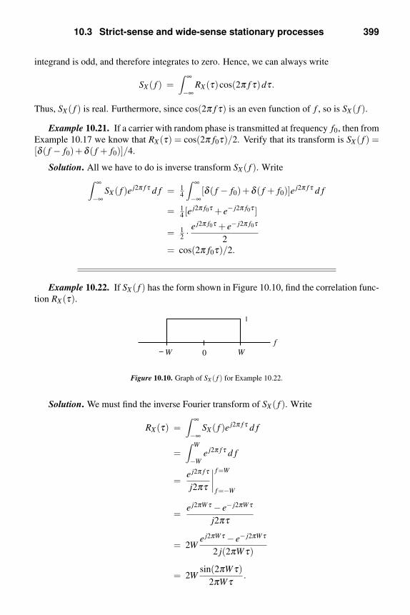
10.3 Strict-sense and wide-sense stationary processes 399
integrand is odd, and therefore integrates to zero. Hence, we can always write
SX ( f ) =∫ ∞
−∞RX (τ)cos(2π f τ)dτ.
Thus, SX ( f ) is real. Furthermore, since cos(2π f τ) is an even function of f , so is SX ( f ).
Example 10.21. If a carrier with random phase is transmitted at frequency f0, then from
Example 10.17 we know that RX (τ) = cos(2π f0τ)/2. Verify that its transform is SX ( f ) =[δ ( f − f0)+δ ( f + f0)]/4.
Solution. All we have to do is inverse transform SX ( f ). Write∫ ∞
−∞SX ( f )e j2π f τ d f = 1
4
∫ ∞
−∞[δ ( f − f0)+δ ( f + f0)]e
j2π f τ d f
= 14[e j2π f0τ + e− j2π f0τ ]
= 12· e j2π f0τ + e− j2π f0τ
2= cos(2π f0τ)/2.
Example 10.22. If SX ( f ) has the form shown in Figure 10.10, find the correlation func-
tion RX (τ).
W0W−f
1
SX
)f(
Figure 10.10. Graph of SX ( f ) for Example 10.22.
Solution. We must find the inverse Fourier transform of SX ( f ). Write
RX (τ) =∫ ∞
−∞SX ( f )e j2π f τ d f
=∫ W
−We j2π f τ d f
=e j2π f τ
j2πτ
∣∣∣∣ f=W
f=−W
=e j2πWτ − e− j2πWτ
j2πτ
= 2We j2πWτ − e− j2πWτ
2 j(2πWτ)
= 2Wsin(2πWτ)
2πWτ.
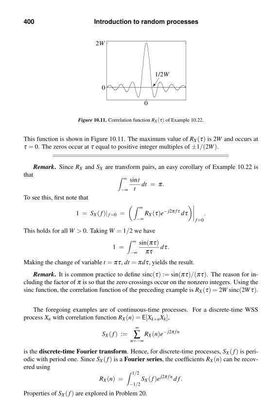
400 Introduction to random processes
2W
0
1/2W
0
Figure 10.11. Correlation function RX (τ) of Example 10.22.
This function is shown in Figure 10.11. The maximum value of RX (τ) is 2W and occurs at
τ = 0. The zeros occur at τ equal to positive integer multiples of ±1/(2W ).
Remark. Since RX and SX are transform pairs, an easy corollary of Example 10.22 is
that ∫ ∞
−∞
sin t
tdt = π.
To see this, first note that
1 = SX ( f )| f=0 =
(∫ ∞
−∞RX (τ)e− j2π f τ dτ
)∣∣∣∣f=0
.
This holds for all W > 0. Taking W = 1/2 we have
1 =
∫ ∞
−∞
sin(πτ)
πτdτ.
Making the change of variable t = πτ , dt = πdτ , yields the result.
Remark. It is common practice to define sinc(τ) := sin(πτ)/(πτ). The reason for in-
cluding the factor of π is so that the zero crossings occur on the nonzero integers. Using the
sinc function, the correlation function of the preceding example is RX (τ) = 2W sinc(2Wτ).
The foregoing examples are of continuous-time processes. For a discrete-time WSS
process Xn with correlation function RX (n) = E[Xk+nXk],
SX ( f ) :=∞
∑n=−∞
RX (n)e− j2π f n
is the discrete-time Fourier transform. Hence, for discrete-time processes, SX ( f ) is peri-
odic with period one. Since SX ( f ) is a Fourier series, the coefficients RX (n) can be recov-
ered using
RX (n) =∫ 1/2
−1/2SX ( f )e j2π f n d f .
Properties of SX ( f ) are explored in Problem 20.

10.4 WSS processes through LTI systems 401
10.4 WSS processes through LTI systems
In this section we show that LTI systems preserve wide-sense stationarity. In other
words, if a WSS process Xt is applied to an LTI system with impulse response h, as shown
in Figure 10.12, then the output
Yt =∫ ∞
−∞h(t −θ)Xθ dθ
is another WSS process. Furthermore, the correlation function of Yt , and the cross-correla-
tion function of Xt and Yt can be expressed in terms of convolutions involving h and RX . By
introducing appropriate Fourier transforms the convolution relationships are converted into
product formulas in the frequency domain.
The derivation of the analogous results for discrete-time processes and systems is carried
out in Problem 31.
tX ( )h t Yt
Figure 10.12. Block diagram of an LTI system with impulse response h(t), input random process Xt , and output
random process Yt .
Time-domain analysis
Recall from Example 10.11 that
mY (t) =∫ ∞
−∞h(τ)mX (t − τ)dτ.
Since Xt is WSS, its mean function mX (t) is constant for all t, say mX (t) ≡ m. Then
mY (t) = m
∫ ∞
−∞h(τ)dτ,
which does not depend on t. Next, from (10.11),
E[Yt1Yt2 ] =∫ ∞
−∞h(β )
(∫ ∞
−∞h(θ)E[Xt1−β Xt2−θ ]dθ
)dβ .
Since Xt is WSS, the expectation inside the integral is just
RX ([t1 −β ]− [t2 −θ ]) = RX ([t1 − t2]− [β −θ ]).
Hence,
E[Yt1Yt2 ] =∫ ∞
−∞h(β )
(∫ ∞
−∞h(θ)RX ([t1 − t2]− [β −θ ])dθ
)dβ ,
which depends on t1 and t2 only through their difference. We have thus shown that the
response of an LTI system to a WSS input is another WSS process with correlation
function
RY (τ) =∫ ∞
−∞h(β )
(∫ ∞
−∞h(θ)RX (τ −β +θ)dθ
)dβ . (10.17)

402 Introduction to random processes
Before continuing the analysis of RY (τ), it is convenient to first look at the cross-
correlation between Xt1 and Yt2 . From (10.10),
E[Xt1Yt2 ] =
∫ ∞
−∞h(θ)E[Xt1Xt2−θ ]dθ
=∫ ∞
−∞h(θ)RX (t1 − t2 +θ)dθ .
If two processes Xt and Yt are each WSS, and if their cross-correlation E[Xt1Yt2 ] depends
on t1 and t2 only through their difference, the processes are said to be jointly wide-sense
stationary (J-WSS). In this case, their univariate cross-correlation function is defined by
RXY (τ) := E[Xt+τYt ].
The generalization of (10.14) is
E[Xt1Yt2 ] = RXY (t1 − t2).
The foregoing analysis shows that if a WSS process is applied to an LTI system, then
the input and output processes are J-WSS with cross-correlation function
RXY (τ) =∫ ∞
−∞h(θ)RX (τ +θ)dθ . (10.18)
Comparing (10.18) and the inner integral in (10.17) shows that
RY (τ) =
∫ ∞
−∞h(β )RXY (τ −β )dβ . (10.19)
Thus, RY is the convolution of h and RXY . Furthermore, making the change of variable
α = −θ , dα = −dθ in (10.18) yields
RXY (τ) =
∫ ∞
−∞h(−α)RX (τ −α)dα. (10.20)
In other words, RXY is the convolution of h(−α) and RX .
Frequency-domain analysis
The preceding convolutions suggest that by applying the Fourier transform, much sim-
pler formulas can be obtained in the frequency domain. The Fourier transform of the system
impulse response h,
H( f ) :=∫ ∞
−∞h(τ)e− j2π f τ dτ,
is called the system transfer function. The Fourier transforms of RX (τ), RY (τ), and RXY (τ)are denoted by SX ( f ), SY ( f ), and SXY ( f ), respectively. Taking the Fourier transform of
(10.19) yields
SY ( f ) = H( f )SXY ( f ). (10.21)
Similarly, taking the Fourier transform of (10.20) yields
SXY ( f ) = H( f )∗SX ( f ), (10.22)

10.5 Power spectral densities for WSS processes 403
since, as shown in Problem 22, for h real, the Fourier transform of h(−τ) is H( f )∗, where
the asterisk ∗ denotes the complex conjugate. Combining (10.21) and (10.22), we have
SY ( f ) = H( f )SXY ( f ) = H( f )H( f )∗SX ( f ) = |H( f )|2SX ( f ).
Thus,
SY ( f ) = |H( f )|2SX ( f ). (10.23)
Example 10.23. Suppose that the process Xt is WSS with correlation function RX (τ) =e−λ |τ |. If Xt is applied to an LTI system with transfer function
H( f ) =√
λ 2 +(2π f )2 I[−W,W ]( f ),
find the system output correlation function RY (τ).
Solution. Our approach is to first find SY ( f ) using (10.23) and then take the inverse
Fourier transform to obtain RY (τ). To begin, first note that
|H( f )|2 = [λ 2 +(2π f )2]I[−W,W ]( f ),
where we use the fact that since an indicator is zero or one, it has the property that it is equal
to its square. We obtain SX ( f ) from the table of Fourier transforms inside the front cover
and write
SY ( f ) = SX ( f )|H( f )|2
=2λ
λ 2 +(2π f )2[λ 2 +(2π f )2]I[−W,W ]( f )
= 2λ I[−W,W ]( f ),
which is proportional to the graph in Figure 10.10. Using the transform table inside the
front cover or the result of Example 10.22,
RY (τ) = 2λ ·2Wsin(2πWτ)
2πWτ.
10.5 Power spectral densities for WSS processes
Motivation
Recall that if v(t) is the voltage across a resistance R, then the instantaneous power is
v(t)2/R, and the energy dissipated is∫ ∞−∞ v(t)2/Rdt. Similarly, if the current through the re-
sistance is i(t), the instantaneous power is i(t)2R, and the energy dissipated is∫ ∞−∞ i(t)2Rdt.
Based on the foregoing observations, the “energy” of any waveform x(t) is defined to
be∫ ∞−∞ |x(t)|2 dt. Of course, if x(t) is the voltage across a one-ohm resistor or the current
through a one-ohm resistor, then∫ ∞−∞ |x(t)|2 dt is the physical energy dissipated.

404 Introduction to random processes
Some signals, such as periodic signals like cos(t) and sin(t), do not have finite energy,
but they do have finite average power; i.e.,
limT→∞
1
2T
∫ T
−T|x(t)|2 dt < ∞.
For periodic signals, this limit is equal to the energy in one period divided by the period
(Problem 32).
Power in a process
For a deterministic signal x(t), the energy or average power serves as a single-number
characterization. For a random process Xt , the analogous quantities∫ ∞
−∞X2
t dt and limT→∞
1
2T
∫ T
−TX2
t dt
are random variables — they are not single-number characterizations (unless extra assump-
tions such as ergodicity are made; see Section 10.10). However, their expectations are
single-number characterizations. Since most processes have infinite expected energy (e.g.,
WSS processes – see Problem 33), we focus on the expected average power,
PX := E
[lim
T→∞
1
2T
∫ T
−TX2
t dt
].
For a WSS process, this becomes
limT→∞
1
2T
∫ T
−TE[X2
t ]dt = limT→∞
1
2T
∫ T
−TRX (0)dt = RX (0).
Since RX and SX are Fourier transform pairs,
RX (0) =
(∫ ∞
−∞SX ( f )e j2π f τ d f
)∣∣∣∣τ=0
=∫ ∞
−∞SX ( f )d f .
Since we also have E[X2t ] = RX (0),
PX = E[X2t ] = RX (0) =
∫ ∞
−∞SX ( f )d f , (10.24)
and we have three ways to express the power in a WSS process.
Remark. From the definition of PX , (10.24) says that for a WSS process,
E
[lim
T→∞
1
2T
∫ T
−TX2
t dt
]= E[X2
t ],
which we call the expected instantaneous power. Thus, for a WSS process, the expected
average power is equal to the expected instantaneous power.

10.5 Power spectral densities for WSS processes 405
W1
W2
W1
− 0W2
−
1
f
Figure 10.13. Bandpass filter H( f ) for extracting the power in the frequency band W1 ≤ | f | ≤W2.
Example 10.24 (power in a frequency band). For a WSS process Xt , find the power in
the frequency band W1 ≤ | f | ≤W2.
Solution. We interpret the problem as asking us to apply Xt to the ideal bandpass filter
with transfer function H( f ) shown in Figure 10.13 and then find the power in the output
process. Denoting the filter output by Yt , we have
PY =∫ ∞
−∞SY ( f )d f
=∫ ∞
−∞|H( f )|2SX ( f )d f , by (10.23),
=∫ −W1
−W2
SX ( f )d f +∫ W2
W1
SX ( f )d f ,
where the last step uses the fact that H( f ) has the form in Figure 10.13. Since, as shown at
the end of Section 10.4, SX ( f ) is even, these last two integrals are equal. Hence,
PY = 2
∫ W2
W1
SX ( f )d f .
To conclude the example, we use the formula for PY to derive the additional result that
SX ( f ) is a nonnegative function. Suppose that W2 = W1 + ∆W , where ∆W > 0 is small.
Then
PY = 2
∫ W1+∆W
W1
SX ( f )d f ≈ 2SX (W1)∆W.
It follows that
SX (W1) ≈ PY
2∆W≥ 0,
since PY = E[Y 2t ] ≥ 0. Since W1 ≥ 0 is arbitrary, and since SX ( f ) is even, we conclude that
SX ( f ) ≥ 0 for all f .
Example 10.24 shows that SX ( f ) is a nonnegative function that, when integrated over
a frequency band, yields the process’s power in that band. This is analogous to the way a
probability density is integrated over an interval to obtain its probability. On account of this
similarity, SX ( f ) is called the power spectral density of the process. The adjective “spec-
tral” means that SX is a function of frequency. While there are infinitely many nonnegative,
even functions of frequency that integrate to PX , there is only one such function that when
integrated over every frequency band gives the power in that band. See Problem 34.

406 Introduction to random processes
The analogous terminology for SXY ( f ) is cross power spectral density. However, in
general, SXY ( f ) can be complex valued. Even if SXY ( f ) is real valued, it need not be
nonnegative. See Problem 35.
White noise
If a WSS process has constant power across all frequencies, it is called white noise.
This is analogous to white light, which contains equal amounts of all the colors found in
a rainbow. To be precise, Xt is called white noise if its power spectral density is constant
for all frequencies. Unless otherwise specified, this constant is usually denoted by N0/2.
Taking the Fourier transform of
RX (τ) =N0
2δ (τ),
where δ is the Dirac delta function, yields
SX ( f ) =N0
2.
Thus, the correlation function of white noise is a delta function. White noise is an ideal-
ization of what is observed in physical noise sources. In real noise sources, SX ( f ) is
approximately constant for frequencies up to about 1000 GHz. For | f | larger than this,
SX ( f ) decays. However, what real systems see is |H( f )|2SX ( f ), where the bandwidth of
the transfer function is well below 1000 GHz. In other words, any hardware filters the noise
so that SY ( f ) is not affected by the exact values of SX ( f ) for the large | f | where SX ( f )begins to decay.
Remark. Just as the delta function is not an ordinary function, white noise is not an
ordinary random process. For example, since δ (0) is not defined, and since E[X2t ] =
RX (0) = (N0/2)δ (0), we cannot speak of the second moment of Xt when Xt is white noise.
In particular, white noise is not a second-order process. Also, since SX ( f ) = N0/2 for white
noise, and since ∫ ∞
−∞
N0
2d f = ∞,
we often say that white noise has infinite average power.
In Figure 10.10, if we let W → ∞, we get SX ( f ) = 1 for all f . Similarly, if we let W → ∞in Figure 10.11, RX (τ) begins to look more and more like δ (τ). This suggests that a process
Xt with correlation function in Figure 10.11 should look more and more like white noise as
W increases. For finite W , we call such a process bandlimited white noise. In Figure 10.14,
we show sample paths Xt with W = 1/2 (top), W = 2 (middle), and W = 4 (bottom). As W
increases, the processes become less smooth and more wiggly. In other words, they contain
higher and higher frequencies.
Example 10.25. Consider the lowpass RC filter shown in Figure 10.15. Suppose that
the voltage source is a white-noise process Xt with power spectral density SX ( f ) = N0/2. If
the filter output is taken to be the capacitor voltage, which we denote by Yt , find its power
spectral density SY ( f ) and the corresponding correlation function RY (τ).

10.5 Power spectral densities for WSS processes 407
0 10 20 30
0
0 10 20 30
0
0 10 20 30
0
Figure 10.14. Bandlimited white noise processes with the power spectral density in Figure 10.10 and the correla-
tion function in Figure 10.11 for W = 1/2 (top), W = 2 (middle), and W = 4 (bottom).
C
R+
−
+−
Figure 10.15. Lowpass RC filter.
Solution. From standard circuit-analysis techniques, the system transfer function be-
tween the input Xt and output Yt is
H( f ) =1
1+ j2π f RC.
Hence,
SY ( f ) = |H( f )|2SX ( f ) =N0/2
1+(2π f RC)2.
If we write
SY ( f ) =N0
4RC· 2/RC
(1/RC)2 +(2π f )2,
then the inverse transform of SY ( f ) can be found by inspection using the table inside the
front cover. We find that
RY (τ) =N0
4RCe−|τ |/RC.
Figure 10.16 shows how the sample paths Yt vary with the filter time constant, RC. In
each case, the process wanders between the top and the bottom of the graph. However, the
top graph is less wiggly than the bottom one, and the middle one has an intermediate amount

408 Introduction to random processes
0 10 20 30
0
1
0 10 20 30
−2
0
2
0 10 20 30
−5
0
5
Figure 10.16. Three realizations of a lowpass RC filter output driven by white noise. The time constants are
RC = 4 (top), RC = 1 (middle), and RC = 1/4 (bottom).
of wiggle. To explain this, recall that the filter time constant is inversely proportional to the
filter bandwidth. Hence, when RC is large, the filter has a small bandwidth and passes only
low-frequency components. When RC is small, the filter has a large bandwidth that passes
both high and low frequency components. A signal with only low frequency components
cannot wiggle as much as a signal with high frequency components.
Example 10.26. A certain communication receiver employs a bandpass filter to reduce
white noise generated in the amplifier. Suppose that the white noise Xt has power spectral
density SX ( f ) = N0/2 and that the filter transfer function H( f ) is given in Figure 10.13.
Find the expected output power from the filter.
Solution. The expected output power is obtained by integrating the power spectral den-
sity of the filter output. Denoting the filter output by Yt ,
PY =
∫ ∞
−∞SY ( f )d f =
∫ ∞
−∞
∣∣H( f )∣∣2SX ( f )d f .
Since∣∣H( f )
∣∣2SX ( f ) = N0/2 for W1 ≤ | f | ≤W2, and is zero otherwise, PY = 2(N0/2)(W2 −W1) = N0(W2 −W1). In other words, the expected output power is N0 times the bandwidthb
of the filter.
Example 10.27. White noise with power spectral density N0/2 is applied to a lowpass
filter with transfer function H( f ) = e−2πλ | f |. Find the output noise power from the filter.
bBandwidth refers to the range of positive frequencies where |H( f )| > 0. The reason for this is that in phys-
ical systems, the impulse response is real. This implies H(− f ) = H( f )∗, and then |H( f )|2 = H( f )H( f )∗ =H( f )H(− f ) is an even function.

10.5 Power spectral densities for WSS processes 409
Solution. To begin, write
SY ( f ) = |H( f )|2SX ( f ) =∣∣∣e−2πλ | f |
∣∣∣2 N0
2=
N0
2e−2π(2λ )| f |.
Since PY =∫ ∞−∞ SY ( f )dy, one approach would be to compute this integral, which can be
done in closed form. However, in this case it is easier to use the fact that PY = RY (0). From
the transform table inside the front cover, we see that
RY (τ) =N0
2π· 2λ(2λ )2 + τ2
,
and it follows that PY = RY (0) = N0/(4πλ ).
Example 10.28. White noise with power spectral density SX ( f ) = N0/2 is applied to a
filter with impulse response h(t) = I[0,T ](t) shown in Figure 10.17. Find (a) the cross power
spectral density SXY ( f ); (b) the cross-correlation, RXY (τ); (c) E[Xt1Yt2 ]; (d) the output power
spectral density SY ( f ); (e) the output auto-correlation, RY (τ); (f) the output power PY .
t
1h(t)
T−T 0
t
h(−t)
T−T 0
1
Figure 10.17. Impulse response h(t) = I[0,T ](t) and h(−t) of Example 10.28.
Solution. (a) Since
SXY ( f ) = H( f )∗SX ( f ) = H( f )∗ · N0
2,
we need to compute
H( f ) =∫ ∞
−∞h(t)e− j2π f t dt =
∫ T
0e− j2π f t dt =
e− j2π f t
− j2π f
∣∣∣∣T0
.
We simplify writing
H( f ) =1− e− j2π f T
j2π f
= e− jπT f Te jπT f − e− jπT f
2 j πT f
= e− jπT f Tsin(πT f )
πT f.

410 Introduction to random processes
It follows that
SXY ( f ) = e jπT f Tsin(πT f )
πT f
N0
2.
(b) Since h(t) is real, the inverse transform of SXY ( f ) = H( f )∗N0/2 is (recall Problem 22)
RXY (τ) = h(−τ)N0/2 = I[0,T ](−τ)N0/2 = I[−T,0](τ)N0/2.
(c) E[Xt1Yt2 ] = RXY (t1 − t2) = I[−T,0](t1 − t2)N0/2.
(d) Since we computed H( f ) in part (a), we can easily write
SY ( f ) = |H( f )|2SX ( f ) = T 2
[sin(πT f )
πT f
]2N0
2.
(e) From the transform table inside the front cover,
RY (τ) =T N0
2(1−|τ|/T )I[−T,T ](τ),
which is shown in Figure 10.18.
(f) Use part (e) to write PY = RY (0) = T N0/2.
0 T− T
N0/2T
Figure 10.18. Output auto-correlation RY (τ) of Example 10.28.
10.6 Characterization of correlation functions
In the preceding sections we have shown that if RX (τ) is the correlation function of a
WSS process, then the power spectral density SX ( f ) is a real, even, nonnegative function of
f .
Conversely, it is shown in Problem 48 of Chapter 11 that given any real, even, nonneg-
ative function of frequency, say S( f ), there is a WSS process whose correlation function is
the inverse Fourier transform of S( f ).Thus, one can ask many questions of the form, “Is R(τ) = · · · a valid correlation func-
tion?”
To show that a given R(τ) is a valid correlation function, you can take its Fourier trans-
form and show that it is real, even, and nonnegative.
On the other hand, if R(τ) is not a valid correlation function, you can sometimes see
this without taking its Fourier transform. For example, if R(τ) is not even, it cannot be a
correlation function since, by Example 10.16, correlation functions are always even.
Another important property of a correlation function R(τ) is that
|R(τ)| ≤ R(0), for all τ. (10.25)

10.6 Characterization of correlation functions 411
In other words, the maximum absolute value of a correlation function is achieved at τ = 0,
and at that point the function is nonnegative. Note that (10.25) does not preclude other
maximizing values of τ; it only says that τ = 0 is one of the maximizers. To derive (10.25),
we first note that if R(τ) = RX (τ) for some process Xt , then
RX (0) = E[X2t ] ≥ 0.
Then use the Cauchy–Schwarz inequality (2.24) to write∣∣RX (τ)∣∣ =
∣∣E[Xt+τ Xt ]∣∣
≤√
E[X2t+τ ]E[X2
t ]
=√
RX (0)RX (0)
= RX (0).
Example 10.29. Determine whether or not R(τ) := τe−|τ | is a valid correlation function.
Solution. Since R(τ) is odd, it cannot be a valid correlation function. Alternatively, we
can observe that R(0) = 0 < e−1 = R(1), violating R(0) ≥ |R(τ)| for all τ .
Example 10.30. Determine whether or not R(τ) := 1/(1 + τ2) is a valid correlation
function.
Solution. It is easy to see that R(τ) is real, even, and its maximum absolute value occurs
at τ = 0. So we cannot rule it out as a valid correlation function. The next step is to check
its Fourier transform. From the table inside the front cover, the Fourier transform of R(τ) is
S( f ) = π exp(−2π| f |). Since S( f ) is real, even, and nonnegative, R(τ) is a valid correlation
function.
Correlation functions of deterministic signals
Up to this point, we have discussed correlation functions for WSS random processes.
However, there is a connection with correlation functions of a deterministic signals.
The correlation function of a real signal v(t) of finite energy is defined by
Rv(τ) :=∫ ∞
−∞v(t + τ)v(t)dt.
Note that Rv(0) =∫ ∞−∞ v(t)2 dt is the signal energy.
Since the formula for Rv(τ) is similar to a convolution integral, for simple functions v(t)such as the one at the top in Figure 10.19, Rv(τ) can be computed directly, and is shown at
the bottom of the figure.

412 Introduction to random processes
1
( )R v
T/3
0 T− Tt
v t( )
0 T− T
Figure 10.19. Deterministic signal v(t) and its correlation function Rv(τ).
Further insight into Rv(τ) can be obtained using Fourier transforms. If v(t) has Fourier
transform V ( f ), then by the inversion formula,
v(t) =∫ ∞
−∞V ( f )e j2π f t d f .
Let us apply this formula to v(t + τ) in the definition of Rv(τ). Then
Rv(τ) =∫ ∞
−∞
(∫ ∞
−∞V ( f )e j2π f (t+τ) d f
)v(t)dt
=∫ ∞
−∞V ( f )
(∫ ∞
−∞v(t)e− j2π f t dt
)∗e j2π f τ d f ,
where we have used the fact that v(t) is real. Since the inner integral is just V ( f ),
Rv(τ) =∫ ∞
−∞|V ( f )|2e j2π f τ d f . (10.26)
Since v(t) is a real signal, V ( f )∗ = V (− f ). Hence, |V ( f )|2 = V ( f )V ( f )∗ = V ( f )V (− f ) is
real, even, and nonnegative, just like a power spectral density. In fact, when a signal has
finite energy; i.e.,∫ ∞−∞ |v(t)|2 dt < ∞, |V ( f )|2 is called the energy spectral density.
10.7 The matched filter
Consider an air-traffic control system which sends out a known, deterministic radar
pulse. If there are no objects in range of the radar, the radar outputs only noise from its
amplifiers. We model the noise by a zero-mean WSS process Xt with power spectral density
SX ( f ). If there is an object in range of the radar, the system returns the reflected radar
pulse, say v(t), which is known, plus the noise Xt . We wish to design a system that decides
whether the received waveform is noise only, Xt , or signal plus noise, v(t)+ Xt . As an aid

10.7 The matched filter 413
( )h ttXv( )t +
vo Y
t( )t +
(
radar
v( )t
Figure 10.20. Block diagram of radar system and matched filter.
to achieving this goal, we propose to take the received waveform and pass it through an LTI
system with impulse response h(t). If the received signal is in fact v(t)+Xt , then as shown
in Figure 10.20, the output of the linear system is∫ ∞
−∞h(t − τ)[v(τ)+Xτ ]dτ = vo(t)+Yt ,
where
vo(t) :=∫ ∞
−∞h(t − τ)v(τ)dτ
is the output signal, and
Yt :=∫ ∞
−∞h(t − τ)Xτ dτ
is the output noise process.
Typically, at the radar output, the signal v(t) is obscured by the noise Xt . For example,
at the top in Figure 10.21, a triangular signal v(t) and broadband noise Xt are shown in
the same graph. At the bottom is their sum v(t)+ Xt , in which it is difficult to discern the
triangular signal. By passing v(t)+Xt through through the matched filter derived below, the
presence of the signal can be made much more obvious at the filter output. The matched
filter output is shown later in Figure 10.23.
We now find the impulse response h that maximizes the output signal-to-noise ratio
(SNR)
SNR :=vo(t0)
2
E[Y 2t0],
where vo(t0)2 is the instantaneous output signal power at time t0, and E[Y 2
t0] is the expected
instantaneous output noise power at time t0. Note that since E[Y 2t0] = RY (0) = PY , we can
also write
SNR =vo(t0)
2
PY
.
Our approach is to obtain an upper bound on the numerator of the form vo(t0)2 ≤ PY ·B,
where B does not depend on the impulse response h. It will then follow that
SNR =vo(t0)
2
PY
≤ PY ·BPY
= B.

414 Introduction to random processes
0 2 4 6 8 10−2
−1
0
1
2
0 2 4 6 8 10−2
−1
0
1
2
Figure 10.21. A triangular signal v(t) and broadband noise Xt (top). Their sum, v(t)+Xt (bottom), shows that the
noise hides the presence of the signal.
We then show how to choose the impulse response so that in fact vo(t0)2 = PY ·B. For this
choice of impulse response, we then have SNR = B, the maximum possible value.
We begin by analyzing the denominator in the SNR. Observe that
PY =∫ ∞
−∞SY ( f )d f =
∫ ∞
−∞|H( f )|2SX ( f )d f .
To analyze the numerator, write
vo(t0) =∫ ∞
−∞Vo( f )e j2π f t0 d f =
∫ ∞
−∞H( f )V ( f )e j2π f t0 d f , (10.27)
where Vo( f ) is the Fourier transform of vo(t), and V ( f ) is the Fourier transform of v(t).Next, write
vo(t0) =∫ ∞
−∞H( f )
√SX ( f ) · V ( f )e j2π f t0√
SX ( f )d f
=∫ ∞
−∞H( f )
√SX ( f ) ·
[V ( f )∗e− j2π f t0√
SX ( f )
]∗d f ,
where the asterisk denotes complex conjugation. Applying the Cauchy–Schwarz inequality
for time functions (Problem 2), we obtain the upper bound,
|vo(t)|2 ≤∫ ∞
−∞|H( f )|2SX ( f )d f︸ ︷︷ ︸
= PY
·∫ ∞
−∞
|V ( f )|2SX ( f )
d f︸ ︷︷ ︸=: B
.
Thus,
SNR =|vo(t0)|2
PY
≤ PY ·BPY
= B.

10.7 The matched filter 415
Now, the Cauchy–Schwarz inequality holds with equality if and only if H( f )√
SX ( f ) is a
multiple of V ( f )∗e− j2π f t0/√
SX ( f ). Thus, the upper bound on the SNR will be achieved if
we take H( f ) to solve
H( f )√
SX ( f ) = αV ( f )∗e− j2π f t0√
SX ( f ),
where α is a constant;c i.e., we should take
H( f ) = αV ( f )∗e− j2π f t0
SX ( f ). (10.28)
Thus, the optimal filter is “matched” to the known signal and known noise power spectral
density.
Example 10.31. Consider the special case in which Xt is white noise with power spec-
tral density SX ( f ) = N0/2. Taking α = N0/2 as well, we have H( f ) =V ( f )∗e− j2π f t0 , which
inverse transforms to h(t) = v(t0 − t), assuming v(t) is real. Thus, the matched filter has an
impulse response which is a time-reversed and translated copy of the known signal v(t).An example of v(t) and the corresponding h(t) are shown in Figure 10.22. As the figure
illustrates, if v(t) is a finite-duration, causal waveform, as any radar “pulse” would be, then
the sampling time t0 can always be chosen so that h(t) corresponds to a causal system.
0 T− Tt
v t( )
t
0 T− T t0
v t( )t −h t( ) =0
Figure 10.22. Known signal v(t) and corresponding matched filter impulse response h(t) in the case of white
noise.
Analysis of the matched filter output
We show that the matched filter forces the components of the output vo(t) +Yt to be
related by
vo(t) = 1α RY (t − t0). (10.29)
cThe constant α must be real in order for the matched filter impulse response to be real.

416 Introduction to random processes
In other words, the matched filter forces the output signal to be proportional to a time-shifted
correlation function. Hence, the maximum value of |vo(t)| occurs at t = t0. Equation (10.29)
also implies that the filter output vo(t)+Yt has the form of a correlation function plus noise.
We now derive (10.29). Since SY ( f ) = |H( f )|2SX ( f ), if H( f ) is the matched filter, then
SY ( f ) =|αV ( f )|2SX ( f )2
SX ( f ) =|αV ( f )|2
SX ( f ),
and
RY (τ) =∫ ∞
−∞
|αV ( f )|2SX ( f )
e j2π f τ d f . (10.30)
Now observe that if we put t0 = t in (10.27), and if H( f ) is the matched filter, then
vo(t) =∫ ∞
−∞α|V ( f )|2SX ( f )
e j2π f (t−t0) d f .
Hence, (10.29) holds.
Example 10.32. If the noise is white with power spectral density SX ( f ) = N0/2, and if
α = N0/2, then comparing (10.30) and (10.26) shows that RY (τ) = αRv(τ), where Rv(τ)is the correlation function of the deterministic signal v(t). We also have vo(t) = Rv(t − t0).When v(t) is the triangular waveform shown at the top in Figure 10.21, the signal vo(t) =Rv(t − t0) and a sample path of Yt are shown at the top in Figure 10.23 in the same graph.
At the bottom is the sum vo(t)+Yt .
0 2 4 6 8 10
0
0.5
0 2 4 6 8 10
0
0.5
Figure 10.23. Matched filter output terms vo(t) and Yt (top) and their sum vo(t)+Yt (bottom), when v(t) is the
signal at the top in Figure 10.19 and H( f ) is the corresponding matched filter.

10.8 The Wiener filter 417
10.8 The Wiener filter
In the preceding section, the available data was of the form v(t)+ Xt , where v(t) was
a known, nonrandom signal, and Xt was a zero-mean, WSS noise process. In this section,
we suppose that Vt is an unknown random process that we would like to estimate based on
observing a related random process Ut . For example, we might have Ut = Vt +Xt , where Xt
is a noise process. However, for generality, we assume only that Ut and Vt are zero-mean,
J-WSS with known power spectral densities and known cross power spectral density.
We restrict attention to linear estimators of the form
Vt =∫ ∞
−∞h(t − τ)Uτ dτ =
∫ ∞
−∞h(θ)Ut−θ dθ , (10.31)
as shown in Figure 10.24. Note that to estimate Vt at a single time t, we use the entire
observed waveform Uτ for −∞ < τ < ∞. Our goal is to find an impulse response h that
minimizes the mean-squared error, E[|Vt − Vt |2]. In other words, we are looking for an
impulse response h such that if Vt is given by (10.31), and if h is any other impulse response,
and we put
Vt =∫ ∞
−∞h(t − τ)Uτ dτ =
∫ ∞
−∞h(θ)Ut−θ dθ , (10.32)
then
E[|Vt −Vt |2] ≤ E[|Vt −Vt |2].To find the optimal filter h, we apply the orthogonality principle (derived below), which
says that if
E
[(Vt −Vt)
∫ ∞
−∞h(θ)Ut−θ dθ
]= 0 (10.33)
for every filter h, then h is the optimal filter.
Before proceeding any further, we need the following observation. Suppose (10.33)
holds for every choice of h. Then in particular, it holds if we replace h by h− h. Making
this substitution in (10.33) yields
E
[(Vt −Vt)
∫ ∞
−∞[h(θ)− h(θ)]Ut−θ dθ
]= 0.
tV^
( )h tUt
observedprocess
unobservedprocess
tV
Figure 10.24. Estimation of an unobserved process Vt by passing an observed process Ut through an LTI system
with impulse response h(t).
418 Introduction to random processes
Since the integral in this expression is simply Vt −Vt , we have that
E[(Vt −Vt)(Vt −Vt)] = 0. (10.34)
To establish the orthogonality principle, assume (10.33) holds for every choice of h.
Then (10.34) holds as well. Now write
E[|Vt −Vt |2] = E[|(Vt −Vt)+(Vt −Vt)|2]= E[|Vt −Vt |2 +2(Vt −Vt)(Vt −Vt)+ |Vt −Vt |2]= E[|Vt −Vt |2]+2E[(Vt −Vt)(Vt −Vt)]+E[|Vt −Vt |2]= E[|Vt −Vt |2]+E[|Vt −Vt |2]≥ E[|Vt −Vt |2],
and thus, h is the filter that minimizes the mean-squared error.
The next task is to characterize the filter h such that (10.33) holds for every choice of h.
Write (10.33) as
0 = E
[(Vt −Vt)
∫ ∞
−∞h(θ)Ut−θ dθ
]= E
[∫ ∞
−∞h(θ)(Vt −Vt)Ut−θ dθ
]=
∫ ∞
−∞E[h(θ)(Vt −Vt)Ut−θ ]dθ
=∫ ∞
−∞h(θ)E[(Vt −Vt)Ut−θ ]dθ
=∫ ∞
−∞h(θ)[RVU (θ)−R
VU(θ)]dθ .
Since this must hold for all h, take h(θ) = RVU (θ)−RVU
(θ) to get∫ ∞
−∞
∣∣RVU (θ)−RVU
(θ)∣∣2 dθ = 0. (10.35)
Thus, (10.33) holds for all h if and only if RVU = RVU
.
The next task is to analyze RVU
. Recall that Vt in (10.31) is the response of an LTI
system to input Ut . Applying (10.18) with X replaced by U and Y replaced by V , we have,
also using the fact that RU is even,
RVU
(τ) = RUV
(−τ) =∫ ∞
−∞h(θ)RU (τ −θ)dθ .
Taking Fourier transforms of
RVU (τ) = RVU
(τ) =∫ ∞
−∞h(θ)RU (τ −θ)dθ (10.36)
yields
SVU ( f ) = H( f )SU ( f ).

10.8 The Wiener filter 419
Thus,
H( f ) =SVU ( f )
SU ( f )(10.37)
is the optimal filter. This choice of H( f ) is called the Wiener filter.
Causal Wiener filters
Typically, the Wiener filter as found above is not causal; i.e., we do not have h(t) = 0
for t < 0. To find such an h, we need to reformulate the problem by replacing (10.31) with
Vt =∫ t
−∞h(t − τ)Uτ dτ =
∫ ∞
0h(θ)Ut−θ dθ ,
and replacing (10.32) with
Vt =∫ t
−∞h(t − τ)Uτ dτ =
∫ ∞
0h(θ)Ut−θ dθ .
Everything proceeds as before from (10.33) through (10.35) except that lower limits of
integration are changed from −∞ to 0. Thus, instead of concluding RVU (τ) = RVU
(τ) for
all τ , we only have RVU (τ) = RVU
(τ) for τ ≥ 0. Instead of (10.36), we have
RVU (τ) =∫ ∞
0h(θ)RU (τ −θ)dθ , τ ≥ 0. (10.38)
This is known as the Wiener–Hopf equation. Because the equation only holds for τ ≥ 0,
we run into a problem if we try to take Fourier transforms. To compute SVU ( f ), we need to
integrate RVU (τ)e− j2π f τ from τ =−∞ to τ = ∞. But we can use the Wiener–Hopf equation
only for τ ≥ 0.
In general, the Wiener–Hopf equation is difficult to solve. However, if U is white noise,
say RU (θ) = δ (θ), then (10.38) reduces to
RVU (τ) = h(τ), τ ≥ 0.
Since h is causal, h(τ) = 0 for τ < 0.
The preceding observation suggests the construction of H( f ) using a whitening filter
as shown in Figure 10.25. If Ut is not white noise, suppose we can find a causal filter K( f )such that when Ut is passed through this system, the output is white noise Wt , by which we
K f( ) H f( )0
Wt
Ut tV^
f( )H
Figure 10.25. Decomposition of the causal Wiener filter using the whitening filter K( f ).

420 Introduction to random processes
mean SW ( f ) = 1. Letting k denote the impulse response corresponding to K, we can write
Wt mathematically as
Wt =∫ ∞
0k(θ)Ut−θ dθ . (10.39)
Then
1 = SW ( f ) = |K( f )|2SU ( f ). (10.40)
Consider the problem of causally estimating Vt based on Wt instead of Ut . The solution is
again given by the Wiener–Hopf equation,
RVW (τ) =
∫ ∞
0h0(θ)RW (τ −θ)dθ , τ ≥ 0.
Since K was chosen so that SW ( f ) = 1, RW (θ) = δ (θ). Therefore, the Wiener–Hopf equa-
tion tells us that h0(τ) = RVW (τ) for τ ≥ 0. Using (10.39), it is easy to see that
RVW (τ) =∫ ∞
0k(θ)RVU (τ +θ)dθ , (10.41)
and thend
SVW ( f ) = K( f )∗SVU ( f ). (10.42)
We now summarize the procedure for designing the causal Wiener filter.
(i) According to (10.40), we must first write SU ( f ) in the form
SU ( f ) =1
K( f )· 1
K( f )∗,
where K( f ) is a causal filter (this is known as spectral factorization).e
(ii) The optimum filter is H( f ) = H0( f )K( f ), where
H0( f ) =∫ ∞
0RVW (τ)e− j2π f τ dτ,
and RVW (τ) is given by (10.41) or by the inverse transform of (10.42).
Example 10.33. Let Ut = Vt +Xt , where Vt and Xt are zero-mean, WSS processes with
E[VtXτ ] = 0 for all t and τ . Assume that the signal Vt has power spectral density SV ( f ) =2λ/[λ 2 +(2π f )2] and that the noise Xt is white with power spectral density SX ( f ) = 1. Find
the causal Wiener filter.
dIf k(θ) is complex valued, so is Wt in (10.39). In this case, as in Problem 46, it is understood that RVW (τ) =E[Vt+τW ∗
t ].eIf SU ( f ) satisfies the Paley–Wiener condition,∫ ∞
−∞
| lnSU ( f )|1+ f 2
d f < ∞,
then SU ( f ) can always be factored in this way.

10.9 The Wiener–Khinchin theorem 421
Solution. From your solution of Problem 59, SU ( f ) = SV ( f )+SX ( f ). Thus,
SU ( f ) =2λ
λ 2 +(2π f )2+1 =
A2 +(2π f )2
λ 2 +(2π f )2,
where A2 := λ 2 +2λ . This factors into
SU ( f ) =A+ j2π f
λ + j2π f· A− j2π f
λ − j2π f.
Then
K( f ) =λ + j2π f
A+ j2π f
is the required causal (by Problem 64) whitening filter. Next, from your solution of Prob-
lem 59, SVU ( f ) = SV ( f ). So, by (10.42),
SVW ( f ) =λ − j2π f
A− j2π f· 2λ
λ 2 +(2π f )2
=2λ
(A− j2π f )(λ + j2π f )
=B
A− j2π f+
B
λ + j2π f,
where B := 2λ/(λ +A). It follows that
RVW (τ) = BeAτ u(−τ)+Be−λτu(τ),
where u is the unit-step function. Since h0(τ) = RVW (τ) for τ ≥ 0, h0(τ) = Be−λτ u(τ) and
H0( f ) = B/(λ + j2π f ). Next,
H( f ) = H0( f )K( f ) =B
λ + j2π f· λ + j2π f
A+ j2π f=
B
A+ j2π f,
and h(τ) = Be−Aτ u(τ).
10.9 The Wiener–Khinchin theorem
The Wiener–Khinchin theorem gives an alternative representation of the power spectral
density of a WSS process. A slight modification of the derivation will allow us to derive the
mean-square ergodic theorem in the next section.
Recall that the expected average power in a process Xt is
PX := E
[lim
T→∞
1
2T
∫ T
−TX2
t dt
].
Let
XTt :=
Xt , |t| ≤ T,
0, |t| > T,

422 Introduction to random processes
so that∫ T−T X2
t dt =∫ ∞−∞
∣∣XTt
∣∣2 dt. The Fourier transform of XTt is
XTf :=
∫ ∞
−∞XT
t e− j2π f t dt =
∫ T
−TXt e− j2π f t dt, (10.43)
and by Parseval’s equation, ∫ ∞
−∞
∣∣XTt
∣∣2 dt =∫ ∞
−∞
∣∣XTf
∣∣2 d f .
We can now write
PX = E
[lim
T→∞
1
2T
∫ T
−TX2
t dt
]= E
[lim
T→∞
1
2T
∫ ∞
−∞
∣∣XTt
∣∣2 dt
]= E
[lim
T→∞
1
2T
∫ ∞
−∞
∣∣XTf
∣∣2 d f
]
=∫ ∞
−∞
(lim
T→∞
E[∣∣XT
f
∣∣2]2T
)d f .
The Wiener–Khinchin theorem says that for a WSS process, the above integrand is exactly
the power spectral density SX ( f ). In particular, since the integrand is nonnegative, the
Wiener–Khinchin theorem provides another proof that SX ( f ) must be nonnegative.
To derive the Wiener–Khinchin theorem, we begin with the numerator,
E[∣∣XT
f
∣∣2] = E[(
XTf
)(XT
f
)∗],
where the asterisk denotes complex conjugation. To evaluate the right-hand side, use (10.43)
to obtain
E
[(∫ T
−TXte
− j2π f t dt
)(∫ T
−TXθ e− j2π f θ dθ
)∗ ].
We can now write
E[∣∣XT
f
∣∣2] =∫ T
−T
∫ T
−TE[XtXθ ]e− j2π f (t−θ) dt dθ
=∫ T
−T
∫ T
−TRX (t −θ)e− j2π f (t−θ) dt dθ (10.44)
=∫ T
−T
∫ T
−T
[∫ ∞
−∞SX (ν)e j2πν(t−θ) dν
]e− j2π f (t−θ) dt dθ
=∫ ∞
−∞SX (ν)
[∫ T
−Te j2πθ( f−ν)
(∫ T
−Te j2πt(ν− f ) dt
)dθ]
dν .
Notice that the inner two integrals decouple so that
E[∣∣XT
f
∣∣2] =∫ ∞
−∞SX (ν)
[∫ T
−Te j2πθ( f−ν) dθ
](∫ T
−Te j2πt(ν− f ) dt
)dν
=∫ ∞
−∞SX (ν) ·
[2T
sin(2πT ( f −ν)
)2πT ( f −ν)
]2
dν .

10.10 Mean-square ergodic theorem for WSS processes 423
We can then write
E[∣∣XT
f
∣∣2]2T
=∫ ∞
−∞SX (ν) ·2T
[sin(2πT ( f −ν)
)2πT ( f −ν)
]2
dν . (10.45)
This is a convolution integral. Furthermore, the quantity multiplying SX (ν) converges to
the delta function δ ( f −ν) as T → ∞.1 Thus,
limT→∞
E[∣∣XT
f
∣∣2]2T
=∫ ∞
−∞SX (ν)δ ( f −ν)dν = SX ( f ),
which is exactly the Wiener–Khinchin theorem.
Remark. The preceding derivation shows that SX ( f ) is equal to the limit of (10.44)
divided by 2T . Thus,
S( f ) = limT→∞
1
2T
∫ T
−T
∫ T
−TRX (t −θ)e− j2π f (t−θ) dt dθ .
As noted in Problem 66, the properties of the correlation function directly imply that this
double integral is nonnegative. This is the direct way to prove that power spectral densities
are nonnegative.
10.10 Mean-square ergodic theorem for WSS processes
As an easy corollary of the derivation of the Wiener–Khinchin theorem, we derive the
mean-square ergodic theorem for WSS processes. This result shows that E[Xt ] can often be
computed by averaging a single sample path over time.
In the process of deriving the weak law of large numbers in Chapter 3, we showed
that for an uncorrelated sequence Xn with common mean m = E[Xn] and common variance
σ2 = var(Xn), the sample mean (or time average)
Mn :=1
n
n
∑i=1
Xi
converges to m in the sense that E[|Mn −m|2] = var(Mn) → 0 as n → ∞ by (3.7). In this
case, we say that Mn converges in mean square to m, and we call this a mean-square law
of large numbers.
Let Yt be a WSS process with mean m = E[Yt ] and covariance function CY (τ). We show
below that if the Fourier transform of CY is continuous at f = 0, then the sample mean (or
time average)
MT :=1
2T
∫ T
−TYt dt → m (10.46)
in the sense that E[|MT −m|2] → 0 as T → ∞.

424 Introduction to random processes
We can view this result as a mean-square law of large numbers for WSS processes.
Laws of large numbers for sequences or processes that are not uncorrelated are often called
ergodic theorems. The point in all theorems of this type is that the expectation E[Yt ] can be
computed by averaging a single sample path over time.
To prove the above result, put Xt := Yt −m so that Xt is zero mean and has correlation
function RX (τ) = CY (τ). If the Fourier transform of CY is continuous at f = 0, then so is
the power spectral density SX ( f ). Write
MT −m =1
2T
∫ T
−TXt dt =
XTf
∣∣f=0
2T,
where XTf was defined in (10.43). Then
E[|MT −m|2] =E[∣∣XT
0
∣∣2]4T 2
=1
2T· E[∣∣XT
0
∣∣2]2T
.
Now use (10.45) with f = 0 to write
E[|MT −m|2] =1
2T
∫ ∞
−∞SX (ν) ·2T
[sin(2πT ν)
2πT ν
]2
dν . (10.47)
By the argument following (10.45), as T → ∞ the integral in (10.47) is approximately SX (0)if SX ( f ) is continuous at f = 0.2 Thus, if SX ( f ) is continuous at f = 0,
E[|MT −m|2] ≈ SX (0)
2T→ 0
as T → ∞.
If the Fourier transform of CY is not available, how can we use the above result? Here
is a sufficient condition on CY that guarantees continuity of its transform without actually
computing it. If RX (τ)=CY (τ) is absolutely integrable, then SX ( f ) is uniformly continuous.
To see this write
|SX ( f )−SX ( f0)| =
∣∣∣∣∫ ∞
−∞RX (τ)e− j2π f τ dτ −
∫ ∞
−∞RX (τ)e− j2π f0τ dτ
∣∣∣∣≤
∫ ∞
−∞|RX (τ)| |e− j2π f τ − e− j2π f0τ |dτ
=∫ ∞
−∞|RX (τ)| |e− j2π f0τ [e− j2π( f− f0)τ −1]|dτ
=∫ ∞
−∞|RX (τ)| |e− j2π( f− f0)τ −1|dτ.
Now observe that |e− j2π( f− f0)τ − 1| → 0 as f → f0. Since RX is absolutely integrable,
Lebesgue’s dominated convergence theorem [3, p. 209] implies that the integral goes to
zero as well.
We also note here that Parseval’s equation shows that (10.47) is equivalent to
E[|MT −m|2] =1
2T
∫ 2T
−2TRX (τ)
(1− |τ|
2T
)dτ
=1
2T
∫ 2T
−2TCY (τ)
(1− |τ|
2T
)dτ.

10.11 Power spectral densities for non-WSS processes 425
Thus, MT in (10.46) converges in mean square to m if and only if
limT→∞
1
2T
∫ 2T
−2TCY (τ)
(1− |τ|
2T
)dτ = 0. (10.48)
Example 10.34. Let Z ∼Bernoulli(p) for some 0 < p < 1, and put Yt := Z for all t. Then
Yt is strictly stationary, but MT = Z is either 0 or 1 for all T and therefore cannot converge to
E[Yt ] = p. It is also easy to see that(10.48) does not hold. Since CY (τ) = var(Z) = p(1− p),
1
2T
∫ 2T
−2TCY (τ)
(1− |τ|
2T
)dτ = p(1− p) → 0.
10.11 Power spectral densities for non-WSS processes
In Section 10.9, we showed that the expected average power in a process Xt can be
written in the form
PX =∫ ∞
−∞
(lim
T→∞
E[∣∣XT
f
∣∣2]2T
)d f .
The derivation of this formula did not assume that Xt is WSS. However, if it is, the Wiener–
Khinchin theorem showed that the integrand was the power spectral density. At the end of
this section, we show that whether or not Xt is WSS,
limT→∞
E[∣∣XT
f
∣∣2]2T
=∫ ∞
−∞RX (τ)e− j2π f τ dτ, (10.49)
where f
RX (τ) := limT→∞
1
2T
∫ T
−TRX (τ +θ ,θ)dθ . (10.50)
Hence, for a non-WSS process, we define its power spectral density to be the Fourier trans-
form of RX (τ),
SX ( f ) :=
∫ ∞
−∞RX (τ)e− j2π f τ dτ.
To justify the name power spectral density, we need to show that its integral over every
frequency band is the power in that band. This will follow exactly as in the WSS case,
provided we can show that the new definition of power spectral density still satisfies SY ( f ) =|H( f )|2SX ( f ). See Problems 71–73.
An important application the foregoing is to cyclostationary processes. A process Yt
is (wide-sense) cyclostationary if its mean function is periodic in t, and if its correlation
function has the property that for fixed τ , RX (τ +θ ,θ) is periodic in θ . For a cyclostationary
process with period T0, it is not hard to show that
RX (τ) =1
T0
∫ T0
0RX (τ +θ ,θ)dθ . (10.51)
fNote that if Xt is WSS, then RX (τ) = RX (τ).

426 Introduction to random processes
Example 10.35. Let Xt be WSS, and put Yt := Xt cos(2π f0t). Show that Yt is cyclosta-
tionary and that
SY ( f ) =1
4[SX ( f − f0)+SX ( f + f0)].
Solution. The mean of Yt is
E[Yt ] = E[Xt cos(2π f0t)] = E[Xt ]cos(2π f0t).
Because Xt is WSS, E[Xt ] does not depend on t, and it is then clear that E[Yt ] has period
1/ f0. Next consider
RY (t +θ ,θ) = E[Yt+θYθ ]
= E[Xt+θ cos(2π f0t +θ)Xθ cos(2π f0θ)]
= RX (t)cos(2π f0t +θ)cos(2π f0θ),
which is periodic in θ with period 1/ f0. To compute SY ( f ), first use a trigonometric identity
to write
RY (t +θ ,θ) =RX (t)
2[cos(2π f0t)+ cos(2π f0t +2θ)].
Applying (10.51) to RY with T0 = 1/ f0 yields
RY (t) =RX (t)
2cos(2π f0t).
Taking Fourier transforms yields the claimed formula for SY ( f ).
Derivation of (10.49)
We begin as in the derivation of the Wiener–Khinchin theorem, except that instead of
(10.44) we have
E[∣∣XT
f
∣∣2] =∫ T
−T
∫ T
−TRX (t,θ)e− j2π f (t−θ) dt dθ
=∫ T
−T
∫ ∞
−∞I[−T,T ](t)RX (t,θ)e− j2π f (t−θ) dt dθ .
Now make the change of variable τ = t −θ in the inner integral. This results in
E[∣∣XT
f
∣∣2] =∫ T
−T
∫ ∞
−∞I[−T,T ](τ +θ)RX (τ +θ ,θ)e− j2π f τ dτ dθ .
Change the order of integration to get
E[∣∣XT
f
∣∣2] =∫ ∞
−∞e− j2π f τ
∫ T
−TI[−T,T ](τ +θ)RX (τ +θ ,θ)dθ dτ.
To simplify the inner integral, observe that I[−T,T ](τ + θ) = I[−T−τ ,T−τ ](θ). Now T − τ is
to the left of −T if 2T < τ , and −T − τ is to the right of T if −2T > τ . Thus,
E[∣∣XT
f
∣∣2]2T
=∫ ∞
−∞e− j2π f τ gT (τ)dτ,
Notes 427
where
gT (τ) :=
⎧⎪⎪⎪⎪⎪⎪⎨⎪⎪⎪⎪⎪⎪⎩
12T
∫ T−τ
−TRX (τ +θ ,θ)dθ , 0 ≤ τ ≤ 2T,
12T
∫ T
−T−τRX (τ +θ ,θ)dθ , −2T ≤ τ < 0,
0, |τ| > 2T.
If T much greater than |τ|, then T −τ ≈ T and −T −τ ≈−T in the above limits of integra-
tion. Hence, if RX is a reasonably-behaved correlation function,
limT→∞
gT (τ) = limT→∞
1
2T
∫ T
−TRX (τ +θ ,θ)dθ = RX (τ),
and we find that
limT→∞
E[∣∣XT
f
∣∣2]2T
=∫ ∞
−∞e− j2π f τ lim
T→∞gT (τ)dτ =
∫ ∞
−∞e− j2π f τ RX (τ)dτ.
Remark. If Xt is actually WSS, then RX (τ +θ ,θ) = RX (τ), and
gT (τ) = RX (τ)(
1− |τ|2T
)I[−2T,2T ](τ).
In this case, for each fixed τ , gT (τ) → RX (τ). We thus have an alternative derivation of the
Wiener–Khinchin theorem.
Notes
10.9: The Wiener–Khinchin theorem
Note 1. To give a rigorous derivation of the fact that
limT→∞
∫ ∞
−∞SX (ν) ·2T
[sin(2πT ( f −ν)
)2πT ( f −ν)
]2
dν = SX ( f ),
it is convenient to assume SX ( f ) is continuous at f . Letting
δT ( f ) := 2T
[sin(2πT f )
2πT f
]2
,
we must show that ∣∣∣∣∫ ∞
−∞SX (ν)δT ( f −ν)dν −SX ( f )
∣∣∣∣ → 0.
To proceed, we need the following properties of δT . First,∫ ∞
−∞δT ( f )d f = 1.
428 Introduction to random processes
This can be seen by using the Fourier transform table to evaluate the inverse transform of
δT ( f ) at t = 0. Second, for fixed ∆ f > 0, as T → ∞,∫ f :| f |>∆ f
δT ( f )d f → 0.
This can be seen by using the fact that δT ( f ) is even and writing∫ ∞
∆ fδT ( f )d f ≤ 2T
(2πT )2
∫ ∞
∆ f
1
f 2d f =
1
2T π2∆ f,
which goes to zero as T → ∞. Third, for | f | ≥ ∆ f > 0,
|δT ( f )| ≤ 1
2T (π∆ f )2.
Now, using the first property of δT , write
SX ( f ) = SX ( f )∫ ∞
−∞δT ( f −ν)dν =
∫ ∞
−∞SX ( f )δT ( f −ν)dν .
Then
SX ( f )−∫ ∞
−∞SX (ν)δT ( f −ν)dν =
∫ ∞
−∞[SX ( f )−SX (ν)]δT ( f −ν)dν .
For the next step, let ε > 0 be given, and use the continuity of SX at f to get the existence
of a ∆ f > 0 such that for | f − ν | < ∆ f , |SX ( f )− SX (ν)| < ε . Now break up the range of
integration into ν such that | f −ν | < ∆ f and ν such that | f −ν | ≥ ∆ f . For the first range,
we need the calculation∣∣∣∣∫ f+∆ f
f−∆ f[SX ( f )−SX (ν)]δT ( f −ν)dν
∣∣∣∣ ≤∫ f+∆ f
f−∆ f|SX ( f )−SX (ν)|δT ( f −ν)dν
≤ ε∫ f+∆ f
f−∆ fδT ( f −ν)dν
≤ ε∫ ∞
−∞δT ( f −ν)dν = ε.
For the second range of integration, consider the integral∣∣∣∣∫ ∞
f+∆ f[SX ( f )−SX (ν)]δT ( f −ν)dν
∣∣∣∣ ≤∫ ∞
f+∆ f|SX ( f )−SX (ν)|δT ( f −ν)dν
≤∫ ∞
f+∆ f(|SX ( f )|+ |SX(ν)|)δT ( f −ν)dν
= |SX ( f )|∫ ∞
f+∆ fδT ( f −ν)dν
+∫ ∞
f+∆ f|SX (ν)|δT ( f −ν)dν .
Observe that ∫ ∞
f+∆ fδT ( f −ν)dν =
∫ −∆ f
−∞δT (θ)dθ ,

Problems 429
which goes to zero by the second property of δT . Using the third property, we have∫ ∞
f+∆ f|SX (ν)|δT ( f −ν)dν =
∫ −∆ f
−∞|SX ( f −θ)|δT (θ)dθ
≤ 1
2T (π∆ f )2
∫ −∆ f
−∞|SX ( f −θ)|dθ ,
which also goes to zero as T → ∞.
10.10: Mean-square ergodic theorem for WSS processes
Note 2. In applying the derivation in Note 1 to the special case f = 0 in (10.47) we do
not need SX ( f ) to be continuous for all f , we only need continuity at f = 0.
Problems
10.2: Characterization of random processes
1. Given waveforms a(t), b(t), and c(t), let
g(t, i) :=
⎧⎨⎩a(t), i = 1,b(t), i = 2,c(t), i = 3,
and put Xt := g(t,Z), where Z is a discrete random variable with P(Z = i) = pi for
i = 1,2,3. Express the mean function and the correlation function of Xt in terms of
the pi and a(t), b(t), and c(t).
2. Derive the Cauchy–Schwarz inequality for complex-valued functions g and h,∣∣∣∣∫ ∞
−∞g(θ)h(θ)∗ dθ
∣∣∣∣2 ≤∫ ∞
−∞|g(θ)|2 dθ ·
∫ ∞
−∞|h(θ)|2 dθ ,
where the asterisk denotes complex conjugation, and for any complex number z,
|z|2 = z · z∗. Hint: The Cauchy–Schwarz inequality for random variables (2.24) was
derived in Chapter 2. Modify the derivation there by replacing expectations of the
form E[XY ] with integrals of the form∫ ∞−∞ g(θ)h(θ)∗ dθ . Watch those complex con-
jugates!
3. Derive the formulas
CX (t1, t2) = RX (t1, t2)−mX (t1)mX (t2)
and
CXY (t1, t2) = RXY (t1, t2)−mX (t1)mY (t2).
4. Show that RX (t1, t2) = E[Xt1 Xt2 ] is a positive semidefinite function in the sense that
for any real or complex constants c1, . . . ,cn and any times t1, . . . ,tn,
n
∑i=1
n
∑k=1
ciRX (ti, tk)c∗k ≥ 0.

430 Introduction to random processes
Hint: Observe that
E
[∣∣∣∣ n
∑i=1
ciXti
∣∣∣∣2] ≥ 0.
5. Let Xt for t > 0 be a random process with zero mean and correlation function RX (t1,t2) = min(t1, t2). If Xt is Gaussian for each t, write down the probability density
function of Xt .
6. Let Xn be a discrete-time random process with mean function mX (n) := E[Xn] and
correlation function RX (n,m) := E[XnXm]. Suppose
Yn :=∞
∑i=−∞
h(n− i)Xi.
(a) Show that
mY (n) =∞
∑k=−∞
h(k)mX (n− k).
(b) Show that
E[XnYm] =∞
∑k=−∞
h(k)RX (n,m− k).
(c) Show that
E[YnYm] =∞
∑l=−∞
h(l)
( ∞
∑k=−∞
h(k)RX (n− l,m− k)
).
10.3: Strict-sense and wide-sense stationary processes
7. Let Xt = cos(2π f t +Θ) be the carrier signal with random phase as in Example 10.8.
(a) Are Xt1 and Xt2 jointly continuous for all choices of t1 = t2? Justify your answer.
Hint: See discussion at the end of Section 7.2.
(b) Show that for any function g(x), E[g(Xt)] does not depend on t.
8. Let Xt be a zero-mean, WSS process with correlation function RX (τ). Let Yt :=Xt cos(2π f t +Θ), where Θ ∼ uniform[−π,π] and Θ is independent of the process Xt .
(a) Find the correlation function of Yt .
(b) Find the cross-correlation function of Xt and Yt .
(c) Is Yt WSS?
9. Find the density of Xt in Problem 7. Hint: Problem 7 above and Problem 35 in
Chapter 5 may be helpful.
10. If a process is nth order strictly stationary, then for k = 1, . . . ,n− 1 it is kth order
strictly stationary. Show this for n = 2; i.e., if Xt is second-order strictly stationary,
show that it is first-order strictly stationary.

Problems 431
11. In Problem 1, take a(t) := e−|t|, b(t) := sin(2πt), and c(t) := −1.
(a) Give a choice of the pi and show that Xt is WSS.
(b) Give a choice of the pi and show that Xt is not WSS.
(c) For arbitrary pi, compute P(X0 = 1), P(Xt ≤ 0, 0≤ t ≤ 0.5), and P(Xt ≤ 0, 0.5≤t ≤ 1).
12. Let Xk be a strictly stationary process, and let q(x1, . . . ,xL) a function of L variables.
Put Yk := q(Xk,Xk+1, . . . ,Xk+L−1). Show that Yk is also strictly stationary. Hint: Show
that the joint characteristic function of Y1+m, . . . ,Yn+m does not depend on m.
13. In Example 10.19, we showed that the process Xn was not strictly stationary because
E[X40 ] = E[X4
n ] for n = 0. Now show that for g(x) := xI[0,∞)(x), E[g(X0)] = E[g(Xn)]for n = 0, thus giving another proof that the process is not strictly stationary.
14. Let q(t) have period T0, and let T ∼ uniform[0,T0]. Is Xt := q(t + T ) WSS? Justify
your answer.
15. Let Xt be as in the preceding problem. Determine whether or not Xt is strictly station-
ary.
16. A discrete-time random process is WSS if E[Xn] does not depend on n and if the
correlation E[XnXm] depends on n and m only through their difference. In this case,
E[XnXm] = RX (n−m), where RX is the univariate correlation function. Show that if
Xn is WSS, then so is Yn := Xn −Xn−1.
17. If a WSS process Xt has correlation function RX (τ) = e−τ2/2, find SX ( f ).
18. If a WSS process Xt has correlation function RX (τ) = 1/(1+ τ2), find SX ( f ).
19. MATLAB. We can use the fft command to approximate SX ( f ) as follows.
(a) Show that
SX ( f ) = 2Re
∫ ∞
0RX (τ)e− j2π f τ dτ.
The Riemann sum approximation of this integral is
N−1
∑n=0
RX (n∆τ)e− j2π f n∆τ ∆τ.
Taking ∆τ = 1/√
N yields the approximation
SX ( f ) ≈ 2√N
ReN−1
∑n=0
RX
(n/√
N)e− j2π f n/
√N .
Specializing to f = k/√
N yields
SX
(k/√
N) ≈ 2√
NRe
N−1
∑n=0
RX
(n/√
N)e− j2πkn/N .

432 Introduction to random processes
(b) The above right-hand side can be efficiently computed with the fft command.
However, as a function of k it is periodic with period N. Hence, the values for
k = N/2 to N −1 are the same as those for k = −N/2 to −1. To rearrange the
values for plotting about the origin, we use the command fftshift. Put the
following script into an M-file.
N = 128;
rootN = sqrt(N);
nvec = [0:N-1];
Rvec = R(nvec/rootN); % The function R(.) is defined
% in a separate M-file below.
Svec = fftshift((2*real(fft(Rvec))))/rootN;
f = (nvec-N/2)/rootN;
plot(f,Svec)
(c) Suppose that RX (τ)= sin(πτ/2)/(πτ/2), where it is understood that RX (0) = 1.
Put the following code in an M-file called R.m:
function y = R(tau)
y = ones(size(tau));
i = find(tau˜=0);
x = pi*tau(i)/2;
y(i) = sin(x)./x;
Use your script in part (b) to plot the approximation of SX ( f ).
(d) Repeat part (c) if RX (τ) = [sin(πτ/4)/(πτ/4)]2. Hint: Remember that to square
every element of a vector s, use the command s.ˆ2, not sˆ2.
20. A discrete-time random process is WSS if E[Xn] does not depend on n and if the
correlation E[Xn+kXk] does not depend on k. In this case we write RX (n) = E[Xn+kXk].For discrete-time WSS processes, the discrete-time Fourier transform of RX (n) is
SX ( f ) :=∞
∑n=−∞
RX (n)e− j2π f n,
which is a periodic function of f with period one. (Hence, we usually plot SX ( f ) only
for | f | ≤ 1/2.)
(a) Show that RX (n) is an even function of n.
(b) Show that SX ( f ) is a real and even function of f .
21. MATLAB. Let Xn be a discrete-time random process as defined in Problem 20. Then
we can use the MATLAB command fft to approximate SX ( f ) as follows.
(a) Show that
SX ( f ) = RX (0)+2Re∞
∑n=1
RX (n)e− j2π f n.
This leads to the approximation
SX ( f ) ≈ RX (0)+2ReN−1
∑n=1
RX (n)e− j2π f n.

Problems 433
Specializing to f = k/N yields
SX (k/N) ≈ RX (0)+2ReN−1
∑n=1
RX (n)e− j2πkn/N .
(b) The above right-hand side can be efficiently computed with the fft command.
However, as a function of k it is periodic with period N. Hence, the values for
k = N/2 to N −1 are the same as those for k = −N/2 to −1. To rearrange the
values for plotting about the origin, we use the command fftshift. Put the
following script into an M-file.
N = 128;
nvec = [0:N-1];
Rvec = R(nvec); % The function R(n) is defined
Rvec(1) = Rvec(1)/2; % in a separate M-file below.
Svec = fftshift((2*real(fft(Rvec))));
f = (nvec-N/2)/N;
plot(f,Svec)
(c) Suppose that RX (n) = sin(πn/2)/(πn/2), where it is understood that RX (0) = 1.
Put the following code in an M-file called R.m:
function y = R(n)
y = ones(size(n));
i = find(n˜=0);
x = pi*n(i)/2;
y(i) = sin(x)./x;
Use your script in part (b) to plot the approximation of SX ( f ).
(d) Repeat part (c) if RX (n) = [sin(πn/4)/(πn/4)]2. Hint: Remember that to square
every element of a vector s, use the command s.ˆ2, not sˆ2.
10.4: WSS processes through LTI systems
22. If h(t) is a real-valued function, show that the Fourier transform of h(−t) is H( f )∗,
where the asterisk ∗ denotes the complex conjugate.
23. If the process in Problem 17 is applied to an ideal differentiator with transfer function
H( f ) = j2π f , and the system output is denoted by Yt , find RXY (τ) and RY (τ).
24. A WSS process Xt with correlation function RX (τ) = 1/(1 + τ2) is passed through
an LTI system with impulse response h(t) = 3sin(πt)/(πt). Let Yt denote the system
output. Find SY ( f ).
25. A WSS input signal Xt with correlation function RX (τ) = e−τ2/2 is passed through an
LTI system with transfer function H( f ) = e−(2π f )2/2. Denote the system output by
Yt . Find (a) SXY ( f ); (b) the cross-correlation, RXY (τ); (c) E[Xt1Yt2 ]; (d) SY ( f ); (e) the
output auto-correlation, RY (τ).

434 Introduction to random processes
26. A zero-mean, WSS process Xt with correlation function (1− |τ|)I[−1,1](τ) is to be
processed by a filter with transfer function H( f ) designed so that the system output
Yt has correlation function
RY (τ) =sin(πτ)
πτ.
Find a formula for the required filter H( f ).
27. Let Xt be a WSS random process. Put Yt :=∫ ∞−∞ h(t − τ)Xτ dτ , and Zt :=
∫ ∞−∞ g(t −
θ)Xθ dθ . Determine whether or not Yt and Zt are J-WSS.
28. Let Xt be a zero-mean WSS random process with SX ( f ) = 2/[1+(2π f )2]. Put Yt :=Xt −Xt−1.
(a) Show that Xt and Yt are J-WSS.
(b) Find SY ( f ).
29. Let Xt be a WSS random process, and put Yt :=∫ t
t−3 Xτ dτ . Determine whether or not
Yt is WSS.
30. Use the Fourier transform table inside the front cover to show that∫ ∞
−∞
( sin t
t
)2
dt = π.
31. Suppose that
Yn :=∞
∑i=−∞
h(n− i)Xi,
where Xn is a discrete-time WSS process as defined in Problem 20, and h(n) is a
real-valued, discrete-time impulse response.
(a) Use the appropriate formula of Problem 6 to show that
E[XnYm] =∞
∑k=−∞
h(k)RX (n−m+ k).
(b) Use the appropriate formula of Problem 6 to show that
E[YnYm] =∞
∑l=−∞
h(l)
( ∞
∑k=−∞
h(k)RX ([n−m]− [l− k])
).
It is now easy to see that Xn and Yn are discrete-time J-WSS processes.
(c) If we put RXY (n) := E[Xn+mYm], and denote its discrete-time Fourier transform
by SXY ( f ), show that
SXY ( f ) = H( f )∗SX ( f ),
where
H( f ) :=∞
∑k=−∞
h(k)e− j2π f k,
and SX ( f ) was defined in Problem 20.

Problems 435
(d) If we put RY (n) := E[Yn+mYm] and denote its discrete-time Fourier transform by
SY ( f ), show that
SY ( f ) = |H( f )|2SX ( f ).
10.5: Power spectral densities for WSS processes
32. Let x(t) be a deterministic signal that is periodic with period T0 and satisfies
E0 :=∫ T0
0|x(t)|2 dt < ∞.
Show that
limT→∞
1
2T
∫ T
−T|x(t)|2 dt =
E0
T0.
Hints: Write T as a multiple of T0 plus “a little bit,” i.e., T = nT0 + τ , where 0 ≤ τ <T0. Then write ∫ T
0|x(t)|2 dt =
∫ nT0
0|x(t)|2 dt +
∫ nT0+τ
nT0
|x(t)|2 dt
= nE0 +∫ τ
0|x(t)|2 dt,
where we have used the fact that x(t) has period T0. Note that this last integral is less
than or equal to E0.
33. For a WSS process Xt , show that the expected energy
E
[∫ ∞
−∞X2
t dt
]is infinite.
34. According to Example 10.24, the integral of the power spectral density over every
frequency band gives the power in that band. Use the following approach to show
that the power spectral density is the unique such function. Show that if∫ W
0S1( f )d f =
∫ W
0S2( f )d f , for all W > 0,
then S1( f ) = S2( f ) for all f ≥ 0. Hint: The function q(W ) :=∫W
0 S1( f )−S2( f )d f is
identically zero for W ≥ 0.
35. By applying white noise to the LTI system with impulse response h(t) = I[−T,T ](t),show that the cross power spectral density can be real but not nonnegative. By ap-
plying white noise to the LTI system with impulse response h(t) = e−tI[0,∞)(t), show
that the cross power spectral density can be complex valued.
36. White noise with power spectral density SX ( f ) = N0/2 is applied to a lowpass filter
with transfer function
H( f ) =
1− f 2, | f | ≤ 1,
0, | f | > 1.
Find the output power of the filter.

436 Introduction to random processes
37. A WSS process Xt is applied to an LTI system with transfer function H( f ). Let Yt
denote the system output. Find the expected instantaneous output power E[Y 2t ] if
RX (τ) = e−(2πτ)2/2 and H( f ) =
√| f |, −1 ≤ f ≤ 1,0, otherwise.
38. White noise with power spectral density N0/2 is applied to a lowpass filter with trans-
fer function H( f ) = sin(π f )/(π f ). Find the output noise power from the filter.
39. White noise with power spectral density SX ( f ) = N0/2 is applied to a lowpass RC
filter with impulse response h(t) = 1RC
e−t/(RC)I[0,∞)(t). Find (a) the cross power spec-
tral density, SXY ( f ); (b) the cross-correlation, RXY (τ); (c) E[Xt1Yt2 ]; (d) the output
power spectral density, SY ( f ); (e) the output auto-correlation, RY (τ); (f) the output
power PY .
40. White noise with power spectral density N0/2 is passed through a linear, time-invar-
iant system with impulse response h(t) = 1/(1 + t2). If Yt denotes the filter output,
find E[Yt+1/2Yt ].
41. White noise with power spectral density SX ( f ) = N0/2 is passed though a filter with
impulse response h(t) = I[−T/2,T/2](t). Find the correlation function of the filter out-
put.
42. Consider the system
Yt = e−t
∫ t
−∞eθ Xθ dθ .
Assume that Xt is zero mean white noise with power spectral density SX ( f ) = N0/2.
Show that Xt and Yt are J-WSS, and find RXY (τ), SXY ( f ), SY ( f ), and RY (τ).
43. Let Xt be a zero-mean wide-sense stationary random process with power spectral
density SX ( f ). Consider the process
Yt :=∞
∑n=−∞
hnXt−n,
with hn real valued.
(a) Show that Xt and Yt are jointly wide-sense stationary.
(b) Show that SY ( f ) has the form SY ( f ) = P( f )SX ( f ) where P is a real-valued,
nonnegative, periodic function of f with period 1. Give a formula for P( f ).
44. System identification. When white noise Wt with power spectral density SW ( f ) =3 is applied to a certain linear time-invariant system, the output has power spectral
density e− f 2. Now let Xt be a zero-mean, wide-sense stationary random process
with power spectral density SX ( f ) = e f 2I[−1,1]( f ). If Yt is the response of the sys-
tem to Xt, find RY (τ) for all τ .

Problems 437
45. Let Wt be a zero-mean, wide-sense stationary white noise process with power spectral
density SW ( f ) = N0/2. Suppose that Wt is applied to the ideal lowpass filter of band-
width B = 1 MHz and power gain 120 dB; i.e., H( f ) = GI[−B,B]( f ), where G = 106.
Denote the filter output by Yt , and for i = 1, . . . ,100, put Xi :=Yi∆t , where ∆t = (2B)−1.
Show that the Xi are zero mean, uncorrelated, with variance σ2 = G2BN0.
46. Extension to complex random processes. If Xt is a complex-valued random proc-
ess, then its auto-correlation function is defined by RX (t1, t2) := E[Xt1X∗t2]. Similarly,
if Yt is another complex-valued random process, their cross-correlation is defined by
RXY (t1, t2) := E[Xt1Y ∗t2]. The concepts of WSS, J-WSS, the power spectral density,
and the cross power spectral density are defined as in the real case. Now suppose
that Xt is a complex WSS process and that Yt =∫ ∞−∞ h(t − τ)Xτ dτ , where the impulse
response h is now possibly complex valued.
(a) Show that RX (−τ) = RX (τ)∗.
(b) Show that SX ( f ) must be real valued.
(c) Show that
E[Xt1Y∗
t2] =
∫ ∞
−∞h(−β )∗RX ([t1 − t2]−β )dβ .
(d) Even though the above result is a little different from (10.20), show that (10.22)
and (10.23) still hold for complex random processes.
10.6: Characterization of correlation functions
47. Find the correlation function corresponding to each of the following power spectral
densities. (a) δ ( f ). (b) δ ( f − f0)+δ ( f + f0). (c) e− f 2/2. (d) e−| f |.
48. Let Xt be a WSS random process with power spectral density SX ( f ) = I[−W,W ]( f ).
Find E[X2t ].
49. Explain why each of the following frequency functions cannot be a power spectral
density. (a) e− f u( f ), where u is the unit step function. (b) e− f 2cos( f ). (c) (1−
f 2)/(1+ f 4). (d) 1/(1+ j f 2).
50. For each of the following functions, determine whether or not it is a valid correlation
function.
(a) sin(τ). (b) cos(τ). (c) e−τ2/2. (d) e−|τ |. (e) τ2e−|τ |. (f) I[−T,T ](τ).
51. Let R0(τ) be a correlation function, and put R(τ) := R0(τ)cos(2π f0τ) for some f0 >0. Determine whether or not R(τ) is a valid correlation function.
52. Let R(τ) be a correlation function, and for fixed τ0 > 0 put
R(τ) := R(τ − τ0)+R(τ + τ0).
Select the best answer from the following (justify your choice):
(a) R(τ) is always a correlation function.

438 Introduction to random processes
(b) For some choice of R(τ) and τ0 > 0, R(τ) is a correlation function.
(c) There is no choice of R(τ) and τ0 > 0 for which R(τ) is a correlation function.
53. Let S( f ) be a real-valued, even, nonnegative function, and put
R(τ) :=∫ ∞
−∞S( f )e j2π f τ dτ.
Show that R(τ) is real-valued, even, and satisfies |R(τ)| ≤ R(0).
54. Let R0(τ) be a real-valued, even function, but not necessarily a correlation function.
Let R(τ) denote the convolution of R0 with itself, i.e.,
R(τ) :=
∫ ∞
−∞R0(θ)R0(τ −θ)dθ .
(a) Show that R(τ) is a valid correlation function.
(b) Now suppose that R0(τ) = I[−T,T ](τ). In this case, what is R(τ), and what is its
Fourier transform?
10.7: The matched filter
55. Determine the matched filter impulse response h(t) if the known radar pulse is v(t) =sin(t)I[0,π](t) and Xt is white noise with power spectral density SX ( f ) = N0/2. For
what values of t0 is the optimal system causal?
56. Determine the matched filter impulse response h(t) if v(t) = e−(t/√
2)2/2 and SX ( f ) =
e−(2π f )2/2.
57. Derive the matched filter for a discrete-time received signal v(n)+ Xn. Hint: Prob-
lems 20 and 31 may be helpful.
10.8: The Wiener filter
58. Suppose Vt and Xt are J-WSS. Let Ut := Vt +Xt . Show that Ut and Vt are J-WSS.
59. Suppose Ut = Vt + Xt , where Vt and Xt are each zero mean and WSS. Also assume
that E[VtXτ ] = 0 for all t and τ . Express the Wiener filter H( f ) in terms of SV ( f ) and
SX ( f ).
60. Using the setup of Problem 59, suppose that the signal has correlation function RV (τ)
=(
sinπτπτ
)2
and that the noise has a power spectral density given by SX ( f ) = 1−I[−1,1]( f ). Find the Wiener filter H( f ) and the corresponding impulse response h(t).
61. Let Vt and Ut be zero-mean, J-WSS. If
Vt =
∫ ∞
−∞h(θ)Ut−θ dθ
is the estimate of Vt using the Wiener filter, show that the minimum mean-squared
error is
E[|Vt −Vt |2] =∫ ∞
−∞
[SV ( f )− |SVU ( f )|2
SU ( f )
]d f .

Problems 439
62. Derive the Wiener filter for discrete-time J-WSS signals Un and Vn with zero means.
Hints: (i) First derive the analogous orthogonality principle. (ii) Problems 20 and 31
may be helpful.
63. Using the setup of Problem 59, find the Wiener filter H( f ) and the corresponding
impulse response h(t) if SV ( f ) = 2λ/[λ 2 +(2π f )2] and SX ( f ) = 1.
Remark. You may want to compare your answer with the causal Wiener filter found
in Example 10.33.
64. Find the impulse response of the whitening filter K( f ) of Example 10.33. Is it causal?
65. The causal Wiener filter h(τ) estimates Vt based only on the observation up to time
t, Uτ ,−∞ < τ ≤ t. Based on this observation, suppose that instead of estimating
Vt , you want to estimate Vt+∆t , where ∆t = 0. When ∆t > 0, this is called prediction.
When ∆t < 0, this is called smoothing. (The ordinary Wiener filter can be viewed as
the most extreme case of smoothing.) For ∆t = 0, let h∆t(τ) denote the optimal filter.
Find the analog of the Wiener–Hopf equation (10.38) for h∆t(τ). In the special case
that Ut is white noise, express h∆t(τ) as a function of ordinary causal Wiener filter
h(τ).
10.9: The Wiener–Khinchin theorem
66. Recall that by Problem 4, correlation functions are positive semidefinite. Use this
fact to prove that the double integral in (10.44) is nonnegative, assuming that RX is
continuous. Hint: Since RX is continuous, the double integral in (10.44) is a limit of
Riemann sums of the form
∑i
∑k
RX (ti − tk)e− j2π f (ti−tk)∆ti∆tk.
10.10: Mean-square ergodic theorem for WSS processes
67. Let Yt be a WSS process. In each of the cases below, determine whether or not1
2T
∫ T−T Yt dt → E[Yt ] in mean square.
(a) The covariance CY (τ) = e−|τ |.
(b) The covariance CY (τ) = sin(πτ)/(πτ).
68. Let Yt = cos(2πt + Θ), where Θ ∼ uniform[−π,π]. As in Example 10.8, E[Yt ] = 0.
Determine whether or not
limT→∞
1
2T
∫ T
−TYt dt → 0.
69. Let Xt be a zero-mean, WSS process. For fixed τ , you might expect
1
2T
∫ T
−TXt+τ Xt dt

440 Introduction to random processes
to converge in mean square to E[Xt+τ Xt ] = RX (τ). Give conditions on the process Xt
under which this will be true. Hint: Define Yt := Xt+τ Xt .
Remark. When τ = 0 this says that 12T
∫ T−T X2
t dt converges in mean square to RX (0)= PX .
70. Let Xt be a zero-mean, WSS process. For a fixed set B ⊂ IR, you might expectg
1
2T
∫ T
−TIB(Xt)dt
to converge in mean square to E[IB(Xt)] = P(Xt ∈ B). Give conditions on the process
Xt under which this will be true. Hint: Define Yt := IB(Xt).
10.11: Power spectral densities for non-WSS processes
71. Give a suitable definition of RXY (τ) and show that the following analog of (10.18)
holds,
RXY (τ) =∫ ∞
−∞h(α)RX (τ +α)dα.
Hint: Formula (10.10) may be helpful. You may also use the assumption that for
fixed α ,
limT→∞
1
2T
∫ T−α
−T−α· · · = lim
T→∞
1
2T
∫ T
−T· · · .
72. Show that the following analog of (10.19) holds,
RY (τ) =∫ ∞
−∞h(β )RXY (τ −β )dβ .
73. Let SXY ( f ) denote the Fourier transform of RXY (τ) that you defined in Problem 71.
Let SX ( f ) denote the Fourier transform of RX (τ) defined in the text. Show that
SXY ( f ) = H( f )∗SX ( f ) and that SY ( f ) = |H( f )|2SX ( f ).
74. Derive (10.51).
Exam preparation
You may use the following suggestions to prepare a study sheet, including formulas men-
tioned that you have trouble remembering. You may also want to ask your instructor for
additional suggestions.
10.1. Definition and examples. There are two ways to think of random processes Xt(ω).For each fixed t, we have a random variable (function of ω), and for fixed ω , we
have a waveform (function of t).
gThis is the fraction of time during [−T,T ] that Xt ∈ B. For example, we might have B = [vmin,vmax] being
the acceptable operating range of the voltage of some device. Then we would be interested in the fraction of time
during [−T,T ] that the device is operating normally.

Exam preparation 441
10.2. Characterization of random processes. For a single random variable, we often do
not know the density or pmf, but we may know the mean and variance. Similarly, for
a random process, we may know only the mean function (10.1) and the correlation
function (10.2). For a pair of processes, the cross-correlation function (10.8) may
also be known. Know how the correlation and covariance functions are related (10.7)
and how the cross-correlation and cross-covariance functions are related (10.9). The
upper bound (10.6) is also important.
10.3. Strict-sense and wide-sense stationary processes. Know properties (i) and (ii)that define a WSS process. Once we know a process is WSS, we write RX (τ) =E[Xt+τ Xt ] for any t. This is an even function of τ .
10.4. WSS processes through LTI systems. LTI systems preserve wide-sense stationar-
ity; i.e., if a WSS process is applied to an LTI system, then the input and output are
J-WSS. Key formulas include (10.22) and (10.23). Do lots of problems.
10.5. Power spectral densities for WSS processes. Know the three expressions for
power (10.24). The power spectral density is a nonnegative function that when inte-
grated over a frequency band yields the power in the band. Do lots of problems.
10.6. Characterization of correlation functions. To guarantee that a function R(τ) is a
correlation function, you must show that its Fourier transform S( f ) is real, even, and
nonnegative. To show a function R(τ) is not a correlation function, you can show
that its transform fails to have one of these three properties. However, it is sometimes
easier to show that R(τ) fails to be real or even, or fails to have its maximum absolute
value at τ = 0 or satisfies R(0) < 0.
10.7. The matched filter. This filter is used for detecting the presence of the known,
deterministic signal v(t) from v(t) + Xt , where Xt is a WSS noise process. The
transfer function of the matched filter is H( f ) in (10.28). Note that the constant αis arbitrary, but should be real to keep the impulse response real. When the noise is
white, the optimal impulse response is h(t) is proportional to v(t0 − t), where t0 is
the filter sampling instant, and may be chosen to make the filter causal.
10.8. The Wiener filter. This filter is used for estimating a random signal Vt based on
measuring a related process Ut for all time. Typically, Ut and Vt are related by
Ut = Vt + Xt , but this is not required. All that is required is knowledge of RVU (τ)and RU (τ). The Wiener filter transfer function is given by (10.37). The causal
Wiener filter is found by the spectral factorization procedure.
10.9. The Wiener–Khinchin theorem. This theorem gives an alternative representation
of the power spectral density of a WSS process.
10.10. Mean-square ergodic theorem. This mean-square law of large numbers for WSS
processes is given in (10.46). It is equivalent to the condition (10.48). However, for
practical purposes, it is important to note that (10.46) holds if CY (τ) is absolutely
integrable, or if the Fourier transform of CY is continuous at f = 0.
10.11. Power spectral densities for non-WSS processes. For such a process, the power
spectral density is defined to be the Fourier transform of RX (τ) defined in (10.50).
For a cyclostationary process, it is important to know that RX (τ) is more easily
expressed by (10.51). And, as expected, for a WSS process, RX (τ) = RX (τ).

442 Introduction to random processes
Work any review problems assigned by your instructor. If you finish them, re-work your
homework assignments.

11
Advanced concepts in random processes
The two most important continuous-time random processes are the Poisson process and
the Wiener process, which are introduced in Sections 11.1 and 11.3, respectively. The con-
struction of arbitrary random processes in discrete and continuous time using Kolmogorov’s
theorem is discussed in Section 11.4.
In addition to the Poisson process, marked Poisson processes and shot noise are in-
troduced in Section 11.1. The extension of the Poisson process to renewal processes is
presented briefly in Section 11.2. In Section 11.3, the Wiener process is defined and then
interpreted as integrated white noise. The Wiener integral is introduced. The approximation
of the Wiener process via a random walk is also outlined. For random walks without finite
second moments, it is shown by a simulation example that the limiting process is no longer
a Wiener process.
11.1 The Poisson process†
A counting process Nt , t ≥ 0 is a random process that counts how many times some-
thing happens from time zero up to and including time t. A sample path of such a process
is shown in Figure 11.1. Such processes always have a staircase form with jumps of height
1
2
3
4
5
tT1 T2 T3 T4 T5
Figure 11.1. Sample path Nt of a counting process.
one. The randomness is in the times Ti at which whatever we are counting happens. Note
that counting processes are right continuous.
Here are some examples of things we might count.
• Nt = the number of radioactive particles emitted from a sample of radioactive material
up to and including time t.
• Nt = the number of photoelectrons emitted from a photodetector up to and including
time t.
• Nt = the number of hits of a website up to and including time t.
†Section 11.1 on the Poisson process can be covered any time after Chapter 5.
443

444 Advanced concepts in random processes
• Nt = the number of customers passing through a checkout line at a grocery store up
to and including time t.
• Nt = the number of vehicles passing through a toll booth on a highway up to and
including time t.
Suppose that 0 ≤ t1 < t2 < ∞ are given times, and we want to know how many things
have happened between t1 and t2. Now Nt2 is the number of occurrences up to and including
time t2. If we subtract Nt1 , the number of occurrences up to and including time t1, then
the difference Nt2 −Nt1 is simply the number of occurrences that happen after t1 up to and
including t2. We call differences of the form Nt2 −Nt1 increments of the process.
A counting process Nt , t ≥ 0 is called a Poisson process if the following three condi-
tions hold.
• N0 ≡ 0; i.e., N0 is a constant random variable whose value is always zero.
• For any 0 ≤ s < t < ∞, the increment Nt − Ns is a Poisson random variable with
parameter λ (t − s); i.e.,
P(Nt −Ns = k) =[λ (t − s)]ke−λ (t−s)
k!, k = 0,1,2, . . . .
Also, E[Nt −Ns] = λ (t − s) and var(Nt −Ns) = λ (t − s). The constant λ is called the
rate or the intensity of the process.
• If the time intervals
(t1, t2],(t2, t3], . . . ,(tn, tn+1]
are disjoint, then the increments
Nt2 −Nt1 ,Nt3 −Nt2 , . . . ,Ntn+1−Ntn
are independent; i.e., the process has independent increments. In other words, the
numbers of occurrences in disjoint time intervals are independent.
Example 11.1. Photoelectrons are emitted from a photodetector at a rate of λ per min-
ute. Find the probability that during each of two consecutive minutes, more than five pho-
toelectrons are emitted.
Solution. Let Ni denote the number of photoelectrons emitted from time zero up through
the ith minute. The probability that during the first minute and during the second minute
more than five photoelectrons are emitted is
P(N1 −N0 ≥ 6∩N2 −N1 ≥ 6).By the independent increments property, this is equal to
P(N1 −N0 ≥ 6)P(N2 −N1 ≥ 6).
Each of these factors is equal to
1−5
∑k=0
λ ke−λ
k!,

11.1 The Poisson process 445
where we have used the fact that the length of the time increments is one. Hence,
P(N1 −N0 ≥ 6∩N2 −N1 ≥ 6) =
(1−
5
∑k=0
λ ke−λ
k!
)2
.
We now compute the mean, correlation, and covariance of a Poisson process. Since
N0 ≡ 0, Nt = Nt −N0 is a Poisson random variable with parameter λ (t −0) = λ t. Hence,
E[Nt ] = λ t and var(Nt) = λ t.
This further implies that E[N2t ] = λ t +(λ t)2. For 0 ≤ s < t, we can compute the correlation
E[NtNs] = E[(Nt −Ns)Ns]+E[N2s ]
= E[(Nt −Ns)(Ns −N0)]+(λ s)2 +λ s.
Since (0,s] and (s, t] are disjoint, the above increments are independent, and so
E[(Nt −Ns)(Ns −N0)] = E[Nt −Ns] ·E[Ns −N0] = λ (t − s) ·λ s.
It follows that
E[NtNs] = (λ t)(λ s)+λ s.
We can also compute the covariance,
cov(Nt ,Ns) = E[(Nt −λ t)(Ns −λ s)]
= E[NtNs]− (λ t)(λ s)
= λ s.
More generally, given any two times t1 and t2,
cov(Nt1 ,Nt2) = λ min(t1, t2).
So far, we have focused on the number of occurrences between two fixed times. Now
we focus on the jump times, which are defined by (see Figure 11.1)
Tn := mint > 0 : Nt ≥ n.
In other words, Tn is the time of the nth jump in Figure 11.1. In particular, if Tn > t, then
the nth jump happens after time t; hence, at time t we must have Nt < n. Conversely, if at
time t, Nt < n, then the nth occurrence has not happened yet; it must happen after time t,
i.e., Tn > t. We can now write
P(Tn > t) = P(Nt < n) =n−1
∑k=0
(λ t)k
k!e−λ t .

446 Advanced concepts in random processes
Since FTn(t) = 1 − P(Tn > t), differentiation shows that Tn has the Erlang density with
parameters n and λ ,
fTn(t) = λ(λ t)n−1e−λ t
(n−1)!, t ≥ 0.
In particular, T1 has an exponential density with parameter λ . Depending on the context,
the jump times may be called arrival times or occurrence times.
In the previous paragraph, we defined the occurrence times in terms of counting process
Nt , t ≥ 0. Observe that we can express Nt in terms of the occurrence times since
Nt =∞
∑k=1
I(0,t](Tk).
To see this, note that each term in the sum is either zero or one. A term is one if and only if
Tk ∈ (0, t]. Hence, the sum counts the number of occurrences in the interval (0, t], which is
exactly the definition of Nt .
We now define the interarrival times,
X1 = T1,Xn = Tn −Tn−1, n = 2,3, . . . .
The occurrence times can be recovered from the interarrival times by writing
Tn = X1 + · · ·+Xn.
We noted above that Tn is Erlang with parameters n and λ . Recalling Problem 55 in Chap-
ter 4, which shows that a sum of i.i.d. exp(λ ) random variables is Erlang with parameters n
and λ , we wonder if the Xi are i.i.d. exponential with parameter λ . This is indeed the case,
as shown in [3, p. 301]. Thus, for all i,
fXi(x) = λe−λx, x ≥ 0.
Example 11.2. Micrometeors strike the space shuttle according to a Poisson process.
The expected time between strikes is 30 minutes. Find the probability that during at least
one hour out of five consecutive hours, three or more micrometeors strike the shuttle.
Solution. The problem statement is telling us that the expected interarrival time is
30 minutes. Since the interarrival times are exp(λ ) random variables, their mean is 1/λ .
Thus, 1/λ = 30 minutes, or 0.5 hours, and so λ = 2 strikes per hour. The number of strikes
during the ith hour is Ni −Ni−1. The probability that during at least 1 hour out of five
consecutive hours, three or more micrometeors strike the shuttle is
P
( 5⋃i=1
Ni −Ni−1 ≥ 3)
= 1−P
( 5⋂i=1
Ni −Ni−1 < 3)
= 1−5
∏i=1
P(Ni −Ni−1 ≤ 2),

11.1 The Poisson process 447
where the last step follows by the independent increments property of the Poisson process.
Since Ni −Ni−1 ∼ Poisson(λ [i− (i−1)]), or simply Poisson(λ ),
P(Ni −Ni−1 ≤ 2) = e−λ (1+λ +λ 2/2) = 5e−2,
and we have
P
( 5⋃i=1
Ni −Ni−1 ≥ 3)
= 1− (5e−2)5 ≈ 0.86.
Example 11.3 (simulation of a Poisson process). Since Tn = X1 + · · ·+Xn, and since the
Xi are i.i.d. exp(λ ), it is easy to simulate a Poisson process and to plot the result. Suppose
we want to plot Nt for 0 ≤ t ≤ Tmax. Using the MATLAB command X = -log(rand
(1))/lambda, we can generate an exp(λ ) random variable. We can collect the sequence
of arrival times with the command T(n) = T(n-1) + X. We do this until we get an
arrival time that exceeds Tmax. If this happens on the nth arrival, we plot only the first n−1
arrivals.
Plotting is a little tricky. In Figure 11.1, the jumps are not connected with vertical lines.
However, with MATLAB it is more convenient to include vertical lines at the jump times.
Since plot operates by “connecting the dots,” to plot Nt on [0,Tmax], we connect the dots
located at
(0,0),(T1,0),(T1,1),(T2,1),(T2,2),(T3,2), . . . ,(Tn−1,n−1),(Tmax,n−1).
For the plot command, we need to generate a vector of times in which the Ti are repeated
and also a vector in which the values of Nt are repeated. An easy way to do this is with the
MATLAB command kron, which implements the Kronecker product of matrices. For our
purposes, all we need is the observation that kron([4 5 6 7],[1 1]) yields [ 4 4
5 5 6 6 7 7 ]. In other words, every entry is repeated. Here is the code to simulate
and plot a Poisson process.
% Plot Poisson Process on [0,Tmax]
%
Tmax = 10;
lambda = 1;
n = 0; % Number of points
Tlast = 0; % Time of last arrival
while Tlast <= Tmax
n = n + 1;
X = -log(rand(1))/lambda; % Generate exp(lambda) RV
Tlast = Tlast + X;
T(n) = Tlast;
end
n = n-1; % Remove last arrival,
T = T(1:n); % which is after Tmax.
fprintf(’There were %g arrivals in [0,%g].\n’,n,Tmax)
tt = kron(T,[1 1]); % Convert [x y z] to [x x y y z z]
tt = [ 0 tt Tmax ];
N = [ 0:n ]; % Values of the Poisson process

448 Advanced concepts in random processes
NN = kron(N,[1 1]);
plot(tt,NN)
axis([0 Tmax 0 n+1])
Try this yourself!
Derivation of the Poisson probabilities
In the definition of the Poisson process, we required that Nt −Ns be a Poisson random
variable with parameter λ (t − s). In particular, this implies that
P(Nt+∆t −Nt = 1)
∆t=
λ∆t e−λ∆t
∆t→ λ ,
as ∆t → 0. The Poisson assumption also implies that
1−P(Nt+∆t −Nt = 0)
∆t=
P(Nt+∆t −Nt ≥ 1)
∆t
=1
∆t
∞
∑k=1
(λ∆t)k
k!
= λ(
1+∞
∑k=2
(λ∆t)k−1
k!
)→ λ ,
as ∆t → 0.
As we now show, the converse is also true as long as we continue to assume that N0 ≡ 0
and that the process has independent increments. So, instead of assuming that Nt −Ns is a
Poisson random variable with parameter λ (t − s), we assume the following.
• During a sufficiently short time interval, ∆t > 0, P(Nt+∆t −Nt = 1) ≈ λ∆t. By this
we mean that
lim∆t↓0
P(Nt+∆t −Nt = 1)
∆t= λ . (11.1)
This property can be interpreted as saying that the probability of having exactly one
occurrence during a short time interval of length ∆t is approximately λ∆t.
• For sufficiently small ∆t > 0, P(Nt+∆t −Nt = 0) ≈ 1−λ∆t. More precisely,
lim∆t↓0
1−P(Nt+∆t −Nt = 0)
∆t= λ . (11.2)
By combining this property with the preceding one, we see that during a short time
interval of length ∆t, we have either exactly one occurrence or no occurrences. In
other words, during a short time interval, at most one occurrence is observed.
For n = 0,1, . . . , let
pn(t) := P(Nt −Ns = n), t ≥ s. (11.3)
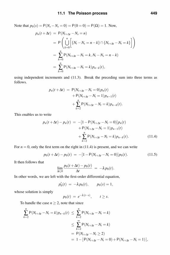
11.1 The Poisson process 449
Note that p0(s) = P(Ns −Ns = 0) = P(0 = 0) = P(Ω) = 1. Now,
pn(t +∆t) = P(Nt+∆t −Ns = n)
= P
(n⋃
k=0
[Nt −Ns = n− k∩Nt+∆t −Nt = k
])
=n
∑k=0
P(Nt+∆t −Nt = k, Nt −Ns = n− k)
=n
∑k=0
P(Nt+∆t −Nt = k)pn−k(t),
using independent increments and (11.3). Break the preceding sum into three terms as
follows.
pn(t +∆t) = P(Nt+∆t −Nt = 0)pn(t)
+P(Nt+∆t −Nt = 1)pn−1(t)
+n
∑k=2
P(Nt+∆t −Nt = k)pn−k(t).
This enables us to write
pn(t +∆t)− pn(t) = −[1−P(Nt+∆t −Nt = 0)]pn(t)
+P(Nt+∆t −Nt = 1)pn−1(t)
+n
∑k=2
P(Nt+∆t −Nt = k)pn−k(t). (11.4)
For n = 0, only the first term on the right in (11.4) is present, and we can write
p0(t +∆t)− p0(t) = −[1−P(Nt+∆t −Nt = 0)]p0(t). (11.5)
It then follows that
lim∆t↓0
p0(t +∆t)− p0(t)
∆t= −λ p0(t).
In other words, we are left with the first-order differential equation,
p′0(t) = −λ p0(t), p0(s) = 1,
whose solution is simply
p0(t) = e−λ (t−s), t ≥ s.
To handle the case n ≥ 2, note that since
n
∑k=2
P(Nt+∆t −Nt = k)pn−k(t) ≤n
∑k=2
P(Nt+∆t −Nt = k)
≤∞
∑k=2
P(Nt+∆t −Nt = k)
= P(Nt+∆t −Nt ≥ 2)
= 1− [P(Nt+∆t −Nt = 0)+P(Nt+∆t −Nt = 1) ],

450 Advanced concepts in random processes
it follows that
lim∆t↓0
∑nk=2 P(Nt+∆t −Nt = k)pn−k(t)
∆t= λ −λ = 0.
Returning to (11.4), we see that for n = 1 and for n ≥ 2,
lim∆t↓0
pn(t +∆t)− pn(t)
∆t= −λ pn(t)+λ pn−1(t).
This results in the differential-difference equation,
p′n(t) = −λ pn(t)+λ pn−1(t), p0(t) = e−λ (t−s). (11.6)
It is easily verified that for n = 1,2, . . . ,
pn(t) =[λ (t − s)]ne−λ (t−s)
n!,
which are the claimed Poisson probabilities, solve (11.6).
Marked Poisson processes
It is frequently the case that in counting arrivals, each arrival is associated with a mark.
For example, suppose packets arrive at a router according to a Poisson process of rate λ ,
and that the size of the ith packet is Bi bytes, where Bi is a random variable. The size Bi
is the mark. Thus, the ith packet, whose size is Bi, arrives at time Ti, where Ti is the ith
occurrence time of the Poisson process. The total number of bytes processed up to time t is
Mt :=Nt
∑i=1
Bi.
We usually assume that the mark sequence is i.i.d. and independent of the Poisson process.
In this case, the mean of Mt can be computed as in Example 7.24. The characteristic function
of Mt can be computed as in Problem 59 in Chapter 7.
Shot noise
Light striking a photodetector generates photoelectrons according to a Poisson process.
The rate of the process is proportional to the intensity of the light and the efficiency of the
detector. The detector output is then passed through an amplifier of impulse response h(t).We model the input to the amplifier as a train of impulses
Xt := ∑i
δ (t −Ti),
where the Ti are the occurrence times of the Poisson process. The amplifier output is
Yt =∫ ∞
−∞h(t − τ)Xτ dτ
=∞
∑i=1
∫ ∞
−∞h(t − τ)δ (τ −Ti)dτ
=∞
∑i=1
h(t −Ti). (11.7)
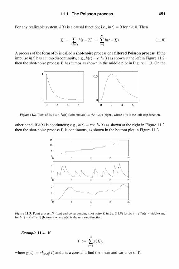
11.1 The Poisson process 451
For any realizable system, h(t) is a causal function; i.e., h(t) = 0 for t < 0. Then
Yt = ∑i:Ti≤t
h(t −Ti) =Nt
∑i=1
h(t −Ti). (11.8)
A process of the form of Yt is called a shot-noise process or a filtered Poisson process. If the
impulse h(t) has a jump discontinuity, e.g., h(t) = e−tu(t) as shown at the left in Figure 11.2,
then the shot-noise process Yt has jumps as shown in the middle plot in Figure 11.3. On the
0 2 4 6
0
1
0 2 4 6
0
0.5
Figure 11.2. Plots of h(t) = e−t u(t) (left) and h(t) = t2e−t u(t) (right), where u(t) is the unit step function.
other hand, if h(t) is continuous; e.g., h(t) = t2e−tu(t) as shown at the right in Figure 11.2,
then the shot-noise process Yt is continuous, as shown in the bottom plot in Figure 11.3.
0 5 10 15 200
5
10
15
0 5 10 15 200
1
2
0 5 10 15 200
1
2
t
Figure 11.3. Point process Nt (top) and corresponding shot noise Yt in Eq. (11.8) for h(t) = e−t u(t) (middle) and
for h(t) = t2e−t u(t) (bottom), where u(t) is the unit step function.
Example 11.4. If
Y :=∞
∑i=1
g(Ti),
where g(τ) := cI(a,b](τ) and c is a constant, find the mean and variance of Y .

452 Advanced concepts in random processes
Solution. To begin, write
Y = c∞
∑i=1
I(a,b](Ti).
Notice that the terms of the sum are either zero or one. A term is one if and only if Ti ∈ (a,b].Hence, this sum simply counts the number of occurrences in the interval (a,b]. But this is
just Nb −Na. Thus, Y = c(Nb −Na). From the properties of Poisson random variables,
E[Y ] = cλ (b− a) and E[Y 2] = c2λ (b− a) + [λ (b− a)]2. We can then write var(Y ) =c2λ (b−a). More important, however, is the fact that we can also write
E[Y ] =∫ ∞
0g(τ)λ dτ and var(Y ) =
∫ ∞
0g(τ)2λ dτ. (11.9)
For Y as in the previous example, it is easy to compute its characteristic function. First
write
ϕY (ν) = E[e jνY ] = E[e jνc(Nb−Na)] = exp[λ (b−a)(z−1)]|z=e jνc .
Thus,
ϕY (ν) = exp
[λ (b−a)(e jνc −1)
]= exp
[∫ ∞
0
(e jνg(τ)−1)λ dτ
]. (11.10)
This last equation follows because when g(τ) = 0, e0 − 1 = 0 too. Equations of the form
(11.9) and (11.10) are usually known as Campbell’s theorem, and they hold for rather
general functions g [34, pp. 28–29]. See also Problem 17.
11.2 Renewal processes
Recall that a Poisson process of rate λ can be constructed by writing
Nt :=∞
∑k=1
I[0,t](Tk),
where the arrival times
Tk := X1 + · · ·+Xk,
and the Xk are i.i.d. exp(λ ) interarrival times. If we drop the requirement that the interarrival
times be exponential and let them have arbitrary density f , then Nt is called a renewal
process.
Because of the similarity between the Poisson process and renewal processes, it is trivial
to modify the MATLAB code of Example 11.3 to simulate a renewal process instead of a
Poisson process. All we have to do is change the formula for X. See Problem 19.
Example 11.5. Hits to the Nuclear Engineering Department’s website form a renewal
process Nt , while hits to the Mechanical Engineering Department’s website form a renewal
process Mt . Assuming the processes are independent, find the probability that the first hit to

11.3 The Wiener process 453
the Nuclear Engineering website occurs before the first hit to the Mechanical Engineering
website.
Solution. Let Xk denote the kth interarrival time of the Nt process, and let Yk denote the
kth interarrival time of the Mt process. Then we need to compute
P(X1 < Y1) =∫ ∞
0P(X1 < Y1|Y1 = y) fY (y)dy,
where we have used the law of total probability, and where fY denotes the common density
of the Yk. Since the renewal processes are independent, so are their arrival and interarrival
times. Using the law of substitution and independence,
P(X1 < Y1) =∫ ∞
0P(X1 < y|Y1 = y) fY (y)dy
=∫ ∞
0P(X1 < y) fY (y)dy
=∫ ∞
0FX (y) fY (y)dy,
where FX is the common cdf of the Xk. (Since Xk has a density, FX is continuous.)
If we let F denote the cdf corresponding to the interarrival density f , it is easy to see
that the mean of the process is
E[Nt ] =∞
∑k=1
Fk(t), (11.11)
where Fk is the cdf of Tk. The corresponding density, denoted by fk, is the k-fold convolution
of f with itself. Hence, in general this formula is difficult to work with. However, there is
another way to characterize E[Nt ]. In the problems you are asked to derive the renewal
equation,
E[Nt ] = F(t)+∫ t
0E[Nt−x] f (x)dx.
The mean function m(t) := E[Nt ] of a renewal process is called the renewal function. Note
that m(0) = E[N0] = 0, and that the renewal equation can be written in terms of the renewal
function as
m(t) = F(t)+
∫ t
0m(t − x) f (x)dx.
11.3 The Wiener process
The theory of wide-sense stationary processes and white noise developed in Chapter 10
provides a satisfactory operational calculus for the analysis and design of linear, time-
invariant systems driven by white noise. However, if the output of such a system is passed
through a nonlinearity, and if we try to describe the result using a differential equation, we
immediately run into trouble.

454 Advanced concepts in random processes
Example 11.6. Let Xt be a wide-sense stationary, zero-mean process with correlation
function RX (τ) = σ2δ (τ). If the white noise Xt is applied to an integrator starting at time
zero, then the output at time t is
Vt :=∫ t
0Xτ dτ,
and the derivative of Vt with respect to t is Vt = Xt . If we now pass Vt through a square-law
device, say
Yt := V 2t ,
then
Yt = 2VtVt = 2VtXt , Y0 = 0.
Hence,
Yt =
∫ t
0Yθ dθ
= 2
∫ t
0Vθ Xθ dθ (11.12)
= 2
∫ t
0
(∫ θ
0Xτ dτ
)Xθ dθ .
It is now easy to see that
E[Yt ] = 2
∫ t
0
∫ θ
0E[Xτ Xθ ]dτ dθ = 2
∫ t
0
∫ θ
0σ2δ (τ −θ)dτ dθ
reduces to
E[Yt ] = 2σ2∫ t
0dθ = 2σ2t.
On the other hand,
E[Yt ] = E[V 2t ] = E
[(∫ t
0Xτ dτ
)(∫ t
0Xθ dθ
)]reduces to ∫ t
0
∫ t
0RX (τ −θ)dτ dθ =
∫ t
0
∫ t
0σ2δ (τ −θ)dτ dθ = σ2t,
which is the correct result.
As mentioned in Section 10.5, white noise does not exist as an ordinary process. This
example illustrates the perils of working with objects that are not mathematically well de-
fined. Although white noise does not exist as an ordinary random process, there is a well
defined process that can take the place of Vt . The Wiener process or Brownian motion
is a random process that models integrated white noise. The Wiener process, and Wiener
integral introduced below, are used extensively in stochastic differential equations. Sto-
chastic differential equations arise in numerous applications. For example, they describe
control systems driven by white noise, heavy traffic behavior of communication networks,
and economic models of the stock market.

11.3 The Wiener process 455
We say that Wt , t ≥ 0 is a Wiener process if the following four conditions hold.
• W0 ≡ 0; i.e., W0 is a constant random variable whose value is always zero.
• For any 0 ≤ s ≤ t < ∞, the increment Wt −Ws is a Gaussian random variable with
zero mean and variance σ2(t − s). In particular, E[Wt −Ws] = 0, and E[(Wt −Ws)2] =
σ2(t − s).• If the time intervals
(t1, t2],(t2, t3], . . . ,(tn, tn+1]
are disjoint, then the increments
Wt2 −Wt1 ,Wt3 −Wt2 , . . . ,Wtn+1−Wtn
are independent; i.e., the process has independent increments.
• For each sample point ω ∈ Ω, Wt(ω) as a function of t is continuous. More briefly,
we just say that Wt has continuous sample paths.
Remark. (i) If the parameter σ2 = 1, then the process is called a standard Wiener
process. Two sample paths of a standard Wiener process are shown in Figure 11.4.
(ii) Since the first and third properties of the Wiener process are the same as those of the
Poisson process, it is easy to show (Problem 26) that
cov(Wt1 ,Wt2) = σ2 min(t1, t2).
Hence, to justify the claim that Wt is a model for integrated white noise, it suffices to show
that the process Vt of Example 11.6 has the same covariance function; see Problem 25.
0 0.2 0.4 0.6 0.8 1−1
0
1
t
0 0.2 0.4 0.6 0.8 1−1
0
1
t
Figure 11.4. Two sample paths of a standard Wiener process.
456 Advanced concepts in random processes
(iii) The fourth condition, that as a function of t, Wt should be continuous, is always
assumed in practice, and can always be arranged by construction [3, Section 37]. The
precise statement of the fourth property is
P(ω ∈ Ω : Wt(ω) is a continuous function of t) = 1,
i.e., the realizations of Wt are continuous with probability one.
(iv) As indicated in Figure 11.4, the Wiener process is very “wiggly.” In fact, it wiggles
so much that it is nowhere differentiable with probability one [3, p. 505, Theorem 37.3].
(v) Although the Wiener process was originally proposed as a model for the path of a
small particle suspended in a fluid, the fact that Wiener-process paths are nowhere differen-
tiable implies the particle has infinite velocity! One way around this problem is to use the
Wiener process (more precisely, the Ornstein–Uhlenbeck process), which is continuous,
to model the velocity, and integrate the velocity to model the particle position [23], [40].
See Problems 32 and 33.
The Wiener integral
The Wiener process is a well-defined mathematical object. We argued above that Wt
behaves like Vt :=∫ t
0 Xτ dτ , where Xt is white noise. If such noise is applied to a linear
time-invariant system starting at time zero, and if the system has impulse response h, then
the output is ∫ ∞
0h(t − τ)Xτ dτ.
If we now suppress t and write g(τ) instead of h(t − τ), then we need a well-defined math-
ematical object to play the role of ∫ ∞
0g(τ)Xτ dτ.
To see what this object should be, suppose that g(τ) is piecewise constant taking the value
gi on the interval (ti, ti+1]. Then∫ ∞
0g(τ)Xτ dτ = ∑
i
∫ ti+1
ti
g(τ)Xτ dτ
= ∑i
gi
∫ ti+1
ti
Xτ dτ
= ∑i
gi
(∫ ti+1
0Xτ dτ −
∫ ti
0Xτ dτ
)= ∑
i
gi(Vti+1−Vti).
Thus, for piecewise-constant functions, integrals with white noise should be replaced by
sums involving the Wiener process.
The Wiener integral of a function g(τ) is denoted by∫ ∞
0g(τ)dWτ ,

11.3 The Wiener process 457
and is defined as follows. For piecewise constant functions g of the form
g(τ) =n
∑i=1
giI(ti,ti+1](τ),
where 0 ≤ t1 < t2 < · · · < tn+1 < ∞, we define∫ ∞
0g(τ)dWτ :=
n
∑i=1
gi(Wti+1−Wti),
where Wt is a Wiener process. Note that the right-hand side is a weighted sum of inde-
pendent, zero-mean, Gaussian random variables. The sum is therefore Gaussian with zero
mean and variance
n
∑i=1
g2i var(Wti+1
−Wti) =n
∑i=1
g2i ·σ2(ti+1 − ti) = σ2
∫ ∞
0g(τ)2 dτ.
Because of the zero mean, the variance and second moment are the same. Hence, we also
have
E
[(∫ ∞
0g(τ)dWτ
)2]= σ2
∫ ∞
0g(τ)2 dτ. (11.13)
For functions g that are not piecewise constant, but do satisfy∫ ∞
0 g(τ)2 dτ < ∞, the Wiener
integral can be defined by a limiting process, which is discussed in more detail in Chap-
ter 13. Basic properties of the Wiener integral are explored in the problems.
Remark. When the Wiener integral is extended to allow random integrands, it is known
as the Ito integral. Using the Ito rule [67], it can be shown that if Yt = W 2t , then
Yt = 2
∫ t
0Wτ dWτ +σ2t
is the correct version of (11.12) in Example 11.6. Since the expected value of the Ito integral
is zero, we find that E[Yt ] = σ2t, which is the correct result. The extra term σ2t in the
equation for Yt is called the Ito correction term.
Random walk approximation of the Wiener process
We present a three-step construction of a continuous-time, piecewise-constant random
process that approximates the Wiener process.
The first step is to construct a symmetric random walk. Let X1,X2, . . . be i.i.d. ±1-valued
random variables with P(Xi = ±1) = 1/2. Then each Xi has zero mean and variance one.
Let S0 ≡ 0, and for n ≥ 1, put
Sn :=n
∑i=1
Xi.
Then Sn has zero mean and variance n. The process Sn,n ≥ 0 is called a symmetric
random walk.

458 Advanced concepts in random processes
The second step is to construct the scaled random walk Sn/√
n. Note that Sn/√
n has
zero mean and variance one. By the central limit theorem, which is discussed in detail in
Chapter 5, the cdf of Sn/√
n converges to the standard normal cdf.
The third step is to construct the continuous-time, piecewise-constant process
W(n)
t :=1√n
Snt,
where τ denotes the greatest integer that is less than or equal to τ . For example, if n = 100
and t = 3.1476, then
W(100)3.1476 =
1√100
S100·3.1476 =1
10S314.76 =
1
10S314.
For example, a sample path of S0,S1, . . . ,S75 is shown at the top in Figure 11.5. The
corresponding continuous-time, piecewise constant process W(75)
t is shown at the bottom
in Figure 11.5. Notice that as the continuous variable t ranges over [0,1], the values of
75t range over the integers 0,1, . . . ,75. Thus, the constant levels seen at the bottom in
Figure 11.5 are 1/√
75 times those at the top.
0 25 50 75
−2
0
2
4
6
k
0 0.25 0.5 0.75 1
−0.2
0
0.2
0.4
0.6
t
Figure 11.5. Sample path Sk,k = 0, . . . ,75 (top). Sample path W(75)
t (bottom).
Figure 11.6 shows a sample path of W(n)
t for n = 150 (top) and for n = 10000 (bottom).
As n increases, the sample paths look more and more like those of the Wiener processes
shown in Figure 11.4.
Since the central limit theorem applies to any i.i.d. sequence with finite variance, the
preceding convergence to the Wiener process holds if we replace the ±1-valued Xi by any
i.i.d. sequence with finite variance.a However, if the Xi only have finite mean but infinite
aIf the mean of the Xi is m and the variance is σ2, then we must replace Sn by (Sn −nm)/σ .
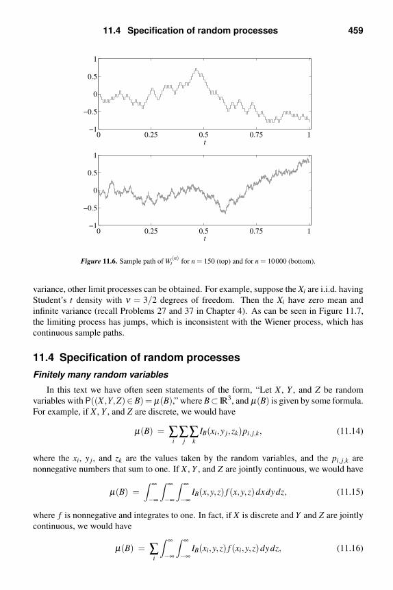
11.4 Specification of random processes 459
0 0.25 0.5 0.75 1−1
−0.5
0
0.5
1
t
0 0.25 0.5 0.75 1−1
−0.5
0
0.5
1
t
Figure 11.6. Sample path of W(n)
t for n = 150 (top) and for n = 10000 (bottom).
variance, other limit processes can be obtained. For example, suppose the Xi are i.i.d. having
Student’s t density with ν = 3/2 degrees of freedom. Then the Xi have zero mean and
infinite variance (recall Problems 27 and 37 in Chapter 4). As can be seen in Figure 11.7,
the limiting process has jumps, which is inconsistent with the Wiener process, which has
continuous sample paths.
11.4 Specification of random processes
Finitely many random variables
In this text we have often seen statements of the form, “Let X , Y , and Z be random
variables with P((X ,Y,Z)∈B) = µ(B),” where B⊂ IR3, and µ(B) is given by some formula.
For example, if X , Y , and Z are discrete, we would have
µ(B) = ∑i
∑j∑k
IB(xi,y j,zk)pi, j,k, (11.14)
where the xi, y j, and zk are the values taken by the random variables, and the pi, j,k are
nonnegative numbers that sum to one. If X , Y , and Z are jointly continuous, we would have
µ(B) =∫ ∞
−∞
∫ ∞
−∞
∫ ∞
−∞IB(x,y,z) f (x,y,z)dxdydz, (11.15)
where f is nonnegative and integrates to one. In fact, if X is discrete and Y and Z are jointly
continuous, we would have
µ(B) = ∑i
∫ ∞
−∞
∫ ∞
−∞IB(xi,y,z) f (xi,y,z)dydz, (11.16)

460 Advanced concepts in random processes
0 0.2 0.4 0.6 0.8 1
−1
−0.5
0
0.5
t
0 0.2 0.4 0.6 0.8 1
−1
−0.5
0
0.5
1
t
Figure 11.7. Two sample paths of Snt/n2/3 for n = 10000 when the Xi have Student’s t density with 3/2 degrees
of freedom.
where f is nonnegative and
∑i
∫ ∞
−∞
∫ ∞
−∞f (xi,y,z)dydz = 1.
The big question is, given a formula for computing µ(B), how do we know that a sample
space Ω, a probability measure P, and functions X(ω), Y (ω), and Z(ω) exist such that we
indeed have
P((X ,Y,Z) ∈ B
)= µ(B), B ⊂ IR3.
As we show in the next paragraph, the answer turns out to be rather simple.
If µ is defined by expressions such as (11.14)–(11.16), it can be shown that µ is a prob-
ability measureb on IR3; the case of (11.14) is easy; the other two require some background
in measure theory, e.g., [3]. More generally, if we are given any probability measure µ on
IR3, we take Ω = IR3 and put P(A) := µ(A) for A ⊂ Ω = IR3. For ω = (ω1,ω2,ω3), we
define
X(ω) := ω1, Y (ω) := ω2, and Z(ω) := ω3.
It then follows that for B ⊂ IR3,
ω ∈ Ω : (X(ω),Y (ω),Z(ω)) ∈ B
reduces to
ω ∈ Ω : (ω1,ω2,ω3) ∈ B = B.
Hence, P((X ,Y,Z) ∈ B) = P(B) = µ(B).
bSee Section 1.4 to review the axioms satisfied by a probability measure.

11.4 Specification of random processes 461
For fixed n ≥ 1, the foregoing ideas generalize in the obvious way to show the existence
of a sample space Ω, probability measure P, and random variables X1, . . . ,Xn with
P((X1,X2, . . . ,Xn) ∈ B
)= µ(B), B ⊂ IRn,
where µ is any given probability measure defined on IRn.
Infinite sequences (discrete time)
Consider an infinite sequence of random variables such as X1,X2, . . . . While (X1, . . . ,Xn)takes values in IRn, the infinite sequence (X1,X2, . . .) takes values in IR∞. If such an infinite
sequence of random variables exists on some sample space Ω equipped with some proba-
bility measure P, then1
P((X1,X2, . . .) ∈ B
), B ⊂ IR∞,
is a probability measure on IR∞. We denote this probability measure by µ(B). Similarly, P
induces on IRn the measure
µn(Bn) = P((X1, . . . ,Xn) ∈ Bn
), Bn ⊂ IRn,
Of course, P induces on IRn+1 the measure
µn+1(Bn+1) = P((X1, . . . ,Xn,Xn+1) ∈ Bn+1
), Bn+1 ⊂ IRn+1.
If we take Bn+1 = Bn × IR for any Bn ⊂ IRn, then
µn+1(Bn × IR) = P((X1, . . . ,Xn,Xn+1) ∈ Bn × IR
)= P
((X1, . . . ,Xn) ∈ Bn,Xn+1 ∈ IR
)= P
((X1, . . . ,Xn) ∈ Bn∩Xn+1 ∈ IR)= P
((X1, . . . ,Xn) ∈ Bn∩Ω)
= P((X1, . . . ,Xn) ∈ Bn
)= µn(Bn).
Thus, we have the consistency condition
µn+1(Bn × IR) = µn(Bn), Bn ⊂ IRn, n = 1,2, . . . . (11.17)
Next, observe that since (X1, . . . ,Xn) ∈ Bn if and only if
(X1,X2, . . . ,Xn,Xn+1, . . .) ∈ Bn × IR×·· · ,
it follows that µn(Bn) is equal to
P((X1,X2, . . . ,Xn,Xn+1, . . .) ∈ Bn × IR×·· ·),
which is simply µ(Bn × IR×·· ·). Thus,
µ(Bn × IR×·· ·) = µn(Bn), Bn ∈ IRn, n = 1,2, . . . . (11.18)

462 Advanced concepts in random processes
The big question here is, if we are given a sequence of probability measures µn on IRn for
n = 1,2, . . . , does there exist a probability measure µ on IR∞ such that (11.18) holds?
To appreciate the complexity of this question, consider the simplest possible case of
constructing a sequence of i.i.d. Bernoulli(1/2) random variables. In this case, for a finite
sequence of zeros and ones, say (b1, . . . ,bn), and with Bn being the singleton set Bn =(b1, . . . ,bn), we want
µn(Bn) = P(X1 = b1, . . . ,Xn = bn) =n
∏i=1
P(Xi = bi) =(1
2
)n
.
We need a probability measure µ on IR∞ that concentrates all its probability on the infinite
sequences of zeros and ones,
S = ω = (ω1,ω2, . . .) : ωi = 0 or ωi = 1 ⊂ IR∞;
i.e., we need µ(S) = 1. Unfortunately, as shown in Example 1.9, the set S is not countable.
Hence, we cannot use a probability mass function to define µ . The general solution to this
difficulty was found by Kolmogorov and is discussed next.
Conditions under which a probability measure can be constructed on IR∞ are known as
Kolmogorov’s consistency theorem or as Kolmogorov’s extension theorem. It says that
if the consistency condition (11.17) holds,c then a probability measure µ exists on IR∞ such
that (11.18) holds [7, p. 188].
We now specialize the foregoing discussion to the case of integer-valued random vari-
ables X1,X2, . . . . For each n = 1,2, . . . , let pn(i1, . . . , in) denote a proposed joint probability
mass function of X1, . . . ,Xn. In other words, we want a random process for which
P((X1, . . . ,Xn) ∈ Bn
)=
∞
∑i1=−∞
· · ·∞
∑in=−∞
IBn(i1, . . . , in)pn(i1, . . . , in).
More precisely, with µn(Bn) given by the above right-hand side, does there exist a measure
µ on IR∞ such that (11.18) holds? By Kolmogorov’s theorem, we just need to show that
(11.17) holds.
We now show that (11.17) is equivalent to
∞
∑j=−∞
pn+1(i1, . . . , in, j) = pn(i1, . . . , in). (11.19)
The left-hand side of (11.17) takes the form
∞
∑i1=−∞
· · ·∞
∑in=−∞
∞
∑j=−∞
IBn×IR(i1, . . . , in, j)pn+1(i1, . . . , in, j). (11.20)
cKnowing the measure µn, we can always write the corresponding cdf as
Fn(x1, . . . ,xn) = µn
((−∞,x1]×·· ·× (−∞,xn]
).
Conversely, if we know the Fn, there is a unique measure µn on IRn such that the above formula holds [3, Sec-
tion 12]. Hence, the consistency condition has the equivalent formulation in terms of cdfs [7, p. 189],
limxn+1→∞
Fn+1(x1, . . . ,xn,xn+1) = Fn(x1, . . . ,xn).

11.4 Specification of random processes 463
Observe that IBn×IR = IBn IIR = IBn . Hence, the above sum becomes
∞
∑i1=−∞
· · ·∞
∑in=−∞
∞
∑j=−∞
IBn(i1, . . . , in)pn+1(i1, . . . , in, j),
which, using (11.19), simplifies to
∞
∑i1=−∞
· · ·∞
∑in=−∞
IBn(i1, . . . , in)pn(i1, . . . , in), (11.21)
which is our definition of µn(Bn). Conversely, if in (11.17), or equivalently in (11.20) and
(11.21), we take Bn to be the singleton set
Bn = ( j1, . . . , jn),
then we obtain (11.19).
The next question is how to construct a sequence of probability mass functions satisfying
(11.19). Observe that (11.19) can be rewritten as
∞
∑j=−∞
pn+1(i1, . . . , in, j)
pn(i1, . . . , in)= 1.
In other words, if pn(i1, . . . , in) is a valid joint pmf, and if we define
pn+1(i1, . . . , in, j) := pn+1|1,...,n( j|i1, . . . , in) · pn(i1, . . . , in),
where pn+1|1,...,n( j|i1, . . . , in) is a valid pmf in the variable j (i.e., is nonnegative and the sum
over j is one), then (11.19) will automatically hold!
Example 11.7. Let q(i) be any pmf. Take p1(i) := q(i), and take pn+1|1,...,n( j|i1, . . . , in):= q( j). Then, for example,
p2(i, j) = p2|1( j|i) p1(i) = q( j)q(i),
and
p3(i, j,k) = p3|1,2(k|i, j) p2(i, j) = q(i)q( j)q(k).
More generally,
pn(i1, . . . , in) = q(i1) · · ·q(in).
Thus, the Xn are i.i.d. with common pmf q.
Example 11.8. Again let q(i) be any pmf. Suppose that for each i, r( j|i) is a pmf in the
variable j; i.e., r is any conditional pmf. Put p1(i) := q(i), and put
pn+1|1,...,n( j|i1, . . . , in) := r( j|in).
Then
p2(i, j) = p2|1( j|i) p1(i) = r( j|i)q(i),

464 Advanced concepts in random processes
and
p3(i, j,k) = p3|1,2(k|i, j) p2(i, j) = q(i)r( j|i)r(k| j).More generally,
pn(i1, . . . , in) = q(i1)r(i2|i1)r(i3|i2) · · ·r(in|in−1).
As we will see in Chapter 12, pn is the joint pmf of a Markov chain with stationary transition
probabilities r( j|i) and initial pmf q(i).
Continuous-time random processes
The consistency condition for a continuous-time random process is a little more compli-
cated. The reason is that in discrete time, between any two consecutive integers, there are
no other integers, while in continuous time, for any t1 < t2, there are infinitely many times
between t1 and t2.
Now suppose that for any t1 < · · · < tn+1, we are given a probability measure µt1,...,tn+1
on IRn+1. Fix any Bn ⊂ IRn. For k = 1, . . . ,n+1, define Bn,k ⊂ IRn+1 by
Bn,k := (x1, . . . ,xn+1) : (x1, . . . ,xk−1,xk+1, . . . ,xn+1) ∈ Bn and xk ∈ IR.
Note the special casesd
Bn,1 = IR×Bn and Bn,n+1 = Bn × IR.
The continuous-time consistency condition is that [53, p. 244] for k = 1, . . . ,n+1,
µt1,...,tn+1(Bn,k) = µt1,...,tk−1,tk+1,...,tn+1
(Bn). (11.22)
If this condition holds, then there is a sample space Ω, a probability measure P, and random
variables Xt such that
P((Xt1 , . . . ,Xtn) ∈ Bn
)= µt1,...,tn(Bn), Bn ⊂ IRn,
for any n ≥ 1 and any times t1 < · · · < tn.
Gaussian processes
A continuous-time random process Xt is said to be Gaussian if for every sequence of
times t1, . . . ,tn, [Xt1 , . . . ,Xtn ]′ is a Gaussian random vector. Since we have defined a random
vector to be Gaussian if every linear combination of its components is a scalar Gaussian
random variable, we see that a random process is Gaussian if and only if every finite linear
combination of samples, say ∑ni=1 ciXti , is a Gaussian random variable. You can use this fact
to show that the Wiener process is a Gaussian process in Problem 46.
dIn the previous subsection, we only needed the case k = n+1. If we had wanted to allow two-sided discrete-
time processes Xn for n any positive or negative integer, then both k = 1 and k = n + 1 would have been needed
(Problem 42).

11.4 Specification of random processes 465
Example 11.9. Show that if a Gaussian process is wide-sense stationary, then it is
strictly stationary.
Solution. Without loss of generality, we assume the process is zero mean. Let R(τ) :=E[Xt+τ Xt ]. Let times t1, . . . ,tn be given, and consider the vectors
X := [Xt1 , . . . ,Xtn ]′ and Y := [Xt1+∆t , . . . ,Xtn+∆t ]
′.
We need to show that P(X ∈ B) = P(Y ∈ B) for any n-dimensional set B. It suffices to
show that X and Y have the same joint characteristic function. Since X and Y are zero-mean
Gaussian random vectors, all we need to do is show that they have the same covariance
matrix. The i j entry of the covariance matrix of X is
E[XtiXt j] = R(ti − t j),
while for Y it is
E[Xti+∆tXt j+∆t ] = R((ti +∆t)− (t j +∆t)
)= R(ti − t j).
Example 11.10. Show that a real-valued function R(t,s) is the correlation function of
a continuous-time random process if and only if for every finite sequence of distinct times,
say t1, . . . ,tn, the n×n matrix with i j entry R(ti, t j) is positive semidefinite.
Solution. If R(t,s) is the correlation function of a process Xt , then the matrix with entries
R(ti, t j) is the covariance matrix of the random vector [Xt1 , . . . ,Xtn ]′. As noted following
Example 8.4, the covariance matrix of a random vector must be positive semidefinite.
Conversely, suppose every matrix with entries R(ti, t j) is positive semidefinite. Imagine
a Gaussian random vector [Y1, . . . ,Yn]′ having this covariance matrix, and put
µt1,...,tn(B) := P((Y1, . . . ,Yn) ∈ B).
Since any subvector of Y is Gaussian with covariance matrix given by appropriate entries
of the covariance matrix of Y , the consistency conditions are satisfied. By Kolmogorov’s
theorem, the required process exists. In fact, the process constructed in this way is Gaussian.
Another important property of Gaussian processes is that their integrals are Gaussian
random variables. If Xt is a Gaussian process, we might consider an integral of the form∫c(t)Xt dt = lim∑
i
c(ti)Xti∆t i.
Since the process is Gaussian, linear combinations of samples Xti are scalar Gaussian ran-
dom variables. We then use the fact that limits of Gaussian random variables are Gaussian.
This is just a sketch of how the general argument goes. For details, see the discussion of
mean-square integrals at the end of Section 13.2 and also Example 14.9.

466 Advanced concepts in random processes
Notes
11.4: Specification of random processes
Note 1. Comments analogous to Note 1 in Chapter 7 apply here. Specifically, the set B
must be restricted to a suitable σ -field B∞ of subsets of IR∞. Typically, B∞ is taken to be
the smallest σ -field containing all sets of the form
ω = (ω1,ω2, . . .) ∈ IR∞ : (ω1, . . . ,ωn) ∈ Bn,
where Bn is a Borel subset of IRn, and n ranges over the positive integers [3, p. 485].
Problems
11.1: The Poisson process
1. Hits to a certain website occur according to a Poisson process of rate λ = 3 per
minute. What is the probability that there are no hits in a 10-minute period? Give a
formula and then evaluate it to obtain a numerical answer.
2. Cell-phone calls processed by a certain wireless base station arrive according to a
Poisson process of rate λ = 12 per minute. What is the probability that more than
three calls arrive in a 20-second interval? Give a formula and then evaluate it to
obtain a numerical answer.
3. Let Nt be a Poisson process with rate λ = 2, and consider a fixed observation interval
(0,5].
(a) What is the probability that N5 = 10?
(b) What is the probability that Ni −Ni−1 = 2 for all i = 1, . . . ,5?
4. A sports clothing store sells football jerseys with a certain very popular number on
them according to a Poisson process of rate three crates per day. Find the probability
that on 5 days in a row, the store sells at least three crates each day.
5. A sporting goods store sells a certain fishing rod according to a Poisson process of
rate two per day. Find the probability that on at least 1 day during the week, the store
sells at least three rods. (Note: week = 5 days.)
6. A popular music group produces a new hit song every 7 months on average. Assume
that songs are produced according to a Poisson process.
(a) Find the probability that the group produces more than two hit songs in 1 year.
(b) How long do you expect it to take until the group produces its 10th song?
7. Let Nt be a Poisson process with rate λ , and let ∆t > 0.
(a) Show that Nt+∆t −Nt and Nt are independent.
(b) Show that P(Nt+∆t = k + |Nt = k) = P(Nt+∆t −Nt = ).
(c) Evaluate P(Nt = k|Nt+∆t = k + ).

Problems 467
(d) Show that as a function of k = 0, . . . ,n, P(Nt = k|Nt+∆t = n) has the binomial(n,p) probability mass function and identify p.
8. Customers arrive at a store according to a Poisson process of rate λ . What is the
expected time until the nth customer arrives? What is the expected time between
customers?
9. During the winter, snowstorms occur according to a Poisson process of intensity λ =2 per week.
(a) What is the average time between snowstorms?
(b) What is the probability that no storms occur during a given 2-week period?
(c) If winter lasts 12 weeks, what is the expected number of snowstorms?
(d) Find the probability that during at least one of the 12 weeks of winter, there are
at least five snowstorms.
10. Space shuttles are launched according to a Poisson process. The average time be-
tween launches is 2 months.
(a) Find the probability that there are no launches during a 4-month period.
(b) Find the probability that during at least 1 month out of four consecutive months,
there are at least two launches.
11. Internet packets arrive at a router according to a Poisson process of rate λ . Find the
variance of the time it takes for the first n packets to arrive.
12. Let U be a uniform[0,1] random variable that is independent of a Poisson process Nt
with rate λ = 1. Put
Yt := Nln(1+tU).
Find the probability generating function of Yt , G(z) := E[zYt ] for real z, including
z = 0.
13. Hits to the websites of the Nuclear and Mechanical Engineering Departments form
two independent Poisson processes, Nt and Mt , respectively. Let λ and µ be their
respective rates. Find the probability that between two consecutive hits to the Nuclear
Engineering website, there are exactly m hits to the Mechanical Engineering website.
14. Diners arrive at popular restaurant according to a Poisson process Nt of rate λ . A
confused maitre d’ seats the ith diner with probability p, and turns the diner away
with probability 1− p. Let Yi = 1 if the ith diner is seated, and Yi = 0 otherwise. The
number diners seated up to time t is
Mt :=Nt
∑i=1
Yi.
Show that Mt is a Poisson random variable and find its parameter. Assume the Yi are
independent of each other and of the Poisson process.
Remark. Mt is an example of a thinned Poisson process.

468 Advanced concepts in random processes
15. Lightning strikes occur according to a Poisson process of rate λ per minute. The
energy of the ith strike is Vi. Assume the energies Vi are i.i.d. random variables that
are independent of the occurrence times (independent of the Poisson process). What
is the expected energy of a storm that lasts for t minutes? What is the average time
between lightning strikes?
16. (This problem uses the methods and notation of Section 6.4.) Let Nt be a Poisson
process with unknown intensity λ . For i = 1, . . . ,100, put Xi = (Ni −Ni−1). Then the
Xi are i.i.d. Poisson(λ ), and E[Xi] = λ . If M100 = 5.170, and S100 = 2.132, find the
95% confidence interval for λ .
17. For 0 ≤ t0 < · · · < tn < ∞, let
g(τ) =n
∑k=1
gkI(tk−1,tk](τ) and h(τ) =
n
∑l=1
hlI(tl−1,tl ](τ),
and put
Y =∞
∑i=1
g(Ti) and Z =∞
∑j=1
h(Tj).
Show that formula for E[Y ] in (11.9) and the formula for the characteristic function
of Y in (11.10) continue to hold. Also show that
cov(Y,Z) =∫ ∞
0g(τ)h(τ)λ dτ.
18. Find the mean and characteristic function of the shot-noise random variable Yt in
equation (11.7). Also find cov(Yt ,Ys). Hint: Use the results of the previous problem.
11.2: Renewal processes
19. MATLAB. Modify the MATLAB code of Example 11.3 and print out a simulation of
a renewal process whose interarrival times are i.i.d. chi-squared with one degree of
freedom.
20. In Example 11.5, suppose Nt is actually a Poisson process of rate λ . Show that the
result of Example 11.5 can be expressed in terms of the moment generating function
of the Yk. Now further simplify your expression in the case that Mt is a Poisson
process of rate µ .
21. Internet packets arrive at a router according to a renewal process whose interarrival
times are uniform[0,1]. Find the variance of the time it takes for the first n packets to
arrive.
22. In the case of a Poisson process, show that the right-hand side of (11.11) reduces to
λ t.
23. Derive the renewal equation
E[Nt ] = F(t)+∫ t
0E[Nt−x] f (x)dx
as follows.

Problems 469
(a) Show that E[Nt |X1 = x] = 0 for x > t.
(b) Show that E[Nt |X1 = x] = 1+E[Nt−x] for x ≤ t.
(c) Use parts (a) and (b) and the law of total probability to derive the renewal equa-
tion.
24. Solve the renewal equation for the renewal function m(t) := E[Nt ] if the interarrival
density is f ∼ exp(λ ). Hint: Take the one-sided Laplace transform of the renewal
equation. It then follows that m(t) = λ t for t ≥ 0, which is what we expect since
f ∼ exp(λ ) implies Nt is a Poisson process of rate λ .
11.3: The Wiener process
25. Let Vt be defined as in Example 11.6. Show that for 0 ≤ s < t < ∞, E[VtVs] = σ2s.
26. For 0 ≤ s < t < ∞, use the definition of the Wiener process to show that E[WtWs] =σ2s.
27. Let Wt be a Wiener process with E[W 2t ] = σ2t. Put Yt := eWt . Find the correlation
function RY (t1, t2) := E[Yt1Yt2 ] for t2 > t1.
28. Let the random vector X = [Wt1 , . . . ,Wtn ]′, 0 < t1 < · · · < tn < ∞, consist of samples
of a Wiener process. Find the covariance matrix of X , and write it out in detail as⎡⎢⎢⎢⎢⎢⎣c11 c12 c13 c1n
c21 c22 c23 c2n
c31 c32 c33 c3n
. . .
cn1 cn2 cn3 cnn
⎤⎥⎥⎥⎥⎥⎦ ,
where each ci j is given explicitly in terms of ti or t j.
29. For piecewise constant g and h, show that∫ ∞
0g(τ)dWτ +
∫ ∞
0h(τ)dWτ =
∫ ∞
0
[g(τ)+h(τ)
]dWτ .
Hint: The problem is easy if g and h are constant over the same intervals.
30. Use (11.13) to derive the formula
E
[(∫ ∞
0g(τ)dWτ
)(∫ ∞
0h(τ)dWτ
)]= σ2
∫ ∞
0g(τ)h(τ)dτ.
Hint: Consider the expectation
E
[(∫ ∞
0g(τ)dWτ −
∫ ∞
0h(τ)dWτ
)2 ],
470 Advanced concepts in random processes
which can be evaluated in two different ways. The first way is to expand the square
and take expectations term by term, applying (11.13) where possible. The second
way is to observe that since∫ ∞
0g(τ)dWτ −
∫ ∞
0h(τ)dWτ =
∫ ∞
0[g(τ)−h(τ)]dWτ ,
the above second moment can be computed directly using (11.13).
31. Let
Yt =∫ t
0g(τ)dWτ , t ≥ 0.
(a) Use (11.13) to show that
E[Y 2t ] = σ2
∫ t
0g(τ)2 dτ.
Hint: Observe that ∫ t
0g(τ)dWτ =
∫ ∞
0g(τ)I(0,t](τ)dWτ .
(b) Show that Yt has correlation function
RY (t1, t2) = σ2∫ min(t1,t2)
0g(τ)2 dτ, t1, t2 ≥ 0.
32. Consider the process
Yt = e−λ tV +
∫ t
0e−λ (t−τ) dWτ , t ≥ 0,
where Wt is a Wiener process independent of V , and V has zero mean and variance
q2. Use Problem 31 to show that Yt has correlation function
RY (t1, t2) = e−λ (t1+t2)(
q2 − σ2
2λ
)+
σ2
2λe−λ |t1−t2|.
Remark. If V is normal, then the process Yt is Gaussian and is known as an Ornstein–
Uhlenbeck process.
33. Let Wt be a Wiener process, and put
Yt :=e−λ t
√2λ
We2λ t .
Show that
RY (t1, t2) =σ2
2λe−λ |t1−t2|.
In light of the remark above, this is another way to define an Ornstein–Uhlenbeck
process.

Problems 471
34. Let Wt be a standard Wiener process, and put
Yt :=∫ t
0g(τ)dWτ
for some function g(t).
(a) Evaluate P(t) := E[Y 2t ]. Hint: Use Problem 31.
(b) If g(t) = 0, show that P(t) is strictly increasing.
(c) Assume P(t) < ∞ for t < ∞ and that P(t) → ∞ as t → ∞. If g(t) = 0, then by
part (b), P−1(t) exists and is defined for all t ≥ 0. If Xt := YP−1(t), compute E[Xt ]
and E[X2t ].
35. So far we have defined the Wiener process Wt only for t ≥ 0. When defining Wt for
all t, we continue to assume that W0 ≡ 0; that for s < t, the increment Wt −Ws is a
Gaussian random variable with zero mean and variance σ2(t − s); that Wt has inde-
pendent increments; and that Wt has continuous sample paths. The only difference is
that s or both s and t can be negative, and that increments can be located anywhere in
time, not just over intervals of positive time. In the following take σ2 = 1.
(a) For t > 0, show that E[W 2t ] = t.
(b) For s < 0, show that E[W 2s ] = −s.
(c) Show that
E[WtWs] =|t|+ |s|− |t − s|
2.
11.4: Specification of random processes
36. Suppose X and Y are random variables with
P((X ,Y ) ∈ A
)= ∑
i
∫ ∞
−∞IA(xi,y) fXY (xi,y)dy,
where the xi are distinct real numbers, and fXY is a nonnegative function satisfying
∑i
∫ ∞
−∞fXY (xi,y)dy = 1.
(a) Show that
P(X = xk) =
∫ ∞
−∞fXY (xk,y)dy.
(b) Show that for C ⊂ IR,
P(Y ∈C) =∫
C
(∑
i
fXY (xi,y)
)dy.
In other words, Y has marginal density
fY (y) = ∑i
fXY (xi,y).
472 Advanced concepts in random processes
(c) Show that
P(Y ∈C|X = xk) =∫
C
[fXY (xk,y)
pX (xk)
]dy.
In other words,
fY |X (y|xk) =fXY (xk,y)
pX (xk).
(d) For B ⊂ IR, show that if we define
P(X ∈ B|Y = y) := ∑i
IB(xi)pX |Y (xi|y),
where
pX |Y (xi|y) :=fXY (xi,y)
fY (y),
then ∫ ∞
−∞P(X ∈ B|Y = y) fY (y)dy = P(X ∈ B).
In other words, we have the law of total probability.
37. Let F be the standard normal cdf. Then F is a one-to-one mapping from (−∞,∞)onto (0,1). Therefore, F has an inverse, F−1:(0,1)→ (−∞,∞). If U ∼ uniform(0,1),show that X := F−1(U) has F for its cdf.
38. Consider the cdf
F(x) :=
⎧⎪⎪⎪⎪⎨⎪⎪⎪⎪⎩0, x < 0,x2, 0 ≤ x < 1/2,
1/4, 1/2 ≤ x < 1,x/2, 1 ≤ x < 2,1, x ≥ 2.
(a) Sketch F(x).
(b) For 0 < u < 1, sketch
G(u) := minx ∈ IR : F(x) ≥ u.Hint: First identify the set
Bu := x ∈ IR : F(x) ≥ u.Then find its minimum element.
39. As illustrated in the previous problem, an arbitrary cdf F is usually not invertible,
either because the equation F(x) = u has more than one solution, e.g., F(x) = 1/4, or
because it has no solution, e.g., F(x) = 3/8. However, for any cdf F , we can always
introduce the functione
G(u) := minx ∈ IR : F(x) ≥ u, 0 < u < 1,
eIn the previous problem, it was seen from the graph of F(x) that x ∈ IR : F(x) ≥ u is a closed semi-infinite
interval, whose left-hand end point is its minimum element. This is true for any cdf because cdfs are nondecreasing
and right continuous.
Problems 473
which, you will now show, can play the role of F−1 in Problem 37. Show that if
0 < u < 1 and x ∈ IR, then G(u) ≤ x if and only if u ≤ F(x).
40. Let G be as defined in the preceding problem, and let U ∼ uniform(0,1). Put X :=G(U) and show that X has cdf F .
41. MATLAB. Write a MATLAB function called G to compute the function G(u) that you
found in Problem 38. Then use the script
n = 10000;
nbins = 20;
U = rand(1,n);
X = G(U);
minX = min(X);
maxX = max(X);
e = linspace(minX,maxX,nbins+1); % edge sequence
H = histc(X,e);
H(nbins) = H(nbins)+H(nbins+1); % explained in Section 6.2
H = H(1:nbins); % resize H
bw = (maxX-minX)/nbins; % bin width
a = e(1:nbins); % left edge sequence
b = e(2:nbins+1); % right edge sequence
bin_centers = (a+b)/2; % bin centers
bar(bin_centers,H/(bw*n),’hist’)
to use your function G to simulate 10 000 realizations of the random variable X with
the cdf of Problem 38 and to plot a histogram of the results. Discuss the relationship
between the histogram and the density of X .
42. In the text we considered discrete-time processes Xn for n = 1,2, . . . . The consistency
condition (11.17) arose from the requirement that
P((X1, . . . ,Xn,Xn+1) ∈ B× IR
)= P
((X1, . . . ,Xn) ∈ B
),
where B ⊂ IRn. For processes Xn with n = 0,±1,±2, . . . , we require not only
P((Xm, . . . ,Xn,Xn+1) ∈ B× IR
)= P
((Xm, . . . ,Xn) ∈ B
),
but also
P((Xm−1,Xm, . . . ,Xn) ∈ IR×B
)= P
((Xm, . . . ,Xn) ∈ B
),
where now B ⊂ IRn−m+1. Let µm,n(B) be a proposed formula for the above right-hand
side. Then the two consistency conditions are
µm,n+1(B× IR) = µm,n(B) and µm−1,n(IR×B) = µm,n(B).
For integer-valued random processes, show that these are equivalent to
∞
∑j=−∞
pm,n+1(im, . . . , in, j) = pm,n(im, . . . , in)

474 Advanced concepts in random processes
and∞
∑j=−∞
pm−1,n( j, im, . . . , in) = pm,n(im, . . . , in),
where pm,n is the proposed joint probability mass function of Xm, . . . ,Xn.
43. Let q be any pmf, and let r( j|i) be any conditional pmf. In addition, assume that
∑k q(k)r( j|k) = q( j). Put
pm,n(im, . . . , in) := q(im)r(im+1|im)r(im+2|im+1) · · ·r(in|in−1).
Show that both consistency conditions for pmfs in the preceding problem are satisfied.
Remark. This process is strictly stationary as defined in Section 10.3 since the upon
writing out the formula for pm+k,n+k(im, . . . , in), we see that it does not depend on k.
44. Let µn be a probability measure on IRn, and suppose that it is given in terms of a joint
density fn, i.e.,
µn(Bn) =∫ ∞
−∞· · ·∫ ∞
−∞IBn(x1, . . . ,xn) fn(x1, . . . ,xn)dxn · · ·dx1.
Show that the consistency condition (11.17) holds if and only if∫ ∞
−∞fn+1(x1, . . . ,xn,xn+1)dxn+1 = fn(x1, . . . ,xn).
45. Generalize Problem 44 for the continuous-time consistency condition (11.22).
46. Show that the Wiener process is a Gaussian process. Hint: For 0 < t1 < · · ·< tn, write⎡⎢⎢⎢⎢⎢⎣Wt1
...
Wtn
⎤⎥⎥⎥⎥⎥⎦ =
⎡⎢⎢⎢⎢⎢⎣1 0 0 0
1 1 0 0
1 1 1 0
. . .
1 1 1 1
⎤⎥⎥⎥⎥⎥⎦
⎡⎢⎢⎢⎢⎢⎣Wt1 −W0
...
Wtn −Wtn−1
⎤⎥⎥⎥⎥⎥⎦ .
47. Let Wt be a standard Wiener process, and let ft1,...,tn denote the joint density of Wt1 , . . . ,Wtn . Find ft1,...,tn and show that it satisfies the density version of (11.22) that you
derived in Problem 45. Hint: Example 8.9 and the preceding problem may be helpful.
48. Let R(τ) be the inverse Fourier transform of a real, even, nonnegative function S( f ).Show that there is a Gaussian random process Xt that has correlation function R(τ).Hint: By the result of Example 11.10, it suffices to show that the matrix with i k entry
R(ti − tk) is positive semidefinite. In other words, if C is the matrix whose i k entry is
Cik = R(ti − tk), you must show that for every vector of real numbers a = [a1, . . . ,an]′,
a′Ca ≥ 0. Recall from Example 8.4 that a′Ca = ∑ni=1 ∑n
k=1 aiakCik.

Exam preparation 475
Exam preparation
You may use the following suggestions to prepare a study sheet, including formulas men-
tioned that you have trouble remembering. You may also want to ask your instructor for
additional suggestions.
11.1. The Poisson process. Know the three properties that define a Poisson process.
The nth arrival time Tn has an Erlang(n,λ ) density. The interarrival times Xn are
i.i.d. exp(λ ). Be able to do simple calculations with a marked Poisson process and
a shot-noise process.
11.2. Renewal processes. A renewal process is similar to a Poisson process, except that
the i.i.d. interarrival times do not have to be exponential.
11.3. The Wiener process. Know the four properties that define a Wiener process. Its
covariance function is σ2 min(t1, t2). The Wiener process is a model for integrated
white noise. A Wiener integral is a Gaussian random variable with zero mean and
variance given by (11.13). The Wiener process is the limit of a scaled random walk.
11.4. Specification of random processes. Kolmogorov’s theorem says that a random
process exists with a specified choice for P((Xt1 , . . . ,Xtn) ∈ B) if whenever we elim-
inate one of the variables, we get the specified formula for the remaining variables.
The other important result is that if a Gaussian process is wide-sense stationary, then
it is strictly stationary.
Work any review problems assigned by your instructor. If you finish them, re-work your
homework assignments.

12
Introduction to Markov chains†
A Markov chain is a random process with the property that given the values of the
process from time zero up through the current time, the conditional probability of the value
of the process at any future time depends only on its value at the current time. This is
equivalent to saying that the future and the past are conditionally independent given the
present (cf. Problem 70 in Chapter 1).
Markov chains often have intuitively pleasing interpretations. Some examples discussed
in this chapter are random walks (without barriers and with barriers, which may be reflect-
ing, absorbing, or neither), queuing systems (with finite or infinite buffers), birth–death
processes (with or without spontaneous generation), life (with states being “healthy,” “sick,”
and “death”), and the gambler’s ruin problem.
Section 12.1 briefly highlights some simple properties of conditional probability that
are very useful in studying Markov chains. Sections 12.2–12.4 cover basic results about
discrete-time Markov chains. Continuous-time chains are discussed in Section 12.5.
12.1 Preliminary results
We present some easily-derived properties of conditional probability. These observa-
tions will greatly simplify some of our calculations for Markov chains.1
Example 12.1. Given any event A and any two integer-valued random variables X and
Y , show that if P(A|X = i,Y = j) depends on i but not j, then in fact P(A|X = i,Y = j) =P(A|X = i).
Solution. We use the law of total probability along with the chain rule of conditional
probability (Problem 3), which says that
P(A∩B|C) = P(A|B∩C)P(B|C). (12.1)
Now, suppose that
P(A|X = i,Y = j) = h(i) (12.2)
for some function of i only. We must show that h(i) = P(A|X = i). Write
P(A∩X = i) = ∑j
P(A∩X = i|Y = j)P(Y = j)
= ∑j
P(A|X = i,Y = j)P(X = i|Y = j)P(Y = j)
= ∑j
h(i)P(X = i|Y = j)P(Y = j), by (12.2),
†Sections 12.1–12.4 can be covered any time after Chapter 3. However, Section 12.5 uses material from
Chapter 5 and Chapter 11.
476

12.2 Discrete-time Markov chains 477
= h(i)∑j
P(X = i|Y = j)P(Y = j)
= h(i)P(X = i).
Solving for h(i) yields h(i) = P(A|X = i) as required.
Example 12.2. The method used to solve Example 12.1 extends in the obvious way to
show that if P(A|X = i,Y = j,Z = k) is a function of i only, then not only does P(A|X =i,Y = j,Z = k) = P(A|X = i), but also
P(A|X = i,Y = j) = P(A|X = i)
and
P(A|X = i,Z = k) = P(A|X = i)
as well. See Problem 1.
12.2 Discrete-time Markov chains
A sequence of integer-valued random variables, X0,X1, . . . is called a Markov chain if
for n ≥ 1,
P(Xn+1 = in+1|Xn = in, . . . ,X0 = i0) = P(Xn+1 = in+1|Xn = in).
In other words, given the sequence of values i0, . . . , in, the conditional probability of what
Xn+1 will be one time unit in the future depends only on the value of in. A random
sequence whose conditional probabilities satisfy this condition is said to satisfy the Markov
property.
Consider a person who has had too much to drink and is staggering around. Suppose
that with each step, the person randomly moves forward or backward by one step. This is
the idea to be captured in the following example.
Example 12.3 (random walk). Let X0 be an integer-valued random variable that is in-
dependent of the i.i.d. sequence Z1,Z2, . . . , where P(Zn = 1) = a, P(Zn = −1) = b, and
P(Zn = 0) = 1− (a+b). Show that if
Xn := Xn−1 +Zn, n = 1,2, . . . ,
then Xn is a Markov chain.
Solution. It helps to write out
X1 = X0 +Z1
X2 = X1 +Z2 = X0 +Z1 +Z2
...
Xn = Xn−1 +Zn = X0 +Z1 + · · ·+Zn.

478 Introduction to Markov chains
0 25 50 75
−2
0
2
4
6
n
Xn
Figure 12.1. Realization of a symmetric random walk Xn.
The point here is that (X0, . . . ,Xn) is a function of (X0,Z1, . . . ,Zn), and hence, Zn+1 and
(X0, . . . ,Xn) are independent. Now observe that
P(Xn+1 = in+1|Xn = in, . . . ,X0 = i0) (12.3)
is equal to
P(Xn +Zn+1 = in+1|Xn = in, . . . ,X0 = i0).
Using the substitution law, this becomes
P(Zn+1 = in+1 − in|Xn = in, . . . ,X0 = i0).
On account of the independence of Zn+1 and (X0, . . . ,Xn), the above conditional probability
is equal to
P(Zn+1 = in+1 − in).
Putting this all together shows that (12.3) depends on in but not on in−1, . . . , i0. By Exam-
ple 12.1, (12.3) must be equal to P(Xn+1 = in+1|Xn = in); i.e., Xn is a Markov chain.
The Markov chain of the preceding example is called a random walk on the integers.
The random walk is said to be symmetric if a = b = 1/2. A realization of a symmetric
random walk is shown in Figure 12.1. Notice that each point differs from the preceding one
by ±1.
To restrict the random walk to the nonnegative integers, we can take Xn = max(0,Xn−1 +Zn) (Problem 2).
Conditional joint PMFs
The Markov property says that
P(Xn+1 = j|Xn = in, . . . ,X0 = i0) = P(Xn+1 = j|Xn = in).
In this subsection, we explore some implications of this equation for conditional joint pmfs.
We show below that
P(Xn+m = jm, . . . ,Xn+1 = j1|Xn = in, . . . ,X0 = i0)
= P(Xn+m = jm, . . . ,Xn+1 = j1|Xn = in).(12.4)

12.2 Discrete-time Markov chains 479
In other words, the conditional joint pmf of Xn+1, . . . ,Xn+m also satisfies a kind of Markov
property.
Although the conditional probability on the left-hand side of (12.4) involves i0, . . . , in,
the right-hand side depends only on in. Hence, it follows from the observations in Exam-
ple 12.2 that we can also write equations like
P(Xn+m = jm, . . . ,Xn+1 = j1|Xn = in,X0 = i0)
= P(Xn+m = jm, . . . ,Xn+1 = j1|Xn = in).(12.5)
Furthermore, summing both sides of (12.5) over all values of j1, all values of j2, . . . , all
values of jm−1 shows that
P(Xn+m = jm|Xn = in,X0 = i0) = P(Xn+m = jm|Xn = in). (12.6)
To establish (12.4), first write the left-hand side as
P(Xn+m = jm︸ ︷︷ ︸A
,Xn+m−1 = jm−1, . . . ,Xn+1 = j1︸ ︷︷ ︸B
|Xn = in, . . . ,X0 = i0︸ ︷︷ ︸C
).
Then use the chain rule of conditional probability (12.1) to write it as
P(Xn+m = jm|Xn+m−1 = jm−1, . . . ,Xn+1 = j1, Xn = in, . . . ,X0 = i0 )
·P(Xn+m−1 = jm−1, . . . ,Xn+1 = j1|Xn = in, . . . ,X0 = i0).
Applying the Markov property to the left-hand factor yields
P(Xn+m = jm|Xn+m−1 = jm−1)
·P(Xn+m−1 = jm−1, . . . ,Xn+1 = j1|Xn = in, . . . ,X0 = i0).
Now apply the foregoing two steps to the right-hand factor to get
P(Xn+m = jm|Xn+m−1 = jm−1)
·P(Xn+m−1 = jm−1|Xn+m−2 = jm−2)
·P(Xn+m−2 = jm−2, . . . ,Xn+1 = j1|Xn = in, . . . ,X0 = i0).
Continuing in this way, we end up with
P(Xn+m = jm, . . . ,Xn+1 = j1|Xn = in, . . . ,X0 = i0)
= P(Xn+m = jm|Xn+m−1 = jm−1)
·P(Xn+m−1 = jm−1|Xn+m−2 = jm−2)...
·P(Xn+2 = j2|Xn+1 = j1)
·P(Xn+1 = j1|Xn = in).
(12.7)
Since the right-hand side depends on in but not on in−1, . . . , i0, the result of Example 12.1
tells us that the above left-hand side is equal to
P(Xn+m = jm, . . . ,Xn+1 = j1|Xn = in).

480 Introduction to Markov chains
Thus, (12.4) holds. Furthermore, since the left-hand sides of (12.4) and (12.7) are the same,
we have the additional formula
P(Xn+m = jm, . . . ,Xn+1 = j1|Xn = in)
= P(Xn+m = jm|Xn+m−1 = jm−1)
·P(Xn+m−1 = jm−1|Xn+m−2 = jm−2)...
·P(Xn+2 = j2|Xn+1 = j1)
·P(Xn+1 = j1|Xn = in).
(12.8)
State space and transition probabilities
The set of possible values that the random variables Xn can take is called the state space
of the chain. In this chapter, we take the state space to be the set of integers or some specified
subset of the integers. The conditional probabilities
P(Xn+1 = j|Xn = i)
are called transition probabilities. In this chapter, we assume that the transition probabil-
ities do not depend on time n. Such a Markov chain is said to have stationary transition
probabilities or to be time homogeneous. For a time-homogeneous Markov chain, we use
the notation
pi j := P(Xn+1 = j|Xn = i)
for the transition probabilities. The pi j are also called the one-step transition probabilities
because they are the probabilities of going from state i to state j in one time step. One
of the most common ways to specify the transition probabilities is with a state transition
diagram as in Figure 12.2. This particular diagram says that the state space is the finite set
0,1, and that p01 = a, p10 = b, p00 = 1−a, and p11 = 1−b. Note that the sum of all the
probabilities leaving a state must be one. This is because for each state i,
∑j
pi j = ∑j
P(Xn+1 = j|Xn = i) = 1.
The transition probabilities pi j can be arranged in a matrix P, called the transition matrix,
whose i j entry is pi j. For the chain in Figure 12.2,
P =
[1−a a
b 1−b
].
0 11− a
a
b
1− b
Figure 12.2. A state transition diagram. The diagram says that the state space is the finite set 0,1, and that
p01 = a, p10 = b, p00 = 1−a, and p11 = 1−b.

12.2 Discrete-time Markov chains 481
The top row of P contains the probabilities p0 j, which is obtained by noting the probabilities
written next to all the arrows leaving state 0. Similarly, the probabilities written next to all
the arrows leaving state 1 are found in the bottom row of P.
Examples
The general random walk on the integers has the state transition diagram shown in
Figure 12.3. Note that the Markov chain constructed in Example 12.3 is a special case in
. . . i . . .
bi
a ia i −1
bi +1
1− ( )a i bi+
Figure 12.3. State transition diagram for a random walk on the integers.
which ai = a and bi = b for all i. The state transition diagram is telling us that
pi j =
⎧⎪⎪⎨⎪⎪⎩bi, j = i−1,
1− (ai +bi), j = i,ai, j = i+1,0, otherwise.
(12.9)
Hence, the transition matrix P is infinite, tridiagonal, and its ith row is[ · · · 0 bi 1− (ai +bi) ai 0 · · · ] .Frequently, it is convenient to introduce a barrier at zero, leading to the state transition
diagram in Figure 12.4. In this case, we speak of a random walk with a barrier. For i ≥ 1,
the formula for pi j is given by (12.9), while for i = 0,
p0 j =
⎧⎨⎩1−a0, j = 0,
a0, j = 1,
0, otherwise.
(12.10)
. . .01− 1 i . . .
bi
a i0a 1a
1b
0a
1− ( )1a 1b+
b 2
a i −1
bi +1
1− ( )a i bi+
Figure 12.4. State transition diagram for a random walk with a barrier at the origin (also called a birth–death
process).

482 Introduction to Markov chains
The transition matrix P is the tridiagonal, semi-infinite matrix
P =
⎡⎢⎢⎢⎢⎢⎣1−a0 a0 0 0 0 · · ·
b1 1− (a1 +b1) a1 0 0 · · ·0 b2 1− (a2 +b2) a2 0 · · ·0 0 b3 1− (a3 +b3) a3
......
.... . .
⎤⎥⎥⎥⎥⎥⎦ .
If a0 = 1, the barrier is said to be reflecting. If a0 = 0, the barrier is said to be absorbing.
Once a chain hits an absorbing state, the chain stays in that state from that time onward.
A random walk with a barrier at the origin has several interpretations. When thinking of
a drunken person staggering around, we can view a wall or a fence as a reflecting barrier; if
the person backs into the wall, then with the next step the person must move forward away
from the wall. Similarly, we can view a curb or step as an absorbing barrier; if the person
trips and falls down when stepping over a curb, then the walk is over.
A random walk with a barrier at the origin can be viewed as a model for a queue with
an infinite buffer. Consider a queue of packets buffered at an Internet router. The state of
the chain is the number of packets in the buffer. This number cannot go below zero. The
number of packets can increase by one if a new packet arrives, decrease by one if a packet is
forwarded to its next destination, or stay the same if both or neither of these events occurs.
A random walk with a barrier at the origin can also be viewed as a birth–death process.
With this terminology, the state of the chain is taken to be a population, say of bacteria. In
this case, if a0 > 0, there is spontaneous generation. If bi = 0 for all i, we have a pure
birth process.
Sometimes it is useful to consider a random walk with barriers at the origin and at N, as
shown in Figure 12.5. The formula for pi j is given by (12.9) above for 1 ≤ i ≤ N − 1, by
(12.10) above for i = 0, and, for i = N, by
pN j =
⎧⎨⎩bN , j = N −1,
1−bN , j = N,0, otherwise.
(12.11)
This chain can be viewed as a model for a queue with a finite buffer, especially if ai = a
and bi = b for all i. When a0 = 0 and bN = 0, the barriers at 0 and N are absorbing, and
the chain is a model for the gambler’s ruin problem. In this problem, a gambler starts at
time zero with 1 ≤ i ≤ N − 1 dollars and plays until he either runs out of money, that is,
absorption into state zero, or his winnings reach N dollars and he stops playing (absorption
01− 1
0a 1a
1b
0a
1− ( )1a 1b+
b 2
. . . N
bN
N −1 1− bN
aN −12aN−
bN−1
1− ( )aN −1 bN−1+
Figure 12.5. State transition diagram for a queue with a finite buffer.

12.2 Discrete-time Markov chains 483
into state N). If N = 2 and b2 = 0, the chain can be interpreted as the story of life if we
view state i = 0 as being the “healthy” state, i = 1 as being the “sick” state, and i = 2 as
being the “death” state. In this model, if you are healthy (in state 0), you remain healthy
with probability 1− a0 and become sick (move to state 1) with probability a0. If you are
sick (in state 1), you become healthy (move to state 0) with probability b1, remain sick (stay
in state 1) with probability 1− (a1 +b1), or die (move to state 2) with probability a1. Since
state 2 is absorbing (b2 = 0), once you enter this state, you never leave.
Consequences of time homogeneity
Notice that the right-hand side of (12.8) involves only one-step transition probabilities.
Hence, for a time-homogeneous chain,
P(Xn+m = jm, . . . ,Xn+1 = j1|Xn = i) = pi j1 p j1 j2 · · · p jm−1 jm . (12.12)
Taking n = 0 yields
P(Xm = jm, . . . ,X1 = j1|X0 = i) = pi j1 p j1 j2 · · · p jm−1 jm . (12.13)
Since the right-hand sides are the same, we conclude that
P(Xn+m = jm, . . . ,Xn+1 = j1|Xn = i) = P(Xm = jm, . . . ,X1 = j1|X0 = i). (12.14)
If we sum (12.14) over all values of j1, all values of j2, . . . , all values of jm−1, we find that
P(Xn+m = jm|Xn = i) = P(Xm = jm|X0 = i). (12.15)
The m-step transition probabilities are defined by
p(m)i j := P(Xm = j|X0 = i). (12.16)
This is the probability of going from state i (at time zero) to state j in m steps. In particular,
p(1)i j = pi j,
and
p(0)i j = P(X0 = j|X0 = i) = δi j,
where δi j denotes the Kronecker delta, which is one if i = j and is zero otherwise. We also
point out that (12.15) says
P(Xn+m = j|Xn = i) = p(m)i j . (12.17)
In other words, the m-step transition probabilities are stationary.

484 Introduction to Markov chains
The Chapman–Kolmogorov equation
The m-step transition probabilities satisfy the Chapman–Kolmogorov equation,
p(n+m)i j = ∑
k
p(n)ik p
(m)k j . (12.18)
This is easily derived as follows.2 First write
p(n+m)i j = P(Xn+m = j|X0 = i)
= ∑k
P(Xn+m = j,Xn = k|X0 = i)
= ∑k
P(Xn+m = j|Xn = k,X0 = i)P(Xn = k|X0 = i).
Now apply the Markov property (cf. (12.6)) and stationarity of the m-step transition proba-
bilities to write
p(n+m)i j = ∑
k
P(Xn+m = j|Xn = k)P(Xn = k|X0 = i)
= ∑k
p(m)k j P(Xn = k|X0 = i)
= ∑k
p(n)ik p
(m)k j .
If we take n = m = 1 in (12.18), we see that
p(2)i j = ∑
k
pik pk j.
In other words, the matrix with entries p(2)i j is exactly the matrix PP, where P is the transi-
tion matrix. Taking n = 2 and m = 1 in (12.18) shows that the matrix with entries p(3)i j is
equal to P2P = P3. In general, the matrix with entries p(n)i j is given by Pn. The Chapman–
Kolmogorov equation says that
Pn+m = PnPm.
Stationary distributions
Until now we have focused on the conditional probabilities pi j and p(n)i j . However, we
can use the law of total probability to write
P(Xn = j) = ∑i
P(Xn = j|X0 = i)P(X0 = i).
Thus, P(Xn = j), which is not a conditional probability, depends on the probability mass
function of initial state X0 of the chain. If we put ρ(n)j := P(Xn = j) and νi := P(X0 = i),
then the above display can be written as
ρ(n)j = ∑
i
νi p(n)i j ,

12.2 Discrete-time Markov chains 485
or in matrix–vector form as
ρ(n) = νPn,
where ρ(n) and ν are row vectors. In general, ρ(n) depends on n, and for large n, powers
of P are difficult to compute. However, there is one case in which there is great simplifica-
tion. Suppose that P(X0 = i) = πi, where π is a probability mass function that satisfies the
equationa
π = πP.
Right multiplication by P on both sides of this equation shows that πP = πP2, and it then
follows that π = πP2. More generally, π = πPn. Hence,
ρ(n)j = π j,
and we see that P(Xn = j) does not depend on n. We make the following general definition.
If π j is a sequence that satisfies
π j = ∑k
πk pk j, π j ≥ 0, and ∑j
π j = 1, (12.19)
then π is called a stationary distribution or equilibrium distribution of the chain.
Example 12.4. Find the stationary distribution of the chain with state transition matrix
P =
⎡⎣ 0 1/4 3/4
0 1/2 1/2
2/5 2/5 1/5
⎤⎦ .
Solution. We begin by writing out the equations
π j = ∑k
πk pk j
for each j. Notice that the right-hand side is the inner product of the row vector π and the
jth column of P. For j = 0, we have
π0 = ∑k
πk pk0 = 0π0 +0π1 + 25π2 = 2
5π2.
For j = 1, we have
π1 = 14π0 + 1
2π1 + 2
5π2
= 14
(25π2
)+ 1
2π1 + 2
5π2,
from which it follows that π1 = π2. As it turns out, the equation for the last value of j is
always redundant. Instead we use the requirement that ∑ j π j = 1. Writing
1 = π0 +π1 +π2 = 25π2 +π2 +π2,
it follows that π2 = 5/12, π1 = 5/12, and π0 = 1/6.
aThe equation π = πP says that π is a left eigenvector of P with eigenvalue 1. To say this another way, I −P
is singular; i.e., there are many solutions of π(I −P) = 0. Since π is a probability mass function, it cannot be the
zero vector. Recall that by definition, eigenvectors are precluded from being the zero vector.

486 Introduction to Markov chains
The solution in the preceding example suggests the following algorithm to find the sta-
tionary distribution a Markov chain with a finite number of states. First, rewrite πP = πas π(P− I) = 0, where the right-hand side is a row vector whose length is the number of
states. Second, we said above that equation for the last value of j is always redundant, and
so we use the requirement ∑ j π j = 1 instead. This amounts to solving the equation πA = y,
where A is obtained by replacing the last column of P− I with all ones, and y = [0, . . . ,0,1].See Problem 11 for a MATLAB implementation.
The next example involves a Markov chain with an infinite number of states.
Example 12.5. The state transition diagram for a queuing system with an infinite buffer
is shown in Figure 12.6. Find the stationary distribution of the chain if a < b.
. . .01− a
a
b
1
a
b
1− ( )a+b
a
b
a
b
i . . .
1− ( )a+b
Figure 12.6. State transition diagram for a queuing system with an infinite buffer.
Solution. We begin by writing out
π j = ∑k
πk pk j (12.20)
for j = 0,1,2, . . . . For each j, the coefficients pk j are obtained by inspection of the state
transition diagram and looking at all the arrows that go into state j. For j = 0, we must
consider
π0 = ∑k
πk pk0.
We need the values of pk0. From the diagram, the only way to get to state 0 is from state
0 itself (with probability p00 = 1−a) or from state 1 (with probability p10 = b). The other
pk0 = 0. Hence,
π0 = π0 (1−a)+π1 b.
We can rearrange this to get
π1 =a
bπ0.
Now put j = 1 in (12.20). The state transition diagram tells us that the only way to enter
state 1 is from states 0, 1, and 2, with probabilities a, 1−(a+b), and b, respectively. Hence,
π1 = π0 a+π1 [1− (a+b)]+π2 b.
Substituting π1 = (a/b)π0 yields π2 = (a/b)2π0. In general, if we substitute π j = (a/b) jπ0
and π j−1 = (a/b) j−1π0 into
π j = π j−1 a+π j [1− (a+b)]+π j+1 b,

12.2 Discrete-time Markov chains 487
then we obtain π j+1 = (a/b) j+1π0. We conclude that
π j =(a
b
) j
π0, j = 0,1,2, . . . .
To solve for π0, we use the fact that
∞
∑j=0
π j = 1,
or
π0
∞
∑j=0
(a
b
) j
= 1.
The geometric series formula shows that
π0 = 1−a/b,
and
π j =(a
b
) j
(1−a/b).
In other words, the stationary distribution is a geometric0(a/b) probability mass function.
Note that we needed a < b to apply the geometric series formula. If a ≥ b, there is no
stationary distribution.
In the foregoing example, when a ≥ b, the chain does not have a stationary distribution.
On the other hand, as the next example shows, a chain can have more than one stationary
distribution; i.e., there may be more than one solution of (12.19).
Example 12.6. Consider the chain in Figure 12.7. Its transition matrix is
P =
⎡⎢⎢⎣2/3 1/3 0 0
2/7 5/7 0 0
0 0 4/5 1/5
0 0 3/4 1/4
⎤⎥⎥⎦ .
It is easy to check that
π =[
6/13 7/13 0 0]
and π =[
0 0 15/19 4/19]
are both probability mass functions that solve πP = π .
0 1
1/3
2/3 4/5
1/5
2 3
2/7
5/7
3/4
1/4
Figure 12.7. A Markov chain with multiple stationary distributions.

488 Introduction to Markov chains
We conclude this section with a sufficient condition to guarantee that if a chain has a
stationary distribution, it is unique.
If for every pair of states i = j there is a path in the state transition diagram from i to j
and a path from j to i, we say that the chain is irreducible. It is shown in [23, Section 6.4]
that an irreducible chain can have at most one stationary distribution.
Example 12.7. The chains in Figures 12.2–12.6 are all irreducible (as long as none of
the parameters a, ai, b, or bi is zero). Hence, the stationary distributions that we found in
Examples 12.4 and 12.5 are unique. The chain in Figure 12.7 is not irreducible.
12.3 Recurrent and transient states
Entrance times and intervisit times
The first time the chain visits state j is given by
T1( j) := mink ≥ 1 : Xk = j.
We call T1( j) the first entrance time or first passage time of state j. It may happen that
Xk = j for any k ≥ 1. In this case, T1( j) = min∅, which we take to be ∞. In other words,
if the chain never visits state j for any time k ≥ 1, we put T1( j) = ∞. Given that the chain
starts in state j, the conditional probability that the chain returns to state j in finite time is
f j j := P(T1( j) < ∞|X0 = j). (12.21)
A state j is said to be recurrent, if f j j = 1,transient, if f j j < 1.
We describe the condition f j j = 1 in words by saying that a recurrent state is one that the
chain is guaranteed to come back to in finite time. Here “guaranteed” means “happens with
conditional probability one.” On the other hand, if f j j < 1, then
P(T1( j) = ∞|X0 = j) = 1− f j j
is positive. Thus, a transient state is one for which there is a positive probability of never
returning.
Example 12.8. Show that state 0 in Figure 12.7 is recurrent.
Solution. It suffices to show that the conditional probability of never returning to state
0 is zero. The only way this can happen starting from state zero is to have
X1 = 1∩X2 = 1∩ · · · .

12.3 Recurrent and transient states 489
To compute the probability of this, we first use the limit property (1.14) to write
P
( ∞⋂n=1
Xn = 1∣∣∣∣X0 = 0
)= lim
N→∞P
( N⋂n=1
Xn = 1∣∣∣∣X0 = 0
)= lim
N→∞p01(p11)
N−1, by (12.13),
= limN→∞
(1
3
)(5
7
)N−1
= 0.
Hence, state 0 is recurrent.
Example 12.9. Show that state 1 in Figure 12.8 is transient.
321 . . .
11
0
1
1/9
8/9
Figure 12.8. State transition diagram for Example 12.9.
Solution. We need to show that there is positive conditional probability of never return-
ing to state 1. From the figure, we see that the chain never returns to state 1 if and only
if starting at time 0 in state 1 it then jumps to state 2 at time 1. The probability of this is
P(X1 = 2|X0 = 1) = 8/9 > 0.
Since T1( j) is a discrete random variable that may take the value ∞, its conditional
expectation is given by the formula
E[T1( j)|X0 = j] :=∞
∑k=1
kP(T1( j) = k|X0 = j)+∞ ·P(T1( j) = ∞|X0 = j) (12.22)
=∞
∑k=1
kP(T1( j) = k|X0 = j)+∞ · (1− f j j).
From this formula we see that the expected time to return to a transient state is infinite. For
a recurrent state, the formula reduces to
E[T1( j)|X0 = j] =∞
∑k=1
kP(T1( j) = k|X0 = j),
which may be finite or infinite. If the expected time to return to a recurrent state is finite,
the state is said to be positive recurrent. Otherwise, the expected time to return is infinite,
and the state is said to be null recurrent.
The nth entrance time of state j is given by
Tn( j) := mink > Tn−1( j) : Xk = j.

490 Introduction to Markov chains
The times between visits to state j, called intervisit times, are given by
D1( j) := T1( j) and Dn( j) := Tn( j)−Tn−1( j), n ≥ 2.
Hence,
Tn( j) = D1( j)+ · · ·+Dn( j). (12.23)
Notation. When the state j is understood, we sometimes drop the ( j) and write Tn or
Dn.
Theorem 1. Given X0 = i, D1( j),D2( j), . . . are independent with D2( j),D3( j), . . . be-
ing i.i.d. If i = j, then D1( j),D2( j), . . . are i.i.d.
Proof. We begin with the observation that the first visit to state j occurs at time n if and
only if X1 = j, X2 = j, . . . , Xn−1 = j, and Xn = j. In terms of events, this is written as
T1 = n = Xn = j,Xn−1 = j, . . . ,X1 = j. (12.24)
Thus,
f(n)i j := P(T1( j) = n|X0 = i)
= P(Xn = j,Xn−1 = j, . . . ,X1 = j|X0 = i)(12.25)
is the conditional probability that given X0 = i, the chain first enters state j at time n. More
generally, for k ≥ 2, if 1 ≤ n1 < n2 < · · · < nk,
T1 = n1, . . . ,Tk = nk = X1 = j, . . . ,Xn1−1 = j,Xn1= j,
Xn1+1 = j, . . . ,Xn2−1 = j,Xn2= j,
...
Xnk−1+1 = j, . . . ,Xnk−1 = j,Xnk= j.
Using this formula along with the Markov property (12.4) and time homogeneity (12.14), it
is not hard to show (Problem 13) that
P(Tk+1 = nk+1|Tk = nk, . . . ,T1 = n1,X0 = i)
= P(Xnk+1= j,Xnk+1−1 = j, . . . ,Xnk+1 = j|Xnk
= j)
= P(Xnk+1−nk= j,Xnk+1−nk−1 = j, . . . ,X1 = j|X0 = j)
= f(nk+1−nk)j j , by (12.25). (12.26)
The next step is to let d1, . . . ,dk be given positive integers. Then
P(D1 = d1, . . . ,Dk = dk|X0 = i)

12.3 Recurrent and transient states 491
is equal to
P(D1 = d1|X0 = i)k
∏m=2
P(Dm = dm|Dm−1 = dm−1, . . . ,D1 = d1,X0 = i). (12.27)
Since D1 = T1, the left-hand factor is f(d1)i j by (12.25). Next, on account of (12.23),
X0 = i,D1 = d1, . . . ,Dm−1 = dm−1= X0 = i,T1 = d1,T2 = d1 +d2, . . . ,Tm−1 = d1 + · · ·+dm−1.
Hence, the mth factor in (12.27) is equal to
P(Tm −Tm−1 = dm|Tm−1 = d1 + · · ·+dm−1, . . . ,T1 = d1,X0 = i).
By the substitution law, this becomes
P(Tm = d1 + · · ·+dm
∣∣Tm−1 = d1 + · · ·+dm−1, . . . ,T1 = d1,X0 = i).
By (12.26), this is equal to
f([d1+···+dm]−[d1+···+dm−1])j j = f
(dm)j j .
We now have that
P(D1 = d1, . . . ,Dk = dk|X0 = i) = f(d1)i j f
(d2)j j · · · f
(dk)j j , (12.28)
which says that the Dk are independent with D2,D3, . . . being i.i.d.
Number of visits to a state and occupation time
The number of visits to state j up to time m is given by the formula
Vm( j) :=m
∑k=1
I j(Xk).
Since this is equal to the amount of time the chain has spent in state j, Vm( j) is also called
the occupation time of state j up to time m.
There is an important relationship between the number of visits to a state and the en-
trance times of that state. To see this relationship, observe that the number of visits to a state
up to time m is less than n if and only if the nth visit has not happened yet; i.e., if and only
if the nth visit occurs after time m. In terms of events, this is written as
Vm( j) < n = Tn( j) > m. (12.29)
The average occupation time up to time m, denoted by Vm( j)/m, is the fraction of time
spent in state j up to time m. If an irreducible chain has a stationary distribution π , the
ergodic theorem below says that Vm( j)/m → π j as m → ∞. In other words, if we watch the

492 Introduction to Markov chains
chain evolve, and we count the fraction of time spent in state j, this fraction is a consistent
estimator of the equilibrium probability π j.
The total number of visits to state j is
V ( j) :=∞
∑k=1
I j(Xk).
Notice that V ( j) = ∞ if and only if the chain visits state j an infinite number of times; in
this case we say that the chain visits state j infinitely often (i.o.). Since V ( j) is equal to the
total time spent in state j, we call V ( j) the total occupation time of state j. We show later
that V ( j) is either a constant random variable equal to ∞ or it has a geometric0 pmf when
conditioned on X0 = j. Thus, either the chain visits state j infinitely often with conditional
probability one, or it visits state j only finitely many times with conditional probability one,
and in this case, the number of visits is a geometric0 random variable.
The key to the derivations in this subsection is the fact that given X0 = j, the intervisit
times Dk are i.i.d. by Theorem 1. Hence, by the law of large numbers,3
1
n
n
∑k=1
Dk → E[Dk|X0 = j], (12.30)
assuming this expectation is finite. Since the Dk( j) are i.i.d. given X0 = j, and since T1( j) =D1( j), we can also write
1
n
n
∑k=1
Dk( j) → E[T1( j)|X0 = j] (12.31)
if this expectation is finite; i.e., if state j is positive recurrent. On account of (12.23), we
can write (12.31) as
Tn( j)
n→ E[T1( j)|X0 = j]. (12.32)
The independence of the Dk can be used to give further characterizations of recurrence
and transience. The total number of visits to j, V ( j), is at least L if and only if the Lth visit
occurs in finite time, i.e., TL( j) < ∞, which happens if and only if D1, . . . ,DL are all finite.
Thus,
P(V ≥ L|X0 = i) = P(D1 < ∞, . . . ,DL < ∞|X0 = i)
= P(D1 < ∞|X0 = i)L
∏k=2
P(Dk < ∞|X0 = i).
We now calculate each factor. Since D1 = T1, we have
P(D1 < ∞|X0 = i) = P(T1( j) < ∞|X0 = i) =: fi j. (12.33)
12.3 Recurrent and transient states 493
Note that the definition here of fi j is the obvious generalization of f j j in (12.21). For k ≥ 2,
P(Dk < ∞|X0 = i) =∞
∑d=1
P(Dk = d|X0 = i)
=∞
∑d=1
f(d)j j , by (12.28),
=∞
∑d=1
P(T1( j) = d|X0 = j), by (12.25),
= P(T1( j) < ∞|X0 = j)= f j j.
Thus,
P(V ( j) ≥ L|X0 = i) = fi j( f j j)L−1. (12.34)
It then follows that
P(V ( j) = L|X0 = i) = P(V ( j) ≥ L|X0 = i)−P(V ( j) ≥ L+1|X0 = i)
= fi j( f j j)L−1(1− f j j). (12.35)
Theorem 2. The total number of visits to state j satisfies
P(V ( j) = ∞|X0 = j) =
1, if f j j = 1 (recurrent),0, if f j j < 1 (transient).
In the transient case,
P(V ( j) = L|X0 = j) = ( f j j)L(1− f j j),
which is a geometric0( f j j) pmf; hence,
E[V ( j)|X0 = j] =f j j
1− f j j
< ∞.
In the recurrent case, E[V ( j)|X0 = j] = ∞.
Proof. In Problem 14 you will show that
P(V ( j) = ∞|X0 = i) = limL→∞
P(V ( j) ≥ L|X0 = i).
Now take i = j in (12.34) and observe that ( f j j)L converges to one or to zero according to
f j j = 1 or f j j < 1. To obtain the pmf of V ( j) in the transient case take i = j in (12.35). The
fact that E[V ( j)|X0 = j] = ∞ for a recurrent state is immediate since by the first part of the
theorem already proved, V ( j) = ∞ with conditional probability one.
We next observe that
E[V ( j)|X0 = j] = E
[ ∞
∑n=1
I j(Xn)
∣∣∣∣ X0 = j
]

494 Introduction to Markov chains
=∞
∑n=1
E[I j(Xn)|X0 = j]
=∞
∑n=1
P(Xn = j|X0 = j)
=∞
∑n=1
p(n)j j .
Combining this with the foregoing results shows that
f j j = 1 (recurrence) ⇔∞
∑n=1
p(n)j j = ∞
f j j < 1 (transience) ⇔∞
∑n=1
p(n)j j < ∞.
(12.36)
A slight modification of the preceding analysis (Problem 15) yieldsb
f j j = 1 (recurrence) ⇒∞
∑n=1
p(n)i j =
∞, fi j > 0,0, fi j = 0,
f j j < 1 (transience) ⇒∞
∑n=1
p(n)i j < ∞.
(12.37)
We next use (12.32) and (12.29) to show that for a positive recurrent state j, Vm( j)/m →1/E[T1( j)|X0 = j]. To simplify the notation, let t := E[T1( j)|X0 = j] and v := 1/t so that
Tn/n → t and we need to show that Vm/m → v. The first fact we need is that if αm → α and
βm → β and if α > β , then for all sufficiently large m, αm > βm. Next, for ε > 0, consider
the quantity m(v + ε), where x denotes the greatest integer less than or equal to x. For
larger and larger m, m(v+ ε) takes larger and larger integer values. Since Tn/n → t,
αm :=Tm(v+ε)m(v+ ε) − t → 0 =: α.
For βm, we take
βm :=m
m(v+ ε) − t =m
m(v+ ε) −1
v.
Now by Problem 16, for any λ > 0, m/λm → 1/λ . Hence,
βm → 1
v+ ε− 1
v=
−εv(v+ ε)
=: β .
bRecall that fi j was defined in (12.33) as the conditional probability that starting from state i, the chain visits
state j in finite time. If there is no path in the state transition diagram from i to j, then it is impossible to go from
i to j and we must have fi j = 0. Conversely, if there is a path, say a path of n transitions, and if this path is taken,
then T1( j) ≤ n. Hence,
0 < P(particular path taken|X0 = i) ≤ P(T1( j) ≤ n|X0 = i) ≤ P(T1( j) < ∞|X0 = i) =: fi j.
Hence, fi j > 0 if and only if there is a path in the state transition diagram from i to j.

12.3 Recurrent and transient states 495
Since α = 0 > −ε/[v(v + ε)] = β , for all large m, we have αm > βm. From the definitions
of αm and βm,Tm(v+ε)m(v+ ε) − t >
m
m(v+ ε) − t,
which is equivalent to
Tm(v+ε) > m.
From (12.29), this implies
Vm < m(v+ ε) ≤ m(v+ ε).
This can be rearranged to getVm
m− v < ε.
A similar argument shows thatVm
m− v > −ε,
from which it then follows that |Vm/m− v| < ε . Hence, Vm/m → v. We have thus proved
the following result.
Theorem 3. If state j is positive recurrent; i.e., if E[T1( j)|X0 = j] < ∞, then (12.31)
and (12.32) hold, and the average occupation time converges:4
Vm( j)
m→ 1
E[T1( j)|X0 = j].
This raises the question, “When is a state positive recurrent?”
Theorem 4. If an irreducible chain has a stationary distribution π , then all states are
positive recurrent, and
π j =1
E[T1( j)|X0 = j].
Proof. See [23, Section 6.4]. In fact, the results in [23] go further; if an irreducible
chain does not have a stationary distribution, then the states of the chain are either all null
recurrent or all transient.
Ergodic theorem for Markov chains. If an irreducible chain has a stationary distribu-
tion π , and h( j) is a bounded function of j, then
limm→∞
1
m
m
∑k=1
h(Xk) → ∑j
h( j)π j. (12.38)

496 Introduction to Markov chains
Remark. If the initial distribution of the chain is taken to be π , then P(Xk = j) = π j for
all k. In this case, the right-hand side of (12.38) is equal to E[h(Xk)]. Hence, the limiting
time average of h(Xk) converges to E[h(Xk)].
Proof of the ergodic theorem. By Theorem 4, all states are positive recurrent and πi =1/E[T1( j)|X0 = j]. Since all states are positive recurrent, we then have from Theorem 3
that Vm( j)/m → 1/E[T1( j)|X0 = j] = π j for every state j. Now consider the special case
h( j) = Is( j) for a fixed state s. Then the average on the left-hand side of (12.38) is
1
m
m
∑k=1
Is(Xk) = Vm(s)/m.
The right-hand side of (12.38) is
∑j
Is( j)π j = πs.
Since Vm(s)/m → πs, this establishes (12.38) for the function h( j) = Is( j). More general
cases for h( j) are considered in the problems.
12.4 Limiting n-step transition probabilities
We showed in Section 12.2 that by the law of total probability,
P(Xn = j) = ∑i
p(n)i j P(X0 = i).
Now suppose that π j := limn→∞ p(n)i j exists and does not depend on i. Then5
limn→∞
P(Xn = j) = limn→∞∑
i
p(n)i j P(X0 = i)
= ∑i
limn→∞
p(n)i j P(X0 = i) (12.39)
= ∑i
π jP(X0 = i)
= π j ∑i
P(X0 = i)
= π j. (12.40)
Notice that the initial probabilities P(X0 = i) do not affect the limiting value of P(Xn = j).Hence, we can approximate P(Xn = j) by π j when n is large, no matter what the initial
probabilities are.
Example 12.10. Show that if all states are transient, then
π j := limn→∞
p(n)i j = 0 for all i, j.
In particular then limn→∞ P(Xn = j) = 0.

12.4 Limiting n-step transition probabilities 497
Solution. If all states j are transient, then by (12.37) we have ∑∞n=1 p
(n)i j < ∞. Since the
sum converges to a finite value, the terms must go to zero as n → ∞.6
If a stationary distribution π exists and we take P(X0 = i) = πi, then we showed in
Section 12.2 that P(Xn = j) = π j for all n. In this case we trivially have
limn→∞
P(Xn = j) = π j. (12.41)
Comparing (12.40) and (12.41), we have the following result.
Theorem 5. If π j := limn→∞ p(n)i j exists and does not depend on i, and if there is a
stationary distribution π , then π j = π j for all j. This further implies uniqueness of the
stationary distribution, since all stationary distributions have to be equal to π .
Since a stationary distribution satisfies ∑ j π j = 1, we see from Example 12.10 combined
with Theorem 5 that if all states are transient, then a stationary distribution cannot exist.
Theorem 6. If π j := limn→∞ p(n)i j exists and does not depend on i, and if the chain has
a finite number of states, then π j is a stationary distribution. By Theorem 5, π is the unique
stationary distribution.
Proof. By definition, the π j are nonnegative. It remains to show that π = πP and that
∑ j π j = 1. By the Chapman–Kolmogorov equation,
p(n+1)i j = ∑
k
p(n)ik pk j.
Taking limits on both sides yields
π j = limn→∞
p(n+1)i j = lim
n→∞∑k
p(n)ik pk j (12.42)
= ∑k
[limn→∞
p(n)ik
]pk j (12.43)
= ∑k
πk pk j.
Thus, π = πP. Note that since the chain has a finite number of states, the sum in (12.42)
has only a finite number of terms. This justifies bringing the limit inside the sum in (12.43).
We next show that ∑ j π j = 1. Write
∑j
π j = ∑j
limn→∞
p(n)i j = lim
n→∞∑j
p(n)i j ,

498 Introduction to Markov chains
where the last step is justified because the sum involves only a finite number of terms. To
conclude, recall that as a function of j, p(n)i j is a pmf. Hence, the sum on the right is 1 for all
i and all n.
If a chain has a finite number of states, then they cannot all be transient; i.e., at least
one state must be recurrent. For if all states were transient, we would have π j = 0 for all j
by Example 12.10, but by Theorem 6 the π j would be a stationary distribution summing to
one.
Example 12.11. Sometimes limn→∞ p(n)i j does not exist due to periodic behavior. Con-
sider the chain in Figure 12.9. Observe that
p(n)01 =
1, n = odd,0, n = even.
In this case, limn→∞ p(n)01 does not exist, although both limn→∞ p
(2n)01 and limn→∞ p
(2n+1)01 do
exist. Even though limn→∞ p(n)i j does not exist, the chain does have a stationary distribution
by Problem 5 with a = b = 1.
1
0 1
1
Figure 12.9. A Markov chain with no limit distribution due to periodic behavior. Note that this is a special case of
Figure 12.2 with a = b = 1. It is also a special case of Figure 12.5 with N = 1 and a0 = b1 = 1.
Example 12.12. Sometimes it can happen that limn→∞ p(n)i j exists, but depends on i.
Consider the chain in Figure 12.7 of the previous section. Even though limn→∞ p(n)01 exists
and is positive, it is clear that limn→∞ p(n)21 = 0. Thus, limn→∞ p
(n)i j depends on i.
Classes of states
When specifying a Markov chain, we usually start either with a state transition diagram
or with a specification of the one-step transition probabilities pi j. To compute the n-step
transition probabilities p(n)i j , we have the Chapman–Kolmogorov equation. However, sup-
pose we just want to know if p(n)i j > 0 for some n? If j = i, we trivially have p
(0)ii = 1. What
if j = i? For j = i, we of course have pi j > 0 if and only if there is an arrow in the state
transition diagram from state i to state j. However, in many cases, there is no arrow directly
from state i to state j because pi j = 0. This is the case in the state transition diagrams in
Figures 12.3–12.6 except when j = i± 1. Now consider two states i and j with no arrow

12.4 Limiting n-step transition probabilities 499
from i to j, but for which there is an intermediate state l such that there is an arrow from
i to l and another arrow from l to j. Equivalently, pil and pl j are positive. Now use the
Chapman–Kolmogorov equation to write
p(2)i j = ∑
k
pik pk j ≥ pil pl j > 0.
Conversely, if p(2)i j > 0, then at least one of the terms in the above sum must be positive.
Hence, if p(2)i j > 0, there must be some state k with pik pk j > 0; i.e., there is an arrow in the
state transition diagram from i to k and another arrow from k to j. In general, to examine
p(n)i j , we apply the Chapman–Kolmogorov equation n−1 times to write
p(n)i j = ∑
k1
pik1p
(n−1)k1 j = ∑
k1
pik1
(∑k2
pk1k2p
(n−2)k2 j
)= · · · = ∑
k1,...,kn−1
pik1pk1k2
· · · pkn−1 j.
Hence, p(n)i j > 0 if and only if there is at least one term on the right with pik1
pk1k2· · · pkn−1 j >
0. But this term is positive if and only if there is an arrow from i to k1, an arrow from k1 to
k2, . . . , and an arrow from kn−1 to j.
We say that state j is accessible or reachable from state i if for some n ≥ 0, p(n)i j > 0. In
other words, starting from state i, there is a positive conditional probability of going from
state i to state j in n steps. We use the notation i → j to mean that j is accessible from i.
Since p(0)ii = 1, state i is always accessible from itself; i.e., i → i. For j = i, we see
from the discussion above that i → j if and only if there is a path (sequence of arrows) in
the state transition diagram from i to j. If i → j and j → i, we write i ↔ j and we say that
i and j communicate. For example, in Figure 12.7, 0 ↔ 1 and 2 ↔ 3, while 1 /↔2. If a
chain satisfies i ↔ j for all states i = j, then the chain is irreducible as defined at the end
of Section 12.2.
Example 12.13. It is intuitively clear that if i → j and j → k, then i → k. Derive this
directly from the Chapman–Kolmogorov equation.
Solution. Since i → j, there is an n ≥ 0 with p(n)i j > 0. Since j → k, there is an m ≥ 0
with p(m)jk > 0. Using the Chapman–Kolmogorov equation, write
p(n+m)ik = ∑
l
p(n)il p
(m)lk ≥ p
(n)i j p
(m)jk > 0.
Since, p(n+m)ik > 0, we have i → k.
It is easy to see that ↔ has the three properties:
(i) i ↔ i; it is reflexive.
(ii) i ↔ j ⇔ j ↔ i; it is symmetric.
(iii) i ↔ j and j ↔ k ⇒ i ↔ k; it is transitive.

500 Introduction to Markov chains
A relation that is reflexive, symmetric, and transitive is called an equivalence relation.
As shown in the problems, an equivalence relation partitions a set into disjoint subsets called
equivalence classes. Each class consists of those elements that are equivalent to each other.
In the case of the relation ↔, two states belong to the same class if and only if they com-
municate. For an irreducible chain, there is only one class. Otherwise, there are multiple
classes.
Example 12.14. The chain in Figure 12.8 consists of the classes 0,1, 2, 3, and
so on. Consider the chain in Figure 12.7. Since 0 ↔ 1 and 2 ↔ 3, the state space of this
chain can be partitioned into the two disjoint classes 0,1 and 2,3.
Theorem 7. If i ↔ j, then either both states are transient or both states are recurrent.
If both are recurrent, then both are either positive recurrent or null recurrent.
Proof. Let p(n)i j > 0 and p
(m)ji > 0. Using the Chapman–Kolmogorov equation twice,
write
∞
∑r=0
p(n+r+m)ii =
∞
∑r=0
∑k
∑l
p(n)il p
(r)lk p
(m)ki
≥∞
∑r=0
p(n)i j p
(r)j j p
(m)ji
= p(n)i j p
(m)ji
∞
∑r=0
p(r)j j .
Combining this with (12.36), we see that if j is recurrent, so is i, and if i is transient, so is j.
To complete the proof of the first part of the theorem, interchange the roles of i and j. For a
proof of the second part of the theorem, see [23].
Example 12.15. States 0 and 1 of the chain in Figure 12.7 communicate, and by Exam-
ple 12.8, state 0 is recurrent. Hence, state 1 is also recurrent.
Similarly, states 0 and 1 of the chain in Figure 12.8 communicate, and by Example 12.9,
state 1 is transient. Hence, state 0 is also transient.
In general, the state space of any chain can be partitioned into disjoint sets T , R1, R2,
. . . , where each Ri is a communicating class of recurrent states, and T is the union of all
classes of transient states. Thus, given any two transient states in T , they may or may not
communicate as in Figure 12.8.
The period of state i is defined as
d(i) := gcdn ≥ 1 : p(n)ii > 0.
where gcd is the greatest common divisor. If d(i) > 1, i is said to be periodic with period
d(i). If d(i) = 1, i is said to be aperiodic.

12.4 Limiting n-step transition probabilities 501
Lemma. If i ↔ j, then d(i) = d( j). In other words, if two states communicate, then they
have the same period.
Proof. It suffices to show that if ν divides every element of n ≥ 1 : p(n)ii > 0, then ν
divides every element of n ≥ 1 : p(n)j j > 0, and conversely. Recall that ν divides n if there
is an integer λ such that n = λν . In this case, we write ν |n. Note that
ν |a and ν |b ⇒ ν |(a±b).
Now, since i ↔ j, there exist r and s with p(r)i j p
(s)ji > 0. Suppose ν divides every element of
n ≥ 1 : p(n)ii > 0. Then in particular, by the Chapman–Kolmogorov equation,
p(r+s)ii ≥ p
(r)i j p
(s)ji > 0,
and it follows that ν |(r + s). Next, if p(n)j j > 0, use the Chapman–Kolmogorov equation to
write
p(r+n+s)ii ≥ p
(r)i j p
(n)j j p
(s)ji > 0.
Thus, ν |(r +n+ s). It now follows that
ν∣∣[(r +n+ s)− (r + s)] or ν |n.
Example 12.16. The chain in Figure 12.9 is irreducible, and each state has period 2. The
chain in Figure 12.7 is not irreducible. For state 0 in Figure 12.7, n ≥ 1 : p(n)00 > 0 ⊃ 1.
Since the only (positive) divisor of 1 is 1, d(0) = 1. Since 0 ↔ 1, d(1) = 1 too.
Theorem 8. If a chain is irreducible and aperiodic, then the limits
π j := limn→∞
P(Xn = j|X0 = i) =1
E[T1( j)|X0 = j], for all i and j,
exist and do not depend on i.
Proof. See [23, Section 6.4].
Discussion: In a typical application we start with an irreducible chain and try to find
a stationary distribution π . If we are successful, then by Theorem 4 it is unique, all states
are positive recurrent, and π j = 1/E[T1( j)|X0 = j]. If the chain is also aperiodic, then by
Theorem 8, π j = π j.
On the other hand, if no stationary distribution exists, then as mentioned in the proof of
Theorem 4, the states of the chain are either all transient or all null recurrent. In either case,
the conditional expectations in Theorem 8 are infinite, and so the π j are all zero.

502 Introduction to Markov chains
In trying to find a stationary distribution, we may be unsuccessful. But is this because
no stationary distribution exists or is it because we are not clever enough to find it? For an
irreducible, aperiodic chain with a finite number of states, a unique stationary distribution
always exists. We can see this as follows. First use Theorem 8 to guarantee the existence of
the limits π j. Then by Theorem 6, π j is the unique stationary distribution.
12.5 Continuous-time Markov chains
A family of integer-valued random variables, Xt , t ≥ 0, is called a Markov chain if
for all n ≥ 1, and for all 0 ≤ s0 < · · · < sn−1 < s < t,
P(Xt = j|Xs = i,Xsn−1= in−1, . . . ,Xs0
= i0) = P(Xt = j|Xs = i).
In other words, given the sequence of values i0, . . . , in−1, i, the conditional probability of
what Xt will be depends only on the condition Xs = i. The quantity P(Xt = j|Xs = i) is
called the transition probability.
Example 12.17. Show that the Poisson process of rate λ is a Markov chain.
Solution. To begin, observe that
P(Nt = j|Ns = i,Nsn−1= in−1, . . . ,Ns0
= i0),
is equal to
P(Nt − i = j− i|Ns = i,Nsn−1= in−1, . . . ,Ns0
= i0).
By the substitution law, this is equal to
P(Nt −Ns = j− i|Ns = i,Nsn−1= in−1, . . . ,Ns0
= i0). (12.44)
Since
(Ns,Nsn−1, . . . ,Ns0
) (12.45)
is a function of
(Ns −Nsn−1, . . . ,Ns1
−Ns0,Ns0
−N0),
and since this is independent of Nt − Ns by the independent increments property of the
Poisson process, it follows that (12.45) and Nt −Ns are also independent. Thus, (12.44) is
equal to P(Nt −Ns = j− i), which depends on i but not on in−1, . . . , i0. It then follows that
P(Nt = j|Ns = i,Nsn−1= in−1, . . . ,Ns0
= i0) = P(Nt = j|Ns = i),
and we see that the Poisson process is a Markov chain.
As shown in the above example,
P(Nt = j|Ns = i) = P(Nt −Ns = j− i) =[λ (t − s)] j−ie−λ (t−s)
( j− i)!(12.46)
12.5 Continuous-time Markov chains 503
depends on t and s only through t − s. In general, if a Markov chain has the property that
the transition probability P(Xt = j|Xs = i) depends on t and s only through t−s, we say that
the chain is time-homogeneous or that it has stationary transition probabilities. In this
case, if we put
pi j(t) := P(Xt = j|X0 = i),
then P(Xt = j|Xs = i) = pi j(t − s). Note that pi j(0) = δi j, the Kronecker delta.
In the remainder of the chapter, we assume that Xt is a time-homogeneous Markov chain
with transition probability function pi j(t). For such a chain, we can derive the continuous-
time Chapman–Kolmogorov equation,
pi j(t + s) = ∑k
pik(t)pk j(s).
To derive this, we first use the law of total conditional probability (Problem 33) to write
pi j(t + s) = P(Xt+s = j|X0 = i)
= ∑k
P(Xt+s = j|Xt = k,X0 = i)P(Xt = k|X0 = i).
Now use the Markov property and time homogeneity to obtain
pi j(t + s) = ∑k
P(Xt+s = j|Xt = k)P(Xt = k|X0 = i)
= ∑k
pk j(s)pik(t). (12.47)
The reader may wonder why the derivation of the continuous-time Chapman–Kolmogo-
rov equation is so much simpler than the derivation of the discrete-time version. The reason
is that in discrete time, the Markov property and time homogeneity are defined in a one-step
manner. Hence, induction arguments are first needed to derive the discrete-time analogs of
the continuous-time definitions!
Behavior of continuous-time Markov chains
In the remainder of the chapter, we assume that for small ∆t > 0,
pi j(∆t) ≈ gi j∆t, i = j, and pii(∆t) ≈ 1+gii∆t.
These approximations tell us the conditional probability of being in state j at time ∆t in the
near future given that we are in state i at time zero. These assumptions are more precisely
written as
lim∆t↓0
pi j(∆t)
∆t= gi j and lim
∆t↓0
pii(∆t)−1
∆t= gii. (12.48)
Note that gi j ≥ 0, while gii ≤ 0. The parameters gi j are called transition rates.
As the next example shows, for a Poisson process of rate λ , gi,i+1 = λ .
504 Introduction to Markov chains
Example 12.18. Calculate the transition rates gi j for a Poisson process of rate λ .
Solution. Since pi,i+1(∆t) = P(N∆t = i+1|N0 = i), we have from (12.46) that
gi,i+1 = lim∆t↓0
pi,i+1(∆t)
∆t= lim
∆t↓0
(λ∆t)e−λ∆t
∆t= λ .
Similarly, since pii(∆t) = P(N∆t = i|N0 = i), we have from (12.46) that
gii = lim∆t↓0
pii(∆t)−1
∆t= lim
∆t↓0
e−λ∆t −1
∆t= −λ .
It is left to Problem 22 to show that gi,i+n = 0 for n ≥ 2.
The length of time a chain spends in one state before jumping to the next state is called
the sojourn time or holding time. It is shown in Problem 31 that the sojourn time in state
i is an exp(−gii) random variable.c Hence, the chain operates as follows. Upon arrival in
state i, the chain stays a length of time that is an exp(−gii) random variable. Then the chain
jumps to state j with some probability pi j. So, if we look at a continuous-time chain only
at the times that it jumps, we get the embedded chain or jump chain with discrete-time
transition probabilities pi j.
The formula for pi j is suggested by the following argument. Suppose the chain is in
state i and jumps to a new state at time t. What is the probability that the new state is j = i?
For small ∆t > 0, consider d
P(Xt = j|Xt = i,Xt−∆t = i) =P(Xt = j,Xt = i,Xt−∆t = i)
P(Xt = i,Xt−∆t = i).
Since j = i implies Xt = j ⊂ Xt = i, the right-hand side simplifies to
P(Xt = j,Xt−∆t = i)
P(Xt = i,Xt−∆t = i)=
P(Xt = j|Xt−∆t = i)
P(Xt = i|Xt−∆t = i)=
pi j(∆t)
1− pii(∆t).
Writing this last quotient aspi j(∆t)/∆t
[1− pii(∆t)]/∆t
and letting ∆t ↓ 0, we get −gi j/gii.
Intuitively, a continuous-time chain cannot jump from state i directly back into state i; if
it did, it really never jumped at all. This suggests that pii = 0, or equivalently, ∑ j =i pi j = 1.
Applying this condition to pi j = −gi j/gii for j = i requires that
∑j =i
gi j = −gii < ∞. (12.49)
Such a chain is said to be conservative.
cFor a Poisson process of rate λ , the sojourn time is just the interarrival time, which is exp(λ ).dAs in the case of the Poisson process, we assume Xt is a right-continuous function of t.

12.5 Continuous-time Markov chains 505
Example 12.19. Consider an Internet router with a buffer that can hold N packets. Sup-
pose that in a short time interval ∆t, a new packet arrives with probability λ∆t or a buffered
packet departs with probability µ∆t. To model the number packets in the buffer at time t, we
use a continuous-time Markov chain with rates gi,i+1 = λ for i = 0, . . . ,N−1 and gi,i−1 = µfor i = 1, . . . ,N as shown in the state transition diagram in Figure 12.10.
0 1 . . . NN −1
y
u
y
u
y
u
y
u
Figure 12.10. State transition diagram for a continuous-time queue with finite buffer.
Notice the diagram follows the convention of not showing gii since it is tacitly assumed
that the chain is conservative. In other words, state transition diagrams for continuous-
time Markov chains assume −gii is equal to the sum of the rates leaving state i. Thus,
in Figure 12.10, g00 = −λ , gNN = −µ , and for i = 1, . . . ,N − 1, gii = −(λ + µ). The
embedded discrete-time chain has the state transition diagram of Figure 12.5 with a0 = 1,
bN = 1, ai = λ/(λ +µ), and bi = µ/(λ +µ) for i = 1, . . . ,N−1. Notice this implies pii = 0
for all i.
Kolmogorov’s differential equations
Using the Chapman–Kolmogorov equation, write
pi j(t +∆t) = ∑k
pik(t)pk j(∆t)
= pi j(t)p j j(∆t)+ ∑k = j
pik(t)pk j(∆t).
Now subtract pi j(t) from both sides to get
pi j(t +∆t)− pi j(t) = pi j(t)[p j j(∆t)−1]+ ∑k = j
pik(t)pk j(∆t). (12.50)
Dividing by ∆t and applying the limit assumptions (12.48),7 we obtain
p′i j(t) = pi j(t)g j j + ∑k = j
pik(t)gk j.
This is Kolmogorov’s forward differential equation, which can be written more com-
pactly as
p′i j(t) = ∑k
pik(t)gk j. (12.51)
To derive the backward equation, observe that since pi j(t + ∆t) = pi j(∆t + t), we can
write
pi j(t +∆t) = ∑k
pik(∆t)pk j(t)

506 Introduction to Markov chains
= pii(∆t)pi j(t)+ ∑k =i
pik(∆t)pk j(t).
Now subtract pi j(t) from both sides to get
pi j(t +∆t)− pi j(t) = [pii(∆t)−1]pi j(t)+ ∑k =i
pik(∆t)pk j(t).
Dividing by ∆t and applying the limit assumptions (12.48),7 we obtain
p′i j(t) = gii pi j(t)+ ∑k =i
gik pk j(t).
This is Kolmogorov’s backward differential equation, which can be written more com-
pactly as
p′i j(t) = ∑k
gik pk j(t). (12.52)
Readers familiar with linear system theory may find it insightful to write the forward and
backward equations in matrix form. Let P(t) denote the matrix whose i j entry is pi j(t),and let G denote the matrix whose i j entry is gi j (G is called the generator matrix or rate
matrix). Then the forward equation (12.51) becomes
P′(t) = P(t)G,
and the backward equation (12.52) becomes
P′(t) = GP(t),
The initial condition in both cases is P(0) = I. Under suitable assumptions, the solution of
both equations is given by the matrix exponential,
P(t) = eGt :=∞
∑n=0
(Gt)n
n!.
When the state space is finite, G is a finite-dimensional matrix, and the theory is straightfor-
ward. Otherwise, more careful analysis is required.
Stationary distributions
In analogy with the discrete-time case, let us put ρ j(t) := P(Xt = j). By the law of total
probability, we have
ρ j(t) = ∑i
P(X0 = i)pi j(t).
Can we find a choice for the initial probabilities, say P(X0 = i) = πi, such that
ρ j(t) = ∑i
πi pi j(t)
does not depend on t; i.e., ρ j(t) = ρ j(0) = π j for all t? Let us differentiate
π j = ∑i
πi pi j(t) (12.53)

Notes 507
with respect to t and apply the forward differential equation (12.51). Then
0 = ∑i
πi
(∑k
pik(t)gk j
)= ∑
k
(∑
i
πi pik(t)
)gk j.
= ∑k
πkgk j, by (12.53).
Combining
0 = ∑k
πkgk j
with the normalization condition ∑k πk = 1 allows us to solve for πk much as in the discrete
case.
Example 12.20. Find the stationary distribution of the continuous-time Markov chain
with generator matrix
G =
⎡⎣ −2 1 1
2 −4 2
2 4 −6
⎤⎦ .
Solution. We begin by writing out the equations
0 = ∑k
πk gk j
for each j. Notice that the right-hand side is the inner product of the row vector π and the
jth column of G. For j = 0, we have
0 = ∑k
πk gk0 = −2π0 +2π1 +2π2,
which implies π0 = π1 +π2. For j = 1, we have
0 = π0 +−4π1 +4π2 = (π1 +π2)−4π1 +4π2,
which implies π1 = 5π2/3. As it turns out, the equation for the last value of j is always
redundant. Instead we use the requirement that ∑ j π j = 1. Writing
1 = π0 +π1 +π2 = (π1 +π2)+5π2/3+π2,
and again using π1 = 5π2/3, we find that π2 = 3/16, π1 = 5/16, and π0 = 1/2.
Notes
12.1: Preliminary results
Note 1. The results of Examples 12.1 and 12.2 are easy to derive using the smoothing
property (13.30). See Example 13.24.

508 Introduction to Markov chains
12.2: Discrete-time Markov chains
Note 2. An alternative derivation of the Chapman–Kolmogorov equation is given in
Example 13.25 using the smoothing property.
12.3: Recurrent and transient states
Note 3. The strong law of large numbers is discussed in Section 14.3. The strong law
of large numbers implies that the convergence in (12.30) is almost sure under P(· |X0 = j).
Note 4. As mentioned in the Note 3, the convergence in (12.30) is almost sure under
P(· |X0 = j). Hence, the same is true for the convergence in (12.31)–(12.32) and in Theo-
rem 3.
12.4: Limiting n-step transition probabilities
Note 5. If the sum in (12.39) contains infinitely many terms, then the interchange of the
limit and sum is justified by the dominated convergence theorem.
Note 6. Let xn be a sequence of real numbers, and let SN := ∑Nn=1 xn denote the sequence
of partial sums. To say that the infinite sum ∑∞n=1 xn converges to some finite real number S
means that SN → S. However, if SN → S, then we also have SN−1 → S. Hence, SN −SN−1 →S−S = 0. However, since
SN −SN−1 =N
∑n=1
xn −N−1
∑n=1
xn = xN ,
we must have xN → 0.
12.4: Continuous-time Markov chains
Note 7. The derivations of both the forward and backward differential equations require
taking a limit in ∆t inside the sum over k. For example, in deriving the backward equation,
we tacitly assumed that
lim∆t↓0
∑k =i
pik(∆t)
∆tpk j(t) = ∑
k =i
lim∆t↓0
pik(∆t)
∆tpk j(t). (12.54)
If the state space of the chain is finite, the above sum is finite and there is no problem. Oth-
erwise, additional technical assumptions are required to justify this step. We now show that
a sufficient assumption for deriving the backward equation is that the chain be conservative;
i.e., that (12.49) hold. For any finite N, observe that
∑k =i
pik(∆t)
∆tpk j(t) ≥ ∑
|k|≤Nk =i
pik(∆t)
∆tpk j(t).
Since the right-hand side is a finite sum,
lim∆t↓0
∑k =i
pik(∆t)
∆tpk j(t) ≥ ∑
|k|≤Nk =i
gik pk j(t).

Problems 509
Letting N → ∞ shows that
lim∆t↓0
∑k =i
pik(∆t)
∆tpk j(t) ≥ ∑
k =i
gik pk j(t). (12.55)
To get an upper bound on the limit, take N ≥ |i| and write
∑k =i
pik(∆t)
∆tpk j(t) = ∑
|k|≤Nk =i
pik(∆t)
∆tpk j(t)+ ∑
|k|>N
pik(∆t)
∆tpk j(t).
Since pk j(t) ≤ 1,
∑k =i
pik(∆t)
∆tpk j(t) ≤ ∑
|k|≤Nk =i
pik(∆t)
∆tpk j(t)+ ∑
|k|>N
pik(∆t)
∆t
= ∑|k|≤N
k =i
pik(∆t)
∆tpk j(t)+
1
∆t
(1− ∑
|k|≤N
pik(∆t)
)
= ∑|k|≤N
k =i
pik(∆t)
∆tpk j(t)+
1− pii(∆t)
∆t− ∑
|k|≤Nk =i
pik(∆t)
∆t.
Since these sums are finite,
lim∆t↓0
∑k =i
pik(∆t)
∆tpk j(t) ≤ ∑
|k|≤Nk =i
gik pk j(t)−gii − ∑|k|≤N
k =i
gik.
Letting N → ∞ shows that
lim∆t↓0
∑k =i
pik(∆t)
∆tpk j(t) ≤ ∑
k =i
gik pk j(t)−gii −∑k =i
gik.
If the chain is conservative, this simplifies to
lim∆t↓0
∑k =i
pik(∆t)
∆tpk j(t) ≤ ∑
k =i
gik pk j(t).
Combining this with (12.55) yields (12.54), thus justifying the backward equation.
Problems
12.1: Preliminary results
1. Show that if P(A|X = i,Y = j,Z = k) depends on i only, say P(A|X = i,Y = j,Z =k) = h(i) for some function h(i), then P(A|X = i,Z = k) = P(A|X = i).

510 Introduction to Markov chains
12.2: Discrete-time Markov chains
2. Let X0,Z1,Z2, . . . be a sequence of independent discrete random variables. Put
Xn = g(Xn−1,Zn), n = 1,2, . . . .
Show that Xn is a Markov chain. For example, if Xn = max(0,Xn−1 + Zn), where
X0 and the Zn are as in Example 12.3, then Xn is a random walk restricted to the
nonnegative integers.
3. Derive the chain rule of conditional probability, P(A∩B|C) = P(A|B∩C)P(B|C).
4. Let Xn be a time-homogeneous Markov chain with transition probabilities pi j. Put
νi := P(X0 = i). Express
P(X0 = i,X1 = j,X2 = k,X3 = l)
in terms of νi and entries from the transition probability matrix.
5. Find the stationary distribution of the Markov chain in Figure 12.2.
6. Draw the state transition diagram and find the stationary distribution of the Markov
chain whose transition matrix is
P =
⎡⎣ 1/2 1/2 0
1/4 0 3/4
1/2 1/2 0
⎤⎦ .
Answer: π0 = 5/12, π1 = 1/3, π2 = 1/4.
7. Draw the state transition diagram and find the stationary distribution of the Markov
chain whose transition matrix is
P =
⎡⎣ 0 1/2 1/2
1/4 3/4 0
1/4 3/4 0
⎤⎦ .
Answer: π0 = 1/5, π1 = 7/10, π2 = 1/10.
8. Draw the state transition diagram and find the stationary distribution of the Markov
chain whose transition matrix is
P =
⎡⎢⎢⎣1/2 1/2 0 0
9/10 0 1/10 0
0 1/10 0 9/10
0 0 1/2 1/2
⎤⎥⎥⎦ .
Answer: π0 = 9/28, π1 = 5/28, π2 = 5/28, π3 = 9/28.
9. Find the stationary distribution of the queuing system with finite buffer of size N,
whose state transition diagram is shown in Figure 12.11.

Problems 511
0 1
a a
b
1− a
1− ( )a b+
b
. . . N
b
N −1 1− b
aa
b
1− ( )a b+
Figure 12.11. State transition diagram for a queue with a finite buffer.
10. Show that the chain in Example 12.6 has an infinite number of stationary distributions.
11. MATLAB. Use the following MATLAB code to find the stationary distributions in
Problems 6–8. (The algorithm is discussed following Example 12.4.)
% Stationary Distribution Solver
%
% Enter transition matrix here:
%
P = [ 1/2 1/2 0 ; 1/4 0 3/4 ; 1/2 1/2 0 ];
%
n = length(P); % number of states
onecol = ones(n,1); % col vec of ones
In = diag(onecol); % n x n identity matrix
y = zeros(1,n); % Create
y(n) = 1; % [ 0 0 0 .... 0 1 ]
A = P - In;
A(:,n) = onecol;
pi = y/A; % Solve pi * A = y
fprintf(’pi = [ ’); % Print answer in
fprintf(’ %g ’,pi); % decimal format
fprintf(’ ]\n\n’)
[num,den] = rat(pi); % Print answer using
fprintf(’pi = [ ’) % rational numbers
fprintf(’ %g/%g ’,[num ; den])
fprintf(’ ]\n\n’)
12.3: Recurrent and transient states
12. Show that
E[T1( j)|X0 = i] =∞
∑k=1
k f(k)i j +∞ · (1− fi j).
Hint: Equations (12.22), (12.25), and (12.33) may be helpful.
13. Give a detailed derivation of the steps in (12.26) in the following special case:
(a) First show that
P(T2 = 5|T1 = 2,X0 = i) = P(X5 = j,X4 = j,X3 = j|X2 = j,X1 = j,X0 = i).

512 Introduction to Markov chains
(b) Now show that
P(X5 = j,X4 = j,X3 = j|X2 = j,X1 = j,X0 = i) = P(X5 = j,X4 = j,X3 = j|X2 = j).
(c) Conclude by showing that
P(X5 = j,X4 = j,X3 = j|X2 = j) = P(X3 = j,X2 = j,X1 = j|X0 = j),
which is P(T1( j) = 3|X0 = j) = f(3)j j = f
(5−2)j j .
14. Use the identity
V = ∞ =∞⋂
L=1
V ≥ L
to show that the total occupation time of state j satisfies
P(V ( j) = ∞|X0 = i) = limL→∞
P(V ( j) ≥ L|X0 = i).
15. Derive (12.37).
16. Given λ > 0, show that m/mλ → 1/λ . Hint: Use the identity x−1 ≤ x ≤ x.
17. Generalize the proof of the ergodic theorem as follows:
(a) Show that (12.38) holds if h( j) = IS( j), where S is a finite subset of states, say
S = s1, . . . ,sn.
(b) Show that (12.38) holds if h( j) = ∑nl=1 clISl
( j), where each Sl is a finite subset
of states.
(c) Show that (12.38) holds if h( j) = 0 for all but finitely many states.
12.4: Limiting n-step transition probabilities
18. MATLAB. Add the following lines to the end of the script of Problem 11:
% Now compare with Pˆm
%
m = input(’Enter a value of m (0 to quit): ’);
while m > 0
Pm = Pˆm
fprintf(’pi = [ ’); % Print pi in decimal
fprintf(’ %g ’,pi); % to compare with Pˆm
fprintf(’ ]\n\n’)
m = input(’Enter a value of m (0 to quit): ’);
end
Again using the data in Problems 6–8, in each case find a value of m so that numeri-
cally all rows of Pm agree with π .
19. MATLAB. Use the script of Problem 18 to investigate the limiting behavior of Pm for
large m if P is the transition matrix of Example 12.6.

Problems 513
20. For any state i, put Ai := k : i ↔ k. The sets Ai are called equivalence classes. For
any two states i and j, show that Ai ∩A j = ∅ implies Ai = A j. In other words, two
equivalence classes are either disjoint or exactly equal to each other.
21. Consider a chain with a finite number of states. If the chain is irreducible and aperi-
odic, is the conditional expected time to return to a state finite? Justify your answer.
12.5: Continuous-time Markov chains
22. For a Poisson process of rate λ , show that for n ≥ 2, gi,i+n = 0.
23. Draw the state transition diagram, and find the stationary distribution of the continu-
ous-time Markov chain with generator matrix
G =
⎡⎣ −1 1 0
2 −5 3
5 4 −9
⎤⎦ .
Answer: π0 = 11/15, π1 = 1/5, π2 = 1/15.
24. MATLAB. Modify the code of Problem 11 to solve for stationary distributions of
continuous-time Markov chains with a finite number of states. Check your script
with the generator matrix of the previous problem and with the generator matrix of
Example 12.20.
25. The general continuous-time random walk is defined by
gi j =
⎧⎪⎪⎨⎪⎪⎩µi, j = i−1,
−(λi + µi), j = i,λi, j = i+1,0, otherwise.
Write out the forward and backward equations. Is the chain conservative?
26. The continuous-time queue with infinite buffer can be obtained by modifying the
general random walk in the preceding problem to include a barrier at the origin. Put
g0 j =
⎧⎨⎩−λ0, j = 0,λ0, j = 1,0, otherwise.
Find the stationary distribution assuming
∞
∑j=1
(λ0 · · ·λ j−1
µ1 · · ·µ j
)< ∞.
If λi = λ and µi = µ for all i, simplify the above condition to one involving only the
relative values of λ and µ .
27. Modify Problem 26 to include a barrier at some finite N. Find the stationary distribu-
tion.

514 Introduction to Markov chains
28. For the chain in Problem 26, let
λ j = jλ +α and µ j = jµ ,
where λ , α , and µ are positive. Put mi(t) := E[Xt |X0 = i]. Derive a differential
equation for mi(t) and solve it. Treat the cases λ = µ and λ = µ separately. Hint:
Use the forward equation (12.51).
29. For the chain in Problem 26, let µi = 0 and λi = λ . Write down and solve the forward
equation (12.51) for p0 j(t). Hint: Equation (11.6).
30. If a continuous-time Markov chain has conservative transition rates gi j, then the corre-
sponding jump chain has transition probabilities pi j = −gi j/gii for j = i, and pii = 0.
(a) Let πk be a pmf that satisfies 0 = ∑k πkgk j, and put D := ∑i πigii. If D is finite,
show that πk := πkgkk/D is a pmf that satisfies π j = ∑k πk pk j,
(b) Let πk be a pmf that satisfies π j = ∑k πk pk j, and put D := ∑i πi/gii. If D is finite,
show that πk := (πk/gkk)/D is a pmf that satisfies 0 = ∑k πkgk j.
(c) If gii does not depend on i, say gii = g, show that in (a) πk = πk and in (b) πk = πk.
In other words, the stationary distributions of the continuous-time chain and the
jump chain are the same when gii does not depend on i.
31. Let T denote the first time a chain leaves state i,
T := mint ≥ 0 : Xt = i.
Show that given X0 = i, T is conditionally exp(−gii). In other words, the time the
chain spends in state i, known as the sojourn time or holding time, has an exponen-
tial density with parameter −gii. Hints: By Problem 50 in Chapter 5, it suffices to
prove that
P(T > t +∆t|T > t,X0 = i) = P(T > ∆t|X0 = i).
To derive this equation, use the fact that if Xt is right-continuous,
T > t if and only if Xs = i for 0 ≤ s ≤ t.
Use the Markov property in the form
P(Xs = i, t ≤ s ≤ t +∆t|Xs = i,0 ≤ s ≤ t)
= P(Xs = i, t ≤ s ≤ t +∆t|Xt = i),
and use time homogeneity in the form
P(Xs = i, t ≤ s ≤ t +∆t|Xt = i) = P(Xs = i,0 ≤ s ≤ ∆t|X0 = i).
To identify the parameter of the exponential density, you may use the formula
lim∆t↓0
1−P(Xs = i,0 ≤ s ≤ ∆t|X0 = i)
∆t= lim
∆t↓0
1−P(X∆t = i|X0 = i)
∆t.

Exam preparation 515
32. The notion of a Markov chain can be generalized to include random variables that are
not necessarily discrete. We say that Xt is a continuous-time Markov process if for
0 ≤ s0 < · · · < sn−1 < s < t,
P(Xt ∈ B|Xs = x,Xsn−1= xn−1, . . . ,Xs0
= x0) = P(Xt ∈ B|Xs = x).
Such a process is time homogeneous if P(Xt ∈ B|Xs = x) depends on t and s only
through t − s. Show that the Wiener process is a Markov process that is time homo-
geneous. Hint: It is enough to look at conditional cdfs; i.e., show that
P(Xt ≤ y|Xs = x,Xsn−1= xn−1, . . . ,Xs0
= x0) = P(Xt ≤ y|Xs = x).
33. Let X , Y , and Z be discrete random variables. Show that the following law of total
probability for conditional probability holds:
P(X = x|Z = z) = ∑y
P(X = x|Y = y,Z = z)P(Y = y|Z = z).
34. Let Xt be a time-homogeneous Markov process as defined in Problem 32. Put
Pt(x,B) := P(Xt ∈ B|X0 = x),
and assume that there is a corresponding conditional density, denoted by ft(x,y) :=fXt |X0
(y|x), such that
Pt(x,B) =∫
Bft(x,y)dy.
Derive the Chapman–Kolmogorov equation for conditional densities,
ft+s(x,y) =∫ ∞
−∞fs(x,z) ft(z,y)dz.
Hint: It suffices to show that
Pt+s(x,B) =∫ ∞
−∞fs(x,z)Pt(z,B)dz.
To derive this, you may assume that a law of total conditional probability holds for
random variables with appropriate conditional densities.
Exam preparation
You may use the following suggestions to prepare a study sheet, including formulas men-
tioned that you have trouble remembering. You may also want to ask your instructor for
additional suggestions.
12.1. Preliminary results. Be familiar with the results of Examples 12.1 and 12.2 and
how to apply them as in the rest of the chapter.

516 Introduction to Markov chains
12.2. Discrete-time Markov chains. Be able to write down the transition matrix given
the state transition diagram, and be able to draw the state transition diagram given
the transition matrix. Know the meaning of the m-step transition probability p(m)i j
in (12.16). Know that stationarity of the one-step transition probabilities implies
stationarity of the m-step transition probabilities as in (12.17). Know the Chapman–
Kolmogorov equation (12.18) as well as the matrix formulation Pn+m = PnPm. Be
able to find stationary distributions π j using the conditions (12.19).
12.3. Recurrent and transient states. Theorem 2 says that the random variable V ( j),which is the total number of visits to state j, is infinite with conditional probability
one if j is recurrent and is a geometric0( f j j) random variable if j is transient. For-
mulas (12.36) and (12.37) give alternative characterizations of recurrent and tran-
sient states. Theorem 4 says that if an irreducible chain has a stationary distribution
π , then all states are positive recurrent, and π j = 1/E[T1( j)|X0 = j]. The Ergodic
Theorem says that if an irreducible chain has a stationary distribution π , then
limm→∞
1
m
m
∑k=1
h(Xk) = ∑j
h( j)π j.
If the initial distribution of the chain is taken to be π , then P(Xk = j) = π j for all k.
In this case, right-hand side is equal to E[h(Xk)]. Hence, the limiting time average
of h(Xk) converges to E[h(Xk)].
12.4. Limiting n-step transition probabilities. In general, the state space of any chain
can be partitioned into disjoint sets T , R1, R2, . . . , where each Ri is a communicating
class of recurrent states, and T is the union of all classes of transient states. When
the entire state space belongs to a single class, the chain is irreducible. Know that
communicating states are all either transient or recurrent and have the same period.
(Hence, transience, recurrence, and periodicity are called class properties.) Be very
familiar with the discussion at the end of the section.
12.5. Continuous-time Markov chains. To do derivations, you must know the Chap-
man–Kolmogorov equation (12.47). The elements of the generator matrix G are
related to the pi j(t) by (12.48). Have a qualitative understanding of the behavior
of continuous-time Markov chains in terms of the sojourn times and the embedded
discrete-time chain. Be able to solve for the stationary distribution π j.
Work any review problems assigned by your instructor. If you finish them, re-work your
homework assignments.

13
Mean convergence and applications
As mentioned at the beginning of Chapter 1, limit theorems are the foundation of the
success of Kolmogorov’s axiomatic theory of probability. In this chapter and the next, we
focus on four different notions of convergence and their implications. The four types of
convergence are, in the order to be studied:
(i) convergence in mean of order p;
(ii) convergence in probability;
(iii) convergence in distribution; and
(iv) almost sure convergence.
When we say Xn converges to X , we usually understand this intuitively as what is known
as almost-sure convergence. However, when we want to talk about moments, say E[X2n ] →
E[X2], we need to exploit results based on convergence in mean of order 2. When we want
to talk about probabilities, say P(Xn ∈ B) → P(X ∈ B), we need to exploit results based on
convergence in distribution. Examples 14.8 and 14.9 are important applications that require
both convergence in mean of order 2 and convergence in distribution. We must also mention
that the central limit theorem, which we made extensive use of in Chapter 6 on confidence
intervals, is a statement about convergence in distribution. Convergence in probability is a
concept we have also been using for quite a while, e.g., the weak law of large numbers in
Section 3.3.
The present chapter is devoted to the study of convergence in mean of order p, while the
remaining types of convergence are studied in the next chapter.
Section 13.1 introduces the notion of convergence in mean of order p. There is also a
discussion of continuity in mean of order p. Section 13.2 introduces the normed Lp spaces.
Norms provide a compact notation for establishing results about convergence in mean of
order p. We also point out that the Lp spaces are complete. Completeness is used to show
that convolution sums like∞
∑k=0
hkXn−k
are well defined. This is an important result because sums like this represent the response
of a causal, linear, time-invariant system to a random input Xk. The section concludes with
an introduction to mean-square integrals. Section 13.3 introduces the Karhunen–Loeve
expansion, which is of paramount importance in signal detection problems. Section 13.4
uses completeness to develop the Wiener integral. Section 13.5 introduces the notion of
projections. The L2 setting allows us to introduce a general orthogonality principle that
unifies results from earlier chapters on the Wiener filter, linear estimators of random vectors,
and minimum mean squared error estimation. The completeness of L2 is also used to prove
the projection theorem. In Section 13.6, the projection theorem is used to establish the
existence of conditional expectation and conditional probability for random variables that
517
518 Mean convergence and applications
may not be discrete or jointly continuous. In Section 13.7, completeness is used to establish
the spectral representation of wide-sense stationary random sequences.
13.1 Convergence in mean of order p
We say that Xn converges in mean of order p to X if
limn→∞
E[|Xn −X |p] = 0,
where 1≤ p < ∞. Note that when X is zero, the expression simplifies to limn→∞ E[|Xn|p] = 0.
Mostly we focus on the cases p = 1 and p = 2. The case p = 1 is called convergence
in mean or mean convergence. The case p = 2 is called mean-square convergence or
quadratic-mean convergence.
Example 13.1. Let Xn ∼N(0,1/n2). Show that√
nXn converges in mean square to zero.
Solution. Write
E[|√nXn|2] = nE[X2n ] = n
1
n2=
1
n→ 0.
In the next example, Xn converges in mean square to zero, but not in mean of order 4.
Example 13.2. Let Xn have density
fn(x) = gn(x)(1−1/n3)+hn(x)/n3,
where gn ∼ N(0,1/n2) and hn ∼ N(n,1). Show that Xn converges to zero in mean square,
but not in mean of order 4.
Solution. For convergence in mean square, write
E[|Xn|2] =1
n2(1−1/n3)+(1+n2)/n3 → 0.
However, using Problem 28 in Chapter 4, we have
E[|Xn|4] =3
n4(1−1/n3)+(n4 +6n2 +3)/n3 → ∞.
The preceding example raises the question of whether Xn might converge in mean of
order 4 to something other than zero. However, by Problem 9 at the end of the chapter, if
Xn converged in mean of order 4 to some X , then it would also converge in mean square to
X . Hence, the only possible limit for Xn in mean of order 4 is zero, and as we saw, Xn does
not converge in mean of order 4 to zero.

13.1 Convergence in mean of order p 519
Example 13.3. Let X1,X2, . . . be uncorrelated random variables with common mean m
and common variance σ2. Show that the sample mean
Mn :=1
n
n
∑i=1
Xi
converges in mean square to m. We call this the mean-square law of large numbers for
uncorrelated random variables.
Solution. Since
Mn −m =1
n
n
∑i=1
(Xi −m),
we can write
E[|Mn −m|2] =1
n2E
[(n
∑i=1
(Xi −m)
)(n
∑j=1
(X j −m)
)]=
1
n2
n
∑i=1
n
∑j=1
E[(Xi −m)(X j −m)]. (13.1)
Since Xi and X j are uncorrelated, the preceding expectations are zero when i = j. Hence,
E[|Mn −m|2] =1
n2
n
∑i=1
E[(Xi −m)2] =nσ2
n2=
σ2
n,
which goes to zero as n → ∞.
Example 13.4 (mean-square ergodic theorem). The preceding example gave a mean-
square law of large numbers for uncorrelated sequences. This example provides a mean-
square law of large numbers for wide-sense stationary sequences. Laws of large num-
bers for sequences that are not uncorrelated are called ergodic theorems. Let X1,X2, . . .be wide-sense stationary; i.e., the Xi have common mean m = E[Xi], and the covariance
E[(Xi −m)(X j −m)] depends only on the difference i− j. Put
C(i) := E[(X j+i −m)(X j −m)].
Show that
Mn :=1
n
n
∑i=1
Xi
converges in mean square to m if and only if
limn→∞
1
n
n−1
∑k=0
C(k) = 0. (13.2)
Note that a sufficient condition for (13.2) to hold is that limk→∞ C(k) = 0 (Problem 3).
520 Mean convergence and applications
Solution. We show that (13.2) implies Mn converges in mean square to m. The converse
is left to the reader in Problem 4. From (13.1), we see that
n2E[|Mn −m|2] =
n
∑i=1
n
∑j=1
C(i− j)
= ∑i= j
C(0)+2 ∑j<i
C(i− j)
= nC(0)+2n
∑i=2
i−1
∑j=1
C(i− j)
= nC(0)+2n
∑i=2
i−1
∑k=1
C(k).
On account of (13.2), given ε > 0, there is an N such that for all i ≥ N,∣∣∣∣ 1
i−1
i−1
∑k=1
C(k)
∣∣∣∣ < ε.
For n ≥ N, the double sum above can be written as
n
∑i=2
i−1
∑k=1
C(k) =N−1
∑i=2
i−1
∑k=1
C(k)+n
∑i=N
(i−1)
[1
i−1
i−1
∑k=1
C(k)
].
The magnitude of the right-most double sum is upper bounded by∣∣∣∣ n
∑i=N
(i−1)
[1
i−1
i−1
∑k=1
C(k)
]∣∣∣∣ < εn
∑i=N
(i−1)
< εn
∑i=1
(i−1)
=εn(n−1)
2
<εn2
2.
It now follows that limn→∞ E[|Mn −m|2] can be no larger than ε . Since ε is arbitrary, the
limit must be zero.
Example 13.5. Let Wt be a Wiener process with E[W 2t ] = σ2t. Show that Wt/t converges
in mean square to zero as t → ∞.
Solution. Write
E
[∣∣∣∣Wt
t
∣∣∣∣2] =σ2t
t2=
σ2
t→ 0.

13.1 Convergence in mean of order p 521
Example 13.6. Let X be a nonnegative random variable with finite mean; i.e., E[X ] < ∞.
Put
Xn := min(X ,n) =
X , X ≤ n,
n, X > n.
The idea here is that Xn is a bounded random variable that can be used to approximate X .
Show that Xn converges in mean to X .
Solution. Since X ≥ Xn, E[|Xn −X |] = E[X −Xn]. Since X −Xn is nonnegative, we can
write
E[X −Xn] =∫ ∞
0P(X −Xn > t)dt,
where we have appealed to (5.16) in Section 5.7. Next, for t ≥ 0, a little thought shows that
X −Xn > t = X > t +n.Hence,
E[X −Xn] =∫ ∞
0P(X > t +n)dt =
∫ ∞
nP(X > θ)dθ ,
which goes to zero as n → ∞ on account of the fact that
∞ > E[X ] =
∫ ∞
0P(X > θ)dθ .
Continuity in mean of order p
A continuous-time process Xt is said to be continuous in mean of order p at t0 if
limt→t0
E[|Xt −Xt0 |p] = 0.
If Xt is continuous in mean of order p for all t0, we just say that Xt is continuous in mean of
order p.
Example 13.7. Show that a Wiener process is mean-square continuous.
Solution. For t > t0,
E[(Wt −Wt0)2] = σ2(t − t0),
while for t < t0,
E[(Wt −Wt0)2] = E[(Wt0 −Wt)
2] = σ2(t0 − t).
In either case, E[(Wt −Wt0)2] = σ2|t − t0| and goes to zero as t → t0.
Example 13.8. Show that a Poisson process of rate λ is continuous in mean.
Solution. For t > t0,
E[|Nt −Nt0 |] = E[Nt −Nt0 ] = λ (t − t0),
while for t < t0,
E[|Nt −Nt0 |] = E[Nt0 −Nt ] = λ (t0 − t).
In either case, E[|Nt −Nt0 |] = λ |t − t0| and goes to zero as t → t0.

522 Mean convergence and applications
The preceding example is a surprising result since a Poisson process has jump discon-
tinuities. However, it is important to keep in mind that the jump locations are random, and
continuity in mean only says that the expected or average distance between Nt and Nt0 goes
to zero.
We now focus on the case p = 2. If Xt has correlation function R(t,s) := E[XtXs], then
Xt is mean-square continuous at t0 if and only if R(t,s) is continuous at (t0, t0). To show
this, first suppose that R(t,s) is continuous at (t0, t0) and write
E[|Xt −Xt0 |2] = R(t, t)−2R(t, t0)+R(t0, t0)
= [R(t, t)−R(t0, t0)]−2[R(t, t0)−R(t0, t0)].
Then for t close to t0, (t, t) is close to (t0, t0) and (t, t0) is also close to (t0, t0). By continuity
of R(t,s) at (t0, t0), it follows that Xt is mean-square continuous at t0. To prove the converse,
suppose Xt is mean-square continuous at t0 and write
R(t,s)−R(t0, t0) = R(t,s)−R(t0,s)+R(t0,s)−R(t0, t0)
= E[(Xt −Xt0)Xs]+E[Xt0(Xs −Xt0)].
Next, by the Cauchy–Schwarz inequality,∣∣E[(Xt −Xt0)Xs]∣∣ ≤
√E[|Xt −Xt0 |2]E[|Xs|2]
and ∣∣E[Xt0(Xs −Xt0)]∣∣ ≤
√E[|Xt0 |2]E[|Xs −Xt0 |2].
For (t,s) close to (t0, t0), t will be close to t0 and s will be close to t0. By mean-square
continuity at t0, both E[|Xt −Xt0 |2] and E[|Xs −Xt0 |2] will be small. We also need the fact
that E[|Xs|2] is bounded for s near t0 (see Problem 18 and the remark following it). It now
follows that R(t,s) is close to R(t0, t0).A similar argument shows that if Xt is mean-square continuous at all t0, then R(t,s) is
continuous at all (τ,θ) (Problem 13).
13.2 Normed vector spaces of random variables
We denote by Lp the set of all random variables X with the property that E[|X |p] < ∞.
We claim that Lp is a vector space. To prove this, we need to show that if E[|X |p] < ∞ and
E[|Y |p] < ∞, then E[|aX +bY |p] < ∞ for all scalars a and b. To begin, recall that the triangle
inequality applied to numbers x and y says that
|x+ y| ≤ |x|+ |y|.
If |y| ≤ |x|, then
|x+ y| ≤ 2|x|,and so
|x+ y|p ≤ 2p|x|p.

13.2 Normed vector spaces of random variables 523
A looser bound that has the advantage of being symmetric is
|x+ y|p ≤ 2p(|x|p + |y|p).
It is easy to see that this bound also holds if |y| > |x|. We can now write
E[|aX +bY |p] ≤ E[2p(|aX |p + |bY |p)]= 2p(|a|pE[|X |p]+ |b|pE[|Y |p]).
Hence, if E[|X |p] and E[|Y |p] are both finite, then so is E[|aX +bY |p].For X ∈ Lp, we put
‖X‖p := E[|X |p]1/p.
We claim that ‖·‖p is a norm on Lp, by which we mean the following three properties hold.
(i) ‖X‖p ≥ 0, and ‖X‖p = 0 if and only if X is the zero random variable.
(ii) For scalars a, ‖aX‖p = |a|‖X‖p.
(iii) For X ,Y ∈ Lp,
‖X +Y‖p ≤ ‖X‖p +‖Y‖p.
As in the numerical case, this is also known as the triangle inequality.
The first two properties are obvious, while the third one is known as Minkowski’s in-
equality, which is derived in Problem 10.
Observe now that Xn converges in mean of order p to X if and only if
limn→∞
‖Xn −X‖p = 0.
Hence, the three norm properties above can be used to derive results about convergence in
mean of order p, as shown next.
Example 13.9. If Xn ∼ N(0,1/n2) and Yn ∼ exp(n), show that Xn −Yn converges in
mean of order 2 to zero.
Solution. We show below that Xn and Yn each converge in mean of order 2 to zero; i.e.,
‖Xn‖2 → 0 and ‖Yn‖2 → 0. By writing
‖Xn −Yn‖2 ≤ ‖Xn‖2 +‖Yn‖2,
it then follows that Xn −Yn converges in mean of order 2 to zero. It now remains to observe
that since
E[X2n ] = 1/n2 and E[Y 2
n ] = 2/n2,
‖Xn‖2 = 1/n → 0 and ‖Yn‖2 =√
2/n → 0 as claimed
524 Mean convergence and applications
Recall that a sequence of real numbers xn is Cauchy if for every ε > 0, for all sufficiently
large n and m, |xn − xm| < ε . A basic fact that can be proved about the set of real numbers
is that it is complete; i.e., given any Cauchy sequence of real numbers xn, there is a real
number x such that xn converges to x [51, p. 53, Theorem 3.11]. Similarly, a sequence of
random variables Xn ∈ Lp is said to be Cauchy if for every ε > 0, for all sufficiently large n
and m,
‖Xn −Xm‖p < ε.
It can be shown that the Lp spaces are complete; i.e., if Xn is a Cauchy sequence of Lp
random variables, then there exists an Lp random variable X such that Xn converges in mean
of order p to X . This is known as the Riesz–Fischer theorem [50, p. 244]. A normed vector
space that is complete is called a Banach space.
Of special interest is the case p = 2 because the norm ‖ ·‖2 can be expressed in terms of
the inner producta
〈X ,Y 〉 := E[XY ], X ,Y ∈ L2.
It is easily seen that
〈X ,X〉1/2 = ‖X‖2.
Because the norm ‖ · ‖2 can be obtained using the inner product, L2 is called an inner-
product space. Since the Lp spaces are complete, L2 in particular is a complete inner-
product space. A complete inner-product space is called a Hilbert space.
The space L2 has several important properties. First, for fixed Y , it is easy to see that
〈X ,Y 〉 is linear in X . Second, the simple relationship between the norm and the inner product
implies the parallelogram law (Problem 23),
‖X +Y‖22 +‖X −Y‖2
2 = 2(‖X‖22 +‖Y‖2
2). (13.3)
Third, there is the Cauchy–Schwarz inequality
∣∣〈X ,Y 〉∣∣ ≤ ‖X‖2‖Y‖2,
which was derived in Chapter 2.
Example 13.10. Show that∞
∑k=1
hkXk
is well defined as an element of L2 assuming that
∞
∑k=1
|hk| < ∞ and E[|Xk|2] ≤ B, for all k,
aFor complex-valued random variables (defined in Section 9.6), we put 〈X ,Y 〉 := E[XY ∗].

13.2 Normed vector spaces of random variables 525
where B is a finite constant.
Solution. Consider the partial sums,
Yn :=n
∑k=1
hkXk.
Observe that each Yn is an element of L2, which is complete. If we can show that Yn is a
Cauchy sequence, then there will exist a Y ∈ L2 with ‖Yn −Y‖2 → 0. Thus, the infinite-sum
expression ∑∞k=1 hkXk is understood to be shorthand for “the mean-square limit of ∑n
k=1 hkXk
as n → ∞.” Next, for n > m, write
Yn −Ym =n
∑k=m+1
hkXk.
Then
‖Yn −Ym‖22 = 〈Yn −Ym,Yn −Ym〉
=
⟨n
∑k=m+1
hkXk,n
∑l=m+1
hlXl
⟩≤
n
∑k=m+1
n
∑l=m+1
|hk| |hl |∣∣〈Xk,Xl〉
∣∣≤
n
∑k=m+1
n
∑l=m+1
|hk| |hl |‖Xk‖2 ‖Xl‖2,
by the Cauchy–Schwarz inequality. Next, since ‖Xk‖2 = E[|Xk|2]1/2 ≤√B,
‖Yn −Ym‖22 ≤ B
(n
∑k=m+1
|hk|)2
.
Since ∑∞k=1 |hk| < ∞ implies1
n
∑k=m+1
|hk| → 0 as n and m → ∞ with n > m,
it follows that Yn is Cauchy.
Now that we know ∑∞k=1 hkXk is well defined (under the assumptions of the example),
the next obvious calculation to perform is
E
[ ∞
∑k=1
hkXk
]=
∞
∑k=1
hkE[Xk].
Are we justified in pushing the expectation through the infinite sum? It turns out that we
are, but to prove it requires the following result.
526 Mean convergence and applications
Example 13.11. Show that if Yn converges in mean of order p to Y , then
limn→∞
E[Yn] = E[Y ].
Solution. To begin, write∣∣E[Yn]−E[Y ]∣∣ =
∣∣E[Yn −Y ]∣∣ ≤ E[|Yn −Y |],
where the inequality follows by Example 4.25. This last expectation goes to zero because,
by Problem 9, convergence in mean of order p implies convergence in mean of order one.
In working Example 13.10, we had the partial sum Yn converging in mean square to the
infinite sum Y . Therefore, by Example 13.11, E[Yn] → E[Y ]. Substituting the appropriate
sums for Yn and Y , we have
limn→∞
E
[n
∑k=1
hkXk
]= E
[ ∞
∑k=1
hkXk
].
Now notice that by linearity,
limn→∞
E
[n
∑k=1
hkXk
]= lim
n→∞
n
∑k=1
E[hkXk] =:∞
∑k=1
E[hkXk].
The foregoing example and discussion have the following application. Consider a
discrete-time, causal, stable, linear, time-invariant system with impulse response hk. Now
suppose that the random sequence Xk is applied to the input of this system. If E[|Xk|2] is
bounded as in the example, thenb the output of the system at time n is
∞
∑k=0
hkXn−k,
which is a well-defined element of L2. Furthermore,
E
[ ∞
∑k=0
hkXn−k
]=
∞
∑k=0
hkE[Xn−k].
Mean-square integrals
We sketch the construction of integrals of the form∫ b
a Xt dt for a zero-mean, mean-
square continuous process Xt with correlation function R(t,s).First, since R(t,s) is continuous, if a = t0 < t1 < · · · < tn = b is a partition of [a,b] such
that the differences ti − ti−1 are sufficiently small, and if τi ∈ [ti−1, ti], then the Riemann
sumn
∑i=1
n
∑j=1
R(τi,τ j)(ti − ti−1)(t j − t j−1) (13.4)
bThe assumption in the example, ∑k |hk| < ∞, is equivalent to the assumption that the system is stable.

13.3 The Karhunen–Loeve expansion 527
is close to the double integral ∫ b
a
∫ b
aR(t,s)dt ds. (13.5)
Next consider the stochastic Riemann sum,
Y =n
∑i=1
Xτi(ti − ti−1), (13.6)
and note that
E[Y 2] = E
[(n
∑i=1
Xτi(ti − ti−1)
)(n
∑j=1
Xτ j(t j − t j−1)
)]is exactly (13.4).
Now consider a sequence of partitions of [a,b]. For the mth partition, form the corre-
sponding stochastic Riemann sum Ym. If as m → ∞, maxi t(m)i − t
(m)i−1 → 0, then E[Y 2
m] con-
verges to (13.5); denote this double integral by I. A slight generalization of the foregoing
(Problem 27) shows that as m,k → ∞, E[YmYk] → I as well. Hence,
E[|Ym −Yk|2] = E[Y 2m]−2E[YmYk]+E[Y 2
k ] → I −2I + I = 0.
Thus Ym is Cauchy in L2. Hence, there is a limit, which we denote by∫ b
a Xt dt. Since each
Ym is zero mean, so is the limit (Example 13.11). Furthermore, the second moment of this
limit is the limit of the second moments of the Ym (Problem 22). It follows that the second
moment of∫ b
a Xt dt is (13.5).
Remark. The reader may wonder why the derivation of the mean-square integral is so
short, while the development of the Riemann integral in calculus courses is so long. The
answer is that we take the existence of the double Riemann integral for granted; i.e., we
exploit the fact that (13.4) gets closer to (13.5) as the partition intervals become small.
13.3 The Karhunen–Loeve expansion
The Karhunen–Loeve expansion says that if a zero-mean process Xt is mean-square
continuous for a ≤ t ≤ b, then
Xt =∞
∑k=1
Akϕk(t), (13.7)
where the Ak are uncorrelated random variables, and the ϕk are deterministic, orthonormal
time functions. In fact, if Xt is a Gaussian process, the Ak are jointly Gaussian (Problem 19
in Chapter 14), and therefore independent. The reason this expansion is so useful is that all
the randomness is collected in the sequence Ak, and all the time dependence is collected in
the nonrandom functions ϕk(t).
A typical application of the Karhunen–Loeve expansion is in the design of receivers for
communication systems. In this case, the received waveform is Xt , which is typically fed
528 Mean convergence and applications
into a bank of matched filters and sampled at time t0 to yield a vector of statistics. If we take
the mth matched-filter impulse response to be hm(t) = ϕm(t0 − t), then(∫ b
ahm(t − s)Xs ds
)∣∣∣∣t=t0
=
∫ b
ahm(t0 − s)Xs ds
=∫ b
aϕm(s)Xs ds
=∫ b
aϕm(s)
( ∞
∑k=1
Akϕk(s)
)ds
=∞
∑k=1
Ak
∫ b
aϕm(s)ϕk(s)ds
= Am,
where the last step follows because the ϕk are orthonormal. In other words, the Karhunen–
Loeve expansion tells us how to create a bank of matched filters that when sampled yields
a vector whose components are uncorrelated, and in the Gaussian case independent.
Here is a sketch of the technical details. The expansion (13.7) is understood in the
mean-square sense; i.e., for each a ≤ t ≤ b,
n
∑k=1
Akϕk(t) (13.8)
converges in mean square to Xt as n → ∞. Next, with R(t,s) := E[XtXs], the ϕk are the
eigenfunctions that solve
∫ b
aR(t,s)ϕk(s)ds = λkϕk(t), a ≤ t ≤ b, (13.9)
for the kth eigenvalue λk. It turns out that the eigenfunctions can be taken to be orthonor-
mal; i.e., ∫ b
aϕk(t)ϕm(t)dt = δkm, (13.10)
Once the eigenfunctions are known, the coefficients Ak are given by the stochastic integral
Ak :=∫ b
aXs ϕk(s)ds. (13.11)
We now show that (13.8) converges in mean square to Xt . Denoting (13.8) by Yn, write
E[|Yn −Xt |2] = E[Y 2n ]−2E[YnXt ]+E[X2
t ].
The last term is just R(t, t). The cross term is
E[YnXt ] =n
∑k=1
ϕk(t)E[AkXt ],
13.3 The Karhunen–Loeve expansion 529
where
E[AkXt ] = E
[(∫ b
aXs ϕk(s)ds
)Xt
]=
∫ b
aE[XsXt ]ϕk(s)ds
=∫ b
aR(t,s)ϕk(s)ds
= λkϕk(t), by (13.9). (13.12)
Hence,
E[YnXt ] =n
∑k=1
λkϕk(t)ϕk(t) =n
∑k=1
λk|ϕk(t)|2.
To compute E[Y 2n ], write
E[Y 2n ] = E
[(n
∑k=1
Akϕk(t)
)(n
∑m=1
Amϕm(t)
)]=
n
∑k=1
n
∑m=1
E[AkAm]ϕk(t)ϕm(t),
where
E[AkAm] = E
[Ak
(∫ b
aXt ϕm(t)dt
)]=
∫ b
aE[AkXt ]ϕm(t)dt
=∫ b
aλkϕk(t)ϕm(t)dt, by (13.12),
= λkδkm, by (13.10).
Thus,c
E[Y 2n ] =
n
∑k=1
λkϕk(t)ϕk(t) =n
∑k=1
λk|ϕk(t)|2.
Putting this all together, we have
E[|Yn −Xt |2] = R(t, t)−n
∑k=1
λkϕk(t)ϕk(t).
As we show next, this goes to zero by Mercer’s theorem [19, Chapter IV].
It is a result of functional analysis [19, Chapter III] that whenever R(t,s) = R(s, t) and∫ b
a
∫ b
a|R(t,s)|2 dt ds < ∞, (13.13)
cIt is shown in Problem 30 that the λk are nonnegative.

530 Mean convergence and applications
there exists a sequence of eigenvalues λk and corresponding orthonormal eigenfunctions
ϕk satisfying (13.9). Mercer’s theorem is a deeper result, which requires two additional
hypotheses. The first hypothesis is that∫ b
a
∫ b
aR(t,s)g(t)g(s)dt ds ≥ 0 (13.14)
for all square-integrable functions g. To verify this, put Y :=∫ b
a g(t)Xt dt, and note that
0 ≤ E[Y 2]
= E
[(∫ b
ag(t)Xt dt
)(∫ b
ag(s)Xs ds
)]=
∫ b
a
∫ b
aR(t,s)g(t)g(s)dt ds.
The second hypothesis of Mercer’s theorem is that R(t,s) be continuous. This is guaranteed
by the assumption that Xt is mean-square continuous. Note that since R(t,s) is continuous,
it is bounded for a ≤ t,s ≤ b [51, p. 89, Theorem 4.15], and therefore (13.13) also holds.
Mercer’s theorem says that as n → ∞,
n
∑k=1
λkϕk(t)ϕk(s)
converges absolutely and uniformly to R(t,s) for a ≤ t,s ≤ b.
Remark. The matrix version of Mercer’s theorem and the discrete-time version of the
Karhunen–Loeve expansion are relatively simple. Just use the decorrelating transformation
of Section 8.2 and see (8.6).
To conclude the discussion, note that if R(t,s) = R(t − s) is the correlation function of a
WSS process with power spectral density S( f ) satisfying 0 <∫ ∞−∞ S( f )d f < ∞, then the ϕk
form a complete orthonormal set in the sense that every square-integrable function g on
[a,b] satisfies
g(t) =∞
∑k=1
gkϕk(t), (13.15)
where
gk =∫ b
ag(t)ϕk(t)dt,
and the convergence of (13.15) is in the sense that
limn→∞
∫ b
a
∣∣∣∣ n
∑k=1
gkϕk(t)−g(t)
∣∣∣∣2 dt = 0.
See [69, Appendix A].
Example 13.12 (signal detection). To transmit a one-bit message, the known, square-
integrable signal gi(t), 0 ≤ t ≤ T , i = 0,1, is transmitted over a channel with additive,
13.3 The Karhunen–Loeve expansion 531
zero-mean, WSS noise Xt having power spectral density S( f ). Design a receiver to detect
the transmitted message.
Solution. The received signal is Yt = gi(t)+Xt for 0 ≤ t ≤ T . Using the eigenfunctions
of the Karhunen–Loeve expansion of Xt , Yt has the representation2
Yt =∞
∑k=1
gikϕk(t)+∞
∑k=1
Akϕk(t),
where gik =∫ T
0 gi(t)ϕk(t)dt. The receiver passes this signal through a bank of matched
filters as discussed at the beginning of the section (take t0 = T ). The mth sampled filter
output is
Zm :=∫ T
0ϕm(t)Yt dt = gim +Am.
As a practical matter, the filter bank can have at most a finite number of filters, say M. We
then stack Z1, . . . ,ZM into an M-dimensional random vector and write down the correspond-
ing likelihood-ratio test (recall Example 5.9 and the discussion following it). If the noise
process is Gaussian, the Am will be jointly Gaussian, and the likelihood ratio takes a simple
form, e.g., Problem 17 in Chapter 5.
If the ϕk do not form a complete orthonormal set, then noiseless signal detection is
possible, as shown in Problem 32.
Example 13.13 (white noise). Let Xt be zero-mean white noise with correlation func-
tion R(t,s) = δ (t − s). Find the eigenvalues and eigenfunctions for the Karhunen–Loeve
expansion of Xt for 0 ≤ t ≤ T .
Solution. Since the process is not mean-square continuous, we cannot, strictly speaking,
apply the expansion. However, let us proceed formally. The eigenvalue problem is∫ T
0R(t,s)ϕ(s)ds = λϕ(t), 0 ≤ t ≤ T. (13.16)
Since R(t,s) = δ (t − s),∫ T
0R(t,s)ϕ(s)ds =
∫ T
0δ (t − s)ϕ(s)ds = ϕ(t),
and so the eigenvalue problem reduces to ϕ(t) = λϕ(t). Hence, the only choice for λ is
λ = 1, and every nonzero function is an eigenfunction.
Example 13.14 (Wiener process). Find the eigenvalues and eigenfunctions for the Kar-
hunen–Loeve expansion of the standard Wiener process on [0,T ].
Solution. Recall that for the standard Wiener process, R(t,s) = min(t,s). Hence, the
eigenvalue problem (13.16) is
λϕ(t) =∫ T
0min(t,s)ϕ(s)ds

532 Mean convergence and applications
=∫ t
0min(t,s)ϕ(s)ds+
∫ T
tmin(t,s)ϕ(s)ds
=∫ t
0sϕ(s)ds+
∫ T
ttϕ(s)ds
=∫ t
0sϕ(s)ds+ t
∫ T
tϕ(s)ds. (13.17)
Differentiating with respect to t yields
λϕ ′(t) = tϕ(t)− tϕ(t)+∫ T
tϕ(s)ds =
∫ T
tϕ(s)ds. (13.18)
Differentiating again yields λϕ ′′(t) = −ϕ(t), or
ϕ ′′(t)+1
λϕ(t) = 0.
It is easily checked that the solution of this differential equation is
ϕ(t) = α cos(t/√
λ )+β sin(t/√
λ ),
where α and β are constants to be determined. From (13.17), ϕ(0) = 0, which implies
α = 0. From (13.18), ϕ ′(T ) = 0, which implies
β√λ
cos(T/√
λ ) = 0.
Since an eigenfunction cannot be the zero function, β = 0 is not an option. The only other
possibility is that T/√
λ be an odd multiple of π/2. Hence, for n = 1,2, . . . ,
λn =
[2T
(2n−1)π
]2
,
and
ϕn(t) =
√2
Tsin
[(2n−1)π
2Tt
],
where the coefficient√
2/T is chosen so that∫ T
0 |ϕn(t)|2 dt = 1.
13.4 The Wiener integral (again)
In Section 11.3, we defined the Wiener integral∫ ∞
0g(τ)dWτ := ∑
i
gi(Wti+1−Wti),
for piecewise constant g, say g(τ) = gi for ti < t ≤ ti+1 for a finite number of intervals, and
g(τ) = 0 otherwise. In this case, since the integral is the sum of scaled, independent, zero
mean, Gaussian increments of variance σ2(ti+1 − ti),
E
[(∫ ∞
0g(τ)dWτ
)2 ]= σ2 ∑
i
g2i (ti+1 − ti) = σ2
∫ ∞
0g(τ)2 dτ.

13.4 The Wiener integral (again) 533
We now define the Wiener integral for arbitrary g satisfying
∫ ∞
0g(τ)2 dτ < ∞. (13.19)
To do this, we use the fact [14, p. 86, Prop. 3.4.2] that for g satisfying (13.19), there always
exists a sequence of piecewise-constant functions gn converging to g in the mean-square
sense
limn→∞
∫ ∞
0|gn(τ)−g(τ)|2 dτ = 0. (13.20)
The set of g satisfying (13.19) is an inner product space if we use the inner product 〈g,h〉=∫ ∞0 g(τ)h(τ)dτ . The corresponding norm is ‖g‖ = 〈g,g〉1/2. Thus, (13.20) implies ‖gn −
g‖→ 0. In particular, this implies gn is Cauchy; i.e., ‖gn −gm‖→ 0 as n,m → ∞ (cf. Prob-
lem 17). Consider the random variables
Yn :=∫ ∞
0gn(τ)dWτ .
Since each gn is piecewise constant, Yn is well defined and is Gaussian with zero mean and
variance
σ2∫ ∞
0gn(τ)2 dτ.
Now observe that
‖Yn −Ym‖22 = E[|Yn −Ym|2]
= E
[∣∣∣∣∫ ∞
0gn(τ)dWτ −
∫ ∞
0gm(τ)dWτ
∣∣∣∣2]= E
[∣∣∣∣∫ ∞
0
[gn(τ)−gm(τ)
]dWτ
∣∣∣∣2]= σ2
∫ ∞
0|gn(τ)−gm(τ)|2 dτ,
since gn −gm is piecewise constant. Thus,
‖Yn −Ym‖22 = σ2‖gn −gm‖2.
Since gn is Cauchy, we see that Yn is too. Since L2 is complete, there exists a random
variable Y ∈ L2 with ‖Yn −Y‖2 → 0. We denote this random variable by
∫ ∞
0g(τ)dWτ ,
and call it the Wiener integral of g.

534 Mean convergence and applications
13.5 Projections, orthogonality principle, projection theorem
Let C be a subset of Lp. Given X ∈ Lp, suppose we want to approximate X by some
X ∈C. We call X a projection of X onto C if X ∈C and if
‖X − X‖p ≤ ‖X −Y‖p, for all Y ∈C.
Note that if X ∈C, then we can take X = X .
Example 13.15. Let C be the unit ball,
C := Y ∈ Lp : ‖Y‖p ≤ 1.For X /∈C, i.e., ‖X‖p > 1, show that
X =X
‖X‖p
.
Solution. First note that the proposed formula for X satisfies ‖X‖p = 1 so that X ∈C as
required. Now observe that
‖X − X‖p =
∥∥∥∥X − X
‖X‖p
∥∥∥∥p
=
∣∣∣∣1− 1
‖X‖p
∣∣∣∣‖X‖p = ‖X‖p −1.
Next, for any Y ∈C,
‖X −Y‖p ≥ ∣∣‖X‖p −‖Y‖p
∣∣, by Problem 21,
= ‖X‖p −‖Y‖p
≥ ‖X‖p −1
= ‖X − X‖p.
Thus, no Y ∈C is closer to X than X .
Much more can be said about projections when p = 2 and when the set we are projecting
onto is a subspace rather than an arbitrary subset.
We now present two fundamental results about projections onto subspaces of L2. The
first result is the orthogonality principle.
Let M be a subspace of L2. If X ∈ L2, then X ∈ M satisfies
‖X − X‖2 ≤ ‖X −Y‖2, for all Y ∈ M, (13.21)
if and only if
〈X − X ,Y 〉 = 0, for all Y ∈ M. (13.22)
Furthermore, if such an X ∈ M exists, it is unique.

13.5 Projections, orthogonality principle, projection theorem 535
Observe that there is no claim that an X ∈M exists that satisfies either (13.21) or (13.22).
In practice, we try to find an X ∈ M satisfying (13.22), since such an X then automatically
satisfies (13.21). This was the approach used to derive the Wiener filter in Section 10.8,
where we implicitly took (for fixed t)
M =
Vt : Vt is given by (10.31) and E[V 2t ] < ∞
.
In Section 8.4, when we discussed linear estimation of random vectors, we implicitly took
M = AY +b : A is a matrix and b is a column vector .When we discussed minimum mean squared error estimation in Section 8.6, we implicitly
took
M =
g(Y ) : g is any function such that E[g(Y )2] < ∞.
Thus, several estimation problems discussed in earlier chapters are seen to be special cases
of finding the projection onto a suitable subspace of L2. Each of these special cases had its
version of the orthogonality principle, and so it should be no trouble for the reader to show
that (13.22) implies (13.21). The converse is also true, as we now show. Suppose (13.21)
holds, but for some Y ∈ M,
〈X − X ,Y 〉 = c = 0.
Because we can divide this equation by ‖Y‖2, there is no loss of generality in assuming
‖Y‖2 = 1. Now, since M is a subspace containing both X and Y , X + cY also belongs to M.
We show that this new vector is strictly closer to X than X , contradicting (13.21). Write
‖X − (X + cY )‖22 = ‖(X − X)− cY‖2
2
= ‖X − X‖22 −|c|2 −|c|2 + |c|2
= ‖X − X‖22 −|c|2
< ‖X − X‖22.
The second fundamental result to be presented is the projection theorem. Recall that
the orthogonality principle does not guarantee the existence of an X ∈ M satisfying (13.21).
If we are not smart enough to solve (13.22), what can we do? This is where the projection
theorem comes in. To state and prove this result, we need the concept of a closed set. We
say that M is closed if whenever Xn ∈ M and ‖Xn −X‖2 → 0 for some X ∈ L2, the limit
X must actually be in M. In other words, a set is closed if it contains all the limits of all
converging sequences from the set.
Example 13.16. Show that the set of Wiener integrals
M :=
∫ ∞
0g(τ)dWτ :
∫ ∞
0g(τ)2 dτ < ∞
is closed.
Solution. A sequence Xn from M has the form
Xn =∫ ∞
0gn(τ)dWτ
536 Mean convergence and applications
for square-integrable gn. Suppose Xn converges in mean square to some X . We must show
that there exists a square-integrable function g for which
X =∫ ∞
0g(τ)dWτ .
Since Xn converges, it is Cauchy (Problem 17). Now observe that
‖Xn −Xm‖22 = E[|Xn −Xm|2]
= E
[∣∣∣∣∫ ∞
0gn(τ)dWτ −
∫ ∞
0gm(τ)dWτ
∣∣∣∣2 ]= E
[∣∣∣∣∫ ∞
0
[gn(τ)−gm(τ)
]dWτ
∣∣∣∣2 ]= σ2
∫ ∞
0|gn(τ)−gm(τ)|2 dτ
= σ2‖gn −gm‖2.
Thus, gn is Cauchy. Since the set of square-integrable time functions is complete (the Riesz–
Fischer theorem again [50, p. 244]), there is a square-integrable g with ‖gn − g‖ → 0. For
this g, write ∥∥∥∥Xn −∫ ∞
0g(τ)dWτ
∥∥∥∥2
2
= E
[∣∣∣∣∫ ∞
0gn(τ)dWτ −
∫ ∞
0g(τ)dWτ
∣∣∣∣2 ]= E
[∣∣∣∣∫ ∞
0
[gn(τ)−g(τ)
]dWτ
∣∣∣∣2 ]= σ2
∫ ∞
0|gn(τ)−g(τ)|2 dτ
= σ2‖gn −g‖2 → 0.
Since mean-square limits are unique (Problem 20), X =∫ ∞
0 g(τ)dWτ .
Remark. The argument in the preceding example also shows that the set of Wiener
integrals is complete.
Projection theorem. If M is a closed subspace of L2, and X ∈ L2, then there exists a
unique X ∈ M such that (13.21) holds.
To prove this result, first put h := infY∈M ‖X −Y‖2. From the definition of the infimum,
there is a sequence Yn ∈ M with ‖X −Yn‖2 → h. We will show that Yn is a Cauchy sequence.
Since L2 is a Hilbert space, Yn converges to some limit in L2. Since M is closed, the limit,
say X , must be in M.
To show Yn is Cauchy, we proceed as follows. By the parallelogram law,
2(‖X −Yn‖22 +‖X −Ym‖2
2) = ‖2X − (Yn +Ym)‖22 +‖Ym −Yn‖2
2
= 4
∥∥∥∥X − Yn +Ym
2
∥∥∥∥2
2
+‖Ym −Yn‖22.
13.6 Conditional expectation and probability 537
Note that the vector (Yn +Ym)/2 ∈ M since M is a subspace. Hence,
2(‖X −Yn‖22 +‖X −Ym‖2
2) ≥ 4h2 +‖Ym −Yn‖22.
Since ‖X −Yn‖2 → h, given ε > 0, there exists an N such that for all n ≥ N, ‖X −Yn‖2 <h+ ε . Hence, for m,n ≥ N,
‖Ym −Yn‖22 < 2((h+ ε)2 +(h+ ε)2)−4h2
= 4ε(2h+ ε),
and we see that Yn is Cauchy.
Since L2 is a Hilbert space, and since M is closed, Yn → X for some X ∈ M. We now
have to show that ‖X − X‖2 ≤ ‖X −Y‖2 for all Y ∈ M. Write
‖X − X‖2 = ‖X −Yn +Yn − X‖2
≤ ‖X −Yn‖2 +‖Yn − X‖2.
Since ‖X −Yn‖2 → h and since ‖Yn − X‖2 → 0,
‖X − X‖2 ≤ h.
Since h ≤ ‖X −Y‖2 for all Y ∈ M, ‖X − X‖2 ≤ ‖X −Y‖2 for all Y ∈ M.
The uniqueness of X is left to Problem 42.
13.6 Conditional expectation and probability
In earlier chapters, we defined conditional expectation and conditional probability sep-
arately for discrete and jointly continuous random variables. We are now in a position to
introduce a more general definition. The new definition reduces to the old ones in those
cases, but can also handle situations where random variables are neither jointly continuous
nor discrete. The new definition is closely related to the orthogonality principle and the
projection theorem.
We begin with two examples to illustrate the need for a more general definition of con-
ditional expectation and conditional probability.
Example 13.17. Consider a communication channel in which a discrete signal X with
pmf pX (xi) is subjected to additive noise Z with density fZ(z). The receiver sees Y = X +Z.
If the signal X and the noise Z are independent, it is easy to show that Y is a continuous
random variable with density fY (y) = ∑i fZ(y− xi) pX (xi) (see, e.g., Example 5.9) and that
fY |X (y|xi) = fZ(y− xi). How do we define the conditional pmf P(X = xi|Y = y)?
Solution. Here is a heuristic approach. Consider the “joint density”
fXY (xi,y) := fY |X (y|xi) pX (xi).
Then it is natural to take
P(X = xi|Y = y) =fXY (xi,y)
fY (y)=
fY |X (y|xi) pX (xi)
fY (y),

538 Mean convergence and applications
and it follows that for reasonable functions v(x),
E[v(X)|Y = y] = ∑i
v(xi)fY |X (y|xi) pX (xi)
fY (y).
Later we show that these formulas satisfy our new definitions.
Example 13.18. Let Θ ∼ uniform[−π,π], and put X := cosΘ and Y := sinΘ. Then X
and Y are both arcsine random variables with common density fY (y) = 1/π√
1− y2 for
−1 < y < 1 (Problem 35 in Chapter 5). However, since
X2 +Y 2 = cos2 Θ+ sin2 Θ = 1,
the random point (X ,Y ) lives on the unit circle, which is a set of zero area. As argued at
the end of Section 7.2, X and Y are not jointly continuous. Intuitively though, since (X ,Y )
is uniformly distributed on the unit circle, given Y = y, X is equally likely to be ±√
1− y2,
and so we expect X to be conditionally a discrete random variable with conditional pmf
P(X = x|Y = y) =
1/2, x = ±
√1− y2,
0, otherwise,
and it follows that for reasonable functions v(x),
E[v(X)|Y = y] = 12v(√
1− y2)+ 1
2v(−√1− y2
).
Later we show that these formulas satisfy our new definitions.
We say that g(Y ) is the conditional expectation of X given Y if
E[Xg(Y )] = E[g(Y )g(Y )], for all bounded functions g. (13.23)
When X and Y are discrete or jointly continuous it is easy to check that g(y) = E[X |Y =y] solves this equation.d However, the importance of this definition is that we can prove the
existence and uniqueness of such a function g even if X and Y are not discrete or jointly
continuous, as long as X ∈ L1. Recall that uniqueness was proved in Problem 47 in Chap-
ter 8.
We first consider the case X ∈ L2. Put
M := g(Y ) : E[g(Y )2] < ∞. (13.24)
It is a consequence of the Riesz–Fischer theorem [50, p. 244] that M is closed. By the
projection theorem combined with the orthogonality principle, there exists a g(Y ) ∈ M such
that
〈X − g(Y ),g(Y )〉 = 0, for all g(Y ) ∈ M.
dSee, for example, the last paragraph of Section 8.6.

13.6 Conditional expectation and probability 539
Since the above inner product is defined as an expectation, it is equivalent to
E[Xg(Y )] = E[g(Y )g(Y )], for all g(Y ) ∈ M.
Since boundedness of g implies g(Y ) ∈ M, (13.23) holds.
When X ∈ L2, we have shown that g(Y ) is the projection of X onto M. For X ∈ L1,
we proceed as follows. First consider the case of nonnegative X with E[X ] < ∞. We can
approximate X by the bounded function Xn = min(n,X) of Example 13.6. Being bounded,
Xn ∈ L2, and the corresponding gn(Y ) exists and satisfies
E[Xng(Y )] = E[gn(Y )g(Y )], for all g(Y ) ∈ M. (13.25)
Since Xn ≤ Xn+1, gn(Y )≤ gn+1(Y ) by Problem 50. Hence, g(Y ) := limn→∞ gn(Y ) exists. To
verify that g(Y ) satisfies (13.23), write3
E[Xg(Y )] = E[
limn→∞
Xng(Y )]
= limn→∞
E[Xng(Y )]
= limn→∞
E[gn(Y )g(Y )], by (13.25),
= E[
limn→∞
gn(Y )g(Y )]
= E[g(Y )g(Y )].
For signed X with E[|X |] < ∞, consider the nonnegative random variables
X+ :=
X , X ≥ 0,0, X < 0,
and X− :=
−X , X < 0,0, X ≥ 0.
Since X+ + X− = |X |, it is clear that X+ and X− are L1 random variables. Since they are
nonnegative, their conditional expectations exist. Denote them by g+(Y ) and g−(Y ). Since
X+−X− = X , it is easy to verify that g(Y ) := g+(Y )− g−(Y ) satisfies (13.23) (Problem 51).
Notation
We have shown that to every X ∈ L1, there corresponds a unique function g(y) such that
(13.23) holds. The standard notation for this function of y is E[X |Y = y], which, as noted
above, is given by the usual formulas when X and Y are discrete or jointly continuous. It
is conventional in probability theory to write E[X |Y ] instead of g(Y ). We emphasize that
E[X |Y = y] is a deterministic function of y, while E[X |Y ] is a function of Y and is therefore
a random variable. We also point out that with the conventional notation, (13.23) becomes
E[Xg(Y )] = E[E[X |Y ]g(Y )
], for all bounded functions g. (13.26)
To see that (13.26) captures our earlier results about conditional expectation, consider
the case in which X and Y are jointly continuous. Then the left-hand side is∫ ∞
−∞
∫ ∞
−∞xg(y) fXY (x,y)dxdy,

540 Mean convergence and applications
and the right-hand side is ∫ ∞
−∞E[X |Y = y]g(y) fY (y)dy.
In particular, taking g(y) ≡ 1 recovers the law of total probability for expectations,
E[X ] =∫ ∞
−∞E[X |Y = y] fY (y)dy. (13.27)
The corresponding result for discrete random variables can be similarly obtained from
(13.26). In fact, taking g(y) ≡ 1 in (13.26) shows that the law of probability in all cases
is expressed by the single unified formula
E[X ] = E[E[X |Y ]
].
Because E[X |Y ] is unique, the characterization (13.26) is a powerful tool for showing
that conjectured formulas for E[X |Y ] are correct and for deriving properties of conditional
expectation.
Example 13.19. If E[|v(X)|] < ∞, show that the conditional expectation formula in Ex-
ample 13.17 satisfies
E[v(X)g(Y )] = E[E[v(X)|Y ]g(Y )
]for all bounded functions g.
Solution. Since
∑i
Ixi(X) = 1,
we can write
E[v(X)g(Y )] = E
[v(X)g(Y )∑
i
Ixi(X)
]= ∑
i
E[v(X)g(Y )Ixi(X)]
= ∑i
E[v(X)g(X +Z)Ixi(X)], since Y = X +Z.
Since v(X)g(X +Z)Ixi(X) = v(xi)g(xi +Z)Ixi(X), we continue with
E[v(X)g(Y )] = ∑i
v(xi)E[g(xi +Z)Ixi(X)]
= ∑i
v(xi)E[g(xi +Z)]E[Ixi(X)], by independence,
= ∑i
v(xi)
∫ ∞
−∞g(xi + z) fZ(z)dz pX (xi)
= ∑i
v(xi)∫ ∞
−∞g(y) fZ(y− xi)dy pX (xi)
=∫ ∞
−∞
[∑
i
v(xi)fZ(y− xi) pX (xi)
fY (y)
]g(y) fY (y)dy.

13.6 Conditional expectation and probability 541
Denoting the quantity in brackets by E[v(X)|Y = y], we have
E[v(X)g(Y )] =∫ ∞
−∞E[v(X)|Y = y]g(y) fY (y)dy
= E[E[v(X)|Y ]g(Y )
]as claimed.
Example 13.20. If E[|v(X)|] < ∞, show that the conditional expectation formula in Ex-
ample 13.18 satisfies
E[v(X)g(Y )] = E[E[v(X)|Y ]g(Y )
]for all bounded functions g.
Solution. Write
E[v(X)g(Y )] = E[v(cosΘ)g(sinΘ)]
=∫ π
−πv(cosθ)g(sinθ)
dθ2π
.
Break up the range of integration into [−π,−π/2], [−π/2,0], [0,π/2], and [π/2,π]. On
each interval, make the change of variable y = sinθ , dy = cosθ dθ , and note that cosθ =
±√
1− sin2 θ = ±√
1− y2. For example,∫ π/2
0v(cosθ)g(sinθ)
dθ2π
=∫ 1
0v(√
1− y2)g(y)
dy
2π√
1− y2,
and, since cosθ is negative on [π/2,π],∫ π
π/2v(cosθ)g(sinθ)
dθ2π
=∫ 0
1v(−√1− y2
)g(y)
dy
−2π√
1− y2
=∫ 1
0v(−√1− y2
)g(y)
dy
2π√
1− y2.
The other two intervals are similar, and so
E[v(X)g(Y )] =∫ 1
−1E[v(X)|Y = y]g(y) fY (y)dy,
where E[v(X)|Y = y] is given as in Example 13.18. Thus,
E[v(X)g(Y )] = E[E[v(X)|Y ]g(Y )
]as claimed.
Example 13.21. If X ∈ L1 and is independent of Y , show that E[X |Y ] = E[X ]. In other
words, E[X |Y ] is a constant function of Y equal to the mean of X .

542 Mean convergence and applications
Solution. If E[X ] is to solve (13.26), we must show that for every bounded function g,
E[Xg(Y )] = E[E[X ]g(Y )
].
However, by independence,
E[Xg(Y )] = E[X ]E[g(Y )] = E[E[X ]g(Y )
],
where in the last step we have moved the constant E[X ] inside the expectation E[g(Y )].
Example 13.22 (linearity). If X and Y are in L1, show that for any constants a and b,
E[aX +bY |Z] = aE[X |Z]+bE[Y |Z].
Solution. For bounded g(z), E[aX +bY |Z] is characterized by writing
E[E[aX +bY |Z]g(Z)
]= E[(aX +bY )g(Z)]
= aE[Xg(Z)]+bE[Y g(Z)],
where we have used the linearity of ordinary expectation. Now the characterization equa-
tions for E[X |Z] and E[Y |Z] are
E[Xg(Z)] = E[E[X |Z]g(Z)] and E[Y g(Z)] = E
[E[Y |Z]g(Z)].
Thus,
E[E[aX +bY |Z]g(Z)
]= aE
[E[X |Z]g(Z)
]+bE
[E[Y |Z]g(Z)
]= E
[(aE[X |Z]+bE[Y |Z])g(Z)],
where we have again used the linearity of ordinary expectation.
Example 13.23 (substitution law). If E[|w(X ,Y )|] < ∞, show that
E[w(X ,Y )|Y = y] = E[w(X ,y)|Y = y].
Solution. To begin, fix any y and write
1 = Iy(Y )+ Iyc(Y ).
Then
w(X ,Y ) = w(X ,Y )[Iy(Y )+ Iyc(Y )]
= w(X ,Y )Iy(Y )+w(X ,Y )Iyc(Y )
= w(X ,y)Iy(Y )+w(X ,Y )Iyc(Y ).
By linearity of conditional expectation,
E[w(X ,Y )|Y ] = E[w(X ,y)Iy(Y )|Y ]+E[w(X ,Y )Iyc(Y )|Y ].

13.6 Conditional expectation and probability 543
By Problem 53,
E[w(X ,y)Iy(Y )|Y ] = E[w(X ,y)|Y ]Iy(Y )
and
E[w(X ,Y )Iyc(Y )|Y ] = E[w(X ,Y )|Y ]Iyc(Y ).
Hence,
E[w(X ,Y )|Y ] = E[w(X ,y)|Y ]Iy(Y )+E[w(X ,Y )|Y ]Iyc(Y ),
and then
E[w(X ,Y )|Y = y] = E[w(X ,y)|Y = y]Iy(y)+E[w(X ,Y )|Y = y]Iyc(y)
= E[w(X ,y)|Y = y]Iy(y)
= E[w(X ,y)|Y = y].
Conditional probability
Many times we have used the fact that every probability can be written as an expectation,
e.g.,
P(X ∈ B) = E[IB(X)].
This suggests that we define
P(X ∈ B|Y = y) := E[IB(X)|Y = y].
Since IB(X) is bounded, it is in L1, and
P(X ∈ B|Y ) := E[IB(X)|Y ]
exists. For example, replacing X with IB(X) in (13.27) yields
P(X ∈ B) =∫ ∞
−∞P(X ∈ B|Y = y) fY (y)dy.
If A is a two-dimensional set, say the disk of radius r centered at the origin, then taking
w(x,y) = IA(x,y) in Example 13.23 yields
P((X ,Y ) ∈ A|Y = y) = P((X ,y) ∈ A|Y = y),
or more explicitly,
P(X2 +Y 2 ≤ r2|Y = y) = P(X2 ≤ r2 − y2|Y = y).
At the beginning of the section, we proposed formulas for E[v(X)|Y = y] in Exam-
ples 13.17 and 13.18, and we verified them in Examples 13.19 and 13.20. Hence, to
verify the proposed formulas for the conditional pmf of X given Y , it suffices to take
v(x) = IB(x) for suitable choices of B. For Example 13.17, taking v(X) = Ixk(X) shows
that P(X = xk|Y = y) has the correct form. For Example 13.18, taking v(X) = Ix(X) shows
that P(X = x|Y = y) has the proposed form.

544 Mean convergence and applications
The smoothing property
For X ∈ L1, the smoothing property of conditional expectation says that
E[X |q(Y )] = E[E[X |Y ]
∣∣q(Y )]. (13.28)
This formula is derived in Problem 54. An important special case arises if Y = [Y1,Y2]′ and
q(Y ) = Y1. Then
E[X |Y1] = E[E[X |Y2,Y1]
∣∣Y1
].
This formula is a kind of law of total probability for conditional expectations. By replacing
X with IB(X) in (13.28), we obtain
E[IB(X)|q(Y )] = E[E[IB(X)|Y ]
∣∣q(Y )],
or, in terms of conditional probability,
P(X ∈ B|q(Y )) = E[P(X ∈ B|Y )
∣∣q(Y )]. (13.29)
The special case Y = [Y1,Y2]′ and q(Y ) = Y1 yields
P(X ∈ B|Y1) = E[P(X ∈ B|Y2,Y1)
∣∣Y1
]. (13.30)
This is exactly the law of total probability for conditional probability.
Example 13.24. Let U and V be random variables, and let A be an event. Suppose that
P(A|U,V ) is a function of V only, say P(A|U,V ) = h(V ) for some function h. Show that
P(A|U,V ) = P(A|V ).
Solution. By the smoothing property and the definition of h,
P(A|V ) = E[P(A|U,V )|V ] = E[h(V )|V ].
By Problem 53, E[h(V )|V ] = h(V )E[1|V ] = h(V ).
Example 13.25 (Chapman–Kolmogorov equation). A sequence of discrete random vari-
ables X0,X1, . . . is called a Markov chain if
P(Xn+1 = j|Xn, . . . ,X0) = P(Xn+1 = j|Xn). (13.31)
The chain is time-homogeneous if
p(i, j) := P(Xn+1 = j|Xn = i)
does not depend on n. Put
p(n)(i, j) := P(Xn = j|X0 = i).
For a time-homogeneous Markov chain, (13.31) can be written as
P(Xn+1 = j|Xn, . . . ,X0) = p(Xn, j).

13.7 The spectral representation 545
The Chapman–Kolmogorov equation says that
p(n+m)(i, j) = ∑k
p(n)(i,k)p(m)(k, j),
or equivalently,
P(Xn+m = j|X0) = ∑k
p(n)(X0,k)p(m)(k, j). (13.32)
Use the smoothing property to derive (13.32).
Solution. Write
P(Xn+m = j|X0) = E[P(Xn+m = j|Xn, . . . ,X0)|X0]
= E[P(Xn+m = j|Xn)|X0], by (13.31),
= ∑k
P(Xn+m = j|Xn = k)P(Xn = k|X0)
= ∑k
P(Xm = j|X0 = k)P(Xn = k|X0), by (12.15),
= ∑k
p(m)(k, j)p(n)(X0,k).
13.7 The spectral representation
Let Xn be a discrete-time, zero-mean, wide-sense stationary process with correlation
function
R(n) := E[Xn+mXm]
and corresponding power spectral density
S( f ) =∞
∑n=−∞
R(n)e− j2π f n (13.33)
so thate
R(n) =∫ 1/2
−1/2S( f )e j2π f n d f . (13.34)
Below we construct the spectral process of Xn. This process is denoted by Z f ,−1/2 ≤f ≤ 1/2 and has the following properties. First, Z−1/2 ≡ 0. Second, E[Z f ] = 0. Third, Z f
has uncorrelated increments with
E[|Z f |2] =
∫ f
−1/2S(ν)dν . (13.35)
eFor some correlation functions, the sum in (13.33) may not converge. However, by Herglotz’s theorem, we
can always replace (13.34) by
R(n) =∫ 1/2
−1/2e j2π f n dS0( f ),
where S0( f ) is the spectral (cumulative) distribution function, and the rest of the section goes through with the
necessary changes. Note that when the power spectral density exists, S( f ) = S′0( f ).
546 Mean convergence and applications
Fourth, Xn has the representation
Xn =
∫ 1/2
−1/2e j2π f n dZ f , (13.36)
where the stochastic integral is defined similarly to the Wiener integral. Fifth, more gener-
ally, for frequency functions G( f ) and H( f ),
∫ 1/2
−1/2G( f )dZ f and
∫ 1/2
−1/2H( f )dZ f
are zero-mean random variables with
E
[(∫ 1/2
−1/2G( f )dZ f
)(∫ 1/2
−1/2H( f )dZ f
)∗]=
∫ 1/2
−1/2G( f )H( f )∗S( f )d f , (13.37)
where∫ 1/2
−1/2|G( f )|2S( f )d f < ∞ and
∫ 1/2
−1/2|H( f )|2S( f )d f < ∞.
Example 13.26. Show that if
Yn :=∞
∑k=−∞
hkXn−k,
then Yn is wide-sense stationary and has power spectral density |H( f )|2S( f ), where
H( f ) :=∞
∑k=−∞
hke− j2π f k.
Solution. Using the spectral representation of Xn−k, we can write
Yn =∞
∑k=−∞
hk
∫ 1/2
−1/2e j2π f (n−k) dZ f
=∫ 1/2
−1/2
( ∞
∑k=−∞
hke− j2π f k
)e j2π f n dZ f
=∫ 1/2
−1/2H( f )e j2π f n dZ f .
Since Yn is an integral against dZ f , Yn has zero mean. Using (13.37), we have
E[YnY ∗m] =
∫ 1/2
−1/2|H( f )|2e j2π f (n−m)S( f )d f .
This shows that Yn is WSS and that RY (n) is the inverse Fourier transform of |H( f )|2S( f ).It follows that SY ( f ) = |H( f )|2S( f ).

13.7 The spectral representation 547
Construction of the spectral process
We now construct the spectral process and derive (13.37) and (13.36). Consider the
space of complex-valued frequency functions,
L2(S) :=
G :
∫ 1/2
−1/2|G( f )|2S( f )d f < ∞
(13.38)
equipped with the inner product
〈G,H〉 :=∫ 1/2
−1/2G( f )H( f )∗S( f )d f
and corresponding norm ‖G‖ := 〈G,G〉1/2. Then L2(S) is a Hilbert space. Furthermore,
every G ∈ L2(S) can be approximated by a trigonometric polynomial of the form
G0( f ) =N
∑n=−N
gne j2π f n. (13.39)
The approximation is in norm; i.e., given any ε > 0, there is a trigonometric polynomial G0
such that ‖G−G0‖ < ε [4, p. 139].
To each frequency function G ∈ L2(S), we now associate an L2 random variable as
follows. For trigonometric polynomials like G0, put
T (G0) :=N
∑n=−N
gnXn. (13.40)
Note that T is well defined (Problem 69). A critical property of these trigonometric polyno-
mials is that (Problem 70)
E[T (G0)T (H0)∗] =
∫ 1/2
−1/2G0( f )H0( f )∗S( f )d f = 〈G0,H0〉,
where H0 is defined similarly to G0. In particular, T is norm preserving on the trigonomet-
ric polynomials; i.e.,
‖T (G0)‖22 = ‖G0‖2.
To define T for arbitrary G ∈ L2(S), let Gn be a sequence of trigonometric polynomials
converging to G in norm; i.e., ‖Gn−G‖→ 0. Then Gn is Cauchy (cf. Problem 17). Further-
more, the linearity and the norm-preservation properties of T on the trigonometric polyno-
mials tell us that
‖Gn −Gm‖ = ‖T (Gn −Gm)‖2 = ‖T (Gn)−T (Gm)‖2,
and we see that T (Gn) is Cauchy in L2. Since L2 is complete, there is a limit random
variable, denoted by T (G) and such that ‖T (Gn)− T (G)‖2 → 0. Note that T (G) is well
defined, norm preserving, linear, and continuous on L2(S) (Problem 71).
There is another way approximate elements of L2(S). Every G ∈ L2(S) can also be
approximated by a piecewise constant function of the following form. For −1/2 ≤ f0 <· · · < fn ≤ 1/2, let
G0( f ) =n
∑i=1
giI( fi−1, fi]( f ).

548 Mean convergence and applications
Given any ε > 0, there is a piecewise constant function G0 such that ‖G−G0‖ < ε . This
is exactly what we did for the Wiener process, but with a different norm. For piecewise
constant G0,
T (G0) =n
∑i=1
giT (I( fi−1, fi]).
Since
I( fi−1, fi] = I[−1/2, fi] − I[−1/2, fi−1],
if we put
Z f := T (I[−1/2, f ]), −1/2 ≤ f ≤ 1/2, (13.41)
then Z f is well defined by Problem 72, and
T (G0) =n
∑i=1
gi(Z fi −Z fi−1).
The family of random variables Z f ,−1/2 ≤ f ≤ 1/2 has many similarities to the Wiener
process (see Problem 73). We write∫ 1/2
−1/2G0( f )dZ f :=
n
∑i=1
gi(Z fi −Z fi−1).
For arbitrary G∈ L2(S), we approximate G with a sequence of piecewise constant functions.
Then Gn will be Cauchy. Since∥∥∥∥∫ 1/2
−1/2Gn( f )dZ f −
∫ 1/2
−1/2Gm( f )dZ f
∥∥∥∥2
= ‖T (Gn)−T (Gm)‖2 = ‖Gn −Gm‖,
there is a limit random variable in L2, denoted by∫ 1/2
−1/2G( f )dZ f ,
and ∥∥∥∥∫ 1/2
−1/2Gn( f )dZ f −
∫ 1/2
−1/2G( f )dZ f
∥∥∥∥2
→ 0.
On the other hand, since Gn is piecewise constant,∫ 1/2
−1/2Gn( f )dZ f = T (Gn),
and since ‖Gn −G‖→ 0, and since T is continuous, ‖T (Gn)−T (G)‖2 → 0. Thus,
T (G) =∫ 1/2
−1/2G( f )dZ f . (13.42)
In particular, taking G( f ) = e j2π f n shows that∫ 1/2
−1/2e j2π f n dZ f = T (G) = Xn,

Notes 549
where the last step follows from the original definition of T . The formula
Xn =∫ 1/2
−1/2e j2π f n dZ f
is called the spectral representation of Xn.
We now summarize the key equations in the construction of the spectral process. First,
when G0( f ) has the form in (13.39), T (G0) is given by (13.40). Once T (G) is defined for
all G ∈ L2(S), the spectral process Z f is given by Z f := T (I(−1/2, f ]). Finally, for G ∈ L2(S),T (G) is given by (13.42). An important step in all of this is that if ‖Gn −G‖ → 0, then
‖T (Gn)−T (G)‖2 → 0.
Notes
13.2: Normed vector spaces of random variables
Note 1. The assumption∞
∑k=1
|hk| < ∞
should be understood more precisely as saying that the partial sum
An :=n
∑k=1
|hk|
is bounded above by some finite constant. Since An is also nondecreasing, the monotonic
sequence property of real numbers [51, p. 55, Theorem 3.14] says that An converges to
a real number, say A. Now, by the same argument used to solve Problem 17, since An
converges, it is Cauchy. Hence, given any ε > 0, for large enough n and m, |An −Am| < ε .
If n > m, we have
An −Am =n
∑k=m+1
|hk| < ε.
13.3: The Karhunen–Loeve expansion
Note 2. If Xt is WSS with integrable power spectral density, then the correlation func-
tion is uniformly continuous. A proof of the dual result, that if the correlation function is in-
tegrable, then the power spectral density is uniformly continuous was given in Section 10.9
in the paragraph following (10.47).
13.6: Conditional expectation and probability
Note 3. The interchange of limit and expectation is justified by Lebesgue’s monotone
and dominated convergence theorems [3, p. 208].
550 Mean convergence and applications
Problems
13.1: Convergence in mean of order p
1. Let U ∼ uniform[0,1], and put
Xn :=√
nI[0,1/n](U), n = 1,2, . . . .
For what values of p ≥ 1 does Xn converge in mean of order p to zero?
2. Let Nt be a Poisson process of rate λ . Show that Nt/t converges in mean square to λas t → ∞.
3. Show that limk→∞ C(k) = 0 implies
limn→∞
1
n
n−1
∑k=0
C(k) = 0,
and thus Mn converges in mean square to m by Example 13.4.
4. Show that if Mn converges in mean square to m, then
limn→∞
1
n
n−1
∑k=0
C(k) = 0,
where C(k) is defined in Example 13.4. Hint: Observe that
n−1
∑k=0
C(k) = E
[(X1 −m)
n
∑k=1
(Xk −m)
]= E[(X1 −m) ·n(Mn −m)].
5. Let Z be a nonnegative random variable with E[Z] < ∞. Given any ε > 0, show that
there is a δ > 0 such that for any event A,
P(A) < δ implies E[ZIA] < ε.
Hint: Recalling Example 13.6, put Zn := min(Z,n) and write
E[ZIA] = E[(Z−Zn)IA]+E[ZnIA].
6. Use the preceding problem to show that if f is a probability density function, then the
corresponding cdf F(x) =∫ x−∞ f (t)dt is continuous. Hint: Let U ∼ uniform[0,1], put
Z := f (x+U), and A := U ≤ ∆x.
7. Derive Holder’s inequality,
E[|XY |] ≤ E[|X |p]1/pE[|Y |q]1/q,

Problems 551
if 1 < p,q < ∞ with 1p+ 1
q= 1. Hint: Let α and β denote the factors on the right-hand
side; i.e., α := E[|X |p]1/p and β := E[|Y |q]1/q. Then it suffices to show that
E[|XY |]αβ
≤ 1.
To this end, observe that by the convexity of the exponential function, for any real
numbers u and v, we can always write
exp[
1pu+ 1
qv]≤ 1
peu + 1
qev.
Now take u = ln(|X |/α)p and v = ln(|Y |/β )q.
8. Derive Lyapunov’s inequality,
E[|Z|α ]1/α ≤ E[|Z|β ]1/β , 1 ≤ α < β < ∞.
Hint: Apply Holder’s inequality to X = |Z|α and Y = 1 with p = β/α .
9. Use Lyapunov’s inequality to show that if Xn converges in mean of order β > 1 to X ,
then Xn converges in mean of order α to X for all 1 ≤ α < β .
10. Derive Minkowski’s inequality,
E[|X +Y |p]1/p ≤ E[|X |p]1/p +E[|Y |p]1/p,
where 1 ≤ p < ∞. Hint: Observe that
E[|X +Y |p] = E[|X +Y | |X +Y |p−1]
≤ E[|X | |X +Y |p−1]+E[|Y | |X +Y |p−1],
and apply Holder’s inequality.
11. Show that a Wiener process is continuous in mean.
12. Show that a Poisson process is mean-square continuous.
13. Show that if Xt is mean-square continuous at all t0, then R(t,s) is continuous at every
point (τ,θ).
Remark. Since mean-square continuity at t0 is equivalent to continuity of R(t,s) at
(t0, t0), we have the important corollary that R(t,s) is continuous everywhere if and
only if R(t,s) is continuous at all diagonal points (t0, t0).
14. Let Xt be a WSS process with R(T ) = R(0) for some T > 0.
(a) Show that Xt is mean-square periodic in the sense that
E[|Xt+T −Xt |2] = 0.
(b) Apply the Cauchy–Schwarz inequality to
R(t +T )−R(t) = E[(Xt+T −Xt)X0]
to show that R(t +T ) = R(t) for all t.

552 Mean convergence and applications
13.2: Normed vector spaces of random variables
15. Show that if Xn converges in mean of order p to X , and if Yn converges in mean of
order p to Y , then Xn +Yn converges in mean of order p to X +Y .
16. If Xt and Yt are continuous in mean of order p, show that Zt := Xt +Yt is also contin-
uous in mean of order p.
17. Let Xn converge in mean of order p to X ∈ Lp. Show that Xn is Cauchy.
18. Let Xn be a Cauchy sequence in Lp. Show that Xn is bounded in the sense that there
is a finite constant K such that ‖Xn‖p ≤ K for all n.
Remark. Since by the previous problem, a convergent sequence is Cauchy, it follows
that a convergent sequence is bounded.
19. Let Xn converge in mean of order p to X ∈ Lp, and let Yn converge in mean of order q
to Y ∈ Lq. Assuming 1 < p,q < ∞ and 1p+ 1
q= 1, show that XnYn converges in mean
to XY .
20. Show that limits in mean of order p are unique; i.e., if Xn converges in mean of order
p to both X and Y , show that E[|X −Y |p] = 0.
21. Show that ∣∣‖X‖p −‖Y‖p
∣∣ ≤ ‖X −Y‖p ≤ ‖X‖p +‖Y‖p.
22. If Xn converges in mean of order p to X , show that
limn→∞
E[|Xn|p] = E[|X |p].
Remark. In fact, since convergence in mean of order p implies convergence in mean
of order r for 1 ≤ r ≤ p (Problem 9), we actually have
limn→∞
E[|Xn|r] = E[|X |r], for 1 ≤ r ≤ p.
23. Derive the parallelogram law,
‖X +Y‖22 +‖X −Y‖2
2 = 2(‖X‖22 +‖Y‖2
2).
24. If ‖Xn −X‖2 → 0 and ‖Yn −Y‖2 → 0, show that
limn→∞
〈Xn,Yn〉 = 〈X ,Y 〉.
25. Show that the result of Example 13.10 holds if the assumption ∑∞k=1 |hk| < ∞ is re-
placed by the two assumptions ∑∞k=1 |hk|2 < ∞ and E[XkXl ] = 0 for k = l.

Problems 553
26. Show that∞
∑k=1
hkXk
is well defined as an element of Lp assuming that
∞
∑k=1
|hk| < ∞ and E[|Xk|p] ≤ B, for all k,
where B is a finite constant.
27. Let a = s0 < s1 < · · · < sν = b be a partition of [a,b], and let θ j ∈ [s j−1,s j]. If
Z =ν
∑j=1
Xθ j(s j − s j−1),
and if Y is given by (13.6), show that
E[Y Z] =n
∑i=1
ν
∑j=1
R(τi,θ j)(ti − ti−1)(s j − s j−1).
28. Let Xt be a mean-square continuous process with correlation function RX (t,s). If
g(t) is a continuous function, use the theory of mean-square integrals to show that∫ ba g(t)Xt dt is well defined and has second moment
∫ b
a
∫ b
ag(t)RX (t,s)g(s)dt ds.
13.3: The Karhunen–Loeve expansion
29. Let Xt be mean-square periodic as in Problem 14. Find the Karhunen–Loeve expan-
sion of Xt on [0,T ]. In other words, find the eigenfunctions ϕk(t) and the eigenvalues
λk of (13.9) when R(t,s) = R(t − s) and R has period T .
30. Show that (13.14) implies the eigenvalues in (13.9) are nonnegative.
31. If (λk,ϕk) and (λm,ϕm) are eigenpairs satisfying (13.9), show that if λk = λm then ϕk
and ϕm are orthogonal in the sense that∫ b
a ϕk(t)ϕm(t)dt = 0.
32. Suppose that in Example 13.12, the process Xt is such that the ϕk do not form a
complete orthonormal set. Then there is a function g that is not equal to its expansion;
i.e.,
ϕ(t) := g(t)−∞
∑k=1
gkϕk(t)
is not the zero function. Here gk :=∫ T
0 g(t)ϕ(t)dt.
554 Mean convergence and applications
(a) Use the formula R(t,s) = ∑∞k=1 λkϕk(t)ϕk(s) of Mercer’s theorem to show that∫ T
0R(t,s)g(s)ds =
∞
∑k=1
λkgkϕk(t).
(b) Show that∫ T
0 R(t,s)ϕ(s)ds = 0.
(c) Use the result of Problem 28 to show that
Z :=∫ T
0Xtϕ(t)dt = 0
in the sense that E[Z2] = 0.
Remark. It follows that if Yt = ϕ(t) + Xt is passed through a single matched filter
based on ϕ , the output is ∫ T
0Ytϕ(t)dt =
∫ T
0ϕ(t)2 dt +Z.
By part (b), Z = 0. Hence, we have noiseless detection; we can take g1(t) = ϕ(t),which is a nonzero function, and we can take g0(t) = 0 for the other waveform. This
is the continuous-time analog of Example 8.8.
33. Let Xt be the Ornstein–Uhlenbeck process on [0,T ] with correlation R(t,s) = e−|t−s|.Investigate the eigenvalues and eigenfunctions for the Karhunen–Loeve expansion.
In particular, show that if 0 < λ < 2 is an eigenvalue, then the corresponding eigen-
function is sinusoidal.
34. Let Xt have the Karhunen–Loeve expansion
Xt =∞
∑k=1
Akϕk(t).
For fixed t, find the projection of Xt onto the subspace
ML =
L
∑i=1
ciAi : the ci are nonrandom
.
13.4: The Wiener integral (again)
35. Recall that the Wiener integral of g was defined to be the mean-square limit of
Yn :=∫ ∞
0gn(τ)dWτ ,
where each gn is piecewise constant, and ‖gn −g‖→ 0. Show that
E
[∫ ∞
0g(τ)dWτ
]= 0,

Problems 555
and
E
[(∫ ∞
0g(τ)dWτ
)2 ]= σ2
∫ ∞
0g(τ)2 dτ.
Hint: Let Y denote the mean-square limit of Yn. By Example 13.11, E[Yn] → E[Y ],and by Problem 22, E[Y 2
n ] → E[Y 2].
36. Use the following approach to show that the limit definition of the Wiener integral is
unique. Let Yn and Y be as in the text. If gn is another sequence of piecewise constant
functions with ‖gn −g‖2 → 0, put
Yn :=∫ ∞
0gn(τ)dWτ .
By the argument that Yn has a limit Y , Yn has a limit, say Y . Show that ‖Y − Y‖2 = 0.
37. Show that the Wiener integral is linear even for functions that are not piecewise con-
stant.
38. Let Wt be a standard Wiener process. For β > 0, put
Xt :=∫ t
0τβ dWτ .
Determine all values of β for which Xt/t converges in mean square to zero.
39. Let Wt be a standard Wiener process, and let the random variable T ∼ exp(λ ) be
independent of the Wiener process. If
YT :=∫ T
0τn dWτ ,
evaluate E[Y 2T ].
40. Let f be a twice continuously differentiable function, and let Wt be a standard Wiener
process.
(a) Show that the derivative of g(t) := E[ f (Wt)] with respect to t is
g′(t) = 12E[ f ′′(Wt)].
Hint: Use the Taylor series approximation
f (Wt+∆t)− f (Wt) ≈ f ′(Wt)(Wt+∆t −Wt)+ 12
f ′′(Wt)(Wt+∆t −Wt)2
along with the independent increments property of the Wiener process.
(b) Use the result of part (a) to find a differential equation for E[eWt ]. Solve the
differential equation.
(c) To check your answer to part (b), evaluate the moment generating function of
Wt at s = 1.

556 Mean convergence and applications
13.5: Projections, orthogonality principle, projection theorem
41. Let C = Y ∈ Lp : ‖Y‖p ≤ r. For ‖X‖p > r, find a projection of X onto C.
42. Show that if X ∈ M satisfies (13.22), it is unique.
43. Let N ⊂ M be subspaces of L2. Assume that the projection of X ∈ L2 onto M exists
and denote it by XM . Similarly, assume that the projection of X onto N exists and
denote it by XN . Show that XN is the projection of XM onto N.
44. The preceding problem shows that when N ⊂ M are subspaces, the projection of X
onto N can be computed in two stages: First project X onto M and then project the
result onto N. Show that this is not true in general if N and M are not both subspaces.
Hint: Draw a disk of radius one. Then draw a straight line through the origin. Identify
M with the disk and identify N with the line segment obtained by intersecting the line
with the disk. If the point X is outside the disk and not on the line, then projecting
first onto the ball and then onto the segment does not give the projection.
Remark. Interestingly, projecting first onto the line (not the line segment) and then
onto the disk does give the correct answer.
45. If Y has density fY , show that M in (13.24) is closed. Hints: (i) Observe that
E[g(Y )2] =∫ ∞
−∞g(y)2 fY (y)dy.
(ii) Use the fact that the set of functions
G :=
g :
∫ ∞
−∞g(y)2 fY (y)dy < ∞
is complete if G is equipped with the norm
‖g‖2Y :=
∫ ∞
−∞g(y)2 fY (y)dy.
(iii) Follow the method of Example 13.16.
46. Let f be a given function that satisfies∫ ∞
0 f (t)2 dt < ∞, and let Wt be a Wiener process
with E[W 2t ] = t. Find the projection of∫ ∞
0f (t)dWt
onto the subspace
M :=
∫ 1
0g(t)dWt :
∫ 1
0g(t)2 dt < ∞
.
47. Let Wt be a Wiener process. For X ∈ L2, find g with∫ ∞
0 g(τ)2 dτ < ∞ to minimize
E
[∣∣∣∣X −∫ ∞
0g(τ)dWτ
∣∣∣∣2].Hint: State an appropriate orthogonality principle. If you need to consider an arbitrary
function g, consider g(τ) = I[0,t](τ), where t is arbitrary.
Problems 557
13.6: Conditional expectation and probability
48. Let X ∼ uniform[−1,1], and put Y = X(1−X).
(a) Find the density of Y .
(b) For v(x) with E[|v(X)|] < ∞, find E[v(X)|Y = y].
49. Let Θ be any continuous random variable taking values in [−π,π]. Put X := cosΘand Y := sinΘ.
(a) Express the density fY (y) in terms of fΘ. Hint: Treat y ≥ 0 and y < 0 separately.
(b) For v(x) with E[|v(X)|] < ∞, find E[v(X)|Y = y].
50. Fix X ∈ L1, and suppose X ≥ 0. Show that E[X |Y ] ≥ 0 in the sense that P(E[X |Y ] <0) = 0. Hints: To begin, note that
E[X |Y ] < 0 =∞⋃
n=1
E[X |Y ] < −1/n.
By limit property (1.15),
P(E[X |Y ] < 0) = limn→∞
P(E[X |Y ] < −1/n).
To obtain a proof by contradiction, suppose that P(E[X |Y ] < 0) > 0. Then for suf-
ficiently large n, P(E[X |Y ] < −1/n) > 0 too. Take g(Y ) = IB(E[X |Y ]) where B =(−∞,−1/n) and consider the defining relationship
E[Xg(Y )] = E[E[X |Y ]g(Y )
].
51. For X ∈ L1, let X+ and X− be as in the text, and denote their corresponding condi-
tional expectations by E[X+|Y ] and E[X−|Y ], respectively. Show that for bounded g,
E[Xg(Y )] = E[(
E[X+|Y ]−E[X−|Y ])g(Y )
].
52. If X ∈ L1, show that E[X |Y ]∈ L1. Hint: You need to show that E[∣∣E[X |Y ]
∣∣]< ∞. Start
with ∣∣E[X |Y ]∣∣ =
∣∣E[X+|Y ]−E[X−|Y ]∣∣.
53. If X ∈ L1 and h is a bounded function, show that
E[h(Y )X |Y ] = h(Y )E[X |Y ].
54. For X ∈ L1, derive the smoothing property of conditional expectation,
E[E[X |Y ]
∣∣q(Y )]
= E[X |q(Y )].
Hint: The result of Problem 53 may be helpful.
Remark. If X ∈ L2, this is an instance of Problem 43.

558 Mean convergence and applications
55. If X ∈ L2 and h(Y ) ∈ L2, then by Holder’s inequality, h(Y )X ∈ L1. Use the orthogo-
nality principle to show that h(Y )E[X |Y ] satisfies
E[h(Y )Xg(Y )] = E[h(Y )E[X |Y ]g(Y )]
for all bounded g. Thus, E[h(Y )X |Y ] exists and is equal to h(Y )E[X |Y ].
56. If X ∈ L1 and if h(Y )X ∈ L1, show that
E[h(Y )X |Y ] = h(Y )E[X |Y ].
Hint: Use a limit argument as in the text to approximate h(Y ) by a bounded function
of Y . Then apply Problem 53.
Remark. Note the special case X ≡ 1, which says that
E[h(Y )|Y ] = h(Y ),
since taking E[1|Y ] = 1 clearly satisfies (13.26).
57. Let X1, . . . ,Xn be i.i.d. L1 random variables, and put Y := X1 + · · ·+Xn. Find E[X1|Y ].Hint: Consider E[Y |Y ] and use properties of conditional expectation.
58. A sequence of L1 random variables Xn,n≥ 1 is said to be a martingale with respect
to another sequence Yn,n ≥ 1 if Xn is a function of Y1, . . . ,Yn and if
E[Xn+1|Yn, . . . ,Y1] = Xn, n ≥ 1.
If Y1,Y2, . . . are i.i.d. with zero-mean, and if Xn := Y1 + · · ·+Yn, show that Xn is a
martingale with respect to Yn.
Remark. If the Yn have positive mean, then E[Xn+1|Yn, . . . ,Y1]≥Xn for n≥ 1, in which
case Xn is said to be a submartingale. If E[Xn+1|Yn, . . . ,Y1] ≤ Xn for n ≥ 1, then Xn
is called a supermartingale. Note that part of the definitions of submartingale and
supermartingale are that Xn be a function of Y1, . . . ,Yn.
59. If Xn is a martingale with respect to Yn, show that E[Xn] = E[X1] for all n.
60. If Xn is a nonnegative supermartingale with respect to Yn, show that 0 ≤ E[Xn]≤ E[X1]for all n.
61. Use the smoothing property of conditional expectation to show that if Z ∈ L1, then
Xn := E[Z|Yn, . . . ,Y1] is a martingale with respect to Yn.
62. Let Y1,Y2, . . . be i.i.d. with common density f (y), and let f (y) be another density. Put
w(y) :=f (y)
f (y).
Show that
Xn :=n
∏i=1
w(Yi)

Problems 559
is a martingale with respect to Yn.
Remark. The function w arises as the likelihood ratio in designing detectors for com-
munication systems, e.g., Problem 17 in Chapter 5.
63. Generalize the preceding problem to the case in which the Yi are dependent with joint
densities fYn···Y1(yn, . . . ,y1). Show that
Xn := wn(Y1, . . . ,Yn)
is a Yn martingale if
wn(y1, . . . ,yn) :=fYn···Y1
(yn, . . . ,y1)
fYn···Y1(yn, . . . ,y1)
,
and fYn···Y1is some other joint density.
64. Let Y0,Y1, . . . be a sequence of continuous random variables with conditional densities
that satisfy the density version of the Markov property,
fYn+1|Yn···Y0(yn+1|yn, . . . ,y0) = fYn+1|Yn
(yn+1|yn).
Further assume that the transition density fYn+1|Yn(z|y) = p(z|y) does not depend on n.
Put X0 ≡ 0, and for n ≥ 1, put
Xn :=n
∑k=1
Wk, where Wk := Yk −∫ ∞
−∞zp(z|Yk−1)dz.
Determine whether or not Xn is a martingale with respect to Yn; i.e., determine
whether or not E[Xn+1|Yn, . . . ,Y0] = Xn.
65. Let Xn be a Markov chain with the state transition diagram in Figure 13.1 where
0 1 . . . NN −1
a aa
1−a 1−a1−a
11
Figure 13.1. State transition diagram for Problem 65.
0 < a < 1. Assume that P(X0 = i0) = 1 for some 0 < i0 < N. Put ρ := (1−a)/a, and
define Yn := ρXn . Determine whether or not Yn is a martingale with respect to Xn. In
other words, determine whether or not E[Yn+1|Xn, . . . ,X0] = Yn for n ≥ 0.
66. A process An is said to be predictable with respect to another process Yn if An is a
function of Y1, . . . ,Yn−1 for n ≥ 2, and if A1 is a constant. The Doob decomposition
says that every submartingale Xn with respect to Yn can be written in the form
Xn = An +Mn,
560 Mean convergence and applications
where An is nondecreasing, i.e., An ≤ An+1, and predictable with respect to Yn, and
Mn is a martingale with respect to Yn. Derive this decomposition. Hint: Start with
A1 = 0 and M1 = X1. Then for n ≥ 1, put
An+1 := An +(E[Xn+1|Yn, . . . ,Y1]−Xn).
Verify that An and Mn = Xn −An satisfy the conditions of the Doob decomposition.
13.7: The spectral representation
67. Use (13.35) and the uncorrelated increments property to show that
E[Z f1 Z∗f2] =
∫ min( f1, f2)
−1/2S(ν)dν .
Do not derive this result using (13.37).
68. Show that for f = 0 and | f | ≤ 1/2, 1n ∑n
k=1 e j2π f n is equal to
e j2π f
n· e jπ f n
e jπ f· sin(π f n)
sin(π f ).
69. Show that the mapping T defined by
G0( f ) =N
∑n=−N
gne j2π f n →N
∑n=−N
gnXn
is well defined; i.e., if G0( f ) has another representation, say
G0( f ) =N
∑n=−N
gne j2π f n,
show thatN
∑n=−N
gnXn =N
∑n=−N
gnXn.
Hint: With dn := gn − gn, it suffices to show that if ∑Nn=−N dne j2π f n = 0, then Y :=
∑Nn=−N dnXn = 0, and for this it is enough to show that E[|Y |2] = 0. Formula (13.34)
may be helpful.
70. Show that if H0( f ) is defined similarly to G0( f ) in the preceding problem, then
E[T (G0)T (H0)∗] =
∫ 1/2
−1/2G0( f )H0( f )∗S( f )d f .
71. (a) Let Gn be a sequence of trigonometric polynomials converging in mean square
to G. Then T (G) is defined to be the mean-square limit of T (Gn). However,
suppose that Gn is another sequence of trigonometric polynomials converging
in mean square to G. Let Y denote the mean-square limit of T (Gn). Show that
Y = T (G). Hint: Show that ‖T (G)−Y‖2 = 0. Use the fact that T is norm
preserving on trigonometric polynomials.

Problems 561
(b) Show that T is norm preserving on L2(S).
(c) Show that T is linear on L2(S).
(d) Show that T is continuous on L2(S).
72. Show that Z f := T (I[−1/2, f ]) is well defined. Hint: It suffices to show that I[−1/2, f ] ∈L2(S).
73. Since ∫ 1/2
−1/2G( f )dZ f = T (G),
use results about T (G) to prove the following.
(a) Show that
E
[∫ 1/2
−1/2G( f )dZ f
]= 0.
(b) Show that
E
[(∫ 1/2
−1/2G( f )dZ f
)(∫ 1/2
−1/2H(ν)dZν
)∗ ]=
∫ 1/2
−1/2G( f )H( f )∗S( f )d f .
(c) Show that Z f has orthogonal (uncorrelated) increments.
74. Let Yn be as in Example 13.26, and assume H ∈ L2(S) defined in (13.38).
(a) Recall that the starting point for defining the spectral process of Xn was the set
of frequency functions L2(S) defined in (13.38). To define the spectral process
of Yn, what is the analog of (13.38)? Denote this analog by L2(SY ).
(b) For a trigonometric polynomial G0 as in the text, put
TY (G0) :=N
∑n=−N
gnYn.
Show that
TY (G0) =∫ 1/2
−1/2G0( f )H( f )dZ f .
(c) For G ∈ L2(SY ) of part (a), show that if GH ∈ L2(S), then
TY (G) =
∫ 1/2
−1/2G( f )H( f )dZ f .
(d) Show that the spectral process of Yn, denoted by Vf := TY (I[−1/2, f ]), is given by
Vf =∫ f
−1/2H(ν)dZν .
(e) For G ∈ L2(SY ), show that∫ 1/2
−1/2G( f )dVf =
∫ 1/2
−1/2G( f )H( f )dZ f .

562 Mean convergence and applications
Exam preparation
You may use the following suggestions to prepare a study sheet, including formulas men-
tioned that you have trouble remembering. You may also want to ask your instructor for
additional suggestions.
13.1. Convergence in mean of order p. Be able to do simple problems based on the def-
inition. As noted in Example 13.4, a sufficient condition for the mean-square law of
large numbers for a WSS sequence is that the covariance function C(k) converge to
zero. Of course, if the Xi are uncorrelated, C(k) = 0 for k = 0. Know the definition of
continuity in mean of order p. A correlation function R(t,s) is jointly continuous at
all (t,s) if and only if it is continuous at all diagonal points of the form (t0, t0). Also,
R is continuous at all diagonal points if and only if Xt is mean-square continuous. A
WSS process is mean-square continuous if and only if its correlation function R(τ)is continuous at τ = 0.
13.2. Normed vector spaces of random variables. The triangle inequality is an impor-
tant tool for proving results about convergence in mean of order p. The space Lp of
random variables with E[|X |p] < ∞ is complete; i.e., if Xn ∈ Lp is Cauchy, then there
exists an X ∈ Lp with ‖Xn −X‖p → 0. In the case of p = 2, the norm is given by
‖X‖2 = 〈X ,X〉1/2, where the inner product is 〈X ,Y 〉 = E[XY ]. Thus, for p = 2, the
Cauchy–Schwarz inequality is an additional tool for proving convergence results.
Because ‖ · ‖2 is given by an inner product, the L2-norm satisfies the parallelogram
law (13.3). If Xt is zero-mean and mean-square continuous, then∫ b
a Xt dt exists and
its variance is given by (13.5).
13.3. The Karhunen–Loeve expansion. For a zero-mean, mean-square-continuous pro-
cess Xt , the relevant formulas are (13.7) and (13.9)–(13.11). When Xt is WSS with
integrable power spectral density, the eigenfunctions of the correlation function form
a complete orthonormal set.
13.4. The Wiener integral (again). The main thing to know is that if g is square in-
tegrable, then the Wiener integral of g exists and is zero mean and has variance
σ2∫ ∞
0 g(τ)2 dτ .
13.5. Projections, orthogonality principle, projection theorem. Understand and be able
to use the the orthogonality principle, which says that (13.21) and (13.22) are equiv-
alent; i.e., one holds if and only if the other does. Of course, the orthogonality
principle does not guarantee the existence of a solution of either (13.21) or (13.22).
The projection theorem says that the projection onto a closed subspace of L2 always
exists; i.e., there is always an X satisfying (13.21).
13.6. Conditional expectation and probability. We used the projection theorem to ul-
timately get the existence of a unique solution E[X |Y ] of characterization (13.26)
when E[|X |] < ∞. Remember E[X |Y ] is a function of the random variable Y . Con-
ditional expectation is linear, satisfies the substitution law, the smoothing property
(Problem 54), and E[h(Y )X |Y ] = h(Y )E[X |Y ] (Problem 56).
13.7. The spectral representation. Know that Z−1/2 ≡ 0, Z f is zero mean with uncorre-
lated increments, and formulas (13.35)–(13.37). Here are the key equations in the
construction of the spectral process. First, when G0( f ) has the form in (13.39),

Exam preparation 563
T (G0) is given by (13.40). Once T (G) is defined for all G ∈ L2(S), the spec-
tral process Z f is given by Z f := T (I(−1/2, f ]). Finally, for G ∈ L2(S), T (G) is
given by (13.42). An important step in all of this is that if ‖Gn −G‖ → 0, then
‖T (Gn)−T (G)‖2 → 0.
Work any review problems assigned by your instructor. If you finish them, re-work your
homework assignments.

14
Other modes of convergence
The three types of convergence: convergence in probability; convergence in distribution;
and almost-sure convergence are related to each other and to convergence in mean of order
p as shown in Figure 14.1. In particular, convergence in mean of order p does not imply
almost-sure convergence, and almost-sure convergence does not imply convergence in mean
of order p for any p. The Exam preparation section at the end of the chapter contains
a summary of important facts about the different kinds of convergence.
mean of order p
almost-sure
in probability in distribution
Figure 14.1. Implications of various types of convergence.
Section 14.1 introduces the notion of convergence in probability. Convergence in prob-
ability was important in Chapter 6 on parameter estimation and confidence intervals, where
it justifies various statistical procedures that are used to estimate unknown parameters.
Section 14.2 introduces the notion of convergence in distribution. Convergence in distri-
bution is often used to approximate probabilities that are hard to calculate exactly. Suppose
that Xn is a random variable whose cumulative distribution function FXn(x) is hard to com-
pute. But suppose that for large n, FXn(x) ≈ FX (x), where FX (x) is a cdf that is easy to
compute. Loosely speaking, when FXn(x)→ FX (x), we say that Xn converges in distribution
to X . In this case, we can approximate FXn(x) by FX (x) if n is large enough. When the
central limit theorem applies, FX is the normal cdf with mean zero and variance one.
Section 14.3 introduces the notion of almost-sure convergence. This kind of conver-
gence is more technically demanding to analyze, but it allows us to discuss important re-
sults such as the strong law of large numbers. Almost-sure convergence also allows us to
derive the Skorohod representation, which is a powerful tool for studying convergence in
distribution.
14.1 Convergence in probability
We say that Xn converges in probability to X if
limn→∞
P(|Xn −X | ≥ ε) = 0 for all ε > 0.
Note that if X is zero, this reduces to limn→∞ P(|Xn| ≥ ε) = 0.
564

14.1 Convergence in probability 565
The first thing to note about convergence in probability is that it is implied by conver-
gence in mean of order p. To see this, use the Markov inequality to write
P(|Xn −X | ≥ ε) = P(|Xn −X |p ≥ ε p) ≤ E[|Xn −X |p]ε p
.
Example 14.1 (weak law of large numbers). Since the sample mean Mn defined in Ex-
ample 13.3 converges in mean square to m, it follows that Mn converges in probability to m.
This is known as the weak law of large numbers.
The second thing to note about convergence in probability is that it is possible to have
Xn converging in probability to X , while Xn does not converge to X in mean of order p for
any p ≥ 1. For example, if U ∼ uniform[0,1], we show that
Xn := nI[0,1/n](U), n = 1,2, . . .
converges in probability to zero, but not in mean of order p for any p ≥ 1. Observe that for
ε > 0,
|Xn| ≥ ε =
U ≤ 1/n, n ≥ ε,
∅, n < ε.
It follows that for all n,
P(|Xn| ≥ ε) ≤ P(U ≤ 1/n) = 1/n → 0.
Thus, Xn converges in probability to zero. However,
E[|Xn|p] = npP(U ≤ 1/n) = np−1,
which does not go to zero as n → ∞.
The third thing to note about convergence in probability is that if g(x,y) is continuous,
and if Xn converges in probability to X , and Yn converges in probability to Y , then g(Xn,Yn)converges in probability to g(X ,Y ). This result is derived in Problem 7. In particular, note
that since the functions g(x,y) = x + y and g(x,y) = xy are continuous, Xn +Yn and XnYn
converge in probability to X +Y and XY , respectively, whenever Xn and Yn converge in
probability to X and Y , respectively.
Example 14.2. Since Problem 7 is somewhat involved, it is helpful to first see the
derivation for the special case in which Xn and Yn both converge in probability to constant
random variables, say u and v, respectively.
Solution. Let ε > 0 be given. We show that
P(|g(Xn,Yn)−g(u,v)| ≥ ε) → 0.
By the continuity of g at the point (u,v), there is a δ > 0 such that whenever (u′,v′) is within
δ of (u,v); i.e., whenever √|u′ −u|2 + |v′ − v|2 < 2δ ,
566 Other modes of convergence
then
|g(u′,v′)−g(u,v)| < ε.
Since √|u′ −u|2 + |v′ − v|2 ≤ |u′ −u|+ |v′ − v|,
we see that
|Xn −u| < δ and |Yn − v| < δ ⇒ |g(Xn,Yn)−g(u,v)| < ε.
Conversely,
|g(Xn,Yn)−g(u,v)| ≥ ε ⇒ |Xn −u| ≥ δ or |Yn − v| ≥ δ .
It follows that
P(|g(Xn,Yn)−g(u,v)| ≥ ε) ≤ P(|Xn −u| ≥ δ )+P(|Yn − v| ≥ δ ).
These last two terms go to zero by hypothesis.
Example 14.3. Let Xn converge in probability to x, and let cn be a converging sequence
of real numbers with limit c. Show that cnXn converges in probability to cx.
Solution. Define the sequence of constant random variables Yn := cn. It is a simple
exercise to show that Yn converges in probability to c. Thus, XnYn = cnXn converges in
probability to cx.
See the Exam preparation section at the end of the chapter for a summary of im-
portant facts about convergence in probability.
14.2 Convergence in distribution
We say that Xn converges in distribution to X , or converges weakly to X if
limn→∞
FXn(x) = FX (x), for all x ∈C(FX ),
where C(FX ) is the set of points x at which FX is continuous. If FX has a jump at a point x0,
then we do not care if
limn→∞
FXn(x0)
exists, and if it does exist, we do not care if the limit is equal to FX (x).
Example 14.4. Let Xn ∼ exp(n); i.e.,
FXn(x) =
1− e−nx, x ≥ 0,
0, x < 0.
As shown in Figure 14.2(a), the pointwise limit of FXn(x) is the function in Figure 14.2(b).
Notice that since this function is left continuous, it cannot be a cdf. However, the function
in Figure 14.2(c) is right continuous, and is in fact the cdf of the zero random variable.1
Since the only discontinuity in Figure 14.2(c) is at x = 0, and since FXn(x) converges to this
function for x = 0, we see that Xn converges in distribution to the zero random variable.

14.2 Convergence in distribution 567
(b)(a)
0
1
n=1
(c)
0
1
0
1
Figure 14.2. (a) Sketch of FXn (x) for increasing values of n. (b) Pointwise limit of FXn (x). (c) Limiting cdf FX (x).
The first thing to note about convergence in distribution is that it is implied by conver-
gence in probability. To derive this result, fix any x at which FX is continuous. For any
ε > 0, write
FXn(x) = P(Xn ≤ x,X ≤ x+ ε)+P(Xn ≤ x,X > x+ ε)
≤ FX (x+ ε)+P(Xn −X < −ε)
≤ FX (x+ ε)+P(|Xn −X | ≥ ε).
It follows that
limn→∞
FXn(x) ≤ FX (x+ ε).
(The limit superior and limit inferior are defined in the Notes.2) Similarly,
FX (x− ε)=P(X ≤ x− ε,Xn ≤ x)+P(X ≤ x− ε,Xn > x)
≤FXn(x)+P(X −Xn < −ε)
≤FXn(x)+P(|Xn −X | ≥ ε),
and we obtain
FX (x− ε) ≤ limn→∞
FXn(x).
Since the liminf is always less than or equal to the limsup, we have
FX (x− ε) ≤ limn→∞
FXn(x) ≤ limn→∞
FXn(x) ≤ FX (x+ ε).
Since FX is continuous at x, letting ε go to zero shows that the liminf and the limsup are
equal to each other and to FX (x). Hence limn→∞ FXn(x) exists and equals FX (x).The second thing to note about convergence in distribution is that if Xn converges in
distribution to X , and if X is a constant random variable, say X ≡ c, then Xn converges in
probability to c. To derive this result, first observe that
|Xn − c| < ε = −ε < Xn − c < ε= c− ε < Xn∩Xn < c+ ε.
It is then easy to see that
P(|Xn − c| ≥ ε) ≤ P(Xn ≤ c− ε)+P(Xn ≥ c+ ε)
≤ FXn(c− ε)+P(Xn > c+ ε/2)
= FXn(c− ε)+1−FXn(c+ ε/2).
568 Other modes of convergence
Since X ≡ c, FX (x) = I[c,∞)(x). Therefore, FXn(c− ε) → 0 and FXn(c+ ε/2) → 1.
The third thing to note about convergence in distribution is that it is possible to have Xn
converging in distribution to X , while Xn does not converge in probability to X . (Of course,
such an X cannot be a constant random variable.) For example, let U ∼ uniform[0,1],and put Xn := U and X := 1−U . It is easy to show that X is also uniform[0,1]. Thus,
FXn(x) = FX (x) for all n and all x, and thus Xn converges in distribution to X . However,
given any 0 < ε < 1, observe that |Xn −X | < ε if and only if
−ε < Xn −X < ε.
Using the definitions of Xn and X , we have
−ε < U − (1−U) < ε,
or1− ε
2< U <
1+ ε2
.
Thus,
P(|Xn −X | < ε) = P
(1− ε2
< U <1+ ε
2
)=
1+ ε2
− 1− ε2
= ε.
This is equivalent to
P(|Xn −X | ≥ ε) = 1− ε → 0 as n → ∞.
The fourth thing to note about convergence in distribution is that it is equivalent to the
condition
limn→∞
E[g(Xn)] = E[g(X)] for every bounded continuous function g. (14.1)
Example 14.5. If Xn converges in distribution to X , show that for every continuous
function c(x), Yn := c(Xn) converges in distribution to Y := c(X).
Solution. It suffices to show that for every bounded continuous function g(y), E[g(Yn)]→E[g(Y )]. Since g(c(x)) is a bounded and continuous function of x, we have E[g(c(Xn))]→E[g(c(X))].
A proof that (14.1) implies convergence in distribution is sketched in Problem 24. Con-
versely, suppose that Xn converges in distribution to X . We sketch a derivation of (14.1).
For any x0 < x1 < · · · < xm, write
E[g(X)] = E[g(X)I(−∞,x0](X)]+m
∑i=1
E[g(X)I(xi−1,xi](X)]+E[g(X)I(xm,∞)(X)].
Since g is bounded, say by B, the first and last terms on the right can be made as small as
we like by taking x0 small and xm large. For example, to bound the last term, write∣∣E[g(X)I(xm,∞)(X)]∣∣ ≤ BP(X > xm) → 0

14.2 Convergence in distribution 569
as the position of xm becomes large. The first term can be similarly bounded by letting
x0 →−∞. Once the positions of the first and last points x0 and xm have been fixed, assume
that m is large enough that the spacing xi − xi−1 is small enough to exploit the uniform
continuity of g on [x0,xm] to write g(x) ≈ g(xi) for x ∈ (xi−1,xi]. Then
E[g(X)] ≈m
∑i=1
E[g(X)I(xi−1,xi](X)]
≈m
∑i=1
E[g(xi)I(xi−1,xi](X)]
=m
∑i=1
g(xi)E[I(xi−1,xi](X)]
=m
∑i=1
g(xi)[FX (xi)−FX (xi−1)]
≈m
∑i=1
g(xi)[FXn(xi)−FXn(xi−1)]
=m
∑i=1
E[g(xi)I(xi−1,xi](Xn)]
≈m
∑i=1
E[g(Xn)I(xi−1,xi](Xn)]
≈ E[g(Xn)],
where in the fifth equation we have assumed that n is large and that the xi are continu-
ity points of FX . (This can always be arranged since the set of discontinuities is at most
countable by Problem 52.)
Example 14.6. Show that if Xn converges in distribution to X , then the characteristic
function of Xn converges to the characteristic function of X .
Solution. Fix any ν , and take g(x) = e jνx. Then
ϕXn(ν) = E[e jνXn ] = E[g(Xn)] → E[g(X)] = E[e jνX ] = ϕX (ν).
The fifth thing to note about convergence in distribution is that it is equivalent to con-
vergence of the corresponding characteristic functions. The fact that ϕXn(ν) → ϕX (ν) for
all ν implies Xn converges in distribution to X is proved in [3, p. 349, Theorem 26.3].
Example 14.7. Let Xn ∼ N(mn,σ2n ), where mn → m and σ2
n → σ2. If X ∼ N(m,σ2),show that Xn converges in distribution to X .
Solution. It suffices to show that the characteristic function of Xn converges to the
characteristic function of X . Write
ϕXn(ν) = e jmnν−σ2n ν2/2 → e jmν−σ2ν2/2 = ϕX (ν).
570 Other modes of convergence
Example 14.8. Let Xn ∼ N(mn,σ2n ). If Xn converges in mean square to some X ∈ L2,
show that X ∼ N(m,σ2), where
m := limn→∞
mn and σ2 := limn→∞
σ2n .
Solution. Recall that if Xn converges in mean square to X , then E[Xn] → E[X ] (Exam-
ple 13.11), and E[X2n ] → E[X2] (Problem 22 in Chapter 13). It follows that
σ2n = E[X2
n ]−m2n → E[X2]− (E[X ])2 =: σ2.
To conclude, we use the fact that convergence in mean square implies convergence in prob-
ability, which implies convergence in distribution, which is equivalent to convergence of the
characteristic functions. Then since
ϕXn(ν) = e jνmn−σ2n ν2/2 → e jνm−σ2ν2/2,
it follows that X ∼ N(m,σ2).
We summarize the preceding example by saying that the mean-square limit of a
sequence of Gaussians is Gaussian with mean and variance equal to the limit of the
means and variances. Note that in these last two examples, it is not required that the Xn be
jointly Gaussian, only that they be individually Gaussian.
Example 14.9. If Xt is a mean-square-continuous Gaussian process, then the mean-
square integral∫ b
a Xt dt is a Gaussian random variable.
Solution. The mean-square integral was developed in Section 13.2 as the mean-square
limit of partial sums of the formn
∑i=1
Xτi(ti − ti−1).
Since Xt is a Gaussian process, these partial sums are Gaussian, and so their mean-square
limit must be a Gaussian random variable.
An important instance of convergence in distribution is the central limit theorem. This
result says that if X1,X2, . . . are independent, identically distributed random variables with
finite mean m and finite variance σ2, and if
Mn :=1
n
n
∑i=1
Xi and Yn :=Mn −m
σ/√
n,
then
limn→∞
FYn(y) = Φ(y) :=1√2π
∫ y
−∞e−t2/2 dt.
14.2 Convergence in distribution 571
In other words, for all y, FYn(y) converges to the standard normal cdf Φ(y) (which is con-
tinuous at all points y). To better see the difference between the weak law of large numbers
and the central limit theorem, we specialize to the case m = 0 and σ2 = 1. In this case,
Yn =1√n
n
∑i=1
Xi.
In other words, the sample mean Mn divides the sum X1 + · · ·+ Xn by n while Yn divides
the sum only by√
n. The difference is that Mn converges in probability (and in distribu-
tion) to the constant zero, while Yn converges in distribution to an N(0,1) random variable.
Notice also that the weak law requires only uncorrelated random variables, while the cen-
tral limit theorem requires i.i.d. random variables. The central limit theorem was derived
in Section 5.6, where examples and problems can also be found. The central limit theorem
was also used to determine confidence intervals in Chapter 6.
Example 14.10. Let Nt be a Poisson process of rate λ . Show that
Yn :=Nnn−λ√λ/n
converges in distribution to an N(0,1) random variable.
Solution. Since N0 ≡ 0,Nn
n=
1
n
n
∑k=1
(Nk −Nk−1).
By the independent increments property of the Poisson process, the terms of the sum are
i.i.d. Poisson(λ ) random variables, with mean λ and variance λ . Hence, Yn has the structure
to apply the central limit theorem, and so FYn(y) → Φ(y) for all y.
The next example is a version of Slutsky’s theorem. We used it in our analysis of
confidence intervals in Chapter 6.
Example 14.11. Let Yn be a sequence of random variables with corresponding cdfs Fn.
Suppose that Fn converges to a continuous cdf F . Suppose also that Un converges in proba-
bility to 1. Show that
limn→∞
P(Yn ≤ yUn) = F(y).
Solution. The result is intuitive. For large n, Un ≈ 1 and Fn(y) ≈ F(y) suggest that
P(Yn ≤ yUn) ≈ P(Yn ≤ y) = Fn(y) ≈ F(y).
The precise details are more involved. Fix any y > 0 and 0 < δ < 1. Then P(Yn ≤ yUn) is
equal to
P(Yn ≤ yUn, |Un −1| < δ )+P(Yn ≤ yUn, |Un −1| ≥ δ ).
The second term is upper bounded by P(|Un−1| ≥ δ ), which goes to zero. Rewrite the first
term as
P(Yn ≤ yUn,1−δ < Un < 1+δ ),

572 Other modes of convergence
which is equal to
P(Yn ≤ yUn,y(1−δ ) < yUn < y(1+δ )). (14.2)
Now this is upper bounded by
P(Yn ≤ y(1+δ )) = Fn(y(1+δ )).
Thus,
limn→∞
P(Yn ≤ yUn) ≤ F(y(1+δ )).
Next, (14.2) is lower bounded by
P(Yn ≤ y(1−δ ), |Un −1| < δ ),
which is equal to
P(Yn ≤ y(1−δ ))−P(Yn ≤ y(1−δ ), |Un −1| ≥ δ ).
Now the second term satisfies
P(Yn ≤ y(1−δ ), |Un −1| ≥ δ ) ≤ P(|Un −1| ≥ δ ) → 0.
In light of these observations,
limn→∞
P(Yn ≤ yUn) ≥ F(y(1−δ )).
Since δ was arbitrary, and since F is continuous,
limn→∞
P(Yn ≤ yUn) = F(y).
The case y < 0 is similar.
See the Exam preparation section at the end of the chapter for a summary of im-
portant facts about convergence in distribution.
14.3 Almost-sure convergence
Let Xn be any sequence of random variables, and let X be any other random variable.
Put
G :=
ω ∈ Ω : limn→∞
Xn(ω) = X(ω).
In other words, G is the set of sample points ω ∈ Ω for which the sequence of real numbers
Xn(ω) converges to the real number X(ω). We think of G as the set of “good” ω’s for which
Xn(ω) → X(ω). Similarly, we think of the complement of G, Gc, as the set of “bad” ω’s
for which Xn(ω) → X(ω).We say that Xn converges almost surely (a.s.) to X if3
P(ω ∈ Ω : lim
n→∞Xn(ω) = X(ω)) = 0. (14.3)
14.3 Almost-sure convergence 573
In other words, Xn converges almost surely to X if the “bad” set Gc has probability zero.
We write Xn → X a.s. to indicate that Xn converges almost surely to X .
If it should happen that the bad set Gc = ∅, then Xn(ω) → X(ω) for every ω ∈ Ω. This
is called sure convergence, and is a special case of almost-sure convergence.
Because almost-sure convergence is so closely linked to the convergence of ordinary
sequences of real numbers, many results are easy to derive.
Example 14.12. Show that if Xn → X a.s. and Yn → Y a.s., then Xn +Yn → X +Y a.s.
Solution. Let GX := Xn → X and GY := Yn → Y. In other words, GX and GY are
the “good” sets for the sequences Xn and Yn respectively. Now consider any ω ∈ GX ∩GY . For such ω , the sequence of real numbers Xn(ω) converges to the real number X(ω),and the sequence of real numbers Yn(ω) converges to the real number Y (ω). Hence, from
convergence theory for sequences of real numbers,
Xn(ω)+Yn(ω) → X(ω)+Y (ω). (14.4)
At this point, we have shown that
GX ∩GY ⊂ G, (14.5)
where G denotes the set of all ω for which (14.4) holds. To prove that Xn +Yn → X +Y a.s.,
we must show that P(Gc) = 0. On account of (14.5), Gc ⊂ GcX ∪Gc
Y . Hence,
P(Gc) ≤ P(GcX )+P(Gc
Y ),
and the two terms on the right are zero because Xn and Yn both converge almost surely.
In order to discuss almost-sure convergence in more detail, it is helpful to characterize
when (14.3) holds. Recall that a sequence of real numbers xn is said to converge to a real
number x if for every ε > 0, there is a positive integer N such that for all n ≥ N, |xn−x|< ε .
Hence,
Xn → X =⋂ε>0
∞⋃N=1
∞⋂n=N
|Xn −X | < ε.
Equivalently,
Xn → X =⋃ε>0
∞⋂N=1
∞⋃n=N
|Xn −X | ≥ ε.
It is convenient to put
An(ε) := |Xn −X | ≥ ε, BN(ε) :=∞⋃
n=N
An(ε),
and
A(ε) :=∞⋂
N=1
BN(ε). (14.6)
574 Other modes of convergence
Then
P(Xn → X) = P
( ⋃ε>0
A(ε)
).
If Xn → X a.s., then
0 = P(Xn → X) = P
( ⋃ε>0
A(ε)
)≥ P
(A(ε0)
)for any choice of ε0 > 0. Conversely, suppose P
(A(ε)
)= 0 for every positive ε . We claim
that Xn → X a.s. To see this, observe that in the earlier characterization of the convergence
of a sequence of real numbers, we could have restricted attention to values of ε of the form
ε = 1/k for positive integers k. In other words, a sequence of real numbers xn converges to
a real number x if and only if for every positive integer k, there is a positive integer N such
that for all n ≥ N, |xn − x| < 1/k. Hence,
P(Xn → X) = P
( ∞⋃k=1
A(1/k)
)≤
∞
∑k=1
P(A(1/k)
).
From this we see that if P(A(ε)
)= 0 for all ε > 0, then P(Xn → X) = 0.
To say more about almost-sure convergence, we need to examine (14.6) more closely.
Observe that
BN(ε) =∞⋃
n=N
An(ε) ⊃∞⋃
n=N+1
An(ε) = BN+1(ε).
By limit property (1.16),
P(A(ε)
)= P
( ∞⋂N=1
BN(ε)
)= lim
N→∞P(BN(ε)
).
The next two examples use this equation to derive important results about almost-sure con-
vergence.
Example 14.13. Show that if Xn → X a.s., then Xn converges in probability to X .
Solution. Recall that, by definition, Xn converges in probability to X if and only if
P(AN(ε)
)→ 0 for every ε > 0. If Xn → X a.s., then for every ε > 0,
0 = P(A(ε)
)= lim
N→∞P(BN(ε)
).
Next, since
P(BN(ε)
)= P
( ∞⋃n=N
An(ε)
)≥ P
(AN(ε)
),
it follows that P(AN(ε)
)→ 0 too.

14.3 Almost-sure convergence 575
Example 14.14. Show that if
∞
∑n=1
P(An(ε)
)< ∞, (14.7)
holds for all ε > 0, then Xn → X a.s.
Solution. For any ε > 0,
P(A(ε)
)= lim
N→∞P(BN(ε)
)= lim
N→∞P
( ∞⋃n=N
An(ε)
)≤ lim
N→∞
∞
∑n=N
P(An(ε)
)= 0, on account of (14.7).
What we have done here is derive a particular instance of the first Borel–Cantelli lemma
(cf. Problem 38 in Chapter 1).
Example 14.15. Let X1,X2, . . . be i.i.d. zero-mean random variables with finite fourth
moment. Show that
Mn :=1
n
n
∑i=1
Xi → 0 a.s.
Solution. We already know from Example 13.3 that Mn converges in mean square to
zero, and hence, Mn converges to zero in probability and in distribution as well. Unfor-
tunately, as shown in the next example, convergence in mean does not imply almost-sure
convergence. However, by the previous example, the almost-sure convergence of Mn to zero
will be established if we can show that for every ε > 0,
∞
∑n=1
P(|Mn| ≥ ε) < ∞.
By the Markov inequality,
P(|Mn| ≥ ε) = P(|Mn|4 ≥ ε4) ≤ E[|Mn|4]ε4
.
By Problem 43, there are finite, nonnegative constants α (depending on E[X4i ]) and β (de-
pending on E[X2i ]) such that
E[|Mn|4] ≤ αn3
+βn2
.
We can now write
∞
∑n=1
P(|Mn| ≥ ε) ≤ αε4
∞
∑n=1
1
n3+
βε4
∞
∑n=1
1
n2< ∞
by Problem 42.

576 Other modes of convergence
The preceding example is an instance of the strong law of large numbers. The deriva-
tion in the example is quite simple because of the assumption of finite fourth moments
(which implies finiteness of the third, second, and first moments by Lyapunov’s inequality).
A derivation assuming only finite second moments can be found in [23, pp. 326–327], and
assuming only finite first moments in [23, pp. 329–331].
Strong law of large numbers (SLLN). Let X1,X2, . . . be independent, identically dis-
tributed random variables with finite mean m. Then
Mn :=1
n
n
∑i=1
Xi → m a.s.
Since almost-sure convergence implies convergence in probability, the following form
of the weak law of large numbers holds.a
Weak law of large numbers (WLLN). Let X1,X2, . . . be independent, identically dis-
tributed random variables with finite mean m. Then
Mn :=1
n
n
∑i=1
Xi
converges in probability to m.
The weak law of large numbers in Example 14.1, which relied on the mean-square ver-
sion in Example 13.3, required finite second moments and uncorrelated random variables.
The above form does not require finite second moments, but does require independent ran-
dom variables.
Example 14.16. Let Wt be a Wiener process with E[W 2t ] = σ2t. Use the strong law to
show that Wn/n converges almost surely to zero.
Solution. Since W0 ≡ 0, we can write
Wn
n=
1
n
n
∑k=1
(Wk −Wk−1).
By the independent increments property of the Wiener process, the terms of the sum are
i.i.d. N(0,σ2) random variables. By the strong law, this sum converges almost surely to
zero.
Example 14.17. We construct a sequence of random variables that converges in mean
to zero, but does not converge almost surely to zero. Fix any positive integer n. Then n
aA proof that does not rely on the strong law can be given [7, pp. 128–130, Theorem 4].

14.3 Almost-sure convergence 577
can be uniquely represented as n = 2m +k, where m and k are integers satisfying m ≥ 0 and
0 ≤ k ≤ 2m −1. Define
gn(x) = g2m+k(x) = I[ k2m , k+1
2m
)(x).For example, taking m = 2 and k = 0,1,2,3, which corresponds to n = 4,5,6,7, we find
g4(x) = I[0, 1
4
)(x), g5(x) = I[ 14, 1
2
)(x),and
g6(x) = I[ 12, 3
4
)(x), g7(x) = I[ 34,1)(x).
For fixed m, as k goes from 0 to 2m −1, g2m+k is a sequence of pulses moving from left to
right. This is repeated for m + 1 with twice as many pulses that are half as wide. The two
key ideas are that the pulses get narrower and that for any fixed x ∈ [0,1), gn(x) = 1 for
infinitely many n.
Now let U ∼ uniform[0,1). Then
E[gn(U)] = P
(k
2m≤ X <
k +1
2m
)=
1
2m.
Since m → ∞ as n → ∞, we see that gn(U) converges in mean to zero. It then follows
that gn(U) converges in probability to zero. Since almost-sure convergence also implies
convergence in probability, the only possible almost-sure limit is zero.b However, we now
show that gn(U) does not converge almost surely to zero. Fix any x ∈ [0,1). Then for each
m = 0,1,2, . . . ,k
2m≤ x <
k +1
2m
for some k satisfying 0 ≤ k ≤ 2m − 1. For these values of m and k, g2m+k(x) = 1. In other
words, there are infinitely many values of n = 2m + k for which gn(x) = 1. Hence, for
0 ≤ x < 1, gn(x) does not converge to zero. Therefore,
U ∈ [0,1) ⊂ gn(U) → 0,
and it follows that
P(gn(U) → 0) ≥ P(U ∈ [0,1)) = 1.
The Skorohod representation
The Skorohod representation says that if Xn converges in distribution to X , then we
can construct random variables Yn and Y with FYn = FXn , FY = FX , and such that Yn converges
almost surely to Y . This can often simplify proofs concerning convergence in distribution.
bLimits in probability are unique by Problem 5.

578 Other modes of convergence
Example 14.18. Let Xn converge in distribution to X , and let c(x) be a continuous func-
tion. Show that c(Xn) converges in distribution to c(X).
Solution. Let Yn and Y be as given by the Skorohod representation. Since Yn converges
almost surely to Y , the set
G := ω ∈ Ω : Yn(ω) → Y (ω)
has the property that P(Gc) = 0. Fix any ω ∈G. Then Yn(ω)→Y (ω). Since c is continuous,
c(Yn(ω)
) → c(Y (ω)
).
Thus, c(Yn) converges almost surely to c(Y ). Now recall that almost-sure convergence im-
plies convergence in probability, which implies convergence in distribution. Hence, c(Yn)converges in distribution to c(Y ). To conclude, observe that since Yn and Xn have the same
cumulative distribution function, so do c(Yn) and c(Xn). Similarly, c(Y ) and c(X) have the
same cumulative distribution function. Thus, c(Xn) converges in distribution to c(X).
We now derive the Skorohod representation. For 0 < u < 1, let
Gn(u) := minx ∈ IR : FXn(x) ≥ u,
and
G(u) := minx ∈ IR : FX (x) ≥ u.By Problem 39(a) in Chapter 11,
G(u) ≤ x ⇔ u ≤ FX (x),
or, equivalently,
G(u) > x ⇔ u > FX (x),
and similarly for Gn and FXn . Now let U ∼ uniform(0,1). By Problem 39(b) in Chapter 11,
Yn := Gn(U) and Y := G(U) satisfy FYn = FXn and FY = FX , respectively.
From the definition of G, it is easy to see that G is nondecreasing. Hence, its set of
discontinuities, call it D, is at most countable (Problem 52), and so P(U ∈ D) = 0 by Prob-
lem 53. We show below that for u /∈ D, Gn(u) → G(u). It then follows that
Yn(ω) := Gn
(U(ω)
) → G(U(ω)
)=: Y (ω),
except for ω ∈ ω : U(ω) ∈ D, which has probability zero.
Fix any u /∈ D, and let ε > 0 be given. Then between G(u)− ε and G(u) we can select
a point x,
G(u)− ε < x < G(u),
that is a continuity point of FX . Since x < G(u),
FX (x) < u.

Notes 579
Since x is a continuity point of FX , FXn(x) must be close to FX (x) for large n. Thus, for large
n, FXn(x) < u. But this implies Gn(u) > x. Thus,
G(u)− ε < x < Gn(u),
and it follows that
G(u) ≤ limn→∞
Gn(u).
To obtain the reverse inequality involving the lim, fix any u′ with u < u′ < 1. Fix any ε > 0,
and select another continuity point of FX , again called x, such that
G(u′) < x < G(u′)+ ε.
Then G(u′) ≤ x, and so u′ ≤ FX (x). But then u < FX (x). Since FXn(x) → FX (x), for large n,
u < FXn(x), which implies Gn(u) ≤ x. It then follows that
limn→∞
Gn(u) ≤ G(u′).
Since u is a continuity point of G, we can let u′ → u to get
limn→∞
Gn(u) ≤ G(u).
It now follows that Gn(u) → G(u) as claimed.
See the Exam preparation section at the end of the chapter for a summary of im-
portant facts about almost-sure convergence.
Notes
14.2: Convergence in distribution
Note 1. In the text up to now, we have usually said that if E[X2] = 0, then X is the zero
random variable. However, it is customary to define X to be the zero random variable if
P(X = 0) = 1; with this definition, it is easy to see that the cdf of X is the unit-step function,
u(x) = I[0,∞)(x). Fortunately, these two definitions are equivalent. If P(X = 0) = 1, then X
is a discrete random variable that takes only the value zero with positive probability. Hence,
E[X2] = 0. Conversely, observe that
P(X = 0) = P(X2 > 0) = P
( ∞⋃n=1
X2 > 1/n)
= limN→∞
P(X2 > 1/N),
where the last step follows by the limit property (1.15). If E[X2] = 0, we can apply the
Markov inequality to obtain P(X2 > 1/N) ≤ NE[X2] = 0. Hence, P(X = 0) = 0 and then
P(X = 0) = 1.
Note 2. The limit inferior, denoted by liminf or lim, and the limit superior, denoted
by limsup or lim, of a sequence of real numbers zn are defined as follows. First put
zn := infk≥n
zk and zn := supk≥n
zk.

580 Other modes of convergence
Then zn ≤ zn. Furthermore, a little thought shows that
zn ≤ zn+1 and zn ≥ zn+1.
In other words, the zn are getting larger, and the zn are getting smaller. Since bounded
monotonic sequences always have limits [51, p. 56], we havec
limn
zn ≤ limn
zn.
Defining
limn
zn := limn
zn and limn
zn := limn
zn,
we have
limn
zn ≤ limn
zn.
Furthermore, it is not too hard to show that the lim inf equals the lim sup if and only if
limn zn exists, in which case, the limit is the common value of the lim inf and the lim sup.
Remark. The reader should note that since zn is increasing, and since zn is decreasing,
limn
zn = supn
zn and limn
zn = infn
zn.
Hence, in the literature, one frequently finds the formulas
limn
zn = supn
infk≥n
zk and limn
zn = infn
supk≥n
zk.
14.3: Almost-sure convergence
Note 3. In order that (14.3) be well defined, it is necessary that the set
ω ∈ Ω : limn→∞
Xn(ω) = X(ω)
be an event in the technical sense of Note 1 in Chapter 1. This is assured by the assumption
that each Xn is a random variable (the term “random variable” is used in the technical sense
of Note 1 in Chapter 2). The fact that this assumption is sufficient is demonstrated in more
advanced texts, e.g., [3, pp. 183–184].
Problems
14.1: Convergence in probability
1. Let Xn ∼ Cauchy(1/n). Show that Xn converges in probability to zero.
cThe sequences treated in this chapter are always bounded. What happens if zn is not bounded? Consider the
following examples: (i) zn = n; (ii) zn = (−1)nn; (iii) zn = [1− (−1)n]n.

Problems 581
2. Let cn be a converging sequence of real numbers with limit c. Define the constant
random variables Yn ≡ cn and Y ≡ c. Show by direct analysis of P(|Yn −Y | ≥ ε) that
Yn converges in probability to Y .
Remark. Here is an easier approach (that you are not to use for your solution of this
problem). Since cn and c are deterministic,
E[|cn − c|] = |cn − c| → 0.
Since convergence in mean implies convergence in probability, Yn converges in prob-
ability to Y .
3. Let U ∼ uniform[0,1], and put
Xn := nI[0,1/√
n ](U), n = 1,2, . . . .
Does Xn converge in probability to zero?
4. Let V be any continuous random variable with an even density, and let cn be any
positive sequence with cn → ∞. Show that Xn := V/cn converges in probability to
zero by direct analysis of P(|Xn| ≥ ε).
Remark. Here are some easier approaches (that you are not to use for your solution
of this problem). If E[|V |] < ∞, write
E[|Xn|] =E[|V |]
cn
→ 0.
Thus, Xn converges in mean, and therefore in probability, to zero. If E[|V |] = ∞, put
Un ≡ 1/cn and Yn = V . Then by Problem 2, Un converges in probability to zero, and
it is easy to see that Yn converges in probability to V . Then, as pointed out in the text,
UnYn converges in probability to 0 ·V = 0.
5. Show that limits in probability are unique; i.e., show that if Xn converges in probabil-
ity to X , and Xn converges in probability to Y , then P(X = Y ) = 0. Hint: Write
X = Y =∞⋃
k=1
|X −Y | ≥ 1/k,
and use limit property (1.15).
6. Suppose you have shown that given any ε > 0, for sufficiently large n,
P(|Xn −X | ≥ ε) < ε.
Show that
limn→∞
P(|Xn −X | ≥ ε) = 0 for every ε > 0.
7. Let g(x,y) be continuous, and suppose that Xn converges in probability to X , and
that Yn converges in probability to Y . In this problem you will show that g(Xn,Yn)converges in probability to g(X ,Y ).

582 Other modes of convergence
(a) Fix any ε > 0. Show that for sufficiently large α and β ,
P(|X | > α) < ε/4 and P(|Y | > β ) < ε/4.
(b) Once α and β have been fixed, we can use the fact that g(x,y) is uniformly
continuous on the rectangle |x| ≤ 2α and |y| ≤ 2β . In other words, there is a
δ > 0 such that for all (x ′,y ′) and (x,y) in the rectangle and satisfying
|x ′ − x| ≤ δ and |y ′ − y| ≤ δ ,
we have
|g(x ′,y ′)−g(x,y)| < ε.
There is no loss of generality if we assume that δ ≤ α and δ ≤ β . Show that if
the four conditions
|Xn −X | < δ , |Yn −Y | < δ , |X | ≤ α, and |Y | ≤ β
hold, then
|g(Xn,Yn)−g(X ,Y )| < ε.
(c) Show that if n is large enough that
P(|Xn −X | ≥ δ ) < ε/4 and P(|Yn −Y | ≥ δ ) < ε/4,
then
P(|g(Xn,Yn)−g(X ,Y )| ≥ ε) < ε.
8. Let X1,X2, . . . be i.i.d. with common finite mean m and common finite variance σ2.
Also assume that γ4 := E[X4i ] < ∞. Put
Mn :=1
n
n
∑i=1
Xi and Vn :=1
n
n
∑i=1
X2i .
(a) Explain (briefly) why Vn converges in probability to σ2 +m2.
(b) Explain (briefly) why
S2n :=
n
n−1
[(1
n
n
∑i=1
X2i
)−M2
n
]converges in probability to σ2.
9. Let Xn converge in probability to X . Assume that there is a nonnegative random
variable Y with E[Y ] < ∞ and such that |Xn| ≤ Y for all n.
(a) Show that P(|X | ≥ Y + 1) = 0. (In other words, |X | < Y + 1 with probability
one, from which it follows that E[|X |] ≤ E[Y ]+1 < ∞.)

Problems 583
(b) Show that Xn converges in mean to X . Hints: Write
E[|Xn −X |] = E[|Xn −X |IAn ]+E[|Xn −X |IAcn],
where An := |Xn − X | ≥ ε. Then use Problem 5 in Chapter 13 with Z =Y + |X |.
10. (a) Let g be a bounded, nonnegative function satisfying limx→0 g(x) = 0. Show that
limn→∞ E[g(Xn)] = 0 if Xn converges in probability to zero.
(b) Show that
limn→∞
E
[ |Xn|1+ |Xn|
]= 0
if and only if Xn converges in probability to zero. Hint: The function x/(1+ x)is increasing for x ≥ 0.
14.2: Convergence in distribution
11. Let cn be a converging sequence of real numbers with limit c. Define the constant
random variables Yn ≡ cn and Y ≡ c. Show that Yn converges in distribution to Y by
direct analysis of FYn and FY .
Remark. Here are some easier approaches (that you are not to use for your solution of
this problem). Since convergence in probability implies convergence in distribution,
this problem is an easy consequence of Problem 2. Alternatively, since convergence
of characteristic functions implies convergence in distribution, observe that
ϕYn(ν) = E[e jνcn ] = e jνcn → e jνc = ϕY (ν).
12. Let X be a random variable, and let cn be a positive sequence converging to limit c.
Show that Yn := cnX converges in distribution to Y := cX by direct analysis of FYn and
FY . Consider separately the cases c = 0 and 0 < c < ∞.
Remark. Here are some easier approaches (that you are not to use for your solution
of this problem). By Problem 2, Un ≡ cn converges in probability to U := c. It is also
easy to see that Vn := X converges in probability to V := X . Then UnVn converges
in probability to UV = cX . Now use the fact that convergence in probability implies
convergence in distribution. A simple proof using characteristic functions as in the
previous remark is also possible.
13. For t ≥ 0, let Xt ≤ Yt ≤ Zt be three continuous-time random processes such that
limt→∞
FXt (y) = limt→∞
FZt (y) = F(y)
for some continuous cdf F . Show that FYt (y) → F(y) for all y.
14. Show that if Xn is sequence of exponential random variables that converges in mean
to some X with 0 < E[X ] < ∞, then X is an exponential random variable.
15. Let Xn converge in distribution to a constant x, and let Yn converge in distribution to a
constant y. Determine whether or not Xn +Yn converges in distribution to x+ y.

584 Other modes of convergence
16. Show that the Wiener integral Y :=∫ ∞
0 g(τ)dWτ is Gaussian with zero mean and
variance σ2∫ ∞
0 g(τ)2 dτ . Hints: The desired integral Y is the mean-square limit of the
sequence Yn defined in Problem 35 in Chapter 13. Use Example 14.8.
17. Let g(t,τ) be such that for each t,∫ ∞
0 g(t,τ)2 dτ < ∞. Define the process
Xt =∫ ∞
0g(t,τ)dWτ .
Use the result of the preceding problem to show that for any 0 ≤ t1 < · · · < tn < ∞,
the random vector of samples X := [Xt1 , . . . ,Xtn ]′ is Gaussian. Hint: Read the first
paragraph of Section 9.2.
18. Let Wt be a Wiener process, and let∫ ∞
0 g(τ)2 dτ < ∞. Put
Xt :=∫ t
0g(τ)dWτ .
Determine whether or not Xt has independent increments.
19. Let Xt be a mean-square-continuous process for a ≤ t ≤ b. If Xt is a Gaussian process,
show that the coefficients Ak in (13.11) of the Karhunen–Loeve expansion are jointly
Gaussian and independent.
20. If the moment generating functions MXn(s) converge to the moment generating func-
tion MX (s), show that Xn converges in distribution to X . Also show that for nonneg-
ative, integer-valued random variables, if the probability generating functions GXn(z)converge to the probability generating function GX (z), then Xn converges in distribu-
tion to X . Hint: The paragraph following Example 14.6 may be useful.
21. Let Xn and X be integer-valued random variables with probability mass functions
pn(k) := P(Xn = k) and p(k) := P(X = k), respectively.
(a) If Xn converges in distribution to X , show that for each k, pn(k) → p(k).
(b) If Xn and X are nonnegative, and if for each k ≥ 0, pn(k) → p(k), show that Xn
converges in distribution to X .
22. Let pn be a sequence of numbers lying between 0 and 1 and such that npn → λ > 0 as
n → ∞. Let Xn ∼ binomial(n, pn), and let X ∼ Poisson(λ ). Show that Xn converges
in distribution to X . Hints: By the previous problem, it suffices to prove that the
probability mass functions converge. Stirling’s formula,
n! ∼√
2π nn+1/2e−n,
by which we mean
limn→∞
n!√2π nn+1/2e−n
= 1,
and the formula
limn→∞
(1− qn
n
)n
= e−q, if qn → q,
may be helpful.

Problems 585
23. Let Xn ∼ binomial(n, pn) and X ∼ Poisson(λ ), where pn and λ are as in the previous
problem. Show that the probability generating function GXn(z) converges to GX (z).
24. Suppose that Xn and X are such that for every bounded continuous function g(x),
limn→∞
E[g(Xn)] = E[g(X)].
Show that Xn converges in distribution to X as follows:
(a) For a < b, sketch the three functions I(−∞,a](t), I(−∞,b](t), and
ga,b(t) :=
⎧⎪⎨⎪⎩1, t < a,
b− t
b−a, a ≤ t ≤ b,
0, t > b.
(b) Your sketch in part (a) shows that
I(−∞,a](t) ≤ ga,b(t) ≤ I(−∞,b](t).
Use these inequalities to show that for any random variable Y ,
FY (a) ≤ E[ga,b(Y )] ≤ FY (b).
(c) For ∆x > 0, use part (b) with a = x and b = x+∆x to show that
limn→∞
FXn(x) ≤ FX (x+∆x).
(d) For ∆x > 0, use part (b) with a = x−∆x and b = x to show that
FX (x−∆x) ≤ limn→∞
FXn(x).
(e) If x is a continuity point of FX , show that
limn→∞
FXn(x) = FX (x).
25. Show that Xn converges in distribution to zero if and only if
limn→∞
E
[ |Xn|1+ |Xn|
]= 0.
Hint: Recall Problem 10.
26. Let f (x) be a probability density function. Let Xn have density fn(x) = n f (nx). De-
termine whether or not Xn converges in probability to zero.
27. Let Xn converge in mean of order 2 to X . Determine whether or not
limn→∞
E
[X2
n e−X2n
]= E
[X2e−X2
].
586 Other modes of convergence
28. For t ≥ 0, let Zt be a continuous-time random process. Suppose that as t → ∞, FZt (z)converges to a continuous cdf F(z). Let u(t) be a positive function of t such that
u(t) → 1 as t → ∞. Show that
limt→∞
P(Zt ≤ zu(t)
)= F(z).
Hint: Your answer should be simpler than the derivation in Example 14.11.
29. Let Zt be as in the preceding problem. Show that if c(t) → c > 0, then
limt→∞
P(c(t)Zt ≤ z
)= F(z/c).
30. Let Zt be as in Problem 28. Let s(t) → 0 as t → ∞. Show that if Xt = Zt + s(t), then
FXt (x) → F(x).
31. Let Nt be a Poisson process of rate λ . Show that
Yt :=Ntt−λ√λ/t
converges in distribution to an N(0,1) random variable. Hints: By Example 14.10,
Yn converges in distribution to an N(0,1) random variable. Next, since Nt is a nonde-
creasing function of t,
Nt ≤ Nt ≤ Nt,
where t denotes the greatest integer less than or equal to t, and t denotes the small-
est integer greater than or equal to t. The preceding two problems and Problem 13
may be useful.
14.3: Almost-sure convergence
32. Let Xn converge almost surely to X .
(a) Show that1
1+X2n
converges almost surely to1
1+X2.
(b) Determine whether or not
limn→∞
E
[1
1+X2n
]= E
[1
1+X2
].
Justify your answer.
33. Let Xn → X a.s. and let Yn → Y a.s. If g(x,y) is a continuous function, show that
g(Xn,Yn) → g(X ,Y ) a.s.
34. Let Xn → X a.s., and suppose that X = Y a.s. Show that Xn → Y a.s. (The statement
X = Y a.s. means P(X = Y ) = 0.)

Problems 587
35. Show that almost-sure limits are unique; i.e., if Xn → X a.s. and Xn → Y a.s., then
X = Y a.s. (The statement X = Y a.s. means P(X = Y ) = 0.)
36. Suppose Xn →X a.s. and Yn →Y a.s. Show that if Xn ≤Yn a.s. for all n, then X ≤Y a.s.
(The statement Xn ≤ Yn a.s. means P(Xn > Yn) = 0.)
37. If Xn converges almost surely and in mean, show that the two limits are equal almost
surely. Hint: Problem 5 may be helpful.
38. In Problem 12, suppose that limn→∞ cn = c = ∞. For each ω , compute the value of
Y (ω) := limn→∞ cnX(ω).
39. Suppose state j of a discrete-time Markov chain is “transient” in the sense that
∞
∑n=1
p(n)i j < ∞,
where p(n)i j := P(Xn = j|X0 = i). Show that the chain visits state j infinitely often with
probability zero; i.e., show that
P
( ∞⋂N=1
∞⋃n=N
Xn = j∣∣∣∣X0 = i
)= 0.
40. Let S be a nonnegative random variable with E[S] < ∞. Show that S < ∞ a.s. Hints:
It is enough to show that P(S = ∞) = 0. Observe that
S = ∞ =∞⋂
n=1
S > n.
Now appeal to the limit property (1.16) and use the Markov inequality.
41. Under the assumptions of Problem 26 in Chapter 13, show that
∞
∑k=1
hkXk
is well defined as an almost-sure limit. Hints: It is enough to prove that
S :=∞
∑k=1
|hkXk| < ∞ a.s.
Hence, the result of the preceding problem can be applied if it can be shown that
E[S] < ∞. To this end, put
Sn :=n
∑k=1
|hk| |Xk|.
By Problem 26 in Chapter 13, Sn converges in mean to S ∈ L1. Use the nonnegativity
of Sn and S along with Problem 22 in Chapter 13 to show that
E[S] = limn→∞
n
∑k=1
|hk|E[|Xk|] < ∞.

588 Other modes of convergence
42. For p > 1, show that ∑∞n=1 1/np < ∞.
43. Let X1,X2, . . . be i.i.d. with γ := E[X4i ], σ2 := E[X2
i ], and E[Xi] = 0. Show that
Mn :=1
n
n
∑i=1
Xi
satisfies E[M4n ] = [nγ +3n(n−1)σ4]/n4.
44. If Xn ∼ Laplace(n), show that Xn converges almost surely to zero.
45. If Xn ∼ Rayleigh(1/n), show that Xn converges almost surely to zero.
46. Let Xn have the Pareto density
fn(x) =(p−1)
np−1x−p, x ≥ 1/n,
for some fixed p > 2. Show that Xn converges almost surely to zero.
47. Let Yn ∼ Bernoulli(pn), and put Xn := X +n2(−1)nYn, where X ∼ N(0,1).
(a) Determine whether or not there is a sequence pn such that Xn converges almost
surely to X but not in mean.
(b) Determine whether or not there is a sequence pn such that Xn converges almost
surely and in mean to X .
48. In Problem 8, explain why the assumption E[X4i ] < ∞ can be omitted.
49. Let Nt be a Poisson process of rate λ . Show that Nt/t converges almost surely to
λ . Hint: First show that Nn/n converges almost surely to λ . Second, since Nt is a
nondecreasing function of t, observe that
Nt ≤ Nt ≤ Nt,
where t denotes the greatest integer less than or equal to t, and t denotes the
smallest integer greater than or equal to t.
50. Let Nt be a renewal process as defined in Section 11.2. Next, let X1,X2, . . . denote
the i.i.d. interarrival times, and let Tn := X1 + · · ·+Xn denote the nth occurrence time.
Assume that the interarrival times have finite, positive mean µ .
(a) Show that almost surely, for any ε > 0 and for all sufficiently large n,
n
∑k=1
Xk < n(µ + ε).
(b) Show that as t → ∞, Nt → ∞ a.s.; i.e., show that for any M, Nt ≥ M for all
sufficiently large t.
(c) Show that n/Tn → 1/µ a.s.

Exam preparation 589
(d) Show that Nt/t → 1/µ a.s. Hints: On account of (c), if we put Yn := n/Tn, then
YNt → 1/µ a.s. since Nt → ∞ by part (b). Also note that
TNt ≤ t < TNt+1.
51. Give an example of a sequence of random variables that converges almost surely to
zero but not in mean.
52. Let G be a nondecreasing function defined on the closed interval [a,b]. Let Dε denote
the set of discontinuities of size greater than ε on [a,b],
Dε := u ∈ [a,b] : G(u+)−G(u−) > ε,
with the understanding that G(b+) means G(b) and G(a−) means G(a). Show that
if there are n points in Dε , then
n < 2[G(b)−G(a)]/ε.
Remark. The set of all discontinuities of G on [a,b], denoted by D[a,b], is simply⋃∞k=1 D1/k. Since this is a countable union of finite sets, D[a,b] is at most countably
infinite. If G is defined on the open interval (0,1), we can write
D(0,1) =∞⋃
n=3
D[1/n,1−1/n].
Since this is a countable union of countably infinite sets, D(0,1) is also countably
infinite by Problem 17 in Chapter 1.
53. Let D be a countably infinite subset of (0,1). Let U ∼ uniform(0,1). Show that
P(U ∈ D) = 0. Hint: Since D is countably infinite, we can enumerate its elements as
a sequence un. Fix any ε > 0 and put Kn := (un − ε/2n,un + ε/2n). Observe that
D ⊂∞⋃
n=1
Kn.
Now bound
P
(U ∈
∞⋃n=1
Kn
).
Exam preparation
You may use the following suggestions to prepare a study sheet, including formulas men-
tioned that you have trouble remembering. You may also want to ask your instructor for
additional suggestions.
14.1. Convergence in probability. There are three important facts to know.
(i) Convergence in mean of order p for any 1 ≤ p < ∞ implies convergence in
probability.

590 Other modes of convergence
(ii) It is possible to have Xn converge in probability to X but not in mean of
order p for any 1 ≤ p < ∞.
(iii) If Xn converges in probability to X and Yn converges in probability to Y , and
if g(x,y) is continuous, then g(Xn,Yn) converges in probability to g(X ,Y ).
14.2. Convergence in distribution. There are seven important facts to know.
(i) If Xn converges in probability to X , then Xn converges in distribution to X .
(ii) If Xn converges in distribution to a constant, then Xn converges in probabil-
ity to that constant.
(iii) It is possible to have Xn converge in distribution to X but not in probability.
(iv) Xn converges in distribution to X if and only if for every bounded continu-
ous function g(x), E[g(Xn)] → E[g(X)]. This can be used to give a simple
proof that if Xn converges in distribution to X , and if c(x) is a continuous
function, then c(Xn) converges in distribution to c(X).
(v) Xn converges in distribution to X if and only if the characteristic functions
ϕXn(ν) converge to ϕX (ν). Examples 14.7–14.9 are important applications
of this fact.
(vi) The central limit theorem.
(vii) Slutsky’s theorem.
14.3. Almost-sure convergence. There are seven important facts to know.
(i) If Xn converges almost surely to X , then Xn converges in probability to X .
(ii) It is possible to have Xn converge in mean to X but not almost surely.
(iii) It is possible to have Xn converge almost surely to X but not in mean (Prob-
lem 51).
(iv) A sufficient condition to guarantee that Xn converges almost surely to X is
that for every ε > 0,
∞
∑n=1
P(|Xn −X | ≥ ε) < ∞.
(v) The strong law of large numbers (SLLN).
(vi) Know two forms of the weak law of large numbers (WLLN).
(vii) The Skorohod representation.
Work any review problems assigned by your instructor. If you finish them, re-work your
homework assignments.
15
Self similarity and long-range dependence
Prior to the 1990s, network analysis and design was carried out using long-established
Markovian models such as the Poisson process [41, p. 1]. As self similarity was observed
in the traffic of local-area networks [35], wide-area networks [43], and in World Wide Web
traffic [13], a great research effort began to examine the impact of self similarity on network
analysis and design. This research has yielded some surprising insights into questions about
buffer size versus bandwidth, multiple-time-scale congestion control, connection duration
prediction, and other issues [41, pp. 9–11].
The purpose of this chapter is to introduce the notion of self similarity and related con-
cepts so that the student can be conversant with the kinds of stochastic processes being
used to model network traffic. For more information, the student may consult the text by
Beran [2], which includes numerous physical models and a historical overview of self sim-
ilarity and long-range dependence.
Section 15.1 introduces the Hurst parameter and the notion of distributional self similar-
ity for continuous-time processes. The concept of stationary increments is also presented.
As an example of such processes, fractional Brownian motion is developed using the Wiener
integral. In Section 15.2, we show that if one samples the increments of a continuous-time
self-similar process with stationary increments, then the samples have a covariance function
with a specific formula. It is shown that this formula is equivalent to specifying the variance
of the sample mean for all values of n. Also, the power spectral density is found up to a
multiplicative constant. Section 15.3 introduces the concept of asymptotic second-order self
similarity and shows that it is equivalent to specifying the limiting form of the variance of
the sample mean. The main result here is a sufficient condition on the power spectral den-
sity that guarantees asymptotic second-order self similarity. Section 15.4 defines long-range
dependence. It is shown that every long-range-dependent process is asymptotically second-
order self similar. Section 15.5 introduces ARMA processes, and Section 15.6 extends this
to fractional ARIMA processes. Fractional ARIMA process provide a large class of models
that are asymptotically second-order self similar.
15.1 Self similarity in continuous time
Loosely speaking, a continuous-time random process Wt is said to be self similar with
Hurst parameter H > 0 if the process Wλ t “looks like” the process λ HWt . If λ > 1, then
time is speeded up for Wλ t compared to the original process Wt . If λ < 1, then time is
slowed down. The factor λ H in λ HWt either increases or decreases the magnitude (but not
the time scale) compared with the original process. Thus, for a self-similar process, when
time is speeded up, the apparent effect is the same as changing the magnitude of the original
process, rather than its time scale.
The precise definition of “looks like” will be in the sense of finite-dimensional distrib-
utions. That is, for Wt to be self similar, we require that for every λ > 0, for every finite
591

592 Self similarity and long-range dependence
collection of times t1, . . . ,tn, all joint probabilities involving Wλ t1, . . . ,Wλ tn are the same
as those involving λ HWt1 , . . . ,λHWtn . The best example of a self-similar process is the
Wiener process. This is easy to verify by comparing the joint characteristic functions of
Wλ t1, . . . ,Wλ tn and λ HWt1 , . . . ,λ
HWtn for the correct value of H (Problem 2).
Implications of self similarity
Let us focus first on a single time point t. For a self-similar process, we must have
P(Wλ t ≤ x) = P(λ HWt ≤ x).
Taking t = 1, results in
P(Wλ ≤ x) = P(λ HW1 ≤ x).
Since λ > 0 is a dummy variable, we can call it t instead. Thus,
P(Wt ≤ x) = P(tHW1 ≤ x), t > 0.
Now rewrite this as
P(Wt ≤ x) = P(W1 ≤ t−Hx), t > 0,
or, in terms of cumulative distribution functions,
FWt (x) = FW1(t−Hx), t > 0.
It can now be shown (Problem 1) that Wt converges in distribution to the zero random
variable as t → 0. Similarly, as t → ∞, Wt converges in distribution to a discrete random
variable taking the values 0 and ±∞.
We next look at expectations of self-similar processes. We can write
E[Wλ t ] = E[λ HWt ] = λ HE[Wt ].
Setting t = 1 and replacing λ by t results in
E[Wt ] = tHE[W1], t > 0. (15.1)
Hence, for a self-similar process, its mean function has the form of a constant times tH for
t > 0.
As another example, consider
E[W 2λ t ] = E
[(λ HWt)
2]
= λ 2HE[W 2
t ]. (15.2)
Arguing as above, we find that
E[W 2t ] = t2H
E[W 21 ], t > 0. (15.3)
We can also take t = 0 in (15.2) to get
E[W 20 ] = λ 2H
E[W 20 ].
Since the left-hand side does not depend on λ , E[W 20 ] = 0, which implies W0 = 0 a.s. Hence,
(15.1) and (15.3) both continue to hold even when t = 0.a
aUsing the formula ab = eb lna, 0H = eH ln0 = e−∞, since H > 0. Thus, 0H = 0.

15.1 Self similarity in continuous time 593
Example 15.1. Assuming that the Wiener process is self similar, show that the Hurst
parameter must be H = 1/2.
Solution. Recall that for the Wiener process, we have E[W 2t ] = σ2t. Thus, (15.2) implies
that
σ2(λ t) = λ 2Hσ2t.
Hence, H = 1/2.
Stationary increments
A process Wt is said to have stationary increments if for every increment τ > 0, the
increment process
Zt := Wt −Wt−τ
is a stationary process in t. If Wt is self similar with Hurst parameter H, and has stationary
increments, we say that Wt is H-sssi.
If Zt is H-sssi, then E[Zt ] cannot depend on t; but by (15.1),
E[Zt ] = E[Wt −Wt−τ ] =[tH − (t − τ)H
]E[W1].
If H = 1, then we must have E[W1] = 0, which by (15.1), implies E[Wt ] = 0. As we see later,
the case H = 1 is not of interest if Wt has finite second moments, and so we always take
E[Wt ] = 0.
If Zt is H-sssi, then the stationarity of the increments and (15.3) imply
E[Z2t ] = E[Z2
τ ] = E[(Wτ −W0)2] = E[W 2
τ ] = τ2HE[W 2
1 ].
Similarly, for t > s,
E[(Wt −Ws)2] = E[(Wt−s −W0)
2] = E[W 2t−s] = (t − s)2H
E[W 21 ].
For t < s,
E[(Wt −Ws)2] = E[(Ws −Wt)
2] = (s− t)2HE[W 2
1 ].
Thus, for arbitrary t and s,
E[(Wt −Ws)2] = |t − s|2H
E[W 21 ].
Note in particular that
E[W 2t ] = |t|2H
E[W 21 ].
Now, we also have
E[(Wt −Ws)2] = E[W 2
t ]−2E[WtWs]+E[W 2s ],
and it follows that
E[WtWs] =E[W 2
1 ]
2[|t|2H −|t − s|2H + |s|2H ]. (15.4)

594 Self similarity and long-range dependence
Fractional Brownian motion
Let Wt denote the standard Wiener process on −∞ < t < ∞ as defined in Problem 35 in
Chapter 11. The standard fractional Brownian motion is the process BH(t) defined by the
Wiener integral
BH(t) :=∫ ∞
−∞gH,t(τ)dWτ ,
where gH,t is defined below. Then E[BH(t)] = 0, and
E[BH(t)2] =∫ ∞
−∞gH,t(τ)2 dτ.
To evaluate this expression as well as the correlation E[BH(t)BH(s)], we must now define
gH,t(τ). To this end, let
qH(θ) :=
θ H−1/2, θ > 0,
0, θ ≤ 0,
and put
gH,t(τ) :=1
CH
[qH(t − τ)−qH(−τ)
],
where
C2H :=
∫ ∞
0
[(1+θ)H−1/2 −θ H−1/2
]2dθ +
1
2H.
First note that since gH,0(τ) = 0, BH(0) = 0. Next,
BH(t)−BH(s) =∫ ∞
−∞[gH,t(τ)−gH,s(τ)]dWτ
= C−1H
∫ ∞
−∞[qH(t − τ)−qH(s− τ)]dWτ ,
and so
E[|BH(t)−BH(s)|2] = C−2H
∫ ∞
−∞|qH(t − τ)−qH(s− τ)|2 dτ.
If we now assume s < t, then this integral is equal to the sum of∫ s
−∞[(t − τ)H−1/2 − (s− τ)H−1/2]2 dτ
and ∫ t
s(t − τ)2H−1 dτ =
∫ t−s
0θ 2H−1 dθ =
(t − s)2H
2H.
To evaluate the integral from −∞ to s, let ξ = s− τ to get∫ ∞
0[(t − s+ξ )H−1/2 −ξ H−1/2]2 dξ ,
which is equal to
(t − s)2H−1∫ ∞
0
[(1+ξ/(t − s)
)H−1/2 − (ξ/(t − s))H−1/2]2
dξ .

15.2 Self similarity in discrete time 595
Making the change of variable θ = ξ/(t − s) yields
(t − s)2H
∫ ∞
0
[(1+θ)H−1/2 −θ H−1/2
]2dθ .
It is now clear that
E[|BH(t)−BH(s)|2] = (t − s)2H , t > s.
Since interchanging the positions of t and s on the left-hand side has no effect, we can write
for arbitrary t and s,
E[|BH(t)−BH(s)|2] = |t − s|2H .
Taking s = 0 yields
E[BH(t)2] = |t|2H .
Furthermore, expanding E[|BH(t)−BH(s)|2], we find that
|t − s|2H = |t|2H −2E[BH(t)BH(s)]+ |s|2H ,
or,
E[BH(t)BH(s)] =|t|2H −|t − s|2H + |s|2H
2. (15.5)
Observe that BH(t) is a Gaussian process in the sense that if we select any sampling
times, t1 < · · · < tn, then the random vector [BH(t1), . . . ,BH(tn)]′ is Gaussian; this is a
consequence of the fact that BH(t) is defined as a Wiener integral (Problem 17 in Chap-
ter 14). Furthermore, the covariance matrix of the random vector is completely determined
by (15.5). On the other hand, by (15.4), we see that any H-sssi process has the same co-
variance function (up to a scale factor). If that H-sssi process is Gaussian, then as far as the
joint probabilities involving any finite number of sampling times, we may as well assume
that the H-sssi process is fractional Brownian motion. In this sense, there is only one H-sssi
process with finite second moments that is Gaussian: fractional Brownian motion. Sample
paths of fractional Brownian motion are shown in Figure 15.1.
15.2 Self similarity in discrete time
Let Wt be an H-sssi process. By choosing an appropriate time scale for Wt , we can focus
on the unit increment τ = 1. Furthermore, the advent of digital signal processing suggests
that we sample the increment process. This leads us to consider the discrete-time increment
process
Xn := Wn −Wn−1.
Since Wt is assumed to have zero mean, the covariance of Xn is easily found using (15.4).
For n > m,
E[XnXm] =E[W 2
1 ]
2[(n−m+1)2H −2(n−m)2H +(n−m−1)2H ].
Since this depends only on the time difference, the covariance function of Xn is
C(n) =σ2
2[|n+1|2H −2|n|2H + |n−1|2H ], (15.6)

596 Self similarity and long-range dependence
0 0.2 0.4 0.6 0.8 1−2
0
2H = 0.15
0 0.2 0.4 0.6 0.8 1-1
0
1H = 0.5
0 0.2 0.4 0.6 0.8 1
-0.2
0
0.2
t
H = 0.85
Figure 15.1. Fractional Brownian motions with H = 0.15, H = 0.5, and H = 0.85.
where σ2 := E[W 21 ].
The foregoing analysis assumed that Xn was obtained by sampling the increments of
an H-sssi process. More generally, a discrete-time, wide-sense stationary (WSS) process is
said to be second-order self similar if its covariance function has the form in (15.6). In this
context it is not assumed that Xn is obtained from an underlying continuous-time process
or that Xn has zero mean. A second-order self-similar process that is Gaussian is called
fractional Gaussian noise, since one way of obtaining it is by sampling the increments of
fractional Brownian motion.
Convergence rates for the mean-square ergodic theorem
Suppose that Xn is a discrete-time, WSS process with mean µ := E[Xn]. It is shown later
in Section 15.4 that if Xn is second-order self similar; i.e., if (15.6) holds, then C(n) → 0.
On account of the mean-square ergodic theorem of Example 13.4, the sample mean
1
n
n
∑i=1
Xi
converges in mean square to µ . But how fast does the sample mean converge? We show
that (15.6) holds if and only if
E
[∣∣∣∣1n n
∑i=1
Xi −µ
∣∣∣∣2] = σ2n2H−2 =σ2
nn2H−1. (15.7)
In other words, Xn is second-order self similar if and only if (15.7) holds. To put (15.7)
into perspective, first consider the case H = 1/2. Then (15.6) reduces to zero for n = 0. In
other words, the Xn are uncorrelated. Also, when H = 1/2, the factor n2H−1 in (15.7) is
not present. Thus, (15.7) reduces to the mean-square law of large numbers for uncorrelated
15.2 Self similarity in discrete time 597
random variables derived in Example 13.3. If 2H−1 < 0, or equivalently H < 1/2, then the
convergence is faster than in the uncorrelated case. If 1/2 < H < 1, then the convergence
is slower than in the uncorrelated case. This has important consequences for determining
confidence intervals, as shown in Problem 6.
To show the equivalence of (15.6) and (15.7), the first step is to define
Yn :=n
∑i=1
(Xi −µ),
and observe that (15.7) is equivalent to E[Y 2n ] = σ2n2H .
The second step is to express E[Y 2n ] in terms of C(n). Write
E[Y 2n ] = E
[(n
∑i=1
(Xi −µ)
)(n
∑k=1
(Xk −µ)
)]=
n
∑i=1
n
∑k=1
E[(Xi −µ)(Xk −µ)]
=n
∑i=1
n
∑k=1
C(i− k). (15.8)
The above sum amounts to summing all the entries of the n×n matrix with i k entry C(i−k).This matrix is symmetric and is constant along each diagonal. Thus,
E[Y 2n ] = nC(0)+2
n−1
∑ν=1
C(ν)(n−ν). (15.9)
Now that we have a formula for E[Y 2n ] in terms of C(n), we follow Likhanov [37, p. 195]
and write
E[Y 2n+1]−E[Y 2
n ] = C(0)+2n
∑ν=1
C(ν),
and then (E[Y 2
n+1]−E[Y 2n ])− (E[Y 2
n ]−E[Y 2n−1]
)= 2C(n). (15.10)
Applying the formula E[Y 2n ] = σ2n2H shows that for n ≥ 1,
C(n) =σ2
2[(n+1)2H −2n2H +(n−1)2H ].
Finally, it is a simple exercise (Problem 7) using induction on n to show that (15.6)
implies E[Y 2n ] = σ2n2H for n ≥ 1.
Aggregation
Consider the partitioning of the sequence Xn into blocks of size m:
X1, . . . ,Xm︸ ︷︷ ︸1st block
Xm+1, . . . ,X2m︸ ︷︷ ︸2nd block
· · ·X(n−1)m+1, . . . ,Xnm︸ ︷︷ ︸nth block
· · · .
598 Self similarity and long-range dependence
The average of the first block is 1m ∑m
k=1 Xk. The average of the second block is 1m ∑2m
k=m+1 Xk.
The average of the nth block is
X(m)n :=
1
m
nm
∑k=(n−1)m+1
Xk. (15.11)
The superscript (m) indicates the block size, which is the number of terms used to compute
the average. The subscript n indicates the block number. We call X(m)n ∞
n=−∞ the aggre-
gated process. We now show that if Xn is second-order self similar, then the covariance
function of X(m)n , denoted by C(m)(n), satisfies
C(m)(n) = m2H−2C(n). (15.12)
In other words, if the original sequence is replaced by the sequence of averages of blocks of
size m, then the new sequence has a covariance function that is the same as the original one
except that the magnitude is scaled by m2H−2.
The derivation of (15.12) is similar to the derivation of (15.7). Put
X(m)ν :=
νm
∑k=(ν−1)m+1
(Xk −µ). (15.13)
Since Xk is WSS, so is X(m)ν . Let its covariance function be denoted by C(m)(ν). Next define
Yn :=n
∑ν=1
X(m)ν .
Just as in (15.10),
2C(m)(n) =(E[Y 2
n+1]−E[Y 2n ])− (E[Y 2
n ]−E[Y 2n−1]
).
Now observe that
Yn =n
∑ν=1
X(m)ν
=n
∑ν=1
νm
∑k=(ν−1)m+1
(Xk −µ)
=nm
∑ν=1
(Xν −µ)
= Ynm,
where this Y is the same as the one defined in the preceding subsection. Hence,
2C(m)(n) =(E[Y 2
(n+1)m]−E[Y 2nm])− (E[Y 2
nm]−E[Y 2(n−1)m]
). (15.14)
Now we use the fact that since Xn is second-order self similar, E[Y 2n ] = σ2n2H . Thus,
C(m)(n) =σ2
2
[((n+1)m
)2H −2(nm)2H +((n−1)m
)2H].
Since C(m)(n) = C(m)(n)/m2, (15.12) follows.

15.2 Self similarity in discrete time 599
The power spectral density
We show that the power spectral densityb of a second-order self-similar process is pro-
portional toc
sin2(π f )∞
∑i=−∞
1
|i+ f |2H+1. (15.15)
Since (15.15) is real, even, nonnegative, and has period one, it is a valid power spectral
density of a wide-sense stationary process. We show that the corresponding covariance
function satisfies (15.6), where, of course, σ2 is the integral of (15.15) over [−1/2,1/2].The proof rests on several observations, all but one of which are easy to see. We showed
above that second-order self similarity in the form of E[Y 2n ] = σ2n2H implies (15.12). Con-
versely, given a wide-sense stationary process Xn and aggregated process X(m)n , if (15.12)
holds, then Xn is second-order self similar. To see this, put n = 0 in (15.12) and obtain
E[Y 2m]
m2H=
C(m)(0)
m2H−2= C(0) = σ2, m = 1,2, . . . ,
i.e., E[Y 2m] = σ2m2H , which is equivalent to the second-order self similarity of Xn. Thus,
(15.12) implies second-order self similarity, which means that (15.6) holds. But if (15.6)
holds, then the corresponding power spectral density is determined up to the constant σ2.
The remainder of the proof rests on the fact (derived below) that for any wide-sense
stationary process with power spectral density S( f ) and aggregated process X(m)n ,
C(m)(n)
m2H−2=
∫ 1
0e j2π f n
(m−1
∑k=0
S([ f + k]/m)
m2H+1
[sin(π f )
sin(π[ f + k]/m)
]2)d f , m = 1,2, . . . .
Since for any wide-sense stationary process we also have
C(n) =∫ 1/2
−1/2S( f )e j2π f n d f =
∫ 1
0S( f )e j2π f n d f ,
if S( f ) satisfies
m−1
∑k=0
S([ f + k]/m)
m2H+1
[sin(π f )
sin(π[ f + k]/m)
]2
= S( f ), m = 1,2, . . . , (15.16)
then (15.12) holds. Now observe that if S( f ) is proportional to (15.15), then (15.16) holds.
The integral formula for C(m)(n)/m2H−2 is derived following Sinai [57, p. 66]. Write
C(m)(n)
m2H−2=
1
m2H−2E[(X
(m)n+1 −µ)(X
(m)1 −µ)]
=1
m2H
(n+1)m
∑i=nm+1
m
∑k=1
E[(Xi −µ)(Xk −µ)]
bIn Chapter 10 we defined the power spectral density to be the Fourier transform of the correlation function. In
this chapter, we define the power spectral density to be the Fourier transform of the covariance function.cThe constant of proportionality can be found using results from Section 15.3; see Problem 14.

600 Self similarity and long-range dependence
=1
m2H
(n+1)m
∑i=nm+1
m
∑k=1
C(i− k)
=1
m2H
(n+1)m
∑i=nm+1
m
∑k=1
∫ 1/2
−1/2S( f )e j2π f (i−k) d f
=1
m2H
∫ 1/2
−1/2S( f )
(n+1)m
∑i=nm+1
m
∑k=1
e j2π f (i−k) d f .
Now write
(n+1)m
∑i=nm+1
m
∑k=1
e j2π f (i−k) =m
∑ν=1
m
∑k=1
e j2π f (nm+ν−k)
= e j2πnmm
∑ν=1
m
∑k=1
e j2π f (ν−k)
= e j2πnm
∣∣∣∣ m
∑k=1
e− j2π f k
∣∣∣∣2.Using the finite geometric series,
m
∑k=1
e− j2π f k = e− j2π f 1− e− j2π f m
1− e− j2π f= e− jπ f (m+1) sin(mπ f )
sin(π f ).
Thus,
C(m)(n)
m2H−2=
1
m2H
∫ 1/2
−1/2S( f )e j2π f nm
[sin(mπ f )
sin(π f )
]2
d f .
Since the integrand has period one, we can shift the range of integration to [0,1] and then
make the change of variable θ = m f . Thus,
C(m)(n)
m2H−2=
1
m2H
∫ 1
0S( f )e j2π f nm
[sin(mπ f )
sin(π f )
]2
d f
=1
m2H+1
∫ m
0S(θ/m)e j2πθn
[sin(πθ)
sin(πθ/m)
]2
dθ
=1
m2H+1
m−1
∑k=0
∫ k+1
kS(θ/m)e j2πθn
[sin(πθ)
sin(πθ/m)
]2
dθ .
Now make the change of variable f = θ − k to get
C(m)(n)
m2H−2=
1
m2H+1
m−1
∑k=0
∫ 1
0S([ f + k]/m)e j2π[ f+k]n
[sin(π[ f + k])
sin(π[ f + k]/m)
]2
d f
=1
m2H+1
m−1
∑k=0
∫ 1
0S([ f + k]/m)e j2π f n
[sin(π f )
sin(π[ f + k]/m)
]2
d f
=∫ 1
0e j2π f n
(m−1
∑k=0
S([ f + k]/m)
m2H+1
[sin(π f )
sin(π[ f + k]/m)
]2)d f .

15.3 Asymptotic second-order self similarity 601
Engineering versus statistics/networking notation
We have been using the term correlation function to refer to the quantity E[XnXm]. This
is the usual practice in engineering. However, engineers studying network traffic follow the
practice of statisticians and use the term correlation function to refer to
cov(Xn,Xm)√var(Xn)var(Xm)
.
In other words, in networking, the term correlation function refers to our covariance function
C(n) divided by C(0). We use the notation
ρ(n) :=C(n)
C(0).
Now assume that Xn is second-order self similar. We have by (15.6) that C(0) = σ2, and so
ρ(n) =1
2[|n+1|2H −2|n|2H + |n−1|2H ].
Let ρ(m) denote the correlation function of X(m)n . Then (15.12) tells us that
ρ(m)(n) :=C(m)(n)
C(m)(0)=
m2H−2C(n)
m2H−2C(0)= ρ(n). (15.17)
15.3 Asymptotic second-order self similarity
We showed in the previous section that second-order self similarity (Eq. (15.6)) is equiv-
alent to (15.7), which specifies
E
[∣∣∣∣1n n
∑i=1
Xi −µ
∣∣∣∣2] (15.18)
exactly for all n. While this is a nice result, it applies only when the covariance function has
exactly the form in (15.6). However, if we only need to know the behavior of (15.18) for
large n, say
limn→∞
E
[∣∣∣∣1n n
∑i=1
Xi −µ
∣∣∣∣2]n2H−2
= σ2∞ (15.19)
for some finite, positive σ2∞, then we can allow more freedom in the behavior of the covari-
ance function. The key to obtaining such a result is suggested by (15.12), which says that
for a second-order self similar process,
C(m)(n)
m2H−2=
σ2
2[|n+1|2H −2|n|2H + |n−1|2H ].
You are asked to show in Problems 9 and 10 that (15.19) holds if and only if
limm→∞
C(m)(n)
m2H−2=
σ2∞
2[|n+1|2H −2|n|2H + |n−1|2H ]. (15.20)
602 Self similarity and long-range dependence
A wide-sense stationary process that satisfies (15.20) is said to be asymptotically second-
order self similar. In the literature, (15.20) is usually written in terms of the correlation
function ρ(m)(n); see Problem 11.
If a wide-sense stationary process has a covariance function C(n), how can we check if
(15.19) or (15.20) holds? Below we answer this question in the frequency domain with a
sufficient condition on the power spectral density. In Section 15.4, we answer this question
in the time domain with a sufficient condition on C(n) known as long-range dependence.
Let us look into the frequency domain. Suppose that C(n) has a power spectral density
S( f ) so thatd
C(n) =∫ 1/2
−1/2S( f )e j2π f n d f .
The following result is proved in [24, Appendix C].
Theorem. If
limf→0
S( f )
| f |α−1= s (15.21)
for some finite, positive s, and if for every 0 < δ < 1/2, S( f ) is bounded on [δ ,1/2], then
the process is asymptotically second-order self similar with H = 1−α/2 and
σ2∞ = s · 4cos(απ/2)Γ(α)
(2π)α(1−α)(2−α). (15.22)
Notice that 0 < α < 1 implies H = 1−α/2 ∈ (1/2,1).
Below we give a specific power spectral density that satisfies the above conditions.
Example 15.2 (Hosking [31, Theorem 1(c)]). Fix 0 < d < 1/2, and lete
S( f ) = |1− e− j2π f |−2d .
Since
1− e− j2π f = 2 je− jπ f e jπ f − e− jπ f
2 j,
we can write
S( f ) = [4sin2(π f )]−d .
Since
limf→0
[4sin2(π f )]−d
[4(π f )2]−d= 1,
dThe power spectral density of a discrete-time process is periodic with period 1, and is real, even, and nonneg-
ative. It is integrable since ∫ 1/2
−1/2S( f )d f = C(0) < ∞.
eAs shown in Section 15.6, a process with this power spectral density is an ARIMA(0,d,0) process. The
covariance function that corresponds to S( f ) is derived in Problem 12.

15.3 Asymptotic second-order self similarity 603
if we put α = 1−2d, then
limf→0
S( f )
| f |α−1= (2π)−2d .
Notice that to keep 0 < α < 1, we needed 0 < d < 1/2.
The power spectral density S( f ) in the above example factors into
S( f ) = [1− e− j2π f ]−d [1− e j2π f ]−d .
More generally, let S( f ) be any power spectral density satisfying (15.21), boundedness away
from the origin, and having a factorization of the form S( f ) = G( f )G( f )∗. Then pass any
wide-sense stationary, uncorrelated sequence though the discrete-time filter G( f ). Then the
output power spectral density is proportional to S( f ),f and therefore asymptotically second-
order self similar.
Example 15.3 (Hosking [31, Theorem 1(a)]). Find the impulse response gn of the filter
G( f ) = [1− e− j2π f ]−d .
Solution. Observe that G( f ) can be obtained by evaluating the z transform (1− z−1)−d
on the unit circle, z = e j2π f . Hence, the desired impulse response can be found by inspection
of the series for (1−z−1)−d . To this end, it is easy to show that the Taylor series for (1+z)d
isg
(1+ z)d = 1+∞
∑n=1
d(d −1) · · ·(d − [n−1])
n!zn.
Hence,
(1− z−1)−d = 1+∞
∑n=1
(−d)(−d −1) · · ·(−d − [n−1])
n!(−z−1)n
= 1+∞
∑n=1
d(d +1) · · ·(d +[n−1])
n!z−n.
By inspection,
gn =
⎧⎨⎩d(d +1) · · ·(d +[n−1])/n!, n > 1,
1, n = 0,0, n < 0.
Note that the impulse response is causal.
fSee Problem 31 in Chapter 10 or Example 13.26.gNotice that if d ≥ 0 is an integer, the product
d(d −1) · · ·(d − [n−1])
contains zero as a factor for n ≥ d +1; in this case, the sum contains only d +1 terms and converges for all complex
z. In fact, the formula reduces to the binomial theorem.
604 Self similarity and long-range dependence
Once we have a process whose power spectral density satisfies (15.21) and boundedness
away from the origin, it remains so after further filtering by stable linear time-invariant
systems. For if ∑n |hn| < ∞, then
H( f ) =∞
∑n=−∞
hne− j2π f n
is an absolutely convergent series and therefore continuous. If S( f ) satisfies (15.21), then
limf→0
|H( f )|2S( f )
| f |α−1= |H(0)|2s.
A wide class of stable filters is provided by autoregressive moving average (ARMA) systems
discussed in Section 15.5.
15.4 Long-range dependence
Loosely speaking, a wide-sense stationary process is said to be long-range dependent
(LRD) if its covariance function C(n) decays slowly as n → ∞. The precise definition of
slow decay is the requirement that for some 0 < α < 1,
limn→∞
C(n)
n−α = c, (15.23)
for some finite, positive constant c. In other words, for large n, C(n) looks like c/nα .
In this section, we prove two important results. The first result is that a second-order self-
similar process is long-range dependent. The second result is that long-range dependence
implies asymptotic second-order self similarity.
To prove that second-order self similarity implies long-range dependence, we proceed
as follows. Write (15.6) for n ≥ 1 as
C(n) =σ2
2n2H [(1+1/n)2H −2+(1−1/n)2H ] =
σ2
2n2Hq(1/n),
where
q(t) := (1+ t)2H −2+(1− t)2H .
For n large, 1/n is small. This suggests that we examine the Taylor expansion of q(t) for t
near zero. Since q(0) = q′(0) = 0, we expand to second order to get
q(t) ≈ q′′(0)
2t2 = 2H(2H −1)t2.
So, for large n,
C(n) =σ2
2n2Hq(1/n) ≈ σ2H(2H −1)n2H−2. (15.24)
It appears that α = 2− 2H and c = σ2H(2H − 1). Note that 0 < α < 1 corresponds to
1/2 < H < 1. Also, H > 1/2 corresponds to σ2H(2H −1) > 0. To prove that these values
of α and c work, write
limn→∞
C(n)
n2H−2=
σ2
2limn→∞
q(1/n)
n−2=
σ2
2limt↓0
q(t)
t2,

15.4 Long-range dependence 605
and apply l’Hopital’s rule twice to obtain
limn→∞
C(n)
n2H−2= σ2H(2H −1). (15.25)
This formula implies the following two facts. First, if H > 1, then C(n)→ ∞ as n → ∞. This
contradicts the fact that covariance functions are bounded (recall that |C(n)| ≤C(0) by the
Cauchy–Schwarz inequality; cf. Section 10.3). Thus, a second-order self-similar process
cannot have H > 1. Second, if H = 1, then C(n) → σ2. In other words, the covariance does
not decay to zero as n increases. Since this situation does not arise in applications, we do
not consider the case H = 1.
We now show that long-range dependence (15.23) impliesh asymptotic second-order
self similarity with H = 1−α/2 and σ2∞ = 2c/[(1−α)(2−α)]. From (15.9),
E[Y 2n ]
n2−α =C(0)
n1−α +2
n−1
∑ν=1
C(ν)
n1−α −2
n−1
∑ν=1
ν C(ν)
n2−α .
We claim that if (15.23) holds, then
limn→∞
n−1
∑ν=1
C(ν)
n1−α =c
1−α, (15.26)
and
limn→∞
n−1
∑ν=1
ν C(ν)
n2−α =c
2−α. (15.27)
Since n1−α → ∞, it follows that
limn→∞
E[Y 2n ]
n2−α =2c
1−α− 2c
2−α=
2c
(1−α)(2−α).
Since n1−α → ∞, to prove (15.26), it is enough to show that for some k,
limn→∞
n−1
∑ν=k
C(ν)
n1−α =c
1−α.
Fix any 0 < ε < c. By (15.23), there is a k such that for all ν ≥ k,∣∣∣C(ν)
ν−α − c
∣∣∣ < ε.
hActually, the weaker condition,
limn→∞
C(n)
(n)n−α = c,
where is a slowly varying function, is enough to imply asymptotic second-order self similarity [64]. The
derivation we present results from taking the proof in [64, Appendix A] and setting (n) ≡ 1 so that no theory of
slowly varying functions is required.

606 Self similarity and long-range dependence
Then
(c− ε)n−1
∑ν=k
ν−α ≤n−1
∑ν=k
C(ν) ≤ (c+ ε)n−1
∑ν=k
ν−α .
Hence, we only need to prove that
limn→∞
n−1
∑ν=k
ν−α
n1−α =1
1−α.
This is done in Problem 16 by exploiting the inequality
n−1
∑ν=k
(ν +1)−α ≤∫ n
kt−α dt ≤
n−1
∑ν=k
ν−α . (15.28)
Note that
In :=∫ n
kt−α dt =
n1−α − k1−α
1−α→ ∞ as n → ∞.
A similar approach is used in Problem 17 to derive (15.27).
15.5 ARMA processes
We say that Xn is an autoregressive moving average (ARMA) process if Xn satisfies
the equation
Xn +a1Xn−1 + · · ·+apXn−p = Zn +b1Zn−1 + · · ·+bqZn−q, (15.29)
where Zn is an uncorrelated sequence of zero-mean random variables with common variance
σ2 = E[Zn]. In this case, we say that Xn is ARMA(p,q). If a1 = · · · = ap = 0, then
Xn = Zn +b1Zn−1 + · · ·+bqZn−q,
and we say that Xn is a moving average process, denoted by MA(q). If instead b1 = · · · =bq = 0, then
Xn = −(a1Xn−1 + · · ·+apXn−p)+Zn,
and we say that Xn is an autoregressive process, denoted by AR(p).To gain some insight into (15.29), rewrite it using convolution sums as
∞
∑k=−∞
akXn−k =∞
∑k=−∞
bkZn−k, (15.30)
where
a0 := 1, ak := 0, k < 0 and k > p,
and
b0 := 1, bk := 0, k < 0 and k > q.
Taking z transforms of (15.30) yields
A(z)X(z) = B(z)Z(z),
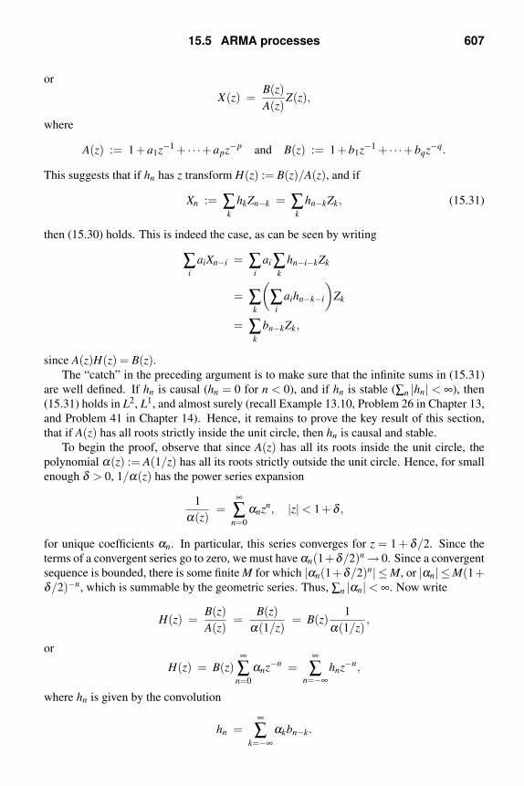
15.5 ARMA processes 607
or
X(z) =B(z)
A(z)Z(z),
where
A(z) := 1+a1z−1 + · · ·+apz−p and B(z) := 1+b1z−1 + · · ·+bqz−q.
This suggests that if hn has z transform H(z) := B(z)/A(z), and if
Xn := ∑k
hkZn−k = ∑k
hn−kZk, (15.31)
then (15.30) holds. This is indeed the case, as can be seen by writing
∑i
aiXn−i = ∑i
ai ∑k
hn−i−kZk
= ∑k
(∑
i
aihn−k−i
)Zk
= ∑k
bn−kZk,
since A(z)H(z) = B(z).The “catch” in the preceding argument is to make sure that the infinite sums in (15.31)
are well defined. If hn is causal (hn = 0 for n < 0), and if hn is stable (∑n |hn| < ∞), then
(15.31) holds in L2, L1, and almost surely (recall Example 13.10, Problem 26 in Chapter 13,
and Problem 41 in Chapter 14). Hence, it remains to prove the key result of this section,
that if A(z) has all roots strictly inside the unit circle, then hn is causal and stable.
To begin the proof, observe that since A(z) has all its roots inside the unit circle, the
polynomial α(z) := A(1/z) has all its roots strictly outside the unit circle. Hence, for small
enough δ > 0, 1/α(z) has the power series expansion
1
α(z)=
∞
∑n=0
αnzn, |z| < 1+δ ,
for unique coefficients αn. In particular, this series converges for z = 1 + δ/2. Since the
terms of a convergent series go to zero, we must have αn(1+δ/2)n → 0. Since a convergent
sequence is bounded, there is some finite M for which |αn(1+δ/2)n| ≤ M, or |αn| ≤ M(1+δ/2)−n, which is summable by the geometric series. Thus, ∑n |αn| < ∞. Now write
H(z) =B(z)
A(z)=
B(z)
α(1/z)= B(z)
1
α(1/z),
or
H(z) = B(z)∞
∑n=0
αnz−n =∞
∑n=−∞
hnz−n,
where hn is given by the convolution
hn =∞
∑k=−∞
αkbn−k.

608 Self similarity and long-range dependence
Since αn and bn are causal, so is their convolution hn. Furthermore, for n ≥ 0,
hn =n
∑k=max(0,n−q)
αkbn−k. (15.32)
In Problem 18, you are asked to show that ∑n |hn| < ∞. In Problem 19, you are asked to
show that (15.31) is the unique solution of (15.30).
15.6 ARIMA processes
Before defining ARIMA processes, we introduce the differencing filter, whose z trans-
form is 1− z−1. If the input to this filter is Xn, then the output is Xn −Xn−1.
A process Xn is said to be an autoregressive integrated moving average (ARIMA)
process if instead of A(z)X(z) = B(z)Z(z), we have
A(z)(1− z−1)dX(z) = B(z)Z(z), (15.33)
where A(z) and B(z) are defined as in the previous section. In this case, we say that
Xn is an ARIMA(p,d,q) process. If we let A(z) = A(z)(1 − z−1)d , it would seem that
ARIMA(p,d,q) is just a fancy name for ARMA(p + d,q). While this is true when d is a
nonnegative integer, there are two problems. First, recall that the results of the previous
section assume A(z) has all roots strictly inside the unit circle, while A(z) has a root at z = 1
repeated d times. The second problem is that we will be focusing on fractional values of d,
in which case A(1/z) is no longer a polynomial, but an infinite power series in z.
Let us rewrite (15.33) as
X(z) = (1− z−1)−d B(z)
A(z)Z(z) = H(z)Gd(z)Z(z),
where H(z) := B(z)/A(z) as in the previous section, and
Gd(z) := (1− z−1)−d .
From the calculations following Example 15.2,i
Gd(z) =∞
∑n=0
gnz−n,
where g0 = 1, and for n ≥ 1,
gn =d(d +1) · · ·(d +[n−1])
n!.
The plan then is to set
Yn :=∞
∑k=0
gkZn−k (15.34)
iSince 1− z−1 is a differencing filter, (1− z−1)−1 is a summing or integrating filter. For noninteger values of
d, (1− z−1)−d is called a fractional integrating filter. The corresponding process is sometimes called a fractional
ARIMA process (FARIMA).

15.6 ARIMA processes 609
and then j
Xn :=∞
∑k=0
hkYn−k. (15.35)
Note that the power spectral density of Yn isk
SY ( f ) = |Gd(ej2π f )|2σ2 = |1− e− j2π f |−2dσ2 = [4sin2(π f )]−dσ2,
using the result of Example 15.2. If p = q = 0, then A(z) = B(z) = H(z) = 1, Xn = Yn, and
we see that the process of Example 15.2 is ARIMA(0,d,0).Now, the problem with the above plan is that we have to make sure that Yn is well
defined. To analyze the situation, we need to know how fast the gn decay. To this end,
observe that
Γ(d +n) = (d +[n−1])Γ(d +[n−1])
...
= (d +[n−1]) · · ·(d +1)Γ(d +1).
Hence,
gn =d ·Γ(d +n)
Γ(d +1)Γ(n+1).
Now apply Stirling’s formula,l
Γ(x) ∼√
2πxx−1/2e−x,
to the gamma functions that involve n. This yields
gn ∼ de1−d
Γ(d +1)
(1+
d −1
n+1
)n+1/2
(n+d)d−1.
Since (1+
d −1
n+1
)n+1/2
=(
1+d −1
n+1
)n+1(1+
d −1
n+1
)−1/2
→ ed−1,
and since (n+d)d−1 ∼ nd−1, we see that
gn ∼ d
Γ(d +1)nd−1
as in Hosking [31, Theorem 1(a)]. For 0 < d < 1/2, −1 < d−1 <−1/2, and we see that the
gn are not absolutely summable. However, since −2 < 2d −2 < −1, they are square sum-
mable. Hence, Yn is well defined as a limit in mean square by Problem 25 in Chapter 13.
The sum defining Xn is well defined in L2, L1, and almost surely by Example 13.10, Prob-
lem 26 in Chapter 13, and Problem 41 in Chapter 14. Since Xn is the result of filtering the
long-range dependent process Yn with the stable impulse response hn, Xn is still long-range
dependent as pointed out in Section 15.4.
jRecall that hn is given by (15.32).kSee Problem 31 in Chapter 10 or Example 13.26.lWe derived Stirling’s formula for Γ(n) = (n−1)! in Example 5.18. A proof for noninteger x can be found in
[5, pp. 300–301].

610 Self similarity and long-range dependence
Problems
15.1: Self similarity in continuous time
1. Show that for a self-similar process, Wt converges in distribution to the zero random
variable as t → 0. Next, identify X(ω) := limt→∞ tHW1(ω) as a function of ω , and
find the probability mass function of the limit in terms of FW1(x).
2. Use joint characteristic functions to show that the Wiener process is self similar with
Hurst parameter H = 1/2.
3. Use joint characteristic functions to show that the Wiener process has stationary in-
crements.
4. Show that for H = 1/2,
BH(t)−BH(s) =
∫ t
sdWτ = Wt −Ws.
Taking t > s = 0 shows that BH(t) =Wt , while taking s < t = 0 shows that BH(s) =Ws.
Thus, B1/2(t) = Wt for all t.
5. Show that for 0 < H < 1,∫ ∞
0
[(1+θ)H−1/2 −θ H−1/2
]2dθ < ∞.
15.2: Self similarity in discrete time
6. Let Xn be a second-order self-similar process with mean µ = E[Xn], variance σ2 =E[(Xn −µ)2], and Hurst parameter H. Then the sample mean
Mn :=1
n
n
∑i=1
Xi
has expectation µ and, by (15.7), variance σ2/n2−2H . If Xn is a Gaussian sequence,
Mn −µσ/n1−H
∼ N(0,1),
and so given a confidence level 1−α , we can choose y (e.g., by Table 6.2) such that
P
(∣∣∣ Mn −µσ/n1−H
∣∣∣≤ y)
= 1−α.
For 1/2 < H < 1, show that the width of the corresponding confidence interval is
wider by a factor of nH−1/2 than the confidence interval obtained if the Xn had been
independent as in Section 6.3.
7. Use (15.10) and induction on n to show that (15.6) implies E[Y 2n ] = σ2n2H for n ≥ 1.
8. Suppose that Xk is wide-sense stationary.
(a) Show that the process X(m)ν defined in (15.13) is also wide-sense stationary.
(b) If Xk is second-order self similar, prove (15.12) for the case n = 0.

Problems 611
15.3: Asymptotic second-order self similarity
9. Show that asymptotic second-order self similarity (15.20) implies (15.19). Hint: Ob-
serve that C(n)(0) = E[(X(n)1 −µ)2].
10. Show that (15.19) implies asymptotic second-order self similarity (15.20). Hint: Use
(15.14), and note that (15.19) is equivalent to E[Y 2n ]/n2H → σ2
∞.
11. Show that a process is asymptotically second-order self similar; i.e., (15.20) holds, if
and only if the conditions
limm→∞
ρ(m)(n) =1
2[|n+1|2H −2|n|2H + |n−1|2H ],
and
limm→∞
C(m)(0)
m2H−2= σ2
∞
both hold.
12. Show that the covariance function corresponding to the power spectral density of
Example 15.2 is
C(n) =(−1)nΓ(1−2d)
Γ(n+1−d)Γ(1−d−n).
This result is due to Hosking [31, Theorem 1(d)]. Hints: First show that
C(n) =1
π
∫ π
0[4sin2(ν/2)]−d cos(nν)dν .
Second, use the change of variable θ = 2π −ν to show that
1
π
∫ 2π
π[4sin2(ν/2)]−d cos(nν)dν = C(n).
Third, use the formula [21, p. 372]∫ π
0sinp−1(t)cos(at)dt =
π cos(aπ/2)Γ(p+1)21−p
pΓ( p+a+1
2
)Γ( p−a+1
2
) .
13. Show that for 0 < α < 1,∫ ∞
0θ α−3 sin2 θ dθ =
21−α cos(απ/2)Γ(α)
(1−α)(2−α).
Remark. The formula actually holds for complex α with 0 < Reα < 2 [21, p. 447].
The formula is used to obtain (15.22) [24, Appendix B].
Hints: (i) Fix 0 < ε < r < ∞, and apply integration by parts to∫ r
εθ α−3 sin2 θ dθ

612 Self similarity and long-range dependence
with u = sin2 θ and dv = θ α−3 dθ .
(ii) Apply integration by parts to the integral∫tα−2 sin t dt
with u = sin t and dv = tα−2dt.
(iii) Use the fact that for 0 < α < 1,m
limr→∞ε→0
∫ r
εtα−1e− jt dt = e− jαπ/2Γ(α).
14. Let S( f ) be given by (15.15). For 1/2 < H < 1, put α = 2−2H.
(a) Evaluate the limit in (15.21). Hint: You may use the fact that
Q( f ) :=∞
∑i=1
1
|i+ f |2H+1
converges uniformly for | f | ≤ 1/2 and is therefore a continuous and bounded
function on [−1/2,1/2].
(b) Evaluate ∫ 1/2
−1/2S( f )d f .
Hint: The above integral is equal to C(0) = σ2. Since (15.15) corresponds
to a second-order self-similar process, not just an asymptotically second-order
self-similar process, σ2 = σ2∞. Now apply (15.22).
15.4: Long-range dependence
15. Show directly that if a wide-sense stationary sequence has the covariance function
C(n) given in Problem 12, then the process is long-range dependent; i.e., (15.23)
holds with appropriate values of α and c [31, Theorem 1(d)]. Hints: Use the Remark
following Problem 14 in Chapter 4, Stirling’s formula,
Γ(x) ∼√
2πxx−1/2e−x,
and the formula (1+d/n)n → ed .
mFor s > 0, a change of variable shows that
limr→∞ε→0
∫ r
εtα−1e−st dt =
Γ(α)
sα .
As in Notes 7 and 8 in Chapter 4, a permanence of form argument allows us to set s = j = e jπ/2.

Exam preparation 613
16. For 0 < α < 1, show that
limn→∞
n−1
∑ν=k
ν−α
n1−α =1
1−α.
Hints: Rewrite (15.28) in the form
Bn +n−α − k−α ≤ In ≤ Bn.
Then
1 ≤ Bn
In
≤ 1+k−α −n−α
In
.
Show that In/n1−α → 1/(1−α), and note that this implies In/n−α → ∞.
17. For 0 < α < 1, show that
limn→∞
n−1
∑ν=k
ν1−α
n2−α =1
2−α.
15.5: ARMA processes
18. Use the bound |αn| ≤ M(1+δ/2)−n to show that ∑n |hn| < ∞, where
hn =n
∑k=max(0,n−q)
αkbn−k, n ≥ 0,
and hn = 0 for n < 0.
19. Assume (15.30) holds and that A(z) has all roots strictly inside the unit circle. Show
that (15.31) must hold. Hint: Compute the convolution
∑n
αm−nYn
first for Yn replaced by the left-hand side of (15.30) and again for Yn replaced by the
right-hand side of (15.30).
20. Let ∑∞k=0 |hk|< ∞. Show that if Xn is WSS, then Yn = ∑∞
k=0 hkXn−k and Xn are J-WSS.
Be sure to justify the interchange of any expectations and infinite sums.
Exam preparation
You may use the following suggestions to prepare a study sheet, including formulas men-
tioned that you have trouble remembering. You may also want to ask your instructor for
additional suggestions.

614 Self similarity and long-range dependence
15.1. Self similarity in continuous time. Know the definition and some of the impli-
cations of self similarity. If the process also has stationary increments and H = 1,
then it is zero mean and its covariance function is given by (15.4). If an H-sssi
process is Gaussian with finite second moments, then the process can be represented
by fractional Brownian motion.
15.2. Self similarity in discrete time. This notion is obtained by sampling a continuous-
time H-sssi process on the integers. More generally, a discrete-time WSS process
whose covariance function has the form (15.6) is said to be second-order self similar.
It is important to know that (15.6) holds if and only if (15.7) holds. Know what the
aggregated process is. Know the relationship between formulas (15.12) and (15.17).
The power spectral density of a second-order self-similar process is proportional to
(15.15).
15.3. Asymptotic second-order self similarity. A process is asymptotically second-
order self similar if instead of (15.12), we have only (15.20) Know that (15.20) holds
if and only if (15.19) holds. The theorem containing (15.21) gives sufficient condi-
tions on the power spectral density to guarantee that the process is asymptotically
second-order self similar.
15.4. Long-range dependence. In the time-domain, if a process is long-range dependent
as in (15.23), then the process is asymptotically second-order self similar.
15.5. ARMA processes. An ARMA process Xn satisfying (15.29) exists and is given by
(15.31) if the impulse response hn is causal and stable. Under these conditions, the
sum in (15.31) converges in L2, L1, and almost surely. If A(z) has all roots strictly
inside the unit circle, then hn is causal and stable.
15.6. ARIMA processes. An ARIMA process determined by (15.33) with 0 < d < 1/2
exists and is given by (15.34) and (15.35). The sum in (15.34) converges in mean
square, and the sum in (15.35) converges in L2, L1, and almost surely.
Work any review problems assigned by your instructor. If you finish them, re-work your
homework assignments.

Bibliography
[1] Abramowitz M. and I. A. Stegun, eds. Handbook of Mathematical Functions, with Formulas, Graphs, and
Mathematical Tables. New York: Dover, 1970.
[2] Beran J. Statistics for Long-Memory Processes. New York: Chapman & Hall, 1994.
[3] Billingsley P. Probability and Measure, 3rd ed. New York: Wiley, 1995.
[4] Brockwell P. J. and R. A. Davis. Time Series: Theory and Methods. New York: Springer-Verlag, 1987.
[5] Buck R. C. Advanced Calculus, 3rd ed. New York: McGraw-Hill, 1978.
[6] Chernoff H. “A measure of asymptotic efficiency for tests of a hypothesis based on the sum of observations,”
Ann. Math. Statist., 23, 493–507, 1952.
[7] Chow Y. S. and H. Teicher. Probability Theory: Independence, Interchangeability, Martingales, 2nd ed.
New York: Springer, 1988.
[8] Chung K. L. Markov Chains with Stationary Transition Probabilities, 2nd ed. Berlin: Springer, 1967.
[9] Churchill R. V., J. W. Brown and R. F. Verhey. Complex Variables and Applications, 3rd ed. New York:
McGraw-Hill, 1976.
[10] Craig J. W. “A new, simple and exact result for calculating the probability of error for two-dimensional signal
constellations,” in Proc. IEEE Milit. Commun. Conf. MILCOM ’91, McLean, VA, Oct. 1991, pp. 571–5.
[11] Cramer H. “Sur un nouveaux theoreme-limite de la theorie des probabilites,” Actualites Scientifiques et
Industrielles 736, pp. 5–23. Colloque consacre a la theorie des probabilites, Vol. 3. Paris: Hermann,
Oct. 1937.
[12] Cramer H. Mathematical Methods of Statistics. Princeton: Princeton University Press, 1946.
[13] Crovella M. and A. Bestavros. “Self-similarity in World Wide Web traffic: Evidence and possible causes,”
Perf. Eval. Rev., 24, 160–9, 1996.
[14] Davis M. H. A. Linear Estimation and Stochastic Control. London: Chapman and Hall, 1977.
[15] Devroye L. Non-Uniform Random Variate Generation. New York: Springer, 1986.
[16] Feller W. An Introduction to Probability Theory and its Applications, Vol. 1, 3rd ed. New York: Wiley,
1968.
[17] Fine T. L. Probability and Probabilistic Reasoning for Electrical Engineering. Upper Saddle River, NJ:
Pearson, 2006.
[18] Gersho A. and R. M. Gray. Vector Quantization and Signal Compression. Boston: Kluwer, 1992.
[19] Gohberg I. and S. Goldberg. Basic Operator Theory. Boston: Birkhauser, 1980.
[20] Gonick L. and W. Smith. The Cartoon Guide to Statistics. New York: HarperPerennial, 1993.
[21] Gradshteyn I. S. and I. M. Ryzhik. Table of Integrals, Series, and Products. Orlando, FL: Academic Press,
1980.
[22] Gray R. M. and L. D. Davisson. Introduction to Statistical Signal Processing. Cambridge, UK: Cambridge
University Press, 2005.
[23] Grimmett G. R. and D. R. Stirzaker. Probability and Random Processes, 3rd ed. Oxford, UK: Oxford Uni-
versity Press, 2001.
[24] Gubner J. A. “Theorems and fallacies in the theory of long-range-dependent processes,” IEEE Trans. Inform.
Theory, 51 (3), 1234–9, 2005.
[25] Haykin S. and B. Van Veen. Signals and Systems, 2nd ed. New York: Wiley, 2003.
[26] Heidelberger P. “Fast simulation of rare events in queuing and reliability models,” ACM Trans. Modeling
615

616 Bibliography
Comput. Simul., 5 (1), 43–85, 1995.
[27] Helstrom C. W. Statistical Theory of Signal Detection, 2nd ed. Oxford, UK: Pergamon, 1968.
[28] Helstrom C. W. Probability and Stochastic Processes for Engineers, 2nd ed. New York: Macmillan, 1991.
[29] Hoel P. G., S. C. Port and C. J. Stone. Introduction to Probability Theory. Boston: Houghton Mifflin, 1971.
[30] Hoffman K. and R. Kunze. Linear Algebra, 2nd ed. Englewood Cliffs, NJ: Prentice-Hall, 1971.
[31] Hosking J. R. M. “Fractional differencing,” Biometrika, 68 (1), 165–76, 1981.
[32] Karlin S. and H. M. Taylor. A First Course in Stochastic Processes, 2nd ed. New York: Academic Press,
1975.
[33] Karlin S. and H. M. Taylor. A Second Course in Stochastic Processes. New York: Academic Press, 1981.
[34] Kingman J. F. C. Poisson Processes. Oxford, U.K.: Clarendon, 1993.
[35] Leland W. E., M. S. Taqqu, W. Willinger and D. V. Wilson. “On the self-similar nature of Ethernet traffic
(extended version),” IEEE/ACM Trans. Networking, 2 (1), 1–15, 1994.
[36] Leon-Garcia A. Probability and Random Processes for Electrical Engineering, 2nd ed. Reading, MA:
Addison-Wesley, 1994.
[37] Likhanov N. “Bounds on the buffer occupancy probability with self-similar traffic,” pp. 193–213, in Self-
Similar Network Traffic and Performance Evaluation, Eds. K. Park and W. Willinger. New York: Wiley,
2000.
[38] O’Hagen A. Probability: Methods and Measurement. London: Chapman and Hall, 1988.
[39] Oppenheim A. V. and A. S. Willsky, with S. H. Nawab. Signals & Systems, 2nd ed. Upper Saddle River, NJ:
Prentice Hall, 1997.
[40] Papoulis A. and S. U. Pillai. Probability, Random Variables, and Stochastic Processes, 4th ed. New York:
McGraw-Hill, 2002.
[41] Park K. and W. Willinger. “Self-similar network traffic: An overview,” pp. 1–38, in Self-Similar Network
Traffic and Performance Evaluation, Eds. K. Park and W. Willinger. New York: Wiley, 2000.
[42] Parzen E. Stochastic Processes. San Francisco: Holden-Day, 1962.
[43] Paxson V. and S. Floyd. “Wide-area traffic: The failure of Poisson modeling,” IEEE/ACM Trans. Network-
ing, 3, 226–44, 1995.
[44] Picinbono B. Random Signals and Systems. Englewood Cliffs, NJ: Prentice Hall, 1993.
[45] Ripley B. D. Stochastic Simulation. New York: Wiley, 1987.
[46] Ross S. M. A First Course in Probability, 6th ed. Upper Saddle River, NJ: Prentice-Hall, 2002.
[47] Ross S. M. Simulation, 3rd ed. San Diego: Academic Press, 2002.
[48] Rothenberg R. I. Probability and Statistics. San Diego: Harcourt Brace Jovanovich, 1991.
[49] Roussas G. A First Course in Mathematical Statistics. Reading, MA: Addison-Wesley, 1973.
[50] Royden H. L. Real Analysis, 2nd ed. New York: MacMillan, 1968.
[51] Rudin W. Principles of Mathematical Analysis, 3rd ed. New York: McGraw-Hill, 1976.
[52] Samorodnitsky G. and M. S. Taqqu. Stable non-Gaussian Random Processes: Stochastic Models with Infi-
nite Variance. New York: Chapman & Hall, 1994.
[53] Shiryayev A. N. Probability. New York: Springer, 1984.
[54] Simon M. K. “A new twist on the Marcum Q function and its application,” IEEE Commun. Lett., 2 (2),
39–41, 1998.
[55] Simon M. K. and D. Divsalar. “Some new twists to problems involving the Gaussian probability integral,”
IEEE Trans. Commun., 46 (2), 200–10, 1998.
[56] Simon M. K. and M.-S. Alouini. “A unified approach to the performance analysis of digital communication
over generalized fading channels,” Proc. IEEE, 86 (9), 1860–77, 1998.

Bibliography 617
[57] Sinai Ya. G. “Self-similar probability distributions,” Theory of Probability and its Applications, XXI (1),
64–80, 1976.
[58] Smith P. J., M. Shafi and H. Gao. “Quick simulation: A review of importance sampling techniques in
communication systems,” IEEE J. Select. Areas Commun., 15 (4), 597–613, 1997.
[59] Snell J. L. Introduction to Probability. New York: Random House, 1988.
[60] Stacy E. W. “A generalization of the gamma distribution,” Ann. Math. Stat., 33 (3), 1187–92, 1962.
[61] Stark H. and J. W. Woods. Probability and Random Processes with Applications to Signal Processing, 3rd
ed. Upper Saddle River, NJ: Prentice Hall, 2002.
[62] Stein E. M. and R. Shakarchi. Fourier Analysis: An Introduction (Princeton Lectures in Analysis I). Prince-
ton, NJ: Princeton University Press, 2003.
[63] Student. “The probable error of a mean,” Biometrika, VI (1), 1–25, 1908.
[64] Tsybakov B. and N. D. Georganas. “Self-similar processes in communication networks,” IEEE Trans. In-
form. Theory, 44 (5), 1713–25, 1998.
[65] Verdu S. Multiuser Detection. Cambridge, UK: Cambridge University Press, 1998.
[66] Viniotis Y. Probability and Random Processes for Electrical Engineers. New York: McGraw-Hill, 1998.
[67] Wong E. and B. Hajek. Stochastic Processes in Engineering Systems. New York: Springer, 1985.
[68] Yates R. D. and D. J. Goodman. Probability and Stochastic Processes: A Friendly Introduction for Electrical
and Computer Engineers, 2nd ed. New York: Wiley, 2005.
[69] Youla D. C. “The use of the method of maximum likelihood in estimating continuous-modulated intelligence
which has been corrupted by noise,” Trans. IRE Prof. Group on Inform. Theory, PGIT-3, 90–106, 1954.
[70] Ziemer R. Z. Elements of Engineering Probability and Statistics. Upper Saddle River, NJ: Prentice Hall,
1997.

Index
AAbel’s theorem, 130
absolutely continuous random variables, 221, 318
absorbing state, 482
acceptance region, 264
accessible state, 499
affine function, 186, 344
aggregated process, 598
almost-sure convergence, 572
almost-sure event, 23
alternative hypothesis, 263
analog-to-digital converter, 150
Anderson–Darling test, 248
angle
of a point in the plane, 354
AR process, see autoregressive process
arcsine random variable, 233, 302, 538
relation to beta, 233
ARIMA, see autoregressive integrated moving av-
erage process
ARMA process, see autoregressive moving average
process
arrival times, 446
associative laws, 10
asymptotic second-order self similarity, 602, 611
asymptotically unbiased estimator, 243
atomic weight, 115
auto-correlation function, 392
autoregressive integrated moving average, 608
autoregressive integrated moving average process,
602
fractional, 608
autoregressive moving average process, 606
autoregressive process, 606
Avogadro’s number, 115
BBanach space, 524
bandlimited white noise, 406
bandwidth, 408
Bayes’ rule, 28, 29
Bernoulli random variable, 71
mean, 81
second moment and variance, 86
simulation, 196
Bernoulli trials, 3
Bernoulli, Jacob, 117
Bessel function, 227
properties, 229
beta function, 175, 176
beta random variable, 175
relation to arcsine random variable, 233
relation to gamma and chi-squared, 325
betting on fair games, 104
biased estimator, 243
binary symmetric channel, 58
binomial approximation
by normal, 213
by Poisson, 115, 584
binomial coefficient, 38, 114
binomial random variable, 113
mean, variance, and pgf, 133
simulation, 197
binomial theorem, 38, 113, 133, 603
birth process, see Markov chain
birth–death process, see Markov chain
birthday problem, 36
bivariate characteristic function, 301
bivariate Gaussian random variables, 309
block matrices, 332
Borel–Cantelli lemma
first, 54, 575
second, 60
Borel set, 56, 96
Borel sets of IR2, 317
Borel σ -field, 56, 96
Brown, Robert, 387
Brownian motion, 387
fractional, see fractional Brownian motion
ordinary, see Wiener process
CCampbell’s theorem, 452
Cantor set, 55
cardinality, 15, 18
Cartesian product, 289
Cauchy random variable, 144
as quotient of Gaussians, 323
as tangent of uniform, 194
cdf, 186
characteristic function, 180
nonexistence of mean, 154
simulation, 194
special case of Student’s t, 176
Cauchy–Schwarz inequality
for column vectors, 331, 355
for random variables, 92, 524
for time functions, 429
Cauchy sequence
of Lp random variables, 524
of real numbers, 524
causal Wiener filter, 419
prediction, 439
smoothing, 439
618

Index 619
cdf, see cumulative distribution function
central chi-squared random variable, see chi-squared
random variable
central limit theorem, 6, 185, 208, 252, 458, 570
compared with weak law of large numbers, 571
central moment, 86
certain event, 23
chain rule, 190
of calculus, 319
of conditional probability, 58, 510
change of variable (multivariate), 341
Chapman–Kolmogorov equation
continuous time, 503
derivation via smoothing property, 544
discrete time, 484
for Markov processes, 515
characteristic function
bivariate, 301
compared with pgf and mgf, 161
multivariate (joint), 337
univariate, 159
Chebyshev inequality, 89, 164, 165, 182
used to derive the weak law, 116
Chernoff bound, 164, 165, 182
Chevalier de Mere, 3
chi-squared random variable, 148, 174
as squared zero-mean Gaussian, 179, 192, 222
cdf – special case of gamma, 225
characteristic function, 179
moment generating function, 179
parameter estimation, 276
relation to F random variable, 325
relation to beta random variable, 325
relation to generalized gamma, 224
see also noncentral chi-squared, 180
simulation, 276
square root of = Rayleigh, 223
chi-squared test, 248
circularly symmetric complex Gaussian, 373
closed set, 535
CLT, see central limit theorem
co-domain of a function, 13
combinatorics, 34
communicating states, 499
commutative laws, 10
complement of a set, 8
complementary cdf
Gaussian, 187, 225
complementary error function, 219
complete orthonormal set, 530
completeness
of the Lp spaces, 524
of the real numbers, 524
complex conjugate, 371
complex Gaussian random vector, 372
complex random variable, 371
complex random vector, 372
conditional cdf, 192, 303
conditional density, 192, 303
conditional expectation
abstract definition, 538
for discrete random variables, 127
for jointly continuous random variables, 302
linearity, 542
smoothing property, 544, 557
conditional independence, 60, 476
conditional probability, 27
for jointly continuous random variables, 303
conditional probability mass functions, 118
confidence interval, 250
confidence level, 250
conservative Markov chain, 504, 508
consistency condition
continuous-time processes, 464
discrete-time processes, 461
continuity in mean of order p, 521
continuous random variable, 139
arcsine, 233
beta, 175
Cauchy, 144
chi-squared, 174
Erlang, 174
exponential, 141
F , 325
gamma, 173
Gaussian = normal, 145
generalized gamma, 224
Laplace, 143
lognormal, 190
Maxwell, 222
multivariate Gaussian, 363
Nakagami, 224
noncentral chi-squared, 182
noncentral Rayleigh, 227
Pareto, 237
Rayleigh, 177
Rice, 227
Student’s t, 176
uniform, 140
Weibull, 171
continuous sample paths, 455
convergence
almost-sure (a.s.), 572
in distribution, 566
in mean of order p, 518
in mean square, 518
in probability, 564
in quadratic mean, 518
of real numbers, 573
sure, 573
weak, 566
convex function, 105
convolution
of densities, 163
of probability mass functions, 125
correlation, 91

620 Index
correlation coefficient, 92, 104, 311
correlation function, 392
engineering definition, 601
of a deterministic signal, 411
of a random process, 389
properties, 391
statistics/networking definition, 601
unbiased estimator of, 397
univariate, for WSS processes, 395
correlation matrix, 334
countable additivity, 23
countable set, 15, 462
countable subadditivity, 26
countably infinite set, 15
counting process, 443
covariance, 94
distinction between scalar and matrix, 335
function, 392
matrix, 335
covering of intervals, 221
Craig’s formula, 322
critical region, 264
critical value, 249, 264
cross power spectral density, 406
cross-correlation
function, 392
univariate, for WSS processes, 402
matrix, 337
cross-covariance
function, 392
matrix, 336
crossover probabilities, 58, 121
cumulative distribution function (cdf), 184
continuous random variable, 185
discrete random variable, 194
joint, 291
multivariate, 351
properties, 205
curve fitting, see regression
cyclostationary process, 425
DdB, see decibel
de Moivre, Abraham, 208
de Moivre–Laplace theorem, 255
De Morgan’s laws, 10
generalized, 12
decibel, 188, 437
decorrelating transformation, 338
applied to a Gaussian vector, 366
delta function, 406
Dirac, 199, 406
Kronecker, 397, 483
diagonal argument, 17
difference of sets, 9
differencing filter, 608
differential entropy, 178
Dirac delta function, 199
discrete random variable, 66
Bernoulli, 71
binomial, 113
geometric, 74
hypergeometric, 256
negative binomial = Pascal, 133
Poisson, 69
uniform, 68
zeta = Zipf, 105
discrete-time Fourier transform, 400
disjoint sets, 9
distribution, 97
distributive laws, 10
generalized, 12
domain of a function, 13
dominated convergence theorem, 424, 508, 549
Doob decomposition, 559
dot product, see inner product
double factorial, 153
double-sided exponential = Laplace, 143
Eeigenvalue, 485, 528
eigenvector, 485
ellipsoids, 368
embedded chain, 504
empty set, 8
energy spectral density, 412
ensemble mean, 241
ensemble variance, 241
entropy, 105
differential, 178
equilibrium distribution, 485
equivalence classes, 500, 513
equivalence relation, 500
ergodic theorem, 397
for Markov chains, 495
mean-square
for WSS processes, 424
for WSS sequences, 519
Erlang random variable, 148, 174
as nth arrival time of Poisson process, 446
as sum of i.i.d. exponentials, 181
cdf – special case of gamma, 225
cumulative distribution function, 174
moment generating function, 179
relation to generalized gamma, 224
simulation, 277
error function, 188, 219
complementary, 219
estimation of nonrandom parameters
covariance matrices, 348
estimation of random vectors
linear MMSE, 344
maximum likelihood (ML), 350
MMSE, 350
estimator
asymptotically unbiased, 243

Index 621
biased, 243
unbiased, 241
event, 7, 43, 580
expectation
additive operator, 84
homogeneous operator, 83
linearity for arbitrary random variables, 163
linearity for discrete random variables, 84
monotonicity for arbitrary random variables, 163
monotonicity for discrete random variables, 106
of a discrete random variable, 80
of an arbitrary random variable, 155
when it is undefined, 82, 154
expected average power, 404
and the Wiener–Khinchin theorem, 421
expected instantaneous power, 404
exponential random variable, 141
difference of = Laplace, 180
double sided, see Laplace random variable
memoryless property, 171
moment generating function, 158
moments, 158
relation to generalized gamma, 224
FF random variable, 325
relation to chi-squared, 325
factorial
double, 153
factorial function, 173
factorial moment, 111
factorization property, 109
fading
channel, 223
Rayleigh, 324
failure rate, 216
constant, 218
Erlang, 237
Pareto, 237
Weibull, 237
FARIMA, see fractional ARIMA
filtered Poisson process, 451
first entrance time, 488
first passage time, 488
Fourier series, 400
as characteristic function, 161
Fourier transform, 398
as bivariate characteristic function, 301
as multivariate characteristic function, 337
as univariate characteristic function, 160
discrete time, 400, 432
inversion formula, 398
fractional ARIMA process, 608
fractional Brownian motion, 594
fractional Gaussian noise, 596
fractional integrating filter, 608
function
co-domain, 13
definition, 13
domain, 13
inverse image, 14
invertible, 14
one-to-one, 14
onto, 14
probability measure as a function, 23
range, 13
Ggambler’s ruin, 482
gamma function, 79, 148, 173
incomplete, 225
gamma random variable, 147, 173
cdf, 225
characteristic function, 160, 179, 180
generalized, 224, 325
moment generating function, 179
moments, 177
parameter estimation, 276, 277
relation to beta random variable, 325
with scale parameter, 174
Gaussian pulse, 160
Gaussian random process, 464
fractional, 595
Karhunen–Loeve expansion, 584
Gaussian random variable, 145
ccdf
approximation, 225
Craig’s formula, 322
definition, 187
table, 189
cdf, 187
related to error function, 219
table, 189
characteristic function, 160, 180
complex, 372
complex circularly symmetric, 373
moment generating function, 157, 159
moments, 152
quotient of = Cauchy, 323
simulation, 194, 278
Gaussian random vector, 363
characteristic function, 365
complex circularly symmetric, 373
joint density, 367
multivariate moments, Wick’s theorem, 377
proper, 373
simulation, 368
generalized density, 199
generalized gamma random variable, 224, 325
relation to Rayleigh, Maxwell, Weibull, 224
generator matrix, 506
geometric random variable, 74
mean, variance, and pgf, 132
memoryless property, 101
geometric series, 52
goodness-of-fit tests, 248

622 Index
greatest common divisor, 500
HH-sssi, 593
Herglotz’s theorem, 545
Hilbert space, 524
histogram, 244
Holder’s inequality, 550
holding time, 504, 514
Hurst parameter, 591
hypergeometric random variable, 256
derivation, 274
hypothesis, 248
hypothesis testing, 262, 263
Ii.i.d., see independent identically distributed
i.o., see infinitely often
ideal gas, 224
identically distributed random variables, 72
importance sampling, 272
impossible event, 22
impulse function, 199
impulse response, 390
impulsive, 199
inclusion–exclusion formula, 24
incomplete gamma function, 225
increment process, 593
increments, 390
increments of a random process, 444
independent events
more than two events, 32
pairwise, 32, 46
two events, 30
independent identically distributed (i.i.d.), 72
independent increments, 444
independent random variables, 71
cdf characterization, 295
ch. fcn. characterization, 302, 338
jointly continuous, 300
multiple, 72
pdf characterization, 301
pmf characterization, 76
uncorrelated does not imply independent, 104, 322,
327
indicator function, 87
infinitely often (i.o.), 492
inner product
of column vectors, 331
of matrices, 355
of random variables, 524
inner-product space, 524
integrating filter, 608
integration by parts formula, 168
intensity of a Poisson process, 444
interarrival times, 446
intersection of sets, 9
intervisit times, 490
inverse image, 14
inverse tangent
principal, 354
irreducible Markov chain, 488, 499
Ito correction term, 457
Ito integral, 457
Ito rule, 457
JJ-WSS, see jointly wide-sense stationary
Jacobian, 341
formulas, 341
Jensen’s inequality, 105
joint characteristic function, 337
joint cumulative distribution function, 291
joint density, 295
joint probability mass function, 75
joint wide-sense stationarity, 402
for discrete-time processes, 434
jointly continuous random variables
bivariate, 295
jointly Gaussian random variables, 363
jointly normal random variables, 363
jump chain, 504
jump times
of a Poisson process, 445
KKarhunen–Loeve expansion, 527
finite-dimensional, 338
Gaussian process, 584
Ornstein–Uhlenbeck process, 554
signal detection, 530
white noise, 531
Wiener process, 531
Kolmogorov
and axiomatic theory of probability, 5, 517
backward equation, 506
characterization of random processes, 388
consistency/extension theorem, 462
forward equation, 505
Kolmogorov–Smirnov test, 248
Kronecker delta, 397, 483
Kronecker product, 103, 447
kurtosis, 86
LLaplace random variable, 143
as difference of exponentials, 180
parameter estimation, 277
quotient of, 324
simulation, 277
variance and moment generating function, 179
Laplace transform, 158
Laplace, Pierre-Simon, 208
law of large numbers
convergence rates, 596

Index 623
mean square, for second-order self-similar sequences,
596
mean square, uncorrelated, 519
mean square, WSS sequences, 519
strong, 273, 576
weak, for independent random variables, 576
weak, for uncorrelated random variables, 116, 565
law of the unconscious statistician, 83, 149
law of total probability, 27, 29
discrete conditioned on continuous, 472
for conditional expectation, 544
for conditional probability, 503, 515, 544
for continuous random variables, 304
for expectation (continuous random variables), 308,
315
for expectation (discrete random variables), 129
unified formula, 540
Lebesgue
dominated convergence theorem, 424, 549
measure, 45, 57
monotone convergence theorem, 169, 549
Leibniz’ rule, 191, 307
derivation, 318
level curves, 310
level sets, 368
likelihood, 127, 192
likelihood ratio
continuous random variables, 193
discrete random variables, 127
martingale, 559
likelihood-ratio test, 127, 136, 193, 223
limit inferior, 567, 579
limit properties of P, 25
limit superior, 567, 579
Lindeberg–Levy theorem, 208
linear estimators, 535
linear MMSE estimator, 344
linear time-invariant system, 390
location parameter, 146
lognormal random variable
definition, 190
moments, 222
long-range dependence, 604
LOTUS, see law of the unconscious statistician
LRD, see long-range dependence
LTI, see linear time-invariant (system)
Lyapunov’s inequality, 576
derived from Holder’s inequality, 551
derived from Jensen’s inequality, 105
MMA process, see moving average process
MAP, see maximum a posteriori probability
Marcum Q function, 228, 322
marginal cumulative distributions, 292
marginal density, 299
marginal probability, 290
marginal probability mass functions, 75
Markov chain, 544
absorbing barrier, 482
accessible state, 499
aperiodic state, 500
birth–death process, 482
Chapman–Kolmogorov equation, 484
communicating states, 499
conservative, 504, 508
continuous time, 502
discrete time, 477
embedded chain, 504
equilibrium distribution, 485
ergodic theorem, 495
first entrance time, 488
first passage time, 488
gambler’s ruin, 482
generator matrix, 506
holding time, 504, 514
intervisit times, 490
irreducible, 488, 499
jump chain, 504
Kolmogorov’s backward equation, 506
Kolmogorov’s forward equation, 505
m-step transition probabilities, 483
model for queue
with finite buffer, 482
with infinite buffer, 482, 513
nth entrance time, 489
null recurrent, 489
occupation time, 491
average, 491
convergence, 495
total, 492, 512
period of a state, 500
periodic state, 500
positive recurrent, 489
pure birth process, 482
random walk
construction, 477
continuous time, 513
definition, 481
symmetric, 478
rate matrix, 506
reachable state, 499
recurrent state, 488
reflecting barrier, 482
sojourn time, 504, 514
state space, 480
state transition diagram, 480
stationary distribution, 485
time homogeneous
continuous time, 503
discrete time, 480
transient state, 488
transition probabilities
continuous time, 502
discrete time, 480
transition probability matrix, 480

624 Index
transition rates, 503
Markov inequality, 88, 164, 182
Markov process, 515
Markov property, 477
martingale, 558
likelihood ratio, 559
Matlab commands
./, 79
.ˆ, 78
axis, 282
bar, 245
besseli, 227
chi2cdf, 227
chi2inv, 259
diag, 340
eig, 340
erf, 219
erfc, 219
erfinv, 252
eye, 346
factorial, 134
fft, 432
fftshift, 433
find, 79, 197
for, 78
format rat, 80
gamcdf, 225
gamma, 173
gammainc, 225
gammaln, 231
geopdf, 79
histc, 244
hold off, 246
hold on, 245
kron, 447
linspace, 247
max, 244
mean, 241
mean (to compute mean vectors), 350
min, 244
nchoosek, 38
ncx2cdf, 227
normcdf, 187
norminv, 252
ones, 197
plot, 247
poisspdf, 79
polyfit, 270
polyval, 270
rand, 194
randn, 194
semilogy, 183
size, 197
sqrt, 276
std, 241
stem, 231
subplot, 282
sum, 78
sum (of matrix), 80
tan, 194
tinv, 257
trace, 331
var, 241
zeros, 197
Matlab M-files
allpairs, 102
bernrnd, 197
binpmf, 231
matrix exponential, 506
matrix inverse formula, 358, 381
maximum a posteriori probability
estimator, 350, 360
maximum a posteriori probability rule
continuous observations, 193
derivation, 131
discrete observations, 126
maximum-likelihood estimator, 350
maximum-likelihood rule, 127, 193
Maxwell random variable, 343
as square root of chi-squared, 223
cdf, 222
relation to generalized gamma, 225
speed of particle in ideal gas, 224
mean, see expectation
mean function, 388
mean matrix, 333
mean time to failure, 216
mean vector, 333
mean-square convergence, 518
mean-square ergodic theorem
for WSS processes, 423
for WSS sequences, 519
mean-square law of large numbers
for uncorrelated random variables, 519
for WSS processes, 424
mean-square periodicity, 551
mean-squared error, 103, 104, 344, 417
measure, 45
median, 170
memoryless property
exponential random variable, 171
geometric random variable, 101
Mercer’s theorem, 529
mgf, see moment generating function
minimum mean squared error, 535
Minkowski’s inequality, 523, 551
mixed random variable, 199
mixture density, 172
noncentral chi-squared, 182
ML, see maximum likelihood
MMSE, see minimum mean-squared error
modified Bessel function of the first kind, 227
properties, 229
moment, 84
central, 86
factorial, 111

Index 625
moment generating function (mgf), 156
compared with pgf and char. fcn., 162
monotone convergence theorem, 169, 549
monotonic sequence property, 549
monotonicity
of E, 106, 163
of P, 24
Monte Carlo estimation, 271
Mother Nature, 23
moving average process, 606
MSE, see mean-squared error
MTTF, see mean time to failure
multinomial coefficient, 42
multivariate change of variable, 374
mutually exclusive sets, 9
mutually independent events, 32
NNakagami random variable, 224, 381
as square root of chi-squared, 224
negative binomial random variable, 133
noiseless detection, 554
discrete time, 339
noncentral chi-squared random variable
as squared non-zero-mean Gaussian, 180, 192,
223
cdf (series form), 227
density (closed form using Bessel function), 228
density (mixture form), 182
moment generating function, 180, 182
noncentrality parameter, 180
parameter estimation, 276
simulation, 277
square root of = Rice, 227
noncentral Rayleigh random variable, 227
square of = noncentral chi-squared, 227
noncentrality parameter, 180, 182
norm
Lp random variables, 523
matrix, 355
vector, 331
norm preserving, 547
normal approximation of the binomial, 213
normal random variable, see Gaussian
nth entrance time, 489
null hypothesis, 263
null recurrent, 489
null set, 8
Ooccupation time, 491
average, 491
convergence, 495
total, 492, 512
occurrence times, 446
odds, 104
one-sided test, 266
one-tailed test, 266
one-to-one, 14
onto, 14
open set, 57
Ornstein–Uhlenbeck process, 456, 470
Karhunen–Loeve expansion, 554
orthogonal increments, 561
orthogonality principle
for regression, 269
general statement, 534
in the derivation of linear estimators, 347
in the derivation of the Wiener filter, 417
orthonormal, 528
outcomes, 7
outer product, 331
overshoot, 234
Ppairwise disjoint sets, 12
pairwise independent events, 32
Paley–Wiener condition, 420
paradox of continuous random variables, 149
parallelogram law, 524, 552
Pareto failure rate, 237
Pareto random variable, 154, 170, 177, 179, 182,
237, 588
partition, 12
Pascal, 3
Pascal random variable = negative binomial, 133
Pascal’s triangle, 114
pdf, see probability density function
period, 500
periodic state, 500
permanence of form argument, 169, 612
permutation, 37
pgf, see probability generating function
π–λ theorem, 221
pmf, see probability mass function
Poisson approximation of binomial, 115, 584
Poisson process, 444
arrival times, 446
as a Markov chain, 502
filtered, 451
independent increments, 444
intensity, 444
interarrival times, 446
marked, 450
occurrence times, 446
rate, 444
shot noise, 451
thinned, 467
Poisson random variable, 69
mean, 81
mean, variance, and pgf, 111
probability generating function, 108
second moment and variance, 86
population mean, 241
population variance, 241
positive definite matrix, 336
626 Index
positive recurrent, 489
positive semidefinite
function, 429
matrix, 336
posterior probability, 30, 126
power
expected average, 404
expected instantaneous, 404
power set, 44
power spectral density, 403, 405
nonnegativity, 422
predictable process, 559
prediction
using the Wiener filter, 439
principal
angle, 354
inverse tangent, 354
principal inverse tangent, 354
prior probabilities, 30, 127
probability
written as an expectation, 87
probability density function (pdf), 139
probability generating function (pgf), 108
compared with mgf and char. fcn., 161
related to z transform, 108
probability mass function (pmf), 67
probability measure, 22, 460
probability space, 43
projection, 534
in linear estimation, 347
onto the unit ball, 534
theorem, 535, 536
proper subset, 8
QQ function
Gaussian, 225, 226
Marcum, 228
quadratic-mean convergence, 518
quantizer, 150
queue, see Markov chain
RIR := (−∞,∞), the real numbers, 11
random matrix, 333
random points on the unit sphere, 325
random process, 383
continuous-time, 386
discrete-time, 383
random sum, 316
random variable
absolutely continuous, 221
complex-valued, 371
continuous, 139
definition, 63
discrete, 66
integer-valued, 67
precise definition, 96
singular, 221
traditional interpretation, 63
random variables
identically distributed, 72
independent, 71
random vector, 333
random walk
approximation of the Wiener process, 457
construction, 477
definition, 481
symmetric, 478
with a barrier at the origin, 481
range of a function, 13
rate matrix, 506
rate of a Poisson process, 444
Rayleigh random variable
as square root of chi-squared, 223
cdf, 222
distance from origin, 141, 224
generalized, 223
moments, 177
parameter estimation, 276
quotient of, 324
relation to generalized gamma, 225
simulation, 276
square of = chi-squared, 223
reachable state, 499
real numbers, IR := (−∞,∞), 11
realization, 383
rectangle formula, 291
recurrent state, 488
reflecting state, 482
reflexive
property of an equivalence relation, 499
regression, 267
curve, 267
relation to conditional expectation, 282
rejection region, 264
relative frequency, 3
reliability function, 215
renewal equation, 453
derivation, 468
renewal function, 453
renewal process, 452, 588
resonant frequency, 233
Rice random variable, 227, 380
square of = noncentral chi-squared, 227
Riemann sum, 391, 431, 439, 526
Riesz–Fischer theorem, 524, 536, 538
Ssample, 240
mean, 115, 240
standard deviation, 241
variance, 241
sample function, 383
sample path, 383
sample space, 6, 22

Index 627
sampling
with replacement, 255
without replacement, 255
sampling without replacement, 274
scale parameter, 146, 174, 224
scatter plot, 268
second-order process, 392
second-order self similarity, 596
self similarity, 591
sequential continuity, 26
set difference, 9
shot noise, 451
σ -algebra, 43
σ -field, 43, 96, 317, 466
signal-to-noise ratio, 94, 188, 413
significance level, 248, 264
Simon’s formula, 327
simulation, 271
confidence intervals, 271
continuous random variables, 193
discrete random variables, 196
Gaussian random vectors, 368
importance sampling, 272
sinc function, 400
singular random variable, 221
skewness, 86
Skorohod representation, 577
derivation, 578
SLLN, see strong law of large numbers
slowly varying function, 605
Slutsky’s theorem, 274, 571
smoothing
using the Wiener filter, 439
smoothing property, 544, 557
SNR, see signal-to-noise ratio
sojourn time, 504, 514
spectral distribution, 545
spectral factorization, 420
spectral process, 545
spectral representation, 549
spontaneous generation, 482
square root of a nonnegative definite matrix, 375
standard deviation, 85
standard normal density, 145
state space of a Markov chain, 480
state transition diagram, see Markov chain
stationary distribution, 485
stationary increments, 593
stationary process, 394
i.i.d. example, 394
of order n, 393
stationary random process
Markov chain example, 474
statistic, 240
statistical independence, 30
statistical regularity, 4
Stirling’s formula, 176, 584, 609, 612
derivation using exponential, 212
derivation using Poisson, 236
more precise version, 212
stochastic process, 383
strictly stationary process, 394
Markov chain example, 474
of order n, 393
strong law of large numbers, 6, 273, 576
Student’s t, 176, 325
cdf converges to normal cdf, 258
density converges to normal density, 176
generalization of Cauchy, 176
moments, 177, 178
submartingale, 558
subset, 8
proper, 8
substitution law, 304
continuous random variables, 308, 315
discrete random variables, 124, 129
general case, 542
sum of squared errors, 268
supermartingale, 558
sure event, 23
symmetric
function, 391
matrix, 334, 335, 374
property of an equivalence relation, 499
random walk, 478
Tt, see Student’s t
thinned Poisson process, 467
tilted density, 273
time constant, 407
time-homogeneity, see Markov chain
trace, 331
transfer function, 402
transient state, 488
transition matrix, see Markov chain
transition probability, see Markov chain
transition rates, 503
transitive
property of an equivalence relation, 499
transpose of a matrix, 330
trial, 3
triangle inequality
for Lp random variables, 523
for numbers, 522
trigonometric identity, 389
twisted density, 273
two-sided test, 265
two-tailed test, 265
Type I error, 264
Type II error, 264
Uunbiased estimator, 241
of a correlation function, 397
uncorrelated random variables, 93

628 Index
example that are not independent, 104, 322, 327
uncountable set, 16
uniform random variable (continuous), 140
cdf, 186
simulation, 194
tangent of = Cauchy, 194
uniform random variable (discrete), 68
union bound, 26
derivation, 54
union of sets, 9
unit impulse, 199
unit-step function, 87, 421
Vvariance, 84
variance formula, 85
Venn diagrams, 8
Wweak law of large numbers, 6, 116, 423, 565, 576
compared with the central limit theorem, 571
Weibull failure rate, 237
Weibull random variable, 171, 222
moments, 178
relation to generalized gamma, 225
white noise, 406
bandlimited, 406
infinite average power, 406
Karhunen–Loeve expansion, 531
whitening filter, 419
Wick’s theorem, 377
wide-sense stationarity
continuous time, 395
discrete time, 431, 432
Wiener filter, 419, 535
causal, 419
for random vectors, 344
prediction, 439
smoothing, 439
Wiener integral, 456, 532
normality, 584
Wiener process, 388, 454
approximation using random walk, 457
as a Markov process, 515
defined for negative and positive time, 471
independent increments, 455
Karhunen–Loeve expansion, 531
normality, 474
relation to Ornstein–Uhlenbeck process, 470
self similarity, 592, 610
standard, 455
stationarity of its increments, 610
Wiener, Norbert, 388
Wiener–Hopf equation, 419
Wiener–Khinchin theorem, 422
alternative derivation, 427
WLLN, see weak law of large numbers
WSS, see wide-sense stationary
Zz transform, 606
related to pgf, 108
Zener diode, 266
zero random variable, 579
zeta random variable, 105
Zipf random variable = zeta, 82, 105