time domain tera hertz spectroscopy and observational probes of prebiotic interstellar gas and ice...

Time-Domain TeraHertz Spectroscopy and ObservationalProbes of Prebiotic Interstellar Gas and Ice Chemistry

Thesis by

Brett Andrew McGuire

In Partial Fulfillment of the Requirements

for the Degree of

Doctor of Philosophy

California Institute of Technology

Pasadena, California

2015

(Defended May 21, 2014)

ii

c© 2015

Brett Andrew McGuire

All Rights Reserved

iii

For Mom & Dad

iv

Acknowledgements

If my time thus far in science has taught me one thing, it is that progress does not occur in isolation.

There are numerous names that should share the author list on this thesis with my own. I can only

hope to include them all here, and suffer the inevitable cringe after printing when I realize the list

will never be complete.

First and foremost I must acknowledge the guidance, support, and encouragement of my parents,

Mark and Mary, not only for their love and kindness through the years, which have been endless,

but for hooking me on science from the very beginning. Some of my earliest memories are of my

mother hosting an after-school science class at our house. We put Ziploc bags over the leaves of

trees and watched the condensation grow within as the plants processed water and light. When

my father was stuck with me because school was out, but college was still running, he would sit

me down at a table during his lectures and give me indicator solutions to play with – my very first

exposure to the world of chemistry (and spectroscopy!). I’m also blessed, and occasionally cursed,

with having Lindsay not only as a great sister, but as the only world record-setting powerlifter in

the family (that’s in print now, Linz, in a library!).

My journey into astrochemistry is solely due to the influence of one man, Professor Ben McCall,

who captured my imagination one rainy evening the fall of my sophomore year when I learned all

about the wacky, crazy chemistry going on in space. Ben took a wildly inexperienced undergrad

and entrusted me with my own project immediately, giving me a sense of being able to operate

independently that I’d never really had previously. Over the years he has continued to be a constant

and invaluable source of wisdom and counsel. I’m also grateful to the entire McCall research group

(more than 20 people during my time there!) for being a second family away from my home.

v

Three individuals bear special recognition for their advice and assistance, both in science and in life:

Colonel Brian Tom, Kyle Crabtree, and Nick Indriolo.

While Ben started me on my path in this field, it was my Master’s advisor, Professor Susanna

Widicus Weaver, who taught me how to be a graduate student, and first introduced me to the world

of observational astronomy. Susanna also invested a great deal of time, effort, and resources in

getting me out of the lab and into both the field, training me to operate a radio telescope hands-on,

and in the community. My professional network expanded exponentially during my time in her

group, and it has lead to many great collaborations since. Once again, my labmates were a second

family to me, and made my experience there a memorable one – thanks Jay, Mary, Jake, and Brian!

I also made some life-long friends during my time at Emory who were instrumental in helping to

maintain my sanity – Jen, David, Lisa, Caitlin, and Mike, especially!

Since moving to Caltech, I’ve had the fortune to make more friends in one space than I think

I’ve had my entire life, who have made the stresses of grad school far more manageable, and though

I can’t list them all here, I’d like to acknowledge those that have had the largest impact on my time

here – Mike, Julian, Marti, Lauren, Beau, Tania, Greg, Matt, and Christine. My labmates – Dan,

Ian, Nate, Jacob, Matt, Xander, Masha, Coco, Alex, and Dana have been fantastic to work with and

great friends. Particular shout-outs go to Sergio Ioppolo and Marco Allodi. Thanks to Sergio for

bringing his years of experience in laboratory spectroscopy to the table, and for being patient and

willing to share that expertise with me. Thanks to Marco, not only I can operate a high-powered

laser system without destroying it or burning the building to the ground, but my English grammar

has greatly improved, and I’ve learned how to play the Frequent Flier programs like an expert. And

finally, my greatest of thanks go to Brandon Carroll, who has stuck with me since my grad school

adventure started more than 5 years ago in Atlanta, and has been an invaluable friend, research

partner, and source of strength through the years.

My thesis is divided into to parts: observational astronomy and laboratory astrophysics. I am

forever indebted to Dr. Anthony Remijan for going out on a limb and trusting me with my first

fully-astronomy-based publication and for sticking with me since. Tony is a never-ending source of

vi

fantastic ideas, a wealth of astronomical knowledge, and a no-nonsense problem solver who always

has my back. Through Tony, I have made numerous forays into the world of radio astronomy and

made connections and collaborations that have advanced my career in this field further than I could

have imagined. I’m lucky enough to continue with Tony as my postdoctoral advisor and look forward

to many great years to come.

And finally, I’m inexpressively thankful to Professor Geoff Blake. Geoff welcomed me into his

group at a time when even I was unsure whether I would ultimately succeed in this effort. I couldn’t

ask for a better mentor as I chase a career in both laboratory chemistry and observational astronomy

than one of the pioneers of the practice himself. He has provided me not only the freedom to explore

the questions that I find interesting, but has lent his vast knowledge and experience, encouragement,

and resources to those explorations. As I pursue my own career in academia, I can only hope to

emulate him by providing my own future students the same incredible experience, and to inspire in

them the same curiosity and love for research that he has in me.

vii

Abstract

Understanding the origin of life on Earth has long fascinated the minds of the global community,

and has been a driving factor in interdisciplinary research for centuries. Beyond the pioneering work

of Darwin, perhaps the most widely known study in the last century is that of Miller & Urey, who

examined the possibility of the formation of prebiotic chemical precursors on the primordial Earth [1].

More recent studies have shown that amino acids, the chemical building blocks of the biopolymers

that comprise life as we know it on Earth, are present in meteoritic samples, and that the molecules

extracted from the meteorites display isotopic signatures indicative of an extraterrestrial origin [2].

The most recent major discovery in this area has been the detection of glycine (NH2CH2COOH), the

simplest amino acid, in pristine cometary samples returned by the NASA STARDUST mission [3].

Indeed, the open questions left by these discoveries, both in the public and scientific communities,

hold such fascination that NASA has designated the understanding of our “Cosmic Origins” as a

key mission priority.

Despite these exciting discoveries, our understanding of the chemical and physical pathways to

the formation of prebiotic molecules is woefully incomplete. This is largely because we do not yet

fully understand how the interplay between grain-surface and sub-surface ice reactions and the gas-

phase affects astrophysical chemical evolution, and our knowledge of chemical inventories in these

regions is incomplete. The research presented here aims to directly address both these issues, so that

future work to understand the formation of prebiotic molecules has a solid foundation from which

to work.

From an observational standpoint, a dedicated campaign to identify hydroxylamine (NH2OH),

potentially a direct precursor to glycine, in the gas-phase was undertaken. No trace of NH2OH was

viii

found. These observations motivated a refinement of the chemical models of glycine formation, and

have largely ruled out a gas-phase route to the synthesis of the simplest amino acid in the ISM. A

molecular mystery in the case of the carrier of a series of transitions was resolved using observational

data toward a large number of sources, confirming the identity of this important carbon-chemistry

intermediate B11244 as l-C3H+ and identifying it in at least two new environments. Finally, the

doubly-nitrogenated molecule carbodiimide HNCNH was identified in the ISM for the first time

through maser emission features in the centimeter-wavelength regime.

In the laboratory, a TeraHertz Time-Domain Spectrometer was constructed to obtain the ex-

perimental spectra necessary to search for solid-phase species in the ISM in the THz region of the

spectrum. These investigations have shown a striking dependence on large-scale, long-range (i.e.

lattice) structure of the ices on the spectra they present in the THz. A database of molecular spec-

tra has been started, and both the simplest and most abundant ice species, which have already been

identified, as well as a number of more complex species, have been studied. The exquisite sensitivity

of the THz spectra to both the structure and thermal history of these ices may lead to better probes

of complex chemical and dynamical evolution in interstellar environments.

ix

Contents

Acknowledgements iv

Abstract vii

I Introduction 1

II Observational Astronomy 4

1 Hydroxylamine (NH2OH) 5

1.1 A Brief History of Hydroxylamine . . . . . . . . . . . . . . . . . . . . . . . . . . . . 5

1.2 Introduction . . . . . . . . . . . . . . . . . . . . . . . . . . . . . . . . . . . . . . . . . 6

1.3 Observations . . . . . . . . . . . . . . . . . . . . . . . . . . . . . . . . . . . . . . . . 8

1.4 Data Analysis and Results . . . . . . . . . . . . . . . . . . . . . . . . . . . . . . . . . 9

1.5 Discussion . . . . . . . . . . . . . . . . . . . . . . . . . . . . . . . . . . . . . . . . . . 12

1.5.1 Formation Mechanisms . . . . . . . . . . . . . . . . . . . . . . . . . . . . . . 16

1.5.2 Protonated Hydroxylamine . . . . . . . . . . . . . . . . . . . . . . . . . . . . 18

1.6 Conclusions . . . . . . . . . . . . . . . . . . . . . . . . . . . . . . . . . . . . . . . . . 19

2 Propynylidynium (l-C3H+ ) 21

2.1 A Brief History of l-C3H+ . . . . . . . . . . . . . . . . . . . . . . . . . . . . . . . . 21

2.2 A Search for l-C3H+ and l-C3H in Sgr B2(N), Sgr B2(OH), and the Dark Cloud TMC-1 25

2.2.1 Observations . . . . . . . . . . . . . . . . . . . . . . . . . . . . . . . . . . . . 25

x

2.2.1.1 Sgr B2(N) . . . . . . . . . . . . . . . . . . . . . . . . . . . . . . . . 26

2.2.1.2 Sgr B2(OH) . . . . . . . . . . . . . . . . . . . . . . . . . . . . . . . 26

2.2.1.3 TMC-1 . . . . . . . . . . . . . . . . . . . . . . . . . . . . . . . . . . 29

2.2.2 Results . . . . . . . . . . . . . . . . . . . . . . . . . . . . . . . . . . . . . . . 29

2.2.2.1 Sgr B2(N) . . . . . . . . . . . . . . . . . . . . . . . . . . . . . . . . 29

2.2.2.2 Sgr B2(OH) . . . . . . . . . . . . . . . . . . . . . . . . . . . . . . . 34

2.2.2.3 TMC-1 . . . . . . . . . . . . . . . . . . . . . . . . . . . . . . . . . . 34

2.2.3 Spectral Fitting . . . . . . . . . . . . . . . . . . . . . . . . . . . . . . . . . . . 34

2.2.4 Discussion . . . . . . . . . . . . . . . . . . . . . . . . . . . . . . . . . . . . . . 36

2.2.5 Conclusions . . . . . . . . . . . . . . . . . . . . . . . . . . . . . . . . . . . . . 37

2.3 An Observational Investigation of the Identity of B11244 (l-C3H+ /C3H– ) . . . . . . 38

2.3.1 Spectroscopic Analysis . . . . . . . . . . . . . . . . . . . . . . . . . . . . . . . 38

2.3.2 Observations . . . . . . . . . . . . . . . . . . . . . . . . . . . . . . . . . . . . 40

2.3.3 Data Analysis . . . . . . . . . . . . . . . . . . . . . . . . . . . . . . . . . . . . 41

2.3.4 Results & Discussion . . . . . . . . . . . . . . . . . . . . . . . . . . . . . . . . 43

2.3.4.1 Anion/Neutral Abundance Ratio . . . . . . . . . . . . . . . . . . . . 43

2.3.4.2 Detection in Sgr B2(N) . . . . . . . . . . . . . . . . . . . . . . . . . 44

2.3.4.3 Non-Detection in IRC+10216 . . . . . . . . . . . . . . . . . . . . . . 46

2.3.4.4 Anion Destruction via Photodetachment . . . . . . . . . . . . . . . 46

2.3.4.5 Non-Detection of Ka = 1 Transitions . . . . . . . . . . . . . . . . . 48

2.3.5 Conclusions . . . . . . . . . . . . . . . . . . . . . . . . . . . . . . . . . . . . . 49

2.4 A CSO Search for l-C3H+ : Detection in the Orion Bar PDR . . . . . . . . . . . . . 51

2.4.1 Introduction . . . . . . . . . . . . . . . . . . . . . . . . . . . . . . . . . . . . 51

2.4.2 Observations and Data Reduction . . . . . . . . . . . . . . . . . . . . . . . . 51

2.4.2.1 Targeted CSO Survey . . . . . . . . . . . . . . . . . . . . . . . . . . 51

2.4.2.2 Unbiased Line Surveys . . . . . . . . . . . . . . . . . . . . . . . . . 53

2.4.3 Results and Data Analysis . . . . . . . . . . . . . . . . . . . . . . . . . . . . . 55

xi

2.4.4 Discussion . . . . . . . . . . . . . . . . . . . . . . . . . . . . . . . . . . . . . . 62

2.4.5 Conclusions . . . . . . . . . . . . . . . . . . . . . . . . . . . . . . . . . . . . . 65

3 Carbodiimide (HNCNH) 67

3.1 Introduction . . . . . . . . . . . . . . . . . . . . . . . . . . . . . . . . . . . . . . . . . 67

3.2 Observations and Results . . . . . . . . . . . . . . . . . . . . . . . . . . . . . . . . . 68

3.3 Discussion . . . . . . . . . . . . . . . . . . . . . . . . . . . . . . . . . . . . . . . . . . 69

III Time-Domain TeraHertz Spectroscopy of Interstellar Ice Analogs 76

4 The Power of THz Spectroscopy 78

5 Experimental Design 81

5.1 Spectrometer Overview . . . . . . . . . . . . . . . . . . . . . . . . . . . . . . . . . . 81

5.2 THz Generation . . . . . . . . . . . . . . . . . . . . . . . . . . . . . . . . . . . . . . 83

5.3 Cryostat Design, Sample Preparation, and Deposition . . . . . . . . . . . . . . . . . 83

5.3.1 Cryostat Design . . . . . . . . . . . . . . . . . . . . . . . . . . . . . . . . . . 83

5.3.2 Sample Preparation and Deposition . . . . . . . . . . . . . . . . . . . . . . . 86

5.4 THz Detection . . . . . . . . . . . . . . . . . . . . . . . . . . . . . . . . . . . . . . . 86

6 Results 92

6.1 Water (H2O) . . . . . . . . . . . . . . . . . . . . . . . . . . . . . . . . . . . . . . . . 92

6.2 Deuterated Water (D2O) . . . . . . . . . . . . . . . . . . . . . . . . . . . . . . . . . 94

6.3 Methanol (CH3OH) . . . . . . . . . . . . . . . . . . . . . . . . . . . . . . . . . . . . 94

6.4 Water-Methanol Mixtures . . . . . . . . . . . . . . . . . . . . . . . . . . . . . . . . . 98

6.5 Methyl Formate (CH3OCHO) . . . . . . . . . . . . . . . . . . . . . . . . . . . . . . . 98

6.6 Carbon Dioxide (CO2) . . . . . . . . . . . . . . . . . . . . . . . . . . . . . . . . . . . 98

6.7 Formaldehyde Functionalization: Formic Acid, Acetic Acid, Acetaldehyde, and Acetone105

6.8 Acetaldehyde (CH3CHO) . . . . . . . . . . . . . . . . . . . . . . . . . . . . . . . . . 105

xii

6.9 Water-Acetaldehyde Mixtures . . . . . . . . . . . . . . . . . . . . . . . . . . . . . . . 106

6.10 Acetone ((CH3)2CO) . . . . . . . . . . . . . . . . . . . . . . . . . . . . . . . . . . . . 110

6.11 Formic Acid (HCOOH) . . . . . . . . . . . . . . . . . . . . . . . . . . . . . . . . . . 110

6.12 Acetic Acid (CH3COOH) . . . . . . . . . . . . . . . . . . . . . . . . . . . . . . . . . 113

7 Discussion 118

7.1 Molecular Motions . . . . . . . . . . . . . . . . . . . . . . . . . . . . . . . . . . . . . 118

7.2 A Lattice-Mode Exception: Formic and Acetic Acid . . . . . . . . . . . . . . . . . . 120

7.3 Mixtures . . . . . . . . . . . . . . . . . . . . . . . . . . . . . . . . . . . . . . . . . . . 122

IV Conclusions 124

A A CSO Broadband Spectral Line Survey of Sgr B2(N)-LMH from 260 - 286 GHz137

A.1 Abstract . . . . . . . . . . . . . . . . . . . . . . . . . . . . . . . . . . . . . . . . . . . 137

A.2 Introduction . . . . . . . . . . . . . . . . . . . . . . . . . . . . . . . . . . . . . . . . . 137

A.3 Observations . . . . . . . . . . . . . . . . . . . . . . . . . . . . . . . . . . . . . . . . 139

A.4 Data Analysis . . . . . . . . . . . . . . . . . . . . . . . . . . . . . . . . . . . . . . . . 139

A.5 Discussion . . . . . . . . . . . . . . . . . . . . . . . . . . . . . . . . . . . . . . . . . . 140

A.6 Spectra . . . . . . . . . . . . . . . . . . . . . . . . . . . . . . . . . . . . . . . . . . . 141

A.7 Deconvolution Routine . . . . . . . . . . . . . . . . . . . . . . . . . . . . . . . . . . . 168

B Spectral Line Catalog for C3H– Through 2 THz 172

C FTIR Spectra of Ices Studied in the THz-TDS 184

xiii

List of Figures

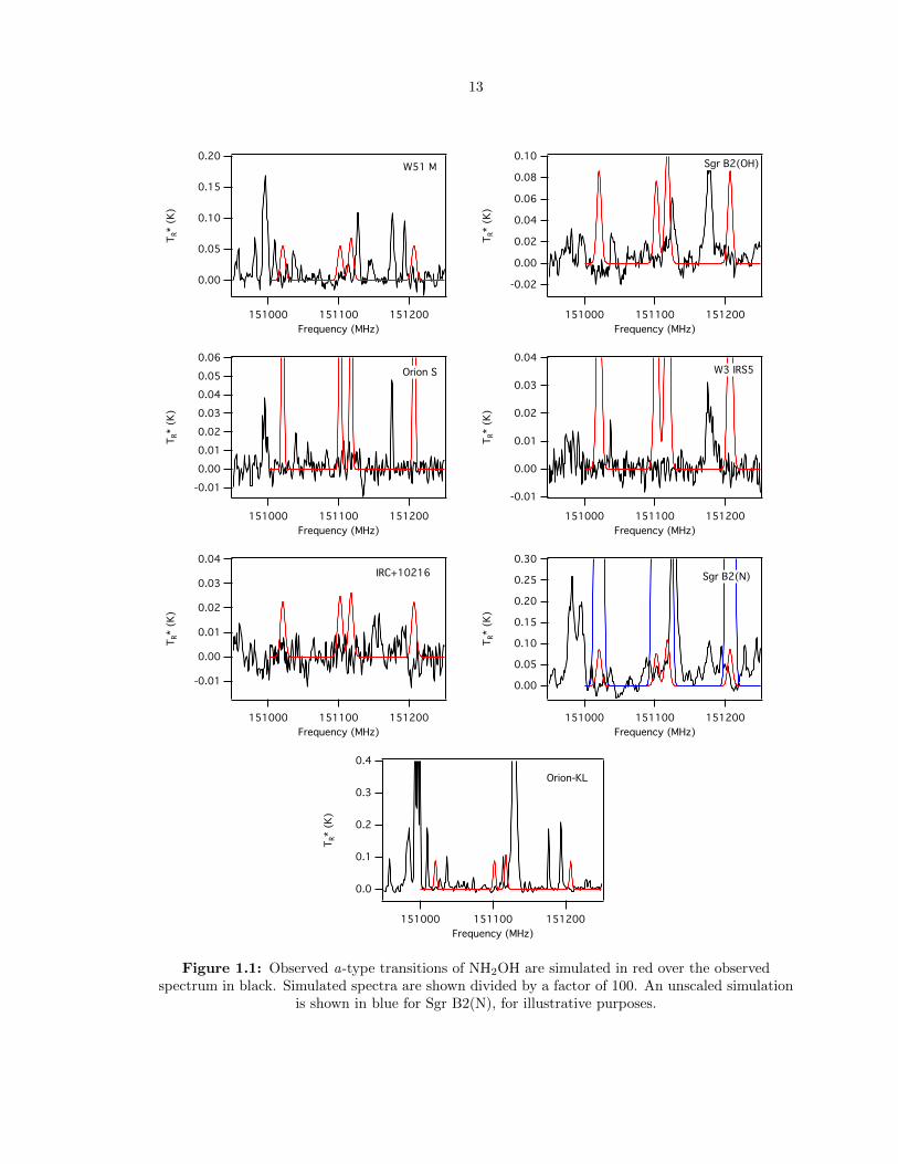
1.1 Observed a-type transitions of NH2OH are simulated in red over the observed spec-

trum in black. Simulated spectra are shown divided by a factor of 100. An unscaled

simulation is shown in blue for Sgr B2(N), for illustrative purposes. . . . . . . . . . . 13

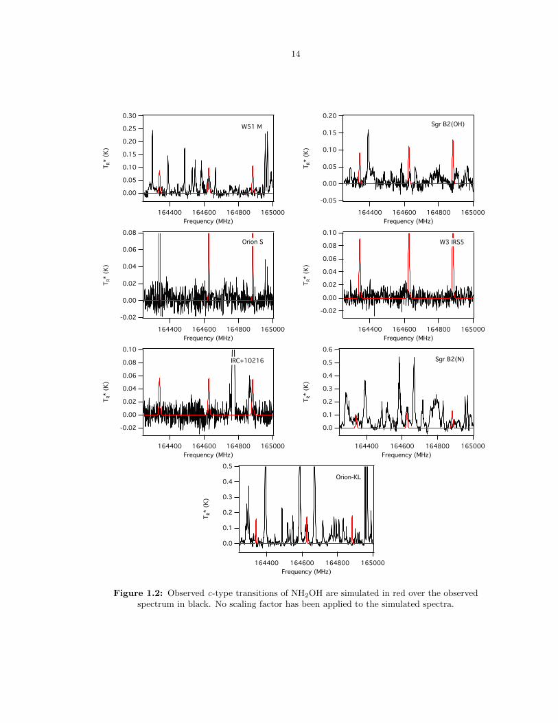
1.2 Observed c-type transitions of NH2OH are simulated in red over the observed spectrum

in black. No scaling factor has been applied to the simulated spectra. . . . . . . . . . 14

1.3 Observed c-type transitions of NH2OH are simulated in red over the observed spectrum

in black. No scaling factor has been applied to the simulated spectra. . . . . . . . . . 15

2.1 Observed transitions of l-C3H+ towards Sgr B2(N). Plots are on a common velocity

scale, with rest frequencies assuming a VLSR = +64 km s−1 and line centers taken

as those fitted by [48]. Blue and red lines indicate the +64 and +82 km s−1 common

velocity components in observations of Sgr B2, respectively. Predictions of line profiles

and intensities in the Sgr B2(N) observations based on the best fit temperature and

column density determined from the J = 1− 0 and J = 2− 1 transitions are shown as

a dashed profile in blue. . . . . . . . . . . . . . . . . . . . . . . . . . . . . . . . . . . . 27

2.2 Observed transitions of l-C3H+ towards Sgr B2(OH). Plots are on a common velocity

scale, with rest frequencies assuming a VLSR = +64 km s−1 and line centers taken

as those fitted by [48]. Blue and red lines indicate the +64 and +82 km s−1 common

velocity components in observations of Sgr B2, respectively. . . . . . . . . . . . . . . . 28

2.3 The J = 3/2−1/2, Ω = 1/2 transitions of l-C3H toward Sgr B2(N) from PRIMOS. Rest

frequency is adjusted for a VLSR = +64 km s−1. Blue and red lines indicate the +64

and +82 km s−1 common velocity components in observations of Sgr B2, respectively. 29

xiv

2.4 The J = 3/2 − 1/2, f -parity transitions of l-C3H toward TMC-1 from [78]. Rest

frequency is adjusted for a VLSR = +5.85 km s−1 . . . . . . . . . . . . . . . . . . . . 30

2.5 The J = 3/2 − 1/2, e-parity transitions of l-C3H toward TMC-1 from [78]. Rest

frequency is adjusted for a VLSR = +5.85 km s−1 . . . . . . . . . . . . . . . . . . . . 30

2.6 The J = 2− 1 transition of l-C3H+ toward TMC-1 from the [78] data. Rest frequency

is adjusted for a VLSR = +5.85 km s−1, and indicated by a blue line. . . . . . . . . . 33

2.7 Simulated spectrum of C3H– at LTE, with an excitation temperature of Tex = 22 K. . 40

2.8 Targeted frequency window around the predicted Ka = 1, 41,4−31,3 transition of C3H–

centered at 89535 MHz. The RMS noise level is 5.8 mK. Three features are observed –

one each attributed to HCO+ and HOC+. A third, located at ∼89580 MHz, has been

positively identified as belonging to a known interstellar species, but has been removed

from the spectra for proprietary reasons. The identity of this line will be published in

a forthcoming paper from Guzman et al. . . . . . . . . . . . . . . . . . . . . . . . . . 43

2.9 Observed transitions of B11244 and l-C3H toward Sgr B2(N) from PRIMOS, and CH

toward Sgr B2(N) from HEXOS. The blue vertical lines are provided to guide the eye

to the diffuse cloud velocity components. The velocity axis is referenced to the rest

frequency of each transition. . . . . . . . . . . . . . . . . . . . . . . . . . . . . . . . . 47

2.10 J = 9 − 8, 10 − 9, and 11 − 10 transitions of l-C3H+ observed toward the Orion Bar

PDR. The spectra are corrected for an observed source LSR velocity of 10.4 km s−1,

and have been baseline-subtracted and Hanning-smoothed to a resolution of 488 kHz

(∼0.7 km s−1). . . . . . . . . . . . . . . . . . . . . . . . . . . . . . . . . . . . . . . . . 55

2.11 J = 10 − 9 spectral window toward target sources. All spectra are adjusted to the

VLSR indicated in Table 2.9, and are vertically offset for clarity. The feature at 224714

MHz is due to C17O. The red vertical line indicates the frequency of the J = 10 − 9

transition. . . . . . . . . . . . . . . . . . . . . . . . . . . . . . . . . . . . . . . . . . . . 56

xv

2.12 J = 12 − 11 spectral window toward target sources. All spectra are adjusted to the

VLSR indicated in Table 2.9, and are vertically offset for clarity. The red vertical line

indicates the frequency of the J = 12− 11 transition. . . . . . . . . . . . . . . . . . . 57

2.13 J = 12 − 11 spectral window toward W51e2 in two different IF settings. Spectra are

DSB, adjusted to a VLSR = +55 km s−1, and are vertically offset for clarity. The red

vertical line indicates the frequency of the J = 12− 11 transition. . . . . . . . . . . . 58

2.14 J = 10 − 9 spectral window toward unbiased line survey sources. All spectra are

adjusted to the VLSR indicated in Table 2.10, and are vertically offset for clarity. The

red vertical line indicates the frequency of the J = 10− 9 transition. . . . . . . . . . . 59







3.1 Carbodiimide (HNCNH) spectral passbands toward Sgr B2(N), recorded from the GBT

PRIMOS Survey. Rotation-torsion doublet transition quantum numbers are shown in

each panel. The passband width displayed is 500 km s−1 in each case. The spectra

are plotted as a function of frequency (MHz), corrected for a LSR source velocity of

+64 km s−1. The blue and red vertical lines indicate the location of the transition rest

frequency (see Table 3.1) at an assumed LSR source velocity of +64 km s−1 and +82

km s−1, respectively. Data in all panels were Hanning-smoothed for display purposes. 70

3.2 Energy level structure of the relevant transitions for the 4.8 GHz maser (top) and 36.6

GHz line (bottom). Energy levels are ordered by increasing energy, but are not drawn

to scale. Allowed transitions are indicated by arrows. . . . . . . . . . . . . . . . . . . 72

xvi

4.1 List of molecules that have been detected in the ISM as of April 2014 from https://www.astro.uni-

koeln.de/cdms/molecules. . . . . . . . . . . . . . . . . . . . . . . . . . . . . . . . . . . 79

4.2 Example infrared ice spectra: Fig. 2 from [137] showing absorption from major ice

constituents in mid-infrared ISO/SWS observations of NGC 7538 IRS 9 (top) and

W33 A (bottom) . . . . . . . . . . . . . . . . . . . . . . . . . . . . . . . . . . . . . . . 80

5.1 Schematic of the TD-THz system. . . . . . . . . . . . . . . . . . . . . . . . . . . . . . 82

5.2 Photographs showing the plasma filament, indicated with a white arrow (left panel),

visible light scattering from the beam block using 800 nm generation (center panel),

and visible light scattering from the beam block using 1745 nm generation (right panel). 84

5.3 Photograph of the high vacuum cryostat showing the cold finger and silicon substrate,

radiation shield, gas dosing line, and TOPAS windows. . . . . . . . . . . . . . . . . . 85

5.4 Schematic drawing of the sample preparation dosing line. The line can be evacuated

either via a rough pump or through the turbomolecular pump, and pressures are mon-

itored via a mass-independent, active capacitance transmitter pressure gauge (MKS

Baratron, Red) between 0.01 Torr and 1100 Torr. Samples are prepared in glass fin-

gers and mixed in the large glass bulb. A separate gas mixture reservoir is also available

to contain samples for long periods prior to deposition, or to allow the facile deposition

of two mixtures in rapid succession. . . . . . . . . . . . . . . . . . . . . . . . . . . . . 87

5.5 Representative time-domain pulse acquired with the THz-TDS. The feature at ∼37 ps

is an etalon arising from the silicon substrate. . . . . . . . . . . . . . . . . . . . . . . . 89

5.6 Cartoon depicting the approximate bandwidth ranges covered by receivers on the Her-

schel Space Telescope, Atacama Large Millimeter Array, and Stratospheric Observatory

for Infrared Astronomy. They are overlaid on a THz power spectrum from the THz-

TDS instrument generated from the FFT of the first 35 ps of the pulse shown in Figure

5.5. The vertical positions of the telescope coverage are arbitrary. . . . . . . . . . . . 91

xvii

6.1 Comparison of THz spectra of crystalline ices studied in the laboratory, all at 10 K.

Traces are vertically offset for clarity, and scaled to show detail. . . . . . . . . . . . . 93

6.2 Qualitative comparison of the spectrum of crystalline water at 10 K (blue) obtained

with the Blake Group THz-TDS system to that of [154]. Adapted from Figure 11 of

[154]. Traces are on equivalent frequency scale; the intensity of the blue trace has been

normalized to that of the peak of the literature trace. . . . . . . . . . . . . . . . . . . 94

6.3 Spectra of crystalline water, deposited at 150 K, at 150 K (red), 75 K (black), and 10

K (blue). Traces have been vertically offset for clarity. . . . . . . . . . . . . . . . . . . 95

6.4 Spectra of amorphous water, deposited at 10 K, at 125 K (orange) and 10 K (blue). . 95

6.5 Comparison of crystalline water, deposited at 150 K, at 150 K (red) and 10 K (blue) to

amorphous water deposited at 10 K at 10 K (blue) and at 150 K after being annealed

to 175 K for 10 minutes (red). Traces have been scaled as indicated to show detail,

and offset vertically for clarity. The annealed ice clearly displays profiles distinct from

both amorphous water and water that was deposited crystalline, indicating that these

THz features are sensitive to the thermal history of the ice. . . . . . . . . . . . . . . . 96

6.6 Spectra of crystalline D2O, deposited at 150 K, at 150 K (red), 75 K (black), and 10

K (blue). Traces have been vertically offset for clarity. . . . . . . . . . . . . . . . . . . 97

6.7 Spectra of crystalline methanol, deposited at 140 K, at 100 K (green), 75 K (black),

and 10 K (blue). Traces have been vertically offset for clarity. . . . . . . . . . . . . . . 99

6.8 Spectra of amorphous methanol, deposited at 10 K, at 75 K (black) and 10 K (blue). 99

6.9 Comparison of crystalline methanol, deposited at 140 K, at 100 K (green) to amorphous

methanol deposited at 10 K at 10 K (blue) and at 100 K after being annealed to 140

K for 10 minutes (red). Traces have been offset vertically for clarity. The annealed ice

clearly displays profiles distinct from both amorphous methanol and methanol that was

deposited crystalline, indicating that these THz features are sensitive to the thermal

history of the ice. . . . . . . . . . . . . . . . . . . . . . . . . . . . . . . . . . . . . . . . 100

xviii

6.10 Spectra of purely crystalline water, purely crystalline methanol, and mixtures of wa-

ter:methanol in ratios of 2:1, 1:1, and 1:2, all deposited crystalline and cooled to 10 K.

Traces are scaled to show detail, and vertically offset for clarity. . . . . . . . . . . . . 101

6.11 Spectra of crystalline methyl formate, deposited at 135 K, at 100 K (green), 75 K

(black), and 10 K (blue). Traces have been vertically offset for clarity. . . . . . . . . . 102

6.12 Spectra of crystalline carbon dioxide, deposited at 75 K, at 75 K (black), 50 K (violet),

and 10 K (blue). Traces have been vertically offset for clarity. Inset shows detail on the

narrowing and blue-shift of the 3.5 THz transition of CO2 with decreasing temperature.103

6.13 Spectra of crystalline carbon dioxide at 10 K (blue), with theoretical predictions from

Crystal 09 overlaid in red based on the crystal structure at ambient pressures. . . . . 104

6.14 Cartoon demonstrating the increasing complexity achievable with the addition of a

single functional group (in this case OH or CH3 radicals) to a simpler, neutral species.

Arrows do not represent reaction pathways or mechanisms. . . . . . . . . . . . . . . . 105

6.15 Spectra of crystalline acetaldehyde, deposited at 125 K, at 100 K (green), 75 K (black),

and 10 K (blue). Traces have been vertically offset for clarity. . . . . . . . . . . . . . . 107

6.16 Spectra of amorphous acetaldehyde, deposited at 10 K, at 100 K (green), 75 K (black),

and 10 K (blue). . . . . . . . . . . . . . . . . . . . . . . . . . . . . . . . . . . . . . . . 107

6.17 Comparison of crystalline acetaldehyde, deposited at 125 K, at 100 K (green) to amor-

phous acetaldehyde deposited at 10 K at 10 K (blue) and at 100 K after being annealed

to 125 K for 5 minutes (green). Traces have been scaled as indicated, and offset ver-

tically for clarity. The annealed ice clearly displays profiles distinct from both amor-

phous acetaldehyde and acetaldehyde that was deposited crystalline, indicating that

these THz features are sensitive to the thermal history of the ice. . . . . . . . . . . . . 108

6.18 Spectra of purely crystalline water, purely crystalline acetaldehyde, and mixtures of

water:acetaldehyde in ratios of 2:1, 1:1, and 1:2, all deposited crystalline and cooled to

10 K. Traces are scaled to show detail, and vertically offset for clarity. . . . . . . . . . 109

xix

6.19 Spectra of crystalline acetone, deposited at 150 K, at 100 K (green), 75 K (black), and

10 K (blue). Traces have been vertically offset for clarity. . . . . . . . . . . . . . . . . 111

6.20 Spectra of amorphous acetone, deposited at 10 K, at 100 K (green), 75 K (black), and

10 K (blue). . . . . . . . . . . . . . . . . . . . . . . . . . . . . . . . . . . . . . . . . . . 111

6.21 Comparison of crystalline acetone, deposited at 150 K, at 100 K (green) to amorphous

acetone deposited at 10 K at 10 K (blue) and at 100 K after being annealed to 150 K

for 10 minutes (green). Traces have been scaled as indicated, and offset vertically for

clarity. The annealed ice clearly displays profiles distinct from both amorphous acetone

and acetone which was deposited crystalline, indicating that these THz features are

sensitive to the thermal history of the ice. . . . . . . . . . . . . . . . . . . . . . . . . . 112

6.22 Spectra of crystalline formic acid, deposited at 150 K, at 100 K (green), 75 K (black),

and 10 K (blue). . . . . . . . . . . . . . . . . . . . . . . . . . . . . . . . . . . . . . . . 114

6.23 Spectra of amorphous formic acid, deposited at 10 K, at 75 K (black), and 10 K (blue). 114

6.24 Comparison of crystalline formic acid, deposited at 150 K, at 10 K (blue) to amorphous

formic acid deposited at 10 K at 10 K (blue) and at 10 K after being annealed to 150

K (blue). Traces have been scaled as indicated, and offset vertically for clarity. While

the annealed ice clearly displays profiles distinct from both amorphous formic acid

and formic acid that was deposited crystalline, the overall profile of the absorption

has remained the same. This is consistent with a strongly-bound dimer structure that

largely prevents reorganization into a wider lattice. . . . . . . . . . . . . . . . . . . . . 115

6.25 Spectra of crystalline acetic acid, deposited at 150 K, at 100 K (green) and 10 K (blue).116

6.26 Spectra of amorphous acetic acid, deposited at 10 K, at 100 K (green), 75 K (black),

and 10 K (blue). . . . . . . . . . . . . . . . . . . . . . . . . . . . . . . . . . . . . . . . 116

xx

6.27 Comparison of crystalline acetic acid acid, deposited at 150 K, at 100 K (green) to

amorphous acetic acid deposited at 10 K at 10 K (blue) and at 100 K after being

annealed to 200 K (green). Traces have been offset vertically for clarity. While the

annealed ice clearly displays an additional small absorption at 2.5 THz, the primary

absorption feature remains largely unchanged. This is may indicate a strongly-bound

dimer structure, similar to formic acid, that largely prevents reorganization into a wider

lattice. . . . . . . . . . . . . . . . . . . . . . . . . . . . . . . . . . . . . . . . . . . . . . 117

7.1 Cartoon depicting the molecular motions that generally lead to transitions arising in the

infrared – intramolecular vibrations – and in the microwave – rotational and torsional

motion. . . . . . . . . . . . . . . . . . . . . . . . . . . . . . . . . . . . . . . . . . . . . 119

7.2 Cartoon depicting the hydrogen-bonded bilayers formed in crystalline water ice. THz

spectroscopy is sensitive to the large-scale, bulk stretching and bending of hydrogen

bonds between and among these bilayers. . . . . . . . . . . . . . . . . . . . . . . . . . 119

7.3 Cartoon depicting the gas-phase hydrogen-bonding arrangement of the formic acid

dimer (not to scale). . . . . . . . . . . . . . . . . . . . . . . . . . . . . . . . . . . . . . 121

A.1 Deconvolved and baseline-subtracted spectrum of Sgr B2(N) from 260 - 286 GHz. . . 140

A.2 Spectrum of Sgr B2(N) from 260.0 - 260.5 GHz . . . . . . . . . . . . . . . . . . . . . . 142










xxi




























xxii
















C.1 FTIR spectrum of amorphous water at 10 K. . . . . . . . . . . . . . . . . . . . . . . . 185

C.2 FTIR spectrum of crystalline water at 140 K. . . . . . . . . . . . . . . . . . . . . . . . 186

C.3 FTIR spectrum of amorphous D2O at 10 K. . . . . . . . . . . . . . . . . . . . . . . . 187

C.4 FTIR spectrum of crystalline D2O at 150 K. . . . . . . . . . . . . . . . . . . . . . . . 188

C.5 FTIR spectrum of crystalline CO at 30 K. Inset shows detail. . . . . . . . . . . . . . . 189

C.6 FTIR spectrum of crystalline CO2 at 75 K. Inset shows detail. . . . . . . . . . . . . . 190

C.7 FTIR spectrum of crystalline formic acid at 150 K. . . . . . . . . . . . . . . . . . . . . 191

C.8 FTIR spectrum of crystalline acetic acid at 180 K. . . . . . . . . . . . . . . . . . . . . 192

C.9 FTIR spectrum of crystalline acetone at 140 K. . . . . . . . . . . . . . . . . . . . . . . 193

C.10 FTIR spectrum of crystalline methanol at 140 K. . . . . . . . . . . . . . . . . . . . . . 194

C.11 FTIR spectrum of crystalline methyl formate at 135 K. . . . . . . . . . . . . . . . . . 195

xxiii

List of Tables

1.1 Observed sources and coordinates (J2000), spectral line widths, and vLSR for each source. 9

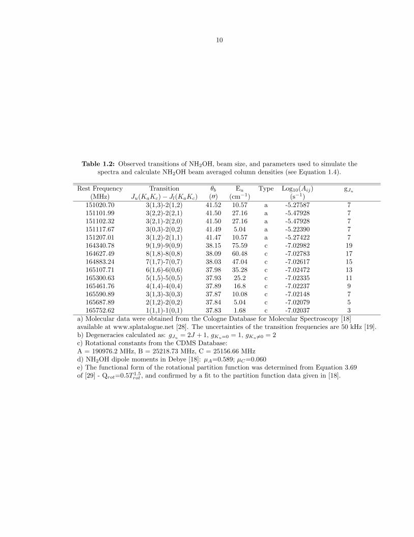
1.2 Observed transitions of NH2OH, beam size, and parameters used to simulate the spec-

tra and calculate NH2OH beam averaged column densities (see Equation 1.4). . . . . 10

1.3 1σ RMS level of T ∗R, upper limits on column density of NH2OH, H2 column density,

relative abundance of NH2OH, and assumed value of Trot. . . . . . . . . . . . . . . . . 12

2.1 Results of the spectroscopic fit of [48] to the eight unidentified transitions. . . . . . . 22

2.2 Transitions of l-C3H+ observed toward Sgr B2(N), Sgr B2(OH), and TMC-1. . . . . . 31

2.3 Transitions of l-C3H observed toward Sgr B2(N) and TMC-1. . . . . . . . . . . . . . . 32

2.4 Best-fit spectroscopic constants obtained by shifting VLSR for the PRIMOS and IRAM

datasets. . . . . . . . . . . . . . . . . . . . . . . . . . . . . . . . . . . . . . . . . . . . 36

2.5 CALPGM catalog simulation of C3H– format. . . . . . . . . . . . . . . . . . . . . . . . 39

2.6 Rotational constants and dipole moments for l-C3H+ and C3H– . . . . . . . . . . . . . 39

2.7 Observed and targeted transitions of B11244, assuming it is C3H−. For simplicity, only

those Ka = 1 transitions specifically searched for in our study are displayed. . . . . . 42

2.8 Column densities and excitation temperatures for l-C3H+ and C3H– in our observa-

tions and from the literature, as well as ratios of these to their neutral counterparts.

Literature values for the ratio of C6H− to neutral C6H are also shown. . . . . . . . . . 45

2.9 Sources, coordinates, VLSR, and source type for the targeted search. . . . . . . . . . . 52

2.10 Sources, coordinates, VLSR, and source type for each observed source from the unbiased

line surveys. . . . . . . . . . . . . . . . . . . . . . . . . . . . . . . . . . . . . . . . . . 53

2.11 Summary of observations of the J = 10− 9 and J = 12− 11 frequency windows. . . . 63

xxiv

2.12 Upper limits for l-C3H+ in each source at 15 K and at 180 K. . . . . . . . . . . . . . 64

3.1 HNCNH Rotation-Torsion Doublets, Spectroscopic, and Observed Astronomical Pa-

rameters . . . . . . . . . . . . . . . . . . . . . . . . . . . . . . . . . . . . . . . . . . . . 71

A.1 Summary of spectral line surveys of Sgr B2(N) . . . . . . . . . . . . . . . . . . . . . . 138

1

Part I

Introduction

2

NASA missions have found some of the most chemically-diverse organic materials ever detected

in astronomical environments, yet there is no agreed-upon chemical pathway as to their formation.

We know from meteorites and, more recently, cometary samples returned by the STARDUST mis-

sion that amino acids, the building blocks of life as we understand it, are present in extraterrestrial

sources [3]. In the last decade, complex gas-grain chemical models have become widely-used tools in

the attempt to understand the chemical pathways that can result in the species observed and their

abundances in interstellar environments. A key goal of these models is to predict the most likely

chemical pathways for the formation of life-essential molecules, such as amino acids. Once found, ob-

servational studies can then be conducted in an attempt to discover the precursor molecules involved

in the reactions predicted by the model. While such methods can be valuable, they suffer from a

lack of both laboratory and observational data with which to constrain them. Thus, observational

follow-ups to these studies are vital.

My work, both in laboratory astrophysics and observational astronomy, aims to address both

of these issues and advance the quest towards the definitive detection and characterization of life-

essential molecules such as glycine in the interstellar medium (ISM). The quest to understand the

chemical evolutionary history of life-essential polymers such as proteins, sugars, and amino acids,

has been a driving force in molecular astrochemistry for several decades. The discovery of these

biopolymer building blocks in meteorites and cometary samples represents a significant clue to

the mechanisms that could eventually lead to the delivery of biotic and prebiotic molecules to

planetesimals, the rocky precursors to planets, but it does not provide a definitive answer to one of

the biggest remaining open questions: Where and when do the majority of these species form? Do

they form in the gas phase before incorporation into comets or directly into planetesimals? Do they

form in the icy mantles of dust grains or comets themselves before delivery? Or, are they largely

formed from precursor molecules after or upon impact with planetesimals? My work has focused on

approaching these questions through a combined effort of observational astronomy and laboratory

astrophysics.

3

To truly begin to understand the complexities of the chemical processes that give rise to species

such as glycine, a thorough understanding of the chemical inventories, and the physical conditions

in which they exist, is essential. Such an understanding requires that observational work encompass

the full range of states in which these species can be formed - from cm- and mm-wave observations

of gas-phase species, to observations of condensed-phase species in the near- to far-infrared. In turn,

the scope and direction of laboratory work is necessarily informed and shaped by these observations.

The observational work presented in Part II is aimed at understanding the breadth of molec-

ular complexity present in the ISM, and how that complexity is affected by, and can be used to

understand, both the physical environments in which molecules are present and the evolution of

those environments. This work relies heavily on complementary laboratory data. While gas-phase

species, such as those discussed in Part II, are relatively well-studied in the laboratory, the body

of work relating to solid-phase species of astrophysical-interest lacks a corresponding depth. The

work presented in Part III aims to address this issue through the construction of a spectrometer and

collection of spectra of astrophysically-relevant species in the largely unexplored TeraHertz (THz)

region of the spectrum. This historically opaque frequency regime has recently become illuminated

through the commissioning of a number of astronomical observatories that operate in this range.

4

Part II

Observational Astronomy

5

Chapter 1

Hydroxylamine (NH2OH)

The bulk of this chapter is reproduced from “A search for hydroxylamine (NH2OH) toward select

astronomical sources,” by R.L. Pulliam, B.A. McGuire, and A.J. Remijan, Astrophysical Journal,

751, 1 (2012) [4].

1.1 A Brief History of Hydroxylamine

Hydroxylamine (NH2OH) has been suggested as a possible reactant precursor in the formation of

interstellar amino acids [5; 6] through the reaction of the neutral, ionized, or protonated species with

with acetic or propanoic acid. In 2008, a state-of-the-art gas-grain model of complex chemistry in

star-forming regions predicted an NH2OH column density as high as 1016 cm−2 toward typical hot

core sources [7]; easily within the detectable limits of modern radio telescopes. Motivated by this

surprisingly large predicted abundance, we searched for NH2OH using the NRAO 12 m Telescope on

Kitt Peak towards IRC+10216, Orion KL, Orion S, Sgr B2(N), Sgr B2(OH), W3IRS5, and W51M.

We found no evidence for NH2OH in any of the sources, and in fact derived upper limits as six

orders of magnitude lower than predicted by models [4]. The details of this work are described in

the remaining sections of this chapter.

Concurrently, laboratory investigations were undertaken by a laboratory astrophysics group in

Leiden to elucidate the mechanisms of NH2OH formation on grain surfaces [8]. In our work, we

assert that there is no reason to assume that hydrogenation of NO proceeds to NH2OH via the same

pathways as CO hydrogenation proceeds to CH3OH, as assumed by [7]. This was confirmed by [8],

6

when it was determined that unlike CO hydrogenation, in which several steps possess a non-trivial

barrier to reaction, NO hydrogen proceeds with no reaction barriers. Using their experimentally-

determined reaction pathways and a model for dark cloud chemistry, they predict peak gas-phase

NH2OH abundances that are well aligned with the upper limits in our observations. Not long after,

the original model of [7] was refined, taking the laboratory work of [8] and others other into account,

and the new model also predicts peak abundances in line with our observed upper limits [9].

Our recent efforts to detect this model have focused on the shocked outflow region L1157-B1.

This region is known to be rich in complex organic molecules despite relatively cool temperatures,

indicating that molecules are formed in the solid phase before being non-thermally desorbed into

the gas phase. We think such regions are ideal candidates for locating NH2OH in sufficiently high

abundance, as these shock processes may liberate additional NH2OH into the gas phase beyond that

which would be present under thermal equilibrium between the grain surface and the surrounding

gas.

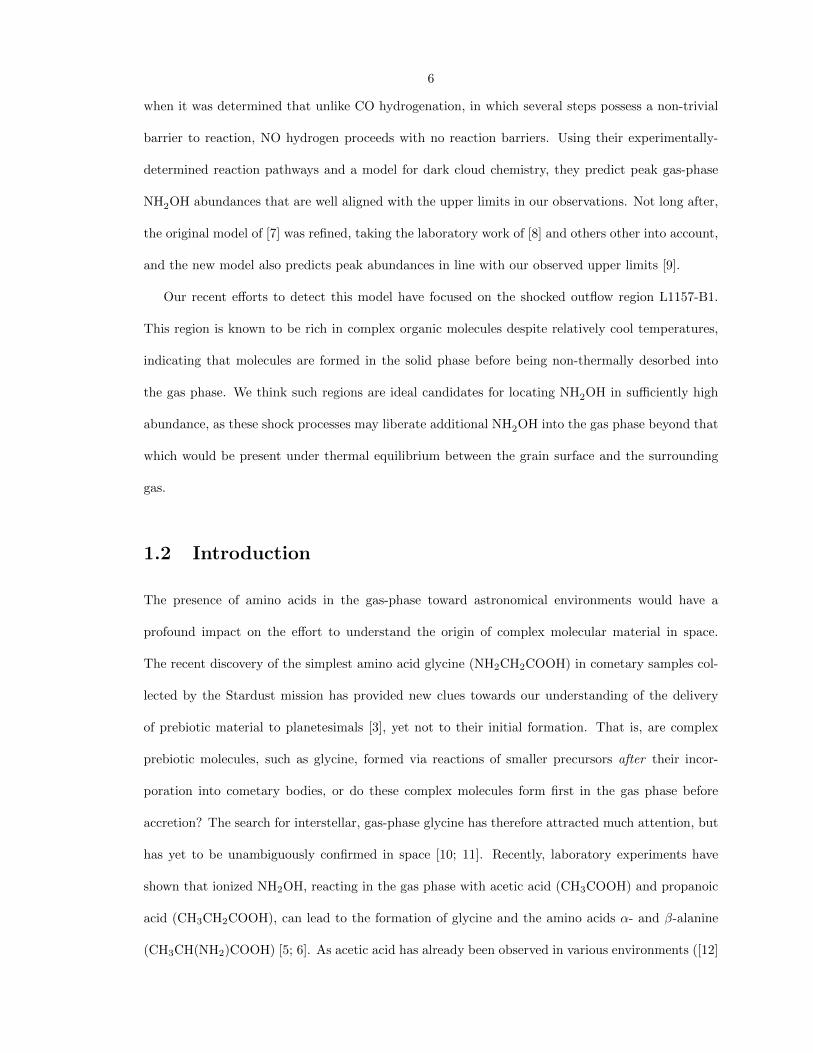
1.2 Introduction

The presence of amino acids in the gas-phase toward astronomical environments would have a

profound impact on the effort to understand the origin of complex molecular material in space.

The recent discovery of the simplest amino acid glycine (NH2CH2COOH) in cometary samples col-

lected by the Stardust mission has provided new clues towards our understanding of the delivery

of prebiotic material to planetesimals [3], yet not to their initial formation. That is, are complex

prebiotic molecules, such as glycine, formed via reactions of smaller precursors after their incor-

poration into cometary bodies, or do these complex molecules form first in the gas phase before

accretion? The search for interstellar, gas-phase glycine has therefore attracted much attention, but

has yet to be unambiguously confirmed in space [10; 11]. Recently, laboratory experiments have

shown that ionized NH2OH, reacting in the gas phase with acetic acid (CH3COOH) and propanoic

acid (CH3CH2COOH), can lead to the formation of glycine and the amino acids α- and β-alanine

(CH3CH(NH2)COOH) [5; 6]. As acetic acid has already been observed in various environments ([12]

7

and references therein), the detection of NH2OH would be of much interest to the astrochemistry

community, helping to answer the question of how these large complex molecules form in astronom-

ical environments.

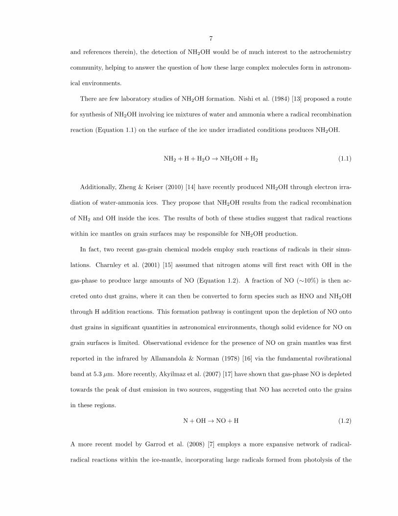
There are few laboratory studies of NH2OH formation. Nishi et al. (1984) [13] proposed a route

for synthesis of NH2OH involving ice mixtures of water and ammonia where a radical recombination

reaction (Equation 1.1) on the surface of the ice under irradiated conditions produces NH2OH.

NH2 + H + H2O→ NH2OH + H2 (1.1)

Additionally, Zheng & Keiser (2010) [14] have recently produced NH2OH through electron irra-

diation of water-ammonia ices. They propose that NH2OH results from the radical recombination

of NH2 and OH inside the ices. The results of both of these studies suggest that radical reactions

within ice mantles on grain surfaces may be responsible for NH2OH production.

In fact, two recent gas-grain chemical models employ such reactions of radicals in their simu-

lations. Charnley et al. (2001) [15] assumed that nitrogen atoms will first react with OH in the

gas-phase to produce large amounts of NO (Equation 1.2). A fraction of NO (∼10%) is then ac-

creted onto dust grains, where it can then be converted to form species such as HNO and NH2OH

through H addition reactions. This formation pathway is contingent upon the depletion of NO onto

dust grains in significant quantities in astronomical environments, though solid evidence for NO on

grain surfaces is limited. Observational evidence for the presence of NO on grain mantles was first

reported in the infrared by Allamandola & Norman (1978) [16] via the fundamental rovibrational

band at 5.3 µm. More recently, Akyilmaz et al. (2007) [17] have shown that gas-phase NO is depleted

towards the peak of dust emission in two sources, suggesting that NO has accreted onto the grains

in these regions.

N + OH→ NO + H (1.2)

A more recent model by Garrod et al. (2008) [7] employs a more expansive network of radical-

radical reactions within the ice-mantle, incorporating large radicals formed from photolysis of the

8

ice constituents already known to be present. These radical “fragments” then react to build up

more complex species as they become mobile on the grain surface through a gradual warm-up

process before being liberated into the gas phase. Formation of NH2OH is predicted to start from

the radical-radical reaction of NH+OH addition on grain surfaces, followed by hydrogenation or

directly by the reaction of OH+NH2. The model predicts an NH2OH column density as high as 1016

cm−2; easily within the detectable limits of modern radio telescopes.

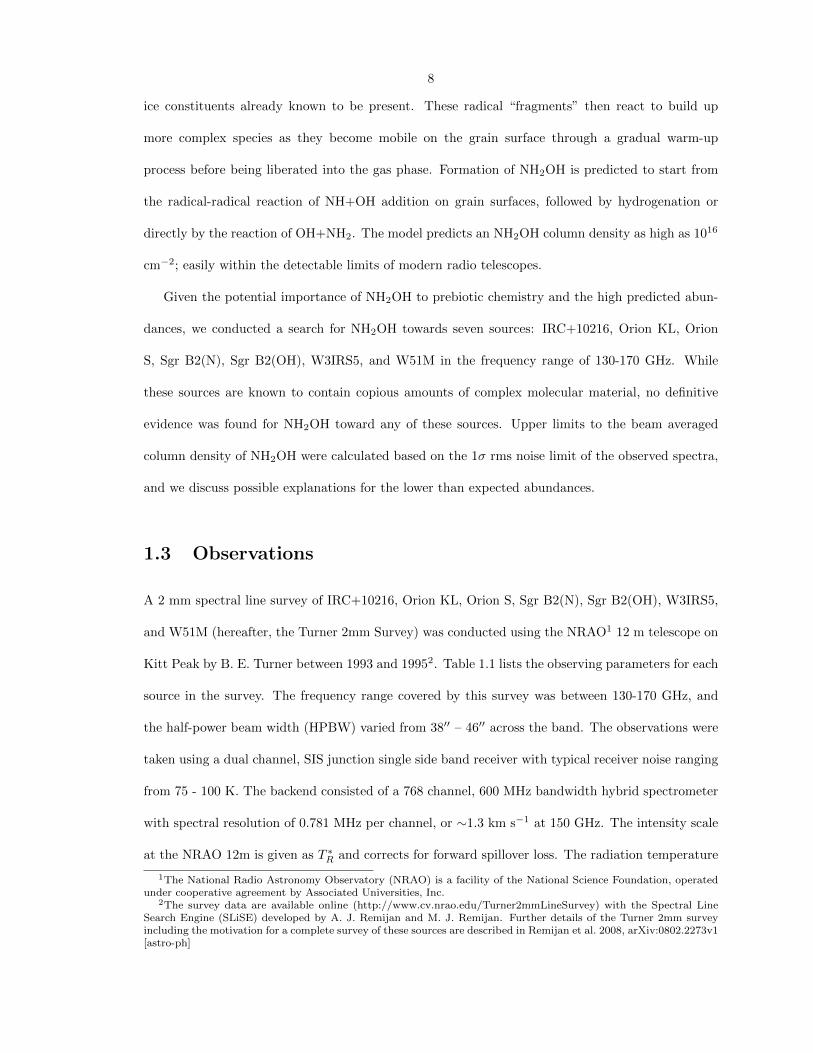
Given the potential importance of NH2OH to prebiotic chemistry and the high predicted abun-

dances, we conducted a search for NH2OH towards seven sources: IRC+10216, Orion KL, Orion

S, Sgr B2(N), Sgr B2(OH), W3IRS5, and W51M in the frequency range of 130-170 GHz. While

these sources are known to contain copious amounts of complex molecular material, no definitive

evidence was found for NH2OH toward any of these sources. Upper limits to the beam averaged

column density of NH2OH were calculated based on the 1σ rms noise limit of the observed spectra,

and we discuss possible explanations for the lower than expected abundances.

1.3 Observations

A 2 mm spectral line survey of IRC+10216, Orion KL, Orion S, Sgr B2(N), Sgr B2(OH), W3IRS5,

and W51M (hereafter, the Turner 2mm Survey) was conducted using the NRAO1 12 m telescope on

Kitt Peak by B. E. Turner between 1993 and 19952. Table 1.1 lists the observing parameters for each

source in the survey. The frequency range covered by this survey was between 130-170 GHz, and

the half-power beam width (HPBW) varied from 38′′ – 46′′ across the band. The observations were

taken using a dual channel, SIS junction single side band receiver with typical receiver noise ranging

from 75 - 100 K. The backend consisted of a 768 channel, 600 MHz bandwidth hybrid spectrometer

with spectral resolution of 0.781 MHz per channel, or ∼1.3 km s−1 at 150 GHz. The intensity scale

at the NRAO 12m is given as T ∗R and corrects for forward spillover loss. The radiation temperature

1The National Radio Astronomy Observatory (NRAO) is a facility of the National Science Foundation, operatedunder cooperative agreement by Associated Universities, Inc.

2The survey data are available online (http://www.cv.nrao.edu/Turner2mmLineSurvey) with the Spectral LineSearch Engine (SLiSE) developed by A. J. Remijan and M. J. Remijan. Further details of the Turner 2mm surveyincluding the motivation for a complete survey of these sources are described in Remijan et al. 2008, arXiv:0802.2273v1[astro-ph]

9

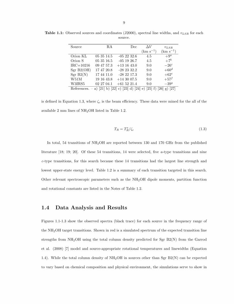
Table 1.1: Observed sources and coordinates (J2000), spectral line widths, and vLSR for eachsource.

Source RA Dec ∆V vLSR

(km s−1) (km s−1)Orion KL 05 35 14.5 -05 22 32.6 4.5 +9a

Orion S 05 35 16.5 -05 19 26.7 4.5 +7b

IRC+10216 09 47 57.3 +13 16 43.0 9.0 −26c

Sgr B2(OH) 17 47 20.8 -28 23 32.2 9.0 +60d

Sgr B2(N) 17 44 11.0 -28 22 17.3 9.0 +62e

W51M 19 16 43.8 +14 30 07.5 9.0 +57f

W3IRS5 02 27 04.1 +61 52 21.4 9.0 −39g

References. – a) [21] b) [22] c) [23] d) [24] e) [25] f) [26] g) [27]

is defined in Equation 1.3, where ζc is the beam efficiency. These data were mined for the all of the

available 2 mm lines of NH2OH listed in Table 1.2.

TR = T ∗R/ζc (1.3)

In total, 54 transitions of NH2OH are reported between 130 and 170 GHz from the published

literature [18; 19; 20]. Of these 54 transitions, 14 were selected, five a-type transitions and nine

c-type transitions, for this search because these 14 transitions had the largest line strength and

lowest upper-state energy level. Table 1.2 is a summary of each transition targeted in this search.

Other relevant spectroscopic parameters such as the NH2OH dipole moments, partition function

and rotational constants are listed in the Notes of Table 1.2.

1.4 Data Analysis and Results

Figures 1.1-1.3 show the observed spectra (black trace) for each source in the frequency range of

the NH2OH target transitions. Shown in red is a simulated spectrum of the expected transition line

strengths from NH2OH using the total column density predicted for Sgr B2(N) from the Garrod

et al. (2008) [7] model and source-appropriate rotational temperatures and linewidths (Equation

1.4). While the total column density of NH2OH in sources other than Sgr B2(N) can be expected

to vary based on chemical composition and physical environment, the simulations serve to show in

10

Table 1.2: Observed transitions of NH2OH, beam size, and parameters used to simulate thespectra and calculate NH2OH beam averaged column densities (see Equation 1.4).

Rest Frequency Transition θb Eu Type Log10(Aij) gJu(MHz) Ju(KaKc)− Jl(KaKc) (′′) (cm−1) (s−1)

151020.70 3(1,3)-2(1,2) 41.52 10.57 a -5.27587 7151101.99 3(2,2)-2(2,1) 41.50 27.16 a -5.47928 7151102.32 3(2,1)-2(2,0) 41.50 27.16 a -5.47928 7151117.67 3(0,3)-2(0,2) 41.49 5.04 a -5.22390 7151207.01 3(1,2)-2(1,1) 41.47 10.57 a -5.27422 7164340.78 9(1,9)-9(0,9) 38.15 75.59 c -7.02982 19164627.49 8(1,8)-8(0,8) 38.09 60.48 c -7.02783 17164883.24 7(1,7)-7(0,7) 38.03 47.04 c -7.02617 15165107.71 6(1,6)-6(0,6) 37.98 35.28 c -7.02472 13165300.63 5(1,5)-5(0,5) 37.93 25.2 c -7.02335 11165461.76 4(1,4)-4(0,4) 37.89 16.8 c -7.02237 9165590.89 3(1,3)-3(0,3) 37.87 10.08 c -7.02148 7165687.89 2(1,2)-2(0,2) 37.84 5.04 c -7.02079 5165752.62 1(1,1)-1(0,1) 37.83 1.68 c -7.02037 3

a) Molecular data were obtained from the Cologne Database for Molecular Spectroscopy [18]available at www.splatalogue.net [28]. The uncertainties of the transition frequencies are 50 kHz [19].b) Degeneracies calculated as: gJu = 2J + 1, gKu=0 = 1, gKu 6=0 = 2c) Rotational constants from the CDMS Database:A = 190976.2 MHz, B = 25218.73 MHz, C = 25156.66 MHzd) NH2OH dipole moments in Debye [18]: µA=0.589; µC=0.060e) The functional form of the rotational partition function was determined from Equation 3.69of [29] - Qrot=0.5T 1.5

rot , and confirmed by a fit to the partition function data given in [18].

11

a qualitative sense that the searched-for transitions of NH2OH are not present toward these sources

beyond the 1σ RMS noise limit, and certainly not present in the abundances predicted by the model.

In several sources, emission features are present at a number of the appropriate center frequencies

for NH2OH. Yet, the strongest transitions of NH2OH in this band are the J = 3-2 manifold near 151

GHz, and in no source are all of the expected transitions observed. This indicates that the observed

emission features are coincidental overlap with other molecular transitions, and that NH2OH is not

observed in these sources.

The column density of an observed species can be calculated using Equation 1.4, following the

convention of [30] (c.f. [31]).

NT =3k

8π3× Qre

Eu/Tex

νSµ2×√π

2ln2× ∆T ∗A∆V/ηb

1− (ehν/kTex−1)(ehν/kTbg−1)

cm−2 (1.4)

Here, NT is the total column density, Qr is the rotational partition function, Eu is the upper

state energy, Tex is the excitation temperature, ν is the frequency of the transition, Sµ2 is the

transition strength, ∆T ∗A is the peak line intensity, ∆V is the line width, ηb is the beam efficiency

at frequency ν, and Tbg is the background temperature. The source of the observed emission is

assumed to completely fill the beam.

Using Equation 1.4, upper limits to the beam averaged column density based on the 1σ RMS

noise limit were calculated, and are reported in Table 1.3. An approximate rotational temperature

appropriate for each source was used based on data available in the references shown in Table 1.3.

For the purposes of this work, CH3OH was used as a primary source of temperature information

when available. CH3OH was chosen due to it structural similarities with NH2OH and its presence

in the majority of these sources, allowing for greater consistency than would be possible using

other molecules, such as amines. Further, the wealth of observational data on CH3OH makes

temperatures derived from its observations more accurate. In any case, the upper limits presented

here are fairly insensitive to the relatively minor range of rotational temperatures observed in these

sources. Fractional abundances with respect to molecular hydrogen were calculated for each source

based on these upper limits. In the case of Sgr B2(N), the Garrod et al. (2008) [7] model predicts

12

Table 1.3: 1σ RMS level of T ∗R, upper limits on column density of NH2OH, H2 column density,relative abundance of NH2OH, and assumed value of Trot.

T ∗R NNH2OH NH2NNH2OH/NH2

TrotSource (mK) (cm−2) (cm−2) (K)Orion KLa 6.4 <2 x 1013 7.0 x 1023 <3 x 10−11 120Orion Sb 4.0 <9 x 1012 1.0 x 1023 <9 x 10−11 80IRC+10216c 5.1 <8 x 1013 3.0 x 1022 <3 x 10−9 200Sgr B2(OH)d 7.0 <3 x 1013 1.0 x 1024 <3 x 10−11 70Sgr B2(N)e 6.6 <2 x 1013 3.0 x 1024 <8 x 10−12 70W51Mf 7.7 <4 x 1013 1.0 x 1024 <4 x 10−11 100W3IRS5g 4.3 <2 x 1013 5.0 x 1023 <3 x 10−11 70a) Trot from [21]; NH2 from [32] and Refs. therein.b) Trot from [22]; NH2

from [32] and Refs. therein.c) Trot from [33]; NH2

from [34]d) Trot from [24]; NH2

from [32] and Refs. therein.e) Trot and NH2 from [25]f) Trot from [26]; NH2 from [32] and Refs. therein.g) Trot and NH2

from [27]

a relative abundance for NH2OH of 3.5 x 10−7 - 4.2 x 10−6, which is up to six orders of magnitude

higher than the observed upper limits.

1.5 Discussion

In this paper, we reported on the negative detection of hydroxylamine (NH2OH) towards several

astronomical sources. Upper limits to the beam averaged column density have also been determined

for each source based on the 1σ RMS noise level in each spectra. Recent chemical models introduced

a new gas-grain chemical network utilizing radical-radical reactions as formation mechanisms [7].

The model reproduces the beam averaged column densities of species such as methanol (CH3OH),

acetaldehyde (CH3CHO), and even glycolaldehyde (CH2(OH)CHO) with excellent agreement with

current observed abundances toward the Sgr B2(N) star-forming region [7]. However, for NH2OH,

the predicted abundances are 3.5×10−7 - 4.2×10−6, nearly six orders of magnitude higher than the

observed upper limits reported in this study. The following sections discuss possible explanations

for this surprising difference, focusing on possible formation and destruction mechanisms.

13

0.20

0.15

0.10

0.05

0.00

TR*

(K)

151200151100151000

Frequency (MHz)

W51 M0.10

0.08

0.06

0.04

0.02

0.00

-0.02

TR*

(K)

151200151100151000

Frequency (MHz)

Sgr B2(OH)

0.06

0.05

0.04

0.03

0.02

0.01

0.00

-0.01

TR*

(K)

151200151100151000

Frequency (MHz)

Orion S

0.04

0.03

0.02

0.01

0.00

-0.01T

R*

(K)

151200151100151000

Frequency (MHz)

W3 IRS5

0.04

0.03

0.02

0.01

0.00

-0.01

TR*

(K)

151200151100151000

Frequency (MHz)

IRC+10216

0.30

0.25

0.20

0.15

0.10

0.05

0.00

TR*

(K)

151200151100151000

Frequency (MHz)

Sgr B2(N)

0.4

0.3

0.2

0.1

0.0

TR*

(K)

151200151100151000

Frequency (MHz)

Orion-KL

Figure 1.1: Observed a-type transitions of NH2OH are simulated in red over the observedspectrum in black. Simulated spectra are shown divided by a factor of 100. An unscaled simulation

is shown in blue for Sgr B2(N), for illustrative purposes.

14

0.6

0.5

0.4

0.3

0.2

0.1

0.0

TR*

(K)

165000164800164600164400

Frequency (MHz)

Sgr B2(N)

0.20

0.15

0.10

0.05

0.00

-0.05

TR*

(K)

165000164800164600164400

Frequency (MHz)

Sgr B2(OH)

0.10

0.08

0.06

0.04

0.02

0.00

-0.02

TR*

(K)

165000164800164600164400

Frequency (MHz)

IRC+10216

0.5

0.4

0.3

0.2

0.1

0.0

TR*

(K)

165000164800164600164400

Frequency (MHz)

Orion-KL

0.08

0.06

0.04

0.02

0.00

-0.02

TR*

(K)

165000164800164600164400

Frequency (MHz)

Orion S

0.10

0.08

0.06

0.04

0.02

0.00

-0.02T

R*

(K)

165000164800164600164400

Frequency (MHz)

W3 IRS5

0.30

0.25

0.20

0.15

0.10

0.05

0.00

TR*

(K)

165000164800164600164400

Frequency (MHz)

W51 M

Figure 1.2: Observed c-type transitions of NH2OH are simulated in red over the observedspectrum in black. No scaling factor has been applied to the simulated spectra.

15

1.0

0.8

0.6

0.4

0.2

0.0

TR*

(K)

166000165800165600165400165200165000

Frequency (MHz)

W51 M

0.4

0.3

0.2

0.1

0.0

TR*

(K)

166000165800165600165400165200165000

Frequency (MHz)

W3 IRS5

1.0

0.8

0.6

0.4

0.2

0.0

TR*

(K)

166000165800165600165400165200165000

Frequency (MHz)

Orion S

1.0

0.8

0.6

0.4

0.2

0.0

TR*

(K)

166000165800165600165400165200165000

Frequency (MHz)

Orion-KL

0.6

0.5

0.4

0.3

0.2

0.1

0.0

TR*

(K)

166000165800165600165400165200165000

Frequency (MHz)

IRC+10216

1.0

0.8

0.6

0.4

0.2

0.0

TR*

(K)

166000165800165600165400165200165000

Frequency (MHz)

Sgr B2(OH)

1.0

0.8

0.6

0.4

0.2

0.0

TR*

(K)

166000165800165600165400165200165000

Frequency (MHz)

Sgr B2(N)

Figure 1.3: Observed c-type transitions of NH2OH are simulated in red over the observedspectrum in black. No scaling factor has been applied to the simulated spectra.

16

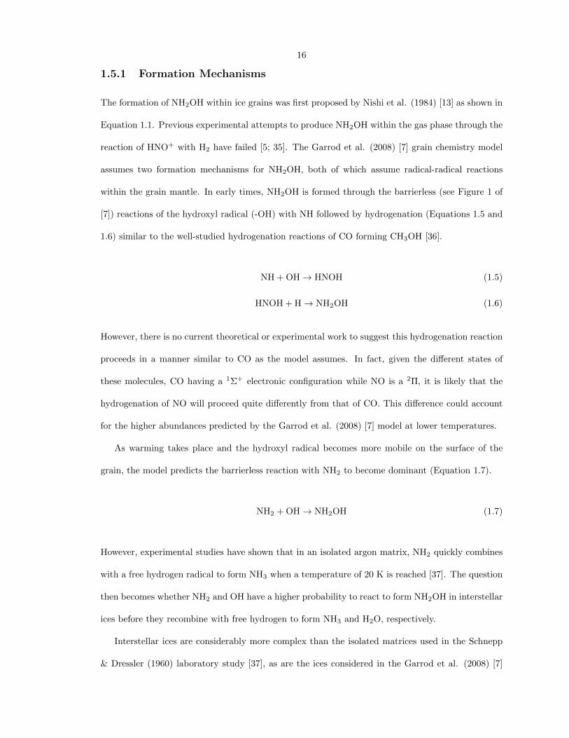
1.5.1 Formation Mechanisms

The formation of NH2OH within ice grains was first proposed by Nishi et al. (1984) [13] as shown in

Equation 1.1. Previous experimental attempts to produce NH2OH within the gas phase through the

reaction of HNO+ with H2 have failed [5; 35]. The Garrod et al. (2008) [7] grain chemistry model

assumes two formation mechanisms for NH2OH, both of which assume radical-radical reactions

within the grain mantle. In early times, NH2OH is formed through the barrierless (see Figure 1 of

[7]) reactions of the hydroxyl radical (-OH) with NH followed by hydrogenation (Equations 1.5 and

1.6) similar to the well-studied hydrogenation reactions of CO forming CH3OH [36].

NH + OH→ HNOH (1.5)

HNOH + H→ NH2OH (1.6)

However, there is no current theoretical or experimental work to suggest this hydrogenation reaction

proceeds in a manner similar to CO as the model assumes. In fact, given the different states of

these molecules, CO having a 1Σ+ electronic configuration while NO is a 2Π, it is likely that the

hydrogenation of NO will proceed quite differently from that of CO. This difference could account

for the higher abundances predicted by the Garrod et al. (2008) [7] model at lower temperatures.

As warming takes place and the hydroxyl radical becomes more mobile on the surface of the

grain, the model predicts the barrierless reaction with NH2 to become dominant (Equation 1.7).

NH2 + OH→ NH2OH (1.7)

However, experimental studies have shown that in an isolated argon matrix, NH2 quickly combines

with a free hydrogen radical to form NH3 when a temperature of 20 K is reached [37]. The question

then becomes whether NH2 and OH have a higher probability to react to form NH2OH in interstellar

ices before they recombine with free hydrogen to form NH3 and H2O, respectively.

Interstellar ices are considerably more complex than the isolated matrices used in the Schnepp

& Dressler (1960) laboratory study [37], as are the ices considered in the Garrod et al. (2008) [7]

17

model, which contain a number of other simple species (e.g. CH4, CH3OH, NH3, CO, CO2, HCOOH,

H2O). As such, NH2 and OH are not the only species present to react with free hydrogen, which

may instead react with itself (to form H2) or with other smaller species. An examination of the

rates of reaction of free hydrogen with these species might therefore be in order to help determine

whether NH2 and OH would be available in sufficient quantities to form a detectable abundance of

NH2OH in the ISM.

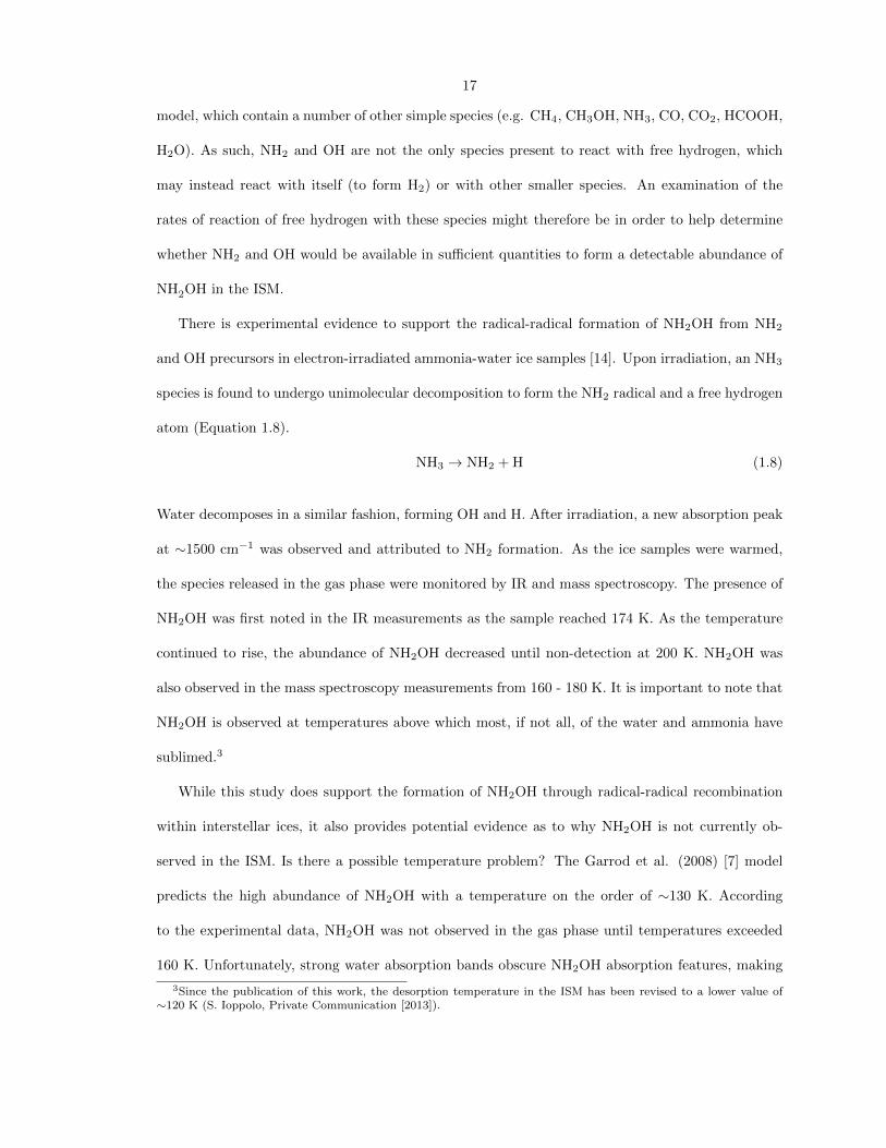
There is experimental evidence to support the radical-radical formation of NH2OH from NH2

and OH precursors in electron-irradiated ammonia-water ice samples [14]. Upon irradiation, an NH3

species is found to undergo unimolecular decomposition to form the NH2 radical and a free hydrogen

atom (Equation 1.8).

NH3 → NH2 + H (1.8)

Water decomposes in a similar fashion, forming OH and H. After irradiation, a new absorption peak

at ∼1500 cm−1 was observed and attributed to NH2 formation. As the ice samples were warmed,

the species released in the gas phase were monitored by IR and mass spectroscopy. The presence of

NH2OH was first noted in the IR measurements as the sample reached 174 K. As the temperature

continued to rise, the abundance of NH2OH decreased until non-detection at 200 K. NH2OH was

also observed in the mass spectroscopy measurements from 160 - 180 K. It is important to note that

NH2OH is observed at temperatures above which most, if not all, of the water and ammonia have

sublimed.3

While this study does support the formation of NH2OH through radical-radical recombination

within interstellar ices, it also provides potential evidence as to why NH2OH is not currently ob-

served in the ISM. Is there a possible temperature problem? The Garrod et al. (2008) [7] model

predicts the high abundance of NH2OH with a temperature on the order of ∼130 K. According

to the experimental data, NH2OH was not observed in the gas phase until temperatures exceeded

160 K. Unfortunately, strong water absorption bands obscure NH2OH absorption features, making

3Since the publication of this work, the desorption temperature in the ISM has been revised to a lower value of∼120 K (S. Ioppolo, Private Communication [2013]).

18

its detection using infrared observations towards hot core regions impossible. However, using the

temperature determined from the laboratory experiments as a basis for subsequent observations, for

regions where the temperature exceeds 160 K, detection in the gas phase should be possible using

millimeter wave observations. It is possible that the NH2OH emission is confined to very compact

(<5′′) hot core regions such as the SgrB2(N-LMH) [38], and that the single dish observations from

this survey are too beam-diluted to detect the emission from this compact region. As such, higher

spatial resolution interferometric observations are needed to more thoroughly couple to the higher

temperature regions in order to detect this species.

Alternatively, observations could be conducted towards molecular sources in shocked regions such

as the bipolar outflow L1157(B) or the Galactic Center. In these types of sources, molecules that

are formed on grain surfaces but that are not liberated into the gas phase by thermal desorption

due to low temperatures are instead ejected into the gas phase by shocks [39]. Detection of NH2OH

in these sources would provide valuable insight into the mechanisms behind its formation pathways

and eventual release into the gas phase.

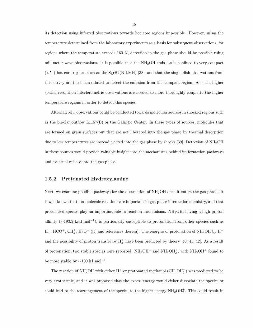
1.5.2 Protonated Hydroxylamine

Next, we examine possible pathways for the destruction of NH2OH once it enters the gas phase. It

is well-known that ion-molecule reactions are important in gas-phase interstellar chemistry, and that

protonated species play an important role in reaction mechanisms. NH2OH, having a high proton

affinity (∼193.5 kcal mol−1), is particularly susceptible to protonation from other species such as

H+3 , HCO+, CH+

5 , H3O+ ([5] and references therein). The energies of protonation of NH2OH by H+

and the possibility of proton transfer by H+3 have been predicted by theory [40; 41; 42]. As a result

of protonation, two stable species were reported: NH3OH+ and NH2OH+2 , with NH3OH+ found to

be more stable by ∼100 kJ mol−1.

The reaction of NH2OH with either H+ or protonated methanol (CH3OH+2 ) was predicted to be

very exothermic, and it was proposed that the excess energy would either dissociate the species or

could lead to the rearrangement of the species to the higher energy NH2OH+2 . This could result in

19

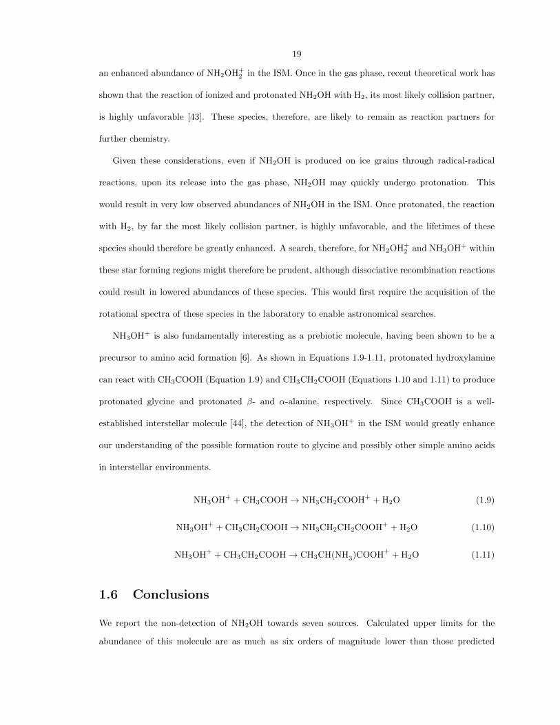
an enhanced abundance of NH2OH+2 in the ISM. Once in the gas phase, recent theoretical work has

shown that the reaction of ionized and protonated NH2OH with H2, its most likely collision partner,

is highly unfavorable [43]. These species, therefore, are likely to remain as reaction partners for

further chemistry.

Given these considerations, even if NH2OH is produced on ice grains through radical-radical

reactions, upon its release into the gas phase, NH2OH may quickly undergo protonation. This

would result in very low observed abundances of NH2OH in the ISM. Once protonated, the reaction

with H2, by far the most likely collision partner, is highly unfavorable, and the lifetimes of these

species should therefore be greatly enhanced. A search, therefore, for NH2OH+2 and NH3OH+ within

these star forming regions might therefore be prudent, although dissociative recombination reactions

could result in lowered abundances of these species. This would first require the acquisition of the

rotational spectra of these species in the laboratory to enable astronomical searches.

NH3OH+ is also fundamentally interesting as a prebiotic molecule, having been shown to be a

precursor to amino acid formation [6]. As shown in Equations 1.9-1.11, protonated hydroxylamine

can react with CH3COOH (Equation 1.9) and CH3CH2COOH (Equations 1.10 and 1.11) to produce

protonated glycine and protonated β- and α-alanine, respectively. Since CH3COOH is a well-

established interstellar molecule [44], the detection of NH3OH+ in the ISM would greatly enhance

our understanding of the possible formation route to glycine and possibly other simple amino acids

in interstellar environments.

NH3OH+ + CH3COOH→ NH3CH2COOH+ + H2O (1.9)

NH3OH+ + CH3CH2COOH→ NH3CH2CH2COOH+ + H2O (1.10)

NH3OH+ + CH3CH2COOH→ CH3CH(NH3)COOH+

+ H2O (1.11)

1.6 Conclusions

We report the non-detection of NH2OH towards seven sources. Calculated upper limits for the

abundance of this molecule are as much as six orders of magnitude lower than those predicted

20

for the species by recent models. Several factors could account for this discrepancy, including the

rapid removal of precursor molecules from ice mantles through reaction with free hydrogen or the

rapid protonation (and subsequent dissociative recombination) of NH2OH by H+, H+3 , CH+

5 , and

other efficient protonation mechanisms. The single dish observations presented here are likely highly

beam-diluted. Higher-resolution interferometric observations could provide the sensitivity required

for detection, and therefore allow better refinement of models that currently predict the presence of

NH2OH in high abundance.

21

Chapter 2

Propynylidynium (l-C3H+ )

Significant portions of this chapter have been reproduced from “A search for l-C3H+ and l-C3H–

in Sgr B2(N), Sgr B2(OH), and the dark cloud TMC-1” by B.A. McGuire et al., Astrophysical

Journal, 774, 56 (2013) [45], “An observational investigation of the identity of B11244 (l-C3H+

/C3H– ?)” by B.A. McGuire et al., Astrophysical Journal, 783, 36 (2014) [46], and “A CSO Search

for l-C3H+ : detection in the Orion Bar PDR” by B.A. McGuire et al., Monthly Notices of the

Royal Astronomical Society, 442, 2901 (2014) [47].

2.1 A Brief History of l-C3H+

The identification and characterization of molecular species in the interstellar medium (ISM) has

traditionally followed a linear progression. Species of interest, perhaps highlighted by chemical

models, are obtained or produced in the laboratory, and their characteristic spectra (rotational,

vibrational, etc.) are measured. These spectra are fit to constants unique to each species that

can then be used, with knowledge of the Hamiltonian, to reproduce the spectra and predict the

appearance of additional features under interstellar conditions. Observations of either the measured

lab features or calculated transitions in the ISM can then be used to unambiguously identify and

characterize new molecules in astronomical environments.

In 2012, Pety et al. reported the detection of a series of eight transitions arising from an uniden-

tified molecular carrier in an Institut de Radioastronomie Millimtrique (IRAM) 30 m telescope

spectral line survey of the Horsehead Photodissociation Region (PDR) [48]. The pattern present

in the transitions indicated a closed-shell linear molecule in its electronic ground state. Based on

this assumption, Pety et al. (2012) fit the transitions using a standard linear-rotor Hamiltonian and

derived the rotational constants shown in Table 2.1. Although no laboratory work was found in the

22

Table 2.1: Results of the spectroscopic fit of [48] to the eight unidentified transitions.

Parameter Value UnitB 11244.9512(0015) MHzD 7.766(040) kHzH 0.56(0.19) HzNote – Uncertainties given in parentheses

in units of the last significant digit.

literature for a linear molecule with such a constant, theoretical studies indicated the l-C3H+ cation

to be an excellent match [49].

Pety et al. (2012) [48] further bolster their assignment by examining the chemistry of l-C3H+

in the Horsehead PDR using the Muedon PDR code for gas-grain chemistry with the Ohio State

University gas-phase chemical network [50; 51]. They find that the dominant formation pathway is

through Reaction 2.1 of C2H2 with C+, while destruction occurs rapidly via Reactions 2.2 & 2.3

with H2.

C2H2

C+

−−→ C3H+ + H (2.1)

C3H+ H2−−→ C3H+2

e−−−→ C3H + H (2.2)

C3H+ H2−−→ C3H+3

e−−−→ C3H2 + H (2.3)

Indeed, these reactions are thought to be the most important gas-phase channels to form other small

hydrocarbons, like C3H and C3H2, which are widely observed in different environments [52; 53].

However, the observed abundances of C3H and C3H2 in PDRs are much higher than what pure gas-

phase models predict. One possible explanation is that polycyclic aromatic hydrocarbons (PAHs) are

fragmented into these small hydrocarbons in PDRs due to the strong UV fields (see, e.g., [54; 55; 56]).

Observations of l-C3H+ would thus brings further constraints to the formation pathways of the small

hydrocarbons in these environments, perhaps providing an alternative explanation for their over-

abundance.

Shortly after the initial detection by Pety et al. (2012) [48], Huang and co-workers challenged

the assignment of the carrier to l-C3H+ based on new, high-level theoretical calculations [57]. They

found that while their calculations for l-C3H+ agree (within typical accuracies) with the fitted value

of B from [48], their D constant differed by more than 40%, while their calculated value for H

differed by three orders of magnitude. These differences fall well outside the predicted accuracy of

the calculations, and form the basis for their dispute of the assignment to l-C3H+ .

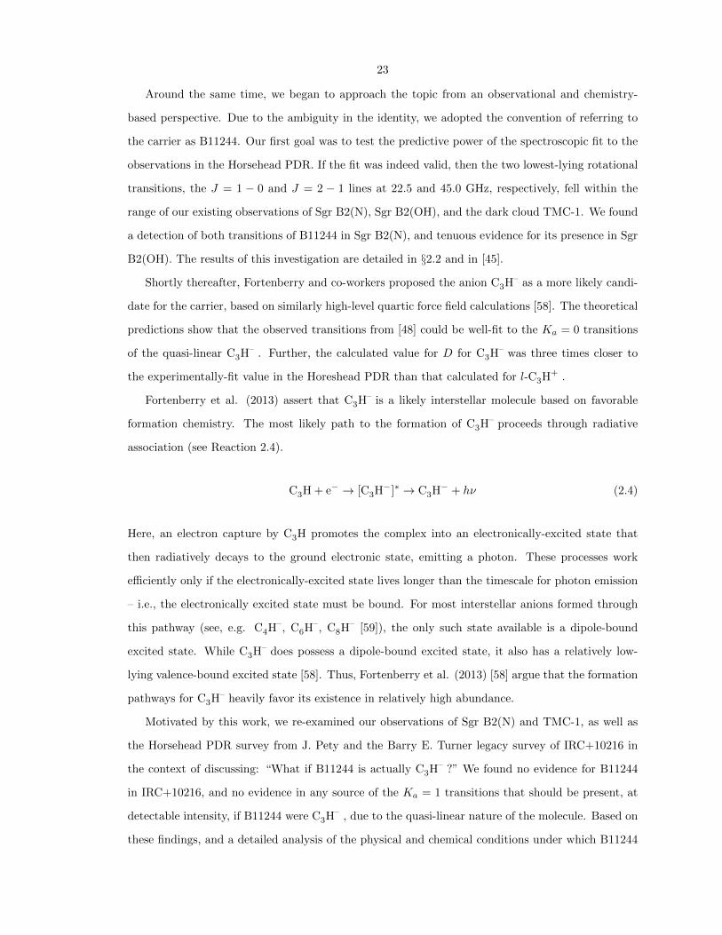
23

Around the same time, we began to approach the topic from an observational and chemistry-

based perspective. Due to the ambiguity in the identity, we adopted the convention of referring to

the carrier as B11244. Our first goal was to test the predictive power of the spectroscopic fit to the

observations in the Horsehead PDR. If the fit was indeed valid, then the two lowest-lying rotational

transitions, the J = 1 − 0 and J = 2 − 1 lines at 22.5 and 45.0 GHz, respectively, fell within the

range of our existing observations of Sgr B2(N), Sgr B2(OH), and the dark cloud TMC-1. We found

a detection of both transitions of B11244 in Sgr B2(N), and tenuous evidence for its presence in Sgr

B2(OH). The results of this investigation are detailed in §2.2 and in [45].

Shortly thereafter, Fortenberry and co-workers proposed the anion C3H– as a more likely candi-

date for the carrier, based on similarly high-level quartic force field calculations [58]. The theoretical

predictions show that the observed transitions from [48] could be well-fit to the Ka = 0 transitions

of the quasi-linear C3H– . Further, the calculated value for D for C3H– was three times closer to

the experimentally-fit value in the Horeshead PDR than that calculated for l-C3H+ .

Fortenberry et al. (2013) assert that C3H– is a likely interstellar molecule based on favorable

formation chemistry. The most likely path to the formation of C3H– proceeds through radiative

association (see Reaction 2.4).

C3H + e− → [C3H−]∗ → C3H− + hν (2.4)

Here, an electron capture by C3H promotes the complex into an electronically-excited state that

then radiatively decays to the ground electronic state, emitting a photon. These processes work

efficiently only if the electronically-excited state lives longer than the timescale for photon emission

– i.e., the electronically excited state must be bound. For most interstellar anions formed through

this pathway (see, e.g. C4H–, C6H–, C8H– [59]), the only such state available is a dipole-bound

excited state. While C3H– does possess a dipole-bound excited state, it also has a relatively low-

lying valence-bound excited state [58]. Thus, Fortenberry et al. (2013) [58] argue that the formation

pathways for C3H– heavily favor its existence in relatively high abundance.

Motivated by this work, we re-examined our observations of Sgr B2(N) and TMC-1, as well as

the Horsehead PDR survey from J. Pety and the Barry E. Turner legacy survey of IRC+10216 in

the context of discussing: “What if B11244 is actually C3H– ?” We found no evidence for B11244

in IRC+10216, and no evidence in any source of the Ka = 1 transitions that should be present, at

detectable intensity, if B11244 were C3H– , due to the quasi-linear nature of the molecule. Based on

these findings, and a detailed analysis of the physical and chemical conditions under which B11244

24

is to be and to not be present, we found no evidence to support the assignment of B11244 to C3H–.

The results of this investigation are detailed in §2.3 and in [46].

In early 2014, Brunken and co-workers [60] measured several transitions of l-C3H+ in the labora-

tory using mass-selective action spectroscopy, and confirmed the assignment of B11244 to

l-C3H+ . This was followed shortly thereafter by theoretical calculations accounting for the vibra-

tional coupling contributions of a shallow CCC bending potential, with the results further supporting

the attribution to l-C3H+ [61].

Finally, while the question of identity has now been resolved, questions remain surrounding the

formation conditions and chemical implications of l-C3H+ . Because l-C3H+ has been definitively

detected in only two environments – the Horsehead PDR and Sgr B2(N) – efforts to explore these

questions are hampered by a lack of information. In an attempt to address this deficiency, we

conducted a wide search of PDRs and complex molecular sources in search of l-C3H+ . In §2.4 and

in [47], we present the results of a brief, targeted campaign of 14 astronomical sources with the

Caltech Submillimeter Observatory (CSO) covering the J = 10 − 9 and J = 12 − 11 transitions of

l-C3H+ . We also examine the J = 10− 9 transition in broadband unbiased line surveys of a further

25 sources.

25

2.2 A Search for l-C3H+ and l-C3H in Sgr B2(N), Sgr B2(OH),

and the Dark Cloud TMC-1

The identification by Pety et al. (2012) [48] of l-C3H+ is significant – the number of molecular

species detected in the ISM via rotational transitions without the a priori knowledge of laboratory

spectra or constants is quite small. Notable among these is the detection of the HCO+ ion, popularly

attributed to unidentified features in observations by Buhl and Snyder in 1970 [62] dubbed “xogen,”

but not definitively detected until laboratory measurements were available nearly six years later

[63] following the suggested theoretical assignment of Klemperer (1970) [64]. The N2H+ ion was

detected in 1975 [65; 66] following observation in 1974 [67], which was confirmed by laboratory

studies in 1976 [68]. Shortly thereafter, Guelin, Green, & Thaddeus identified the C3N [69] and

C4H [70] radicals based on their observations, which were confirmed by theoretical studies [71] and

laboratory measurements several years later [72]. More recently, strong evidence for the detection

of the C5N– anion has been found towards IRC+10216 in work by Cernicharo et al. (2008) [73],

supported by the ab initio calculations of Botschwina et al. (2008) [74].

In light of the work by Huang et al. (2013) [57], we examined observational data toward three

sources beyond the Horsehead PDR – Sgr B2(N), Sgr B2(OH), and TMC-1 – in an attempt to

confirm the robustness of the spectroscopic fit determined in [48], and to provide context for the

debate. The results of those observations are presented here.

2.2.1 Observations

The cm-wave data presented here towards Sgr B2(N) were taken as part of the PRebiotic Interstellar

MOlecular Survey (PRIMOS) project using the National Radio Astronomy Observatory’s (NRAO)

100-m Robert C. Byrd Green Bank Telescope. The PRIMOS key project began in January of 2008,

and observations continue to expand its frequency coverage. This project provides high-resolution,

high-sensitivity spectra of the Sgr B2(N-LMH) complex centered at (J2000) α = 17h47m19s.8, δ

= -2822′17′′ with nearly continuous frequency coverage from 1 - 50 GHz. The 2 mm observations

(hereafter the Turner Survey) were conduced by Barry E. Turner using the NRAO 12-m Telescope on

Kitt Peak between 1993 – 1995 towards a number of sources, including Sgr B2(N) and the associated

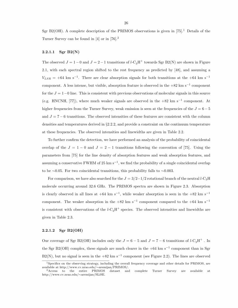
26

Sgr B2(OH). A complete description of the PRIMOS observations is given in [75].1 Details of the

Turner Survey can be found in [4] or in [76].2

2.2.1.1 Sgr B2(N)

The observed J = 1− 0 and J = 2− 1 transitions of l-C3H+ towards Sgr B2(N) are shown in Figure

2.1, with each spectral region shifted to the rest frequency as predicted by [48], and assuming a

VLSR = +64 km s−1. There are clear absorption signals for both transitions at the +64 km s−1

component. A less intense, but visible, absorption feature is observed in the +82 km s−1 component

for the J = 1−0 line. This is consistent with previous observations of molecular signals in this source

(e.g. HNCNH, [77]), where much weaker signals are observed in the +82 km s−1 component. At

higher frequencies from the Turner Survey, weak emission is seen at the frequencies of the J = 6− 5

and J = 7− 6 transitions. The observed intensities of these features are consistent with the column

densities and temperatures derived in §2.2.2, and provide a constraint on the continuum temperature

at these frequencies. The observed intensities and linewidths are given in Table 2.2.

To further confirm the detection, we have performed an analysis of the probability of coincidental

overlap of the J = 1 − 0 and J = 2 − 1 transitions following the convention of [75]. Using the

parameters from [75] for the line density of absorption features and weak absorption features, and

assuming a conservative FWHM of 25 km s−1, we find the probability of a single coincidental overlap

to be ∼0.05. For two coincidental transitions, this probability falls to ∼0.003.

For comparison, we have also searched for the J = 3/2−1/2 rotational branch of the neutral l-C3H

molecule occurring around 32.6 GHz. The PRIMOS spectra are shown in Figure 2.3. Absorption

is clearly observed in all lines at +64 km s−1, while weaker absorption is seen in the +82 km s−1

component. The weaker absorption in the +82 km s−1 component compared to the +64 km s−1

is consistent with observations of the l-C3H+ species. The observed intensities and linewidths are

given in Table 2.3.

2.2.1.2 Sgr B2(OH)

Our coverage of Sgr B2(OH) includes only the J = 6 − 5 and J = 7 − 6 transitions of l-C3H+ . In

the Sgr B2(OH) complex, these signals are much clearer in the +64 km s−1 component than in Sgr

B2(N), but no signal is seen in the +82 km s−1 component (see Figure 2.2). The lines are observed

1Specifics on the observing strategy, including the overall frequency coverage and other details for PRIMOS, areavailable at http://www.cv.nrao.edu/∼aremijan/PRIMOS/.

2Access to the entire PRIMOS dataset and complete Turner Survey are available athttp://www.cv.nrao.edu/∼aremijan/SLiSE.

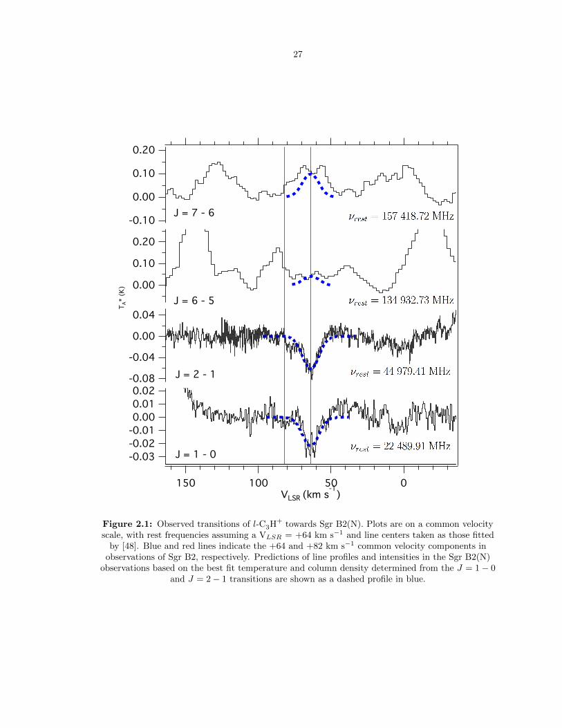
27

-0.03

-0.02

-0.01

0.00

0.01

0.02

150 100 50 0VLSR (km s

-1)

-0.08

-0.04

0.00

0.04

0.20

0.10

0.00

-0.10

0.20

0.10

0.00

TA*

(K)

Vrest = 22489.91 MHz

J = 1 - 0

J = 2 - 1

J = 6 - 5

J = 7 - 6

Figure 2.1: Observed transitions of l-C3H+ towards Sgr B2(N). Plots are on a common velocityscale, with rest frequencies assuming a VLSR = +64 km s−1 and line centers taken as those fitted

by [48]. Blue and red lines indicate the +64 and +82 km s−1 common velocity components inobservations of Sgr B2, respectively. Predictions of line profiles and intensities in the Sgr B2(N)

observations based on the best fit temperature and column density determined from the J = 1− 0and J = 2− 1 transitions are shown as a dashed profile in blue.

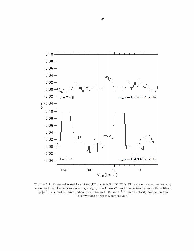
28

0.10

0.08

0.06

0.04

0.02

0.00

-0.02

-0.04

0.10

0.08

0.06

0.04

0.02

0.00

-0.02

-0.04

150 100 50 0

VLSR (km s-1

)

TA*

(K)

Vrest = 22489.91 MHz

J = 6 - 5

J = 7 - 6

Figure 2.2: Observed transitions of l-C3H+ towards Sgr B2(OH). Plots are on a common velocityscale, with rest frequencies assuming a VLSR = +64 km s−1 and line centers taken as those fitted

by [48]. Blue and red lines indicate the +64 and +82 km s−1 common velocity components inobservations of Sgr B2, respectively.

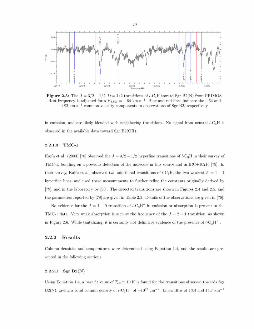
29

-0.10

-0.05

0.00

0.05

TA*

(K)

32670326603265032640326303262032610

Frequency (MHz)

(f)

F =

2 -

1

(f)

F =

1 -

0

(e)

F =

1 -

0

(e)

F =

2 -

1

(e)

F =

1 -

1

(f)

F =

1 -

1

Figure 2.3: The J = 3/2− 1/2, Ω = 1/2 transitions of l-C3H toward Sgr B2(N) from PRIMOS.Rest frequency is adjusted for a VLSR = +64 km s−1. Blue and red lines indicate the +64 and

+82 km s−1 common velocity components in observations of Sgr B2, respectively.

in emission, and are likely blended with neighboring transitions. No signal from neutral l-C3H is

observed in the available data toward Sgr B2(OH).

2.2.1.3 TMC-1

Kaifu et al. (2004) [78] observed the J = 3/2− 1/2 hyperfine transitions of l-C3H in their survey of

TMC-1, building on a previous detection of the molecule in this source and in IRC+10216 [79]. In

their survey, Kaifu et al. observed two additional transitions of l-C3H, the two weakest F = 1 − 1

hyperfine lines, and used these measurements to further refine the constants originally derived by

[79], and in the laboratory by [80]. The detected transitions are shown in Figures 2.4 and 2.5, and

the parameters reported by [78] are given in Table 2.3. Details of the observations are given in [78].

No evidence for the J = 1 − 0 transition of l-C3H+ in emission or absorption is present in the

TMC-1 data. Very weak absorption is seen at the frequency of the J = 2 − 1 transition, as shown

in Figure 2.6. While tantalizing, it is certainly not definitive evidence of the presence of l-C3H+ .

2.2.2 Results

Column densities and temperatures were determined using Equation 1.4, and the results are pre-

sented in the following sections.

2.2.2.1 Sgr B2(N)

Using Equation 1.4, a best fit value of Tex ' 10 K is found for the transitions observed towards Sgr

B2(N), giving a total column density of l-C3H+ of ∼1013 cm−2. Linewidths of 13.4 and 14.7 km−1

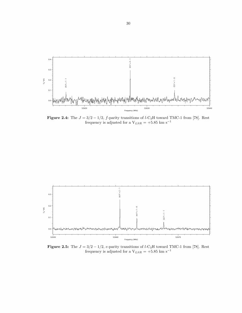
30

0.4

0.3

0.2

0.1

0.0

TA*

(K)

326403263032620

Frequency (MHz)

(f)

F =

2 -

1

(f)

F =

1 -

0

(f)

F =

1 -

1

Figure 2.4: The J = 3/2− 1/2, f -parity transitions of l-C3H toward TMC-1 from [78]. Restfrequency is adjusted for a VLSR = +5.85 km s−1

0.3

0.2

0.1

0.0

TA*

(K)

326703266032650

Frequency (MHz)

(e)

F =

1 -

0

(e)

F =

2 -

1

(e)

F =

1 -

1

Figure 2.5: The J = 3/2− 1/2, e-parity transitions of l-C3H toward TMC-1 from [78]. Restfrequency is adjusted for a VLSR = +5.85 km s−1

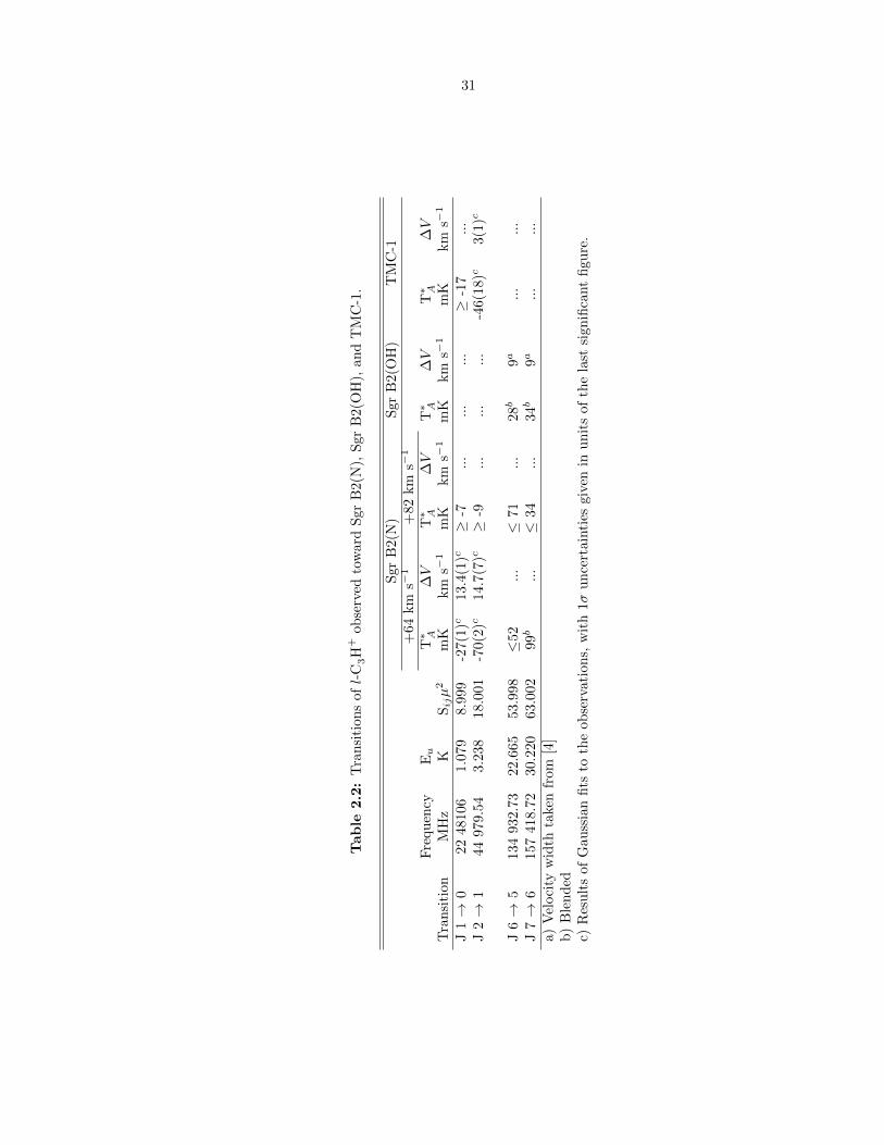
31

Tab

le2.2

:T

ran

siti

on

sofl-

C3H

+ob

serv

edto

ward

Sgr

B2(N

),S

gr

B2(O

H),

an

dT

MC

-1.

Sgr

B2(N

)S

gr

B2(O

H)

TM

C-1

+64

km

s−1

+82

km

s−1

Fre

qu

ency

Eu

T∗ A

∆V

T∗ A

∆V

T∗ A

∆V

T∗ A

∆V

Tra

nsi

tion

MH

zK

Sijµ2

mK

km

s−1

mK

km

s−1

mK

km

s−1

mK

km

s−1

J1→

022

4810

61.

079

8.9

99

-27(1

)c13.4

(1)c

≥-7

...

...

...

≥-1

7..

.J

2→

144

979.

543.

238

18.0

01

-70(2

)c14.7

(7)c

≥-9

...

...

...

-46(1

8)c

3(1

)c

J6→

513

493

2.73

22.6

6553.9

98

≤52

...

≤71

...

28b

9a..

...

.J

7→

615

741

8.72

30.2

2063.0

02

99b

...

≤34

...

34b

9a..

...

.a)

Vel

oci

tyw

idth

take

nfr

om[4

]b

)B

len

ded

c)R

esult

sof

Gau

ssia

nfi

tsto

the

ob

serv

ati

on

s,w

ith

1σu

nce

rtain

ties

giv

enin

un

its

of

the

last

sign

ifica

nt

figu

re.

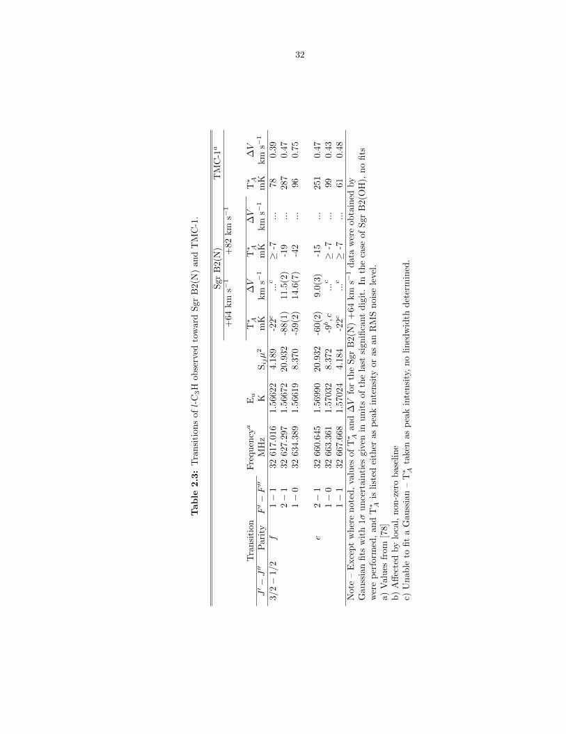
32

Tab

le2.3

:T

ran

siti

on

sofl-

C3H

ob

serv

edto

ward

Sgr

B2(N

)an

dT

MC

-1.

Sgr

B2(N

)T

MC

-1a

+64

km

s−1

+82

km

s−1

Tra

nsi

tion

Fre

qu

ency

aEu

T∗ A

∆V

T∗ A

∆V

T∗ A

∆V

J′−J′′

Par

ity

F′−F′′

MH

zK

Sijµ2

mK

km

s−1

mK

km

s−1

mK

km

s−1

3/2−

1/2

f1−

132

617.0

16

1.5

6622

4.1

89

-22c

...c

≥-7

...

78

0.3

92−

132

627.2

97

1.5

6672

20.9

32

-88(1

)11.5

(2)

-19

...

287

0.4

71−

032

634.3

89

1.5

6619

8.3

70

-59(2

)14.6

(7)

-42

...

96

0.7

5

e2−

132

660.6

45

1.5

6990

20.9

32

-60(2

)9.0

(3)

-15

...

251

0.4

71−

032

663.3

61

1.5

7032

8.3

72

-9b,c

...c

≥-7

...

99

0.4

31−

132

667.6

68

1.5

7024

4.1

84

-22c

...c

≥-7

...

61

0.4

8N

ote

–E

xce

pt

wh

ere

not

ed,

valu

esof

T∗ A

an

d∆V

for

the

Sgr

B2(N

)+

64

km

s−1

data

wer

eob

tain

edby

Gau

ssia

nfi

tsw

ith

1σ

un

cert

ainti

esgiv

enin

un

its

of

the

last

sign

ifica

nt

dig

it.

Inth

eca

seof

Sgr

B2(O

H),

no

fits

wer

ep

erfo

rmed

,an

dT∗ A

isli

sted

eith

eras

pea

kin

ten

sity

or

as

an

RM

Sn

ois

ele

vel.

a)V

alu

esfr

om[7

8]b

)A

ffec

ted

by

loca

l,n

on-z

ero

base

lin

ec)

Un

able

tofi

ta

Gau

ssia

n–

T∗ A

take

nas

pea

kin

ten

sity

,n

oli

ned

wid

thd

eter

min

ed.

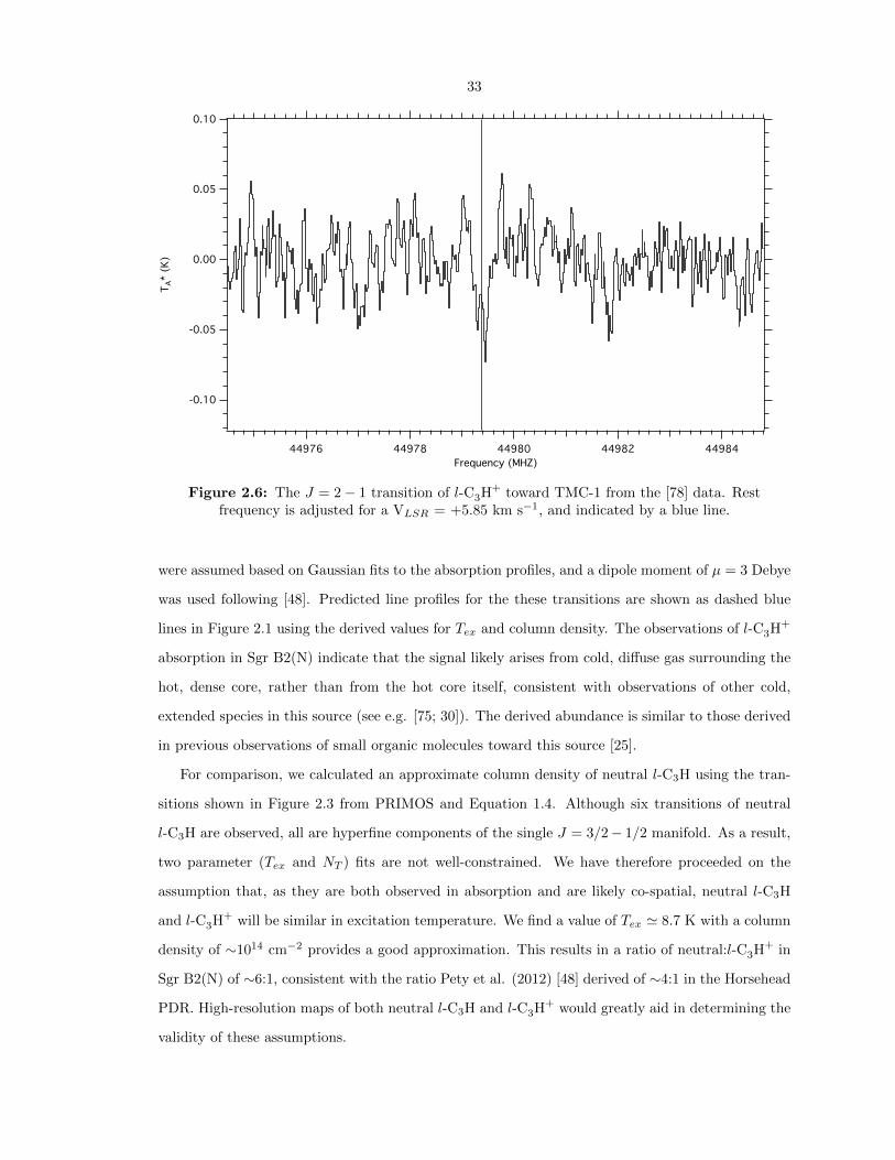
33

-0.10

-0.05

0.00

0.05

0.10

TA*

(K)

4498444982449804497844976

Frequency (MHZ)

Figure 2.6: The J = 2− 1 transition of l-C3H+ toward TMC-1 from the [78] data. Restfrequency is adjusted for a VLSR = +5.85 km s−1, and indicated by a blue line.

were assumed based on Gaussian fits to the absorption profiles, and a dipole moment of µ = 3 Debye

was used following [48]. Predicted line profiles for the these transitions are shown as dashed blue

lines in Figure 2.1 using the derived values for Tex and column density. The observations of l-C3H+

absorption in Sgr B2(N) indicate that the signal likely arises from cold, diffuse gas surrounding the

hot, dense core, rather than from the hot core itself, consistent with observations of other cold,

extended species in this source (see e.g. [75; 30]). The derived abundance is similar to those derived

in previous observations of small organic molecules toward this source [25].

For comparison, we calculated an approximate column density of neutral l-C3H using the tran-

sitions shown in Figure 2.3 from PRIMOS and Equation 1.4. Although six transitions of neutral

l-C3H are observed, all are hyperfine components of the single J = 3/2− 1/2 manifold. As a result,

two parameter (Tex and NT ) fits are not well-constrained. We have therefore proceeded on the

assumption that, as they are both observed in absorption and are likely co-spatial, neutral l-C3H

and l-C3H+ will be similar in excitation temperature. We find a value of Tex ' 8.7 K with a column

density of ∼1014 cm−2 provides a good approximation. This results in a ratio of neutral:l-C3H+ in

Sgr B2(N) of ∼6:1, consistent with the ratio Pety et al. (2012) [48] derived of ∼4:1 in the Horsehead

PDR. High-resolution maps of both neutral l-C3H and l-C3H+ would greatly aid in determining the

validity of these assumptions.

34

The observed behavior of l-C3H+ in moving from absorption to emission with increasing fre-

quency is not unique to this molecule in Sgr B2(N). For example, CH2OHCHO [30], CNCHO [81],

CH3CHO [82], and especially HCCCHO (R. Loomis, private communication), among others (includ-

ing CH3OH and H2CO), display similar behavior. This is largely a function of decreasing continuum

temperature with frequency. In fact, the J = 6 − 5 and J = 7 − 6 transitions provide a constraint

on the background continuum temperatures above the CMB of ∼1 K at 135 GHz, and ∼0.5 K at

157 GHz.

2.2.2.2 Sgr B2(OH)

In Sgr B2(OH), only two lines fall within the frequency of the Turner Survey observations, the lower

of which (at 135 GHz) is clearly blended (see Figure 2.2). As such, here we calculate only an upper

limit to l-C3H+ column density on the assumption that all of the emission at the peak of each signal

arises from l-C3H+ . A line width of 9 km s−1 was assumed based on the analysis of nearby spectral

regions from the same dataset by [4]. Based on these values, a best fit Tex of ∼79 K gives an upper

limit on the column density of ≤ 1.5× 1013 cm−2.

2.2.2.3 TMC-1

The lack of any definitive signal from l-C3H+ towards TMC-1 precludes any quantitative determina-

tion of a column density. However, assuming the weak absorption signal at 44.9 GHz does arise from

J = 2 − 1 of l-C3H+ , a zeroth-order approximation of the column density can be obtained using

Equation 1.4 and an estimated temperature of ∼9 K [83]. Such an analysis results in an estimated

upper limit to the column density of ∼6× 1011 cm−2.

For comparison, the column density of neutral l-C3H, assuming the same temperature of ∼9 K,

is ∼9 × 1012 cm−2 in this source. This results in a ratio of 15:1, two and a half times that in Sgr

B2(N), and almost four times that in the Horsehead PDR. Given the large uncertainties involved,

however, these numbers are not inconsistent.

2.2.3 Spectral Fitting

The spectroscopic parameters and line list for l-C3H+ as listed in the CDMS catalog is accessible

in full via www.splatalogue.net. Huang et al. (2013) [57] question the assignment of the observed

transitions to l-C3H+ based on large discrepancies between observed and calculated values for the

D and H distortion constants. The predictions of [48] were robust enough to predict the J = 1− 0

35

and J = 2− 1 transitions presented in §2.2.1.1. However, in an effort to confirm their values for the

D and H constants, we have refit the molecular signals using the frequencies for the J = 1− 0 and

J = 2− 1 transitions determined from our observations.

The observed transitions of l-C3H+ were fit using the CALPGM [84] program suite, using a

standard linear rotor Hamiltonian giving energies as shown in Equation 2.5.

E(J) = BJ(J + 1)−D(J(J + 1))2 +H(J(J + 1))3 + L(J(J + 1))4 +M(J(J + 1))5 + (...) (2.5)

CALPGM is designed to fit spectroscopic constants of a model Hamiltonian to a set of observed

transitions using an iterative least-squares fitting algorithm. Following Pety et al. (2012) [48], we

include first (D) and second (H) order centrifugal distortion constants in the Hamiltonian, producing

a fit to the unshifted transitions with an RMS observed minus calculated value of 0.0862 MHz, below

the average observational uncertainty of 0.1015 MHz. Addition of higher order terms L and M in

equation 2.5 is found to improve the RMS of the fit by ∼10 kHz for each additional term, and

give a RMS change in the predicted frequencies of ∼90 kHz and 80 kHz for L and M respectively.

These corrections are below the experimental uncertainty, and therefore of questionable physical

significance; thus, only the first and second order corrections are included in the final fits. As a final

step, the 1σ uncertainty of all fit parameters was computed using the PIFORM program.3

The spectral resolution of the PRIMOS observations is significantly higher than those from

[48]; ∼21 kHz versus 49 and 195 kHz. However, the linewidths of the observed transitions in Sgr

B2(N) used in the fit are broad compared to those observed by Pety et al. (2012) [48] in the

Horsehead PDR (13.3 & 14.7 km s−1 versus ∼1 km s−1), thus introducing additional uncertainty in

the measurement of the line centers. Further, as discussed by Pety et al. (2012) [48], the absolute

accuracy of the spectroscopic constants is determined by the accuracy to which the VLSR velocity of

l-C3H+ emission is known. The use of two independent observational datasets towards two separate

sources compounds this issue.

While we cannot mitigate the uncertainty due to the broad lineshapes, we have attempted to

minimize the effects of uncertainty in VLSR. To account for this, a minimization of the fit RMS was

performed by varying the VLSR offsets for the PRIMOS dataset and the IRAM dataset independently

over a range of -3 km s−1 to +3 km s−1. The results of this analysis indicate that convergence is

quickly reached with minimal variation in either dataset. Based on their observations of similar

molecules, Pety et al. (2012) [48] determined an uncertainty level of ±0.2 km s−1 for the IRAM

3Z. Kisiel, PIFORM available at http://www.ifpan.edu.pl/∼kisiel/asym/asym.htm#piform

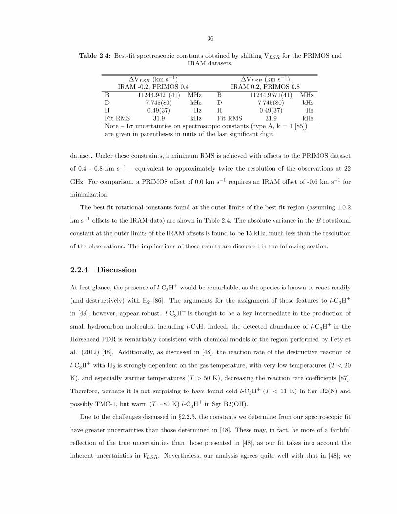
36

Table 2.4: Best-fit spectroscopic constants obtained by shifting VLSR for the PRIMOS andIRAM datasets.

∆VLSR (km s−1) ∆VLSR (km s−1)IRAM -0.2, PRIMOS 0.4 IRAM 0.2, PRIMOS 0.8

B 11244.9421(41) MHz B 11244.9571(41) MHzD 7.745(80) kHz D 7.745(80) kHzH 0.49(37) Hz H 0.49(37) HzFit RMS 31.9 kHz Fit RMS 31.9 kHzNote – 1σ uncertainties on spectroscopic constants (type A, k = 1 [85])are given in parentheses in units of the last significant digit.

dataset. Under these constraints, a minimum RMS is achieved with offsets to the PRIMOS dataset

of 0.4 - 0.8 km s−1 – equivalent to approximately twice the resolution of the observations at 22

GHz. For comparison, a PRIMOS offset of 0.0 km s−1 requires an IRAM offset of -0.6 km s−1 for

minimization.

The best fit rotational constants found at the outer limits of the best fit region (assuming ±0.2

km s−1 offsets to the IRAM data) are shown in Table 2.4. The absolute variance in the B rotational

constant at the outer limits of the IRAM offsets is found to be 15 kHz, much less than the resolution

of the observations. The implications of these results are discussed in the following section.

2.2.4 Discussion

At first glance, the presence of l-C3H+ would be remarkable, as the species is known to react readily

(and destructively) with H2 [86]. The arguments for the assignment of these features to l-C3H+

in [48], however, appear robust. l-C3H+ is thought to be a key intermediate in the production of

small hydrocarbon molecules, including l-C3H. Indeed, the detected abundance of l-C3H+ in the

Horsehead PDR is remarkably consistent with chemical models of the region performed by Pety et

al. (2012) [48]. Additionally, as discussed in [48], the reaction rate of the destructive reaction of

l-C3H+ with H2 is strongly dependent on the gas temperature, with very low temperatures (T < 20

K), and especially warmer temperatures (T > 50 K), decreasing the reaction rate coefficients [87].

Therefore, perhaps it is not surprising to have found cold l-C3H+ (T < 11 K) in Sgr B2(N) and

possibly TMC-1, but warm (T ∼80 K) l-C3H+ in Sgr B2(OH).

Due to the challenges discussed in §2.2.3, the constants we determine from our spectroscopic fit

have greater uncertainties than those determined in [48]. These may, in fact, be more of a faithful

reflection of the true uncertainties than those presented in [48], as our fit takes into account the

inherent uncertainties in VLSR. Nevertheless, our analysis agrees quite well with that in [48]; we

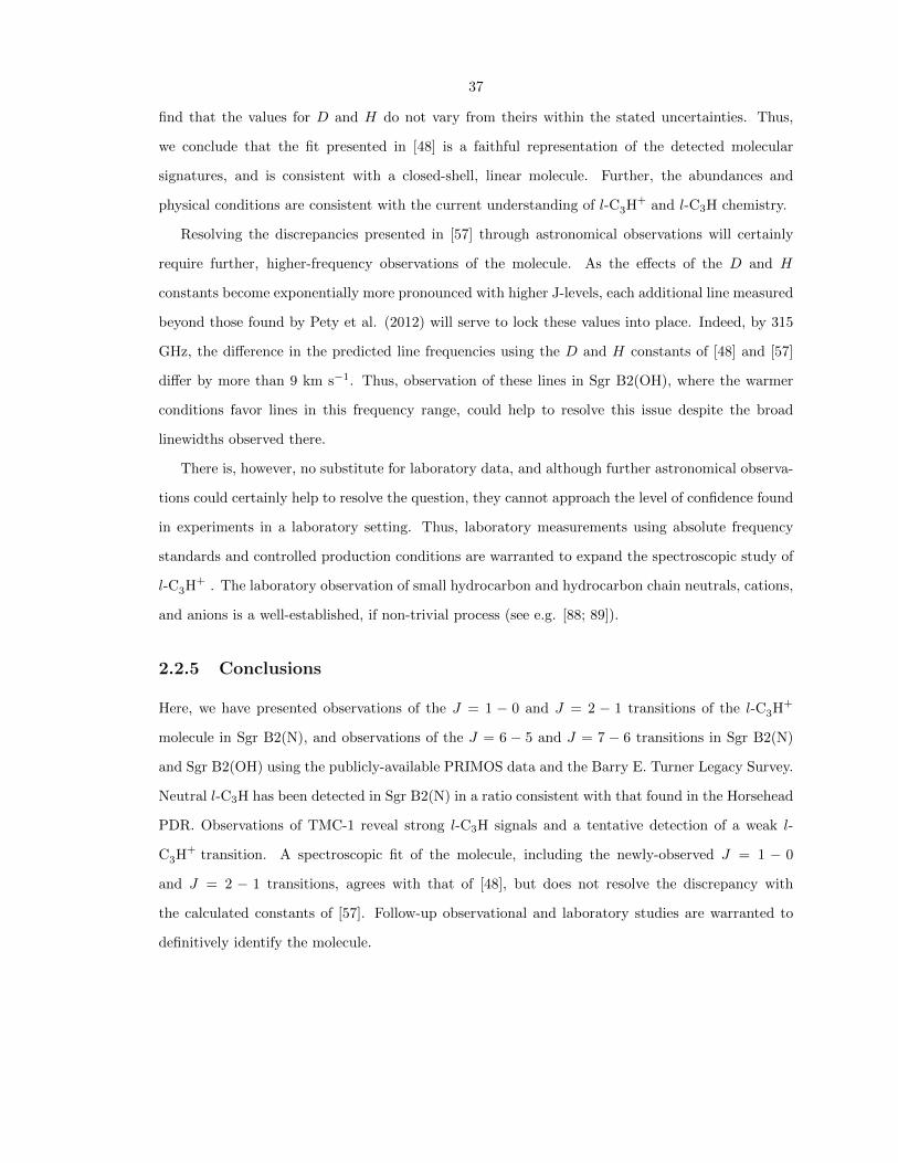
37

find that the values for D and H do not vary from theirs within the stated uncertainties. Thus,

we conclude that the fit presented in [48] is a faithful representation of the detected molecular

signatures, and is consistent with a closed-shell, linear molecule. Further, the abundances and

physical conditions are consistent with the current understanding of l-C3H+ and l-C3H chemistry.

Resolving the discrepancies presented in [57] through astronomical observations will certainly

require further, higher-frequency observations of the molecule. As the effects of the D and H

constants become exponentially more pronounced with higher J-levels, each additional line measured

beyond those found by Pety et al. (2012) will serve to lock these values into place. Indeed, by 315

GHz, the difference in the predicted line frequencies using the D and H constants of [48] and [57]

differ by more than 9 km s−1. Thus, observation of these lines in Sgr B2(OH), where the warmer

conditions favor lines in this frequency range, could help to resolve this issue despite the broad

linewidths observed there.

There is, however, no substitute for laboratory data, and although further astronomical observa-

tions could certainly help to resolve the question, they cannot approach the level of confidence found

in experiments in a laboratory setting. Thus, laboratory measurements using absolute frequency

standards and controlled production conditions are warranted to expand the spectroscopic study of

l-C3H+ . The laboratory observation of small hydrocarbon and hydrocarbon chain neutrals, cations,

and anions is a well-established, if non-trivial process (see e.g. [88; 89]).

2.2.5 Conclusions

Here, we have presented observations of the J = 1 − 0 and J = 2 − 1 transitions of the l-C3H+

molecule in Sgr B2(N), and observations of the J = 6 − 5 and J = 7 − 6 transitions in Sgr B2(N)

and Sgr B2(OH) using the publicly-available PRIMOS data and the Barry E. Turner Legacy Survey.

Neutral l-C3H has been detected in Sgr B2(N) in a ratio consistent with that found in the Horsehead

PDR. Observations of TMC-1 reveal strong l-C3H signals and a tentative detection of a weak l-

C3H+ transition. A spectroscopic fit of the molecule, including the newly-observed J = 1 − 0

and J = 2 − 1 transitions, agrees with that of [48], but does not resolve the discrepancy with

the calculated constants of [57]. Follow-up observational and laboratory studies are warranted to

definitively identify the molecule.

38

2.3 An Observational Investigation of the Identity of B11244

(l-C3H+ /C3H

– )

In this section, we re-examine the observations of Pety et al. (2012) [48] toward the Horsehead

PDR, as well as PRebiotic Interstellar MOlecular Survey (PRIMOS) observations of Sgr B2(N), the

Kaifu et al. (2004) [78] survey of TMC-1, and the Barry E. Turner legacy survey of IRC+10216

in the context of discussing: “What if B11244 is actually C3H– ?” Due to the uncertainty in the

assignment, here we adopt the convention of referring to the carrier as B11244. In §2.3.1, we discuss

the spectroscopy of C3H– using the properties derived by Fortenberry et al. (2013) [58], and present

simulated spectra. In §2.3.2, we briefly outline the observations used, and in §2.3.3 discuss the

analysis of these observations. Finally, in §2.3.4, we present the results of our findings, and discuss

them in the context of determining the identity of B11244.

2.3.1 Spectroscopic Analysis

Table 2.6 provides the rotational constants and dipole moments used in this work to describe B11244,

assuming it is l-C3H+ or C3H– . The spectroscopic constants and fit for l-C3H+ are provided in [48],

and their predictive power confirmed in [45]. Fortenberry et al. (2013) [58] provide a high-accuracy

equilibrium structure for C3H– , rotational constants, and dipole moments. These moments are not

in the principal axis (PA) system, but can readily be converted to the PA system with a simple

coordinate rotation resulting in µx → µa = 1.63 Debye and µy → µb = 1.41 Debye. Indeed, the

magnitude of this rotation is small, such that the value of these dipole moments remains essentially

unchanged. Were the observed transitions in [48] and [45] due to C3H– , they would be a-type,

Ka = 0 transitions, and thus (B + C) and DJ could be well-determined from these lines. To

obtain these constants, the observed transitions were fit using the CALPGM suite of programs.

An asymmetric-top Hamiltonian with a Watson S reduction in the Ir representation was used.4

The remaining constants were necessarily used as-is from the theoretical calculations. A simulated

spectrum of C3H– at 22 K using this combined set of constants is displayed in Figure 2.7. A full

CALPGM catalog for C3H– to 2 THz is also provided in Appendix B (see Table 2.5).

4Full details on the expressions and algorithms can be found in the CALPGM documentation and refs. therein.The interested reader may find that the analytical analysis presented in [90] provides a useful (and more approachable)approximation.

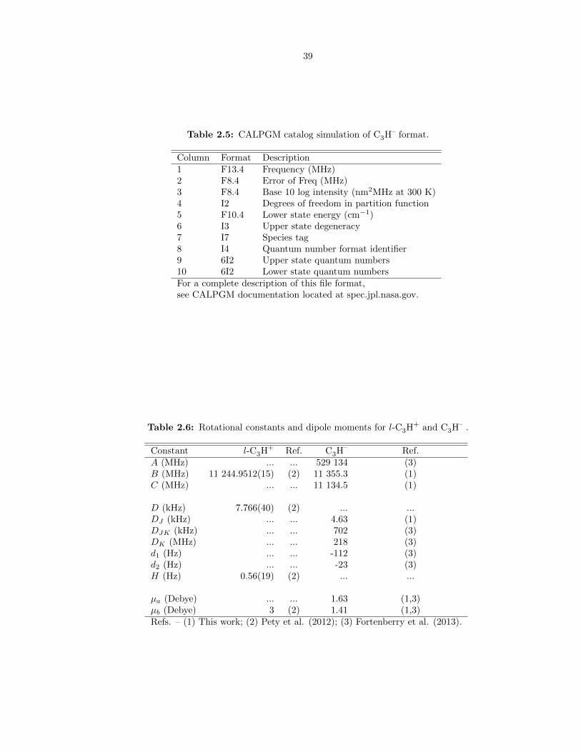
39

Table 2.5: CALPGM catalog simulation of C3H– format.

Column Format Description1 F13.4 Frequency (MHz)2 F8.4 Error of Freq (MHz)3 F8.4 Base 10 log intensity (nm2MHz at 300 K)4 I2 Degrees of freedom in partition function5 F10.4 Lower state energy (cm−1)6 I3 Upper state degeneracy7 I7 Species tag8 I4 Quantum number format identifier9 6I2 Upper state quantum numbers10 6I2 Lower state quantum numbersFor a complete description of this file format,see CALPGM documentation located at spec.jpl.nasa.gov.

Table 2.6: Rotational constants and dipole moments for l-C3H+ and C3H– .

Constant l-C3H+ Ref. C3H– Ref.A (MHz) ... ... 529 134 (3)B (MHz) 11 244.9512(15) (2) 11 355.3 (1)C (MHz) ... ... 11 134.5 (1)

D (kHz) 7.766(40) (2) ... ...DJ (kHz) ... ... 4.63 (1)DJK (kHz) ... ... 702 (3)DK (MHz) ... ... 218 (3)d1 (Hz) ... ... -112 (3)d2 (Hz) ... ... -23 (3)H (Hz) 0.56(19) (2) ... ...

µa (Debye) ... ... 1.63 (1,3)µb (Debye) 3 (2) 1.41 (1,3)Refs. – (1) This work; (2) Pety et al. (2012); (3) Fortenberry et al. (2013).

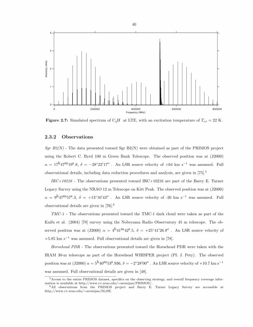
40

4

3

2

1

0

Inte

nsi

ty (

Arb

)

8000006000004000002000000

Frequency (MHz)

Figure 2.7: Simulated spectrum of C3H– at LTE, with an excitation temperature of Tex = 22 K.

2.3.2 Observations

Sgr B2(N) - The data presented toward Sgr B2(N) were obtained as part of the PRIMOS project

using the Robert C. Byrd 100 m Green Bank Telescope. The observed position was at (J2000)

α = 17h47m19s.8, δ = −2822′17′′ . An LSR source velocity of +64 km s−1 was assumed. Full

observational details, including data reduction procedures and analysis, are given in [75].5

IRC+10216 - The observations presented toward IRC+10216 are part of the Barry E. Turner

Legacy Survey using the NRAO 12 m Telescope on Kitt Peak. The observed position was at (J2000)

α = 9h47m57s.3, δ = +1316′43′′ . An LSR source velocity of -26 km s−1 was assumed. Full

observational details are given in [76].6

TMC-1 - The observations presented toward the TMC-1 dark cloud were taken as part of the

Kaifu et al. (2004) [78] survey using the Nobeyama Radio Observatory 45 m telescope. The ob-

served position was at (J2000) α = 4h41m42s.5, δ = +2541′26.9′′ . An LSR source velocity of

+5.85 km s−1 was assumed. Full observational details are given in [78].

Horsehead PDR - The observations presented toward the Horsehead PDR were taken with the

IRAM 30-m telescope as part of the Horsehead WHISPER project (PI: J. Pety). The observed

position was at (J2000) α = 5h40m53s.936, δ = −228′00′′ . An LSR source velocity of +10.7 km s−1

was assumed. Full observational details are given in [48].

5Access to the entire PRIMOS dataset, specifics on the observing strategy, and overall frequency coverage infor-mation is available at http://www.cv.nrao.edu/∼aremijan/PRIMOS/.

6All observations from the PRIMOS project and Barry E. Turner Legacy Survey are accessible athttp://www.cv.nrao.edu/∼aremijan/SLiSE.

41

2.3.3 Data Analysis

The column density of B11244 in each source, assuming local thermodynamic equilibrium (LTE), can

be calculated using Equation 1.4. In the case of l-C3H+ , the partition function is well-approximated

by the standard linear-molecule formula given by Eq. 2.6, with B expressed in Hz. For C3H– , Eq.

2.7, with σ = 1 and rotational constants with units of MHz, is appropriate [29]. The accuracy of Qr

for the anion is dependent on the accuracy of the rotational constants used. Thus, there is likely an

uncertainty of a few percent in the value of Qr used here. In any case, the partition function for the

anion rapidly outpaces that of the cation above Tex ∼ 8 K.

Qr (l-C3H+) ' kT

hB= 1.85(T ) (2.6)

Qr (C3H−) ' 5.34× 106

σ

(T 3

ABC

)1/2

= 0.65(Tex)3/2 (2.7)

To calculate upper limits of l-C3H+ in IRC+10216, we use the molecule-specific parameters

given in [45], and the upper limit ∆T ∗A and ∆V values given in Table 2.7. The line parameters and

molecule-specific parameters used for all C3H– calculations are given in Table 2.7.

While the observed Ka = 0 transitions allow us to constrain B and C reasonably well, the lack

of any confirmed detection of a Ka = 1 transition limits the overall accuracy in predicting the

frequencies of these lines. However, the expected intensity of these lines, given a derived column

density and temperature, is likely to be fairly accurate under LTE conditions. In the Horsehead

PDR, these lines should have a peak intensity of Tmb ∼ 20 − 28 mK for J ′′ = 3 to 6, using the

derived conditions from the Ka = 0 transitions. In Sgr B2(N), the expected intensities are below

detectable values in our observations.

We calculate a theoretical uncertainty in the center frequencies for these transitions of σ ∼ 370

MHz for the J = 4− 3 transition to as much as σ ∼ 650 MHz for the J = 7− 6 transition. At LTE,

the strongest of these lines fall within the 3 mm window of the Pety et al. (2012) [48] survey. Due to

the uncertainties in the line centers, we have searched a region equal to each transition’s uncertainty

on either side of each predicted line center. After identifying all known lines within this range, we

find no detection of any signals which could be assigned to a Ka = 1 transition of C3H− at the

RMS noise level of the observations (∼5− 10 mK), despite peak predicted intensities of 20 - 28 mK

at LTE. An example spectrum of the region searched around the predicted 41,4 − 31,3 transition is

shown in Figure 2.8.

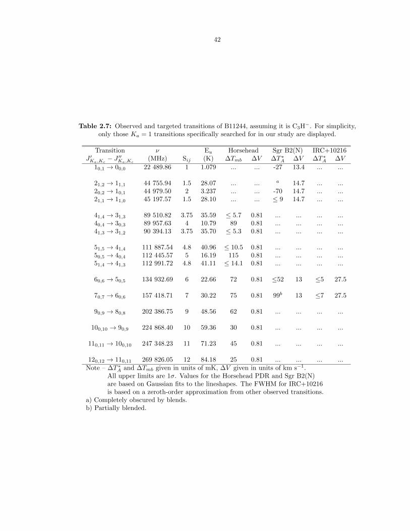
42

Table 2.7: Observed and targeted transitions of B11244, assuming it is C3H−. For simplicity,only those Ka = 1 transitions specifically searched for in our study are displayed.

Transition ν Eu Horsehead Sgr B2(N) IRC+10216J ′Ka,Kc

− J ′′Ka,Kc(MHz) Sij (K) ∆Tmb ∆V ∆T ∗A ∆V ∆T ∗A ∆V

10,1 → 00,0 22 489.86 1 1.079 ... ... -27 13.4 ... ...

21,2 → 11,1 44 755.94 1.5 28.07 ... ... a 14.7 ... ...20,2 → 10,1 44 979.50 2 3.237 ... ... -70 14.7 ... ...21,1 → 11,0 45 197.57 1.5 28.10 ... ... ≤ 9 14.7 ... ...

41,4 → 31,3 89 510.82 3.75 35.59 ≤ 5.7 0.81 ... ... ... ...40,4 → 30,3 89 957.63 4 10.79 89 0.81 ... ... ... ...41,3 → 31,2 90 394.13 3.75 35.70 ≤ 5.3 0.81 ... ... ... ...

51,5 → 41,4 111 887.54 4.8 40.96 ≤ 10.5 0.81 ... ... ... ...50,5 → 40,4 112 445.57 5 16.19 115 0.81 ... ... ... ...51,4 → 41,3 112 991.72 4.8 41.11 ≤ 14.1 0.81 ... ... ... ...

60,6 → 50,5 134 932.69 6 22.66 72 0.81 ≤52 13 ≤5 27.5

70,7 → 60,6 157 418.71 7 30.22 75 0.81 99b 13 ≤7 27.5

90,9 → 80,8 202 386.75 9 48.56 62 0.81 ... ... ... ...

100,10 → 90,9 224 868.40 10 59.36 30 0.81 ... ... ... ...

110,11 → 100,10 247 348.23 11 71.23 45 0.81 ... ... ... ...

120,12 → 110,11 269 826.05 12 84.18 25 0.81 ... ... ... ...Note – ∆T ∗A and ∆Tmb given in units of mK, ∆V given in units of km s−1.

All upper limits are 1σ. Values for the Horsehead PDR and Sgr B2(N)are based on Gaussian fits to the lineshapes. The FWHM for IRC+10216is based on a zeroth-order approximation from other observed transitions.

a) Completely obscured by blends.b) Partially blended.

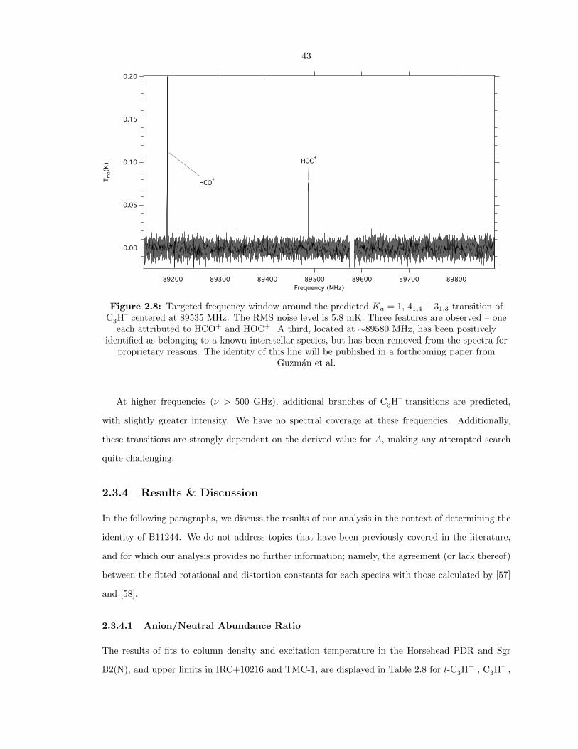
43

0.20

0.15

0.10

0.05

0.00

Tm

b(K

)

89800897008960089500894008930089200

Frequency (MHz)

HCO+

HOC+

V_rms = 0.00576301

Figure 2.8: Targeted frequency window around the predicted Ka = 1, 41,4 − 31,3 transition ofC3H– centered at 89535 MHz. The RMS noise level is 5.8 mK. Three features are observed – one

each attributed to HCO+ and HOC+. A third, located at ∼89580 MHz, has been positivelyidentified as belonging to a known interstellar species, but has been removed from the spectra for

proprietary reasons. The identity of this line will be published in a forthcoming paper fromGuzman et al.

At higher frequencies (ν > 500 GHz), additional branches of C3H– transitions are predicted,

with slightly greater intensity. We have no spectral coverage at these frequencies. Additionally,

these transitions are strongly dependent on the derived value for A, making any attempted search

quite challenging.

2.3.4 Results & Discussion

In the following paragraphs, we discuss the results of our analysis in the context of determining the

identity of B11244. We do not address topics that have been previously covered in the literature,

and for which our analysis provides no further information; namely, the agreement (or lack thereof)

between the fitted rotational and distortion constants for each species with those calculated by [57]

and [58].

2.3.4.1 Anion/Neutral Abundance Ratio

The results of fits to column density and excitation temperature in the Horsehead PDR and Sgr

B2(N), and upper limits in IRC+10216 and TMC-1, are displayed in Table 2.8 for l-C3H+ , C3H– ,

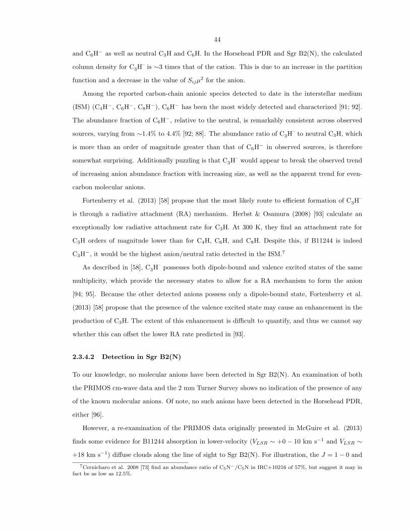
44

and C6H− as well as neutral C3H and C6H. In the Horsehead PDR and Sgr B2(N), the calculated

column density for C3H– is ∼3 times that of the cation. This is due to an increase in the partition

function and a decrease in the value of Sijµ2 for the anion.

Among the reported carbon-chain anionic species detected to date in the interstellar medium

(ISM) (C4H−, C6H−, C8H−), C6H− has been the most widely detected and characterized [91; 92].

The abundance fraction of C6H−, relative to the neutral, is remarkably consistent across observed

sources, varying from ∼1.4% to 4.4% [92; 88]. The abundance ratio of C3H– to neutral C3H, which

is more than an order of magnitude greater than that of C6H− in observed sources, is therefore

somewhat surprising. Additionally puzzling is that C3H– would appear to break the observed trend

of increasing anion abundance fraction with increasing size, as well as the apparent trend for even-

carbon molecular anions.

Fortenberry et al. (2013) [58] propose that the most likely route to efficient formation of C3H–

is through a radiative attachment (RA) mechanism. Herbst & Osamura (2008) [93] calculate an

exceptionally low radiative attachment rate for C3H. At 300 K, they find an attachment rate for

C3H orders of magnitude lower than for C4H, C6H, and C8H. Despite this, if B11244 is indeed

C3H−, it would be the highest anion/neutral ratio detected in the ISM.7

As described in [58], C3H– possesses both dipole-bound and valence excited states of the same

multiplicity, which provide the necessary states to allow for a RA mechanism to form the anion

[94; 95]. Because the other detected anions possess only a dipole-bound state, Fortenberry et al.

(2013) [58] propose that the presence of the valence excited state may cause an enhancement in the

production of C3H. The extent of this enhancement is difficult to quantify, and thus we cannot say

whether this can offset the lower RA rate predicted in [93].

2.3.4.2 Detection in Sgr B2(N)

To our knowledge, no molecular anions have been detected in Sgr B2(N). An examination of both

the PRIMOS cm-wave data and the 2 mm Turner Survey shows no indication of the presence of any

of the known molecular anions. Of note, no such anions have been detected in the Horsehead PDR,

either [96].

However, a re-examination of the PRIMOS data originally presented in McGuire et al. (2013)

finds some evidence for B11244 absorption in lower-velocity (VLSR ∼ +0− 10 km s−1 and VLSR ∼

+18 km s−1) diffuse clouds along the line of sight to Sgr B2(N). For illustration, the J = 1− 0 and

7Cernicharo et al. 2008 [73] find an abundance ratio of C5N−/C5N in IRC+10216 of 57%, but suggest it may infact be as low as 12.5%.

45

Tab

le2.8

:C

olu

mn

den

siti

esan

dex

cita

tion

tem

per

atu

res

forl-

C3H

+an

dC

3H

–in

ou

rob

serv

ati

on

san

dfr

om

the

lite

ratu

re,

as

wel

las

rati

os

of

thes

eto

thei

rn

eutr

alco

unte

rpart

s.L

iter

atu

reva

lues

for

the

rati

oof

C6H−

ton

eutr

al

C6H

are

als

osh

own

.

l-C

3H

+C

3H

–C

3H

l-C

3H

+/C

3H

C3H−

/C

3H

C6H−

/C

6H

Sou

rce

N(1

011

cm−1)

Tex(K

)N

(101

1cm−1)

Tex(K

)N

(101

1cm−1)

(%)

(%)

(%)

Hor

seh

ead

PD

R4.

8(9)

(1)

14(2

)(1)

12(1

)a22(4

)a21(7

)(1)

23(3

)57(1

6)

≤9

Sgr

B2(

N)

240(

30)b

8b

790(9

0)b

8b3000

(300)b

8(1

)26(8

)..

.c

IRC

+10

216

≤6

32

≤40

32

560

≤1.1

≤7.1

3(2

)(2)

TM

C-1

≤6d

9≤

250d

990(

3)

≤7

≤278

2.5

(0.4

)(4)

Not

e–

Un

cert

ainti

esar

egi

ven

inp

aren

thes

esin

un

its

of

the

last

sign

ifica

nt

dig

it,

an

dare

1σ.

All

valu

esw

ere

calc

ula

ted

for

this

work

un

less

oth

erw

ise

note

d.

Ref

s.–

(1)

[48]

(2)

[88]

(3)

[78]

(4)

[92]

a)T

oen

sure

con

sist

ency

wit

hth

el-

C3H

+va

lues

det

erm

ined

in[4

8],

thes

eva

lues

hav

eb

een

det

erm

ined

via

aro

tati

ond

iagr

aman

alysi

s.A

leas

t-sq

uare

sfi

tan

aly

sis

sugges

tsth

at

this

colu

mn

den

sity

may

act

uall

yb

ea

fact

or

of

2h

igh

er.

b)

Th

ese

valu

esar

esl

ightl

yre

vis

edfr

omth

ose

in[4

5].

Wh

ile

re-e

xam

inin

gth

ed

ata

for

this

stu

dy,

itb

ecam

ecl

ear

that

the

tran

siti

onat

45G

Hz,

rega

rdle

ssof

the

carr

ier,

isli

kely

hig

hly

sub

-th

erm

al.

We

ther

efore

base

ou

rfi

gu

res

her

eon

the

22.5

GH

ztr

ansi

tion

only

,an

dass

um

eth

e“st

an

dard

”8

Kex

cita

tion

tem

per

atu

res

for

cold

mole

cule

sin

this

sou

rce.

We

hav

eex

ten

ded

this

tem

per

atu

reto

ou

rp

revio

us

an

aly

sis

of

C3H

inth

isso

urc

e,as

wel

l.c)

Th

ere

hav

eb

een

no

rep

orte

dd

etec

tion

sof,

an

dw

ese

en

oev

iden

cefo

r,th

ep

rese

nce

of

C6H−

inS

gr

B2(N

).d

)B

ased

ona

tenta

tive

det

ecti

onof

the

45

GH

ztr

an

siti

on

on

ly,

wh

ich

,like

H2C

O,

dis

pla

ys

an

om

alo

us

ab

sorp

tion

agai

nst

the

2.7

KC

MB

inth

isso

urc

e.

46

J = 2− 1 transitions of B11244 are shown in Figure 2.9 in comparison to the known CH absorption

spectra toward SgrB2(N)8. The strongest observed transition of l-C3H is also shown and displays

low-velocity absorption as well, although the ∼0 km s−1 component is blended with the +64 km s−1

main component of the l-C3H, J = 3/2− 1/2, f -parity, F = 1− 0 transition.

While numerous cationic species have been detected in these diffuse clouds (see, e.g., [98; 99]),

the possibility of anion chemistry in these regions is not well-understood. Indeed, no anions have

previously been seen in these line-of-sight clouds. The indication of B11244 in these regions, pre-

sented here, will hopefully be a motivating factor that will drive future studies. Investigations of

this diffuse gas, which displays chemistry distinct from regions such as IRC+10216 and Sgr B2(N),

will certainly prove invaluable in furthering our understanding of gas-phase ion chemistry.

2.3.4.3 Non-Detection in IRC+10216

IRC+10216 has been the preeminent source for the detection of anionic species. The carbon-chain

anions C4H−, C6H−, and C8H− have all detected in this source [100; 101; 88; 102], as well as the

cyano-anions CN−, C3N−, and C5N− [103; 104; 73]. As shown in Table 2.7, however, we see no

signal from B11244 toward this source at an RMS of ∼5-7 mK. Given the known abundance of

the neutral C3H, we can determine upper limits to the anion fraction. We assume a rotational

temperature of 32 K – similar to that of C6H− and C8H− in this source, and slightly higher than

that of C4H−. This results in an upper limit abundance fraction of C3H−/C3H of only ∼7% (see

Table 2.8), about twice that of C6H− and less than half of the lower edge of our error bars in Sgr

B2(N).

2.3.4.4 Anion Destruction via Photodetachment

Kumar et al. (2013) [105] have recently shown that UV photodetachment may be the dominant

destruction mechanism of interstellar anions in IRC+10216. Their models assume the standard

interstellar UV radiation field (c.f. [106]), and find that UV photodetachment is significant at these

values. In the Horsehead PDR, however, the UV field is ∼60 times the standard UV value [107]. It

is therefore contradictory that despite a far higher (destructive) UV field, C3H– would be present in

the Horsehead PDR with an anion:neutral ratio 8 times higher than the upper limit for IRC+10216.

8The CH spectra shown are from the HEXOS survey of Sgr B2(N). Full observational, reduction, and analysisdetails are available in [75] and [97].

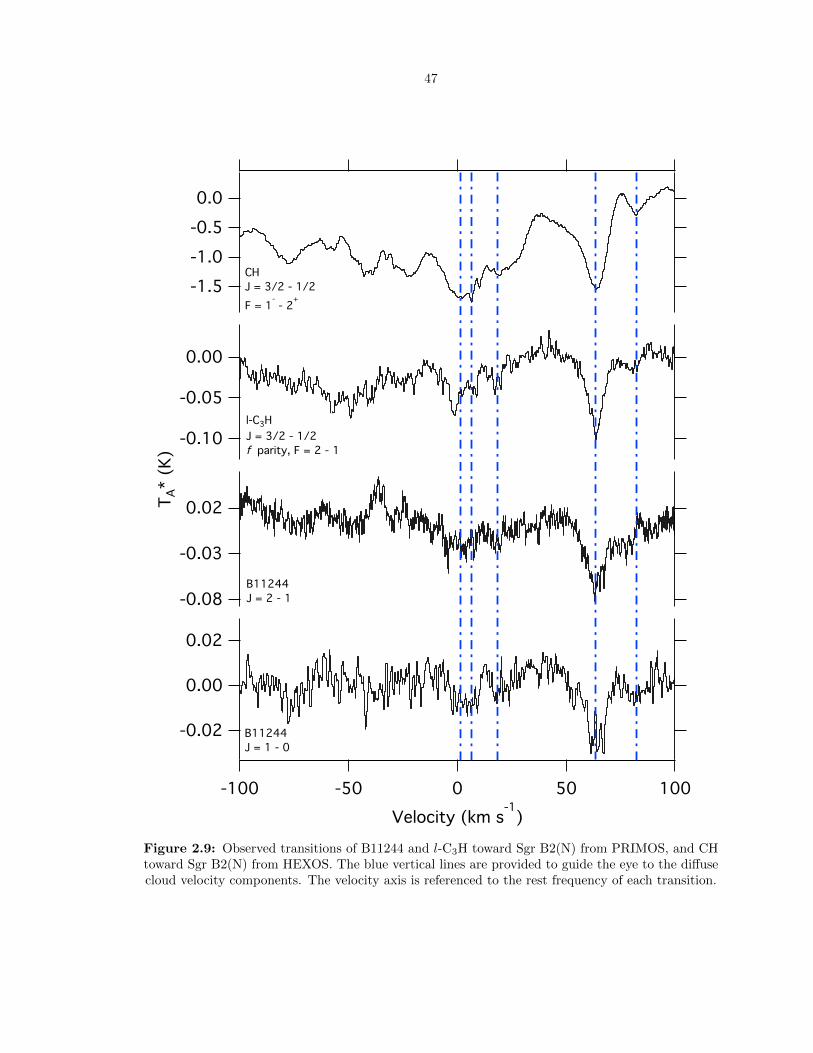
47

-0.02

0.00

0.02

-100 -50 0 50 100

Velocity (km s-1

)

-0.08

-0.03

0.02

-1.5

-1.0

-0.5

0.0

-0.10

-0.05

0.00

TA*

(K)

B11244

J = 1 - 0

B11244

J = 2 - 1

CH

J = 3/2 - 1/2

F = 1- - 2

+

l-C3H

J = 3/2 - 1/2

f parity, F = 2 - 1

Figure 2.9: Observed transitions of B11244 and l-C3H toward Sgr B2(N) from PRIMOS, and CHtoward Sgr B2(N) from HEXOS. The blue vertical lines are provided to guide the eye to the diffusecloud velocity components. The velocity axis is referenced to the rest frequency of each transition.

48

2.3.4.5 Non-Detection of Ka = 1 Transitions

The lack of detection of any signal that could reasonably be attributed to emission from Ka = 1

transitions strongly disfavors the assignment of B11244 to C3H−. In the Horsehead PDR, the Ka = 0

transitions of B11244 are well-modeled by LTE assumptions, and thus we do expect the intensity of

the Ka = 1 transitions to be reasonably well-predicted. It should be noted, however, that a single

molecule can display distinctly different excitation temperatures and column densities between two

K ladders. Indeed, previous observations of HNCO toward OMC-1 show distinct differences between

LTE column density and temperature measurements in high-K and low-K ladders [108]. The authors

attribute this to radiative excitation of the higher-K, higher-energy states through strongly allowed

b-type transitions at far-infrared (far-IR) wavelengths.

In the case of C3H– , we can examine three limiting cases that may apply in the Horsehead PDR:

LTE conditions, the influence of a weak far-IR radiation field, and the influence of a strong far-IR

radiation field.

LTE

As shown in §2.3.3, under LTE conditions, the Ka = 1 transitions of C3H– have predicted inten-

sities of 20 - 28 mK. These are clearly not detected in our spectra at the RMS noise level of the

observations (∼ 5− 10 mK). Thus, we can say with some certainty that C3H– is not present in the

Horsehead PDR under LTE conditions.

Weak far-IR radiation field

In the case of a weak far-IR radiation field, and assuming low to moderate H2 densities in the region

(i.e. non-LTE), the population of the Ka = 1, 2, ... levels will be largely dominated by radiative

selection rules. Any population driven into the Ka = 1, 2, ... levels by collisions will rapidly decay

back into the Ka = 0 states via radiative emission. For C3H– , this will result in a decrease in the

observed intensity of the Ka = 1 transitions, relative to the Ka = 0 transitions, as compared to LTE.

In this case, the lack of detected Ka = 1 transitions does not provide a constraint on the presence

of C3H– .

Strong far-IR radiation field

We now examine the case of a strong far-IR radiation field, and low to moderate H2 densities in the

region (i.e. non-LTE). For transitions arising from low-energy states, the relative populations will be

49

determined by the rotational excitation temperature of the molecule (Tex = 22 K). For transitions

from higher-energy states connected by far-IR transitions, the relative populations of the energy

levels will be determined by the color temperature of the dust radiation field at that frequency if

that temperature is higher than Tex. Thus, the Ka = 1, 2, ... transitions would be relatively more

intense than predicted by LTE simulations at Tex. This is the case for HNCO in OMC-1 [108],

where the higher-K transitions are more intense than predicted from observations of the lower-K

transitions.

In the Horsehead PDR, Goicoechea et al. (2009) [109] measure the millimeter dust continuum to

have a temperature Td ' 30 K. Under these circumstances, we would expect the Ka = 1 transitions

to have intensities of ∼27− 34 mK. We can therefore conclude that assuming B11244 is subject to

the radiation field measured in [109], C3H– is not the carrier.

It is clear from the two non-LTE cases discussed above that the location of B11244 within the

Horsehead PDR region is critical. Interferometric mapping of the location of B11244, relative to the

measured continuum levels in this region, will provide considerable insight into the mechanisms at

work.

2.3.5 Conclusions

We have presented an analysis of observations of the Horsehead PDR, Sgr B2(N), IRC+10216, and

TMC-1 with the goal of determining the identity of B11244. Our findings can be summarized as

follows.

1. If B11244 is C3H– , it would display the highest anion:neutral ratio yet observed in the ISM

(57% in the Horsehead PDR).

2. We find no evidence for C3H– emission in observations toward IRC+10216, and place an upper

limit on the anion:neutral ratio in this source well below that found in the Horsehead PDR

and Sgr B2(N).

3. Recent work has shown UV photodetachment is a dominant destruction pathway for molecular

anions [105]. Despite a UV field more than 60 times that of IRC+10216, C3H– would be present

in the Horsehead PDR with an anion:neutral ratio more than 8 times that of the upper limit

in IRC+10216.

4. We find no evidence for the Ka = 1 lines of C3H– in observations of the Horsehead PDR. We

examine three limiting cases for conditions within the Horsehead PDR, and find that a weak

50

far-IR radiation field can account for the lack of observed Ka = 1 transitions. LTE conditions

or the presence of a strong far-IR radiation field, however, strongly disfavor the presence of

C3H– . A significant far-IR radiation field has been reported for the Horsehead PDR, but it is

unclear whether B11244 is subject to this radiation.

The observational evidence presented here, taken as a whole, casts doubt on the assignment of

B11244 to C3H– , favoring instead the cation, l-C3H+ , as the most likely candidate. The evidence is,

however, circumstantial; a definitive answer will almost certainly require laboratory confirmation.

Indeed, K.N. Crabtree and co-workers at the Harvard-Smithsonian Center for Astrophysics have

undertaken such work using Fourier-transform microwave spectroscopy. Preliminary evidence is

suggestive of the cationic species. The full results of the laboratory investigation will be published

in an upcoming paper (K.N. Crabtree, Private Communication).

Additional observations of the Horsehead PDR, with the aim of detecting the b-type transitions

of C3H– , predicted to be strongest between 500 - 600 GHz, would also provide further evidence.

Perhaps more insightful would be interferometric observations to discover the spatial correlation, or

lack thereof, of B11244 with the previously-observed far-IR radiation field. Finally, further observa-

tions of the diffuse gas along the sightline to Sgr B2(N) would likely prove fruitful in understanding

the possibility of anion chemistry in these regions.

51

2.4 A CSO Search for l-C3H+ : Detection in the Orion Bar

PDR

2.4.1 Introduction

While the question of identity has now been resolved, questions remain surrounding the formation

conditions and chemical implications of l-C3H+ . Because l-C3H+ has been definitively detected in

only two environments – the Horsehead PDR and Sgr B2(N) – efforts to explore these questions are

hampered by a lack of information. In an attempt to address this deficiency, we have conducted

a wide search of PDRs and complex molecular sources in search of l-C3H+ . Here, we present the

results of a brief, targeted campaign of 14 astronomical sources with the Caltech Submillimeter

Observatory (CSO) covering the J = 10 − 9 and J = 12 − 11 transitions of l-C3H+ . We also

examine the J = 10− 9 transition in broadband unbiased line surveys of a further 25 sources. The

observational details are given in §2.4.2, resulting spectra are presented and data reduction strategies

are outlined in §2.4.3, and a discussion follows in §2.4.4.

2.4.2 Observations and Data Reduction

Observations as part of the targeted campaign to detect l-C3H+ were conducted over the course of

4 nights in May 2013, 2 nights in October 2013, 2 nights in November 2013, and 2 nights in January

2014 as part of early remote observing trials using the CSO. The dataset of 25 unbiased molecular

line surveys was obtained with the CSO between September 2007 and June 2013 in the frequency

region of the J = 10− 9 transition.

2.4.2.1 Targeted CSO Survey

Observations as part of the targeted campaign to detect l-C3H+ were conducted over the course

of 4 nights in May 2013, 2 nights in October 2013, 2 nights in November 2013, and 2 nights in

January 2014 as part of early remote observing trials using the CSO. The CSO 230/460 GHz double

side band (DSB) heterodyne sidecab receiver, operating in its 210 - 290 GHz mode, was used in

moderately good weather (τ ∼ 0.07 − 0.12) resulting in typical system temperatures of Tsys ∼ 250

K. The backend consisted of two Fast Fourier Transform Spectrometers (FFTS): FFTS1 provided 1

GHz of DSB spectra at 122 kHz resolution while FFTS2 provided two, 2 GHz DSB spectral windows

at 269 kHZ resolution. For the Orion Bar observations, the receiver was additionally used in its 170

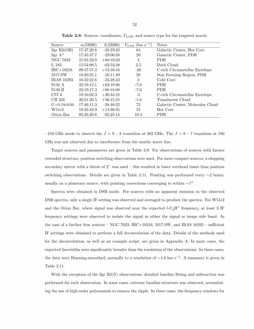
52

Table 2.9: Sources, coordinates, VLSR, and source type for the targeted search.

Source α(J2000) δ(J2000) VLSR (km s−1) NotesSgr B2(OH) 17:47:20.8 -28:23:32 64 Galactic Center, Hot CoreSgr A* 17:45:37.7 -29:00:58 20 Galactic Center, PDRNGC 7023 21:01:33.9 +68:10:33 3 PDRL 183 15:54:08.5 -02:52:48 2.5 Dark CloudIRC+10216 09:47:57.4 +13:16:44 -26 C-rich Circumstellar EnvelopeM17-SW 18:20:25.1 -16:11:49 20 Star Forming Region, PDRIRAS 16293 16:32:22.6 -24:28:33 3 Cold CoreS140 A 22:19:12.1 +63:18:06 -7.6 PDRS140 B 22:19:17.3 +68:18:08 -7.6 PDRCIT 6 10:16:02.3 +30:34:18 -2 C-rich Circumstellar EnvelopeCB 228 20:51:20.5 +56:15:45 -1.6 Translucent CloudG+0.18-0.04 17:46:11.3 -28:48:22 72 Galactic Center, Molecular CloudW51e2 19:23:43.9 +14:30:35 55 Hot CoreOrion Bar 05:35:20.6 -05:25:14 10.4 PDR

- 210 GHz mode to observe the J = 9 − 8 transition at 202 GHz. The J = 8 − 7 transition at 180

GHz was not observed due to interference from the nearby water line.

Target sources and parameters are given in Table 2.9. For observations of sources with known

extended structure, position switching observations were used. For more compact sources, a chopping

secondary mirror with a throw of 2′ was used – this resulted in lower overhead times than position

switching observations. Details are given in Table 2.11. Pointing was performed every ∼2 hours,

usually on a planetary source, with pointing corrections converging to within ∼1′′ .

Spectra were obtained in DSB mode. For sources with no apparent emission in the observed

DSB spectra, only a single IF setting was observed and averaged to produce the spectra. For W51e2

and the Orion Bar, where signal was observed near the expected l-C3H+ frequency, at least 3 IF

frequency settings were observed to isolate the signal in either the signal or image side band. In

the case of a further four sources – NGC 7023, IRC+10216, M17-SW, and IRAS 16293 – sufficient

IF settings were obtained to perform a full deconvolution of the data. Details of the methods used

for the deconvolution, as well as an example script, are given in Appendix A. In most cases, the

expected linewidths were significantly broader than the resolution of the observations. In these cases,

the data were Hanning-smoothed, normally to a resolution of ∼1.6 km s−1. A summary is given in

Table 2.11.

With the exception of the Sgr B2(N) observations, detailed baseline fitting and subtraction was

performed for each observation. In some cases, extreme baseline structure was observed, necessitat-

ing the use of high-order polynomials to remove the ripple. In these cases, the frequency windows for

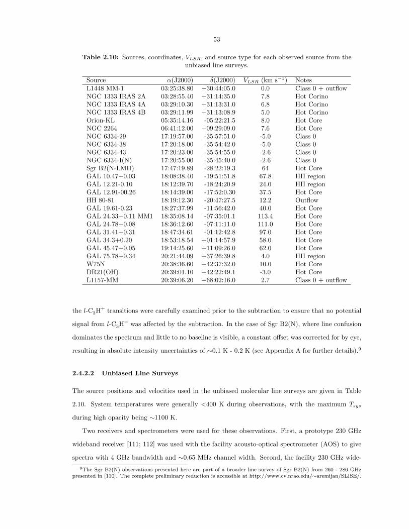
53

Table 2.10: Sources, coordinates, VLSR, and source type for each observed source from theunbiased line surveys.

Source α(J2000) δ(J2000) VLSR (km s−1) NotesL1448 MM-1 03:25:38.80 +30:44:05.0 0.0 Class 0 + outflowNGC 1333 IRAS 2A 03:28:55.40 +31:14:35.0 7.8 Hot CorinoNGC 1333 IRAS 4A 03:29:10.30 +31:13:31.0 6.8 Hot CorinoNGC 1333 IRAS 4B 03:29:11.99 +31:13:08.9 5.0 Hot CorinoOrion-KL 05:35:14.16 -05:22:21.5 8.0 Hot CoreNGC 2264 06:41:12.00 +09:29:09.0 7.6 Hot CoreNGC 6334-29 17:19:57.00 -35:57:51.0 -5.0 Class 0NGC 6334-38 17:20:18.00 -35:54:42.0 -5.0 Class 0NGC 6334-43 17:20:23.00 -35:54:55.0 -2.6 Class 0NGC 6334-I(N) 17:20:55.00 -35:45:40.0 -2.6 Class 0Sgr B2(N-LMH) 17:47:19.89 -28:22:19.3 64 Hot CoreGAL 10.47+0.03 18:08:38.40 -19:51:51.8 67.8 HII regionGAL 12.21-0.10 18:12:39.70 -18:24:20.9 24.0 HII regionGAL 12.91-00.26 18:14:39.00 -17:52:0.30 37.5 Hot CoreHH 80-81 18:19:12.30 -20:47:27.5 12.2 OutflowGAL 19.61-0.23 18:27:37.99 -11:56:42.0 40.0 Hot CoreGAL 24.33+0.11 MM1 18:35:08.14 -07:35:01.1 113.4 Hot CoreGAL 24.78+0.08 18:36:12.60 -07:11:11.0 111.0 Hot CoreGAL 31.41+0.31 18:47:34.61 -01:12:42.8 97.0 Hot CoreGAL 34.3+0.20 18:53:18.54 +01:14:57.9 58.0 Hot CoreGAL 45.47+0.05 19:14:25.60 +11:09:26.0 62.0 Hot CoreGAL 75.78+0.34 20:21:44.09 +37:26:39.8 4.0 HII regionW75N 20:38:36.60 +42:37:32.0 10.0 Hot CoreDR21(OH) 20:39:01.10 +42:22:49.1 -3.0 Hot CoreL1157-MM 20:39:06.20 +68:02:16.0 2.7 Class 0 + outflow

the l-C3H+ transitions were carefully examined prior to the subtraction to ensure that no potential

signal from l-C3H+ was affected by the subtraction. In the case of Sgr B2(N), where line confusion

dominates the spectrum and little to no baseline is visible, a constant offset was corrected for by eye,

resulting in absolute intensity uncertainties of ∼0.1 K - 0.2 K (see Appendix A for further details).9

2.4.2.2 Unbiased Line Surveys

The source positions and velocities used in the unbiased molecular line surveys are given in Table

2.10. System temperatures were generally <400 K during observations, with the maximum Tsys

during high opacity being ∼1100 K.

Two receivers and spectrometers were used for these observations. First, a prototype 230 GHz

wideband receiver [111; 112] was used with the facility acousto-optical spectrometer (AOS) to give

spectra with 4 GHz bandwidth and ∼0.65 MHz channel width. Second, the facility 230 GHz wide-

9The Sgr B2(N) observations presented here are part of a broader line survey of Sgr B2(N) from 260 - 286 GHzpresented in [110]. The complete preliminary reduction is accessible at http://www.cv.nrao.edu/∼aremijan/SLISE/.

54

band receiver [113] was used with the facility FFTS to give spectra with 4 GHz bandwidth and ∼0.27

MHz channel width. Rest frequencies of 223.192 – 251.192 GHz were used, with a 4 GHz separation

between frequency settings. IF offsets of 4.254, 6.754, 5.268, and 7.795 GHz were applied to each

rest frequency. Additional IF offsets of 6.283, 4.753, 5.767, and 7.269 GHz were applied to the two

lowest rest frequency settings on each source to ensure a minimum frequency sampling redundancy

of 6. Most frequencies were sampled by 8 separate frequency settings to enable deconvolution of the

DSB spectra.

The raw data were intensity calibrated using the standard chopper wheel calibration method,

which placed the intensities on the atmosphere-corrected temperature scale, T ∗A. A chopping fre-

quency of 1.1 Hz was used with a chopper throw of either 70±8′′ or 90±8′′ . A noise level of ≤30 mK

was achieved by adjusting integration times based on the Tsys value determined for each frequency

setting. Pointing offsets were checked at a minimum of every two hours, and were consistent to

≤5′′ each night. Each spectrum was also compared to previous spectra for intensity consistency as

an independent verification of the pointing accuracy. The 230 GHz full-width-half-power beam size

was 33.4′′ for the prototype receiver, and 35.54′′ for the facility receiver.

The CLASS software package included in the GILDAS suite of programs (Institut de Radioas-

tronomie Millimetrique, Grenoble, France) was used for the data reduction and deconvolution. A

first-degree baseline function was used to remove baselines from the DSB spectra. Spurious noise

features were removed by blanking the affected channels prior to deconvolution. The cleaned and

baseline subtracted spectra were resampled with a 1 MHz uniform channel spacing. The standard

CLASS deconvolution routine was used to deconvolve the spectra. The initial deconvolution assumed

no gain variations between the sidebands. A second deconvolution was then constrained using this

first result, with the sideband gains being allowed to vary. The strong spectral features (i.e. those

with intensities >2 K) were masked during deconvolution to prevent the introduction of spurious

features. These features were added back into the spectrum after deconvolution. All intensities were

then set to the main beam temperature scale, Tmb, where Tmb = T ∗A/ηmb; the main beam efficiency

was determined through observations of planets to be ηmb = 60 ± 9% for both receivers. The noise

level in the final spectra is ≤25 mK on the Tmb scale. The deconvolved spectra in the frequency

range covering the l-C3H+ lines are shown in Figures 2.14 – 2.16.

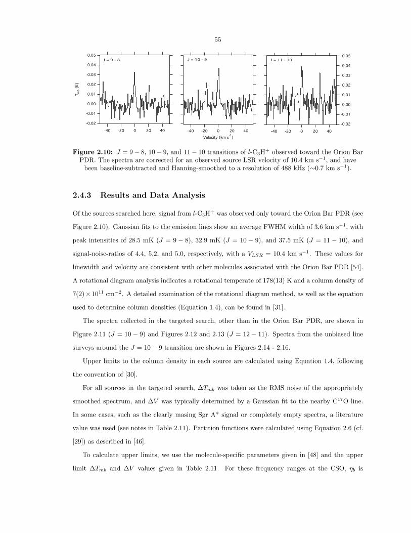
55

0.05 0.05

0.04 0.04

0.03 0.03

0.02 0.02

0.01 0.01

0.00 0.00

-0.01 -0.01

-0.02 -0.02

-40 -20 0 20 40

0.05

0.04

0.03

0.02

0.01

0.00

-0.01

-0.02

-40 -20 0 20 40

Velocity (km s-1

)

0.05

0.04

0.03

0.02

0.01

0.00

-0.01

-0.02

Tm

b (

K)

-40 -20 0 20 40

J = 9 - 8 J = 10 - 9 J = 11 - 10

Figure 2.10: J = 9− 8, 10− 9, and 11− 10 transitions of l-C3H+ observed toward the Orion BarPDR. The spectra are corrected for an observed source LSR velocity of 10.4 km s−1, and have

been baseline-subtracted and Hanning-smoothed to a resolution of 488 kHz (∼0.7 km s−1).

2.4.3 Results and Data Analysis

Of the sources searched here, signal from l-C3H+ was observed only toward the Orion Bar PDR (see

Figure 2.10). Gaussian fits to the emission lines show an average FWHM width of 3.6 km s−1, with

peak intensities of 28.5 mK (J = 9 − 8), 32.9 mK (J = 10 − 9), and 37.5 mK (J = 11 − 10), and

signal-noise-ratios of 4.4, 5.2, and 5.0, respectively, with a VLSR = 10.4 km s−1. These values for

linewidth and velocity are consistent with other molecules associated with the Orion Bar PDR [54].

A rotational diagram analysis indicates a rotational temperate of 178(13) K and a column density of

7(2)×1011 cm−2. A detailed examination of the rotational diagram method, as well as the equation

used to determine column densities (Equation 1.4), can be found in [31].

The spectra collected in the targeted search, other than in the Orion Bar PDR, are shown in

Figure 2.11 (J = 10 − 9) and Figures 2.12 and 2.13 (J = 12 − 11). Spectra from the unbiased line

surveys around the J = 10− 9 transition are shown in Figures 2.14 - 2.16.

Upper limits to the column density in each source are calculated using Equation 1.4, following

the convention of [30].

For all sources in the targeted search, ∆Tmb was taken as the RMS noise of the appropriately

smoothed spectrum, and ∆V was typically determined by a Gaussian fit to the nearby C17O line.

In some cases, such as the clearly masing Sgr A* signal or completely empty spectra, a literature

value was used (see notes in Table 2.11). Partition functions were calculated using Equation 2.6 (cf.

[29]) as described in [46].

To calculate upper limits, we use the molecule-specific parameters given in [48] and the upper

limit ∆Tmb and ∆V values given in Table 2.11. For these frequency ranges at the CSO, ηb is

56

3

2

1

0

Tm

b (

K)

225000224900224800224700224600

Frequency (MHz)

Sgr B2(OH)

Sgr A*

NGC 7023

IRC+10216

L183

M17-SW

IRAS 16293

S140 A

S140 B

CIT 6

CB 228

G+0.18-0.04

Figure 2.11: J = 10− 9 spectral window toward target sources. All spectra are adjusted to theVLSR indicated in Table 2.9, and are vertically offset for clarity. The feature at 224714 MHz is due

to C17O. The red vertical line indicates the frequency of the J = 10− 9 transition.

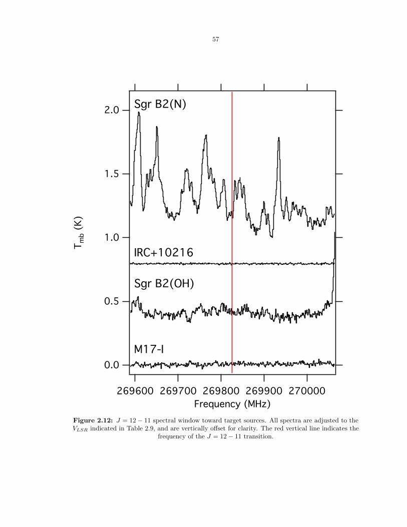
57

2.0

1.5

1.0

0.5

0.0

Tm

b (

K)

270000269900269800269700269600

Frequency (MHz)

Sgr B2(N)

IRC+10216

Sgr B2(OH)

M17-I

Figure 2.12: J = 12− 11 spectral window toward target sources. All spectra are adjusted to theVLSR indicated in Table 2.9, and are vertically offset for clarity. The red vertical line indicates the

frequency of the J = 12− 11 transition.

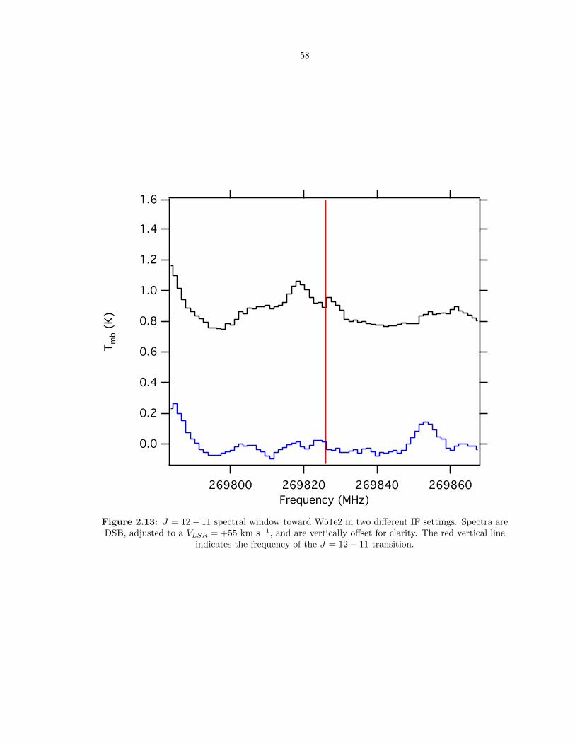
58

1.6

1.4

1.2

1.0

0.8

0.6

0.4

0.2

0.0

Tm

b (

K)

269860269840269820269800

Frequency (MHz)

Figure 2.13: J = 12− 11 spectral window toward W51e2 in two different IF settings. Spectra areDSB, adjusted to a VLSR = +55 km s−1, and are vertically offset for clarity. The red vertical line

indicates the frequency of the J = 12− 11 transition.

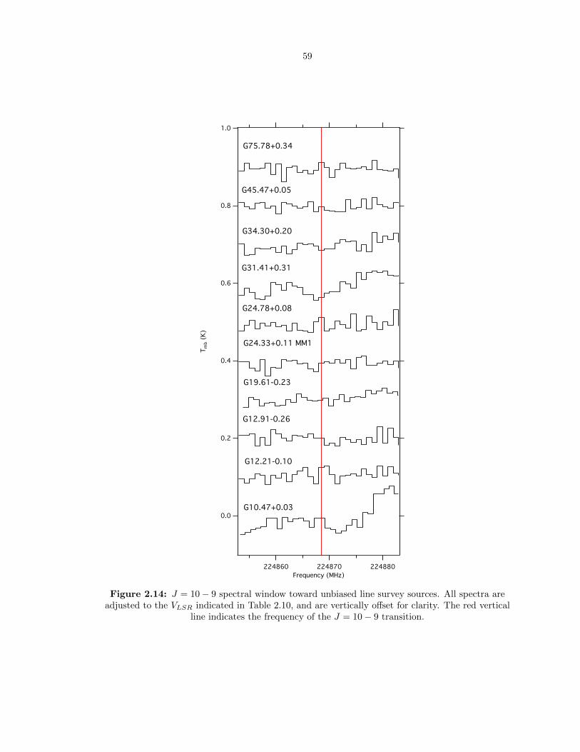
59

1.0

0.8

0.6

0.4

0.2

0.0

Tm

b (

K)

224880224870224860

Frequency (MHz)

G10.47+0.03

G12.21-0.10

G12.91-0.26

G19.61-0.23

G24.33+0.11 MM1

G24.78+0.08

G31.41+0.31

G34.30+0.20

G45.47+0.05

G75.78+0.34

Figure 2.14: J = 10− 9 spectral window toward unbiased line survey sources. All spectra areadjusted to the VLSR indicated in Table 2.10, and are vertically offset for clarity. The red vertical

line indicates the frequency of the J = 10− 9 transition.

60

1.2

1.0

0.8

0.6

0.4

0.2

0.0

Tm

b (

K)

224880224870224860

Frequency (MHz)

DR21(OH)

HH80-81

L1157-MM

L1448 MM-1

W75N

Orion-KL

SgrB2(N-LMH)



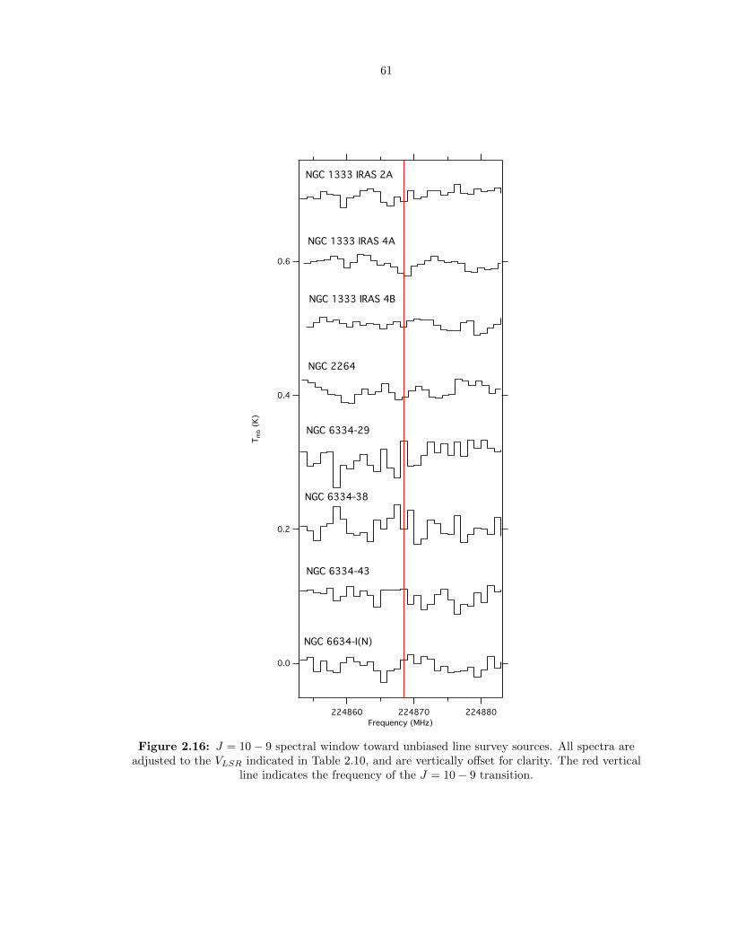
61

0.6

0.4

0.2

0.0

Tm

b (

K)

224880224870224860

Frequency (MHz)

NGC 6634-I(N)

NGC 6334-43

NGC 6334-38

NGC 6334-29

NGC 2264

NGC 1333 IRAS 4B

NGC 1333 IRAS 4A

NGC 1333 IRAS 2A



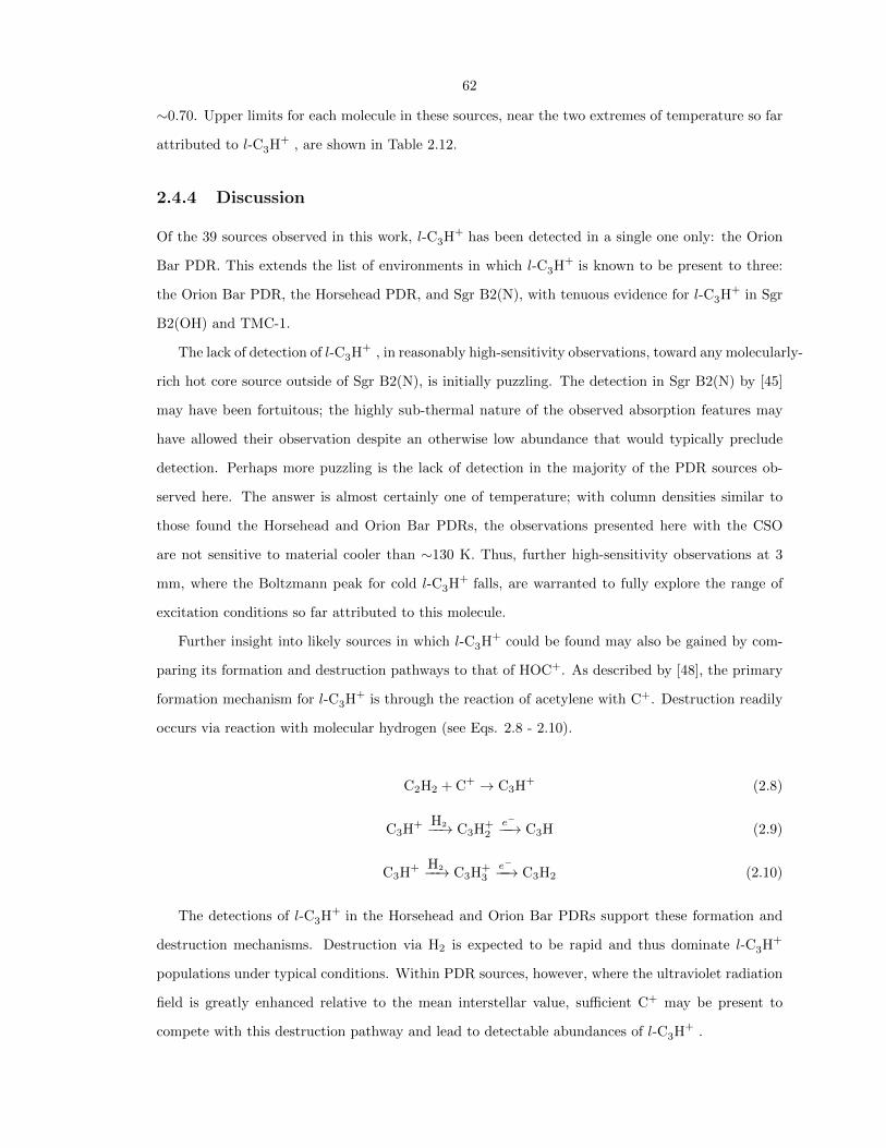
62

∼0.70. Upper limits for each molecule in these sources, near the two extremes of temperature so far

attributed to l-C3H+ , are shown in Table 2.12.

2.4.4 Discussion

Of the 39 sources observed in this work, l-C3H+ has been detected in a single one only: the Orion

Bar PDR. This extends the list of environments in which l-C3H+ is known to be present to three:

the Orion Bar PDR, the Horsehead PDR, and Sgr B2(N), with tenuous evidence for l-C3H+ in Sgr

B2(OH) and TMC-1.

The lack of detection of l-C3H+ , in reasonably high-sensitivity observations, toward any molecularly-

rich hot core source outside of Sgr B2(N), is initially puzzling. The detection in Sgr B2(N) by [45]

may have been fortuitous; the highly sub-thermal nature of the observed absorption features may

have allowed their observation despite an otherwise low abundance that would typically preclude

detection. Perhaps more puzzling is the lack of detection in the majority of the PDR sources ob-

served here. The answer is almost certainly one of temperature; with column densities similar to

those found the Horsehead and Orion Bar PDRs, the observations presented here with the CSO

are not sensitive to material cooler than ∼130 K. Thus, further high-sensitivity observations at 3

mm, where the Boltzmann peak for cold l-C3H+ falls, are warranted to fully explore the range of

excitation conditions so far attributed to this molecule.

Further insight into likely sources in which l-C3H+ could be found may also be gained by com-

paring its formation and destruction pathways to that of HOC+. As described by [48], the primary

formation mechanism for l-C3H+ is through the reaction of acetylene with C+. Destruction readily

occurs via reaction with molecular hydrogen (see Eqs. 2.8 - 2.10).

C2H2 + C+ → C3H+ (2.8)

C3H+ H2−−→ C3H+2

e−−−→ C3H (2.9)

C3H+ H2−−→ C3H+3

e−−−→ C3H2 (2.10)

The detections of l-C3H+ in the Horsehead and Orion Bar PDRs support these formation and

destruction mechanisms. Destruction via H2 is expected to be rapid and thus dominate l-C3H+

populations under typical conditions. Within PDR sources, however, where the ultraviolet radiation

field is greatly enhanced relative to the mean interstellar value, sufficient C+ may be present to

compete with this destruction pathway and lead to detectable abundances of l-C3H+ .

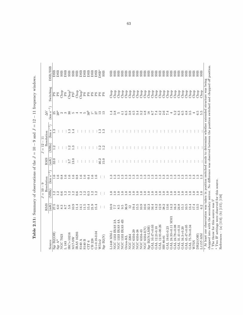
63

Tab

le2.1

1:

Su

mm

ary

of

ob

serv

ati

on

sof

theJ

=10−

9an

dJ

=12−

11

freq

uen

cyw

ind

ows.

J=

10−

9J

=12−

11

RM

SR

esolu

tion

RM

SR

esolu

tion

∆V

Sou

rce

(mK

)(M

Hz)

(km

s−1)

(mK

)(M

Hz)

(km

s−1)

(km

s−1)

Sw

itch

ing

DS

B/S

SB

Sgr

B2(O

H)

27.5

1.2

1.6

32.0

1.2

1.3

25

PS

DS

BS

gr

A*

6.0

1.2

1.6

...

...

...

20a

PS

DS

BN

GC

7023

8.3

0.6

0.8

...

...

...

2C

hop

SS

BL

183

8.7

1.2

1.6

...

...

...

3P

SD

SB

IRC

+10216

5.8

1.2

1.6

3.7

1.2

1.3

30

Ch

op†

SS

BM

17-S

W10.9

1.2

1.6

13.0

1.3

1.4

5P

S‡

SS

BIR

AS

16293

11.4

0.6

0.8

...

...

...

4C

hop

SS

BS

140

A14.1

1.2

1.6

...

...

...

4C

hop†

DS

BS

140

B11.5

1.2

1.6

...

...

...

5P

SD

SB

CIT

615.4

0.3

0.4

...

...

...

30b

PS

DS

BC

B228

21.9

1.2

1.6

...

...

...

1c

PS

DS

BG

+0.1

8-0

.04

15.4

1.2

1.6

...

...

...

27

PS

DS

BW

51e2

...

...

...

46.2

1.2

1.3

13

PS

DS

B?

Sgr

B2(N

)..

...

....

15.0

1.2

1.3

13

PS

SS

B

L1448

MM

-110.9

1.0

1.3

...

...

...

1.4

Ch

op

SS

BN

GC

1333

IRA

S2A

7.7

1.0

1.3

...

...

...

3.8

Ch

op

SS

BN

GC

1333

IRA

S4A

8.5

1.0

1.3

...

...

...

5C

hop

SS

BN

GC

1333

IRA

S4B

9.5

1.0

1.3

...

...

...

4.1

Ch

op

SS

BO

rion

-KL

36.9

1.0

1.3

...

...

...

6.5

Ch

op

SS

BN

GC

2264

12

1.0

1.3

...

...

...

3.8

Ch

op

SS

BN

GC

6334-2

919.4

1.0

1.3

...

...

...

4.5

Ch

op

SS

BN

GC

6334-3

815.5

1.0

1.3

...

...

...

3.4

Ch

op

SS

BN

GC

6334-4

310.9

1.0

1.3

...

...

...

3.2

Ch

op

SS

BN

GC

6334-I

(N)

10.6

1.0

1.3

...

...

...

4.8

Ch

op

SS

BS

gr

B2(N

-LM

H)

32.3

1.0

1.3

...

...

...

18

Ch

op

SS

BG

AL

10.4

7+

0.0

334.4

1.0

1.3

...

...

...

8.7

Ch

op

SS

BG

AL

12.2

1-0

.10

14.2

1.0

1.3

...

...

...

7.4

Ch

op

SS

BG

AL

12.9

1-0

0.2

612.9

1.0

1.3

...

...

...

4.2

Ch

op

SS

BH

H80-8

138.2

1.0

1.3

...

...

...

2.6

Ch

op

SS

BG

AL

19.6

1-0

.23

13.6

1.0

1.3

...

...

...

7.4

Ch

op

SS

BG

AL

24.3

3+

0.1

1M

M1

14.2

1.0

1.3

...

...

...

4C

hop

SS

BG

AL

24.7

8+

0.0

816.3

1.0

1.3

...

...

...

5.2

Ch

op

SS

BG

AL

31.4

1+

0.3

124.8

1.0

1.3

...

...

...

6.3

Ch

op

SS

BG

AL

34.3

+0.2

015.1

1.0

1.3

...

...

...

6.5

Ch

op

SS

BG

AL

45.4

7+

0.0

510.5

1.0

1.3

...

...

...

4.8

Ch

op

SS

BG

AL

75.7

8+

0.3

413.4

1.0

1.3

...

...

...

3.5

Ch

op

SS

BW

75N

17.4

1.0

1.3

...

...

...

4C

hop

SS

BD

R21(O

H)

13.5

1.0

1.3

...

...

...

6.5

Ch

op

SS

BL

1157-M

M6.2

1.0

1.3

...

...

...

5.5

Ch

op

SS

B†

At

least

on

eob

serv

ati

on

was

taken

inp

osi

tion

swit

ched

mod

eto

det

erm

ine

wh

eth

erex

ten

ded

stru

ctu

rew

as

bei

ng

chop

ped

into

wit

hth

ese

con

dary

mir

ror.

No

diff

eren

cew

as

ob

serv

edb

etw

een

the

posi

tion

swit

ched

an

dch

op

ped

off

posi

tion

.‡

Th

eth

row

for

this

sou

rce

was

5′

?T

wo

IFse

ttin

gs

wer

eob

serv

edfo

rth

isso

urc

e.R

efer

ence

s–

(a)

[114];

(b)

[115];

[116]

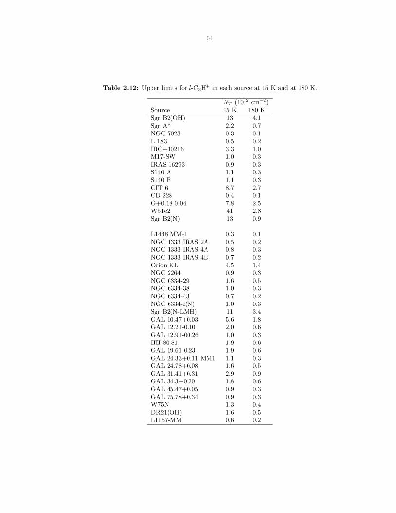
64

Table 2.12: Upper limits for l-C3H+ in each source at 15 K and at 180 K.

NT (1012 cm−2)Source 15 K 180 KSgr B2(OH) 13 4.1Sgr A* 2.2 0.7NGC 7023 0.3 0.1L 183 0.5 0.2IRC+10216 3.3 1.0M17-SW 1.0 0.3IRAS 16293 0.9 0.3S140 A 1.1 0.3S140 B 1.1 0.3CIT 6 8.7 2.7CB 228 0.4 0.1G+0.18-0.04 7.8 2.5W51e2 41 2.8Sgr B2(N) 13 0.9

L1448 MM-1 0.3 0.1NGC 1333 IRAS 2A 0.5 0.2NGC 1333 IRAS 4A 0.8 0.3NGC 1333 IRAS 4B 0.7 0.2Orion-KL 4.5 1.4NGC 2264 0.9 0.3NGC 6334-29 1.6 0.5NGC 6334-38 1.0 0.3NGC 6334-43 0.7 0.2NGC 6334-I(N) 1.0 0.3Sgr B2(N-LMH) 11 3.4GAL 10.47+0.03 5.6 1.8GAL 12.21-0.10 2.0 0.6GAL 12.91-00.26 1.0 0.3HH 80-81 1.9 0.6GAL 19.61-0.23 1.9 0.6GAL 24.33+0.11 MM1 1.1 0.3GAL 24.78+0.08 1.6 0.5GAL 31.41+0.31 2.9 0.9GAL 34.3+0.20 1.8 0.6GAL 45.47+0.05 0.9 0.3GAL 75.78+0.34 0.9 0.3W75N 1.3 0.4DR21(OH) 1.6 0.5L1157-MM 0.6 0.2

65

A comparison can be made with the chemistry of HOC+, which is also formed, directly and

indirectly, through reactions of C+, and destroyed by reaction with H2 to form HCO+ (see Eqs.

2.11 - 2.13, c.f. [117; 54]). Thus, observations of a high HOC+ abundance (or, alternatively, an

enhanced [HOC+]/[HCO+] ratio) may be indicative of chemical and physical conditions that will

also favor the production of l-C3H+ , and act as a probe to guide future sources.

H2OC+

−−→ HOC+ (2.11)

OHC+

−−→ CO+ H2−−→ HOC+ (2.12)

HOC+ H2−−→ HCO+ (2.13)

Indeed, such an enhanced HOC+ abundance (and enhanced [HOC+]/[HCO+] ratio) has already

been detected toward both the Orion Bar PDR [54] and the Horsehead PDR [109], with these values

peaking in the region of the PDR. A similarly enhanced presence of HOC+ is detected by [54] in

observations of the NGC 7023 PDR, for which l-C3H+ is not detected in these CSO observations.

This suggests that perhaps l-C3H+ is simply too cold to be detected in our observations at this

sensitivity, and that observations at lower frequencies may result in a detection.

Observations of HOC+ in diffuse clouds by [118] find abundance ratios of [HOC+]/[HCO+]

comparable to that of the extreme cases of PDR enhancements in the Orion Bar and NGC 7023.

This is consistent with the tentative detections of l-C3H+ absorption in diffuse, spiral arm clouds

by [45] along the line of sight to Sgr B2(N), and suggests these sources may be intriguing targets for

future observations.

Finally, detections of HOC+ toward other regions with enhanced FUV flux provide other tanta-

lizing sources for future study. A small list of these sources includes, for example, the Monocerous

R2 ultracompact HII region [119] and the external galaxies NGC 253 [120] and M 82 [121].

2.4.5 Conclusions

We have examined the results of both a dedicated campaign targeting l-C3H+ in 14 sources, as well

as 25 additional sources from unbiased molecular line surveys with frequency coverage coincident

with l-C3H+ transitions. We detect the presence of l-C3H+ in only a single source: the Orion Bar

PDR. These observations are only sensitive to relatively warm material, and follow-up observations

at lower frequencies are necessary to obtain a complete picture ofl-C3H+ in these sources. Finally, a

comparison to the chemistry of HOC+ has shown that HOC+ has the potential to serve as a tracer

66

of l-C3H+ . Previous observations of HOC+ can therefore be used as a guide to efficiently target

new sources in additional searches for l-C3H+ .

67

Chapter 3

Carbodiimide (HNCNH)

The bulk of this chapter is reproduced from “Interstellar carbodiimide (HNCNH) - A new astronom-

ical detection from the GBT PRIMOS survey via maser emission features,” by B.A. McGuire et al.,

Astrophysical Journal Letters, 758, L33 (2012) [77].

3.1 Introduction

Historically, searches for new astronomical molecules resulted in the detection of favorable, high

line strength transitions based on a thermal approximation to the excitation of these species in

interstellar environments. At the temperatures of hot molecular cores inside molecular clouds, these

transitions often reside at (sub)millimeter wavelengths. However, line confusion near the Boltzmann

peak can lead to ambiguous identifications, and the peak intensities of low abundance, large organic

molecules may never rise above the noise floor or the confusion limit. The success of molecule

searches at centimeter wavelengths has shown that unique excitation conditions can lead to the

unambiguous identification of very low abundance species with high accuracy.

Carbodiimide (HNCNH) is the second most stable isomer of cyanamide (NH2CN), with NH2CN

being more stable by ∼4.0 kcal mol−1 [122; 123]. Since the detection of NH2CN by Turner et al.

(1975) [124] toward the high-mass star-forming region Sgr B2(N), HNCNH has been recognized as

a candidate interstellar molecule. HNCNH is also a tautomer of NH2CN, and can be formed via an

isomerization reaction whereby a H atom can migrate along the molecular backbone from the amine

group. At room temperature, HNCNH is in thermally-induced equilibrium with NH2CN at a fraction

of ∼1%. Given typical abundances of NH2CN, and temperatures in many astrophysical environments

of << 300 K, gas-phase tautomerization of NH2CN is unlikely to produce HNCNH in appreciable

abundance. Yet, HNCNH may exist in detectable abundance out of thermal equilibrium with NH2CN

68

as in the case of interstellar hydrogen cyanide (HCN) and interstellar hydrogen isocyanide (HNC),

in which HNC is in greater abundance in some clouds (see [125] and references therein).

Although tautomerization is likely inefficient in the gas phase under interstellar conditions, ex-

perimental studies have shown NH2CN → HNCNH conversion in water ices and matrices is far

more efficient ([126] and references therein). In the solid phase, the association of up to five water

molecules with NH2CN on an ice surface has been shown to significantly lower the activation barrier

to tautomerization and promote the production of HNCNH [126]. In fact, HNCNH formation on

a water-ice surface is shown to occur at temperatures as low as 70 K. The relative abundance of

HNCNH formed from this process has been measured to range from 4% of NH2CN at 80 K to as

much as 13% at 140 K [126]. In the laboratory, HNCNH sublimation occurs between 80 - 170 K,

with no additional desorption observed above 170 K [122]. In the ISM, non-thermal desorption via

shocks is also a likely liberation mechanism. Assuming that tautomerization of NH2CN on dust

grain ice mantles is the dominant formation pathway for HNCNH, and that subsequent desorption

occurs for both species, the gas phase abundance of HNCNH may be capped at ∼10% of NH2CN.

NH2CN has an estimated column density of ∼2×1014 cm−2 towards Sgr B2(N) [25]; we therefore

anticipate an HNCNH column density on the order of ∼1013 cm−2. If thermal emission at hot core

temperatures dominates the spectrum of HNCNH, the most favorable high line strength transitions

are at millimeter and submillimeter wavelengths. Nevertheless, we have previously used the Robert

C. Byrd Green Bank Telescope (GBT) to detect new molecular species including trans-methyl for-

mate [75], and cyanoformaldehyde [81], which only had measurable astronomical line intensities

detected at centimeter wavelengths. Encouraged by these results, we searched for centimeter wave

transitions of HNCNH. All data were taken as part of the PRebiotic Interstellar MOlecular Survey

(PRIMOS), and targeted rotation-torsion transitions of HNCNH selected from the Cologne Database

for Molecular Spectroscopy1,2 [18]. Our results are presented in §3.2. In §3.3, we evaluate the prob-

ability of mis-assigning these features to HNCNH, and discuss evidence that observed transitions are

masing. Further, we explore the usefulness of our technique as a method for new molecule detection.

3.2 Observations and Results

All data used for this project were taken as part of the National Radio Astronomy Observatory’s

(NRAO) 100-m Robert C. Byrd Green Bank Telescope (GBT) PRebiotic Interstellar MOlecule

1Original laboratory data cataloged from Birk et al. (1980) [127], Wagener et al. (1995) [128], & Jabs et al. (1997)[129].

2Available at www.splatalogue.net [28].

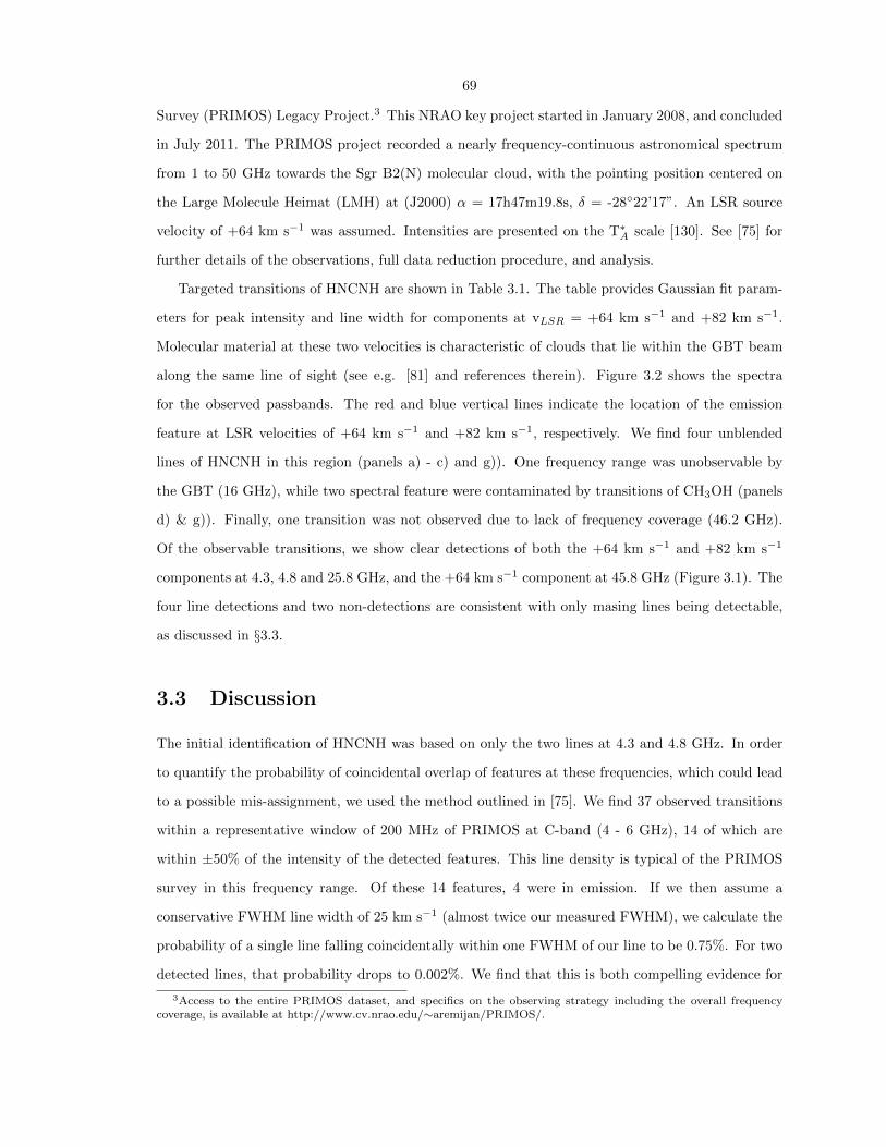
69

Survey (PRIMOS) Legacy Project.3 This NRAO key project started in January 2008, and concluded

in July 2011. The PRIMOS project recorded a nearly frequency-continuous astronomical spectrum

from 1 to 50 GHz towards the Sgr B2(N) molecular cloud, with the pointing position centered on

the Large Molecule Heimat (LMH) at (J2000) α = 17h47m19.8s, δ = -2822’17”. An LSR source

velocity of +64 km s−1 was assumed. Intensities are presented on the T∗A scale [130]. See [75] for

further details of the observations, full data reduction procedure, and analysis.

Targeted transitions of HNCNH are shown in Table 3.1. The table provides Gaussian fit param-

eters for peak intensity and line width for components at vLSR = +64 km s−1 and +82 km s−1.

Molecular material at these two velocities is characteristic of clouds that lie within the GBT beam

along the same line of sight (see e.g. [81] and references therein). Figure 3.2 shows the spectra

for the observed passbands. The red and blue vertical lines indicate the location of the emission

feature at LSR velocities of +64 km s−1 and +82 km s−1, respectively. We find four unblended

lines of HNCNH in this region (panels a) - c) and g)). One frequency range was unobservable by

the GBT (16 GHz), while two spectral feature were contaminated by transitions of CH3OH (panels

d) & g)). Finally, one transition was not observed due to lack of frequency coverage (46.2 GHz).

Of the observable transitions, we show clear detections of both the +64 km s−1 and +82 km s−1

components at 4.3, 4.8 and 25.8 GHz, and the +64 km s−1 component at 45.8 GHz (Figure 3.1). The

four line detections and two non-detections are consistent with only masing lines being detectable,

as discussed in §3.3.

3.3 Discussion

The initial identification of HNCNH was based on only the two lines at 4.3 and 4.8 GHz. In order

to quantify the probability of coincidental overlap of features at these frequencies, which could lead

to a possible mis-assignment, we used the method outlined in [75]. We find 37 observed transitions

within a representative window of 200 MHz of PRIMOS at C-band (4 - 6 GHz), 14 of which are

within ±50% of the intensity of the detected features. This line density is typical of the PRIMOS

survey in this frequency range. Of these 14 features, 4 were in emission. If we then assume a

conservative FWHM line width of 25 km s−1 (almost twice our measured FWHM), we calculate the

probability of a single line falling coincidentally within one FWHM of our line to be 0.75%. For two

detected lines, that probability drops to 0.002%. We find that this is both compelling evidence for

3Access to the entire PRIMOS dataset, and specifics on the observing strategy including the overall frequencycoverage, is available at http://www.cv.nrao.edu/∼aremijan/PRIMOS/.

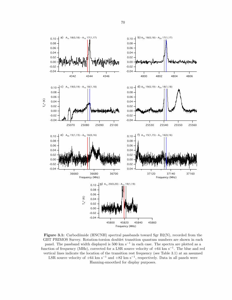
70

0.10

0.08

0.06

0.04

0.02

0.00

-0.02

-0.04

371603714037120

Frequency (MHz)

0.10

0.08

0.06

0.04

0.02

0.00

-0.02

-0.04

367003668036660

Frequency (MHz)

0.10

0.08

0.06

0.04

0.02

0.00

-0.02

-0.04

TA*

(K)

45860458404582045800

Frequency (MHz)

0.10

0.08

0.06

0.04

0.02

0.00

-0.02

-0.04

434643444342

0.10

0.08

0.06

0.04

0.02

0.00

-0.02

-0.04

4806480448024800

0.10

0.08

0.06

0.04

0.02

0.00

-0.02

-0.04

TA*

(K)

25100250902508025070

0.10

0.08

0.06

0.04

0.02

0.00

-0.02

-0.04

25560255502554025530

a) b)

c) d)

e) f)

g)

A1s 18(0,18) - A1d 17(1,17) A2s 18(0,18) - A2d 17(1,17)

A1s 19(0,19) - A1d 18(1,18) A2s 19(0,19) - A2d 18(1,18)

A2d 15(1,15) - A2s 16(0,16) A1d 15(1,15) - A1s 16(0,16)

A1s 20(0,20) - A1d 19(1,19)

Figure 3.1: Carbodiimide (HNCNH) spectral passbands toward Sgr B2(N), recorded from theGBT PRIMOS Survey. Rotation-torsion doublet transition quantum numbers are shown in eachpanel. The passband width displayed is 500 km s−1 in each case. The spectra are plotted as a

function of frequency (MHz), corrected for a LSR source velocity of +64 km s−1. The blue and redvertical lines indicate the location of the transition rest frequency (see Table 3.1) at an assumed

LSR source velocity of +64 km s−1 and +82 km s−1, respectively. Data in all panels wereHanning-smoothed for display purposes.

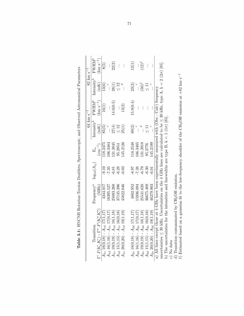
71

Tab

le3.1

:H

NC

NH

Rot

ati

on

-Tors

ion

Dou

ble

ts,

Sp

ectr

osc

op

ic,

an

dO

bse

rved

Ast

ron

om

ical

Para

met

ers

64

km

s−1

82

km

s−1

Tra

nsi

tion

Fre

qu

ency

alo

g 10(A

ij)

Eu

Inte

nsi

tyb

FW

HM

bIn

ten

sity

bF

WH

Mb

Γ′

J′ (

K′ a,K′ c)

-Γ′′

J′′(K′′ a,K′′ c)

(MH

z)(c

m−1)

(mK

)(k

ms−

1)

(mK

)(k

ms−

1)

A1s

18(0

,18)

-A

1d

17(1

,17)

4344.0

17

-9.1

0118.2

475

85(5

)16(1

)13(6

)8(5

)A

1d

16(1

,16)

-A

1s

17(0

,17)

16395.5

27

-7.3

5106.3

484

...

c..

...

.c

...

A1s

19(0

,19)

-A

1d

18(1

,18)

25083.2

68

-6.8

1131.3

845

27(4

)14.0

(0.5

)28(1

)22(2

)A

1d

15(1

,15)

-A

1s

16(0

,16)

37135.3

96

-6.2

895.2

854

≤12

...

≤12

...

A1s

20(0

,20)

-A

1d

19(1

,19)

45822.0

46

-6.0

3145.2

126

25(1

)13(2

)..

.d

...

A2s

18(0

,18)

-A

2d

17(1

,17)

4802.9

52

-8.9

7118.2

548

89(2

)15.9

(0.4

)23(2

)12(1

)A

2d

16(1

,16)

-A

2s

17(0

,17)

15936.0

94

-7.3

8106.3

405

...

c..

...

.c

...

A2s

19(0

,19)

-A

2d

18(1

,18)

25541.6

20

-6.7

9131.3

918

...

d..

.(5

0)f

(12)f

A2d

15(1

,15)

-A

2s

16(0

,16)

36675.4

69

-6.3

095.2

776

≤11

...

≤11

...

A2s

20(0

,20)

-A

2d

19(1

,19)

46279.9

03

-6.0

1145.2

199

...

c..

...

.c

...

a)A

llli

nes

exce

pt

thos

eat

4G

Hz

hav

eb

een

exp

erim

enta

lly

mea

sure

dw

ith

(Ob

s-

Calc

)fr

equ

ency

un

cert

ainti

es≤

30kH

z.U

nce

rtain

ties

on

the

4G

Hz

lin

esare

calc

ula

ted

tob

e≤

30

kH

z,ty

pe

A,

k=

2(2σ

)[8

5].

b)

Th

eu

nce

rtai

nti

esfo

rth

ein

ten

siti

esan

dli

new

idth

sare

typ

eB

,k

=1

(1σ

)[8

5].

c)N

od

ata

d)

Tra

nsi

tion

conta

min

ated

by

CH

3O

Hem

issi

on

.f)

Est

imat

edb

ased

ona

gau

ssia

nfi

tto

the

low

-fre

qu

ency

shou

lder

of

the

CH

3O

Hem

issi

on

at

+82

km

s−1

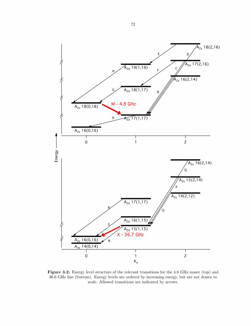
72

210

Ka

A2s 14(0,14)

A2s 16(0,16)

A2d 15(1,15)

A2d 16(1,15)

A2d 17(1,17)

A2s 14(2,12)

A2s 15(2,14)

A2s 16(2,14)

210

A2s 16(0,16)

A2d 17(1,17)

A2s 18(0,18)

A2d 18(1,17)

A2s 16(2,14)

A2d 19(1,19)A2s 17(2,16)

A2s 18(2,16)

M - 4.8 GHz

A

B

C

DE

F

G

H

X - 36.7 GHz

N

S

RO

P

Q

Energ

y

Figure 3.2: Energy level structure of the relevant transitions for the 4.8 GHz maser (top) and36.6 GHz line (bottom). Energy levels are ordered by increasing energy, but are not drawn to

scale. Allowed transitions are indicated by arrows.

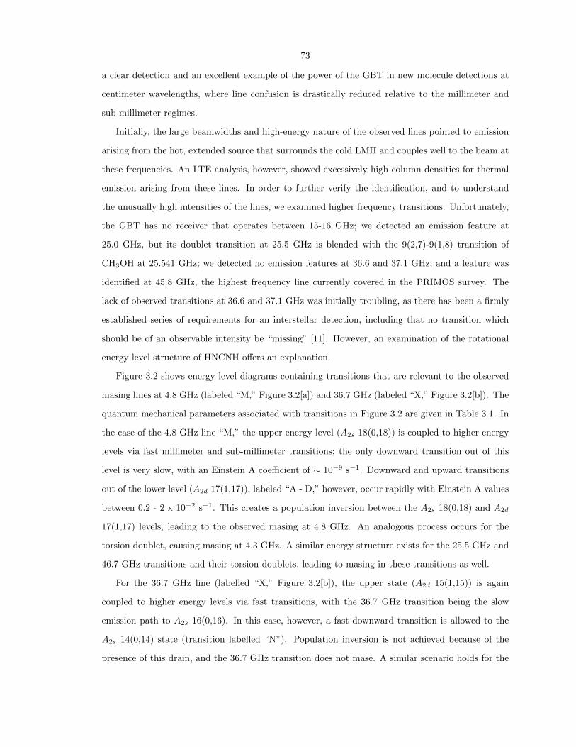
73

a clear detection and an excellent example of the power of the GBT in new molecule detections at

centimeter wavelengths, where line confusion is drastically reduced relative to the millimeter and

sub-millimeter regimes.

Initially, the large beamwidths and high-energy nature of the observed lines pointed to emission

arising from the hot, extended source that surrounds the cold LMH and couples well to the beam at

these frequencies. An LTE analysis, however, showed excessively high column densities for thermal

emission arising from these lines. In order to further verify the identification, and to understand

the unusually high intensities of the lines, we examined higher frequency transitions. Unfortunately,

the GBT has no receiver that operates between 15-16 GHz; we detected an emission feature at

25.0 GHz, but its doublet transition at 25.5 GHz is blended with the 9(2,7)-9(1,8) transition of

CH3OH at 25.541 GHz; we detected no emission features at 36.6 and 37.1 GHz; and a feature was

identified at 45.8 GHz, the highest frequency line currently covered in the PRIMOS survey. The

lack of observed transitions at 36.6 and 37.1 GHz was initially troubling, as there has been a firmly

established series of requirements for an interstellar detection, including that no transition which

should be of an observable intensity be “missing” [11]. However, an examination of the rotational

energy level structure of HNCNH offers an explanation.

Figure 3.2 shows energy level diagrams containing transitions that are relevant to the observed

masing lines at 4.8 GHz (labeled “M,” Figure 3.2[a]) and 36.7 GHz (labeled “X,” Figure 3.2[b]). The

quantum mechanical parameters associated with transitions in Figure 3.2 are given in Table 3.1. In

the case of the 4.8 GHz line “M,” the upper energy level (A2s 18(0,18)) is coupled to higher energy

levels via fast millimeter and sub-millimeter transitions; the only downward transition out of this

level is very slow, with an Einstein A coefficient of ∼ 10−9 s−1. Downward and upward transitions

out of the lower level (A2d 17(1,17)), labeled “A - D,” however, occur rapidly with Einstein A values

between 0.2 - 2 x 10−2 s−1. This creates a population inversion between the A2s 18(0,18) and A2d

17(1,17) levels, leading to the observed masing at 4.8 GHz. An analogous process occurs for the

torsion doublet, causing masing at 4.3 GHz. A similar energy structure exists for the 25.5 GHz and

46.7 GHz transitions and their torsion doublets, leading to masing in these transitions as well.

For the 36.7 GHz line (labelled “X,” Figure 3.2[b]), the upper state (A2d 15(1,15)) is again

coupled to higher energy levels via fast transitions, with the 36.7 GHz transition being the slow

emission path to A2s 16(0,16). In this case, however, a fast downward transition is allowed to the

A2s 14(0,14) state (transition labelled “N”). Population inversion is not achieved because of the

presence of this drain, and the 36.7 GHz transition does not mase. A similar scenario holds for the

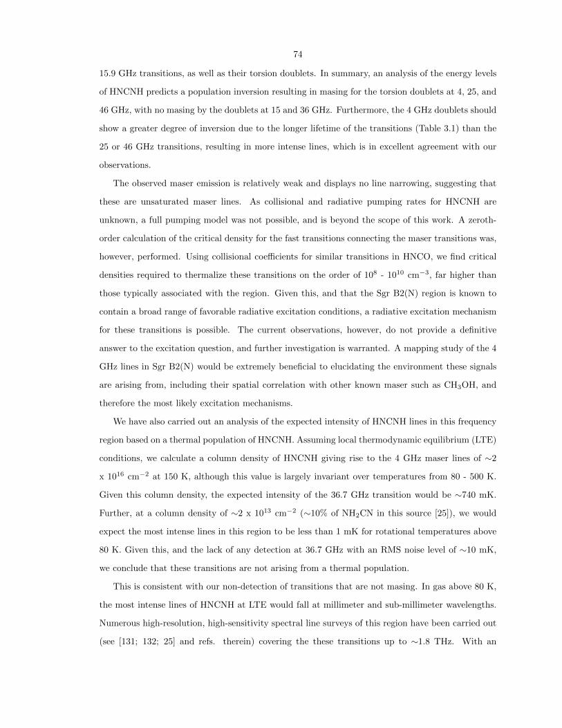
74

15.9 GHz transitions, as well as their torsion doublets. In summary, an analysis of the energy levels

of HNCNH predicts a population inversion resulting in masing for the torsion doublets at 4, 25, and

46 GHz, with no masing by the doublets at 15 and 36 GHz. Furthermore, the 4 GHz doublets should

show a greater degree of inversion due to the longer lifetime of the transitions (Table 3.1) than the

25 or 46 GHz transitions, resulting in more intense lines, which is in excellent agreement with our

observations.

The observed maser emission is relatively weak and displays no line narrowing, suggesting that

these are unsaturated maser lines. As collisional and radiative pumping rates for HNCNH are

unknown, a full pumping model was not possible, and is beyond the scope of this work. A zeroth-

order calculation of the critical density for the fast transitions connecting the maser transitions was,

however, performed. Using collisional coefficients for similar transitions in HNCO, we find critical

densities required to thermalize these transitions on the order of 108 - 1010 cm−3, far higher than

those typically associated with the region. Given this, and that the Sgr B2(N) region is known to

contain a broad range of favorable radiative excitation conditions, a radiative excitation mechanism

for these transitions is possible. The current observations, however, do not provide a definitive

answer to the excitation question, and further investigation is warranted. A mapping study of the 4

GHz lines in Sgr B2(N) would be extremely beneficial to elucidating the environment these signals

are arising from, including their spatial correlation with other known maser such as CH3OH, and

therefore the most likely excitation mechanisms.

We have also carried out an analysis of the expected intensity of HNCNH lines in this frequency

region based on a thermal population of HNCNH. Assuming local thermodynamic equilibrium (LTE)

conditions, we calculate a column density of HNCNH giving rise to the 4 GHz maser lines of ∼2

x 1016 cm−2 at 150 K, although this value is largely invariant over temperatures from 80 - 500 K.

Given this column density, the expected intensity of the 36.7 GHz transition would be ∼740 mK.

Further, at a column density of ∼2 x 1013 cm−2 (∼10% of NH2CN in this source [25]), we would

expect the most intense lines in this region to be less than 1 mK for rotational temperatures above

80 K. Given this, and the lack of any detection at 36.7 GHz with an RMS noise level of ∼10 mK,

we conclude that these transitions are not arising from a thermal population.

This is consistent with our non-detection of transitions that are not masing. In gas above 80 K,

the most intense lines of HNCNH at LTE would fall at millimeter and sub-millimeter wavelengths.

Numerous high-resolution, high-sensitivity spectral line surveys of this region have been carried out

(see [131; 132; 25] and refs. therein) covering the these transitions up to ∼1.8 THz. With an

75

abundance of 10% NH2CN, the strongest transitions under LTE emission at 80 K would be on the

order of the RMS noise level of the survey observations. With increasing temperature, the expected

line strengths decrease rapidly. Thus, at these column densities, a thermal population of HNCNH

would likely not be detectable in even the most sensitive line surveys to date.

This is in itself remarkable. A heroic effort has been performed in recent years in compiling

molecular inventories and facilitating new molecule detections using state-of-the-art millimeter and

sub-millimeter observatories and molecular line surveys. These surveys have provided invaluable

information on the physical and chemical conditions present in the ISM, and their high scientific

value is unquestionable. They suffer, however, from extremely high line densities and long integration

times relative to lower-frequency telescopes. Because of this, identifications of new molecular species,

especially those in low abundance, can be difficult due to the line confusion at the noise floor and

the degree of coincidental overlap of target lines with other molecular transitions.

In this work, we have shown that a molecule that would be undetectable via transitions arising

from a thermal population can be identified via maser transitions at centimeter wavelengths. This

detection was possible only through low-frequency surveys of a chemically-rich region by the GBT

through a dedicated project (PRIMOS). The number of transitions that display significant maser

activity in any given molecule is likely to be small, but weak masing behavior has been observed in a

number of molecules, such as H2CO and NH3 [133; 134]. In addition, at centimeter wavelengths, the

lack of line confusion makes definitive identification of a species possible with only a small number

of observed transitions. This may represent a new strategy for searches for key molecules of interest

to the astrochemistry and astrobiology communities that have not yet been detected due to their

low abundances.

In summary, we have detected four transitions of carbodiimide (HNCNH) towards Sgr B2(N)

with very high confidence. All four signals have been found to be the result of maser activity. We

also report two transitions that were not detected, consistent with HNCNH only being detectable

towards Sgr B2(N) through maser lines. This detection presents a new methodology for searches

for interstellar molecular candidates that may be too low in abundance to be detected in thermal

emission by modern radio observatories.

76

Part III

Time-Domain TeraHertz

Spectroscopy of Interstellar Ice

Analogs

77

Portions of this Part have been reproduced from “THz and mid-IR spectroscopy of interstellar ice

analogs: methyl and carboxylic acid groups,” by S. Ioppolo, B.A. McGuire, M.A. Allodi, and G.A.

Blake, Faraday Discussions 168, in press (2014) [135] and “The structure and dynamics of carbon

dioxide and water containing ices investigated via THz and mid-IR spectroscopy,” by M.A. Allodi, S.

Ioppolo, M.J. Kelley, B.A. McGuire, and G.A. Blake, Phys. Chem. Chem. Phys., 16, 3442 (2014)

[136].

78

Chapter 4

The Power of THz Spectroscopy

While the number of known molecules identified in the gas phase continues to increase (see Figure

4.1), identification of solid-phase molecules has been remarkably slower. The majority of these

are simple, abundant ice constituents - H2O, CH3OH, CO, CO2, H2CO, CH4, and HCOOH [137].

Identification of complex species, such as methyl formate (CH3OCHO), which are widely observed

in high abundance in the gas phase but must be formed primarily in the solid-phase [7; 9], is so far

lacking. Additionally, the number of sources in which any measurements of ices have been made is

limited. This is likely due to several complicating factors.

First, the features arising from these solid-phase species in the infrared are often relatively broad,

resulting in overlapping and confused signals in observations. Second, the sample set of sources from

which we may observe these species in ices is limited, relative to gas-phase species, as we can observe

these species only in absorption, rather than emission. At thermal equilibrium, detectable emission

requires that the energy of the observed transition be much less than the populated energy levels –

i.e. hν kT . In the infrared, this generally requires temperatures in excess of 500 K, far too hot to

sustain an ice. Additionally, absorption measurements in the infrared (see Figure 4.2) must be made

against a background radiation source (background star or embedded protostar), as the continuum

radiation field in these regions is not sufficiently high at temperatures required to maintain an ice.

Observations in the THz region of the spectrum will resolve both of these issues. Here, hν is suf-

ficiently small that temperatures less than ∼150 K can provide detectable emission, and background

black- and gray-body continuum levels are often sufficient to allow for absorption measurements with-

out the need of a background star or embedded radiation source. The combination of these factors

vastly increases the number of target sources available for observation. Preliminary indications are

that the spectra of solid-phase molecules in the THz are more distinctive than those in the infrared,

and provide information on the structure, temperature, and thermal history of the ice. While some

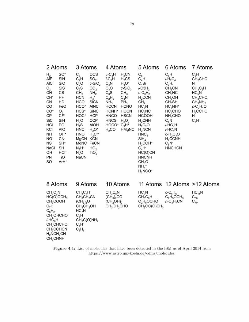
79

H2 AlF AlCl C2 CH CH+ CN CO CO+ CP SiC HCl KCl NH NO NS NaCl OH PN SO

SO+ SiN SiO SiS CS HF HD FeO O2 CF+ SiH PO AlO OH+ CN- SH+ SH HCl+ TiO ArH+

C3 C2H C2O C2S CH2 HCN HCO HCO+ HCS+ HOC+ H2O H2S HNC HNO MgCN MgNC N2H+ N2O NaCN

OCS SO2 c-SiC2 CO2 NH2 H3

+ SiCN AlNC SiNC HCP CCP AlOH H2O+ H2Cl+ KCN FeCN HO2 TiO2

c-C3H l-C3H C3N C3O C3S C2H2 NH3 HCCN HCNH+ HNCO HNCS HOCO+ H2CO

H2CN H2CS H3O+ c-SiC3 CH3 C3N- PH3 HCNO HOCN HSCN H2O2 C3H+ HMgNC

C5 C4H C4Si l-C3H2 c-C3H2 H2CCN CH4 HC3N HC2NC HCOOH H2CNH H2C2O H2NCN HNC3 SiH4 H2COH+ C4H- HC(O)CN HNCNH CH3O NH4

+ H2NCO+

C5H l-H2C4 C3H4 CH3CN CH3NC CH3OH CH3SH HC3NH+ HC2CHO NH2CHO C5N l-HC4H l-HC4N c-H2C3O H2CCNH C5N- HNCHCN

C6H CH2CHCN CH3C2H HC5N CH3CHO CH3NH2 c-C2H4O H2CCHOH C6H-

2 Atoms 3 Atoms 4 Atoms 5 Atoms 6 Atoms 7 Atoms

CH3C3N HC(O)OCH3 CH3COOH C7H C6H2 CH2OHCHO l-HC6H CH2CHCHO CH2CCHCN H2NCH2CN CH3CHNH

CH3C4H CH3CH2CN (CH3)2O CH3CH2OH HC7N C8H CH3C(O)NH2 C8H- C3H6

CH3C5N (CH3)2CO (CH2OH)2 CH3CH2CHO

8 Atoms 9 Atoms 10 Atoms HC9N CH3C6H C2H5OCHO CH3OC(O)CH3

c-C6H6 C2H5OCH3 n-C3H7CN

HC11N C60 C70

11 Atoms 12 Atoms >12 Atoms

Figure 4.1: List of molecules that have been detected in the ISM as of April 2014 fromhttps://www.astro.uni-koeln.de/cdms/molecules.

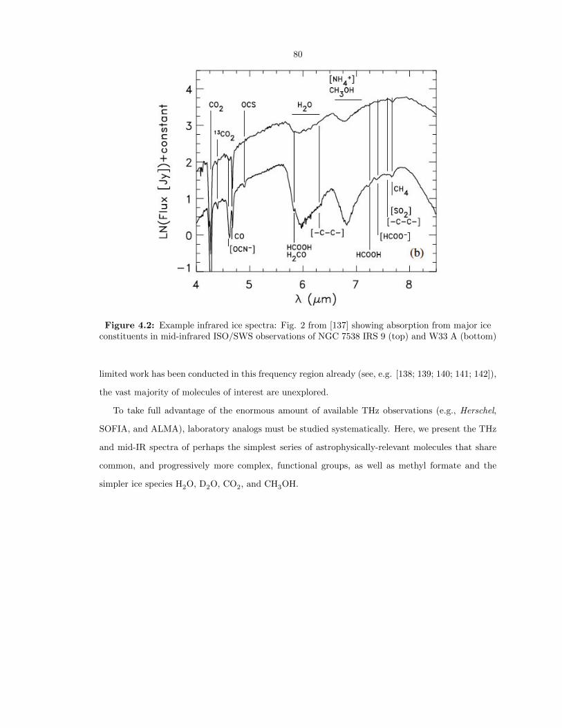
80

Figure 4.2: Example infrared ice spectra: Fig. 2 from [137] showing absorption from major iceconstituents in mid-infrared ISO/SWS observations of NGC 7538 IRS 9 (top) and W33 A (bottom)

limited work has been conducted in this frequency region already (see, e.g. [138; 139; 140; 141; 142]),

the vast majority of molecules of interest are unexplored.

To take full advantage of the enormous amount of available THz observations (e.g., Herschel,

SOFIA, and ALMA), laboratory analogs must be studied systematically. Here, we present the THz

and mid-IR spectra of perhaps the simplest series of astrophysically-relevant molecules that share

common, and progressively more complex, functional groups, as well as methyl formate and the

simpler ice species H2O, D2O, CO2, and CH3OH.

81

Chapter 5

Experimental Design

5.1 Spectrometer Overview

The details of the TeraHertz Time-Domain Spectrometer (THz-TDS) have been published previously

[136; 135], and recent improvements will be covered in full in the thesis by M. A. Allodi (2015). An

overview of the instrument is presented here to provide context for the spectroscopic details presented

in Chapter 6.

A diagram of the instrument is provided in Figure 5.1 as a reference to the reader. Briefly, pulsed

(∼320 fs full width at zero crossing) THz radiation is generated via plasma filamentation using

the output of a pulsed (∼35 fs) 800 nm regenerative amplifier coupled with an optical parametric

amplifier producing light at 1745 nm (see §5.2). The THz pulse is focused onto a 1” high-resistivity

intrinsic-silicon substrate upon which an ice of interest has been generated via vapor deposition

(see §5.3). Finally, the remaining THz signal is focused onto a non-linear gallium phosphide (GaP)

crystal and detected via electro-optic (EO) sampling (§5.4).

In addition to the THz spectrometer, a mid-IR Fourier-transform infrared (FTIR) spectrometer

(Nicolet 6700) is coupled into the system. The THz and mid-IR radiation are aligned with the

cryostat such that they probe the same region of the sample/substrate. The FTIR spectrometer

provides spectra with 1 cm−1 resolution over a range of 400 cm−1 to 4000 cm−1, and is used for

diagnostic purposes and monitoring of the ices during deposition and spectral acquisition. Spectra

of the ices discussed in §6 obtained with the FTIR are provided in Appendix C.

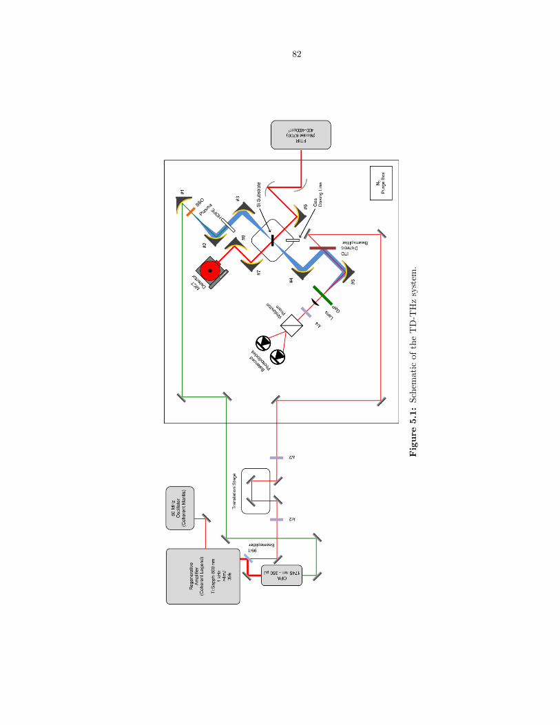
82

Fig

ure

5.1

:S

chem

ati

cof

the

TD

-TH

zsy

stem

.

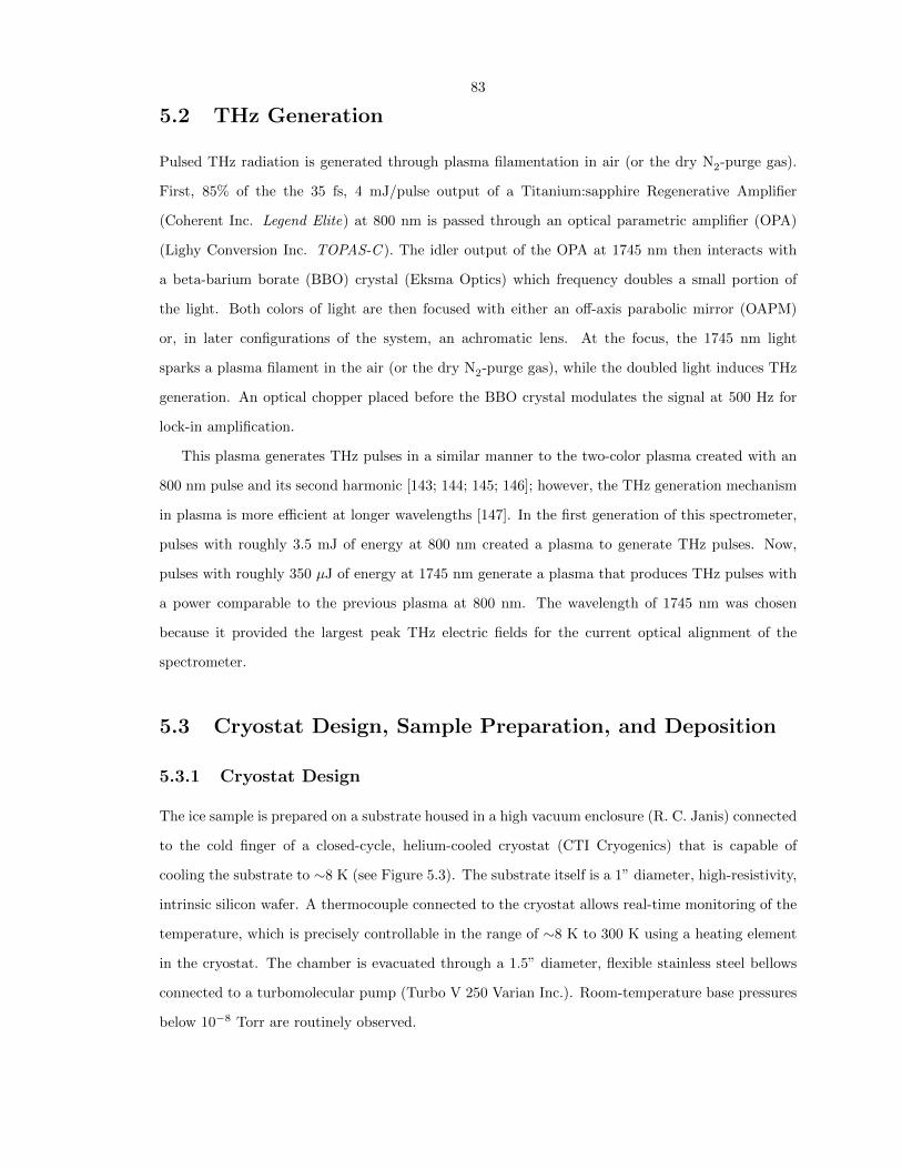
83

5.2 THz Generation

Pulsed THz radiation is generated through plasma filamentation in air (or the dry N2-purge gas).

First, 85% of the the 35 fs, 4 mJ/pulse output of a Titanium:sapphire Regenerative Amplifier

(Coherent Inc. Legend Elite) at 800 nm is passed through an optical parametric amplifier (OPA)

(Lighy Conversion Inc. TOPAS-C ). The idler output of the OPA at 1745 nm then interacts with

a beta-barium borate (BBO) crystal (Eksma Optics) which frequency doubles a small portion of

the light. Both colors of light are then focused with either an off-axis parabolic mirror (OAPM)

or, in later configurations of the system, an achromatic lens. At the focus, the 1745 nm light

sparks a plasma filament in the air (or the dry N2-purge gas), while the doubled light induces THz

generation. An optical chopper placed before the BBO crystal modulates the signal at 500 Hz for

lock-in amplification.

This plasma generates THz pulses in a similar manner to the two-color plasma created with an

800 nm pulse and its second harmonic [143; 144; 145; 146]; however, the THz generation mechanism

in plasma is more efficient at longer wavelengths [147]. In the first generation of this spectrometer,

pulses with roughly 3.5 mJ of energy at 800 nm created a plasma to generate THz pulses. Now,

pulses with roughly 350 µJ of energy at 1745 nm generate a plasma that produces THz pulses with

a power comparable to the previous plasma at 800 nm. The wavelength of 1745 nm was chosen

because it provided the largest peak THz electric fields for the current optical alignment of the

spectrometer.

5.3 Cryostat Design, Sample Preparation, and Deposition

5.3.1 Cryostat Design

The ice sample is prepared on a substrate housed in a high vacuum enclosure (R. C. Janis) connected

to the cold finger of a closed-cycle, helium-cooled cryostat (CTI Cryogenics) that is capable of

cooling the substrate to ∼8 K (see Figure 5.3). The substrate itself is a 1” diameter, high-resistivity,

intrinsic silicon wafer. A thermocouple connected to the cryostat allows real-time monitoring of the

temperature, which is precisely controllable in the range of ∼8 K to 300 K using a heating element

in the cryostat. The chamber is evacuated through a 1.5” diameter, flexible stainless steel bellows

connected to a turbomolecular pump (Turbo V 250 Varian Inc.). Room-temperature base pressures

below 10−8 Torr are routinely observed.

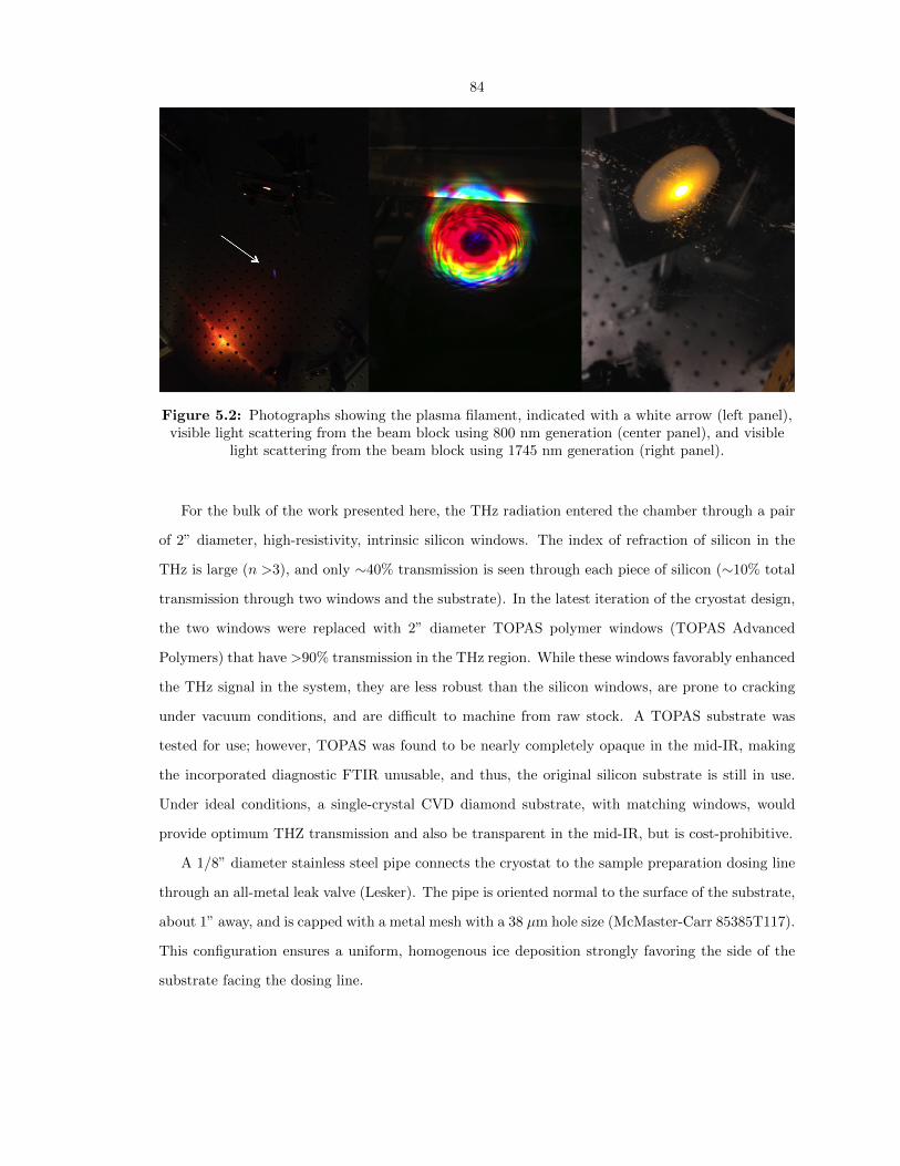
84

Figure 5.2: Photographs showing the plasma filament, indicated with a white arrow (left panel),visible light scattering from the beam block using 800 nm generation (center panel), and visible

light scattering from the beam block using 1745 nm generation (right panel).

For the bulk of the work presented here, the THz radiation entered the chamber through a pair

of 2” diameter, high-resistivity, intrinsic silicon windows. The index of refraction of silicon in the

THz is large (n >3), and only ∼40% transmission is seen through each piece of silicon (∼10% total

transmission through two windows and the substrate). In the latest iteration of the cryostat design,

the two windows were replaced with 2” diameter TOPAS polymer windows (TOPAS Advanced

Polymers) that have >90% transmission in the THz region. While these windows favorably enhanced

the THz signal in the system, they are less robust than the silicon windows, are prone to cracking

under vacuum conditions, and are difficult to machine from raw stock. A TOPAS substrate was

tested for use; however, TOPAS was found to be nearly completely opaque in the mid-IR, making

the incorporated diagnostic FTIR unusable, and thus, the original silicon substrate is still in use.

Under ideal conditions, a single-crystal CVD diamond substrate, with matching windows, would

provide optimum THZ transmission and also be transparent in the mid-IR, but is cost-prohibitive.

A 1/8” diameter stainless steel pipe connects the cryostat to the sample preparation dosing line

through an all-metal leak valve (Lesker). The pipe is oriented normal to the surface of the substrate,

about 1” away, and is capped with a metal mesh with a 38 µm hole size (McMaster-Carr 85385T117).

This configuration ensures a uniform, homogenous ice deposition strongly favoring the side of the

substrate facing the dosing line.

85

Figure 5.3: Photograph of the high vacuum cryostat showing the cold finger and siliconsubstrate, radiation shield, gas dosing line, and TOPAS windows.

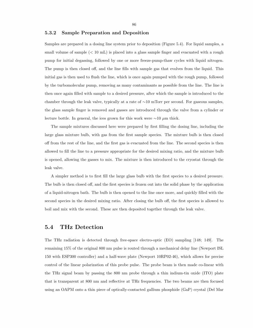
86

5.3.2 Sample Preparation and Deposition

Samples are prepared in a dosing line system prior to deposition (Figure 5.4). For liquid samples, a

small volume of sample (< 10 mL) is placed into a glass sample finger and evacuated with a rough

pump for initial degassing, followed by one or more freeze-pump-thaw cycles with liquid nitrogen.

The pump is then closed off, and the line fills with sample gas that evolves from the liquid. This

initial gas is then used to flush the line, which is once again pumped with the rough pump, followed

by the turbomolecular pump, removing as many contaminants as possible from the line. The line is

then once again filled with sample to a desired pressure, after which the sample is introduced to the

chamber through the leak valve, typically at a rate of ∼10 mTorr per second. For gaseous samples,

the glass sample finger is removed and gasses are introduced through the valve from a cylinder or

lecture bottle. In general, the ices grown for this work were ∼10 µm thick.

The sample mixtures discussed here were prepared by first filling the dosing line, including the

large glass mixture bulb, with gas from the first sample species. The mixture bulb is then closed

off from the rest of the line, and the first gas is evacuated from the line. The second species is then

allowed to fill the line to a pressure appropriate for the desired mixing ratio, and the mixture bulb

is opened, allowing the gasses to mix. The mixture is then introduced to the cryostat through the

leak valve.

A simpler method is to first fill the large glass bulb with the first species to a desired pressure.

The bulb is then closed off, and the first species is frozen out into the solid phase by the application

of a liquid-nitrogen bath. The bulb is then opened to the line once more, and quickly filled with the

second species in the desired mixing ratio. After closing the bulb off, the first species is allowed to

boil and mix with the second. These are then deposited together through the leak valve.

5.4 THz Detection

The THz radiation is detected through free-space electro-optic (EO) sampling [148; 149]. The

remaining 15% of the original 800 nm pulse is routed through a mechanical delay line (Newport ISL

150 with ESP300 controller) and a half-wave plate (Newport 10RP02-46), which allows for precise

control of the linear polarization of this probe pulse. The probe beam is then made co-linear with

the THz signal beam by passing the 800 nm probe through a thin indium-tin oxide (ITO) plate

that is transparent at 800 nm and reflective at THz frequencies. The two beams are then focused

using an OAPM onto a thin piece of optically-contacted gallium phosphide (GaP) crystal (Del Mar

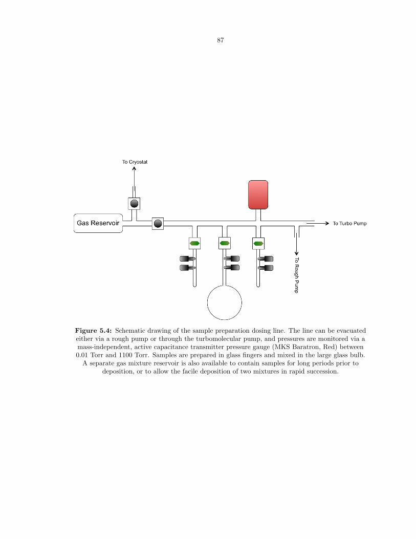
87

Figure 5.4: Schematic drawing of the sample preparation dosing line. The line can be evacuatedeither via a rough pump or through the turbomolecular pump, and pressures are monitored via amass-independent, active capacitance transmitter pressure gauge (MKS Baratron, Red) between0.01 Torr and 1100 Torr. Samples are prepared in glass fingers and mixed in the large glass bulb.

A separate gas mixture reservoir is also available to contain samples for long periods prior todeposition, or to allow the facile deposition of two mixtures in rapid succession.

88

Photonics, Inc.). This crystal is different from the one used by [136], because it has a thin EO active

layer optically contacted to a thicker inactive layer. A GaP (110) layer 200 µm thick, and capable

of EO sampling, is optically contacted to a GaP (100) layer 4 mm thick that is EO inactive. This

provides the advantage of pushing etalon features, or recurrences of the pulse in the time domain,

outside of the window being scanned. As a result, the signal-to-noise of the data as a whole improves

because the etalon features are not efficiently removed by the background subtraction in parts of

the spectrum where the signal-to-noise is low.

When focused onto the crystal together, the electric field of the THz pulse (10s of ps in length

after passing through the cryostat and sample) acts as a DC-bias on the crystal, as seen by the

35 fs 800 nm pulse. The THz light generates a transient birefringence in the GaP via the Pockels

effect, which rotates the polarization of the 800 nm pulses. The magnitude of this change is linearly

proportion to the intensity of the THz electric field applied at the time of interaction, in the small

THz field limit. By varying the length of the probe line via the mechanical delay line, the timing of

arrival of the 800 nm pulse with respect to the THz pulse can be controlled. In this way, the probe

pulse can be made to fully sample the THz pulse out to a delay of >100 ps.

After passing through the GaP crystal, the 800 nm probe beam is focused, and propagates

through a quarter-wave plate (Newport 10RP04-46) to create a circularly-polarized beam, which

is then split into orthogonal polarizations by a Wollaston Prism (Thorlabs WP20). The signal is

then measured as a difference signal on a pair of balanced, bare photodiodes. When no THz light is

present, no difference signal is observed. Under the applied electric field of a THz pulse, a difference

in the two polarizations is observed by the photodiodes, corresponding to the intensity of the THz

electric field at the time of interaction of the pulses. This signal is then sent to a lock-in amplifier

(Stanford Research Systems SR830) that records the spectrum as a function of delay.

A representative time-domain trace acquired with the spectrometer is shown in Figure 5.5. For

the majority of the results shown in §6, only ∼12 ps of the pulse were collected and used, as the

original beam block caused an etalon feature that arose shortly thereafter and made the data past

that point unusable. The resolution of the spectra collected is approximately equal to the inverse

of the length of scan in the time domain. For these experiments, this yields a ∼90 GHz resolution

in the frequency domain. Recently, a thicker beam block was obtained that pushed the etalon out

beyond the range of the scan, and as a result, ∼35 ps of the pulse were collected for the crystalline

H2O, D2O, CO2, and methyl formate shown in §6. The duration of the scan is now limited by the

substrate etalon at ∼37 ps. This has resulted in a resolution of ∼30 GHz in the frequency domain.

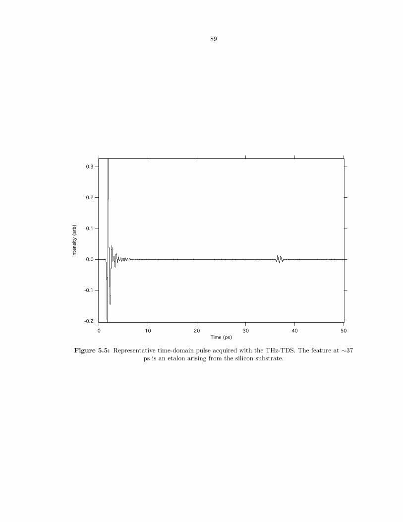
89

0.3

0.2

0.1

0.0

-0.1

-0.2

Inte

nsi

ty (

arb

)

50403020100

Time (ps)

Figure 5.5: Representative time-domain pulse acquired with the THz-TDS. The feature at ∼37ps is an etalon arising from the silicon substrate.

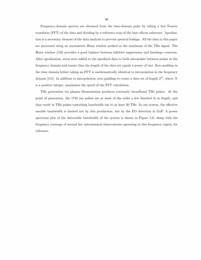
90

Frequency-domain spectra are obtained from the time-domain pulse by taking a fast Fourier

transform (FFT) of the data and dividing by a reference scan of the bare silicon substrate. Apodiza-

tion is a necessary element of the data analysis to prevent spectral leakage. All the data in this paper

are processed using an asymmetric Hann window peaked at the maximum of the THz signal. The

Hann window [150] provides a good balance between sidelobe suppression and lineshape concerns.

After apodization, zeros were added to the apodized data to both interpolate between points in the

frequency domain and ensure that the length of the data set equals a power of two. Zero padding in

the time domain before taking an FFT is mathematically identical to interpolation in the frequency

domain [151]. In addition to interpolation, zero padding to create a data set of length 2N , where N

is a positive integer, maximizes the speed of the FFT calculation.

THz generation via plasma filamentation produces extremely broadband THz pulses. At the

point of generation, the 1745 nm pulses are at most of the order a few hundred fs in length, and

thus result in THz pulses containing bandwidth out to at least 20 THz. In our system, the effective

useable bandwidth is limited not by this production, but by the EO detection in GaP. A power

spectrum plot of the detectable bandwidth of the system is shown in Figure 5.6, along with the

frequency coverage of several key astronomical observatories operating in this frequency region, for

reference.

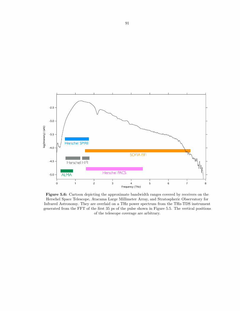
91

Figure 5.6: Cartoon depicting the approximate bandwidth ranges covered by receivers on theHerschel Space Telescope, Atacama Large Millimeter Array, and Stratospheric Observatory for

Infrared Astronomy. They are overlaid on a THz power spectrum from the THz-TDS instrumentgenerated from the FFT of the first 35 ps of the pulse shown in Figure 5.5. The vertical positions

of the telescope coverage are arbitrary.

92

Chapter 6

Results

A comparison of the ices studied presented here is shown in Figure 6.1. Spectra of each individual

species is presented and discussed in detail in the following sections.

6.1 Water (H2O)

Crystalline water was formed through the deposition of 5 Torr of gaseous water over a period of 5

minutes at 150 K. Amorphous water was formed through the deposition of 4 Torr of gaseous water

over a period of 7 minutes at 10 K.

Crystalline water (Figure 6.3) shows a single sharp band at 6.9 THz (H-bond stretching between

hydrogen-bonded bilayers), 5.7 THz (out-of-phase vibration within a bilayer), 4.9 THz (proton

disordered motion), 4.3 THz, and 1.9 THz (O-O-O bending motion) [152; 153]. The features at

4.9 THz and 6.9 THz display a narrowing and blue shift with decreasing temperature. Amorphous

water (Figure 6.4) ice displays strong, broad absorption bands at 4.6 THz and 6.2 THz. Crystalline

water is the most well-studied in the literature in this frequency region (see, e.g. [154; 140]). A

qualitative comparison of the spectrum of crystalline water ice obtained in our instrument to that

of [154] is shown in Figure 6.2.

Amorphous water that has been annealed to 175 K for a period of 10 minutes presents a set of

features that appear to be a blending of both amorphous and purely crystalline water ice (Figure

6.5). The peak at 6.9 THz appears to shift somewhat, and to grow in on top of the amorphous

features.

93

8642

Frequency (THz)

(x3) CH3OH

(x3) (CH3)2CO

CH3CHO

HCOOH

(x3) CH3COOH

(x15) CO2

Rela

tive A

bso

rbance

(x2.3) CH3OCHO

(x3) H2O

Figure 6.1: Comparison of THz spectra of crystalline ices studied in the laboratory, all at 10 K.Traces are vertically offset for clarity, and scaled to show detail.

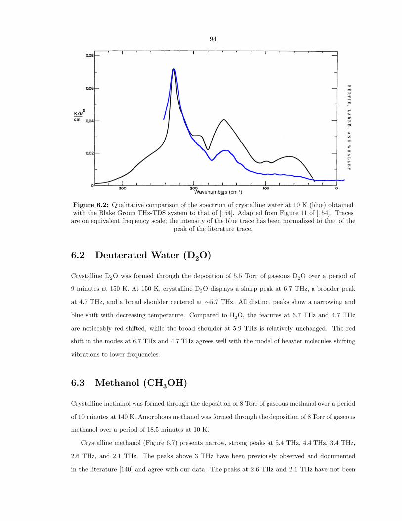
94

Figure 6.2: Qualitative comparison of the spectrum of crystalline water at 10 K (blue) obtainedwith the Blake Group THz-TDS system to that of [154]. Adapted from Figure 11 of [154]. Traces

are on equivalent frequency scale; the intensity of the blue trace has been normalized to that of thepeak of the literature trace.

6.2 Deuterated Water (D2O)

Crystalline D2O was formed through the deposition of 5.5 Torr of gaseous D2O over a period of

9 minutes at 150 K. At 150 K, crystalline D2O displays a sharp peak at 6.7 THz, a broader peak

at 4.7 THz, and a broad shoulder centered at ∼5.7 THz. All distinct peaks show a narrowing and

blue shift with decreasing temperature. Compared to H2O, the features at 6.7 THz and 4.7 THz

are noticeably red-shifted, while the broad shoulder at 5.9 THz is relatively unchanged. The red

shift in the modes at 6.7 THz and 4.7 THz agrees well with the model of heavier molecules shifting

vibrations to lower frequencies.

6.3 Methanol (CH3OH)

Crystalline methanol was formed through the deposition of 8 Torr of gaseous methanol over a period

of 10 minutes at 140 K. Amorphous methanol was formed through the deposition of 8 Torr of gaseous

methanol over a period of 18.5 minutes at 10 K.

Crystalline methanol (Figure 6.7) presents narrow, strong peaks at 5.4 THz, 4.4 THz, 3.4 THz,

2.6 THz, and 2.1 THz. The peaks above 3 THz have been previously observed and documented

in the literature [140] and agree with our data. The peaks at 2.6 THz and 2.1 THz have not been

95

0.6

0.4

0.2

0.0

-0.2

Rela

tive A

bso

rbance

7654321

Frequency (THz)

c-H2O

Figure 6.3: Spectra of crystalline water, deposited at 150 K, at 150 K (red), 75 K (black), and 10K (blue). Traces have been vertically offset for clarity.

0.30

0.25

0.20

0.15

0.10

0.05

0.00

Rela

tive A

bso

rbance

654321

Frequency (THz)

a-H2O

Figure 6.4: Spectra of amorphous water, deposited at 10 K, at 125 K (orange) and 10 K (blue).

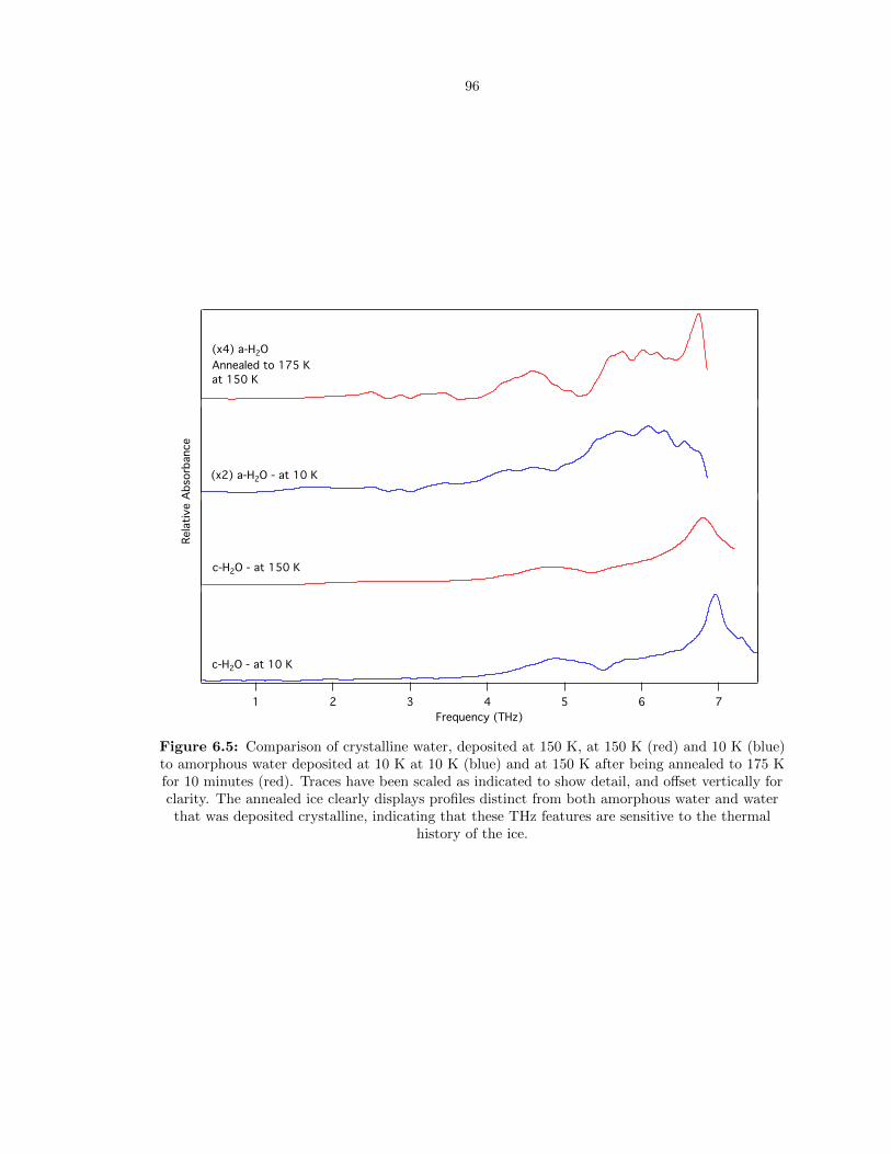
96

7654321

Frequency (THz)

(x4) a-H2O

Annealed to 175 K

at 150 K

(x2) a-H2O - at 10 K

c-H2O - at 150 K

c-H2O - at 10 K

Rela

tive A

bso

rbance

Figure 6.5: Comparison of crystalline water, deposited at 150 K, at 150 K (red) and 10 K (blue)to amorphous water deposited at 10 K at 10 K (blue) and at 150 K after being annealed to 175 Kfor 10 minutes (red). Traces have been scaled as indicated to show detail, and offset vertically forclarity. The annealed ice clearly displays profiles distinct from both amorphous water and waterthat was deposited crystalline, indicating that these THz features are sensitive to the thermal

history of the ice.

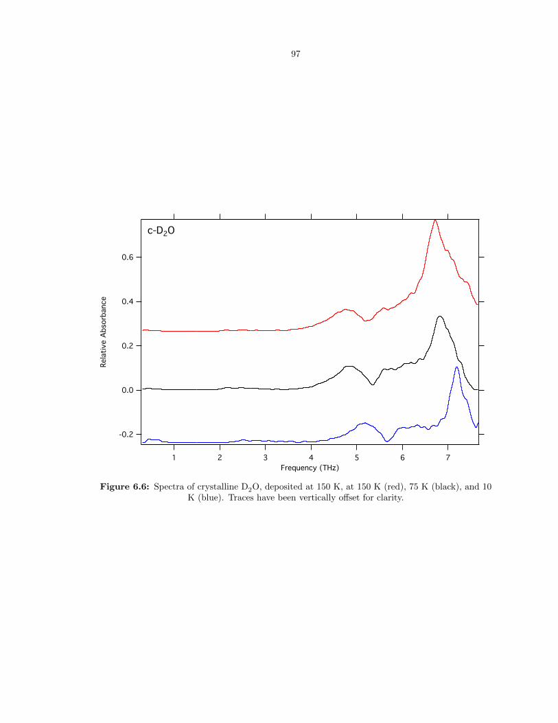
97

0.6

0.4

0.2

0.0

-0.2

Rela

tive A

bso

rbance

7654321

Frequency (THz)

c-D2O

Figure 6.6: Spectra of crystalline D2O, deposited at 150 K, at 150 K (red), 75 K (black), and 10K (blue). Traces have been vertically offset for clarity.

98

previously reported. All distinct peaks show a narrowing and blue shift with decreasing temperature.

Amorphous methanol (Figure 6.8) shows a broad feature at 4.4 THz and potentially a second feature

at 6.8 THz, though this is reaching the limit of our noise floor in these data. These features have

been previously observed, as well [140].

Amorphous methanol that has been annealed to 140 K for a period of 10 minutes shows a set of

features that is clearly distinct from those displayed by amorphous and purely crystalline methanol

(Figure 6.9). In particular, the sharp mode at 5.4 THz is significantly broadened and weaker.

6.4 Water-Methanol Mixtures

Three mixtures of water and methanol were prepared in ratios of 2:1, 1:1, and 1:2 water:methanol

and deposited crystalline at 140 K over a period of 20 minutes, 17.5 minutes, and 15 minutes,

respectively, before being cooled to 10 K (Figure 6.10). In the case of the 2:1 water:methanol

mixture, the spectra are dominated by crystalline water features, displaying few disruptions from

the presence of the methanol. The 1:1 mixture displays a spectrum that strongly resembles that of

amorphous water ice, while the 2:1 mixture displays a spectrum that shows significant disruptions

to the amorphous water profile.

6.5 Methyl Formate (CH3OCHO)

Crystalline methyl formate was formed through the deposition of 6 Torr of gaseous methyl formate

over a period of 4.5 minutes at 135 K. Crystalline methyl formate presents narrow features at 1.75

THz, 2.2 THz, 2.3 THz, 2.5 THz, 2.9 THz, and 3.3 THz. A broader peak at 3.1 THz shows indications

that it may be a blend of two narrower features. Several smaller features are possibly visible up to

4 THz, and a pair of weak features may be present at 370 GHz and 470 GHz. All distinct peaks

show a narrowing and blue shift with decreasing temperature.

6.6 Carbon Dioxide (CO2)

Crystalline carbon dioxide was formed through the deposition of 6 Torr of gaseous carbon dioxide

over a period of 2 minutes at 75 K. The spectrum of crystalline carbon dioxide (Figure 6.12) shows

only two weak, but distinct and narrow transitions at 2.1 THz and 3.5 THz. Both of these features

display a narrowing and blue shift with decreasing temperature (see inset of Figure 6.12 for detail).

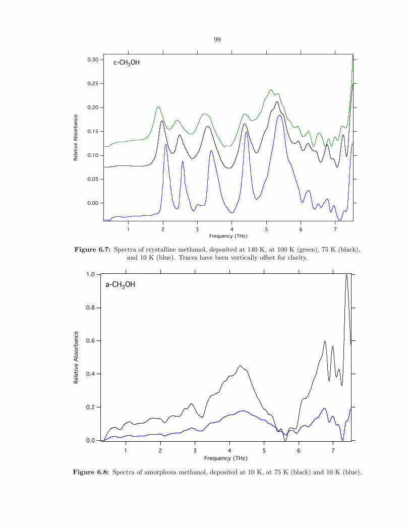
99

0.30

0.25

0.20

0.15

0.10

0.05

0.00

Rela

tive A

bso

rbance

7654321

Frequency (THz)

c-CH3OH

Figure 6.7: Spectra of crystalline methanol, deposited at 140 K, at 100 K (green), 75 K (black),and 10 K (blue). Traces have been vertically offset for clarity.

1.0

0.8

0.6

0.4

0.2

0.0

Rela

tive A

bso

rbance

7654321

Frequency (THz)

a-CH3OH

Figure 6.8: Spectra of amorphous methanol, deposited at 10 K, at 75 K (black) and 10 K (blue).

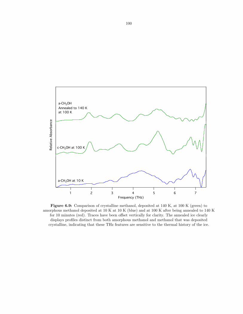
100

7654321

Frequency (THz)

Rela

tive A

bso

rbance

a-CH3OH

Annealed to 140 K

at 100 K

c-CH3OH at 100 K

a-CH3OH at 10 K

Figure 6.9: Comparison of crystalline methanol, deposited at 140 K, at 100 K (green) toamorphous methanol deposited at 10 K at 10 K (blue) and at 100 K after being annealed to 140 K

for 10 minutes (red). Traces have been offset vertically for clarity. The annealed ice clearlydisplays profiles distinct from both amorphous methanol and methanol that was deposited

crystalline, indicating that these THz features are sensitive to the thermal history of the ice.

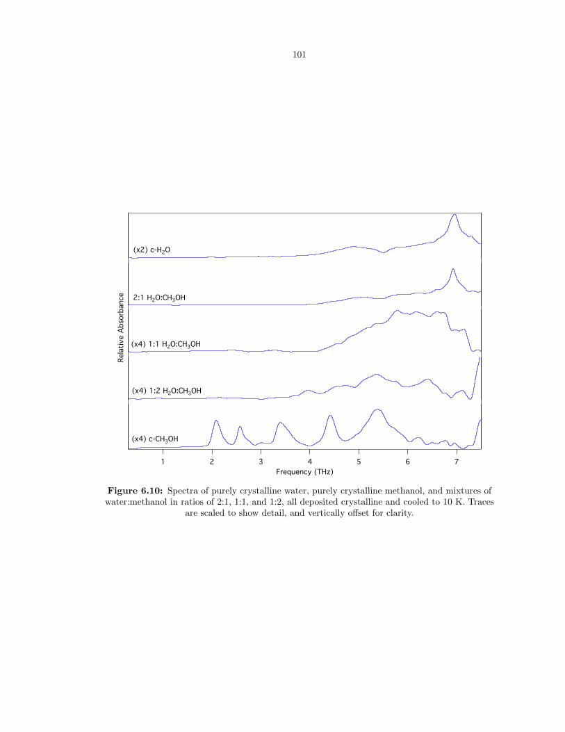
101

7654321

Frequency (THz)

Rela

tive A

bso

rbance

(x2) c-H2O

2:1 H2O:CH3OH

(x4) 1:1 H2O:CH3OH

(x4) 1:2 H2O:CH3OH

(x4) c-CH3OH

Figure 6.10: Spectra of purely crystalline water, purely crystalline methanol, and mixtures ofwater:methanol in ratios of 2:1, 1:1, and 1:2, all deposited crystalline and cooled to 10 K. Traces

are scaled to show detail, and vertically offset for clarity.

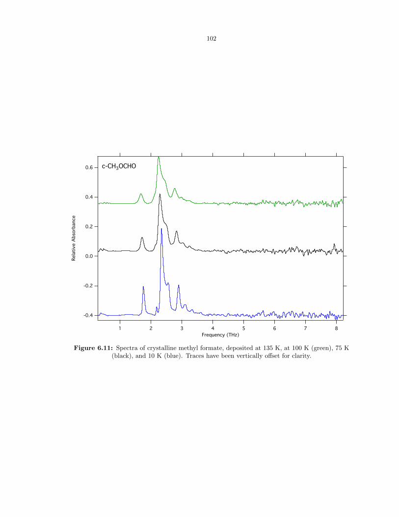
102

0.6

0.4

0.2

0.0

-0.2

-0.4

Rela

tive A

bso

rbance

87654321

Frequency (THz)

c-CH3OCHO

Figure 6.11: Spectra of crystalline methyl formate, deposited at 135 K, at 100 K (green), 75 K(black), and 10 K (blue). Traces have been vertically offset for clarity.

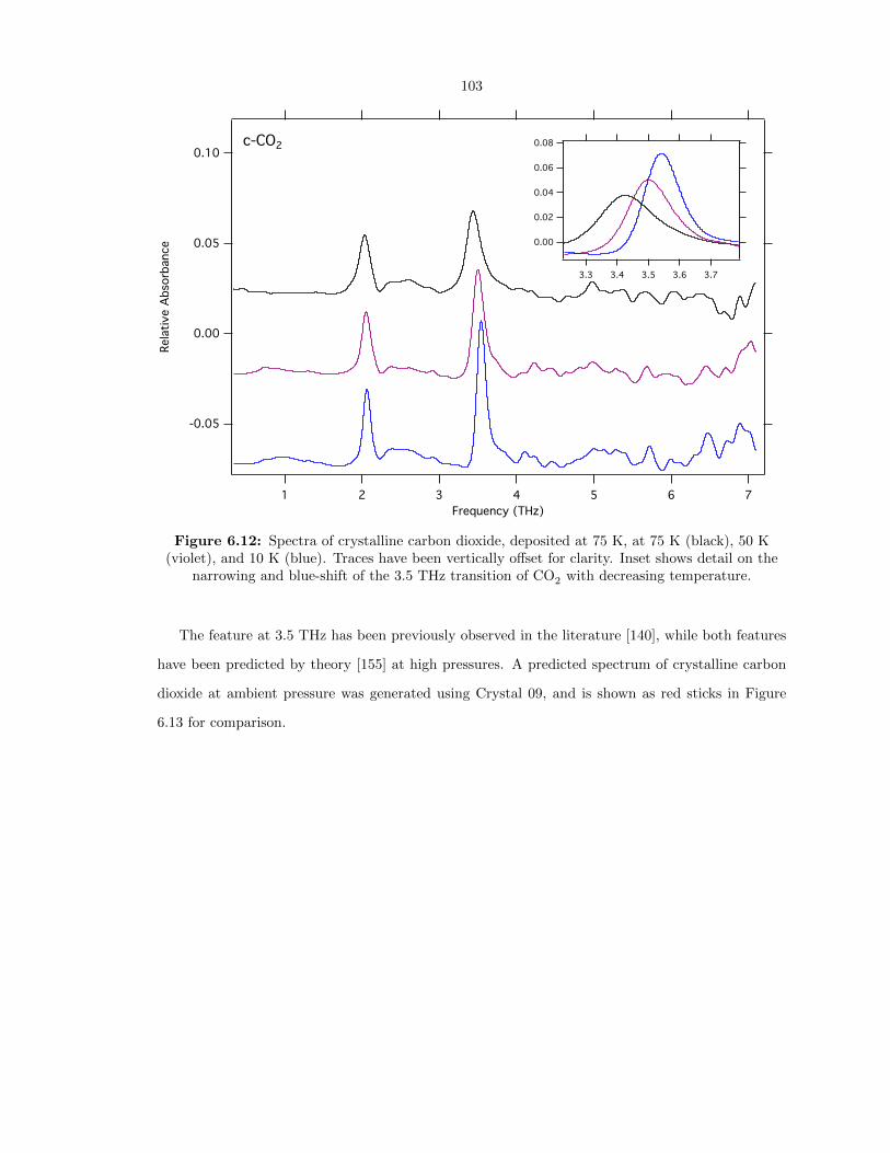
103

0.10

0.05

0.00

-0.05

Rela

tive A

bso

rbance

7654321

Frequency (THz)

0.08

0.06

0.04

0.02

0.00

3.73.63.53.43.3

c-CO2

Figure 6.12: Spectra of crystalline carbon dioxide, deposited at 75 K, at 75 K (black), 50 K(violet), and 10 K (blue). Traces have been vertically offset for clarity. Inset shows detail on the

narrowing and blue-shift of the 3.5 THz transition of CO2 with decreasing temperature.

The feature at 3.5 THz has been previously observed in the literature [140], while both features

have been predicted by theory [155] at high pressures. A predicted spectrum of crystalline carbon

dioxide at ambient pressure was generated using Crystal 09, and is shown as red sticks in Figure

6.13 for comparison.

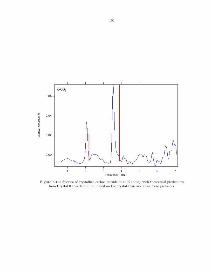
104

0.06

0.04

0.02

0.00

Rela

tive A

bso

rbance

7654321

Frequency (THz)

c-CO2

Figure 6.13: Spectra of crystalline carbon dioxide at 10 K (blue), with theoretical predictionsfrom Crystal 09 overlaid in red based on the crystal structure at ambient pressures.

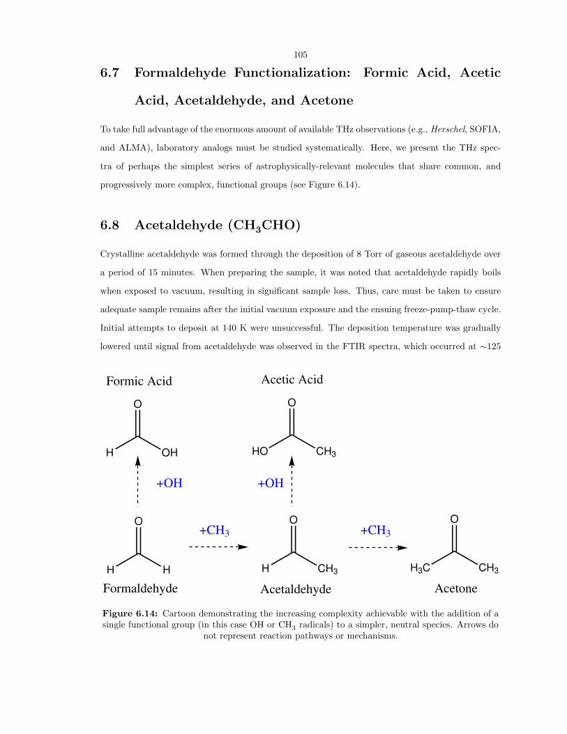
105

6.7 Formaldehyde Functionalization: Formic Acid, Acetic

Acid, Acetaldehyde, and Acetone

To take full advantage of the enormous amount of available THz observations (e.g., Herschel, SOFIA,

and ALMA), laboratory analogs must be studied systematically. Here, we present the THz spec-

tra of perhaps the simplest series of astrophysically-relevant molecules that share common, and

progressively more complex, functional groups (see Figure 6.14).

6.8 Acetaldehyde (CH3CHO)

Crystalline acetaldehyde was formed through the deposition of 8 Torr of gaseous acetaldehyde over

a period of 15 minutes. When preparing the sample, it was noted that acetaldehyde rapidly boils

when exposed to vacuum, resulting in significant sample loss. Thus, care must be taken to ensure

adequate sample remains after the initial vacuum exposure and the ensuing freeze-pump-thaw cycle.

Initial attempts to deposit at 140 K were unsuccessful. The deposition temperature was gradually

lowered until signal from acetaldehyde was observed in the FTIR spectra, which occurred at ∼125

O

H H

O

H OH

O

H CH3

O

HO CH3

O

H3C CH3

+OH +OH

+CH3 +CH3

Formic Acid Acetic Acid

Formaldehyde Acetaldehyde Acetone

Figure 6.14: Cartoon demonstrating the increasing complexity achievable with the addition of asingle functional group (in this case OH or CH3 radicals) to a simpler, neutral species. Arrows do

not represent reaction pathways or mechanisms.

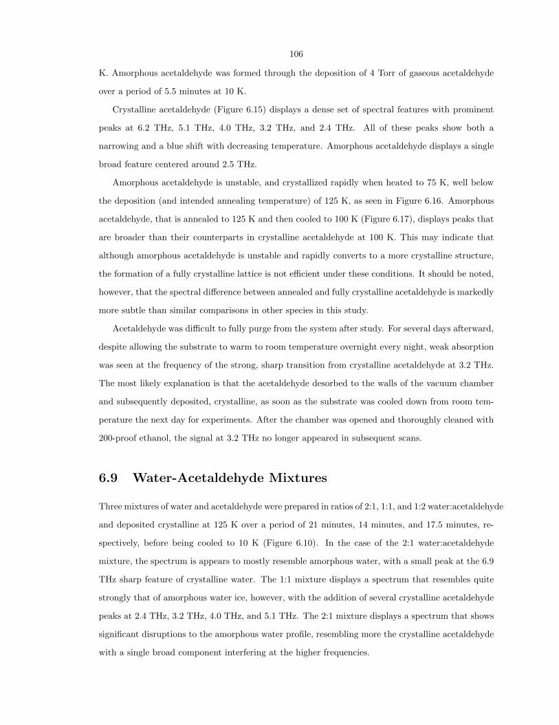
106

K. Amorphous acetaldehyde was formed through the deposition of 4 Torr of gaseous acetaldehyde

over a period of 5.5 minutes at 10 K.

Crystalline acetaldehyde (Figure 6.15) displays a dense set of spectral features with prominent

peaks at 6.2 THz, 5.1 THz, 4.0 THz, 3.2 THz, and 2.4 THz. All of these peaks show both a

narrowing and a blue shift with decreasing temperature. Amorphous acetaldehyde displays a single

broad feature centered around 2.5 THz.

Amorphous acetaldehyde is unstable, and crystallized rapidly when heated to 75 K, well below

the deposition (and intended annealing temperature) of 125 K, as seen in Figure 6.16. Amorphous

acetaldehyde, that is annealed to 125 K and then cooled to 100 K (Figure 6.17), displays peaks that

are broader than their counterparts in crystalline acetaldehyde at 100 K. This may indicate that

although amorphous acetaldehyde is unstable and rapidly converts to a more crystalline structure,

the formation of a fully crystalline lattice is not efficient under these conditions. It should be noted,

however, that the spectral difference between annealed and fully crystalline acetaldehyde is markedly

more subtle than similar comparisons in other species in this study.

Acetaldehyde was difficult to fully purge from the system after study. For several days afterward,

despite allowing the substrate to warm to room temperature overnight every night, weak absorption

was seen at the frequency of the strong, sharp transition from crystalline acetaldehyde at 3.2 THz.

The most likely explanation is that the acetaldehyde desorbed to the walls of the vacuum chamber

and subsequently deposited, crystalline, as soon as the substrate was cooled down from room tem-

perature the next day for experiments. After the chamber was opened and thoroughly cleaned with

200-proof ethanol, the signal at 3.2 THz no longer appeared in subsequent scans.

6.9 Water-Acetaldehyde Mixtures

Three mixtures of water and acetaldehyde were prepared in ratios of 2:1, 1:1, and 1:2 water:acetaldehyde

and deposited crystalline at 125 K over a period of 21 minutes, 14 minutes, and 17.5 minutes, re-

spectively, before being cooled to 10 K (Figure 6.10). In the case of the 2:1 water:acetaldehyde

mixture, the spectrum is appears to mostly resemble amorphous water, with a small peak at the 6.9

THz sharp feature of crystalline water. The 1:1 mixture displays a spectrum that resembles quite

strongly that of amorphous water ice, however, with the addition of several crystalline acetaldehyde

peaks at 2.4 THz, 3.2 THz, 4.0 THz, and 5.1 THz. The 2:1 mixture displays a spectrum that shows

significant disruptions to the amorphous water profile, resembling more the crystalline acetaldehyde

with a single broad component interfering at the higher frequencies.

107

1.0

0.5

0.0

-0.5

Rela

tive A

bso

rbance

7654321

Frequency (THz)

c-CH3CHO

Figure 6.15: Spectra of crystalline acetaldehyde, deposited at 125 K, at 100 K (green), 75 K(black), and 10 K (blue). Traces have been vertically offset for clarity.

0.30

0.25

0.20

0.15

0.10

0.05

0.00

Rela

tive A

bso

rbance

654321

Frequency (THz)

a-CH3CHO

Figure 6.16: Spectra of amorphous acetaldehyde, deposited at 10 K, at 100 K (green), 75 K(black), and 10 K (blue).

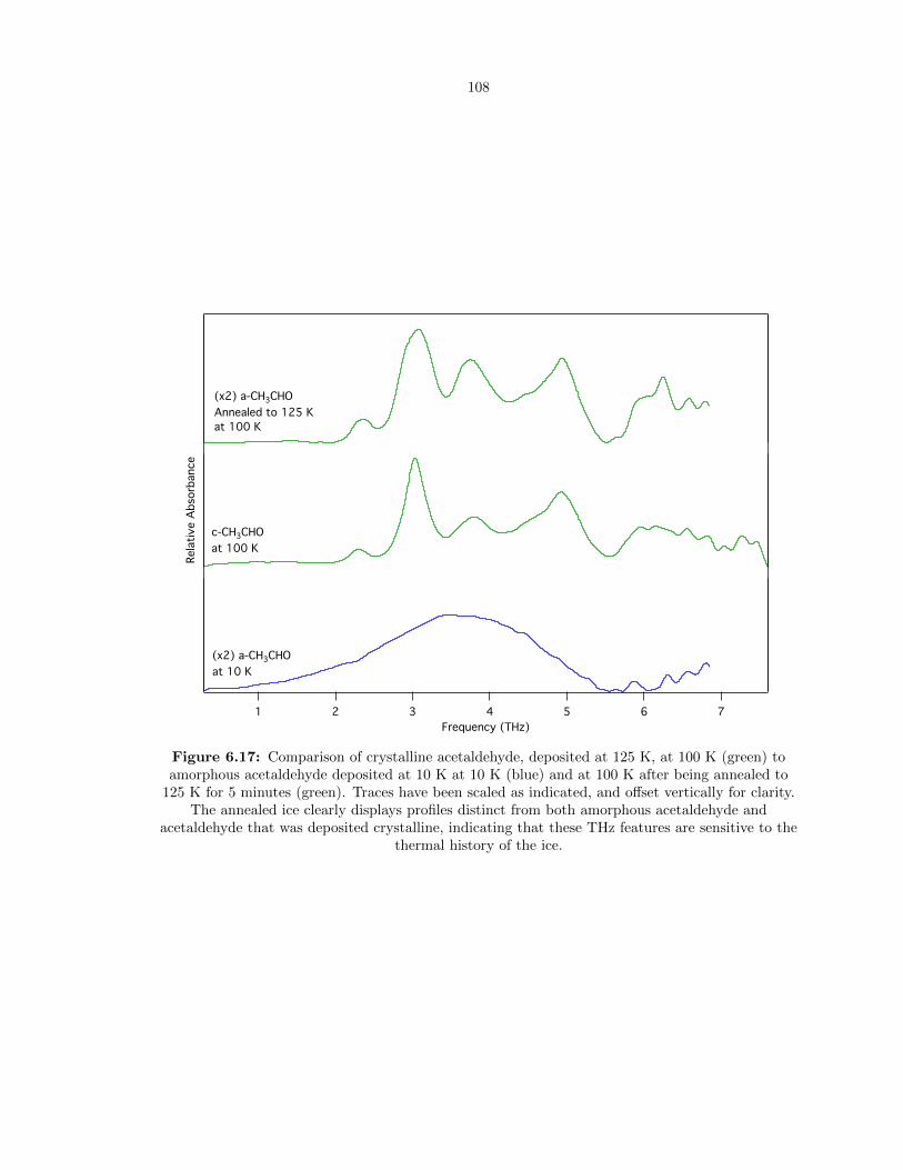
108

7654321

Frequency (THz)

Rela

tive A

bso

rbance

(x2) a-CH3CHO

Annealed to 125 K

at 100 K

c-CH3CHO

at 100 K

(x2) a-CH3CHO

at 10 K

Figure 6.17: Comparison of crystalline acetaldehyde, deposited at 125 K, at 100 K (green) toamorphous acetaldehyde deposited at 10 K at 10 K (blue) and at 100 K after being annealed to

125 K for 5 minutes (green). Traces have been scaled as indicated, and offset vertically for clarity.The annealed ice clearly displays profiles distinct from both amorphous acetaldehyde and

acetaldehyde that was deposited crystalline, indicating that these THz features are sensitive to thethermal history of the ice.

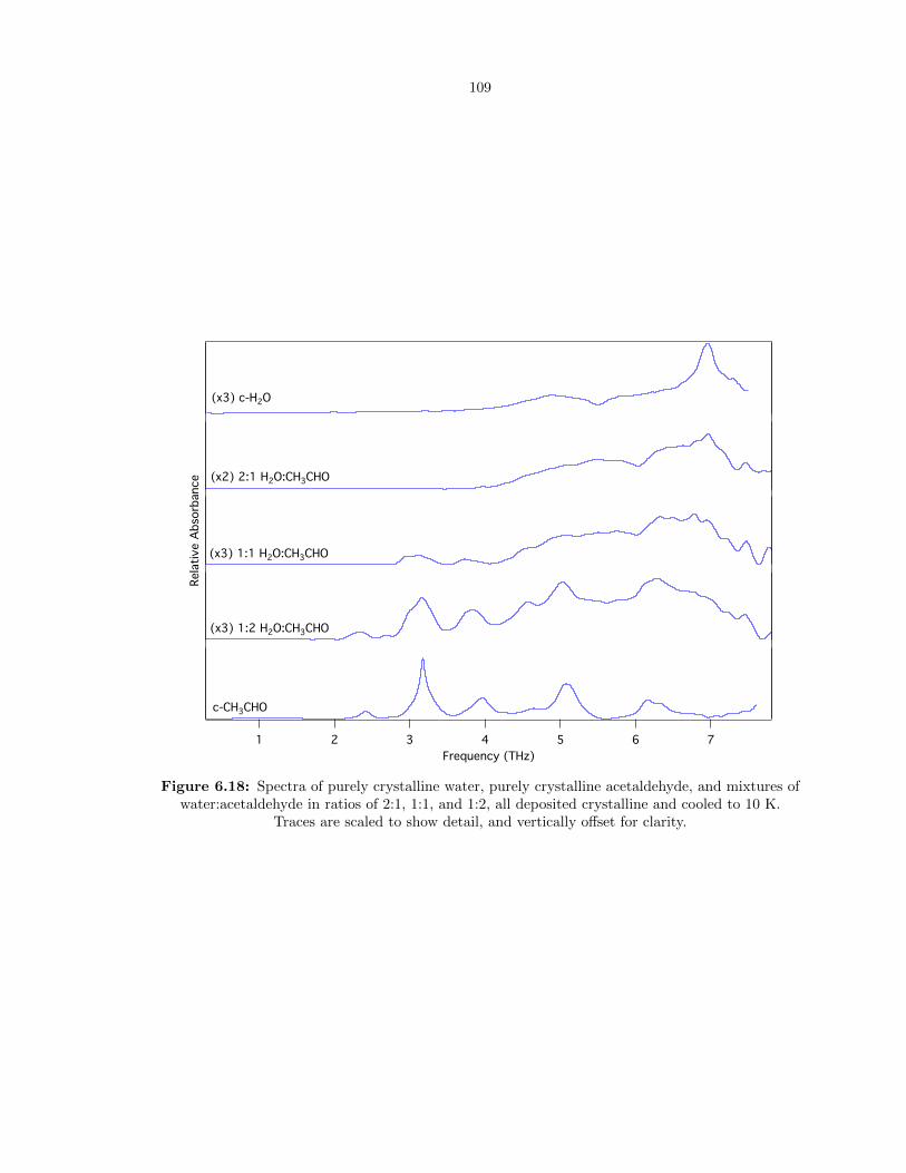
109

7654321

Frequency (THz)

Rela

tive A

bso

rbance

(x3) c-H2O

(x2) 2:1 H2O:CH3CHO

(x3) 1:1 H2O:CH3CHO

(x3) 1:2 H2O:CH3CHO

c-CH3CHO

Figure 6.18: Spectra of purely crystalline water, purely crystalline acetaldehyde, and mixtures ofwater:acetaldehyde in ratios of 2:1, 1:1, and 1:2, all deposited crystalline and cooled to 10 K.

Traces are scaled to show detail, and vertically offset for clarity.

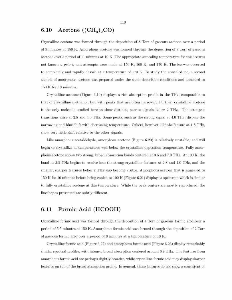
110

6.10 Acetone ((CH3)2CO)

Crystalline acetone was formed through the deposition of 8 Torr of gaseous acetone over a period

of 9 minutes at 150 K. Amorphous acetone was formed through the deposition of 8 Torr of gaseous

acetone over a period of 11 minutes at 10 K. The appropriate annealing temperature for this ice was

not known a priori, and attempts were made at 150 K, 160 K, and 170 K. The ice was observed

to completely and rapidly desorb at a temperature of 170 K. To study the annealed ice, a second

sample of amorphous acetone was prepared under the same deposition conditions and annealed to

150 K for 10 minutes.

Crystalline acetone (Figure 6.19) displays a rich absorption profile in the THz, comparable to

that of crystalline methanol, but with peaks that are often narrower. Further, crystalline acetone

is the only molecule studied here to show distinct, narrow signals below 2 THz. The strongest

transitions arise at 2.8 and 4.0 THz. Some peaks, such as the strong signal at 4.0 THz, display the

narrowing and blue shift with decreasing temperature. Others, however, like the feature at 1.8 THz,

show very little shift relative to the other signals.

Like amorphous acetaldehyde, amorphous acetone (Figure 6.20) is relatively unstable, and will

begin to crystallize at temperatures well below the crystalline deposition temperature. Fully amor-

phous acetone shows two strong, broad absorption bands centered at 3.5 and 7.0 THz. At 100 K, the

band at 3.5 THz begins to resolve into the strong crystalline features at 2.8 and 4.0 THz, and the

smaller, sharper features below 2 THz also become visible. Amorphous acetone that is annealed to

150 K for 10 minutes before being cooled to 100 K (Figure 6.21) displays a spectrum which is similar

to fully crystalline acetone at this temperature. While the peak centers are mostly reproduced, the

lineshapes presented are subtly different.

6.11 Formic Acid (HCOOH)

Crystalline formic acid was formed through the deposition of 4 Torr of gaseous formic acid over a

period of 5.5 minutes at 150 K. Amorphous formic acid was formed through the deposition of 2 Torr

of gaseous formic acid over a period of 8 minutes at a temperature of 10 K.

Crystalline formic acid (Figure 6.22) and amorphous formic acid (Figure 6.23) display remarkably

similar spectral profiles, with intense, broad absorption centered around 6.8 THz. The features from

amorphous formic acid are perhaps slightly broader, while crystalline formic acid may display sharper

features on top of the broad absorption profile. In general, these features do not show a consistent or

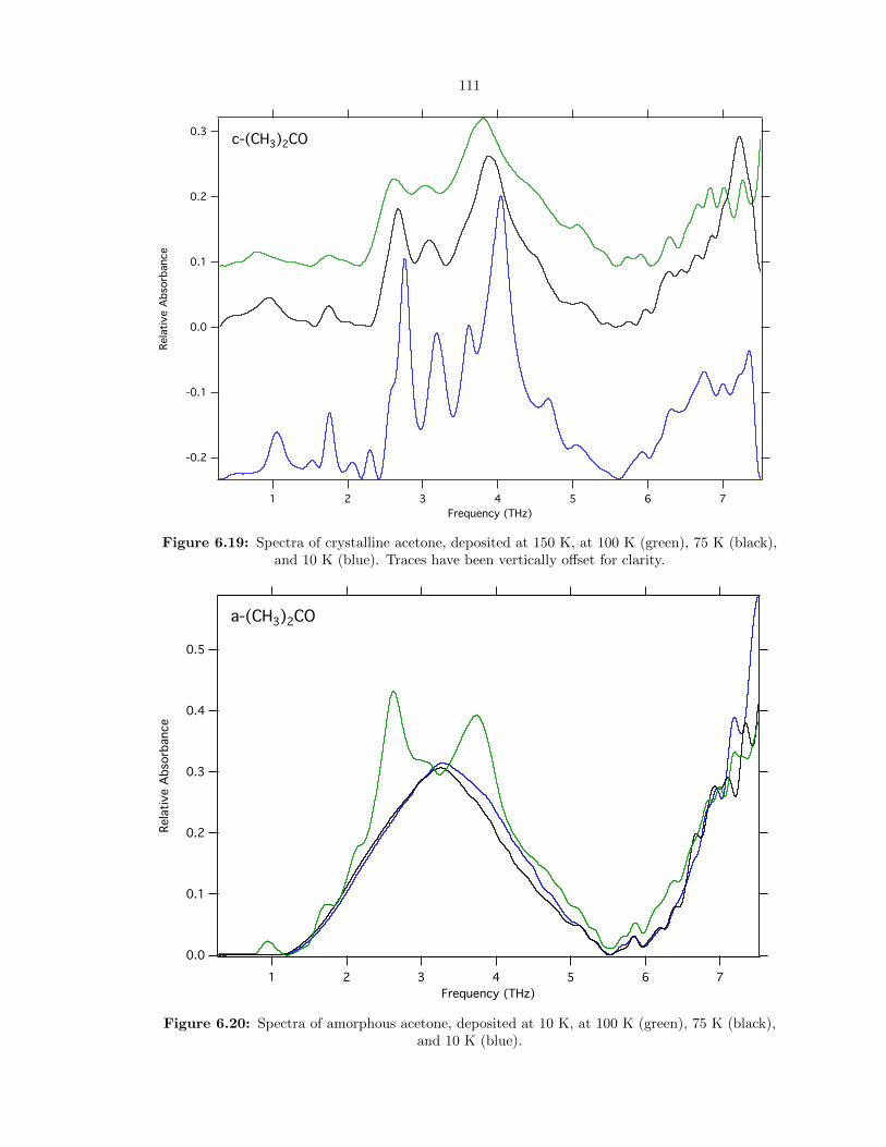
111

0.3

0.2

0.1

0.0

-0.1

-0.2

Rela

tive A

bso

rbance

7654321

Frequency (THz)

c-(CH3)2CO

Figure 6.19: Spectra of crystalline acetone, deposited at 150 K, at 100 K (green), 75 K (black),and 10 K (blue). Traces have been vertically offset for clarity.

0.5

0.4

0.3

0.2

0.1

0.0

Rela

tive A

bso

rbance

7654321

Frequency (THz)

a-(CH3)2CO

Figure 6.20: Spectra of amorphous acetone, deposited at 10 K, at 100 K (green), 75 K (black),and 10 K (blue).

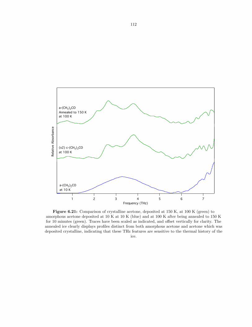
112

7654321

Frequency (THz)

Rela

tive A

bso

rbance

a-(CH3)2CO

Annealed to 150 K

at 100 K

(x2) c-(CH3)2CO

at 100 K

a-(CH3)2CO

at 10 K

Figure 6.21: Comparison of crystalline acetone, deposited at 150 K, at 100 K (green) toamorphous acetone deposited at 10 K at 10 K (blue) and at 100 K after being annealed to 150 Kfor 10 minutes (green). Traces have been scaled as indicated, and offset vertically for clarity. Theannealed ice clearly displays profiles distinct from both amorphous acetone and acetone which wasdeposited crystalline, indicating that these THz features are sensitive to the thermal history of the

ice.

113

easily discernible narrowing or blue shift with decreasing temperature, as has been widely observed

in other species.

Annealed formic acid (Figure 6.24) displays a spectral profile that appears distinct from amor-

phous and fully crystalline formic acid. The uncertainty in the origin of the structure observed over

the broad feature, however, makes any attempt at a more rigorous comparison difficult.

6.12 Acetic Acid (CH3COOH)

Crystalline acetic acid was formed through the deposition of 4 Torr of gaseous acetic acid over

a period of 3 minutes at 150 K. It was noted that the acetic acid froze more rapidly than most

species during the freeze-pump-thaw cycle. After freezing, the sample was exposed to vacuum for a

significant amount of time, but no melting was observed. Despite this, when the line was allowed

to fill with gas, the pressure rose rapidly to 13 Torr. At this point, the sample appeared to remain

solid, but had formed a hollow tube structure in the sample finger, and was no longer cold to the

touch. After some time, the sample did eventually melt. The FTIR clearly indicated the presence

of pure, crystalline acetic acid. Amorphous acetic acid was formed through the deposition of 2 Torr

of gaseous acetic acid over a period of 3 minutes at 10 K. In this case, a warm water bath was

introduced after the sample was frozen and exposed to vacuum. The sample melted more rapidly.

As with formic acid, crystalline acetic acid (Figure 6.25) and amorphous acetic acid (Figure 6.26)

display markedly similar profiles, with broad absorption centered around 6.0 THz. Unlike formic

acid, however, crystalline acetic acid displays an additional, albeit weak absorption feature at 2.6

THz that is not seen in amorphous formic acid. By monitoring the signal from acetic acid with

the FTIR, we experimentally determined that all acetic acid desorbed from the substrate at around

220 K. An annealing temperature of 200 K was therefore chosen. After annealing to 200 K for 5

minutes and cooling back to 100 K, the annealed acetic acid shows the feature at 2.6 THz, as well

as displaying a narrowing in the band at 6.0 THz, relative to both crystalline and amorphous acetic

acid.

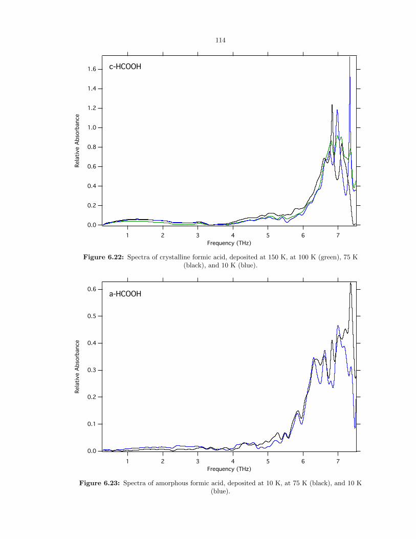
114

1.6

1.4

1.2

1.0

0.8

0.6

0.4

0.2

0.0

Rela

tive A

bso

rbance

7654321

Frequency (THz)

c-HCOOH

Figure 6.22: Spectra of crystalline formic acid, deposited at 150 K, at 100 K (green), 75 K(black), and 10 K (blue).

0.6

0.5

0.4

0.3

0.2

0.1

0.0

Rela

tive A

bso

rbance

7654321

Frequency (THz)

a-HCOOH

Figure 6.23: Spectra of amorphous formic acid, deposited at 10 K, at 75 K (black), and 10 K(blue).

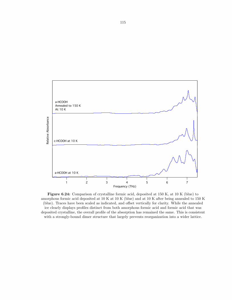
115

7654321

Frequency (THz)

Rela

tive A

bso

rbance

a-HCOOH at 10 K

c-HCOOH at 10 K

a-HCOOH

Annealed to 150 K

At 10 K

Figure 6.24: Comparison of crystalline formic acid, deposited at 150 K, at 10 K (blue) toamorphous formic acid deposited at 10 K at 10 K (blue) and at 10 K after being annealed to 150 K(blue). Traces have been scaled as indicated, and offset vertically for clarity. While the annealedice clearly displays profiles distinct from both amorphous formic acid and formic acid that was

deposited crystalline, the overall profile of the absorption has remained the same. This is consistentwith a strongly-bound dimer structure that largely prevents reorganization into a wider lattice.

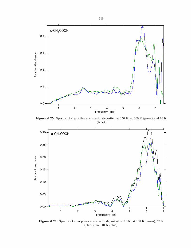
116

0.4

0.3

0.2

0.1

0.0

Rela

tive A

bso

rbance

7654321

Frequency (THz)

c-CH3COOH

Figure 6.25: Spectra of crystalline acetic acid, deposited at 150 K, at 100 K (green) and 10 K(blue).

0.30

0.25

0.20

0.15

0.10

0.05

0.00

Rela

tive A

bso

rbance

7654321

Frequency (THz)

a-CH3COOH

Figure 6.26: Spectra of amorphous acetic acid, deposited at 10 K, at 100 K (green), 75 K(black), and 10 K (blue).

117

7654321

Frequency (THz)

Rela

tive A

bso

rbance

a-CH3COOH

Annealed to 200 K

at 100 K

c-CH3COOH

at 100 K

a-CH3COOH

at 10 K

Figure 6.27: Comparison of crystalline acetic acid acid, deposited at 150 K, at 100 K (green) toamorphous acetic acid deposited at 10 K at 10 K (blue) and at 100 K after being annealed to 200K (green). Traces have been offset vertically for clarity. While the annealed ice clearly displays anadditional small absorption at 2.5 THz, the primary absorption feature remains largely unchanged.This is may indicate a strongly-bound dimer structure, similar to formic acid, that largely prevents

reorganization into a wider lattice.

118

Chapter 7

Discussion

7.1 Molecular Motions

The THz spectra presented here probe a set of molecular motions that is distinct from those at both

higher and lower frequencies. Generally speaking, transitions in the infrared (like those in Appendix

C) arise from the intramolecular motions of molecules – the bending and stretching of bonds within a

single molecule, perhaps perturbed somewhat by interactions with surrounding species (solids, neat

liquids) or solvents – while transitions in the microwave arise from the pure rotational or torsional

motions of a single molecule (see Figure 7.1). Signals arising in the THz region of the spectrum,

however, probe a distinctly different regime.

The pure rotational motion of some lighter molecules, and the torsional motion of complex

species such as methanol, has transitions from intramolecular motion in the range of 1 to a few

THz. However, the bulk of the transitions observed in the THz arise from the intermolecular

motion of molecules. In particular, the long-range, bulk motion (i.e. lattice modes) of hydrogen-

bonded structures seems to dominate this spectral region. The most-studied of these is the case of

crystalline water, which shows transitions arising from the bulk motion of hydrogen-bonded bilayers

with respect to one another [152; 153] (see Figure 7.2). It is therefore of little surprise that the THz

spectra collected with our instrument for crystalline ices present both more numerous and more

distinct features than those from amorphous ices. This also offers the ability to probe the effects of

impurities on the large-scale structure (i.e. hydrogen-bonding networks) in these crystalline ices.

Indeed, the THz spectra of these ices appear to be exquisitely sensitive to this structure, and to

any disruption in the crystalline network. Perhaps the most extreme example of this is shown in

Figure 6.17. Amorphous acetaldehyde appears to require very little thermal energy to reorganize

into a crystalline structure, with distinctly crystalline features arising in samples that are heated to

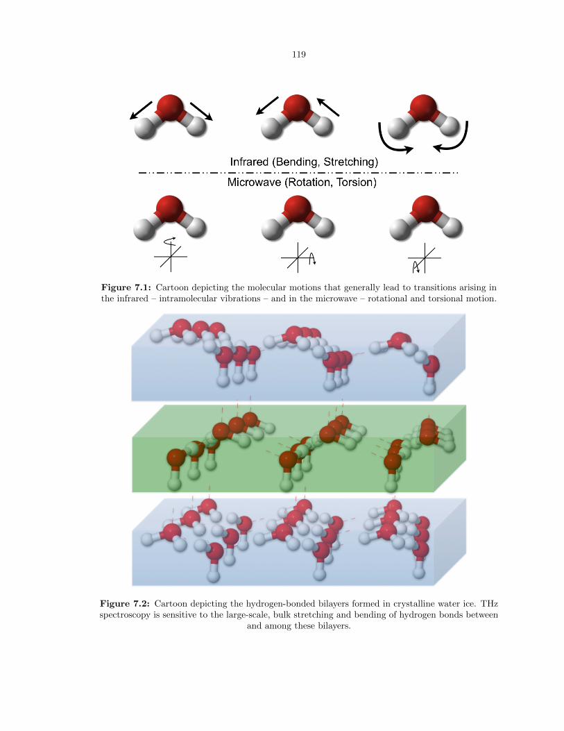
119

Figure 7.1: Cartoon depicting the molecular motions that generally lead to transitions arising inthe infrared – intramolecular vibrations – and in the microwave – rotational and torsional motion.

Figure 7.2: Cartoon depicting the hydrogen-bonded bilayers formed in crystalline water ice. THzspectroscopy is sensitive to the large-scale, bulk stretching and bending of hydrogen bonds between

and among these bilayers.

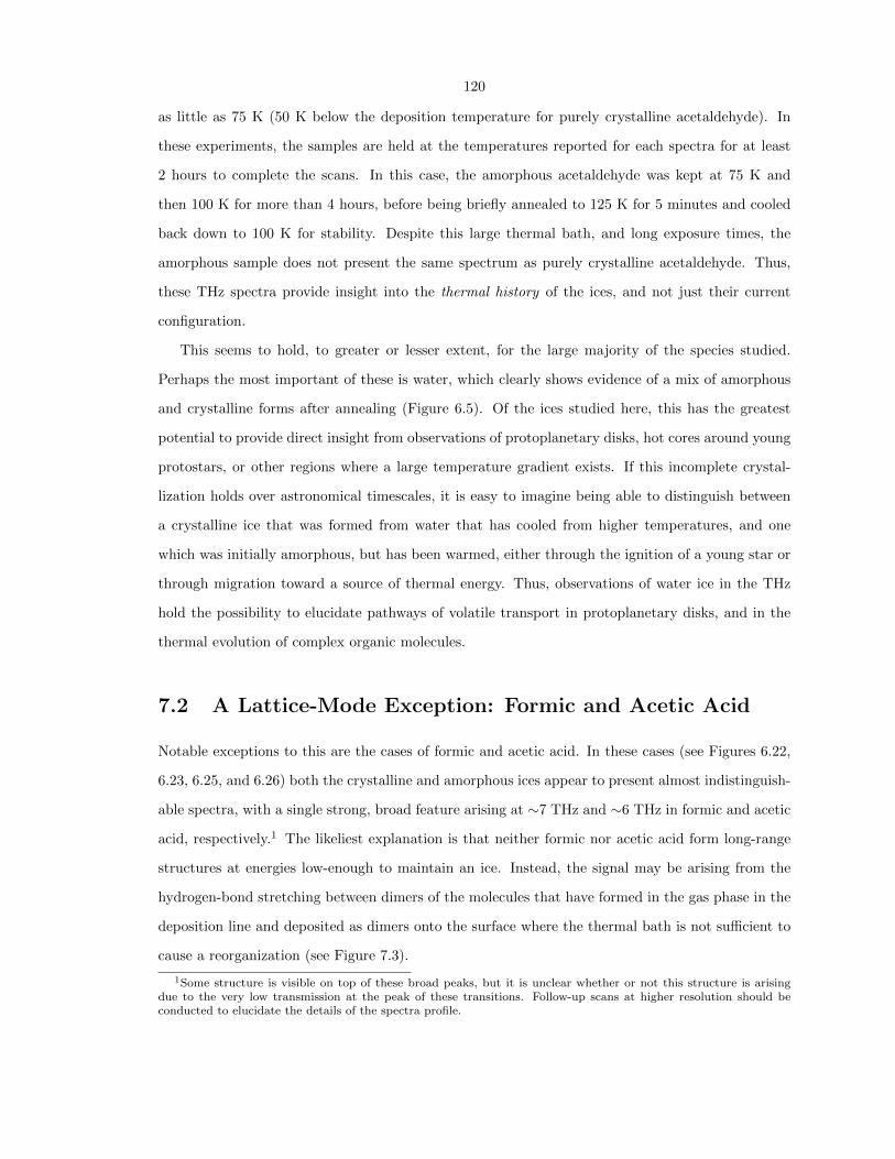
120

as little as 75 K (50 K below the deposition temperature for purely crystalline acetaldehyde). In

these experiments, the samples are held at the temperatures reported for each spectra for at least

2 hours to complete the scans. In this case, the amorphous acetaldehyde was kept at 75 K and

then 100 K for more than 4 hours, before being briefly annealed to 125 K for 5 minutes and cooled

back down to 100 K for stability. Despite this large thermal bath, and long exposure times, the

amorphous sample does not present the same spectrum as purely crystalline acetaldehyde. Thus,

these THz spectra provide insight into the thermal history of the ices, and not just their current

configuration.

This seems to hold, to greater or lesser extent, for the large majority of the species studied.

Perhaps the most important of these is water, which clearly shows evidence of a mix of amorphous

and crystalline forms after annealing (Figure 6.5). Of the ices studied here, this has the greatest

potential to provide direct insight from observations of protoplanetary disks, hot cores around young

protostars, or other regions where a large temperature gradient exists. If this incomplete crystal-

lization holds over astronomical timescales, it is easy to imagine being able to distinguish between

a crystalline ice that was formed from water that has cooled from higher temperatures, and one

which was initially amorphous, but has been warmed, either through the ignition of a young star or

through migration toward a source of thermal energy. Thus, observations of water ice in the THz

hold the possibility to elucidate pathways of volatile transport in protoplanetary disks, and in the

thermal evolution of complex organic molecules.

7.2 A Lattice-Mode Exception: Formic and Acetic Acid

Notable exceptions to this are the cases of formic and acetic acid. In these cases (see Figures 6.22,

6.23, 6.25, and 6.26) both the crystalline and amorphous ices appear to present almost indistinguish-

able spectra, with a single strong, broad feature arising at ∼7 THz and ∼6 THz in formic and acetic

acid, respectively.1 The likeliest explanation is that neither formic nor acetic acid form long-range

structures at energies low-enough to maintain an ice. Instead, the signal may be arising from the

hydrogen-bond stretching between dimers of the molecules that have formed in the gas phase in the

deposition line and deposited as dimers onto the surface where the thermal bath is not sufficient to

cause a reorganization (see Figure 7.3).

1Some structure is visible on top of these broad peaks, but it is unclear whether or not this structure is arisingdue to the very low transmission at the peak of these transitions. Follow-up scans at higher resolution should beconducted to elucidate the details of the spectra profile.

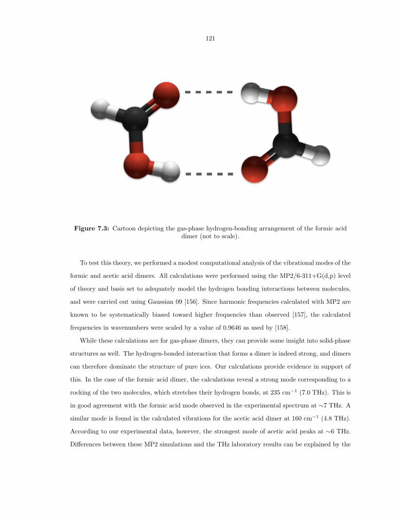
121

Figure 7.3: Cartoon depicting the gas-phase hydrogen-bonding arrangement of the formic aciddimer (not to scale).

To test this theory, we performed a modest computational analysis of the vibrational modes of the

formic and acetic acid dimers. All calculations were performed using the MP2/6-311+G(d,p) level

of theory and basis set to adequately model the hydrogen bonding interactions between molecules,

and were carried out using Gaussian 09 [156]. Since harmonic frequencies calculated with MP2 are

known to be systematically biased toward higher frequencies than observed [157], the calculated

frequencies in wavenumbers were scaled by a value of 0.9646 as used by [158].

While these calculations are for gas-phase dimers, they can provide some insight into solid-phase

structures as well. The hydrogen-bonded interaction that forms a dimer is indeed strong, and dimers

can therefore dominate the structure of pure ices. Our calculations provide evidence in support of

this. In the case of the formic acid dimer, the calculations reveal a strong mode corresponding to a

rocking of the two molecules, which stretches their hydrogen bonds, at 235 cm−1 (7.0 THz). This is

in good agreement with the formic acid mode observed in the experimental spectrum at ∼7 THz. A

similar mode is found in the calculated vibrations for the acetic acid dimer at 160 cm−1 (4.8 THz).

According to our experimental data, however, the strongest mode of acetic acid peaks at ∼6 THz.

Differences between these MP2 simulations and the THz laboratory results can be explained by the

122

more constrained nature of the molecules in the ice that can cause the frequency of this rocking

vibration to be higher in energy in the solid phase than in the gas phase.

Overall, while the predicted mode of acetic acid does not agree perfectly with the experimentally-

measured transition, the calculations produce the same red shift in frequency, relative to the formic

acid mode, as observed in the experiments. This offers evidence to support our assignments of these

transitions, as a model of harmonic vibrations predicts a decrease in frequency when mass is in-

creased, as is the case when a heavier functional group is added (-CH3 vs H). Therefore, similarities

between THz spectra of amorphous and crystalline acidic ices can be explained by the direct depo-

sition of acidic dimers onto the substrate. As a result of the strong hydrogen-bonding interaction

between dimers, the features around 6 and 7 THz remain largely unchanged when the molecules are

deposited at high temperatures or when amorphous ices are annealed.

7.3 Mixtures

Although there are some mixed binary and more complex ices reported in literature in the far-IR

region of the electromagnetic spectrum, there are no data available at low frequencies (between 0.3

and 3 THz). For instance, Moore and Hudson [140] mixed water with other interstellar relevant

species with a ratio of 10:1 and 2:1. All of their amorphous ices were deposited at 13 K, while the

crystalline mixtures were obtained by annealing amorphous ices to 155 K and cooling them back

to 13 K. This procedure may lead to some desorption, diffusion, and reorganization. However, we

showed that annealed ices are hardly fully crystalline unless the ice is annealed to temperatures close

to their desorption temperature for several minutes. This can also cause desorption of part of the ice.

Allodi et al. [136] showed that CO2 mixed in water ice segregates at higher temperatures between

the bilayers of water ice, disrupting the crystalline structure of water ice. Spectra of these mixtures

are hard to interpret if not supported by proper THz ice-database that includes spectra of pure ices

at different temperatures and different mixtures deposited at high temperatures. Therefore, our goal

here is the investigation of the spectral changes of crystalline ice when binary mixtures are deposited

at different ratios and high temperature.

Figure 6.10 shows mixtures of water with methanol in ratios of 2:1, 1:1, and 1:2 deposited

fully crystalline at 140 K. The mixture at 2:1 H2O:CH3OH shows little change from that of purely

crystalline H2O. This is in sharp contrast to the study of CO2 and H2O mixtures in [136], where even

with dilutions as high as 10:1 H2O:CO2, severe disruption of the H2O hydrogen-bonding network

is seen (see Figure 8 of [136]). Indeed, at a mixture ratio of 5:1 H2O:CO2, there is no evidence for

123

crystalline structure at all, with the ice appearing fully amorphous. At the 10:1 H2O:CO2 dilution,

a hint of the crystalline H2O feature around 7.2 THz can be seen, but is barely above the noise

level. This is in sharp contrast to the 2:1 H2O:CH3OH mixture studied here. In this case, the ice

appears nearly fully crystalline, with all features still clearly visible. This is likely due to the ability

for CH3OH to substitute in to the hydrogen-bonding network of H2O without largely disrupting the

long-range motion.

At an even ratio of 1:1 H2O:CH3OH, the ice appears fully amorphous, which is perhaps unsur-

prising, as despite the ability of both species to form hydrogen bonds, the lack of a dominant member

prevents an overall ordered structure from forming. This conclusion seems to be supported by the

1:2 H2O:CH3OH mixture where modes of crystalline CH3OH have clearly begun to be visible. This

indicates that the ice has formed an ordered structure similar to that of purely crystalline CH3OH,

with H2O impurities participating in the hydrogen-bonding lattice.

A similar, but subtly different effect is seen when the mixture partner is acetaldehyde (see Figure

6.18). In this case, the CH3CHO, while a better hydrogen-bonding impurity than CO2, does not

appear to participate as fully in the network as CH3OH. As a result, the spectra of 2:1 H2O:CH3CHO

appears nearly fully amorphous, with only a small crystalline H2O feature still visible. The CH3CHO,

however, appears to be much more tolerant of H2O impurities than CH3OH, with purely crystalline

CH3CHO features clearly appearing in the 1:1 mixture. At an enrichment of 1:2 H2O:CH3CHO, the

ice appears nearly fully crystalline CH3CHO. Another possibility is that the H2O and CH3CHO are

porous enough that the dopant species has segregated, and has crystallized within the pores of the

primary constituent.

124

Part IV

Conclusions

125

The work presented here attacks the issue of understanding the chemical evolution of prebiotic

and biotic materials, such as amino acids, from multiple fronts. From an observational standpoint,

the identification of carbodiimide in the ISM for the first time has added a new molecule to the

known molecular inventory. Beyond this result, and perhaps more importantly, it has hopefully

opened others up to the possibility that searches for molecules that should be undetectable under

LTE conditions may yet be fruitful. With the thoughtful exploitation of phenomena such as masing,

important transient or intermediate species, which have a non-negligible effect on the overall chemical

and physical evolution of a system, may yet be detected.

Through the studies of l-C3H+ presented here, it has been shown that careful examination of

the chemistry and chemical environments probed by the observations can provide a robust and deep

insight into the mechanisms at work and the species present. Without any laboratory work having

been conducted, and examining only archival observational data, C3H– was dismissed as the carrier

of B11244 based on an analysis of the chemistry at work in the environments where it had been

detected. This work now expands, seeking to explore how l-C3H+ can probe the environments, and

the thus-far rare conditions in which it is present in detectable abundance.

Again, using only archival observational data, a serious gap in the completeness of state-of-the-

art gas-grain astrochemical models was closed by the report of a non-detection of hydroxylamine in

a number of complex molecular sources. As a result of this work, what is perhaps the last efficient

route to the formation of glycine in the gas phase has been challenged, and new astrochemical models

now turn to reactions on and within the icy mantles of dust grains to form this important species.

While the primary composition of these icy environments is relatively well-understood, there

has been no definitive observational evidence for the presence of any molecules more complex than

methanol in the solid phase. The construction of a THz-TDS system to study astrophysical ices

has begun to open up a region of the electromagnetic spectrum that has been almost completely

unexplored in terms of observing solid-phase species in the ISM. This work has revealed not only

the richness of spectral features in the THz region, but the exquisite sensitivity of these spectra on

the long-range structure of the ices as well. While traditional observations in the mid-IR offer a

somewhat comparable insight into this structure, the THz has, at least preliminarily, demonstrated

an unparalleled and exciting ability to probe the thermal history of the ices. Should such a history

be observable in observational spectra in the THz, the potential insight gained into the physical

evolution, dynamics, and mass transport within protostellar cores and protoplanetary systems is

remarkable.

126

These initial studies of ices in the THz-TDS instrument, and the conclusions drawn from them,

are largely based on a qualitative assessment of the relative positions, intensities, and profiles of the

signals observed. This is a natural and expected consequence of the foundational work being done

with this system; there is essentially no prior body of knowledge from which to build on, and thus,

this work must necessarily begin from the most basic of analyses, and yet, such efforts can only

achieve so much. The full potential of these endeavors cannot be realized until the basic forces at

work are quantified, and the underlying physical phenomena elucidated. The use of the relatively

basic theoretical simulations of dimers to understand the behavior of formic and acetic acids, and

to predict, with surprising accuracy, the observed modes of CO2 using periodic boundary condition-

constrained solid-state calculations, represent a first step into a larger world. The sensitivity of

these observations to ordered structure demands deeper theoretical investigations into the long-range

lattice structures present in these ices. For example, mixtures of methanol and acetaldehyde with

water generate an immediate awareness that understanding the interplay and transitions between

these distinctly separate ordered domains will be a complex undertaking that will rely on both

computational and laboratory efforts. The inherently time-domain nature of these studies extends

their utility by offering the opportunity to probe directly the optical constants of a species of interest,

without the need for approximate treatments of indirect data.

These studies illuminate both the early (i.e. the formative, complex molecular nebulae) and the

late (i.e. the incorporation into, or formation of amino acids in cometary ices) stages of complex

prebiotic organic chemistry along the pathway to the formation of primitive life on Earth. They

examine the two disparate, yet intricately interconnected phases of chemical evolution in the ISM

by probing, or offering the means to probe, the composition and the chemistry of both the gas and

solid phases of organic matter. In the end, it is not enough that we know what is out there, between

the stars; rather, it is our goal to understand how it all fit together, sometime in the last 13.7 billion

years (give or take), to make us.

127

Bibliography

[1] S. L. Miller and H. C. Urey, “Organic Compound Synthesis on the Primitive Earth,” Science,130, 245–251 (1959).

[2] O. Botta and J. L. Bada, “Extraterrestrial organic compounds in meteorites,” Surveys inGeophysics, 23, 411–467 (2002).

[3] J. E. Elsila, D. P. Glavin, and J. P. Dworkin, “Cometary glycine detected in samples returnedby Stardust,” Meteoritics & Planetary Science, 44, 1323–1330 (2009).

[4] R. L. Pulliam, B. A. McGuire, and A. J. Remijan, “A search for hydroxylamine (NH2OH)toward select astronomical sources,” The Astrophysical Journal , 751, 1 (2012).

[5] V. Blagojevic, S. Petrie, and D. K. Bohme, “Gasphase syntheses for interstellar carboxylicand amino acids,” Monthly Notices of the Royal Astronomical Society , 339, L7–L11 (2003).

[6] J. L. Snow, G. Orlova, V. Blagojevic, and D. K. Bohme, “Gas-phase ionic syntheses of aminoacids: β versus α,” Journal of the American Chemical Society , 129, 9910–9917 (2007).

[7] R. T. Garrod, S. L. W. Weaver, and E. Herbst, “Complex Chemistry in Star-forming Regions:An Expanded Gas-Grain Warm-up Chemical Model,” Astrophys. J., 682, 283 (2008).

[8] E. Congiu, G. Fedoseev, S. Ioppolo, F. Dulieu, H. Chaabouni et al., “NO ice hydrogenation:a solid pathway to NH2OH formation in space,” The Astrophysical Journal , 750, L12 (2012).

[9] R. T. Garrod, “A three-phase chemical model of hot cores: the formation of glycine,” TheAstrophysical Journal , 765, 60 (2013).

[10] Y.-J. Kuan, S. B. Charnley, H.-C. Huang, W.-L. Tseng, and Z. Kisiel, “Interstellar Glycine,”The Astrophysical Journal , 593, 848–867 (2003).

[11] L. Snyder, F. Lovas, J. Hollis, D. Friedel, P. Jewell et al., “A rigorous attempt to verifyinterstellar glycine,” Astrophys. J., 619, 914–930 (2005).

[12] Y. S. J. Shiao, L. W. Looney, A. J. Remijan, L. E. Snyder, and D. N. Friedel, “First aceticacid survey with CARMA in hot molecular cores,” The Astrophysical Journal Letters, 716,286–298 (2010).

[13] N. Nishi, H. Shinohara, and T. Okuyama, “Photodetachment, photodissociation, and photo-chemistry of surface molecules of icy solids containing NH3 and pure H2O ices,” The Journalof chemical physics, 80, 3898 (1984).

[14] W. Zheng and R. I. Kaiser, “Formation of hydroxylamine (NH2OH) in electron-irradiatedammonia-water ices,” Journal of Physical Chemistry , 114, 5251–5255 (2010).

[15] S. B. Charnley, S. D. Rodgers, and P. Ehrenfreund, “Gas-grain chemical models of star-forming molecular clouds as constrained by ISO and SWAS observations,” A&A, 378, 1024–1036 (2001).

128

[16] L. J. Allamandola and C. A. Norman, “Infra-red emission lines from molecules in grain man-tles,” Astronomy & Astrophysics, 63, L23–L26 (1978).

[17] M. Akyilmaz, D. R. Flower, P. Hily-Blant, G. Pineau des Forets, and C. M. Walmsley, “Thedepletion of NO in pre-protostellar cores,” A&A, 462, 221–230 (2007).

[18] H. S. P. Muller, F. Schloder, J. Stutzki, and G. Winnewisser, “The Cologne Database forMolecular Spectroscopy, CDMS: a useful tool for astronomers and spectroscopists,” Journalof Molecular Structure, 742, 215–227 (2005).

[19] I. Morino, K. M. T. Yamada, H. Klein, S. P. Belov, G. Winnewisser et al., “Terahertz rotationalspectra of NH2OH in the ground and some low excited vibrational states,” Journal of MolecularStructure, 517, 367–373 (2000).

[20] S. Tsunekawa, “Microwave Spectrum of Hydroxylamine,” Journal of the Physical Society ofJapan, 33, 167 (1972).

[21] L. M. Ziurys and D. McGonagle, “The spectrum of Orion-KL at 2 millimeters (150-160 GHz),”The Astrophysical Journal Supplement Series (ISSN 0067-0049), 89, 155–187 (1993).

[22] K. M. Menten, C. M. Walmsley, C. Henkel, and T. L. Wilson, “Methanol in the Orion region. I -Millimeter-wave observations. II - The 25 GHz masers revisited,” Astronomy and Astrophysics(ISSN 0004-6361), 198, 253–273 (1988).

[23] W. B. Latter and S. B. Charnley, “Methanol in the Circumstellar Envelope of IRC+ 10216,”The Astrophysical Journal Letters, 463, L37 (1996).

[24] B. E. Turner, “A molecular line survey of Sagittarius B2 and Orion-KL from 70 to 115 GHz.II-Analysis of the data.” The Astrophysical Journal Supplement Series, 76, 617–686 (1991).

[25] A. Nummelin, P. Bergman, A. Hjalmarson, P. Friberg, W. Irvine et al., “A three-position spec-tral line survey of sagittarius B2 between 218 and 263 GHz. II. Data analysis,” AstrophysicalJournal Supplement Series, 128, 213–243 (2000).

[26] T. J. Millar, P. D. Brown, H. Olofsson, and A. Hjalmarson, “The detection of ethanol inW51M,” Astronomy and Astrophysics (ISSN 0004-6361), 205, L5–L7 (1988).

[27] F. P. Helmich, D. J. Jansen, T. de Graauw, T. D. Groesbeck, and E. F. van Dishoeck, “Physicaland chemical variations within the W3 star-forming region. 1: SO2, CH3OH, and H2CO,”Astronomy and Astrophysics (ISSN 0004-6361), 283, 626–634 (1994).

[28] A. J. Remijan, A. Markwick-Kemper, and ALMA Working Group on Spectral Line Frequen-cies, “Splatalogue: Database for Astronomical Spectroscopy,” in “American AstronomicalSociety Meeting Abstracts,” #132.11 (2007).

[29] W. Gordy and R. L. Cook, Microwave Molecular Spectra, New York, NY: Wiley, 3 ed. (1984).

[30] J. M. Hollis, P. R. Jewell, F. J. Lovas, and A. Remijan, “Green bank telescope observationsof interstellar glycolaldehyde: low-temperature sugar,” The Astrophysical Journal , 613, L45(2004).

[31] P. F. Goldsmith and W. D. Langer, “Population diagram analysis of molecular line emission,”Astrophys. J., 517, 209 (1999).

[32] M. Womack, L. M. Ziurys, and S. Wyckoff, “Estimates of N2 abundances in dense molecularclouds,” Astrophysical Journal , 393, 188–192 (1992).

[33] N. A. Patel, K. H. Young, C. A. Gottlieb, P. Thaddeus, R. W. Wilson et al., “An Interfero-metric Spectral-line Survey of IRC+10216 in the 345 GHz Band,” The Astrophysical JournalSupplement Series, 193, 17 (2011).

129

[34] J. Cernicharo, L. B. F. M. Waters, L. Decin, P. Encrenaz, A. G. G. M. Tielens et al., “Ahigh-resolution line survey of IRC+10216 with Herschel/HIFI,” A&A, 521, L8 (2010).

[35] S. G. Lias, J. E. Bartmess, J. F. Liebman, J. L. Holmes, R. D. Levin et al., “Gas-phase ionand neutral thermochemistry,” JOURNAL OF PHYSICAL AND CHEMICAL REFERENCEDATA, 17, 1–861 (1988).

[36] D. E. Woon, “Modeling gas-grain chemistry with quantum chemical cluster calculations. I.Heterogeneous hydrogenation of CO and H2CO on icy grain mantles,” Astrophys. J., 569, 541(2002).

[37] O. Schnepp and K. Dressler, “Photolysis of Ammonia in a Solid Matrix at Low Temperatures,”The Journal of chemical physics, 32, 1682 (1960).

[38] Y. Miao, D. M. Mehringer, Y.-J. Kuan, and L. E. Snyder, “Complex molecules in SagittariusB2(N): The importance of grain chemistry,” Astrophysical Journal , 445, L59–L62 (1995).

[39] M. A. Requena-Torres, J. Martin-Pintado, A. Rodrıguez-Franco, S. Martın, N. J. Rodrıguez-Fernandez et al., “Organic molecules in the Galactic center,” A&A, 455, 971–985 (2006).

[40] P. Boulet, F. Gilardoni, J. Weber, H. Chermette, and Y. Ellinger, “Theoretical study ofinterstellar hydroxylamine chemistry: protonation and proton transfer mediated by H3+.”Chemical Physics, 244, 163–174 (1999).

[41] F. Angelelli, M. Aschi, F. Cacace, F. Pepi, and G. de Petris, “Gas-Phase Reactivity of Hydrox-ylamine toward Charged Electrophiles. A Mass Spectrometric and Computational Study of theProtonation and Methylation of H2NOH,” The Journal of Physical Chemistry , 99, 6551–6556(1995).

[42] P. Perez and R. Contreras, “A theoretical analysis of the gas-phase protonation of hydroxy-lamine, methyl-derivatives and aliphatic amino acids,” Chemical Physics Letters, 293, 239–244(1998).

[43] L. Largo, V. M. Rayon, C. Barrientos, A. Largo, and P. Redondo, “Chemical Physics Letters,”Chemical Physics Letters, 476, 174–177 (2009).

[44] D. M. Mehringer, L. E. Snyder, Y. Miao, and F. J. Lovas, “Detection and confirmation ofinterstellar acetic acid,” The Astrophysical Journal Letters, 480, L71 (1997).

[45] B. A. McGuire, P. B. Carroll, R. A. Loomis, G. A. Blake, J. M. Hollis et al., “A search forl -C3H+ and l -C3H in Sgr B2(N), Sgr B2(OH), and the dark cloud TMC-1,” The AstrophysicalJournal , 774, 56 (2013).

[46] B. A. McGuire, P. B. Carroll, P. Gratier, V. Guzman, J. Pety et al., “An observationalinvestigation of the identity of B11244 (l -C3H+/C3H−),” The Astrophysical Journal , 783, 36(2014).

[47] B. A. McGuire, P. B. Carroll, J. L. I. Sanders, S. L. Widicus Weaver, G. A. Blake et al.,“A CSO search for l -C3H+: detection in the Orion Bar PDR,” Monthly Notices of the RoyalAstronomical Society , 442, 2901–2908 (2014).

[48] J. Pety, P. Gratier, V. Guzman, E. Roueff, M. Gerin et al., “The IRAM-30 m line survey ofthe Horsehead PDR,” A&A, 548, A68 (2012).

[49] S. Ikuta, “An ab initio MO study on structures and energetics of C3H−, C3H, and C3H+,”The Journal of chemical physics, 106, 4536 (1997).

[50] J. Le Bourlot, F. Le Petit, C. Pinto, E. Roueff, and F. Roy, “Surface chemistry in the inter-stellar medium,” A&A, 541, A76 (2012).

130

[51] F. Le Petit, C. Nehme, J. Le Bourlot, and E. Roueff, “A model for atomic and molecularinterstellar gas: The Meudon PDR code,” The Astrophysical Journal Supplement Series, 164,506 (2006).

[52] B. E. Turner, E. Herbst, and R. Terzieva, “The physics and chemistry of small translucentmolecular clouds. XIII. The basic hydrocarbon chemistry,” The Astrophysical Journal Supple-ment Series, 126, 427 (2000).

[53] V. Wakelam, I. W. M. Smith, E. Herbst, J. Troe, W. Geppert et al., “Reaction Networks forInterstellar Chemical Modelling: Improvements and Challenges,” Space Science Reviews, 156,13–72 (2010).

[54] A. Fuente, A. Rodr guez Franco, S. Garc a Burillo, J. Mart n Pintado, and J. H. Black,“Observational study of reactive ions and radicals in PDRs,” A&A, 406, 899–913 (2003).

[55] D. Teyssier, D. Foss, M. Gerin, J. Pety, A. Abergel et al., “Carbon budget and carbon chemistryin Photon Dominated Regions,” A&A, 417, 135–149 (2004).

[56] J. Pety, D. Teyssier, D. Fosse, M. Gerin, E. Roueff et al., “Are PAHs precursors of smallhydrocarbons in photo-dissociation regions? The Horsehead case,” A&A, 435, 885–899 (2005).

[57] X. Huang, R. C. Fortenberry, and T. J. Lee, “Spectroscopic constants and vibrational fre-quencies for l -C3H+ and isotopologues from highly accurate quartic force fields: the detectionof l -C3H+in the Horsehead Nebula PDR questioned,” The Astrophysical Journal , 768, L25(2013).

[58] R. C. Fortenberry, X. Huang, T. D. Crawford, and T. J. Lee, “High-accuracy quartic forcefield calculations for the spectroscopic constants and vibrational frequencies of 11A l -C3H−:A possible link to lines observed in the Horsehead Nebula photodissociation region,” TheAstrophysical Journal , 772, 39 (2013).

[59] T. Pino, M. Tulej, F. Guthe, M. Pachkov, and J. P. Maier, “Photodetachment spectroscopyof the C2nH-(n= 2-4) anions in the vicinity of their electron detachment threshold,” Journalof Chemical Physics, 116, 6126–6131 (2002).

[60] S. Brunken, L. Kluge, A. Stoffels, O. Asvany, and S. Schlemmer, “Laboratory rotational spec-trum of l -C3H+ and confirmation of its astronomical detection,” The Astrophysical Journal ,783, L4 (2014).

[61] P. Botschwina, C. Stein, P. Sebald, B. Schroder, and R. Oswald, “Strong theoretical supportfor the assignment of B11244 to l -C3H+,” Astrophysical Journal , 787, 72 (2014).

[62] D. Buhl and L. E. Snyder, “Unidentified Interstellar Microwave Line,” Nature, 228, 267–269(1970).

[63] R. C. Woods, T. A. Dixon, R. J. Saykally, and P. G. Szanto, “Laboratory microwave spectrumof HCO+,” Physical Review Letters, 35, 1269–1272 (1975).

[64] W. Klemperer, “Carrier of the interstellar 89.190 GHz line,” Nautre, 227, 1230 (1970).

[65] S. Green, J. A. J. Montgomery, and P. Thaddeus, “Tentative identification of U93.174 as themolecular ion N2H+,” Astrophysical Journal , 193, L89–L91 (1974).

[66] P. Thaddeus and B. E. Turner, “Confirmation of interstellar N2H+,” Astrophysical Journal ,201, L25–L26 (1975).

[67] B. E. Turner, “U93.174 - A new interstellar line with quadrupole hyperfine splitting,” Astro-physical Journal , 193, L83–L87 (1974).

131

[68] R. J. Saykally, T. A. Dixon, T. G. Anderson, P. G. Szanto, and R. C. Woods, “Laboratorymicrowave spectrum and rest frequencies of the N2H+ ion,” Astrophysical Journal Lettersv.205 , 205, L101 (1976).

[69] M. Guelin and P. Thaddeus, “Tentative detection of the C3N radical,” Astrophysical JournalLetters, 212, L81 (1977).

[70] M. Guelin, S. Green, and P. Thaddeus, “Detection of the C4H radical toward IRC+10216,”Astrophysical Journal , 224, L27–L30 (1978).

[71] S. Wilson and S. Green, “Theoretical study of the butadiynyl and cyanoethynyl radicals -Support for the identification of C3N in IRC+10216,” Astrophysical Journal , 212, L87–L90(1977).

[72] C. A. Gottlieb, E. W. Gottlieb, P. Thaddeus, and H. Kawamura, “Laboratory detection of theC3N an C4H free radicals,” Astrophysical Journal , 275, 916–921 (1983).

[73] J. Cernicharo, M. Guelin, M. Agundez, M. C. McCarthy, and P. Thaddeus, “Detection of C5Nand vibrationally excited C6H in IRC+10216,” The Astrophysical Journal , 688, L83 (2008).

[74] P. Botschwina and R. Oswald, “Carbon chains of type C2n+1N (n=2–6): A theoretical studyof potential interstellar anions,” The Journal of chemical physics, 129, 044305 (2008).

[75] J. L. Neill, M. T. Muckle, D. P. Zaleski, A. L. Steber, B. H. Pate et al., “Laboratory andtentative interstellar detection of trans-methyl formate using the publicly available GreenBank Telescope PRIMOS Survey,” The Astrophysical Journal , 755, 153 (2012).

[76] A. J. Remijan, D. P. Leigh, A. J. Markwick-Kemper, and B. E. Turner, “Complete 2mmSpectral Line Survey (130-170 GHz) of Sgr B2N, Sgr B2OH, IRC +10216, Orion (KL), Orion-S, W51M, and W3(IRS5),” ArXiv e-prints (2008).

[77] B. A. McGuire, R. A. Loomis, C. M. Charness, J. F. Corby, G. A. Blake et al., “Interstellarcarbodiimide (HNCNH): a new astronomical detection from the GBT PRIMOS survey viamaser emission features,” The Astrophysical Journal , 758, L33 (2012).

[78] N. Kaifu, M. Ohishi, K. Kawaguchi, S. Saito, S. Yamamoto et al., “A 8.8–50GHz CompleteSpectral Line Survey toward TMC-1 I. Survey Data,” Publications of the Astronomical Societyof Japan, 56, 69–173 (2004).

[79] P. Thaddeus, C. A. Gottlieb, A. Hjalmarson, L. Johansson, W. M. Irvine et al., “Astronomicalidentification of the C3H radical,” Astrophys. J., 294, L49–L53 (1985).

[80] C. A. Gottlieb, E. W. Gottlieb, P. Thaddeus, and J. M. Vrtilek, “The rotational spectrum ofthe C3H radical,” Astrophys. J., 303, 446–450 (1986).

[81] A. J. Remijan, J. M. Hollis, F. J. Lovas, W. D. Stork, P. R. Jewell et al., “Detection of inter-stellar cyanoformaldehyde (CNCHO),” Astrophysical Journal Letters, 675, L85–L88 (2008).

[82] J. M. Hollis, A. J. Remijan, P. R. Jewell, and F. J. Lovas, “Cyclopropenone (cH2C3O): a newinterstellar ring molecule,” The Astrophysical Journal , 642, 933–939 (2006).

[83] S. V. Kalenskii, V. I. Slysh, P. F. Goldsmith, and L. E. Johansson, “A 4-6 GHz Spectral Scanand 8-10 GHz Observations of the Dark Cloud TMC-1,” Astrophys. J., 610, 329 (2004).

[84] H. M. Pickett, “The fitting and prediction of vibration-rotation spectra with spin interactions,”Journal of Molecular Spectroscopy , 148, 371–377 (1991).

[85] B. N. Taylor and C. E. Kuyatt, “Guidelines for Evaluating and Expressing the Uncertainty ofNIST Measurement Results,” NIST Technical Note 1297 (1994).

132

[86] V. G. Anicich and W. T. J. Huntress, “A survey of bimolecular ion-molecule reactions for usein modeling the chemistry of planetary atmospheres, cometary comae, and interstellar clouds,”Astrophysical Journal Supplement Series, 62, 553–672 (1986).

[87] I. Savic and D. Gerlich, “Temperature variable ion trap studies of C3Hn+ with H2 and HD,”

Phys. Chem. Chem. Phys., 7, 1026 (2005).

[88] M. C. McCarthy, C. A. Gottlieb, H. Gupta, and P. Thaddeus, “Laboratory and astronomicalidentification of the negative molecular ion C6H−−,” The Astrophysical Journal , 652, L141(2006).

[89] M. Bogey, C. Demuynck, and J. L. Destombes, “Laboratory detection of the protonated carbondioxide by submillimeter wave spectroscopy,” Astronomy & Astrophysics, 138, L11 (1984).

[90] S. R. Polo, “Energy Levels of Slightly Asymmetric Top Molecules,” Canadian Journal ofPhysics, 35, 880–885 (1957).

[91] H. Gupta, C. A. Gottlieb, M. C. McCarthy, and P. Thaddeus, “A survey of C4H, C6H, andC6H−− with the Green Bank Telescope,” The Astrophysical Journal , 691, 1494–1500 (2009).

[92] M. A. Cordiner, J. V. Buckle, E. S. Wirstrom, A. O. H. Olofsson, and S. B. Charnley, “On theubiquity of molecular anions in the dense interstellar medium,” The Astrophysical Journal ,770, 48 (2013).

[93] E. Herbst and Y. Osamura, “Calculations on the formation rates and mechanisms for CnHanions in interstellar and circumstellar media,” Astrophys. J., 679, 1670 (2008).

[94] F. Guthe, M. Tulej, M. V. Pachkov, and J. P. Maier, “Photodetachment spectrum of l -C3H2−:

The role of dipole bound states for electron attachment in interstellar clouds,” Astrophys. J.,555, 466 (2001).

[95] F. Carelli, M. Satta, T. Grassi, and F. A. Gianturco, “Carbon-rich molecular chains in pro-toplanetary and planetary atmospheres: Quantum mechanisms and electron attachment ratesfor anion formation,” The Astrophysical Journal , 774, 97 (2013).

[96] M. Agundez, J. Cernicharo, M. Guelin, M. Gerin, M. C. McCarthy et al., “Search for anionsin molecular sources: C 4H -detection in L1527,” A&A, 478, L19–L22 (2008).

[97] J. L. Neill, E. A. Bergin, D. C. Lis, P. Schilke, N. R. Crockett et al., “Herschel observations ofEXtraordinary Sources: Analysis of the full Herschel/HIFI molecular line survey of SagittariusB2(N),” Astrophysical Journal , In Revision (2014).

[98] M. Gerin, M. De Luca, J. Black, J. R. Goicoechea, E. Herbst et al., “Interstellar OH+, H2O+

and H3O+ along the sight-line to G10.6–0.4,” A&A, 518, L110 (2010).

[99] B. Godard, E. Falgarone, M. Gerin, P. Hily-Blant, and M. De Luca, “Molecular absorptionlines toward star-forming regions: a comparative study of HCO+, HNC, HCN, and CN,” A&A,520, A20 (2010).

[100] H. Gupta, S. Brunken, F. Tamassia, C. A. Gottlieb, M. C. McCarthy et al., “Totational spectraof the carbon chain negative ions C4H−− and C8H−−,” The Astrophysical Journal , 655, L57(2007).

[101] J. Cernicharo, M. Guelin, M. Agundez, K. Kawaguchi, M. McCarthy et al., “Astronomicaldetection of C4H−, the second interstellar anion,” A&A, 467, L37–L40 (2007).

[102] A. J. Remijan, J. M. Hollis, F. J. Lovas, M. A. Cordiner, T. J. Millar et al., “Detection ofC8H−−and comparison with C8H toward IRC+10216,” The Astrophysical Journal , 664, L47(2007).

133

[103] M. Agundez, J. Cernicharo, M. Guelin, C. Kahane, E. Roueff et al., “Astronomical identifica-tion of CN−, the smallest observed molecular anion,” A&A, 517, L2 (2010).

[104] P. Thaddeus, C. A. Gottlieb, H. Gupta, S. Brunken, M. C. McCarthy et al., “Laboratory andastronomical detection of the negative molecular ion C3N,” Astrophys. J., 677, 1132 (2008).

[105] S. S. Kumar, D. Hauser, R. Jindra, T. Best, S. Roucka et al., “Photodetachment as a destruc-tion mechanism for CN− and C3N− anions in circumstellar envelopes,” The AstrophysicalJournal , 776, 25 (2013).

[106] B. T. Draine, “Photoelectric heating of interstellar gas,” The Astrophysical Journal SupplementSeries, 36, 595 (1978).

[107] E. Habart, A. Abergel, C. M. Walmsley, D. Teyssier, and J. Pety, “Density structure of theHorsehead nebula photo-dissociation region,” A&A, 437, 177–188 (2005).

[108] G. A. Blake, E. C. Sutton, C. R. Masson, and T. G. Phillips, “Molecular abundances in OMC-1- The chemical composition of interstellar molecular clouds and the influence of massive starformation,” Astrophys. J., 315, 621–645 (1987).

[109] J. R. Goicoechea, J. Pety, M. Gerin, P. Hily-Blant, and J. Le Bourlot, “The ionization fractiongradient across the Horsehead edge: an archetype for molecular clouds,” A&A, 498, 771–783(2009).

[110] B. A. McGuire, P. B. Carroll, and A. J. Remijan, “A CSO broadband spectral line survey ofSgr B2(N)-LMH from 260 - 286 GHz,” ArXiv e-prints, astro-ph.GA (2013).

[111] A. B. Kaul, B. Bumble, K. A. Lee, H. G. LeDuc, F. Rice et al., “Fabrication of wide-IF 200–300GHz superconductor–insulator–superconductor mixers with suspended metal beam leadsformed on silicon-on-insulator,” Journal of Vacuum Science & Technology B: Microelectronicsand Nanometer Structures, 22, 2417 (2004).

[112] F. Rice, M. Sumner, J. Zmuidzinas, R. Hu, H. G. LeDuc et al., “SIS mixer design for a broad-band millimeter spectrometer suitable for rapid line surveys and redshift determinations,”4855, 301–311 (2003).

[113] J. W. Kooi, A. Kovacs, M. C. Sumner, G. Chattopadhyay, R. Ceria et al., “A 275-425-GHztunerless waveguide receiver based on AlN-Barrier SIS technology,” IEEE Transactions onMicrowave Theory and Techniques, 55, 2086–2096.

[114] S. Martın, J. Martin-Pintado, M. Montero-Castano, P. T. P. Ho, and R. Blundell, “Survivingthe hole,” A&A, 539, A29 (2012).

[115] W. Chau, Y. Zhang, J.-i. Nakashima, S. Deguchi, and S. Kwok, “Molecular line observationsof the carbon-rich circumstellar envelope CIT 6 at 7 mm wavelengths,” The AstrophysicalJournal , 760, 66 (2012).

[116] Y. Morisawa, H. Hoshina, Y. Kato, Z. Simizu, S. Kuma et al., “Search for CCH−, NCO−, andNCS−negative ions in molecular clouds,” Publications of the Astronomical Society of Japan,57, 325–334 (2005).

[117] M. A. Smith, S. v. Schlemmer, J. von Richthofen, and D. Gerlich, “HOC++ H2 isomerizationrate at 25 K: Implications for the observed [HCO+]/[HOC+] ratios in the interstellar medium,”The Astrophysical Journal Letters, 578, L87 (2002).

[118] H. Liszt, R. Lucas, and J. H. Black, “The abundance of HOC+ in diffuse clouds,” A&A, 428,117–120 (2004).

[119] D. Ginard, M. Gonzalez Garcıa, A. Fuente, J. Cernicharo, T. Alonso-Albi et al., “Spectral linesurvey of the ultracompact HII region Monoceros R2,” A&A, 543, A27 (2012).

134

[120] S. Martın, J. Martin-Pintado, and S. Viti, “Photodissociation chemistry footprints in thestarburst galaxy NGC 253,” The Astrophysical Journal Letters, 706, 1323–1330 (2009).

[121] A. Fuente, S. Garcıa-Burillo, M. Gerin, D. Teyssier, A. Usero et al., “Photon-dominatedchemistry in the nucleus of M82: Widespread HOC+ emission in the inner 650 parsec disk,”The Astrophysical Journal Letters, 619, L155 (2005).

[122] F. Duvernay, T. Chiavassa, F. Borget, and J.-P. Aycard, “Experimental Study of WaterIceCatalyzed Thermal Isomerization of Cyanamide into Carbodiimide: Implication for PrebioticChemistry,” Journal of the American Chemical Society , 126, 7772–7773 (2004).

[123] F. Tordini, A. Bencini, M. Bruschi, L. De Gioia, G. Zampella et al., “Theoretical study ofhydration of cyanamide and carbodiimide,” The Journal of Physical Chemistry A, 107, 1188–1196 (2003).

[124] B. E. Turner, H. S. Liszt, N. Kaifu, and A. G. Kisliakov, “Microwave detection of interstellarcyanamide,” Astrophysical Journal , 201, L149–L152 (1975).

[125] T. L. Allen, J. D. Goddard, and H. F. Schaefer, “A possible role for triplet H2CN+ isomersin the formation of HCN and HNC in interstellar clouds,” The Journal of chemical physics,73, 3255 (1980).

[126] F. Duvernay, T. Chiavassa, F. Borget, and J.-P. Aycard, “Carbodiimide production fromcyanamide by UV irradiation and thermal reaction on amorphous water ice,” Journal of Phys-ical Chemistry , 109, 603–608 (2005).

[127] M. Birk, M. Winnewisser, and E. A. Cohen, “The rotational-torsional spectrum of carbodi-imide - a probe for the unusual dynamics,” Journal of Molecular Spectroscopy , 136, 402–445(1989).

[128] V. Wagener, M. Winnewisser, and M. Bellini, “The RQKa, branches of carbodiimide, HNCNH,between 1.8 and 3.3 THz,” Journal of Molecular Spectroscopy , 170, 323–334 (1995).

[129] W. Jabs, M. Winnewisser, S. Belov, T. Klaus, and G. Winnewisser, “The rQ1 branch ofcarbodiimide, HNCNH, at 1.1 THz,” Chemical Physics, 225, 77–91 (1997).

[130] B. L. Ulich and R. W. Haas, “Absolute calibration of millimeter-wavelength spectral lines.”Astrophysical Journal , 30, 247–258 (1976).

[131] S. Wang, E. A. Bergin, N. R. Crockett, P. F. Goldsmith, D. C. Lis et al., “Herschelobservationsof EXtra-Ordinary Sources (HEXOS): Methanol as a probe of physical conditions in OrionKL,” A&A, 527, A95 (2011).

[132] B. Tercero, J. Cernicharo, J. R. Pardo, and J. R. Goicoechea, “A line confusion limited mil-limeter survey of OrionKL I. Sulfur carbon chains,” A&A, 517, A96 (2010).

[133] J. R. Forster, W. M. Goss, T. L. Wilson, D. Downes, and H. R. Dickel, “A formaldehyde maserin NGC 7538,” Astronomy & Astrophysics, 84, L1–L3 (1980).

[134] R. A. Gaume, K. J. Johnston, H. A. Nguyen, T. L. Wilson, H. R. Dickel et al., “NGC 7538 IRS 1- Subarcsecond resolution recombination line and (N-15)H3 maser observations,” AstrophysicalJournal , 376, 608–614 (1991).

[135] S. Ioppolo, B. A. McGuire, M. A. Allodi, and G. A. Blake, “THz and mid-IR spectroscopy ofinterstellar ice analogs: methyl and carboxylic acid groups,” Faraday Discussions, – (2014).

[136] M. A. Allodi, S. Ioppolo, M. J. Kelley, B. A. McGuire, and G. A. Blake, “The structureand dynamics of carbon dioxide and water containing ices investigated via THz and mid-IRspectroscopy,” Phys. Chem. Chem. Phys., 16, 3442 (2014).

135

[137] A. C. Boogert and P. Ehrenfreund, “Interstellar ices,” arXiv preprint astro-ph/0311163 (2003).

[138] J. E. Bertie, “Far-Infrared Spectra of the Ices,” Applied Spectroscopy , 22, 634–640 (1968).

[139] J. E. Bertie and S. M. Jacobs, “Far-infrared absorption by ices I h and I c at 4.3 K and thepowder diffraction pattern of ice I c,” Journal of Chemical Physics, 67, 2445–2448 (1977).

[140] M. H. Moore and R. L. Hudson, “Far-infrared spectra of cosmic-type pure and mixed ices,”Astronomy and Astrophysics Suppl. 103 , 103, 45–56 (1994).

[141] M. H. Moore and R. L. Hudson, “Far-infrared spectral studies of phase changes in water iceinduced by proton irradiation,” Astrophysical Journal , 401, 353–360 (1992).

[142] R. L. Hudson and M. H. Moore, “FAR-IR spectral changes accompanying proton irradiationof solids of astrochemical interest,” Radiation Physics and Chemistry , 45, 779–789 (1995).

[143] D. J. Cook and R. M. Hochstrasser, “Intense terahertz pulses by four-wave rectification inair,” Optics letters, 25, 1210–1212 (2000).

[144] X. Xie, J. Dai, and X. C. Zhang, “Coherent Control of THz Wave Generation in AmbientAir,” Physical Review Letters, 96, 075005 (2006).

[145] K.-Y. Kim, J. H. Glownia, A. J. Taylor, and G. Rodriguez, “Terahertz emission from ultrafastionizing air in symmetry-broken laser fields,” Optics Express, 15, 4577–4584 (2007).

[146] K. Y. Kim, A. J. Taylor, J. H. Glownia, and G. Rodriguez, “Coherent control of terahertzsupercontinuum generation in ultrafast laser–gas interactions,” Nat Photon, 2, 605–609 (2008).

[147] M. Clerici, M. Peccianti, B. E. Schmidt, L. Caspani, M. Shalaby et al., “Wavelength Scalingof Terahertz Generation by Gas Ionization,” Physical Review Letters, 110, 253901 (2013).

[148] D. H. Auston, A. M. Johnson, P. R. Smith, and J. C. Bean, “Picosecond optoelectronicdetection, sampling, and correlation measurements in amorphous semiconductors,” AppliedPhysics Letters, 37, 371 (1980).

[149] Q. Wu and X. C. Zhang, “Free-space electro-optic sampling of terahertz beams,” AppliedPhysics Letters, 67, 3523 (1995).

[150] R. B. Blackman and J. W. Tukey, The Measurement of Power Spectra, from the Point of Viewof Communications Engineerings, Dover (1959).

[151] J. O. Smith, Mathematics of the Discrete Fourier Transform (DFT), with Audio Applications,W3K Publishing, 2 ed. (2007).

[152] S. Krishnamurthy, R. Bansil, and J. Wiafe-Akenten, “Low-frequency Raman spectrum ofsupercooled water,” The Journal of chemical physics, 79, 5863 (1983).

[153] G. Profeta and S. Scandolo, “Far-infrared spectrum of ice Ih: A first-principles study,” PhysicalReview B , 84, 024103 (2011).

[154] J. E. Bertie, “Absorptivity of ice I in the range 4000–30 cm1,” The Journal of chemical physics,50, 4501 (1969).

[155] K. Kobashi and T. Kihara, “Molecular librations of solid CO2 under high pressure based onKihara core potentials,” The Journal of chemical physics, 72, 3216 (1980).

[156] M. J. Frisch, G. W. Trucks, H. B. Schlegel, G. E. Scuseria, M. A. Robb et al., “Gaussian 09Revision D.01,” .

[157] C. J. Cramer, Essentials of Computational Chemistry , Wiley, 2 ed. (2004).

136

[158] J. A. Pople, A. P. Scott, M. W. Wong, and L. Radom, “scaling factors for obtaining fun-damental vibrational frequencies and zero-point energies from HF/6–31G* and MP2/6–31G*harmonic frequencies,” Israel Journal of Chemistry , 33, 345–350 (1993).

[159] A. Belloche, K. M. Menten, C. Comito, H. S. P. Muller, P. Schilke et al., “Detection of aminoacetonitrile in Sgr B2(N),” A&A, 482, 179–196 (2008).

[160] D. N. Friedel, L. E. Snyder, B. E. Turner, and A. Remijan, “A Spectral Line Survey of Selected3 Millimeter Bands toward Sagittarius B2(N-LMH) Using the National Radio AstronomyObservatory 12 Meter Radio Telescope and the Berkeley-Illinois-Maryland Association Array.I. The Observational Data,” The Astrophysical Journal , 600, 234–253 (2004).

[161] A. Nummelin, P. Bergman, A. Hjalmarson, P. Friberg, W. M. Irvine et al., “A three-positionspectral line survey of Sagittarius B2 between 218 and 263 GHz. I. The observational data,”The Astrophysical Journal Supplement Series, 117, 427 (1998).

[162] J. L. Neill, E. A. Bergin, D. C. Lis, T. G. Phillips, M. Emprechtinger et al., “Broadband analysistechniques for Herschel/HIFI spectral surveys of chemically rich star-forming regions,” Journalof Molecular Spectroscopy , 280, 150–154 (2012).

137

Appendix A

A CSO Broadband Spectral LineSurvey of Sgr B2(N)-LMH from260 - 286 GHz

The entirety of this appendix is reproduced from “A CSO broadband spectral line survey of Sgr

B2(N)-LMH from 260 - 286 GHz,” by B.A. McGuire et al., arXiv:1306.0927 (2013).

A.1 Abstract

Presented here are the results of a broadband spectral line survey of the Sgr B2(N) - LMH region from

260 - 286 GHz using the Caltech Submillimeter Observatory. The data were taken over the course

of a single night (May 26, 2013) during the course of science testing of the remote observational

capabilities of the facility. The data are freely available to public both as raw, double-side band

observational data and as a minimally-reduced ascii spectrum. The procedural scripts used for the

preliminary data reduction using CLASS are provided as well. The observational parameters and

preliminary data reduction procedures are detailed. Finally, we provide instructions for accessing

the data, as well as comment on the robustness of the preliminary reduction.

A.2 Introduction

Advances in the state-of-the-art during the last decade have made the acquisition of broadband,

high-resolution, and high-sensitivity spectral line surveys a time-efficient process. These surveys have

great staying power. By collecting data over a wide range in frequency space, rather than focusing

on small windows around molecular transitions of interest, the data can be mined repeatedly for

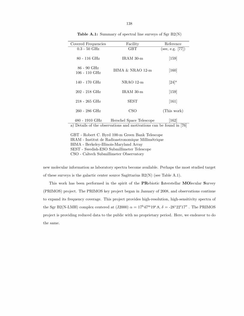
138

Table A.1: Summary of spectral line surveys of Sgr B2(N)

Covered Frequencies Facility Reference0.3 - 50 GHz GBT (see, e.g. [77])

80 - 116 GHz IRAM 30-m [159]

86 - 90 GHzBIMA & NRAO 12-m [160]

106 - 110 GHz

140 - 170 GHz NRAO 12-m [24]a

202 - 218 GHz IRAM 30-m [159]

218 - 265 GHz SEST [161]

260 - 286 GHz CSO (This work)

480 - 1910 GHz Herschel Space Telescope [162]a) Details of the observations and motivations can be found in [76]

GBT - Robert C. Byrd 100-m Green Bank TelescopeIRAM - Institut de Radioastronomique MillimetriqueBIMA - Berkeley-Illinois-Maryland ArraySEST - Swedish-ESO Submillimeter TelescopeCSO - Caltech Submillimeter Observatory

new molecular information as laboratory spectra become available. Perhaps the most studied target

of these surveys is the galactic center source Sagittarius B2(N) (see Table A.1).

This work has been performed in the spirit of the PRebiotic Interstellar MOlecular Survey

(PRIMOS) project. The PRIMOS key project began in January of 2008, and observations continue

to expand its frequency coverage. This project provides high-resolution, high-sensitivity spectra of

the Sgr B2(N-LMH) complex centered at (J2000) α = 17h47m19s.8, δ = -2822′17′′ . The PRIMOS

project is providing reduced data to the public with no proprietary period. Here, we endeavor to do

the same.

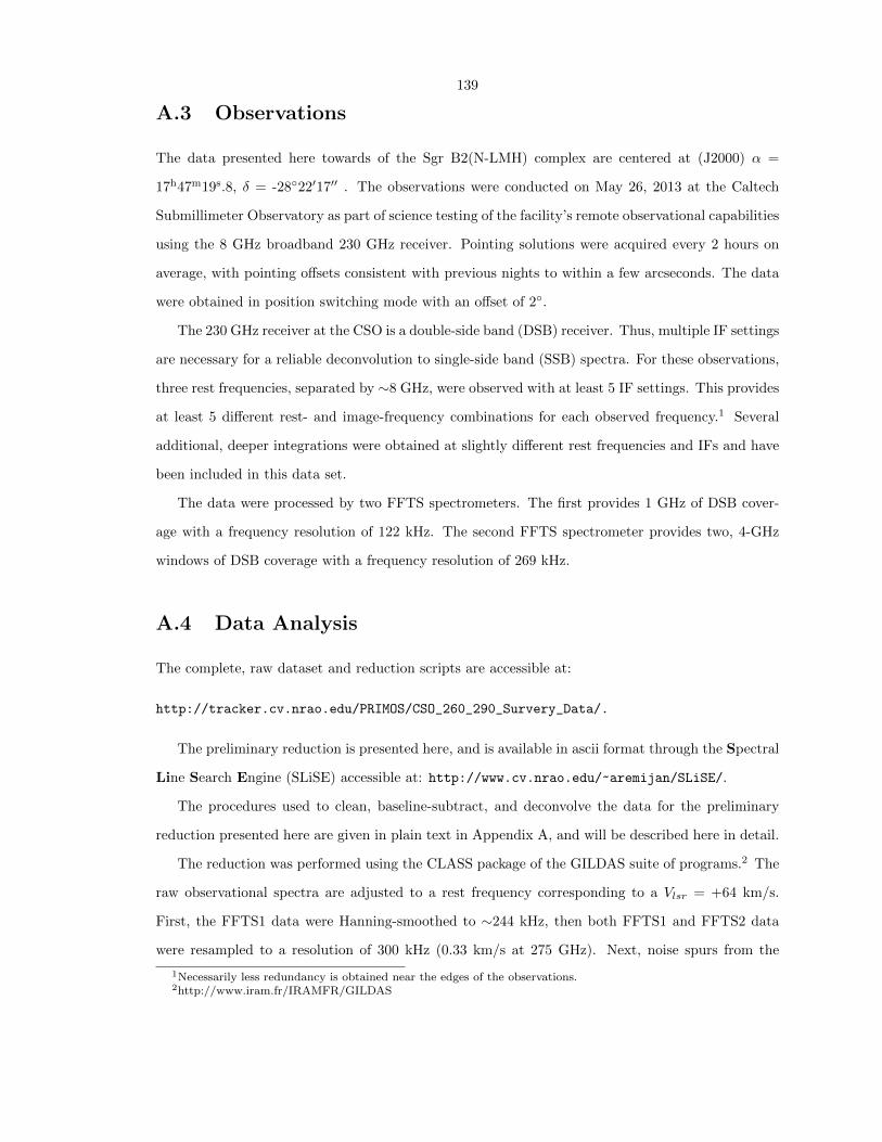
139

A.3 Observations

The data presented here towards of the Sgr B2(N-LMH) complex are centered at (J2000) α =

17h47m19s.8, δ = -2822′17′′ . The observations were conducted on May 26, 2013 at the Caltech

Submillimeter Observatory as part of science testing of the facility’s remote observational capabilities

using the 8 GHz broadband 230 GHz receiver. Pointing solutions were acquired every 2 hours on

average, with pointing offsets consistent with previous nights to within a few arcseconds. The data

were obtained in position switching mode with an offset of 2.

The 230 GHz receiver at the CSO is a double-side band (DSB) receiver. Thus, multiple IF settings

are necessary for a reliable deconvolution to single-side band (SSB) spectra. For these observations,

three rest frequencies, separated by ∼8 GHz, were observed with at least 5 IF settings. This provides

at least 5 different rest- and image-frequency combinations for each observed frequency.1 Several

additional, deeper integrations were obtained at slightly different rest frequencies and IFs and have

been included in this data set.

The data were processed by two FFTS spectrometers. The first provides 1 GHz of DSB cover-

age with a frequency resolution of 122 kHz. The second FFTS spectrometer provides two, 4-GHz

windows of DSB coverage with a frequency resolution of 269 kHz.

A.4 Data Analysis

The complete, raw dataset and reduction scripts are accessible at:

http://tracker.cv.nrao.edu/PRIMOS/CSO_260_290_Survery_Data/.

The preliminary reduction is presented here, and is available in ascii format through the Spectral

Line Search Engine (SLiSE) accessible at: http://www.cv.nrao.edu/~aremijan/SLiSE/.

The procedures used to clean, baseline-subtract, and deconvolve the data for the preliminary

reduction presented here are given in plain text in Appendix A, and will be described here in detail.

The reduction was performed using the CLASS package of the GILDAS suite of programs.2 The

raw observational spectra are adjusted to a rest frequency corresponding to a Vlsr = +64 km/s.

First, the FFTS1 data were Hanning-smoothed to ∼244 kHz, then both FFTS1 and FFTS2 data

were resampled to a resolution of 300 kHz (0.33 km/s at 275 GHz). Next, noise spurs from the

1Necessarily less redundancy is obtained near the edges of the observations.2http://www.iram.fr/IRAMFR/GILDAS

http://www.cv.nrao.edu/~aremijan/SLiSE/

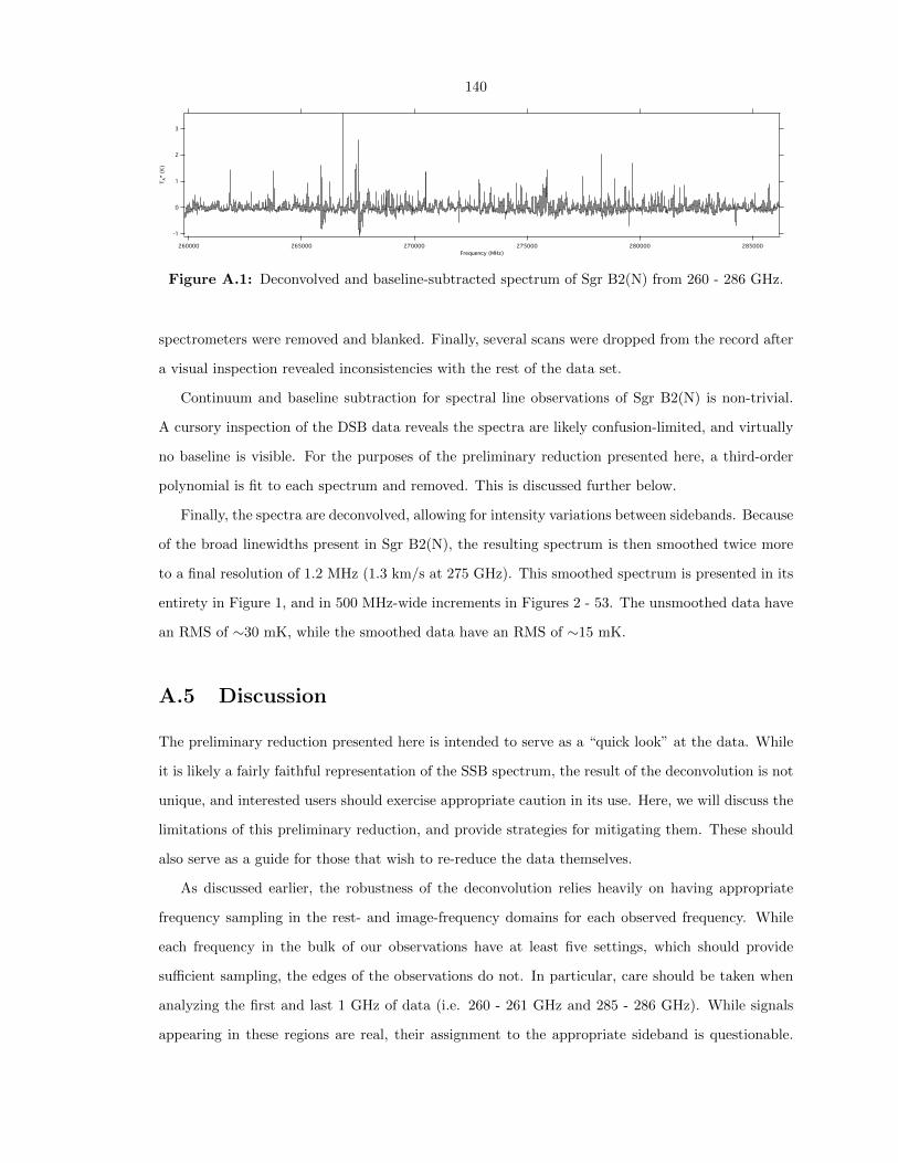
140

3

2

1

0

-1

TA*

(K)

285000280000275000270000265000260000

Frequency (MHz)

Figure A.1: Deconvolved and baseline-subtracted spectrum of Sgr B2(N) from 260 - 286 GHz.

spectrometers were removed and blanked. Finally, several scans were dropped from the record after

a visual inspection revealed inconsistencies with the rest of the data set.

Continuum and baseline subtraction for spectral line observations of Sgr B2(N) is non-trivial.

A cursory inspection of the DSB data reveals the spectra are likely confusion-limited, and virtually

no baseline is visible. For the purposes of the preliminary reduction presented here, a third-order

polynomial is fit to each spectrum and removed. This is discussed further below.

Finally, the spectra are deconvolved, allowing for intensity variations between sidebands. Because

of the broad linewidths present in Sgr B2(N), the resulting spectrum is then smoothed twice more

to a final resolution of 1.2 MHz (1.3 km/s at 275 GHz). This smoothed spectrum is presented in its

entirety in Figure 1, and in 500 MHz-wide increments in Figures 2 - 53. The unsmoothed data have

an RMS of ∼30 mK, while the smoothed data have an RMS of ∼15 mK.

A.5 Discussion

The preliminary reduction presented here is intended to serve as a “quick look” at the data. While

it is likely a fairly faithful representation of the SSB spectrum, the result of the deconvolution is not

unique, and interested users should exercise appropriate caution in its use. Here, we will discuss the

limitations of this preliminary reduction, and provide strategies for mitigating them. These should

also serve as a guide for those that wish to re-reduce the data themselves.

As discussed earlier, the robustness of the deconvolution relies heavily on having appropriate

frequency sampling in the rest- and image-frequency domains for each observed frequency. While

each frequency in the bulk of our observations have at least five settings, which should provide

sufficient sampling, the edges of the observations do not. In particular, care should be taken when

analyzing the first and last 1 GHz of data (i.e. 260 - 261 GHz and 285 - 286 GHz). While signals

appearing in these regions are real, their assignment to the appropriate sideband is questionable.

141

To mitigate this, transitions from a molecule of interest should be identified in neighboring spectral

windows or, in the case of the 260 - 261 GHz data, in the Nummelin et al. (1998) survey data.

The use of a third-order polynomial fit to the data to remove baselines is certainly not ideal. While

simple and effective, this method suffers from sensitivity to large changes in the average intensity

within a scan, for instance, due to an abnormally strong line. Further, the average intensity will be

above the actual noise floor, with the result that the zero point of the intensity scale is somewhat

higher than the noise floor. A visual inspection of the data reveals this offset is likely between 0.1

and 0.2 mK, and thus, the absolute intensities of the lines are expected to vary by at least this much

(the relative intensities of the line peak to the surrounding baseline are likely much more robust).

Very bright lines can sometimes introduce ghosting artifacts into the SSB spectrum during de-

convolution. Given that the brightest observed intensity in this spectrum is only ∼3 K (at 266.838

GHz [likely CH3OH]), these ghosts are unlikely to be of any real concern; however, a meticulous

reduction would remove the strongest signals from the spectrum prior to deconvolution, then man-

ually stitch the signals back in afterwards. The trade-off is a slight increase in RMS noise in the

image band corresponding to the removed line, as less data were available at that frequency during

the deconvolution.

Finally, the resultant SSB spectrum was visually compared to the sum total of all DSB spectra. It

was during this process that several scans were identified as inconsistent. In general, these were cases

of 4 out of 5 settings at a particular frequency indicating the presence of a line in that sideband,

while the fifth did not. The most common cause of this is bad lock in the receiver frequencies.

While this visual inspection was thorough, due to the rough nature of this reduction, the interested

user should take care to check the DSB spectra themselves against any particularly weak molecular

signals. This is especially true for the identification of new molecular signals.

A more robust reduction and analysis is planned to follow in the coming months. Until then,

interested users are encouraged to use (and re-reduce) the existing dataset as they see fit. We ask

only that you cite our work as the data source, and please notify us by e-mail of any resulting

publications or presentations. Those wishing for further observational or data-related details should

contact the authors directly.

A.6 Spectra

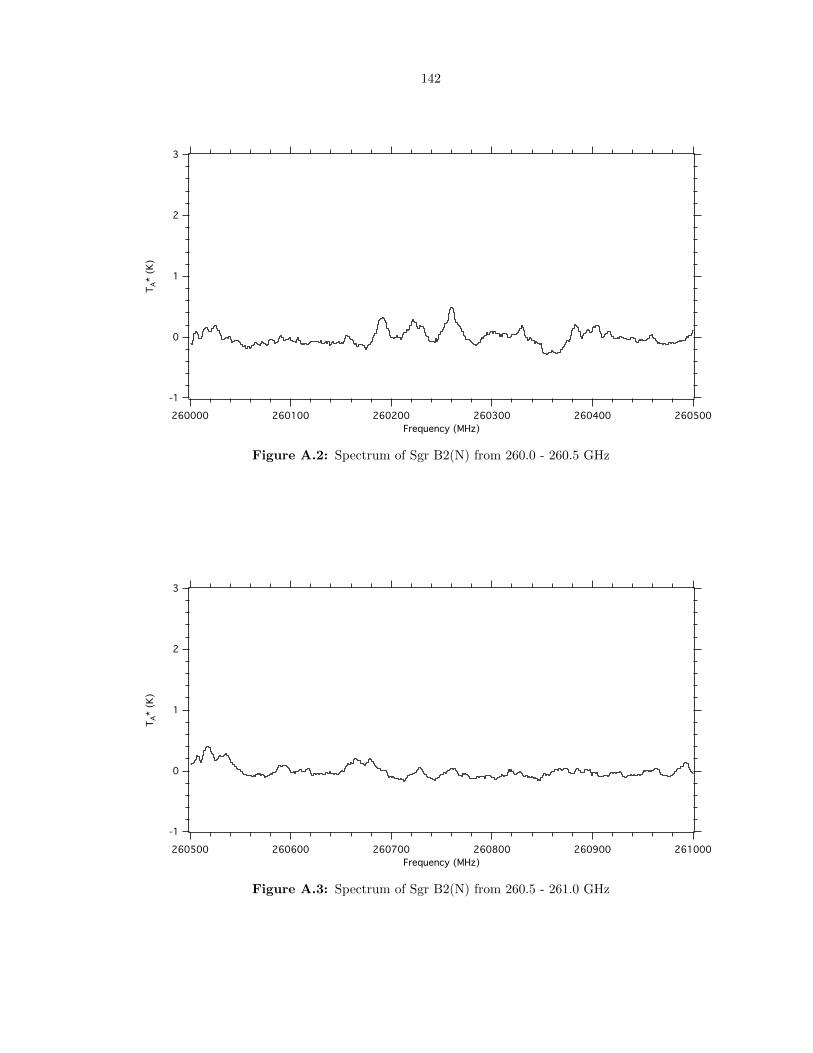
142

3

2

1

0

-1

TA*

(K)

260500260400260300260200260100260000

Frequency (MHz)

Figure A.2: Spectrum of Sgr B2(N) from 260.0 - 260.5 GHz

3

2

1

0

-1

TA*

(K)

261000260900260800260700260600260500

Frequency (MHz)


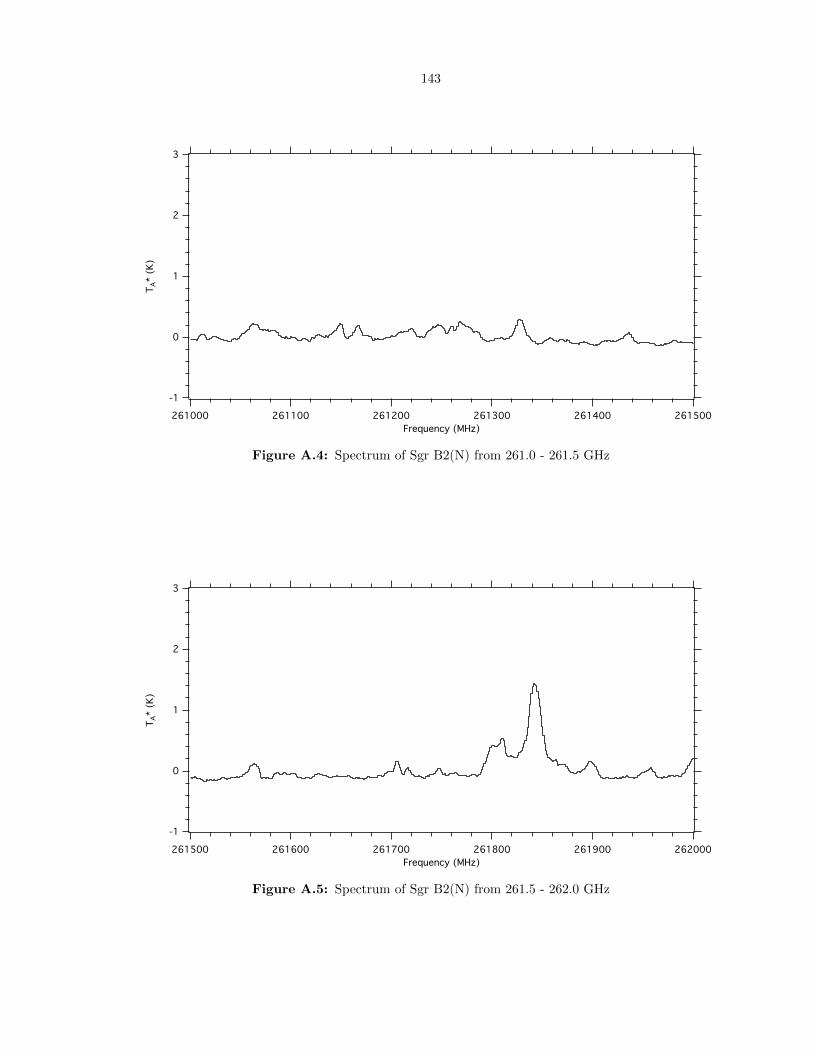
143

3

2

1

0

-1

TA*

(K)

261500261400261300261200261100261000

Frequency (MHz)


3

2

1

0

-1

TA*

(K)

262000261900261800261700261600261500

Frequency (MHz)


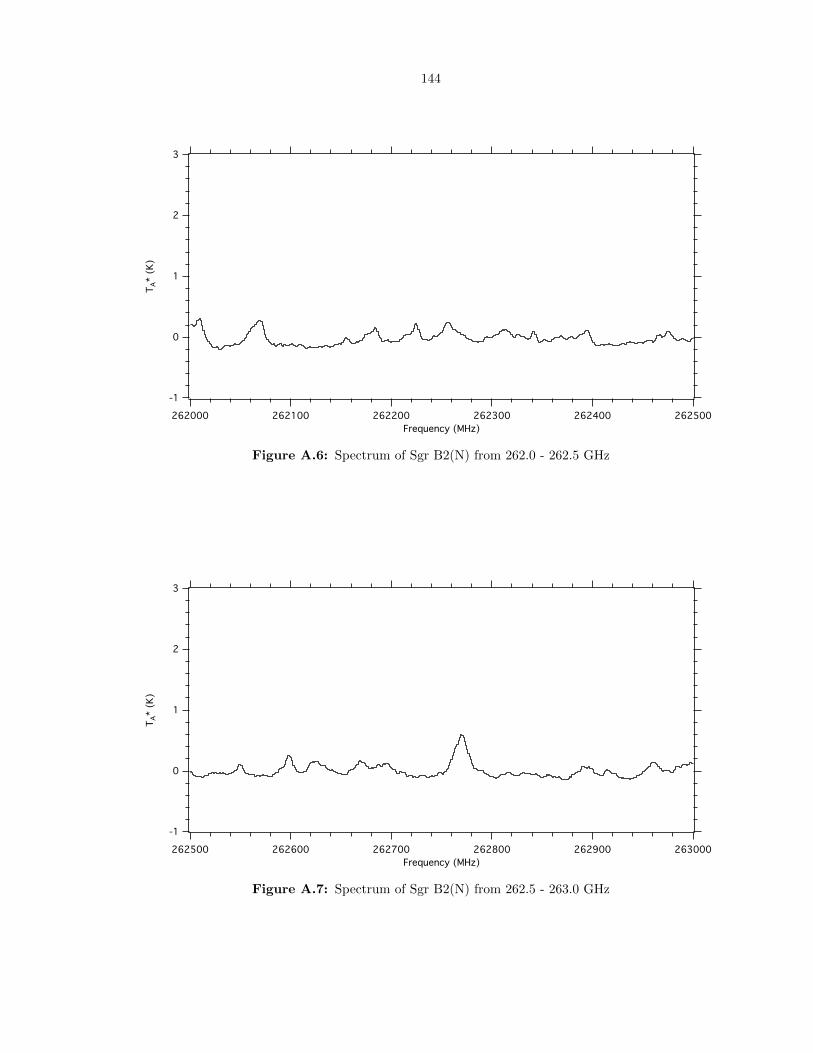
144

3

2

1

0

-1

TA*

(K)

262500262400262300262200262100262000

Frequency (MHz)


3

2

1

0

-1

TA*

(K)

263000262900262800262700262600262500

Frequency (MHz)


145

3

2

1

0

-1

TA*

(K)

263500263400263300263200263100263000

Frequency (MHz)


3

2

1

0

-1

TA*

(K)

264000263900263800263700263600263500

Frequency (MHz)


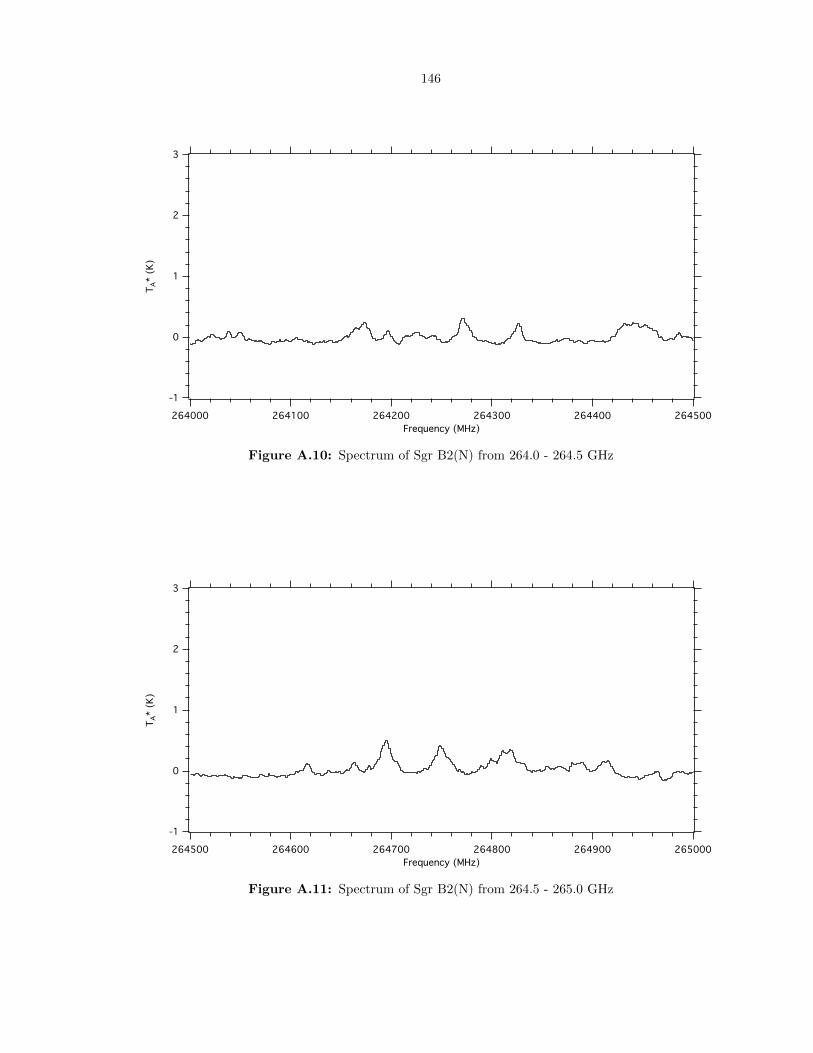
146

3

2

1

0

-1

TA*

(K)

264500264400264300264200264100264000

Frequency (MHz)


3

2

1

0

-1

TA*

(K)

265000264900264800264700264600264500

Frequency (MHz)


147

3

2

1

0

-1

TA*

(K)

265500265400265300265200265100265000

Frequency (MHz)


3

2

1

0

-1

TA*

(K)

266000265900265800265700265600265500

Frequency (MHz)


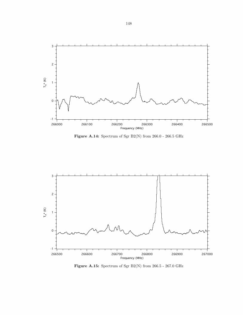
148

3

2

1

0

-1

TA*

(K)

266500266400266300266200266100266000

Frequency (MHz)


3

2

1

0

-1

TA*

(K)

267000266900266800266700266600266500

Frequency (MHz)


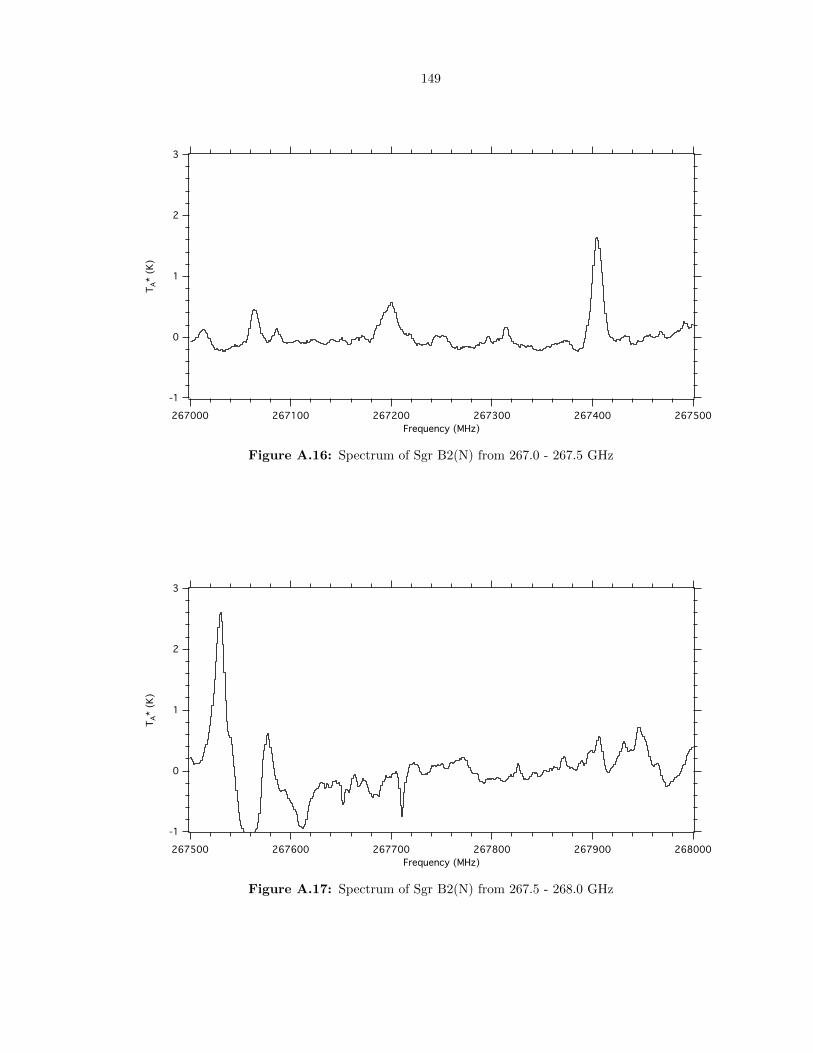
149

3

2

1

0

-1

TA*

(K)

267500267400267300267200267100267000

Frequency (MHz)


3

2

1

0

-1

TA*

(K)

268000267900267800267700267600267500

Frequency (MHz)


150

3

2

1

0

-1

TA*

(K)

268500268400268300268200268100268000

Frequency (MHz)


3

2

1

0

-1

TA*

(K)

269000268900268800268700268600268500

Frequency (MHz)


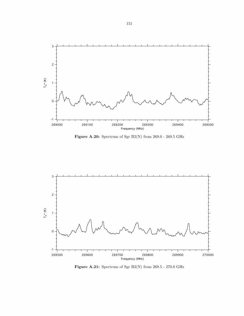
151

3

2

1

0

-1

TA*

(K)

269500269400269300269200269100269000

Frequency (MHz)


3

2

1

0

-1

TA*

(K)

270000269900269800269700269600269500

Frequency (MHz)


152

3

2

1

0

-1

TA*

(K)

270500270400270300270200270100270000

Frequency (MHz)


3

2

1

0

-1

TA*

(K)

271000270900270800270700270600270500

Frequency (MHz)


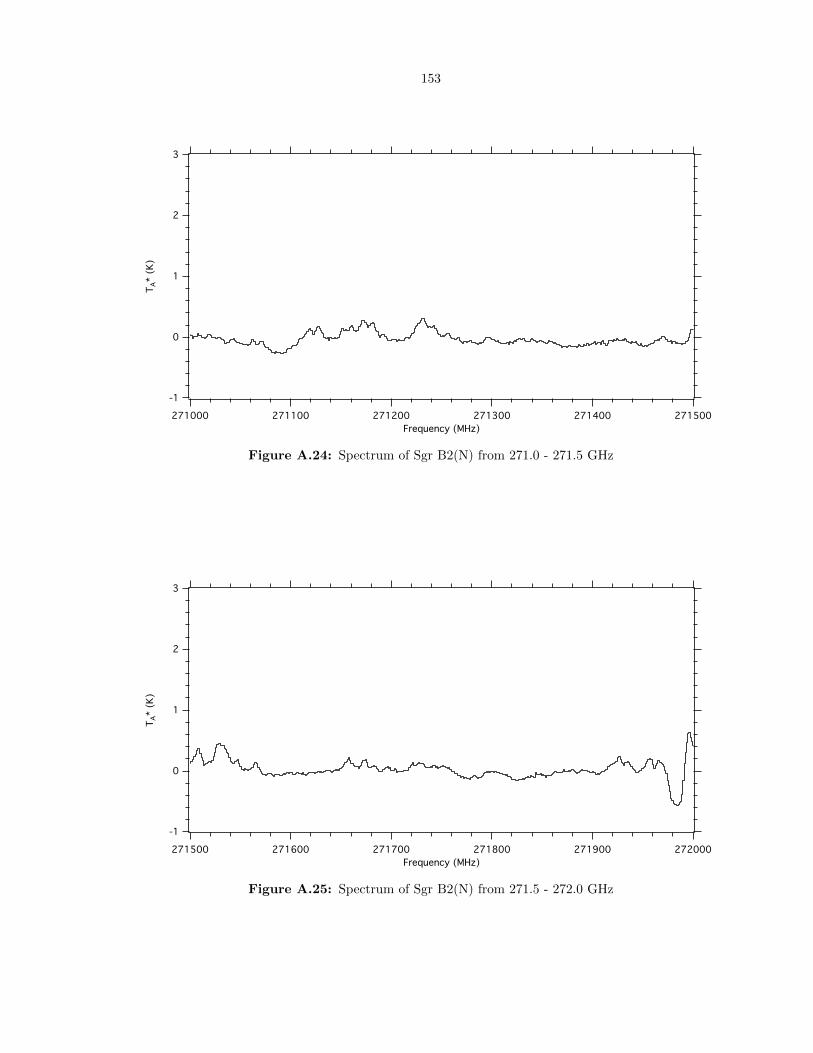
153

3

2

1

0

-1

TA*

(K)

271500271400271300271200271100271000

Frequency (MHz)


3

2

1

0

-1

TA*

(K)

272000271900271800271700271600271500

Frequency (MHz)


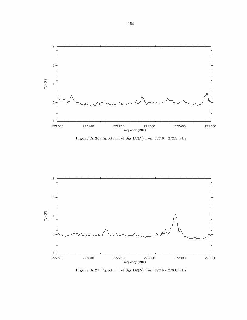
154

3

2

1

0

-1

TA*

(K)

272500272400272300272200272100272000

Frequency (MHz)


3

2

1

0

-1

TA*

(K)

273000272900272800272700272600272500

Frequency (MHz)


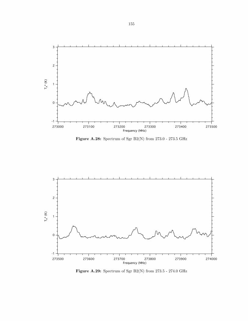
155

3

2

1

0

-1

TA*

(K)

273500273400273300273200273100273000

Frequency (MHz)


3

2

1

0

-1

TA*

(K)

274000273900273800273700273600273500

Frequency (MHz)


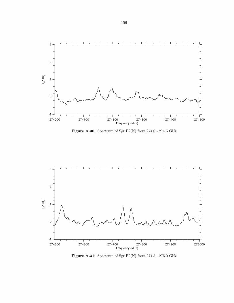
156

3

2

1

0

-1

TA*

(K)

274500274400274300274200274100274000

Frequency (MHz)


3

2

1

0

-1

TA*

(K)

275000274900274800274700274600274500

Frequency (MHz)


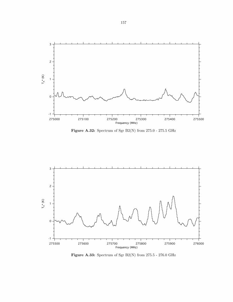
157

3

2

1

0

-1

TA*

(K)

275500275400275300275200275100275000

Frequency (MHz)


3

2

1

0

-1

TA*

(K)

276000275900275800275700275600275500

Frequency (MHz)


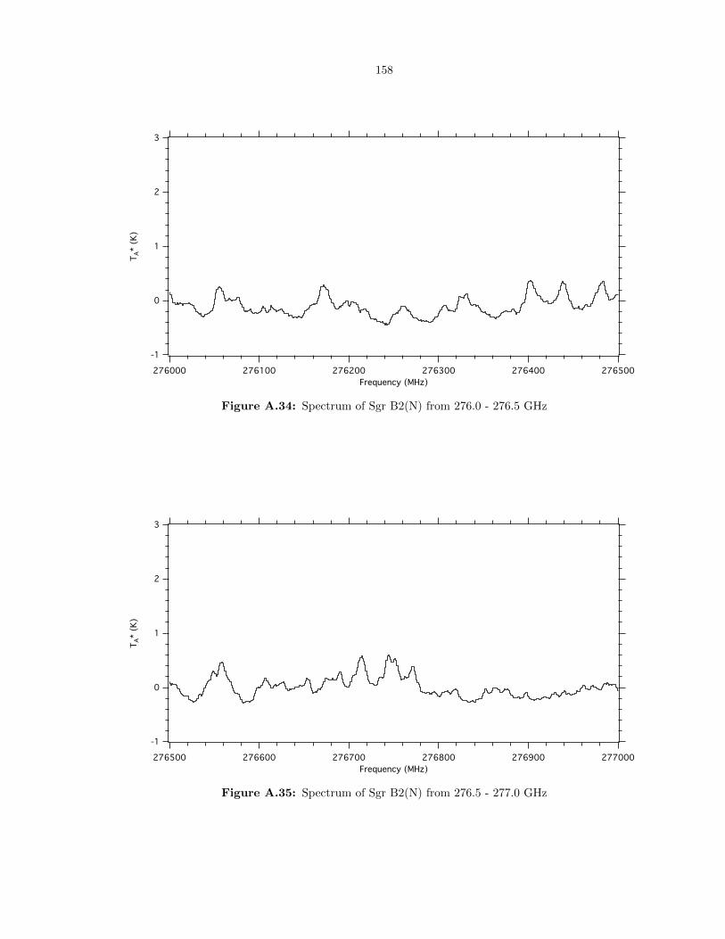
158

3

2

1

0

-1

TA*

(K)

276500276400276300276200276100276000

Frequency (MHz)


3

2

1

0

-1

TA*

(K)

277000276900276800276700276600276500

Frequency (MHz)


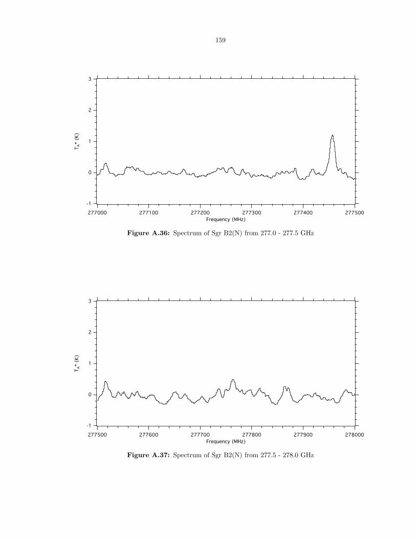
159

3

2

1

0

-1

TA*

(K)

277500277400277300277200277100277000

Frequency (MHz)


3

2

1

0

-1

TA*

(K)

278000277900277800277700277600277500

Frequency (MHz)


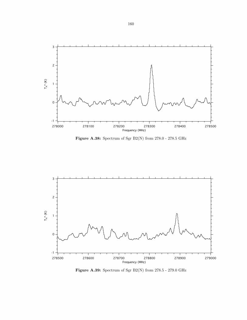
160

3

2

1

0

-1

TA*

(K)

278500278400278300278200278100278000

Frequency (MHz)


3

2

1

0

-1

TA*

(K)

279000278900278800278700278600278500

Frequency (MHz)


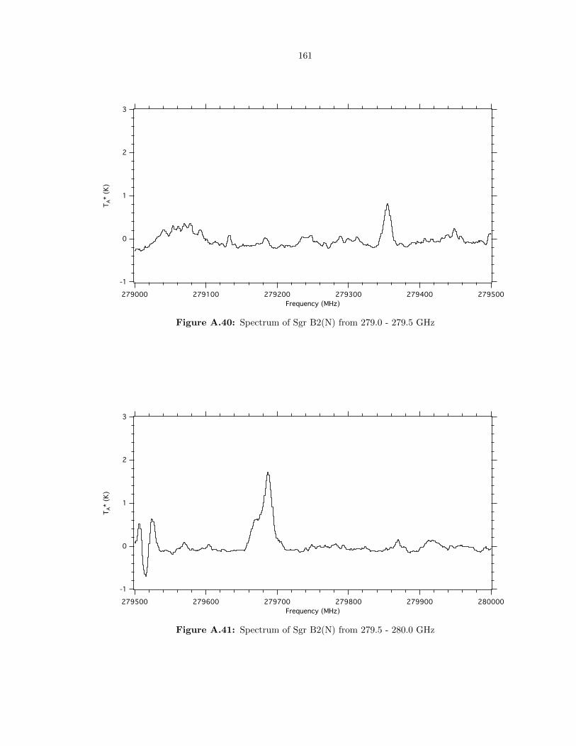
161

3

2

1

0

-1

TA*

(K)

279500279400279300279200279100279000

Frequency (MHz)


3

2

1

0

-1

TA*

(K)

280000279900279800279700279600279500

Frequency (MHz)


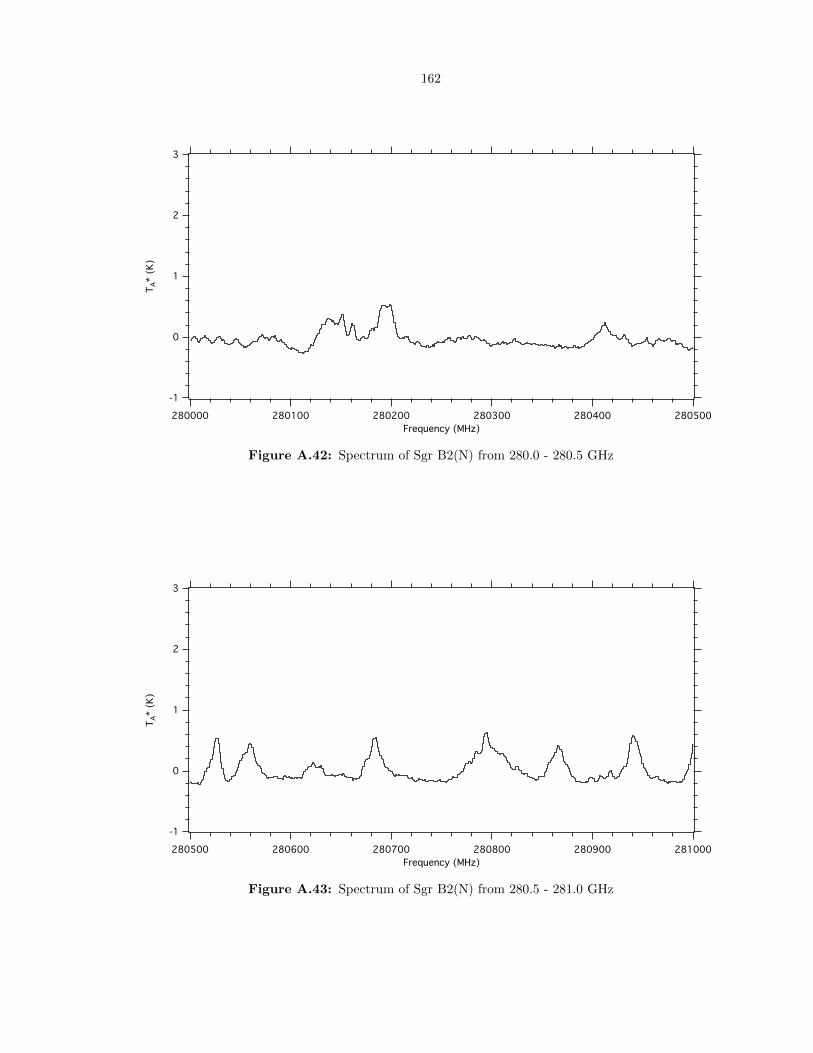
162

3

2

1

0

-1

TA*

(K)

280500280400280300280200280100280000

Frequency (MHz)


3

2

1

0

-1

TA*

(K)

281000280900280800280700280600280500

Frequency (MHz)


163

3

2

1

0

-1

TA*

(K)

281500281400281300281200281100281000

Frequency (MHz)


3

2

1

0

-1

TA*

(K)

282000281900281800281700281600281500

Frequency (MHz)


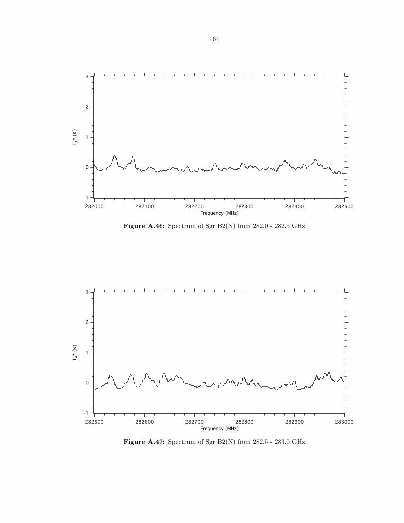
164

3

2

1

0

-1

TA*

(K)

282500282400282300282200282100282000

Frequency (MHz)


3

2

1

0

-1

TA*

(K)

283000282900282800282700282600282500

Frequency (MHz)


165

3

2

1

0

-1

TA*

(K)

283500283400283300283200283100283000

Frequency (MHz)


3

2

1

0

-1

TA*

(K)

284000283900283800283700283600283500

Frequency (MHz)


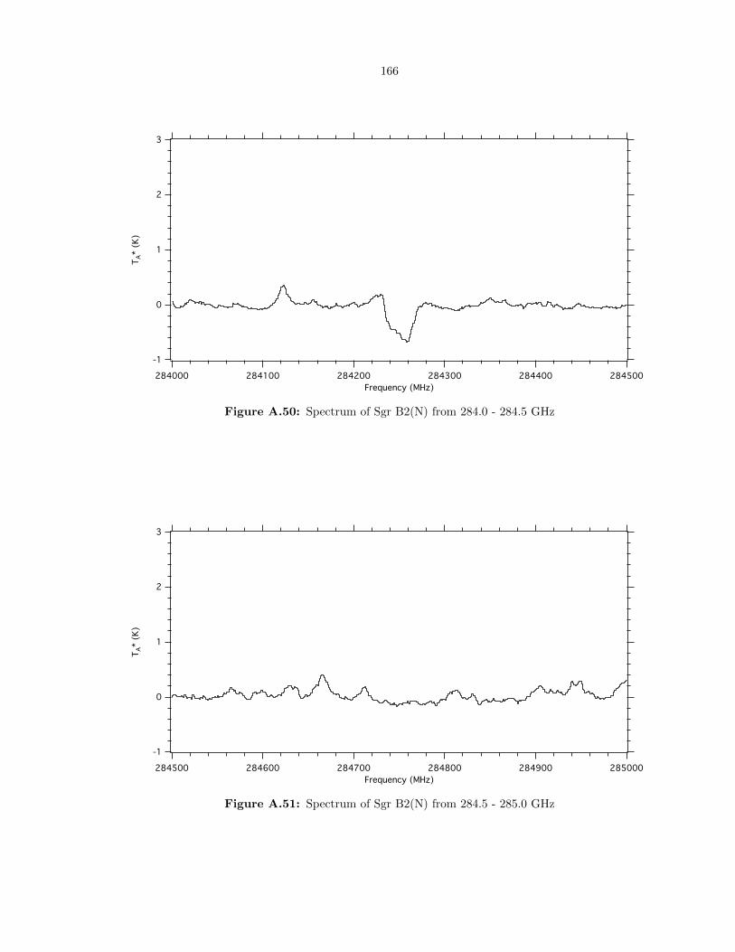
166

3

2

1

0

-1

TA*

(K)

284500284400284300284200284100284000

Frequency (MHz)


3

2

1

0

-1

TA*

(K)

285000284900284800284700284600284500

Frequency (MHz)


167

3

2

1

0

-1

TA*

(K)

285500285400285300285200285100285000

Frequency (MHz)


3

2

1

0

-1

TA*

(K)

286000285900285800285700285600285500

Frequency (MHz)


168

A.7 Deconvolution Routine

file in sgrb2n.dat

$rm sgrb2n.sm

file out sgrb2n.sm multiple

set tele "CSO FFTS 1W"

find

for i 1 to found

get n

smooth

write

next

set tele "CSO FFTS 2B1"

find

for i 1 to found

get n

write

next


find

for i 1 to found

get n

write

next

set tele

set mode x t

set mode y t

file in sgrb2n.sm

$rm sgrb2n.rs

file out sgrb2n.rs multiple

set u c

set var spec write

find

for i 1 to found

get n

a\resam ’nchan/0.3*fres’ ’rchan/0.3*fres’ int(frequency) 0.3 f /nofft

write

next

set tele

set mode x t

set mode y t

file in sgrb2n.rs

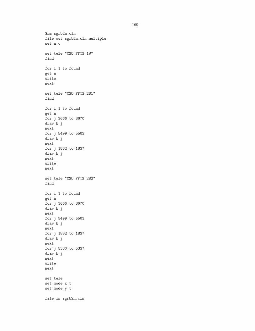
169

$rm sgrb2n.cln

file out sgrb2n.cln multiple

set u c

set tele "CSO FFTS 1W"

find

for i 1 to found

get n

write

next


find

for i 1 to found

get n

for j 3666 to 3670

draw k j

next

for j 5499 to 5503

draw k j

next

for j 1832 to 1837

draw k j

next

write

next


find

for i 1 to found

get n

for j 3666 to 3670

draw k j

next

for j 5499 to 5503

draw k j

next

for j 1832 to 1837

draw k j

next

for j 5330 to 5337

draw k j

next

write

next

set tele

set mode x t

set mode y t

file in sgrb2n.cln

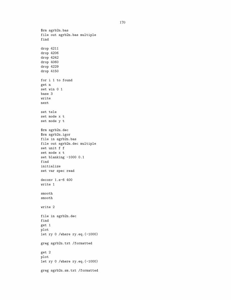
170

$rm sgrb2n.bas

file out sgrb2n.bas multiple

find

drop 4211

drop 4206

drop 4242

drop 4060

drop 4229

drop 4150

for i 1 to found

get n

set win 0 1

base 3

write

next

set tele

set mode x t

set mode y t

$rm sgrb2n.dec

$rm sgrb2n.igor

file in sgrb2n.bas

file out sgrb2n.dec multiple

set unit f f

set mode x t

set blanking -1000 0.1

find

initialize

set var spec read

deconv 1.e-6 400

write 1

smooth

smooth

write 2

file in sgrb2n.dec

find

get 1

plot

let ry 0 /where ry.eq.(-1000)

greg sgrb2n.txt /formatted

get 2

plot

let ry 0 /where ry.eq.(-1000)

greg sgrb2n.sm.txt /formatted

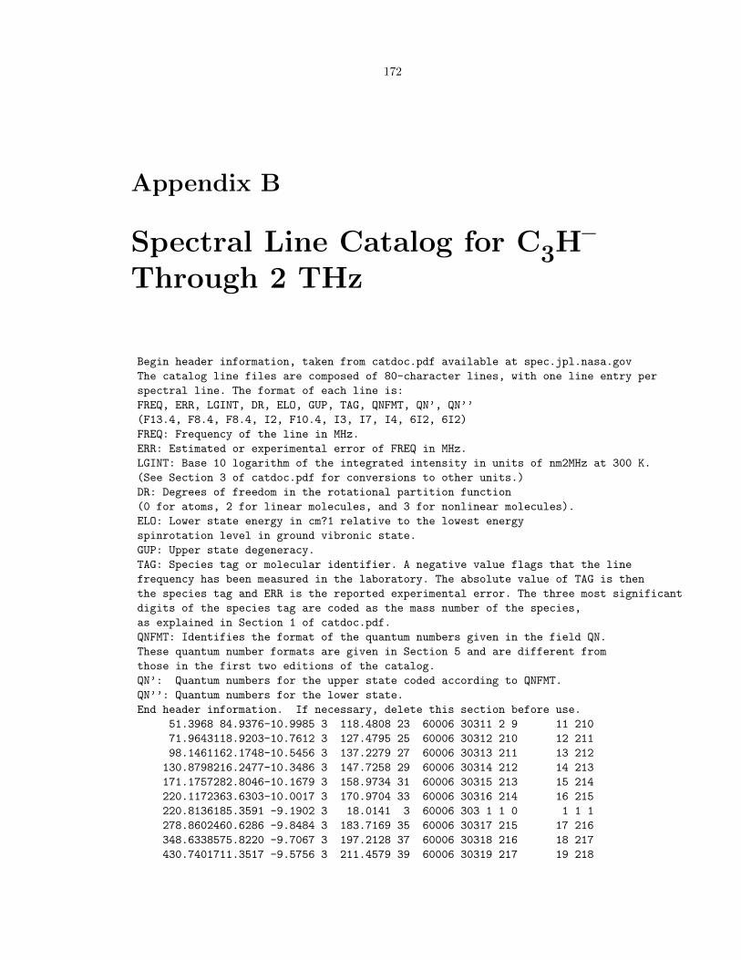
172

Appendix B

Spectral Line Catalog for C3H–

Through 2 THz

Begin header information, taken from catdoc.pdf available at spec.jpl.nasa.gov

The catalog line files are composed of 80-character lines, with one line entry per

spectral line. The format of each line is:

FREQ, ERR, LGINT, DR, ELO, GUP, TAG, QNFMT, QN’, QN’’

(F13.4, F8.4, F8.4, I2, F10.4, I3, I7, I4, 6I2, 6I2)

FREQ: Frequency of the line in MHz.

ERR: Estimated or experimental error of FREQ in MHz.

LGINT: Base 10 logarithm of the integrated intensity in units of nm2MHz at 300 K.

(See Section 3 of catdoc.pdf for conversions to other units.)

DR: Degrees of freedom in the rotational partition function

(0 for atoms, 2 for linear molecules, and 3 for nonlinear molecules).

ELO: Lower state energy in cm?1 relative to the lowest energy

spinrotation level in ground vibronic state.

GUP: Upper state degeneracy.

TAG: Species tag or molecular identifier. A negative value flags that the line

frequency has been measured in the laboratory. The absolute value of TAG is then

the species tag and ERR is the reported experimental error. The three most significant

digits of the species tag are coded as the mass number of the species,

as explained in Section 1 of catdoc.pdf.

QNFMT: Identifies the format of the quantum numbers given in the field QN.

These quantum number formats are given in Section 5 and are different from

those in the first two editions of the catalog.

QN’: Quantum numbers for the upper state coded according to QNFMT.

QN’’: Quantum numbers for the lower state.

End header information. If necessary, delete this section before use.

51.3968 84.9376-10.9985 3 118.4808 23 60006 30311 2 9 11 210

71.9643118.9203-10.7612 3 127.4795 25 60006 30312 210 12 211

98.1461162.1748-10.5456 3 137.2279 27 60006 30313 211 13 212

130.8798216.2477-10.3486 3 147.7258 29 60006 30314 212 14 213

171.1757282.8046-10.1679 3 158.9734 31 60006 30315 213 15 214

220.1172363.6303-10.0017 3 170.9704 33 60006 30316 214 16 215

220.8136185.3591 -9.1902 3 18.0141 3 60006 303 1 1 0 1 1 1

278.8602460.6286 -9.8484 3 183.7169 35 60006 30317 215 17 216

348.6338575.8220 -9.7067 3 197.2128 37 60006 30318 216 18 217

430.7401711.3517 -9.5756 3 211.4579 39 60006 30319 217 19 218

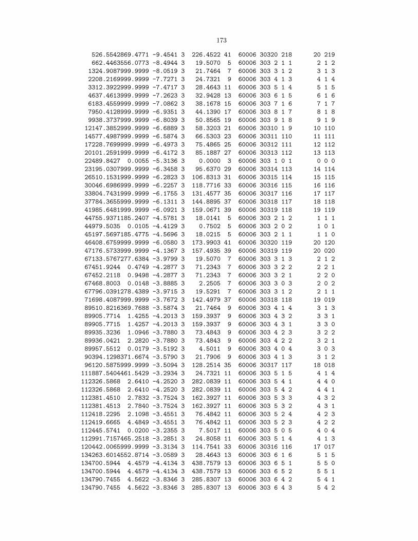
173

526.5542869.4771 -9.4541 3 226.4522 41 60006 30320 218 20 219

662.4463556.0773 -8.4944 3 19.5070 5 60006 303 2 1 1 2 1 2

1324.9087999.9999 -8.0519 3 21.7464 7 60006 303 3 1 2 3 1 3

2208.2169999.9999 -7.7271 3 24.7321 9 60006 303 4 1 3 4 1 4

3312.3922999.9999 -7.4717 3 28.4643 11 60006 303 5 1 4 5 1 5

4637.4613999.9999 -7.2623 3 32.9428 13 60006 303 6 1 5 6 1 6

6183.4559999.9999 -7.0862 3 38.1678 15 60006 303 7 1 6 7 1 7

7950.4128999.9999 -6.9351 3 44.1390 17 60006 303 8 1 7 8 1 8

9938.3737999.9999 -6.8039 3 50.8565 19 60006 303 9 1 8 9 1 9

12147.3852999.9999 -6.6889 3 58.3203 21 60006 30310 1 9 10 110

14577.4987999.9999 -6.5874 3 66.5303 23 60006 30311 110 11 111

17228.7699999.9999 -6.4973 3 75.4865 25 60006 30312 111 12 112

20101.2591999.9999 -6.4172 3 85.1887 27 60006 30313 112 13 113

22489.8427 0.0055 -5.3136 3 0.0000 3 60006 303 1 0 1 0 0 0

23195.0307999.9999 -6.3458 3 95.6370 29 60006 30314 113 14 114

26510.1531999.9999 -6.2823 3 106.8313 31 60006 30315 114 15 115

30046.6986999.9999 -6.2257 3 118.7716 33 60006 30316 115 16 116

33804.7431999.9999 -6.1755 3 131.4577 35 60006 30317 116 17 117

37784.3655999.9999 -6.1311 3 144.8895 37 60006 30318 117 18 118

41985.6481999.9999 -6.0921 3 159.0671 39 60006 30319 118 19 119

44755.9371185.2407 -4.5781 3 18.0141 5 60006 303 2 1 2 1 1 1

44979.5035 0.0105 -4.4129 3 0.7502 5 60006 303 2 0 2 1 0 1

45197.5697185.4775 -4.5696 3 18.0215 5 60006 303 2 1 1 1 1 0

46408.6759999.9999 -6.0580 3 173.9903 41 60006 30320 119 20 120

47176.5733999.9999 -4.1367 3 157.4935 39 60006 30319 119 20 020

67133.5767277.6384 -3.9799 3 19.5070 7 60006 303 3 1 3 2 1 2

67451.9244 0.4749 -4.2877 3 71.2343 7 60006 303 3 2 2 2 2 1

67452.2118 0.9498 -4.2877 3 71.2343 7 60006 303 3 2 1 2 2 0

67468.8003 0.0148 -3.8885 3 2.2505 7 60006 303 3 0 3 2 0 2

67796.0391278.4389 -3.9715 3 19.5291 7 60006 303 3 1 2 2 1 1

71698.4087999.9999 -3.7672 3 142.4979 37 60006 30318 118 19 019

89510.8216369.7688 -3.5874 3 21.7464 9 60006 303 4 1 4 3 1 3

89905.7714 1.4255 -4.2013 3 159.3937 9 60006 303 4 3 2 3 3 1

89905.7715 1.4257 -4.2013 3 159.3937 9 60006 303 4 3 1 3 3 0

89935.3236 1.0946 -3.7880 3 73.4843 9 60006 303 4 2 3 3 2 2

89936.0421 2.2820 -3.7880 3 73.4843 9 60006 303 4 2 2 3 2 1

89957.5512 0.0179 -3.5192 3 4.5011 9 60006 303 4 0 4 3 0 3

90394.1298371.6674 -3.5790 3 21.7906 9 60006 303 4 1 3 3 1 2

96120.5875999.9999 -3.5094 3 128.2514 35 60006 30317 117 18 018

111887.5404461.5429 -3.2934 3 24.7321 11 60006 303 5 1 5 4 1 4

112326.5868 2.6410 -4.2520 3 282.0839 11 60006 303 5 4 1 4 4 0

112326.5868 2.6410 -4.2520 3 282.0839 11 60006 303 5 4 2 4 4 1

112381.4510 2.7832 -3.7524 3 162.3927 11 60006 303 5 3 3 4 3 2

112381.4513 2.7840 -3.7524 3 162.3927 11 60006 303 5 3 2 4 3 1

112418.2295 2.1098 -3.4551 3 76.4842 11 60006 303 5 2 4 4 2 3

112419.6665 4.4849 -3.4551 3 76.4842 11 60006 303 5 2 3 4 2 2

112445.5741 0.0200 -3.2355 3 7.5017 11 60006 303 5 0 5 4 0 4

112991.7157465.2518 -3.2851 3 24.8058 11 60006 303 5 1 4 4 1 3

120442.0065999.9999 -3.3134 3 114.7541 33 60006 30316 116 17 017

134263.6014552.8714 -3.0589 3 28.4643 13 60006 303 6 1 6 5 1 5

134700.5944 4.4579 -4.4134 3 438.7579 13 60006 303 6 5 1 5 5 0

134700.5944 4.4579 -4.4134 3 438.7579 13 60006 303 6 5 2 5 5 1

134790.7455 4.5622 -3.8346 3 285.8307 13 60006 303 6 4 2 5 4 1

134790.7455 4.5622 -3.8346 3 285.8307 13 60006 303 6 4 3 5 4 2

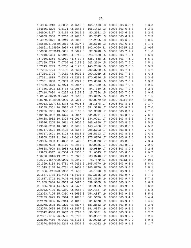
174

134856.6218 4.8083 -3.4546 3 166.1413 13 60006 303 6 3 4 5 3 3

134856.6226 4.8104 -3.4546 3 166.1413 13 60006 303 6 3 3 5 3 2

134900.5187 3.6195 -3.2016 3 80.2341 13 60006 303 6 2 5 5 2 4

134903.0336 7.7763 -3.2016 3 80.2342 13 60006 303 6 2 4 5 2 3

134932.6871 0.0219 -3.0066 3 11.2525 13 60006 303 6 0 6 5 0 5

135588.6706559.2811 -3.0507 3 28.5748 13 60006 303 6 1 5 5 1 4

144661.6148999.9999 -3.1574 3 102.0060 31 60006 30315 115 16 016

156638.8733643.6651 -2.8649 3 32.9428 15 60006 303 7 1 7 6 1 6

157010.6364 6.9912 -4.6712 3 628.7638 15 60006 303 7 6 1 6 6 0

157010.6364 6.9912 -4.6712 3 628.7638 15 60006 303 7 6 2 6 6 1

157149.0799 7.0766 -4.0178 3 443.2510 15 60006 303 7 5 2 6 5 1

157149.0799 7.0766 -4.0178 3 443.2510 15 60006 303 7 5 3 6 5 2

157254.2724 7.2432 -3.5604 3 290.3269 15 60006 303 7 4 3 6 4 2

157254.2724 7.2432 -3.5604 3 290.3269 15 60006 303 7 4 4 6 4 3

157331.1819 7.6342 -3.2271 3 170.6396 15 60006 303 7 3 5 6 3 4

157331.1838 7.6389 -3.2271 3 170.6396 15 60006 303 7 3 4 6 3 3

157382.0679 5.7224 -2.9967 3 84.7339 15 60006 303 7 2 6 6 2 5

157386.0922 12.3738 -2.9967 3 84.7340 15 60006 303 7 2 5 6 2 4

157418.7080 0.0255 -2.8159 3 15.7534 15 60006 303 7 0 7 6 0 6

158184.8679653.8440 -2.8568 3 33.0975 15 60006 303 7 1 6 6 1 5

168778.4138999.9999 -3.0301 3 90.0072 29 60006 30314 114 15 015

179013.2247733.8345 -2.7005 3 38.1678 17 60006 303 8 1 8 7 1 7

179235.5351 10.3585 -5.0165 3 851.3828 17 60006 303 8 7 1 7 7 0

179235.5351 10.3585 -5.0165 3 851.3828 17 60006 303 8 7 2 7 7 1

179438.5982 10.4325 -4.2917 3 634.0011 17 60006 303 8 6 2 7 6 1

179438.5982 10.4325 -4.2917 3 634.0011 17 60006 303 8 6 3 7 6 2

179596.8208 10.5611 -3.7606 3 448.4930 17 60006 303 8 5 3 7 5 2

179596.8208 10.5611 -3.7606 3 448.4930 17 60006 303 8 5 4 7 5 3

179717.0621 10.8108 -3.3513 3 295.5723 17 60006 303 8 4 4 7 4 3

179717.0621 10.8108 -3.3513 3 295.5723 17 60006 303 8 4 5 7 4 4

179805.0295 11.3941 -3.0425 3 175.8876 17 60006 303 8 3 6 7 3 5

179805.0333 11.4033 -3.0425 3 175.8876 17 60006 303 8 3 5 7 3 4

179862.7538 8.5176 -2.8255 3 89.9836 17 60006 303 8 2 7 7 2 6

179868.7909 18.4953 -2.8255 3 89.9839 17 60006 303 8 2 6 7 2 5

179903.4547 0.0334 -2.6536 3 21.0043 17 60006 303 8 0 8 7 0 7

180780.1816749.0291 -2.6925 3 38.3740 17 60006 303 8 1 7 7 1 6

192791.4567999.9999 -2.9249 3 78.7579 27 60006 30313 113 14 014

201349.3188 14.6781 -5.4431 3 1105.8770 19 60006 303 9 8 1 8 8 0

201349.3188 14.6781 -5.4431 3 1105.8770 19 60006 303 9 8 2 8 8 1

201386.5241823.2903 -2.5588 3 44.1390 19 60006 303 9 1 9 8 1 8

201637.2742 14.7444 -4.6495 3 857.3615 19 60006 303 9 7 2 8 7 1

201637.2742 14.7444 -4.6495 3 857.3615 19 60006 303 9 7 3 8 7 2

201865.7084 14.8509 -4.0477 3 639.9865 19 60006 303 9 6 3 8 6 2

201865.7084 14.8509 -4.0477 3 639.9865 19 60006 303 9 6 4 8 6 3

202043.7106 15.0350 -3.5656 3 454.4837 19 60006 303 9 5 4 8 5 3

202043.7106 15.0350 -3.5656 3 454.4837 19 60006 303 9 5 5 8 5 4

202179.0095 15.3914 -3.1818 3 301.5670 19 60006 303 9 4 5 8 4 4

202179.0095 15.3914 -3.1818 3 301.5670 19 60006 303 9 4 6 8 4 5

202278.0628 16.2209 -2.8877 3 181.8853 19 60006 303 9 3 7 8 3 6

202278.0698 16.2378 -2.8877 3 181.8853 19 60006 303 9 3 6 8 3 5

202342.4530 12.1037 -2.6793 3 95.9831 19 60006 303 9 2 8 8 2 7

202351.0785 26.3586 -2.6793 3 95.9837 19 60006 303 9 2 7 8 2 6

202386.7450 0.0472 -2.5135 3 27.0052 19 60006 303 9 0 9 8 0 8

203374.4850844.9248 -2.5509 3 44.4042 19 60006 303 9 1 8 8 1 7

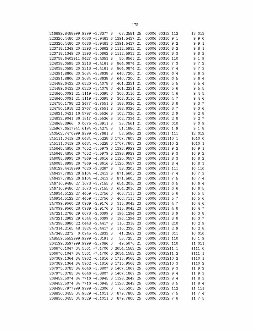
175

216699.8488999.9999 -2.8377 3 68.2581 25 60006 30312 112 13 013

223320.4480 20.0686 -5.9463 3 1391.5437 21 60006 30310 9 1 9 9 0

223320.4480 20.0686 -5.9463 3 1391.5437 21 60006 30310 9 2 9 9 1

223718.1349 20.1293 -5.0862 3 1112.5932 21 60006 30310 8 2 9 8 1

223718.1349 20.1293 -5.0862 3 1112.5932 21 60006 30310 8 3 9 8 2

223758.6402911.9427 -2.4353 3 50.8565 21 60006 30310 110 9 1 9

224038.0595 20.2213 -4.4161 3 864.0874 21 60006 30310 7 3 9 7 2

224038.0595 20.2213 -4.4161 3 864.0874 21 60006 30310 7 4 9 7 3

224291.8606 20.3684 -3.8638 3 646.7200 21 60006 30310 6 4 9 6 3

224291.8606 20.3684 -3.8638 3 646.7200 21 60006 30310 6 5 9 6 4

224489.6432 20.6220 -3.4078 3 461.2231 21 60006 30310 5 5 9 5 4

224489.6432 20.6220 -3.4078 3 461.2231 21 60006 30310 5 6 9 5 5

224640.0091 21.1119 -3.0395 3 308.3110 21 60006 30310 4 6 9 4 5

224640.0091 21.1119 -3.0395 3 308.3110 21 60006 30310 4 7 9 4 6

224750.1798 22.2477 -2.7551 3 188.6326 21 60006 30310 3 8 9 3 7

224750.1918 22.2767 -2.7551 3 188.6326 21 60006 30310 3 7 9 3 6

224821.0421 16.5797 -2.5526 3 102.7326 21 60006 30310 2 9 9 2 8

224832.9041 36.1817 -2.5526 3 102.7334 21 60006 30310 2 8 9 2 7

224868.3966 0.0675 -2.3911 3 33.7561 21 60006 30310 010 9 0 9

225967.6517941.6194 -2.4275 3 51.1880 21 60006 30310 1 9 9 1 8

240502.7470999.9999 -2.7661 3 58.5080 23 60006 30311 111 12 012

245111.0419 26.6484 -6.5228 3 1707.7808 23 60006 3031110 1 1010 0

245111.0419 26.6484 -6.5228 3 1707.7808 23 60006 3031110 2 1010 1

245648.4856 26.7052 -5.5979 3 1398.9929 23 60006 30311 9 2 10 9 1

245648.4856 26.7052 -5.5979 3 1398.9929 23 60006 30311 9 3 10 9 2

246085.8995 26.7869 -4.8616 3 1120.0557 23 60006 30311 8 3 10 8 2

246085.8995 26.7869 -4.8616 3 1120.0557 23 60006 30311 8 4 10 8 3

246129.4418999.7020 -2.3267 3 58.3203 23 60006 30311 111 10 110

246437.7852 26.9104 -4.2413 3 871.5605 23 60006 30311 7 4 10 7 3

246437.7852 26.9104 -4.2413 3 871.5605 23 60006 30311 7 5 10 7 4

246716.9486 27.1073 -3.7155 3 654.2016 23 60006 30311 6 5 10 6 4

246716.9486 27.1073 -3.7155 3 654.2016 23 60006 30311 6 6 10 6 5

246934.5122 27.4459 -3.2756 3 468.7113 23 60006 30311 5 6 10 5 5

246934.5122 27.4459 -3.2756 3 468.7113 23 60006 30311 5 7 10 5 6

247099.9560 28.0989 -2.9176 3 315.8042 23 60006 30311 4 7 10 4 6

247099.9560 28.0989 -2.9176 3 315.8042 23 60006 30311 4 8 10 4 7

247221.2786 29.6073 -2.6399 3 196.1294 23 60006 30311 3 9 10 3 8

247221.2982 29.6544 -2.6399 3 196.1294 23 60006 30311 3 8 10 3 7

247298.3980 22.0443 -2.4417 3 110.2318 23 60006 30311 210 10 2 9

247314.2165 48.1824 -2.4417 3 110.2330 23 60006 30311 2 9 10 2 8

247348.2272 0.0945 -2.2833 3 41.2569 23 60006 30311 011 10 010

248559.5552999.9999 -2.3191 3 58.7255 23 60006 30311 110 10 1 9

264199.3597999.9999 -2.7086 3 49.5076 21 60006 30310 110 11 011

266676.1047 34.5361 -7.1700 3 2054.1582 25 60006 3031211 1 1111 0

266676.1047 34.5361 -7.1700 3 2054.1582 25 60006 3031211 2 1111 1

267389.1364 34.5902 -6.1816 3 1715.9568 25 60006 3031210 2 1110 1

267389.1364 34.5902 -6.1816 3 1715.9568 25 60006 3031210 3 1110 2

267975.3785 34.6646 -5.3807 3 1407.1869 25 60006 30312 9 3 11 9 2

267975.3785 34.6646 -5.3807 3 1407.1869 25 60006 30312 9 4 11 9 3

268452.5074 34.7716 -4.6945 3 1128.2642 25 60006 30312 8 4 11 8 3

268452.5074 34.7716 -4.6945 3 1128.2642 25 60006 30312 8 5 11 8 4

268498.7977999.9999 -2.2306 3 66.5303 25 60006 30312 112 11 111

268836.3453 34.9329 -4.1011 3 879.7808 25 60006 30312 7 5 11 7 4

268836.3453 34.9329 -4.1011 3 879.7808 25 60006 30312 7 6 11 7 5

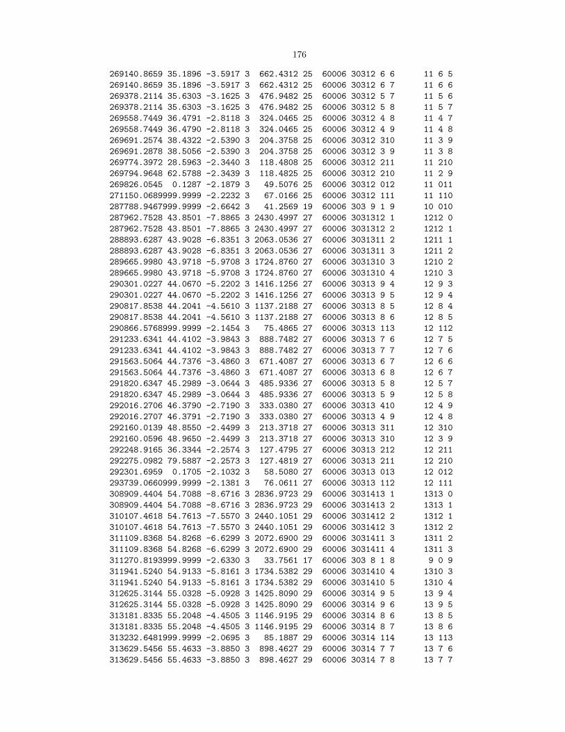
176

269140.8659 35.1896 -3.5917 3 662.4312 25 60006 30312 6 6 11 6 5

269140.8659 35.1896 -3.5917 3 662.4312 25 60006 30312 6 7 11 6 6

269378.2114 35.6303 -3.1625 3 476.9482 25 60006 30312 5 7 11 5 6

269378.2114 35.6303 -3.1625 3 476.9482 25 60006 30312 5 8 11 5 7

269558.7449 36.4791 -2.8118 3 324.0465 25 60006 30312 4 8 11 4 7

269558.7449 36.4790 -2.8118 3 324.0465 25 60006 30312 4 9 11 4 8

269691.2574 38.4322 -2.5390 3 204.3758 25 60006 30312 310 11 3 9

269691.2878 38.5056 -2.5390 3 204.3758 25 60006 30312 3 9 11 3 8

269774.3972 28.5963 -2.3440 3 118.4808 25 60006 30312 211 11 210

269794.9648 62.5788 -2.3439 3 118.4825 25 60006 30312 210 11 2 9

269826.0545 0.1287 -2.1879 3 49.5076 25 60006 30312 012 11 011

271150.0689999.9999 -2.2232 3 67.0166 25 60006 30312 111 11 110

287788.9467999.9999 -2.6642 3 41.2569 19 60006 303 9 1 9 10 010

287962.7528 43.8501 -7.8865 3 2430.4997 27 60006 3031312 1 1212 0

287962.7528 43.8501 -7.8865 3 2430.4997 27 60006 3031312 2 1212 1

288893.6287 43.9028 -6.8351 3 2063.0536 27 60006 3031311 2 1211 1

288893.6287 43.9028 -6.8351 3 2063.0536 27 60006 3031311 3 1211 2

289665.9980 43.9718 -5.9708 3 1724.8760 27 60006 3031310 3 1210 2

289665.9980 43.9718 -5.9708 3 1724.8760 27 60006 3031310 4 1210 3

290301.0227 44.0670 -5.2202 3 1416.1256 27 60006 30313 9 4 12 9 3

290301.0227 44.0670 -5.2202 3 1416.1256 27 60006 30313 9 5 12 9 4

290817.8538 44.2041 -4.5610 3 1137.2188 27 60006 30313 8 5 12 8 4

290817.8538 44.2041 -4.5610 3 1137.2188 27 60006 30313 8 6 12 8 5

290866.5768999.9999 -2.1454 3 75.4865 27 60006 30313 113 12 112

291233.6341 44.4102 -3.9843 3 888.7482 27 60006 30313 7 6 12 7 5

291233.6341 44.4102 -3.9843 3 888.7482 27 60006 30313 7 7 12 7 6

291563.5064 44.7376 -3.4860 3 671.4087 27 60006 30313 6 7 12 6 6

291563.5064 44.7376 -3.4860 3 671.4087 27 60006 30313 6 8 12 6 7

291820.6347 45.2989 -3.0644 3 485.9336 27 60006 30313 5 8 12 5 7

291820.6347 45.2989 -3.0644 3 485.9336 27 60006 30313 5 9 12 5 8

292016.2706 46.3790 -2.7190 3 333.0380 27 60006 30313 410 12 4 9

292016.2707 46.3791 -2.7190 3 333.0380 27 60006 30313 4 9 12 4 8

292160.0139 48.8550 -2.4499 3 213.3718 27 60006 30313 311 12 310

292160.0596 48.9650 -2.4499 3 213.3718 27 60006 30313 310 12 3 9

292248.9165 36.3344 -2.2574 3 127.4795 27 60006 30313 212 12 211

292275.0982 79.5887 -2.2573 3 127.4819 27 60006 30313 211 12 210

292301.6959 0.1705 -2.1032 3 58.5080 27 60006 30313 013 12 012

293739.0660999.9999 -2.1381 3 76.0611 27 60006 30313 112 12 111

308909.4404 54.7088 -8.6716 3 2836.9723 29 60006 3031413 1 1313 0

308909.4404 54.7088 -8.6716 3 2836.9723 29 60006 3031413 2 1313 1

310107.4618 54.7613 -7.5570 3 2440.1051 29 60006 3031412 2 1312 1

310107.4618 54.7613 -7.5570 3 2440.1051 29 60006 3031412 3 1312 2

311109.8368 54.8268 -6.6299 3 2072.6900 29 60006 3031411 3 1311 2

311109.8368 54.8268 -6.6299 3 2072.6900 29 60006 3031411 4 1311 3

311270.8193999.9999 -2.6330 3 33.7561 17 60006 303 8 1 8 9 0 9

311941.5240 54.9133 -5.8161 3 1734.5382 29 60006 3031410 4 1310 3

311941.5240 54.9133 -5.8161 3 1734.5382 29 60006 3031410 5 1310 4

312625.3144 55.0328 -5.0928 3 1425.8090 29 60006 30314 9 5 13 9 4

312625.3144 55.0328 -5.0928 3 1425.8090 29 60006 30314 9 6 13 9 5

313181.8335 55.2048 -4.4505 3 1146.9195 29 60006 30314 8 6 13 8 5

313181.8335 55.2048 -4.4505 3 1146.9195 29 60006 30314 8 7 13 8 6

313232.6481999.9999 -2.0695 3 85.1887 29 60006 30314 114 13 113

313629.5456 55.4633 -3.8850 3 898.4627 29 60006 30314 7 7 13 7 6

313629.5456 55.4633 -3.8850 3 898.4627 29 60006 30314 7 8 13 7 7

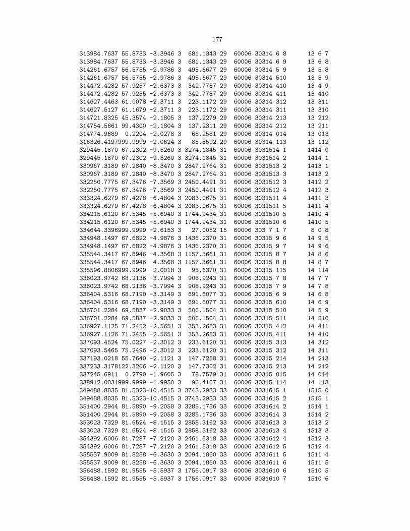
177

313984.7637 55.8733 -3.3946 3 681.1343 29 60006 30314 6 8 13 6 7

313984.7637 55.8733 -3.3946 3 681.1343 29 60006 30314 6 9 13 6 8

314261.6757 56.5755 -2.9786 3 495.6677 29 60006 30314 5 9 13 5 8

314261.6757 56.5755 -2.9786 3 495.6677 29 60006 30314 510 13 5 9

314472.4282 57.9257 -2.6373 3 342.7787 29 60006 30314 410 13 4 9

314472.4282 57.9255 -2.6373 3 342.7787 29 60006 30314 411 13 410

314627.4463 61.0078 -2.3711 3 223.1172 29 60006 30314 312 13 311

314627.5127 61.1679 -2.3711 3 223.1172 29 60006 30314 311 13 310

314721.8325 45.3574 -2.1805 3 137.2279 29 60006 30314 213 13 212

314754.5661 99.4300 -2.1804 3 137.2311 29 60006 30314 212 13 211

314774.9689 0.2204 -2.0278 3 68.2581 29 60006 30314 014 13 013

316326.4197999.9999 -2.0624 3 85.8592 29 60006 30314 113 13 112

329445.1870 67.2302 -9.5260 3 3274.1845 31 60006 3031514 1 1414 0

329445.1870 67.2302 -9.5260 3 3274.1845 31 60006 3031514 2 1414 1

330967.3189 67.2840 -8.3470 3 2847.2764 31 60006 3031513 2 1413 1

330967.3189 67.2840 -8.3470 3 2847.2764 31 60006 3031513 3 1413 2

332250.7775 67.3476 -7.3569 3 2450.4491 31 60006 3031512 3 1412 2

332250.7775 67.3476 -7.3569 3 2450.4491 31 60006 3031512 4 1412 3

333324.6279 67.4278 -6.4804 3 2083.0675 31 60006 3031511 4 1411 3

333324.6279 67.4278 -6.4804 3 2083.0675 31 60006 3031511 5 1411 4

334215.6120 67.5345 -5.6940 3 1744.9434 31 60006 3031510 5 1410 4

334215.6120 67.5345 -5.6940 3 1744.9434 31 60006 3031510 6 1410 5

334644.3396999.9999 -2.6153 3 27.0052 15 60006 303 7 1 7 8 0 8

334948.1497 67.6822 -4.9876 3 1436.2370 31 60006 30315 9 6 14 9 5

334948.1497 67.6822 -4.9876 3 1436.2370 31 60006 30315 9 7 14 9 6

335544.3417 67.8946 -4.3568 3 1157.3661 31 60006 30315 8 7 14 8 6

335544.3417 67.8946 -4.3568 3 1157.3661 31 60006 30315 8 8 14 8 7

335596.8806999.9999 -2.0018 3 95.6370 31 60006 30315 115 14 114

336023.9742 68.2136 -3.7994 3 908.9243 31 60006 30315 7 8 14 7 7

336023.9742 68.2136 -3.7994 3 908.9243 31 60006 30315 7 9 14 7 8

336404.5316 68.7190 -3.3149 3 691.6077 31 60006 30315 6 9 14 6 8

336404.5316 68.7190 -3.3149 3 691.6077 31 60006 30315 610 14 6 9

336701.2284 69.5837 -2.9033 3 506.1504 31 60006 30315 510 14 5 9

336701.2284 69.5837 -2.9033 3 506.1504 31 60006 30315 511 14 510

336927.1125 71.2452 -2.5651 3 353.2683 31 60006 30315 412 14 411

336927.1126 71.2455 -2.5651 3 353.2683 31 60006 30315 411 14 410

337093.4524 75.0227 -2.3012 3 233.6120 31 60006 30315 313 14 312

337093.5465 75.2496 -2.3012 3 233.6120 31 60006 30315 312 14 311

337193.0218 55.7640 -2.1121 3 147.7258 31 60006 30315 214 14 213

337233.3178122.3206 -2.1120 3 147.7302 31 60006 30315 213 14 212

337245.6911 0.2790 -1.9605 3 78.7579 31 60006 30315 015 14 014

338912.0031999.9999 -1.9950 3 96.4107 31 60006 30315 114 14 113

349488.8035 81.5323-10.4515 3 3743.2933 33 60006 3031615 1 1515 0

349488.8035 81.5323-10.4515 3 3743.2933 33 60006 3031615 2 1515 1

351400.2944 81.5890 -9.2058 3 3285.1736 33 60006 3031614 2 1514 1

351400.2944 81.5890 -9.2058 3 3285.1736 33 60006 3031614 3 1514 2

353023.7329 81.6524 -8.1515 3 2858.3162 33 60006 3031613 3 1513 2

353023.7329 81.6524 -8.1515 3 2858.3162 33 60006 3031613 4 1513 3

354392.6006 81.7287 -7.2120 3 2461.5318 33 60006 3031612 4 1512 3

354392.6006 81.7287 -7.2120 3 2461.5318 33 60006 3031612 5 1512 4

355537.9009 81.8258 -6.3630 3 2094.1860 33 60006 3031611 5 1511 4

355537.9009 81.8258 -6.3630 3 2094.1860 33 60006 3031611 6 1511 5

356488.1592 81.9555 -5.5937 3 1756.0917 33 60006 3031610 6 1510 5

356488.1592 81.9555 -5.5937 3 1756.0917 33 60006 3031610 7 1510 6

178

357269.4248 82.1354 -4.8990 3 1447.4097 33 60006 30316 9 7 15 9 6

357269.4248 82.1354 -4.8990 3 1447.4097 33 60006 30316 9 8 15 9 7

357905.2734 82.3941 -4.2764 3 1168.5586 33 60006 30316 8 8 15 8 7

357905.2734 82.3941 -4.2764 3 1168.5586 33 60006 30316 8 9 15 8 8

357908.9210999.9999 -2.6125 3 21.0043 13 60006 303 6 1 6 7 0 7

357959.1436999.9999 -1.9416 3 106.8313 33 60006 30316 116 15 115

358416.8141 82.7822 -3.7251 3 920.1328 33 60006 30316 7 9 15 7 8

358416.8141 82.7822 -3.7251 3 920.1328 33 60006 30316 710 15 7 9

358822.7039 83.3967 -3.2450 3 702.8289 33 60006 30316 610 15 6 9

358822.7039 83.3967 -3.2450 3 702.8289 33 60006 30316 611 15 610

359139.1867 84.4472 -2.8368 3 517.3815 33 60006 30316 511 15 510

359139.1867 84.4472 -2.8368 3 517.3815 33 60006 30316 512 15 511

359380.2185 86.4649 -2.5013 3 364.5070 33 60006 30316 413 15 412

359380.2187 86.4653 -2.5013 3 364.5070 33 60006 30316 412 15 411

359557.9300 91.0315 -2.2391 3 244.8562 33 60006 30316 314 15 313

359558.0604 91.3457 -2.2391 3 244.8562 33 60006 30316 313 15 312

359662.3614 67.6529 -2.0513 3 158.9734 33 60006 30316 215 15 214

359711.3028148.4782 -2.0512 3 158.9791 33 60006 30316 214 15 213

359713.6796 0.3470 -1.9007 3 90.0072 33 60006 30316 016 15 015

361495.6891999.9999 -1.9350 3 107.7156 33 60006 30316 115 15 114

371323.1202 97.7943-10.1354 3 3754.9510 35 60006 3031715 2 1615 1

371323.1202 97.7943-10.1354 3 3754.9510 35 60006 3031715 3 1615 2

373353.8726 97.8595 -9.0144 3 3296.8951 35 60006 3031714 3 1614 2

373353.8726 97.8595 -9.0144 3 3296.8951 35 60006 3031714 4 1614 3

375078.5849 97.9337 -8.0108 3 2870.0919 35 60006 3031713 4 1613 3

375078.5849 97.9337 -8.0108 3 2870.0919 35 60006 3031713 5 1613 4

376532.8318 98.0242 -7.0989 3 2473.3531 35 60006 3031712 5 1612 4

376532.8318 98.0242 -7.0989 3 2473.3531 35 60006 3031712 6 1612 5

377749.5549 98.1404 -6.2672 3 2106.0455 35 60006 3031711 6 1611 5

377749.5549 98.1404 -6.2672 3 2106.0455 35 60006 3031711 7 1611 6

378759.0633 98.2962 -5.5096 3 1767.9828 35 60006 3031710 7 1610 6

378759.0633 98.2962 -5.5096 3 1767.9828 35 60006 3031710 8 1610 7

379589.0357 98.5126 -4.8233 3 1459.3269 35 60006 30317 9 8 16 9 7

379589.0357 98.5126 -4.8233 3 1459.3269 35 60006 30317 9 9 16 9 8

380264.5237 98.8239 -4.2069 3 1180.4971 35 60006 30317 8 9 16 8 8

380264.5237 98.8239 -4.2069 3 1180.4971 35 60006 30317 810 16 8 9

380319.3062999.9999 -1.8881 3 118.7716 35 60006 30317 117 16 116

380807.9597 99.2905 -3.6602 3 932.0883 35 60006 30317 710 16 7 9

380807.9597 99.2905 -3.6602 3 932.0883 35 60006 30317 711 16 710

381064.0275999.9999 -2.6275 3 15.7534 11 60006 303 5 1 5 6 0 6

381239.1744100.0287 -3.1837 3 714.7979 35 60006 30317 611 16 610

381239.1744100.0287 -3.1837 3 714.7979 35 60006 30317 612 16 611

381575.4444101.2899 -2.7783 3 529.3611 35 60006 30317 512 16 511

381575.4444101.2899 -2.7783 3 529.3611 35 60006 30317 513 16 512

381831.6413103.7112 -2.4447 3 376.4946 35 60006 30317 414 16 413

381831.6416103.7119 -2.4447 3 376.4946 35 60006 30317 413 16 412

382020.7770109.1657 -2.1841 3 256.8498 35 60006 30317 315 16 314

382020.9540109.5922 -2.1841 3 256.8498 35 60006 30317 314 16 313

382129.7277 81.1228 -1.9973 3 170.9704 35 60006 30317 216 16 215

382178.7519 0.4249 -1.8475 3 102.0060 35 60006 30317 017 16 016

382188.4707178.1205 -1.9972 3 170.9778 35 60006 30317 215 16 214

384077.3506999.9999 -1.8818 3 119.7738 35 60006 30317 116 16 115

393155.8498116.0866 -9.9477 3 3767.3370 37 60006 3031815 3 1715 2

393155.8498116.0866 -9.9477 3 3767.3370 37 60006 3031815 4 1715 3

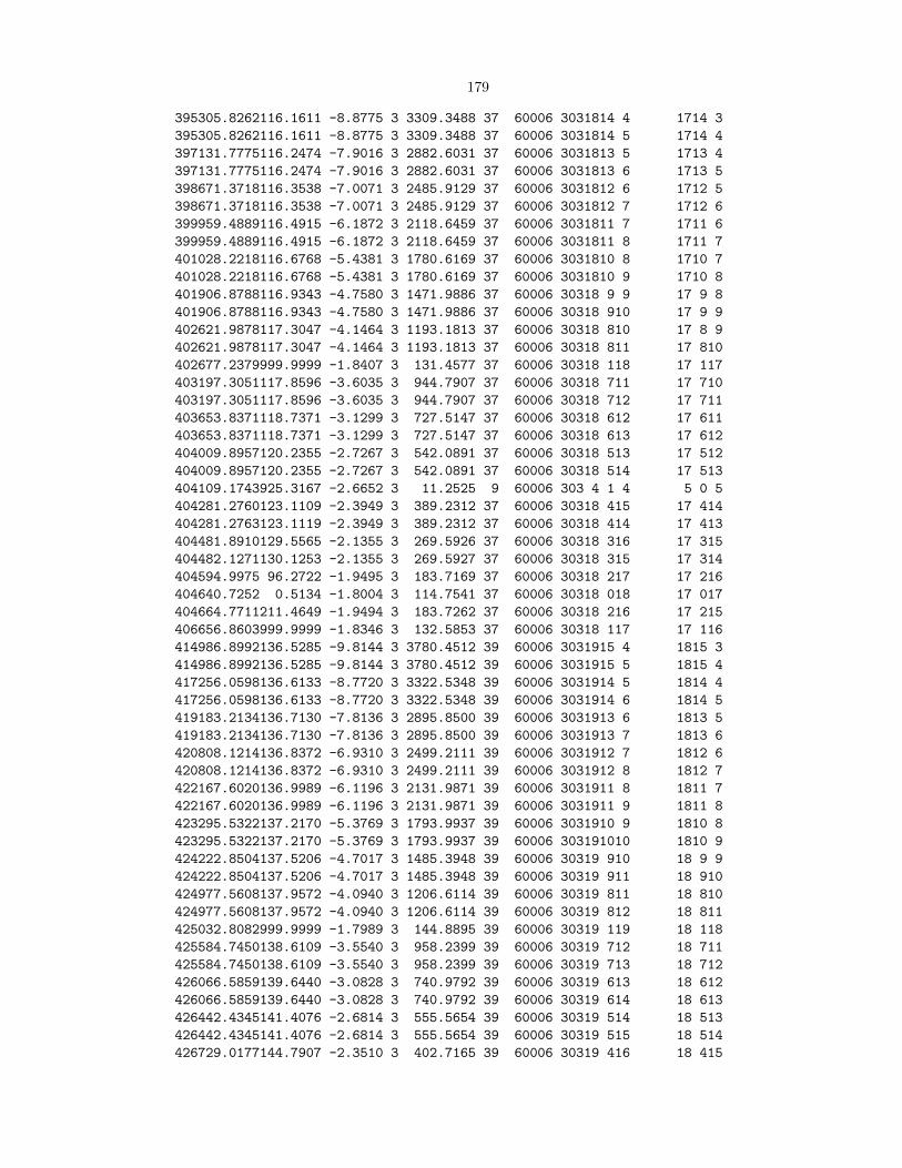
179

395305.8262116.1611 -8.8775 3 3309.3488 37 60006 3031814 4 1714 3

395305.8262116.1611 -8.8775 3 3309.3488 37 60006 3031814 5 1714 4

397131.7775116.2474 -7.9016 3 2882.6031 37 60006 3031813 5 1713 4

397131.7775116.2474 -7.9016 3 2882.6031 37 60006 3031813 6 1713 5

398671.3718116.3538 -7.0071 3 2485.9129 37 60006 3031812 6 1712 5

398671.3718116.3538 -7.0071 3 2485.9129 37 60006 3031812 7 1712 6

399959.4889116.4915 -6.1872 3 2118.6459 37 60006 3031811 7 1711 6

399959.4889116.4915 -6.1872 3 2118.6459 37 60006 3031811 8 1711 7

401028.2218116.6768 -5.4381 3 1780.6169 37 60006 3031810 8 1710 7

401028.2218116.6768 -5.4381 3 1780.6169 37 60006 3031810 9 1710 8

401906.8788116.9343 -4.7580 3 1471.9886 37 60006 30318 9 9 17 9 8

401906.8788116.9343 -4.7580 3 1471.9886 37 60006 30318 910 17 9 9

402621.9878117.3047 -4.1464 3 1193.1813 37 60006 30318 810 17 8 9

402621.9878117.3047 -4.1464 3 1193.1813 37 60006 30318 811 17 810

402677.2379999.9999 -1.8407 3 131.4577 37 60006 30318 118 17 117

403197.3051117.8596 -3.6035 3 944.7907 37 60006 30318 711 17 710

403197.3051117.8596 -3.6035 3 944.7907 37 60006 30318 712 17 711

403653.8371118.7371 -3.1299 3 727.5147 37 60006 30318 612 17 611

403653.8371118.7371 -3.1299 3 727.5147 37 60006 30318 613 17 612

404009.8957120.2355 -2.7267 3 542.0891 37 60006 30318 513 17 512

404009.8957120.2355 -2.7267 3 542.0891 37 60006 30318 514 17 513

404109.1743925.3167 -2.6652 3 11.2525 9 60006 303 4 1 4 5 0 5

404281.2760123.1109 -2.3949 3 389.2312 37 60006 30318 415 17 414

404281.2763123.1119 -2.3949 3 389.2312 37 60006 30318 414 17 413

404481.8910129.5565 -2.1355 3 269.5926 37 60006 30318 316 17 315

404482.1271130.1253 -2.1355 3 269.5927 37 60006 30318 315 17 314

404594.9975 96.2722 -1.9495 3 183.7169 37 60006 30318 217 17 216

404640.7252 0.5134 -1.8004 3 114.7541 37 60006 30318 018 17 017

404664.7711211.4649 -1.9494 3 183.7262 37 60006 30318 216 17 215

406656.8603999.9999 -1.8346 3 132.5853 37 60006 30318 117 17 116

414986.8992136.5285 -9.8144 3 3780.4512 39 60006 3031915 4 1815 3

414986.8992136.5285 -9.8144 3 3780.4512 39 60006 3031915 5 1815 4

417256.0598136.6133 -8.7720 3 3322.5348 39 60006 3031914 5 1814 4

417256.0598136.6133 -8.7720 3 3322.5348 39 60006 3031914 6 1814 5

419183.2134136.7130 -7.8136 3 2895.8500 39 60006 3031913 6 1813 5

419183.2134136.7130 -7.8136 3 2895.8500 39 60006 3031913 7 1813 6

420808.1214136.8372 -6.9310 3 2499.2111 39 60006 3031912 7 1812 6

420808.1214136.8372 -6.9310 3 2499.2111 39 60006 3031912 8 1812 7

422167.6020136.9989 -6.1196 3 2131.9871 39 60006 3031911 8 1811 7

422167.6020136.9989 -6.1196 3 2131.9871 39 60006 3031911 9 1811 8

423295.5322137.2170 -5.3769 3 1793.9937 39 60006 3031910 9 1810 8

423295.5322137.2170 -5.3769 3 1793.9937 39 60006 303191010 1810 9

424222.8504137.5206 -4.7017 3 1485.3948 39 60006 30319 910 18 9 9

424222.8504137.5206 -4.7017 3 1485.3948 39 60006 30319 911 18 910

424977.5608137.9572 -4.0940 3 1206.6114 39 60006 30319 811 18 810

424977.5608137.9572 -4.0940 3 1206.6114 39 60006 30319 812 18 811

425032.8082999.9999 -1.7989 3 144.8895 39 60006 30319 119 18 118

425584.7450138.6109 -3.5540 3 958.2399 39 60006 30319 712 18 711

425584.7450138.6109 -3.5540 3 958.2399 39 60006 30319 713 18 712

426066.5859139.6440 -3.0828 3 740.9792 39 60006 30319 613 18 612

426066.5859139.6440 -3.0828 3 740.9792 39 60006 30319 614 18 613

426442.4345141.4076 -2.6814 3 555.5654 39 60006 30319 514 18 513

426442.4345141.4076 -2.6814 3 555.5654 39 60006 30319 515 18 514

426729.0177144.7907 -2.3510 3 402.7165 39 60006 30319 416 18 415

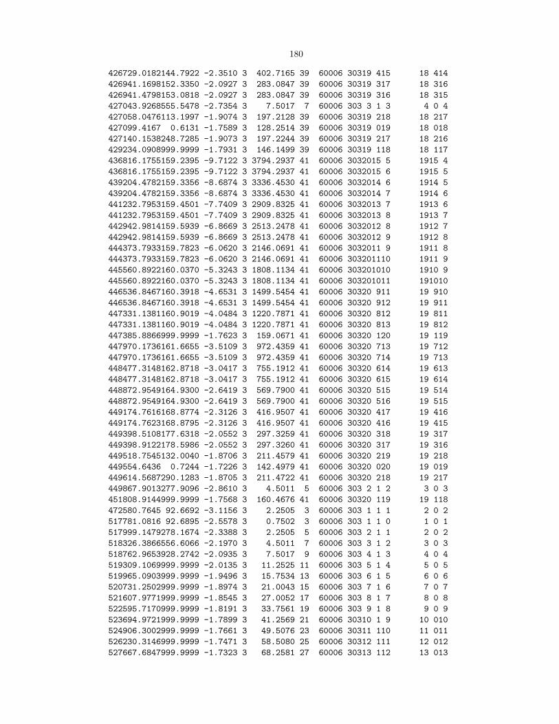
180

426729.0182144.7922 -2.3510 3 402.7165 39 60006 30319 415 18 414

426941.1698152.3350 -2.0927 3 283.0847 39 60006 30319 317 18 316

426941.4798153.0818 -2.0927 3 283.0847 39 60006 30319 316 18 315

427043.9268555.5478 -2.7354 3 7.5017 7 60006 303 3 1 3 4 0 4

427058.0476113.1997 -1.9074 3 197.2128 39 60006 30319 218 18 217

427099.4167 0.6131 -1.7589 3 128.2514 39 60006 30319 019 18 018

427140.1538248.7285 -1.9073 3 197.2244 39 60006 30319 217 18 216

429234.0908999.9999 -1.7931 3 146.1499 39 60006 30319 118 18 117

436816.1755159.2395 -9.7122 3 3794.2937 41 60006 3032015 5 1915 4

436816.1755159.2395 -9.7122 3 3794.2937 41 60006 3032015 6 1915 5

439204.4782159.3356 -8.6874 3 3336.4530 41 60006 3032014 6 1914 5

439204.4782159.3356 -8.6874 3 3336.4530 41 60006 3032014 7 1914 6

441232.7953159.4501 -7.7409 3 2909.8325 41 60006 3032013 7 1913 6

441232.7953159.4501 -7.7409 3 2909.8325 41 60006 3032013 8 1913 7

442942.9814159.5939 -6.8669 3 2513.2478 41 60006 3032012 8 1912 7

442942.9814159.5939 -6.8669 3 2513.2478 41 60006 3032012 9 1912 8

444373.7933159.7823 -6.0620 3 2146.0691 41 60006 3032011 9 1911 8

444373.7933159.7823 -6.0620 3 2146.0691 41 60006 303201110 1911 9

445560.8922160.0370 -5.3243 3 1808.1134 41 60006 303201010 1910 9

445560.8922160.0370 -5.3243 3 1808.1134 41 60006 303201011 191010

446536.8467160.3918 -4.6531 3 1499.5454 41 60006 30320 911 19 910

446536.8467160.3918 -4.6531 3 1499.5454 41 60006 30320 912 19 911

447331.1381160.9019 -4.0484 3 1220.7871 41 60006 30320 812 19 811

447331.1381160.9019 -4.0484 3 1220.7871 41 60006 30320 813 19 812

447385.8866999.9999 -1.7623 3 159.0671 41 60006 30320 120 19 119

447970.1736161.6655 -3.5109 3 972.4359 41 60006 30320 713 19 712

447970.1736161.6655 -3.5109 3 972.4359 41 60006 30320 714 19 713

448477.3148162.8718 -3.0417 3 755.1912 41 60006 30320 614 19 613

448477.3148162.8718 -3.0417 3 755.1912 41 60006 30320 615 19 614

448872.9549164.9300 -2.6419 3 569.7900 41 60006 30320 515 19 514

448872.9549164.9300 -2.6419 3 569.7900 41 60006 30320 516 19 515

449174.7616168.8774 -2.3126 3 416.9507 41 60006 30320 417 19 416

449174.7623168.8795 -2.3126 3 416.9507 41 60006 30320 416 19 415

449398.5108177.6318 -2.0552 3 297.3259 41 60006 30320 318 19 317

449398.9122178.5986 -2.0552 3 297.3260 41 60006 30320 317 19 316

449518.7545132.0040 -1.8706 3 211.4579 41 60006 30320 219 19 218

449554.6436 0.7244 -1.7226 3 142.4979 41 60006 30320 020 19 019

449614.5687290.1283 -1.8705 3 211.4722 41 60006 30320 218 19 217

449867.9013277.9096 -2.8610 3 4.5011 5 60006 303 2 1 2 3 0 3

451808.9144999.9999 -1.7568 3 160.4676 41 60006 30320 119 19 118

472580.7645 92.6692 -3.1156 3 2.2505 3 60006 303 1 1 1 2 0 2

517781.0816 92.6895 -2.5578 3 0.7502 3 60006 303 1 1 0 1 0 1

517999.1479278.1674 -2.3388 3 2.2505 5 60006 303 2 1 1 2 0 2

518326.3866556.6066 -2.1970 3 4.5011 7 60006 303 3 1 2 3 0 3

518762.9653928.2742 -2.0935 3 7.5017 9 60006 303 4 1 3 4 0 4

519309.1069999.9999 -2.0135 3 11.2525 11 60006 303 5 1 4 5 0 5

519965.0903999.9999 -1.9496 3 15.7534 13 60006 303 6 1 5 6 0 6

520731.2502999.9999 -1.8974 3 21.0043 15 60006 303 7 1 6 7 0 7

521607.9771999.9999 -1.8545 3 27.0052 17 60006 303 8 1 7 8 0 8

522595.7170999.9999 -1.8191 3 33.7561 19 60006 303 9 1 8 9 0 9

523694.9721999.9999 -1.7899 3 41.2569 21 60006 30310 1 9 10 010

524906.3002999.9999 -1.7661 3 49.5076 23 60006 30311 110 11 011

526230.3146999.9999 -1.7471 3 58.5080 25 60006 30312 111 12 012

527667.6847999.9999 -1.7323 3 68.2581 27 60006 30313 112 13 013

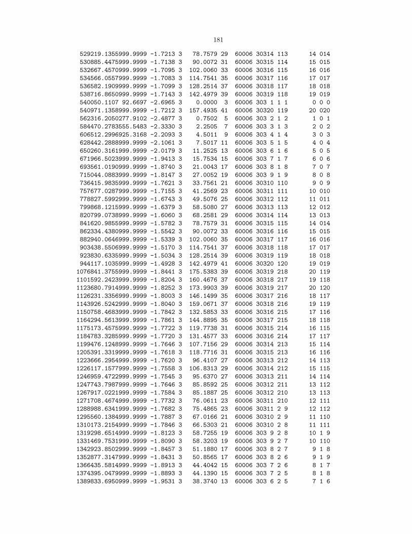
181

529219.1355999.9999 -1.7213 3 78.7579 29 60006 30314 113 14 014

530885.4475999.9999 -1.7138 3 90.0072 31 60006 30315 114 15 015

532667.4570999.9999 -1.7095 3 102.0060 33 60006 30316 115 16 016

534566.0557999.9999 -1.7083 3 114.7541 35 60006 30317 116 17 017

536582.1909999.9999 -1.7099 3 128.2514 37 60006 30318 117 18 018

538716.8650999.9999 -1.7143 3 142.4979 39 60006 30319 118 19 019

540050.1107 92.6697 -2.6965 3 0.0000 3 60006 303 1 1 1 0 0 0

540971.1358999.9999 -1.7212 3 157.4935 41 60006 30320 119 20 020

562316.2050277.9102 -2.4877 3 0.7502 5 60006 303 2 1 2 1 0 1

584470.2783555.5483 -2.3330 3 2.2505 7 60006 303 3 1 3 2 0 2

606512.2996925.3168 -2.2093 3 4.5011 9 60006 303 4 1 4 3 0 3

628442.2888999.9999 -2.1061 3 7.5017 11 60006 303 5 1 5 4 0 4

650260.3161999.9999 -2.0179 3 11.2525 13 60006 303 6 1 6 5 0 5

671966.5023999.9999 -1.9413 3 15.7534 15 60006 303 7 1 7 6 0 6

693561.0190999.9999 -1.8740 3 21.0043 17 60006 303 8 1 8 7 0 7

715044.0883999.9999 -1.8147 3 27.0052 19 60006 303 9 1 9 8 0 8

736415.9835999.9999 -1.7621 3 33.7561 21 60006 30310 110 9 0 9

757677.0287999.9999 -1.7155 3 41.2569 23 60006 30311 111 10 010

778827.5992999.9999 -1.6743 3 49.5076 25 60006 30312 112 11 011

799868.1215999.9999 -1.6379 3 58.5080 27 60006 30313 113 12 012

820799.0738999.9999 -1.6060 3 68.2581 29 60006 30314 114 13 013

841620.9855999.9999 -1.5782 3 78.7579 31 60006 30315 115 14 014

862334.4380999.9999 -1.5542 3 90.0072 33 60006 30316 116 15 015

882940.0646999.9999 -1.5339 3 102.0060 35 60006 30317 117 16 016

903438.5506999.9999 -1.5170 3 114.7541 37 60006 30318 118 17 017

923830.6335999.9999 -1.5034 3 128.2514 39 60006 30319 119 18 018

944117.1035999.9999 -1.4928 3 142.4979 41 60006 30320 120 19 019

1076841.3755999.9999 -1.8441 3 175.5383 39 60006 30319 218 20 119

1101592.2423999.9999 -1.8204 3 160.4676 37 60006 30318 217 19 118

1123680.7914999.9999 -1.8252 3 173.9903 39 60006 30319 217 20 120

1126231.3356999.9999 -1.8003 3 146.1499 35 60006 30317 216 18 117

1143926.5242999.9999 -1.8040 3 159.0671 37 60006 30318 216 19 119

1150758.4683999.9999 -1.7842 3 132.5853 33 60006 30316 215 17 116

1164294.5613999.9999 -1.7861 3 144.8895 35 60006 30317 215 18 118

1175173.4575999.9999 -1.7722 3 119.7738 31 60006 30315 214 16 115

1184783.3285999.9999 -1.7720 3 131.4577 33 60006 30316 214 17 117

1199476.1248999.9999 -1.7646 3 107.7156 29 60006 30314 213 15 114

1205391.3319999.9999 -1.7618 3 118.7716 31 60006 30315 213 16 116

1223666.2954999.9999 -1.7620 3 96.4107 27 60006 30313 212 14 113

1226117.1577999.9999 -1.7558 3 106.8313 29 60006 30314 212 15 115

1246959.4722999.9999 -1.7545 3 95.6370 27 60006 30313 211 14 114

1247743.7987999.9999 -1.7646 3 85.8592 25 60006 30312 211 13 112

1267917.0221999.9999 -1.7584 3 85.1887 25 60006 30312 210 13 113

1271708.4674999.9999 -1.7732 3 76.0611 23 60006 30311 210 12 111

1288988.6341999.9999 -1.7682 3 75.4865 23 60006 30311 2 9 12 112

1295560.1384999.9999 -1.7887 3 67.0166 21 60006 30310 2 9 11 110

1310173.2154999.9999 -1.7846 3 66.5303 21 60006 30310 2 8 11 111

1319298.6514999.9999 -1.8123 3 58.7255 19 60006 303 9 2 8 10 1 9

1331469.7531999.9999 -1.8090 3 58.3203 19 60006 303 9 2 7 10 110

1342923.8502999.9999 -1.8457 3 51.1880 17 60006 303 8 2 7 9 1 8

1352877.3147999.9999 -1.8431 3 50.8565 17 60006 303 8 2 6 9 1 9

1366435.5814999.9999 -1.8913 3 44.4042 15 60006 303 7 2 6 8 1 7

1374395.0479999.9999 -1.8893 3 44.1390 15 60006 303 7 2 5 8 1 8

1389833.6950999.9999 -1.9531 3 38.3740 13 60006 303 6 2 5 7 1 6

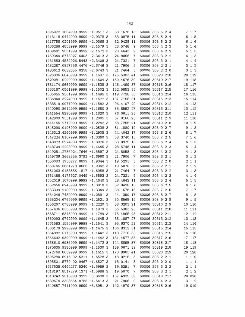
182

1396022.1804999.9999 -1.9517 3 38.1678 13 60006 303 6 2 4 7 1 7

1413118.0442999.9999 -2.0378 3 33.0975 11 60006 303 5 2 4 6 1 5

1417758.0201999.9999 -2.0368 3 32.9428 11 60006 303 5 2 3 6 1 6

1436288.4852999.9999 -2.1579 3 28.5748 9 60006 303 4 2 3 5 1 4

1439601.9551999.9999 -2.1572 3 28.4643 9 60006 303 4 2 2 5 1 5

1459344.8773927.6403 -2.3413 3 24.8058 7 60006 303 3 2 2 4 1 3

1461553.4534926.5443 -2.3408 3 24.7321 7 60006 303 3 2 1 4 1 4

1482287.0827556.4476 -2.6746 3 21.7906 5 60006 303 2 2 1 3 1 2

1483612.0632555.8258 -2.6743 3 21.7464 5 60006 303 2 2 0 3 1 3

1526886.6843999.9999 -1.1697 3 175.5383 41 60006 30320 218 20 119

1529081.0299999.9999 -1.1604 3 160.4676 39 60006 30319 217 19 118

1531174.9669999.9999 -1.1538 3 146.1499 37 60006 30318 216 18 117

1533167.0561999.9999 -1.1502 3 132.5853 35 60006 30317 215 17 116

1535055.9361999.9999 -1.1495 3 119.7738 33 60006 30316 214 16 115

1536840.3224999.9999 -1.1522 3 107.7156 31 60006 30315 213 15 114

1538519.0077999.9999 -1.1582 3 96.4107 29 60006 30314 212 14 113

1540090.8612999.9999 -1.1680 3 85.8592 27 60006 30313 211 13 112

1541554.8290999.9999 -1.1820 3 76.0611 25 60006 30312 210 12 111

1542909.9331999.9999 -1.2005 3 67.0166 23 60006 30311 2 9 11 110

1544155.2719999.9999 -1.2242 3 58.7255 21 60006 30310 2 8 10 1 9

1545290.0196999.9999 -1.2538 3 51.1880 19 60006 303 9 2 7 9 1 8

1546313.4260999.9999 -1.2905 3 44.4042 17 60006 303 8 2 6 8 1 7

1547224.8167999.9999 -1.3360 3 38.3740 15 60006 303 7 2 5 7 1 6

1548023.5924999.9999 -1.3926 3 33.0975 13 60006 303 6 2 4 6 1 5

1548709.2293999.9999 -1.4645 3 28.5748 11 60006 303 5 2 3 5 1 4

1549281.2786924.7646 -1.5597 3 24.8058 9 60006 303 4 2 2 4 1 3

1549739.3663555.3792 -1.6960 3 21.7906 7 60006 303 3 2 1 3 1 2

1550083.1936277.8899 -1.9344 3 19.5291 5 60006 303 2 2 0 2 1 1

1550745.5681278.0686 -1.9342 3 19.5070 5 60006 303 2 2 1 2 1 2

1551063.9158556.1817 -1.6958 3 21.7464 7 60006 303 3 2 2 3 1 3

1551488.4178927.0449 -1.5593 3 24.7321 9 60006 303 4 2 3 4 1 4

1552019.1070999.9999 -1.4640 3 28.4643 11 60006 303 5 2 4 5 1 5

1552656.0243999.9999 -1.3918 3 32.9428 13 60006 303 6 2 5 6 1 6

1553399.2189999.9999 -1.3349 3 38.1678 15 60006 303 7 2 6 7 1 7

1554248.7480999.9999 -1.2891 3 44.1390 17 60006 303 8 2 7 8 1 8

1555204.6769999.9999 -1.2521 3 50.8565 19 60006 303 9 2 8 9 1 9

1556267.0788999.9999 -1.2220 3 58.3203 21 60006 30310 2 9 10 110

1557436.0350999.9999 -1.1979 3 66.5303 23 60006 30311 210 11 111

1558711.6346999.9999 -1.1789 3 75.4865 25 60006 30312 211 12 112

1560093.9742999.9999 -1.1645 3 85.1887 27 60006 30313 212 13 113

1561583.1585999.9999 -1.1541 3 95.6370 29 60006 30314 213 14 114

1563179.2998999.9999 -1.1475 3 106.8313 31 60006 30315 214 15 115

1564882.5175999.9999 -1.1442 3 118.7716 33 60006 30316 215 16 116

1566692.9390999.9999 -1.1442 3 131.4577 35 60006 30317 216 17 117

1568610.6986999.9999 -1.1472 3 144.8895 37 60006 30318 217 18 118

1570635.9380999.9999 -1.1530 3 159.0671 39 60006 30319 218 19 119

1572768.8059999.9999 -1.1615 3 173.9903 41 60006 30320 219 20 120

1595280.6915 92.5311 -1.6528 3 18.0215 5 60006 303 2 2 1 1 1 0

1595501.5770 92.9467 -1.6527 3 18.0141 5 60006 303 2 2 0 1 1 1

1617535.0462277.5340 -1.5989 3 19.5291 7 60006 303 3 2 2 2 1 1

1618197.8517279.1371 -1.5988 3 19.5070 7 60006 303 3 2 1 2 1 2

1618243.2513999.9999 -6.3680 3 157.4935 39 60006 30319 217 20 020

1639674.3308554.8785 -1.5413 3 21.7906 9 60006 303 4 2 3 3 1 2

1640657.7411999.9999 -6.3951 3 142.4979 37 60006 30318 216 19 019

183

1641000.3171559.0574 -1.5411 3 21.7464 9 60006 303 4 2 2 3 1 3

1661698.4305924.4362 -1.4875 3 24.8058 11 60006 303 5 2 4 4 1 3

1663092.3866848.0797 -6.4279 3 128.2514 35 60006 30317 215 18 018

1663909.1619933.3111 -1.4872 3 24.7321 11 60006 303 5 2 3 4 1 4

1683607.2335999.9999 -1.4388 3 28.5748 13 60006 303 6 2 5 5 1 4

1685544.6412669.8926 -6.4669 3 114.7541 33 60006 30316 214 17 017

1686924.6552999.9999 -1.4384 3 28.4643 13 60006 303 6 2 4 5 1 5

1705400.6309999.9999 -1.3955 3 33.0975 15 60006 303 7 2 6 6 1 5

1708012.0903521.3648 -6.5125 3 102.0060 31 60006 30315 213 16 016

1710047.1459999.9999 -1.3950 3 32.9428 15 60006 303 7 2 5 6 1 6

1727078.5167999.9999 -1.3572 3 38.3740 17 60006 303 8 2 7 7 1 6

1730492.4521399.0089 -6.5655 3 90.0072 29 60006 30314 212 15 015

1733277.0635999.9999 -1.3565 3 38.1678 17 60006 303 8 2 6 7 1 7

1748640.7881999.9999 -1.3236 3 44.4042 19 60006 303 9 2 8 8 1 7

1752983.5770299.5550 -6.6267 3 78.7579 27 60006 30313 211 14 014

1756614.9173999.9999 -1.3227 3 44.1390 19 60006 303 9 2 7 8 1 8

1770087.3453999.9999 -1.2943 3 51.1880 21 60006 30310 2 9 9 1 8

1775483.4477219.9512 -6.6971 3 68.2581 25 60006 30312 210 13 013

1780061.2974999.9999 -1.2932 3 50.8565 21 60006 30310 2 8 9 1 9

1791418.0916999.9999 -1.2689 3 58.7255 23 60006 30311 210 10 1 9

1797990.1788157.3638 -6.7781 3 58.5080 23 60006 30311 2 9 12 012

1803616.8736999.9999 -1.2677 3 58.3203 23 60006 30311 2 9 10 110

1812632.9336999.9999 -1.2473 3 67.0166 25 60006 30312 211 11 110

1820502.0168109.1772 -6.8713 3 49.5076 21 60006 30310 2 8 11 011

1827282.3966999.9999 -1.2459 3 66.5303 25 60006 30312 210 11 111

1833731.7811999.9999 -1.2292 3 76.0611 27 60006 30313 212 12 111

1843017.3400 72.9943 -6.9790 3 41.2569 19 60006 303 9 2 7 10 010

1851058.6971999.9999 -1.2276 3 75.4865 27 60006 30313 211 12 112

1854714.5476999.9999 -1.2143 3 85.8592 29 60006 30314 213 13 112

1865534.6581 46.6360 -7.1042 3 33.7561 17 60006 303 8 2 6 9 0 9

1874946.6864999.9999 -1.2127 3 85.1887 29 60006 30314 212 13 113

1875581.1497999.9999 -1.2026 3 96.4107 31 60006 30315 214 14 113

1888052.6122 28.1418 -7.2512 3 27.0052 15 60006 303 7 2 5 8 0 8

1896331.5080999.9999 -1.1938 3 107.7156 33 60006 30316 215 15 114

1898947.3561999.9999 -1.2008 3 95.6370 31 60006 30315 213 14 114

1910569.9747 15.7693 -7.4265 3 21.0043 13 60006 303 6 2 4 7 0 7

1916965.5466999.9999 -1.1879 3 119.7738 35 60006 30317 216 16 115

1923061.7783999.9999 -1.1920 3 106.8313 33 60006 30316 214 15 115

1933085.6491 7.9940 -7.6403 3 15.7534 11 60006 303 5 2 3 6 0 6

1937483.1934999.9999 -1.1848 3 132.5853 37 60006 30318 217 17 116

1947291.1054999.9999 -1.1860 3 118.7716 35 60006 30317 215 16 116

1955598.6697 3.5096 -7.9105 3 11.2525 9 60006 303 4 2 2 5 0 5

1957884.3807999.9999 -1.1842 3 146.1499 39 60006 30319 218 18 117

1971636.5702999.9999 -1.1827 3 131.4577 37 60006 30318 216 17 117

1978108.2018 1.2280 -8.2737 3 7.5017 7 60006 303 3 2 1 4 0 4

1978169.0444999.9999 -1.1862 3 160.4676 41 60006 30320 219 19 118

1996099.4862999.9999 -1.1821 3 144.8895 39 60006 30319 217 18 118

184

Appendix C

FTIR Spectra of Ices Studied inthe THz-TDS

Where available, spectra of unsaturated samples of species studied in the FTIR are presented here.

These spectra are background-subtracted using a scan of the blank substrate, but have had no

correction made to the baseline in post-processing. They are intended as a guide to future work for

a qualitative identification of an ice species probed by the FTIR, and not for quantitative assignment

of vibrational modes or intensities.

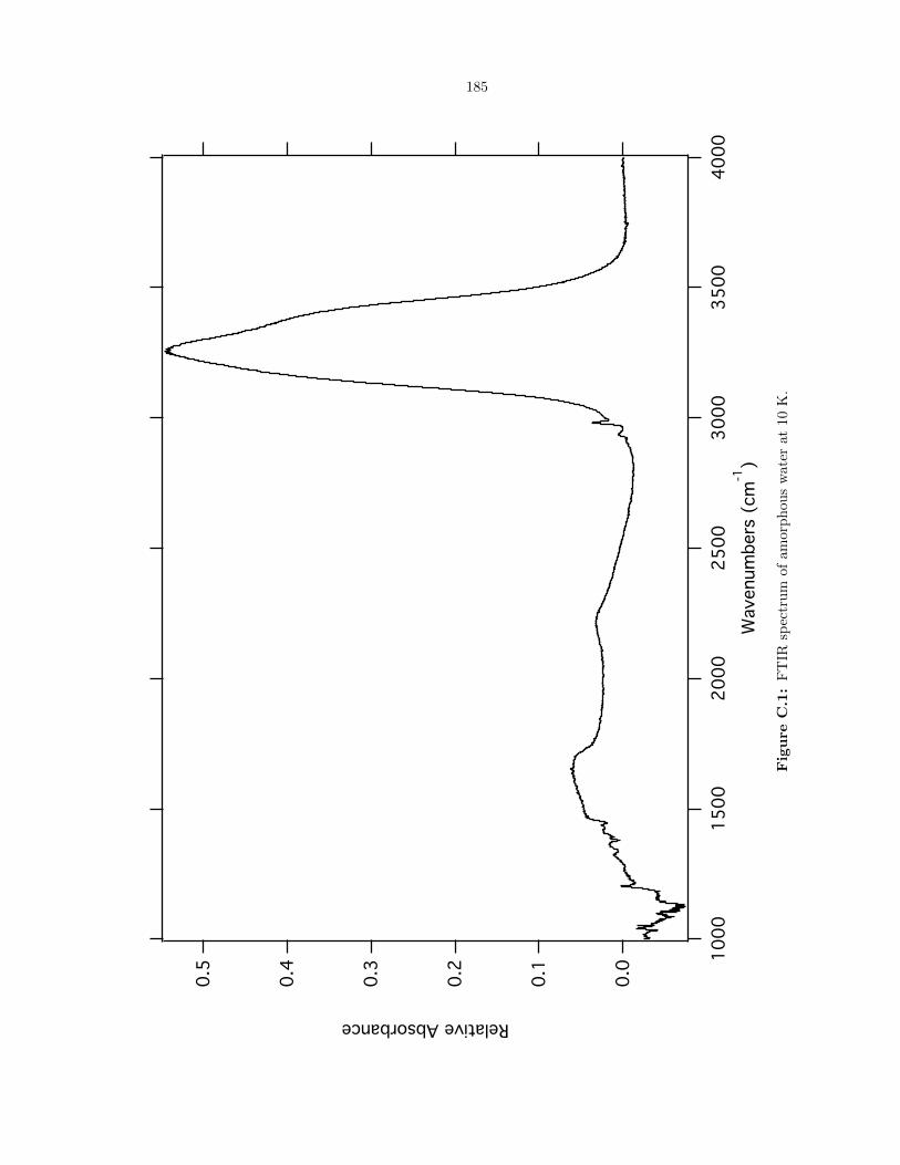
185

0.5

0.4

0.3

0.2

0.1

0.0

Relative Absorbance

4000

3500

3000

2500

2000

1500

1000

Wavenum

bers

(cm

-1)

Fig

ure

C.1

:F

TIR

spec

tru

mof

am

orp

hou

sw

ate

rat

10

K.

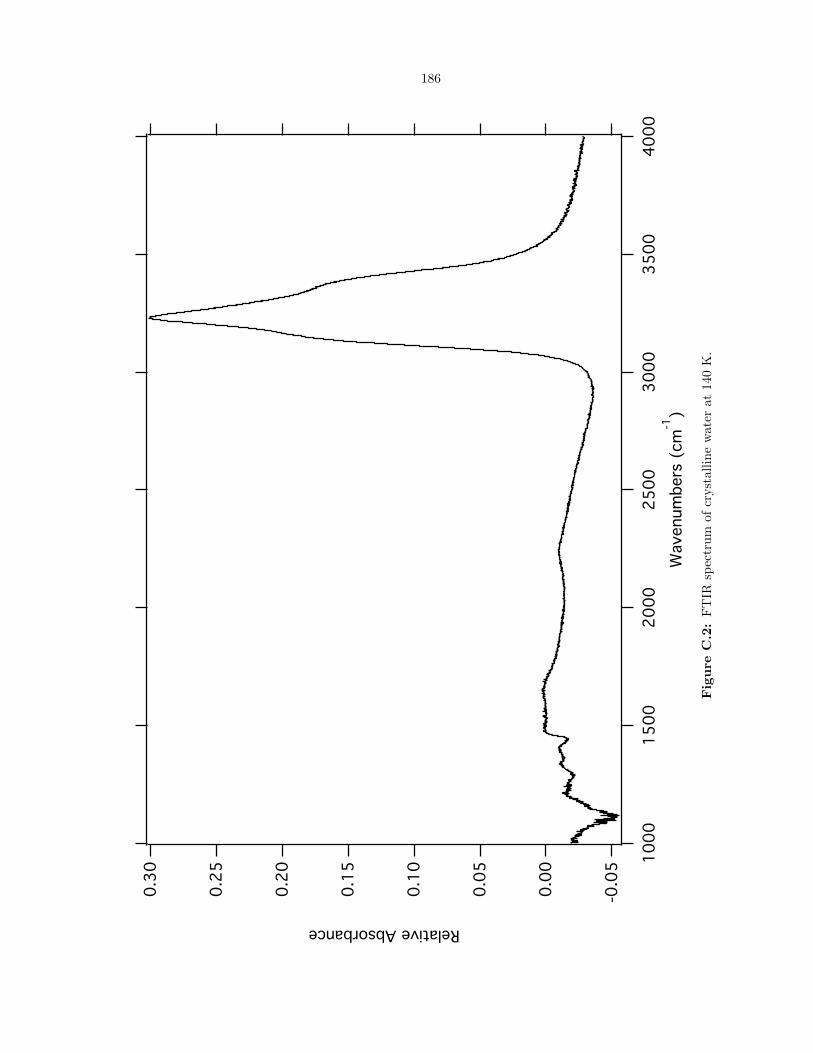
186

0.3

0

0.2

5

0.2

0

0.1

5

0.1

0

0.0

5

0.0

0

-0.0

5

Relative Absorbance

4000

3500

3000

2500

2000

1500

1000

Wavenum

bers

(cm

-1)

Fig

ure

C.2

:F

TIR

spec

tru

mof

cryst

all

ine

wate

rat

140

K.

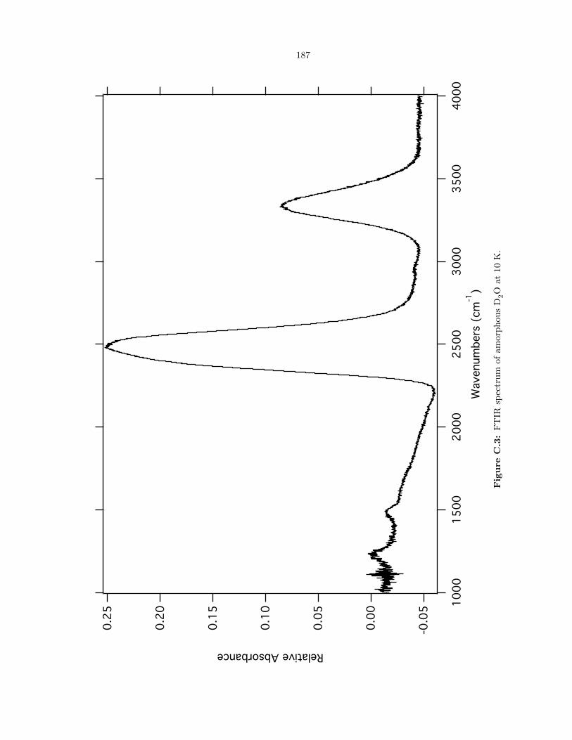
187

0.2

5

0.2

0

0.1

5

0.1

0

0.0

5

0.0

0

-0.0

5

Relative Absorbance

4000

3500

3000

2500

2000

1500

1000

Wavenum

bers

(cm

-1)

Fig

ure

C.3

:F

TIR

spec

tru

mof

am

orp

hou

sD

2O

at

10

K.

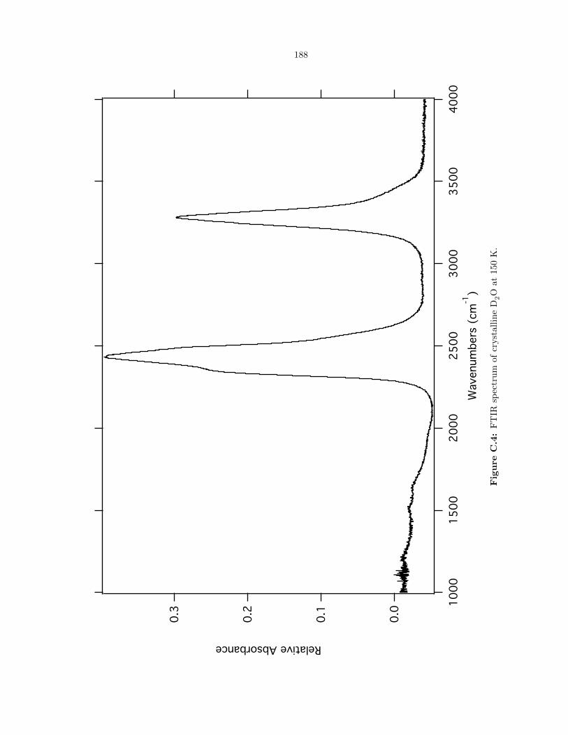
188

0.3

0.2

0.1

0.0

Relative Absorbance

4000

3500

3000

2500

2000

1500

1000

Wavenum

bers

(cm

-1)

Fig

ure

C.4

:F

TIR

spec

tru

mof

cryst

all

ine

D2O

at

150

K.

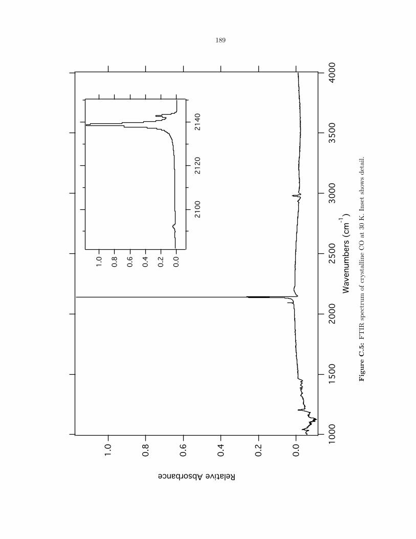
189

1.0

0.8

0.6

0.4

0.2

0.0

Relative Absorbance

4000

3500

3000

2500

2000

1500

1000

Wavenum

bers

(cm

-1)

1.0

0.8

0.6

0.4

0.2

0.0

2140

2120

2100

Fig

ure

C.5

:F

TIR

spec

tru

mof

cryst

all

ine

CO

at

30

K.

Inse

tsh

ows

det

ail.

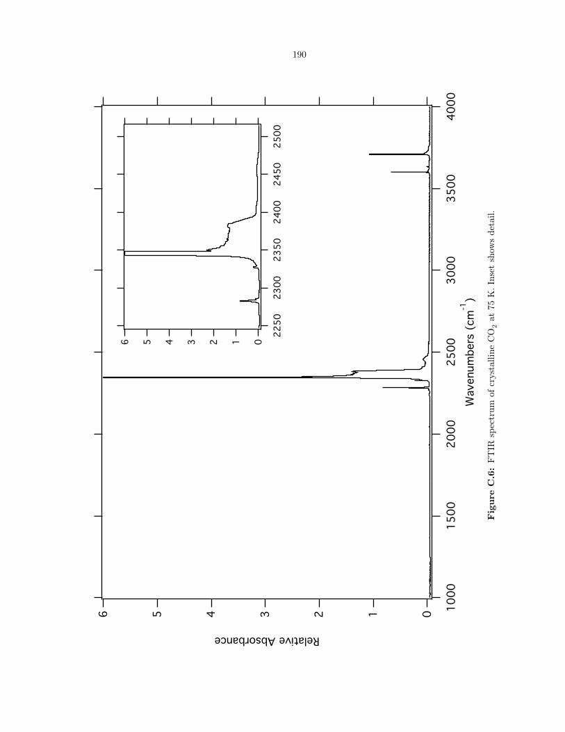
190

6 5 4 3 2 1 0

Relative Absorbance

4000

3500

3000

2500

2000

1500

1000

Wavenum

bers

(cm

-1)

6 5 4 3 2 1 0

2500

2450

2400

2350

2300

2250

Fig

ure

C.6

:F

TIR

spec

tru

mof

cryst

all

ine

CO

2at

75

K.

Inse

tsh

ows

det

ail

.

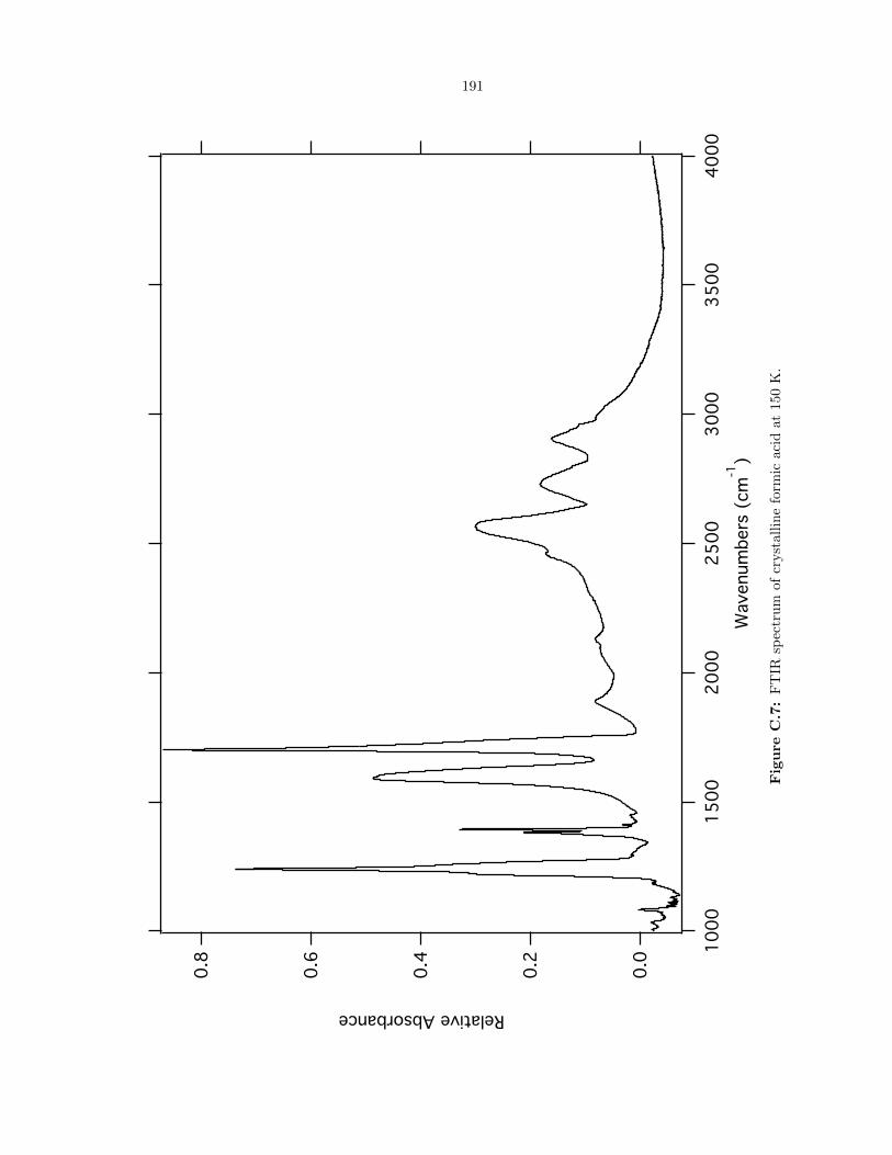
191

0.8

0.6

0.4

0.2

0.0

Relative Absorbance

4000

3500

3000

2500

2000

1500

1000

Wavenum

bers

(cm

-1)

Fig

ure

C.7

:F

TIR

spec

tru

mof

cryst

all

ine

form

icaci

dat

150

K.

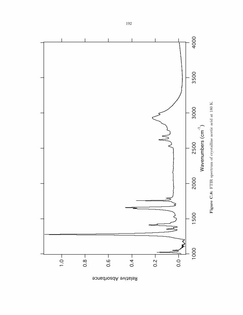
192

1.0

0.8

0.6

0.4

0.2

0.0

Relative Absorbance

4000

3500

3000

2500

2000

1500

1000

Wavenum

bers

(cm

-1)

Fig

ure

C.8

:F

TIR

spec

tru

mof

cryst

all

ine

ace

tic

aci

dat

180

K.

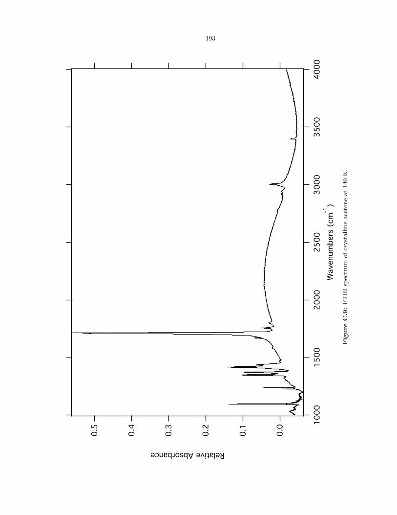
193

0.5

0.4

0.3

0.2

0.1

0.0

Relative Absorbance

4000

3500

3000

2500

2000

1500

1000

Wavenum

bers

(cm

-1)

Fig

ure

C.9

:F

TIR

spec

tru

mof

cryst

all

ine

ace

ton

eat

140

K.

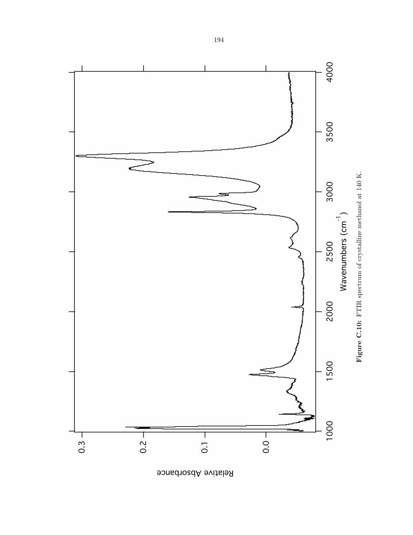
194

0.3

0.2

0.1

0.0

Relative Absorbance

4000

3500

3000

2500

2000

1500

1000

Wavenum

bers

(cm

-1)

Fig

ure

C.1

0:

FT

IRsp

ectr

um

of

cryst

all

ine

met

han

ol

at

140

K.

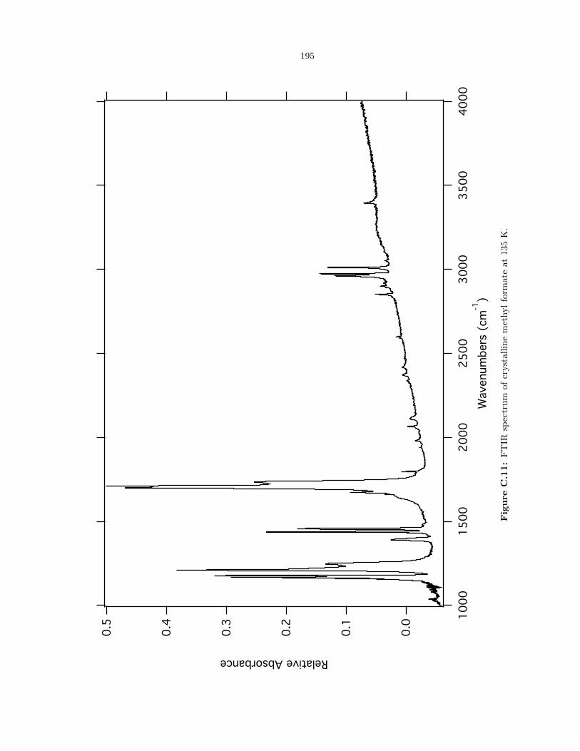
195

0.5

0.4

0.3

0.2

0.1

0.0

Relative Absorbance

4000

3500

3000

2500

2000

1500

1000

Wavenum

bers

(cm

-1)

Fig

ure

C.1

1:

FT

IRsp

ectr

um

of

cryst

all

ine

met

hyl

form

ate

at

135

K.

time domain tera hertz spectroscopy and observational probes of prebiotic interstellar gas and ice...

Education

great deal of time

world of chemistry

professor ben mccall

school science class

brett andrew mcguire

ice chemistry thesis

crazy chemistry

family thats