Time Response Analysis (Part – II)

1. A critically damped, continuous-time, second order system, when sampled,

will have (in Z domain)

(a) A simple pole

(b) Double pole on real axis

(c) Double pole on imaginary axis

(d) A pair of complex conjugate poles

[GATE 1988: 2 Marks]

Soln. For critically damped continuous time second order system roots of

denominator are: 𝒔𝟐 + 𝟐 𝝃𝝎𝒏𝒔 + 𝝎𝒏𝟐 = 𝟎 𝒘𝒉𝒆𝒏 𝝃 = 𝟏, 𝒔𝟐 + 𝟐𝝎𝒏𝒔 + 𝝎𝒏

𝟐 = 𝟎

(𝒔 + 𝝎𝒏)𝟐 = 𝟎

Root are 𝒔 = −𝝎𝒏, −𝝎𝒏

Double pole on real axis

Option (b)

2. A second-order system has transfer function given by 𝐺(𝑠) =25

𝑆2+8𝑠+25. If

the system, initially at rest, is subjected to a unit step input at t = 0, the

second peak in the response will occur at

(a) 𝜋 𝑠𝑒𝑐

(b) 𝜋 3 𝑠𝑒𝑐⁄

(c) 2𝜋 3 𝑠𝑒𝑐⁄

(d) 𝜋 2 𝑠𝑒𝑐⁄

[GATE 1991: 2 Marks]

Soln. 𝑮(𝒔) =𝟐𝟓

𝑺𝟐+𝟖𝒔+𝟐𝟓

𝝎𝒏𝟐 = 𝟐𝟓

𝝎𝒏 = 𝟓

𝟐 𝝃𝝎𝒏 = 𝟖

𝝃 =𝟖

𝟏𝟎= 𝟎. 𝟖

𝝎𝒅 = 𝝎𝒏√𝟏 − 𝝃𝟐

= 𝟓√𝟏 − (𝟎. 𝟖)𝟐 = 𝟑

for 2nd peak n = 3

𝒕𝒑 =𝒏𝝅

𝝎𝒅=

𝟑𝝅

𝟑= 𝝅 𝒔𝒆𝒄

Option (a)

3. The poles of a continuous time oscillator are ……..

[GATE 1994: 1 Mark]

Soln. The poles of a continuous time oscillator are imaginary

4. The response of an LCR circuit to a step input is

(a) Over damped

(b) Critically damped

(c) Oscillatory

If the transfer function has

(i) poles on the negative real axis

(ii) poles on the imaginary axis

(iii) multiple poles on the positive real axis

(iv) poles on the positive real axis

(v) multiple poles on the negative real axis

[GATE: 1994: 2 Marks]

Soln. The response of an LCR circuit to a step input

(a) over damped case 𝝃 > (𝟏) 𝒑𝒐𝒍𝒆𝒔 𝒐𝒏 𝒕𝒉𝒆 𝒏𝒆𝒈𝒂𝒕𝒊𝒗𝒆 𝒓𝒆𝒂𝒍 𝒂𝒙𝒊𝒔

𝑪(𝒔)

𝑹(𝒔)=

𝝎𝒏𝟐

𝒔𝟐 + 𝟐 𝝃 𝝎𝒏𝒔 + 𝝎𝒏𝟐

Roots of denominator are 𝒔 = −𝝃 𝝎𝒏 ± 𝝎𝒏√𝝃𝟐 − 𝟏

(b) critically damped 𝝃 = 𝟏 − − − − − (𝟓)

𝑪(𝒔)

𝑹(𝒔)=

𝝎𝒏𝟐

𝒔𝟐 + 𝟐 𝝎𝒏𝒔 + 𝝎𝒏𝟐

=𝝎𝒏

𝟐

(𝒔+𝝎𝒏)𝟐 , 𝒔 = −𝝎𝒏, −𝝎𝒏

It has multiple poles on the negative real axis

(c) oscillatory – (2) poles on the imaginary axis

𝝃 = 𝟎

𝒔 = ± 𝒋𝝎𝒏

Option a –1, b – 5, c – 2

5. Match the following codes with List-I with List-II:

List – I

(a) Very low response at very high frequencies

(b) Over shoot

(c) Synchro-control transformer output

List – II

(i) Low pass systems

(ii) Velocity damping

(iii) Natural frequency

(iv) Phase-sensitive

modulation

(v) Damping ratio

[GATE 1944: 2 Marks]

Soln. (a) very low response at very high frequencies → low pass system

(b) over sheet → Damping ratio

(c) synchro – control transformer output → phase sensitive

modulation

Option: a – 1, b – 5, c – 4

6. For a second order system, damping ratio (𝜉), 𝑖𝑠 0 < 𝜉 < 1, then the roots of

the characteristic polynomial are

(a) real but not equal

(b) real and equal

(c) complex conjugates

(d) imaginary

[GATE 1995: 1 Mark]

Soln. 𝝃 < 𝟏 underdamped system, roots of denominator

𝒔𝟐 + 𝟐 𝝃 𝝎𝒏𝒔 + 𝝎𝒏𝟐 = 𝟎

Are 𝒔 = −𝝃𝝎𝒏 ± 𝒋𝝎𝒏√𝟏 − 𝝃𝟐

Roots are complex conjugate

Option (c)

7. If 𝐿[𝑓(𝑡)] =2(𝑆+1)

𝑆2+2𝑆+5 𝑡ℎ𝑒𝑛 𝑓(0+) 𝑎𝑛𝑑 𝑓(∞) are given by

(a) 0,2 respectively

(b) 2. 0 respectively

(c) 0, 1 respectively

(d) 2/5, 0 respectively

[Note: L’ stands for ‘Laplace Transform of]

[GATE 1995: 1 Mark]

Soln. 𝑭(𝒔) =𝟐(𝒔+𝟏)

𝒔𝟐+𝟐𝒔+𝟓

𝒇(𝟎+) = 𝐥𝐢𝐦𝒔→∞

𝑺𝑭(𝒔) =𝟐𝒔𝟐+𝟐𝒔

𝒔𝟐+𝟐𝒔+𝟓

= 𝐥𝐢𝐦𝒔→∞

𝟐+𝟐

𝒔

𝟏+𝟐

𝒔+

𝟓

𝒔𝟐

=𝟐+𝟎

𝟏+𝟎= 𝟐

𝒇(∞) = 𝐥𝐢𝐦𝒔→𝟎

𝑺𝑭(𝒔) =𝟐𝒔𝟐+𝟐𝒔

𝒔𝟐+𝟐𝒔+𝟓= 𝟎

Option (b)

8. The final value theorem is used to find the

(a) steady state value of the system output

(b) initial value of the system output

(c) transient behavior of the system output

(d) none of these

[GATE 1995: 1 Mark]

Soln. The final value theorem is used to find the steady state value of the

system.

Option (a)

9. 𝐼𝑓 𝐹(𝑠) =𝜔

𝑆2+𝜔2, then the value of lim

𝑡→∞𝑓(𝑡),

{𝑤ℎ𝑒𝑟𝑒 𝐹(𝑠)𝑖𝑠 𝑡ℎ𝑒 𝐿[𝑓(𝑡)]}

(a) cannot be determined

(b) is zero

(c) is unity

(d) is infinite

[GATE 1998: 1 Mark]

Soln. 𝑭(𝒔) =𝝎

𝒔𝟐+𝝎𝟐

𝑭(𝒔) =𝝎

𝒔𝟐+𝝎𝟐 has poles 𝒔 ± 𝒋𝝎 (pure imaginary) it is oscillatory

function hence final value 𝐥𝐢𝐦𝒕→∞

𝒇(𝒕) can not be determined

10. Consider a feedback control system with loop transfer function

𝐺(𝑠)𝐻(𝑠) =𝐾(1 + 0.5𝑠)

𝑠(1 + 𝑠)(1 + 2𝑠)

The type of the closed loop system is

(a) zero

(b) one

(c) two

(d) three

[GATE 1998: 1 Mark]

Soln. 𝑮(𝒔) 𝑯(𝒔) =𝒌(𝟏+𝟎.𝟓𝒔)

𝒔(𝟏+𝒔)(𝟏+𝟐𝒔)

The number of poles at the origin of open loop transfer function given

the type of the system. It is a type one system

Option (b)

11. The unit impulse response of a linear time invariant system is the unit step

function u(t). For t > 0, the response of the system to an excitation

𝑒−𝑎𝑡𝑢(𝑡), 𝑎 > 0 will be

(a) 𝑎𝑒−𝑎𝑡

(b) (1/𝑎)(1 − 𝑒−𝑎𝑡)

(c) 𝑎(1 − 𝑒−𝑎𝑡)

(d) 1 − 𝑒−𝑎𝑡

[GATE 1998: 2 Marks]

Soln. 𝑯(𝒔) =𝟏

𝒔

System excitation 𝒓(𝒕) = 𝒆−𝒂𝒕 𝒖(𝒕)

𝑹(𝒔) =𝟏

𝒔+𝒂

Response of the system 𝑪(𝒔) = 𝑹(𝒔) 𝑯(𝒔) =𝟏

𝒔(𝒔+𝒂)

𝑪(𝒔) =𝟏

𝒂[

𝟏

𝒔−

𝟏

(𝒔+𝒂)]

𝑪(𝒕) =𝟏

𝒂[𝟏 − 𝒆−𝒂𝒕]

Option (b)

12. If the characteristic equation of a closed-loop system is 𝑠2 + 2𝑠 + 2 = 0,

then the system is

(a) Overdamped

(b) Critically damped

(c) Under damped

(d) undamped

Soln. Characteristic equation of closed loop system is 𝒔𝟐 + 𝟐𝒔 + 𝟐 = 𝟎

Comparing with 2nd order equation

𝒔𝟐 + 𝟐 𝝃𝝎𝒏 + 𝝎𝒏𝟐 = 𝟎

𝟐 𝝃𝝎𝒏 = 𝟐

𝝃 =𝟏

𝝎𝒏

𝝎𝒏𝟐 = 𝟐, 𝝎𝒏 = √𝟐, 𝝃 =

𝟏

√𝟐 which is less than 1

It is case of under damped

Option (c)

13. Consider a system with the transfer function (𝑠) =𝑠+6

𝐾𝑠2+𝑠+6 . Its damping

ratio will be 0.5 when the value of K is

(a) 2/6

(b) 3

(c) 1/6

(d) 6

[GATE 2002: 1 Mark]

Soln. Transfer function 𝑮(𝒔) =𝒔+𝟔

𝒌𝒔𝟐+𝒔+𝟔

Damping ratio 𝝃 = 𝟎. 𝟓

Comparing with 2nd order equation 𝒔𝟐 + 𝟐 𝝃𝝎𝒏𝒔 + 𝝎𝒏𝟐

𝑮(𝒔) =𝒔+𝟔

𝒌[𝒔𝟐+𝒔

𝒌+

𝟔

𝒌]

𝝎𝒏𝟐 =𝟔

𝒌, 𝝎𝒏 = √

𝟔

𝒌

𝟐 𝝃𝝎𝒏 =𝟏

𝒌

𝟐 𝝃√𝟔

𝒌=

𝟏

𝒌

𝟐 × 𝟎. 𝟓√𝟔

𝒌=

𝟏

𝒌

𝒐𝒓 𝟔

𝒌=

𝟏

𝒌𝟐

𝒐𝒓 𝒌 =𝟏

𝟔

Option (c)

14. A casual system having the transfer function 𝐻(𝑠) =1

𝑠+2 is excited with

10𝑢(𝑡). The time at which the output reaches 99% of its steady state value is

(a) 2.7 sec

(b) 2.5 sec

(c) 2.3 sec

(d) 2.1 sec

[GATE 2004: 2 Marks]

Soln. 𝑯(𝒔) =𝟏

𝒔+𝟐

𝒓(𝒕) = 𝟏𝟎𝝁(𝒕)

𝑹(𝒔) =𝟏𝟎

𝒔

𝑪(𝒔) = 𝑯(𝒔) 𝑹(𝒔) =𝟏𝟎

𝒔(𝒔+𝟐)

𝑪(𝒔) =𝟓

𝒔−

𝟓

𝒔+𝟐

𝑪(𝒕) = 𝟓[𝟏 − 𝒆−𝟐𝒕]

Steady state value = 5

99% of the steady value reaches at

𝟓[𝟏 − 𝒆−𝟐𝒕] =𝟓×𝟗𝟗

𝟏𝟎𝟎

𝟓(𝟏 − 𝒆−𝟐𝒕) = 𝟓 × 𝟎. 𝟗𝟗

𝟏 − 𝒆−𝟐𝒕 = 𝟎. 𝟗𝟗

Or 𝒆−𝟐𝒕 = 𝟎. 𝟏

−𝟐𝒕 = 𝒍𝒏(𝟎. 𝟏)

𝒕 = 𝟐. 𝟑 𝒔𝒆𝒄

Option (c)

15. The transfer function of a plant is (𝑠) =5

(𝑠+5)(𝑠2+𝑠+1) . The second order

approximation of T(s) using dominant pole concept is

(a) 1

(𝑠+5)(𝑠+1)

(b) 5

(𝑠+5)(𝑠+1)

(c) 5

(𝑠2+𝑠+1)

(d) 1

(𝑠2+𝑠+1)

[GATE 2007: 2 Marks]

Soln. Transfer function =𝟓

(𝒔+𝟓)(𝒔𝟐+𝒔+𝟏)

=𝟓

𝟓(𝒔

𝟓+𝟏)(𝒔𝟐+𝒔+𝟏)

The poles nearer to imaginary axis dominates nature of time response

and are called dominant poles. The factor that has to be eliminated

should be in time constant form so, 𝑻(𝒔) =𝟏

𝒔𝟐+𝒔+𝟏

Option (d)

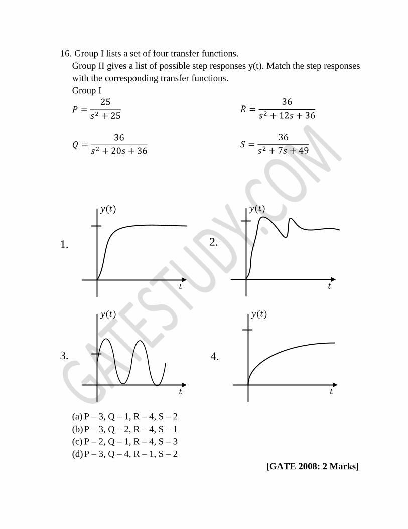
16. Group I lists a set of four transfer functions.

Group II gives a list of possible step responses y(t). Match the step responses

with the corresponding transfer functions.

Group I

𝑃 =25

𝑠2 + 25

𝑄 =36

𝑠2 + 20𝑠 + 36

𝑅 =36

𝑠2 + 12𝑠 + 36

𝑆 =36

𝑠2 + 7𝑠 + 49

𝑦(𝑡)

𝑡

𝑦(𝑡)

𝑡

𝑦(𝑡)

𝑡

𝑦(𝑡)

𝑡

1. 2.

3. 4.

(a) P – 3, Q – 1, R – 4, S – 2

(b) P – 3, Q – 2, R – 4, S – 1

(c) P – 2, Q – 1, R – 4, S – 3

(d) P – 3, Q – 4, R – 1, S – 2

[GATE 2008: 2 Marks]

Soln. The figure 1 is a case of critically damped, Figure 2 underdamped,

Figure 3 undamped, figure 4 is overdamped

The given transfer function

𝑷 =𝟐𝟓

𝒔𝟐 + 𝟐𝟓

𝑸 =𝟑𝟔

𝒔𝟐 + 𝟐𝟎𝒔 + 𝟑𝟔

𝑹 =𝟑𝟔

𝒔𝟐 + 𝟏𝟐𝒔 + 𝟑𝟔

𝑺 =𝟑𝟔

𝒔𝟐 + 𝟕𝒔 + 𝟒𝟗

Comparing the given transfer function with

𝝎𝒏

𝟐

𝒔𝟐+𝟐 𝝃 𝝎𝒏𝒔+𝝎𝒏𝟐 , 𝑷 =

𝟐𝟓

𝒔𝟐+𝟐𝟓

𝝎𝒏 = 𝟓, 𝝃 = 𝟎

P is undamped, matched to figure 3 so P – 3

𝑸 =𝟑𝟔

𝒔𝟐+𝟐𝟎𝒔+𝟑𝟔 , 𝝎𝒏 = 𝟔

𝟐 𝝃 𝝎𝒏 = 𝟐𝟎

𝝃 =𝟐𝟎

𝟐×𝟔= 𝟏. 𝟔𝟕

Q is overdamped matched to fig. 4 Q – 4

𝑹 =𝟑𝟔

𝒔𝟐+𝟏𝟐𝒔+𝟑𝟔 , 𝝎𝒏 = 𝟔

𝟐 𝝃 𝝎𝒏 = 𝟏𝟐

𝝃 =𝟏𝟐

𝟐×𝟔

= 1

R is critically damped matched to fig 1, R – 1

𝑺 =𝟒𝟗

𝒔𝟐+𝟕𝒔+𝟒𝟗 , 𝝎𝒏 = 𝟕

𝟐 𝝃 𝝎𝒏 = 𝟕

𝝃 =𝟕

𝟐×𝟕= 𝟎. 𝟓

= 1

S is underdamped matched to fig 2

Option (d) P – 3, Q – 4, R – 1, S – 2

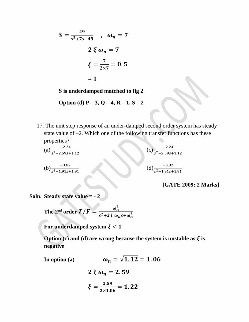
17. The unit step response of an under-damped second order system has steady

state value of –2. Which one of the following transfer functions has these

properties?

(a) −2.24

𝑠2+2.59𝑠+1.12

(b) −3.82

𝑠2+1.91𝑠+1.91

(c) −2.24

𝑠2−2.59𝑠+1.12

(d) −3.82

𝑠2−1.91𝑠+1.91

[GATE 2009: 2 Marks]

Soln. Steady state value = - 2

The 2nd order 𝑻 𝑭⁄ =𝝎𝒏

𝟐

𝒔𝟐+𝟐 𝝃 𝝎𝒏𝒔+𝝎𝒏𝟐

For underdamped system 𝝃 < 𝟏

Option (c) and (d) are wrong because the system is unstable as 𝝃 is

negative

In option (a) 𝝎𝒏 = √𝟏. 𝟏𝟐 = 𝟏. 𝟎𝟔

𝟐 𝝃 𝝎𝒏 = 𝟐. 𝟓𝟗

𝝃 =𝟐.𝟓𝟗

𝟐×𝟏.𝟎𝟔= 𝟏. 𝟐𝟐

𝝃 > 𝟏 hence it is wrong

In option (b) 𝑻. 𝑭 =−𝟑.𝟖𝟐

𝒔𝟐+𝟏.𝟗𝟏𝒔+𝟏.𝟗𝟏

𝝎𝒏 = √𝟏. 𝟗𝟏 = 𝟏. 𝟑𝟖

𝟐 𝝃 𝝎𝒏 = 𝟏. 𝟗𝟏

𝝃 =𝟏.𝟗𝟏

𝟐×𝟏.𝟑𝟖= 𝟎. 𝟔𝟗

𝝃 < 𝟏 so system is underdamped

Option (b)

18. The differential equation 100𝑑2𝑦

𝑑𝑡2− 20

𝑑𝑦

𝑑𝑡+ 𝑦 = 𝑥(𝑡) describes a system

with an input 𝑥(𝑡) and an output 𝑦(𝑡). The system, which is initially relaxed,

is exited, by a unit step input. The output y(t) can be represented by the

waveform.

(a) (b)

(c) (d)

[GATE 2011: 1 Mark]

Soln. 𝟏𝟎𝟎𝒅𝟐𝒚

𝒅𝒕𝟐 − 𝟐𝟎𝒅𝒚

𝒅𝒕+ 𝒚 = 𝒙(𝒕)

Taking Laplace transform of both sides

𝟏𝟎𝟎 𝒔𝟐𝒚(𝒔) − 𝟐𝟎 𝒔 𝒚 (𝒔) + 𝒚(𝒔) = 𝑿(𝒔) =𝟏

𝒔

(𝟏𝟎𝟎𝒔𝟐 − 𝟐𝟎𝒔 + 𝟏)𝒚(𝒔) =𝟏

𝒔

𝒚(𝒔) =𝟏

𝒔(𝟏𝟎𝒔−𝟏)𝟐 Poles are at 𝒔 = 𝟎,

𝟏

𝟏𝟎,

𝟏

𝟏𝟎

Poles are on the right hand side of s plane so given system is unstable

Option (a) represents unstable system.

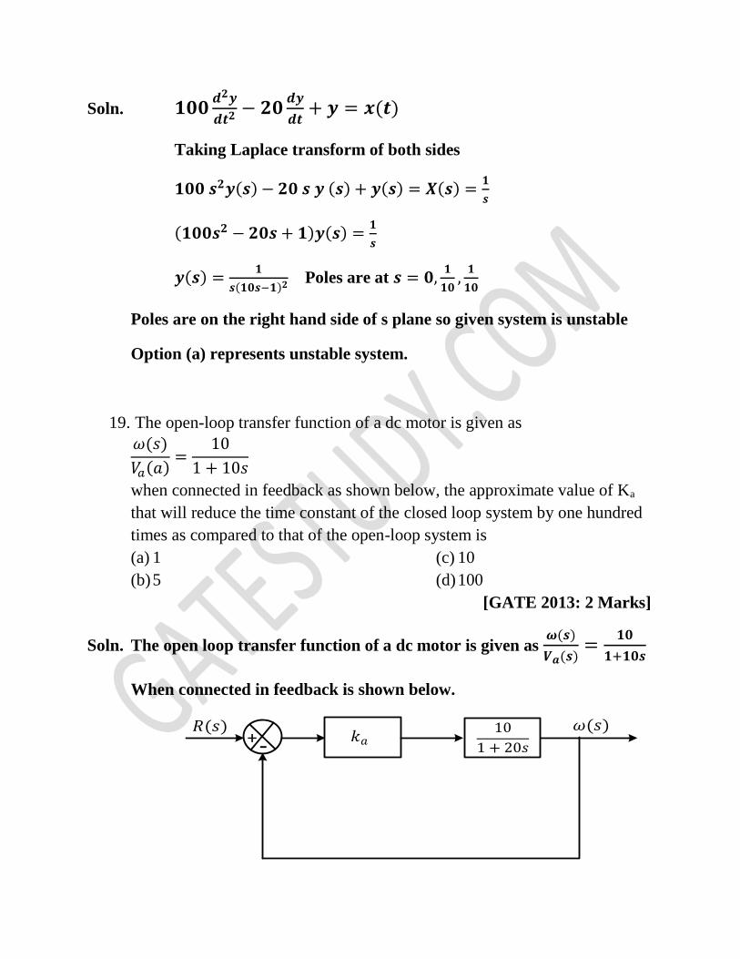
19. The open-loop transfer function of a dc motor is given as

𝜔(𝑠)

𝑉𝑎(𝑎)=

10

1 + 10𝑠

when connected in feedback as shown below, the approximate value of Ka

that will reduce the time constant of the closed loop system by one hundred

times as compared to that of the open-loop system is

(a) 1

(b) 5

(c) 10

(d) 100

[GATE 2013: 2 Marks]

Soln. The open loop transfer function of a dc motor is given as 𝝎(𝒔)

𝑽𝒂(𝒔)=

𝟏𝟎

𝟏+𝟏𝟎𝒔

When connected in feedback is shown below.

+- 𝑘𝑎 10

1 + 20𝑠

𝜔(𝑠) 𝑅(𝑠)

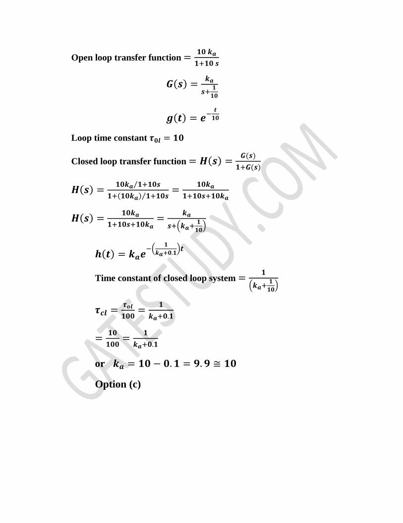
Open loop transfer function =𝟏𝟎 𝒌𝒂

𝟏+𝟏𝟎 𝒔

𝑮(𝒔) =𝒌𝒂

𝒔+𝟏

𝟏𝟎

𝒈(𝒕) = 𝒆−𝒕

𝟏𝟎

Loop time constant 𝝉𝟎𝒍 = 𝟏𝟎

Closed loop transfer function = 𝑯(𝒔) =𝑮(𝒔)

𝟏+𝑮(𝒔)

𝑯(𝒔) =𝟏𝟎𝒌𝒂 𝟏+𝟏𝟎𝒔⁄

𝟏+(𝟏𝟎𝒌𝒂) 𝟏+𝟏𝟎𝒔⁄=

𝟏𝟎𝒌𝒂

𝟏+𝟏𝟎𝒔+𝟏𝟎𝒌𝒂

𝑯(𝒔) =𝟏𝟎𝒌𝒂

𝟏+𝟏𝟎𝒔+𝟏𝟎𝒌𝒂=

𝒌𝒂

𝒔+(𝒌𝒂+𝟏

𝟏𝟎)

𝒉(𝒕) = 𝒌𝒂𝒆−(

𝟏

𝒌𝒂+𝟎.𝟏)𝒕

Time constant of closed loop system =𝟏

(𝒌𝒂+𝟏

𝟏𝟎)

𝝉𝒄𝒍 =𝝉𝒐𝒍

𝟏𝟎𝟎=

𝟏

𝒌𝒂+𝟎.𝟏

=𝟏𝟎

𝟏𝟎𝟎=

𝟏

𝒌𝒂+𝟎.𝟏

or 𝒌𝒂 = 𝟏𝟎 − 𝟎. 𝟏 = 𝟗. 𝟗 ≅ 𝟏𝟎

Option (c)

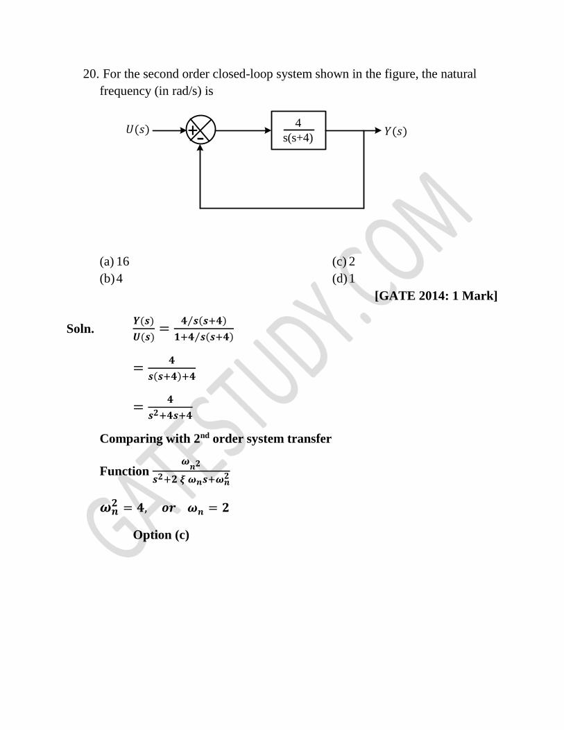
20. For the second order closed-loop system shown in the figure, the natural

frequency (in rad/s) is

+-4

s(s+4)𝑌(𝑠) 𝑈(𝑠)

(a) 16

(b) 4

(c) 2

(d) 1

[GATE 2014: 1 Mark]

Soln. 𝒀(𝒔)

𝑼(𝒔)=

𝟒 𝒔(𝒔+𝟒)⁄

𝟏+𝟒 𝒔(𝒔+𝟒)⁄

=𝟒

𝒔(𝒔+𝟒)+𝟒

=𝟒

𝒔𝟐+𝟒𝒔+𝟒

Comparing with 2nd order system transfer

Function 𝝎

𝒏𝟐

𝒔𝟐+𝟐 𝝃 𝝎𝒏𝒔+𝝎𝒏𝟐

𝝎𝒏𝟐 = 𝟒, 𝒐𝒓 𝝎𝒏 = 𝟐

Option (c)