title a comparison of swat, hspf and shetran/gopc for
TRANSCRIPT

Provided by the author(s) and University College Dublin Library in accordance with publisher policies. Please
cite the published version when available.
Downloaded 2018-02-01T01:54:24Z
The UCD community has made this article openly available. Please share how this access benefits you. Your
story matters! (@ucd_oa)
Some rights reserved. For more information, please see the item record link above.
Title A comparison of SWAT, HSPF and SHETRAN/GOPC formodelling phosphorus export from three catchments in Ireland
Author(s) Nasr, Ahmed Elssidig; Bruen, Michael; Jordan, Phillip; Moles,Richard; Kiely, Gerard; Byrne, Paul
Publicationdate 2007-03
Publicationinformation Water Research, 41 (5): 1065-1073
Publisher Elsevier
Link to onlineversion http://dx.doi.org/10.1016/j.watres.2006.11.026
Itemrecord/moreinformation
http://hdl.handle.net/10197/2276
Publisher'sstatement All rights reserved
Publisher'sversion (DOI) http://dx.doi.org/10.1016/j.watres.2006.11.026

1
A comparison of SWAT, HSPF and SHETRAN/GOPC for modelling phosphorus 1
export from three catchments in Ireland 2
3
Ahmed Nasra , Michael Bruen
a,*, Philip Jordan
b, Richard Moles
c, Gerard Kiely
d, Paul 4
Byrnec 5
a Centre for Water Resources Research, University College Dublin, Earlsfort Terrace, 6
Dublin 2, Ireland. Tel.: +353-1-7167378; Fax: +353-1-7167399; E-mail address: 7
bSchool of Environmental Sciences, University of Ulster, Coleraine, NI 9
cDepartment of Chemical and Environmental Science, University of Limerick 10
dDepartment of Civil and Environmental Engineering, University College Cork 11
12
13
14
15
16
17
18
19
20
21
22
23

2
Abstract 1
Recent extensive water quality surveys in Ireland revealed that diffuse phosphorus (P) 2
pollution originating from agricultural land and transported by runoff and subsurface 3
flows is the primary cause of the deterioration of surface water quality. P transport from 4
land to water can be described by mathematical models that vary in modelling approach, 5
complexity and scale (plot, field and catchment). Here, three mathematical models 6
(SWAT, HSPF and SHETRAN/GOPC) of diffuse P pollution have been tested in three 7
Irish catchments to explore their suitability in Irish conditions for future use in 8
implementing the European Water Framework Directive. After calibrating the models, 9
their daily flows and total phosphorus (TP) exports are compared and assessed. The 10
HSPF model was the best at simulating the mean daily discharge while SWAT gave the 11
best calibration results for daily TP loads. Annual TP exports for the three models and for 12
two empirical models were compared with measured data. No single model is 13
consistently better in estimating the annual TP export for all three catchments. 14
15
Keywords: Phosphorus; SWAT; HSPF; SHETRAN; GOPC 16
17
1. Introduction 18
The introduction of the Water Framework Directive in Europe (EEC, 2000) required 19
Member States to review water quality problems in all their water bodies. In Ireland, 20
riverine and lake eutrophication due to diffuse pollution has been identified as a major 21
problem (Earle, 2003) and phosphorus (P) is the limiting nutrient controlling 22

3
eutrophication in inland waters (McGarrigle et al., 2002). Therefore an effective way to 1
tackle eutrophication is to control P inputs, both from point and diffuse sources. 2
3
Formerly, phosphorous from point sources was the major cause of serious pollution 4
incidents in most Irish rivers (McGarrigle et al., 2002). However, in response to the 5
Urban Wastewater Directive (EEC, 1991) many wastewater treatment plants in Ireland 6
were upgraded to include a tertiary process resulting in a large reduction in pollution 7
from point sources. Now, in many catchments most nutrients entering rivers are from 8
diffuse sources and therefore, this study modelled this influence, concentrating on P 9
transport in three Irish catchments. The catchments were chosen on the basis of 10
availability of the data required by the models and because they have different climate, 11
land use and soil types. The modelled variable is total phosphorus (TP) load because of 12
its direct relationship with impacts on receiving waters (Hilton et al., 2006). 13
14
According to the DPSIR conceptual framework (Drivers, Pressures, State, Impact and 15
Response) (Irvine et al., 2005) that will guide the selection of modelling techniques in 16
Ireland, it is likely that the most useful models will be of the physically-based or 17
mechanistic types. Three widely used, physically-based, models were selected to cover a 18
range of variation in (i) the complexity of their representation of the physical, chemical, 19
and bio-chemical processes involved in P mobilisation and transport, (ii) the degree of 20
complexity in spatial disaggregation of the catchment, and (iii) the normal simulation 21
time step. The models are: Soil Water and Analysis Tools (SWAT) (Arnold et al., 1998); 22
Hydrological Simulation Program – FORTRAN (HSPF) (Bicknell et al., 1997); and 23
4
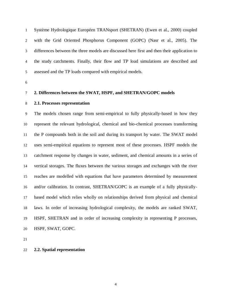
Système Hydrologique Européen TRANsport (SHETRAN) (Ewen et al., 2000) coupled 1
with the Grid Oriented Phosphorus Component (GOPC) (Nasr et al., 2005). The 2
differences between the three models are discussed here first and then their application to 3
the study catchments. Finally, their flow and TP load simulations are described and 4
assessed and the TP loads compared with empirical models. 5
6
2. Differences between the SWAT, HSPF, and SHETRAN/GOPC models 7
2.1. Processes representation 8
The models chosen range from semi-empirical to fully physically-based in how they 9
represent the relevant hydrological, chemical and bio-chemical processes transforming 10
the P compounds both in the soil and during its transport by water. The SWAT model 11
uses semi-empirical equations to represent most of these processes. HSPF models the 12
catchment response by changes in water, sediment, and chemical amounts in a series of 13
vertical storages. The fluxes between the various storages and exchanges with the river 14
reaches are modelled with equations that have parameters determined by measurement 15
and/or calibration. In contrast, SHETRAN/GOPC is an example of a fully physically-16
based model which relies wholly on relationships derived from physical and chemical 17
laws. In order of increasing hydrological complexity, the models are ranked SWAT, 18
HSPF, SHETRAN and in order of increasing complexity in representing P processes, 19
HSPF, SWAT, GOPC. 20
21
2.2. Spatial representation 22

5
The three models have different procedures for representing spatial variation within the 1
catchment. 2
SWAT divides the catchment into a number of sub-catchments, each of which has 3
a number of Hydrologic Response Units (HRUs) with uniform land use and soil 4
types (without reference to their actual spatial position within the sub-catchment). 5
HSPF divides the catchment on the basis of land use alone. Each land use can 6
consist of pervious and impervious parts. 7
In SHETRAN/GOPC, the catchment is divided into a horizontal orthogonal grid 8
network and in the vertical direction by a column of horizontal layers at each grid 9
square. Each grid element can have different land use and hydraulic properties. 10
The channel system is represented on the boundaries of the grid squares. 11
12
2.3. Temporal resolution 13
SWAT operates only at a daily time step. Both HSPF and SHETRAN/GOPC can 14
simulate at any time step from one minute up to one day. In all cases, the input time 15
series should always be available at intervals equal to or less than the simulation time 16
step. 17
18
3. Study catchments 19
The Clarianna catchment (23 km2) is located in County Tipperary in an area which is one 20
of the most intensively farmed catchments within the lower Shannon region. The Dripsey 21
catchment (15 km2) is located near the town of Donoughmore in the south of Ireland and 22

6
ultimately drains into Inniscarra lake, a freshwater lake that in recent years has 1
experienced signs of eutrophication (Scanlon et al., 2004). 2
The Oona Water catchment (96 km2) is located in County Tyrone and ultimately drains 3
into Lough Neagh which is a water source for Belfast. 4
5
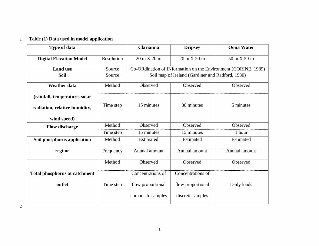
4. Data 6
The model comparisons are based on simulations of daily time series of discharge and TP 7
load at each catchment outlet. Data used in these simulations are summarised in Table 8
(1). Each of the three models has been calibrated for the period from 1/12/2000 to 9
29/7/2001 in the Clarianna catchment, and from 1/1/2002 to 31/12/2002 in the Dripsey 10
and Oona Water catchments. To allow HSPF and SHETRAN show their best 11
performances, the available time step resolution of the input data has been also employed 12
as a time step of simulation. As SWAT’s time step must be one day, daily input time 13
series for it were derived from the available high resolution input data. 14
15
The only input of P was assumed to be direct application of fertiliser and animal slurries 16
on the land. In the Clarianna and Dripsey catchments, the total annual P load applied on 17
the soil was taken as 15 kg P.ha-1
in line with the National (Teagasc) recommendations 18
(Teagasc, 1998). For the Oona Water catchment, P inputs of 18.9 million kg P to the soil 19
were assumed based on a P balance in Northern Ireland (Jordon, 2003). In each 20
catchment, the estimated value of the total annual P load has been distributed evenly over 21
the twelve months of the year. 22
23

7
The observed TP concentrations at the outlet of the three catchments (Jordan et al., 2005) 1
are summarised in Table (1) and daily TP loads were calculated from these and flow data. 2
The modelled TP is the sum of the dissolved and sediment-attached P load estimates. 3
4
5. Model calibration and parameter estimation 5
5.1. Approach used in the calibration 6
Manual calibration has been used in the vast majority of reported applications of the three 7
models (e.g. Jha et al., 2002; Wang et al., 1999; Bathurst, 1986) although some very 8
limited attempts at automatic calibration have been made (e.g. Eckhardt and Arnold, 9
2001; Doherty and Johnston, 2003). Despite the considerable effort that has to be made to 10
implement automatic calibration in these studies the results obtained were still within the 11
range of the manually calibrated models. 12
13
To avoid the complexity and computational demands that arise when using automatic 14
calibration (which would not allow these models to be used in many practical situations) 15
a simple manual strategy was employed to calibrate the parameters of the three models to 16
produce reasonable estimates for both discharges and TP loads. The three models were 17
first calibrated to produce reasonable simulations of the discharge. Then the parameters 18
of the best flow calibration were used without any further change during the P 19
calibration, following the three step strategy proposed by Gupta et al. (2003; p. 11). 20
21
5.2. Initial estimates of model parameters (Level Zero estimates) 22

8
The main objective for the Level Zero estimates is to populate a default data set of 1
parameters for the three models for each of the three test catchments. The SWAT and 2
HSPF models can automatically produce default values for all model parameters by 3
linking each soil and land use type with corresponding internal tables of default 4
parameters. For the third model, the SHETRAN/GOPC combination, the initial values of 5
the SHETRAN parameters were all taken from guidance given in its user’s manual. 6
7
5.3. Improving the parameter estimates (Level One estimates) 8
The effective parameters for flow simulation in HSPF were based on USEPA (2000). For 9
its phosphorous modelling, the method used assumes a first order kinetics equation to 10
represent each of the soil P processes. Each equation contains two parameters, the 11
kinetics rate, which is calibrated manually, and the temperature coefficient, which is 12
maintained at a specified value (USEPA, 2000). For the SWAT model the user’s manual 13
guidance was followed to improve the parameter values for flow and nutrient simulation. 14
15
The SHETRAN model was developed to be used without calibration due to the physical 16
nature of its parameters which are intended to be obtained from direct measurements. 17
However in most previous applications of this model (e.g. Anderton et al., 2002), some 18
parameters have been calibrated and this has been done here. 19
20
To illustrate the complexity of each model in terms of parameter calibration, Tables (2) 21
and (3) give the number of the effective parameters and the methods by which they have 22
been used in the water and P simulations, and also cite the source for the methods. We 23

9
refer the reader to the user’s manual of each model for definitions and descriptions of the 1
parameters and these are not repeated here. However, the number of parameters which 2
can be adjusted for the three models is reported in Tables (2) and (3). 3
4
5.4. Adjustment of the parameters (Level Two estimates) 5
Manual improvement of effective parameters for complex models is difficult to carry out 6
in a reliable and consistent manner due to (i) large numbers of parameters, (ii) 7
equifinality, (iii) parameter sensitivity, and (iv) uncertainty (Gupta et al., 2003). In this 8
study, however, the manual calibration is to provide results corresponding to practical 9
situations when these models are used by typical users with only a general knowledge of 10
sophisticated calibration techniques. Thus the models are compared in terms of their 11
likely performances in reality rather than their potential best performances if unlimited 12
calibration resources were available. 13
14
A systematic approach to manual calibration has been followed in this study where for 15
each model and in each catchment, one parameter was changed at a time and the resulting 16
shapes of the hydrograph in the flow calibration or load graphs in the P calibration were 17
visually compared with the observed. In addition, the Nash-Sutcliffe index (Nash and 18
Sutcliffe, 1970) was also calculated for each model run. In the flow calibration, first the 19
focus was on visually matching the peaks, then on matching the flow recessions and 20
finally on the low flow values. This requires sequential adjustment to the particular 21
parameters in the models that influence each of the three components of the hydrograph. 22
The P calibration followed a similar procedure where the focus was first on the high 23

10
values, then on the low values, and finally on the overall shape of the simulated time 1
series. 2
3
6. Comparison criteria 4
The three models are compared both on their daily and annual results. Two criteria are 5
used to assess the models in simulating the daily discharges and TP loads. Firstly, for 6
each catchment, the flow hydrograph was plotted together with the rainfall hyetograph so 7
that the flow simulation and its consistency with rainfall can be observed and the daily 8
TP results were superimposed on the graph. This allows a direct visual appreciation of 9
the influence of the hydrological modelling on the transport of P. Importantly, it also 10
reveals many systematic aspects of the model performance such as tendencies to over or 11
under estimate, which are seasonal or related to flow or rainfall, and tendencies to match 12
high peaks but not low ones. These tendencies would be difficult to detect with a single 13
numerical index. 14
15
The second criterion is based on two numerical measures: the Nash-Sutcliffe index (R2); 16
and the fraction of the mean of the squares of the errors due to bias (B%MSSE). These 17
are calculated as follows: 18
n
i
i
n
i
ii
xx
xx
R
1
2
2
1
^
2 1 (1) 19

11
nxx
xx
MSSEBn
i
i /
%
1
2
2
^
(2) 1
where ix is the observed value, ^
ix is the value estimated by a model,
x is the mean of 2
the observed values,
^
x is the mean of the estimated values, and n is the number of data 3
values. 4
5
The R2 index describes the ability of the model to explain the variability in the data, 6
while the B%MSSE index describes the model’s ability to match the central tendency 7
(mean) of the data. A good model is one that has a good visual match to the observed 8
data, with a value of R2 close to one, and a small value of B%MSSE. 9
10
7. Comparison with simple empirical models 11
The three physically-based models are compared with two empirical models specifically 12
developed to estimate annual TP export. The first, (DM) is derived from an equation 13
developed by Daly et al. (2006) specifically for use in Irish conditions and the second 14
model (ECM) is an export coefficient model (Johnes, 1996) used in the UK. 15
16
8. Results 17
8.1. Discharge performance 18
The hydrographs of observed and estimated discharge (Figs (1.a) (2.a) (3.a)) show that, in 19
general, none of the models is able to replicate the entire shape of the hydrographs 20

12
throughout the simulation period. However, HSPF is the best at matching the discharge 1
hydrographs and SWAT performed better than SHETRAN. The noticeable weakness in 2
SHETRAN is its failure to adequately model the flow peaks and recessions. Most of its 3
estimated peaks are either very much higher or lower than the observations and also the 4
estimated flow recession is not as flat as the observed. 5
6
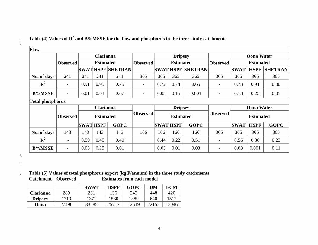
The numerical criteria for the flow simulations from each model are compared in Table 7
(4). The best results for R2 are 0.95, 0.74, and 0.91 and for the HSPF model in the 8
Clarianna, Dripsey, and Oona respectively. The R2 for SWAT (0.91) is better than for 9
SHETRAN (0.74) in the Dripsey. However, SHETRAN has an R2 of 0.8 which is better 10
than the 0.73 for SWAT in the Oona. The B%MSSE values for all three models in 11
Clarianna are all low and this means that the bias in estimating the mean of the observed 12
flow was not the major source of error. In the Dripsey and Oona, the B%MSSE value for 13
HSPF is high compared to SWAT and SHETRAN with the latter giving the best results 14
for B%MSSE for these two catchments. 15
16
8.2. Daily TP results 17
Figs ((1.b), (2.b), and (3.b)) show the TP results. SWAT performed quite well in all three 18
catchments. The GOPC TP load performance is second, despite the problems with the 19
flow estimates. It is quite surprising that HSPF was the worst for TP load in the three 20
catchments although it was best for discharges. The main reason for this could be its 21
smaller scope for calibration due to the fewer number of P parameters, as show in Table 22

13
(3), and this indicates the limited capability of the first order kinetics equation used in the 1
P simulation by HSPF. 2
3
The numerical criteria for TP loads are summarised in Table (4). In the Clarianna, the 4
value of R2 for SWAT (0.59) is the best while the corresponding value for GOPC (0.40) 5
is the worst of the three models. HSPF has the highest B%MSSE while the other two 6
models have low values, indicating that their bias is less significant. In the Dripsey, the 7
best R2 value of 0.51 is obtained from the GOPC model while the HSPF model value was 8
the worst (0.22). All three models have low B%MSSE values indicating an overall 9
acceptable bias performance in this catchment. In the Oona, SWAT has the best R2 (0.56) 10
while its B%MSSE value is second best to the HSPF value. The GOPC has the worst R2 11
(0.23) and B%MSSE values. 12
13
8.3. Annual TP export results 14
Table (5) shows the observed and modelled values of annual TP export from each 15
catchment. In the Clarianna, SWAT and GOPC are the best of the five models. Both 16
empirical models greatly overestimated the TP export while HSPF underestimates. In the 17
Dripsey, all models except DM are comparable with the observations, with HSPF being 18
the best. In the Oona, SWAT is the only model that overestimated the TP export although 19
the result is still acceptable. HSPF and DM also give acceptable results, although lower 20
than the observed, whereas the GOPC and EM significantly underestimate. 21
22
The results from the three physically-based models are better than the results from the 23
two empirical models. This is not surprising because the empirical models are fitted to a 24

14
larger number of different catchments and are an average of the responses over a larger 1
area and have much less catchment-specific information. 2
3
9. Conclusions 4
In the three catchments, the HSPF model was best in simulating the mean daily 5
discharges. Discharge results from SWAT and SHETRAN were acceptable despite 6
occasional deficiencies. Nevertheless, the best simulation for daily TP loads in the study 7
catchments was by SWAT. The TP performance of the SHETRAN/GOPC combination 8
was good although hampered by its discharge simulation. In terms of TP export, no single 9
model was best for all three catchments, however the three physically-based models gave 10
annual TP export estimates closer to the measurements than the two empirical models. In 11
the short term, we recommend using SWAT for TP load estimation. 12
13
Acknowledgements 14
This project was supported by the National Development Programme (NDP) through the 15
RTDI programme and co-funded by the Irish EPA and Teagasc (2000-LS-2.2.2-M2). In 16
the Oona Water, we acknowledge the use of hydrology data from the Rivers Agency 17
(Department of Agriculture and Rural Development, NI) and infrastructure from the 18
NERC funded CHASM project (NER/H/S/1999/00164). 19
20
References 21
1. Anderton, S.P., Larton, J., White, S.M., Llorens, P., Gallart, F., Salvany, C., 22
O’Connell, P.E., 2002. Internal evaluation of a physically-based distributed model 23

15
using data from a Mediterranean mountain catchment. Hydrology and Earth 1
System Sciences 6(1), 67–83. 2
2. Arnold, J.G., Srinivasan, R., Muttiah, R.S., Williams, J.R., 1998. Large area 3
hydrological modelling and assessment Part I: Model development. Journal of the 4
American Water Resources Association (JAWRA) 34(1), 73-89. 5
3. Bathurst, J.C., 1986. Physically-based distributed modelling of an upland 6
catchment using the System Hydrologique European. Journal of Hydrology 87, 7
79-102. 8
4. Bicknell, B.R., Imhoff, J.C., Donigian, A.S., Johanson, R.C., 1997. Hydrological 9
Simulation Program – FORTRAN (HSPF), User’s Manual for release 11. EPA – 10
600/R-97/080. United States Environmental Protection Agency, Athens, GA. 11
5. Co-ORdination of INformation on the Environment (CORINE), 1989. Land 12
Cover Project, The Nomenclature. Commission of the European Communities, 13
Directorate-General Environment Nuclear Safety and Civil Protection, Rue de la 14
Loi 200, B-1049 Brussels, Belgium. 15
6. Daly, K., Mills, P., and Styles, D., 2006. Eutrophication from agriculture sources - 16
Modelling phosphorus loss from soils. Environmental Protection Agency, 17
Johnstown Castle, Co. Wexford, Ireland. (In press). 18
7. Doherty, J., Johnston, J.M., 2003. Methodologies for calibration and predictive 19
analysis of a watershed model. Journal of the American Water Resources 20
Association (JAWRA) 39(2), 251-256. 21

16
8. Earle, J.R., 2003. The Three Rivers Project – water quality monitoring and 1
management systems in the Boyne, Liffey and Suir Catchments in Ireland. Water 2
Science and Technology 47(7-8), 217-225. 3
9. Eckhardt, K., Arnold, J.G., 2001. Automatic calibration of a distributed catchment 4
model. Journal of Hydrology 251, 103-109. 5
10. EEC (European Economic Community), 2000. The council of 23 October 2000 6
establishing a framework for Community action in the field of water policy 7
(2000/60/EC). Official Journal of the European Communities L327, 1-72. 8
11. EEC (European Economic Community), 1991. The council of 21 May 1991 9
concerning urban wastewater treatment (91/271/EEC). Official Journal of the 10
European Communities L135, 40-52. 11
12. Ewen, J., Parkin, G., O’Connell, E., 2000. SHETRAN: Distributed basin flow and 12
transport modelling system. Journal of Hydrologic Engineering 5(3), 250-258. 13
13. Feddes, R.A., Kowalik, P., Neuman, S.P., Bresler, E., 1976. Finite difference and 14
finite element simulation of field water uptake by plants. Hydrological Science 15
Bulletin 21, 81-98. 16
14. Gardiner, M.J., Radford, T., 1980. Soil Associations of Ireland and their land use 17
potential (Explanatory Bulletin to Soil Map of Ireland 1980). Published by An 18
Foras Taluntais, 19 Sandymount Avenue, Dublin 4, Ireland. 19
15. Gupta, H.V., Sorooshian S., Hogue, T.S., Boyle, D.P., 2003. Advances in 20
automatic calibration of watershed models. In: Calibration of watershed models, 21
Edited by: Duan, Q., Gupta, H.V., Sorooshian, S., Rousseau, A.N., Turcotte, R., 22
American Geophysical Union, Washington DC, USA, pp. 9-28. 23

17
16. Hargreaves, G.L., Hargreaves, G.H., Riely, J.P., 1985. Agriculture benefits for 1
Senegal River Basin. Journal of Irrigation and Drainage Engineering (ASCE) 2
111(2), 113-124. 3
17. Hilton, J., O’Hare, M., Bowes, M.J., Jones, J.I., 2006. How green is my river? A 4
new paradigm of eutrophication in rivers. Science of the Total Environment 365, 5
66-83. 6
18. Irvine, K., Mills, P., Bruen, M., Walley, W., Hartnett, M., Black, A., Tynan, S., 7
Duck, R., Bragg, O., Rowen, J., Wilson, J., Johnston, P., O’Toole, C., 2005. 8
Water Framework Directive – An assessment of mathematical modelling in its 9
implementation in Ireland. Environmental Protection Agency, Johnstown Castle, 10
Co. Wexford, Ireland. 11
19. Jha, M., Gassman, P.W., Secchi, S., Gu, R., Arnold, J., 2002. Impact of watershed 12
subdivision level on flows, sediment loads, and nutrient losses predicted by 13
SWAT. Working Paper 02-WP 315, Centre for Agriculture and Rural 14
Development, Iowa State University, USA. 15
20. Johnes, P.J., 1996. Evaluation and management of the impact of land use change 16
on the nitrogen and phosphorus load delivered to surface waters: the export 17
coefficient modelling approach, Journal of Hydrology 183, 323-349. 18
21. Jordan, P., Menary, W., Daly, K., Kiely, G., Morgan, G., Byrne, P., Moles, R., 19
2005. Patterns and processes of phosphorus transfer from Irish grassland soils to 20
rivers – Integration of laboratory and catchment studies. Journal of Hydrology 21
304, 20-34. 22

18
22. Jordan, P., 2003. Soil phosphorus balance in Northern Ireland for the year. 1
Personal Communication. School of Environmental Sciences, University of 2
Ulster, Coleraine, NI. 3
23. McGarrigle, M.L., Bowman, J.J., Clabby, K.J., Lucey, J., Cunningham, P., 4
MacCarthaigh, M., Keegan, M., Cantrell, B., Lehane, M., Clenaghan, C., Toner, 5
P.F., 2002. Water quality in Ireland. Environmental Protection Agency, P.O. Box 6
3000, Johnstown Castle Estate, County Wexford, Ireland. 7
24. Monteith, J.L., 1965. Evaporation and environment. In: The State and Movement 8
of Water in Living Organisms, Proceedings of 15th Symposium Society for 9
Experimental Biology, Swansea. Cambridge University Press, London, pp. 205-10
234. 11
25. Nash, J.E., Sutcliffe, J.V., 1970. River flow forecasting through conceptual 12
models. Part 1. A discussion of principles. Journal of Hydrology 10, 282-290. 13
26. Nasr, A., Taskinein, A., Bruen, M., 2005. Developing an independent, generic, 14
phosphorus modelling component for use with grid-oriented, physically based 15
distributed catchment models. Water Science and Technology 51(3-4), 135-142. 16
27. Priestley, C.H.B., Taylor, R.J., 1972. On the assessment of surface heat flux and 17
evaporation using large-scale parameters. Monthly Weather Revision 100, 81-92. 18
28. Ritchie, J.T., 1972. Model for predicting evaporation from a row crop with 19
incomplete cover. Water Resources Research 8, 1204-1213. 20
29. Rutter, A.J., Kershaw, K.A., Robins, P.C., Morton, A.J., 1971/72. A predictive 21
model of rainfall interception in forests - Part I: Derivation of the model from 22
19
observations in a plantation of Corsican pine. Agriculture Meteorology 9, 367-1
384. 2
30. Scanlon, T.M., Kiely, G., Xie, Q., 2004. A nested catchment approach for 3
defining the hydrological controls on non-point phosphorus transport. Journal of 4
Hydrology 291, 218-231. 5
31. Soil Conservation Service (SCS), 1972. SCS National Engineering Handbook, 6
Sec. 4, Hydrology. United States department of Agriculture. 7
32. Teagasc (Agriculture and Food Development Authority), 1998. Nutrient advice 8
for phosphorus and potassium fertiliser. Johnstown Castle Laboratory, Wexford, 9
Ireland. 10
33. USEPA, 2000. BASINS Technical Note 6: Estimating hydrologic and hydraulic 11
parameters for HSPF. EPA-823-R-00-012, United States Environmental 12
Protection Agency, Office of Water (4305), USA. 13
34. Wang, M., Duru, J.O., Hjelmfelt, A.T., Ghidey, F., 1999. Environmental 14
modelling of a claypan watershed Using HSPF model. Paper submitted to the 15
Storm and Urban Water Systems Modelling Conference, Toronto, Ontario, 16
Canada. 17
18
19
20
21
22
23
24
1
Table (1) Data used in model application 1
Type of data Clarianna Dripsey Oona Water
Digital Elevation Model Resolution 20 m X 20 m 20 m X 20 m 50 m X 50 m
Land use Source Co-ORdination of INformation on the Environment (CORINE, 1989)
Soil Source Soil map of Ireland (Gardiner and Radford, 1980)
Weather data
(rainfall, temperature, solar
radiation, relative humidity,
wind speed)
Method Observed Observed Observed
Time step 15 minutes 30 minutes 5 minutes
Flow discharge Method Observed Observed Observed
Time step 15 minutes 15 minutes 1 hour
Soil phosphorus application
regime
Method Estimated Estimated Estimated
Frequency Annual amount Annual amount Annual amount
Total phosphorus at catchment
outlet
Method Observed Observed Observed
Time step
Concentrations of
flow proportional
composite samples
Concentrations of
flow proportional
discrete samples
Daily loads
2

2
Table (2) Summary of the methods used and parameters required to simulate processes of the water component of SWAT, 1
HSPF, and SHETRAN models 2
Process
SWAT HSPF SHETRAN
Method No. of
parameters Method
No. of
parameters Method
No. of
parameters
Interception Water balance 1
Water balance - Rutter et al. (1971/72) 5
Potential
evapotranspiration
(EP)
Monteith (1965)/
Priestley and Taylor
(1972)/
Hargreaves et al. (1985)
- User defined
EP -
User defined EP/
Monteith (1965) -
Actual evaporation
(Ea) Ritchie (1972)
2
Accounting
procedure
4
Feddes et al. (1976) 2
Runoff SCS (1972)
5
Empirical
relations
8
Approximation of
St. Venant equation 1
Infiltration Water balance
Variably-saturated
sub-surface model 6
Inter/Return flow Kinematic model 2
Baseflow Linear reservoir model
5
Linear
reservoir
model
2
Percolation to
groundwater Water balance
Empirical
relation 1
River flow routing Variable storage/
Muskingum
3
Water balance -
Approximation of
St. Venant equation 1
Total = 18 Total = 15 Total = 15

3
Table (3) Summary of the methods used and parameters required to simulate processes of the phosphorus component of 1
SWAT, HSPF, and GOPC models 2
Process
SWAT HSPF GOPC
Method No. of
parameters Method
No. of
parameters Method
No. of
parameters
Soil P processes
(adsorption/desorption,
mineralisation/immobi-
lisation, plant uptake)
Mass balance 6
First order
kinetics
equation
5
Mass balance 7
Leaching of P Empirical
relation
1
Mass Balance
-
Advection
equation 1
Dissolution of P
in runoff water
Empirical
relation 1
Mass Balance
-
Empirical
relation 1
Overland transport
of dissolved P
Linear reservoir
model -
Not simulated
by this model - Mass balance 2
Subsurface transport
of dissolved P
User defined
concentration 1 Mass Balance -
Advection
equation 1
Transport of attached
or particulate P
Empirical
relation 1 Mass balance -
Empirical
relation 1
Total = 10 Total = 5 Total =13
3
4
4
Table (4) Values of R2 and B%MSSE for the flow and phosphorus in the three study catchments 1
2
Flow
Observed
Clarianna
Observed
Dripsey
Observed
Oona Water
Estimated Estimated Estimated
SWAT HSPF SHETRAN SWAT HSPF SHETRAN SWAT HSPF SHETRAN
No. of days 241 241 241 241 365 365 365 365 365 365 365 365
R2 - 0.91 0.95 0.75 - 0.72 0.74 0.65 - 0.73 0.91 0.80
B%MSSE - 0.01 0.03 0.07 - 0.03 0.15 0.001 - 0.13 0.25 0.05
Total phosphorus
Observed
Clarianna
Observed
Dripsey
Observed
Oona Water
Estimated Estimated Estimated
SWAT HSPF GOPC SWAT HSPF GOPC SWAT HSPF GOPC
No. of days 143 143 143 143 166 166 166 166 365 365 365 365
R2 - 0.59 0.45 0.40 0.44 0.22 0.51 - 0.56 0.36 0.23
B%MSSE - 0.03 0.25 0.01 0.03 0.01 0.03 - 0.03 0.001 0.11
3
4
Table (5) Values of total phosphorus export (kg P/annum) in the three study catchments 5
Catchment Observed Estimates from each model
SWAT HSPF GOPC DM ECM
Clarianna 289 231 136 243 448 420
Dripsey 1719 1371 1530 1389 640 1512
Oona 27496 33285 25717 12519 22152 15046

1
Figure (1) Clarianna catchment: Results of the three models (a) Flow, and (b) Total 1
phosphorus load 2
3
4
5
6
7
8
9
10
11
12
13
14
15
16
17
18
19
20
21
22
23
24
25
26
27
28
29
30
31
0
4
8
12
16
20
01-12-01 30-01-02 31-03-02 30-05-02
TP
(k
gP
.day
-1)
Observed
SWAT
HSPF
GOPC
0
2
4
6
8
10
Dis
char
ge
(mm
. d
ay-1
)
0
10
20
30
40
50
60
Rai
nfa
ll (
mm
. d
ay-1
)
Observed
SWAT
HSPF
SHETRAN
(a)
(b)

2
Figure (2) Dripsey catchment: Results of the three models (a) Flow, and (b) Total 1
phosphorus load 2
3
4
5
6
7
8
9
10
11
12
13
14
15
16
17
18
19
20
21
22
23
24
25
26
27
28
29
30
31
0
4
8
12
16
20
24
28
32
Dis
char
ge
(mm
. d
ay-1
)
0
15
30
45
60
75
90
Rai
nfa
ll (
mm
. d
ay-1
)Observed
SWAT
HSPF
SHETRAN
0
20
40
60
80
100
01-01-02 02-03-02 01-05-02 30-06-02 29-08-02 28-10-02 27-12-02
TP
(k
g P
. d
ay-1
)
Observed
SWAT
HSPF
GOPC
(a)
(b)

3
Figure (3) Oona Water catchment: Results of the three models (a) Flow, and (b) 1
Total phosphorus load 2
3
4
5
6
7
8
9
10
11
12
13
14
15
16
17
18
19
20
21
0
4
8
12
16
20
24
28
32
Dis
char
ge
(mm
. d
ay-1
)
0
20
40
60
80
100
120
140
Rai
nfa
ll (
mm
. d
ay-1
)
Observed
SWAT
HSPF
SHETRAN
0
200
400
600
800
1000
1200
01-01-02 02-03-02 01-05-02 30-06-02 29-08-02 28-10-02 27-12-02
TP
(k
g P
. d
ay-1
)
Observed
SWAT
HSPF
GOPC
(a)
(b)