to finite difference time domain for simulation of surface
TRANSCRIPT
ContributiontoFinite‐DifferenceTime‐DomainproceduresforsimulationofSurfaceAcousticWave
RFIDtags
A thesis presented to
Universidad de los Andes
and
The Doctoral School Sicma of Télécom Bretagne
by
OmarArielNovaManosalva
In partial fulfillment of the requirements for the degree of
Doctor in Engineering
Bogotá, May 2015
N° d’ordre : 2015telb0358
Sous le sceau de l’Université européenne de Bretagne
Télécom Bretagne
En accréditation conjointe avec l’Ecole Doctorale Sicma
Co-tutelle avec Universidad de los Andes
Contribution to Finite-Difference Time-Domain procedures for simulation of Surface Acoustic Wave RFID
tags
Thèse de Doctorat
Mention : Sciences et Technologies de l’Information et de la Communication
Présentée par Omar Ariel Nova Manosalva
Département : Micro-ondes
Laboratoire : Lab-STICC Pôle : MOM
Directeurs de thèse : Néstor Peña Michel Ney
Soutenue le 29 mai 2015 Jury : M. Raphaël Gillard, Professeur à l'INSA de Rennes (Rapporteur) M. Smaïl Tedjini, Professeur à LCIS (Rapporteur) M. Néstor Peña, Professeur à Universidad de los Andes (Directeur de thèse) M. Michel Ney, Professeur à Télécom Bretagne (Directeur de thèse) M. Juan Carlos Bohórquez, Professeur à Universidad de los Andes (Examinateur)

i
Acknowledgements
Ph.D. Thesis – Omar Ariel Nova Manosalva
Acknowledgements
I want to thank my thesis directors, professors Néstor Peña and Michel Ney, for their relevant guidance and timely support in the development of this thesis. Their valuable comments and suggestions prompted me to go further to achieve a better work. I specially appreciate their timely orientation at times when we attempted to deviate from our main objective. The work done by their side throughout these years has made me a better researcher and a better person.
I also thank the members of the research groups GEST (Grupo de Electrónica y Sistemas de Telecomunicaciones) at Universidad de los Andes and Lab-STICC at Télécom Bretagne for their permanent support and fruitful discussions that provided an alternative point of view, so necessary in times when I got stuck on some problems.
I am also very grateful to Universidad de los Andes and Télécom Bretagne for having provided all logistical and academic resources for the proper development of my thesis project.
I would also like to thank the funding institutions of this work: the Department of Electrical and Electronic Engineering of Universidad de los Andes, the Department of Microwaves of Télécom Bretagne, the Administrative Department of Science, Technology and Innovation of Colombia (Colciencias) and the Eiffel Scholarship of the Ministry of Foreign Affairs of France. The successful completion of this project would not have been possible without their financial support.
And finally I want to thank my parents and my sisters for always being present and being the support and the motivation needed to continue moving forward.

ii Ph.D. Thesis – Omar Ariel Nova Manosalva
Table of contents
Tableofcontents
1. INTRODUCTION .......................................................................................................... 1
1.1. RFID technology ...................................................................................................... 1
1.1.1. Active RFID tags .............................................................................................. 1
1.1.2. Passive RFID tags ............................................................................................. 2
1.2. Problem statement .................................................................................................... 5
1.3. State of the art of SAW RFID tags .......................................................................... 7
1.4. Scope of the thesis ................................................................................................. 10
1.5. Contributions ......................................................................................................... 11
1.6. Document organization .......................................................................................... 13
1.7. List of publications ................................................................................................ 14
1.8. References .............................................................................................................. 14
2. STATE OF THE ART .................................................................................................. 19
2.1. Methods for the simulation of SAW RFID tags .................................................... 19
2.1.1. Existing methods for the simulation of SAW RFID tags ............................... 21
2.1.2. Restrictions of the existing methods for the simulation of SAW RFID tags . 28
2.2. FDTD for simulation of SAW devices .................................................................. 29
2.3. Stability in FDTD simulation of SAW devices ..................................................... 35
2.4. PML for simulation of electroacoustic wave propagation ..................................... 40
2.5. Challenges in the 3D simulation of SAW RFID tags ............................................ 45
2.5.1. SH–SAW simulation ...................................................................................... 45
2.5.2. Geometric variations in the transverse direction ............................................ 46
2.6. Computational complexity of the problem ............................................................ 48
2.7. References .............................................................................................................. 51
3. FDTD SIMULATION OF SAW RFID TAGS IN 2D ................................................. 55
3.1. Introduction ............................................................................................................ 55
3.2. Problem statement in 2D ........................................................................................ 56
3.3. FDTD formulation in 2D ....................................................................................... 57
3.4. FDTD simulation results ........................................................................................ 60

iii Ph.D. Thesis – Omar Ariel Nova Manosalva
Table of contents
3.5. Influence of the electrode thickness ....................................................................... 62
3.6. Conclusion ............................................................................................................. 65
3.7. References .............................................................................................................. 66
4. FDTD FORMULATION IN 3D FOR SIMULATION OF ELECTROACOUSTIC WAVE PROPAGATION IN ANISOTROPIC MEDIA ...................................................... 69
4.1. Governing equations in 3D .................................................................................... 70
4.2. FDTD update equations in 3D ............................................................................... 72
4.2.1. Discretization grid .......................................................................................... 72
4.2.2. PML absorbing boundary condition ............................................................... 74
4.2.3. Stress-free boundary condition ....................................................................... 75
4.2.4. Quasi-static approximation ............................................................................. 76
4.2.5. Obtained FDTD update equations .................................................................. 77
4.3. FDTD simulation of SAW IDTs in 3D .................................................................. 78
4.3.1. Problem statement .......................................................................................... 79
4.3.2. Simulation results ........................................................................................... 81
4.4. PML stability in 3D FDTD simulation of electroacoustic wave propagation in piezoelectric crystals with different symmetry class ........................................................ 83
4.4.1. 3D FDTD formulation .................................................................................... 84
4.4.2. PML stability verification ............................................................................... 84
4.5. Computation of the IDT input admittance from FDTD simulations ..................... 91
4.5.1. Numerical procedure ...................................................................................... 92
4.5.2. Simulated IDTs ............................................................................................... 97
4.5.3. Simulation results ........................................................................................... 98
4.5.4. Procedure for impedance coupling ............................................................... 101
4.6. Conclusion ........................................................................................................... 104
4.7. References ............................................................................................................ 105
5. CONCLUSIONS AND FUTURE WORK ................................................................. 109
5.1. Conclusions .......................................................................................................... 109
5.2. Future work .......................................................................................................... 111
APPENDIX A. Governing equations for the 2D problem ................................................. 115
APPENDIX B. FDTD update equations in 2D for lithium niobate (LiNbO3) with Euler angles (0°, 38°, 0°) ............................................................................................................. 117

iv Ph.D. Thesis – Omar Ariel Nova Manosalva
Table of contents
APPENDIX C. Governing equations for the 3D problem.................................................. 119
APPENDIX D. FDTD update equations in 3D for bismuth germanate (Bi4Ge3O12) with Euler angles (0°, 0°, 0°) ...................................................................................................... 121

1
1. Introduction
Ph.D. Thesis – Omar Ariel Nova Manosalva
1. INTRODUCTION
1.1. RFIDtechnologyRadio Frequency Identification (RFID) is a technology for labeling and identifying objects that represents an alternative and an improvement over its closest competitor, the barcode labeling [1] [2]. Amongst the advantages of RFID are the possibility to operate in a no line of sight (NLOS) condition, the larger amount of information that can be stored, the higher physical robustness and the possibility of simultaneously interrogating several RFID tags. The RFID applications are widening every day, however the most known applications are for building access control, inventory management, collecting of road tolls, ticketing of passengers in transportation systems, prevention of thefts in shops and recently the Internet of Things (IoT) [3].
According to the presence or absence of on-board battery, the RFID tags can be classified in two groups: active and passive tags [4]. This classification is illustrated in Fig. 1.1, where the mentioned types and the corresponding sub-types are presented.
1.1.1. ActiveRFIDtagsThese tags are characterized for the presence of a battery integrated into them. The battery allows them to operate in the far-field region of the reader. The identification code is stored in the memory of an integrated circuit and is sent back to the reader, after modulation, when the tag is interrogated. They also include an integrated antenna to receive the interrogation signal and transmit the response.
The major advantages of this kind of tags are:
- The reading range is the longest: it is about 30 m. - The presence of the on-board battery gives enough available power to feed different
kinds of additional electronic circuits, including sensors. - Given its power autonomy, the tag can initiate the communication without necessity
of any interrogation signal.

2
1. Introduction
Ph.D. Thesis – Omar Ariel Nova Manosalva
Fig. 1.1. RFID tags classification
However, the active tags have the following problems:
- The lifetime is very short, since it is limited by the lifetime of the battery. - Battery outages can cause misreads of the stored information. - The cost is high because of the presence of the battery. - The size is large.
1.1.2. PassiveRFIDtagsThese tags are characterized by the absence of an integrated battery. They take the required energy from the interrogation signal sent by the reader. They can operate either in the far-field or in the near-field region of the reader, depending on the operation principle that they use, as it will be discussed later.
The main advantages of the passive tags are:
- The lifetime is practically unlimited, since they do not require a battery. - The manufacture is much less expensive. - The size and weight are not determined by the battery, so they can be done as small
as necessary.
The disadvantages of the passive tags are:
- The reading range is limited because the power drawn from the interrogation signal must be higher than a certain threshold for correct operation.
- The lack of autonomous power supply limits the number of additional electronic circuits that can be integrated into a tag.
3
1. Introduction
Ph.D. Thesis – Omar Ariel Nova Manosalva
The passive RFID tags can be classified into two sub-types, according to the presence or absence of an integrated circuit (IC) into them. These sub-types are discussed next:
1.1.2.1. IC‐basedpassivetagsThese tags are the most widely used in current applications, given their small size and ease of attachment to different structures [5]. These tags store the identification code in the memory of an IC. The reading range depends on the frequency range of operation. For LF (low frequency) tags, the reading range is the shortest of all, this is about 10 cm; while for HF (high frequency) tags, this is up to 1 m, and for UHF (ultra-high frequency), this can be as long as 9 m [6]. The way in which the tag draws the energy from the interrogation signal relies on the Faraday’s principle of magnetic induction [4]. The reader generates an alternating magnetic field in its locality. When the tag is immersed into this field, it is converted to a voltage in its terminals by means of a coiled antenna. Then, the voltage is rectified and coupled to a capacitor in order to accumulate charges and power the tag chip. The tag responds by sending back the code stored in the memory of the chip. This response is done by means of load modulation, in which the load of the coiled antenna is changed by means of the tag’s electronics. The change of load produces a change of the current flowing through the tag’s coil, which can be sensed by the reader as a change in the magnetic field that it receives from the tag.
1.1.2.2. ChiplesstagsThe main characteristic of this kind of tags is that they do not use neither a battery nor an integrated circuit or chip [1] [2]. In this case, the identification code is not stored on a chip but is associated to some physical characteristics of the tag. Although they also draw some energy from the interrogation signal, they do not use it to power any internal circuit but to scatter part of this energy back to the reader. Therefore, they require less energy from the reader, and the reading range is more determined by the sensitivity of the reader than by the tag itself. Thus, these tags can operate in the far field region of the reader, with reading ranges depending on the tag’s operation principle. This principle allows classification of the chipless tags into two categories: the resonator–based and the delay line–based tags.
1. Chipless resonator–based tags
The identification code of these tags is frequency-coded. They are designed for reading ranges of about 40 cm. The typical structure of one of these tags includes two cross-polarized antennas to receive the interrogation signal and then send back the response to the reader [7]. Between the two antennas, a series of resonators is inserted. The frequency response of each resonator is of the stop-band type, so they can be designed to insert a transmission zero in their corresponding resonant frequency. The absence or presence of a transmission zero in a previously agreed set of frequencies are interpreted as bits ‘0’ or ‘1’ of the identification code. Various tags using this principle have been proposed. In [8], a dual-band tag based on stub-loaded resonators and two rhomboid ultra-wideband antennas
4
1. Introduction
Ph.D. Thesis – Omar Ariel Nova Manosalva
is proposed. In [9], a compact tag compatible with a credit card format and based on simple ‘U’ shaped microstrip resonators is presented.
2. Chipless delay line–based tags
The SAW RFID tags, which are the modeling object of this thesis, belong to this kind of tags. The identification code of these tags is time-coded. This type of tags are based on delay lines attached to an antenna that receives the interrogation signal and then send the response back to the reader. The interrogation signal is coupled to the antenna and is propagated through the delay line. Then, by a reflection mechanism, this signal is sent back to the antenna where it is radiated to the reader. The reflection mechanism is the responsible of converting the interrogation signal into the response signal, according to the identification code associated to the tag. Depending on this mechanism, two kinds of delay line–based tags are defined:
- Tags with delay lines implemented with transmission lines
As presented in [10] and [11], in this kind of tags a transmission line, working as a delay line, is attached to an antenna. When the interrogation signal reaches the tag, a response signal is generated with two different modes: a structural mode, due to the backscattering occurring when the interrogation signal hits the tag; and the tag mode, depending on the load connected to the transmission line. The structural mode reaches the reader before the tag mode. The time difference between these two modes is the signature or the identification code of the tag. Since only the time delay of the tag mode is affected by the load connected to the transmission line, the signature of the tag is changed by changing this load. Reading ranges up to 1.8m can be obtained with these tags. Since the time delays are on the order of nanoseconds, the readers must be carefully designed to make them able to work with this extremely small time.
- Tags with delay lines based on surface acoustic waves (SAW)
These tags, also known as SAW RFID tags, are the modeling object of this thesis. They are based on the piezoelectric effect [12], by means of which the electromagnetic waves reaching the tag antenna are converted into acoustic waves that are propagated through a piezoelectric substrate. For the electromagnetic-to-acoustic conversion the key element is the interdigital transducer (IDT). The surface acoustic waves (SAW) generated by the IDT allow reading the identification code stored in the tag. The identification code is determined from the arrival time of the SAW echoes to the IDT. The time delays are on the order of microseconds. This is a great advantage of the SAW tags over the transmission line–based tags. With time delays on the order of microseconds, the reading process is simpler. The maximum reported reading ranges of SAW tags are about 10 m [13] [14].

5
1. Introduction
Ph.D. Thesis – Omar Ariel Nova Manosalva
1.2. ProblemstatementRadio Frequency Identification (RFID) tags are nowadays very well developed, both in the active and passive versions. Passive tags are of special interest, given the power restrictions that RFID systems must fulfill [15]. Among the passive tags, one based on the surface acoustic wave (SAW) technology was proposed in 1975 [16], but it was only in the 90s that research about SAW RFID tags has gained some interest again [17] [18] [19]. This is due to the development of the micro- and nanometer lithographic technology that enabled the fabrication of this kind of tags. Since then, development of SAW RFID tags entered a rapid race that, nowadays, makes them competitive with the traditional IC based ones. However, although the potential great number of codes that can be stored into a single SAW RFID tag is a significant advantage over the traditional ones, there are still some issues that must be looked at to make it the best option for RFID technology. These issues involve size and loss reduction, temperature effect compensation and increase of data capacity and reading range [20]. To completely characterize the SAW RFID tag and to obtain an optimized design process, convenient numerical procedures are required.
SAW RFID tag operation is based on the piezoelectric effect, which is observed in some dielectrics that present an electrical response (electric polarization) when a mechanical stimulus (mechanical stress) is applied. The reverse effect is also observed in these materials, that is, a mechanical response (mechanical deformation) to an electrical stimulus (electric field) [12].
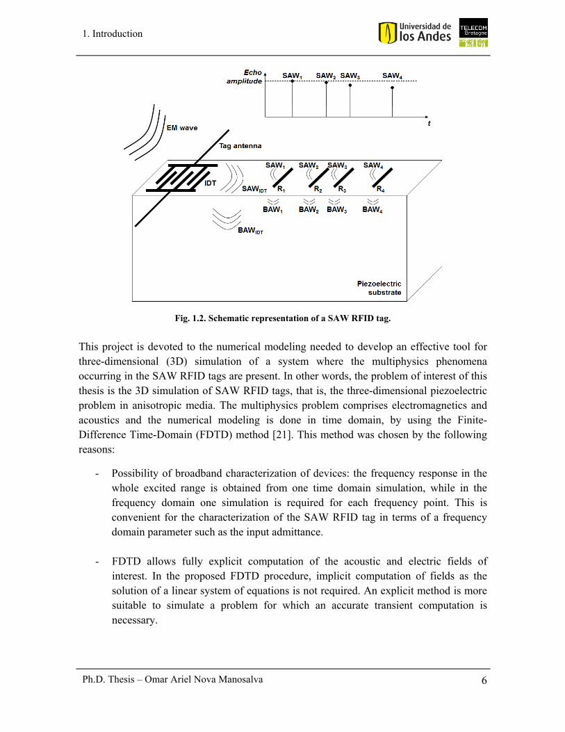
A schematic representation of a SAW RFID tag is presented in Fig. 1.2. In this representation, the main components of a tag are observed: the transducer, implemented as an interdigital transducer (IDT), and the reflectors (R1, R2, R3 and R4). Both the IDT and the reflectors consist of electrode arrays printed on a piezoelectric substrate. The IDT converts the electromagnetic waves, coming from the external reader, into acoustic waves. The electromagnetic energy is coupled to the IDT by means of the tag antenna connected to its terminals. The acoustic waves are of two kinds: bulk acoustic waves (BAW), propagating through the bulk of substrate, and surface acoustic waves (SAW), propagating along the surface of it [15]. The surface waves are those that enable the reading of the identification code stored on the tag. They travel through the surface and interact with the reflectors printed on it. A part of the surface waves is reflected back to the IDT and, depending on the time of arrival of each reflected SAW pulse (or echo), it is possible to determine the position of each reflector and hence, the identification code stored on the tag. Bulk waves are generated both by the IDT and by the scattering process occurring in each reflector. These waves are losses for the SAW RFID tag, which must be reduced. All SAW echoes (SAW1, SAW2, SAW3 and SAW4) should have uniform amplitudes, as presented in Fig. 1.2. To achieve this, special design of reflectors must be done [20].
6
1. Introduction
Ph.D. Thesis – Omar Ariel Nova Manosalva
Fig. 1.2. Schematic representation of a SAW RFID tag.
This project is devoted to the numerical modeling needed to develop an effective tool for three-dimensional (3D) simulation of a system where the multiphysics phenomena occurring in the SAW RFID tags are present. In other words, the problem of interest of this thesis is the 3D simulation of SAW RFID tags, that is, the three-dimensional piezoelectric problem in anisotropic media. The multiphysics problem comprises electromagnetics and acoustics and the numerical modeling is done in time domain, by using the Finite-Difference Time-Domain (FDTD) method [21]. This method was chosen by the following reasons:
- Possibility of broadband characterization of devices: the frequency response in the whole excited range is obtained from one time domain simulation, while in the frequency domain one simulation is required for each frequency point. This is convenient for the characterization of the SAW RFID tag in terms of a frequency domain parameter such as the input admittance.
- FDTD allows fully explicit computation of the acoustic and electric fields of interest. In the proposed FDTD procedure, implicit computation of fields as the solution of a linear system of equations is not required. An explicit method is more suitable to simulate a problem for which an accurate transient computation is necessary.

7
1. Introduction
Ph.D. Thesis – Omar Ariel Nova Manosalva
- The problem to be modeled in the simulation of the SAW RFID tags is a radar problem in which the position of the reflectors is determined from the time delay of the echoes. This kind of problems is more suitably modeled in the time domain.
- FDTD allows full wave analysis of the piezoelectric governing equations. It avoids introducing simplifying assumptions for the modeling of three dimensional structures as those introduced in the Finite Element / Boundary Element Method (FEM/BEM) [22] [23], the most popular frequency domain method used for the simulation of SAW RFID tags. Then, tags with any geometric arrangement can be simulated with the proposed FDTD procedure.
1.3. StateoftheartofSAWRFIDtagsThe typical structure of the currently implemented SAW RFID tags is presented in Fig. 1.3.
Fig. 1.3. Structure of currently implemented SAW RFID tags (taken from [20]).
In this structure, the encoding reflectors are followed by some checksum or error correction reflectors, which are typically 2. This set of encoding + checksum reflectors is surrounded by one start reflector and one end reflector, used for synchronization of the reading process [20]. In light of the above presented structure, it is evident that the SAW RFID tag of Fig. 1.2 is just a schematic representation, since the number of tag reflectors must be always greater than 4 (2 start-end reflectors + 2 checksum reflectors).
Regarding the number of encoding reflectors, a minimum of 4 has been reported in [20] for the commercially available tags manufactured by the German company Baumer Ident and the Austrian company CTR. With this number of encoding reflectors, 10.000 different codes are achieved. A maximum of 33 encoding reflectors have been reported in [19] and [24]. In [19], the 33 reflectors are arranged in 4 different tracks, as presented in Fig. 1.4. This is done to reduce the tag length. The differences in attenuation caused by the differences in initial delay between the 4 tracks are compensated by using different apertures for each track.

8
1. Introduction
Ph.D. Thesis – Omar Ariel Nova Manosalva
Fig. 1.4. SAW RFID tag with 33 encoding reflectors arranged in 4 tracks (taken from [19]).
In [24], the 33 reflectors are arranged in 33 different tracks, that is, one independent track for each reflector, as depicted in Fig. 1.5. This is done to eliminate the interference caused by internal reflections between the encoding reflectors. As in [19], the difference in insertion attenuation of each track is compensated by means of different apertures of the reflectors. An additional problem resulting with this configuration is the non-uniformity of the SAW pulse generated by the central IDT, given its great aperture, required to cover the 33 tracks.
Fig. 1.5. SAW RFID tag with 33 encoding reflectors arranged in 33 tracks (taken from [24]).
Between the minimum and the maximum number of encoding reflectors reported in the literature, different number of these reflectors is used in the commercially available SAW RFID tags. For example, the German company SAW Components manufactures tags with 16 and 20 bits, which corresponds to number of codes in the order of 104 and 106, respectively [25]. For its part, the U.S. company RF SAW produces tags with 24 and 96 bits, that is, number of codes between 107 and 1028, respectively [26]. The number of reflectors required for the mentioned commercial implementations depends on the type of codification used in the tag. As it will be shown later, this codification can be done in time, in frequency or in a combination between time and phase. For example, if codification in time is used, with 16 slots of time (possible time positions) for each reflector, 4 bits are encoded with each reflector, and a total of 24 reflectors are required to encode the 96 bits of the tags implemented by the company RF SAW.

9
1. Introduction
Ph.D. Thesis – Omar Ariel Nova Manosalva
As introduced above, codification of SAW RFID tags is not restricted to the time domain, but this is also possible in the frequency domain and, additionally, with a scheme combining time and phase codification. These codification types are presented below.
- Codification in time:
This type of codification is also known as time position encoding or pulse position modulation (PPM) [20]. This is the simplest and the most widely used in commercial SAW tags [27]. It is based on the division of the delay time into slots of fixed duration. These time slots are arranged in groups and each group is assigned to one reflector. For example, the slots can be grouped in sets of 5, where the 4 initial slots are occupied by a reflector and the final slot is reserved to insert a space between two consecutive groups. In this example, 2 bits are encoded with each reflector and, therefore, if 10 reflectors are used, a total of 220
codes (~106 codes) can be implemented.
Not only binary codification is used, but also decimal codification. An example of decimal codification is found in the above mentioned SAW tags implemented by the companies Baumer Ident and CTR, where 10.000 different codes are achieved with 4 reflectors [20]. This is because each reflector can occupy 10 different time slots. With a decimal codification, it corresponds to 104 different codes.
This codification is the simplest to be implemented in the SAW RFID tags, and also in the readers. In this case, the reader is limited to look for pulses in a group of time slots [15].
- Codification in frequency:
This kind of codification is also known as orthogonal frequency coding (OFC) [28]. This is based on reflectors with frequency dependent reflectivity. These reflectors are narrowband and their response is called orthogonal in frequency because when a reflector has maximum reflectivity, the reflectivity of the others is close to zero. An advantage of this codification is that losses are reduced because reflectors with strong reflectivity can be used. However, a major limitation is that it does not allow a large number of codes [20].
- Codification in time and phase:
In this type of codification, the conventional time encoding (PPM) is combined with small displacements of the reflectors around the central position of the time slots to implement the phase codification. To do it, the fact that the width of the reflectors is 102 times smaller than the width of the time slots is exploited. This allows displacing the reflectors by small lengths of λ/8 around the central position of each time slot, with λ the SAW wavelength. This small displacement corresponds to phase variations of 90°. Therefore, 4 different phases can be associated to each time slot, which means a great increase in the number of codes [20, 29]. This codification requires readers able to measure with high precision the phase of the reflected pulses.

10
1. Introduction
Ph.D. Thesis – Omar Ariel Nova Manosalva
Regarding the typical width of the electrodes and the distance between them, it depends on the frequency range of operation and on the used piezoelectric substrate. Currently, the most commonly used frequency range is the 2.45 GHz ISM band, with frequencies ranging between 2400 and 2483.5 MHz. For the central frequency of 2.45 GHz, the SAW wavelength (λ) is about 1.6 μm in 128°YX lithium niobate (LiNbO3) substrate. In conventional single-electrode IDT, the pitch or period (p) is λ/2 and the metallization ratio (MR), defined as the ratio between the width of the electrodes (w) and the pitch (p), is 0.5. As p = w + s, where s is the separation between electrodes, the above stated relations imply that w = s ≈ 0.4 μm at 2.45 GHz in 128°YX LiNbO3 substrate.
1.4. ScopeofthethesisThe project is oriented to develop a volumic numerical procedure in time domain able to simulate the multiphysics phenomena occurring in a SAW RFID tag, by using the FDTD method. Therefore, the problem to be modeled is the three-dimensional piezoelectric problem in anisotropic media.
The SAW RFID tag is the modeling object of the project, so the numerical procedure is oriented to its characterization. The characterization is done both in time domain and in frequency domain. In time domain the identification code is determined, while in frequency domain the tag input admittance is computed. The identification code is determined from the time delay of each SAW echo received by the IDT. Uniformity of the echo amplitudes is verified to verify the proper operation of the device as an RFID tag, that is, the readability of the stored code. Once this condition is verified, the coupling to the tag antenna is addressed by computing the tag input admittance. The admittance is computed in the frequency domain from the time domain fields obtained from the FDTD simulation. These fields are Fourier transformed into the frequency domain to compute the power flowing out the IDT and the voltage between its terminals. With these two quantities, the input admittance is computed. The optimum coupling with the antenna is achieved when the tag admittance is the complex conjugate of the antenna admittance. The modeling of the antenna is out of the scope of this project. This can be done by means of commercial software for antenna analysis. The variation of the tag design to obtain a required input admittance is also out of the scope of the project. However, the developed simulation tool can be readily applied to optimize the input admittance through parametric analysis. The described procedures for the determination of the identification code and the input admittance, from time domain simulations, are original contributions of this thesis.
Great importance is given to the absorbing boundary condition (ABC) in this project, as it allows conveniently limit the computational domain of the simulated SAW device. The used ABC is the Perfectly Matched Layer (PML) [30] [31]. The stability of the PML is an important issue when this boundary is applied on anisotropic materials as the piezoelectric substrates of the SAW RFID tags. Some PML instability problems reported for certain

11
1. Introduction
Ph.D. Thesis – Omar Ariel Nova Manosalva
piezoelectric substrates in [32] and [33] are overcome. The methodology to obtain stable PML boundaries for piezoelectric crystals with different symmetry is also an original contribution of this thesis.
The FDTD formulation is done in three dimensions, including the PML boundaries, for piezoelectric substrates with different symmetries. Due to the excessive computational resources required to simulate a whole SAW RFID tag in 3D, the proposed procedures to determine the identification code and the input admittance are applied and tested on 2D simulations. However, the 3D simulation capability of the developed numerical procedure is verified through the simulation of IDT’s on different substrates. The 3D simulation of a whole SAW RFID tag is out of the scope of this project, as well as the optimization of the tag design. These tasks can be accomplished by using High Performance Computing (HPC) tools.
1.5. Contributions1. Procedure for the determination of the identification code stored in the SAW RFID
tag from the fields computed in the time domain simulation.
Since the identification code is stored in the tag as the time delays of the SAW echoes received by the IDT, this code can be directly determined from the fields computed in the FDTD simulation. The time delays of the SAW echoes can be determined through observation of the time evolution of any of the fields computed in the FDTD simulation, at a point close to the IDT. Given the low amplitude of the SAW echoes, logarithmic scale is used to facilitate the discrimination of them. In contrast to this direct procedure in the time domain, the determination of the identification code through the FEM/BEM method requires a more complex procedure. This procedure includes the following steps [34]: computation in the frequency domain of the S11 parameter for the entire tag and the IDT alone, subtraction of the S11 for the IDT alone from the S11 for the entire tag, weighting of the absolute value of the subtraction to make it small at the ends of the studied frequency range, and finally Fourier transformation of the weighted subtraction into the time domain. As a result of this transformation, the time position of the SAW echoes is obtained.
The procedure proposed in this thesis allows the determination of the identification code just by observation of one of the simulated fields. This makes it a more convenient procedure for tag characterization and less susceptible to numerical errors than the conventional procedure used by the FEM/BEM method.
This contribution was published in [35] and [36] and is presented in chapter 3 of this document.
2. FDTD formulation in three dimensions on anisotropic materials to perform full wave simulation of the multiphysics phenomena occurring in the SAW RFID tag.
12
1. Introduction
Ph.D. Thesis – Omar Ariel Nova Manosalva
A general 3D FDTD formulation is developed to allow full wave analysis of the piezoelectric governing equations. This analysis is applied to simulate the multiphysics problem, combining acoustics and electromagnetics, in which SAW RFID tags are based. The FDTD formulation is applied to model the electroacoustic wave propagation in different piezoelectric substrates (anisotropic materials), with different crystal symmetry class [12]. The formulation includes: discretization of the piezoelectric governing equations [12] in time and space; irregular meshing with finer mesh in the regions of high field variation; boundary conditions to limit the computational domain, free-surface boundary [37, 38] on the substrate surface and absorbing boundary implemented as PML [30] [31] on the other substrate boundaries; and excitation with a distributed source given by the electric field (E) induced in the substrate when the IDT electrodes are polarized [33] [39].
As the developed FDTD formulation allows full wave simulation in 3D, it can be applied to SAW RFID tags with any geometric arrangement. In particular, it is possible to consider geometry variations of the SAW RFID tag in the transverse direction. The consideration of the transverse direction in the FEM/BEM method, commonly used for simulation of SAW RFID tags, is done through the introduction of simplifying assumptions that limit the variations that can be simulated in this direction [22] [23]. Thus, the proposed numerical procedure provides a design tool with greater freedom for modeling in the three spatial directions.
This contribution was published in [35] and [40] and is presented in chapter 4 of this document.
3. Spatial discretization scheme to ensure the PML stability on piezoelectric substrates with different crystal symmetry class.
PML stability is achieved for 3D FDTD simulation of electroacoustic wave propagation on different piezoelectric crystals, including a substrate previously reported as unstable [32] [33]. The stability is achieved for substrates with different crystal symmetry class by ensuring a central-difference scheme in the FDTD spatial discretization grid. By using this discretization scheme, all the substrates for which PML stability is demonstrated in the continuous medium, are also stable in the discrete medium. PML stability in the discrete medium is demonstrated by considerations of energy conservation. This is done by observing the time evolution of the total energy of the piezoelectric system. If no increase of this energy is observed, PML stability is demonstrated.
With the proposed discretization scheme, PML stability can be achieved independently of the crystal symmetry class of the piezoelectric substrate. This enables the simulation of SAW RFID tags on many of the substrates that exhibit favorable properties for the SAW technology.
This contribution was published in [40] and is presented in section 4.4 of this document.

13
1. Introduction
Ph.D. Thesis – Omar Ariel Nova Manosalva
4. Procedure for the computation of the SAW RFID tag input admittance from the fields computed in the time domain simulation.
In this project, the tag input admittance is obtained directly from the fields computed in the FDTD simulation. After a Fourier transformation into the frequency domain, the fields are used to compute the power flowing out the IDT and the voltage between its terminals. These two quantities allow the computation of the input admittance from its definition, in all the excited frequency range. On the other hand, in the FEM/BEM method, the tag input admittance is obtained from two of the computed fields: the electric potential and the surface charge density [41] [42]. The IDT voltage is obtained from the electric potential, and the current flowing through it. The current is computed from the surface charge density. With the voltage and the current, the input admittance can be computed from its definition. One simulation is required for each point of the studied frequency range.
The proposed procedure for input admittance computation from a time domain simulation is an original contribution of this thesis. With respect to the conventional procedure used by the FEM/BEM method, the proposed procedure has the advantage of computing the admittance from fields directly obtained from the simulation of the physical governing equations, without using a semi-analytical approach like that employed in the FEM/BEM method, in which a Green’s function is used [41] [42].
This contribution was published in [43] and is presented in section 4.5 of this document.
1.6. DocumentorganizationThis document is organized in chapters as follows:
In chapter 2, the review of the state of the art is done, presenting the existing methods for the simulation of SAW RFID tags, the application of FDTD for the simulation of SAW devices, with the corresponding considerations of stability and absorbing boundary conditions, and the challenges arising for the 3D simulation of SAW RFID tags.
In chapter 3, the procedure for the determination of the SAW RFID tag identification code from FDTD simulations in 2D is presented, including the 2D FDTD formulation and the used irregular meshing. The boundary conditions and the application of the quasi-static approximation are also discussed.
In chapter 4, the 3D FDTD formulation for simulation of electroacoustic wave propagation in SAW devices is developed, including a detailed description of the discretization grid, the boundary conditions (PML and stress-free) and the quasi-static approximation that can be applied in SAW devices. FDTD simulation of SAW IDTs in 3D is also included as validation of the developed formulation. In section 4.4, the conditions to achieve PML stability in 3D FDTD simulations on piezoelectric crystals with different symmetry class

14
1. Introduction
Ph.D. Thesis – Omar Ariel Nova Manosalva
are discussed. The PML stability is demonstrated both in the continuous and the discretized media. In the continuous medium, stability conditions are verified, while in the discretized medium, stability is demonstrated from energy conservation. In section 4.5, the procedure for the computation of the IDT input admittance from FDTD simulations is described. The computation is done from the power flowing out the IDT and the voltage between its terminals. The proposed procedure is validated with the input admittance computation of two IDTs, from 2D FDTD simulations.
Finally, in chapter 5, the conclusions of the thesis and the future work envisioned for the project are presented.
1.7. ListofpublicationsThe original contributions of this thesis are found in the following list of publications.
- Journal paper:
O. Nova, N. Peña, and M. Ney, "Perfectly matched layer stability in 3-D finite-difference time-domain simulation of electroacoustic wave propagation in piezoelectric crystals with different symmetry class," Ultrasonics, Ferroelectrics and Frequency Control, IEEE Transactions on, vol. 62, pp. 600-603, March, 2015.
- Conference papers:
1. O. Nova, N. Peña, and M. Ney, "Time-domain modeling of SAW RFID tags," in Conférence Européenne sur les Méthodes Numériques en Electromagnétisme, NUMELEC 2012, Marseille, France, 2012, pp. 48-49.
2. O. Nova, N. Peña, and M. Ney, "FDTD simulation of SAW RFID tags," in RFID-Technologies and Applications (RFID-TA), 2012 IEEE International Conference on, Nice, France, 2012, pp. 259-262.
3. O. Nova, N. Peña, and M. Ney, "Computation of SAW RFID tag input admittance from FDTD simulation," in International Symposium on Electric and Magnetic Fields, EMF 2013, Bruges, Belgium, 2013.
1.8. References[1] V. D. Hunt, A. Puglia, and M. Puglia, RFID: A guide to Radio Frequency
Identification. Hoboken, N.J.: John Wiley & Sons, 2007. [2] K. Finkenzeller, RFID Handbook: Fundamentals and Applications in Contactless
Smart Cards, Radio Frequency Identification and Near-Field Communication, 3rd ed. Hoboken, N.J.: John Wiley & Sons, 2010.
15
1. Introduction
Ph.D. Thesis – Omar Ariel Nova Manosalva
[3] A. N. Nambiar, "RFID Technology: A Review of its Applications," in World Congress on Engineering and Computer Science, San Francisco, USA, 2009, pp. 1-7.
[4] R. Want, "An introduction to RFID technology," Pervasive Computing, IEEE, vol. 5, pp. 25-33, 2006.
[5] J.-P. Curty, M. Declercq, C. Dehollain, and N. Joehl, Design and Optimization of Passive UHF RFID Systems. New York, NY: Springer, 2007.
[6] J.-W. Lee and B. Lee, "A Long-Range UHF-Band Passive RFID Tag IC Based on High-Q Design Approach," Industrial Electronics, IEEE Transactions on, vol. 56, pp. 2308-2316, 2009.
[7] S. Preradovic, I. Balbin, N. C. Karmakar, and G. F. Swiegers, "Multiresonator-Based Chipless RFID System for Low-Cost Item Tracking," Microwave Theory and Techniques, IEEE Transactions on, vol. 57, pp. 1411-1419, 2009.
[8] D. Girbau, J. Lorenzo, A. Lazaro, C. Ferrater, and R. Villarino, "Frequency-Coded Chipless RFID Tag Based on Dual-Band Resonators," Antennas and Wireless Propagation Letters, IEEE, vol. 11, pp. 126-128, 2012.
[9] A. Vena, E. Perret, and S. Tedjini, "A Fully Printable Chipless RFID Tag With Detuning Correction Technique," Microwave and Wireless Components Letters, IEEE, vol. 22, pp. 209-211, 2012.
[10] A. Ramos, D. Girbau, A. Lazaro, and S. Rima, "IR-UWB radar system and tag design for time-coded chipless RFID," in Antennas and Propagation (EUCAP), 2012 6th European Conference on, 2012, pp. 2491-2494.
[11] D. Dardari and R. D'Errico, "Passive Ultrawide Bandwidth RFID," in Global Telecommunications Conference, 2008. IEEE GLOBECOM 2008. IEEE, 2008, pp. 1-6.
[12] B. A. Auld, Acoustic Fields and Waves in Solids, 2nd ed. vol. 1. Malabar, FL: Krieger Publishing Company, 1990.
[13] C. C. W. F. Ruppel, T. A., Advances in surface acoustic wave technology, systems and applications vol. 2. Singapore: World Scientific Publishing, 2001.
[14] C. S. Hartmann and L. T. Claiborne, "Fundamental Limitations on Reading Range of Passive IC-Based RFID and SAW-Based RFID," in RFID, 2007. IEEE International Conference on, 2007, pp. 41-48.
[15] S. Harma, "Surface acoustic wave RFID tags: Ideas, developments and experiments," Doctoral Dissertation, Department of Applied Physics, Helsinki University of Technology, Helsinki, 2009.
[16] D. E. N. Davies, M. J. Withers, and R. P. Claydon, "Passive coded transponder using an acoustic-surface-wave delay line," Electronics Letters, vol. 11, pp. 163-164, 1975.
[17] L. Reindl and W. Ruile, "Programmable reflectors for SAW-ID-tags," in Ultrasonics Symposium, 1993. Proceedings., IEEE 1993, 1993, pp. 125-130 vol.1.
[18] V. P. Plessky, S. N. Kondratiev, R. Stierlin, and F. Nyffeler, "SAW tags: new ideas," in Ultrasonics Symposium, 1995. Proceedings., 1995 IEEE, 1995, pp. 117-120 vol.1.
[19] L. Reindl, G. Scholl, T. Ostertag, H. Scherr, U. Wolff, and F. Schmidt, "Theory and application of passive SAW radio transponders as sensors," Ultrasonics, Ferroelectrics, and Frequency Control, IEEE Transactions on, vol. 45, pp. 1281-1292, 1998.
16
1. Introduction
Ph.D. Thesis – Omar Ariel Nova Manosalva
[20] V. P. Plessky and L. M. Reindl, "Review on SAW RFID tags," Ultrasonics, Ferroelectrics, and Frequency Control, IEEE Transactions on, vol. 57, pp. 654-668, 2010.
[21] A. Taflove and S. C. Hagness, Computational Electrodynamics: The Finite-Difference Time-Domain Method, 3rd ed. Norwood, MA: Artech House, 2005.
[22] M. Solal, C. Li, and J. Gratier, "Measurement and FEM/BEM simulation of transverse effects in SAW resonators on lithium tantalate," Ultrasonics, Ferroelectrics and Frequency Control, IEEE Transactions on, vol. 60, pp. 2404-2413, 2013.
[23] V. Plessky, P. Turner, N. Fenzi, and V. Grigorievsky, "Interaction between the Rayleigh-type SAW and the SH-wave in a periodic grating on a 128°-LN substrate," in Ultrasonics Symposium (IUS), 2010 IEEE, 2010, pp. 167-170.
[24] L. Reindl, "Track-changing structures on YZ-LiNbO3," in Ultrasonics Symposium, 1997. Proceedings., 1997 IEEE, 1997, pp. 77-82 vol.1.
[25] SAW-Components, "Product Catalogue - SAW components," SAW-COMPONENTS-Dresden-GmbH, Ed., January 2015 ed. Dresden, Germany: SAW-Components, 2015.
[26] RFSAW, "The First Commercial Global SAW Tag (GST) System," RFSAW, Ed., Rev 1.0 ed. Richardson, Texas: RFSAW, 2015.
[27] L. M. Reindl and I. M. Shrena, "Wireless measurement of temperature using surface acoustic waves sensors," Ultrasonics, Ferroelectrics, and Frequency Control, IEEE Transactions on, vol. 51, pp. 1457-1463, 2004.
[28] D. C. Malocha, D. Puccio, and D. Gallagher, "Orthogonal frequency coding for SAW device applications," in Ultrasonics Symposium, 2004 IEEE, 2004, pp. 1082-1085 Vol.2.
[29] S. Harma, W. G. Arthur, C. S. Hartmann, R. G. Maev, and V. P. Plessky, "Inline SAW RFID tag using time position and phase encoding," Ultrasonics, Ferroelectrics, and Frequency Control, IEEE Transactions on, vol. 55, pp. 1840-1846, 2008.
[30] W. C. Chew and Q. H. Liu, "Perfectly Matched Layers for Elastodynamics: A New Absorbing Boundary Condition," Journal of Computational Acoustics, vol. 04, pp. 341-359, 1996.
[31] F. Chagla, C. Cabani, and P. M. Smith, "Perfectly matched layer for FDTD computations in piezoelectric crystals," in Ultrasonics Symposium, 2004 IEEE, 2004, pp. 517-520 Vol.1.
[32] F. Chagla and P. M. Smith, "Stability considerations for perfectly matched layers in piezoelectric crystals," in Ultrasonics Symposium, 2005 IEEE, 2005, pp. 434-437.
[33] F. Chagla and P. M. Smith, "Finite difference time domain methods for piezoelectric crystals," Ultrasonics, Ferroelectrics and Frequency Control, IEEE Transactions on, vol. 53, pp. 1895-1901, 2006.
[34] S. Harma and V. P. Plessky, "Extraction of frequency-dependent reflection, transmission, and scattering parameters for short metal reflectors from FEM-BEM simulations," Ultrasonics, Ferroelectrics and Frequency Control, IEEE Transactions on, vol. 55, pp. 883-889, 2008.
[35] O. Nova, N. Peña, and M. Ney, "FDTD simulation of SAW RFID tags," in RFID-Technologies and Applications (RFID-TA), 2012 IEEE International Conference on, Nice, France, 2012, pp. 259-262.
17
1. Introduction
Ph.D. Thesis – Omar Ariel Nova Manosalva
[36] O. Nova, N. Peña, and M. Ney, "Time-domain modeling of SAW RFID tags," in Conférence Européenne sur les Méthodes Numériques en Electromagnétisme, NUMELEC 2012, Marseille, France, 2012, pp. 48-49.
[37] C. T. Schröder, "On the interaction of elastic waves with buried land mines: An investigation using the finite-difference time-domain method," Doctoral Dissertation, School Elect. Comput. Eng., Georgia Inst. Technol., Atlanta, GA, 2001.
[38] R. W. Graves, "Simulating seismic wave propagation in 3D elastic media using staggered-grid finite differences," Bulletin of the Seismological Society of America, vol. 86, pp. 1091-1106, 1996.
[39] K.-Y. Wong and W.-Y. Tam, "Analysis of the frequency response of SAW filters using finite-difference time-domain method," Microwave Theory and Techniques, IEEE Transactions on, vol. 53, pp. 3364-3370, 2005.
[40] O. Nova, N. Peña, and M. Ney, "Perfectly matched layer stability in 3-D finite-difference time-domain simulation of electroacoustic wave propagation in piezoelectric crystals with different symmetry class," Ultrasonics, Ferroelectrics and Frequency Control, IEEE Transactions on, vol. 62, pp. 600-603, March, 2015.
[41] P. Ventura, J. M. Hode, and B. Lopes, "Rigorous analysis of finite SAW devices with arbitrary electrode geometries," in Ultrasonics Symposium, 1995. Proceedings., 1995 IEEE, 1995, pp. 257-262 vol.1.
[42] P. Ventura, J. M. Hode, J. Desbois, and M. Solal, "Combined FEM and Green's function analysis of periodic SAW structure, application to the calculation of reflection and scattering parameters," Ultrasonics, Ferroelectrics and Frequency Control, IEEE Transactions on, vol. 48, pp. 1259-1274, 2001.
[43] O. Nova, N. Peña, and M. Ney, "Computation of SAW RFID tag input admittance from FDTD simulation," in International Symposium on Electric and Magnetic Fields, EMF 2013, Bruges, Belgium, 2013.

18 Ph.D. Thesis – Omar Ariel Nova Manosalva
19 Ph.D. Thesis – Omar Ariel Nova Manosalva
2. State of the art
2. STATEOFTHEART
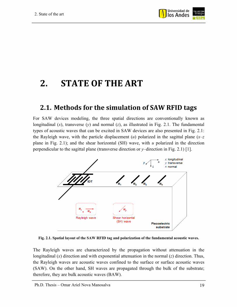
2.1. MethodsforthesimulationofSAWRFIDtagsFor SAW devices modeling, the three spatial directions are conventionally known as longitudinal (x), transverse (y) and normal (z), as illustrated in Fig. 2.1. The fundamental types of acoustic waves that can be excited in SAW devices are also presented in Fig. 2.1: the Rayleigh wave, with the particle displacement (u) polarized in the sagittal plane (x–z plane in Fig. 2.1); and the shear horizontal (SH) wave, with u polarized in the direction perpendicular to the sagittal plane (transverse direction or y–direction in Fig. 2.1) [1].
Fig. 2.1. Spatial layout of the SAW RFID tag and polarization of the fundamental acoustic waves.
The Rayleigh waves are characterized by the propagation without attenuation in the longitudinal (x) direction and with exponential attenuation in the normal (z) direction. Thus, the Rayleigh waves are acoustic waves confined to the surface or surface acoustic waves (SAW). On the other hand, SH waves are propagated through the bulk of the substrate; therefore, they are bulk acoustic waves (BAW).
20 Ph.D. Thesis – Omar Ariel Nova Manosalva
2. State of the art
Before presenting the methods that have been proposed for the simulation of SAW RFID tags, it is convenient to introduce the piezoelectric governing equations. These equations can be presented in an analogous manner to the electromagnetic governing equations or Maxwell’s equations as follows.
The main fields of the piezoelectric governing equations are the stress (T) and the particle velocity (v). They are analogous to the electric field (E) and the magnetic field (H), respectively, in the Maxwell’s equations. For their part, the secondary fields in the piezoelectric case are the strain (S) and the momentum density (p), analogous to the electric flux density (D) and the magnetic flux density (B), respectively, for the electromagnetic case [2].
In piezoelectricity, as in electromagnetics, the main fields (T, v) are related to the secondary ones (S, p) by means of the constitutive relations presented below:
:ET e E c S ( 2.1 )
p v ( 2.2 )
where e is the tensor of piezoelectric stress constants, cE is the tensor of stiffness constants for constant E and ρ is the mass density. The operator double dot product (:) is defined in [2].
In ( 2.1 ) it is worth noting that the field T is coupled not only to the mechanic field S but also to the electric field E. This shows the multiphysics nature of the piezoelectric problem, where the mechanic and the electric fields are coupled together.
The piezoelectric governing equation analogous to the Maxwell-Faraday equation, which relates the main electric field (E) with the main magnetic field (H), is the equation of motion, which relates the main acoustic fields T and v, as presented below:
vT
t
( 2.3 )
Finally, the equation analogous to the Maxwell-Ampère equation, which relates the main magnetic field (H) with the secondary electric field (D), is the strain – displacement relation, which relates the main acoustic field v with the secondary acoustic field S, as follows:
s
Sv
t
( 2.4 )
21 Ph.D. Thesis – Omar Ariel Nova Manosalva
2. State of the art
where the acoustic field operator s is the symmetric gradient defined in [2].
2.1.1. ExistingmethodsforthesimulationofSAWRFIDtagsThe four most used methods for the simulation of SAW RFID tags are presented. Three of them are analytical methods (COM, P-matrix and δ-function) while the other uses a semi-analytical approach (FEM/BEM). Among the analytical procedures, both the COM and the P-matrix method make use of traveling waves in the formulation. For its part, the δ-function method models the generated SAW as the sum of acoustic plane waves originated in each IDT finger. The semi-analytical method FEM/BEM combines analytical Green’s functions with numerical procedures for the computation of the fields involved in the multiphysics phenomenon. The formulation of the four mentioned methods is done in the frequency domain.
2.1.1.1. FEM/BEM method (Finite Element Method / Boundary ElementMethod)
This is a semi-analytical method that makes use of Green’s functions to model the multiphysics problem involved in the SAW RFID tag operation. This method combines the Finite Element Method (FEM) to model the electrodes of transducers and reflectors and the Boundary Element Method to model the semi-infinite piezoelectric substrate [3] [4]. The computed acoustic fields are the particle displacement (u) at the substrate surface and the stress vector on the surface in the normal direction (ts). The computed electric fields are the electric potential (Φ) and the surface charge density (σ). A semi-infinite dyadic Green’s function (G) is used to relate u with ts and Φ with σ, by using BEM on the semi-infinite piezoelectric substrate, as showed in ( 2.5 ).
/2
/2
'' '
'
p np s
p npn
u x t xG x x dx
x x
( 2.5 )
where p is the period of the electrode array printed on the surface and x is the direction in which this array is oriented (longitudinal direction in Fig. 2.1).
By defining the harmonic periodic Green’s function, pG x , as
2p j n
n
G x G x np e
( 2.6 )
the relation in ( 2.5 ) becomes

22 Ph.D. Thesis – Omar Ariel Nova Manosalva
2. State of the art
/2
/2
'' '
'
p sp
p
u x t XG x X dX
x X
( 2.7 )
where the change of variable ' 'X x np was applied along with the relations
2j ns st x np t x e and 2j nx np x e , known as Floquet’s theorem.
At the same time, both ts and σ are expressed as the sum of a series of NCH first class Chebyshev polynomials of rank n, Tn(x):
2
1
/
1 /
CHs
Nts n
nn
bt x T x a
x bx a
( 2.8 )
where a is the half electrode width and bts and bσ are the unknown coefficient vectors of the expansion in ( 2.8 ).
By replacing ( 2.8 ), the ( 2.7 ) relation becomes
21
'/' '
1 '/
CHs
Nat np
an n
bu x T x aG x x dx
x b x a
( 2.9 )
From ( 2.9 ), two linear equation systems with NCH equations and 2NCH unknowns each one are formulated, as indicated in ( 2.10 ).
1
, 1CH
s
Ntu
mn CHnm n
bcm N
c b
B
( 2.10 )
where the unknowns are the coefficient vectors cu, cΦ, bts and bσ. The two equations systems presented in ( 2.10 ) are independently written below:
1 1sCH CH CH CHu mn tN N N N
c b B
( 2.11 )
1 1CH CHCH CHmnN NN N
c b B
( 2.12 )
where the subscripts indicate the size of the matrices.

23 Ph.D. Thesis – Omar Ariel Nova Manosalva
2. State of the art
Both ( 2.11 ) and ( 2.12 ) are linear systems with NCH equations. The 2NCH unknowns of ( 2.11 ) are the elements of the two coefficient vectors cu and bts, while the 2NCH unknowns of ( 2.12 ) are the elements of cΦ and bσ.
Bmn is a NCH x NCH matrix that is computed as a double integral of the harmonic periodic
Green’s function, pG x :
2
0 0cos cos cos cosp
mn
aB G a m n d d
p
( 2.13 )
By applying FEM on the electrodes of transducers and reflectors, the linear system in ( 2.14 ) is derived:
2K M U F ( 2.14 )
In this system, the nodal displacement vector (U) is related to the force vector (F) by means of the stiffness matrix (K) and the mass matrix (M). F is defined in terms of the stress (ts) as:
es
i s iF t x W x dx
( 2.15 )
where Γes is the interface electrode-substrate and Wi is the FEM basis function associated with node i. To apply the FEM method, the electrodes are discretized into triangular finite elements with six nodes and three points.
By solving ( 2.14 ), a direct relationship between cu and bts is found:
su e tc b Y ( 2.16 )
where Ye is a NCH x NCH matrix. Then, the equation system ( 2.11 ) now have NCH equations with NCH unknowns (the elements of the vector bts).
To solve the system ( 2.12 ), the electrical boundary condition Φ = 1 on Γes is used. In this way, the vector cΦ is given by:
; 1
0; 1m
a p mc
m
( 2.17 )

24 Ph.D. Thesis – Omar Ariel Nova Manosalva
2. State of the art
for m = 1, …, NCH. Then, the system ( 2.12 ) now have NCH equations with NCH unknowns (the elements of the vector bσ).
By solving the two NCH x NCH equation systems derived as described above, the coefficient vectors bts and bσ are found and, therefore, the ts and σ fields are obtained in the entire tag from ( 2.8 ), while the u and Φ fields are determined from ( 2.9 ).
2.1.1.2. COM(CouplingofModes)modelThe objective of the method is to obtain two acoustic fields, particle velocity (v) and mechanical stress (T), and two electric fields, electric potential (Φ) and electric displacement (D) [5] [6]. These fields are modeled as forward and backward traveling waves of a SAW mode. When this mode is propagated on free or unperturbed surface, the unperturbed fields are defined:
0jsk xv v z e ( 2.18 )
0jsk xT T z e ( 2.19 )
0jsk xz e ( 2.20 )
0jsk xD D z e ( 2.21 )
where k0 = 2π/p, p is the period of the electrode array, sk0 =ω/V, ω is the angular frequency and V is the SAW phase velocity. The x and z directions are the longitudinal and normal directions, respectively, as defined in Fig. 2.1. However, in this case the direction z positive is opposite to that shown in Fig. 2.1.
When the substrate surface is perturbed by thin metal strips (electrodes), the modes in ( 2.18 ) to ( 2.21 ) that are propagated in opposite directions couple to each other to originate the coupled perturbed fields, v’, T’, Φ’ and D’. These fields are expressed in terms of the uncoupled perturbed fields as shown below:
0 0
' ''
' ''
' ''
' ''
jsk x jsk x
v z v zv
T z T zTA x e A x e
z z
D z D zD
( 2.22 )
where ' , ' , 'v z T z z and 'D z are the uncoupled perturbed fields. 'v z and
'T z can be approximated by their corresponding unperturbed fields v z and T z
because the thin metal strips do not affect considerably the mechanical field distribution.
On the contrary, ' z and 'D z are totally different from their corresponding
25 Ph.D. Thesis – Omar Ariel Nova Manosalva
2. State of the art
unperturbed fields, because the electric field distribution is greatly affected by the electrodes.
The unknown amplitudes A+(x) and A-(x) in ( 2.22 ) are determined from a pair of differential equations called the coupled-mode amplitude equations:
0
0
12
211 12
12
* 212 11
j s k x
j s k x
A x A xj j edA x A xdx
j e j
( 2.23 )
where the coupling coefficients 11 and 12 are given in terms of the coefficients coming
from the electric perturbation ( 11E and 12E ) and those coming from the mechanical
perturbation ( 11M and 12M ), as indicated below:
11 11 11E M ( 2.24 )
12 12 12E M ( 2.25 )
Explicit expressions for 11E , 12E , 11M and 12M are given in [5]. These expressions are
not presented here for space considerations.
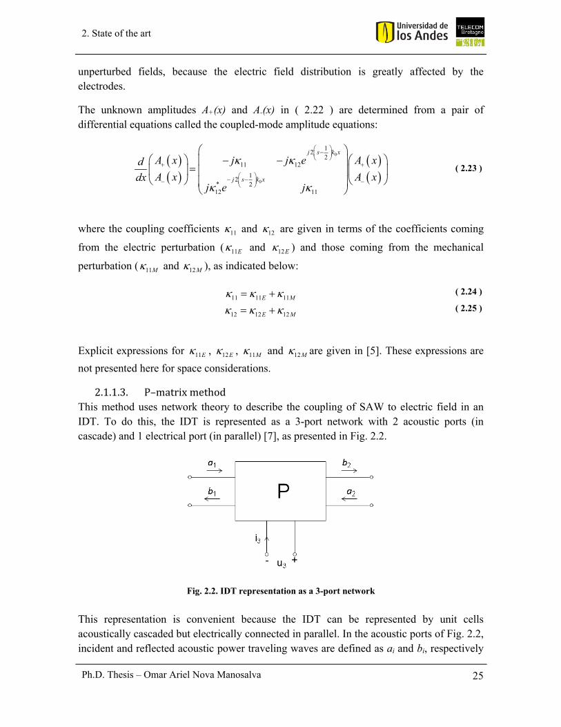
2.1.1.3. P–matrixmethodThis method uses network theory to describe the coupling of SAW to electric field in an IDT. To do this, the IDT is represented as a 3-port network with 2 acoustic ports (in cascade) and 1 electrical port (in parallel) [7], as presented in Fig. 2.2.
Fig. 2.2. IDT representation as a 3-port network
This representation is convenient because the IDT can be represented by unit cells acoustically cascaded but electrically connected in parallel. In the acoustic ports of Fig. 2.2, incident and reflected acoustic power traveling waves are defined as ai and bi, respectively

26 Ph.D. Thesis – Omar Ariel Nova Manosalva
2. State of the art
(i = 1, 2). The acoustic power wave amplitudes are given in terms of mechanical force (f) and particle velocity (v) as follows:
1
2 2i i a i
a
a f Z vZ
( 2.26 )
1
2 2i i a i
a
b f Z vZ
( 2.27 )
where Za is the acoustic impedance. Definitions in ( 2.26 ) and ( 2.27 ) are chosen to meet the equation of acoustic radiated power in terms of the traveling waves, a and b, namely
2 2*1Re
2avP f v b a
( 2.28 )
In the electrical port of Fig. 2.2, a current (i3) and a voltage (u3) are defined. This representation allows modeling the IDT by means of a 3x3 matrix called P-matrix, which is a combination between a scattering matrix (S-matrix) and an admittance matrix (Y-matrix). The termination conditions required to define the P-matrix elements can be established experimentally, as occurs for the S-matrix. However, the P-matrix represents better the cascade connection of the acoustic ports and the parallel connection of the electrical ports occurring in the IDT unit cells. The relation between acoustic and electric quantities given by the P–matrix is presented below.
1 11 12 13 1
2 21 22 23 2
3 31 32 33 3
b P P P a
b P P P a
i P P P u
( 2.29 )
The elements P11, P12, P21 and P22 form a 2x2 acoustic scattering matrix, relating the incident and reflected acoustic power waves. The P33 element is an electrical admittance term, relating the electrical current and voltage. The P13 and P23 elements represent the transfer function voltage-to-SAW and can be computed when the incident acoustic waves are zero (a1 = a2 = 0). The P31 and P32 elements are the transfer function SAW-to-short circuit current and are computed when the voltage is zero (u3 = 0).
2.1.1.4. DeltafunctionmodelThis method exploits the fact that the particle displacement in a piezoelectric substrate is driven by the electric field gradient. As this gradient is larger at the finger edges of an IDT, it is modeled as a Dirac delta function (δ-function) at each finger edge [8-10], as illustrated in Fig. 2.3.

27 Ph.D. Thesis – Omar Ariel Nova Manosalva
2. State of the art
The δ functions act as an acoustic energy source. An external voltage excitation of the form j te is applied on the IDT. Then, each IDT finger radiates an acoustic plane wave in the
positive x-direction (see Fig. 2.3). The wave generated in the opposite direction is not considered in the analysis. Therefore, the SAW generated by a transmitter IDT, S(f), is given by a summation of plane waves originated by the δ-function sources, as presented below:
1
2( ) exp exp 2
N
nn
fS f j x x j ft
V
( 2.30 )
where N is the total number of finger edges in the transmitter IDT, f is the frequency in hertz, V is the SAW phase velocity and xn is the position of each finger edge.
Fig. 2.3. Representation of the electric field gradient as δ functions at electrode edges
Similarly, the output of a receiver IDT is given by the summation of all the transmitted waves in ( 2.30 ) as they pass under each receiver finger. It results in the double sum of ( 2.31 ).
1 1
( ) 2( ) exp
( )
M No
n m n mm ni
V f fH f I I j x y
V f V
( 2.31 )
where H(f) is the transfer function of the SAW device, Vo(f) is the output voltage for an input voltage Vi(f), M is the total number of finger edges in the receiver IDT, In and Im are coefficients with magnitude and phase proportional to the electric field gradient at each edge, and ym is the position of each finger edge at the receiver IDT.
The sign of In and Im of two consecutive edges corresponding to the same electrode must be the same, while the amplitude is independently assigned according to the electric field gradient at each edge. This gradient is determined by the interdigital spacing and the degree of overlapping between consecutive electrodes (apodization of electrodes). By controlling the apodization of the electrodes, the shape of the transfer function H(f) can be adjusted as desired.

28 Ph.D. Thesis – Omar Ariel Nova Manosalva
2. State of the art
2.1.2. Restrictionsof theexistingmethods for the simulationofSAWRFIDtags
Modeling restrictions for each of the discussed methods are presented below.
2.1.2.1. RestrictionsoftheFEM/BEMmethodAlthough its expansion to 3D modeling is possible, it is a complex process due to the following aspects:
- To consider the interaction between Rayleigh and SH waves, the frequencies at which this phenomenon takes place must be estimated [11].
- To simplify the involved Green’s functions evaluation, a false periodicity in the transverse direction must be introduced [12].
- Optimal meshing strategies are required, as described in [13], to ensure an appropriate transition between different kinds of mesh used in the transducer: triangular mesh in the buses and vertices and rectangular mesh in the remaining regions.
2.1.2.2. RestrictionsoftheCOMmodelThe main simplifying assumptions of this model are the following [5]:
- It is developed under the assumption of infinite grating of the transducer: this is not always the case for the IDT of a SAW RFID tag, in which short transducers can be used.
- The grating must be periodic, which limits the design versatility that a SAW transducer can have.
- Waves must be non-dispersive: Phase velocity must be independent of frequency, which is not always true. Dispersive waves arise in devices conformed by layered substrates [1].
- Narrowband analysis is done in a short range around the operational frequency, f0.
2.1.2.3. RestrictionsoftheP–matrixmethodThe main restrictions of this method are the following [7]:
- P–matrix computation for reflective IDTs is very complex. - Only one type of acoustic wave can be present, either the Rayleigh wave or the SH
wave, but not both simultaneously. - Wave amplitude is considered to be uniform in the transverse direction: it is not
possible to consider transverse variations of the IDT, such as apodization of the electrodes or diffraction at their ends.
2.1.2.4. RestrictionsoftheDeltafunctionmodelThis model can only be applied in very simple cases where the following conditions are met [8-10]:

29 Ph.D. Thesis – Omar Ariel Nova Manosalva
2. State of the art
- The problem is one-dimensional: extension to two-dimensional or three-dimensional cases is difficult.
- IDTs are non-reflective. - IDTs are unidirectional: because wave generation is only considered in one
direction. - Propagation conditions are ideal: there is no propagation loss and no diffraction at
the electrode ends. - Waves are non-dispersive: This is not always the case. As stated before, dispersive
waves are excited in layered devices.
2.2. FDTDforsimulationofSAWdevicesTo the knowledge of the author, FDTD has not been previously applied for simulation of SAW RFID tags. The only publication in this regard is that of the author, in [14]. On the other hand, FDTD has been widely used for the simulation of SAW devices. These devices are employed in applications different from RFID, such as: filters and resonators, piezoelectric transducers and nondestructive evaluation (NDE).
FDTD was first proposed for simulation of SAW devices in [15]. The governing equations used in that work are two Maxwell’s equations, the Maxwell–Faraday law ( 2.32 ) and the Maxwell-Ampère law ( 2.33 ), combined with two piezoelectric governing equations, the strain-displacement relation ( 2.34 ) and the equation of motion ( 2.35 ), as presented below.
B HE
t t
( 2.32 )
TDH E dT
t t
( 2.33 )
' Es
Sv d E s T
t t
( 2.34 )
vT
t
( 2.35 )
Equations ( 2.32 ) to ( 2.35 ) are in matrix notation. The electric fields involved in these equations are: E (electric field vector), B (magnetic flux density vector), H (magnetic field vector) and D (electric flux density or electric displacement vector). The acoustic fields are: T (stress vector), v (particle velocity vector) and S (strain vector). The constitutive parameters are: μ (3x3 magnetic permeability matrix), εT (3x3 electric permittivity matrix for constant T), d (3x6 piezoelectric strain coefficient matrix), sE (6x6 compliance coefficient matrix for constant E) and ρ (diagonal 3x3 material density matrix). The
acoustic field operator s in ( 2.34 ) is the symmetric gradient [2].

30 Ph.D. Thesis – Omar Ariel Nova Manosalva
2. State of the art
To do the FDTD formulation in [15], the problem of having different time scales for the acoustic and the electromagnetic phenomena is solved by using a quasi-static approximation [2]. This approximation can be applied because the acoustic wavelength is 105 times smaller than the electromagnetic wavelength and the length of the piezoelectric substrate is very small as compared with the electromagnetic wavelength (while this length contains about 1000 acoustic wavelengths). Then, a quasi-static approximation can be applied to the electromagnetic part of the problem, that is, 0E H and E , with Φ the electric potential. By applying this approximation, the equations ( 2.32 ) to ( 2.35 ) are simplified to obtain:
0 T E dTt
( 2.36 )
' Esv d E s T
t
( 2.37 )
vT
t
( 2.38 )
Finally, the stiffened compliance matrix ( ˆEs ), defined as
1ˆ 'E E Ts s d d
( 2.39 )
is introduced in ( 2.37 ) to obtain
ˆEs
Tv s
t
( 2.40 )
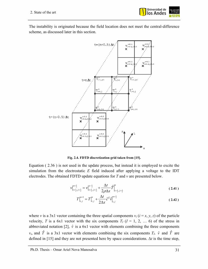
Equations ( 2.38 ) and ( 2.40 ) are discretized according to an FDTD scheme in two dimensions (in the sagittal plane or x–z plane of Fig. 2.1). In this way, the update equations to compute the T and v fields in each time step are obtained. The FDTD scheme uses the discretization grid in space and time presented in Fig. 2.4. In this figure, the subscripts of the fields indicate the cell position into the discretization grid, while the superscripts indicate the time instance in which the field is computed.
The time discretization follows a scheme known as leapfrog scheme, also used in electromagnetics [16, 17], in which v is updated midway between two consecutive updates of T. To meet the FDTD scheme, in [15] the v field is arbitrarily located at half grid points and computed at half time instances (see Fig. 2.4). Conversely, the T field is located at integer grid points and computed at integer time instances (see Fig. 2.4). The arbitrary location of these fields into the discretization grid produces instability of the simulation.
31 Ph.D. Thesis – Omar Ariel Nova Manosalva
2. State of the art
The instability is originated because the field location does not meet the central-difference scheme, as discussed later in this section.
Fig. 2.4. FDTD discretization grid taken from [15].
Equation ( 2.36 ) is not used in the update process, but instead it is employed to excite the simulation from the electrostatic E field induced after applying a voltage to the IDT electrodes. The obtained FDTD update equations for T and v are presented below.
1 12 2
1 1 1 1 1 12 2 2 2 2 2, , ,
ˆ2
nn n
i j i j i j
tv v T
x
( 2.41 )
121
, , ,ˆ ˆ
2
nn n E
i j i j i j
tT T c v
x
( 2.42 )
where v is a 3x1 vector containing the three spatial components vi (i = x, y, z) of the particle velocity, T is a 6x1 vector with the six components TI (I = 1, 2, … 6) of the stress in abbreviated notation [2], v is a 6x1 vector with elements combining the three components
vi, and T is a 3x1 vector with elements combining the six components TI. v and T are defined in [15] and they are not presented here by space considerations. Δt is the time step,

32 Ph.D. Thesis – Omar Ariel Nova Manosalva
2. State of the art
Δx is the spatial step and ˆEc is the stiffened stiffness matrix, computed as the inverse
matrix of ˆEs in ( 2.39 ).
The approach of updating only the acoustic fields T and v through the FDTD algorithm, while the electrostatic E field is used to excite the simulation, is also employed in this thesis. However, the difference with [15] lies in the discretization cell. In this thesis, field location into the cell is chosen to meet the central-difference scheme. The central-difference scheme must be fulfilled in the discretization of the governing equations. In particular, the discretization of the equation of motion ( 2.38 ) must satisfy this scheme. By way of illustration, the update equation for vx, obtained from ( 2.38 ), is analyzed. This equation is presented in ( 2.43 ), where Δx, Δy and Δz are the steps in the three spatial directions.
0.5 0.5
1 1, , , , , , 1, ,
6 6, , , 1,
5 5, , , , 1
n n n n
x xi j k i j k i j k i j k
n n
i j k i j k
n n
i j k i j k
tv v T T
x
tT T
y
tT T
z
( 2.43 )
According to ( 2.43 ), in a central-difference scheme the location of vx into the grid should be such that it is surrounded by T1 in the x-direction, by T6 in the y-direction and by T5 in the z-direction. Clearly this is not fulfilled by the discretization grid in Fig. 2.4, because the T components are never in line with the v components. Then, this grid does not meet the central-difference scheme. In the next chapter, it is shown that the discretization grid used in this thesis does satisfy the central-difference scheme. In other words, it is shown that the piezoelectric governing equations require field values at positions that lead naturally to discretization grid used in this thesis. It occurs in the same way in which the Maxwell’s equations lead naturally to the Yee grid [16].
The FDTD formulation in [15] was used for the simulation of electroacoustic wave propagation in different piezoelectric crystals [18]. However, PML instabilities were reported for certain substrates [18, 19]. In this thesis, it is demonstrated that PML stability can be achieved in the referred substrates by ensuring a central-difference scheme in the FDTD discretization grid, as presented by the author in [20]. The PML instability reported in [18, 19] is originated by the field location in the spatial discretization grid, which does not meet the central-difference scheme, as mentioned before.
A staggered grid that meets the central-difference scheme was proposed in [21]. However, this analysis is restricted to two-dimensional elastodynamic problems in isotropic media. The problem of interest of this thesis is the 3D simulation of SAW RFID tags, that is, the

33 Ph.D. Thesis – Omar Ariel Nova Manosalva
2. State of the art
three-dimensional piezoelectric problem in anisotropic media. Therefore, this problem cannot be modeled with the staggered grid proposed in [21]. Another staggered grid is presented in [22]. This grid is intended for simulation of electroacoustic wave propagation in piezoelectric (anisotropic) media, but this is only for the two-dimensional case. Further, the FDTD formulation is simplified to be applied on a special kind of artificial piezoelectric material known as piezoelectric superlattice (PSL) [23, 24].
The staggered grid used in this thesis is based on the works [25-27]. The spatial discretization grids proposed in each of these three works are presented in Fig. 2.5. The fields involved in the grid of [25] (Fig. 2.5a) are E (electric field), σ (stress) and u (particle velocity). In the grid of [26] (Fig. 2.5b), the fields involved are the same of [25] but with different denomination: E (electric field), T (stress) and v (particle velocity). In the grid of [27] (Fig. 2.5c) the used fields are only T (stress) and V (particle velocity), since the simulated wave is purely acoustic. In [25] and [26], the electroacoustic wave propagation in anisotropic media is addressed for applications of nondestructive evaluation (NDE) and microwave filters, respectively. In both works, the quasi-static approximation is used [2]. Grids fully staggered in space and time are proposed. The grid in [25] (Fig. 2.5a) is intended for three-dimensional simulation, while that in [26] (Fig. 2.5b) is limited to two-dimensional modeling. However, the 3D grid in [25] is developed in cylindrical coordinates for the simulation of axisymmetrical geometries. Moreover, absorbing boundary conditions are not used in [25], because the axisymmetrical geometries can be simulated just with axial and stress-free boundary conditions. It avoids the problem of PML instability reported in other works. For its part, the grid in [27] (Fig. 2.5c) is also fully staggered in space and time. This grid is developed in three dimensions, but is limited to the simulation of acoustic wave propagation in isotropic media occurring in the geophysical problem of buried land mines detection. No coupling with the electric field is presented in [27].
One of the main applications of FDTD in SAW devices is for the simulation of piezoelectric transducers. The FDTD simulation of such transducers was first proposed in [28], where the analysis is restricted to the one-dimensional case. The FDTD formulation is complex in this work, as five fields are updated in each time step: the stress (T), the particle velocity (v), the electric field (E), the electric displacement (D) and the terminal voltage of the transducer (VT). In the FDTD formulation of this thesis, only the T and v fields are updated in each time step, while the E field is used as a distributed source [18, 26].
In [29] the FDTD analysis of piezoelectric transducers is extended to two dimensions. However, the used procedure is not completely explicit. This is because, apart from the T and v fields, the electric potential (Φ) is also updated, resulting in implicit equations to obtain Φ.

34 Ph.D. Thesis – Omar Ariel Nova Manosalva
2. State of the art
(a)
(b)
(c)
Fig. 2.5. Staggered spatial discretization grids proposed in different works. (a) Grid taken from [25]. (b) Grid taken from [26]. (c) Grid taken from [27].
35 Ph.D. Thesis – Omar Ariel Nova Manosalva
2. State of the art
A first approach to the 3D modeling of piezoelectric transducers is done in [30]. However, the proposed method is an implicit finite-difference method that typically results in 7000 linear equations to obtain the particle displacement (u) and the electric potential (Φ). No staggered grid is used in [30], just a finite-difference approximation of the governing equations.
Another approach to the 3D FDTD simulation of piezoelectric transducers is presented in [31]. This approach uses fully staggered grids in space and time. However, the FDTD formulation is done in cylindrical coordinates to be applied on an axially symmetric geometry. The simulated problem does not require the use of absorbing boundary conditions. The FDTD formulation is only applied on a transversely isotropic piezoelectric. The stability of the method is not verified in other kind of anisotropic piezoelectric substrates. The fields of stress (T) and particle displacement (u) are explicitly computed, but the electric potential (Φ) is implicitly obtained as the solution of a linear system of equations.
In this thesis, the three-dimensional piezoelectric problem in anisotropic media is simulated through a fully explicit FDTD method. This is done because an explicit method is more suitable to simulate a problem for which an accurate transient computation is required.
Recently, FDTD has been used in the field of nondestructive evaluation (NDE), for the simulation of the crack detection problem [32]. This detection is done through the analysis of the interaction between SAW pulses and cracks. A staggered grid in space and time is used [33]. The computed fields are the stress (T) and the particle displacement (u). However, the simulation is limited to isotropic materials in two dimensions. No absorbing boundaries are implemented. Another recent application of FDTD to SAW devices is for the simulation of frequency shifters based on ring resonators [34]. These resonators are implemented by putting a piezoelectric layer on a silicon-on-insulator (SOI) layer. IDTs on the piezoelectric layer are used for SAW generation. The generated SAW modulates the refractive index of an optical waveguide implemented within the resonator. This modulation causes the resonance frequency shift.
2.3. StabilityinFDTDsimulationofSAWdevicesThe FDTD method is a conditionally stable method in which a stability criterion must be fulfilled by the time step to obtain stable simulations. This stability criterion gives the value of a critical time step (Δtcr) in terms of the material properties and the spatial discretization (Δx, Δy, Δz). To achieve stability, the time step (Δt) must be smaller than the critical time step [17].
For FDTD simulation of SAW devices, the conventional Courant stability criterion [17] has been used [15, 18]. This criterion is presented in ( 2.44 ).
36 Ph.D. Thesis – Omar Ariel Nova Manosalva
2. State of the art
max2 2 2
1 1
1 1 1t
V
x y z
( 2.44 )
where Vmax is the largest wave velocity in the medium
Nevertheless, for anisotropic media the critical time step given by the Courant criterion is not the real one. This is because this criterion assumes that the largest wave velocity (Vmax) is valid for every propagation direction in the medium [35]. However, in an anisotropic medium the wave velocity depends on the propagation direction and then, it is not correct to use just one wave velocity for the whole medium. Therefore, by using Vmax in ( 2.44 ), the obtained critical time step is not the correct one. However, this false critical time step results to be always smaller than the correct one. It allows obtaining stable simulations with the false critical time step. The problem is that more simulation time is consumed if the false critical time step is used. Valuable simulation time can be spared by considering the anisotropy of the medium. This is done in [35], where a stability criterion is derived for orthotropic media, an special kind of anisotropic media [36]. The derivation of this criterion is presented below.
The solution f of a finite-difference method in the time t+Δt (f t+Δt) can be given in terms of the solution in the time t (f t) as:
t t tf Gf ( 2.45 )
where G is the approximation matrix.
Similarly, the solution in the time t+nΔt (f t+nΔt) is given by
t n t n tf G f ( 2.46 )
It can be shown that the method is stable if the absolute values of all eigenvalues of G are smaller or equal to 1 (|λi| ≤ 1).
To obtain the approximation matrix G for a given FDTD staggered grid, a harmonic ansatz for the fields computed through the FDTD algorithm must be inserted into the update equations. In this case, the computed fields are the particle displacement (u) and the stress (T). The harmonic ansatz are:
0 exp x y zu u J k i x k j y k k z ( 2.47 )
0 exp x y zT T J k i x k j y k k z ( 2.48 )

37 Ph.D. Thesis – Omar Ariel Nova Manosalva
2. State of the art
where i, j, k denote the grid position in the x, y, z directions, respectively, Δx, Δy, Δz are the
steps in the three spatial directions, 1J , kx, ky, kz are the wavenumbers in the x, y, z directions, respectively, and u0, T0 are initial vectors of u, T, respectively.
By inserting the ansatz ( 2.47 ) and ( 2.48 ) into the update equations given in [35], the following matrix equations are obtained.
1 10 0 0 02
2n n nu u u ATt
( 2.49 )
0 0T nT CA u ( 2.50 )
where the superscripts of u0 indicate the time instance, ρ is the density, C is the stiffness matrix, and A is a matrix given by:
0 0 0
0 0 0
0 0 0
yx z
y x z
yxz
ss s
x y z
s s sA
y x z
sss
z x y
( 2.51 )
with sx, sy, sz given by:
sin2x x
xs k
( 2.52 )
sin2y y
ys k
( 2.53 )
sin2z z
zs k
( 2.54 )
To obtain an equation with the form of ( 2.45 ), ( 2.50 ) is substituted into ( 2.49 ), which results in ( 2.55 )
1 10 0 0 02
2n n n T nu u u ACA ut
( 2.55 )
By regrouping ( 2.55 ), ( 2.56 ) is obtained:

38 Ph.D. Thesis – Omar Ariel Nova Manosalva
2. State of the art
21
0 01
0 0
2
0
Tn n
n n
tACA I Iu u
u uI
( 2.56 )
where I is the identity matrix.
The equation ( 2.56 ) already has the form of ( 2.45 ), since it can be seen as
1n nw Gw ( 2.57 )
Then, the eigenvalues of G, λi (i = 1, 2), must be found and the stability criterion (|λi| ≤ 1) verified. To do it, a second harmonic ansatz in the time domain given by
0 0 expnu u J n t ( 2.58 )
is inserted into ( 2.55 ) to obtain:
0 02
12 Tu ACA u
t
( 2.59 )
where λ is an eigenvalue of G and is given by:
exp J t ( 2.60 )
By defining v as
2
12v
t
( 2.61 )
equation ( 2.59 ) results in
0 0Tvu ACA u ( 2.62 )
This equation is an eigenvalue problem, where v is an eigenvalue of ACAT.
From ( 2.61 ), the two solutions for λ are obtained:
39 Ph.D. Thesis – Omar Ariel Nova Manosalva
2. State of the art
21,2 1F F
( 2.63 )
with F given by:
2
12
tF v
( 2.64 )
Since λi (i = 1, 2) are the eigenvalues of the approximation matrix G, the condition |λi| ≤ 1 must be satisfied. To fulfill this condition, F must satisfy -1 ≤ F ≤ 1. It results in the following conditions for the three eigenvalues v of the matrix ACAT (ACAT is a 3x3 matrix):
0v ( 2.65 )
24v
t
( 2.66 )
According to ( 2.65 ), the three eigenvalues v are negative. The critical time step (Δtcr) is obtained from ( 2.66 ) by solving for Δt. The expression for Δtcr is:
4mincrt
v
( 2.67 )
The minimum value of 4 v , for the three eigenvalues v, is taken in ( 2.67 ) to get Δtcr.
Therefore, the procedure to obtain Δtcr is reduced to compute the three eigenvalues v of the matrix ACAT and then the value of Δtcr by means of ( 2.67 ). To obtain the minimum value of Δtcr, the matrix ACAT must be computed for the maximum values of the variables sx, sy, sz defined in ( 2.52 ) - ( 2.54 ), that is sx = sy = sz = 1. Simulation stability is achieved for Δt ≤ Δtcr. This is the stability criterion used for all the FDTD simulations presented in this document.
In [35], it has been shown that the use of Δtcr computed from ( 2.67 ) instead of that given by the Courant criterion ( 2.44 ) results in 38% of reduction in the simulation time in a material with strong anisotropy. This is a considerable saving of simulation time.
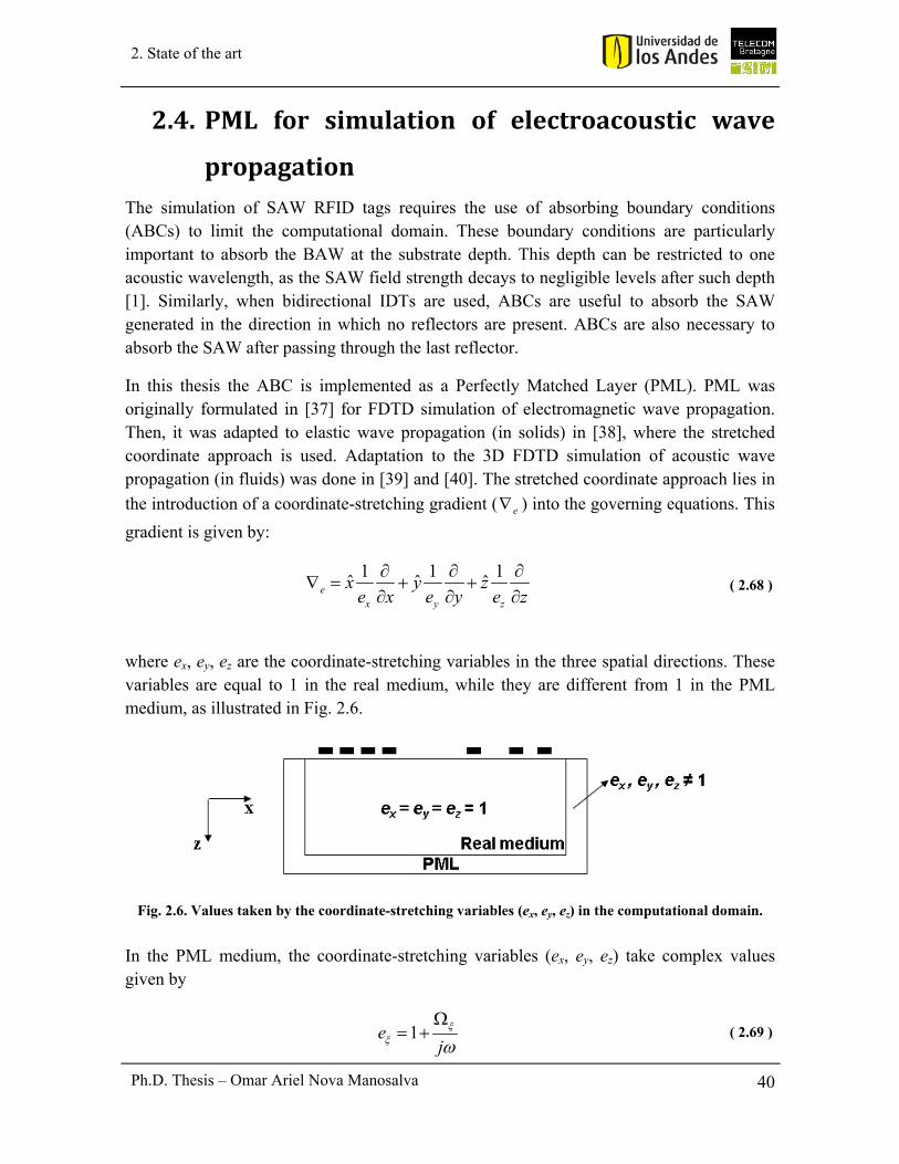
40 Ph.D. Thesis – Omar Ariel Nova Manosalva
2. State of the art
2.4. PML for simulation of electroacoustic wave
propagationThe simulation of SAW RFID tags requires the use of absorbing boundary conditions (ABCs) to limit the computational domain. These boundary conditions are particularly important to absorb the BAW at the substrate depth. This depth can be restricted to one acoustic wavelength, as the SAW field strength decays to negligible levels after such depth [1]. Similarly, when bidirectional IDTs are used, ABCs are useful to absorb the SAW generated in the direction in which no reflectors are present. ABCs are also necessary to absorb the SAW after passing through the last reflector.
In this thesis the ABC is implemented as a Perfectly Matched Layer (PML). PML was originally formulated in [37] for FDTD simulation of electromagnetic wave propagation. Then, it was adapted to elastic wave propagation (in solids) in [38], where the stretched coordinate approach is used. Adaptation to the 3D FDTD simulation of acoustic wave propagation (in fluids) was done in [39] and [40]. The stretched coordinate approach lies in
the introduction of a coordinate-stretching gradient ( e ) into the governing equations. This
gradient is given by:
1 1 1ˆ ˆ ˆe
x y z
x y ze x e y e z
( 2.68 )
where ex, ey, ez are the coordinate-stretching variables in the three spatial directions. These variables are equal to 1 in the real medium, while they are different from 1 in the PML medium, as illustrated in Fig. 2.6.
Fig. 2.6. Values taken by the coordinate-stretching variables (ex, ey, ez) in the computational domain.
In the PML medium, the coordinate-stretching variables (ex, ey, ez) take complex values given by
1ej
( 2.69 )

41 Ph.D. Thesis – Omar Ariel Nova Manosalva
2. State of the art
with ξ: x, y, z and Ωξ being the PML loss profile defined as
max
m
PML
l
N
( 2.70 )
where Ωmax = Amax NPML / ∆t. Amax is a parameter to be optimized and NPML is the number of PML cells. Δlξ is the distance between the PML cell and the border of the real medium, and the exponent m is another parameter to be optimized that takes values between 2 and 4.
In the PML medium, losses on propagating waves are generated. The origin of these losses can be explained by considering a plane wave propagating in a lossless medium given by
jkxe . If the coordinate-stretching variables are complex, as occurs in the PML medium, the
stretching of coordinates can be seen as a change of variable 'x x r j , where x’ is
the stretched coordinate. With this change of variable, jkxe becomes ' 'kx jkrxe e , where the
term 'kxe produces wave attenuation in the stretched coordinate x’ of the PML medium [38].
From the definitions of eξ and Ωξ in ( 2.69 ) and ( 2.70 ), respectively, and considering the values taken by eξ in the computational domain (see Fig. 2.6), the values taken by Ωξ are easily established: Ωξ = 0 in the real medium and Ωξ ≠ 0 in the PML medium, as illustrated in Fig. 2.7.
Fig. 2.7. Values taken by the PML loss profile (Ωx, Ωy, Ωz) in the computational domain.
To be more precise, Ωx, Ωy and Ωz are not simultaneously equal to 0 in all the regions of the PML medium. This only occurs in the corner regions of the PML, as illustrated in Fig. 2.8 taken from [40]. In this figure, the variables sx, sy and sz correspond to the coordinate-stretching variables denominated in this thesis ex, ey and ez, respectively. In Fig. 2.8 it is shown that the coordinate-stretching variable sξ (ξ: x, y, z) takes a complex value just in those regions where the PML is perpendicular to the ξ direction.
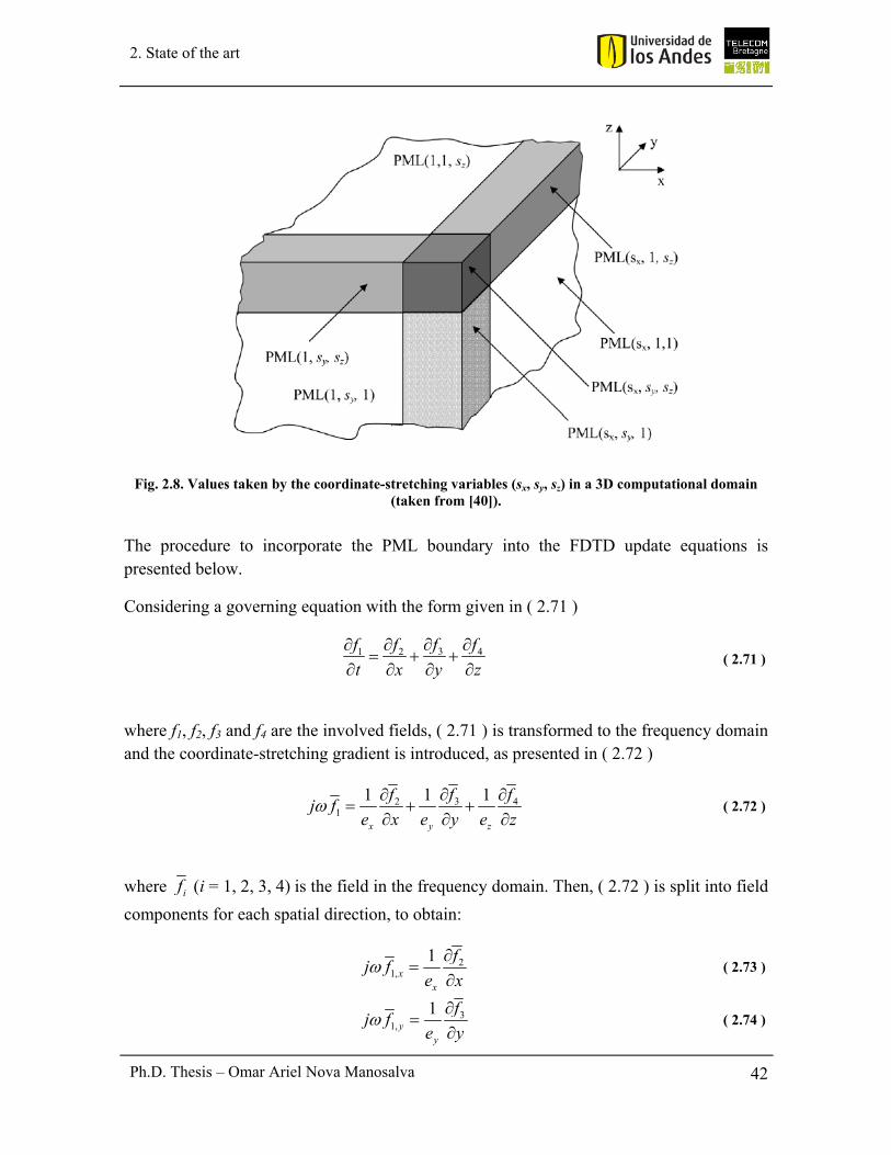
42 Ph.D. Thesis – Omar Ariel Nova Manosalva
2. State of the art
Fig. 2.8. Values taken by the coordinate-stretching variables (sx, sy, sz) in a 3D computational domain (taken from [40]).
The procedure to incorporate the PML boundary into the FDTD update equations is presented below.
Considering a governing equation with the form given in ( 2.71 )
31 2 4ff f f
t x y z
( 2.71 )
where f1, f2, f3 and f4 are the involved fields, ( 2.71 ) is transformed to the frequency domain and the coordinate-stretching gradient is introduced, as presented in ( 2.72 )
32 41
1 1 1
x y z
ff fj f
e x e y e z
( 2.72 )
where if (i = 1, 2, 3, 4) is the field in the frequency domain. Then, ( 2.72 ) is split into field
components for each spatial direction, to obtain:
21,
1x
x
fj f
e x
( 2.73 )
31,
1y
y
fj f
e y
( 2.74 )
43 Ph.D. Thesis – Omar Ariel Nova Manosalva
2. State of the art
41,
1z
z
fj f
e z
( 2.75 )
The derivation is done hereinafter only for the split equation corresponding to the x direction ( 2.73 ). However, the derivation for the other directions follows the same procedure. By replacing the coordinate-stretching variable definition ( 2.69 ) into ( 2.73 ), the following equation is obtained:
21,
1
1x
x
fj f
x
j
( 2.76 )
This equation can be rearranged as:
21,x x
fj f
x
( 2.77 )
By transforming ( 2.77 ) back into the time-domain ( 2.78 ) is obtained:
21,x x
ff
t x
( 2.78 )
Equation ( 2.78 ) is the split governing equation in the x direction, with the PML boundary incorporated. To obtain the corresponding FDTD update equation, ( 2.78 ) must be conveniently discretized. By doing this, ( 2.79 ) is obtained:
1 0.5 0.51, 1, 0.5 2 2, , , , 1, , , ,
1, , ,
n n n nx x ni j k i j k i j k i j k
x x i j k
f f f ff
t x
( 2.79 )
where the subscripts indicate the grid position and the superscripts the time instance. Δt and Δx are the temporal and the spatial step, respectively. In a staggered grid, the f1 field can only be updated either in integer time instances or in half time instances. In this case, f1 is
chosen to be updated only in integer time instances. Then, the field sample 0.5
1, , ,
n
x i j kf
must be
approximated by:
0.5 1
1, 1, 1,, , , , , ,
1
2
n n n
x x xi j k i j k i j kf f f
( 2.80 )

44 Ph.D. Thesis – Omar Ariel Nova Manosalva
2. State of the art
By introducing ( 2.80 ) into ( 2.79 ), the following equation is obtained:
1 0.5 0.5
1, 1, 1 2 2, , , , 1, , , ,1, 1,, , , ,2
n n n nx x n ni j k i j k i j k i j kx
x xi j k i j k
f f f ff f
t x
( 2.81 )
Finally, equation ( 2.81 ) can be rearranged to obtain the FDTD update equation for f1,x presented in ( 2.82 ).
1 0.5 0.5
1, 1, 2 21, , , ,, , , ,
2 2
2 2
n n n nxx x i j k i j ki j k i j k
x x
t tf f f f
t x t
( 2.82 )
To express the update equations in a more compact form, it is conventional to define auxiliary variables as the following:
2
2x
xx
t
t
( 2.83 )
2
2xx
t
x t
( 2.84 )
Therefore, the update equation in ( 2.82 ) can be written in a more compact form as:
1 0.5 0.5
1, 1, 2 21, , , ,, , , ,
n n n n
x x x x i j k i j ki j k i j kf f f f
( 2.85 )
Equation ( 2.85 ) is in the form in which FDTD update equations including PML boundaries are conventionally presented.
Application of the PML in anisotropic media is presented in [41]. However, the analysis is limited to the two-dimensional elastodynamic case, where the coupling between electric and acoustic fields is not considered. An approach to the PML for absorption of elastic waves in piezoelectric substrates is presented in [42]. In this work, a PML variation known as Convolution-PML (C-PML) is proposed. With this variation, splitting of the computed fields is not required [43]. However, in [42] the developed C-PML formulation is only applied to FEM-based simulations in COMSOL Multiphysics software. No FDTD simulations are done. Another PML formulation in which the field splitting is not required is presented in [44]. No splitting is necessary because the PML is treated as an anisotropic medium itself to allow the matching between its acoustic impedance and that of the
45 Ph.D. Thesis – Omar Ariel Nova Manosalva
2. State of the art
computational domain. The formulation is done in three dimensions for both FEM and FDTD simulation of elastic wave propagation in anisotropic media. However, the governing equations are purely elastic, that is, they do not consider the coupling with the electric fields.
In [45] PML was first applied to absorb electroacoustic waves in 2D FDTD simulations on piezoelectric media. However, PML instability for FDTD simulations on certain piezoelectric crystals was reported in [19] and [18]. A new PML formulation for electroacoustic waves in piezoelectric materials was developed in [46]. This new formulation is stable in two-dimensional FDTD simulations on lithium niobate (LiNbO3). PML stability is not demonstrated for the three-dimensional case or for other substrates with different crystal symmetry class. In this thesis, PML stability is achieved in three-dimensional FDTD simulations on three substrates with different crystal symmetry class:
orthorhombic 2mm (barium sodium niobate, Ba2NaNb5O15), cubic 43m (bismuth germanate, Bi4Ge3O12), and trigonal 3m (lithium niobate, LiNbO3). The substrate of bismuth germanate, reported as unstable in [19] and [18], is among the substrates for which PML stability is demonstrated in this thesis [20]. PML stability in the continuous medium is verified by evaluating the sufficient stability conditions given in [36]. To maintain the PML stability in the discretized medium, the discretization grid is adapted to meet a central-difference scheme [20]. PML stability is demonstrated by verifying that the total energy of the piezoelectric system does not increase after reaching the steady state, as proposed in [47] for the elastodynamic case.
2.5. Challenges in the3D simulationof SAWRFID
tags
2.5.1. SH–SAWsimulationThe 2D methods for simulation of SAW RFID tags are restricted to model the problem in the sagittal plane (x–z plane in Fig. 2.1). Therefore, simulation of SH waves cannot be done by means of 2D methods, since fields polarized in the transverse direction (y–direction in Fig. 2.1) cannot be taken into account [48].
If the IDT electrodes are long enough, that is, if their aperture or length in the transverse direction (W) is greater than 15 acoustic wavelengths (λ) [49], no variation of the fields can be assumed in the transverse direction. Thus, the derivative of fields in this direction can be assumed equal to zero (∂/∂y = 0) and the 3D governing equations can be simplified [48]. However, fields polarized in the y–direction must be still considered.
46 Ph.D. Thesis – Omar Ariel Nova Manosalva
2. State of the art
When the IDT electrodes are not long enough (W < 15λ), field variation in the y–direction must be considered. Hence, in this case ∂/∂y = 0 cannot be assumed and the 3D governing equations must be entirely considered.
The numerical procedures for simulation of SH-SAW waves that are proposed in [48] and [49] assume ∂/∂y = 0. This assumption restricts the modeling to IDTs with long electrodes (W > 15λ). In addition, this assumption also prevents simulation of geometric variations of the electrodes in the transverse direction. It limits the design versatility of the SAW technology, which is one of its main advantages [50]. As mentioned in section 2.1, other works that address the 3D simulation of SAW devices [11] [12] [13] are also compelled to introduce some simplifying assumptions to enable the modeling. Therefore, complete consideration of the three spatial directions in the SAW RFID tag modeling is still required. In this thesis, an FDTD procedure is proposed to achieve it. This procedure allows 3D simulation through the full wave modeling of the 3D piezoelectric governing equations.
2.5.2. GeometricvariationsinthetransversedirectionPiezoelectric substrates used in SAW RFID tags have lengths of several hundred of acoustic wavelengths [1]. Taking advantage of this property, transducers and reflectors can be located and oriented on the piezoelectric substrate with many degrees of freedom. It gives great versatility to the tag geometric pattern, which can be realized by means of the photolithographic fabrication process. In view of this versatility, it is convenient to have numerical methods for 3D tag simulation, able to consider geometric variations of transducers and reflectors in the transverse direction. Some of these variations are illustrated in Fig. 2.9 and discussed below.
2.5.2.1. SlantedorfannedtransducersThese are transducers in which the separation between consecutive electrodes, or pitch, is continuously varied in the transverse direction, as shown in Fig. 2.9a. In this figure, the pitch is larger at the lower side of the IDT and smaller at the upper side [51]. This is done to increase the operational bandwidth of the transducer, since the signal is better generated at transverse locations where the pitch corresponds to half the wavelength. In this way, a flat response is obtained into the operational bandwidth, as well as sharp cutoffs at the ends of the passband region and a good stop-band rejection. This kind of IDTs can be used in ultra-wideband SAW RFID tags, as an alternative to the IDT geometry proposed in [52], in which the pitch is varied only in the longitudinal direction. To simulate the continuous pitch variation in the transverse direction, a simulator with 3D modeling capability is required.
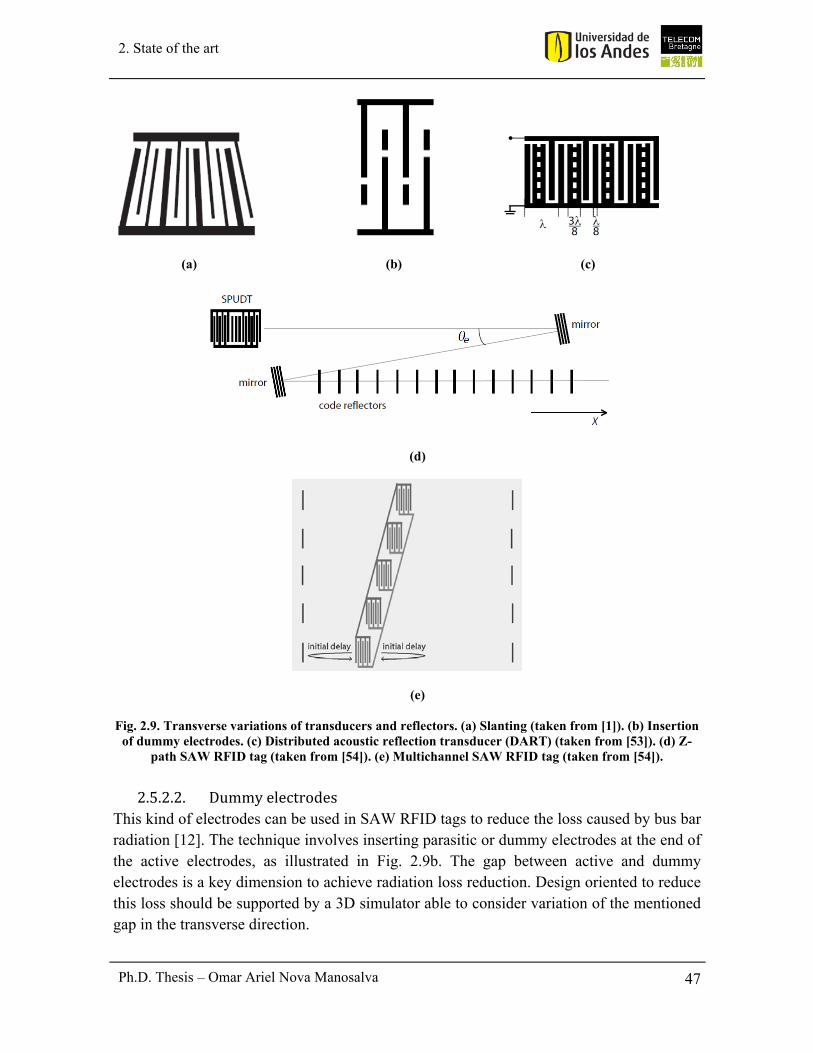
47 Ph.D. Thesis – Omar Ariel Nova Manosalva
2. State of the art
(a) (b) (c)
(d)
(e)
Fig. 2.9. Transverse variations of transducers and reflectors. (a) Slanting (taken from [1]). (b) Insertion of dummy electrodes. (c) Distributed acoustic reflection transducer (DART) (taken from [53]). (d) Z-
path SAW RFID tag (taken from [54]). (e) Multichannel SAW RFID tag (taken from [54]).
2.5.2.2. DummyelectrodesThis kind of electrodes can be used in SAW RFID tags to reduce the loss caused by bus bar radiation [12]. The technique involves inserting parasitic or dummy electrodes at the end of the active electrodes, as illustrated in Fig. 2.9b. The gap between active and dummy electrodes is a key dimension to achieve radiation loss reduction. Design oriented to reduce this loss should be supported by a 3D simulator able to consider variation of the mentioned gap in the transverse direction.
48 Ph.D. Thesis – Omar Ariel Nova Manosalva
2. State of the art
2.5.2.3. Distributedacousticreflectiontransducer(DART)This is a special IDT geometry with acoustic reflection dot elements distributed in the transverse direction of the electrodes (Fig. 2.9c) [55]. This dot arrangement makes the transducer to be unidirectional and, in turn, allows control of its internal reflectivity [53]. Then, DART is a good choice to reduce loss of SAW RFID tags, since it directs all the SAW energy in a single direction (no energy is lost in the other direction) and controls the internal reflections loss. It also allows tag size reduction, as reflectors are located on only one side of the transducer. To support the DART design, it is required a 3D simulator able to consider the arrangement in the transverse direction of the reflection dot elements.
2.5.2.4. Z‐pathSAWRFIDtagThis design is proposed to reduce the tag length by using the same space for both the initial delay and the code reflectors (Fig. 2.9d) [54]. Conventional inline tags require twice the length of Z-path tags. This is achieved by folding the propagation path of the SAW by means of two inclined reflectors (mirrors). The first inclined reflector is located at the end of the initial delay path. This reflector redirects the SAW towards the second inclined reflector, located under the IDT, in the transverse direction. Finally, the SAW is directed towards the code reflectors to complete the code reading process as in a conventional tag. The SAW echoes travel the same path in the opposite direction. A 3D simulator able to consider the transverse direction is required for the Z-path tag design. Tilt angle of the inclined reflectors and coupling of the inclined reflectors with both the IDT and the code reflectors are two aspects that must be considered in the transverse direction.
2.5.2.5. MultichannelSAWRFIDtagThis is another approach to tag length reduction in the longitudinal direction [56] [57]. In this tag, the code is stored in the distance between the transducer and the reflectors located at both sides of it, in one acoustic channel. Several channels are arranged in parallel, in the transverse direction (Fig. 2.9e). To design this kind of tags, a 3D simulator is essential. Coupling between parallel channels is an issue to be considered since it is a major source of losses for the tag.
2.6. ComputationalcomplexityoftheproblemThe typical dimensions of a SAW RFID tag are presented in Fig. 2.10. The larger dimension is in the longitudinal direction, where the initial delay path and the distances between reflectors amount to a length of 1000 acoustic wavelengths (λa). In the transverse direction, the IDT aperture is about 60 λa, and in the normal direction, the depth of the substrate can be restricted to 3 λa because the SAW is confined to a depth of about 1 λa.
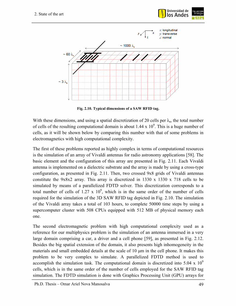
49 Ph.D. Thesis – Omar Ariel Nova Manosalva
2. State of the art
Fig. 2.10. Typical dimensions of a SAW RFID tag.
With these dimensions, and using a spatial discretization of 20 cells per λa, the total number of cells of the resulting computational domain is about 1.44 x 10⁹. This is a huge number of cells, as it will be shown below by comparing this number with that of some problems in electromagnetics with high computational complexity.
The first of these problems reported as highly complex in terms of computational resources is the simulation of an array of Vivaldi antennas for radio astronomy applications [58]. The basic element and the configuration of this array are presented in Fig. 2.11. Each Vivaldi antenna is implemented on a dielectric substrate and the array is made by using a cross-type configuration, as presented in Fig. 2.11. Then, two crossed 9x8 grids of Vivaldi antennas constitute the 9x8x2 array. This array is discretized in 1330 x 1330 x 718 cells to be simulated by means of a parallelized FDTD solver. This discretization corresponds to a total number of cells of 1.27 x 10⁹, which is in the same order of the number of cells required for the simulation of the 3D SAW RFID tag depicted in Fig. 2.10. The simulation of the Vivaldi array takes a total of 103 hours, to complete 50000 time steps by using a supercomputer cluster with 508 CPUs equipped with 512 MB of physical memory each one.
The second electromagnetic problem with high computational complexity used as a reference for our multiphysics problem is the simulation of an antenna immersed in a very large domain comprising a car, a driver and a cell phone [59], as presented in Fig. 2.12. Besides the big spatial extension of the domain, it also presents high inhomogeneity in the materials and small embedded details at the scale of 10 μm in the cell phone. It makes this problem to be very complex to simulate. A parallelized FDTD method is used to accomplish the simulation task. The computational domain is discretized into 5.04 x 10⁹ cells, which is in the same order of the number of cells employed for the SAW RFID tag simulation. The FDTD simulation is done with Graphics Processing Unit (GPU) arrays for
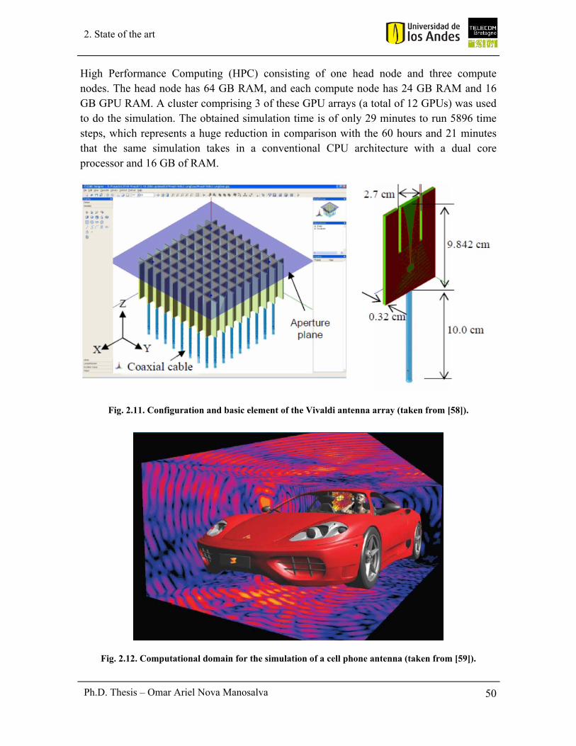
50 Ph.D. Thesis – Omar Ariel Nova Manosalva
2. State of the art
High Performance Computing (HPC) consisting of one head node and three compute nodes. The head node has 64 GB RAM, and each compute node has 24 GB RAM and 16 GB GPU RAM. A cluster comprising 3 of these GPU arrays (a total of 12 GPUs) was used to do the simulation. The obtained simulation time is of only 29 minutes to run 5896 time steps, which represents a huge reduction in comparison with the 60 hours and 21 minutes that the same simulation takes in a conventional CPU architecture with a dual core processor and 16 GB of RAM.
Fig. 2.11. Configuration and basic element of the Vivaldi antenna array (taken from [58]).
Fig. 2.12. Computational domain for the simulation of a cell phone antenna (taken from [59]).
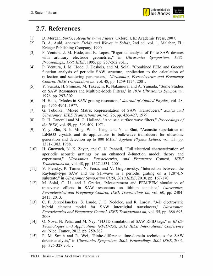
51 Ph.D. Thesis – Omar Ariel Nova Manosalva
2. State of the art
2.7. References[1] D. Morgan, Surface Acoustic Wave Filters. Oxford, UK: Academic Press, 2007. [2] B. A. Auld, Acoustic Fields and Waves in Solids, 2nd ed. vol. 1. Malabar, FL:
Krieger Publishing Company, 1990. [3] P. Ventura, J. M. Hode, and B. Lopes, "Rigorous analysis of finite SAW devices
with arbitrary electrode geometries," in Ultrasonics Symposium, 1995. Proceedings., 1995 IEEE, 1995, pp. 257-262 vol.1.
[4] P. Ventura, J. M. Hode, J. Desbois, and M. Solal, "Combined FEM and Green's function analysis of periodic SAW structure, application to the calculation of reflection and scattering parameters," Ultrasonics, Ferroelectrics and Frequency Control, IEEE Transactions on, vol. 48, pp. 1259-1274, 2001.
[5] Y. Suzuki, H. Shimizu, M. Takeuchi, K. Nakamura, and A. Yamada, "Some Studies on SAW Resonators and Multiple-Mode Filters," in 1976 Ultrasonics Symposium, 1976, pp. 297-302.
[6] H. Haus, "Modes in SAW grating resonators," Journal of Applied Physics, vol. 48, pp. 4955-4961, 1977.
[7] G. Tobolka, "Mixed Matrix Representation of SAW Transducers," Sonics and Ultrasonics, IEEE Transactions on, vol. 26, pp. 426-427, 1979.
[8] R. H. Tancrell and M. G. Holland, "Acoustic surface wave filters," Proceedings of the IEEE, vol. 59, pp. 393-409, 1971.
[9] Y. y. Zhu, N. b. Ming, W. h. Jiang, and Y. a. Shui, "Acoustic superlattice of LiNbO3 crystals and its applications to bulk‐wave transducers for ultrasonic generation and detection up to 800 MHz," Applied Physics Letters, vol. 53, pp. 1381-1383, 1988.
[10] H. Gnewuch, N. K. Zayer, and C. N. Pannell, "Full electrical characterization of aperiodic acoustic gratings by an enhanced -function model: theory and experiment," Ultrasonics, Ferroelectrics, and Frequency Control, IEEE Transactions on, vol. 48, pp. 1527-1531, 2001.
[11] V. Plessky, P. Turner, N. Fenzi, and V. Grigorievsky, "Interaction between the Rayleigh-type SAW and the SH-wave in a periodic grating on a 128°-LN substrate," in Ultrasonics Symposium (IUS), 2010 IEEE, 2010, pp. 167-170.
[12] M. Solal, C. Li, and J. Gratier, "Measurement and FEM/BEM simulation of transverse effects in SAW resonators on lithium tantalate," Ultrasonics, Ferroelectrics and Frequency Control, IEEE Transactions on, vol. 60, pp. 2404-2413, 2013.
[13] C. F. Jerez-Hanckes, S. Laude, J. C. Nedelec, and R. Lardat, "3-D electrostatic hybrid element model for SAW interdigital transducers," Ultrasonics, Ferroelectrics and Frequency Control, IEEE Transactions on, vol. 55, pp. 686-695, 2008.
[14] O. Nova, N. Peña, and M. Ney, "FDTD simulation of SAW RFID tags," in RFID-Technologies and Applications (RFID-TA), 2012 IEEE International Conference on, Nice, France, 2012, pp. 259-262.
[15] P. M. Smith and R. Wei, "Finite-difference time-domain techniques for SAW device analysis," in Ultrasonics Symposium, 2002. Proceedings. 2002 IEEE, 2002, pp. 325-328 vol.1.

52 Ph.D. Thesis – Omar Ariel Nova Manosalva
2. State of the art
[16] K. Yee, "Numerical solution of initial boundary value problems involving Maxwell's equations in isotropic media," Antennas and Propagation, IEEE Transactions on, vol. 14, pp. 302-307, 1966.
[17] A. Taflove and S. C. Hagness, Computational Electrodynamics: The Finite-Difference Time-Domain Method, 3rd ed. Norwood, MA: Artech House, 2005.
[18] F. Chagla and P. M. Smith, "Finite difference time domain methods for piezoelectric crystals," Ultrasonics, Ferroelectrics and Frequency Control, IEEE Transactions on, vol. 53, pp. 1895-1901, 2006.
[19] F. Chagla and P. M. Smith, "Stability considerations for perfectly matched layers in piezoelectric crystals," in Ultrasonics Symposium, 2005 IEEE, 2005, pp. 434-437.
[20] O. Nova, N. Peña, and M. Ney, "Perfectly matched layer stability in 3-D finite-difference time-domain simulation of electroacoustic wave propagation in piezoelectric crystals with different symmetry class," Ultrasonics, Ferroelectrics and Frequency Control, IEEE Transactions on, vol. 62, pp. 600-603, March, 2015.
[21] M. Sato, "Diagonally Staggered Grid for Elastodynamic Analysis Using the Finite-Difference Time-Domain Method," in Ultrasonics Symposium, 2006. IEEE, 2006, pp. 1394-1397.
[22] C. Zhang, Y. Q. Qin, G. Zhao, and Y. Y. Zhu, "Two-dimensional FDTD simulation for the acoustic propagation in a piezoelectric superlattice," in Ultrasonics Symposium (IUS), 2009 IEEE International, 2009, pp. 2031-2032.
[23] Y.-y. Zhu, X.-j. Zhang, Y.-q. Lu, Y.-f. Chen, S.-n. Zhu, and N.-b. Ming, "New Type of Polariton in a Piezoelectric Superlattice," Physical Review Letters, vol. 90, p. 053903, 2003.
[24] C.-p. Huang and Y.-y. Zhu, "Piezoelectric-Induced Polariton Coupling in a Superlattice," Physical Review Letters, vol. 94, p. 117401, 2005.
[25] M. Ferri, F. Camarena, J. Redondo, R. Picó, and M. R. Avis, "Explicit finite-difference time-domain scheme for the simulation of 1-3 piezoelectric effect in axisymmetrical configurations," Wave Motion, vol. 49, pp. 569-584, 2012.
[26] K.-Y. Wong and W.-Y. Tam, "Analysis of the frequency response of SAW filters using finite-difference time-domain method," Microwave Theory and Techniques, IEEE Transactions on, vol. 53, pp. 3364-3370, 2005.
[27] C. T. Schröder, "On the interaction of elastic waves with buried land mines: An investigation using the finite-difference time-domain method," Doctoral Dissertation, School Elect. Comput. Eng., Georgia Inst. Technol., Atlanta, GA, 2001.
[28] Z.-P. Chi, Z.-P. Zhao, and N. Li, "The modeling of piezoelectric transducers using the FDTD method," in Machine Learning and Cybernetics, 2008 International Conference on, 2008, pp. 2154-2159.
[29] Y. Yamada and M. Sato, "Application of Extended Finite-Difference Time-Domain Method to Two-Dimensional Dynamic Analysis of a Piezoelectric Vibrator," Japanese Journal of Applied Physics, vol. 37, p. 255, 1998.
[30] J. S. Hornsby and D. K. Das-Gupta, "Finite-difference modeling of piezoelectric composite transducers," Journal of Applied Physics, vol. 87, pp. 467-473, 2000.
[31] F. May and J. Dual, "Focusing of pulses in axially symmetric elastic tubes with fluid filling and piezo actuator by a finite difference simulation and a method of time reversal," Wave Motion, vol. 43, pp. 311-322, 2006.
53 Ph.D. Thesis – Omar Ariel Nova Manosalva
2. State of the art
[32] A. M. Lomonosov and P. Hess, "Finite-Difference Simulation of the Interaction of Surface Acoustic Waves with Partially Closed Surface-Breaking Cracks," International Journal of Thermophysics, vol. 34, pp. 1376-1384, 2013.
[33] A. M. Lomonosov, P. V. Grigoriev, and P. Hess, "Sizing of partially closed surface-breaking microcracks with broadband Rayleigh waves," Journal of Applied Physics, vol. 105, pp. 1-7, 2009.
[34] G. Fan, Y. Li, C. Hu, L. Lei, D. Zhao, H. Li, and Z. Zhen, "A novel concept of acousto-optic ring frequency shifters on silicon-on-insulator technology," Optics & Laser Technology, vol. 63, pp. 62-65, 2014.
[35] I. A. Veres, "Stability analysis of second- and fourth-order finite-difference modelling of wave propagation in orthotropic media," Ultrasonics, vol. 50, pp. 431-438, 2010.
[36] E. Bécache, S. Fauqueux, and P. Joly, "Stability of perfectly matched layers, group velocities and anisotropic waves," Journal of Computational Physics, vol. 188, pp. 399-433, 2003.
[37] J.-P. Berenger, "A perfectly matched layer for the absorption of electromagnetic waves," Journal of Computational Physics, vol. 114, pp. 185-200, 1994.
[38] W. C. Chew and Q. H. Liu, "Perfectly Matched Layers for Elastodynamics: A New Absorbing Boundary Condition," Journal of Computational Acoustics, vol. 04, pp. 341-359, 1996.
[39] X. Yuan, D. Borup, J. W. Wiskin, M. Berggren, R. Eidens, and S. A. Johnson, "Formulation and validation of Berenger's PML absorbing boundary for the FDTD simulation of acoustic scattering," Ultrasonics, Ferroelectrics, and Frequency Control, IEEE Transactions on, vol. 44, pp. 816-822, 1997.
[40] T. K. Katsibas and C. S. Antonopoulos, "A general form of perfectly matched layers for three-dimensional problems of acoustic scattering in lossless and lossy fluid media," Ultrasonics, Ferroelectrics, and Frequency Control, IEEE Transactions on, vol. 51, pp. 964-972, 2004.
[41] F. Collino and C. Tsogka, "Application of the perfectly matched absorbing layer model to the linear elastodynamic problem in anisotropic heterogeneous media," Geophysics, vol. 66, pp. 294-307, 2001.
[42] Y. Li, O. Bou Matar, V. Preobrazhensky, and P. Pernod, "Convolution-Perfectly Matched Layer (C-PML) absorbing boundary condition for wave propagation in piezoelectric solid," in Ultrasonics Symposium, 2008. IUS 2008. IEEE, 2008, pp. 1568-1571.
[43] O. Bou Matar, V. Preobrazhensky, and P. Pernod, "Two-dimensional axisymmetric numerical simulation of supercritical phase conjugation of ultrasound in active solid media," The Journal of the Acoustical Society of America, vol. 118, pp. 2880-2890, 2005.
[44] Y. Zheng and X. Huang, "Anisotropic Perfectly Matched Layers for Elastic Waves in Cartesian and Curvilinear Coordinates," Massachusetts Institute of Technology, Earth Resources Laboratory, 2002.
[45] F. Chagla, C. Cabani, and P. M. Smith, "Perfectly matched layer for FDTD computations in piezoelectric crystals," in Ultrasonics Symposium, 2004 IEEE, 2004, pp. 517-520 Vol.1.

54 Ph.D. Thesis – Omar Ariel Nova Manosalva
2. State of the art
[46] A. O. Montazeri, M. H. Bakr, and Y. M. Haddara, "A PML for Electroacoustic Waves in Piezoelectric Materials Using FDTD," Applied Computational Electromagnetics Society Journal, vol. 26, pp. 464-472, 2011.
[47] D. Gsell, T. Leutenegger, and J. Dual, "Modeling three-dimensional elastic wave propagation in circular cylindrical structures using a finite-difference approach," The Journal of the Acoustical Society of America, vol. 116, pp. 3284-3293, 2004.
[48] T. D. Kenny, T. B. Pollard, E. Berkenpas, and M. Pereira da Cunha, "FEM/BEM impedance and power analysis for measured LGS SH-SAW devices," Ultrasonics, Ferroelectrics and Frequency Control, IEEE Transactions on, vol. 53, pp. 402-411, 2006.
[49] T. B. Pollard, T. D. Kenny, J. F. Vetelino, and M. P. da Cunha, "Pure SH-SAW propagation, transduction and measurements on KNbO3," Ultrasonics, Ferroelectrics and Frequency Control, IEEE Transactions on, vol. 53, pp. 199-208, 2006.
[50] V. P. Plessky and L. M. Reindl, "Review on SAW RFID tags," Ultrasonics, Ferroelectrics, and Frequency Control, IEEE Transactions on, vol. 57, pp. 654-668, 2010.
[51] E. Bausk, R. Taziev, and A. Lee, "Synthesis of slanted and quasi-slanted SAW transducers," Ultrasonics, Ferroelectrics, and Frequency Control, IEEE Transactions on, vol. 51, pp. 1002-1009, 2004.
[52] S. Harma, V. P. Plessky, L. Xianyi, and P. Hartogh, "Feasibility of ultra-wideband SAW RFID tags meeting FCC rules," Ultrasonics, Ferroelectrics, and Frequency Control, IEEE Transactions on, vol. 56, pp. 812-820, 2009.
[53] S. Harma, "Surface acoustic wave RFID tags: Ideas, developments and experiments," Doctoral Dissertation, Department of Applied Physics, Helsinki University of Technology, Helsinki, 2009.
[54] S. Harma, V. P. Plessky, C. S. Hartmann, and W. Steichen, "Z-path SAW RFID tag," Ultrasonics, Ferroelectrics, and Frequency Control, IEEE Transactions on, vol. 55, pp. 208-213, 2008.
[55] T. Kodama, H. Kawabata, Y. Yasuhara, and H. Sato, "Design of Low-Loss SAW Filters Employing Distributed Acoustic Reflection Transducers," in IEEE 1986 Ultrasonics Symposium, 1986, pp. 59-64.
[56] V. P. Plessky, S. N. Kondratiev, R. Stierlin, and F. Nyffeler, "SAW tags: new ideas," in Ultrasonics Symposium, 1995. Proceedings., 1995 IEEE, 1995, pp. 117-120 vol.1.
[57] H. Skeie and D. Armstrong, "Passive interrogator label system with a surface acoustic wave transponder operating at its third harmonic and having increased bandwidth," 1988.
[58] N.-T. Huang, R. Mittra, R. Maaskant, and W. Yu, "Investigation of the vivaldi array for Square Kilometer Array (SKA) application using the parallelized FDTD code GEMS on the LOFAR blue gene/L supercomputer," in Antennas and Propagation Society International Symposium, 2007 IEEE, 2007, pp. 2341-2344.
[59] G. Del-Castillo, C. Mason, N. Chavannes, and M. Okoniewski, "High performance, high accuracy FDTD implementation on GPU architectures," Microwave Engineering Europe, pp. 10-14, July/August 2010.

55
3. FDTD simulation of SAW RFID tags in 2D
Ph.D. Thesis – Omar Ariel Nova Manosalva
3. FDTDSIMULATIONOFSAWRFIDTAGSIN2D
3.1. IntroductionPassive RFID tags are of great interest today since the absence of battery gives significant advantages regarding size, lifetime and manufacturing costs [1]. This kind of tags can be classified into integrated circuit (IC)-based tags and chipless tags. The former are the most widely used in current applications. The operation of the IC-based tags is based on a coiled antenna employed to draw the energy from the interrogation signal, by using the Faraday’s principle of magnetic induction. This energy is used to feed the chip that stores the identification code [2]. Conversely, in the chipless tags the identification code is not stored in a chip memory but in some physical features of the tag [3]. Chipless tags can be frequency-coded or time-coded. The frequency-coded tags are based on resonators that insert their signature in the frequency response of the tag [4] while the time-coded tags are based on delay-lines that set the identification code according to their length. These delay lines can be implemented as transmission lines [5, 6], for which delay times are on the order of nanoseconds. Such delay lines can be also implemented as surface acoustic waves (SAW) delay lines [7-9], with more suitable delay times on the order of microseconds.
SAW RFID tags are based on the piezoelectric effect [10] that allows converting the electromagnetic waves reaching the tag antenna into acoustic waves. This is done by means of an interdigital transducer (IDT) printed on a piezoelectric substrate. Part of the generated acoustic waves is propagated through the surface of the substrate and enables the reading of the identification code stored in the tag. This code corresponds to the distances between the IDT and some metallic reflectors printed on the substrate surface.
In this chapter, the FDTD simulation of SAW RFID tags in 2D is addressed. A simple tag geometry is simulated, consisting of a 5 periods single-electrode IDT and 3 reflectors. Propagation of incident and reflected acoustic waves or echoes is characterized through the FDTD simulation. Time position and insertion loss corresponding to each echo are also
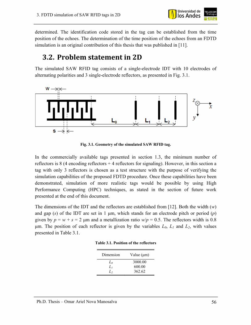
56
3. FDTD simulation of SAW RFID tags in 2D
Ph.D. Thesis – Omar Ariel Nova Manosalva
determined. The identification code stored in the tag can be established from the time position of the echoes. The determination of the time position of the echoes from an FDTD simulation is an original contribution of this thesis that was published in [11].
3.2. Problemstatementin2DThe simulated SAW RFID tag consists of a single-electrode IDT with 10 electrodes of alternating polarities and 3 single-electrode reflectors, as presented in Fig. 3.1.
Fig. 3.1. Geometry of the simulated SAW RFID tag.
In the commercially available tags presented in section 1.3, the minimum number of reflectors is 8 (4 encoding reflectors + 4 reflectors for signaling). However, in this section a tag with only 3 reflectors is chosen as a test structure with the purpose of verifying the simulation capabilities of the proposed FDTD procedure. Once these capabilities have been demonstrated, simulation of more realistic tags would be possible by using High Performance Computing (HPC) techniques, as stated in the section of future work presented at the end of this document.
The dimensions of the IDT and the reflectors are established from [12]. Both the width (w) and gap (s) of the IDT are set in 1 μm, which stands for an electrode pitch or period (p) given by p = w + s = 2 μm and a metallization ratio w/p = 0.5. The reflectors width is 0.8 μm. The position of each reflector is given by the variables L0, L1 and L2, with values presented in Table 3.1.
Table 3.1. Position of the reflectors
Dimension Value (μm)
L0 3000.00 L1 600.00 L2 362.62

57
3. FDTD simulation of SAW RFID tags in 2D
Ph.D. Thesis – Omar Ariel Nova Manosalva
The tag is implemented on a lithium niobate (LiNbO3) piezoelectric substrate with cut 128°YX or Euler angles (0°, 38°, 0°) [10]. The tag operation bandwidth ranges from 870MHz to 1080 MHz [12], which gives a central frequency of 975MHz. By using the SAW phase velocity of 3978.97 m/s given in [12] for the specified orientation of the piezoelectric crystal, the acoustic wavelength (λa) at the central frequency is 4.08μm. The total tag length (in x-direction of Fig. 3.1) is 4002.62μm, which is about 1000 λa, while the tag depth (in z-direction of Fig. 3.1) is only 4 μm, which is close to 1 λa. The depth can be restricted to 1 λa because the field variation associated to the Rayleigh SAW wave is limited to this depth [13]. The huge tag length of about 1000 λa makes it necessary to use an irregular meshing for the spatial discretization of the computational domain. To do it, a coarse mesh is used in the regions with low field variation and a fine mesh is implemented around the tag electrodes, where the field variation is high.
The modeling of the structure is done in 2D, for the sagittal plane (x–z plane in Fig. 3.1). This is possible because the IDT aperture or length in the y-direction is long enough, that is, the aperture is higher than 15 λa. Then, both the electric and the acoustic fields can be assumed invariant in the y-direction. In other words, the aperture of the IDT and reflectors is irrelevant for the modeling problem. The thickness of the electrodes is considered negligible and they are assumed to be perfect conductors.
The governing equations for the 2D problem are presented in Appendix A. By way of example, the equation for the T1 and vx fields are presented below.
11 1 11 13 15
x x xz z zx z
E v vT E v ve e c c c
t t t x z z x
( 3.1 )
511xv TT
t x z
( 3.2 )
3.3. FDTDformulationin2DThe governing equations in 2D were discretized according to [14]. Spatial discretization was done by using a staggered grid with a cell as the presented in Fig. 3.2, where the fields located on the shadow region are those associated to the cell. The temporal discretization was done according to the leapfrog scheme [14].
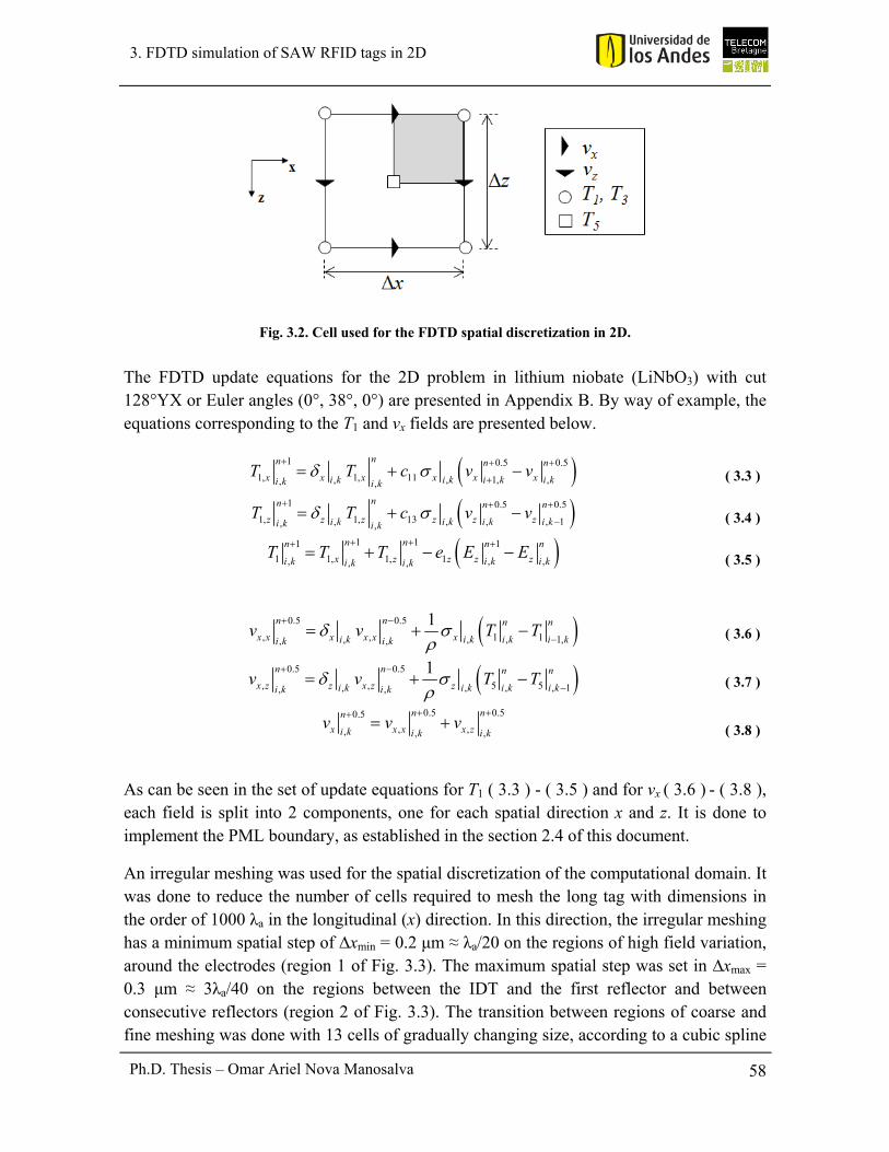
58
3. FDTD simulation of SAW RFID tags in 2D
Ph.D. Thesis – Omar Ariel Nova Manosalva
Fig. 3.2. Cell used for the FDTD spatial discretization in 2D.
The FDTD update equations for the 2D problem in lithium niobate (LiNbO3) with cut 128°YX or Euler angles (0°, 38°, 0°) are presented in Appendix B. By way of example, the equations corresponding to the T1 and vx fields are presented below.
1 0.5 0.5
1, 1, 11, , 1, ,, ,
nn n n
x x x x x xi k i k i k i ki k i kT T c v v
( 3.3 )
1 0.5 0.5
1, 1, 13, , , , 1, ,
nn n n
z z z z z zi k i k i k i ki k i kT T c v v
( 3.4 )
1 11 1
1 1, 1, 1, , ,, ,
n nn n n
x z z z zi k i k i ki k i kT T T e E E
( 3.5 )
0.5 0.5
, , 1 1, , , 1,, ,
1n n n n
x x x x x xi k i k i k i ki k i kv v T T
( 3.6 )
0.5 0.5
, , 5 5, , , , 1, ,
1n n n n
x z z x z zi k i k i k i ki k i kv v T T
( 3.7 )
0.5 0.50.5
, ,, , ,
n nn
x x x x zi k i k i kv v v
( 3.8 )
As can be seen in the set of update equations for T1 ( 3.3 ) - ( 3.5 ) and for vx ( 3.6 ) - ( 3.8 ), each field is split into 2 components, one for each spatial direction x and z. It is done to implement the PML boundary, as established in the section 2.4 of this document.
An irregular meshing was used for the spatial discretization of the computational domain. It was done to reduce the number of cells required to mesh the long tag with dimensions in the order of 1000 λa in the longitudinal (x) direction. In this direction, the irregular meshing has a minimum spatial step of ∆xmin = 0.2 μm ≈ λa/20 on the regions of high field variation, around the electrodes (region 1 of Fig. 3.3). The maximum spatial step was set in ∆xmax = 0.3 μm ≈ 3λa/40 on the regions between the IDT and the first reflector and between consecutive reflectors (region 2 of Fig. 3.3). The transition between regions of coarse and fine meshing was done with 13 cells of gradually changing size, according to a cubic spline
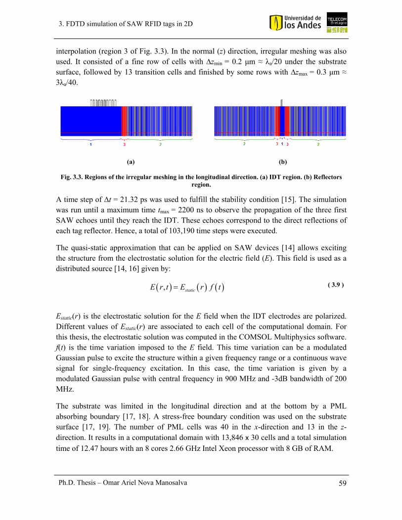
59
3. FDTD simulation of SAW RFID tags in 2D
Ph.D. Thesis – Omar Ariel Nova Manosalva
interpolation (region 3 of Fig. 3.3). In the normal (z) direction, irregular meshing was also used. It consisted of a fine row of cells with ∆zmin = 0.2 μm ≈ λa/20 under the substrate surface, followed by 13 transition cells and finished by some rows with ∆zmax = 0.3 μm ≈ 3λa/40.
(a) (b)
Fig. 3.3. Regions of the irregular meshing in the longitudinal direction. (a) IDT region. (b) Reflectors region.
A time step of ∆t = 21.32 ps was used to fulfill the stability condition [15]. The simulation was run until a maximum time tmax = 2200 ns to observe the propagation of the three first SAW echoes until they reach the IDT. These echoes correspond to the direct reflections of each tag reflector. Hence, a total of 103,190 time steps were executed.
The quasi-static approximation that can be applied on SAW devices [14] allows exciting the structure from the electrostatic solution for the electric field (E). This field is used as a distributed source [14, 16] given by:
, staticE r t E r f t ( 3.9 )
Estatic(r) is the electrostatic solution for the E field when the IDT electrodes are polarized. Different values of Estatic(r) are associated to each cell of the computational domain. For this thesis, the electrostatic solution was computed in the COMSOL Multiphysics software. f(t) is the time variation imposed to the E field. This time variation can be a modulated Gaussian pulse to excite the structure within a given frequency range or a continuous wave signal for single-frequency excitation. In this case, the time variation is given by a modulated Gaussian pulse with central frequency in 900 MHz and -3dB bandwidth of 200 MHz.
The substrate was limited in the longitudinal direction and at the bottom by a PML absorbing boundary [17, 18]. A stress-free boundary condition was used on the substrate surface [17, 19]. The number of PML cells was 40 in the x-direction and 13 in the z-direction. It results in a computational domain with 13,846 x 30 cells and a total simulation time of 12.47 hours with an 8 cores 2.66 GHz Intel Xeon processor with 8 GB of RAM.
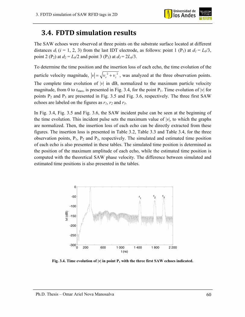
60
3. FDTD simulation of SAW RFID tags in 2D
Ph.D. Thesis – Omar Ariel Nova Manosalva
3.4. FDTDsimulationresultsThe SAW echoes were observed at three points on the substrate surface located at different distances di (i = 1, 2, 3) from the last IDT electrode, as follows: point 1 (P1) at d1 = L0/3, point 2 (P2) at d2 = L0/2 and point 3 (P3) at d3 = 2L0/3.
To determine the time position and the insertion loss of each echo, the time evolution of the
particle velocity magnitude, 2 2x zv v v , was analyzed at the three observation points.
The complete time evolution of |v| in dB, normalized to the maximum particle velocity magnitude, from 0 to tmax, is presented in Fig. 3.4, for the point P1. Time evolution of |v| for points P2 and P3 are presented in Fig. 3.5 and Fig. 3.6, respectively. The three first SAW echoes are labeled on the figures as r1, r2 and r3.
In Fig. 3.4, Fig. 3.5 and Fig. 3.6, the SAW incident pulse can be seen at the beginning of the time evolution. This incident pulse sets the maximum value of |v|, to which the graphs are normalized. Then, the insertion loss of each echo can be directly extracted from these figures. The insertion loss is presented in Table 3.2, Table 3.3 and Table 3.4, for the three observation points, P1, P2 and P3, respectively. The simulated and estimated time position of each echo is also presented in these tables. The simulated time position is determined as the position of the maximum amplitude of each echo, while the estimated time position is computed with the theoretical SAW phase velocity. The difference between simulated and estimated time positions is also presented in the tables.
Fig. 3.4. Time evolution of |v| in point P1 with the three first SAW echoes indicated.
0 200 600 1 000 1 400 1 800 2 200-300
-250
-200
-150
-100
-50
0
t (ns)
|v| (
dB)
r1
r2
r3
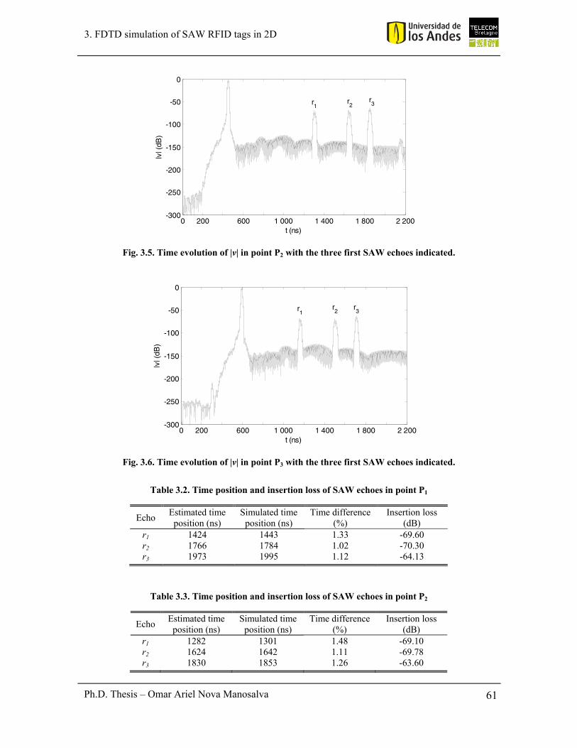
61
3. FDTD simulation of SAW RFID tags in 2D
Ph.D. Thesis – Omar Ariel Nova Manosalva
Fig. 3.5. Time evolution of |v| in point P2 with the three first SAW echoes indicated.
Fig. 3.6. Time evolution of |v| in point P3 with the three first SAW echoes indicated.
Table 3.2. Time position and insertion loss of SAW echoes in point P1
Echo Estimated time position (ns)
Simulated time position (ns)
Time difference (%)
Insertion loss (dB)
r1 1424 1443 1.33 -69.60 r2 1766 1784 1.02 -70.30 r3 1973 1995 1.12 -64.13
Table 3.3. Time position and insertion loss of SAW echoes in point P2
Echo Estimated time position (ns)
Simulated time position (ns)
Time difference (%)
Insertion loss (dB)
r1 1282 1301 1.48 -69.10 r2 1624 1642 1.11 -69.78 r3 1830 1853 1.26 -63.60
0 200 600 1 000 1 400 1 800 2 200-300
-250
-200
-150
-100
-50
0
t (ns)
|v| (
dB)
r1
r2
r3
0 200 600 1 000 1 400 1 800 2 200-300
-250
-200
-150
-100
-50
0
t (ns)
|v| (
dB)
r1
r2
r3
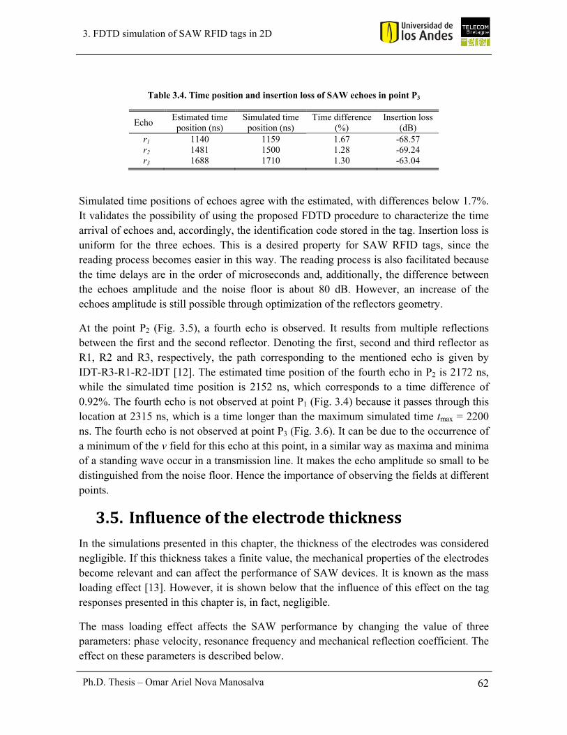
62
3. FDTD simulation of SAW RFID tags in 2D
Ph.D. Thesis – Omar Ariel Nova Manosalva
Table 3.4. Time position and insertion loss of SAW echoes in point P3
Echo Estimated time position (ns)
Simulated time position (ns)
Time difference (%)
Insertion loss (dB)
r1 1140 1159 1.67 -68.57 r2 1481 1500 1.28 -69.24 r3 1688 1710 1.30 -63.04
Simulated time positions of echoes agree with the estimated, with differences below 1.7%. It validates the possibility of using the proposed FDTD procedure to characterize the time arrival of echoes and, accordingly, the identification code stored in the tag. Insertion loss is uniform for the three echoes. This is a desired property for SAW RFID tags, since the reading process becomes easier in this way. The reading process is also facilitated because the time delays are in the order of microseconds and, additionally, the difference between the echoes amplitude and the noise floor is about 80 dB. However, an increase of the echoes amplitude is still possible through optimization of the reflectors geometry.
At the point P2 (Fig. 3.5), a fourth echo is observed. It results from multiple reflections between the first and the second reflector. Denoting the first, second and third reflector as R1, R2 and R3, respectively, the path corresponding to the mentioned echo is given by IDT-R3-R1-R2-IDT [12]. The estimated time position of the fourth echo in P2 is 2172 ns, while the simulated time position is 2152 ns, which corresponds to a time difference of 0.92%. The fourth echo is not observed at point P1 (Fig. 3.4) because it passes through this location at 2315 ns, which is a time longer than the maximum simulated time tmax = 2200 ns. The fourth echo is not observed at point P3 (Fig. 3.6). It can be due to the occurrence of a minimum of the v field for this echo at this point, in a similar way as maxima and minima of a standing wave occur in a transmission line. It makes the echo amplitude so small to be distinguished from the noise floor. Hence the importance of observing the fields at different points.
3.5. InfluenceoftheelectrodethicknessIn the simulations presented in this chapter, the thickness of the electrodes was considered negligible. If this thickness takes a finite value, the mechanical properties of the electrodes become relevant and can affect the performance of SAW devices. It is known as the mass loading effect [13]. However, it is shown below that the influence of this effect on the tag responses presented in this chapter is, in fact, negligible.
The mass loading effect affects the SAW performance by changing the value of three parameters: phase velocity, resonance frequency and mechanical reflection coefficient. The effect on these parameters is described below.
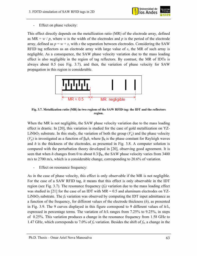
63
3. FDTD simulation of SAW RFID tags in 2D
Ph.D. Thesis – Omar Ariel Nova Manosalva
- Effect on phase velocity:
This effect directly depends on the metallization ratio (MR) of the electrode array, defined as MR = w / p, where w is the width of the electrodes and p is the period of the electrode array, defined as p = w + s, with s the separation between electrodes. Considering the SAW RFID tag reflectors as an electrode array with large value of s, the MR of such array is negligible. As a consequence, the SAW phase velocity variation due to the mass loading effect is also negligible in the region of tag reflectors. By contrast, the MR of IDTs is always about 0.5 (see Fig. 3.7), and then, the variation of phase velocity for SAW propagation in this region is considerable.
Fig. 3.7. Metallization ratio (MR) in two regions of the SAW RFID tag: the IDT and the reflectors region.
When the MR is not negligible, the SAW phase velocity variation due to the mass loading effect is drastic. In [20], this variation is studied for the case of gold metallization on YZ-LiNbO3 substrate. In this study, the variation of both the group (Vg) and the phase velocity (Vp) is investigated as a function of βRh, where βR is the phase constant for Rayleigh waves and h is the thickness of the electrodes, as presented in Fig. 3.8. A computer solution is compared with the perturbation theory developed in [20], observing good agreement. It is seen that when h changes from 0 to about 0.3/βR, the SAW phase velocity varies from 3400 m/s to 2700 m/s, which is a considerable change, corresponding to 20.6% of variation.
- Effect on resonance frequency:
As in the case of phase velocity, this effect is only observable if the MR is not negligible. For the case of a SAW RFID tag, it means that this effect is only observable in the IDT region (see Fig. 3.7). The resonance frequency (f0) variation due to the mass loading effect was studied in [21] for the case of an IDT with MR = 0.5 and aluminum electrodes on YZ-LiNbO3 substrate. The f0 variation was observed by computing the IDT input admittance as a function of the frequency, for different values of the electrode thickness (h), as presented in Fig. 3.9. The 9 curves displayed in this figure correspond to 9 different values of h/λ, expressed in percentage terms. The variation of h/λ ranges from 7.25% to 9.25%, in steps of 0.25%. This variation produces a change in the resonance frequency from 1.58 GHz to 1.47 GHz, which corresponds to 7.0% of f0 variation. Besides the shift of f0, a change in the
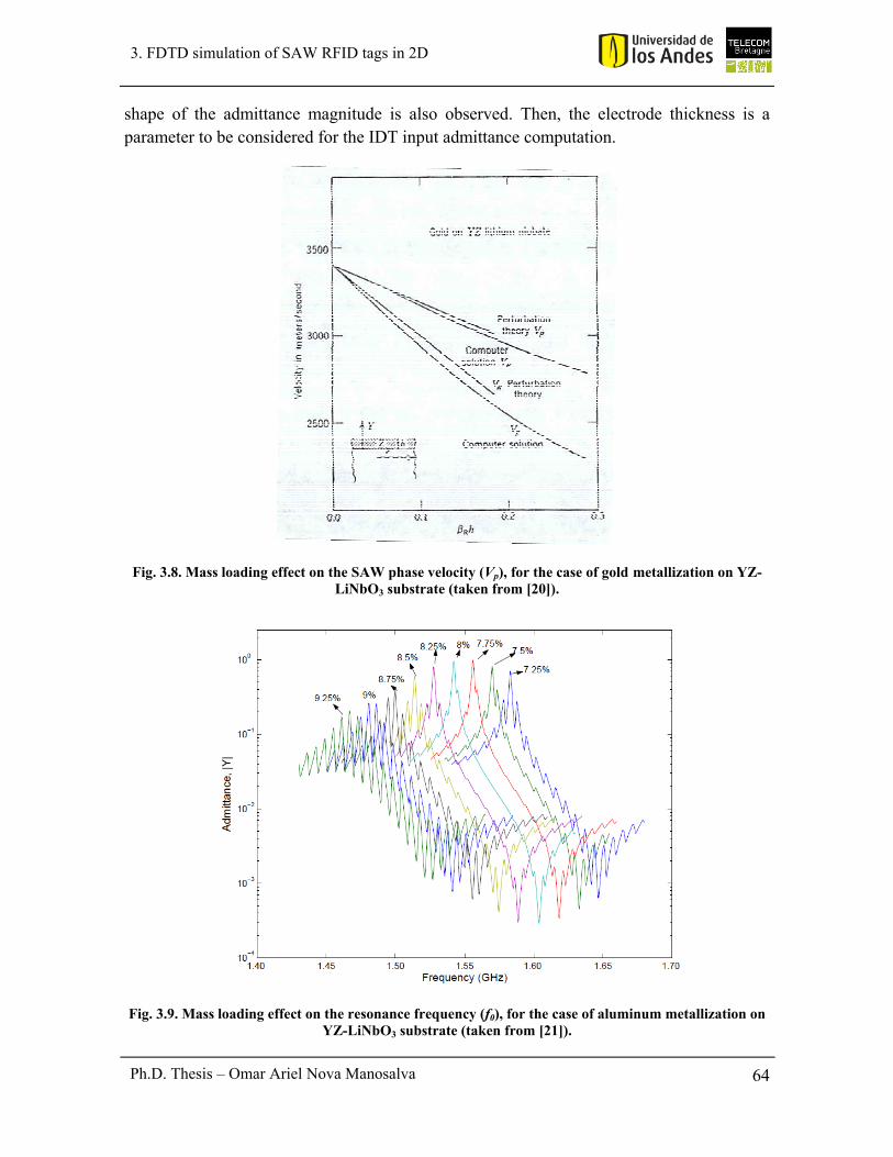
64
3. FDTD simulation of SAW RFID tags in 2D
Ph.D. Thesis – Omar Ariel Nova Manosalva
shape of the admittance magnitude is also observed. Then, the electrode thickness is a parameter to be considered for the IDT input admittance computation.
Fig. 3.8. Mass loading effect on the SAW phase velocity (Vp), for the case of gold metallization on YZ-LiNbO3 substrate (taken from [20]).
Fig. 3.9. Mass loading effect on the resonance frequency (f0), for the case of aluminum metallization on YZ-LiNbO3 substrate (taken from [21]).
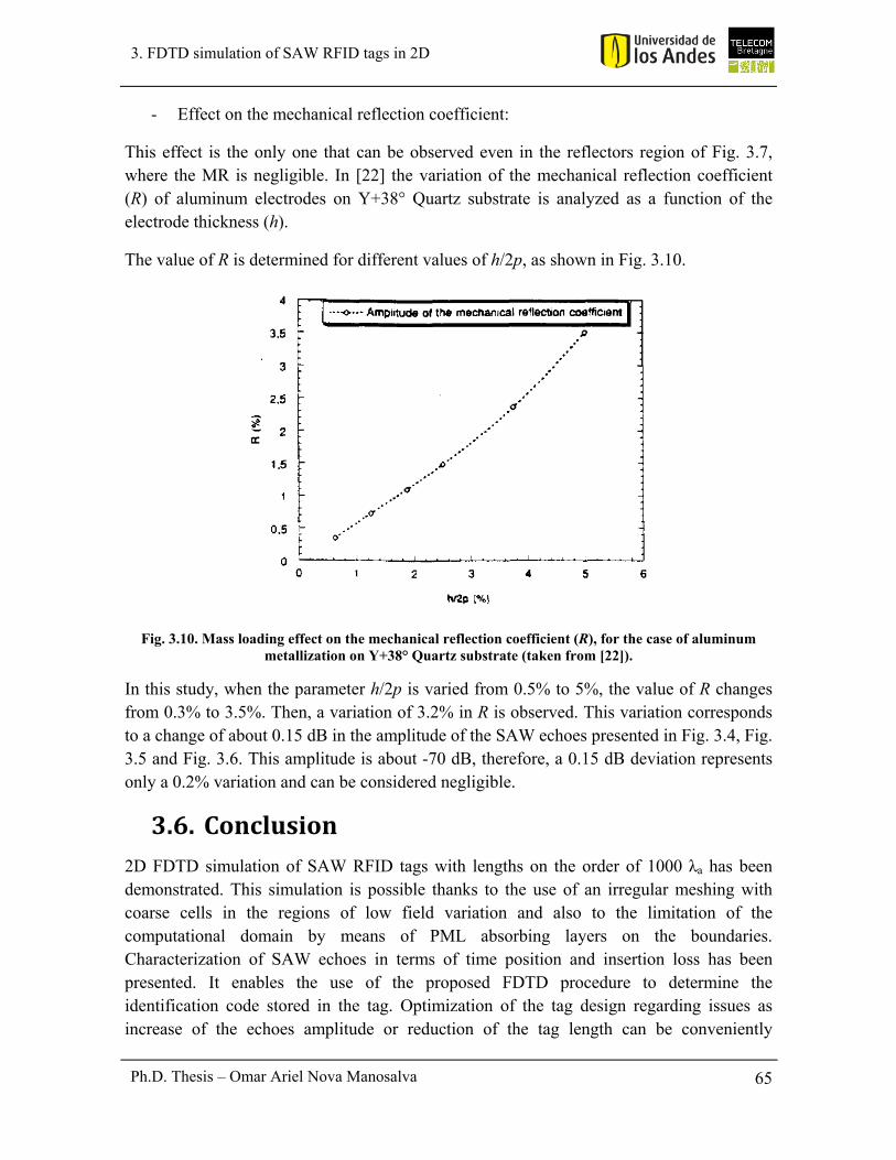
65
3. FDTD simulation of SAW RFID tags in 2D
Ph.D. Thesis – Omar Ariel Nova Manosalva
- Effect on the mechanical reflection coefficient:
This effect is the only one that can be observed even in the reflectors region of Fig. 3.7, where the MR is negligible. In [22] the variation of the mechanical reflection coefficient (R) of aluminum electrodes on Y+38° Quartz substrate is analyzed as a function of the electrode thickness (h).
The value of R is determined for different values of h/2p, as shown in Fig. 3.10.
Fig. 3.10. Mass loading effect on the mechanical reflection coefficient (R), for the case of aluminum metallization on Y+38° Quartz substrate (taken from [22]).
In this study, when the parameter h/2p is varied from 0.5% to 5%, the value of R changes from 0.3% to 3.5%. Then, a variation of 3.2% in R is observed. This variation corresponds to a change of about 0.15 dB in the amplitude of the SAW echoes presented in Fig. 3.4, Fig. 3.5 and Fig. 3.6. This amplitude is about -70 dB, therefore, a 0.15 dB deviation represents only a 0.2% variation and can be considered negligible.
3.6. Conclusion2D FDTD simulation of SAW RFID tags with lengths on the order of 1000 λa has been demonstrated. This simulation is possible thanks to the use of an irregular meshing with coarse cells in the regions of low field variation and also to the limitation of the computational domain by means of PML absorbing layers on the boundaries. Characterization of SAW echoes in terms of time position and insertion loss has been presented. It enables the use of the proposed FDTD procedure to determine the identification code stored in the tag. Optimization of the tag design regarding issues as increase of the echoes amplitude or reduction of the tag length can be conveniently

66
3. FDTD simulation of SAW RFID tags in 2D
Ph.D. Thesis – Omar Ariel Nova Manosalva
supported by the presented FDTD procedure. More complicated geometric arrangements of transducers and reflectors can be addressed, for which, the extension of the method to the 3D case will be necessary.
3.7. References[1] V. D. Hunt, A. Puglia, and M. Puglia, RFID: A guide to Radio Frequency
Identification. Hoboken, N.J.: John Wiley & Sons, 2007. [2] J.-P. Curty, M. Declercq, C. Dehollain, and N. Joehl, Design and Optimization of
Passive UHF RFID Systems. New York, NY: Springer, 2007. [3] K. Finkenzeller, RFID Handbook: Fundamentals and Applications in Contactless
Smart Cards, Radio Frequency Identification and Near-Field Communication, 3rd ed. Hoboken, N.J.: John Wiley & Sons, 2010.
[4] S. Preradovic, I. Balbin, N. C. Karmakar, and G. F. Swiegers, "Multiresonator-Based Chipless RFID System for Low-Cost Item Tracking," Microwave Theory and Techniques, IEEE Transactions on, vol. 57, pp. 1411-1419, 2009.
[5] A. Ramos, D. Girbau, A. Lazaro, and S. Rima, "IR-UWB radar system and tag design for time-coded chipless RFID," in Antennas and Propagation (EUCAP), 2012 6th European Conference on, 2012, pp. 2491-2494.
[6] D. Dardari and R. D'Errico, "Passive Ultrawide Bandwidth RFID," in Global Telecommunications Conference, 2008. IEEE GLOBECOM 2008. IEEE, 2008, pp. 1-6.
[7] D. E. N. Davies, M. J. Withers, and R. P. Claydon, "Passive coded transponder using an acoustic-surface-wave delay line," Electronics Letters, vol. 11, pp. 163-164, 1975.
[8] C. S. Hartmann, "A global SAW ID tag with large data capacity," in Ultrasonics Symposium, 2002. Proceedings. 2002 IEEE, 2002, pp. 65-69 vol.1.
[9] V. P. Plessky and L. M. Reindl, "Review on SAW RFID tags," Ultrasonics, Ferroelectrics, and Frequency Control, IEEE Transactions on, vol. 57, pp. 654-668, 2010.
[10] B. A. Auld, Acoustic Fields and Waves in Solids, 2nd ed. vol. 1. Malabar, FL: Krieger Publishing Company, 1990.
[11] O. Nova, N. Peña, and M. Ney, "FDTD simulation of SAW RFID tags," in RFID-Technologies and Applications (RFID-TA), 2012 IEEE International Conference on, Nice, France, 2012, pp. 259-262.
[12] S. Harma and V. P. Plessky, "Extraction of frequency-dependent reflection, transmission, and scattering parameters for short metal reflectors from FEM-BEM simulations," Ultrasonics, Ferroelectrics and Frequency Control, IEEE Transactions on, vol. 55, pp. 883-889, 2008.
[13] D. Morgan, Surface Acoustic Wave Filters. Oxford, UK: Academic Press, 2007. [14] K.-Y. Wong and W.-Y. Tam, "Analysis of the frequency response of SAW filters
using finite-difference time-domain method," Microwave Theory and Techniques, IEEE Transactions on, vol. 53, pp. 3364-3370, 2005.
[15] I. A. Veres, "Stability analysis of second- and fourth-order finite-difference modelling of wave propagation in orthotropic media," Ultrasonics, vol. 50, pp. 431-438, 2010.

67
3. FDTD simulation of SAW RFID tags in 2D
Ph.D. Thesis – Omar Ariel Nova Manosalva
[16] F. Chagla and P. M. Smith, "Finite difference time domain methods for piezoelectric crystals," Ultrasonics, Ferroelectrics and Frequency Control, IEEE Transactions on, vol. 53, pp. 1895-1901, 2006.
[17] C. T. Schröder, "On the interaction of elastic waves with buried land mines: An investigation using the finite-difference time-domain method," Doctoral Dissertation, School Elect. Comput. Eng., Georgia Inst. Technol., Atlanta, GA, 2001.
[18] T. K. Katsibas and C. S. Antonopoulos, "A general form of perfectly matched layers for three-dimensional problems of acoustic scattering in lossless and lossy fluid media," Ultrasonics, Ferroelectrics, and Frequency Control, IEEE Transactions on, vol. 51, pp. 964-972, 2004.
[19] M. Sato, "Comparing three methods of free boundary implementation for analyzing elastodynamics using the finite-difference time-domain formulation," Acoustical Science and Technology, vol. 28, pp. 49-52, 2007.
[20] B. A. Auld, Acoustic Fields and Waves in Solids, 2nd ed. vol. 2. Malabar, FL: Krieger Publishing Company, 1990.
[21] T. Kannan, "Finite Element Analysis of Surface Acoustic Wave Resonators," Master of Science Thesis, Department of Electrical Engineering, University of Saskatchewan, Saskatoon, Saskatchewan, 2006.
[22] P. Ventura, J. Desbois, and L. Boyer, "A mixed FEM/analytical model of the electrode mechanical perturbation for SAW and PSAW propagation," in Ultrasonics Symposium, 1993. Proceedings., IEEE 1993, 1993, pp. 205-208 vol.1.

68 Ph.D. Thesis – Omar Ariel Nova Manosalva
69 Ph.D. Thesis – Omar Ariel Nova Manosalva
4. FDTD formulation in 3D for simulation of electroacoustic wave propagation in anisotropic media
4. FDTD FORMULATION IN3D FORSIMULATIONOFELECTROACOUSTICWAVE PROPAGATION INANISOTROPICMEDIA
The problem of interest of this thesis is the three-dimensional simulation of SAW RFID tags. This involves the simulation of three-dimensional electroacoustic wave propagation in anisotropic piezoelectric media. To realize this simulation, a 3D FDTD formulation is proposed. This formulation has the following characteristics:
- It is a fully-explicit formulation. This is done because an explicit method is more suitable to simulate a problem for which an accurate transient computation is required.
- It allows full-wave simulation in three dimensions. It avoids introducing simplifying assumptions for the modeling of three dimensional structures.
- It is a general formulation directly derived from the fundamental governing equations of piezoelectricity. Then, it can be particularized for any crystal symmetry class and orientation of the piezoelectric substrate.
- It is designed to be excited by the electric field E induced by the polarization of the IDT electrodes. The E field is used as a distributed source [1, 2].
- It uses the quasi-static approximation [3] to address the multiscale problem originated by the difference in the time scales of the acoustic and the electromagnetic phenomena.
The FDTD formulation is presented in two steps: first, the definition of the governing equations to be used and, then, the discretization of such equations to obtain the FDTD update equations. To transform the governing equations into update equations, a central-difference scheme is used in space and time. The discretization is done by considering an

70 Ph.D. Thesis – Omar Ariel Nova Manosalva
4. FDTD formulation in 3D for simulation of electroacoustic wave propagation in anisotropic media
irregular meshing and two boundary conditions: the PML absorbing boundary and the stress-free boundary.
4.1. Governingequationsin3DThe FDTD formulation is based on the four fundamental governing equations of piezoelectricity [3]:
- The equation of motion:
vT
t
( 4.1 )
- The strain-displacement relation:
s
Sv
t
( 4.2 )
- The piezoelectric constitutive relations (with T as the dependent acoustic variable): Also known as the piezoelectric stress equations, they are two equations that relate the acoustic with the electric fields.
:ET e E c S ( 4.3 )
:SD E e S ( 4.4 )
The involved acoustic fields are:
- T: stress (tensor of rank 2)
- v: particle velocity
- S: strain (tensor of rank 2)
The electric fields are:
- E: electric field
- D: electric displacement
The material parameters are:
- ρ: mass density
- ,e e : piezoelectric stress constants (tensors of rank 3)

71 Ph.D. Thesis – Omar Ariel Nova Manosalva
4. FDTD formulation in 3D for simulation of electroacoustic wave propagation in anisotropic media
- cE: stiffness for constant E (tensor of rank 4)
- εS: permittivity for constant S (tensor of rank 2)
The acoustic field operators used in ( 4.1 ) and ( 4.2 ) are the divergence ( ) and the
symmetric gradient ( s ), respectively [3]. In ( 4.3 ) and ( 4.4 ), single dot product ( ) and
double dot product (:) are employed [3]. When equations ( 4.1 ) to ( 4.4 ) are expressed in
matrix form, the acoustic field operators and s can be replaced by their matrix
representations, as presented in [3], while the dot products become conventional matrix products. To express equations ( 4.1 ) to ( 4.4 ) in matrix form, the acoustic and electric fields, as well as the material parameters, are replaced by their matrix representations, as indicated below:
- Stress, [T]: 6x1 vector, with elements TI in abbreviated subscripts [3].
- Particle velocity, [v]: 3x1 vector, with elements vi in full subscripts [3].
- Strain, [S]: 6x1 vector, with elements SI in abbreviated subscripts.
- Electric displacement, [D]: 3x1 vector, with elements Di in full subscripts.
- Electric field, [E]: 3x1 vector, with elements Ei in full subscripts.
- Mass density, ρ: 1x1 constant.
- Piezoelectric stress constant [ ]e : 3x6 matrix, with elements eiJ in combined notation
of full and abbreviated subscripts.
- Piezoelectric stress constant [ ] [ ]te e , where superscript t represents the matrix
transpose.
- Stiffness for constant E, [cE]: 6x6 matrix, with elements cIJ in abbreviated subscripts.
- Permittivity for constant S, [εS]: 3x3 matrix, with elements εSij in full subscripts.
Equations ( 4.1 ) to ( 4.3 ) are a system of three equations with three unknowns: T, v and S, since E is the known excitation field. Equation ( 4.4 ) is used to compute D from E and S, after completing the FDTD simulation. However, to reduce the complexity of the FDTD update algorithm, we can obtain a system of two equations with two unknowns, by eliminating the field S in equations ( 4.1 ) to ( 4.3 ). It can be done by differentiating ( 4.3 ) with respect to time and replacing the term ∂S/∂t from ( 4.2 ) in the differentiated equation. In this way, equation ( 4.5 ) is obtained, while ( 4.6 ) is the same equation ( 4.1 ), after solving for ∂v/∂t.

72 Ph.D. Thesis – Omar Ariel Nova Manosalva
4. FDTD formulation in 3D for simulation of electroacoustic wave propagation in anisotropic media
t Es
T Ee c v
t t
( 4.5 )
1vT
t
( 4.6 )
Equations ( 4.5 ) and ( 4.6 ) constitute a 2x2 equation system, which is in matrix notation. To obtain the FDTD update equations for every component of the T and v fields, equations ( 4.5 ) and ( 4.6 ) must be expanded to get a form suited to space and time discretization.
Expansion of ( 4.5 ) results in a set of 6 equations, one for each component of the T field. The governing equation corresponding to the T1 component is presented below:
11 1 1 11 12 13 14
15 16
y y yx xz z zx y z
yx xz
E v vE vT E v ve e e c c c c
t t t t x y z z y
vv vvc c
z x y x
( 4.7 )
The other 5 equations for the remaining T components are presented in Appendix C.
Similarly, expansion of ( 4.6 ) results in 3 equations for the components of v. The equation corresponding to the vx component is presented below.
5 611xv T TT
t x z y
( 4.8 )
The other 2 equations for the remaining v components are presented in Appendix C.
The 9 governing equations presented in Appendix C must be discretized to obtain the FDTD update equations, as presented in the next section.
4.2. FDTDupdateequationsin3D
4.2.1. DiscretizationgridThe computational domain is divided into cells. To conform a spatial staggered grid as that presented in [2, 4, 5], the cell definition presented in Fig. 4.1 is used. The field components located on the shadow region of Fig. 4.1 are the components associated to the cell. The location of the field components into the cell ensures a central-difference scheme. The 3 governing equations for the v components (presented in Appendix C as (C.7), (C.8) and (C.9)) require field values at positions that lead naturally to the discretization cell presented
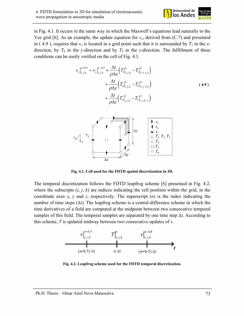
73 Ph.D. Thesis – Omar Ariel Nova Manosalva
4. FDTD formulation in 3D for simulation of electroacoustic wave propagation in anisotropic media
in Fig. 4.1. It occurs in the same way in which the Maxwell’s equations lead naturally to the Yee grid [6]. As an example, the update equation for vx, derived from (C.7) and presented in ( 4.9 ), requires that vx is located in a grid point such that it is surrounded by T1 in the x-direction, by T6 in the y-direction and by T5 in the z-direction. The fulfillment of these conditions can be easily verified on the cell of Fig. 4.1.
0.5 0.5
1 1, , , , , , 1, ,
6 6, , , 1,
5 5, , , , 1
n n n n
x xi j k i j k i j k i j k
n n
i j k i j k
n n
i j k i j k
tv v T T
x
tT T
y
tT T
z
( 4.9 )
Fig. 4.1. Cell used for the FDTD spatial discretization in 3D.
The temporal discretization follows the FDTD leapfrog scheme [6] presented in Fig. 4.2, where the subscripts (i, j, k) are indices indicating the cell position within the grid, in the coordinate axes x, y and z, respectively. The superscript (n) is the index indicating the number of time steps (Δt). The leapfrog scheme is a central-difference scheme in which the time derivatives of a field are computed at the midpoint between two consecutive temporal samples of this field. The temporal samples are separated by one time step Δt. According to this scheme, T is updated midway between two consecutive updates of v.
Fig. 4.2. Leapfrog scheme used for the FDTD temporal discretization.

74 Ph.D. Thesis – Omar Ariel Nova Manosalva
4. FDTD formulation in 3D for simulation of electroacoustic wave propagation in anisotropic media
4.2.2. PMLabsorbingboundaryconditionA perfectly matched layer (PML) is used as absorbing boundary condition (ABC). This condition is used on all the boundaries of the computational domain, except on the surface. Thus, the PML allows restricting the substrate depth to 1 λa. Similarly, the tag dimensions in the longitudinal and transverse directions (see Fig. 2.1) are restricted to the regions occupied by the electrodes.
The PML formulation uses the stretched coordinate approach presented in [7] and [8] and widely discussed in section 2.4 of this document. The PML loss profile, Ωξ, is defined as in [5], for each spatial direction ξ: x, y, z:
, ,max, ,
m
i j k
i j kPML
l
N
( 4.10 )
The amplitude Ωmax is given by Ωmax = Amax NPML / ∆t. Amax is a parameter to be optimized and NPML is the number of PML cells. Usually a good absorption level is achieved with NPML < 20. Δlξ is the distance between the PML cell and the border of the real medium, and the exponent m is another parameter to be optimized that takes values between 2 and 4.
The PML loss profile Ωξ = 0 within the real medium. In the PML corresponding to faces perpendicular to the x-axis, Ωy = 0 and Ωz = 0. In the same manner, in PML faces normal to the y-axis, Ωx = 0 and Ωz = 0, while in PML faces normal to the z-axis, Ωx = 0 and Ωy = 0. In the PML edges, only one of the three Ωξ (with ξ: x, y, z) is equal to zero, while in the PML corners, Ωξ is different from zero in the three spatial directions [8].
To introduce the PML loss profile into the 9 governing equations of Appendix C, they must be split into components for each spatial direction [5], as presented in section 2.4 of this document. Therefore, from each governing equation, 4 update equations are obtained: 3 split equations for each spatial direction and 1 equation to compute the total value of the corresponding field component.
To express the update equations in a compact form, auxiliary variables δξ and σξ are defined for each direction ξ: x, y, z, in terms of the PML loss profile (Ωξ), the time step (Δt) and the spatial step (Δξ), as presented in section 2.4 of this document:
, ,
, ,
, ,
2
2i j k
i j k
i j k
t
t
( 4.11 )
, ,
, , , ,
2
2i j k
i j k i j k
t
t
( 4.12 )

75 Ph.D. Thesis – Omar Ariel Nova Manosalva
4. FDTD formulation in 3D for simulation of electroacoustic wave propagation in anisotropic media
4.2.3. Stress‐freeboundaryconditionSince the SAW excitation occurs on the surface, where there is an interface substrate-air, a special boundary condition must be used on this interface. For elastic wave propagation, the air can be modeled as free space, and the boundary condition at the interface substrate-air is called free boundary condition [9]. Several formulations of free boundary condition have been proposed, namely, the zero-stress formulation (ZSF) [5, 10], the vacuum formulation (VAF) [11] and the transmission line formulation (TLF) [12]. The advantage of VAF and TLF over ZSF is that the first two formulations do not require the use of an artificial grid in the free space [9]. However, the ZSF has been showed to be more precise than the others [9, 10]. That is why, in this thesis the ZSF is used at the substrate surface interface, under the name of stress-free boundary condition.
To establish the stress-free boundary condition, the interface substrate-free space must be considered (Fig. 4.3). The general stress boundary condition states that the stress applied on any interface must be continuous [3]. In free space all the stress components are zero, that is, Tx = 0, Ty = 0, Tz = 0, where Tξ is the stress applied on a face normal to the ξ-axis (ξ: x, y, z) [3], as illustrated in Fig. 4.3. Then, the stress applied on the substrate surface must be
zero, that is, Tz = 0 on the surface. As Tz is given by ˆ ˆ ˆxz yz zzT x T y T z zT [3], then, the
stress boundary condition requires Txz = 0, Tyz = 0, Tzz = 0 in full subscripts, or equivalently, T3 = 0, T4 = 0, T5 = 0 in abbreviated subscripts [3].
Fig. 4.3. Implementation of the stress-free boundary condition at the substrate surface.
To meet the stress-free boundary condition at the substrate surface (in k=1), an extra artificial row must be added above the surface, in k=0, as illustrated in Fig. 4.3. Then, by considering the field component location in the discretization cell of Fig. 4.1, the stress-free boundary condition results in:
3 3, ,1 , ,00
n n
i j i jT T
( 4.13 )
4 4, ,1 , ,0 02
n n
i j i jT T
( 4.14 )

76 Ph.D. Thesis – Omar Ariel Nova Manosalva
4. FDTD formulation in 3D for simulation of electroacoustic wave propagation in anisotropic media
5 5, ,1 , ,0 02
n n
i j i jT T
( 4.15 )
This is because the component T3 is located exactly on the interface, while the components T4 and T5 are located Δz/2 under the interface. Then, T3 is directly made equal to zero in the row k = 1, while T4 and T5 must be averaged between the rows k = 1 and k = 0 before being equaled to zero. The stress-free boundary condition can be expressed in a better way as:
3 3, ,1 , ,00
n n
i j i jT T
( 4.16 )
4 4, ,1 , ,0
n n
i j i jT T
( 4.17 )
5 5, ,1 , ,0
n n
i j i jT T ( 4.18 )
These are the conditions that must be enforced in the FDTD update equations on the substrate surface to meet the stress-free boundary condition.
4.2.4. Quasi‐staticapproximationThe electroacoustic wave propagation in piezoelectric crystals is a multiscale problem because the time scales of the acoustic and the electromagnetic phenomena are different. The acoustic phase velocity in a piezoelectric crystal is in the order of 103 m/s, that is, 105 times lower than the electromagnetic. Then, for a given frequency, the acoustic wavelength is also 105 times lower than the electromagnetic. SAW RFID tag length is in the order of 10-3 m, while its operation frequency is around 109 Hz. At this frequency, about 1000 acoustic wavelengths fit into the tag length, while only 10-2 electromagnetic wavelengths are contained into this length. Therefore, it can be assumed that the electromagnetic wave hardly changes into the tag, and a quasi-static approximation can be used [3].
The quasi-static approximation can be expressed in terms of the electric field (E) and the electric potential (Φ) as follows:
E ( 4.19 )
0E ( 4.20 )
This approximation greatly simplifies the analysis of the piezoelectric phenomenon. Two direct consequences in the FDTD analysis are presented below.
1. Discretization fitted to the elastic wave propagation phenomenon.
The quasi-static approximation allows the use of a spatial step in the order of 1/20 of the acoustic wavelength. The electromagnetic wavelength, which is 105 times higher, is not
77 Ph.D. Thesis – Omar Ariel Nova Manosalva
4. FDTD formulation in 3D for simulation of electroacoustic wave propagation in anisotropic media
considered for the spatial discretization. Similarly, the critical time step (Δtcr) can be computed considering only the elastic case. In this way, the computed Δtcr is in the order of 10-12 s and the required number of time steps to observe the complete process of SAW generation and reflection is about 105. If Δtcr was computed by considering the electromagnetic phase velocity instead of the acoustic one, the required number of time steps would be 1010, which is a number impossible to handle in a conventional FDTD simulation.
2. Excitation from the electrostatic solution for the electric field (E).
As presented previously in section 3.3, the quasi-static approximation allows exciting the structure from the electrostatic solution for the electric field (Estatic), by using the E field as a distributed source [1, 2] given by:
, staticE r t E r f t ( 4.21 )
The spatial variation of the excitation is given by Estatic(r), while the time variation is determined by f(t), which usually is a modulated Gaussian pulse or a continuous wave signal.
4.2.5. ObtainedFDTDupdateequationsThe FDTD update equations are obtained from the 9 governing equations presented in Appendix C, after applying the discretization scheme above described. The governing equations corresponding to the T components (C.1) – (C.6) are discretized differently depending on the piezoelectric crystal symmetry and orientation. This is because different terms of these equations can be canceled, depending on which elements of the stiffness matrix [cE] and the piezoelectric stress matrix [e] are zero. Therefore, different update equations are obtained for the T components, depending on the piezoelectric crystal symmetry and orientation. By contrast, the update equations for the v components (those derived from the governing equations (C.7) – (C.9)) are the same for all the symmetries and orientations of the piezoelectric crystal. This is because the only material parameter involved in these equations is the mass density (ρ), which is always different from zero.
As the FDTD update equations can be up to 36 (4 for each of the 9 governing equations in
Appendix C), only those corresponding to bismuth germanate (Bi4Ge3O12) with cubic 43msymmetry and Euler angles (0°, 0°, 0°) [3] are presented in Appendix D. By way of example, the update equations corresponding to the T1 and vx fields for this substrate are presented below:
1 0.5 0.5
1, 1, 11, , , , 1, , , ,, , , ,
nn n n
x x x x x xi j k i j k i j k i j ki j k i j kT T c v v
( 4.22 )

78 Ph.D. Thesis – Omar Ariel Nova Manosalva
4. FDTD formulation in 3D for simulation of electroacoustic wave propagation in anisotropic media
1 0.5 0.5
1, 1, 12, , , , , , , , , 1,, ,
nn n n
y y y y y yi j k i j k i j k i j k i j ki j kT T c v v
( 4.23 )
1 0.5 0.5
1, 1, 13, , , , , , , , 1, , , ,
nn n n
z z z z z zi j k i j k i j k i j ki j k i j kT T c v v
( 4.24 )
11 11
1 1, 1, 1,, , , , , ,, ,
nn nn
x y zi j k i j k i j ki j kT T T T
( 4.25 )
0.5 0.5
, , 1 1, , , , , , 1, ,, , , ,
1n n n n
x x x x x xi j k i j k i j k i j ki j k i j kv v T T
( 4.26 )
0.5 0.5
, , 6 6, , , 1,, , , , , , , ,
1n n n n
x y y x y y i j k i j ki j k i j k i j k i j kv v T T
( 4.27 )
0.5 0.5
, , 5 5, , , , , , , , 1, , , ,
1n n n n
x z z x z zi j k i j k i j k i j ki j k i j kv v T T
( 4.28 )
0.50.5 0.50.5
, , ,, , , , , ,, ,
nn nn
x x x x y x zi j k i j k i j ki j kv v v v
( 4.29 )
As shown in the set of update equations for T1 ( 4.22 ) - ( 4.25 ) and for vx ( 4.26 ) - ( 4.29 ), each field is split into 3 components, one for each spatial direction. This is necessary to implement the PML boundary, as commented in the section 2.4 of this document.
For space reasons, the update equations for the other two substrates simulated in this thesis (barium sodium niobate and lithium niobate) are not presented in this document.
4.3. FDTDsimulationofSAWIDTsin3DThree-dimensional simulation of SAW IDTs has been addressed by the FEM/BEM method [13-15]. However, to make the 3D simulation possible, some simplifying assumptions are introduced. Such assumptions include: false periodicity in the transverse direction to simplify the involved Green’s functions evaluation [13] and estimation of the frequencies at which the interaction between Rayleigh and SH waves occurs [14]. Besides, complex meshing strategies are required to ensure an adequate modeling of the electric charge singularities in the corners and edges of the SAW transducers [15].
In the same way, 3D simulation of SAW IDTs is not possible with the P-matrix method because wave amplitude is considered to be uniform in the transverse direction [16]. For their part, the delta function model is stated in just one dimension [17] and the COM method assumes infinite grating of the transducer [18], which prevents the simulation of IDTs with reduced number of periods. IDTs with few periods are used for SH-SAW generation, in which transducers with lengths of only 1.5 to 5.5 acoustic wavelengths are able to generate SH-SAW with up to 98% efficiency [19].
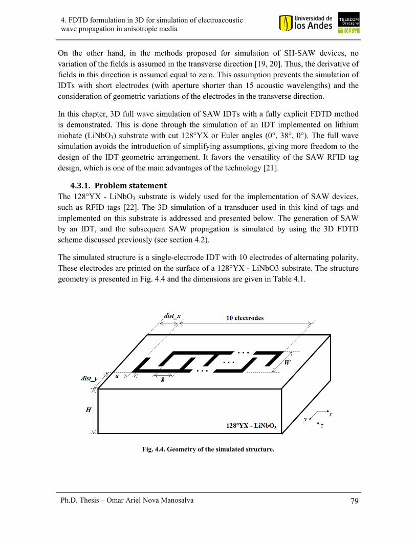
79 Ph.D. Thesis – Omar Ariel Nova Manosalva
4. FDTD formulation in 3D for simulation of electroacoustic wave propagation in anisotropic media
On the other hand, in the methods proposed for simulation of SH-SAW devices, no variation of the fields is assumed in the transverse direction [19, 20]. Thus, the derivative of fields in this direction is assumed equal to zero. This assumption prevents the simulation of IDTs with short electrodes (with aperture shorter than 15 acoustic wavelengths) and the consideration of geometric variations of the electrodes in the transverse direction.
In this chapter, 3D full wave simulation of SAW IDTs with a fully explicit FDTD method is demonstrated. This is done through the simulation of an IDT implemented on lithium niobate (LiNbO3) substrate with cut 128°YX or Euler angles (0°, 38°, 0°). The full wave simulation avoids the introduction of simplifying assumptions, giving more freedom to the design of the IDT geometric arrangement. It favors the versatility of the SAW RFID tag design, which is one of the main advantages of the technology [21].
4.3.1. ProblemstatementThe 128°YX - LiNbO3 substrate is widely used for the implementation of SAW devices, such as RFID tags [22]. The 3D simulation of a transducer used in this kind of tags and implemented on this substrate is addressed and presented below. The generation of SAW by an IDT, and the subsequent SAW propagation is simulated by using the 3D FDTD scheme discussed previously (see section 4.2).
The simulated structure is a single-electrode IDT with 10 electrodes of alternating polarity. These electrodes are printed on the surface of a 128°YX - LiNbO3 substrate. The structure geometry is presented in Fig. 4.4 and the dimensions are given in Table 4.1.
Fig. 4.4. Geometry of the simulated structure.
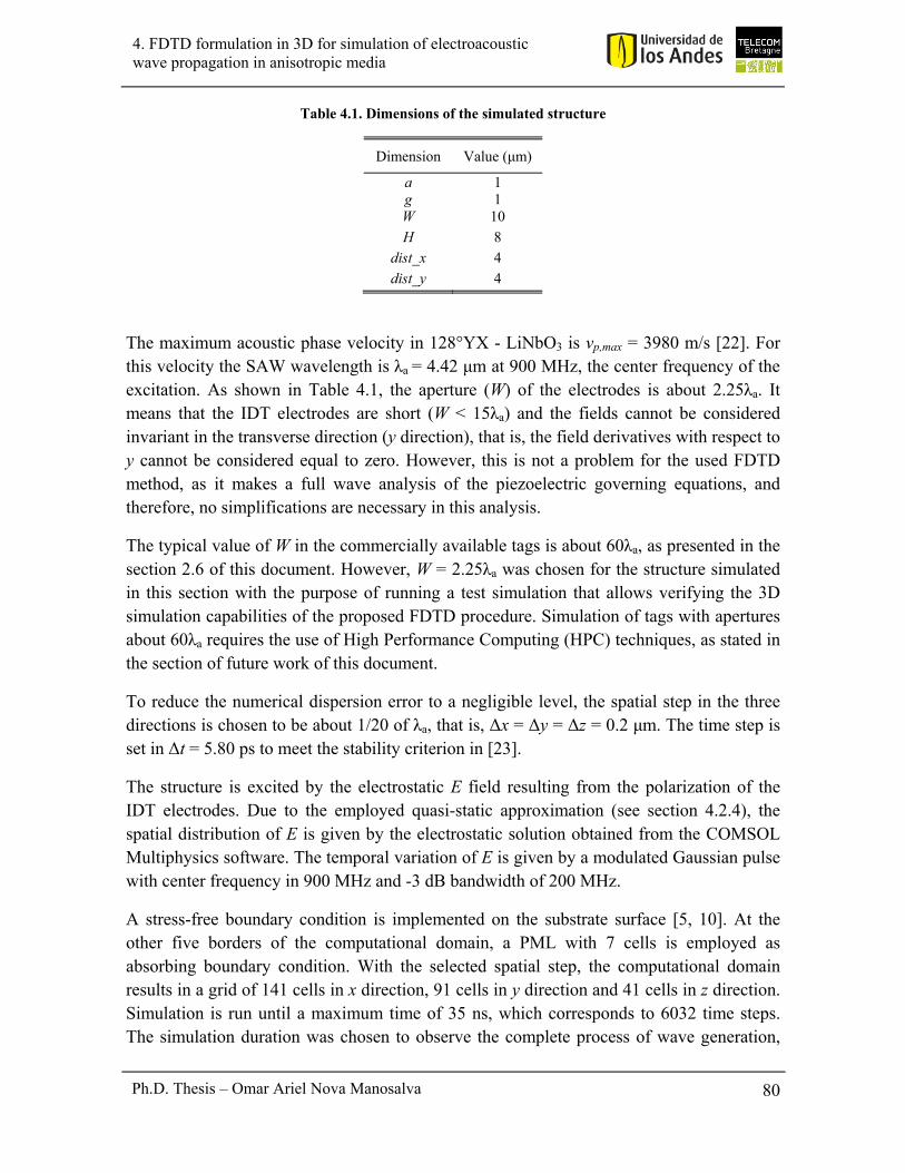
80 Ph.D. Thesis – Omar Ariel Nova Manosalva
4. FDTD formulation in 3D for simulation of electroacoustic wave propagation in anisotropic media
Table 4.1. Dimensions of the simulated structure
Dimension Value (μm)
a 1 g 1 W 10
H 8
dist_x 4
dist_y 4
The maximum acoustic phase velocity in 128°YX - LiNbO3 is vp,max = 3980 m/s [22]. For this velocity the SAW wavelength is λa = 4.42 μm at 900 MHz, the center frequency of the excitation. As shown in Table 4.1, the aperture (W) of the electrodes is about 2.25λa. It means that the IDT electrodes are short (W < 15λa) and the fields cannot be considered invariant in the transverse direction (y direction), that is, the field derivatives with respect to y cannot be considered equal to zero. However, this is not a problem for the used FDTD method, as it makes a full wave analysis of the piezoelectric governing equations, and therefore, no simplifications are necessary in this analysis.
The typical value of W in the commercially available tags is about 60λa, as presented in the section 2.6 of this document. However, W = 2.25λa was chosen for the structure simulated in this section with the purpose of running a test simulation that allows verifying the 3D simulation capabilities of the proposed FDTD procedure. Simulation of tags with apertures about 60λa requires the use of High Performance Computing (HPC) techniques, as stated in the section of future work of this document.
To reduce the numerical dispersion error to a negligible level, the spatial step in the three directions is chosen to be about 1/20 of λa, that is, Δx = Δy = Δz = 0.2 μm. The time step is set in Δt = 5.80 ps to meet the stability criterion in [23].
The structure is excited by the electrostatic E field resulting from the polarization of the IDT electrodes. Due to the employed quasi-static approximation (see section 4.2.4), the spatial distribution of E is given by the electrostatic solution obtained from the COMSOL Multiphysics software. The temporal variation of E is given by a modulated Gaussian pulse with center frequency in 900 MHz and -3 dB bandwidth of 200 MHz.
A stress-free boundary condition is implemented on the substrate surface [5, 10]. At the other five borders of the computational domain, a PML with 7 cells is employed as absorbing boundary condition. With the selected spatial step, the computational domain results in a grid of 141 cells in x direction, 91 cells in y direction and 41 cells in z direction. Simulation is run until a maximum time of 35 ns, which corresponds to 6032 time steps. The simulation duration was chosen to observe the complete process of wave generation,

81 Ph.D. Thesis – Omar Ariel Nova Manosalva
4. FDTD formulation in 3D for simulation of electroacoustic wave propagation in anisotropic media
propagation and absorption by the PML boundary. Simulation takes 8.73 hours in a 2.66 GHz Intel Xeon processor with 8 GB of RAM.
4.3.2. Simulationresults
(a) (b)
(c) (d)
(e) (f)
Fig. 4.5. Snapshots of vx (in m/s) at the x-y plane located on the substrate surface (z = 0). (a) t = 5.83 ns. (b) t = 11.67 ns. (c) t = 17.50 ns. (d) t = 23.33 ns. (e) t = 29.17 ns. (f) t = 35.00 ns.
82 Ph.D. Thesis – Omar Ariel Nova Manosalva
4. FDTD formulation in 3D for simulation of electroacoustic wave propagation in anisotropic media
(a) (b)
(c) (d)
(e) (f)
Fig. 4.6. Snapshots of vx (in m/s) at the x-z plane located at y = dist_y + W / 3. (a) t = 5.83 ns. (b) t = 11.67 ns. (c) t = 17.50 ns. (d) t = 23.33 ns. (e) t = 29.17 ns. (f) t = 35.00 ns.
To verify the proper SAW generation, propagation and absorption by the PML, snapshots of the particle velocity vx were taken at different cuts of the simulated structure: 4 x-y cuts and 4 x-z cuts. The snapshots taken at the x-y cut corresponding to the substrate surface (z = 0) are presented in Fig. 4.5. In Fig. 4.6, the snapshots taken at the x-z cut located at y =

83 Ph.D. Thesis – Omar Ariel Nova Manosalva
4. FDTD formulation in 3D for simulation of electroacoustic wave propagation in anisotropic media
dist_y + W / 3 (see Fig. 4.4) are shown. Snapshots were taken at 6 equally spaced time points along the duration of the simulation.
As can be seen in Fig. 4.5 and Fig. 4.6, the process of SAW generation and propagation has been properly simulated in three dimensions. In Fig. 4.5, SAW generation from the electric IDT excitation is evident, as well as wave propagation in x direction. Good performance of the PML is verified, since it efficiently absorbs the generated SAW. In Fig. 4.6, BAW generation associated to SAW excitation is observed. Once more, PML proves its efficiency to absorb both the SAW and BAW.
The good performance of the PML has been demonstrated in a qualitative way by means of the snapshots in Fig. 4.5 and Fig. 4.6. This is demonstrated in a more formal and quantitative way in section 4.4.2.2, by using the principle of energy conservation.
4.4. PML stability in 3D FDTD simulation ofelectroacoustic wave propagation inpiezoelectriccrystalswithdifferentsymmetryclass
The FDTD method was introduced by Yee [6] in 1966, for simulation of electromagnetic problems. Then, this method was adapted for simulation of elastodynamic phenomena in geophysical problems [24, 25]. FDTD has also been used for the simulation of electroacoustic wave propagation in piezoelectric crystals [26]. In this direction, one of the main applications of the finite-difference methods has been the simulation of piezoelectric transducers in two dimensions [27] and three dimensions [28, 29]. The appearance of numerical reflections at the boundaries of the computational domain requires the use of absorbing boundary conditions (ABC). The most commonly used ABC is the perfectly matched layer (PML), initially formulated by Berenger [30] for electromagnetic waves and adapted to elastodynamics in [7]. PML has been also applied for absorption of electroacoustic waves in piezoelectric media [31]. Some simulation instabilities arise for certain piezoelectric crystals when PML is used, as reported in [32] and [1]. A new PML formulation for electroacoustic waves is developed in [33]. This new formulation is shown to be stable in two-dimensional (2D) simulations on lithium niobate (LiNbO3). In this chapter, the PML is shown to be stable in three-dimensional (3D) simulations on two substrates with different crystal symmetry class: barium sodium niobate (Ba2NaNb5O15),
with orthorhombic 2mm symmetry, and bismuth germanate (Bi4Ge3O12), with cubic 43m
symmetry. Bismuth germanate is the substrate for which instability problems had been previously reported in [32] and [1]. For this substrate, PML stability in the continuous medium is demonstrated by evaluating the sufficient stability conditions given in [34]. PML stability in the discretized medium is achieved without necessity of modifying the
84 Ph.D. Thesis – Omar Ariel Nova Manosalva
4. FDTD formulation in 3D for simulation of electroacoustic wave propagation in anisotropic media
PML formulation, by adapting the discretization grid to meet a central-difference scheme. Stability is demonstrated by verifying that the total energy of the piezoelectric system does not increase after reaching the steady state.
The central-difference nature of the FDTD method is ensured through a discretization grid that is fully staggered in both space and time domains, as presented in [4]. The 3D FDTD formulation in [4] is complemented in this thesis by the inclusion of an absorbing boundary condition (PML) to allow simulation of configurations different from the axisymmetrical ones.
The spatial discretization scheme proposed to ensure the PML stability on piezoelectric substrates with different crystal symmetry class is an original contribution of this thesis that was published in [35].
4.4.1. 3DFDTDformulationFrom the fundamental equations of piezoelectricity [3], the 3D FDTD governing equations are extracted to update the stress T and the particle velocity v. These equations are presented in ( 4.5 ) and ( 4.6 ) and are expanded in Appendix C. The excitation is applied on the E field, as done for surface acoustic wave (SAW) device simulation, where the static E field is used as a distributed source [1, 2].
The computational domain is divided in cells. A cell definition similar to that presented in [5] is used. This cell is presented in Fig. 4.1. The location of the field components into the cell is done to ensure a central-difference scheme. A PML is used as absorbing boundary condition. The PML formulation uses the stretched coordinate approach presented in [7] and [8]. The PML loss profile is defined in [5].
4.4.2. PMLstabilityverificationAs stated before, PML instability problems were reported for the bismuth germanate substrate [1, 32]. In these references, instability is attributed to the substrate properties in the continuous medium. That is why in this section the PML stability is initially demonstrated in the continuous medium of bismuth germanate and, then, the stability is investigated in the discretized medium for this substrate and also for the barium sodium niobate substrate.
4.4.2.1. PML stability verification in the continuous medium of bismuthgermanate
PML stability in the continuous medium of bismuth germanate was verified in this thesis through evaluation of the sufficient stability conditions given in Theorem 5 and Theorem 6 of [34]. Two necessary and one sufficient condition for the PML stability in the case of elastic wave propagation are stated in [34], for the continuous medium of an orthotropic substrate. Then, PML stability demonstration must begin by verifying that the substrate of bismuth germanate has orthotropic symmetry.

85 Ph.D. Thesis – Omar Ariel Nova Manosalva
4. FDTD formulation in 3D for simulation of electroacoustic wave propagation in anisotropic media
Verification of the orthotropic symmetry of bismuth germanate
To verify the orthotropic symmetry of bismuth germanate, with Euler angles (0°, 0°, 0°), the symmetry of the 3x3 stiffness matrix (C3x3) defined in [34] for 2D propagation is analyzed. It is done for two planes of propagation: the x–y plane and the x–z plane. The stiffness constants are taken from [3], where the 6x6 stiffness matrix (C6x6) for 3D propagation is given.
For bismuth germanate, the 3x3 stiffness matrix (C3x3) is given by:
- For propagation in the x–y plane:
6 6 6 6 6 6
3 3 6 6 6 6 6 6
6 6 6 6 6 6
1,1 1, 2 1,6
2,1 2, 2 2,6
6,1 6, 2 6,6
c c c
C c c c
c c c
( 4.30 )
- For propagation in the x–z plane:
6 6 6 6 6 6
3 3 6 6 6 6 6 6
6 6 6 6 6 6
1,1 1,3 1,5
3,1 3,3 3,5
5,1 5,3 5,5
c c c
C c c c
c c c
( 4.31 )
where c6x6(i,j) is the element (i,j) of the C6x6 matrix given in [3].
It can be verified that for propagation both in the x–y plane and the x–z plane of bismuth germanate, the C3x3 matrix results to be the same. This matrix is:
113 3 2
1.1580 0.2700 0
1 10 0.2700 1.1580 0
0 0 0.4360
NC
m
( 4.32 )
This matrix satisfies the orthotropic symmetry defined in [34], namely:
- c13 = c31 = 0 - c23 = c32 = 0 - c11 > 0 - c22 > 0 - c33 > 0 - c11c22 - c12
2 > 0
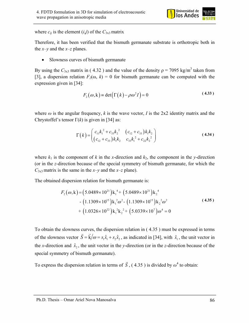
86 Ph.D. Thesis – Omar Ariel Nova Manosalva
4. FDTD formulation in 3D for simulation of electroacoustic wave propagation in anisotropic media
where cij is the element (i,j) of the C3x3 matrix
Therefore, it has been verified that the bismuth germanate substrate is orthotropic both in the x–y and the x–z planes.
Slowness curves of bismuth germanate
By using the C3x3 matrix in ( 4.32 ) and the value of the density ρ = 7095 kg/m3 taken from [3], a dispersion relation F2(ω, k) = 0 for bismuth germanate can be computed with the expression given in [34]:
22 , k det 0F k I ( 4.33 )
where ω is the angular frequency, k is the wave vector, I is the 2x2 identity matrix and the Chrystoffel’s tensor Γ(k) is given in [34] as:
2 211 1 33 2 12 33 1 2
2 212 33 1 2 33 1 22 2
c k c k c c k kk
c c k k c k c k
( 4.34 )
where k1 is the component of k in the x-direction and k2, the component in the y-direction (or in the z-direction because of the special symmetry of bismuth germanate, for which the C3x3 matrix is the same in the x–y and the x–z plane).
The obtained dispersion relation for bismuth germanate is:
21 4 21 42 1 2
15 2 2 15 2 21 2
22 2 2 7 41 2
, k 5.0489 10 k + 5.0489 10 k
- 1.1309 10 k - 1.1309 10 k
+ 1.0326 10 k k + 5.0339 10 0
F
( 4.35 )
To obtain the slowness curves, the dispersion relation in ( 4.35 ) must be expressed in terms
of the slowness vector 1 1 2 2ˆ ˆkS s x s x
, as indicated in [34], with 1x , the unit vector in
the x-direction and 2x , the unit vector in the y-direction (or in the z-direction because of the
special symmetry of bismuth germanate).
To express the dispersion relation in terms of S
, ( 4.35 ) is divided by ω4 to obtain:
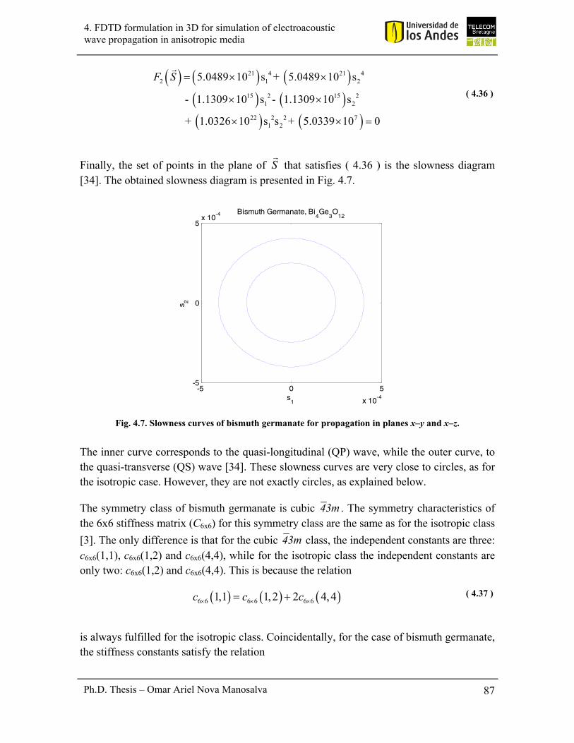
87 Ph.D. Thesis – Omar Ariel Nova Manosalva
4. FDTD formulation in 3D for simulation of electroacoustic wave propagation in anisotropic media
21 4 21 42 1 2
15 2 15 21 2
22 2 2 71 2
5.0489 10 s + 5.0489 10 s
- 1.1309 10 s - 1.1309 10 s
+ 1.0326 10 s s + 5.0339 10 0
F S
( 4.36 )
Finally, the set of points in the plane of S
that satisfies ( 4.36 ) is the slowness diagram [34]. The obtained slowness diagram is presented in Fig. 4.7.
Fig. 4.7. Slowness curves of bismuth germanate for propagation in planes x–y and x–z.
The inner curve corresponds to the quasi-longitudinal (QP) wave, while the outer curve, to the quasi-transverse (QS) wave [34]. These slowness curves are very close to circles, as for the isotropic case. However, they are not exactly circles, as explained below.
The symmetry class of bismuth germanate is cubic 43m . The symmetry characteristics of the 6x6 stiffness matrix (C6x6) for this symmetry class are the same as for the isotropic class
[3]. The only difference is that for the cubic 43m class, the independent constants are three: c6x6(1,1), c6x6(1,2) and c6x6(4,4), while for the isotropic class the independent constants are only two: c6x6(1,2) and c6x6(4,4). This is because the relation
6 6 6 6 6 61,1 1,2 2 4,4c c c ( 4.37 )
is always fulfilled for the isotropic class. Coincidentally, for the case of bismuth germanate, the stiffness constants satisfy the relation
s1
s 2
Bismuth Germanate, Bi4Ge
3O
12
-5 0 5
x 10-4
-5
0
5x 10
-4
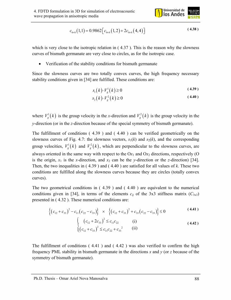
88 Ph.D. Thesis – Omar Ariel Nova Manosalva
4. FDTD formulation in 3D for simulation of electroacoustic wave propagation in anisotropic media
6 6 6 6 6 61,1 0.9862 1, 2 2 4, 4c c c ( 4.38 )
which is very close to the isotropic relation in ( 4.37 ). This is the reason why the slowness curves of bismuth germanate are very close to circles, as for the isotropic case.
Verification of the stability conditions for bismuth germanate
Since the slowness curves are two totally convex curves, the high frequency necessary stability conditions given in [34] are fulfilled. These conditions are:
11 0gs k V k ( 4.39 )
22 0gs k V k ( 4.40 )
where 1gV k is the group velocity in the x-direction and 2
gV k is the group velocity in the
y-direction (or in the z-direction because of the special symmetry of bismuth germanate).
The fulfillment of conditions ( 4.39 ) and ( 4.40 ) can be verified geometrically on the slowness curves of Fig. 4.7: the slowness vectors, s1(k) and s2(k), and the corresponding
group velocities, 1gV k and 2
gV k , which are perpendicular to the slowness curves, are
always oriented in the same way with respect to the Ox1 and Ox2 directions, respectively (O is the origin, x1 is the x-direction, and x2 can be the y-direction or the z-direction) [34]. Then, the two inequalities in ( 4.39 ) and ( 4.40 ) are satisfied for all values of k. These two conditions are fulfilled along the slowness curves because they are circles (totally convex curves).
The two geometrical conditions in ( 4.39 ) and ( 4.40 ) are equivalent to the numerical conditions given in [34], in terms of the elements cij of the 3x3 stiffness matrix (C3x3) presented in ( 4.32 ). These numerical conditions are:
2 2
12 33 11 22 33 12 33 33 22 33 0c c c c c c c c c c ( 4.41 )
2
12 33 11 22
2 212 33 11 22 33
2 (i)
(ii)
c c c c
c c c c c
( 4.42 )
The fulfillment of conditions ( 4.41 ) and ( 4.42 ) was also verified to confirm the high frequency PML stability in bismuth germanate in the directions x and y (or z because of the symmetry of bismuth germanate).
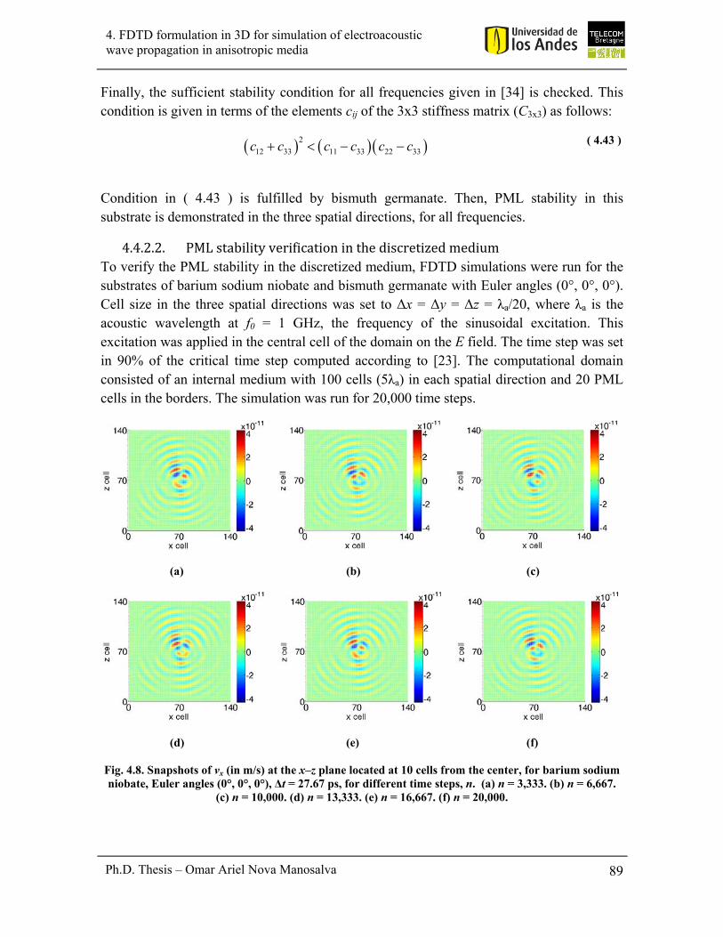
89 Ph.D. Thesis – Omar Ariel Nova Manosalva
4. FDTD formulation in 3D for simulation of electroacoustic wave propagation in anisotropic media
Finally, the sufficient stability condition for all frequencies given in [34] is checked. This condition is given in terms of the elements cij of the 3x3 stiffness matrix (C3x3) as follows:
2
12 33 11 33 22 33c c c c c c ( 4.43 )
Condition in ( 4.43 ) is fulfilled by bismuth germanate. Then, PML stability in this substrate is demonstrated in the three spatial directions, for all frequencies.
4.4.2.2. PMLstabilityverificationinthediscretizedmediumTo verify the PML stability in the discretized medium, FDTD simulations were run for the substrates of barium sodium niobate and bismuth germanate with Euler angles (0°, 0°, 0°). Cell size in the three spatial directions was set to Δx = Δy = Δz = λa/20, where λa is the acoustic wavelength at f0 = 1 GHz, the frequency of the sinusoidal excitation. This excitation was applied in the central cell of the domain on the E field. The time step was set in 90% of the critical time step computed according to [23]. The computational domain consisted of an internal medium with 100 cells (5λa) in each spatial direction and 20 PML cells in the borders. The simulation was run for 20,000 time steps.
(a) (b) (c)
(d) (e) (f)
Fig. 4.8. Snapshots of vx (in m/s) at the x–z plane located at 10 cells from the center, for barium sodium niobate, Euler angles (0°, 0°, 0°), Δt = 27.67 ps, for different time steps, n. (a) n = 3,333. (b) n = 6,667.
(c) n = 10,000. (d) n = 13,333. (e) n = 16,667. (f) n = 20,000.

90 Ph.D. Thesis – Omar Ariel Nova Manosalva
4. FDTD formulation in 3D for simulation of electroacoustic wave propagation in anisotropic media
Snapshots of the particle velocity component vx in the x–z plane located at 10 cells from the center of the domain are presented in Fig. 4.8 and Fig. 4.9 for barium sodium niobate and bismuth germanate, respectively.
(a) (b) (c)
(d) (e) (f)
Fig. 4.9. Snapshots of vx (in m/s) at the x–z plane located at 10 cells from the center, for bismuth germanate, Euler angles (0°, 0°, 0°), Δt = 39.69 ps, for different time steps, n. (a) n = 3,333. (b) n =
6,667. (c) n = 10,000. (d) n = 13,333. (e) n = 16,667. (f) n = 20,000.
Snapshots of Fig. 4.8 and Fig. 4.9 indicate that the PML is stable and is properly absorbing the continuous wave excitation at f0 = 1 GHz. However, a more formal demonstration of the PML stability is done by using the total energy of the piezoelectric system. If the PML is stable, this energy must not increase after reaching the steady state, in the case of a sinusoidal excitation. Discrete strain energy (dUS) and discrete kinetic energy (dUv) can be defined within each grid cell, by assuming that they are constant within the cell, as presented in [36] for the elastodynamic case. Similarly, discrete electrical energy (dUE) can be defined from [3]. The discrete energy definitions are presented below, along with the definition of the total energy of the piezoelectric system (U) for each time step n.
, , , , , , , ,
1:
2
n n n
S i j k i j k i j k i j kd U T S dV
( 4.44 )
, , , , , , , ,2
n n n
v i j k i j k i j k i j kd U v v dV
( 4.45 )
, , , , , , , ,
1
2
n n n
E i j k i j k i j k i j kd U E D dV
( 4.46 )

91 Ph.D. Thesis – Omar Ariel Nova Manosalva
4. FDTD formulation in 3D for simulation of electroacoustic wave propagation in anisotropic media
, , , , , ,
n n n n
S v Ei j k i j k i j ki j k
U dU dU dU
( 4.47 )
where the subscripts i, j, k indicate the cell position and the superscript n, the time step. S is the strain tensor, the double dot product ‘:’ between T and S is defined in [3], D is the electric displacement field and dV is the volume of one cell.
The total energy, U, was computed in each time step for both substrates. Results are presented in Fig. 4.10.
(a) (b)
Fig. 4.10. Total energy of the piezoelectric system computed in each time step for the substrates (a) barium sodium niobate and (b) bismuth germanate.
Fig. 4.10 shows that the total energy establishes in the steady state after the initial transient. The oscillation observed in the insets of Fig. 4.10 corresponds to the continuous wave excitation at f0 = 1 GHz. No increase in energy is observed after the establishment of the steady state. Hence, PML stability is verified in a formal way for both substrates.
4.5. ComputationoftheIDTinputadmittancefromFDTDsimulations
A fundamental aspect for the design of RFID tags based on delay lines is the determination of the input admittance of such lines. This admittance is used to optimize the coupling between the delay line and the antenna connected to it. The admittance of the delay line must be the complex conjugate of that of the antenna, to maximize the power transfer.
One of the challenges faced by the SAW RFID technology is the reduction of power loss and the increase of reading range [21, 37]. In this direction, coupling between the SAW delay line and the antenna connected to it is an important issue. By optimizing this coupling the power transferred from the reader to the SAW delay line can be maximized. The maximization of power transfer leads to reduction of losses and, at the same time, to

92 Ph.D. Thesis – Omar Ariel Nova Manosalva
4. FDTD formulation in 3D for simulation of electroacoustic wave propagation in anisotropic media
increase the distance from the reader at which the tag can operate, that is, to increase the reading range. Hence the importance of characterizing the tag input admittance.
In this chapter, the input admittance of an interdigital transducer (IDT) associated to a SAW RFID tag is computed by means of an FDTD method. The IDT input admittance computed in this way is a good approximation to the input admittance of the entire tag because, as showed in [22], the tag reflectors only add a small oscillation around the IDT input admittance. It makes the mean value of the tag input admittance to be equal to the IDT input admittance. Then, for purposes of coupling with the tag antenna, the tag input admittance can be assumed equal to the IDT input admittance.
In the FEM/BEM method, the input admittance is computed from the electric potential and the surface charge density. These fields are obtained from a semi-analytical approach that involves the use of Green’s functions [38, 39]. On the contrary, in this thesis the input admittance is computed from fields obtained after a full wave analysis of the governing equations in time domain. These fields are used to obtain the power flowing out the IDT and the voltage between its terminals, which allow the input admittance computation. By means of a Fourier transformation the input admittance is computed in all the excited frequency range from a single FDTD simulation. The procedure proposed to compute the input admittance from a time domain simulation and by using the power flux is an original contribution of this thesis. This contribution was published in [40].
4.5.1. Numericalprocedure
4.5.1.1. DefinitionofinputadmittanceThe input admittance (Yin) of a one-port circuit is defined in terms of the total voltage (V) and current (I) at a specified terminal plane as Yin = I / V. In turn, the total power flux (Pflux) through a closed surface S surrounding the source is given by
*1 1
2 2flux SP VI dS PoyntingP n
( 4.48 )
where PPoynting is the Poynting vector and n is a unit inward vector normal to the surface S [41].
By replacing I*=V* Yin* into ( 4.48 ), with ‘*’ indicating the complex conjugate, an expression for Yin in terms of Pflux is obtained as presented in ( 4.49 ), where |V|2 = VV* has been used.
*
2
2 fluxin
PY
V
( 4.49 )
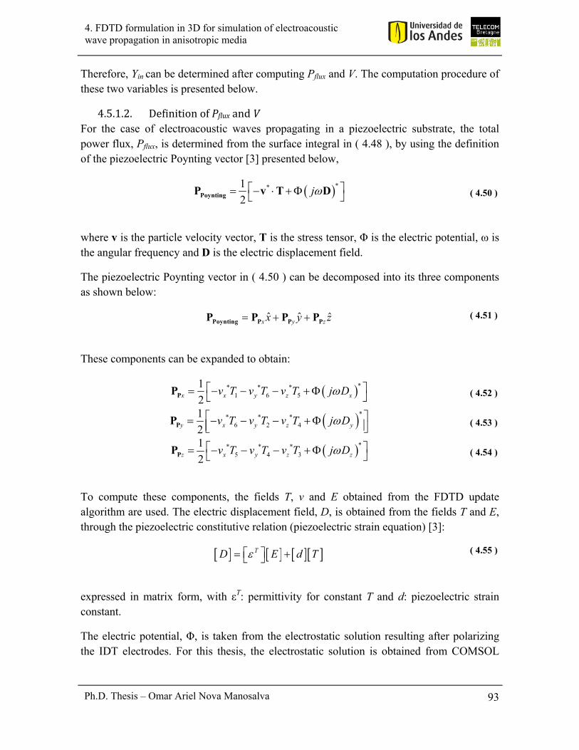
93 Ph.D. Thesis – Omar Ariel Nova Manosalva
4. FDTD formulation in 3D for simulation of electroacoustic wave propagation in anisotropic media
Therefore, Yin can be determined after computing Pflux and V. The computation procedure of these two variables is presented below.
4.5.1.2. DefinitionofPfluxandVFor the case of electroacoustic waves propagating in a piezoelectric substrate, the total power flux, Pflux, is determined from the surface integral in ( 4.48 ), by using the definition of the piezoelectric Poynting vector [3] presented below,
**1
2j PoyntingP v T D
( 4.50 )
where v is the particle velocity vector, T is the stress tensor, Φ is the electric potential, ω is the angular frequency and D is the electric displacement field.
The piezoelectric Poynting vector in ( 4.50 ) can be decomposed into its three components as shown below:
ˆ ˆ ˆx y zx y z Poynting P P PP P P P ( 4.51 )
These components can be expanded to obtain:
** * *1 6 5
1
2x x y z xv T v T v T j D PP
( 4.52 )
** * *6 2 4
1
2y x y z yv T v T v T j D PP
( 4.53 )
** * *5 4 3
1
2z x y z zv T v T v T j D PP
( 4.54 )
To compute these components, the fields T, v and E obtained from the FDTD update algorithm are used. The electric displacement field, D, is obtained from the fields T and E, through the piezoelectric constitutive relation (piezoelectric strain equation) [3]:
TD E d T ( 4.55 )
expressed in matrix form, with εT: permittivity for constant T and d: piezoelectric strain constant.
The electric potential, Φ, is taken from the electrostatic solution resulting after polarizing the IDT electrodes. For this thesis, the electrostatic solution is obtained from COMSOL

94 Ph.D. Thesis – Omar Ariel Nova Manosalva
4. FDTD formulation in 3D for simulation of electroacoustic wave propagation in anisotropic media
Multiphysics software. It can be done thanks to the quasi-static approximation discussed in the section 4.2.4 of this document.
The surface integral of ( 4.48 ) is computed on a surface S defined as the union of the three faces presented in Fig. 4.11: the lateral faces S1 and S2 and the bottom face S3. The lateral faces are located at the borders of the IDT to collect the power carried by the SAW (propagating in x) when they have just been generated by the IDT. The bottom face is placed at a depth of 2 acoustic wavelengths (λa), where the SAW amplitude is already negligible. This face is necessary to collect the power carried by the bulk acoustic waves (BAW) propagating in z. Although this power is low, it should be considered for the Pflux computation.
The total voltage at the source, V, corresponds to the voltage at the terminals of the IDT. Thus, it is computed by means of the following line integral,
LV d E L ( 4.56 )
where the integration line L is taken to be the path between two consecutive electrodes with opposite polarity. The expression in ( 4.56 ) is valid thanks to the quasi-static approximation that can be applied to this problem (see section 4.2.4).
Fig. 4.11. Integration surfaces for the computation of the total power flux, Pflux.
All the above presented equations for the computation of Pflux and V are in the frequency domain. Then, fields obtained from the FDTD simulation must be converted to the frequency domain before doing the admittance computation. A Fast Fourier Transform (FFT) algorithm is used for this purpose. The time domain fields located on the integration surface of ( 4.48 ) or the integration line of ( 4.56 ) are converted to the frequency domain with the FFT algorithm. Then, the integration process is done to obtain Pflux and V as a function of frequency. Finally, the desired IDT input admittance, Yin, is computed with ( 4.49 ).
4.5.1.3. ComputationofPfluxandVBy considering the equations ( 4.48 ) and ( 4.51 ) to ( 4.54 ), the equations to compute Pflux are:
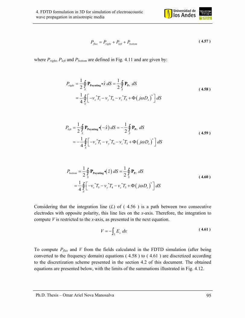
95 Ph.D. Thesis – Omar Ariel Nova Manosalva
4. FDTD formulation in 3D for simulation of electroacoustic wave propagation in anisotropic media
flux right left bottomP P P P ( 4.57 )
where Pright, Pleft and Pbottom are defined in Fig. 4.11 and are given by:
** * *1 6 5
1 1ˆ
2 2
1
4
right x
S S
x y z x
S
P x dS dS
v T v T v T j D dS
Poynting PP P
( 4.58 )
** * *1 6 5
1 1ˆ
2 2
1
4
left x
S S
x y z x
S
P x dS dS
v T v T v T j D dS
Poynting PP P
( 4.59 )
** * *5 4 3
1 1ˆ
2 2
1
4
bottom z
S S
x y z z
S
P z dS dS
v T v T v T j D dS
Poynting PP P
( 4.60 )
Considering that the integration line (L) of ( 4.56 ) is a path between two consecutive electrodes with opposite polarity, this line lies on the x-axis. Therefore, the integration to compute V is restricted to the x-axis, as presented in the next equation.
xLV E dx ( 4.61 )
To compute Pflux and V from the fields calculated in the FDTD simulation (after being converted to the frequency domain) equations ( 4.58 ) to ( 4.61 ) are discretized according to the discretization scheme presented in the section 4.2 of this document. The obtained equations are presented below, with the limits of the summations illustrated in Fig. 4.12.

96 Ph.D. Thesis – Omar Ariel Nova Manosalva
4. FDTD formulation in 3D for simulation of electroacoustic wave propagation in anisotropic media
Fig. 4.12. Limits of the integration surfaces for the computation of Pflux.
,,
, ,,
, ,, , ,,
, ,
*1 , ,, ,
*6 , ,, ,
* , , , ,5 , ,, ,
*
, , , ,
1
4
x end y zx end y z
z end x end y zx end y z
x end y z x end y zy y z z ini x end y zx end y z
x end y z x end y z
x i i ii i i
yi i i ii i i
right i i i i i ii i i i z i i ii i i
xi i i i i i
v T
v T
P z yv T
j D
,y end
ini
i
( 4.62 )
,,
, ,,
, ,, , ,,
, ,
*1 , ,, ,
*6 , ,, ,
* , , , ,5 , ,, ,
*
, , , ,
1
4
x ini y zx ini y z
z end x ini y zx ini y z
x ini y z x ini y zy y z z ini x ini y zx ini y z
x ini y z x ini y z
x i i ii i i
yi i i ii i i
left i i i i i ii i i i z i i ii i i
xi i i i i i
v T
v T
P z yv T
j D
,y end
ini
i
( 4.63 )
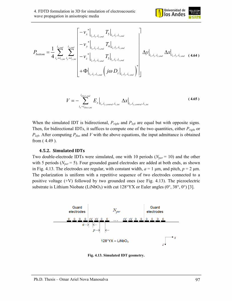
97 Ph.D. Thesis – Omar Ariel Nova Manosalva
4. FDTD formulation in 3D for simulation of electroacoustic wave propagation in anisotropic media
,,
, ,,
, ,, ,,
, ,
*5 , ,, ,
*4 , ,, ,
* , , , ,3 , ,, ,
*
, , , ,
1
4
x y z endx y z end
y end x y z endx y z end
x y z end x y z endx x y y ini x y z endx y z end
x y z end x y z end
x i i ii i i
yi i i ii i i
bottom i i i i i ii i i i z i i ii i i
zi i i i i i
v T
v T
P y xv T
j D
,
,
x end
ini
i
( 4.64 )
,
, , , ,,
, , , ,
elect end
x y central z ini x y central z inix elect ini
i
x i i i i i ii i
V E x
( 4.65 )
When the simulated IDT is bidirectional, Pright and Pleft are equal but with opposite signs. Then, for bidirectional IDTs, it suffices to compute one of the two quantities, either Pright or Pleft. After computing Pflux and V with the above equations, the input admittance is obtained from ( 4.49 ).
4.5.2. SimulatedIDTsTwo double-electrode IDTs were simulated, one with 10 periods (Nper = 10) and the other with 5 periods (Nper = 5). Four grounded guard electrodes are added at both ends, as shown in Fig. 4.13. The electrodes are regular, with constant width, a = 1 μm, and pitch, p = 2 μm. The polarization is uniform with a repetitive sequence of two electrodes connected to a positive voltage (+V) followed by two grounded ones (see Fig. 4.13). The piezoelectric substrate is Lithium Niobate (LiNbO3) with cut 128°YX or Euler angles (0°, 38°, 0°) [3].
Fig. 4.13. Simulated IDT geometry.

98 Ph.D. Thesis – Omar Ariel Nova Manosalva
4. FDTD formulation in 3D for simulation of electroacoustic wave propagation in anisotropic media
The simulated IDTs meet the assumptions done to derive the Yin analytical expressions in [42], which are used as a benchmark for the simulations. These assumptions are listed below:
- The IDT is non-reflective: this assumption is met because double-electrode IDTs are non-reflective.
- The end effects at the IDT borders are negligible: this is met by adding guard electrodes.
- The number of periods (Nper) is higher than a threshold, which in this case is Nper = 4.
- The electrodes are regular: they have constant width (a) and pitch (p). - The polarization is uniform: the polarization sequence is periodic.
Then, the IDT input admittance obtained from the FDTD simulation can be validated by comparison with the value obtained from the analytical expressions of [42].
The proposed procedure for IDT input admittance computation was tested in 2D FDTD simulations on the sagittal plane (plane x–z). The discretization grid presented in section 3.3 was used. An irregular meshing with a maximum step size of 3λa/40 = 0.6 μm and a minimum of λa/20 = 0.4 μm was implemented, as discussed in section 3.3. To satisfy the stability criterion in [23], a time step Δt = 21.32 ps was employed. The discretization of the computational domain resulted in a grid of 1949 x 244 cells for the 10-periods IDT and of 1749 x 244 cells for the 5-periods IDT. A total of 16400 time steps were simulated, which corresponds to a maximum simulated time of 350 ns. The simulations were run in an 8 cores 2.66 GHz Intel Xeon processor with 8 GB of RAM and took 73.51 minutes for the 10-periods IDT and 65.97 minutes for the 5-periods IDT.
The simulation was excited with the electrostatic E field resulting after polarizing the IDT electrodes, as described in section 4.2.4. The temporal variation of this excitation was a modulated Gaussian pulse with center frequency f0 = 450 MHz. The bandwidth of the used Gaussian pulse allows admittance characterization between 100 MHz and 800 MHz.
4.5.3. SimulationresultsSome snapshots of the particle velocity vx for the 10-periods IDT are shown. IDT input admittance results are presented in magnitude and phase for the two simulated IDTs, with 10 periods and 5 periods. Simulated admittance is compared with the theoretical value obtained from the analytical expressions of [42].
4.5.3.1. SnapshotsoftheparticlevelocityvxTo verify the correct generation and propagation of the acoustic waves (SAW and BAW), some snapshots of the particle velocity vx are presented for the 10-periods IDT.
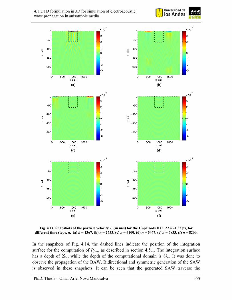
99 Ph.D. Thesis – Omar Ariel Nova Manosalva
4. FDTD formulation in 3D for simulation of electroacoustic wave propagation in anisotropic media
(a)
(b)
(c)
(d)
(e)
(f)
Fig. 4.14. Snapshots of the particle velocity vx (in m/s) for the 10-periods IDT, Δt = 21.32 ps, for different time steps, n. (a) n = 1367. (b) n = 2733. (c) n = 4100. (d) n = 5467. (e) n = 6833. (f) n = 8200.
In the snapshots of Fig. 4.14, the dashed lines indicate the position of the integration surface for the computation of Pflux, as described in section 4.5.1. The integration surface has a depth of 2λa, while the depth of the computational domain is 8λa. It was done to observe the propagation of the BAW. Bidirectional and symmetric generation of the SAW is observed in these snapshots. It can be seen that the generated SAW traverse the
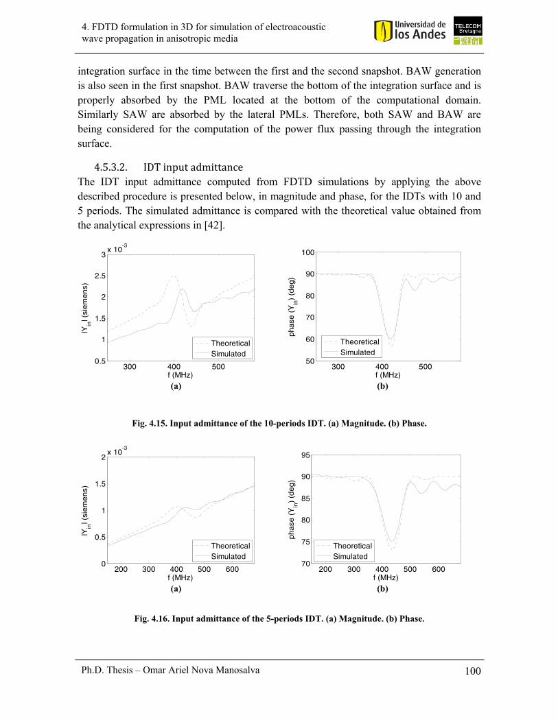
100 Ph.D. Thesis – Omar Ariel Nova Manosalva
4. FDTD formulation in 3D for simulation of electroacoustic wave propagation in anisotropic media
integration surface in the time between the first and the second snapshot. BAW generation is also seen in the first snapshot. BAW traverse the bottom of the integration surface and is properly absorbed by the PML located at the bottom of the computational domain. Similarly SAW are absorbed by the lateral PMLs. Therefore, both SAW and BAW are being considered for the computation of the power flux passing through the integration surface.
4.5.3.2. IDTinputadmittanceThe IDT input admittance computed from FDTD simulations by applying the above described procedure is presented below, in magnitude and phase, for the IDTs with 10 and 5 periods. The simulated admittance is compared with the theoretical value obtained from the analytical expressions in [42].
(a)
(b)
Fig. 4.15. Input admittance of the 10-periods IDT. (a) Magnitude. (b) Phase.
(a)
(b)
Fig. 4.16. Input admittance of the 5-periods IDT. (a) Magnitude. (b) Phase.
300 400 5000.5
1
1.5
2
2.5
3x 10
-3
f (MHz)
|Yin
| (si
emen
s)
TheoreticalSimulated
300 400 50050
60
70
80
90
100
f (MHz)
phas
e (Y
in)
(deg
)
TheoreticalSimulated
200 300 400 500 6000
0.5
1
1.5
2x 10
-3
f (MHz)
|Yin
| (si
emen
s)
TheoreticalSimulated
200 300 400 500 60070
75
80
85
90
95
f (MHz)
phas
e (Y
in)
(deg
)
TheoreticalSimulated

101 Ph.D. Thesis – Omar Ariel Nova Manosalva
4. FDTD formulation in 3D for simulation of electroacoustic wave propagation in anisotropic media
In Fig. 4.15 and Fig. 4.16, the phase of the input admittance agrees well with the theoretical reference. In this phase, the capacitive behavior of the admittance is observed at both sides of the resonance region, where the phase is equal to 90 degrees. Although the magnitude differs a little more from the theoretical reference, for the two simulated IDTs, it also predicts adequately the capacitive behavior of the admittance by showing a slope very close to the theoretical.
The value of the computed input admittance at the center frequency (f0), 420.5 MHz for the 10-periods IDT and 435.5 MHz for the 5-periods IDT, is presented in Table 4.2 for both IDTs, along with the value of the corresponding input impedance.
Table 4.2. Input admittance and impedance for both simulated IDTs at the center frequency, f0
IDT Input admittance (siemens) Input impedance (Ω)
10-periods (1.08 + j 1.89) x 10-3 229.05 – j 398.17 5-periods (0.27 + j 1.02) x 10-3 244.80 – j 918.00
A procedure to couple the computed IDT input impedance with that of the tag antenna is presented in section 4.5.4.
The differences observed in the admittance magnitude of Fig. 4.15 and Fig. 4.16 are basically a problem of amplitude deviation in the resonance region. However, these differences can be attributed to a failure in the fulfillment of the assumptions done in [42] to derive the analytical expressions for the computation of Yin. These assumptions, previously mentioned, include no-reflectivity of the IDT and negligible end effects. To comply with the condition of no-reflectivity, double-electrode IDTs were used because it is assumed that this electrode arrangement cancels the internal reflections of the IDT. However, it is possible that these reflections are not completely canceled, which can produce the observed deviations in the admittance magnitude. On the other hand, to reduce the end effects to a negligible level, guard electrodes were added at the IDT borders. Nevertheless, it is possible that the end effects are still present in spite of the added guard electrodes. Another source of error is the failure to consider the electrode thickness in the admittance computation. The consideration of this parameter is proposed as one of the issues to explore in the future work of this thesis.
4.5.4. ProcedureforimpedancecouplingThis procedure is based on the Thévenin equivalent circuit presented in Fig. 4.17.

102 Ph.D. Thesis – Omar Ariel Nova Manosalva
4. FDTD formulation in 3D for simulation of electroacoustic wave propagation in anisotropic media
Fig. 4.17. Thévenin equivalent circuit used for the optimization of the IDT-antenna coupling (taken from [43]).
In Fig. 4.17, Zs is the antenna input impedance, defined as Zs=Rs+jXs, and Zin=Rin+jXin is the IDT input impedance. The power at the input of the IDT, Pin, [43] is given by:
2
2
1
2in
in S
s in
RP V
Z Z
( 4.66 )
The power available at the source, PAVS, which is equal to the maximum power at the input of the IDT, when Zin=Zs
* [43], is given by:
21
8S
AVSs
VP
R
( 4.67 )
The Match factor at the source (Cs) is defined as indicated below [43]:
2
41 1in s in
sAVS s in
P R RC
P Z Z
( 4.68 )
To optimize the IDT-antenna coupling, Cs is used as the optimization variable. An example of Cs optimization is presented below.
In this example, the purpose is to optimize the coupling between a commercial SAW RFID tag, manufactured by the company CTR, and a PIFA antenna designed according to [44]. The tag input impedance was measured and is presented in Fig. 4.18.
The PIFA input impedance was obtained from simulations in Ansoft HFSS. The results of each stage of the optimization procedure are presented in Fig. 4.19, in terms of Cs. In this figure, Cs is expressed in dB, according to:
2
410log 1 s in
s
s in
R RC dB
Z Z
( 4.69 )

103 Ph.D. Thesis – Omar Ariel Nova Manosalva
4. FDTD formulation in 3D for simulation of electroacoustic wave propagation in anisotropic media
When the value of Cs in dB is zero, no-power is being delivered to the tag, while when it approximates to -∞, all the available power at the source is being delivered to the tag. The points of Cs = -10 dB correspond to Pin = 0.9PAVS, which can be considered as an acceptable coupling figure.
Fig. 4.18. Measured input impedance of a SAW RFID tag manufactured by CTR (taken from [45]).
Fig. 4.19. Match factor at the source, Cs, for different configurations of the tag-antenna system (taken from [45]).
2 2.2 2.4 2.6 2.8 3-60
-40
-20
0
20
40
Frequency (GHz)
Inpu
t im
peda
nce,
Zin
-SA
W (
ohm
)
Re(Zin-SAW
)
Im(Zin-SAW
)

104 Ph.D. Thesis – Omar Ariel Nova Manosalva
4. FDTD formulation in 3D for simulation of electroacoustic wave propagation in anisotropic media
In Fig. 4.19, three stages of the optimization procedure are referred: The first (no radome) corresponds to the tag-antenna coupling when the antenna does not have a radome. The second (radome non-compensated) is the coupling when a radome is implemented on the antenna without variation of the antenna dimensions. The third (radome compensated) is the final stage of the optimization and corresponds to the coupling when some adjustments to the antenna dimensions are done to improve the coupling. It is worth noting that, after the optimization procedure, a good tag-antenna coupling (Cs < -10 dB) is obtained for the frequency range between 2.355 GHz and 2.410 GHz.
4.6. ConclusionThree-dimensional simulation capability of the proposed FDTD method has been demonstrated. A fully explicit FDTD method has been employed to do a 3D full wave simulation of the multiphysics problem. The explicit computation of all the involved fields allows an accurate transient analysis of the problem. The full wave analysis avoids the introduction of simplifications in the piezoelectric governing equations, enabling the analysis of devices in which field variation occurs in all the spatial directions. This is demonstrated through the simulation of an IDT with short electrodes (W < 15λa) for which the fields in the transverse direction cannot be considered invariant.
Proper performance of the PML boundary in 3D simulations has been proved. This boundary adequately absorbs the acoustic waves generated by the IDT, both the SAW and the BAW. The PML boundary operates correctly even when this is located very close to the IDT borders, as done in the presented simulation, where the PML is located at distances of 1λa and 2λa from the IDT borders. This allows imposing tight limits to the computational domain, which results in reduction of the simulation time.
To simulate larger structures, such as entire SAW RFID tags or IDTs with larger apertures (W > 15λa) or with more complex geometries, high performance computing (HPC) techniques should be implemented. This is proposed as future work of this thesis.
PML stability in three-dimensional FDTD simulations of electroacoustic wave propagation was achieved, for piezoelectric crystals with different symmetry class. The conventional PML formulation for absorption of electroacoustic waves can be maintained as the PML stability is achieved by ensuring a central-difference scheme in the FDTD discretization grid. The PML stability is demonstrated for bismuth germanate and barium sodium niobate after applying the FDTD central-difference scheme. This demonstration is done by showing that the total energy of the piezoelectric system remains constant in the steady state. In this way, PML instability problems previously reported for bismuth germanate are solved. This is done for the discretized medium, after verifying the PML stability in the continuous medium.

105 Ph.D. Thesis – Omar Ariel Nova Manosalva
4. FDTD formulation in 3D for simulation of electroacoustic wave propagation in anisotropic media
Computation of the IDT input admittance has been done from fields calculated in a time-domain simulation. The procedure applied to compute the admittance is an original contribution of this thesis, as it makes use of the power flux and the terminal voltage in contrast to the conventional approach that uses the electrical surface charge density and the voltage. Explicit equations are given to compute the power flux and voltage in terms of the fields calculated in the FDTD simulation. These fields are obtained from a full wave analysis of the piezoelectric governing equations. Then, the proposed procedure for admittance computation can be applied to IDTs with any geometric arrangement. In addition, both SAW and BAW contributions are considered in the admittance computation. Characterization of the admittance in all the frequency range of interest is possible from a single FDTD simulation. The IDT input admittance obtained from the proposed procedure can be used to optimize the coupling between the SAW RFID tag and the antenna connected to the IDT terminals.
4.7. References[1] F. Chagla and P. M. Smith, "Finite difference time domain methods for
piezoelectric crystals," Ultrasonics, Ferroelectrics and Frequency Control, IEEE Transactions on, vol. 53, pp. 1895-1901, 2006.
[2] K.-Y. Wong and W.-Y. Tam, "Analysis of the frequency response of SAW filters using finite-difference time-domain method," Microwave Theory and Techniques, IEEE Transactions on, vol. 53, pp. 3364-3370, 2005.
[3] B. A. Auld, Acoustic Fields and Waves in Solids, 2nd ed. vol. 1. Malabar, FL: Krieger Publishing Company, 1990.
[4] M. Ferri, F. Camarena, J. Redondo, R. Picó, and M. R. Avis, "Explicit finite-difference time-domain scheme for the simulation of 1-3 piezoelectric effect in axisymmetrical configurations," Wave Motion, vol. 49, pp. 569-584, 2012.
[5] C. T. Schröder, "On the interaction of elastic waves with buried land mines: An investigation using the finite-difference time-domain method," Doctoral Dissertation, School Elect. Comput. Eng., Georgia Inst. Technol., Atlanta, GA, 2001.
[6] K. Yee, "Numerical solution of initial boundary value problems involving Maxwell's equations in isotropic media," Antennas and Propagation, IEEE Transactions on, vol. 14, pp. 302-307, 1966.
[7] W. C. Chew and Q. H. Liu, "Perfectly Matched Layers for Elastodynamics: A New Absorbing Boundary Condition," Journal of Computational Acoustics, vol. 04, pp. 341-359, 1996.
[8] T. K. Katsibas and C. S. Antonopoulos, "A general form of perfectly matched layers for three-dimensional problems of acoustic scattering in lossless and lossy fluid media," Ultrasonics, Ferroelectrics, and Frequency Control, IEEE Transactions on, vol. 51, pp. 964-972, 2004.
[9] M. Sato, "Comparing three methods of free boundary implementation for analyzing elastodynamics using the finite-difference time-domain formulation," Acoustical Science and Technology, vol. 28, pp. 49-52, 2007.
106 Ph.D. Thesis – Omar Ariel Nova Manosalva
4. FDTD formulation in 3D for simulation of electroacoustic wave propagation in anisotropic media
[10] R. W. Graves, "Simulating seismic wave propagation in 3D elastic media using staggered-grid finite differences," Bulletin of the Seismological Society of America, vol. 86, pp. 1091-1106, 1996.
[11] T. Ohminato and B. A. Chouet, "A free-surface boundary condition for including 3D topography in the finite-difference method," Bulletin of the Seismological Society of America, vol. 87, pp. 494-515, 1997.
[12] M. Sato and N. Nishizuka, "Setting of Free Boundaries in Numerical Analysis of Elastic Waves by FD-TD Method," Journal of the Japan Society for Simulation Technology, vol. 19, pp. 143-149, 2000.
[13] M. Solal, C. Li, and J. Gratier, "Measurement and FEM/BEM simulation of transverse effects in SAW resonators on lithium tantalate," Ultrasonics, Ferroelectrics and Frequency Control, IEEE Transactions on, vol. 60, pp. 2404-2413, 2013.
[14] V. Plessky, P. Turner, N. Fenzi, and V. Grigorievsky, "Interaction between the Rayleigh-type SAW and the SH-wave in a periodic grating on a 128°-LN substrate," in Ultrasonics Symposium (IUS), 2010 IEEE, 2010, pp. 167-170.
[15] C. F. Jerez-Hanckes, S. Laude, J. C. Nedelec, and R. Lardat, "3-D electrostatic hybrid element model for SAW interdigital transducers," Ultrasonics, Ferroelectrics and Frequency Control, IEEE Transactions on, vol. 55, pp. 686-695, 2008.
[16] G. Tobolka, "Mixed Matrix Representation of SAW Transducers," Sonics and Ultrasonics, IEEE Transactions on, vol. 26, pp. 426-427, 1979.
[17] R. H. Tancrell and M. G. Holland, "Acoustic surface wave filters," Proceedings of the IEEE, vol. 59, pp. 393-409, 1971.
[18] Y. Suzuki, H. Shimizu, M. Takeuchi, K. Nakamura, and A. Yamada, "Some Studies on SAW Resonators and Multiple-Mode Filters," in 1976 Ultrasonics Symposium, 1976, pp. 297-302.
[19] T. B. Pollard, T. D. Kenny, J. F. Vetelino, and M. P. da Cunha, "Pure SH-SAW propagation, transduction and measurements on KNbO3," Ultrasonics, Ferroelectrics and Frequency Control, IEEE Transactions on, vol. 53, pp. 199-208, 2006.
[20] T. D. Kenny, T. B. Pollard, E. Berkenpas, and M. Pereira da Cunha, "FEM/BEM impedance and power analysis for measured LGS SH-SAW devices," Ultrasonics, Ferroelectrics and Frequency Control, IEEE Transactions on, vol. 53, pp. 402-411, 2006.
[21] V. P. Plessky and L. M. Reindl, "Review on SAW RFID tags," Ultrasonics, Ferroelectrics, and Frequency Control, IEEE Transactions on, vol. 57, pp. 654-668, 2010.
[22] S. Harma and V. P. Plessky, "Extraction of frequency-dependent reflection, transmission, and scattering parameters for short metal reflectors from FEM-BEM simulations," Ultrasonics, Ferroelectrics and Frequency Control, IEEE Transactions on, vol. 55, pp. 883-889, 2008.
[23] I. A. Veres, "Stability analysis of second- and fourth-order finite-difference modelling of wave propagation in orthotropic media," Ultrasonics, vol. 50, pp. 431-438, 2010.
[24] R. Madariaga, "Dynamics of an expanding circular fault," Bulletin of the Seismological Society of America, vol. 66, pp. 639-666, 1976.
107 Ph.D. Thesis – Omar Ariel Nova Manosalva
4. FDTD formulation in 3D for simulation of electroacoustic wave propagation in anisotropic media
[25] J. Virieux, "SH-wave propagation in heterogeneous media: velocity-stress finite-difference method," Geophysics, vol. 49, pp. 1933-1942, 1984.
[26] P. M. Smith and R. Wei, "Finite-difference time-domain techniques for SAW device analysis," in Ultrasonics Symposium, 2002. Proceedings. 2002 IEEE, 2002, pp. 325-328 vol.1.
[27] Y. Yamada and M. Sato, "Application of Extended Finite-Difference Time-Domain Method to Two-Dimensional Dynamic Analysis of a Piezoelectric Vibrator," Japanese Journal of Applied Physics, vol. 37, p. 255, 1998.
[28] J. S. Hornsby and D. K. Das-Gupta, "Finite-difference modeling of piezoelectric composite transducers," Journal of Applied Physics, vol. 87, pp. 467-473, 2000.
[29] F. May and J. Dual, "Focusing of pulses in axially symmetric elastic tubes with fluid filling and piezo actuator by a finite difference simulation and a method of time reversal," Wave Motion, vol. 43, pp. 311-322, 2006.
[30] J.-P. Berenger, "A perfectly matched layer for the absorption of electromagnetic waves," Journal of Computational Physics, vol. 114, pp. 185-200, 1994.
[31] F. Chagla, C. Cabani, and P. M. Smith, "Perfectly matched layer for FDTD computations in piezoelectric crystals," in Ultrasonics Symposium, 2004 IEEE, 2004, pp. 517-520 Vol.1.
[32] F. Chagla and P. M. Smith, "Stability considerations for perfectly matched layers in piezoelectric crystals," in Ultrasonics Symposium, 2005 IEEE, 2005, pp. 434-437.
[33] A. O. Montazeri, M. H. Bakr, and Y. M. Haddara, "A PML for Electroacoustic Waves in Piezoelectric Materials Using FDTD," Applied Computational Electromagnetics Society Journal, vol. 26, pp. 464-472, 2011.
[34] E. Bécache, S. Fauqueux, and P. Joly, "Stability of perfectly matched layers, group velocities and anisotropic waves," Journal of Computational Physics, vol. 188, pp. 399-433, 2003.
[35] O. Nova, N. Peña, and M. Ney, "Perfectly matched layer stability in 3-D finite-difference time-domain simulation of electroacoustic wave propagation in piezoelectric crystals with different symmetry class," Ultrasonics, Ferroelectrics and Frequency Control, IEEE Transactions on, vol. 62, pp. 600-603, March, 2015.
[36] D. Gsell, T. Leutenegger, and J. Dual, "Modeling three-dimensional elastic wave propagation in circular cylindrical structures using a finite-difference approach," The Journal of the Acoustical Society of America, vol. 116, pp. 3284-3293, 2004.
[37] C. S. Hartmann and L. T. Claiborne, "Fundamental Limitations on Reading Range of Passive IC-Based RFID and SAW-Based RFID," in RFID, 2007. IEEE International Conference on, 2007, pp. 41-48.
[38] P. Ventura, J. M. Hode, and B. Lopes, "Rigorous analysis of finite SAW devices with arbitrary electrode geometries," in Ultrasonics Symposium, 1995. Proceedings., 1995 IEEE, 1995, pp. 257-262 vol.1.
[39] P. Ventura, J. M. Hode, J. Desbois, and M. Solal, "Combined FEM and Green's function analysis of periodic SAW structure, application to the calculation of reflection and scattering parameters," Ultrasonics, Ferroelectrics and Frequency Control, IEEE Transactions on, vol. 48, pp. 1259-1274, 2001.
[40] O. Nova, N. Peña, and M. Ney, "Computation of SAW RFID tag input admittance from FDTD simulation," in International Symposium on Electric and Magnetic Fields, EMF 2013, Bruges, Belgium, 2013.
108 Ph.D. Thesis – Omar Ariel Nova Manosalva
4. FDTD formulation in 3D for simulation of electroacoustic wave propagation in anisotropic media
[41] R. E. Collin, Foundations for Microwave Engineering, 2nd ed. New York: Mc Graw-Hill, 1992.
[42] D. Morgan, Surface Acoustic Wave Filters. Oxford, UK: Academic Press, 2007. [43] N. Peña, J. C. Bohórquez, J. A. Herrera, and D. Rincón, Microelectrónica para RF.
Madrid, Spain: Ciencia y Tecnología para el Desarrollo (CYTED), 2005. [44] K.-L. Wong, Compact and Broadband Microstrip Antennas. New York, NY: John
Wiley & Sons, 2002. [45] GEST, Internal Communication. Bogotá: Grupo de Electrónica y Sistemas de
Telecomunicaciones (GEST), Department of Electrical and Electronic Engineering, Universidad de los Andes, 2010.

109
5. Conclusions and future work
Ph.D. Thesis – Omar Ariel Nova Manosalva
5. CONCLUSIONS AND FUTUREWORK
5.1. ConclusionsAn FDTD procedure to simulate the SAW RFID multiphysics problem, combining acoustics and electromagnetics, has been proposed. The coupling between acoustics and electromagnetics is addressed with a quasi-static approximation. This approximation allows exciting the acoustic waves from the electrostatic E field induced by polarization of the IDT electrodes. The FDTD procedure allows simulation of three-dimensional electroacoustic wave propagation in anisotropic piezoelectric media. This is done by means of the full wave analysis of the piezoelectric governing equations and the explicit computation of all the acoustic and electric fields involved in the problem. The full wave analysis avoids the introduction of simplifications in the governing equations, enabling the simulation of tags with any geometric arrangement in the three spatial directions. The explicit computation of all fields allows an accurate transient analysis of the problem. It makes the proposed procedure to be very suited for the simulation of the SAW RFID problem, in which the main objective is the determination of the identification code stored in the position of the tag reflectors. This position is determined from the transient response of the tag, as the time delay of the SAW echoes received by the IDT. The proposed FDTD procedure also allows the SAW RFID tag characterization in the frequency domain. It is done by means of the tag input admittance computation from the computed fields in time domain, after a Fourier transformation. One single FDTD simulation enables the broadband characterization of the input admittance.
The proposed 3D FDTD formulation is a general formulation directly derived from the fundamental governing equations of piezoelectricity. This formulation can be particularized for any crystal symmetry class and orientation of the piezoelectric substrate. The formulation has been proved to be stable in piezoelectric crystals with three different
symmetry classes: orthorhombic 2mm (barium sodium niobate, Ba2NaNb5O15), cubic 43m
(bismuth germanate, Bi4Ge3O12), and trigonal 3m (lithium niobate, LiNbO3). Stability of
110
5. Conclusions and future work
Ph.D. Thesis – Omar Ariel Nova Manosalva
the FDTD procedure is ensured by meeting a stability criterion specially formulated for anisotropic media. However, it is shown that satisfaction of this criterion is not sufficient to obtain stable simulations. It is also necessary to ensure the compliance of the central-difference scheme in the spatial discretization grid. It is demonstrated that the proposed spatial discretization grid, apart from fulfilling the central-difference scheme, is also a cell to which the piezoelectric governing equations lead naturally, in the same way in which the Maxwell’s equations lead to the Yee grid.
The SAW RFID tag length is in the order of 1000 acoustic wavelengths (λa) and most of this length is free of electrodes. In the region free of electrodes the field variation is low as compared with the electrodes region. Then, a good strategy to reduce the number of cells of the computational domain is the use of irregular meshing. In this meshing, coarse mesh is used in the region free of electrodes, while fine mesh is implemented in the electrodes region. A maximum spatial step of 3λa/40 and a minimum of λa/20 are used.
A stress-free boundary condition is implemented on the substrate surface. It models the air-substrate interface in which the SAW generation and propagation occur. In the other boundaries of the computational domain a PML absorbing boundary is implemented. The stretched coordinate formulation is used for the PML. PML instability problems reported in previous works are overcome by ensuring the central-difference scheme of the spatial discretization grid, as discussed above.
In this thesis, special importance is given to the PML boundary, as this allows limiting the computational domain to the region where the wave phenomenon is of interest. Only with the PML boundary, simulation of SAW RFID tags becomes possible, because the absence of absorbing boundary would result in domains excessively large, impossible to simulate. That is why careful verification of the PML stability is done for different crystal symmetries and orientations. This is done both in the continuous and the discretized medium. Once the stability is verified in the continuous medium, it is sufficient to use a central-difference scheme to ensure the stability in the discretized medium. Stability in the discretized medium is demonstrated by checking that the total energy of the piezoelectric system does not increase after reaching the steady state. This is done for a large number of time steps, 20,000 in this case.
The time characterization of the SAW RFID tag is done by determining the time delays of the SAW echoes received by the IDT. This is done by direct observation of the time evolution of the fields computed in the FDTD procedure, either the stress (T) or the particle velocity (v). In this way, not only the time delays are determined but also the insertion loss of each echo. Then, it is possible to verify if the SAW echoes amplitude is appropriate to be detected. Thus, a complete characterization of the identification code stored in the tag is accomplished.
111
5. Conclusions and future work
Ph.D. Thesis – Omar Ariel Nova Manosalva
The frequency characterization of the SAW RFID tag is done by computing its input admittance. This is done from the fields computed in the time domain simulation after a Fourier transformation. The IDT input admittance is taken as a good approximation of the entire tag input admittance because the tag reflectors just add a small oscillation around the IDT admittance. This admittance is obtained from the power flowing out the IDT and the voltage between its terminals. This approach allows considering both the SAW and the BAW contributions to the admittance. In addition, as the proposed procedure is based on the power flux generated by the IDT, regardless the IDT geometry, it can be applied to obtain the input admittance of an IDT with any geometric arrangement. One single FDTD simulation is sufficient to characterize the admittance in all the frequency range of interest.
The 3D simulation capability of the proposed FDTD procedure is demonstrated through the 3D simulation of an IDT. This IDT has short electrodes, with aperture less than 15λa, which prevents to assume that the fields are invariant in the transverse direction. Then, the 3D full wave simulation capability of the proposed FDTD procedure is exploited to simulate the fields with variation in all spatial directions. The acoustic wave generation and propagation phenomena are properly simulated in 3D thanks to the good performance of the PML absorbing boundary. The PML effectively absorbs the generated SAW and BAW, even when it is implemented on boundaries very close to the IDT, at distances of only 1λa and 2λa from the IDT borders. This enables the imposition of tight limits to the computational domain, to simulate only the region of interest, which results in reduction of the simulation time.
5.2. FutureworkAn FDTD procedure for 3D simulation of the SAW RFID multiphysics problem combining acoustics and electromagnetics has been proposed and validated. However, 3D simulation of large structures as an entire SAW RFID tag with the proposed FDTD procedure requires the implementation of High Performance Computing (HPC) techniques. The HPC implementation would enable the use of the proposed FDTD procedure as a design tool of SAW RFID tags. Some of the tasks that the HPC would make possible are listed below:
- Optimization of the tag geometric arrangement, including geometric variations in the transverse direction. This optimization should be aimed to improve the performance of the tag on issues that currently arise as technology challenges, such as: reduction of size and loss, and increase of reading range and number of codes. The geometric variations to be considered include those presented in section 2.5.2 of this document: slanted transducers, dummy electrodes, distributed acoustic reflection transducers (DART), Z-path SAW RFID tags and multichannel SAW RFID tags.
- Characterization in time and frequency of the SAW RFID tag from 3D simulations. As presented in this thesis, the time characterization is the determination of the

112
5. Conclusions and future work
Ph.D. Thesis – Omar Ariel Nova Manosalva
identification code stored in the tag, while the frequency characterization is the computation of the tag input admittance. Variations of the 3D geometric parameters of the tag can be used to optimize the insertion loss of the SAW echoes constituting the identification code. Variation of the physical parameters can also be used to adjust the value of the tag input admittance to be coupled with that of the antenna connected to the IDT.
- Parametric simulations based on the 3D geometric features of the tag. These simulations should be aimed to characterize the tag performance as a function of different geometric parameters. This would enable the optimization of the tag performance regarding the above mentioned issues.
In addition to the HPC implementation, other interesting extensions of the work presented in this thesis are:
- Definition of a measurement procedure for the experimental characterization of the tag input admittance. In this way, experimental results could be compared with simulation results.
- Consideration of the effect of the electrode thickness on the input admittance computed through the procedure proposed in this thesis.
- Study of PML stability criteria in the continuous medium for general anisotropic media, to complement the criteria proposed for orthotropic media that are used in this thesis.
- Study of the electrostatic problem involved in the excitation of piezoelectric media from an IDT and coupling of this excitation into the FDTD simulation. This is necessary as the COMSOL electrostatic simulation takes a long time for large 3D structures.
- Dispersion analysis of the proposed method to determine the optimum size of the spatial step. The conventional criterion used in FDTD to avoid dispersion problems dictates the utilization of a spatial step equal to one twentieth of the acoustic wavelength. However, a dispersion analysis of the piezoelectric problem could enable the use of a larger spatial step.
- Definition of benchmarking problems to be solved with the existing methods for the analysis of SAW RFID tags. This benchmarking work would enable the progress of the numerical techniques employed for the modeling of SAW tags. The benchmarking problems should be defined in a similar way to some electromagnetic problems used for this purpose, for example, the simulation of planar antennas by means of different numerical methods such as: Method of Moments (MoM), Finite Element Method (FEM), Finite-Difference Time-Domain (FDTD) and Finite Integration Technique (FIT).

113
Appendices
Ph.D. Thesis – Omar Ariel Nova Manosalva
APPENDICES

114 Ph.D. Thesis – Omar Ariel Nova Manosalva

115 Ph.D. Thesis – Omar Ariel Nova Manosalva
Appendix A
APPENDIX A. Governing equations forthe2Dproblem
The 3 governing equations corresponding to the T field components involved in the 2D problem (T1, T3 and T5) are presented below.
11 1 11 13 15
x x xz z zx z
E v vT E v ve e c c c
t t t x z z x
( A.1 )
33 3 31 33 35
x x xz z zx z
T E v vE v ve e c c c
t t t x z z x
( A.2 )
55 5 51 53 55
x x xz z zx z
T E v vE v ve e c c c
t t t x z z x
( A.3 )
The 2 governing equations corresponding to the v field components involved in the 2D problem (vx, vz) are presented below.
511xv TT
t x z
( A.4 )
3 51z T Tv
t z x
( A.5 )

116 Ph.D. Thesis – Omar Ariel Nova Manosalva
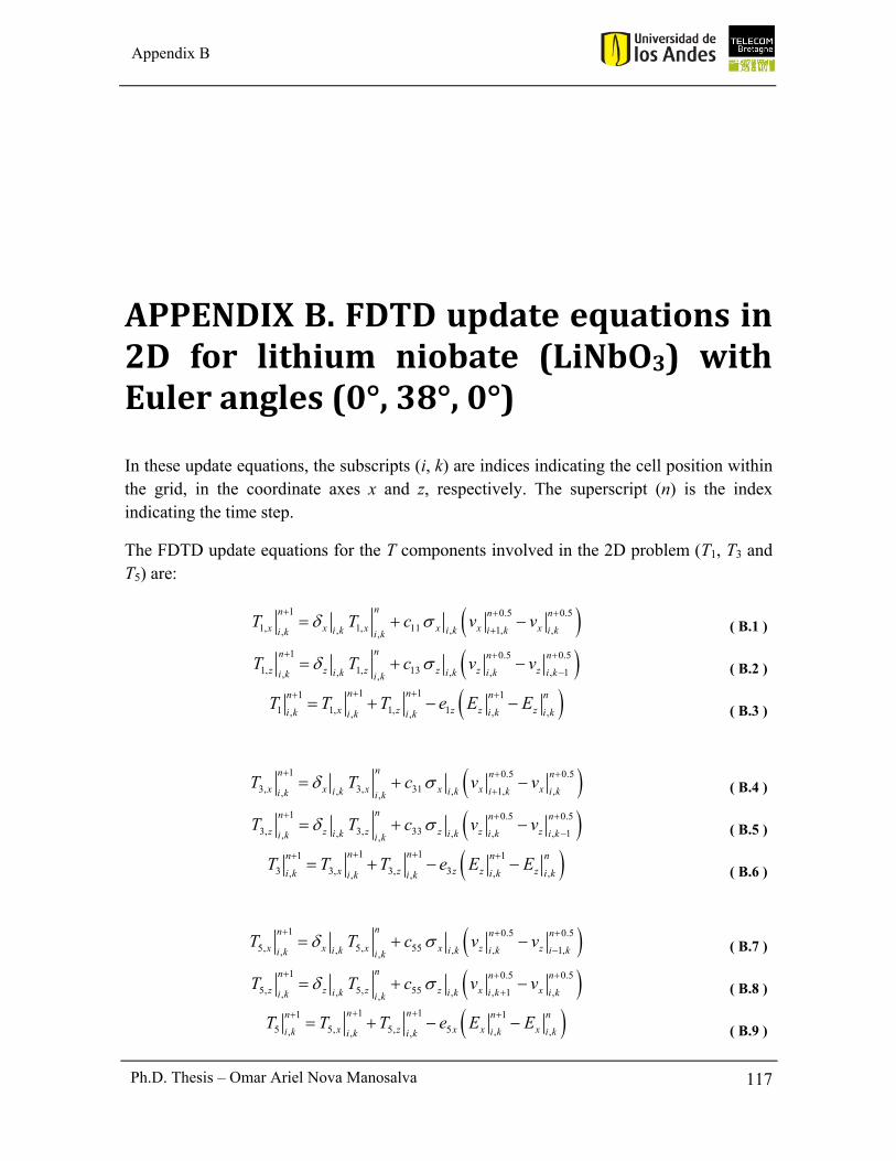
117 Ph.D. Thesis – Omar Ariel Nova Manosalva
Appendix B
APPENDIXB.FDTDupdateequationsin2D for lithium niobate (LiNbO3) withEulerangles(0°,38°,0°)
In these update equations, the subscripts (i, k) are indices indicating the cell position within the grid, in the coordinate axes x and z, respectively. The superscript (n) is the index indicating the time step.
The FDTD update equations for the T components involved in the 2D problem (T1, T3 and T5) are:
1 0.5 0.5
1, 1, 11, , 1, ,, ,
nn n n
x x x x x xi k i k i k i ki k i kT T c v v
( B.1 )
1 0.5 0.5
1, 1, 13, , , , 1, ,
nn n n
z z z z z zi k i k i k i ki k i kT T c v v
( B.2 )
1 11 1
1 1, 1, 1, , ,, ,
n nn n n
x z z z zi k i k i ki k i kT T T e E E
( B.3 )
1 0.5 0.5
3, 3, 31, , 1, ,, ,
nn n n
x x x x x xi k i k i k i ki k i kT T c v v
( B.4 )
1 0.5 0.5
3, 3, 33, , , , 1, ,
nn n n
z z z z z zi k i k i k i ki k i kT T c v v
( B.5 )
1 11 1
3 3, 3, 3, , ,, ,
n nn n n
x z z z zi k i k i ki k i kT T T e E E
( B.6 )
1 0.5 0.5
5, 5, 55, , , 1,, ,
nn n n
x x x x z zi k i k i k i ki k i kT T c v v
( B.7 )
1 0.5 0.5
5, 5, 55, , , 1 ,, ,
nn n n
z z z z x xi k i k i k i ki k i kT T c v v
( B.8 )
1 11 1
5 5, 5, 5, , ,, ,
n nn n n
x z x x xi k i k i ki k i kT T T e E E
( B.9 )
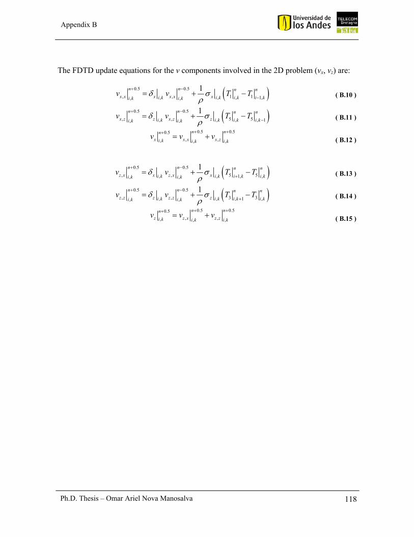
118 Ph.D. Thesis – Omar Ariel Nova Manosalva
Appendix B
The FDTD update equations for the v components involved in the 2D problem (vx, vz) are:
0.5 0.5
, , 1 1, , , 1,, ,
1n n n n
x x x x x xi k i k i k i ki k i kv v T T
( B.10 )
0.5 0.5
, , 5 5, , , , 1, ,
1n n n n
x z z x z zi k i k i k i ki k i kv v T T
( B.11 )
0.5 0.50.5
, ,, , ,
n nn
x x x x zi k i k i kv v v
( B.12 )
0.5 0.5
, , 5 5, , 1, ,, ,
1n n n n
z x x z x xi k i k i k i ki k i kv v T T
( B.13 )
0.5 0.5
, , 3 3, , , 1 ,, ,
1n n n n
z z z z z zi k i k i k i ki k i kv v T T
( B.14 )
0.5 0.50.5
, ,, , ,
n nn
z z x z zi k i k i kv v v
( B.15 )
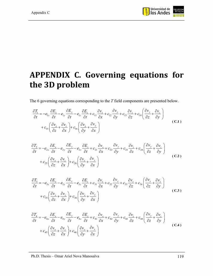
119
Appendix C
Ph.D. Thesis – Omar Ariel Nova Manosalva
APPENDIX C. Governing equations forthe3Dproblem
The 6 governing equations corresponding to the T field components are presented below.
11 1 1 11 12 13 14
15 16
y y yx xz z zx y z
yx xz
E v vE vT E v ve e e c c c c
t t t t x y z z y
vv vvc c
z x y x
( C.1 )
22 2 2 21 22 23 24
25 26
y y yx xz z zx y z
yx xz
E v vE vT E v ve e e c c c c
t t t t x y z z y
vv vvc c
z x y x
( C.2 )
33 3 3 31 32 33 34
35 36
y y yx xz z zx y z
yx xz
E v vT E vE v ve e e c c c c
t t t t x y z z y
vv vvc c
z x y x
( C.3 )
44 4 4 41 42 43 44
45 46
y y yx xz z zx y z
yx xz
E v vE vT E v ve e e c c c c
t t t t x y z z y
vv vvc c
z x y x
( C.4 )

120
Appendix C
Ph.D. Thesis – Omar Ariel Nova Manosalva
55 5 5 51 52 53 54
55 56
y y yx xz z zx y z
yx xz
E v vT E vE v ve e e c c c c
t t t t x y z z y
vv vvc c
z x y x
( C.5 )
66 6 6 61 62 63 64
65 66
y y yx xz z zx y z
yx xz
E v vT E vE v ve e e c c c c
t t t t x y z z y
vv vvc c
z x y x
( C.6 )
The 3 governing equations corresponding to the v field components are presented below.
5 611xv T TT
t x z y
( C.7 )
62 41yv TT T
t y z x
( C.8 )
3 541z T Tv T
t z y x
( C.9 )

121
Appendix D
Ph.D. Thesis – Omar Ariel Nova Manosalva
APPENDIXD.FDTDupdateequationsin3D for bismuth germanate (Bi4Ge3O12)withEulerangles(0°,0°,0°)
In these update equations, the subscripts (i, j, k) are indices indicating the cell position within the grid, in the coordinate axes x, y and z, respectively. The superscript (n) is the index indicating the time step.
The FDTD update equations for the T components are:
1 0.5 0.5
1, 1, 11, , , , 1, , , ,, , , ,
nn n n
x x x x x xi j k i j k i j k i j ki j k i j kT T c v v
( D.1 )
1 0.5 0.5
1, 1, 12, , , , , , , , , 1,, ,
nn n n
y y y y y yi j k i j k i j k i j k i j ki j kT T c v v
( D.2 )
1 0.5 0.5
1, 1, 13, , , , , , , , 1, , , ,
nn n n
z z z z z zi j k i j k i j k i j ki j k i j kT T c v v
( D.3 )
11 11
1 1, 1, 1,, , , , , ,, ,
nn nn
x y zi j k i j k i j ki j kT T T T
( D.4 )
1 0.5 0.5
2, 2, 21, , , , 1, , , ,, , , ,
nn n n
x x x x x xi j k i j k i j k i j ki j k i j kT T c v v
( D.5 )
1 0.5 0.5
2, 2, 22, , , , , , , , , 1,, ,
nn n n
y y y y y yi j k i j k i j k i j k i j ki j kT T c v v
( D.6 )
1 0.5 0.5
2, 2, 23, , , , , , , , 1, , , ,
nn n n
z z z z z zi j k i j k i j k i j ki j k i j kT T c v v
( D.7 )
11 11
2 2, 2, 2,, , , , , ,, ,
nn nn
x y zi j k i j k i j ki j kT T T T
( D.8 )
1 0.5 0.5
3, 3, 31, , , , 1, , , ,, , , ,
nn n n
x x x x x xi j k i j k i j k i j ki j k i j kT T c v v
( D.9 )
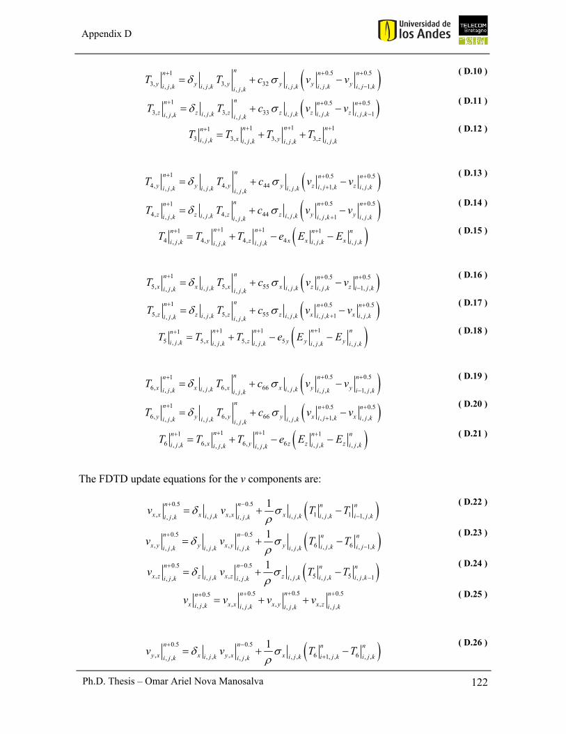
122
Appendix D
Ph.D. Thesis – Omar Ariel Nova Manosalva
1 0.5 0.5
3, 3, 32, , , , , , , , , 1,, ,
nn n n
y y y y y yi j k i j k i j k i j k i j ki j kT T c v v
( D.10 )
1 0.5 0.5
3, 3, 33, , , , , , , , 1, , , ,
nn n n
z z z z z zi j k i j k i j k i j ki j k i j kT T c v v
( D.11 )
11 11
3 3, 3, 3,, , , , , ,, ,
nn nn
x y zi j k i j k i j ki j kT T T T
( D.12 )
1 0.5 0.5
4, 4, 44 , 1, , ,, , , , , ,, ,
nn n n
y y y y z zi j k i j ki j k i j k i j ki j kT T c v v
( D.13 )
0.5 0.51
4, 4, 44, , , ,, , , , 1 , ,, ,
n n nn
z z z z y yi j k i j ki j k i j k i j ki j kT T c v v
( D.14 )
1 11 1
4 4, 4, 4, , , , , ,, ,, ,
n nn n n
y z x x xi j k i j k i j ki j ki j kT T T e E E
( D.15 )
1 0.5 0.5
5, 5, 55, , , , , , 1, ,, , , ,
nn n n
x x x x z zi j k i j k i j k i j ki j k i j kT T c v v
( D.16 )
1 0.5 0.5
5, 5, 55, , , , , , 1 , ,, , , ,
nn n n
z z z z x xi j k i j k i j k i j ki j k i j kT T c v v
( D.17 )
11 11
5 5, 5, 5, , , , , , , , , ,
n nn nn
x z y y yi j k i j k i j k i j k i j kT T T e E E
( D.18 )
0.5 0.51
6, 6, 66, , , ,, , , , 1, ,, ,
n n nn
x x x x y yi j k i j ki j k i j k i j ki j kT T c v v
( D.19 )
1 0.5 0.5
6, 6, 66 , 1, , ,, , , , , ,, ,
nn n n
y y y y x xi j k i j ki j k i j k i j ki j kT T c v v
( D.20 )
111 1
6 6, 6, 6, , , , , ,, , , ,
nnn n n
x y z z zi j k i j k i j ki j k i j kT T T e E E
( D.21 )
The FDTD update equations for the v components are:
0.5 0.5
, , 1 1, , , , , , 1, ,, , , ,
1n n n n
x x x x x xi j k i j k i j k i j ki j k i j kv v T T
( D.22 )
0.5 0.5
, , 6 6, , , 1,, , , , , , , ,
1n n n n
x y y x y y i j k i j ki j k i j k i j k i j kv v T T
( D.23 )
0.5 0.5
, , 5 5, , , , , , , , 1, , , ,
1n n n n
x z z x z zi j k i j k i j k i j ki j k i j kv v T T
( D.24 )
0.50.5 0.50.5
, , ,, , , , , ,, ,
nn nn
x x x x y x zi j k i j k i j ki j kv v v v
( D.25 )
0.5 0.5
, , 6 6, , , , 1, , , ,, , , ,
1n n n n
y x x y x xi j k i j k i j k i j ki j k i j kv v T T
( D.26 )
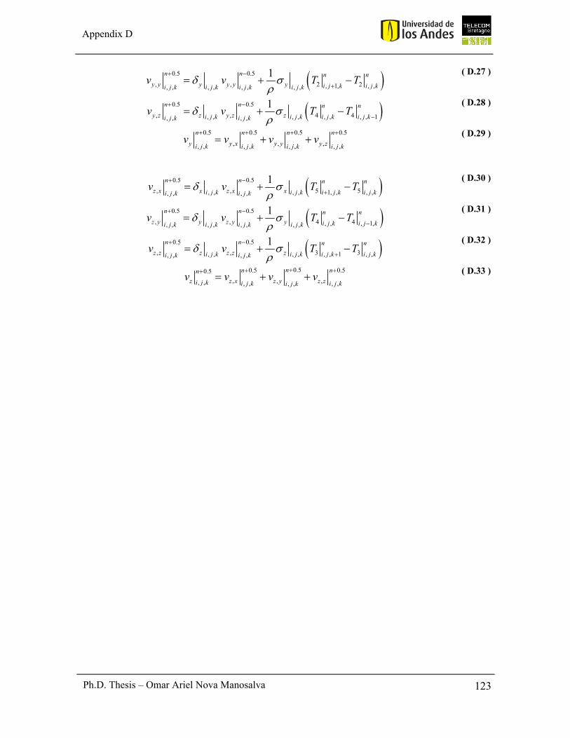
123
Appendix D
Ph.D. Thesis – Omar Ariel Nova Manosalva
0.5 0.5
, , 2 2, 1, , ,, , , , , , , ,
1n n n n
y y y y y y i j k i j ki j k i j k i j k i j kv v T T
( D.27 )
0.5 0.5
, , 4 4, , , , , , , , 1, , , ,
1n n n n
y z z y z zi j k i j k i j k i j ki j k i j kv v T T
( D.28 )
0.5 0.5 0.5 0.5
, , ,, , , , , , , ,
n n n n
y y x y y y zi j k i j k i j k i j kv v v v
( D.29 )
0.5 0.5
, , 5 5, , , , 1, , , ,, , , ,
1n n n n
z x x z x xi j k i j k i j k i j ki j k i j kv v T T
( D.30 )
0.5 0.5
, , 4 4, , , 1,, , , , , , , ,
1n n n n
z y y z y y i j k i j ki j k i j k i j k i j kv v T T
( D.31 )
0.5 0.5
, , 3 3, , , , , , 1 , ,, , , ,
1n n n n
z z z z z zi j k i j k i j k i j ki j k i j kv v T T
( D.32 )
0.50.5 0.50.5
, , ,, , , , , ,, ,
nn nn
z z x z y z zi j k i j k i j ki j kv v v v
( D.33 )