to the university of wyoming: the members of the …€¦ · assessing the conflict between wind...
TRANSCRIPT
To The University of Wyoming:
The members of the Committee approve the thesis of Natalie C. Macsalka
presented on September 6, 2011.
Benjamin S. Rashford, Chairperson
Matthew Holloran, External Department Member
Roger Coupal
APPROVED:
Dr. R. Coupal, Department Head, Department of Agriculture and Applied
Economics.
Frank Galey, Dean, College of Agriculture and Natural Resources

i
Macsalka, Natalie, Assessing the conflict between wind energy development and sage-grouse
conservation in Wyoming: An application using a spatial explicit wind
development model, M.S., Department of Agricultural and Applied
Economics, September 6, 2011.
Concern about energy independence and climate change have driven state and federal
governments to promote renewable energy production, mainly in the form of wind generated
electricity. There are social costs of wind energy development, however, that can lower its
environmental value. Most notably, wind turbines can impact wildlife and wildlife habitat.
Wind-wildlife conflicts are particularly intense in Wyoming, which has more high-quality wind
resources than all other western states combined. Wyoming also has the largest amount of intact
sagebrush ecosystem, which provides habitat for 64% of the known greater sage-grouse
(Centrocercus urophasianus) population in the eastern portion of the species range. The greater
sage-grouse was recently listed as a candidate on the endangered species list due largely to
threats from energy development. Current legislation in Wyoming restricts wind energy
development within greater sage-grouse core breeding areas. This suggests that the tradeoff
between wind development and greater sage-grouse persistence is steep.
I develop an econometric model to estimate the probability of wind development across
26 million acres of Wyoming. I then use these probabilities to simulate a range of wind energy
build-out levels, with and without the current sage-grouse core-area restrictions. The model
predicts that locations closer to transmission lines with higher wind classes are most likely to be
occupied in the future by a wind farm. Some of the high probability wind locations also coincide
with sage-grouse core breeding areas. Thus, there is potential for conflict between sage-grouse
conservation and future wind development. There is relatively little conflict at low build-out
levels (1,650 MW); however, as more wind development is distributed across the landscape,
conflict increases. In the absence of conservation a build-out of 13,770 MW results in potential
impacts to 1,346 males on 56 leks (2.4% of Wyoming’s male population based on 2007
maximum lek counts). Restricting development in sage-grouse core areas (as defined by WY
state governor in executive order 2011-5) will result in 324 males on 19 leks being potentially
influenced, a reduction of 1.82% with an energy development opportunity cost of a 4% reduction
in wind energy profits. Thus, while there are certain to be conflicts between sage-grouse and
wind energy development, my results suggests that Wyoming can harness its vast wind resources
while conserving sage-grouse.

ASSESSING THE CONFLICT BETWEEN WIND ENERGY DEVELOPMENT AND SAGE-
GROUSE CONSERVATION IN WYOMING: AN APPLICATION USING A SPATIALLY
EXPLICIT WIND DEVELOPMENT MODEL.
By
Natalie C. Macsalka
A thesis submitted to the Department of Agricultural and Applied Economics
and the University of Wyoming
in partial fulfillment of the requirements
for the degree of
MASTER OF SCIENCE
in
AGRICULTURE AND APPLIED ECONOMICS
Laramie, Wyoming
December 2011

iii
© 2011, Natalie Macsalka

iv
Acknowledgements
I think the question isn’t really who to thank but who not to thank. I appreciate everyone
at the University of Wyoming and all the private, state, and non-profit organizations who assisted
me with finding answers to my unending questions. I thank WYGISC staff members Teal
Wyckoff, Sean Lanning and Shannon Albeke for their kind and knowledgeable assistance,
especially at times when I know they too were on a deadline.
I certainly could not have finished with a smiling, happy face without the support and
love of my family (Thanks Mom!), friends and my fiancé Aaron Rutledge. Finally, I was
blessed with a wonderful committee who provided the knowledge, encouragement and guidance
I so very much needed. I will forever be grateful to Dr. Benjamin Rashford for his enthusiasm,
insights and unconditional support he so tirelessly gave. Oh, and I cannot forget to thank coffee!

v
TABLE OF CONTENTS 1 Introduction ............................................................................................................................. 1
2 Background/Literature Review................................................................................................ 6
2.1 Brief History of Sage-Grouse Conservation .................................................................... 6
2.2 Energy Impacts to Sage-Grouse ....................................................................................... 9
2.3 Wind Development ........................................................................................................ 13
2.3.1 Wind Siting ............................................................................................................. 15
3 Methods ................................................................................................................................. 18
3.1 Empirical Model of Wind Farm Location Decisions ..................................................... 18
3.1.1 Data ......................................................................................................................... 19
3.1.2 Estimation Issues .................................................................................................... 25
3.1.3 Logit Model Results ................................................................................................ 28
4 Simulating Wind Farm Build-Out Scenarios and Assessing Sage-grouse Habitat Conflicts 33
4.1 Wind Build-Out Scenarios ............................................................................................. 33
4.2 Measures to Capture Tradeoff between Wind Energy Development and Sage-grouse . 35
4.2.1 Profit ....................................................................................................................... 35
4.2.2 Sage-Grouse Impacts .............................................................................................. 36
4.2.3 Method to Assess Tradeoffs between Wind Development and Sage-grouse. ........ 39
4.3 Results and Policy Implications ..................................................................................... 41
5 Conclusion ............................................................................................................................. 49
6 Future research ...................................................................................................................... 52
7 Literature Cited ...................................................................................................................... 55
8 Appendix ............................................................................................................................... 61
8.1 Data Descriptions ........................................................................................................... 61
8.2 Appendix Results ........................................................................................................... 65

vi
LIST OF TABLES
Table 1. Descriptive Statisticsa of Continuous Explanatory Variables. ....................................... 25
Table 2. Average Values of Explanatory Variables between Parcels With and Without Wind
Turbines. ............................................................................................................................... 25
Table 3. Average Parameter Estimates across bootstraps. ........................................................... 29
Table 4. Average Marginal Effects Across Parcels. .................................................................... 30
Table 5. Average Predicted Probability of Observing a Wind Farm Grouped by Parcels With
(Y=1) and Without (Y=0) Existing Wind Farms. ................................................................. 31
Table 6. Capacity Factors by Wind Class used to Estimate Total Wind Farm Revenue. ............ 36
Table 7. Characteristics of Wyoming Game and Fish Sage-grouse Lek Data in Wyoming
through 2010. ........................................................................................................................ 39
Table 8. Wind Energy (MWh) and Profits for Alternative Build-out Scenarios given Current and
All Transmissiona .................................................................................................................. 44
Table 9. Impact of Wind Development on Sage-Grouse for Alternative Build-Out Levels
Assuming No Sage-grouse Conservation Policies at 6.4km Buffer ..................................... 45
Table 10. Number of Sage-Grouse Core-Area Parcels Impacted by Unrestricted Build-Out ..... 46
Table 11. Effect of Core Area Restrictions on Wind Farm Profits and Sage-Grouse with a Build-
Out of 8,790 MW .................................................................................................................. 47
Table 12. Effect of Core Area Restrictions on Wind Farm Profits and Sage-Grouse with a Build-
Out of 13,770 MW ................................................................................................................ 48
Table 13. Exclusion list for Econometric Model. ......................................................................... 61
Table 14. Impact of Wind Development on Sage-Grouse for Alternative Build-Out Levels
Assuming No Sage-grouse Conservation Policies at 3.2km buffer. ..................................... 65

vii
Table 15. Core Area Restrictions Expected Lek Impacts within 6.4km Buffer. ......................... 66
LIST OF FIGURES
Figure 1. WAFWA Greater sage-grouse management zones. ........................................................ 7
Figure 2. Map of feasible area (after exclusions) for the wind farm site decision model. ........... 24
Figure 3. Map of predicted wind development locations in comparison to Qualified Resource
Areas. .................................................................................................................................... 32
Figure 4. Map of predicted wind development locations in comparison to existing wind turbines
and met tower locations. ....................................................................................................... 33
Figure 5. Version 3 map of Wyoming executive order protecting sage-grouse core breeding
areas. ..................................................................................................................................... 41
Figure 6. Various build-out levels for the current plus proposed transmission: a. 1,650 MW, b.
4,020 MW, c. 8,790 MW, and d.13,770 MW. ...................................................................... 43
Figure 7. Map of 13,770 MW build-out for unrestricted (a) and with core restrictions (b). ........ 49
Figure 8. Wyoming environmental conflicts map ........................................................................ 64
Figure 9. 50m wind resource map for Wyoming available from Wind Powering America. ........ 65

1
1 Introduction
Societal concern for energy independence and climate change mitigation have driven
state and federal policies towards promoting renewable energy production as an alternative to
fossil fuels. Wind generated electricity is currently the fastest growing and least-cost utility scale
renewable technology being widely implemented. For instance, wind energy is currently the
third largest energy source (behind Natural Gas, and Coal) being added to the US electric grid –
during the five previous years it was ranked second (Wiser and Bolinger 2011).
The United States is the second largest global emitter of greenhouse gases (GHG’s)
(Krupnick et al. 2010), with electrical power generation responsible for more pollution than any
other single activity (EIA 2011). Generating electricity with wind is non-polluting, renewable
and potentially reduces greenhouse gas emissions by displacing fossil fuel generation. One
estimate concluded a 1.5MW wind turbine displaces 2,700 metric tons of CO2 per year (DOE
2008). However, as with all land use activities, there are social costs of wind energy
development that can lower its environmental value. Most notably, wind turbines can create
visual disamenities and directly or indirectly impact wildlife and their habitats. While not
discussed further here, a recent economic study predicted the visual impacts from an offshore
wind project in Nantucket, Cape Cod and Martha’s Vineyard to cause a loss of $57,000,000
annually in tourism dollars (Haughton et al. 2003).
The potential impacts from wind energy development to wildlife species and their
habitats include both direct and indirect impacts. Direct impacts may include mortality from
blade strikes and barotrauma (damage from air pressure differences caused by spinning turbine
blades), and habitat loss. Indirect impacts include avoidance or displacement behavior, the
introduction of invasive plant species, and increases in predators (USFWS 2011). The most
widely documented impacts thus far are bird and bat fatalities caused by direct collision or
2
barotrauma (in bats) with turbines, support structures, or transmission infrastructure (The
Wildlife Society 2007). Wind turbines sit atop structures 80 meters high with average rotor
diameters (blade tips) of 84.3 meters (Wiser and Bolinger 2011). Groups of turbines are
clustered together into wind farms of 60-1,000 turbines1 spanning large areas. While the direct
disturbance of each wind turbine is small, 1-3 acres per turbine, the extensive fragmentation of
the landscape from all the components of a wind farm (e.g., turbines, transmission, substations,
facilities, and roads) poses a larger potential threat to wildlife than collision with turbines
(Kuvlesky et al 2007).
Wind farm siting has become a large issue for wind energy developers and land
managers. To illustrate, while the quality of the wind resource (high consistent wind speeds)
may be the most important factor affecting profitability (EWEA 2009), approximately 10-25% of
proposed wind energy projects are delayed or canceled because of environmental concerns (DOE
2008). The value of proper siting to maximize winds environmental benefits is illustrated by the
United States Fish and Wildlife Service: “siting of a wind energy project is the most important
element in avoiding effects to species and their habitats” (USFWS 2011: p. 8).
Many economies in the West rely on developing vast reserves of energy and minerals to
sustain themselves. Land use management decisions between conflicting uses, such as managing
for profits and managing for wildlife, require tradeoffs. This places a critical need on identifying
management objectives that balance energy demands and wildlife habitat protection. This
conflict has become particularly notable in Wyoming where the economy is more dependent on
energy than any other state in the Intermountain West (Haggerty and Mehl 2009). Wyoming is
first in coal production, 2nd
in natural gas production (EIA 2011) and contains more than 50% of
1 Calculated number of turbines based on: Average wind farm nameplate capacity of 120 MW in 2007, 91 MW in
2009 (Market Report 2007, 2009) and the largest wind farm project (Choke Cherry Sierra Madre) in Wyoming of
2,500MW divided by current average turbine size of 1.5 MW (Wiser and Bolinger 2011) or for the largest, 2.5 MW.

3
the best class 5-7 winds in the Western US (WREZ 2009). A recent study (National Grid 2008)
characterized Wyoming as the “jewel of the region for wind resource” – identifying Wyoming as
the lowest cost renewable energy solution for the Desert Southwest. Wyoming’s productive
wind resource has not gone unnoticed. Wyoming is currently ranked 10th
in the country for
installed wind capacity (1,412 MW), and has another 7,869.5 MW in various planning stages
(AWEA, 2011a).
At the same time, Wyoming contains the largest amount of intact sagebrush ecosystem
remaining, which provides habitat for 64% of the known greater-sage-grouse population
(Centrocercus urophasianus) in the eastern portion of its range (Doherty 2008). The greater
sage-grouse (hereafter sage-grouse) is a game bird endemic to the western United States
(Connelly et al 2004), which is experiencing range wide population declines. The distribution of
oil, gas, and wind energy resources closely align with critical sagebrush habitats (Doherty 2008).
Researchers have shown that sage-grouse populations decline with oil and gas development
(Holloran 2005; Doherty 2008). These declines occur when sage-grouse avoid infrastructure and
when development’s cumulative impacts affect reproduction or survival (Naugle 2011, pp 55-
70). Many of the impacts from traditional energy development are expected to occur with wind
energy development. For example, the impacts of roads and transmission infrastructure are
common to all production and generating facilities (NRC 2007).
Together these factors make Wyoming a high conflict area for balancing energy
development (in this case wind energy) and wildlife conservation. In 2005, United States Fish
Wildlife Service (USFWS) identified energy development as the most significant extinction risk
to sage-grouse in the eastern portion of its range (WY and MT) (Johnson and Holloran 2010).
The USFWS concluded in 2010 that greater sage-grouse were warranted for protection under the

4
Endangered Species Act (1973), but because threats to the species are moderate and do not occur
across their range at an equal intensity, the listing was precluded by other species under more
severe extinction risk (USFWS 2010). A recent study by Doherty (2008) identified that
Wyoming has the highest percentage of sage-grouse core breeding areas at risk from both fossil
fuel and wind energy development.
The risks of an endangered species listing and the potential losses of energy tax revenues
led the Wyoming Governors office to implement an executive order to protect sage-grouse core
breeding areas (Executive order 2011-5). The Wyoming Core area executive order is “designed
to maintain existing suitable sage-grouse habitat by permitting development activities in core
areas in a way that will not cause declines in sage-grouse populations” (Executive order 2011-5).
In Core areas, land use activities are limited and regulated based on their known impacts to
grouse through buffer requirements, mitigation, and other best management practices. For
example, each project developer must complete a Project Implementation Area Analysis (PIAA)
(Executive order 2011-5- Attachment B). The PIAA identifies all occupied leks within a 4 mile
boundary around the project area and then a 4 mile boundary around each occupied lek within
that boundary. All occupied leks within the project area are considered to be “affected” by the
proposed project. This information is then used in a Density/Disturbance Calculation Tool to
determine the maximum allowable disturbance (up to 5% per 640 acres). In addition to the
PIAA the executive order establishes stipulations regarding: No Surface Occupancy, seasonal
use, noise, and location of roads and overhead lines that must be followed by a project developer
(see Executive order 2011-5- Attachment B for list). However, in the case of wind energy
development, where scientific understanding of potential impacts is lacking, no development is

5
recommended in sage-grouse core areas. This recommendation will be “reevaluated on a
continuous basis as new science, information and data emerges” (Executive Order 2011-5).
To date, planning tools that compare the best remaining areas for sage-grouse with the
extent of current and anticipated wind development have only considered raw wind resource
potential (Naugle et al. 2009; Doherty 2008). An approach that incorporates the economic
considerations of developers when selecting locations will more accurately frame the level of
risk of wind energy development to species, such as sage-grouse. For example, a developer
searching for a wind farm site would certainly prefer higher wind speeds that produce more
energy, thus higher profits, than energy produced with lower wind speeds. However, the
developer must also consider the tradeoff between remote high quality wind resources that lack
transmission access (thus an added expense), and lower quality resources closer to demand loads
and existing transmission. Because all habitat protection is not equal and protecting habitat is
costly, allocating conservation efforts to lands that have accounted for economic considerations
in addition to biological threat will assure a better “bang per buck” for conservation efforts.
I develop an econometric model to estimate parcel level probability of wind energy
development for the state of Wyoming. I use GIS to incorporate site specific and landscape
characteristics that impact the profitability of wind development. Next I use the model to
simulate a range of wind energy build-out levels to account for uncertainty in the actual level of
wind power development that may occur in Wyoming. I apply the econometric model and wind
energy build-out scenarios to current sage-grouse management policy in Wyoming to quantify
the risk of wind development on sage-grouse populations. With information on costs (i.e.,
foregone profits) the tradeoff between sage-grouse and wind development can be identified by

6
jointly modeling sage-grouse and wind production from these alternative wind development
scenarios.
2 Background/Literature Review
2.1 Brief History of Sage-Grouse Conservation
An extensive body of literature now exists studying the ecology of the greater sage-
grouse. Connelly et al. (2004) thoroughly summarizes the population ecology, habitat, impacts
and threats, and conservation of the greater sage-grouse and its habitat. Sage-grouse are
considered a “sagebrush obligate” species as they rely on large contiguous sagebrush ecosystems
throughout their lifecycle for both food and cover. These sagebrush habitats are among the most
imperiled ecosystems in North America with few areas remaining undisturbed or unaltered from
pre-settlement condition (Knick et al. 2003). Since the 1960’s sage-grouse populations have
declined by at least 17-47% (Connelly 2000). Currently sage-grouse occupy habitat in 11
western states and two Canadian provinces-half of their historical pre-settlement range (Connelly
et al. 2004).
Conservation and management efforts for greater sage-grouse populations and their
habitats occur in all 11 states with habitat for sage-grouse (Connelly et al. 2004). Sage-grouse in
WY are managed within Western Association of Fish and Wildlife Agencies Management zones
I and II (Fig 1), which, along with management zones IV and V, encompass the core populations
of sage-grouse and have the highest reported densities (USFWS 2008).

7
Figure 1. WAFWA Greater sage-grouse management zones.
Numerous threats both anthropogenic and natural have been identified all involving the
loss, fragmentation or degradation of sagebrush habitats as well as direct mortalities to the bird.
Impacts include: residential development and urbanization, agriculture, energy development,
improper grazing, West Nile virus, weather and climate change, invasive species, fences, and
fire. Specific threats to sage-grouse populations vary across its range. For example, in Montana
a large amount of the sage-grouse habitat is on private lands and these lands are increasingly
being converted to agriculture whereas in Nevada and the Great Basin, threats include invasive
plant species and fire; in Wyoming and northern Colorado energy development is the major
threat;. Further, the cumulative impacts from a combination of sources can create a stronger
overall impact to populations. Still, the sage-grouse is doing well in some portions of their
range. Research suggests that conserving large landscapes with suitable habitat is important for
conservation of sage-grouse (Connelly unpublished) and scientists call for protection of the last
remaining strongholds as the focus of conservation. The sage-grouse is considered a valuable

8
species for managing the sagebrush ecosystem because of its strong correlation to intact
sagebrush. A study by Rowland 2006 tested the efficacy of using the sage-grouse as an umbrella
species of the overall health of the sagebrush ecosystem. They found that protective
management of sage-grouse habitats would provide high conservation coverage for other
sagebrush obligate species.
Sage-grouse have seasonal habitats over large areas with some populations moving
between two-three distinct winter, breeding, and summer seasonal ranges (migratory), while
others have highly integrated seasonal ranges (resident) (Connelly et al. 2004). Because of these
seasonal use differences the total area of a home range varies based on whether the population is
migratory or resident and can be up to 2,700 km2
(Connelly 2000) with a single bird requiring an
estimated 10,000 acres (Pat Diebert, USFWS, Cheyenne, WY, pers. comm.).
Sagebrush is a major food source for adults throughout the year (Connelly et al. 2004).
Sage-grouse select habitat with different aged stands of sagebrush and a healthy understory of
forbs and grasses. In winter, sage-grouse rely exclusively on sagebrush for food and cover. In
the breeding season sage-grouse select large contiguous stands dominated by sagebrush to
provide for mating, nesting and early brood rearing activities (Connelly et al. 2004). The iconic
image of the sage-grouse is defined by the elaborate courtship displays performed by males on
lek sites to attract females during the breeding season (Connelly et al. 2004). These lek locations
are selected in proximity to relatively dense sagebrush stands suitable for nesting. In relatively
contiguous habitats females nest within close proximity to the breeding lek with the bulk of sage-
grouse nests found under sagebrush (Connelly 2000). During early brood rearing, females raise
their brood within short distances of the nest in areas with less sagebrush canopy cover foraging
on a diet of forbs and insects; in addition to sagebrush. As broods age and forbs dry out the birds
9
move to summer habitats (e.g., riparian, upland meadows, sagebrush grasslands), which may be
relatively far from nesting/early brood-rearing habitat. Both male and female sage-grouse
exhibit high fidelity (i.e., return to the same area year after year) to breeding and nesting sites
(Connelly et al. 2004).
2.2 Energy Impacts to Sage-Grouse
There is a growing body of literature documenting the impacts of traditional energy
development on sage-grouse populations. The direct and indirect impacts of traditional energy
development on sagebrush habitats include the physical removal of sagebrush (clearing an area)
fragmentation of habitat (e.g., well pads, roads, transmission), soil disturbance, increases in:
noise pollution, vehicle traffic, predation from raptors, and increases in mesopredators and
invasive plant species (Connelly et al. 2004). Negative impacts have been identified in
numerous sage-grouse populations from coal bed natural gas, deep gas and oil (Naugle et al.
2011, pp.55-70) and wind energy development is expected to cause similar impacts. These
studies show sage-grouse avoid energy development. In natural gas fields yearling females
avoided infrastructure when selecting sites for nests and yearling males avoided leks inside
development (Holloran 2005). Both the density of well pads and distance to infrastructure is
associated with declining lek attendance. Holloran (2005) found male lek attendance declined
with distance to active drilling rigs, producing gas wells and main haul roads. These lek impacts
are most severe near the lek but were discernable at distances greater than 6 km, often resulting
in loss of leks within gas fields (Naugle et al. 2011). A review of recent studies found oil and
gas development in excess of 1 pad/2.6 km2 resulted in impacts to breeding populations and
impacts from conventional well densities exceeded the species’ threshold of tolerance (Naugle et
al. 2009).

10
The impacts of wind energy development on sage-grouse populations are relatively
unknown – several studies in Wyoming have been initiated but are in their infancy. For instance,
funding was recently granted to two projects in Wyoming related to proposed wind
developments (NWCC 2011). One will focus on behavior and habitat use by male sage-grouse
at the Chokecherry Sierra Madre Wind project and another will be a continuation of research in
Carbon County initiated in 2009 studying wind energy development impacts on sage-grouse
habitat selection and demographics. Research from traditional energy development has
identified a time lag between the onset of development activities and lek loss making long term
research necessary to identify impacts to sage-grouse populations. Holloran (2005) identified a 3
to 4 year time lag in natural gas fields resulting from high female nest site fidelity (adults
continue to use areas regardless of development) but lower survival of nesting adult sage-grouse
combined with avoidance behavior by yearlings that are displaced to the periphery. So adults
return to areas regardless of development and as a result experience higher death rates (i.e., not
adapting) whereas yearlings that have not yet become imprinted to a breeding or nesting site are
displaced (Naugle 2010). A similar time lag was identified with the black grouse and wind
energy development in Austria. The first year of operation reported no impacts to the population
but by the fifth year the population was declining (Zeiler 2009). Because of the lag, it may be
several years before population level impacts of wind energy development on sage-grouse are
known.
One of the expected impacts from wind energy development includes direct mortalities
through collisions with turbines, towers, distribution and transmission lines and vehicles
(Johnson and Holloran 2010). Grouse are grouped into poor fliers (Johnson and Holloran 2010)
and the highest collision probability for sage-grouse and wind turbines is expected where

11
structures are located between foraging and loafing habitats (USFWS 2008). However, while
some collisions may occur it is unlikely that these direct mortalities would lead to population
declines (USFWS 2008).
The largest impacts from wind development are expected from fragmentation that may
displace sage-grouse and/or reduce survival (Johnson and Holloran 2010). Habitat fragmentation
is a primary cause of population declines because sage-grouse require contiguous sagebrush
(Johnson and Holloran 2010). Fragmentation occurs through actual loss of habitat that leaves
remaining habitat in non-contiguous patches or functional loss from alteration that leaves the
habitat patches unusable (Johnson and Holloran 2010). Studies of the fragmentation impacts
from power lines found population impacts out to five miles (Johnson and Holloran 2010).
Power lines can be a collision risk to sage-grouse and may increase predation risk by acting as
perches and nesting sites for ravens and raptors (Johnson and Holloran 2010). Current estimates
of line length for proposed long distance transmission lines originating in Wyoming range from
180 miles for a line to Colorado, to 1,100 miles to send power to California (WIA 2011). These
lines are in addition to the collector lines from individual wind turbines and short distance
distribution lines to nearby towns.
The road networks across the landscape are also a source of fragmentation. Impacts from
roads include direct habitat loss, direct mortality, spread of invasive plant species, increased
access for predators, and noise (USFWS 2008). Currently less than 5% of the sagebrush habitat
for sage-grouse is further than 2.5 km from a road (Connelly unpublished). Roads have been
found to cause declines in male lek attendance within 1.9 miles of main haul roads with just one
vehicle a day in oil and gas development (Johnson and Holloran 2010). A recent study of the
land area impacts of current wind development found that roads account for the highest percent

12
of area impacted (Denholm et al. 2009). This suggests that roads within wind energy
development may have similar impacts as those identified in oil and gas development. The
largest difference is that gas wells require daily road travel whereas wind turbines are monitored
by computer; therefore, they should require less vehicle visits (Johnson and Holloran 2010).
Scientists speculate that turbine towers will decrease habitat suitability (USFWS 2008)
and displace sage-grouse from former areas (USFWS 2008). Sage-grouse will avoid areas,
including otherwise suitable habitat, because of raptors perching on transmission and other
structures, emissions, or other human presence such as vehicle traffic, and noise (Johnson and
Holloran 2010).
Given the potential impacts of wind energy development to sage-grouse populations,
specific mitigation measures have been suggested, including: slowing the cut in speed of turbines
during certain times (the wind speed that turbines begin turning and start generating electricity),
buffers around important habitat, and proper siting measures to avoid impacts. Johnson and
Holloran (2010) listed potential mitigation measures suggested by various entities including:
buffering leks, disallowing construction within four miles of a lek during breeding, restoring
temporarily disturbed areas, controlling and managing for invasive species, preventing fire,
limiting road development, using un-guyed meteorological towers, and enhancing habitat.
However, the efficacy of mitigation measures is unknown. Holloran (2005) and Walker et al.
(2007) document the ineffectiveness of implemented mitigation measures in natural gas fields in
Wyoming. Avoiding energy developments in sage-grouse habitats is currently the most effective
known mitigation measure (Matt Holloran, WWC, Laramie, WY, personal communication).
13
2.3 Wind Development
Much of the wind energy development completed to date in the United States can be
traced to market and regulatory incentives including Renewable Portfolio Standards (RPS) and
the Production Tax Credit. As of 2010, global installed wind capacity had reached 196,203 MW
with the United States second in installed capacity with 40,180MW (WWEA 2010). From 1999-
2009, 61% of wind power capacity built in the US was located in states with RPS – policies that
require a percentage of energy to be generated from renewable resources (Wiser and Bolinger
2010). Currently, 29 States and the District of Columbia have a RPS and another 7 states have
renewable portfolio goals (FERC 2011). In the west, only Wyoming and Idaho lack RPS or
portfolio goals. Although Wyoming lacks a RPS, the state is expected to play a large role in
renewable energy production because of its strong wind resource and lack of in-state demand.
The Production Tax Credit (PTC) is a powerful subsidy that essentially reduces the price
of wind-generated electricity (DOE 2008) by providing renewable energy developers a $21
dollar/MWh inflation adjusted tax credit for the first 10 years of generating power. This short
term incentive (typically available for two years or less at a time) has created uncertainty in the
wind market resulting in boom and bust development. The power of the PTC can be seen in
three pronounced lulls in wind development in the years 2000, 2002 and 2004 (Wiser 2008) all
due to temporary lapses in the PTC. More recently, the American Recovery and Reinvestment
Act of 2009 extended the PTC through 2012 and added an Investment tax credit2 or 30% cash
grant (AWEA 2010) effectively maintaining growth in the wind industry despite the financial
crisis.
Clearly, the current drivers of wind development are well known, and there is certainly
no question the United States has wind resource potential with estimates projecting more than
2 Section 1603 Investment Tax Credit

14
8,000 GW of economically recoverable land based wind resource (DOE 2008). However, there
is uncertainty regarding where and at what level wind energy development will occur. In 2010
the wind industry experienced lower capacity additions due to low wholesale electricity prices,
low demand for new electricity and low natural gas prices (Wiser and Bollinger 2011).
Moreover, the constraints on existing transmission and lack of new transmission have been cited
as the greatest barrier to rapid development of utility scale wind energy (WREZ 2009). Finally,
as I already alluded to, potential impacts to wildlife and their habitats as well as visual impacts
are complicating the role of present and future wind development.
Since wind energy development is driven largely by its potential to limit GHG emissions,
rather than as a substitute for diminishing fossil fuel resources (peak oil and coal is expected in
2030, peak natural gas in 2050) (Kerr, 2010) its benefits to society should outweigh its costs. To
illustrate, the United States Fish and Wildlife Service (USFWS) states that climate change may
be one of the greatest challenges it has ever faced in conserving fish wildlife and their habitats
and “a projects contribution to one aspect of ecosystem health (air quality) should not come at
the expense of other aspects of the ecosystem” (USFWS 2011, p. 3).
Although wind energy is considered for its lower environmental impacts due to lower
GHG emissions it shares some similarities with traditional fossil fuel development. For one, the
area impacted by wind development is similar to the area impacted by the production of a natural
gas, geothermal and oil, where 3-5% of area is impacted by structures and clearing of area and
the other 95-97% of the areas impact comes from fragmenting habitat, species avoidance and
direct mortality (McDonald et al., 2009). Meeting just 20% (305 GW) of U.S. electricity
demand with wind energy would require approximately 50,000 square kilometers of land area
(DOE 2008). This would require the equivalent of 152,500 turbines at 2 MW each placed across

15
the landscape. But the benefits may outweigh the costs if wind energy developments are
properly sited. One major difference between wind energy development and traditional energy
development (i.e., oil, gas and coal) is that external effects (land use) are largely local versus the
widespread effects of fossil fuel generation (Cropper 2010). Wind energy is both generated and
produced in a local area creating impacts that are, for the most part, felt by local populations both
human and wildlife. One caveat is the transmission lines shared by both wind and traditional
energy development, which impact all communities along its route. In contrast, the production
and generation of fossil fuels creates a global externality with the emissions sent into the
atmosphere in addition to local impacts.
2.3.1 Wind Siting
There are many aspects to developing a wind farm that can affect overall costs of
construction and performance (Mark Griswold, pers. comm.). A developer searching for a site
faces constraints related to: land, environmental, cultural, political, wind resource, available
markets, and engineering/constructability. To extract the most out of the wind and avoid
influence from surrounding terrain or structures, turbines must be spaced a certain distance from
one another, as well as setback distances from road and other structures. Currently there have
been several large-scale efforts to provide guidance (i.e., National Wind Coordinating Council,
USFWS) in the siting of wind energy development to minimize impacts to wildlife and sensitive
landscapes. The USFWS created Voluntary Guidelines for land based wind to assist in avoiding
and minimizing impacts to wildlife and their habitats (USFWS 2011). The guidelines provide an
iterative decision making process based on science and expected impacts to help developers
make siting, construction and operational decisions.

16
The Department of Interior Bureau of Land Management (BLM) which manages 245
million acres of surface land throughout the west released a Programmatic Environmental Impact
Statement (PEIS) as a provision of the National Environmental Policy Act that evaluated wind
energy’s potential impacts on public lands. The result of the PEIS and a Biological Assessment
(BA) was to implement a Wind Energy Development Program that establishes best management
practices to guide wind development. In addition, as part of the PEIS and as directed by Section
368 of the Energy Policy Act, the BLM along with other government entities designated energy
corridors on public lands in 11 western states with the preferred routes for pipelines and
transmission with minimal potential harmful impacts to the environment, wildlife and their
habitat. They also identify certain projects as “fast track projects” to facilitate “environmentally
responsible development on public lands.” Projects labeled “fast track” receive expedited
processing and are permitted easier in part because of low environmental impacts. Additionally,
a map of Wind Energy Potential on BLM lands with minimal constraints was created for
Wyoming that removed from development sage-grouse core areas, historic trails, wilderness
study areas, no surface occupancy areas and visual resource management areas.
At the state level, Wyoming has developed a Wind Energy Development-Environmental
Conflicts map (see appendix Figure 8) indicating areas with wind classes 4 and greater that have
minimal environmental conflicts (WGFD 2010). This map takes into consideration Wyoming’s
protected lands as well as crucial habitat and range for many of Wyoming’s wildlife species,
including the greater sage-grouse. These efforts provide guidance as to where
wildlife/environmental conflicts exist but do not consider the suite of economic variables (only
wind class was considered) crucial to wind energy developers.

17
There are currently two publically available datasets that have identified economically
feasible renewable resource areas within the western interconnect: the Western Renewable
Energy Zones (WREZ 2009), and the Western Wind Integration Study (WWIS 2010). The
Western Interconnection is one of three separate transmission systems in the United States. The
western states, including Wyoming fall into the Western Interconnection. The Western
Governors Association, along with numerous stakeholder groups, is developing Western
Renewable Energy Zones (WREZ) to facilitate development of renewable energy development
and transmission expansion (WREZ 2009). WREZ identify the lowest delivered cost and lowest
environmental impact areas for renewable resource development. Currently, the Western
Governors Association has identified Qualified Resource Areas (QRA), which include the best
resources in each state. Each QRA has a minimum of 1, 500 MW of power within 100 miles of
the center, enough to support the construction of a 500 kV high voltage transmission line. While
this study helps to pinpoint large areas of economically feasible resource potential (see inset fig
3) it does not indicate where wind development is most likely to be located given the full suite of
economic incentives facing private wind developers. Additionally, many wildlife and
environmental exclusions, including the governor’s sage-grouse core area, were implemented
after QRAs were developed; therefore the map cannot be used to analyze sage-grouse conflict.
The Western Wind Integration Study (WWIS 2010) was created to examine the operation
impact of up to 35% energy penetration from wind and aims to understand the costs and
operating impacts due to winds variability and uncertainty. The study included the entire
western interconnect at 4-km2 intervals, with each grid cell supporting 30MW of wind power.
Selection criteria was based on geographic scenarios to examine tradeoffs between local

18
resources with low capacity factors3 and distant wind resources with high capacity factor but
requiring long distance transmission. In their local scenario AZ, NV, and CO produce most of
the wind; in their “Mega Scenario,” Wyoming produces the most. While the dataset is
informative to my research, their dataset only includes areas within 50 miles of existing or
planned transmission or in WREZ. Their data therefore precludes many areas that are
technically feasible for wind development. Excluding these areas a-priori could bias wind siting
predictions and therefore systematically misrepresent potential sage-grouse conflict.
3 Methods
3.1 Empirical Model of Wind Farm Location Decisions
Before I can assess the potential conflict between wind energy development and sage-
grouse it is first necessary to identify the most likely locations for wind energy development. A
wind developer’s location decision is complicated by many technical, economic, social and
environmental constraints. Although some of the factors driving location decisions are
unobservable in a modeling environment (e.g., site-specific environmental concerns), I assume
developers are utility maximizers, and that developer utility is primarily determined by profits.
Then, using the standard random utility model framework, a representative wind developer
chooses among i alternative locations (i = 1,…, N), to maximize utility Ui:.
(1) Max Ui = Vi + ei
Utility is not observed directly in this approach, I only observe the attributes of
alternative sites that influence representative utility (Vi). Unobserved factors influencing utility
of site choice are captured in the error term (ei). Given that I do not observe the random error
3 Capacity factor is used to measure the productivity of a generating facility and is calculated as: amount of energy
actually produced during a given time period/ amount of energy produced if operating at nameplate capacity (Doe
2008).

19
term for each location, I can only model the site decision probabilistically. Following the
random utility literature (see e.g., Train 2003), the probability that a wind developer chooses
parcel i is:
(2) Pi = Prob (Ui > Uj, j ≠ i)
= Prob (Vi + ei > Vj + ej, j ≠ i)
= Prob (Vi – Vj > ej – ei, j ≠ i).
Given (2), a wind developer’s site decision can be empirically modeled as a binary
outcome using discrete choice modeling techniques. Discrete choice models are widely used to
model this type of location decision (Train 2003). By selecting observable site attributes that
economic theory suggests will influence the siting decision (i.e., influence representative utility),
and by assuming ei is distributed iid extreme value, the probability in (2) can be estimated using
a standard binary logit model of the following general form:
(3) 1
( 1| )1
i XP Y
e
,
where Yi is a dichotomous outcome variable equal to 1 if a wind turbine is observed on parcel i
and zero otherwise, X is an N×k matrix of explanatory variables believed to influence the profit
of developing a wind farm on parcel i, and β is a k×1 vector of parameters to be estimated.
Rather than choosing parameters that minimize the sum of squared errors as in linear regression,
logistic regression chooses parameters that maximize the likelihood of observing the sample
values. Thus the resulting estimators are those that agree most closely with the observed data
(Hosmer and Lemeshow 2000).
3.1.1 Data
The variables I use to specify the logistic model (3) are derived from spatial data using a
GIS. I first use ArcMap 10 fishnet tool (ESRI 2010) to partition the state of Wyoming into a

20
uniform grid at a spatial scale of 3.2 km2 (800 acres) for a total of 81,500 grid cells. The grid
creates the spatial unit of analysis for my regression model. This scale represents an
improvement from highly aggregated models, such as the WREZ model (WREZ 2009), and
allows me to observe tradeoffs between potential locations for a representative wind farm. In
addition, the scale is similar to the scale used in the recently completed Western Wind
Integration Study (WWIS 2010). Within a grid cell, hereafter referred to as parcel, I assume
characteristics are homogeneous with heterogeneity expected across parcels. Consistent with the
empirical motivation above, I include variables expected to influence wind farm profitability:
wind resource, land ownership, distance to transmission and roads, elevation, and slope.
Accurate wind resource measurements are very important to the profitability of a wind
project because the amount of energy available in the wind increases with the cube of the wind
speed (EWEA 2000). Thus, a 10% reduction in expected wind speeds causes a 30% fall in
expected energy yield (WWEA 2011). I measure wind resource using wind power class4 data
extrapolated to 50m hub height originally created by National Renewable Energy Lab (NREL)
and obtained from Wyoming Geolibrary (WyGISC 2011). Wind power classes (WPC) range
from 1-7 (1 = poor, 7 = excellent) with WPC > 2 considered feasible for utility scale wind
development – class 3 is equivalent to wind speeds of at least 6.4 m/s (14.3 mph). Since the
NREL wind resource dataset was first created, wind turbine technology has reached 80m hub
heights. Wind speeds generally increase with turbine height; as a result there is potential for
wind speeds at 80m to be higher than those measured at 50m (DOE 2008). Experts at NREL,
however, indicate that for Wyoming there are minimal differences between wind output at 50m
4 Simulated and validated meteorological wind data of average annual wind speed at 10m
extrapolated to 50m height.

21
and 80m (Donna Heimiller, NREL, Golden, CO, pers. comm.); thus, the 50m wind data should
accurately capture the relative tradeoff in wind potential across parcels.
Access to transmission is as important as good wind resource for wind project
development (Windustry 2011). Developers face a tradeoff between remote high quality wind
resources that lack transmission access, and lower quality resources closer to demand loads and
existing transmission. Acquiring accurate transmission data, however, is difficult and expensive
as detailed data is not publically available. In lieu of an actual vector layer of digitized
transmission lines, I use a derivative product created by Wyoming Geographical Information
Sciences Center (Lanning, 2010). This layer is essentially a distance, in meters, from the
centroid of each parcel to the nearest transmission line above 115 kV. In addition, since most
transmission in Wyoming is at or near capacity, much of the anticipated wind development will
require new transmission. There are six proposed interstate transmission projects currently under
development in Wyoming with over 15,000 MW of capacity (WIA 2011). Therefore, I also
collect data on distance to all proposed transmission lines. Since the proposed transmission was
not in place when the currently observed wind farms were located, proposed transmission cannot
help explain the site decisions used in the logit model. I, instead, use the distance to proposed
transmission to inform the build-out scenario simulations (see Section 4).
Wind farms can be placed on state, private, or federally managed lands. Data on existing
wind farms suggest that developers prefer state and private lands due to less strict regulations.
On non-federal lands, the main legal constraints on wind development are in accordance with the
Bald and Golden Eagle Protection Act, Migratory Bird Treaty Act, and the Endangered Species
Act (NRC 2007). Federal lands, however, are also governed by the National Environmental
Policy Act (NEPA), which requires environmental review of all actions and an Environmental

22
Impact Statement when there are potentially significant environmental effects (NRC 2007).
These additional federal requirements add time and money to wind development projects.
Locally, the Wyoming sage-grouse core area policies as interpreted for wind energy
development are upheld on both federal and state lands, but are only applied to private lands
when a wind farm project is required to seek a permit from the DEQ Industrial Siting Council.
This occurs when a projects cost is greater than $178.3 million or contains more than 30 wind
turbines (W.S. 18-5-503). When projects are not subject to the Industrial siting they are still
required to submit a detailed summary of any “significant adverse environmental, social or
economic effects ... together with any preliminary plan developed to alleviate any of the adverse
effects” (W.S. 18-5-503). I derive land ownership categories (federal, state, and private) from
the Wyoming surface ownership data layer (Wyoming GeoLibrary, 2011) to capture potential
tradeoffs of siting wind farms on different land ownership types. Lands that were not attributed
to the three above categories were removed from the dataset (e.g., water and Department of
Defense land).
Along with wind resource and access to transmission, an economically viable wind farm
must be technically and physically accessible. Both distance to roads and complexity of terrain
influence the capital cost of a project (WWEA 2011). I include distance to the nearest federal or
state highway to proxy for accessibility and transportation issues. Road data was obtained from
the Wyoming Geolibrary. I also use 90m digital elevation data (DEM) to determine the slope
and elevation of each parcel. Slope and elevation proxy for terrain characteristics that can
increase wind farm development costs (DOE 2008).
The data on the explanatory variables vary in spatial scale. Before applying the discrete
choice model described in (3), I first summarize explanatory variables so that each parcel has one

23
value for each variable. I perform sensitivity analysis to identify the statistic that most accurately
captures the variation within a parcel. Based on sensitivity results, I use the mean (i.e., area
weighted average within each parcel) to represent wind class, slope, and elevation, and majority
(i.e., category with the largest share of each parcel) to summarize landownership. For each
parcel, I assign the dependent variable a value of one if at least one wind turbine is observed in a
parcel and zero otherwise. The wind turbine dataset is a combination of two sources, with 776
turbines identified by O’Donnell (2010) and three additional farms from Federal Aviation
Administration data (FAA 2010). In total, the dataset contains 24 wind farms with 956 turbines.
Finally, before estimating the logit model I remove all parcels that have zero probability
of being developed (i.e., are technically or legally infeasible). Early in the development stages
developers will make an assessment of known environmental and land use constraints that
impede where they can place wind turbines and associated infrastructure. Excluding infeasible
areas is consistent since, in logistic regression, a probability for an alternative is never exactly
zero; thus if an alternative has no chance of being selected it should be removed from the choice
set or it will bias parameter estimates (Train 2003).
Where appropriate I followed the decision criteria of the DOE 20% by 2030 study (DOE
2008) to determine excluded areas; however, I omitted some DOE criteria because they were too
coarse for the scale of my study. Specifically, I excluded areas with the following
characteristics: incompatible land uses (e.g., municipalities and airports), incompatible land
cover (e.g., water), regulations/rules forbidding development (e.g., state/federal parks and
wildlife management areas), and technical infeasibility (e.g., excessive slope) (see appendix for
full list of exclusion criteria). I also exclude all parcels with average wind classes 1 and 2, which
are considered by NREL to be uneconomical for utility scale wind turbines. I did, however,

24
retain two wind farms that overlapped with exclusion areas (BLM wilderness habitat
management) – the Foot Creek Rim and the Casper Wind Farm – to maintain sufficient
dependent variable observations. The excluded area encompassed 51,621 parcels, approximately
167,122 km2. The resulting final dataset includes 33,379 parcels (Fig. 2) with 140 parcels
containing at least one wind turbine. As expected the feasible area contains substantial variation
in the value of explanatory variables – both across parcels (Table 1), and between parcels with
and without wind turbines (Table 2).
Figure 2. Map of feasible area (after exclusions) for the wind farm site decision model.

25
Table 1. Descriptive Statisticsa of Continuous Explanatory Variables.
Table 2. Average Values of Explanatory Variables between Parcels With and Without Wind
Turbines.
Average Value
Binary
Response Windmean Disttrans Distroads Slope
Demmean
(m) Priv (%)
State
(%)
Fed
(%)
0 3.79 17.07 8.34 6.63 1,883.77 64.53% 4.92% 30.54%
1 4.47 7.42 6.03 3.18 1,988.55 89.29% 5.71% 5%
3.1.2 Estimation Issues
I incorporate two separate estimation issues into my modeling framework. First, there is
likely to be spatial dependence between the parcel-level error terms given the spatially explicit
nature of the data. Intuitively, error in estimation (i.e., error variance) for one location, due to,
for example, measurement error or omitted variables, will likely be correlated with the errors for
Variableb Mean Std. Dev Min Max
Windmean 3.79 1.06 2.03 7
Slopemean 3.53 3.73 0 26.75
Demmean 1,845.06 393.15 974.34 3409.2
Distroads 8.63 6.68 0.92 40.14
Distrans 12.73 10.88 0 49.66
a Descriptive statistics are calculated across parcels.
b WINDMEAN is average windclass, SLOPEMEAN is
average slope measured in degrees, DEMMEAN is average
elevation measured in meters. DISTROADS and DISTRANS
are the distance to roads and distance to transmission
measured in miles.

26
neighboring locations. As a result the error terms in the logit model will violate the identical and
independently distributed (IID) assumption causing bias in parameter estimates and predictions.
Second, the final dataset includes 33,379 parcels potentially available for wind energy
development, of which only 140 contain wind turbines. Hence the dataset contains a
significantly higher proportion of parcels without wind turbines then parcels with an observed
wind turbine (i.e., the proportion of parcels with at least one wind turbine is 0.0042). Logit
models estimated with data exhibiting rare-events (significantly higher proportion of “no
events”) result in biased probability predictions – predictions systematically underestimate the
probability of the rare event occurring (King and Zeng, 2001). Given that my primary interest is
to predict the probability of observing a wind farm at a given location in space (i.e., site choice),
I must correct for the rare events bias to apply a logit model.
I use the procedure developed by King and Zeng (2001) to correct for rare events and
apply a bootstrap estimation procedure to reduce the likelihood of spatial error dependence5.
Bias created by data exhibiting rare events can be corrected using a sampling procedure that
increases the observed proportion of the rare outcome (i.e., the realization of Y=1) (see King and
Zeng, 2001 for details). To illustrate, King and Zeng 2001 show that when a logit model has
explanatory power, the “ones” (the rare event) are statistically more informative than zeros,
having both higher predicted probabilities and smaller variances. Thus, additional observations
of “ones” will cause the variance of an estimate to drop more than additional observations of
“zeroes”. Unfortunately, sampling techniques such as sampling on Y generally results in sample
selection bias. Thus, the solution to one problem generates another. King and Zeng (2001),
5 Alternatively, a nested-logit or mixed logit model could be used to correct for error dependence;
however, I lack the information necessary to systematically define appropriate nests that result in
IID errors across nests but correlation within.

27
however, developed a rare-events procedure to correct for rare events in logit models without
adding additional sample selection bias.
I apply the following rare-events bootstrap procedure to correct the logit model for rare
events bias and reduce any potential bias caused by spatial error dependence:
1) Apply a case-cohort sampling procedure to select a sub-sample of the original data that
contains a higher proportion of “yes events”. Specifically, I select a sample that contains
all observations of existing wind farms (i.e., Yi = 1) and a random sample of observations
without wind farms (i.e., Yi = 0). Several sample sizes were considered but yielded no
differences in relative probabilities, so I used a sample size of 840 (i.e., 140 yes-events
and 700 randomly sampled no-events).
2) Estimate the logit model (3) on the case-cohort sample, retaining the parameter estimates
ˆkb .
3) Correct the parameter estimate of the intercept term following King and Zeng (2001).
King and Zeng (2001) show that all parameter estimates except the intercept term are
consistently estimated in the logit model, even with the case-cohort sampling procedure
for sample selection using the method of prior correction (King and Zeng, 2001: 700):
(4) 0 0
1ˆ ln1
yb b
y
,
where,
0b is the corrected intercept estimate,
0b̂ is intercept estimate from the logit model applied to the case-cohort sample,
is the proportion of observations with Yi = 1 in the original data, and
y is the proportion of observations with Yi = 1 in the case-cohort sample.
28
4) Repeat steps 1-3 by drawing new case-cohort samples (j = 1,…, J samples). I assume
that drawing random samples greatly reduces the likelihood of observing many parcels
that are spatially or temporally correlated, and therefore reduces any potential bias caused
by error dependence.
3.1.3 Logit Model Results
Model Tests
I check for multicollinearity by examining variance inflation factors (VIF). VIF in the
model ranges from 1 to 1.4, well below the rule of thumb of values >10 that are cause of
concern. Each bootstrapped model is also significantly different from zero according to standard
Wald Tests. Hosmer-Lemeshow test for over-dispersion indicate no oversdispersion for all
bootstrap samples with Pearsons and Deviance statistics at or around 1. I did a correlation test
on the overall bootstrap sample and found no significant correlation between explanatory
variables. Lastly, I perform a t-test of the slope parameters and all were statistically different
from 0 at the 1% level.
Parameter Estimates
The rare events bootstrap procedure above generates J (J=100) consistent estimates of
each parameter ( ˆkb , k = 1,2,…K) in the logit model (3). The width of the CI around the average
mean parameter estimates converge at J=100 bootstraps, thus drawing additional samples is
unlikely to change the parameter estimates or predicted probabilities in a meaningful way. I
report the parameter estimates and standard errors for the simple average across the 100
bootstraps (Table 3), which are calculated as:
(5) 1
1ˆ ˆJ
k kj
j
b bJ
,
where ˆkjb is the parameter estimate on the k
th variable in the j
th sample

29
Table 3. Average Parameter Estimates across bootstraps.
Variable Coefficient
Intercept -11.76
(0.00)a
Windmean 0.3398
(0.00)
Slopemean -0.045
(0.046)
Private 2.38
(0.00)
State 2.05
(0.00)
Demmean 0.0019
(0.00)
Distrans -0.000019
(0.000002)
Distroads -0.000034
(0.000001)
a p-values
As expected wind mean (average wind class), private land and state land are positive.
Likewise slope, federal lands (the intercept), distance to roads and distance to transmission are
negative. Intuitively, the likelihood of observing a wind farm is greater on parcels with higher
wind classes and those dominated by private or state lands. Similarly, parcels on steeper slopes
and farther away from transmission and roads are less preferred for wind development.
Elevation is positive in the model, this makes sense because higher elevations exhibit higher
wind classes. However, not many high elevation wind sites are being considered in Wyoming
due to lack of access and transmission, among other things. Keeping elevation in the model
always resulted in a smaller AIC.
Marginal Effects

30
Since the magnitude of parameter estimates is difficult to interpret directly in logit
models (i.e., because of the non-linear logit function), I also calculate the marginal effects (ME)
of relevant parameters. I calculate marginal effects as the average across all 3,379,000
bootstrapped observations to measure the effects of a change in the parameter estimates on the
probability of a wind farm (Table 4). Specifically, the average marginal effect of variable x on
the probability of observing at least one wind farm is given by:
(7) 1 1 1 1
1 1 1 11
J I J Iij
x x ij ij
j i j i
PME b P P
J I x J I
Had I just computed the marginal effects at the mean of all explanatory variables, it is possible
that none of the parcels actually exhibit those mean values.
Table 4. Average Marginal Effects Across Parcels.
Variable Marginal Effect
Windmean 0.0015
Slopemean -0.00019 (0.05)a
Demmean 0.000008
Private 0.01
State 0.009
Distrans -0.00013
Distroads -0.0002 a Calculated P-value, all other variables are <0.001
The ME for continuous variables (windmean, slopemean, demmean, distrans, and
distroads) can be interpreted as the change in the probability of observing a wind turbine in a
given parcel for a one unit change in each explanatory variable, ceteris paribus. Thus, a one unit
increase in the average windclass (recall I use WINDMEAN) increases the probability of
observing a wind turbine by 0.1%. Similarly, a one degree increase in the slope of a parcel
decreases the probability of observing a wind turbine 0.02%. The interpretation of ME of
landownership, a categorical variable, is a bit different since it can only take on discrete values:
state, private, federal. The ME shows the difference in the predicted probabilities for parcels in

31
one category relative to the reference category (i.e., federal land). Thus, parcels dominated by
private or state land are, on average, approximately 1% more likely to have a wind turbine than
federal parcels. Although these marginal effects appear small, they are significant relative to the
average probabilities (see below). The average probability across all parcels of observing a wind
turbine is 1.13%; thus, a 0.1% change in the probability represents a significant increase.
Predicted Probabilities of Observing a Wind Farm
The rare-events bootstrap procedure generates a set of 100 parameter estimates for each
explanatory variable, one for each bootstrapped sample. Thus, the model results can be used to
generate 3,379,000 predicted probabilities (i.e., 100 predictions for each parcel). At a minimum,
there are 33,379 probabilities when averaged across bootstrapped samples:
(6) 1
1 J
i ij
j
P PJ
.
For simplicity, I report various average predicted probabilities across parcels to highlight the
models ability to predict within sample. Overall, the predicted probabilities are small – the
average probability of observing at least one wind turbine is 1.13%. These relatively small
probabilities are consistent, however, with the rare-events nature of the data. They are also
intuitively consistent. Wyoming contains large areas with suitable characteristics for wind
development that have yet to be developed; thus, the probability of one specific parcel being
developed should be relatively low. Despite the small probabilities, the model deciphers well
within sample between yes- and no-events (Table 5). Parcels with observed wind turbines have,
on average, predicted probabilities more than twice as large as parcels without turbines.
Table 5. Average Predicted Probability of Observing a Wind Farm Grouped by Parcels With
(Y=1) and Without (Y=0) Existing Wind Farms.
Turbine
Present
Avg mean
prob Min Max

32
1 1.13% 0.03% 8.89%
0 0.43% 0.0009% 17%
The model also predicts consistently with expectations. One way to confirm how the
model performs is to compare the predicted probabilities to those areas identified as Qualified
Resource Areas (QRA) as part of the WREZ initiative (WREZ 2009) (Figure 3). As mentioned
previously, Qualified Resource Areas in Wyoming are based on the best wind resource areas
sufficient to justify at least a 500 kV AC transmission line ~1,500 MW and within 100 miles of
the geographic center of a QRA. The QRA’s shown in figure 3 are those designated prior to
consideration for wildlife, so they are before core area exclusions. The new QRA maps no
longer have QRA in the central portion of the state. Specifically areas in Carbon, Fremont and
much of Natrona County were removed (see inset Fig 3).
Figure 3. Map of predicted wind development locations in comparison to Qualified Resource
Areas.

33
As shown in figure 3, the majority of the higher probabilities are contained within QRAs.
Thus, my model appears generally consistent with results from other predictions. Additionally,
my predicted probabilities are highly positively correlated with existing turbines and met towers
(Figure 4). Since met towers are significant investments for wind developers, their locations
likely identify the areas where developers are currently concentrating development efforts.
Figure 4. Map of predicted wind development locations in comparison to existing wind turbines
and met tower locations.
4 Simulating Wind Farm Build-Out Scenarios and Assessing Sage-grouse Habitat Conflicts
4.1 Wind Build-Out Scenarios
The level of wind development that will actually occur in Wyoming and across the
United States is uncertain. In order to represent a range of possible future landscapes I selected
five wind energy build-out scenarios that were modeled for Wyoming in the WWIS 2010. The
levels range from a low of 1,650 MW to a high of 13,770 MW, including: 1,650 MW, 3,390

34
MW, 4,020 MW, 8,790 MW, and 13,770 MW. In addition, I also model a build-out of 12,000
MW as utilized in the Wyoming Wind Collector System and Integration Study (ICF International
2011). As of January 2011 Wyoming’s installed capacity had reached 1,412 MW (AWEA
2011); thus, the 1,650 MW scenario is essentially a doubling of existing wind energy capacity.
This level of development will be met with the Choke Cherry and Sierra Madre wind project
alone, a 2,500 MW wind development planned for Carbon County (Power Company of
Wyoming 2011). The middle build-out scenario (8,790 MW), is realistic in the short term as
there are currently 7,869.5 MW of wind energy projects in the transmission queue in Wyoming
(AWEA 2011). The high end build-out scenarios (12,000-13,770 MW) represent longer term
possibilities based on current capacity levels of proposed transmission in Wyoming (WIA 2011),
build-out predictions by the DOE (2008), and levels of wind energy development already
observed in states such as Texas (10,135 MW) (AWEA 2011b).
Following the methods developed in the (WWIS 2010), I assume each parcel can fit 10, 3
MW Vestas V90 turbines with a rotor diameter of 90m.6 Each parcel available for wind
development is therefore a “representative” wind farm that supports 30MW of nameplate
capacity. A wind developer’s minimum desired wind farm size is at least 30 MW (Power
Naturally 2005).
There are, for practical purposes, an infinite number of different ways a new wind farm
could appear on the landscape and still be consistent with the probabilities predicted in my logit
model7. In order to simulate the most likely spatial distribution of new wind farms, I define a
6 The WWIS uses a spacing of 10 Rotor Diameters between strings (that is 900m) and 4 rotor diameters between
turbines (that is 360m). They also buffer the edges because the next grid cell could also contain turbines. We used
½ the spacing required between strings for the edges. So the whole grid is buffered by 180 meters on all sides
leaving a usable space of 1620 × 1620. On the diagonal we calculate 12 turbines and 8 turbines on the horizontally. 7 In the small build-out scenario (1,650 MW) there are 4.6561×E
175 possible unique ways the wind farms could be
distributed across the 33,379 parcels.

35
build out scenario (e.g., amount of new MWs) and translate it into a number of new wind farms
(i.e., parcels with 30 MWs). Wind farms are assigned to parcels according to each parcel’s
average predicted probabilities – the parcels with the highest probabilities are assumed to be
developed first. The highest probability parcels are selected in descending order until the build-
out level is reached. This approach results in the expected wind farm distribution given the
predicted probabilities, but ignores the potential variability in alternative locations (particularly
given the relatively small difference in predicted probabilities). Unfortunately, computational
constraints limit my ability to run enough simulations to arrive at the frequency distributions of
all possible landscape combinations, thus I cannot calculate confidence intervals for the
predicted wind farm locations.
4.2 Measures to Capture Tradeoff between Wind Energy Development and Sage-grouse
4.2.1 Profit
In addition to the predicted probabilities, which are in theory correlated with profitability,
I calculate a coarse measure of profit that captures additional unique characteristics of each
parcel. Profit is calculated as the difference between total revenue and total annualized cost. I
calculate total revenue by multiplying the total MWh’s generated in a year by a price of $50/
MWh (DOE 2010 wind technologies report weighted average price of wind energy $45MWh ).
Total energy generated in a year is calculated by adjusting nameplate capacity with the capacity
factor8 (CF) specific to the wind class observed in the parcel (Table 6). The CF estimates were
developed by the DOE (2008) and used in Kieskecker et al. (2010). Thus, total energy generated
per parcel per year is given by:
(8) Energy (MWh/parcel/yr) = 3 MW/turbine × 8,760 hours/year × 10 turbines/parcel × CF
8 Capacity factor is used to measure the productivity of a generating facility and is calculated as: amount of energy
actually produced during a given time period/ amount of energy produced if operating at nameplate capacity (Doe
2008). For example, each 30MW parcel operating at 100% CF would produce 262,800 MWh/year.

36
Table 6. Capacity Factors by Wind Class used to Estimate Total Wind Farm Revenue.
Wind Power Class Capacity Factor (%) MWh/year
3 38 99,864
4 43 113,004
5 46 120,888
6 49 128,772
7 53 139,284
The main elements impacting the cost of wind power can be broken down into capital
costs and variable costs (Blanco, 2008). Capital costs can be as much as 80% of the total cost of
a project over its entire life. Electricity produced, and hence variable costs, is a function of the
local wind resource, the technical specifications of the wind turbine, site characteristics and
reductions based on capacity factor and line losses (Blanco, 2008). I calculate total cost using
the following assumptions: a capital cost of $2,000,000/MW (WWIS 2009), transmission costs
for 230 kV feeder lines of $600,000 per mile (Matt Grant, pers. Comm.)9, and a terrain slope
penalty that increases ¼ of the capital cost by 2.5% per degree of terrain slope (DOE 2008). I
use a fixed cost for O&M of $50,000/MW (E3 2010). Finally I annualize costs by assuming a
wind farm useful life of 25 years (EWEA 2009) and a discount rate of 4%.
4.2.2 Sage-Grouse Impacts
Counts of male sage-grouse on leks are the primary method used by scientists to estimate
abundance, and are used as indicators of population level habitat selection because of the close
proximity in which hens nest to the breeding lek (Doherty 2008). In addition, long term lek
9 Cost per mile of transmission depends on capacity required. The literature supports estimates based on $/KW or
$/MW/mile. Wiser (2009) examined recent projects average transmission cost and found $500/KW, whereas the
Wyoming Collector study assumes $1 million mile for a 230kV line (not including substations/transformers). My
cost estimate is consistent with the size lines built by existing wind farms according to Industrial siting applications I
select the cost for a 230kV line.

37
count data is available across the species range (Connelly et al 2000). Most land management
strategies for protecting sage-grouse include various stipulations about the distance from a lek
that anthropogenic activities can take place, as well as timing restrictions and mitigation
measures near leks. For example, the BLM stipulates no surface occupancy during the breeding
season within a 0.4 km (0.25 mile) radius around leks and noise and other development activities
are often limited seasonally within 0.8-3.2 km’s (0.5-2 miles) of leks (USFWS 2008).
As reviewed earlier, researchers have identified negative impacts to sage-grouse at
various distances from traditional energy development. Walker (2007) reported negative impacts
on lek attendance out to 3.2 km (2 miles) of coal bed methane development. In natural gas fields
Holloran (2005) observed declines in male lek attendance extending to 6.2 km (3.9 miles) from
natural gas wells, with the most severe impacts within 5 km of drilling activities and 3km of
producing wells. To protect sage-grouse populations, Connelly et al. (2000) suggested different
buffers from leks based on whether the sage-grouse population is migratory or non-migratory
and whether the surrounding sagebrush is uniformly or non-uniformly distributed. They suggest
a 3.2 km buffer for non-migratory birds in uniform habitat and 4.19 km (2.6 mile) for non-
migratory birds when habitat is non-uniform. Connelly et al. (2000) also suggests the lek can be
treated as the focal point of year round management for non-migratory populations; however,
they recommend a buffer of 18 km (11.2 miles) for migratory populations. Alternatively, the
USFWS recommends an 8.05 km (5 mile) buffer from leks to wind farms in prairie grouse
habitat (USFWS 2008). Other research has shown that the 0.25 km and 3.2 km buffer around
active sage-grouse leks during breeding season is inadequate to prevent adverse impacts to sage-
grouse at a local level (USFWS 2008). The existing research demonstrates that there is
significant uncertainty regarding the appropriate buffer size to eliminate energy development

38
impacts on sage-grouse. Nonetheless, the buffer approach remains a significant component of
ongoing policy development (a buffer of 6.4-8.4 km is used in core breeding area identification)
and is therefore relevant concept for my analysis.
Given the literature on disturbance, I identify parcels within a 3.2 km buffer and 6.4 km
buffer from each lek location. The 6.4 km (4 mile) buffer is used because female nest selection
occurs in relation to the breeding lek, with 79% of nests located within a 6.4 km radius of leks
(Doherty 2008) - within that distance is defined as breeding habitat (USFWS 2008). The 6.4 km
buffer is therefore likely to identify potential population impacts. For each build-out scenario I
calculate the number of leks and number of males (i.e., to capture differences in lek quality)
expected to be impacted. A lek is assumed to be impacted if a wind farm is placed within the
buffer distance. These impacts may include but are not limited to: displacement to lower quality
habitat, lower nest success, direct bird mortality etc. Wyoming State-wide lek data through 2010
was acquired through the Wyoming Game and Fish Department (WGFD) FTP site. I use the
WGFD definition of an occupied lek (a lek that has been active at least one strutting season in
the last 10 years) and, determine peak male count as the largest count of males observed between
the years 2007-2010. Wyoming currently has 1,899 leks with total peak male count of 56,006
(Table 7). I use the total peak male count of 56,006 to determine proportion of the population
impacted. Since I retain all occupied leks as defined by the WYGFD; 461 of the 1,899 occupied
leks have 0 males from 2007-2010. Therefore it is possible that some lek conflicts that are
identified in my analysis may currently have no strutting males within the last three years-this
would however be captured in the total number of peak males.

39
Table 7. Characteristics of Wyoming Game and Fish Sage-grouse Lek Data in Wyoming
through 2010.
Wyoming Lek Data Characteristics
Number of Leks
Largest Lek
Avg. Lek size
Total Peak Males
1,899
292 males
29.5 males (s.d. 37.33)
56,006
4.2.3 Method to Assess Tradeoffs between Wind Development and Sage-grouse.
I assess the level of conflict between wind development and sage-grouse populations
using two scenarios. First, I use the lek buffers discussed above to evaluate the expected impacts
to sage-grouse populations by the different wind build-out levels assuming no sage-grouse
conservation policies. Thus, for each build-out level, I first identify the parcels most likely to be
developed given the probabilities predicted in the logit model. Then, for each parcel selected, I
determine expected MWh produced and profits, and the number of sage-grouse leks potentially
impacted. These predictions provide a baseline of expected wind energy production in the
absence of any sage-grouse conservation policies (i.e., unrestricted development).
Second, using the same selection criteria described for wind build out in the unrestricted
development model, I implement Wyoming’s sage-grouse core area conservation strategy. The
core area strategy was developed by the Wyoming Governors Sage-grouse Implementation team
following methods developed in Doherty (2008) to identify priority landscapes based on high-
abundance population areas or “core areas.” Using this approach Doherty found 75% of the
breeding population in the eastern portion of its range is protected within 30% of the area. The
40
final designation of core areas in Wyoming (Core Breeding areas Version 3; Figure 5) were
negotiated and reflect some removal of actual core breeding areas as first developed to reflect
current/planned land uses in certain areas. The core area represents habitats where restrictions
apply to several activities to the extent the state has regulatory authority. Currently Wyoming’s
core area policy (Executive order 2011-5) restricts wind energy development within core areas.
To simulate the core area policy, I remove all core area parcels such that they cannot be
chosen in any build-out scenario. All but three Wyoming Counties (Goshen, Platte and Laramie)
include some core area (Figure 5). The counties with the highest potential conflict between wind
resources class three and greater and sage-grouse core areas include: Fremont, Natrona, Albany,
Carbon, and to a lesser extent, Sweetwater and Converse counties. After removing all parcels
that are within the core (10,416), the final dataset contains 22,823 parcels available for wind
development. Then, for each build-out scenario, I select parcels for wind development and
determine MWh, profits and leks impacted using the same procedure described above. I can
then compare the build-out results between the unrestricted and core-area scenarios to determine
the effect of the core area policy on wind development and sage-grouse.

41
Figure 5. Version 3 map of Wyoming executive order protecting sage-grouse core breeding
areas.
I use an extension of Doherty (2008) for assessing tradeoffs where he overlaps high
biological value core areas with wind classes 4 and greater to frame the development risk to
sage-grouse populations (i.e., identifying areas of high energy high sage-grouse conflict). I use
our econometric results to identify the most likely locations for wind development within the
state, versus relying on wind class maps alone to determine conflict areas.
4.3 Results and Policy Implications
I ran unrestricted build-out scenarios on current and current plus proposed transmission
separately. The difference between the two datasets is that current only includes the currently
available transmission and current plus proposed includes the current lines and all proposed

42
transmission lines. Most development, regardless of transmission scenario, was concentrated in
the south central portion of the State including: Albany, Carbon, Laramie, Natrona and either
Fremont or Sweetwater (negligible development) counties depending on the scenario (Figure 6).

43
Figure 6. Various build-out levels for the current plus proposed transmission: a. 1,650 MW, b.
4,020 MW, c. 8,790 MW, and d.13,770 MW.
For the large build-out (13,770 MW), the average characteristics of parcel chosen were:
wind class six, transmission length of three miles, elevation of 2,348 meters, slope of 3.6 degrees
and private land ownership. Although many parcels were the same between the two
transmission models (407 of the 459 parcels in the large build-out), the models do show some
variation in parcels selected for development under alternative transmission assumptions. In
addition, more annual profits and energy are generated in every build-out scenario with the
current plus proposed relative to the current transmission (Table 8). Hereafter, I focus on the
results for current plus proposed transmission, since some new transmission will be required to
accommodate all but the smallest build-out scenarios, and refer only to the current transmission
as a relative comparison.

44
Table 8. Wind Energy (MWh) and Profits for Alternative Build-out Scenarios given Current and
All Transmissiona
Build-Out
Level (MW)
Current Transmission All Transmission
MWh Profit MWh Profit
1,650 7,229,628 $60,702,631 7,313,724 $64,812,893
3,390 14,919,156 $124,970,514 14,982,228 $130,358,537
4,020 17,678,556 $146,288,015 17,770,536 $154,219,360
8,790 38,552,760 $307,462,035 38,676,276 $323,532,119
12,000 52,378,668 $401,146,682 52,636,212 $430,859,404
13,770 60,073,452 $457,577,080 60,220,620 $483,865,132 a Current transmission refers to the model results assuming that only the current electrical
transmittion lines are available; All transmission includes all current transmission plus assumes
that all proposed transmission lines are installed.
As expected, sage-grouse lek impacts vary by build-out scenario (Table 9). A parcel for
development is assumed to impact a sage-grouse lek if it is within the 3.2 km buffer or the 6.4
km buffer. Clearly the measured number of lek impacts will be greater at the 6.4 km buffer
distance than at 3.2 km because more leks will fall into the buffer zone. As alluded to previously
distance impacts at a 3.2km buffer have been well documented in Holloran 2005. My
discussion, however, will largely focus on the lek impacts observed with the 6.4km distance
(buffer) because I did not want to make the mistake of having the impact be at a larger scale than
my discussion. The results of the 3.2 km buffer are reported in the appendix (Table 14).
With the smallest build-out scenario (1,650 MW) and unrestricted development (i.e., no
core-area restrictions), my results suggest that there is little conflict between wind development
and sage-grouse leks. This implies that 100% of the best parcels for development (i.e., the 55
highest probability parcels selected in this scenario) are not located near leks. This small build-
out scenario, however, is likely to be met immediately with the upcoming Choke Cherry and
Sierra Madre wind project and much larger development levels are expected for Wyoming in the
future.

45
Table 9. Impact of Wind Development on Sage-Grouse for Alternative Build-Out Levels
Assuming No Sage-grouse Conservation Policies at 6.4km Buffer
Build-Out
Level (MW)
Impacts with Current
Transmissiona,b
Impacts with All
Transmissiona,b
Leks Males Leks Males
1,650 0 0 3 29
3,390 1 1 5 67
4,020 1 1 8 169
8,790 25 757 41 1086
12,000 36 958 50 1277
13,770 50 1281 56 1346 a Current transmission refers to the model results assuming that only the current electrical
transmittion lines are available; All transmission includes all current transmission plus assumes
that all proposed transmission lines are installed. b This is the number of leks impacted at 6.4km buffer. Leks can be impacted by multiple parcels
potentially resulting in a larger impact.
As the build-out level increases, so to do the conflicts with sage-grouse. This is expected
as the number of parcels increases to meet the number of new MW’s required. The more parcels
required increases the chance that the best wind parcels are also close to leks. Impacts to sage-
grouse leks increase quickly at first in the model. For example, notice the jump from eight lek
impacts with a build-out of 4,020 MW (134 parcels) to 41 lek impacts with the addition of 4,770
MW for a total of 8,790 MW (293 parcels). The bulk of the 159 additional parcels selected to
meet this new demand were concentrated just east of the center of Carbon county-an area
containing numerous leks. However, it appears that the lek impacts become less steep at the
largest build-out, suggesting diminishing returns. The parcels with the highest lek impacts were
located in Carbon County with a few impacts occurring in Albany County.
The results above assumed no sage-grouse core area restrictions. Many parcels selected
in the unrestricted build-out scenarios, however, were core parcels (Table 10). With the core

46
area policy imposed, impacts on sage-grouse are substantially reduced. For simplicity I focus on
two of the larger build-out scenarios, 8,790 MW and 13,770 MW. A build-out of 8,790 MW
requires 293 parcels (234,582 acres). In the unrestricted model with access to current and
proposed transmission the parcels selected potentially impact 1,086 males (based on 2007-2010
maximum male lek counts) on 41 leks. Additionally, of the parcels selected in the unrestricted
model, 37 are within core areas. Thus, imposing the core requires some wind farms to be
relocated.
Table 10. Number of Sage-Grouse Core-Area Parcels Impacted by Unrestricted Build-Out
Build-Out
Level (MW)
Current Transmissiona All Transmission
a
Core
Parcels
% of
build-out
Core
Parcels
% of build-
out
1,650 0 1
3,390 0 3 2.7%
4,020 0 5 3.7%
8,790 16 5.5% 37 13%
12,000 40 10% 67 17%
13,770 54 12% 83 18% a Current transmission refers to the model results assuming that only the current electrical
transmittion lines are available; All transmission includes all current transmission plus assumes
that all proposed transmission lines are installed.
With the core area restrictions in place, the same 8,790 MW modeled in the unrestricted
build-out can be developed without impacting any core breeding areas (as defined by the state of
Wyoming Executive order 2011-5) by relocating the wind farms to lower probability parcels.
Applying the 6.4 km buffer framework, 11 leks with 220 males would still potentially be
impacted (see appendix Table 15). This level of impact is, however, relatively small; 0.39% of
the Wyoming population of peak males.
The affect on wind farm profits of relocating development outside core areas is also
relatively small (Table 11). With a build-out of 8,790 MW, applying the core area restrictions

47
results in a profit loss of 0.03% ($10,031,066) for the current plus proposed transmission
scenario. This profit loss appears to be related to an increase in the average distance to roads and
distance to transmission, as well as a decrease in the average wind class for parcels displaced in
the restricted scenario.
The average wind class decreased by 0.05 which resulted in twelve parcels that were
located in class 7 wind resources in the unrestricted scenario to be sited in areas with class 6
winds with the core area restrictions (i.e., displaced to lower capacity factor sites). In addition,
the distance to transmission increased by 0.28 miles and distance to roads increased by 0.16
miles. As a comparison, build-out restrictions with current transmission has a profit loss of
0.001% ($392,118). The larger loss in profits from the current plus proposed dataset is likely
because of the larger number of core parcels that were impacted during the unrestricted build-out
(13% vs. 5.5%; see Table 10); thus, the core restrictions displace more wind development to
lower probability parcels when proposed transmission is included. For example, there are 21
more core parcels that are impacted by the unrestricted current plus proposed than with current
transmission only. Restricting development in core areas given current plus proposed
transmission results in a loss of 134,028 MWh, versus 21,024 MWh with current transmission
only. While the effect on profits of the core policy is small relative to total profits, it still
represents a substantial opportunity cost to protect sage-grouse. The current plus proposed
results, for example, imply an opportunity cost of approximately $334,368.87 per lek protected
or $11,583.22 per male protected.
Table 11. Effect of Core Area Restrictions on Wind Farm Profits and Sage-Grouse with a Build-
Out of 8,790 MW
Transmissiona Unrestricted
b Core
Profit MWh Profit MWh

48
Current $307,462,035 38,552,760 $307,069,916 38,531,736
Current plus
Proposed $323,532,119 38,676,276 $313,501,053 38,542,248
a Current transmission refers to the model results assuming that only the current electrical
transmittion lines are available; All transmission includes all current transmission plus assumes
that all proposed transmission lines are installed. b Unrestricted does not include any core are wind development restrictions
At the largest build-out level (13,770MW), the unrestricted build-out potentially impacts
1,346 males on 56 leks (Table 12). A build-out of 13,770 MW requires 459 parcels and, of
these, 18% (83 parcels) in the unrestricted model are located in sage-grouse core areas (Figure
7). In this scenario the implementation of the governor’s core area management strategy results
in more wind farms being displaced just outside of and along the core area boundary (Figure 7).
Assuming a 6.4-km impact distance, development along the boundary will influence habitat in
the core. This displacement results in a total profit loss of $18,574,676 and a loss of 239,148
MWh of energy. Applying the same 6.4 km buffer as in the unrestricted build-out there are still
expected impacts to 324 males on 19 leks (0.58% of the Wyoming peak males). These results
imply an opportunity cost of approximately $502,018.27 per lek protected or $18,174.83 per
male protected.
Table 12. Effect of Core Area Restrictions on Wind Farm Profits and Sage-Grouse with a Build-
Out of 13,770 MW
Transmissiona Unrestricted
b Core
Profit MWh Profit MWh
Current $457,577,080 60,073,452 $454,486,564 59,944,680
Current plus proposed $483,865,132 60,220,620 $465,290,456 59,981,472 a Current transmission refers to the model results assuming that only the current electrical
transmittion lines are available; All transmission includes all current transmission plus assumes
that all proposed transmission lines are installed. b Unrestricted does not include any core are wind development restrictions

49
Figure 7. Map of 13,770 MW build-out for unrestricted (a) and with core restrictions (b).
In all four 13,770 MW build-out scenarios (Unrestricted, Core, Current, and Current
plus Proposed) 360 of the 459 parcels are the same no matter the transmission model. Most of
this development is concentrated in the south-Central portion of the state. There is potentially an
important bridge (i.e., habitat that is conducive and limited that maintains and facilitates
movements between populations) from North Park, CO, north into the sage-grouse populations
in central and southwest Wyoming (USFWS 2008). This bridge is not expected to be impacted
based on results in figure 7; however, development predicted across a stretch of core area
extending into the Medicine Bow/Hanna country (bottom center figure 7a) may present a
potential barrier. Development in this region may have a larger impact than just the areas within
6.4 km buffer because of larger scale fragmentation (Matt Holloran, WWC, Laramie, WY,
personal communication).
5 Conclusion
This study examines the tradeoff between wind energy development and sage-grouse
conservation in Wyoming. An econometric model of wind farm location was estimated and the
(a) (b)

50
results were used to predict wind farm locations for alternative wind farm build-out scenarios
(1,650 MW to 13,770MW). For each scenario, I estimate the expected wind farm profits and
sage-grouse impacts (i.e., number of leks or peak males in proximity to a wind farm). Lastly,
current Wyoming sage-grouse management policy restricting wind farm development in sage-
grouse core areas was applied to the econometric model to assess effectiveness of the core area
and to capture differences in costs and conservation threat from an unrestricted build-out
scenario.
Results suggest that Wyoming can harness its vast wind resources while conserving sage-
grouse. At low build-out levels there is relatively little overlap between the most likely wind
development parcels (i.e., parcels with the highest predicted probability of containing a wind
farm) and sage-grouse leks. Conflict increases, however, at higher build-out levels. The number
of leks potentially impacted increases from 8 leks at 4,020 MW to 41 leks at 8,790 MW. They
then become less steep at the largest build-out considered (13,770 MW) with 56 sage-grouse leks
(2.4% of the Wyoming peak male population) potentially impacted by wind farms. These results
provide indications of the spatial location and development level where threats to sage-grouse
are most severe.
Impacts were largely mitigated by restricting development in sage-grouse core areas
(0.58% of Wyoming’s peak male population remains potentially impacted). However, even with
core area protection there may still be habitat in the core that is impacted. Wind farms on the
edge of core will influence some core habitat even though they do not impact the lek itself.
Nonetheless, my analysis shows that the core area restrictions largely protect Wyoming’s sage-
grouse population. However, imposing the core-area development restrictions is not costless.
By relocating wind farms outside of core areas (i.e., to parcels with lower probabilities of being

51
developed), wind farm profits are reduced by 0.03% to 4% across build-out scenarios. While
these profit losses are relatively small, they imply opportunity costs of $334,369 to $502,018 per
lek protected.
Though my results suggest a low opportunity cost of sage-grouse conservation, the
analysis is not the result of a social optimization model). Therefore, my results do not
necessarily represent the optimal amount of sage-grouse conservation and wind energy
development. The current limited scientific understanding of wind farm impacts to sage-grouse
restricts our ability to infer actual impacts or to quantify a value for sage-grouse. I also assume
that all leks within a 3.2 km or 6.4 km buffer around wind farms would experience an impact.
These buffers are consistent with existing literature on disturbance; however, few studies have
been completed that examine the specific impacts to sage-grouse of wind farms. Thus, the
degree of impact from placing a wind farm near a lek remains an open question. If, for example,
future research indicates that wind farms have severe negative population-level impacts (e.g.,
from both direct impacts and interference with migration), then the opportunity cost of sage-
grouse protection from wind development could be higher than my estimates.
Results of this analysis indicate that the development of Wyoming’s wind resources may
not represent as large of a direct threat to sage-grouse as thought, especially in comparison with
other extractive industries. Expansion of traditional energy sources is likely to play a much
larger role on the future landscape than wind farms. Future oil and gas development, for
example, is predicted to cause an additional 7-19% decline from 2007 lek counts by impacting
4.7 million hectares of shrub and grassland (Copeland et al. 2009). Furthermore, wind energy
will require additional fossil fuels, such as natural gas, to balance wind energy’s variability. For
example, for each 9,000 MW of transmission built there will be demand for up to 90,000

52
MMBTU/day for natural gas to “firm wind energy” [i.e., balance wind’s lower capacity factor]
(Ellenbecker 2010).
The Wyoming Governor’s office has stated that the core area policy justifies being more
lenient to development activities outside the core. The loss of MWh from sage-grouse core
restrictions may mean that developers need more land area to produce the same amount of MWh,
potentially impacting more land and species. Forcing wind energy development outside of core
breeding areas could potentially influence more of the peripheral leks, which could negatively
influence populations. In fragmented landscapes peripheral populations are important to
maintaining genetic diversity and are important to species persistence. Many of the impacts
measured in my model at the 6.4km buffer after the core area was implemented were to
peripheral leks (Figure 7).
Perhaps the most interesting results in this analysis hint to the placement of proposed
transmission as a potential opportunity to reduce impacts to sage-grouse while having less
economic impact on wind developers (e.g., cost per mile of transmission). Transmission is a
high cost component because of the low capacity factor of wind turbines and the remoteness of
good wind resources. In my model, most development is located close to planned and existing
transmission lines – much of which is outside of sage-grouse core area. If new transmission
lines proposed turbines are located near high quality winds and outside of sage-grouse core areas
it should represent an economic incentive for wind developers while protecting sage-grouse
(note: this appears to be one of the Wyoming Infrastructure Authority’s objectives, see ICF 2011,
WIA 2011).
6 Future research
Results of this thesis raise many questions for future research as well lessons learned to
improve the existing model’s results. There are several potential improvements to the

53
econometric model that would further refine estimates of the tradeoffs between wind farm
development and sage-grouse. Improvements in data would improve model precision. For
example, wind associations (i.e., landowner cooperatives that promote wind energy on their
property) have become common in WY; however, I lack data to include associations in my
model. Additionally, because of the limited number of wind farms, I could not include any
temporal variables (e.g., energy prices or federal policies) in my model. Once a longer time-
series is available, researchers will be better able to statistically model the spatial and temporal
drivers of wind farm development. The econometric model may also be improved by
considering more sophisticated techniques to address spatial autocorrelation, such as a stratified
sampling design (e.g., eliminating nearest neighbors) and a mixed logit estimation procedure.
Another model run could have been conducted with just proposed transmission. Neither
the current nor the current plus proposed transmission model predicted much development in the
south-eastern portion of the state, an area that is expected to receive substantial wind build-out
(ICF 2011). I suspect a model run with just proposed transmission would shift the development
to the SE portion of the state, where the bulk of the proposed transmission lines as well as
Western Renewable Energy Zones are planned (WREZ 2009, WIA 2011). Development in the
eastern portion of the state would represent a shift from the shrub steppe ecosystem to
Wyoming’s short grass prairie ecosystems.
In addition to the econometric model, my simulation of build-out scenarios could also be
refined. I allocated new wind farms to individual parcels assuming that each parcel could
contain a 30 MW wind farm. This implies that a single isolated parcel could be assigned a wind
farm based on the probability estimates. This scale, however, is at the low end of current
nameplate capacity of a wind farm. In 2009, the average U.S. wind farm size was 91MW (Wiser

54
and Bolinger et al. 2009). A more sophisticated simulation procedure could account for
agglomeration of parcels, thereby capturing larger developments. Such a procedure may
reallocate wind farms across the landscape thereby implying different tradeoffs between wind
development and sage-grouse.
Lastly, my analysis concentrates solely on the distance impacts to leks from a wind farm;
however, studies have shown that sage-grouse are also negatively influenced by density effects
(Holloran 2005, Walker et al. 2007). Future research accounting for the density of turbines in
both an individual wind farm and the agglomeration of wind farms would produce more precise
estimates of sage-grouse impacts. Second, the greatest impacts from wind development are
anticipated to come from habitat fragmentation effects, which – with wind energy development –
are likely to come from transmission and road infrastructure. I believe my model does
incorporate the area of some of this infrastructure (e.g., I assume 30 MW per 3.24 km2)
but
incorporating these linear features into the modeling environment would improve results.
Finally, future research should account for indirect effects of development on sage grouse, such
as avoidance impacts (i.e., displacement) on habitat selection and demographics, and cumulative
impacts from multiple land-use activities.

55
7 Literature Cited
Arnett, E. B., D.B. Inkley, D.H. Johnson, R. P. Larkin, S. Manes, A.M. Manville, J.R. Mason, et
al. 2007. Impacts of wind energy facilities on wildlife and wildlife habitat. Technical
Review 07-1. Bethesda, MD: The Wildlife Society.
AWEA (American Wind Energy Association). 2010. Winds of Change A Manufacturing
Blueprint for the Wind Industry. Washington D.C
AWEA (American Wind Energy Association). 2011a. Wind Energy Facts: Wyoming.
American Wind Energy Association. Washington D.C., 1p.
http://www.awea.org/learnabout/publications/upload/1Q-11-Wyoming.pdf.
Accessed 10 June 2011.
AWEA (American Wind Energy Association). 2011b. Wind Energy Facts: Texas. American
Wind Energy Association. Washington D.C., 1p.
http://www.awea.org/learnabout/publications/upload/1Q-11-Texas.pdf. Accessed 10 June
2011.
Blanco, María Isabel. 2009. The economics of wind energy. Renewable & sustainable energy
reviews (1364-0321), 13 (6-7), p. 1372.
BLM (Bureau of Land Management). 2010. Wind energy potential on BLM lands with minimal
conflicts.
http://www.blm.gov/pgdata/etc/medialib/blm/wy/programs/energy/reco.Par.51550.File.da
t/wind_constraints.pdf. Accessed 15 July 2011.
BLM (Bureau of Land Management). 2008. Final Programmatic Environmental Impact
Statement, Designation of Energy Corridors on Federal Land in the 11 Western States
(DOE/EIS-0386) (DOE and DOI 2008).
Connelly, J.W. 2000. Guidelines to manage sage-grouse populations and their habitats. Wildlife
Society Bulletin (0091-7648), 28 (4), p. 967.
Connelly, J. W., S. T. Knick, M. A. Schroeder, and S. J. Stiver. 2004. Conservation Assessment
of Greater Sage-grouse and Sagebrush Habitats. Western Association of Fish and
Wildlife Agencies. Unpublished Report. Cheyenne, Wyoming.
Connelly et al (In Press). Greater Sage-Grouse: Ecology and conservation of a landscape species
and its habitat. Cooper Ornithological Society publisher. USGS. Studies in Avian
Biology.
Copeland Holly, D. K., Naugle David, Pocewicz Amy, Kiesecker Joseph. 2009. Mapping oil and
gas development potential in the US Intermountain West and estimating impacts to
species. Plos one (1932-6203), 4 (10) p. e7400.

56
Cropper, Maureen. 2010. Hidden Costs of Energy: Unpriced Consequences of Energy
Production and Use. Committee on Health, Environmental, and Other External Costs and
Benefits of Energy Production and Consumption; National Research
Council. National Academy of Sciences. The National Academies Press. Washington,
D.C.
Denholm, Paul, Hand Maureen, Jackson Maddalena and Ong Sean. 2009. Land-Use
Requirements of Modern Wind Power Plants in the United States. National Renewable
Energy Lab (NREL), Golden CO. Technical Report TP-6A2-45834.
DOE (Department of Energy). 2008. 20% Wind Energy by 2030 Increasing Wind Energy’s
Contribution to U.S. Electricity Supply. Oak Ridge TN: Department of Energy, Office of
Scientific and Technical Information.
Doherty, Kevin E. 2008. Sage-Grouse and Energy Development: Integrating Science with
Conservation Planning To Reduce Impacts. The University of Montana, Missoula, MT.
E3 (Energy + Environmental Economics). 2010. State of Wyoming Wind Energy Costing
Model. http://www.ethree.com/. Accessed 10 May 2011.
EIA (United States Energy Information Administration), 2011. www.eia.gov/coal and
www.eia.gov/naturalgas. Accessed 10 Aug 2011.
Ellenbecker, Steve. 2010. Executive Director of Wyoming Infrastructure Authority. Presentation
to Wyoming Task Force On Wind Energy, May 27, 2010 Casper, WY
ESRI (Environmental Systems Resource Institute). 2010. ArcMap 10. ESRI, Redlands,
California.
EWEA (European Wind Energy Association). 2009. The Economics of Wind Energy A Report
by the European Wind Energy Association 2009
Executive order 2011-5 Office of the Governor. The State of Wyoming. Cheyenne, Wyoming :
Wyoming Interagency Sage-grouse Update 2011Greater Sage-Grouse Core Area
Protection Executive order 2011-5 State of Wyoming
http://gf.state.wy.us/wildlife/wildlife_management/sagegrouse/Sage_Grouse_EO_2011_5
.pdf. Accessed 7 July 2011.
Ferc (Federal Energy Regulatory Commission). 2011. Market Oversight Renewable Portfolio
Standards and goals. http://www.ferc.gov/market-oversight/othr-mkts/renew/othr-rnw-
rps.pdf. Accessed 10 Aug 2011.

57
Haggerty Julia, Mehl, Chris. 2009. Impacts of Energy Development in Wyoming, With a Case
Study of Sweetwater County. 2009. Headwaters Economics. Bozeman, MT
http://www.headwaterseconomics.org/energy/WYdigest.pdf. Accessed 10 Nov 2010.
Haughton, Jonathan, Giuffre, Douglas, Barrett, John. 2003. Blowing in the wind: Offshore Wind
and the Cape Cod Economy. The Beacon Hill Institute at Suffolk University
Holloran, Matt J.,2005. Greater Sage-Grouse (Centrocercus urophasianus) Population Response
To Natural Gas Field Development In Western Wyoming. Department of Zoology and
Physiology, University of Wyoming, Laramie, WY.
Hosmer DW and Lemeshow S. 2000. Applied logistic regression. Wiley, New York.
ICF International 2011. Wyoming Wind Collector System and Integration Study.
Johnson, Greg and Holloran, Matt. 2010. Greater sage-grouse and wind energy development a
review of the issues. Western EcoSystems Technolgy Inc.
Kerr, Richard A. 2010. Do we have the energy for the next transition? Science 8/13/2010 (New
York, N.Y.) (0036-8075), 329 (5993), p. 780.
Kiesecker JM, Evans JS, Fargione J, Doherty K, Foresman KR, et al. 2011. Win-Win for Wind
and Wildlife: A Vision to Facilitate Sustainable Development. PLoS ONE 6(4)
King and Zeng. 2001. Logistic Regression in rare events data. Political Analysis 9 (2):137-163.
Knick, S. T., D. S. Dobkin, et al. (2003). "Teetering on the edge or too late? Conservation and
research issues for avifauna of sagebrush habitats." Condor 105(4): 611-634.
Krupnick, Alan J., Parry, Iam W.H., Walls, Margaret, Knowles, Tony, and Hayes Kristen. 2010.
Resources for the Future and the National energy policy institute. Toward a New
National Energy Policy: Assessing the Options. Washington, DC: Resources for the
Future, 2010
Kuvlesky, William P. 2007. Wind Energy Development and Wildlife Conservation: Challenges
and Opportunities. The Journal of wildlife management (0022-541), 71 (8), p. 2487.
Lewis, David J. 2009. Targeting Incentives to Reduce Habitat Fragmentation. American Journal
of Agricultural Economics (0002-9092), 91(4), p. 1080.
McDonald RI, Fargione J, Kiesecker J, Miller WM, Powell J. 2009. Energy Sprawl or Energy
Efficiency: Climate Policy Impacts on Natural Habitat for the United States of America.
PLoS one (1932-6203), 4(8), p. e6802.

58
National Grid. 2008. The West’s Renewable Energy Future: A Contribution by National Grid.
http://www.nationalgridus.com/non_html/transmission-WestRenewableFuture.pdf.
Accessed 20 June 2011.
NWCC (National Wind Coordinating Collaborative). 2011. NWCC Sage-Grouse Research
Collaborative Awards Funding for Research in 2011. [Press release].
http://www.nationalwind.org/assets/sage_grouse/SGC_Funding_Award_Press_Release_F
inal__05-09-11_.pdf. Retrieved 10 July 2011.
Naugle David E., Doherty Kevin E, Walker Brett L., Holloran Matthew J. and Copeland Holly.
2010. Energy Development and Greater Sage-Grouse. Chapter 21. Studies in Avian
Biology. No 38.
Naugle, D. E., K. E. Doherty, B. L. Walker, H. E. Copeland, M. J. Holloran, and J. D. Tack.
2011. Sage-grouse and cumulative impacts of energy development. pp. 55-70 in D. E.
Naugle (editor). Energy development and wildlife conservation in western North
America. Island Press, Washington, DC, USA.
Naugle, D. E., K. E. Doherty, B. L. Walker, M. J. Holloran, and H. E. Copeland. 2011. Energy
development and sage-grouse. pp. 489-503 in S. T. Knick and J. W. Connelly (editors).
Greater Sage-Grouse: ecology and conservation of a landscape species and its habitats.
Studies in Avian Biology (vol. 38), University of California Press, Berkeley, CA, USA.
NRC (National Research Council). 2007. Environmental Impacts of Wind-Energy Projects,
Committee on Environmental Impacts of Wind Energy Projects, May 2007
prepublication. The National Academies Press, Washington DC.
Power Company of Wyoming 2011. Choke Cherry Sierra Madre Wind Project LLC.
http://www.powercompanyofwyoming.com. Accessed 21 Aug 2011.
Power Naturally 2005. Wind Power Project Site: Identification and Land Requirements.
NYSERDA. Albany, New York.
Rowland, Mary M. 2006. Greater sage-grouse as an umbrella species for sagebrush associated
vertebrates. Biological Conservation (0006-3207), 129 (3), p. 323.
Stiver, Stan (in press). “The legal status of greater sage-grouse.” Studies in Avian Biology.
The Wildlife Society 2007. Impacts of Wind Energy Facilities on Wildlife and Wildlife Habitat.
Technical Review 07-2 September 2007.
Train, K.E. 2003. Discrete Choice Methods with Simulation. New York: Cambridge University
Press.
59
USFWS (United States Fish and Wildlife Service). 2008. Greater Sage-grouse interim status
update. Mountain-Prairie Region Wyoming Ecological Services Office.
USFWS (United States Fish and Wildlife Service). 2010. Proposed Rules March 2010. 50 CFR
Part 17. FWS-R6-ES-2010-0018. MO 92210-0-0008-B2. http://www.fws.gov/mountain-
prairie/species/birds/sagegrouse/FR03052010.pdf. Accessed 5 June 2011.
USFWS (United States Fish and Wildlife Service). 2011 Draft Land Based Wind Energy
Guidelines. Recommendations on measures to avoid, minimize, and compensate for
effects to fish, wildlife and their habitats. Feb 8, 2011. Washington, D.C.
Walker, BL, Naugle DE, Doherty KE. 2007. Greater Sage-Grouse Population Response to
Energy Development and Habitat Loss. The Journal of wildlife management (0022-
541X), 71 (8), p. 2644.
WIA (Wyoming Infrastructure Authority). 2011. Transmission Projects
http://wyia.org/projects/transmission-projects/. Accessed on 3 Aug 2011.
Wind turbine Dataset: O’Donnell, M.S., and Fancher, T.S., 2010, Spatial mapping and
attribution of Wyoming wind turbines: U.S. Geological Survey Data Series DS 524.
Windustry 2011. Community Wind Toolbox Chapter 14: Interconnection-Getting Energy to
Market. http://www.windustry.org/your-wind-project/community-wind/community-
wind-toolbox/chapter-14-interconnection/community-wind-to#uttads. Accessed 1 Aug
2011.
Wiser, R., and G. Barbose. April 2008 Renewables Portfolio Standards in the United States: A
Status Report with Data through 2007,” LBNL-154E. http://eetd.lbl.gov/ea/ems/re-
pubs.html. Accessed 12 May 2011.
Wiser Ryan and Bolinger Mark 2010. 2009. Wind Technologies Market Report. DOE
(Department of Energy)
Wiser Ryan and Bolinger Mark 2011. 2010 Wind Technologies Market Report. DOE
(Department of Energy)
Wyoming Department of Environmental Quality. Wyoming Industrial Development Information
and Siting Act W.S. 35-12-109
WREZ (Western Renewable Energy Zones)-Phase 1 Report. 2009. Mapping concentrated, high
quality resources to meet demand in the Western Interconnection’s distant markets. June
2009
WWEA (World Wind Energy Association) 2010. World Wind Energy Report. World Wind
Energy Association. . Germany.

60
WWIS (Western Wind Integration Study) 2010. Western Wind And Solar Study. Prepared for
the National Renewable Energy Lab by GE Energy.
http://www.nrel.gov/wind/systemsintegration/pdfs/2010/wwsis_final_report.pdf.
Accessed 10 Nov 2010.
Wyoming Game and Fish 2010. Wind Energy Development-Environmental Conflicts map.
Wyoming Geolibrary 2011. Wind Resource Potential at 50m Height for Wyoming. University of
Wyoming.
Zeiler, Hubert P. (2009). Impact of wind power plants on black grouse, Lyrurus tetrix, in Alpine
regions. Folia zoological. (0139-7893), 58(2), p. 173.
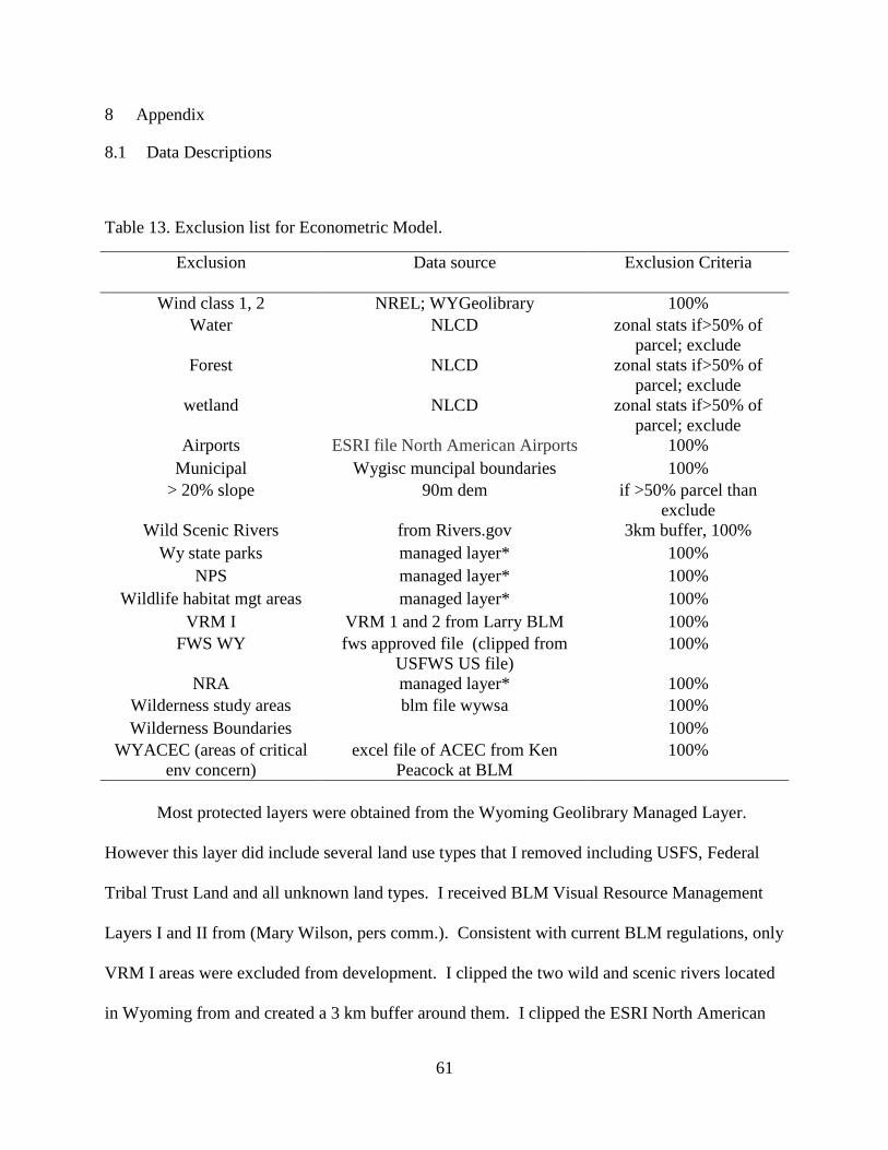
61
8 Appendix
8.1 Data Descriptions
Table 13. Exclusion list for Econometric Model.
Exclusion Data source Exclusion Criteria
Wind class 1, 2 NREL; WYGeolibrary 100%
Water NLCD zonal stats if>50% of
parcel; exclude
Forest NLCD zonal stats if>50% of
parcel; exclude
wetland NLCD zonal stats if>50% of
parcel; exclude
Airports ESRI file North American Airports 100%
Municipal Wygisc muncipal boundaries 100%
> 20% slope 90m dem if >50% parcel than
exclude
Wild Scenic Rivers from Rivers.gov 3km buffer, 100%
Wy state parks managed layer* 100%
NPS managed layer* 100%
Wildlife habitat mgt areas managed layer* 100%
VRM I VRM 1 and 2 from Larry BLM 100%
FWS WY fws approved file (clipped from
USFWS US file)
100%
NRA managed layer* 100%
Wilderness study areas blm file wywsa 100%
Wilderness Boundaries 100%
WYACEC (areas of critical
env concern)
excel file of ACEC from Ken
Peacock at BLM
100%
Most protected layers were obtained from the Wyoming Geolibrary Managed Layer.
However this layer did include several land use types that I removed including USFS, Federal
Tribal Trust Land and all unknown land types. I received BLM Visual Resource Management
Layers I and II from (Mary Wilson, pers comm.). Consistent with current BLM regulations, only
VRM I areas were excluded from development. I clipped the two wild and scenic rivers located
in Wyoming from and created a 3 km buffer around them. I clipped the ESRI North American

62
Airports to Wyoming. I use two different criteria for excluding parcels. I extracted open water,
perennial ice/snow, deciduous forest, evergreen forest, mixed forest, woody wetlands, emergent
herbaceous wetlands, and created a polygon layer from National Land Cover Database
2001NLCD and excluded water, forest, wetlands if >50% of the parcel contained any of these
features. I exclude all parcels that had any portion of a protected area, municipal, or airport
within its boundary. All GIS data layers were re-projected to Wyoming Lambert and converted
to 90m raster.
DATA
A. Wind turbine Dataset: O’Donnell, M.S., and Fancher, T.S., 2010, Spatial mapping and
attribution of Wyoming wind turbines: U.S. Geological Survey Data Series DS 524.
B. Distance to transmission The transmission dataset was a 1-off product from WYGISC
derived from Rextag Strategies Zone 3 Electricity Transmission data. Proposed
transmission was a 1-off product from Amy Pocewicz at The Nature Conservancy
C. QRA: Obtained original QRA from private source, obtained public QRA at Mercator
(WREZ 2011)
D. Lek DATA: Wyoming Game and Fish FTP site
GIS Data steps:
Wind Turbines
I merge two datasets into one to include all existing wind turbines in Wyoming as of
2010. I use a point dataset from USGS of wind turbines existing before 2010 (O’Donnell and
Fancher 2010). In addition, I added GIS point locations from the Federal Aviation
Administration for two wind farms10
that went online in 2010. I removed three wind farms
10
Dunlap and Top of the World

63
(Warren Air force Base, Liberty Turbine Test and Cheyenne TM Vertical Axis) from the dataset
because they do not match the theoretical economic decision maker I am modeling (i.e., the site
decision for these wind farms is unlikely to be consistent with profit maximization). The dataset
contains a total of 24 wind farms 11
with 956 (+20 points that come from the FAA Dunlap farm
that were not actually built) wind turbines ranging from 0.6 MW to 2.3 MW. The data span six
counties including: Albany, Carbon, Converse, Laramie, Natrona, and Uinta. Pacificorp is the
largest purchaser of power in the dataset.
As an alternate wind resource dataset I received three-year average (2008-2010) 12km
NAM WPD for Wyoming from the program GEMPAK as well as a two-year winter average
(2008-2009) 12 km NAM from Tom Parish in Atmospheric Sciences. The file was uploaded to
ARCGIS and re-projected to WYLAM. This data is point class and to be useable I needed a
smooth continuous surface. Following Tchou, I used natural neighbors which interpolate data
between points using thiessen polygons.
Wind resource and landownership were converted from polygon to 90m raster to match
the scale of the 90m elevation dataset. This was necessary to use Zonal statistics based on the
fishnet (grid). Landownership was also reclassified to four classes, private, state, federal and
other-other was then dropped. Slope was derived from the 90m DEM in % (0-181, which
corresponds to a degree slope of 0-61). Distance to roads, and transmission was done to the
proximity to the centroid of the grid.
11
This total counts stages of wind farms as separate farms (e.g., Foote Creek 1, 2 and 3).

64
Figure 8. Wyoming environmental conflicts map

65
Figure 9. 50m wind resource map for Wyoming available from Wind Powering America.
8.2 Appendix Results
Table 14. Impact of Wind Development on Sage-Grouse for Alternative Build-Out Levels
Assuming No Sage-grouse Conservation Policies at 3.2km buffer.
Build-Out
Level (MW)
Impacts with Current
Transmissiona,b
Impacts with All
Transmissiona,b
Leks Males Leks Males
1,650 0 0 0 0
3,390 0 0 1 3
4,020 0 0 3 28
8,790 12 185 16 304
12,000 17 282 19 394
13,770 22 360 27 604

66
a Current transmission refers to the model results assuming that only the current electrical
transmittion lines are available; All transmission includes all current transmission plus assumes
that all proposed transmission lines are installed. b This is the number of leks impacted at 3.2km buffer. Leks can be impacted by multiple parcels
potentially resulting in a larger impact.
Table 15. Core Area Restrictions Expected Lek Impacts within 6.4km Buffer.
Build-Out
Level (MW)
Impacts with Current
Transmissiona,b
Impacts with All
Transmissiona,b
Leks Males Leks Males
8,790 8 153 11 220
13,770 14 281 19 324