FACULTY OF INFORMATION TECHNOLOGY AND ELETRICAL ENGINEERING

Heikki Korhonen

Tool for Analyzing Data Transfer Scenarios in eNodeB

Master’s Thesis

Degree Programme in Computer Science and Engineering

July 2016

Korhonen H. (2016) Tool for Analyzing Data Transfer Scenarios in eNodeB. University of Oulu, Faculty of Information Technology and Electrical Engineering.

Master’s Thesis, 57 p.

ABSTRACT

In software development, debugging is one option for finding a bug. Source code

can be debugged by entering print statements to investigate values of variables

or by using a dedicated debugger tool. With a debugger, the program can be

stopped at a certain point and see the values of variables, without changing the

code.

Real-time software code is complex. Complex source code always requires

careful testing, design and quality assurance. Debugging helps to achieve these

requirements. Debugging is harder in a real-time environment and it takes

more time which means that developers must have effective debugging tools. To

be effective in debugging in a real-time environment, it requires an informative

logging tool.

This thesis concentrates to help LTE L2 debugging with the tool implemented

in this work. The logging tool parses the binary data got from eNodeB to a

readable form in a text file. Traced fields and values can be investigated in a

certain time. With this L2 data flow can be verified.

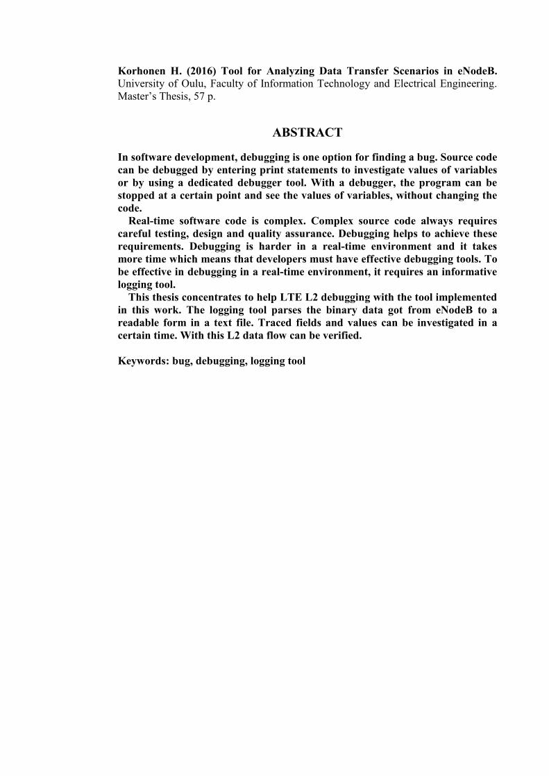
Keywords: bug, debugging, logging tool

Korhonen H. (2016) Analysointityökalu LTE tukiaseman tiedonsiirron

tutkimiseen. Oulun yliopisto, tieto- ja sähkötekniikan tiedekunta. Diplomityö, 57 s.

TIIVISTELMÄ

Ohjelmistokehityksessä virheenjäljittämistä käytetään vian löytämiseen.

Virheenjäljitystä voidaan tehdä lisäämällä lähdekoodin tulostuslauseita, joilla

tutkitaan esimerkiksi muuttujien arvoa halutulla hetkellä koodissa. Toinen tapa

on virheenjäljittäjän käyttäminen koodia ajettaessa. Silloin ohjelma voidaan

pysäyttää haluttuun kohtaan ja tutkia muuttujien sen hetkisiä arvoja ilman

koodimuutoksia.

Reaaliaikainen koodi on kompleksista ja vaatii aina huolellista testausta sekä

laadunvarmistusta. Virheenjäljitys on reaaliaikaisessa ympäristössä

hankalampaa ja aikaa vievää, jolloin ohjelmistokehittäjillä täytyy olla

tehokkaat virheenjäljitystyökalut. Reaaliaikaisessa ohjelmistossa tehokas

virheenjäljitys vaatii myös informatiivisen lokityökalun.

Tämä diplomityö keskittyy auttamaan LTE L2 virheenjäljitystä työssä

toteutettavan lokityökalun avulla. Lokityökalu purkaa eNodeB –tukiasemasta

saadut binääritiedostot lukemiskelpoiseen muotoon tekstitiedostoon.

Tekstitiedostosta voidaan tutkia halutulla ajanhetkellä olevien jäljitettyjen

muuttujien arvoja. Tällä voidaan varmistaa, onko LTE L2:n tiedonvirtaus

sujunut onnistuneesti.

Avainsanat: ohjelmointivirhe, virheenjäljitys, loki, eNodeB

TABLE OF CONTENTS

ABSTRACT

TIIVISTELMÄ

TABLE OF CONTENTS

FOREWORD

ABBREVIATIONS

1. INTRODUCTION ................................................................................................ 8 2. LTE ....................................................................................................................... 9

2.1. LTE Architecture ...................................................................................... 9

2.2. LTE L2 Radio Protocols......................................................................... 11 2.2.1. PDCP ......................................................................................... 13 2.2.2. RLC ........................................................................................... 13

2.2.3. MAC .......................................................................................... 15 2.3. Data transmission flow in LTE layers .................................................... 15

2.3.1. Downlink ................................................................................... 16 3. ANALYZATION TOOLS FOR LTE ................................................................ 18

3.1. Network traffic analyzers ....................................................................... 18 3.1.1. Network Traffic Analysis Platform ........................................... 19 3.1.2. OpenAirInterface Traffic Generator .......................................... 20

3.1.3. TestelDroid ................................................................................ 22 3.2. Interface analyzers .................................................................................. 23

3.2.1. Artiza Networks FURA: LTE Network Analyzer ..................... 23 3.2.2. Sanjole WaveJudge 5000 LTE .................................................. 24

3.2.3. EXFO Family ............................................................................ 25 3.3. Protocol analyzers .................................................................................. 27

3.3.1. Wireshark .................................................................................. 28 3.3.2. R&S CMWmars multifunctional logfile analyzer .................... 28 3.3.3. R&S ROMES4 Drive Test Software ......................................... 29

3.3.4. Cobham Wireless Single TM500 network test system ............. 30 3.4. Summary of listed tools .......................................................................... 31

4. IMPLEMENTATION ........................................................................................ 33 4.1. Used language and tools ......................................................................... 33

4.1.1. Python ........................................................................................ 33 4.1.2. Subversion ................................................................................. 33 4.1.3. Continuous integration .............................................................. 34

4.2. Data Trace Tool API .............................................................................. 34 4.2.1. Design ........................................................................................ 34

4.2.2. Sequence .................................................................................... 35 4.2.3. Binary file format ...................................................................... 36

4.3. Data Trace Tool Parser ........................................................................... 39 4.3.1. Binary file reading ..................................................................... 40 4.3.2. Metadata handling ..................................................................... 40

4.3.3. Main data handling .................................................................... 42

4.3.4. Output printing .......................................................................... 42

4.4. Test environment .................................................................................... 44 4.4.1. Python unittest ........................................................................... 44 4.4.2. Robot Framework ...................................................................... 48

5. DISCUSSION .................................................................................................... 49 5.1. Results and evaluation ............................................................................ 49 5.2. Future...................................................................................................... 51

6. SUMMARY ....................................................................................................... 53

7. REFERENCES ................................................................................................... 54

FOREWORD

This Master’s Thesis was done for Nokia Mobile Networks in an LTE UP SW team.

The topic of the thesis was devised in Fall 2015 and I started working on my thesis in

December 2015. The development of the resulted software and the writing of the

thesis document were done concurrently between December 2015 and May 2016.

I would like to thank Nokia Mobile Networks for the opportunity to write this

thesis. Furthermore, I would especially thank to my instructors, Mr. Timo

Pääkkönen, Dr. Jorma Taramaa, Mr. Ari-Pekka Taskila and the whole Feature Team

8. Your guidance and support has been extremely valuable and helpful during the

process. Your feedback and knowledge has helped to steer the development process

in the right direction. I also want to thank Prof. Olli Silven and Dr. Jani Boutellier for

supervising this thesis and for your important feedback.

Oulu, 14.07.2016

Heikki Korhonen

ABBREVIATIONS

2G Second generation mobile networks

3G Third generation mobile networks

4G Fourth generation mobile networks

3GPP Third Generation Partnership Project

API Application Programming Interface

CI Continuous Integration

CS Circuit Switching

CSV Comma Separated Values

DL Downlink

eNodeB Evolved Node B

EPC Evolved Packet Core

EPS Evolved Packet System

E-UTRAN Evolved Universal Terrestrial Radio Access Network

FDD Frequency Division Duplex

GSM Global System for Mobile Communications

HSDPA High Speed Downlink Access

HSS Home Subscriber Server

L1 Layer 1

L2 Layer 2

L3 Layer 3

LTE Long Term Evolution

MAC Medium Access Control

MIMO Multiple Input Multiple Output

MM Mobility Management

MME Mobility Management Entity

PDCP Packet Data Convergence Protocol

PDU Protocol Data Unit

PS Packet Switching

RB Radio Bearer

RLC Radio Link Control

RRC Radio Resource Control

SAE System Architecture Evolution

SCM Source Code Management

SDU Service Data Unit

S-GW Serving Gateway

SVN Subversion

SW Software

TB Transport Block

TDD Time Division Duplex

TDD Test Driven Development

UL Uplink

UP User Plane

S-GW Serving Gateway

P-GW Packet Data Network Gateway

PCRF Policy and Charging Rules Function

UL Uplink

UE User Equipment

1. INTRODUCTION

The number of mobile subscribers has increased tremendously in recent years. Voice

communication has become mobile in a massive way and the mobile is the preferred

way for voice communication. The end users expect high data performance and the

operators request high data capacity with a low cost of data delivery. LTE (Long

Term Evolution) is designed to meet these targets. [1]

LTE has three different Layers: Layer 1 is physical, Layer 2 works as a data-link

layer and Layer 3 provides the network layer functions. The Third Generation

Partnership Project produces the technical specifications, but the implementation is

left to the manufacturers. [1]

LTE’s software characteristics is real-time and inter-process communications

based, which means the code is quite complex. Complex code always requires

careful testing and quality assurance. Debugging helps to achieve these requirements.

Debugging is used to identify and remove bugs but when we are in a real-time

operating system, finding the bugs is hard and takes time [2]. That means the

developers of LTE software must have effective debugging tools. They also must

have very informative logging tools to help debugging the LTE code. [3]

Data Trace is a trace buffer based tool, which writes values to the trace buffer

when it executes significant points in the base code. When something fails, the user

looks at the trace buffer to see a portion of the program history. The Data Trace Tool

is also used for analyzing the data flow in Layer 2. The more data is gathered to the

trace buffer, the more informative the tool will be.

The Data Trace Tool has a few important requirements which it must meet. Each

requirement is identified with a number.

1. It must have support for time and User Equipment (UE) based analyzing.

2. It must prove if the LTE Layer 2 data flow has succeeded correctly or

incorrectly.

3. It must integrate with the Layer 2 code.

4. It must work with the test environment.

5. The tool must also be capable of producing the log file in a clear and

easily readable form so that it is easy to see the trace flow and locate the

error from the traced fields and values.

This master’s thesis presents analysis tools in eNodeB. In this work the Data Trace

parser is implemented and Layer 2 data will be presented. Also documentation for

the Data Trace parser is produced and other analysis tools in LTE are listed in the

documentation. Chapter 2 consists of basic information of LTE such as overview,

features and performance. LTE architecture is also presented in this chapter. Chapter

3 goes in to detail about other commercialized analysis tools used in LTE: how and

where these work and what information these are gathering. Chapter 4 consists of the

implementing and testing part of the Data Trace Tool. Chapter 5 describes the results

of the implemented tool and discusses the future with the Data Trace Tool. Chapter 6

summarizes the thesis work.

9

2. LTE

LTE is a wireless mobile radio technology. The Third Generation Partnership Project

(3GPP) started the LTE project in 2004 and it evolved from the Universal

Telecommunication System (UMTS) which in turn evolved from the Global System

for Mobile Communications (GSM). [1]

LTE has many advantages compared to older generations, such as high data rates

in downlink and uplink. It also has low latency for connecting to the network and

power saving states. Frequency Division Duplex (FDD) and Time Division Duplex

(TDD) can be used on the same platform and LTE supports backwards compatibility

to older networks such as GSM, CDMA and WCDMA. [1]

LTE is also very capable in its performance, such as mobility speed 350km/h and

high peak data rates for both uplink (75 Mbps) and downlink (450 Mbps with CA

and 2 x 2 MIMO). [1, 4]

To achieve these very high data rates, it is necessary to increase the transmission

bandwidths over those that can be supported by a single carrier or channel. This

method is called CA (Carrier Aggregation). Using LTE Advanced CA, it allows to

utilize more than one carrier and in this way increase the overall transmission

bandwidth. CA is supported by both FDD and TDD. This ensures that both FDD

LTE and TDD LTE are able to meet the high data throughput requirements. [5]

LTE also supports MIMO (Multiple Input Multiple Output), where there is 1 x 2

and 1 x 4 available for uplink side and 2 x 2, 4 x 2, 4 x 4 for downlink side. MIMO

schemes are characterized by the number of antennas transmitting in to the air, M,

and the number of antennas receiving those same signals at the receiver(s), N;

designates as “MxN”. For example, the downlink may use four transmit antennas at

the base station and two receive antennas in the terminal, which is referred to as “4x2

MIMO”. [6]

FDD and TDD are the duplexing modes that LTE uses and turbo coding is used for

channel coding. The transmission bandwidth can be selected between 1.4 MHz and

20 MHz. [1, 6]

2.1. LTE Architecture

When LTE has promised high numerical performance, it also needs high quality and

performance capable network architecture. LTE Architecture consists of four main

high level domains: User Equipment (UE), Evolved Universal Terrestrial Radio

Access Network (E-UTRAN), Evolved Packet Core (EPC) and Services domain. [1]

Operator Services and the Internet are located in the Services domain. EPC

handles the technology related to a core network and connect all other services to the

Services domain. The E-UTRAN establishes and handles the connection between the

UEs and EPC. eNodeB is responsible for radio resource management and it is the

only component in E-UTRAN. The UE consist of all devices which are able to

connect to the LTE network, such as mobile phones and tablets. Figure 1 shows a

LTE Architecture overview. [7, 8, 9]

UE consist of all the devices that can access the LTE network, which are typically

hand held devices such as smart phones, tablets or even data cards that are embedded

in laptops. Universal Subscriber Identity Module (USIM) is part of the UE but it is a

separated module from the UE. USIM is an application which is imported in a card

10

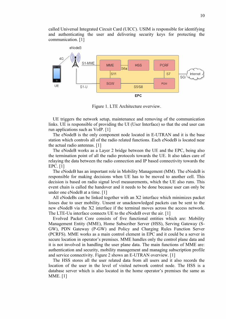
called Universal Integrated Circuit Card (UICC). USIM is responsible for identifying and authenticating the user and delivering security keys for protecting the communication. [1]

Figure 1. LTE Architecture overview.

UE triggers the network setup, maintenance and removing of the communication

links. UE is responsible of providing the UI (User Interface) so that the end user can run applications such as VoIP. [1]

The eNodeB is the only component node located in E-UTRAN and it is the base station which controls all of the radio related functions. Each eNodeB is located near the actual radio antennas. [1]

The eNodeB works as a Layer 2 bridge between the UE and the EPC, being also the termination point of all the radio protocols towards the UE. It also takes care of relaying the data between the radio connection and IP based connectivity towards the EPC. [1]

The eNodeB has an important role in Mobility Management (MM). The eNodeB is responsible for making decisions when UE has to be moved to another cell. This decision is based on radio signal level measurements, which the UE also runs. This event chain is called the handover and it needs to be done because user can only be under one eNodeB at a time. [1]

All eNodeBs can be linked together with an X2 interface which minimizes packet losses due to user mobility. Unsent or unacknowledged packets can be sent to the new eNodeB via the X2 interface if the terminal moves across the access network. The LTE-Uu interface connects UE to the eNodeB over the air. [1]

Evolved Packet Core consists of five functional entities which are: Mobility Management Entity (MME), Home Subscriber Server (HSS), Serving Gateway (S-GW), PDN Gateway (P-GW) and Policy and Charging Rules Function Server (PCRFS). MME works as a main control element in EPC and it could be a server in secure location in operator’s premises. MME handles only the control plane data and it is not involved in handling the user plane data. The main functions of MME are: authentication and security, mobility management and managing subscription profile and service connectivity. Figure 2 shows an E-UTRAN overview. [1]

The HSS stores all the user related data from all users and it also records the location of the user in the level of visited network control node. The HSS is a database server which is also located in the home operator’s premises the same as MME. [1]

11

Figure 2. E-UTRAN overview.

The S-GW has an important role in control functions and it is only responsible for its own resources. The S-GW allocates its resources based on requests from the MME, the P-GW and the PCRF, which are setupping, modifying and clearing the bearers for the UE. When the UE is in connected mode, the S-GW forwards all the data flows between eNodeB and the P-GW. When the UE is in idle mode, eNodeB releases its resources and the data path terminates in the S-GW. If the S-GW receives data packets from the P-GW, it will buffer the packets and request the MME for paging the UE. [1]

The P-GW is the router between the EPS and the outside world, i.e. Packet data networks, and it acts as the IP point of attachment in the UE. The P-GW allocates the IP address to the UE and the UE uses that to communicate with other IP hosts on the Internet. If communication towards the S-GW is based on GTP, the P-GW performs the mapping between the IP data flows to GTP tunnels. The P-GW sets up bearers which are requested from the PCRF or the S-GW. [1]

The PCRF is a network component which is responsible for Policy and Charging Control (PCC). Whenever a new bearer is set up, the PCRF sends the PCC rules. Bearer set-up is required when the UE initially connects to the network and the default bearer will be set up, which means that also one or more dedicated bearers are set up. The PCRF also provides the PCC rules based on request from the P-GW or the S-GW in the PMIP case. [1]

2.2. LTE L2 Radio Protocols

The main task of the LTE L2 radio interface protocols is to set up, reconfigure and release the Radio Bearer that provides the means for transferring the EPS bearer. Layer 2 consists of three different radio protocols: Medium Access Control (MAC), Radio Link Control (RLC) and Packet Data Convergence Protocol (PDCP). Figure 3 and Figure 4 shows LTE Layer 2 Radio protocols in the LTE protocol stack. [1]

Signaling Radio Bearer (SRB) and Data Radio Bearer (DRB) are the two types of Radio Bearers in LTE. Signaling messages are carried by SRBs and DRBs carry the user data. The bearer defines how the UE data is treated when it travels across the network connecting two or more points. The EPS Bearer is the pipeline through which data traffic flows within the Evolved Packet System. The EPS Bearer components are shown in Figure 5. [10]

12

Figure 3. LTE User plane protocol stack.

Figure 4. LTE Control plane protocol stack.

13

Figure 5. EPS Bearer components.

2.2.1. PDCP

The PDCP layer has three main functionalities which are: header compression and decompression of the IP packets, ciphering and deciphering both the user plane data and most of the control plane data, and integrity protection and verification. [1]

Header compression and decompression is based on the Robust Header Compression (ROCH) protocol. The compression is more important when small payload IP packets are being handled. A large IP header could be a significant source of overhead for small data rates. [1]

Ciphering and deciphering is done for both the user plane and most of the control plane. This was done in the MAC and RLC layers in 3G networks. [1]

Integrity protection and verification is done for control plane data and its meaning is to ensure that control information is coming from the correct source. [1]

2.2.2. RLC

The RLC layer has a few key functionalities which are: transferring the PDUs received from higher layers such as the PDCP to the MAC and vice versa, error correction with ARQ, concatenation/segmentation, and protocol error handling to detect and recover from the protocol error states caused by signaling errors. [1]

The RLC can operate in three different modes. They are: Transparent Mode (TM), Unacknowledged Mode (UM), and Acknowledged Mode (AM). [1]

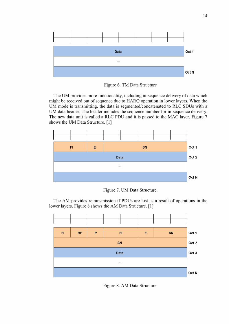
When the RLC is in the TM, it only delivers and receives PDUs on a logical channel but does not add any headers. This means that PDUs are not tracked. Figure 6 shows the TM Data Structure. [1]

14

Figure 6. TM Data Structure The UM provides more functionality, including in-sequence delivery of data which

might be received out of sequence due to HARQ operation in lower layers. When the UM mode is transmitting, the data is segmented/concatenated to RLC SDUs with a UM data header. The header includes the sequence number for in-sequence delivery. The new data unit is called a RLC PDU and it is passed to the MAC layer. Figure 7 shows the UM Data Structure. [1]

Figure 7. UM Data Structure. The AM provides retransmission if PDUs are lost as a result of operations in the

lower layers. Figure 8 shows the AM Data Structure. [1]

Figure 8. AM Data Structure.

15

The AM Data can also be re-segmented to fit the physical layer resources available

for the retransmissions. The header now contains information of the last correctly received packet on the receiving side along with the sequence numbers, as for the UM operation.

2.2.3. MAC

The main task of the MAC layer is to map the logical channels to the transport channels. Other tasks are multiplexing/demultiplexing of the RLC Payload Data Units (PDUs) into/from Transport Blocks (TBs) and delivering them to the physical layer on transport channels. The MAC is also responsible for traffic volume measurement reporting, error correction trough HARQ to control the uplink, and downlink physical layer retransmission handling with the scheduling functionality in eNodeB. The MAC also takes care of priority handling between logical channels of one UE and between UEs and transport format selection. [1]

2.3. Data transmission flow in LTE layers

Figure 8 shows the data flow of Layer 1 and Layer 2. When a layer receives a packet, it is called an SDU and when layer sends the packet, it is called a PDU. The downlink data flow is explained in Subsection 2.3.1. Figure 9 shows the LTE data flow through different protocol layers. [1]

Figure 9. LTE data flow through different protocol layers.

16

2.3.1. Downlink

The downlink data flow starts from the IP layer, which sends IP packets to the PDCP layer. The PDCP performs header compression and adds PDCP headers to these PDCP SDUs. The header compression includes the removal of the ID header (minimum 20 bytes) from the PDU and then a Token (1-4 bytes) is added. The PDCP layer submits the PDCP PDUs (RLC SDUs) to the RLC layer. Figure 10 shows the PDCP header compression. [1]

Figure 10. PDCP header compression. The RLC layer receives the RLC SDUs (PDCP PDUs) and does segmentation on

them. RLC segmentation might include splitting a large RLC SDU into multiple RLC PDUs or packing several small RLC SDUs into a single PDU. Then the RLC adds a header which is based on the RLC mode of operation. After that the RLC sends these RLC PDUs (MAC SDUs) to the MAC layer. [1]

The MAC layer receives the MAC SDUs (RLC PDUs) and then packs the MAC PDUs. A MAC PDU consists of the MAC header, MAC SDUs and MAC control elements. Then the MAC layer submits the MAC PDUs (or Transport Blocks) to the physical layer for transmitting onto physical channels. [1]

The TTI (Transmission Time Interval) is a time based parameter in telecommunication networks. The TTI will be determined based on the length of time required to transmit one block and in the LTE case it is shortened to 1 ms to achieve lower latencies. Figure 11 shows the LTE FDD-frame structure and Figure 12 shows the LTE TDD-frame structure. [1]

Figure 11. FDD-frame structure in LTE.

17

Figure 12. TDD-frame structure in LTE.

18

3. ANALYZATION TOOLS FOR LTE

Complex software requires more testing and quality assurance, which needs to be

done very carefully [2]. Debugging is needed when those requirements are met

successfully. Effective debugging needs help from tracing tools [3]. Debugging is the

main operation for finding and removing the bugs. Debugging is always started when

a program fails to accomplish its intended task. The debugging operation itself is not

immune to flaws, and when failing to accomplish its mission, the debugging

operation itself needs to be debugged. [11]

The most primitive way to debug a program is to insert so-called debug

statements. During execution debug statements print information such as what

statements are executed or what values particular variables have at a particular point.

Debug statements let the user observe a program’s behavior. The most important

things in this debugging method are where to insert debug statements, what kind of

information to print, and what to comprehend by analyzing the output. [12]

Another way to debug is to use debugging tools which provide only low-level

facilities. These tools help programmers to insert breakpoints, inspect states at those

points during program execution, change the values of variables and program parts

and then continue the execution. [12]

There are also buffer based trace debugging tools, which let the programmer

observe or analyze a program’s execution history. Software stub technology is

applied for trace debugging when in runtime. Software stub is a module which acts

for the called module and gives the same output as an actual product. By embedding

trace points in programs, developers could have a real-time observation of the

information output by trace points during the runtime of programs, such as

interaction information among modules and the running sequence of programs. [13]

LTE analyzation tools are basically for logging (buffer based tracing) because LTE

is based on real-time. There are different kinds of tools, for example, purely software

based, which are in-house-tools, or monitoring tools in UE. Another option is all-in-

one multitechnology protocol analyzers which consist of a hardware kit and a

software based analysis tool. These are typically commercial tools, because the user

can use them in the lab and also in the field. The tools can trace data protocol-,

interface- and layer levels.

The functionalities of the following listed tools will be compared to the

requirements listed in the introduction. Every tool is compared to those requirements

and the following summary chapter summarizes all the tools compared to those

requirements.

All the tools are separated to three different categories: Network traffic analyzers,

interface analyzers, and protocol analyzers. One tool is chosen from each category

and added to the summary. The motive for this inspection is to understand supply,

aspects, and facilities.

3.1. Network traffic analyzers

In this section, the following tools will be analyzed: Network Traffic Analysis

Platform, OpenAirInterface Traffic Generator, and TestelDroid.

19

3.1.1. Network Traffic Analysis Platform

A network traffic analysis is a platform to conduct mobile traffic data. The platform is designed and implemented following a multilevel architecture with a collecting module, a distributing module, a batch & stream processing module, an interface module, and a cluster manager. Figure 13 shows the architecture of an in-house-developed network traffic analysis platform. The Platform could be deployed in 2G, 3G and 4G networks. [14]

Figure 13. Architecture of Network Traffic Analysis Platform.

The collecting module monitors the network traffic using the Traffic Monitoring System (TMS). The TMS is deployed between the RAN (Radio Access Network) and the CN (Core Network), and it captures all downlink and uplink IP packets and generates the flow records. All flow records are collected by the Collector and transferred to a distributing module. [14]

The Distributing module reads flow records from the collector and distributes the data to the batch & stream processing module. The distributing module provides load balancing, fault tolerance, and good scalability. [14]

The batch & Stream processing is a Hadoop-based system. The batch processing module is responsible for offline analysis. The Hadoop Distributed File System (HDFS) and the Hadoop Database (HBase) are built for storing a huge amount of traffic data. For data analyzing, Hive-QL and Pig Latin are used for analyzing the data more conveniently. The stream processing module is composed of Kafka and Storm, among which Kafka is a high throughput messaging system for real-time data and Storm is a distributed real-time computation system. With these two open source tools, it is easier to develop this real-time computing application. [14]

The interface module consists of the Graphical User Interface (GUI), which allows presenting analysis results in a user-friendly manner. At the same time, analysts can write and execute Pig scripts through the web directly. [14]

The Cluster Manager is a self developed software which can monitor software and hardware on each server. It can collect performance statistics of servers such as CPU,

20

memory, disk, and network utilization. Figure 14 presents the Network Traffic Analysis Platform focus in LTE. [14]

The collected dataset includes information such as userID, timestamp, latitude & longitude (eNodeB’s location), and signaling procedure Code. [14]

Figure 14. Network Traffic Analysis Platform focus in LTE

This tool presents the analysis results in a readable form, and can analyze the userID and timestamp. It does not integrate with the desired Layer 2 code and test environment, which means that the tool does not meet all of the requirements. [14]

3.1.2. OpenAirInterface Traffic Generator

The OTG is a realistic packet-level traffic generation tool for emerging application scenarios. It is developed in C under Linux and deployed for the OpenAirInterface LTE/LTE-A platform allowing the traffic to be generated with soft real-time and hard real-time constraint. [15]

With this tool, OWD (One-Way Delay) can be measured in the soft real-time mode for the LTE operating in a TDD frame configuration 3 for 5MHz bandwidth. End-to-end OWD is measured in the data-plane. Figure 15 and Figure 16 present measured and estimated OWD performance for virtual game per network segment. Figure 17 shows the OpenAirInterface Traffic Generator focus in LTE. [15]

Figure 15. Experimentation setup and OWD latency budget.

21

One example of the many possible Machine-type communication (MTC) games is

the virtual race (virtual bicycle race using real bicycles). Opponents are at different locations and during the race with the sensor data on the order of 1KB. For the simulation, a simple cellular network topology is used, composed of one eNodeB and one static UEs to measure the best case performance. For the RAN, time synchronization between the eNodeB and the UE is used in terms of frame and subframe number and converted to time in milli-seconds. Each frame represents 10 ms and each sub-frame represents 1ms. The end-to-end network setup is emulated on the same physical machine, thus avoiding additional time-synchronization. The simulation is run for 1 minute (6000 LTE TDD frames). [15]

Figure 16. OWD Analysis for M2M Virtual Game Application.

Figure 17. OpenAirInterface Traffic Generator focus in LTE.

22

This tool does not meet the given requirements at all. This tool can only measure

end-to-end OWD data-plane delays and OWD’s performance when LTE is operating

in the TDD frame configuration. And it only tested for 6000 LTE TDD Frames (1

minute). [15]

3.1.3. TestelDroid

TestelDroid is an Android-based tool for monitoring communications performance

and radio issues. This tool collects not only simple metrics, such as throughput, but

also radio parameters, such as received signal strength, radio access technology in

use, current IP traffic and much more, to obtain a fully detailed picture to

characterize the scenario where the results have been obtained. Table 1 summarizes

the main functionalities provided by TestelDroid. [16]

Table 1. TestelDroid capabilities

Capabilities Detailed monitored parameters

Network

Operator, RAT (Radio Access Technology), CID (Cell Identification), LAC

(Location Area Code), RSSI (Radio Signal Strength Indicator), PSC (Primary

Scrambling Code)

Neighboring cells

PSC, RSSI, RSCP (Received Signal Code Power), RAT (Radio Access

Technology)

Battery Battery level, Temperature (C), Voltage (mV), Current (mA)

GPS Longitude, Latitude, Altitude, Speed

IP Traffic Pcap format, Arrival timestamps,

Promiscuous mode

Connectivity test Ping, Open ports

Active traffic test

Server-Client mobile-to-mobile, Transfer

of auto-generated file, Bit rate monitoring,

Average transfer speed

The collected data can be logged using highly analyzable plain text files (except

for traffic capture, which is stored in a PCAP format). The data collected by

TestelDroid can be used by experimenters to analyze the traffic in more detail and

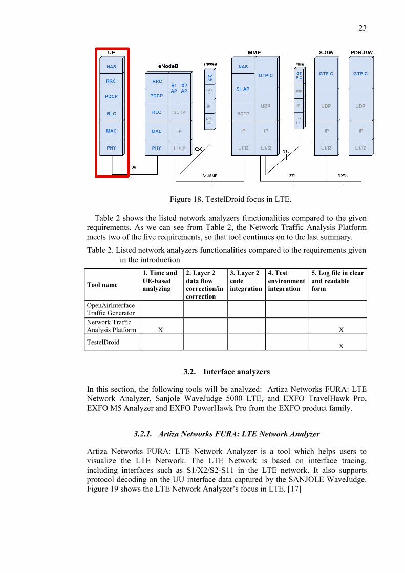
using their own tools and methodologies. Figure 18 shows TestelDroid’s focus in

LTE. [16]

This tool is purely collecting values from the UE side and the debugger cannot

prove the LTE flow succession or unsuccession from these values. This tool does not

have the required functionalities which means it does not meet the requirements at

all. [16]

23

Figure 18. TestelDroid focus in LTE. Table 2 shows the listed network analyzers functionalities compared to the given

requirements. As we can see from Table 2, the Network Traffic Analysis Platform meets two of the five requirements, so that tool continues on to the last summary.

Table 2. Listed network analyzers functionalities compared to the requirements given in the introduction

Tool name

1. Time and UE-based analyzing

2. Layer 2 data flow correction/incorrection

3. Layer 2 code integration

4. Test environment integration

5. Log file in clear and readable form

OpenAirInterface Traffic Generator

Network Traffic Analysis Platform

X

X

TestelDroid

X

3.2. Interface analyzers

In this section, the following tools will be analyzed: Artiza Networks FURA: LTE Network Analyzer, Sanjole WaveJudge 5000 LTE, and EXFO TravelHawk Pro, EXFO M5 Analyzer and EXFO PowerHawk Pro from the EXFO product family.

3.2.1. Artiza Networks FURA: LTE Network Analyzer

Artiza Networks FURA: LTE Network Analyzer is a tool which helps users to visualize the LTE Network. The LTE Network is based on interface tracing, including interfaces such as S1/X2/S2-S11 in the LTE network. It also supports protocol decoding on the UU interface data captured by the SANJOLE WaveJudge. Figure 19 shows the LTE Network Analyzer’s focus in LTE. [17]

24

Figure 19. Artiza Networks FURA: LTE Network Analyzer focus in LTE.

The Artiza Network’s FURA LTE Network Analyzer is purely meant for interface analysis and its focus is so succinct that it does not meet the requirements at all. [17]

3.2.2. Sanjole WaveJudge 5000 LTE

The Sanjole’s WaveJudge works as a wireless protocol sniffer, capturing the full over-the-air conversation of upper layer messages, including RF signal characteristics, for off-line analysis. Wavejudge 5000 shows the RF signals time-correlated with upper-layer protocol messages for investigating and isolating the true root cause of the symptoms or failures. With Wavejudge the user analyzes all upper layer protocols, including MAC, RLC, PDCP, RRC and NAS, while correlating messages to the PHY layer. Figure 20 shows Wavejudge’s focus in LTE. [18]

Figure 20. Sanjole Wavejudge 5000 focus in LTE.

25

Wavejudge 5000 has support for the decoding of MAC, RLC, PDCP, RRC and

NAS with full correlation to the PHY layer. It is capable of analyzing ARQ and HARQ processes, scheduling errors, and Layer 1 – Layer 3 throughput. It can also verify eNodeB channel outputs. This tool captures the data from the air-interface, which means it does not meet the requirements. [18]

3.2.3. EXFO Family

In this chapter three EXFO’s analyzation tools are compared: EXFO TrawelHawk Pro, EXFO M5 Analyzer, and EXFO PowerHawk Pro.

EXFO TravelHawk Pro is a portable wireless network troubleshooting tool. It is a troubleshooting tool for mobile network operators and it can be deployed in a live field network or in the lab. TravelHawk Pro is designed for three main operations: LTE/IMS, packet-switched (PS) core and circuit- switched (CS) core end-to-end network analysis, Internet protocol (IP) application data analysis, and data capturing. [19]

TravelHawk Pro supports line-rate capturing and live analysis capabilities where LTE core signaling is deciphered, analyzed and correlated over all interfaces. For example, session behavior from S1-MME, S11 and X2 can be correlated. [19]

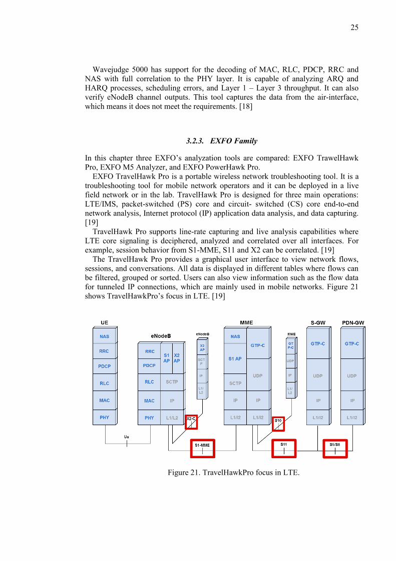
The TravelHawk Pro provides a graphical user interface to view network flows, sessions, and conversations. All data is displayed in different tables where flows can be filtered, grouped or sorted. Users can also view information such as the flow data for tunneled IP connections, which are mainly used in mobile networks. Figure 21 shows TravelHawkPro’s focus in LTE. [19]

Figure 21. TravelHawkPro focus in LTE.

26

EXFO TravelHawk Pro does not gather data from Layer 2, which is the key requirement. TravelHawk Pro collects data from interfaces and supports calculation of throughput, jitter and delay measurements from control-plane sessions or user-plane flows. This tool does not meet the requirements. [19]

EXFO M5 analyzer is a software-based mobile network analyzer. It supports online and offline detailed analysis, functional testing from Ethernet-based signaling, and live network troubleshooting with NSN eNodeB. [20]

The M5 Analyzer allows real-time analysis of Ethernet-based interfaces, such as GERAN, UTRAN, LTE, PS and CS core. The M5 Analyzer has a Windows-style graphical user interface and automated configuration. Network traffic analysis is illustrated by clear graphics and issues are highlighted. Figure 22 shows the M5 Analyzer’s focus in LTE. [20]

Figure 22. M5 Analyzer focus in LTE.

The M5 analyzer has support only for EPC interface analysis, detailed decoding, session analysis and session correlation over the LTE and EPC interfaces. It produces a nice readable logfile, but does not collect data which is able to prove Layer 2 data flow as correct/incorrect. This tool does not meet the requirements. [20]

EXFO PowerHawk Pro is a multi-user live network analyzer. In addition it includes network service optimization and live network troubleshooting tools. PowerHawk Pro can be deployed in LTE, 3G and 2G mobile networks to measure user- and application-level quality of service to visualize the quality from a customer’s perspective. PowerHawk Pro collects data, such as KPIs and configurable counters, IP and user-plane-analysis for more than 1000 applications, and signaling processing for LTE interfaces. PowerHawk Pro correlates both control- and user-plane traffic across all interfaces to show a full, end-to-end view of both signaling and user-plane data. Figure 23 shows PowerHawkPro’s focus in LTE. [21]

PowerHawk Pro has decoding support for GTP-C and NAS protocols. It also has an EPC Signaling Analysis Module, which supports such interfaces as S1, X2, S11, S10 and S5/S8. This also collecting information of the LTE interfaces, which is not a requirement for the Data Trace Tool. This tool does not meet the requirements. [21]

27

Figure 23. PowerHawkPro focus in LTE.

Table 3 shows the functionalities of the listed interface analyzers compared to the given requirements. As we can see from Table 2, Sanjole Wavejudge 5000 LTE met two of the five requirements, so that tool continues on to the last summary.

Table 3. Functionalities of the listed interface analyzers compared to the requirements given in the Introduction

Tool name

1. Time and UE-based analyzing

2. Layer 2 data flow correction/incorrection

3. Layer 2 code integration

4. Test environment integration

5. Log file in clear and readable form

Artiza Network FURA: LTE Network Analyzer

X

Sanjole Wavejudge 5000 LTE

X

X

EXFO TravelHawk Pro

X

EXFO PowerHawk Pro

X

EXFO M5 Analyzer

X

3.3. Protocol analyzers

In this section the following tools will be analyzed: Wireshark, R&S CMWmars multifunctional logfile analyzer, R&S RomeS4 Drive Test Software, and Cobham Wireless Single TM500 network test system.

28

3.3.1. Wireshark

Wireshark is a network protocol analyzer. It allows the user to see what is happening on his/her network at a microscopic level. Wireshark supports deep inspection of hundreds of protocols, live capture, and offline analysis. It can be deployed in several platforms, such as Windows, Linux, OS X, Solaris and many others. Wireshark exports the output to XML, PostScript, CSV or plain text. Figure 24 shows Wireshark’s focus in LTE. [22]

Figure 24. Wireshark focus in LTE.

Wireshark provides support for LTE protocols, such as PDCP, RRC, RLC and MAC. Values such as UEId, DRB, SRB, Systime, C-RNTI, UL Frames, UL Bytes, UL Mbit/sec, UL Padding%, CCCH, and LCID, which can be measured and analyzed with the Wireshark LTE Protocol analyzer. [22]

This tool meets the requirements quite well: it supports Layer 2, it collects the right values for proving the data flow correctness/incorrectness, and it produces information in a clear and readable way. The only problem is that Wireshark does not integrate into the desired Layer 2 code and testing environments. That causes lack in the needed requirements. [22]

3.3.2. R&S CMWmars multifunctional logfile analyzer

R&S®CMWmars is a message analyzer for all R&S®CMW signaling applications. The user can analyze recorded message log files or trace information on the fly in real-time while a test is running. With a graphical user interface the user can narrow down the root cause of signaling protocol and lower layer problems. The multifunctional log file analyzer supports all information elements of all the protocol layers in LTE, including the IP layer. Figure 25 shows the focus of CMWmars in LTE. [23]

29

Figure 25. CMWmars focus in LTE.

This tool has access to all protocol stack layers in LTE. It collects data such as ueID, time stamp, layer name, direction, PDU info and also other values, such as RBId and the RRC result. CMWmars also has a table view of all recorded messages by timestamp, with the option to search and filter according to specific criteria. The main problem of this tool is that it cannot integrate with the necessary Layer 2 code and test environment. This tool does not meet the requirements. [23]

3.3.3. R&S ROMES4 Drive Test Software

The R&S®ROMES4 is an all-in-one solution for network analysis and optimization. Figure 26 shows the Drive Test Software’s focus in LTE. [24]

Figure 26. Drive Test Software focus in LTE.

30

Drive Test Software provides solutions for coverage measurements, interface identification, performance measurements and quality analysis in mobile networks. Data is processed instantly and statistics are calculated and shown in real-time using a graphical user interface. This tool can trace key parameters, mobile activity and L3 protocol messages. It has also the LTE scanner and the location estimation for eNodeB, and the indoor measurement tools.

The Drive Test Software supports only an overview of Layer 1 and Layer 3. It is a display of mobile phone activities in Layer 3. It has also fast analysis of interrupted corrections. It has also an overview of such network parameters as power / quality, serving cell, and CS/PS call info. This tool has several functionalities, but not those mentioned in the introduction, which means that this tool does not meet the requirements. [24]

3.3.4. Cobham Wireless Single TM500 network test system

The Cobham Wireless Single TM500 network test system supports real-world scenario emulation, validating the capacity and performance of 4G base stations, and complex networks. The TM500 is a scalable test system for validating network performance as experienced by end users, across multiple cells and different radio access technologies. The TM500 has remote and automation API, it can be deployed in the lab and over the air, and it has LTE compliant operation at Layer 1, Layer 2, and higher layers (RRC/NAS). [25]

The TM500 can measure MAC transmit and receive statistics, overhead due to padding ratio in RLC, L1 and L2 latency measurements, and transport monitoring such as MAC, RLC and PDCP inputs and outputs in test points. Figure 27 shows the focus of the Cobham Wireless Single TM500 network test system in LTE. [25]

Figure 27. Cobham Wireless Single TM500 network test system focus in LTE.

The TM500 can measure EPC performance, Voice quality (VoLTE, CS), Data

QoS, and max throughput and input & output statistics from Layer 2 radio protocols. The other functionalities of this tool are mainly on the testing side, which leaves the

31

analyzing side quite poor. The basic idea behind the requirements is in helping to

debug the code, which this tool is not planned to. This tool also does not meet the

requirements. [25]

Table 4 shows functionalities of the listed protocol analyzers compared to the

given requirements. As we can see from Table 3, Wireshark and R&S CMWmars

Multifunctional Logfile Analyzer meet three of the five requirements. Both of them

have time and UE-based analyzing, they can prove L2 data flow

correction/incorrection, and they have a nice graphical user interface. Because

CMWmars is only a logfile analyzer and it needs a supporting module to take care of

tracing the data, Wireshark continues onto the last summary.

Table 4. The functionalities of the listed protocol analyzers compared to the

requirements given in the Introduction

Tool name

1. Time and

UE-based

analyzing

2. Layer 2

data flow

correction/in

correction

3. Layer 2

code

integration

4. Test

environment

integration

5. Log file in

clear and

readable form

Wireshark

X X

X R&S CMWmars

Multifunctional

Logfile Analyzer

X

X

X

R&S ROMES4

Drive Test

Software

X

Cobham Wireless

Single TM500

Network Test

System

X

3.4. Summary of analyzed tools

Table 5 summarizes the selected tools from different areas and compares them to the

requirements, which are given in the Introduction. The tools in Table 5 were chosen

on the basis of the filled requirements in different tool categories. After the Table, a

decision is given regarding to the functionalities of the listed tools when compared to

requirements needed.

Table 5. Functionalities of the listed tools compared to the requirements given in the

Introduction

Tool name

1. Time and

UE-based

analyzing

2. Layer 2

data flow

correction/in

correction

3. Layer 2

code

integration

4. Test

environment

integration

5. Log file in

clear and

readable form

Network Traffic

Analysis Platform X

X

Sanjole

Wavejudge 5000

LTE

X

X

Wireshark X X X

32

Table 5 shows that there is no tool that meets all the necessary requirements. Some

of them are close but they have integration problems with the Layer 2 code and

testing environment. Therefore the Data Trace Tool needs to be implemented. In

chapter 4, implementation and testing of the Data Trace Tool is presented.

33

4. IMPLEMENTATION

The Data Trace Tool consists of two different software modules. The Data Trace

Tool API works as an interface to the Layer 2 code. The Layer 2 code calls this API

to write metadata based on defined trace points. Then the Data Trace Tool creates the

binary file, which consists of the metadata and the data. The Data Trace Tool Parser

parses the metadata, and with its help, it can also parse the main data. Finally it

produces a text file and a CSV file, where the traced fields and their values are

printed.

4.1. Used language and tools

This section presents the programming languages and tools used in the

implementation. The test environment tools are listed afterwards. The

implementations were programmed in Python and C++ using the Test Driven

Development (TDD) method. All scripts and source codes are stored in a Subversion

(SVN) source code repository. Continuous integration is handled by Jenkins, which

runs jobs (different builds and test lists). Software Configuration Management works

on SVN and triggers CI jobs automatically.

4.1.1. Python

The Data Trace Tool Parser was selected to be implemented in Python because

Python has several built-in modules, which are suitable for binary parsing. Python

also has good integrity with the Robot Framework-based test automation system.

Python is an easy to learn, powerful programming language. It has efficient high-

level data structures and a simple but effective approach to object-oriented

programming. Python has an elegant syntax and dynamic typing, together with its

interpreted nature. That makes Python an ideal language for scripting and rapid

application development in many areas on most platforms. Python also has large

standard libraries which support many common programming tasks, for example

connecting to web servers, searching text with regular expressions, reading, and

modifying files. [26, 27]

Python can be easily extended by adding new modules implemented in complied

language such as C or C++. Python runs on many different computers and operating

systems, such as Windows, MacOS and many brands of UNIX. [27]

4.1.2. Subversion

Subversion (SVN) is an open source version control system made by Apache.

Subversion manages files and directories, and the changes made to them over time.

This allows the user to recover older versions of their data or examine the history of

how their data has been changed. Subversion can operate across networks, which

allows it to be used by people on different computers. That also allows users to work

with the code simultaneously and commit the changes to the SVN repository.

Because the work is versioned, users do not need to fear erroneous code, because the

previous working version can always be recovered and restored. [28]

34

During this thesis, the source codes of the implementations were stored in the SVN

repository. Development was mostly done in the feature team branch of the

repository and then merged to the main branch.

4.1.3. Continuous integration

Continuous integration (CI) is a software engineering practice in which isolated

changes are immediately tested and reported on when they are added to a larger code

base. The goal of CI is to provide rapid feedback so that if a defect is introduced in to

the code base, it can be identified and corrected as soon as possible. Continuous

integration software tools can be used to automate the testing and build a document

trail. [29]

Continuous integration for software is handled by an application called Jenkins.

Jenkins runs jobs that can include different builds and test lists. The jobs are initiated

by software configuration management (SCM) changes. This means that when a

developer uploads his or her changes into the version control system, Jenkins notices

this and initiates the jobs. If some of the jobs fail, the person who committed the

changes can be identified with the commit revision number. Every job has its own

page where history can be searched. Every job has its specific pages, which can

show, for example, the generated log files of the tests, and test results are also sent by

email. [30]

Jenkins was used in this thesis for automatic execution of unit tests every time a

commit was made to the repository. In addition, the finished Data Trace Tool runs in

regression in Jenkins.

4.2. Data Trace Tool API

The Data Trace Tool API offers an interface to Layer 2 code which can write Data

Trace values via buffer to a binary file. The required trace points must be defined in

the API and then called in the API in Layer 2 code. Via the API, the Layer 2 code

generates a binary file, which consists of data based on written metadata.

4.2.1. Design

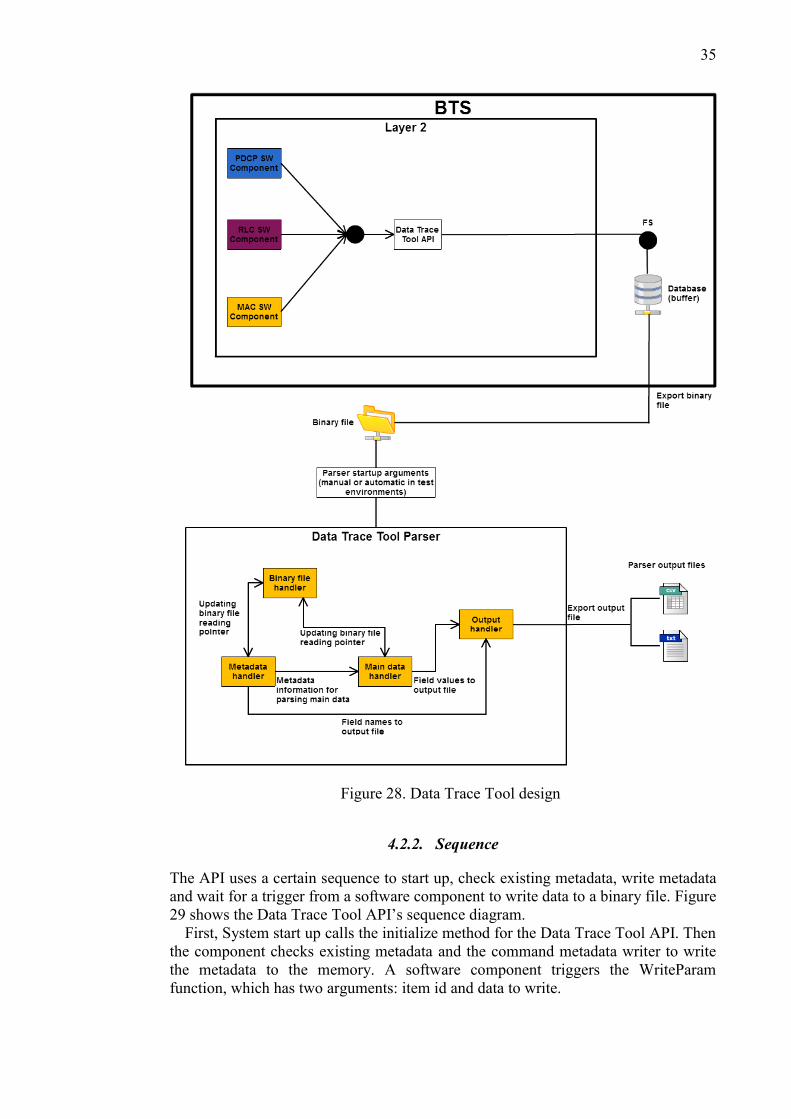
The Data Trace Tool consists of two different software modules. The Data Trace

Tool API works inside eNodeB and exports a binary file, which the Data Trace Tool

Parser handles and outputs a nice and readable log file. Figure 28 shows the Data

Trace Tool design.

The Data Trace Tool API works inside a base station and offers an interface to the

Layer 2 protocol software components. Those components can write data trace

values to a buffer using the API. The API generates a binary file based on the

metadata and data stored in the buffer. Then the binary file is exported as an output.

The Parser takes care of handling the binary file. The Parser can be started

manually from a command line or automatically in test environments. It takes two

arguments: input and output. Then it generates two different output files: one text file

and one CSV-based file.

35

Figure 28. Data Trace Tool design

4.2.2. Sequence

The API uses a certain sequence to start up, check existing metadata, write metadata and wait for a trigger from a software component to write data to a binary file. Figure 29 shows the Data Trace Tool API’s sequence diagram.

First, System start up calls the initialize method for the Data Trace Tool API. Then the component checks existing metadata and the command metadata writer to write the metadata to the memory. A software component triggers the WriteParam function, which has two arguments: item id and data to write.

36

Figure 29. Data Trace Tool API sequence diagram. The software component can be any component defined in the Layer 2 code. After

receiving the WriteParam command, the Layer 2 code writes the required data to a binary file in the file system by using the API. From the file system the binary file is exported to the Data Trace Tool Parser for data handling.

4.2.3. Binary file format

Binary files are usually thought of as being a sequence of bytes, which means the binary digits (bits) are grouped in octets (depending on the processor architecture). Binary files typically contain bytes that are intended to be interpreted as compiled computer programs. Binary files can also contain images, sounds or compressed versions of other files. Some binary files contain headers, blocks of metadata used by a computer program to interpret the data in the file. The header often contains a signature or numerical identifier, which can identify the format. For example, a GIF file can contain multiple images, and headers are used to identify and describe each block of image data.

A Data Trace Tool binary file consists of metadata and main data. The metadata contains the information on what traced values there are in the main data and how long (in bits) they are. With this information, the parser is able to convert the traced values (main data) to a human-readable form. The Data Trace Tool binary file structure is shown in Figure 30.

In the beginning of a Data Trace Tool binary file there is a metadata title, which consists of the amount of cores and indices. A core is an actual processing unit inside the Central Processing Unit (CPU). There is one main data index for each core. Each core has its own area from the main data index to the next core main data start. The last core’s area is from its main data start to the end of the binary file (file size in bytes). Each core has also the internal start and stop indices.

Because of the ring buffer, valid data can start anywhere from the area and loop over the core area. For example, if the core 1 main data start index is 1000 and the next core’s main data start index is 61000, then the core 1 internal start index is 15 000 and core 1 internal stop index is 15 000. It means that valid data begins from index 15 000, continues to the main data index of the next core, and then jumps to

37

the beginning of the core 1 main data index and goes on to the core 1 internal stop index. This method is available for all cores inside the binary file.

Figure 30. Data Trace Tool binary file structure.

Before every traced field, the field’s length is described as an amount of bits, for

example (05, ItemId). That tells how many bits in main data are used for that field’s value, and also the parser knows to read and convert the right amount of bits to a human-readable form.

BSR stands for Buffer Status Report from the UE to the network carrying the information on how much data is in the UE buffer to be sent out. It is a MAC layer message from the UE to the networks, which asks for permission to send the data. [31]

38

A Radio Network Temporary Identifier (RNTI) is used to identify one specific

radio channel from other radio channel and one user from another user. C-RNTI

stands for Cell RNTI and it is used for the transmission to a specific UE. [32]

In any communication, one of the most important requirements would be that the

transmitter and the receiver operate at the same synch, more technically speaking that

the transmitter and the receiver should operate in synchronized mode. Both of them

have their own clocks and those clocks must be synchronized before the

communication starts. In LTE, a System Frame Number (SFN) comes from a clock

which is ticking at 10ms intervals and has numbers between 0 – 1023. Another clock

is ticking at 1 ms intervals and has numbers between 0 – 9, and this number is called

the sub frame number. Before the transmitter (eNodeB) and the receiver (UE) start

communicating, both of them have to set these two clocks to be the same number and

this synchronization happens during the cell search and timing synchronization

process. The UE get the SFN sync from the MIB, which carries the SFN in it. In our

case the combination of these numbers is called LTETime. [33]

The Data Radio Bearer ID (DRBID) is used to identify a DRB per UE. [63] The

Logical Channel ID (LCID) is one of the most important components of a MAC

header. It tells the characteristics or the destination of the MAC data. For example, it

tells whether the MAC data is for a control signal, user data or a signaling message.

[32]

The QoS Class Identifier (QCI) is a special identifier defining the quality of packet

communication provided by LTE. The range of the class is from 1 to 9. Each of these

classes is defined in the following table. Table 6 shows the QCI class definitions.

[34]

Table 6. QCI class definitions

QCI Resource

type Priority

Packet Delay

Budget

Packet

Error Loss

Rate Example Services

1 GBR 2 100 ms 10-2

Conversational voice

2

GBR

4 150 ms 10-3 Conversational video

3 GBR 3 50 ms 10-3

Real Time Gaming

4 GBR 5 300 ms 10-6 Non-Conversational Video (Buffered

Streaming)

5 Non-GBR 1 100 ms 10-6

IMS Signalling

6 Non-GBR 6 300 ms 10-6

Video (Buffered Streaming)

TCP-based (e.g., www, email, chat, ftp, p2p

file sharing, progressive video, etc.)

7 Non-GBR 7 100 ms 10-3

Voice, Video (Live Streaming), Interactive

Gaming

8 Non-GBR 8 300 ms 10-6

Video (Buffered Streaming), TCP-based

(e.g., www, email, chat, ftp,

p2p file sharing, progressive video, etc.)

9 Non-GBR 9 300 ms 10-6

Video (Buffered Streaming), TCP-based

(e.g., www, email, chat, ftp, p2p file

sharing, progressive video, etc.)

39

The RLCMODE tells in which mode the RLC-protocol is operating: TM for

Transparent Mode, UM for Unacknowledged Mode and AM for Acknowledged

Mode. [35] BsrDataOctets tells the amount of DataOctets in BSR. In computers, an

octet is a sequence of eight bits. An octet is thus an eight-bit byte. Since a byte is not

eight bits in all computer systems, “octet” provides a nonambiguous term.

PDCPSDUInBytes tells the size of PDCPSDU in bytes and with the same logic,

PDCPSN tells the sequence number of PDCP.

VTa is a RLC protocol acknowledgement state variable. This state variable holds

the value of the SN following SN of the last in-sequence acknowledged AM PDU.

This forms the lower edge of the transmission window of acceptable

acknowledgements. It is initially set to 0. For the purpose of initializing the protocol,

this value shall be assumed to be the first SN following the last in-sequence

acknowledged AM PDU. [35]

VTs is a RLC protocol send state variable. This state variable holds the value of

the SN to be assigned for the next newly generated AM PDU. It is initially set to 0,

and it is updated whenever the AM RLC entity delivers an AM PDU with an SN,

which is VTs. [35]

Next part in metadata is the common metadata which consist of ItemId & Systime,

CRNTI, and LTETime. Common metadata means that it is added in the beginning of

every item based metadata.

In Figure 29, there is an example of three different trace points, which are: Buffer

Status Report (BSR), PDCP, and RLC. Trace points are defined in the metadata

section after the common metadata. Every item has an identifying number (ItemId),

so they can be identified from the main data. For example, the BSR-trace point has 0,

PDCP has 1, and so on. For new tracing points, empty space is allocated between

metadata and main data.

In main data, every item starts with an ItemId and Systime, so that the Parser can

convert the right data. The rest of the common metadata (CRNTI and LTETime)

values are written after those. Item based data values are written next. Values are

written based on Figure 29, and after the common data come item based data and

then the next item. All the valid data is inside the core’s internal start and stop

indices. The Parser takes care of converting the values and connecting them to the

right field names.

4.3. Data Trace Tool Parser

The Data Trace Tool Parser implementation consists of four different components,

which are: binary file reading, metadata handling, main data handling, and printing to

output file.

In Python, binary file is opened with the open() function with mode “rb” to read.

When reading binary, it is important to know that all data returned will be in byte

strings, not text strings. It is also good to know that indexing and iteration return

integer byte values instead of byte strings. If it is necessary to read text from a binary

file, it must be decoded first.

To read the contents of a binary file, f.read(size) is called, which reads the given

quantity of data regarding to parameter size. Parsing field names and values require

that the binary file is read at least to the point where parsing will be executed. For

40

example, if the binary file is opened and read, the function is used to read the first

four bytes, bytes after that cannot be handled. When handling binary files, it is good

to know that indexing always starts from zero.

In Python, there are two built-in functions for parsing binary data. The first one is

binascii. The binascii module contains a number of methods to convert between

binary and various ASCII-encoded binary representations. Binascii.hexlify returns

the hexadecimal representation of the binary data. Every byte of data is converted

into the corresponding 2-digit hex representation. The result string is therefore twice

as long as the length of data. [36]

The struct module performs conversions between Python values and C structs

represented as Python strings. This module can be used for handling binary data in

files or from network connections. Struct.unpack returns a string containing the

values packed according to the given format. The arguments must match the values

required by the format exactly. [37]

4.3.1. Binary file reading

The binary file reading component opens the binary file regarding to a given

parameter (binary file name). It also takes the binary file size in bytes with

os.path.getsize function. The total size of the binary file is needed when looping

through the file. Also year, month and day are taken directly from the handled

binary file. One binary file is read at a time. Code Fragment 1 shows the procedure

used to read one binary file.

Code Fragment 1. Binary file reading example

def read_binary_file(filename):

binary_file = open(filename, "rb")

binary_file_size_in_bytes = os.path.getsize(filename)

time = os.path.getmtime(filename)

dt = datetime.datetime.fromtimestamp(time)

return binary_file

4.3.2. Metadata handling

Metadata tells information about the main data. In the binary file, the first four bytes

tell the number of cores traced in that file. If that value is zero, this means that there

is no main data at all and the parser enables the empty binary flag. This flag is

checked in the beginning of all software components in the parser. If it is on, the

components stop executing and return an empty output text-file.

The parser reads the first four bytes and decodes the number of cores with the

struct.unpack function. After that the binary file reading function reads the main data

start indices of every core. It is necessary to read four bytes for each core. The main

data indices are again parsed with the struct.unpack function. Code Fragment 2

shows the procedure used to parse a number of cores and the main data start indices

of every core.

41

Code Fragment 2. Amount of cores and main data index parsing example

def parse_cores_and_index_of_data_start():

Initialize empty binary file flag to 0

Read four bytes of binary file

Parse number of cores

Save number of cores

If number of cores is 0

Set empty binary file flag to 1

return

Read number of cores * 4 amount of bytes of binary file

Initialize read start and read stop indices

For loop over amount of cores

Parse data start index of core

Save data start index of core

Update read start and read stop indices

return saved information

After that the parser reads from the bytes the amount of the first core’s data start.

That allows the parsing of all of the metadata to the beginning of the main data start.

The parser parses the core’s internal start and stop indices with the binascii.hexlify

function. Those indices guarantee that time is parsed in the correct order. Code

Fragment 3 shows the procedure used to parse the core’s internal start and stop

indices.

Code Fragment 3. Core internal start and stop indices parsing example

def parse_core_start_and_stop_indices():

Check empty binary file flag

Read to the first core main data index of binary file

Make a for loop to loop over amount of number of cores

Parse internal core data start index

Save internal core data start index

Update read start and read stop indices

Parse internal core data stop index

Save internal core data stop index

Update read start and read stop indices

return saved information

Then the parser starts to parse the common metadata, which is added to the

beginning of all data items in the main data. Common metadata consists of metadata

id, time, CRNTI and LTETime. After the common metadata, the parser moves to

parse all the metadata fields. The parser slices the required data from the read buffer

and uses binascii.hexlify to convert the data to a readable form. Code Fragment 4

shows the procedure used to parse the common metadata.

Code Fragment 4. Common metadata parsing example

def parse_common_metadata():

Check empty binary file flag

Update read start and read stop indices

Slice wanted area from read buffer

Make while loop for the slice

Parse size of item

Parse item name

Check if parsed size of item and item name is already saved

Update read start and read stop indices

return saved information

42

4.3.3. Main data handling

Main data consists of the traced field name and value. Main data is parsed on the

basis of the metadata information. There is an item id declared for all item structures

and main data is parsed on the basis of this id. Also the common data, which is

located at the beginning of every item structure, is parsed.

Main data handling is based on two nested for loops and one while loop which is

inside of the inner for loop. The outermost for loop handles core data start indices,

the inner for loop handles internal core start and stop indices, and the while loop

handles updating the binary file read start and stop indices, parsing the right data

(based on the item id) correctly, and saving the parsed data. Code Fragment 5 shows

the procedure used to parse the main data.

Code Fragment 5. Main data parsing example

def parse_main_data():

Check empty binary file flag

For loop over core main data start indices

Read amount of data based on core main data indices

For loop over core internal start and stop indices

While loop byte by byte

Initialize read start and read stop indices

Parse item id

Parse data from item structure based on item id

Save data

Update read start and read stop indices

remove current core internal start and stop indices

break

return saved information

In the main data, time is also parsed in its own function. Time must be masked and

shifted out of the item id and time structure. Code Fragment 6 shows the procedure

used to parse time.

Code Fragment 6. Systime parsing example

def parse_systime():

Receive item id and time struct

Mask time out of item id and time struct

Mask and shift hour out of time

Mask and shift minute out of time

Mask and shift second out of time

Mask and shift millisecond out of time

Save all variables to the list

return list

4.3.4. Output printing

Output printing is the last component of the parser. First, it creates a list containing

all the parsed field names. This list is printed to the top of the output file. Under each

field name the corresponding value is printed. Because the same values could be

43

traced, duplicates must be removed. Python’s sets module is used to remove

duplicates from the list. Code Fragment 7 shows the procedure used to remove

duplicates from the field name list.

Code Fragment 7. Removal of duplicate field names example

def collect_field_names_to_one_list_and_remove_duplicates():

Collect all field names to one list

Initialize list without duplicates

Initialize set

For loop over field name list

If field name not in set

Add field name to list without duplicates

Add field name to set

return field name list without duplicates

Printing consists of two different parts. The first one is to print the field names to

the top of the output file separated from each other by spaces. The second part is to

print the traced values to the corresponding field area. That is done by indexing the

output file. Every character is counted and an index can be defined for each field

name. Then field names from the lines of the data list and the field name list are

compared. Every field name’s corresponding value is printed to the index, which is

declared in the field name list. Code Fragment 8 shows the procedure used to print

the data.

Code Fragment 8. Text file printing example

def print_to_txt_file():

Collect field name list

Collect lines of data list

Initialize list of item size and item name

Initialize char count

Initialize list of item name and char indices

with open("output.txt", "w") as f:

For loop over list of item size and item name

Write field name to output file

Count exact index for each field name

Append field name and index to list of item name and

char indices

Write line change

For loop over list of item name and char indices

For loop over lines of data list

For loop over row in lines of data list

Check correct field name

Write value to correct index based on field name

Write line change

44

4.4. Test environment

The Data trace parser tool is tested at three different levels of testing. The first level

is Python unittest. With Python unittest it is possible to test that the parser works

correctly, for example if the CRNTI and its value is written as hexadecimal into the

binary file, the parser must output CRNTI and the correct in human-readable form.

The unit tests the smallest testable parts of the software by running the test locally

and making sure that functions and classes works as intented.

The second level is the System Component Tests. SCTs verify the software’s

functionalities in the real eNodeB hardware. The SCTs use the Robot Framework as

the test automation framework and continuous integration is handled by an open

source continuous integration tool called Jenkins. Running the parser with the Robot

Framework testing automation framework ensures that the parser works in

continuous integration. It also ensures that the parser works in higher level testing.

The third level is Entity Testing. The parser is tested in the whole LTE entity and it is

the last testing phase compared to a real base station.

4.4.1. Python unittest

The Python unittest testing framework is a Python version of Junit (Java version).

Unittest supports test automation, sharing of setup and shutdown code for tests,

aggregation of tests into collections, and independence of the tests from the reporting

framework. Python unittest supports some important concepts, which are test fixture,

test case, test suite, and test runner. [38]

A test fixture represents the preparation needed to perform one or more tests and

any associate cleanup actions. This may include, for example, creating temporary or

proxy databases, directories, or starting a server process. [38]

A test case is the smallest unit of testing. It checks for a specific response to a

particular set of inputs. Unittest provides a base class, TestCase, which can be used

for creating a new test class. [38]

In Data Trace Tool Parser unit tests, binary files are written using Python modules

and then tested to see that the Parser outputs valid data. Every piece of data is written

by own functions at the unit test class setup. That allows usage of written binary files

at any time in the unit testing class. Code Fragment 9 shows the procedure used in

TestCase setup.

Code Fragment 9. Unittest setUp example

def setUp():

Initialize ParserClass()

Call binary writing functions

Python unittest’s setUp function allows the user to define instructions before and

after each test method. Unittest testing framework will automatically call for setUp

when the user run the test.

45

Title will be created first, consisting of an amount of cores and indices regarding to

data start and the core’s internal start and stop. Code Fragment 10 shows the

procedure used to create a metadata title.

Code Fragment 10. Creating a metadata title example

def make_metadata_title():

Collect given title arguments to list

Initialize list to return hexadecimal title values

For loop over title list

Use struct pack to pack each decimal value to hexadecimal

value

Append hexadecimal value to return list

return list of hexadecimal title values

First given arguments are collected to the list, which consists of the metadata title.

Then the list of returning hexadecimal values is initialized. The for loop over decimal

title values, which handles every value and converts it to a hexadecimal value using

the Python Struct module. Every value is appended to the return list, which is

returned after the for loop.

Common metadata is created similarly. Code Fragment 11 shows the procedure

used to create the common metadata.

Code Fragment 11. Creating a common metadata example

def make_common_metadata():

Collect common meta data to list

Initialize list to return hexadecimal common metadata values

For loop over common metadata list

Use struct pack to pack decimal value size to hexadecimal

Append hexadecimal value to return list

Use struct pack to pack each string to hexadecimal value

Append hexadecimal value to return list

return list of hexadecimal common metadata values

Creating common metadata is done similarly as creating the metadata title. The

only difference is that when common metadata is created, it has two things to

convert: decimal value size and string name. They are appended one after the other to

the returning list. This same procedure is used to create item based metadata.

Creating an item id and systime for the binary file consists of masking and shifting

bits because they are in same unsigned integer of size 32. The first 5 bits are from the

item id and the rest 27 bits are for the sys time. Code Fragment 12 shows the

procedure used to create the item id and systime.

Code Fragment 12. Creating the itemid and systime example

def make_item_id_and_sys_time():

Collect item id and sys time to variables

Make and convert sys time from inputted values

Make and convert item id from inputted values

Pack item id and sys time to same variable

return converted item id and sys time

46

First the item id and sys time are collected to variables. Then both of them are

created and converted by shifting and masking bits. After that they are packed to one

unsigned integer 32 and returned.

Other main data values are packed differently because each of them is in its own

variable. Code Fragment 13 shows the procedure used to convert other main data

values to the binary file.

Code Fragment 13. Creating other main data values example

def make_other_main_data_values():

Collect values to list

Initialize list to return hexadecimal main data values

For loop over main data values list

Use struct pack to pack decimal value size to hexadecimal

Append hexadecimal value to return list

return list of hexadecimal main data values

This is almost the same procedure used in packing the metadata title. Only decimal

values are needed to convert to the hexadecimal value.

After creating all the necessary data for the binary file, the binary write function is

called, which gathers all the data and writes it to a binary file. Code Fragment 14

shows the procedure used to write the binary file.

Code Fragment 14. Writing the binary file example

def write_binary_file():

Collect title

Collect common metadata

Collect item based metadata

Collect main data

Open binary file to write on

Write metadata

Write necessary zeros between metadata and main data

Write main data

The function calls all the necessary functions and gathers data to two different

lists. The metadata is collected into its own list and the main data to its own list.

Then the binary file is opened to write the data. First the metadata is written and then

the necessary zeros between the metadata and the main data. Finally, the main data is

written into the binary file.

The level of test function defines which level is tested from the Data Trace Tool

Parser. This function takes two arguments, binary file name to test on and the level of

test. The level of test can be metadata title, common metadata, all metadata, sys time

and main data. Code Fragment 15 shows the procedure used to define the level of

test.

Each level is tested and it also tests the whole parsing flow when testing one

handler. This function can be called to test cases and compared to expected list.

47

Code Fragment 15. Defining level of test example

def level_of_test(filename, test_level):

Initialize and open binary file

if (test_level == "title"):

Call function from source file which return metadata

title values

Save values to list

elif (test_level == "common_metadata"):

Run source file function which parses title values from

binary file

Call function from source file which return common

metadata values

Save values to list

elif (test_level == "all_metadata"):

Run source file function which parses title values from

binary file

Run source file function which parses common metadata

from binary file

Call function from source file which return all metadata

values

Save values to list

elif (test_level == "systime"):

Run source file function which parses title values from

binary file

Run source file function which parses common metadata

from binary file

Run source file function which parses main data from

binary file

Call function from source file which return sys time

values

Save values to list

else:

Run source file function which parses title values from

binary file

Run source file function which parses common metadata

from binary file

Run source file function which parses main data from

binary file

Call function from source file which return all main

data

Save values to list

return saved list

A single test function is quite simple. It has an expected list and the real list, which

is created by the test. Then the lists are compared using the lists assert. Code

Fragment 16 shows the procedure used with a single test function.

Code Fragment 16. General test function procedure

def test_function():

Define expected list

Get real list from level of test function

Compare expected list and real list with list assert

48

4.4.2. Robot Framework

Robot Framework is a generic test automation framework for acceptance testing and

acceptance test-driven development (ATDD). It has easy-to-use tabular test data

syntax and it uses the keyword-driven testing approach. Its testing capabilities can be

extended using test libraries implemented either with Python or Java, and users can

create new-higher-level keywords from existing ones using the same syntax used for

creating test cases. The core framework is implemented using Python. [39]

The advantages of Robot Framework are its easily approachable syntax and the

extensive log files that it creates. The test cases should be written in such a way that

the name describes the test’s intent and the test case itself should be easily

understandable. [40]

Robot Framework has also pre- and post conditions or setups and teardowns to

tests. This means that if multiple tests were added to the test suite, they would

automatically run the test setup and teardown. [39, 40]

Data Trace Tool has test cases for each trace point: BSR, RLC and PDCP. It also

has two cases for tracing from all points at the same time; one case for one user and

another case for five users.

Each case set has its own running variable to the parser and a parameter for getting

values from a certain trace point. After the data is sent and scheduled, the test case

gets the binary files from all cores and triggers the Data Trace Tool Parser to run the

binary files. Finally, the Data Trace Tool Parser outputs the text file and the CSV-

based file.

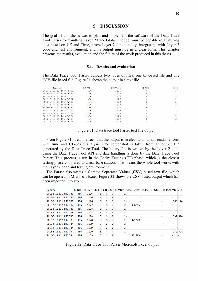
49

5. DISCUSSION

The goal of this thesis was to plan and implement the software of the Data Trace

Tool Parser for handling Layer 2 traced data. The tool must be capable of analyzing

data based on UE and Time, prove Layer 2 functionality, integrating with Layer 2

code and test environment, and its output must be in a clear form. This chapter

presents the results, evaluation and the future of the work produced in this thesis.

5.1. Results and evaluation

The Data Trace Tool Parser outputs two types of files: one txt-based file and one

CSV-file based file. Figure 31 shows the output in a text file.

Figure 31. Data trace tool Parser text file output.

From Figure 31, it can be seen that the output is in clear and human-readable form

with time and UE-based analysis. The screenshot is taken from an output file

generated by the Data Trace Tool. The binary file is written by the Layer 2 code

using the Data Trace Tool API and data handling is done by the Data Trace Tool

Parser. This process is run in the Entity Testing (ET) phase, which is the closest

testing phase compared to a real base station. That means the whole tool works with

the Layer 2 code and testing environment.

The Parser also writes a Comma Separated Values (CSV) based text file, which

can be opened in Microsoft Excel. Figure 32 shows the CSV-based output which has

been imported into Excel.

Figure 32. Data Trace Tool Parser Microsoft Excel output.

50

The file has a .txt extension but the header row and all the values are separated by commas from each other. That allows the use of Microsoft Excel’s Data feature to import the text file as an external data range.

The CSV-based Excel output is basically the same as the text based, but Excel has a Filter feature which allows the filtering of data. Filtered data displays only the rows that meet the selected criteria and hides those rows that the user does not want displayed. Also more than one column can be filtered. Figure 33 shows an example of the UE-based filtering options.

Figure 33. Data Trace Tool Parser Microsoft Excel filtered output The filtering option is really important when the user wants to find a particular

value, and this kind of feature is not supported with a basic text file. For example, in LTE troubleshooting, certain UE-based values need to be found and this feature helps to find them quickly from the mass of data.

Performance measurements were done for the Data Trace Tool. Two different measure cases were run, first with the Data Trace Tool off and the second with the Data Trace Tool gathering data from all defined trace points. The CPU load increased a few percentage point.

Overall, the Data Trace Tool meets the given requirements at this point. Figure 34 shows the Data Trace Tool focus in LTE.

Figure 34. Data Trace Tool focus in LTE.

51

The Data Trace Tool can analyze data by UE and time from Layer 2, it works in

the Layer 2 testing environment and outputs a nice, readable output from which

Layer 2 functionality can be analyzed. The future work is now easy to continue with

the help of the information provided in this thesis work.

Table 6 shows the implemented Data Trace Tool compared to a summary of the

listed tools from different categories. As the Table 6 shows, the Data Trace Tool

meets all the given requirements and that is why it needed to be implemented.

Table 6. Functionalities of the listed tool compared with the requirements given in

the Introduction

Tool name

1. Time and

UE-based

analyzing

2. Layer 2

data flow

correction/in

correction

3. Layer 2

code

integration

4. Test

environment

integration

5. Log file in

clear and

readable form

Data Trace Tool X X X X X

Network Traffic

Analysis Platform X

X

Sanjole

Wavejudge 5000

LTE

X

X

Wireshark

X X

X

5.2. Future

Many features and functionalities have been discussed and pondered for the Data

Trace Tool, and the implementation will continue. Only the basic features were

included in the scope of this thesis, which are binary file handling, metadata

handling, main data handling, and output handling for text file and CSV-based Excel

file. This tool has a lot of potential, especially in the data parsing phase. Python has a

lot of tools to handle data in many ways, for example trace lines, graphs, time lines

and so on.

At the moment, the Data Trace Tool gathers data from three different trace points,

which are shown in Figure 29. More trace points can be added and their data can be

analyzed but this requires careful testing first before it can be used. Python also

provides a lot of possibilities for ways data can be analyzed and handled. That gives

a lot of potential to the tool and more data means that the tool is more informative.

A feature which supports data gathering from the field (e.g. from a customer’s

base station) would be good, because it allows for quick troubleshooting in field.

Also, this tool can be used in testing automation as well. By turning on the Data

Trace Tool in required test cases, the test case can be verified.

52

Performance optimizations also need future work. For example, by optimizing the

cache the CPU load will be reduced.

Generally, this tool can be used as an effective logging tool, helping debugging in

troubleshooting issues in the LTE Layer 2, but it requires more support features and

the CPU load must also be take into account. A feature which allows to use a stream

buffer instead of a ring buffer would be good. A stream buffer enables the gathering

of data over a longer time. This feature would require more work so it can be used

wider in Layer 2 troubleshooting issues.

53

6. SUMMARY

The objective of this thesis work was to help debugging and quality assurance in the

LTE Layer 2 software. The LTE Layer 2 software characteristics are mostly real-

time based, which means that the code is complex in that part. Complex software

requires careful testing and quality assurance. To solve the issue, an informative

logging tool is introduced as it can make troubleshooting easier and quicker.

Few important requirements were given to the logging tool, which would solve the

issue in a customized environment. Also, several commercial logging tools were

listed and compared to the requirements. There are tools from EXFO, Rohde &

Schwartz, Wireshark and so on, but none of the listed tools can meet all the

requirements. Most of them can analyze data by UE, prove Layer 2 functionality, and

have a clear and readable output. But the biggest lack of functionality is integration

with the Layer 2 code and testing environment. That makes the required tool quite

customized and specific, which is why it was decided to implement the Data Trace

Tool. This also allows the tool to be modified and improved, if something specific is

needed in the future.

The Data Trace Tool consists of two software modules, which are the Data Trace

Tool API and the Data Trace Tool Parser. The API works as an interface to the Layer

2 code, which uses the API to write data from defined trace points. The Data Trace

Tool Parser parses the data and outputs data to file.

Trace points must be defined in the API and then the write function called at the

right point in the Layer 2 code. The API creates a binary file / binary files, which

consist of metadata of the traced data and the main data. The metadata contains the

information of main data: the amount of cores, start and stop indices of the data and

which fields are traced, and the length of their values in bits.

The Data Trace Tool Parser takes care of the data handling. The Parser is generic,

which means it can parse different kind of files: different amount of cores, different

metadata, and values of course. First it reads the metadata from the binary file /

binary files and based on that, parses the main data, and then brings the information

into human-readable form as a text file and a CSV-file.

The Data Trace Tool has been tested in three different levels, which are: unit

testing, SCT-testing, and ET-testing. In unit testing, the smallest modules (API and

Parser) are tested to see that both of them work correctly. For example, that the API

writes correct information into the binary file and the Parser outputs valid values

from the binary file. In SCT-testing, the Data Trace Tool was tested with Robot

Framework, which tests the Data Trace Tool integration with the Layer 2. In the ET-

testing phase, the whole tool is also tested and it is the closest testing phase

compared to real a base station.

The Data Trace Tool meets the requirements, it supports UE and time based

analyzing, it integrates with the Layer 2 code and testing environment, it can prove

functionality of the Layer 2, and it outputs a clear log file. However, further

development is still needed to achieve longer traces and a feature for taking traces in

field (e.g. customer’s base station). Python has a lot of libraries for different ways of

handling data and more trace points can be added to Data Trace Tool API, which

gives this tool great potential for solving troubleshooting issues.

54

7. REFERENCES

[1] H. Holma and A. Toskala, LTE for UMTS OFDMA and SC-FDMA

based Radio Access, Chichester: John Wiley & Sons Ltd., 2009.

[2] Glenford J. Myers, Corey Sandler, Tom Badgett, The Art of Software

Testing, Third Edition. John Wiley & Sons, 2012.

[3] Abhik Roychoudhury, Embedded Systems and Software Validation.

Morgan Kaufmann Publishers, 2009.

[4] LTE-Advanced Carrier Aggregation Optimization (2015). Nokia

Solutions and Networks, Espoo, 16s.

[5] 3GPP.org, “Carrier Aggregation explained”, [Online]. Available:

http://www.3gpp.org/technologies/keywords-acronyms/101-carrier-

aggregation-explained. [Accessed 11.02.2016]

[6] 3GPP.org, “LTE-Advanced”, [Online]. Available:

http://www.3gpp.org/technologies/keywords-acronyms/97-lte-

advanced. [Accessed 05.02.2016]

[7] V-G Nguyen, T-X Do, YoungHan Kim (2016) SDN and Virtualization-

Based LTE Mobile Network Architectures: A comprehensive Survey.

Wireless Personal Communications Volume 86 Issue 3, pp 1401-1438.

DOI: 10.1007/s11277-015-2997-7.

[8] F. Firmin, “The Evolved Packet Core”, [Online]. Available:

http://www.3gpp.org/technologies/keywords-acronyms/100-the-

evolved-packet-core. [Accessed 06.01.2016]

[9] 3GPP TS 36.300 version 13.3.0 Release 13 (2015) LTE Evolved

Universal Terrestrial Radio Access (E-UTRA) and Evolved Universal

Terrestrial radio Access Network (E-UTRAN) Overall description Stage

2. [Accessed 19.06.2016]

[10] Sassan Ahmadi, LTE-Advanced: A Practical System Approach to

Understanding the 3GPP LTE Releases 10 and 11 Radio Access

Technologies, Academic Press, 2014.

[11] Kinsun Tam (2011) Debugging Debugging. Proc. 2011 IEE 35th

Annual Computer Software and Applications Conference Workshops

(COMPSACW), pp 512-515. DOI: 10.1109/COMPSACW.2011.93.

[12] Keijiro Araki, Zengo Furukawa, Jingde Cheng (1991) A General

Framework for Debugging. IEEE Software 1991, Volume 8, Issue 3, pp

14-20. DOI: 10.1109/52.88939.

[13] Jian-Hong Zheng, Liang Yan (2012) Study and Design of Embedded

Trace Debugging Technology Based on Virtual Technology. Proc.

Wavelet Active Media Technology and Information Processing

55

(ICWAMTIP) International Conference, pp 346-349. DOI:

10.1109/ICWAMTIP.2012.6413510.

[14] Haiyang He, Yuanyuan Qiao, Sheng Gao, Jie Yang, Jung Guo (2015)

Prediction of User Mobility Pattern on a Network Traffic Analysis

Platform. Proc. MobiArch ’15 Proceedings of the 10th international

Workshop on Mobility in the Evolving Internet Architecture, New

York, NY, USA, pp 39-44. DOI: 10.1145/2795381.2795389.

[15] Aymen Hafsaoui, Navid Nikaein, Christian Bonnet (2013) Analysis and

Experimentation with a Realistic Traffic Generation Tool For Emerging

Application Scenarios. Proc. SimuTools ’13 Proceedings of the 6th

International Institute for Computer Sciences, Social-Informatics and

Telecommunications Engineering (ICST) Conference on Simulation

Tools and Techniques, Brussels, Belgium, pp 268-273.

[16] Almudena Diaz-Zayas, Cesar A. Garcia-Perez, Alvaro M. Recio-Perez,

Pedro Merino-Gomez (2015) PerformLTE: A Testbed for LTE Testing

in the Future Internet. Proc. Wired/Wireless Internet Communications,

13th International Conference, WWIC, Malaga, Spain, May 25-27, pp

46-59.

[17] Artiza Networks, “FURA: The Essential Tool to Visualize the whole

LTE Network”, [Online]. Available:

http://www.artizanetworks.com/lte/lte_sol_net_concept.html. [Accessed

29.01.2016]

[18] Sanjole, “Wavejudge 5000 LTE Benefits and Features”, [Online].

Available: http://www.sanjole.com/our-products/lte-

analyzer/wavejudgefeatures-lte/. [Accessed 30.01.2016]

[19] EXFO, “TravelHawk Pro Portable Wireless Network Troubleshooting

Tool”, [Online]. Available:

http://www.exfo.com/Documents/TechDocuments/Specification_Sheets

/Specs_TravelHawk-Pro_V12_en.pdf. [Accessed 02.02.2016]

[20] EXFO, “M5 Analyzer Software-Based Mobile Network Analyzer”,

[Online]. Available:

http://www.exfo.com/Documents/TechDocuments/Specification_Sheets

/Specs_M5-Analyzer_en.pdf. [Accessed 06.02.2016]

[21] EXFO, “PowerHawk Pro Multi-User Live Network Analyzer”,

[Online]. Available:

http://www.exfo.com/Documents/TechDocuments/Specification_Sheets

/Specs_PowerHawk-Pro_en.pdf. [Accessed 07.02.2016]

[22] Wireshark, “Wireshark”, [Online]. Available:

https://www.wireshark.org/. [Accessed 10.02.2016]

[23] R&S, “R&S CMWmars multifunctional logfile analyzer”, [Online].

Available: https://cdn.rohde-

56

schwarz.com/pws/dl_downloads/dl_common_library/dl_brochures_and

_datasheets/pdf_1/CMW_Platform_bro_en_5214-2833-12_v0200.pdf

pp. 33. [Accessed 20.02.2016]

[24] R&S, “R&S ROMES4 Drive Test Software Mobile coverage and QoS

measurements in mobile network”, [Online]. Available:

https://cdn.rohde-

schwarz.com/pws/dl_downloads/dl_common_library/dl_brochures_and

_datasheets/pdf_1/ROMES4_bro_en_5214-2062-12_v0601.pdf.

[Accessed 25.02.2016]

[25] Cobham, “New All-In-One Multi-Standard Wireless Network

Validation System”, [Online]. Available:

http://www.cobham.com/communications-and-

connectivity/wireless/news/new-all-in-one-multi-standard-wireless-

network-validation-system/. [Accessed 26.02.2016]

[26] Python.org, “The Python Tutorial – Python 2.7.11 Documentation”,

[Online]. Available: https://docs.python.org/2.7/tutorial/. [Accessed

02.04.2016]

[27] Python Wiki, “BeginnersGuide – Overview”, [Online]. Available:

https://wiki.python.org/moin/BeginnersGuide/Overview. [Accessed

03.04.2016]

[28] Apache, “Apache Subversion”, [Online]. Available:

https://subversion.apache.org/. [Accessed 05.04.2016]

[29] John Watkins, Agile Testing: How to Succeed in an Extreme Testing

Environment, Cambridge University Press, 2009.

[30] Jenkins Wiki, “What is Jenkins?”, [Online]. Available:

https://wiki.jenkins-ci.org/display/JENKINS/Meet+Jenkins. [Accessed

15.04.2016]

[31] 3GPP TS 36.321 version 13.1.0 Release 13 (2016) LTE Evolved

Universal Terrestrial Radio Access (E-UTRA) Medium Access Control

(MAC) Protocol specification. [Accessed 23.05.2016]

[32] 3GPP TS 36.331 version 13.1.0 Release 13 (2015) LTE Evolved

Universal Terrestrial Radio Access (E-UTRA) Radio Resource Control

(RRC) Protocol specification. [Accessed 24.05.2016]

[33] 3GPP TS 36.211 version 13.1.0 Release 13 (2015) LTE Evolved

Universal Terrestrial Radio Access (E-UTRA) Physical channels and

modulation. [Accessed 25.05.2016]

[34] 3GPP TS 23.203 version 13.7.0 Release 13 (2015) Digital cellular

telecommunications system (Phase 2+) (GSM) Universal Mobile

Telecommunications System (UMTS) LTE Policy and charging control

architecture. [Accessed 26.05.2016]

57

[35] 3GPP TS 36.322 version 13.1.0 Release 13 (2015) LTE Evolved

Universal Terrestrial Radio Access (E-UTRA) Radio Link Control

(RLC) Protocol specification. [Accessed 27.05.2016]

[36] Python.org, “binascii – Convert between binary and ASCII”, [Online].

Available: https://docs.python.org/2/library/binascii.html. [Accessed

29.04.2016]

[37] Python.org, “struct – Interpret strings as packed binary data”, [Online].

Available: https://docs.python.org/2/library/struct.html. [Accessed

30.04.2016]

[38] Python.org, “unittest – Unit testing framework”, [Online]. Available:

https://docs.python.org/2/library/unittest.html. [Accessed 30.04.2016]

[39] Robot Framework.org, “Robot Framework”, [Online]. Available:

http://robotframework.org/. [Accessed 02.05.2016]

[40] Pekka Klärck, “Robot Framework Introduction”, [Online]. Available:

http://www.slideshare.net/pekkaklarck/robot-framework-introduction.

[Accessed 03.05.2016]