top-down parsing earley parsing - computer sciencecs415/lectures/weimer-pl-earley-01.pdf · –...

#1

Top-Down ParsingTop-Down ParsingEarley ParsingEarley Parsing

#2

And it's gonna be totally awesome!And it's gonna be totally awesome!

#3

Motivating Question

• Given this grammar G:– E E + T– E T– T T * int– T int– T ( E )

• Is the string int * (int + int) in L(G)? – Give a derivation or prove that it is not.

#4

Revenge of Theory

• How do we tell if DFA P is equal to DFA Q?– We can do: “is DFA P empty?”

• How?

– We can do: “P := not Q” • How?

– We can do: “P := Q intersect R” • How?

– So do: “is P intersect not Q empty?”

• Does this work for CFG X and CFG Y?• Can we tell if s is in CFG X?

#5

Outline• Recursive Descent Parsing

– Left Recursion

• Historical Approaches– LL, LR, LALR

• Dynamic Programming• Earley's Algorithm

– Chart States– Operations– Example

#6

In One Slide• A top-down parser starts to work from the initial grammar rules

(rather than from the initial tokens). A recursive descent parser exhaustively tries all productions in the grammar. It is top-down, may backtrack and cannot handle left-recursive grammars. Left recursion can be eliminated. Historical approaches such as LL, LR and LALR cannot handle all context-free grammars. They can be efficient.

• Dynamic programming is a problem-solving technique based on optimal substructure: solutions to subproblems yield solutions to overall problems.

• Earley parsers are top-down and use dynamic programming. An Earley state records incremental information: when we started, what has been seen so far, and what we expect to see. The Earley chart holds a set of states for each input position. Shift, reduce and closure operations fill in the chart.

• You enjoy parsing. Parsing is easy and fun.

#7

In One Slide• A top-down parser starts to work from the initial grammar rules

(rather than from the initial tokens). A recursive descent parser exhaustively tries all productions in the grammar. It is top-down, may backtrack and cannot handle left-recursive grammars. Left recursion can be eliminated. Historical approaches such as LL, LR and LALR cannot handle all context-free grammars. They can be efficient.

• Dynamic programming is a problem-solving technique based on optimal substructure: solutions to subproblems yield solutions to overall problems.

• Earley parsers are top-down and use dynamic programming. An Earley state records incremental information: when we started, what has been seen so far, and what we expect to see. The Earley chart holds a set of states for each input position. Shift, reduce and closure operations fill in the chart.

• You enjoy parsing. Parsing is easy and fun.

#8

Intro to Top-Down Parsing

• Terminals are seen in order of appearance in the token stream:

t1 t2 t3 t4 t5

The parse tree is constructed– From the top– From left to right

A

t1 B

C

t2

D

t3

t4

t4

#9

Recursive Descent Parsing

• We’ll try recursive descent parsing first– “Try all productions exhaustively, backtrack”

• Consider the grammar E T + E | T

T ( E ) | int | int * T

• Token stream is: int * int• Start with top-level non-terminal E

• Try the rules for E in order

#10

Recursive Descent Example

• Try E0 T1 + E2

• Then try a rule for T1 ( E3 )– But ( does not match input token int

• Try T1 int . Token matches.

– But + after T1 does not match input token *

• Try T1 int * T2

– This will match but + after T1 will be unmatched

• Have exhausted the choices for T1

– Backtrack to choice for E0

E T + E | TT ( E ) | int | int * T Input = int * int

#11

Recursive Descent Example (2)

• Try E0 T1

• Follow same steps as before for T1

– And succeed with T1 int * T2 and T2 int

– With the following parse treeE0

T1

int * T2

int

E T + E | TT ( E ) | int | int * T Input = int * int

#12

Recursive Descent Parsing

• Parsing: given a string of tokens t1 t2 ... tn, find its parse tree

• Recursive descent parsing: Try all the productions exhaustively– At a given moment the fringe of the parse tree

is: t1 t2 … tk A …

– Try all the productions for A: if A BC is a production, the new fringe is t1 t2 … tk B C …

– Backtrack if the fringe doesn’t match the string – Stop when there are no more non-terminals

#13

When Recursive Descent Does Not Work

• Consider a production S S a:– In the process of parsing S we try the above rule– What goes wrong?

#14

When Recursive Descent Does Not Work

• Consider a production S S a:– In the process of parsing S we try the above rule– What goes wrong?

• A left-recursive grammar has S + S for some

Recursive descent does not work in such cases– It goes into an infinite loop

#15

What's Wrong With That Picture?

#16

Elimination of Left Recursion

• Consider the left-recursive grammarS S |

• S generates all strings starting with a and followed by a number of

• Can rewrite using right-recursion S T

T T |

#17

Example ofEliminating Left Recursion

• Consider the grammarS 1 | S 0

( = 1 and = 0 )

It can be rewritten asS 1 T

T 0 T |

#18

More Left Recursion Elimination

• In generalS S 1 | … | S n | 1 | … | m

• All strings derived from S start with one of 1,…,m and continue with several instances of 1,…,n

• Rewrite as S 1 T | … | m T

T 1 T | … | n T |

#19

General Left Recursion

• The grammar S A | A S

is also left-recursive because

S + S • This left-recursion can also be eliminated• See book, Section 2.3• Detecting and eliminating left recursion are

popular test questions

#20

Summary of Recursive Descent• Simple and general parsing strategy

– Left-recursion must be eliminated first– … but that can be done automatically

• Unpopular because of backtracking– Thought to be too inefficient (repetition)

• We can avoid backtracking– Sometimes ...

#21

Sometimes Things Are Perfect

• The “.ml-lex” format you emit in PA2 • Will be the input for PA3

– actually the reference “.ml-lex” will be used

• It can be “parsed” directly– You always know just what to do next

• Ditto with the “.ml-ast” output of PA3• Just write a few mutually-recursive functions• They read in the input, one line at a time

#22

Historical Approaches

• In the past, I/O was slow and memory was small. Many sacrifices were made to optimize parsing.– Basic idea: “If we don't handle all grammars, we can go

faster on simpler grammars.” Also: table no backtrack.→

• LL(k) – Left to right scan of input, Leftmost derivation, predict using k tokens. Parse by making a table.

• LR(k) – Left to right scan of input, Rightmost derivation, predict using k tokens. Parse by making a table.

• LALR(k) – Left to right scan of input, Rightmost derivation, predict using k tokens. Parse by making a table, but merge some states in that table. Yacc, bison, etc. use LALR(1).

#23

The Sacrifice• LL(1) languages can be LL(1) parsed

– A language Q is LL(1) if there exists an LL(1) table such the LL(1) parsing algorithm using that table accepts exactly the strings in Q

– Essentially, the table has to be perfect: no entry can be ambiguous or multiply defined.

• Sadly, LL(1) != CFG.• Sadly, LR(1) != CFG.• Sadly, LALR(1) != CFG.

– See textbook for definitive Venn diagram.

#24

The Sacrifice• LL(1) languages can be LL(1) parsed

– A language Q is LL(1) if there exists an LL(1) table such the LL(1) parsing algorithm using that table accepts exactly the strings in Q

– Essentially, the table has to be perfect: no entry can be ambiguous or multiply defined.

• Sadly, LL(1) != CFG.• Sadly, LR(1) != CFG.• Sadly, LALR(1) != CFG.

– See textbook for definitive Venn diagram.

Q: Books (727 / 842)

•Name 5 of the 9 major characters in A. A. Milne's 1926 books about a "bear of very little brain" who composes poetry and eats honey.

#26

Dynamic Programming• “Program” = old word for “table of entries”

– cf. the program (= “schedule”) at a concert

• Dynamic Programming means– “Fill in a chart or table at run-time.” – Same idea as memoization.

• Works when the problem has the optimal substructure property– Solution to Big Problem can be constructed from

solutions to Smaller Subproblems.

• Shortest path, spell checking, ...

#27

Simple Dynamic Programming• Dynamic Programming for Fibonacci

– N 1 2 3 4 5 6– Chart 1 1 2 3 5 8– chart[N] = chart[N-1] + chart[N-2]– Reduces runtime of Fibo from Bad to Linear

#28

Dynamic Programming for Parsing• Dynamic Programming for Fibonacci

– N 1 2 3 4 5 6– Chart 1 1 2 3 5 8– chart[N] = chart[N-1] + chart[N-2]– Reduces runtime of Fibo from Bad to Linear

• Dynamic Programming for Parsing– N 1 2 3 4 5 6– Tokens x + ( y * z– Chart < I'll explain in a minute > – chart[N] = “list of possible parses of tokens 1...N”

#29

Earley's Algorithm

• Earley's Algorithm is an incremental left-to-right top-down parsing algorithm that works on arbitrary context-free grammars.

• Systematic Hypothesis Testing– Before processing token #X, it has already

considered all hypotheses consistent with tokens #1 to #X-1.

– Substructure: parsing token #X is solved in terms of parsing sequences of tokens from #1 to #X-1

#30

…

…

#31

Parsing State

• Earley is incremental and left-to-right• Consider: E E + E | E * E | ( E ) | int →• We use a “•” to mark “where we are now”• Example: E E + → • E

– I am trying to parse E E + E→– I have already seen E + (before the dot)– I expect to see E (after the dot)

• General form: X a → • b – a, b: sequences of terminals and non-terminals

#32

Dot Example

• E E + E | E * E | ( E ) | int → E E + E int

• Input so far: int +• Current state: E E + → • E

#33

Dotty Example

• E E + E | E * E | ( E ) | int →• Input so far: ( int ) • State could be: E ( E ) → •

• But also: E E → • + E• Or: E E → • * E

E

( )E

int

E

( )E

int

E

E+ E

( )E

int

E

E*

#34

Origin Positions

• E E + E | E * E | ( E ) | int →• Example Input-So-Far #1: int

– Possible Current State: E int → •

• Example Input-So-Far #2: int + int– Possible Current State: E int → •

• Must track the input position just before the matching of this production began.

#35

Origin Positions

• E E + E | E * E | ( E ) | int →• Example Input-So-Far #1: int

– Possible Current State: E int → • , from 0

• Example Input-So-Far #2: int + int– Possible Current State: E int → • , from 2

• Must track the input position just before the matching of this production began.

int + int 0 1 2 3

#36

Earley States• Let X be a non-terminal• Let a and b be (possibly-empty) sequences of

terminals and non-terminals• Let X → ab be a production in your grammar• Let j be a position in the input• Each Earley State is a tuple < X → a • b , j >

– We are currently parsing an X– We have seen a, we expect to see b– We started parsing this X after seeing the first j

tokens from the input.

#37

Introducing: Parse Tables

#38

Earley Parse Table (= Chart)

• An Earley parsing table (or chart) is a one-dimensional array. Each array element is a set of Earley states.– chart[i] holds the set of valid parsing states we

could be in after seeing the first i input tokens

#39

Earley Parse Table (= Chart)

• An Earley parsing table (or chart) is a one-dimensional array. Each array element is a set of Earley states.– chart[i] holds the set of valid parsing states we

could be in after seeing the first i input tokens

• Then the string tok1...tok

n is in the language

of a grammar with start symbol S iff – chart[n] contains < S ab→ • , 0 > for some

production rule S ab in the grammar. →– We then say the parser accepts the string.

#40

Earley Parsing Algorithm

• Input:– Grammar G (start symbol S, productions X ab)→

– Input Tokens tok1...tok

n

• Work:chart[0] = { < S → •ab , 0 > } for i = 0 to n complete chart[i] using G and chart[0]...chart[i]

• Output:– true iff < S ab→ • , 0 > in chart[n]

#41

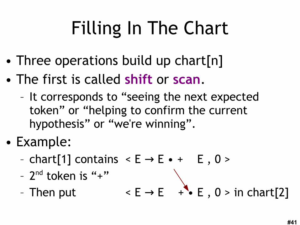
Filling In The Chart

• Three operations build up chart[n]• The first is called shift or scan.

– It corresponds to “seeing the next expected token” or “helping to confirm the current hypothesis” or “we're winning”.

• Example: – chart[1] contains < E E → • + E , 0 >– 2nd token is “+” – Then put < E E + → • E , 0 > in chart[2]

#42

Formal shift operation

• Whenever– chart[i] contains < X ab → • cd , j >– c is a terminal (not a non-terminal)– the (i+1)th input token is c

• The shift operation– Adds < X ab→ c • d , j > to chart[i+1]

#43

Filling In The Chart (2)• The second operation is the closure or

predictor.– It corresponds to “expanding rewrite rules” or

“substituting in the definitions of non-terminals”

• Suppose the grammar is:S E→ E E + E | E – E | int→

• If chart[0] has < S → • E , 0 > then add< E → • E + E , 0 >< E → • E – E , 0 >< E → • int, 0 >

#44

Formal closure operation

• Whenever– chart[i] contains < X ab → • cd , j >– c is a non-terminal– The grammar contains < c p q r > →

• The closure operation– Adds < c → • p q r , i > to chart[i]

– Note < c → • p q r , i > because “we started parsing this c after seeing the first i tokens from the input.”

#45

Filling In The Chart (3)

• The third operation is reduction or completion.– It corresponds to “finishing a grammar rewrite rule” or

“being done parsing a non-terminal” or “doing a rewrite rule in reverse and then shifting over the non-terminal”.

• Suppose:– E int | E + E | E – E | ( E ) , input is “( int” →– chart[2] contains < E int → • , 1 > – chart[1] contains < E ( → • E ) , 0 > – Then chart[2] += < E ( E → • ) , 0 >

#46

Formal reduce operation

• Whenever– chart[i] contains < X ab → • , j >

(The dot must be all the way to the right!)

– chart[j] contains < Y q → • X r , k >

• The reduce operation– Adds < Y q X → • r , k > to chart[i]

– Note < Y q X → • r , k > because “we started parsing this Y after seeing the first k tokens from the input.”

#47

This is easy and fun.

• This is not as hard as it may seem.

• Let's go practice it!

#48

Shift Practice

• chart[3] contains< S E → • , 0 > < E E → • – E , 0 >< E E → • + E , 0> < E E – E → • , 0 >< E E → • – E , 2> < E E → • + E , 2 >< E int → • , 2 >

• The 4th token is “+”. What does shift bring in?

#49

Shift Practice

• chart[3] contains< S E → • , 0 > < E E → • – E , 0 >< E E → • + E , 0> < E E – E → • , 0 >< E E → • – E , 2> < E E → • + E , 2 >< E int → • , 2 >

• The 4th token is “+”. What does shift bring in? < E E + → • E , 0>< E E + → • E , 2 >… are both added to chart[4].

#50

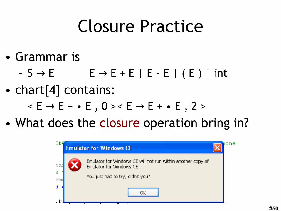
Closure Practice

• Grammar is– S E→ E E + E | E – E | ( E ) | int →

• chart[4] contains:< E E + → • E , 0 >< E E + → • E , 2 >

• What does the closure operation bring in?

#51

Closure Practice

• Grammar is– S E→ E E + E | E – E | ( E ) | int →

• chart[4] contains:< E E + → • E , 0 >< E E + → • E , 2 >

• What does the closure operation bring in?< E → • E + E , 4 >< E → • E – E , 4 >< E → • ( E ) , 4 > < E → • int , 4 >… are all added to chart[4].

#52

Reduction Practice• chart[4] contains:

< E E + → • E , 0 >< E E + → • E , 2 >< E → • E + E , 4 >< E → • E – E , 4 >< E → • ( E ) , 4 > < E → • int , 4 >

• chart[5] contains:– < E int → • , 4 >

• What does the reduce operator bring in?

#53

Reduction Practice• chart[4] contains:

< E E + → • E , 0 >< E E + → • E , 2 >< E → • E + E , 4 >< E → • E – E , 4 >< E → • ( E ) , 4 > < E → • int , 4 >

• chart[5] contains:– < E int → • , 4 >

• What does the reduce operator bring in?< E E + E → • , 0 >< E E + E → • , 2 >< E E → • + E , 4 >< E E → • – E , 4 >

– … are all added to chart[5]. (Plus more in a bit!)

#54

Earley Parsing Algorithm

• Input: CFG G, Tokens tok1...tok

n

• Work:chart[0] = { < S → •ab , 0 > } for i = 0 to n repeat use shift, reduce and closure on chart[i] until no new states are added

• Output:– true iff < S ab→ • , 0 > in chart[n]

#55

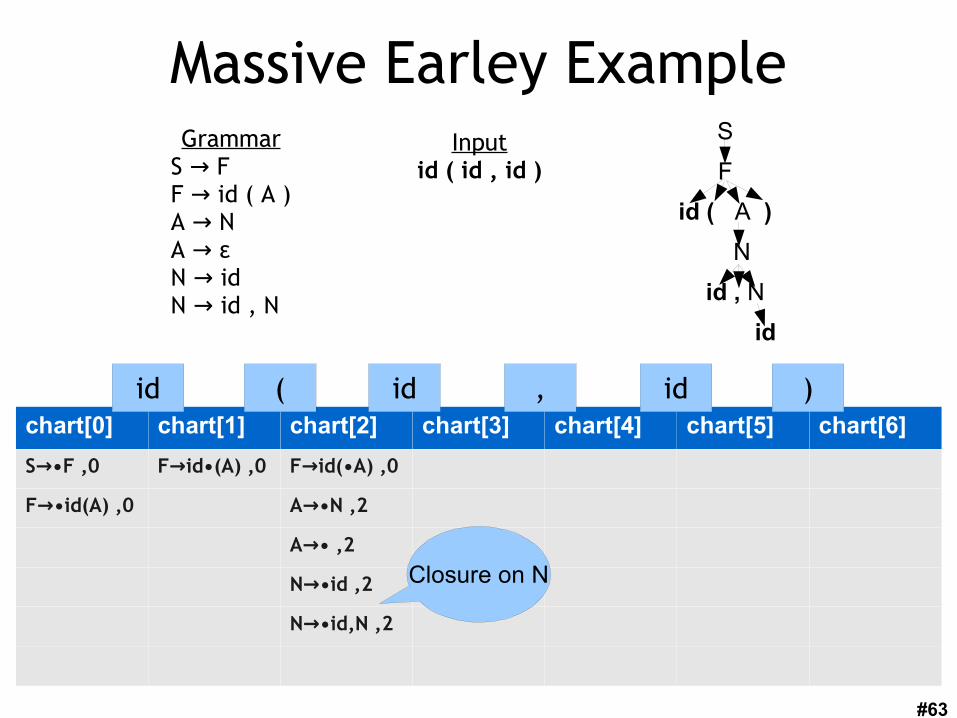
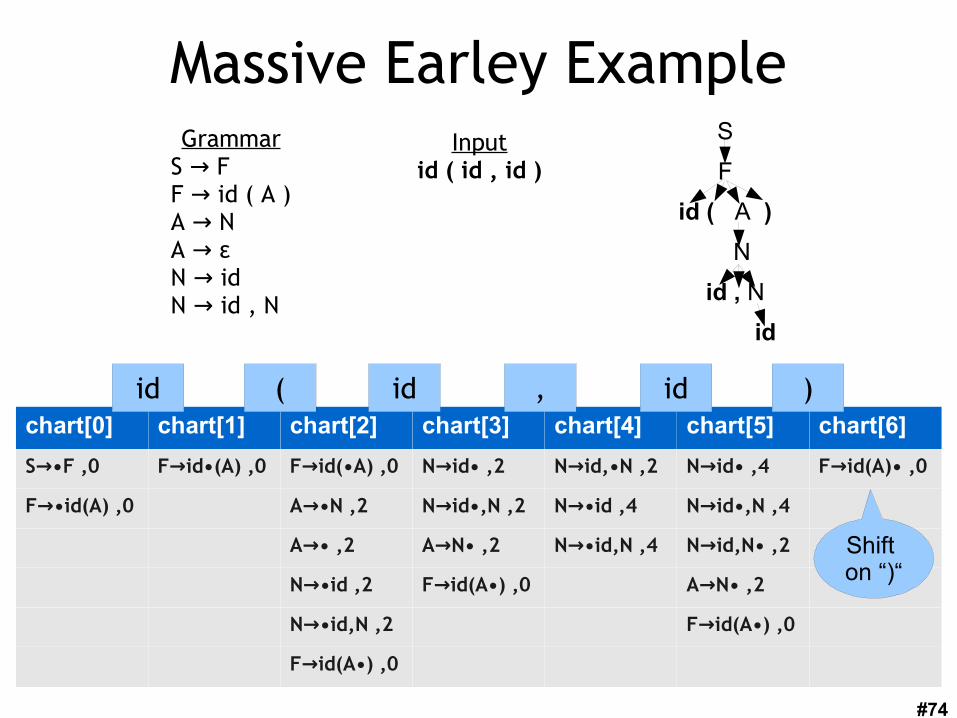
Massive Earley ExampleGrammar

S F→F id ( A )→A N →A → εN id →N id , N→

Inputid ( id , id )

S

F

id ( A )

N

id , N

id

#56

Massive Earley Example

chart[0] chart[1] chart[2] chart[3] chart[4] chart[5] chart[6]

GrammarS F→F id ( A )→A N →A → εN id →N id , N→

id ( id , id )

Inputid ( id , id )

S

F

id ( A )

N

id , N

id

#57




id ( id , id )

Inputid ( id , id )

S

F

id ( A )

N

id , N

id

#58



S→•F ,0


id ( id , id )

Inputid ( id , id )

S

F

id ( A )

N

id , N

id

#59



S→•F ,0

F→•id(A) ,0


id ( id , id )

Inputid ( id , id )

S

F

id ( A )

N

id , N

id

Closure on F

#60



S→•F ,0 F→id•(A) ,0

F→•id(A) ,0


id ( id , id )

Inputid ( id , id )

S

F

id ( A )

N

id , N

id

Shift on “id”

#61



S→•F ,0 F→id•(A) ,0 F→id(•A) ,0

F→•id(A) ,0


id ( id , id )

Inputid ( id , id )

S

F

id ( A )

N

id , N

id

Shift on “(”

#62



S→•F ,0 F→id•(A) ,0 F→id(•A) ,0

F→•id(A) ,0 A→•N ,2

A→• ,2


id ( id , id )

Inputid ( id , id )

S

F

id ( A )

N

id , N

id

Closure on A

#63



S→•F ,0 F→id•(A) ,0 F→id(•A) ,0

F→•id(A) ,0 A→•N ,2

A→• ,2

N→•id ,2

N→•id,N ,2


id ( id , id )

Inputid ( id , id )

S

F

id ( A )

N

id , N

id

Closure on N

#64



S→•F ,0 F→id•(A) ,0 F→id(•A) ,0

F→•id(A) ,0 A→•N ,2

A→• ,2

N→•id ,2

N→•id,N ,2

F→id(A•) ,0


id ( id , id )

Inputid ( id , id )

S

F

id ( A )

N

id , N

id

Reduce on A

#65



S→•F ,0 F→id•(A) ,0 F→id(•A) ,0 N→id• ,2

F→•id(A) ,0 A→•N ,2 N→id•,N ,2

A→• ,2

N→•id ,2

N→•id,N ,2

F→id(A•) ,0


id ( id , id )

Inputid ( id , id )

S

F

id ( A )

N

id , N

id

Shift on “id”

#66



S→•F ,0 F→id•(A) ,0 F→id(•A) ,0 N→id• ,2

F→•id(A) ,0 A→•N ,2 N→id•,N ,2

A→• ,2 A N→ • ,2

N→•id ,2

N→•id,N ,2

F→id(A•) ,0


id ( id , id )

Inputid ( id , id )

S

F

id ( A )

N

id , N

id

Reduce on N

#67



S→•F ,0 F→id•(A) ,0 F→id(•A) ,0 N→id• ,2

F→•id(A) ,0 A→•N ,2 N→id•,N ,2

A→• ,2 A N→ • ,2

N→•id ,2 F→id(A•) ,0

N→•id,N ,2

F→id(A•) ,0


id ( id , id )

Inputid ( id , id )

S

F

id ( A )

N

id , N

id

Reduce on A

#68



S→•F ,0 F→id•(A) ,0 F→id(•A) ,0 N→id• ,2 N→id,•N ,2

F→•id(A) ,0 A→•N ,2 N→id•,N ,2

A→• ,2 A N→ • ,2

N→•id ,2 F→id(A•) ,0

N→•id,N ,2

F→id(A•) ,0


id ( id , id )

Inputid ( id , id )

S

F

id ( A )

N

id , N

id

Shift on “,”

#69



S→•F ,0 F→id•(A) ,0 F→id(•A) ,0 N→id• ,2 N→id,•N ,2

F→•id(A) ,0 A→•N ,2 N→id•,N ,2 N→•id ,4

A→• ,2 A N→ • ,2 N→•id,N ,4

N→•id ,2 F→id(A•) ,0

N→•id,N ,2

F→id(A•) ,0


id ( id , id )

Inputid ( id , id )

S

F

id ( A )

N

id , N

id

Closure on N

#70



S→•F ,0 F→id•(A) ,0 F→id(•A) ,0 N→id• ,2 N→id,•N ,2 N id→ • ,4

F→•id(A) ,0 A→•N ,2 N→id•,N ,2 N→•id ,4 N→id•,N ,4

A→• ,2 A N→ • ,2 N→•id,N ,4

N→•id ,2 F→id(A•) ,0

N→•id,N ,2

F→id(A•) ,0


id ( id , id )

Inputid ( id , id )

S

F

id ( A )

N

id , N

id

Shift on “id”

#71





A→• ,2 A N→ • ,2 N→•id,N ,4 N→id,N• ,2

N→•id ,2 F→id(A•) ,0

N→•id,N ,2

F→id(A•) ,0


id ( id , id )

Inputid ( id , id )

S

F

id ( A )

N

id , N

id

Reduceon N

#72





A→• ,2 A N→ • ,2 N→•id,N ,4 N→id,N• ,2

N→•id ,2 F→id(A•) ,0 A N→ • ,2

N→•id,N ,2

F→id(A•) ,0


id ( id , id )

Inputid ( id , id )

S

F

id ( A )

N

id , N

id

Reduceon N

#73





A→• ,2 A N→ • ,2 N→•id,N ,4 N→id,N• ,2

N→•id ,2 F→id(A•) ,0 A N→ • ,2

N→•id,N ,2 F→id(A•) ,0

F→id(A•) ,0


id ( id , id )

Inputid ( id , id )

S

F

id ( A )

N

id , N

id

Reduceon A

#74



S→•F ,0 F→id•(A) ,0 F→id(•A) ,0 N→id• ,2 N→id,•N ,2 N id→ • ,4 F→id(A)• ,0


A→• ,2 A N→ • ,2 N→•id,N ,4 N→id,N• ,2

N→•id ,2 F→id(A•) ,0 A N→ • ,2

N→•id,N ,2 F→id(A•) ,0

F→id(A•) ,0


id ( id , id )

Inputid ( id , id )

S

F

id ( A )

N

id , N

id

Shift on “)“

#75




F→•id(A) ,0 A→•N ,2 N→id•,N ,2 N→•id ,4 N→id•,N ,4 S F→ • ,0

A→• ,2 A N→ • ,2 N→•id,N ,4 N→id,N• ,2

N→•id ,2 F→id(A•) ,0 A N→ • ,2

N→•id,N ,2 F→id(A•) ,0

F→id(A•) ,0


id ( id , id )

Inputid ( id , id )

S

F

id ( A )

N

id , N

id

Reduceon F

#76




F→•id(A) ,0 A→•N ,2 N→id•,N ,2 N→•id ,4 N→id•,N ,4 S F→ • ,0

A→• ,2 A N→ • ,2 N→•id,N ,4 N→id,N• ,2

N→•id ,2 F→id(A•) ,0 A N→ • ,2

N→•id,N ,2 F→id(A•) ,0

F→id(A•) ,0


id ( id , id )

Inputid ( id , id )

S

F

id ( A )

N

id , N

id

Accept!

#77

Homework• WA2 (written homework) due Monday

• Read Chapter 2.3.3, etc. • Read earley.py

• Midterm 1 Next Wednesday

top-down parsing earley parsing - computer sciencecs415/lectures/weimer-pl-earley-01.pdf · –...

Documents